University of Southampton Research Repository

University of Southampton Research Repository

Copyright © and Moral Rights for this thesis and, where applicable, any accompanying data are

retained by the author and/or other copyright owners. A copy can be downloaded for personal

non‐commercial research or study, without prior permission or charge. This thesis and the

accompanying data cannot be reproduced or quoted extensively from without first obtaining

permission in writing from the copyright holder/s. The content of the thesis and accompanying

research data (where applicable) must not be changed in any way or sold commercially in any

format or medium without the formal permission of the copyright holder/s.

When referring to this thesis and any accompanying data, full bibliographic details must be

given, e.g.

Thesis: Author (Year of Submission) "Full thesis title", University of Southampton, name of the

University Faculty or School or Department, PhD Thesis, pagination.

Data: Author (Year) Title. URI [dataset]

UNIVERSITY OF SOUTHAMPTON

FACULTY OF ENGINEERING AND APPLIED SCIENCE

Department of Electronics and Computer Science

A STUDY OF FEASIBILITY OF IMPLIMENTING A DIGITAL LOUDSPEAKER ARRAY

by

Sangchai Monkronthong

A thesis submitted in partial fulfilment for the degree of Doctor of Philosophy

3 May 2018

UNIVERSITY OF SOUTHAMPTON

ABSTRACT

FACULTY OF ENGINEERING AND APPLIED SCIENCE

Department of Electronics and Computer Science

Thesis for the degree of Doctor of Philosophy

A STUDY OF THE FEASIBILITY OF IMPLIMENTING A DIGITAL LOUDSPEAKER ARRAY

Sangchai Monkronthong

The common method in audio player for sound generation with a loudspeaker is driving analogue

electrical signals while this thesis will study an alternative method for application of a loudspeaker

with digital signals. This thesis found feasibility of driving loudspeaker with digital pulses

according to the concept of Multiple‐level Digital Loudspeaker Array (MDLA) and discovered

generation of sound from ultrasound with potential.

The concept of a MDLA can be applied as an alternative method to produce Amplitude

Modulation (AM) sound. The new concept extends from Digital Loudspeaker Array (DLA) by

application of Pulse Width Modulation (PWM). By Application‐Specific Integrated Circuit system

(ASICs), the clock speed would reach 1 GHz. With the chip, DLA will require only 7 speaklets for

the reproduction of 16 bit audio.

A novel concept of sound generation from ultrasound originates from the concept of AM sound of

Audio Spotlight technology. The new concept applies mechanical amplitude demodulation for

improvement in efficiency of sound generation.

A rectifying loudspeaker is introduced for sound generation according to the concept. The

loudspeaker uses a secondary source as the main source of sound generation, while vibration of

the primary source is applied for speed control of air particles like a valve. The structure of the

loudspeaker is adapted from the human voice system and can be fabricated by MEMs

i

Table of Contents

Table of Contents ............................................................................................................ i

List of Tables ................................................................................................................... v

List of Figures ................................................................................................................ vii

DECLARATION OF AUTHORSHIP ..................................................................................... xv

Acknowledgements ..................................................................................................... xvii

Nomenclature .............................................................................................................. xix

Chapter 1: Overview of the Research .................................................................... 1

1.1 Research Inspiration ................................................................................................ 1

1.2 Big Picture of Work .................................................................................................. 1

1.2.1 “If an ideal speaklet (a tiny loudspeaker) for DLA did exist, what would

the characteristics of sound of the array be?”, found in Chapter 3. ......... 2

1.2.2 “If DLAs are applied in a real speaklet, what will its characteristics of

sound be?” ................................................................................................. 3

1.2.3 “If a speaklet will generate rectified AM sound, what should its structure

be?” ............................................................................................................ 4

1.3 Goals of Thesis ......................................................................................................... 5

1.4 Statement of Problems, Proposed Solutions and Their Outcome........................... 5

1.4.1 Sound Quality ............................................................................................ 6

1.4.2 Interference among Pressure Responses of Digital Electrical Pulses ........ 8

1.4.3 Efficiency in Sound Generation ................................................................. 9

1.5 Scope of Work ........................................................................................................ 10

1.6 Contribution ........................................................................................................... 11

1.6.1 Three Requirement of Digital Sound Reconstruction.............................. 11

1.6.2 MDLA. ...................................................................................................... 11

1.6.3 Rectifying loudspeaker ............................................................................ 12

1.7 Document Structure .............................................................................................. 12

1.8 Publication ............................................................................................................. 13

Chapter 2: A Review of Sound Generation and Digital Loudspeaker Array ...........15

ii

2.1 Sound and Ultrasonic ............................................................................................ 16

2.1.1 Wave Propagation ................................................................................... 16

2.1.2 Characteristics of Acoustic Wave ............................................................ 18

2.1.3 Sound and Ultrasound with Wave Behaviours ....................................... 20

2.1.4 Hearing, Hearing Criteria and Risk Caused by Sound and Ultrasound .... 25

2.2 Sound and Ultrasonic Generation ......................................................................... 28

2.2.1 Piezoelectric Technologies ...................................................................... 28

2.2.2 Electro‐magnetic technologies ................................................................ 33

2.2.3 Sound Generation with Ultrasound ........................................................ 39

2.2.4 The Voice as Bio‐loudspeaker ................................................................. 43

2.3 Concept of Digital Loudspeaker Array ................................................................... 47

2.3.1 Concept of Digital reconstruction ........................................................... 47

2.3.2 Terminology of Acoustic Response ......................................................... 48

2.3.3 Requirement of Digital reconstruction ................................................... 49

2.3.4 Typical Structure of a Digital Loudspeaker Array .................................... 50

2.3.5 Design of Array and Sound Beam ............................................................ 51

2.4 Mathematical Loudspeaker Model and Wave Propagation ................................. 54

2.4.1 Vibration for a Point Mass ....................................................................... 54

2.4.2 Wave Propagation for a Point Source ..................................................... 58

Chapter 3: Characterization of an Multiple‐Level Digital Loudspeaker Array

(MDLA) with Rectifying Speaklets ................................................................. 69

3.1 Concept of Multiple‐Level Digital Loudspeaker Array ........................................... 69

3.2 Mathematical Model of Acoustic Response of the Ideal Rectifying Loudspeaker 70

3.2.1 Physical Model of the ideal rectifying source ......................................... 70

3.2.2 Mathematical Model ............................................................................... 71

3.2.3 Computation of Acoustic response for a MDLA ...................................... 75

3.3 Assumptions and Results of Simulation of a MDLA .............................................. 77

3.3.1 Assumptions, Results and Fulfilment of Digital Reconstruction

Requirement ............................................................................................ 77

3.3.2 Response time and Improvement in Linearity ........................................ 79

iii

3.3.3 Assumptions and Results of Sound Field, Acoustic Output and Spectrum

of MDLA ................................................................................................... 82

3.4 Amplitude Modulation in Acoustics and Loudness ............................................. 108

3.4.1 Amplitude Modulation in Acoustics ...................................................... 108

3.4.2 Loudness of AM sound .......................................................................... 110

3.4.3 Advantage of Rectified AM Sound ......................................................... 110

3.5 Discussion and Summary ..................................................................................... 111

Chapter 4: Multi‐Level Digital Loudspeaker Array Based on Piezoelectric .......... 115

4.1 Experiments ......................................................................................................... 115

4.1.1 Setup of Experiments ............................................................................. 115

4.1.2 Experiment Acoustic Response of Loudspeakers to digital pulse and

attempt to stop to vibration .................................................................. 117

4.1.3 Experiment to Determine the Relationship between Pulse Width of

Driving Signal and Amplitude of Acoustic Wave ................................... 124

4.1.4 Experiment of MDLA .............................................................................. 130

4.2 Finite Element Model of a speaklet with DLA Based on PZT actuators ............... 140

4.2.1 Objective ................................................................................................ 140

4.2.2 FEM Modelling and Parameters ............................................................ 140

4.2.3 Characterization of Diaphragm Vibration Response: ............................ 143

4.2.4 Results .................................................................................................... 143

4.2.5 Discussion .............................................................................................. 145

4.3 Summary .............................................................................................................. 146

Chapter 5: A Potential Implementation for an Acoustic Rectifying Loudspeaker 149

5.1 Acoustic Rectifying Loudspeaker ......................................................................... 149

5.1.1 Principles ................................................................................................ 149

5.1.2 FEM Modelling ....................................................................................... 157

5.1.3 Results .................................................................................................... 160

5.1.4 Discussion .............................................................................................. 162

5.2 Summary .............................................................................................................. 164

iv

Chapter 6: Conclusion and Future Work ............................................................ 165

6.1 Conclusion ........................................................................................................... 165

6.1.1 Landscape of Thesis ............................................................................... 165

6.1.2 Difference between DLA and Traditional Loudspeakers ....................... 170

6.2 Future Works ....................................................................................................... 171

6.2.1 Intellectual Challenge of Design ............................................................ 171

6.2.2 Realization of Mathematical Model ...................................................... 173

6.2.3 Ear Canal as a Biological Acoustic Low Pass Filter ................................. 173

Appendices ................................................................................................................. 175

Appendix A ................................................................................................................. 177

Appendix B ................................................................................................................. 179

Glossary of Terms ....................................................................................................... 181

List of References........................................................................................................ 183

v

List of Tables

Table 1‐1: Numbers of levels are required in sound reproduction with different qualities of PCM

bits for a 70‐speaklet DLA. ................................................................................. 6

Table 1‐2: Summary of parameters and resolution of a speaklet ................................................. 8

Table 2‐1: Typical Noise Levels [25] ............................................................................................. 27

Table 2‐2: Material and their characteristics for acoustic transducers following Figure 2‐6b [28]29

Table 3‐1: Comparison of sound generation between a spherical source and a rectifying source71

Table 3‐2: Results of linear regression. ........................................................................................ 78

Table 3‐3: Radius of sound source in millimetre (mm) for phase angles and frequencies ....... 107

Table 3‐4: Comparison between AM in telecommunication and in acoustics .......................... 109

Table 4‐1: Summary of acoustic response of speaklets to a short rectangular pulse ............... 120

Table 4‐2: Values of pulse rate and pulse width in experiments ............................................... 125

Table 4‐3: Results of linear regression of the piezoelectric buzzer with pulse width between1 and

20 µsec. .......................................................................................................... 127

Table 4‐4: Results of linear regression of the ultrasonic transducer with pulse width between 1

and 10 µsec. ................................................................................................... 129

Table 4‐5: Parameters of pulse rate and pulse width ................................................................ 131

Table 4‐6: Parameters in the FEM model .................................................................................. 141

Table 5‐1: Parameters of modelling of the rectifying loudspeaker ........................................... 158

Table 6‐1: A summary of differences between a DLA and a normal analogue array ................ 170

vii

List of Figures

Figure 2‐1: Schematic diagram of wave propagation. ................................................................. 17

Figure 2‐2: Transmission and reflection of a sound wave when its direction is perpendicular to a

boundary of two media after Kremkau, F. [5]. ................................................ 21

Figure 2‐3: Wave front of transmission (or radiation) and reflection of sound wave when the wave

travel out from a pipe. ..................................................................................... 23

Figure 2‐4: Beam Width of transducer after Olympus NDT [21] ................................................. 25

Figure 2‐5: Robinson‐Dadson curves are one of many sets of equal‐loudness contours for the

human ear after Gelfand, S.[23]. ..................................................................... 26

Figure 2‐6:a) Typical acoustic transducer after Uchino, K.[29] b) MEMS Speaklet after Dejaeger, R.

et al[6] c) piezoelectric acoustic actuator after Kim, H. et al [27]. .................. 29

Figure 2‐7: Schematic configurations a) SMS and b) PMP where P shows the polarization direction,

while E shows applied electric field direction for each layer after Kim, H. et al

[27] ................................................................................................................... 31

Figure 2‐8: a) diagrammatic representation of an ultrasonic transducer and b) the

transducers.after Senthilkumar and Vinothraj [32] ........................................ 31

Figure 2‐9: Analogous circuit of a piezoelectric transducer ........................................................ 32

Figure 2‐10: Schematic diagram of a buzzer ................................................................................ 33

Figure 2‐11:a) a) Magnetic flux within the core b) Magnetic flux outside the core c) Equivalent

circuit after Fitzgerald, A. el at [34] ................................................................. 34

Figure 2‐12: Moving coil loudspeaker .......................................................................................... 37

Figure 2‐13: a) and b) fabricated microspeaker c) layout of microspeaker d) inner and outer part

membrane placement after Weber, C. et al[35] ............................................. 38

Figure 2‐14: a) Non‐linear relationship between pressure and specific volume (red line) b)

Distortion due to non‐linearity of media (red line) after Croft, J.[9] ............... 39

viii

Figure 2‐15: Temporal and frequency response of one transducer with amplitude modulation

circuits for an audio frequency of 2 kHz and carrier frequency 44 kHz. ......... 41

Figure 2‐16: Temporal and frequency response of two transducers with different frequencies of

fu1 and fu2 (42 and 46 kHz) (b) .......................................................................... 41

Figure 2‐17: Non‐linear interaction process in air (frequencies in green font produced by non‐

linearity) after Wen‐Kung,T [39] ..................................................................... 42

Figure 2‐18: a) Structure of transducer after Yoneyama, M. and Fujimoto, J. [40]] and b)

Construction of loudspeaker after Croft, J.[9]. ............................................... 42

Figure 2‐19: Difference of beam width of a 10 mm diameter transducer emitting sound at 2kHz

between a parametric array and an ordinary sound source after Kamakura, T.

and Aoki,K.[30.] ............................................................................................... 43

Figure 2‐20: Air Flow Patterns from a Larynx a) bright tone b) dark tone after Arthur, B. [16] . 44

Figure 2‐21: A mechanical analogous model of the larynx after Arthur, B. [16] ......................... 45

Figure 2‐22 Velocity distribution next to a boundary after White, F. ......................................... 46

Figure 2‐23 The acoustic sound is ideally reconstructed by 2‐bit DLA (4 speaklets).Each speaklet is

driven by a train of constant pulses in order to generate clicks. Different points

(A, B, C and D) in wave are dependent on number of speaklet emitting the click.

......................................................................................................................... 48

Figure 2‐24: The reconstruction of a conventional analogue loudspeaker, which shows the relation

between the positions of diaphagm and the positions in the the acoutic

waveform. The movement of diaphagm are forced by the electrical input signal

feeding the loudspeaker. ................................................................................. 48

Figure 2‐25: an acoustic output of a speaklet is driven by a discrete pulse after Diamond, B. M. et

al.[1] ................................................................................................................. 49

Figure 2‐26: Typical structure of DLA system after Tatlas, N. [13]. ............................................. 50

Figure 2‐27: Interspacing (garray) of a two‐dimensional array ...................................................... 51

Figure 2‐28 the relation between interspacing and wavelength after Ballou, G. [49]. ............... 52

Figure 2‐29: Far‐field polar beam of width Lx with offset angle βx after Hawksford, M. O. J. H [48].

......................................................................................................................... 53

ix

Figure 2‐30: Delay paths for each speaklet for beam offset angle after Hawksford, M. O. J. H [48].

......................................................................................................................... 53

Figure 2‐31: Mass‐Spring damper Model .................................................................................... 54

Figure 3‐1 (a) Traditional DLA and (b) MDLA ............................................................................... 69

Figure 3‐2 (a) a spherical source, (b) the ideal rectifying source ................................................. 70

Figure 3‐3: Acoustic response of two pulses feeding a speaklet with different time. ................ 76

Figure 3‐4: Acoustic response of driving two speaklets on different locations ........................... 76

Figure 3‐5: Spatial output of two pulses feeding a speaklet at a moment (t) ............................. 77

Figure 3‐6: Graph of a mechanical pulse driving a speaklet with pulse width of 4.685 µs and its

acoustic response. (b) The relationship between maximum pressure and pulse

width and the relationship between response time and pulse width. ........... 78

Figure 3‐7: The digital reconstruction for level at 2100 , reproduced by 4 speaklets with different

levels 937, 937,226 and 0, which are the sum of 2100 (937+ 937+226=2100).79

Figure 3‐8: The digital reconstruction for levels from 935 to 940 ............................................... 80

Figure 3‐9: Maximum pressure for the acoustic response of all levels (65590 levels). ............... 81

Figure 3‐10: The sinusoidal input of 2.2 kHz and its digitally reconstructed output. .................. 81

Figure 3‐11: The sinusoidal input of 200 Hz and its digitally reconstructed output. ................... 82

Figure 3‐12: Typical system of pulse assignment ........................................................................ 83

Figure 3‐13: The combination codes of the four schemes of pulse assignment ......................... 84

Figure 3‐14: The pulse streams of the four pulse assignment for an audio stream. ................... 84

Figure 3‐15: Speaklets in a linear array, the observing points and pattern in simulation result. 85

Figure 3‐16: Acoustic response of 4 speaklet MDLA at the front of the array (0°) ..................... 86

Figure 3‐17: Acoustic response of 4 speaklet MDLA at the front of the array for pulse assignment

2. ...................................................................................................................... 87


3. ...................................................................................................................... 87

x


4. ...................................................................................................................... 88

Figure 3‐20: Acoustic response of 4 speaklet MDLA at different angles from ‐90 to 0 for pulse

assignment1. ................................................................................................... 89

Figure 3‐21: Acoustic response of 4 speaklet MDLA at different angles from 0 to 90 for pulse

assignment 1. .................................................................................................. 90

Figure 3‐22: Sound field and acoustic response for pulse assignment 1. The main image of pulse

assignment 1 shows sound field for 10 kHz with 4 speaklets while the satellite

images show acoustic output with different angle of ‐90,60,‐30, 0, 30, 60 and 90.

......................................................................................................................... 93

Figure 3‐23 : Sound field and acoustic response for pulse assignment 2. The main image shows

sound field for 10 kHz with 4 speaklets while the satellite images show acoustic

output with different angle of ‐90,60,‐30, 0, 30, 60 and 90. .......................... 93

Figure 3‐24: Sound field and acoustic response for pulse assignment 3. The main image shows



Figure 3‐25 : Sound field and acoustic response for pulse assignment 4. The main image of shows



Figure 3‐26: Sound field and acoustic spectrums for pulse assignment 1. The main image shows


spectrums with different angle of ‐90,60,‐30, 0, 30, 60 and 90 ...................... 95










xi

Figure 3‐30: Sound field, the spectral response and sound distortion of a 16 speaklet DLA emitting

a digital audio stream of 2 kHz for pulse assignment1. ................................... 98


a digital audio stream of 2 kHz for for pulse assignment2. ............................. 98





Figure 3‐34: Sound field , the spectral response and sound distortion of 8 speaklets DLA emitting

digital audio stream of 20 Hz for pulse assignment1. ................................... 100







Figure 3‐38: Directivity of audible frequency, natural frequency of speaklet and harmonic

frequency for pulse assignment 1. ................................................................ 103







Figure 3‐42: temporal and frequency of acoustic response of rectified amplitude modulation when

frequency of audio (2 kHz) and carrier (44 kHz) are equal ............................ 108

Figure 4‐1: Configuration of Digitally‐Driving Speaklet Experiment .......................................... 115

Figure 4‐2: Pressure output of a piezoelectric buzzer. .............................................................. 119

xii

Figure 4‐3: Pressure output of a magnetic buzzer .................................................................... 119

Figure 4‐4: Pressure output of an ultrasonic transducer .......................................................... 120

Figure 4‐5: The conceptual result of the double pulse technique ............................................ 122

Figure 4‐6: Pressure response of the ultrasonic transduce with double pulse technique ........ 123

Figure 4‐7: The pressure output of a piezoelectric buzzer when feeding the digital pulse at 22 kHz

and pulse width 1,5,10 and 20 µsec. ............................................................. 125

Figure 4‐8: The pressure output of a piezoelectric buzzer when feeding the digital pulse with pulse

width 20.µsec at 14, 18, 26 and 30 kHz......................................................... 126

Figure 4‐9: Relationship between the amplitude and the pulse width for pulse rate of 14, 18, 22,

26, 30 kHz. ..................................................................................................... 127

Figure 4‐10: The pressure output of an ultrasonic transduce when feeding the digital pulse at 40

kHz and pulse width 1,4,8 and 12 µsec. ........................................................ 128

Figure 4‐11: The pressure output of an ultrasonic transducer when feeding the digital pulse with

pulse width 12.µsec at 32, 36, 44 and 48 kHz. .............................................. 128


44, 46 kHz. ..................................................................................................... 129

Figure 4‐13: Frequency components of amplitude modulation from Section 3.4.1. ................ 131

Figure 4‐14: The pressure output of a piezoelectric buzzer when driving it with pulse rate at 22

kHz and audio frequency of 1, 2,4 and 7 kHz. ............................................... 133





Figure 4‐17: The pressure output of a ultrasonic transducer when driving it with pulse rate at 40




xiii



Figure 4‐20: The pressure output of a magnetic buzzer when driving it with pulse rate at 18 kHz

and audio frequency of 1, 2,4 and 7 kHz. ...................................................... 137





Figure 4‐23: PZT speaklet cross section schematic view and FEM model ................................. 140

Figure 4‐24: Components in piezoelectric devices module ....................................................... 142

Figure 4‐25: Convergence plot of maximum displacement of a speaklet VS the number of mesh

points ............................................................................................................. 142

Figure 4‐26: The displacement and frequency response of a speaklet with 12 mm, 0.2 mm and

9.1mm diameter, thickness of diaphragm and diameter of electrodes

respectively. ................................................................................................... 143

Figure 4‐27: The result of the two main parameters: the displacement of oscillation and the first

resonant frequency obtained from FEM ....................................................... 144

Figure 5‐1: Frequency components of AM (a) and half‐wave rectified AM (b) ......................... 150

Figure 5‐2: Schematic diagram of wave propagation of a piston or a diaphragm. ................... 151

Figure 5‐3: Structure of a Rectifying Loudspeaker ..................................................................... 153

Figure 5‐4: Operational stages of the rectifying loudspeaker ................................................... 153

Figure 5‐5: Schematic diagram of wave propagation of a rectifying loudspeaker. ................... 154

Figure 5‐6: MSD model of the rectifying loudspeaker ............................................................... 155

Figure 5‐7: Schematic and FEM of diffuse and the gap between the disc and the diffuse. ...... 157

Figure 5‐8: Components in fluid structure interaction module ................................................. 159

Figure 5‐9: Convergence plot of velocity of the air flow in the front of the hole. ..................... 159

Figure 5‐10: Air flow in the speaklet at the maximum displacement. ....................................... 160

xiv

Figure 5‐11: Comparison between displacement and velocity and between displacement of flow

pressure. ........................................................................................................ 161

Figure 5‐12: A practical structure of rectifying loudspeaker ..................................................... 164

Figure 6‐1: Conception layer of speaklets ................................................................................. 166

Figure 6‐2: Common and proposed conditions of wave propagation ....................................... 167

Figure 6‐3: Design layer of speaklets ......................................................................................... 168

Figure 6‐4: Practical layer of speaklets ...................................................................................... 169

Figure 6‐5: Perspectives of design of a rectifying loudspeaker. ................................................ 171

Figure 6‐6: Performance of diffuser after White, F. [44] ........................................................... 172

Figure 6‐7: a) Head and Torso Simulator b) Positive scenarios of the hypothesis. ................... 174

xv

DECLARATION OF AUTHORSHIP

I, Sangchai Monkronthong declare that this thesis and the work presented in it are my own and

has been generated by me as the result of my own original research.

A Study of the Feasibility of Implementing a Digital Loudspeaker Array ............................................

..............................................................................................................................................................

I confirm that:

1. This work was done wholly or mainly while in candidature for a research degree at this

University;

2. Where any part of this thesis has previously been submitted for a degree or any other

qualification at this University or any other institution, this has been clearly stated;

3. Where I have consulted the published work of others, this is always clearly attributed;

4. Where I have quoted from the work of others, the source is always given. With the exception

of such quotations, this thesis is entirely my own work;

5. I have acknowledged all main sources of help;

6. Where the thesis is based on work done by myself jointly with others, I have made clear

exactly what was done by others and what I have contributed myself;

7. Parts of this work have been published as:

Monkronthong, S. White, N and Harris, N. “Multiple‐Level Digital Loudspeaker Array”,

the 28th European Conference on Solid‐State Transducers, September 2014

Monkronthong, S. White, N and Harris, N. “A study of efficient speaklet driving

mechanisms for use in a digital loudspeaker array based on PZT actuators”, the

Sensors Application Symposium 2016, April 2016.

Signed: ...............................................................................................................................................

Date: ...............................................................................................................................................

xvii

Acknowledgements

Working in this thesis impresses me like an adventure in an unknown world; the exploration of

electronic men in the acoustic world. I unintentionally stepped into the route even acoustic

people might be not familiar, which is called a transient‐state wave propagation. However I, as a

scout, discovered “the promised land, a land flowing milk and honey” Through the way in years of

work, I have been accompanied and supported by many people. It is with pleasure that I now take

this opportunity to express my gratitude for all of them.

This work would not have been possible without the aid and guidance of my supervisor team of

Prof. Neil White and Dr. Nicholas Harris. I thank Prof. Neil White especially for introducing me to

this interesting topic of Digital Loudspeaker Array. When I was faced with dilemmas of research

approaches, they were friendly prompt to give directions, advises and supports.

I would like to express my gratitude for Dr. Filiopo Fazi, Associate Professor in Institute of Sound

and Vibration Research (ISVR). These are great opportunities for me as an electronic student to

meet him as an acoustic examiner. He gave valuable comments and encouragements for this

research in the couple times of oral examination.

I would like to thank Dr. Khemapat Tontiwattanakul, who was an acoustic PhD student. He is my

friend and personal acoustic advisor. He dedicated his precious times for me. He gave a brief

lecture and demonstrated programming and conduct of experiments in an acoustic domain

several times. I acknowledge him that he expertizes a basis of acoustics I require for this research.

I would like to thank Ministry of Science and Technology of Thai government and Naresuan

University in Thailand for the provision of scholarship for study in University of Southampton

through the years of working.

I would like to dedicate my work as a sacrificial offering to the king of kings, who reigns over all

Thai people’s hearts.

xix

Nomenclature

a area constant

A Cross‐section Area of flow

An A‐weighing value at frequency n Hz

The area of the neck of diffuser

Amplitude of audio

Amplitude of carrier

Cross‐section area of core

Cross‐section area of air gap

B Adiabatic bulk modulus

Bd The damping constant

Magnetic flux density

c Sound speed

CPZT Capacitance of a transducer

Constant of coil

The life force constant

Pile constant

Constant of piston

D Diameter

Dc Directivity constant

Dcore Diameter of core

Dgap Diameter of flux at the gap

Dmagnet Diameter of magnet

dr Delay path

e Induced voltage

f frequency

xx

f0 The fundamental resonant frequency

fB The inertial force of damping

fe The external force

fk The inertial force of spring

fm The inertial force of mass

fn The natural frequency

fs Sampling frequency

fu Frequency of ultrasound

f Magnetic force

Frequency of audio

The force from coil

Frequency of carrier

Life force

Magnetomotive force

Force density

g Gravity

garray Interspacing

h Thickness of diaphragm

Hp Height of pile

Hz Hertz, unit of frequency, cycles per second

H Number of speaklets in a column

i current

iPZT Current feeding in a transducer

k Wave number

kh The ratio of specific heats

km kilometre

xxi

Kq The charge output per unit displacement

Ks The spring constant

lair Length of the air gap

Length of coil

L inductance

Lx Beam width

M Weight of Mass

N Coil turn

Ncore Number of core

p Acoustic pressure

p< Acoustic pressure of wave incidence

p> Acoustic pressure of wave reflection

prad Acoustic pressure of wave radiation

pref Threshold of hearing

prms the mean‐square pressure

p The power at the terminal of the coil

P Pressure constant or Flow pressure

A constant pressure of the air pump

q Electrical charge

Q Volume flow rate

r Radius of sound source

rshape Shape constant

Path index

R Distance from source

R0 Location of source

R2 the coefficient of determination

xxii

Rh The ideal gas constant equal to 287 J/kg*°K

RL Resistant of Load

RPZT Resistance of a transducer

Rrad Radiation resistance

Resistance of coil

Reluctance of air gap

Total reluctance

Se The electric sensitivity

SPLn Sound Pressure Level at a frequency of n Hz

t time

T A period of a cycle of the wave

u Velocity

v voltage

Vpp Peak‐to‐peak voltage

w Displacement

The first derivation of displacement

The average velocity

The second derivation of displacement

The displacement of the gap

W Number of speaklets in a raw

A constant amplitude

Distance between the core and the weight

Width of the electrical pulse

The perimeter of the disc

Wp Width of pile

x Distance of the transverse of the wave

xxiii

Xrad Radiation reactance

Y Young’s modulus

z The specific acoustic impedance

A level of flow

Z Acoustic impedance

Z0 Acoustic impedance at x = 0

Zrad Radiation impedance

α Spreading angle

βx Beam angle

ρ Density

Current density

/ Velocity gradient

Damping ratio

The elevation angle

Wavelength

Poison’s ratio

Proportional damping

Pi constant, the ratio of circle’s circumference to diameter

Shear stress

The azimuthal angle

Angular frequency

Flux

Partial derivation

Angular natural frequency

∈ The dielectric of free space

∈ The relative dielectric constant

xxiv

Flux linkage

The damped natural frequency

Angular frequency of the external force

°C Celsius, a unit of temperature

°K Kalvin, a unit of temperature

µ Viscosity

The damping ratio

Chapter 1

1

Chapter 1: Overview of the Research

This chapter is written for the purpose of understanding the essence of the whole thesis, and

gives a guideline for navigation throughout the main body of the thesis. Due to this thesis evolving

multidisciplinary sciences, such as acoustics, MicroElectroMechanical system (MEMs),

telecommunication and fluid mechanics, some of the work is based on empirical approaches.

1.1 Research Inspiration

The common method in audio players for sound generation with a loudspeaker is by driving

analogue electrical signals, which have waveforms similar to the recorded sounds. This thesis will

study an alternative method for application of a loudspeaker using digital signals, which merely

have on and off modes. This concept was first introduced as Digital Loudspeaker Array (DLA) by

Busbridge et al and Diamond et al [1][2]. A few groups in academia have been involved in this

field since 2002 (more detail in the introduction of Chapter 2). Most acoustic scientists and

engineers might believe that it is impossible for DLA to produce as high quality sound as an

analogue loudspeaker. The problems will be clarified in Section 1.4.Although research into DLAs

might not be common, the creative inspiration comes from belief in changing to the digital era.

Audio players used to be fully analogue devices, such as cassette tapes, but in the present day,

audio players are digital devices such as iPods and stereo players. All components within the

audio players, such as recorded data, data processors and circuits, are digital, except for the

loudspeakers. These still require a Digital to Analogue Convertor (DAC). If the player’s system

became fully digital, what would the characteristics of sound of the array be, and what gap in

sound quality would there be between an analogue loudspeaker and DLA? In addition, there is

capital investment for application on this concept based on MEMs such as Audiopixels[3] and

Usound[4] companies although they keep their productions secret. DLA is of interest here, to

explore the possibility of implementation.

1.2 Big Picture of Work

This thesis will explore the feasibility of the generation of sound from ultrasound by driving with

digital pulses, according to the concept of DLA, as described in Chapter2.3. The concept of sound

generation of DLA is similar to the parametric array in that these reproduce sound from

ultrasound, but they differ in electrical inputs. Digital signals are fed into a DLA, while analogue

signals are applied to a parametric array. How the sound is generated, and brief details of

parametric arrays, are described in Chapter2.2.3.

Chapter 1

2

There are three main questions in the exploration of the feasibility of the implementation of DLA

according to digital sound reconstruction of Diamond et al [2].

1.2.1 “If an ideal speaklet (a tiny loudspeaker) for DLA did exist, what would the

characteristics of sound of the array be?”, found in Chapter 3.

An ideal speaklet is mathematically simulated with Matlab for demonstration of its wave

propagation. The ‘ideal speaklet’ means the speaklet has characteristics according to the

requirements of digital sound reconstruction stated by Diamond et al, described in Chapter 2.3.3.

In addition, ‘the ideal’ means simplification in order to easily understand its behaviours, similar to

the study of the ideal spring or ideal gas.

The vibration and radiation of the speaklets are modelled as a Mass‐Spring Dumper (MSD) and a

point source, respectively. The wave propagation is simulated by the transient‐state wave

equation, because speaklets in DLA are driven by short discrete pulses. The wave propagation is

transient, different from the steady‐state propagation where speaklets are driven by a continuous

analogue signal. The steady‐state propagation is different from the transient‐state propagation at

the waveform of vibration. The waveform in transient‐state is , while the waveform in

steady‐state is . The wave equation for transient state is based on the Helmholz steady‐

state equation (more detail in Chapter 2.4.2).

The ideal condition for high efficiency in sound generation from ultrasound is achieved by the

directly proportional relationship between the acoustic pressure (p) and the displacement (w) of

the surface of the acoustic source (pαw) when the multiplication of the square between the wave

number (k) and the radius of the source (r) is significantly greater than 1 ((kr)2>>1).This means the

displacement is directly proportional to the velocity (u) of particles (uαw), and the velocity is

directly proportional to the acoustic pressure (pαu). This condition can be applied with a large

ultrasonic source diameter while the usual condition (low frequency) is directly proportional

between acoustic pressure (p) and the second derivative of the displacement ( ) of particles at

acoustic surface(pα ) (more detail about the mathematical model in Chapter3.2).

The ideal condition of a source results in high efficiency in sound reproduction from ultrasound,

because the sound level of the ideal speaklet directly affects the level of audio wave from the

mechanical demodulation of Amplitude Modulation (AM) ultrasound, rather than relying only on

acoustic non‐linearity of the air medium, which is referred as a phenomenon of beat frequency.

The waveform of the ultrasound generated by the ideal DLA becomes the half‐wave Rectified

Amplitude Modulation, because the condition enables the speaklet to ideally generate ultrasound

with half waves, which only has a compression stage in the wave cycle but does not have a

Chapter 1

3

rarefaction stage as the usual longitudinal wave does. The waveform can be seen in the acoustic

response figures in Chapter3.3.2 and 3.3.3.7, for example Figure 3‐10. According to

telecommunication principles, the AM wave is demodulated by a rectifier to extract the audio

wave.

A great advantage of sound generation from ultrasound is efficiency in controlling sound in a

small boundary due to ultrasound traversing in far shorter distance than sound wave. The

rectified sound, which has high frequencies, can be more highly attenuated than a normal sound,

which has low frequencies. For example, the difference of attenuation between 1 and 40 kHz is

from 5 to 1300 dB/km at 70% relatively humidity, as shown in Appendix A. The height of

attenuation enables DLA to control the boundary of sound coverage for a small area (3‐4 m2).

The way a DLA works is that a loudspeaker is physically divided into a number of tiny,

independent loudspeakers. These speaklets within a DLA can produce different sounds or

ultrasounds, which are combined into one voice (a meaningful sound), similar to a choir, where

singers make different sounds for a song in harmony.

This thesis will demonstrate four schemes of pulse assignment by raising all speaklet pulses at the

same time.

It was found that although the sound fields of the patterns are different, the voice and sound

directivity of the array are almost the same. The behaviour of directivity is similar to that of a

normal loudspeaker where sound beams are formed when the frequency of the sound is higher

(more details in Chapter3.3.3).

1.2.2 “If DLAs are applied in a real speaklet, what will its characteristics of sound be?”

In Chapter 4, experiments were conducted in order to test how well the characteristics of speaklet

samples satisfied the requirements of digital sound reconstruction, involving the first and third

requirements of emitting time, as defined in Figure 2‐25, and linearity. The second requirement of

uniformity of speaklets is omitted because of dependence on fabrication.

The frequency response of the speaklet is tested by the frequency‐sweeping method as

the major feature for indication of samples. The details of the tests for the ideal and real

cases are in Chapter 3.3.1, 3.3.2, 4.1.2.1 and 4.1.3.

It was found that the pressure responses of real speaklets can meet the third

requirement, but cannot meet the first requirement. The pressure response of a speaklet

is maximized when the pulse rate driving into the speaklet is equal to its natural

frequency.

Chapter 1

4

Experiment 4.1.4 demonstrates application of DLA on real speaklets. Three samples of speaklets

consisted of

a magnetic buzzer,

a Lead Zirconate Titanate (PZT) buzzer and

an ultrasonic transduce.

It was found that the waveform of pressure responses of the samples were AM, but due to their

frequency response some of the waveforms were not consistent. The best case of sound

generation in the experiment was a 40‐kHz ultrasonic transducer applied with a pulse rate of 40

kHz, as shown in Figure 4‐17 . The case is a validation of sound generation from ultrasound while

in the other cases, AM waves are formed but they do not generate sound from ultrasound.

Therefore, real case diaphragm‐based speaklets can generate AM sound, but they cannot

generate sound with a half‐wave RecAM waveform similar to the ideal case. As a consequence,

the speaklets in the array is required to have a very high intensity of ultrasound (more than

100dBSPL) in order to generate sound with reasonable loudness.

Another negative fact about ultrasonic transducers producing sound is that their sound beam is

very narrow, while a common requirement for a loudspeaker is that it has a wide beam. The ideal

speaklets in DLA should be as small as possible in order to expand the beam width, while emitting

ultrasound intensity high enough for the frequency beat. In reality it might be impossible for

common loudspeakers because the size and the intensity of speaklets are a trade‐off. The details

about the design of PZT‐based speaklets is in Chapter 4.2.

1.2.3 “If a speaklet will generate rectified AM sound, what should its structure be?”

From this problem of a great gap between the ideal and reality we come to the final question in

Chapter 5. To begin with, the reason a diaphragm‐based speaklet cannot generate a rectifying

sound is because the displacement of a diaphragm in a wave cycle has positive and negative or

moves forward and backward (for more detail see Chapter 5.1.1).

Therefore, a pressure supply is introduced into the loudspeaker in order to rectify movement and

velocity of air particles, and reinforce acoustic pressure. The air flows are designed to collide and

rapidly change in direction and magnitude of velocity. These cause sound generation (for more

detail see Chapter 5.1.1.1).

Chapter 1

5

An FEM model is created for demonstration of the relationship between the velocity at orifice and

the displacement of diaphragm, when the displacement is predefined (for more detail see

Chapter 5.1.2).

Although the velocity is approximately directly proportional to the displacement because the

relationship is the unsteady‐state flow, their audible frequency components are not distorted (for

more detail see Chapter 0).

Evidence to show that the beam width of the loudspeaker is far wider than the traditional

ultrasonic transmitter is the small diameter of the opening ‐ in the order of microns ‐ and the fact

that the direction of the velocity spreads according to the angles of the diffuser.

In addition to the AM sound becoming rectified AM sound, the structure enables the loudspeaker

to have features similar to the ideal speaklet, which has a tiny diameter and high intensity of

sound. Therefore, the rectifying loudspeaker is a wide‐beam ultrasonic transducer (for more

detail see Chapter 5.1.4).

In conclusion, an abstract landscape of this thesis is illustrated to show the coherence of the work.

The fundamental differences between DLA and a normal loudspeaker are clarified. The

intellectual challenges in the design of a rectifying loudspeaker are presented.

1.3 Goals of Thesis

To derive acoustic impulse response of the ideal rectified sound source to show that the

source can generate the rectified AM sound;

To simulate a MDLA with rectified sources from the mathematical derivation as speaklets

to investigate its temporal, spatial and spectral acoustic output as well as directivity;

To implement the MDLA concept on real electro‐acoustic transducers and investigate its

characteristics according to the requirements of digital reconstruction;

To design a potential structure for the rectified source with FEM software and show that

it can produce acoustic pressure in a form of the rectified AM signal.

1.4 Statement of Problems, Proposed Solutions and Their Outcome.

The statement of problems can be divided into three parts. Each part identifies a problem in the

implementation of DLA, a solution is proposed to deal with the problem, and the result of the

application of the solution is evaluated.

Chapter 1

6

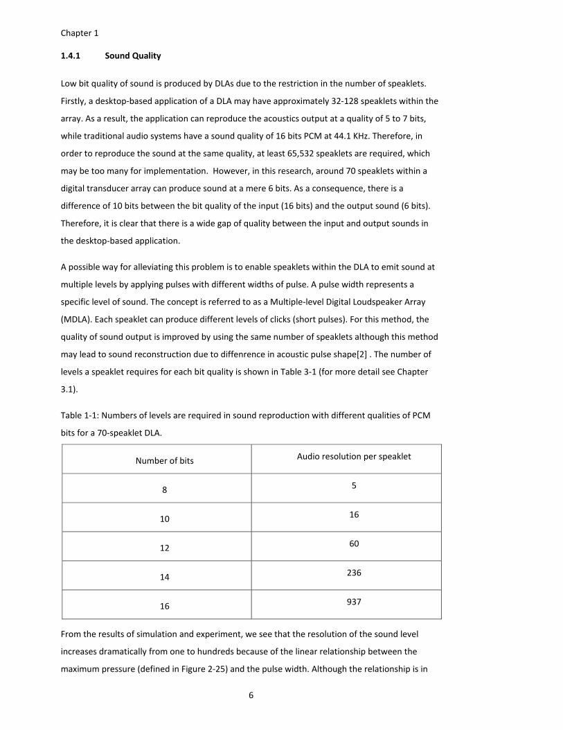
1.4.1 Sound Quality

Low bit quality of sound is produced by DLAs due to the restriction in the number of speaklets.

Firstly, a desktop‐based application of a DLA may have approximately 32‐128 speaklets within the

array. As a result, the application can reproduce the acoustics output at a quality of 5 to 7 bits,

while traditional audio systems have a sound quality of 16 bits PCM at 44.1 KHz. Therefore, in

order to reproduce the sound at the same quality, at least 65,532 speaklets are required, which

may be too many for implementation. However, in this research, around 70 speaklets within a

digital transducer array can produce sound at a mere 6 bits. As a consequence, there is a

difference of 10 bits between the bit quality of the input (16 bits) and the output sound (6 bits).

Therefore, it is clear that there is a wide gap of quality between the input and output sounds in

the desktop‐based application.

A possible way for alleviating this problem is to enable speaklets within the DLA to emit sound at

multiple levels by applying pulses with different widths of pulse. A pulse width represents a

specific level of sound. The concept is referred to as a Multiple‐level Digital Loudspeaker Array

(MDLA). Each speaklet can produce different levels of clicks (short pulses). For this method, the

quality of sound output is improved by using the same number of speaklets although this method

may lead to sound reconstruction due to diffenrence in acoustic pulse shape[2] . The number of

levels a speaklet requires for each bit quality is shown in Table 3‐1 (for more detail see Chapter

3.1).

Table 1‐1: Numbers of levels are required in sound reproduction with different qualities of PCM

bits for a 70‐speaklet DLA.

Number of bits Audio resolution per speaklet

8 5

10 16

12 60

14 236

16 937

From the results of simulation and experiment, we see that the resolution of the sound level

increases dramatically from one to hundreds because of the linear relationship between the

maximum pressure (defined in Figure 2‐25) and the pulse width. Although the relationship is in

Chapter 1

7

fact non‐linear, within a certain range of widths it becomes linear. The range depends on a pulse

period (inverse of pulse rate feeding to a speaklet) and the resolution is computed from the range

of linearity divided by a clock period (inverse of clock speed of digital pulse generator). In the

mathematical model, a speaklet has 937 levels, while the ultrasonic transducer in the experiment

has 1000 levels, as shown in Table 1‐2. The details are found in Chapter 3.3.1 and 4.1.3.4.2.

Because the computational logics of the digital pulse generator do not demand extensive

computation, if it is designed and fabricated by the Application‐Specific Integrated Circuit system

(ASICs) the clock speed would reach 1 GHz. With the chip, the DLA will require only 7 speaklets for

the reproduction of 16‐bit audio.

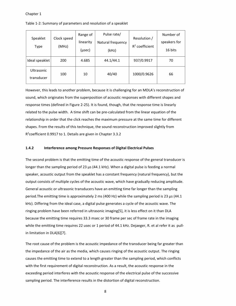
Chapter 1

8

Table 1‐2: Summary of parameters and resolution of a speaklet

Speaklet

Type

Clock speed

(MHz)

Range of

linearity

(μsec)

Pulse rate/

Natural frequency

(kHz)

Resolution /

R2 coefficient

Number of

speakers for

16 bits

Ideal speaklet 200 4.685 44.1/44.1 937/0.9917 70

Ultrasonic

transducer 100 10 40/40 1000/0.9626 66

However, this leads to another problem, because it is challenging for an MDLA’s reconstruction of

sound, which originates from the superposition of acoustic responses with different shapes and

response times (defined in Figure 2‐25). It is found, though, that the response time is linearly

related to the pulse width. A time shift can be pre‐calculated from the linear equation of the

relationship in order that the click reaches the maximum pressure at the same time for different

shapes. From the results of this technique, the sound reconstruction improved slightly from

R2coefficient 0.9917 to 1. Details are given in Chapter 3.3.2

1.4.2 Interference among Pressure Responses of Digital Electrical Pulses

The second problem is that the emitting time of the acoustic response of the general transducer is

longer than the sampling period of 23 µs (44.1 kHz). When a digital pulse is feeding a normal

speaker, acoustic output from the speaklet has a constant frequency (natural frequency), but the

output consists of multiple cycles of the acoustic wave, which have gradually reducing amplitude.

General acoustic or ultrasonic transducers have an emitting time far longer than the sampling

period.The emitting time is approximately 2 ms (400 Hz) while the sampling period is 23 µs (44.1

kHz). Differing from the ideal case, a digital pulse generates a cycle of the acoustic wave. The

ringing problem have been referred in ultrasonic imaging[5], it is less effect on it than DLA

because the emitting time requires 33.3 msec or 30 frame per sec of frame rate in the imaging

while the emitting time requires 22 usec or 1 period of 44.1 kHz. Dejaeger, R. et al refer it as pull‐

in limitation in DLA[6][7].

The root cause of the problem is the acoustic impedance of the transducer being far greater than

the impedance of the air as the media, which causes ringing of the acoustic output. The ringing

causes the emitting time to extend to a length greater than the sampling period, which conflicts

with the first requirement of digital reconstruction. As a result, the acoustic response in the

exceeding period interferes with the acoustic response of the electrical pulse of the successive

sampling period. The interference results in the distortion of digital reconstruction.

Chapter 1

9

The proposed method is to use double electrical pulses to stimulate a stroke of acoustic response.

The two electrical pulses should create oscillations of acoustic responses with different phases of

180 degrees. Therefore the oscillation of the two pulses start to cancel each other out, since the

phase of total acoustic output shifts 180 degrees, as shown in Figure 4‐5. The amplitude of the

total acoustic output, represented as the purple line in Figure 4‐5, reduces dramatically since the

second peak of oscillation of the response is similar to the ideal acoustic response of the DLA.

The driving speaklet pulses consist of two pulses of the same width. The first pulse is to stimulate

a speaklet to emit a stroke of acoustic output; the other pulse is tostop the vibration of the

diaphragm of the speaklet. The head‐to head period of the pulse couple is adjusted in order to

create the largest difference between the first peak and the second peak of the acoustic output

for a certain pulse width. It was found that the period is equal to a half period of the natural

frequency of the speaklet. However, this method can only be applied to a speaklet with a single

frequency of free vibration (more details in Chapter 4.1.3.2 and 4.1.2.2.3).

In the experiment in Chapter 4.1.2.2.4, the results did not meet expectations, because the total

response of the pulse couple were significantly attenuated. This results from the acoustic

response of the transducer not reaching the maximum amplitude at the first cycle of the

response, as shown in Figure 4‐4. The acoustic responses of the pulse couple cancel each other.

Because the emitting time cannot be reduced, interference among the acoustic pulses is allowed.

In other words, the first requirement is ignored. As a consequence of this, it is found that the

amplitude of acoustic response of each frequency of pulse rate depends on the frequency

response of the speaklet. The amplitude is maximized when the pulse rate is equal to the

resonant frequency, as shown in the experiments in Chapter 4.1.3. This occurrence is similar to

the application of the ordinary analogue electrical sinusoidal signal into a loudspeaker, but they

are different in the shape of the waveform.

1.4.3 Efficiency in Sound Generation

Sound generation from ultrasound is based on the principle of frequency beat. The research

involved in this area, uses a parametric array. The problem of sound generation is that loudness of

sound relies on the non‐linearity of an acoustic medium. As a result, the intensity of ultrasound is

high enough for an ultrasonic transducer array to generate sound with reasonable loudness[8].

This is described in detail in Chapter 2.2.3 and 4.1.4.

Due to the fact that the sound, which is generated from ultrasound, is in an AM waveform, the

sound can be considered according to the principle of telecommunication. This means that the

Chapter 1

10

sound is the modulated wave. People would not hear the sound if the acoustic medium was linear

(for more detail see Chapter 3.4.1 and 5.1.1).

From this point, in order to find a solution, the AM sound should be demodulated in order to

extract the sound, which is a modulating wave, from its carrier. The demodulation can be

performed by a loudspeaker, which is designed for the application of the condition of acoustic

rectification.

Although there is no concrete evidence for the rectifying loudspeaker, there is good evidence

from FEM simulation which shows that displacement is directly proportional to velocity (for more

detail see Chapter 0).

Another problem of sound generation from ultrasound is that the width of the sound beam of an

ultrasonic transducer is very narrow. The root causes are the flat diaphragm of the transducers

and their large diameters compared to the wavelengths of ultrasound. These characteristics result

in directional radiation of the transducers.

With the structure of the rectifying loudspeaker, there is clear evidence for a wide sound beam

from FEM simulation. The diameter hole, which is the velocity transition surface and acts like a

sound source, is tiny, at20 µm. The diaphragm of the loudspeaker vibrates at a frequency of 40

kHz. The beam width is 308 degrees (for more detail see Chapter 5.1.4.1).

In addition, the sound source of the loudspeaker is a secondary source, which is not a physical but

a virtual acoustic surface. The acoustic surface is derived from the collision of a huge number of

air particles and a rapid change in air velocity. The surface has a curved shape, as shown in Figure

5‐10.

1.5 Scope of Work

This thesis is written to explore the feasibility of the implementation of a DLA, but not to design

and fabricate the array. The work concentrates on sound generated from ultrasound. The method

of exploration is quick observation of hearing on frequency only, and study focusing on

conception, but with little detail on design and fabrication.

Identifying whether DLA can reproduce sound or whether humans can hear it, because

speaklets within the array generate sound from ultrasound. Normally sound humans can

hear is identified by frequency and sound level, but frequency is the primary factor,

because if the frequency of a wave is out of the audible frequency range, humans cannot

hear it, however high the amplitude of ultrasound. Therefore, this research focuses only

Chapter 1

11

on frequencies of emitted waves, while sound levels are ignored, because sound level is

related to design and fabrication.

Differentiating between a DLA and an analogue loudspeaker, and analysis of their

advantages and disadvantages based on the concept of sound generation, not based on

their structure or the fabrication of speaklets. Most of the work involved mathematical

modelling and finite element modelling (FEM). Experiments were conducted to

investigate the relationships between electrical inputs, pressure outputs and the

frequency responses of speaklet samples. The samples are not prototypes but on‐shelf

transducers.

1.6 Contribution

In study about feasibility of implementing speaklets for DLA concept, we discover

1.6.1 Three Requirement of Digital Sound Reconstruction

Implementing speaklets within Digital Loudspeaker Array (DLA) is investigated by basing on the

three requirement of digital sound reconstruction described in Section 2.3.3

For the first requirement, due to the short emitting time of impulse responses in ten

microseconds of the speaklet, Chapter 3 found that the dumping ratio of the speaklet

requires 0.8 at 44.1 kHz to meet this requirement. Chapter 4 did not find a speaklet with

the required dumping ratio from real electro‐acoustic transducers and FEMs. Therefore,

the speaklet for this requirement cannot be found in this study.

Regarding the second requirement, the uniformity in the impulse response of the

speaklet with the array cannot be investigated because this requirement has to be tested

after fabrication process of speaklet.

For the third requirement, the linearity in amplitude of impulse response, with MDLA

concept, mathematical model speaklets, FEM speaklets and real transducers met this

requirement.

1.6.2 MDLA.

The concept of the Multiple‐level Digital Loudspeaker Array (MDLA) is innovatively

applied as an alternative method to produce amplitude modulation (AM) sound which is

generated from the ultrasound. The concept of AM sound is developed from Audio

Spotlight technology[9] which is the commercial name of a parametric array. The AM

applies analogue electrical drive while MDLA applies digital one.

Chapter 1

12

The new concept is extended from Digital Loudspeaker Array (DLA) by the application of

the Pulse Width Modulation (PWM) which is the fundamental technique for robots in

motor speed control.

1.6.3 Rectifying loudspeaker

A rectifying loudspeaker introduces a constant supply of air pressure into the sound

generating system while the common loudspeakers have merely electrical supplies. A

main goal of the loudspeaker is to produce half‐wave rectified AM sound to improve the

efficiency of sound generation. The word “rectifying” refers to the method of amplitude

demodulation which is the original technique of radio broadcasting.

The structure of the rectified loudspeaker is adapted from the human voice system, and

can be fabricated by MEMs. A vibrating disc or diaphragm of the loudspeaker primarily

applies as a valve for speed control of air particles from the pump to an air cone outlet.

As a result, the air particles in front of a hole within the outlet of the loudspeaker move

only in one direction, i.e. moving forwards and not going backwards. The air particles in

front of diaphragms of common loudspeakers, on the other hand, move back and forth

according to the movement of the diaphragms.

1.7 Document Structure

This thesis is divided into six chapters:

Chapter 2 provides a thorough background of acoustics, hearing and sound generation from

loudspeakers, ultrasound and humans. It reviews the concept of DLA, which is the main topic of

this thesis. It shows the fundamentals of the mathematical model of vibration and acoustic

radiation. The radiation covers both steady‐state and transient‐state radiation.

Chapter 3‐6 describes the original work:

Chapter 3 describes the mathematical model for speaklets within DLA, the conditions of acoustic

rectification and application of the model, and the conditions according to the requirements of

digital sound reconstruction.

Chapter 4 describes the experiments in application of the loudspeaker according to the concept of

DLA. It also includes a study of the design of PZT‐ based transducers as DLA with FEM modelling.

Chapter 5 describes the principles and structure of a rectifying loudspeaker, and performs

validation of the structure according to the conditions of acoustic rectification.

Chapter 1

13

Chapter 6 summarizes the conclusion discussed in this thesis and provides recommendations for

the design of the loudspeaker and future research for this area.

1.8 Publication

Monkronthong, S. White, N and Harris, N. “Multiple‐Level Digital Loudspeaker Array”, the 28th

European Conference on Solid‐State Transducers, September 2014

Monkronthong, S. White, N and Harris, N. “A study of efficient speaklet driving mechanisms for

use in a digital loudspeaker array based on PZT actuators”, the Sensors Application Symposium

2016, April 2016.

Chapter 2

15

Chapter 2: A Review of Sound Generation and Digital

Loudspeaker Array

The concept of a digital loudspeaker array (DLA) was first published in 2002 by Busbridge et al

and Diamond et al [1][2]. The digital loudspeaker array consists of a number of speaklets (tiny

loudspeakers), each of which is driven by a stream of rectangular pulses with constant width and

amplitude in order to produce sound. Tatlas et al studied in topologies of speaklets effect on

acoustic distortion in 2004[10]. Although, there were patents of digital loudspeakers, which

consist of multiple piezoelectric transducers with different sizes in 1963 or multiple voice coils in

1977, they were not tiny loudspeakers and do not conform with the concept of DLA[11]. A few

groups conduct experiment with available small loudspeakers[12][13]. In 2006, Audio Pixels

Limited was founded. They employ the concept of DLA to generate sound by using low cost

microelectromechanical systems (MEMs)[3].In 2012 Dejaeger et al started to fabricate 64‐

speaklet DLA and in 2015 they fabricated 256‐speaklets of DLA with 2.6 mm diameter. They claim

that it produces the sound level of 100 dBSPL at 13 cm from the array[6][7]. Throughout the past

ten years, a very limited number of reseachers work in this area. This may be because the

significant problem with the DLA is that the bit quality of the acoustic output depends on the

number of speaklets. Typically, for conventional audio systems, this is 16 bits. Consequently, a

DLA would require 65532 speaklets in order to reproduce the sound at the same quality as a

conventional loudspeaker. We propose a concept of a multiple‐level digital loudspeaker (MDLA)

which increases the number of levels of sound that a speaklet can emit. The detail will be given in

Chapter 3.

In order to investigate feasibility of implement of multiple‐level digital loudspeaker array (MDLA),

which is a technique of making sound from ultrasonic with digital voltage driver, this chapter gives

background knowledge to the investigation. This chapter is divided into four main sections. The

first section briefs on characteristics of sound and ultrasound waves. The wave behaviours such as

attenuation and reflection are described in similarity and difference between sound and

ultrasound. Effects of the waves on humans such as loudness of sound and risks are identified.

This will give enough information to understand principles of sound and ultrasound waves for

readers with no acoustic backgrounds. The second section investigates some available

technologies, which are used for making loudspeakers and ultrasonic transducers, such as

piezoelectric and electromagnetic technologies. Excitation force of each loudspeaker will be

expressed in terms of specifications of the loudspeaker such as driving voltage, the inductance of

a coil and the capacitance of piezoelectric transducer. The forces will be mathematically analysed

Chapter 2

16

in Chapter 4 for digital voltage driver and evaluation of the technologies for MDLA. A parametric

array is a technology for making sound from ultrasound, which is similar to MDLA but it feeds

electrical analogue signal. It is interesting because this technology has launched some commercial

products. The technology is referred as audio spotlight. The airborne output will be used as a

reference to compare with the output of MDLA in Chapter 3 and 4. It will describe how the array

makes sounds. Voice system of a human is another sound generator, which is basics of the new

structure of loudspeaker proposed in Chapter 5. The third section reviews concepts of digital

loudspeaker array (DLA) MDLA is developed from. The final section gives a detail about the

mathematical model of vibration and wave radiation. The radiation model cover the steady state

case, which is applied for normal (analogue) loudspeaker and the transient‐state case, which are

derived for a digital loudspeaker. The session prepares a basis for analysing the ideal model in

Chapter 3.

2.1 Sound and Ultrasonic

Waves can be categorized into two types: mechanical and electromagnetic. Transverse

electromagnetic waves do not need any medium, while transverse mechanical waves do need a

medium. In other words, mechanical waves cannot propagate through a vacuum. Sound and

ultrasound waves are mechanical waves and travel on a medium at the same speed. The speed of

propagation of a mechanical wave is determined by the density and the stiffness of the medium it

is travelling in. Sound and ultrasound are longitudinal waves, in which the vibration of the

molecules in the medium is in the same direction as the propagation of the overall wave. A period

of the longitudinal wave consists of one cycle of compression and rarefaction of atmospheric

pressure. However, they are different in the range of frequencies. The range of frequencies of

sound is between 20 Hz and 20 kHz, while the range of frequencies of ultrasound is above 20

kHz[14].

2.1.1 Wave Propagation

Sound and ultrasound waves can be generated from the movement of a piston or a diaphragm.

They travel through the air with a constant speed. In order to understand the mechanism of

propagation of an acoustic wave, which involves acoustic pressure and airflow rate, the process

may be conceptually, but not actually described as a piston mounted in the end of a uniform

square pipe.The air inside the pipe may be divided into cubes, which are linearly aligned. The air

blocks are conceptually formed and their surfaces are joined together and bonded with a high

damping spring. Similarly, the surface of the piston is attached to the surface of the air block, as

shown in Figure 2‐1.

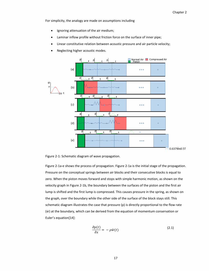
Chapter 2

17

For simplicity, the analogy are made on assumptions including

Ignoring attenuation of the air medium;

Laminar inflow profile without friction force on the surface of inner pipe;

Linear constitutive relation between acoustic pressure and air particle velocity;

Neglecting higher acoustic modes.

Figure 2‐1: Schematic diagram of wave propagation.

Figure 2‐1a‐e shows the process of propagation. Figure 2‐1a is the initial stage of the propagation.

Pressure on the conceptual springs between air blocks and their consecutive blocks is equal to

zero. When the piston moves forward and stops with simple harmonic motion, as shown on the

velocity graph in Figure 2‐1b, the boundary between the surfaces of the piston and the first air

lump is shifted and the first lump is compressed. This causes pressure in the spring, as shown on

the graph, over the boundary while the other side of the surface of the block stays still. This

schematic diagram illustrates the case that pressure (p) is directly proportional to the flow rate

( ) at the boundary, which can be derived from the equation of momentum conservation or

Euler’s equation[14]:

(2.1)

Chapter 2

18

where and x are density of air. The wave speed (c), which is constant, is substituted in the

equation and both sides of the equation are taken by the integral of dt The equation can be

expressed as[14]:

(2.2)

If is the simple harmonic motion of the boundary, it is defined as:

(2.3)

is a constant amplitude of velocity and ω is the circular frequency in radians per second. It can

be expressed as [14]:

2

(2.4)

T is a repeating period of the simple harmonic. The next stage in Figure 2‐1c, when the first block

returns to its original shape, the boundary between the piston and itself stays still, but it pushes

the boundary between itself and the second block, causing it to shift with velocity, as shown in

the velocity graph. As a result of the boundary shifting with (t), pressure on the spring between

the first and second blocks rises in direct relation to , while pressure on the other spring of

the first chunk drops to zero. This shows momentum energy transfer from the first lump to the

second lump. In the next stage in Figure 2‐1d, the process is similar to the previous stage but the

forward movement of the boundary between the second and the third chunks results in the

second chunk returning to its original shape, but the third chunk being compressed. This causes

the acoustic pressure on the abstract spring to move from the spring between the first and

second chunks to the spring between the second and third chunks. In Figure 2‐1e, the acoustic

pressure will travel through the train of chunks with a constant speed of c, while the air chunks in

the flow move with a displacement of ∗ /2. The average velocity can be computed

from:

sin 0.637 (2.5)

2.1.2 Characteristics of Acoustic Wave

An acoustic wave is a wave derived from an oscillation of particles and transferring energy

through a medium. There are four major characteristics of a wave: frequency, wavelength, speed

and amplitude.

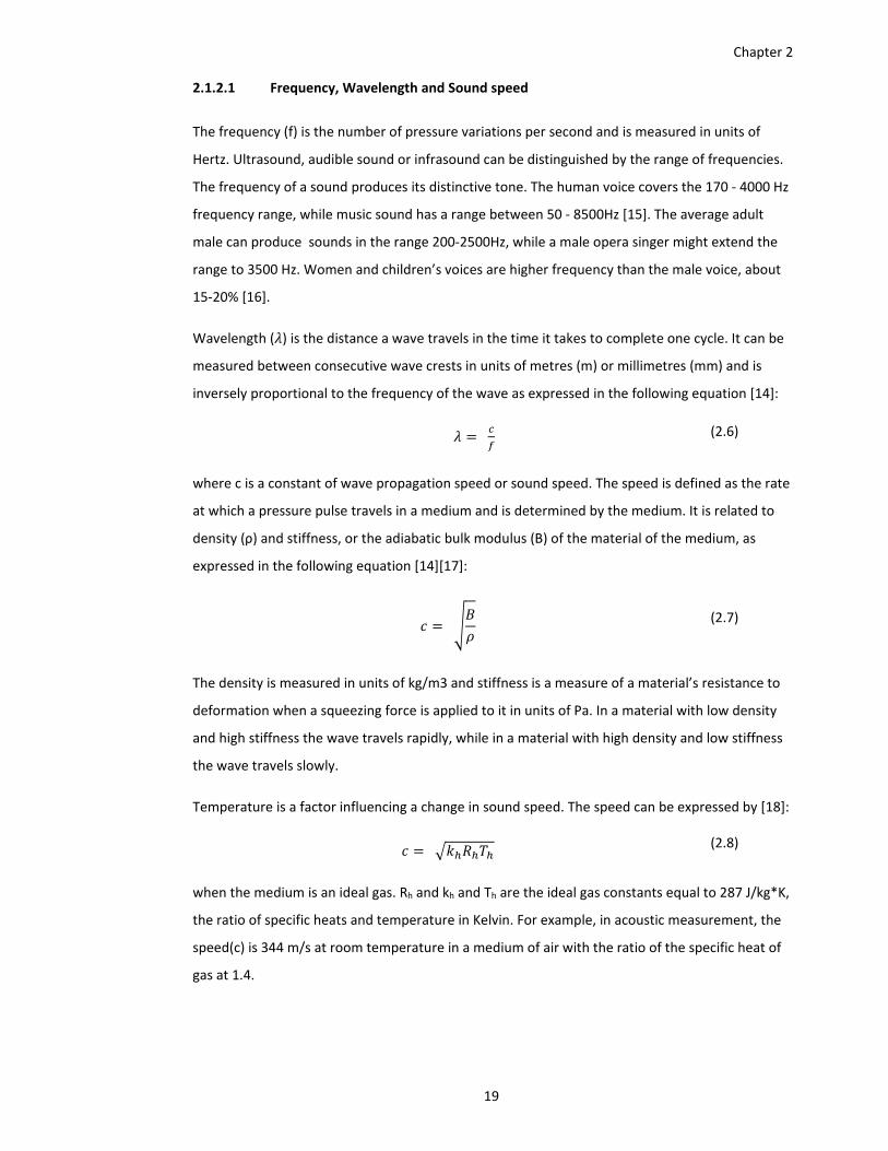
Chapter 2

19

2.1.2.1 Frequency, Wavelength and Sound speed

The frequency (f) is the number of pressure variations per second and is measured in units of

Hertz. Ultrasound, audible sound or infrasound can be distinguished by the range of frequencies.

The frequency of a sound produces its distinctive tone. The human voice covers the 170 ‐ 4000 Hz

frequency range, while music sound has a range between 50 ‐ 8500Hz [15]. The average adult

male can produce sounds in the range 200‐2500Hz, while a male opera singer might extend the

range to 3500 Hz. Women and children’s voices are higher frequency than the male voice, about

15‐20% [16].

Wavelength ( ) is the distance a wave travels in the time it takes to complete one cycle. It can be

measured between consecutive wave crests in units of metres (m) or millimetres (mm) and is

inversely proportional to the frequency of the wave as expressed in the following equation [14]:

(2.6)

where c is a constant of wave propagation speed or sound speed. The speed is defined as the rate

at which a pressure pulse travels in a medium and is determined by the medium. It is related to

density (ρ) and stiffness, or the adiabatic bulk modulus (B) of the material of the medium, as

expressed in the following equation [14][17]:

(2.7)

The density is measured in units of kg/m3 and stiffness is a measure of a material’s resistance to

deformation when a squeezing force is applied to it in units of Pa. In a material with low density

and high stiffness the wave travels rapidly, while in a material with high density and low stiffness

the wave travels slowly.

Temperature is a factor influencing a change in sound speed. The speed can be expressed by [18]:

(2.8)

when the medium is an ideal gas. Rh and kh and Th are the ideal gas constants equal to 287 J/kg*K,

the ratio of specific heats and temperature in Kelvin. For example, in acoustic measurement, the

speed(c) is 344 m/s at room temperature in a medium of air with the ratio of the specific heat of

gas at 1.4.

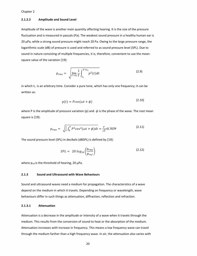
Chapter 2

20

2.1.2.2 Amplitude and Sound Level

Amplitude of the wave is another main quantity affecting hearing. It is the size of the pressure

fluctuation and is measured in pascals (Pa). The weakest sound pressure in a healthy human ear is

20 µPa, while a strong sound pressure might reach 20 Pa. Owing to the large pressure range, the

logarithmic scale (dB) of pressure is used and referred to as sound pressure level (SPL). Due to

sound in nature consisting of multiple frequencies, it is, therefore, convenient to use the mean‐

square value of the variation [19]:

lim→

1

(2.9)

in which t1 is an arbitrary time. Consider a pure tone, which has only one frequency; it can be

written as:

(2.10)

where P is the amplitude of pressure variation (p) and is the phase of the wave. The root mean

square is [19]:

√=0.707P

(2.11)

The sound pressure level (SPL) in decibels (dBSPL) is defined by [19]:

20 (2.12)

where pref is the threshold of hearing, 20 µPa.

2.1.3 Sound and Ultrasound with Wave Behaviours

Sound and ultrasound waves need a medium for propagation. The characteristics of a wave

depend on the medium in which it travels. Depending on frequency or wavelength, wave

behaviours differ in such things as attenuation, diffraction, reflection and refraction.

2.1.3.1 Attenuation

Attenuation is a decrease in the amplitude or intensity of a wave when it travels through the

medium. This results from the conversion of sound to heat or the absorption of the medium.

Attenuation increases with increase in frequency. This means a low frequency wave can travel

through the medium farther than a high frequency wave. In air, the attenuation also varies with

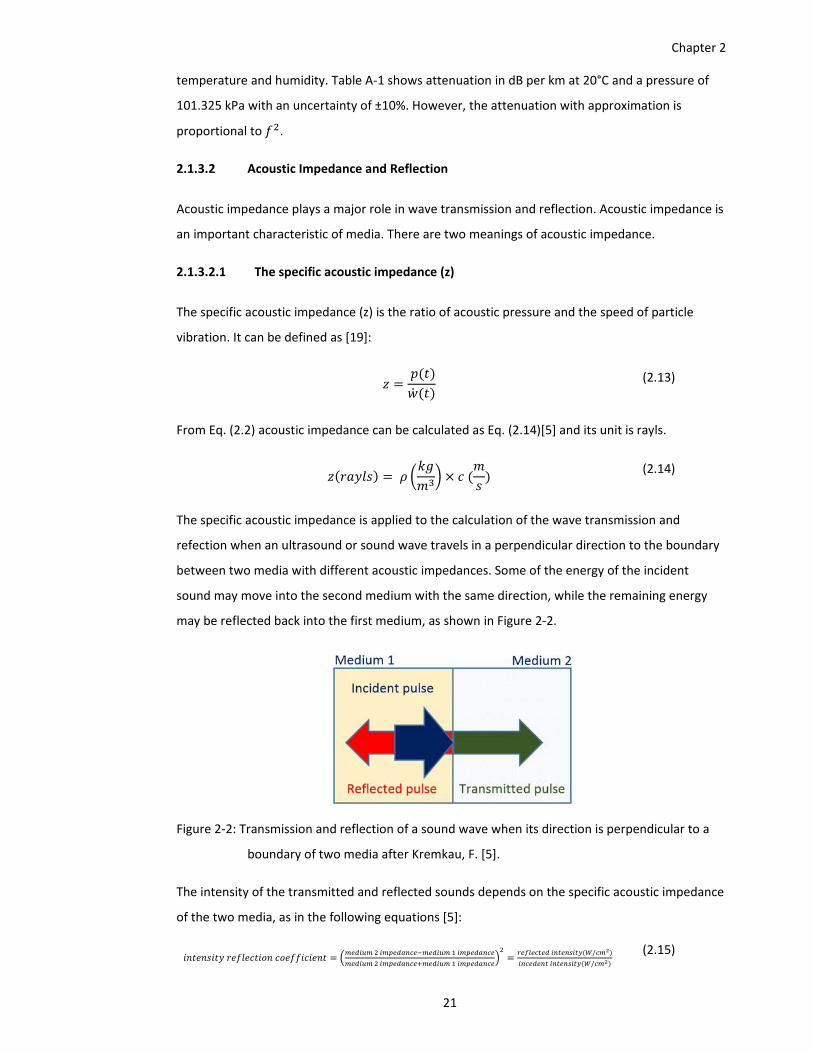
Chapter 2

21

temperature and humidity. Table A‐1 shows attenuation in dB per km at 20°C and a pressure of

101.325 kPa with an uncertainty of ±10%. However, the attenuation with approximation is

proportional to .

2.1.3.2 Acoustic Impedance and Reflection

Acoustic impedance plays a major role in wave transmission and reflection. Acoustic impedance is

an important characteristic of media. There are two meanings of acoustic impedance.

2.1.3.2.1 The specific acoustic impedance (z)

The specific acoustic impedance (z) is the ratio of acoustic pressure and the speed of particle

vibration. It can be defined as [19]:

(2.13)

From Eq. (2.2) acoustic impedance can be calculated as Eq. (2.14)[5] and its unit is rayls.

(2.14)

The specific acoustic impedance is applied to the calculation of the wave transmission and

refection when an ultrasound or sound wave travels in a perpendicular direction to the boundary

between two media with different acoustic impedances. Some of the energy of the incident

sound may move into the second medium with the same direction, while the remaining energy

may be reflected back into the first medium, as shown in Figure 2‐2.

Figure 2‐2: Transmission and reflection of a sound wave when its direction is perpendicular to a

boundary of two media after Kremkau, F. [5].

The intensity of the transmitted and reflected sounds depends on the specific acoustic impedance

of the two media, as in the following equations [5]:

/

/ (2.15)

Chapter 2

22

1

/ 2

/ 2

(2.16)

where intensity reflection coefficient is the fraction of the reflected intensity divided by the

incident intensity and intensity transmission coefficient is the fraction of the transmitted intensity

divided by the incident intensity.

From Eq. (2.15), the dB loss of energy can be obtained as Eq. (2.17) when the reflected intensity is

considered as loss [5]:

10 (2.17)

From these equations, it can be seen that when sound travels from one medium to another with a

different acoustic impedance, there will be loss of energy whenever it travels from high

impedance to low impedance or from low impedance to high impedance.

2.1.3.2.2 The acoustic impedance (Z)

The acoustic impedance (Z) is defined as the ratio of acoustic pressure to acoustic volume flow (q)

[19]:

(2.18)

The volume flow q(t) depends on the shape of duct[19].

(2.19)

where (a) is the cross‐sectional area of a duct. The relationship between acoustic impedance and

the specific acoustic impedance is expressed in Eq.(2.18).

The acoustic impedance is applied to the calculation of the wave transmission and refection when

an ultrasound or sound wave travels in the same medium but in different shape of duct. The size

of the duct will affect the change in acoustic impedance. As a result, the effect on the reflected

and transmitted waves at the boundary of change of size of duct is similar to a change in medium.

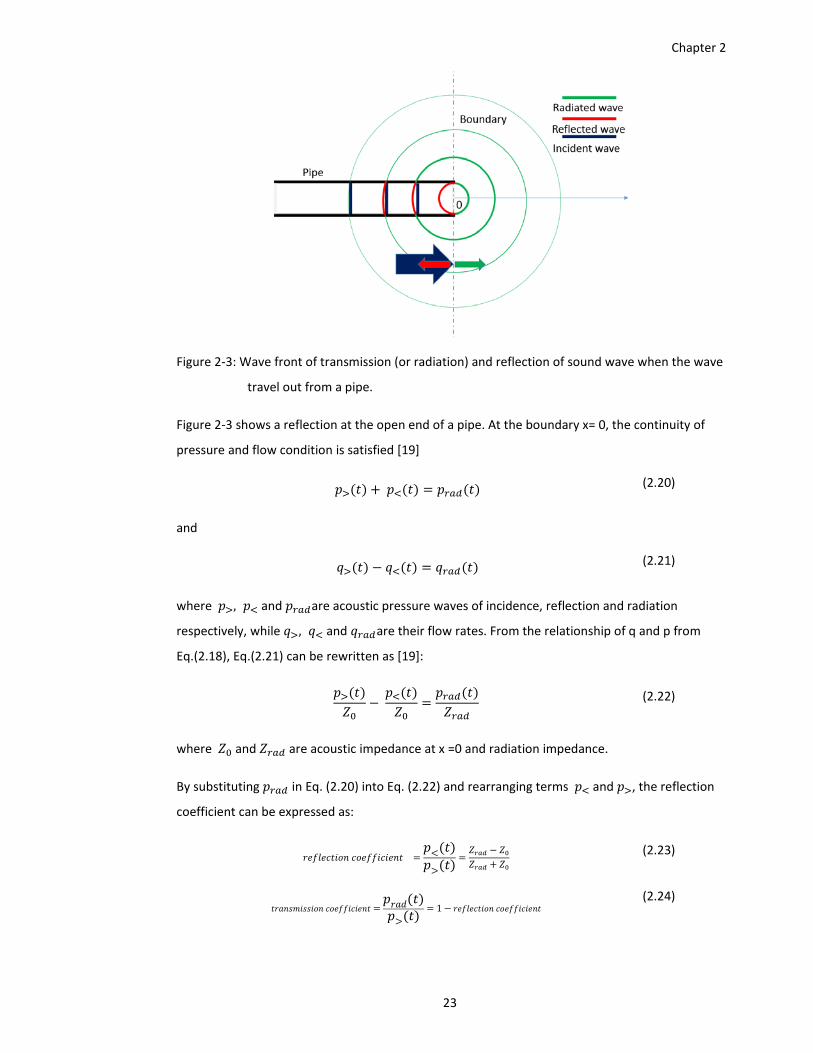
Chapter 2

23

Figure 2‐3: Wave front of transmission (or radiation) and reflection of sound wave when the wave

travel out from a pipe.

Figure 2‐3 shows a reflection at the open end of a pipe. At the boundary x= 0, the continuity of

pressure and flow condition is satisfied [19]

(2.20)

and

(2.21)

where , and are acoustic pressure waves of incidence, reflection and radiation

respectively, while , and are their flow rates. From the relationship of q and p from

Eq.(2.18), Eq.(2.21) can be rewritten as [19]:

(2.22)

where and are acoustic impedance at x =0 and radiation impedance.

By substituting in Eq. (2.20) into Eq. (2.22) and rearranging terms and , the reflection

coefficient can be expressed as:

(2.23)

1 (2.24)

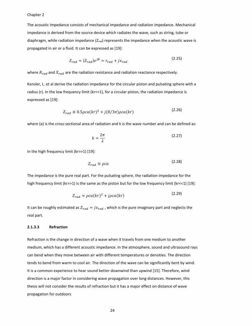
Chapter 2

24

The acoustic Impedance consists of mechanical impedance and radiation impedance. Mechanical

impedance is derived from the source device which radiates the wave, such as string, tube or

diaphragm, while radiation impedance (Zrad) represents the impedance when the acoustic wave is

propagated in air or a fluid. It can be expressed as [19]:

| | (2.25)

where and are the radiation resistance and radiation reactance respectively.

Kensler, L. et al derive the radiation impedance for the circular piston and pulsating sphere with a

radius (r). In the low frequency limit (kr<<1), for a circular piston, the radiation impedance is

expressed as [19]:

≅ 0.5 8/3 (2.26)

where (a) is the cross‐sectional area of radiation and k is the wave number and can be defined as:

2

(2.27)

In the high frequency limit (kr>>1) [19]:

≅ (2.28)

The impedance is the pure real part. For the pulsating sphere, the radiation impedance for the

high frequency limit (kr>>1) is the same as the piston but for the low frequency limit (kr<<1) [19]:

(2.29)

It can be roughly estimated as , which is the pure imaginary part and neglects the

real part.

2.1.3.3 Refraction

Refraction is the change in direction of a wave when it travels from one medium to another

medium, which has a different acoustic impedance. In the atmosphere, sound and ultrasound rays

can bend when they move between air with different temperatures or densities. The direction

tends to bend from warm to cool air. The direction of the wave can be significantly bent by wind.

It is a common experience to hear sound better downwind than upwind [15]. Therefore, wind

direction is a major factor in considering wave propagation over long distances. However, this

thesis will not consider the results of refraction but it has a major effect on distance of wave

propagation for outdoors

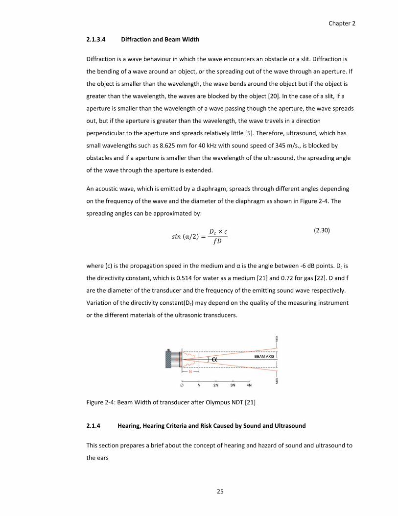
Chapter 2

25

2.1.3.4 Diffraction and Beam Width

Diffraction is a wave behaviour in which the wave encounters an obstacle or a slit. Diffraction is

the bending of a wave around an object, or the spreading out of the wave through an aperture. If

the object is smaller than the wavelength, the wave bends around the object but if the object is

greater than the wavelength, the waves are blocked by the object [20]. In the case of a slit, if a

aperture is smaller than the wavelength of a wave passing though the aperture, the wave spreads

out, but if the aperture is greater than the wavelength, the wave travels in a direction

perpendicular to the aperture and spreads relatively little [5]. Therefore, ultrasound, which has

small wavelengths such as 8.625 mm for 40 kHz with sound speed of 345 m/s., is blocked by

obstacles and if a aperture is smaller than the wavelength of the ultrasound, the spreading angle

of the wave through the aperture is extended.

An acoustic wave, which is emitted by a diaphragm, spreads through different angles depending

on the frequency of the wave and the diameter of the diaphragm as shown in Figure 2‐4. The

spreading angles can be approximated by:

α/2 (2.30)

where (c) is the propagation speed in the medium and α is the angle between ‐6 dB points. Dc is

the directivity constant, which is 0.514 for water as a medium [21] and 0.72 for gas [22]. D and f

are the diameter of the transducer and the frequency of the emitting sound wave respectively.

Variation of the directivity constant(Dc) may depend on the quality of the measuring instrument

or the different materials of the ultrasonic transducers.

Figure 2‐4: Beam Width of transducer after Olympus NDT [21]

2.1.4 Hearing, Hearing Criteria and Risk Caused by Sound and Ultrasound

This section prepares a brief about the concept of hearing and hazard of sound and ultrasound to

the ears

Chapter 2

26

2.1.4.1 Hearing

Any pressure variation in the air that the human ear can detect may be defined as sound, while

ultrasound is also a pressure variation, but humans cannot perceive it because the frequencies

are too high. Besides frequency, amplitude of sound pressure is another main factor in human

hearing. The human ear is not equally sensitive at all frequencies. In order to give the same

subjective loudness, different frequency tones must be produced at different sound levels, as

shown in this set of equal loudness contours, Figure 2‐5

Figure 2‐5: Robinson‐Dadson curves are one of many sets of equal‐loudness contours for the

human ear after Gelfand, S.[23].

Loudness can be defined as the perceived sound level, while sound level can be defined as the

magnitude of the sound exposure. In order to make loudness in all frequencies have the same or

nearly the same values, the sound level in dBSPL is multiplied by A‐weighting values (An), which

match with the frequencies, as shown in Table B‐1. Sound loudness level ( ) in units of dBA can

be computed by [24]:

10 10

(2.31)

where all frequency is composed of the sound or noise. The A‐weighting is commonly used as the

weighting when referring to health and safety noise exposure levels. For example, sound sources

and their common sound levels are shown in Table 2‐1. Below 85 dBA for 8 hours is considered

safe by Health and Safety Executives. However, A‐weighting is not defined for frequencies over 20

kHz.

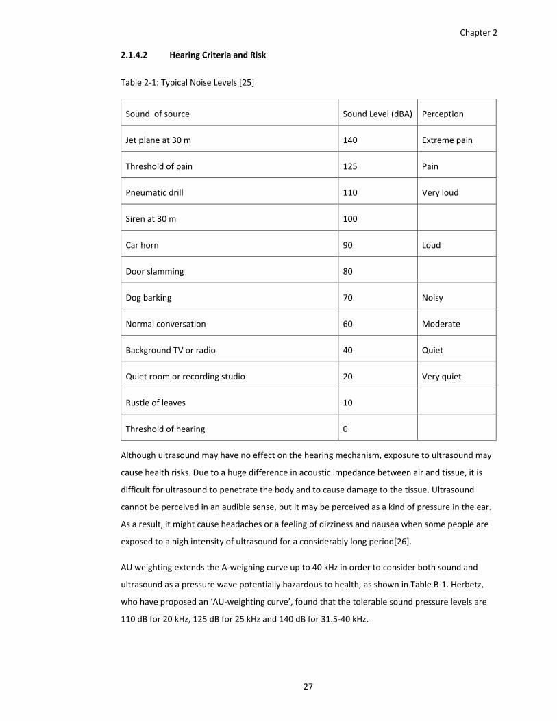
Chapter 2

27

2.1.4.2 Hearing Criteria and Risk

Table 2‐1: Typical Noise Levels [25]

Sound of source Sound Level (dBA) Perception

Jet plane at 30 m 140 Extreme pain

Threshold of pain 125 Pain

Pneumatic drill 110 Very loud

Siren at 30 m 100

Car horn 90 Loud

Door slamming 80

Dog barking 70 Noisy

Normal conversation 60 Moderate

Background TV or radio 40 Quiet

Quiet room or recording studio 20 Very quiet

Rustle of leaves 10

Threshold of hearing 0

Although ultrasound may have no effect on the hearing mechanism, exposure to ultrasound may

cause health risks. Due to a huge difference in acoustic impedance between air and tissue, it is

difficult for ultrasound to penetrate the body and to cause damage to the tissue. Ultrasound

cannot be perceived in an audible sense, but it may be perceived as a kind of pressure in the ear.

As a result, it might cause headaches or a feeling of dizziness and nausea when some people are

exposed to a high intensity of ultrasound for a considerably long period[26].

AU weighting extends the A‐weighing curve up to 40 kHz in order to consider both sound and

ultrasound as a pressure wave potentially hazardous to health, as shown in Table B‐1. Herbetz,

who have proposed an ‘AU‐weighting curve’, found that the tolerable sound pressure levels are

110 dB for 20 kHz, 125 dB for 25 kHz and 140 dB for 31.5‐40 kHz.

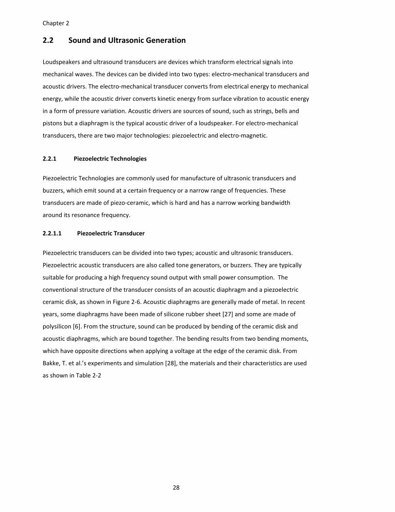
Chapter 2

28

2.2 Sound and Ultrasonic Generation

Loudspeakers and ultrasound transducers are devices which transform electrical signals into

mechanical waves. The devices can be divided into two types: electro‐mechanical transducers and

acoustic drivers. The electro‐mechanical transducer converts from electrical energy to mechanical

energy, while the acoustic driver converts kinetic energy from surface vibration to acoustic energy

in a form of pressure variation. Acoustic drivers are sources of sound, such as strings, bells and

pistons but a diaphragm is the typical acoustic driver of a loudspeaker. For electro‐mechanical

transducers, there are two major technologies: piezoelectric and electro‐magnetic.

2.2.1 Piezoelectric Technologies

Piezoelectric Technologies are commonly used for manufacture of ultrasonic transducers and

buzzers, which emit sound at a certain frequency or a narrow range of frequencies. These

transducers are made of piezo‐ceramic, which is hard and has a narrow working bandwidth

around its resonance frequency.

2.2.1.1 Piezoelectric Transducer

Piezoelectric transducers can be divided into two types; acoustic and ultrasonic transducers.

Piezoelectric acoustic transducers are also called tone generators, or buzzers. They are typically

suitable for producing a high frequency sound output with small power consumption. The

conventional structure of the transducer consists of an acoustic diaphragm and a piezoelectric

ceramic disk, as shown in Figure 2‐6. Acoustic diaphragms are generally made of metal. In recent

years, some diaphragms have been made of silicone rubber sheet [27] and some are made of

polysilicon [6]. From the structure, sound can be produced by bending of the ceramic disk and

acoustic diaphragms, which are bound together. The bending results from two bending moments,

which have opposite directions when applying a voltage at the edge of the ceramic disk. From

Bakke, T. et al.’s experiments and simulation [28], the materials and their characteristics are used

as shown in Table 2‐2

Chapter 2

29

Figure 2‐6:a) Typical acoustic transducer after Uchino, K.[29] b) MEMS Speaklet after Dejaeger, R.

et al[6] c) piezoelectric acoustic actuator after Kim, H. et al [27].

Table 2‐2: Material and their characteristics for acoustic transducers following Figure 2‐6b [28]

Material Thickness

(nm)

Pre‐stress

(MPa)

Young’s

modulus

(GPa)

Poisson ratio Density

(kg/m)3

Au 214 282 78 0.44 19,300

PZT 1888[28],

360[6]

110 PZT‐5A PZT‐5A 7,750

Pt 198 839 168 0.38 21,090

SiO2 2319 ‐177 70 0.3 2,200

Si 7077 0 170 0.28 2,330

The vibration of the piezo‐buzzer results from applying an alternating voltage to the electrodes of

the transducer. The electrical alternation makes the transducer, which is attached to the

diaphragm, extend and shrink. This causes bending of the diaphragm, both concave and convex. If

the diaphragm vibrates rapidly, a sound wave will be generated.

The first natural frequency can be typically calculated by Eq.(2.32)[30][31]:

Chapter 2

30

1

(2.32)

where rshape is a shape constant depending on the ratio of length to width. Constants of rshape are

1.654 for a square diaphragm [30] and 1.648 for a circular diaphragm [31]. D is the diameter for a

circular, or the length for a square diaphragm, while h is the thickness of the diaphragm. Y, and

are Young’s modulus, Poisson’s ratio and density of the ceramic material (kg / m).

For small microstructures, the surface and friction forces are additionally considered for the

volume and inertial effects. Therefore, the first natural frequency is also affected by the

compressive or tensile stress (T), which appears on the films, as shown in Eq.(2.33) [30]:

1

(2.33)

Piezoelectric ceramics can consist of a single active layer (bending‐mode) or multiple active layers

(multilayer mode). Generally, a bending mode actuator produces a smaller force but a larger

displacement than the multilayer mode actuator. Therefore, most acoustic applications are

designed with the bending mode because it provides large displacement at low voltage. However,

Kim, H. et al [27] proposed a multilayer mode actuator, which consists of three active multilayers

of piezoelectric elements or multimorph, with larger displacement and larger generative force in

2014. They show that the serial multimorph in serial connection (SMS) and the parallel

multimorph in parallel connection (PMP) configuration produce a large displacement and a large

force. SMS consists of two tripled‐layer multimorphs, which are serially connected during

polarization and electric field drive. PMP consists of two triple‐layered multimorphs, which are

parallel connected during polarization and electric field drive, shown in Figure 2‐7. The acoustic

actuators fabricated with the configuration of SMS and PMP and assembled according to Figure

2‐6c had high average sound pressure levels (SPLs) of 83.1 and 85.7 at a distance of 10 cm.

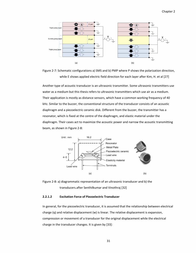
Chapter 2

31

Figure 2‐7: Schematic configurations a) SMS and b) PMP where P shows the polarization direction,

while E shows applied electric field direction for each layer after Kim, H. et al [27]

Another type of acoustic transducer is an ultrasonic transmitter. Some ultrasonic transmitters use

water as a medium but this thesis refers to ultrasonic transmitters which use air as a medium.

Their application is mostly as distance sensors, which have a common working frequency of 40

kHz. Similar to the buzzer, the conventional structure of the transducer consists of an acoustic

diaphragm and a piezoelectric ceramic disk. Different from the buzzer, the transmitter has a

resonator, which is fixed at the centre of the diaphragm, and elastic material under the

diaphragm. Their cases act to maximize the acoustic power and narrow the acoustic transmitting

beam, as shown in Figure 2‐8:

Figure 2‐8: a) diagrammatic representation of an ultrasonic transducer and b) the

transducers.after Senthilkumar and Vinothraj [32]

2.2.1.2 Excitation Force of Piezoelectric Transducer

In general, for the piezoelectric transducer, it is assumed that the relationship between electrical

charge (q) and relative displacement (w) is linear. The relative displacement is expansion,

compression or movement of a transducer for the original displacement while the electrical

charge in the transducer changes. It is given by [33]:

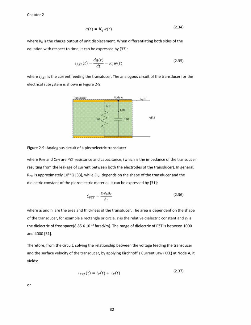
Chapter 2

32

(2.34)

where Kq is the charge output of unit displacement. When differentiating both sides of the

equation with respect to time, it can be expressed by [33]:

(2.35)

where is the current feeding the transducer. The analogous circuit of the transducer for the

electrical subsystem is shown in Figure 2‐9.

Figure 2‐9: Analogous circuit of a piezoelectric transducer

where RPZT and CPZT are PZT resistance and capacitance, (which is the impedance of the transducer

resulting from the leakage of current between both the electrodes of the transducer). In general,

RPZT is approximately 1011 Ω [33], while CPZT depends on the shape of the transducer and the

dielectric constant of the piezoelectric material. It can be expressed by [31]:

(2.36)

where at and ht are the area and thickness of the transducer. The area is dependent on the shape

of the transducer, for example a rectangle or circle. is the relative dielectric constant and is

the dielectric of free space(8.85 X 10‐12 farad/m). The range of dielectric of PZT is between 1000

and 4000 [31].

Therefore, from the circuit, solving the relationship between the voltage feeding the transducer

and the surface velocity of the transducer, by applying Kirchhoff’s Current Law (KCL) at Node A, it

yields:

(2.37)

or

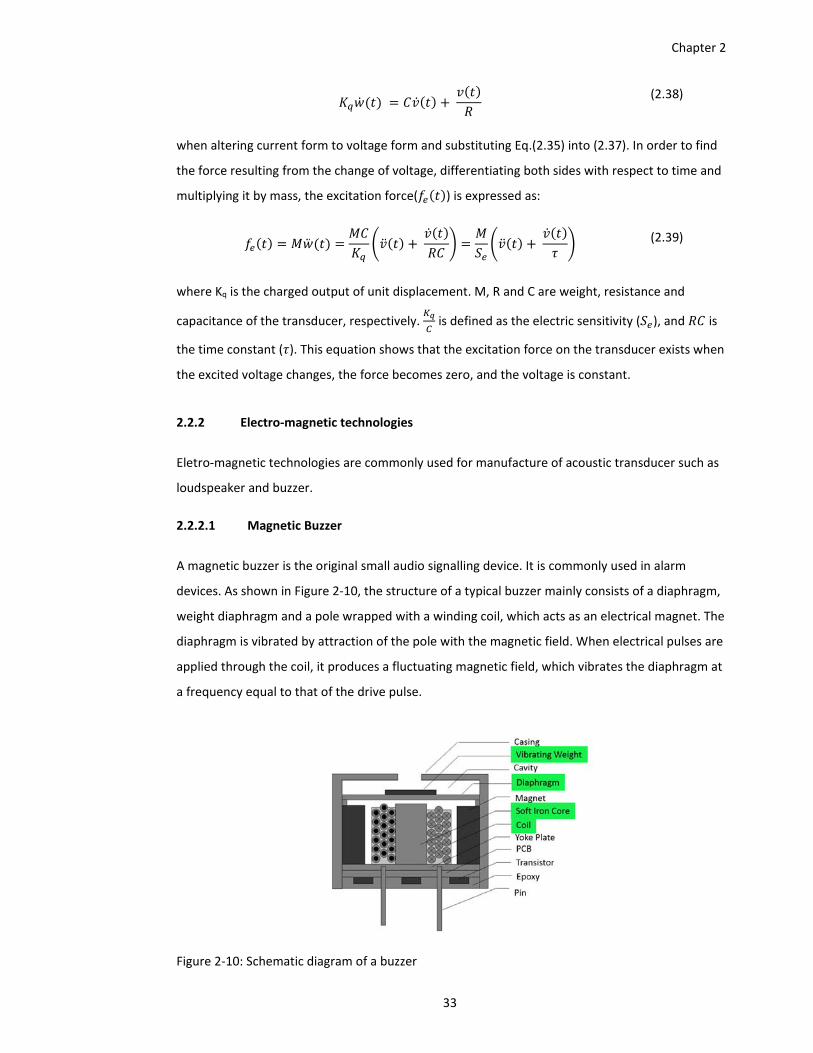
Chapter 2

33

(2.38)

when altering current form to voltage form and substituting Eq.(2.35) into (2.37). In order to find

the force resulting from the change of voltage, differentiating both sides with respect to time and

multiplying it by mass, the excitation force( ) is expressed as:

(2.39)

where Kq is the charged output of unit displacement. M, R and C are weight, resistance and

capacitance of the transducer, respectively. is defined as the electric sensitivity ( ), and is

the time constant ( ). This equation shows that the excitation force on the transducer exists when

the excited voltage changes, the force becomes zero, and the voltage is constant.

2.2.2 Electro‐magnetic technologies

Eletro‐magnetic technologies are commonly used for manufacture of acoustic transducer such as

loudspeaker and buzzer.

2.2.2.1 Magnetic Buzzer

A magnetic buzzer is the original small audio signalling device. It is commonly used in alarm

devices. As shown in Figure 2‐10, the structure of a typical buzzer mainly consists of a diaphragm,

weight diaphragm and a pole wrapped with a winding coil, which acts as an electrical magnet. The

diaphragm is vibrated by attraction of the pole with the magnetic field. When electrical pulses are

applied through the coil, it produces a fluctuating magnetic field, which vibrates the diaphragm at

a frequency equal to that of the drive pulse.

Figure 2‐10: Schematic diagram of a buzzer

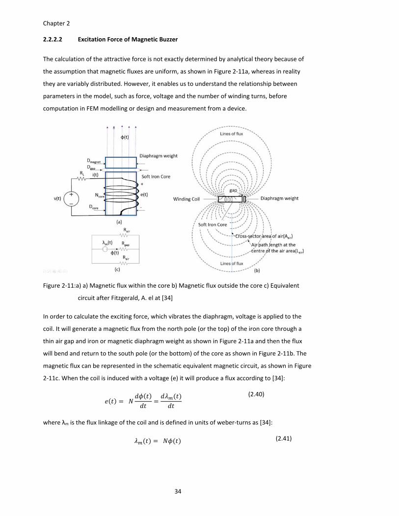
Chapter 2

34

2.2.2.2 Excitation Force of Magnetic Buzzer

The calculation of the attractive force is not exactly determined by analytical theory because of

the assumption that magnetic fluxes are uniform, as shown in Figure 2‐11a, whereas in reality

they are variably distributed. However, it enables us to understand the relationship between

parameters in the model, such as force, voltage and the number of winding turns, before

computation in FEM modelling or design and measurement from a device.

Figure 2‐11:a) a) Magnetic flux within the core b) Magnetic flux outside the core c) Equivalent

circuit after Fitzgerald, A. el at [34]

In order to calculate the exciting force, which vibrates the diaphragm, voltage is applied to the

coil. It will generate a magnetic flux from the north pole (or the top) of the iron core through a

thin air gap and iron or magnetic diaphragm weight as shown in Figure 2‐11a and then the flux

will bend and return to the south pole (or the bottom) of the core as shown in Figure 2‐11b. The

magnetic flux can be represented in the schematic equivalent magnetic circuit, as shown in Figure

2‐11c. When the coil is induced with a voltage (e) it will produce a flux according to [34]:

(2.40)

where λm is the flux linkage of the coil and is defined in units of weber‐turns as [34]:

(2.41)

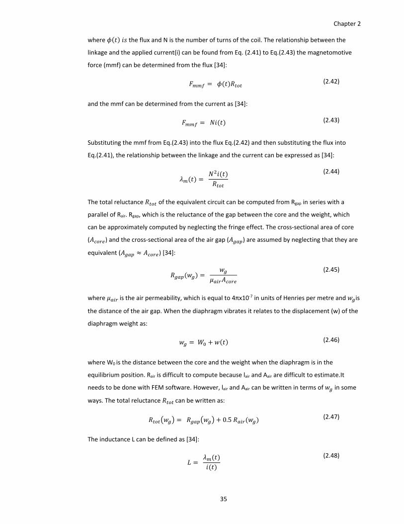
Chapter 2

35

where the flux and N is the number of turns of the coil. The relationship between the

linkage and the applied current(i) can be found from Eq. (2.41) to Eq.(2.43) the magnetomotive

force (mmf) can be determined from the flux [34]:

(2.42)

and the mmf can be determined from the current as [34]:

(2.43)

Substituting the mmf from Eq.(2.43) into the flux Eq.(2.42) and then substituting the flux into

Eq.(2.41), the relationship between the linkage and the current can be expressed as [34]:

(2.44)

The total reluctance of the equivalent circuit can be computed from Rgap in series with a

parallel of Rair. Rgap, which is the reluctance of the gap between the core and the weight, which

can be approximately computed by neglecting the fringe effect. The cross‐sectional area of core

( ) and the cross‐sectional area of the air gap ( ) are assumed by neglecting that they are

equivalent ( ) [34]:

(2.45)

where is the air permeability, which is equal to 4πx10‐7 in units of Henries per metre and is

the distance of the air gap. When the diaphragm vibrates it relates to the displacement (w) of the

diaphragm weight as:

(2.46)

where W0 is the distance between the core and the weight when the diaphragm is in the

equilibrium position. Rair is difficult to compute because lair and Aair are difficult to estimate.It

needs to be done with FEM software. However, lair and Aair can be written in terms of in some

ways. The total reluctance can be written as:

0.5 (2.47)

The inductance L can be defined as [34]:

(2.48)

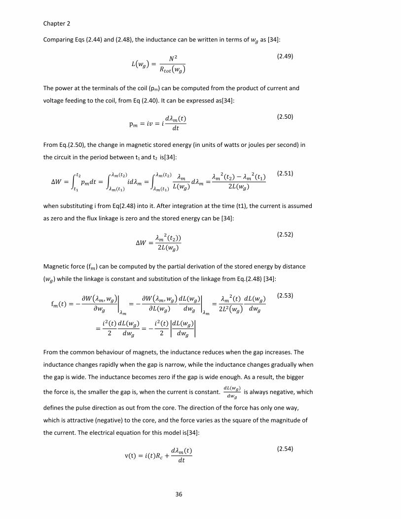
Chapter 2

36

Comparing Eqs (2.44) and (2.48), the inductance can be written in terms of as [34]:

(2.49)

The power at the terminals of the coil (pm) can be computed from the product of current and

voltage feeding to the coil, from Eq (2.40). It can be expressed as[34]:

p (2.50)

From Eq.(2.50), the change in magnetic stored energy (in units of watts or joules per second) in

the circuit in the period between t1 and t2 is[34]:

Δ 2

(2.51)

when substituting i from Eq(2.48) into it. After integration at the time (t1), the current is assumed

as zero and the flux linkage is zero and the stored energy can be [34]:

Δ2

(2.52)

Magnetic force (f ) can be computed by the partial derivation of the stored energy by distance

( ) while the linkage is constant and substitution of the linkage from Eq.(2.48) [34]:

f, ,

2

2 2

(2.53)

From the common behaviour of magnets, the inductance reduces when the gap increases. The

inductance changes rapidly when the gap is narrow, while the inductance changes gradually when

the gap is wide. The inductance becomes zero if the gap is wide enough. As a result, the bigger

the force is, the smaller the gap is, when the current is constant. is always negative, which

defines the pulse direction as out from the core. The direction of the force has only one way,

which is attractive (negative) to the core, and the force varies as the square of the magnitude of

the current. The electrical equation for this model is[34]:

v t (2.54)

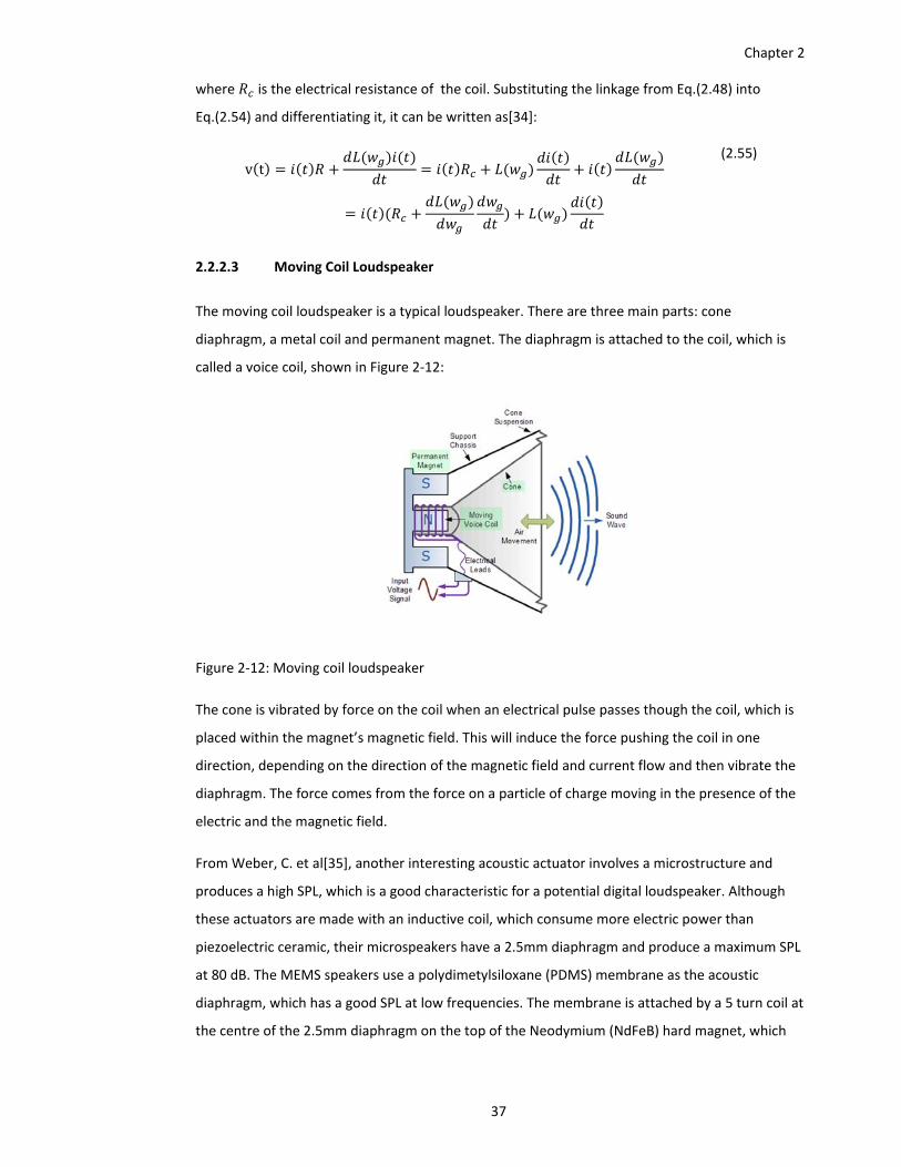
Chapter 2

37

where is the electrical resistance of the coil. Substituting the linkage from Eq.(2.48) into

Eq.(2.54) and differentiating it, it can be written as[34]:

v t

(2.55)

2.2.2.3 Moving Coil Loudspeaker

The moving coil loudspeaker is a typical loudspeaker. There are three main parts: cone

diaphragm, a metal coil and permanent magnet. The diaphragm is attached to the coil, which is

called a voice coil, shown in Figure 2‐12:

Figure 2‐12: Moving coil loudspeaker

The cone is vibrated by force on the coil when an electrical pulse passes though the coil, which is

placed within the magnet’s magnetic field. This will induce the force pushing the coil in one

direction, depending on the direction of the magnetic field and current flow and then vibrate the

diaphragm. The force comes from the force on a particle of charge moving in the presence of the

electric and the magnetic field.

From Weber, C. et al[35], another interesting acoustic actuator involves a microstructure and

produces a high SPL, which is a good characteristic for a potential digital loudspeaker. Although

these actuators are made with an inductive coil, which consume more electric power than

piezoelectric ceramic, their microspeakers have a 2.5mm diaphragm and produce a maximum SPL

at 80 dB. The MEMS speakers use a polydimetylsiloxane (PDMS) membrane as the acoustic

diaphragm, which has a good SPL at low frequencies. The membrane is attached by a 5 turn coil at

the centre of the 2.5mm diaphragm on the top of the Neodymium (NdFeB) hard magnet, which

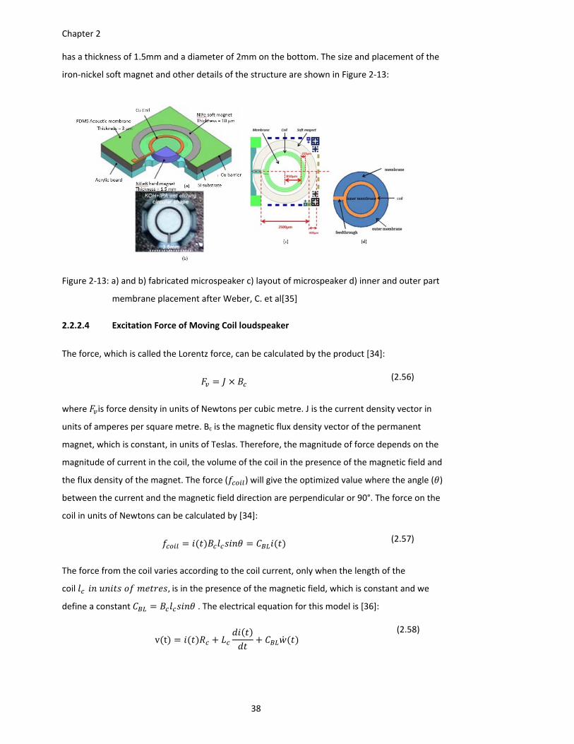
Chapter 2

38

has a thickness of 1.5mm and a diameter of 2mm on the bottom. The size and placement of the

iron‐nickel soft magnet and other details of the structure are shown in Figure 2‐13:

Figure 2‐13: a) and b) fabricated microspeaker c) layout of microspeaker d) inner and outer part

membrane placement after Weber, C. et al[35]

2.2.2.4 Excitation Force of Moving Coil loudspeaker

The force, which is called the Lorentz force, can be calculated by the product [34]:

(2.56)

where is force density in units of Newtons per cubic metre. J is the current density vector in

units of amperes per square metre. Bc is the magnetic flux density vector of the permanent

magnet, which is constant, in units of Teslas. Therefore, the magnitude of force depends on the

magnitude of current in the coil, the volume of the coil in the presence of the magnetic field and

the flux density of the magnet. The force ( ) will give the optimized value where the angle ( )

between the current and the magnetic field direction are perpendicular or 90°. The force on the

coil in units of Newtons can be calculated by [34]:

(2.57)

The force from the coil varies according to the coil current, only when the length of the

coil ,is in the presence of the magnetic field, which is constant and we

define a constant . The electrical equation for this model is [36]:

v t (2.58)

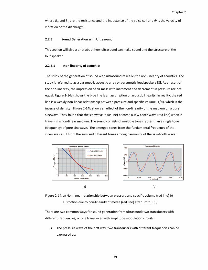
Chapter 2

39

where and are the resistance and the inductance of the voice coil and is the velocity of

vibration of the diaphragm.

2.2.3 Sound Generation with Ultrasound

This section will give a brief about how ultrasound can make sound and the structure of the

loudspeaker.

2.2.3.1 Non linearity of acoustics

The study of the generation of sound with ultrasound relies on the non‐linearity of acoustics. The

study is referred to as a parametric acoustic array or parametric loudspeakers [8]. As a result of

the non‐linearity, the impression of air mass with increment and decrement in pressure are not

equal. Figure 2‐14a) shows the blue line is an assumption of acoustic linearity. In reality, the red

line is a weakly non‐linear relationship between pressure and specific volume (1/ ), which is the

inverse of density). Figure 2‐14b shows an effect of the non‐linearity of the medium on a pure

sinewave. They found that the sinewave (blue line) become a saw‐tooth wave (red line) when it

travels in a non‐linear medium. The sound consists of multiple tones rather than a single tone

(frequency) of pure sinewave. The emerged tones from the fundamental frequency of the

sinewave result from the sum and different tones among harmonics of the saw‐tooth wave.

Figure 2‐14: a) Non‐linear relationship between pressure and specific volume (red line) b)

Distortion due to non‐linearity of media (red line) after Croft, J.[9]

There are two common ways for sound generation from ultrasound: two transducers with

different frequencies, or one transducer with amplitude modulation circuits.

The pressure wave of the first way, two transducers with different frequencies can be

expressed as:

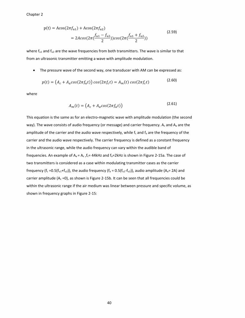
Chapter 2

40

p t Acos 2 Acos 2

2 22

22

(2.59)

where fu1 and fu2 are the wave frequencies from both transmitters. The wave is similar to that

from an ultrasonic transmitter emitting a wave with amplitude modulation.

The pressure wave of the second way, one transducer with AM can be expressed as:

2 2 2 (2.60)

where

2 (2.61)

This equation is the same as for an electro‐magnetic wave with amplitude modulation (the second

way). The wave consists of audio frequency (or message) and carrier frequency. Ac and Aa are the

amplitude of the carrier and the audio wave respectively, while fc and fa are the frequency of the

carrier and the audio wave respectively. The carrier frequency is defined as a constant frequency

in the ultrasonic range, while the audio frequency can vary within the audible band of

frequencies. An example of Aa = Ac ,fc= 44kHz and fa=2kHz is shown in Figure 2‐15a. The case of

two transmitters is considered as a case within modulating transmitter cases as the carrier

frequency (fc =0.5(fu1+fu2)), the audio frequency (fa = 0.5(fu1‐fu2)), audio amplitude (Aa= 2A) and

carrier amplitude (Ac =0), as shown is Figure 2‐15b. It can be seen that all frequencies could be

within the ultrasonic range if the air medium was linear between pressure and specific volume, as

shown in frequency graphs in Figure 2‐15:

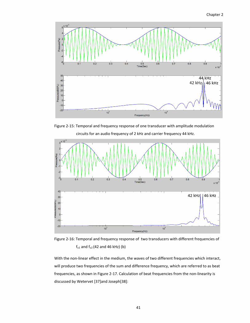
Chapter 2

41

Figure 2‐15: Temporal and frequency response of one transducer with amplitude modulation

circuits for an audio frequency of 2 kHz and carrier frequency 44 kHz.

Figure 2‐16: Temporal and frequency response of two transducers with different frequencies of

fu1 and fu2 (42 and 46 kHz) (b)

With the non‐linear effect in the medium, the waves of two different frequencies which interact,

will produce two frequencies of the sum and difference frequency, which are referred to as beat

frequencies, as shown in Figure 2‐17. Calculation of beat frequencies from the non‐linearity is

discussed by Wetervet [37]and Joseph[38]:

Chapter 2

42

Figure 2‐17: Non‐linear interaction process in air (frequencies in green font produced by non‐

linearity) after Wen‐Kung,T [39]

2.2.3.2 Parametric Array

In their early state, parametric loudspeakers were developed from piezo‐ceramic transducers.

This made the loudspeaker reproduce sound in a very limited bandwidth. Based on

polyvinylidenedifluoride(PVDF), a thin moving film, the bandwidth of the loudspeakers is

extended to be able to reproduce broadband audio signals with reasonable loudness. Several

patents have been granted and some commercial products based on parametric loudspeakers are

available. It is referred as audio spotlight.

Figure 2‐18: a) Structure of transducer after Yoneyama, M. and Fujimoto, J. [40]] and b)

Construction of loudspeaker after Croft, J.[9].

The structure of the loudspeaker is shown in Figure 2‐18a. The first loudspeaker was built with a

diameter of 44.45 mm with 85 holes of a diameter of 3.57 mm. The holes were arranged in a tight

hexagonal pattern with interspacing of 4.06 mm. The thickness of the film was 0.28 µm. Under

the film was a nearly full vacuum in order to prevent sound radiation to the back. The resonant

frequency was 37.23 kHz and the output was 136 dBSPL with 73.6 Vpp . Due to the considerately

high voltage, the loudspeaker required a high power amplifier for feeding the modulated signal

into the loudspeaker. Because the frequency response of transducers is quite steep, an equalizer

was required to adjust the frequency response, as shown in Figure 2‐18b.

Although a parametric array can produce audible sound, its beam width is very narrow because

the wave frequencies, which are emitted with the amplitude modulation by the loudspeaker, are

very high and within the ultrasonic frequency range, while the beam of sound from the transducer

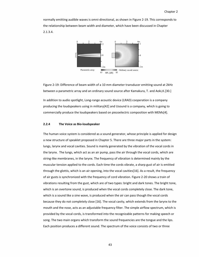
Chapter 2

43

normally emitting audible waves is omni‐directional, as shown in Figure 2‐19. This corresponds to

the relationship between beam width and diameter, which have been discussed in Chapter

2.1.3.4.

Figure 2‐19: Difference of beam width of a 10 mm diameter transducer emitting sound at 2kHz

between a parametric array and an ordinary sound source after Kamakura, T. and Aoki,K.[30.]

In addition to audio spotlight, Long‐range acoustic device (LRAD) cooperation is a company

producing the loudspeakers using in military[42] and Usound is a company, which is going to

commercially produce the loudspeakers based on piezoelectric composition with MEMs[4].

2.2.4 The Voice as Bio‐loudspeaker

The human voice system is considered as a sound generator, whose principle is applied for design

a new structure of speaklet proposed in Chapter 5. There are three major parts in the system:

lungs, larynx and vocal cavities. Sound is mainly generated by the vibration of the vocal cords in

the larynx. The lungs, which act as an air pump, pass the air through the vocal cords, which are

string‐like membranes, in the larynx. The frequency of vibration is determined mainly by the

muscular tension applied to the cords. Each time the cords vibrate, a sharp gust of air is emitted

through the glottis, which is an air opening, into the vocal cavities[16]. As a result, the frequency

of air gusts is synchronized with the frequency of cord vibration. Figure 2‐20 shows a train of

vibrations resulting from the gust, which are of two types: bright and dark tones. The bright tone,

which is an overtone sound, is produced when the vocal cords completely close. The dark tone,

which is a sound like a sine wave, is produced when the air can pass though the vocal cords

because they do not completely close [16]. The vocal cavity, which extends from the larynx to the

mouth and the nose, acts as an adjustable frequency filter. The simple airflow spectrum, which is

provided by the vocal cords, is transformed into the recognizable patterns for making speech or

song. The two main organs which transform the sound frequencies are the tongue and the lips.

Each position produces a different sound. The spectrum of the voice consists of two or three

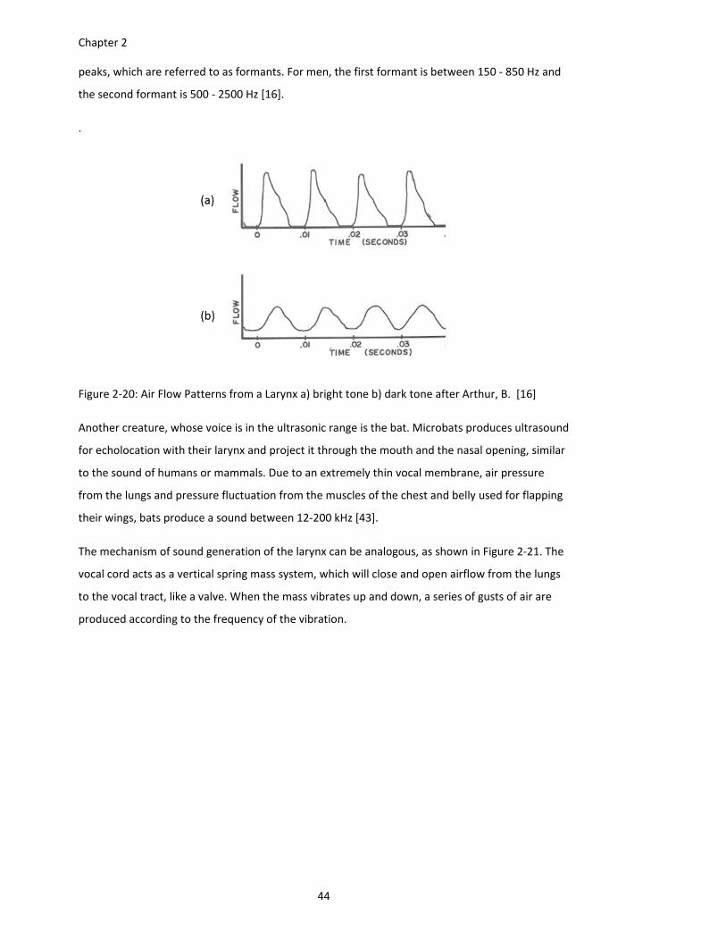
Chapter 2

44

peaks, which are referred to as formants. For men, the first formant is between 150 ‐ 850 Hz and

the second formant is 500 ‐ 2500 Hz [16].

.

Figure 2‐20: Air Flow Patterns from a Larynx a) bright tone b) dark tone after Arthur, B. [16]

Another creature, whose voice is in the ultrasonic range is the bat. Microbats produces ultrasound

for echolocation with their larynx and project it through the mouth and the nasal opening, similar

to the sound of humans or mammals. Due to an extremely thin vocal membrane, air pressure

from the lungs and pressure fluctuation from the muscles of the chest and belly used for flapping

their wings, bats produce a sound between 12‐200 kHz [43].

The mechanism of sound generation of the larynx can be analogous, as shown in Figure 2‐21. The

vocal cord acts as a vertical spring mass system, which will close and open airflow from the lungs

to the vocal tract, like a valve. When the mass vibrates up and down, a series of gusts of air are

produced according to the frequency of the vibration.

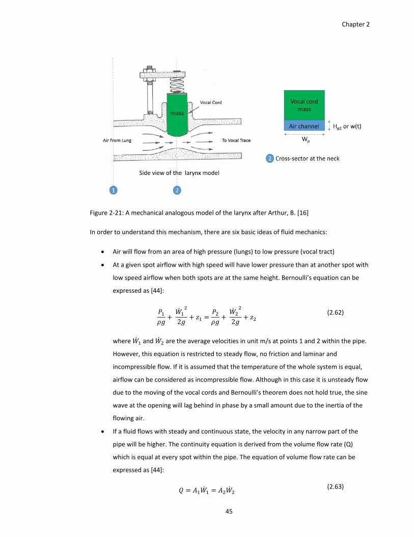
Chapter 2

45

Figure 2‐21: A mechanical analogous model of the larynx after Arthur, B. [16]

In order to understand this mechanism, there are six basic ideas of fluid mechanics:

Air will flow from an area of high pressure (lungs) to low pressure (vocal tract)

At a given spot airflow with high speed will have lower pressure than at another spot with

low speed airflow when both spots are at the same height. Bernoulli’s equation can be

expressed as [44]:

2 2

(2.62)

where and are the average velocities in unit m/s at points 1 and 2 within the pipe.

However, this equation is restricted to steady flow, no friction and laminar and

incompressible flow. If it is assumed that the temperature of the whole system is equal,

airflow can be considered as incompressible flow. Although in this case it is unsteady flow

due to the moving of the vocal cords and Bernoulli’s theorem does not hold true, the sine

wave at the opening will lag behind in phase by a small amount due to the inertia of the

flowing air.

If a fluid flows with steady and continuous state, the velocity in any narrow part of the

pipe will be higher. The continuity equation is derived from the volume flow rate (Q)

which is equal at every spot within the pipe. The equation of volume flow rate can be

expressed as [44]:

(2.63)

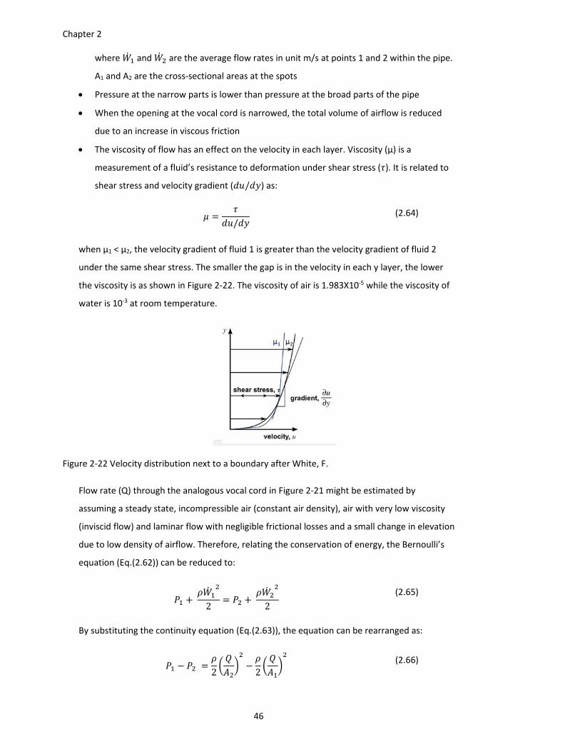
Chapter 2

46

where and are the average flow rates in unit m/s at points 1 and 2 within the pipe.

A1 and A2 are the cross‐sectional areas at the spots

Pressure at the narrow parts is lower than pressure at the broad parts of the pipe

When the opening at the vocal cord is narrowed, the total volume of airflow is reduced

due to an increase in viscous friction

The viscosity of flow has an effect on the velocity in each layer. Viscosity (µ) is a

measurement of a fluid’s resistance to deformation under shear stress ( ). It is related to

shear stress and velocity gradient ( / ) as:

/ (2.64)

when µ1 < µ2, the velocity gradient of fluid 1 is greater than the velocity gradient of fluid 2

under the same shear stress. The smaller the gap is in the velocity in each y layer, the lower

the viscosity is as shown in Figure 2‐22. The viscosity of air is 1.983X10‐5 while the viscosity of

water is 10‐3 at room temperature.

Figure 2‐22 Velocity distribution next to a boundary after White, F.

Flow rate (Q) through the analogous vocal cord in Figure 2‐21 might be estimated by

assuming a steady state, incompressible air (constant air density), air with very low viscosity

(inviscid flow) and laminar flow with negligible frictional losses and a small change in elevation

due to low density of airflow. Therefore, relating the conservation of energy, the Bernoulli’s

equation (Eq.(2.62)) can be reduced to:

2 2

(2.65)

By substituting the continuity equation (Eq.(2.63)), the equation can be rearranged as:

2 2

(2.66)

Chapter 2

47

Solving for Q, the equation can be rearranged into multiplication of 3 terms; area of the neck

of the pipe, ratio of areas between the pipe and the neck and the pressure difference as

shown in:

1

1

2 (2.67)

If we define that the pipe is rectangular with height (Hp) and width (Wp) as shown in Figure

2‐21, the area of the neck is dependent on the height of the neck (Hp2) when the width (Wp) of

the whole pipe is the same and constant. The height of the neck varies according to the

displacement of the vocal cord mass. If the height of the neck is far smaller than the height of

the pipe and the change in displacement (of vibration of vocal cord) is very small compared to

the height of the pipe, the second term can be approximately constant and equal to 1. If we

define the pressure difference between the lungs (P1) and the neck (P2) as constant, the third

term is constant. Therefore, the volume flow rate varies directly as the displacement of the

vocal cord mass (w(t)) where is a constant as shown in:

2

(2.68)

Although this equation is not exactly correct because Bernoulli’s theorem does not hold true

in unsteady flow from the vibration of the vocal cord, it is a good approximation for

calculation in FEM modelling software.

A rapid change of the volume flow rate can generate sound with frequencies according to

vibration of the air gate or the vocal cord.

2.3 Concept of Digital Loudspeaker Array

This section will review the principle of digital loudspeaker array and its related works

2.3.1 Concept of Digital reconstruction

The working principle of a digital loudspeaker array (DLA), or a digital transducer array (DTA) is

the reproduction of acoustic sound by an array of speakers directly accepting a digital signal.

Therefore, the acoustic sound is directly translated from a digital signal without digital to

analogue conversion (DAC) [45]. In other words, the process of DAC is shifted to the very end of

the audio reproduction. This reproduction results from the overlapping effect among steams of

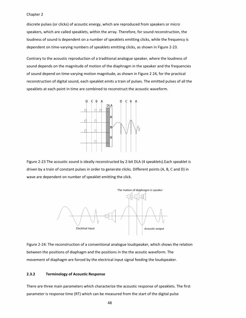
Chapter 2

48

discrete pulses (or clicks) of acoustic energy, which are reproduced from speakers or micro

speakers, which are called speaklets, within the array. Therefore, for sound reconstruction, the

loudness of sound is dependent on a number of speaklets emitting clicks, while the frequency is

dependent on time‐varying numbers of speaklets emitting clicks, as shown in Figure 2‐23.

Contrary to the acoustic reproduction of a traditional analogue speaker, where the loudness of

sound depends on the magnitude of motion of the diaphragm in the speaker and the frequencies

of sound depend on time‐varying motion magnitude, as shown in Figure 2 24, for the practical

reconstruction of digital sound, each speaklet emits a train of pulses. The emitted pulses of all the

speaklets at each point in time are combined to reconstruct the acoustic waveform.

Figure 2‐23 The acoustic sound is ideally reconstructed by 2‐bit DLA (4 speaklets).Each speaklet is

driven by a train of constant pulses in order to generate clicks. Different points (A, B, C and D) in

wave are dependent on number of speaklet emitting the click.

Figure 2‐24: The reconstruction of a conventional analogue loudspeaker, which shows the relation

between the positions of diaphagm and the positions in the the acoutic waveform. The

movement of diaphagm are forced by the electrical input signal feeding the loudspeaker.

2.3.2 Terminology of Acoustic Response

There are three main parameters which characterize the acoustic response of speaklets. The first

parameter is response time (RT) which can be measured from the start of the digital pulse

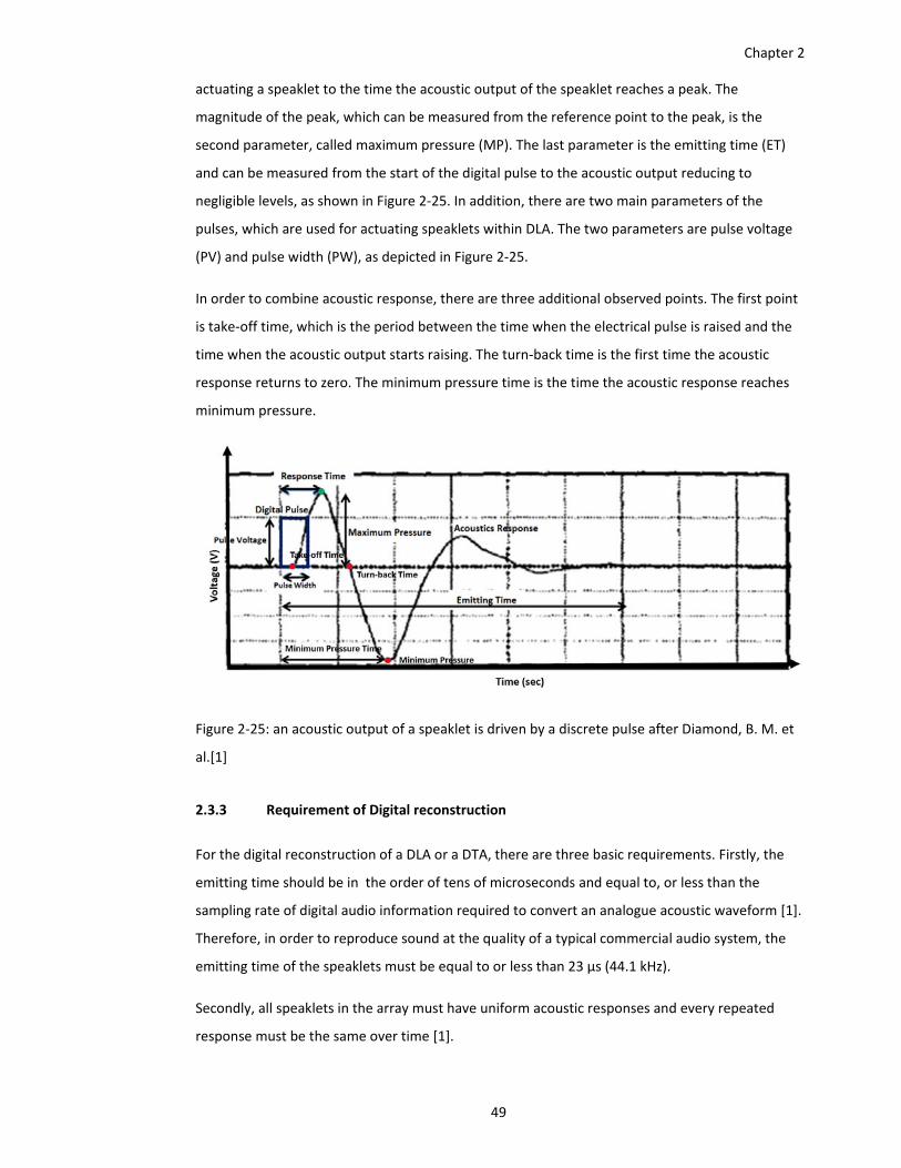
Chapter 2

49

actuating a speaklet to the time the acoustic output of the speaklet reaches a peak. The

magnitude of the peak, which can be measured from the reference point to the peak, is the

second parameter, called maximum pressure (MP). The last parameter is the emitting time (ET)

and can be measured from the start of the digital pulse to the acoustic output reducing to

negligible levels, as shown in Figure 2‐25. In addition, there are two main parameters of the

pulses, which are used for actuating speaklets within DLA. The two parameters are pulse voltage

(PV) and pulse width (PW), as depicted in Figure 2‐25.

In order to combine acoustic response, there are three additional observed points. The first point

is take‐off time, which is the period between the time when the electrical pulse is raised and the

time when the acoustic output starts raising. The turn‐back time is the first time the acoustic

response returns to zero. The minimum pressure time is the time the acoustic response reaches

minimum pressure.

Figure 2‐25: an acoustic output of a speaklet is driven by a discrete pulse after Diamond, B. M. et

al.[1]

2.3.3 Requirement of Digital reconstruction

For the digital reconstruction of a DLA or a DTA, there are three basic requirements. Firstly, the

emitting time should be in the order of tens of microseconds and equal to, or less than the

sampling rate of digital audio information required to convert an analogue acoustic waveform [1].

Therefore, in order to reproduce sound at the quality of a typical commercial audio system, the

emitting time of the speaklets must be equal to or less than 23 µs (44.1 kHz).

Secondly, all speaklets in the array must have uniform acoustic responses and every repeated

response must be the same over time [1].

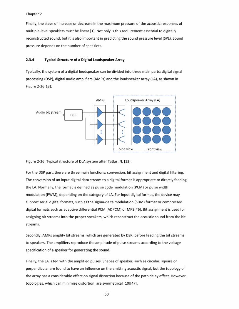
Chapter 2

50

Finally, the steps of increase or decrease in the maximum pressure of the acoustic responses of

multiple‐level speaklets must be linear [1]. Not only is this requirement essential to digitally

reconstructed sound, but it is also important in predicting the sound pressure level (SPL). Sound

pressure depends on the number of speaklets.

2.3.4 Typical Structure of a Digital Loudspeaker Array

Typically, the system of a digital loudspeaker can be divided into three main parts: digital signal

processing (DSP), digital audio amplifiers (AMPs) and the loudspeaker array (LA), as shown in

Figure 2‐26[13]:

Figure 2‐26: Typical structure of DLA system after Tatlas, N. [13].

For the DSP part, there are three main functions: conversion, bit assignment and digital filtering.

The conversion of an input digital data stream to a digital format is appropriate to directly feeding

the LA. Normally, the format is defined as pulse code modulation (PCM) or pulse width

modulation (PWM), depending on the category of LA. For input digital format, the device may

support serial digital formats, such as the sigma‐delta modulation (SDM) format or compressed

digital formats such as adaptive differential PCM (ADPCM) or MP3[46]. Bit assignment is used for

assigning bit streams into the proper speakers, which reconstruct the acoustic sound from the bit

streams.

Secondly, AMPs amplify bit streams, which are generated by DSP, before feeding the bit streams

to speakers. The amplifiers reproduce the amplitude of pulse streams according to the voltage

specification of a speaker for generating the sound.

Finally, the LA is fed with the amplified pulses. Shapes of speaker, such as circular, square or

perpendicular are found to have an influence on the emitting acoustic signal, but the topology of

the array has a considerable effect on signal distortion because of the path delay effect. However,

topologies, which can minimize distortion, are symmetrical [10][47].

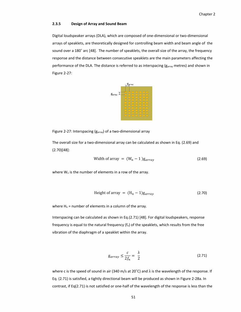
Chapter 2

51

2.3.5 Design of Array and Sound Beam

Digital loudspeaker arrays (DLA), which are composed of one‐dimensional or two‐dimensional

arrays of speaklets, are theoretically designed for controlling beam width and beam angle of the

sound over a 180˚ arc [48]. The number of speaklets, the overall size of the array, the frequency

response and the distance between consecutive speaklets are the main parameters affecting the

performance of the DLA. The distance is referred to as interspacing (garray metres) and shown in

Figure 2‐27:

Figure 2‐27: Interspacing (garray) of a two‐dimensional array

The overall size for a two‐dimensional array can be calculated as shown in Eq. (2.69) and

(2.70)[48]:

Width of array W 1 g (2.69)

where Wn is the number of elements in a row of the array.

Height of array H 1 g (2.70)

where Hn = number of elements in a column of the array.

Interspacing can be calculated as shown in Eq.(2.71) [48]. For digital loudspeakers, response

frequency is equal to the natural frequency (fn) of the speaklets, which results from the free

vibration of the diaphragm of a speaklet within the array.

g2

λ2 (2.71)

where c is the speed of sound in air (340 m/s at 20˚C) and λ is the wavelength of the response. If

Eq. (2.71) is satisfied, a tightly directional beam will be produced as shown in Figure 2‐28a. In

contrast, if Eq(2.71) is not satisfied or one‐half of the wavelength of the response is less than the

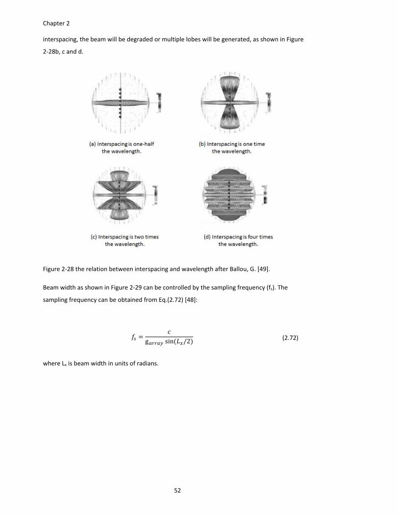
Chapter 2

52

interspacing, the beam will be degraded or multiple lobes will be generated, as shown in Figure

2‐28b, c and d.

Figure 2‐28 the relation between interspacing and wavelength after Ballou, G. [49].

Beam width as shown in Figure 2‐29 can be controlled by the sampling frequency (fs). The

sampling frequency can be obtained from Eq.(2.72) [48]:

g sin /2 (2.72)

where Lx is beam width in units of radians.

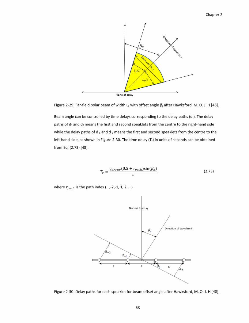
Chapter 2

53

Figure 2‐29: Far‐field polar beam of width Lx with offset angle βx after Hawksford, M. O. J. H [48].

Beam angle can be controlled by time delays corresponding to the delay paths (dr). The delay

paths of d1 and d2 means the first and second speaklets from the centre to the right‐hand side

while the delay paths of d‐1 and d‐2 means the first and second speaklets from the centre to the

left‐hand side, as shown in Figure 2‐30. The time delay (Tr) in units of seconds can be obtained

from Eq. (2.73) [48]:

g 0.5 sin (2.73)

where is the path index (…,‐2,‐1, 1, 2, …)

Figure 2‐30: Delay paths for each speaklet for beam offset angle after Hawksford, M. O. J. H [48].

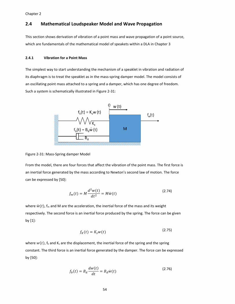
Chapter 2

54

2.4 Mathematical Loudspeaker Model and Wave Propagation

This section shows derivation of vibration of a point mass and wave propagation of a point source,

which are fundamentals of the mathematical model of speakets within a DLA in Chapter 3

2.4.1 Vibration for a Point Mass

The simplest way to start understanding the mechanism of a speaklet in vibration and radiation of

its diaphragm is to treat the speaklet as in the mass‐spring damper model. The model consists of

an oscillating point mass attached to a spring and a damper, which has one degree of freedom.

Such a system is schematically illustrated in Figure 2‐31:

Figure 2‐31: Mass‐Spring damper Model

From the model, there are four forces that affect the vibration of the point mass. The first force is

an inertial force generated by the mass according to Newton’s second law of motion. The force

can be expressed by [50]:

(2.74)

where , fm and M are the acceleration, the inertial force of the mass and its weight

respectively. The second force is an inertial force produced by the spring. The force can be given

by [1]:

(2.75)

where , fk and Ks are the displacement, the inertial force of the spring and the spring

constant. The third force is an inertial force generated by the damper. The force can be expressed

by [50]:

(2.76)

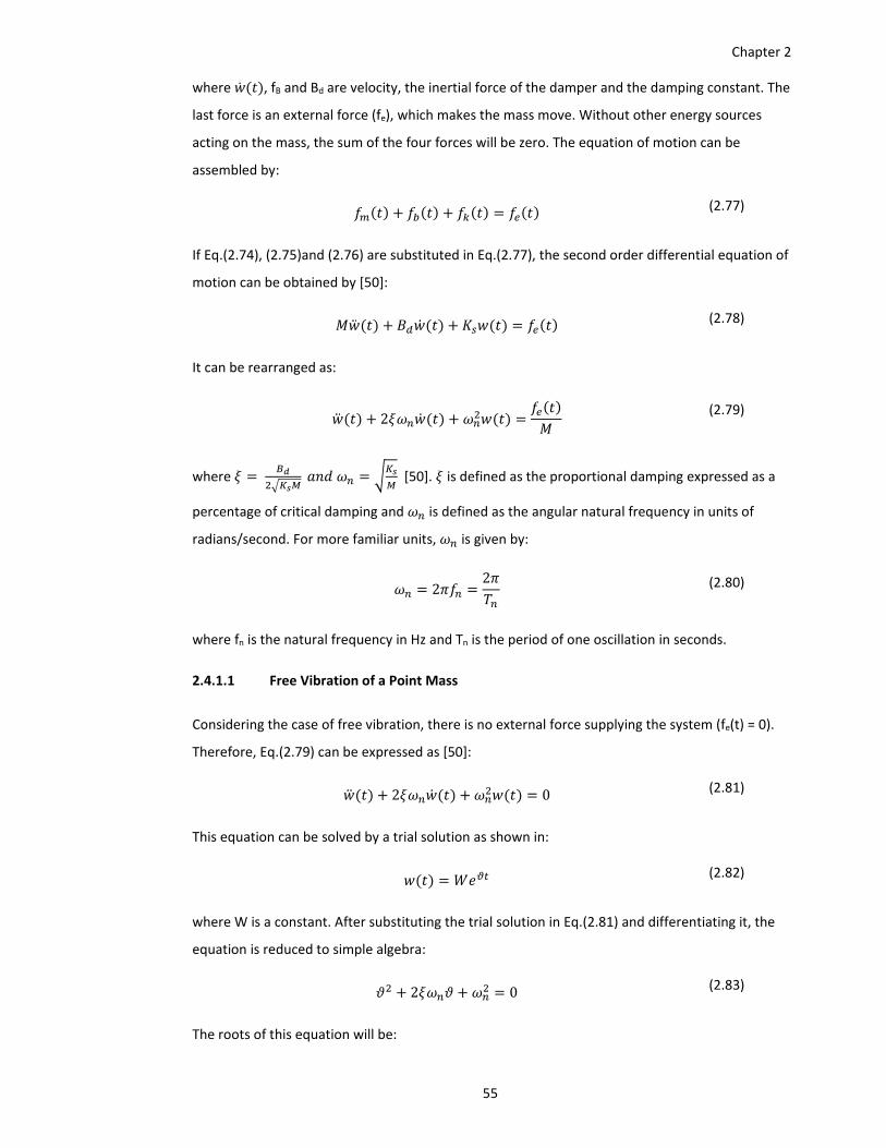
Chapter 2

55

where , fB and Bd are velocity, the inertial force of the damper and the damping constant. The

last force is an external force (fe), which makes the mass move. Without other energy sources

acting on the mass, the sum of the four forces will be zero. The equation of motion can be

assembled by:

(2.77)

If Eq.(2.74), (2.75)and (2.76) are substituted in Eq.(2.77), the second order differential equation of

motion can be obtained by [50]:

(2.78)

It can be rearranged as:

2 (2.79)

where [50]. is defined as the proportional damping expressed as a

percentage of critical damping and is defined as the angular natural frequency in units of

radians/second. For more familiar units, is given by:

22

(2.80)

where fn is the natural frequency in Hz and Tn is the period of one oscillation in seconds.

2.4.1.1 Free Vibration of a Point Mass

Considering the case of free vibration, there is no external force supplying the system (fe(t) = 0).

Therefore, Eq.(2.79) can be expressed as [50]:

2 0 (2.81)

This equation can be solved by a trial solution as shown in:

(2.82)

where W is a constant. After substituting the trial solution in Eq.(2.81) and differentiating it, the

equation is reduced to simple algebra:

2 0 (2.83)

The roots of this equation will be:

Chapter 2

56

(2.84)

where the damping ratio is defined as [50] :

(2.85)

and the damped natural frequency ( ) is defined as [50]:

1 (2.86)

From this equation, the damping conditions can be defined by the magnitude of proportional

damping ( ). If 1, or an underdamped condition, the periodic oscillation will decay. If 1 or

in an overdamped condition, the motion will decay, but not periodically. 1 causes a periodic

and critically damped oscillation.

Therefore, the real solution of Eq.(2.81) is given by substituting (2.84) into the trial solution of

(2.82):

(2.87)

where A and B are arbitrary constants. In order to make the whole expression real, constant B

must be the complex conjugate of A because any complex number z, z + z* = 2 Re{z}. If the

arbitrary constant A is defined as a complex number ( ) and the complex notation is

expressed by introducing Euler’s Formula:

cos (2.88)

cos (2.89)

the solution can be expressed as:

2 2 (2.90)

Cd and Dd are defined as 2 and 2 respectively. This can be rearranged as[50]

(2.91)

This can also rearranged as:

(2.92)

Chapter 2

57

where and are constants. , arctan / and . This

solution might be referred to as transient‐state representation. From the equation, the term

causes exponential decay and emulates a damping effect, while has an effect on the condition

of damping and period of oscillation.

2.4.1.2 Forced Vibration of a Point Mass

Considering the case of forced vibration, let us assume a harmonic force is supplied to the system.

The force can be described as:

(2.93)

where and are the amplitude of and the angular frequency of the external force. The time

response resulting from this force can be calculated by substituting the force back to the second‐

order differential equation of motion (Eq.(2.79)). This can be expressed as:

2 (2.94)

For the steady‐state assumption, the trial solution of this equation can be given by:

(2.95)

where Af and Bf are constants. If Eq.(2.95) is differentiated, the first and second derivatives are

given as:

(2.96)

and

(2.97)

After substituting these equations into Eq.(2.94), two equations for solving Af

and Bf can be obtained from coefficients of cosine and sine terms.

This solution is not the general equation of motion but is only represented as the

steady‐state part. The solution from Eq.(2.95) can also be expressed in

exponential terms similar to the rearrangement of Eq.(2.92):

(2.98)

Chapter 2

58

where Ef and Wf are constants. , arctan / and

.

However, the time response of this forced system consists of a transient part

and a steady‐state part. In other words, it is the sum of the transient and steady‐

state solutions, as shown in:

(2.99)

2.4.2 Wave Propagation for a Point Source

This section shows derivation of steady‐state and transient‐state wave propagation of a point

source. The function of is represented as the waveform in transient‐state, while

is the waveform in steady‐state. The wave equation for transient state is based on the Helmholz

steady‐state equation.

2.4.2.1 Steady‐State Plane Wave for one Dimension

For a study of the relationship between sound pressure on a medium and the vibration of a

diaphragm surface, there are two major equations. This first equation is Euler’s equation:

(2.100)

where p is sound pressure, w is displacement of the diaphragm and is the density of the

acoustic medium. This equation shows the relationship between the sound pressure and the

vibration while force components act on a volume element according to Newton’s second law.

From the equation, the pressure is only dependent on the z coordinate, which is perpendicular to

the vibrating surface. The other equation is given by [51]:

or

(2.101)

(2.102)

where B is the adiabatic bulk modulus. This equation shows the relationship between the sound

pressure and the vibration resulting from the displacement of the diaphragm. Substituting

Chapter 2

59

Eq.(2.102) into Eq.(2.1) and partially differentiating both sides of the equation with respect to z

and moving it to the left, this can be obtained [51]:

0 (2.103)

This equation shows the relationship between the temporal and spatial variation of the pressure

field, which is referred to as the one‐dimensional wave equation[51]. From this equation, sound

velocity (c) can be derived as [51]:

(2.104)

When a wave stays in the steady state, the harmonic solution of the wave equation can be

assumed as [51]:

, ] (2.105)

Substituting this equation into Eq.(2.103) and differentiating it, the wave equation becomes a

second‐order differential equation with spatial coordinates [51]:

0 (2.106)

This equation is denoted as the one‐dimensional Helmholz equation, or the steady‐state wave

equation. It can be referred to as the Helmholz equation[51]:

0 (2.107)

where k is defined as the acoustic wave number [51]:

2

(2.108)

when combining Eq.(2.104) into the equation. From the Helmholtz equation, the general solution

can be assumed as [51]:

(2.109)

where and are arbitrary constants. Substituting this equation back into Eq.(2.105), the

equation is obtained as[51]:

, (2.110)

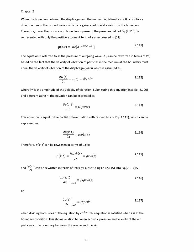
Chapter 2

60

When the boundary between the diaphragm and the medium is defined as z= 0, a positive z

direction means that sound waves, which are generated, travel away from the boundary.

Therefore, if no other source and boundary is present, the pressure field of Eq.(2.110). is

represented with only the positive exponent term of z as expressed in [51]:

, (2.111)

The equation is referred to as the pressure of outgoing wave. can be rewritten in terms of ,

based on the fact that the velocity of vibration of particles in the medium at the boundary must

equal the velocity of vibration of the diaphragm( ),which is assumed as:

(2.112)

where is the amplitude of the velocity of vibration. Substituting this equation into Eq.(2.100)

and differentiating it, the equation can be expressed as:

,

(2.113)

This equation is equal to the partial differentiation with respect to z of Eq.(2.111), which can be

expressed as:

,,

(2.114)

Therefore, , can be rewritten in terms of :

, (2.115)

and , can be rewritten in terms of by substituting Eq.(2.115) into Eq.(2.114)[51]

,

(2.116)

or

(2.117)

when dividing both sides of the equation by .This equation is satisfied when z is at the

boundary condition. This shows relation between acoustic pressure and velocity of the air

particles at the boundary between the source and the air.

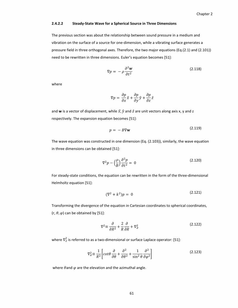
Chapter 2

61

2.4.2.2 Steady‐State Wave for a Spherical Source in Three Dimensions

The previous section was about the relationship between sound pressure in a medium and

vibration on the surface of a source for one‐dimension, while a vibrating surface generates a

pressure field in three orthogonal axes. Therefore, the two major equations (Eq.(2.1) and (2.101))

need to be rewritten in three dimensions. Euler’s equation becomes [51]:

(2.118)

where

and w is a vector of displacement, while , and are unit vectors along axis x, y and z

respectively. The expansion equation becomes [51]:

(2.119)

The wave equation was constructed in one dimension (Eq. (2.103)), similarly, the wave equation

in three dimensions can be obtained [51]:

0 (2.120)

For steady‐state conditions, the equation can be rewritten in the form of the three‐dimensional

Helmholtz equation [51]:

0 (2.121)

Transforming the divergence of the equation in Cartesian coordinates to spherical coordinates,

(r, , ) can be obtained by [51]:

≡2

(2.122)

where 2 is referred to as a two‐dimensional or surface Laplace operator: [51]:

≡1 1

sin

(2.123)

where and are the elevation and the azimuthal angle.

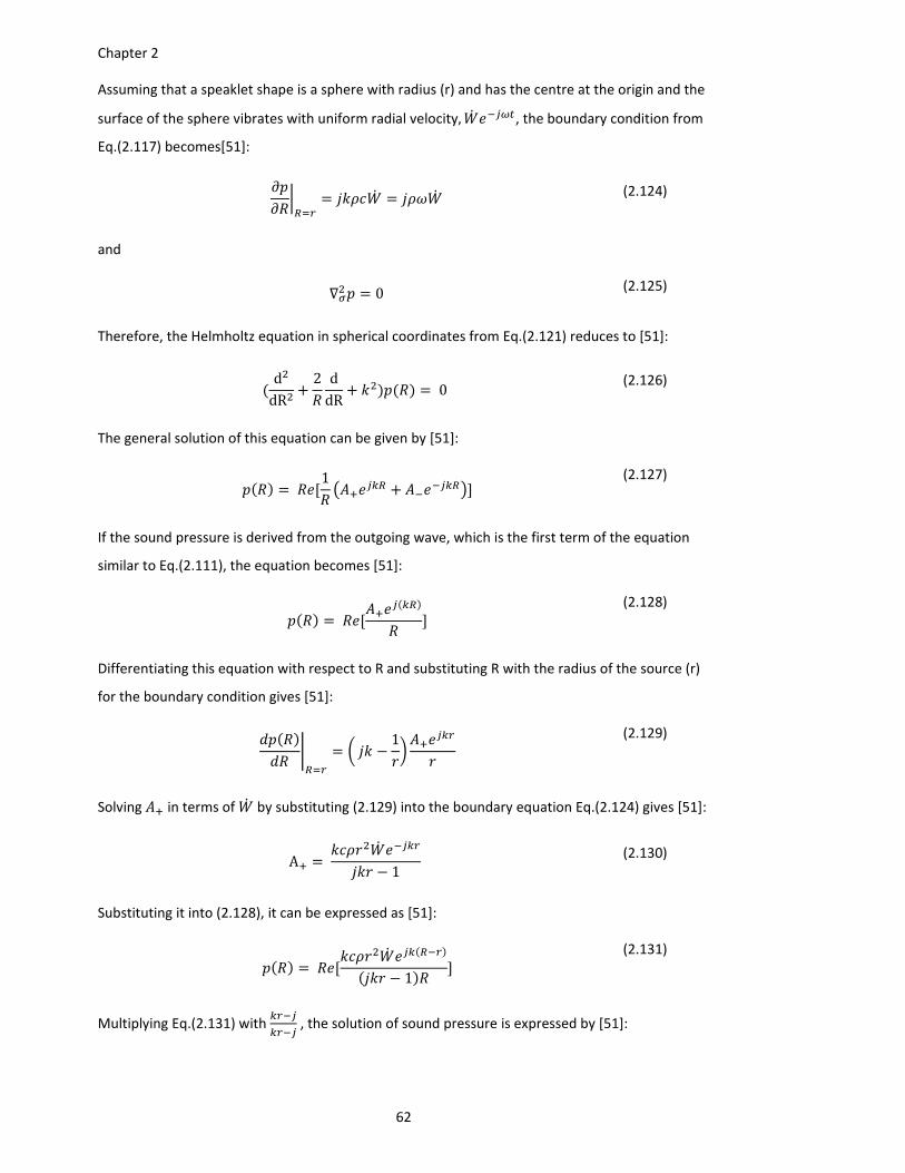
Chapter 2

62

Assuming that a speaklet shape is a sphere with radius (r) and has the centre at the origin and the

surface of the sphere vibrates with uniform radial velocity, , the boundary condition from

Eq.(2.117) becomes[51]:

(2.124)

and

0 (2.125)

Therefore, the Helmholtz equation in spherical coordinates from Eq.(2.121) reduces to [51]:

ddR

2 ddR

0 (2.126)

The general solution of this equation can be given by [51]:

1

(2.127)

If the sound pressure is derived from the outgoing wave, which is the first term of the equation

similar to Eq.(2.111), the equation becomes [51]:

(2.128)

Differentiating this equation with respect to R and substituting R with the radius of the source (r)

for the boundary condition gives [51]:

1

(2.129)

Solving in terms of by substituting (2.129) into the boundary equation Eq.(2.124) gives [51]:

A 1

(2.130)

Substituting it into (2.128), it can be expressed as [51]:

1

(2.131)

Multiplying Eq.(2.131) with , the solution of sound pressure is expressed by [51]:

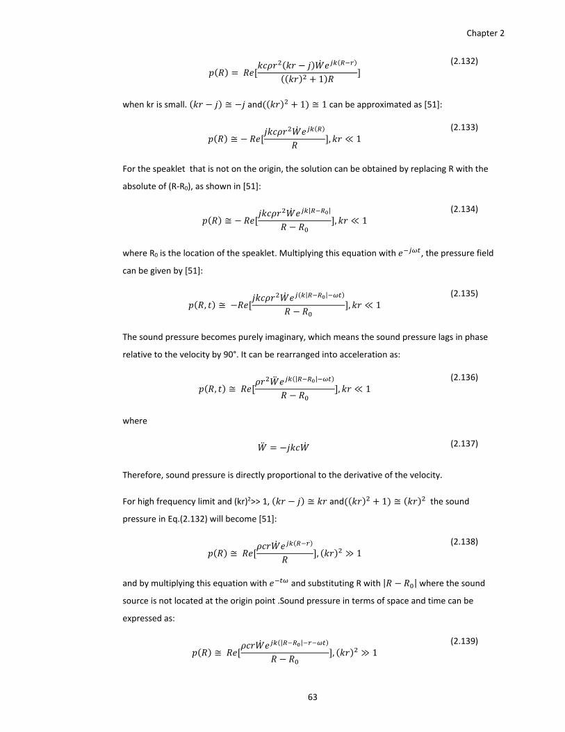
Chapter 2

63

1

(2.132)

when kr is small. ≅ and 1 ≅ 1 can be approximated as [51]:

≅ , ≪ 1 (2.133)

For the speaklet that is not on the origin, the solution can be obtained by replacing R with the

absolute of (R‐R0), as shown in [51]:

≅| |

, ≪ 1 (2.134)

where R0 is the location of the speaklet. Multiplying this equation with , the pressure field

can be given by [51]:

, ≅ | |

, ≪ 1 (2.135)

The sound pressure becomes purely imaginary, which means the sound pressure lags in phase

relative to the velocity by 90°. It can be rearranged into acceleration as:

, ≅| |

, ≪ 1 (2.136)

where

(2.137)

Therefore, sound pressure is directly proportional to the derivative of the velocity.

For high frequency limit and (kr)2>> 1, ≅ and 1 ≅ the sound

pressure in Eq.(2.132) will become [51]:

≅ , ≫ 1 (2.138)

and by multiplying this equation with and substituting R with | | where the sound

source is not located at the origin point .Sound pressure in terms of space and time can be

expressed as:

≅ | |

, ≫ 1 (2.139)

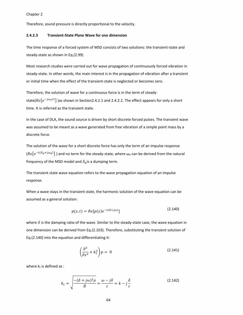
Chapter 2

64

Therefore, sound pressure is directly proportional to the velocity.

2.4.2.3 Transient‐State Plane Wave for one dimension

The time response of a forced system of MSD consists of two solutions: the transient‐state and

steady‐state as shown in Eq.(2.99)

Most research studies were carried out for wave propagation of continuously forced vibration in

steady‐state. In other words, the main interest is in the propagation of vibration after a transient

or initial time when the effect of the transient‐state is neglected or becomes zero.

Therefore, the solution of wave for a continuous force is in the term of steady‐

state( )as shown in Section2.4.2.1 and 2.4.2.2. The effect appears for only a short

time. It is referred as the transient state.

In the case of DLA, the sound source is driven by short discrete forced pulses. The transient wave

was assumed to be meant as a wave generated from free vibration of a simple point mass by a

discrete force.

The solution of the wave for a short discrete force has only the term of an impulse response

( ) and no term for the steady‐state, where ωd can be derived from the natural

frequency of the MSD model and is a dumping term.

The transient state wave equation refers to the wave propagation equation of an impulse

response.

When a wave stays in the transient state, the harmonic solution of the wave equation can be

assumed as a general solution:

, (2.140)

where is the damping ratio of the wave. Similar to the steady‐state case, the wave equation in

one dimension can be derived from Eq.(2.103). Therefore, substituting the transient solution of

Eq.(2.140) into the equation and differentiating it:

0 (2.141)

where kt is defined as :

(2.142)

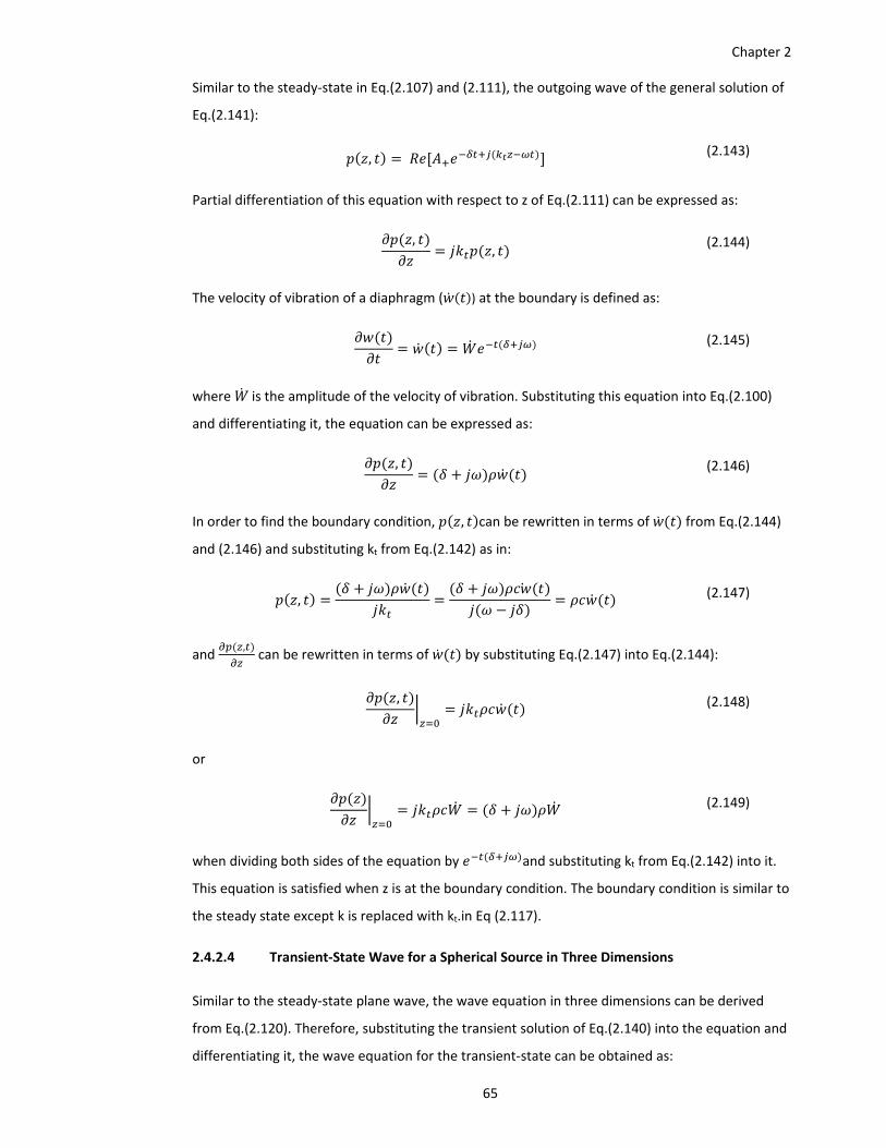
Chapter 2

65

Similar to the steady‐state in Eq.(2.107) and (2.111), the outgoing wave of the general solution of

Eq.(2.141):

, (2.143)

Partial differentiation of this equation with respect to z of Eq.(2.111) can be expressed as:

,,

(2.144)

The velocity of vibration of a diaphragm ( ) at the boundary is defined as:

(2.145)

where is the amplitude of the velocity of vibration. Substituting this equation into Eq.(2.100)

and differentiating it, the equation can be expressed as:

,

(2.146)

In order to find the boundary condition, , can be rewritten in terms of from Eq.(2.144)

and (2.146) and substituting kt from Eq.(2.142) as in:

, (2.147)

and , can be rewritten in terms of by substituting Eq.(2.147) into Eq.(2.144):

,

(2.148)

or

(2.149)

when dividing both sides of the equation by and substituting kt from Eq.(2.142) into it.

This equation is satisfied when z is at the boundary condition. The boundary condition is similar to

the steady state except k is replaced with kt.in Eq (2.117).

2.4.2.4 Transient‐State Wave for a Spherical Source in Three Dimensions

Similar to the steady‐state plane wave, the wave equation in three dimensions can be derived

from Eq.(2.120). Therefore, substituting the transient solution of Eq.(2.140) into the equation and

differentiating it, the wave equation for the transient‐state can be obtained as:

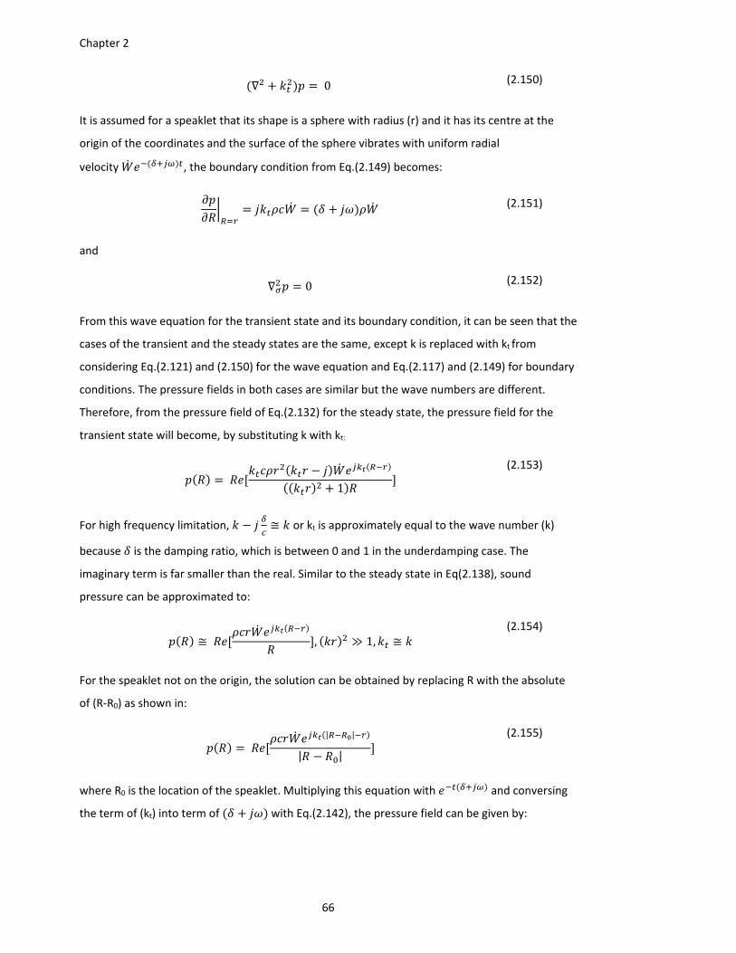
Chapter 2

66

0 (2.150)

It is assumed for a speaklet that its shape is a sphere with radius (r) and it has its centre at the

origin of the coordinates and the surface of the sphere vibrates with uniform radial

velocity , the boundary condition from Eq.(2.149) becomes:

(2.151)

and

0 (2.152)

From this wave equation for the transient state and its boundary condition, it can be seen that the

cases of the transient and the steady states are the same, except k is replaced with kt from

considering Eq.(2.121) and (2.150) for the wave equation and Eq.(2.117) and (2.149) for boundary

conditions. The pressure fields in both cases are similar but the wave numbers are different.

Therefore, from the pressure field of Eq.(2.132) for the steady state, the pressure field for the

transient state will become, by substituting k with kt:

1

(2.153)

For high frequency limitation, ≅ or kt is approximately equal to the wave number (k)

because is the damping ratio, which is between 0 and 1 in the underdamping case. The

imaginary term is far smaller than the real. Similar to the steady state in Eq(2.138), sound

pressure can be approximated to:

≅ , ≫ 1, ≅ (2.154)

For the speaklet not on the origin, the solution can be obtained by replacing R with the absolute

of (R‐R0) as shown in:

| |

| |

(2.155)

where R0 is the location of the speaklet. Multiplying this equation with and conversing

the term of (kt) into term of with Eq.(2.142), the pressure field can be given by:

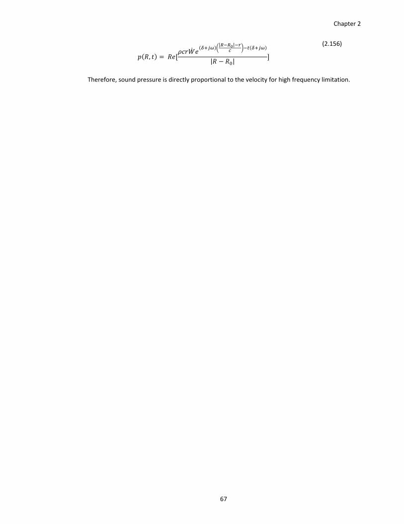
Chapter 2

67

,

| |

| |

(2.156)

Therefore, sound pressure is directly proportional to the velocity for high frequency limitation.

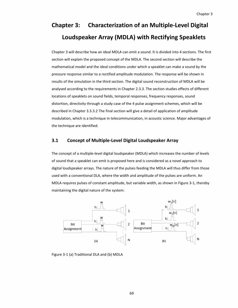
Chapter 3

69

Chapter 3: Characterization of an Multiple‐Level Digital

Loudspeaker Array (MDLA) with Rectifying Speaklets

Chapter 3 will describe how an ideal MDLA can emit a sound. It is divided into 4 sections. The first

section will explain the proposed concept of the MDLA. The second section will describe the

mathematical model and the ideal conditions under which a speaklet can make a sound by the

pressure response similar to a rectified amplitude modulation. The response will be shown in

results of the simulation in the third section. The digital sound reconstruction of MDLA will be

analysed according to the requirements in Chapter 2.3.3. The section studies effects of different

locations of speaklets on sound fields, temporal responses, frequency responses, sound

distortion, directivity through a study case of the 4 pulse assignment schemes, which will be

described in Chapter 3.3.3.2 The final section will give a detail of application of amplitude

modulation, which is a technique in telecommunication, in acoustic science. Major advantages of

the technique are identified.

3.1 Concept of Multiple‐Level Digital Loudspeaker Array

The concept of a multiple‐level digital loudspeaker (MDLA) which increases the number of levels

of sound that a speaklet can emit is proposed here and is considered as a novel approach to

digital loudspeaker arrays. The nature of the pulses feeding the MDLA will thus differ from those

used with a conventional DLA, where the width and amplitude of the pulses are uniform. An

MDLA requires pulses of constant amplitude, but variable width, as shown in Figure 3‐1, thereby

maintaining the digital nature of the system:

Figure 3‐1 (a) Traditional DLA and (b) MDLA

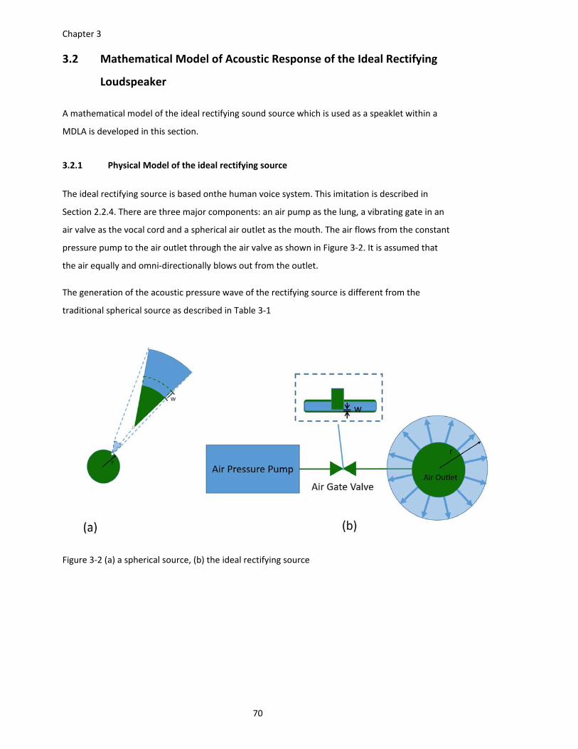
Chapter 3

70

3.2 Mathematical Model of Acoustic Response of the Ideal Rectifying

Loudspeaker

A mathematical model of the ideal rectifying sound source which is used as a speaklet within a

MDLA is developed in this section.

3.2.1 Physical Model of the ideal rectifying source

The ideal rectifying source is based onthe human voice system. This imitation is described in

Section 2.2.4. There are three major components: an air pump as the lung, a vibrating gate in an

air valve as the vocal cord and a spherical air outlet as the mouth. The air flows from the constant

pressure pump to the air outlet through the air valve as shown in Figure 3‐2. It is assumed that

the air equally and omni‐directionally blows out from the outlet.

The generation of the acoustic pressure wave of the rectifying source is different from the

traditional spherical source as described in Table 3‐1

Figure 3‐2 (a) a spherical source, (b) the ideal rectifying source

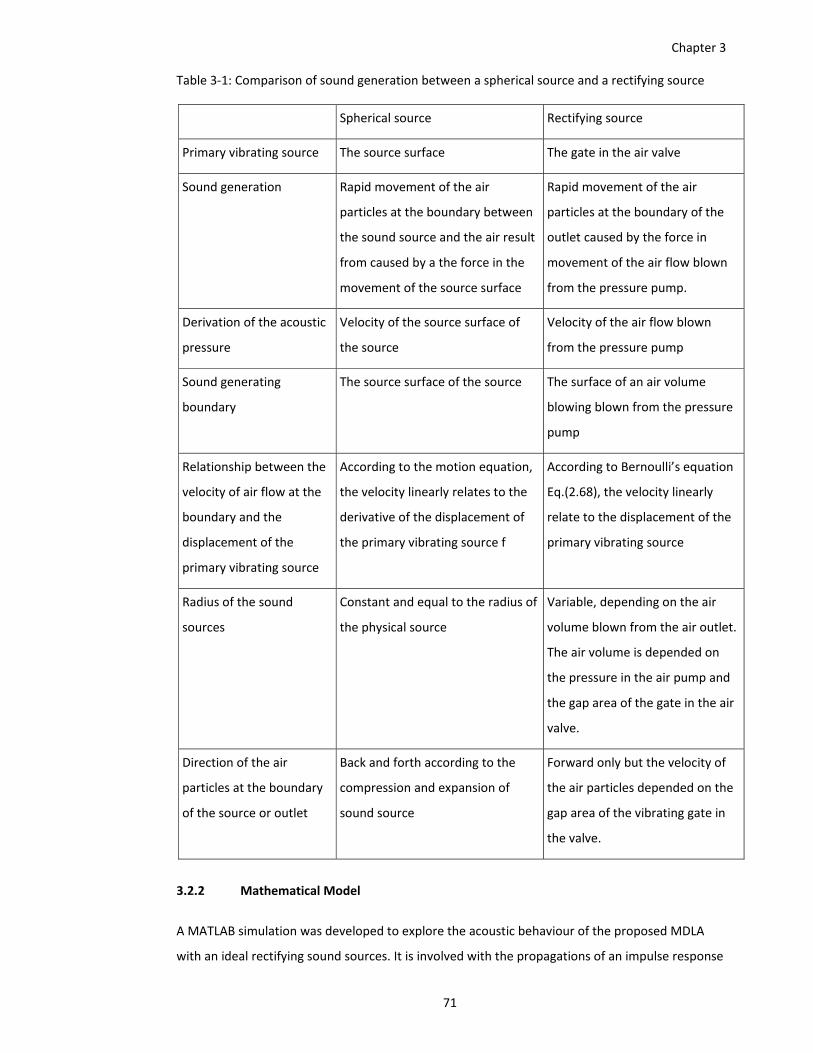
Chapter 3

71

Table 3‐1: Comparison of sound generation between a spherical source and a rectifying source

Spherical source Rectifying source

Primary vibrating source The source surface The gate in the air valve

Sound generation Rapid movement of the air

particles at the boundary between

the sound source and the air result

from caused by a the force in the

movement of the source surface

Rapid movement of the air

particles at the boundary of the

outlet caused by the force in

movement of the air flow blown

from the pressure pump.

Derivation of the acoustic

pressure

Velocity of the source surface of

the source

Velocity of the air flow blown

from the pressure pump

Sound generating

boundary

The source surface of the source The surface of an air volume

blowing blown from the pressure

pump

Relationship between the

velocity of air flow at the

boundary and the

displacement of the

primary vibrating source

According to the motion equation,

the velocity linearly relates to the

derivative of the displacement of

the primary vibrating source f

According to Bernoulli’s equation

Eq.(2.68), the velocity linearly

relate to the displacement of the

primary vibrating source

Radius of the sound

sources

Constant and equal to the radius of

the physical source

Variable, depending on the air

volume blown from the air outlet.

The air volume is depended on

the pressure in the air pump and

the gap area of the gate in the air

valve.

Direction of the air

particles at the boundary

of the source or outlet

Back and forth according to the

compression and expansion of

sound source

Forward only but the velocity of

the air particles depended on the

gap area of the vibrating gate in

the valve.

3.2.2 Mathematical Model

A MATLAB simulation was developed to explore the acoustic behaviour of the proposed MDLA

with an ideal rectifying sound sources. It is involved with the propagations of an impulse response

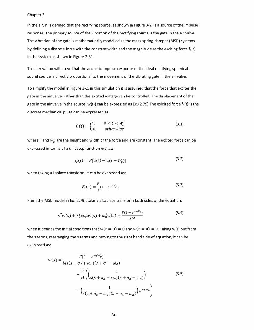
Chapter 3

72

in the air. It is defined that the rectifying source, as shown in Figure 3‐2, is a source of the impulse

response. The primary source of the vibration of the rectifying source is the gate in the air valve.

The vibration of the gate is mathematically modelled as the mass‐spring‐damper (MSD) systems

by defining a discrete force with the constant width and the magnitude as the exciting force fe(t)

in the system as shown in Figure 2‐31.

This derivation will prove that the acoustic impulse response of the ideal rectifying spherical

sound source is directly proportional to the movement of the vibrating gate in the air valve.

To simplify the model in Figure 3‐2, in this simulation it is assumed that the force that excites the

gate in the air valve, rather than the excited voltage can be controlled. The displacement of the

gate in the air valve in the source (w(t)) can be expressed as Eq.(2.79).The exicited force fe(t) is the

discrete mechanical pulse can be expressed as:

, 00,

(3.1)

where F and are the height and width of the force and are constant. The excited force can be

expressed in terms of a unit step function u(t) as:

(3.2)

when taking a Laplace transform, it can be expressed as:

1 (3.3)

From the MSD model in Eq.(2.79), taking a Laplace transform both sides of the equation:

21

(3.4)

when it defines the initial conditions that 0 0and 0 0. Taking w(s) out from

the s terms, rearranging the s terms and moving to the right hand side of equation, it can be

expressed as:

1

1

1

(3.5)

Chapter 3

73

where and 1 . The s terms can be written into the summation of three terms by partial fraction as:

1

1 1 0.5

0.5

1 1 0.5

1 1

0.5

1 1

(3.6)

After taking the terms out, it can been seen that the coefficients of the last two terms are a

complex conjugation, when 1 . This means they are equal in real part and imaginary part in

their magnitude, but the signs of the imaginary part are different. Taking an inverse Laplace

transform of the s‐terms, it can be written as:

1

1 ∗

(3.7)

where ∗ is a complex conjugation of and we define that:

∗ 0.5

1 1

0.52 1

12 1 1

(3.8)

It can be written as a complex number by multiplying . As a result, the first term is

the real part and the second term is the imaginary part when 1.

From the vibration equation in Eq. (3.7), there is a summation of three terms. The first term is a

unit step function. The step function of displacement is differentiated to solve its velocity

equation and it becomes zero. This term can be ignored. For the case of the ideal rectified source,

constitutive relationship among displacement and velocity and acoustic pressure becomes linear.

Because a single force is considered in the equation, the step function exists. In reality of the

discrete pulses, there are a couple of the forces occurring at the rising edge and falling edge of the

pulse, which have the same magnitude but different in the sign. The step function will be

cancelled with the step function from the opposite force. Generally, the width of the pulse is small

comparing to the period of the vibration. Hence the step function could be neglected.

Chapter 3

74

The other two terms of the vibration produce the transient‐state waves of the impulse response.

The second term of Eq. (3.7) produces a term of the outgoing wave, while the third term produces

the incoming wave. For spherical sources, the outgoing wave is considered, but the incoming

wave is omitted because only the outgoing wave travels across the space.

Eq.(3.5), which is composed of the s terms and the delay of the s term with Wp, can be inverse

Laplace transformed by substituting the outgoing wave back into the equation. The displacement

can be expressed as:

,∗

(3.9)

From the equation it can be seen that two impulse responses are generated at both the rising and

falling edge of a pulse with the width of Wp. It can be expressed in the lumped form of the

transient vibrations as:

, (3.10)

where ∗

and re‐defining 1 , 1 .

For acoustic pressure of the ideal rectifying source, it is not considered at velocity of the air

particles on the vibrating surface of the gate similar to the spherical source case, but the velocity

of air particles flowing out from the air outlet through the controlled air flow valve. Hence, the

velocity of the air flow at the outlet is linearly varied by the displacement of the gate in the valve

according to Bernoulli’s theorem. A possible evidence of the relationship is the human voice

system, which is discussed in Section 2.2.4. Substituting Eq.(3.10) into w(t) in Eq.(2.68), the

velocity of the air flow can be expressed as:

, (3.11)

where (a) is the cross‐sectional area of the gap in valve the air pass through the gate. It notes

that is not derivative of the displacement term but it is represented as velocity of the air flow

Therefore, the velocity can be rewritten in terms of movement of the vibrating gate by:

, , (3.12)

where

For radiation of an ideal rectifying source, it is assumed frequency of vibration of the gate is high

in a ultrasonic range and (kr)2>>1 ,where r is radius of the source as shown in Figure 3‐2b. As a

Chapter 3

75

consequence of the assumption, the acoustic pressure of a source is directly proportional to

velocity of air particles at boundary of the source. In other words, the acoustic wave is in phase

with variation of the velocity, or acoustic impedance of the source is a pure real number

according to the transient‐state wave propagation as discussed in Section 2.4.2.4. When (kr)2>>1,

the relationship between acoustic pressure of the source and velocity of the air flow blowing from

the outlet can be rewritten by substituting (t,Wp) in Eq.(3.11) into (t) in Eq.(2.156) as:

, ,

| |

| |

(3.13)

where r, R and R0 is the radius of the sound source, distance from the source and location of the

source respectively. It can be lumped by terms of the radius, the distance and sound speed

(| |

) as time shift due to distance (tR) and the wave equation of the rectifying source can be

rewritten as:

, , , (3.14)

where

| |

(3.15)

and

| |

(3.16)

Therefore, the wave equation at a point location (R) can be written in terms of vibrating

displacement by substituting Eq.(3.12) into (3.14)

, , (3.17)

where , P, W and are constant and pure real numbers. This equation shows the acoustic

pressure directly proportional to the displacement vibration with a time shift for the ideal sound

radiation ((kr)2>>1). Effect of a value of kr on the propagating wave is discussed in Section 3.3.3.9

3.2.3 Computation of Acoustic response for a MDLA

Acoustic responses of speaklets within MDLA can be computed by Eq. (3.13). There are three

scenarios for computing the acoustic response

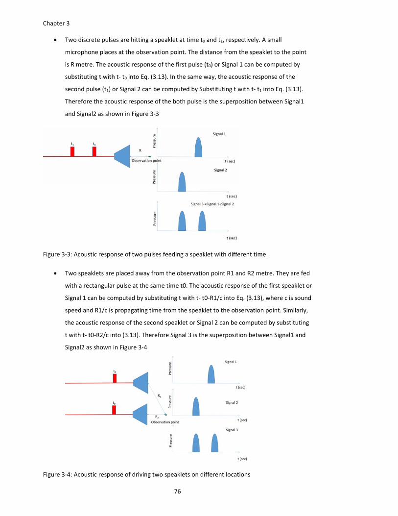
Chapter 3

76

Two discrete pulses are hitting a speaklet at time t0 and t1, respectively. A small

microphone places at the observation point. The distance from the speaklet to the point

is R metre. The acoustic response of the first pulse (t0) or Signal 1 can be computed by

substituting t with t‐ t0 into Eq. (3.13). In the same way, the acoustic response of the

second pulse (t1) or Signal 2 can be computed by Substituting t with t‐ t1 into Eq. (3.13).

Therefore the acoustic response of the both pulse is the superposition between Signal1

and Signal2 as shown in Figure 3‐3

Figure 3‐3: Acoustic response of two pulses feeding a speaklet with different time.

Two speaklets are placed away from the observation point R1 and R2 metre. They are fed

with a rectangular pulse at the same time t0. The acoustic response of the first speaklet or

Signal 1 can be computed by substituting t with t‐ t0‐R1/c into Eq. (3.13), where c is sound

speed and R1/c is propagating time from the speaklet to the observation point. Similarly,

the acoustic response of the second speaklet or Signal 2 can be computed by substituting

t with t‐ t0‐R2/c into (3.13). Therefore Signal 3 is the superposition between Signal1 and

Signal2 as shown in Figure 3‐4

Figure 3‐4: Acoustic response of driving two speaklets on different locations

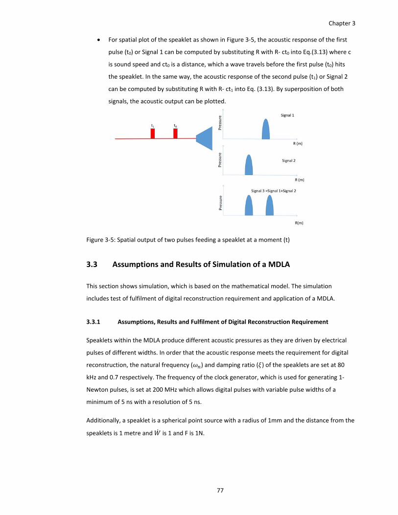
Chapter 3

77

For spatial plot of the speaklet as shown in Figure 3‐5, the acoustic response of the first

pulse (t0) or Signal 1 can be computed by substituting R with R‐ ct0 into Eq.(3.13) where c

is sound speed and ct0 is a distance, which a wave travels before the first pulse (t0) hits

the speaklet. In the same way, the acoustic response of the second pulse (t1) or Signal 2

can be computed by substituting R with R‐ ct1 into Eq. (3.13). By superposition of both

signals, the acoustic output can be plotted.

Figure 3‐5: Spatial output of two pulses feeding a speaklet at a moment (t)

3.3 Assumptions and Results of Simulation of a MDLA

This section shows simulation, which is based on the mathematical model. The simulation

includes test of fulfilment of digital reconstruction requirement and application of a MDLA.

3.3.1 Assumptions, Results and Fulfilment of Digital Reconstruction Requirement

Speaklets within the MDLA produce different acoustic pressures as they are driven by electrical

pulses of different widths. In order that the acoustic response meets the requirement for digital

reconstruction, the natural frequency ( ) and damping ratio ( ) of the speaklets are set at 80

kHz and 0.7 respectively. The frequency of the clock generator, which is used for generating 1‐

Newton pulses, is set at 200 MHz which allows digital pulses with variable pulse widths of a

minimum of 5 ns with a resolution of 5 ns.

Additionally, a speaklet is a spherical point source with a radius of 1mm and the distance from the

speaklets is 1 metre and is 1 and F is 1N.

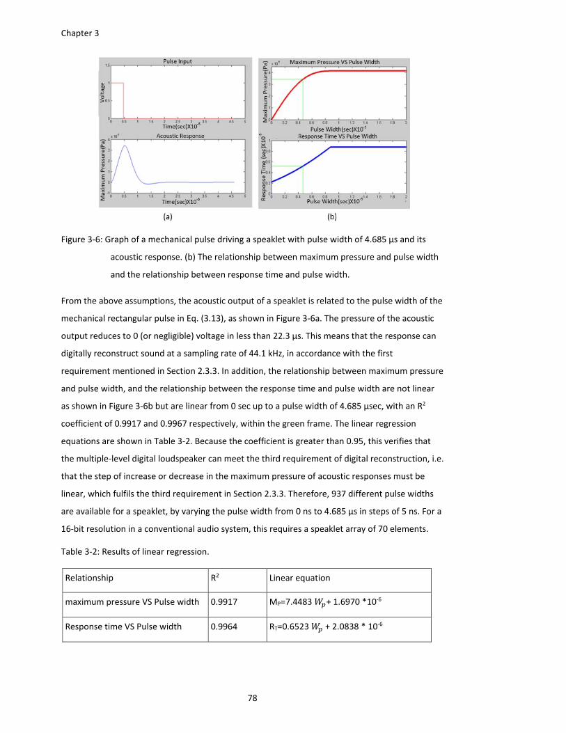
Chapter 3

78

Figure 3‐6: Graph of a mechanical pulse driving a speaklet with pulse width of 4.685 µs and its

acoustic response. (b) The relationship between maximum pressure and pulse width

and the relationship between response time and pulse width.

From the above assumptions, the acoustic output of a speaklet is related to the pulse width of the

mechanical rectangular pulse in Eq. (3.13), as shown in Figure 3‐6a. The pressure of the acoustic

output reduces to 0 (or negligible) voltage in less than 22.3 µs. This means that the response can

digitally reconstruct sound at a sampling rate of 44.1 kHz, in accordance with the first

requirement mentioned in Section 2.3.3. In addition, the relationship between maximum pressure

and pulse width, and the relationship between the response time and pulse width are not linear

as shown in Figure 3‐6b but are linear from 0 sec up to a pulse width of 4.685 μsec, with an R2

coefficient of 0.9917 and 0.9967 respectively, within the green frame. The linear regression

equations are shown in Table 3‐2. Because the coefficient is greater than 0.95, this verifies that

the multiple‐level digital loudspeaker can meet the third requirement of digital reconstruction, i.e.

that the step of increase or decrease in the maximum pressure of acoustic responses must be

linear, which fulfils the third requirement in Section 2.3.3. Therefore, 937 different pulse widths

are available for a speaklet, by varying the pulse width from 0 ns to 4.685 μs in steps of 5 ns. For a

16‐bit resolution in a conventional audio system, this requires a speaklet array of 70 elements.

Table 3‐2: Results of linear regression.

Relationship R2 Linear equation

maximum pressure VS Pulse width 0.9917 MP=7.4483 + 1.6970 *10‐6

Response time VS Pulse width 0.9964 RT=0.6523 + 2.0838 * 10‐6

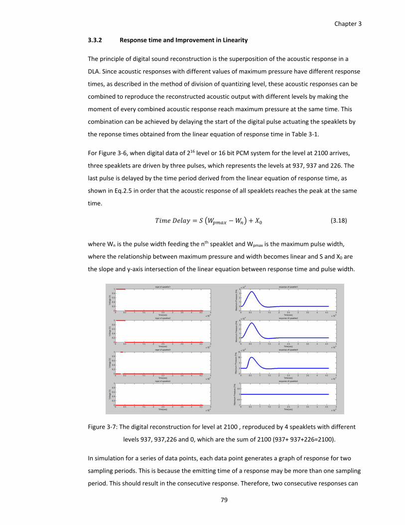
Chapter 3

79

3.3.2 Response time and Improvement in Linearity

The principle of digital sound reconstruction is the superposition of the acoustic response in a

DLA. Since acoustic responses with different values of maximum pressure have different response

times, as described in the method of division of quantizing level, these acoustic responses can be

combined to reproduce the reconstructed acoustic output with different levels by making the

moment of every combined acoustic response reach maximum pressure at the same time. This

combination can be achieved by delaying the start of the digital pulse actuating the speaklets by

the reponse times obtained from the linear equation of response time in Table 3‐1.

For Figure 3‐6, when digital data of 216 level or 16 bit PCM system for the level at 2100 arrives,

three speaklets are driven by three pulses, which represents the levels at 937, 937 and 226. The

last pulse is delayed by the time period derived from the linear equation of response time, as

shown in Eq.2.5 in order that the acoustic response of all speaklets reaches the peak at the same

time.

(3.18)

where Wn is the pulse width feeding the nth speaklet and Wpmax is the maximum pulse width,

where the relationship between maximum pressure and width becomes linear and S and X0 are

the slope and y‐axis intersection of the linear equation between response time and pulse width.

Figure 3‐7: The digital reconstruction for level at 2100 , reproduced by 4 speaklets with different

levels 937, 937,226 and 0, which are the sum of 2100 (937+ 937+226=2100).

In simulation for a series of data points, each data point generates a graph of response for two

sampling periods. This is because the emitting time of a response may be more than one sampling

period. This should result in the consecutive response. Therefore, two consecutive responses can

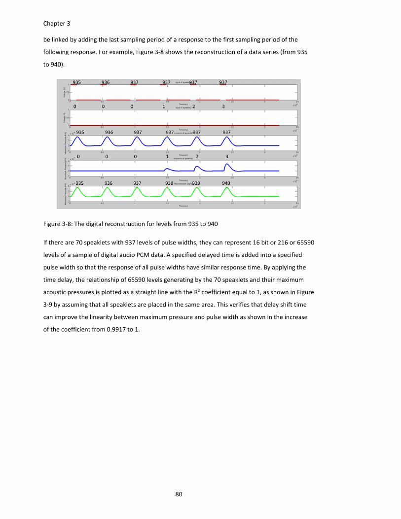
Chapter 3

80

be linked by adding the last sampling period of a response to the first sampling period of the

following response. For example, Figure 3‐8 shows the reconstruction of a data series (from 935

to 940).

Figure 3‐8: The digital reconstruction for levels from 935 to 940

If there are 70 speaklets with 937 levels of pulse widths, they can represent 16 bit or 216 or 65590

levels of a sample of digital audio PCM data. A specified delayed time is added into a specified

pulse width so that the response of all pulse widths have similar response time. By applying the

time delay, the relationship of 65590 levels generating by the 70 speaklets and their maximum

acoustic pressures is plotted as a straight line with the R2 coefficient equal to 1, as shown in Figure

3‐9 by assuming that all speaklets are placed in the same area. This verifies that delay shift time

can improve the linearity between maximum pressure and pulse width as shown in the increase

of the coefficient from 0.9917 to 1.

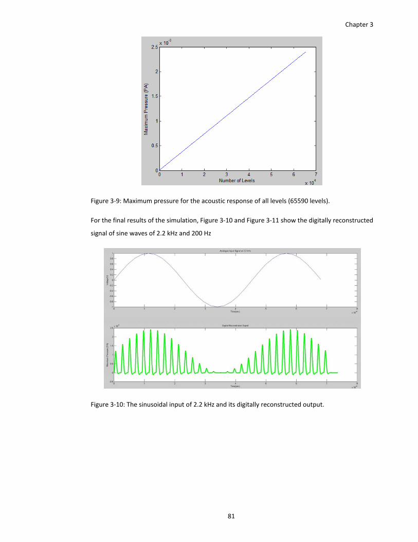
Chapter 3

81

Figure 3‐9: Maximum pressure for the acoustic response of all levels (65590 levels).

For the final results of the simulation, Figure 3‐10 and Figure 3‐11 show the digitally reconstructed

signal of sine waves of 2.2 kHz and 200 Hz

Figure 3‐10: The sinusoidal input of 2.2 kHz and its digitally reconstructed output.

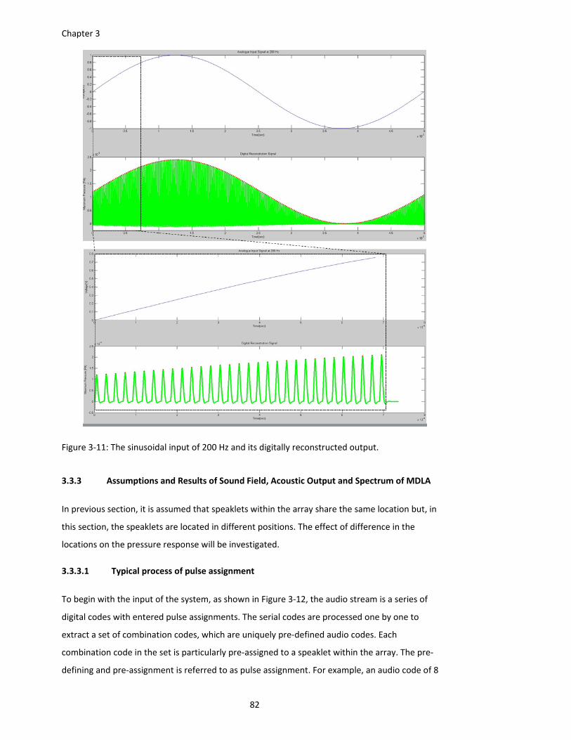
Chapter 3

82

Figure 3‐11: The sinusoidal input of 200 Hz and its digitally reconstructed output.

3.3.3 Assumptions and Results of Sound Field, Acoustic Output and Spectrum of MDLA

In previous section, it is assumed that speaklets within the array share the same location but, in

this section, the speaklets are located in different positions. The effect of difference in the

locations on the pressure response will be investigated.

3.3.3.1 Typical process of pulse assignment

To begin with the input of the system, as shown in Figure 3‐12, the audio stream is a series of

digital codes with entered pulse assignments. The serial codes are processed one by one to

extract a set of combination codes, which are uniquely pre‐defined audio codes. Each

combination code in the set is particularly pre‐assigned to a speaklet within the array. The pre‐

defining and pre‐assignment is referred to as pulse assignment. For example, an audio code of 8

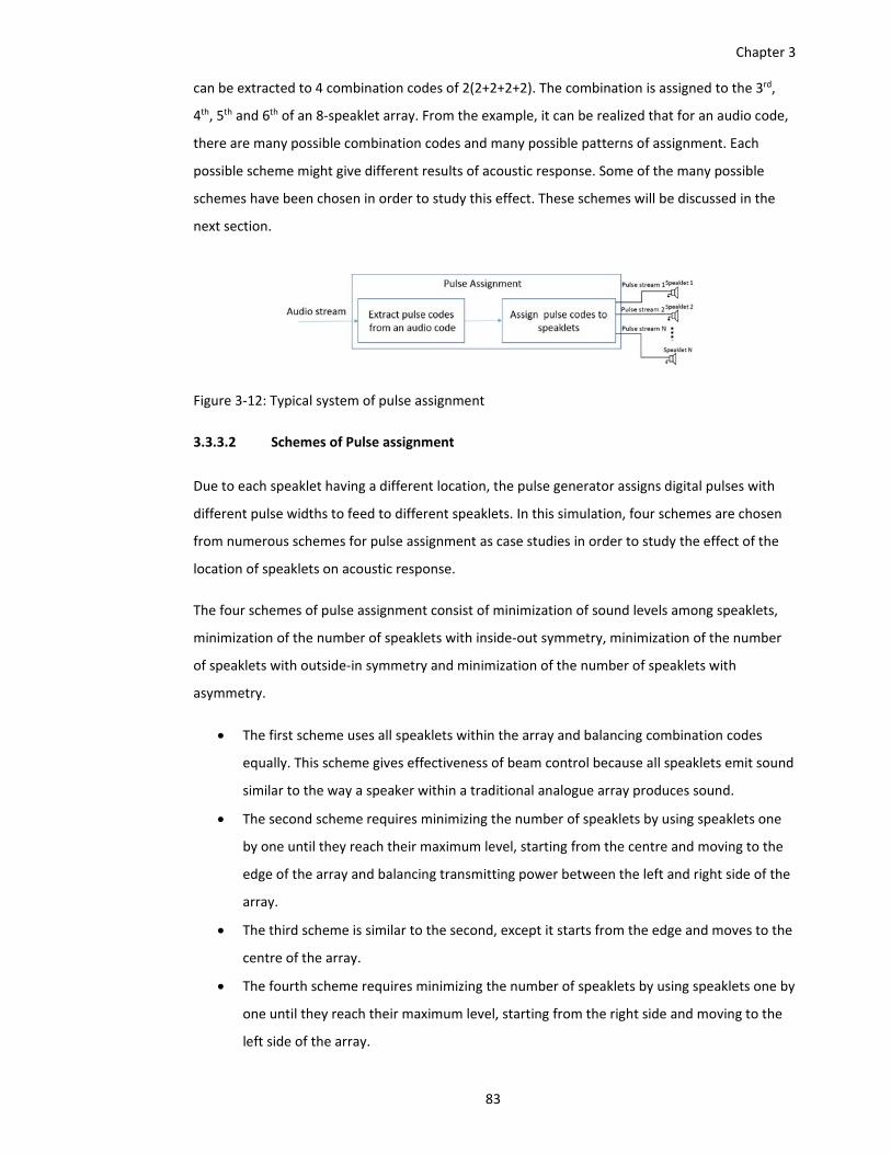
Chapter 3

83

can be extracted to 4 combination codes of 2(2+2+2+2). The combination is assigned to the 3rd,

4th, 5th and 6th of an 8‐speaklet array. From the example, it can be realized that for an audio code,

there are many possible combination codes and many possible patterns of assignment. Each

possible scheme might give different results of acoustic response. Some of the many possible

schemes have been chosen in order to study this effect. These schemes will be discussed in the

next section.

Figure 3‐12: Typical system of pulse assignment

3.3.3.2 Schemes of Pulse assignment

Due to each speaklet having a different location, the pulse generator assigns digital pulses with

different pulse widths to feed to different speaklets. In this simulation, four schemes are chosen

from numerous schemes for pulse assignment as case studies in order to study the effect of the

location of speaklets on acoustic response.

The four schemes of pulse assignment consist of minimization of sound levels among speaklets,

minimization of the number of speaklets with inside‐out symmetry, minimization of the number

of speaklets with outside‐in symmetry and minimization of the number of speaklets with

asymmetry.

The first scheme uses all speaklets within the array and balancing combination codes

equally. This scheme gives effectiveness of beam control because all speaklets emit sound

similar to the way a speaker within a traditional analogue array produces sound.

The second scheme requires minimizing the number of speaklets by using speaklets one

by one until they reach their maximum level, starting from the centre and moving to the

edge of the array and balancing transmitting power between the left and right side of the

array.

The third scheme is similar to the second, except it starts from the edge and moves to the

centre of the array.

The fourth scheme requires minimizing the number of speaklets by using speaklets one by

one until they reach their maximum level, starting from the right side and moving to the

left side of the array.

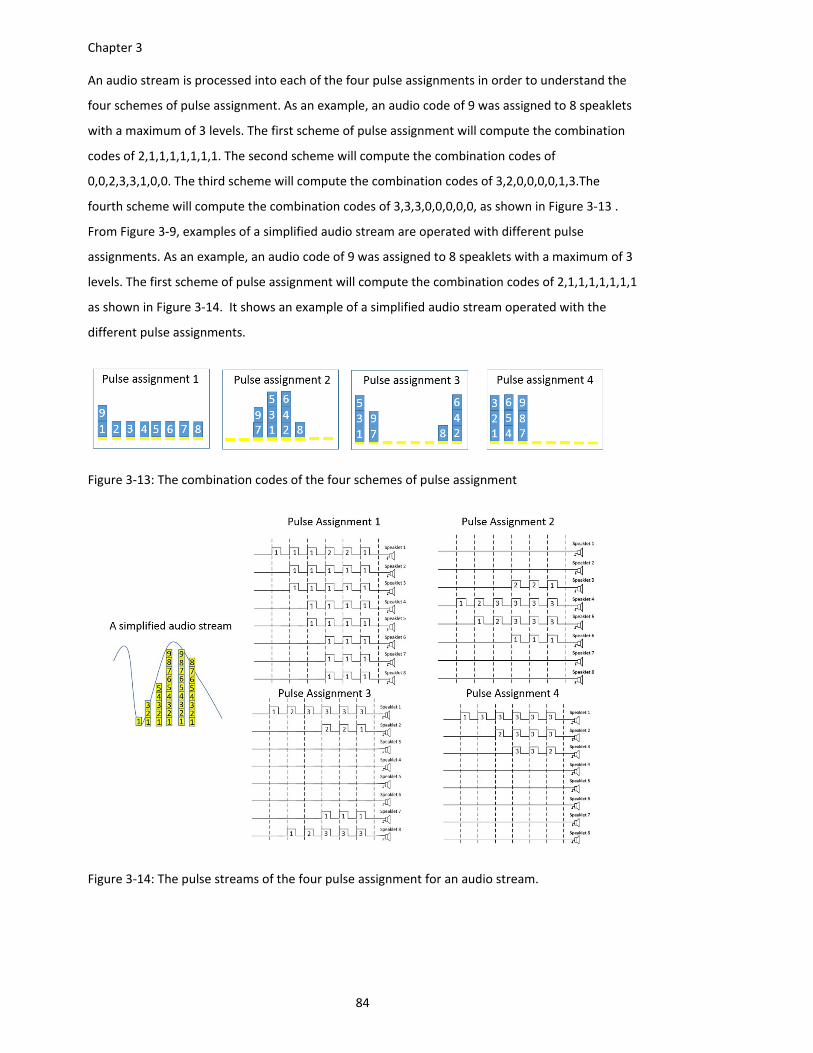
Chapter 3

84

An audio stream is processed into each of the four pulse assignments in order to understand the

four schemes of pulse assignment. As an example, an audio code of 9 was assigned to 8 speaklets

with a maximum of 3 levels. The first scheme of pulse assignment will compute the combination

codes of 2,1,1,1,1,1,1,1. The second scheme will compute the combination codes of

0,0,2,3,3,1,0,0. The third scheme will compute the combination codes of 3,2,0,0,0,0,1,3.The

fourth scheme will compute the combination codes of 3,3,3,0,0,0,0,0, as shown in Figure 3‐13 .

From Figure 3‐9, examples of a simplified audio stream are operated with different pulse

assignments. As an example, an audio code of 9 was assigned to 8 speaklets with a maximum of 3

levels. The first scheme of pulse assignment will compute the combination codes of 2,1,1,1,1,1,1,1

as shown in Figure 3‐14. It shows an example of a simplified audio stream operated with the

different pulse assignments.

Figure 3‐13: The combination codes of the four schemes of pulse assignment

Figure 3‐14: The pulse streams of the four pulse assignment for an audio stream.

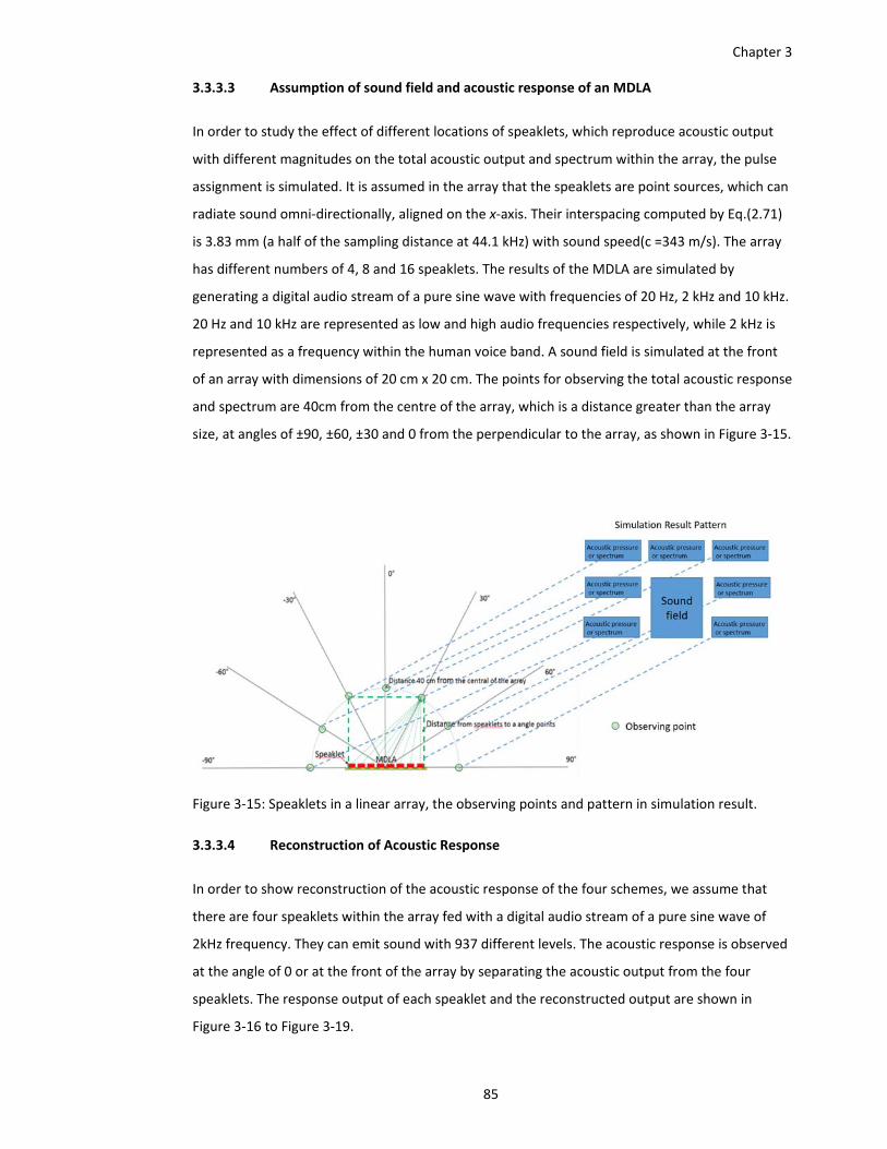
Chapter 3

85

3.3.3.3 Assumption of sound field and acoustic response of an MDLA

In order to study the effect of different locations of speaklets, which reproduce acoustic output

with different magnitudes on the total acoustic output and spectrum within the array, the pulse

assignment is simulated. It is assumed in the array that the speaklets are point sources, which can

radiate sound omni‐directionally, aligned on the x‐axis. Their interspacing computed by Eq.(2.71)

is 3.83 mm (a half of the sampling distance at 44.1 kHz) with sound speed(c =343 m/s). The array

has different numbers of 4, 8 and 16 speaklets. The results of the MDLA are simulated by

generating a digital audio stream of a pure sine wave with frequencies of 20 Hz, 2 kHz and 10 kHz.

20 Hz and 10 kHz are represented as low and high audio frequencies respectively, while 2 kHz is

represented as a frequency within the human voice band. A sound field is simulated at the front

of an array with dimensions of 20 cm x 20 cm. The points for observing the total acoustic response

and spectrum are 40cm from the centre of the array, which is a distance greater than the array

size, at angles of ±90, ±60, ±30 and 0 from the perpendicular to the array, as shown in Figure 3‐15.

Figure 3‐15: Speaklets in a linear array, the observing points and pattern in simulation result.

3.3.3.4 Reconstruction of Acoustic Response

In order to show reconstruction of the acoustic response of the four schemes, we assume that

there are four speaklets within the array fed with a digital audio stream of a pure sine wave of

2kHz frequency. They can emit sound with 937 different levels. The acoustic response is observed

at the angle of 0 or at the front of the array by separating the acoustic output from the four

speaklets. The response output of each speaklet and the reconstructed output are shown in

Figure 3‐16 to Figure 3‐19.

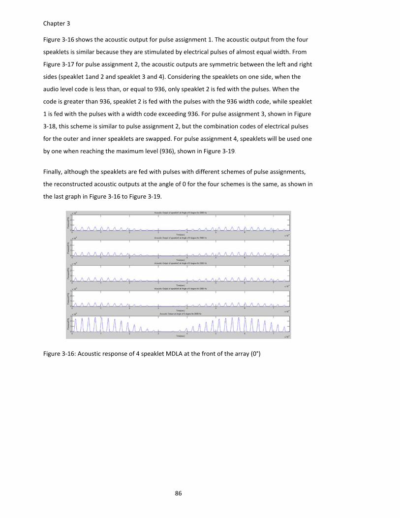
Chapter 3

86

Figure 3‐16 shows the acoustic output for pulse assignment 1. The acoustic output from the four

speaklets is similar because they are stimulated by electrical pulses of almost equal width. From

Figure 3‐17 for pulse assignment 2, the acoustic outputs are symmetric between the left and right

sides (speaklet 1and 2 and speaklet 3 and 4). Considering the speaklets on one side, when the

audio level code is less than, or equal to 936, only speaklet 2 is fed with the pulses. When the

code is greater than 936, speaklet 2 is fed with the pulses with the 936 width code, while speaklet

1 is fed with the pulses with a width code exceeding 936. For pulse assignment 3, shown in Figure

3‐18, this scheme is similar to pulse assignment 2, but the combination codes of electrical pulses

for the outer and inner speaklets are swapped. For pulse assignment 4, speaklets will be used one

by one when reaching the maximum level (936), shown in Figure 3‐19.

Finally, although the speaklets are fed with pulses with different schemes of pulse assignments,

the reconstructed acoustic outputs at the angle of 0 for the four schemes is the same, as shown in

the last graph in Figure 3‐16 to Figure 3‐19.

Figure 3‐16: Acoustic response of 4 speaklet MDLA at the front of the array (0°)

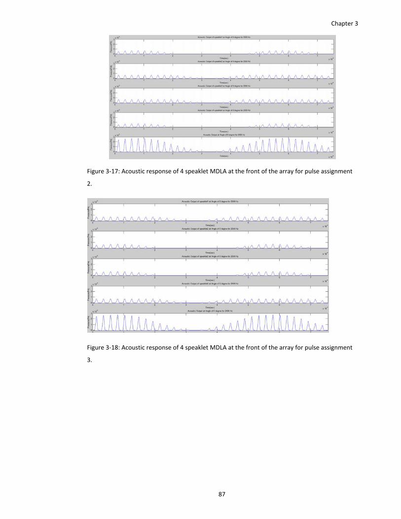
Chapter 3

87


2.


3.

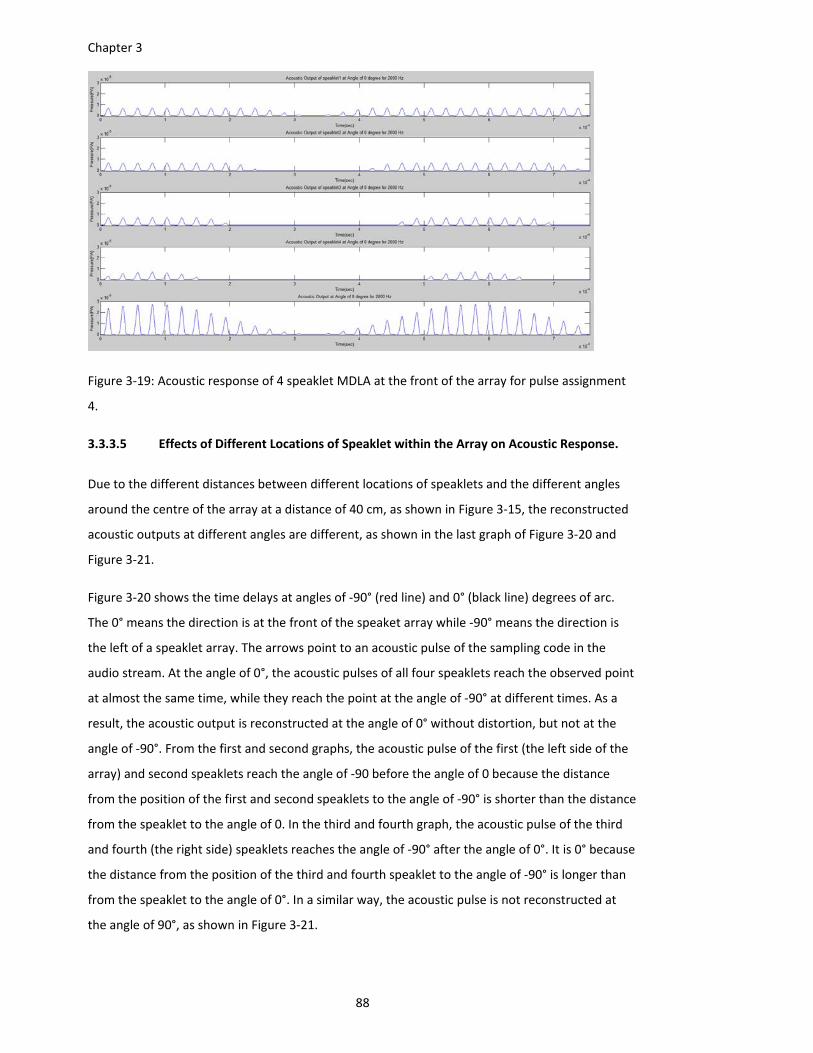
Chapter 3

88


4.

3.3.3.5 Effects of Different Locations of Speaklet within the Array on Acoustic Response.

Due to the different distances between different locations of speaklets and the different angles

around the centre of the array at a distance of 40 cm, as shown in Figure 3‐15, the reconstructed

acoustic outputs at different angles are different, as shown in the last graph of Figure 3‐20 and

Figure 3‐21.

Figure 3‐20 shows the time delays at angles of ‐90° (red line) and 0° (black line) degrees of arc.

The 0° means the direction is at the front of the speaket array while ‐90° means the direction is

the left of a speaklet array. The arrows point to an acoustic pulse of the sampling code in the

audio stream. At the angle of 0°, the acoustic pulses of all four speaklets reach the observed point

at almost the same time, while they reach the point at the angle of ‐90° at different times. As a

result, the acoustic output is reconstructed at the angle of 0° without distortion, but not at the

angle of ‐90°. From the first and second graphs, the acoustic pulse of the first (the left side of the

array) and second speaklets reach the angle of ‐90 before the angle of 0 because the distance

from the position of the first and second speaklets to the angle of ‐90° is shorter than the distance

from the speaklet to the angle of 0. In the third and fourth graph, the acoustic pulse of the third

and fourth (the right side) speaklets reaches the angle of ‐90° after the angle of 0°. It is 0° because

the distance from the position of the third and fourth speaklet to the angle of ‐90° is longer than

from the speaklet to the angle of 0°. In a similar way, the acoustic pulse is not reconstructed at

the angle of 90°, as shown in Figure 3‐21.

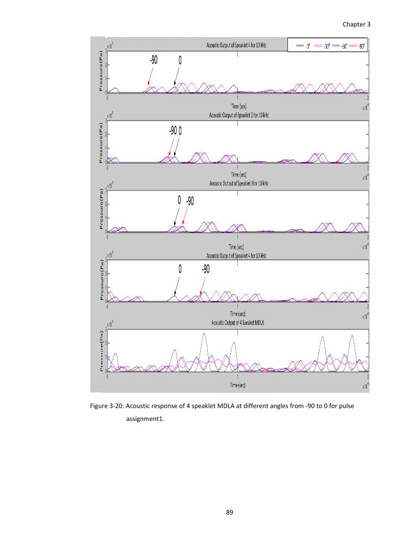
Chapter 3

89

Figure 3‐20: Acoustic response of 4 speaklet MDLA at different angles from ‐90 to 0 for pulse

assignment1.

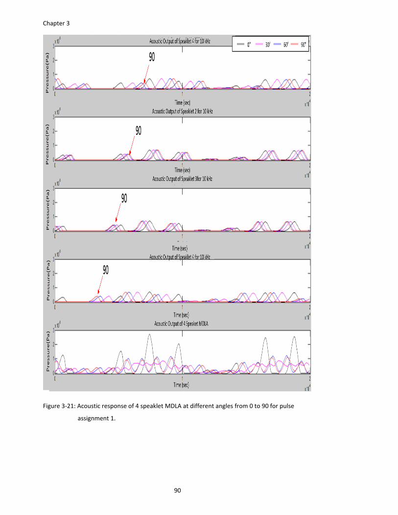
Chapter 3

90

Figure 3‐21: Acoustic response of 4 speaklet MDLA at different angles from 0 to 90 for pulse

assignment 1.

Chapter 3

91

3.3.3.6 Effects of Digital Circuit (DC )component

It can be clearly seen that the acoustic responses for the rectified source are the rectified AM

sound from Figure 3‐16 to Figure 3‐21. A DC component appears. In other words, average

pressure of the signal is not zero.

The DC components might increase the atmosphere pressure. This may cause the danger in the

eardrums or in the hearing ability if the magnitude of DC component is too high. For digital

transmission, a low frequency signal with a DC component cannot pass a low‐pass filter. However,

the ears can endure a small range of the variation of the atmosphere pressure.

The DC component of the pressure signal shows non‐conservative circumstance. The air particles

as a medium not only vibrate but also move from place to place. It is different from the acoustic

response of a common sound which has not a DC component. The air particles vibrate at the

same location.

3.3.3.7 Results of sound field and acoustic response

The results of the simulation are shown to present general characteristics of the acoustic

response of the MDLA and its harmonic distortion. In order to investigate the spectrum of the

acoustic response of the array, a Fast Fourier Transform (FFT) with a sampling rate of 160 kHz and

2000 data points of window size is applied. A finite impulse response (FIR) low pass filter with 256

taps is used for antialiasing.

For sound reconstruction within the MDLA, there are two additional points to consider: firstly,

due to differences in pulse width, the response times of individual speaklets will be different. In

order to ensure that the speaklets produce an acoustic response which reaches maximum

pressure at the same time, the delay of sending electrical pulses needs to be calculated from the

relationship between the response time and pulse width. Secondly, due to the acoustic output of

the MDLA, resulting from a superposition of the response of the speaklets within the array, there

are a variety of combinations of different levels of speaklets, allowing the same quantized level of

output of the array. Therefore, a specific combination of levels is assigned for a specific quantizing

level of output. This simulation will show temporal and frequency responses of the four schemes

of the pulse assignment.

3.3.3.8 General Characters of Acoustic Response

The sound field intensity was also simulated, by assuming that the speaklets are point sources

aligning on the x‐axis and their interspacing is equal to 3.83 mm (half the sampling distance at

44.1 kHz), as shown in Figure 3‐15. The sampling distance can be calculated by the multiplication

Chapter 3

92

between the wave speed and the sampling period, which is the reciprocal of the sampling rate.

The figure shows the spectral response from an array at a distance of 40cm from the centre of the

array through different angles and acoustic outputs.

Figure 3‐22 and Figure 3‐29 shows both the temporal directivity response and the spectral

content at that angle with a number of speaklets for an audio frequency of 10kHz. It can be seen

that the outputs consist of three main components of frequency, especially at an angle of 0

degrees (i.e. directly in front of the element). The first component is the required audible

frequency, which is reproduced by digital reconstruction. The second component depends on the

natural frequency of the speaklets, which is around 44.1 kHz. The last component is a harmonic

frequency of 71.9 kHz, which results from the sum of side bands of 44.1 kHz AM wave. However,

the last two components have no effect on hearing because they are beyond the response of the

human ear.

Different pulse assignments make different sound fields depending on the series of combination

codes defined in the schemes of pulse assignment. The difference in the sound fields of different

pulse assignments still results in a difference in acoustic response observed in all directions,

except at the angle of 0 (at the front of the array), which have the same acoustic response, as

shown from Figure 3‐22 to Figure 3‐29. In addition, symmetric pulse assignments have a direct

effect in symmetric sound beams of the array, as with pulse assignments 1 to 3, which have the

same acoustic response between the pairs of plus and minus angles (±30, ±60 and ±90).

Asymmetric pulse assignments (pulse assignment 4) have different acoustic outputs in every

direction, as shown in Figure 3‐25.

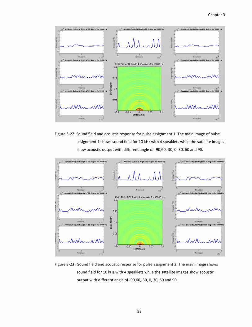
Chapter 3

93

Figure 3‐22: Sound field and acoustic response for pulse assignment 1. The main image of pulse

assignment 1 shows sound field for 10 kHz with 4 speaklets while the satellite images

show acoustic output with different angle of ‐90,60,‐30, 0, 30, 60 and 90.

Figure 3‐23 : Sound field and acoustic response for pulse assignment 2. The main image shows


output with different angle of ‐90,60,‐30, 0, 30, 60 and 90.

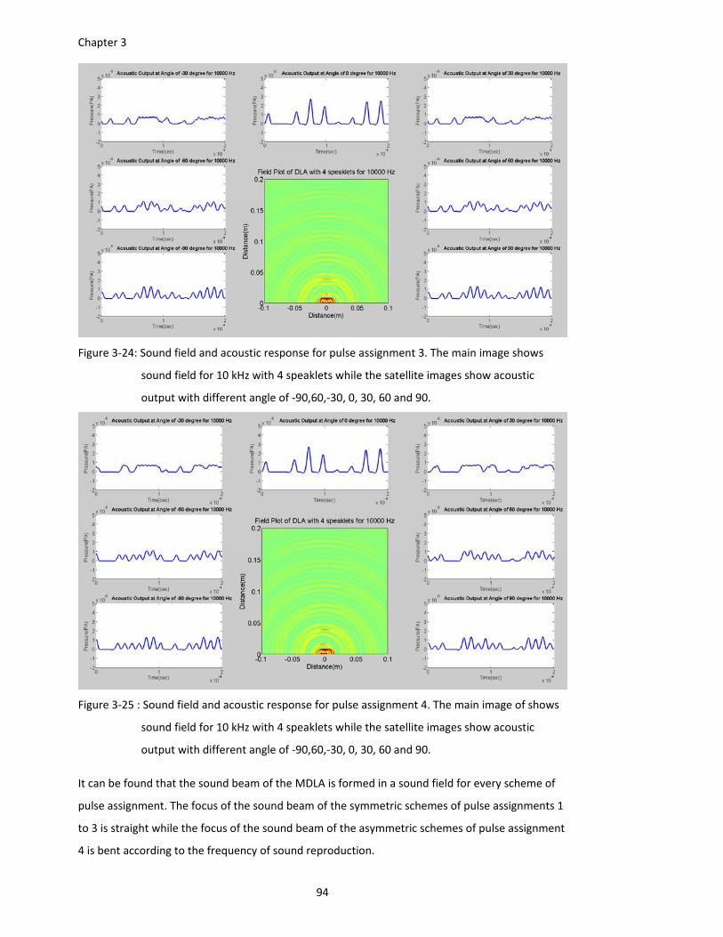
Chapter 3

94

Figure 3‐24: Sound field and acoustic response for pulse assignment 3. The main image shows



Figure 3‐25 : Sound field and acoustic response for pulse assignment 4. The main image of shows



It can be found that the sound beam of the MDLA is formed in a sound field for every scheme of

pulse assignment. The focus of the sound beam of the symmetric schemes of pulse assignments 1

to 3 is straight while the focus of the sound beam of the asymmetric schemes of pulse assignment

4 is bent according to the frequency of sound reproduction.

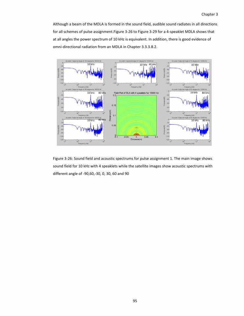
Chapter 3

95

Although a beam of the MDLA is formed in the sound field, audible sound radiates in all directions

for all schemes of pulse assignment.Figure 3‐26 to Figure 3‐29 for a 4‐speaklet MDLA shows that

at all angles the power spectrum of 10 kHz is equivalent. In addition, there is good evidence of

omni‐directional radiation from an MDLA in Chapter 3.3.3.8.2.


sound field for 10 kHz with 4 speaklets while the satellite images show acoustic spectrums with

different angle of ‐90,60,‐30, 0, 30, 60 and 90

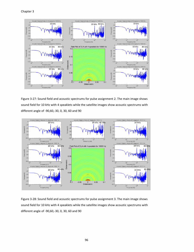
Chapter 3

96







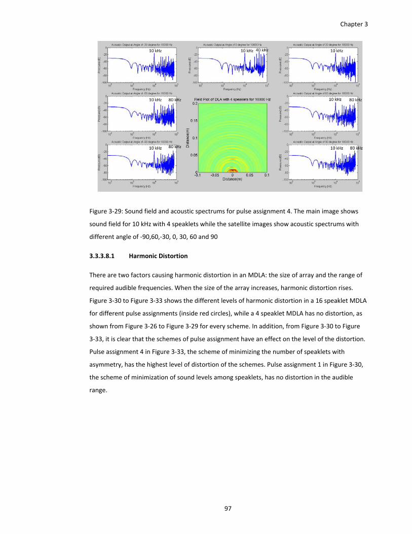
Chapter 3

97




3.3.3.8.1 Harmonic Distortion

There are two factors causing harmonic distortion in an MDLA: the size of array and the range of

required audible frequencies. When the size of the array increases, harmonic distortion rises.

Figure 3‐30 to Figure 3‐33 shows the different levels of harmonic distortion in a 16 speaklet MDLA

for different pulse assignments (inside red circles), while a 4 speaklet MDLA has no distortion, as

shown from Figure 3‐26 to Figure 3‐29 for every scheme. In addition, from Figure 3‐30 to Figure

3‐33, it is clear that the schemes of pulse assignment have an effect on the level of the distortion.

Pulse assignment 4 in Figure 3‐33, the scheme of minimizing the number of speaklets with

asymmetry, has the highest level of distortion of the schemes. Pulse assignment 1 in Figure 3‐30,

the scheme of minimization of sound levels among speaklets, has no distortion in the audible

range.

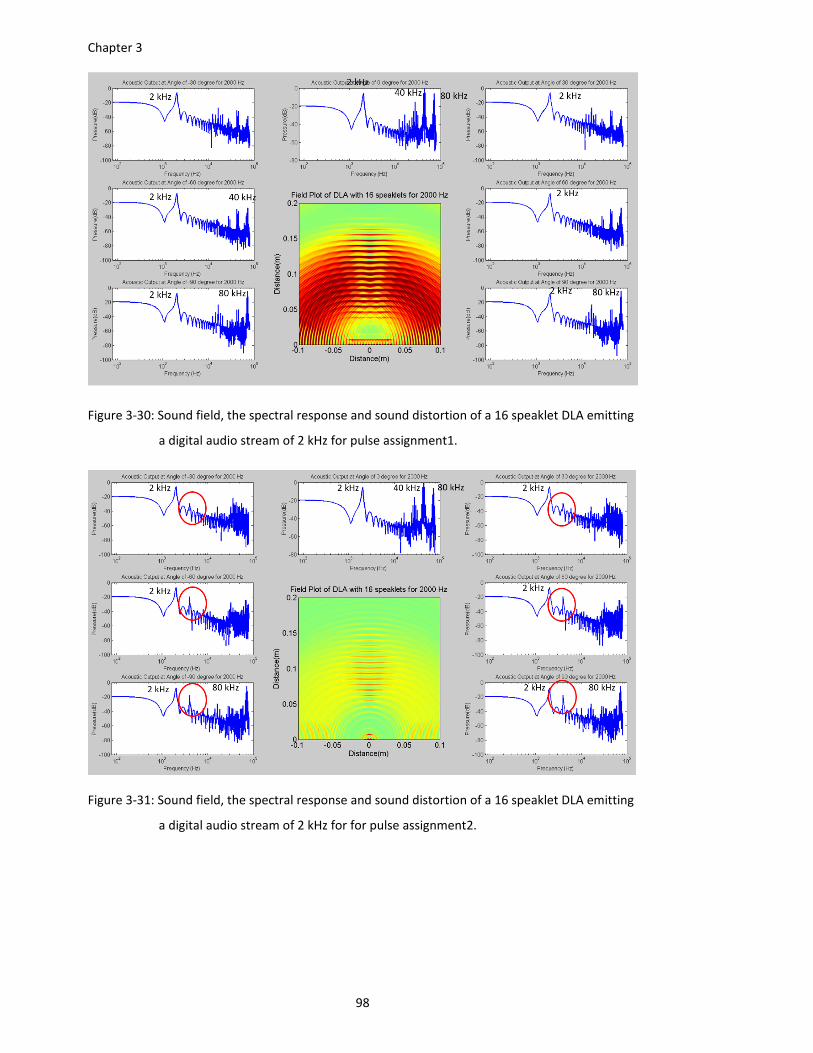
Chapter 3

98


a digital audio stream of 2 kHz for pulse assignment1.


a digital audio stream of 2 kHz for for pulse assignment2.

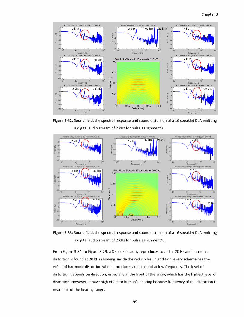
Chapter 3

99





From Figure 3‐34 to Figure 3‐29, a 8 speaklet array reproduces sound at 20 Hz and harmonic

distortion is found at 20 kHz showing inside the red circles. In addition, every scheme has the

effect of harmonic distortion when it produces audio sound at low frequency. The level of

distortion depends on direction, especially at the front of the array, which has the highest level of

distortion. However, it have high effect to human’s hearing because frequency of the distortion is

near limit of the hearing range.

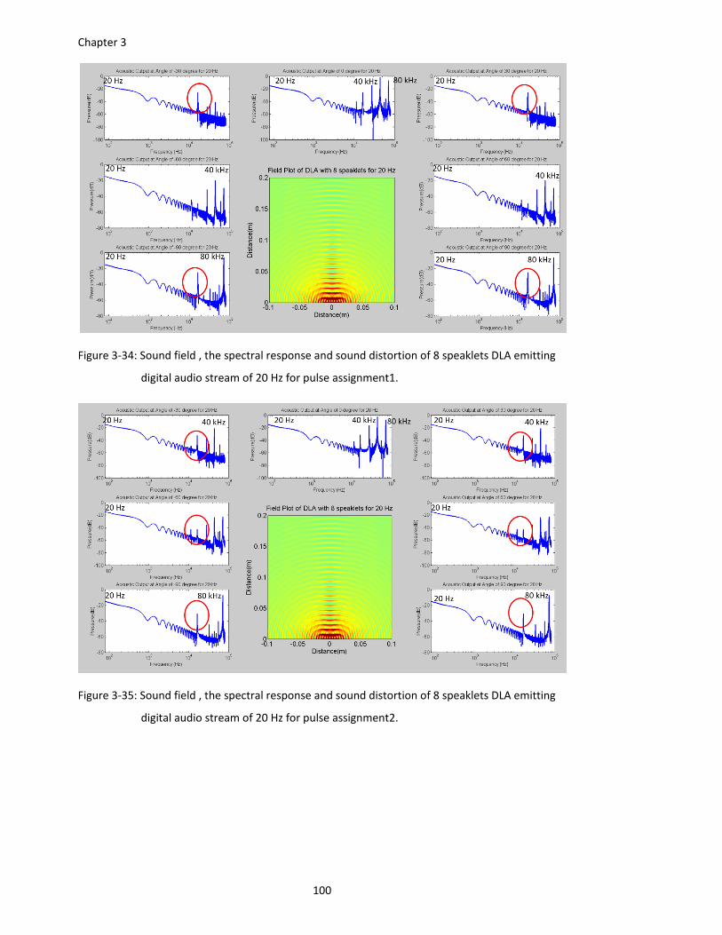
Chapter 3

100


digital audio stream of 20 Hz for pulse assignment1.



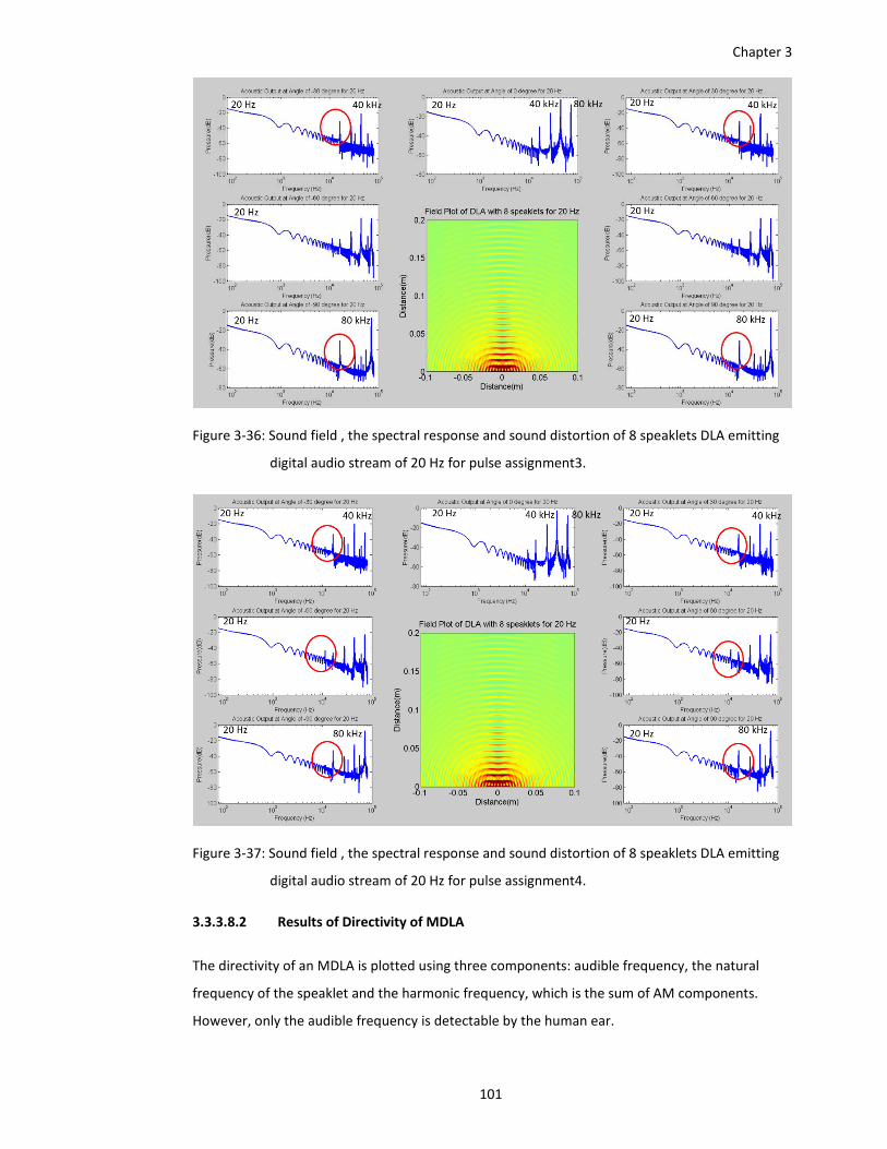
Chapter 3

101





3.3.3.8.2 Results of Directivity of MDLA

The directivity of an MDLA is plotted using three components: audible frequency, the natural

frequency of the speaklet and the harmonic frequency, which is the sum of AM components.

However, only the audible frequency is detectable by the human ear.

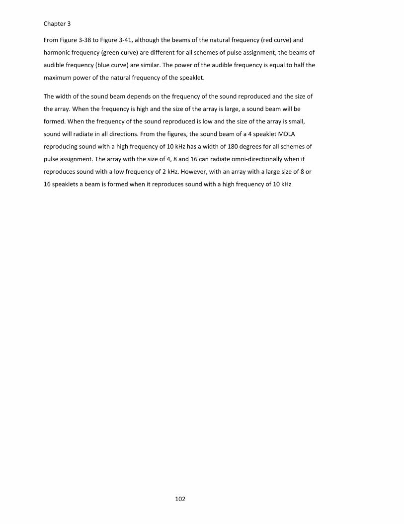
Chapter 3

102

From Figure 3‐38 to Figure 3‐41, although the beams of the natural frequency (red curve) and

harmonic frequency (green curve) are different for all schemes of pulse assignment, the beams of

audible frequency (blue curve) are similar. The power of the audible frequency is equal to half the

maximum power of the natural frequency of the speaklet.

The width of the sound beam depends on the frequency of the sound reproduced and the size of

the array. When the frequency is high and the size of the array is large, a sound beam will be

formed. When the frequency of the sound reproduced is low and the size of the array is small,

sound will radiate in all directions. From the figures, the sound beam of a 4 speaklet MDLA

reproducing sound with a high frequency of 10 kHz has a width of 180 degrees for all schemes of

pulse assignment. The array with the size of 4, 8 and 16 can radiate omni‐directionally when it

reproduces sound with a low frequency of 2 kHz. However, with an array with a large size of 8 or

16 speaklets a beam is formed when it reproduces sound with a high frequency of 10 kHz

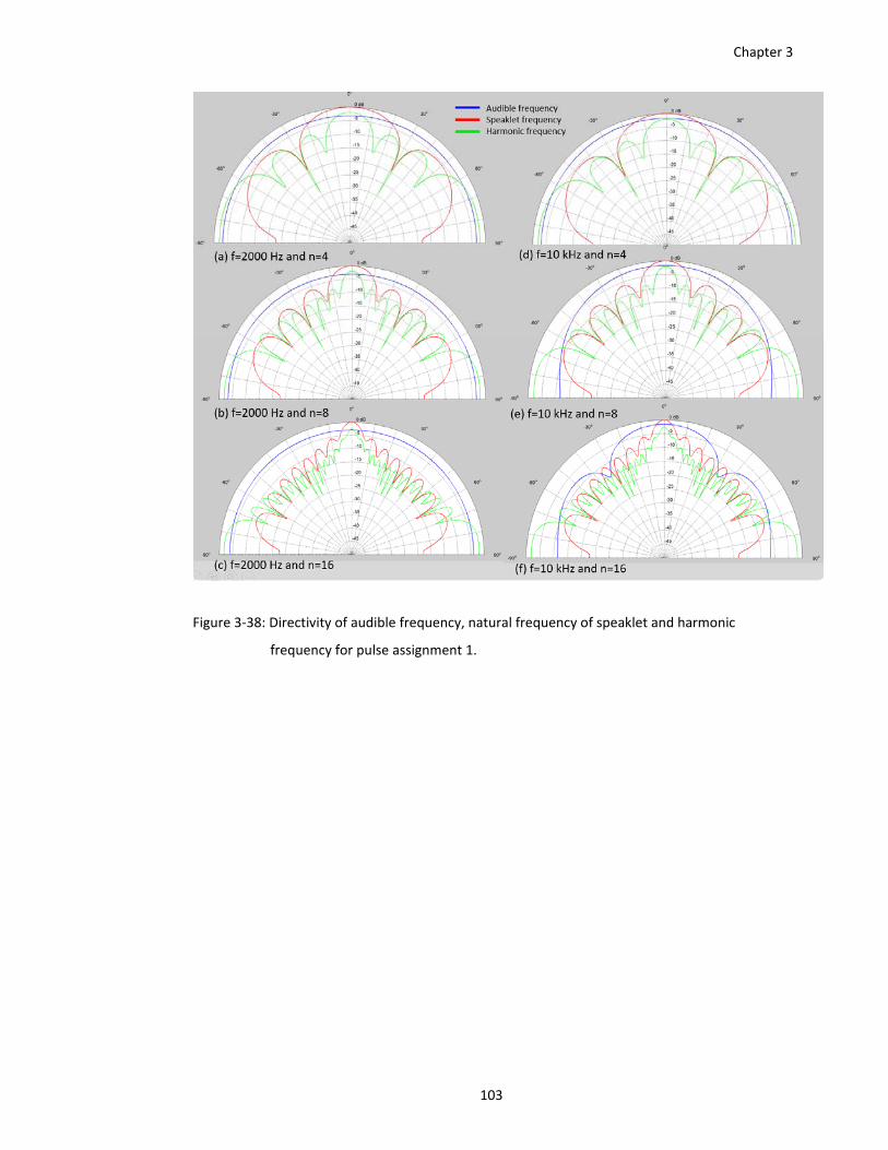
Chapter 3

103


frequency for pulse assignment 1.

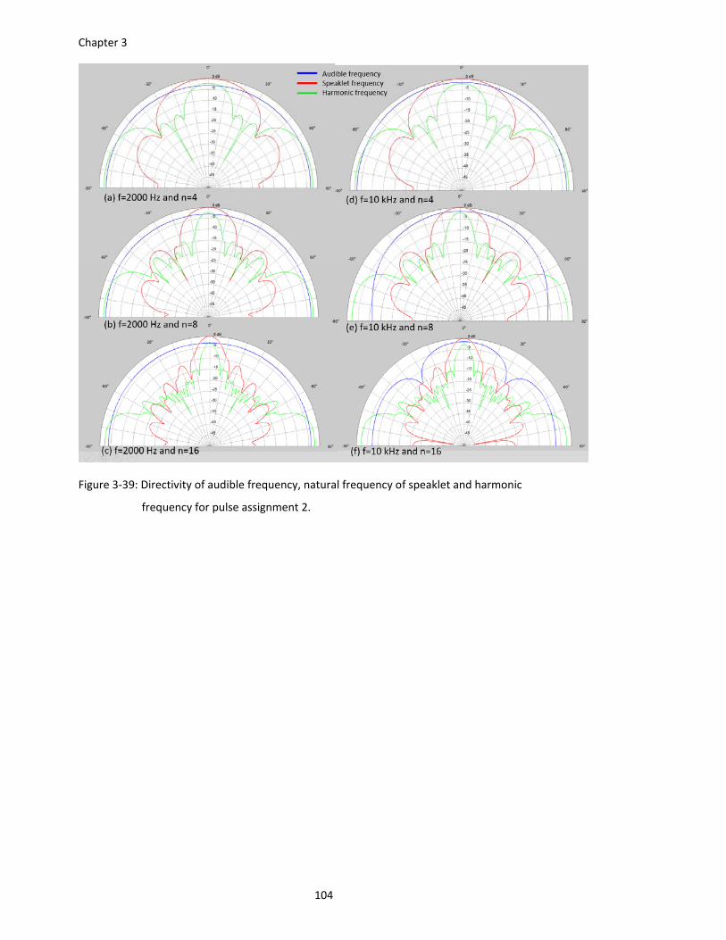
Chapter 3

104



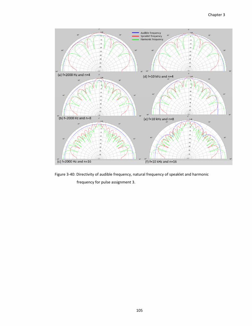
Chapter 3

105



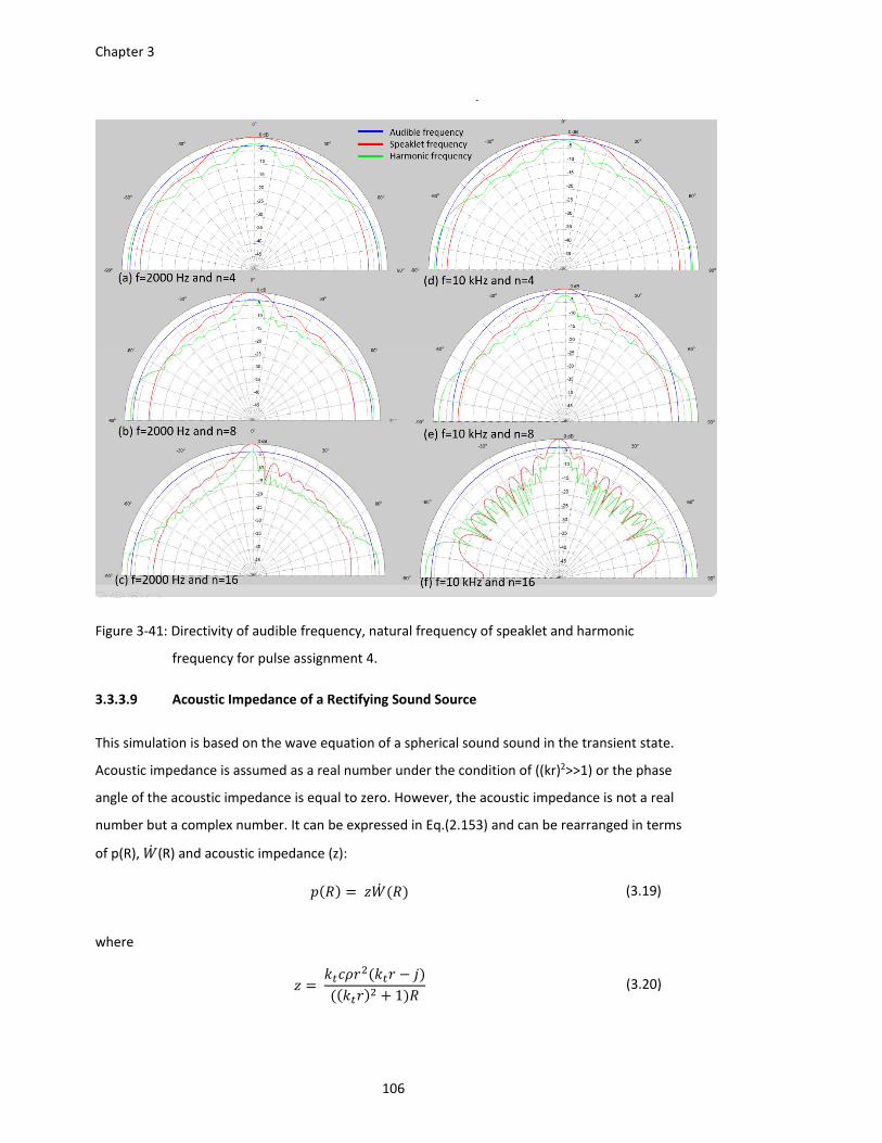
Chapter 3

106



3.3.3.9 Acoustic Impedance of a Rectifying Sound Source

This simulation is based on the wave equation of a spherical sound sound in the transient state.

Acoustic impedance is assumed as a real number under the condition of ((kr)2>>1) or the phase

angle of the acoustic impedance is equal to zero. However, the acoustic impedance is not a real

number but a complex number. It can be expressed in Eq.(2.153) and can be rearranged in terms

of p(R), (R) and acoustic impedance (z):

(3.19)

where

1

(3.20)

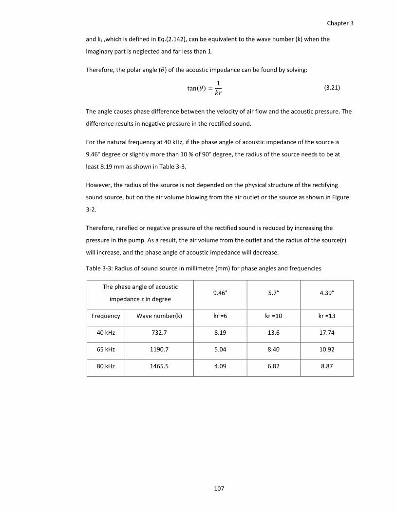
Chapter 3

107

and kt ,which is defined in Eq.(2.142), can be equivalent to the wave number (k) when the

imaginary part is neglected and far less than 1.

Therefore, the polar angle ( ) of the acoustic impedance can be found by solving:

tan1 (3.21)

The angle causes phase difference between the velocity of air flow and the acoustic pressure. The

difference results in negative pressure in the rectified sound.

For the natural frequency at 40 kHz, if the phase angle of acoustic impedance of the source is

9.46° degree or slightly more than 10 % of 90° degree, the radius of the source needs to be at

least 8.19 mm as shown in Table 3‐3.

However, the radius of the source is not depended on the physical structure of the rectifying

sound source, but on the air volume blowing from the air outlet or the source as shown in Figure

3‐2.

Therefore, rarefied or negative pressure of the rectified sound is reduced by increasing the

pressure in the pump. As a result, the air volume from the outlet and the radius of the source(r)

will increase, and the phase angle of acoustic impedance will decrease.

Table 3‐3: Radius of sound source in millimetre (mm) for phase angles and frequencies

The phase angle of acoustic

impedance z in degree 9.46° 5.7° 4.39°

Frequency Wave number(k) kr =6 kr =10 kr =13

40 kHz 732.7 8.19 13.6 17.74

65 kHz 1190.7 5.04 8.40 10.92

80 kHz 1465.5 4.09 6.82 8.87

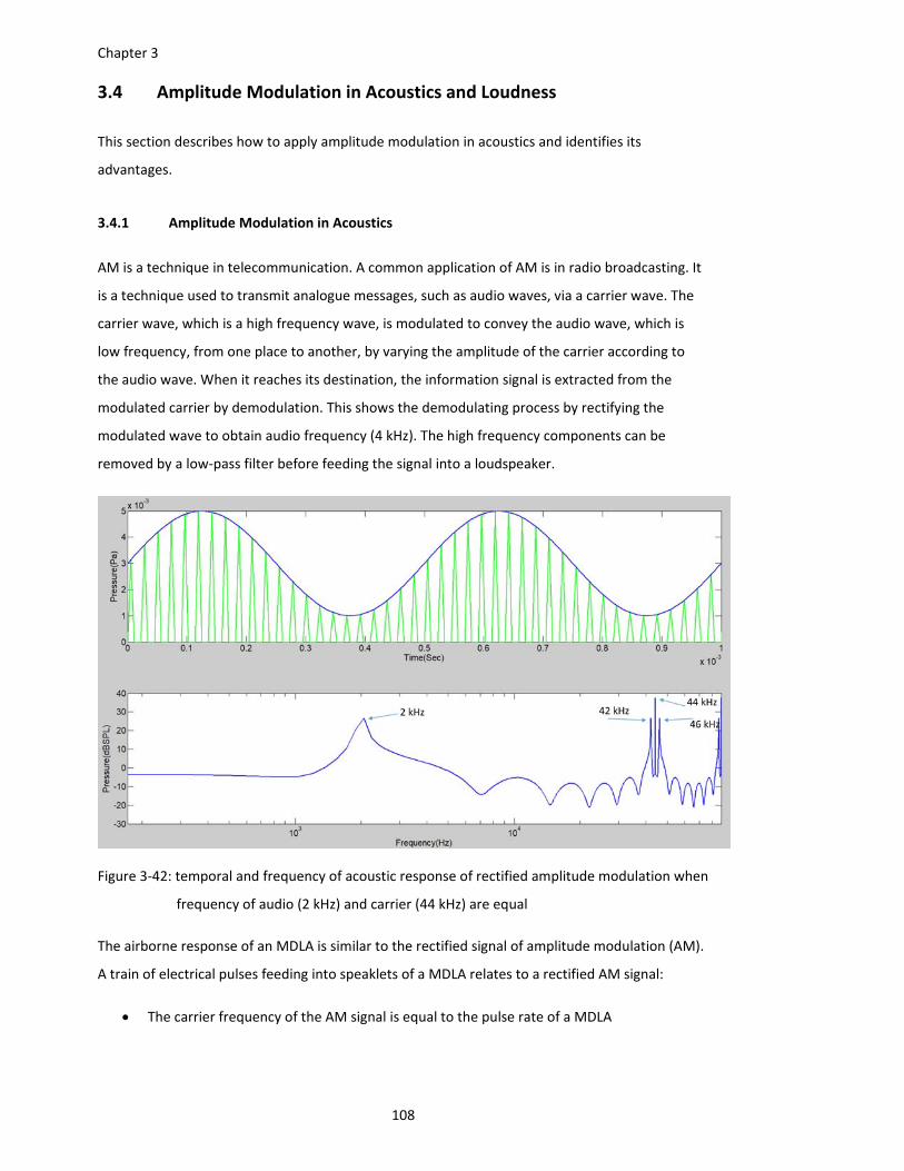
Chapter 3

108

3.4 Amplitude Modulation in Acoustics and Loudness

This section describes how to apply amplitude modulation in acoustics and identifies its

advantages.

3.4.1 Amplitude Modulation in Acoustics

AM is a technique in telecommunication. A common application of AM is in radio broadcasting. It

is a technique used to transmit analogue messages, such as audio waves, via a carrier wave. The

carrier wave, which is a high frequency wave, is modulated to convey the audio wave, which is

low frequency, from one place to another, by varying the amplitude of the carrier according to

the audio wave. When it reaches its destination, the information signal is extracted from the

modulated carrier by demodulation. This shows the demodulating process by rectifying the

modulated wave to obtain audio frequency (4 kHz). The high frequency components can be

removed by a low‐pass filter before feeding the signal into a loudspeaker.

Figure 3‐42: temporal and frequency of acoustic response of rectified amplitude modulation when

frequency of audio (2 kHz) and carrier (44 kHz) are equal

The airborne response of an MDLA is similar to the rectified signal of amplitude modulation (AM).

A train of electrical pulses feeding into speaklets of a MDLA relates to a rectified AM signal:

The carrier frequency of the AM signal is equal to the pulse rate of a MDLA

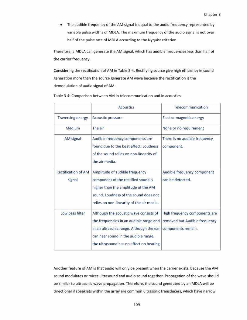
Chapter 3

109

The audible frequency of the AM signal is equal to the audio frequency represented by

variable pulse widths of MDLA. The maximum frequency of the audio signal is not over

half of the pulse rate of MDLA according to the Nyquist criterion.

Therefore, a MDLA can generate the AM signal, which has audible frequencies less than half of

the carrier frequency.

Considering the rectification of AM in Table 3‐4, Rectifying source give high efficiency in sound

generation more than the source generate AM wave because the rectification is the

demodulation of audio signal of AM.

Table 3‐4: Comparison between AM in telecommunication and in acoustics

Acoustics Telecommunication

Traversing energy Acoustic pressure Electro‐magnetic energy

Medium The air None or no requirement

AM signal Audible frequency components are

found due to the beat effect. Loudness

of the sound relies on non‐linearity of

the air media.

There is no audible frequency

component.

Rectification of AM

signal

Amplitude of audible frequency

component of the rectified sound is

higher than the amplitude of the AM

sound. Loudness of the sound does not

relies on non‐linearity of the air media.

Audible frequency component

can be detected.

Low pass filter Although the acoustic wave consists of

the frequencies in an audible range and

in an ultrasonic range. Although the ear

can hear sound in the audible range,

the ultrasound has no effect on hearing

High frequency components are

removed but Audible frequency

components remain.

Another feature of AM is that audio will only be present when the carrier exists. Because the AM

sound modulates or mixes ultrasound and audio sound together. Propagation of the wave should

be similar to ultrasonic wave propagation. Therefore, the sound generated by an MDLA will be

directional if speaklets within the array are common ultrasonic transducers, which have narrow

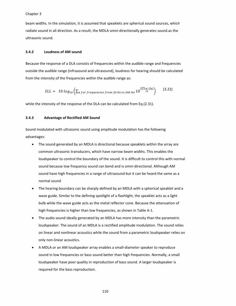
Chapter 3

110

beam widths. In the simulation, it is assumed that speaklets are spherical sound sources, which

radiate sound in all direction. As a result, the MDLA omni‐directionally generates sound.as the

ultrasonic sound.

3.4.2 Loudness of AM sound

Because the response of a DLA consists of frequencies within the audible range and frequencies

outside the audible range (infrasound and ultrasound), loudness for hearing should be calculated

from the intensity of the frequencies within the audible range as:

10 ∑ 10 (3.22)

while the intensity of the response of the DLA can be calculated from Eq.(2.31).

3.4.3 Advantage of Rectified AM Sound

Sound modulated with ultrasonic sound using amplitude modulation has the following

advantages:

The sound generated by an MDLA is directional because speaklets within the array are

common ultrasonic transducers, which have narrow beam widths. This enables the

loudspeaker to control the boundary of the sound. It is difficult to control this with normal

sound because low frequency sound can bend and is omni‐directional. Although AM

sound have high frequencies in a range of ultrasound but it can be heard the same as a

normal sound

The hearing boundary can be sharply defined by an MDLA with a spherical speaklet and a

wave guide. Similar to the defining spotlight of a flashlight, the speaklet acts as a light

bulb while the wave guide acts as the metal reflector cone. Because the attenuation of

high frequencies is higher than low frequencies, as shown in Table A‐1.

The audio sound ideally generated by an MDLA has more intensity than the parametric

loudspeaker. The sound of an MDLA is a rectified amplitude modulation. The sound relies

on linear and nonlinear acoustics while the sound from a parametric loudspeaker relies on

only non‐linear acoustics.

A MDLA or an AM loudspeaker array enables a small‐diameter speaker to reproduce

sound in low frequencies or bass sound better than high frequencies. Normally, a small

loudspeaker have poor quality in reproduction of bass sound. A larger loudspeaker is

required for the bass reproduction.

Chapter 3

111

3.5 Discussion and Summary

A Multiple‐Level Digital Loudspeaker Array (MDLA) generates sound by feeding a train of electrical

rectangular pulses with constant pulse height but variable pulse widths into speaklets (tiny

loudspeakers). This chapter studied the ideal case of an MDLA by assuming a speaklet as an MSD

model, which does not take into consideration the details and limitations of the speaklets, such as

their structure and driving circuits and assumes the speaklet is a spherical source driven by a

discrete force. The force produces two transient responses at the rising and falling edges of a

pulse. The conditions for the production of sound in this simulation are that the velocity of

vibration is directly proportional to the displacement of vibration, as Eq.(3.11) and that the sound

pressure is directly proportional to the velocity as Eq.(3.17). Sound pressure is computed by Eq.

(3.13).

The ideal speaklet in a digital loudspeaker requires a high damping ratio (0.7 in this simulation) in

order to meet the first requirement of digital reconstruction. The high damping of a speaklet

makes its acoustic response short. The response has only one acoustic pulse or a second pulse

significantly smaller in amplitude than the first one.

The relationship between maximum pressure and pulse width and the relationship between

response time and pulse width are linear up to pulse widths of 4.685 μs, with R2 coefficients of

0.9917 and 0.9967 respectively (fulfilling the third requirement). Therefore, 937 different pulse

widths are available for a speaklet, by varying the pulse width from 0 ns to 4.685 μs in steps of 5

ns. For a 16‐bit resolution in a conventional audio system, this requires a speaklet array of 70

elements.

The range of linear relationship between the amplitude of acoustic response and the pulse width

of an electrical pulse can be approximately equal to a quarter of a period of the natural frequency

of vibration of the speaklet ( =44.1 kHz), which is 5.668 μsec while the period of linearity is 4.685

μsec.

Due to feeding with different width pulses, the acoustic response time of each pulse width is

different. However, the response time is linearly related to pulse width. The time shift can be

calculated in order that acoustic pulses of different pulse widths can rise at the same time. The

time shift can improve the linearity for a small angle of listening from 0.9917 to 1, but for a wide

angle of listening, time shift might not help to improve the linearity.

The resolution of the sound of a speaklet within a DLA is dependent on the ratio between the

range of linearity and the period of clock frequency of the electrical pulse generator. The clock

speed of market Field‐Programmable Gate Array (FPGA) boards is 50 or 100 MHz.

Chapter 3

112

The sound field intensity was also simulated, by assuming that the speaklets are point sources

aligned on the x‐axis and their interspacing is equal to 3.83 mm (half the sampling distance at 44.1

kHz). The spectral response is observed for an array at a distance of 40 cm from the centre of the

array through different angles and acoustic outputs. Four schemes of pulse assignment are

assumed to study the effect of location of the speaklets on acoustic response. Both the temporal

response and the spectral content are shown at different angles with different numbers of

speaklets.

Due to the acoustic output of an MDLA resulting from a superposition of the response of the

speaklets within the array, the scheme of pulse assignments needs to be pre‐defined for a

quantizing level of digital audio (16 bits or 65,536 levels) because there are various combinations,

which assign different pulse widths to different speaklets to reconstruct the level. Different pulse

assignment schemes give different acoustic responses, different distortion and different

directivity. These differences result from the combination of acoustic pulses travelling from the

different locations of the speaklets. Therefore, a specific combination of the levels is assigned for

a specific quantizing level of the output. The best scheme for minimizing distortion from the four

schemes in this study is bit assignment 1, which assigns pulse widths with minimization of sound

levels among the speaklets.

The spectrum of acoustic response of an MDLA consists of three main components of frequency,

especially at an angle of 0 degrees (i.e. directly in front of the element). The first component is the

required audible frequency, which is reproduced by the difference in AM frequencies. The second

component depends on the natural frequency of the speaklets, which is around 44.1 kHz. The last

component is a harmonic frequency of 71.9 kHz, which results from the sum of AM frequencies.

However, the last two components have no effect on hearing because they are beyond the

response of the human ear. These three frequency components are plotted for directivity. For a

frequency of 2 kHz, sound radiates omnidirectionally. For a frequency of 10 kHz, as the number of

speaklets increases, the response is more directional for all schemes of pulse assignment. This

behaviour is similar to the behaviour of analogue loudspeakers. The larger the diaphragm of the

loudspeaker, the more directionally it reproduces sound. Although the response may be different

at different angles, the power spectrums at the audio frequency of the response are the same.

The response has high amplitude directly at the front of the array but the audible spectrums are

the same in all directions.

The results of the simulation demonstrate that the MDLA can reproduce audio. However, the

simulation has not taken into account some practical issues such as:

• Impedance mismatch and efficiency of the piezoelectric element

Chapter 3

113

• The directivity of an individual speaklet within the array resulting from its shape and size

• Non‐uniformity of acoustic outputs of the speaklets due to imperfections in the fabrication

process

• Difference in delay time from the pulse generator to the different locations of speaklets

• Non‐ideal shape of the rectangular pulse, because of the transition state limitations of

transistors

The speaklets in the array are also linearly aligned in this simulation, while the array alignment

will be square in the practical implementation.

In addition, the condition of kr >> 1 in the rectifying source is assumed because it constitutes the

linear relation the acoustic pressure and the velocity of air flow from the air outlet. The radius (r)

of the source include the radius of air outlet and air volume blown out from the outlet to push the

air in atmosphere. Therefore, the radius varies by the air volume from the outlet. If pressure from

the pump is high enough, the condition can be satisfied. However, in reality, it is difficult in

measuring the radius of the source

Although the study of sound reproduction of an MDLA from the simulation is only for an ideal

case, it indicates that people will be able to hear the sound reproduced by the MDLA, and gives

confidence that good performance is possible from the concept, despite the presence of

ultrasonic frequency components.

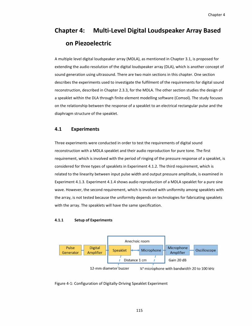
Chapter 4

115

Chapter 4: Multi‐Level Digital Loudspeaker Array Based

on Piezoelectric

A multiple level digital loudspeaker array (MDLA), as mentioned in Chapter 3.1, is proposed for

extending the audio resolution of the digital loudspeaker array (DLA), which is another concept of

sound generation using ultrasound. There are two main sections in this chapter. One section

describes the experiments used to investigate the fulfilment of the requirements for digital sound

reconstruction, described in Chapter 2.3.3, for the MDLA. The other section studies the design of

a speaklet within the DLA through finite element modelling software (Comsol). The study focuses

on the relationship between the response of a speaklet to an electrical rectangular pulse and the

diaphragm structure of the speaklet.

4.1 Experiments

Three experiments were conducted in order to test the requirements of digital sound

reconstruction with a MDLA speaklet and their audio reproduction for pure tone. The first

requirement, which is involved with the period of ringing of the pressure response of a speaklet, is

considered for three types of speaklets in Experiment 4.1.2. The third requirement, which is

related to the linearity between input pulse width and output pressure amplitude, is examined in

Experiment 4.1.3. Experiment 4.1.4 shows audio reproduction of a MDLA speaklet for a pure sine

wave. However, the second requirement, which is involved with uniformity among speaklets with

the array, is not tested because the uniformity depends on technologies for fabricating speaklets

with the array. The speaklets will have the same specification.

4.1.1 Setup of Experiments

Figure 4‐1: Configuration of Digitally‐Driving Speaklet Experiment

Chapter 4

116

The experimental set‐up can be divided into two sides as shown in Figure 4‐1: transmitting and

receiving. The transmitting side consists of:

A pulse generator producing a train of rectangular pulses with different widths but the

same height. In this research, the generator implemented is DE2‐115, which is an FPGA

board having a 100 MHz oscillator clock and a PC connecting module with serial

communication RS232.

A digital amplifier, a simple high frequency switching circuit, which can be implemented

with a transistor. In this research, the amplifier is implemented by L293D, which is a

Darlington transistor integrated circuit (IC) designed to provide drive currents up to 600

mA at voltages from 4.5 to 36 V and a transition time faster than 330 nsec.

The speaklets are tiny loudspeakers, the responses of which will be investigated when

driven by digital pulses.

The main objective of experiments is to explore MDLA concept for sound reproduction. The

proposed method is designed for driving a high number of speaklets within an array with digital

signals. However, in this research, an array of speaklets have not been fabricated. The experiment

with off‐the‐shelf electro‐acoustic transducers is an alternative way for the proof, which is

sufficient for characterising acoustic response from MDLA concept.

Three representative transducers of piezoelectric and electro‐magnetic technologies for sound

and ultrasound generators are described in Section 2.2.1 and 2.1.2.

A piezoelectric buzzer has a structure as shown in Figure 2‐6a similar to a real DLA, as

shown in Figure 2‐6b, but they are different in size and material. The buzzer has an

aluminium diaphragm with 12 mm diameter and 250 µm thickness.

An ultrasonic transducer has different structure from the buzzer as shown Figure 2‐8The

transducer has an aluminium diaphragm with 10 mm diameter and 300 µm thickness. It is

designed from the transmitting ultrasonic signal at 40 kHz.

Magnetic buzzer has electro‐magnetic transducer as shown in Figure 2‐10. operating in a

low voltage range between 3 and 16 V and having an aluminium diaphragm with 10 mm

diameter and 250 µm. With the electro‐magnetic technology, an array of microspeakers is

fabricated as shown Figure 2‐13. It is used as a MDLA.

The receiving side consists of:

A ¼ inch free‐field microphone, type 4939, with a frequency response between 4 Hz to

100 kHz and a sensitivity of 4mV per Pa

A microphone amplifier with a gain up to 50 dB and bandwidth up to 80 kHz

Chapter 4

117

An oscilloscope for measuring the electrical input to a speaklet, and the pressure output

from the microphone

Driving electrical rectangular pulses to speaklets is controlled by Matlab‐implemented programs

on a PC connected with FPGA for charactertics of a pulse train. The program have three modes

for generating pulse. Each mode has different main parameters but share the same FPGA‐

connecting parameters: serial port number, data transfer rate and CPU speed of FPGA.

Experimental methodology is described in a procedure section in each experiment.

Mode 1: Single pulse generator has two major defining parameters of a pulse rate and a pulse

width. This mode is used in Experiment 4.1.2.1 and 4.1.3. It generates a pulse with a defined

constant width in a defined pulse period.

Mode 2: Double pulse generator has four parameters; a pulse rate, the first pulse width, the

second pulse width and a pulse interval. It generates two pulses in a defined pulse period. This

mode is used in Experiment 4.1.2.2. The widths of the first pulse and the second pulse are equally

defined. The pulse interval is duration between the rising edges of the pulses.

Mode 3: MDLA generator has four parameters; a pulse rate, a pure tone frequency, minimum and

maximum pulse widths. It generates a pulse in a defined period. The pulse width respresents a

quatizing sound level of the pure tone. The minimum and maximum of widths are defined within

the range of linearity between the pulse width of electrical input pulses and the amplitude of the

pressures. This mode is used in Experiment 4.1.4.

4.1.2 Experiment Acoustic Response of Loudspeakers to digital pulse and attempt to stop

to vibration

The experiments were conducted for testing satisfaction of the first requirement of digital sound

reconstruction, which is involved with the interval of oscillation of pressure output.

4.1.2.1 Driving single pulse

The experiment investigates pressure response when a pulse feeds a speaklet.

4.1.2.1.1 Objective

To study acoustic response and its spectrum when driving speaklets with a discrete pulse

with a constant width and voltage.

To investigate emitting time(ET) of the response

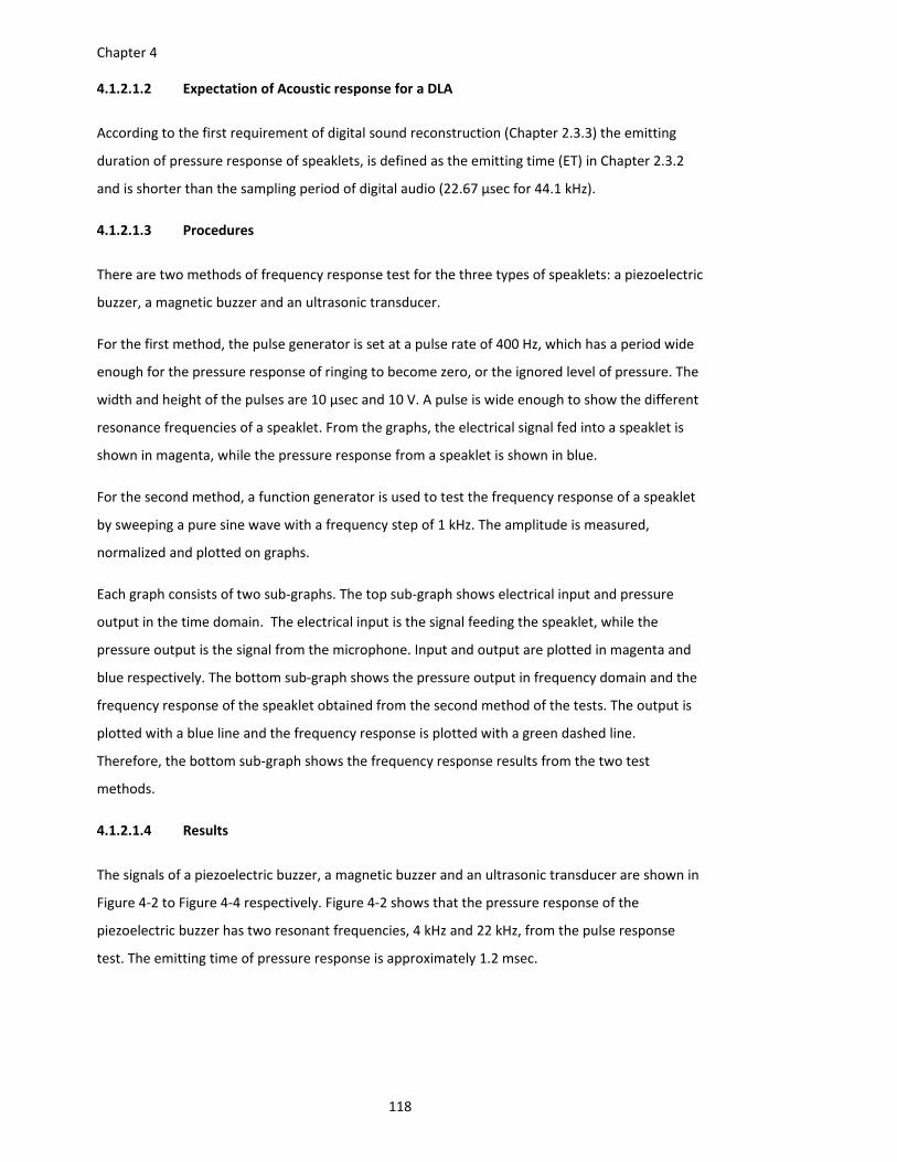
Chapter 4

118

4.1.2.1.2 Expectation of Acoustic response for a DLA

According to the first requirement of digital sound reconstruction (Chapter 2.3.3) the emitting

duration of pressure response of speaklets, is defined as the emitting time (ET) in Chapter 2.3.2

and is shorter than the sampling period of digital audio (22.67 µsec for 44.1 kHz).

4.1.2.1.3 Procedures

There are two methods of frequency response test for the three types of speaklets: a piezoelectric

buzzer, a magnetic buzzer and an ultrasonic transducer.

For the first method, the pulse generator is set at a pulse rate of 400 Hz, which has a period wide

enough for the pressure response of ringing to become zero, or the ignored level of pressure. The

width and height of the pulses are 10 µsec and 10 V. A pulse is wide enough to show the different

resonance frequencies of a speaklet. From the graphs, the electrical signal fed into a speaklet is

shown in magenta, while the pressure response from a speaklet is shown in blue.

For the second method, a function generator is used to test the frequency response of a speaklet

by sweeping a pure sine wave with a frequency step of 1 kHz. The amplitude is measured,

normalized and plotted on graphs.

Each graph consists of two sub‐graphs. The top sub‐graph shows electrical input and pressure

output in the time domain. The electrical input is the signal feeding the speaklet, while the

pressure output is the signal from the microphone. Input and output are plotted in magenta and

blue respectively. The bottom sub‐graph shows the pressure output in frequency domain and the

frequency response of the speaklet obtained from the second method of the tests. The output is

plotted with a blue line and the frequency response is plotted with a green dashed line.

Therefore, the bottom sub‐graph shows the frequency response results from the two test

methods.

4.1.2.1.4 Results

The signals of a piezoelectric buzzer, a magnetic buzzer and an ultrasonic transducer are shown in

Figure 4‐2 to Figure 4‐4 respectively. Figure 4‐2 shows that the pressure response of the

piezoelectric buzzer has two resonant frequencies, 4 kHz and 22 kHz, from the pulse response

test. The emitting time of pressure response is approximately 1.2 msec.

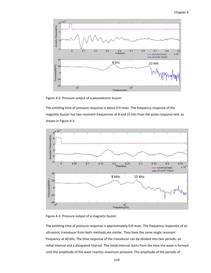
Chapter 4

119

Figure 4‐2: Pressure output of a piezoelectric buzzer.

The emitting time of pressure response is about 0.9 msec. The frequency response of the

magnetic buzzer has two resonant frequencies at 8 and 15 kHz from the pulse response test, as

shown in Figure 4‐3.

Figure 4‐3: Pressure output of a magnetic buzzer

The emitting time of pressure response is approximately 0.8 msec. The frequency responses of an

ultrasonic transducer from both methods are similar. They have the same single resonant

frequency at 40 kHz. The time response of the transducer can be divided into two periods: an

initial interval and a dissipated interval. The initial interval starts from the time the wave is formed

until the amplitude of the wave reaches maximum pressure. The amplitude of the periods of

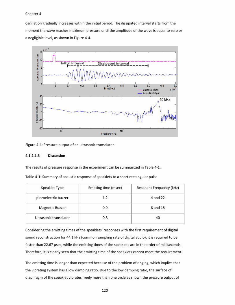
Chapter 4

120

oscillation gradually increases within the initial period. The dissipated interval starts from the

moment the wave reaches maximum pressure until the amplitude of the wave is equal to zero or

a negligible level, as shown in Figure 4‐4.

Figure 4‐4: Pressure output of an ultrasonic transducer

4.1.2.1.5 Discussion

The results of pressure response in the experiment can be summarized in Table 4‐1:

Table 4‐1: Summary of acoustic response of speaklets to a short rectangular pulse

Speaklet Type Emitting time (msec) Resonant Frequency (kHz)

piezoelectric buzzer 1.2 4 and 22

Magnetic Buzzer 0.9 8 and 15

Ultrasonic transducer 0.8 40

Considering the emitting times of the speaklets’ responses with the first requirement of digital

sound reconstruction for 44.1 kHz (common sampling rate of digital audio), it is required to be

faster than 22.67 µsec, while the emitting times of the speaklets are in the order of milliseconds.

Therefore, it is clearly seen that the emitting time of the speaklets cannot meet the requirement.

The emitting time is longer than expected because of the problem of ringing, which implies that

the vibrating system has a low damping ratio. Due to the low damping ratio, the surface of

diaphragm of the speaklet vibrates freely more than one cycle as shown the pressure output of

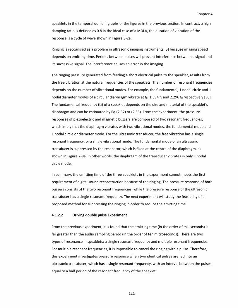
Chapter 4

121

speaklets in the temporal domain graphs of the figures in the previous section. In contract, a high

damping ratio is defined as 0.8 in the ideal case of a MDLA, the duration of vibration of the

response is a cycle of wave shown in Figure 3‐2a.

Ringing is recognised as a problem in ultrasonic imaging instruments [5] because imaging speed

depends on emitting time. Periods between pulses will prevent interference between a signal and

its successive signal. The interference causes an error in the imaging.

The ringing pressure generated from feeding a short electrical pulse to the speaklet, results from

the free vibration at the natural frequencies of the speaklets. The number of resonant frequencies

depends on the number of vibrational modes. For example, the fundamental, 1 nodal circle and 1

nodal diameter modes of a circular diaphragm vibrate at f0, 1.594 f0 and 2.296 f0 respectively [36].

The fundamental frequency (f0) of a speaklet depends on the size and material of the speaklet’s

diaphragm and can be estimated by Eq.(2.32) or (2.33). From the experiment, the pressure

responses of piezoelectric and magnetic buzzers are composed of two resonant frequencies,

which imply that the diaphragm vibrates with two vibrational modes, the fundamental mode and

1 nodal circle or diameter mode. For the ultrasonic transducer, the free vibration has a single

resonant frequency, or a single vibrational mode. The fundamental mode of an ultrasonic

transducer is suppressed by the resonator, which is fixed at the centre of the diaphragm, as

shown in Figure 2‐8a. In other words, the diaphragm of the transducer vibrates in only 1 nodal

circle mode.

In summary, the emitting time of the three speaklets in the experiment cannot meets the first

requirement of digital sound reconstruction because of the ringing. The pressure response of both

buzzers consists of the two resonant frequencies, while the pressure response of the ultrasonic

transducer has a single resonant frequency. The next experiment will study the feasibility of a

proposed method for suppressing the ringing in order to reduce the emitting time.

4.1.2.2 Driving double pulse Experiment

From the previous experiment, it is found that the emitting time (in the order of milliseconds) is

far greater than the audio sampling period (in the order of ten microseconds). There are two

types of resonance in speaklets: a single resonant frequency and multiple resonant frequencies.

For multiple resonant frequencies, it is impossible to cancel the ringing with a pulse. Therefore,

this experiment investigates pressure response when two identical pulses are fed into an

ultrasonic transducer, which has a single resonant frequency, with an interval between the pulses

equal to a half period of the resonant frequency of the speaklet.

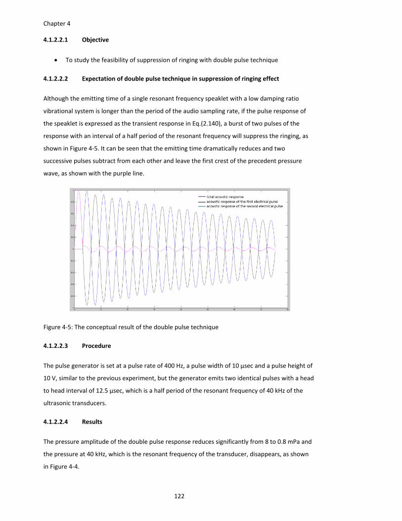
Chapter 4

122

4.1.2.2.1 Objective

To study the feasibility of suppression of ringing with double pulse technique

4.1.2.2.2 Expectation of double pulse technique in suppression of ringing effect

Although the emitting time of a single resonant frequency speaklet with a low damping ratio

vibrational system is longer than the period of the audio sampling rate, if the pulse response of

the speaklet is expressed as the transient response in Eq.(2.140), a burst of two pulses of the

response with an interval of a half period of the resonant frequency will suppress the ringing, as

shown in Figure 4‐5. It can be seen that the emitting time dramatically reduces and two

successive pulses subtract from each other and leave the first crest of the precedent pressure

wave, as shown with the purple line.

Figure 4‐5: The conceptual result of the double pulse technique

4.1.2.2.3 Procedure

The pulse generator is set at a pulse rate of 400 Hz, a pulse width of 10 µsec and a pulse height of

10 V, similar to the previous experiment, but the generator emits two identical pulses with a head

to head interval of 12.5 µsec, which is a half period of the resonant frequency of 40 kHz of the

ultrasonic transducers.

4.1.2.2.4 Results

The pressure amplitude of the double pulse response reduces significantly from 8 to 0.8 mPa and

the pressure at 40 kHz, which is the resonant frequency of the transducer, disappears, as shown

in Figure 4‐4.

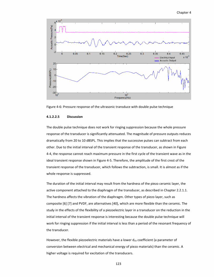
Chapter 4

123

Figure 4‐6: Pressure response of the ultrasonic transduce with double pulse technique

4.1.2.2.5 Discussion

The double pulse technique does not work for ringing suppression because the whole pressure

response of the transducer is significantly attenuated. The magnitude of pressure outputs reduces

dramatically from 20 to 10 dBSPL. This implies that the successive pulses can subtract from each

other. Due to the initial interval of the transient response of the transducer, as shown in Figure

4‐4, the response cannot reach maximum pressure in the first cycle of the transient wave as in the

ideal transient response shown in Figure 4‐5. Therefore, the amplitude of the first crest of the

transient response of the transducer, which follows the subtraction, is small. It is almost as if the

whole response is suppressed.

The duration of the initial interval may result from the hardness of the piezo ceramic layer, the

active component attached to the diaphragm of the transducer, as described in Chapter 2.2.1.1.

The hardness affects the vibration of the diaphragm. Other types of piezo layer, such as

composite [6] [7] and PVDF, are alternatives [40], which are more flexible than the ceramic. The

study in the effects of the flexibility of a piezoelectric layer in a transducer on the reduction in the

initial interval of the transient response is interesting because the double pulse technique will

work for ringing suppression if the initial interval is less than a period of the resonant frequency of

the transducer.

However, the flexible piezoelectric materials have a lower d33 coefficient (a parameter of

conversion between electrical and mechanical energy of piezo materials) than the ceramic. A

higher voltage is required for excitation of the transducers.

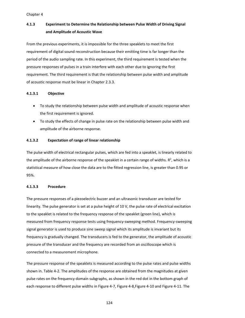
Chapter 4

124

4.1.3 Experiment to Determine the Relationship between Pulse Width of Driving Signal

and Amplitude of Acoustic Wave

From the previous experiments, it is impossible for the three speaklets to meet the first

requirement of digital sound reconstruction because their emitting time is far longer than the

period of the audio sampling rate. In this experiment, the third requirement is tested when the

pressure responses of pulses in a train interfere with each other due to ignoring the first

requirement. The third requirement is that the relationship between pulse width and amplitude

of acoustic response must be linear in Chapter 2.3.3.

4.1.3.1 Objective

To study the relationship between pulse width and amplitude of acoustic response when

the first requirement is ignored.

To study the effects of change in pulse rate on the relationship between pulse width and

amplitude of the airborne response.

4.1.3.2 Expectation of range of linear relationship

The pulse width of electrical rectangular pulses, which are fed into a speaklet, is linearly related to

the amplitude of the airborne response of the speaklet in a certain range of widths. R2, which is a

statistical measure of how close the data are to the fitted regression line, is greater than 0.95 or

95%.

4.1.3.3 Procedure

The pressure responses of a piezoelectric buzzer and an ultrasonic transducer are tested for

linearity. The pulse generator is set at a pulse height of 10 V, the pulse rate of electrical excitation

to the speaklet is related to the frequency response of the speaklet (green line), which is

measured from frequency response tests using frequency‐sweeping method. Frequency‐sweeping

signal generator is used to produce sine sweep signal which its amplitude is invariant but its

frequency is gradually changed. The transducers is fed to the generator, the amplitude of acoustic

pressure of the transducer and the frequency are recorded from an oscilloscope which is

connected to a measurement microphone.

The pressure response of the speaklets is measured according to the pulse rates and pulse widths

shown in. Table 4‐2. The amplitudes of the response are obtained from the magnitudes at given

pulse rates on the frequency domain subgraphs, as shown in the red dot in the bottom graph of

each response to different pulse widths in Figure 4‐7, Figure 4‐8,Figure 4‐10 and Figure 4‐11. The

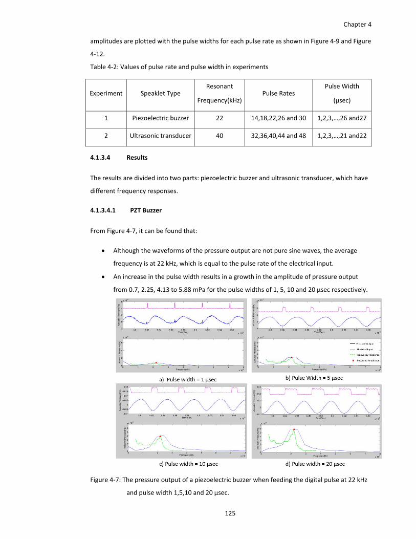
Chapter 4

125

amplitudes are plotted with the pulse widths for each pulse rate as shown in Figure 4‐9 and Figure

4‐12.

Table 4‐2: Values of pulse rate and pulse width in experiments

Experiment Speaklet Type Resonant

Frequency(kHz)Pulse Rates

Pulse Width

(µsec)

1 Piezoelectric buzzer 22 14,18,22,26 and 30 1,2,3,…,26 and27

2 Ultrasonic transducer 40 32,36,40,44 and 48 1,2,3,…,21 and22

4.1.3.4 Results

The results are divided into two parts: piezoelectric buzzer and ultrasonic transducer, which have

different frequency responses.

4.1.3.4.1 PZT Buzzer

From Figure 4‐7, it can be found that:

Although the waveforms of the pressure output are not pure sine waves, the average

frequency is at 22 kHz, which is equal to the pulse rate of the electrical input.

An increase in the pulse width results in a growth in the amplitude of pressure output

from 0.7, 2.25, 4.13 to 5.88 mPa for the pulse widths of 1, 5, 10 and 20 µsec respectively.

Figure 4‐7: The pressure output of a piezoelectric buzzer when feeding the digital pulse at 22 kHz

and pulse width 1,5,10 and 20 µsec.

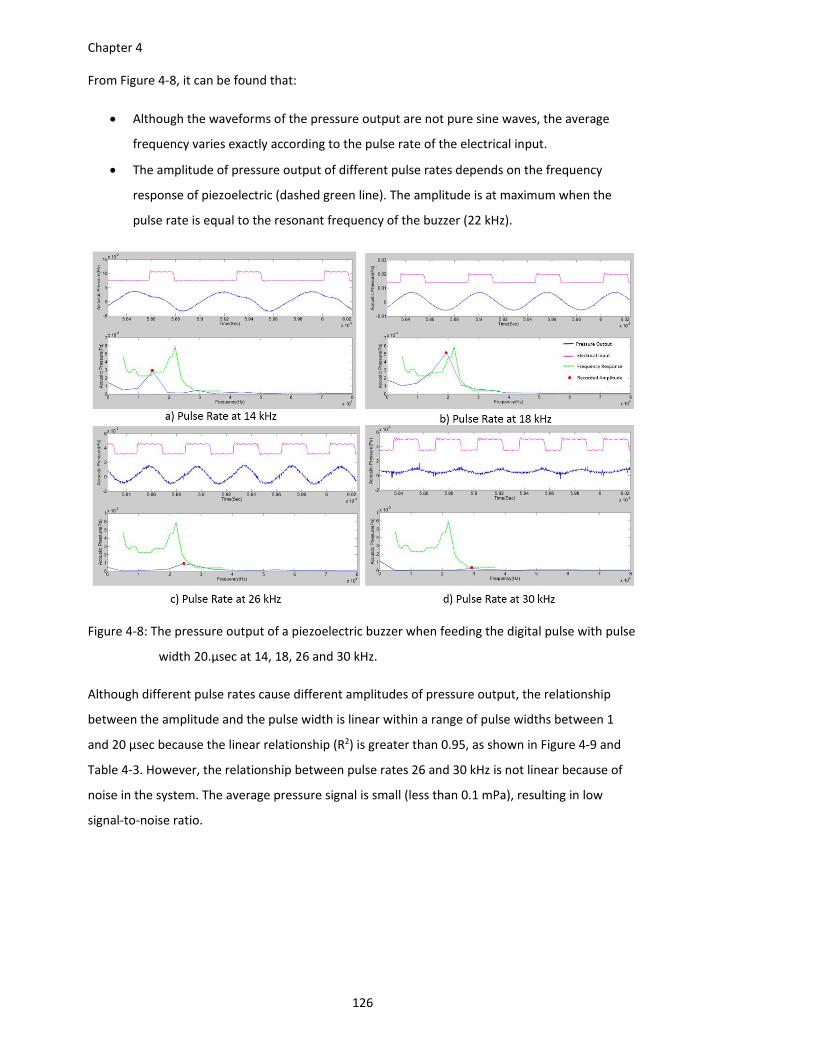
Chapter 4

126

From Figure 4‐8, it can be found that:

Although the waveforms of the pressure output are not pure sine waves, the average

frequency varies exactly according to the pulse rate of the electrical input.

The amplitude of pressure output of different pulse rates depends on the frequency

response of piezoelectric (dashed green line). The amplitude is at maximum when the

pulse rate is equal to the resonant frequency of the buzzer (22 kHz).

Figure 4‐8: The pressure output of a piezoelectric buzzer when feeding the digital pulse with pulse

width 20.µsec at 14, 18, 26 and 30 kHz.

Although different pulse rates cause different amplitudes of pressure output, the relationship

between the amplitude and the pulse width is linear within a range of pulse widths between 1

and 20 µsec because the linear relationship (R2) is greater than 0.95, as shown in Figure 4‐9 and

Table 4‐3. However, the relationship between pulse rates 26 and 30 kHz is not linear because of

noise in the system. The average pressure signal is small (less than 0.1 mPa), resulting in low

signal‐to‐noise ratio.

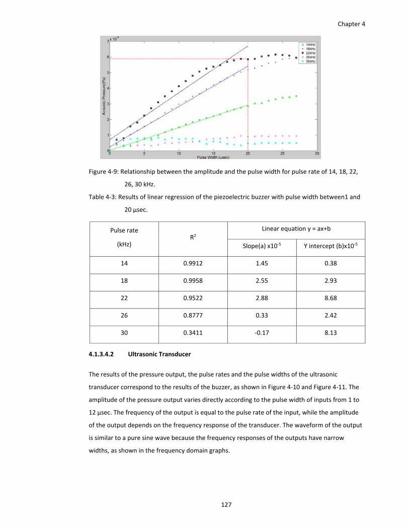
Chapter 4

127


26, 30 kHz.

Table 4‐3: Results of linear regression of the piezoelectric buzzer with pulse width between1 and

20 µsec.

Pulse rate

(kHz) R2

Linear equation y = ax+b

Slope(a) x10‐5 Y intercept (b)x10‐5

14 0.9912 1.45 0.38

18 0.9958 2.55 2.93

22 0.9522 2.88 8.68

26 0.8777 0.33 2.42

30 0.3411 ‐0.17 8.13

4.1.3.4.2 Ultrasonic Transducer

The results of the pressure output, the pulse rates and the pulse widths of the ultrasonic

transducer correspond to the results of the buzzer, as shown in Figure 4‐10 and Figure 4‐11. The

amplitude of the pressure output varies directly according to the pulse width of inputs from 1 to

12 µsec. The frequency of the output is equal to the pulse rate of the input, while the amplitude

of the output depends on the frequency response of the transducer. The waveform of the output

is similar to a pure sine wave because the frequency responses of the outputs have narrow

widths, as shown in the frequency domain graphs.

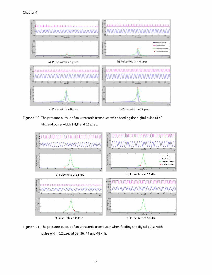
Chapter 4

128

Figure 4‐10: The pressure output of an ultrasonic transduce when feeding the digital pulse at 40

kHz and pulse width 1,4,8 and 12 µsec.

Figure 4‐11: The pressure output of an ultrasonic transducer when feeding the digital pulse with

pulse width 12.µsec at 32, 36, 44 and 48 kHz.

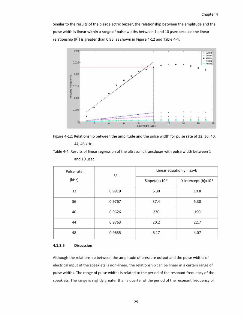
Chapter 4

129

Similar to the results of the piezoelectric buzzer, the relationship between the amplitude and the

pulse width is linear within a range of pulse widths between 1 and 10 µsec because the linear

relationship (R2) is greater than 0.95, as shown in Figure 4‐12 and Table 4‐4.


44, 46 kHz.

Table 4‐4: Results of linear regression of the ultrasonic transducer with pulse width between 1

and 10 µsec.

Pulse rate

(kHz) R2

Linear equation y = ax+b

Slope(a) x10‐5 Y intercept (b)x10‐5

32 0.9919 6.30 10.8

36 0.9767 37.4 5.30

40 0.9626 230 190

44 0.9763 20.2 22.7

48 0.9635 6.17 4.07

4.1.3.5 Discussion

Although the relationship between the amplitude of pressure output and the pulse widths of

electrical input of the speaklets is non‐linear, the relationship can be linear in a certain range of

pulse widths. The range of pulse widths is related to the period of the resonant frequency of the

speaklets. The range is slightly greater than a quarter of the period of the resonant frequency of

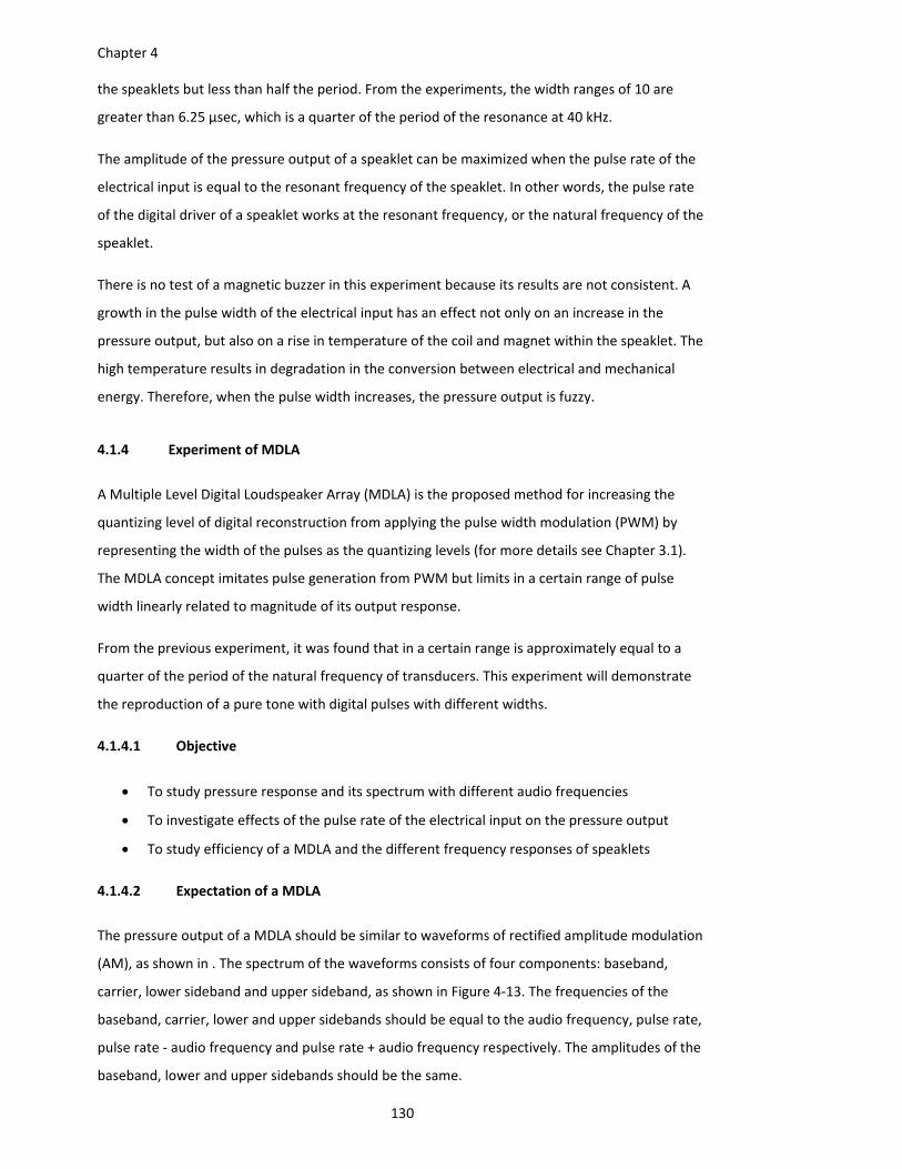
Chapter 4

130

the speaklets but less than half the period. From the experiments, the width ranges of 10 are

greater than 6.25 µsec, which is a quarter of the period of the resonance at 40 kHz.

The amplitude of the pressure output of a speaklet can be maximized when the pulse rate of the

electrical input is equal to the resonant frequency of the speaklet. In other words, the pulse rate

of the digital driver of a speaklet works at the resonant frequency, or the natural frequency of the

speaklet.

There is no test of a magnetic buzzer in this experiment because its results are not consistent. A

growth in the pulse width of the electrical input has an effect not only on an increase in the

pressure output, but also on a rise in temperature of the coil and magnet within the speaklet. The

high temperature results in degradation in the conversion between electrical and mechanical

energy. Therefore, when the pulse width increases, the pressure output is fuzzy.

4.1.4 Experiment of MDLA

A Multiple Level Digital Loudspeaker Array (MDLA) is the proposed method for increasing the

quantizing level of digital reconstruction from applying the pulse width modulation (PWM) by

representing the width of the pulses as the quantizing levels (for more details see Chapter 3.1).

The MDLA concept imitates pulse generation from PWM but limits in a certain range of pulse

width linearly related to magnitude of its output response.

From the previous experiment, it was found that in a certain range is approximately equal to a

quarter of the period of the natural frequency of transducers. This experiment will demonstrate

the reproduction of a pure tone with digital pulses with different widths.

4.1.4.1 Objective

To study pressure response and its spectrum with different audio frequencies

To investigate effects of the pulse rate of the electrical input on the pressure output

To study efficiency of a MDLA and the different frequency responses of speaklets

4.1.4.2 Expectation of a MDLA

The pressure output of a MDLA should be similar to waveforms of rectified amplitude modulation

(AM), as shown in . The spectrum of the waveforms consists of four components: baseband,

carrier, lower sideband and upper sideband, as shown in Figure 4‐13. The frequencies of the

baseband, carrier, lower and upper sidebands should be equal to the audio frequency, pulse rate,

pulse rate ‐ audio frequency and pulse rate + audio frequency respectively. The amplitudes of the

baseband, lower and upper sidebands should be the same.

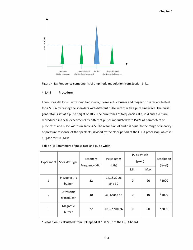
Chapter 4

131

Figure 4‐13: Frequency components of amplitude modulation from Section 3.4.1.

4.1.4.3 Procedure

Three speaklet types: ultrasonic transducer, piezoelectric buzzer and magnetic buzzer are tested

for a MDLA by driving the speaklets with different pulse widths with a pure sine wave. The pulse

generator is set at a pulse height of 10 V. The pure tones of frequencies at 1, 2, 4 and 7 kHz are

reproduced in these experiments by different pulses modulated with PWM as parameters of

pulse rates and pulse widths in Table 4‐5. The resolution of audio is equal to the range of linearity

of pressure response of the speaklets, divided by the clock period of the FPGA processor, which is

10 psec for 100 MHz.

Table 4‐5: Parameters of pulse rate and pulse width

Experiment Speaklet TypeResonant

Frequency(kHz)

Pulse Rates

(kHz)

Pulse Width

(µsec) Resolution

(level)

Min Max

1 Piezoelectric

buzzer 22

14,18,22,26

and 30 0 20 *2000

2 Ultrasonic

transducer 40 36,40 and 44 0 10 *1000

3 Magnetic

buzzer 22 18, 22 and 26 0 20 *2000

*Resolution is calculated from CPU speed at 100 MHz of the FPGA board

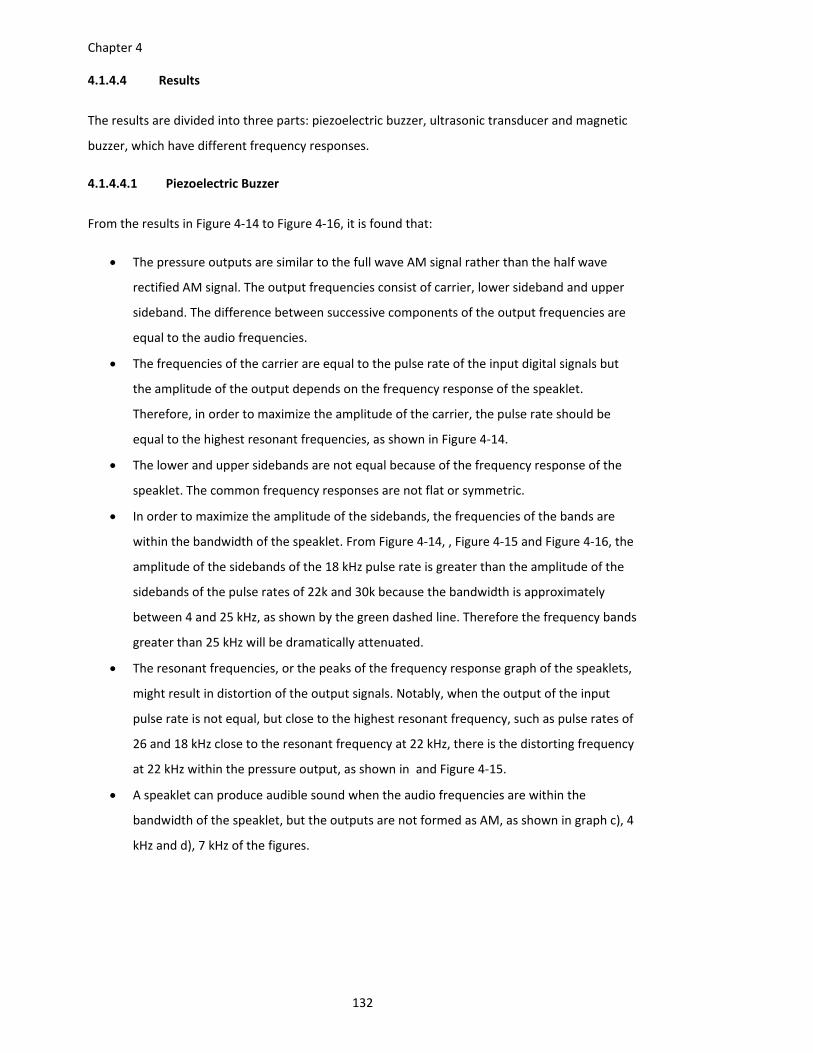
Chapter 4

132

4.1.4.4 Results

The results are divided into three parts: piezoelectric buzzer, ultrasonic transducer and magnetic

buzzer, which have different frequency responses.

4.1.4.4.1 Piezoelectric Buzzer

From the results in Figure 4‐14 to Figure 4‐16, it is found that:

The pressure outputs are similar to the full wave AM signal rather than the half wave

rectified AM signal. The output frequencies consist of carrier, lower sideband and upper

sideband. The difference between successive components of the output frequencies are

equal to the audio frequencies.

The frequencies of the carrier are equal to the pulse rate of the input digital signals but

the amplitude of the output depends on the frequency response of the speaklet.

Therefore, in order to maximize the amplitude of the carrier, the pulse rate should be

equal to the highest resonant frequencies, as shown in Figure 4‐14.

The lower and upper sidebands are not equal because of the frequency response of the

speaklet. The common frequency responses are not flat or symmetric.

In order to maximize the amplitude of the sidebands, the frequencies of the bands are

within the bandwidth of the speaklet. From Figure 4‐14, , Figure 4‐15 and Figure 4‐16, the

amplitude of the sidebands of the 18 kHz pulse rate is greater than the amplitude of the

sidebands of the pulse rates of 22k and 30k because the bandwidth is approximately

between 4 and 25 kHz, as shown by the green dashed line. Therefore the frequency bands

greater than 25 kHz will be dramatically attenuated.

The resonant frequencies, or the peaks of the frequency response graph of the speaklets,

might result in distortion of the output signals. Notably, when the output of the input

pulse rate is not equal, but close to the highest resonant frequency, such as pulse rates of

26 and 18 kHz close to the resonant frequency at 22 kHz, there is the distorting frequency

at 22 kHz within the pressure output, as shown in and Figure 4‐15.

A speaklet can produce audible sound when the audio frequencies are within the

bandwidth of the speaklet, but the outputs are not formed as AM, as shown in graph c), 4

kHz and d), 7 kHz of the figures.

Chapter 4

133


kHz and audio frequency of 1, 2,4 and 7 kHz.



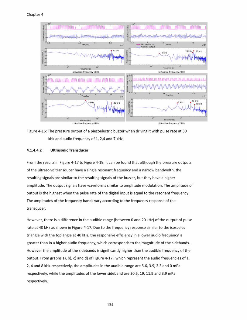
Chapter 4

134



4.1.4.4.2 Ultrasonic Transducer

From the results in Figure 4‐17 to Figure 4‐19, it can be found that although the pressure outputs

of the ultrasonic transducer have a single resonant frequency and a narrow bandwidth, the

resulting signals are similar to the resulting signals of the buzzer, but they have a higher

amplitude. The output signals have waveforms similar to amplitude modulation. The amplitude of

output is the highest when the pulse rate of the digital input is equal to the resonant frequency.

The amplitudes of the frequency bands vary according to the frequency response of the

transducer.

However, there is a difference in the audible range (between 0 and 20 kHz) of the output of pulse

rate at 40 kHz as shown in Figure 4‐17. Due to the frequency response similar to the isosceles

triangle with the top angle at 40 kHz, the responsive efficiency in a lower audio frequency is

greater than in a higher audio frequency, which corresponds to the magnitude of the sidebands.

However the amplitude of the sidebands is significantly higher than the audible frequency of the

output. From graphs a), b), c) and d) of Figure 4‐17 , which represent the audio frequencies of 1,

2, 4 and 8 kHz respectively, the amplitudes in the audible range are 5.6, 3.9, 2.3 and 0 mPa

respectively, while the amplitudes of the lower sideband are 30.5, 19, 11.9 and 3.9 mPa

respectively.

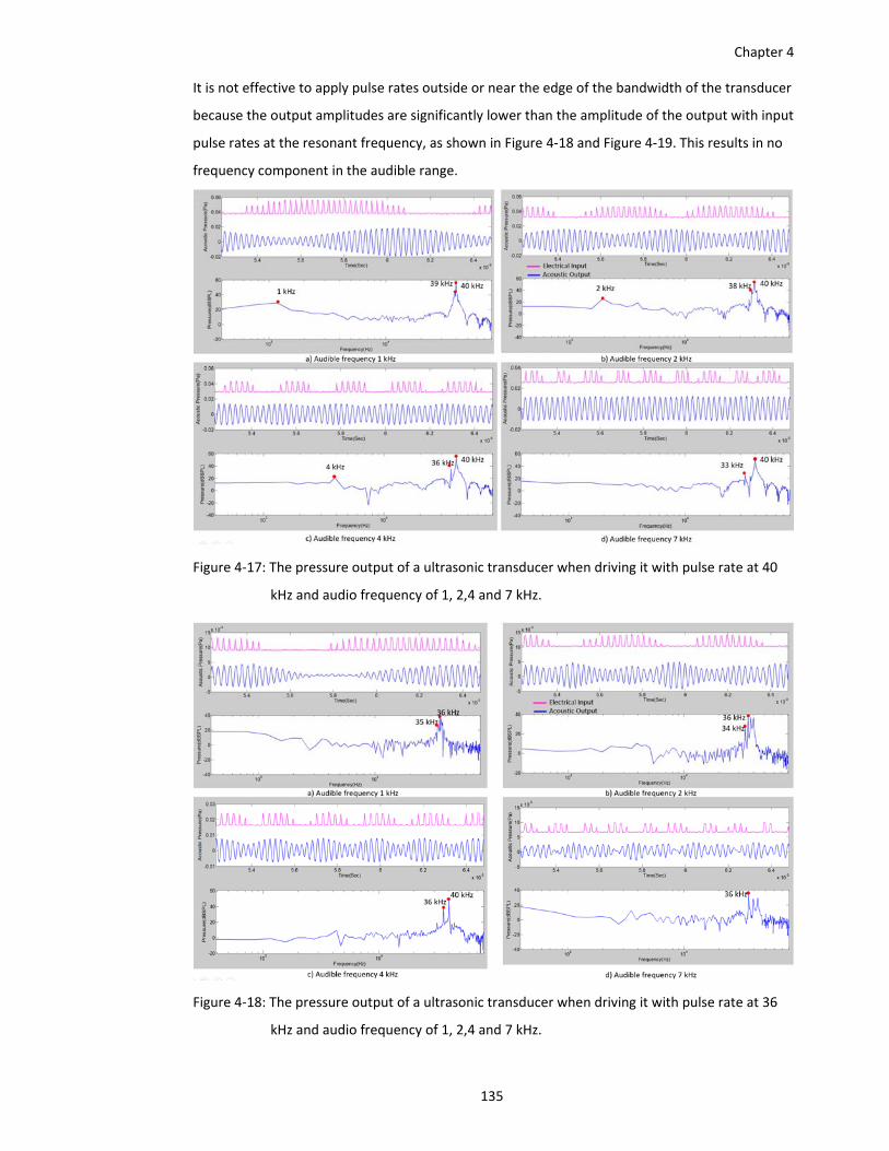
Chapter 4

135

It is not effective to apply pulse rates outside or near the edge of the bandwidth of the transducer

because the output amplitudes are significantly lower than the amplitude of the output with input

pulse rates at the resonant frequency, as shown in Figure 4‐18 and Figure 4‐19. This results in no

frequency component in the audible range.





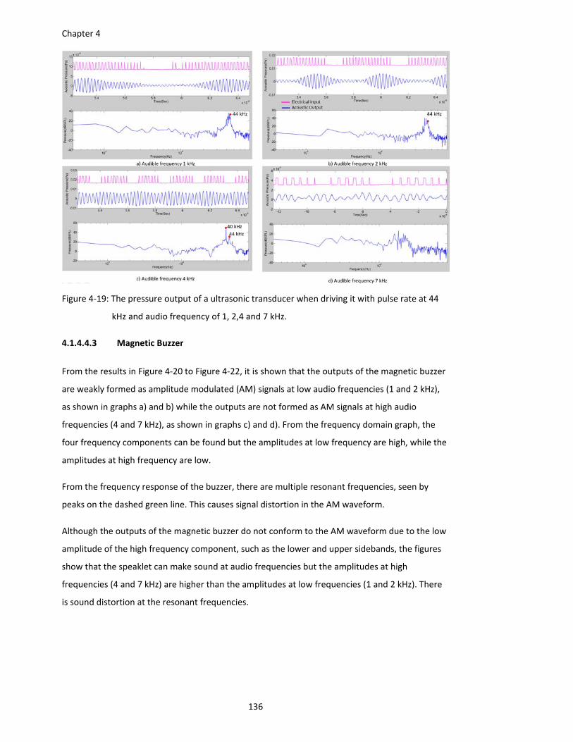
Chapter 4

136



4.1.4.4.3 Magnetic Buzzer

From the results in Figure 4‐20 to Figure 4‐22, it is shown that the outputs of the magnetic buzzer

are weakly formed as amplitude modulated (AM) signals at low audio frequencies (1 and 2 kHz),

as shown in graphs a) and b) while the outputs are not formed as AM signals at high audio

frequencies (4 and 7 kHz), as shown in graphs c) and d). From the frequency domain graph, the

four frequency components can be found but the amplitudes at low frequency are high, while the

amplitudes at high frequency are low.

From the frequency response of the buzzer, there are multiple resonant frequencies, seen by

peaks on the dashed green line. This causes signal distortion in the AM waveform.

Although the outputs of the magnetic buzzer do not conform to the AM waveform due to the low

amplitude of the high frequency component, such as the lower and upper sidebands, the figures

show that the speaklet can make sound at audio frequencies but the amplitudes at high

frequencies (4 and 7 kHz) are higher than the amplitudes at low frequencies (1 and 2 kHz). There

is sound distortion at the resonant frequencies.

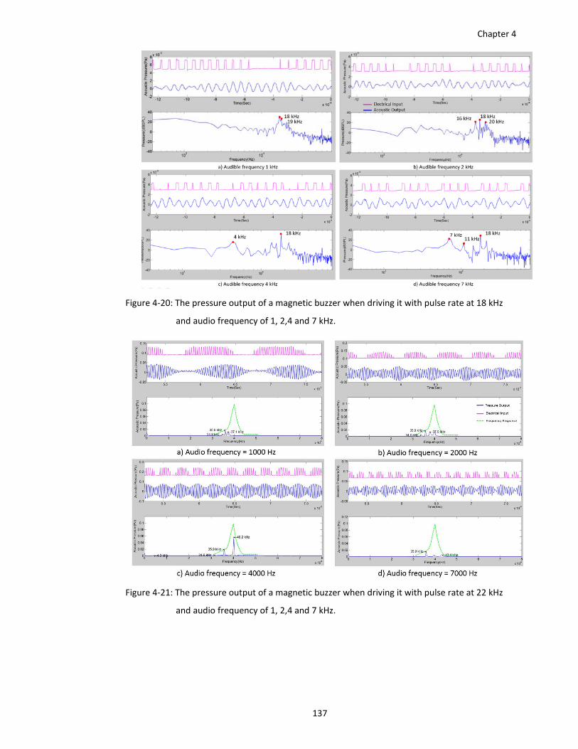
Chapter 4

137


and audio frequency of 1, 2,4 and 7 kHz.



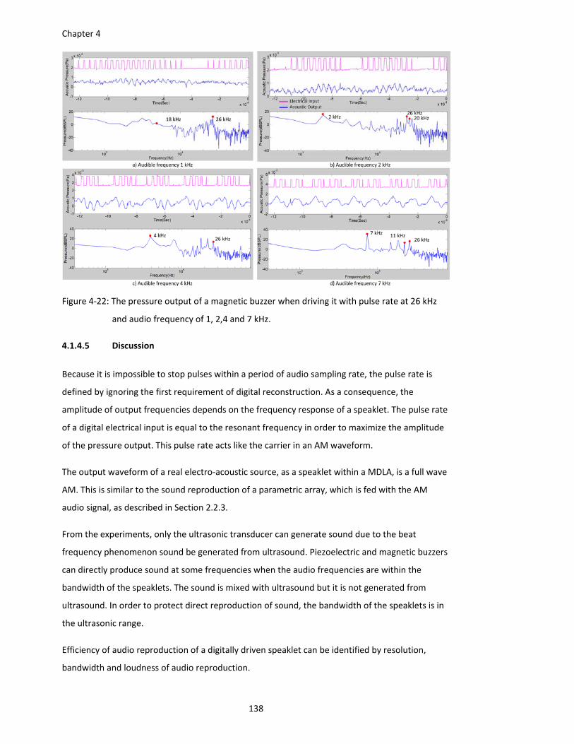
Chapter 4

138



4.1.4.5 Discussion

Because it is impossible to stop pulses within a period of audio sampling rate, the pulse rate is

defined by ignoring the first requirement of digital reconstruction. As a consequence, the

amplitude of output frequencies depends on the frequency response of a speaklet. The pulse rate

of a digital electrical input is equal to the resonant frequency in order to maximize the amplitude

of the pressure output. This pulse rate acts like the carrier in an AM waveform.

The output waveform of a real electro‐acoustic source, as a speaklet within a MDLA, is a full wave

AM. This is similar to the sound reproduction of a parametric array, which is fed with the AM

audio signal, as described in Section 2.2.3.

From the experiments, only the ultrasonic transducer can generate sound due to the beat

frequency phenomenon sound be generated from ultrasound. Piezoelectric and magnetic buzzers

can directly produce sound at some frequencies when the audio frequencies are within the

bandwidth of the speaklets. The sound is mixed with ultrasound but it is not generated from

ultrasound. In order to protect direct reproduction of sound, the bandwidth of the speaklets is in

the ultrasonic range.

Efficiency of audio reproduction of a digitally driven speaklet can be identified by resolution,

bandwidth and loudness of audio reproduction.

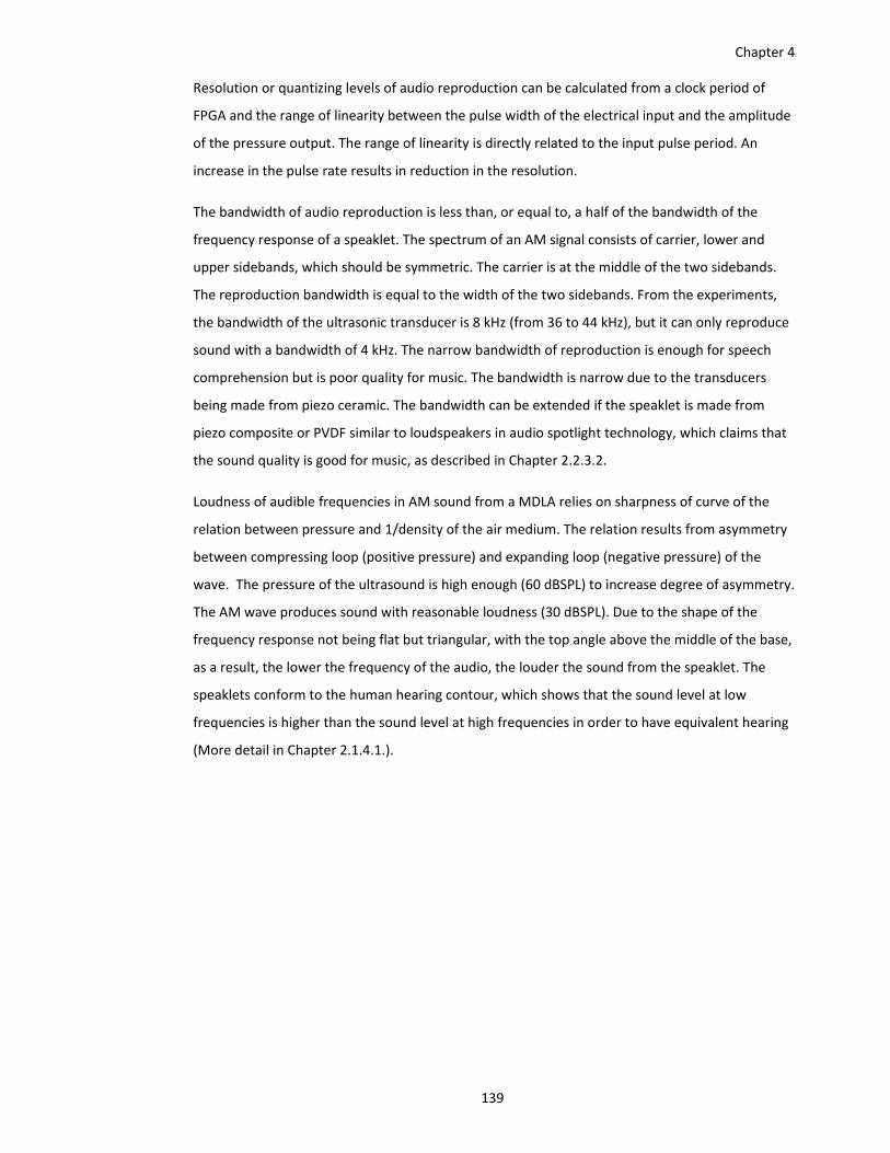
Chapter 4

139

Resolution or quantizing levels of audio reproduction can be calculated from a clock period of

FPGA and the range of linearity between the pulse width of the electrical input and the amplitude

of the pressure output. The range of linearity is directly related to the input pulse period. An

increase in the pulse rate results in reduction in the resolution.

The bandwidth of audio reproduction is less than, or equal to, a half of the bandwidth of the

frequency response of a speaklet. The spectrum of an AM signal consists of carrier, lower and

upper sidebands, which should be symmetric. The carrier is at the middle of the two sidebands.

The reproduction bandwidth is equal to the width of the two sidebands. From the experiments,

the bandwidth of the ultrasonic transducer is 8 kHz (from 36 to 44 kHz), but it can only reproduce

sound with a bandwidth of 4 kHz. The narrow bandwidth of reproduction is enough for speech

comprehension but is poor quality for music. The bandwidth is narrow due to the transducers

being made from piezo ceramic. The bandwidth can be extended if the speaklet is made from

piezo composite or PVDF similar to loudspeakers in audio spotlight technology, which claims that

the sound quality is good for music, as described in Chapter 2.2.3.2.

Loudness of audible frequencies in AM sound from a MDLA relies on sharpness of curve of the

relation between pressure and 1/density of the air medium. The relation results from asymmetry

between compressing loop (positive pressure) and expanding loop (negative pressure) of the

wave. The pressure of the ultrasound is high enough (60 dBSPL) to increase degree of asymmetry.

The AM wave produces sound with reasonable loudness (30 dBSPL). Due to the shape of the

frequency response not being flat but triangular, with the top angle above the middle of the base,

as a result, the lower the frequency of the audio, the louder the sound from the speaklet. The

speaklets conform to the human hearing contour, which shows that the sound level at low

frequencies is higher than the sound level at high frequencies in order to have equivalent hearing

(More detail in Chapter 2.1.4.1.).

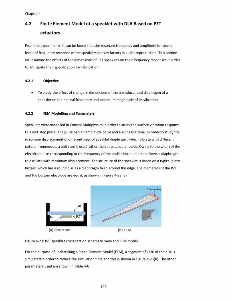
Chapter 4

140

4.2 Finite Element Model of a speaklet with DLA Based on PZT

actuators

From the experiments, it can be found that the resonant frequency and amplitude (or sound

level) of frequency response of the speaklets are key factors in audio reproduction. This section

will examine the effects of the dimensions of PZT speaklets on their frequency responses in order

to anticipate their specification for fabrication.

4.2.1 Objective

To study the effect of change in dimensions of the transducer and diaphragm of a

speaklet on the natural frequency and maximum magnitude of its vibration.

4.2.2 FEM Modelling and Parameters

Speaklets were modelled in Comsol Multiphysics in order to study the surface vibration response

to a unit step pulse. The pulse had an amplitude of 5V and a 40 ns rise time. In order to study the

maximum displacement of different sizes of speaklet diaphragm, which vibrate with different

natural frequencies, a unit step is used rather than a rectangular pulse. Owing to the width of the

electrical pulse corresponding to the frequency of the oscillation, a unit step allows a diaphragm

to oscillate with maximum displacement. The structure of the speaklet is based on a typical piezo

buzzer, which has a round disc as a diaphragm fixed around the edge. The diameters of the PZT

and the bottom electrode are equal, as shown in Figure 4‐23 (a)

Figure 4‐23: PZT speaklet cross section schematic view and FEM model

For the purpose of undertaking a Finite Element Model (FEM), a segment of 1/10 of the disc is

simulated in order to reduce the simulation time and this is shown in Figure 4‐23(b). The other

parameters used are shown in Table 4‐6

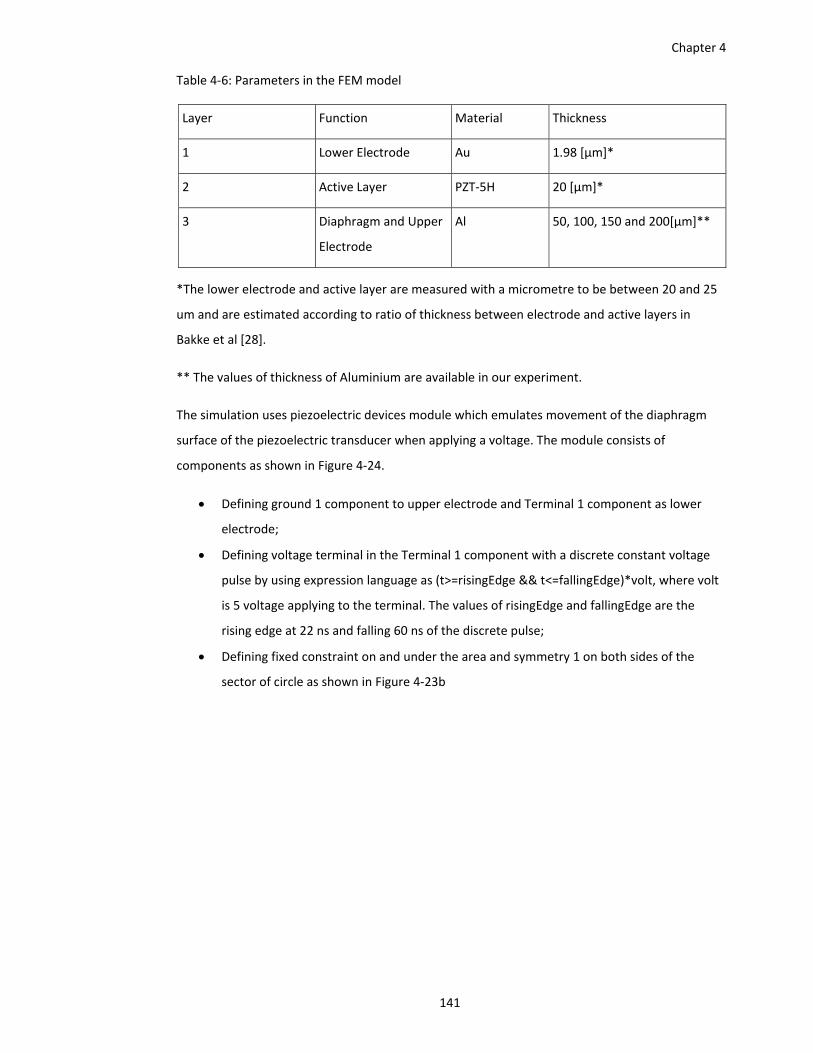
Chapter 4

141

Table 4‐6: Parameters in the FEM model

Layer Function Material Thickness

1 Lower Electrode Au 1.98 [µm]*

2 Active Layer PZT‐5H 20 [µm]*

3 Diaphragm and Upper

Electrode

Al 50, 100, 150 and 200[µm]**

*The lower electrode and active layer are measured with a micrometre to be between 20 and 25

um and are estimated according to ratio of thickness between electrode and active layers in

Bakke et al [28].

** The values of thickness of Aluminium are available in our experiment.

The simulation uses piezoelectric devices module which emulates movement of the diaphragm

surface of the piezoelectric transducer when applying a voltage. The module consists of

components as shown in Figure 4‐24.

Defining ground 1 component to upper electrode and Terminal 1 component as lower

electrode;

Defining voltage terminal in the Terminal 1 component with a discrete constant voltage

pulse by using expression language as (t>=risingEdge && t<=fallingEdge)*volt, where volt

is 5 voltage applying to the terminal. The values of risingEdge and fallingEdge are the

rising edge at 22 ns and falling 60 ns of the discrete pulse;

Defining fixed constraint on and under the area and symmetry 1 on both sides of the

sector of circle as shown in Figure 4‐23b

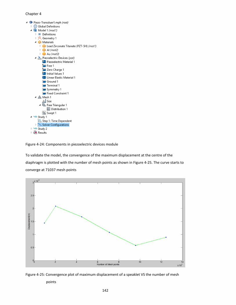
Chapter 4

142

Figure 4‐24: Components in piezoelectric devices module

To validate the model, the convergence of the maximum displacement at the centre of the

diaphragm is plotted with the number of mesh points as shown in Figure 4‐25. The curve starts to

converge at 71037 mesh points

Figure 4‐25: Convergence plot of maximum displacement of a speaklet VS the number of mesh

points

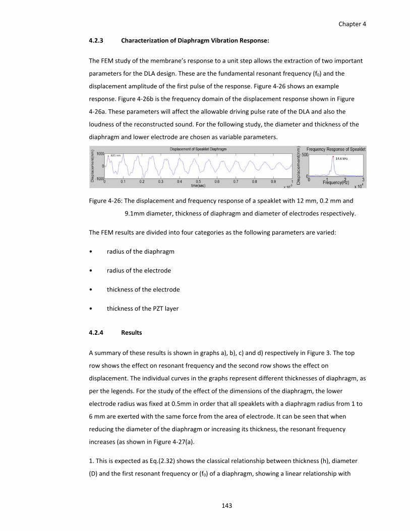
Chapter 4

143

4.2.3 Characterization of Diaphragm Vibration Response:

The FEM study of the membrane’s response to a unit step allows the extraction of two important

parameters for the DLA design. These are the fundamental resonant frequency (f0) and the

displacement amplitude of the first pulse of the response. Figure 4‐26 shows an example

response. Figure 4‐26b is the frequency domain of the displacement response shown in Figure

4‐26a. These parameters will affect the allowable driving pulse rate of the DLA and also the

loudness of the reconstructed sound. For the following study, the diameter and thickness of the

diaphragm and lower electrode are chosen as variable parameters.

Figure 4‐26: The displacement and frequency response of a speaklet with 12 mm, 0.2 mm and

9.1mm diameter, thickness of diaphragm and diameter of electrodes respectively.

The FEM results are divided into four categories as the following parameters are varied:

• radius of the diaphragm

• radius of the electrode

• thickness of the electrode

• thickness of the PZT layer

4.2.4 Results

A summary of these results is shown in graphs a), b), c) and d) respectively in Figure 3. The top

row shows the effect on resonant frequency and the second row shows the effect on

displacement. The individual curves in the graphs represent different thicknesses of diaphragm, as

per the legends. For the study of the effect of the dimensions of the diaphragm, the lower

electrode radius was fixed at 0.5mm in order that all speaklets with a diaphragm radius from 1 to

6 mm are exerted with the same force from the area of electrode. It can be seen that when

reducing the diameter of the diaphragm or increasing its thickness, the resonant frequency

increases (as shown in Figure 4‐27(a).

1. This is expected as Eq.(2.32) shows the classical relationship between thickness (h), diameter

(D) and the first resonant frequency or (f0) of a diaphragm, showing a linear relationship with

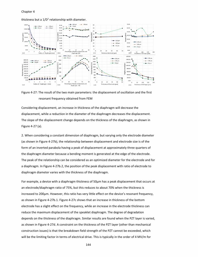
Chapter 4

144

thickness but a 1/D2 relationship with diameter.

Figure 4‐27: The result of the two main parameters: the displacement of oscillation and the first

resonant frequency obtained from FEM

Considering displacement, an increase in thickness of the diaphragm will decrease the

displacement, while a reduction in the diameter of the diaphragm decreases the displacement.

The slope of the displacement change depends on the thickness of the diaphragm, as shown in

Figure 4‐27 (a).

2. When considering a constant dimension of diaphragm, but varying only the electrode diameter

(as shown in Figure 4‐27b), the relationship between displacement and electrode size is of the

form of an inverted parabola having a peak of displacement at approximately three quarters of

the diaphragm diameter because a bending moment is generated at the edge of the electrode.

The peak of the relationship can be considered as an optimized diameter for the electrode and for

a diaphragm. In Figure 4‐27b.2, the position of the peak displacement with ratio of electrode to

diaphragm diameter varies with the thickness of the diaphragm.

For example, a device with a diaphragm thickness of 50μm has a peak displacement that occurs at

an electrode/diaphragm ratio of 75%, but this reduces to about 70% when the thickness is

increased to 200μm. However, this ratio has very little effect on the device’s resonant frequency,

as shown in Figure 4‐27b.1. Figure 4‐27c shows that an increase in thickness of the bottom

electrode has a slight effect on the frequency, while an increase in the electrode thickness can

reduce the maximum displacement of the speaklet diaphragm. The degree of degradation

depends on the thickness of the diaphragm. Similar results are found when the PZT layer is varied,

as shown in Figure 4‐27d. A constraint on the thickness of the PZT layer (other than mechanical

construction issues) is that the breakdown field strength of the PZT cannot be exceeded, which

will be the limiting factor in terms of electrical drive. This is typically in the order of 4 MV/m for

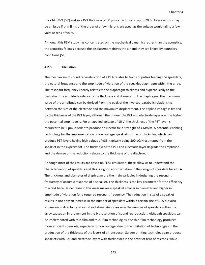
Chapter 4

145

thick film PZT [52] and so a PZT thickness of 50 μm can withstand up to 200V. However this may

be an issue if thin films of the order of a few microns are used, as the voltage would fall to a few

volts or tens of volts.

Although this FEM study has concentrated on the mechanical dynamics rather than the acoustics,

the acoustics follows because the displacement drives the air and they are linked by boundary

conditions [51].

4.2.5 Discussion

The mechanism of sound reconstruction of a DLA relates to trains of pulses feeding the speaklets,

the natural frequency and the amplitude of vibration of the speaklet diaphragm within the array.

The resonant frequency linearly relates to the diaphragm thickness and hyperbolically to the

diameter. The amplitude relates to the thickness and diameter of the diaphragm. The maximum

value of the amplitude can be derived from the peak of the inverted‐parabolic relationship

between the size of the electrode and the maximum displacement. The applied voltage is limited

by the thickness of the PZT layer, although the thinner the PZT and electrode layer are, the higher

the potential amplitude is. For an applied voltage of 10 V, the thickness of the PZT layer is

required to be 2 µm in order to produce an electric field strength of 4 MV/m. A potential enabling

technology for the implementation of low voltage speaklets is thin or thick‐film, which can

produce PZT layers having high values of d33, typically being 300 pC/N estimated from the

speaklet in the experiment. The thickness of the PZT and electrode layer degrade the amplitude

and the degree of the reduction relates to the thickness of the diaphragm.

Although most of the results are based on FEM simulation, these allow us to understand the

characterization of speaklets and this is a good approximation in the design of speaklets for a DLA.

The thickness and diameter of diaphragm are the main variables in designing the resonant

frequency of acoustic response of a speaklet. The thickness is the key parameter for the efficiency

of a DLA because decrease in thickness makes a speaklet smaller in diameter and higher in

amplitude of vibration for a required resonant frequency. The reduction in size of a speaklet

results in not only an increase in the number of speaklets within a certain size of DLA but also

expansion in directivity of sound radiation. An increase in the number of speaklets within the

array causes an improvement in the bit resolution of sound reproduction. Although speaklets can

be implemented with thin‐film and thick‐film technologies, the thin‐film technology produces

more efficient speaklets, especially for low voltage, due to the limitation of technologies in the

production of the thickness of the layers of a transducer. Screen printing technology can produce

speaklets with PZT and electrode layers with thicknesses in the order of tens of microns, while

Chapter 4

146

thin‐film technology can produce an electrode layer with thickness in the order of one‐tenth of a

micron and a PZT layer with thickness in the order of a micron, in order to obtain an electric field

strength of 4 MV/m (10 V across 2.5 microns).

However, the response of a speaklet to a digital pulse from the FEM simulation is vibration on the

surface of the diaphragm. It is sufficient to study the resonant frequency of the acoustic response

because the frequencies of the vibrating surface and acoustic response are the same. In order to

quantify the loudness and directivity of sound, the response has to transform the vibration on the

diaphragm into radiation of the sound by using the wave equations. Therefore, the development

of the FEM simulation would make interesting work in future.

4.3 Summary

The pressure response of speaklets was not demonstrated to be capable of meeting a key

requirement for digital sound reconstruction, in that the response should stop before rising edge

of the following pulse (more detail in Chapter 3.3.3.4). The responses of the speaklets have low

damping ratios, which result in a long emitting time (in the order of milliseconds). The pulse rate

which corresponds to the requirement is in the order of a hundred Hz, but the rate is too slow to

reproduce sound from the audio stream, which has a sampling rate of 44.1 kHz.

The reduction of ringing of the response to a rectangular pulse by raising a second pulse, referred

to as the double pulse technique, is not effective because of the multiple resonant frequencies of

the response of the speaklets and the initial interval of the response, as described in Chapter

4.1.2.2. Because it is impossible to meet the first requirement, the first requirement is ignored

and allows the response of consecutive pulses to overlap each other. As a consequence of the

ignorance, the amplitude of the response of a speaklet to the pulse rate is related to the

frequency response of the speaklet because the interference between successive pulses. The

amplitude will maximize when the pulse rate is equal to the resonant frequency of the speaklet.

The relationship between the pulse width of the driving signal and the amplitude of the acoustic

wave can be linear for a certain range of pulse widths. The range is directly related to the pulse

period.

Driving a speaklet according to the concept of a MDLA produces the pressure response like an AM

waveform. The frequency response of a speaklet should have a single resonance frequency in

order to protect frequency distortion at the resonant frequency. The bandwidth of a MDLA

speaklet requires twice the audio bandwidth. An 8 kHz bandwidth of a speaklet can only produce

Chapter 4

147

a 4 kHz audio bandwidth. The loudness of a MDLA relies on the non‐linear acoustic of the air

medium, similar to a parametric array.

The relationship between the dimensions of a speaklet and its acoustic response when feeding a

rectangle pulse shows that:

Diameter of diaphragm of a speaklet is inversely related to the resonant frequency of the

speaklet while the diameter is directly related to the amplitude of the response

Thickness of diaphragm is directly related to the resonance frequency of the speaklet,

while the thickness is inversely related to the amplitude of the response

Change in diameter of transducer has a slight effect (less than 10 %)on variation in the

resonance frequency, but an increase in diameter changes the amplitude of the response

Change in thickness of the transducer has a slight effect (less than 10%)on variation in the

resonance frequency and amplitude if the thickness is less than 50 µm

In conclusion, the pressure response of a MDLA with diaphragm based piezoelectric speaklets can

generate sound with AM waveform by relying on non‐linear acoustic medium but it is lower

efficiency between loudness and the total transmitting wave enegy than the sound with half‐wave

rectified AM as the ideal case in Chapter 3. In the next chapter, a novel structure of a loudspeaker

is introduced for sound generation with half‐wave rectified AM waveform.

Chapter 5

149

Chapter 5: A Potential Implementation for an Acoustic

Rectifying Loudspeaker

5.1 Acoustic Rectifying Loudspeaker

This chapter will introduce the concept of a rectifying loudspeaker and perform the validation of

the proposed conditions for acoustic rectification in Chapter 3. Pressure (p) is directly

proportional to velocity (u), which is directly proportional to displacement (w) of the diaphragm,

but only the proportional relationship between the displacement and the velocity is

demonstrated in this chapter. Although this demonstration have not yet complete the validation,

it is a good evidence that the loudspeaker has a potential for generating a rectified sound while

the demonstration of the proportional relationship between pressure and velocity will be a

further work, which is described in Chapter 6.1.1. The main reasons why AM sound requires a

rectifier are addressed by consideration of sound in the frequency domain, and why a analogue

loudspeaker or a transducer cannot produce the rectified sound is addressed by illustration in

schematic diagrams of wave propagation. A proposed structure and mechanism for a rectifying

loudspeaker is presented.

The validation of the condition is performed by a simplified structure. The advantages and

efficiency are assessed and a practical structure is identified in the discussion section.

5.1.1 Principles

From the previous chapter, it was seen that a waveform of pressure output of multiple‐level

digital loudspeaker array (MDLA) is similar to a waveform of amplitude modulation. Although it

can make sound, due to the non‐linearity of the air medium between pressure and specific

volume as described in Chapter 2.2.3.1, the efficiency of sound is low because the ratio of sound

level to the magnitude of the side bands is low ‐ approximately 1:10 as shown earlier in Figure

4‐17

In order to increase the ratio to 1:1, the waveform of pressure output of the MDLA needs to be

rectified, which can be achieved by demodulation of the modulated wave. The ratio will increase

and the sound level will not only be indirectly affected by the non‐linear acoustic medium, but the

level is directly affected by the amplitude of the side band i.e. the modulated audio signal. As in

the ideal case of the MDLA described in Chapter 3, the output waveform is half‐wave rectified

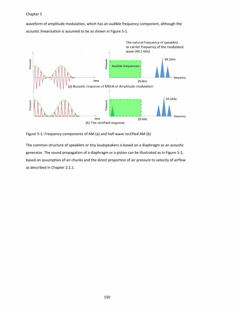
Chapter 5

150

waveform of amplitude modulation, which has an audible frequency component, although the

acoustic linearization is assumed to be as shown in Figure 5‐1.

Figure 5‐1: Frequency components of AM (a) and half‐wave rectified AM (b)

The common structure of speaklets or tiny loudspeakers is based on a diaphragm as an acoustic

generator. The sound propagation of a diaphragm or a piston can be illustrated as in Figure 5‐2,

based on assumption of air chunks and the direct proportion of air pressure to velocity of airflow

as described in Chapter 2.1.1.

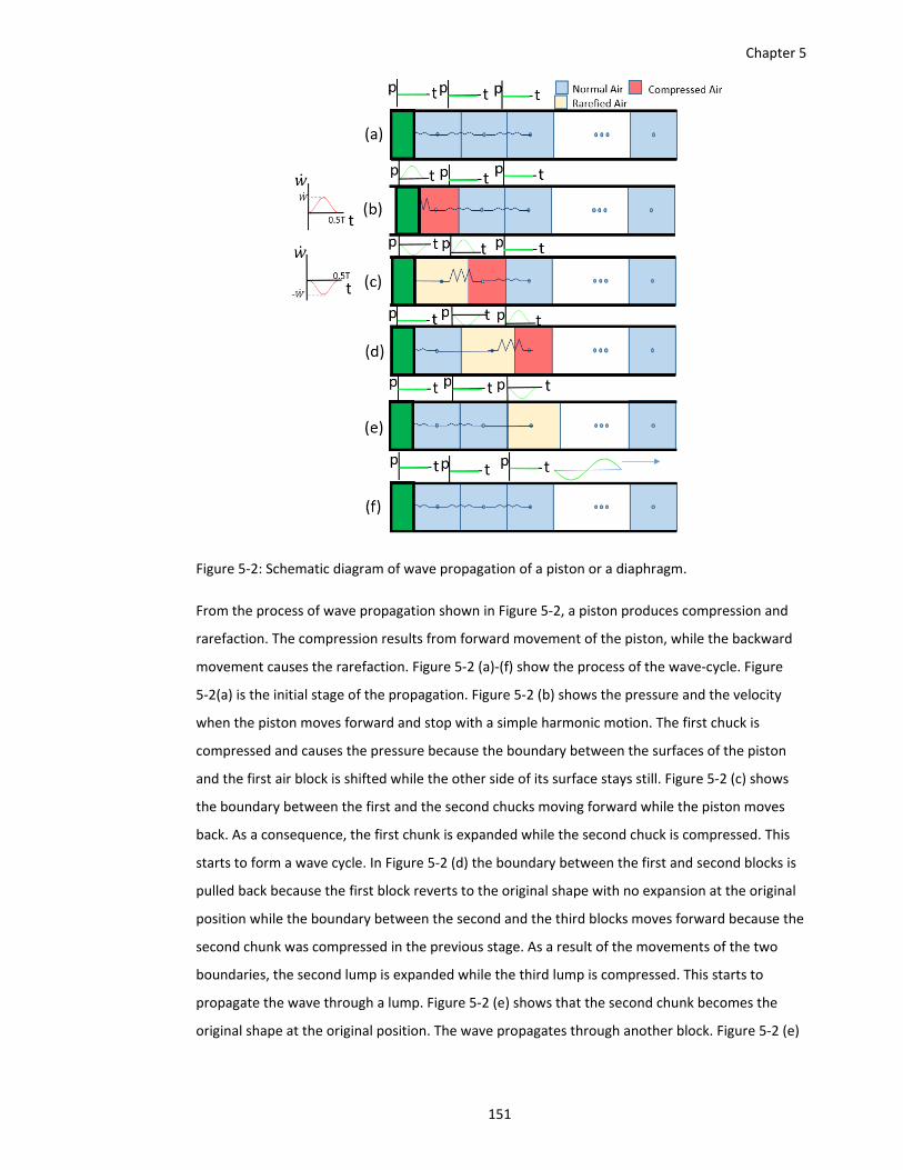
Chapter 5

151

Figure 5‐2: Schematic diagram of wave propagation of a piston or a diaphragm.

From the process of wave propagation shown in Figure 5‐2, a piston produces compression and

rarefaction. The compression results from forward movement of the piston, while the backward

movement causes the rarefaction. Figure 5‐2 (a)‐(f) show the process of the wave‐cycle. Figure

5‐2(a) is the initial stage of the propagation. Figure 5‐2 (b) shows the pressure and the velocity

when the piston moves forward and stop with a simple harmonic motion. The first chuck is

compressed and causes the pressure because the boundary between the surfaces of the piston

and the first air block is shifted while the other side of its surface stays still. Figure 5‐2 (c) shows

the boundary between the first and the second chucks moving forward while the piston moves

back. As a consequence, the first chunk is expanded while the second chuck is compressed. This

starts to form a wave cycle. In Figure 5‐2 (d) the boundary between the first and second blocks is

pulled back because the first block reverts to the original shape with no expansion at the original

position while the boundary between the second and the third blocks moves forward because the

second chunk was compressed in the previous stage. As a result of the movements of the two

boundaries, the second lump is expanded while the third lump is compressed. This starts to

propagate the wave through a lump. Figure 5‐2 (e) shows that the second chunk becomes the

original shape at the original position. The wave propagates through another block. Figure 5‐2 (e)

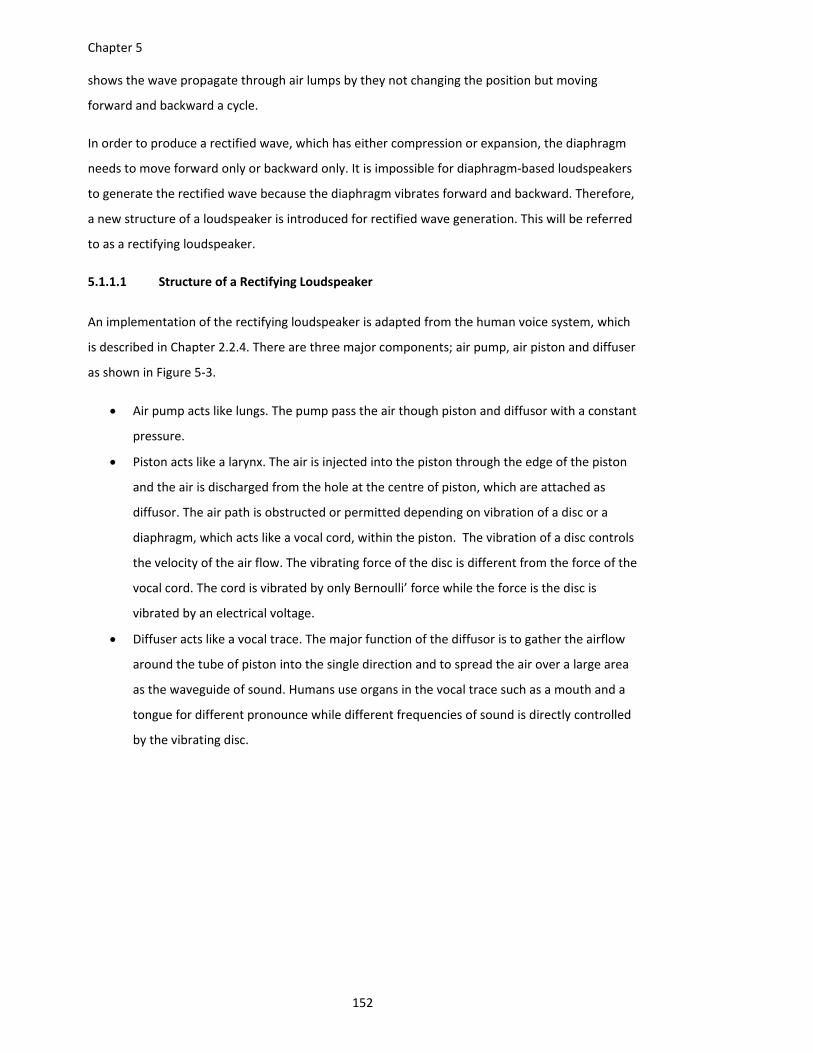
Chapter 5

152

shows the wave propagate through air lumps by they not changing the position but moving

forward and backward a cycle.

In order to produce a rectified wave, which has either compression or expansion, the diaphragm

needs to move forward only or backward only. It is impossible for diaphragm‐based loudspeakers

to generate the rectified wave because the diaphragm vibrates forward and backward. Therefore,

a new structure of a loudspeaker is introduced for rectified wave generation. This will be referred

to as a rectifying loudspeaker.

5.1.1.1 Structure of a Rectifying Loudspeaker

An implementation of the rectifying loudspeaker is adapted from the human voice system, which

is described in Chapter 2.2.4. There are three major components; air pump, air piston and diffuser

as shown in Figure 5‐3.

Air pump acts like lungs. The pump pass the air though piston and diffusor with a constant

pressure.

Piston acts like a larynx. The air is injected into the piston through the edge of the piston

and the air is discharged from the hole at the centre of piston, which are attached as

diffusor. The air path is obstructed or permitted depending on vibration of a disc or a

diaphragm, which acts like a vocal cord, within the piston. The vibration of a disc controls

the velocity of the air flow. The vibrating force of the disc is different from the force of the

vocal cord. The cord is vibrated by only Bernoulli’ force while the force is the disc is

vibrated by an electrical voltage.

Diffuser acts like a vocal trace. The major function of the diffusor is to gather the airflow

around the tube of piston into the single direction and to spread the air over a large area

as the waveguide of sound. Humans use organs in the vocal trace such as a mouth and a

tongue for different pronounce while different frequencies of sound is directly controlled

by the vibrating disc.

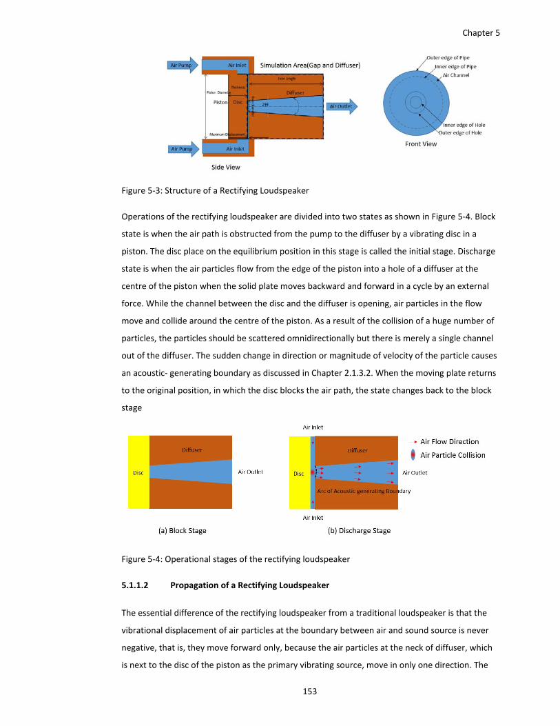
Chapter 5

153

Figure 5‐3: Structure of a Rectifying Loudspeaker

Operations of the rectifying loudspeaker are divided into two states as shown in Figure 5‐4. Block

state is when the air path is obstructed from the pump to the diffuser by a vibrating disc in a

piston. The disc place on the equilibrium position in this stage is called the initial stage. Discharge

state is when the air particles flow from the edge of the piston into a hole of a diffuser at the

centre of the piston when the solid plate moves backward and forward in a cycle by an external

force. While the channel between the disc and the diffuser is opening, air particles in the flow

move and collide around the centre of the piston. As a result of the collision of a huge number of

particles, the particles should be scattered omnidirectionally but there is merely a single channel

out of the diffuser. The sudden change in direction or magnitude of velocity of the particle causes

an acoustic‐ generating boundary as discussed in Chapter 2.1.3.2. When the moving plate returns

to the original position, in which the disc blocks the air path, the state changes back to the block

stage

Figure 5‐4: Operational stages of the rectifying loudspeaker

5.1.1.2 Propagation of a Rectifying Loudspeaker

The essential difference of the rectifying loudspeaker from a traditional loudspeaker is that the

vibrational displacement of air particles at the boundary between air and sound source is never

negative, that is, they move forward only, because the air particles at the neck of diffuser, which

is next to the disc of the piston as the primary vibrating source, move in only one direction. The

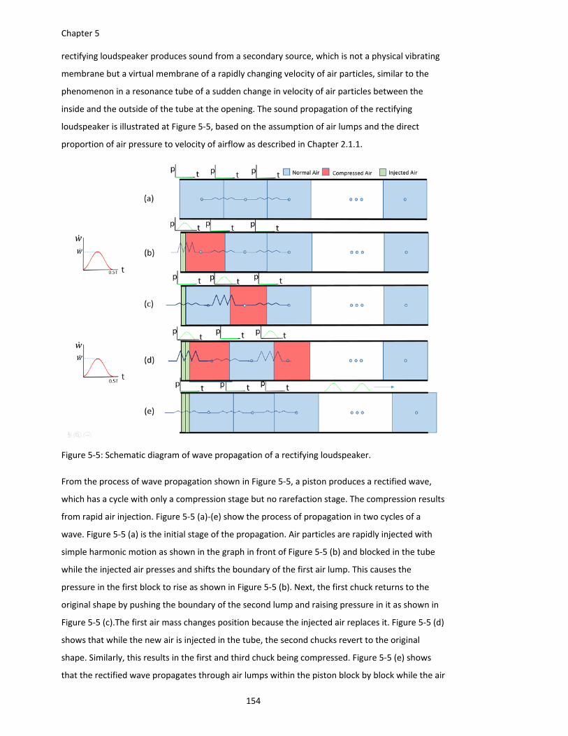
Chapter 5

154

rectifying loudspeaker produces sound from a secondary source, which is not a physical vibrating

membrane but a virtual membrane of a rapidly changing velocity of air particles, similar to the

phenomenon in a resonance tube of a sudden change in velocity of air particles between the

inside and the outside of the tube at the opening. The sound propagation of the rectifying

loudspeaker is illustrated at Figure 5‐5, based on the assumption of air lumps and the direct

proportion of air pressure to velocity of airflow as described in Chapter 2.1.1.

Figure 5‐5: Schematic diagram of wave propagation of a rectifying loudspeaker.

From the process of wave propagation shown in Figure 5‐5, a piston produces a rectified wave,

which has a cycle with only a compression stage but no rarefaction stage. The compression results

from rapid air injection. Figure 5‐5 (a)‐(e) show the process of propagation in two cycles of a

wave. Figure 5‐5 (a) is the initial stage of the propagation. Air particles are rapidly injected with

simple harmonic motion as shown in the graph in front of Figure 5‐5 (b) and blocked in the tube

while the injected air presses and shifts the boundary of the first air lump. This causes the

pressure in the first block to rise as shown in Figure 5‐5 (b). Next, the first chuck returns to the

original shape by pushing the boundary of the second lump and raising pressure in it as shown in

Figure 5‐5 (c).The first air mass changes position because the injected air replaces it. Figure 5‐5 (d)

shows that while the new air is injected in the tube, the second chucks revert to the original

shape. Similarly, this results in the first and third chuck being compressed. Figure 5‐5 (e) shows

that the rectified wave propagates through air lumps within the piston block by block while the air

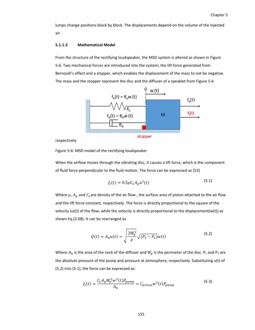
Chapter 5

155

lumps change positions block by block. The displacements depend on the volume of the injected

air.

5.1.1.3 Mathematical Model

From the structure of the rectifying loudspeaker, the MSD system is altered as shown in Figure

5‐6. Two mechanical forces are introduced into the system; the lift force generated from

Bernoulli’s effect and a stopper, which enables the displacement of the mass to not be negative.

The mass and the stopper represent the disc and the diffuser of a speaklet from Figure 5‐6

respectively

Figure 5‐6: MSD model of the rectifying loudspeaker

When the airflow moves through the vibrating disc, it causes a lift force, which is the component

of fluid force perpendicular to the fluid motion. The force can be expressed as [53]

0.5 (5.1)

Where , and are density of the air flow , the surface area of piston attached to the air flow

and the lift force constant, respectively. The force is directly proportional to the square of the

velocity (u(t)) of the flow, while the velocity is directly proportional to the displacement(w(t)) as

shown Eq.(2.68). It can be rearranged as

2

(5.2)

Where is the area of the neck of the diffuser and is the perimeter of the disc. P1 and P2 are

the absolute pressure of the pump and pressure at atmosphere, respectively. Substituting u(t) of

(5.2) into (5.1), the force can be expressed as:

(5.3)

Chapter 5

156

Where is the constant pressure of the air pump above the atmospheric pressure and

is a constant of the piston. The ratio of the area of the hole and the area of the

piston have an effect on the force. An increase in Ap or decrease in Ah results in an increase in the

force. The lift force is represented in the term of the square of the displacement and the constant

pump pressure. The mathematical model of the rectifying loudspeaker can be expressed as

2 (5.4)

This equation is a non‐linear differential equation, which might be difficult to solve. The solution

should be achievable using FEM software. However, it shows the lift force is involved with a free

vibration because it is a term of displacement. Due to the term of square of displacement, the

free vibration is not sinusoidal and its waveform might be similar to the air‐flow pattern of a dark

tone of the larynx as shown in Figure 2‐20b. Therefore, the lift force generates a constant pattern

of the wave while the external force (fe(t)) will change the amplitude of the pattern in each wave

cycle.

The stopper is designed as a fixed surface. When the mass vibrates, it hits the stopper. The

movement of the diaphragm can be analysed by using collision of equations. The fundamental

equations of the collision can be divided into two extreme cases of perfectly elastic and perfectly

inelastic collision. The elastic collision is that the total kinetic energy is conserved as well as the

total momentum of the disc and the fixed diffuser while the inelastic collision is that the total

energy is lost or transferred into other energy[54]. In this model for the perfectly elastic collision,

the velocity before and after collision are equal as with

(5.5)

Where Ua and Ub are the velocity at a moment after and before the collision, respectively, under

the assumption that the stopper does not move. For the perfectly inelastic collision the velocity

after collision is equal to zero

0 (5.6)

However, in the practical collision, the kinetic energy is partly lost depending on the elasticity of

the material of the diaphragm and the diffuser. This will be studied as a part of the future work

section in Chapter 6.2.1 .

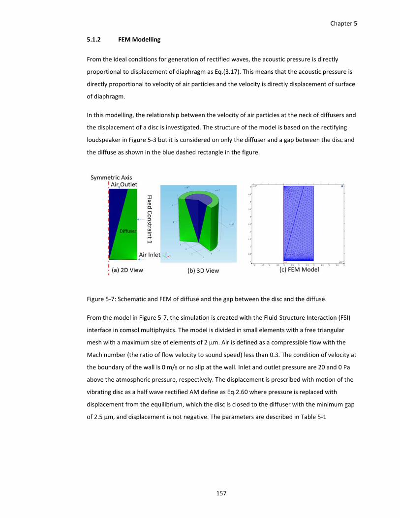
Chapter 5

157

5.1.2 FEM Modelling

From the ideal conditions for generation of rectified waves, the acoustic pressure is directly

proportional to displacement of diaphragm as Eq.(3.17). This means that the acoustic pressure is

directly proportional to velocity of air particles and the velocity is directly displacement of surface

of diaphragm.

In this modelling, the relationship between the velocity of air particles at the neck of diffusers and

the displacement of a disc is investigated. The structure of the model is based on the rectifying

loudspeaker in Figure 5‐3 but it is considered on only the diffuser and a gap between the disc and

the diffuse as shown in the blue dashed rectangle in the figure.

Figure 5‐7: Schematic and FEM of diffuse and the gap between the disc and the diffuse.

From the model in Figure 5‐7, the simulation is created with the Fluid‐Structure Interaction (FSI)

interface in comsol multiphysics. The model is divided in small elements with a free triangular

mesh with a maximum size of elements of 2 µm. Air is defined as a compressible flow with the

Mach number (the ratio of flow velocity to sound speed) less than 0.3. The condition of velocity at

the boundary of the wall is 0 m/s or no slip at the wall. Inlet and outlet pressure are 20 and 0 Pa

above the atmospheric pressure, respectively. The displacement is prescribed with motion of the

vibrating disc as a half wave rectified AM define as Eq.2.60 where pressure is replaced with

displacement from the equilibrium, which the disc is closed to the diffuser with the minimum gap

of 2.5 µm, and displacement is not negative. The parameters are described in Table 5‐1

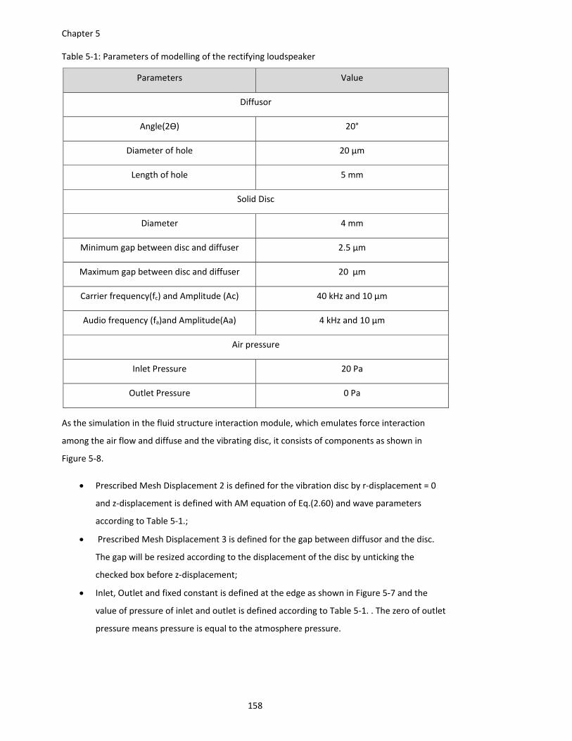
Chapter 5

158

Table 5‐1: Parameters of modelling of the rectifying loudspeaker

Parameters Value

Diffusor

Angle(2ϴ) 20°

Diameter of hole 20 µm

Length of hole 5 mm

Solid Disc

Diameter 4 mm

Minimum gap between disc and diffuser 2.5 µm

Maximum gap between disc and diffuser 20 µm

Carrier frequency(fc) and Amplitude (Ac) 40 kHz and 10 µm

Audio frequency (fa)and Amplitude(Aa) 4 kHz and 10 µm

Air pressure

Inlet Pressure 20 Pa

Outlet Pressure 0 Pa

As the simulation in the fluid structure interaction module, which emulates force interaction

among the air flow and diffuse and the vibrating disc, it consists of components as shown in

Figure 5‐8.

Prescribed Mesh Displacement 2 is defined for the vibration disc by r‐displacement = 0

and z‐displacement is defined with AM equation of Eq.(2.60) and wave parameters

according to Table 5‐1.;

Prescribed Mesh Displacement 3 is defined for the gap between diffusor and the disc.

The gap will be resized according to the displacement of the disc by unticking the

checked box before z‐displacement;

Inlet, Outlet and fixed constant is defined at the edge as shown in Figure 5‐7 and the

value of pressure of inlet and outlet is defined according to Table 5‐1. . The zero of outlet

pressure means pressure is equal to the atmosphere pressure.

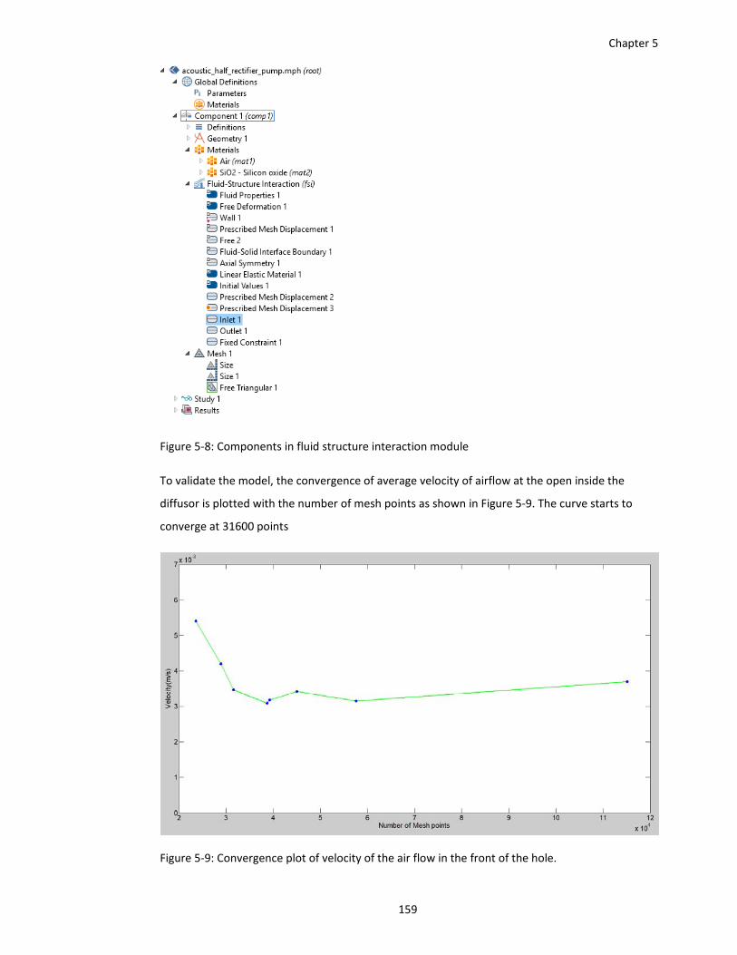
Chapter 5

159

Figure 5‐8: Components in fluid structure interaction module

To validate the model, the convergence of average velocity of airflow at the open inside the

diffusor is plotted with the number of mesh points as shown in Figure 5‐9. The curve starts to

converge at 31600 points

Figure 5‐9: Convergence plot of velocity of the air flow in the front of the hole.

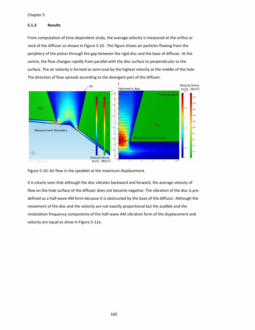
Chapter 5

160

5.1.3 Results

From computation of time‐dependent study, the average velocity is measured at the orifice or

neck of the diffuser as shown in Figure 5‐10 . The figure shows air particles flowing from the

periphery of the piston through the gap between the rigid disc and the base of diffuser. At the

centre, the flow changes rapidly from parallel with the disc surface to perpendicular to the

surface. The air velocity is formed as semi‐oval by the highest velocity at the middle of the hole.

The direction of flow spreads according to the divergent part of the diffuser.

Figure 5‐10: Air flow in the speaklet at the maximum displacement.

It is clearly seen that although the disc vibrates backward and forward, the average velocity of

flow on the hole surface of the diffuser does not become negative. The vibration of the disc is pre‐

defined as a half‐wave AM form because it is obstructed by the base of the diffusor. Although the

movement of the disc and the velocity are not exactly proportional but the audible and the

modulation frequency components of the half‐wave AM vibration form of the displacement and

velocity are equal as show in Figure 5‐11a.

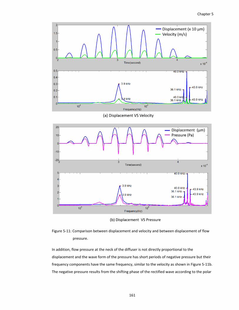
Chapter 5

161

Figure 5‐11: Comparison between displacement and velocity and between displacement of flow

pressure.

In addition, flow pressure at the neck of the diffuser is not directly proportional to the

displacement and the wave form of the pressure has short periods of negative pressure but their

frequency components have the same frequency, similar to the velocity as shown in Figure 5‐11b.

The negative pressure results from the shifting phase of the rectified wave according to the polar

Chapter 5

162

angle of acoustic impedance as described in Section 3.3.3.9. In addition, the amplitude of pressure

is related to the pressure of the air supply (20 Pa).

5.1.4 Discussion

From the results, it is clearly seen that the velocity moves forward from the surface of the

opening, which is designed for the secondary sound source. This implies that the displacement of

air particles at the hole has one direction according to the direction of the velocity, while the disc

moves forward and backward. The movement of the disc is the primary vibration sound, but acts

like a valve, resulting in the velocity of airflow into the hole. Although air supply is introduced in

the system, which increases in complexity, it rectifies direction of movement and velocity at the

hole.

Although the model is designed for demonstration of direct proportion between the velocity and

the displacement, the pressure flow at the velocity transition boundary is shown, but it is

demonstrated that it is the acoustic pressure. Its waveform looks like the wave slightly shift

phase, which reflects the wave equation of (2.132) . The wave equation is represented as the

actual wave radiation of a spherical sound source and has a complex number term of kr‐j , which

identifies phase shift. This is different from the simplified wave of (2.139) in the ideal case, which

is a real number. The variables k and r are the wave number and radius of sound source

respectively. The real part of the complex number is significantly greater than the imaginary part,

the wave is slightly shifted in its phase similar to the waveform of the flow pressure.

5.1.4.1 Advantages of Rectifying Loudspeakers

In addition to the waveform of the velocity being rectified, there are other benefits from

introduction of an air pressure supply.

Ultrasonic pressure depends not only on a force from a transducer attached to the

diaphragm, but also pressure of the supply. Although the flow pressure has not yet been

demonstrated to be the acoustic pressure, the acoustic pressure is proportional to the

velocity of the air flow, which is proportional to the pressure of the air supply according to

Bernoulli’s equation, according to the wave equation. Therefore the air supply enables a

small transducer to generate high ultrasonic pressure.

The beam width is wider than the traditional ultrasonic transducer. Although the model

didn’t show directivity of the loudspeaker, there are two good pieces of evidence for the

claim. The beam width is related to the ratio between diameter of diaphragm, which

generate ultrasound, and the wavelength. In this model, the diameter of the hole of

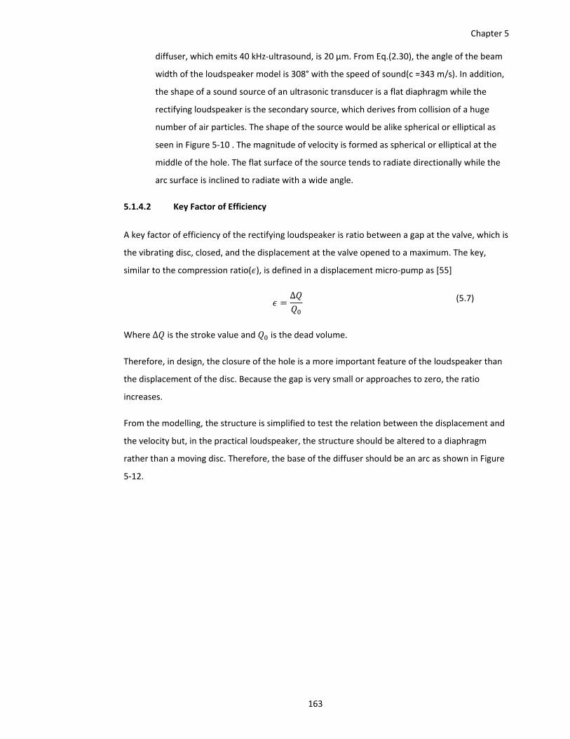
Chapter 5

163

diffuser, which emits 40 kHz‐ultrasound, is 20 µm. From Eq.(2.30), the angle of the beam

width of the loudspeaker model is 308° with the speed of sound(c =343 m/s). In addition,

the shape of a sound source of an ultrasonic transducer is a flat diaphragm while the

rectifying loudspeaker is the secondary source, which derives from collision of a huge

number of air particles. The shape of the source would be alike spherical or elliptical as

seen in Figure 5‐10 . The magnitude of velocity is formed as spherical or elliptical at the

middle of the hole. The flat surface of the source tends to radiate directionally while the

arc surface is inclined to radiate with a wide angle.

5.1.4.2 Key Factor of Efficiency

A key factor of efficiency of the rectifying loudspeaker is ratio between a gap at the valve, which is

the vibrating disc, closed, and the displacement at the valve opened to a maximum. The key,

similar to the compression ratio( ), is defined in a displacement micro‐pump as [55]

∆ (5.7)

Where ∆ is the stroke value and is the dead volume.

Therefore, in design, the closure of the hole is a more important feature of the loudspeaker than

the displacement of the disc. Because the gap is very small or approaches to zero, the ratio

increases.

From the modelling, the structure is simplified to test the relation between the displacement and

the velocity but, in the practical loudspeaker, the structure should be altered to a diaphragm

rather than a moving disc. Therefore, the base of the diffuser should be an arc as shown in Figure

5‐12.

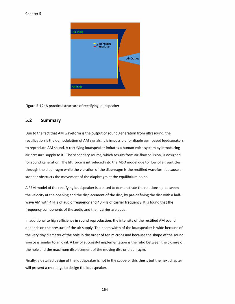
Chapter 5

164

Figure 5‐12: A practical structure of rectifying loudspeaker

5.2 Summary

Due to the fact that AM waveform is the output of sound generation from ultrasound, the

rectification is the demodulation of AM signals. It is impossible for diaphragm‐based loudspeakers

to reproduce AM sound. A rectifying loudspeaker imitates a human voice system by introducing

air pressure supply to it. The secondary source, which results from air‐flow collision, is designed

for sound generation. The lift force is introduced into the MSD model due to flow of air particles

through the diaphragm while the vibration of the diaphragm is the rectified waveform because a

stopper obstructs the movement of the diaphragm at the equilibrium point.

A FEM model of the rectifying loudspeaker is created to demonstrate the relationship between

the velocity at the opening and the displacement of the disc, by pre‐defining the disc with a half‐

wave AM with 4 kHz of audio frequency and 40 kHz of carrier frequency. It is found that the

frequency components of the audio and their carrier are equal.

In additional to high efficiency in sound reproduction, the intensity of the rectified AM sound

depends on the pressure of the air supply. The beam width of the loudspeaker is wide because of

the very tiny diameter of the hole in the order of ten microns and because the shape of the sound

source is similar to an oval. A key of successful implementation is the ratio between the closure of

the hole and the maximum displacement of the moving disc or diaphragm.

Finally, a detailed design of the loudspeaker is not in the scope of this thesis but the next chapter

will present a challenge to design the loudspeaker.

Chapter 6

165

Chapter 6: Conclusion and Future Work

6.1 Conclusion

This chapter describes the coherence of the chapters in the body of the thesis, and summarises

the essentials of the thesis. It is divided into three parts: illustration of the overall thesis,

identification of the differences of DLA, and explanation of the challenges in design of a rectifying

loudspeaker.

6.1.1 Landscape of Thesis

The main objective of this research is to investigate the possibility in the implementation of the

MDLA. This study explores electro‐acoustic transducer technologies and analyses their mechanical

and electrical characteristics which affect the conversion from electrical energy to acoustic

energy.

The exploration is performed by various methods – some with mathematical models, some with

FEM software and some with experiments. A landscape is drawn to show the conversion from

electrical energy to acoustic energy. It can be divided into three layers: conception, design and

practical.

6.1.1.1 Conception Layer

The conception layer of this study refers to the study on the literature on the concepts of

transducers in energy conversion to understand the mechanism of electro‐acoustic transducers.

The literature includes the studies on electrical and mechanical characteristics and on wave

propagation of the ideal case of spherical source.

The studies on the electro‐acoustic conversion of transducer can be divided into two conceptual

transducers: electromechanical and acoustic transducers. Electromechanical transducers convert

electrical energy into mechanical energy, while the acoustic transducers convert mechanical

energy into acoustic energy. The electrical energy is in the form of voltage (v(t)). The mechanical

energy can be in the form of external force fe(t) or movement (w(t)), while the acoustic energy is

in the form of acoustic pressure(p(t)) as shown in Figure 6‐1. From the figure, the red numbers

indicate the section numbers and the green arrows show the paths of investigation.

From the conception layer, as shown in Figure 6‐1,

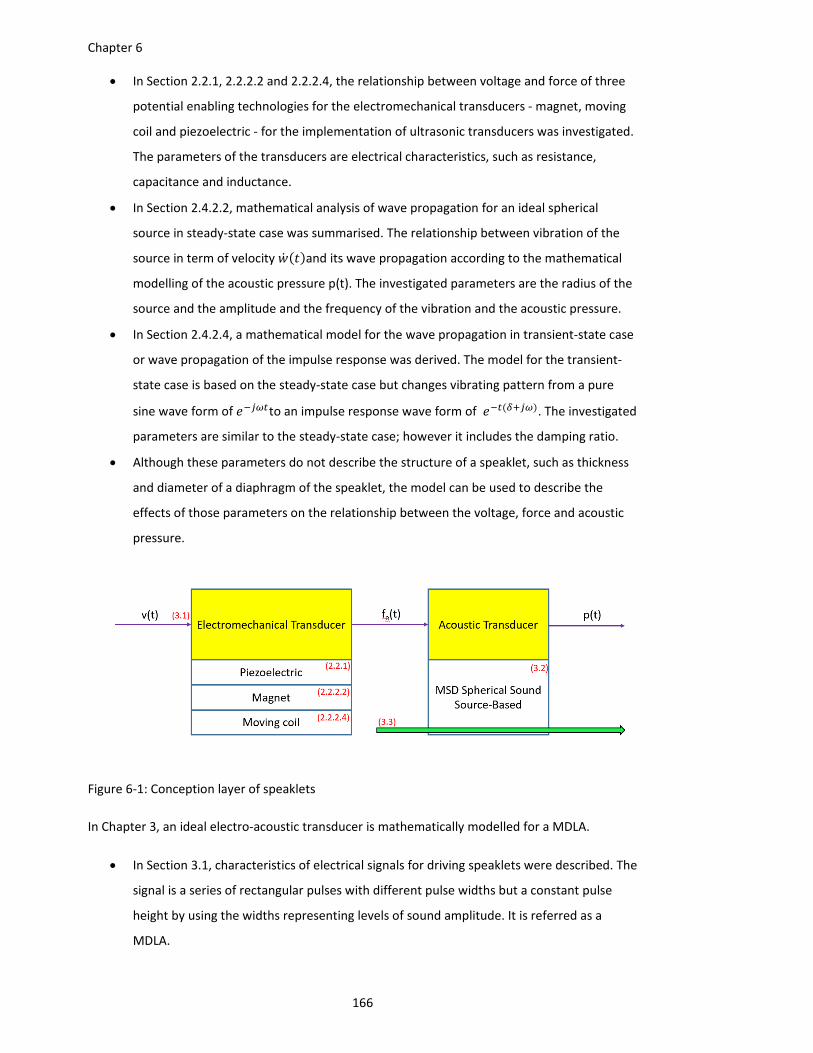
Chapter 6

166

In Section 2.2.1, 2.2.2.2 and 2.2.2.4, the relationship between voltage and force of three

potential enabling technologies for the electromechanical transducers ‐ magnet, moving

coil and piezoelectric ‐ for the implementation of ultrasonic transducers was investigated.

The parameters of the transducers are electrical characteristics, such as resistance,

capacitance and inductance.

In Section 2.4.2.2, mathematical analysis of wave propagation for an ideal spherical

source in steady‐state case was summarised. The relationship between vibration of the

source in term of velocity and its wave propagation according to the mathematical

modelling of the acoustic pressure p(t). The investigated parameters are the radius of the

source and the amplitude and the frequency of the vibration and the acoustic pressure.

In Section 2.4.2.4, a mathematical model for the wave propagation in transient‐state case

or wave propagation of the impulse response was derived. The model for the transient‐

state case is based on the steady‐state case but changes vibrating pattern from a pure

sine wave form of to an impulse response wave form of . The investigated

parameters are similar to the steady‐state case; however it includes the damping ratio.

Although these parameters do not describe the structure of a speaklet, such as thickness

and diameter of a diaphragm of the speaklet, the model can be used to describe the

effects of those parameters on the relationship between the voltage, force and acoustic

pressure.

Figure 6‐1: Conception layer of speaklets

In Chapter 3, an ideal electro‐acoustic transducer is mathematically modelled for a MDLA.

In Section 3.1, characteristics of electrical signals for driving speaklets were described. The

signal is a series of rectangular pulses with different pulse widths but a constant pulse

height by using the widths representing levels of sound amplitude. It is referred as a

MDLA.

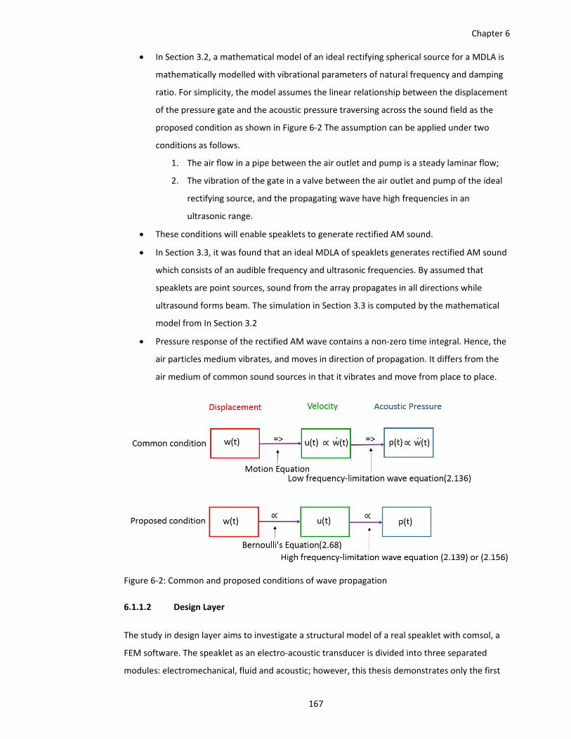
Chapter 6

167

In Section 3.2, a mathematical model of an ideal rectifying spherical source for a MDLA is

mathematically modelled with vibrational parameters of natural frequency and damping

ratio. For simplicity, the model assumes the linear relationship between the displacement

of the pressure gate and the acoustic pressure traversing across the sound field as the

proposed condition as shown in Figure 6‐2 The assumption can be applied under two

conditions as follows.

1. The air flow in a pipe between the air outlet and pump is a steady laminar flow;

2. The vibration of the gate in a valve between the air outlet and pump of the ideal

rectifying source, and the propagating wave have high frequencies in an

ultrasonic range.

These conditions will enable speaklets to generate rectified AM sound.

In Section 3.3, it was found that an ideal MDLA of speaklets generates rectified AM sound

which consists of an audible frequency and ultrasonic frequencies. By assumed that

speaklets are point sources, sound from the array propagates in all directions while

ultrasound forms beam. The simulation in Section 3.3 is computed by the mathematical

model from In Section 3.2

Pressure response of the rectified AM wave contains a non‐zero time integral. Hence, the

air particles medium vibrates, and moves in direction of propagation. It differs from the

air medium of common sound sources in that it vibrates and move from place to place.

Figure 6‐2: Common and proposed conditions of wave propagation

6.1.1.2 Design Layer

The study in design layer aims to investigate a structural model of a real speaklet with comsol, a

FEM software. The speaklet as an electro‐acoustic transducer is divided into three separated

modules: electromechanical, fluid and acoustic; however, this thesis demonstrates only the first

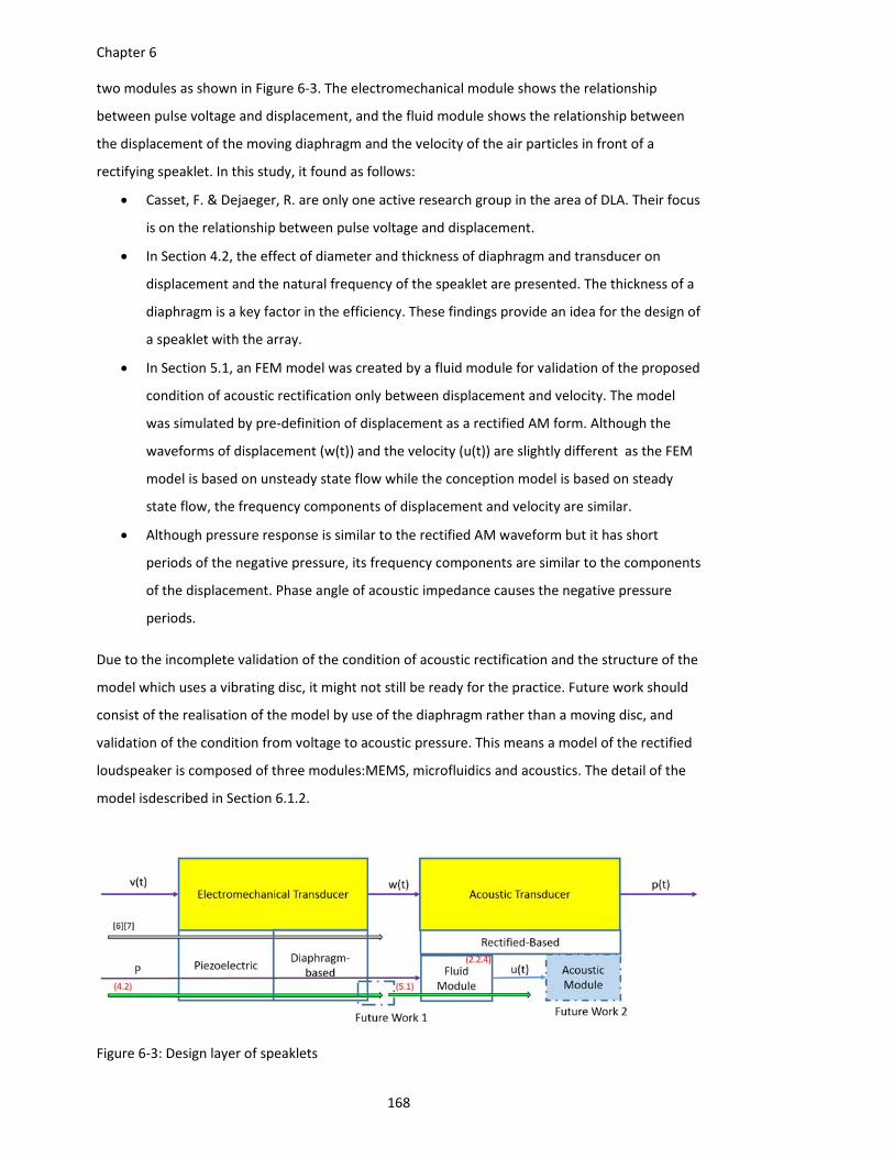
Chapter 6

168

two modules as shown in Figure 6‐3. The electromechanical module shows the relationship

between pulse voltage and displacement, and the fluid module shows the relationship between

the displacement of the moving diaphragm and the velocity of the air particles in front of a

rectifying speaklet. In this study, it found as follows:

Casset, F. & Dejaeger, R. are only one active research group in the area of DLA. Their focus

is on the relationship between pulse voltage and displacement.

In Section 4.2, the effect of diameter and thickness of diaphragm and transducer on

displacement and the natural frequency of the speaklet are presented. The thickness of a

diaphragm is a key factor in the efficiency. These findings provide an idea for the design of

a speaklet with the array.

In Section 5.1, an FEM model was created by a fluid module for validation of the proposed

condition of acoustic rectification only between displacement and velocity. The model

was simulated by pre‐definition of displacement as a rectified AM form. Although the

waveforms of displacement (w(t)) and the velocity (u(t)) are slightly different as the FEM

model is based on unsteady state flow while the conception model is based on steady

state flow, the frequency components of displacement and velocity are similar.

Although pressure response is similar to the rectified AM waveform but it has short

periods of the negative pressure, its frequency components are similar to the components

of the displacement. Phase angle of acoustic impedance causes the negative pressure

periods.

Due to the incomplete validation of the condition of acoustic rectification and the structure of the

model which uses a vibrating disc, it might not still be ready for the practice. Future work should

consist of the realisation of the model by use of the diaphragm rather than a moving disc, and

validation of the condition from voltage to acoustic pressure. This means a model of the rectified

loudspeaker is composed of three modules:MEMS, microfluidics and acoustics. The detail of the

model isdescribed in Section 6.1.2.

Figure 6‐3: Design layer of speaklets

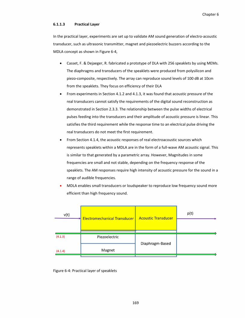
Chapter 6

169

6.1.1.3 Practical Layer

In the practical layer, experiments are set up to validate AM sound generation of electro‐acoustic

transducer, such as ultrasonic transmitter, magnet and piezoelectric buzzers according to the

MDLA concept as shown in Figure 6‐4,

Casset, F. & Dejaeger, R. fabricated a prototype of DLA with 256 speaklets by using MEMs.

The diaphragms and transducers of the speaklets were produced from polysilicon and

piezo‐composite, respectively. The array can reproduce sound levels of 100 dB at 10cm

from the speaklets. They focus on efficiency of their DLA

From experiments in Section 4.1.2 and 4.1.3, it was found that acoustic pressure of the

real transducers cannot satisfy the requirements of the digital sound reconstruction as

demonstrated in Section 2.3.3. The relationship between the pulse widths of electrical

pulses feeding into the transducers and their amplitude of acoustic pressure is linear. This

satisfies the third requirement while the response time to an electrical pulse driving the

real transducers do not meet the first requirement.

From Section 4.1.4, the acoustic responses of real electroacoustic sources which

represents speaklets within a MDLA are in the form of a full‐wave AM acoustic signal. This

is similar to that generated by a parametric array. However, Magnitudes in some

frequencies are small and not stable, depending on the frequency response of the

speaklets. The AM responses require high intensity of acoustic pressure for the sound in a

range of audible frequencies.

MDLA enables small transducers or loudspeaker to reproduce low frequency sound more

efficient than high frequency sound.

Figure 6‐4: Practical layer of speaklets

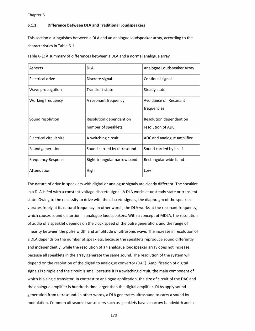
Chapter 6

170

6.1.2 Difference between DLA and Traditional Loudspeakers

This section distinguishes between a DLA and an analogue loudspeaker array, according to the

characteristics in Table 6‐1.

Table 6‐1: A summary of differences between a DLA and a normal analogue array

Aspects DLA Analogue Loudspeaker Array

Electrical drive Discrete signal Continual signal

Wave propagation Transient‐state Steady state

Working frequency A resonant frequency Avoidance of Resonant

frequencies

Sound resolution Resolution dependant on

number of speaklets

Resolution dependant on

resolution of ADC

Electrical circuit size A switching circuit ADC and analogue amplifier

Sound generation Sound carried by ultrasound Sound carried by itself

Frequency Response Right triangular narrow band Rectangular wide band

Attenuation High Low

The nature of drive in speaklets with digital or analogue signals are clearly different. The speaklet

in a DLA is fed with a constant‐voltage discrete signal. A DLA works at unsteady state or transient

state. Owing to the necessity to drive with the discrete signals, the diaphragm of the speaklet

vibrates freely at its natural frequency. In other words, the DLA works at the resonant frequency,

which causes sound distortion in analogue loudspeakers. With a concept of MDLA, the resolution

of audio of a speaklet depends on the clock speed of the pulse generation, and the range of

linearity between the pulse width and amplitude of ultrasonic wave. The increase in resolution of

a DLA depends on the number of speaklets, because the speaklets reproduce sound differently

and independently, while the resolution of an analogue loudspeaker array does not increase

because all speaklets in the array generate the same sound. The resolution of the system will

depend on the resolution of the digital to analogue convertor (DAC). Amplification of digital

signals is simple and the circuit is small because it is a switching circuit, the main component of

which is a single transistor. In contrast to analogue application, the size of circuit of the DAC and

the analogue amplifier is hundreds time larger than the digital amplifier. DLAs apply sound

generation from ultrasound. In other words, a DLA generates ultrasound to carry a sound by

modulation. Common ultrasonic transducers such as speaklets have a narrow bandwidth and a

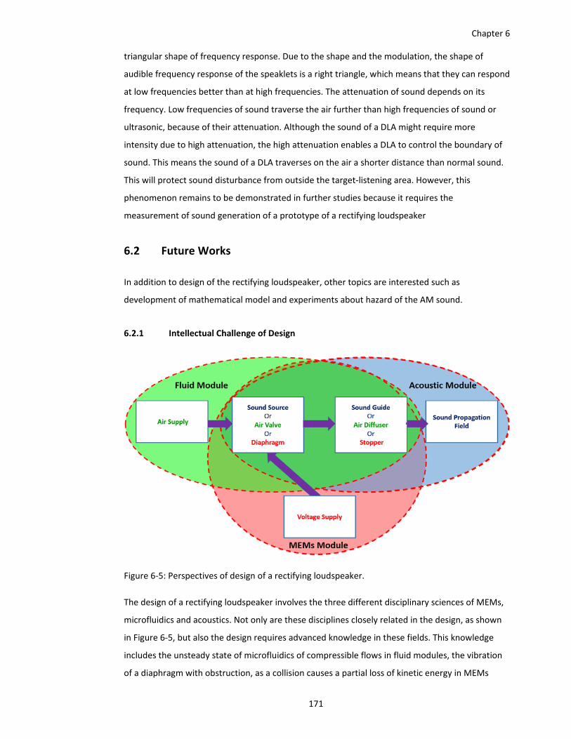
Chapter 6

171

triangular shape of frequency response. Due to the shape and the modulation, the shape of

audible frequency response of the speaklets is a right triangle, which means that they can respond

at low frequencies better than at high frequencies. The attenuation of sound depends on its

frequency. Low frequencies of sound traverse the air further than high frequencies of sound or

ultrasonic, because of their attenuation. Although the sound of a DLA might require more

intensity due to high attenuation, the high attenuation enables a DLA to control the boundary of

sound. This means the sound of a DLA traverses on the air a shorter distance than normal sound.

This will protect sound disturbance from outside the target‐listening area. However, this

phenomenon remains to be demonstrated in further studies because it requires the

measurement of sound generation of a prototype of a rectifying loudspeaker

6.2 Future Works

In addition to design of the rectifying loudspeaker, other topics are interested such as

development of mathematical model and experiments about hazard of the AM sound.

6.2.1 Intellectual Challenge of Design

Figure 6‐5: Perspectives of design of a rectifying loudspeaker.

The design of a rectifying loudspeaker involves the three different disciplinary sciences of MEMs,

microfluidics and acoustics. Not only are these disciplines closely related in the design, as shown

in Figure 6‐5, but also the design requires advanced knowledge in these fields. This knowledge

includes the unsteady state of microfluidics of compressible flows in fluid modules, the vibration

of a diaphragm with obstruction, as a collision causes a partial loss of kinetic energy in MEMs

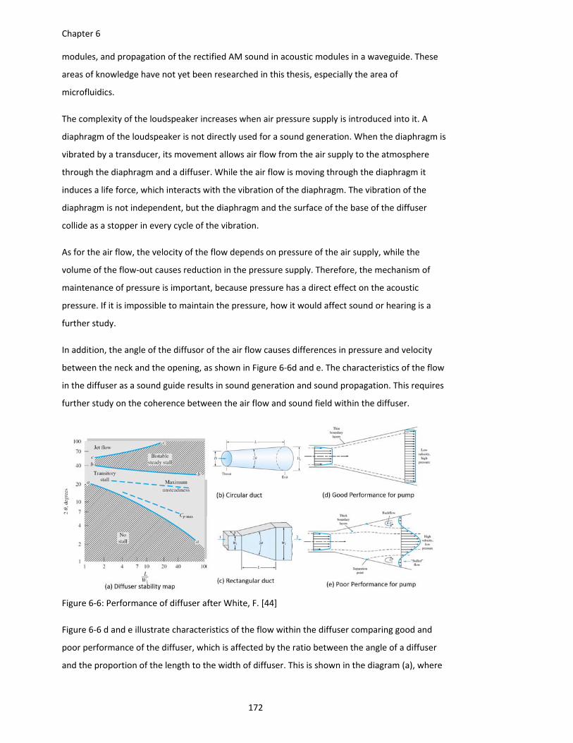
Chapter 6

172

modules, and propagation of the rectified AM sound in acoustic modules in a waveguide. These

areas of knowledge have not yet been researched in this thesis, especially the area of

microfluidics.

The complexity of the loudspeaker increases when air pressure supply is introduced into it. A

diaphragm of the loudspeaker is not directly used for a sound generation. When the diaphragm is

vibrated by a transducer, its movement allows air flow from the air supply to the atmosphere

through the diaphragm and a diffuser. While the air flow is moving through the diaphragm it

induces a life force, which interacts with the vibration of the diaphragm. The vibration of the

diaphragm is not independent, but the diaphragm and the surface of the base of the diffuser

collide as a stopper in every cycle of the vibration.

As for the air flow, the velocity of the flow depends on pressure of the air supply, while the

volume of the flow‐out causes reduction in the pressure supply. Therefore, the mechanism of

maintenance of pressure is important, because pressure has a direct effect on the acoustic

pressure. If it is impossible to maintain the pressure, how it would affect sound or hearing is a

further study.

In addition, the angle of the diffusor of the air flow causes differences in pressure and velocity

between the neck and the opening, as shown in Figure 6‐6d and e. The characteristics of the flow

in the diffuser as a sound guide results in sound generation and sound propagation. This requires

further study on the coherence between the air flow and sound field within the diffuser.

Figure 6‐6: Performance of diffuser after White, F. [44]

Figure 6‐6 d and e illustrate characteristics of the flow within the diffuser comparing good and

poor performance of the diffuser, which is affected by the ratio between the angle of a diffuser

and the proportion of the length to the width of diffuser. This is shown in the diagram (a), where

Chapter 6

173

W in the diagram can represent the width of a rectangular duct or the diameter of the circular

duct.

6.2.2 Realization of Mathematical Model

Since the purpose of the mathematical model is to understand the mechanism of sound

generation from ultrasound of a DLA, especially frequencies of the generated sound, the model is

simplified by ignoring some parameters relating to the amplitude of the wave. The wave equation

in the model is Eq.(2.156), which is an estimated equation, for simplification.

In order to develop the mathematical model for estimation, further work would realize the model

of a speaklet by using Eq.(2.153) which reflects the real wave propagation more than Eq. (2.156).

Furthermore, the model starts from the mechanical force to the acoustic pressure. In order to

realize it, the model should start from the input voltage. The literature provides the mathematical

relation between the force and voltage, such as piezoelectric and magnet speaklets, as described

in Chapter2.2.

In the ideal case, the speaklets in the array are also linearly aligned, while the array will be square

in the practical implementation. In addition, studies on the effect of the interspacing of array to

AM sound is useful to design of DLA. These topics are of interest because they will give ideas

regarding sound beam form before FEM and implementation.

6.2.3 Ear Canal as a Biological Acoustic Low Pass Filter

Although ultrasound is widely used for radars, and industrial and medical detectors and cleaners,

sound generation from ultrasound as a loudspeaker such as with Audio Spotlight is very limited

because people are not familiar with it, and are scared of the danger of ultrasonic exposure.

However, a high intensity of ultrasound will not damage health through the skin, even sensitive

skin, because of a huge difference of acoustic impedance between the air and the tissue. On the

other hand, the effect of pressure on the eardrums as biological pressure sensors is ambiguous, as

described in 2.1.4.2 .

Should this ambiguity lead to further study, the characterization of acoustic waves at the

eardrums would be of interest. Consideration of an ear canal as an acoustic low pass filter would

be beneficial to the design of rectifying loudspeakers, for deciding on bandwidth and the intensity

of ultrasound.

A precise idea of the configuration of the experiments is shown in Figure 6‐7. AM sound will

transmit to a human model using a microphone with a frequency response of 20 to 100 kHz

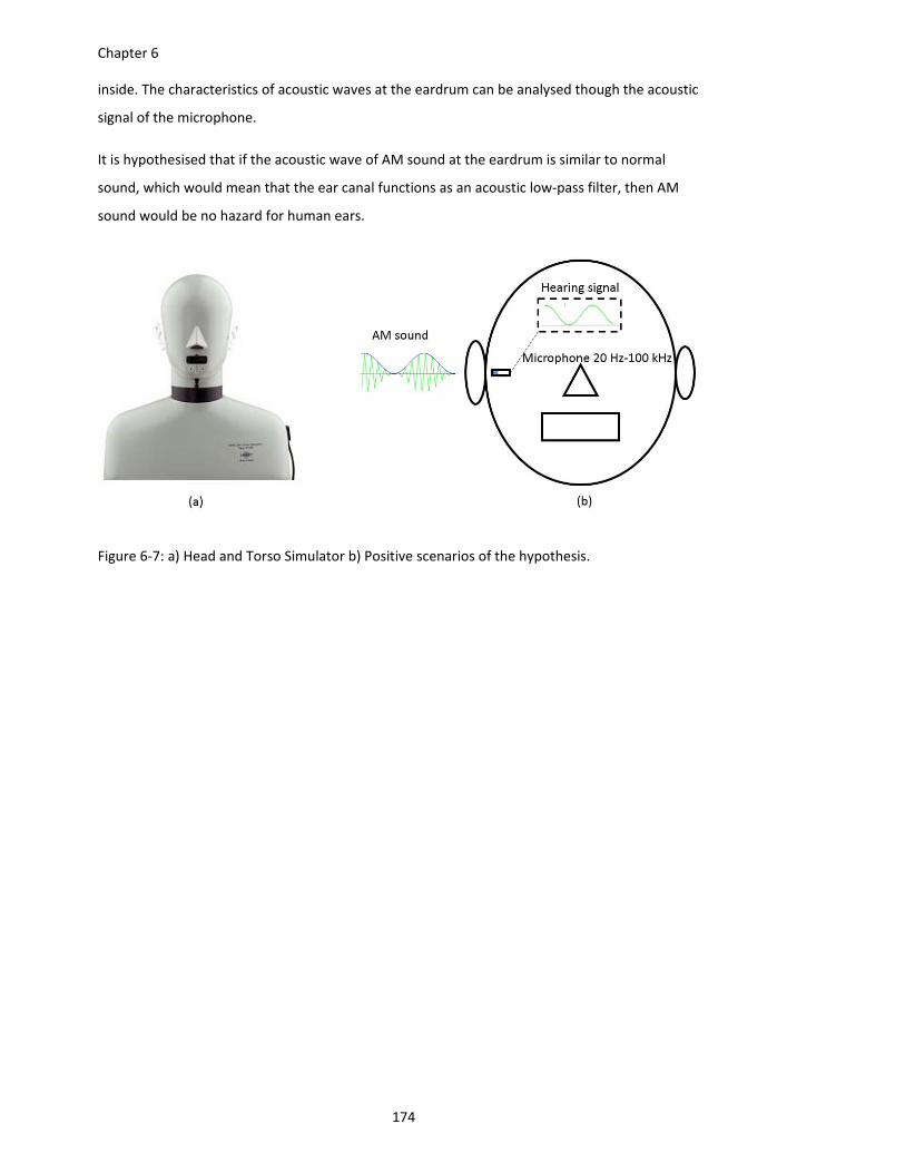
Chapter 6

174

inside. The characteristics of acoustic waves at the eardrum can be analysed though the acoustic

signal of the microphone.

It is hypothesised that if the acoustic wave of AM sound at the eardrum is similar to normal

sound, which would mean that the ear canal functions as an acoustic low‐pass filter, then AM

sound would be no hazard for human ears.

Figure 6‐7: a) Head and Torso Simulator b) Positive scenarios of the hypothesis.

Appendices

175

Appendices

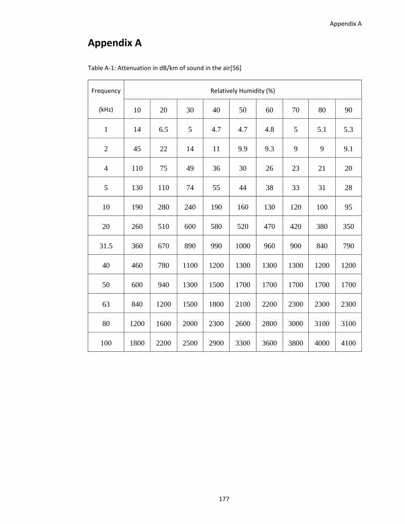
Appendix A

177

Appendix A

Table A‐1: Attenuation in dB/km of sound in the air[56]

Frequency

(kHz)

Relatively Humidity (%)

10 20 30 40 50 60 70 80 90

1 14 6.5 5 4.7 4.7 4.8 5 5.1 5.3

2 45 22 14 11 9.9 9.3 9 9 9.1

4 110 75 49 36 30 26 23 21 20

5 130 110 74 55 44 38 33 31 28

10 190 280 240 190 160 130 120 100 95

20 260 510 600 580 520 470 420 380 350

31.5 360 670 890 990 1000 960 900 840 790

40 460 780 1100 1200 1300 1300 1300 1200 1200

50 600 940 1300 1500 1700 1700 1700 1700 1700

63 840 1200 1500 1800 2100 2200 2300 2300 2300

80 1200 1600 2000 2300 2600 2800 3000 3100 3100

100 1800 2200 2500 2900 3300 3600 3800 4000 4100

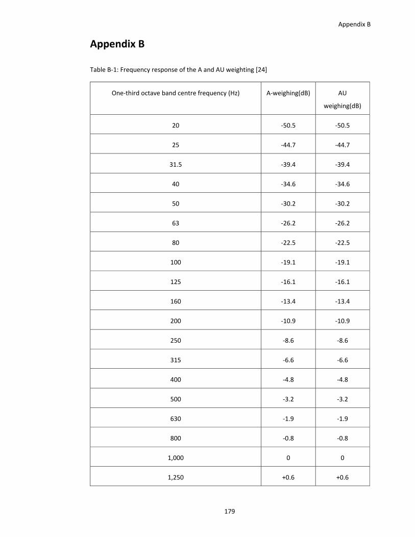
Appendix B

179

Appendix B

Table B‐1: Frequency response of the A and AU weighting [24]

One‐third octave band centre frequency (Hz) A‐weighing(dB) AU

weighing(dB)

20 ‐50.5 ‐50.5

25 ‐44.7 ‐44.7

31.5 ‐39.4 ‐39.4

40 ‐34.6 ‐34.6

50 ‐30.2 ‐30.2

63 ‐26.2 ‐26.2

80 ‐22.5 ‐22.5

100 ‐19.1 ‐19.1

125 ‐16.1 ‐16.1

160 ‐13.4 ‐13.4

200 ‐10.9 ‐10.9

250 ‐8.6 ‐8.6

315 ‐6.6 ‐6.6

400 ‐4.8 ‐4.8

500 ‐3.2 ‐3.2

630 ‐1.9 ‐1.9

800 ‐0.8 ‐0.8

1,000 0 0

1,250 +0.6 +0.6

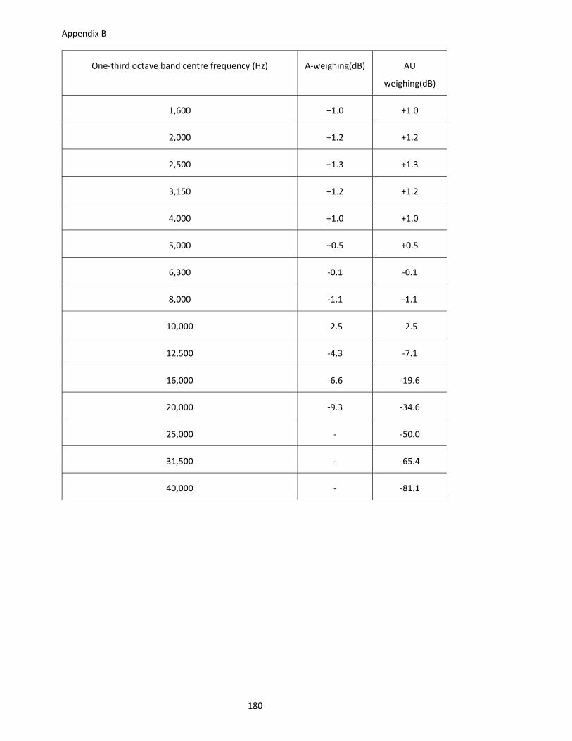
Appendix B

180

One‐third octave band centre frequency (Hz) A‐weighing(dB) AU

weighing(dB)

1,600 +1.0 +1.0

2,000 +1.2 +1.2

2,500 +1.3 +1.3

3,150 +1.2 +1.2

4,000 +1.0 +1.0

5,000 +0.5 +0.5

6,300 ‐0.1 ‐0.1

8,000 ‐1.1 ‐1.1

10,000 ‐2.5 ‐2.5

12,500 ‐4.3 ‐7.1

16,000 ‐6.6 ‐19.6

20,000 ‐9.3 ‐34.6

25,000 ‐ ‐50.0

31,500 ‐ ‐65.4

40,000 ‐ ‐81.1

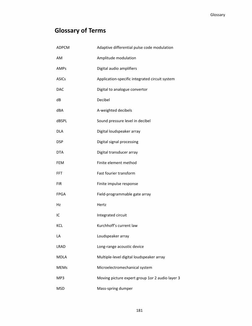
Glossary

181

Glossary of Terms

ADPCM Adaptive differential pulse code modulation

AM Amplitude modulation

AMPs Digital audio amplifiers

ASICs Application‐specific integrated circuit system

DAC Digital to analogue convertor

dB Decibel

dBA A‐weighted decibels

dBSPL Sound pressure level in decibel

DLA Digital loudspeaker array

DSP Digital signal processing

DTA Digital transducer array

FEM Finite element method

FFT Fast fourier transform

FIR Finite impulse response

FPGA Field‐programmable gate array

Hz Hertz

IC Integrated circuit

KCL Kurchhoff’s current law

LA Loudspeaker array

LRAD Long‐range acoustic device

MDLA Multiple‐level digital loudspeaker array

MEMs Microelectromechanical system

MP3 Moving picture expert group 1or 2 audio layer 3

MSD Mass‐spring dumper

Glossary

182

NDFEB Neodymium

Pa Pascal

PCM Pulse code modulation

PDMS Polydimetylsiloxane

PMP The parallel multimorph in parallel connection

PWM Pulse width modulation

PZT Lead zirconate titanate

SDM Sigma‐delta modulation

SLL Sound loudness level

SMS The serial multimorph in serial connection

SPL Sound pressure level

Bibliography

183

List of References

[1] B. M. Diamond, J. J. Neumann, and K. J. Gabriel, “Digital Sound Reconstruction Using

Arrays of CMOS‐MEMS Microspeakers,” in Fifteenth IEEE International Conference on

Micro Electro Mechanical Systems, 2002, no. 412, pp. 292–295.

[2] S. C. Busbridge, P. A. Fryer, and Y. Huang, “Digital Loudspeaker Technology: Current State

and Future Developments,” in AES 118th Convertion, 2002.

[3] M. Klasco, “MEMS Microspeakers Are Truly Digital Transducers,” audioxpress, 2016.

[Online]. Available: http://www.audioxpress.com/article/MEMS‐Microspeakers‐Are‐Truly‐

Digital‐Transducers.

[4] Yole, “Silicon speakers are ready for volume production,” I‐Micronews, 2016. [Online].

Available: http://www.i‐micronews.com/mems‐sensors/7563‐silicon‐speakers‐are‐ready‐

for‐volume‐production‐2.html. [Accessed: 15‐Dec‐2016].

[5] F. W. Kremkau, Diagnostic Ultrasound: Principles and Instrument, 6th ed. W.B. SAUNDERS

COMPANY, 2006.

[6] R. Dejaeger, F. Casset, B. Desloges, G. Le Rhun, P. Robert, S. Fanget, Q. Leclère, K. Ege, and

J.‐L. Guyader, “Development and Characterization of a Piezoelectrically Actuated MEMS

Digital Loudspeaker,” Procedia Eng., vol. 47, pp. 184–187, Jan. 2012.

[7] F. Casset, R. Dejaeger, B. Laroche, B. Desloges, Q. Leclere, R. Morisson, Y. Bohard, J. P.

Goglio, J. Escato, and S. Fanget, “A 256 MEMS Membrane Digital Loudspeaker Array Based

on PZT Actuators,” Procedia Eng., vol. 120, pp. 49–52, 2015.

[8] F. J. Pompei, “Sound From Ultrasound: The Parametric Array as an Audible Sound Source,”

pp. 1–132, 2002.

[9] J. Croft, James and J. O. Norris, “Theory, History, and the Advancement of Parametric

Loudspeakers,” 2003.

[10] N. A. Tatlas and J. Mourjopoulos, “Digital Loudspeaker Arrays driven by 1‐bit signals,” in

Audio Eng. Soc.116th Convention, 2004.

[11] Y. Cohen, “Digital Loudspeakers,” audiopixels., 2011. [Online]. Available:

http://www.audiopixels.com.au/index.cfm/news/videos/digital‐loudspeakers‐video/.

[12] P. Valoušek, “A Digital Loudspeaker : Experimental Construction,” vol. 46, no. 4, 2006.

Bibliography

184

[13] N. Tatlas, A. E. S. A. Member, and F. Kontomichos, “Design and Performance of a Sigma –

Delta Digital Loudspeaker Array Prototype *,” vol. 57, no. 1, 2009.

[14] J. D. Turner and A. J. Pretlove, Acoustics of Engineering, 2nd ed. Macmillan Education LTD,

1991.

[15] E. F. Alton and K. C. Pohlmann, Master Handbook of Acoustics, 6th ed. 2015.

[16] Benade H. Arthur, Fundamentals of Musical Acoustics. 1976.

[17] W. M. Rubio, F. Buiochi, J. C. Adamowski, and E. C. N. Silva, “Modeling of functionally

graded piezoelectric ultrasonic transducers,” Ultrasonics, vol. 49, no. 4–5, pp. 484–494,

2009.

[18] C. T. Crowe, D. F. Elger, B. C. Williams, and J. A. Roberson, Engineering Fluid Mechanics, 9th

ed. John Willey & Sons, 2010.

[19] L. E. Kinsler, A. R. Frey, A. B. Coppens, and J. V Sanders, “Fundamentals of acoustics,”

Fundamentals of Acoustics, 4th Edition, by Lawrence E. Kinsler, Austin R. Frey, Alan B.

Coppens, James V. Sanders, pp. 560. ISBN 0‐471‐84789‐5. Wiley‐VCH, December 1999., vol.

1. p. 560, 1999.

[20] S. A. Gelfand, Hearing: An Introduction to Psychological and Physiological Acoustics, 4th ed.

Marcel Dekker, 2004.

[21] O. NDT, “Ultrasonic Transducers Technical Notes,” 2006.

[22] A. Vladišauskas, “Directivity characteristics of ultrasonic transducers for flow

measurements,” ULTRAGRASAS, vol. 2, no. 2, pp. 2–5, 2001.

[23] S. A. Gelfand, Hearing: An Introduction to Psychological and Physiological Acoustics, 4th ed.

Marcel Dekker, 2004.

[24] U. of S. B.W. Lawton (Institute of Sound and Vibration Research, “Damage to human

hearing by airborne sound of very high frequency or ultrasonic frequency,” p. 86, 2001.

[25] C. H. Hansen, “Fundamentals of Acoustics,” in Occupational exposure to noise: Evaluation,

prevention and control, 1994, pp. 23–52.

[26] H. Kuttruff, Ultrasonics:Fundamentals and Applications. Springer Netherlands, 1991.

[27] H. J. Kim, W. S. Yang, and K. S. No, “The vibrational characteristics of the triple‐layered

multimorph ceramics for high performance piezoelectric acoustic actuators,” J.

Bibliography

185

Electroceramics, May 2014.

[28] T. Bakke, A. Vogl, O. Żero, F. Tyholdt, I.‐R. Johansen, and D. Wang, “A novel ultra‐planar,

long‐stroke and low‐voltage piezoelectric micromirror,” J. Micromechanics

Microengineering, vol. 20, no. 6, p. 64010, Jun. 2010.

[29] K. Uchino, “Introduction to Piezoelectric Actuators and Transducers,” 2003.

[30] P. Gaucher, “Piezoelectric Micro‐electro‐mechanical Systems for Acoustic Applications.”

[31] I. Henderson, Piezoelectricx Ceramics: Principle and Application, 2nd ed. APC International,

Ltd, 2011.

[32] S. Senthilkumar and R. Vinothraj, “Design and study of ultrasound‐based automatic patient

movement monitoring device for quantifying the intrafraction motion during teletherapy

treatment.,” J. Appl. Clin. Med. Phys., vol. 13, no. 6, p. 3709, 2012.

[33] E. O. Doebelin, Measurement Systems Application and Design, 4th ed. McGraw‐Hill, 1990.

[34] F. A. E., C. J. Kingsley, and S. D. Uman, Electric Machinery. McGraw‐Hill, 2003.

[35] C. Weber, Y. C. Chen, and Y. T. Cheng, “The Study of the Inductive Coil to the Acoustic

Performance of Electromagnetic Driven Microspeaker,” in Eurosensors 2014 Conference

Preceeding, 2014, vol. 0, pp. 1–4.

[36] J. Chernof, “Principles of loudspeaker design and operation,” IRE Trans. Audio, vol. 5, no. 5,

pp. 117–127, 1957.

[37] P. J. Westervelt, “Parametric Acoustic Array,” Acoust. Soc. Am., vol. 35, no. 4, pp. 535–537,

1963.

[38] P. F. Joseph, “The Use of Airborne Ultrasonics for Generating Audible Sound Beam,” J.

Audio Eng., vol. 47, no. 9, pp. 726–731, 1999.

[39] T. Wen‐Kung, “Beam Width Control for a Dicectional Audible Sound System,” Int. J. Innov.

Control, vol. 9, no. 7, pp. 3061–3078, 2013.

[40] M. Yoneyama and J. Fujimoto, “The audio spotlight: An application of nonlinear interaction

of Sound waves to a new type of loudspeaker design,” Audio, vol. 73, no. May, pp. 1532–

1536, 1983.

[41] T. Kamakura and K. Aoki, “A Highly Directional Audio System Using A Parametric Array In

Air,” 9th West. Pacific Acoust. Conf., vol. 0, 2006.

Bibliography

186

[42] C. Woodford, “Directional loudspeakers,” explainthatstuff, 2016. [Online]. Available:

http://www.explainthatstuff.com/directional‐loudspeakers.html.

[43] J. A. Thomas, C. F. Moss, and M. Vater, Eds., Echolocation in Bats and Dolphins. Saunder

College, 2004.

[44] F. M. White, “Fluid Mechanics,” McGraw‐Hill, p. 1024, 2009.

[45] B. M. Diamond, “Digital Sound Reconstruction Using Arrays of SMOD‐MEMS

Microspeakers,” 2002.

[46] F. Cohen, D. Lewin, S. Kaplan, A. Sromin, and B. Simon, “IMPROVED SPEAKER APPARATUS

AND METHODS USEFUL IN CONJUNCTION THEREWITH.,” WO200966290A2, 2009.

[47] J. Mendoza‐López, S. C. Busbridge, and P. A. Fryer, “Sound Field Characterisation in Audio

Reproduction with the Bit‐Grouped Digital,Transducer Array,” in the 120th AES Convention,

2009.

[48] M. O. J. Hawksford, “Smart Digital Loudspeaker Arrays,” in 110th Convention of the Audio‐

Engineering‐Society, 2003, vol. 51, no. 12, pp. 1133–1162.

[49] G. Ballou, Electroacoustic Devices: Microphones and Loudspeakers. Elsevier, 2009.

[50] G. Takács and B. Rohaľ‐Ilkiv, Model Predictive Vibration Control. Springer, 2012.

[51] M. C. Junger and D. Feit, Sound, Structures and Their Interaction, 2nd ed. The MIT Press,

1972.

[52] N. R. Harris, M. Hill, N. M. White, and S. P. Beeby., “Acoustic power output measurements

for thick‐film PZT transducers,” Electron. Lett., vol. 40, no. 10, pp. 636–637, 2004.

[53] P. J. Pritchard, Fluid Machanics, 8th ed. Wiley, 2012.

[54] N. OzKaya and Nordin Margareta, Fundamentatals of Biomechanics, Equalibrium, Motion

and deformation, 2nd ed. Springer‐Verlag New York Berlin Heidelberg, 1998.

[55] M. Richter, R. Linnemann, and P. Woias, “Robust design of gas and liquid micropumps,”

Sensors Actuators, A Phys., vol. 68, no. 1–3 pt 2, pp. 480–486, 1998.

[56] G. W. C. Kaye and T. H. Laby, “The speed and attenuation of sound,” Natianal Physiccal

Laboratory, 1995. [Online]. Available:

http://www.kayelaby.npl.co.uk/general_physics/2_4/2_4_1.html#speed_of_sound_in_air.

[Accessed: 28‐Jul‐2016].

University of Southampton Research Repository

Documents