UNIVERSITY OF MARYLAND COMPUTER SCIENCE … · the Computer Science Center of the University ... 5 SEQUENTIAL DECISION RULE AND PROBABILITY OF ERROR 5.1 DECISION STATISTIC ... solution

UNIVERSITY OF MARYLANDCOMPUTER SCIENCE CENTER

COLLEGE PARK, MARYLAND

N72-13131

Unclas08409

(NASA-CR-124692) PERFORMANCE OF OPTIMUMDETECTOR STRUCTURES FOR NOISY INTERSYMBOLINTERFERENCE CHANNELS J.D. Womer, et'al(Maryland Univ.) Jul. 1971 190 p CSCL 17B

(NASA CR OR TMX OR AD NUMBER)(CATEGORY)

G 3/07J

k'2 -- arP- 7s3 ?~

https://ntrs.nasa.gov/search.jsp?R=19720005482 2018-07-18T13:37:50+00:00Z

Technical Report TR-164 July 1971

AFOSR-71-1982

PERFORMANCE OF OPTIMUM DETECTOR STRUCTURESFOR NOISY INTERSYMBOL INTERFERENCE CHANNELS

by

J. D. Womer*, B. D. Fritchman*, and LN. Kanal *

*Department of Electrical Engineering,Bethlehem, Pa.

Lehigh University,

**Computer Science Center, University of Maryland, CollegePark, Md.

FOREWORD

This investigation was conducted by JO Do Womer,

Bo Do Fritchman and L. No Kanal (Principal Investigator).

It was sponsored by the Mathematical and Information Sciences

Directorate, Air Force Systems Command, UoSoAoFo under grant

AFOSR 71-1982 to the University of Maryland. Lto Colo Russell

Bo Ives, UoSoAoFo, served as technical monitor. Dro Fritchman's

work on this program was partly supported by the Department

of Electrical Engineering, Lehigh University, Bethlehem,

Pennsylvania and Dro Kanal's work was supported in part by

the Computer Science Center of the University of Maryland,

College Park, Maryland.

i

ABSTRACT

When transmitting digital information by radio or wire-

line systems, errors may arise from additive noise and from

successively transmitted signals interfering with one another.

This report presents new results on evaluating the probability

of error, ioeo performance, of optimum detector structures

which are obtained when compound statistical decision theory

is used to unravel noisy intersymbol interference patterns in

the received signal, It includes a comparative study of the

performance of certain detector structures and approximations

to them, and the performance of a transversal equalizer.

The report also shows that the optimum compound statistical

decision procedure is not equivalent, either to subtracting

out the interfering energy from the received signal, or to

gathering together the energy which is dispersed throughout

the received signal,

ii

Chapter 1

1.1

1.2

Chapter 2

2.1

2.2

Chapter 3

3.1

3.2

TABLE OF CONTENTS

FOREWORD

ABSTRACT

TABLE OF CONTENTS

LIST OF FIGURES

LIST OF TABLES

TECHNICAL SUMMARY

INTRODUCTION

PROBLEM BACKGROUND

SCOPE OF THE WORK

INTERSYMBOL INTERFERENCE

SOURCE OF INTERSYMBO-L INTERFERENCE

FORMULATION OF' THE' PROBLEM

COMBATING INTERSYMBOL INTERFERENCE

WAVEFORM SHAPING

TRANSVERSAL EQUALIZERS

iii

i

ii

iii

vii

ix

1

4

4

16

20

20

24

35

35

37

4 APPLICATION OF DECISION THEORY TO

INTERSYMBOL INTERFERENCE

4.1 DECISION THEORY

4.1.1 SIMPLE DECISION THEORY

4.1.2 COMPOUND DECISION THEORY

4.1.3 SEQUENTIAL COMPOUND DECTgSJON THEORY

4.2 APPLICATION OF DECISION THEOP¥

4.2.1 CHANG AND HANCOCK DETECTOR

4.2.2 MINIMIZATION OF THE EXPECTED

NUMBER OF ERRORS

4.3 SEQUENTIAL DETECTION

4.4 CRITERIA OF OPTIMALITY

5 SEQUENTIAL DECISION RULE AND PROBABILITY

OF ERROR

5.1 DECISION STATISTIC

5.2 CALCULATION OF DECISION STATISTIC

5.3 DECISION REGION

5.4 PROBABILITY OF ERROR

iv

Chapter

Chapter

42

42

45

47

50

54

57

59

62

63

63

65

68

71

5.5 DIFFERENCE EQUATION

5.6 REGION OF CONVERGENCE

5.7 APPLICABILITY OF SEQUENTIAL PROCEDURE

6 OPTIMUM DETECTION FOR BLOCK TRANSMISSION

OF LENGTH N

6.1 DECISION RULE

6.2 INDEPENDENCE THEOREMS

6.3 EVALUATION OF DECISION STATISTIC

6.4 RECURSIVE RELATIONSHIPS

6.5 DECISION REGION

6.6 PROBABILITY OF ERROR

6.7 GENERALIZED DECISION REGION AND

PROBABILITY OF ERROR

6.8 REDUCTION OF JOINT-CONDITIONAL

PROBABILITY

7 DATA ANALYSIS

8 CONCLUSION

8.1 SUMMARY

v

Chapter

Chapter

Chapter

74

75

85

86

86

87

90

93

101

105

108

113

121

144

144

8.2

APPENDIX A

APPENDIX B

APPENDIX C

APPENDIX D

SUGGESTIONS FOR FURTHER RESEARCH

SEQUENTIAL DIFFERENCE EQUATION

CONVERGENCE OF v2

SUFFICIENT CONDITION FOR CONVERGENCE

OF DIFFERENCE EQUATION SOLUTION

PROOF OF THEOREMS

REFERENCES

vi

148

151

157

160

163

177

LIST OF FIGURES

Fig. 1 Communication system model

Fig. 2 Ideal channel' characteristics

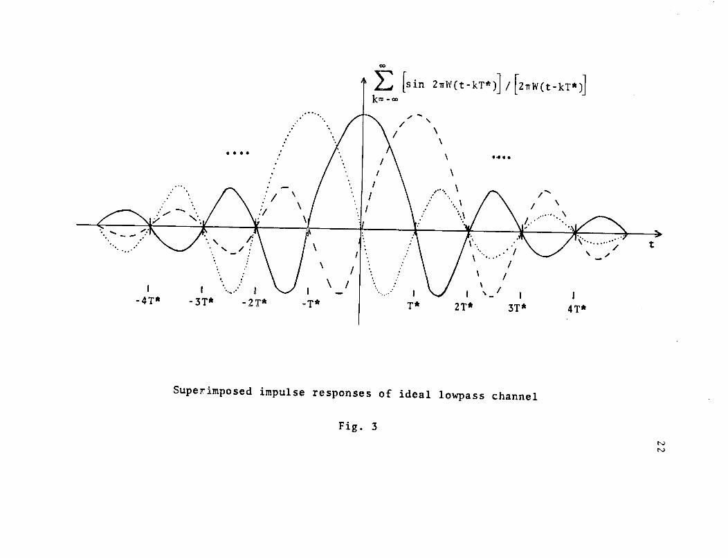
Fig. 3 Superimposed impulse responses of ideal

lowpass channel

Fig. 4 Bandpass communication system'model

Fig. 5 Equivalent lowpass communication system

model

Fig. 6 Equivalent waveform generator

Fig. 7 Model of communication system studied

Fig. 8 Schematic of. transversal equalizer

Fig. 9 Decision regions for sequential procedure

with m- 4

Fig. 10 Decision region and probability of error for

sequential decision procedure with m = 2

Fig. 11 Regions of convergence of the difference

equation solution for L = 3 (h 1= 1)

vii

5

21

22

25

27

28

30

38

69

72

81

Fig. 12 Detector performance (h1 = 5/8, h2 = 1,

h3

= 1/2) 127

Fig. 13 Detector performance (h1

= 1/8, h2 = 1,

h3

= 1/4) 128

Fig. 14 Detector performance (hI

= 1, h2

= 0.1,

h3

= 0.8) 129

Fig. 15 Detector performance (h1 = h2

= h3 = 1) 137

Fig. 16 Comparison of compound procedure with other

types of detection (hl = 1, h2 = 0.1,

h =0.8) 138

Fig. 17 Comparison of compound procedure with other

types of detection (h1 = h2 = h3 = 1) 139

Fig. 18 Comparison of compound procedure with other

types of detection (h1 = 1/8, h2

= 1,

h3

= 1/4) 140

Fig. 19 Comparison of compound procedure with other

types of detection (hi

= 5/8, h2 = 1,

h 3 = 1/2) 141

viii

Table I

Table II

Table III

LIST OF TABLES

Probability densities obtainable from

equation (118)

Calculated means and variances

Information Measure

ix

117

125

135

PERFORMANCE OF OPTIMUM DETECTOR STRUCTURES

FOR NOISY INTERSYMBOL INTERFERENCE CHANNELS

TECHNICAL SUMMARY

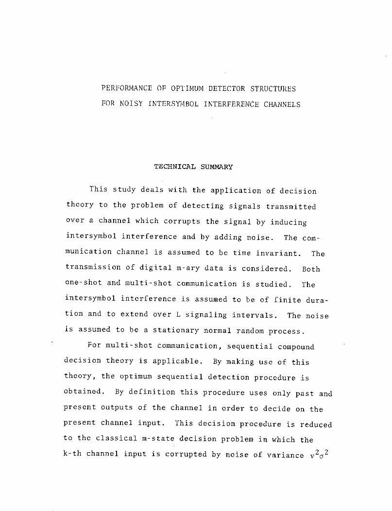
This study deals with the application of decision

theory to the problem of detecting signals transmitted

over a channel which corrupts the signal by inducing

intersymbol interference and by adding noise. The com-

munication channel is assumed to be time invariant. The

transmission of digital m-ary data is considered. Both

one-shot and multi-shot communication is studied. The

intersymbol interference is assumed to be of finite dura-

tion and to extend over L signaling intervals. The noise

is assumed to be a stationary normal random process.

For multi-shot communication, sequential compound

decision theory is applicable. By making use of this

theory, the optimum sequential detection procedure is

obtained. By definition this procedure uses only past and

present outputs of the channel in order to decide on the

present channel input. This decision procedure is reduced

to the classical m-state decision problem in which the

k-th channel input is corrupted by noise of variance v2a2

2

(a2 is the noise variance of the actual physical channel).

Note, v2 is a function of k. The calculation of the

performance, which this formulation allows, has not

previously been realized.

The relationship between the channel impulse res-

ponse and v2 (and thus, indirectly, the performance of

the decision procedure) is considered. The relationship

involves a difference equation. The convergence of the

solution of the difference equation is studied.

For one-shot transmission, the optimum compound

decision procedure is presented. This compound procedure

results in a generalized expression which can be used to

approximate the decision regions and the associated

probability of error. The probability of error is not

obtainable in closed form, but is studied in depth for

the case L = 3.

In general, it is not known how to evaluate the

actual performance of the compound decision procedure.

Hence, approximations are obtained which approximate the

true optimum compound performance. A channel "output

directed approximation" and several channel "input dir-

ected approximations" are presented.

A comparison is made between the calculated sequen-

tial compound performance, the simulated optimum compound

performance, the performance of a transversal equalizer,

and the performance obtained by means of one of the above

3

approximations. For all channel impulse responses con-

sidered, at least one of the approximations was in very

good agreement with the simulated optimum compound pro-

cedure. For the impulse responses studied, a method is

presented whereby the best approximation can be selected

merely by examining the values of the sampled impulse

response. Finally, the results show that the optimum

compound procedure is not equivalent to either subtracting

out the interfering energy from the received signal or to

gathering together the energy which is dispersed through-

out the received signal.

4

Chapter 1

INTRODUCTION

1.1 PROBLEM BACKGROUND

The transmission of information from a "transmitter"

to a "receiver" is fraught with the possibility of incor-

rect reception of the information whether it be communica-

tion via speech, radio waves, sonar, or even a glance

between a man and his wife. The errors in reception are

induced by the transmitter, the receiver, or the "channel"

over which the information is transmitted.

In particular, in the transmission of digital informa-

tion by means of radio or wireline systems, errors will

occur in the reception of the digits. The system design

goal is to reduce the rate of making an error to as low a

value as possible. A model for this communication system is

given in Fig. 1. The transmitter obtains the information

from the information source and sends it over the channel.

The receiver receives the information from the channel and

presents it to the information destination. The channel

includes all parts of the communication system between the

transmitter and receiver over which the information is

transferred. There are essentially two sources of error

in this type of communication system.

Communication system model

Fig. 1

cl

6

Errors may arise from additive noise. This is a random

fluctuation in the received signal which may be due to

noise radiation from the sky, thermal noise in resistors,

shot noise in electron tubes and solid state devices or

other random signals that arise due to the physical attri-

butes of the communication system. Errors also arise from

distortion of the transmitted signal. Distortion may be

defined as departures of the signaling waveforms from the

ideal when the departures are not strictly random. Some

typical causes of this are bandlimiting filters within

the system, echos due to improper impedance matching at

system interfaces, and multiply received signals scattered

from different layers of the Ionosphere or Troposphere.

Such forms of distortion may cause successively transmitted

signals to interfere with one another in which case the

distortion is said to cause intersymbol interference.

Intersymbol interference is, therefore, an undesired

time-overlap of signaling waveforms which may occur in the

transmission of successive digits. If the received signal

waveform is non-zero for a finite time interval, then only

a finite number of symbols are part of the intersymbol

interference. For instance, suppose that the digital

symbols are transmitted at a rate of 1/T bauds and that

the received signal is sampled at the corresponding rate

of 1/T samples per second. Then for a finite duration of

the received signal waveform, the sampled output values

7

are functions of a finite number of digital inputs--i.e.

each sampled output value is dependent on more than one

input. (The output, of course, depends on the noise as

well.) If the output depends on L inputs, the intersymbol

interference is said to extend over L symbols.

Intersymbol interference is especially severe at

high data rates. If one desires to transmit without

intersymbol interference and can tolerate low data rates,

intersymbol interference can be circumvented simply by

transmitting a digit and then waiting until the effects

of that digit become zero at the receiver before trans-

mitting the next digit. Nyquist [1] has shown that, for

an ideal channel (constant amplitude response and linear

phase response), the highest rate at which a symbol can

be transmitted without intersymbol interference is 1/T*

bauds where T* = 1/2W is the positive frequency band-

width of the system. For non-ideal channels of bandwidth

W it is still possible to transmit at the Nyquist rate

but not without some intersymbol interference. Histori-

cally, the most common way of transmitting digital data

was to transmit binary symbols at a symbol rate consider-

ably less than 1/T*. Intersymbol interference was thus

not that much of a problem. Most of the errors were due

to the additive noise in the system. With the advent of

computers and the desire for remote communication with

computers, it has become increasingly desirable to

8

transmit at higher and higher data rates. At these higher

data rates, as the symbol rate approaches 2W' bauds, where

W' is the nominal value for the bandwidth of the channel,

intersymbol interference becomes more of a problem and

attention has been given to the study of the transmission

of digital information in the presence of intersymbol

interference and noise.

There are two general ways to combat intersymbol

interference. They are as follows:

i. use a signaling scheme which either

eliminates intersymbol interference

or holds it to a tolerable level.

ii. use a detection scheme which compensates

for the intersymbol interference and

noise.

Various methods, which are used to counteract intersymbol

interference, will be discussed below. These methods

include methods from each of the above two categories.

All methods are subject to restrictions imposed by the

finite width of the frequency spectrum of the communica-

tion system.

Four methods which belong to the first category will

be discussed. The first of these methods is to transmit

m-ary symbols instead of binary. The data rate can thus

be increased without increasing the symbol rate [2].

Thus, by transmitting at the highest symbol rate at which

9

intersymbol interference does not occur, the rate of trans-

mission of information can be increased without causing

intersymbol interference by increasing m, the number of

signaling waveforms. This increase in the input alphabet

is done at the expense of increasing the effect that the

noise has in causing an error in the reception of the

symbol.

In most electronic communications, modulation of a

carrier by the mwaveforms of the input alphabet is neces-

sary. For a fixed-length alphabet the data rate per

cycle of bandwidth depends on the type of modulation used.

Vestigial sideband amplitude modulation (VSG-AM) or single

sideband amplitude modulation (SSB-AM) leads to a higher

data rate than does double sideband amplitude modulation

(DSB-AM) [3,4]. The data rate per cycle of bandwidth for

SSB-AM is twice that of DSB-AM while that for VSG-AM is

almost as high as the data rate for SSB-AM.

Spectrum shaping can also be used as a means of

transmission without intersymbol interference. An

example of this is a raised cosine response [3]. The

frequency spectrum of the communication system is modified

by input and output filtering so that the spectrum has a

raised cosine shape. Just as the Nyquist rate gives a

maximum symbol rate for the ideal channel a maximum symbol

rate can be calculated for the raised cosine channel. The

maximum symbol rate for the raised cosine channel is less,

10

on a per unit bandwidth basis, than the Nyquist rate. To

retain the same data rate leads to increased bandwidth

requirements. The raised cosine channel, in many cases,

is a closer approximation to a real channel than is the

ideal channel and thus is a more realistic communication

model.

Another form of spectrum shaping [5] specifies the

shapes of time-limited transmitted waveforms which are

necessary in order to ensure that, after passing through

the (linear) channel, the received waveforms are also

time-limited. For certain channels, the signaling wave-

forms can be so chosen that the time duration of both the

transmitted signal and the received signal can be made

arbitrarily small. Thus for each element of the input

alphabet, a proper shape of the corresponding signaling

waveform can be chosen so that no intersymbol interference

occurs.

A fourth technique which may be used is that of

partial response signaling [3,6]. This includes duobinary

[7] and polybinary signaling [8]. These methods are

closely aligned to the above described method of input

signal shaping. However, these techniques result in

intersymbol interference over a limited number of sampling

times. The input signal is selected so that, by proper

compensation in the receiver, the transmitted message

(neglecting the effects of the additive noise) would be

11

received correctly in spite of the intersymbol inter-

ference. Because of the increase in the number of

signaling levels, these methods exhibit a greater degree

of noise sensitivity than other simpler signaling tech-

niques.

The above procedures are ways in which intersymbol

interference can be eliminated or handled with relative

ease. Ideally then high data rates can be achieved with

little or no intersymbol interference. However, due to

departures from the ideal, intersymbol interference still

occurs and becomes a problem. Also the above schemes

cannot in general counteract intersymbol interference at

symbol rates which approach the Nyquist upper limit of

2W bauds. Methods from the second category (given above)

are thus necessary to compensate for intersymbol inter-

ference and thus allow for the correct detection of the

transmitted symbols in the presence of intersymbol inter-

ference and noise.

Probably one of the more obvious ways of transmitting

information in the face of unreliable reception is to use

redundancy coding. This remains a valid method when the

received signal is corrupted by intersymbol interference

and additive noise. The coding scheme used is selected

so that errors which occur in the communication system

may be detected and corrected. This method may not per-

form satisfactorily if an error burst occurs. The use of

12

redundancy coding works for moderate data rates but breaks

down for high data rates [9,10].

Another method of compensation is to use quantized

feedback [ll]. With this method the receiver takes the

signal received during any signaling interval, say

kT < t 5 (k+l)T and decides on which of the mn possible

symbols was transmitted. Based on this decision and

assuming the channel characteristics are known at the

receiver, the reiailo.nr of trhe signal due to the trans-

mitted symbol is generated. This generated "tail" is

then subtracted from the received signal. Thus the symbol

transmitted at time KT has no effect on the waveform pre-

sented to the detection circuitry for time t ? (k+l) T.

Proceeding sequentially in this manner for all inputs,

the intersymbol interference can be removed in the

receiver. This scheme is based on the assumption that

the symbol is always detected correctly. If noise is

present errors may occur. A resulting drawback in this

procedure is that one error may lead to the occurrence

of many more errors.

Probably the most widely used method of compensating

for intersymbol interference is to use linear equalization

[9,12-17]. Here the received signal is passed through a

linear filter prior to detection. The linear filter

usually consists of a properly terminated tapped delay

line (or its digital equivalent) with taps spaced every

13

T seconds. This type of filter is called a transversal

equalizer. The tap gains are set so as to minimize some

measure of the intersymbol interference or the inter-

symbol interference plus noise. The sum of tap outputs

with each tap output multiplied by its respective gain

is used in the receiver to make a decision on the value

of the transmitted symbol. Although all transversal

equalizers have essentially the same form different

measures of interference may be used. This leads to

different methods for computing the tap gains.

Some also employ decision feedback and some adaptively

compute tap gains. A more detailed discussion of the

transversal equalizer and its use in the compensation of

intersymbol interference is given in Chapter 3.

Another possible way of treating the detection

problem is to use statistical decision theory. The

reason that this treatment is necessary is given below.

The methods of the first category which are listed

above are ways in which, ideally, transmission of digital

symbols can occur without intersymbol interference. For

a real communication system this unfortunately does not

happen. Departures from the ideal result in intersymbol

interference occurring in spite of the techniques which

may be used in an attempt to prevent the occurrence of

intersymbol interference. Thus techniques from the second

category-compensation for intersymbol interference-

14

assumes great importance in achieving good data trans-

mission. However, the methods given above for the

compensation of intersymbol interference all havedr-aw-

backs. Partialresponse signaling leads to an enhancement

of the effects that the noise has on the received signal.

Quantized feedback leads to fatal error propagations.

The use of transversal equalizers imposes a linear

solution on a detection problem that, in fact, actually

has a non-linear solution. As such, the transversal

equalizer is a sub-optimum solution to the detection of

signals in the presence of intersymbol interference and

noise. The other above detection methods are.also sub-

optimal. A better solution-i.e. a detection scheme which

has a lower probability of error-should be sought. For

best data transmission it is.necessary to seek the

optimal or best detection procedure.

This optimum detection or decision.procedure can be

obtained from the results of decision theory. Decision

theory specifies what decision should be made about the

value of a symbol in order that the probability of making

an error is minimized. By.means of decision theory., Chang

and Hancock [18] have presented a soluti.on to the problem

of detecting symbols transmitted over a noisy intersymbol

interference.channel. Their solution is an approximation

to the optimum detection procedure which uses the min-

imization of the probability of making an error in the

15

message as an optimality criterion. A more common and,

perhaps, more useful optimality criterion is the minimiza-

tion of the expected number of errors in a message. This

latter optimality criterion is used in this report. The

application of statistical decision theory to noisy inter-

symbol interference channels and the results of such an

application are the main concern of this investigation.

We develop the optimal procedure for the detection of

symbols in the presence of both intersymbol interference

and noise, and present a calculable measure of the prob-

ability of error inherent in the decision procedure. Note

for the sub-optimal procedures mentioned above and for the

Chang and Hancock procedure, the probability of error

associated with each procedure could not, in general, be

calculated. The performance (probability of error) could

be obtained only by simulating the procedure on a computer.

Our investigation also allows the comparison of the perfor-

mance of some sub-optimal procedures with the performance of

the optimal procedure. Such a study was needed, for it

provides a specification of what the optimum detector

structure should be for good data transmission and what

the associated expected performance would be. The specific

nature of the study presented in this report is outlined

in Sec. 1.2.

16

1.2 SCOPE OF THE WORK

This study deals with 'the transmissions of m-ary

digital data over a noisy intersymbol interference channel

which has interference extending over L signaling periods.

The noise is considered to be uniform over,the frequency

spectrum of interest. The noise samples are considered to

have a normal distribution. Both one-shot and multi-shot

transmission is examined. The channel impulse response is

assumed to be time invariant'and is assumed known. It is

expected that the results--obtained can- b'e extende'd to

time variant channels: without' a gfreat'deal of difficulty.

As pointed out in Sec. 2.:,2, these restrictions are not

too prohibitive.

The optimum detection of the transmitted symbols is

considered for both one-shot and multi-shot transmissions.

For both these cases the optimum detection procedure with

its associated decision regions is derived. For each of

these cases the theoretical probability of error is given.

For multi-shot transmission, the p'robability of error is

calculated. For one-shot transmission good approximations

to the probability of error are calculated.

Note that the calculation of the probability of error

or of its approximation is important. This calculation

provides a basis for the evaluation of schemes which are

proposed for the compensation of intersymbol interference.

17

It allows one to determine how well the proposed procedure

works in relation to the optimum procedure. The calcula-

tion also allows one, with relative ease, to determine how

the performance is affected by a change in the impulse

response of the channel. This would allow one to design his

communication system to obtain best results by shaping his

impulse response so that good performance could be obtained.

Regions in which the optimum rule performs well are speci-

fied in the report. Another important facet of this

calculation is that it avoids the need for simulations in

order to obtain an estimate of the probability of error.

Due to the complexity of the calculation, the probability

of error associated with various schemes proposed by other

authors [5-9, 11-18] to compensate for intersymbol inter-

ference was not calculated. The probability of error was

obtained only by simulation of the classification pro-

cedure on a digital computer. To get an accurate estimate

of the probability of error at high signal-to-noise ratios

means that many transmitted symbols must be simulated.

The calculations presented in this report avoid the expense

of long computer simulations.

Finally, the report presents comparisons of the

performance of the optimum procedure, the approximations

to the performance and the simulated performance of a

transversal equalizer.

18

In Chapter 2 a discussion of the noisy intersymbol

interference channel and a model for that channel is pre-

sented. Chapter 3 discusses in more detail several of the

detection schemes which have been presented above. Since

decision theory is used in arriving at the evaluation of

the probability of error, Chapter 4 gives a tutorial pre-

sentation of those aspects of decision theory which are

used in this report. Chapter 4 also considers the

work by Chang and Hancock dealing with the application of

decision theory to noisy intersymbol interference channels.

In Chapter 5, sequential compound decision theory is

applied to the multi-shot transmission case. The rule

for decision is presented along with the theoretical

probability of error. The types of channel impulse re-

sponses for which the rule is applicable along with an

indication of the relationship between the performance and

the impulse response is also given. Chapter 6 presents

the application of non-sequential decision theory to one

shot transmission, the resulting decision region, and the

theoretical probability of error. In Chapter 7, the

probability of error, evaluated as described in Chapters

5 and 6, is given for various channels. Comparisons are

made between

i. calculated probability of error

ii. calculated approximations to the probability

of error

19

iii. probability of error obtained from simula-

tions of the optimum decision procedure

iv. probability of error obtained by simulations

of the transversal equalizer

Chapter 8 gives a summary and suggestions for further work.

20

Chapter 2

INTERSYMBOL INTERFERENCE

2.1 SOURCE OF INTERSYMBOL INTERFERENCE

As noted in Chapter 1, intersymbol interference is a

problem for moderate to high data rates. Sunde [19] gives

a presentation which shows how the physical characteristics

of the channel bring about intersymbol interference.

Intersymbol interference is caused by deviations in the

phase and gain characteristics of the channel in the band-

pass region and by low frequency cut-off of the signal in

the bandpass.

As an example, consider the transmission of amplitude

modulated impulses through an ideal iowpass channel with

gain and phase characteristics as given in Fig. 2. The

symbols are transmitted at a rate of one symbol every

T* = 1/2W seconds. The impulse response of the channel

sin 2WTrtis the well known sin 2Wwt This function has a zero

crossing at every point which is a multiple of T* seconds

away from the peak which occurs at t = 0. Now if a symbol

is transmitted every T* seconds, the received signal will

sin 2W7rtconsist of superimposed W responses as shown in

Fig. 3. The magnitude of the peaks is dependent on the

value of the transmitted symbol. The peaks are separated

21

A (w)

W

Amplitude characteristic, A(w)

Fig. 2a

~(w)

,__ ' (X)

I

Phase characteristic, ¢(w)

Fig. 2b

Ideal channel characteristics

Fig. 2

E [sin 2IV(t-kT*)]/ [2rrW(t-kT*)]

k--

/ .E""' \ //\ \

I \.. \ \

t\ ,

/' /

I '' J ... ... ,. jI -3T* -2T* -T* T* 2T* 3T*

Superimposed impulse responses of ideal lowpass channel

I4T*

Fig. 3

* · S0

-4T*

:I I

23

by a distance of T* seconds. Since the peak value due to

any symbol occurs where the response to all other trans-

mitted symbols is zero, i.e. at t = + iT*, i = 0, 1, ... , ,

intersymbol interference (at these instances) is eliminated

in the sampled received waveform and in the detection

process. Nyquist's theorem states that for this ideal

channel, a symbol rate of 2W bauds is the highest rate

that can be obtained for which the transmitted waveform

can be reconstructed at the receiver.

For a real channel, the amplitude response is no

longer constant, the phase response is not linear and the

frequency cut-off is not sharp. One effect of all this is

to make the time separating the zero crossings of the

impulse response greater than T* seconds. If one would

continue to transmit and sample every T* seconds, the

sampled received signal would be corrupted by intersymbol

interference. Because of the desire for high data rate

communication all modern systems must be designed with

intersymbol interference in mind. The detection process

must be one which makes a good decision about the trans-

mitted symbol in the presence of both intersymbol inter-

ference and noise.

24

2.2 FORMULATION OF THE PROBLEM

In order to study intersymbol interference a model

for the communication system is necessary. A commonly

accepted model for a digital communication system is given

in Fig. 4. The inputs, Bk, k = 1, ... , N, which are

discrete random variables, may take on one of m values

(for m-ary data)*. The time interval between inputs will

be taken to be T seconds. The random input at time kT is

denoted by Bk. Bk takes on one of the values bl, ... , bm

The channel of Fig. 4 is, in general, a bandpass channel

with transfer function HB(w). The channel adds noise,

N(t), to the signal. N(t) is a random process. Let

si(t-kT) be the transmitted signal corresponding to the

input Bk when Bk = bi, i.e.

Sk(t-kT) = si(t-kT).

Then the total transmitted signal, S(t), is the sum of the

component signalsN

S(t) = Sk(t-kT ) .

k=lAfter passage through the channel, the signal is demodulated,

sampled every T seconds and passed through a detector. The

detector uses the sampled received waveform to generate

*Note throughout the paper when upper case letters are usedto denote random variables, lower case letters will denotethe values of the random value.

Receiver

Bandpass communication system model

Fig. 4u-i

26

estimates, B1,..., BN

of the values of B1,...,BN.

It is desirable to consider communication over an

equivalent low pass system. To do this the modulator,

demodulator, and actual channel are incorporated into an

equivalent low pass channel and a low pass equivalent of

Sk(t-kT) is generated by the waveform generator. This

situation is shown in Fig. 5. The equivalent signal,

S (t), generated by the low pass system can be specified

in terms of the actual transmitted signal, S(t). The

transformation is given by

Seq(t) = S+(t) e-j 2nf o t

and S(t) = Re[Seq(t) ej2rfot]

where S+(t) is the analytic signal having as its spectrum

double the positive frequency spectrum of S(t) and fo is

the carrier frequency of the actual communication system.

Seq (t) is in general a complex signal. For DSB-AM, how-

ever, S (t) is real. For VSG-AM, SSB-AM, frequency shifteq

keying (FSK) and phase shift keying (PSK), S e(t) is

complex valued.

The equivalent waveform generator of Fig. 5 may be

considered to be an impulse generator, the output of which

consists of impulses modulated by the input symbols,

followed by a filter as shown in Fig. 6. The communication

system of Fig. 4 can thus be reduced to that shown in

Receiver

Equivalent lowpass communication system model

Fig. 5

Input

B1 ,...,BN

Seq (t)eq

Equivalent waveform generator

Fig. 6

Impulse

Generator

N

6: Bk6 (t-kT)-1 Filter

HS (W)

29

Fig. 7. Here H(w) is the transfer function of the channel

with corresponding impulse response h(t). H(w) and h(t)

are related by the following equations:

h(t) 1 f H(w/27) ejwt dw

-00

H(w/27r) = h(t) e-

jt dt.

-00

The system of Fig. 7 is the communication system model

which will be used for this report.

For this paper it will be assumed that DSB-AM is used.

This assumption is done for simplicity in the analysis of

the problem. The assumption implies that h(t) is real.

Assumptions of SSB-AM, VSG-AM, PSK, or FSK would lead to

a complex valued h(t). It is expected that a complex

valued h(t) would lead, without too much difficulty, to

results similar to thou wVhich will be presented. An

indication of what would happen for a complex valued h(t)

is given in Sec. 8.2.

The assumption is also made that the channel impulse

response is time invariant. This is not too prohibitive

a restriction since a time variant channel can be approx-

imated by a temporal succession of different channels.

For instance, equally spaced sounding signals could be

transmitted over a time variant channel. The purpose of

the sounding signals would be to measure the channel

N

Receiver

Model of communication system studied

Fig. 7

31

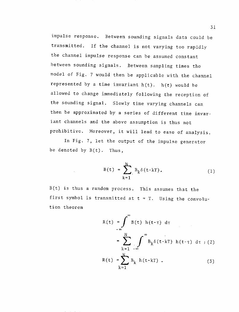
impulse response. Between sounding signals data could be

transmitted. If the channel is not varying too rapidly

the channel impulse response can be assumed constant

between sounding signals. Between sampling times the

model of Fig. 7 would then be applicable with the channel

represented by a time invariant h(t). h(t) would be

allowed to change immediately following the reception of

the sounding signal. Slowly time varying channels can

then be approximated by a series of different time invar-

iant channels and the above assumption is thus not

prohibitive. Moreover, it will lead to ease of analysis.

In Fig. 7, let the output of the impulse generator

be denoted by B(t). Thus,

B(t) = Bk6(t-kT). (1)

k=l

B(t) is thus a random process. This assumes that the

first symbol is transmitted at t = T. Using the convolu-

tion theorem

00

R(t) = B(t) h(t-T) dT- co

N m0

=E Bk6(t-kT) h(t-T) dT ;(2)

k=l -c

R(t) = Bk h(t-kT) . (3)k=l

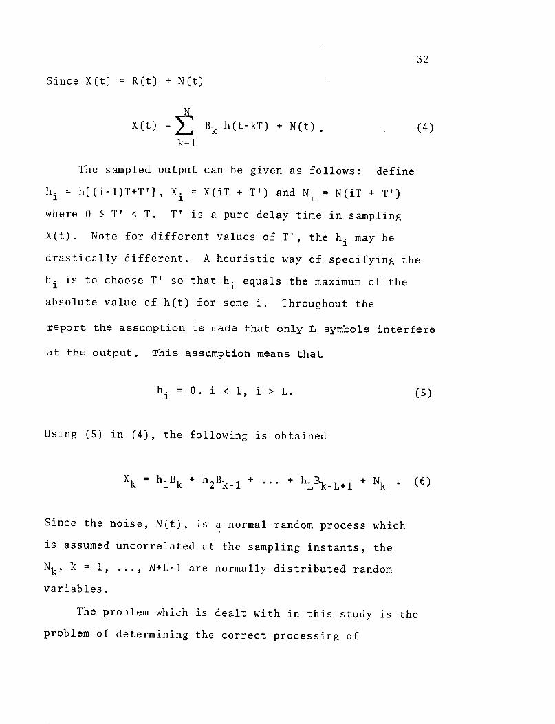
32

Since X(t) = R(t) + N(t)

X(t) = Bk h(t-kT) + N(t). (4)

k=l

The sampled output can be given as follows: define

h i = h[(i-l)T+T'], Xi = X(iT + T') and Ni = N(iT + T ')

where 0 < T' < T. T' is a pure delay time in sampling

X(t). Note for different values of T', the hi may be

drastically different. A heuristic way of specifying the

hi

is to choose T' so that hiequals the maximum of the

absolute value of h(t) for some i. Throughout the

report the assumption is made that only L symbols interfere

at the output. This assumption means that

hi

= 0. i < 1, i > L. (5)

Using (5) in (4), the following is obtained

Xk hlBk+ h2 Bk-l + ... + hLBk-L+1 + Nk (6)

Since the noise, N(t), is a normal random process which

is assumed uncorrelated at the sampling instants, the

Nk, k = 1, ... , N+L-1 are normally distributed random

variables.

The problem which is dealt with in this study is the

problem of determining the correct processing of

33

Xk, k = 1, ... , N+L-1 so that the "best" estimate of the

input sequence, B1, ... , BN, can be determined. This

means that the optimum detector structure as specified

from decision theory must be studied. The following are

assumptions which will be employed in studying the

detector process.

i. h(t) is known-it is either known

a priori or obtained through measure-

ments of the channel

ii. the sampling operation performed in the

detector is perfectly synchronous.

iii. the a priori probability of a symbol = 1/m

(equally likely inputs).

iv. noise samples are uncorrelated and are

normally distributed with mean 0 and

variance a2

Note throughout this report that a random variable

X, is normally distributed will be noted as

X - N(p,a2 ) where p is the mean and a2 the variance of the

distribution. Thus iv. means that Nk ~ N(0,a2),

k = 1,..., N+L-1.

With these assumptions and the results of decision

theory the optimum detector structure for the communication

system of Fig. 7 can be specified. The detector is studied

with a view towards finding the decision regions and

specifying or approximating the probability of error. This

34

is done for both one-shot and multi-shot transmission of

data. Prior to this study, however, several methods

which have been used to combat intersymbol interference

will be examined briefly in Chapter 3.

35

Chapter 3

COMBATING INTERSYMBOL INTERFERENCE

3.1, WAVEFORM SHAPING

Before reviewing decision theory and studying its

application to intersymbol interference channels, it will

perhaps be interesting and useful to study non-decision

theory oriented approaches which have been taken in an

attempt to combat intersymbol interference. One approach

that is taken by Gerst and Diamond [5], is input waveform

shaping. They choose si(t-kT) (see Sec. 2.2) so that it

is zero for t < kT and t ? (k+l)T. In addition, the form

of si(t-kT) is chosen so that the output due to the

kth input is zero for t < kT and t > (k+l)T. Thus

transmitting at a rate cf one symbol every T seconds there

would be no intersymbol interference in the system. Gerst

and Diamond state that such a si(t-kT) can be found if the

system is a general lumped-parameter system or a general

finite RC transmission line. A difficulty with this

approach isthat, for implementation, a knowledge of the

impulse response is necessary at the transmitter. In many

cases, the impulse response is unknown at the transmitter.

In this case, input waveform shaping would be impracticable

to use. Furthermore, the use of input waveform shaping

36

increases the bandwidth requirement of the system. This

is often undesirable.

37

3.2 TRANSVERSAL EQUALIZERS

Probably the method that is currently most commonly

used in an effort to combat intersymbol interference is

that which employs transversal equalizers. As shown in

Fig. 8, a transversal equalizer consists of a properly

terminated tapped delay line (TDL) or its digital equiva-

lent with M taps. Each tap output is weighted by the

corresponding tap gain ci, i = +0,..., +M21 The weighted

tap outputs are then summed to give the transversal

equalizer output.

Note when the transversal equalizer is connected in

tandem with a communication system with impulse response

h(t), the impulse response of the tandem system is given

by e(t) withM-1

2

e(t) = cih(t-iT+TD) (7)

1i 2

where TD is the value of t at the peak of h(t).

Define en = e(nT). Then the sampled impulse response of

the tandem system is given by

M-1

en = ci

h((n-i)T+TD). (8)

-M+ 12

The equalizer is usually designed so that the value of eo

is large compared to the other sampled values of e(t).

Tapped Delay Line (TDL)

Schematic of transversal equalizer

00Fig. 8

39

For best performance the equalizer makes a decision on an

input Bkwhen the value of Bk has the greatest effect on

the output of the equalizer. Denote this output as

(eout)k. Then since eo >> ei, i f 0,

(eout)k= E en B

k - n

n=- c M-1co 2

= E E ci h((n-i)T + TD) Bk n. (9)n = - - - -M+l

2

This sampled output of the tandem communication system,

(eout)k, is put into a quantizer. The decision as to the

value of Bk is then made based on the quantization of

(eout)k-

The tap gains, ci, are determined by solving a set of

simultaneous linear equations. There are many different

versions of transversal equalizers which are employed.

They differ in the criterion used to arrive at the simul-

taneous equations for the tap gains and the method of

solution of these equations. Define

M-1 M-12 2

1 2 j 2

j O j O

There are then three different criteria which are commonly

used to arrive at the values for the tap gains. These are

40

- minimization of Da [3, 12] (this does not

take the noise into account)

- minimization of D8

[3, 12-14] (this also does

not take the noise samples into account)

- minimization of mean-square error due to both

intersymbol interference and noise

[3, 15, 16].

These three criteria are used in arriving at the linear

simultaneous equations which are solved for the tap gain

values. These equations can be solved using matrix algebra

or with the use of iterative techniques. There are three

basic iterative techniques which are used. One technique

uses a fixed-increment adjustment to the tap gains. The

sign of the increment depends on whether the tap gain value

is above or below the optimum value. Another procedure

uses two increment sizes. A large increment is applied to

a tap gain if the tap gain value is very much in error and

a small increment if the tap gain value is close to the

optimum value. A third iterative technique is based on a

steepest descent approach and uses an increment size which

is proportional to the gradient of the mean-square-error-

surface for each particular tap.

The iterative techniques can be applied prior to data

transmission by transmitting test signals before the data

signals. Alternatively, the iterative techniques can be

applied during data transmission by transmitting a test

41

signal periodically or by using the data signals themselves

to adjust the tap gains.

A transversal equalizer which makes use of decisions

made on previous inputs in deciding on the value of the

present input has been developed by Austin [12]. In

deciding on the value of Bk his "decision-feedback

equalizer" uses a quantized feedback procedure in order

to subtract from the received signal all the effects of

symbols B1,...,Bkl . The decisions on B1,...,Bk_

1have

previously been made. In applying this detection pro-

cedure it is assumed that all previous decisions are

correct. In addition, Austin's equalizer uses a criterion

which minimizes the mean-square error due both to inter-

symbol interference and noise which, in theory, minimizes

the effects of Bk+l,...,BN on the decision process.

The reader is referred to the above cited references

for a discussion of the performances of the various trans-

versal equalizers described. The transversal equalizer

implements a linear procedure in making a decision on an

input. The optimum solution, as described in Chapter 4,

has a non-linear structure. Thus the transversal equalizer,

although it performs very well for some impulse responses,

restricts the receiver structure to be linear when in fact

the optimum solution is non-linear.

42

Chapter 4

APPLICATION OF DECISION THEORY TO INTERSYMBOL INTERFERENCE

4.1 DECISION THEORY

In order to determine the structure of the best

receiver, use must be made of the results of decision

theory. Basically, decision theory is a means whereby an

object or quantity is classified as belonging to one of

several classes. This classification is dependent on the

values of measurements which are made on the object or

quantity. For instance, consider the mass production of

some electronic device. Some devices are defective and

some are non-defective. Suppose it is known that the input

resistance of defective devices is normally distributed

with a mean of 100K ohms and that the input resistance of

non-defective devices is normally distributed with a mean

of 200K ohms. Assume further that the variances of the

distributions are known. Decision theory tells one whether

to classify a device as defective or non-defective based on

the measurement of the input resistance of the device.

Associated with each decision about the class to which the

device belongs is a probability of error. This probability

of error is also determined from the results of decision

theory.

43

Decision theory can be split into three parts-simple,

compound, and sequential compound. A brief review of these

three parts of decision theory is presented prior to

applying decision theory to noisy intersymbol interference

channels. The following definitions are used:

Xk = (Xlk, ..., Xnk) - a vector random variable

corresponding to the measurements made

on the kth object;

Xk (Xlk, ..., Xnk) - the measured values of Xk;

S = set of all possible values which Xk may

assume;

i = class or state of nature to which the

unknbwn belongs;

= {i i = 1,...,r} i.e. Q is the set of all

possible classes in which the unknown

may belong;

j = decision that is made on the unknown i.e.

the class in which the unknown is said

to belong;

A = {j I j = 1,...,s} i.e. A is the set of all

possible decisions that can be made

about the unknown;

L.. = loss incurred in classifying the unknown

as belonging to class j when the state

of nature is i;

44

t(jIX) = probability of classifying the unknown

in class j given the value of X that is

observed. (t is called the "randomized

decision function").

Note, usually A = Q although this need not necessarily be

so. If for all X, t(j I X)= 1 for some j c A and

t(j' X) = O for all other j's A and j' f j, then

t(j | X) is a non-randomized decision function.

45

4.1.1 SIMPLE DECISION THEORY

In simple decision theory, there is one observation

vector, X1, and one object about which a decision must be

made. The r x s loss matrix {Lij} is assumed known. The

object is to determine t(j I X1).

Define the "risk function", R(i,t) as the expected

loss incurred by using the decision rule t(j I X1) given

that the object to be classified came from class i [20].

Then

R(i,t) = Lij t(j I X1)p(X1 I i) dX1

(10)

j=l S

where p(X1 I i) is the probability density function of the

random variable X1 given that the object actually came from

class i. Define the a priori probability of the class

being i as qi. Note, qi = 1. The average or Bayes

risk is then

r

R(q,t) = R(i,t)qi

i=l

= E E qiLijt(j I X1 )p(X1 I i)dX1 . (11)

s j=l i=l

As a criterion of classification a t(j I X1) is chosen so

that the Bayes risk is minimized. For the usual case of

46

a non-randomized decision rule, minimizing the Bayes risk

r

is equivalent to minimizing L Lijp(Xl I i)qi . A com-

i=l

monly treated situation is that in which L.. = 1 - 6...1j 1J

In this case the minimization of the Bayes risk is

achieved by setting j equal to that i for which

P(X1 I i)qi is maximized.

If the statistical characteristics of X1 and the

a priori probabilities are known the optimal procedure can

be implemented. If the a priori probabilities are not

known, a scheme for classification can be based on

minimizing the maximum Bayes risk [20]. This procedure

is called a "minimax procedure".

4;

4.1.2 COMPOUND DECISION THEORY

In contrast to simple decision theory in which,

based on the value of a vector random variable, a decision

about one unknown is made, compound decision theory makes

a decision about N unknowns based on N random vector var-

iables.

Let Ok = (01',...'k) be a random vector which consists

of the first k unknowns. Also let Xk be a vector composed

of the first k Xi, i.e. Xk = (X1, ...,Xk). The value of

A k is denoted by xk = (xl,...,Xk). The results of compound

decision theory are predicated on the assumption that diven

0.i the probability density function of Xi is independent

of the other X.'s and other O.'s. That is

p(Xil Xil'Xi+l.,...XN0N) = P(X i lO-i) (lo

The oi

need not be independent. A compound decision rule

is given as tN = (tl,...,tN) wherie tk = tk(i KXN) is

deofined, in a manner analogous to the definition of

t(j I Xl) in Sec. 4.1, as the probability ot dec id i ng

k j given the value of XN that is oseve. n a

manner analogous to that o1f simple decsis on theor!y de t'i n

the "ith component r isk I'unction", IZ( N,ti), ,s the

expected loss ilncturrled on the ith dec is.io on by ustisng the

48

decision rule ti

(j I I N )

R(3N.tNi) =J E Leij ti(j l N ) PNIN) dXl...dXN

SN j=l

where SN, the N-fold cartesian product of S, is the range

of XN. The compound risk, R(ON,tN), is then defined as

the average of the component risks

N

R(N.tN )= 1i/N R(N'ti)i=l

s N

R(N,tN) = 1/N E E Le ti(iN) P N

sN j=1 i-1

dX1 ... dXN .

Let G(ON) be an a priori probability distribution of

oN over the domain 2N (QN is the N-fold cartesian product

of Q). The compound Bayes risk is then given [20] as the

average of the compound risk as follows:

R(G,tN) = N N R (N',tN)G(eN)

N -NNs

= 1/N ± R(G,ti)

where i=l

R(G,ti) = Z R(N',ti)G (-N)N

ON E Q

The criterion for making an optimum decision is to minimize

49

the Bayes risk. This is equivalent to choosing tN so that

R(G,ti) is minimized for every i. Denote the tN which

minimizes R(G,tN) as tNG.IN G is called the "compound

Bayes procedure".

For the common case of a non-randomized decision

rule the criterion is equivalent to setting ti(jIXN) = 1

for that j for which

E Leij

p(XNIN)G(N) = LoijP(XNOiE) (13)

-N 1i

is a minimum. For the special but common case of

A = Q and L0

j = 1-6., the minimization of (13) reduces

to the maximization of p(XNIOi)P(Oi). Note if the Oi

are

independent, the minimization of (13) reduces to maximizing

P(Xi lOi)P(Oi) .

Abend [20] states that compound decision theory is

necessary if the states of nature are not independent or

if the a priori probabilities are not known. For the

purposes of this study it is assumed that the a priori

probabilities are known. In this study compound decision

theory will be employed in those cases in which the states

of nature are not independent.

In Sec. 4.2.1 application of the above results are

made to intersymbol interference channels. Before doing

so a special case of compound decision theory-sequential

compound decision theory--will be studied.

2$

50

4.1.3 SEQUENTIAL COMPOUND DECISION THEORY

In compound decision theory, a scheme, which was based

on all observed values, for making decisions was derived.

In some cases all N observations are not available when a

decision about some Ok must be made. If only the first k

observations, Xk, are available when the decision is made

on the kth unknown, 0k, the results of sequential compound

decision theory apply. The decision rule is called a

"sequential compound decision rule".

To obtain this sequential compound decision rule one

proceeds in a manner analogous to that of the compound

case. The assumption is again made that given Ok, Xk is

independent of the other Xi's and Oi's, i.e.

P(XklXk-,Xk+,...,XN,O0N) = p(XKIOk). (14)

Using the notation of Sec. 4.1.2 the Bayes risk is given

N[20] by R(G,tN) K(G where

Y 'N) E R(G'tk) wherek=l

R(G,tk) = k L0 . tk(jlXk)P(XkIOk)G(Gk)dX (15)OksEk k

For optimality the decision rule is chosen to minimize the

Bayes risk. This is equivalent to minimizing, for every

k, R(G,tk). As before, for a non-randomized decision rule,

51

this is equivalent to setting tk(j I jk ) = 1 for that j

which minimizes

E LOk j p(XkIOk)G(2k) = E LOk P(Xk',Ok) . (16)

Ok Ok

In Sec. 4.3 this optimization criterion is applied to the

intersymbol interference channel to obtain a decision rule.

52

4.2 APPLICATION OF DECISION THEORY

For the one-shot transmission of N symbols, the

optimum receiver can be given. Let the sequence

(B1,...,BN) be denoted by the random variable 7. Let

fi be one of the mN possible sequences which X can

assume. XN is the set of measurements. Xk is given as

in eq. (6). Then based on XN a decision is required

about r. Simple decision theory is applicable. Thus

from Sec. 4.1.1 r is chosen equal to Tj for that r.

for which

Q E L P(XNI = i)G ( = i) (17)

1i 1 T

is minimized; here G(O = ri) is the a priori probability

associated with f. For L = 1-6 , this reduces to1ij ij

-choose X = ij for that tj for which P(XfNlr = lrj)G(r = fj)

or P(r = jlIXN) is maximized, i.e. E is chosen equal to

7j if P(r = fjljiN) Ž P(7 = Tj,IlX) for all j' f j. This

rule could be implemented to make a decision about the

value of the inputs. The rule provides for the minimiza-

tion of the probability of making an error in the message.

It is the optimum rule if the minimization of message

error is used as a standard of optimality. There is a

drawback to this procedure. As N increases the number

53

of different .r increases as mN . Thus for N large theJ

number of calculations necessary to implement this pro-

cedure would be prohibitively large and the process

would be impractical. An approximation to this rule will

be examined in Sec. 4.2.1.

54

4.2.1 CHANG AND HANCOCK DETECTOR

As noted above the optimum detector of Sec. 4.2 is

impractical to implement due to the complexity of imple-

mentation growing as m . By turning to compound decision

theory and a different loss function Chang and Hancock

[18] find a less complex detection scheme which can be

implemented. They define

= A + Bk .B L-2 + L-lk k Bk Bklm ++ Bk-L+2 m + Bk-L+l m (18

A decision is made as to the value of the states,

Oi, i = 1,...,N. From this decision about the Oi's, they

determine the values of the transmitted symbols, BN. The

detector that Chang and Hancock seek is optimal from the

viewpoint of minimization of the probability of making an

error in the estimation of a state, 0j.

From (6) it can be seen that Xk depends only on

Bk ... ,BkL+ 1and a noise term*. Hence eq. (12) is

satisfied and the application of compound decision theory

is justified. The states of nature are not independent

and hence compound decision theory is necessary. Assuming

*

As noted previously the noise terms are assumed to beuncorrelated zero-mean normal random variables.

55

equal a priori probabilities and letting L.O.O = 1-6ij

the optimum solution is to set Ok

= j for that j for which

P(XN[Ok = j) or equivalently P(Ok = jjXN) is maximized.

This loss function insures that the probability of making

an error in the decision about the value of the state is

minimized. Since P(XN) is independent of the value of

Ok' the rule may be expressed as-set Ok = j for that j

for which

P(Ok = jlXN)P(N) (19)

is maximized.

This is the decision rule which Chang and Hancock use.

They have developed a method whereby (19) is calculated

sequentially. The degree of complexity of the detector

thus increases only linearly with N. As noted in Sec. 4.2

the complexity of the detector obtained using simple

decision theory increases as mN. Furthermore, Chang and

Hancock note that if rT is the true state of nature and

if P(r = 7TIXN) > 1, then their detector is equivalent to

the optimum detector of Sec. 4.2.

This detector implementation has several drawbacks.

Because 0i is not independent of Oi_ 1 not all possible

sequences of Oi, i = 1,...,N are realizable. In the case

of an error made in the decision about the value of Oi an

improper sequence of O's may occur. This sequence would

56

not yield a unique determination of the input signals

Bi, i = 1,...,N. If this non-unique determination of the

Bi

is over J adjacent symbols, Ba,...,B a+J_1 Chang and

Hancock suggest that a maximum likelihood decision be made

on the J symbols. Thus, let the sequence Ba,...,B a+J 1

be denoted by J and let iJ be one of the mJ possible

values for the sequence B ,...,B +j_1. Then as in

Sec. 4.2, the maximum likelihood procedure is to set

J= '.J for that .jJ for which P(TJ = J X ) is aw = wrj fof hat 7T fr hchPTr 7

maximum.

A second drawback to the Chang and Hancock procedure

is that the information must be transmitted in blocks of

N m-ary digits with adequate guard space between adjacent

blocks. This means that if N is large, one must wait a

long time after the initiation of the transmission to

receive all the outputs and start classifying the inputs.

The reception of the first part of the message is not

possible until all of the message has been received. If

N is small this is not a very big problem; however, the

effective rate of transmission is then very much reduced

from one digit every T seconds.

57

4.2.2 MINIMIZATION OF THE EXPECTED NUMBER OF ERRORS

It has been pointed out [21, 22] that the optimum

receiver, as derived from decision theory can be

expressed in a manner other than that given in Sec. 4.2.

Using the notation of Sec. 4.2, decision theory says to

minimize

Q P(7 = Lij

I IN)

and set j equal to that value for which Q is a minimum.

Instead of defining a loss function as per Chang and

Hancock (Sec. 4.2.1) define [21]

N

L i- j L(B ,B a).

a=1

L(B ,B ~) is the loss incurred by saying Ba = bg

= l,...,m when, in fact, B = b, i= 1,...,m.

Furthermore, let L(B c,Be ) = 1-6 . This choice of

a loss function is equivalent to minimizing the risk

associated with classifying each input symbol, i.e. it

minimizes the expected number of errors. Using this

loss function

58

N

Q C= c=l

Q = L

Ot=l

Nm

E L(B ,B )P(Tr = Tri XN ),

i=l

Z L(B ,B aB)P(B = b IXN)'=1

(20)

(21)

Q is minimized if for each a, Ba is set equal to that b5

for which P(Bs

= b IXN) is maximized. The optimum

detector, for this loss function, then calculates

P(Ba = bCIXN ) and uses this statistic to make a decision.

Since

P(Bo = bJ|XN) = . . EB *..,B

-'-L+l

P(O lXN)

where O0 is given in (18), p(Ba = byiN) could be

calculated in a sequential manner and the optimum detector

implemented. Simulations of this procedure have not been

published. It is important to note [22] that the detector

based on this procedure is non-linear. Thus the trans-

versal equalizer and matched filter techniques of Chapter 3,

being linear, are sub-optimum.

59

4.3 SEQUENTIAL DETECTION

As noted in Sec. 4.2.1, a drawback to the Chang and

Hancock pircedure is that all of the signal must be

received prior to making a decision on any input. This

is also a drawback to the optimum rule of Sec. 4.2.2. In

some cases it may be very important to make a decision

about the inputs as the message is received. This

involves a sequential procedure which will be derived

below. The derivation will be analogous to the derivation

for the rule of Sec. 4.2.2 [21]. This involves a sequen-

tial decision procedure and sequential compound decision

theory is applicable.

Define k = B1,...,Bk. Let 8ki be one of the mk

possible sequences which Ok can assume. With these

definitions p(XjlX1,...,X ) = p(Xjl j

and sequential compound decision theory is applicable.

From Sec. 4.1.3 the quantity to be minimized is

Q=E Lekiekj LP(Xk' k =ki). (22)

ki

Minimizing Q is the same as minimizing

Q' L 6 P(Ok = OkiPkXN). (23)

ki 'k i

k 60Define L = . L(B ,B g) where L(B ,B g) isekie kja aEdefined as in Sec. 4.2.2. Then

Q' = j E L(B ,Ba) P(Ek = OkiIXN)a=l ek.kik m

E E L(Bac'g E- P(B, .,B kI1k)O=l 4=l 1 1 Bk

ifa

And finally

k m

Q' = L L(B c,B )P(B= bcLXk). (24)C=l r=1

Letting L(B ,B ) = 1-6~, Q' is minimized if for each

a, P(BU = b lXk) is maximized. The sequential compound

rule then says set B equal to that b for which

P(Ba = bj Xk) is maximized for all a = 1,...,k.

The rule states that, after receiving the kth measure-

ment, a decision is made on Bk by maximizing P(Bk = brlXk).

This sequential procedure will be denoted as a "backward-

looking one-sided rule". This terminology is used because

the classification of Bk depends only on the samples in

the past as measured from time equal to kT-i.e. for

t s kT. The samples used are those which appear only on

one side of Bk. The application of the backward looking

one-sided rule and the compound rule (Sec. 4.2.2) to noisy

intersymbol interference channels will be investigated

61

with a view toward implementation of the procedure and the

evaluation of the probability of error inherent in the

procedure.

62

4.4 CRITERIA OF OPTIMALITY

The two optimum detectors of Sec. 4.2 and 4.2.2 are

derived using two different loss functions. This results

in two different implementations of an optimum decision

procedure. The implementation of Sec. 4.2 minimizes the

probability of making an error in the received message.

The compound detector of Sec. 4.2.2 and the sequential

detector of Sec. 4.3 is a realization of a decision pro-

cedure which uses minimization of the expected number of

errors as the optimality criterion.

Which optimum detector one uses is dependent on

whether one wants to minimize the probability of making

an error in the message or whether one wants to minimize

the expected number of errors in the message. The latter

is more commonly used in communication problems since, if

redundant coding of the signal is carried out prior to

transmission, a few errors in detection can occur and the

message sequence can still be decoded and received cor-

rectly. Thus minimization of the expected number of

errors is the criterion which is usually used in detec-

tion theory [23];hence, the detection procedures of

Sec. 4.2.2 and 4.3 will be evaluated while the detection

procedure of Sec. 4.2 will not be evaluated.

63

Chapter 5

SEQUENTIAL DECISION RULE AND PROBABILITY OF ERROR

5.1 DECISION STATISTIC

In evaluating the decision rule, determining the

decision region, and finding the probability of error, the

assumptions given in Sec. 2.2 are used. In addition, the

loss function associated with a decision is assumed to be

the same as that given in Sec. 4.3.

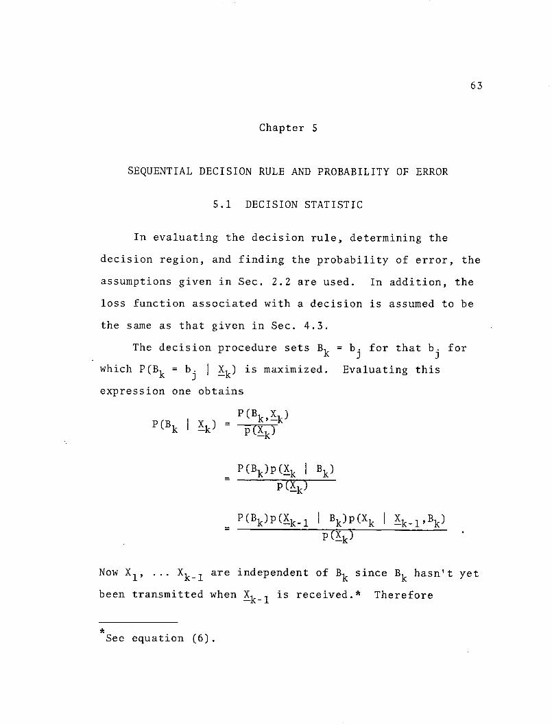
The decision procedure sets Bk = bj for that bj for

which P(Bk = bj I Xk ) is maximized. Evaluating this

expression one obtains

P(BkXk )P(Bk I Xk) = P(,k)

P(Bk)P(Xk I Bk)

P(Xk )

P(Bk)P (Xk_l I Bk)P(Xk I Xk l,Bk)

P(Xk )

Now X 1, ... Xk 1l are independent of Bk since Bk hasn't yet

been transmitted when Xk- 1 is received.* Therefore

See equation (6).

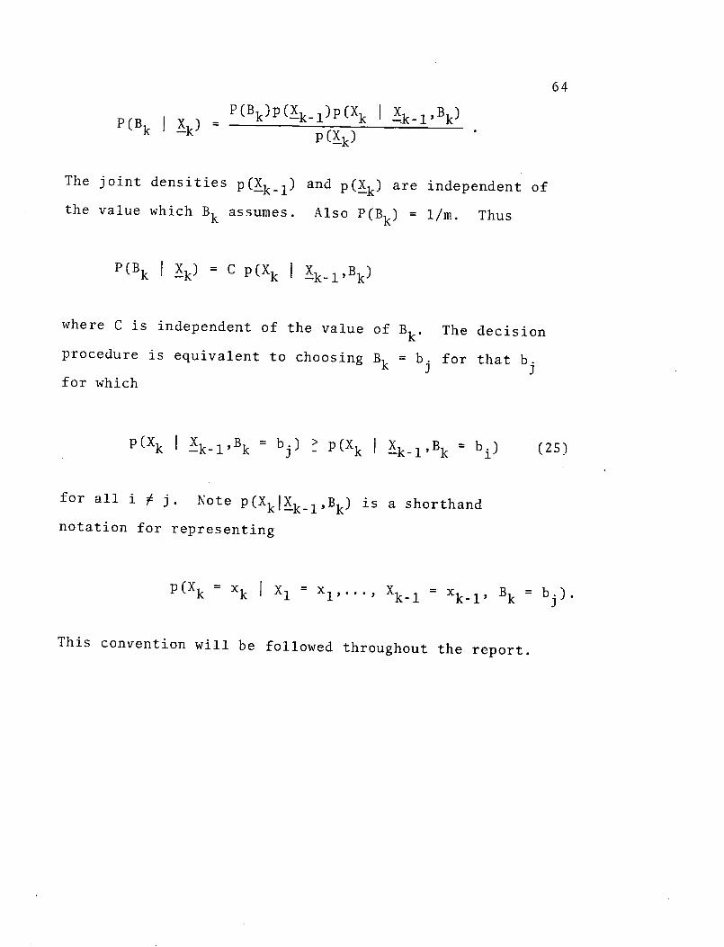
P(Bk I k) =

P(Bk)P(Xk-1)P (Xk I xk- 'Bk)

p (x k )

The joint densities P(Xkl1) and p(Xk) are independent of

the value which Bk assumes. Also P(Bk) = 1/m. Thus

P(Bk I k) = C p(Xk I X

k-lBk)

where C is independent of the value of Bk.

procedure is equivalent to choosing Bk = b

for which

The decision

for that b.J

p(Xk I Xk-lBk = bj) > P(Xk I Xk_ ,Bk = bi) (25)

for all i f j. Note P(XklXklBk) is a shorthand

notation for representing

P(Xk = xk I X x1 ... Xk_1 = Xk. 1, Bk = bj).

This convention will be followed throughout the report.

64

65

5.2 CALCULATION OF DECISION STATISTIC

By using the expressions for X1,...,Xk obtained

through the use of equation (6), Xk can be expressed in a

manner which renders the decision statistic,

P(XklXk l,Bk = bj) calculable. The specification of

this probability will now be considered. Equation (6)

is rewritten below as

X.j = hlBj

+ h2Bjl +...+ hLBjL+1 + Nj.

For the k components of Xk, k equations can be written.

This system of equations appears as follows:

Xk = hlBk +

Xk-l = hlBk- +

Xk_2 = hlBk-2 +

h 2 Bk- 1

h 2 Bk-2

h 2 Bk-3

+...+ hLBk-L+ 1

+...+ hLBkL

+...+ hLBk-L-1

+ Nk (26a)

+ Nk-1 (26b)

+ Nk-2 (26c)

XL = hlBL

X2 = hlB2

X 1 X1 = hlB 1

+ h2BL- +...+ hLB1

+ h2B1

+ NL

+ N2

+ N1

This system of k equations has k unknowns (the Bk).

these equations Xk can be obtained as a function of

(26d)

(26e)

(26f)

From

Bk and

66

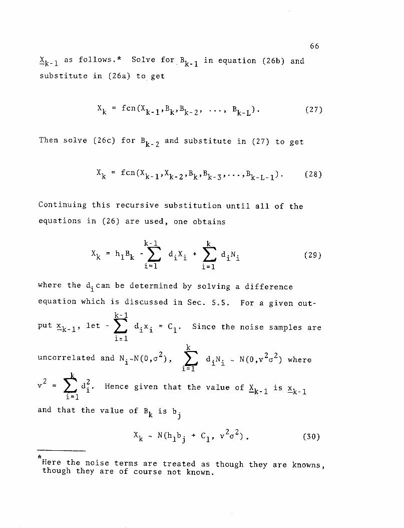
Xk-1 as follows.* Solve for Bkl1 in equation (26b) and

substitute in (26a) to get

Xk = fcn(Xk-l,Bk,Bk 2, ... , Bk-L). (27)

Then solve (26c) for Bk_ 2 and substitute in (27) to get

Xk = fcn(Xk-l,Xk_2 ,Bk,Bk_3 , .. , B k_-L-l) (28)

Continuing this recursive substitution until all of the

equations in (26) are used, one obtains

k-l k

Xk = hlBk - E diXi + E diNi (29)i=l i=l

where the dican be determined by solving a difference

equation which is discussed in Sec. 5.5. For a given out-

k-l

put xk-l' let dixi = C. Since the noise samples are

i=lk

uncorrelated and Ni-N(O,a2), diN N(O,v2a2) where12

v = di Hence given that the value of Xk-1 is xk-1

i=l

and that the value of Bk is bj

Xk - N(hlbj + C1 , v2C2)2 (30)

*Here the noise terms are treated as though they are knowns,though they are of course not known.

67

Thus the conditional probability density function of Xk

is known and the sequential decision procedure can be

realized. This specification of the density allows the

probability of error associated with the sequential com-

pound decision procedure to be calculated.. Prior to the

study of this probability of error, the associated

decision regions will be examined in Sec.! 5.3.

68

5.3 DECISION REGION

The specification of the decision regions associated

with the sequential compound decision procedure proceeds

as follows. For each value of the variable Bk, a different

normal distribution is obtained. For m-ary transmission

let the values of Bk be

bj = (-m +2j - 1)A (31)

where A can be specified in terms of the signal-to-noise

ratio (SNR) and the hias

a2SNRA L S (32)

i=l

There are thus m different density functions corresponding

to the m different values of Bk which must be evaluated.

The decision about which value of Bk was transmitted,

resulting in the minimum number of expected errors, requires

a comparison of these m different density functions. As

indicated by equation (30) each density function has the

same shape. Adjacent means are separated by a distance of

2Ahl. As an example, the probability densities for the

case m = 4 are given in Fig. 9.

P(Xk IXk-l',Bk=-A)

C -2Ah C C *2Ah X1 1 1 1 1 k

Decision regions for sequential procedure with m = 4

Fig. 9

o,tq0

70

As illustrated in Fig. 9, the sequential decision

problem has been reduced to the classical one-dimensional

m-state decision problem. Applying the decision criterion

(25), the decision regions may be determined. If a

received value of Xk falls in the decision region Rj, on

the Xk axis, then Bk is classified as belonging to class

j. For the situation illustrated the decision regions

are

R1: Xk < (C1 - 2Ahl)

R2: (C1 - 2Ahl) < Xk < C1

R3: C1 < Xk < (C1 + 2Ahl)

R4: (C1 + 2Ahl) < Xk

In general, since C1 is a function of Xk-l' the

decision region is a function of Xk-l. Note that the

Xk-l are related through the di. Since the hi are

related to the dithrough a difference equation (Sec. 5.5),

the effect of the impulse response on the decision regions

is related to the effect that the d. have on the decision1

regions. Consequently the relationship of the di to the

hiwill be studied (Sec. 5.5 and 5.6).

71

5.4 PROBABILITY OF ERROR

Based on the decision regions that were obtained in

Sec. 5.3, the probability of error (performance) of the

sequential compound detector can be determined for the

general case of m-ary transmission. This probability of

error would be the same as that which is specified for

the classical m-state decision problem. The probability

of error takes on a simple form for equal a priori prob-

abilities and m = 2. For this case, the probability

densities are as shown in Fig. 10. If Xk> C2 ,Bk is

classified as +A. Bk is classified as -A otherwise. The

probability of error, P(e), is defined as

P(c) = [1/2]P(Bk is classified as +AIBk actually equals -A)

+ [1/2]P(Bk is classified as -AIBk actually equals +A).

Due to the symmetry involved,

P(Bk is classified as +AIBk actually equals -A)

= P(Bk is classified as -AIBk actually equals +A).

Thus P(c) = P(Bk is classified as +AIBk actually equals -A).

Hence, from Fig. 10, after a change of variables

t = (Xk-C 2+Ahl)/va, one obtains

co

t 2/2P(E) = 1/,2 f e dt (33)

D

P(X IXk B =- A)\ k -k-i kP(Xklk- i'B k=+A)\ k'Xk-1k

C2 Xk

Kt--- -2Ahl -

Decision region and probability of error for sequential decision procedure with m = 2

Fig. 10

73

where D h (SNR)]/ [( h )]

- i=l

Since v2 d i , the probability of error is

i=l

dependent on how di behaves. In order to keep the prob-

ability of error of the classification within reasonable

bounds, v2 should not be too larg'e. It is certainly not

desired that v2 tend to infinity as k tends to infinity.

As will be shown in Sec. 5.5, the didepend on the value

of the hi and thus they depend on the impulse response of

the channel. For N large, the use of the sequential

procedure must be restricted 'to those'impulse responses

for which v2 tends to limit C3 as k tends to infinity.

It is noted here that the hi's affect the performance

of the sequential detector not only through v2 but also

through hi 2 . To get excellent performance v2 must be

i=l

small and hi2 must be close to [maxhi . The types of

impulse responses for which the sequential detector will

perform well are indicated in Sec. 5.6.

74

5.5 DIFFERENCE EQUATION

As stated in Sec. 5.2, the di

are solutions of a dif-

ference equation. This difference equation results from

the recursive substitutions that were necessary in order

to find Xk as a function of Xk-1 and Bk (See Appendix A).

The difference equation is given below.

hLdi

+ hLldi_ + ... + hldi L+1

= 0 (34)

This equation is subject to the constraints that

dk, dkl, ... dkL+2 are specified. The equation may be

solved by methods outlined by Goldberg [24]. This equation

has not been solved in closed form. However, given the

values of hi, a recursive solution should be obtainable.

As noted, both the decision region and the probability

of error depend on diand thus on h

i. The relationship of

hi

and diwill now be studied in an attempt to determine

for which impulse responses the sequential decision pro-

cedure would be expected to yield good performance.

75

5.6 REGION OF CONVERGENCE

The performance of the sequential procedure is a

L k

function of hi, hi2 and di 2 = v2 Since v2 is

i=l i=li

a measure of the effective variance in the classical

decision problem, a smaller v 2 leads to better perform-

ance. v2 will be investigated in the limit as k tends

to infinity. This investigation of v2, will lead to a

specification of those impulse responses for which the

sequential rule is applicable.

Prior to analyzing the solution of the difference

equation, a transformation is applied to the difference

equation. In eq. (34) it should be noted that, because

the initial conditions are specified in terms of

dk, ... , dkL+l, the di

are a function of k. The di

thus

change with time since k changes with time. The object

of the transformation is to make the solution of the

difference equation independent of time. Accordingly,

the transformation

(i) + k-(i) (35)

is used. At the same time replace d by c. The trans-

formed equation then becomes

76

hlci + hc + h2ci... + hLCiL+ = 0 (36)

The initial conditions for equation (36) are specified

in terms of co,....,C L 1. Thus, as desired, the ci

are

independent of time. Equation (29) becomes

k-l k

Xk = hlBk - k-iXi + Ck-iNi+ (37)i=l i=l

k-l

The effect of this transformation is to make v2 ci 2 .

i=O

Thus in order to insure that v2 is bounded it is necessary

to bound E ci2 Accordingly the conditions under which

co i=O

E i2 converges will now be studied.i=O

Following Goldberg (24) the auxiliary equation assoc-

iated with (36) is

zL-1 + (h2/h) + (h3 /h1 )z +. (hL/hl) = 0.(38)

The solution of (36) has the form (for distinct roots)

jo L-1

Ci = E Fjrji + E Fjrji

cos(iOj + Ej) (39)j=1 j=j +l

where rj, j i jo, are real roots of the auxiliary equation

(38) and rj and Oj, j > jo, are the modulus and phase angle

77

of the j-th root of (38). F. and E. are determined from

the initial conditions. Eq. (39) can be written as

I.-1

Ci = Fjrji. cos(iOj + Ej) (40)

j=l

where 0 = 0 and E.= T/2 for j < j . Using the expression

for ci given by (40), it can be shown (see Appendix B)

that a necessary and sufficient condition for the con-

vergence of E ci is that the roots of the auxiliary

i=O

equation fall within the unit circle in the z-plane. If

there are multiple roots, a similar analysis results in

the same necessary and sufficient conditions for the

convergence of the series. (See Appendix C.)

From Marden [25], in a result attributed to Gauss, a

sufficient condition for all zeros of (38) to be inside

the unit circle in the z-plane is that

I(hi/hl)l < 1/[/2 (L-l)] (41)

for i > 2.

A more useful procedure is to use a method given by

Jury [26]. The inside of the unit circle in the z-plane

is mapped into the .negative real half of the w-plane by

the bilinear transformation

(w+ 1)(W - 1)

78

With this transformation, equation (38) becomes

D0wL1 + DlwL + ... + DL_2W + DL1

= 0 (42)

where

b-i (-l

( ) -ga 1, 1 j ) (\ 2(, -2

-.. + (l) jl l)(L -a) + (l)(l)] (43)

and (n) is the binomial coefficient. Applying the Hurewitz

criterion to insure that the roots of (42) all fall in the

left half plane, one obtains some necessary and sufficient

conditions to insure that the roots of (38) fall within

the unit circle in the z-plane. The convergence criteria,

for various L, are given in (44)-(47). These equations are

given for normalized hi. The hi are normalized by dividing

each hi by hi. Thus hi = 1. Note, the normalized hi will

be used throughout the remainder of Chapter 5 except as

noted.

L = 3

1 + h 3 > 0 (44)

1 - h 3 > 0

1 - h 2 + h 3 > 0

79

L = 4

1 + h 2 + h+ h 4 > O0 (45)

3(1 - h4 ) + h2

- h 3 > 0

3(1 + h4 ) - h2

- h 3 > 0

1 - h 2 + h 3 - h4 > 0

4 h32 h4 0

L = 5

TO = 1 + h2 + h3 + h4 + h5 > 0 (46)

T1

= 4(1 - h5) + 2(h2 - h4 ) > 0

T2

= 6(1 - h5) - 2h3 > 0

T3 = 4(1 - h5) + 2(h4 - h2) > 0

T4 = 1 -h2

+ h3

- h4

+ h > 0

A = T1 T 2 - ToT 3 > 0

T3 - T 1 T4 > 0

L = 6

T = 1 +h 2 + h3 + h 4 + h 5 + h 6 > 0 (47)

T1 = 5(1 - h6) + 3(h 2 - hs) + h 3 - h4 > 0

T2

10(1 + h6 ) + 2(h 2 + h 5) - 2(h3 + h4 ) > O0

T 3 = 10(1 - h6 ) + 2(h5 - h 2) + 2(h4 - h 3) > O0

T4

= 5(1 + h6) - 3(h2 + h5 ) + h 3 + h 4 > 0

T = 1 2 + h - h + h h5 hh > 0

Y1 T1 T 2 ToT3 > 0

2= T3 Y 1 T1(T 1T 4 - ToT5 ) > 0

T4Y 2 T5[T2 Y1 - TO(T1T 4 - TOTS)] > 0

80

These equations define a region in (L - 1) dimensional

space. If the hifall within this region E ci2 will con-

i=Overge and lim ci = 0 as i + a. For L = 3, this region is

the region indicated by the solid lines of Fig. 11. It is

interesting to note that in this case the region is

symmetric about the h3 axis but not about the h2 axis.

A sufficient condition to insure that v2 will converge

is that the hi of an impulse response fall within any sub-

region of the triangle of Fig. 11. A simple sub-region of

this triangle is one which is defined by lh2 1+1h3 1 < 1

shown by the dotted lines of Fig. 11. The convergence

region for L = 4 is a complicated three-dimensional figure.

While this figure has not been drawn, upon examination of

(45), it can be seen that ± Ihil < 1 is a sub-region of

i=2the region of convergence. Thus E Ihil ' 1

i=2

is a sufficient condition for the convergence of the

solution of the difference equation. For any L,

LE Ihihl ' 1 is a sufficient condition for the convergence

i=2

of the difference equation (see Appendix C). Note the

sufficient condition given by Marden is shown by the shaded

square in Fig. 11.

The fact that the solution of the difference equation

converges is important. It would also be desirable to

81

h3

+1

1 Xm m+1 h2 >

Regions of convergence of the

difference equation solution for L - 3 (h1=l)

Fig.11

82

know at what rate it converges since better performance of

the detector would be expected for those cases in which

the solution converges rapidly. The convergence of

E ci depends on the maximum value of rj. The smaller

i=O

the largest root, rmax, the faster the convergence of v2 .

Thus the criterion which must be satisfied so that all

roots of (38) fall within a circle of radius r in the

z-plane will be investigated.

Using the transformation

z = r(w + 1)W - 1

the area Izi < r is mapped into the left half of the

w-plane. Define

Dj = Eha= r [( j))(1 + 2 -2 (48)

a-\L-a + (- )a+ (a-l

Applying the Hurewitz criterion, equations identical to

(44) - (47) are obtained with all expressions in (42),

(44) - (47) replaced by their hat equivalents, all h.

^ L-ireplaced by hi (r) h1 , and the l's in (44) - (47)

replaced by (r)-

For L = 3 the equations become

^ 2 ^(r) + h2r +3? > 0

(r) 2 h3 > 0

(r)2 h2r + h3 > .

The region defined by these equations is shown by the

dashed triangle of Fig. 11. For a given (h2, h3 ), the

triangle can be found which passes through the point

(h2, h3). From this triangle the maximum value of rj

can be found. Although the value of rmax gives an

indication of the behavior of E ci2, it can not provide

i=O 0o

detailed information since the value of E ci2 depends

i=O

on the initial conditions imposed on the difference

equation (these depend on hi) and on the values of the

roots of (38) which are inside the circle Izl = rmax

In addition to E ci2, the performance of the

i=O L

sequential procedure also depends on E hi2. For two

i=ldifferent difference equations with equal values of

00~~~~~~~~ L

E ci2 the difference equation which has E hi2

i=O i=l

closest to [max hil]2 will yield the best performance.i

83

84

L

This is true since as E hi2 - [maxihil 2 all of the

i=lsignal power tends to be in the main lobe of the impulse

response.

85

5.7 APPLICABILITY OF SEQUENTIAL PROCEDURE

Deciding on the symbols sequentially has advantages

in that the first parts of the message can be determined

before the entire message is received. If the channel is

to transmit information, this method can not be applied if

the impulse response falls outside of the region of con-

vergence. If the impulse response falls within the con-

vergence region the sequential procedure will operate

with varying degrees of success depending on the values

co L

of E ci2 and E hi2.

i=O i=lIf the sequential procedure does not work satisfac-

torily, it is necessary to consider the compound rule,

which is discussed in Chapter 6, or some modification of

this rule such as the deferred decision rule discussed

in Sec. 8.2.

86

Chapter 6

OPTIMUM DETECTION FOR BLOCK TRANSMISSION OF LENGTH N

6.1 DECISION RULE

For the transmission of a block of N symbols, the

optimum receiver of Sec. 4.2.2 will be studied. This

receiver bases its estimate of an input on all observed

output samples. In order to minimize the expected number

of errors, this optimum receiver sets Bk bj for that j

for which

P(Bk = b=

bi

I N+L-1) for all i~j.(49)

Note for N input symbols there are N + L - 1 output

samples because each input is spread over L sampling

periods. In order to implement the optimum receiver

P(Bk I XN+L1) must be calculated. Before studying the

decision statistic, P(Bk I sN+L-1)' several theorems which

will aid in the evaluation of P(Bk I XN+L-1) will be given.

87

6.2 INDEPENDENCE THEOREMS

Let (Xk) be a set the elements of which are the

random variables X 1,...,Xk. Let (Xk)j be one of the 2k

subsets of (Xk). Also define an "L-1 neighbor of Xi" as

any X. which is an element of the set

{X i-L+i'. .Xi-iXi+ ... ,X i+L I. In addition define

(B) to be the set with B1,...,BN

as elements and let

(B)j be one of the 2N subsets of (B). Let Uj be a

subset of (B) such that for a certain (XN+Ll)j

Uj = U {B, . ,Ba L+1 Xa E(XN+L-l)j.

Thus U. is necessary and sufficient in order to specify,

with the exception of a noise term, each Xa E(XN+L l)j

by means of equation (6). For example, let

(XN+L-l)j = (Xk,Xk+2,Xk+3L} Then

Uj {B(k+2 ,Bk+',. ..Bk-L+,B k+3L'B k+3L-l' ' k+2L+l

The following theorems are presented. The proofs are

given in Appendix D.

Thm: 1: P(Xk+L+iIBk) = p(Xk+L+i) for i = 0,1,...,N-k-l

and P(Xk-ilBk) = P(Xk-i) for i = 1,...,k-l.

Consider X = (XN+L l)j u (XN+L-l)k and

88

S = (B)MU(B)j where (XN+L-l)j n (XN+L-l)k = ~ and

(B)M n (B)j = i . The partitioning of 8 is accomplished

by setting (B) n (U {BB X +L x(B~j

=

~ (a a a+L_1 a

Define X*= {,...,X +L 1 B E (B)j}) X. The

partitioning of X is attained by letting (XN+Ll1)j be the

subset of (XN+L-1) such that

(XN+Ll)j = (X ) U [ U({L-1 neighbors of Xi*jXi* is known

to belong to (XN+Lil)j}l)X) ]

Note the definition of (XN+Ll)j is recursive. First

the L-1 neighbors of Xi, such that X

iE X*, which are also

elements of X are found. Then the L-1 neighbors of these

neighbors, which are also elements of X, are found. This

process continues until no more elements can be found

which are L-1 neighbors of a previously found element and

which are also elements of X. When this occurs (XN+Ll)j

has been specified. Note also that (B)M n (UjU Uk) = {.

The following theorem is given.

Thm. 2:

p(Xls) = P((XN+L-l)j I (B)j)P((XN+L-)k).

Two corollaries which will be used are given.

Cor. 2.1 P((Xki)j I Bk) = P((Xk-i)j) for 1 5 i < k - 1

89

Cor. 2.2 Let (Xk)U be any subset of {Xk+L+i I i ' 0}

then p((Xk)U I Bk,(Xk-i)j) = P((Xk)u I (Xk-i)j)

In particular, these theorems mean that

Cor. 2.3

and

Cor. 2.4

P(Xk I Xki,BkXk+L,-',XN+L )=C4P(XklIkl)Bk,

P(Xk+L-1 I Xkl',Bk'Xk+L, .,'XN+L-1) =

C5P(XK+L_1 I Bk'Xk+L' *,XN+Ll1)

where C4 and C5 are independent of the value of Bk.

A further theorem is necessary.

Thm. 3 P(Xk+L-1 I Xk,BkXk+L,'' XN+Ll) =

P(Xk+L- 1 I Bk'Xk+L,..',XN+L-1 )·

With the aid of these theorems and corollaries, the

decision statistic is evaluated in Sec. 6.3.

90

6.3 EVALUATION OF DECISION STATISTIC

The analysis of the decision statistic proceeds as

follows.

P(Bk I XN+L-1) -P(_N+L-l lBk) P(Bk)

P (N+L-1 )

P(Bk)P(Xk_1 I Bk) P(Xk-...X N+L 1 I Xkl'Bk)P(XN+L- 1 )

By Cor. 2.1 P(Bk I XN+L-1)

P(Bk ) P(Xk-l) P(Xk ...*'XN+L_ 1 I -kl,Bk)P(X-N+L-1 )

= P(Bk) P(Xk-l) P(Xk+L,..' ,XN+L 1 I Xkl,Bk)

P(Xk' '. Xk+Ll_ 1 .kliBkXkXN+L-1).

,X~~~~~~L-, Ek LL ·

By Cor. 2.2

P(Bk I XN+L-1)P(Bk) P(Xk-l ) P(Xk+L,. ,XN+L-l lXk-1)

P (_N+L- 1 )

P(Xk...,Xk+L-1 I Xk_,Bk,Xk+L''',XN+L-l)

91

P(Bk) P(-Xk-l 1

) P(Xk+L'-' .,X N+L-1 I Xk-l)Define C =

6 P(XN+L~1 )

Thus P(Bk I XN+L-1) =

C6 P(Xk,...,Xk+L_ I Xk-1,Bk,Xk+L,.. ,XN+L 1).(SC)

Hence applying criterion (49) is equivalent to setting

Bk

= bj for that j for which

P(Xk ,..Xk+L-l _ kl'Bk = bj, Xk+L, ,X N+L-i) >

P(Xk'.. ,Xk+L-l I Xk-1' Bk b i, Xk+L,. xN+L1) (51)

for all i f j.

This joint-conditional probability can be broken down into

the product of L conditional probabilities.

P(Xk,..., X k+L- 1 I Xk-l', Bk , Xk+l ... *XN+L_ 1)

L-1= 1T P(Xk+j

j =o

where Dj is now defined to be one of the 2L subsets ofJ

{Xk,... ,Xk+L-l}

In order to evaluate the optimum procedure these

conditional probabilities must be evaluated. Since the

(52)I Xk- 1,BkXk+L' ' XN+L-1,Dj )

92

Xk+j are given by (6), in order to evaluate (52) it is

necessary to find a relationship between the B.'s and the

Xi 's. This relationship, which is recursive, is specified

through difference equations. These relationships are

studied in Sec. 6.4.

93

6.4 RECURSIVE RELATIONSHIPS

For the transmission of data in blocks of N symbols

over a noisy communication channel which causes inter-

symbol interference over L symbols the following

equations apply.

= hlB

1

=hlB2 +h 2 B1

= hlBL + h 2 BL-1 +...+

+ N1

(53a)

+ N2

(53b)

hL-1 B2 + hLB1

+ NL

(53c)

+ h2Bj 1 +-+2 j-l hL- Bj-L+2 + hLB-L+l + Nj (53d)

.3i

= hlBN + h2BN- 1 +...+ hL-1 BN-L+2 + hLBN-L+1 + NN (53e)

hL-1BNXN+L-2

XN+L-1

+ hLBN-l1

hLB N

+ NN+L-2

(53f)

+ NN+L-1(.53gg)

From (6), Xk+j can be written as

Xk+j = hlBk+j +...+ hj+lBk +...+ hLBk+j-L+l + Nk+j (54)

In evaluating (52), it is desirable to find Xk+j

as a

function of Xk-l,BkXk+L ,...XN+L-1i and Dj. In order to

X1

X2

XL

Xj = hlB j

XN

94

find this functional relationship all of the B i's except

Bk must be eliminated from equation (54). This requires

that Ba be expressed in terms of (XN+L-l)j and (B) . For

L odd, L + 1 equations can be obtained which relate Ba

to other B's, to the X i's and to the N.'s. These L + 1

equations will now be examined.

Write equation (6) for Xj_ . Solve this equation for

Bj_ 1 and use the resulting expression to eliminate Bj_ 1

from equation (53d). In a similar manner use Xj_2,..., X1

to find Bj 2,...,B1. The following equation is obtained.

Bj = gi (Xj-i+l Nj-i+l) (55)

i=l

where gi is given by the difference equation

hlgi

+ h2gi- 1 +...+ hLgiL+1 = 0. (56)

This is the relationship and difference equation which was

obtained in the study of the sequential compound procedure

in Chapter 5.

Another expression for Bj can be obtained as follows.

Write equation (6) for Xj 1. Solve this equation for

Bj_ 2 and use the resulting expression to eliminate Bj_ 2

from equation (53d). Similarly, Bj_3,...,B1 can be

found in terms of Xj_ 2,...,X2. After a shift in index,

B. can be written asJ

95

j L gij (Xj-i+2 -Nj+ 2 ) + bljBj+1 (57)

i=l

where gij and blj are given in terms of a non-linear dif-

ference equation. In a manner similar to that of Sec. 4.3,

equation (55) will be denoted as a "first order backward-

looking equation" and (57) will be denoted as a "second

order backward-looking equation".

Proceeding in the above manner, the remaining (L-3)/2

backward-looking equations can be obtained. They are given

in equation (58).

j

Bj = (gij)2(Xj-i+3i=l

- Nj i+3 ) + (blj)2 Bj+l

+ (b2j)2Bj+2

(58, 1)

Bj = (gij)3 (Xj-i+4

i=l

- Nji+ 4 ) + (blj)3

Bj+l

(58,2)

+ (b 2j)3 Bj+2 + (b3j)3 Bj+ 3

Bj = (gij) (L-l)/2 (Xj-i+(L+l)/2i=l

+ (blj)(L-1)/2 Bj+

- Nj-i+(L+)/2 )

+*-'+ (b(L-1)/2,j)(L-1)/2 Bj+(L-1)/2 (58,(L-3)/2)

Here the (gij~ and (bnj)v are specified in terms of non-

linear difference equations. Equation (58,v) will be

denoted as the "v+2nd order backward-looking equation".

96

In addition to backward-looking equations, forward-

looking equations can be obtained. In these forward-

looking equations Bj is not a function of any Xi for i ' j.

The first order forward-looking equation can be obtained

by writing equation (6) for Xj+L and solving this equation

for Bj+l. The resulting expression can then be used in

the equation for Xj+L_ 1 to eliminate Bj+l. In the same

manner, Bj+2,...,B N can be expressed in terms of

Xj+L+',...,XN+L- 1. The first order forward-looking

equation.then becomes

N-j

B. (= fiX. N. ) (59)E (Xj+i+L-1 - Nj+i+L-1)i=0

where fi is given by the difference equation

hLfi + hL-lfi +...+h fi-L+l = 0. (60)

These equations, (59) and (60), are the equations that

would result from a "forward sequential compound pro-

cedure" -i.e. one which sequentially makes a decision on

the value of the inputs by deciding on the value of BN

first, then the value of BN-l' etc., until the values of

all the inputs have been specified.

The second order forward-looking equation can be

obtained by solving for Bj+l,...,BN in terms of

Xj+L-1 ...,XN+L- 2. The expressions thus obtained are

97

used to eliminate all of the B's except Bj and Bj_1

from

the expression for Xj+L_2. The expression thus obtained

is

N-j

Bj = L fij (Xj+i+L-2 - Nj+i+L-2) + alj Bj-l1 (61)i=O

Here the fij and the alj are specified in terms of a non-

linear difference equation. In a manner similar to that

of the backward-looking equations, the remaining (L-3)/2

forward-looking equations can be obtained. They are

N-j

B. (f) (X N ) +j j(f^ij)2 (Xj+i+L-3 j+i+L-i=O

+ (alj)2 Bj_ 1 + (a2j)2 Bj_ 2 (62,1)N-j

gj (f ij)(L-1)/2 (Xj+i+(L-1)/2 - Nj+i+(L-1)/2)i=O

+ (alj)(L-1)/2 Bj-1

+*'+ (a(L-1)/2,j)(L- 1)/2 Bj_(L-1)/2)

(62,(L-3)/2

(62,i) will be called a O+2nd order forward-looking equation.

The (fij)v and the (a j)v are specified in terms of non-

linear difference equations.

In order to show the nature of the difference equa-

tions and for illustrative examples consider the special

case L = 3. The backward-looking equations become

jBj = Z gi (Xj-i+l-Nj-i+l)

i=l

jBj = gi,j

i=l(X j-i+2 -Nj-i+ 2 ) + bl,j Bj+l

and the forward-looking equations become

N-j

Bj = fi (Xj+i+2i=O

Bj = fij (+i+i=O

(64)

Nj+i+2)

- Nj+i+l) + al,j Bj-1. (66)

Here f. is a solution of1

h3f i + h2fi + hfi 2 = 03 i 2 i-l 1 i-2 (67)

and gi is a solution of

hlgi + h2gi_1 + h3 gi-2 = 0. (68)

Also fij is given by

(69)

k=jUk

and alj is given by

98

(63)

I

(-hl)iq ., _.1 ; - =

99

lj = -h3/uj 70)

where uj is obtained from the following difference equation

hh3

u. = h 2 3. (71)uj-l

The difference equation relating the f.. is given by

.-=hlfi-lzj (72)i] Ui+

j

The gij and the blj are given by

^ ~(-h 3 )

gij = j (73)

lI ukk=j-i

and

bj = -h1/uj (74)

In difference equation form, the gij are given by

=h (75)

For this special case of L = 3, the decision

regions associated with the compound decision procedure

will be specified in Sec. 6.5. Also, the associated

100

probability will be studied, for L = 3, in Sec. 6.6.

101

6.5 DECISION REGION

Consider the conditional probabilities of (52), i.e.

P(Xk+j lk i 'Bk'Xk+L ... XN+L-l 'Dj. (76)

Using the forward-looking and backward-looking equations

for Bj given in Sec. 6.4, Xk+j can be expressed in terms

of some or all of the elements of the condition in (76).

Note, if all of the elements of the condition in (76) do

not appear in this expression for Xk+j, the conditional

probability density for Xk+j

given in (77) will be an

approximation to the actual conditional probability

density. The case L = 3 will be examined. Using the

above mentioned expressions for Xk+j, the most general

forms of the conditional probabilities are as follows:

Xk I N(ZkkB k + Fk, k , Vk,l )

Xk+l ~ N(Zk+l,kBk + Fk+l,k,' Vk 2 ) (77)

Xk+2 ~ N(Zk+2,kBk + Fk+2,k' k,3 2)

Here

Fk,k Yk,k+lXk+l + Yk,k+2Xk+2 + Mk,k

Fk+l,k = Yk+l,kXk + Yk+l,k+2Xk+2 + Mk+l,k (78)

Fk+2,k = Yk+2,kXk + Yk+2,k+lXk+l + Mk+2,k

102

Vk j 2 is the variance associated with Xk+j_ 1 when a

decision is to be made about the value of Bk. Since the

expression for Xk+j is, in general, not equal to the

expression for Xk+ j , Vk is generally not equal

to vk j, . In Fk+ , k the M's are independent of the value

of Bk,Xk, Xk+l, or Xk+2 . The y's and z's depend on the

h i through the difference equations.

Thus, in general, for L = 3

P(BklXN+2) = Co 21 T 1

Vk,l k,2 k,3

p(-1/2)(Xk - zkkBk Fk k) · exp .9 2

2L[ Vk,1

exp (-/2)(Xk+l - Zk+l,k k - Fk+l, k)2]* exp

e (-1/2)(Xp k+2 V,+2kBk Fk+2,k)1exp 2

[ vk'3 -(79)

Here CO is independent of the value of Bk.

The above is a multi-dimensional probability in L

space. For m-ary inputs, the value of Bk can be deter-

mined by using decision theory. Bk is set equal to

103

b. for that j for which

P(Bk =j N+2) > P(B k b ibI N+ 2 )

for all i f j. The decision regions may be determined

from classical decision theory. For the particular case

of binary inputs, i.e. Bk can take on the value +A (see

Sec. 5.3), the decision regions are

Bk=A

P(Bk = AIXN+2 ) > P(Bk -AN+2 (80)

Bk=-A

Upon evaluating (80) the decision region can be expressed

as

Bk=A

ZV 2YX - ZV 2M 0. (81)

Bk=-A

Here Z = [Zk,k' Zk+l,k Zk+2,k] '

1vkl 0 0

v -l= 0 1 0Vk,2

0 0Vk,3

-Yk,k+l

1

-Yk+2,k+l

and M =

-Yk,k+2

-Yk+l,k+2

1

Mkk

Mk+l,k

Mk+2,k

104

1

-Yk+1,k

-Yk+2,k

Xk

Xk+l

Xk+ 2

105

6.6 PROBABILITY OF ERROR

For the decision region and conditional probabilities

given in Sec. 6.5, the probability of error can be cal-

culated. For the general case of m-ary input signals,

the results of classical decision theory for m states of

nature with multi-dimensional probability density functions

would be applied.

For the particular case of binary inputs, the prob-

ability of error P(c), is given by

P(c) = P(Bk = -A)P(Bk is classified as +AIBk= -A)

+ P(Bk = +A)P(Bk is classified as -AIBk= +A).

For the case of equally likely inputs,

P(Bk = -A) = P(Bk = +A) = 1/2. Also

P(Bk is classified as +AIBk actually equals -A)

= P(Bk is classified as -AIBk actually

equals +A).

Thus P(E) = P(Bk is classified as +AIBk actually equals -A).

Define R as the decision region for which Bk is set equal

to +A. Then

P(C) = f P(Bk = -AIN+L- l)d-N+L- )

R

+00

P (C) = f- co

+00 +0 2

-00 Xk+ 1

1

Vk,lvk,2Vk,3

· exp -(1/2)(xk + Zk,kA Fkk)/ kl ]

* exp [-(1/2)(Xk+1

+ Zk+l,kA - Fk+l,k) 2/k,2 2]

' exp [-(1/2)(Xk+2 + Zk+2,kA - Fk+2,k) 2/k,3 2]

dXk+l dXk+ 2 dXk(83)

where the limit on the integral, Xk+l, is that expression

which is obtained for Xk+l from the equation,

ZV- 2YX - ZV- 2 M = 0.

W2

w3

(84)

and let

W = 1 [YX + zT M]

106

(82)4

Define

(85)

107

Then (83) becomes

co 00 00

P(C) = f ]f (1/2)'3/2 exp [(-1/2)wTw]aw2 dw1dwld3. (86)

- 0 - 0 W2

Here the limit on the integral, w 2, is that expression

which is obtained for w2 from the equation,

ZV- 1W - ZV 2 = 0. (87)

Thus

w2 2=vk,-2 [ kkWl Z k+2 kw3 k k

Zk+l,k L Vk,l Vk,3 Vk,l

Zk+,k2 Zk2 1+ 2 ,+ 2 (88)

Vk, 2 Vk,3

The right side of (86) can be evaluated (perhaps by

numerical methods on the computer) and the probability of

error calculated.

108

6.7 GENERALIZED DECISION REGION AND PROBABILITY OF ERROR

The decision region and associated probability of

error for a general value of L will be considered.

Define

=I [Zkk'Zk+lk'e. ' Zk+L-l,k]

1

Vkl 0

0

-Yk,k -y

.Yk+L-lk . . -Y-Yk+L-llk

1Vk,L

k,k+L-l

k+L-l,k+L-l

where Yii = -1

V-1V

109

Xk Mk,k

X = ., and M

Xk+L-l1 Mk+L-l ,k

With these definitions

P(Bk I XN+L- 1)

L/2

=C' (21 L

v= Vk,i

exp[ 2YX-ZTBk-M)T(V 2)(YX-ZTBk -M) (89)

where CO is independent of the value of Bk. This is again

a multi-variate probability in L space. For m-ary inputs,

Bk can be classified by methods of classical decision

theory. The decision is determined by setting Bk = b

for that b. for which

P(Bk = bj XN+L-1) > P(Bk = bilXN+L-l)

for all i # j. The probability of error can also be

determined by classical decision theory.

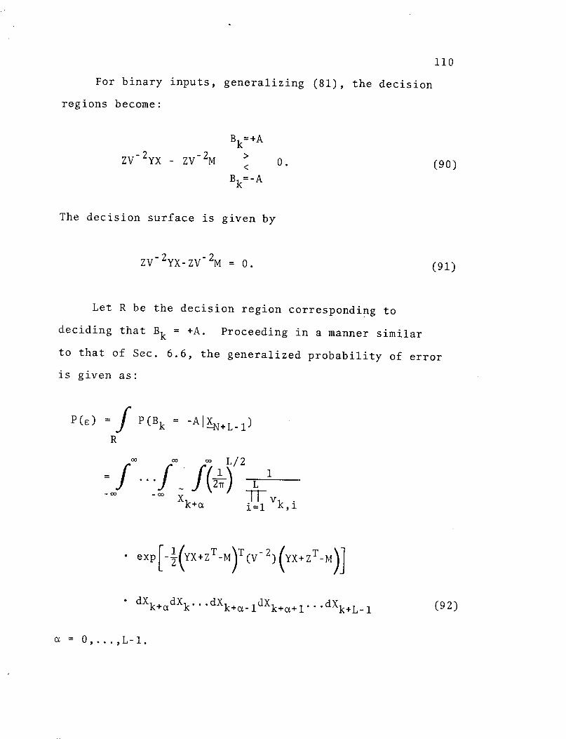
110

For binary inputs, generalizing (81), the decision

regions become:

Bk=+A

ZV-2YX - ZV 2 M > 0(90)

Bk=-A

The decision surface is given by

ZV-2YX-ZV- 2 M = 0. (91)

Let R be the decision region corresponding to

deciding that Bk = +A. Proceeding in a manner similar

to that of Sec. 6.6, the generalized probability of error

is given as:

P(E) f P(Bk = -AlN+L-1

)

R

c co 0L/2

1 f.f.j )co - ° XrVk iv

k+ot i=l Vk,i

* exp[ 1-(YX+ZTM)T(V- 2(YX+ZTM)]

* dXk+cdXk .. dXk+a-1 dXk+c +l... dXk+L- (92)

a = O,...,L-1.

111

As in Sec. 6.6, the limit on the integral, Xk+, is that

expression which is obtained for Xk+a from equation (91).

Let

w

w

and define

= V1 [ YX + T M](93)

Substituting in (92), the generalized probability of error

becomes

:P(f f ( )L// exp[(-1/2)WTW] dw+ldw.

-co -3o W +1

.. dw dw +2...dwL (94)

where the limit on the integral, w +l, is that expression

which is obtained for w +1 from the equation

zv - Z 2zT 0. (95)

Solving one obtains

112

v 2 L

W+ 1 Zk+aik v2 1i=l k ,i i=l Vk,i

i Z a+1 i c o+l

The probability can thus in theory be calculated. It may

however be necessary to calculate the probability of error

by computer using numerical techniques. As it turns out,

the probability cannot be calculated exactly but an

approximation is obtained. The performance of the pro-

cedure depends on the D. of (52) which in turn depend on

the break-up of the joint conditional probability (50).

The break-up of (50) will be examined in the next

section.

113

6.8 REDUCTION OF JOINT-CONDITIONAL PROBABILITY

It was pointed out in Sec. 6.3 that the optimum rule

maximizes p(Xk,...,Xk+LlliXl,BkXk+L,...,XN+Ll). Since

it was not known how to calculate this, it was written as

the product of L conditional probabilities-i.e.

P(Xk+jlIk-lBBk'Xk+L...XN+L Dj) (96)

for the L possible D.. This reduction of the joint

conditional probability is not unique. There are L!

possible ways to write (50) as a product of L conditional

probabilities. It is not known how to calculate some of

the P(Xk+jIXk -lBkXk+Lt...,XN+Ll- Dj) exactly. Using

equation (6) and the forward-looking and backward-looking

equations, Xk+j

can be found as a function of Bk and some

of the Xi, i.e.

Xk+j = fcn[Bk,(Dj)i] (97)

where (Dj)i is defined here to be a subset of

{Xk-l,Xk+L,...,XN+Ll, Dj}. (Dj)i contains those terms and

only those terms which appear explicitly in the transformed

equation for Xk+j. In some cases one or more of the X's

in the conditional part of (96) do not appear explicitly

in the relationship (97) for Xk+j. The conditional

probability (96), however, is not independent of the X's

114

that do not appear. Thus equation (96) was not always

able to be calculated. It can, however, be approximated

by P(Xk+j Bk,(Dj)i).

The optimum rule will be approximated by

L-1-T P(Xk+j I (Dj)i,Bk). How good an approximation this

is depends on how well P(Xk+j I Bk,(Dj)i) approximates

P(Xk+j I Xk-l,BkXk+L, ... X N+Ll Dj ) . This in turn depends

on which Dj appears in the probability expression. Thus

the closeness of the approximation depends on which of

the L! reductions of (50) is closen. Since there are

N+L-1 equations, the XN+L-1' and only N unknowns, the

BN, the relationship for Xk+j, as determined by the

recursive relationships, is not unique. For a given con-

ditional probability density,

P(Xk+jlXklBkXk+L..., XN+L 1,Dj), the closeness of

the approximation depends also on which of the several

solutions for Xk+j

is used.

For example, for the case L = 3, letting

k = Xk-l'B k'Xk+ 3 ..'' 'XN+2',

P(XkXk+lXk+2 I XklBkXk+3,...,XN+2 ) can be written in

six ways as follows:

P(Xk'X1k+l'Xk+2Dk) =P (XkIDk)p(Xk+lI Dk'Xk)P(Xk+2 Dk'Xk'Xk+l)

(98a)

115

= p(XklDk)P(Xk+21 DkXk)p(Xk+l DkXkXk+2 ) (98b)

P(Xk+ll Dk)pX kDk, Xk+l)p(X k+ DkXk+l Xk ID,Xk) (98c)

A A A

=(Xk+lID k )p

(X k+21DkX k+l)p(XklDkX k+l',k+2 ) (98d)

A A A

= p(Xk+2 IDk)p(XkIDk,Xk+2 )p(Xk+l IDkXkk+2 ) (98e)

P(Xk+21D k)P(Xk+1 1DkXk+2)P(XkIDkXk+lXk+2.( 98f)

Because of the non-uniqueness of the functional

relationships (97) for Xk,Xk+l, and Xk+ 2 there are usually

several ways to approximate one of the conditional prob-

abilities of (98). For instance, there are four ways to

solve for Xk+l which may be used to approximate

P(Xk+llXk,Xk+ 2 ,Dk). These four solutions are given in

(100). They were obtained by using combinations of forward-

looking and backward-looking equations when substituting

for Bk+l and Bkl in the equation

Xk+l = hlBk+l + h 2 Bk + h 3 Bkl + Nk+l. (99)

The four expressions for Xk+l are

N-k-l

Xk+l = h2 Bk + h1 E fi(Xk+i+3-Nk+i+3)

+ h3 gi(Xk-i-Nk-i) + Nk+l (100a)

i=l

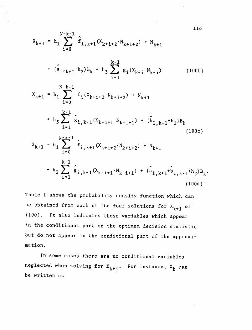
116N-k-l A

Xk+-l ' h1 2; fi,k+l(Xk+i+2 Nk+i+ 2) Nk+li=O

k-l

+ (allk+l+h2)Bk + h3 gi(Xk-i-Nk-i) (100b)i=l

N-k-l

Xk+l= hl fi(Xk+i+3 -Nk+i+3 ) + Nk+li=O

k-l

h3 + gik-l(Xk-i+l-Nk-i+l) + (bl,k-l+h2)Bki=l (lOOc)(100c)

N-k-l

Xk+l = h fi,k+l(Xk+i+2 Nk+i+2) + Nk+li=O

k-l

+ h3 gi k-l(Xk-i+l-N ki+l) + (a, k+l+bl k-l+h2 )Bk·

i=1(100d)

Table I shows the probability density function which can

be obtained from each of the four solutions for Xk+l of

(100). It also indicates those variables which appear

in the conditional part of the optimum decision statistic

but do not appear in the conditional part of the approxi-

mation.

In some cases there are no conditional variables

neglected when solving for Xk+j. For instance, Xk can

be written as

Random variables of

P(Xk+ lXkXk+2,D k )

Equation Probability densitynot appearing explicitly

in probability density

(118,1) P(Xk+IXk lBkXk+3 ... XN2) Xk, Xk+2k+3' N+2 k+2

(118,2) P(Xk+lIXk iBkXk+2, ...XN+ ) Xk, XN+2

(118,3) (X k+lliX2,...,XkB kXk+3 ....XN+2) X

1, Xk

+ 2

(118,4) P(Xk+llX2 , ... Xk,Bk,Xk+2,...,XN+ 1 ) X1, XN+2

Probability densities obtainable from equation (118)

Table I

118

Xk = hlBk + h 2 gl(Xkl 1 -Nk-1)

k-2

+ (h 3 gi + h 2 gi+l) (Xk-i-l-Nk - i - 1 ) + Nk' (101)i=l

Since by Cor. 2.3, p(XklDk) C4 p(Xkl , l)Bk), every vari-

able in the condition appears in (101). Thus p(XklXk l,Bk)

can be calculated.

It can thus be seen that there are many approximations

which can be used to approximate p(Xk,Xk+l,Xk+2lDk). The

best approximation is that which yields the lowest prob-

ability of error. One of the L! reductions of (50) must

be chosen, and for this reduction, the L conditional

probability densities must be found which minimize the

probability of error. No analytical derivation is given

as to which is the best reduction to use. A heuristic

way of specifying which expression for Xk+j

to use in

solving for the conditional probability densities is to

specify that whenever possible, the order of the equations

(of Sec. 6.4) used should be that order for which the

solution of the corresponding difference equation con-

verges. By following this procedure, the effective

variance associated with each Xk+j is minimized. Note, the

criterion for the convergence of the solution of the

first order difference equations is the same as for the

difference equation of the sequential compound case.

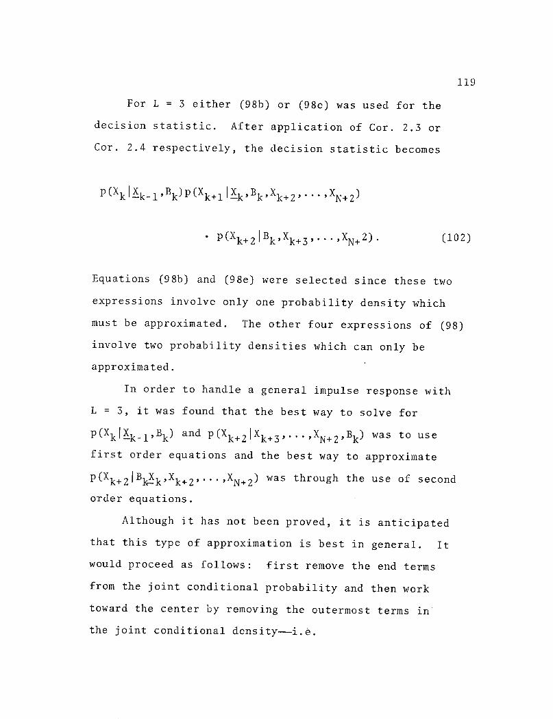
119

For L = 3 either (98b) or (98e) was used for the

decision statistic. After application of Cor. 2.3 or

Cor. 2.4 respectively, the decision statistic becomes

P(XkIk-1 ,Bk)P(Xk+l 1ik,BkXk+ 2, .. ,XN+2 )

* P(Xk+2 Bk,Xk+3 ,...,XN+2). (102)

Equations (98b) and (98e) were selected since these two

expressions involve only one probability density which

must be approximated. The other four expressions of (98)

involve two probability densities which can only be

approximated.

In order to handle a general impulse response with

L = 3, it was found that the best way to solve for

p(XkIXkl,Bk) and P(Xk+21Xk+3 ,...XN+2 ,Bk) was to use

first order equations and the best way to approximate

P(Xk+2 IBkXkXk+2,...-XN+2 ) was through the use of second

order equations.

Although it has not been proved, it is anticipated

that this type of approximation is best in general. It

would proceed as follows: first remove the end terms

from the joint conditional probability and then work

toward the center by removing the outermost terms in

the joint conditional density-i.e.

120A

P(Xk... ,Xk+L- 1 I Dk)

P(XklDk)P(Xk+l IDk'Xk'Xk+L-1) ...

.. P(Xk+L-1IDk,Xk,...,Xk+L- 3,Xk+L+l'...,Xk+L-1l) ..2 2 2

...-P(Xk+L 21DkXkXk+lXk+L-1)(Xk+L-1DkXk). (103)

Also it is expected that the best way to solve for Xk+j

is to use (j+l)th order equations to solve for

Xkj for j = 1,... L-1 and ith order equations to solvek+j

for Xk+L i for i = 1,..., 2L-

An evaluation of the sequential procedure and the

approximation to the optimum compound procedure is pre-

sented in Chapter 7.

121

Chapter 7

DATA ANALYSIS

The compound and sequential compound procedures of

Chapters 5 and 6 were evaluated. The compound procedure

presented in Chapter 6 involved the use of cumbersome

non-linear difference equations. The solutions of the

difference equations were not obtained in closed form.

Also, the evaluation of equation (94) involved an L-

dimensional integration. In general, this integral

could not be evaluated in closed form. The evaluation

of (94) may only be obtained by using numerical

integration techniques. This would mean that a large

amount of computer time is necessary in order to evaluate

the compound procedure. Because of these difficulties

the compound procedure was evaluated only for the case

L = 3. For this case, the difference equations are not

too overly cumbersome. An evaluation of the integral

of (94), though still difficult, can be made without

the cost of the resulting computer program becoming pro-

hibitive. The sequential compound procedure can be

evaluated with ease for any value of L. However, in order

to compare the sequential compound performance with the

compound performance, it too was evaluated for only the

case L = 3.

122

For the compound case, the reduction of (50) as

given in (102) was used as a decision statistic. This

decision statistic is reproduced below.

P(XkXk-_l,Bk)p(Xk+llXk,BkXk+2, ' ' ,XN+2)

* P(Xk+2 IBkXk+3,...,XN+2 ). (104)

The first term of (104), p(XkjXk_l,Bk) , is the decision

statistic for the sequential case. As pointed out in

Sec. 6.8, it is possible to calculate p(XkiXk_l,Bk). In

a similar manner it is also possible to calculate

P(Xk+2Bk,Xk+3,...,XN+2). However, since,using first

and second order forward-looking and backward-looking

equations, an explicit expression was not found for Xk+l

in terms of Xk,Bk,Xk+2, ... XN+2, P(Xk+llXk,Bk'Xk+2 , ... XN+2 )

could not be calculated. Thus in order to use this decision

statistic, approximations to p(Xk+llXBk, Xk+2 ,XN+2)

must be obtained. One type of approximation which may be

used are those approximations which may be obtained by

expressing Xk in terms of Bk and some of the following

terms: XkXk+ 2 ,...,XN+ 2 . Using these Xi's there are

four ways in which Xk+l can be expressed as a function of

Bk

. These four ways are given in (100). This in turn

yields four approximations-i.e.

123

P(Xk+l I Xk-1,Bk,Xk+3, · ,XN+ 2 ),

P(Xk+l I

P(Xk+l I

P(Xk+1 I

X2' ... Xk'BkXk+3,..',XN+2),

X 2 ,. ..,Xk,Bk,Xk+ 2 ,.. .,XN+),

Xk-1,Bk'Xk+ 2'' *'XN+l)

-which may be used to approximate

P(Xk+l I Ik,Bk,Xk+2 .. . XN+2).

For all impulse responses considered, for the four above

approximations, p(Xk+l I X 2,...,XkBkXk+2,..., XN+ 1)

proved to be the best approximation to

P(Xk+l I Ik,BkXk+i, '. XN+2) .

This is believed to be true in general. The decision

statistic which incorporates the above approximation--i.e.

P(Xk I X ki ,Bk)P(Xk+l I X2,...,XkBkXk+2,..,X N+ 1)

' P(Xk+2 I BkXk+3 ... ,XN+2 )

-will be termed an "output directed approximation" to the

decision statistic. Let Xk+lN(zk+l,kBk+ Fk+l,ke vk,2

in p(Xk+l X2 . ,XkBkXXk+2 . X ) and let v 2k~~l 2 kI kI Xk)2an let k~l

124

Vk 3 , Zkk Zk+2 k be defined as in Sec. 6.5. In order

to evaluate both the compound and sequential compound

decision procedures it is necessary to solve for

v2 = Vk 12, 2 Vk32 and the associated means Zkk,

Zk+l,k, Zk+2,k. A FORTRAN IV computer program was

written which obtained these quantities. The program was

run on Lehigh University's CDC-6400 computer. The program

was written to call, as a subprogram, a routine which cal-

culated the output-directed approximate probability of

error associated with the decision procedure. The prob-

ability of error as given in (86) involves a triple

integral. A change from Cartesian coordinates to

cylinderical coordinates results in the triple integral

of (86) being reduced to a double integral. Using a

Univac double integration subroutine, a subprogram was

written which evaluates this two-dimensional probability

of error integral. Table II shows vk i and the associated

Zk+i1l k for various impulse responses.

As a result of the calculation of the vk i , i =

1,2,3, it was found that, for all impulse responses

investigated, if N tends to infinity and if i # io,

vk 2 > . v 2 tended to a limit v 2 as N tended toVk i +

'

vki o

infinity. Here io is chosen to be equal to that value of

i for which, as N tends to infinity, the limit of vk2i

exists. This means that in the limit as N tends to

infinity only Xk+i -1 carries any information about Bk.

2 2 2hh h3v k 1Vk,l V,2 k,3 Zk,k Zk+l,k Zk+2,k

1 1.9 .95 188 4.2-104 2506 1 7.29 .953 3

.625 1 .5 13.2 2.9-10 3.6'10 .625 -.61 .5

.125 1 .25 5.1042 1.09 2-1028 .125 .935 .252 21 0.1 0.8 2.78 8.2-10 7.4-10 1 5.0 .8

42 551 0.1 -. 1 1.02 1042 10 1 .37 -. 1

1 0.1 .95 9.5 9.4-104 113 1 -.49 .95

.333 1 .25 6.6.1042 1.24 1055 .333 .816 .25

1 1.05 .025 233 18.6 1058 1 .97 .025

1 .9 -.05 9.7 1.3-103 10125 1 .95 .05

Calculated means

Table

and variances

II

O1Ln

126

Thus, for all impulse responses investigated, the three-

dimensional output directed probability of error integral

can be reduced to a one-dimensional gaussian integral which

can be solved by table look-up. Although it has not been

proved, it is expected that this divergence of all but one

of the vk i occurs for all impulse responses with L = 3.

It is anticipated that this situation holds true for larger

values of L. The complicated decision structure would then

be reduced to a classical m-state one-dimensional structure.

Note, throughout this presentation, vk 32 may be con-

sidered to be equal to infinity for N + a. This may be

seen to be not a restrictive assumption since upon studying

the region of convergence for both vk2 and vk2 itis

evident that vk 1 and v 2 can not both be convergent.

Thus if the impulse response is such that vk 3 2 would

actually be convergent the interchange of hl and h3 would

ensure that the new vk32 would be divergent and thus tend

to infinity as N + a. Furthermore, this interchange of

h i and h3 has no effect on the "output directed" or the

below described "input directed" approximations to the

probability of error. It also has no effect on the actual

performance.

For m-ary signaling, the output directed approximate

probability of error was evaluated for m=2, N=50, and k=25.

This performance is shown in FigsJ2-14 as a function of sig-

nal-to-noise ratio (SNR) (SNR =( hi2 A2 )/N where A is

i=l

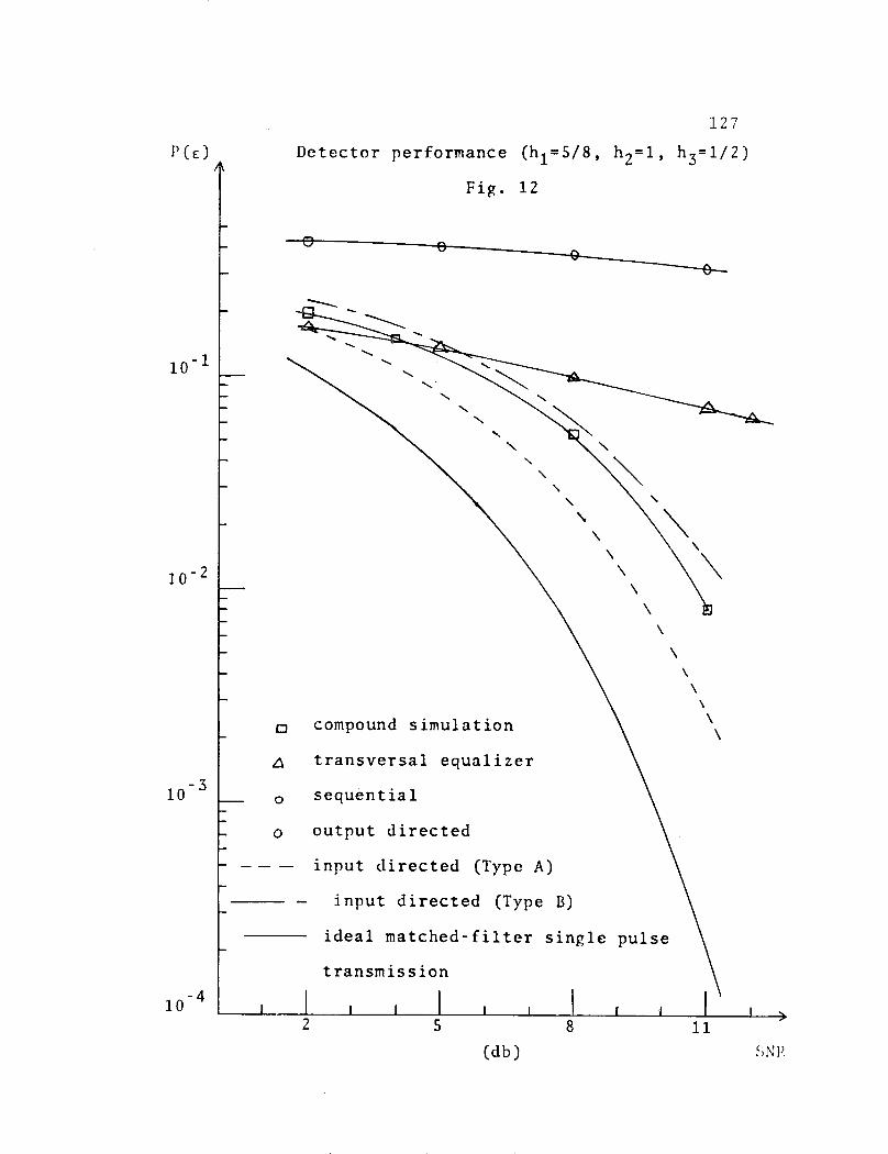
127

Detector performance (hl=5/8, h2=1, h3=1/2)

Fig. 12

e -- ---

N\

\ \

\N " \'

o compound simulation

b transversal equalizer

_ sequential

o output directed

- - -input directed (Type A)

- input directed (Type B)

ideal matched-filter single pulse

transmission

I I I I I II2 5 8

(db)

p(E)

1O-1

10-2

-310

I I

11L

'SNP

128

P(E) * Detector performance (h1 -1/8, h2-1, h3=1/4)

Fig. 13

10'1

10- 2

o compound simulation

10-3 A transversal equalizer

.- -- sequential

-o output directed \

input directed (Type A)

-- input directed (Type B)

ideal matched-filter single pulse

,q4 i transmissio

2 5 8 11

(db) SNR

129

Detector performance (hl.l, h2 =0.1, h3=0.8)

Fig. 14

- _~

13 compound simulation

a transversal equalizer

o sequential

- O output directed

input directed (Type A)

_ --input directed (Type B)

ideal matched-filter single pulse

transmission

l l I I l2 5 8

I

11

(db)

P (E)

-110

-210

-310

ISNR

130

the magnitude of the input signal voltage and No is the

noise power) for three different impulse responses. These

graphs also show, as an absolute lower bound to the actual

probability of error, the probability of error associated

with the matched filter single-pulse-transmission case.

A program was written to simulate a transversal

equalizer which uses, as a criterion for setting the tap

gains, a minimization of the mean square error due to both

intersymbol interference and noise [3]. The results of

the simulations are shown in Figs. 12-14. All simulations

were made with 15 taps on the TDL of the equalizer.

Another program was developed which simulates the

compound decision procedure. The results of these simula-

tions are also plotted in Figs. 12-14. For these simula-

tions N was taken to be equal to 30. The probability of

error that is plotted is the probability of error averaged

over all B's.

For all three impulse responses, the output directed

approximate performance is larger than the actual

simulated performance. It is interesting to note that for

low SNR the calculation and simulation are in better

agreement than for high SNR. The simulated performance of

the transversal equalizer falls between the output directed

calculation and the simulation of the compound procedure.

The closeness of the calculation to the compound simulation

depends on the impulse response.

131

The results also demonstrate that the transversal

equalizer performs close to the optimum compound procedure

at low SNR but deviates markedly from the optimum compound

procedure at high SNR. Thus at high SNR, where the dis-

turbance caused by intersymbol interference in much

greater than the disturbance caused by additive noise,

neither the transversal equalizer nor the output directed

calculation approximates the true performance as well as

at low SNR.

As can be seen, for the impulse responses of Fig. 12

and Fig. 14, the output directed calculation does not give

a very good approximation to the actual compound perform-

ance. Moreover, since p(Xk+l I XkBkXk+2,...XN+2) can

only be approximated while the other two probability terms

of (104) can be calculated, this discrepancy, for these

impulse responses, is due partly to the fact that the

approximation used for p(Xk+l I XkBkXk+2 ,...XN+2) is

not good enough. Accordingly other approximations must be

sought for p(Xk+l I XkBk Xk+ 2 ,.,NXN+2 )

A type of approximation which has proved fruitful is

attained by allowing input symbols to become part of the

condition on Xk+l. That is,p(Xk+l I XkBkXk+2 ,..XN+ 2 )

will be approximated by p(Xk+l I XkBNXk+2 ,... N+2) or

by P(Xk+ I Xk'B1,.. .,Bk 2 ,Bk,...,BNXk+ 2,... XN+2 )-

These types of approximations will be termed "input

directed approximations". Note

132

P(Xk+l I k'!,N'Xk+2,'' ,XN+2 ) = P(Xk+l I Bk+lBkBk-1) and

P(Xk+l I kBl...,BNk'2Bk ... ,BNXk+2',..XN+2 ) can be

shown to be equal to

P(Xk+l I Bk,Bk_2,Bk_3,Bk+lXkXk-l) . (105)

Just as it was impossible to calculate

P(Xk+l I jkBkXk+2 .. XN+2 ) because X k+ could not be

explicitly expressed in terms of Xk,Bk,Xk+2,...,XN+2,

P(Xk+l I Bk'Bk-2,Bk-3,Bk+lXk,Xkl1) also can not be cal-

culated because Xk+l can not be explicitly expressed in

terms of Bk Bk -2Bk- 3 ,X k, Xkl1

Thus approximations to

P(Xk+l I BkBk_ 2,Bk-3,Bk+lXk,Xk l) are necessary. Two

approximations which are of interest are

P(Xk+l I BkBk+lXk,Bk_2) and

P(Xk+l I BkBk+lXk-lBk_2 2 Bk_ 3) Note,it is necessary

that Bk+l appears in the condition of (105) since if it

didn't Xk+2would appear in the condition of the approxima-

tion to (105). Since Xk+2 does not provide information

about Bk (Vk,32 + A) use can not be made of Xk+ 2. This

necessitates the use of Bk+l in the condition of (105).

There are thus three input directed approximations for

P(Xk+l I jk,BkXk+2 ...,XN+2) which are of interest.

These approximations are

P(Xk+l I Bk+lBkBk-1) (106a)

133

P(Xk+l I Bk+lBk,XkBk-2) (106b)

P(Xk+l I Bk+lBkXk-l,Bk_2 2 Bk_3). (106c)

Note, equation (106a) will be called a Type A input

directed approximation and (106b,c) will be designated as

Type B. For each impulse response one of the expressions

of (106) must be chosen to approximate

P(Xk+l I ~kBkXk+2 ... ,XN+2 ) in (104). This expression

should be that expression of (106) for which the input

directed approximate performance is closest to the actual

simulated performance.

In order to specify which is the best type of input

approximation to use, the concept of amount of information

which a probability density provides about Bk must be

developed. For the case of Bk = +A and Bk = -A, two

probability densities can be obtained for each of the

expressions in (106). The amount of information in each

of the expressions of (106) can then be heuristically

specified as being proportional to the ratio of the distance

between the means to the standard deviation of the distribu-

tion. Since

134

Xk+l = hlBk+l + h2 Bk + h3 Bkl + Nk+l (107a)

hlBk+l + h2 Bk + (h3 /hl)(Xkl - Nkl) + Nk+l (107b)

= hBk+ + (h2 -hlh3 /h2)Bk + (h3 /h2)(Xk-Nk) + Nk+l

(107c)

this ratio can be given as in Table III for the impulse

responses studied.

For all impulse responses investigated, the Type B

input directed approximation which provides the most in-

formation about Bk generally proved to be the best input

directed approximation. If the amount of information

about Bk provided by the Type A approximation is greater

than that provided by Type B, then Figs. 12 and 13 seem

to indicate that at a high enough SNR a Type A approxima-

tion would be the best to use. Thus, the rule that is

used to select the best input directed approximation is-

select the Type B approximation which provides the most

information about Bk; however, if Type A provides more

information about B than does Type B and the SNR is high

enough, select Type A. For the SNR studied, Table III

gives the best input directed approximations which were

obtainable for the indicated impulse responses.

The input directed performance calculations are shown

in Fig. 12-14. It can be seen that this input directed

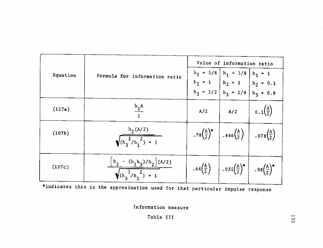
Value of information ratio

hi = S/8 h1= 1/8 hi = 1

Equation Formula for information ratioh

2= 1 h

2= 1 h 2 = 0.1

h3 = 1/2 h3 = 1/4 h3

= 0.8

(117a) h2A A/2 A/2 0.12

h2 (A/2) (fA\ A A(107b) 2 /h 2) * .7 8 (A) .446) .078A

(h /h) + 13 1

[hz (h h3)/h 2J(A/2) (A)* A(107c) .642 .9352 .98

*indicates this is the approximation used for that particular impulse response1

*indicates this is the approximation used for that particular impulse response

Information measure

Table IIIU1t~

136

performance approximation agrees very well with the actual

simulated performance. Discrepancies may be due to sample

size problems in the simulated performance. It thus

appears that a good approximation to the compound perform-

ance has been found. It is anticipated that this type of

approximation will, in general, give a good indication of

the actual performance.

Fig. 15 shows the matched filter single-pulse-trans-

mission performance, simulated actual performance, and

performance of a transversal equalizer for hi = h2 = h3 = 1.

This is a channel which Austin [12] defines as having

maximum distortion. It is interesting to note that this

channel yields better performance than does one with a

h = 5/8, h2

= 1, and h3

= 1/2 impulse response.

For each of the four above impulse responses Figs.

16-19 show the ideal single-pulse-transmission performance,

the simulated actual performance and the calculated per-

formance of a theoretical scheme whereby the energy in the

sidelobes of the impulse response would be exactly sub-

tracted out of the received signal. There has been

speculation that the best that one could do at the receiver

is to subtract out this energy in the sidelobes. These

results show that this is not so. For the impulse responses

of Fig. 16 and Fig. 17, the compound procedure does better

than simply subtracting out the sidelobe energy. For the

impulse response of Fig. 18 the compound procedure yields

Detector performance (hl=h2=h3=l)

Fig. 15

O compound simula

a transversal equ;

ideal matched-f

pulse trai

I I I I2 5

tion

alizer

ilter single

nsmission

1 II I I l l8

(db)

137P(E)

-110

-210

-310

0-41011

SNR

138

Comparison of compound procedure with other

types of detection (h1-1, h2 -0.1, h3

-0.8)

Fig. 16

compound simulation

ideal matched-filter single

pulse transmission

-subtraction of sidelobe energies

from received signal

I I l I I I I2 5 8

I I I

11(db)

P()- 1

-l10

-210

-310

L

0 �

I

I

SNR

139

P(E) Comparison of compound procedure with other

types of detection (h1 =h2 =h3 =1)

Fig. 17

-110

'1

-210

-3 a compound simulation10

10 ideal matched-filter single

pulse transmission

_ - subtraction of sidelobe energies

from received signal

10-410 I, 2 5 8 112 5 8 11

(db) SNR

140

Comparison of compound procedure with other

types of detection (h1-1/8, h2 -1, h3-1/4)

Fig. 18

a compound simulation

ideal matched-filter single

pulse transmission

_____ - subtraction of sidelobe energies

from received signal

I I5

,I I 8

(db)11

SNR

P (c)

-110

-310

I2

m

I I l

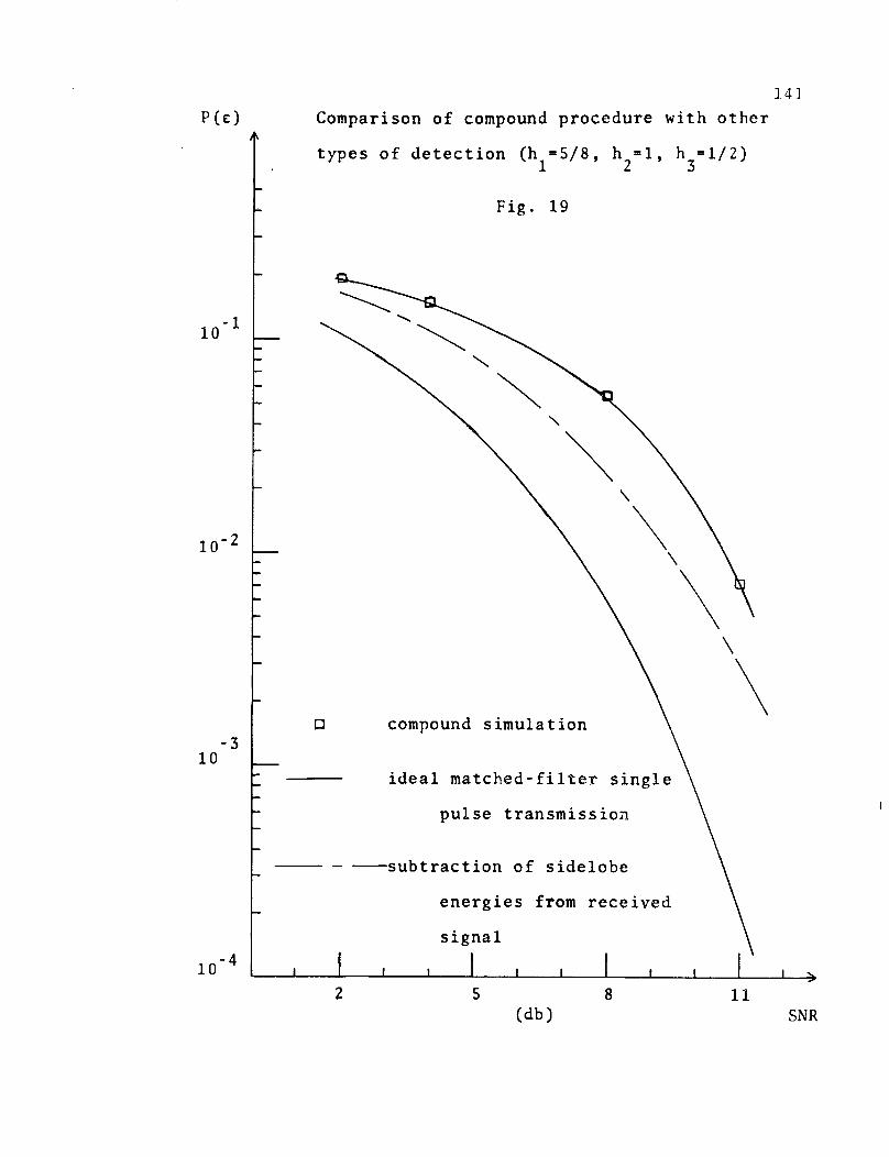
141

Comparison of compound procedure with other

types of detection (hl=5/8, h2=1, h3=1/2)

Fig. 19

compound simulation

ideal matched-filter single

pulse transmission

_ - -subtraction of sidelobe

energies from received

signal

I I l II I I I I 2 5 8

I11

(db)

p(c)

-110

10-2

-310

0-410 I \

SNR

142

essentially the same performance as that which would occur

by subtracting out the energy. In Fig. 19, the decision

procedure does not work as well as that procedure which

would result if the sidelobe energy could be exactly sub-

tracted out. However, Fig. 19 does show that, as the SNR

is increased, the optimum procedure does approach that per-

formance which would result if the sidelobe energy could

be exactly subtracted out of the received signal. Figs.

16-19 indicate that as the SNR is increased to a high

enough value it is likely that the optimum compound

detector will always do better than subtracting out the

energy in the sidelobes. It is not known how to specify,

for an arbitrary impulse response, what this value of SNR

would be.

The results indicate that a very good approximation

to the actual performance can be found. This was true for

each of the impulse responses investigated and it is

expected to be true in general for impulse responses with

L = 3. Also, a similar procedure should be obtainable for

L > 3. The results also show that the compound detector

does better, in some cases, than just subtracting out the

side-lobe energy. Finally, the compound performance was

shown to be poorer for a channel with h1 = 5/8, h2

= 1, and

h3 = 1/2 than for a channel with hl=h2=h3=l. Thus Austin's

[12] maximal distortion channel does not yield poorest per-

formance. This seems intuitively surprising since a channel

143

with maximal distortion would intuitively be expected to

yield a poorer performance than a channel with another

impulse response.

Suggestions for further research into noisy inter-

symbol interference channels are given in Sec. 8.2.*

All computer programs used in this study will be availablefrom the authors' files for five years.

144

Chapter 8

CONCLUSION

8.1 SUMMARY

This report has considered the transmission of m-ary

symbols over a baseband communication system which induces

intersymbol interference over L adjacent symbols. While

research in this field has by no means been exhausted by

this work, results which are significant and which

should aid in further research into the noisy intersymbol

interference problem have been attained. Both one-shot

and multi-shot transmission were considered. For multi-

shot transmission sequential compound decision theory was

used to specify the decision regions and to calculate the

associated probability of error. The performance can be

calculated for any value of L. In order for this pro-

cedure to be applicable, the sampled values of the impulse

response must fall within a L-dimensional region. This

region is specified for L = 3,4,5 and 6. The multi-shot

detection problem was reduced to a classical m-state

classification problem.

The case of one-shot transmission was also studied.

Here, through the use of decision theory, the optimum

decision statistic was also obtained. Since this

145

statistic can not be calculated exactly, output directed

and input directed approximations are made in order to

estimate the probability of error in the one-shot trans-

mission case. The output directed approximation makes

use of only received signals in arriving at the approxi-

mate probability of error. The input directed approxima-

tions assume that some of the input symbols are known at

the receiver. The input directed approximations make use

of these input symbols in arriving at the probability of

error calculation. The closeness of the approximation

to the actual simulated performance depends on the nature

of the impulse response. Note, knowledge of the inputs

is not necessary at the receiver in order to calculate

the input directed probability of error.

In the output directed approximation, it was found

that for all impulse responses considered, as N tends to

infinity only one of the sampled outputs provides any

information about Bk. This reduces the output directed

approximation to a simple one-dimensional decision problem.

Although this was only investigated for the case L = 3,

it is expected that this type of reduction of the output

directed approximation will be valid for any value of L.

For all cases considered the input directed approxi-

mation was very close to the actual simulated performance.

For only one of the impulse responses considered did the

output directed approximation give a good indication of

146

the actual performance. It is expected that, in general,

the input directed approximation will yield a close

approximation to the actual performance. This is a

significant result since with this approximation the

optimum performance can be calculated with ease. This

knowledge would be useful if one is faced with the

problem of choosing one of several different channels

over which to transmit data. It also provides a standard

with which to compare other sub-optimal filtering and

detection techniques.

It was also found that at low SNR the transversal

equalizer and the compound procedure yielded essentially

the same performance. At higher SNR the compound pro-

cedure was found to perform considerably better than did

the transversal equalizer.

Another significant result of this research was that

the performance, for some impulse responses, was found to

be better than that which would be obtained if the

decision could be made after the sidelobe energies would

be exactly subtracted out of the received signal. This

disproves the idea currently held by some that the best

that one could do would be to subtract out the energy in

the sidelobes of the impulse response and then make a

decision about the input. The results also indicate that

the compound performance does not achieve the performance

that would be obtained by matched filter detection of a

147

single transmitted pulse; although, in some cases, the per-

formance of the two is quite close. This would disprove

another theory held by some that the compound procedure

somehow gathers up all the energy at the output due to

each input and then makes a decision about the input based

on this collected energy (as a matched filter does when a

single pulse is transmitted). However, the optimum com-

pound procedure does make use of some of the dispersed

energy.

148

8.2 SUGGESTIONS FOR FURTHER RESEARCH

There are questions which this research leaves

unanswered. Probably the most obvious area in which

further work could be done is in the extension of the

work on compound detection to impulse responses with L

greater than three. It would be desirable to study the

solution of the higher order difference equations with

the aim of finding, if possible, for what impulse responses

the solutions of the difference equations converge. It

would perhaps also be interesting and fruitful to inves-

tigate approximations to the compound procedure and to

compare these approximations with the simulated actual

performance and with the performance of the transversal

equalizer for these higher values of L.

As noted in Sec. 2.2 complex valued impulse responses

may occur in baseband systems. These types of impulse

responses do not lead to conceptual difficulties but

mathematical difficulties may arise. With a complex

impulse response, each of the Xk+i, i = 0,...,L-l, are

vector random variables. Instead of the Xk+i being

normally distributed, the Xk+i have a bivariate normal

distribution. The sequential procedure would then involve

m different bivariate normal distributions with simple

m-state classification procedures being applicable. The

149

compound procedure of Sec. 6.5 would become a decision

procedure in 2L dimensional space with m states of nature.

The associated probability of error would be an integra-

tion over this expanded space. The specific details of

this procedure could be investigated in further research.

The optimum sequential decision procedure has been

investigated in this report. In some cases of data recep-

tion a delayed sequential rule-i.e. one where Xk+D is

available when the decision on Bk must be made-is applic-

able and desirable. This delayed sequential procedure is

in one sense an approximation to the compound procedure.

This delayed sequential procedure could be investigated

with a view to calculating or bounding the associated

probability of error.

Since the input directed approximation gave good

results, an area which may be fruitful for further work

is an investigation of 'h1 e optimum classification method

and the associated probability of error for a decision

feedback procedure and for a recursive type of decision

procedure. The recursive procedure would make a prelimin-

ary decision about the input symbols. Based on these

decisions and the channel output a second level decision

could be made about each input symbol. These decisions

could in turn be used to arrive at a third level decision.

This recursive process could continue to the M-th level.

The probability of error associated with the M-th level

150

decision could be investigated to determine if it approxi-

mates the performance of the optimum compound procedure

and, if it does, the convergence of the approximation to

the actual performance could be investigated as a function

of M.

Further work could be done for the case of L = 3. It

would be interesting to know how the shape of the impulse

response affects the behavior of the compound rule in

relation to a scheme which subtracts out the energy in

the sidelobes.

Finally this work could be extended by studying, for

L = 3, m-ary transmission, m > 2, and comparing actual

compound performance, the calculated compound performance,

and the performance of the transversal equalizer.

The problem of communication over a noisy intersymbol

interference channel has by no means been solved in this

report. This work does bring one a step closer to an

easier evaluation of sub-optimal detection procedures

which have been or will be proposed. This work will also

serve to indicate how the channel impulse response might

be shape-d in order to achieve good data communication.

151

APPENDIX A

SEQUENTIAL DIFFERENCE EQUATION

The derivation of the difference equation, (34), of

Sec. 5.5 is presented. The difference equation is

reproduced here as

hLd i + hL ldi- 1 +...+ hldi-L+l = 0. (A-1)

Applying the transformation of Sec. 5.6, (A-1) becomes

h. + h2ci- +..+ hLciL = 0 .1 2 h Li-L+l (A-2)

The derivation of (A-2) is considered. After establishing

(A-2), (A-1) can be obtained by applying a transformation

to (A-2). The analysis is given below.

From (6) the following expressions are given

Xk =hlBk + h 2 Bk-l +...+ hLBkL+l + Nk (A-3)

Xk-l = hlBk 1l + h2 Bk_ 2 +...+ hLBk L+ Nk-l (A-4)

Xk-2 hB k + hBk +...+ h B + N (A-5)1 k-2 2 k-3 L k-L-1 k-2

From (A-4), Bk_1

is found to be

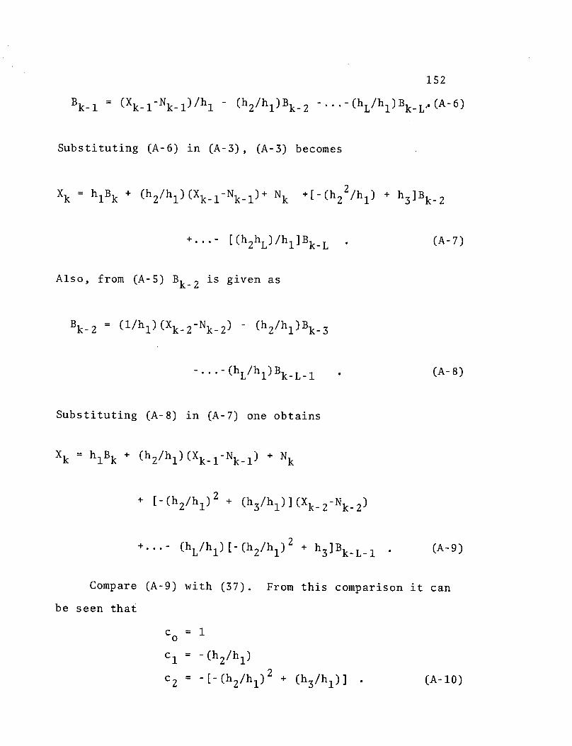
152

Bk-l = (Xkl-Nk-l)/hl - (h2 /hl)Bk 2 -...- (hL/hl)BkL.(A-6 )

Substituting (A-6) in (A-3), (A-3) becomes

Xk = hlBk + (h2 /hl)(Xk-l-Nk-l)+ Nk

+'..- [(h2 hL)/hi]Bk-L

Also, from (A-5) Bk_2 is given as

Bk_2

= (1/hl)(Xk_2 -Nk-2 ) - (h2 /hl)Bk-3

·'.-(hL/hi)Bk- L-1

Substituting (A-8) in (A-7) one obtains

Xk =hlBk + (h2 /h1 )(Xk-l-Nk_ 1 ) + N k

+ [-(h2 /h 1 )2 + (h3 /hl)](Xk-2 Nk-2 )

+...- (hL/hl)[-(h2 /hl)2 + h 3 ]Bk-L_1

+[-(h22/hl) + h 3 ]Bk- 22 1 k-

(A-7)

(A-8)

(A-9)

Compare (A-9) with (37). From this comparison it can

be seen that

1

c1

= - (h2 /hl)

c2 = -[-(h2 /hl) 2 + (h3 /hl) ](A-10)

c =O

153

The equations in (A-10) can be rewritten in difference

equation form as:

c =O

1

hlc1 + h 2 co = 0

hlC2 + h 2 c 1 + h 3 co

= 0.

Assume that for any j, such that j < L,

Cj_l = (-l/hl) (h2 cj- 2 + --+ hjco),

then the following equations apply

a-l

Xa hlB + c i(Ni-Xi) +Na

i=l

for all a ' j. Thus

a

Ba = - (C1,-i/hl)(Ni-X i )

i=l

for all a < j. From (6), for j < L,

Xj+l = hlBj+l + h2Bj

+ h3Bjl +...+ h B + hj+lB 1 + Nj+l ·

(A-15)

(A-15), the expression for Xj+l becomes

(A-ll)

(A-12)

(A-13)

(A-14)

Using (A-14) in

Xj+1 = hlBj+1 - (h 2 /hl) 2 cj- i (N i -X i )

i=l

j-1

- (h 3 /hl) Ei=l

Cj. i -1 (Ni-Xi)

2

...- (hj/hl) E c2- i(Ni-Xi)

i=l

-(hj+l/hl)o(N1-Xl) + Nj+l. (A-16)

After expanding (A-16) the coefficient of (N1-X1) is

- (h2 /hl)cj_1 (h3/hl)cj-2 (hj/h1 )c

1- (hj+l/hl)co .

(A-17)

By definition this equals cj. Thus, by induction

Cjl = (-l/hl)(h2cj - 2 +...+ hjCo) (A-18)

for any j " L. In particular for j = L, the following

equation has been established

hlCL-l + h2 cL +...+ hLc = 0 .1 L-1 2 L-2 (A-19)

Now consider j > L and assume that

Cj_1 = (-l/hl)(h2 cj_ 2 +...+ hLCj-L) (A-20)

Then the following equation applies for all a 5 j.

154

Ba = (ce-i/hl) (Ni-Xi)

i=l

From (6)

Xj+ 1 = hBj+l + h2Bj +...+ hLBjL+2

Using (A-21) in (A-22), the expression for Xj+l becomes

Xj+1 = Nj+1 + hlBj+1 -(h2/hl) t cji(Ni-Xi)

i=l

-(h 3 /hl) ' cj i- 1 (Ni-Xi )

i=l

j-L+2

-...- (hL/h) =

i=lCj-i-L+2(Ni Xi) . (A-23)

After expanding (A-23) the coefficient of (N1-X1) is

-(h 2 /hl)cjl-1 -(h 3 /hl)cj 2 -''- (hL/hl)cj -L+l (A- 24)

By definition, this is equal to cj. Thus

hlcj

+ h 2 cj- 1 +...+ hLcj-L+l = 0 (A-25)

and (A-2) has been proven by induction. Apply the trans-

formation (i) - k - (i) to (A-25) and change the variables

from ci to di. The following equation results:

hLdj + hLldj_ 1 +...+ hldj-L+l

155

(A-21)

(A-22)

(A-26)

156

This is the same as (A-i) and the difference equation is

thus derived.

157

APPENDIX B

CONVERGENCE OF v2

Necessary and sufficient conditions for the conver-k

gence, as k + -, of v2 = di 2 are presented below.

From Sec. 5.6, i=l

k2 = L di2

i=l1i=l

0

i2

i=O

k-l oo

= E c 2 and lim v2 =k+ =oo

i=0 i=O

2c.i1

L-1

= 1 E Fj2 rj2i cos 2 (iOj + Ej)i=0 j=1

L-1 L-12 : E=

j=l c=l

iFF a(rjr ) cos(iOj + Ej)

c os (iOc + E)

L-l 2 2ia2L-1 co

= F2 rj cos2

(iOj + Ej)j=1 i=0

L-1 L-1

+ 2 E FjFa

j=l a=o

./j

0o

L=d (r r )i=O

cos (iOj + Ej)

cos (iOa + E ) . (B-1)

co co

Since E (r. 2 )i cos(iO. + Ej) (r 2)i

i=O i=O

(B-2)

co

+2Ei=O

158

co

and since E (rj 2 ) i converges if r. < 1 each of the L-1i=O

infinite series in the first term of the right hand side

of (B-1) converges if, for all j, -1 < rj < 1.co

Also since (rjr ) cos (iej + Ej)cos(iOa + E+ )i=O

(B-3)

<E (rj r) i

i=Oco

and since E (rjr )i converges if Ir rjj < 1, each ofi=0

the 2(L-1)(L-2) infinite series in the second term of the

right hand side of (B-l) converge if, for all

j, -1 < rj < 1. Thus if the roots of the auxiliary

equation fall within the unit circle in the z-plane

v2 will converge to some limit as k tends to I.

The convergence of E ci2 (or lack thereof) for thei=O

case in which one or more of the roots of the auxiliary

equation fall on or outside the unit circle will now be

investigated. Let rj, = max {rj} then

E (ci/rij) = 2 F2, cos2(iGO. + Ej )

i=O i=O

CO L 2

E F 2 (r/rj )2i cos2 (ioj + Ej)i=O j=l

joj'

159

L-1 L-1 i

+2 E E E FjFa(rjr /rji,2) cos(iOj + Ej)cos(iOa + Ea)

afjBy arguments identical to those given above, all of the

L-1 infinite series of the second term of the right hand

side of (B-4) and the 2(L-1)(L-2) infinite series of the

third term of the right hand side of (B-4) converge. It

remains to investigate F E cos2(ij' + Ej,).

i=O

Since cos (iOj, + Ej,) is an undamped function

the infinite series, E (ci/rj,)2, diverges [24]. Then

i=O X

by Thm. 39, p. 29 of Fort [27], E ci2 also diverges.

i=0

Thus a necessary and sufficient condition for the con-

vergence of v2 is that the roots of (37) fall within the

unit circle in the z-plane.

160

APPENDIX C

SUFFICIENT CONDITION FOR CONVERGENCE OF

DIFFERENCE EQUATION SOLUTION

The problem is to find conditions under which the

solution of the difference equation

Cn+L- 1 + alCn+L-2 +...+ aL-1 Cn = 0 (C-l)

satisfies

C Cn2 <n=O

00o

Here ai = hi+l/hl. The general solution of (C-1) is1 ~/l h eea slto f(-)i

nml-1+...+ n alml)Cn = n1 (all + n1l2

n n( "21 m2 -1+ Z2 n( m21 + na 2 2 +-.. + n a2m2)

+...+ Z k (ekl + nk2 + ' ' ' + n km)'k

where Zl,. ..z k are the distinct roots of

L-1 + a zL-2b-i~~ +...+ aL-2Z + aL-l = 0 (C-2)

with respective multiplicities ml,...,mk (ml +...+ mk = L-)

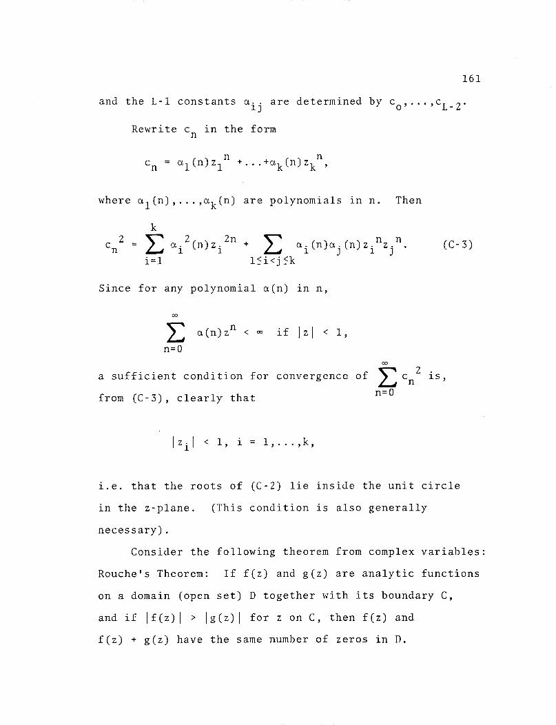
161

and the L-1 constants cij are determined by Co,. .. CL 2 .

Rewrite cn in the form

Cn = al(n)zln +...+ak(n)zkn ,

where al(n),...,ak(n) are polynomials in n. Then

k

2 =E Caii(n)zin ai(n)aj(n)z (C-3)

i=l l<i<j<k

Since for any polynomial a(n) in n,

0o

E: ua(n)zn < Xc if Izl < 1,

n=O

a sufficient condition for convergence of E cn2 is,

from (C-3), clearly that n=0

IZil < 1, i = 1,...,k,

i.e. that the roots of (C-2) lie inside the unit circle

in the z-plane. (This condition is also generally

necessary).

Consider the following theorem from complex variables:

Rouche's Theorem: If f(z) and g(z) are analytic functions

on a domain (open set) D together with its boundary C,

and if If(z)l > jg(z)l for z on C, then f(z) and

f(z) + g(z) have the same number of zeros in D.

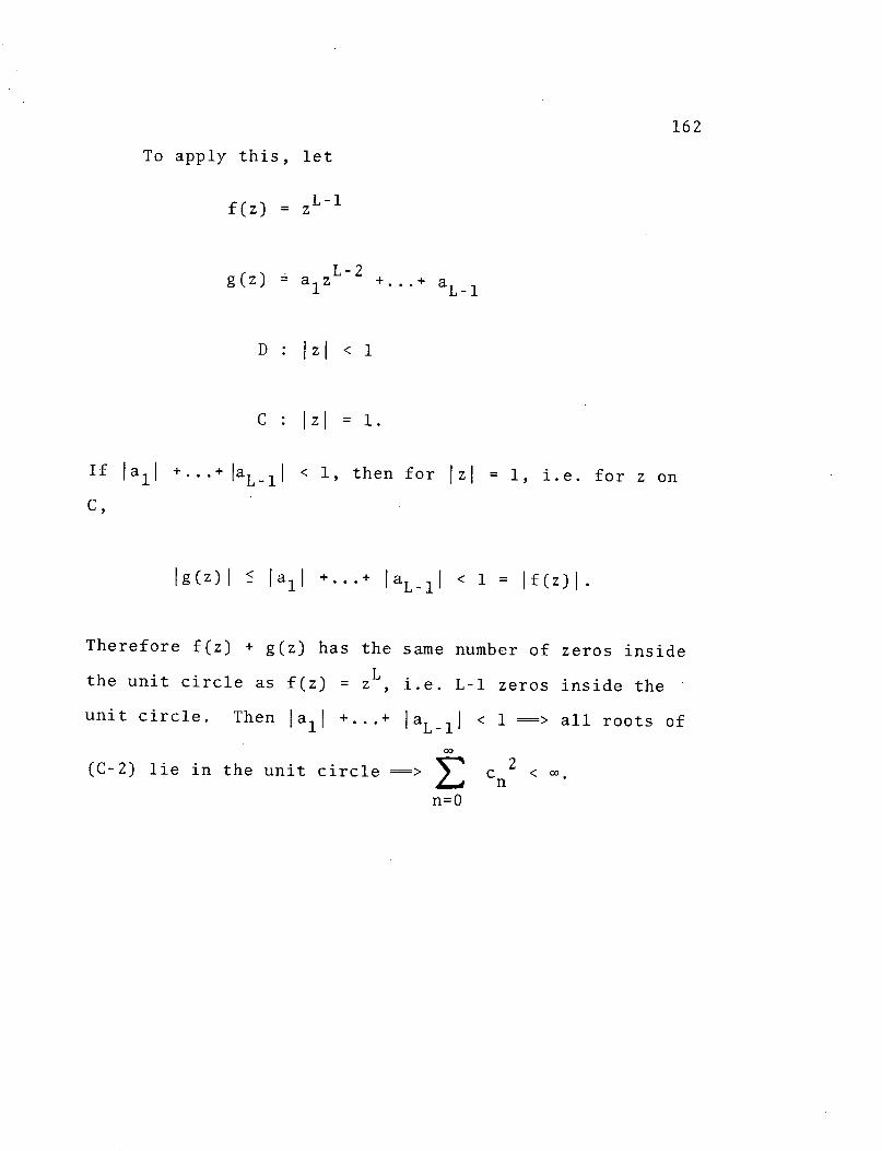
162

To apply this, let

f(z) = zL-l

g(z) = alz +...+ aLl1

D : Izl < 1

c: IZ = 1.

If all +...+laL-11

C,

< 1, then for Izl = 1, i.e. for z on

Ig(z)l < lall +...+ laL-ll < 1 = If(z)l.

Therefore f(z) + g(z) has the same number of zeros inside

Lthe unit circle as f(z) = z , i.e. L-l zeros inside the

unit circle. Then lall +...+ laL- 1 l < 1 => all roots of

0oo

(C-2) lie in the unit circle = > En=O

c 2 < 0.n

163

APPENDIX D

PROOF OF THEOREMS

Using the notation of Sec. 6.2, the proof of the

theorems presented in that section are given below.

Thm. 1

a.) p(Xk+L+i I Bk) = P(Xk+L+i)

b.) P(Xk_i I Bk) = P(Xk-i)

i = 0,1,...,N-K-1;

i = l,...,k-l.

Proof Part a:

p(Xk+L+i I Bk)

Bk+L+i

Bk+L+

] P(Xk+L+i,Bk+i+l, . . Bk+L+i I Bk)

Bk+i+l

P(Bk+i+l .''B. k+L+i I Bk)

i Bk+i+l

P(Xk+L+i I Bk+i+l'... Bk+L+iBk) .

By (6) and the assumption of independent inputs,

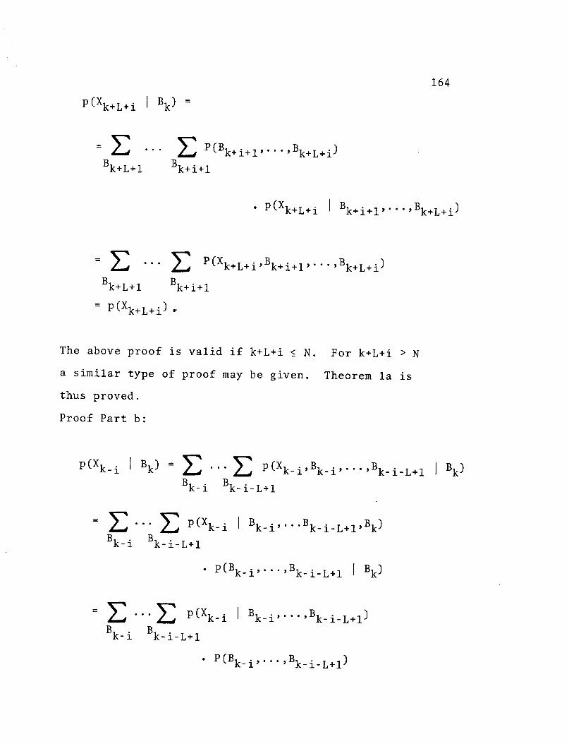
164

P(Xk+L+i I Bk)

E ... P(Bk+i+l ... Bk+L+i)

Bk+L+1 Bk+i+l

* P(Xk+L+i I Bk+i+l'. ,'Bk+L+i)

= *** ' P(Xk+L+i'Bk+i+l'... 'Bk+L+i)

Bk+L+l Bk+i+l

= p(Xk+L+i) .

The above proof is valid if k+L+i < N. For k+L+i > N

a similar type of proof may be given. Theorem la is

thus proved.

Proof Part b:

P(X ki I B k ) : P(Xk-i'Bk-i'.' ' Bk-i-L+l Bk)

Bk-i Bk-i-L+l

:= '' ' ~ p(Xk-i I Bk-i,'..Bk-i-L+1,Bk)Bk-i Bk-i-L+l

p(Bk-i, .B k- i-L+ 1 I Bk)

= ''' . P(Xk-i I Bk-i,...,Bk-i-L+l)

Bk-i Bk-i-L+l

P(Bk-i,...,Bk-iL+l)

165

= j... C P(Xk-i'Bk-i'.' . Bk-i-L+l)

Bk-i Bk-i-L+

= p (Xk-i)

The above proof is valid if k-i-L > O. For k-i-L < O, a

similar kind of proof may be given. Theorem 1 is thus

proved.

Thm. 2

p(XI ) = P((XN+L-l)j I (B)j ) P((XN+L-1)k)

Proof:

From the definitions of (XN+L-l)k and (XN+L-_)j, U kUj j

Let (B)j = Uj - (B)j, then

p(XIO) = P((XN+L-l)j(XN+L-l)kl(B )j,(B)M)

= ~ P((XN+L-l)j'(XN+L-l)k'Uk,B)I(B)j,(B)M)

Uk (B)j

= C P(Uk,(B) iJ(B)j,(B)M)Uk (B)j

P((XN+L_)j,(XN+L i)kBUk,(B)j,(B)j,(B)M) .

Since independent inputs are assumed,

P(Uk,(B)jl(B)j,(B)M) = P(Uk)P( B)j)

= P(Uk)P((B)ji(B).

166

Also since Uk and Uj statistically specify (XN+L-l)j and

(XN+L-l)k (by definition)

P((XN+L-l)j(XN+L l)k lUk, (B)j,(B)j ,( B ) M )

= P((XN+L-l)j,(XN+L-l)klUk,(B)j,(B ) j).

Thus

P((XN+L-_)j, ( X N + L-l) k l(B)j,(B)M) =

= E E P(Uk)P((B)jI(B)j)Uk (B)

P((XN+L-l) j,(XN+Ll)klUk, (B)j, (B)j)

E E CP(Uk)P((B)jl(B)j)p((XN+L-)jIUk, (Bj),(B) j

Uk (B)j

p ((XN+L 1) k IUkUj (XN+L-l)j)

= E E P(Uk)P((B)jI(B)j)p((XN+L-1)jl(B)j,(Bj)U

k (B)j

P((XN+L-l)klUk)

= E EP((XN+Ll)j,(B)jI(B) j)P((XN+L-l)k'Uk)Uk (B) j

167

: C P((XN+L-l)k'Uk) P((XN+L-l)j'(B)jI(B)j)

Uk (B)j

= P((XN+L-l)kUk)P((XN+LN+L)jI(B)j)

Uk

= P((XN+L- 1 )j I(B)j) P((XN+L-1)k'Uk)Uk

= P((XN+Ll)jI(B) j)P((XN+L-)k) q.e.d.

Cor. 2.1 p((Xki)jIBk) = p((Xki)j)

Proof: Let (Xki)j be equal to X and let Bk be equal

to B in Theorem 2. Note that Uj Bk = . Then

p(XIB) = P(Xk i)j lBk)

= C P((Xki)jUj IBk)

U.J

= C P(UjlBk)P((Xk-i)j IBkUj)U.

= C P(Uj)p((Xk-i)jlUj)= P((Xk-i)j,Uj)U. U.

P((Xk i)j) q.e.d.

Cor. 2.2

P(Xk)uIBK(Xk_-)j) = P((Xk)UI (X k-a)

168

Proof:

P((Xk)U IBk, (Xk )j ) =p ( (Xk)u, (Xk- )j Bk)

P ((Xk a)j ]Bk)

Let (Xk)U u(Xk_ )j = X and let Bk be equal to 8 in Theorem

2. Note (UUUUj)n Bk = $. Then

p(Xlj) = p(XIBk)

UU

UU

UU

UU

UU

= p(X).

Also, by Cor. 2.1,

U.

Uj

U.3

Uj3

p((Xk a)j IBk)

P(X,Ou,Uj IBk)

P(Uu,Uj IBk)P(XlBkUu, Uj)

P(Uu,Uj)p(XIUu,Uj)

P (XU,UUj )

= P((Xka) j)·

Therefore

p ( (Xk)U Bk (Xk a ) ) =

169

p ( (Xk)U, (Xk- ) j)

P((Xk -) j )

= p((Xk)Ul (Xk-t)j) q.e.d.

Note in the course of proving Cor. 2.2 the following

relationships were established:

P((Xk)U'(Xk-a) j IBk) = p((Xk)U, (Xk- c)j); (D -1)

P( (Xk)U IBk) = p((Xk)U) .

N

Cor. 2.3

P (XklXk-l,BkXk+L,..,XN+L- 1) = C4 P(XkIXkl,Bk).

Proof:

P(XkXk+L,' -XN+L- 1 Bk)

P(Xk -1'Xk+L'' XN+L-1 IBk)P(Xklik-i'Bk'Xk+L'' 'XN+L-1 )

=

Now, by Theorem 2,

P(-kXk+L,' ,XN+L-l i Bk) = p(XklBk)P(Xk+L .. , XN+L ).

Also, p(XklBk) = P(XklXk-lBk)P(Xk-llBk).

(D -2)

By Cor. 2.1, P(k_ llBk) = P(Xkl). From (D-1),

P(Xk lXk+L, -*,XN+Ll IBk) = P(k-l1,Xk+L. .,'XN+L_1)

Thus P(XklXk lBkXk+L',...,N+L-1)

P(Xklk-lB'B k)p(Xk-l)p(Xk+L'... 'XN+L-1)

P (k-'l Xk+L' ' XN+L-1)

= C 4 p(XkjXki,Bk)

where

C4= P(Xk-1)P(Xk+L' ''XN+L 1 )

P(Xk-l Xk+L' - 'XN+L-1)

0

C4 is independent of the value of Bk. q.e.d.

Cor. 2.4:

P Xk+L-1 -X-k- i'Bk' Xk+L' ' XN+L-1 )

= C5 P(Xk+L-llBkXk+L,. . ,XN+L-1

)·

Proof:

P(Xk+L_1 Xlk 1,Bk,Xk+ + L- 1) =

P(Xk+L-lXk-lXk+L,'' ' XN+L- 1 Bk)

P(Xk-lXk+L, .. ,XN+L 1JBk)

170

171

From Thm.2

P(4Xkl,Xk+L-1 ,' ' ' XN+LlIBk) =

P(Xk+L- i...,XN+L lBk)P(Xk-l)

and from (D-1),

P(k-l'Xk+L, ***,'XN+L-1 IBk) =

* IXN+L- 1)

Also P(Xk+Ll,...,XN+L-1IBk) =

P (Xk+L-1 Xk+L ,...,XN+L-,1Bk )

P(Xk+L, ,''XN+L-1 IBk)

Using (D-2),

P(Xk+L,... ,XN+L-l IB k) = P(Xk+L,..'XN+L 1)

Thus P(Xk+L_ lI Xk_ ,B k X k+L,..,'XN+LI

1)

P(Xk+L-1IBk,Xk+L ' '''XN+L-1)P(Xk+L...XN+L-1)P(Xk-1)

P(Xk- 1'Xk+L ' 'XN+L-1)

= Csp(Xk+L_ 11 Bk,Xk+L,.'XN+L-1)

P(Xk-lXk+L,·

where C5 =.P(Xk+L'' .,'XN+L-l)P(Xk-l)

P (Xk- l'Xk+L ' 'XN+L-1 )

is a quantity independent of the value of Bk and the cor-

ollary is proved.

Thm. 3: P(Xk+L llk,Bk,Xk+L'..., X N+L1))

= P(Xk+L-llBkXk+L,... XN+L-i)

Proof:

Note, throughout this proof it will be assumed that the

Biare statistically independent.

P(Xk+L ll 1Xk,Bk,Xk+L, .. XXN+L_1)P(Xk+L-1 ''...XN+LlXlk,Bk)

P(Xk+L, .. ,XN+L-1 IXk,Bk)

(D-3)

p(Xk+L 1 '. . XN+L-1 Xk,Bk) =

''' P(X k+L-1I' ' ,XN+L- 1Bk+l'' '''BNIXk'Bk)

BN

P(Xk+L-1,'' ,XN+L 1 IBk,' . .,BN,Xk)

BN

. p(Bk+l,. ,BNIXk,Bk).

P(Bk+l, .. ,BNIXk,Bk)=P(Bk+l',... ' , BN, Xk )

p(IkIBlk)

172

k+Bk+l

k+lBk+1

(D-4)

P (Bk+l.. 'BN)p(XklBk,... BN)

P (XkBk)

Now P(XklBk,.. ,BN)

B1B1

P(XkBklIBk... ,BN).. BkB k-1

=EB1

EB

1

B1

... EBk- 1

Bk- 1

... EBk- 1

= p(CklBk)

Substituting

P(XklBN)P(Bk- 1 Bk,''''BN )

P(Xk Bk)P (Bk-1 Bk)

P(k'k,Bk- 1 Bk )

(D-6)

(D-6 ) in (D-5)

P(Bk+l,...,BNIXk,Bk) = P(Bk+l,. .,BN) ,

Now substituting (D-7) in (D-4) and noting that

P(Bk+ ., BN ) P(Bk+l,..,BN IBk) and

P(Xk+L-1i..' ,XN+L_1IBk,... ,BNXk) =

P(Xk+L-I''''XN+L-1IBk ,''BN))' one obtains

173

(D-5)

(D-7)

P (Xk+L- 1 '

Bk+l

.. 'XN+L-1 Xk'Bk) =

P(Xk+L-1' '' XN+L-1 IBk,. ,BN)

BN

' P(Bk+l .. ' BNIBk)

B+..

Bk+l

E P(X k+L-'...',XN+L-, Bk+' ...BNIBk)BN

= P(Xk+L-1...,XN+L- 1 1 B k)

Examining the denominator of (D-3)

P(Xk+L...'X ,N+L- 1 Xk,Bk)

... E P(Xk+L,..,XN+L--1Bk+l .,BN.lk,B k)Bk+l BN

Bk+l

.. P(X k+L'...,XN+L-1XkBk'''' 'B N)BN

. P(Bk+l, .. ,BN IXk,Bk)

P(Bk+l,... ,BNIXk,Bk)P(X-k'Bk+l' ''B NIBk)

P(Xk I Bk)

P(Bk+l''.. BNIB k )p (XkBk'.''. BN)

P (Xk IBk)

174

(D-8)

(D-9)

Using (D-6 )

P(Bk+l',...BNIXk,Bk) = P(Bk+l,.' .,BN)

Using (D-10) in (D-9) and noting that

P(Xk+L'''''XN+L-1 IXkBk,'' ,BN)=

P(Xk+L...',XN+LlIBk+l-...,BN) one obtains

P (Xk+L,·

Bk+l

· .,XN+L1I-XkBk) =

.. E p(Xk+L,...,XN+L-1 Bk+l'...' BN)BN

P(Bk+l,. ,BN)

P(Xk+ L , · .X N+L-1iBk+ 1 , .B N)

Bk+l.. EBN

BN

= P(Xk+L,.',XN+LL_1)

Substituting (D-11) and (D-8) in (D-3)

P(Xk+L- lIXk,BkXk+L,...,XN+L_1)P(Xk+L-1' ''X N+L-1 IBk)

P(Xk+L, . ,XN+L_1)

P(Xk+L-_ IB k, X k+ L, . .X N+ L_ ) p ( X k+L1BkX N+L l IB k )

P(Xk+L ·. ,XN+L-1)

175

(D-10)

(D-11)

176

By (D-2) P(Xk+L,...,XN+L1 IBk) = P(Xk+L *,..,XN+Li).

Thus p(Xk+L_ lIkBXB k+L.. .,XN+L-1) =

P(Xk+L-1 IBk' Xk+L' ... XN+L-1) q.e.d.

177

REFERENCES

1. Nyquist, H., "Certain topics in telegraph trans-

mission theory,' Transactions of the AIEE, vol.

47, pp. 617-644, April 1928.

2. Wozencraft, J. M., and Jacobs, I. M., Principles of

Communication Engineering. New York: John

Wiley & Sons, Inc., 1965.

3. Lucky, R. W., Salz, J., and Weldon, E. J., Jr.,

Principles of Data Communication. New York:

McGraw-Hill, 1968.

4. Sunde, E. D., "Theoretical fundamentals of pulse

transmission-Pt. II," Bell System Technical

Journal, vol. 33, pp. 987-1010, July 1954.

5. Gerst, I. and Diamond, J., "The elimination of inter-

symbol interference by input signal shaping,"

Proceedings IRE, vol. 49, pp. 1195-1203, July

1961.

6. Kretzmer, E. R., "Generalization of a technique for

binary data communication," IEEE Transactions on

Communication Technology, vol. COM-14, pp. 67,68,

Feb. 1966.

178

7. Lender, A., "Correlative level coding for binary data

transmission," IEEE Spectrum, vol. 3, pp. 104-

115, Feb. 1966.

8. Howson, R. D., "An analysis of the capabilities of

polybinary data transmission," IEEE Transactions

on Communication Technology, vol. COM-13, pp.

312-319, September 1965.

9. DiToro, M. J., "Communication in time-frequency

spread media using adaptive equalization,"

Proceedings of the IEEE, vol. 56, pp. 1653-

1679, October 1968.

10. Lebow, I. L., McHugh, P. G., Parker, A. C., Rosen, P.,

and Wozencraft, J. M., "Application of sequential

decoding to high-rate data communication on a

telephone line," IEEE Transactions on Informa-

tion Theory (Correspondence), vol IT-9, pp.

124-126, April 1963.

11. Bennett, W. R., "Synthesis of active networks,"

Proceedings of the Symposium on Modern Network

Synthesis. pp. 45-61, New York, April 1955.

12. Austin, M. E., Decision-Feedback Equalization for

Digital Communication over Dispersive Channels,

Tech. Rept. #461, Research Laboratory of Electron-

ics, MIT, Cambridge, Mass., August 1967.

179

13. Lucky, R. W., "Automatic equalization for digital

communication," Bell System Technical Journal,

vol. 44, pp. 547-588, April 1965.

14. , "Techniques for adaptive equalization

of digital communication," Bell System Technical

Journal, vol. 45, pp. 255-286, February 1966.

15. Niessen, C. W. and Drouilhet, P. R., Jr., "Adaptive

equalizer for pulse transmission," 1967 IEEE

International Conference on Communications,

Digest of Technical Papers (Minneapolis, Minn.,

June 12-14, 1967), p. 117.

16. Proakis, J. G. and Miller, J. H., "An adaptive

receiver for digital signaling through channels

with intersymbol interference," IEEE Trans-

actions on Information Theory, vol. IT-15, pp.

484-497, July 1969.

17. Aein, J. M. and Hancock, J. C., "Reducing the effects

of intersymbol interference with correlation

receivers," IEEE Transactions on Information

Theory, vol. IT-9, pp. 167-175, July 1963.

18. Chang, R. W. and Hancock, J. C., "On receiver struc-

tures for channels having memory," IEEE Trans-

actions on Information Theory, vol. IT-12, pp.

463-468, October 1966.

180

19. Sunde, E. D., "Theoretical fundamentals of pulse trans-

mission-Pt. I," Bell System Technical Journal,

vol. 33, pp. 721-788, May 1954.

20. Abend, K., "Compound decision procedures for unknown

distributions and for dependent states of nature,"

Pattern Recognition. L. N. Kanal ed., Washington,

D. C.: Thompson, 1968.

21. Abend, K., Harley, T. J., Fritchman, B. D., and

Gumacos, C., "On optimum receivers for channels

having memory," IEEE Transactions on Information

Theory (Correspondence), vol. IT-14, pp. 819-820,

November 1968.

22. Bowen, R. R., "Bayesian decision procedure for inter-

fering digital signals," IEEE Transactions on

Information Theory (Correspondence), vol. IT-15,

pp. 506-507, July 1969.

23. Helstrom, C. W., Statistical Theory of Signal Detec-

tion. New York: Macmillian Co., 1960.

24. Goldberg, S., Introduction to Difference Equations.

New York: John Wiley & Sons, Inc. 1958.

25. Marden, M., The Geometry of the Zeros of a Polynomial

in a Complex Variable. New York: American

Mathematical Society, 1949.

181

26. Jury, E. I., Sampled-Data Control Systems. New York:

John Wiley 4 Sons, Inc., 1958.

27. Fort, T., Infinite Series. Oxford: Oxford University

Press, 1930.

UNCLASSIFIE DSecurity Classification

DOCUMENT CONTROL DATA - R & D_-_ (Security classification of title, body of abstract and indexing annotation must be entered when the overall report is classified)I. O,.IGINATING ACTIVITY (Corporate author) 12a. REPORT SECURITY CLASSIFICATION

Computer Science Center UnclassifiedUniversity of Maryland 2b. GROUP

College Park, Maryland 207423. REPORT TITLE

Performance of Optimum Detector Structures For Noisy IntersymbolInterference Channels

4. DESCRIPTIVE NOTES (Type of report and inclusive dates)

Technical Report September 1970 - August 19715. AUTHOR(S) (First name, middle initial, last name)

J. D. Womer, B.D. Fritchman and L.N. Kanal

6. REPORT DATE 7a. TOTAL NO. OF PAGES 7b. NO. OF REFS

August 1971 190 278a. CONTRACT OR GRANT NO. 9a. ORIGINATOR'S REPORT NUMBER(S)

AFOSR7 1-1982b. PROJECT NO.

9b. OTHER REPORT NO(S) (Any other numbers that may be assignedthis report)

d.

10. DISTRIBUTION STATEMENT

Distribution of this document is unlimited

11. SUPPLEMENTARY NOTES 112. SPONSORING MILITARY ACTIVITY Math. & Info.Sciences, AFOSR, Air Force SystemsCommand, 1400 Wilson Blvd.Arlington, Virginia 22209

13. ABSTRACT When transmitting digital information by radio or wireline systems,errors may arise from additive noise and from successively transmittedsignals interfering with one another. This report presents new results onevaluating the probability of error, i.e. performance, of optimum detectorstructures which are obtained when compound statistical decision theory isused to unravel noisy intersymbol interference patterns in the received signal.It includes a comparative study of the performance of certain detector structureand approximations to them, and the performance of a transversal equalizer.The report also shows that the optimum compound statistical decisionprocedure is not equivalent, either to subtracting out the interfering energyfrom the received signal, or to gathering together the energy which isdispersed throughout the received signal.

DD FOV .R1 4 7 3 TT NC ASSTF1EDSecurity Classification

UNCLASSIFIE DSecurity Classification

DOCUMENT CONTROL DATA - R & D(Security classifieation of title, body of abstract and indexing annotation must be entered when the overall report is classified

1. O¥:IGINTING ACTIVITY (Corporate author) 2a. REPORT SECURITY CLASSIFICATIONComputer Science Center UnclassifiedUniversity of Maryland 2b. GROUP

College Park, Maryland 207 423. REPORT TITLE

Performance of Optimum Detector Structures For Noisy IntersymbolInterference Channels

4. DESCRIPTIVE NOTES (Type of report and inclusive dates)

Technical Report September 1970 - August 19715. AUTHOR(S) (First name, middle initial, last name)

J. D. Womer, B.D.Fritchman and L.N.Kanal

6. REPORT DATE 7a. TOTAL NO. OF PAGES 7b. NO. OF REFS

August 1971 190 278a. CONTRACT OR GRANT NO. 9a. ORIGINATOR'S REPORT NUMBER(S)

AFOSR7 1-1982b. PROJECT NO.

c. 9b. OTHER REPORT NO(S) (Any other numbers that may be assignedthis report)

d.

10. DISTRIBUTION STATEMENT

Distribution of this document is unlimited

11. SUPPLEMENTARY NOTES 12i. SPONSORING MILITARY ACTIVITY Math, & Info.Sciences, AFOSR, Air Force SystemsCommand, 1400 Wilson Blvd.

.Arlington, Virginia 2220913. ABSTRACT When transmitting digital information by radio or wireline systems,errors may arise from additive noise and from successively transmittedsignals interfering with one another. This report presents new results onevaluating the probability of error, i.e. performance, of optimum detectorstructures which are obtained when compound statistical decision theory isused to unravel noisy intersymbol interference patterns in the received signal.It includes a comparative study of the performance of certain detector structureand approximations to them, and the performance of a transversal equalizer.The report also shows that the optimum compound statistical decisionprocedure is not equivalent, either to subtracting out the interfering energyfrom the received signal, or to gathering together the energy which isdispersed throughout the received signal.

D D, FOV 1 4 7 3 NCLASSIFEDUNC LASSIFI:E: DSecurity Classification

II