University of Illinois Urbana, Illinois STATISTICAL ...

ILLINOIS STATE WATER SURVEY

ATMOSPHERIC SCIENCES SECTION

at the

University of Illinois Urbana, Illinois

STATISTICAL ANALYSIS OF SUB-SYNOPTIC METEOROLOGICAL PATTERNS

by

Pieter J. Feteris Principal Investigator

Glenn E. Stout Project Director

FINAL REPORT N a t i o n a l S c i e n c e F o u n d a t i o n GA-1321

O c t o b e r 1 5 , 1968

CONTENTS

Page

Introduction 1 Background 1 Objectives 2 Source of data 4 Data editing 4 Problems encountered 8

Acknowledgments 8

Reports written during period of the grants 8

Results of various phases of the work , . . . 9 Relationships between stability and vertical velocity 9 Influence of windshear on low and medium level convection . . . . 21 Relationships between synoptic scale flow characteristics and

low level circulation patterns 25 Interpretation of the time dependence of the vertical motion

field from nephanalyses 34 Feasibility of displaying synoptic data as the time dependence

of space averages and standard deviations 40 Summary and conclusions . . . . . 44

References 46

Appendix A Lightning and rain in relation to sub-synoptic flow parameters, by John W. Wilson and Pieter J. Feteris . 49

Appendix B Computation of kinematic vertical velocities, by Pieter J. Feteris and John W. Wilson 68

Appendix C Synoptic repunch program, by Parker T. Jones III and Robert C. Swaringen 72

INTRODUCTION

Background

This paper is the last in a series of research reports covering a three-year period during which the National Science Foundation, under Grants GP-5196 and GA-1321, has supported the research. A complete list of reports appears elsewhere in this paper. The first two Progress Reports have dealt mainly with techniques, data preparation, and selected case studies; in this Final Report are presented the results of the past year's efforts.

The study described here was inspired by research which dealt with the interaction between convective circulations and their environment. At the time that theoretical studies and scattered observational evidence started to be reported in the literature, a large quantity of observational material from dense networks of raingages, lightning counters, and volunteer observers in the Netherlands was made available without charge. Also, the complete teletype output from the rather dense network of meteorological stations in Western Europe became available. This material opened the possibility-of verifying various theories on the interaction of local circulations and synoptic scale flow, and also offered hopes of exploring sub-synoptic scale vertical motions that were believed to trigger off convection in an apparently haphazard way.

Theoretical work along these lines has been reported by Estoque (1961, 1962) and by Sasaki (1960). Estoque predicted the behavior of sea breezes from a model which had the local time-dependent temperature field near the coastline and the prevailing large-scale wind field as output. Although wet ascent was not incorporated in this model, it seemed to predict the banded structure of convective precipitation that is observed when unstable air blows parallel to the coast during the period of rainfall (Boer and Feteris, 1968).

Sasaki studied the energy conversions during squall line formation ahead of a cold front and found that the kinetic energy of a squall line in its incipient state could be explained by the release of potential energy of the atmosphere in the frontal region. Once the overturning had begun, the feedback between the advection and development of temperature fields and between the advection and development of associated vertical windshear patterns sustained rising motions ahead of the front and sinking motions near the front. The initial ageostrophic flow represented by unbalance -of the thermal wind and the actual windshear was recognized as an important factor in the energy conversion. Subsequent squall line development was enhanced by the release of latent heat. The vertical velocity patterns had dimensions corresponding to a wavelength of 100 miles.

Observational evidence of the interaction between convective circulations and the environmental wind field have been published by various investigators. Findlater (1964) presented cases in which sub-synoptic features in the flow pattern over England were readily identifiable several hours before the first development of showers and thunderstorms, and he predicted where their formation would take place. Most of these features were a result of sea breezes which developed in fairly weak general synoptic scale flow. The other papers deal rather with the behavior of existing storms in relation to the ambient flow.

- 2 -

Browning and Ludlam (1962) analyzed a hailstorm that developed in an unstable a i r mass in which there was a strong windshear throughout the troposphere. The storm was found to be self-propagating and moved at an angle of about 15 degrees to the r ight of the general winds in the troposphere. Just ahead of the storm, the low level a i r acquired an increased component towards the l e f t of the storm and apparently, a f ter r i s ing in the updraft, flowed away from the storm in the anvil top at a considerable angle to the le f t of the general wind. Dry midtropospheric a i r that moved into the storm from the rear l e f t side was subsequently cooled by rain apparently sustained in the downdrafts in th i s storm. This downdraft, by undercutting and l i f t i ng the moist a i r on i t s r igh t f lank, caused the storm to continue to feed on the supply of heat and moisture along i t s path.

Newton and Fankhauser (1964) noted that individual convective storms may move to the r ight or l e f t of the mean wind in the cloud layer if they develop in s i tuat ions where the wind veers strongly with height . The larger storms move to the r ight of the mean wind and t h e i r speed is considerably slower than the speed of the mean wind. Hence, under the same environmental condit ions, different storms may move in different ways. An explanation for th i s behavior was given on the ,basis of exchange of momentum between the a i r from lower and higher levels inside the storm, non-hydrostatic pressure differences along i t s core, and on the basis of the water budget of small and large storms.

Goldman (1966), and Fujita and Grandoso (1968) discussed observations of s p l i t t i n g thunderstorms in strong environmental wind f i e lds . In the complicated flow patterns near the surface that accompany thunderstorms, some storms may suck up a i r with anticyclonic c i rcu la t ions . Others entrain a i r with cyclonic c i rcu la t ions , and hence s t a r t to ro t a t e . During the i r upward development the cyclonic storm veers and t ravels slowly, while the anticyclonic storm backs to the l e f t and t ravels f a s t . Since the storms also influence the ambient flow and the convergence of moisture towards the i r pa ths , the i r apparently haphazard way of formation and dissipation is not surpr is ing. Looking at the problem from a somewhat different angle, Malkus (1965) in a review of studies of cumulus growth in the t rop ics , has emphasized the importance of circulat ions on the la rger scale for the i r control of convective scale developments. Apparently the synoptic scale disturbance does not produce giant cloud towers by simply building up in a moist layer , the scale-of-motion in teract ion is more complex and probably at l eas t pa r t i a l l y dynamic.

From th i s review of the l i t e r a t u r e one would be l e f t with the impression that the behavior of showers and thunderstorms is extremely complex and governed by many different factors . However, s t a b i l i t y , small-scale low-level flow pa t t e rns , ve r t i ca l windshear and synoptic scale or sub-synoptic scale ve r t i ca l motions emerge as important parameters that require further study.

Objectives

The objectives of th i s study were f i r s t to investigate s t a t i s t i c a l l y the dependence of convective r a i n f a l l , l ightning and h a i l on s t a b i l i t y , windshear and the supply of water vapor and sensible heat . Secondly, efforts were made to establ ish how the development of cloud pat terns and patterns of flow, temperature and mixing r a t io depend on certain simple character is t ics of the synoptic scale flow, such as the dimensions of circulat ion systems, pressure

- 3 -

gradients and streamline curvatures. The time-dependence of the low level pat terns could be represented by the time sequence of space averages and standard deviations of the meteorological var iables . In th i s way, it was hoped to assess these relat ionships for a l l cases without going into detailed analysis and to separate days with pronounced time-dependence of small-scale patterns from those with smooth flow and a more uniform dis t r ibut ion of the meteorological var iables . The next steps were (1) to se lect typical examples for detailed three-dimensional analysis and (2) to devote considerable at tent ion to in teres t ing relat ionships that would emerge from the s t a t i s t i c a l analysis as well as to large departures from the average t rends. After l i t e r a t u r e study and conversations with experts in the f ie ld of cloud physics, weather modification and short range forecasting, the following goals were set up for th i s project :

1. Establish for various kinds of synoptic-scale flow the factors that help to organize sub-synoptic scale circulat ion pa t t e rns , for instance:

a. Differential heating (sea breeze, juxtaposit ion of moist cloudy a i r to dry warm a i r ) .

b. Vertical motions on the synoptic or sub-synoptic sca le . c. Vertical windshear. d. Depth of the convectively unstable layer and the amount of i n s t a b i l i t y

( less energy may be required for ve r t i ca l motions in deep unstable atmospheres).

2. Establish under what circumstances low-level pat terns of certain meteorological variables are long-lived or shor t - l ived and whether th is depends on temperature, depth, water vapor content of the unstable layer and on synoptic scale flow charac te r i s t i c s .

3. After three-dimensional analysis of the wind f ie ld and the dis t r ibut ion of ve r t i ca l ve loc i t i e s , try to trace back the a i r that feeds showers and thunderstorms. Are there means of predicting the regions where cumulus clouds s t a r t to develop and then go through the cumulonimbus cycle? From what sources and how fast is a i r drawn into regions with strong convection and how are these located with respect to the t rajectory of a sub-synoptic scale circulat ion system?

4. Establish whether cloud and precipi ta t ion pat terns are "snapshots" of the instantaneous ve r t i ca l velocity d is t r ibut ion or whether they are re la ted rather to the average ver t i ca l displacement experienced by the a i r on i t s t ra jec tory . How do moisture content and s t a b i l i t y affect the response time of cloud and precipi ta t ion to changes in the flow pat tern?

5. Establish whether extensive cirrus uncinus formation precedes the organization of convection into circulat ion systems under conditions of weak temperature contrasts at the surface and l i t t l e ve r t i ca l motion. Ice crystals from cirrus clouds may i n i t i a t e prec ip i ta t ion formation in the clouds below. If these clouds are supercooled, la tent heat of fusion may provide the energy for convective circulat ions and eventually form mesoscale or even synoptic scale circulat ions (Braham, 1967).

- 4 -

6. Establish whether e l e c t r i c a l discharges are important in increasing the collection efficiency of raindrops and in enhancing the production of ra in . Is the t o t a l deposit of water precipi ta ted by convective storms and the number of l ightning discharges posi t ively re la ted? Do they both increase with parameters l ike i n s t a b i l i t y , low-level moisture inf lux, and ve r t i ca l displacement of the air?' Is the t o t a l number of lightning flashes a s ignif icant predictor of t o t a l r a in fa l l in addition to other predic tors 0

Is the occurrence of e l e c t r i c a l discharges in convective clouds in any-way related to the production of large ha i l ?

Source of data

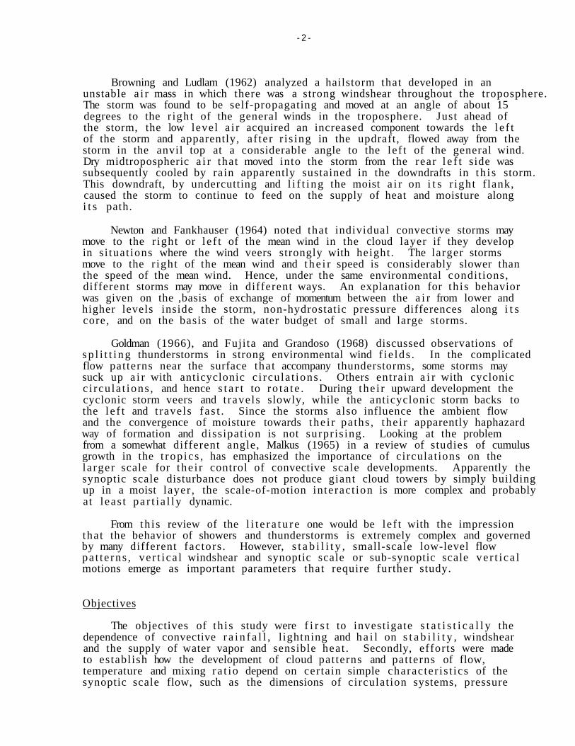
The raw material for the study of the character is t ics of sub-synoptic meteorological patterns and the i r re la t ion to the synoptic-scale flow was obtained from a rather unique combination of data from dense networks of r a in fa l l s t a t i o n s , volunteer observers, and lightning counters in the Netherlands, along with both routine and special teletype data from the area in which dense networks are located. The synoptic network also is quite dense in th i s region, and mil i tary ac t i v i t i e s over Western Europe during 1964-1966 prompted the collection of p i lo t r epor t s , special reports and extra radiosonde and upper wind measurements. Figure 1 represents the d is t r ibut ion of synoptic and upper-air s ta t ions with respect to the two ra in fa l l networks; figure 2 shows the dis t r ibut ion of lightning counters over the southwestern r a in fa l l network, which consists of 700 raingages. In addition to these data, temperatures were given of the sea surface and inland waters.

The radiosonde observations were made at midnight and midday, local time. Upper winds were measured at 6-hour intervals and occasionally at 2-hour intervals by mil i tary s t a t i ons . Coded radar reports were issued on demand, and hence were scanty. Rainfall was measured at 24-hour in tervals except when the weather was very showery, then it was measured twice a day. Layer-type cloud precipi ta t ion that was measured before or after the convective rain by a number of s ta t ions was graphically subtracted from the r a in f a l l maps that were obtained in analyzed form. Most of the l ightning counters were not provided with a recorder, so lightning counts were accumulated by the l ightning s ta t ions for the period of a storm. Only occasionally was there an observer who counted flashes at 5- or 10-minute in t e rva l s . Therefore, the only comparison that could be made was between t o t a l counts of cloud-to-ground flashes and the t o t a l r a i n f a l l received from the storm.

Complete data were collected from about 400 days of convective ac t iv i ty with several cases of severe storms on one end of the spectrum and marginal or no shower formation on the other.

Data edit ing

Maps of surface pressure, wind, temperature, humidity mixing r a t i o and patterns of cloud charac ter is t ics were plot ted by computer programs, most of which have been described in the Firs t Progress Report. Hourly space-averages and standard deviations of these variables were also machine-computed. Since only one format could be adopted for the computer input the standard surface synoptic format was chosen, but many reports from a i r f ie lds were coded in

Figure 1 Network of synoptic and upper air stations The micronets of rainfall stations and lightning counters are indicated by quadrangles

Figure 2. Location of lightning counters with respect to geography of the rainfall network in the southwestern part of the Netherlands.

- 7 -

different formats and had to be edited. Also, in raw form the synoptic reports contained many coding and typing e r ro r s , and par ts that were garbled during transmission. At f i r s t it seemed expensive and cumbersome to design a machine editing program, and the data were edited manually. Though less involved, manual edit ing appeared to be very slow and time consuming, so that only 70 cases could be processed. When it became clear that only certain types of errors occurred, such as temperatures being coded 5 or 10 degrees off, an edit ing program was writ ten to study the f eas ib i l i t y of machine ed i t ing .

It appears now that inconsistent coding of weather and cloud types and gross errors in the coding of temperatures and pressures can also be corrected by simple programs which are inexpensive to run. The problem remains of how to cope with different coding formats. A source of gross errors in the evaluation of s t a t i s t i c s on cloud type appeared to be the different procedures of reporting clouds in Western Europe and the United S ta tes . This was detected after most of the data were processed, and hence the investigation of the time-dependence of cloud pattern behavior in re la t ion to sub-synoptic and synoptic scale flow had to be repeated.

It may be of in t e re s t to comment on these differences. In most European countries showery precipi ta t ion in the present weather code must be accompanied by a cumulonimbus in the cloud code: CL must be e i ther 3 or 9. If the cumulonimbus is obscured and other low type clouds are present , these clouds are reported in special groups preceded by the number 8. These groups also contain information about amount and height of the cloud base. Intermit tent prec ip i ta t ion that is not thought to be of a showery nature is coded in the 60 or 70 groups of the WW-code, and in that case the cloud type that is observed is reported in the N-group as well as in the 8-groups. The problem of how to distinguish between convective precipi ta t ion and layer-type cloud precipi ta t ion is solved by the observer, who has to make a judgement on the basis of fluctuations of precipi ta t ion in tens i ty or the cloud type that preceded the onset of the prec ip i ta t ion . Provided that a good dis t inct ion between showers and intermit tent layer-type cloud rain can be made, th is procedure would clearly bring out the correspondence between the ve r t i ca l development of convective clouds and the occurrence of showers. However, in the United States the low cloud reported during a shower is that which is seen at that moment and the decision whether a cumulonimbus was present or not is le f t to the analyst . Feeding the relat ionship into the computer would then involve map analysis , and inspection of r a i n f a l l amounts or radar echoes.

In the se t of available data both procedures were followed by different s t a t i ons , some of which were operated by the United States Air Force at tha t time and by some c iv i l s ta t ions that did not use the 8-groups. The confusion that arose from t h i s , though unimportant for the forecaster , proved to be f a t a l for the in terpre ta t ion of the s t a t i s t i c a l r e s u l t s . A randomly selected sample of observations was made to conform with the Western European procedure and the averages and standard deviations of low type clouds were recomputed. The or iginal and corrected values showed a difference of 30 percent , which would render the resu l t s of time-dependence studies of cloud pat tern behavior useless . Hence, only a number of hand corrected case studies are described in th is repor t .

It appears tha t different coding procedures and formats are the main stumbling block for the s t a t i s t i c a l treatment of teletype data, but that machine edi t ing can be made to conform to the coding rules for present weather and cloud type at l i t t l e cost .

- 8 -

Problems encountered

During the course of the inves t iga t ions , it was found that there was often insufficient resolution in time of the upper wind and radiosonde data to study the l i f e cycle of disturbances during the i r passage over the network. The study of the time dependence of pat terns of meteorological variables was hampered by problems of edi t ing the synoptic data for the computer. Radar and a i rcraf t observations appeared too scanty for meaningful studies of cloud depths and the development of p rec ip i ta t ion . Access to the raw data from the radiosonde and pibal ascents would have f ac i l i t a t ed the planned trajectory computations to a great extent. The computation of ver t i ca l veloci t ies by means other than the kinematic technique proved to be very cumbersome. Hence, the at tent ion had to be focused on instantaneous relat ionships between synoptic-scale flow and patterns of meteorological var iables , and these could only be compared to the to t a l output of convective systems in the form of lightning and ra in while these passed over one of the r a in f a l l networks. Hai l fa l l was rare during most of the period. Hence, only parts of the proposed objectives could be accomplished, and the number of cases studied was l imited to 70. The resul ts are presented in this report .

ACKNOWLEDGMENTS

The author wishes to express h i s thanks to the chief of the Meteorologica l Service of the Royal Netherlands Air Fo rce , and to Major J. H. Boer of the same organ iza t ion for p rov id ing the t e l e t y p e d a t a , wi thout which t h i s s tudy would not have been p o s s i b l e . Considerable a s s i s t a n c e in synopt ic ana lys i s was rece ived from Messrs. Parker T. Jones and Ross F. E l l i s , both U. S. Air Force fo r eca s t e r s working temporar i ly on the p r o j e c t . The s t a t i s t i c a l ana lyses were performed by Mr. John W. Wilson. Robert C. Swaringer, a p a r t - t i m e s tuden t employee, provided inva luab le a s s i s t a n c e in both e r r o r checking and computer programming; h i s e f f o r t s were p a r t i c u l a r l y app rec i a t ed .

Other pa r t - t ime employees c o n t r i b u t i n g to t h i s work were s t u d e n t s : Joan B a t e s , Roland Cobb, and Ronald Love; and Air Force e n l i s t e d f o r e c a s t e r personnel B i l l y Conley and Charles Sp ice r .

Messrs. Glenn E. S t o u t , Floyd A. Huff, and Richard G. Semonin k ind ly reviewed the manuscr ip t .

REPORTS WRITTEN DURING PERIOD OF THE GRANTS

Feter i s , P. J . , 1966. Relation of l ightning, r a in f a l l and ha i l to the propert ies of mesoscale meteorological pa t te rns . F i rs t Progress Report, National Science Foundation Grant GP-5196 .

- 9 -

F e t e r i s , P . J . , 1967. Non-advective changes in the mesoscale moisture d i s t r i b u t i o n and t h e i r r e l a t i o n to convection and l o c a l c i r c u l a t i o n s . Paper p resen ted at the Conference of the American Meteorological Soc ie ty on Phys ica l Processes in the Lower Atmosphere, March 20-22, Ann Arbor, Michigan.

Boer, J . H . , P. J . F e t e r i s , and J. W. Wilson, 1967. Short-range l i g h t n i n g c o u n t e r s , a research t o o l . Proceedings of Severe Local Storm Conference, American Meteorological Soc i e ty , October 19-20, 49-54.

F e t e r i s , P . J . , 1967. Mesoscale c i r c u l a t i o n d i f fe rences r e l a t e d to thunderstorm development. Proceedings of Severe Local Storm Conference, American Meteorological Soc i e ty , October 19-20, 246-257.

F e t e r i s , P . J . , 1967. Re la t ion o f l i g h t n i n g , r a i n f a l l and h a i l t o the p r o p e r t i e s of mesoscale meteoro log ica l p a t t e r n s . Second Progress Repor t , Na t iona l Science Foundation Grant GP-5196.

Boer, J. H . , and P. J. F e t e r i s , 1968. The inf luence of the sea on the d i s t r i b u t i o n of l i g h t n i n g and r a i n on a c o a s t a l a rea . Annalen der Meteorologie , Neue Folge , to be pub l i shed .

Wilson, J . W., and P. J . F e t e r i s , 1968. Lightning and r a i n in r e l a t i o n to sub-synopt ic flow parameters . Appendix A to t h i s pape r , submit ted to J . Appl. Meteor, for p u b l i c a t i o n .

RESULTS OF VARIOUS PHASES OF THE WORK

Rela t ionsh ips between s t a b i l i t y and v e r t i c a l v e l o c i t y

Under condi t ions of weak flow and s t eep v e r t i c a l temperature lapse r a t e s over the cont inen t of Western Europe, thunderstorms sometimes become organized in c l u s t e r s about 50 to 200 km in diameter which are surrounded by a reas of c l e a r weather . There is often l i t t l e i n d i c a t i o n of these developments on the surface map o the r than t h a t the p ressure f i e l d and the flow are modified by e x i s t i n g groups of thunderstorms of which the l i f e cycle and displacement a re d i f f i c u l t to p r e d i c t . Such a s i t u a t i o n has been repor ted on ( F e t e r i s , 1967) and i t was found t h a t d e t a i l e d analyses of the th ree-d imens iona l temperature and wind f i e l d s revea led the ex i s t ence of f a i r l y s t rong v e r t i c a l motions which occurred in columns 100 to 400 km wide. The maximum h o r i z o n t a l dimensions and the maximum v e r t i c a l v e l o c i t i e s were found in the middle or upper t roposphere and the v e r t i c a l motion p a t t e r n s often had a double t or quadruple t s t r u c t u r e which suggests l o c a l s o l e n o i d a l c i r c u l a t i o n s o r wave-l ike o s c i l l a t i o n s . S imi la r o s c i l l a t i o n s have been noted by Krei tzberg (1968) and the re are a l so s c a t t e r e d r epor t s of p res su re v a r i a t i o n s and wind f l u c t u a t i o n s at the s u r f a c e , sometimes with a s soc i a t ed wea ther , t h a t suggest the occurrence of these d i s tu rbances in the synopt ic s c a l e flow. C h a r a c t e r i s t i c dimensions range from 50 to about 500 km (Ferguson, 1967, Pothecary , 1954).

The th ree -d imens iona l analyses r epor t ed e a r l i e r by F e t e r i s (1967) , which are reproduced in f igures 3, 4 , and 5, a l so suggested t h a t the coupling of

Figure 3. Vertical velocity, relative humidity, and clouds on 24 May 1964 at 1200 GMT.

Figure 4. Vertical velocity, relative humidity, and clouds on 25 May 1964 at 1200 GMT.

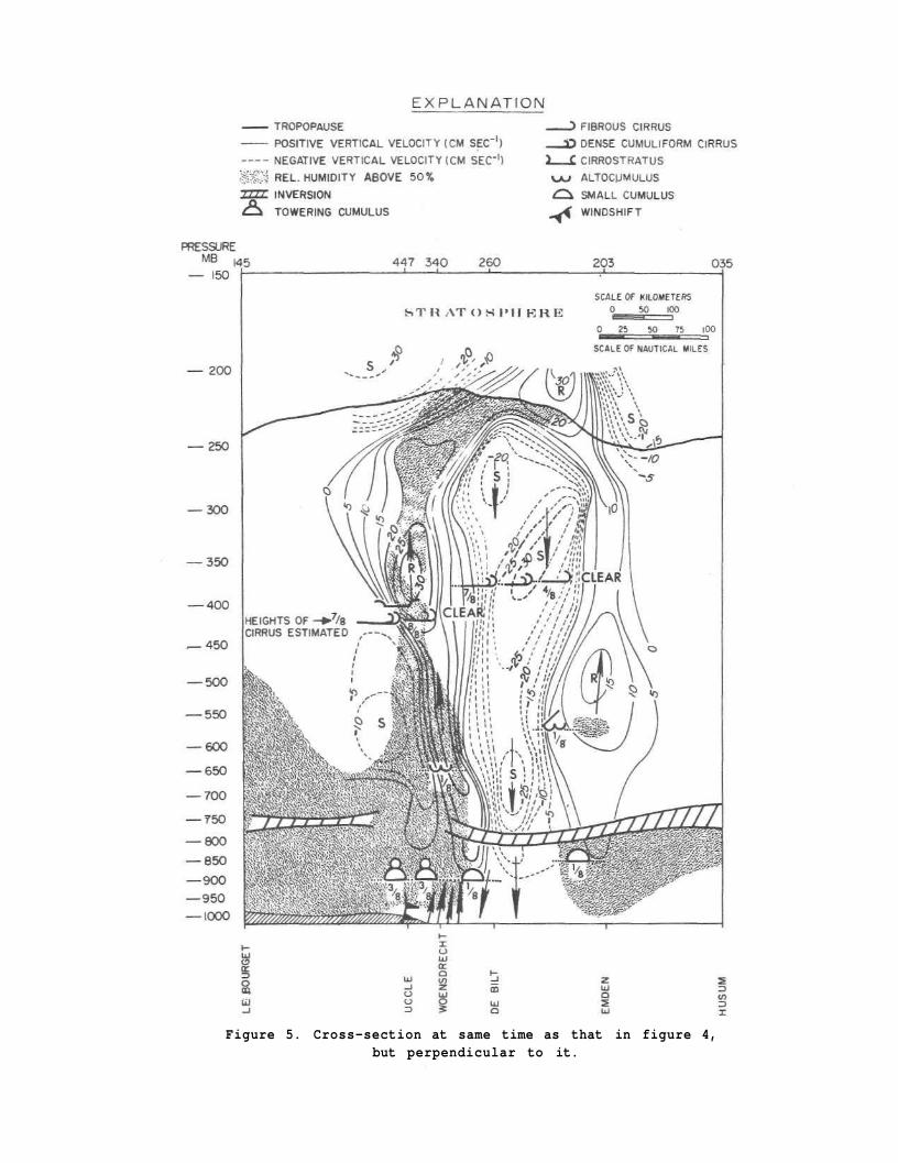
Figure 5. Cross-section at same time as that in figure 4, but perpendicular to it.

-13-

ver t i ca l motions in the upper troposphere with those in the lower troposphere depends very much on the dis t r ibut ion of s t a t i c s t a b i l i t y below the tropopause. In that par t i cu la r case, s table layers acted as bar r ie rs between the motion f ields in the upper and lower troposphere, but occasionally gaps in these bar r ie rs allowed the ver t i ca l motions to extend to the surface where they s tar ted to organize convection a few hours before the onset of thunderstorms. To arrive at a firmer relat ionship between s t a t i c s t a b i l i t y and ve r t i ca l motion fields several cross-sections of potent ia l temperature, r e l a t ive humidity and wind were made through the sub-synoptic scale network area. An example of such a cross-section is shown in figure 6. On the smaller scales the re la t ionship between horizontal thermal f ields and the ve r t i ca l windshear becomes ra ther loose (Forsythe, 1945, Kreitzberg, 1968) due to ve r t i ca l gradients in the curvatures of the streamlines, but where the data indicated th is re la t ionship the potent ia l temperature l ines were given the appropriate slope. Pressure analyses on several isentropic surfaces over the area were used to ensure a three-dimensionally consistent analysis . S ta t ic s t a b i l i t i e s (-d0/dp) were computed for each of the radiosonde ascents , and between s ta t ions the s t a b i l i t y was evaluated from the spacing of the potent ia l temperature l ines on the cross-section. Vertical veloci t ies were machine computed following a kinematic technique proposed by Panofsky (1946) which is described in Appendix B.

Cross-sections of ve r t i ca l velocity and -d0/dp are presented in figures 7, 8, and 9. Figure 9 shows how subsidence suppressed deep convection on the l a s t day of the set but s t i l l with large fluctuations which were present in the ver t i ca l velocity superimposed on the general sinking motion.

It can be noted from the cross-sections that ver t i ca l velocity maxima are present where -d0/dp is less than 0.05 °K mb-1 except where moist ascent is indicated by high humidit ies, cloud or prec ip i ta t ion . Where the s t a t i c s t a b i l i t y approaches or exceeds 0.1 °K mb - 1 , ve r t i ca l velocity maxima of opposite sign are arranged along the v e r t i c a l ; elsewhere, they tend to be arranged along the horizontal . The negative relat ionship between ver t i ca l motions and s t a t i c s t a b i l i t y can also be displayed on isentropic surfaces, using the cross-sections as a guide for areas between s t a t ions . Such an analysis is presented in figure 10 for the isentropic surface of 320 °K. The resu l t s defini tely locate the ver t i ca l velocity doublet in the upper troposphere on the area with lowest s t a t i c s t a b i l i t y . In fac t , the maximum downward velocity of 70 cm sec - 1 occurred where -d0/dp was close to zero. The preference of large ve r t i ca l velocity maxima for levels above 500 mb can be explained by the i r coincidence with regions of nearly dry adiabatic lapse r a t e s , which frequently occur in the upper troposphere. In these regions the energy required to sustain such motions is small.

It is in te res t ing to compare the ve r t i ca l velocity f ie ld on the 320 °K surface with that which would be obtained from the adiabatic technique by which -dp/dt is computed from pressure , streamline and isotach analysis . Streamlines and isotachs were drawn free-hand using observed winds ra ther than Montgomery streamfunctions. This method was preferred to that of computing the wind from the balance equation, since scale character is t ics alone already predict large ageostrophic deviations and unbalanced flow which are also strongly time dependent. From the analysis presented in figure 11 it can be seen that the adiabatic ver t i ca l velocity maxima occur closely to the location of the kinematic ver t i ca l velocity extremes. However, the components of ve r t i ca l velocity deduced from the upslope and downslope ascent on the isentropic surface i t s e l f a re , in th is pa r t i cu la r case, an order of magnitude smaller than those calculated

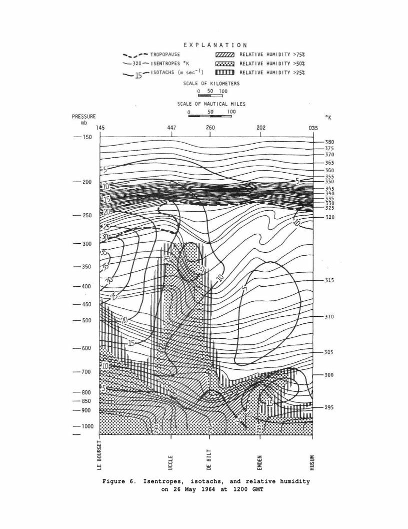
Figure 6. Isentropes, isotachs, and relative humidity on 26 May 1964 at 1200 GMT

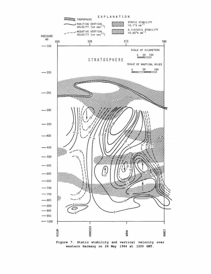
Figure 7. Static stability and vertical velocity over western Germany on 26 May 1964 at 1200 GMT.

Figure 8. Static stability and vertical velocity over France, Belgium, and the Netherlands on 26 May 1964 at 1200 GMT.

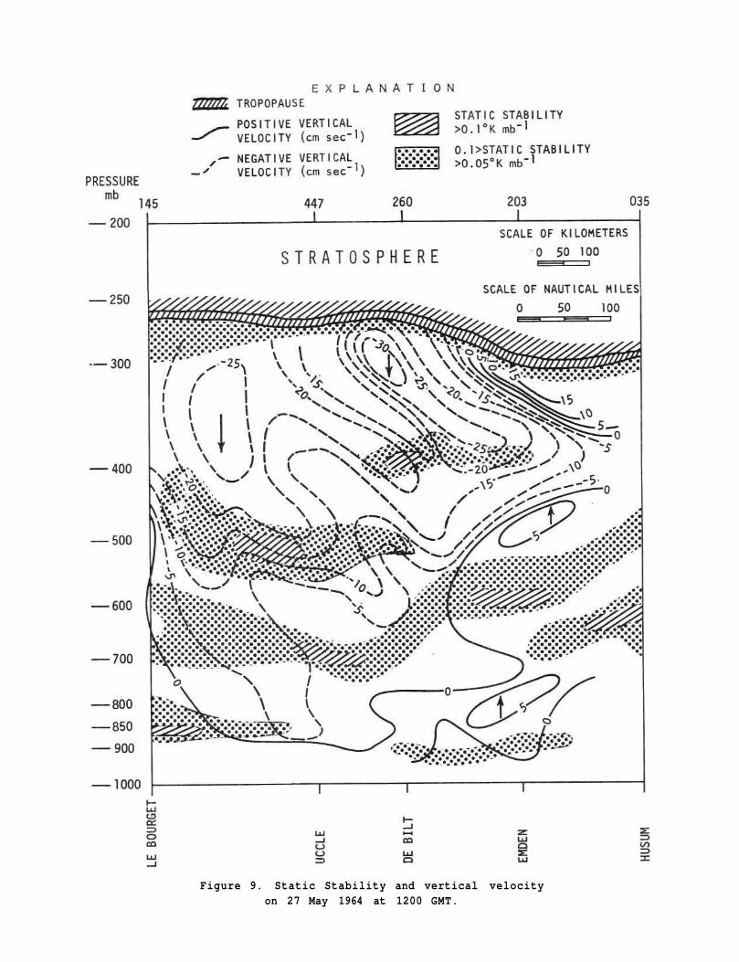
Figure 9. Static Stability and vertical velocity on 27 May 1964 at 1200 GMT.

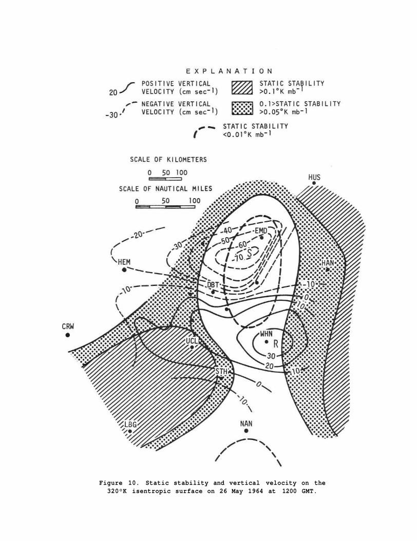
Figure 10. Static stability and vertical velocity on the 320°K isentropic surface on 26 May 1964 at 1200 GMT.

Figure 11. Vertical velocity on the 320°K isentropic surface on 26 May 1964 at 1200 GMT, computed by the adiabatic method.

- 2 0 -

by the kinematic technique. Hence, the other components must have been due mostly to the dry ascent or descent of parts of the isentropic surface i t s e l f . In other words, the sub-synoptic scale ver t i ca l motions and the i r ve r t i ca l gradients have a large effect on the s t ab i l i za t ion or destabi l izat ion of the a i r . This effect is mostly marked where the s t a t i c s t a b i l i t y is already large . Note how the s t ab i l i za t ion is s t i l l in progress near 450 mb and 700 mb on the r ight hand side of figure 7 and between 600-700 mb in parts of figure 8. There is a poss ib i l i ty of a feedback between this s t ab i l i za t ion and the modification of the ve r t i ca l motion pa t te rns . This would imply that the formation and dissipation of s table layers is highly time dependent. This may explain the e r r a t i c occurrence of gaps in the barr iers between upper and lower troposphere, which allow the organization of convection near the surface and the subsequent formation of thunderstorms.

The question arises whether ver t i ca l motions and s t a b i l i t y are also negatively re la ted in s i tuat ions that differ from th i s par t i cu la r case study and, in pa r t i cu la r , in stronger flow. A s t a t i s t i c a l study would then also have to be based on ve r t i ca l velocity computation techniques that are less prone to errors than the kinematic technique when applied to strong flows. An omega equation sui table for ver t ica l veloci t ies on the sub-synoptic scale would have to incorporate many terms and th is procedure would become cumbersome (see for instance Krishnamurty, 1968). Instead it was hypothesized that deep convection was l ikely to occur where no bar r ie rs existed in the form of layers of high s t a t i c s t a b i l i t y , and hence a negative correlat ion between convective precipi ta t ion and s t a t i c s t a b i l i t y would be expected.

S t a t i s t i c a l r e s u l t s . In order to s t a t i s t i c a l l y t e s t th is hypothesis, relat ionships were sought among the following variables:

(a) The maximum s t a t i c s t a b i l i t y found between 825 and 300 mb; (b) the pressure level on which the maximum s t a t i c s t a b i l i t y

was centered; (c) the depth of the layer of maximum s t a t i c s t a b i l i t y ; (d) the larges t s t a t i c s t a b i l i t i e s adjacent to the levels of

825, 700, 500, and 400 mb respect ively; (e) the present weather code.

In the present weather code the numbers that pertained to prec ip i ta t ion and thunderstorms in the past hour (21-25, 26, 27, 29) as well as those indicating showers and thunderstorms near but not at the s ta t ion (15, 16, 17) were changed to the 60 ' s , 70 ' s , 80 ' s , and 9 0 ' s , whichever was appropriate.

The variables were determined for five radiosonde s ta t ions twice a day during 65 days with showers and thunderstorms. The frequency of occurrence (in percent of sample s ize) of various present weather observations at the radiosonde s ta t ions is given in table 1, which shows that prec ip i ta t ion was infrequent on the days considered.

- 2 1 -

Table 1. Frequency of Occurrence of Cer ta in Types of Weather

Weather

Percentage

No p r e c i p .

81.4

Drizzle

0.8

Rain

7 .1

Showers

9.0

Thunderstorms

1.7

Table 2 shows tha t t he s t a t i c s t a b i l i t y (-d9/dp) of the most s t a b l e l aye r s is usua l ly between 0.10 and 0.18 °K/mb; the maximum frequency in t h i s i n t e r v a l shows up for a l l types of weather except for showers. I t has in t h a t case s h i f t e d to somewhat l a r g e r s t a b i l i t i e s . The d i s t r i b u t i o n seems to be a l i t t l e narrower for thunders torms , but in gene ra l the soundings may show q u i t e s t a b l e l aye r s in thunders torms. According to t a b l e 3 the l o c a t i o n of t h e s t a b l e l aye r s may be anywhere between 825 and 300 mb in f a i r weather c a s e s , as w e l l as in s i t u a t i o n s with s t r a t i f i e d r a i n . In s i t u a t i o n s with showers the s t a b l e s t l aye r s are found most f requent ly between 300 and 400 mb; t h i s tendency seems to be even more marked in thunderstorms though the sample s i z e is too smal l to draw any firm conc lus ions . Table 4 shows t h a t the th ickness of the s t a b l e s t l aye r is usua l ly between 10 and 19 mb, except in thunderstorms where the maximum frequency f a l l s between 0 and 9 mb. Otherwise , there is not much d i f fe rence between the var ious weather t ypes .

S i t u a t i o n s with showers may be a s s o c i a t e d with h ighe r s t a t i c s t a b i l i t i e s i n the upper t roposphere ; o therwise , i t must be sa id t h a t n e i t h e r the s t a b i l i ­t y , the depth , nor the h e i g h t of the s t a b l e s t l a y e r are r e l a t e d f i rmly enough to the occurrence of convective p r e c i p i t a t i o n and l i g h t n i n g to be of value as a s t a b i l i t y index.

Apparently the d i s t r i b u t i o n o f the s t a t i c s t a b i l i t y does not p r e d i c t concurrent weather but i t may p r e d i c t where s t rong r i s i n g and s ink ing motions are l i k e l y to organize convect ion. For the purpose of l oca t i ng these reg ions on sub-synopt ic sca le weather maps a s t a t i c s t a b i l i t y index may tu rn out to be use fu l as a t o o l .

Inf luence of windshear on low and medium l e v e l convection

Windshear is known to i n h i b i t t he v e r t i c a l development of moist convection (Byers and Braham, 1949; Byers and B a t t a n , 1949; Malkus, 1952; Malkus and Score r , 1955) , s ince i t causes t h e cumulus clouds to s l a n t and to inc rease the depth over which e ros ion of the bubbles or plumes occurs . In l a rge cumulus towers v e r t i c a l exchange of momentum is known to take p lace (Newton, 1963) and it can be argued t h a t t h i s may a l s o happen in any p a r t of the atmosphere where the s t a b i l i t y allows v e r t i c a l motions t o be s u s t a i n e d with l i t t l e l o s s o f k i n e t i c energy. Where s t a b l e l aye r s ac t as impenetrable boundaries for v e r t i c a l motions one would expect the windshear to reach high v a l u e s , and thus t h e r e would be a p o s i t i v e c o r r e l a t i o n between s t a b i l i t y and shea r . In t h a t case p r e f e r r e d areas for the development of thunderstorms would be those where the flow s t agna t e s temporar i ly while the atmosphere is u n s t a b l e . Such condi t ions are sometimes found a few hundred km behind cold f ron t s in uns tab le p o l a r a i r masses , but t he re have a l so been r e p o r t s of thunderstorms which developed in s t r o n g shea r (Newton, 1963; H i t s c h f e l d , 1960, Dessens, 1960).

Table 2. Frequency of Occurrence of Given S t a t i c S t a b i l i t i e s in the S t a b l e s t Layer for Cer ta in Weather Types

S t a t i c s t a b i l i t y of the s t a b l e s t l a y e r ( 1 0 - 2 °K mb - 1 )

Weather 0-9 10-19 20-29 30-39 40-49 50-59 60-69 70-79 80-89 90-99 TOTALS

No precip. 61 274 139 42 8 1 1 2 1 0 529

(11.5) (51.8) (26.2) (7.9) (1.6) (0.2) (0.2) (0.4) (0.2) (0.0) (100)

Rain 9 27 12 3 1 0 0 0 0 0 52

(17.4) (51.8) (23.1) (5.8) (1.9) (0.0) (0.0) (0.0) (0.0) (0.0) (100)

Showers 5 21 21 8 3 1 0 0 0 0 59

(8.5) (35.6) (35.6) (13.5) (5.1) (1.7) (0.0) (0.0) (0.0) (0.0) (100)

Thunderstorms 2 5 2 2 0 0 0 0 0 0 11

(18.2) (45.4) (18.2) (18.2) (0.0) (0.0) (0.0) (0.0) (0.0) (0.0) (100)

TOTALS 77 327 174 55 12 2 2 2 1 0 652

(11.8) (50.2) (26.7) (8.4) (1.8) (0.3) (0. 3) (0. 3) (0.2) (0.0) (100)

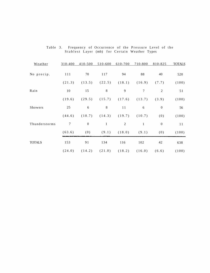
Tab le 3 . Frequency o f O c c u r r e n c e o f t h e P r e s s u r e L e v e l o f t h e S t a b l e s t L a y e r (mb) f o r C e r t a i n Wea the r Types

Weather 310-400 410-500 510-600 610-700 710-800 810-825 TOTALS

No p r e c i p . 111 70 117 94 88 40 520

( 2 1 . 3 ) ( 1 3 . 5 ) ( 2 2 . 5 ) ( 1 8 . 1 ) ( 1 6 . 9 ) ( 7 . 7 ) ( 1 0 0 )

Rain 10 15 8 9 7 2 51

( 1 9 . 6 ) ( 2 9 . 5 ) ( 1 5 . 7 ) ( 1 7 . 6 ) ( 1 3 . 7 ) ( 3 . 9 ) (100 )

Showers 25 6 8 11 6 0 56

( 4 4 . 6 ) ( 1 0 . 7 ) ( 1 4 . 3 ) ( 1 9 . 7 ) ( 1 0 . 7 ) ( 0 ) (100)

Thunder s to rms 7 0 1 2 1 0 11

( 6 3 . 6 ) ( 0 ) ( 9 . 1 ) ( 1 8 . 0 ) ( 9 . 1 ) ( 0 ) (100 )

TOTALS 153 91 134 116 102 42 638

( 2 4 . 0 ) ( 1 4 . 2 ) ( 2 1 . 0 ) ( 1 8 . 2 ) ( 1 6 . 0 ) ( 6 . 6 ) ( 1 0 0 )

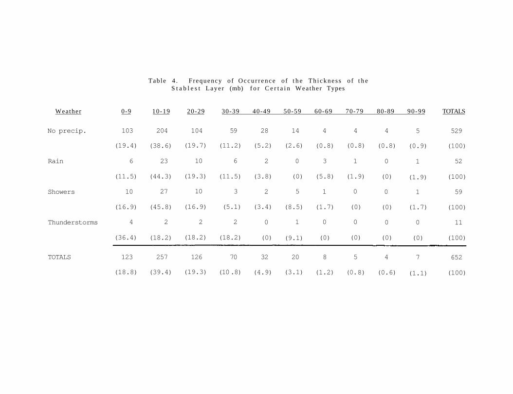
Table 4 . F requency o f O c c u r r e n c e o f t h e T h i c k n e s s o f t h e S t a b l e s t L a y e r (mb) f o r C e r t a i n Wea the r Types

Weather 0-9 10-19 20-29 30-39 40-49 50-59 60-69 70-79 80-89 90-99 TOTALS

No precip. 103 204 104 59 28 14 4 4 4 5 529 (19.4) (38.6) (19.7) (11.2) (5.2) (2.6) (0.8) (0.8) (0.8) (0.9) (100)

Rain 6 23 10 6 2 0 3 1 0 1 52

(11.5) (44.3) (19.3) (11.5) (3.8) (0) (5.8) (1.9) (0) (1.9) (100)

Showers 10 27 10 3 2 5 1 0 0 1 59

(16.9) (45.8) (16.9) (5.1) (3.4) (8.5) (1.7) (0) (0) (1.7) (100)

Thunderstorms 4 2 2 2 0 1 0 0 0 0 11

(36.4) (18.2) (18.2) (18.2) (0) (9.1) (0) (0) (0) (0) (100)

TOTALS 123 257 126 70 32 20 8 5 4 7 652 (18.8) (39.4) (19.3) (10 .8) (4.9) (3.1) (1.2) (0. 8) (0.6) (1.1) (100)

- 2 5 -

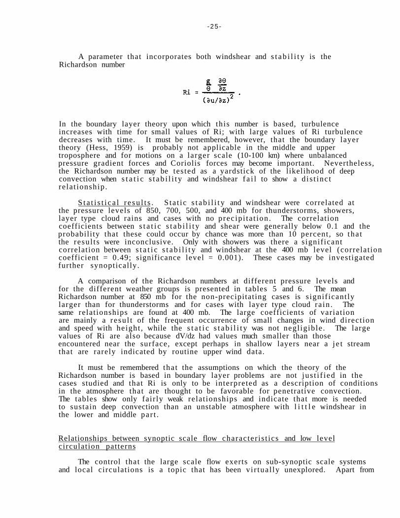
A parameter that incorporates both windshear and s t a b i l i t y is the Richardson number

In the boundary layer theory upon which this number is based, turbulence increases with time for small values of Ri; with large values of Ri turbulence decreases with time. It must be remembered, however, that the boundary layer theory (Hess, 1959) is probably not applicable in the middle and upper troposphere and for motions on a larger scale (10-100 km) where unbalanced pressure gradient forces and Coriolis forces may become important. Nevertheless, the Richardson number may be tes ted as a yardstick of the likelihood of deep convection when s t a t i c s t a b i l i t y and windshear f a i l to show a d i s t inc t re la t ionship .

S t a t i s t i c a l r e s u l t s . S ta t i c s t a b i l i t y and windshear were correlated at the pressure levels of 850, 700, 500, and 400 mb for thunderstorms, showers, layer type cloud rains and cases with no prec ip i ta t ion . The correlat ion coefficients between s t a t i c s t a b i l i t y and shear were generally below 0.1 and the probabil i ty that these could occur by chance was more than 10 percent , so tha t the resu l t s were inconclusive. Only with showers was there a s ignif icant correlat ion between s t a t i c s t a b i l i t y and windshear at the 400 mb level (correlat ion coefficient = 0.49; significance level = 0.001). These cases may be investigated further synoptical ly.

A comparison of the Richardson numbers at different pressure levels and for the different weather groups is presented in tables 5 and 6. The mean Richardson number at 850 mb for the non-precipitat ing cases is s ignif icant ly larger than for thunderstorms and for cases with layer type cloud ra in . The same relat ionships are found at 400 mb. The large coefficients of variat ion are mainly a r e su l t of the frequent occurrence of small changes in wind direct ion and speed with height , while the s t a t i c s t a b i l i t y was not negl ig ib le . The large values of Ri are also because dV/dz had values much smaller than those encountered near the surface, except perhaps in shallow layers near a j e t stream that are rarely indicated by routine upper wind data.

It must be remembered tha t the assumptions on which the theory of the Richardson number is based in boundary layer problems are not jus t i f i ed in the cases studied and that Ri is only to be interpreted as a description of conditions in the atmosphere that are thought to be favorable for penetrative convection. The tables show only fair ly weak relat ionships and indicate that more is needed to sustain deep convection than an unstable atmosphere with l i t t l e windshear in the lower and middle par t .

Relationships between synoptic scale flow charac ter i s t ics and low level circulat ion patterns

The control that the large scale flow exerts on sub-synoptic scale systems and local circulations is a topic that has been v i r tua l ly unexplored. Apart from

Table 5. Comparison of Means and Standard Deviations of Richardson Number and Static Stability for Different Types of Weather

(y is the average, 0 the standard deviation and cv the coefficient of variation)

RICHARDSON NUMBER STATIC STABILITY μ σ cv μ σ cv

850 24.3 101.0 4.16 .032 .061 1.91

700 614.1 1023.2 16.80 .053 .067 1.26

500 83.5 369.1 4.42 .057 .043 0.76

400 209.4 206.2 9.80 .061 .060 1.01

850 11.8 17.3 1.47 .040 .022 0.55

700 108.2 270.8 2.50 .048 .032 0.67

500 46.9 93.3 1.99 .062 .036 0.59

400 85.0 160.0 1.88 .053 .031 0.59

850 27.3 85.3 3.12 .030 .034 1.13

700 149.8 324.4 2.17 .059 .034 0.58

500 27.2 49.4 1.82 .046 .033 0.72

400 54.6 79.7 1.46 .067 .049 0.73

850 7.6 18.2 2.40 .023 .027 1.17

700 106.9 225.8 2.12 .040 .023 0.58

500 124.5 330.5 2.66 .044 .030 0.68

400 43.3 78.4 1.81 .055 .028 0.51

Table 6. Probabilities of Obtaining Larger Differences in the Means of Ri Between Various Weather

Types from Random Sampling

850 mb

Thunders to rms

Showers

Rain

700 mb

Thunders to rms

Showers

Rain

500 mb

Thunders to rms

Showers

Rain

400 mb

Thunders to rms

Showers

Rain

None

< . 0 1

.80

. 0 1

None

.26

.30

.26

None

. 3 8

< . 0 1

. 08

None

. 0 8

. 1 1

. 74

Rain

.36

.20

Rain

. 9 8

. 48

Rain

.30

. 18

Rain

.09

.22

Showers

.46

Showers

.46

Showers

.10

Showers

. 48

-28-the work by Browning and Ludlam (1962), Newton and Fankhauser (1964), Goldman (1966), and Fujita and Grandoso (1968) tha t deals mainly with large thunderstorms, and the sea breeze studies by Estoque (1962), there are very few reports that re la te the development of local circulat ions and sub-synoptic prec ip i ta t ion systems to a i r mass properties and the synoptic scale flow character is t ics (Findlater , 1964, McNair and Barthram, 1966). In strong flows d i f fe ren t i a l heating would be expected to have l i t t l e influence on the organization of convection, since the a i r does not have time to take up suff icient heat and moisture while traveling fast over hot or moist spots . There are cases of thunderstorm development in strong synoptic scale flows (K.N.M.I., 1960-1962). However, these are associated with strong temperature advection in the upper troposphere along the cyclonic side of j e t streams which causes rapid changes in the s t a b i l i t y of the a i r . Perhaps there may be also strong ver t i ca l motions associated with these changes, but they have not been studied in de t a i l . It can only be said that pers is tent strong winds are most l ikely in regions where large pressure gradients exis t over elongated areas with s t r a igh t or s l igh t ly anticyclonical ly curved flow. One would expect that in those regions the space and time variat ions of wind di rec t ion, wind speed, temperature and dewpoint would show very l i t t l e fluctuation and that the cloud patterns would remain ra ther uniform.

S t a t i s t i c a l r e s u l t s . Time graphs of space averages and standard deviations over the synoptic network were made of the following l i s t of dependent var iables :

D, the wind direction V, the wind speed 0, the potent ia l temperature w, the humidity mixing r a t i o

θe, the equivalent potent ia l temperature.

The midnight (0000 GMT) and midday (1200 GMT) values of these variables were related to the following independent variables at corresponding map times:

Ds, direct ion of the surface isobars (upstream) Ks, curvature of the isobars L s , arc length for which the curvature was representative

(centered over the sub-synoptic network) Vp, pressure gradient D5, direct ion of the 500 mb contours K5, curvature of the 500 mb contours L5 , arc length for which the curvature was representative Vh, contour gradient ST, average of 10 sea surface temperature measurements along the

coast of Belgium, the Netherlands and Northwestern Germany σ(ST), standard deviation of the sea surface temperature.

Tables 7 and 8 show the correlations between the 10 dependent and the 10 independent variables at midnight and midday respectively. The only strong

Table 7. Cor re l a t ion Coef f ic ien t s Between P r e d i c t o r s and Pred ic tands at 0000 GMT, and P r o b a b i l i t i e s of Obtaining Larger

Values from Random Sampling

D σ(D) V ' σ(V) θ σ(θ) w σ(w) θe σ ( θ e )

DS .59 - . 0 7 . 28 .19 - . 0 2 - . 0 4 - . 0 7 - . 3 4 - . 1 4 - . 1 2

< . 0 1 .29 .02 .07 .44 .38 .29 < . 0 1 . 14 .17

KS - . 0 2 - . 0 8 .09 .06 - . 0 3 - . 1 5 .17 - . 1 4 . 15 - . 1 7

. 44 . 2 7 .24 .32 . 4 1 .12 .09 .14 .12 .09

LS .10 - . 1 3 .15 - . 0 3 . 03 - . 1 3 - . 2 7 . 00 - . 2 4 - . 0 7

.22 .15 .12 . 4 1 . 4 1 .15 .02 .95 . 03 .29

VP . 33 - . 5 0 .76 .30 .27 - . 2 1 - . 1 8 - . 2 2 - . 1 0 - . 2 0

< . 0 1 < . 0 1 < . 0 1 < . 0 1 .02 .05 . 08 . 04 .22 .06

D5 .20 .06 .02 .20 . 1 1 .15 .20 . 2 1 .17 .25

.06 .32 .44 .06 .19 .12 .06 .05 .09 .02

K5 . 04 .25 - . 1 3 - . 0 8 .00 - . 0 3 - . 1 1 - . 0 4 - . 1 4 .00

. 38 .02 .15 .27 .45 . 4 1 .19 . 3 8 .14 .45

L 5 . 0 1 . 0 4 .08 .00 .00 - . 0 7 , - . 0 4 - . 0 4 - . 1 6 - . 1 0

. 47 . 3 8 .27 .45 .45 .29 . 38 . 3 8 .10 .22

Vh . 47 - . 2 8 . 43 .15 - . 0 1 - . 1 9 - . 2 1 - . 3 0 - . 2 3 - . 1 6

< . 0 1 . 02 < . 0 1 .12 .47 .07 .05 < . 0 1 . 04 .10

ST .06 - . 2 1 .12 .12 .02 - . 0 2 - . 2 3 .00 - . 1 7 - . 0 5

.32 .05 .17 .17 .44 .44 .04 .45 .09 .35

a(ST) .02 - . 1 3 .02 .02 .02 - . 1 9 - . 1 4 - . 1 4 - . 1 6 - . 2 6

. 44 .15 .44 .44 .44 .07 .14 .14 .10 .02

Table 8. Cor re l a t ion Coeff ic ient Between P r e d i c t o r s and Pred ic tands at 1200 GMT, and P r o b a b i l i t i e s of Obtaining Larger

Values from Random Sampling

D σ(D) V σ(V) θ σ(θ) w σ(w) θe σ ( θ e )

D s . 62 - . 3 1 .37 .19 - . 4 0 - . 2 1 - . 2 6 - . 3 0 - . 3 7 - . 2 0

< . 0 1 < . 0 1 < . 0 1 .07 < . 0 1 .05 .02 <.01 < . 0 1 .06

K s - . 1 2 - . 0 6 .05 .02 .16 .00 .14 .22 .16 . 1 1

. 1 7 .32 .34 .44 .10 .50 .14 .04 .10 .19

L s . 1 7 - . 3 0 .39 .20 - . 3 2 - . 2 5 - . 3 8 - . 3 1 - . 3 6 - . 3 5

.09 < . 0 1 < . 0 1 .06 < . 0 1 .02 <.0l < . 0 1 < . 0 1 <.0l

VP - . 0 4 - . 4 2 .76 .44 .32 .06 - . 2 4 - . 1 7 - . 3 1 - . 0 9

. 3 8 <.01 < . 0 1 < . 0 1 < . 0 1 .32 . 03 .09 < . 0 1 .25

D5 .05 .00 . 1 1 - . 1 8 . 03 . 1 1 - . 1 2 .02 - . 0 3 . 0 3

. 3 4 .50 .19 . 08 . 4 1 .19 .17 .44 . 4 1 . 4 1

*5 . 3 3 - . 0 9 - . 0 1 - . 0 3 - . 3 9 - . 4 4 - . 3 3 - . 4 6 - . 3 9 - . 4 5

< . 0 1 .25 .47 . 4 1 <.0l < . 0 1 < . 0 1 < . 0 1 < . 0 1 < . 0 1

L5 . 1 3 - . 0 2 . 18 .05 - . 0 0 .04 - . 0 1 - . 0 1 - . 0 0 - . 0 3

. 15 .44 .08 .34 .50 . 38 .47 .47 .50 . 4 1

v h .39 - . 4 2 . 6 1 . 3 1 - . 4 1 - . 1 4 - . 2 5 - . 2 7 - . 3 6 - . 2 1

< . 0 1 < .01 < . 0 1 < . 0 1 < . 0 1 .14 .02 .02 < . 0 1 .05

ST - . 0 8 - . 1 4 . 03 .10 . 1 8 .14 . 08 .17 .15 . 1 3

.27 .14 . 4 1 .22 . 0 8 .14 .27 .09 .12 .15

o(ST) . 1 7 - . 1 3 - . 0 1 - . 0 5 - . 0 1 - . 1 5 - . 0 6 - . 1 2 - . 0 3 - . 1 1

.09 .15 .47 .34 .47 .12 .32 .17 . 4 1 .19

-31-

relationships that emerge from the nighttime data are the expected increase of the windspeed and its space standard deviation with increasing pressure gradient and with increasing 500 mb contour gradients whereas the standard deviation of the wind direction over the network decreases with these variables. Weaker relationships exist between average and standard deviation of the humidity mixing ratio and the 500 mb contour gradient, indicating the presence of more uniformly mixed dryer air near the surface below areas with strong upper winds. The negative correlation between the direction of the surface winds and the standard deviation of the humidity mixing ratio over the network is probably due to a local effect. With onshore winds, moisture is advected inland from the sea over which it may be more uniformly distributed than over the continent.

Around midday when convective mixing is vigorous over a depth of 3 km or more, significant relationships appear between the network averages and standard deviations of almost all dependent variables and the arc length over which the curvature of the flow is representative. The average and standard deviation of the arc length are 817 and 608 km respectively, which is representative of the synoptic scale. Apparently, in small disturbances the air is warmer and more moist near the surface with less uniform temperature and moisture fields than in situations where large scale pressure systems control the flow over the network. Note, however, that the relationships between the network variables and the curvature itself are poor, which is contrary to the expectation of moisture convergence in cyclonically curved flow and moisture divergence in anticyclonically curved flow. However, there are significant negative relationships between the curvature of the 500 mb flow with warmer, more moist and less homogeneous surface air below straight or anticyclonically curved contours, regardless of the scale of the disturbance (L5). The dependence of the surface variables on the pressure gradient and the 500 mb contour gradient does not differ significantly from those found for the nighttime cases. Daytime differential heating is greater in smaller scale surface pressure systems and increases with anticyclonically curved flow at 500 mb; the humidity mixing ratio patterns are more outstanding in small scale pressure systems and below small scale anticyclonically curved disturbances in the 500 mb flow in which the contour gradient is weak.

Finally, the standard deviation of each dependent variable was in turn predicted by all other dependent and independent variables by means of stepwise multiple regression. The variables added to the regression equation are those which give the greatest reduction in the unexplained variation, at a particular confidence level. The final results yield only those predictors that are statistically significant at the adopted confidence level. Variables not included may still have a relationship to the predictor, but the relationship is not as strong as with the predictors chosen. Tables 9 and 10 show the results of the multiple regression analyses. The numbers beneath each predictor are standardized regression coefficients and indicate, by their magnitude, the relative importance of each variable. The coefficient of determination r2 is the proportion of the total variability in the dependent variable which has been explained by the regression equation.

At nighttime the winds are more variable with colder air and weaker flow and there is less variability with onshore winds. The only interesting relationships are those with the 500 mb flow, but they are also the weakest.

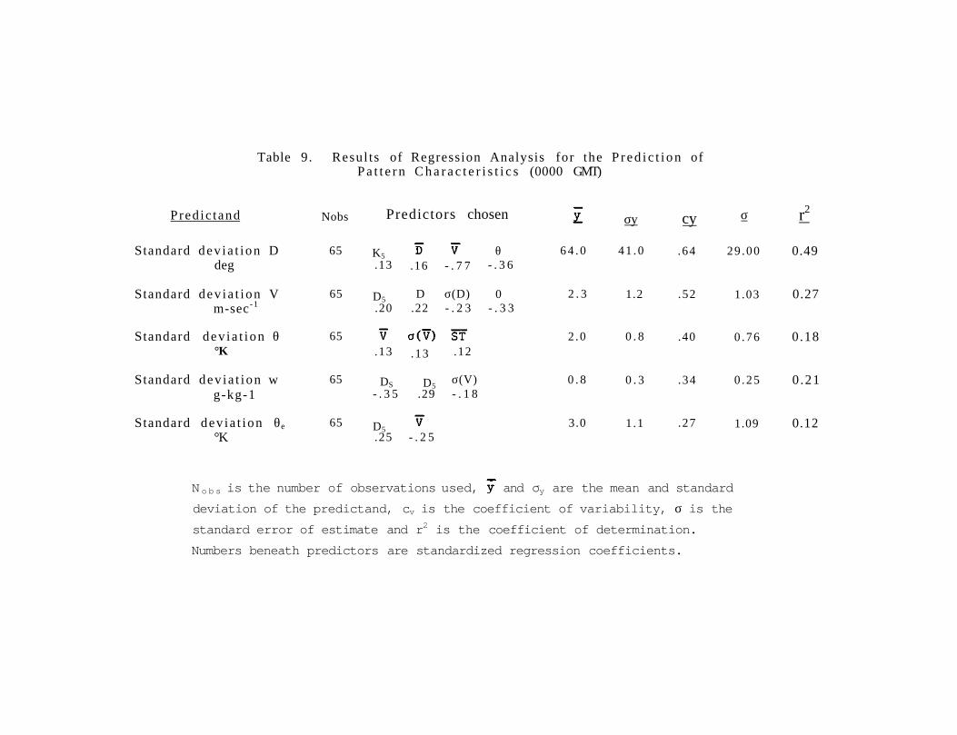
Table 9. Resul ts of Regression Analysis for the P r e d i c t i o n of P a t t e r n C h a r a c t e r i s t i c s (0000 GMT)

Pred ic tand

Standard dev ia t ion D deg

Standard dev ia t ion V m-sec -1

Standard dev ia t ion θ °K

Standard dev ia t ion w g-kg-1

Standard dev ia t ion θe °K

Nobs Predictors chosen σy cy σ r2

65 K5 .13 .16 - . 7 7

θ - . 3 6

6 4 . 0 4 1 . 0 .64 29 .00 0.49

65 D5 .20

D .22

σ(D) - . 2 3

0 - . 3 3

2 . 3 1.2 .52 1.03 0.27

65 .13 .13 .12

2 .0 0 . 8 .40 0 .76 0.18

65 DS - . 3 5

D5 .29

σ(V) - . 1 8

0 . 8 0 . 3 .34 0 .25 0.21

65 D5 .25 - . 2 5

3.0 1 .1 .27 1.09 0.12

N o b s is the number of observations used, and σy are the mean and standard deviation of the predictand, cv is the coefficient of variability, σ is the standard error of estimate and r2 is the coefficient of determination. Numbers beneath predictors are standardized regression coefficients.

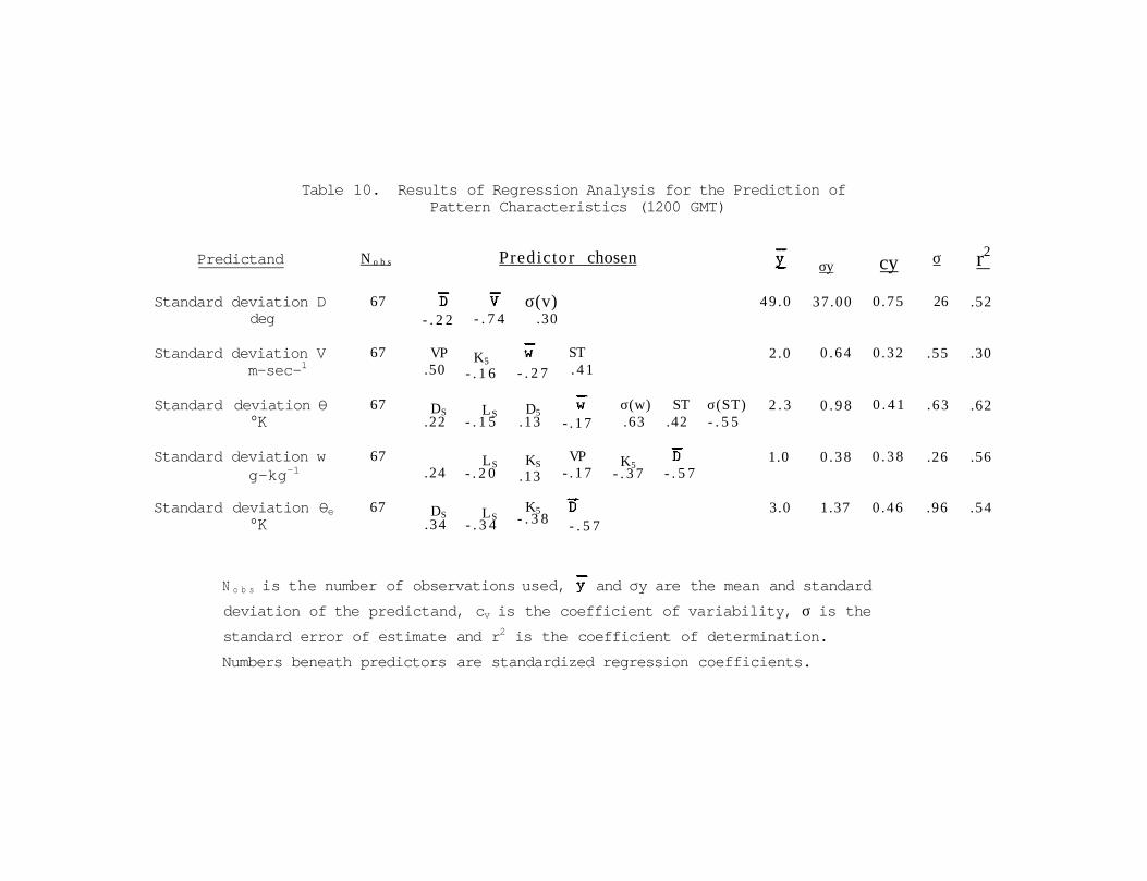
Table 10. Results of Regression Analysis for the Prediction of Pattern Characteristics (1200 GMT)

Predictand

Standard deviation D deg

Standard deviation V m-sec-1

Standard deviation θ °K

Standard deviation w g-kg-1

Standard deviation θe °K

N o b s Predictor chosen σy cy σ r2

67 - . 2 2 - . 7 4

σ(v) .30

49 .0 37 .00 0 .75 26 .52

67 VP .50

K5 - . 1 6 - . 2 7

ST . 4 1

2 .0 0 . 6 4 0 .32 .55 .30

67 DS .22

LS - . 1 5

D5 . 13 - . 1 7

σ(w) .63

ST .42

σ(ST) - . 5 5

2 . 3 0 . 9 8 0 . 4 1 . 63 .62

67 .24

LS - . 2 0

KS . 13

VP - . 1 7

K5 - . 3 7 - . 5 7

1.0 0 . 3 8 0 . 3 8 .26 .56

67 DS . 34

LS - . 3 4

K5 - . 3 8 - . 5 7

3.0 1.37 0 .46 .96 .54

N o b s is the number of observations used, and σy are the mean and standard deviation of the predictand, cv is the coefficient of variability, σ is the standard error of estimate and r2 is the coefficient of determination. Numbers beneath predictors are standardized regression coefficients.

-34-

Cyclonically curved westerly flow apparently causes more variability in the wind pattern at night. Synoptic theory and experience suggest that these situations are associated with unstable polar air,in which nighttime cooling is strong. The regression analysis for the daytime cases shows again a strong dependence among the dependent variables of the wind pattern. These dominate over any other relationships. Strong surface pressure gradients and anti-cyclonically curved 500 mb contours seem to accompany either gustiness or pronounced isotach patterns at the surface. As shown earlier, temperature and relative humidity patterns become more definite in smaller synoptic scale disturbances in the surface isobars, with cyclonic curvature near the surface and anticyclonic curvature at 500 mb. Also the patterns are more definite with advection over land.

The positive relation between the sea temperature and the standard deviations of windspeed and potential temperature are intriguing as is the negative correlation between the standard deviations of sea temperature and potential temperature. Note that in the sample of data studied the sea temperature increased as the season progressed; this may mean that temperature and moisture may be more variable over the network in late summer.

It must be remember that these studies were intended as a prelude to a more detailed investigation into the nature of the significant relationships and to individual case studies that would give more insight into the causes of pattern formation. These studies have to be left to the future.

Interpretation of the time dependence of the vertical motion field from nephanalyses

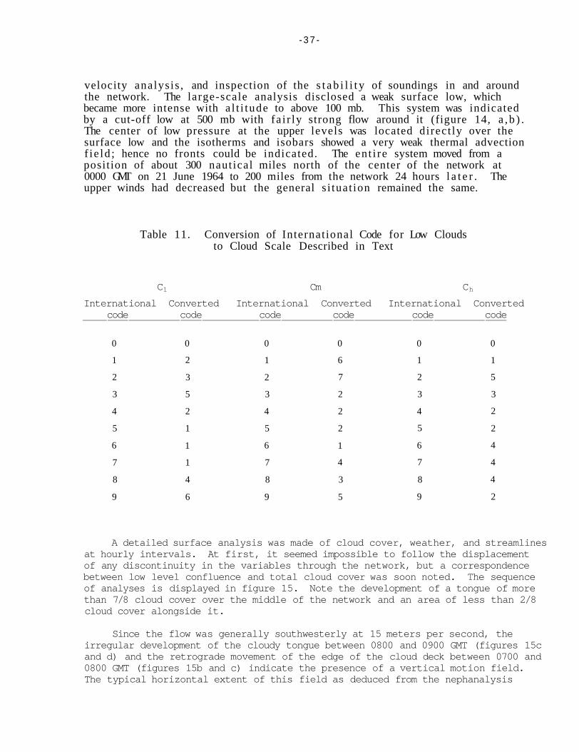
Introduction. Hourly space averages and standard deviations of low cloud type C1, cloud amount N and the number of reports of rain, showers, and thunderstorms were displayed in the format of figures 12a and b for 80 days in 1964 on which convective precipitation was reported. The low cloud type was weighted according to Feteris (1966) so that increasing numbers indicate increasing vertical development or changes from the non-precipitating to the precipitating stage or both (see table 11). Stratification of convective clouds is indicated by decreasing numbers. It was noted that the means of the low cloud type on 21 and 22 June were greater than on any other day. It was also noted that the reported number of showers, thunderstorms, and layer-type cloud precipitation was quite different from one day to the next (compare figures 12 and 13), while the mean and standard deviation of C1 were the same on both days.

On 21 June there were few reports of thunderstorms or stratified rain, while on the next day the number increased markedly. Since the weighted low cloud scale generally assumed that a high mean would indicate generally deep convective precipitation and a low mean would indicate either layer-type cloud precipitation or none, a case study was performed to solve the apparent inconsistency between cloud type and precipitation.

Synoptic analysis. Four forms of analysis were chosen for the case study. These were synoptic scale analysis, sub-synoptic surface, vertical

Figure 12. Statistics of cloud type and cover on 21 June 1964 (a); and precipitation on 21 June 1964 (solid lines represent present

weather, dashed lines represent present plus occurrences in last hour)(b).

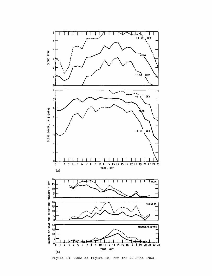
Figure 13. Same as figure 12, but for 22 June 1964.

- 3 7 -

velocity analys is , and inspection of the s t a b i l i t y of soundings in and around the network. The large-scale analysis disclosed a weak surface low, which became more intense with a l t i tude to above 100 mb. This system was indicated by a cut-off low at 500 mb with fa i r ly strong flow around it (figure 14, a , b ) . The center of low pressure at the upper levels was located direct ly over the surface low and the isotherms and isobars showed a very weak thermal advection f ie ld ; hence no fronts could be indicated. The ent i re system moved from a position of about 300 naut ical miles north of the center of the network at 0000 GMT on 21 June 1964 to 200 miles from the network 24 hours l a t e r . The upper winds had decreased but the general s i tuat ion remained the same.

Table 11. Conversion of Internat ional Code for Low Clouds to Cloud Scale Described in Text

C1 Cm Ch

International Converted International Converted International Converted code code code code code code

0 0 0 0 0 0

1 2 1 6 1 1

2 3 2 7 2 5

3 5 3 2 3 3

4 2 4 2 4 2

5 1 5 2 5 2

6 1 6 1 6 4

7 1 7 4 7 4

8 4 8 3 8 4

9 6 9 5 9 2

A detailed surface analysis was made of cloud cover, weather, and streamlines at hourly intervals. At first, it seemed impossible to follow the displacement of any discontinuity in the variables through the network, but a correspondence between low level confluence and total cloud cover was soon noted. The sequence of analyses is displayed in figure 15. Note the development of a tongue of more than 7/8 cloud cover over the middle of the network and an area of less than 2/8 cloud cover alongside it.

Since the flow was generally southwesterly at 15 meters per second, the irregular development of the cloudy tongue between 0800 and 0900 GMT (figures 15c and d) and the retrograde movement of the edge of the cloud deck between 0700 and 0800 GMT (figures 15b and c) indicate the presence of a vertical motion field. The typical horizontal extent of this field as deduced from the nephanalysis

Figure 14. Synoptic situation of 21 June 1964: surface map (a), and 500 mb map (b).

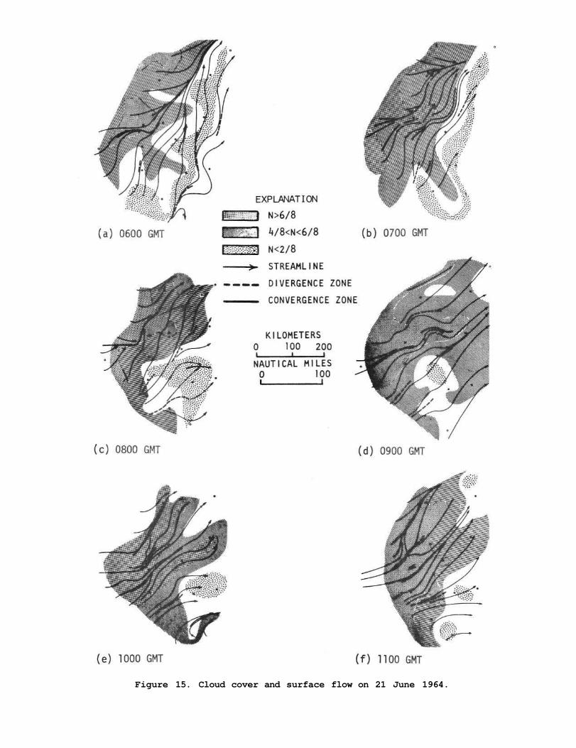
Figure 15. Cloud cover and surface flow on 21 June 1964.

/ -40-

corresponds to a wavelength between 100 and 250 km, and the positive correspondence between cloud cover and confluence indicates that the vertical motions must have extended downwards from at least the medium cloud level to the surface. The life history of the couplet of cloud formation and cloud dissipation seems to cover a period of somewhat less than 6 hours.

Since this case study fell on a weekend, there was not sufficient coverage of pibals and rawinsondes to allow a vertical velocity analysis of that great detail in space and time, but the 500 mb vertical velocity field computed from the regular radiosonde observations at 1200 GMT agrees in general with what was observed at the surface. Figures 16 and 17 show the super­position of the 500 mb vertical velocity on the nephanalysis and on the surface streamline pattern. Note the absence of high and medium cloud in the area of sinking motions and the occurrence of an altostratus deck and steady rain where the air was rising. The superposition of the vertical velocity pattern on the surface streamline pattern indicates that the columns of rising and sinking air extended downwards to the surface. This can also be seen on the cross-section in figure 18.

On 22 June there were more reports of showers and there was more cloud cover than on 21 June (figures 12b and 13b). A considerable amount of medium cloud prevented the observers from seeing distant cumulonimbus clouds. Nephanalyses failed to show interesting features as did the surface streamline patterns.

The analysis of the soundings showed significant differences between the two days. For both parcel and layer displacement methods, the soundings of 21 June were conditionally unstable or neutral at best, while those for 22 June were generally absolutely unstable. On 21 June the tropopause was between 300 and 350 mb, while on 22 June it was between 350 and 400 mb. All of this can be viewed as a consequence of the fact that the center of the deep low pressure system moved closer to the network.

Feasibility of displaying synoptic data as the time dependence of space averages and standard deviations

The question arises whether a time-display of space averages and standard deviations of low cloud type C1 total cloud cover N and the number of reported showers, thunderstorms, or layer-type cloud rains would show the difference between situations with pronounced vertical motion patterns over the network and those with more general ascent.

Figures 12 and 13 clearly show the increase in total cloud cover and the number of reports of various types of precipitation on 21 and 22 June, but apart from a higher standard deviation in the morning of 21 June, the time-dependence of C1 was almost similar on both days. One would then infer the same degree of vertical development of convective clouds from both graphs. However, the number of reports of showers and thunderstorms indicates that there must have been many more cumulonimbus clouds on 22 June, and the synoptic analysis described in the previous section showed more areas free of deep convective clouds on 21 June.

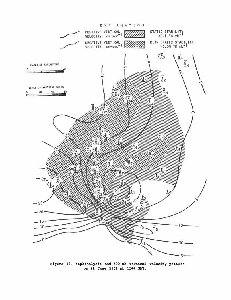
Figure 16. Nephanalysis and 500 mb vertical velocity pattern on 21 June 1964 at 1200 GMT.

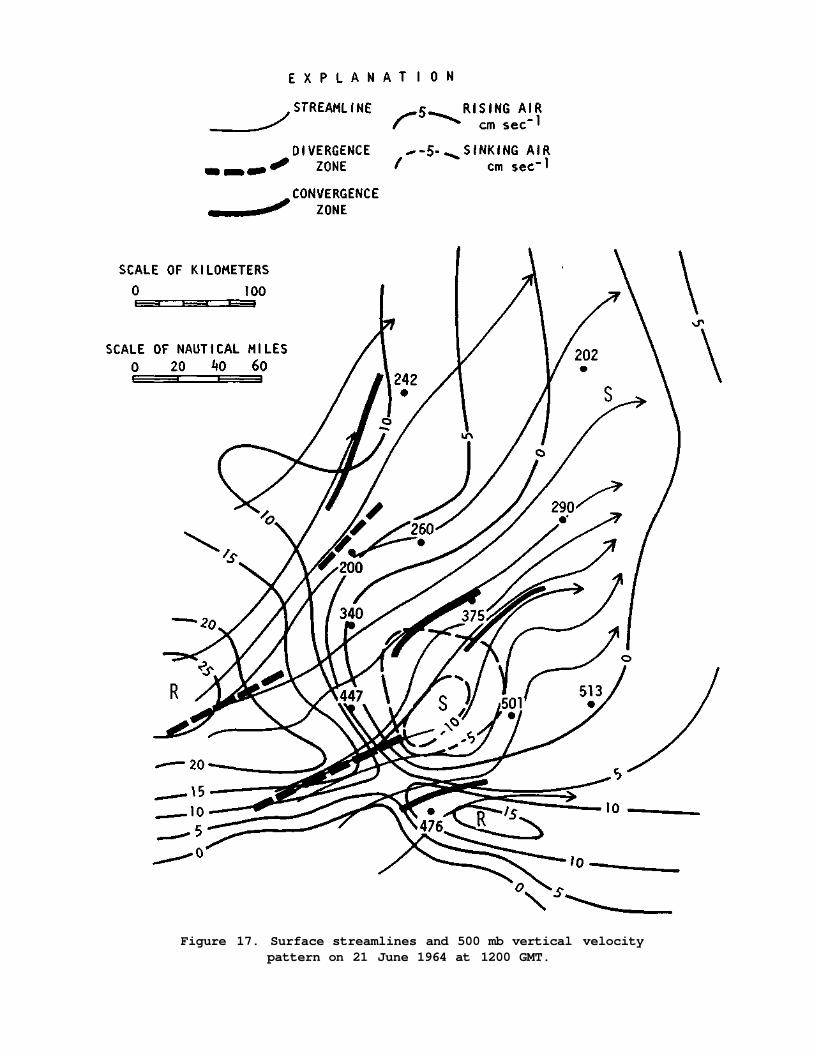
Figure 17. Surface streamlines and 500 mb vertical velocity pattern on 21 June 1964 at 1200 GMT.

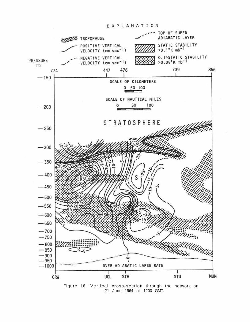
Figure 18. V e r t i c a l c ross - sec t i on through the network on 21 June 1964 at 1200 GMT.

-44-

Figure 19 shows the overlap of the field of view of the synoptic stations for clouds with a vertical extent of 3 km. This overlap enhances the possibility of considerable duplication of reports of deep convective clouds, when the clouds are scattered and the sky is clear in between. Since the cloud cover was less on 21 June than on 22 June, the observers were able to see more distant cumulonimbus clouds and thus reported them. On the next day, the greater amount of middle cloud obscured the view of the observers and hence they were only able to report cumulonimbus in the immediate vicinity of their station. The increase in the number of cumulonimbus clouds from one day to the other was not evident from the statistics , and this means that the transition from a situation with numerous showers and thunderstorms embedded in a medium cloud deck to one with scattered groups of storms surrounded by clear sky would go unnoticed if only the 24-hour graphs of averages and standard deviations were inspected. This surely is a disadvantage of having a dense network of cloud observers. An advantage would be that the transition from a large amount of weakly developed cumuliform clouds to scattered groups of cumulonimbus clouds would be overemphasized, and thus show up clearly, as would the development of showers during the day after a morning with clear skies.

SUMMARY AND CONCLUSIONS

Analysis of data from a dense network of radiosonde and upper wind stations over Western Europe has revealed the existence of sub-synoptic scale disturbances which are associated with vertical velocities from 10 to 100 cm per second. These disturbances have wavelengths between 100 and 500 km. The vertical velocity maxima are invariably found in regions with static stabilities below 0.05 °K/mb which often occur in the upper troposphere. In the more stable layers and also near the tropopause, vertical velocity gradients are still large enough to modify considerably the static stability of the atmosphere within a short time, since the total vertical velocities are an order of magnitude larger than their adiabatic components. In some cases the vertical motions extend downward to the surface where their presence is indicated by convergence and divergence in the wind fields at station level. They cause convection to become organized into groups of showers and thunderstorms.

Nephanalyses made at the time of release of the radiosondes show a notable absence of high and medium cloud above scattered cumulus clouds in areas of descent, while altostratus type clouds or vigorous shower activity are found in areas where the air is ascending. Hourly nephanalyses indicate a life time of these circulations between one and six hours. The low cloud cover shows more rapid fluctuations than that of medium and high clouds.

The relationships between static stability and weather are found to be extremely weak. Hence, neither the depth nor the height of stable layers predict the absence of rain or showers and neither does the static stability in the stablest layer. However, such an index may prove useful for the prediction of location and intensity of vertical motion patterns.

Figure 19. Overlap of the fields of view of the synoptic stations for clouds with tops below 3 km, seen under an elevation angle of 7°.

-46-

It is possible to relate the development of pronounced wind, temperature and moisture patterns near the surface to features of the synoptic scale flow, such as the dimensions of troughs and ridges, pressure and contour gradients and sometimes curvature of the streamlines. However, the curvature of the isobars at the surface is very weakly related to moisture convergence or to the wind pattern itself. The exploration of these relationships has hardly begun and needs to be put on a firmer physical basis.

Studies of the time dependence of meteorological variables at the surface using teletype data are hampered by different coding procedures and different formats for special observations. Also, the coding rules are often changed with time. Manual editing proved to be very tedious and time-consuming but machine editing may solve many of these problems at lower costs. Otherwise, there is sufficient resolution in space and time of the surface synoptic network to allow investigation of sub-synoptic scale circulations.

The resolution in space of the radiosonde and upper wind network is excellent for studies on the smaller scale, but most systems seem to have lifetime much shorter than the 6-hour interval between the regular wind observations and the 12-hour interval between soundings.

REFERENCES

Boer, J. H., and P. J. Feteris, 1968. The influence of the sea on the distribution of lightning and rain on a coastal area. Annalen der Meteorologie, Neue Folge, to be published.

Browning, K. A., and F. H. Ludlam, 1962. Radar analysis of a hailstorm. Quart. J. Roy. Meteor. Soc, 88, 117-135.

Byers, H. R. , and L. J. Battan, 1949. Some effects of vertical windshear on thunderstorm structure. Bull. Amer. Meteor. Soc, 30, 172-173.

and R. R. Braham, 1949. The Thunderstorm. Washington, D. C., U. S. Dept. of Commerce, 287 pp.

Dessens, H., 1960. Severe hailstorms associated with very strong winds between 6,000 and 12,000 meters. Physics of Precipitation, Geophysical Monograph No. 5, Washington, D. C, American Geophysical Union, 333-338.

Estoque, M. A. 1961. A theoretical investigation of the sea breeze. Quart. J. Roy. Meteor. Soc, 88, 136-146.

1962. The sea breeze as a function of the prevailing synoptic situation. J. Atmos. Sci., 19, 224-250.

Feteris, P. J., 1966. Relation of lightning, rainfall and hail to the properties of mesoscale meteorological patterns. First Progress Report, National Science Foundation Grant GP-5196, Illinois State Water Survey, 59 pp.

-47-

Feteris, P. J., 1967. Mesoscale circulation differences related to thunderstorm development. Proceedings Fifth Conference on Severe Local Storms, Boston, American Meteorological Society, 246-255.

Ferguson, H. L. , 1967. Mathematical and synoptic aspects of a small scale wave disturbance over the lower Great Lakes area. J.'Appl. Meteor., 6, 523-529.

Findlater, J., 1964. The sea breeze and inland convection-- an example of their interrelation. Meteor. Mag., 93, 82-89.

Forsythe, G. E., 1945. A generalization of the thermal wind equation to arbitrary horizontal flow. Bull. Amer. Meteor. Soc, 26, 371-376.

Fujita, T., and H. Grandoso, 1968. Split of a thunderstorm into—cyclonic and anticyclonic storms and their motion as determined from numerical model experiments. J. Atmos. Sci., 25, 416-439.

Goldman, J. L., 1966. The role of the Kutta-Joukowski force in. cloud systems with circulation. National Severe Storms Laboratory, Technical Note 48, NSSL 27, 21-34.

Gray, W. M., 1966. The mutual variation of wind, shear" and baroclinity in the cumulus convective atmosphere of the hurricane. Atmospheric Science Paper No. 104, Department of Atmospheric Science', Colorado State University, Fort Collins, Colorado.

Hess, S. L., 1959. Introduction to Theoretical Meteorology. New York, Henry Holt and Company, 362 pp.

Hitschfeld, W., 1960. The motion and erosion of convective storms in severe vertical windshear. J. Meteor., 17, 270-282.

K.N.M.I., 1960-1962. Onweders en Optische Verschijnselen. Vol. 73 (1953) -80 (1959). Annual Thunderstorm Reports, Staatsdrukkerij en Uitgeverijbedrijf, 's Gravenhage.

Kreitzberg, C. W. , 1968. The mesoscale wind field in an occlusion. J. Appl. Meteor., 7, 53-67.

Krishnamurti, T. N., 1968. A diagnostic balance model for studies of weather systems of low and high latitudes. Mon. Wea. Rev., 96, 197-207.

Malkus, J. S., 1952. Recent advances in the study of convective clouds and their interaction with the environment. Tellus, 4, 83-84.

1965. Tropical convection and air-sea boundary exchange, a survey. Geofisica Internacional, 5, 21-32.

and R. S. Scorer, 1955. The erosion of cumulus towers. J. Meteor., 12, 55-56.

McNair, R. R., and J. A. Barthram, 1966. Mesoscale investigation of a squall line. Meteor. Mag., 95, 304-309.

-48-

Newton, C. W. , 1963. Dynamics of severe convective storms. Meteorological Monographs, 5, (27), Boston, Amer. Meteor. Soc., 33-57.

and J. C. Fankhauser, 1964. On the movements of convective storms with emphasis on size discrimination in relation to water budget requirements. J. Appl. Meteor., 3, 651-668.

Panofsky, H. A., 1946. Methods of computing vertical motion in the atmosphere. J. Meteor., 3, 45-49.

Pothecary, J. J. W., 1954. Short period variations in surface pressure and wind. Quart. J. Roy. Meteor. Soc, 80, 395-401.

-49-

APPENDIX A

Lightning and Rain in Relation to Sub-synoptic Plow Parameters*

By John W. Wilson and Pieter J. Feteris

ABSTRACT

Dense networks of lightning counters, raingages, observers, and radiosonde stations were used to collect data for 59 days during 1964 when convective rainfall fell over western Europe. Manual and statistical analyses were performed to determine the relationships among rainfall, vertical windshear, stability, flashing rate, and sub-synoptic flow.

In general, weak relationships between the various parameters were found. Most significant were the negative correlations between stability and rainfall amount, and between surface wet-bulb potential temperature and the area covered by rain.

1. Introduction To a thunderstorm observer the distribution and time dependence

of lightning and precipitation seems rather complex. Some storms give numerous flashes and little rain, while others give only a few discharges and copious ram. In the severest storms both rain and lightning are usually abundant.

An attempt to study the time-dependence between lightning and rain was made by Aalders (1916, 1918), who found that certain parts

*Being submitted to J. Appl. Meteor. for publication

-50-

of thunderstorms that produced cloud-to-ground lightning could be tracked by means of cross-bearings. He also noticed that cloud-to-ground lightning was often followed by a rain gush or the development of precipitation streaks underneath the cloud base at the location of the flash. This subject was brought up again by Moore et al. (1964), who proposed a very plausible theory to explain the rain gush. The theory was based on the increase of collisions and coagulation coefficients between cloud droplets and raindrops in the strong electric fields generated by the lightning discharge. These results are strongly supported by Battan (1965), who found a very pronounced proportionality between the amount of rain and the number of ground discharges produced by the thunderstorm. Other evidence that indicates a positive correlation between lightning and rain has been reported by Dingle (1963), Dingle and Gatz (1963), Fujiwara (l96l), and Mueller (1963). A review of the available observational evidence has been presented by Goyer (1965).

On the other hand, there is evidence that occasionally numerous cloud-to-ground flashes occur, followed by little or no precipitation (Peteris, 1960). One may then raise the question whether the relationship between the efficiency of the thunder­cloud as a precipitator and the development of strong electrical fields is controlled by larger scale processes such as the distri­bution of vertical velocities and the horizontal flow in and around the clouds.

The purpose of this paper is to find whether a high number of cloud-to-ground flashes is correlated with a large amount of rain, and whether the ratio between the two variables depends upon

-51-

the supply of heat and moisture on which the clouds can draw and upon their upward development.

The availability of a network of short-range lightning counters and a dense network of raingages (Boer, 1967) has now provided the means for a more detailed investigation of the dependence of rain­fall and lightning on the ambient flow, the stability of the atmosphere, and the surface wet-bulb potential temperature. Case studies (Browning and Ludlam, 1962) have indicated that the behavior of certain types of thunderstorms is strongly controlled by these variables. Peteris (1965) in a study of 455 thunderstorms in the Netherlands over a period of 5 years, has found a weak negative correspondence between cloud-to-ground lightning in thunderstorms and the intensity of the synoptic scale flow in which they occurred. However, this relationship was based upon the number of reports of lightning damage. Since this is also a function of population density and the distribution of vulnerable objects over the country, any meteorological relationships that might be present are obscured.

2. Data and data processing Since 1960 a network of 15 modified Pierce short-range

lightning counters has been operating in the Netherlands. The area under surveillance by the overlapping ranges of these counters, roughly 11,000 km2, contains about 600 raingages and 110 volunteer thunderstorm observers, and is imbedded in a mesonetwork of surface and upper air stations which covers 60,000 km2. Further details are given by Peteris (1966) and Boer (1967).

-52-

Lightning observations that were followed by thunder within 3 seconds were considered to be cloud-to-ground lightning. By plotting the positions of the ground discharges as reported by the observers, areas traversed by lightning cells could be delineated. The distance between observers was generally less than 5 km, so it seems plausible that only a few flashes were not seen and recorded by at least one observer. As a circular or nearly circular lightning cell (distinguished from a thunderstorm cell because precipitation need not fall from the former) moves it traces an elliptical path, or swath. Maps with lightning cell swaths, hail swaths, and rainfall patterns were prepared by Boer for 59 days with thunderstorms that passed over the network in 1964. Examples are shown in Figs. 1 and 2.

It should be noted that the rainfall maps contain data for a 24-hour period. Any precipitation which did not accompany lightning will result in excessive rain for the day. A solution to this problem was approximated by Boer. During a warm front passage if the rain amounts collected in approximately 20 raingages which were read several times daily showed little variation, the precipitation was assumed to be from stratified clouds. The rainfall for the entire network was then decreased by an appro­priate amount to correct for this non-convective precipitation. This is only an approximation, but the results are closer to the true convective rainfall than if no correction was applied.

The ranges of the lightning counters were fixed, but varied from 8 to 40 km over the network. This enabled overlapping of the areas intercepted by the counters, thus decreasing the possibility of lightning cells missing any counters.

Figure 1. Lightning counters and cell swaths on 22 June 1964.

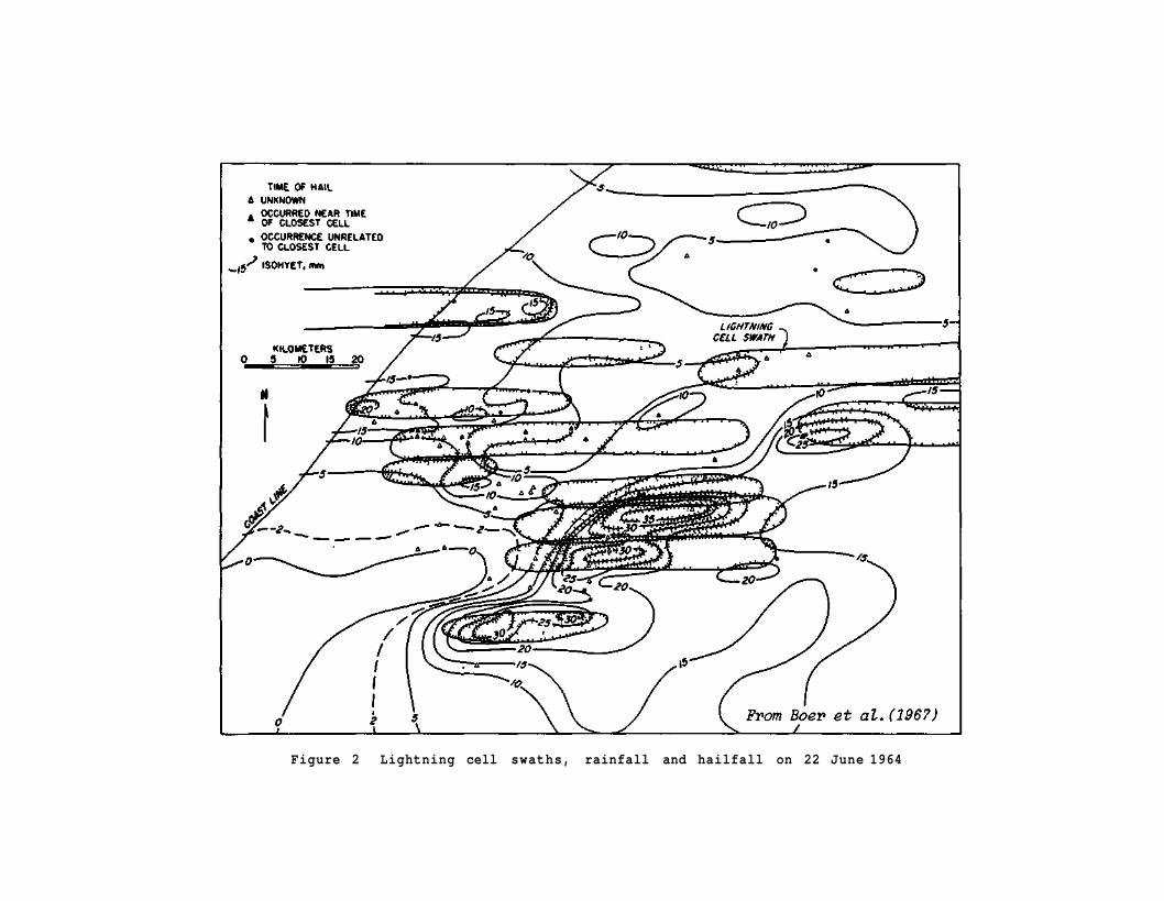
Figure 2 Lightning cell swaths, rainfall and hailfall on 22 June 1964

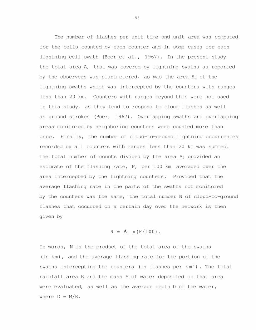
-55-

The number of flashes per unit time and unit area was computed for the cells counted by each counter and in some cases for each lightning cell swath (Boer et al., 1967). In the present study the total area A, that was covered by lightning swaths as reported by the observers was planimetered, as was the area A2 of the lightning swaths which was intercepted by the counters with ranges less than 20 km. Counters with ranges beyond this were not used in this study, as they tend to respond to cloud flashes as well as ground strokes (Boer, 1967). Overlapping swaths and overlapping areas monitored by neighboring counters were counted more than once. Finally, the number of cloud-to-ground lightning occurrences recorded by all counters with ranges less than 20 km was summed. The total number of counts divided by the area A2 provided an estimate of the flashing rate, P, per 100 km averaged over the area intercepted by the lightning counters. Provided that the average flashing rate in the parts of the swaths not monitored by the counters was the same, the total number N of cloud-to-ground flashes that occurred on a certain day over the network is then given by

N = A1 x(F/100).

In words, N is the product of the total area of the swaths (in km), and the average flashing rate for the portion of the swaths intercepting the counters (in flashes per km2). The total rainfall area R and the mass M of water deposited on that area were evaluated, as well as the average depth D of the water, where D = M/R.

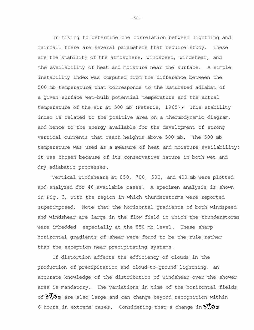
-56-

In trying to determine the correlation between lightning and rainfall there are several parameters that require study. These are the stability of the atmosphere, windspeed, windshear, and the availability of heat and moisture near the surface. A simple instability index was computed from the difference between the 500 mb temperature that corresponds to the saturated adiabat of a given surface wet-bulb potential temperature and the actual temperature of the air at 500 mb (Feteris, 1965)• This stability index is related to the positive area on a thermodynamic diagram, and hence to the energy available for the development of strong vertical currents that reach heights above 500 mb. The 500 mb temperature was used as a measure of heat and moisture availability; it was chosen because of its conservative nature in both wet and dry adiabatic processes.

Vertical windshears at 850, 700, 500, and 400 mb were plotted and analyzed for 46 available cases. A specimen analysis is shown in Pig. 3, with the region in which thunderstorms were reported superimposed. Note that the horizontal gradients of both windspeed and windshear are large in the flow field in which the thunderstorms were imbedded, especially at the 850 mb level. These sharp horizontal gradients of shear were found to be the rule rather than the exception near precipitating systems.

If distortion affects the efficiency of clouds in the production of precipitation and cloud-to-ground lightning, an accurate knowledge of the distribution of windshear over the shower area is mandatory. The variations in time of the horizontal fields of are also large and can change beyond recognition within 6 hours in extreme cases. Considering that a change in

Figure 3. Example analyses of windspeed and vertical windshear for 18 July 1964, 1200 GMT, at four levels over European rainfall network

Thunderstorms occurring at this time are in shaded area.

-58-

does not only depend upon the change in thermal field, but also upon the change in curvature of the streamlines and the variation with height of the curvature (Forsythe, 1945), the windshear may vary substantially in rapidly developing small circulation systems.

3. Statistical analyses To establish whether the heat input into convective storms,

the stability, and the flow in the ambient atmosphere have an effect on the correlation between rainfall and cloud-to-ground lightning, a regression analysis was performed on the data. Five dependent variables (predictands) and 10 independent variables (predictors) were chosen for the study. The dependent variables were:

A/R the percentage of rain area which was traversed by lightning cells; A is the total area traversed by lightning cells (formerly called A1) and R is the total area that received rainfall on a particular day.

N/M the flashing rate per mass of rainwater; N is the total number of cloud-to-ground flashes evaluated over A, and M is the mass of rain in units of 103 kg that fell on R.

F the flashing rate per 100 km2. in F the natural logarithm of F.

D the average rainfall depth in millimeters over the area R.

The independent variables (predictors) were: θsw the surface wet-bulb potential temperature (deg C) in

the region from where storms over the network drew their supply of moist air.

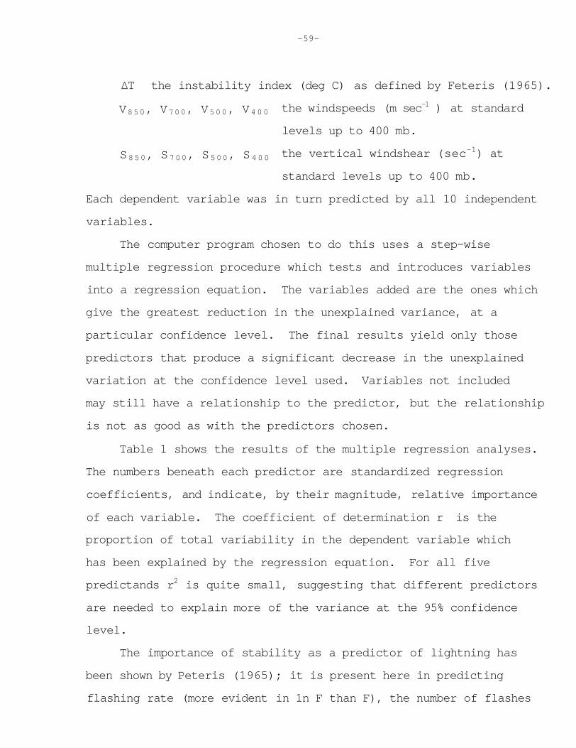
-59-

ΔT the instability index (deg C) as defined by Feteris (1965). V850, V700, V500, V 4 0 0

S850, S700, S500, S 4 0 0

the windspeeds (m sec-1 ) at standard levels up to 400 mb. the vertical windshear (sec-1) at standard levels up to 400 mb.

Each dependent variable was in turn predicted by all 10 independent variables.

The computer program chosen to do this uses a step-wise multiple regression procedure which tests and introduces variables into a regression equation. The variables added are the ones which give the greatest reduction in the unexplained variance, at a particular confidence level. The final results yield only those predictors that produce a significant decrease in the unexplained variation at the confidence level used. Variables not included may still have a relationship to the predictor, but the relationship is not as good as with the predictors chosen.

Table 1 shows the results of the multiple regression analyses. The numbers beneath each predictor are standardized regression coefficients, and indicate, by their magnitude, relative importance of each variable. The coefficient of determination r is the proportion of total variability in the dependent variable which has been explained by the regression equation. For all five predictands r2 is quite small, suggesting that different predictors are needed to explain more of the variance at the 95% confidence level.

The importance of stability as a predictor of lightning has been shown by Peteris (1965); it is present here in predicting flashing rate (more evident in 1n F than F), the number of flashes

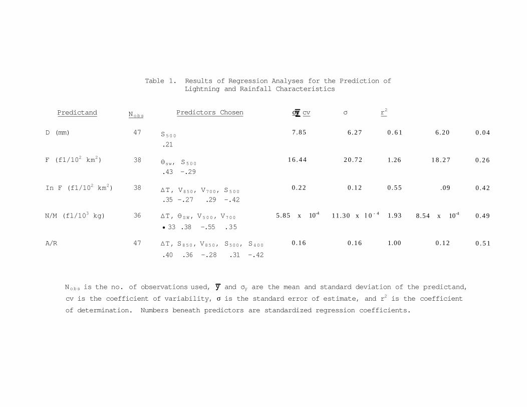
Table 1. Results of Regression Analyses for the Prediction of Lightning and Rainfall Characteristics

Predictand Nobs Predictors Chosen σy cv σ r2

D (mm)

F (f1/102 km2)

In F (f1/102 km2)

N/M (fl/103 kg)

A/R

47

38

38

36

47

S500 .21

θsw, S 5 0 0 .43 -.29

ΔT, V850, V700, S 5 0 0 .35 -.27 .29 -.42

ΔT, θ S W, V 5 0 0, V700

• 33 .38 -.55 .35

ΔT, S850, V850, S500, S400

.40 .36 -.28 .31 -.42

7 .85 6 . 2 7 0 . 6 1 6 .20 0 . 0 4

1 6 . 4 4 2 0 . 7 2 1.26 1 8 . 2 7 0 . 2 6

0 .22 0 .12 0 . 5 5 .09 0 . 4 2

5 .85 x 10-4 11 .30 x l 0 - 4 1.93 8.54 x 10-4 0 .49

0 .16 0 .16 1.00 0 .12 0 . 5 1

Nobs is the no. of observations used, and σy are the mean and standard deviation of the predictand, cv is the coefficient of variability, σ is the standard error of estimate, and r2 is the coefficient of determination. Numbers beneath predictors are standardized regression coefficients.

-61-

per amount of rainfall from a storm, and the percentage of rain area covered by lightning cells. Vonnegut's (1963) charge separ­ation theory, which uses vertical velocities (and hence stability) as a prime mechanism for creation of electric fields in clouds, is also supported by the data.

Vertical windshear appears to be related to the flashing rate; at 500 mb the two are negatively correlated, suggesting that tilting of the electric dipole in the cloud may decrease its rate of discharge.

Inclusion of θsw into the predicting equation for N/M is to be expected, as the wet-bulb potential temperature is a good tracer of moist adiabatic motions, and hence rainfall. The predicting equation for rainfall depth D does not contain θsw; the two are not related at the 95% confidence level, but probably would be at a lower level.

Tables 2 and 3 list the correlation coefficients among the predictors and predictands, respectively. Table 4 lists the correlation coefficients between wet-bulb potential temperature, instability index and rainfall characteristics. The probabilities of obtaining larger correlation coefficients from random sampling are indicated in parentheses in all three tables. Relative independence between variables can be inferred from the probabilities; the closer to unity the probability, the more independent the two variables. The probabilities can be thought of as significance levels (1.0 - confidence level).

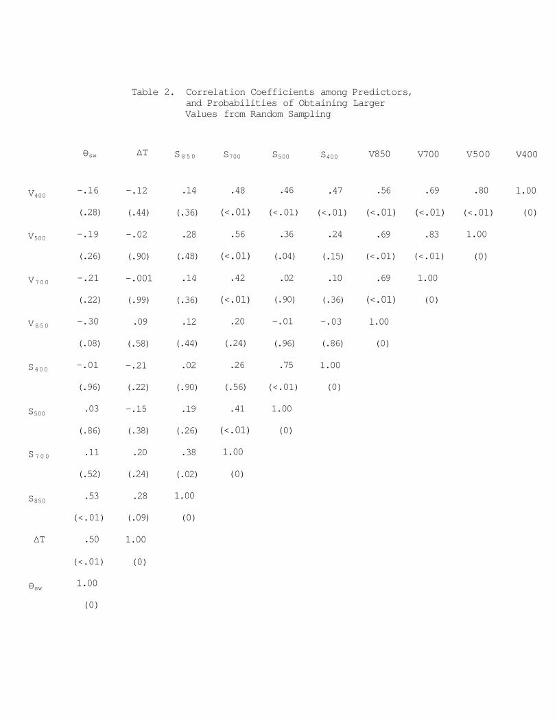
Table 2. Correlation Coefficients among Predictors, and Probabilities of Obtaining Larger Values from Random Sampling

θsw ΔT S850 S700 S500 S400 V850 V700 V500 V400

V400 -.16 -.12 .14 .48 .46 .47 .56 .69 .80 1.00

(.28) (.44) (.36) (<.01) (<.01) (<.01) (<.01) (<.01) (<.01) (0)

V500 -.19 -.02 .28 .56 .36 .24 .69 .83 1.00

(.26) (.90) (.48) (<.01) (.04) (.15) (<.01) (<.01) (0)

V700 -.21 -.001 .14 .42 .02 .10 .69 1.00

(.22) (.99) (.36) (<.01) (.90) (.36) (<.01) (0)

V850 -.30 .09 .12 .20 -.01 -.03 1.00

(.08) (.58) (.44) (.24) (.96) (.86) (0)

S400 -.01 -.21 .02 .26 .75 1.00

(.96) (.22) (.90) (.56) (<.01) (0)

S500 .03

(.86)

-.15

(.38)

.19

(.26)

.41

(<.01) 1.00

(0)

S 7 0 0 .11

(.52)

.20

(.24)

.38

(.02)

1.00

(0)

S850 .53

(<.01)

.28

(.09)

1.00

(0)

ΔT .50 1.00

(<.01) (0)

θsw 1.00

(0)

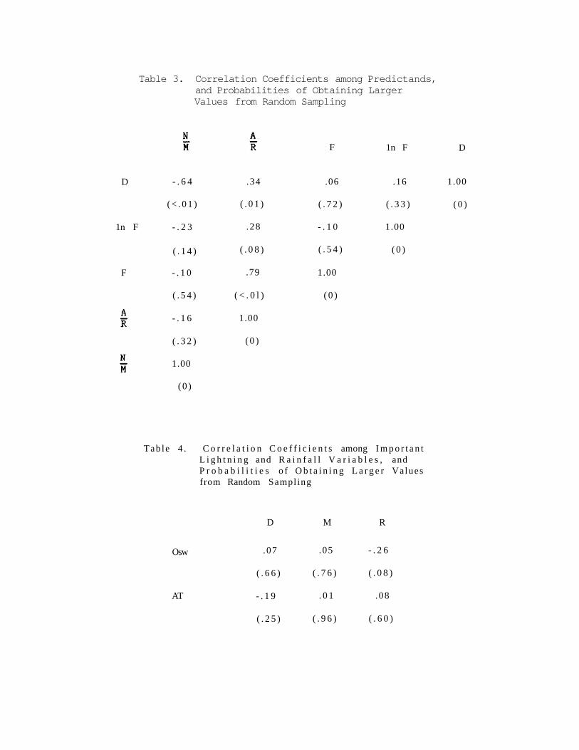
Table 3. Correlation Coefficients among Predictands, and Probabilities of Obtaining Larger Values from Random Sampling

F

D - . 6 4 .34 .06 .16 1.00

( < . 0 1 ) ( . 0 1 ) ( . 7 2 ) ( . 3 3 ) ( 0 )

1n F - . 2 3 . 28 - . 1 0 1.00

( . 1 4 ) ( . 0 8 ) ( . 5 4 ) ( 0 )

F - . 1 0 .79 1.00

( . 5 4 ) ( < . 0 l ) ( 0 )

- . 1 6

( . 3 2 )

1.00

( 0 )

1.00

( 0 )

Tab le 4 . C o r r e l a t i o n C o e f f i c i e n t s among I m p o r t a n t L i g h t n i n g and R a i n f a l l V a r i a b l e s , and P r o b a b i l i t i e s o f O b t a i n i n g L a r g e r Values from Random Sampling

D M R

Osw .07 .05 - . 2 6

( . 6 6 ) ( . 7 6 ) ( . 0 8 )

AT - . 1 9 . 0 1 .08

( . 2 5 ) ( . 9 6 ) ( . 6 0 )

1n F D

-64-

4. Summary and conclusions Detailed analyses of lightning frequency, rainfall, stability,

and windshear have been performed for 59 days of convective precipitation in 1964. The data were provided by dense networks of lightning counters, raingages, observers, and radiosonde stations located in western Europe. A step-wise multiple regression technique was used to predict, with ten independent variables, five characteristics of lightning and rainfall.

Several things are evident from these analyses: 1. the correlations between rainfall depth and both lightning

frequency and wet-bulb potential temperature are low; 2. stability and rainfall depth are negatively correlated,

but the relationship is valid only to the 0.25 significance level;

3. the area covered by rain and the surface wet-bulb potential temperature are negatively correlated;

4. vertical windshear at 500 mb and the flashing rate are negatively correlated, suggesting that tilting of the electric dipole in a cloud may decrease the cloud's capability of discharging to earth;

5. more predictors are needed to completely describe the predictands used for the statistical analyses.

ACKNOWLEDGMENTS

The data used in this study was collected and prepared by Major J. H. Boer of the Meteorological Service of the Netherlands Air Force. His personal time and efforts spent in analyzing the

-65

rainfall and lightning maps is truly appreciated. Dr. P. T. Schickedanz assisted in the statistical analysis for this paper; the authors are grateful for his time. Messrs. G. E. Stout, P. A. Huff, and R. G. Semonin kindly reviewed the paper and offered helpful suggestions. The work was supported by the National Science Foundation under Grants GP-5196 and GA-1321.

REFERENCES

Aalders, A. J., 1916. Over de electrische ontladingen tijdens het onweer. (About the electrical discharges during the thunderstorm), Hemel en Dampkring, 14. 1918. Over de electrische ontladingen tijdens het onweer.

Hemel en Dampkring, 15. Battan, L. J., 1965. Some factors governing precipitation and

lightning from convective clouds, J. Atmos. Sci., 22, 79-85. Boer, J. H., 1967. A verification of the accuracy of short-range

lightning counters. Weather, 22, 321-330. P. J. Feteris, and J. W. Wilson, 1967. Short-range lightning

counters, a research tool. Proceedings, Fifth Conference on Severe Local Storms, Boston, Amer. Meteor. Soc, 49-54.

Browning, K. A., and P. H. Ludlam, 1962. Airflow in convective storms. Quart. J. Roy. Meteor. Soc, 88, 117-135.

Dingle, A. N., 1963. Raindrop size studies. Pinal Report, APCRL Contract No. AF 19(628)-28l, Department of Meteorology and Oceanography, The University of Michigan, Ann Arbor, 23 pp.

-66-

and D. F. Gatz, 1963. Rain scavenging of particulate matter from the atmosphere. Pinal Report, AEC Contract No. AT(ll-l)-739, Department of Meteorology and Oceanography, The University of Michigan, Ann Arbor, 102 pp.

Peteris, P. J., 1960. The thunderstorm of July 6, 1952. Onweders en Optische Verschijnselen, Part 73. KNMI. (Annual Thunderstorm Reports, Staatsdrukkerij en Uitgeverijbedrijf•s Gravenhage, Netherlands). 1965. Statistical studies on thunderstorm situations in

the Netherlands. J. Appl. Meteor., 4, 178-185. 1966. Relation of lightning, rainfall and hail to the

properties of mesoscale meteorological patterns. First Progress Report, NSF Contract No. GP-5196, Illinois State Water Survey, Urbana, 59 pp.

Forsythe, G. G., 1945• A generalization of the thermal wind equation to arbitrary horizontal flow. Bull. Amer. Meteor. Soc., 26, 371-375.

Fujiwara, M., 1961. Raindrop size distribution with rainfall types and weather conditions. Research Report No. 8., Contract DA-36-039 SC-87280, Illinois State Water Survey, Urbana, 48 pp.

Goyer, G. G., 1965. The effects of lightning on hydrometeors and rainfall. Proceedings, International Conference on Cloud Physics. Tokyo, Japan, 375-379.

Moore, C. B., B. Vonnegut, E. A. Vrablik, and D. A. McCaig, 1964. Gushes of rain and hail after lightning. J. Atmos. Sci., 21, 646-665.

-67-

Mueller, E. A., 1963° Investigation of the quantitative determination of point and areal precipitation by radar echo measurements. Sixth Quarterly Tech. Rep., Contract No. DA-36-O39 SC-87280, Illinois State Water Survey, Urbana, 13 pp.

Vonnegut, B., 1963. Some facts and speculations concerning the origin and role of thunderstorm electricity. Meteor. Monographs, 5(27), Boston, Amer. Meteor. Soc., 224-241.

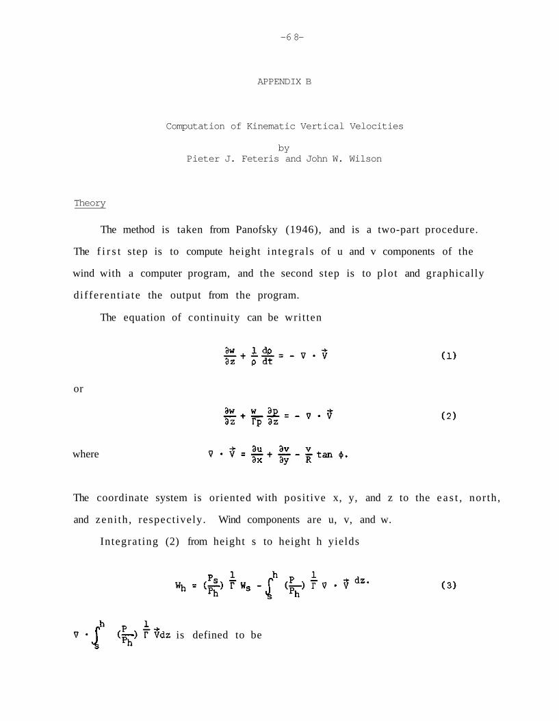
-6 8-

APPENDIX B

Computation of Kinematic Vertical Velocities

by Pieter J. Feteris and John W. Wilson

Theory

The method is taken from Panofsky (1946), and is a two-part procedure.

The f i r s t step is to compute height in tegra ls of u and v components of the

wind with a computer program, and the second step is to plot and graphically

d i f ferent ia te the output from the program.

The equation of continuity can be writ ten

or

where

The coordinate system is oriented with posit ive x, y, and z to the e a s t , north,

and zeni th , respectively. Wind components are u, v, and w.

Integrat ing (2) from height s to height h yields

is defined to be

-69-

This expands upon differentiation to

Assuming and because (5) reduces to

But, from (3),

so that

or

The components of the vector integral in (7),

- 7 0 -

are the integrals to be calculated by the computer. This is to be done for a

number of points (observing s t a t i o n s ) , thus completxng the f i r s t step of the

procedure.

For the second s tep , maps of each component printed are drawn and analyzed

(one map per height per component). A grid is overlaid on the ∫udz map and

values read at each gridpoint . Shift the overlay one grid distance to the l e f t ,

subtract the two values, and plot the difference on another map. The same

procedure is used to shif t the ∫vdz map in the -y direct ion. Now graphically

add the two maps. The negative of the ve r t i ca l velocity f ie ld is then found.

This program is written ,in FORTRAN IV for both the IBM 7094 and 360/75

computers. Input format is ident ica l to that of the ,windshear program described

by Feteris (1966).

Outline of the algorithm

I. Computer programmed

A. Decompose each data point (height) into i t s u and v components.

B. F i t a fourth degree polynomial through the" prof i le of the u-components and another through the v-components, ( t h i s allows for three inf lect ion points in the p ro f i l e s ) .

C. Compute o∫h udz and o∫h vdz for each data level h in the p ro f i l e s , and pr in t the r e s u l t s .

I I . Manual operations

A. Plot a horizontal map of o∫h udz and another for o∫h vdz for any-level h.

B. Analyze these maps.

C. Graphically di f ferent ia te each component to find

-71-

1. Place a grid over the o∫h udz map, and read the values at each gridpoint.

2. Shift the grid one gridlength to the left and read the values at each gridpoint.

3. Subtract the unshifted point values from the shifted ones and plot the results on a new map and analyze this map.

4. Repeat steps 1-3 for the o∫h vdz map, but shift the grid vertically down one gridlength.

5. Graphically add the two new maps; multiply these values by (-1).

D. This is a map of the vertical velocity field from the surface to height h.

E. Repeat A-D for each height desired.

References

Feteris, P. J., 1966. Relation of lightning, rainfall and hail to the properties of mesoscale meteorological patterns. First Progress Report, National Science Foundation Grant GP-5196, Illinois State Water Survey, Urbana, 59 pp.

Panofsky, H. A., 1946. Methods of computing vertical motion in the atmosphere. J. Meteor., 3, 45-49.

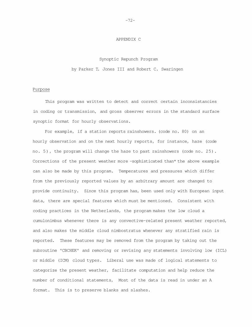
-72-

APPENDIX C

Synoptic Repunch Program

by Parker T. Jones III and Robert C. Swaringen

Purpose

This program was written to detect and correct certain inconsistancies

in coding or transmission, and gross observer errors in the standard surface

synoptic format for hourly observations.

For example, if a station reports rainshowers. (code no. 80) on an

hourly observation and on the next hourly reports, for instance, haze (code

no. 5), the program will change the haze to past rainshowers (code no. 25).

Corrections of the present weather more -sophisticated than* the above example

can also be made by this program. Temperatures and pressures which differ

from the previously reported values by an arbitrary amount are changed to

provide continuity. Since this program has, been used only with European input

data, there are special features which must be mentioned. Consistent with

coding practices in the Netherlands, the program makes the low cloud a

cumulonimbus whenever there is any convective-related present weather reported,

and also makes the middle cloud nimbostratus whenever any stratified rain is

reported. These features may be removed from the program by taking out the

subroutine "CBCHEK" and removing or revising any statements involving low (ICL)

or middle (ICM) cloud types. Liberal use was made of logical statements to

categorize the present weather, facilitate computation and help reduce the

number of conditional statements, Most of the data is read in under an A

format. This is to preserve blanks and slashes.

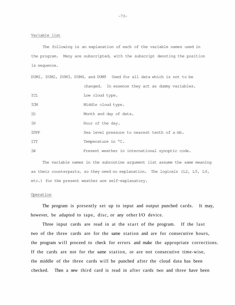
-73-

Variable list

The following is an explanation of each of the variable names used in

the program. Many are subscripted, with the subscript denoting the position

is sequence.

DUM1, DUM2, DUM3, DUM4, and DUM9 Used for all data which is not to be

ICL

ICM

ID

IH

IPPP

ITT

IW

changed. In essence they act as dummy variables.

Low cloud type.

Middle cloud type.

Month and day of data.

Hour of the day.

Sea level pressure to nearest tenth of a mb.

Temperature in °C.

Present weather in international synoptic code.

The variable names in the subroutine argument list assume the same meaning

as their counterparts, so they need no explanation. The logicals (L2, L5, L6,

etc.) for the present weather are self-explanatory.

Operation

The program is presently se t up to input and output punched cards. It may,

however, be adapted to tape , d i sc , or any other I/O device.

Three input cards are read in at the s t a r t of the program. If the l a s t

two of the three cards are for the same s ta t ion and are for consecutive hours,

the program wi l l proceed to check for errors and make the appropriate correct ions.

If the cards are not for the same s t a t i on , or are not consecutive time-wise,

the middle of the three cards wi l l be punched af ter the cloud data has been

checked. Then a new third card is read in af ter cards two and three have been

-74-

rearranged to become cards one and two. This process is continued until the

end of the ,data is reached or until a break of 24 hours or more is encountered

in the data. When such a break is found the program terminates and the message

"Dates of input data are not concurrent" is printed out.

Input of data

The data must first be punched on cards using the given format. Next

the cards are sorted by station number so that all the reports for the same

station will be together and in chronological order. One blank card must be

put at the front of the data deck and another at the end. It is important

that a blank card also be inserted each place the station number changes.

This means there will be a blank between the last card of one data set and

the first card of the next data set. This is very necessary since it prevents

the computer from averaging temperatures and pressures from two different

stations. The number of input cards is determined only by the limitations of

the facility being used. The input must, however, be for successive days

even though there need not be a full 24 hours of data for any one day.

Input format

The station number is in columns 1, 2, and 3. The height of the station

(in meters or feet) is punched in columns 4, 5, and 6. The synoptic observation

is punched according to the following format, the letters being consistent with

the standard international synoptic code and "b" meaning a blank space.

Column 1 2 3 4 5 6 7 8 9 10 11 12 13 14 15 16 17 18 19 20 Data I I I Z Z Z b N D D F F b V V W W W b P

Column 21 22 23 24 25 26 27 28 29 30 31 32 33 34 35 36 37 38 39 40 Data P P T T b Nh C1 h Cm Ch b TD TD a p p b 7 R R

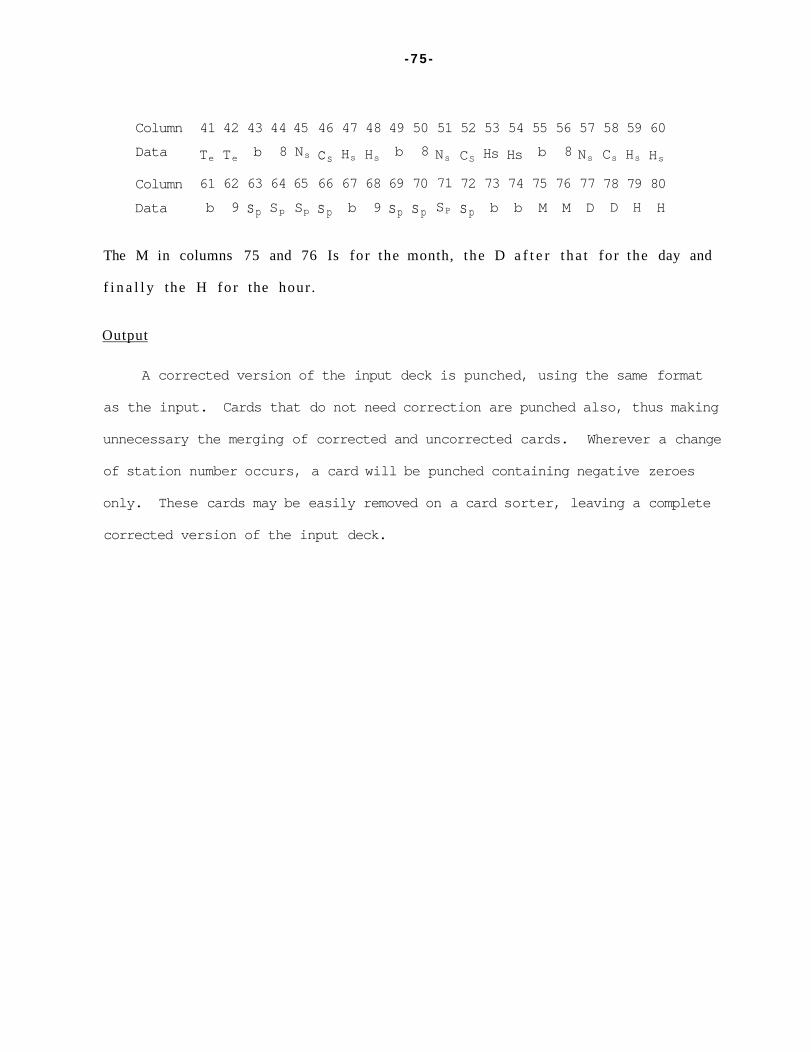
- 75 -

Column 41 42 43 44 45 46 47 48 49 50 51 52 53 54 55 56 57 58 59 60 Data Te Te b 8 Ns cs Hs Hs b 8 Ns CS Hs Hs b 8 Ns Cs Hs Hs

Column 61 62 63 64 65 66 67 68 69 70 71 72 73 74 75 76 77 78 79 80 Data b 9 sp Sp Sp sp b 9 sp sp SP sp b b M M D D H H

The M in columns 75 and 76 Is for the month, the D a f t e r t ha t for the day and

f i n a l l y the H fo r the hour .

Output

A corrected version of the input deck is punched, using the same format

as the input. Cards that do not need correction are punched also, thus making

unnecessary the merging of corrected and uncorrected cards. Wherever a change

of station number occurs, a card will be punched containing negative zeroes

only. These cards may be easily removed on a card sorter, leaving a complete

corrected version of the input deck.