UNIVERSITY OF CALIFORNIA, SAN DIEGO ... - eScholarship.org

UNIVERSITY OF CALIFORNIA, SAN DIEGO

Growth Modeling of the Normal Human Fetal Left Ventricle and a Patient-Specific Case Study of Hypoplastic Left Heart Syndrome

A Thesis submitted in partial satisfaction of the requirements for the degree Master of Science

in

Bioengineering

by

Devleena Kole

Committee in Charge: Jeffrey Omens, Chair

Andrew McCulloch, Co-Chair Sukriti Dewan Adam Engler

2016

Copyright

Devleena Kole, 2016

All rights reserved.

iii

The Thesis of Devleena Kole is approved, and it is acceptable in quality and form for publication on microfilm and electronically: _______________________________________________________________________ _______________________________________________________________________ ________________________________________________________________________ Co-Chair ________________________________________________________________________

Chair

University of California, San Diego

2016

iv

EPIGRAPH

The little space within the heart is as great as the vast universe. The heavens and the earth

are there, and the sun and the moon and the stars. Fire and lightning and winds are there,

and all that now is and all that is not.

Swami Prabhavananda

v

TABLE OF CONTENTS

Signature Page . . . . . . . . . . . . . . . . . . . . . . . . . . . . . . . . . . . . . . . . . . . . . . . . . . . . . . . . . iii

Epigraph . . . . . . . . . . . . . . . . . . . . . . . . . . . . . . . . . . . . . . . . . . . . . . . . . . . . . . . . . . . . . . iv

Table of Contents . . . . . . . . . . . . . . . . . . . . . . . . . . . . . . . . . . . . . . . . . . . . . . . . . . . . . . . v

List of Figures . . . . . . . . . . . . . . . . . . . . . . . . . . . . . . . . . . . . . . . . . . . . . . . . . . . . . . . . viii

List of Tables . . . . . . . . . . . . . . . . . . . . . . . . . . . . . . . . . . . . . . . . . . . . . . . . . . . . . . . . . xii

Acknowledgments . . . . . . . . . . . . . . . . . . . . . . . . . . . . . . . . . . . . . . . . . . . . . . . . . . . . . xiv

Abstract of the Thesis . . . . . . . . . . . . . . . . . . . . . . . . . . . . . . . . . . . . . . . . . . . . . . . . . . .xvi

Chapter 1. Background . . . . . . . . . . . . . . . . . . . . . . . . . . . . . . . . . . . . . . . . . . . . . . . . . . 1

1.1 Significance . . . . . . . . . . . . . . . . . . . . . . . . . . . . . . . . . . . . . . . . . . . . . . . . . . 1

1.2 Cardiac Developmental Physiology . . . . . . . . . . . . . . . . . . . . . . . . . . . . . . . . 4

1.2.1 Embryonic . . . . . . . . . . . . . . . . . . . . . . . . . . . . . . . . . . . . . . . . . . .4

1.2.2 Fetal . . . . . . . . . . . . . . . . . . . . . . . . . . . . . . . . . . . . . . . . . . . . . . . .5

1.2.3 Neonatal. . . . . . . . . . . . . . . . . . . . . . . . . . . . . . . . . . . . . . . . . . . . .7

1.3 Cardiac Mechanics . . . . . . . . . . . . . . . . . . . . . . . . . . . . . . . . . . . . . . . . . . . . . 9

1.3.1 Anatomy and Ventricular Function . . . . . . . . . . . . . . . . . . . . . . . 9

1.3.2 Myocardial Mechanical Properties . . . . . . . . . . . . . . . . . . . . . . . 13

1.4 Computational Modeling . . . . . . . . . . . . . . . . . . . . . . . . . . . . . . . . . . . . . . .. 14

1.4.1 Introduction . . . . . . . . . . . . . . . . . . . . . . . .. . . . . . . . . . . . . . . . . 14

1.4.2 Modeling of Cardiac Structures . . . . . . . . . . . . . . . . . . . . . . . . . 16

1.4.3 Growth Modeling . . . . . . . . . . . . . . . . . . . . . . . . . . . . . . . . . . . . 18

1.5 Clinical Relevance . . . . . . . . . . . . . . . . . . . . . . . . . . . . . . . . . . . . . . . . . . . .. 20

vi

1.6 Specific Aims . . . . . . . . . . . . . . . . . . . . . . . . . . . . . . . . . . . . . . . . . . . . . . . .22

Chapter 2. Model Selection for Normal Human Fetal LV Growth . . . . . . . .. . . . . . . . . 24

2.1 Methods . . . . . . . . . . . . . . . . . . . . . . . . . . . . . . . . . . . . . . . . . . . . . . . . . . . . .24

2.1.1 Study Design . . . . . . . . . . . . . . . . . . . . . . . . . . . . . . . . . . . . . . . . . 25

2.1.2 Mesh Generation . . . . . . . . . . . . . . . . . . . . . . . . . . . . . . . . . . . . . . 26

2.1.3 Material Properties . . . . . . . . . . . . . . . . . . . . . . . . . . . . . . . . . . . . 28

2.1.4 Growth Law . . . . . . . . . . . . . . . . . . . . . . . . . . . . . . . . . . . . . . . . . . 29

2.1.5 Statistical Analysis using Z-scores . . . . . . . . . . . . . . . . . . . . . . . .. 31

2.2 Results . . . . . . . . . . . . . . . . . . . . . . . . . . . . . . . . . . . . . . . . . . . . . . . . . . . . . 33

2.2.1 Z-score Analysis for Model Selection . . . . . . . . . . . . . . . . . . . . . . 33

2.2.2 Model for Normal Human Fetal LV Growth . . . . . . . . . . . . . . . . .39

2.3 Discussion . . . . . . . . . . . . . . . . . . . . . . . . . . .. . . . . . . . . . . . . . . . . . . . . . . . .42

2.3.1 Statistical Analysis using Z-scores . . . . . . . . . . . . . . . . . . . . . . . . .42

2.3.2 Model for Normal Human Fetal LV Growth. . . . . . . . . . . . . . . . . 45

Chapter 3. Growth Model Sensitivity . . . . . . . . . . . . . . . . . . . . . . . . . . . . . . . . . . . . . . . 47

3.1 Methods . . . . . . . . . . . . . . . . . . . . . . . . . . . . . . . . . . . . . . . . . . . . . . . . . . . . .47

3.1.1 Study Design . . . . . . . . . . . . . . . . . . . . . . . . . . . . . . . . . . . . . . . . . 48

3.1.2 Growth Model Sensitivity Analysis . . . . . . . . . . . . . . . . . . . . . . . 50

3.2 Results of Growth Model Sensitivity Analysis . . . . . . . . . . . . . . . . . . . . . . .54

3.2.1 Overview of Cases with Vo = same . . . . . . . . . . . . . . . . . . . . .. . . 54

3.2.2 Overview of Cases with Vo ≠ same . . . . . . . . . . . . . . . . . . . . . . . 75

3.2.3 Summary of Growth Model Sensitivity Analysis . . . . . . . . . . . . .88

3.3 Discussion . . . . . . . . . . . . . . . . . . . . . . . . . . . . . . . . . . . . . . . . . . . . . . . . . . 90

vii

Chapter 4. Reverse Growth . . . . . . . . . . . . . . . . . . . . . . . . . . . . . . . . . . . . . . . . . . . . . . .95

4.1 Methods . . . . . . . . . . . . . . . . . . . . . . . . . . . . . . . . . . . . . . . . . . . . . . . . . . . . .95

4.2 Results . . . . . . . . . . . . . . . . . . . . . . . . . . . . . . . . . . . . . . . . . . . . . . . . . . . . . .96

4.3 Discussion . . . . . . . . . . . . . . . . . . . . . . . . . . . . . . . . . . . . . . . . . . . . . . . . . . .99

Chapter 5. Patient-Specific Case Study of HLHS . . . . . . . . . . . . . . . . . . . . . . . . . . . . .104

5.1 Methods . . . . . . . . . . . . . . . . . . . . . . . . . . . . . . . . . . . . . . . . . . . . . . . . . . .. 104

5.1.1 Clinical Measurements . . . . . . . . . . . . . . . . . . . . . . . . . . . . . . . . 104

5.1.2 Mesh Generation . . . . . . . . . . . . . . . . . . . . . . . . . . . . . . . . . . . . . .105

5.2 Results . . . . . . . . . . . . . . . . . . . . . . . . . . . . . . . . . . . . . . . . . . . . . . . . . . . . 107

5.3 Discussion . . . . . . . . . . . . . . . . . . . . . . . . . . . . . . . . . . . . . . . . . . . . . . . . . .110

Chapter 6. Conclusions . . . . . . . . . . . . . . . . . . . . . . . . . . . . . . . . . . . . . . . . . . . . . . . . .114

References . . . . . . . . . . . . . . . . . . . . . . . . . . . . . . . . . . . . . . . . . . . . . . . . . . . . . . . . . . .117  

viii

LIST OF FIGURES

Figure 1.1: Atrial pressure and stroke volume relationship in the fetal and

mature heart . . . . . . . . . . . . . . . . . . . . . . . . . . . . . . . . . . . . . . . . . . . . . . . 6 Figure 1.2: Pressure-Volume diagram of the cardiac cycle . . . . . . . . . . . . . . . . . . . . 11 Figure 2.1: Workflow for developing a clinically relevant normal human fetal

LV growth model . . . . . . . . . . . . . . . . . . . . . . . . . . . . . . . . . . . . . . . . . . 25 Figure 2.2: An ellipsoid mesh in prolate spheroidal coordinate system (𝜆, 𝜇, 𝜃)

and its relationship to rectangular Cartesian coordinate system (X1, X2, X3) . . . . . . . . . . . . . . . . . . . . . . . . . . . . . . . . . . . . . . . . . . . . . . 28

Figure 2.3: Z-score distribution of fetal LV inner diameter at an unloaded state . . . . . . . . . . . . . . . . . . . . . . . . . . . . . . . . . . . . . . . . . . . . . . . . . . . . . 34 Figure 2.4: Z-score distribution of fetal LV inner length at an unloaded state . . . . . . . . . . . . . . . . . . . . . . . . . . . . . . . . . . . . . . . . . . . . . . . . . . . . . 34 Figure 2.5: Z-score distribution of fetal LV average wall thickness at an unloaded state . . . . . . . . . . . . . . . . . . . . . . . . . . . . . . . . . . . . . . . . . . . . . 35 Figure 2.6: Z-score distribution of fetal LV inner diameter at a loaded state . . . . . . . . . . . . . . . . . . . . . . . . . . . . . . . . . . . . . . . . . . . . . . . . . . . . . 36 Figure 2.7: Z-score distribution of fetal LV inner length at a loaded state . . . . . . . . . . . . . . . . . . . . . . . . . . . . . . . . . . . . . . . . . . . . . . . . . . . . . 36 Figure 2.8: Refined mesh of Model 24, the working reference model for normal human fetal LV growth . . . . . . . . . . . . . . . . . . . . . . . . . . . . . . . 39 Figure 2.9: Inflation curve describing the normal pressure-volume relations at mid gestation in a human fetal LV . . . . . . . . . . . . . . . . . . . . . . . . . . . 39 Figure 2.10: Simulated normal volumetric growth in the fetal LV cavity (top) and free wall (bottom) from mid gestation to birth . . . . . . . . . . . . 40 Figure 2.11: Simulated normal shape growth in the fetal LV cavity from mid gestation to birth . . . . . . . . . . . . . . . . . . . . . . . . . . . . . . . . . . . . . . . .41 Figure 3.1: Case 1 Inflation curve (top) and LV cavity volumetric growth (bottom) . . . . . . . . . . . . . . . . . . . . . . . . . . . . . . . . . . . . . . . . . . . . . . . . . .56

ix

Figure 3.2: Case 2 Inflation curve (top) and LV cavity volumetric growth (bottom) . . . . . . . . . . . . . . . . . . . . . . . . . . . . . . . . . . . . . . . . . . . . . . . . . .57 Figure 3.3: Case 3 Inflation curve (top) and LV cavity volumetric growth (bottom) . . . . . . . . . . . . . . . . . . . . . . . . . . . . . . . . . . . . . . . . . . . . . . . . . .58 Figure 3.4 Linear regression lines fitted to the data in Cases 1 (open blue circles) and 3 (open orange circles) . . . . . . . . . . . . . . . . . . . . . . . . . . . . 59 Figure 3.5 A visual representation of %Growth in the LV cavity and free wall as it changes with respect to EDP in Cases 1 and 2 . . . . . . . . . . . . 61 Figure 3.6 A visual representation of %Growth in the LV cavity and free wall as it changes with respect to EDV-Vo in Cases 1 and 3 . . . . . . . . 62 Figure 3.7 A visual representation of %Growth in the LV cavity and free wall as it changes with respect to Cpass in Cases 2 and 3 . . . . . . . . . . . 64 Figure 3.8: Case 6 Inflation curve (top) and LV cavity volumetric growth (bottom) . . . . . . . . . . . . . . . . . . . . . . . . . . . . . . . . . . . . . . . . . . . . . . . . . . 66 Figure 3.9: Case 6 Inflation curve (top) and LV cavity volumetric growth (bottom) . . . . . . . . . . . . . . . . . . . . . . . . . . . . . . . . . . . . . . . . . . . . . . . . . . 67 Figure 3.10: Case 6 comparing the effect of shape on %Growth of LV cavity volume . . . . . . . . . . . . . . . . . . . . . . . . . . . . . . . . . . . . . . . . . . . . . 68 Figure 3.11: A visual representation of %Growth in the LV cavity and free wall as it changes with respect to wall thickness in Case 6 . . . . . . . . . . 69 Figure 3.12: A visual representation of %Growth in the LV cavity and free wall as it changes with respect to SA:LA in Case 6 . . . . . . . . . . . . . . . . 70 Figure 3.13: A visual representation of %Growth in the LV cavity and free wall as it changes with respect to SA in Case 6 . . . . . . . . . . . . . . . . . . . 71 Figure 3.14: A visual representation of %Growth in the LV cavity and free wall as it changes with respect to LA in Case 6 . . . . . . . . . . . . . . . . . . . 72 Figure 3.15: Case 7 Inflation curves of models with asymmetric wall stiffness . . . . . . . . . . . . . . . . . . . . . . . . . . . . . . . . . . . . . . . . . . . . . . . . . . .73 Figure 3.16: Case 7 LV cavity volumetric growth in models of asymmetric wall stiffness when grown at same EDP . . . . . . . . . . . . . . . . . . . . . . . . . . . . . 73

x

Figure 3.17: Case 7 LV cavity volumetric growth in models of asymmetric wall stiffness when grown at same EDV-Vo . . . . . . . . . . . . . . . . . . . . . . . . . .74 Figure 3.18: A visual representation of %Growth in the LV cavity and free wall for the models of asymmetric wall stiffness in Case 7 . . . . . . . . . . 74 Figure 3.19: Case 4 Inflation curves for models of varying foci, thereby differential unloaded volumes (normal focus: 9.5) . . . . . . . . . . . . . . . . . 76 Figure 3.20: Case 4 LV cavity volumetric growth in models of varying foci, grown at same EDP (top) and same EDV-Vo (bottom) . . . . . . . . . . . . . .77 Figure 3.21: A visual representation of %Growth in the LV cavity and free wall as it changes with respect to EDV-Vo in models of varying foci . . . . . . . . . . . . . . . . . . . . . . . . . . . . . . . . . . . . . . . . . . . . . . . 78 Figure 3.22: A visual representation of %Growth in the LV cavity and free wall as it changes with respect to EDP in models of varying foci . . . . . . . . . . . . . . . . . . . . . . . . . . . . . . . . . . . . . . . . . . . . . . . 79 Figure 3.23: Case 6 Inflation curves for models of varying shape, set to grow at same EDP (top) and same EDV-Vo . . . .. . . . . . . . . . . . . . . . . . .82 Figure 3.24: Case 6 LV cavity volumetric growth in models of varying shape, grown at same EDP (top) and same EDV-Vo (bottom) . . . . . . . . . . . . . .83 Figure 3.25: A visual representation of %Growth in the LV cavity and free wall as it changes with respect to EDV-Vo (top) and EDP (bottom) in models of varying width . . . . . . . . . . . . . . . . . .. . . . . . . . . . . . . . . . . . 84 Figure 3.26: A visual representation of %Growth in the LV cavity and free wall as it changes with respect to EDV-Vo (top) and EDP (bottom) in models of varying length . . . . . . . . . . . . . . . . . . . . . . . . . . . . . . . . . . . 85 Figure 3.27: Case 7 Inflation curves of models with differential wall stiffness and unloaded volume . . . . . . . . . . . . . . . . . . . . . .. . . . . . . . . . . . . . . . . . .86 Figure 3.28: Case 7 LV cavity volumetric growth in models of asymmetric wall stiffness when grown at same EDP (top) and same EDV-Vo (bottom) . . . . . . . . . . . . . . . . . . . . . . . . . . . . . . . . . . . . . . . . . .. 87 Figure 3.29: A visual representation of %Growth in the LV cavity and free wall for the models of asymmetric wall stiffness and differential unloaded volumes in Case 7 . . . . . . . . . . . . . . . . . . . . . . . . 88

xi

Figure 3.30: Linear regression line describing the effect of change in wall thickness on LV cavity volumetric growth . . . . . . . . . . . . . . . . . . . . . . .94 Figure 4.1: Mesh reverse grown from 22 weeks to 15 weeks displays warped element (left) not present at 17.2 weeks (right) . . . . . . . . . . . . . . . . . . . .97 Figure 4.2: Simulated volumetric growth in forward and reverse direction . . . . . . . 98 Figure 4.3: LV dimensions at 17.2 weeks gestation as reported in literature compared with values from reverse growth model . . .. . . . . . . . . . . . . .101 Figure 4.4: Mapping of LV cavity (top) and free wall (bottom) volumes from 5-40 weeks gestation, as reported in literature . . . . . . . . . . . . . . .102 Figure 5.1: Screenshot of LV end-diastolic measurements obtained for HLHS patient at first time point (23.1 weeks) . . . . . . . . . . . . . . . . . . . .105 Figure 5.2: Three-dimensional FE models based on echocardiographic mid gestation data in normal (left) and HLHS (right) cases . . . . . . . . . 108 Figure 5.3: Simulated LV cavity volumetric growth (top) and dimensions in HLHS patient (bottom) . . . . . . . . . . . . . . . . . . . . . . . . . . . . . . . . . . . 109 Figure 5.4: Diagram of a typical heart compared with one with HLHS . . . . . . . . ..110

xii

LIST OF TABLES

Table 1.1: Terms describing cardiac performance.. . . . . . . . . . . . . . . . . . . . . . . . . . 13 Table 2.1: Passive material properties of the LV growth model .. . . . . . . . . . . . . . . 29 Table 2.2: Growth parameters of the LV model .. . . . . . . . . . . . . . . . . . . . . . . . . . . .31 Table 2.3: Mid gestational fetal LV dimensions at an unloaded state, as reported in literature . . . . . . . . . . .. . . . . . . . . . . . . . . . . . . . . . . . . . . . 33 Table 2.4: Mid gestational fetal LV echocardiographic dimensions at a loaded state, as reported in literature .. . . . . . . . . . . . . . . . . . . . . . . . . . 35 Table 2.5: Compiled Z-score distribution of model geometries pre- and post growth . . . . . . . . . . . .. . . . . . . . . . . . . . . . . . . . . . . . . . . . . . . . . . . . 37 Table 2.6: Cumulative Z-scores for the model geometries . . . . . . . . . . . . . . . . . . .. 38 Table 3.1: Input parameters of interest in the study of growth model sensitivity . . . . . . . . . . . . . . . . . . . . . . . . . . . . . . . . . . . . . . . . . . . 48 Table 3.2: Overview of cases designed to discern the effect of the target variable on growth .. . . . . . . . . . . . . . . . . . . . . . . . . . . . . . . . . . . ..49 Table 3.3: List of parameters within each case where those varying from normal are marked with ‘x’. . . . . . . . . . . . . . . . . . . . . . . . . . . . . . . . . . . 54 Table 3.4: Representation of the input parameters in Cases 1 and 2, and the relative contribution of EDP towards growth . . . . . . . . . . . . . . . . . ..60 Table 3.5: Representation of the input parameters in Cases 1 and 3, and the relative contribution of EDV-Vo towards growth . . . . . . . . . . . . . . .61 Table 3.6: Representation of the input parameters in Cases 2 and 3, and the relative contribution of CPass towards growth . . . . . . . . . . . . . . . . ..63 Table 3.7: Representation of the input parameters in Case 6B, and the relative contribution of wall thickness towards growth . . . . . . . . . . . . . .68 Table 3.8: Representation of the input parameters in Case 6B, and the relative contribution of SA:LA towards growth . . . . . . . . . . . . . . . . . . . 69

xiii

Table 3.9: Representation of the input parameters in Case 6B, and the relative contribution of SA towards growth . . . . . . . . . . . . . . . . . . . . . . 70 Table 3.10: Representation of the input parameters in Case 6B, and the relative contribution of LA towards growth . . . . . . . . . . . . . . . . . . . . . . 71 Table 3.11: Representation of the input parameters in Case 4A, and the relative contribution of EDV-Vo towards growth . . . . . . . . . . . . . . . . . 78 Table 3.12: Representation of the input parameters in Case 4A, and the relative contribution of EDP towards growth . . . .. . . . . . . . . . . . . . . . . 79 Table 3.13: Regression equations describe the effect of the target variable on growth when unloaded volume is same as normal . . . . . . . . . . . . . . .89 Table 3.14: %Growth in LV cavity and free wall from mid gestation to birth. . . . . ..89 Table 3.15: Inducing a 10% decrease in the input parameters and the observed effect on growth at birth when unloaded volume is same as normal . . . . . . . . . . . . . . . . . . . . . . . . . . . . . . . . . . . . . . . . . . . . .89 Table 3.16: Regression equations describe the effect of the target variable on growth when unloaded volume is varying . . . . . . . . . . . . . . . . . . . . . 90 Table 3.17: Inducing a 10% decrease in the input parameters and the observed effect on growth at birth when unloaded volume is varying from normal . . . . . . . . . . . . . . . . . . . . . . . . . . . . . . . . . . . . . . . . 90 Table 5.1: LV dimensions of the HLHS patient at 23.1 weeks gestation retrospectively measured from fetal echocardiographic images. . . . . . .106

xiv

ACKNOWLEDGEMENTS

I would like to express my sincerest gratitude to my mentors without whom this

work would not be possible. First and foremost, I would like to thank Dr. Jeff Omens and

Dr. Andrew McCulloch for welcoming me to the Cardiac Mechanics Research Group and

giving me the opportunity to conduct research in a field that I have been fascinated with

for years. I am grateful for their professional guidance and am humbled to have been a

part of this group. I would especially like to thank Dr. Sukriti Dewan, to whom I am

indebted for her mentorship, patience, and constant willingness to help during the past

year. I am so grateful for her support as she answered my million questions and pointed

me in the right direction in times of frustration.

I would like to give special thanks to everyone who helped me with this project,

especially Giulia Conca for training me on the ins and outs of Continuity and Dr. Adarsh

Krishnamurthy for his unconditional guidance and invaluable support with the technical

aspects of the project. Part of this work involved collaboration with pediatric

cardiologists at Rady Children’s Hospital in San Diego, California. I would like to thank

Dr. Vishal Nigam and Dr. Heather Sun for collaborating with me and answering all of my

clinical questions with patience. I would also like to thank them, along with Dr. Michael

Puchalski from the Primary Children’s Hospital in Salt Lake City, Utah, for providing the

patient data used to develop the patient-specific model in Chapter 5.

xv

Lastly, I would like to express my deepest gratitude to my friends and family for

their unwavering support. In particular, I want to thank my mother for instilling in me

the values that she did and always encouraging me in times of struggle. My father, for

emphasizing the nobility of scientific research and showing me the value of honest, hard

work. My brother, for teaching me most everything I know about the world, for his

constant belief in me, and for our lifelong friendship. My sister-in-law, for being my

reminder that you can achieve anything when you give all of your mind and heart. Last

but not least, to Sankha, for his unfaltering day-to-day support during this time and for

helping me maintain perspective when life gets overwhelming.

xvi

ABSTRACT OF THE THESIS

Growth Modeling of the Normal Human Fetal Left Ventricle and a Patient-Specific Case Study of Hypoplastic Left Heart Syndrome

by

Devleena Kole

Master of Science in Bioengineering

University of California, San Diego, 2016

Professor Jeffrey Omens, Chair

Professor Andrew McCulloch, Co-Chair

Congenital heart defects such as hypoplastic left heart syndrome (HLHS) develop

during gestation due to altered biomechanical stimuli during fetal growth. Currently,

predicting growth behavior in hypoplastic hearts using mid gestational fetal

echocardiography is a clinical challenge. In order to more accurately predict and optimize

the outcomes of congenital heart defects on individual patients, first a comprehensive

understanding of normal fetal growth and its sensitivity to various biomechanical stimuli

is necessary. Computational models based on realistic in-vivo geometry contribute

xvii

significantly to the understanding of cardiac physiology and mechanics. Though

structural and functional development of the human heart is well understood, there are

limited computational models of this process, specifically at the fetal stage. Therefore,

there is a growing need for a robust computational model of the normal human fetal heart

based on clinical measurements that can predict organ-level growth and can be used as a

benchmark to compare against disease models. A novel three-dimensional (3D) finite

element (FE) model of the human fetal left ventricle (LV) was developed using human

fetal geometry at 22 weeks gestation. The model, in which cardiac myocyte growth rates

as a function of end-diastolic strain, which correlates with ventricular filling, can predict

organ-level growth. Predictions from the model were validated with LV

echocardiographic dimensions from 22 to 40 weeks. An extreme sensitivity analysis was

conducted to study the effects of size, shape, preload, ventricular filling, and material

properties on fetal LV growth. The model provides insight into the parameters that

growth is most sensitive to, in which growth is quantified as changes in LV cavity

volume, wall volume, cavity shape, and wall thickness from mid gestation to birth. This

is extremely useful when prioritizing patient-specific model parameters and improving

the predictive capability of the model. In addition, a retrospective case study for a severe

HLHS patient was conducted using mid gestation echocardiographic data. The model

predicted a severely hypoplastic LV consistent with the patient’s diagnosis and replicated

LV short-axis and long-axis dimensions from late-gestation data. The work presented in

this study is a step towards the development of a clinical tool that may be used to predict

LV size and shape at birth based on mid gestation data.

1

CHAPTER 1

BACKGROUND

1.1 Significance In 2012 there were 19.15 births per 1,000 of the total world population on average

[1]. In the United States alone, every year there are 13 live births per 1,000 of the

population [2]. In 2014, this translated to a total of 3,988,076 births, of which

approximately 3% are affected by birth defects accounting for 20% of all infant deaths

(3,4). Congenital heart defects (CHDs) are the most common type of birth defects,

affecting nearly 1% of all births (roughly 40,000) per year in the United States. CHDs are

a leading cause of birth defect-associated infant mortality, specifically contributing to

4.2% of all neonatal deaths, which occur when the baby is less than 28 days old [5].

Although approximately half of the cases of CHD have minor consequences or can be

corrected with surgical intervention, 1 in 3 newborns with a potentially severe CHD-

derived cardiac malformation may leave the hospital undiagnosed, and it is recognized

that delayed diagnosis of CHD impairs the outcome of surgery in neonates [6, 7].

Screening for disturbances in fetal growth, particularly structural abnormalities of the

2

heart, becomes imperative to prenatal detection of CHDs. Ultrasound examination during

the first trimester of pregnancy can successfully be used to detect fetuses at high risk of

major CHD even in cases of a normal karyotype, based on nuchal translucency thickness

measurements [8]. During the second and third trimesters, routine ultrasound

examination, which includes visualization and interpretation of the fetal heart’s four-

chamber view along with outflow tract views at mid gestation (16 to 24 weeks’

gestational age), has been well established as an efficient and accurate diagnostic tool for

prenatal detection of a majority of cardiac anomalies and malformations [7]. Diagnosis of

CHD via fetal echocardiography allows for a smooth transition between the pre- and

post-natal phases, appropriate counseling for the parents, and the opportunity to provide

immediate care at birth [11].

Despite the recent advancements in ultrasound technology and the widespread use of

ultrasound, prenatal detection rates have varied widely for CHD. A recent study found

significant geographic variation in rates of prenatal detection of CHD in the United States

(range 11.8%-53.4%, P <.0001) and significant variability in detection identified on four-

chamber view as opposed to outflow track visualization (57% vs. 32%, P<.0001) [12].

This can be attributed in part to sonographer experience, transducer frequency, maternal

obesity, abdominal scars, gestational age, amniotic fluid volume, and fetal position [9].

Another major contributing factor is the lack of suitable national and international

standards for prenatal screening similar to those used for monitoring infant growth.

Without uniform standards and guidelines, there is a significant variation in clinical

decision-making regarding fetal growth patterns, which leads to diagnostic uncertainty,

difficulties comparing outcomes across populations, and comprised health for affected

3

newborns [10].

Recent efforts have been made to compile data for fetal hearts during healthy

pregnancies to characterize growth patterns of normal fetal cardiac growth. In cases of

suspected cardiac structural anomalies, previously compiled databases with

measurements of cardiac structures via fetal echocardiography help to confirm and define

abnormalities, especially when values can be compared to an accepted range of standard

measurements derived from normal healthy fetuses over a range of gestational ages [13].

This is especially imperative because fetal cardiac physiology differs from the adult,

mature cardiovascular system, which has been vastly explored and characterized, so

clinicians must rely on echocardiography to gain insight into fetal growth patterns.

Although ultrasound technology has made it possible to take measurements of cardiac

structures in a non-invasive manner, these studies can be limited due to the technical

difficulties of obtaining measurements from the fetal heart via an indirect method,

subjective assumptions that are made to compensate for poor image resolution, and lack

of specialized expertise of the sonographer [13]. Despite these challenges, technological

advances and increasing experience have improved the evaluation and assessment of fetal

heart structures, in conjunction with the generation of normative dimensional and flow

data that can be used to facilitate diagnosis of CHDs and contribute significantly to our

understanding of the normal development of fetal cardiac structures and function, which

is critical for improving prenatal care and for development of timely and effective post-

natal intervention [14].

4

1.2 Cardiac Developmental Physiology

The heart is the first organ to fully form and function in human development.

Much of our understanding of early cardiac development in the human embryo and its

underlying mechanisms is extrapolated from development research in model organisms,

such as the chick, mouse, and frog [15, 16]. With advances in medical imaging,

researchers have been able to overcome technical challenges that arise when gathering

information from histological sections of human embryos, and instead reconstruct

sectioned images in 3D to then facilitate comprehensive understanding of the complex

morphological changes that occur in the developing heart, specifically in the early first

trimester [15].

1.2.1 Embryonic

The cells fated to become the heart are among the first cell lineages formed in the

human embryo. By day 15 of human development, the primitive streak forms, which

initiates formation of the three germ layers: ectoderm, endoderm, and mesoderm. The

first mesodermal germ layer cells that migrate through the primitive streak give rise to the

heart.

Embryonic development of the heart begins with the formation of two lateral endocardial

tubes that grow and by the third week of human development converge towards each

other to merge and form a single endocardial tube, the tubular heart. The tubular heart

quickly divides into five distinct region within the tubes: truncus arteriosus, bulbus

5

cordis, primitive ventricle, primitive atrium, and sinus venosus. Initially, all blood flows

into the sinus venosus and contractions drive the blood from tail to head, or from the

sinus venosus to the truncus arteriosus. Eventually, the truncus arteriosus divides to form

the ascending aorta and pulmonary artery; the bulbus cordis develops into the right

ventricle; the primitive ventricle forms the LV; the primitive atrium becomes the front

parts of the left and right atria and their appendages, and the sinus venous connects to the

fetal circulation [15, 16].

As the heart begins to beat, a cascade of signals initiates the process of heart tube

looping. From days 22 to 28 of human development, the heart tube elongates on the right

side, looping and exhibiting the first signs of left-right asymmetry of the body. During

this process, the heart tube increases significantly in length, which is an important step

for the proper alignment of the inflow (venous) and outflow (atrial) tracts. At this stage of

development, the chambers of the heart are in position and demarcated while primitive

vasculature is extensively remodeled. Septa form within the atria and ventricles to

separate the left and right sides of the heart during which time the valves also develop.

Cardiac activity is visible beginning at approximately 5 weeks of clinical gestation [15,

16].

1.2.2 Fetal

The primitive vasculature of the heart is bilaterally symmetric initially, but

undergoes extensive remodeling during weeks 4 to 8 of development. Although the heart

is, at this stage, able to generate coordinated contractions, the fetal myocardium still

differs from the adult, fully mature myocardium. 60% of fetal myocardium is composed

6

of non-contractile elements compared to 30% in the adult myocardium, which

significantly affects cellular replication. Cardiomyocytes contain the contractile elements

of the heart and receive signals to exit the cell cycle at the time of birth. While fetal

cardiomyocytes are able to divide and increase in number (hyperplasia), adult

cardiomyocytes can only grow in size (hypertrophy). Fetal myocardium also

demonstrates a difference in the process of rapid removal of calcium from troponin C, the

mechanism responsible for myocardial relaxation [17].

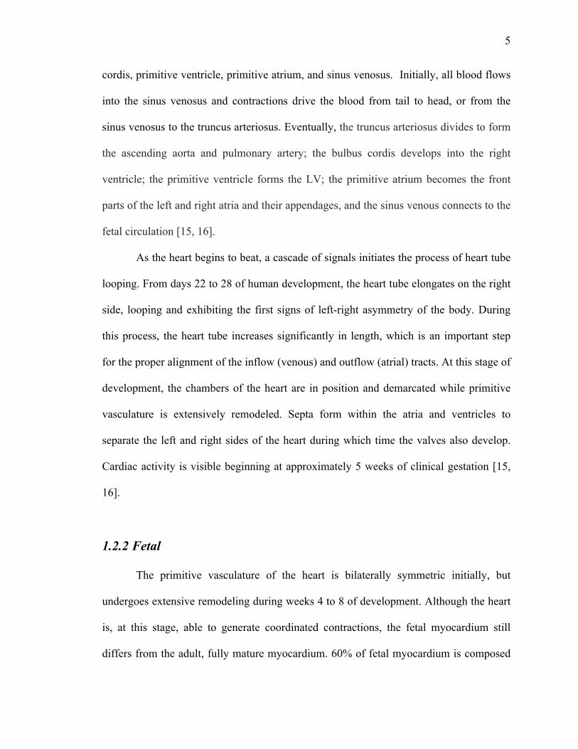
These impaired relaxation and stiffness properties in fetal myocardium may

account for limitations in stroke volume augmentation unique to the fetal heart. The adult

myocardium follows the Frank-Starling law, which predicts that with increasing preload

there is an increase in stroke volume. The fetal myocardium operates at the upper limit of

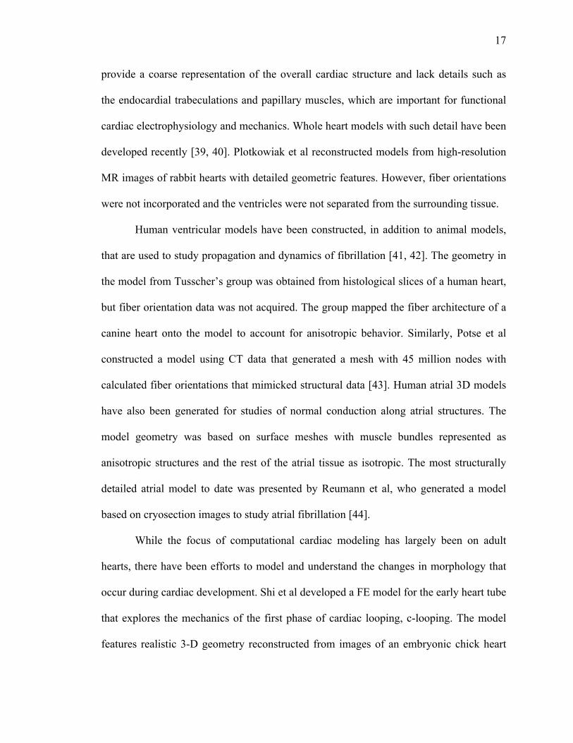
this law where there is a plateau (Figure 1.1).

Figure 1.1: Atrial pressure and stroke volume relationship in the fetal and mature heart. Reprinted with permission from “Fetal Cardiovascular Physiology" by J. Rychik, 2004, Pediatric Cardiology [17].    

Alternative theories suggest that fetal stroke volume may be limited by ventricular

constraints that arise from the surrounding tissues including the chest wall and the lungs,

7

which limit fetal ventricular preload and cardiac function. These constraints are relieved

at birth, which accounts for the significant increase in LV preload and stroke volume in

newborns. Hence, fetal myocardium due to its immature myocardial architecture and

ventricular constraints can only increase stroke volume to a small degree in response to

increase in preload [17].

Unlike the adult heart, fetal ventricles work in parallel rather than in series. Due to

the presence of the ductus arteriosus and foramen ovale, there are almost identical

pressures in the aorta and pulmonary artery, and atria respectively. Hence, the left and

right ventricles are also subjected to the same filling pressure and their combined

ventricular output perfuses the fetal system. The LV primarily perfuses the coronary and

cerebral circulations through the ascending aorta and the RV perfuses the lower body and

placental circulation through ductus arteriosus and descending aorta [17, 18].

1.2.3 Neonatal

At birth, there are transitional events in the cardiovascular system to ensure that

the newborn has adequate systemic blood flow and pressures. The ventricles begin to

work in series, rather than in parallel, and the fetal extracardiac and intracardiac shunts

close. Epinephrine levels increase during labor and at birth to mediate increased cardiac

output and myocardial contractility, which are critical during changes in myocardial

function and the associated stresses of transition. Oxygen availability increases due to the

shifting of oxygenation from the placenta to the lungs. Oxygen delivery in the neonate at

rest is estimated to be 75% higher than in the adult. This also leads to an increase in

blood volume in the arterial system since blood that no longer needs to return to the

8

placenta instead is accommodated in the systemic circulation and, as a result, systemic

blood pressure increases over the first hours to days after birth. The ductus venosus is

closed within minutes of birth due to cessation of placental blood flow. Pressure changes

within the chambers, specifically the left atrial pressure rising and exceeding that of the

right atrium, causes the foramen ovale to close and functionally separate the atria by 30

months of age. At birth, the ductus arteriosus begins to constrict but does not fully close

for a few days in a healthy, full term infant. This leaves a small shunt of blood from the

aorta to the left pulmonary artery, which eventually decreases as a result of pulmonary

arterial pressure falling below the systemic level due to reduced pulmonary vascular

resistance. The ductus arteriosus achieves functional closure by 96 hours in nearly all

infants. Due to these changes in the cardiovascular system at birth, the nonfunctional

vessels form ligaments and fetal structures such as the foramen ovale remain as vestiges

of the fetal circulatory system [19].

The neonatal myocardium undergoes structural and functional changes that

contribute to a functional cardiovascular system for the newborn. The newborn

myocardium contains less non-contractile tissue than the fetal myocardium and the

myocytes become more cylindrical. The myocardium is able to generate increased force

and influenced by ventricular preload, myocardial contractility, heart rate, and ventricular

afterload. Myofibrils increase in number, become more organized, and have an improved

ability to shorten. This leads to an increase in cross-bridge formations and therefore

greater force generation. The LV increases in mass more than the right while the latter

becomes more compliant. There is a significant increase in the combined ventricular

output after birth but the neonatal myocardium still operates at the upper limit of the

9

Frank-Starling law discussed above and must fully undergo a maturation process into

adult myocardium [19].

1.3 Cardiac Mechanics

The fully mature, adult myocardium along with the atrioventricular and semilunar

valves contribute to the primary function of the heart, which is fundamentally

mechanical—to pump blood throughout the body’s circulation system. The heart

contracts approximately 2.5 billion times during the average human life span, adapting to

the constantly changing demands of the system. The heart is a highly complex organ

whose geometry, structure, and boundary conditions are three-dimensional and often

irregular, heterogeneous, and time varying. In addition, the constitutive properties of the

myocardium are nonlinear, anisotropic, and heterogeneous. Over the past several

decades, enormous efforts have been made to formulate and validate mathematical

descriptions, or constitutive laws, of the complex nature of the ventricular myocardium

for passive and active mechanics. This section discusses cardiac function within the

context of mechanical properties of the myocardium. While the focus is on the normal

heart, it is important to consider that these properties may be altered as a result of

abnormal development and growth, which has an impact on cardiac mechanics and

function [20].

1.3.1 Anatomy and Ventricular Function

The heart is a muscular organ that consists of four pumping chambers, the right

and left atria and ventricles. The atria receive blood that returns to the heart: the right

10

atrium receives deoxygenated blood via the superior and inferior vena cava, whereas the

left atrium receives oxygenated blood from the lungs via the pulmonary veins. The atria

and ventricles are bridged via the atrioventricular valves: the tricuspid in the right side

and the mitral in the left side of the heart. These valves are connected to the papillary

muscles that extend from the ventricular cavities via collagenous fibers called chordae

tendineae. The ventricles pump blood from the heart: the right ventricle pumps blood to

the lungs through the pulmonary valve and pulmonary arteries, and the LV through the

aorta to the rest of the body. The cardiac wall itself is perfused via the coronary arteries

and is divided into three distinct layers: an inner layer called the endocardium, a middle

layer called the myocardium, and an outer layer called the epicardium. The endocardium

is a thin layer composed of collagen and elastin as well as a layer of endothelial cells that

act as a direct interface between the blood and the wall. The myocardium, as discussed

previously, consists of myocytes that are arranged into locally parallel muscle fibers and

endow the heart with its ability to pump blood. The epicardium is also a thin layer

consisting of collagen and elastic fibers. In addition to these three layers, the heart is

surrounded by the pericardium, a thicker layer of collagen and elastin that serves to limit

the gross motion of the heart [20].

The ventricles are three-dimensional pressure chambers with walls that vary in

thickness regionally and temporally during the cardiac cycle. The ventricular walls in the

normal heart vary in thickness from the base to apex. The ventricles consist of complex

three-dimensional muscle fiber architecture. The primary mechanical parameters of the

cardiac pump are blood pressure and volume flow rate, with ventricular pressure being

the most important boundary condition [20]. The cyclic mechanical function of the heart

11

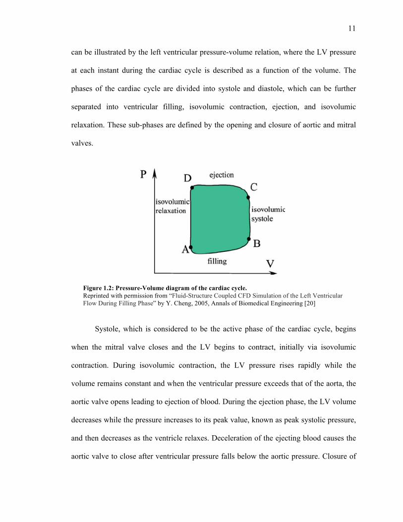
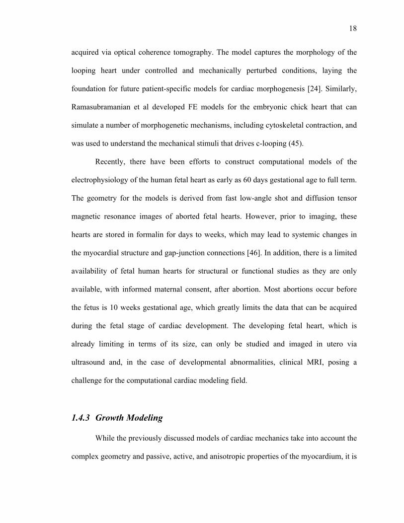
can be illustrated by the left ventricular pressure-volume relation, where the LV pressure

at each instant during the cardiac cycle is described as a function of the volume. The

phases of the cardiac cycle are divided into systole and diastole, which can be further

separated into ventricular filling, isovolumic contraction, ejection, and isovolumic

relaxation. These sub-phases are defined by the opening and closure of aortic and mitral

valves.

Systole, which is considered to be the active phase of the cardiac cycle, begins

when the mitral valve closes and the LV begins to contract, initially via isovolumic

contraction. During isovolumic contraction, the LV pressure rises rapidly while the

volume remains constant and when the ventricular pressure exceeds that of the aorta, the

aortic valve opens leading to ejection of blood. During the ejection phase, the LV volume

decreases while the pressure increases to its peak value, known as peak systolic pressure,

and then decreases as the ventricle relaxes. Deceleration of the ejecting blood causes the

aortic valve to close after ventricular pressure falls below the aortic pressure. Closure of

Figure 1.2: Pressure-Volume diagram of the cardiac cycle. Reprinted with permission from “Fluid-Structure Coupled CFD Simulation of the Left Ventricular Flow During Filling Phase” by Y. Cheng, 2005, Annals of Biomedical Engineering [20]

12

the aortic valve marks the beginning of diastole.

Diastole is the period of left ventricular relaxation and filling, which begins with

the aortic valve closing and ends with the mitral valve closing. Closure of the aortic valve

leads to isovolumic relaxation in the LV, in which the LV pressure decreases while

maintaining constant volume. When the LV pressure falls below the left atrial pressure,

the mitral valve opens and ventricular filling occurs, and the cycle continues.

As the ventricle fills with blood and the volume increases, the pressure within the

chamber passively increases. This relationship is not linear and is limited by the

compliance of the ventricular wall, where a more compliant ventricle will allow for a

larger change in filling volume for a given change in pressure. LV compliance curves

describe this inflation by plotting the change in pressure versus change in volume. At low

pressures, the LV compliance curve is almost linear, but begins to curve more steeply at

higher volumes and pressures. The slope of this relationship is the reciprocal of

compliance, or ventricular stiffness. LV compliance is determined by structural properties

of the cardiac muscle, such as the fiber orientation, and the state of ventricular

contraction and relaxation. For instance, in ventricular hypertrophy, the compliance is

lower because the ventricular wall thickness is increased; hence, end-diastolic pressure

(EDP) is higher at any given change in end-diastolic volume (EDV) [21, 22].

The net volume ejected by the LV per unit time is defined as the cardiac output

and is determined by a number of factors, defined in Table 1.1 along with other terms

related to cardiac performance relevant to this study.

13

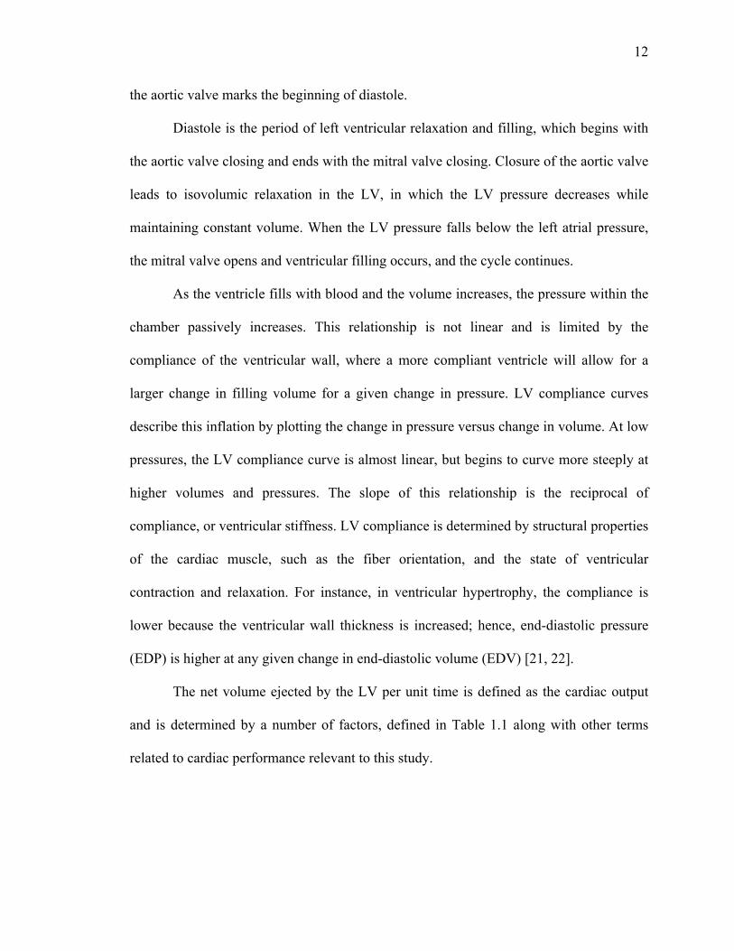
Table 1.1 Terms describing cardiac performance.

Term Definition

Preload The ventricular wall tension just prior to contraction, clinically

approximated by the EDP

Ventricular

filling

Volume of blood that fill the ventricles during diastole (= EDV-Vo)

Stroke Volume Volume of blood ejected from the ventricle in systole (= EDV – ESV)

Ejection Fraction The fraction of EDV ejected from the ventricle per beat (= SV/EDV)

Cardiac Output Volume of blood ejected from the ventricle per minute (= SV x HR)

1.3.2 Myocardial Mechanical Properties

Constitutive laws used to describe the mechanical behavior of the ventricular

myocardium are formulated with material parameters obtained from mechanical testing,

such as uniaxial and biaxial tests. Uniaxial are useful for identifying general

characteristics of the tissue behavior, but are not adequate for determining the three-

dimensional constitutive behavior of the myocardium. Biaxial tests are valuable tools that

enable estimation of myocardial constitutive parameters as they can measure the force

and displacement (stress and strain) along orthogonal fiber and cross-fiber axes.

Mechanical behavior of the heart and global cardiac function requires a

mathematical description not only for the passive properties, but also the mechanics of

the active cardiac muscle fibers. Cardiac myocytes exhibit a specific activation profile

based on location within the myocardium. Active stresses generated by cardiac muscle

fibers are dependent on parameters, such as activation time, shortening velocity,

14

sarcomere length, and intracellular calcium concentration. The active mechanical

properties are also patient-specific parameters that may vary between individuals.

Therefore, parameters such as the twitch duration scaling factor, the active stress-scaling

parameter, and the relationship between time-to-peak tension and sarcomere length need

to be estimated in a patient-specific manner [23].

1.4 Computational Modeling

Computational models based on realistic geometry contribute significantly to the

quantitative and qualitative understanding of cardiac physiology and mechanics.

Previously, computational models have been utilized to provide insight into the

morphogenetic process of cardiac looping in the embryonic chick heart, cardiac growth in

the post-natal rat, and the complex mechanisms regulating cardiac signaling networks in

human hearts [24-26]. The following section will briefly introduce common

computational approaches to model three-dimensional cardiac structures and review

selected models of cardiac physiology and mechanics.

1.4.1 Introduction

Anatomical computational models of the heart with realistic fiber orientation that

represent cardiac anatomy have been developed based on histo-anatomical slices, from

measurements taken on explanted hearts, or by segmenting pictures of histo-anatomical

slices. With the evolution of computer-aided design and improvement in medical imaging

technology, 3D cardiac models can be constructed from in-vivo or ex-vivo images. The

15

rising trend and need for personalized medicine has also enabled the development of

patient-specific cardiac computational models that are based on in-vivo images that can

be taken via MRI, CT, or ultrasound for in-utero patients. There are many challenges

associated with computational modeling of a dynamic organ such as the heart; however,

3D cardiac models are becoming increasingly complex and starting to be used in clinical

settings [27].

Computational cardiac mechanics is at the intersection of continuum mechanics,

materials science and numerical methods. Continuum mechanics is based on the

hypothesis that matter is continuous, which is not exactly true but provides an adequate

description of the deformation of matter based on the equilibrium equations. These

equilibrium equations are derived from conservation laws of mass, momentum, and

energy, and apply to all materials and living tissues. For any given material or tissue, the

constitutive stress-strain relationship describes how much force is developed under

stretch or strain, or vice versa. Hence, the constitutive stress-strain relationship describes

the mechanical behavior of the material. While there are many formulations of stress-

strain relationships for cardiac tissue, they all share the key features of having a nonlinear

and anisotropic relationship, and the ability to contract in the muscle fiber direction once

stimulated. The equations from continuum mechanics and constitutive stress-strain are

combined to yield a set of coupled partial differential equations, which when solved can

describe the displacement, stress, and strain at every material point within the heart wall.

However, these equations cannot be solved analytically for realistic geometries and

boundary conditions, so numerical approaches must be utilized. Numerical methods are

often used to approximate systems of differential equations in cardiac mechanics with the

16

most widely used method being the finite element (FE) method due to its versatility and

solid theoretical foundation. The FE method operates by discretizing the original

continuous problem, splitting the structure into subparts called elements whose vertices

are called nodes [28].

The FE model developed in this study was numerically solved using Continuity

6.4, a problem-solving environment for multi-scale modeling of cardiac biomechanics,

biotransport, and electrophysiology. It is distributed free for academic research by the

National Biomedical Computation Resource and can be downloaded at

http://www.continuity.ucsd.edu/Continuity.

1.4.2 Modeling of Cardiac Structures

Previously, several computational models of cardiac structures and the whole

heart have been developed that contribute to the understanding of cardiac physiology in

animal models as well as humans. In addition, several FE models of cardiac mechanics

have been developed to study pump function in relation to the 3D geometrical, passive,

active, and anisotropic properties of the myocardium [29-35]. This section will provide a

brief overview of past efforts in modeling cardiac structures.

Established whole heart models of the heart are FE biventricular models based on

structural information obtained by a combination of mechanical and histological

measurements, built largely using data from animal anatomies, such as rabbit or dog [36-

38]. The models were generated by fitting the nodal parameters of piecewise polynomials

in a prolate coordinate system using least squares. Smooth estimates of the geometry and

fiber structure of the ventricles were obtained using Hermite interpolation. These models

17

provide a coarse representation of the overall cardiac structure and lack details such as

the endocardial trabeculations and papillary muscles, which are important for functional

cardiac electrophysiology and mechanics. Whole heart models with such detail have been

developed recently [39, 40]. Plotkowiak et al reconstructed models from high-resolution

MR images of rabbit hearts with detailed geometric features. However, fiber orientations

were not incorporated and the ventricles were not separated from the surrounding tissue.

Human ventricular models have been constructed, in addition to animal models,

that are used to study propagation and dynamics of fibrillation [41, 42]. The geometry in

the model from Tusscher’s group was obtained from histological slices of a human heart,

but fiber orientation data was not acquired. The group mapped the fiber architecture of a

canine heart onto the model to account for anisotropic behavior. Similarly, Potse et al

constructed a model using CT data that generated a mesh with 45 million nodes with

calculated fiber orientations that mimicked structural data [43]. Human atrial 3D models

have also been generated for studies of normal conduction along atrial structures. The

model geometry was based on surface meshes with muscle bundles represented as

anisotropic structures and the rest of the atrial tissue as isotropic. The most structurally

detailed atrial model to date was presented by Reumann et al, who generated a model

based on cryosection images to study atrial fibrillation [44].

While the focus of computational cardiac modeling has largely been on adult

hearts, there have been efforts to model and understand the changes in morphology that

occur during cardiac development. Shi et al developed a FE model for the early heart tube

that explores the mechanics of the first phase of cardiac looping, c-looping. The model

features realistic 3-D geometry reconstructed from images of an embryonic chick heart

18

acquired via optical coherence tomography. The model captures the morphology of the

looping heart under controlled and mechanically perturbed conditions, laying the

foundation for future patient-specific models for cardiac morphogenesis [24]. Similarly,

Ramasubramanian et al developed FE models for the embryonic chick heart that can

simulate a number of morphogenetic mechanisms, including cytoskeletal contraction, and

was used to understand the mechanical stimuli that drives c-looping (45).

Recently, there have been efforts to construct computational models of the

electrophysiology of the human fetal heart as early as 60 days gestational age to full term.

The geometry for the models is derived from fast low-angle shot and diffusion tensor

magnetic resonance images of aborted fetal hearts. However, prior to imaging, these

hearts are stored in formalin for days to weeks, which may lead to systemic changes in

the myocardial structure and gap-junction connections [46]. In addition, there is a limited

availability of fetal human hearts for structural or functional studies as they are only

available, with informed maternal consent, after abortion. Most abortions occur before

the fetus is 10 weeks gestational age, which greatly limits the data that can be acquired

during the fetal stage of cardiac development. The developing fetal heart, which is

already limiting in terms of its size, can only be studied and imaged in utero via

ultrasound and, in the case of developmental abnormalities, clinical MRI, posing a

challenge for the computational cardiac modeling field.

1.4.3 Growth Modeling

While the previously discussed models of cardiac mechanics take into account the

complex geometry and passive, active, and anisotropic properties of the myocardium, it is

19

important to consider that tissue properties are not constant over time as the tissue

undergoes growth and remodeling in response to changes in mechanical loading [47-51].

Clinically, this is most evident in left ventricular hypo- or hypertrophy in response to

hemodynamic under- or overloading, respectively. Furthermore, regional changes in

loading, as induced by asynchronous contraction, result in asymmetric wall thickening

[52]. Hence, it becomes important to incorporate features of growth and remodeling into

models of cardiac mechanics and eventually more precisely estimate or predict long-term

outcome of clinical interventions that cause changes in load.

3D FE models have been developed that enable computation of volumetric

growth in patient specific geometries [53-56, 84]. In these models, volumetric growth is

defined as a deformation that can potentially change the initial, unloaded shape, volume,

and state of stress of the tissue [57-59]. Growth is dependent on the initial tissue

configuration as the stresses are constitutively related to growth deformation and the

initial stress-free configuration remains fixed throughout the entire growth process. An

alternative approach considers the tissue as a mixture of constituents, each of which

exhibits continuous turnover [60]. Hence, this disregards the initial configuration and

constitutive laws relating internal stresses to growth deformation are not related to a fixed

reference configuration, but rather to an evolving configuration throughout growth [61].

Based on these approaches, Kroon et al were able to simulate load induced

inhomogeneous volumetric growth in a FE model of the LV consisting of 252, 27-noded

hexahedral elements [62]. Kerckhoffs applied a novel strain-based growth law to a

passively loaded FE model of a newborn residually stressed rat LV. This model was able

to qualitatively reproduce physiological postnatal growth in the rat LV on both the

20

chamber and cellular level, which included increase in cavity and wall dimensions [25].

Furthermore, Kerckhoffs applied the growth law to a nonlinear FE model of the beating

canine ventricles with realistic fiber anatomy coupled to a lumped-parameter model of

circulation that included the heart valves. The model was allowed to adapt in shape in

response to mechanical stimuli and grow to a final state with new geometry and

hemodynamics. The model was able to reproduce most physiological responses,

including both acute and chronic changes in structure and function, even when integrated

with models of pressure-overloaded (by aortic stenosis) and volume-overloaded (by

mitral regurgitation) canine whole hearts. The strain-based growth law was able to drive

wall thickening during pressure-overload as opposed to the more commonly stress-based

stimuli [63]. Therefore, this serves as a framework for future work in improving validated

patient-specific growth models of the heart including single ventricle models that aim to

understand the mechanics of cardiac development.

1.5. Clinical Relevance

Recent efforts have been able to combine experimental findings and computational

models to reduce the complexity and accelerate insight into cardiac mechanics,

mechanisms of disease, and signaling networks that mediate cardiac development in both

normal and diseased states. Models are often validated with experimental data and they

also integrate well with experimental studies to explain observations and test new

hypotheses. As evident, computational models including patient-specific models of the

adult human heart are growing in number and complexity, improving with increasing

21

demand for personalized medicine, advancement in medical imaging technology, and

evolution of well-annotated cardiac atlases.

Compared to established models of adult cardiac structures and whole heart,

computational models of the human fetal heart, which can contribute significantly to the

knowledge base of cardiac development, are vastly limited. Although structural and

functional development of the human heart is well understood, there are limited

computational models of this process, specifically at the fetal stage. Unlike the embryonic

stage, which deals with cell proliferation and the morphological development of cardiac

structures, the fetal stage focuses on the development of the mechanics of the heart,

specifically as the heart starts to beat at 4 weeks gestation. The majority of significant

cardiovascular lesions in the fetus develops within the first trimester and is presumed to

be present at the time of second trimester ultrasound examinations [64]. Moreover,

pathophysiological conditions of the heart that impair the proper mechanical function of

the heart such as hypoplastic left heart syndrome (HLHS), which is a CHD leading to an

under-developed LV that provides inadequate blood flow post-natally, endocardial

fibroelastosis (EFE), which is a thickening of the ventricular endocardium causing

myocardial dysfunction, and aortic and mitral valve stenosis can all be detected during

the fetal stage. Currently, there are chick models of HLHS and EFE that quantify

myocardial performance and study the abnormal hemodynamics and flow patterns in

these diseases [65, 66], stem cell models of HLHS that are used to explore the genetic

abnormalities and functional differences [67], and human genetic studies that aim to

identify mutations in genes important for early heart formation that may lead to HLHS

[68]. Due to the nature of animal model and ex-vivo experiments, the primary limitation

22

with all of these studies is that they cannot adequately represent the pathophysiological

behavior of HLHS in a human fetus in-utero. Computational cardiac models of HLHS

based on realistic fetal geometry and patient-specific data can faithfully elucidate the

mechanical behavior of the disease and be used as a clinical tool to predict the growth of

the fetus, allowing adequate preparation for post-natal intervention.

In order to contextualize the findings of these disease models and identify the

functional differences from a normally developing heart, it is critical to first understand

and characterize the growth behavior and mechanical properties of a normal human fetal

heart under different physiological conditions. Therefore, there is a growing need for a

robust computational model of the normal human fetal heart based on clinical

measurements that can predict organ-level growth and can be used as a benchmark to

compare against disease models.

1.6 Specific Aims

Computational growth modeling of the average, normal human fetal heart is

improved by data acquisition that can accurately reproduce physiological behavior of the

heart. This data provides unique information specific to the fetal heart including the 3D

geometry, mechanical parameters, and clinical measures of function. To build an accurate

model, reliable clinical and experimental measurements as well as robust methods for

optimizing the developed model are necessary. Hence, the goal of this study was to

develop a robust single ventricle model of an average human fetal heart and to

characterize normal growth behavior in order to serve as a reference model for future

23

studies. A goal for these types of computational methodologies is to develop patient-

specific models of cardiac developmental pathophysiology to predict outcomes and serve

as a clinical tool for anticipating treatment options.

The current study is divided into four aims, as follows:

1. To statistically analyze 23 model geometries of the left ventricle of the human

fetal heart at mid gestational age to identify the best fit geometry satisfying ex-

vivo unloaded geometry, end diastolic geometry and clinical measures of function

at end diastole (pressure and volume).

2. To use the normal fetal LV model to assess the sensitivity of the growth model

and quantify how changes in individual growth model parameters affect

volumetric and shape behavior.

3. To test the ability of the model in predicting reverse growth from 22 weeks

gestation to an in vivo unloaded state at the onset of fetal growth.

4. To develop a patient-specific model of HLHS based on data at mid gestation and

test the predictive capability of the model in a case study

24

CHAPTER 2

Model Selection for Normal Human Fetal LV Growth

2.1 Methods

Developing a reliable and predictive growth model of a normal fetal LV requires

several criteria to be considered in estimating model parameters from available clinical

and experimental data. An initial requirement is to define the unloaded ventricular

geometry that, when loaded at normal preload, results in the end diastolic geometry. A

second requirement is to simultaneously adjust the resting material properties of the

myocardium so that the end diastolic pressure-volume relation matches human

measurements, as reported in literature. A third requirement is to validate the geometry

by allowing it to grow to term and ensuring that the dimensions found at birth match

those reported in literature [69].

With the above requirements met, the resulting geometry will serve as the

reference, unloaded state for the normal fetal LV growth model. To develop such a

geometry, however, is an iterative process as it becomes necessary to mathematically

optimize the geometry based on the results of the previous iteration and adjust the

25

geometry, preload, and resting material properties to reach the optimal combination of

results. Therefore, it is just as necessary to conduct a statistical analysis of all of the

developed geometries to determine the best-fit geometry suitable for model development.

2.1.1 Study Design

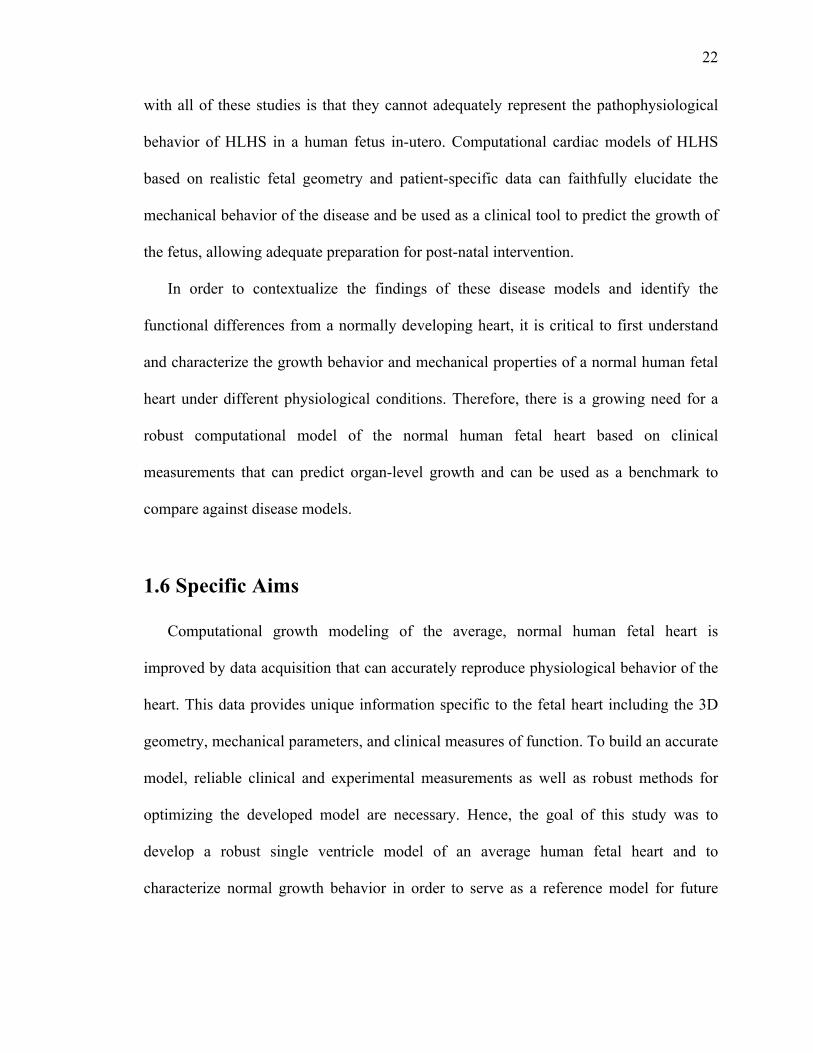
Figure 2.1: Workflow for developing a clinically relevant normal human fetal LV growth model.  

The study design for this aim is outlined above in Figure 2.1. The end goal is to

develop a computational model describing normal growth of a human fetal left ventricle

from mid gestation to birth. The first step is to generate a mesh representing the unloaded

geometry of the fetal LV at mid gestation (22 weeks). This requires accurate data from a

large sample size of healthy fetuses regarding the geometry of the fetal LV in terms of

short- and long-axis dimensions, as well as wall thickness measurements from different

Mesh Generation

•  Develop mesh for unloaded geometry at mid gestation •  Refine mesh and obtain undeformed nodes

Inflation

•  Set passive material properties •  Inflate linearly to EDP •  Calculate deformed nodes at EDP

Growth

•  Apply growth law with initial conditions •  Run 10,000 simulations •  Calculate nodal solutions at each step

Model Results

•  Calibrate to convert steps to gestational weeks •  Plot volumetric and shape growth •  Calculate %Growth from mid gestation to

birth

26

sections of the ventricle. The resulting mesh is refined to generate the working unloaded

mesh. The second step in the workflow is to incorporate the passive myocardial

properties and inflate the mesh in incremental load steps from unloaded to a selected end-

diastolic cavity pressure, uniformly imposed on the endocardium, resulting in the end-

diastolic geometry at mid gestation. The third step is to apply a strain-based growth law

to the inflated mesh, while keeping pressure constant, and allowing the simulation to run

for a number of growth steps that correspond to growth from mid gestation to birth (40

weeks), calculating nodal solutions and strain distribution at each step size. The final step

is to calibrate for time and plot the resulting growth from mid gestation to birth.

Numerically, normal growth is quantified by calculating percent change from 22 weeks

to 40 weeks gestation in LV cavity volume, shape, wall volume, and thickness.

2.1.2 Mesh Generation

Previously, 24 geometries were iteratively developed to match (a) ex-vivo

unloaded geometry, (b) end diastolic geometry as measured from echocardiography, and

(c) clinical measures of end-diastolic function (EDP and EDV) as measured by in utero

catheterization and echocardiography at mid gestation. In order to generate a clinically

relevant mesh, the normal ranges for these data were compiled from literature.

Since obtaining data for unloaded geometry is not yet clinically feasible in-vivo,

measurements from isolated, fixed human organ donor hearts were extrapolated. Arteaga-

Martinez et al reported measurements of LV anteroposterior and lateral diameters, inflow

and outflow tract lengths, and thickness of walls at different levels of 103 total hearts

from 13 to 20 weeks’ gestation [70]. End-diastolic LV short- and long-axis dimensions

27

from mid gestation to term were extracted from Z-score equations relative to estimated

gestational age reported by McElhinney et al. The Z-scores were calculated based on

unpublished fetal norms that were derived from data collected at Children’s Hospital

Boston between 2005 and 2007 on 232 normal fetuses [71]. End-diastolic LV pressures

were extracted at mid gestation from a study by Johnson et al that directly measured

pressures in 39 normal fetuses [72]. To obtain end-diastolic LV volumes from mid

gestation to term, first LV stroke volumes were extracted from mid gestation to term

from a study conducted by Kenny et al, in which Doppler echocardiography was used to

quantify stroke volume in 52 normal fetuses [73]. Then, the EDVs were calculated at

each gestational week as 30% more than the stroke volume.

The left ventricular measurements obtained were used to generate a FE mesh in a

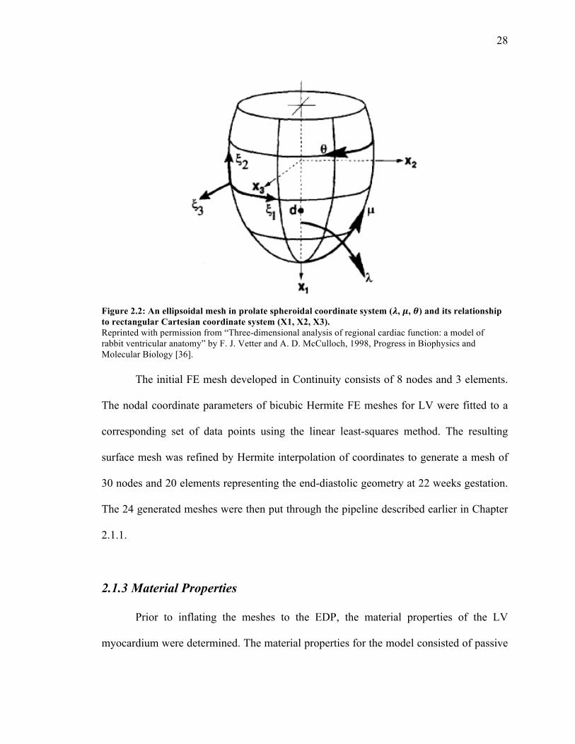
prolate spheroidal coordinate system as it is an ideal coordinate system for describing the

ellipsoidal nature of the heart: a thick-walled truncated ellipsoidal shell bounded by inner

and outer surfaces (Figure 2.2). The relationship between the rectangular Cartesian

coordinate system and the prolate spheroidal coordinate system is given by:

𝑌1 = 𝑑𝑐𝑜𝑠ℎΛ  𝑐𝑜𝑠𝑀

𝑌2 = 𝑑𝑠𝑖𝑛ℎΛ  sinM  cosΘ

𝑌3 = 𝑑𝑠𝑖𝑛ℎΛ  𝑠𝑖𝑛𝑀  𝑠𝑖𝑛Θ

where the focal length d is a parameter used for dimensional scaling of the mesh and is

determined by:

𝑑! = 𝑏! − 𝑎!

where the major radius b is the distance between the origin and the apex along the x-axis

and the minor radius a is the radius at the origin.

28

Figure 2.2: An ellipsoidal mesh in prolate spheroidal coordinate system (𝝀, 𝝁, 𝜽) and its relationship to rectangular Cartesian coordinate system (X1, X2, X3). Reprinted with permission from “Three-dimensional analysis of regional cardiac function: a model of rabbit ventricular anatomy” by F. J. Vetter and A. D. McCulloch, 1998, Progress in Biophysics and Molecular Biology [36].  

The initial FE mesh developed in Continuity consists of 8 nodes and 3 elements.

The nodal coordinate parameters of bicubic Hermite FE meshes for LV were fitted to a

corresponding set of data points using the linear least-squares method. The resulting

surface mesh was refined by Hermite interpolation of coordinates to generate a mesh of

30 nodes and 20 elements representing the end-diastolic geometry at 22 weeks gestation.

The 24 generated meshes were then put through the pipeline described earlier in Chapter

2.1.1.

2.1.3 Material Properties

Prior to inflating the meshes to the EDP, the material properties of the LV

myocardium were determined. The material properties for the model consisted of passive

29

properties only and described by a strain energy law W, assumed to be transversely

isotropic and slightly compressible [74, 75]:

𝑊 =12𝐶𝑝𝑎𝑠 ∗ 𝑒! − 1 + 𝐶!"#$ det 𝑭 − 1 ln det 𝑭 /2

where F is the deformation gradient tensor and

𝑄 = 𝑏!𝐸!!! + 𝑏! 𝐸!!! + 𝐸!!! + 2𝐸!"! +  𝑏!"(2𝐸!"! + 2𝐸!"! )

Eff is the strain in the fiber direction, Err is transmural radial strain transverse to

the fiber, Ecc is cross-fiber strain perpendicular to the former two, and the remaining are

associated shear strains. Cpas, Ccomp, bf, bc, and bfr are material parameters, which

were obtained from Omens et al [76]. With these material parameters set, the meshes

were inflated from an unloaded state to a deformed state.

Table 2.1: Passive material properties of the LV growth model

Coefficient Description Value

Cpas [kPa] Passive stress scaling constant 0.33

bf Fiber strain coefficient 9.2

bc Cross-fiber strain coefficient 2.0

bfr Shear-strain coefficient 3.7

Ccomp Bulk modulus 350

2.1.4 Growth Law

The inflated mesh was then set to grow from mid gestation to birth at a constant

EDP with the parameters listed in Table 2.2. Our group previously developed a strain-

based volumetric growth model that deforms the stress-free tissue configuration B0 to a

30

grown configuration Bg, which may not be stress-free; the methods are detailed in [63].

Briefly, the growth model is based on a multiplicative decomposition of the deformation

gradient F:

𝐹   =  𝐹!  .𝐹!  

The growth deformation gradient Fg applies between B0 and an intermediate

configuration B’g. The latter is a stress-free growth state where local kinematic

compatibility conditions do not apply. The deformation gradient Fe describes the elastic

deformation between B’g and Bg and the Cauchy stress in the tissue is only dependent on

this. Fg, on the other hand, describes plastic deformation. Volumetric growth is linearly

related to biomechanical stimuli, which are derived from a difference in fiber and cross-

fiber strain with fixed values. The deformation gradient tensors are defined with respect

to the local fiber orientation (with component Fff in the fiber direction, Fcc in cross-fiber

direction parallel to the wall, and Frr the radial component perpendicular to the two

former). This allows for the definition of a transversely isotropic growth tensor. The

cumulative growth deformation gradient tensor F(n)g is updated each growth step with the

incremental deformation gradient tensor Fg,i. Fg,i,ff describes incremental growth in the

fiber direction due to addition of sarcomeres in series whereas Fg,i,cc and Fg,i,rr describe

growth due to sarcomere addition in parallel. beta_l and beta_t are growth rate constants

in fiber and cross-fiber direction respectively and Δt is the time step. The homeostatic set

points for fiber and cross-fiber strains (Eff,set, Ecc,set) are chosen to be 0 with the

assumption that hemodynamic load is low in the fetal heart, which would lead to

approximately zero average strains with respect to the unloaded reference state [63].

31

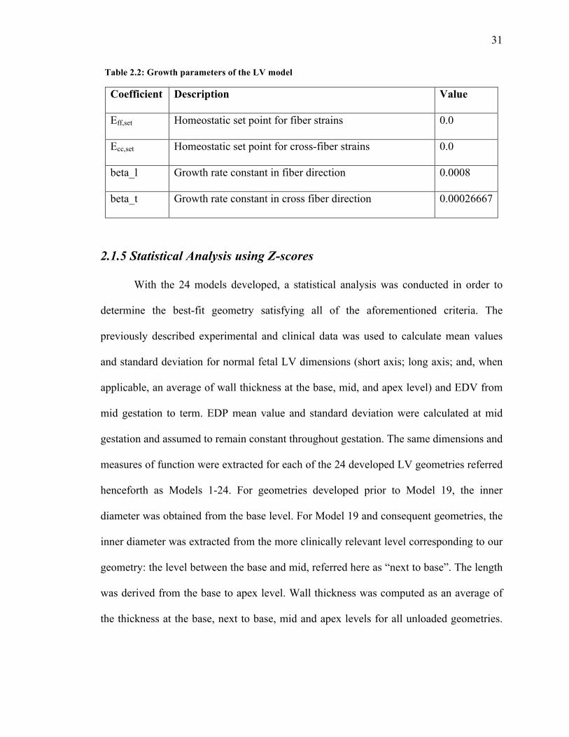
Table 2.2: Growth parameters of the LV model

Coefficient Description Value

Eff,set Homeostatic set point for fiber strains 0.0

Ecc,set Homeostatic set point for cross-fiber strains 0.0

beta_l Growth rate constant in fiber direction 0.0008

beta_t Growth rate constant in cross fiber direction 0.00026667

2.1.5 Statistical Analysis using Z-scores

With the 24 models developed, a statistical analysis was conducted in order to

determine the best-fit geometry satisfying all of the aforementioned criteria. The

previously described experimental and clinical data was used to calculate mean values

and standard deviation for normal fetal LV dimensions (short axis; long axis; and, when

applicable, an average of wall thickness at the base, mid, and apex level) and EDV from

mid gestation to term. EDP mean value and standard deviation were calculated at mid

gestation and assumed to remain constant throughout gestation. The same dimensions and

measures of function were extracted for each of the 24 developed LV geometries referred

henceforth as Models 1-24. For geometries developed prior to Model 19, the inner

diameter was obtained from the base level. For Model 19 and consequent geometries, the

inner diameter was extracted from the more clinically relevant level corresponding to our

geometry: the level between the base and mid, referred here as “next to base”. The length

was derived from the base to apex level. Wall thickness was computed as an average of

the thickness at the base, next to base, mid and apex levels for all unloaded geometries.

32

End diastolic volume was a direct output from Continuity based on the origin of the

mesh.

For the 24 geometries, Z-scores were computed comparing LV dimensions and

measures of end diastolic function for the unloaded and loaded state at mid gestation to

determine the magnitude of deviation from the measured mean. A Z-score is defined as

𝑍𝑠𝑐𝑜𝑟𝑒 =𝑥 − 𝜇𝜎

where x is the observed measurement, 𝜇 is the expected measurement (experimental

mean) and 𝜇 is the standard deviation of the population [77]. Z-scores above the

population mean have a positive value and those below the population mean have a

negative value. While the sign indicates direction of deviation from the mean, the Z-score

value conveys magnitude of deviation, which is of more interest for the statistical

analyses in this study. Hence, absolute Z-scores were used in calculations whereas plots

were based on the raw Z-score values.

With all criteria weighted equally, the LV geometries of the fetal heart with the

cumulative minimum Z-score that best fit the described data for geometric and functional

measures at mid gestation were identified as the starting reference models for normal

human fetal growth. Finally, LV short- and long-axis dimension data were extracted for

each of the reference models from mid gestation to birth. Of these, the reference model

that best predicted shape for the entire gestational period, as scored using least Z-scores,

was identified as the working reference model for normal human fetal growth for the

remainder of this study.

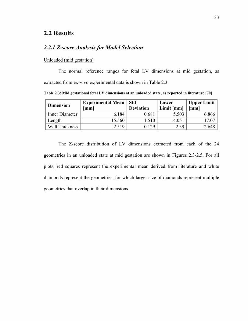
33

2.2 Results

2.2.1 Z-score Analysis for Model Selection

Unloaded (mid gestation)

The normal reference ranges for fetal LV dimensions at mid gestation, as

extracted from ex-vivo experimental data is shown in Table 2.3.

Table 2.3: Mid gestational fetal LV dimensions at an unloaded state, as reported in literature [70]

Dimension Experimental Mean [mm]

Std Deviation

Lower Limit [mm]

Upper Limit [mm]

Inner Diameter 6.184 0.681 5.503 6.866 Length 15.560 1.510 14.051 17.07 Wall Thickness 2.519 0.129 2.39 2.648

The Z-score distribution of LV dimensions extracted from each of the 24

geometries in an unloaded state at mid gestation are shown in Figures 2.3-2.5. For all

plots, red squares represent the experimental mean derived from literature and white

diamonds represent the geometries, for which larger size of diamonds represent multiple

geometries that overlap in their dimensions.

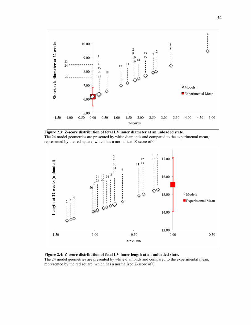
34

Figure 2.3: Z-score distribution of fetal LV inner diameter at an unloaded state. The 24 model geometries are presented by white diamonds and compared to the experimental mean, represented by the red square, which has a normalized Z-score of 0.

Figure 2.4: Z-score distribution of fetal LV inner length at an unloaded state. The 24 model geometries are presented by white diamonds and compared to the experimental mean, represented by the red square, which has a normalized Z-score of 0.  

N

M O

5.00

6.00

7.00

8.00

9.00

10.00

-1.50 -1.00 -0.50 0.00 0.50 1.00 1.50 2.00 2.50 3.00 3.50 4.00 4.50 5.00

Shor

t-ax

is d

iam

eter

at 2

2 w

eeks

z-scores

Models

Experimental Mean

23 24

1 3 4 19 20 21

22 18

17 11

2 9 10 16

5 8

4

14

13 15

7 12

13.00

14.00

15.00

16.00

17.00

-1.50 -1.00 -0.50 0.00 0.50

Len

gth

at 2

2 w

eeks

(unl

oade

d)

z-scores

Models

Experimental Mean 2 3 4

20 17

21 23

19 22

24 18

5 7 10 14 15

6 11

12 13

1 16

8 9

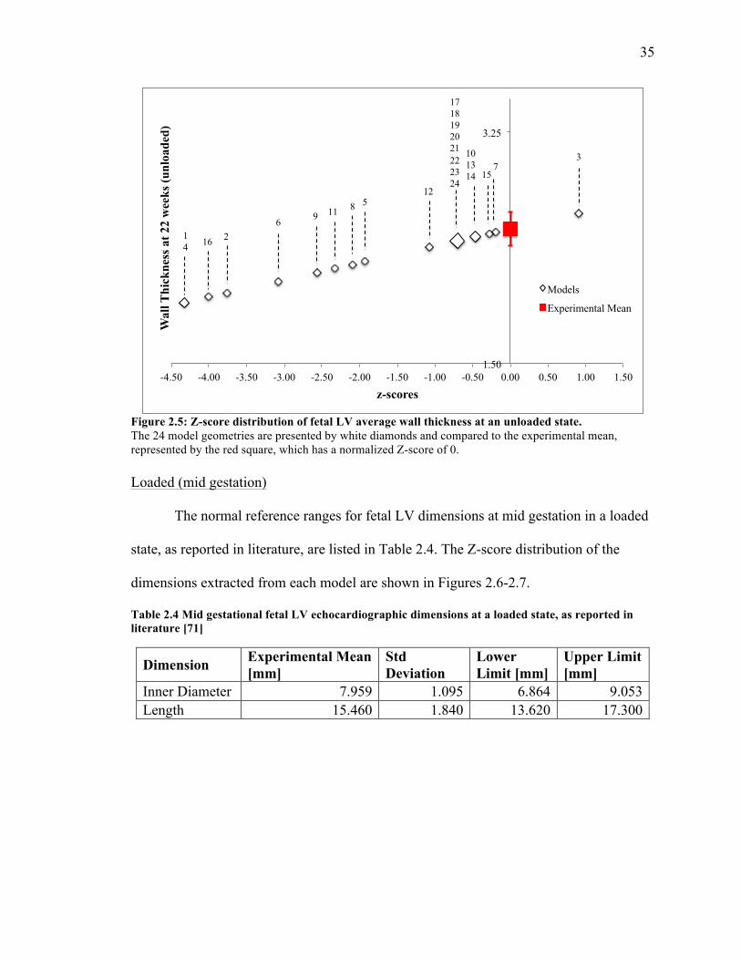
35

Figure 2.5: Z-score distribution of fetal LV average wall thickness at an unloaded state. The 24 model geometries are presented by white diamonds and compared to the experimental mean, represented by the red square, which has a normalized Z-score of 0.  Loaded (mid gestation)

The normal reference ranges for fetal LV dimensions at mid gestation in a loaded

state, as reported in literature, are listed in Table 2.4. The Z-score distribution of the

dimensions extracted from each model are shown in Figures 2.6-2.7.

Table 2.4 Mid gestational fetal LV echocardiographic dimensions at a loaded state, as reported in literature [71]

Dimension Experimental Mean [mm]

Std Deviation

Lower Limit [mm]

Upper Limit [mm]

Inner Diameter 7.959 1.095 6.864 9.053 Length 15.460 1.840 13.620 17.300

1.50

3.25

-4.50 -4.00 -3.50 -3.00 -2.50 -2.00 -1.50 -1.00 -0.50 0.00 0.50 1.00 1.50

Wal

l Thi

ckne

ss a

t 22

wee

ks (u

nloa

ded)

z-scores

Models

Experimental Mean

17 18 19 20 21 22 23 24

1 4 16 2

6 9 11 8 5 12

7 3 10

13 14

15

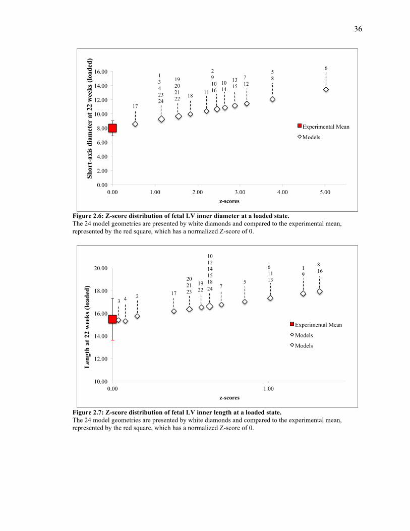
36

Figure 2.6: Z-score distribution of fetal LV inner diameter at a loaded state. The 24 model geometries are presented by white diamonds and compared to the experimental mean, represented by the red square, which has a normalized Z-score of 0.  

Figure 2.7: Z-score distribution of fetal LV inner length at a loaded state. The 24 model geometries are presented by white diamonds and compared to the experimental mean, represented by the red square, which has a normalized Z-score of 0.        

0.00

2.00

4.00

6.00

8.00

10.00

12.00

14.00

16.00

0.00 1.00 2.00 3.00 4.00 5.00

Shor

t-ax

is d

iam

eter

at 2

2 w

eeks

(loa

ded)

z-scores

Experimental Mean

Models

17

1 3 4 23 24

19 20 21 22

18

11

2 9 10 16

7 12

6 10

14

13 15

5 8

0.00

2.00

4.00

6.00

8.00

10.00

12.00

14.00

16.00

0.00 1.00 2.00 3.00 4.00 5.00

Shor

t-ax

is d

iam

eter

at 2

2 w

eeks

(loa

ded)

z-scores

Experimental Mean

Models

17

1 3 4 23 24

19 20 21 22

18

11

2 9 10 16

7 12

6 10

14

13 15

5 8

10.00

12.00

14.00

16.00

18.00

20.00

0.00 1.00

Len

gth

at 2

2 w

eeks

(loa

ded)

z-scores

Experimental Mean

Models

Models

8 16

1 9

6 11 13

7

5

10 12 14 15 18 24

20 21 23

17

19 22

2

4

3

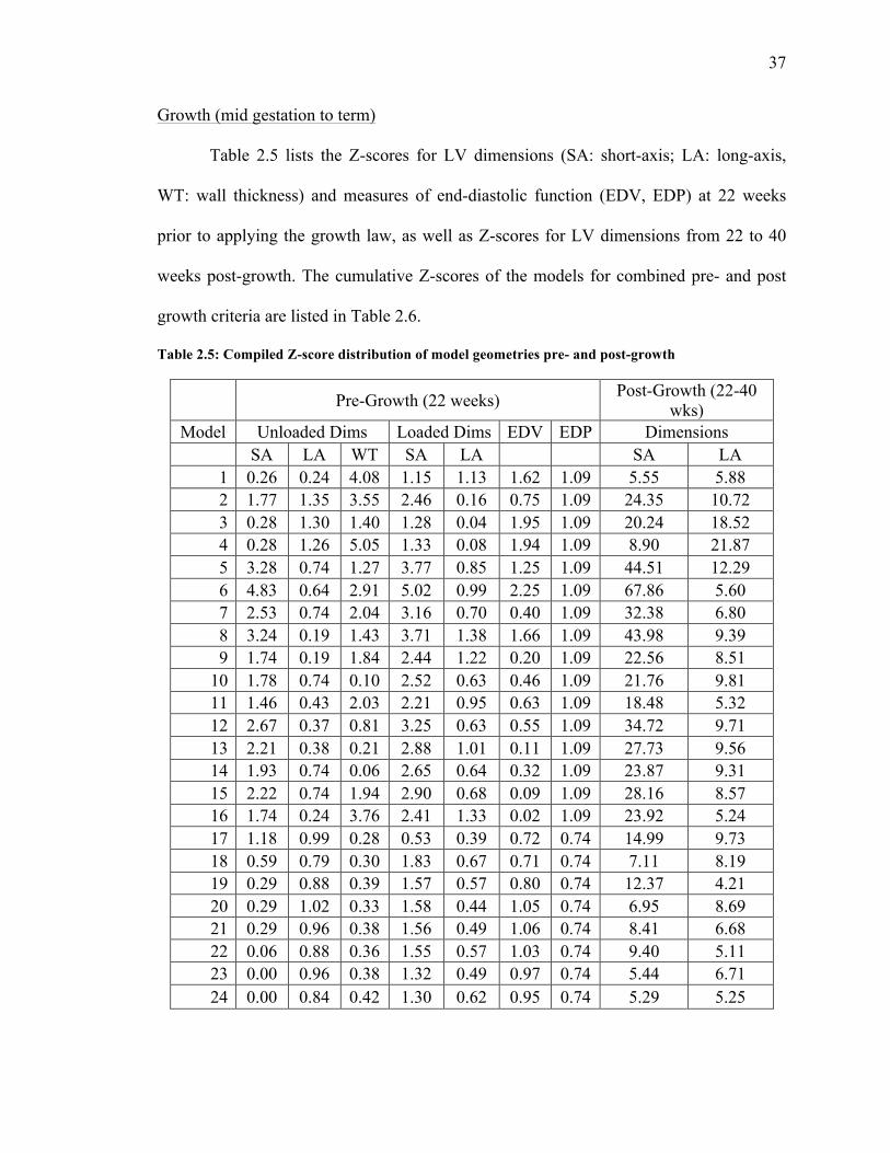
37

Growth (mid gestation to term)

Table 2.5 lists the Z-scores for LV dimensions (SA: short-axis; LA: long-axis,

WT: wall thickness) and measures of end-diastolic function (EDV, EDP) at 22 weeks

prior to applying the growth law, as well as Z-scores for LV dimensions from 22 to 40

weeks post-growth. The cumulative Z-scores of the models for combined pre- and post

growth criteria are listed in Table 2.6.

Table 2.5: Compiled Z-score distribution of model geometries pre- and post-growth

Pre-Growth (22 weeks) Post-Growth (22-40 wks)

Model Unloaded Dims Loaded Dims EDV EDP Dimensions SA LA WT SA LA SA LA

1 0.26 0.24 4.08 1.15 1.13 1.62 1.09 5.55 5.88 2 1.77 1.35 3.55 2.46 0.16 0.75 1.09 24.35 10.72 3 0.28 1.30 1.40 1.28 0.04 1.95 1.09 20.24 18.52 4 0.28 1.26 5.05 1.33 0.08 1.94 1.09 8.90 21.87 5 3.28 0.74 1.27 3.77 0.85 1.25 1.09 44.51 12.29 6 4.83 0.64 2.91 5.02 0.99 2.25 1.09 67.86 5.60 7 2.53 0.74 2.04 3.16 0.70 0.40 1.09 32.38 6.80 8 3.24 0.19 1.43 3.71 1.38 1.66 1.09 43.98 9.39 9 1.74 0.19 1.84 2.44 1.22 0.20 1.09 22.56 8.51

10 1.78 0.74 0.10 2.52 0.63 0.46 1.09 21.76 9.81 11 1.46 0.43 2.03 2.21 0.95 0.63 1.09 18.48 5.32 12 2.67 0.37 0.81 3.25 0.63 0.55 1.09 34.72 9.71 13 2.21 0.38 0.21 2.88 1.01 0.11 1.09 27.73 9.56 14 1.93 0.74 0.06 2.65 0.64 0.32 1.09 23.87 9.31 15 2.22 0.74 1.94 2.90 0.68 0.09 1.09 28.16 8.57 16 1.74 0.24 3.76 2.41 1.33 0.02 1.09 23.92 5.24 17 1.18 0.99 0.28 0.53 0.39 0.72 0.74 14.99 9.73 18 0.59 0.79 0.30 1.83 0.67 0.71 0.74 7.11 8.19 19 0.29 0.88 0.39 1.57 0.57 0.80 0.74 12.37 4.21 20 0.29 1.02 0.33 1.58 0.44 1.05 0.74 6.95 8.69 21 0.29 0.96 0.38 1.56 0.49 1.06 0.74 8.41 6.68 22 0.06 0.88 0.36 1.55 0.57 1.03 0.74 9.40 5.11 23 0.00 0.96 0.38 1.32 0.49 0.97 0.74 5.44 6.71 24 0.00 0.84 0.42 1.30 0.62 0.95 0.74 5.29 5.25

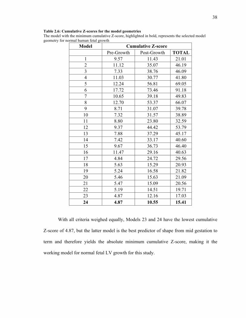
38

Table 2.6: Cumulative Z-scores for the model geometries The model with the minimum cumulative Z-score, highlighted in bold, represents the selected model geometry for normal human fetal growth

Model Cumulative Z-score Pre-Growth Post-Growth TOTAL

1 9.57 11.43 21.01 2 11.12 35.07 46.19 3 7.33 38.76 46.09 4 11.03 30.77 41.80 5 12.24 56.81 69.05 6 17.72 73.46 91.18 7 10.65 39.18 49.83 8 12.70 53.37 66.07 9 8.71 31.07 39.78 10 7.32 31.57 38.89 11 8.80 23.80 32.59 12 9.37 44.42 53.79 13 7.88 37.29 45.17 14 7.42 33.17 40.60 15 9.67 36.73 46.40 16 11.47 29.16 40.63 17 4.84 24.72 29.56 18 5.63 15.29 20.93 19 5.24 16.58 21.82 20 5.46 15.63 21.09 21 5.47 15.09 20.56 22 5.19 14.51 19.71 23 4.87 12.16 17.03 24 4.87 10.55 15.41

With all criteria weighed equally, Models 23 and 24 have the lowest cumulative

Z-score of 4.87, but the latter model is the best predictor of shape from mid gestation to

term and therefore yields the absolute minimum cumulative Z-score, making it the

working model for normal fetal LV growth for this study.

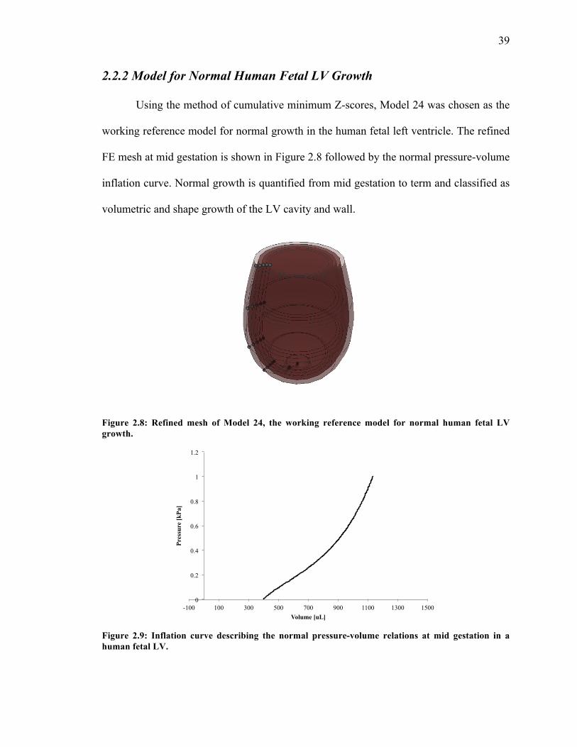
39

2.2.2 Model for Normal Human Fetal LV Growth

Using the method of cumulative minimum Z-scores, Model 24 was chosen as the

working reference model for normal growth in the human fetal left ventricle. The refined

FE mesh at mid gestation is shown in Figure 2.8 followed by the normal pressure-volume

inflation curve. Normal growth is quantified from mid gestation to term and classified as

volumetric and shape growth of the LV cavity and wall.

Figure 2.8: Refined mesh of Model 24, the working reference model for normal human fetal LV growth.

Figure 2.9: Inflation curve describing the normal pressure-volume relations at mid gestation in a human fetal LV.

0

0.2

0.4

0.6

0.8

1

1.2

-100 100 300 500 700 900 1100 1300 1500

Pres

sure

[kPa

]

Volume [uL]

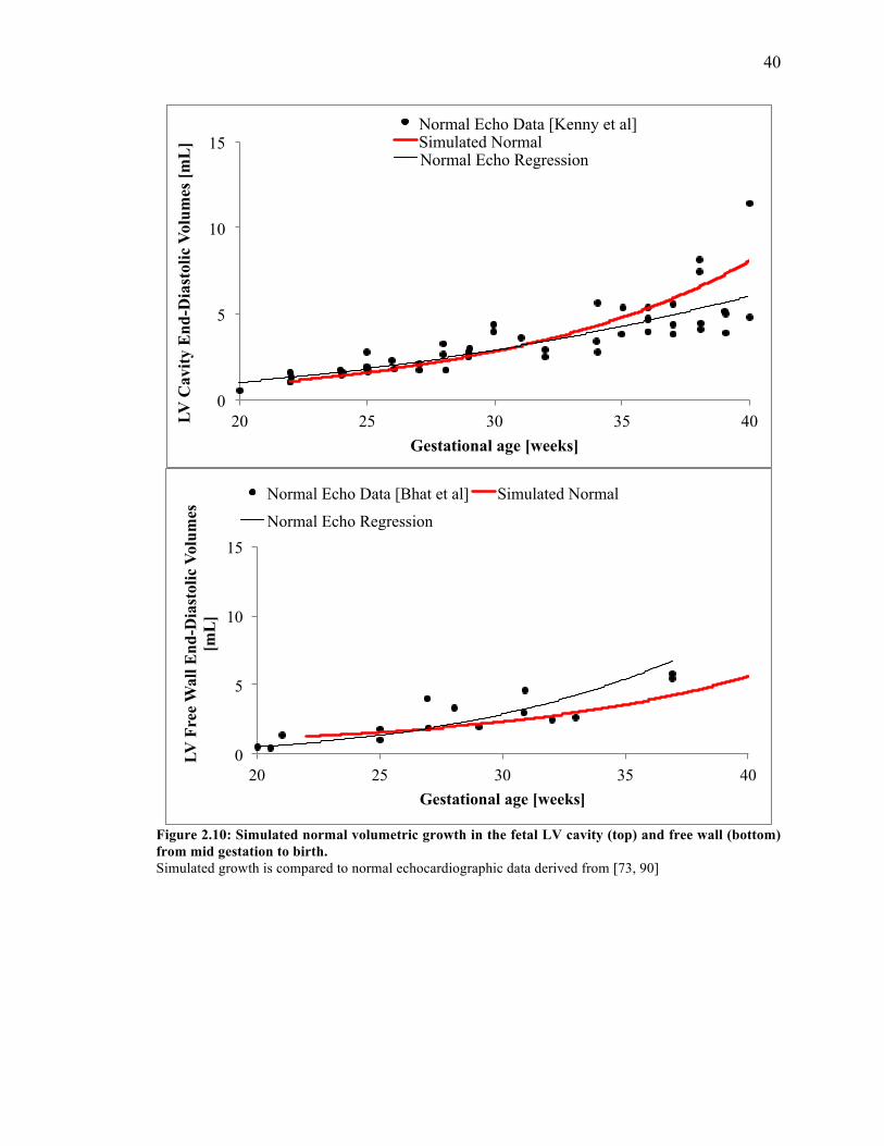
40

Figure 2.10: Simulated normal volumetric growth in the fetal LV cavity (top) and free wall (bottom) from mid gestation to birth. Simulated growth is compared to normal echocardiographic data derived from [73, 90]  

0

5

10

15

20 25 30 35 40 LV C

avity

End

-Dia

stol

ic V

olum

es [m

L]

Gestational age [weeks]

Normal Echo Data [Kenny et al] Simulated Normal Normal Echo Regression

0

5

10

15

20 25 30 35 40

LV F

ree

Wal

l End

-Dia

stol

ic V

olum

es

[mL

]

Gestational age [weeks]

Normal Echo Data [Bhat et al] Simulated Normal

Normal Echo Regression

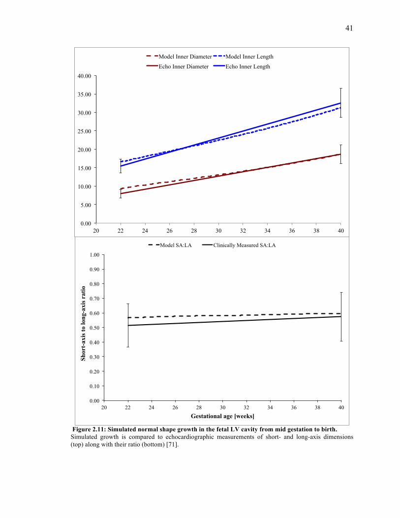
41

Figure 2.11: Simulated normal shape growth in the fetal LV cavity from mid gestation to birth. Simulated growth is compared to echocardiographic measurements of short- and long-axis dimensions (top) along with their ratio (bottom) [71].

0.00

5.00

10.00

15.00

20.00

25.00

30.00

35.00

40.00

20 22 24 26 28 30 32 34 36 38 40

Model Inner Diameter Model Inner Length

Echo Inner Diameter Echo Inner Length

0.00

0.10

0.20

0.30

0.40

0.50

0.60

0.70

0.80

0.90

1.00

20 22 24 26 28 30 32 34 36 38 40

Shor

t-ax

is to

long

-axi

s ra

tio

Gestational age [weeks]

Model SA:LA Clinically Measured SA:LA

42

2.3 Discussion

The goal of the statistical analysis was to identify the model that best satisfied

experimental and clinical data for normal fetal LV dimensions and end-diastolic

measures of function at mid gestation and best predicted shape growth from mid

gestation to birth. The selected model would then serve as the working reference model

for normal growth in the human fetal LV.

2.3.1 Statistical Analysis using Z-scores

Model 24 was chosen as the best-fit geometry, serving as the reference model for

normal fetal LV growth based on a scoring method of least Z-scores. Another method

commonly used is sum of absolute errors, which is calculated as the sum of the absolute

values of the residuals between the observed and expected mean values. However, the

method of Z-scores was preferred in this study because the equation takes into

consideration the sample size of the varying data sets that were used to extract LV

dimensions and measures of end diastolic function.

Z-scores are commonly used and have major advantages for the presentation of

data in various scientific fields [77-80]. However, they remain an imperfect

approximation and the drawbacks are important to note. First, Z-scores are based on the

mean and standard deviation of experimental data, which are only estimates of values that

vary widely within the population. Second, to have statistical confidence in the

experimental mean requires an extremely large sample size, particularly with studies

conducted on human patients due to the heterogeneity presented patient to patient. Not all

43

the datasets used had a large sample size, especially at a specific time point. For instance,

the Johnson study reported intracardiac pressure measurements from 39 normal fetuses

during 20 to 40 weeks gestation [72]. However, for this study, only the data from mid

gestation (22 weeks) was of interest, which had a sample size of 4 fetuses. Inappropriate

averaging of data across insufficient numbers of patients that may not adequately

represent the variance in the normal population can lead to under- or overestimation of Z-

scores. Thirdly, as with any manual measurements, a degree of variability is unavoidable

and may lead to Z-scores that incorrectly amplify errors in measurements [77]. Another

criticism of presenting data in the form of Z-scores is that resetting to a common metric

may lead to loss of the meaningful nature of raw data. However, this was accounted for in

this study by presenting the Z-score distribution along with its corresponding raw data

point as extracted from literature and the 24 models.

Developing the fetal LV growth model involves a three-stage process of refining

the unloaded mesh to fit experimental data, inflating the mesh to a prescribed preload at

mid gestation, and then growing the inflated model from mid gestation to term. This

process has a sequential nature of methods, requiring optimization of the geometry at

each stage and therefore allowing elimination of geometries after a given stage. However,

it was of interest to conduct an unbiased statistical test of all 24 geometries without

taking the sequential nature of the workflow into account during the analyses. Z-scores

were computed for all geometries at each stage to get a comprehensive overview of the

developed geometries from mid gestation to term. In addition, the selection criteria for

this study were all weighed equally; i.e. the selected geometry was required to best-fit

experimental and clinical data for unloaded geometry, end-diastolic geometry and clinical

44

measures of function at end-diastole. However, there may be interest in weighing the

criteria differently or in investigating which parameters growth is most sensitive to at any

given stage. For this reason, Z-scores were reported at each stage and an elimination

process was not chosen to present the data.

Lastly, it is important to emphasize that the 24 geometries were developed in an

iterative process, learning from the previous geometry. This serves as explanation for

why the later geometries better fit the experimental and clinical data, as specific features

of the model became intelligible over time. One such example is with the measurement of

the short-axis dimension. Clinically and experimentally, the LVEDD is measured at the

plane below the mitral valve. This measurement was thought to correspond to the base

plane of our LV geometry so for geometries developed prior to Model 19, the inner

diameter was obtained from the base level. For Model 19 and consequent geometries, the

inner diameter was extracted from the more clinically relevant level corresponding to our

geometry: the level between the base and mid, referred here as “next to base”. Similarly,

the normal preload applied to the models was adjusted after the development of Model

20, prior to which the geometries were inflated at a comparatively lower preload (600

Pa). 0.75 kPa was chosen as the normal preload at mid gestation for the consequent

geometries based on the pressure measurements presented in the study by Johnson et al

[72]. While this iterative learning process may have affected the development of the 24

geometries, conducting a statistical analysis and disregarding the sequence of the

methods used to develop the geometries addressed this bias and led to the selection of the

best fit geometry that satisfied all of the selected criteria for a normal fetal LV model, and

henceforth the working model for the remainder of this study.

45

2.3.2 Model for Normal Human Fetal LV Growth

The single ventricle fetal growth model presented here has several limitations worth

noting. The fetal growth model was approximated with a truncated ellipsoid without the

RV and, hence, circulation. This is a simplified, idealized geometry that fails to take into

account the loading on the septum from the RV, which would affect fiber and cross-fiber

strains. Hence, the results presented here represent LV free wall growth rather than septal

growth. This simplification of geometry may explain discrepancies in LV short- to long-

axis ratio measurements between simulation and experiment.

In the current model, the growth law developed by Kerckhoffs assumes that end-

diastolic fiber strains serve as the growth stimulus based on a previously proposed

hypothesis [48, 61, 82, 90]. Volumetric growth is linearly related to biomechanical

stimuli, derived from an imbalance in fiber and cross-fiber strains. However, cardiac

hypertrophy and remodeling can also be triggered by neurohormonal factors and their

downstream signaling pathways [91]. The model presented here only considers normal

LV growth as a result of changes in biomechanical stimuli.

In the model, growth will continue indefinitely because the fiber and cross-fiber

strains are not able to reach their zero set points due to the constant 0.75 kPa pressure that

is prescribed. The fixed set point values in the model can be gradually increased to halt

growth, as demonstrated by Kerckhoffs in [25]; however, in our study, fiber and cross-

fiber strains are assumed to be zero because the hemodynamic load is low in the fetal

heart, which would lead to approximately zero average strains. Another assumption is

that the growth rate constants in fiber and cross-fiber direction remain constant

throughout fetal growth. The model can be tuned further to match experimental and

46

clinical data by incorporating variable growth rates and passive material properties that

change temporally and spatially within the ventricular wall.

47

CHAPTER 3

Growth Model Sensitivity

3.1 Methods

With any complex systems consisting of multiple variables, it can be informative

to perform a sensitivity analysis, whereby the levels of key parameters are adjusted

systematically in order to quantitatively measure the impact that different parameters

have on outcomes of the system as well as to understand the interaction behavior between

the variables. Greater understanding of the sensitivity of a computational model to the

input parameters is extremely valuable in improving the predictive capacity of the model.

This is especially useful when modeling a process as complex and responsive to stimuli

as fetal ventricular growth. Computational models offer the ideal platform to conduct this

type of analysis as they can overcome the shortcomings inherent to studying growth

behavior in the fetus in-utero. The objective of this aim was to conduct a growth model

sensitivity analysis to comprehensively test the role of specific model parameters in

resulting volumetric and shape growth of the normal fetal LV at birth.

48

3.1.1 Study Design

The parameters that were of interest in this study and their clinical significance are

listed in Table 3.1. Using the values of these parameters from the normal growth model

as reference points, several cases were designed to isolate the impact of one or multiple

variables.

Table 3.1: Input parameters of interest in the study of growth model sensitivity

Input Parameter Description/Clinical Significance

Vo Initial Unloaded Volume

EDV-Vo Ventricular filling

EDP Preload

Cpass (wall stiffness) Ventricular wall material properties

WT Average Wall Thickness

Short- to long-axis ratio (SA:LA) Cavity Shape

Each case was purposefully designed to target the effect of one variable while

keeping all others same as the normal model when applicable. However, the nature of the

growth model requires that multiple variables are interdependent, making it difficult to

discern the effect of a single variable on growth. For instance, with all other parameters

held constant, ventricular filling cannot be varied in a model without inducing a change

in preload. For this reason, a different model must be developed introducing a third

variable that is independent of the other two, which then allows us to keep either

ventricular filling or preload constant in the initial case. For cases with co-variables such

as these, multiple cases were designed to isolate the effect of the single variable. Within

49

each case, the target variable was varied across a range of values centered about the

normal reference value. The cases along with their target variable(s) and associated co-

variable(s) are listed in Table 3.2. By taking a logical approach in the case design, we

were able to generate linear regression equations describing the effect of a single

parameter on volumetric and shape growth relative to the normal model. The outputs of

interest for each case were the percentage growth of LV cavity and wall volume, cavity

shape, and average wall thickness relative to normal growth from mid gestation to birth.

Table 3.2: Overview of cases designed to discern the effect of the target variable on growth

Case Number Target Variable(s) Co-Variable(s)

1-3 EDV-Vo, EDP Cpass

4A-B EDV-Vo, EDP None

6A SA:LA Vo, EDV-Vo, EDP

6B SA:LA, WT None

7A-L Cpass (asymmetric) Vo, EDV-Vo, EDP

Since the effect on growth was of interest in this study, four growth parameters

were considered: LV cavity volume, wall volume, cavity shape, and wall thickness.

Briefly, the change in volumetric and shape growth from mid gestation to birth was

calculated as %Growth. Then the effect of each input parameter on these growth outputs

was represented as d(%Growth)/d(Target Variable) derived from linear regression

equations where x = %change in the Target Variable and y = %Growth, both relative to

normal. This output parameter can be used to make conclusions about the relative

contribution of a given parameter towards growth. For every unit of increase in x, y

50

changes by the output parameter dy/dx, hence implication that a relatively higher

magnitude d(%Growth)/d(Target Variable) indicates greater contribution of that variable

towards growth.

3.1.2 Growth Model Sensitivity Analysis

The cases listed in Table 3.2 will be presented here in two sections: one, in which

the models within the cases are of same initial, unloaded volume equivalent to that of the

normal fetal LV model; and the other, in which the unloaded volume varies.

Overview of Cases with Vo = same

Cases 1-3

Cases 1, 2, and 3 were designed to isolate the effect that ventricular filling and

preload have on growth. In Case 1, the normal unloaded mesh was inflated to 1kPa and

then the growth law was applied at varying preloads. Since the unloaded volume is

constant, these growth models exhibit varying ventricular filling (EDV-Vo). In this case,

two parameters, preload and ventricular filling, are changing making it difficult to make

conclusions about their individual contribution to growth. For this reason, a third variable

Cpass, the stress-scaling coefficient, is introduced in Cases 2 and 3 as it can be

independently varied without affecting the other two parameters. This also allows us to

keep ventricular filling constant in Case 2 while preload varies, and vice versa in Case 3.

Because in both cases Cpass is varied in the same degree relative to normal, we are able

to discern the individual contribution of preload on growth by comparing cases 1 and 2,

and the impact of ventricular filling by comparing Cases 1 and 3.

51

The resulting inflation curves and volumetric cavity growth were plotted. Along

with volumetric LV cavity growth, linear regression equations were generated for Cases

1 and 3 describing growth (relative to normal) in the other output variables: LV wall

volume, cavity shape, and wall` thickness, where growth is quantified as change in the

output from 22 to 40 weeks. This procedure was repeated for Cases 1 and 2 with preload

as the independent variable. These generated slopes can be used to make conclusions

about the relative contribution of a given parameter, in this case ventricular filling and

preload, towards growth. Briefly, the slope of a regression equation is a measure of both

the direction and magnitude of the relationship between the independent and dependent

variables. For every unit of increase in the independent variable, growth changes by the

slope value, hence the implication that a relatively higher magnitude of slope indicates

greater contribution of that independent variable towards growth. Of course, a positive

slope value indicates positive correlation with growth and vice versa, and the strength of

correlation is indicated by the R2 value.

Case 6B

Case 6B was designed to quantify the effect of LV cavity shape on volumetric and

shape growth by either changing short-axis to long-axis ratio or average wall thickness of

the LV. To achieve this, four unloaded geometries were created with the same unloaded

volume as the normal unloaded geometry. Two geometries were developed by changing

the location of the epicardium nodes uniformly along the LV to yield a thick-walled LV

(Thick; WT: +30%) and a thin-walled LV (Thin; WT: -30%) relative to normal. The

other two were developed by manipulating the overall shape of the LV to yield

52

“TallNarrow” (SA:LA: -17%; WT: -10%) and “ShortWide” (SA:LA: +26%; WT: -5%)

geometries, both of which had thin walls relative to the normal.

Case 7 (Vo = same)

Case 7 was designed to investigate whether increasing the stress scaling coefficient to

induce ventricular wall stiffness asymmetrically rather than symmetrically, as in Cases 2

and 3, has an impact on fetal LV growth. The endocardial, mid-wall, and epicardial

elements of the LV free wall normally exhibit a cpass of 0.33 kPa. For this case, the

stress scaling coefficient was increased to 1.00 kPa for the endo, mid, and epi elements

individually, while the remaining elements exhibited normal wall stiffness. These meshes

were grown from mid gestation to birth at (a) a constant preload of 0.75 kPa, and at (b) a

constant ventricular filling of 430 µL. Regression equations were generated for Case 7 (b)

allowing us to compare LV volumetric and shape growth as a gradient of position in the

LV free wall.

Overview of Cases with Vo ≠same

Case 4

Case 4 was designed to discern the individual contribution of ventricular filling

(4A) and preload (4B) to growth, as in Cases 1-3, but with an unloaded volume differing

from that of the normal model. Within each case, five geometries with varying initial

unloaded volumes were generated by changing the focus of the mesh, which induces a

size change in the LV while maintaining the proportion (i.e. SA to LA ratio). While the

short- and long axis dimensions and wall thickness are different from normal at mid

gestation, the dimensions are the same between 4A and 4B, enabling us to compare the

two models and derive conclusions about the target variables.

53

Case 6

Case 6 was designed to quantify the correlation between shape and growth by

varying either the short- or long-axis dimensions in the initial unloaded mesh, resulting in

four geometries with non-proportional changes in the ratio and therefore varying

unloaded volumes. Two geometries were developed by decreasing or increasing the

short-axis dimension relative to normal to yield a narrow (Narrow; SA: -32%) or wide

(Wide; SA: +32%) LV, respectively. Decreasing or increasing the long-axis dimension

relative to normal yielded another set of geometries with a LV short (Short; LA: -13%) or

tall in length (Tall; LA: +10%), respectively. The four geometries were then inflated and

grown at (a) a constant preload of 0.75 kPa, and at (b) a constant ventricular filling of 383

µL.

Case 7 (Vo ≠ same)

As in Case 7 with unloaded volume held the same as normal, this case was designed

to discern the individual contribution of asymmetric wall stiffness on growth. As before,

the stress scaling coefficient was increased to 0.66 kPa and 1.00 kPa for the endo, mid,

and epi elements individually, while the remaining exhibited normal wall stiffness, or in

combination. These meshes were grown from mid gestation to birth at (a) a constant

preload of 0.75 kPa, and at (b) a constant ventricular filling of 543 µL.

Using the generated regression equations, the percentage growth relative to normal

was predicted given a 10% decrease for each parameter with the constraint that unloaded

volume is same as normal. This was repeated for the cases where unloaded volume varies

from that of the normal model.

54

3.2 Results of Growth Model Sensitivity Analysis

As in the methods, the results for the growth model sensitivity analysis presented

here will be divided into two sections: one, in which the models within each case have

the same initial, unloaded volume as that of the normal model; and another, in which the

unloaded volume varies as its own independent parameter.

3.2.1 Overview of Cases with Vo = same

Cases 1-3

Table 3.3 shows the list of parameters for each case where the ones marked with

‘x’ represent the parameters with values varying from those in the normal model. Figures

3.1-3.3 describe the resulting inflation and LV cavity volumetric growth for each case. To

reiterate, in these cases the individual effect of preload and ventricular filling on growth

is isolated given three cases where a third variable, Cpass, is used to hold one of the two

parameters constant.

Table 3.3: List of parameters within each case where those varying from normal are marked with ‘x’

Cases Vo EDP EDV-Vo Cpass 1 x x 2 x x 3 x x

In Case 1, the models grown at higher EDPs grow more in terms of LV cavity

volume, which is clinically accurate as increase in ventricular preload dramatically

55

increases ventricular stroke volume by altering the force of contraction of the

myocardium. The inflation curves for Cases 2 and 3 show that models with increased

ventricular wall stiffness require higher pressures to reach the same EDV as more

compliant LVs. When EDV-Vo is held constant as in Case 2, there is no observed

difference in the growth between the differentially stiff LVs; however, this is not

observed in Case 3 when EDP is held constant.

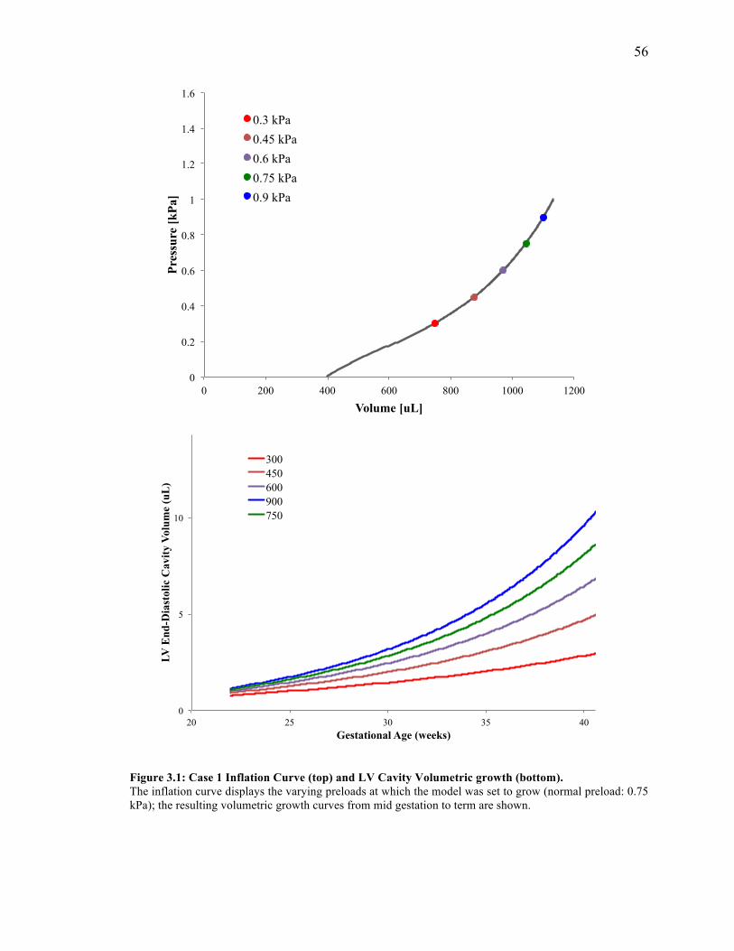
56

Figure 3.1: Case 1 Inflation Curve (top) and LV Cavity Volumetric growth (bottom). The inflation curve displays the varying preloads at which the model was set to grow (normal preload: 0.75 kPa); the resulting volumetric growth curves from mid gestation to term are shown.

0

0.2

0.4

0.6

0.8

1

1.2

1.4

1.6

0 200 400 600 800 1000 1200

Pres

sure

[kPa

]

Volume [uL]

0.3 kPa 0.45 kPa 0.6 kPa 0.75 kPa 0.9 kPa

0

5

10

20 25 30 35 40

LV E

nd-D

iast

olic

Cav

ity V

olum

e (u

L)

Gestational Age (weeks)

300 450 600 900 750

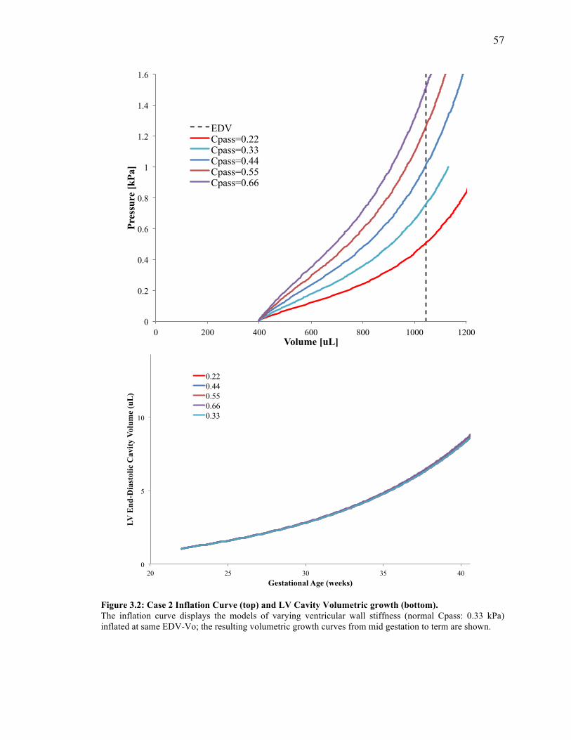
57

Figure 3.2: Case 2 Inflation Curve (top) and LV Cavity Volumetric growth (bottom).  The inflation curve displays the models of varying ventricular wall stiffness (normal Cpass: 0.33 kPa) inflated at same EDV-Vo; the resulting volumetric growth curves from mid gestation to term are shown.

0

5

10

20 25 30 35 40

LV E

nd-D

iast

olic

Cav

ity V

olum

e (u

L)

Gestational Age (weeks)

0.22 0.44 0.55 0.66 0.33

0

0.2

0.4

0.6

0.8

1

1.2

1.4

1.6

0 200 400 600 800 1000 1200

Pres

sure

[kPa

]

Volume [uL]

EDV Cpass=0.22 Cpass=0.33 Cpass=0.44 Cpass=0.55 Cpass=0.66

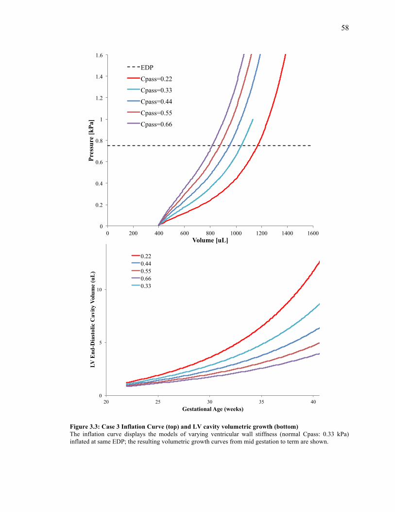
58

 Figure 3.3: Case 3 Inflation Curve (top) and LV cavity volumetric growth (bottom) The inflation curve displays the models of varying ventricular wall stiffness (normal Cpass: 0.33 kPa) inflated at same EDP; the resulting volumetric growth curves from mid gestation to term are shown.

0

5

10

20 25 30 35 40

LV E

nd-D

iast

olic

Cav

ity V

olum

e (u

L)

Gestational Age (weeks)

0.22 0.44 0.55 0.66 0.33

0

0.2

0.4

0.6

0.8

1

1.2

1.4

1.6

0 200 400 600 800 1000 1200 1400 1600

Pres

sure

[kPa

]

Volume [uL]

EDP

Cpass=0.22

Cpass=0.33

Cpass=0.44

Cpass=0.55

Cpass=0.66

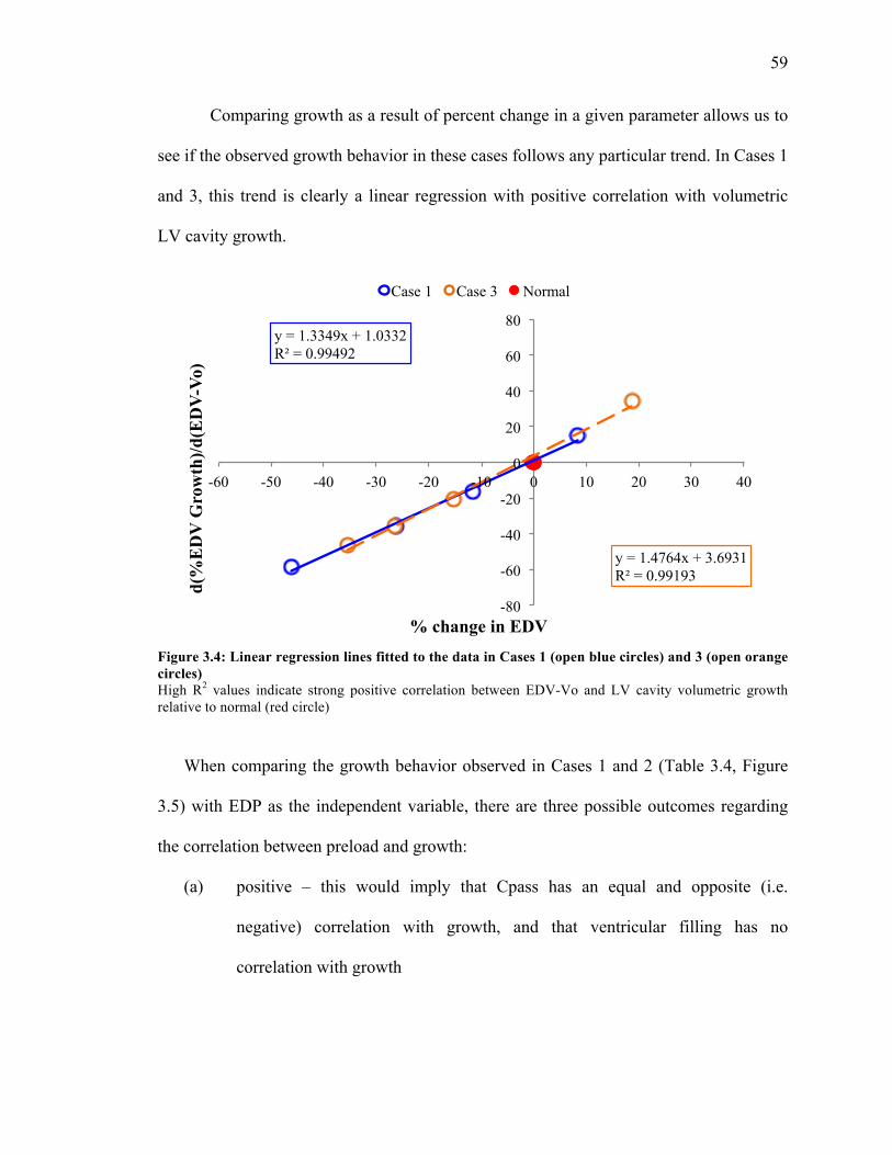
59

Comparing growth as a result of percent change in a given parameter allows us to

see if the observed growth behavior in these cases follows any particular trend. In Cases 1

and 3, this trend is clearly a linear regression with positive correlation with volumetric

LV cavity growth.

Figure 3.4: Linear regression lines fitted to the data in Cases 1 (open blue circles) and 3 (open orange circles)  High R2 values indicate strong positive correlation between EDV-Vo and LV cavity volumetric growth relative to normal (red circle)

When comparing the growth behavior observed in Cases 1 and 2 (Table 3.4, Figure

3.5) with EDP as the independent variable, there are three possible outcomes regarding

the correlation between preload and growth:

(a) positive – this would imply that Cpass has an equal and opposite (i.e.

negative) correlation with growth, and that ventricular filling has no

correlation with growth

y = 1.3349x + 1.0332 R² = 0.99492

y = 1.4764x + 3.6931 R² = 0.99193

-80

-60

-40

-20

0

20

40

60

80

-60 -50 -40 -30 -20 -10 0 10 20 30 40

d(%

ED

V G

row

th)/d

(ED

V-V

o)

% change in EDV

Case 1 Case 3 Normal

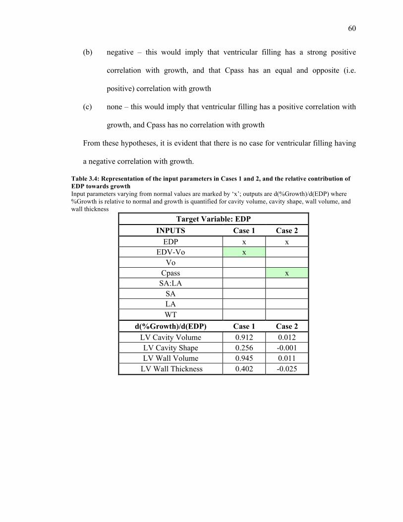
60

(b) negative – this would imply that ventricular filling has a strong positive

correlation with growth, and that Cpass has an equal and opposite (i.e.

positive) correlation with growth

(c) none – this would imply that ventricular filling has a positive correlation with

growth, and Cpass has no correlation with growth

From these hypotheses, it is evident that there is no case for ventricular filling having

a negative correlation with growth.

Table 3.4: Representation of the input parameters in Cases 1 and 2, and the relative contribution of EDP towards growth Input parameters varying from normal values are marked by ‘x’; outputs are d(%Growth)/d(EDP) where %Growth is relative to normal and growth is quantified for cavity volume, cavity shape, wall volume, and wall thickness

Target Variable: EDP INPUTS Case 1 Case 2

EDP x x EDV-Vo x

Vo Cpass x SA:LA

SA LA WT

d(%Growth)/d(EDP) Case 1 Case 2 LV Cavity Volume 0.912 0.012 LV Cavity Shape 0.256 -0.001 LV Wall Volume 0.945 0.011

LV Wall Thickness 0.402 -0.025

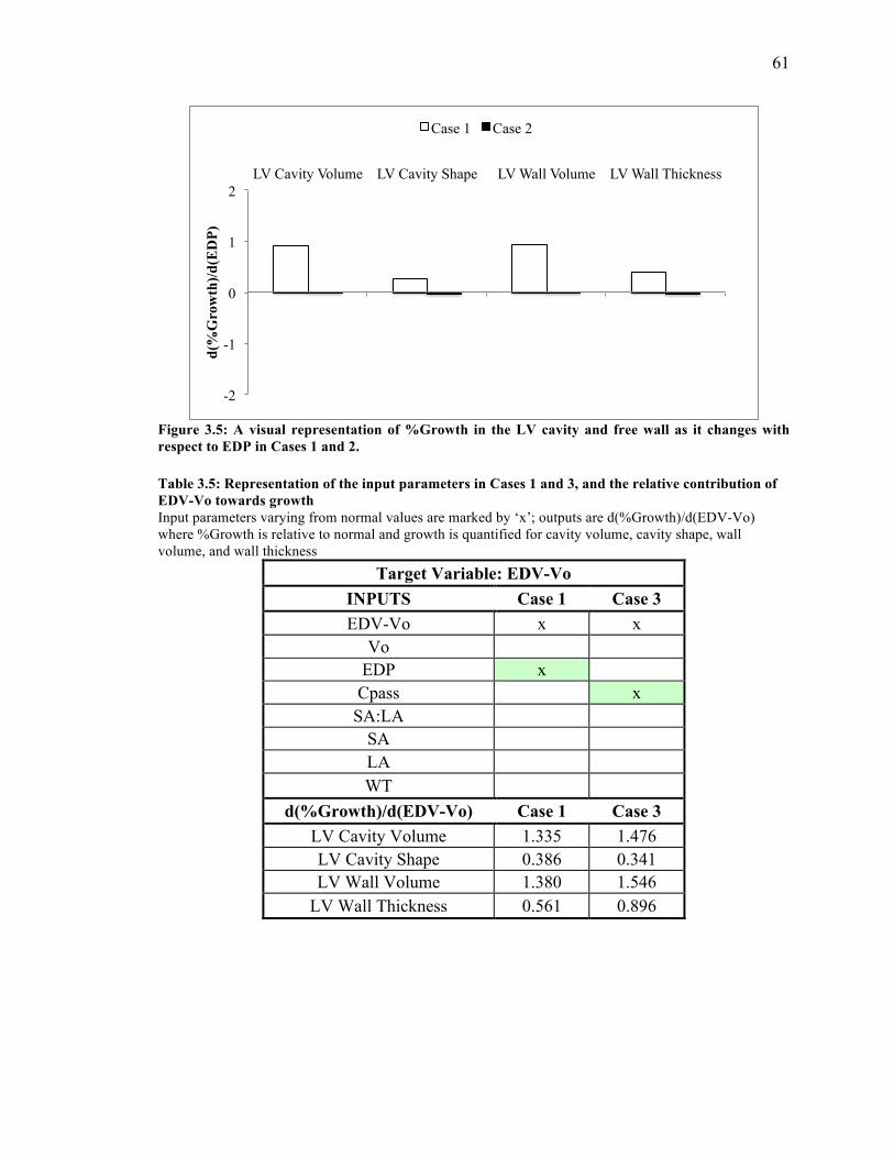
61

Figure 3.5: A visual representation of %Growth in the LV cavity and free wall as it changes with respect to EDP in Cases 1 and 2.

 Table 3.5: Representation of the input parameters in Cases 1 and 3, and the relative contribution of EDV-Vo towards growth Input parameters varying from normal values are marked by ‘x’; outputs are d(%Growth)/d(EDV-Vo) where %Growth is relative to normal and growth is quantified for cavity volume, cavity shape, wall volume, and wall thickness

Target Variable: EDV-Vo INPUTS Case 1 Case 3 EDV-Vo x x

Vo EDP x Cpass x SA:LA

SA LA WT

d(%Growth)/d(EDV-Vo) Case 1 Case 3 LV Cavity Volume 1.335 1.476 LV Cavity Shape 0.386 0.341 LV Wall Volume 1.380 1.546

LV Wall Thickness 0.561 0.896

-2

-1

0

1

2 LV Cavity Volume LV Cavity Shape LV Wall Volume LV Wall Thickness

d(%

Gro

wth

)/d(E

DP)

Case 1 Case 2

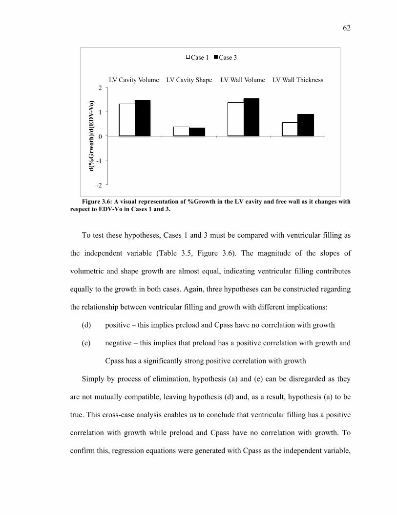
62

Figure 3.6: A visual representation of %Growth in the LV cavity and free wall as it changes with respect to EDV-Vo in Cases 1 and 3.  

To test these hypotheses, Cases 1 and 3 must be compared with ventricular filling as

the independent variable (Table 3.5, Figure 3.6). The magnitude of the slopes of

volumetric and shape growth are almost equal, indicating ventricular filling contributes

equally to the growth in both cases. Again, three hypotheses can be constructed regarding

the relationship between ventricular filling and growth with different implications:

(d) positive – this implies preload and Cpass have no correlation with growth

(e) negative – this implies that preload has a positive correlation with growth and

Cpass has a significantly strong positive correlation with growth

Simply by process of elimination, hypothesis (a) and (e) can be disregarded as they

are not mutually compatible, leaving hypothesis (d) and, as a result, hypothesis (a) to be

true. This cross-case analysis enables us to conclude that ventricular filling has a positive

correlation with growth while preload and Cpass have no correlation with growth. To

confirm this, regression equations were generated with Cpass as the independent variable,

-2

-1

0

1

2 LV Cavity Volume LV Cavity Shape LV Wall Volume LV Wall Thickness

d(%

Grw

oth)

/d(E

DV

-Vo)

Case 1 Case 3

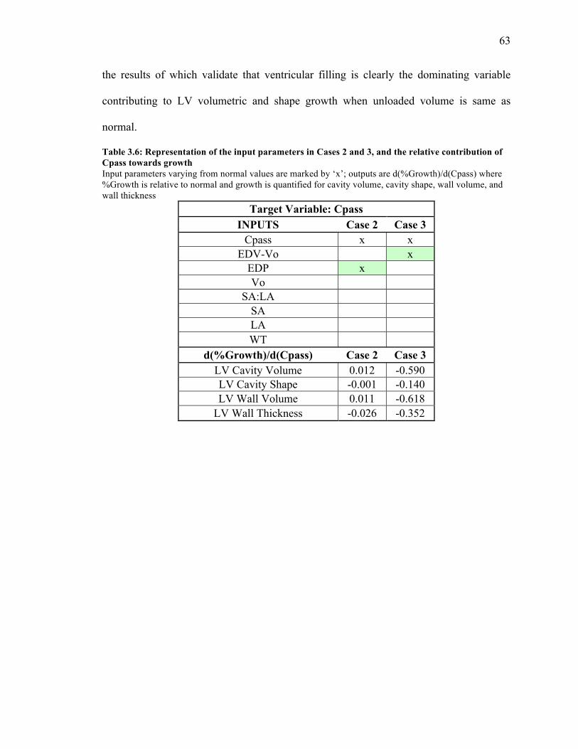
63

the results of which validate that ventricular filling is clearly the dominating variable

contributing to LV volumetric and shape growth when unloaded volume is same as

normal.

Table 3.6: Representation of the input parameters in Cases 2 and 3, and the relative contribution of Cpass towards growth Input parameters varying from normal values are marked by ‘x’; outputs are d(%Growth)/d(Cpass) where %Growth is relative to normal and growth is quantified for cavity volume, cavity shape, wall volume, and wall thickness

Target Variable: Cpass INPUTS Case 2 Case 3

Cpass x x EDV-Vo x

EDP x Vo

SA:LA SA LA WT

d(%Growth)/d(Cpass) Case 2 Case 3 LV Cavity Volume 0.012 -0.590 LV Cavity Shape -0.001 -0.140 LV Wall Volume 0.011 -0.618

LV Wall Thickness -0.026 -0.352

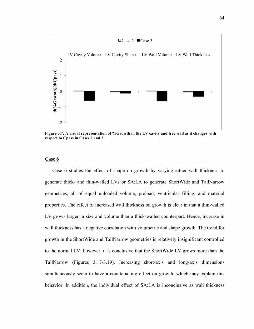
64

Figure 3.7: A visual representation of %Growth in the LV cavity and free wall as it changes with respect to Cpass in Cases 2 and 3.

Case 6

Case 6 studies the effect of shape on growth by varying either wall thickness to

generate thick- and thin-walled LVs or SA:LA to generate ShortWide and TallNarrow

geometries, all of equal unloaded volume, preload, ventricular filling, and material

properties. The effect of increased wall thickness on growth is clear in that a thin-walled

LV grows larger in size and volume than a thick-walled counterpart. Hence, increase in

wall thickness has a negative correlation with volumetric and shape growth. The trend for

growth in the ShortWide and TallNarrow geometries is relatively insignificant controlled

to the normal LV; however, it is conclusive that the ShortWide LV grows more than the

TallNarrow (Figures 3.17-3.19). Increasing short-axis and long-axis dimensions

simultaneously seem to have a counteracting effect on growth, which may explain this

behavior. In addition, the individual effect of SA:LA is inconclusive as wall thickness

-2

-1

0

1

2 LV Cavity Volume LV Cavity Shape LV Wall Volume LV Wall Thickness

d(%

Grw

oth)

/d(C

pass

)

Case 2 Case 3

65

was a co-variable in the case of TallNarrow and ShortWide due to the constraints of the

model.

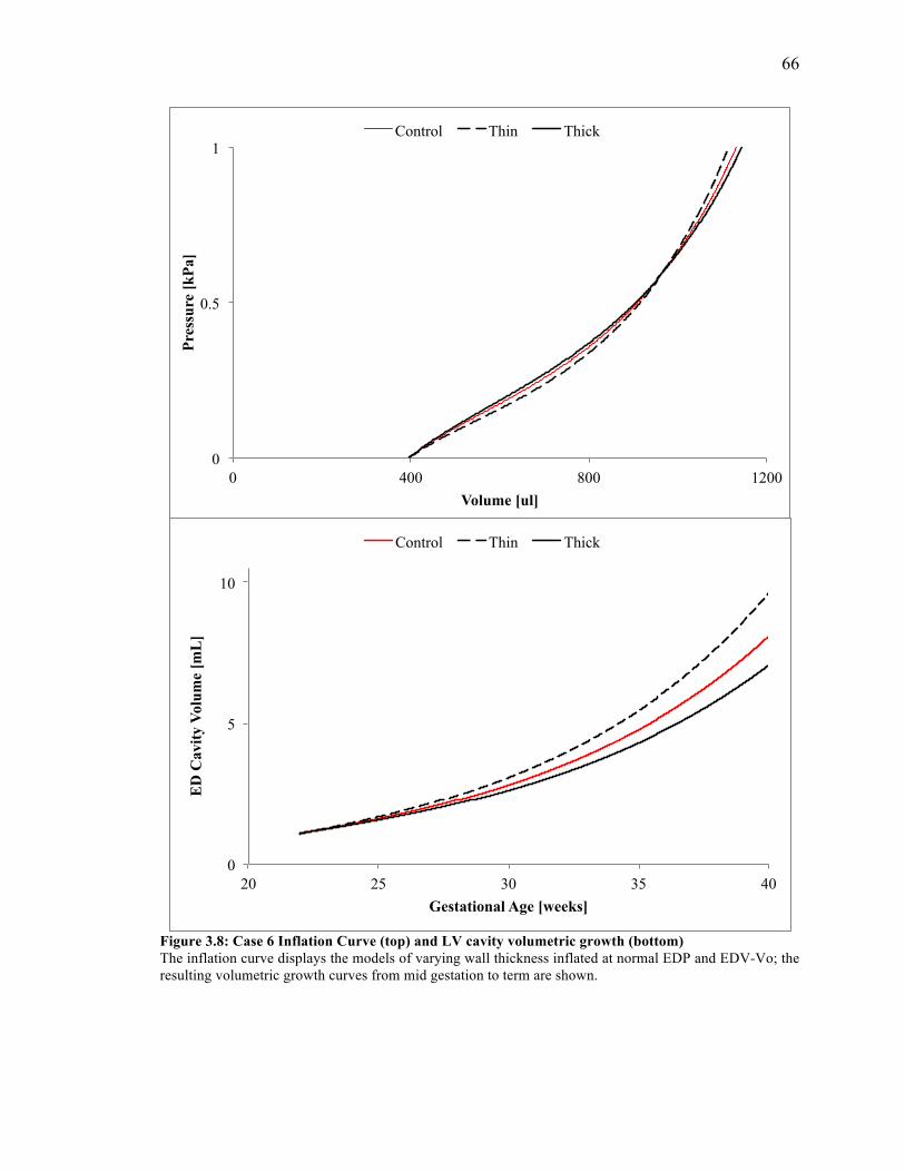
66

Figure 3.8: Case 6 Inflation Curve (top) and LV cavity volumetric growth (bottom)  The inflation curve displays the models of varying wall thickness inflated at normal EDP and EDV-Vo; the resulting volumetric growth curves from mid gestation to term are shown.

0

0.5

1

0 400 800 1200

Pres

sure

[kPa

]

Volume [ul]

Control Thin Thick

0

5

10

20 25 30 35 40

ED

Cav

ity V

olum

e [m

L]

Gestational Age [weeks]

Control Thin Thick

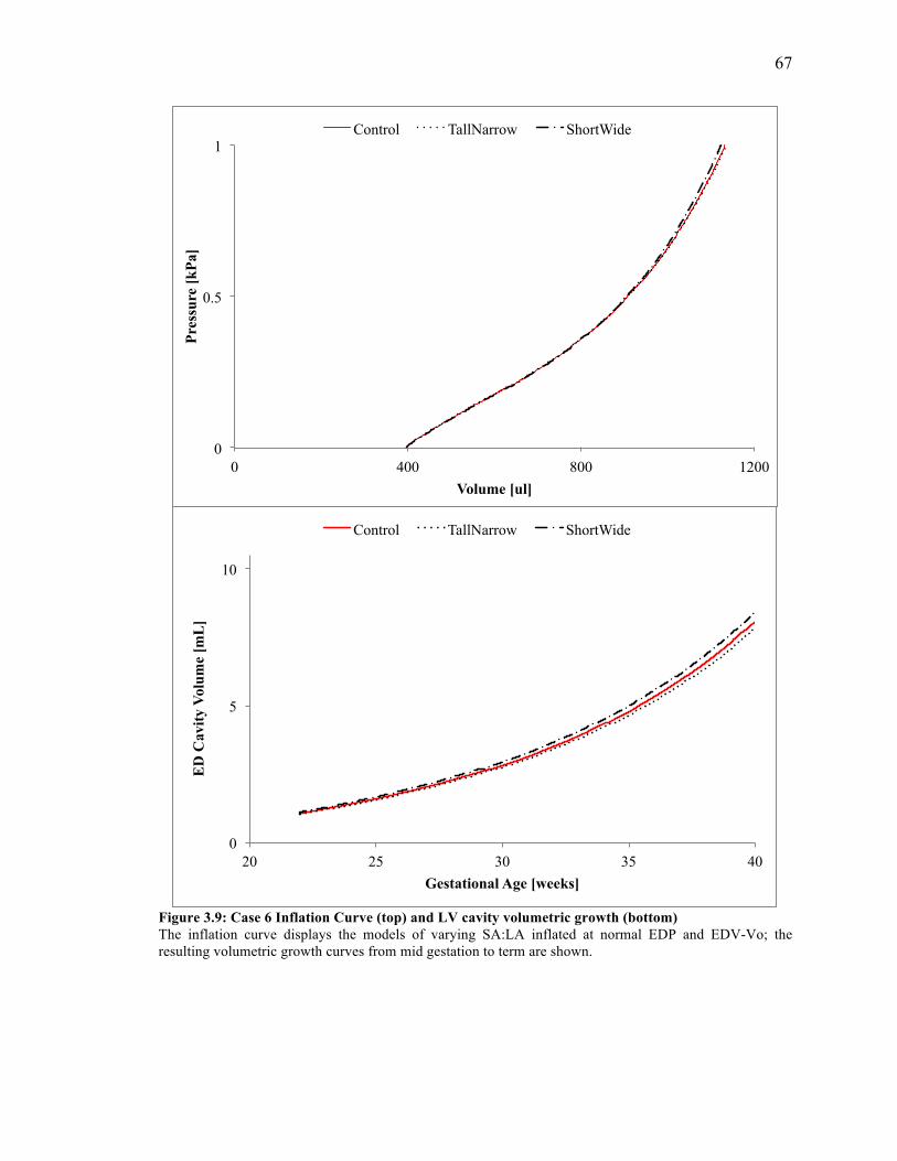
67

Figure 3.9: Case 6 Inflation Curve (top) and LV cavity volumetric growth (bottom) The inflation curve displays the models of varying SA:LA inflated at normal EDP and EDV-Vo; the resulting volumetric growth curves from mid gestation to term are shown.

0

0.5

1

0 400 800 1200

Pres

sure

[kPa

]

Volume [ul]

Control TallNarrow ShortWide

0

5

10

20 25 30 35 40

ED

Cav

ity V

olum

e [m

L]

Gestational Age [weeks]

Control TallNarrow ShortWide

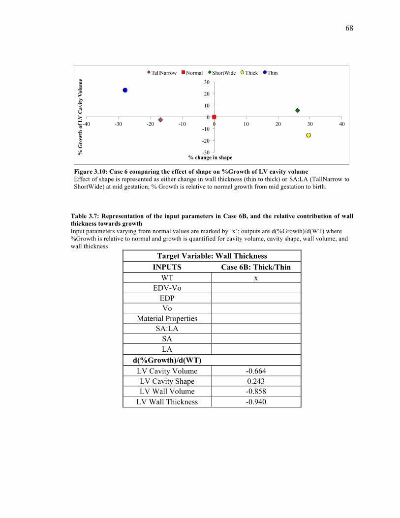
68

Table 3.7: Representation of the input parameters in Case 6B, and the relative contribution of wall thickness towards growth Input parameters varying from normal values are marked by ‘x’; outputs are d(%Growth)/d(WT) where %Growth is relative to normal and growth is quantified for cavity volume, cavity shape, wall volume, and wall thickness

Target Variable: Wall Thickness INPUTS Case 6B: Thick/Thin

WT x EDV-Vo

EDP Vo

Material Properties SA:LA

SA LA

d(%Growth)/d(WT) LV Cavity Volume -0.664 LV Cavity Shape 0.243 LV Wall Volume -0.858

LV Wall Thickness -0.940

-30

-20

-10

0

10

20

30

-40 -30 -20 -10 0 10 20 30 40

% G

row

th o

f LV

Cav

ity V

olum

e

% change in shape

TallNarrow Normal ShortWide Thick Thin

Figure 3.10: Case 6 comparing the effect of shape on %Growth of LV cavity volume Effect of shape is represented as either change in wall thickness (thin to thick) or SA:LA (TallNarrow to ShortWide) at mid gestation; % Growth is relative to normal growth from mid gestation to birth.

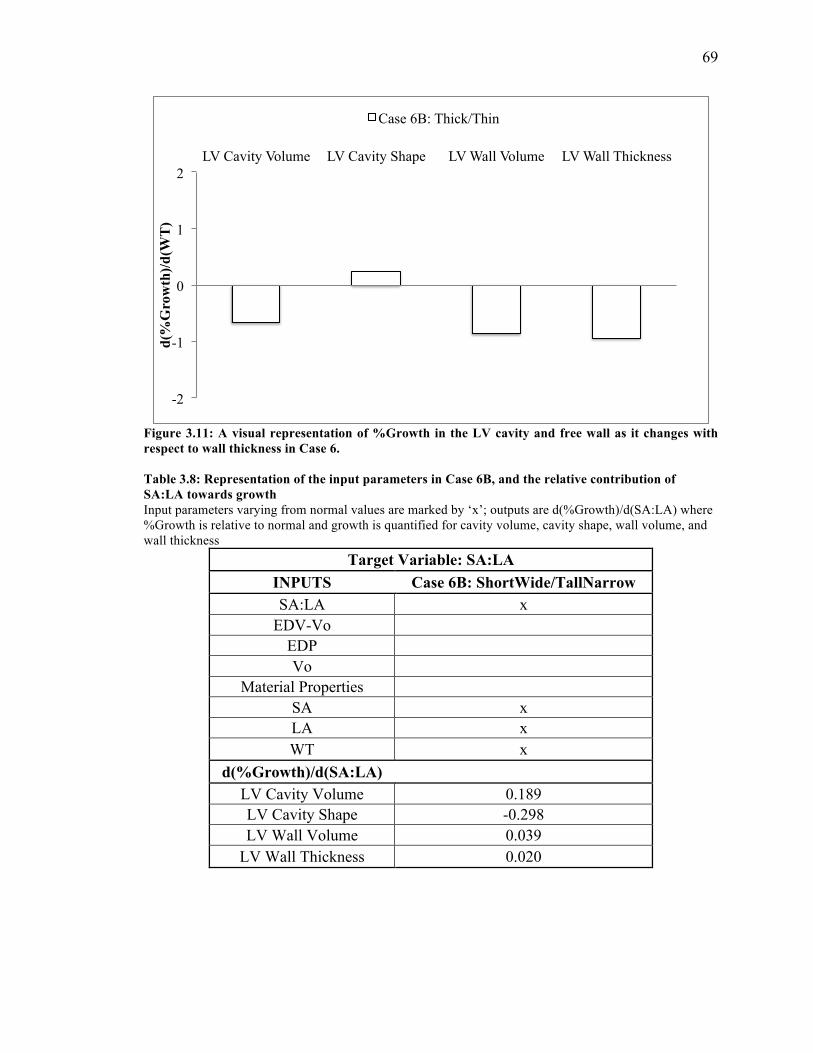
69

Figure 3.11: A visual representation of %Growth in the LV cavity and free wall as it changes with respect to wall thickness in Case 6.   Table 3.8: Representation of the input parameters in Case 6B, and the relative contribution of SA:LA towards growth Input parameters varying from normal values are marked by ‘x’; outputs are d(%Growth)/d(SA:LA) where %Growth is relative to normal and growth is quantified for cavity volume, cavity shape, wall volume, and wall thickness

Target Variable: SA:LA INPUTS Case 6B: ShortWide/TallNarrow SA:LA x

EDV-Vo EDP Vo

Material Properties SA x LA x WT x

d(%Growth)/d(SA:LA) LV Cavity Volume 0.189 LV Cavity Shape -0.298 LV Wall Volume 0.039

LV Wall Thickness 0.020

-2

-1

0

1

2 LV Cavity Volume LV Cavity Shape LV Wall Volume LV Wall Thickness

d(%

Gro

wth

)/d(W

T)

Case 6B: Thick/Thin

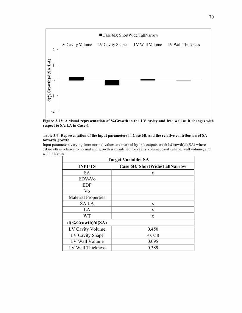
70

Figure 3.12: A visual representation of %Growth in the LV cavity and free wall as it changes with respect to SA:LA in Case 6.  Table 3.9: Representation of the input parameters in Case 6B, and the relative contribution of SA towards growth Input parameters varying from normal values are marked by ‘x’; outputs are d(%Growth)/d(SA) where %Growth is relative to normal and growth is quantified for cavity volume, cavity shape, wall volume, and wall thickness

Target Variable: SA INPUTS Case 6B: ShortWide/TallNarrow

SA x EDV-Vo

EDP Vo

Material Properties SA:LA x

LA x WT x

d(%Growth)/d(SA) LV Cavity Volume 0.450 LV Cavity Shape -0.758 LV Wall Volume 0.095

LV Wall Thickness 0.389

-2

-1

0

1

2 LV Cavity Volume LV Cavity Shape LV Wall Volume LV Wall Thickness

d(%

Gro

wth

)/d(S

A:L

A)

Case 6B: ShortWide/TallNarrow

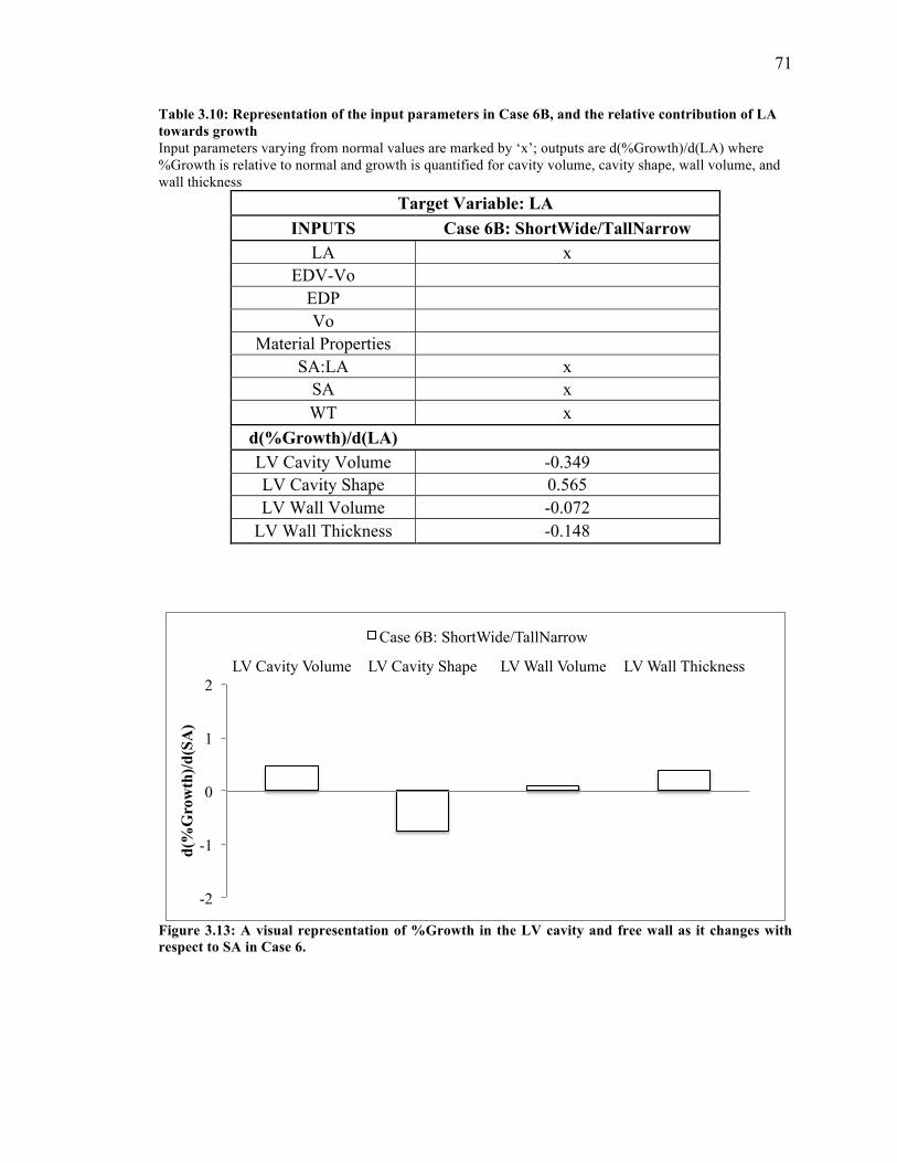
71

Table 3.10: Representation of the input parameters in Case 6B, and the relative contribution of LA towards growth Input parameters varying from normal values are marked by ‘x’; outputs are d(%Growth)/d(LA) where %Growth is relative to normal and growth is quantified for cavity volume, cavity shape, wall volume, and wall thickness

Target Variable: LA INPUTS Case 6B: ShortWide/TallNarrow

LA x EDV-Vo

EDP Vo

Material Properties SA:LA x

SA x WT x

d(%Growth)/d(LA) LV Cavity Volume -0.349 LV Cavity Shape 0.565 LV Wall Volume -0.072

LV Wall Thickness -0.148

Figure 3.13: A visual representation of %Growth in the LV cavity and free wall as it changes with respect to SA in Case 6.  

-2

-1

0

1

2 LV Cavity Volume LV Cavity Shape LV Wall Volume LV Wall Thickness

d(%

Gro

wth

)/d(S

A)

Case 6B: ShortWide/TallNarrow

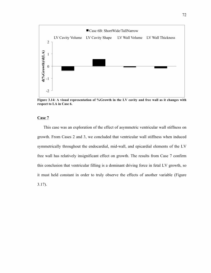
72

Figure 3.14: A visual representation of %Growth in the LV cavity and free wall as it changes with respect to LA in Case 6.  

Case 7

This case was an exploration of the effect of asymmetric ventricular wall stiffness on

growth. From Cases 2 and 3, we concluded that ventricular wall stiffness when induced

symmetrically throughout the endocardial, mid-wall, and epicardial elements of the LV

free wall has relatively insignificant effect on growth. The results from Case 7 confirm

this conclusion that ventricular filling is a dominant driving force in fetal LV growth, so

it must held constant in order to truly observe the effects of another variable (Figure

3.17).

-2

-1

0

1

2 LV Cavity Volume LV Cavity Shape LV Wall Volume LV Wall Thickness

d(%

Gro

wth

)/d(L

A)

Case 6B: ShortWide/TallNarrow

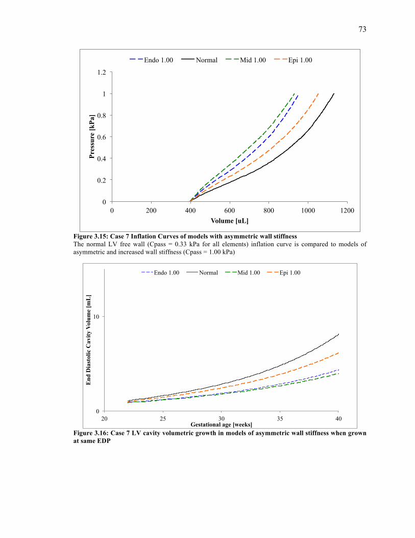
73

Figure 3.15: Case 7 Inflation Curves of models with asymmetric wall stiffness  The normal LV free wall (Cpass = 0.33 kPa for all elements) inflation curve is compared to models of asymmetric and increased wall stiffness (Cpass = 1.00 kPa)

Figure 3.16: Case 7 LV cavity volumetric growth in models of asymmetric wall stiffness when grown at same EDP

0

0.2

0.4

0.6

0.8

1

1.2

0 200 400 600 800 1000 1200

Pres

sure

[kPa

]

Volume [uL]

Endo 1.00 Normal Mid 1.00 Epi 1.00

0

10

20 25 30 35 40

End

Dia

stol

ic C

avity

Vol

ume

[mL

]

Gestational age [weeks]

Endo 1.00 Normal Mid 1.00 Epi 1.00

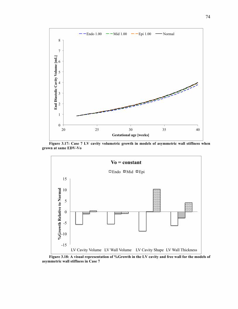
74

Figure 3.17: Case 7 LV cavity volumetric growth in models of asymmetric wall stiffness when grown at same EDV-Vo

Figure 3.18: A visual representation of %Growth in the LV cavity and free wall for the models of asymmetric wall stiffness in Case 7

0

1

2

3

4

5

6

7

8

20 25 30 35 40

End

Dia

stol

ic C

avity

Vol

ume

[mL

]

Gestational age [weeks]

Endo 1.00 Mid 1.00 Epi 1.00 Normal

-15

-10

-5

0

5

10

15

LV Cavity Volume LV Wall Volume LV Cavity Shape LV Wall Thickness

%G

row

th R

elat

ive

to N

orm

al

Vo = constant

Endo Mid Epi

75

From Figure 3.18, we can conclude that when unloaded volume and ventricular filling

are held constant, increasing the stiffness in the endocardial, mid-wall, and epicardial

elements has a positive correlation with growth of the LV cavity shape (SA:LA, WT) as a

gradient of position in the free wall from endocardial to epicardial elements. Increasing

the stiffness of the endocardial elements has a decreased effect on volumetric growth

whereas relatively insignificant change in growth is observed for the stiffer mid-wall and

epicardial elements.  

3.2.2 Overview of Cases with Vo ≠ same

Case 4

Interestingly, when unloaded volume is variable, preload is the dominating

variable contributing to volumetric cavity and wall growth with a positive correlation.

This is a direct reversal of the hierarchy observed when unloaded volume is controlled

for.

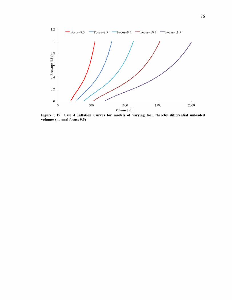
76

Figure 3.19: Case 4 Inflation Curves for models of varying foci, thereby differential unloaded volumes (normal focus: 9.5)                                  

0

0.2

0.4

0.6

0.8

1

1.2

0 500 1000 1500 2000

Pres

sure

[kPa

]

Volume [uL]

Focus=7.5 Focus=8.5 Focus=9.5 Focus=10.5 Focus=11.5

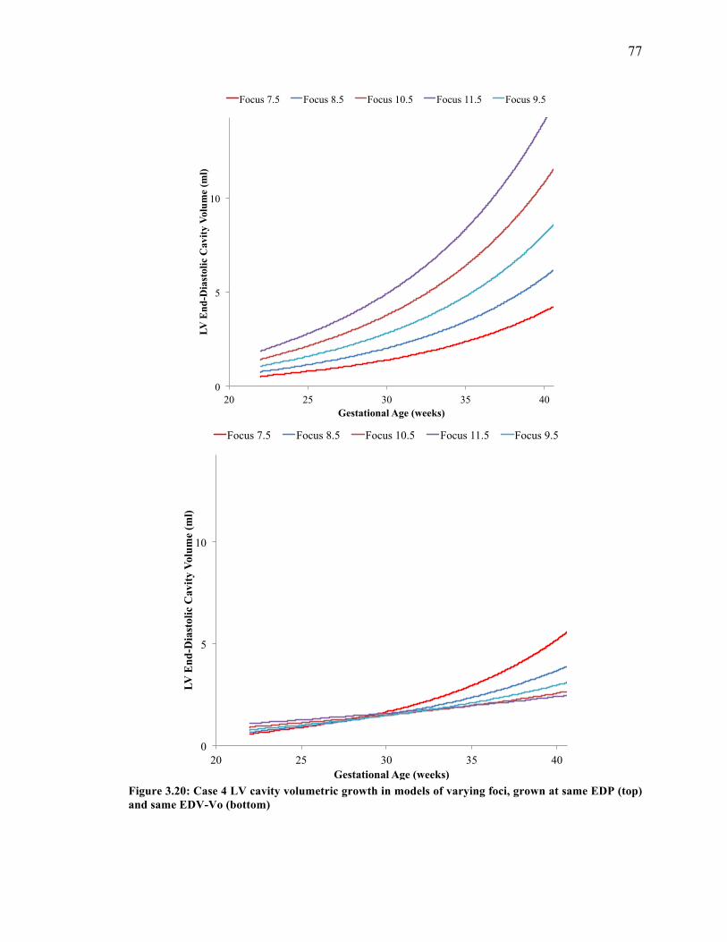
77

Figure 3.20: Case 4 LV cavity volumetric growth in models of varying foci, grown at same EDP (top) and same EDV-Vo (bottom)

0

5

10

20 25 30 35 40

LV E

nd-D

iast

olic

Cav

ity V

olum

e (m

l)

Gestational Age (weeks)

Focus 7.5 Focus 8.5 Focus 10.5 Focus 11.5 Focus 9.5

0

5

10

20 25 30 35 40

LV E

nd-D

iast

olic

Cav

ity V

olum

e (m

l)

Gestational Age (weeks)

Focus 7.5 Focus 8.5 Focus 10.5 Focus 11.5 Focus 9.5

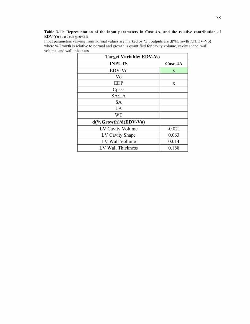
78

Table 3.11: Representation of the input parameters in Case 4A, and the relative contribution of EDV-Vo towards growth Input parameters varying from normal values are marked by ‘x’; outputs are d(%Growth)/d(EDV-Vo) where %Growth is relative to normal and growth is quantified for cavity volume, cavity shape, wall volume, and wall thickness

Target Variable: EDV-Vo INPUTS Case 4A EDV-Vo x

Vo EDP x Cpass SA:LA

SA LA WT

d(%Growth)/d(EDV-Vo) LV Cavity Volume -0.021 LV Cavity Shape 0.063 LV Wall Volume 0.014

LV Wall Thickness 0.168  

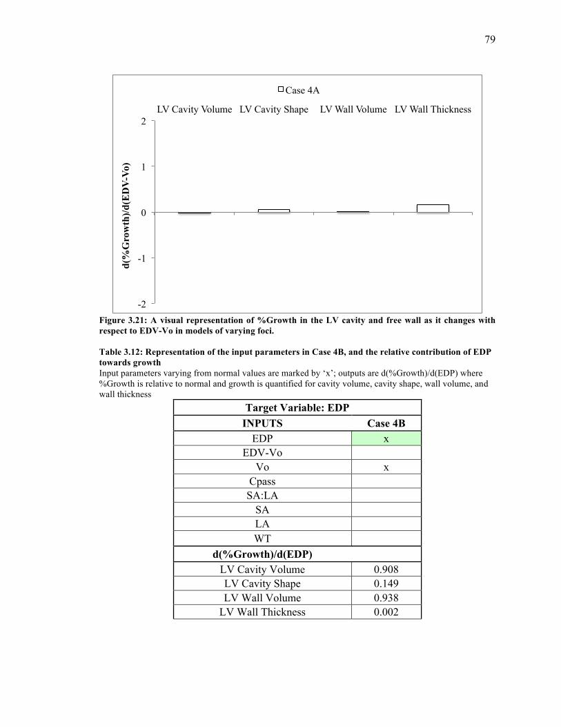
79

Figure 3.21: A visual representation of %Growth in the LV cavity and free wall as it changes with respect to EDV-Vo in models of varying foci. Table 3.12: Representation of the input parameters in Case 4B, and the relative contribution of EDP towards growth Input parameters varying from normal values are marked by ‘x’; outputs are d(%Growth)/d(EDP) where %Growth is relative to normal and growth is quantified for cavity volume, cavity shape, wall volume, and wall thickness

Target Variable: EDP INPUTS Case 4B

EDP x EDV-Vo

Vo x Cpass SA:LA

SA LA WT

d(%Growth)/d(EDP) LV Cavity Volume 0.908 LV Cavity Shape 0.149 LV Wall Volume 0.938

LV Wall Thickness 0.002

-2

-1

0

1

2 LV Cavity Volume LV Cavity Shape LV Wall Volume LV Wall Thickness

d(%

Gro

wth

)/d(E

DV

-Vo)

Case 4A

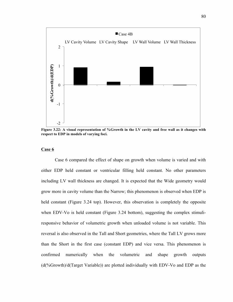
80

Figure 3.22: A visual representation of %Growth in the LV cavity and free wall as it changes with respect to EDP in models of varying foci.  

Case 6

Case 6 compared the effect of shape on growth when volume is varied and with

either EDP held constant or ventricular filling held constant. No other parameters

including LV wall thickness are changed. It is expected that the Wide geometry would

grow more in cavity volume than the Narrow; this phenomenon is observed when EDP is

held constant (Figure 3.24 top). However, this observation is completely the opposite

when EDV-Vo is held constant (Figure 3.24 bottom), suggesting the complex stimuli-

responsive behavior of volumetric growth when unloaded volume is not variable. This

reversal is also observed in the Tall and Short geometries, where the Tall LV grows more

than the Short in the first case (constant EDP) and vice versa. This phenomenon is

confirmed numerically when the volumetric and shape growth outputs

(d(%Growth)/d(Target Variable)) are plotted individually with EDV-Vo and EDP as the

-2

-1

0

1

2 LV Cavity Volume LV Cavity Shape LV Wall Volume LV Wall Thickness

d(%

Gro

wth

)/d(E

DP)

Case 4B

81

target variables (Figures 3.25, 3.26). The results from this case are not as conclusive as

the previous cases and needs further investigation before claiming the individual

contribution of shape on volumetric and shape growth when unloaded volume is not

constant.

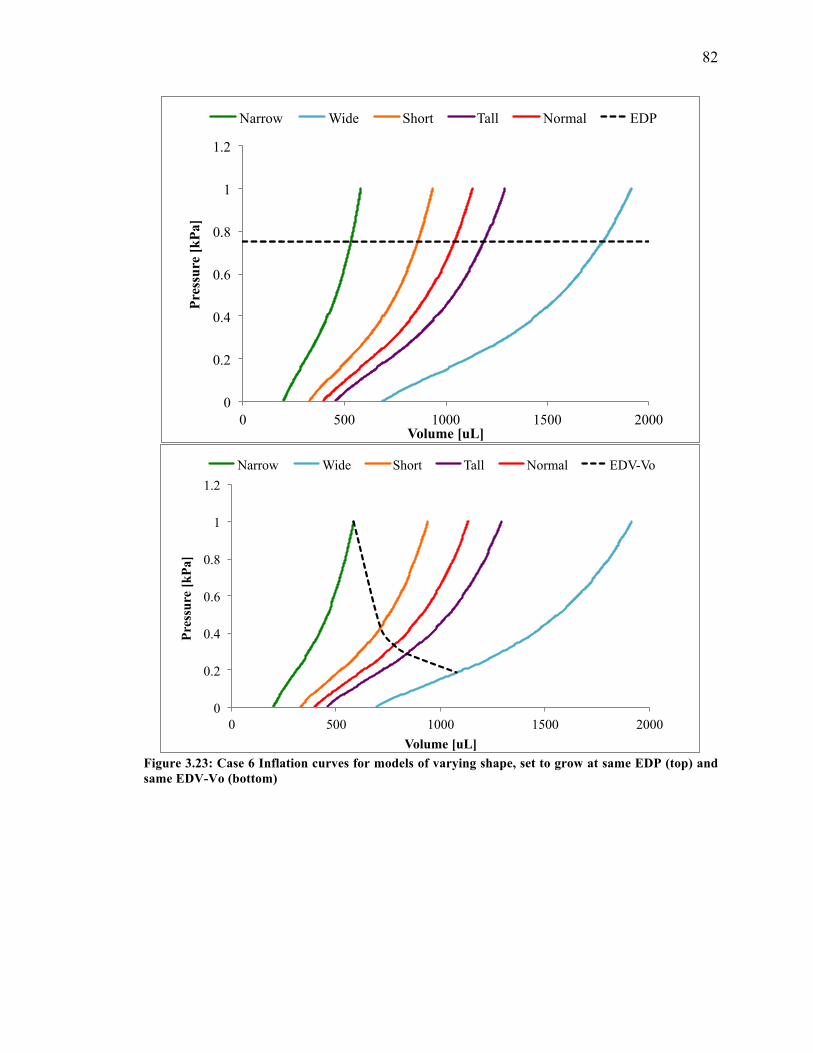
82

Figure 3.23: Case 6 Inflation curves for models of varying shape, set to grow at same EDP (top) and same EDV-Vo (bottom)  

0

0.2

0.4

0.6

0.8

1

1.2

0 500 1000 1500 2000

Pres

sure

[kPa

]

Volume [uL]

Narrow Wide Short Tall Normal EDP

0

0.2

0.4

0.6

0.8

1

1.2

0 500 1000 1500 2000

Pres

sure

[kPa

]

Volume [uL]

Narrow Wide Short Tall Normal EDV-Vo

83

Figure 3.24: Case 6 LV cavity volumetric growth in models of varying shape, grown at same EDP (top) and same EDV-Vo (bottom)  

0

10

20

20 25 30 35 40 End

Dia

stol

ic C

avity

Vol

ume

[mL

]

Gestational age [weeks]

Normal Wide Short Tall Narrow

0

10

20

20 25 30 35 40

End

Dia

stol

ic C

avity

Vol

ume

[mL

]

Gestational age [weeks]

Wide

Short

Tall

Normal

Narrow

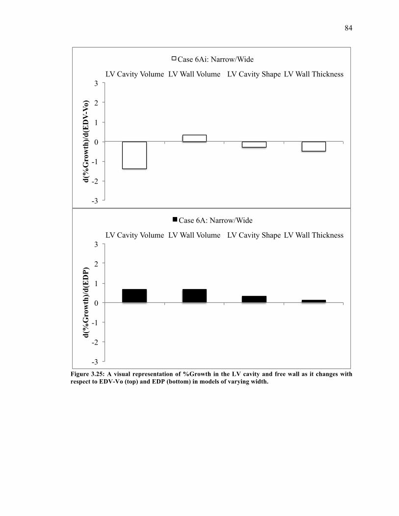
84

Figure 3.25: A visual representation of %Growth in the LV cavity and free wall as it changes with respect to EDV-Vo (top) and EDP (bottom) in models of varying width.  

-3

-2

-1

0

1

2

3 LV Cavity Volume LV Wall Volume LV Cavity Shape LV Wall Thickness

d(%

Gro

wth

)/d(E

DV

-Vo)

Case 6Ai: Narrow/Wide

-3

-2

-1

0

1

2

3 LV Cavity Volume LV Wall Volume LV Cavity Shape LV Wall Thickness

d(%

Gro

wth

)/d(E

DP)

Case 6A: Narrow/Wide

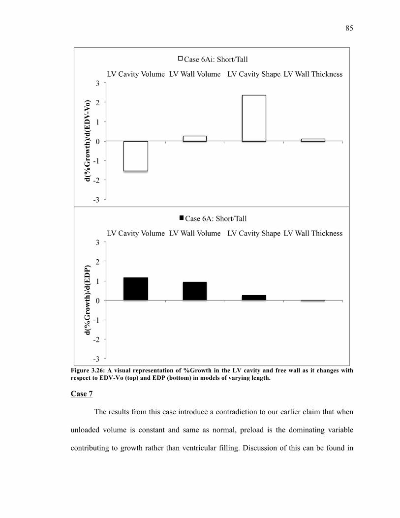
85

Figure 3.26: A visual representation of %Growth in the LV cavity and free wall as it changes with respect to EDV-Vo (top) and EDP (bottom) in models of varying length. Case 7

The results from this case introduce a contradiction to our earlier claim that when

unloaded volume is constant and same as normal, preload is the dominating variable

contributing to growth rather than ventricular filling. Discussion of this can be found in

-3

-2

-1

0

1

2

3 LV Cavity Volume LV Wall Volume LV Cavity Shape LV Wall Thickness

d(%

Gro

wth

)/d(E

DV

-Vo)

Case 6Ai: Short/Tall

-3

-2

-1

0

1

2

3 LV Cavity Volume LV Wall Volume LV Cavity Shape LV Wall Thickness

d(%

Gro

wth

)/d(E

DP)

Case 6A: Short/Tall

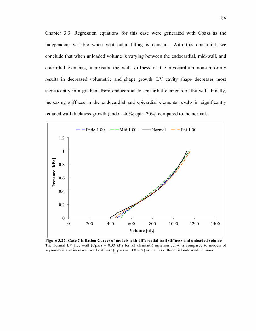
86

Chapter 3.3. Regression equations for this case were generated with Cpass as the

independent variable when ventricular filling is constant. With this constraint, we

conclude that when unloaded volume is varying between the endocardial, mid-wall, and

epicardial elements, increasing the wall stiffness of the myocardium non-uniformly

results in decreased volumetric and shape growth. LV cavity shape decreases most

significantly in a gradient from endocardial to epicardial elements of the wall. Finally,

increasing stiffness in the endocardial and epicardial elements results in significantly

reduced wall thickness growth (endo: -40%; epi: -70%) compared to the normal.

Figure 3.27: Case 7 Inflation Curves of models with differential wall stiffness and unloaded volume  The normal LV free wall (Cpass = 0.33 kPa for all elements) inflation curve is compared to models of asymmetric and increased wall stiffness (Cpass = 1.00 kPa) as well as differential unloaded volumes

0

0.2

0.4

0.6

0.8

1

1.2

0 200 400 600 800 1000 1200 1400

Pres

sure

[kPa

]

Volume [uL]

Endo 1.00 Mid 1.00 Normal Epi 1.00

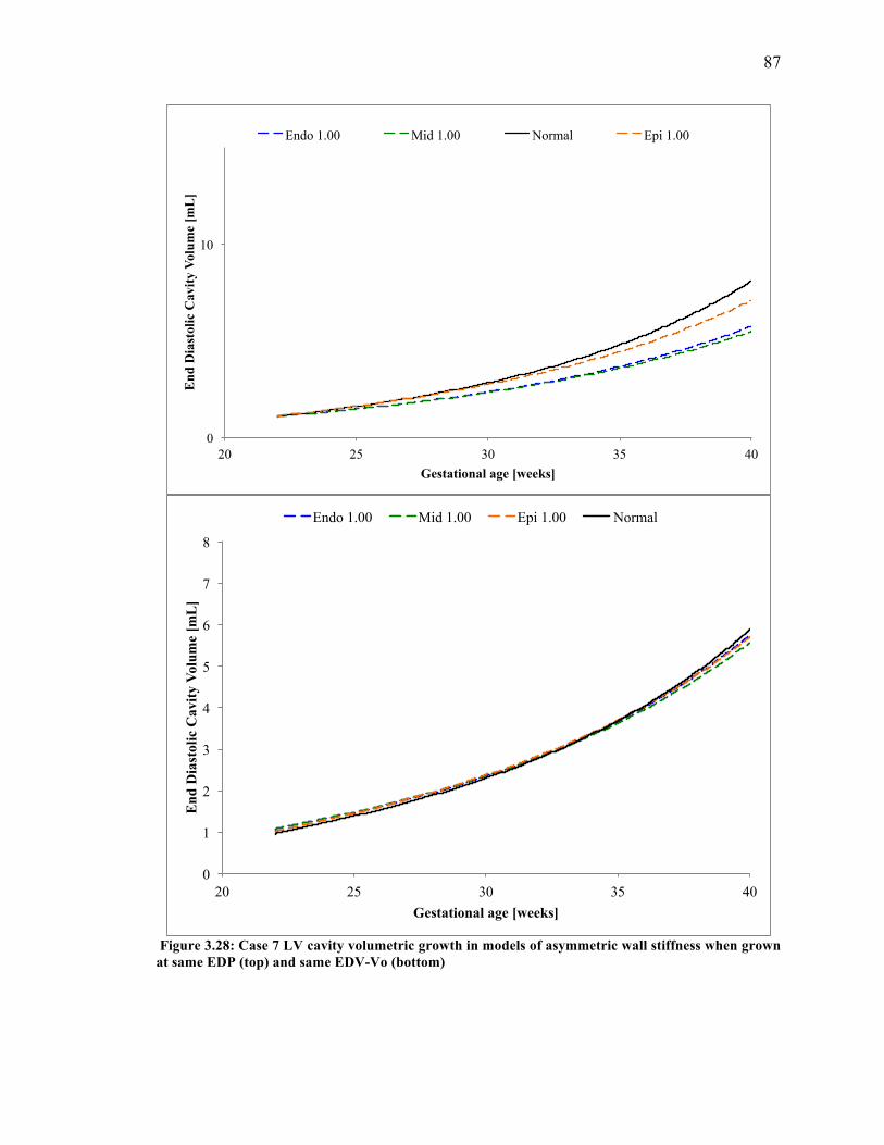
87

Figure 3.28: Case 7 LV cavity volumetric growth in models of asymmetric wall stiffness when grown at same EDP (top) and same EDV-Vo (bottom)

0

1

2

3

4

5

6

7

8

20 25 30 35 40

End

Dia

stol

ic C

avity

Vol

ume

[mL

]

Gestational age [weeks]

Endo 1.00 Mid 1.00 Epi 1.00 Normal

0

10

20 25 30 35 40

End

Dia

stol

ic C

avity

Vol

ume

[mL

]

Gestational age [weeks]

Endo 1.00 Mid 1.00 Normal Epi 1.00

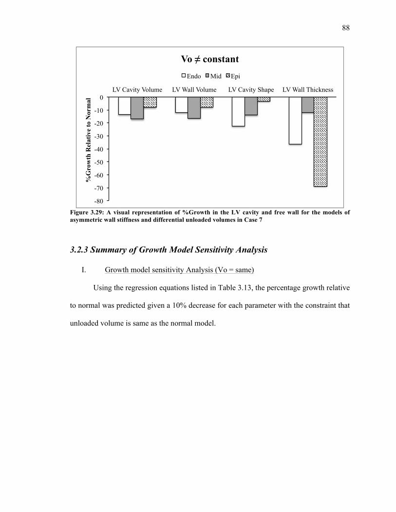
88

Figure 3.29: A visual representation of %Growth in the LV cavity and free wall for the models of asymmetric wall stiffness and differential unloaded volumes in Case 7

3.2.3 Summary of Growth Model Sensitivity Analysis

I. Growth model sensitivity Analysis (Vo = same)

Using the regression equations listed in Table 3.13, the percentage growth relative

to normal was predicted given a 10% decrease for each parameter with the constraint that

unloaded volume is same as the normal model.

-80

-70

-60

-50

-40

-30

-20

-10

0 LV Cavity Volume LV Wall Volume LV Cavity Shape LV Wall Thickness

%G

row

th R

elat

ive

to N

orm

al

Vo ≠ constant

Endo Mid Epi

89

Table 3.13: Regression equations describe the effect of the target variable on growth when unloaded volume is same as normal The linear equations predict change in %Growth at birth relative to the normal model (Y), where growth is quantified for LV cavity volume, wall volume, cavity shape, and wall thickness. The input (X) is the percent change in the target variable value relative to normal at mid gestation.

Target Variable

Regression Equation describing %change in growth relative to normal

LV Cavity Volume Wall Volume Cavity Shape Wall Thickness

EDV-Vo Y= 1.34*X + 1.03 Y= 1.38*X + 0.84 Y= 0.39*X + 0.16 Y= 0.56*X – 0.23 WT Y= -0.66*X + 2.84 Y= -0.86 + 3.57 Y= 0.24*X – 0.27 Y= -0.94*X + 1.10

Cpass Y= 0.01*X + 0.96 Y= 0.01*X + 0.56 Y= -0.0006*X+0.2 Y= -0.03*X – 0.25

EDP Y= 0.01*X + 0.94 Y=0.01*X + 0.55 Y= -.0006*X+0.2 Y= -0.02*X – 0.27

 Table 3.14: %Growth in LV cavity and free wall from mid gestation to birth

Normal

%Growth from mid gestation to birth:

Cavity Volume Wall Volume Cavity Shape Wall Thickness

672.6 339.6 37.8 -8.09

Table 3.15: Inducing a 10% decrease in the input parameters and the observed effect on growth at birth when unloaded volume is same as normal %Growth is quantified at birth as relative to normal

10% decrease

in

%Growth Relative to Normal LV Cavity

Volume LV Wall Volume

LV Cavity Shape

LV Wall Thickness

EDV-Vo -12.3 -12.96 -3.69 -5.84 WT +9.47 12.14 -2.70 +8.35

CPass +0.836 0.455 +0.21 +0.005 EDP +0.817 0.439 +0.208 -0.025

II. Growth model sensitivity Analysis (Vo ≠ same)

Using the regression equations listed in Table 3.16, the percentage growth relative

to normal was predicted given a 10% decrease for each parameter without any constraint

on unloaded volume.

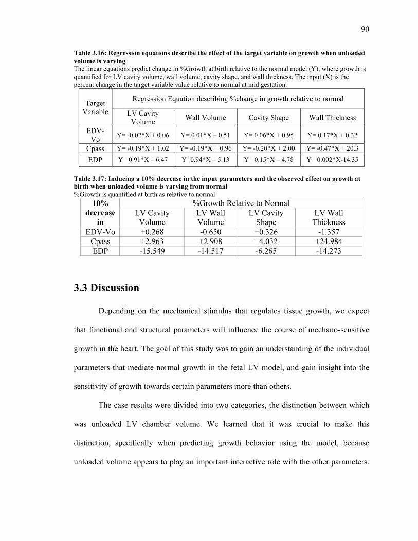
90

Table 3.16: Regression equations describe the effect of the target variable on growth when unloaded volume is varying The linear equations predict change in %Growth at birth relative to the normal model (Y), where growth is quantified for LV cavity volume, wall volume, cavity shape, and wall thickness. The input (X) is the percent change in the target variable value relative to normal at mid gestation.

Target Variable

Regression Equation describing %change in growth relative to normal

LV Cavity Volume Wall Volume Cavity Shape Wall Thickness

EDV-Vo Y= -0.02*X + 0.06 Y= 0.01*X – 0.51 Y= 0.06*X + 0.95 Y= 0.17*X + 0.32

Cpass Y= -0.19*X + 1.02 Y= -0.19*X + 0.96 Y= -0.20*X + 2.00 Y= -0.47*X + 20.3

EDP Y= 0.91*X – 6.47 Y=0.94*X – 5.13 Y= 0.15*X – 4.78 Y= 0.002*X-14.35

Table 3.17: Inducing a 10% decrease in the input parameters and the observed effect on growth at birth when unloaded volume is varying from normal %Growth is quantified at birth as relative to normal

10% decrease

in

%Growth Relative to Normal LV Cavity

Volume LV Wall Volume

LV Cavity Shape

LV Wall Thickness

EDV-Vo +0.268 -0.650 +0.326 -1.357 Cpass +2.963 +2.908 +4.032 +24.984 EDP -15.549 -14.517 -6.265 -14.273

3.3 Discussion

Depending on the mechanical stimulus that regulates tissue growth, we expect

that functional and structural parameters will influence the course of mechano-sensitive

growth in the heart. The goal of this study was to gain an understanding of the individual

parameters that mediate normal growth in the fetal LV model, and gain insight into the

sensitivity of growth towards certain parameters more than others.

The case results were divided into two categories, the distinction between which

was unloaded LV chamber volume. We learned that it was crucial to make this

distinction, specifically when predicting growth behavior using the model, because

unloaded volume appears to play an important interactive role with the other parameters.

91

To reiterate, when unloaded volume is constant and the same as our normal model, we

concluded that ventricular filling is the dominating variable contributing to LV

volumetric and cavity growth, and that growth is least sensitive to changes in pressure

preload. However, when unloaded volume varies from that of the normal model, this

observed trend completely flips with preload being the dominating variable mediating

growth. This is challenged in one case when material properties are introduced as a

variable by inducing stiffness in the elements of the myocardial wall. In that case,

ventricular filling is again the dominating variable and change in preload has seemingly

no individual effect on growth, suggesting that stiffness of the myocardial wall

suppresses the effect on growth typically observed by changing preload. This hypothesis

must be tested further when unloaded volume is constant and variable in order to

elucidate the nature of the potential interactive behavior between preload and material

properties.

Categorizing the growth model sensitivity analysis by unloaded volume can also

be useful in its application clinically. The cases with unloaded volume held constant can

shed insight into normal growth behavior of the fetal heart, specifically when the LV is of

a size similar to our assumed normal (397 µL) but more importantly when determining

clinical intervention or drug therapies for a specific patient. There are clinical cases such

as in ventricular septal defect, where the fetal patient has a cardiac malformation that

must be surgically repaired by placing a shunt or performing reconstruction surgery. For

these procedures, it is difficult to predict the growth behavior of the fetus including the

size, shape and mechanical consequences. Our growth model sensitivity analysis would

be useful here as it can predict the growth behavior in terms of volume and shape,

92

including wall thickness growth, given the percent change in the parameter of interest.

On the other hand, the analysis with unloaded volume varying from that of a normal fetal

LV at mid gestation can be extremely useful when predicting LV growth for a patient

with a heart significantly different in size, as in the case of HLHS.

While the growth model sensitivity analysis improves understanding of normal

growth in the fetal LV, there are several limitations of this method worth discussing.

First, the method is based on a logical approach of case design and inference that is not

established as a statistical method of sensitivity analysis. Second, within each case, there

are only a few points above and below the normal reference value that are used to

generate linear regression lines. While the nature of normal growth predicted by the

model is, in fact, mostly linear, there is a definite need to increase the number of data

points in order to improve confidence in the resulting correlation behavior between the

parameters and growth. Third, in some cases the independent variable was not varied by

the same degree above or below the normal reference value due to the complex iterative

nature of developing these unloaded geometries. However, this limitation can also be

vastly improved by increasing the number of data points, resulting in a more

comprehensive analysis within each case.

Fourth, the individual effects of a few parameters could not be elucidated

completely, specifically in the case of short-axis to long-axis ratio when unloaded volume

is constant. As mentioned previously, manipulating the unloaded geometry in order to

understand the effect of SA:LA while keeping all other parameters (unloaded volume,

preload, ventricular filling, wall thickness) constant is difficult and often involves

compromise. In the case above, wall thickness could not be controlled for, which

93

complicates the conclusions that can be made. However, because we know the individual

effect of wall thickness as in the case of Thick versus Thin, it is still possible to make

inferences about the effect of SA:LA by assuming that wall thickness plays the same role.

For example, the ShortWide and TallNarrow geometries were 5% and 10% thinner than

normal, respectively. Based on the regression equation with wall thickness as the

independent variable and focusing on just volumetric cavity growth, one can predict that

a 5% and 10% thinner LV would grow 6% and 9% more than normal. The ShortWide

geometry does grow approximately +6%, most likely suggesting that the changes in

SA:LA did not contribute to growth at all. On the other hand, the TallNarrow geometry

grows 2.5% less than normal. This is peculiar and may be due to the limitation that the

SA:LA for TallNarrow was varied by only -17% while ShortWide was varied by +27%.

Further work must be done to account for this variability before making conclusions

about the relative contribution of SA:LA towards growth.

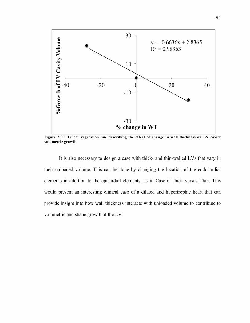
94

Figure 3.30: Linear regression line describing the effect of change in wall thickness on LV cavity volumetric growth  

It is also necessary to design a case with thick- and thin-walled LVs that vary in

their unloaded volume. This can be done by changing the location of the endocardial

elements in addition to the epicardial elements, as in Case 6 Thick versus Thin. This

would present an interesting clinical case of a dilated and hypertrophic heart that can

provide insight into how wall thickness interacts with unloaded volume to contribute to

volumetric and shape growth of the LV.

y = -0.6636x + 2.8365 R² = 0.98363

-30

-10

10

30

-40 -20 0 20 40

%G

row

th o

f LV

Cav

ity V

olum

e

% change in WT

95

CHAPTER 4

Reverse Growth

Although a number of models describe the process of ventricular remodeling,

there are few that describe its reversal. Reverse modeling of the ventricles has been

observed clinically after mitral valve repairs or implantation of a LVAD. These

interventions lead to a reduction in ventricular loading after sufficient and prolonged

unloading of the ventricles [84]. The growth law as described in this study, developed by

Kerckhoffs et al, was used to model ventricular growth in the fetus from mid gestation to

birth. The objective of this aim was to adapt the growth law in the reverse direction and

to model fetal LV growth from mid gestation to an in vivo unloaded state.

4.1 Methods

The previously described growth law was applied such that the magnitude of the

growth rates were constant as in forward growth, but the direction of growth was

negative to yield reverse growth while keeping all parameters the same. The time

calibration was adjusted to calculate gestational age in the reverse direction. The growth

96

law was applied to the reference model of normal fetal growth and allowed to grow

backwards. LV dimensions were extracted from the model at the earliest time point and

compared to short-axis, long-axis, and average wall thickness dimensions of the normal

fetal LV in both an unloaded state and loaded state, as reported in literature. Thorough

mapping of end-diastolic cavity and wall volumes, wall mass, and EDPs from early

gestation (5 weeks) to birth was conducted [73, 92-97]. This comprehensive overview of

fetal development was used to compare the compatibility of our results with clinically

and experimentally observed features of left ventricular growth in the normal fetus.

4.2 Results

The LV fetal growth model was able to reverse grow from 22 weeks gestation to

approximately 15 weeks gestation at which point the LV cavity volume was near zero (9

µL) in the model. However, the resulting mesh at this time point had a warped element

(Figure 4.1), so reverse growth behavior in the model was analyzed from mid gestation

up until the point that the mesh exhibits no warping of any elements and associated

nodes, which occurred at 17.2 weeks gestation. LV cavity and wall volumetric growth in

the forward and reverse direction as described by the model is shown in Figure 4.2.

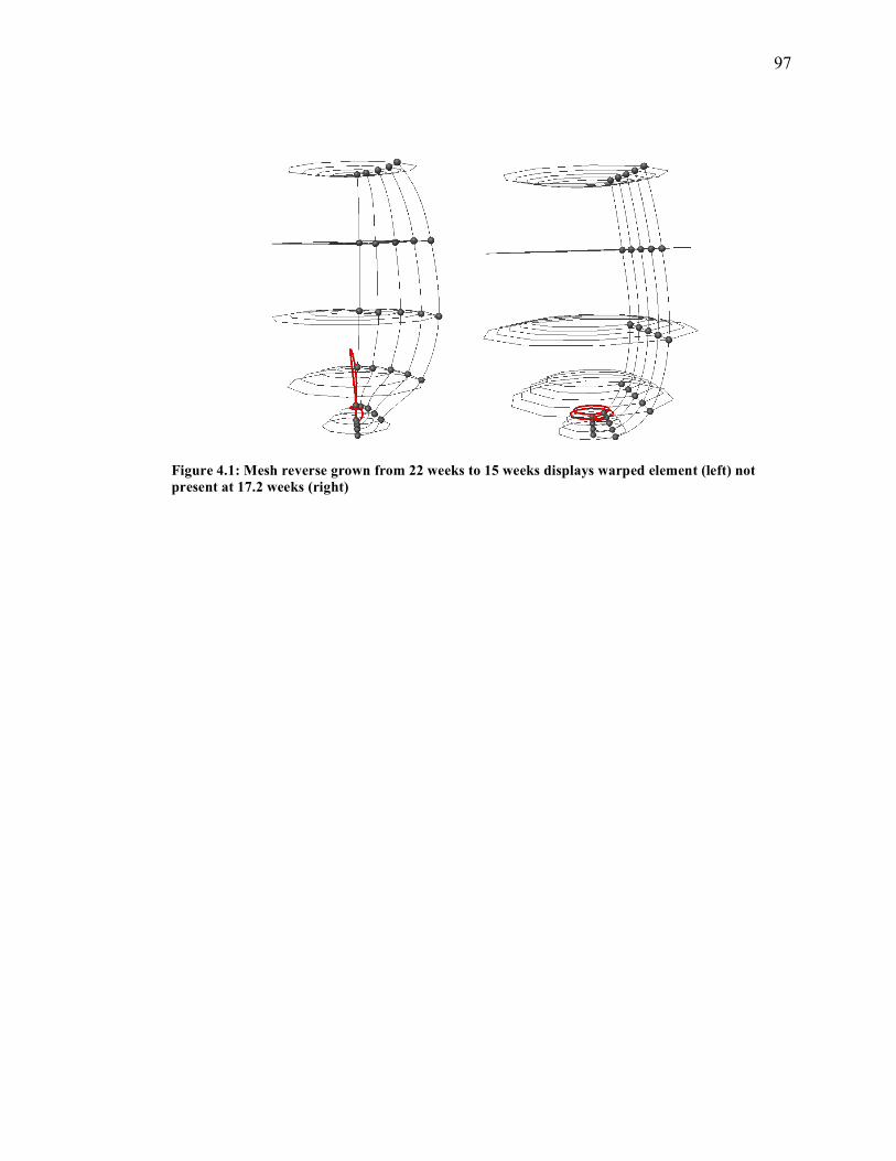
97

Figure 4.1: Mesh reverse grown from 22 weeks to 15 weeks displays warped element (left) not present at 17.2 weeks (right)

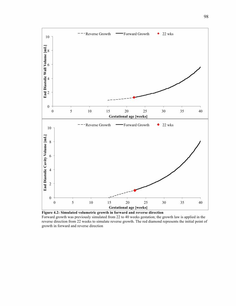
98

Figure 4.2: Simulated volumetric growth in forward and reverse direction Forward growth was previously simulated from 22 to 40 weeks gestation; the growth law is applied in the reverse direction from 22 weeks to simulate reverse growth. The red diamond represents the initial point of growth in forward and reverse direction

0

2

4

6

8

10

0 5 10 15 20 25 30 35 40

End

Dia

stol

ic W

all V

olum

e [m

L]

Gestational age [weeks]

Reverse Growth Forward Growth 22 wks

0

2

4

6

8

10

0 5 10 15 20 25 30 35 40

End

Dia

stol

ic C

avity

Vol

ume

[mL

]

Gestational age [weeks]

Reverse Growth Forward Growth 22 wks

99

4.3 Discussion

Myocardial hypertrophy and extracellular matrix (ECM) remodeling can be

defined as changes in the heart geometry and function that occur over an extensive period

of time as a result of pathology (heart disease, CHD) or physiology (growth and

development, pregnancy, aging etc.). Hypertrophy and ECM remodeling can be similar in

some cases. For instance, cellular hypertrophy is the response in both hypertensive heart

disease and post-natal heart development due to pressure overloading. Remodeling may

initially behave as a compensatory mechanism to normalize function under

pathophysiological stimuli. This explains why during pressure loading, LV wall thickness

increases as it normalizes wall stresses [81].

Hypertrophy-related changes in the LV geometry can be classified into concentric

and eccentric hypertrophy. During concentric hypertrophy, the LV wall thickens with

minimal change in chamber volume whereas during eccentric hypertrophy, the LV wall

thins and the chamber volume decreases significantly. The mechanism behind this type of

wall thickening and LV dilation is explained by the parallel and serial addition of

sarcomeres in the myocytes, respectively. Hypertrophy and remodeling, in addition to

geometrical changes, can also induce functional changes that affect myocardial

contraction at the myocyte level. Increased myocardial stiffness, which can impair

diastolic filling, is a hallmark of diastolic heart failure with preserved ejection fraction.

This increase in myocardial stiffness has been attributed to a delayed relaxation of the

myocyte’s contraction. These global changes that occur during growth and remodeling

can be traced to the geometrical and functional changes in the myocytes [81].

100

Several computational models based on the concept of finite volume growth have

been developed, as described previously [61, 63 82, 83]. These ventricular growth models

were developed with either ventricular myofiber stress as the stimulant of growth or with

ventricular myofiber and/or myocardial cross-fiber strain as the primary stimulant.

Guccione et al recently presented a constitutive strain-drive growth model capable of

describing both ventricular remodeling and reverse modeling under pathological

conditions. The model was able to predict key features in the end-diastolic pressure-

volume relationship that is observed experimentally and clinically during ventricular

growth and reverse growth [84].

The goal of this aim was to adapt our growth law in the reverse direction to test its

ability to predict LV growth at time points prior to mid gestation. Model compatibility

with clinically and experimentally observed LV dimensions in healthy fetuses were

compared at 17.2 weeks gestation (Figure 4.3). Figure 4.4 shows LV cavity and wall

volumetric growth derived from echocardiographic measurements from multiple studies.

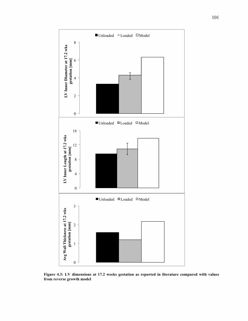
101

Figure 4.3: LV dimensions at 17.2 weeks gestation as reported in literature compared with values from reverse growth model

0

2

4

6

8

LV I

nner

Dia

met

er a

t 17.

2 w

ks

gest

atio

n [m

m]

Unloaded Loaded Model

0

4

8

12

16

LV I

nner

Len

gth

at 1

7.2

wks

ge

stat

ion

[mm

]

Unloaded Loaded Model

0

1

2

3

Avg

Wal

l Thi

ckne

ss a

t 17.

2 w

ks

gest

atio

n [m

m]

Unloaded Loaded Model

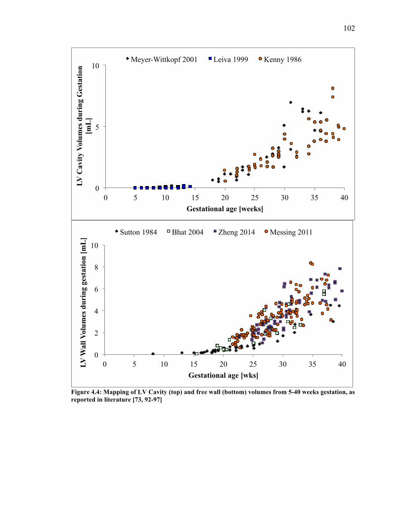
102

Figure 4.4: Mapping of LV Cavity (top) and free wall (bottom) volumes from 5-40 weeks gestation, as reported in literature [73, 92-97]  

0

2

4

6

8

10

0 5 10 15 20 25 30 35 40 LV W

all V

olum

es d

urin

g ge

stat

ion

[mL

]

Gestational age [wks]

Sutton 1984 Bhat 2004 Zheng 2014 Messing 2011

0

5

10

0 5 10 15 20 25 30 35 40

LV C

avity

Vol

umes

dur

ing

Ges

tatio

n [m

L]

Gestational age [weeks]

Meyer-Wittkopf 2001 Leiva 1999 Kenny 1986

103

It is noteworthy that the model when grown in the reverse direction has an applied

preload of 0.75 kPa as in the forward direction. The fetal LV from mid gestation to term

can be modeled with a constant preload, as described earlier, because the EDP does not

change significantly until birth. The growth model was developed based on this

assumption that may not apply prior to mid gestation. The pressure in the LV prior to 22

weeks gestation is significantly lower and exhibits a relatively steeper slope over time as

the heart continues to develop and grow in size during early gestation.

The strain-based growth law in both forward and reverse direction does not

account for the dynamics of pressure development or myocardial stiffness during growth.

While this may be a valid assumption after mid gestation, this is a limitation when

modeling growth in early gestation. The growth law utilized in this model can be

modified to incorporate remodeling by varying the passive stiffness of the myocardium

dependent on either volume or time. For example, Kerckhoffs et al previously used the

growth law to predict concentric and eccentric cardiac growth during pressure and

volume overload [63]. However, remodeling prior to mid gestation was not studied in our

model of reverse growth.

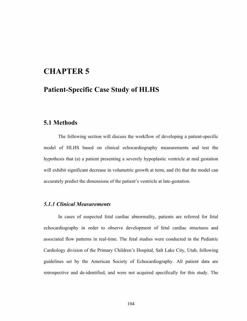
104

CHAPTER 5

Patient-Specific Case Study of HLHS

5.1 Methods

The following section will discuss the workflow of developing a patient-specific

model of HLHS based on clinical echocardiography measurements and test the

hypothesis that (a) a patient presenting a severely hypoplastic ventricle at mid gestation

will exhibit significant decrease in volumetric growth at term, and (b) that the model can

accurately predict the dimensions of the patient’s ventricle at late-gestation.

5.1.1 Clinical Measurements

In cases of suspected fetal cardiac abnormality, patients are referred for fetal

echocardiography in order to observe development of fetal cardiac structures and

associated flow patterns in real-time. The fetal studies were conducted in the Pediatric

Cardiology division of the Primary Children’s Hospital, Salt Lake City, Utah, following

guidelines set by the American Society of Echocardiography. All patient data are

retrospective and de-identified, and were not acquired specifically for this study. The

105

studies were IRB approved and conducted at 23.1 weeks gestation with a follow-up at

30.1 weeks; fetal age was determined by standard protocols by obstetricians.

Measurements of the hypoplastic LV were made retrospectively by a pediatric

cardiologist at Rady Children’s Hospital, San Diego, California. The measurements taken

were of the left ventricular internal and external diameters (width) at the base and mid-

level, as well as the inner and outer length of the cavity. Figure 5.1 displays a screenshot

with the measurements taken for this patient at the first time point. Measurements were

only made when the image quality allowed clear definition of the structures in the four-

chamber projection of the fetal heart at the end of diastole.

Figure 5.1: Screenshot of LV end-diastolic measurements obtained for HLHS patient at first time point (23.1 weeks)      5.1.2 Mesh Generation

The left ventricular measurements obtained at end-diastole as described above

were used to calculate the wall thickness at the base, mid, and apex levels. Table 5.1 lists

the LV measurements corresponding to the HLHS patient at 23.1 weeks used to generate

a FE mesh in a prolate spheroidal coordinate system as described in Chapter 2.1.2. The

resulting surface mesh was refined to generate a mesh of 30 nodes and 20 elements

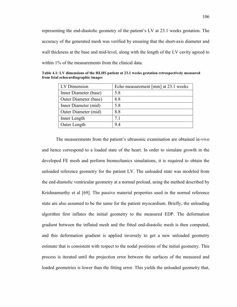
106

representing the end-diastolic geometry of the patient’s LV at 23.1 weeks gestation. The

accuracy of the generated mesh was verified by ensuring that the short-axis diameter and

wall thickness at the base and mid-level, along with the length of the LV cavity agreed to

within 1% of the measurements from the clinical data.

Table 4.1: LV dimensions of the HLHS patient at 23.1 weeks gestation retrospectively measured from fetal echocardiographic images

LV Dimension Echo measurement [mm] at 23.1 weeks Inner Diameter (base) 5.8 Outer Diameter (base) 8.8 Inner Diameter (mid) 5.8 Outer Diameter (mid) 8.8 Inner Length 7.1 Outer Length 9.4

The measurements from the patient’s ultrasonic examination are obtained in-vivo

and hence correspond to a loaded state of the heart. In order to simulate growth in the

developed FE mesh and perform biomechanics simulations, it is required to obtain the

unloaded reference geometry for the patient LV. The unloaded state was modeled from

the end-diastolic ventricular geometry at a normal preload, using the method described by

Krishnamurthy et al [69]. The passive material properties used in the normal reference

state are also assumed to be the same for the patient myocardium. Briefly, the unloading

algorithm first inflates the initial geometry to the measured EDP. The deformation

gradient between the inflated mesh and the fitted end-diastolic mesh is then computed,

and this deformation gradient is applied inversely to get a new unloaded geometry

estimate that is consistent with respect to the nodal positions of the initial geometry. This

process is iterated until the projection error between the surfaces of the measured and

loaded geometries is lower than the fitting error. This yields the unloaded geometry that,

107

when loaded to the measured EDP, deforms to the measured end-diastolic geometry

developed previously with the same passive material properties [63, 69].

The unloaded ventricular geometry constitutes the anatomic model of the patient

LV. The anatomic model and the passive constitutive model comprise the patient-specific

fetal LV model. The model is inflated to the EDP to obtain the deformed nodal

properties, which are inputted as initial conditions for the growth model. This method is

the same as described for setting up the growth model of a normal fetal LV, as described

earlier. The model is allowed to grow to term and LV dimensions are extracted at 30.1

weeks gestation to compare with the measured echocardiographic data at that time point.

5.2 RESULTS

In a case study, using echocardiographic data (LV geometry) from a HLHS

patient at 23.1 weeks, the patient-specific growth model with normal preload and is able

to predict a hypoplastic LV at birth and replicate clinical measurements of LV

dimensions at 30.1 weeks. The model predicts a 50% reduction in LV EDV (1.1 mL) and

a 60% reduction in LV wall volume (2.1 mL) at birth, consistent with the patient

diagnosis of a severely hypoplastic LV.

The model replicates LV short-axis inner diameters at the base (6.5 mm) and mid

level (7.4 mm), inner length (8.5 mm) and outer length (10.5 mm) with error ranges

shown in Figure 5.3. The patient-specific model is not able to accurately replicate the LV

wall thickness measurements at base and mid (-50% error); possible theories and

limitations are discussed in Chapter 5.3.

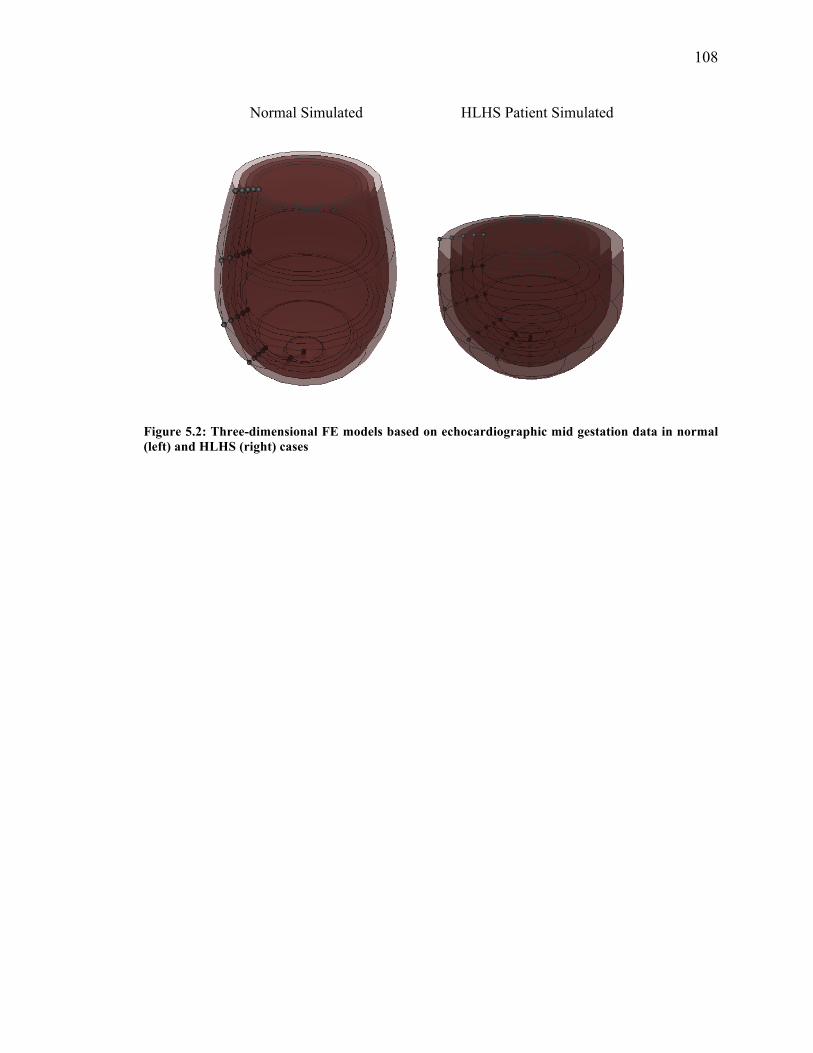
108

Figure 5.2: Three-dimensional FE models based on echocardiographic mid gestation data in normal (left) and HLHS (right) cases

Normal Simulated HLHS Patient Simulated

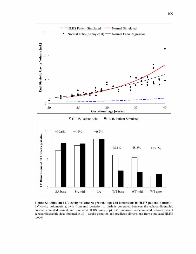
109

 Figure 5.3: Simulated LV cavity volumetric growth (top) and dimensions in HLHS patient (bottom) LV cavity volumetric growth from mid gestation to birth is compared between the echocardiographic normal, simulated normal, and simulated HLHS cases (top); LV dimensions are compared between patient echocardiographic data obtained at 30.1 weeks gestation and predicted dimensions from simulated HLHS model  

0

5

10

15

20 25 30 35 40

End

Dia

stol

ic C

avity

Vol

ume

[mL

]

Gestational age [weeks]

HLHS Patient Simulated Normal Simulated

Normal Echo [Kenny et al] Normal Echo Regression

0

5

10

SA base SA mid LA WT base WT mid WT apex

LV D

imen

sion

s at

30.

1 w

eeks

ges

tatio

n

HLHS Patient Echo HLHS Patient Simulated

+4.2%

+15.5%

+19.6%

-48.1% -48.2%

+0.7%

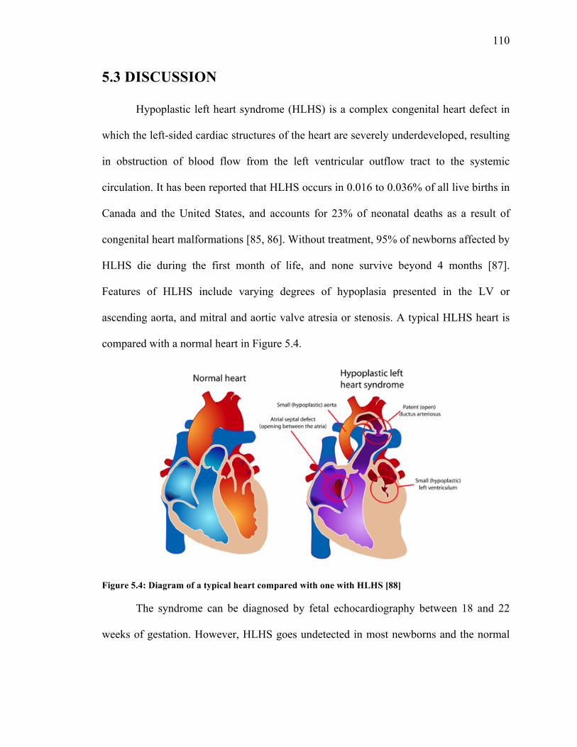
110

5.3 DISCUSSION

Hypoplastic left heart syndrome (HLHS) is a complex congenital heart defect in

which the left-sided cardiac structures of the heart are severely underdeveloped, resulting

in obstruction of blood flow from the left ventricular outflow tract to the systemic

circulation. It has been reported that HLHS occurs in 0.016 to 0.036% of all live births in

Canada and the United States, and accounts for 23% of neonatal deaths as a result of

congenital heart malformations [85, 86]. Without treatment, 95% of newborns affected by

HLHS die during the first month of life, and none survive beyond 4 months [87].

Features of HLHS include varying degrees of hypoplasia presented in the LV or

ascending aorta, and mitral and aortic valve atresia or stenosis. A typical HLHS heart is

compared with a normal heart in Figure 5.4.

Figure 5.4: Diagram of a typical heart compared with one with HLHS [88]  

The syndrome can be diagnosed by fetal echocardiography between 18 and 22

weeks of gestation. However, HLHS goes undetected in most newborns and the normal

111

physiological changes that occur upon birth lead to severe hemodynamic disturbances in

the infant. The clinical presentation of HLHS occurs as systemic and coronary perfusion

is critically decreased, leading to metabolic acidosis, tissue hypoxia, and eventually

vascular shock or death. Presently, HLHS is managed by a three-stage palliative

reconstructive surgery that creates unobstructed systemic blood flow from the right

ventricle to the aorta (Norwood, Stage 1) and connects the superior and inferior vena

cava (Fontan, Stage 2) to the pulmonary arteries, facilitating the transition to a

physiologically normal circulation. The last stage involves closure of the fenestration,

resulting in the right ventricle pumping oxygenated blood through a reconstructed aorta

and deoxygenated blood returning directly to the lungs. Survival rates for all infants with

combined three-staged procedures has been reported to be 63 to 80% at one year of age

and 58 to 72% at five years of age [86]. An alternative to surgery is infant heart

transplantation, which has reported survival rates of 76% at five years and 70% at seven

years, but many infants die while awaiting a donor heart due to complications [86].

Although fetal echocardiography allows an accurate prenatal diagnosis of HLHS

at mid gestation, providing the opportunity to plan management and counseling for the

family, Galindo et al reported an overall survival rate of 36% for these prenatally

diagnosed fetuses [89]. The outlook for fetuses affected by HLHS is poor due to the

limitations posed by early diagnosis via fetal echocardiography and inability to predict

the outcome of the fetal hypoplastic heart upon birth. Patient-specific computational

modeling of developing fetuses with HLHS could serve to improve prenatal diagnosis by

providing insight into the biomechanics and growth behavior of the affected ventricle.

112

Our model was based on patient-specific LV geometry at mid gestation and was

able to replicate short-axis and long-axis dimension data from late-gestation. It was not

able to replicate wall thickness measurements at the base and mid level, though it

predicted wall thickness at the apex level accurately. This is likely due to the altered

geometry as it plays a significant role in altering strain distribution, thereby leading to

differential addition of sarcomeres in series or parallel. A greater understanding of the

strain distribution may shed insight into the mechanism underlying the significant wall

thickening observed in hypoplastic hearts; however, our study did not explore this facet

of fetal growth. Our HLHS model predicts a severely hypoplastic LV at birth in

comparison to the normal simulated LV. Our conclusions from the growth model

sensitivity analysis (Chapter 3.2) support this prediction as we observed reduced

volumetric growth in a thick-walled LV.

Fetal LV dimensions obtained from pre-recorded echocardiographic images are

valuable measurements as they provide the most clinically relevant and accurate inflation

about ventricular structure in HLHS patients. Despite the retrospective method used,

these images contain several types of artifacts as they are taken in real time. In addition,

hypoplastic ventricles are of smaller scale relative to normally developing ventricles,

which compounds the difficulty of taking accurate measurements. While measurements

were only made when the structures were visibly clear and delineated, there is the

possibility of introducing error due to manual handling of data. For this case study, six

dimensional measurements were provided at different planes; increasing the number of

data points and including flow data would allow for more constraints on the developed

mesh and, therefore, a more faithful patient-specific geometry. In addition, measurements

113

at more than two time points would be valuable in validating the patient-specific model

and its predictive capability. For future studies, protocols need to be developed to ensure

consistent methods between patients and, if possible, reduce manual error by having

multiple experts obtain measurements.

It is noteworthy that the ventricular geometry was imaged at end-diastole when

the heart experiences a significant amount of load. An unloading algorithm developed by

Krishnamurthy et al was used to predict the unloaded configuration of the 3D FE model

under normal preload and passive material properties, which may not hold true for the

patient-specific case [69]. It is impossible to obtain unloaded geometry from

echocardiographic images and presently it is not standard protocol to obtain a measure of

preload via fetal cardiac catheterization in utero. However, the predicted unloaded

geometry is able to successfully deform to the measured end-diastolic geometry,

demonstrating promising results. Repeating this with a larger set of patients would serve

to validate the algorithm as well as the ability of the growth model to predict dimensions

at a future time point.

114

CHAPTER 6

CONCLUSIONS

The single ventricle growth model for a normal human fetal LV presented here

was developed based on experimental and clinical geometric and functional data. The

model is able to accurately represent normal volumetric and shape growth of the fetal LV

from mid gestation to birth. The model is also capable of simulating reverse growth from

mid gestation to an in vivo state of near zero LV cavity volume, providing a

comprehensive overview of fetal growth from the onset of cardiac function to birth. The

sensitivity of the growth model to several model parameters was quantified, which led to

an understanding of the individual clinically relevant parameters that mediate normal

growth in the fetal LV. Finally, a patient-specific growth model for HLHS was developed

that was able to replicate clinical echocardiographic measurements for LV shape at a later

time point and predict severe hypoplasia at birth.

Patient-specific and clinically relevant computational models offer potential for

studying the complex biomechanical and electrophysiological behavior of the heart in its

normal and diseased states. For this reason, significant efforts have been made to develop

protocols for building specific models and demonstrate the predictive capabilities of these

115

models by comparison with experimental results and clinical measurements.

Incorporation of growth and remodeling in patient-specific and clinically relevant

computational models offers the capacity to understand the complex mechanisms and

biomechanical stimuli underlying normal cardiac development as well as in

pathophysiology. The next step is to explore the clinical feasibility of these

computational models and the benefits they can offer to physicians in optimizing clinical

outcomes and surgical interventions. A main focus of this study was to develop a

physiologically relevant FE model describing normal growth in the human fetal model

that can ideally be used as a clinical tool, especially considering the limited scope of fetal

cardiac computational models.

The developed single ventricle model for normal fetal growth is a significant step

towards building patient-specific models based on fetal echocardiography data. Since

ventricular geometry is one of the major model parameters that determine cardiac

function, the focus of this study was to optimize the single ventricle geometry. In the

future, it would be invaluable to generate a bi-ventricular mesh of the fetal heart with

circulation in order to improve the physiological relevance of the model as well as

understand the interaction effects between the ventricles in a normal and diseased state.

This would be specifically useful in a clinical case such as HLHS because the right

ventricle often compensates for the reduced function in the LV. Identifying the

biomechanical stimuli that drive this behavior and quantifying the consequential effects

on cardiac growth would shed insight into the defect.

The methods developed in this thesis serve to facilitate understanding of fetal

growth behavior undergoing normal development and provide a benchmark model for

116

normal growth in the human fetal LV, enabling comparison with patient-specific fetal LV

models. This is, to the best of our knowledge, one of the first computational models that

describe cardiac growth behavior in the human fetus by integrating information from

multiple clinical measurements and predicts patient diagnoses based on mid gestation

echocardiographic geometry. Ultimately, with further refinement, the model has potential

to aid physicians in surgical planning to achieve optimal therapeutic outcomes.

Computational models such as these will be invaluable tools in understanding the

complex stimuli-responsive behavior of organ-level fetal growth.

117

REFERENCES 1. Central Intelligence Agency (2012). "Field Listing: Birth Rate." The World Factbook.

Retrieved June 4, 2012, from https://www.cia.gov/library/publications/the-world-factbook/fields/2054.html.

2. The World Bank (2016). "Birth rate, crude (per 1,000 people)." Retrieved June 4,

2016, from http://data.worldbank.org/indicator/SP.DYN.CBRT.IN. 3. Centers for Disease Control and Prevention (2015). "Birth Data." National Center for

Health Statistics. Retrieved June 4, 2016, from http://www.cdc.gov/nchs/nvss/births.htm.

4. Centers for Disease Control and Prevention (2016). "Data & Statistics." Birth

Defects. Retrieved June 4, 2016, from http://www.cdc.gov/ncbddd/birthdefects/data.html.

5. Centers for Disease Control and Prevention (2015). "Data & Statistics." Congenital

Heart Defects (CHDs). Retrieved June 4, 2016, from http://www.cdc.gov/ncbddd/heartdefects/data.html.

6. Averiss, I. E. and H. M. Gardiner (2013). "Improving prenatal detection of major

congenital heart disease." Australasian Journal of Ultrasound in Medicine 16(4): 156-157.

7. Buskens, E., Grobbee, D. E., Frohn-Mulder, I. M. E., Stewart, P. A., Juttmann, R. E.,

Wladimiroff, J. W., & Hess, J. (1996). Efficacy of Routine Fetal Ultrasound Screening for Congenital Heart Disease in Normal Pregnancy. Circulation, 94(1), 67-72.

8. Gembruch, U., Shi, C., & Smrcek, J. M. (2000). Biometry of the fetal heart between

10 and 17 weeks of gestation. Fetal Diagn Ther, 15(1), 20-31. 9. International Society of Ultrasound in, O. and Gynecology (2006). "Cardiac screening

examination of the fetus: guidelines for performing the 'basic' and 'extended basic' cardiac scan." Ultrasound Obstet Gynecol 27(1): 107-113.

10. Papageorghiou, A. T., Ohuma, E. O., Altman, D. G., Todros, T., Ismail, L. C.,

Lambert, A., et al. International standards for fetal growth based on serial ultrasound measurements: the Fetal Growth Longitudinal Study of the INTERGROWTH-21st Project. The Lancet, 384(9946), 869-879.

118

11. Rychik, J., Ayres, N., Cuneo, B., Gotteiner, N., Hornberger, L., Spevak, P. J., & Van Der Veld, M. (2004). American Society of Echocardiography guidelines and standards for performance of the fetal echocardiogram. J Am Soc Echocardiogr, 17(7), 803-810.

12. Quartermain, M. D., Pasquali, S. K., Hill, K. D., Goldberg, D. J., Huhta, J. C., Jacobs,

J. P., et al. (2015). Variation in Prenatal Diagnosis of Congenital Heart Disease in Infants. Pediatrics, 136(2), e378-e385.

13. Sharland, G. K. and L. D. Allan (1992). "Normal fetal cardiac measurements derived

by cross-sectional echocardiography." Ultrasound Obstet Gynecol 2(3): 175-181. 14. Hornberger, L. K. (2010). "Role of quantitative assessment in fetal

echocardiography." Ultrasound Obstet Gynecol 35(1): 4-6. 15. Dhanantwari, P., Lee, E., Krishnan, A., Samtani, R., Yamada, S., Anderson, S., et al.

(2009). Human Cardiac Development in the First Trimester. A High-Resolution Magnetic Resonance Imaging and Episcopic Fluorescence Image Capture Atlas, 120(4), 343-351.

16. Martinsen, B. J. and J. L. Lohr (2005). Cardiac Development. Handbook of Cardiac

Anatomy, Physiology, and Devices. P. A. Iaizzo. Totowa, NJ, Humana Press: 15-23. 17. Rychik, J. (2004). "Fetal cardiovascular physiology." Pediatr Cardiol 25(3): 201-209. 18. Itskovitz-Eldor, J., Thaler, I., (2005). Fetal and Maternal Cardiovascular Physiology

(pp. 113-119). In D. Maulik (Ed.), Doppler Ultrasound in Obstetrics and Gynecology. Germany, Springer-Verlag Berlin Heidelberg.

19. Blackburn, S., (2013). Maternal, fetal, and neonatal physiology: a clinical perspective

(pp. 280-285). Elsevier Saunders. 20. Cheng, Y., Oertel, H., & Schenkel, T. (2005). Fluid-structure coupled CFD

simulation of the left ventricular flow during filling phase. Ann Biomed Eng, 33(5), 567-576.

21. Klabunde, R. E. (2015). "Ventricular Compliance." Cardiovascular Physiology

Concepts. Retrieved June 4, 2016, from http://cvphysiology.com/Cardiac%20Function/CF014.htm.

22. Burtt, D. (1998). "Normal Circulation and Congestive Heart Failure." Retrieved June

4, 2016, from http://www.brown.edu/Courses/Bio_281-cardio/cardio/handout1.htm. 23. Guccione JM, Waldman LK, and McCulloch AD. Mechanics of active contraction in

cardiac muscle: Part II--Cylindrical models of the systolic left ventricle. J Biomech

119

Eng 115: 82-90, 1993. 24. Shi, Y., et al. (2014). "Bending and twisting the embryonic heart: a computational

model for c-looping based on realistic geometry." Front Physiol 5: 297. 25. Kerckhoffs, R. C. (2012). "Computational modeling of cardiac growth in the post-

natal rat with a strain-based growth law." J Biomech 45(5): 865-871. 26. Yang, J. H. and J. J. Saucerman (2011). "Computational models reduce complexity

and accelerate insight into cardiac signaling networks." Circ Res 108(1): 85-97. 27. Lopez-Perez, A., Sebastian, R., & Ferrero, J. M. (2015). Three-dimensional cardiac

computational modelling: methods, features and applications.BioMedical Engineering OnLine, 14, 35.

28. Lee, L. C., Genet, M., Dang, A. B., Ge, L., Guccione, J. M., & Ratcliffe, M. B.

(2014). Applications of Computational Modeling in Cardiac Surgery. Journal of Cardiac Surgery, 29(3), 293–302.

29. Bovendeerd PHM, Arts T, Huyge JM, van Campen DH, Reneman RS (1992)

Dependence of local left ventricular wall mechanics on myocardial fiber orientation: a model study. J Biomech 25: 1129–1140

30. Costa KD, Holmes JW, McCulloch AD (2001) Modeling cardiac mechanical

properties in three dimensions. Phil Trans R Soc Lond A 359: 1233–1250 31. Geerts-Ossevoort L (2003) Cardiac myofiber orientation: a mechanism for

adaptation? Ph.D. thesis, Eindhoven University of Technology, Eindhoven, The Netherlands

32. Kerckhoffs RCP, Bovendeerd PHM, Kotte JCS, Prinzen FW, Smits K, Arts T

(2003) Homogeneity of cardiac contraction despite physiological asynchrony of depolarization: A model study. Ann Biomed Eng 31: 536–547

33. Nash MP, Hunter PJ (2000) Computational mechanics of the heart: from tissue

structure to ventricular function. J Elas 61: 113–141 34. Stevens C, Remme E, LeGrice IJ, Hunter P (2003) Ventricular mechanics in

diastole: material parameter sensitivity. J Biomech 36: 737–748 35. Usyk TP, LeGrice IJ, McCulloch AD (2002) Computational model of three-

dimensional cardiac electromechanics. Comp Visual Sci 4: 249–257 36. Vetter, F. J. and A. D. McCulloch (1998). "Three-dimensional analysis of regional

cardiac function: a model of rabbit ventricular anatomy." Prog Biophys Mol Biol

120

69(2-3): 157-183. 37. Hunter, P. J., Nielsen, P. M., Smaill, B. H., LeGrice, I. J., & Hunter, I. W. (1992). An

anatomical heart model with applications to myocardial activation and ventricular mechanics. Crit Rev Biomed Eng, 20(5-6), 403-426.

38. Nielsen, P. M., Le Grice, I. J., Smaill, B. H., & Hunter, P. J. (1991). Mathematical

model of geometry and fibrous structure of the heart. Am J Physiol, 260(4 Pt 2), H1365-1378.

39. Plotkowiak, M., Rodriguez, B., Plank, G., Schneider, J. E., Gavaghan, D., Kohl, P., &

Grau, V. (2008). High Performance Computer Simulations of Cardiac Electrical Function Based on High Resolution MRI Datasets. In M. Bubak, G. D. van Albada, J. Dongarra, & P. M. A. Sloot (Eds.), Computational Science – ICCS 2008: 8th International Conference, Kraków, Poland, June 23-25, 2008, Proceedings, Part I (pp. 571-580). Berlin, Heidelberg: Springer Berlin Heidelberg.

40. Plank, G., Burton, R. A., Hales, P., Bishop, M., Mansoori, T., Bernabeu, M. O., et al.

(2009). Generation of histo-anatomically representative models of the individual heart: tools and application. Philos Trans A Math Phys Eng Sci, 367(1896), 2257-2292.

41. Keldermann, R. H., ten Tusscher, K. H., Nash, M. P., Hren, R., Taggart, P., &

Panfilov, A. V. (2008). Effect of heterogeneous APD restitution on VF organization in a model of the human ventricles. Am J Physiol Heart Circ Physiol, 294(2), H764-774.

42. Ten Tusscher, K. H., Hren, R., & Panfilov, A. V. (2007). Organization of ventricular

fibrillation in the human heart. Circ Res, 100(12), e87-101. 43. Potse, M., Dube, B., Richer, J., Vinet, A., & Gulrajani, R. M. (2006). A comparison

of monodomain and bidomain reaction-diffusion models for action potential propagation in the human heart. IEEE Trans Biomed Eng, 53(12 Pt 1), 2425-2435.

44. Reumann, M., Bohnert, J., Seemann, G., Osswald, B., & Dossel, O. (2008).

Preventive ablation strategies in a biophysical model of atrial fibrillation based on realistic anatomical data. IEEE Trans Biomed Eng, 55(2 Pt 1), 399-406.

45. Ramasubramanian, A., Nerurkar, N. L., Achtien, K. H., Filas, B. A., Voronov, D. A.,

& Taber, L. A. (2008). On Modeling Morphogenesis of the Looping Heart Following Mechanical Perturbations. Journal of Biomechanical Engineering,130(6), 061018.

46. Pervolaraki, E., Anderson, R. A., Benson, A. P., Hayes-Gill, B., Holden, A. V.,

Moore, B. J., . . . Zhang, H. (2013). Antenatal architecture and activity of the human heart. Interface Focus, 3(2), 20120065.

121

47. Donker DW, Volders PGA, Arts T, Bekkers BCAM, Hofstra L, Spätjens RLHMG,

Beekman JDM, Borgers M, Crijns HJGM, Vos MA (2005). End-diastolic myofiber stress and ejection strain increase with ventricular volume overload: Serial in-vivo analyses in dogs with complete atrioventricular block. Basic Res Cardiol 100: 1–11

48. Holmes JW (2004). Candidate mechanical stimuli for hypertrophy during volume

overload. J Appl Physiol 97: 1453–1460 49. MacKenna D, Summerour SR, Villarreal FJ (2000). Role of mechanical factors in

modulating fibroblast function and extracellular matrix synthesis. Cardiovasc Res 46: 257–263

50. Sadoshima J, Izumo S (1997). The cellular and molecular response of cardiac

myocytes to mechanical stress. Ann Rev Physiol 59: 551–571 51. Simpson DG, Majeski M, Borg TK, Terracio L (1999). Regulation of cardiac

myocyte protein turnover and myofibrillar structure in vitro by specific directions of stretch. Circ Res 85: e59–e69

52. van Oosterhout, Prinzen FW, Arts T, Schreuder JJ, Vanagt WYR, Cleutjens JPM,

Reneman RS (1998). Asynchronous electrical activation induces asymmetrical hypertrophy of the left ventricular wall. Circ 98: 588–595

53. Alastrue V, Pena EA, Martinez MA, Doblare M (2007). Assessing the use of the

opening angle method to enforce residual stresses in patient-specific arteries. Ann Biomed Eng 35: 1821–1837

54. Kuhl E, Maas R, Himpel G, Menzel A (2007). Computational modeling of arterial

wall growth: Attempts towards patient-specific simulations based on computer tomography. Biomechan Model Mechanobiol 6: 321–331

55. Ramasubramanian A, Latacha KS, Benjamin JM, Voronov DA, Ravi A, Taber LA

(2006). Computational model for early cardiac looping. Ann Biomed Eng 34: 1655–1669

56. Rodriguez JR, Giocolea JM, Gabaldon F (2007). A volumetric model for growth of

arterial walls with arbitrary geometry and loads. J Biomech 40: 961–971 57. Rodriguez EK, Hoger A, McCulloch AD (1994). Stress-dependent finite growth in

soft elastic tissues. J Biomech 27: 455–467 58. Skalak E, Dasgupta G, Moss M, Otten E, Dullemeijer P, Vilmann H (1982).

Analytical description of growth. J Theor Biol 94: 555–577

122

59. Taber LA (1998). A model for aortic growth based on fluid shear and fiber stresses. J Biomech Eng 120: 348–354

60. Humphrey JD, Rajagopal KR (2002). A constrained mixture model for growth and

remodeling of soft tissues. Math Mod Method Appl Sci 12: 407–430 61. Kroon, W., Delhaas, T., Arts, T., & Bovendeerd, P. (2009). Computational modeling

of volumetric soft tissue growth: application to the cardiac left ventricle. Biomech Model Mechanobiol, 8(4), 301-309.

62. Kroon, W., Delhaas, T., Arts, T., & Bovendeerd, P. (2007). Constitutive Modeling of

Cardiac Tissue Growth. In F. B. Sachse & G. Seemann (Eds.), Functional Imaging and Modeling of the Heart: 4th International Conference, FIHM 2007, Salt Lake City, UT, USA, June 7-9, 2007. Proceedings (pp. 340-349). Berlin, Heidelberg: Springer Berlin Heidelberg.

63. Kerckhoffs, R. C., Omens, J., & McCulloch, A. D. (2012). A single strain-based

growth law predicts concentric and eccentric cardiac growth during pressure and volume overload. Mech Res Commun, 42, 40-50.

64. Hornberger, L. K., Bromley, B., Lichter, E., & Benacerraf, B. R. (1996).

Development of severe aortic stenosis and left ventricular dysfunction with endocardial fibroelastosis in a second trimester fetus. J Ultrasound Med, 15(9), 651-654.

65. Sedmera, D., Stopkova, T., & Pesevski, Z. (2013). Chick embryonic model of

hypoplastic left heart syndrome: endocardial fibroelastosis. European Heart Journal, 34(suppl 1). doi:10.1093/eurheartj/eht308.P1443

66. Pesevski, Z. (2014). "Early myocardial changes in experimental chick model of

hypoplastic left heart syndrome (547.10)." The FASEB Journal 28(1). 67. Jiang, Y., Habibollah, S., Tilgner, K., Collin, J., Barta, T., Al-Aama, J. Y., et al.

(2014). An induced pluripotent stem cell model of hypoplastic left heart syndrome (HLHS) reveals multiple expression and functional differences in HLHS-derived cardiac myocytes. Stem Cells Transl Med, 3(4), 416-423.

68. Benson, D. W., Martin, L. J., & Lo, C. W. Genetics of Hypoplastic Left Heart

Syndrome. The Journal of Pediatrics, 173, 25-31. 69. Krishnamurthy, A., Villongco, C. T., Chuang, J., Frank, L. R., Nigam, V., Belezzuoli,

E., … Kerckhoffs, R. C. (2013). Patient-Specific Models of Cardiac Biomechanics. Journal of Computational Physics, 244, 4–21.

70. Arteaga-Martinez, M., Halley-Castillo, E., Garcia-Pelaez, I., Villasis-Keever, M. A.,

123

Aguirre, O. M., & Vizcaino-Alarcon, A. (2009). Morphometric study of the ventricular segment of the human fetal heart between 13 and 20 weeks' gestation. Fetal Pediatr Pathol, 28(2), 78-94.

71. McElhinney, D. B., Marshall, A. C., Wilkins-Haug, L. E., Brown, D. W., Benson, C.

B., Silva, V., … Tworetzky, W. (2009). Predictors of Technical Success and Postnatal Biventricular Outcome After In Utero Aortic Valvuloplasty for Aortic Stenosis With Evolving Hypoplastic Left Heart Syndrome. Circulation, 120(15), 1482–1490.

72. Johnson, P., Maxwell, D. J., Tynan, M. J., & Allan, L. D. (2000). Intracardiac

pressures in the human fetus. Heart, 84(1), 59-63. 73. Kenny, J. F., Plappert, T., Doubilet, P., Saltzman, D. H., Cartier, M., Zollars, L., et al.

(1986). Changes in intracardiac blood flow velocities and right and left ventricular stroke volumes with gestational age in the normal human fetus: a prospective Doppler echocardiographic study. Circulation, 74(6), 1208-1216.

74. Guccione, J. M., McCulloch, A. D., & Waldman, L. K. (1991). Passive material

properties of intact ventricular myocardium determined from a cylindrical model. J Biomech Eng, 113(1), 42-55.

75. Doll, S. and K. Schweizerhof (1999). "On the Development of Volumetric Strain

Energy Functions." Journal of Applied Mechanics 67(1): 17-21. 76. Omens, J. H., MacKenna, D. A., & McCulloch, A. D. (1993). Measurement of strain

and analysis of stress in resting rat left ventricular myocardium. J Biomech, 26(6), 665-676.

77. Chubb, H., & Simpson, J. M. (2012). The use of Z-scores in paediatric

cardiology. Annals of Pediatric Cardiology, 5(2), 179–184. 78. Jeffries, K. J., Schooler, C., Schoenbach, C., Herscovitch, P., Chase, T. N., & Braun,

A. R. (2002). The Functional Neuroanatomy of Tourette's Syndrome: An FDG PET Study III: Functional Coupling of Regional Cerebral Metabolic Rates. Neuropsychopharmacology, 27(1), 92-104.

79. Wences, A. H. and M. C. Schatz (2015). "Metassembler: merging and optimizing de

novo genome assemblies." Genome Biology 16(1): 1-10. 80. Adiyaman, A., Dechering, D. G., Boggia, J., Li, Y., Hansen, T. W., & Kikuya, M.

International Database on Ambulatory Blood Pressure Monitoring in Relation to Cardiovascular Outcomes, I. (2008). Determinants of the ambulatory arterial stiffness index in 7604 subjects from 6 populations. Hypertension, 52(6), 1038-1044.

81. Lee, L. C., Kassab, G. S., & Guccione, J. M. (2016). Mathematical modeling of

124

cardiac growth and remodeling. Wiley Interdisciplinary Reviews: Systems Biology and Medicine, 8(3), 211-226.

82. Goktepe, S., Abilez, O. J., Parker, K. K., & Kuhl, E. (2010). A multiscale model for

eccentric and concentric cardiac growth through sarcomerogenesis. J Theor Biol, 265(3), 433-442.

83. Rausch, M. K., Dam, A., Goktepe, S., Abilez, O. J., & Kuhl, E. (2011).

Computational modeling of growth: systemic and pulmonary hypertension in the heart. Biomech Model Mechanobiol, 10(6), 799-811.

84. Lee, L. C., Genet, M., Acevedo-Bolton, G., Ordovas, K., Guccione, J. M., & Kuhl, E.

(2015). A computational model that predicts reverse growth in response to mechanical unloading. Biomechanics and Modeling in Mechanobiology, 14(2), 217–229.

85. Connor, J. A. and R. Thiagarajan (2007). "Hypoplastic left heart syndrome."

Orphanet J Rare Dis 2: 23. 86. Fruitman, D. S. (2000). Hypoplastic left heart syndrome: Prognosis and management

options. Paediatrics & Child Health, 5(4), 219–225. 87. Jalali, A., Nataraj, C., Jones, G., & Licht, D. (2011). Computational Modeling of

Hypoplastic Left Heart Syndrome (HLHS) in Newborn Babies. 23rd Biennial Conference on Mechanical Vibration and Noise, Washington, DC, ASME.

88. Ruiz, Mariana (2006). Diagram of Hypoplastic Left Heart Syndrome. Retrieved June

4, 2016, from https://en.wikipedia.org/wiki/Hypoplastic_left_heart_syndrome. 89. Galindo, A., Nieto, O., Villagra, S., Graneras, A., Herraiz, I., & Mendoza, A. (2009).

Hypoplastic left heart syndrome diagnosed in fetal life: associated findings, pregnancy outcome and results of palliative surgery. Ultrasound Obstet Gynecol, 33(5), 560-566.

90. Omens, J. H. (1998). Stress and strain as regulators of myocardial growth. Prog

Biophys Mol Biol, 69(2-3), 559-572. 91. Lorenz, K., Schmitt, J. P., Vidal, M., & Lohse, M. J. (2009). Cardiac hypertrophy:

targeting Raf/MEK/ERK1/2-signaling. Int J Biochem Cell Biol, 41(12), 2351-2355. 92. Meyer-Wittkopf, M., Cole, A., Cooper, S. G., Schmidt, S., & Sholler, G. F. (2001).

Three-dimensional quantitative echocardiographic assessment of ventricular volume in healthy human fetuses and in fetuses with congenital heart disease. J Ultrasound Med, 20(4), 317-327.

125

93. Leiva, M. C., Tolosa, J. E., Binotto, C. N., Weiner, S., Huppert, L., Denis, A. L., & Huhta, J. C. (1999). Fetal cardiac development and hemodynamics in the first trimester. Ultrasound Obstet Gynecol, 14(3), 169-174.

94. St John Sutton, M. G., Raichlen, J. S., Reichek, N., & Huff, D. S. (1984). Quantitative

assessment of right and left ventricular growth in the human fetal heart: a pathoanatomic study. Circulation, 70(6), 935-941.

95. Bhat, A. H., Corbett, V., Carpenter, N., Liu, N., Liu, R., Wu, A., et al. (2004). Fetal

ventricular mass determination on three-dimensional echocardiography: studies in normal fetuses and validation experiments. Circulation, 110(9), 1054-1060.

96. Zheng, X. Z., Yang, B., & Wu, J. (2014). Fetal left ventricular mass determination on

2-dimensional echocardiography using area-length calculation methods. J Ultrasound Med, 33(2), 349-354.

97. Messing, B., Cohen, S. M., Valsky, D. V., Shen, O., Rosenak, D., Lipschuetz, M., &

Yagel, S. (2011). Fetal heart ventricular mass obtained by STIC acquisition combined with inversion mode and VOCAL. Ultrasound Obstet Gynecol, 38(2), 191-197.