university of california san diego - eScholarship

UNIVERSITY OF CALIFORNIA SAN DIEGO

Benchmarking and Acceleration of Machine Learning and Analytics Pipelinesfor Large Microbiome Datasets

A dissertation submitted in partial satisfaction of the

requirements for the degree

Doctor of Philosophy

in

Bioinformatics and Systems Biology

by

George Wesley Armstrong

Committee in charge:

Professor Rob Knight, ChairProfessor Pieter Dorrestein, Co-ChairProfessor Vineet BafnaProfessor Gal MishneProfessor Glenn Tesler

2022

Copyright

George Wesley Armstrong, 2022

All rights reserved.

The dissertation of George Wesley Armstrong is ap-

proved, and it is acceptable in quality and form for pub-

lication on microfilm and electronically.

University of California San Diego

2022

iii

DEDICATION

To my parents, family, and friends.

iv

EPIGRAPH

Computers are good at following instructions, but not at reading your mind.

—Donald Knuth

v

TABLE OF CONTENTS

Dissertation Approval Page . . . . . . . . . . . . . . . . . . . . . . . . . . . . . . . iii

Dedication . . . . . . . . . . . . . . . . . . . . . . . . . . . . . . . . . . . . . . . . . iv

Epigraph . . . . . . . . . . . . . . . . . . . . . . . . . . . . . . . . . . . . . . . . . v

Table of Contents . . . . . . . . . . . . . . . . . . . . . . . . . . . . . . . . . . . . . vi

List of Figures . . . . . . . . . . . . . . . . . . . . . . . . . . . . . . . . . . . . . . viii

List of Tables . . . . . . . . . . . . . . . . . . . . . . . . . . . . . . . . . . . . . . . ix

Acknowledgements . . . . . . . . . . . . . . . . . . . . . . . . . . . . . . . . . . . . x

Vita . . . . . . . . . . . . . . . . . . . . . . . . . . . . . . . . . . . . . . . . . . . . xiii

Abstract of the Dissertation . . . . . . . . . . . . . . . . . . . . . . . . . . . . . . . xv

Chapter 1 Applications and comparison of dimensionality reduction methods formicrobiome data . . . . . . . . . . . . . . . . . . . . . . . . . . . . . 11.1 Introduction: what is dimensionality reduction and why do we do

it? . . . . . . . . . . . . . . . . . . . . . . . . . . . . . . . . . . 21.2 Specific features of microbiome data that complicate dimension-

ality reduction . . . . . . . . . . . . . . . . . . . . . . . . . . . . 51.2.1 High dimensionality . . . . . . . . . . . . . . . . . . . . . 91.2.2 Sparsity . . . . . . . . . . . . . . . . . . . . . . . . . . . 91.2.3 Compositionality . . . . . . . . . . . . . . . . . . . . . . 101.2.4 Repeated measures . . . . . . . . . . . . . . . . . . . . . 101.2.5 Feature interpretation . . . . . . . . . . . . . . . . . . . 111.2.6 Complex patterns . . . . . . . . . . . . . . . . . . . . . . 11

1.3 Strategies for dimensionality reduction in the microbiome . . . . 121.3.1 Compositionally Aware . . . . . . . . . . . . . . . . . . . 131.3.2 Pseudocounts and Imputation . . . . . . . . . . . . . . . 131.3.3 Incorporating Phylogeny . . . . . . . . . . . . . . . . . . 141.3.4 Operates on Generalized Beta-Diversity Matrix . . . . . 161.3.5 Linear vs. Non-Linear Methods . . . . . . . . . . . . . . 171.3.6 Repeated Measures . . . . . . . . . . . . . . . . . . . . . 181.3.7 Feature Importance . . . . . . . . . . . . . . . . . . . . . 19

1.4 Uses of dimensionality reduction for microbiome data . . . . . . 201.5 Artifacts and cautionary tales in dimensionality reduction . . . . 261.6 Discussion . . . . . . . . . . . . . . . . . . . . . . . . . . . . . . 311.7 Acknowledgments . . . . . . . . . . . . . . . . . . . . . . . . . . 35

vi

Chapter 2 Efficient computation of Faith’s phylogenetic diversity with applica-tions in characterizing microbiomes . . . . . . . . . . . . . . . . . . . 362.1 Introduction . . . . . . . . . . . . . . . . . . . . . . . . . . . . . 372.2 Results . . . . . . . . . . . . . . . . . . . . . . . . . . . . . . . . 39

2.2.1 Stacked Faith’s PD provides a faster and memory-efficientimplementation over the previous state-of-the-art algorithm. 39

2.2.2 Phylogenetic diversity is a suitable metric to analyze stoolmetagenomic samples . . . . . . . . . . . . . . . . . . . . 45

2.3 Discussion . . . . . . . . . . . . . . . . . . . . . . . . . . . . . . 472.4 Methods . . . . . . . . . . . . . . . . . . . . . . . . . . . . . . . 50

2.4.1 Construction of benchmarking tables . . . . . . . . . . . 502.4.2 Benchmarking time and memory estimates . . . . . . . . 502.4.3 Carbon footprint estimation . . . . . . . . . . . . . . . . 512.4.4 FINRISK processing . . . . . . . . . . . . . . . . . . . . 512.4.5 Power estimation for mean difference in alpha diversity . 522.4.6 Phylogenetic Visualization . . . . . . . . . . . . . . . . . 52

2.5 Data Access . . . . . . . . . . . . . . . . . . . . . . . . . . . . . 532.6 Acknowledgements . . . . . . . . . . . . . . . . . . . . . . . . . 53

Chapter 3 Uniform Manifold Approximation and Project (UMAP) reveals com-posite patterns and resolves visualization artifacts in microbiome data 553.1 Importance . . . . . . . . . . . . . . . . . . . . . . . . . . . . . 563.2 Observation . . . . . . . . . . . . . . . . . . . . . . . . . . . . . 573.3 Acknowledgements . . . . . . . . . . . . . . . . . . . . . . . . . 67

Chapter 4 Swapping metagenomics preprocessing pipeline components offers speedand sensitivity increases . . . . . . . . . . . . . . . . . . . . . . . . . 684.1 Importance . . . . . . . . . . . . . . . . . . . . . . . . . . . . . 694.2 Observation . . . . . . . . . . . . . . . . . . . . . . . . . . . . . 704.3 Acknowledgements . . . . . . . . . . . . . . . . . . . . . . . . . 78

Appendix A Supplemental Material for Chapter 3 . . . . . . . . . . . . . . . . . . 79

Appendix B Supplemental Material for Chapter 4 . . . . . . . . . . . . . . . . . . 82

Bibliography . . . . . . . . . . . . . . . . . . . . . . . . . . . . . . . . . . . . . . . 85

vii

LIST OF FIGURES

Figure 1.1: Overview of dimensionality reduction pipeline. . . . . . . . . . . . . . . 4Figure 1.2: Examples of dimensionality reduction techniques applied to publicly

available microbiome data . . . . . . . . . . . . . . . . . . . . . . . . . 21

Figure 2.1: Partially aggregating branch lengths reduces the space complexity of thealgorithm. . . . . . . . . . . . . . . . . . . . . . . . . . . . . . . . . . . 41

Figure 2.2: SFPhD outperforms the reference implementation in terms of runtimeand memory usage. . . . . . . . . . . . . . . . . . . . . . . . . . . . . . 45

Figure 2.3: Phylogenetic diversity provides increased statistical power to differenti-ate age groups in shotgun metagenomics but not in 16S rRNA sequencing. 46

Figure 2.4: Phylogenetic tree colored by age-group log of the likelihood ratio of olderto younger adults per node . . . . . . . . . . . . . . . . . . . . . . . . 48

Figure 3.1: Comparison of PCoA and UMAP visualizations of cluster and gradientpatterns on real data. . . . . . . . . . . . . . . . . . . . . . . . . . . . 59

Figure 3.2: PCoA and UMAP comparison on 8,280 samples from the Human Mi-crobiome Project (HMP). . . . . . . . . . . . . . . . . . . . . . . . . . 65

Figure 4.1: Minimap2 provides improved error, sensitivity, and runtime for host-filtering over the current open-source pipeline. . . . . . . . . . . . . . . 74

Figure 4.2: When comparing broad sets of extraction kits and sample types, Min-imap2/Fastp processing results do not differ in biological interpretationcompared to current processing methods. . . . . . . . . . . . . . . . . 76

Figure A.1: Graphical abstract. . . . . . . . . . . . . . . . . . . . . . . . . . . . . . 79Figure A.2: Simulated missing data on keyboard study. . . . . . . . . . . . . . . . 80Figure A.3: Alternative views for PCoA and UMAP comparison on 8,280 samples

from the Human Microbiome Project (HMP). . . . . . . . . . . . . . . 81

Figure B.1: Comparison of total processing pipeline. . . . . . . . . . . . . . . . . 83Figure B.2: Minimap2 gives poor taxonomic assignment compared to commonly used

methods. . . . . . . . . . . . . . . . . . . . . . . . . . . . . . . . . . . 84

viii

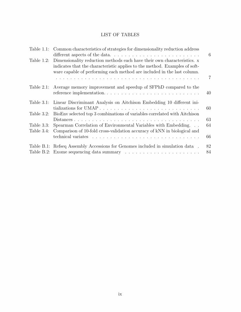
LIST OF TABLES

Table 1.1: Common characteristics of strategies for dimensionality reduction addressdifferent aspects of the data. . . . . . . . . . . . . . . . . . . . . . . . . 6

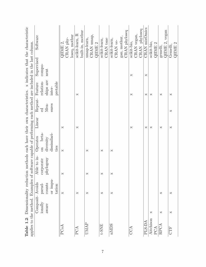
Table 1.2: Dimensionality reduction methods each have their own characteristics. xindicates that the characteristic applies to the method. Examples of soft-ware capable of performing each method are included in the last column.. . . . . . . . . . . . . . . . . . . . . . . . . . . . . . . . . . . . . . . . 7

Table 2.1: Average memory improvement and speedup of SFPhD compared to thereference implementation. . . . . . . . . . . . . . . . . . . . . . . . . . . 40

Table 3.1: Linear Discriminant Analysis on Aitchison Embedding 10 different ini-tializations for UMAP . . . . . . . . . . . . . . . . . . . . . . . . . . . . 60

Table 3.2: BioEnv selected top 3 combinations of variables correlated with AitchisonDistances . . . . . . . . . . . . . . . . . . . . . . . . . . . . . . . . . . . 63

Table 3.3: Spearman Correlation of Environmental Variables with Embedding. . . 64Table 3.4: Comparison of 10-fold cross-validation accuracy of kNN in biological and

technical variates . . . . . . . . . . . . . . . . . . . . . . . . . . . . . . 66

Table B.1: Refseq Assembly Accessions for Genomes included in simulation data . 82Table B.2: Exome sequencing data summary . . . . . . . . . . . . . . . . . . . . . 84

ix

ACKNOWLEDGEMENTS

Firstly, I would like to thank my parents, Douglas and Marjory Armstrong, for

prioritizing education and doing everything within their power for over two and a half

decades to empower me to achieve my goals. I would not be in this position today if it had

not been for their ongoing love and support.

I would also like to recognize my loving partner, teammate, and confidant, Connie

Chiang, who has unconditionally encouraged me to pursue my passions and been there to

see me through some of the most difficult aspects of the last few years.

Working on a Ph. D. and figuring out what to do next has been the largest, least-

structured challenge I have encountered to date. For that reason, I would like to thank

my advisor, Rob Knight for providing his expertise, rational outlook, and flexibility. This

work, along with my next steps, would not have been possible without him.

Mentorship does not just come from a single source—I also received invaluable and

immeasurable support from Yoshiki Vazquez-Baeza, Cameron Martino, and Daniel McDon-

ald. Many others I crossed paths with in the Knight Lab have also made this work possible

through miscellaneous conversations, encouragement, and friendship: Gibraan Rahman,

Dan Hakim, Marcus Fedarko, Imran McGrath, Kalen Cantrell, Lisa Marotz, Celeste Alla-

band, Justin Shaffer, Antonio Gonzalez Pena, and Shi Huang.

A doctoral dissertation is not complete without a committee—I would like to thank

my committee members Gal Mishne, Glenn Tesler, Pieter Dorrestein, and Vineet Bafna for

their collaboration and encouragement on this work.

x

Finally, I would like to extend my gratitude to many people from various stages

of life who have contributed to this work influencing the path I took to get here: Ahmet

Ay, Will Cipolli, Darren Strash, Michael Hay, Duke Writer, Dan Crowe, Diana Virgo,

Sundaram Thirukkurungudi, Ben Apple, Tanner Gill, Ha Vu, Ben Harris, Adam Officer,

Owen Chapman, and the 2018 BISB/BMI cohort.

Chapter 1, in full, is a reprint of the material as it appears in “Applications and

Comparison of Dimensionality Reduction Methods for Microbiome Data.” George Arm-

strong, Gibraan Rahman, Cameron Martino, Daniel McDonald, Antonio Gonzalez, Gal

Mishne, and Rob Knight. Frontiers in Bioinformatics 2, 2022. The dissertation author

was the primary investigator and co-first author of this paper.

Chapter 2, in full, is a reprint of the material as it appears in “Efficient computation

of Faith’s phylogenetic diversity with applications in characterizing microbiomes.” George

Armstrong, Kalen Cantrell, Shi Huang, Daniel McDonald, Niina Haiminen, Anna Paola

Carrieri, Qiyun Zhu, Antonio Gonzalez, Imran McGrath, Kristen Beck, Daniel Hakim, Aki

S Havulinna, Guillaume Meric, Teemu Niiranen, Leo Lahti, Veikko Salomaa, Mohit Jain,

Michael Inouye, Austin D Swafford, Ho-Cheol Kim, Laxmi Parida, Yoshiki Vazquez-Baeza

and Rob Knight. Genome Research 31, 2021. The dissertation author was the primary

investigator and the first author of this paper.

Chapter 3, in full, is a reprint of the material as it appears in “Uniform Manifold

Approximation and Projection (UMAP) Reveals Composite Patterns and Resolves Visu-

alization Artifacts in Microbiome Data.” George Armstrong, Cameron Martino, Gibraan

Rahman, Antonio Gonzalez, Yoshiki Vazquez-Baeza, Gal Mishne, and Rob Knight. mSys-

xi

tems 6, 2021. The dissertation author was the primary investigator and the first author of

this paper.

Chapter 4, in full, is a reprint of the material as it appears in “Swapping metage-

nomics preprocessing pipeline components offers speed and sensitivity increases.” George

Armstrong, Cameron Martino, Justin Morris, Behnam Khaleghi, Jaeyoung Kang, Jeff

DeReus, Qiyun Zhu, Daniel Roush, Daniel McDonald, Antonio Gonzalez, Justin Shaffer,

Carolina Carpenter, Mehrbod Estaki, Stephen Wandro, Sean Eilert, Ameen Akel, Justin

Eno, Ken Curewitz, Austin D. Swafford, Niema Moshiri, Tajana Rosing, and Rob Knight.

mSystems e0137821, 2022. The dissertation author was a primary investigator and co-first

author of this paper.

xii

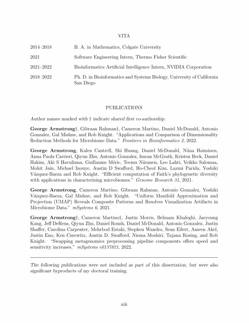
VITA

2014–2018 B. A. in Mathematics, Colgate University

2021 Software Engineering Intern, Thermo Fisher Scientific

2021–2022 Bioinformatics Artificial Intelligence Intern, NVIDIA Corporation

2018–2022 Ph. D. in Bioinformatics and Systems Biology, University of CaliforniaSan Diego

PUBLICATIONS

Author names marked with † indicate shared first co-authorship.

George Armstrong†, Gibraan Rahman†, Cameron Martino, Daniel McDonald, AntonioGonzalez, Gal Mishne, and Rob Knight. “Applications and Comparison of DimensionalityReduction Methods for Microbiome Data.” Frontiers in Bioinformatics 2, 2022.

George Armstrong, Kalen Cantrell, Shi Huang, Daniel McDonald, Niina Haiminen,Anna Paola Carrieri, Qiyun Zhu, Antonio Gonzalez, Imran McGrath, Kristen Beck, DanielHakim, Aki S Havulinna, Guillaume Meric, Teemu Niiranen, Leo Lahti, Veikko Salomaa,Mohit Jain, Michael Inouye, Austin D Swafford, Ho-Cheol Kim, Laxmi Parida, YoshikiVazquez-Baeza and Rob Knight. “Efficient computation of Faith’s phylogenetic diversitywith applications in characterizing microbiomes.” Genome Research 31, 2021.

George Armstrong, Cameron Martino, Gibraan Rahman, Antonio Gonzalez, YoshikiVazquez-Baeza, Gal Mishne, and Rob Knight. “Uniform Manifold Approximation andProjection (UMAP) Reveals Composite Patterns and Resolves Visualization Artifacts inMicrobiome Data.” mSystems 6, 2021.

George Armstrong†, Cameron Martino†, Justin Morris, Behnam Khaleghi, JaeyoungKang, Jeff DeReus, Qiyun Zhu, Daniel Roush, Daniel McDonald, Antonio Gonzalez, JustinShaffer, Carolina Carpenter, Mehrbod Estaki, Stephen Wandro, Sean Eilert, Ameen Akel,Justin Eno, Ken Curewitz, Austin D. Swafford, Niema Moshiri, Tajana Rosing, and RobKnight. “Swapping metagenomics preprocessing pipeline components offers speed andsensitivity increases.” mSystems e0137821, 2022.

The following publications were not included as part of this dissertation, but were alsosignificant byproducts of my doctoral training.

xiii

Cameron Martino, Liat Shenhav, Clarisse A Marotz, George Armstrong, Daniel McDon-ald, Yoshiki Vazquez-Baeza, James T Morton, Lingjing Jiang, Maria Gloria Dominguez-Bello, Austin D Swafford, Eran Halperin, Rob Knight. “Context-aware dimensionality re-duction deconvolutes gut microbial community dynamics.” Nature biotechnology 39, 2021.

Kalen Cantrell, Marcus W. Fedarko, Gibraan Rahman, Daniel McDonald, Yimeng Yang,Thant Zaw, Antonio Gonzalez, Stefan Janssen, Mehrbod Estaki, Niina Haiminen, KristenL. Beck, Qiyun Zhu, Erfan Sayyari, James T. Morton, George Armstrong, AnupriyaTripathi, Julia M. Gauglitz, Clarisse Marotz, Nathaniel L. Matteson, Cameron Martino,Jon G. Sanders, Anna Paola Carrieri, Se Jin Song, Austin D. Swafford, Pieter C. Dorrestein,Kristian G. Andersen, Laxmi Parida, Ho-Cheol Kim, Yoshiki Vazquez-Baeza, Rob Knight.“EMPress Enables Tree-Guided, Interactive, and Exploratory Analyses of Multi-omic DataSets.” mSystems e01216-20, 2021.

Qiyun Zhu, Shi Huang, Antonio Gonzalez, Imran McGrath, Daniel McDonald, NiinaHaiminen, George Armstrong, Yoshiki Vazquez-Baeza, Julian Yu, Justin Kuczynski,Gregory D. Sepich-Poore, Austin D. Swafford, Promi Das, Justin P. Shaffer, Franck Lejze-rowicz, Pedro Belda-Ferre, Aki S. Havulinna, Guillaume Meric, Teemu Niiranen, Leo Lahti,Veikko Salomaa, Ho-Cheol Kim, Mohit Jain, Michael Inouye, Jack A. Gilbert, Rob Knight.“Phylogeny-Aware Analysis of Metagenome Community Ecology Based on Matched Ref-erence Genomes while Bypassing Taxonomy.” mSystems e00167-22, 2022.

Clarisse Marotz, Pedro Belda-Ferre, Farhana Ali, Promi Das, Shi Huang, Kalen Cantrell,Lingjing Jiang, Cameron Martino, Rachel E Diner, Gibraan Rahman, Daniel McDonald,George Armstrong, Sho Kodera, Sonya Donato, Gertrude Ecklu-Mensah, Neil Gottel,Mariana C Salas Garcia, Leslie Y Chiang, Rodolfo A Salido, Justin P Shaffer, KareninaSanders, Greg Humphrey, Gail Ackermann, Niina Haiminen, Kristen L Beck, Ho-CheolKim, Anna Paola Carrieri, Laxmi Parida, Yoshiki Vazquez-Baeza, Francesca J Torriani,Rob Knight, Jack Gilbert, Daniel A Sweeney, Sarah M Allard. “SARS-CoV-2 detectionstatus associates with bacterial community composition in patients and the hospital envi-ronment.” Microbiome 9, 2021.

Igor Sfiligoi, George Armstrong, Antonio Gonzalez, Daniel McDonald, Rob Knight.“Optimizing UniFrac with OpenACC yields 1000x speed increase”. Under Review at mSys-tems, 2022.

Cameron Martino, Daniel McDonald, Kalen Cantrell, Amanda Hazel Dilmore, YoshikiVazquez-Baeza, Liat Shenhav, Justin P. Shaffer, Gibraan Rahman, George Armstrong,Celeste Allaband, Se Jin Song, Rob Knight. “Compositionally aware phylogenetic beta-diversity measures better resolve microbiomes associated with phenotype.” In Press atmSystems, 2022.

xiv

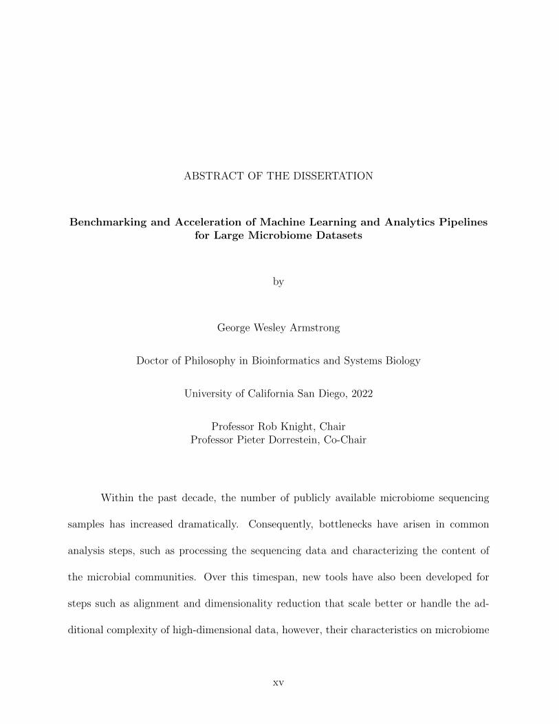
ABSTRACT OF THE DISSERTATION

Benchmarking and Acceleration of Machine Learning and Analytics Pipelinesfor Large Microbiome Datasets

by

George Wesley Armstrong

Doctor of Philosophy in Bioinformatics and Systems Biology

University of California San Diego, 2022

Professor Rob Knight, ChairProfessor Pieter Dorrestein, Co-Chair

Within the past decade, the number of publicly available microbiome sequencing

samples has increased dramatically. Consequently, bottlenecks have arisen in common

analysis steps, such as processing the sequencing data and characterizing the content of

the microbial communities. Over this timespan, new tools have also been developed for

steps such as alignment and dimensionality reduction that scale better or handle the ad-

ditional complexity of high-dimensional data, however, their characteristics on microbiome

xv

data were previously uncharacterized. In this dissertation, we accelerate the analysis of

microbiomes by introducing new methods or benchmarking alternatives. Additionally,

we compare the results of novel methodology to existing best-practices on gold-standard

datasets to determine whether the methods adequately address the specific challenges of

microbiome data.

In the first part of this work, Chapter 1 reviews many aspects of microbiome data

that necessitate the use of microbiome-specific techniques for analyzing collections of mi-

crobial communities. Chapter 2 then introduces SFPhD, a novel approach for calculating

phylogenetic alpha diversity that leverages the characteristics of microbiome data to speed

up and reduce the memory requirements of a costly single-sample characterization.

In the second part of the work, we apply recently developed tools for machine learn-

ing and sequencing pre-processing to demonstrate their potential for elucidating complex

relationships in microbial data and reducing the lead time for supporting clinical appli-

cations of metagenomic sequencing, respectively. Chapter 3 demonstrates how Uniform

Manifold Approximation and Projection (UMAP) provides succinct representations of data

compared to the long-time standard method of microbial ecology, Principal Coordinates

Analysis (PCoA). Importantly, UMAP provides different guarantees about the preservation

of local/global geometry in its representation and careful consideration should be given

to its application. In Chapter 4, we show that the popular metagenomic preprocessing

pipeline of Atropos for adapter trimming and Bowtie2 for host filtering can be replaced by

a substantially faster combination of Fastp and Minimap2, respectively. Furthermore, we

have determined that the results this new pipeline produces are comparable to the outputs

xvi

produced by the original pipeline.

xvii

Chapter 1

Applications and comparison of

dimensionality reduction methods for

microbiome data

1

Dimensionality reduction techniques are a key component of most microbiome stud-

ies, providing both the ability to tractably visualize complex microbiome datasets and the

starting point for additional, more formal, statistical analyses. In this review, we discuss

the motivation for applying dimensionality reduction techniques, the special characteristics

of microbiome data such as sparsity and compositionality that make this difficult, the dif-

ferent categories of strategies that are available for dimensionality reduction, and examples

from the literature of how they have been successfully applied (together with pitfalls to

avoid). We conclude by describing the need for further development in the field, in par-

ticular combining the power of phylogenetic analysis with the ability to handle sparsity,

compositionality, and non-normality, as well as discussing current techniques that should

be applied more widely in future analyses.

1.1 Introduction: what is dimensionality reduction

and why do we do it?

To a first approximation, life on Earth consists of complex microbial communities,

with “familiar” multicellular organisms such as plants and animals being rounding errors

in terms of cell count and biomass. The genetic repertoire of such a community is called

a “microbiome” [143], although the term “microbiome” is often also loosely applied to

the collection of microbes that make up the community. In either sense, microbiomes

are typically incredibly complex, containing vast numbers of species and genes, and how

samples relate, even in well-studied contexts, are not predetermined. For example, in

2

the Earth Microbiome Project (EMP) [141] and the work leading up to it [84, 20, 76],

an ontology constructed from the microbe’s perspective based on community similarities

and differences revealed many surprises, such as a deep separation between free-living and

host-associated samples, and between saline- and non-saline samples. Accordingly, to truly

understand the microbial perspective, we must get acquainted with the structure of the data

in human-interpretable formats. This is especially important when we need to separate

new biological discoveries from technical artifacts, such as distinguishing clusters related

to different habitats on the human body from artifacts caused by different sequencing

methodologies such as PCR primers [140].

When microbiome sequencing data are arranged into count tables, such as those that

count 16S amplicon sequence variants (ASVs) or the microbial genes present in a sample,

the number of features being counted across all of the samples often vastly outnumbers the

number of samples observed. This phenomenon of having many features, and particularly

having far more features than samples, is a hallmark of high-dimensionality. For example,

the EMP [141] contained 23,828 samples and represented 307,572 ASVs, where each of

these measures a dimension of the resulting ASV count table. This degree of high feature

dimensionality creates difficulties for interpreting data and calculating meaningful statis-

tics, since humans cannot visualize more than 3 dimensions, many of the features are noisy

or redundant, the number of hypotheses that explain the data is far greater than the num-

ber of observations, and the number of features can cause run-time issues for downstream

analysis. These are all common consequences of the “curse of dimensionality”. Dimen-

sionality reduction transforms a high-dimensional dataset into a representation with fewer

3

dimensions, while retaining the key relationships among samples from the full dataset,

making analysis tractable. Accordingly, dimensionality reduction is a core step in micro-

biome analyses, both for creating human-understandable visualizations of the data and as

the basis for further analysis. The EMP used dimensionality reduction to produce plots of

the same samples using 3 coordinates (in contrast to the the 307,572 ASVs) that demon-

strate the large difference between host-associated and non-host associated microbiomes,

and between saline and non-saline free-living microbiomes (Figure 1.1). These differences

in microbial communities were subsequently statistically validated. This example is partic-

ularly salient because it shows the value of preserving the structure of the data while using

much less information to represent it. Owing to its importance, dimensionality reduction

methods are included in many analysis packages, including QIIME 2 [13], mothur [123],

and phyloseq [99], as well as online software such as Qiita [44] and MG-RAST [61].

Figure 1.1: Overview of dimensionality reduction pipeline. (A) Nucleotide se-quences from a biological experiment are organized in a feature table (B) containing theabundance of each feature (e.g., OTU, ASV, MAG) in each sample. (C) Beta diversityplots showing unweighted UniFrac coordinates of EMP annotated by EMPO levels 2 and3. (C) is a derivative of Figure 2C from “A communal catalogue reveals Earth’s multiscalemicrobial diversity” by Thompson et al. (2017) used under CC BY 4.0.

4

In this review, we describe how the characteristics of microbiome data complicate

dimensionality reduction. We then discuss common strategies for dimensionality reduction

(Table 1.1), examining in detail whether and how they address each of the aspects that, in

conjunction, confound e microbiome analysis. Tried-and-true techniques, although useful,

often have conceptual and practical problems that limit their utility in the microbiome,

due to the inability to handle the data’s most salient traits simultaneously (Table 1.2).

In this light, we then focus on examples of how dimensionality reduction techniques have

been used in the literature, highlighting biological findings that have been revealed by each,

while also discussing what may have been obscured. We then discuss common artifacts of

widely used dimensionality reduction techniques, including specific pitfalls that users of

these techniques must avoid in order to draw conclusions that are robust, reproducible,

and well-supported by their data. We end with guidance on how dimensionality reduction

should be used responsibly by practitioners in the field, and with an outlook describing

how additional techniques that are seldom used today might provide valuable advances.

1.2 Specific features of microbiome data that compli-

cate dimensionality reduction

“Microbiome data” most often refers to sequencing results from two primary method-

ologies. The first class of microbiome sequencing is known as “amplicon sequencing” where

a specific gene or region of a gene is targeted in each sample. 16S, 18S, and ITS sequenc-

ing approaches all fall under this class of methods. Variants of the targeted nucleotide

5

Table 1.1: Common characteristics of strategies for dimensionality reduction address dif-ferent aspects of the data.

Term DefinitionCompositionally aware Transforms data to account for non-independence

of features in sequence count data.

Pseudo-counts or imputa-tion

Requires no/minimal zeroes in the feature tabledue to numerical issues (such as logarithm trans-form being undefined on zeroes).

Able to incorporate phy-logeny

Method is calculated with awareness of how eachsampled microbial community is evolutionarilyrepresented relative to other samples.

Operates on beta-diversitydissimilarities

Dimensionality reduction step is performed onpairwise dissimilarities (arbitrary metric) betweensamples, rather than the feature table itself.

Linear Lower dimensional coordinates are computed vialinear transform of features.

Repeated measures Subjects are sampled multiple times. Commonlysampled longitudinally.

Feature relationships are in-terpretable

The method indicates the relevance of input micro-bial features with regard to its output coordinates.

Supervised component Method takes explanatory sample variables as anadditional input.

6

Table

1.2:Dim

ension

alityreductionmethodseach

havetheirow

ncharacteristics.

xindicates

that

thecharacteristic

applies

tothemethod.Exam

plesof

softwarecapab

leof

perform

ingeach

methodareincluded

inthelast

column.

Com

posit-

ionally

aware

Avoids

pseud-

counts

orim

pu-

tation

Able

toin-

corporate

phylogeny

Operates

onbeta-

diversity

dissimilari-

ties

Linear

Rep

eat-

ed Mea-

sures

Feature

relation

-shipsare

inter-

pretable

Supervised

compo-

nent

Softw

are

PCoA

xx

xx

QIIME2,

CRAN

phy-

loseq,mothur

PCA

xx

xscikit-learn,R

built-in,mothur

UMAP

xx

xumap

-learn,

CRAN

umap

,QIIME2

t-SNE

xx

xscikit-learn,

CRAN

tsne

nMDS

xx

xscikit-learn,

CRAN

ve-

gan,mothur,

CRAN

phyloseq

CCA

xx

xscikit-bio,

CRAN

vegan,

CRAN

phyloseq

PLS-D

Ax

xx

CRAN

mixOmics

Aitchison

PCA

xx

xscikit-bio,

QIIME2

RPCA

xx

xx

gemelli,

QIIME2,

vegan

CTF

xx

xx

xGem

elli,

QIIME2

7

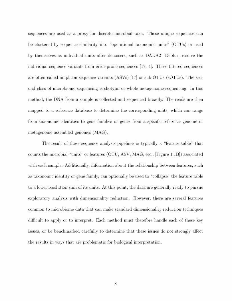
sequences are used as a proxy for discrete microbial taxa. These unique sequences can

be clustered by sequence similarity into “operational taxonomic units” (OTUs) or used

by themselves as individual units after denoisers, such as DADA2 Deblur, resolve the

individual sequence variants from error-prone sequences [17, 4]. These filtered sequences

are often called amplicon sequence variants (ASVs) [17] or sub-OTUs (sOTUs). The sec-

ond class of microbiome sequencing is shotgun or whole metagenome sequencing. In this

method, the DNA from a sample is collected and sequenced broadly. The reads are then

mapped to a reference database to determine the corresponding units, which can range

from taxonomic identities to gene families or genes from a specific reference genome or

metagenome-assembled genomes (MAG).

The result of these sequence analysis pipelines is typically a “feature table” that

counts the microbial “units” or features (OTU, ASV, MAG, etc., [Figure 1.1B]) associated

with each sample. Additionally, information about the relationship between features, such

as taxonomic identity or gene family, can optionally be used to “collapse” the feature table

to a lower resolution sum of its units. At this point, the data are generally ready to pursue

exploratory analysis with dimensionality reduction. However, there are several features

common to microbiome data that can make standard dimensionality reduction techniques

difficult to apply or to interpret. Each method must therefore handle each of these key

issues, or be benchmarked carefully to determine that these issues do not strongly affect

the results in ways that are problematic for biological interpretation.

8

1.2.1 High dimensionality

In this context, “dimensionality” refers to the number of features in a feature table.

Microbiome data typically have far more features than samples. Across studies ranging

from tens of samples to tens of thousands of samples, the number of features for taxonomic

data typically exceeds the number of samples by 20-fold or more. With gene oriented

data, the number of genes represented in a metagenomic study typically exceeds samples

by several orders of magnitude. This can lead many statistical methods to overfit or to

produce artifactual results.

1.2.2 Sparsity

Most microbes are not found in most samples, even of the same biospecimen type,

for example, most human stool specimens from the same population have relatively low

shared taxa [3]. As a result, a feature table containing counts of each microbe in each

sample often has many zeros corresponding to unobserved microbes. Most 16S microbiome

datasets do not have even as many as 10% of the possible entries observed in most of the

specimens. Feature tables with this over-abundance of unobserved counts are said to be

“sparse”, posing problems for statistical analysis. Moreover, the proportion of observed

values tends to decrease as additional samples are sequenced, often leading to tables with

density well below 1% [49, 92].

9

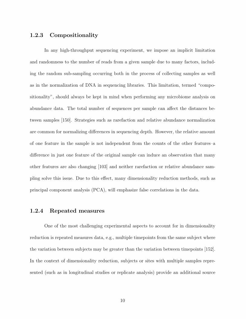
1.2.3 Compositionality

In any high-throughput sequencing experiment, we impose an implicit limitation

and randomness to the number of reads from a given sample due to many factors, includ-

ing the random sub-sampling occurring both in the process of collecting samples as well

as in the normalization of DNA in sequencing libraries. This limitation, termed “compo-

sitionality”, should always be kept in mind when performing any microbiome analysis on

abundance data. The total number of sequences per sample can affect the distances be-

tween samples [150]. Strategies such as rarefaction and relative abundance normalization

are common for normalizing differences in sequencing depth. However, the relative amount

of one feature in the sample is not independent from the counts of the other features–a

difference in just one feature of the original sample can induce an observation that many

other features are also changing [103] and neither rarefaction or relative abundance sam-

pling solve this issue. Due to this effect, many dimensionality reduction methods, such as

principal component analysis (PCA), will emphasize false correlations in the data.

1.2.4 Repeated measures

One of the most challenging experimental aspects to account for in dimensionality

reduction is repeated measures data, e.g., multiple timepoints from the same subject where

the variation between subjects may be greater than the variation between timepoints [152].

In the context of dimensionality reduction, subjects or sites with multiple samples repre-

sented (such as in longitudinal studies or replicate analysis) provide an additional source

10

of variation that can inhibit interpretation of the experimental effect of interest; the sam-

ples from a single subject can be highly correlated, resulting in between-subject differences

dominating the ordination (e.g., [132]).

1.2.5 Feature interpretation

Analysis of high-dimensional microbiome data is often motivated to find microbial

biomarkers associated with observed differences in sample communities [36]. This line of

inquiry is of interest for diagnosis and/or prognosis of disease status, dysbiosis, and a

host of other biological questions. Although this task is often addressed with differential

abundance methods, those methods make specific statistical assumptions and may not

correspond to the group separation observed in an exploratory analysis performed with any

dimensionality reduction method [79]. Thus, methods that offer a quantitative justification

of their representation in terms of the microbial features are often desirable. However,

methods with feature importance that are not specifically designed for the microbiome

often fail to account for compositionality, which can include many false positives due to the

induced correlation of features, and sparsity, where important but infrequently observed

features will not be detected (false negatives).

1.2.6 Complex patterns

Microbiome data are often assumed to contain clusters or gradients [68]. For exam-

ple, multiple samples swabbed from one’s own keyboard are more likely to be similar to

each other than samples from another individual’s keyboard [37], and the microbial compo-

11

sition of soils is expected to vary continuously with soil pH [74]. However, with larger and

larger datasets with many covariates and metadata on these being collected, more complex

patterns can be detected [31], such as grouping by both biological and technical factors in

the case of the Human Microbiome Project [140]. Furthermore, many conventional dimen-

sionality reduction methods, such as PCA, assume the data lie in a linear subspace, and

this assumption is violated by microbiome data [115, 137, 42, 45].

1.3 Strategies for dimensionality reduction in the mi-

crobiome

The problems that complicate dimensionality reduction in microbiome data are

scattered throughout the analysis pipeline. Difficulties can arise immediately from the

raw sequence count data. Many can be corrected before the dimensionality reduction step,

with careful preprocessing, though this can raise other issues. Furthemore, beta-diversity

analysis, which seeks to quantify the pairwise differences in microbial communities among

all samples with dissimilarity metrics (tailored to microbiome data), is often helpful for

addressing many of the aforementioned circumstances [112]. Algorithms that are able to

incorporate these metrics are particularly valuable, and this can be done in a variety of

ways. Finally, additional constraints can be placed on dimensionality reduction algorithms

to account for study design or provide additional information about the correspondence

between the features and the reduced dimensions. In this section, we discuss each of these

strategies in depth.

12

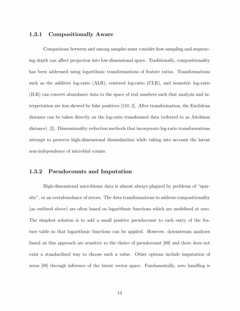
1.3.1 Compositionally Aware

Comparisons between and among samples must consider how sampling and sequenc-

ing depth can affect projection into low-dimensional space. Traditionally, compositionality

has been addressed using logarithmic transformations of feature ratios. Transformations

such as the additive log-ratio (ALR), centered log-ratio (CLR), and isometric log-ratio

(ILR) can convert abundance data to the space of real numbers such that analysis and in-

terpretation are less skewed by false positives [110, 2]. After transformation, the Euclidean

distance can be taken directly on the log-ratio transformed data (referred to as Aitchison

distance) [2]. Dimensionality reduction methods that incorporate log-ratio transformations

attempt to preserve high-dimensional dissimilarities while taking into account the latent

non-independence of microbial counts.

1.3.2 Pseudocounts and Imputation

High-dimensional microbiome data is almost always plagued by problems of “spar-

sity”, or an overabundance of zeroes. The data transformations to address compositionality

(as outlined above) are often based on logarithmic functions which are undefined at zero.

The simplest solution is to add a small positive pseudocount to each entry of the fea-

ture table so that logarithmic functions can be applied. However, downstream analyses

based on this approach are sensitive to the choice of pseudocount [69] and there does not

exist a standardized way to choose such a value. Other options include imputation of

zeros [89] through inference of the latent vector space. Fundamentally, zero handling is

13

complicated by the inherent unknowability of the zero generating processes for each zero

instance. In [131], they characterize the three different types of zero-generating processes

(ZGP) as sampling, biological, and technical and demonstrate how the results of different

zero-handling processes are affected by the (unknowable) mix of ZGPs in a given dataset.

Recently Martino et al. introduced a version of the CLR transform that only computes

the geometric mean on the non-zero components of a given sample [90]. This avoids the

problem of logarithms being undefined at 0 and thus dimensionality reduction through this

method is robust to the high levels of sparsity in microbiome data.

1.3.3 Incorporating Phylogeny

Organisms identified using microbiome data can be related to one another through

hierarchical structures that describe their evolutionary relationships. Typically, these struc-

tures take the form of either a taxonomy or a phylogeny. A taxonomy is a description of

the organism relationships, generally derived subjectively using multiple biological criteria.

A phylogeny, in contrast, is an inference of a tree, commonly with branch lengths, derived

from quantitative algorithms that are typically applied to microbial, nucleic acid, or pro-

tein sequence data. Taxonomies have the advantage of being more directly interpretable

because hierarchical structures correspond to a defined organization and classification pat-

tern curated by experts in the field. However, these assignments and hierarchies are often

putative and subject to change as more information about microbial taxa emerges. In

contrast, phylogenies are derived from quantitative measures of sequence similarity from

sample reads. These data structures are more easily incorporated into statistical analyses

14

but often at the cost of less interpretability as the hierarchical structures do not necessarily

map to pre-defined microbial relationships. These evolutionary relationships, particularly

phylogenies, add information to microbiome analysis, because related organisms are more

likely to exhibit similar phenotypes (although counterexamples do exist, especially closely

related taxa such as Escherichia and Shigella, which are very similar genetically but pro-

duce different clinical phenotypes).

When comparing the similarity of pairs of microbial communities, it is possible to

utilize these hierarchical structures, and derive a metric that computes a distance as a

function of shared evolutionary history [82]. Specifically, communities that are very similar

will share most of their evolutionary history, whereas those that are very dissimilar will

have relatively little in common. A popular form of phylogenetically-aware distances is

the suite of UniFrac metrics, which includes both quantitative [83] and qualitative [82]

forms. Numerous extensions to UniFrac have been developed [23, 22], including variants

that account explicitly for the compositional nature of microbiome data [151]. Because

these metrics all utilize not only exactly observed features, but also the relationships among

features, they can better account for the sparsity of microbiome data which manifests at the

tips of a phylogenetic tree (because most microbes are not observed in most environments).

In contrast, a metric like the Euclidean distance is limited to only the information at the

tips of these hierarchies, and, worse, assumes that all features at the tips are equally

related to one another (so that in a tree consisting of a mouse, a rat, and a squid, there

is no allowance for the fact that the two rodents are much more similar to each other

than they are to the squid). Neither phylogenetic nor non-phylogenetic beta-diversity

15

measures explicitly model differences in sequencing depth per sample (this occurs because

of uncontrolled variation in how efficiently each sample is amplified and incorporated into

molecular libraries for sequencing), although these differences in depth can be standardized

through rarefaction [150].

1.3.4 Operates on Generalized Beta-Diversity Matrix

Many of the issues outlined above can be easily addressed at the sample dissimilarity

level rather than directly through dimensionality reduction algorithms. A number of dis-

similarity/distance metrics have been developed to account for factors such as phylogenetic

data incorporation, compositionality, or sparsity that output a sample by sample matrix

estimating high-dimensional dissimilarity. These dissimilarity matrices represent the over-

all community differences between pairwise samples calculated by a chosen beta-diversity

metric. Dimensionality reduction methods that operate on arbitrary dissimilarity metrics

are attractive options because the complex handling of the various feature table issues can

be split into the choice of dissimilarity metric and the choice of dimensionality reduction

algorithm. This adds a layer of flexibility for researchers to analyze their data depending

on their needs. Methods based on multidimensional scaling approaches such as PCoA [66]

and nMDS [65] attempt to preserve as much as possible the pairwise distances between

subjects. Other methods such as t-distributed stochastic neighbor embedding (t-SNE) [144]

and Uniform Manifold Approximation and Projection (UMAP) [97] are non-linear dimen-

sionality reduction techniques that aim to find a low-dimensional representation such that

similar data points are placed closed together and dissimilar points are pushed apart. A

16

caveat of these methods is that they can be very sensitive to the choice of dissimilarity

used. Patterns that may appear from one measure of dissimilarity may not be as apparent

in a different measure. As an example, phylogenetic metrics such as UniFrac may differ

from non-phylogenetic metrics such as Bray-Curtis depending on the strength of phyloge-

netic contribution [129]. The choice of dissimilarity metric should therefore be considered

carefully, as different dimensionality reduction techniques yield visually and statistically

very different results on the same data [67].

1.3.5 Linear vs. Non-Linear Methods

Principal coordinates analysis (PCoA) and PCA are popular dimensionality reduc-

tion techniques that fall under the “linear” category. Linear techniques attempt to reduce

or transform the data such that an approximation of the original data can be reconstructed

by a weighted sum of the resulting coordinates. These methods typically involve comput-

ing decompositions/factorizations of the data that are highly computationally efficient and

work well on data that is naturally linear. Various other techniques, such as robust Aitchi-

son PCA (RPCA) [90], and nonnegative matrix factorization (NMF) [75] also fall under

this class of techniques.

Other methods fall under the “non-linear” category, which perform more complex

transformations that often excel at preserving different patterns that may not be linear.

This category includes methods such as the non-metric multidimensional scaling (nMDS),

t-SNE, and UMAP. These methods can more succinctly represent complex patterns, but

possibly at the expense of additional computation. Furthermore, these models tend to have

17

randomness (such as from initialization) and more hyperparameters that the output can be

highly sensitive to, so it is usually necessary to run these algorithms multiple times to ensure

the conclusions are reproducible. Other non-linear methods that have seen less frequent

use in the microbiome data (and bioinformatics generally) include kernel PCA [124], locally

linear embeddings [118], Laplacian eigenmaps [11], and ISOMAP [138].

Unlike its close, linear counterpart PCoA, nMDS performs the ordination onto a pre-

specified number of dimensions and operates on the ranks of the dissimilarities, rather than

the dissimilarities themselves. This rank-based approach can be beneficial for representing

data that departs from the assumptions of linearity. Other non-linear methods, such as

t-SNE and UMAP, also transform the data onto a pre-specified number of dimensions, and

operate by assuming the high-dimensional data follows a non-linear structure that can be

represented with fewer dimensions.

1.3.6 Repeated Measures

If the biological variable of interest occurs at the subject level, repeated samples

(such as through a longitudinal study design) can artificially inflate how tight a cluster

appears in low-dimensional space. Dimensionality reduction methods for microbiome need

to be designed for the purpose of handling this kind of data, with the intent to represent

the relationships between explanatory variables while accounting for the inherent similarity

between samples from the same subject. Methods to account for repeated measures can

incorporate the relationship between individual samples and subjects by machine learning

approaches [91]. There has also been discussion about incorporating prior sample relation-

18

ship information into ordinations through Bayesian methods [117]. Nevertheless, methods

that incorporate repeated measures remain an underexplored area in dimensionality reduc-

tion literature.

1.3.7 Feature Importance

When the lower-dimensional representation of microbial communities shows separa-

tion between sample groups, a natural next question is what microbes or groups of microbes

are driving such a separation. Dimensionality reduction methods that return a quantitative

relationship between individual microbial features and the latent lower-dimensional space

are a powerful class of methods that can demystify the construction of the lower-dimensional

axes. However, certain methods that attempt to find high-dimensional patterns, such as

non-linear methods, do not have an explicit interpretable correspondence between the out-

put coordinates and the input features.

The most relevant category of methods that do provide feature importance is the

biplot ordination family of approaches. Biplots display both the samples and the driving

variable vectors in reduced dimension space (Figure 1.2 A,D,E,H). For example, PCA nat-

urally quantifies the contribution of each microbe to the principal component axes through

matrix factorization into linear combinations of features. RPCA modifies this approach to

account for compositionality and sparsity while retaining interpretable feature loadings [90].

Another set of ecologically motivated matrix factorization methods is the correspondence

analysis (CA) family. The general CA method can be thought of as an implementation

of PCA that operates on count data. It is also possible to explicitly incorporate sample

19

metadata into these dimensionality reduction methods. Researchers are often interested in

the explanatory power of their sample metadata (site, pH, subject, etc.). Certain dimen-

sionality reduction methods can take as input both a feature table and a table of sample

metadata to jointly estimate the low-dimensional representation of samples as well as the

relative contribution of the provided metadata vectors. The general goal of these methods

is to determine whether and/or which explanatory variables may be driving the differences

in microbial communities among samples. Canonical correspondence analysis (CCA) is an

extension of CA that incorporates sample variables of interest to determine which covari-

ates are associated with the placement of samples and feature vectors in low-dimensional

space [139]. The results of CCA can be visualized as a “tri-plot” where samples are simulta-

neously visualized with the relative contribution of features and explanatory variables near

related samples. [119, 106] Partial least squares discriminant analysis (PLS-DA) is a similar

approach that uses only categorical sample metadata (classification) in the construction of

lower-dimensional axes [9, 119]. The contribution of these sample variables can then be

quantified and visualized in the projection, motivating subsequent statistical analysis of

associations between sample metadata and specific microbial taxa.

1.4 Uses of dimensionality reduction for microbiome

data

Over the past decade, PCoA has seen an increase in use in microbiome analyses,

and it is the primary ordination method for beta-diversity included by default in workflows

20

Figure 1.2: Examples of dimensionality reduction techniques applied to publiclyavailable microbiome data. (Top) Beta-diversity plots of soil samples colored by pHfrom [74]. (Bottom) Beta-diversity plots of murine fecal samples colored by diet and an-tibiotics usage from [128]. (HFD = high-fat diet, NC = normal chow, ABX = antibiotics).PCA plots (A,E) show extremely high sample overlap due to outliers and characteristic“spike” artifacts. The top three taxa driving variation also overlap as shown by arrowsuperposition. (B) “Horseshoe” pattern emerges for samples following ecological gradientssuch as pH. RPCA plots (D,H) show the top three taxa driving separation of groups. (F)and (G) show strong overlap of HFD + ABX samples resolved by (H).

21

such as QIIME 2 [13]. It is typically used for exploratory visualization, as it excels at

rendering biologically relevant patterns, such as clusters and gradients [68]. When used as

an exploratory tool, observed patterns are often followed with statistical analysis on the

original feature tables or dissimilarity matrices [39], such as ANOSIM [25], PERMANOVA

(aka Adonis) [5], ANCOM [86], or bioenv [25]. It should also be noted that some of these

statistical techniques use the full table or dissimilarity matrix, not the reduced dimension

matrix as visualized (at least by default), and may therefore introduce incongruent results

between the statistics and the visualization.

Exploratory visualizations have revealed microbial-associated patterns in applica-

tions ranging from host-associated gut microbiomes to soil, ocean, and other environ-

mental microbiome contexts. For example, studies have applied PCoA to demonstrate

differences between host groups, such as differences between humans’, chimpanzees’, and

gorillas’ gut microbial taxa [18], or the correspondence between human gut microbiomes

and westernization [18, 155]. Host microbiome-disease associations have also been identi-

fied using PCoA, such as in the case of colorectal cancer [156] in humans and metritis in

cows [40]. Uses also extend to host-environment relationships, such as demonstrating the

differences between oyster digestive glands, oyster shells, and their surrounding soils [6].

The microbiome-shaping roles of environmental factors such as salinity in shaping free-

living environments [84], pH in arctic soils [85] and depth in the ocean [135] have also

been elucidated with PCoA. In many of these cases, the PCoA visualizations demonstrat-

ing separation between groups were subsequently followed by statistical validation with

PERMANOVA or ANOSIM.

22

In numerous other instances, PCoA has also been used to make claims that extend

beyond exploratory group differences followed by statistical analysis. For example, Half-

varson et al. fit a plane to the healthy subjects in the first three coordinates of a PCoA

and then used the distance to this plane to associate dissimilarities in the microbiome

with the severity of irritable bowel disease (IBD) [48]; this approach has subsequently been

replicated [44]. Others have used regression of participant and microbiome characteristics

(e.g., age and alpha diversity, respectively) on PCoA coordinates to determine whether the

given factors have a significant relationship with microbial community composition in the

context of dietary interventions [71]. In one case, while providing visualization with PCoA

and statistical confirmation with ANOSIM, Vangay et al. additionally plotted ellipses for

visualizing cluster centers/spread in their PCoA coordinates [145]. In another instance,

Metcalf et al. showed the correspondence of dissimilarities between the 16S rRNA pro-

files and chloroplast marker profiles by performing a Procrustes analysis on the separate

ordinations of the different data types [100].

We note that the choice of dissimilarity metric can have a significant impact on the

low-rank embedding depending on the dataset. Shi et al. review the effect of high and low-

abundance operational taxonomic units have on unsupervised clustering of Bray-Curtis and

unweighted UniFrac [130]. Marshall et al. compare Bray-Curtis ordination with weighted

UniFrac on marine sediment samples and note that the most relevant clustering variable

differed depending on the dissimilarity used [88]. These results imply that interpretation of

low-dimensional embeddings and the putative driving variables must be performed in the

context of the choice of dissimilarity. Metrics such as Bray-Curtis and weighted UniFrac

23

take into consideration the abundance of individual microbes in each sample which can be

important for datasets with many rare taxa. In contrast, some dissimilarity metrics such

as Jaccard and unweighted UniFrac are only defined on presence-absence data, which may

mask this property. Furthermore, phylogenetic metrics such as the UniFrac suite of metrics

are best when the evolutionary relationships among microbial features is of interest in the

context of sample communities. These metrics may also be more appropriate than other

methods for datasets with particularly high sparsity.

PCA is arguably the most widely used and popular form of dimensionality reduction,

which does not allow generalized beta-diversity distances (e.g., PCoA or UMAP), but does

allow for the direct interpretation of feature importances relative to sample separations in

the ordination. However, due to compositionality and sparsity, PCA often leads to spuri-

ous results on microbiome data [104, 49]. Aitchison PCA attempts to fix these issues by

using log transformation, but imputation is required (because the log of zero is undefined).

Therefore, [90] proposed the adoption of RPCA for dimensionality reduction. This method

has been shown to discriminate between sample groups in a wide array of biological con-

texts, including fecal microbiota transplants [43], cancer [8], and HIV [107]. Moreover, the

generalized version of this technique accounts for repeated measures, allowing for large im-

provements in the ability to discriminate subjects by phenotypes across time or space [91].

This advantage has been crucial in the statistical analysis of complicated longitudinal ex-

perimental designs such as early infant development models [133]. Feature loadings from

these PCA-based methods can be used to inform selection of microbial features for log-ratio

analysis [36, 103], leading to novel biomarker discovery.

24

For feature interpretation, CCA is the most commonly used CA-based method for

analyzing high dimensional microbiome data, due to its ability to incorporate sample meta-

data into the low-rank embeddings. This strategy has shown success in differentiating

clinical outcomes following stem cell transplantation [56] as well as diarrhea status in chil-

dren [34]. CCA has also shown success in projecting environmental samples into lower-

dimensional space such as in rhizosphere microbial communities [12, 111], and aerosol

samples [134]. Another approach designed for microbial feature interpretation has been

posed by [153], explicitly modeling the ZGP through a zero-inflation model. This method

attempts to optimize a statistical model for jointly estimating the “true” zero-generating

probability as well as the Poisson rate of each microbial count.

Of non-linear methods, nMDS has historically been more widely used in microbiome

data analysis, in part because it can incorporate an arbitrary dissimilarity measure. Fur-

thermore, since nMDS is a rank-based approach, it is less likely than linear methods to

be highly influenced by outliers in beta-diversity dissimilarities. Recent uses have involved

using nMDS to show differences in the gastric microbiome between samples from patients

with gastric cancer cases against the control of gastric dyspepsia (recurrent indigestion

without apparent cause) [21] and demonstrating differences in the gut microbiome based

on diabetes status [28]. In both of these cases, the visual distinction between groups was

supported by PERMANOVA.

Other non-linear methods have been increasingly used for analyzing other types of

sequencing data, especially in the single-cell genomics field, but have not yet been widely

deployed in the microbiome. The most popular of these methods for visualization, t-SNE

25

and UMAP, are starting to see more use in the microbiome field. [154] developed a method

to classify microbiome samples using t-SNE embeddings. We recently reviewed the usage

and provided recommendations for implementing UMAP for microbiome data [7]. UMAP

with an input beta-diversity dissimilarity matrix can reveal biological signals that may be

difficult to see with traditional methods such as PCoA.

1.5 Artifacts and cautionary tales in dimensionality

reduction

Dimensionality reduction is incredibly useful and has led to many interesting bio-

logical conclusions. However, when using dimensionality reduction techniques, one must be

careful how results are interpreted. There are known examples of patterns that are induced

by the properties of the data alone (rather than the relationships among specific samples

or groups of samples), and others that are a product of the method itself. Here, we discuss

several known issues, as well as insights to evaluating the degree to which an ordination

represents the actual data.

One of the most well-known artifacts in microbial ecology is the horseshoe ef-

fect [113], wherein the ordination has a curvilinear pattern along what otherwise appears

to be a linear gradient. This pattern can occur when a variable, such as soil pH [74] or

length of time of corpse decay [101] corresponds with drastic changes in microbiome com-

position on a continuous scale. Since the characteristic “bend” in the horseshoe typically

occurs along the second coordinate of a PCoA (Figure 1.2), it can obfuscate additional

26

gradients/associations along that axis. Recent research in the topic has also identified

that indeed, it is unlikely the horseshoe appears from a real effect, and instead it is a

product of the limitations of many distance metrics to capture distance along a gradient

when no features are shared between many of the samples (i.e., saturation) [104], which

can be an issue with many common metrics, such as Euclidean, Jaccard, and Bray-Curtis

distances [104]. As a result, a possible remedy for the artifact is to use a distance metric

that considers the relationships between features, such that two samples that share no fea-

tures do not necessarily have the same dissimilarity as two different samples that share no

features, e.g., UniFrac or weighted UniFrac. If a phylogenetic metric does not resolve the

issue, it may be possible to avoid the horseshoe artifact by using RPCA or a non-linear

method (e.g., UMAP). “Spikes” are another artifact, more prevalent on cluster-structured

data, where outliers dominate the embedding and it fails to separate into clusters in the

visualization [147]. Spikes also appear to be mitigated with an appropriate choice in dis-

tance metric, such as UniFrac [49]. In both cases, since the issues are with representing

the distances between distant or extreme samples, non-linear methods (such as UMAP or

nMDS) that disregard the distance values of outliers to provide a potential workaround to

reveal secondary gradients or the obfuscated cluster structures [7]. Though it is possible

that the benefits offered by non-linear methods for the horseshoe effect are limited by the

aspect ratio of the gradient [64], and potentially the parameters of the algorithms.

Dimensionality reduction is also commonly used in other bioinformatic disciplines.

Particularly, single-cell transcriptomics has used dimensionality reduction prolifically, with

many publications using PCA, t-SNE, or UMAP visualizations. Furthermore, single-cell

27

RNA-seq data shares many properties with microbiome data, including sparsity/zero-

inflation, sequencing depth differences, and even phylogenetic relationships [70]. This

connection is further strengthened by the fact that researchers in both disciplines in-

vestigate similar types of questions, albeit with different underlying data. Microbiome

researchers often ask whether there is a difference between different treatments or disease-

statuses [81, 29], and which microbes contribute to those differences (i.e., differential abun-

dance analysis). Similarly, transcriptomics may investigate parallel scenarios [105, 136],

where the goal is to discover transcripts whose expression stratifies the desired groups (i.e.,

differential expression).

Despite these similarities, the most popular methods for dimensionality reduction in

microbiome and single-cell publications differ significantly, with PCoA being more prevalent

among microbiome publications, and t-SNE (or variants [80]) and UMAP more prevalent

in single-cell publications [62]. Given the similarities in hypotheses and the properties of

the data, but use of different methods, it is reasonable to suppose that methods such as

t-SNE and UMAP have potential utility in the microbiome. However, global distances are

not necessarily preserved in these methods, therefore distances between different clusters

should not be interpreted as demonstrating similarity or dissimilarity. Consequently, recent

research concerning the representation of single-cell RNA-seq research should also be taken

into account when applying these methods to microbiome data.

First, t-SNE and UMAP are fairly complex algorithms that have many hyperpa-

rameters that can be adjusted, so it is important to be able to evaluate the faithfulness

of the embeddings they produce. The evaluation of dimensionality reduction has been

28

performed with many different measures, each of which has its own characteristics. Some

measures reward embeddings that adequately preserve the local-scale structures in the em-

bedding but do not necessarily penalize inaccurate representations of large distances in

the original high-dimensional data, like the KNN evaluation measure [62], which takes the

average accuracy of the k=10 nearest neighbors in the reduced dimensions compared to

the original space. Others, such as the correlation (either Pearson or Spearman) between

distances in the original space and reduced dimensions have been used [62, 63, 10]. The

correlation measure generalizes whether the two representations overall are similar, i.e.,

close points in the original space are close in the low-dimensional space, and similar for

far points. However, high correlation does not guarantee that the fine-scale structures

have been preserved. Additionally, measures that use additional metadata about known

classes can be used, such as the KNC measure [62], which measures whether the closest

class/category centers to a given center are preserved in the embedding. KNC emphasizes

the preservation of relationships between classes, but not necessarily structures within the

classes or between distant classes. These measures have been used to evaluate the qual-

ity of several dimensionality reduction methods across a variety of parameter settings on

complex datasets. Notably, Kobak and Berens (2019) demonstrated on several single-cell

transcriptomics datasets, that t-SNE with the default value for “perplexity” performed well

at representing the relationships between nearby points (KNN), but poorly at representing

the large-scale patterns (KNC and CPD). However, when they increased the perplexity

parameter, they achieved improved KNC and CPD at the expense of a decreased KNN

score [62]. Kobak and Linderman (2021) observed with CPD that the best method (be-

29

tween t-SNE and UMAP) can vary by dataset [63]. So, in practice, it may be necessary to

compare multiple dimensionality reduction methods (and parameter settings) on a dataset

using the measure that best suits the question, e.g., use the CPD measure when seeking a

visualization of earth microbiomes by environment to show which environments are similar

to each other.

Furthermore, since UMAP and t-SNE are algorithms that require configurable (pos-

sibly random) initializations, particular attention has been paid to their reproducibility. A

metric to evaluate reproducibility comes from [10], which measures the preservation of pair-

wise distances in the embeddings by comparing an embedding on a subset of the points to

location of those points in the embedding of the entire dataset. In its original application,

the reproducibility measure was used to demonstrate UMAP providing more reproducible

results than t-SNE and variants of t-SNE. However, [63] showed that with appropriate

(spectral) initialization, t-SNE can perform just as well by this metric as UMAP. While

reproducibility is important, this metric should be applied carefully, because it fails to ac-

count for rotations in the embedding. Another important concern related to reproducibility

is whether even random noise will yield apparent clusters. This phenomenon has been ob-

served with t-SNE [149], and whether other dimensionality reduction techniques are also

susceptible to this effect warrants further systematic investigation. However, because these

benchmarks are all performed within transcriptomics, further validation is needed to de-

termine whether the conclusions generalize to microbiome data. These measures provide

a starting point for evaluating the application of non-linear dimensionality reduction tech-

niques on microbiome data.

30

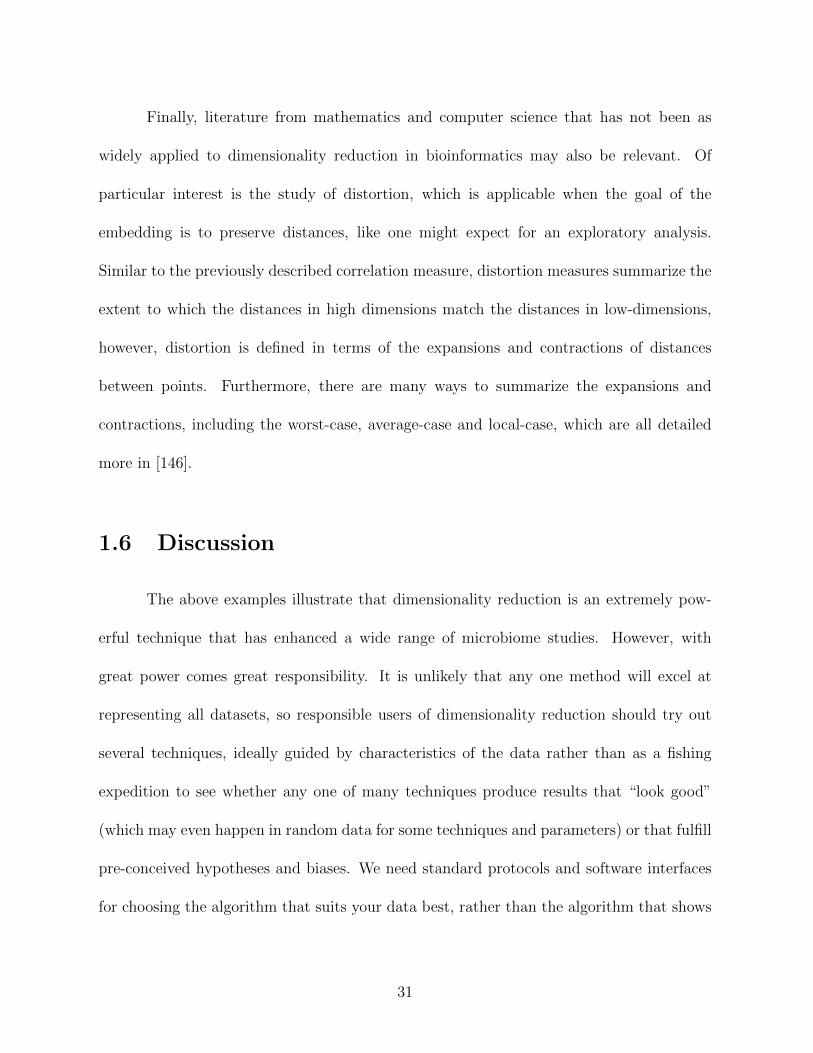
Finally, literature from mathematics and computer science that has not been as

widely applied to dimensionality reduction in bioinformatics may also be relevant. Of

particular interest is the study of distortion, which is applicable when the goal of the

embedding is to preserve distances, like one might expect for an exploratory analysis.

Similar to the previously described correlation measure, distortion measures summarize the

extent to which the distances in high dimensions match the distances in low-dimensions,

however, distortion is defined in terms of the expansions and contractions of distances

between points. Furthermore, there are many ways to summarize the expansions and

contractions, including the worst-case, average-case and local-case, which are all detailed

more in [146].

1.6 Discussion

The above examples illustrate that dimensionality reduction is an extremely pow-

erful technique that has enhanced a wide range of microbiome studies. However, with

great power comes great responsibility. It is unlikely that any one method will excel at

representing all datasets, so responsible users of dimensionality reduction should try out

several techniques, ideally guided by characteristics of the data rather than as a fishing

expedition to see whether any one of many techniques produce results that “look good”

(which may even happen in random data for some techniques and parameters) or that fulfill

pre-conceived hypotheses and biases. We need standard protocols and software interfaces

for choosing the algorithm that suits your data best, rather than the algorithm that shows

31

what you want to see if you squint at it correctly. Methods are needed both for diagnosing

the issues that may be most prevalent in your data and affecting your representation, and

for rationally choosing among different methods that could be applied to a given dataset.

Developing these methods is a key priority for the field.

Dimensionality reduction for the purposes of visualization has somewhat different

goals from dimensionality reduction for other purposes, and developing a better appreci-

ation of this distinction is important for practice in the field. The goal of dimensionality

reduction for visualization is primarily for exploratory overview by human observers (do

groups differ from one another, is there overall structure such as gradients in the data). As

such, visualization is usually done with three dimensions (more can be examined through

parallel plots), while the intrinsic dimensionality of the data may be higher. Visualization

is typically only the first step in the data analysis pipeline, and is followed by downstream

analysis, such as multivariate analysis/regression (PERMANOVA, ANOSIM, PERMDISP)

either on the original distances or on a dimensionality-reduced version of the data (which

can be higher than three dimensions). These results can also be used to motivate super-

vised differential abundance modeling, such as to determine which groups separate and

then determine which microbes are driving these separations.

Dimensionality reduction is thus often an early step in a multi-step pipeline. What

downstream analyses is dimensionality reduction a step towards, and how are these ac-

complished? Feature loadings (i.e., the importance of particular taxa or genes) can be

interpreted using log ratios in tools such as DEICODE, which can then be visualized in

Qurro. Classification can be accomplished using machine learning techniques such as ran-

32

dom forests, allowing estimates of classifier accuracy and group stability, and also allowing

tests of the reusability of these models, e.g., applying a model of human inflammatory

bowel disease to dogs [148] or models of aging between different human populations [54]. A

popular strategy is to use a lower-dimensional embedding for traditional statistical analysis,

such as using PCA or PCoA coordinates as inputs for regression, classification, clustering,

and other analyses. However, as we have seen, many dimensionality reduction methods

induce various kinds of artifacts or distortions, and cannot generalize well beyond the data

on which the model was initially optimized on, including, PCoA, nMDS, RPCA/CTF,

and UMAP/t-SNE. Consequently, analyses on these coordinates should be performed with

caution. Furthermore, since the parameters and software versions used with these methods

have the potential to be highly influential to their results, we recommend that these always

be reported for dimensionality reduction methods.

Given the large numbers of publications that have used dimensionality reduction on

microbiome data, we can start to draw conclusions about which dimensionality reduction

strategies should be more widely used, and which less widely used. On larger, sparser,

compositional datasets, we recommend against the use of conventional PCA, Bray-Curtis

and Jaccard distances, and pseudocounts. Conventional PCA presents the clearest case

of a method that should not be used on microbiome data due the sparsity and composi-

tional nature of the data. UniFrac and weighted UniFrac are essentially phylogenetically

informed versions of Jaccard and Bray-Curtis beta-diversity metrics respectively. Due to

the current default generation of a phylogeny in most 16S and shotgun analyses, there is

no reason not to use the phylogenetic counterparts, which have been shown to have better

33

discriminatory power. Pseudocounts should not be used because the choice of pseudocount

impacts the lower-dimensional embedding, and there is no clear method for determining

which pseudocount value is best.

In contrast, CTF and non-linear methods should be used more in microbiome con-

texts. As the cost of acquiring microbiome data continues to decrease, experimental designs

are getting increasingly complex, and include repeated measures, longitudinal studies, batch

effects, etc. We therefore need methods that can determine which biological signals are rel-

evant among all these confounding factors. Additionally, we are increasingly recognizing

that many relationships between/among samples are non-linear. Using non-linear methods

can potentially explain more of such datasets with fewer dimensions, although additional

benchmarking is required to understand the performance of these methods.

Our analyses suggest some important gaps in the field that could be important areas

for future development. There are no dimensionality reduction methods yet that are both

able to incorporate phylogeny and are compositionally aware. Several methods, such as

Robust PCA and CTF, control for the sparsity, non-normality, compositionality, and are

adaptable to specific study-designs of microbiome data but do not incorporate phylogenetic

information. In contrast, phylogenetic techniques do not account for sparsity and compo-

sitionality, and some also perform poorly with non-normality. A unified method that is

appropriate for any microbiome study is therefore still in the future, despite many impor-

tant recent advances. The ability to perform this task using a generalizable dissimilarity

measure would be particularly useful, because it would allow for full utilization of PCoA

and non-linear methods including nMDS and UMAP.

34

Taken together, we conclude that dimensionality reduction is a key part of many,

if not most, of the highest-impact microbiome studies performed to date. We can expect

this situation to continue into the future, especially as larger study designs and datasets

continue to accumulate, and additional method development advances increase the speed

and range of applicability of these techniques.

1.7 Acknowledgments

This work was supported in part by grants NSF 2038509, NIH U24CA248454, NIH

1DP1AT010885, and by CRISP, one of six centers in JUMP, a Semiconductor Research

Corporation (SRC) program sponsored by DARPA.

Chapter 1, in full, is a reprint of the material as it appears in “Applications and

Comparison of Dimensionality Reduction Methods for Microbiome Data.” George Arm-

strong, Gibraan Rahman, Cameron Martino, Daniel McDonald, Antonio Gonzalez, Gal

Mishne, and Rob Knight. Frontiers in Bioinformatics 2, 2022. The dissertation author

was the primary investigator and co-first author of this paper.

35

Chapter 2

Efficient computation of Faith’s

phylogenetic diversity with

applications in characterizing

microbiomes

36

The number of publicly available microbiome samples is continually growing. As

dataset size increases, bottlenecks arise in standard analytical pipelines. Faith’s phyloge-

netic diversity is a highly utilized phylogenetic alpha diversity metric that has thus far failed

to effectively scale to trees with millions of vertices. Stacked Faith’s Phylogenetic Diversity

(SFPhD) enables calculation of this widely adopted diversity metric at a much larger scale

by implementing a computationally efficient algorithm. The algorithm reduces the amount

of computational resources required, resulting in more accessible software with a reduced

carbon footprint, as compared to previous approaches. The new algorithm produces iden-

tical results to the previous method. We further demonstrate that the phylogenetic aspect

of Faith’s PD provides increased power in detecting diversity differences between younger

and older populations in the FINRISK study’s metagenomic data.

2.1 Introduction

In microbiome research, particular attention is given to evaluating the diversity

of microbes within samples [93, 140, 141]. Alpha diversity (within sample diversity), in

particular, can summarize the breadth of microbial diversity present in a sample. There are

many examples of associations between various host factors and alpha diversity, including

country [93], disease status [41, 148], diet [93], and age [155] among many others [157, 58].

Modern DNA sequencing instruments have enabled microbiome studies at the scale of tens

of thousands of samples, which presents a computational challenge for metrics that rely on a

phylogeny, such as Faith’s Phylogenetic Diversity (Faith’s PD) [35]. Faith’s PD is computed

37

by summing the branch lengths (edge weights) of the phylogeny that exclusively represent

the sequences contained in a biological sample. The amount of memory and number of

necessary operations needed to calculate Faith’s PD depends on the number of edges in

the phylogenetic tree, as well as the number of samples in the underlying data table. In

today’s increasingly large and sparse datasets and meta-analyses, these phylogenetic trees

and tables can exceed 100,000s of samples and millions of tree tips [96]. Recent advances

have enabled efficient computation of the UniFrac metric for beta diversity, which is also a

metric computed over phylogenetic trees [82]. Specifically, Striped UniFrac [96] improves

upon previous UniFrac implementations [50] by using space- and time-efficient tree data

structures [27] and reducing the number of vectors required to store intermediate scores in

the tree. Additionally, the usefulness of techniques like Faith’s PD and UniFrac remains

underexplored for metagenomics sequencing. Recent molecular protocol optimizations, such

as SHOGUN [53], have enabled the metagenomic characterization of large human cohorts

[120, 15, 60]. In this context, the applicability of Faith’s PD has largely been limited

by the technical difficulties associated with constructing phylogenies from metagenomic

features [159]. Efforts like the Web of LIfe (WoL) [159] and Genome Taxonomy Database

(GTDB) [108, 109] are now addressing this issue by providing a phylogenomic tree as part

of their database releases that can be used for phylogeny-informed analysis.

Motivated by these advances in algorithms and resources for analyzing phylogenies,

phylogenomic trees, and sparse data, we developed a new algorithm and implementation,

Stacked Faith’s Phylogenetic Diversity (SFPhD), for rapidly computing Faith’s PD. SF-

PhD produces identical results to those of previous algorithms for computing this metric

38

while producing a speedup of up to 64x and requiring as little as 0.21% of the memory

in our benchmarks (Table 2.1). The key advances of SFPhD are using a sparse matrix

representation, an efficient tree structure, and partial aggregation of metric constituents.

Our BSD-licensed implementation of this algorithm is available in the ‘unifrac’ package

(via PyPI and bioconda [46]), which has 50,714 total conda downloads and 34,141 conda

downloads since the introduction of SFPhD, as of the time of writing (May 13, 2021). The

package produces a C/C++ shared library with Python bindings and is additionally link-

able by any programming language (https://github.com/biocore/unifrac). Additionally, by

investigating the previously documented relationship between age and bacterial richness of

the gut microbiome [30], we demonstrate that accounting for phylogeny in metagenomic

data can increase the statistical power for detecting group differences.

2.2 Results

2.2.1 Stacked Faith’s PD provides a faster and memory-efficient

implementation over the previous state-of-the-art algorithm.

We introduce Stacked Faith’s PD (SFPhD), a novel algorithm and implementation

to compute Faith’s Phylogenetic Diversity that uses the structure of microbiome data along

with other practical considerations to achieve decreased time and memory requirements.

An example feature table is shown in Figure 2.1A, with a corresponding phylogenetic tree

39

Table

2.1:Average

mem

oryim

provementan

dspeedupof

SFPhD

compared

tothereference

implementation

.

Tim

e(s)

Mem

ory(kbytes)

#ofSamples

skbio

SFPhD

Speedup

(x)

skbio

SFPhD

Improvement(x

)1250

18.6

4.67

3.98

10001242.8

312815.6

31.97

2500

32.8

5.12

6.41

19114300.4

313834.8

60.91

5000

79.75

6.31

12.64

36727706.4

315124

116.55

10000

270.34

8.76

30.86

75866321.6

317413.2

239.01

20000

910.62

14.17

64.26

152783905.2

320837.6

476.2

40000

*25.58

N/A

*326895.2

N/A

80000

*47.26

N/A

*339670

N/A

*Nojobswereab

leto

becompletedwiththeprescribed

resources.

40

Figure 2.1: Partially aggregating branch lengths reduces the space complexityof the algorithm. (A) Faith’s PD calculation depends on the representation of featurespresent in samples. In the table, the letters (R, O, B, K) represent samples and the num-bers (0, 1, 2, 4, 6, 9, 10) represent features. A 1 in an entry indicates the presence of afeature in the sample. SFPhD uses sparse table data structures, which reduce memory byonly keeping track of the non-zero values in a matrix (highlighted in gray). (B) A mockreference phylogenetic tree is shown, with the features from (A) as tips. Labels for thesamples from (A) are located next to tips that they contain. The nodes are labeled bytheir order in a post-order traversal of the tree. (C) Graphic depiction of the referenceimplementation’s calculation of Faith’s PD by first aggregating the presence/absence in-formation for each branch in the tree, followed by multiplication by the branch lengths toget the metric constituents, and finally a sum over the entire branch ×metric constituenttable. (D) Graphic representation of the execution of SFPhD. On the left, the stack ofpresence/absence information is shown at three points during the algorithm’s execution (i,ii, ii). Each of these times shows the stack immediately before memory is freed. On theright, the state of the partially aggregated phylogenetic diversity (PD) is shown after eachnode is added to the stack. Each row represents the vector after a step in the algorithm.In practice, there is only one such vector. (E) The balanced parentheses representation forthe phylogenetic tree from (B).

41

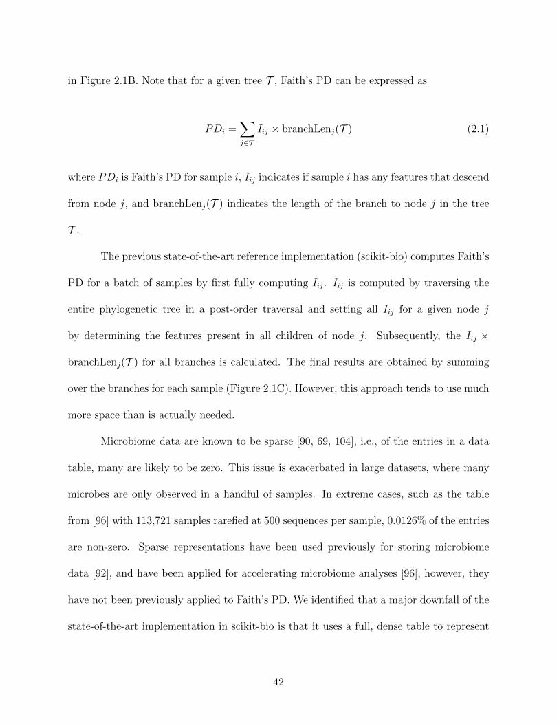
in Figure 2.1B. Note that for a given tree T , Faith’s PD can be expressed as

PDi =∑j∈T

Iij × branchLenj(T ) (2.1)

where PDi is Faith’s PD for sample i, Iij indicates if sample i has any features that descend

from node j, and branchLenj(T ) indicates the length of the branch to node j in the tree

T .

The previous state-of-the-art reference implementation (scikit-bio) computes Faith’s

PD for a batch of samples by first fully computing Iij. Iij is computed by traversing the

entire phylogenetic tree in a post-order traversal and setting all Iij for a given node j

by determining the features present in all children of node j. Subsequently, the Iij ×

branchLenj(T ) for all branches is calculated. The final results are obtained by summing

over the branches for each sample (Figure 2.1C). However, this approach tends to use much

more space than is actually needed.

Microbiome data are known to be sparse [90, 69, 104], i.e., of the entries in a data

table, many are likely to be zero. This issue is exacerbated in large datasets, where many

microbes are only observed in a handful of samples. In extreme cases, such as the table

from [96] with 113,721 samples rarefied at 500 sequences per sample, 0.0126% of the entries

are non-zero. Sparse representations have been used previously for storing microbiome

data [92], and have been applied for accelerating microbiome analyses [96], however, they

have not been previously applied to Faith’s PD. We identified that a major downfall of the

state-of-the-art implementation in scikit-bio is that it uses a full, dense table to represent

42

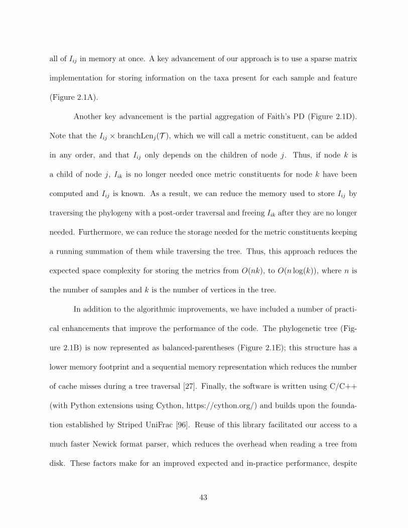
all of Iij in memory at once. A key advancement of our approach is to use a sparse matrix

implementation for storing information on the taxa present for each sample and feature

(Figure 2.1A).

Another key advancement is the partial aggregation of Faith’s PD (Figure 2.1D).

Note that the Iij × branchLenj(T ), which we will call a metric constituent, can be added

in any order, and that Iij only depends on the children of node j. Thus, if node k is

a child of node j, Iik is no longer needed once metric constituents for node k have been

computed and Iij is known. As a result, we can reduce the memory used to store Iij by

traversing the phylogeny with a post-order traversal and freeing Iik after they are no longer

needed. Furthermore, we can reduce the storage needed for the metric constituents keeping

a running summation of them while traversing the tree. Thus, this approach reduces the

expected space complexity for storing the metrics from O(nk), to O(n log(k)), where n is

the number of samples and k is the number of vertices in the tree.

In addition to the algorithmic improvements, we have included a number of practi-

cal enhancements that improve the performance of the code. The phylogenetic tree (Fig-

ure 2.1B) is now represented as balanced-parentheses (Figure 2.1E); this structure has a

lower memory footprint and a sequential memory representation which reduces the number

of cache misses during a tree traversal [27]. Finally, the software is written using C/C++

(with Python extensions using Cython, https://cython.org/) and builds upon the founda-

tion established by Striped UniFrac [96]. Reuse of this library facilitated our access to a

much faster Newick format parser, which reduces the overhead when reading a tree from

disk. These factors make for an improved expected and in-practice performance, despite

43

the time complexity and worst-case memory complexity remaining the same.

To demonstrate the scalability of SFPhD, we used a collection of 307,237 public and

anonymized private 16S rRNA V4 microbiome samples amounting to 1,264,796 phylogenetic

tree tips (after rarefaction at 500 sequences per sample). The samples were retrieved using

the redbiom command line interface [94] which queried a cache of public and anonymized

private studies available in Qiita [44]. Amplicon sequence variants (ASVs) were placed into

the Greengenes [44, 95] phylogeny using SEPP [102]. Computing the full alpha diversity

vector took SFPhD 1 hour and 5 minutes wall-clock time and required a maximum resident

set size of less than 3 GB (see Methods for hardware details). In addition, we iteratively

measured runtime and memory consumption for increasingly large random subsets of sam-

ples while fixing the size of the tree at 100,000 tips (Figure 2.2 A,B). For the iteration

with 20,000 samples, the memory usage of the reference implementation exceeded 150 GB

and the process ran for over 15 minutes. Contrastingly, with SFPhD, the process took 14

seconds to execute and required less than 0.5 GB of memory. Additionally, using Green Al-

gorithms [73], we estimated the carbon footprint of the scikit-bio reference implementation

on the 20,000 sample table is 12.84 g CO2e, whereas we estimated the carbon footprint of

SFPhD would be 0.04 g CO2e in the United States, which is a 321-fold reduction in impact

on global warming.

44

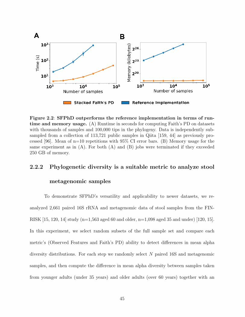
Figure 2.2: SFPhD outperforms the reference implementation in terms of run-time and memory usage. (A) Runtime in seconds for computing Faith’s PD on datasetswith thousands of samples and 100,000 tips in the phylogeny. Data is independently sub-sampled from a collection of 113,721 public samples in Qiita [159, 44] as previously pro-cessed [96]. Mean of n=10 repetitions with 95% CI error bars. (B) Memory usage for thesame experiment as in (A). For both (A) and (B) jobs were terminated if they exceeded250 GB of memory.

2.2.2 Phylogenetic diversity is a suitable metric to analyze stool

metagenomic samples

To demonstrate SFPhD’s versatility and applicability to newer datasets, we re-

analyzed 2,661 paired 16S rRNA and metagenomic data of stool samples from the FIN-

RISK [15, 120, 14] study (n=1,563 aged 60 and older, n=1,098 aged 35 and under) [120, 15].

In this experiment, we select random subsets of the full sample set and compare each

metric’s (Observed Features and Faith’s PD) ability to detect differences in mean alpha

diversity distributions. For each step we randomly select N paired 16S and metagenomic

samples, and then compute the difference in mean alpha diversity between samples taken

from younger adults (under 35 years) and older adults (over 60 years) together with an

45

Figure 2.3: Phylogenetic diversity provides increased statistical power to differ-entiate age groups in shotgun metagenomics but not in 16S rRNA sequencing.(A) Statistical power to differentiate young adults from old adults in two alpha diver-sity metrics at different sample sizes using 16S rRNA sequencing in the FINRISK cohort.(B) Same as (A) but for shallow shotgun metagenomic sequencing.

empirical p-value. For both 16S and metagenomics, the alpha diversity of younger adults

is lower than in older adults. In metagenomics, but not in 16S sequencing, Faith’s PD

provides improved statistical power over a phylogenetically-agnostic alternative (Figure 2.3

A,B). With 16S data, the difference between the two metrics is subtle (Figure 2.3A). In

both cases, the statistical power increases as the number of samples grows. With metage-

nomic data, the number of observed features shows a weaker effect compared to Faith’s PD

regardless of the number of samples (Figure 2.3B). Unlike 16S datasets (5,600 features),

metagenomic datasets (1,700 features) are resolution-limited by the reference databases.

Whereas the nature of amplicon sequence variants (ASVs) allow for a broader feature

space that can capture age-differences without the need for a phylogeny.

By computing the log of the likelihood ratio of older to younger adult samples present

46

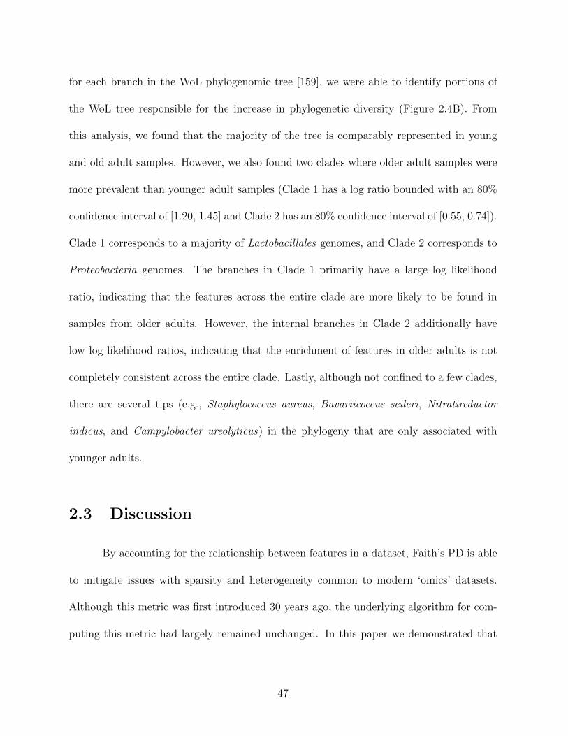
for each branch in the WoL phylogenomic tree [159], we were able to identify portions of

the WoL tree responsible for the increase in phylogenetic diversity (Figure 2.4B). From

this analysis, we found that the majority of the tree is comparably represented in young

and old adult samples. However, we also found two clades where older adult samples were

more prevalent than younger adult samples (Clade 1 has a log ratio bounded with an 80%

confidence interval of [1.20, 1.45] and Clade 2 has an 80% confidence interval of [0.55, 0.74]).

Clade 1 corresponds to a majority of Lactobacillales genomes, and Clade 2 corresponds to

Proteobacteria genomes. The branches in Clade 1 primarily have a large log likelihood

ratio, indicating that the features across the entire clade are more likely to be found in

samples from older adults. However, the internal branches in Clade 2 additionally have

low log likelihood ratios, indicating that the enrichment of features in older adults is not

completely consistent across the entire clade. Lastly, although not confined to a few clades,

there are several tips (e.g., Staphylococcus aureus, Bavariicoccus seileri, Nitratireductor

indicus, and Campylobacter ureolyticus) in the phylogeny that are only associated with

younger adults.

2.3 Discussion

By accounting for the relationship between features in a dataset, Faith’s PD is able

to mitigate issues with sparsity and heterogeneity common to modern ‘omics’ datasets.

Although this metric was first introduced 30 years ago, the underlying algorithm for com-

puting this metric had largely remained unchanged. In this paper we demonstrated that

47

Figure 2.4: Phylogenetic tree colored by age-group log of the likelihood ratioof older to younger adults per node. (A) Distribution of Faith’s PD by age group onthe full dataset. (B) Web of Life (WoL) Phylogenetic tree with branches colored by the logof likelihood ratio of old adults compared to young adults in descendants of the branch,for the FINRISK dataset. The inner circle is colored by the log of likelihood ratio of olderadults compared to younger adults in the tips of the tree. The outer circle is colored by thephylum of the taxon represented by each tree tip. Red ellipses mark two clades enrichedfor samples from older individuals.

48

our novel algorithm, SFPhD, performed efficiently on datasets with hundreds of thousands

of samples and millions of tree tips.

An important aspect of SFPhD’s underlying algorithm is substituting calculation

of the full presence/absence table over the phylogeny, for a tree traversal that partially

aggregates diversity values and frees presence/absence information when no longer needed.

The result is a high-performance implementation that demonstrates improved scaling, with

the number of samples in the input dataset. Much of the engineering work here was facili-

tated by the balanced parenthesis tree implementation provided in the UniFrac package [96].

Therefore, we believe that increasing the availability of efficient and flexible data structures

for bioinformatic analyses, is likely to accelerate and facilitate the development of novel

analytical methods. In a broader sense, this is similar to the impact of NumPy’s [96, 52]

N-dimensional array in image processing, machine learning, neuroscience, and other fields.

In addition, in a stool metagenomic study Faith’s PD demonstrates increased statis-

tical power compared to Observed Features for differentiating younger from older subjects

based on their microbial communities. In this context, we show that while the choice of

alpha diversity metric did not make a significant difference for the 16S dataset in this study,

Faith’s PD consistently provided increased statistical power for determining age-based dif-

ferences in the shotgun metagenomic sequencing data. While this metric was originally

developed to analyze data with vastly different statistical and biological properties, its

use here demonstrates the versatility and applicability behind measuring diversity using a

tree. Although we show the utility of SFPhD in large and complex microbiome studies,

the underlying implementation is not tied to a particular molecular technology. Thus, we

49

envision that this implementation will be relevant to fields outside of microbiology, like nu-

trition and metabolomics research, that only recently began adopting trees for analytical

tasks [142, 59].

2.4 Methods

2.4.1 Construction of benchmarking tables

Data for the benchmarking in this study were subsampled from a BIOM table of

113,721 and 761,003 ASVS, which is composed of studies aggregated from several large

sources of publicly available microbiome data in Qiita [4, 44]. This data table was produced

as in [96]. The data was subset by uniformly randomly sampling the desired number of

ASVs and samples from the table. Ten different tables were created for each number of

samples and ASVs. The insertion tree from [96] was collapsed to only contain sequences that

were selected to be included in the given subsampled table. The table with 307,237 public

and anonymized private 16S rRNA V4 microbiome samples and 1,264,796 phylogenetic tree

tips was also prepared as in [96], but included samples with private sequencing data from

Qiita.

2.4.2 Benchmarking time and memory estimates

The SFPhD implementation available in the python package unifrac v0.10.0 was

used. The reference implementation uses the Faith’s PD implementation from scikit-bio

v0.5.4.

50

All methods were run single-threaded on shared compute nodes that were not run-

ning other compute tasks. The nodes all had Intel(R) Xeon(R) CPU E5-2640 v3 @ 2.60GHz

processors. A job was terminated if it exceeded 6 hours of wall time or 250 GB of memory

(system max). Space was tracked using GNU Time. Time for both implementations was

tracked with a python wrapper script. The time needed to parse data is not included in

the scikit-bio timings, but is included in the SFPhD timings, due to the lack of access

to this information in the unifrac interface. This is acceptable given that it results in a

conservative estimate of the speedup with SFPhD.

2.4.3 Carbon footprint estimation

The Green Algorithms interface [73] was used to estimate the Carbon Dioxide equiv-

alent (CO2e) of the benchmarked methods. The Intel(R) Xeon(R) CPU E5-2640 v3 CPUs

used in benchmarking have a Thermal Design Power (TDP) per core of the 11.25 TDP /

core.

2.4.4 FINRISK processing

The 16S rRNA data were demultiplexed, quality filtered, and denoised with de-

blur [4]. The Greengenes [95] 13.8 with a clustering level of 99% was used as the reference

phylogeny for open-reference feature picking with SEPP [102]. ASVs with a total frequency

fewer than 10 were discarded, and the table was then rarefied to a sampling depth of 1000

reads/sample. The resulting table and insertion tree were used for calculation of Faith’s PD.

The shotgun metagenomic data were trimmed and quality filtered using Atropos [33]. They

51

were aligned to the WoL database using SHOGUN pipeline (v1.0.8) with a Bowtie2 align-

ment option. A table was generated from the alignments using the OGU workflow [158].

OGUs with a total frequency fewer than 10 were discarded, and the table was then rarefied

to a sampling depth of 1000 reads/sample. The WoL phylogenomic tree [158, 159] was used

for Faith’s PD. Both tables were filtered to include only samples from individuals 35 and

younger (younger criteria) or 60 and older (older criteria).

2.4.5 Power estimation for mean difference in alpha diversity

For a given N (shown on horizontal axis in Figure 2.3 A,B), the FINRISK processed

samples matching the younger/older criteria were sampled to this depth. On the subsam-

pled data, the difference in mean alpha diversity between younger and older adults d, was

computed. A null distribution, D, was generated by repeating 1000 repetitions of shuffling

the age category associated with an alpha diversity and recomputing the difference of mean

alpha diversity between the groups. The p-value was computed by finding the percentile

of d in D. This test procedure was repeated for 1000 repetitions. The power for N is

estimated as the proportion of tests found significant at α = 0.05.

2.4.6 Phylogenetic Visualization

Tree was visualized using EMPress [19]. A node in the tree was considered old if its

agelog > 0 and young if its agelog < 0.

52

2.5 Data Access

The data used for benchmarking Faith’s PD timing and memory usage are available

as per the Striped UniFrac paper [96]. The code for the benchmarking is available on

GitHub (https://github.com/biocore/faiths-pd-benchmarking). The data and code needed

for benchmarking the FINRISK metagenomics data are also available on GitHub. The SF-

PhD code is available in the unifrac python package (https://github.com/biocore/unifrac).

2.6 Acknowledgements

This work was supported in part by IBM Research AI through the AI Horizons

Network, the Center for Microbiome Innovation at UC San Diego, the Academy of Finland

grant 321351 and the Emil Aaltonen Foundation (to T.N.), the National Institutes of Health

grant R01ES027595 (to M.J.), the Academy of Finland grants 321356 and 335525 (A.S.H),

the Academy of Finland grant 295741 (L.L.). MI was supported by the Munz Chair of

Cardiovascular Prediction and Prevention. VS was supported by the Finnish Foundation

for Cardiovascular Research.

Chapter 2, in full, is a reprint of the material as it appears in “Efficient computation

of Faith’s phylogenetic diversity with applications in characterizing microbiomes.” George

Armstrong, Kalen Cantrell, Shi Huang, Daniel McDonald, Niina Haiminen, Anna Paola

Carrieri, Qiyun Zhu, Antonio Gonzalez, Imran McGrath, Kristen Beck, Daniel Hakim, Aki

S Havulinna, Guillaume Meric, Teemu Niiranen, Leo Lahti, Veikko Salomaa, Mohit Jain,

Michael Inouye, Austin D Swafford, Ho-Cheol Kim, Laxmi Parida, Yoshiki Vazquez-Baeza

53

and Rob Knight. Genome Research 31, 2021. The dissertation author was the primary

investigator and the first author of this paper.

54

Chapter 3

Uniform Manifold Approximation

and Project (UMAP) reveals

composite patterns and resolves

visualization artifacts in microbiome

data

55

Microbiome data are sparse and high-dimensional, so effective visualization of these

data requires dimensionality reduction. To date, the most commonly used method for

dimensionality reduction in the microbiome is calculation of between-sample microbial dif-

ferences (beta diversity), followed by Principal Coordinates Analysis (PCoA). Uniform

Manifold Approximation and Projection (UMAP) is an alternative method that can re-

duce the dimensionality of beta diversity distance matrices. Here, we demonstrate the

benefits and limitations of using UMAP for dimensionality reduction on microbiome data.

Using real data, we demonstrate that UMAP can improve the representation of clusters,

especially when the clusters are composed of multiple subgroups. Additionally, we show

that UMAP provides improved correlation of biological variation along a gradient with a

reduced number of coordinates of the resulting embedding. Finally, we provide parameter

recommendations that emphasize the preservation of global geometry. We therefore con-

clude that UMAP should be routinely used as a complementary visualization method for

microbiome beta diversity studies.

3.1 Importance

UMAP provides an additional method to visualize microbiome data. The method is

extensible to any beta diversity metric used with PCoA, and our results demonstrate that

UMAP can indeed improve visualization quality and correspondence with biological and

technical variables of interest. The software to perform this analysis is available under an

open-source license and can be obtained at https://github.com/knightlab-analyses/umap-

56

microbiome-benchmarking; additionally, we have provided a QIIME 2 plugin for UMAP at

https://github.com/biocore/q2-umap.

3.2 Observation

An important step in microbiome research is visualizing the relationships between

samples. In the study of microbial communities through next generation sequencing (NGS),

these comparisons are typically done through the visualization of beta diversities with

principal coordinates analysis (PCoA) [66] (Figure A.1). Although alternatives such as

conventional principal component analysis (PCA), non-metric multidimensional scaling

(NMDS) [65] and t-distributed stochastic neighbor embedding (t-SNE) [144] are some-

times applied, PCoA in particular has been widely adopted by the microbiome community.

Due to the high dimensional and highly sparse nature of the data, which presents chal-

lenges on sequence count data [1, 90], one major benefit of PCoA over other methods on

untransformed count data is that it accommodates a generalized distance matrix (of beta

diversities, for the microbiome). This allows use of distance metrics that are better-suited

for sparse data (e.g., Bray-Curtis [16], Jaccard [57], UniFrac [82]). Uniform Manifold Ap-

proximation and Projection (UMAP) [97] is a method that has gained traction in single-cell

genomics analysis [51]. Whereas PCoA performs an eigendecomposition that focuses on

linearly preserving the pairwise distances between the samples (global structure), UMAP

uses a non-linear graph construction and embedding method to optimize an objective that

allows for a trade-off between emphasizing local structures and preserving distances glob-

57

ally. This trade-off is primarily controlled by the ‘n neighbors’ and ‘min dist’ parameters of

UMAP. The ‘n neighbors’ parameter controls the number of neighbors whose local topology

is preserved, so global distances are preserved when it is high. The ‘min dist’ parameter

controls the minimum distance between samples in the embedding, which affects the spread

of clusters. Low values of ‘min dist’ allow UMAP to emphasize the similarity of dense clus-

ters of samples, whereas larger values of ‘min dist’ will focus on preserving distances more

broadly. Both UMAP and PCoA operate on a generalized distance (beta diversity) matrix,

appropriate for microbiome data (Figure A.1). While the use of UMAP on microbiome

data has been noted (11) the utility of UMAP on microbiome data remains underexplored.

Using real datasets, we compared both visual qualities and quantitative measures of UMAP

to PCoA on well understood datasets. We additionally applied UMAP to data from the

Human Microbiome Project (HMP) [140] to demonstrate its characteristics on a larger

dataset with more complex sources of variation. Discrete clusters are one common pattern

that microbial communities can exhibit [68]. The ‘keyboard data’ from [37] contains 16S

samples (n = 99, features = 1399, 5% dense) from the keyboards and fingers of 3 subjects.

PCoA on the Aitchison distances on these samples can recover the cluster structure of the

subjects in the data (Figure 3.1A). We compared this to UMAP (n neighbors = 15 and

n neighbors = 80, min dist = 1) and found that UMAP can also recover the cluster struc-

ture of the subjects (Figure 3.1 B,C). We also saw that UMAP produced two-dimensional

coordinates with improved separation within subjects by sample type. This was further

supported by improved LDA classification of sample type stratified by subject (Table 3.1).

To quantitatively assess the dimensionality reduction, we performed a supervised

58

Figure 3.1: Comparison of PCoA and UMAP visualizations of cluster andgradient patterns on real data. The keyboard data set contains samples from threedifferent subjects’ keyboards (surface) and their hands (skin). (A) PCoA on Aitchisondistances (pseudocount=1) demonstrates a strong separation between M2 and the othersubjects, as well as separation between subjects M3 and M9. (B) A UMAP (n neigh-bors=15, min dist=1) visualization demonstrates stronger clustering by subject, with adifferent relative positioning of the clusters by subject. The plot also emphasizes clusteringby sample type. (C) UMAP with an increased n neighbors parameter (n neighbors=80,min dist=1) reflects the same relative positioning of clusters as PCoA. It also demonstratesthe improved localization by sample type within subjects. (D) On the “88 soils” data, PCoAon the Aitchison distances demonstrates a horseshoe pattern with pH distributed along thehorseshoe. (E) Soil moisture deficit is also distributed along the horseshoe, and (F) thereis not a strong association between mean annual temperature and position on the PCoA.(G) In the UMAP (n neighbors=80, min dist=1), followed by centering/rotation with PCA

59

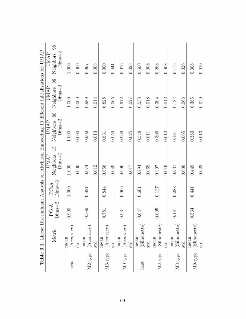
Table

3.1:LinearDiscrim

inan

tAnalysison

Aitchison

Embedding10

differentinitialization

sforUMAP

Metric

PCoA

Dim

s=2

PCoA

Dim

s=3

UMAP

Neigh

bors=

15Dim

s=2

UMAP

Neigh

bors=

80Dim

s=2

UMAP

Neigh

bors=

98Dim

s=2

UMAP

Neigh

bors=

98Dim

s=2

host

mean

(Accuracy)

0.990

1.000

1.000

1.000

1.000

1.000

std

0.000

0.000

0.000

0.000

M2-type

mean

(Accuracy)

0.789

0.921

0.974

0.992

0.989

0.997

std

0.012

0.013

0.014

0.008

M3-type

mean

(Accuracy)

0.781

0.844

0.856

0.831

0.828

0.900

std

0.049

0.059

0.065

0.041

M9-type

mean

(Accuracy)

0.931

0.966

0.990

0.969

0.972

0.976

std

0.017

0.025

0.027

0.023

host

mean

(Silhou

ette)

0.647

0.601

0.794

0.548

0.533

0.500

std

0.069

0.011

0.018

0.008

M2-type

mean

(Silhou

ette)

0.095

0.127

0.297

0.306

0.304

0.263

std

0.019

0.012

0.012

0.008

M3-type

mean

(Silhou

ette)

0.181

0.288

0.231

0.181

0.184

0.175

std

0.036

0.065

0.066

0.026

M9-type

mean

(Silhou

ette)

0.534

0.441

0.449

0.383

0.385

0.308

std

0.023

0.013

0.029

0.020

60

classification with Linear Discriminant Analysis (LDA) and as well as an unsupervised

evaluation of clustering using the silhouette measure on the low dimensional representa-

tions. The LDA classification, which solely measures separability, demonstrated higher

accuracy of sample type (stratified by subject) on UMAP with two components compared

to PCoA with two or three components for all subjects (Table 3.1). Silhouette scores, which

measure cluster separation and density, demonstrated that host separation is improved with

UMAP with a low ‘n neighbors’ value, but not for a higher ‘n neighbors’ value, which is

likely due to the reduced distance between clusters in the UMAP coordinates with higher

‘n neighbors’. The method with the highest within-host sample-type silhouette varied for

each host. A simulated missing data analysis, where entries were randomly masked from

samples, demonstrated that these results are sensitive to missing values (Figure A.2). In

dimensionality reduction, it is not only important for clusters to be separated; the posi-

tioning of clusters with respect to their similarity to other clusters, i.e., preserving global

distances, is desirable. In the PCoA visualization (Figure 3.1A) the samples of subjects

M3 and M9 are similar to each other in the plot, and both are distant from M2. This

corresponds with the expectation that M3 and M9 are more similar, because they shared

an office. Additionally, this agrees with the original distances, where the mean Aitchison

distance between M3 and M9 samples is 13.87± 0.11, (95% CI), whereas the mean M2-M3

distance is 19.89 ± 0.11, (95% CI), and the mean M2-M9 distance is 18.94 ± 0.12. (95%

CI). However, for UMAP with n neighbors = 15 in Figure 3.1B, the relative position of

the clusters has changed (M9 is closer to M2 than it is to M3). Using the default ‘spec-

tral’ initialization option, which is recommended for preserving global structure [63], we

61

found that on only 34 / 50 initializations with different random seeds and n neighbors =

15, UMAP produced clusters with the correct relative positioning. However, when we in-

crease the parameter to n neighbors = 80, which represents a large majority of the samples,

the visualization retains separation by subject (Figure 3.1C), and 50 / 50 initializations

produced clusters with the correct relative positioning.

Ecological gradients are another common pattern that microbial communities can

exhibit [68]. The ‘88 soils’ data from [74] contains 16S samples (n = 88, features = 5627,

4% dense) from 88 different soils with additional measurements of the soil. A Bio-Env

test [25] reveals that the top three soil variates corresponding with the Aitchison distances

are pH, moisture deficit, and mean annual temperature (Table 3.2). In the PCoA of

the Aitchison distances, which displays a horseshoe artifact [104, 32], pH is distributed

along the horseshoe (Fig 1d). To quantitatively assess the visualization of gradients in

the data, similarly to [68], we calculated the Spearman correlation of the components of

the ordination with the ecological variable. We found that soil pH is strongly correlated

with the first component (Spearman r = 0.934) (Table 3.2). Soil Moisture deficit is also

distributed along the horseshoe (Figure 3.1E), with PCoA-1 (Spearman r = 0.828). There

is a mild correlation between Mean Annual Temperature and the second PCoA coordinate

(Spearman r = 0.313), although a pattern is difficult to see visually due to the horseshoe

artifact (Figure 3.1F).

On the gradient problem, we fit UMAP with the parameters used with the keyboard

data (min dist = 1, n neighbors = 80). Since the UMAP algorithm does not guarantee

the direction with the most variance in its output coordinates is axis-aligned, we use PCA

62

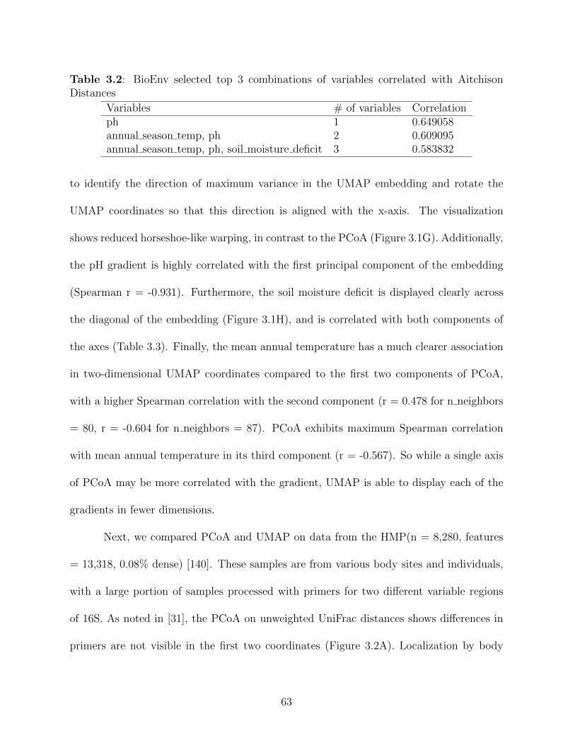
Table 3.2: BioEnv selected top 3 combinations of variables correlated with AitchisonDistances

Variables # of variables Correlationph 1 0.649058annual season temp, ph 2 0.609095annual season temp, ph, soil moisture deficit 3 0.583832

to identify the direction of maximum variance in the UMAP embedding and rotate the

UMAP coordinates so that this direction is aligned with the x-axis. The visualization

shows reduced horseshoe-like warping, in contrast to the PCoA (Figure 3.1G). Additionally,

the pH gradient is highly correlated with the first principal component of the embedding

(Spearman r = -0.931). Furthermore, the soil moisture deficit is displayed clearly across

the diagonal of the embedding (Figure 3.1H), and is correlated with both components of

the axes (Table 3.3). Finally, the mean annual temperature has a much clearer association

in two-dimensional UMAP coordinates compared to the first two components of PCoA,

with a higher Spearman correlation with the second component (r = 0.478 for n neighbors

= 80, r = -0.604 for n neighbors = 87). PCoA exhibits maximum Spearman correlation

with mean annual temperature in its third component (r = -0.567). So while a single axis

of PCoA may be more correlated with the gradient, UMAP is able to display each of the

gradients in fewer dimensions.

Next, we compared PCoA and UMAP on data from the HMP(n = 8,280, features

= 13,318, 0.08% dense) [140]. These samples are from various body sites and individuals,

with a large portion of samples processed with primers for two different variable regions

of 16S. As noted in [31], the PCoA on unweighted UniFrac distances shows differences in

primers are not visible in the first two coordinates (Figure 3.2A). Localization by body

63

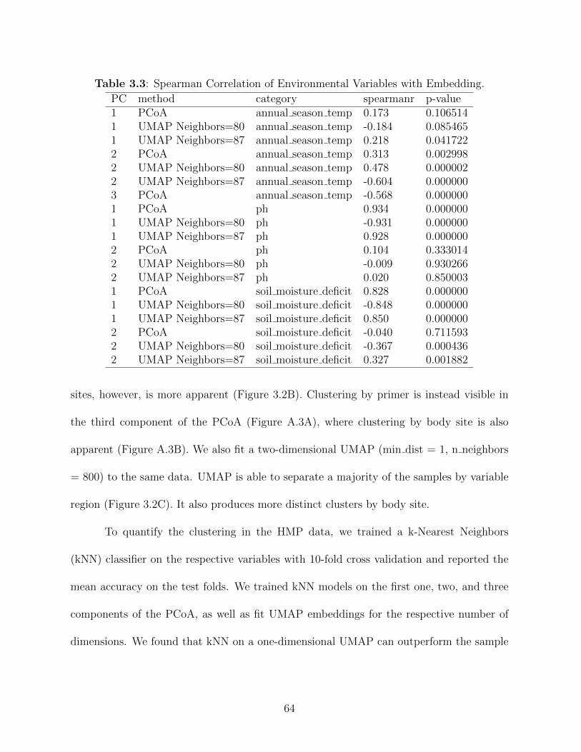
Table 3.3: Spearman Correlation of Environmental Variables with Embedding.

PC method category spearmanr p-value1 PCoA annual season temp 0.173 0.1065141 UMAP Neighbors=80 annual season temp -0.184 0.0854651 UMAP Neighbors=87 annual season temp 0.218 0.0417222 PCoA annual season temp 0.313 0.0029982 UMAP Neighbors=80 annual season temp 0.478 0.0000022 UMAP Neighbors=87 annual season temp -0.604 0.0000003 PCoA annual season temp -0.568 0.0000001 PCoA ph 0.934 0.0000001 UMAP Neighbors=80 ph -0.931 0.0000001 UMAP Neighbors=87 ph 0.928 0.0000002 PCoA ph 0.104 0.3330142 UMAP Neighbors=80 ph -0.009 0.9302662 UMAP Neighbors=87 ph 0.020 0.8500031 PCoA soil moisture deficit 0.828 0.0000001 UMAP Neighbors=80 soil moisture deficit -0.848 0.0000001 UMAP Neighbors=87 soil moisture deficit 0.850 0.0000002 PCoA soil moisture deficit -0.040 0.7115932 UMAP Neighbors=80 soil moisture deficit -0.367 0.0004362 UMAP Neighbors=87 soil moisture deficit 0.327 0.001882

sites, however, is more apparent (Figure 3.2B). Clustering by primer is instead visible in

the third component of the PCoA (Figure A.3A), where clustering by body site is also

apparent (Figure A.3B). We also fit a two-dimensional UMAP (min dist = 1, n neighbors

= 800) to the same data. UMAP is able to separate a majority of the samples by variable

region (Figure 3.2C). It also produces more distinct clusters by body site.

To quantify the clustering in the HMP data, we trained a k-Nearest Neighbors

(kNN) classifier on the respective variables with 10-fold cross validation and reported the

mean accuracy on the test folds. We trained kNN models on the first one, two, and three

components of the PCoA, as well as fit UMAP embeddings for the respective number of

dimensions. We found that kNN on a one-dimensional UMAP can outperform the sample

64

Figure 3.2: PCoA and UMAP comparison on 8,280 samples from the HumanMicrobiome Project (HMP). In the HMP data, when samples prepared with differentprimers are analyzed jointly, (A) there appears to be no separation between primers in thefirst two coordinates of PCoA and (B) mild separation by body site. In the same number ofdimensions, UMAP is able to both (C) emphasize the differences between samples preparedwith different variable regions and (D) improve clustering by body site. Both methods usethe unweighted UniFrac distances on the HMP data rarefied to 1,000 sequences per sample.

65

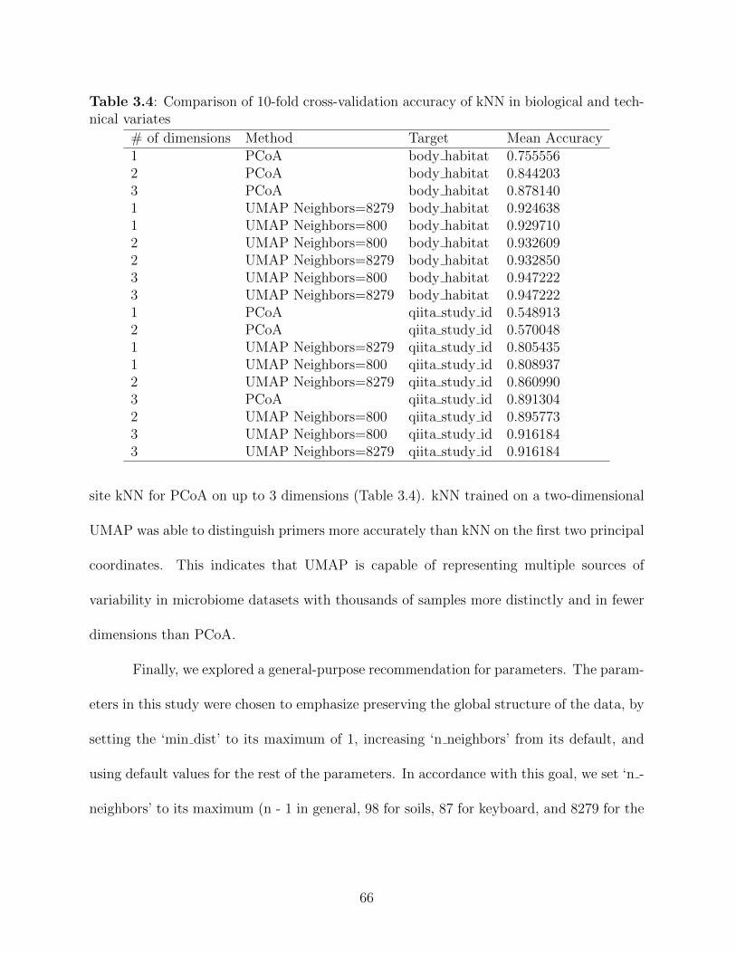
Table 3.4: Comparison of 10-fold cross-validation accuracy of kNN in biological and tech-nical variates

# of dimensions Method Target Mean Accuracy1 PCoA body habitat 0.7555562 PCoA body habitat 0.8442033 PCoA body habitat 0.8781401 UMAP Neighbors=8279 body habitat 0.9246381 UMAP Neighbors=800 body habitat 0.9297102 UMAP Neighbors=800 body habitat 0.9326092 UMAP Neighbors=8279 body habitat 0.9328503 UMAP Neighbors=800 body habitat 0.9472223 UMAP Neighbors=8279 body habitat 0.9472221 PCoA qiita study id 0.5489132 PCoA qiita study id 0.5700481 UMAP Neighbors=8279 qiita study id 0.8054351 UMAP Neighbors=800 qiita study id 0.8089372 UMAP Neighbors=8279 qiita study id 0.8609903 PCoA qiita study id 0.8913042 UMAP Neighbors=800 qiita study id 0.8957733 UMAP Neighbors=800 qiita study id 0.9161843 UMAP Neighbors=8279 qiita study id 0.916184

site kNN for PCoA on up to 3 dimensions (Table 3.4). kNN trained on a two-dimensional

UMAP was able to distinguish primers more accurately than kNN on the first two principal

coordinates. This indicates that UMAP is capable of representing multiple sources of

variability in microbiome datasets with thousands of samples more distinctly and in fewer

dimensions than PCoA.

Finally, we explored a general-purpose recommendation for parameters. The param-

eters in this study were chosen to emphasize preserving the global structure of the data, by

setting the ‘min dist’ to its maximum of 1, increasing ‘n neighbors’ from its default, and

using default values for the rest of the parameters. In accordance with this goal, we set ‘n -

neighbors’ to its maximum (n - 1 in general, 98 for soils, 87 for keyboard, and 8279 for the

66

HMP) and re-ran the previous analyses. With this parameter setting, the results remain

largely unchanged (Table 3.4). Our benchmarks demonstrate the potential for improved

performance and interpretability for both cluster and gradient microbiome data by using

UMAP with its parameters set with the intent to preserve global geometry. Given that

both algorithms provide different guarantees with respect to the preservation of distances

in embeddings, we conclude that UMAP should be routinely used for microbiome analyses

as a complement to PCoA. In order to facilitate using UMAP, we have made it conveniently

available via QIIME2 [13] and Qiita [44] plugins.

3.3 Acknowledgements

This work was supported in part by IBM Research AI through the AI Horizons

Network, the Center for Microbiome Innovation at UC San Diego.

Chapter 3, in full, is a reprint of the material as it appears in “Uniform Manifold

Approximation and Projection (UMAP) Reveals Composite Patterns and Resolves Visu-

alization Artifacts in Microbiome Data.” George Armstrong, Cameron Martino, Gibraan

Rahman, Antonio Gonzalez, Yoshiki Vazquez-Baeza, Gal Mishne, and Rob Knight. mSys-

tems 6, 2021. The dissertation author was the primary investigator and the first author of

this paper.

67

Chapter 4

Swapping metagenomics

preprocessing pipeline components

offers speed and sensitivity increases

68

Increasing data volumes on high-throughput sequencing instruments such as the

NovaSeq 6000 leads to long computational bottlenecks for common metagenomics data

preprocessing tasks such as adaptor and primer trimming and host removal. Here we

test whether faster recently developed computational tools (Fastp and Minimap2) can

replace widely used choices (Atropos and Bowtie2), obtaining dramatic accelerations with

additional sensitivity and minimal loss of specificity for these tasks. Furthermore, the

taxonomic tables resulting from downstream processing provide biologically comparable

results. However, we demonstrate that for taxonomic assignment, Bowtie2’s specificity

is still required. We suggest that periodic re-evaluation of pipeline components, together

with improvements to standardized APIs to chain them together, will greatly enhance the

efficiency of common bioinformatics tasks while also facilitating incorporation of further

optimized steps running on GPUs, FPGAs, or other architectures. We also note that

a detailed exploration of available algorithms and pipeline components is an important

step that should be taken before optimization of less efficient algorithms on advanced or

non-standard hardware.

4.1 Importance

In shotgun metagenomics studies that seek to relate changes in microbial DNA across

samples, processing the data on a computer often takes longer than obtaining the data from

the sequencing instrument. Recently developed software packages that perform individual

steps in the pipeline of data processing in principle offer speed advantages, but in practice

69

may contain pitfalls that prevent their use, for example, they may make approximations

that introduce unacceptable errors in the data. Here we show that differences in choices

of these components can speed up overall data processing by 5-fold or more on the same

hardware while maintaining a high degree of correctness, greatly reducing the time taken

to interpret results. This is an important step for using the data in clinical settings, where

the time taken to obtain the results may be critical for guiding treatment.

4.2 Observation

The universal first step in processing metagenomic and metatranscriptomic data is

quality filtering and trimming (i.e., removing low-quality reads and removing sequences

introduced as technical artifacts such as sequencing adaptors and PCR primers), so that

only high-quality data that corresponds to nucleic acid sequences in the original samples is

retained. For samples derived from humans, or where host DNA dominates over microbial

DNA (for example, biopsy specimens, surface swabs from skin or plants, etc.), filtering

out sequences that are derived from the host rather than microbes is also important for

ethical and/or technical reasons. Increasing data volumes with newer sequencing instru-

mentation have transformed these steps from minor nuisances to efforts that require major

computation, typically involving clusters or cloud computing solutions.

A widely used combination for quality filtering, trimming and host filtering is At-

ropos [33] plus Bowtie2 [72], both of which are popular and widely used tools for these

tasks. A few of the many examples of publications that have used either tool for these

70

tasks include comparisons of multiple pipelines for nucleic acid extraction [126], analysis

of a large Finnish cardiac risk cohort [121], the popular KneadData preprocessing tool [98]

and a recent paper examining the metavirome of the mosquito Aedes aegypti [116].

As datasets have scaled rapidly, the need for near-real-time processing to support

clinical applications such as choice of antibiotics in sepsis, determination of respiratory

symptoms as bacterial or viral (including novel pathogens such as SARS-CoV-2), and choice

of anti-cancer medications have prompted exploration of hardware acceleration approaches

such as GPUs [122], FPGAs [127], and in-memory computing approaches [47] for key

analysis steps, including alignment. Driven by weeks- to months-long delays in processing

data from large projects, in the DARPA-sponsored JUMP-CRISP project, we sought to

benchmark and characterize the slow steps in the popular Atropos plus Bowtie2 pipeline.

However, prior to proceeding directly to implementation of this pipeline on an alterna-

tive architecture, we sought to determine whether other CPU-based tools might provide

sufficient performance improvement and/or provide a better candidate for acceleration.

Here we explored other combinations of popular methods, and found that the com-

bination of Fastp [24] (trimming) and Minimap2 [78] (host-filtering) performed best. We

then demonstrated that this faster combination of processing produces outputs that are

quantitatively similar to previous conventional methods in both data-driven simulation

data and real data derived from a broad set of extraction kits and sample types.

While implementing the host-filtering benchmarks, we discovered a read count lim-

itation with Bowtie2. When used on large sequencing data sets, the reads after 232 were

not included in Bowtie2’s output, prohibiting successful application of host-filtering on full

71

NovaSeq lanes. We subsequently fixed this and the update is available in Bowtie2 v2.4.2

or later (see https://github.com/BenLangmead/bowtie2/pull/312). We used this updated

version in our benchmarks.

To evaluate runtime performance, we used the popular CAMI-Sim package [38], one

of the important outputs of the CAMI (Critical Assessment of Metagenome Interpretation)

project [125], to generate simulated datasets containing known amounts of host genome con-

tamination. The simulated data contained 150 bp reads sampled from 10 microbial and 1

human reference genome (Table B.1). Errors were simulated into the reads with ART [55]

using Illumina default error profiles. Minimap2 (preset for short-reads), Bowtie2 (which

allows several preset modes that trade-off sensitivity for speed) and BWA MEM [77] (no

presets, so defaults were used) were run with 12 threads to align the simulated reads to a

different human reference (T2T CHM13). Figure 4.1 documents the reduction in read mis-

classification (Figure 4.1A) and false negatives (Figure 4.1B) of host-filtering by Minimap2

and BWA MEM over Bowtie2. Minimap2 provides a 1.6-8.3-fold improvement in speed of

computation on the same data, compared to the most sensitive version of Bowtie2, while

offering 10.5-44.3-fold improvement over BWA (Figure 4.1C). Compared to Bowtie2, Min-

imap2’s runtime performs more favorably with the amount of host contamination, making

it suitable for even highly host contaminated samples such as tissue biopsies, saliva, nasal

cavity, skin, and vaginal samples, which can contain 90% host DNA [114, 87]. It is also

notable that while Bowtie2 and BWA MEM process reads at a relatively constant rate

across all the tested read counts, Minimap2 does not achieve optimal performance until

it operates on a larger number of reads (Figure 4.1D). For runtime, we have focused on

72

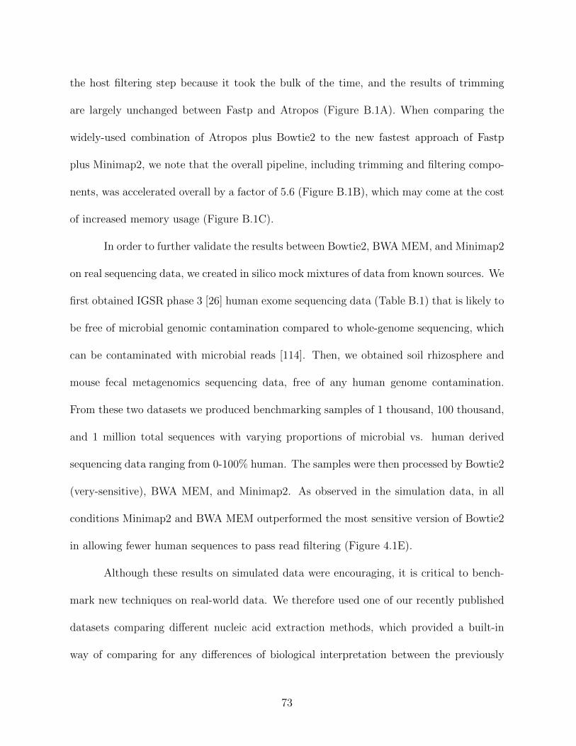
the host filtering step because it took the bulk of the time, and the results of trimming

are largely unchanged between Fastp and Atropos (Figure B.1A). When comparing the

widely-used combination of Atropos plus Bowtie2 to the new fastest approach of Fastp

plus Minimap2, we note that the overall pipeline, including trimming and filtering compo-

nents, was accelerated overall by a factor of 5.6 (Figure B.1B), which may come at the cost

of increased memory usage (Figure B.1C).

In order to further validate the results between Bowtie2, BWAMEM, and Minimap2

on real sequencing data, we created in silico mock mixtures of data from known sources. We

first obtained IGSR phase 3 [26] human exome sequencing data (Table B.1) that is likely to

be free of microbial genomic contamination compared to whole-genome sequencing, which

can be contaminated with microbial reads [114]. Then, we obtained soil rhizosphere and

mouse fecal metagenomics sequencing data, free of any human genome contamination.

From these two datasets we produced benchmarking samples of 1 thousand, 100 thousand,

and 1 million total sequences with varying proportions of microbial vs. human derived

sequencing data ranging from 0-100% human. The samples were then processed by Bowtie2

(very-sensitive), BWA MEM, and Minimap2. As observed in the simulation data, in all

conditions Minimap2 and BWA MEM outperformed the most sensitive version of Bowtie2

in allowing fewer human sequences to pass read filtering (Figure 4.1E).

Although these results on simulated data were encouraging, it is critical to bench-

mark new techniques on real-world data. We therefore used one of our recently published

datasets comparing different nucleic acid extraction methods, which provided a built-in

way of comparing for any differences of biological interpretation between the previously

73

Figure 4.1: Minimap2 provides improved error, sensitivity, and runtime forhost-filtering over the current open-source pipeline. Comparison of aligners forhost-filtering on 1 million CAMI-sim simulated reads by (A) error and (B) human readsfailed to align to the reference (false negative rate). (C) Time and (D) processing ratecomparison across aligners of 1 million, 10 million, and 50 million CAMI-sim simulatedreads. Minimap2 is shown for 100 million and 250 million reads. (E) False negative rateof host filtering on data with real reads combined from separate exome sequencing andnon-human metagenomics studies.

74

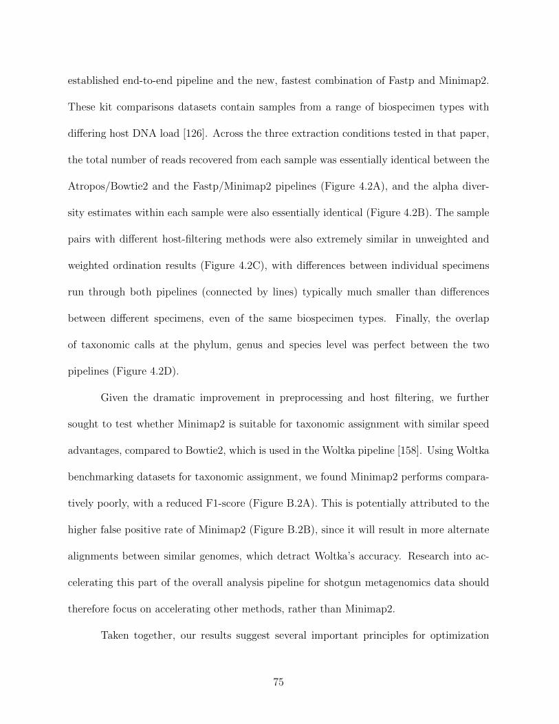
established end-to-end pipeline and the new, fastest combination of Fastp and Minimap2.

These kit comparisons datasets contain samples from a range of biospecimen types with

differing host DNA load [126]. Across the three extraction conditions tested in that paper,

the total number of reads recovered from each sample was essentially identical between the

Atropos/Bowtie2 and the Fastp/Minimap2 pipelines (Figure 4.2A), and the alpha diver-

sity estimates within each sample were also essentially identical (Figure 4.2B). The sample

pairs with different host-filtering methods were also extremely similar in unweighted and

weighted ordination results (Figure 4.2C), with differences between individual specimens

run through both pipelines (connected by lines) typically much smaller than differences

between different specimens, even of the same biospecimen types. Finally, the overlap

of taxonomic calls at the phylum, genus and species level was perfect between the two

pipelines (Figure 4.2D).

Given the dramatic improvement in preprocessing and host filtering, we further

sought to test whether Minimap2 is suitable for taxonomic assignment with similar speed

advantages, compared to Bowtie2, which is used in the Woltka pipeline [158]. Using Woltka

benchmarking datasets for taxonomic assignment, we found Minimap2 performs compara-

tively poorly, with a reduced F1-score (Figure B.2A). This is potentially attributed to the

higher false positive rate of Minimap2 (Figure B.2B), since it will result in more alternate

alignments between similar genomes, which detract Woltka’s accuracy. Research into ac-

celerating this part of the overall analysis pipeline for shotgun metagenomics data should

therefore focus on accelerating other methods, rather than Minimap2.

Taken together, our results suggest several important principles for optimization

75

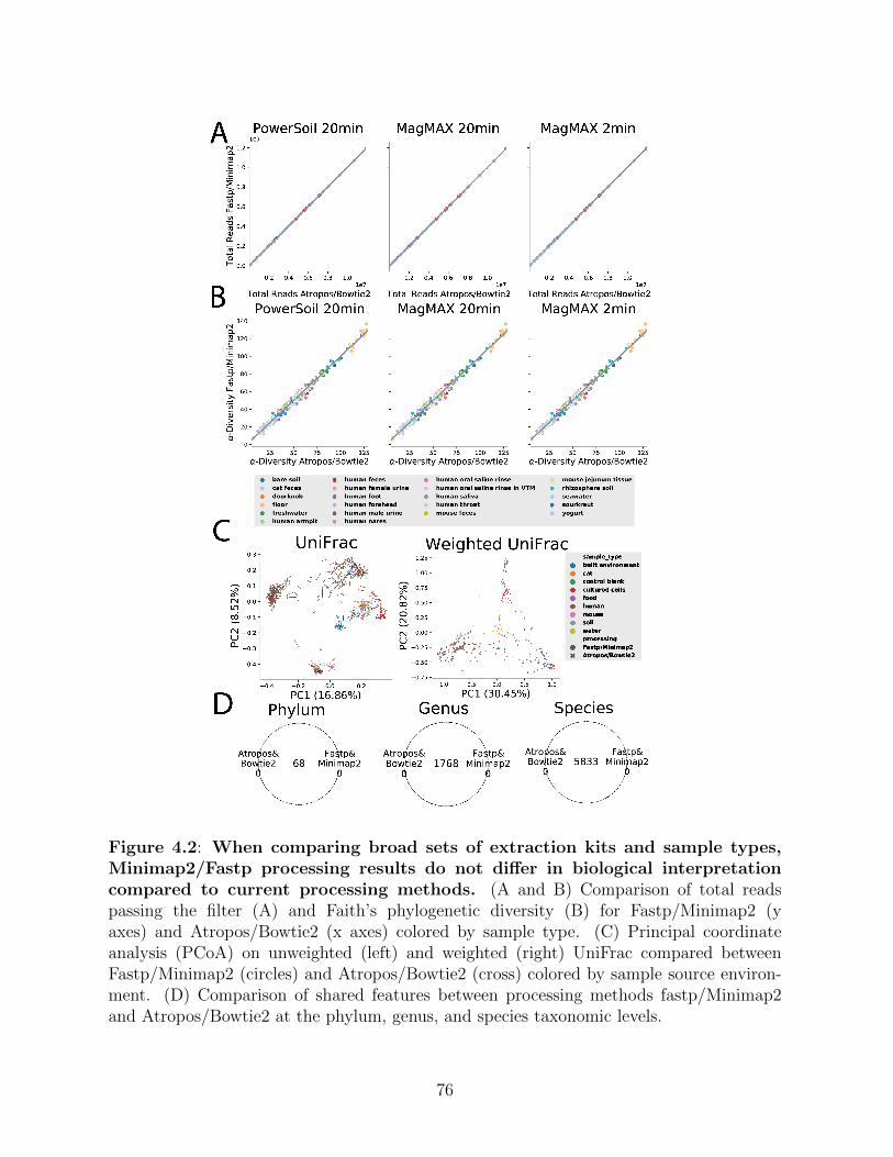
Figure 4.2: When comparing broad sets of extraction kits and sample types,Minimap2/Fastp processing results do not differ in biological interpretationcompared to current processing methods. (A and B) Comparison of total readspassing the filter (A) and Faith’s phylogenetic diversity (B) for Fastp/Minimap2 (yaxes) and Atropos/Bowtie2 (x axes) colored by sample type. (C) Principal coordinateanalysis (PCoA) on unweighted (left) and weighted (right) UniFrac compared betweenFastp/Minimap2 (circles) and Atropos/Bowtie2 (cross) colored by sample source environ-ment. (D) Comparison of shared features between processing methods fastp/Minimap2and Atropos/Bowtie2 at the phylum, genus, and species taxonomic levels.

76

of shotgun metagenomics workflows. First, even widely used pipeline components should

be periodically re-evaluated to test whether more efficient implementations or better al-

gorithms are available and can be substituted with substantial speed improvements. This

benchmarking is facilitated by standardized options and interfaces, and standardized datasets,

and we make the datasets we produced here available for reuse. Second, before investing

substantial effort in developing nonstandard hardware or approaches to accelerate a spe-

cific algorithm, it is worth checking whether a better CPU-based algorithm is available,

and then, if it is, optimizing that other algorithm instead. Finally, caution is warranted

in generalizing which pipeline steps a given algorithm or implementation is used for. Al-

though Minimap2 and Bowtie2 both fundamentally perform the same task (approximate

string match to a database, albeit with different mechanisms), Minimap2’s failure on the

taxonomic assignment task warrants further investigation to test whether the algorithm

could be adapted to this task or whether there are fundamental limitations.

Our current work therefore provides an important practical improvement with a

speedup in common metagenomics preprocessing tasks, which we have already made avail-

able to the community via incorporation into Qiita [44]. Future work will be needed to

assess and adapt alignment-free approaches, which often provide improvements in runtime

over alignment methods, for both host-filtering and taxonomic assignment tasks. These

advancements also point the way towards further optimization that will allow real-time

or near-real-time use of metagenomic and/or metatranscriptomic data in clinical decision

making, where time is often of the essence.

77

4.3 Acknowledgements

This work was supported in part by CRISP, one of six centers in JUMP, a Semicon-

ductor Research Corporation (SRC) program sponsored by DARPA.

https://crisp.engineering.virginia.edu/. J.P.S. was supported by NIH/NIGMS IRACDA

K12 GM068524.

Chapter 4, in full, is a reprint of the material as it appears in “Swapping metage-

nomics preprocessing pipeline components offers speed and sensitivity increases.” George

Armstrong, Cameron Martino, Justin Morris, Behnam Khaleghi, Jaeyoung Kang, Jeff

DeReus, Qiyun Zhu, Daniel Roush, Daniel McDonald, Antonio Gonzalez, Justin Shaffer,

Carolina Carpenter, Mehrbod Estaki, Stephen Wandro, Sean Eilert, Ameen Akel, Justin

Eno, Ken Curewitz, Austin D. Swafford, Niema Moshiri, Tajana Rosing, and Rob Knight.

mSystems e0137821, 2022. The dissertation author was a primary investigator and co-first

author of this paper.

78

Appendix A

Supplemental Material for Chapter 3

Figure A.1: Graphical abstract. UMAP can operate on distance matrices of arbitrarydistance metrics (UniFrac, Bray-Curtis, Aitchison), similarly to PCoA.

79

Figure A.2: Simulated missing data on keyboard study. A proportion of the entriesof the table were randomly masked (20 repetitions per ablation level) from the featuretable, and dimensionality reduction followed by LDA was run on each of the tables. Hostaccuracy is the accuracy for identifying the correct subject. The subject-type accuraciesare specific sample-type accuracies specific to the individual.

80

Figure A.3: Alternative views for PCoA and UMAP comparison on 8,280 sam-ples from the Human Microbiome Project (HMP). (A) PCoA-3 shows separationby primers and (B) some symmetry of sample site by primer. (C) UMAP separates theprimers as well as (D) body sites in only one dimension.

81

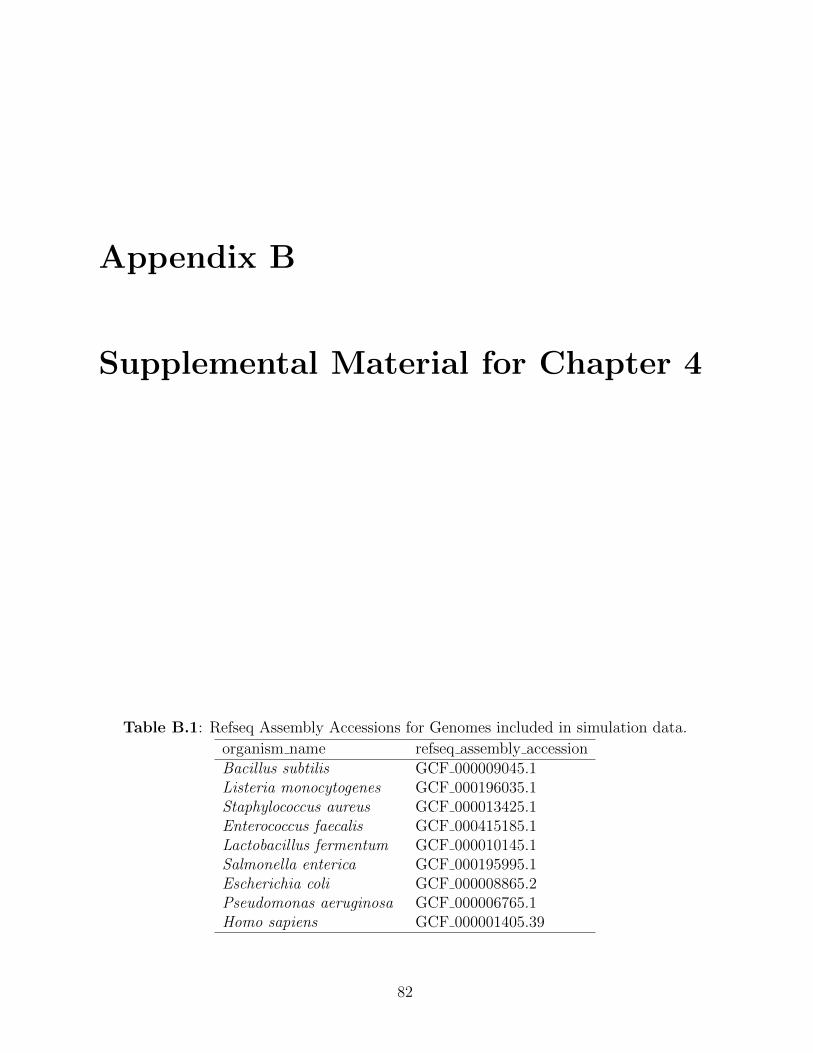
Appendix B

Supplemental Material for Chapter 4

Table B.1: Refseq Assembly Accessions for Genomes included in simulation data.

organism name refseq assembly accessionBacillus subtilis GCF 000009045.1Listeria monocytogenes GCF 000196035.1Staphylococcus aureus GCF 000013425.1Enterococcus faecalis GCF 000415185.1Lactobacillus fermentum GCF 000010145.1Salmonella enterica GCF 000195995.1Escherichia coli GCF 000008865.2Pseudomonas aeruginosa GCF 000006765.1Homo sapiens GCF 000001405.39

82

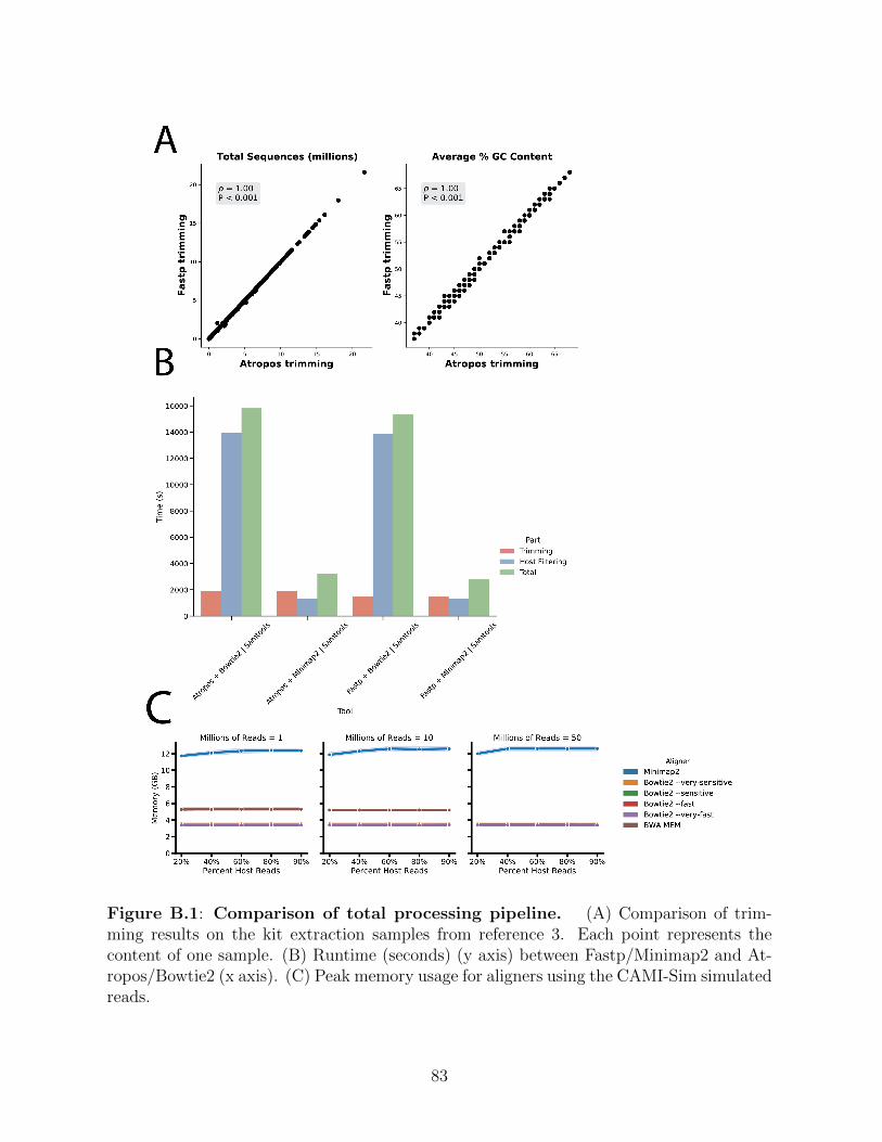
Figure B.1: Comparison of total processing pipeline. (A) Comparison of trim-ming results on the kit extraction samples from reference 3. Each point represents thecontent of one sample. (B) Runtime (seconds) (y axis) between Fastp/Minimap2 and At-ropos/Bowtie2 (x axis). (C) Peak memory usage for aligners using the CAMI-Sim simulatedreads.

83

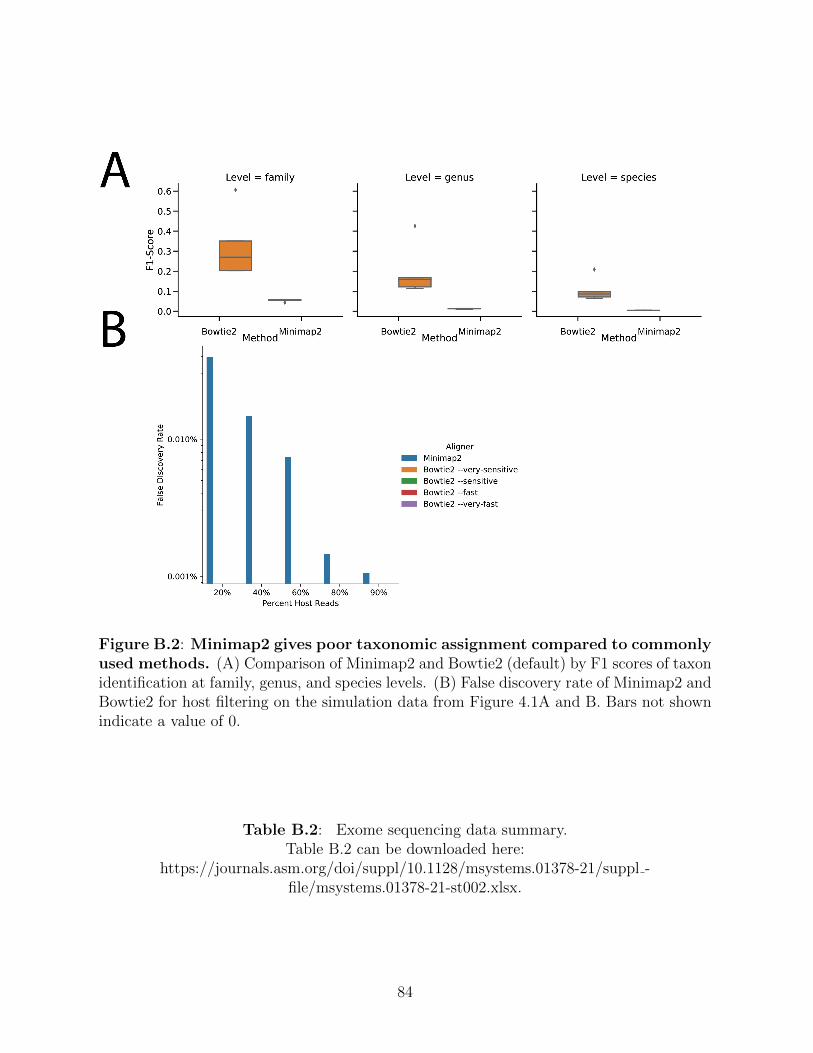
Figure B.2: Minimap2 gives poor taxonomic assignment compared to commonlyused methods. (A) Comparison of Minimap2 and Bowtie2 (default) by F1 scores of taxonidentification at family, genus, and species levels. (B) False discovery rate of Minimap2 andBowtie2 for host filtering on the simulation data from Figure 4.1A and B. Bars not shownindicate a value of 0.

Table B.2: Exome sequencing data summary.Table B.2 can be downloaded here:

https://journals.asm.org/doi/suppl/10.1128/msystems.01378-21/suppl -file/msystems.01378-21-st002.xlsx.

84

Bibliography

[1] J Aitchison. Principal component analysis of compositional data. Biometrika,70(1):57–65, April 1983.

[2] J Aitchison and Michael J Greenacre. Biplots of compositional data. Journal of theRoyal Statistical Society: Series C (Applied Statistics), 51:375–392, 2002.

[3] Celeste Allaband, Daniel McDonald, Yoshiki Vazquez-Baeza, Jeremiah J Minich,Anupriya Tripathi, David A Brenner, Rohit Loomba, Larry Smarr, William J Sand-born, Bernd Schnabl, Pieter Dorrestein, Amir Zarrinpar, and Rob Knight. Micro-biome 101: Studying, analyzing, and interpreting gut microbiome data for clinicians.Clin. Gastroenterol. Hepatol., 17(2):218, January 2019.

[4] Amnon Amir, Daniel McDonald, Jose A Navas-Molina, Evguenia Kopylova, James TMorton, Zhenjiang Zech Xu, Eric P Kightley, Luke R Thompson, Embriette R Hyde,Antonio Gonzalez, and Rob Knight. Deblur rapidly resolves Single-Nucleotide com-munity sequence patterns. mSystems, 2(2), March 2017.

[5] Marti J Anderson. Permutational multivariate analysis of variance (PERMANOVA),2017.

[6] Ann Arfken, Bongkeun Song, Jeff S Bowman, and Michael Piehler. Denitrificationpotential of the eastern oyster microbiome using a 16S rRNA gene based metabolicinference approach. PLoS One, 12(9):e0185071, September 2017.

[7] George Armstrong, Cameron Martino, Gibraan Rahman, Antonio Gonzalez, YoshikiVazquez-Baeza, Gal Mishne, and Rob Knight. Uniform manifold approximation andprojection (UMAP) reveals composite patterns and resolves visualization artifacts inmicrobiome data. mSystems, 6(5):e0069121, October 2021.

[8] Prerna Bali, Joanna Coker, Ivonne Lozano-Pope, Karsten Zengler, and MarygorretObonyo. Microbiome signatures in a fast- and Slow-Progressing gastric cancer murinemodel and their contribution to gastric carcinogenesis, 2021.

[9] Matthew Barker and William Rayens. Partial least squares for discrimination. J.Chemom., 17(3):166–173, March 2003.

85

[10] Etienne Becht, Leland McInnes, John Healy, Charles-Antoine Dutertre, ImmanuelW H Kwok, Lai Guan Ng, Florent Ginhoux, and Evan W Newell. Dimensionalityreduction for visualizing single-cell data using UMAP, 2019.

[11] Mikhail Belkin and P Niyogi. Laplacian eigenmaps and spectral techniques for em-bedding and clustering. In NIPS’01: Proceedings of the 14th International Conferenceon Neural Information Processing Systems: Natural and Synthetic, 2001.

[12] Maria-Soledad Benitez, Shannon L Osborne, and R Michael Lehman. Previous cropand rotation history effects on maize seedling health and associated rhizosphere mi-crobiome. Sci. Rep., 7(1):15709, November 2017.

[13] Evan Bolyen, Jai Ram Rideout, Matthew R Dillon, Nicholas A Bokulich, Chris-tian C Abnet, Gabriel A Al-Ghalith, Harriet Alexander, Eric J Alm, ManimozhiyanArumugam, Francesco Asnicar, Yang Bai, Jordan E Bisanz, Kyle Bittinger, AskerBrejnrod, Colin J Brislawn, C Titus Brown, Benjamin J Callahan, Andres MauricioCaraballo-Rodrıguez, John Chase, Emily K Cope, Ricardo Da Silva, Christian Diener,Pieter C Dorrestein, Gavin M Douglas, Daniel M Durall, Claire Duvallet, Christian FEdwardson, Madeleine Ernst, Mehrbod Estaki, Jennifer Fouquier, Julia M Gauglitz,Sean M Gibbons, Deanna L Gibson, Antonio Gonzalez, Kestrel Gorlick, Jiarong Guo,Benjamin Hillmann, Susan Holmes, Hannes Holste, Curtis Huttenhower, Gavin AHuttley, Stefan Janssen, Alan K Jarmusch, Lingjing Jiang, Benjamin D Kaehler,Kyo Bin Kang, Christopher R Keefe, Paul Keim, Scott T Kelley, Dan Knights, IrinaKoester, Tomasz Kosciolek, Jorden Kreps, Morgan G I Langille, Joslynn Lee, RuthLey, Yong-Xin Liu, Erikka Loftfield, Catherine Lozupone, Massoud Maher, ClarisseMarotz, Bryan D Martin, Daniel McDonald, Lauren J McIver, Alexey V Melnik,Jessica L Metcalf, Sydney C Morgan, Jamie T Morton, Ahmad Turan Naimey,Jose A Navas-Molina, Louis Felix Nothias, Stephanie B Orchanian, Talima Pear-son, Samuel L Peoples, Daniel Petras, Mary Lai Preuss, Elmar Pruesse, Lasse BuurRasmussen, Adam Rivers, Michael S Robeson, 2nd, Patrick Rosenthal, Nicola Segata,Michael Shaffer, Arron Shiffer, Rashmi Sinha, Se Jin Song, John R Spear, Austin DSwafford, Luke R Thompson, Pedro J Torres, Pauline Trinh, Anupriya Tripathi,Peter J Turnbaugh, Sabah Ul-Hasan, Justin J J van der Hooft, Fernando Vargas,Yoshiki Vazquez-Baeza, Emily Vogtmann, Max von Hippel, William Walters, YunhuWan, Mingxun Wang, Jonathan Warren, Kyle C Weber, Charles H D Williamson,Amy D Willis, Zhenjiang Zech Xu, Jesse R Zaneveld, Yilong Zhang, Qiyun Zhu, RobKnight, and J Gregory Caporaso. Reproducible, interactive, scalable and extensiblemicrobiome data science using QIIME 2. Nat. Biotechnol., 37(8):852–857, August2019.

[14] Katja Borodulin, Hanna Tolonen, Pekka Jousilahti, Antti Jula, Anne Juolevi, SeppoKoskinen, Kari Kuulasmaa, Tiina Laatikainen, Satu Mannisto, Markku Peltonen,Markus Perola, Pekka Puska, Veikko Salomaa, Jouko Sundvall, Suvi M Virtanen, andErkki Vartiainen. Cohort profile: The national FINRISK study. Int. J. Epidemiol.,47(3):696–696i, November 2017.

86

[15] Katja Borodulin, Erkki Vartiainen, Markku Peltonen, Pekka Jousilahti, Anne Juolevi,Tiina Laatikainen, Satu Mannisto, Veikko Salomaa, Jouko Sundvall, and PekkaPuska. Forty-year trends in cardiovascular risk factors in finland. Eur. J. PublicHealth, 25(3):539–546, June 2015.

[16] J Roger Bray, J Roger Bray, and J T Curtis. An ordination of the upland forestcommunities of southern wisconsin, 1957.

[17] Benjamin J Callahan, Paul J McMurdie, and Susan P Holmes. Exact sequencevariants should replace operational taxonomic units in marker-gene data analysis.ISME J., 11(12):2639–2643, July 2017.

[18] Tayte P Campbell, Xiaoqing Sun, Vishal H Patel, Crickette Sanz, David Morgan,and Gautam Dantas. The microbiome and resistome of chimpanzees, gorillas, andhumans across host lifestyle and geography. ISME J., 14(6):1584–1599, March 2020.

[19] Kalen Cantrell, Marcus W Fedarko, Gibraan Rahman, Daniel McDonald, YimengYang, Thant Zaw, Antonio Gonzalez, Stefan Janssen, Mehrbod Estaki, Niina Haimi-nen, Kristen L Beck, Qiyun Zhu, Erfan Sayyari, James T Morton, George Arm-strong, Anupriya Tripathi, Julia M Gauglitz, Clarisse Marotz, Nathaniel L Matte-son, Cameron Martino, Jon G Sanders, Anna Paola Carrieri, Se Jin Song, Austin DSwafford, Pieter C Dorrestein, Kristian G Andersen, Laxmi Parida, Ho-Cheol Kim,Yoshiki Vazquez-Baeza, and Rob Knight. EMPress enables Tree-Guided, interactive,and exploratory analyses of multi-omic data sets. mSystems, 6(2), March 2021.

[20] J Gregory Caporaso, Christian L Lauber, William A Walters, Donna Berg-Lyons,Catherine A Lozupone, Peter J Turnbaugh, Noah Fierer, and Rob Knight. Globalpatterns of 16S rRNA diversity at a depth of millions of sequences per sample. Proc.Natl. Acad. Sci. U. S. A., 108 Suppl 1:4516–4522, March 2011.

[21] Natalia Castano-Rodrıguez, Khean-Lee Goh, Kwong Ming Fock, Hazel M Mitchell,and Nadeem O Kaakoush. Dysbiosis of the microbiome in gastric carcinogenesis,2017.

[22] Qin Chang, Yihui Luan, and Fengzhu Sun. Variance adjusted weighted UniFrac:a powerful beta diversity measure for comparing communities based on phylogeny.BMC Bioinformatics, 12:118, April 2011.

[23] Jun Chen, Kyle Bittinger, Emily S Charlson, Christian Hoffmann, James Lewis,Gary D Wu, Ronald G Collman, Frederic D Bushman, and Hongzhe Li. Associatingmicrobiome composition with environmental covariates using generalized UniFracdistances. Bioinformatics, 28(16):2106–2113, August 2012.

[24] Shifu Chen, Yanqing Zhou, Yaru Chen, and Jia Gu. fastp: an ultra-fast all-in-oneFASTQ preprocessor. Bioinformatics, 34(17):i884–i890, September 2018.

87

[25] K R Clarke and M Ainsworth. A method of linking multivariate community structureto environmental variables, 1993.

[26] Laura Clarke, Susan Fairley, Xiangqun Zheng-Bradley, Ian Streeter, Emily Perry,Ernesto Lowy, Anne-Marie Tasse, and Paul Flicek. The international genome sampleresource (IGSR): A worldwide collection of genome variation incorporating the 1000genomes project data. Nucleic Acids Res., 45(D1):D854–D859, January 2017.

[27] Joshimar Cordova and Gonzalo Navarro. Simple and efficient fully-functional succincttrees, 2016.

[28] Taraprasad Das, Rajagopalaboopathi Jayasudha, Samakalyana Chakravarthy,Gumpili Sai Prashanthi, Archana Bhargava, Mudit Tyagi, Padmaja Kumari Rani,Rajeev Reddy Pappuru, Savitri Sharma, and Sisinthy Shivaji. Alterations in the gutbacterial microbiome in people with type 2 diabetes mellitus and diabetic retinopathy.Sci. Rep., 11(1):2738, February 2021.

[29] Lawrence A David, Corinne F Maurice, Rachel N Carmody, David B Gootenberg,Julie E Button, Benjamin E Wolfe, Alisha V Ling, A Sloan Devlin, Yug Varma,Michael A Fischbach, Sudha B Biddinger, Rachel J Dutton, and Peter J Turn-baugh. Diet rapidly and reproducibly alters the human gut microbiome. Nature,505(7484):559–563, December 2013.

[30] Jacobo de la Cuesta-Zuluaga, Scott T Kelley, Yingfeng Chen, Juan S Escobar, Noel TMueller, Ruth E Ley, Daniel McDonald, Shi Huang, Austin D Swafford, Rob Knight,and Varykina G Thackray. Age- and Sex-Dependent patterns of gut microbial diver-sity in human adults. mSystems, 4(4), July 2019.

[31] Justine Debelius, Se Jin Song, Yoshiki Vazquez-Baeza, Zhenjiang Zech Xu, AntonioGonzalez, and Rob Knight. Tiny microbes, enormous impacts: what matters in gutmicrobiome studies? Genome Biol., 17(1):217, October 2016.

[32] Persi Diaconis, Sharad Goel, and Susan Holmes. Horseshoes in multidimensionalscaling and local kernel methods, 2008.

[33] John P Didion, Marcel Martin, and Francis S Collins. Atropos: specific, sensitive,and speedy trimming of sequencing reads. PeerJ, 5:e3720, August 2017.

[34] Ener C Dinleyici, Daniel Martınez-Martınez, Ates Kara, Adem Karbuz, Nazan Dalgic,Ozge Metin, Ahmet S Yazar, Sirin Guven, Zafer Kurugol, Ozden Turel, MehmetKucukkoc, Olcay Yasa, Makbule Eren, Metehan Ozen, Jose Manuel Martı, CarlosP Garay, Yvan Vandenplas, and Andres Moya. Time series analysis of the microbiotaof children suffering from acute infectious diarrhea and their recovery after treatment.Front. Microbiol., 9:1230, June 2018.

[35] Daniel P Faith. Conservation evaluation and phylogenetic diversity. Biol. Conserv.,61(1):1–10, 1992.

88

[36] Marcus W Fedarko, Cameron Martino, James T Morton, Antonio Gonzalez, GibraanRahman, Clarisse A Marotz, Jeremiah J Minich, Eric E Allen, and Rob Knight. Vi-sualizing ’omic feature rankings and log-ratios using qurro. NAR Genom Bioinform,2(2), April 2020.

[37] Noah Fierer, Christian L Lauber, Nick Zhou, Daniel McDonald, Elizabeth K Costello,and Rob Knight. Forensic identification using skin bacterial communities. Proc. Natl.Acad. Sci. U. S. A., 107(14):6477–6481, April 2010.

[38] Adrian Fritz, Peter Hofmann, Stephan Majda, Eik Dahms, Johannes Droge, Jes-sika Fiedler, Till R Lesker, Peter Belmann, Matthew Z DeMaere, Aaron E Darling,Alexander Sczyrba, Andreas Bremges, and Alice C McHardy. CAMISIM: simulatingmetagenomes and microbial communities. Microbiome, 7(1):17, February 2019.

[39] Jessica Galloway-Pena and Blake Hanson. Tools for analysis of the microbiome, 2020.

[40] K N Galvao, C H Higgins, M Zinicola, S J Jeon, H Korzec, and R C abstract =Bicalho. Effect of pegbovigrastim administration on the microbiome found in thevagina of cows postpartum.

[41] Dirk Gevers, Subra Kugathasan, Lee A Denson, Yoshiki Vazquez-Baeza, WillVan Treuren, Boyu Ren, Emma Schwager, Dan Knights, Se Jin Song, Moran Yas-sour, Xochitl C Morgan, Aleksandar D Kostic, Chengwei Luo, Antonio Gonzalez,Daniel McDonald, Yael Haberman, ThomasWalters, Susan Baker, Joel Rosh, MichaelStephens, Melvin Heyman, James Markowitz, Robert Baldassano, Anne Griffiths,Francisco Sylvester, David Mack, Sandra Kim, Wallace Crandall, Jeffrey Hyams,Curtis Huttenhower, Rob Knight, and Ramnik J Xavier. The treatment-naive mi-crobiome in new-onset crohn’s disease. Cell Host Microbe, 15(3):382–392, March2014.

[42] James L Ginter and Robert M Thorndike. Correlational procedures for research,1979.

[43] Oleg V Goloshchapov, Evgenii I Olekhnovich, Sergey V Sidorenko, Ivan S Moiseev,Maxim A Kucher, Dmitry E Fedorov, Alexander V Pavlenko, Alexander I Manolov,Vladimir V Gostev, Vladimir A Veselovsky, Ksenia M Klimina, Elena S Kostryukova,Evgeny A Bakin, Alexander N Shvetcov, Elvira D Gumbatova, Ruslana V Kle-menteva, Alexander A Shcherbakov, Margarita V Gorchakova, Juan Jose Egozcue,Vera Pawlowsky-Glahn, Maria A Suvorova, Alexey B Chukhlovin, Vadim M Govorun,Elena N Ilina, and Boris V Afanasyev. Long-term impact of fecal transplantation inhealthy volunteers. BMC Microbiol., 19(1):312, December 2019.

[44] Antonio Gonzalez, Jose A Navas-Molina, Tomasz Kosciolek, Daniel McDonald,Yoshiki Vazquez-Baeza, Gail Ackermann, Jeff DeReus, Stefan Janssen, Austin DSwafford, Stephanie B Orchanian, Jon G Sanders, Joshua Shorenstein, Hannes Hol-ste, Semar Petrus, Adam Robbins-Pianka, Colin J Brislawn, Mingxun Wang, Jai Ram

89

Rideout, Evan Bolyen, Matthew Dillon, J Gregory Caporaso, Pieter C Dorrestein,and Rob Knight. Qiita: rapid, web-enabled microbiome meta-analysis. Nat. Methods,15(10):796–798, October 2018.

[45] P Greig-Smith. The development of numerical classification and ordination. Vegetatio,42(1):1–9, October 1980.

[46] Bjorn Gruning, The Bioconda Team, Ryan Dale, Andreas Sjodin, Brad A Chapman,Jillian Rowe, Christopher H Tomkins-Tinch, Renan Valieris, and Johannes Koster.Bioconda: sustainable and comprehensive software distribution for the life sciences,2018.

[47] Saransh Gupta, Mohsen Imani, Behnam Khaleghi, Venkatesh Kumar, and TajanaRosing. RAPID: A ReRAM processing in-memory architecture for DNA sequencealignment. In 2019 IEEE/ACM International Symposium on Low Power Electronicsand Design (ISLPED). IEEE, July 2019.

[48] Jonas Halfvarson, Colin J Brislawn, Regina Lamendella, Yoshiki Vazquez-Baeza,William A Walters, Lisa M Bramer, Mauro D’Amato, Ferdinando Bonfiglio, DanielMcDonald, Antonio Gonzalez, Erin E McClure, Mitchell F Dunklebarger, RobKnight, and Janet K Jansson. Dynamics of the human gut microbiome in inflamma-tory bowel disease. Nat Microbiol, 2:17004, February 2017.

[49] Micah Hamady and Rob Knight. Microbial community profiling for human micro-biome projects: Tools, techniques, and challenges. Genome Res., 19(7):1141–1152,July 2009.

[50] Micah Hamady, Catherine Lozupone, and Rob Knight. Fast UniFrac: facilitatinghigh-throughput phylogenetic analyses of microbial communities including analysisof pyrosequencing and PhyloChip data. ISME J., 4(1):17–27, January 2010.

[51] Yuhan Hao, Stephanie Hao, Erica Andersen-Nissen, William MMauck, Shiwei Zheng,Andrew Butler, Maddie J Lee, Aaron J Wilk, Charlotte Darby, Michael Zagar, PaulHoffman, Marlon Stoeckius, Efthymia Papalexi, Eleni P Mimitou, Jaison Jain, AviSrivastava, Tim Stuart, Lamar B Fleming, Bertrand Yeung, Angela J Rogers, Ju-liana M McElrath, Catherine A Blish, Raphael Gottardo, Peter Smibert, and RahulSatija. Integrated analysis of multimodal single-cell data. October 2020.

[52] Charles R Harris, K Jarrod Millman, Stefan J van der Walt, Ralf Gommers, PauliVirtanen, David Cournapeau, Eric Wieser, Julian Taylor, Sebastian Berg, Nathaniel JSmith, Robert Kern, Matti Picus, Stephan Hoyer, Marten H van Kerkwijk, MatthewBrett, Allan Haldane, Jaime Fernandez Del Rıo, Mark Wiebe, Pearu Peterson, PierreGerard-Marchant, Kevin Sheppard, Tyler Reddy, Warren Weckesser, Hameer Abbasi,Christoph Gohlke, and Travis E Oliphant. Array programming with NumPy. Nature,585(7825):357–362, September 2020.

90

[53] Benjamin Hillmann, Gabriel A Al-Ghalith, Robin R Shields-Cutler, Qiyun Zhu,Daryl M Gohl, Kenneth B Beckman, Rob Knight, and Dan Knights. Evaluatingthe information content of shallow shotgun metagenomics. mSystems, 3(6), Novem-ber 2018.

[54] S Huang, N Haiminen, A P Carrieri, R Hu, L Jiang, L Parida, B Russell, C Allaband,A Zarrinpar, Y Vazquez-Baeza, P Belda-Ferre, H Zhou, H C Kim, A D Swafford,R Knight, and Z Z Xu. Human skin, oral, and gut microbiomes predict chronologicalage. mSystems, 5(1), February 2020.

[55] Weichun Huang, Leping Li, Jason R Myers, and Gabor T Marth. ART: a next-generation sequencing read simulator. Bioinformatics, 28(4):593–594, February 2012.

[56] Anna Cacilia Ingham, Katrine Kielsen, Malene Skovsted Cilieborg, Ole Lund, Su-san Holmes, Frank M Aarestrup, Klaus Gottlob Muller, and Sunje Johanna Pamp.Specific gut microbiome members are associated with distinct immune markers inpediatric allogeneic hematopoietic stem cell transplantation. Microbiome, 7(1):131,September 2019.

[57] Paul Jaccard. THE DISTRIBUTION OF THE FLORA IN THE ALPINE ZONE.New Phytologist, 11(2):37–50, 1912.

[58] Ian B Jeffery, Denise B Lynch, and Paul W O’Toole. Composition and temporalstability of the gut microbiota in older persons. ISME J., 10(1):170–182, January2016.

[59] Abigail J Johnson, Pajau Vangay, Gabriel A Al-Ghalith, Benjamin M Hillmann,Tonya L Ward, Robin R Shields-Cutler, Austin D Kim, Anna KonstantinovnaShmagel, Arzang N Syed, Jens Walter, Ravi Menon, Katie Koecher, and Dan Knights.Daily sampling reveals personalized Diet-Microbiome associations in humans. CellHost Microbe, 25(6):789–802.e5, June 2019.

[60] Robert C Kaplan, Zheng Wang, Mykhaylo Usyk, Daniela Sotres-Alvarez, Martha LDaviglus, Neil Schneiderman, Gregory A Talavera, Marc D Gellman, Bharat Thya-garajan, Jee-Young Moon, Yoshiki Vazquez-Baeza, Daniel McDonald, Jessica SWilliams-Nguyen, Michael C Wu, Kari E North, Justin Shaffer, Christopher C Sol-lecito, Qibin Qi, Carmen R Isasi, Tao Wang, Rob Knight, and Robert D Burk. Gutmicrobiome composition in the hispanic community health Study/Study of latinos isshaped by geographic relocation, environmental factors, and obesity. Genome Biol.,20(1):1–21, November 2019.

[61] K P Keegan, E M Glass, and F Meyer. MG-RAST, a metagenomics service foranalysis of microbial community structure and function. Methods Mol. Biol., 1399,2016.

91

[62] Dmitry Kobak and Philipp Berens. The art of using t-SNE for single-cell transcrip-tomics. Nat. Commun., 10(1):5416, November 2019.

[63] Dmitry Kobak and George C Linderman. Initialization is critical for preserving globaldata structure in both t-SNE and UMAP. Nat. Biotechnol., 39(2):156–157, February2021.

[64] Dhruv Kohli, Alex Cloninger, and Gal Mishne. LDLE: Low distortion local eigen-maps. J. Mach. Learn. Res., 2021.

[65] J B Kruskal. Multidimensional scaling by optimizing goodness of fit to a nonmetrichypothesis, 1964.

[66] Joseph Kruskal and Myron Wish. Multidimensional scaling. SAGE Publications,1978.

[67] Justin Kuczynski, Christian L Lauber, William A Walters, Laura Wegener Parfrey,Jose C Clemente, Dirk Gevers, and Rob Knight. Experimental and analytical toolsfor studying the human microbiome. Nat. Rev. Genet., 13(1):47–58, December 2011.

[68] Justin Kuczynski, Zongzhi Liu, Catherine Lozupone, Daniel McDonald, Noah Fierer,and Rob Knight. Microbial community resemblance methods differ in their ability todetect biologically relevant patterns. Nat. Methods, 7(10):813, October 2010.

[69] M Senthil Kumar, Eric V Slud, Kwame Okrah, Stephanie C Hicks, Sridhar Hannen-halli, and Hector Corrada Bravo. Analysis and correction of compositional bias insparse sequencing count data. BMC Genomics, 19(1):799, November 2018.

[70] David Lahnemann, Johannes Koster, Ewa Szczurek, Davis J McCarthy, Stephanie CHicks, Mark D Robinson, Catalina A Vallejos, Kieran R Campbell, Niko Beeren-winkel, Ahmed Mahfouz, Luca Pinello, Pavel Skums, Alexandros Stamatakis, CamilleStephan-Otto Attolini, Samuel Aparicio, Jasmijn Baaijens, Marleen Balvert, Buys deBarbanson, Antonio Cappuccio, Giacomo Corleone, Bas E Dutilh, Maria Florescu,Victor Guryev, Rens Holmer, Katharina Jahn, Thamar Jessurun Lobo, Emma MKeizer, Indu Khatri, Szymon M Kielbasa, Jan O Korbel, Alexey M Kozlov, Tzu-HaoKuo, Boudewijn P F Lelieveldt, Ion I Mandoiu, John C Marioni, Tobias Marschall,Felix Molder, Amir Niknejad, Lukasz Raczkowski, Marcel Reinders, Jeroen de Ridder,Antoine-Emmanuel Saliba, Antonios Somarakis, Oliver Stegle, Fabian J Theis, HuanYang, Alex Zelikovsky, Alice C McHardy, Benjamin J Raphael, Sohrab P Shah, andAlexander Schonhuth. Eleven grand challenges in single-cell data science. GenomeBiol., 21(1):1–35, February 2020.

[71] Jennifer M Lang, Calvin Pan, Rita M Cantor, W H Wilson Tang, Jose Carlos Garcia-Garcia, Ira Kurtz, Stanley L Hazen, Nathalie Bergeron, Ronald M Krauss, and Al-dons J Lusis. Impact of individual traits, saturated fat, and protein source on thegut microbiome. MBio, 9(6), December 2018.

92

[72] Ben Langmead and Steven L Salzberg. Fast gapped-read alignment with bowtie 2.Nat. Methods, 9(4):357–359, March 2012.

[73] Loıc Lannelongue, Jason Grealey, and Michael Inouye. Green algorithms: Quantify-ing the carbon footprint of computation. Advanced Science, 2100707, 2021.

[74] Christian L Lauber, Micah Hamady, Rob Knight, and Noah Fierer. Pyrosequencing-Based assessment of soil ph as a predictor of soil bacterial community structure atthe continental scale. Applied and Environmental Microbiology, 75(15):5111–5120,2009.

[75] D D Lee and H S Seung. Learning the parts of objects by non-negative matrixfactorization. Nature, 401(6755):788–791, October 1999.

[76] Ruth E Ley, Catherine A Lozupone, Micah Hamady, Rob Knight, and Jeffrey IGordon. Worlds within worlds: evolution of the vertebrate gut microbiota. Nat. Rev.Microbiol., 6(10):776–788, October 2008.

[77] Heng Li. Aligning sequence reads, clone sequences and assembly contigs with BWA-MEM. March 2013.

[78] Heng Li. Minimap2: pairwise alignment for nucleotide sequences. Bioinformatics,34(18):3094–3100, September 2018.

[79] Huang Lin and Shyamal Das Peddada. Analysis of microbial compositions: a reviewof normalization and differential abundance analysis. NPJ Biofilms Microbiomes,6(1):60, December 2020.

[80] George C Linderman, Manas Rachh, Jeremy G Hoskins, Stefan Steinerberger, andYuval Kluger. Fast interpolation-based t-SNE for improved visualization of single-cellRNA-seq data. Nat. Methods, 16(3):243–245, February 2019.

[81] Veronica Llorens-Rico, Ann C Gregory, Johan Van Weyenbergh, Sander Jansen, TinaVan Buyten, Junbin Qian, Marcos Braz, Soraya Maria Menezes, Pierre Van Mol, LoreVanderbeke, Christophe Dooms, Jan Gunst, Greet Hermans, Philippe Meersseman,Els Wauters, Johan Neyts, Diether Lambrechts, Joost Wauters, and Jeroen Raes.Clinical practices underlie COVID-19 patient respiratory microbiome compositionand its interactions with the host. Nat. Commun., 12(1):1–12, October 2021.

[82] Catherine Lozupone and Rob Knight. UniFrac: a new phylogenetic method forcomparing microbial communities. Appl. Environ. Microbiol., 71(12):8228–8235, De-cember 2005.

[83] Catherine A Lozupone, Micah Hamady, Scott T Kelley, and Rob Knight. Quantitativeand qualitative beta diversity measures lead to different insights into factors thatstructure microbial communities. Appl. Environ. Microbiol., 73(5):1576–1585, March2007.

93

[84] Catherine A Lozupone and Rob Knight. Global patterns in bacterial diversity. Proc.Natl. Acad. Sci. U. S. A., 104(27):11436–11440, July 2007.

[85] Lucie A Malard, Muhammad Z Anwar, Carsten S Jacobsen, and David A Pearce.Biogeographical patterns in soil bacterial communities across the arctic region. FEMSMicrobiol. Ecol., 95(9), September 2019.

[86] Siddhartha Mandal, Will Van Treuren, Richard A White, Merete Eggesbø, RobKnight, and Shyamal D Peddada. Analysis of composition of microbiomes: a novelmethod for studying microbial composition. Microb. Ecol. Health Dis., 26:27663, May2015.

[87] Clarisse A Marotz, Jon G Sanders, Cristal Zuniga, Livia S Zaramela, Rob Knight,and Karsten Zengler. Improving saliva shotgun metagenomics by chemical host DNAdepletion. Microbiome, 6(1):42, February 2018.

[88] Ian P G Marshall, Ge Ren, Marion Jaussi, Bente Aa Lomstein, Bo Barker Jørgensen,Hans Røy, and Kasper U Kjeldsen. Environmental filtering determines family-levelstructure of sulfate-reducing microbial communities in subsurface marine sediments.ISME J., 13(8):1920–1932, August 2019.

[89] J A Martın-Fernandez, C Barcelo-Vidal, and V Pawlowsky-Glahn. Dealing with zerosand missing values in compositional data sets using nonparametric imputation. Math.Geol., 35(3):253–278, April 2003.

[90] Cameron Martino, James T Morton, Clarisse A Marotz, Luke R Thompson, AnupriyaTripathi, Rob Knight, and Karsten Zengler. A novel sparse compositional techniquereveals microbial perturbations. mSystems, 4(1), January 2019.

[91] Cameron Martino, Liat Shenhav, Clarisse A Marotz, George Armstrong, Daniel Mc-Donald, Yoshiki Vazquez-Baeza, James T Morton, Lingjing Jiang, Maria GloriaDominguez-Bello, Austin D Swafford, Eran Halperin, and Rob Knight. Context-aware dimensionality reduction deconvolutes gut microbial community dynamics.Nat. Biotechnol., 39(2):165–168, February 2021.

[92] Daniel McDonald, Jose C Clemente, Justin Kuczynski, Jai Ram Rideout, JesseStombaugh, Doug Wendel, Andreas Wilke, Susan Huse, John Hufnagle, Folker Meyer,Rob Knight, and J Gregory Caporaso. The biological observation matrix (BIOM)format or: how I learned to stop worrying and love the ome-ome. Gigascience, 1(1),July 2012.

[93] Daniel McDonald, Embriette Hyde, Justine W Debelius, James T Morton, AntonioGonzalez, Gail Ackermann, Alexander A Aksenov, Bahar Behsaz, Caitriona Bren-nan, Yingfeng Chen, Lindsay DeRight Goldasich, Pieter C Dorrestein, Robert RDunn, Ashkaan K Fahimipour, James Gaffney, Jack A Gilbert, Grant Gogul, Jes-sica L Green, Philip Hugenholtz, Greg Humphrey, Curtis Huttenhower, Matthew A

94

Jackson, Stefan Janssen, Dilip V Jeste, Lingjing Jiang, Scott T Kelley, Dan Knights,Tomasz Kosciolek, Joshua Ladau, Jeff Leach, Clarisse Marotz, Dmitry Meleshko,Alexey V Melnik, Jessica L Metcalf, Hosein Mohimani, Emmanuel Montassier, JoseNavas-Molina, Tanya T Nguyen, Shyamal Peddada, Pavel Pevzner, Katherine S Pol-lard, Gholamali Rahnavard, Adam Robbins-Pianka, Naseer Sangwan, Joshua Shoren-stein, Larry Smarr, Se Jin Song, Timothy Spector, Austin D Swafford, Varykina GThackray, Luke R Thompson, Anupriya Tripathi, Yoshiki Vazquez-Baeza, Alison Vr-banac, Paul Wischmeyer, Elaine Wolfe, Qiyun Zhu, American Gut Consortium, andRob Knight. American gut: an open platform for citizen science microbiome research.mSystems, 3(3), May 2018.

[94] Daniel McDonald, Benjamin Kaehler, Antonio Gonzalez, Jeff DeReus, Gail Acker-mann, Clarisse Marotz, Gavin Huttley, and Rob Knight. redbiom: a rapid samplediscovery and feature characterization system. mSystems, 4(4), June 2019.

[95] Daniel McDonald, Morgan N Price, Julia Goodrich, Eric P Nawrocki, Todd Z De-Santis, Alexander Probst, Gary L Andersen, Rob Knight, and Philip Hugenholtz. Animproved greengenes taxonomy with explicit ranks for ecological and evolutionaryanalyses of bacteria and archaea. ISME J., 6(3):610–618, March 2012.

[96] Daniel McDonald, Yoshiki Vazquez-Baeza, David Koslicki, Jason McClelland, NicolaiReeve, Zhenjiang Xu, Antonio Gonzalez, and Rob Knight. Striped UniFrac: enablingmicrobiome analysis at unprecedented scale. Nat. Methods, 15(11):847–848, Novem-ber 2018.

[97] Leland McInnes, John Healy, and James Melville. UMAP: Uniform manifold approx-imation and projection for dimension reduction. February 2018.

[98] Lauren J McIver, Galeb Abu-Ali, Eric A Franzosa, Randall Schwager, Xochitl C Mor-gan, Levi Waldron, Nicola Segata, and Curtis Huttenhower. biobakery: a meta’omicanalysis environment. Bioinformatics, 34(7):1235–1237, April 2018.

[99] Paul J McMurdie and Susan Holmes. phyloseq: an R package for reproducible in-teractive analysis and graphics of microbiome census data. PLoS One, 8(4):e61217,April 2013.

[100] Jessica L Metcalf, Se Jin Song, James T Morton, Sophie Weiss, Andaine Seguin-Orlando, Frederic Joly, Claudia Feh, Pierre Taberlet, Eric Coissac, Amnon Amir,Eske Willerslev, Rob Knight, Valerie McKenzie, and Ludovic Orlando. Evaluatingthe impact of domestication and captivity on the horse gut microbiome. Sci. Rep.,7(1):15497, November 2017.

[101] Jessica L Metcalf, Zhenjiang Zech Xu, Sophie Weiss, Simon Lax, Will Van Treuren,Embriette R Hyde, Se Jin Song, Amnon Amir, Peter Larsen, Naseer Sangwan,Daniel Haarmann, Greg C Humphrey, Gail Ackermann, Luke R Thompson, Chris-tian Lauber, Alexander Bibat, Catherine Nicholas, Matthew J Gebert, Joseph F

95

Petrosino, Sasha C Reed, Jack A Gilbert, Aaron M Lynne, Sibyl R Bucheli, David OCarter, and Rob Knight. Microbial community assembly and metabolic function dur-ing mammalian corpse decomposition. Science, 351(6269):158–162, January 2016.

[102] S Mirarab, N Nguyen, and T Warnow. SEPP: SATe-enabled phylogenetic placement.Pac. Symp. Biocomput., pages 247–258, 2012.

[103] James T Morton, Clarisse Marotz, Alex Washburne, Justin Silverman, Livia SZaramela, Anna Edlund, Karsten Zengler, and Rob Knight. Establishing microbialcomposition measurement standards with reference frames. Nat. Commun., 10(1):1–11, June 2019.

[104] James T Morton, Liam Toran, Anna Edlund, Jessica L Metcalf, Christian Lauber,and Rob Knight. Uncovering the horseshoe effect in microbial analyses. mSystems,2(1), January 2017.

[105] Jennifer Ocasio, Benjamin Babcock, Daniel Malawsky, Seth J Weir, Lipin Loo,Jeremy M Simon, Mark J Zylka, Duhyeong Hwang, Taylor Dismuke, Marina Sokol-sky, Elias P Rosen, Rajeev Vibhakar, Jiao Zhang, Olivier Saulnier, Maria Vladoiu,Ibrahim El-Hamamy, Lincoln D Stein, Michael D Taylor, Kyle S Smith, Paul ANorthcott, Alejandro Colaneri, Kirk Wilhelmsen, and Timothy R Gershon. scRNA-seq in medulloblastoma shows cellular heterogeneity and lineage expansion supportresistance to SHH inhibitor therapy. Nat. Commun., 10(1):1–17, December 2019.

[106] O Paliy and V Shankar. Application of multivariate statistical techniques in microbialecology. Mol. Ecol., 25(5):1032–1057, March 2016.

[107] Prince Kofi Parbie, Taketoshi Mizutani, Aya Ishizaka, Ai Kawana-Tachikawa,Lucky Ronald Runtuwene, Sayuri Seki, Christopher Zaab-Yen Abana, Dennis Kushi-tor, Evelyn Yayra Bonney, Sampson Badu Ofori, Satoshi Uematsu, Seiya Imoto,Yasumasa Kimura, Hiroshi Kiyono, Koichi Ishikawa, William Kwabena Ampofo, andTetsuro Matano. Dysbiotic fecal microbiome in HIV-1 infected individuals in ghana.Front. Cell. Infect. Microbiol., 11:646467, May 2021.

[108] Donovan H Parks, Maria Chuvochina, Pierre-Alain Chaumeil, Christian Rinke,Aaron J Mussig, and Philip Hugenholtz. A complete domain-to-species taxonomyfor bacteria and archaea. Nat. Biotechnol., 38(9):1079–1086, April 2020.

[109] Donovan H Parks, Maria Chuvochina, David W Waite, Christian Rinke, AdamSkarshewski, Pierre-Alain Chaumeil, and Philip Hugenholtz. A standardized bac-terial taxonomy based on genome phylogeny substantially revises the tree of life.Nat. Biotechnol., 36(10):996–1004, November 2018.

[110] Vera Pawlowsky-Glahn and Antonella Buccianti. Compositional Data Analysis: The-ory and Applications. John Wiley & Sons, September 2011.

96

[111] Juan E Perez-Jaramillo, Vıctor J Carrion, Mirte Bosse, Luiz F V Ferrao, Mattiasde Hollander, Antonio A F Garcia, Camilo A Ramırez, Rodrigo Mendes, and Jos MRaaijmakers. Linking rhizosphere microbiome composition of wild and domesticatedphaseolus vulgaris to genotypic and root phenotypic traits. ISME J., 11(10):2244–2257, October 2017.

[112] Evelyn Chrystalla Pielou. The measurement of diversity in different types of biologicalcollections. J. Theor. Biol., 13:131–144, December 1966.

[113] J Podani and I Miklos. Resemblance coefficients and the horseshoe effect in principalcoordinates analysis, 2002.

[114] Gregory D Poore, Evguenia Kopylova, Qiyun Zhu, Carolina Carpenter, SerenaFraraccio, Stephen Wandro, Tomasz Kosciolek, Stefan Janssen, Jessica Metcalf,Se Jin Song, Jad Kanbar, Sandrine Miller-Montgomery, Robert Heaton, Rana Mckay,Sandip Pravin Patel, Austin D Swafford, and Rob Knight. Microbiome analyses ofblood and tissues suggest cancer diagnostic approach. Nature, 579(7800):567–574,March 2020.

[115] Catherine Potvin and Derek A Roff. Distribution-Free and robust statistical methods:Viable alternatives to parametric statistics, 1993.

[116] Maria E Ramos-Nino, Daniel M Fitzpatrick, Scott Tighe, Korin M Eckstrom, Lind-sey M Hattaway, Andy N Hsueh, Diana M Stone, Julie Dragon, and Sonia Cheetham.High prevalence of phasi charoen-like virus from wild-caught aedes aegypti in grenada,W.I. as revealed by metagenomic analysis, 2020.

[117] Boyu Ren, Sergio Bacallado, Stefano Favaro, Susan Holmes, and Lorenzo Trippa.Bayesian nonparametric ordination for the analysis of microbial communities. J.Am. Stat. Assoc., 112(520):1430–1442, February 2017.

[118] S T Roweis and L K Saul. Nonlinear dimensionality reduction by locally linearembedding. Science, 290(5500), December 2000.

[119] Daniel Ruiz-Perez, Haibin Guan, Purnima Madhivanan, Kalai Mathee, and GiriNarasimhan. So you think you can PLS-DA? BMC Bioinformatics, 21(1):1–10,December 2020.

[120] Aaro Salosensaari, Ville Laitinen, Aki Havulinna, Guillaume Meric, Susan Cheng,Markus Perola, Liisa Valsta, Georg Alfthan, Michael Inouye, Jeramie D Watrous, TaoLong, Rodolfo Salido, Karenina Sanders, Caitriona Brennan, Gregory C Humphrey,Jon G Sanders, Mohit Jain, Pekka Jousilahti, Veikko Salomaa, Rob Knight, LeoLahti, and Teemu Niiranen. Taxonomic signatures of Long-Term mortality risk inhuman gut microbiota. medRxiv, page 2019.12.30.19015842, January 2020.

97

[121] Aaro Salosensaari, Ville Laitinen, Aki S Havulinna, Guillaume Meric, Susan Cheng,Markus Perola, Liisa Valsta, Georg Alfthan, Michael Inouye, Jeramie D Watrous, TaoLong, Rodolfo A Salido, Karenina Sanders, Caitriona Brennan, Gregory C Humphrey,Jon G Sanders, Mohit Jain, Pekka Jousilahti, Veikko Salomaa, Rob Knight, Leo Lahti,and Teemu Niiranen. Taxonomic signatures of cause-specific mortality risk in humangut microbiome. Nat. Commun., 12(1):2671, May 2021.

[122] Edans Flavius de Oliveira Sandes, Guillermo Miranda, Xavier Martorell, EduardAyguade, George Teodoro, and Alba Cristina Magalhaes Melo. CUDAlign 4.0: Incre-mental speculative traceback for exact Chromosome-Wide alignment in GPU clusters.IEEE Transactions on Parallel and Distributed Systems, 27(10):2838–2850, 2016.

[123] Patrick D Schloss, Sarah L Westcott, Thomas Ryabin, Justine R Hall, Martin Hart-mann, Emily B Hollister, Ryan A Lesniewski, Brian B Oakley, Donovan H Parks,Courtney J Robinson, Jason W Sahl, Blaz Stres, Gerhard G Thallinger, David JVan Horn, and Carolyn F Weber. Introducing mothur: open-source, platform-independent, community-supported software for describing and comparing microbialcommunities. Appl. Environ. Microbiol., 75(23):7537–7541, December 2009.

[124] Bernhard Scholkopf, Alexander Smola, and Klaus-Robert Muller. Kernel principalcomponent analysis. In ADVANCES IN KERNEL METHODS - SUPPORT VEC-TOR LEARNING, 1999.

[125] Alexander Sczyrba, Peter Hofmann, Peter Belmann, David Koslicki, Stefan Janssen,Johannes Droge, Ivan Gregor, Stephan Majda, Jessika Fiedler, Eik Dahms, AndreasBremges, Adrian Fritz, Ruben Garrido-Oter, Tue Sparholt Jørgensen, Nicole Shapiro,Philip D Blood, Alexey Gurevich, Yang Bai, Dmitrij Turaev, Matthew Z DeMaere,Rayan Chikhi, Niranjan Nagarajan, Christopher Quince, Fernando Meyer, MonikaBalvociute, Lars Hestbjerg Hansen, Søren J Sørensen, Burton K H Chia, Bertrand De-nis, Jeff L Froula, Zhong Wang, Robert Egan, Dongwan Don Kang, Jeffrey J Cook,Charles Deltel, Michael Beckstette, Claire Lemaitre, Pierre Peterlongo, GuillaumeRizk, Dominique Lavenier, Yu-Wei Wu, Steven W Singer, Chirag Jain, Marc Strous,Heiner Klingenberg, Peter Meinicke, Michael D Barton, Thomas Lingner, Hsin-HungLin, Yu-Chieh Liao, Genivaldo Gueiros Z Silva, Daniel A Cuevas, Robert A Ed-wards, Surya Saha, Vitor C Piro, Bernhard Y Renard, Mihai Pop, Hans-Peter Klenk,Markus Goker, Nikos C Kyrpides, Tanja Woyke, Julia A Vorholt, Paul Schulze-Lefert,Edward M Rubin, Aaron E Darling, Thomas Rattei, and Alice C McHardy. Criti-cal assessment of metagenome interpretation-a benchmark of metagenomics software.Nat. Methods, 14(11):1063–1071, November 2017.

[126] Justin P Shaffer, Clarisse Marotz, Pedro Belda-Ferre, Cameron Martino, StephenWandro, Mehrbod Estaki, Rodolfo A Salido, Carolina S Carpenter, Livia S Zaramela,Jeremiah J Minich, Mackenzie Bryant, Karenina Sanders, Serena Fraraccio, Gail Ack-ermann, Gregory Humphrey, Austin D Swafford, Sandrine Miller-Montgomery, and

98

Rob Knight. A comparison of DNA/RNA extraction protocols for high-throughputsequencing of microbial communities. Biotechniques, 70(3):149–159, March 2021.

[127] Hurmat Ali Shah, Laiq Hasan, and Nasir Ahmad. An optimized and low-cost FPGA-based DNA sequence alignment–a step towards personal genomics. Conf. Proc. IEEEEng. Med. Biol. Soc., 2013:2696–2699, 2013.

[128] Shabnam Shalapour, Xue-Jia Lin, Ingmar N Bastian, John Brain, Alastair D Burt,Alexander A Aksenov, Alison F Vrbanac, Weihua Li, Andres Perkins, Takaji Matsu-tani, Zhenyu Zhong, Debanjan Dhar, Jose A Navas-Molina, Jun Xu, Rohit Loomba,Michael Downes, Ruth T Yu, Ronald M Evans, Pieter C Dorrestein, Rob Knight,Christopher Benner, Quentin M Anstee, and Michael Karin. Inflammation-inducedIgA+ cells dismantle anti-liver cancer immunity. Nature, 551(7680):340–345, Novem-ber 2017.

[129] V Shankar, R Agans, and O Paliy. Advantages of phylogenetic distance based con-strained ordination analyses for the examination of microbial communities. Sci. Rep.,7(1):6481, July 2017.

[130] Yushu Shi, Liangliang Zhang, Christine Peterson, Kim-Anh Do, and Robert Jenq.Performance determinants of unsupervised clustering methods for microbiome data.2021.

[131] Justin D Silverman, Kimberly Roche, Sayan Mukherjee, and Lawrence A David.Naught all zeros in sequence count data are the same. Comput. Struct. Biotechnol.J., 18:2789–2798, January 2020.

[132] Se Jin Song, Amnon Amir, Jessica L Metcalf, Katherine R Amato, Zhenjiang ZechXu, Greg Humphrey, and Rob Knight. Preservation methods differ in fecal micro-biome stability, affecting suitability for field studies. mSystems, 1(3), May 2016.

[133] Se Jin Song, Jincheng Wang, Cameron Martino, Lingjing Jiang, Wesley K Thompson,Liat Shenhav, Daniel McDonald, Clarisse Marotz, Paul R Harris, Caroll D Hernan-dez, Nora Henderson, Elizabeth Ackley, Deanna Nardella, Charles Gillihan, ValentinaMontacuti, William Schweizer, Melanie Jay, Joan Combellick, Haipeng Sun, Iza-skun Garcia-Mantrana, Fernando Gil Raga, Maria Carmen Collado, Juana I Rivera-Vinas, Maribel Campos-Rivera, Jean F Ruiz-Calderon, Rob Knight, and Maria Glo-ria Dominguez-Bello. Naturalization of the microbiota developmental trajectory ofcesarean-born neonates after vaginal seeding, 2021.

[134] Felipe F C Souza, Prince P Mathai, Theotonio Pauliquevis, Eduardo Balsanelli,Fabio O Pedrosa, Emanuel M Souza, Valter A Baura, Rose A Monteiro, Leonardo MCruz, Rodrigo A F Souza, Meinrat O Andreae, Cybelli G G Barbosa, Isabella Hrabede Angelis, Beatriz Sanchez-Parra, Christopher Phlker, Bettina Weber, Emil Ruff,Rodrigo A Reis, Ricardo H M Godoi, Michael J Sadowsky, and Luciano F Huergo.

99

Influence of seasonality on the aerosol microbiome of the amazon rainforest. Sci.Total Environ., 760:144092, March 2021.

[135] Shinichi Sunagawa, Luis Pedro Coelho, Samuel Chaffron, Jens Roat Kultima, KarineLabadie, Guillem Salazar, Bardya Djahanschiri, Georg Zeller, Daniel R Mende,Adriana Alberti, Francisco M Cornejo-Castillo, Paul I Costea, Corinne Cruaud,Francesco d’Ovidio, Stefan Engelen, Isabel Ferrera, Josep M Gasol, Lionel Guidi,Falk Hildebrand, Florian Kokoszka, Cyrille Lepoivre, Gipsi Lima-Mendez, JuliePoulain, Bonnie T Poulos, Marta Royo-Llonch, Hugo Sarmento, Sara Vieira-Silva,Celine Dimier, Marc Picheral, Sarah Searson, Stefanie Kandels-Lewis, Tara Oceanscoordinators, Chris Bowler, Colomban de Vargas, Gabriel Gorsky, Nigel Grimsley,Pascal Hingamp, Daniele Iudicone, Olivier Jaillon, Fabrice Not, Hiroyuki Ogata,Stephane Pesant, Sabrina Speich, Lars Stemmann, Matthew B Sullivan, Jean Weis-senbach, Patrick Wincker, Eric Karsenti, Jeroen Raes, Silvia G Acinas, and PeerBork. Ocean plankton. structure and function of the global ocean microbiome. Sci-ence, 348(6237):1261359, May 2015.

[136] S Taavitsainen, N Engedal, S Cao, F Handle, A Erickson, S Prekovic, D Wetterskog,T Tolonen, E M Vuorinen, A Kiviaho, R Natkin, T Hakkinen, W Devlies, S Hentti-nen, R Kaarijarvi, M Lahnalampi, H Kaljunen, K Nowakowska, H Syvala, M Blauer,P Cremaschi, F Claessens, T Visakorpi, T L J Tammela, T Murtola, K J Granberg,A D Lamb, K Ketola, I G Mills, G Attard, W Wang, M Nykter, and A Urbanucci.Single-cell ATAC and RNA sequencing reveal pre-existing and persistent cells asso-ciated with prostate cancer relapse. Nat. Commun., 12(1):1–16, September 2021.

[137] Barbara G Tabachnick and Linda S Fidell. Using Multivariate Statistics. 2013.

[138] J B Tenenbaum, V de Silva, and J C Langford. A global geometric framework fornonlinear dimensionality reduction. Science, 290(5500), December 2000.

[139] C J F ter Braak. Canonical Correspondence Analysis: A New Eigenvector Techniquefor Multivariate Direct Gradient Analysis. 1985.

[140] The Human Microbiome Project Consortium. Structure, function and diversity ofthe healthy human microbiome. Nature, 486(7402):207–214, June 2012.

[141] Luke R Thompson, Jon G Sanders, Daniel McDonald, Amnon Amir, Joshua Ladau,Kenneth J Locey, Robert J Prill, Anupriya Tripathi, Sean M Gibbons, Gail Acker-mann, Jose A Navas-Molina, Stefan Janssen, Evguenia Kopylova, Yoshiki Vazquez-Baeza, Antonio Gonzalez, James T Morton, Siavash Mirarab, Zhenjiang Zech Xu,Lingjing Jiang, Mohamed F Haroon, Jad Kanbar, Qiyun Zhu, Se Jin Song, TomaszKosciolek, Nicholas A Bokulich, Joshua Lefler, Colin J Brislawn, Gregory Humphrey,Sarah M Owens, Jarrad Hampton-Marcell, Donna Berg-Lyons, Valerie McKenzie,Noah Fierer, Jed A Fuhrman, Aaron Clauset, Rick L Stevens, Ashley Shade, Kather-ine S Pollard, Kelly D Goodwin, Janet K Jansson, Jack A Gilbert, Rob Knight,

100

and Earth Microbiome Project Consortium. A communal catalogue reveals earth’smultiscale microbial diversity. Nature, 551(7681):457–463, November 2017.

[142] Anupriya Tripathi, Yoshiki Vazquez-Baeza, Julia M Gauglitz, Mingxun Wang, KaiDuhrkop, Melissa Nothias-Esposito, Deepa D Acharya, Madeleine Ernst, Justin J Jvan der Hooft, Qiyun Zhu, Daniel McDonald, Asker D Brejnrod, Antonio Gonzalez,Jo Handelsman, Markus Fleischauer, Marcus Ludwig, Sebastian Bocker, Louis-FelixNothias, Rob Knight, and Pieter C Dorrestein. Chemically informed analyses ofmetabolomics mass spectrometry data with qemistree. Nat. Chem. Biol., 17(2):146–151, February 2021.

[143] Peter J Turnbaugh, Ruth E Ley, Micah Hamady, Claire M Fraser-Liggett,Rob Knight, and Jeffrey I Gordon. The human microbiome project. Nature,449(7164):804–810, October 2007.

[144] Laurens van der Maaten and Geoffrey Hinton. Visualizing data using t-SNE. J.Mach. Learn. Res., 9(86):2579–2605, 2008.

[145] Pajau Vangay, Abigail J Johnson, Tonya L Ward, Gabriel A Al-Ghalith, Robin RShields-Cutler, Benjamin M Hillmann, Sarah K Lucas, Lalit K Beura, Emily AThompson, Lisa M Till, Rodolfo Batres, Bwei Paw, Shannon L Pergament, Pim-panitta Saenyakul, Mary Xiong, Austin D Kim, Grant Kim, David Masopust, Eric CMartens, Chaisiri Angkurawaranon, Rose McGready, Purna C Kashyap, Kathleen ACulhane-Pera, and Dan Knights. US immigration westernizes the human gut micro-biome. Cell, 175(4):962–972.e10, November 2018.

[146] Leena Chennuru Vankadara and Ulrike von Luxburg. Measures of distortion formachine learning. Adv. Neural Inf. Process. Syst., 31, 2018.

[147] Yoshiki Vazquez-Baeza, Antonio Gonzalez, Larry Smarr, Daniel McDonald, James TMorton, Jose A Navas-Molina, and Rob Knight. Bringing the dynamic microbiometo life with animations. Cell Host Microbe, 21(1):7–10, January 2017.

[148] Yoshiki Vazquez-Baeza, Embriette R Hyde, Jan S Suchodolski, and Rob Knight. Dogand human inflammatory bowel disease rely on overlapping yet distinct dysbiosisnetworks, 2016.

[149] Martin Wattenberg, Fernanda Viegas, and Ian Johnson. How to use t-SNE effectively.Distill, 1(10):e2, October 2016.

[150] Sophie Weiss, Zhenjiang Zech Xu, Shyamal Peddada, Amnon Amir, Kyle Bittinger,Antonio Gonzalez, Catherine Lozupone, Jesse R Zaneveld, Yoshiki Vazquez-Baeza,Amanda Birmingham, Embriette R Hyde, and Rob Knight. Normalization and micro-bial differential abundance strategies depend upon data characteristics. Microbiome,5(1):1–18, March 2017.

101

[151] Ruth G Wong, Jia R Wu, and Gregory B Gloor. Expanding the UniFrac toolbox.PLoS One, 11(9):e0161196, September 2016.

[152] Gary D Wu, Jun Chen, Christian Hoffmann, Kyle Bittinger, Ying-Yu Chen, Sue AKeilbaugh, Meenakshi Bewtra, Dan Knights, William A Walters, Rob Knight, RohiniSinha, Erin Gilroy, Kernika Gupta, Robert Baldassano, Lisa Nessel, Hongzhe Li,Frederic D Bushman, and James D Lewis. Linking Long-Term dietary patterns withgut microbial enterotypes. Science, 334(6052):105, October 2011.

[153] Tianchen Xu, Ryan T Demmer, and Gen Li. Zero-inflated poisson factor model withapplication to microbiome read counts. Biometrics, 77(1):91–101, March 2021.

[154] Xueli Xu, Zhongming Xie, Zhenyu Yang, Dongfang Li, and Ximing Xu. A t-SNEbased classification approach to compositional microbiome data. Front. Genet.,11:620143, December 2020.

[155] Tanya Yatsunenko, Federico E Rey, Mark J Manary, Indi Trehan, Maria GloriaDominguez-Bello, Monica Contreras, Magda Magris, Glida Hidalgo, Robert N Bal-dassano, Andrey P Anokhin, Andrew C Heath, Barbara Warner, Jens Reeder, JustinKuczynski, J Gregory Caporaso, Catherine A Lozupone, Christian Lauber, Jose Car-los Clemente, Dan Knights, Rob Knight, and Jeffrey I Gordon. Human gut micro-biome viewed across age and geography. Nature, 486(7402):222–227, May 2012.

[156] Caroline Young, Henry M Wood, Ramakrishnan Ayloor Seshadri, Pham Van Nang,Carlos Vaccaro, Luis Contreras Melendez, Mayilvahanan Bose, Mai Van Doi,Tamara Alejandra Pinero, Camilo Tapia Valladares, Julieta Arguero, Alba FuentesBalaguer, Kelsey N Thompson, Yan Yan, Curtis Huttenhower, and Philip Quirke.The colorectal cancer-associated faecal microbiome of developing countries resemblesthat of developed countries. Genome Med., 13(1):1–13, February 2021.

[157] Nicholas D Youngblut, Georg H Reischer, William Walters, Nathalie Schuster, ChrisWalzer, Gabrielle Stalder, Ruth E Ley, and Andreas H Farnleitner. Host diet andevolutionary history explain different aspects of gut microbiome diversity among ver-tebrate clades. Nat. Commun., 10(1):2200, May 2019.

[158] Qiyun Zhu, Shi Huang, Antonio Gonzalez, Imran McGrath, Daniel McDonald, NiinaHaiminen, George Armstrong, Yoshiki Vazquez-Baeza, Julian Yu, Justin Kuczynski,Gregory D Sepich-Poore, Austin D Swafford, Promi Das, Justin P Shaffer, FranckLejzerowicz, Pedro Belda-Ferre, Aki S Havulinna, Guillaume Meric, Teemu Niiranen,Leo Lahti, Veikko Salomaa, Ho-Cheol Kim, Mohit Jain, Michael Inouye, Jack AGilbert, and Rob Knight. OGUs enable effective, phylogeny-aware analysis of evenshallow metagenome community structures. April 2021.

[159] Qiyun Zhu, Uyen Mai, Wayne Pfeiffer, Stefan Janssen, Francesco Asnicar, Jon GSanders, Pedro Belda-Ferre, Gabriel A Al-Ghalith, Evguenia Kopylova, Daniel Mc-Donald, Tomasz Kosciolek, John B Yin, Shi Huang, Nimaichand Salam, Jian-Yu Jiao,

102

Zijun Wu, Zhenjiang Z Xu, Kalen Cantrell, Yimeng Yang, Erfan Sayyari, MaryamRabiee, James T Morton, Sheila Podell, Dan Knights, Wen-Jun Li, Curtis Hutten-hower, Nicola Segata, Larry Smarr, Siavash Mirarab, and Rob Knight. Phylogenomicsof 10,575 genomes reveals evolutionary proximity between domains bacteria and ar-chaea. Nat. Commun., 10(1):5477, December 2019.

103