University and labour market outcomes: what matters? The case of Italy? Daniël Van Nijlen and Béatrice d’Hombres EUR 23081 EN - 2008

Welcome message from author
This document is posted to help you gain knowledge. Please leave a comment to let me know what you think about it! Share it to your friends and learn new things together.
Transcript

University and labour market outcomes what matters
The case of Italy
Danieumll Van Nijlen and Beacuteatrice drsquoHombres
EUR 23081 EN - 2008
The Institute for the Protection and Security of the Citizen provides research-based systems-oriented support to EU policies so as to protect the citizen against economic and technological risk The Institute maintains and develops its expertise and networks in information communication space and engineering technologies in support of its mission The strong cross-fertilisation between its nuclear and non-nuclear activities strengthens the expertise it can bring to the benefit of customers in both domains European Commission Joint Research Centre Institute for the Protection and Security of the Citizen Centre for Research on Lifelong Learning (CRELL) Contact information Address Danieumll Van Nijlen Centre for Educational Effectiveness and Evaluation Dekenstraat 2 3000 Leuven Belgium E-mail danielvannijlenpedkuleuvenbe Tel +32 16326096 Fax +32 16325790 httpipscjrceceuropaeu httpwwwjrceceuropaeu Legal Notice Neither the European Commission nor any person acting on behalf of the Commission is responsible for the use which might be made of this publication
Europe Direct is a service to help you find answers to your questions about the European Union
Freephone number ()
00 800 6 7 8 9 10 11
() Certain mobile telephone operators do not allow access to 00 800 numbers or these calls may be billed
A great deal of additional information on the European Union is available on the Internet It can be accessed through the Europa server httpeuropaeu JRC 40877 EUR 23081 EN ISBN 978-92-79-08177-4 ISSN 1018-5593 DOI 10278861327 Luxembourg Office for Official Publications of the European Communities copy European Communities 2008 Reproduction is authorised provided the source is acknowledged Printed in Italy
1
Table of contents Introduction 3 Purpose of the study 4 Theoretical background 5
Performance indicators in (higher) education 5 Research on labor market outcomes and (higher) education 7 Context Italian university structure 8
Data 8 The ISTAT-survey 8 Sample 8
Method 9 Variables 10
Dependent variables 10 Explanatory variables 10 Educational background respondent 11 Labor background respondent 11 Demographic variables 11 Family background 11
Results employment status 12 Sample 12 Educational background respondent 12 Labor background respondent 14 Demographic variables 14 Family background 15 Field of study 16 Multinomial logistic model 17 Empty model identifying the variance components 18 Taking into account field of study 18 Explaining the variance region 19 Explaining the variance respondent characteristics 20 Educational background respondent 20 Labor background respondent 22 Demographic variables 22
2
Family background 23 Field of study 24
Results wages 27 Sample 27 Descriptive statistics 28 Empty model identifying the variance components 28 Educational background respondent 29 Labor background respondent 30 Demographic variables 30 Family background 31 Field of study 32 Taking into account field of study 34 Explaining the variance respondent characteristics 34 Educational background respondent 36 Labor background respondent 37 Demographic variables 38 Family background 39 Fields of study 40
Discussion 43 Employment status 43 Wages 44 Conclusions 44
3
Introduction
One of the major elements coloring European higher education was the Bologna process that was
initiated in the Bologna declaration of June 1999 and currently instigates higher education reform
in 45 European countries The Bologna process aims to create a European Higher Education Area
by 2010 by implementing reforms that harmonize higher education within Europe (Eurydice
2007) By means of these reforms it is aimed to create a more competitive and more attractive
higher education across Europe The key elements of the Bologna process are the adoption of a
common university system of degrees based on three cycles the promotion of mobility by
implementing the lsquoDiploma Supplementrsquo and establishing a credit transfer system and finally
the favoring of European cooperation in quality assurance to facilitate the comparison of
qualifications across Europe To evaluate the progress of these reforms and to support quality
assurance it is crucial to think about and discuss the features of a valid evaluation system
Currently several national and international evaluation systems for higher education institutions
exist in the form of rankings Well-known and often cited are two international rankings the
Academic ranking of World Universities (ARWU) from Shanghairsquos Jiao Tong University
released for the first time in 2003 (last ranking in February 2007) and the World University
Ranking (WUR) from the Times Higher Education Supplement (THES) first released in 2004 (last
ranking in 2006)
In the ARWU universities are ranked in accordance to their academic and research performances
using as criteria the number of Nobel laureates highly cited researchers articles published in
Nature and Science articles in Science Citation Index (SCI)-expanded and Social Science
Citation Index (SSCI) and a composite indicator of academic performance normalized by the size
of the institution In the THES World University Ranking (WUR) the opinion of scientists and
international employers plays a crucial role Around 3700 researchers and employers are asked to
indicate the best universities This ldquopeer reviewrdquo counts for 50 in the total score of a university
In addition the following other criteria are used research impact in terms of citations per faculty
member staffstudent ratio percentage of students and staff recruited internationally
However these international rankings are often criticized because of the sole focus on academic
research output thus ignoring eg non-publicized output and labor market output for the students
The applied approach also disadvantages universities that are more oriented towards social
sciences and humanities and universities from non-English speaking countries
4
Some national examples of higher education quality evaluation systems can be found across
Europe In Germany the lsquoCentrum fuumlr Hogschulentwicklungrsquo (CHE) (wwwchede) makes a
ranking of more than 280 higher education institutions in Germany Austria and Switzerland
Austrian universities are included in the ranking in 2004 and Swiss universities are included in
2005 (German-speaking universities) This ranking does not provide an overall ranking but a
detailed analysis the ranking deliberately chooses not to add the different aspects of the survey
together to produce an overall score Instead of league positions for the individual universities
league groups are reported Universities are placed into one of three groups Top Group Middle
Group or Bottom Group The provided ranking is subject-specific Aggregation at the level of
whole universities offers no useful information as a decision-making aid for prospective students
who want to study a specific subject In the future the applied methodology will be extended to
the Netherlands and Flanders in a CHE-pilot project (November 2007)
In Italy the newspaper La Repubblica started in 2000 with the publication of performance-based
league tables of universities by field of study These rankings are based on raw data from a
number of sources including the Italian National Statistical Office (ISTAT) and the Ministry of
Education University and Research (MURST) The criteria used for these tables refer to different
aspects of university quality (research outcomes student participation student progression and
achievement teaching and the degree of internationalization) but labor market performance of
the graduates is not included as a criterion Moreover these league tables contain lsquogrossrsquo
performance indicators implying that they do not take into account eg the selective inflow of
students and researchers into the university
Purpose of the study
The current paper aims to elaborate on and contribute to the development of valid evaluation
systems for higher education institutions while focusing on the labor market opportunities of the
graduates As a case study data regarding the labor market position of Italian university graduates
will be investigated
Labor market is a crucial aspect in the evaluation of performance of higher education institutions
In their discussion on the use of statistics and indicators to evaluate universities in Europe
Trinczek and West (1999) point to the increasing importance of the education-employment
relationship in the evaluation of higher education To justify the public expenditure on higher
education one expects the system to produce qualifications that are relevant for the labor market
Also if the labor market opportunities of graduates from different universities differ significantly
5
this might indicate to different quality of the courses offered at the universities However one
should be aware that this kind of differences might also merely indicate a different perceived
reputation of the universities by the employers Finally studentsrsquo choices can benefit from
information about the labor market opportunities and introducing market principles can increase
the competition amongst universities and hopefully increase quality of the provided education
Theoretical background
A first part of this section discusses the use of performance indicators in education This will
point to certain caveats with regard to this use caveats that in the remainder of the paper will be
taken into account The second part of this section more specifically will focus on the link
between education and labor market performance Finally the specific context of the Italian
university structure will be introduced
Performance indicators in (higher) education
Following Goldstein and Spiegelhalter (1996) a performance indicator can be defined as a
ldquosummary statistical measurement on an institution or system which is intended to be related to
the lsquoqualityrsquo of its functioningrdquo (p385) An institution or system can refer to any type of
structure but in the current context will refer to schools or higher educational institutions cq
universities
The introduction of performance indicators in education but in other fields as well can be seen to
serve three general goals (Goldstein amp Myers 1996 Marshall Shekelle Leatherman amp Brook
2000 Rowe 2000 Visscher Karsten de Jong amp Bosker 2000) A first goal is public
accountability of the educational institutions for their performance The two other goals relate to
creating a quasi-market situation in education The use of performance indicators as a second
goal allows consumers (parents or students) to make an informed choice about where to
lsquopurchasersquo education A third goal is to influence through a market-like mechanism the
behaviour of the providing institution and hence the quality of the provided product cq
education Pugh Coates and Adnett (2005) point to a fourth goal being to inform policy makers
on elements like budget allocations and policy initiatives (see eg Jongbloed amp Vossensteyn
2001 for a discussion of the degree of performance based university funding in 11 OECD-
countries)
A very crude use of performance indicators are the so-called lsquoleague tablesrsquo in which institutions
are listed based on raw unadjusted data However there is a general consensus that institutions
6
cannot be held responsible for elements influencing their performance that are beyond their
control and thus that rankings based on raw unadjusted data are not desirable This means that
certain factors should be taken into account before any meaningful comparison can be made
results need to be contextualized
Together with their introduction the use of performance indicators has always been controversial
and a source for debate (eg Jones 2000) In this debate some limitations of the use of
performance indicators arise and next to the intended effects as mentioned above some
unintended effects surface when performance indicators are applied (Visscher et al 2000) One
general criticism was expressed by Goldstein and Myers (1996) pointing to the general
misconception that the use of any information on performance is often perceived to be better than
no information However it is crucial to be aware of the problems that can be related to the
presentation of the information the limitations and the risks involved One should be aware of the
implications of providing the information and should avoid misinterpretations by carefully
pointing to caveats We will now more specifically discuss some of the risks and limitations
related to the use of performance indicators
If the applied methodology or the data used are fundamentally flawed institutional damage can
be caused by incorrect inferences about the performance Moreover inevitably if rankings are
made adjusted or not there will be lsquowinnersrsquo and lsquolosersrsquo A process of lsquonaming and shamingrsquo
might be triggered reinforcing and enhancing the resulting ranking of institutions and making it
very difficult for the lsquolosersrsquo to improve their position and performance (Rowe 2000) Among the
unintended effects are also a focus of the educational institutions on the educational aspects that
are captured by the performance indicators and consequently possible neglect of other aspects
Certain limitations can be considered to be inherent to the use of performance indicators
(Goldstein amp Myers 1996) First of all results are always based on the performance of a prior
group of students and thus it might be possible that the current state of the educational institution
might be different from the reported one Second the statistical procedures used (ie for the
adjustments for background characteristics) only deliver estimates within a certain margin of
error As a result there is always some uncertainty about the exact position of the institution
Finally there might be relevant external factors that are not taken into account when estimating
the performances The absence of these factors will distort the estimation and the comparisons
being made
Because of these limitations of and risks to the use of performance indicators some principles
should be applied in presenting the results on performance indicators (Goldstein amp Myers 1996
7
Rowe 2000) The first principle is that of contextualization Fair comparisons can only be made
if the appropriate adjustments are made for externalcontextual factors (eg characteristics of the
inflowing students) A second principle pertains to the inherent uncertainty of the results There is
a need for interval estimation for the results in which this uncertainty is explicitly displayed
Thirdly results should be presented for multiple indicators to avoid unwanted concentration on
one aspect of performance A fourth principle applies when institutions can be identified in the
presentation of the results and states that there should be the possibility of institutional response
to their results The first three principles will be explicitly applied in the current paper Because of
the absence of the identification of individual universities the fourth principle is redundant
Research on labor market outcomes and (higher) education
A study of Gangl (2000) focuses on the entry in the labor market across Europe He studied cross-
national differences in entering the labor market for 12 European countries based on 1992-1997
data from the Labor Force Survey Using multilevel analysis it became possible to address
microlevel and macrolevel aspects concurrently rather than strictly focusing on macrolevel
factors The study showed that controlling for differing economic contexts for the countries
institutional differences both with regard to education and labor market between countries play a
crucial role in the cross-national differences in labor market entry However the focus of the
study lies on the country level determinants of labor market opportunities Other studies
investigate the impact of the educational institutions on the labor market position of their
graduates and will be discussed in the remainder of the section
Bosker van der Velden and van de Loo (1997) look at the effects of colleges for higher
vocational education on the labor market opportunities of their students in the Netherlands They
investigate more specifically the impact on unemployment the level of employment hourly wage
and monthly wage Applying multilevel modeling their results show that colleges hardly differ in
the labor market characteristics of their graduates Also the labor market performance of the
colleges change considerably once input variables are taken into account McGuinnes (2003)
studied the impact of university quality on the labor market outcomes for a cohort of UK
graduates Again results indicated that the labor market position of graduates only depended to a
limited extent on the university attended Both studies did however indicate that field of study
showed to be an important determinant of labor market success of the graduates Naylor Smith
and McKnight (2002) investigated results regarding the earnings of graduates for UK universities
based on 1993 data They did find an impact of the university on the earnings but again it was
shown that there was a substantial difference between adjusted (contextualized) and unadjusted
8
university results The dependent variable in this case however was not the individually reported
earnings but an average earning that was linked to an occupation thus reducing the variance at
the level of the individual respondent Several recent studies treated the relationship between
universities and labor market outcomes in Italy (Biggeri Bini amp Grilli 2001 Brunello amp
Capellari 2005 Di Pietro amp Cutillo 2006)
Context Italian university structure
Before the Bologna-reform of higher education the structure of education in universities in Italy
was mainly based on one level A university offered the qualification of Laurea whose duration
varied across fields of study but was at least four years By the end of the 1980rsquos so-called
lsquoDiplomi Universitarirsquo were introduced with a duration of three years to respond to an increasing
demand for shorter studies However the proportion of students enrolled in the latter courses was
limited because they were only offered in a limited number of fields of study and the diploma was
hardly recognized when someone wanted to pursue another degree afterwards After the Bologna
reform a uniform three-cycle system was introduced In Italy this reform came into effect in the
academic year 20012002 In addition a national credit system was introduced together with
diploma supplement certification Also a national committee in charge of the evaluation and
accreditation of the university system was formed Finally the reform increased the autonomy of
the universities and consequently there is greater issue of accountability for the universities
Data
The ISTAT-survey
The data for this study stem from a survey executed by the Italian National Statistical Institute
(ISTAT) in 2004 This survey targeted respondents that graduated from an Italian University in
2001 This group of students graduated in the pre-Bologna reform university structure The focus
of the survey lies on the labor market experiences of the respondents during the three years
following their graduation from university The survey contains extensive information on
demographic characteristics of the respondents as well as the educational background and
information on the family background of the respondent The survey was carried out using a
computer-assisted telephone interview
Sample
The target population for this survey consisted of 155664 students that graduated from an Italian
university in 2001 The sampling procedure used stratification for gender university and field of
9
study (corso di laurea) Resulting from a response rate of 676 of an initial sample of about
39000 students in the end 26006 students participated in the survey representing about 16 of
the targeted population
Method
Because of the grouping structure in the data it is necessary to take this structure into account
when performing the analyses There are two possible approaches to dealing with such multilevel
data using either models with fixed coefficients or models with random coefficients (Snijders amp
Bosker 1999) The choice between these approaches can be based on several grounds (for a
discussion see Snijders amp Bosker (1999)) but an important aspect is whether the considered
groups can be regarded as a sample from a population in which case a random coefficients model
is appropriate Given the research goal of the present paper this seems to be an appropriate
approach The models were estimated using the MLwiN-software (Rasbash Steele Browne amp
Prosser 2004)
The analyses were performed stepwise (Van Damme et al 2002) The starting point was a model
with a random intercept without any explanatory variables This is referred to as the empty
model In this model the total variance in the data is partitioned into a variance component for
each level of the data In this case three variance components will be distinguished one
pertaining to the university level one to the faculty level and finally one level that refers to the
individual respondents In a next step explanatory variables will be included into the model First
we will include field of study then region and finally all remaining explanatory variables are
added to the model These analyses will allow us to identify the relevant variables
The applied model can be described as follows for respondent i of faculty j in university k
(1)
(2)
where
ν0k ~N(0σ2ν0) = university level variance
μ0jk ~N(0σ2μ0) = faculty level variance
εijk ~N(0σ2ε) = individual level variance
ijkijkjkijk xy εββ ++= 10
kjkjk 0000 νμββ ++=
10
Note that in the empty model no explanatory variables are included and as a consequence the
model simplifies to
(3)
and the variances can be used to partition the variability in the data
This approach will enable us to see which variables play an important role in the labor-market
situation of someone who recently graduated from university and where the main determinants
should be situated at the level of the individual the faculty or the university In other words to
what extent does the university have an impact on the labor market position of its graduates
Variables
Dependent variables
First the job opportunities of the graduates will be studied This is done by using a dependent
variable that distinguishes three groups in the graduates respondents that are pursuing further
studies respondents that are unemployed and finally graduates that are employed at the time of
the survey
A second part of the analyses focuses on wage as the dependent variable First the equations are
estimated for the hourly wage calculated based on the available data in the survey The
respondents reported their monthly salary together with the number of hours paid work they
perform each week As an approximation for the hourly wage the monthly salary was divided by
four times the number of hours of paid work per week In a next step the natural logarithm of this
hourly wage was taken and included as the dependent variable (Wooldridge 2003) Secondly the
monthly salary was used as a dependent variable The monthly wage reflects the actual income of
the respondent and in that way reflects more accurately the actual financial situation This means
that the results for the monthly wage provide an important complementary picture to the results
for the hourly wage
Both results will be discussed separately first focusing on the employment status and then
followed by the results on the wage level
Explanatory variables
The available and relevant variables from the survey could be classified in four groups A first
group of variables refers to the educational background of the respondent The second group of
variables concerns the labor background The third group describes demographic variables for the
ijkjkijky εβ += 0
11
respondent and finally a group of variables pertains to the family background of the graduate
The variables will be discussed likewise
Educational background respondent
A first group of variables pertained to the educational background of the respondent Regarding
the secondary education of the respondent information was available on the field of study and the
result obtained when graduating from secondary school the so-called maturitagrave The field of study
was recoded in four groups vocational technical general and other The results for secondary
school were expressed as a variable with a maximum score of 60
A second group of variables described the course of the university studies for each respondent
Information was available whether respondents finished their studies within due time and if not
how many years longer it took them It was also asked if the respondent already had obtained
another degree before (lsquolaurearsquo or lsquouniversity diplomarsquo) The result obtained when graduated was
also known as a six-category ordinal variable Additionally it was registered if someone
graduated lsquocum laudersquo Other information pertained to the attendance of classes (four categories)
if the respondent had interrupted a study before and if the university was at the same place as
where the student lived
Labor background respondent
Two variables were included into the analyses that referred to the labor background of the
respondent First it was considered to be relevant to take into account of the fact that the
respondent was working during its studies let it be occasional work or a continuous job Second
it was included whether or not someone took the national exam (lsquoabilitazione professionalersquo) that
is mandatory to be allowed to perform a professional activity as a self-employed worker
Demographic variables
Some demographic information on the respondent was included The gender of the respondent
was included whether someone had the Italian nationality whether someone had children and the
marital status The latter variable consisted of four categories single living togethermarried
separateddivorced widowed Also the current region of residence of the respondent was
included This variable was recoded distinguishing five regions within Italy (North-west North-
east Central South Islands)
Family background
12
The information on the family background that was included pertained primarily to the
educational and occupational status of both parents For both variables the respondents were
asked to report on the status of the parents when the respondent was 14 years old For the
educational status a distinction in six categories was made no degree primary school degree
lower secondary education higher secondary education university degree and finally a lsquolaurearsquo
or doctoral degree For the occupational status of the father five categories were used employed
looking for a job pensioned deceased or other condition For the mother a sixth category was
added housewife Additionally information on the fact if someone was a single child was used
Results employment status
Sample
For the employment status analyses the sample size was reduced because of missing data for
some variables of interest For 332 respondents their labor-situation was unknown Apart from
this group an additional group of respondents had to be excluded because of missing data on the
relevant background variables The final sample included in the current analyses consisted of
24074 respondents These respondents were grouped in 490 facultyuniversity combinations and
68 universities
In this sample 1972 of the respondents were still students at the time of the survey 965 were
unemployed and 7063 employed This illustrates that to get a more complete picture of the
employment status of the graduates it is important to not only focus on the distinction employed-
unemployed but to include the comparison to pursuing further studies simultaneously in the
analysis Before presenting the results of the analyses we will first discuss the descriptive
statistics for the current sample The discussion will focus on the composition of the group of
graduates with regard to the explanatory variables The raw data for the labor market position are
provided as well but it is important to be aware that these are data without any other factor taken
into account
Educational background respondent
Students graduating from university mostly got a secondary school degree from general education
and only a limited group had a vocational degree One of the striking elements in the data about
the educational background of the respondents is that about three quarters of the students do not
finish their tertiary degree within the foreseen number of years (lsquofuori corsorsquo) Moreover it takes
these students on average more than two years longer to finish the degree Only a limited group of
students obtained another academic degree before the laurea
13
Table 1 Descriptive statistics employment position graduates (educational background)
Educational background
N=24074 Student Unemployed Employed Secondary school type
General school 6468 2473 921 6606 Technical school 2632 1084 948 7967 Vocational school 326 1224 1173 7602 Other type 574 824 1424 7751
Result secondary education 4941 5135 4831 4902 Finished course
In time 2652 2884 616 6501 Longer 7348 1643 1092 7266 How many years 255 229 274 258
Other degree No 9601 2027 975 6997 Laurea 054 1628 853 7519 Diplome Univ 346 481 709 8810
Graduation result Cat_1 017 244 732 9024 Cat_2 329 796 1049 8154 Cat_3 794 1151 1047 7802 Cat_4 1286 1069 1009 7862 Cat_5 4244 1693 1024 7283 Cat_6 3331 2996 824 6180 Cum laude 2391 3345 766 5889
Attendance Never 536 891 1085 8023 Sometimes 2000 1232 1305 7464 Regular 5124 1432 1012 7556 Mandatory 2340 4033 547 5421
Interrupted study No 8811 2066 971 6963 Si 1189 1275 926 7800
University same place No 6236 1856 1012 7132 Si 3764 2164 888 6948
About a quarter of the students graduated cum laude Most students regularly attended classes
while for somewhat less than a quarter of the students classes were mandatory The vast majority
14
did not interrupt another study before About two thirds graduated from a university that was not
located in the place they lived
Labor background respondent
About half of the students carried out an occasional job during their studies and about 40 did
not have any job during that time A substantial group of 14 had a continuous job while being a
student About half of the graduates took the national exam for professional qualification
Table 2 Descriptive statistics employment position graduates (labor background)
Labor background
N=24074 Student Unemployed Employed Working during studies
No 3853 3119 1183 5698 Occasional work 4739 1478 936 7586 Continuous work 1409 495 469 9063
Exam professional qual No 5113 1241 1234 7525 Si 4887 2737 684 6579
Demographic variables
The sample consisted of a slightly higher number of females than males A very limited number
of the respondents did not have the Italian nationality The vast majority did not have a family yet
at the time of the survey
Table 3 Descriptive statistics employment position graduates (demographic variables)
Demographic variables
N=24074 Student Unemployed Employed Gender
Male 4814 1780 369 7551 Female 5186 2150 1241 6610
Italian nationality No 034 2469 988 6543 Si 9966 1970 965 7065
Children No 8933 2082 883 7036 Si 1067 1051 1659 7290
Marital status
15
Single 7164 2205 919 6877 Marriedliving together 2823 1417 1086 7497 Separateddivorced 067 807 745 8447 Widowed 006 000 2143 7857
Region North-west 2751 1534 510 7955 North-east 1994 1690 617 7694 Central 2396 2061 893 7046 South 1961 2449 1792 5758 Islands 898 2658 1521 5821
Family background
Somewhat over half of the fathers finished at least upper-secondary education but a considerable
group only finished primary education or did not have any degree A comparable pattern is found
for the mother with a lower number of university degrees With regard to the occupational status
of the father almost all of the graduatesrsquo fathers were employed when the graduate was 14 With
regard to the motherrsquos occupational status about half of them was employed and almost all the
others were housewives The majority of the graduates was not a single child
Table 4 Descriptive statistics employment position graduates (family background)
Family background
N=24074 Student Unemployed Employed Educational status father
No degree 078 802 1658 7540 Primary education 1541 1418 1108 7474 Lower-secondary education 2487 1647 1010 7343 Upper-secondary education 3432 1792 903 7305 Diplome univ 074 2316 734 6949 Laurea or PhD 2389 2954 901 6145
Educational status mother No degree 097 1288 2189 6524 Primary education 1943 1445 1127 7428 Lower-secondary education 2769 1650 924 7426 Upper-secondary education 3507 2058 952 6990 Diplome univ 148 2325 1120 6555 Laurea or PhD 1536 3032 774 6194
Occupational status father Employed 9619 1977 961 7062 Looking for a job 045 1743 1835 6422
16
Pensioned 175 1777 924 7299 Deceased 146 1818 938 7244 Other condition 015 3143 2000 4857
Occupational status mother Looking for a job 048 1391 1217 7391 Pensioned 276 2440 783 6777 Deceased 041 1224 816 7959 Employed 5130 2120 887 6994 Housewife 4496 1788 1066 7146 Other condition 009 1818 455 7727
Single child No 8425 1972 1000 7028 Si 1575 1973 781 7247
Field of study
Medicine engineering and economics-statistics are by far the fields with the highest number of
graduates Psychology and physiotherapy only deliver a small number of graduates Note that
over 60 of the medicine graduates pursue further studies while on the other hand almost none
of the graduates in teaching and physiotherapy continue to be a student
Table 5 Descriptive statistics employment position graduates (field of study)
Field of study
N=24074 Student Unemployed Employed Science 496 1891 1029 7079 Chemistry-pharmaceutics 516 1464 451 8085 Geology-biology 480 2197 1107 6696 Medicine 1662 6149 332 3518 Engineering 1418 615 434 8951 Architecture 459 506 1013 8481 Agricultural engineering 373 1260 1148 7592 Economics-statistics 1408 1100 944 7956 Political-social sciences 509 449 1020 8531 Law 925 2453 1905 5642 Literature 587 984 1969 7047 Linguistics 338 394 1845 7761 Teaching 360 277 1328 8395 Psychology 228 1093 1202 7705 Education-physics 241 276 741 8983
17
Multinomial logistic model
If the studied dependent variable is categorical in the multilevel equation a logistic link function
instead of the usual linear link function will be used More specifically a multinomial logistic
model will be applied since the dependent variable consists of three unordered categories
(employed student unemployed) As with dummy-coded independent variables one of the
categories will be chosen as a reference This means that the resulting parameters will refer to the
effect of a 1-unit increase of the variable on the log-odds of being in this specific category rather
than in the reference category It might be easier to interpret the exponential of the parameter that
refers to the multiplicative effect of 1-unit increase on the odds of being in a specific category
rather than the reference category
In the current analyses lsquoemployedrsquo will be used as a reference category The analyses were
performed in several steps In a first step an empty model was estimated to identify what
contribution each level makes to the total variability Some specific problems rise for the
evaluation of significance of variance components in the case of logistic models
Estimation in the case of multinomial logistic models is done using quasi-likelihood methods (see
Rasbash et al 2004 for more detailed information on the estimation procedures) This renders
the likelihood value unreliable and hence a likelihood ratio test is unavailable to compare
models An alternative is to use a Wald-test (compare the variance parameters to the standard
error) but this test is approximate because variance parameters are not normally distributed
In logistic models the level 1-variance is not estimated because it is function of the explanatory
variables included in the model For instance if yijk is a binary variable the variance equals πijk (1-
πijk) where πijk differs depending on the value of the explanatory variables As a solution to this
issue the distribution for εijk was chosen to be logistic with a variance of π23 asymp 329 As a
consequence the variance at the higher levels can be computed using 329 as the variance
component for the first level ie the respondent
In later models explanatory variables were added and it was investigated what the impact on the
observed variability was
By applying the multinomial model the equation that compares the probability of being a student
to the probability of being employed and the equation that compares the probability of being
unemployed to being employed are estimated jointly The results for both comparisons will be
reported in separate columns of the tables but it is important to be aware that they were always
modeled simultaneously
18
Empty model identifying the variance components
For the part of the analysis that referred to the probability of being a student none of the
variability could be attributed to the university level So there was no overall effect of the
university on this On the other hand 345 of the variance was situated at the faculty level This
means that the majority of the variability was related to characteristics of the individual
respondents (655) but a considerable amount was related to the faculty
Regarding the probability of being unemployed there was both a significant variance at the
university level as the faculty level In both cases about 9 of the variance could be situated at
that level
Table 6 Empty model employment position graduates
Parameter
Student Unemployment
Estimate SE Estimate SE FIXED
Intercept -1861 0062 -2081 0087 RANDOM
University 0000 0000 0368 0086 Faculty 1442 0117 0378 0048 Respondent na na na na
Because of the joint estimation of the equations for lsquostudentrsquo and lsquounemploymentrsquo it is possible to
estimate the covariance between the residuals at the faculty level This covariance was 0229 with
a standard error of 056 Faculties with a higher number of graduates that are still students tend to
have a slightly higher number of unemployed graduates
Taking into account field of study
As field of study plays an important role in the job opportunities and also is related to different
traditions of prolonged study it was thought useful to look at the variance components when this
variable is controlled for In fact field of study is probably responsible for a large amount of the
variability at the faculty level so by including it in the equation it can be seen how much of this
variability remains
As expected including field of study had a considerable impact on the variance components For
the lsquostudentrsquo-part of the equation the variability at the faculty level has decreased by 87 and for
lsquounemploymentrsquo no variance at the faculty level remained There has been a small increase in the
19
variance at the university level though which can be attributed to the fact that the level-1
variance is dependent on the variables included in the equation
Table 7 Model employment position graduates including field of study
Parameter
Student Unemployment
Estimate SE Estimate SE FIXED
Intercept -1337 0108 -1980 0128 RANDOM
University 0000 0000 0405 0079 Faculty 0187 0026 0000 0000 Respondent na na na na
After controlling for the field of study of the variability in the probability of being a student 54
could be situated at the faculty level For being unemployed 11 of the variability was related to
the university No covariance between the residuals at the faculty level was estimated because all
faculty variance for unemployment was captured by the field of study
Explaining the variance region
As region is a crucial determinant in the labor market opportunities it was included in the
equation separately to investigate the impact on the remaining variability Region was included
using four dummies and the North-West as a reference
Table 8 Model employment position graduates including field of study and region
Parameter
Student Unemployment
Estimate SE Estimate SE FIXED
Intercept -1706 0109 -2615 0120 RANDOM
University 0000 0000 0043 0014 Faculty 0122 0020 0000 0000 Respondent na na na na
Including region further reduces the variance at the faculty level in being a student Another
additional 35 of the variance was captured by regional characteristics By including field of
study and region into the equation less 10 of the original variance at the faculty level remains
20
The faculty still has some impact on the probability of being a student compared to being
employed but it is limited to about 35 of the total variance
With regard to unemployment about 90 of the variance at the university level could be
explained by the current region of residence of the respondent As a consequence very limited
variability in unemployment at the level of the university is left (somewhat over 1) after region
is controlled for
The main determinants for the labor market position of the Italian graduate with regard to the
employmentunemploymentstudent distinction seem to be next to characteristics of the graduate
the specific characteristics of the field of study and the region In a subsequent analysis it will be
investigated which characteristics of the graduates have an effect on their labor market position
Explaining the variance respondent characteristics
Consequently the respondent characteristics regarding the educational labor and family
background together with some demographic information were included in the equation The
data on the obtained result in secondary education was centered on its mean
Table 9 Full model employment position graduates
Parameter
Student Unemployment
Estimate SE Estimate SE FIXED
Intercept -3279 1093 -2145 0768 RANDOM
University 0000 0000 0026 0011 Faculty 0116 0020 0000 0000 Respondent na na na na
Because of differential composition of faculties and universities for these individual level
variables they can also explain some of the variance at higher levels The variance at the faculty
level is slightly reduced for lsquostudentrsquo the university level variance for unemployment diminished
even further and in this model this variance is almost non-existing
Educational background respondent
With regard to the comparison being unemployed or employed the impact of the educational
background appears to be rather limited The two most important factors are the result that was
obtained in secondary education and the number of years it took longer than the foreseen time to
21
finish the degree A bit counterintuitive might be the positive impact of an interrupted study for
the employment probability This however might be hypothesized to be partially attributable to a
higher age of these respondents which in its turn might be related to a bigger need for
employment Also school type had some impact on the employment status of the graduate
Table 10 Parameter estimates model employment position graduates (educational background)
Parameter Educational background Student Unemployed Estimate SE Estimate SE Secondary school type
General school 0582 0128 -0202 0125 Technical school 0387 0133 -0229 0128 Other type 0243 0168 -0331 0147
Result secondary education 0011 0003 -0011 0004 Finished course
Longer -0305 0066 0017 0087 How many years -0062 0022 0098 0024
Other degree Laurea 0506 0260 0199 0318 Diplome Univ -0487 0188 -0247 0160
Graduation result Cat_2 0875 1043 0447 0656 Cat_3 1198 1037 0359 0649 Cat_4 1049 1036 0446 0647 Cat_5 1405 1035 0438 0646 Cat_6 1574 1036 0416 0650 Cum laude 0411 0072 -0094 0092
Attendance Never -0194 0115 -0141 0106 Sometimes -0056 0060 0059 0059 Mandatory -0180 0063 -0066 0083
Interrupted study -0599 0070 -0205 0075 University same place -0142 0041 -0036 0050
In general the educational background seems to have a larger impact on the probability of being
a student than it has on the probability of being unemployed For instance graduating cum laude
in this case becomes highly significant Also school type now clearly has an effect with people
from general and technical education having a higher probability to pursue further studies than
people with a vocational secondary education Having interrupted a study before has a negative
impact on the chances of being a student as for people who already obtained a lsquodiploma
22
universitariorsquo Although the former one can also be considered as a selection criterion for further
studies both results can also indicate that having spent already a considerable number of years as
a student reduces the willingness or possibility (because of lack of financial resources) to
continue studying A similar interpretation can be made for the results pertaining to the time spent
to finish the degree This concurrently can be resulting from it being used as a selection criterion
but from lsquostudy fatiguersquo as well
Labor background respondent
Table 11 Parameter estimates model employment position graduates (labor background)
Parameter Labor background Student Unemployed Estimate SE Estimate SE Working during studies
Occasional work -0404 0043 -0580 0051 Continuous work -1163 0093 -1676 0100
Exam professional qual -0423 0068 -0193 0069
Labor background does seem to have a considerable impact on the labor market position of the
graduate The included variables at the same time reduce the probability of prolonging studies
and the probability of being unemployed This effect is not unexpectedly very clear for
graduates who had a continuous job at the time of graduation It also makes sense that the
graduates who took the national exam for professional qualification are less likely to continue to
be a student and are more likely to be employed For occasional work there is also a clear effect
but interpretation is less straightforward Maybe this result can be attributed to a less financially
favorable background that forces them to do occasional work during their studies but at the same
time forces them to enter labor market as soon as possible instead of pursuing further studies
Demographic variables
Demographic variables seem to have a considerable impact on the labor market position of the
graduates Female graduates have at the same time a higher probability of being a student and
being unemployed implying that three years after graduation a considerably smaller group of
females will have entered the labor market Nationality on the other hand does not have an
impact but non-Italians are a very small group which is reflected in the large standard error
Having a family or not is clearly reflected in the occupational position Having a child decreased
the probability of being a student but at the same time increased the probability of being
unemployed Being married or living together on the other hand also decreases the chances of
23
being a student but also results in a lower probability of being unemployed The same goes for
being separated or divorced These results might partially be attributed to the higher age of this
group of people
Table 12 Parameter estimates model employment position graduates (demographic variables)
Parameter Demographic variables Student Unemployed Estimate SE Estimate SE Female 0208 0042 0497 0053 Italian nationality 0087 0312 -0694 0374 Children -0189 0087 0796 0081 Marital status
Marriedliving together -0246 0053 -0176 0064 Separateddivorced -0684 0337 -0712 0323 Widowed - - 0324 0711
Region North-east 0200 0077 0174 0098 Central 0393 0074 0623 0089 South 0807 0075 1311 0085 Islands 0604 0096 1181 0110
With regard to the current region of residence a clear pattern raises with the more southern
regions having a higher probability of unemployment but at the same time a higher number of
students One might hypothesize from this result that university graduates because of the low
employment prospects decide to invest in further studies and postpone the actual entry into the
labor market
Family background
In general the family background has a very limited impact on the probability of being a student
If the father had no degree when the respondent was 14 there is a lower chance of being a
student However this pertains to a very small group of the respondents The same goes for the
positive effect of the group lsquoother conditionrsquo with respect to the occupational status of the father
There is a minor positive effect when the father obtained a laurea or a PhD which is the case for
a considerable part of the respondents
Also for unemployment the impact of the family background is limited There is a clear negative
effect if the mother has no degree on the employment probability of the respondent but again this
24
is only the case for a limited number of the respondents Strangely enough a laurea or PhD for
the father results in a higher probability of being unemployed
Table 13 Parameter estimates model employment position graduates (family background)
Parameter Family background Student Unemployed Estimate SE Estimate SE Educational status father
No degree -0763 0339 -0026 0252 Primary education 0008 0078 0042 0085 Lower-secondary education 0065 0058 0057 0067 Diplome univ 0282 0229 -0230 0318 Laurea or PhD 0124 0055 0205 0069
Educational status mother No degree 0437 0250 0848 0209 Primary education 0054 0075 0093 0084 Lower-secondary education 0078 0058 0001 0068 Diplome univ -0033 0161 0357 0188 Laurea or PhD 0108 0061 -0146 0082
Occupational status father Looking for a job 0089 0296 0512 0267 Pensioned -0036 0153 -0243 0178 Deceased 0092 0163 -0014 0193 Other condition 1104 0431 0701 0466
Occupational status mother Looking for a job -0370 0314 -0011 0301 Pensioned 0189 0117 0041 0157 Deceased -0564 0355 -0197 0403 Employed 0010 0045 -0028 0053 Other condition 0593 0627 -1069 1055
Single child -0005 0055 -0012 0070
Field of study
The results for field of study show that clearly graduates in medicine have a much higher
probability of pursuing further studies To a lesser extent this is also the case for graduates from
law In linguistics teaching and political sciences the chances of the respondents being a student
three years after graduation are considerably lower Graduates in engineering and chemistry-
pharmaceutics show a lower probability of being unemployed An opposite result is found for law
and literature graduates However overall the differences between fields of study when
25
comparing employment to unemployment are less prevalent than when comparing employment to
pursuing further studies
Table 14 Parameter estimates model employment position graduates (field of study)
Parameter Field of study Student Unemployed Estimate SE Estimate SE Chemistry-pharmaceutics -0066 0157 -0937 0182 Geology-biology 0314 0141 0149 0144 Medicine 2233 0145 -0328 0160 Engineering -1063 0150 -0842 0144 Architecture -1117 0207 -0081 0157 Agricultural engineering -0141 0168 0167 0156 Economics-statistics -0506 0128 -0233 0120 Political-social sciences -1337 0189 0015 0144 Law 0715 0127 0689 0119 Literature -0626 0151 0664 0128 Linguistics -1675 0220 0449 0142 Teaching -1770 0253 0113 0158 Psychology -0028 0219 0469 0183 Education-physics -1140 0342 0257 0233
In Table 14 all fields of study can be compared to the occupational status for science graduates
but it is also valuable to make the pairwise comparison for all the other fields of study To do so
these results are plotted by constructing for each field of study a confidence interval around the
estimated parameter By checking the overlap of the confidence intervals one can evaluate
statistical significance If the intervals overlap the difference is not significant if there is no
overlap between the intervals the fields of study do differ significantly To test the difference
between two fields of study at the 05-level confidence intervals need to be constructed by
multiplying the standard error by 139 (Goldstein amp Healy 1995)1 and not the commonly used
95 confidence interval calculated multiplying the standard error by 196
1 ldquoIt is a common statistical misconception to suppose that two quantities whose 95 confidence intervals
just fail to overlap are significantly different at the 5 significance levelrdquo (Goldstein amp Healy 1995
p175)
26
Figure 1 Pairwise comparison fields of study employment-student
These pairwise comparisons are plotted in Figure 1 for the comparison employment-study and
Figure 2 for the comparison employment-unemployment The result for science is reflected in the
intercept and is indicated as a dashed line
In Figure 1 the exceptional position of medicine is clearly illustrated All the other fields are
situated more closely together but still some considerable differences can be observed With
regard to unemployment Figure 2 clearly illustrates the good performance of graduates from
engineering and chemistrypharmaceutics They outperform all other fields when it comes to the
number of unemployed students three years after graduation In this plot the performance of
medicine graduates is less extreme but still very good as most other fields show a significantly
higher unemployment probability
27
Figure 2 Pairwise comparison fields of study employment-unemployment
Results wages
This section of the paper concentrates on the results for the wage level both the hourly wage and
the monthly wage Results will be discussed simultaneously for both variables Before discussing
the results of the analyses the composition of the sample for the included variables will be
discussed
Sample
For the present analyses the sample size was reduced because of the exclusion of certain groups
of respondents and because of missing data for variables of interest A large part of respondents
was excluded because of the fact that they were either not employed at the time of the survey
(7489) or only have a seasonal or occasional job (1933) For this group no data on the salary is
available Additionally for 332 respondents their labor-situation was unknown Moreover 1326
respondents do indicate that they perform paid working hours but do not report a monthly salary
and where thus also excluded from the sample This exclusion resulted in a reduced sample of
14926 respondents for which data on the salary was available Apart from this group an
28
additional group of respondents had to be excluded because of missing data on the relevant
background variables The final sample included in the current analyses consisted of 13979
respondents These respondents were grouped in 487 facultyuniversity combinations and 67
universities
Descriptive statistics
The following tables (15-19) present the composition of the sample for the current analyses
together with the average hourly wage and the average monthly wage Again these averages can
provide some idea of where the main differences lie but one should be aware that these are raw
results in which none of the possibly crucial determinants are taken into account Also the
composition of the sample changes for some aspects because of the differing probability of being
employed for certain groups of respondents For instance the proportion of students graduating
from medicine is much smaller in this sample as more of these graduates pursue further studies
and as a consequence do not receive a salary
Empty model identifying the variance components
The empty model without any explanatory variable provides us with information on the
partitioning of the variability in the data over the different levels of the grouping structure In the
present case it allows to see how much of the variability in the wages can be attributed to the
universities the faculties within the universities or the individual respondents
The first model that was estimated included three levels in accordance with the data structure
This model resulted in a zero variance for the university level for the hourly wage Because the
default setting in MLwiN is to replace negative variance with a zero variance it might be
worthwhile to allow a negative variance at this level to check what the actual value of this
variance is This revealed that there was a very small negative variance detected at this level The
observation of a small negative variance is considered not to be very strange if the true value for
the variance is zero or close to zero because in that case one is measuring near the boundaries of
the parameter space
29
Educational background respondent
Table 15 Descriptive statistics hourly and monthly wage (educational background)
Educational background
N=13979 Average hourly wage
Average monthly wage
Secondary school type General school 5959 868 1222 Technical school 3085 860 1245 Vocational school 330 904 1256 Other type 626 968 1078
Result secondary education 4909 - - Finished course
In time 2353 958 1277 Longer 7647 847 1204 How many years 257 - -
Other degree No 9489 860 1220 Laurea 059 892 1315 Diplome Univ 452 1136 1246
Graduation result Cat_1 021 906 1278 Cat_2 389 866 1315 Cat_3 892 850 1265 Cat_4 1465 854 1238 Cat_5 4433 856 1214 Cat_6 2799 918 1197 Cum laude 1877 942 1205
Attendance Never 630 948 1282 Sometimes 2145 858 1199 Regular 5658 838 1199 Mandatory 1567 989 1306
Interrupted study No 8712 863 1218 Si 1288 936 1244
University same place No 6292 878 1227 Si 3708 865 1218
30
Labor background respondent
Table 16 Descriptive statistics hourly and monthly wage (labor background)
Labor background
N=13979 Average hourly wage
Average monthly wage
Working during studies No 2952 865 1213 Occasional work 5103 832 1187 Continuous work 1946 992 1324
Exam professional qual No 5757 842 1170 Si 4243 915 1290
Demographic variables
Table 17 Descriptive statistics hourly and monthly wage (demographic variables)
Demographic variables
N=13979 Average hourly wage
Average monthly wage
Gender Male 5180 901 1336 Female 4820 843 1098
Italian nationality No 017 1028 1361 Si 9973 872 1221
Children No 8883 851 1213 Si 1117 1043 1284
Marital status Single 6857 847 1206 Marriedliving together 3060 925 1251 Separateddivorced 077 1117 1411 Widowed 006 1233 1201
Region North-west 3252 896 1279 North-east 2214 864 1226 Central 2411 859 1211 South 1449 855 1153 Islands 675 879 1113
31
Family background
Table 18 Descriptive statistics hourly and monthly wage (family background)
Family background
N=13979 Average hourly wage
Average monthly wage
Educational status father No degree 078 977 1261 Primary education 1655 863 1178 Lower-secondary education 2637 860 1207 Upper-secondary education 3596 866 1231 Diplome univ 070 941 1273 Laurea or PhD 1964 904 1256
Educational status mother No degree 085 983 1221 Primary education 2088 867 1188 Lower-secondary education 2933 872 1229 Upper-secondary education 3474 868 1233 Diplome univ 134 905 1197 Laurea or PhD 1286 989 1228
Occupational status father Employed 9603 872 1222 Looking for a job 043 836 1217 Pensioned 187 871 1203 Deceased 155 886 1216 Other condition 012 1183 1028
Occupational status mother Looking for a job 055 831 1034 Pensioned 270 845 1203 Deceased 044 802 1211 Employed 5064 866 1219 Housewife 4556 883 1227 Other condition 010 784 1003
Single child No 8334 873 1219 Si 1666 872 1233
32
Field of study
Table 19 Descriptive statistics hourly and monthly wage (field of study)
Field of study
N=13979 Average hourly wage
Average monthly wage
Science 521 928 1200 Chemistry-pharmaceutics 648 849 1285 Geology-biology 447 829 1129 Medicine 484 1259 1535 Engineering 1954 866 1379 Architecture 490 778 1206 Agricultural engineering 381 796 1137 Economics-statistics 1756 808 1240 Political-social sciences 666 818 1192 Law 707 785 1119 Literature 572 874 990 Linguistics 370 849 1055 Teaching 459 864 1021 Psychology 237 937 1000 Education-physics 308 1256 1187
33
The three-level empty model showed that apparently none of the variability in the wage-levels
could be attributed to an overall effect of the university in which the respondent was enrolled
Based on this result it was chosen to continue with a model that drops the university level from
the equation This empty model reveals that of the total variance in hourly wage 117 is situated
at the faculty level and the remaining 883 of the variance is situated at the level of the
individual respondent
Table 20 Empty model hourly wage
Parameter
Empty model 3L Empty model 2L
Estimate SE Estimate SE FIXED
Intercept 2092 0005 2089 0007 RANDOM
University -0000 0000 - - Faculty 0015 0001 0014 0001 Respondent 0113 0001 0113 0001
DEVIANCE 9847096 9850103
A comparable result was obtained for the monthly wages No significant variance was found at
the level of the university so also for the monthly wage no overall effect of the university was
found As a consequence the university level was dropped from the model and a 2-level model
was estimated In this model 115 of the variance was situated at the faculty level The
remaining variability was related to the respondent level In order to facilitate presentation of the
results monthly wages were presented in thousands
Table 21 Empty model monthly wage
Parameter
Empty model 3L Empty model 2L
Estimate SE Estimate SE FIXED
Intercept 1172 0010 1172 0009 RANDOM
University 0001 0001 - - Faculty 0024 0002 0025 0002 Respondent 0192 0002 0192 0002
DEVIANCE 17223380 17225040
34
Taking into account field of study
First the field of study is added to this empty model because this allows taking into account field-
specific labor market characteristics As a reference category lsquosciencersquo was used and the other
fields were dummy coded The basic characteristics of the model are described in Table 22
Table 22 Model hourly and monthly wage including field of study
Parameter Empty model + field of study Hourly wage Monthly wage Estimate SE Estimate SE FIXED
Intercept 2149 0015 1167 0022 RANDOM
University - - - - Faculty 0002 0000 0006 0001 Respondent 0113 0001 0192 0002
DEVIANCE 9371125 16845550
For the hourly wage by including the field of study into the equation the vast majority (877) of
the differences between faculties is explained If the field of study is taken into account only 16
of the variability can be attributed to the faculties and the remaining 984 of the differences in
wage level is due to factors related to the individual respondents Also for the monthly wage the
majority (76) of the faculty variance is explained Only 3 of the remaining variability is
situated at the faculty level for the monthly wage
Basically this means that in general within a field of study the overall impact of the university is
fairly limited and that the main factor in determining the wage level both hourly as monthly is
related to the characteristics of the respondent The variance at the faculty level is still significant
though so some differences are still observed
Explaining the variance respondent characteristics
To get some more insight in the factors that influence the wage-level a model is estimated with
the respondent characteristics included both for the hourly wage and the monthly wage These
variables can explain variance at the level of the respondent but can possibly also explain
variance at the higher level of the faculty due to differential composition of the faculties for these
variables All described variables were included at once into the model For the categorical
variables dummy-coding was used and the reference categories used are indicated in Tables 1-5
To facilitate interpretation of the intercept the continuous variable lsquoresult secondary educationrsquo
35
was centered on its mean The overall result for both models is described in Table 23 The results
for the specific variables will be discussed separately below
Table 23 Full model hourly and monthly wage
Parameter Full model Hourly wage Monthly wage Estimate SE Estimate SE FIXED
Intercept 2263 0084 1298 0108 RANDOM
University - - - - Faculty 0001 0000 0003 0001 Respondent 0106 0001 0176 0002
DEVIANCE 8403369 15565890
If the respondent characteristics are added to the equation about 92 of the differences in hourly
wage between faculties can be explained and 88 in monthly wage If we take into account the
above mentioned respondent characteristics and the field of study almost all of the remaining
variability in the wage level can be attributed to specificities of the individual respondents The
variance at the faculty level albeit small for both variables is still significant2 (Verbeke amp
Molenberghs 2000) so there are some differences between faculties in the expected wage level
Actually this implies that within certain fields some universities have higher wage level
expectations but in general this effect is fairly limited
At the respondent level only somewhat over 6 of the observed variance could be explained by
the included variables for the hourly wage and 83 for the monthly wage This means that of the
differences between respondents within faculties only a limited part could be captured by the
included variables In total 16 of the variance in hourly wage levels is explained by the field of
study and the included respondent characteristics For the monthly wage 175 of the variance
could be captured In the end for the hourly and monthly wage respectively only 1 and 17 of
the variance is situated at the faculty level
The following tables present the parameters for each of the groups of explanatory variables For
each parameter the standard error is indicated together with the significance Significance was
tested at the 5 1 and 01 level indicated by the number of stars For each group of variables
2 The deviance increases with 26 and 58 respectively if faculty level is dropped from the model
36
first the results for the hourly wage will be discussed followed by a discussion for the monthly
wage
Educational background respondent
In Table 24 the parameters for the variables regarding the educational background of the
respondent are presented The influence of the secondary education on the current hourly wage
level of the respondent showed to be limited to the group of lsquootherrsquo type of schools being lsquoscuola
magistralersquo lsquoistituto magistralersquo and lsquoistituto drsquoartersquo This group consists of a disproportional
high number of teachers explaining the high hourly wage as the number of official paid hours for
a fulltime job is lower for teachers The obtained result in secondary education did not influence
the wage level Regarding the academic career of the student an important aspect in the wage
level turned out to be the fact if the student had obtained another degree before the current one
more specifically a lsquodiploma universitariorsquo Also a significant positive effect was seen for
graduating cum laude although other categories referring to the graduation result did not
influence the wage level Students that did not finish there studies within due time had a
significantly lower wage level compared to students that did finish in time The number of years
the students finished out of time did not matter
Results regarding class attendance are somewhat unexpected as every group performs better than
the group of students that regularly attended the classes Most striking is the clear positive effect
for students that never attended classes This cannot be attributed to the fact that this group might
be students that had a continuous job during their studies because this variable is also included in
the model Interrupting another study before did not have a negative impact on the wage level If
the location of the university was in the same place as where the respondent lives it had a positive
effect on the hourly wage level
The correspondence of the result for monthly wage to the hourly wage result is only limited The
highly significant effect of lsquoOther typersquo-schools disappears which supports the explanation for
the significant effect for hourly wage Again finishing the course in due time has a positive effect
on the wage level and there is an additional effect of the number of years out of time
Graduating cum laude now only has a limited positive effect Again class attendance clearly has
an effect on the monthly wage but strangely enough there is a disadvantage for the students that
regularly attend classes The location of the university no longer has a significant impact On the
other hand an interrupted study now has a small positive effect
37
Table 24 Parameter estimates hourly and monthly wage (educational background)
Parameter Educational background Hourly wage Monthly wage Estimate SE Estimate SE Secondary school type
General school 0009 0016 -0032 0021 Technical school 0015 0016 -0025 0021 Other type 0101 0020 -0017 0025
Result secondary education 0001 0000 0000 0001 Finished course
Longer -0040 0010 -0043 0013 How many years 0003 0003 -0010 0004
Other degree Laurea 0018 0037 0041 0048 Diplome Univ 0084 0017 0025 0022
Graduation result Cat_2 -0012 0061 0075 0079 Cat_3 -0025 0061 0053 0078 Cat_4 -0019 0060 0058 0078 Cat_5 -0007 0060 0076 0078 Cat_6 -0006 0061 0071 0079 Cum laude 0049 0011 0036 0015
Attendance Never 0068 0013 0091 0017 Sometimes 0018 0008 0022 0010 Mandatory 0014 0010 0033 0012
Interrupted study 0013 0009 0025 0011 University same place 0017 0006 0013 0008
Labor background respondent
The available information on the labor background of the respondent indicated that occasional
work did not have an impact on the hourly wage but if the respondent already had a continuous
job at the time of the studies wage was considerably higher This can be expected based on job
experience that results in a higher salary Also people that took the national exam for professional
qualification have a significantly higher hourly wage level
Also for the monthly wage there is a clear positive effect of having a continuous job during the
studies However occasional work now also has a (smaller) positive effect The national exam for
professional qualification does not have a positive effect on the monthly wage level
38
Table 25 Parameter estimates hourly and monthly wage (labor background)
Parameter Labor background Hourly wage Monthly wage Estimate SE Estimate SE Working during studies
Occasional work 0010 0007 0028 0009 Continuous work 0114 0009 0184 0012
Exam professional qual 0060 0009 -0005 0011
Demographic variables
When one takes into account the field of study and other respondent characteristics females still
have a considerably lower hourly wage On the other hand nationality does not have an impact on
the wage level but the proportion of non-Italian respondents is very low so the power for this test
is limited (which is reflected in the standard error)
The higher wage level for people with children and married people probably can be partly
explained by different tax levels for people that have children and are married as net wages are
reported Also people that are separated or divorced have slightly higher wage levels than single
people This effect probably can be mainly attributed to a higher age for this group For a lot of
respondents age is not known but for those it is known it shows that of the divorced group the
majority is in the highest age group while for the singles the majority is in the two middle age
groups Partly age also explains the effect for being married
Table 26 Parameter estimates hourly and monthly wage (demographic variables)
Parameter Demographic variables Hourly wage Monthly wage Estimate SE Estimate SE Female -0076 0006 -0181 0008 Italian nationality -0080 0054 -0023 0069 Children 0088 0011 0045 0014 Marital status
Marriedliving together 0029 0007 0046 0009 Separateddivorced 0072 0032 0178 0042 Widowed 0132 0116 0088 0150
Region North-East -0021 0009 -0024 0012 Central -0039 0009 -0057 0012 South -0062 0010 -0115 0013 Islands -0032 0013 -0135 0018
39
The region that the respondent is currently residing in clearly has an impact on the wage level All
regions show a significantly lower hourly wage level than the North-West This difference is the
biggest for the South of the country For the demographic variables the results for the hourly
wage and monthly wage is quite similar although the effect of being divorced and for the Islands
is stronger for the monthly wage
Family background
In general the impact of the family background on the hourly wage is very limited The
educational status of neither of the parents has an effect on the hourly wage level
Table 27 Parameter estimates hourly and monthly wage (family background)
Parameter Family background Hourly wage Monthly wage Estimate SE Estimate SE Educational status father
No degree 0011 0036 -0009 0046 Primary education -0017 0010 -0047 0013 Lower-secondary education -0010 0008 -0022 0010 Diplome univ 0022 0034 0057 0044 Laurea or PhD 0013 0009 0013 0011
Educational status mother No degree 0010 0035 -0023 0045 Primary education -0014 0010 -0027 0013 Lower-secondary education -0004 0008 -0004 0010 Diplome univ 0001 0025 -0047 0033 Laurea or PhD -0002 0010 -0028 0013
Occupational status father Looking for a job -0022 0042 0005 0055 Pensioned -0003 0021 0019 0027 Deceased -0001 0022 -0015 0029 Other condition 0171 0080 -0073 0103
Occupational status mother Looking for a job -0048 0038 -0144 0049 Pensioned -0035 0018 -0041 0023 Deceased -0070 0042 -0064 0054 Employed -0014 0006 -0015 0008 Other condition -0083 0088 -0159 0113
Single child -0010 0008 -0007 0010
40
The occupational status of the father also has no impact except for the container-category lsquoother
conditionrsquo which shows a higher wage level This group represents only a very small portion of
the respondents but still the effect turns out to be significant For the occupational status of the
mother there is a small negative effect if the mother was pensioned when the respondent was 14
or if she was employed Being a single child had no impact on the wage
For the monthly wage the educational status of the parents did have some impact If the father had
degree of primary education this was clearly reflected in a lower monthly wage level To a lesser
extent this is also the case of the father obtained a degree of lower-secondary education For the
educational status of the mother a slightly negative effect was observed of the mother had a
primary education degree Strangely enough there was also a comparable negative effect if the
mother had obtained a laurea or a PhD With regard to the occupational status of the parents a
negative effect on the monthly wage was found if the mother was looking for a job at the time the
respondent was 14 years old
Fields of study
Table 28 presents the estimates of the parameters for different fields of study together with the
respective standard errors It shows that the hourly wage for all fields of study differ significantly
from the wage level for lsquosciencesrsquo taking into account the characteristics of the respondent
Table 28 Parameter estimates hourly and monthly wage (field of study)
Parameter Field of study Hourly wage Monthly wage Estimate SE Estimate SE Chemistry-pharmaceutics -0082 0020 0125 0028 Geology-biology -0115 0020 -0036 0028 Medicine 0171 0023 0284 0031 Engineering -0089 0018 0167 0025 Architecture -0237 0023 0008 0031 Agricultural engineering -0174 0022 -0057 0030 Economics-statistics -0099 0016 0056 0022 Political-social sciences -0148 0019 -0042 0026 Law -0188 0018 -0060 0025 Literature -0114 0020 -0207 0027 Linguistics -0100 0021 -0097 0029 Teaching -0130 0022 -0195 0030 Psychology -0063 0027 -0194 0037 Education-physics 0074 0029 -0231 0040
41
For the monthly wage this is not always the case and moreover for some fields the sign of the
difference is opposite to the one for the hourly wage For engineering eg the hourly wage is
significantly lower than that for science while the monthly wage is significantly higher
In Table 28 all fields of study can be compared to the wage level for sciences but it is also
valuable to make the pairwise comparison for all the other fields of study To do so these results
are plotted by constructing for each field of study a confidence interval around the estimated
parameter By checking the overlap of the confidence intervals one can evaluate statistical
significance
Figure 3 Pairwise comparison fields of study ndash hourly wage
If the intervals overlap the difference is not significant if there is no overlap between the
intervals the countries do differ significantly To test the difference between two fields of study at
the 05-level confidence intervals need to be constructed by multiplying the standard error by
42
139 (Goldstein amp Healy 1995)3 and not the commonly used 95 confidence interval calculated
multiplying the standard error by 196 These pairwise comparisons are plotted in Figure 3 for the
hourly wages and Figure 4 for the monthly wages The result for science is reflected in the
intercept and is indicated as a dashed line
It can be seen from Figure 3 that respondents graduated as physicians clearly have a higher hourly
wage level than any other field of study Other fields with a rather high wage level are science
and physiotherapy On the other hand the hourly wage level for architecture is lower than the
wage level in all the other fields Also law agricultural engineering and political-social sciences
show considerably lower hourly wage levels The differences for the other fields are more
limited It is important to be aware that these results take into account the different elements
included in the model so they do not reflect the raw wage differences
Figure 4 Pairwise comparison fields of study ndash monthly wage
3 ldquoIt is a common statistical misconception to suppose that two quantities whose 95 confidence intervals
just fail to overlap are significantly different at the 5 significance levelrdquo (Goldstein amp Healy 1995
p175)
43
As was already mentioned above the pattern for the monthly wage differs considerably from the
pattern that was observed concerning the hourly wage (see Figure 4) Again medicine is the field
with clearly the highest wage but apart from that the results are very different The graduates
from physiotherapy are now at the lower end of the wages while engineers and chemists are now
situated at the high end of the scale Other fields that are now considerably lower are literature
teaching and psychology
Discussion
The current study investigates the impact of universities in Italy on the labor market position of
their graduates More specifically the effect on the employment status and wage level three years
after graduation is studied To perform the analyses multilevel modeling is applied thus enabling
to disentangle the impact of the universities from other factors at play
Employment status
With regard to the employment status of the graduates three groups were distinguished students
unemployed respondents and employed respondents The latter group was used as a reference
group and it was estimated which factors had an effect on the probability of being a student and
the probability of being unemployed There was no overall impact of the university on the
probability of being a student However the faculty did have a considerable impact and could
account for about 35 of the observed differences When the field of study was entered into the
equation almost 90 of the variability at the faculty level could be attributed to the field of study
By including region as an explanatory factor some more of the faculty variance was explained
Taking into account these two elements 35 of the variability was accounted for by the faculty
the respondent graduated from and clearly the most important factor was the individual graduate
On the probability of being unemployed in the unadjusted model 9 of the variability could be
attributed to the university and the same percentage was accounted for by the faculty When field
of study was included all the variance at the faculty level disappeared while the university
variance remained stable However if region was added to the equation about 90 of the
variability at the university level was accounted for This resulted in only about 1 of the
remaining variability that could be attributed to aspects of the university attended
The main determinants for the employment status of the Italian graduate seem to be specific
characteristics of the graduate but field of study and the region where the graduate currently
resides turn out to be crucial determinants as well The field of study was crucial both in
44
determining the probability of being a student and being unemployed and region was a very
important element in the employment probabilities of the graduates
In a final model all respondent characteristics were included in the model This shows that
demographic variables have a considerable impact on the employment status of the graduates
with females having a higher unemployment probability and at the same time showing a higher
probability of being a student The same pattern can be seen on the geographical north-south axis
The labor background of the graduate also turns out to be an important determinant of the labor
market position Previous job experience drastically reduces the probability of pursuing further
studies but also reduces the probability of being unemployed The same pattern shows for people
who took the national exam to become an independent worker The educational background has
some impact but mostly for pursuing further studies For the unemployment probability the effect
is fairly limited The impact of the family background on the employment status of the graduate
turns out to be very limited
Wages
Both the empty model for the hourly wage as the one for the monthly wage showed that there was
no significant overall effect of the university on the wage level of the graduates For both
variables somewhat less than 12 of the variation in the results could be attributed to the faculty
the respondent graduated from Then field of study was added to the model to take into account
field specific labor market characteristics Almost 90 of the faculty variance in hourly wage
was captured by the field of study For the monthly wage about three quarters of this variance was
accounted for by the field of study Of the remaining variance 16 and 3 respectively are
related to the faculty This means that in general the impact of the faculty is very limited only for
some fields of study there will be significant differences in the wage levels between different
universities
When one takes a look at the complete model with all explanatory variables included again the
demographic variables had a considerable impact Female graduates again are disadvantaged and
geographically the north-south axis shows a decreasing wage level Having a family or not was
reflected in the wage level as well Previous job experience not unexpectedly bore some positive
effect The educational background had a limited impact on the wages As for the employment
status family background turns out to not be a major determinant of the salary three years after
graduation
Conclusions
45
An important aspect in the interpretation of the current results is that it concerns people that
finished a university course which in itself a selected group that differs from the group entering
higher education Hence all reported effects need to be interpreted within these qualifications
For instance the small effect of family background of course cannot be converted into a general
statement about the influence of family background on someonersquos labor market position
Of course the reported results only concern Italian universities and cannot be used to draw
general conclusions about the impact of universities on the labor market position of their
graduates Moreover the data pertain to the situation three years after graduation Results might
be different if a different timeframe was studied However some general conclusions can surely
be drawn from the present results
The use of multilevel models which are commonly applied in school effectiveness research
show to be a very useful tool to get a clear picture of the general impact of higher education
institutions on different relevant indicators of educational quality The use of these models can
easily be extended to indicators on research performance or other indicators that are thought to be
relevant in the accountability of educational institutions By decomposing the total variability in
the indicator into several sources corresponding to the different levels of the structure one
cannot only make a statement about whether the university matters It enables to establish as well
to which extent the university matters what the relative impact of the university is compared to
other sources of variability like the faculty or the individual graduate
The main determinant of the labor market position of the university graduate turn out to be
characteristics that are related to the individual student both for the employment status as the
wage level In general the university attended might have some impact but it is fairly limited
when local labor market characteristics are corrected for and when the field of study is taken into
account This result is in line with the studies of Bosker et al (1997) and McGuinness (2003)
As a consequence it is clear that raw ranking of educational institutions (the so-called league
tables) is a dangerous exercise This is a well-established fact within school-effectiveness
research but this kind of league tables are still widely spread when it concerns the performance
of higher education institutions Not only it has become clear that uncontextualized unadjusted
rankings disregard crucial factors that institutions cannot be held accountable for like the labor
market characteristics of the region This reflects the first principle that was introduced by
Goldstein and Myers (1996) It was also shown that the vast majority of the universities will not
show any significant differences in their performance in the relevant indicators At best for
certain fields of study a group of better performing and underperforming universities could be
46
distinguished from the big lsquobunchrsquo of universities in the middle This result points to the necessity
of incorporating the principle of uncertainty when performances are reported Although some
university might be ranked higher than another one this does not imply that their performance
actually is different By using multiple indicators the third principle of Goldstein and Myers
(1996) it is possible to get a more detailed picture of the impact of universities on the labor
market position of their graduates
In line with Goldstein and Spiegelhalter (1996) the current analyses show that one should be
aware of the limitations of rankings even with adjustment for input factors that lie beyond the
institutionrsquos control in judging differences between educational institutions Their value mainly
lies in the identification of institutions at the extremes that should be considered for further
investigation As Goldstein and Spiegelhalter (1996) state ldquowe can use rankings as screening
instruments but not as definitive judgments on individual institutionsrdquo (p397)
47
References
Biggeri L Bini M amp Grilli L (2001)The Transition from University to Work A Multilevel
Approach to the Analysis of the Time to Obtain the First Job Journal of the Royal Statistical
Society Series A (Statistics in Society) 164 293-305
Bosker RJ van der Velden RKW amp van de Loo PJE (1997) Differential effects of
colleges on the labor market succes of their graduates Maastricht ROA
Brunello G amp Cappellari L (2005) The Labor Market Effects of Alma Mater Evidence from
Italy IZA Discussion Paper No 1562 Bonn IZA
Di Pietro G amp Cutillo A (2006) University Quality and Labor Market Outcomes in Italy
Labor 20 37ndash62
Eurydice (2007) Focus on the Structure of Higher Education in Europe 200607 National
Trends in the Bologna Process Brussels Eurydice
Gangl Markus (2000) Education and Labor Market Entry across Europe the Impact of
Institutional Arrangements in Training Systems and Labor Markets MZES Working Paper 25
Mannheim MZES
Goldstein H amp Healy MJR (1995) The graphical presentation of a collection of means
Journal of the Royal Statistical Society Ser A 158 175-177
Goldstein H amp Myers K (1996) Freedom of information towards a code of ethics for
performance indicators Research Intelligence 57 12-16
Goldstein H amp Spiegelhalter DJ (1996) League tables and their limitations Statistical issues
in comparisons of institutional performance Journal of the Royal Statistical Society Series A
(Statistics in Society) 159 385-443
Jones K (2000) A Regrettable Oversight or a Significant Omission Ethical considerations in
quantitative research in education In H Simons and R Usher (Eds) Situated Ethics in
Educational Research (pp147-161) London Routledge
Jongbloed B amp Vossensteyn H (2001) Keeping Up Performances An International Survey of
Performance-Based Funding In Higher Education Journal of Higher Education Policy and
Management 23 127ndash145
Marshall NM Shekelle PG Leatherman S amp Brook RH (2000) Public disclosure of
performance data learning from the US experience Quality in Health Care 9 53-57
48
Smith J Naylor R amp McKnight A (2002) Sheer Class The Extent and Sources of Variation
in the UK Graduate Earnings Premium CASE paper Ndeg054 London CASE
Pugh G Coates G amp Adnett N (2005) Performance indicators and widening participation in
UK higher education Higher Education Quarterly 59 19-39
Rowe K (2000) Assessment League Tables and School Effectiveness Consider the Issues and
lsquoLetrsquos Get Realrsquo Journal of Educational Enquiry 1 73-98
Snijders TAB amp Bosker RJ (1999) Multilevel analysis An introduction to basic and
advanced multilevel modeling London Sage
Trinczek R amp West A (1999) Using Statistics and Indicators to Evaluate Universities in
Europe Aims Fields Problems Recommendations European Journal of Education 34 343-
356
Van Damme J De Fraine B Van Landeghem G Opdenakker MC amp Onghena P (2002) A
new study on educational effectiveness in secondary schools in Flanders an introduction School
Effectiveness and School Improvement 13 383-397
Verbeke G amp Molenberghs G (2000) Linear mixed models for longitudinal data New York
Springer
Visscher A Karsten S de Jong T amp Bosker R (2000) Evidence on the intended and
unintended effects of publishing school performance indicators Evaluation and Research in
Education 14 254-267
Woodridge JM (2003) Introductory econometrics A modern approach 2e Mason OH
Thomson South Western
European Commission EUR 23081 EN ndash Joint Research Centre ndash Institute for the Protection and Security of the Citizen Title University and labor market outcomes what matters Author(s) Danieumll Van Nijlen Beacuteatrice drsquoHombres Luxembourg Office for Official Publications of the European Communities 2008 ndash 48 ndash 21 x 2970 cm EUR ndash Scientific and Technical Research series ndash ISSN 1018-5593 ISBN 978-92-79-08177-4 DOI 10278861327 Abstract Labor market performance of graduates is an important aspect in the evaluation of institutions for higher education In this report we investigate the determinants of the labor market performances for tertiary students in Italy More specifically the impact of the university on wage level and employment probability is studied after controlling for relevant characteristics of student inflow and aspects of the labor market context It is shown that it is crucial to take into account these aspects to make an accurate evaluation of the university impact on the labor market performance of their graduates The main determinant of the labor market position of the university graduate turn out to be characteristics that are related to the individual student both for the employment status as the wage level In general the university attended might have some impact but it is fairly limited Raw ranking of educational institutions (the so-called league tables) is shown to be a dangerous exercise Uncontextualized unadjusted rankings disregard crucial factors that institutions cannot be held accountable for This is a well-established fact within school-effectiveness research but this kind of league tables are still widely spread when it concerns the performance of higher education institutions
How to obtain EU publications Our priced publications are available from EU Bookshop (httpbookshopeuropaeu) where you can place an order with the sales agent of your choice The Publications Office has a worldwide network of sales agents You can obtain their contact details by sending a fax to (352) 29 29-42758
The mission of the JRC is to provide customer-driven scientific and technical support for the conception development implementation and monitoring of EU policies As a service of the European Commission the JRC functions as a reference centre of science and technology for the Union Close to the policy-making process it serves the common interest of the Member States while being independent of special interests whether private or national
LB-N
A-23081-EN
-C
- First Pagepdf
- Pages from vannijlen_dhombres_univ_defpdf
- Last pagepdf
-
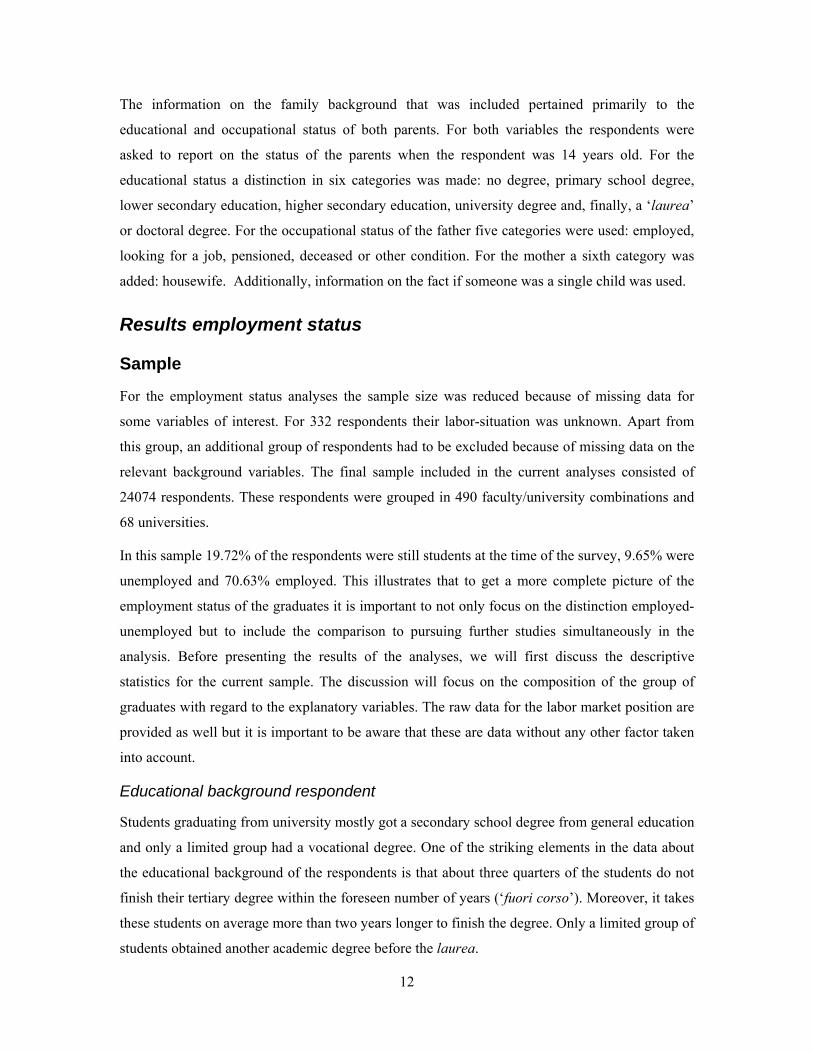
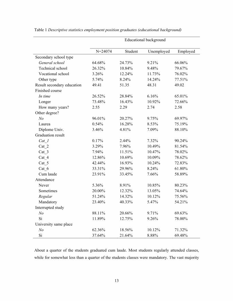
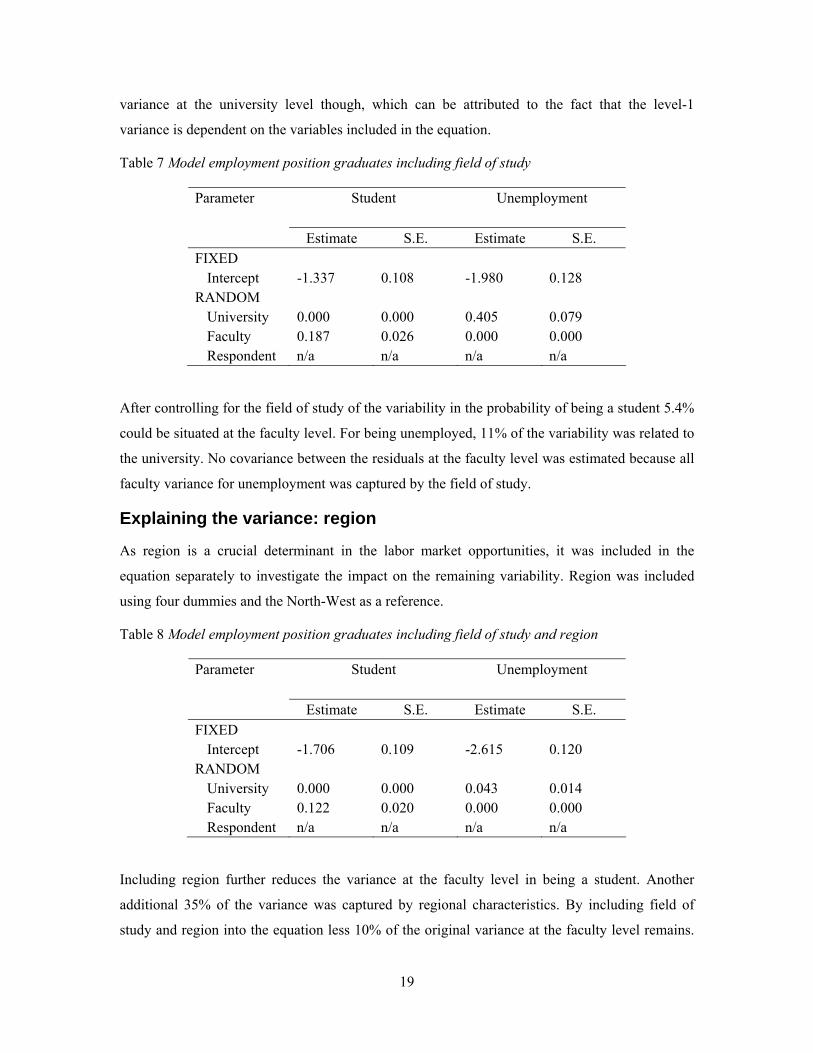
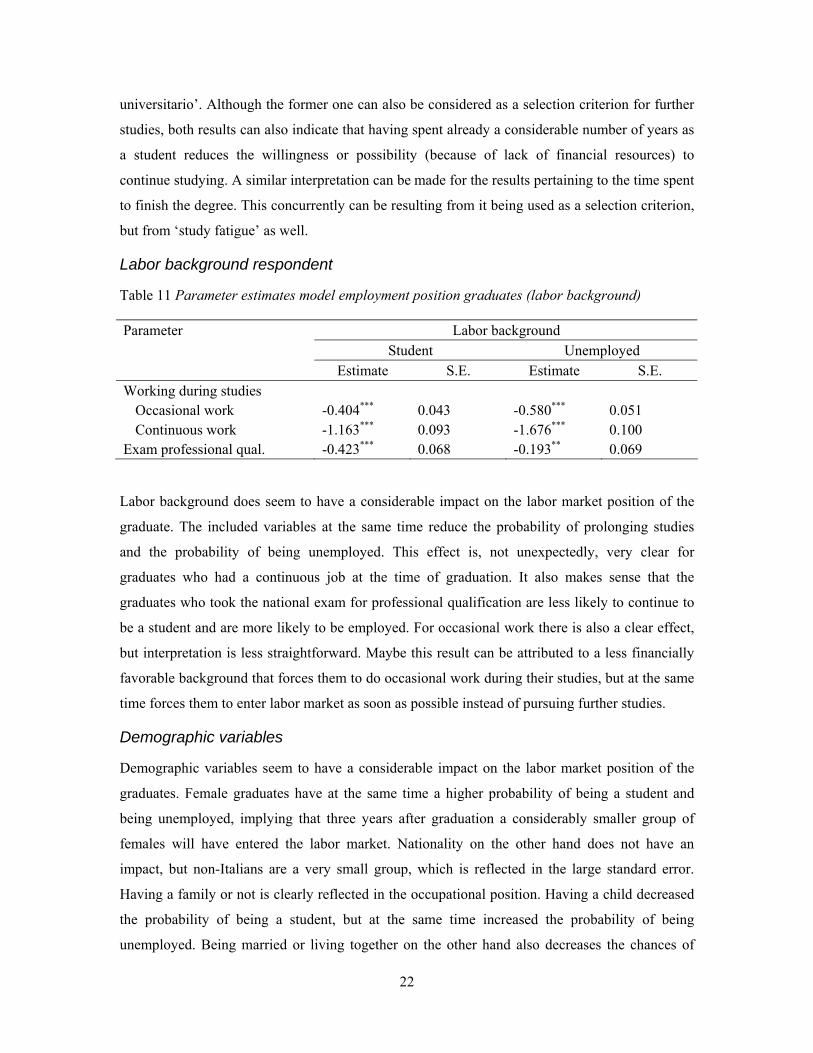
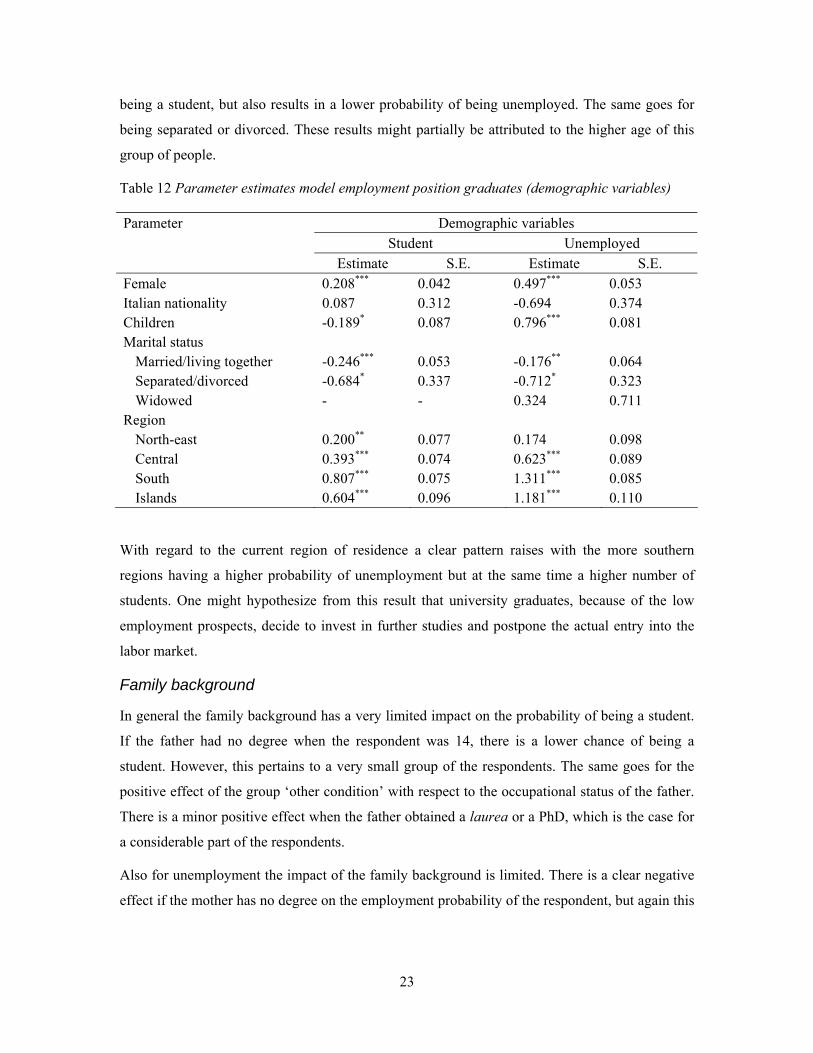
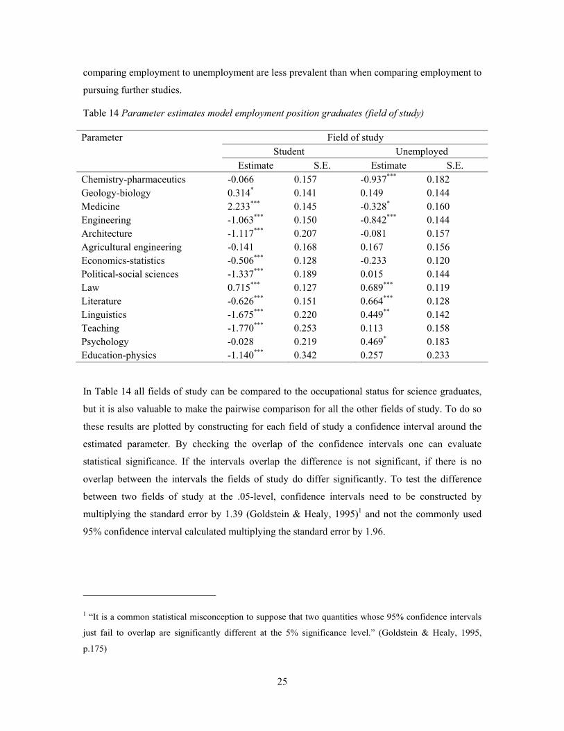
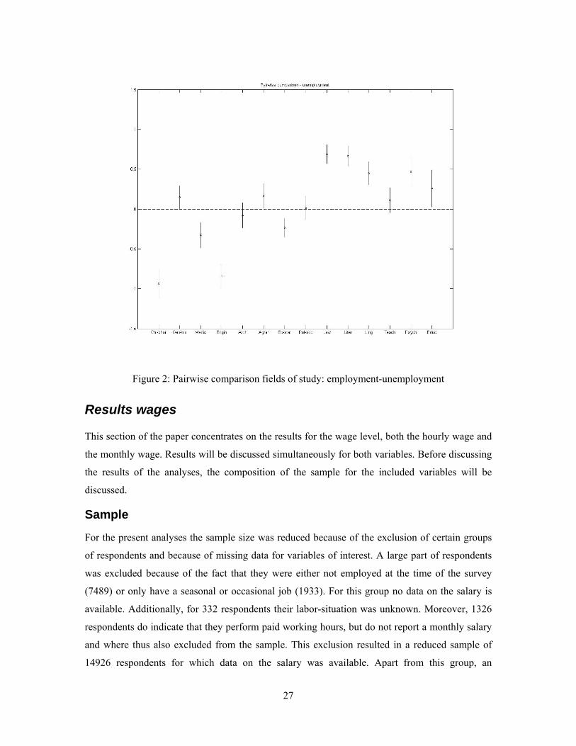
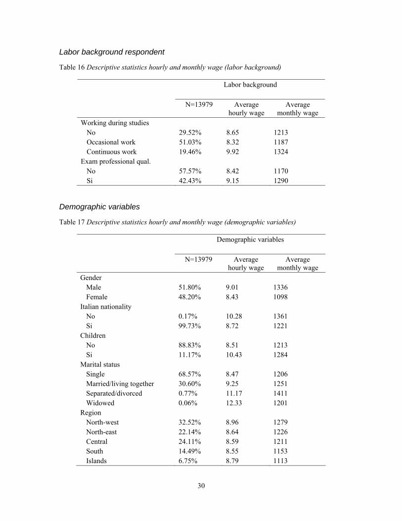
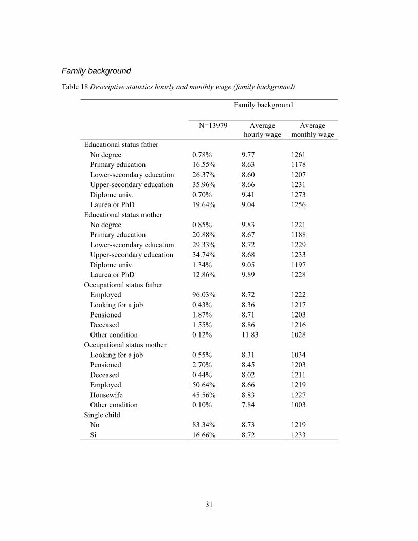
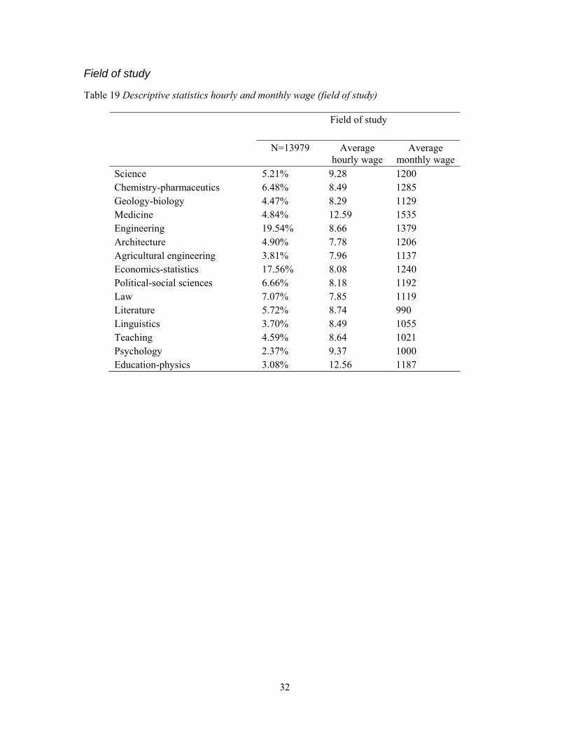
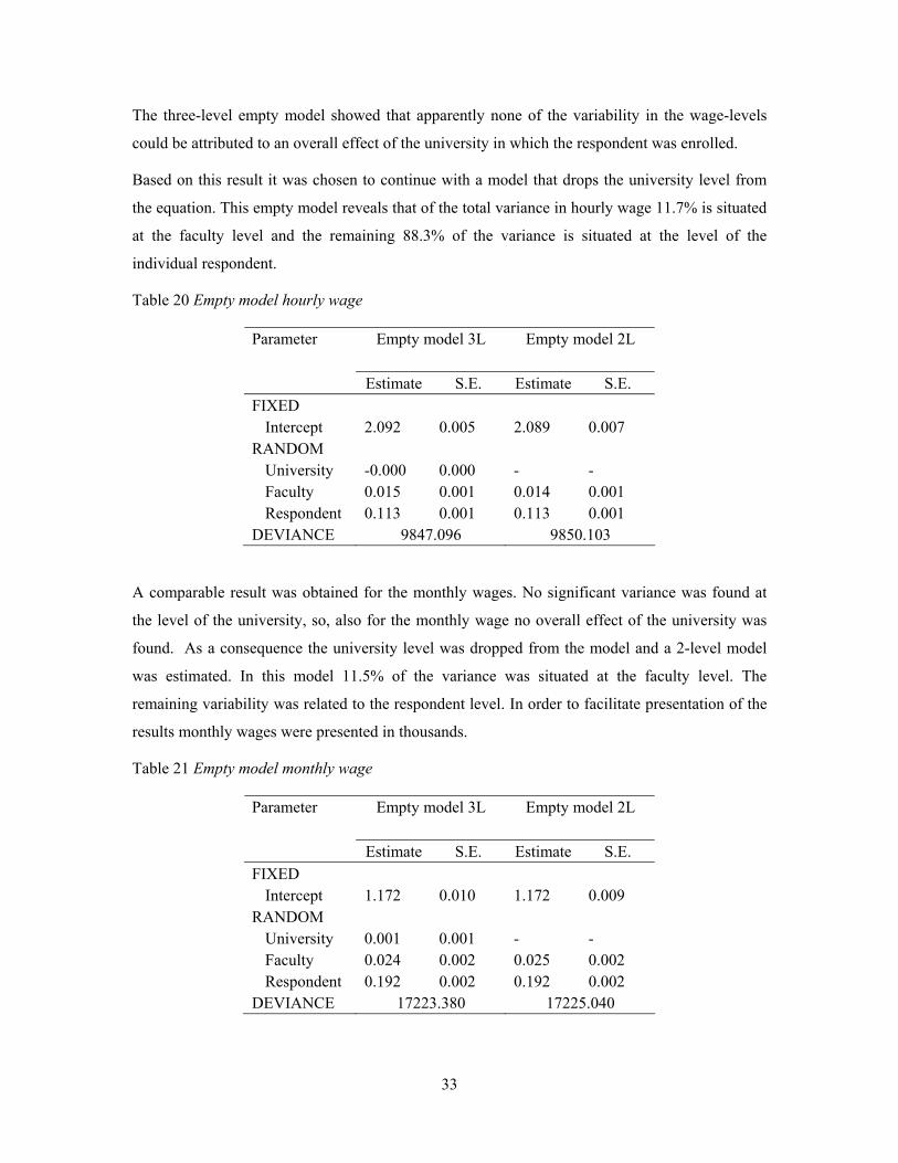
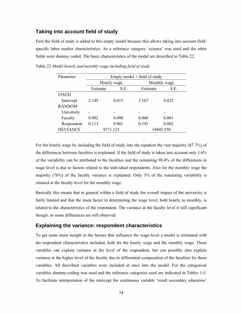
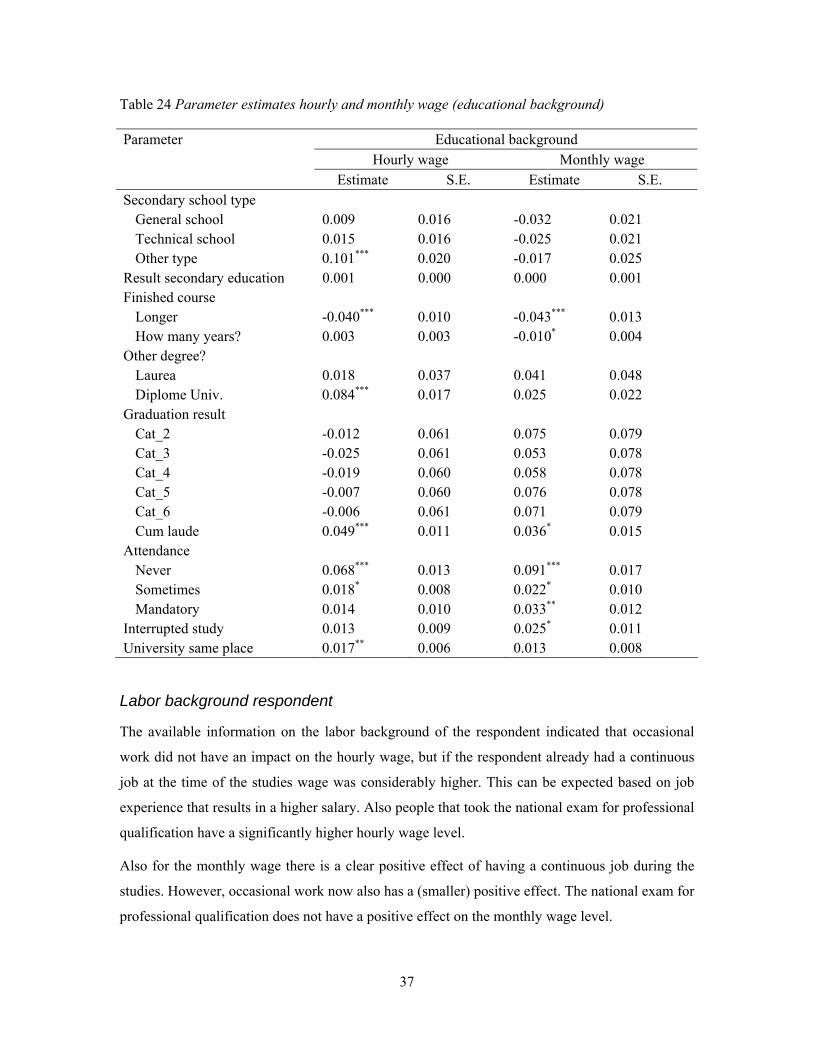
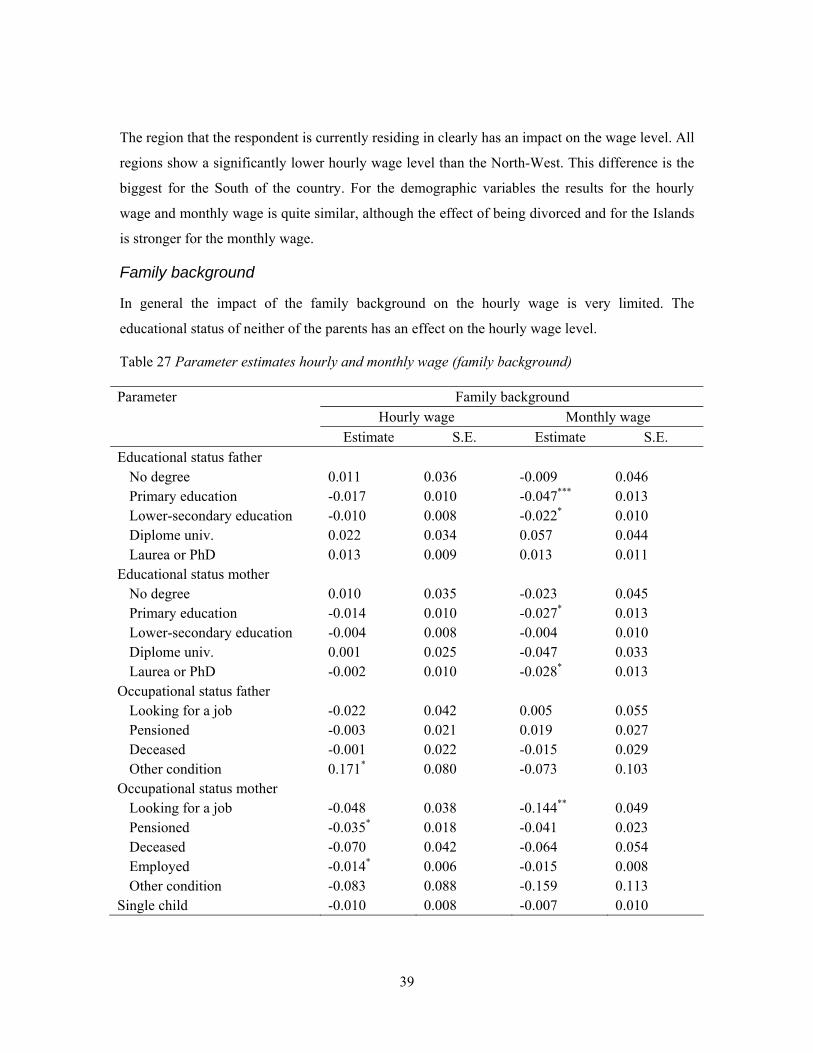
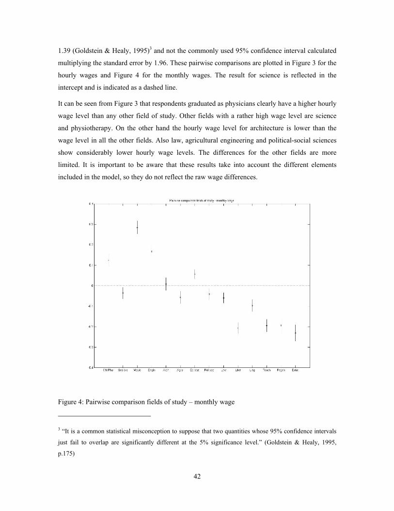
Related Documents