UNIVERSITÀ DEGLI STUDI DI PADOVA ... - economia.unipd.it

UNIVERSITÀ DEGLI STUDI DI PADOVA

Dipartimento di Scienze Economiche “Marco Fanno”

A DISCRETE CHOICE MODEL OF CONSUMPTION OF CULTURAL GOODS IN ITALY:

THE CASE OF MUSIC

DONATA FAVARO Università di Padova

CARLOFILIPPO FRATESCHI Università di Padova

December 2005

“MARCO FANNO” WORKING PAPER N.10

A Discrete Choice Model of Consumption of Cultural Goods in Italy: the Case of Music

Donata Favaro and Carlofilippo Frateschi * Dept. of Economics, University of Padua

Abstract

In this paper we present an empirical analysis of the ‘patterns of cultural choice’ in the musical domain in Italy. By employing micro data from the Italian Survey on Households. Citizens and Leisure, we investigate the way in which musical tastes appear to be differentiated in the Italian society. The main goal of the paper is to verify whether musical tastes could be characterised by the traditionally accepted dichotomy between an élite of ‘cultural snobs’ and a mass of consumers of ‘lowbrow’ genres or whether they are diversified, with the presence of a new group of “cultural omnivores”. By applying the discrete choice analysis, we implement a multivariate logit model in which each equation represents the choice of one of the mutually exclusive alternatives. Our dependent variable is constructed in a way to exactly identify the set of the alternatives and to include all possible individual choices. Our estimates point to the existence of different ‘degrees of omnivorouness’ and capture the differences between individuals listening to (or attending concerts of) only one musical genre, more than one genre or all genres.

J.E.L. Classification: D12, C25, Z1 Keywords: Cultural consumption, Differentiation of musical tastes, Discrete choice

models.

* E-mail: [email protected]; [email protected] Address: Department of Economics, university of Padua. Via del santo 33, I-35123, Padua, Italy

2

1. Introduction1

Despite the existence of a rapidly growing body of literature in the field of cultural economics, in Italy, as Fuortes notes (Fuortes 2002, p. 153), among the various areas typically investigated within this discipline (production, financing, organisation, etc.) the study of the demand for cultural goods is relatively underdeveloped.

This weakness is even more apparent – and, we could say, even more striking if we compare it with the situation in other countries – when it comes to the empirical estimates of the determinants of demand. The contributions to this issue have been relatively scarce, and have dealt with it either with time-series or cross-sectional analyses at the aggregate level (Bonato et al., 1990; Brosio and Santagata, 1992; Trimarchi, 1994; Gorelli, 1994; Taormina and Franzoni, 1997; Fuortes, 2001; Fuortes et al., 2002; Pasquali, 2002), or on the basis of individual data collected through surveys undertaken on the initiative of single cultural institutions or of regional "cultural observatories".

Even more rare have been the attempts at estimating, with reference to the Italian situation, the determinants of the demand for cultural goods and services with the help of individual-level information collected from representative samples of the national population. As far as we know, indeed, Zanardi (1998) is the only published work where an investigation of this kind, specifically a microeconometric analysis of the demand for cultural entertainment activities in Italy, is carried out. This is in stark contrast, as above said, with the current tendency in the field, where more and more empirical contributions are being published that use nation-wide micro data in order to estimate the determinants of various cultural consumption patterns2.

In this paper we follow this stream of literature, and present an empirical analysis of the ‘patterns of cultural choice’ in the musical domain in Italy. By employing micro data from the Italian Survey on Households. Citizens and Leisure (ISTAT, Indagine Multiscopo sulle Famiglie. I cittadini e il tempo libero) for the year 2000, we investigate in particular the way in which musical tastes appear to be differentiated in the Italian society. The main goal of the paper is to verify whether musical tastes appear to be characterised by the traditionally accepted dichotomy between an elite of ‘cultural snobs’ and a mass of consumers of ‘lowbrow’ genres or whether they are diversified, with the presence of a new group of “cultural omnivores”.

1 This research has been carried out as part of the activity of the Research Group "Demand and supply functions in the artistic and cultural system", financed by the University of Padua Research Grant CPDA027187/2002. 2 Two recently published works contain comprehensive surveys of the relevant literature in this regard. The first one (Pettit (2000) is a detailed commented inventory of 29 data sets containing information on public participation in (and attitudes towards) the arts in the USA and Canada, where one can also find bibiographic references to the many scholarly works and publications based upon the surveyed data sets. The second one (Mc Carthy, Ondaatje and Zakaras, 2001) analyses the key empirical and theoretical contributions of the literature on participation in the arts. See also: Kracman, 1996; Gray, 1998; Bihagen and Katz-Gerro, 2000; Prieto-Rodriguez and Fernandez-Blanco, 2000; Van Eijck 2001; Coulangeon 2003; Fisher and Preece, 2003.

3

2. Musical preferences and the emergence of "cultural omnivores": a brief review of the recent empirical literature

About a dozen years ago Peterson and Simkus (1992), in an empirical work based on aggregate data from the 1982 nation-wide Survey of Public Participation in the Arts in the U.S., described what they presented as an historical shift in the "patterns of cultural choice".

Investigating, in particular, the way in which musical tastes appeared to be differentiated in the U.S. society, they found out that the traditionally accepted dichotomy between an elite of "cultural snobs" – exclusively devoted to "highbrow" musical genres like opera and classical music – and a mass of consumers of "lowbrow" genres (like pop or country music, rock, blues, etc.) tended to be partly superseded because of the emergence of a new group of "cultural omnivores", appreciating a much wider range of musical genres than the "cultural snobs". In a later work, Peterson and Kern (1996) replicated the analysis with data from the 1992 Survey of Public Participation in the Arts, finding an increase in the degree of "omnivorousness" in the musical preferences of the american public.

In recent years, this hypothesized transformation in the patterns of musical tastes has been studied empirically by other authors which, using individual-level information collected from representative samples of the population, have estimated the existence and the determinants of analogous shifts in musical consumption patterns in various countries: Spain (Prieto-Rodríguez and Fernández-Blanco 2000), the Netherlands (Van Eijck, 2001), France (Coulangeon 2003), and Canada (Fisher and Preece, 2003). Since these work differ quite substantially – as to analytical framework, objectives, methods, variables considered, coverage, and results – we offer a brief comparative overview of their main features.

As far as the the main research question is concerned, the contribution by Prieto-Rodríguez and Fernández-Blanco (PRFB 2000) does not deal directly with the existence and characteristics of a specific category of "omnivore" musical consumers: the principal aim of the authors is indeed to explore the differences between the consumption of popular and classical music in the Spanish social context. As we shall see, however, their work can be interpreted as offering us, indirectly, some interesting suggestions also in relation to the "omnivorousness" issue, which on the contrary is taken explicitly into consideration by the other three essays.

As to the coverage, all four contributions base the empirical analysis on representative nation-wide surveys, conducted in different years comprised between 1987 and 1998: a) PRFB 2000 is based on the "Structure, Conscience and Class Biography Survey", carried out in Spain in 1991 with a sample of about 6,600 people3; b) the investigation by Coulangeon (2003) is built on the "Enquête sur les pratiques culturelles des Français", a survey conducted in 1997 by the French Ministry of Culture on a representative sample of about 4,000 individuals; c) Van Eijck (2001) studies the social differentiation of musical tastes in the Netherlands on the basis of the 1987 survey on the "cultural participation of the Dutch population", with a representative sample composed of about 4,000 respondents; d) the Canadian situation, finally, is studied by Fisher and Preece (2003) by using two Time Use Surveys carried out in 1992 and 1998 by Statistics Canada, with reference to large

3 Which among others things dealt with the usage of time and the consumption of cultural goods among the Spanish population over eighteen years old.

4

representative samples of the Canadian adult population (with about 10,000 respondents).

One very important issue is, of course, the selection of the most appropriate dependent variable to be "explained". In this regard, most works on the structure of musical consumption focus on one or more of the following: a) the stated preferences of individuals among various musical genres; b) the individually declared habits of listening to music, through various media (radio, TV, records, CDs, Mp3 files, etc), with differing frequencies for different genres; c) the individually recalled frequency of attendance to concerts of a variety of musical genres. As a matter of fact, three out of four of the empirical works under scrutiny (the ones regarding Spain, France, and the Netherlands) focus on the "listening habits" of the population, while only Fisher and Preece (2003) use data on musical concerts attendance.

As Coulangeon states, a case can be made in favour of using the "listening habits" as the main dependent variable by arguing, in particular, that what gets measured when referring to the frequence of listening to different musical genres is probably closer to the real, "latent" preferences of individuals, in comparison to either a) more general and vague questions regarding their "musical tastes" (where one can imagine, among other things, that people could be induced by the very setting of the questionnaire survey to declare more "legitimate" tastes) or, b) to data on concerts attendance where, as the author says, other constraints relating to age or geographical localisation may have an added effect (Coulangeon 2003, pp. 8-9).

On this very last point, however, it should be added that among the factors capable of constraining the choice of attending to live concerts one should at least mention the opportunity cost of time, the availability of leisure time, the price of tickets and the amount of other correlated expenses: in other words, the factors tipically at work in any consumption choice. Therefore, choosing to focus one's research on "listening habits" as opposed to "concert attendance" should be properly interpreted as an alternative between a) evaluating the configuration and intensity of individual musical tastes or b) explaining the structure and dimension of individual musical consumption decisions.

Having said this, it is nonetheless true that in most cases the researchers' choices on these subjects are heavily constrained by data availability. That is why, for instance, in PRFB (2000), owing to some inherent limitations of the Spanish survey which does not contain information on different ways of music listening nor on attendance at live musical events, the authors concentrate on the "listening habits" declared by the interviewees in response to a question asking how often they listen to popular (including pop, rock, and folk) or classical music4. Or why in Coulangeon (2003) the analysis is centered on the replies to the question about the musical genres listened to more frequently: as the authors admits, this is more or less a forced choice, since this is the only question in the survey with the possibility of multiple answers.

In the other two cases, however, there is no explicit mention of data constraints: it could thus be assumed that the dependent variables chosen by the authors – listening habits for Van Eick (2001)5, live concerts attendance for Fisher and Preece (2003) – are more deeply rooted on their prominent research objectives: respectively, the social

4 The respondent could choose among five different levels of listening frequency: never, annually, monthly, weekly or daily. 5 In the Dutch Survey the respondents were asked, among others things, to indicate how often ("seldom or never"; "every now and then"; "often") they listened to each of thirteen different musical genres.

5

differentiation of musical taste patterns in the Netherlands and the evolution (by size and composition) of Canadian performing arts audiences6.

Turning now to the issue of the statistical methods, one cannot avoid noticing their almost total heterogeneity: in fact, each of the four contributions makes use of quite different instruments and techniques.

As to the categorization of genres and behaviours, in PRFB (2003) two groupings of people are distinguished, the "classical music fans" and the "pop music fans" (including pop, rock, and folk music listeners), assigning respondents to one or the other group on the condition that they listen to the respective musical genre(s) "at least once a week". In quite the same vein, Fisher and Preeece (2003) choose a simple dichotomy between "classical music" (attendance to a least one symphonic, chamber, choral or opera music concert in one year) and "other music" (attendance to a least one pop, rock, jazz, blues, folk or country music concerts during the survey year). They then classify as "snobs" people that attend only classical music concerts, "no classical" those that attend only "other music" concerts, "omnivores" the individuals attending concerts of both types and, lastly, "nomusic" people that attend neither type of concerts.

Both the other two authors, instead, make use of much more complex instruments, based on some variety of factorial analysis, in order to identify the number and structure of the profiles of preferences. Coulangeon (2003), after showing how the number of genres "listened to", among the seventeen categories listed in the survey7, varies with the socio-professional status (with, for example, students, professionals, and higher level employees showing a higher degree of eclecticism in their musical tastes), applies a multiple correspondence analysis in order to show the relationship between the various combinations of genres and the degree of eclecticism in the musical choices. Building on such an analysis, that leads to the extraction of four factors, the author proceeds to the identification of five "typologies of attitudes" (or "preference profiles") connected to musical tastes, characterising different groups of individuals according to their degree of musical eclecticism.

Van Eick (2003), on his part, uses a preliminary univariate statistical analysis that leads him to find: 1) that there is a significant positive association between the number of musical genres listened to8, on the one hand, and both the level of

6 While recognizing that the involvement with music may be more passive or active (such as

listening to the TV, radio, or CDs; attending a live performance; playing an instrument or singing), the authors explain their exclusive focus on attendance at live performances because of "the important role audiences play for local artists and arts organizations, and the communities in which they reside" (Fisher and Preece 2003, p. 73). 7 The survey identifies seventeen genres or groups of genres: "1) Variétés, chansons; 2) Variétés internationales (disco, dance, techno, funk, etc.); 3) Musique classique (dont musique baroque); 4) Musiques du monde (reggae, salsa, musique africaine, etc.); 5) Rock; 6) Musique d'ambiance ou musique pour danser (tango, valse); 7) Jazz; 8) Musique folklorique ou traditionelle; 9) Opéra; 10) Musique de film ou de comédie musicale; 11) Opérette; 12) Hard rock, punk, trash, heavy metal; 13) Rap; 14) Musique contemporaine; 15) Chansons pour enfants; 16) Musique militaire; 17) Other genres (Coulangeon 2003, p. 10). 8 The thirteen musical genres considered in the Dutch survey are grouped into three categories: highbrow (chamber music, classical music, opera and jazz); middlebrow (blues/dixieland, pop/rock, top40/disco, chanson/sentimental songs); lowbrow (folk, gospel/spiritual, accordion/guitar/mandolin, operetta, brass band). The main independent variables used by the author are: gender; level of education, occupational status; active participation in music; affinity with highbrow culture. (van Eick 2001, pp. 1170-73).

6

education ("the higher a person's schooling level, the larger the number of genres he or she appreciates") and the occupational status (van Eick 2001, p. 1173);

2) that "status groups differ more with respect to the number of genres that are listened to 'now and then' than the number of genres that are listened to 'often'." The rationale behind such a divergence is that even the omnivores, while exhibiting a certain degree of eclecticism in their appreciation of a quite broad range of genres, apparently maintain strong preferences for a smaller number of really favorite genres.

Apart from, and beyond, such a raw "degree of omnivorousness", the author identifies, with a factorial analysis, four clusters of musical genres associated with specific "musical taste patterns" (a folk pattern, a highbrow pattern, a pop pattern, and an omnivore pattern, as a combination of the highbrow and the pop).

As to the following phase of their analyses, all authors proceed basically by using some kind of multivariate statistical analysis, aiming at investigating the covariation between their respective dependent variable(s) of choice and a set of explanatory variables reflecting a wide array of socio-demographic, occupational and other personal characteristics. The following Table 1 shows a synthetic comparison of these right-hand side variables:

Table 1. Synoptic view of the main explanatory variables in four contributions

PRFB 2000

Coulangeon 2003

Van Eick 2001

Fisher and Preece 2003

Explanatory variables Gender x x x x Age age > 18 age > 19 age > 24 age > 14 Educational level x x x x Type of occupation x x x Occupational condition x x Income x x Marital status x x Children at home x x Housework burden x City size x x Region x x Being musically active x Musical education x Social origin (fathers' occupation) x Parents' educational level x "Affinity with highbrow culture" x Participation in some other leisure activities x

As can be seen, apart form the three basic socio-demographic variables (gender,

age, and education), different vectors of independent variables have been chosen as relevant, at least as it can be derived from the published estimates: they point to personal characteristics, familiar responsibilities, occupational and socioeconomic

7

status, and geographical factors. Additionally, Coulangeon (2003) and Van Eick (2001) take into consideration some form of musical competence (acquired through active involvement and/or some education and training in the musical field), while in PRFB (2000) and again in Coulangeon (2003) there is an attempt at introducing some proxies (fathers' occupation, parents' educational level) for the cultural and social environment and heritage. Finally, both Van Eick (2001) and Fisher and Preece (2003) add as explanatory variables some measure of the participation in other cultural and/or leisure activities, either tipically "highbrow"9 or more diversified10.

As to the estimation techniques and results, there is again much heterogeneity. PRFB (2000) in their analysis expound a theoretical model, along the lines of Lévy-Garboua and Montmarquette (1996), where the probability of consuming one of the two types of music ("classic" or "popular") is analysed, in a utility maximization context, within a discrete choice approach. Two equations are therefore specified and estimated with a bivariate probit model, where the unobserved preferences of the individuals for, respectively, classical and popular music are expressed as a function of a vector of explanatory variables and two vectors of random disturbances.

The main result that the authors derive from their estimates is that, since the two vectors of random disturbances do not appear to be linearly independent (their correlation coefficient, at 0.489, is significantly different from zero), the hypothesis that classical music fans and popular music fans belong to two separate and independent groups can be rejected. After controlling for the various socioeconomic characteristics of respondents, the authors conclude, indeed, that "both groups have a common background that we can identify with the presence of an "innate" taste for music that allow us to believe that, if you are a music fan, you listen to both classical and popular music." (Prieto-Rodríguez and Fernández-Blanco 2000, p. 159). In other words, on the basis of their analysis it can be said that, at least in Spain, all music fans show an omnivorous behaviour.

In the case of Van Eick (2001), he uses the four clusters of musical genres previously identified by means of a factorial analysis (folk, highbrow, pop, and omnivore), as the dependent variable of a path analysis. His main results are, firstly, that classical music genres are more appreciated by women, by older persons, and, especially, by individuals with higher educational level and by people which actively participate in musical activities: however, the occupational group to which the individual belongs has no significant impact. Secondly, the "omnivore pattern" looks as a mainly male and young dominated factor, again with a strong and significative effect of education and of "being musically active" and no significance for the occupational status. Thirdly, the "pop" pattern is negatively correlated with age, level of education, and also with active music participation (with gender and occupational status being not significant).

In the final step of Coulangeon's (2003) investigation, on the other hand, belonging to one of the "preference profiles" previously identified with a factorial analysis is then conceptualized as one of the five alternatives constituting the values possibly taken by the dependent variable in a multinomial logit regression. The main results of his complex and multilayered procedure are the following:

9 The indicator "affinity with highbrow culture" is a scale consisting of eight items reflecting interest in the arts (visual arts, dance, opera, theater, literature) or cultural participation (attending music, dance or theater performances, visitng museum and exhibitions, visiting architectural objects) (Van Eick 2001, p. 1182). 10 Fisher and Preece (2003) add six separate variables that concern: reading newspapers, magazines or books, going to the movies, participating in sport activities, attending church.

8

a) the most important elements explaining the "social stratification of musical tastes" appear to be a generational component and an economic component, since age and income enter with significant coefficients – either positive of negative – in all estimates, while the coefficients of the level of education and the socio-occupational status are generally not significant (with the exception of the profile centered on the preference for classical music, opera and jazz);

b) possessing a certain degree of musical competence (being it mostly self-taught trough the practice of music or acquired through some formal musical education) emerges as an important component in the building-process of musical tastes; interestingly enough, this element appear to be very robust, and tends to supersede the effects of most socio-demographic variables.

Fisher and Preece (2003), finally, use four separate OLS regressions, where on the left hand side there are two binary indicator variables taking the values 1 if the individual is classified, respectively, as as a snob or as an omnivore, and zero otherwise, in order to estimate how, in 1992 and 1998, individual characteristics influence someone's musical attendance behaviour 11. Their main results are the following:

a) an increase in both the number and percentage of omnivores between 1992 and 1998: while the classical music audience has remained stable, its composition has clearly shifted in the sense that "an increasing proportion of classical musical audience now attends live performance of other music as well, as opposed to attending classical music performances alone" (Fisher and Preece 2003, p. 75);

b) while education and income have strong positive and significative effects on both the "snobs" and the "omnivores" variable, the sizes of the age effects are larger for snobs: this group, therefore, appears "more concentrated than omnivores among older segments of the population" (Fisher and Preece 2003, p. 77);

c) women and foreign-born individuals are more likely to be snobs, while men and people living in urban areas are more likely to be omnivores.

3. Music related activities in the "Citizens and Leisure" Survey.

The multipurpose survey "Citizens and Leisure", carried out by the Italian National

Institute for Statistics (ISTAT) in the year 2000, has the aim of acquiring information on leisure activities practiced by the Italian population, with an emphasis on cultural consumption and the use of information technologies. The survey was conducted in December 2000 with a two-stage stratified sampling scheme, and reached a total of 54239 individuals in 19996 families. (ISTAT 2002)

As usual, a first part of the enquiry relates to some key demographic and socioeconomic characteristics of the individuals, such as age, sex, marital status, educational attainment, family composition, occupational condition, professional status, sector of economic activity, area of residence, city of residence size. While the survey also contains a question on the level of family income, this information does not appear neither in the ISTAT publications illustrating the aggregate results of the survey nor in the raw data files (where the relevant field in the individual records is empty). Needless to say, from our point of view this is a most unfortunate fact, given the presumably high relevance of individual/family incomes in influencing the 11 Apart from the main independent variables liste in Table 1, two other variables are added by the autors, country of birth and first language spoken as a child, which are specifically relevant to the Canadian situation of a country with sizeable immigration flows.

9

demand for cultural (and non-cultural) goods and services. We try to control for that lack of information by using some proxy of the individual income level, such as the occupational condition and the type of occupation.

In the main section of the survey, the respondents are asked about their cultural habits, cultural preferences and cultural practices in various areas (cinema, theater, visual arts, performing arts, music, etc.). In the case of music, the survey provides quite detailed information on three main aspects of the behavior of respondents: their listening habits, their attendance to live concerts, and their active personal involvement in music-related practices.

More specifically, each individual over eleven years old is asked: a) How frequently – daily; a few times a week; once a week; a few times a month;

a few times a year; never – does s/he happen to listen to some music; b) How frequently – often; sometimes; never – does s/he listen to specific musical

genres, among a list of fourteen (with the possibility of multiple choices)12; c) how many times approximately – never;1-3; 4-6; 7-12; more than 12 times – did

s/he go, in the preceding 12 months, to concerts of: 1) classical music; 2) opera; 3) rock or pop music; 4) jazz, blues; 5) folk, traditional music;

d) Whether and how often, in her/his leisure time, s/he plays an instrument, composes music or sings in a choir, and whether such activities are carried out in the context of courses organized by schools or associations.

In order to make comparable analyses between listening habits and attendance to

concerts, we group the numerous musical genres in two categories: Classical Music (CM) and Pop Music (PM). Variable CM is meant to include musical tastes for either classical music or opera; the variable assumes unitary value in case the individual declares to listen to (or attend concerts of) either classical music or opera. PM is constructed in a way to identify people listening to (or attending concerts of) either rock or pop or jazz/blues or folk/traditional music.

4. The econometric model

Following the most recent empirical results, surveyed in part 213, on the emergence of a new group of “cultural omnivores” appreciating a much wider range of musical genres than “cultural snobs”, in this paper we focus on identifying the profiles that characterise individuals loving different genres of music. The main question we aim to answering is whether individuals listening to different musical genres do differ in their characteristics. More precisely, we try to verify whether people having a taste only for classical music (“snob” people) significantly differ in their socio-economic characteristics from individuals having preferences for other musical genres (“no classical” individuals) and from individuals loving both classical music and other musical genres (“omnivores”).

In order to identify “snobs”, “no classical consumers” and “omnivores” it is not sufficient to distinguish music alternatives into CM and PM; in doing that, indeed, omnivores and snobs are subgroups of individuals choosing alternatives CM or PM. 12 Musical genres are listed as follows: 1) classical music; 2) opera; 3) folk, regional, traditional; 4) pop music; 5) rock, punk; 6) jazz, blues; 7) disco, house; 8) techno, rap; 9) ethnic and world music; 10) new age; 11) heavy metal, dark; 12) country; 13) childrens' music; 14) latin music. 13 Peterson and Simkus (1992), Peterson and Kern (1996), Van Eijck (2001), Fisher and Preece (2003), Coulangeon (2003) and Prieto-Rodríguez and Fernández-Blanco (2000)

10

In order to properly define the set of alternatives individuals face, it is necessary to reclassify music alternatives in the following categories, identified by subscripts nm, c, o and a14.

nmM is the alternative of not listening to any musical genre;

cM is the alternative of listening to CM but not to PM;

oM is the alternative of listening only to PM.;

aM is the alternative of listening to both CM and PM. Our individual chooses among J=4 alternatives maximising her utility function,

defined by a random utility model. The utility she obtains from any choice j is given by ijU , j=1,…,J. The consumer chooses the alternative that provides the greatest utility; she chooses alternative k if and only if ijik UU > kj ≠∀ .

As researchers, we are not able to exactly know the decision maker’s utility. Therefore we rely on a representative utility; a function ijV of the decision maker’s characteristics and of the attributes of alternative j, ijx . Given ijij UV ≠ , in order to capture the aspects that are not observed by the researcher, ijU is decomposed into

ijijij εVU += . Error terms ijε are treated as random terms, with joint density of the

random vector iJi1i ε,...,εε = denoted by ( )iεf . Given the density function we can define the probability that the ith individual chooses alternative k:

( )kjUU ijikik ≠∀>= obPrP

( )kjobPr ≠∀+>+= ijijikik εVεV ( )kjobPr ≠∀<−= ijikikij V-Vεε Using the density function, the cumulative probability can be rewritten as:

( ) ( ) ( ) iiijikikijε

ijikikij dεεfkjV-VεεIV-Vεε ≠∀<−=≠∀<−= ∫kjobPrPik

Where I(.) is the indicator function. I(.) is equal to 1 when the expression in parentheses is true and 0 otherwise.

Assuming a logit distribution, ( ) ijij e

ij eeε−−ε−=εf , the closed form expression of the

logit choice probability is:

14 In doing so we respect one of the fundamental characteristics that belong to a discrete choice model [Train (2002)]. As it is well knwon, the set of alternatives, that is the choice set open to a decision maker, needs to exhibit three characteristics. 1) First, the alternatives must be mutually lusive from the decision maker’s perspective: choosing one alternative necessarily implies not choosing any of the other alternatives. 2) Second, the choice set must be exhaustive, in that all possible alternatives are included. 3) Third, the number of alternatives must be finite.

11

∑=

jV

V

ij

ik

eePik

We specify, as usual, a representative utility as linear in parameters, ijxβ′=ijV .

Therefore

∑β′

β′

=j

x

x

ij

ij

eePik

The model specified above presents the general characteristics of any discrete

choice model. In particular, the only parameters that can be estimated (identified) are those that capture differences across alternatives. So we normalise our model with respect to the alternative of not listening to music.

The error term in a the multinomial logit model is generally supposed to be identically and independently normally distributed with mean zero and variance εσ . However, since our dataset is derived from a household survey and observations can not necessarily be considered independent among individuals of the same family, we correct for this possibility specifying the likely dependency of the errors within each household.

We carry out separate analyses of the choice of listening to music and the choice of attending to live music concerts by estimating two separate multinomial logit discrete choice models; we firmly believe that the two models can differ in many respect, one of which being the role played by economic determinants in affecting individual choices. Although our dataset does not allow controlling for individual and family different sources of income, we are able to capture the impact of economic determinants through the inclusion of variables catching the occupational status (whether employed or unemployed/inactive) and the type of occupation done by the person.

In order to identify the three categories of “music lovers” we first estimate a general model; once we get the estimates we test for the significant difference between any pair of coefficients belonging to two different choices. Thereafter, we proceed in estimating a constrained model in which we impose the constrains on the parameters15. Marginal effects of the final models (constrained) are reported in Tables 2 and 3 while estimates are in the Appendix.

The X matrixes include individual socio-economic characteristics. We control for gender (dummy “Female” assuming value one for females and zero otherwise), age, educational level, occupational condition, type of occupation, marital status and urban-geographical characteristics.

The variable age is split into four cohorts with a dummy for individuals of between 19 and 29 years old, a dummy for people of 30-44 age, and other two dummies for 45-64 and for over 65 years old individuals.

We expect a significant impact of the highest educational levels both on the probability to listen to some musical genres and on the attendance to live concerts. A higher educational level can justify the preference for more snobbish musical tastes

15 We impose equal coefficients when the null hypothesis is can not be accepted at a probability level equal or lower than 10%.

12

and, because of its correlation with income, it can let the individual afford more expensive musical events, like an opera or a symphonic orchestra concert. Our educational variables are defined as dummies for each of the following educational levels: no education, primary education, secondary education (upper-secondary education) and tertiary education (university education).

Occupational status and type of occupation dummies16 capture the effects of two interrelated factors: disposable income and availability of leisure time. Work inactivity could probably explain a lower attendance to musical events due to the income effect, although the high availability of time would justify a higher participation to those events; furthermore, an occupation correlated with more income and more responsibility would positively affect attending more expensive and more socially considered musical events. However, individuals in those occupations are likely to have a low availability of leisure time.

We control for the following type of occupation categories: blue-collar, white-collar, apprenticeship worker, upper-level white-collar, manager, elementary-school teacher, secondary-school teacher, entrepreneur, self-employer, professional and firm associate (plus some other minor categories).

We add a dummy “Musician” for individuals singing, composing or playing and a dummy “Attending school of music” if she attends any course of music.

We control for the marital status -unmarried, married, separated, divorced and widow- and for having children 0-5 or 6-13 years old. Other controls are included for the five Italian macro-regions17 and for the size of the municipality of residence18.

Our sample includes only individuals older than 19 years.

5. Results

Marginal effects of the constrained models are presented in Tables 2 and 3; the corresponding coefficients are reported in the Appendix. Given the structure of the model, although the coefficients of some regressors are constrained to be equal between two or more alternatives, marginal effects can be different among those alternatives.

Observing the estimated coefficients we can see that individuals choosing different alternatives do differentiate both when we deal with listening tastes and when we look at live concert attendance. However, differences become sharper when we focus on live concert attendance.

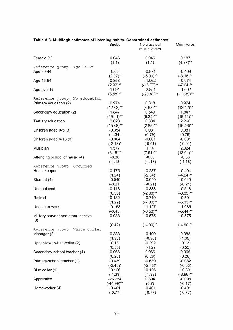
Concerning the listening behaviour (Table A.3 in the Appendix), individuals have different significant characteristics affecting the probability of choosing among musical alternatives; differences are related to age, the highest educational levels, gender and occupational status. Some characteristics have significant common coefficients among all alternatives: this is the case of most of the variables capturing the effect of different types of occupations. Being a primary-school teacher, an apprentice worker or a self-employed negatively affects the probability of listening to any alternative compared to the reference type of occupation (being a white-collar).

16 We distinguish among occupied, non-occupied, house-keeper, student, retired, disable, military servant and other types of inactive. 17 North-West, North-East, Centre, South and Islands 18 The categories are: Central municipality of a metropolitan area; Suburb of a metropolitan area; municipality with not more than 2000 inhabitants; municipality wih 2001-10000 inhabitants; municipality with 10001-50000 inhabitants; municipality with more than 50000 inhabitans.

13

Even regional, city-size and marital status dummies have in general common coefficients among all alternatives. Other individual characteristics are pair wise equal; primary and secondary education have significant common coefficients between alternatives cM and aM .

In terms of marginal effects (Table 2) most of the variables, especially those concerning age, education and type of occupation, differently affect the probability of choosing to listen to only classical music, only pop music or all musical genres.

Being a female strongly increases the probability of listening to all musical genres (by 3.46%); on the contrary it negatively contributes to the choice of other alternatives, no classical music in particular.

Age is a characteristic that strongly identifies the three musical patterns. As age increases, the preference for only classical genres rises; on the contrary, tastes for no classical music decrease as age rises. Indeed, omnivorous preferences are positively influenced by being in the age-groups 30-44 and 45-65, while the oldest age-group (older than 65) does not significantly affects the preference for all musical genres. Although individuals of central age-groups (45-64) show both snobbish and omnivorous tastes, the marginal effect of belonging to that age cohort is higher in the case of omnivores.

The higher the educational level the higher the probability of being snobbish or omnivorous. On the contrary, higher educational levels imply a lower taste for no classical music. However, the additional contribution of higher educational levels is relatively more important for snobbish than for omnivorous preferences; having a tertiary education more than doubles the probability of being a snob while it increases the probability of being omnivore by only one third.

In general, having young children does not significantly affects the choice of listening to music and even when the effect is significant –as in the case of snobs- its level is almost null.

Being a “Musician” has a strongly positive effect on being omnivorous and a negative effect on listening to only pop music, while it has no significant effect on being a snob. Attending a school of music has no significant effect in any alternative.

Our estimates show an interesting result with respect to the occupational status. When statistically significant, dummies capturing the effect of being in an unemployed or inactive occupational status have a negative marginal effect on the probability of being either a no classical or an omnivore and a positive effect on the probability of being a snob. With respect to the type of occupation, employees in a higher occupational position relative to white-collars (Managers and Upper-level white-collars) show stronger snobbish and omnivorous tastes and lower preferences for only pop music. The opposite is true for blue-collars and apprentices. Being a teacher has a significantly different effect from the reference type of occupation only if being a primary-school teacher; in that case it strongly augments the probability of being an omnivore (by 10%) while decreasing the probability of being a no classical listener.

The marginal effects of regional dummies underline the negative effect on having some taste for music of living in Southern Italy. On the contrary, people from the North have a positive incremental effect on the probability of listening to no classical music and of being omnivores. City size dummies detect the negative effect of living in small municipalities. As the size of the municipality increases, the probability of being snob or omnivore increases; preferences for no classical music are not affected by the size of the municipality.

14

Table 2. Listening habits. Marginal effects Snobs No classical

music loversOmnivores

Female* -.0009 -.0241 .0346(-3.74) (-3.83) (5.52)

Reference group: Age 19-29Age 30-44* .0312 -.1499 .054

(3.37) (-12.73) (4.55)Age 45-64* .0655 -.3157 .0909

(5.56) (-28.20) (6.75)Age over 65* .1344 -.4200 .016

(5.59) (-34.05) (0.84)Reference group: No educationPrimary education* .0082 -.1102 .1578

(8.34) (-6.36) (9.61)Secondary education* .0162 -.2370 .3127

(12.40) (-13.11) (17.83)Tertiary education* .0367 -.3566 .4065

(6.35) (-23.69) (25.23)Children aged 0-5* -.0069 .0078 .0056

(-2.05) (1.41) (1.41)Children aged 6-13* -.0060 .0031 .0022

(-2.60) (0.70) (0.70)Musician* .0018 -.1526 .2428

(0.69) (-14.46) (22.93)Attending school of music* -.0008 -.0217 -.0156

(-1.03) (-1.04) (-1.04)Reference group: OccupiedHousekeeper* .0096 .01146 -.0503

(3.40) (1.03) (-5.03)Student* -.0001 -.0026 -.0019

(-0.21) (-0.21) (-0.21)Unemployed* .0117 -.0067 -.0508

(.36) (-0.32) (-2.66)Retired* .0167 -.0914 .0110

(5.10) (-7.60) (0.95)Unable to work* .0208 -.1057 -.0633

(1.69) (-3.18) (-1.85)Military servant and otherinactive*

.0144 -.0451 -.0323

(2.40) (-4.64) (-4.65)Reference group: White-collarManager* .0058 -.1055 .1116

(3.25) (-2.88) (3.30)Upper-level white-collar* .0044 -.0981 .0852

(3.35) (-3.69) (3.43)Secondary-school teacher* .0001 .0034 .0025

(0.27) (0.27) (0.27)Primary-school teacher* -.0051 -.1367 .1020

(-4.50) (-4.69) (3.37)Blue collar* .0015 .04041 -.0644

(3.68) (3.78) (-6.44)Apprentice* -.0213 .1251 -.0873

(-16.5) (2.48) (-1.97)Homeworker* -.0001 -.0247 -.0178

(-0.67) (-0.67) (-.67)Entrepreneur* -.0002 -.0047 -.0033

(-0.43) (-0.43) (-0.43)Professional* -.0002 -.0067 -.0048

(-0.61) (-0.61) (-0.61)Self employed* -.0007 -.0193 -.0139

(-2.70) (-2.75) (-2.75)

15

Cooperative partner* -.0003 -.0074 -.0053(-0.30) (-0.30) (-0.30)

Family business collaborator* -.0018 -.0481 -.0345(-2.64) (-2.67) (-2.67)

Reference group: CentreNorth east* .0007 .0177 .0127

(5.57) (5.87) (5.86)North west* .0006 .0159 .0114

(4.95) (5.15) (5.14)South* -.0003 -.0093 -.0067

(-2.63) (-2.66) (-2.66)Islands* .0002 .0045 .0032

(1.13) (1.14) (1.14)Reference group: Centre of metropolitan areaMunicipalities suburb ofmetropolitan area*

.0002 .0052 .0037

(1.04) (1.04) (1.04)Municipalities up to 2000 inhab.* -.0066 .0207 -.0664

(-2.88) (1.35) (-4.97)Municipalities 2001-10000 inhab.* -.0013 .0030 -.0252

(-2.87) (0.31) (-2.90)Municipalities 10001-50000 inhab.* -.0017 .0123 -.0336

(-3.83) (1.28) (-3.92)Municipalities > 50000 inhab.* -.0006 -.0153 -.0110

(-2.99) (-3.04) (-3.04)Reference group: UnmarriedMarried* .0001 .0020 .0014

(0.53) (0.53) (0.53Separated* .0002 .0049 .0035

(0.49) (0.49) (0.49)Legally separated* .0004 .0108 .0078

(1.35) (1.36) (1.36)Divorced* .0004 .0119 .0085

(1.48) (1.48) (1.48)Widow* -.0005 -.0130 -.0094

(-2.56) (-2.60) (-2.60)Marginal effect Probability .0191 .5108 .3669

(*) dy/dx is for discrete change of dummy variable from 0 to 1

Shifting to the results of the model on live concert attendance (Table A.4 in the

Appendix), we notice a sharper differentiation among individuals choosing different musical alternatives than in the model on listening tastes. Differences in the characteristics of people choosing different alternatives are sharper than in the case of listening habits; only a few characteristics have significant common coefficients among all alternatives; this is the case of some of the occupational dummies, of the dummies on marital status and of the number of children younger than 14. Having children negatively affects the possibility of attending any genre of concert, especially when children are particularly young.

Looking at marginal effects, we detect both some similarities and several differences with respect to the model on listening preferences.

Being a female still positively affects the probability of being omnivore, although the absolute incidence is much lower than in the case of listening habits. In the latter case being female increases the probability of having omnivorous tastes by 3.4 percentage points; in the former case by only 0.6%.

The age characteristic strongly identifies the three musical patterns, as in the previous model. Similarly, as age rises snobbish preferences increase and no classical

16

tastes decrease; omnivorous preferences are particularly influenced by being 45-64 years old.

Differently from the model on listening habits, education has a significant and positive effect on whatever musical alternative we observe. Higher educational levels imply a higher probability of being either snobbish or omnivore or no classical music lover. However, we detect a particularly strong positive effect of the highest educational level on the attendance of classical music concerts; having a university degree doubles the probability of being a snob relative to having a lower educational diploma. Table 3. Live concerts attendance. Marginal effects

Snobs No classicalmusic lovers

Omnivores

Female* .0093 -.0139 .0066(6.40) (-4.78) (3.66)

Reference group: Age 19-29Age 30-44* .0307 -.0265 .0129

(6.36) (-7.13) (3.69)Age 45-64* .0534 -0.608 .0192

(8.50) (-14.44) (4.82)Age over 65* .0569 -.1009 .0057

(5.85) (-21.55) (1.05)Reference group: No educationPrimary education* .0320 .0348 .0137

(4.14) (3.83) (3.76)Secondary education* .0959 .0546 .0440

(4.60) (4.69) (6.79)Tertiary education* .2562 .0382 .0714

(4.44) (2.38) (5.01)Children aged 0-5* -.0088 -.0302 -.0119

(-7.91) (-8.30) (-8.09)Children aged 6-13* -.0020 -.0069 -.0027

(-1.80) (-1.81) (-1.81)Musician* .0268 .0920 .0590

(12.72) (14.39) (10.39)Attending school of music* .0227 -.0014 .0308

(5.21) (-0.19) (5.20)Reference group: OccupiedHousekeeper* .0014 -.0204 -.0080

(0.52) (-4.88) (-4.85)Student* .0050 .0171 .0068

(2.73) (2.74) (2.72)Unemployed* -.0055 -.0191 -.0075

(-3.34) (-3.37) (-3.35)Retired* .0117 -.0362 .0029

(3.52) (-6.19) (0.76)

Unable to work * -.0213 -.0279 -.0110(-9.35) (-2.44) (-2.44)

Military servant and otherinactive*

.0023 -.0328 .0031

(0.54) (-3.85) (0.54)

Reference group: White collarManager* .0086 .0296 .0117

(2.24) (2.25) (2.24)

Upper-level white-collar* .0041 -.0209 .0056(1.14) (-2.47) (1.14)

Secondary-school teacher* .0133 .0059 .0180(2.72) (0.49) (2.71)

Primary-school teacher* .0039 .0132 .0052

17

(1.35) (1.35) (1.35)

Blue collar* -.0040 -.0139 -.0055(-3.86) (-3.92) (-3.90)

Homeworker * -.0264 .0033 .0013(-21.0) (0.24) (0.24)

Assistant* -.0043 -.0149 -.0059(-0.89) (-0.89) (-0.89)

Entrepreneur* .0207 -.0182 -.0072(2.11) (-2.21) (-2.21)

Professional* .0032 .0110 .0044(1.56) (1.56) (1.55)

Self employed* -.0039 -.01345 -.0053(-3.04) (-3.06) (-3.06)

Cooperative partner* .0060 .0207 .0082(1.26) (1.26) (1.26)

Family business collaborator* -.0019 -.0064 -.0025(-0.63) (-0.63) (-0.63)

Reference group: CentreNorth east* .0063 .02146 .0085

(4.49) (4.56) (4.56)

North west* .0014 .0048 .0019(1.15) (1.16) (1.16)

South* .-.0025 -.0085 -.0034(-2.18) (-2.19) (-2.18)

Islands* .0000 .0003 0.0000(-0.31) (4.89) (-0.31)

Reference group: Centre of metropolitan areaMunicipalities up to 2000 inhab.* .0025 .0084 .0033

(1.46) (1.46) (1.46)

Municipalities 2001-10000 inhab.* -.0015 .0235 -.0021(-0.57) (2.64) (-0.57)

Municipalities 10001-50000 inhab.* .0004 .0281 .0006(0.25) (4.71) (0.25)

Municipalities > 50000 inhab.* -.0005 .0113 -.0007(-0.31) (2.04) (-0.31)

Municipalities up to 2000 inhab.* .0030 .0103 .0041(1.96) (1.96) (1.96)

Reference group: UnmarriedMarried* -.0095 -.0326 -.0129

(-7.50) (-7.82) (-7.61)

Separated* -.0074 -.0254 -.0100(-3.44) (-3.48) (-3.46)

Legally separated* -.0059 -.0202 -.0080(-2.89) (-2.92) (-2.91)

Divorced* .0012 .0042 .0017(0.43) (0.43) (0.43)

Widow* -.0115 -.053 -.0155(-6.87) (-9.19) (-7.02)

Marginal effect Probability .0235 .0807 .0319

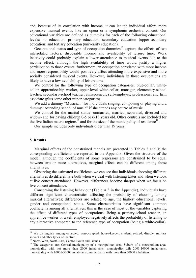
As we already noticed, having children acts as a constraint in the choice of

attending any genre of concert. Occupational status dummies –capturing the effect of being in an inactive or

unemployed occupational status- behave differently than in the model on listening habits. In particular, we detect a generalised negative effect –when significant- due to being unemployed or inactive (either housekeeper, unable to work or military servant and other inactive). On the contrary, students positively contribute to the choice of any music alternative, with a higher effect in the case of no classical music. Being

18

retired indeed has a positive effect on snobbish preferences and a negative effect on no classical music.

With respect to the type of occupation, Managers and Professionals show a stronger preference -with respect to the reference group (White-collars)- for any music alternative, with a particular interest in no classical music. Entrepreneurs strictly prefer classical music while self-employed negatively affect the choice of any music alternative. Employees in a lower occupational position relative to white-collars show less interest for any genre of concert. Being a secondary-school teacher increases the probability of being a snob and an omnivore.

The marginal effects of regional and city size dummies are similar to those detected in the listening habit model.

6. Discussion and conclusions The analysis presented in this paper suggests that in the Italian situation, as

depicted by the 2000 ISTAT survey "Citizens and leisure", it is indeed possible to identify three diversified configurations of musical preferecens and consumption (a snob, a pop, and and omnivorous one), strongly correlated to a set of individual socio-demographic or regional characteristics, both when we consider the listening habits and when we look at live concerts attendance.

In our study, the adoption of an analytical model based on a discrete choice approach and the subsequent estimation of a multinomial logit model gave us the possibility of clearly identifying the mutually exclusive alternatives among which individuals can exert their musical choices, therefore deriving what we deem as a more correct estimation of the significance and impact of the various explanatory variables.

In particular, a few important conclusions can be drawn, first of all, from an evaluation of the estimated coefficients. In the case of listening habits, a) the coefficients relative to the "snob", the "no classical music", or the "omnivore" pattern do differ significantly among individuals, but almost exlusively according to the following personal characteristics: age, educational level, taking part actively in musical activities, and gender (but only for the "omnivores"); b) on the other hand, most of the coefficients referring to the type of occupation have common values for all or some of the equations, and the same applies for the marital status, the city size and the region of residence: in other words, for these caracteristics we cannot detect a significant impact on the differentiation of listening habits.

In the case of attendance to concerts, the most important point to note is that the characteristics of people choosing different alternatives are much sharply defined than in the case of listening habits. Variables such as gender, age, level of education and musical activity (or training) maintain their strong significance in differentiating among the three identified patterns of consumption. Additionally, only a few characteristics have significant common coefficients among all alternatives: this is the case for some of the independent variables regarding the occupational position, the marital status, end the presence of children younger than 14 years old.

By looking at the marginal effects regarding the listening habits, we can see that most of the variables, especially those concerning age, education, and type of occupation, have a different impact on the probability of being a "snob", "nonclassical", or "omnivore" listener. Additionally, the regional dummies show a significant difference between Southern and Northern Italy, as well as an effect

19

related to the city size: in fact, both the "snob" and the "omnivore" patterns of music listening preferences could be characterized as urban or metropolitan, since their probability increases significantly with the size of the city of residence.

As to the attendance to concerts, the marginal effects of different variables show some similarities and several differences with respect to the model of listening preferences. Being a female still positively affects the probability of being omnivore - although the absolute impact is much lower than in the listening case – and also the age strongly identifies the different attendance patterns: in particular, an omnivorous consumption behaviour is strongly influenced by being 45-64 years old. The level of education implies a significant and positive effect on any pattern: however, we detect a particularly strong impact in the case of classical music, since having a university degree doubles the probability of being a "snob" if compared to a lower education degree. As to the occupational status, it can be detected a negative effect on concert attendance –when significant- due to being unemployed or inactive (either housekeeper, unable to work or military servant and other inactive), while on the contrary being a student positively contributes to the choice of any concert attendance alternative.

20

Bibliographic references Bihagen, E. - Katz-Gerro, T. (2000), "Culture consumption in Sweden: The stability of

gender differences", Poetics, 27, pp. 327-349. Bonato, L., Gagliardi, F., Gorelli, S. (1990), "The Demand for Live Performing Arts in

Italy", Journal of Cultural Economics, n. 14, pp. 41-52. Brosio, G and Santagata, W, (1992), Rapporto sull'economia delle arti e dello

spettacolo in Italia, Torino, Edizioni della Fondazione G.Agnelli, 1992. Coulangeon, Ph. (2003), "La stratification sociale des goûts musicaux. Le modèle de la

légitimité culturelle en question", Revue française de sociologie, 44-1, pp. 3-33. Fisher, T.C.G. - Preece, S.B., (2003), "Evolution, extinction, or status quo? Canadian

performing arts audiences in the 1990s", Poetics 31 (2003) 69–86 Fuortes, C., (2001), "La domanda di beni culturali in Italia. Alla ricerca di un modello

esplicativo", Economia della Cultura, (XI), n. 3, pp. 363-378. Fuortes, C., (2002), "La domanda e i consumi culturali", Economia della cultura, (XII),

n.2, pp. 153-156. Fuortes, C., Pignatti, M., Ricci, A., Savo, L., (2002), "Una stima econometrica della

domanda di beni culturali in Italia", Economia della cultura, (XII), n.2, pp. 247-252.

Gorelli, S. (1994), "La domanda", in: Carla Bodo (a cura di), Rapporto sull'economia della cultura in Italia 1980-1990, Roma, pp. 315-334.

Gray, C.M. (1998), "Hope for the Future? Early Exposure to the Arts and Adult Visits to Art Museums", Journal of Cultural Economics, 22, pp. 87-98.

ISTAT, (2002), Indagine Multiscopo sulle famiglie “I cittadini e il tempo libero”, Roma.

Kracman, K. (1996), "The effect of school-based arts instruction on attendance at museums and the performing arts", Poetics, 24, 203-218

Lévy-Garboua, L. - C. Montmarquette (1996) “A Microeconometric Study of Theatre Demand”, Journal of Cultural Economics 20, pp. 25-50.

Mc Carthy, K., Ondaatje, E, Zakaras, L. (2001), Guide to the literature in the participation in the arts, RAND Foundation, Santa Monica.

Pasquali, F. (2002), "Spese e consumi culturali in Italia in un'analisi di lungo periodo", Economia della cultura, (XII), n.2, pp. 179-192

Peterson, R.A. - Simkus, A. (1992), "How Musical Taste Groups Mark Occupational Status Groups", in: Lamont, M.- Fournier (eds), Cultivating Differences: Symbolic Boundaries and the Making of Inequality, Univ. of Chicago Press, pp. 152-168.

Peterson, R - Kern, R., (1996), "Changing highbrow taste: from snob to omnivore", American Sociological Review, 61, 900–907.

Pettit, B. (2000), "Resources for studying public participation in and attitudes towards the arts", Poetics (27), pp. 351-395.

Prieto-Rodríguez, J. - Fernández-Blanco, V. (2000), "Are Popular and Classical Music Listeners the Same People?", Journal of Cultural Economics, 24, pp. 147-164.

Taormina, A., Franzoni, D. (1997), “La composizione sociodemografica della domanda” in: Trezzini, L. (a cura di), Rapporto sull'economia dello spettacolo dal vivo in Italia (1980 - 1990), Roma, Bulzoni, pp. 217 - 221.

Train K.E., 2002, “Discrete choice models with simulation”, Cambridge University Press.

21

Trimarchi, M. (1994), "L'offerta e la domanda di cultura in Italia: evoluzione, composizione e distribuzione territoriale", in: Carla Bodo (a cura di), Rapporto sull'economia della cultura in Italia 1980-1990, Roma, pp. 130-140.

Van Eijck, K, (2001), "Social differentiation in musical taste patterns", Social Forces, 79, 1163–1185.

Zanardi, A. (1998), “La domanda d’intrattenimenti culturali: un’analisi microeconometrica per l’Italia”, in Santagata, W. (a cura di), Economia dell’arte. Istituzioni e mercati dell’arte e della cultura, Torino, UTET Libreria, pp. 123-144.

22

Appendix Table A.1. Summary statistics. Listening to music

nmM cM oM aM mean sd mean sd mean sd mean sd Female 0.5498 0.4976 0.5000 0.5002 0.5075 0.5000 0.5280 0.4992 Age 30-44 0.1033 0.3043 0.1006 0.3010 0.3511 0.4773 0.3237 0.4679 Age 45-64 0.3379 0.4730 0.3824 0.4862 0.2950 0.4560 0.3567 0.4791 Age over 65 0.5346 0.4988 0.5000 0.5002 0.1186 0.3234 0.1624 0.3688 Primary education 0.6434 0.4790 0.6039 0.4893 0.5596 0.4965 0.4276 0.4947 Secondary education 0.1166 0.3210 0.2190 0.4137 0.3446 0.4753 0.4098 0.4918 Tertiary education 0.0261 0.1594 0.1119 0.3154 0.0509 0.2198 0.1359 0.3427 Children aged 0-5 0.0402 0.1964 0.0274 0.1632 0.1419 0.3490 0.1203 0.3253 Children aged 6-13 0.0724 0.2592 0.0652 0.2470 0.1871 0.3900 0.1666 0.3726 Musician 0.0153 0.1229 0.0818 0.2742 0.0878 0.2831 0.1820 0.3858 Attending school of music 0.0044 0.0666 0.0282 0.1656 0.0227 0.1490 0.0497 0.2173 Housekeeper 0.1774 0.3820 0.1715 0.3771 0.1789 0.3833 0.1491 0.3562 Student 0.0044 0.0666 0.0032 0.0567 0.0460 0.2095 0.0520 0.2221 Unemployed 0.0163 0.1265 0.0145 0.1196 0.0293 0.1687 0.0229 0.1496 Retired 0.4672 0.4990 0.4960 0.5002 0.1399 0.3469 0.2017 0.4013 Unable to work 0.0233 0.1509 0.0121 0.1093 0.0085 0.0917 0.0061 0.0777 Military servant and other inactive 0.0813 0.2734 0.0483 0.2145 0.0220 0.1467 0.0211 0.1439 Manager 0.0029 0.0539 0.0137 0.1162 0.0049 0.0702 0.0164 0.1270 Upper-level white-collar 0.0048 0.0688 0.0169 0.1290 0.0109 0.1036 0.0301 0.1710 Secondary-school teacher 0.0043 0.0654 0.0137 0.1162 0.0096 0.0977 0.0253 0.1571 Primary-school teacher 0.0048 0.0688 0.0040 0.0633 0.0084 0.0912 0.0217 0.1456 Blue collar 0.0858 0.2801 0.0668 0.2498 0.2093 0.4068 0.1187 0.3234 Apprentice 0.0008 0.0277 0.0000 0.0000 0.0067 0.0814 0.0027 0.0520 Homeworker 0.0012 0.0350 0.0016 0.0401 0.0027 0.0517 0.0018 0.0419 Entrepreneur 0.0089 0.0939 0.0072 0.0849 0.0171 0.1295 0.0187 0.1353 Professional 0.0086 0.0923 0.0201 0.1405 0.0197 0.1391 0.0395 0.1948 Self employed 0.0516 0.2211 0.0378 0.1909 0.0819 0.2742 0.0660 0.2483 Cooperative partner 0.0018 0.0429 0.0008 0.0284 0.0053 0.0726 0.0043 0.0656 Family business collaborator 0.0072 0.0846 0.0024 0.0491 0.0118 0.1078 0.0086 0.0925 North east 0.1538 0.3607 0.2246 0.4175 0.1881 0.3908 0.2417 0.4281 North west 0.1762 0.3810 0.2770 0.4477 0.2051 0.4038 0.2478 0.4317 South 0.3571 0.4792 0.2230 0.4164 0.3065 0.4611 0.2372 0.4254 Islands 0.1019 0.3025 0.0845 0.2783 0.1158 0.3200 0.0909 0.2875 Municipalities suburb of metropolitan area 0.0643 0.2453 0.1087 0.3114 0.0955 0.2939 0.1029 0.3038 Municipalities up to 2000 inhabitants 0.1188 0.3235 0.0620 0.2412 0.0903 0.2866 0.0746 0.2627 Municipalities 2001-10000 inhabitants 0.2989 0.4578 0.2456 0.4306 0.2988 0.4578 0.2784 0.4482 Municipalities 10001-50000 inhabitants 0.2694 0.4437 0.2456 0.4306 0.2697 0.4438 0.2525 0.4345 Municipalities more than 50000 inhabitants 0.1596 0.3662 0.1828 0.3866 0.1561 0.3629 0.1778 0.3824 Married 0.6431 0.4791 0.6763 0.4681 0.6183 0.4858 0.6297 0.4829 Separated 0.0072 0.0846 0.0129 0.1128 0.0114 0.1060 0.0134 0.1149 Legally separated 0.0089 0.0939 0.0105 0.1018 0.0140 0.1176 0.0181 0.1335 Divorced 0.0086 0.0923 0.0129 0.1128 0.0122 0.1099 0.0166 0.1278 Widow 0.2340 0.4234 0.1763 0.3813 0.0575 0.2328 0.0707 0.2563

23

Table A.2. Summary statistics. Listening to music

nmM cM oM aM mean sd mean sd mean sd mean sd Female 0.5295 0.4991 0.5753 0.4945 0.4542 0.4979 0.5059 0.5000 Age 30-44 0.2855 0.4516 0.2815 0.4499 0.3436 0.4749 0.3040 0.4601 Age 45-64 0.3363 0.4725 0.4342 0.4958 0.2158 0.4114 0.3402 0.4738 Age over 65 0.2458 0.4306 0.1959 0.3970 0.0382 0.1916 0.1416 0.3487 Primary education 0.5758 0.4942 0.3288 0.4699 0.3784 0.4850 0.4209 0.4938 Secondary education 0.2830 0.4505 0.4288 0.4951 0.5125 0.4999 0.4023 0.4905 Tertiary education 0.0603 0.2380 0.2315 0.4219 0.0976 0.2968 0.1445 0.3517 Children aged 0-5 0.1198 0.3248 0.0829 0.2758 0.1047 0.3061 0.0853 0.2794 Children aged 6-13 0.1598 0.3665 0.1466 0.3538 0.1497 0.3568 0.1452 0.3523 Musician 0.0670 0.2500 0.2337 0.4233 0.2501 0.4331 0.3178 0.4658 Attending school of music 0.0159 0.1250 0.0740 0.2618 0.0637 0.2442 0.0723 0.2590 Housekeeper 0.1854 0.3886 0.1397 0.3468 0.0939 0.2917 0.1237 0.3293 Student 0.0258 0.1585 0.0349 0.1837 0.1158 0.3200 0.0732 0.2606 Unemployed 0.0243 0.1541 0.0185 0.1348 0.0296 0.1695 0.0228 0.1492 Retired 0.2492 0.4326 0.2753 0.4468 0.0691 0.2536 0.1771 0.3818 Unable to work 0.0117 0.1074 0.0021 0.0453 0.0048 0.0694 0.0120 0.1091 Military servant and other inactive 0.0373 0.1895 0.0192 0.1372 0.0115 0.1068 0.0277 0.1641 Manager 0.0069 0.0828 0.0288 0.1672 0.0095 0.0970 0.0150 0.1215 Upper-level white-collar 0.0138 0.1167 0.0459 0.2093 0.0173 0.1305 0.0309 0.1731 Secondary-school teacher 0.0105 0.1018 0.0479 0.2137 0.0168 0.1284 0.0335 0.1800 Primary-school teacher 0.0101 0.0998 0.0192 0.1372 0.0188 0.1359 0.0182 0.1338 Blue collar 0.1545 0.3614 0.0699 0.2550 0.1993 0.3995 0.1309 0.3373 Apprentice 0.0033 0.0571 0.0000 0.0000 0.0115 0.1068 0.0042 0.0649 Homeworker 0.0021 0.0453 0.0021 0.0453 0.0022 0.0472 0.0023 0.0477 Entrepreneur 0.0161 0.1259 0.0226 0.1487 0.0142 0.1181 0.0176 0.1314 Professional 0.0206 0.1421 0.0486 0.2152 0.0333 0.1795 0.0407 0.1976 Self employed 0.0721 0.2586 0.0445 0.2063 0.0706 0.2561 0.0664 0.2490 Cooperative partner 0.0037 0.0607 0.0034 0.0584 0.0071 0.0838 0.0059 0.0763 Family business collaborator 0.0095 0.0969 0.0075 0.0865 0.0115 0.1068 0.0088 0.0934 North east 0.1871 0.3900 0.2808 0.4496 0.2423 0.4285 0.2650 0.4414 North west 0.2167 0.4120 0.2562 0.4367 0.2039 0.4029 0.2210 0.4150 South 0.3018 0.4591 0.1781 0.3827 0.2642 0.4410 0.2161 0.4117 Islands 0.1006 0.3009 0.0774 0.2673 0.1387 0.3457 0.0905 0.2869 Municipalities suburb of metropolitan area 0.0919 0.2889 0.1103 0.3133 0.0937 0.2914 0.0762 0.2653 Municipalities up to 2000 inhabitants 0.0895 0.2855 0.0541 0.2263 0.0966 0.2955 0.0742 0.2622 Municipalities 2001-10000 inhabitants 0.2872 0.4525 0.2630 0.4404 0.3291 0.4699 0.2799 0.4490 Municipalities 10001-50000 inhabitants 0.2680 0.4429 0.2301 0.4211 0.2460 0.4307 0.2620 0.4398 Municipalities more than 50000 inhabitants 0.1614 0.3679 0.2096 0.4072 0.1603 0.3670 0.1888 0.3914 Married 0.6589 0.4741 0.6596 0.4740 0.4499 0.4975 0.5534 0.4972 Separated 0.0114 0.1063 0.0123 0.1104 0.0102 0.1007 0.0120 0.1091 Legally separated 0.0141 0.1177 0.0171 0.1298 0.0142 0.1181 0.0156 0.1240 Divorced 0.0120 0.1090 0.0219 0.1465 0.0142 0.1181 0.0208 0.1428 Widow 0.1102 0.3132 0.0726 0.2596 0.0166 0.1277 0.0570 0.2318

24

Table A.3. Multilogit estimates of listening habits. Constrained estimates Snobs No classical

music lovers Omnivores

Female (1) 0.046 0.046 0.187 (1.1) (1.1) (4.37)** Reference group: Age 19-29 Age 30-44 0.66 -0.871 -0.409 (2.07)* (-6.90)** (-3.16)** Age 45-64 0.853 -1.962 -0.974 (2.92)** (-15.77)** (-7.64)** Age over 65 1.091 -2.851 -1.602 (3.58)** (-20.87)** (-11.39)** Reference group: No education Primary education (2) 0.974 0.318 0.974 (12.42)** (4.68)** (12.42)** Secondary education (2) 1.847 0.549 1.847 (19.11)** (6.25)** (19.11)** Tertiary education 2.628 0.384 2.266 (15.48)** (2.85)** (16.46)** Children aged 0-5 (3) -0.354 0.081 0.081 (-1.34) (0.79) (0.79) Children aged 6-13 (3) -0.364 -0.001 -0.001 (-2.13)* (-0.01) (-0.01) Musician 1.577 1.14 2.024 (8.18)** (7.61)** (13.64)** Attending school of music (4) -0.36 -0.36 -0.36 (-1.18) (-1.18) (-1.18) Reference group: Occupied Housekeeper 0.175 -0.237 -0.404 (1.24) (-2.54)* (-4.24)** Student (4) -0.049 -0.049 -0.049 (-0.21) (-0.21) (-0.21) Unemployed 0.113 -0.383 -0.518 (0.35) (-2.60)** (-3.33)** Retired 0.182 -0.719 -0.501 (1.29) (-7.80)** (-5.33)** Unable to work -0.153 -1.127 -1.085 (-0.45) (-6.53)** (-5.44)** Military servant and other inactive (3)

0.088 -0.575 -0.575

(0.42) (-4.90)** (-4.90)** Reference group: White collar Manager (2) 0.388 -0.109 0.388 (1.35) (-0.36) (1.35) Upper-level white-collar (2) 0.13 -0.292 0.13 (0.55) (-1.2) (0.55) Secondary-school teacher (4) 0.066 0.066 0.066 (0.26) (0.26) (0.26) Primary-school teacher (1) -0.639 -0.639 -0.082 (-2.48)* (-2.48)* (-0.33) Blue collar (1) -0.126 -0.126 -0.39 (-1.33) (-1.33) (-3.96)** Apprentice -26.754 0.394 -0.098 (-44.99)** (0.7) (-0.17) Homeworker (4) -0.401 -0.401 -0.401 (-0.77) (-0.77) (-0.77)

25

Entrepreneur (4) -0.086 -0.086 -0.086 (-0.44) (-0.44) (-0.44) Professional (4) -0.122 -0.122 -0.122 (-0.64) (-0.64) (-0.64) Self employed (4) -0.327 -0.327 -0.327 (-3.04)** (-3.04)** (-3.04)** Cooperative partner (4) -0.133 -0.133 -0.133 (-0.31) (-0.31) (-0.31) Family business collaborator (4) -0.698 -0.698 -0.698 (-3.34)** (-3.34)** (-3.34)** Reference group: Centre North east (4) 0.367 0.367 0.367 (5.41)** (5.41)** (5.41)** North west (4) 0.32 0.32 0.32 (4.85)** (4.85)** (4.85)** South (4) -0.17 -0.17 -0.17 (-2.76)** (-2.76)** (-2.76)** Islands (4) 0.088 0.088 0.088 (1.11) (1.11) (1.11) Reference group: Centre of metropolitan area Municipalities suburb of metropolitan area (4)

0.101 0.101 0.101

(1.01) (1.01) (1.01) Municipalities up to 2000 inhabitants

-0.828 -0.379 -0.616

(-4.46)** (-3.82)** (-6.05)** Municipalities 2001-10000 inhabitants (2)

-0.286 -0.21 -0.286

(-3.54)** (-2.65)** (-3.54)** Municipalities 10001-50000 inhabitants (2)

-0.305 -0.187 -0.305

(-3.82)** (-2.37)* (-3.82)** Municipalities more than 50000 inhabitants (4)

-0.27 -0.27 -0.27

(-3.24)** (-3.24)** (-3.24)** Reference group: Umarried Married 0.038 0.038 0.038 (0.53) (0.53) (0.53) Separated (4) 0.096 0.096 0.096 (0.47) (0.47) (0.47) Legally separated (4) 0.224 0.224 0.224 (1.24) (1.24) (1.24) Divorced (4) 0.247 0.247 0.247 (1.34) (1.34) (1.34) Widow (4) -0.23 -0.23 -0.23 (-2.79)** (-2.79)** (-2.79)** Constant -3.63 2.913 0.83 (-11.61)** (17.19)** (4.72)** Observations 40684 40684 40684 Robust z statistics in parentheses * significant at 5%; ** significant at 1% (1) Common coefficient between equations cM and oM .

(2) Common coefficient between equations cM and aM .

(3) Common coefficient between equations oM and aM . (4) Common coefficient among all equations

26

Table A.4. Multilogit estimates of attending live concerts. Constrained estimates Snobs No classical

music lovers Omnivores

Female 0.398 -0.169 0.211 (6.23)** (-4.30)** (3.53)** Reference group: Age 19-29 Age 30-44 1.038 -0.333 0.395 (7.68)** (-5.69)** (3.99)** Age 45-64 1.571 -0.859 0.558 (11.20)** (-11.90)** (5.17)** Age over 65 1.454 -1.898 0.129 (8.04)** (-14.38)** (0.78) Reference group: No education Primary education (3) 1.417 0.530 0.530 (4.47)** (4.10)** (4.10)** Secondary education 2.533 0.861 1.359 (7.65)** (6.35)** (9.19)** Tertiary education 3.247 0.947 1.808 (9.73)** (6.22)** (10.84)** Children aged 0-5 (4) -0.498 -0.498 -0.498 (-7.26)** (-7.26)** (-7.26)** Children aged 6-13 (4) -0.102 -0.102 -0.102 (-1.76) (-1.76) (-1.76) Musician (1) 1.038 1.038 1.358 (19.91)** (19.91)** (16.60)** Attending school of music (2) 0.747 0.045 0.747 (6.76)** (0.41) (6.76)** Reference group: Occupied Housekeeper (3) 0.029 -0.306 -0.306 (0.25) (-4.47)** (-4.47)** Student (4) 0.228 0.228 0.228 (2.95)** (2.95)** (2.95)** Unemployed (4) -0.305 -0.305 -0.305 (-3.02)** (-3.02)** (-3.02)** Retired 0.413 -0.535 0.063 (3.58)** (-5.31)** (0.53) Unable to work (3) -2.224 -0.489 -0.489 (-3.13)** (-2.11)* (-2.11)* Military servant and other inactive (2)

0.061 -0.542 0.061

(0.35) (-3.04)** (0.35) Reference group: White collar Manager (4) 0.372 0.372 0.372 (2.54)* (2.54)* (2.54)* Upper-level White-collar (2) 0.150 -0.311 0.150 (1.04) (-2.06)* (1.04) Secondary-school teacher (2) 0.494 0.114 0.494 (3.31)** (0.73) (3.31)** Primary-school teacher (4) 0.178 0.178 0.178 (1.43) (1.43) (1.43) Blue-collar (4) -0.210 -0.210 -0.210 (-3.73)** (-3.73)** (-3.73)** Apprentice (3) -27.378 0.016 0.016 (-165.89)** (0.08) (0.08) Homeworker (4) -0.233 -0.233 -0.233 (-0.81) (-0.81) (-0.81) Entrepreneur (3) 0.631 -0.261 -0.261

27

(2.65)** (-1.79) (-1.79) Professional (4) 0.150 0.150 0.150 (1.64) (1.64) (1.64) Self employed (4) -0.206 -0.206 -0.206 (-2.87)** (-2.87)** (-2.87)** Cooperative partner (4) 0.270 0.270 0.270 (1.38) (1.38) (1.38) Family business collaborator (4) -0.095 -0.095 -0.095 (-0.61) (-0.61) (-0.61) Reference group: Centre North east (4) 0.288 0.288 0.288 (4.88)** (4.88)** (4.88)** North west (4) 0.069 0.069 0.069 (1.17) (1.17) (1.17) South (4) -0.125 -0.125 -0.125 (-2.14)* (-2.14)* (-2.14)* Islands/100 (2) 0.000 0.004 0.000 (0.02) (4.77)** (0.02) Reference group: Centre of metropolitan area Municipalities suburb of metropolitan area (4)

0.117 0.117 0.117

(1.51) (1.51) (1.51) Municipalities up to 2000 inhabitants (2)

-0.044 0.283 -0.044

(-0.34) (2.83)** (-0.34) Municipalities 2001-10000 inhabitants (2)

0.053 0.354 0.053

(0.63) (4.95)** (0.63) Municipalities 10001-50000 inhabitants (2)

-0.011 0.147 -0.011

(-0.14) (2.03)* (-0.14) Municipalities more than 50000 inhabitants (4)

0.143 0.143 0.143

(2.03)* (2.03)* (2.03)* Reference group: Unmarried Married (4) -0.448 -0.448 -0.448 (-8.21)** (-8.21)** (-8.21)** Separated (4) -0.423 -0.423 -0.423 (-2.96)** (-2.96)** (-2.96)** Legally separated (4) -0.325 -0.325 -0.325 (-2.58)** (-2.58)** (-2.58)** Divorced (4) 0.059 0.059 0.059 (0.44) (0.44) (0.44) Widow (4) -0.707 -1.013 -0.707 (-6.25)** (-6.66)** (-6.25)** Constant -6.513 -1.799 -4.353 (-17.01)** (-11.31)** (-23.00)** Observations 41060 41060 41060 Robust z statistics in parentheses * significant at 5%; ** significant at 1% (1) Common coefficient between equations cM and oM .

(2) Common coefficient between equations cM and aM .

(3) Common coefficient between equations oM and aM . (4) Common coefficient among all equations