Universit` a degli Studi di Padova Dipartimento di Fisica e Astronomia “Galileo Galilei” Corso di Laurea Magistrale in Fisica Superconducting transport through a quantum dot with spin-orbit coupling Relatore: Dott. Luca Dell’Anna Laureanda: Cli` o Efthimia Agrapidis Matricola: 1081527 Anno Accademico 2014/2015

Welcome message from author
This document is posted to help you gain knowledge. Please leave a comment to let me know what you think about it! Share it to your friends and learn new things together.
Transcript
Universita degli Studi di Padova
Dipartimento di Fisica e Astronomia “Galileo Galilei”
Corso di Laurea Magistrale inFisica
Superconducting transport through a quantum dotwith spin-orbit coupling
Relatore:Dott. Luca Dell’Anna
Laureanda: Clio Efthimia AgrapidisMatricola: 1081527
Anno Accademico 2014/2015

If you try and take a cat apart to see how it works, the
first thing you have on your hands is a nonworking
cat.
D. Adams, The Salmon of Doubt: Hitchhiking
the Galaxy One Last Time

ABSTRACT
Transport properties in mesoscopic systems are and have
been of great scientific interest. In this work, we numerically
analyze in detail the Josephson current in a double quantum
dot with spin orbit coupling and an applied magnetic field in
the limit of large |∆|, finding characteristic discontinuities in
the current-phase relation and giving a possible explanation
for their appearance. Furthermore, we put the basis for the
numerical computation of the current in the non equilibrium
case, making use of the Keldysh formalism.
i

Contents
1 Introduction 1
2 The system 3
2.1 Mesoscopic systems . . . . . . . . . . . . . . . . . . . . . . . . . . . . 3
2.2 Superconducting leads . . . . . . . . . . . . . . . . . . . . . . . . . . 4
2.3 Josephson current . . . . . . . . . . . . . . . . . . . . . . . . . . . . 6
2.4 Andreev reflections . . . . . . . . . . . . . . . . . . . . . . . . . . . . 11
3 Equilibrium case 13
3.1 The system’s Hamiltonian . . . . . . . . . . . . . . . . . . . . . . . . 13
3.1.1 Superconducting atomic limit . . . . . . . . . . . . . . . . . . 15
3.2 Current-phase relation . . . . . . . . . . . . . . . . . . . . . . . . . . 17
3.2.1 Varying χ . . . . . . . . . . . . . . . . . . . . . . . . . . . . . 17
3.2.2 Varying λ . . . . . . . . . . . . . . . . . . . . . . . . . . . . . 20
3.2.3 Varying α . . . . . . . . . . . . . . . . . . . . . . . . . . . . . 22
3.2.4 Varying ε and B . . . . . . . . . . . . . . . . . . . . . . . . . 24
3.2.5 Varying T0 . . . . . . . . . . . . . . . . . . . . . . . . . . . . . 26
3.2.6 Varying δ . . . . . . . . . . . . . . . . . . . . . . . . . . . . . 29
3.3 Physical significance of the current discontinuity . . . . . . . . . . . 31
3.3.1 Majorana quasiparticles in condensed matter physics . . . . . 31
3.3.2 Mapping the system to a Kitaev chain . . . . . . . . . . . . . 33
4 Non-equilibrium case 37
4.1 Keldysh formalism for out of equilibrium systems . . . . . . . . . . . 37
4.2 Computing the current . . . . . . . . . . . . . . . . . . . . . . . . . . 42
5 Conclusions 49
Bibliography 50
iii

Introduction1Transport properties in nanoscopic and mesoscopic systems have always at-
tracted a lot of interest, for their potential applications, both from experimental and
theoretical sides. The realization of perfectly tunable setups is a challenging task for
the experimentalists, and, at the same time, an extraordinary playground for the
theorists to benchmark their models and predictions. Nowadays nanotechnologies
are improving faster and faster, not only in assempling always new nano-structures,
but also in controlling and tuning the physical knobs of those novel devices. Hence,
systems like superconductor-quantum dot-superconductor (S-QD-S) junction are
more and more precisely characterized in their components. In these systems,
quantum dots can be provided by semiconductor nanowires.
Recently it has been proved that a p-wave superconductor can be realized
putting a quantum wire with strong spin-orbit interaction (InAs, InSb..) on top of
a conventional s-wave superconductor (Nb, Ti, Tl) [1]. It has been shown [2, 3, 4]
that in such system Majorana edge states should appear.
In this thesis we will focus our attention to a double level quantum dot with
spin-orbit coupling in contact with two s-wave superconductors. A quantum dot
is a physical structure small enough to exhibit quantum mechanical properties. It
may have a number n of accessible levels. In the studied case, the quantum dot
has two levels. This permits to include the spin-orbit interaction effects in our
model. In a system composed by a quantum dot between two superconductors, it
is expected to observe a current flowing even in the equilibrium conditions. This
current is known as Josephson current.
The Josephson effect was predicted by B. D. Josephson in 1962 [5] and first
observed by Anderson and Rowell in 1963 [6]. The original work by Josephson
has been later extended by others (e.g. de Gennes in 1966 [7]) to include any
type of “weak link” between the superconductors. From its first observation,
this effect has been both theoretically and experimentally studied, leading to
different development, e.g. in sensor for detecting ultralow magnetic field and weak
electromagnetic radiation. The Josephson effect can be roughly described as the
presence of a current occurring in the equilibrium state in systems of the form
superconductor-material-superconductor. The material can be a normal conductor
(SNS junction), an insulator (SIS junction), a double barries (SINIS junction), a
ferromagnet (SFS junction), a two dimensional electron gas (S-2DEG-S junction)
or a constriction (ScS junction). This current depends on the difference between
the phases of the order parameters characterizing the two superconductors. This
dependence is called current-phase relation (CPR or CφR). The form of the flowing
Josephson current in the weak contact limit is IJ = Ic sin(φ). This phenomenon is
strictly related to Andreev reflection, which are better treated in section 2.4. The
Andreev reflections lead to the destruction of Cooper pairs allowing for electrons to
pass through the impurity, bringing to the existence of the Josephson current.
1
Chapter 1. Introduction
In the following chapter of this thesis, we are going to describe the theory related
to mesoscopic systems and superconductors, showing how the Josephson current
can be computed and giving a brief description of Andreev reflections. Next, in
the third chapter, we are focusing on a specific model of a double quantum dot
with spin orbit coupling between superconducting leads in the equilibrium case,
computing the Josephson current as the dot Hamiltonian parameters vary. In
closing this chapter, we demonstrate how this model can be mapped into a Kitaev
chain in a certain energy limit, thus connecting the discontinuity of the current to
Majorana fermions signatures. In the fourth chapter, we study the same system
out of equilibrium, finding a good form for the current to be numerically computed.
Finally, we present the conclusion of our work.
2
The system2In this chapter, we are going to give an overview on the theory concerning the
“ingredients” composing our system, that is a double quantum dot with spin-orbit
coupling between superconducting leads. In particular, we are going to start from
the definition of mesoscopic systems and quantum dots, then recall the BCS theory
for superconductors. Moreover, we will explain the Josephson current phenomenon
and, finally, we will introduce Andreev reflections.
2.1 Mesoscopic systems
The main characteristic of mesoscopic systems is that they are coherent, i.e. the
quantum mechanical coherence length is longer than the sample size. This implies
that all the phenomena regarding those systems are of quantum nature and shall
be treat using the quantum formalism. As we are dealing with a coherence length,
a good characterization of a mesoscopic system is possible via comparison of its
typical lengths. Following H. Bruus and K. Flensberg [8], the important length
scales are the coherence length `φ, the energy relaxation length, `in, the elastic
mean free path, `0, the Fermi wave length of the electron, λF , the atomic Bohr
radius, a0, and of course the sample size, L. A mesoscopic regime is then such that
a0 λF 6 `0 < L < `φ 6 `in (2.1)
Typical mesocopic systems are composed by quantum dots between some kind of
leads (superconductors, metals). Specifically, those quantum dots are experimentally
provided, for example, by semiconducting nanowires. A quantum dot can be think
of as a confined atom whose orbital levels are “controlled” in the sense that they are
not all accessible, i.e. just a fixed number n of levels is available for the electrons.
Quantum dots may also act as magnetic impurities. Thus, we also have evidence
of Kondo effect is such systems. This effect describes an unusual scattering process
of conduction electrons in a a metal with magnetic impurities. It was first predicted
by J. Kondo in 1964 [9], who demonstrated how a contribution porportional to
ln T is present at low temperature. Important contribution to its understanding
were provided by P.W. Anderson with his Anderson impurity model and the
accompanying renormalization theory [10] . We are not entering into the details of
the calculation, but we report that this scattering process requires a spin-flip in the
impurity. The possibility to observe this phenomenon in quantum dot junctions was
theoretically proposed by Glazman and Raikh, Ng and Lee, both in 1988 [11, 12].
For this effect to be seen in quantum dot, it is necessary that at least one unpaired
electron behaves ad a magnetic impurity, i.e. a quantum dot surely undergoes
Kondo effect if it has an odd number of electron in it. However, this is not the only
required condition, in fact, we are at temperature well below the Kondo temperature
TK, and hence the unpaired electron is more probably in a state far under the Fermi
3
Chapter 2. The system
level, while there is an empty state above this level. This implies that there is a
terribly small probability for an electron to enter the dot from the leads: this is
known as the Coulomb blockade regime. Nonetheless, at very low temperatures
when a Kondo resonance develops at the Fermi level, arising from the interaction of
the unpaired dot electron with the electrons in the lead and reservoirs, the states
in the resonance allow the electron to pass through freely, the first observation of
such a phenomenon was made in 1998 [13]. More experimental results linked to
this effect in quantum dots can be found, e.g., in references [14, 15, 16].
This peculiar systems have a distinct behavior which we will underline in the
next sections.
2.2 Superconducting leads
Superconductivity was first observed by H. K. Onnes in 1911. He noticed that
really pure samples of different metals showed a dropping in the resistance while
the temperature decreased. Moreover, the critical temperature Tc at which the
dropping occurred depended on the material. As the resistance is the inverse
of the conductance, he called this phenomenon superconductivity. Besides the
zero-resistivity, superconductors have important magnetic characteristics, like the
Meissner effect, consisting of the ejection of the magnetic field lines from the interior
of the superconductor.
After those experimental discoveries, it was proposed, in 1935 [?], a phenomeno-
logical model, known as London theory, that could well reproduce the observation,
but was not able to give a microscopic explanation to the phenomenon.
The microscopic theory was introduced in 1957 and it is noted as BCS theory by
the initial of Bardeen, Copper and Schrieffer citeBCS1, BCS2. We can summarize
their work as follows:
1. There exists an effectively attractive interaction between the electrons (due
to the electron-phonon coupling)
2. Two electrons above the Fermi sea plus an attractive interactions give rise to
a coupled state (known as Cooper pairs)
3. The ground state is a coherent state made of Cooper pairs
The action for the BCS model reads:
S =
∫dr∫dτ
[∑σ
(ψσ(r, τ)(∂τ −
∇2
2m − µ)ψσ(r, τ))− gψ↑(r, τ)ψ↓(r, τ)ψ↓(r, τ)ψ↑(r, τ)
](2.2)
We now need to decouple the two-bodies interaction term. From the point of
view related to the Hubbard-Stratonovich transformation we are performing, there
are no differences in separating the interaction term via an operator related to the
density or via an operator related to the Cooper pairs. However, those two channels
4
2.2. Superconducting leads
are physically different, and it is important to enucleate the one that is better from
an energetic point of view. We then write
e∫gψ↑ψ↓ψ↓ψ↑ =
∫D(∆∗∆)e−
∫ |∆2|g −(∆∗ψ↓ψ↑+∆ψ↑ψ↓) (2.3)
We now introduce the Nambu space, which has a 2 × 2 structure. We start
defining the Nambu spinors
Ψ =
(ψ↑ψ↓
)Ψ† = (ψ↑ ψ↓) (2.4)
Thus, we can write the partition function
Z =
∫(Ψ†Ψ)
∫D(∆∗∆)e−
∫ |∆|2g −Ψ†G−1Ψ (2.5)
And the propagator G−1 is a 2× 2 matrix in Nambu space
G−1 =
(−∂τ +
∇2
2m + µ ∆
∆∗ −∂τ −∇2
2m − µ
)(2.6)
Exploiting the Gaussian form of the integration in Ψ†, Ψ, we have
Z =
∫D(∆∗∆)e−
∫ |∆|2g −ln[G−1] (2.7)
In the saddle-point approximation, and with the additional assumption that
the minimizing ∆ is homogeneous, we find the gap equation:
1g= ν0
∫ωD0
dξ
tanh(√
ξ2+|∆|2
2T
)√ξ2 + |∆|2
(2.8)
|∆| = 2 hωDe− 1gν0 at T = 0 (2.9)
Where ωD is the Debye frequency and ν0 is the density of states in the Fermi level.
We remark that this form for ∆ is valid for T = 0. In general, ∆ will depend on the
temperature and, given that it is related to the Cooper pairs coupling energy, we
can assert |∆| is the superconducting order parameter.
To see the temperature dependence of our order parameter, we suppose tem-
perature fluctuations to decrease the |∆| value and that there exist a critical value
T = Tc such that |∆| = 0. From the gap equation, we get Tc = γ/π2ωde− 1gν0 .
Employing Ginzburg-Landau theory for phase transitions, we expand the action
near Tc until fourth order in |∆| (note that all the odd contribution to the term
Tr lnG−1 vanishes) and find that the transition is of the second order: for T < Tcwe have two minima that, while T increases versus Tc, shift until they both reach
the local maximum, vanishing.
We conclude this excursus in superconductivity theory inserting an external
electromagnetic field in the system via minimal substitution.Writing the gap in the
5
Chapter 2. The system
form ∆ = ∆0e2iθ, it is easy to see that the BCS model is not invariant for U(1)
transformation. We can get rid of the gap phase via a unitary trnsformation
U =
(e−iθ 0
0 eiθ
)In this way, if the phase fluctuates in time-space, we will have additional terms
on the diagonal of G−1. Expanding for small electromagnetic field and small phase
fluctuation, then taking the field to be null, we write the Goldstone action for
superconductors
S[θ] =
∫dτ
∫dr[c1(∂τθ)
2 + c2(∇θ)2]
(2.10)
with c1 ∝ ν and c2 ∝ ns/2m, where ns is the Cooper pairs density.
2.3 Josephson current
The Josephson current is a macroscopic quantum phenomenon that occurs at
a junction between two superconductors and consists of a supercurrent, i.e. a
dissipationless current at equilibrium, flowing between the two superconductors.
Denoting with Nj the electron number operator in the j = L,R lead, we have
〈IL〉 = 〈NL〉 = i[H,NL]〈IR〉 = 〈NR〉 = i[H,NR]
The J-current is the half net current
I =〈IL〉− 〈IR〉
2 (2.11)
The Hamiltonian H is necessarily composed of the superconductors contribution
and of a tunelling Hamiltonian describing the tunneling effect within the super-
conductors and the junction. As we are dealing with a superconductor-quantum
dot-superconductor system, we will also include the dot Hamiltonian. Thus
H = H0 +Hdot +Ht
Where H0 describes the superconductors, Hdot is the dot Hamiltonian and Ht is
the tunneling one. They respectively read
H0 =
∫d3k
(2π)3
∑σ,j
[ε(k) − µj]c†σ,j(k)cσ,j(k)
−
∫d3k
(2π)3
∑j
(∆jc†↑,j(k)c
†↓,j(−k) + h.c.
)(2.12a)
Ht =−
∫d3k
(2π)3
∑σ,j
(tjcσ,p(k)d†σ + h.c.
)(2.12b)
Hdot =ε0(n↑ + n↓) −U
2 (n↑ − n↓)2 (2.12c)
6
2.3. Josephson current
The last equation, derives from an Anderson-type Hamiltonian. Using ε0 = E0+U/2and n2
σ = nσ = d†σdσ = 0, 1, we get
Hdot = E0∑σ
nσ +Un↑n↓
= E0(n↑ + n↓) +U
2 (n↑ + n↓) −U
2 (n↑ + n↓) +Un↑n↓
= ε0(n↑ + n↓) −U
2 (n↑ − n↓)2
We assume the tunnel couplings tL/R to the dot to be real and k-independent for
simplicity.
Let us first consider the equilibrium problem (µL = µR), i.e. work in Euclidean
time. With fermion Matsubara frequencies ωn = (2n + 1)π/β and Grassmann
fields ψ, ψ corresponding to the operators cσ,p(k, τ), c†(k, τ):
ψσ,p(k, τ) = 1β
∑ωn
e−iωnτψσ,p(k,ωn) (2.13a)
ψσ,p(k, τ) = 1β
∑ωn
eiωnτψσ,p(k,ωn) (2.13b)
we can form Nambu 2-spinors, as seen in section 2.2. We will use the abbreviation∑ ′=
1β
∑ωn
∫d3k
(2π)3
The Euclidean action S0 describing H0 is the usual superconducting action
S0 = −∑j
∑ ′Ψ†j(k,ωn)G−1
j (k,ωn)Ψj(k,ωn) (2.14)
with
G−1j (k,ωn) =
(iωn − εk ∆j
∆j iωn + εk
)(2.15)
To incude µj, let εk → εk − µj. Computing the inverse we have
Gj(k,ωn) =1
ω2n + ε2
k + |∆j|2
(−iωn − εk ∆j
∆j −iωnεk
)(2.16)
We also define the bispinors for the Grassmann fields of the dot
D(τ) =
(d↑(τ)
d↓(τ)
)=
1β
∑ωn
e−iωnτD(ωn) D(ωn) =
(d↑(ωn)
d↓(−ωn)
)
Note that
D†D =(d↑ d↓
)(d↑d↓
)= d↑d↓ + d↓d↓ = n↑ − n↓ (2.17)
While, denoting the Pauli matrix acting on the Nambu space with τi
D†τ3D =(d↑ d↓
)(1 00 −1
)(d↑d↓
)= n↑ + n↓ (2.18)
7
Chapter 2. The system
Using (2.17) and (2.18) we can write, for the dot action
Sdot =
∫dτ
(D†(τ)(∂ττ0 + ε0τ3)D(τ) −
U
2 (D†D)2)
(2.19)
The coupling between leads and dot gives the action
SI =∑j
tj∑ ′ (
D†(ωn)τ3Ψj(k,ωn) + Ψ†j(k,ωn)τ3D(ωn))
(2.20)
as can be seen via direct calculation.
We are interested in the current through the dot. We are still working in the
equilibrium case, so there is no applied voltage (V = 0). The current through the
left/right contact oriented towards the dot is:
Ij=L/R = e
⟨d
dt
∑k,σnσ,j(k)
⟩= e
⟨d
dt
∑k,σc†σ,j(k)cσ,j(k)
⟩(2.21)
= e
⟨∑k,σ
[d
dtc†σ,j(k)
]cσ,j(k) +
∑k,σc†σ,j(k)
[d
dtcσ,j(k)
]⟩(2.22)
Computing the commutators and averaging over imaginary time gives (j = +1 for
j = L, j = −1 for j = R).
I = −ie
2 hβ
∑ ′∑j
jtj
⟨[Ψ†jD − D†Ψj
]⟩(2.23)
t is to be noted that the elements of the form c†↑c†↓ from the commutators with H0
remaining in the∑σ are of the form ∼ ∆∗ when we consider the expectation value,
so they cancel out between themselves.
To extract the Josephson current I, in the equilibrium case, we can add a source
term to the total action:
SJ = −iew
2β h
∑j
jtj∑ ′ (
D†Ψj − Ψ†jD)
(2.24)
Thus, the partition function is
Z(w) =
∫D[Ψ†Ψ]
∫D[D†D] exp[−(S0 + SI + Sdot + SJ)] (2.25)
and we can write the current as
IJ =d
dwlnZ(w = 0) = 1
Z(w = 0)d
dwZ(w = 0) (2.26)
Introducing new Grassman auxiliary bispinors K, K†, we can integrate the Nambu
spinors and find an effective dot action. We define
K(τ) =
(τ3 ±
iewp
2β τ0
)D(τ) (2.27)
8
2.3. Josephson current
Thus
exp
[−
∫β0dτ
∫dk
(2π)3
(Ψ†G−1Ψ + D†(∂ττ0 + ε0τ3)D −
U
2 (D†D)2 + tj(d†τ3Ψ + Ψ†τ3D)
−iew
2β hptj(D†Ψ − Ψ†D)
)]→ exp
−∑j
∑ ′ (Ψ†j(−Gj)
−1Ψj + tj(KΨj + Ψ†jK))
(2.28)
Now we have a quadratic form in Ψ, so we can use the generalized Gaussian
integration and write, for the effective action Senv ( the prefactor is put into the
normalization)
e−Senv =
∫D[Ψ†Ψ]exp
−∑j
∑ ′ (Ψ†j(−Gj)
−1Ψj + tj(KΨj + Ψ†jK)) =
= exp
−∑j
t2j∑ ′
K†GjK
And we found
Senv =1β
∑ωn
K†(ωn)Σ(ωn)K(ωn) (2.29)
with
Σ(ωn) =∑j
t2j
∫d3k
(2π)3Gj(k,ωn) (2.30)
and this is a matrix in Nambu space. We define a 3D density of states and we
assume it is identical on both sides
N0 =k2F
2π2vf(2.31)
We also define hybridization matrix elements
Γj = πN0t2j (2.32)
We re-absorbe µj in εk and, once computed the angular integrals, we have
Σ(ωn) =∑j
t2j
∫+∞0
k2dk
2π21
ω2n + ε2
k + |∆|2
(−iωn − εk ∆j
∆j −iωn + εk
)
'∑j
t2jN0
∫∞−∞ dε
1ω2n + ε2 + |∆|2
(−iωn − ε ∆j
∆j −iωn + ε
)(2.33)
When we integrate, the terms linear in ε vanish. We continue defining the self-energy
Σ(ωn) = τ3Σ(ωn)τ3 = −∑j
Γj
π
∫+∞0
dε
ω2n + ε2 + |∆2
j |
(iωn ∆j
∆j iωn
)(2.34)
9
Chapter 2. The system
We now split the effective action into different components.
The w independent term is
Senv(w = 0) = 1β
∑ωn
D†(ωn)Σ(ωn)D(ωn) (2.35)
For the Josephson current, we need the terms linear in w. We call this contribution
S ′env and is such that the complete term is given by wS ′env
S ′env =1β
∑ωn
ie
2βj(D†τ3ΣD − D†Στ3D
)= −
ie
2β1β
∑ωn
pD†[Σ, τ3
]D (2.36)
We denominate the Josephson self-energy
ΣJ(ωn) =−iej
2β
[Σ, τ3
]=∑j
ieΓj
2βπj∫+∞
0p
∫dε
ω2n + |∆j|2 + ε2
[(−iωn ∆j
−∆j iωn
)−
(−iωn −∆j∆j iωn
)]
=∑j
ieΓj
βπj
∫dε
ω2n + |∆j|2 + ε2
(0 ∆j
−∆j 0
)(2.37)
And we conclude
S ′env =1β
∑ωn
D†ΣJ(ωn)D(ωn) (2.38)
Therefore the elimination of the leads cost us the introduction of a self-energy for
the dot. We can now integrate in dε with∫dε(E2 + ε2)−1
= π/|E|.
Σ(ωn) = −∑j
Γj√ω2n + |∆j|2
(iωn ∆j
∆j iωn
)(2.39a)
ΣJ(ωn) =∑j
ieΓj
βj
1√ω2n + |∆j|2
(0 ∆j
−∆j 0
)(2.39b)
In a symmetric situation we have |∆j| = ∆, Γj = Γ/2 and φL = −φR = φ/2. Then
Σ(ωn) = −Γ
2√ωn + ∆2
[(iωn ∆e
iφ2
∆e−iφ2 iωn
)+
(iωn ∆e−
iφ2
∆eiφ2 iωn
)]
= −Γ
2√ωn + ∆2
(2iωn ∆(e
iφ2 + e−
iφ2 )
∆(e−iφ2 + e
iφ2 ) 2iωn
)
= −Γ√
ωn + ∆2
(2iωn ∆ cos(φ/2)
∆ cos(φ/2) iωn
)
= −Γ√
ωn + ∆2
(iωnτ0 + ∆ cos(φ/2)τ1
)(2.40)
and similarly we find
ΣJ(ωn) = −eΓ∆ sin(φ/2) hβ√∆2 +ω2
n
τ1 (2.41)
10
2.4. Andreev reflections
2.4 Andreev reflections
We close this first chapter with a brief review on Andreev reflections.
We consider a superconductor-normal conductor-superconductor (SNS) junction.
At the NS interface, the electrical current is partially converted into supercurrent,
the conversion depending on the nature of the interface.
If we have a high-barrier tunneling junction the fraction of the current delivered
to the supercurrent as a nonequilibrium charge can be computed considering the
charge of each quasiparticle injected and the injection rate. For T ≈ 0 and an
applied bias eV = ∆, the quasiparticle is created by injecting an electron right
in the gap edge Ek = ∆. This leads to a null contribution to the nonequilibrium
charge, as those states are a mixture of hole and electrons and, thus, have zero
charge. If the bias (or the temperature) is higher, the transmitted charge is nonzero
and it tends to unity for Ek ∆.
In the opposite limit, we have what is known as Andreev reflections. For electron
with E ∆, we recover what said above. The major effect is given by electrons
with E < ∆: when the interface is reached, they cannot enter the superconductor
as quasiparticles because there are no quasiparticles states in the gap and they are
reflected back in the normal conductor as holes, leading to a transferred charge of
2e across the interface. In the limit of kT and eV ∆, all electrons are Andreev
reflected and this implies a differential conductance value twice that in the normal
state.
Normally, a real junction will be in a state enclosed between this two limits. In
a 1982 classic work, Klapwijk et al. [17, 18] presented what is now called the BTK
model for multiple Andreev reflections. They studied different kind of barriers at
the NS interface from the metallic limit to the tunnel junction and computed a
family of I − V curves. Let us consider an electron incidenting into the left lead
after being accelerated by the eV bias: it undergoes an Andreev reflection and it is
reflected back as a hole in the metallic link. As the charge of the particle is now
opposite to the initial one, this is accelerated to the right lead and then Andreev
reflected, this time as an electron. The transferred charge is always 2e. Actual
computation for the I − V dependence have to take into account all the possible
trajectories and use a Boltzmann equation approach if considering a barrier at the
interface.
11

Equilibrium case3In this chapter, we are going to introduce the Hamiltonian of the system and
study the current behavior in the equilibrium case, while varying the parameters
regulating the dot Hamiltonian. In our calculations, we are taking e = h = Kb = 1.
3.1 The system’s Hamiltonian
The Hamiltonian is composed by three different contribution
H = Hd +Ht +Hl (3.1)
Where Hd is the dot Hamiltonian, Ht the tunneling Hamiltonian and Hl the
superconducting leads Hamiltonian. The characterizing property of the considered
system is the spin-orbit interaction in the quantum-dot. The spin-orbit coupling is a
quantum effect due to the interaction between the particle’s spin and its motion. At
the atomic level, it is observed as a splitting of the spectral lines and we can modeled
it as a term proportional to L · S. In condensed matter physics, the most striking
observation of this interaction is the Rashba effect discovered in 1959 and sometimes
referred to as Rashba-Dresselhaus effect, which is seen in two-dimensional systems.
In particular, the Rashba effect is a momentum-dependent splitting of the spin bands
in two-dimensional semiconducting heterostructures, generated by a combination
of atomic spin-orbit coupling and the asymmetry of the confining potential in the
direction perpendicular to the plane. Dresselhaus spin-orbit coupling, instead, is
generated by the asymmetry in the bulk. This interaction can be written as
VSO =αR h
(σxpy − σypx) +αD h
(σxpx − σypy) (3.2)
Where αR, αD are the coupling strength of the Rashba and the Dresselhaus effect
respectively.
In our model, we are going to consider a Rashba type spin-orbit interaction
in the quantum dot. It is to be noted that a double quantum dot is the minimal
working assumption for the spin-orbit coupling to be effective. Indeed, in a simple
quantum dot this effect would not provide changes in the system Hamiltonian, as
no spin-flip would be present.
As seen above, Hl can be written as
Hl =∑j=L,R
∑kΨ†jk
(ξk ∆j
∆j −ξk
)Ψjk (3.3)
We are going to assume ∆L = ∆R ≡ ∆ and ∆ > 0 real-valued, as its phase is guaged
away from here and included into Ht.
We are neglecting the Coulomb interaction between electrons in the dot, thus
we write
Hd =∑
nσ,n ′σ ′d†nσ hnσ,n ′σ ′ dn ′σ ′ (3.4)
13
Chapter 3. Equilibrium case
Where d†nσ creates a dot electron with spin σ with orbital quantum number n.
h is a 4 × 4 Hermitian matrix that encapsulates the single-particle content. In
particular:
h = (µτ0 + ετz)σ0 + Bτ0σz + ατy[cos(χ)σz + sin(χ)σy] (3.5)
And τx,y,z (σx,y,z) are Pauli matrices in orbital (spin) space, χ is a parameter
related to the “angle” between the SOC and the Zeeman magnetic field B.
Finally, the tunneling Hamiltonian
Ht =∑j=L,R
∑k
2∑n=1
Ψ†jk Tj,nDn + h.c. (3.6)
Tj,n =
(eiφj/2tj,n 0
0 −e−iφj/2t∗j,n
)Here φj is the superconducting phase of the j lead and we have introduced Nambu
spinors for the dot: Dn = (dn,↑, d†n,↓)T .
We have already seen in sec. 2.3 how the Josephson current flows across the
dot between the leads and that it follows, from the ground-state average,
Ij =2e h∂φjF (3.7)
With F = −T lnZ the free energy and Z has the form
Z = ZlTrd(e−βHd T e−St)
Where Trd is the trace over the dot Hilbert space and we have denoted with T the
time-ordering operator, with Zl the partition function of the leads and with St the
tunneling action. From Wick’s theorem, it follows that
St = −12
∫β0dτdτ ′〈THt(τ)Ht(τ ′)〉l
Inserting Ht
St =12
∫β0dτdτ ′
∑nn ′
D†n(τ)Σnn ′(τ− τ′)Dn ′(τ
′)
Where
Σnn ′(τ− τ′) = 2
∑j
T†j,nGl(τ− τ
′)Tj,n ′
Here, Gl is the superconducting Green function of the j lead and it is calculated
from (2.6). Thus,
Σnn ′(τ) =∑j=L,R
Γ(j)n,n ′
(∂τ ∆e−iφj
∆eiφj ∂τ
)f(τ)
14
3.1. The system’s Hamiltonian
with f(τ) = T∑m
e−iωmτ√ω2m−∆2 , and m is the label in the Matsubara frequency space
ωm = πT(2m+ 1). The 2× 2 Hermitian matrix Γ(j)nn ′ = 2πν0t
∗j,ntj,n ′ describes the
tunnel contacts and can be modeled as
Γ (j) = γj
(eλj eiδj
e−iδj e−λj
)(3.8)
where γj > 0 gives the overall hybridization strength of the respective contact,
λj parametrizes the orbital asymmetry and δj is an inter-orbital phase shift. We
remark that, since δj is independent of spin, it has nothing to do with the SOC.
For later purposes, we define the relative inter-orbital phase shift as
δ = δL − δR (3.9)
3.1.1 Superconducting atomic limit
We restrain our study to the specific case where ∆ represents the biggest energy
scale in the system. Formally, this is achieved taking the limit ∆→∞. In this limit,
f(τ)→ ∆−1δ(τ) and the partition function Z depends on an effective Hamiltonian
Heff = Hd +12∑j=L,R
∑nm
(Γ(j)nme
iφjdn↓dm↑ + h.c.)
(3.10)
Introducing the basis |1, ↑〉 , |2, ↓〉 , |1, ↓〉 , |2, ↑〉, the single particle matrix h reads:
h =
µ+ ε+ B −α sin χ 0 iα cosχ−α sin χ µ− (ε+ B) iα cosχ 0
0 −iα cosχ µ+ ε− B α sin χ−iα cosχ 0 α sin χ µ− (ε− B)
(3.11)
Assuming µ = 0 without losing in generality, we can write the effective Hamiltonian
Heff = (ε+ B)d†1↑d1↑ − (ε+ B)d†2↓d2↓ + (ε− B)d†1↓d1↓ − (ε− B)d†2↑d2↑
+ α sin χ(d†1↓d2↑ − d†1↑d2↓ + h.c.) + α cosχ(id†1↑d2↑ − id
†1↓d2 ↓ +h.c.)
+ (∆1(φ)eiθ1(φ)d
†2↑d†1↓ + h.c.) + (∆2(φ)e
iθ2(φ)d†1↑d†2↓ + h.c.)
+ eλ(ρ(φ)eiη(φ)d1↓d1↑ + h.c.) + e−λ(ρ(φ)eiη(φ)d2↓d2↑ + h.c.) (3.12)
From the hybridization matrices (3.8) and from (3.10) we get the complex-valued
effective pairing amplitude ∆1eiθ1 = 1
2∑j γje
−i(φj+δj). Introducing γ ≡ (γL +
15
Chapter 3. Equilibrium case
γR)/2, we may gauge away the overall phase∑j(φj + δj)/2
12 [γLe
−i(φL+δL) + γRe−i(φR+δR)] =
=12e
−i(φL+δL+φR+δR)/2[γLe−i(φL+δL−φR−δR)/2 + γRe
−i(φR+δR−φL−δL)/2
=12e
−iΘ
[γL cos
(φ+ δ
2
)− iγL sin
(φ+ δ
2
)+γR cos
(φ+ δ
2
)+ iγR sin
(φ+ δ
2
)]=
12e
−iΘ
[(γR + γL) cos
(φ+ δ
2
)+ i(γR − γL) sin
(φ+ δ
2
)]
where we have used Θ = (φL + δL + φR + δR)/2 and φ = φL − φR. We can now
find
∆1(φ) =12
√cos2
(φ+ δ
2
)(γR + γL)2 + sin2
(φ+ δ
2
)(γR − γL)2
=12
√(γL + γR)2 − 4γLγR sin2
(φ+ δ
2
)
=12(γL + γR)
√1 − 4 γLγR
(γL + γR)2 sin2(phi+ δ
2
)
= γ
√1 − T0 sin2
(φ+ δ
2
)(3.13)
T0 = 4 γLγR(γL + γR)2 (3.14)
θ1(φ) = tan−1
sin(φ+δ
2
)(γR + γL)
cos(φ+δ
2
)(γL + γR)
= tan−1
[γR − γLγL + γR
tan(φ+ δ
2
)](3.15)
In an analogous manner, we have
∆2(φ) = γ
√1 − T0 sin2
(φ− δ
2
)(3.16)
θ2(φ) = tan−1[γR − γLγR + γL
tan(φ− δ
2
)](3.17)
ρ(φ) = γ
√1 − T0 sin2
(φ
2
)(3.18)
η(φ) = tan−1[γR − γLγR + γL
tan(φ
2
)](3.19)
16
3.2. Current-phase relation
It is easy to see that those amplitudes and phases parameters differ one from
another in their dependence on the relative inter orbital phase δ. Defining the
spinor D = (d1↑,d2↓,d1↓,d2↑,d1 ↑†,d†2↓,d†1↓,d
†2↑)T , we now write the Hamiltonian
in matricial form, so that Heff = D†HD, where H reads
H =
ε+B2 −α2 sin χ 0 iα2 cosχ 0 ∆2
2 eiθ2 ρ
2 e−iη+λ 0
−α2 sin χ −ε+B2 iα2 cosχ 0 −∆22 eiθ2 0 0 −ρ2 e
−iη−λ
0 −iα2 cosχ ε−B2
α2 sin χ −ρ2 e
−iη+λ 0 0 −∆12 eiθ1
−iα2 cosχ 0 α2 sin χ −ε−B2 0 ρ
2 e−iη−λ ∆1
2 eiθ1 0
0 −∆22 e
−iθ2 −ρ2 eiη+λ 0 −ε+B2
α2 sin χ 0 iα2 cosχ
∆22 e
−iθ2 0 0 ρ2 eiη−λ α
2 sin χ ε+B2 iα2 cosχ 0
ρ2 eiη+λ 0 0 ∆1
2 e−iθ1 0 −iα2 cosχ −ε−B2 −α2 sin χ
0 −ρ2 eiη−λ −∆1
2 e−iθ1 0 −iα2 cosχ 0 −α2 sin χ ε−B
2
(3.20)
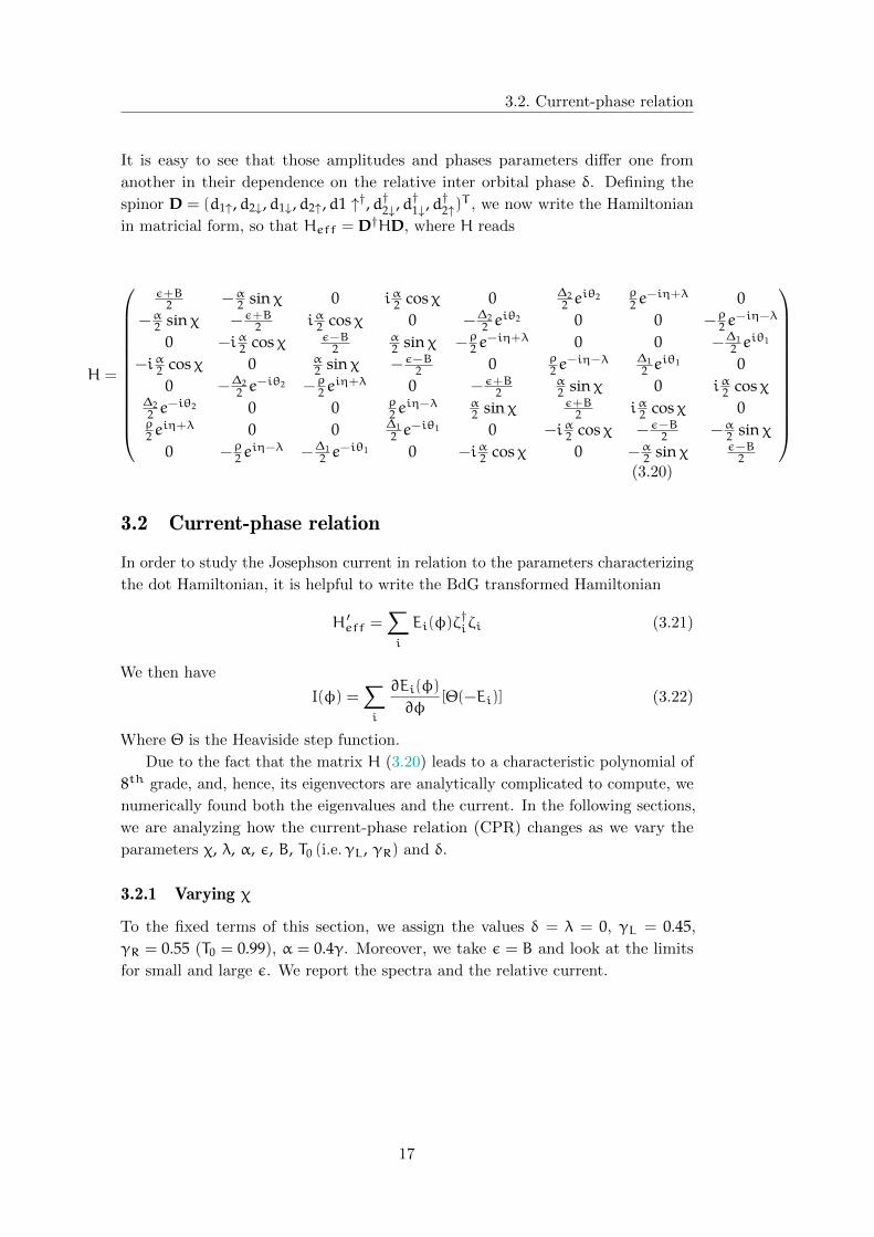
3.2 Current-phase relation
In order to study the Josephson current in relation to the parameters characterizing
the dot Hamiltonian, it is helpful to write the BdG transformed Hamiltonian
H ′eff =∑i
Ei(φ)ζ†iζi (3.21)
We then have
I(φ) =∑i
∂Ei(φ)
∂φ[Θ(−Ei)] (3.22)
Where Θ is the Heaviside step function.
Due to the fact that the matrix H (3.20) leads to a characteristic polynomial of
8th grade, and, hence, its eigenvectors are analytically complicated to compute, we
numerically found both the eigenvalues and the current. In the following sections,
we are analyzing how the current-phase relation (CPR) changes as we vary the
parameters χ, λ, α, ε, B, T0 (i.e.γL, γR) and δ.
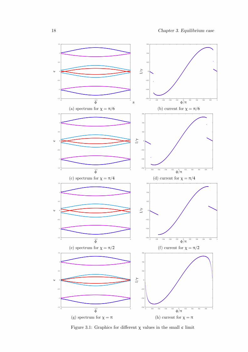
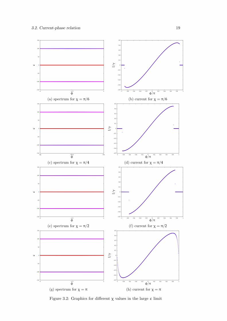
3.2.1 Varying χ
To the fixed terms of this section, we assign the values δ = λ = 0, γL = 0.45,
γR = 0.55 (T0 = 0.99), α = 0.4γ. Moreover, we take ε = B and look at the limits
for small and large ε. We report the spectra and the relative current.
17
18 Chapter 3. Equilibrium case
-1.5
-1
-0.5
0
0.5
1
1.5
-π -π/2 π
ε
φ s
(a) spectrum for χ = π/6
−0.6
−0.4
−0.2
0
0.2
0.4
0.6
−1 −0.8 −0.6 −0.4 −0.2 0 0.2 0.4 0.6 0.8 1
I/γ
φ/π
(b) current for χ = π/6
-1.5
-1
-0.5
0
0.5
1
1.5
-π -π/2 π
ε
φ
(c) spectrum for χ = π/4
−0.6
−0.4
−0.2
0
0.2
0.4
0.6
−1 −0.8 −0.6 −0.4 −0.2 0 0.2 0.4 0.6 0.8 1
I/γ
φ/π
(d) current for χ = π/4
-1.5
-1
-0.5
0
0.5
1
1.5
-π -π/2 π
ε
φ
(e) spectrum for χ = π/2
−0.6
−0.4
−0.2
0
0.2
0.4
0.6
−1 −0.8 −0.6 −0.4 −0.2 0 0.2 0.4 0.6 0.8 1
I/γ
φ/π
(f) current for χ = π/2
-1.5
-1
-0.5
0
0.5
1
1.5
-π -π/2 π
ε
φ
(g) spectrum for χ = π
−0.6
−0.4
−0.2
0
0.2
0.4
0.6
−1 −0.8 −0.6 −0.4 −0.2 0 0.2 0.4 0.6 0.8 1
I/γ
φ/π
(h) current for χ = π
Figure 3.1: Graphics for different χ values in the small ε limit
3.2. Current-phase relation 19
-150
-100
-50
0
50
100
150
-π -π/2 π
ε
φ
(a) spectrum for χ = π/6
−0.5
−0.4
−0.3
−0.2
−0.1
0
0.1
0.2
0.3
0.4
0.5
−1 −0.8 −0.6 −0.4 −0.2 0 0.2 0.4 0.6 0.8 1
I/γ
φ/π
(b) current for χ = π/6
-150
-100
-50
0
50
100
150
-Π4 -Π4/2 Π4
ε
φ
(c) spectrum for χ = π/4
−0.5
−0.4
−0.3
−0.2
−0.1
0
0.1
0.2
0.3
0.4
0.5
−1 −0.8 −0.6 −0.4 −0.2 0 0.2 0.4 0.6 0.8 1
I/γ
φ/π
(d) current for χ = π/4
-150
-100
-50
0
50
100
150
-π -π/2 π
ε
φ
(e) spectrum for χ = π/2
−0.5
−0.4
−0.3
−0.2
−0.1
0
0.1
0.2
0.3
0.4
0.5
−1 −0.8 −0.6 −0.4 −0.2 0 0.2 0.4 0.6 0.8 1
I/γ
φ/π
(f) current for χ = π/2
-150
-100
-50
0
50
100
150
-π -π/2 π
ε
φ
(g) spectrum for χ = π
−0.5
−0.4
−0.3
−0.2
−0.1
0
0.1
0.2
0.3
0.4
0.5
−1 −0.8 −0.6 −0.4 −0.2 0 0.2 0.4 0.6 0.8 1
I/γ
φ/π
(h) current for χ = π
Figure 3.2: Graphics for different χ values in the large ε limit
Chapter 3. Equilibrium case
We immediately see the presence of a discontinuity in the current for χ =
π/6,π/4,π/2, while the function is continuous when χ = π. Physically, this means
that the flat part is bigger when the SOC field is orthogonal to the Zeeman field,
while it vanishes when they are parallel, i.e. the SOC field is just “added” to the
magnetic one.Looking at the spectra, we recognize that the presence of the jump
is due to the overlapping in zero of the two lowest energy bands (red lines in the
graphs). Moreover, the straight parts at the endings of the graphics increases with χ
until it reaches the value χ = π/2, then they decrease again, vanishing when χ = π.
The main difference between the small and the large limit is that the straight parts
are horizontal in the latter case, which point us to the typical step function shape.
Furthermore, we remark that the spectra are exactly the same, near zero, in both
cases, even if it is not visible from the plots reported here.
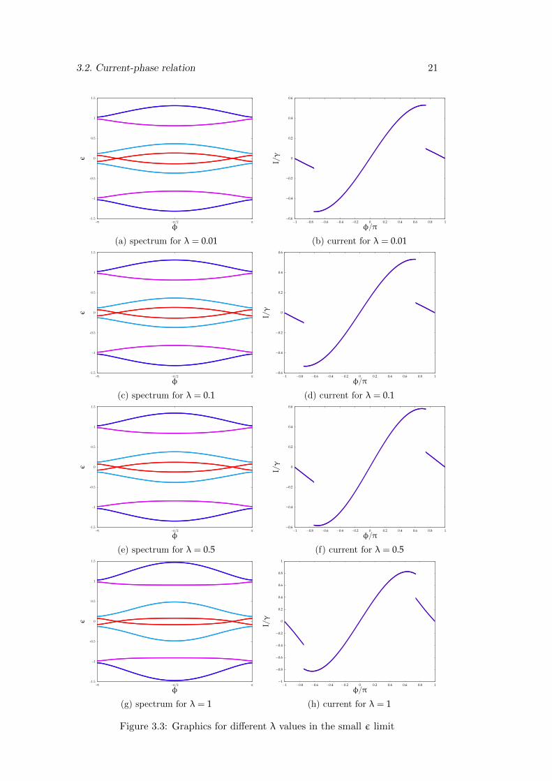
3.2.2 Varying λ
We take the fixed values to be as in the previous section, setting the value χ = π/2and varying the λ value. Physically, λ is related to the hopping modulus |ti,j|
2,
i = 1, 2 and j = L,R, thus it gives an amplitude of the tunneling probability between
the j lead and the ith dot level. Again, we look at the small and the large limit
for the energy. Furthermore, we are only considering the symmetric case λL = λR,
so that the Hamiltonian can be written as in (3.20). We analysed the values
λ = 0.01, 0.1, 0.5, 1.
20
3.2. Current-phase relation 21
-1.5
-1
-0.5
0
0.5
1
1.5
-π -π/2 π
ε
φ
(a) spectrum for λ = 0.01
−0.6
−0.4
−0.2
0
0.2
0.4
0.6
−1 −0.8 −0.6 −0.4 −0.2 0 0.2 0.4 0.6 0.8 1
I/γ
φ/π
(b) current for λ = 0.01
-1.5
-1
-0.5
0
0.5
1
1.5
-π -π/2 π
ε
φ
(c) spectrum for λ = 0.1
−0.6
−0.4
−0.2
0
0.2
0.4
0.6
−1 −0.8 −0.6 −0.4 −0.2 0 0.2 0.4 0.6 0.8 1
I/γ
φ/π
(d) current for λ = 0.1
-1.5
-1
-0.5
0
0.5
1
1.5
-π -π/2 π
ε
φ
(e) spectrum for λ = 0.5
−0.6
−0.4
−0.2
0
0.2
0.4
0.6
−1 −0.8 −0.6 −0.4 −0.2 0 0.2 0.4 0.6 0.8 1
I/γ
φ/π
(f) current for λ = 0.5
-1.5
-1
-0.5
0
0.5
1
1.5
-π -π/2 π
ε
φ
(g) spectrum for λ = 1
−1
−0.8
−0.6
−0.4
−0.2
0
0.2
0.4
0.6
0.8
1
−1 −0.8 −0.6 −0.4 −0.2 0 0.2 0.4 0.6 0.8 1
I/γ
φ/π
(h) current for λ = 1
Figure 3.3: Graphics for different λ values in the small ε limit
Chapter 3. Equilibrium case
−0.5
−0.4
−0.3
−0.2
−0.1
0
0.1
0.2
0.3
0.4
0.5
−1 −0.8 −0.6 −0.4 −0.2 0 0.2 0.4 0.6 0.8 1
I/γ
φ/π
(a) current for λ = 0.01
−0.5
−0.4
−0.3
−0.2
−0.1
0
0.1
0.2
0.3
0.4
0.5
−1 −0.8 −0.6 −0.4 −0.2 0 0.2 0.4 0.6 0.8 1
I/γ
φ/π
(b) current for λ = 0.1
−0.5
−0.4
−0.3
−0.2
−0.1
0
0.1
0.2
0.3
0.4
0.5
−1 −0.8 −0.6 −0.4 −0.2 0 0.2 0.4 0.6 0.8 1
I/γ
φ/π
(c) current for λ = 0.5
−0.5
−0.4
−0.3
−0.2
−0.1
0
0.1
0.2
0.3
0.4
0.5
−1 −0.8 −0.6 −0.4 −0.2 0 0.2 0.4 0.6 0.8 1
I/γ
φ/π
(d) current for λ = 1
Figure 3.4: Graphics for different λ values in the large ε limit
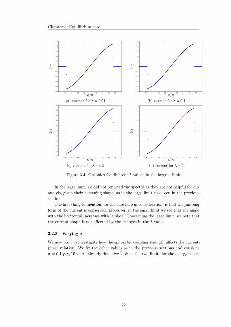
In the large limit, we did not reported the spectra as they are not helpful for our
analyis, given their flattening shape, as in the large limit case seen in the previous
section.
The first thing to mention, for the case here in consideration, is that the jumping
form of the current is conserved. Moreover, in the small limit we see that the angle
with the horizontal increases with lambda. Concerning the large limit, we note that
the current shape is not affected by the changes in the λ value.
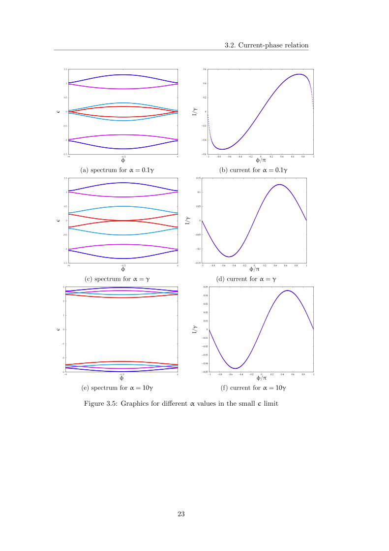
3.2.3 Varying α
We now want to investigate how the spin-orbit coupling strength affects the current-
phase relation. We fix the other values as in the previous sections and consider
α = 0.1γ,γ, 10γ. As already done, we look at the two limits for the energy scale.
22
3.2. Current-phase relation
-1.5
-1
-0.5
0
0.5
1
1.5
-π -π/2 π
ε
φ
(a) spectrum for α = 0.1γ
−0.6
−0.4
−0.2
0
0.2
0.4
0.6
−1 −0.8 −0.6 −0.4 −0.2 0 0.2 0.4 0.6 0.8 1
I/γ
φ/π
(b) current for α = 0.1γ
-1.5
-1
-0.5
0
0.5
1
1.5
-π -π/2 π
ε
φ
(c) spectrum for α = γ
−0.15
−0.1
−0.05
0
0.05
0.1
0.15
−1 −0.8 −0.6 −0.4 −0.2 0 0.2 0.4 0.6 0.8 1
I/γ
φ/π
(d) current for α = γ
-3
-2
-1
0
1
2
3
-π -π/2 π
ε
φ
(e) spectrum for α = 10γ
−0.05
−0.04
−0.03
−0.02
−0.01
0
0.01
0.02
0.03
0.04
0.05
−1 −0.8 −0.6 −0.4 −0.2 0 0.2 0.4 0.6 0.8 1
I/γ
φ/π
(f) current for α = 10γ
Figure 3.5: Graphics for different α values in the small ε limit
23
Chapter 3. Equilibrium case
−0.5
−0.4
−0.3
−0.2
−0.1
0
0.1
0.2
0.3
0.4
0.5
−1 −0.8 −0.6 −0.4 −0.2 0 0.2 0.4 0.6 0.8 1
I/γ
φ/π
(a) current for α = 0.1γ
−0.0015
−0.001
−0.0005
0
0.0005
0.001
0.0015
−1 −0.8 −0.6 −0.4 −0.2 0 0.2 0.4 0.6 0.8 1
I/γ
φ/π
(b) current for α = γ
−0.0015
−0.001
−0.0005
0
0.0005
0.001
0.0015
−1 −0.8 −0.6 −0.4 −0.2 0 0.2 0.4 0.6 0.8 1
I/γ
φ/π
(c) current for α = 10γ
Figure 3.6: Graphics for different α values in the large ε limit
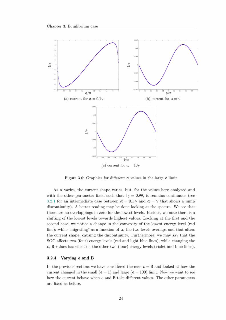
As α varies, the current shape varies, but, for the values here analyzed and
with the other parameter fixed such that T0 = 0.99, it remains continuous (see
3.2.1 for an intermediate case between α = 0.1γ and α = γ that shows a jump
discontinuity). A better reading may be done looking at the spectra. We see that
there are no overlappings in zero for the lowest levels. Besides, we note there is a
shifting of the lowest levels towards highest values. Looking at the first and the
second case, we notice a change in the convexity of the lowest energy level (red
line): while “migrating” as a function of α, the two levels overlaps and that alters
the current shape, causing the discontinuity. Furthermore, we may say that the
SOC affects two (four) energy levels (red and light-blue lines), while changing the
ε, B values has effect on the other two (four) energy levels (violet and blue lines).
3.2.4 Varying ε and B
In the previous sections we have considered the case ε = B and looked at how the
current changed in the small (ε = 1) and large (ε = 100) limit. Now we want to see
how the current behave when ε and B take different values. The other parameters
are fixed as before.
24
3.2. Current-phase relation
-1.5
-1
-0.5
0
0.5
1
1.5
-π -π/2 π
ε
φ
(a) spectrum for B = 1.1, ε = 1
−0.6
−0.4
−0.2
0
0.2
0.4
0.6
−1 −0.8 −0.6 −0.4 −0.2 0 0.2 0.4 0.6 0.8 1
I/γ
φ/π
(b) current for B = 1.1, ε = 1
-2
-1.5
-1
-0.5
0
0.5
1
1.5
2
-π -π/2 π
ε
φ
(c) spectrum for B = 1.5, ε = 1
−0.4
−0.3
−0.2
−0.1
0
0.1
0.2
0.3
0.4
−1 −0.8 −0.6 −0.4 −0.2 0 0.2 0.4 0.6 0.8 1
I/γ
φ/π
(d) current for B = 1.5, ε = 1
-15
-10
-5
0
5
10
15
-π -π/2 π
ε
φ
(e) spectrum for B = 15, ε = 10
−1e− 05
−8e− 06
−6e− 06
−4e− 06
−2e− 06
0
2e− 06
4e− 06
6e− 06
8e− 06
1e− 05
−1 −0.8 −0.6 −0.4 −0.2 0 0.2 0.4 0.6 0.8 1
I/γ
φ/π
(f) current for B = 15, ε = 10
25
Chapter 3. Equilibrium case
−0.005
−0.004
−0.003
−0.002
−0.001
0
0.001
0.002
0.003
0.004
0.005
−1 −0.8 −0.6 −0.4 −0.2 0 0.2 0.4 0.6 0.8 1
I/γ
φ/π
(a) current for B = 10, ε = 50
−0.0015
−0.001
−0.0005
0
0.0005
0.001
0.0015
−1 −0.8 −0.6 −0.4 −0.2 0 0.2 0.4 0.6 0.8 1
I/γ
φ/π
(b) current for B = 50, ε = 10
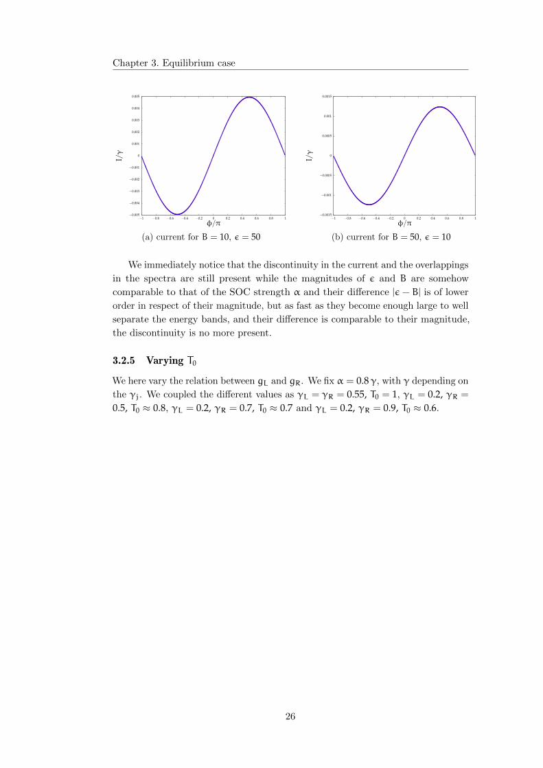
We immediately notice that the discontinuity in the current and the overlappings
in the spectra are still present while the magnitudes of ε and B are somehow
comparable to that of the SOC strength α and their difference |ε− B| is of lower
order in respect of their magnitude, but as fast as they become enough large to well
separate the energy bands, and their difference is comparable to their magnitude,
the discontinuity is no more present.
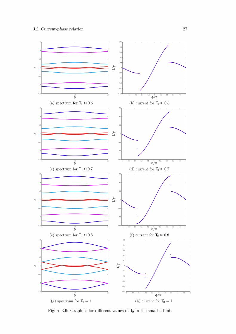
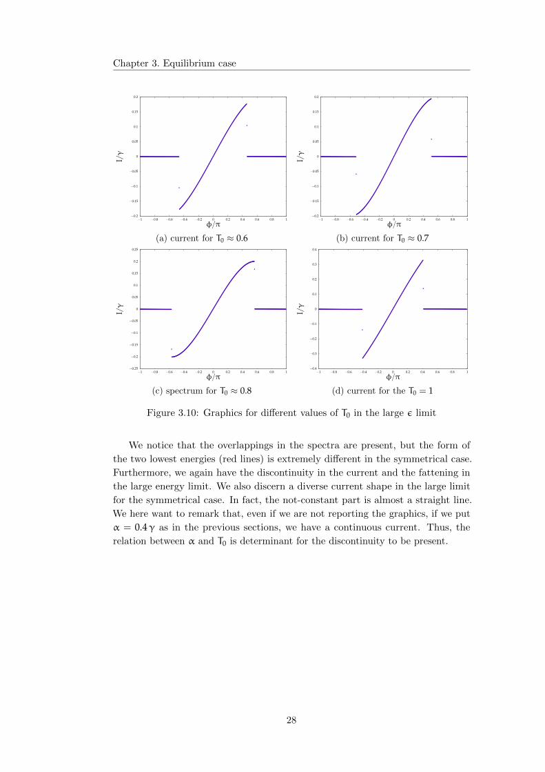
3.2.5 Varying T0
We here vary the relation between gL and gR. We fix α = 0.8γ, with γ depending on
the γj. We coupled the different values as γL = γR = 0.55, T0 = 1, γL = 0.2, γR =
0.5, T0 ≈ 0.8, γL = 0.2, γR = 0.7, T0 ≈ 0.7 and γL = 0.2, γR = 0.9, T0 ≈ 0.6.
26
3.2. Current-phase relation 27
-1.5
-1
-0.5
0
0.5
1
1.5
-π -π/2 π4
ε
φ
(a) spectrum for T0 ≈ 0.6
−0.25
−0.2
−0.15
−0.1
−0.05
0
0.05
0.1
0.15
0.2
0.25
−1 −0.8 −0.6 −0.4 −0.2 0 0.2 0.4 0.6 0.8 1
I/γ
φ/π
(b) current for T0 ≈ 0.6
-1.5
-1
-0.5
0
0.5
1
1.5
-π -π/2 π4
ε
φ
(c) spectrum for T0 ≈ 0.7
−0.3
−0.2
−0.1
0
0.1
0.2
0.3
−1 −0.8 −0.6 −0.4 −0.2 0 0.2 0.4 0.6 0.8 1
I/γ
φ/π
(d) current for T0 ≈ 0.7
-1.5
-1
-0.5
0
0.5
1
1.5
-π -π/2 π
ε
φ
(e) spectrum for T0 ≈ 0.8
−0.3
−0.2
−0.1
0
0.1
0.2
0.3
−1 −0.8 −0.6 −0.4 −0.2 0 0.2 0.4 0.6 0.8 1
I/γ
φ/π
(f) current for T0 ≈ 0.8
-1.5
-1
-0.5
0
0.5
1
1.5
-π -π/2 π4
ε
φ
(g) spectrum for T0 = 1
−0.5
−0.4
−0.3
−0.2
−0.1
0
0.1
0.2
0.3
0.4
0.5
−1 −0.8 −0.6 −0.4 −0.2 0 0.2 0.4 0.6 0.8 1
I/γ
φ/π
(h) current for T0 = 1
Figure 3.9: Graphics for different values of T0 in the small ε limit
Chapter 3. Equilibrium case
−0.2
−0.15
−0.1
−0.05
0
0.05
0.1
0.15
0.2
−1 −0.8 −0.6 −0.4 −0.2 0 0.2 0.4 0.6 0.8 1
I/γ
φ/π
(a) current for T0 ≈ 0.6
−0.2
−0.15
−0.1
−0.05
0
0.05
0.1
0.15
0.2
−1 −0.8 −0.6 −0.4 −0.2 0 0.2 0.4 0.6 0.8 1
I/γ
φ/π
(b) current for T0 ≈ 0.7
−0.25
−0.2
−0.15
−0.1
−0.05
0
0.05
0.1
0.15
0.2
0.25
−1 −0.8 −0.6 −0.4 −0.2 0 0.2 0.4 0.6 0.8 1
I/γ
φ/π
(c) spectrum for T0 ≈ 0.8
−0.4
−0.3
−0.2
−0.1
0
0.1
0.2
0.3
0.4
−1 −0.8 −0.6 −0.4 −0.2 0 0.2 0.4 0.6 0.8 1
I/γ
φ/π
(d) current for the T0 = 1
Figure 3.10: Graphics for different values of T0 in the large ε limit
We notice that the overlappings in the spectra are present, but the form of
the two lowest energies (red lines) is extremely different in the symmetrical case.
Furthermore, we again have the discontinuity in the current and the fattening in
the large energy limit. We also discern a diverse current shape in the large limit
for the symmetrical case. In fact, the not-constant part is almost a straight line.
We here want to remark that, even if we are not reporting the graphics, if we put
α = 0.4γ as in the previous sections, we have a continuous current. Thus, the
relation between α and T0 is determinant for the discontinuity to be present.
28
3.2. Current-phase relation
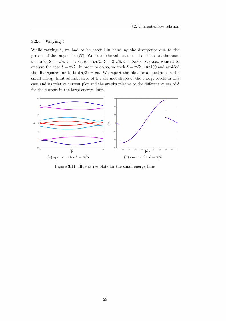
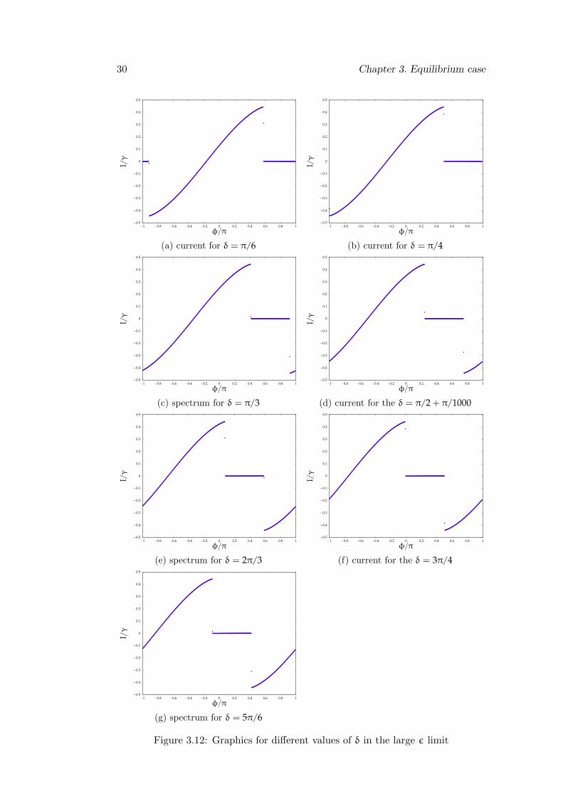
3.2.6 Varying δ
While varying δ, we had to be careful in handling the divergence due to the
present of the tangent in (??). We fix all the values as usual and look at the cases
δ = π/6, δ = π/4, δ = π/3, δ = 2π/3, δ = 3π/4, δ = 5π/6. We also wanted to
analyze the case δ = π/2. In order to do so, we took δ = π/2 + π/100 and avoided
the divergence due to tan(π/2) = ∞. We report the plot for a spectrum in the
small energy limit as indicative of the distinct shape of the energy levels in this
case and its relative current plot and the graphs relative to the different values of δ
for the current in the large energy limit.
-1.5
-1
-0.5
0
0.5
1
1.5
-π -π/2 π4
ε
φ
(a) spectrum for δ = π/6
−0.6
−0.4
−0.2
0
0.2
0.4
0.6
−1 −0.8 −0.6 −0.4 −0.2 0 0.2 0.4 0.6 0.8 1
I/γ
φ/π
(b) current for δ = π/6
Figure 3.11: Illustrative plots for the small energy limit
29
30 Chapter 3. Equilibrium case
−0.5
−0.4
−0.3
−0.2
−0.1
0
0.1
0.2
0.3
0.4
0.5
−1 −0.8 −0.6 −0.4 −0.2 0 0.2 0.4 0.6 0.8 1
I/γ
φ/π
(a) current for δ = π/6
−0.5
−0.4
−0.3
−0.2
−0.1
0
0.1
0.2
0.3
0.4
0.5
−1 −0.8 −0.6 −0.4 −0.2 0 0.2 0.4 0.6 0.8 1
I/γ
φ/π
(b) current for δ = π/4
−0.5
−0.4
−0.3
−0.2
−0.1
0
0.1
0.2
0.3
0.4
0.5
−1 −0.8 −0.6 −0.4 −0.2 0 0.2 0.4 0.6 0.8 1
I/γ
φ/π
(c) spectrum for δ = π/3
−0.5
−0.4
−0.3
−0.2
−0.1
0
0.1
0.2
0.3
0.4
0.5
−1 −0.8 −0.6 −0.4 −0.2 0 0.2 0.4 0.6 0.8 1
I/γ
φ/π
(d) current for the δ = π/2 + π/1000
−0.5
−0.4
−0.3
−0.2
−0.1
0
0.1
0.2
0.3
0.4
0.5
−1 −0.8 −0.6 −0.4 −0.2 0 0.2 0.4 0.6 0.8 1
I/γ
φ/π
(e) spectrum for δ = 2π/3
−0.5
−0.4
−0.3
−0.2
−0.1
0
0.1
0.2
0.3
0.4
0.5
−1 −0.8 −0.6 −0.4 −0.2 0 0.2 0.4 0.6 0.8 1
I/γ
φ/π
(f) current for the δ = 3π/4
−0.5
−0.4
−0.3
−0.2
−0.1
0
0.1
0.2
0.3
0.4
0.5
−1 −0.8 −0.6 −0.4 −0.2 0 0.2 0.4 0.6 0.8 1
I/γ
φ/π
(g) spectrum for δ = 5π/6
Figure 3.12: Graphics for different values of δ in the large ε limit
3.3. Physical significance of the current discontinuity
Concerning the example for the small energy limit, we see how the overlappings
in the spectrum are present and the discontinuity in the current too. The distinct
behavior in respect of what has been seen in the previous sections is the horizontal
shifting in the spectrum. Moreover, this shifting is easily observed in the reported
graphics for the current in the large energy limit: as δ increases, the current shape
remains the same while there is a “movement” to the left.
3.3 Physical significance of the current discontinuity
We have seen a discontinuity arises in the current under a certain parameters regime.
We now want to relate this phenomenon to its physical cause and significance. In
order to do so, we will introduce the concepts and formalism regarding Majorana
fermions (MFs) in condensed matter physics, then demonstrate how our system
can be mapped into a Kitaev chain in a well defined energy limit.
3.3.1 Majorana quasiparticles in condensed matter physics
Majorana fermions (MFs) are fermionic particles which are their own antiparticles.
Whether they exist or not as elementary particles is still unclear. It is conventional,
in condensed matter to refer to particular quasiparticles, that shows Majorana
characteristic, as Majorana fermions, even if they exhibit a non-Abelian anyonic
statistic [4]. Thus, in line with the literature, we will refer, in this text, to
those quasiparticles as Majorana fermions. In the case just described, a MF is a
quasiparticle which is its ‘own hole’. Furthermore, A Majorana particle can be seen
as half of a fermion, or in other words, a fermion can be obtained as a superposition
of two MFs. We can always split a fermionic wave-function in two parts: a real one
and an imaginary one. This may seem as just a mathematical operation without
physical significance or consequences: that is true if the MFs are spatially localized
and hence their wave-functions overlap significantly, so that they recombine, but if
they are spatially separated (or prevented from overlapping) the physical meaning
becomes clear. Moreover, such a highly delocalized fermionic state is protected
from almost all kinds of decoherence as it is not affected by local perturbations
acting on jus one of its Majorana constituent. The state can be manipulated using
the fact that MFs have non-Abelian statistics, thus a physical exchange of MFs has
a non trivial effect on the state [19].
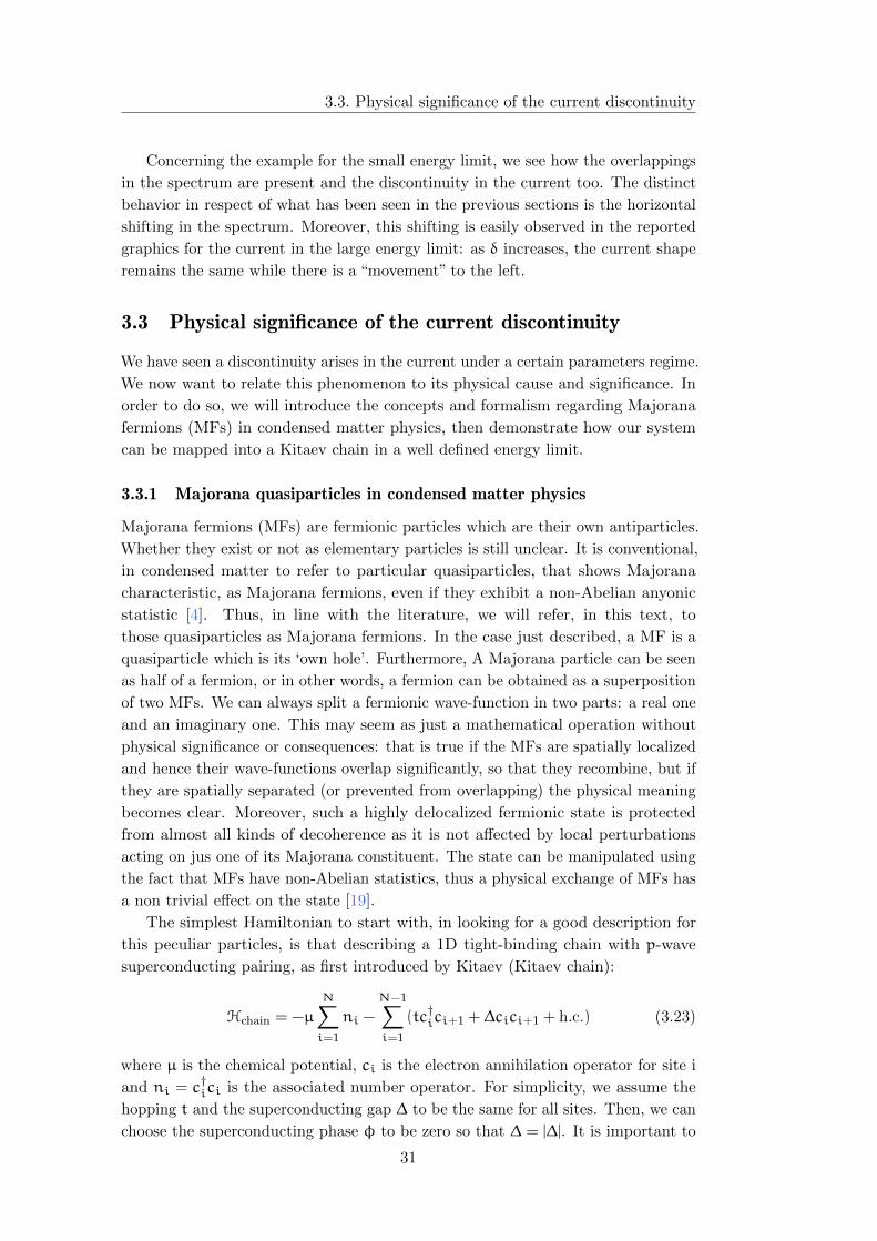
The simplest Hamiltonian to start with, in looking for a good description for
this peculiar particles, is that describing a 1D tight-binding chain with p-wave
superconducting pairing, as first introduced by Kitaev (Kitaev chain):
Hchain = −µ
N∑i=1
ni −
N−1∑i=1
(tc†ici+1 + ∆cici+1 + h.c.) (3.23)
where µ is the chemical potential, ci is the electron annihilation operator for site i
and ni = c†ici is the associated number operator. For simplicity, we assume the
hopping t and the superconducting gap ∆ to be the same for all sites. Then, we can
choose the superconducting phase φ to be zero so that ∆ = |∆|. It is important to
31
Chapter 3. Equilibrium case
note that time reversal symmetry is broken in the Hamiltonian (3.23), since we have
suppressed the spin label thus considering just one value for the spin projection:
this symmetry breaking is fundamental for MFs as we now that, in the time sector,
we can consider the antiparticles to be the particles going back in time, so, if the
system is time-invariant, we cannot tell the particles from the antiparticles. Going
back to our systems, the superconducting pairing is non-standard, since it couples
electrons with the same spin. Moreover, electrons on neighboring sites are paired.
In order to write eq. (3.23) in terms of Majorana operators we define two
Hermitian operators as
γi,1 = c†i + ci (3.24a)
γi,2 = i(c†i − ci) (3.24b)
And, inverting, we see that this gives γi,1 and γi,2 as “real” and “imaginary” parts
of the electrons operators
ci =12(γi,1 + iγi,2) (3.25a)
c†i =
12(γi,1 − iγi,2) (3.25b)
From their definition, these operators are Hermitian and, therefore, Majorana
operators.
To better understand Majorana physics, we consider the case µ = 0, t = ∆.
Inserting eq (3.25a) and (3.25b) into the Hamiltonian (3.23), we have
Hchain = −t
N−1∑i=1
(c†ici+1 + cici+1 + c†i+1ci + c
†i+1c
†i)
= −t
4
N−1∑i=1
[(γi,1 − iγi,2)(γi+1,1 + iγi+1,2) + (γi,1 + iγi,2)(γi+1,1 + iγi+1,2)
+ (γi+1,1 − iγi+1,2)(γi,1 + iγi,2) + (γi+1,1 − iγi+1,2)(γi,1 − iγi,2)]
= −it
N−1∑i=1
γi,2γi+1,1 (3.26)
And (3.26) is just the diagonalized Hamiltonian. To see it, we can go back to
a fermionic representation constructing new “normal” fermions operators ci by
combining Majorana operators on neighboring sites:
ci = (γi+1,1 + iγi,2)/2 (3.27)
We then find
−iγi,2γi+1,1 = 2c†i ci = 2ni
Therefore
Hchain = 2tN−1∑i=1
c†i ci (3.28)
32
3.3. Physical significance of the current discontinuity
We then see that ci are annihilation operators corresponding to the eigenstates and
the energy cost of creating a ci fermion is 2t. We may hence say that the Majorana
operators are merely a formal way of rewriting the Hamiltonian and the physical
excitations are fermionic states at finite energy, obtained by a superposition of
nearest neighbor MFs. So, there appears to be nothing special about eq (3.26).
Nevertheless, we notice that the Majorana operators γN,2 and γ1,1, localized at the
two ends of the wire, are completely missing from eq. (3.26). We may rearrange
this two Majorana operators to describe a single fermionic state
cM = (γN,2 + iγ1,1)/2 (3.29)
As the MFs associated to the operators γ2,N and γ1,1 are localized at the two
opposite ends of the chain, we conclude that this state is highly non-local and, since
the fermion operator is absent from the Hamiltonian, occupying the corresponding
state requires zero energy. We know that, normally, superconductors have a non-
degenerate ground state consisting of superposition of even-particle-number states
(condensate of Cooper pairs). In contrast to this, the Hamiltonian (3.23) allows
for an odd number of quasiparticles at zero energy cost. The ground state is thus
twofold degenerate: corresponding to have in total an even or odd number of
electrons in the superconductor. This property is also called parity and corresponds
to the eigenvalue of the number operator associated to the zero-energy fermion,
nM = c†McM = 0(1) for even (odd) parity.
We have considered only the very special case with µ = 0 and ∆ = t. It can be
shown that the Majorana end states remain as long as the chemical potential lies
within the gap, |µ| < 2t. In this general case the MFs are not completely localized
at the ends but decay exponentially away from the edges [19]. Moreover, the MFs
remain at zero energy only if the wire is long enough that they do not overlap.
Another, easier, way to see the MFs are zero-energy modes is to notice that
we are actually interested in systems where the particles are electrons while the
antiparticles are holes. We know that electrons have energy E > 0, where we have
put EF = 0, and holes have energy −E. Then, if we consider the set of fermionic
operators ξ(E), ξ†(E), the following relation is true
ξ(E) = ξ†(−E)
Then, at the Fermi level, we have ξ = ξ†, and we have concluded.
Majorana fermions in condensed matter physics have other peculiar properties,
but we are not entering their detail as our work is not related to them and a good
dissertation would require way more expertise and space than ours.
3.3.2 Mapping the system to a Kitaev chain
Following the work by Brunetti et al. [21], we now demonstrate how the discontinuity
in the current is related to the occurrence of MFs states.
First, we have seen how a peculiar Θ Heaviside function shape occurs in the
current form in the large limit, and how the energy scale relation between the SOC,
ε and B is essential to the overlapping in the spectra and the current jumping
33
Chapter 3. Equilibrium case
discontinuity. Furthermore, we have considered the connection between B and ε in
the large limit and observed that the discontinuity vanishes when B 6= ε. Thus, we
will consider the parameter regime
∆ ε+ B max(α, |ε− B|,γL,R,µ) (3.30)
and ε = B, while µ = 0 as already set above. Moreover, we set χ = π/2 in order to
have a block-diagonal dot Hamiltonian matrix h (3.11). We can now simplify our
system noting that the upper-block state (2, ↓) is always full, while the state (1, ↑)is always empty. We can then write a truncated effective Hamiltonian H ′eff, acting
only within the lower right block described by the (effectively spinless) fermion
operators d1,↓ ≡ d1, d2,↑ ≡ d2
H ′eff = (µ+ ε− B)d†1d1 + [µ− (ε− B)]d†2d2
+(αd†1d2 + ∆(φ)e
iθ(φ)d†2d†1 + h.c.
)(3.31)
The fact that we have dropped the spin indices should point to the Kitaev chain
(3.23) and the considerations done in section 3.3.1. Using equations (3.13) (3.14)
(3.15), we put ∆1(φ) ≡ ∆(φ) and θ1(φ) ≡ θ(φ). H ′eff can be diagonalized in terms
of fermionic Bogoliubov-de Gennes quasiparticle operators
η± =12
[d1 + d2 ± eiθ
(d†1 − d
†2
)](3.32)
wich yields
H ′eff =∑±E±(φ)
(η†±η± −
12
)E± = α± ∆(φ) (3.33)
The current phase relation follows from (3.33)
I(φ) = 2∂φ∆[Θ(−E+) −Θ(−E−)] (3.34)
Where Θ is the Heaviside function. Notice that I = 0 for ∆ < α. as both energies
E± = α± ∆ have the same sign. Therefore
I(φ) = Θ(∆(φ) − α)I0(φ) (3.35)
I0(φ) =γ
2T0 sin(φ+ δ)√
1 − T0 sin2[(φ+ δ)/2]
The CPR (3.35) is 2π-periodic in φ and vanishes (reappears) at the boundaries
between ground states with opposite fermion parity. These boundaries coincides
with the formation points of MBSs. In fact, we have seen that Majoranas are zero
energy modes in sec 3.3. In the case considered, we can have zero energy just for
E− = 0. This implies
∆(φ) = α (3.36)
This corresponds to a pair of Majorana fermions that can be represented via the
operator ξ1 = −i(η− − η†−) and ξ2 = η− + η†−. To avoid recombination, the MFs
34
3.3. Physical significance of the current discontinuity
have to be spatially separated. Looking at the actual form of the ξi operators
ξ1 = −i
2
[(1 − e−iθ
)d1 +
(1 − e−iθ
)d2 +
(−1 − eiθ
)d†1 +
(−1 + eiθ
)d†2
](3.37)
ξ2 =12
[(1 − e−iθ
)d1 +
(1 + e−iθ
)d2 +
(1 − eiθ
)d†1 +
(1 + eiθ
)d†2
](3.38)
Imposing the spatial separation (i.e. a Majorana fermion in one dot and the second
in the other), we find a condition for θ
θ = 0ξ1 = −i[d1 − d
†1]
ξ2 = d2 + d†2
(3.39)
θ = π
ξ1 = −i[d2 − d
†2]
ξ2 = d1 + d†1
(3.40)
Thus, we finally have the condition
θ(φ) = 0 modπ (3.41)
From eq. (3.15), we see there are two possibilities to satisfy this condition:
1. Choose equal hybridization strength γL = γR = γ. Then, T0 = 1, thus
∆ = γ| cos[(φ+ δ)/2] = α
2. If γL 6= γR, we may adjust φ = −δ (mod 2π)and then we hav a MBS pair
when γ = α
35

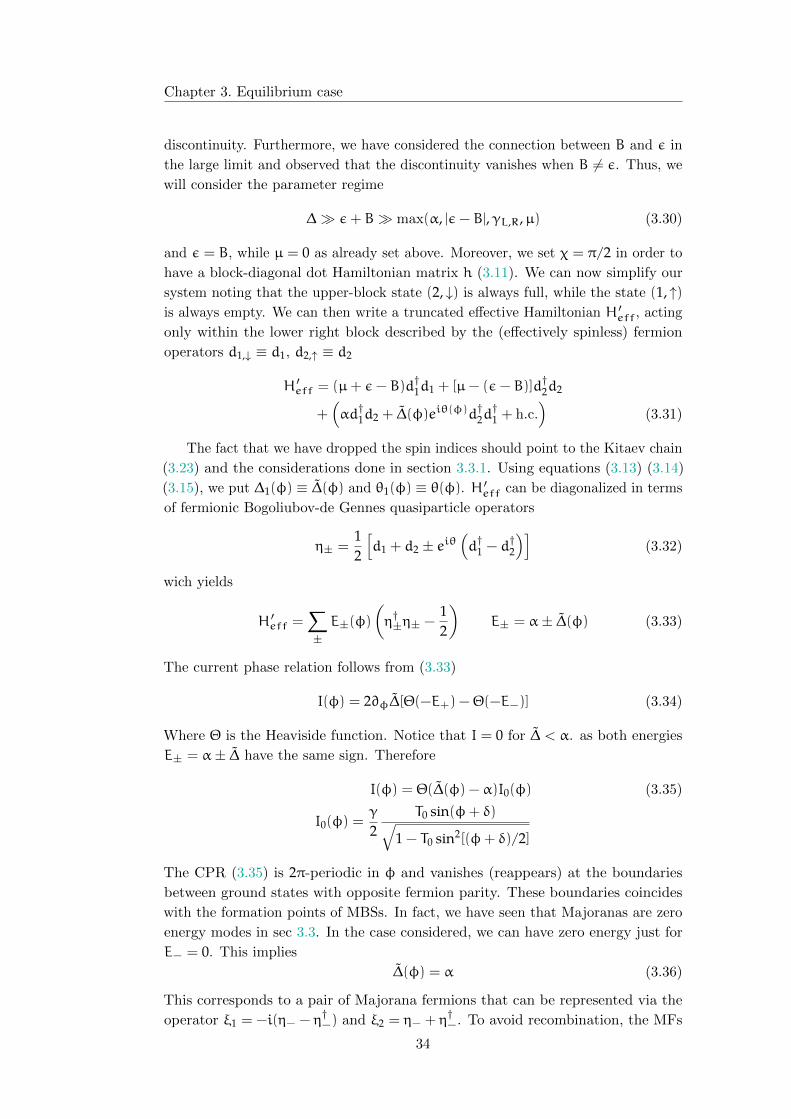
Non-equilibrium case44.1 Keldysh formalism for out of equilibrium systems
It is known that, in an equilibrium situation, the time evolution operator U(t, t ′) is
such that U(−∞, t) = U(∞, t), as the system recovers to the same non-perturbed
state |φ0〉 for t→ ±∞. This fact is used while studying the perturbation theory for
the Green’s function, and leads to the well known Feynman diagram and Dyson’s
equation. In the case of a non-equilibrium situation this is not true anymore, as
nothing assures that at t = +∞ we will retrieve the same state we had at t = −∞.
In fact, with the loss of the equilibrium hypothesis, the temporal symmetry is lost
too. Hence, it may seem like it is not possible to have a perturbative expansion as
we had in the previous case.
The way out was given by Keldysh who redefined the time contour in order to
be able to write the expectation value of an operator as a (Keldysh) time ordered
expectation value. Before introducing the Keldysh formalism, it is useful to review
the well known formulas of the equilibrium case:
〈A(t)〉 = 〈ΨI(t)|AI(t) |ΨI(t)〉〈ΨI(t)|ΨI(t)〉
(4.1)
Where the“I” subscript stands for Interaction (or Dirac) picture. In the adiabatic
hypothesis, we can substitute V(t)→ limη→0 V(t)e−η|t|. Assuming that at t = −∞the system was in the state |φ0〉 and that, at t, it has evolved to |ΨI(t)〉, we can
write for (4.1):
〈A(t)〉 = 〈φ0|U(−∞, t)AI(t)U(t,−∞) |φ0〉〈φ0|U(−∞, t)U(t,−∞) |φ0〉
(4.2)
So, in the equilibrium case;
〈A(t)〉 = 〈φ0|U(∞, t)AI(t)U(t,−∞) |φ0〉〈φ0|U(∞, t)U(t,−∞) |φ0〉
And it follows
〈A(t)〉 = 〈φ0|T[AI(t)U(∞,−∞)] |φ0〉〈φ0|U(∞,−∞) |φ0〉
(4.3)
While equation (4.2) is valid in any case the last two (4.1), (4.3) are not. In
order to generalize this writing for the non-equilibrium case, we here introduce the
Keldysh contour
37
Chapter 4. Non-equilibrium case
−∞upper branch (+)
+∞lower branch (−)
−∞Figure 4.1: Keldish time contour
With this time contour, the system starts form the state |φ0〉 at t = −∞, evolves
out of equilibrium while the time becomes arbitrarily large to reach t = +∞, then
“subsequently” goes back to the initial state as the time returns to t = −∞, as
shown in figure 4.1. In this manner, we have recovered the temporal symmetry we
had in the equilibrium case.
It is important to note that the distinction between the two branches becomes
essential when we are time-ordering the operators. We define the Keldysh contour
time-ordering operator Tc and the evolution operator along the Keldysh contour
Uc = U−(−∞,∞)U+(∞,−∞). Then, we can write:
〈A(t)〉 = 〈φ0|Tc[AI(t)Uc(∞,−∞)] |φ0〉〈φ0|Uc(∞,−∞) |φ0〉
(4.4)
In analogy with the known perturbative expansion for U(t, t ′), we write:
U+(+∞,−∞) = 1 +∑n
(−i)n
n!
∫+∞−∞ dt1 . . .
∫+∞−∞ dtnT[VI(t1) . . . VI(tn)] (4.5a)
U−(−∞,+∞) = 1 +∑n
(−i)n
n!
∫−∞+∞ dt1 . . .
∫−∞+∞ dtnT[VI(t1) . . . VI(tn)] (4.5b)
The operator T is defined in the lower branch of the Keldysh contour and thus
the times are ordered backwards. Inserting expressions (4.5) in (4.4) we have the
desired perturbative expansion of 〈A(t)〉. Furthermore, the Wick’s theorem is still
valid.
The Green’s function is modified as follows in order to have a theory formally
equivalent to the equilibrium case:
Gij(tα, t ′β) = −i 〈Ψh|Tc[ciσ(tα)c†jσ(t′β)] |ΨH〉 (4.6)
where α and β are indices taking values +,− to indicate the Keldysh contour
branches.
At this point, we need to distinguish between four different possibilities for the
“positioning” of the two times in the Keldysh Green’s function.
• t = t+ and t ′ = t ′+Both arguments are in the upper branch, so they are time-ordered as usual
and we have
G++ij = −i
⟨Tc[ciσ(t)c†jσ(t
′)]⟩
= −i⟨T[ciσ(t)c†jσ(t
′)]⟩
(4.7)
38
4.1. Keldysh formalism for out of equilibrium systems
From equation (4.7) we see that this is the conventional casual Green’s function
• t = t+ and t ′ = t ′−We now have to be careful and observe that a time in the lower branch is
intrinsically in the “future” in respect to a time in the upper branch. We have:
G+−ij (t, t ′) = i
⟨c†jσ(t
′)ciσ(t)⟩
(4.8)
This function is sometimes referred to as the Keldysh Green’s function and it
plays a central role in out of equilibrium systems.
• t = t− and t ′ = t ′+From the considerations above
G−+ij = −i
⟨ciσ(t)c†jσ(t
′)⟩
(4.9)
and this function is closely related to (4.8).
• t = t− and t ′ = t ′−Both the times are in the lower branch, so we use the time-anti-ordering
operator TG−−ij = −i
⟨T[ciσ(t)c†jσ(t
′)]⟩
(4.10)
This is really similar to the usual Green’s function (4.8) but with the times
ordered in the reversed sense.
A concise way to express the propagator in the Keldysh space is
G =
(G++ G+−
G−+ G−−
)(4.11)
And this form makes clear that we have doubled our initial time space.
In the Keldysh formalism, the perturbative expansion of the propagators becomes
formally equivalent to the equilibrium case, the only difference being that now we
deal with 2x2 matrixes in the Keldysh space. In time space, the Dyson’s equation
will be
G(t, t ′) = g(t, t ′) +∫dt1
∫dt2 g(t, t1)Σ(t1, t2)G(t2, t ′) (4.12)
Where g is the unperturbed Green’s function and Σ is the self-energy. In a stationary
situation, propagators and self-energies will depend only on time intervals and we
can compute the Fourier transform and write the Dyson’s equation in the frequency
space:
G(ω) = g(ω) + g(ω)Σ(ω)G(ω) (4.13)
We remark that both equation (4.12) and equation (4.13) are in Keldysh space.
It is to be noted that in the Keldysh formalism the denominator 〈φ0|Uc |φ0〉does not play any role. It is easily seen if |φ0〉 is normalized since, in this case we
straightforward have
Uc = U(−∞,+∞)U(+∞,−∞) = 139
Chapter 4. Non-equilibrium case
An attentive reader may arise the question on how the disconnected diagrams
vanishes in this formalism: they simply cancel out between themselves at every
order of the perturbation, as it can be seen using the Wick’s theorem.
For later purposes, it is helpful to enumerate the main properties of the Keldysh
propagators:
• The four Green’s function G++, G+−, G−+, G−− are not indipendent. They
verify
G++ + G−− = G+− + G−+ (4.14)
• The Keldysh Green’s functions are linearly related to the advanced and
retarded Green’s function Ga and Gr:
Gr = G++ − G+− = −G−− + G−+ (4.15a)
Ga = G++ − G−+ = −G−− + G+− (4.15b)
• For we have seen that the four Green’s functions are not independent, we
conclude only three of them are strictly necessary to express the 2x2 Keldysh
matrix G. Moreover, we can eliminate the G++ and G−− using the relation
between Keldysh Green’s functions and retarded and advanced Green’s func-
tions. A possible way to eliminate G++ and G−− is by means of a rotation
in the Keldysh space that gives(G++ G+−
G−+ G−−
)=⇒
(0 Ga
Gr GF
)(4.16)
where GF = G+− +G−+. This representation is usually known as triangular
representation: we will denote the matrix propagators in this representation
with G. Transforming the Dyson’s equation from the Keldysh representation
to the triangular representation, we have
G = g + g Σ G (4.17)
Where the self-energy matrix has the form:
Σ =
(Ω Σr
Σa 0
)(4.18)
Where Ω = Σ+− +Σ−+. For the self-energy, we have the following relations:
Σr = Σ++ + Σ+− = −(Σ−− + Σ−+) (4.19a)
Σa = Σ++ + Σ−+ = −(Σ−− + Σ+−) (4.19b)
From equations (4.17) and (4.18) we conclude that both the retarded and the
advanced Green’s functions satisfy their own equations
Gr,a = gr,a + gr,aΣr,aGr,a (4.20)
By similar consideration, GF satisfies the following Dyson’s equation:
GF = gF + gF ΣaGa + gr ΣrGF + grΩ Ga (4.21)
40
4.1. Keldysh formalism for out of equilibrium systems
• In order to write the Dyson’s equation for the Keldysh function G+−, we
first point out to an important property in Keldysh space, that is: every +−
element of any matrixes product can be expressed in terms of exclusively
retarded, advanced and +− quantities in the following manner:
(ABC . . . YZ)+− = A+−Ba . . . Za + ArB+−Ca . . . Za + . . .+ArBr . . . Y+−Za + Ar . . . YrZ+− (4.22)
We now may use this to rewrite the Dyson’s equation for the standard Keldysh
representation
G+− = g+− + (g Σ G)+− (4.23)
Using (4.22) we have
G+− = g+− + g+− ΣaGa + gr Σ+− Ga + gr ΣrG+− (4.24)
The function G−+ satisfies a similar equation with + and − exchanged. We
now want to write (4.24) in a more symmetrical form. First, we take out
G+− as common factor
G+− = (I − gr Σr)−1g+−(I + ΣaGa) + (I − gr Σr)−1grΣ+−Ga (4.25)
From the Dyson’s equation for the retarded Green function, we have
Gr = gr + gr ΣrGr ⇒ (I − gr Σr)Gr = gr ⇒ Gr = (I − gr Σr)−1gr (4.26)
Moreover
(I + Gr Σr)(I − gr Σr) = I + Gr Σr + grΣr + Gr Σr gr Σr
= I + Gr Σr + gr Σr + (Gr − gr)Σr = I (4.27)
Thus
G+− = (I + Gr Σr)g+−(I + ΣaGa) + Gr Σ+− Ga (4.28)
And analogous for G−+.
Before passing to the calculations for our model, let us consider a system of
non-interacting electrons in equilibrium. Let H0 be the correspondent Hamiltonian.
In this case, all unperturbed Green’s functions depend exclusively on the difference
of their time arguments and it is possible to obtain the Fourier transform in the
frequency space. We still focus on the G+−. From its definition in time space
G+−ij (t) = i
⟨c†jσ(0)ciσ(t)
⟩This function is evidently related to the electron distribution in equilibrium. Al-
though the temperature is a parameter that does not explicitly appear in the
Keldysh formalism, it can be introduced in the following way through the equilib-
rium Fermi distribution function. Evaluating the above expression for t = 0 and
i = j
G+−ii (0) = i 〈niσ〉 =
∫+∞−∞
dω
2π G+−ii (ω) (4.29)
41
Chapter 4. Non-equilibrium case
Where niσ is the average occupation of the one electron quantum state (iσ). This
equation states that G+−ii (ω) = 2π i ρii(ω)f(ω) where ρii(ω) is the electronic
density of states projected on the state |i〉 and f(ω) is the Fermi distribution
function. By means of a same argument, we have G−+ii (ω) = −2π i ρii(ω)[1−f(ω)].
This results indicates that irrespective of the one-electron basis, G+−(ω) ∝ f(ω)
and G−+(ω) ∝ [1 − f(ω)]. Now, using (4.14) and (4.15) we have
Ga(t) − Gr(t) = G+−(t) − G−+(t)
Therefore
G+−(ω) = [Ga(ω) − Gr(ω)]f(ω) (4.30a)
G−+(ω) = −[Ga(ω) − Gr(ω)][1 − f(ω)] (4.30b)
Equations (4.30) are still valid for a system of interacting electrons and will come
handy in computing the form of the Josephson current in the next section.
4.2 Computing the current
The difference between the system we are considering here and what analyzed in
the previous section is that we are now applying an external voltage within the
superconductors. Hence, the system is now out of equilibrium. The definition of
the left/right current, obviously, is the same as the one given above. Nevertheless,
the actual computation of the Josephson current has a different form, following the
Keldysh formalism introduced in the previous section. We follow the steps as in
Dolcini and Dell’Anna [22].
First of all, the presence of an applied voltage can be modeled introducing a
time dependence in the tunneling coupling, i.e. writing
tj,n(t) = tj,n(0)exp(ijωVt/2)
and we have defined
ωV =eV h
Next, we remark that the Hamiltonian matrix h can be diagonalized via a
unitary transformation U
dnσ = (Uσ)njDm m = 1, . . . , 4 (4.31)
Hence, we write
Hd =
4∑i=1
εiD†iDi (4.32)
We have denoted with εi the eigenvalues. In our case, they have the form
ε1,2 = ∓√α2 + B2 + ε2 −
√2√B2(α2 + 2ε2 + α2 cos(2χ)) (4.33a)
ε3,4 = ∓√α2 + B2 + ε2 +
√2√B2(α2 + 2ε2 + α2 cos(2χ)) (4.33b)
42
4.2. Computing the current
We define U↑(↓) as a 2× 4 upper (lower) submatrix of U.
Now, we introduce the block-diagonal 2× 8 tunneling matrix
Tj =
((t1,j t2,j)U↑ 0
0 −(t∗1,j t∗2,j)U
∗↓
)(4.34)
and its time dependence is given by
Tj(t) =
(eijωVt/2 0
0 e−ijωVt/2
)Tj(0) (4.35)
We rewrite the j tunneling matrix as
Ht,j =∑
k؆k Tj(t)D + h.c. (4.36)
where we have denote with D = (D1, · · · , D4,D†1, · · · ,D†4)T . We observe that the
matrices Tj are in Nambu space. Adding the Keldysh structure to the Nambu form,
we define the 4× 16
Tj =
(Tj 00 −Tj
)(4.37)
Thus, we can write the current in the form
Ij(t) = −2Re∑
kTr8(σz)8[T†j (t)Gkj,0(t, t)]+− (4.38)
Where (σz)8 = σz ⊗ I4. The Green function appearing in the current formula is
the lead-dot Green function, with entries
iGη1,η2kj,0 (t1, t2) = 〈Ψ
(η1)k,j (t1) (D†)(η2)(t2)〉 (4.39)
with η1, η2 indices in Keldysh space. Exploiting the Keldysh-Dyson equation
Gkj,0(t, t) =∫+∞−∞ gkj,kj(t, t ′)Tj(t ′)G(t ′, t) (4.40)
where gkj,kj is the Green function of the j lead and G is the Green function of the
dot. Inserting (4.39) into (4.38), we have (overlooking the prefactors)
Ij =∑
kTr8(σz)8[T†j (t)Gkj,0(t, t)]+−
=∑
kTr8(σz)8[
∫+∞−∞ T
†j (t)gkj,kj(t, t ′)Tj(t ′)G(t ′, t)dt ′]+−
=
∫+∞−∞ dt ′Tr8(σz)8[Σj(t, t ′)G(t ′, t)]+− (4.41)
Where we have made use of the linearity property of the trace, the integral and the
summation and we have defined
Σj(t, t ′) =∑
kT†j (t)gkj,kj(t
′, t)Tj(t ′) (4.42)
43
Chapter 4. Non-equilibrium case
And the dot’s Green function can be computed using the Keldysh-Dyson equation
as
G = G0 + G0(ΣL + ΣR)G
G0 = (I − G0(ΣL + ΣR))G
G =
[([I − G0(ΣL + ΣR)]
−1G0
)−1]−1
=[G−1
0 [I − G0(ΣL + ΣR)]−1
= (G−10 − ΣL − ΣR)
−1 (4.43)
and G0 describes the isolated dot.
We now introduce a discrete Fourier transform in order to write the current de-
composed in its harmonic representation. We denote the discrete Fourier transform
of an arbitrary two time arguments f(t1, t2) with f(n1,n2;ω) and define it as
f(t1, t2) =∞∑
n,m=−∞∫F
dω
2π e−i(ω+nωV)t1ei(ω+mωv)t2f(n,m;ω) (4.44)
and F is the fundamental domain given by
F =[−ωV2 , ωV2
](4.45)
The inverse transformation reads
2πδ(ω1 −ω2)f(n1,n2;ω) =
∫+∞−∞ dt
∫+∞−∞ dt ′f(t, t ′)ei(ω1+n1ωv)te−i(ω2+n2ωV)t
′
(4.46)
with the constraint ω1, ω2 ∈ F. If the function f(t1, t2) depends only on the times
difference, its discrete Fourier transform reads
f(n1,n2;ω) = δn1,n2 f(ω+ n1ωV) (4.47)
Where f(ω) is the usual Fourier transform.
Before continuing in computing Σj, we take a step back and calculate the leads
Green function gkjkj. First, we not the leads are in equilibrium, so that
∑kgkj,kj(t, t ′) =
∫+∞−∞
dω
2π e−iω(t−t ′)gj(ω) = gj(t− t
′) (4.48)
Denoting with ρ(εF) the density of states, we get (in Nambu space)
gr/aj (ω) =
πρ(εF)√∆2p − (ω± iη)2
[−ωσ0 + ∆pσ1] (4.49)
Now, for |ω| < ∆p the square root is real and
gr/aj (ω) = πρ(εF)
−ωσ0 + ∆jσ1√∆2j −ω
2(4.50)
44
4.2. Computing the current
We specify the (dimensionless) quasiparticle density of states
Nj(ω) =ω√
ω2 − ∆2j
Θ(ω2 − ∆2j) (4.51)
where Θ(r) is the Heaviside step function. For |ω| > ∆j the square root is complex
and we have
gr/aj = ∓iπρ(εf)Nj(ω)[σ0 − (∆j/ω)σ1] (4.52)
We now pass in the continuum limit using∑
k → ρ(εF)∫+∞−∞ dεk and note that the
terms linear in εk cancel out
∑kgr/akj,kj(ω) =
∑k
(ω± iη− εk ∆j
∆j ω± iη+ εk
)−1
= ρ(εF)
∫+∞−∞
dε
ε2 + ∆2j − (ω± iη)2
(−(ω± iη) ∆j
∆j −(ω± iη)
)(4.53)
Using (4.30) we get
gj(ω) = πρ(εF)
τ3−ωΘ(∆j − |ω|)√
∆2j −ω
2+ iNj(ω)
(2f(ω) − 1 2f(ω)
2f(ω) − 2 2f(ω) − 1
)K
⊗
(1 −
∆jω
−∆jω 1
)N
(4.54)
And here we have denoted with τ3 the z-Pauli matrix in Keldysh space.
We can now proceed and compute the transformed Σj.
Σj(n1,n2;ω) =
∫+∞−∞ dt
∫+∞−∞ dt ′Σj(t, t ′)ei(ω1+n1ωV)te−i(ω2+n2ωV)t
′
=∑
k
∫+∞−∞ dt
∫+∞−∞ dt ′T
†j (t)gkj,kj(t, t ′)Tj(t ′)ei(ω1+n1ωV)te−i(ω2+n2ωV)t
′
=∑
k
∫+∞−∞ dt
∫+∞−∞ dt ′T
†j (0)e
−ijσzωVt/2gkj,kj(t, t ′)eijσzωVt′/2Tj(0)
ei(ω1+n1ωV)te−i(ω2+n2ωV)t′
We see that the two Keldysh tunneling matrices in the last line are time-independent.
Thus, we can put them out of the integral. Moreover, we momentarily drop the
summation in the following calculations.
Σj(n1,n2;ω) =
∫+∞−∞ dt
∫+∞−∞ dt ′ei(ω1+n1ωV−jσzωV/2)tgkj,kj(t, t ′)e−i(ω2+n2ωV−jσzωV/2)t ′
We remember that the leads Green function has a K ⊗ N tensor structure and
that the tunneling entries are in Nambu space. Thus, we consider the ij-entries in
Nambu space for g and compute
45
Chapter 4. Non-equilibrium case
(ei[ω1+(n1−j/2)ωV ]t 0
0 ei[ω1+(n1+j/2)ωV ]t
)(g11 g12g21 g22
)(e−i[ω2+(n2−j/2)ωV ]t ′ 0
0 e−i[ω2+(n2+j/2)ωV ]t ′
)=
=
(ei[ω1+(n1−j/2)ωV ]t g11 e
−i[ω2+(n2−j/2)ωV ]t ′ ei[ω1+(n1−j/2)ωV ]t g12e−i[ω2+(n2+j/2)ωV ]t ′
ei[ω1+(n1+j/2)ωV ]t g21 e−i[ω2+(n2−j/2)ωV ]t ′ ei[ω1+(n1+j/2)ωV ]t g22e
−i[ω2+(n2+j/2)ωV ]t ′
)
Exploiting equation (4.47), we get
Σj(n1,n2;ω) = T†j (0)
δn2,n1
[gj(ω+ n1ωV − jωV
2
]11
δn2,n1−j
[gj(ω+ n1ωV − jωV
2 )]
12δn2,n1+j
[gj(ω+ n1ωV − jωV
2 )]
21δn2,n1
[gj(ω+ n1ωV − jωV
2 )]
22
Tj(0)
(4.55)
The transformed dot’s Green function can then be easily calculated, as the isolated
Green function is easily found to be
G−10 (n1,n2;ω) = δn1,n2G
−10 (ω+ n1ωV) (4.56)
G−10 (ω) =
[ωI8 − σz ⊗ diag(ε1, . . . , ε4)
]τ3
Having all the components, we can now perform a discrete Fourier transformation
on the current (4.41). We focus on the term relative to ΣjG
∫+∞−∞ Σj(t, t ′)G(t ′, t) =
∫+∞−∞
[+∞∑
n,m=−∞∫F
dω
2π e−i(ω+nωV)tei(ω+mωV)t
′Σj(n,m;ω)
+∞∑n1,m1=−∞
∫F
dω ′
2π e−i(ω ′+n1ωV)t
′ei(ω+m1ωV)tG(n1,m1;ω)
]δm,n1
=∑n,mn1,m1
∫F
dω
2π
∫F
dω ′[Σj(n,m;ω)G(n1,m1;ω ′)
ei[(ω′−ω)−(n−m1)ωV ]tδ
(ω ′ −ω− (m− n1)ωV
)δm,n1
]=∑n,mn1,m1
∫F
dω
2π Σj(n,m;ω)G(n1,m1;ω+ (m− n1)ωV)ei(m−n1−n+m1)ωVtδm,n1
=∑n,mm ′
eim′ωVt
∫F
dω
2π Σj(n,m;ω)G(m,n+m ′,ω) (4.57)
Where, in the first passage, we have inserted the δm,n1 in order to be able to
perform the matrix product, in the second and third passage we have performed
the integration over dt ′ and dω ′ respectively and in the fourth passage we have
defined m1 − n = m ′. Inserting (4.57) into (4.41) we finally have
Ij(t) = −1π
Re
+∞∑m=−∞ e
imωVt
∫F
dωTr8(σz)8
[+∞∑
n1,n2=−∞Σj(n1,n2;ω)G(n2,n1 +m;ω)
]+−
(4.58)
46
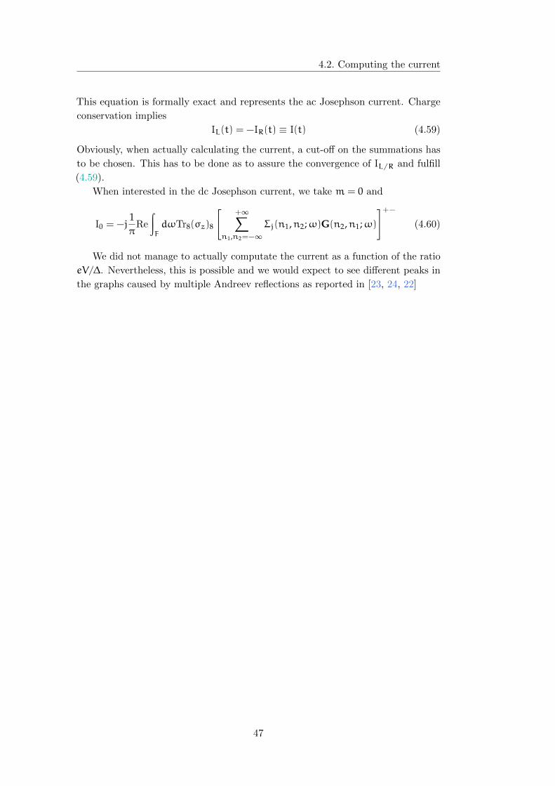
4.2. Computing the current
This equation is formally exact and represents the ac Josephson current. Charge
conservation implies
IL(t) = −IR(t) ≡ I(t) (4.59)
Obviously, when actually calculating the current, a cut-off on the summations has
to be chosen. This has to be done as to assure the convergence of IL/R and fulfill
(4.59).
When interested in the dc Josephson current, we take m = 0 and
I0 = −j1π
Re
∫F
dωTr8(σz)8
[+∞∑
n1,n2=−∞Σj(n1,n2;ω)G(n2,n1;ω)
]+−
(4.60)
We did not manage to actually computate the current as a function of the ratio
eV/∆. Nevertheless, this is possible and we would expect to see different peaks in
the graphs caused by multiple Andreev reflections as reported in [23, 24, 22]
47

Conclusions5In this work, we considered a system made by a double quantum dot in contact
with two superconducting leads and focused on the Josephson current flowing
through it at equilibrium.
In particular, we studied the current-phase relation in the presence of a Rashba-
like spin-orbit coupling and of a Zeeman term, in the limit of large superconducting
order parameter. Changing all the parameters involved, we found different current-
phase relations and corresponding sets of Andreev energy levels.
We showed that the spin-orbit term makes the profile of the Josephson current
very peculiar and unusual. In the presence of spin-orbit coupling and Zeeman field,
in fact, the Josephson current exhibits some discontinuities as a function of the
phase difference. In a certain limit, these discontinuities can be related to the
formation of the so-called Majorana bound states.
In the last part of the work, we considered the same system but driven out of
equilibrium by an applied voltage, deriving an explicit expression for the current.
The aim was to study the effect of spin-orbit and Zeeman field (specially in the
range of parameters where the corresponding equilibrium Josephson current is
discontinuous) on the current-voltage curve and, in particular, on the multiple
Andreev reflection peaks, which are features expected to occur for eV/2|∆| < 1. We
are still working on that and we are planning to develop a code for this purpose.
49

Bibliography5[1] L. Fu and C. L. Kane,“Superconducting proximity effect and majorana fermions
at the surface of a topological insulator,” Phys. Rev. Lett., vol. 100, no. 9, 2008.
1
[2] N. Read and D. Green, “Paired states of fermions in two dimensions with
breaking of parity and time-reversal symmetries and the fractional quantum
hall effect,” Phys. Rev. B, vol. 61, no. 15, 2000. 1
[3] K. Sengupta, I. Zutic, H.-J. Kwon, V. M. Yakovenko, and S. D. Sarma,
“Midgap edge states and pairing symmetry of quasi-one-dimensional organic
superconductors,” Phys. Rev. B, vol. 63, no. 14, 2001. 1
[4] D. A. Ivanov, “Non-abelian statistics of half-quantum vortices in p -wave
superconductors,” Phys. Rev. Lett., vol. 86, no. 2, 2001. 1, 31
[5] B. Josephson, “Possible new effects in superconductive tunneling,” Phys. Lett,
vol. 1, no. 251, 1962. 1
[6] P.W.Anderson and J. Rowell, “Probable observation of the josephson tunnel
effect,” Phys. Rev. Lett., vol. 10, no. 230, 1963. 1
[7] P. D. Gennes, “Coupling between ferromagnets through a superconducting
layer,” Phys. Lett., vol. 1, no. 23, 1966. 1
[8] H. Bruus and K. Flensberg, Many-body quantum theory in condensed matter
physics: An Introduction. OUP Oxford, 2004. 3
[9] J. Kondo, “Resistance minimum in dilute magnetic alloys,” Progress of Theore-
tycal Physics, vol. 32, no. 1, 1964. 3
[10] P. Anderson, “A poor man's derivation of scaling laws for the kondo problem,”
J. Phys. C: Solid State Phys., vol. 3, no. 12, 1970. 3
[11] L. Glazman and M. Raikh, “Resonant kondo transparency of a barrier with
quasilocal impurity states,” Jetp. Phys., vol. 47, no. 8, 1988. 3
[12] T. K. Ng and P. A. Lee, “On-site coulomb repulsion and resonant tunneling,”
Phys. Rev. Lett., vol. 61, no. 15, 1988. 3
[13] D. Goldhaber-Gordon, J. Gores, M. A. Kastner, H. Shtrikman, D. Mahalu,
and U. Meirav, “From the kondo regime to the mixed-valence regime in a
single-electron transistor,” Phys. Rev. Lett., vol. 81, no. 23, 1998. 4
[14] S. Sasaki, S. D. Franceschi, J. M. Elzerman, N. G. van der Wiel, M. Eto,
S. Tarucha, and L. P. Kouwenhoven, “Kondo effect in an integer-spin quantum
dot,” Nature, vol. 405, no. 6788, 2000. 4
51
BIBLIOGRAPHY
[15] S. Cronenwett, T. Oosterkamp, and L. Kouwenhoven, “A tunable kondo effect
in quantum dots,” Science, vol. 281, no. 5376, 1998. 4
[16] H. Jeong, A. Chang, and M. Melloch, “The kondo effect in an artificial quantum
dot molecule,” Science, vol. 293, no. 5538, 2001. 4
[17] T. Klapwijk, G. Blonder, and M. Tinkham, “Explanation of subharmonic
energy gap structure in superconducting contacts,” Physica B+C, vol. 109-110,
1982. 11
[18] G. E. Blonder, M. Tinkham, and T. M. Klapwijk, “Transition from metallic
to tunneling regimes in superconducting microconstrictions: Excess current,
charge imbalance, and supercurrent conversion,” Phys. Rev. B, vol. 25, no. 7,
1982. 11
[19] M. Leijnse and K. Flensberg, “Introduction to topological superconductivity
and majorana fermions,” Semicond. Sci. Technol., vol. 27, no. 12, 2012. 31, 33
[20] J. Alicea, Y. Oreg, G. Refael, F. von Oppen, and M. P. A. Fisher, “Non-abelian
statistics and topological quantum information processing in 1d wire networks,”
Nat. Phys., vol. 7, no. 5, 2011.
[21] A. Brunetti, A. Zazunov, A. Kundu, and R. Egger, “Anomalous josephson
current, incipient time-reversal symmetry breaking, and majorana bound states
in interacting multilevel dots,” Phys. Rev. B, vol. 88, no. 14, 2013. 33
[22] F. Dolcini and L. Dell’Anna, “Multiple andreev reflections in a quantum dot
coupled to superconducting leads: Effect of spin-orbit coupling,” Phys. Rev. B,
vol. 78, no. 2, 2008. 42, 47
[23] A. L. Yeyati, J. C. Cuevas, A. Lopez-Davalos, and A. Martın-Rodero, “Resonant
tunneling through a small quantum dot coupled to superconducting leads,”
Phys. Rev. B, vol. 55, no. 10, 1997. 47
[24] M. R. Buitelaar, W. Belzig, T. Nussbaumer, B. Babic, C. Bruder, and C. Scho-
nenberger, “Multiple andreev reflections in a carbon nanotube quantum dot,”
Phys. Rev. Lett., vol. 91, no. 5, 2003. 47
[25] A. Kamenev, Field Theory of Non-Equilibrium Systems. Cambridge University
Press, 2011.
[26] M. Tinkham, Introduction to superconductivity. Dover Pubns, 2004.
52
Related Documents

![Universit a degli Studi di Padova - Benvenuti su [email protected]](https://static.cupdf.com/doc/110x72/623144e01cb07c303d32a836/universit-a-degli-studi-di-padova-benvenuti-su-emailprotected.jpg)


