Universality and scaling study of the critical behavior of the two-dimensional Blume-Capel model in short-time dynamics

arX

iv:c

ond-

mat

/020

4346

v1 [

cond

-mat

.sta

t-m

ech]

16

Apr

200

2 Universality and scaling study of the critical behavior of the two-dimensional

Blume-Capel model in short-time dynamics

Roberto da Silva∗, Nelson A. Alves†, and J. R. Drugowich de Felıcio‡

Departamento de Fısica e Matematica, FFCLRP Universidade de Sao Paulo, Avenida Bandeirantes 3900,

CEP 014040-901, Ribeirao Preto, Sao Paulo, Brazil

(February, 26, 2002)

In this paper we study the short-time behavior of the Blume-Capel model at the tricritical pointas well as along the second order critical line. Dynamic and static exponents are estimated byexploring scaling relations for the magnetization and its moments at early stage of the dynamicevolution. Our estimates for the dynamic exponent, at the tricritical point, are z = 2.215(2) andθ = −0.53(2).

Keywords: short-time dynamics, critical phenomena, dynamic exponent, Blume-Capel model, Monte Carlo simula-tions.

PACS-No.: 64.60.Fr, 64.60.Ht, 02.70.uu, 75.10.Hk

1. INTRODUCTION

Numerical simulation in the short-time regime has become an important tool to study phase transitions and criticalphenomena. The reason is that universality and scaling behavior are already present in the dynamic systems since theearly stages of their evolution [1,2]. Moreover, this kind of approach reveals the existence of a new and unsuspectedcritical exponent. As shown by Janssen et al. [1] on basis of renormalization group theory, if we tune the parametersat their critical values but with initial configurations characterized by nonequilibrium states, the time evolution ofquantities like magnetization exhibit a polynomial behavior governed by an exponent θ, which is independent of theknown set of static exponents and of the dynamical critical exponent z. This new exponent characterizes the socalled “critical initial slip”, the anomalous behavior of the magnetization when the system is quenched to the criticaltemperature Tc. Working with systems without conserved quantities, model A in the terminology of Halperin et al.

[3], Janssen et al. found a scaling form for the moments of the magnetization, which sets soon after a microscopictime scale tmic. Those relations have been confirmed in several numerical experiments [4–6]. For the kth moment ofthe magnetization, this scaling form reads

M (k)(t, τ, L, m0) = b−kβ/νM (k)(b−zt, b1/ντ, b−1L, bx0m0) . (1)

Here b is an arbitrary spatial scaling factor, t is the time evolution and τ is the reduced temperature, τ = (T −Tc)/Tc.As usual, the exponents β and ν are the well-known static exponents, whereas z is the dynamic one. Equation (1)depends on the initial magnetization m0 and gives origin to the new exponent x0, the scaling dimension of the initialmagnetization, related to θ by θ = (x0 − β/ν)/z.

For a large lattice size L and small initial magnetization m0, the system in its early stage presents small spatial andtemporal correlation lengths, which may eliminate usual finite size problems. In this limit, if we choose the scalingfactor b = t1/z [1,5,6] at the critical temperature (τ = 0), we obtain

M(t, m0) ∼ m0tθ (2)

from the scaling relation (1). The exponent θ has been calculated for the two-dimensional (2d) [5,7] and three-dimensional (3d) [7,8] Ising models, 2d 3-state Potts model [5], Ising model with next-nearest neighbor interactions[9] and Ising model with a line of defects [10]. In addition, this short-time universal behavior was found in irreversiblemodels with synchronous [11] and continuous time dynamics [12]. In all of those cases, a positive value for θ has been

found, that indicates a surprising initial increasing of the magnetization in the short-time regime t0 ∼ m−z/x0

0 . Thiseffect can be related to a “mean field” behavior since the system presents small correlation length in the beginning of

∗E-mail: [email protected]†E-mail: [email protected]‡E-mail: [email protected]

1

the time evolution. Thus, when the system is quenched to the critical temperature Tc, it feels as being in an orderedstate since Tc < T MF

c [13].On the other hand, as shown by Janssen and Oerding [14], the behavior of a thermodynamic system is more complex

at a tricritical point (TP) and the corresponding exponent θ may attain negative values.At a tricritical point the magnetization shows a crossover from the logarithmic behavior M(t) ∼ m0(ln(t/t0))

−a atshort times t << m−4

0 to t−1/4 power law with logarithmic corrections, M(t) ∼ (t/ln(t/t0))−1/4 in 3 dimensions. The

above behavior can be stated in the generalized form

M(t) = m0 (ln(t/t0))−aFM

((t

ln(t/t0)

)1/4

(ln(t/t0))−a m0

), (3)

where FM (x) ∼ 1 or FM (x) ∼ 1/x, respectively for vanishing and large arguments. Below 3 dimensions it reduces tothe scaling form

M(t) ∼ m0tθ . (4)

Here θ is the exponent related to the tricritical point of the relaxation process at early times and it is expected toassume negative values.

In this paper, we perform short-time Monte Carlo (MC) simulations to explore the critical dynamics of the 2dBlume-Capel model. We evaluate the dynamic exponents θ and z, besides the static exponents ν and β at thetricritical point. To the best of our knowledge this is the first time it is done numerically. We also estimate thedynamic exponents along the critical line. We observe a clear trend toward the values of z and θ for the corresponding2d Ising values when the crystal field D becomes large and negative, indicating dynamic universality in the limitD → −∞.

The paper is organized as follows. In the next section we present the model and its phase diagram. Sec. III containsthe main scaling relations and describes our short-time MC simulations. Results are presented for critical points onthe second-order line. In Sec. IV, we explore the short-time dynamics to study the tricritical behavior. Sec. Vcontains a brief outlook and concluding remarks.

2. THE MODEL

The Blume-Capel [15] (BC) model is a spin-1 model which has been used to describe the behavior of 3He − 4Hemixtures along the λ line and near the critical mixing point. Apart from its practical interest, the BC model hasintrinsic interest since it is the simplest generalization of the Ising model (s = 1/2) exhibiting a rich phase diagram withfirst and second-order transition lines besides a tricritical point. In real systems tricritical points appear in 3He− 4Hemixtures, such that when a small fraction of 3He is added to 4He, a critical line terminates at a concentration of 3Heapproximately at 0.67. The BC model or its well known generalization, the Blume-Emery-Grifftihs model [16,17] wasstudied by mean-field approximation, real space and renormalization group schemes [18], Monte Carlo renormalizationgroup approach [19] and finite-size scaling combined with conformal invariance [20–22]. The Hamiltonian of the two-dimensional model is

H = −J∑

<i,j>

SiSj + D∑

i=1

S2i , (5)

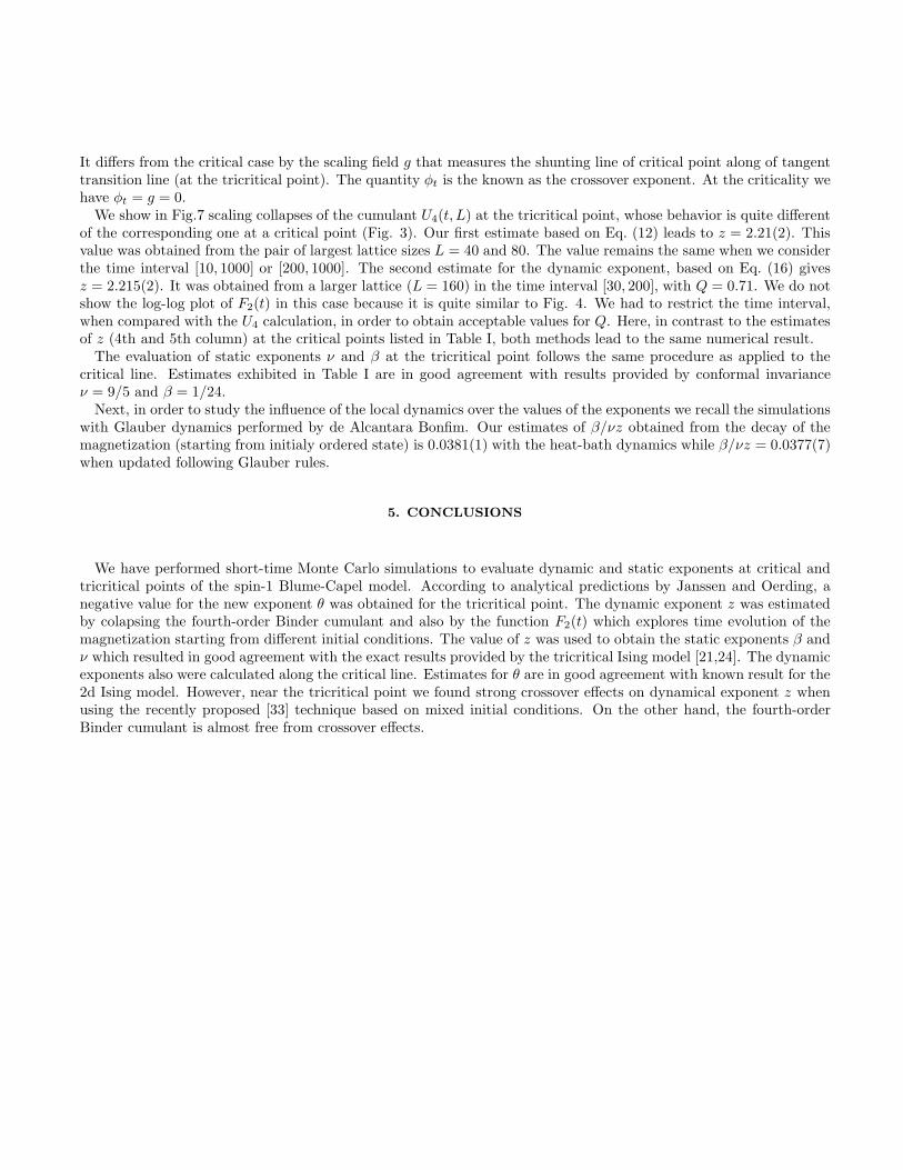
where < i, j > indicates nearest neighbors on L2 lattices and Si = {−1, 0, 1}. The parameter J is the exchangecoupling constant and D is the crystal field. We show its phase diagram in Fig. 1. Table I lists points on thesecond order critical line and the tricritical point where we have performed our simulations. Points in Table I wereobtained from [23] and from a private communication of the authors in [22]. That table also contains our results forthe corresponding critical and tricritical exponents.

We remark that along the critical line, this model presents a critical behavior similar to that of the Ising model.However, exactly at the tricritical point the exponents change abruptly. They are given by the dimensions of theirreducible representations of the Virasoro algebra [24,25] with central charge (conformal anomaly number) c = 7/10[21]. In [20] finite-size scaling combined with conformal invariance permited to observe a smooth change betweenIsing-like and tricritical behavior. In finite systems, Ising-like behavior is reached only when D → −∞. In that limitη/2(2 − 1/ν) → 0.125 that is the exact value for the Ising model. In our short-time simulations the same kind ofcrossover behavior is observed for the dynamic exponents z and θ when we move along the critical line.

2

Table 1. Critical parameters and exponents for 2d Blume-Capel model.

D/J kBT/J θ z z 1/ν 1/ν β(Eq. (12)) (Eq. (16)) (Eqs. (17) and (12)) (Eqs. (17) and (16)) (Eq. (14))

critical points0 1.6950 0.194(3) 2.159(6) 2.1057(7) 0.97(2) 0.99(2) 0.134(2)-3 2.0855 0.193(5) 2.156(5) 2.1276(5) 0.99(1) 1.00(1) 0.125(2)-5 2.1855 0.187(5) 2.154(4) 2.1387(6) 0.99(3) 1.00(3) 0.125(4)

tricritical point1.9655 0.610 -0.53(2) 2.21(2) 2.215(2) 1.864(6) 1.86(2) 0.0453(2)

3. NON-EQUILIBRIUM SHORT-TIME DYNAMICS AT A CRITICAL POINT

In short-time MC simulations critical slowing down can be neglected. It happens because spatial and time correlationlengths are small in the early stages of evolution. On the other hand, we need to deal with several samples taken overindependent initial configurations since the systems which are being simulated are far from equilibrium. In fact thisapproach requires calculation of average (over samples) magnetization and of its moments M (k)(t),

M (k)(t) =1

NsLkd

Ns∑

j=1

Ld∑

i=1

σij(t)

k

, (6)

where σij(t) denotes the value of spin i of jth sample at the tth MC sweep. Here Ns denotes the number of samplesand Ld is the volume of the system. This kind of simulation is performed NB times to obtain our final estimates infunction of t. In this paper, the dynamic evolution of the spins {σi} is local and updated by the heat-bath algorithm.

A. The critical initial slip

The evolution of the kth moment of magnetization in the initial stage of the dynamic relaxation can be obtained fromEq. (1) for large lattice sizes L at τ = 0 with b = t1/z. This yields

M (k)(t, m0) = t−kβ/νzM (k)(1, tx0/zm0) . (7)

By expanding the corresponding first moment equation for small m0, we obtain Eq. (2) under the condition that

tx0/zm0 is sufficiently small, which sets a time scale t0 ∼ m−z/x0

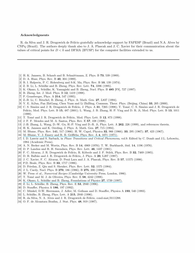
0 [1,4,6] where that phenomena can be observed.In Fig. 2a we present our results for the exponent θ at the critical point kBTc/J = 1.695 and Dc/J = 0, for lattice

size L = 80 and 5 different initial magnetizations m0. Our estimates for each θ = θ(m0) were obtained from NB = 5independent bins with NS = 10000, for t up to 100 sweeps. Figure 2b illustrates the numerical evaluation of θ form0 = 0.02 from a log-log plot of the magnetization versus time. The linear fitting in Fig. 2a gives θ = 0.193(2) withgoodness of fit [26] Q = 0.72.

Another method has been recently proposed by Tome and de Oliveira [27] to evaluate θ. It avoids the sharppreparation of samples with defined and nonzero magnetization and the delicate numerical extrapolation m0 → 0.The method is based on the time correlation function of the total magnetization,

C(t) =1

Ld

⟨Ld∑

i=1

Ld∑

j=1

σi(t)σj(0)

⟩. (8)

Starting from random initial configurations the above correlation behaves as C(t) ∼ tθ, which permits us to obtainthe exponent θ from a log-log plot of C(t) versus t. We obtained θ = 0.194(3) for kBTc/J = 1.695 and Dc/J = 0choosing the time interval [20 − 150] due to the highest value of Q (Q = 0.99). This value is in complete agreementwith our above estimate of the exponent θ and it is consistent within error bars with previous results for the 2d Isingmodel. In table I we also present results for θ at several points of the critical line.

3

B. Dynamic critical exponent z

The observables in short-time analysis are described by different scaling relations according to the initial magnetiza-tions. In particular, the second moment M (2)(t, L) in Eq. (6),

M (2) =1

L2d

⟨Ld∑

i=1

σ2i

⟩+

1

L2d

Ld∑

i6=j

〈σiσj〉 , (9)

with m0 = 0 behaves as L−d since in the short-time evolution the spatial correlation length is very small whencompared with the lattice size L. Thus, we arrive at [5,6]

M (2)(t, L) = t−2β/νz M (2)(1, t−1/zL) ∼ t(d−2β/ν)/z . (10)

This equation can be used to determine relations involving static critical exponents and the dynamic exponent z[6,28]. However, a way to evaluate independently the exponent z is through out the time-dependent fourth-orderBinder cumulant at the critical temperature (τ = 0),

U4(t, L, m0) = 1 −M (4)(t, L, m0)

3(M (2)(t, L, m0)

)2 , (11)

which obeys the equation

U4(t, L, m0) = U4(b−zt, b−1L, bx0m0) . (12)

If we set m0 = 0, we eliminate the dependence on the exponent x0 and the exponent z can be evaluated throughscaling collapses of the generalized cumulant for different lattice sizes [4,29]. To match the Binder cumulants U4(t1, L1)and U4(t2, L2) obtained from two time series for lattice sizes L1 and L2, respectively, with b = L2/L1 (L2 > L1), we

interpolate the series U4(t, L1) to obtain U4(b−zt, L1). Next, we define the function

χ2(z) =1

tf − ti

tf∑

t=ti

[U4(b

−zt, L1) − U4(t, L2)]2

, (13)

where the best estimate for z corresponds to the one which minimizes χ2(z).In Fig. 3 we show the scaling collapses of the Binder cumulants for different lattice sizes. We have collapsed

the following pairs of lattices (L1, L2) = (10, 20), (20, 40) and (40, 80). From the largest pair of lattices we obtainedz = 2.159(6) in the time interval [50− 1000]. Our final error estimate is based on 25 different collapses obtained fromNB = 5 independent bins for each lattice size.

Another universal behavior of the dynamic relaxation process also described by Eq. (1) can be obtained with theinitial condition m0 = 1 [30–32]. This condition is related to another fixed point in the context of renormalizationgroup approach. Thus, starting from an initial ordered state one obtains a power law decay of the magnetization atthe critical temperature,

M(t) ∼ t−β/νz , (14)

when we choose b−zt = 1 in the limit of L → ∞. Taking into account this relation, another method has been proposed[6] to estimate the dynamic exponent z. This approach uses the second cumulant

U2(t, L) =M (2)(t, L)

(M(t, L))2− 1 , (15)

which should take the simple form U2(t, L → ∞) ∼ td/z. The advantage of this procedure is that curves for differentlattices lay on the same straight line in a log-log plot without any re-scaling in time. However, this technique has notbeen successful in at least two well known models: the two-dimensional q = 3 Potts model [6] and the Ising modelwith three spin interactions in just one direction [10]. The reason for the above disagreement may be related to thebehavior of the second term of r.h.s in Eq. (9) when m0 = 1. We have proposed [33] that this behavior could indeedbe obtained working with the ratio F2 = M (2)/M2 with different initial conditions for each moment. As we know

4

the behavior of the second moment of the magnetization when samples are initially disordered (m0 = 0) and also thetime dependence of the magnetization when samples are initially ordered (m0 = 1), we easily obtain

F2(t) =M (2)(t, L)

∣∣m0=0

(M(t, L))2|m0=1

∼ td/z . (16)

A log-log plot with error bars for the critical point kBTc/J = 1.695 and Dc/J = 0 is presented in Fig. 4 for L = 160.We obtained z = 2.1057(7) with Q = 0.99 in the range [30− 200], which does not agree with the value obtained fromEq. (12). However, as we move away from the tricritical point, the values of z obtained (Table 1) with Eq. (16) showa clear trend toward the expected value of the dynamic exponent z (z = 2.1567(7)) of the 2d Ising model [33]. On theother hand, the values obtained from the cumulant in Eq. (12) remain essentially the same along the entire criticalline. It seems the cumulant U4 is less sensitive to crossover effects than the mixed method.

C. Static exponents and universality class

The exponent 1/νz can be obtained by differentiating lnM(t, τ, m0) with respect to the temperature at Tc,

∂ lnM(t, τ, L)

∂τ

∣∣∣∣τ=0

∼ t1/νz , (17)

if we consider the scaling relation for the magnetization when the initial state of samples is ordered (m0 = 1) [29].Our results for νz were obtained through finite diferences at Tc±δ with δ = 0.001. They rely on NB = 5 independent

bins with Ns = 5000 samples each for L = 160. The time interval [80 − 200] corresponds to the range where thegoodness of fit parameter attains its highest value (Q = 0.99).

In Fig. 5 we show the log-log behavior of the derivative ∂τ lnM(t) at kBTc/J = 1.695 and Dc/J = 0. In Table Iwe present our final estimates of 1/ν. The 6th column is obtained with the estimates of z from Eq. (12) (data in 4thcolumn), while the 7th column corresponds to estimates for ν with values of z from Eq. (16) (data in 5th column).

Since we have already collected estimates for νz, it is straightforward to obtain estimates for β following Eq. (14).Our estimates of β are presented in the last column. Our values in Table I can be compared with theoretical predictionsfor an Ising like critical point (1/ν = 1, β = 1/8).

4. RESULTS FROM SHORT-TIME DYNAMICS AT THE TRICRITICAL POINT

From the results presented in Refs. [1] and [14] we can describe the time dependence of the magnetization (k = 1)for the 2d Blume-Capel model as

M(t) ∼

m0tθ , 0 < t < t0 , where θ ≥ 0

t−β/νz , t0 < t < tI

m0tθ , 0 < t < t0 , where θ ≤ 0

t−β/νz , t0 < t < tI

criticalpoint

tricriticalpoint

(18)

for an initial small magnetization m0. Here tI stands for the time before the system has reached the thermalization.We also included in Table I our estimates for θ, z, 1/ν and β at the tricritical point kBTt/J = 0.610 and Dt/J =

1.9655 working with lattice size L = 80.In Fig. 6a we show the values of θ for 5 different initial magnetizations m0 at the tricritical point and in Fig. 6b

the time evolution of the magnetization for m0 = 0.08 in a log-log plot. Our estimates for each θ(m0) were obtainedfrom NB = 20 independent bins with NS = 10000 samples, for t up to 80 sweeps. The linear extrapolation in Fig.6a gives θ = −0.53(2) with goodness of fit Q = 0.75. The corresponding study with the time correlation functionin Eq. (8) also gives θ = −0.53(2) with Q = 0.99 in the time interval [20 − 80]. The generalization of the dynamicscaling relation for the kth moment of the magnetization at a tricritical point can be written as [34]

M (k)(t, τ, g, L, m0) = b−kβt/νM (k)(b−zt, b1/ντ, bφt/νg, b−1L, bx0m0). (19)

5

It differs from the critical case by the scaling field g that measures the shunting line of critical point along of tangenttransition line (at the tricritical point). The quantity φt is the known as the crossover exponent. At the criticality wehave φt = g = 0.

We show in Fig.7 scaling collapses of the cumulant U4(t, L) at the tricritical point, whose behavior is quite differentof the corresponding one at a critical point (Fig. 3). Our first estimate based on Eq. (12) leads to z = 2.21(2). Thisvalue was obtained from the pair of largest lattice sizes L = 40 and 80. The value remains the same when we considerthe time interval [10, 1000] or [200, 1000]. The second estimate for the dynamic exponent, based on Eq. (16) givesz = 2.215(2). It was obtained from a larger lattice (L = 160) in the time interval [30, 200], with Q = 0.71. We do notshow the log-log plot of F2(t) in this case because it is quite similar to Fig. 4. We had to restrict the time interval,when compared with the U4 calculation, in order to obtain acceptable values for Q. Here, in contrast to the estimatesof z (4th and 5th column) at the critical points listed in Table I, both methods lead to the same numerical result.

The evaluation of static exponents ν and β at the tricritical point follows the same procedure as applied to thecritical line. Estimates exhibited in Table I are in good agreement with results provided by conformal invarianceν = 9/5 and β = 1/24.

Next, in order to study the influence of the local dynamics over the values of the exponents we recall the simulationswith Glauber dynamics performed by de Alcantara Bonfim. Our estimates of β/νz obtained from the decay of themagnetization (starting from initialy ordered state) is 0.0381(1) with the heat-bath dynamics while β/νz = 0.0377(7)when updated following Glauber rules.

5. CONCLUSIONS

We have performed short-time Monte Carlo simulations to evaluate dynamic and static exponents at critical andtricritical points of the spin-1 Blume-Capel model. According to analytical predictions by Janssen and Oerding, anegative value for the new exponent θ was obtained for the tricritical point. The dynamic exponent z was estimatedby colapsing the fourth-order Binder cumulant and also by the function F2(t) which explores time evolution of themagnetization starting from different initial conditions. The value of z was used to obtain the static exponents β andν which resulted in good agreement with the exact results provided by the tricritical Ising model [21,24]. The dynamicexponents also were calculated along the critical line. Estimates for θ are in good agreement with known result for the2d Ising model. However, near the tricritical point we found strong crossover effects on dynamical exponent z whenusing the recently proposed [33] technique based on mixed initial conditions. On the other hand, the fourth-orderBinder cumulant is almost free from crossover effects.

6

Acknowledgments

R. da Silva and J. R. Drugowich de Felıcio gratefully acknowledge support by FAPESP (Brazil) and N.A. Alves byCNPq (Brazil). The authors deeply thank also to J. A. Plascak and J. C. Xavier for their communication about thevalues of critical points for D < 0 and DFMA (IFUSP) for the computer facilities extended to us.

[1] H. K. Janssen, B. Schaub and B. Schmittmann, Z. Phys. B 73, 539 (1989).[2] D. A. Huse, Phys. Rev. B 40, 304 (1989).[3] B. I. Halperin, P. C. Hohenberg and S-K. Ma, Phys. Rev. B 10, 139 (1974).[4] Z. B. Li, L. Schulke and B. Zheng, Phys. Rev. Lett. 74, 3396 (1995).[5] K. Okano, L. Schulke, K. Yamagishi and B. Zheng, Nucl. Phys. B 485 [FS], 727 (1997).[6] B. Zheng, Int. J. Mod. Phys. B 12, 1419 (1998).[7] P. Grassberger, Phys. A 214, 547 (1995).[8] Z.-B. Li, U. Ritschel, B. Zheng, J. Phys. A: Math. Gen. 27, L837 (1994).[9] Y. E. AiJun, Pan ZhiGang, Chen Yuan and Li ZhiBing, Commun. Theor. Phys. (Beijing, China) 33, 205 (2000).

[10] C. S. Simoes and J. R. Drugowich de Felıcio, J. Phys. A 31, 7265 (1998); T. Tome, C. S. Simoes and J. R. Drugowich deFelıcio, Mod. Phys. Lett. B 15, 487 (2001); L. Wang, J. B. Zhang, H. P. Ying and D. R. Ji, Mod. Phys. Lett. B 13, 1011(1999).

[11] T. Tome and J. R. Drugowich de Felıcio, Mod. Phys. Lett. B 12, 873 (1998).[12] J. F. F. Mendes and M. A. Santos, Phys. Rev. E 57, 108 (1998).[13] J.-B. Zhang, L. Wang, D.-W. Gu, H.-P. Ying and D.-R. Ji, Phys. Lett. A 262, 226 (1999), and references therein.[14] H. K. Janssen and K. Oerding, J. Phys. A: Math. Gen. 27, 715 (1994).[15] M. Blume, Phys. Rev. 141, 517 (1966). H. W. Capel, Physica 32, 966 (1966); 33, 295 (1967); 37, 423 (1967).[16] M. Blume, V. J. Emery and R. B. Griffiths, Phys. Rev. A 4, 1071 (1971).[17] I. D. Lawrie and S. Sarbach, in Phase Transitions and Critical Phenomena, vol.9. Edited by C. Domb and J.L. Lebowitz,

1984 (Academic Press).[18] A. N. Berker and M. Wortis, Phys. Rev. B 14, 4969 (1976); T. W. Burkhardt, ibid. 14, 1196 (1976).[19] D. P. Landau and R. H. Swendsen, Phys. Rev. Lett. 46, 1437 (1981).[20] F. C. Alcaraz, J. R. Drugowich de Felıcio, R. Koberle and J. F. Stilck, Phys. Rev. B 32, 7469 (1985).[21] D. B. Balbao and J. R. Drugowich de Felıcio, J. Phys. A 20, L207 (1987).[22] J. C. Xavier, F. C. Alcaraz, D. Pena Lara and J. A. Plascak, Phys. Rev. B 57, 11575 (1998).[23] P.D. Beale, Phys. Rev. B 33, 1717 (1986).[24] D. Friedan, Z. Qiu and S. Shenker, Phys. Rev. Lett. 52, 1575 (1984).[25] J. L. Cardy, Nucl. Phys. B 270, 186 (1986); B 275, 200 (1986).[26] W. Press et al., Numerical Recipes (Cambridge University Press, London, 1986).[27] T. Tome and M. J. de Oliveira, Phys. Rev. E 58, 4242 (1998).[28] K. Okano, L. Schulke and B. Zheng, Foundations of Physics 27, 1739 (1997).[29] Z. Li, L. Schulke, B. Zheng, Phys. Rev. E 53, 2940 (1996).[30] D. Stauffer, Physica A 186, 197 (1992).[31] C. Munkel, D.W. Heermann, J. Adler, M. Gofman and D. Stauffer, Physica A 193, 540 (1993).[32] L. Schulke, B. Zheng, Phys. Lett. A 215, 2940 (1996).[33] R. da Silva, N. A. Alves and J. R. Drugowich de Felıcio, cond-mat/0111288.[34] O. F. de Alcantara Bonfim, J. Stat. Phys. 48, 919 (1987).

7

(Fig.1) 1. Phase diagram of the Blume-Capel model. The dashed curve is a first-order transition line and the solid isa second order one. These curves are connected by a tricritical point (TP). The marked points (×, •) correspond to thesimulated values.

8

(Fig.2a) 2. Exponent θ in function of initial magnetizations m0 for square lattices with L = 80. The straight line is aleast-square fit to the data.

(Fig.2b) 3. Time evolution of the magnetization for L = 80 and m0 = 0.02.

9

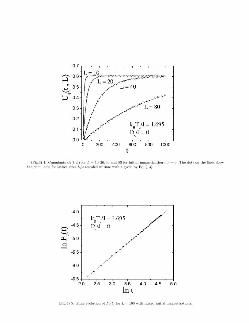
(Fig.3) 4. Cumulants U4(t, L) for L = 10, 20, 40 and 80 for initial magnetization m0 = 0. The dots on the lines showthe cumulants for lattice sizes L/2 rescaled in time with z given by Eq. (13).

(Fig.4) 5. Time evolution of F2(t) for L = 160 with mixed initial magnetizations.

10

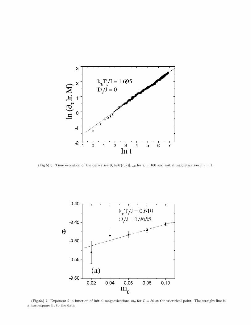
(Fig.5) 6. Time evolution of the derivative ∂τ lnM(t, τ )|τ=0 for L = 160 and initial magnetization m0 = 1.

(Fig.6a) 7. Exponent θ in function of initial magnetizations m0 for L = 80 at the tricritical point. The straight line isa least-square fit to the data.

11

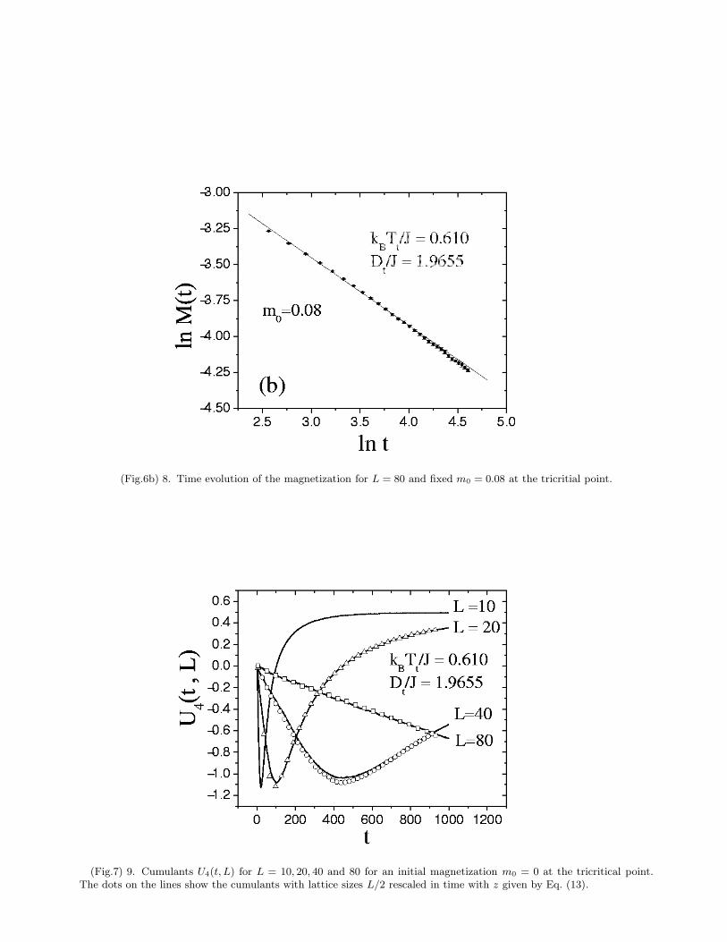
(Fig.6b) 8. Time evolution of the magnetization for L = 80 and fixed m0 = 0.08 at the tricritial point.

(Fig.7) 9. Cumulants U4(t, L) for L = 10, 20, 40 and 80 for an initial magnetization m0 = 0 at the tricritical point.The dots on the lines show the cumulants with lattice sizes L/2 rescaled in time with z given by Eq. (13).

12