Universal Gr¶bner Bases for Designs of Experiments

Rend. Istit. Mat. Univ. TriesteVol. XXXVII, 95–119 (2005)

Universal Grobner Bases forDesigns of Experiments

Hugo Maruri-Aguilar (∗)

Contribution to “School (and Workshop) on Computational Algebrafor Algebraic Geometry and Statistics”, Torino, September 2004.

Summary. - Universal Grobner bases (UGB) are a useful tool toobtain a set of different models identified by an experimental de-sign. Usually, the algorithms to obtain a UGB for the ideal ofa design are computationally intensive. Babson et al. (2003)propose a methodology to construct UGB in polynomial time.Their methodology constructs a list of term orders based uponthe Hilbert zonotope. We focus on the generation of such a list.We use results on hyperplane arrangements to present a theoremwhich simplifies the computation of term orders for designs intwo dimensions. Our theorem constructs directly the normal fanof the Hilbert zonotope.

1. Introduction

When analyzing an experiment, it is useful to consider different al-ternative models; for example in a computer experiment where thecost of every run is high and only a reduced number of runs is pos-sible. In the analysis stage, we may want to have different modelsat hand, maybe to choose a simulator of our experiment. Then we

(∗) Author’s address: Hugo Maruri-Aguilar, Department of Statistics, Universityof Warwick, Coventry CV4 7AL, UK, e-mail: [email protected]: Zonotope, Hilbert scheme, Universal Grobner bases (UGB), Normal fan,Fan of a design.

96 H. MARURI-AGUILAR

can select a model based on the interpretation as well as the usualstatistical criteria. A search through all the potential identifiablemodels would be impossible and thus we must restrict our class ofmodels. In the present work we consider only the class of hierar-chical polynomial models. This class has been studied previouslyin literature under the names “well-formed”, “hierarchical” or “hi-erarchically well-formulated” models, see Bates et al. (2003) andPeixoto (1990). We also restrict the search to full rank models toensure identifiability.

The search algorithms we are interested in are based on algebraictechniques and return a large subset of the class we are interested in.Depending on the design, sometimes the algebraic techniques returnthe whole class. However, the algebraic techniques rely on importantresults from polytopal geometry. For this reason, Sections 2 and 3introduce both (algebraic and polytopal) notations and explain thelink between them. In Section 4 we introduce an important polytopecalled the Hilbert zonotope, and describe its role in our problem. InSection 5 we give a new theorem which simplifies the current use ofthe zonotope in two dimensions. Some computational details are inthe appendix.

2. Algebra and design of experiments

Pistone and Wynn (1996) pioneered the use of Grobner bases in ex-perimental design. They demonstrate that computational commu-tative algebra (CCA) is a useful tool, not only to propose differentmodels, but also to study generalized confounding of models andmodel terms. We start by defining the experimental design and theclass of models we will be considering along this work.

Definition 2.1. An experimental design is a finite set of n distinctpoints D ⊂ R

d, where d is the number of factors and n is the numberof runs.

The class of hierarchical polynomial models we are interested in isin one-to-one correspondence with the set of staircases defined next.

Definition 2.2. A staircase is a nonempty subset λ of the set Nd of

non-negative integer vectors such that if u ∈ λ and v ≤ u (coordinate-

UNIVERSAL GROBNER BASES etc. 97

wise) then v ∈ λ. Let(

Nd

n

)

stairdenote the finite set of staircases with

n elements.

The cardinality of(

Nd

n

)

stairfor d = 2, 3 is computed by MacMa-

hon’s classic formulas (see Appendix 7.1), while for d ≥ 4 it is still anopen problem, see Onn and Sturmfels (1999). The log map acts fromthe terms in R[x1, . . . , xd] to Z

d as log(xα11 · · · xαd

d ) = (α1, . . . , αd).Then, one applies it to the terms in a hierarchical polynomial modeland obtains a staircase.

Example 2.3. The hierarchical model {1, x1, x2, x1x2} corresponds

to the staircase{(

00

),(10

),(01

),(11

)}∈

(N

2

4

)

stair.

Definition 2.4. Let

V dn :=

⋃

λ∈(Nd

n)

stair

λ (1)

denote the union of all n-staircases in Nd.

The computation of V dn can be simplified by noting that V d

n ={v ∈ N

d :∏d

i=1 (vi + 1) ≤ n}. Babson et al. (2003) use the asymp-totic bound O(n(log n)d−1) for the cardinality of V d

n .

Example 2.5. For n = 5, d = 2, we have seven different staircases,and their union is

V 25 =

{(00

),(10

),(20

),(30

),(40

),(01

),(02

),(03

),(04

),(11

)},

see Figure 1 .

Now we give the basic elements for identifying models using CCA.The reader is referred to Cox et al. (1996) for a comprehensiveresource on algebraic geometry and to Pistone et al. (2000) for theuse of CCA in statistics.

Definition 2.6. The design ideal I is the set of all polynomials thatvanish on the design: I = {f ∈ R[x1, . . . , xd] : f(x) = 0 for all x ∈D}.


v1

v2

Figure 1: Picture of V 25 . The dashed curve corresponds to (v1 +

1)(v2 + 1) = 5

Here R[x1, . . . , xd] is the ring of polynomials in x1, . . . , xd indeter-minates, which for simplicity we write as R[x]. The ideal I is gener-ated by a finite set of polynomials G and we write I = 〈g : g ∈ G〉 ={∑

g∈G gh, h ∈ R[x]}. The length of an ideal I is the dimension of thequotient space R[x]/I, where the quotient space R[x]/I is the class ofall polynomials in R[x] modulo the ideal, e.g. for every f in R[x] wecan construct a representative [f ] = {g ∈ R[x] such thatf − g ∈ I}.Our search for models identifiable by a design can be expressed pre-cisely as the search for basis for R[x]/I. This important fact enablesus to use algebraic techniques to solve our problem.

Definition 2.7. A term ordering τ is an ordering relation ≻ on theterms xα, α ∈ N

d that satisfies i) xα ≻ 1 for all xα and ii) if forα, β, γ ∈ N

d we have xα ≻ xβ, then xαxγ ≻ xβxγ.

Note that a term ordering corresponds to an ordering relation onN

d. The leading term of a polynomial f is the largest term in f withrespect to the term ordering τ . We write LTτ (f).

Definition 2.8. A Grobner basis for an ideal I with respect to aterm order τ is a finite subset Gτ ⊂ I such that 〈LTτ (g) : g ∈ Gτ 〉 =〈LTτ (f) : f ∈ I〉.

Definition 2.9. A reduced Grobner basis (RGB) of I is a Grob- nerbasis Gτ such that i) the coefficient of LTτ (g) is one for all g ∈ Gτ ,ii) for all g ∈ Gτ , no monomial of g lies in 〈LTτ (f) : f ∈ Gτ\g〉

A model for the responses at the design is identified by all thoseterms which cannot be divided by the leading terms of Gτ . This basisis the hierarchical polynomial model we look for.


Example 2.10. Consider the following non-regular fraction of a fac-

torial 32 experiment: D ={(0

0

),(10

),(01

),( 1−1

),(−1

1

)}

. For a term

ordering in which x1 ≻ x2, we construct the following RGB (leadingterms underlined) Gτ = {x2

1 + 2x1x2 + x22 − x1 − x2, x

32 − x2, x1x

22 −

x1x2 − x22 + x2} and we identify the model {1, x1, x2, x1x2, x

22}.

Caboara et al. (1997) enlarged upon Pistone and Wynn’s ideas,and defined the fan of an experimental design as the set of all hier-archical models identifiable by a given design. Caboara et al. distin-guished between algebraic fan (models obtained with Grobner basismethods by varying the term ordering), and statistical fan (all hi-erarchical polynomial models identified by the design). In examples2.11 and 2.12 we illustrate the algebraic and statistical fan for thedesign given in example 2.10. Throughout this work, we will usealgebra to obtain the algebraic fan of the design.

Next we outline the algebraic approach to computing the fan.The main idea is to construct a universal Grobner basis (UGB) forthe design ideal I. The UGB of a (design) ideal is defined as

U(I) :=⋃

τ

Gτ , (2)

where Gτ is a RGB under the term ordering τ , and τ runs over allterm orderings. Once we have U(I), we can list the algebraic fan ofthe design. We refer to Weispfenning (1987) for details on propertiesof UGBs.

Example 2.11. (cont. of Example 2.10) The UGB of I is

U(I) = {x21 + 2x1x2 + x2

2︸︷︷︸

−x1 − x2, x32

︸︷︷︸

−x2, x31

︸︷︷︸

−x1,

x1x22

︸︷︷︸

−x1x2 − x22 + x2, x2

1x2︸︷︷︸

−x21 − x1x2 + x1},

where the terms underlined with “ ” are the leading terms for thecondition x1 ≻ x2; and we underline with “

︸︷︷︸” the leading terms

for x1 ≺ x2. We observe that

1. every polynomial in U(I) vanishes at every design point, andthe set of equations for U(I) has no other solution than thedesign points;


2. the set of term orders is partitioned by the conditions x1 ≻ x2

and x1 ≺ x2. Thus U(I) is indeed a UGB. Moreover, U(I)is the union of two RGBs and, in this sense, is minimal andunique;

3. the algebraic fan of D is thus formed by {1, x1, x2, x1x2, x22}

and {1, x1, x2, x1x2, x21} which are obtained as those terms not

divisible by the leading terms for x1 ≻ x2 and x1 ≺ x2 respec-tively.

However, in general to compute UGB using Equation (2) directlyis not possible, as there is an infinite number of term orderings.Moreover, many different term orderings yield the same Gτ . A sur-prising fact proved by Mora and Robbiano (1988) is that for anyideal, the union in Equation (2) is finite. Thus we need an efficientway to generate term orders and to compute UGBs. This will be thetopic of the next subsection.

We end this subsection by noting that algebra gives some of themodels we seek, but not necessarily all of them. There are staircasesthat cannot be obtained by algebraic means and still are identifiable.

Example 2.12. (cont. of Example 2.11) The model

{1, x1, x2, x21, x

22} (3)

is identifiable by the design as the design matrix

1 x1 x2 x21 x2

2

1 0 0 0 01 1 0 1 01 0 1 0 11 1 −1 1 11 −1 1 1 1

is full rank. Indeed by exhaustive search one can show that the sta-tistical fan of D is composed of {1, x1, x2, x1x2, x

22}, {1, x1, x2, x

21, x

22}

and {1, x1, x2, x1x2, x21}. Now we explain why we cannot obtain

Model 3 by algebraic methods. The following is a generating set ofpolynomials for I: {f1 = x3

1−x1, f2 = x32−x2, f3 = x2

1+2x1x2+x22−

x1 − x2}. We have that for any τ , LTτ (f1) = x31 and LTτ (f2) = x3

2;


and to obtain Model 3 we need LTτ (f3) = x1x2 for some τ . The pre-vious statement implies x1x2 ≻ x2

1 and x1x2 ≻ x22 simultaneously.

This in turn means that x2 ≻ x1 and x2 ≺ x1, which is not possiblefor any term ordering.

3. Polytopes for the algebra

We start this subsection with the basic definitions of polytopal geom-etry, for which references are Ziegler (1994) and Grumbaum (2003);later we present the use of polytopes in relation to Grobner bases,for which basic references are Bayer and Morrison (1988), Mora andRobbiano (1988) and Sturmfels (1995).

3.1. Basic definitions

A d−dimensional polytope P may be specified as the set of solutionsof a system of linear inequalities

Ax ≤ b,

where A is a real matrix of d columns and b, x ∈ Rd. If the polytope

P is not bounded, then we refer to it as a polyhedron. For a boundedpolytope, the positions of the vertices may be found using a processcalled vertex enumeration, see Avis and Fukuda (1991). A particu-lar type of bounded polytopes are zonotopes, which are defined asfollows.

Definition 3.1. The zonotope of a finite set of vectors V ⊂ Rd is

given by the following Minkowski sum

Z(V ) :=∑

v∈V

[−v, v],

where the summand [−v, v] = [−1, 1] · v is the line segment between−v and v in R

d.

Example 3.2. Consider V ={(1

0

),(01

)}⊂ R

2. We compute Z(V )

by Minkowski-summing the line segments[(−1

0

),(10

)]and

[( 0−1

),(01

)]

,

e.g. for every vector a in the first line segment, we add every vector bin the second line segment. The result is the square Z(V ) = [−1, 1]×[−1, 1] = [−1, 1]2.


PC

′

1 C′

2

C′

3

C′

4

C′

5

QC1

C2C3

Figure 2: The polytopes P and Q and their normal fans N (P ) andN (Q). P is a refinement of Q.

A polyhedron of the form Ax ≥ 0 is called a polyhedral cone. Apointed cone is a cone that contains the origin. Then every poly-hedral cone is a pointed cone. Polyhedral cones admit anotherdescription, that is as the positive hull of a set of vectors. Thepositive hull of V is the set {

∑viλi : vi ∈ V, λi ≥ 0}. Now,

for a polyhedron P ⊂ Rd and ω ∈ R

d, we define a face of P asF = {u ∈ P : ω · u ≥ ω · v ∀v ∈ P}.

A complete fan is a family of pointed polyhedral cones in Rd in

such a way that its union is all of Rd. The normal fan N (P ) of

a d−polytope P ⊂ Rd is the collection CF of all vectors a ∈ R

d

such that the linear function x → a · x on P is maximized by allpoints on F ; where F is a non-empty face of P . The constructionof the normal fan is illustrated in Figure 2 for two bidimensionalpolytopes P and Q. Note that for every vertex h, its normal coneCh is generated as the positive hull of the normal vectors of adjacentfacets.

Theorem 3.3. (Ziegler, 1994) Let Z = Z(V ) ⊆ Rd be a zonotope.

Then the normal fan N (Z) of Z is the fan FA of the hyperplanearrangement


A = AV := {H1, . . . ,Hp}

in Rd given by

Hi := {c ∈ (Rd)∗ : cvi = 0, vi ∈ V }.

Here (Rd)∗ represents the dual vector space which is the realvector space of all linear functions R

d → R. These are real rowvectors of length d.

A polyhedron P is a refinement of a polyhedron Q if the normalfan of P is a refinement of that of Q. The refinement means that theclosure of each normal cone of Q is the union of closures of normalcones of P . The closure of a cone is the cone plus its boundary. InFigure 2 we illustrate an example of refinement. The polytope P is arefinement of Q as the cones of N (Q) can be expressed as unions ofthe cones in N (P ), namely C1 = C ′

1∪C ′2, C2 = C ′

3 and C3 = C ′4∪C ′

5.

3.2. Polyhedra to compute UGBs

For the rest of this section, it is necessary to elaborate on designideals as part of the theory of Hilbert schemes. We refer the readerto Miller and Sturmfels (2004) and just recall that Hilbert schemesHilbd

n are algebraic varieties that parametrize families of ideals inpolynomial rings, where d is the number of indeterminates of factorsand n is the dimension of the quotient space, i.e. the number ofdesign points. For example, the Hilbert scheme Hilb2

2 consists ofall ideals I ⊂ R[x1, x2] for which the quotient space R[x1, x2]/I hasdimension 2 as a R−vector space, i.e. in our case, this comprises allthe possible polynomial ideals generated by two points in the plane.The starting point for the computation of the UGB for an ideal I isthe construction of the state polyhedron S(I).

A subset λ ⊂ Nd of n elements is basic for the ideal I ∈ Hilbd

n

if the R−vector space lin{xv : v ∈ λ} := {∑

v∈λ αvxv} satisfies

lin{xv : v ∈ λ} ∩ I = {0}. A hierarchical model obtained withCCA techniques is basic for the design ideal. Now, for a basic setλ, we define its sum as

∑

v∈λ v. The basis polytope of I ∈ Hilbdn is

the convex hull of sums of basic sets of I in V dn , that is B(I) :=

conv({∑

v∈λ v : λ ⊂ V dn , λ basic for I}

). The state polyhedron of


I ∈ Hilbdn is given by S(I) := B(I) + R

d+. This last sum is inter-

preted as a Minkowski sum, and Rd+ ⊂ R

d is the positive orthant.The vectors w ∈ Z

d>0 ⊂ R

d+ are used to order terms by the

product w · α, for example we order the terms x21x2, x3

2, x1x2 asx2

1x2 ≻ x1x2 ≻ x32 with w =

(31

), but as x3

2 ≻ x21x2 ≻ x1x2 with

w′ =(23

).

We construct the normal fan of S(I). Let Ch be the normal conecorresponding to the vertex h of S(I). We have that

⋃

h Ch = Rd+.

Now, for every vertex h, Grobner theory states that the vectors {w :w ∈ Z

d>0, w ∈ Ch} will give the same RGB. In this sense, every cone

Ch creates an equivalence class of ordering vectors. For this reason,we need only one w for every cone, and let Gw be the RGB obtainedwith the ordering vector w. We compute the UGB by

U(I) :=⋃

w

Gw. (4)

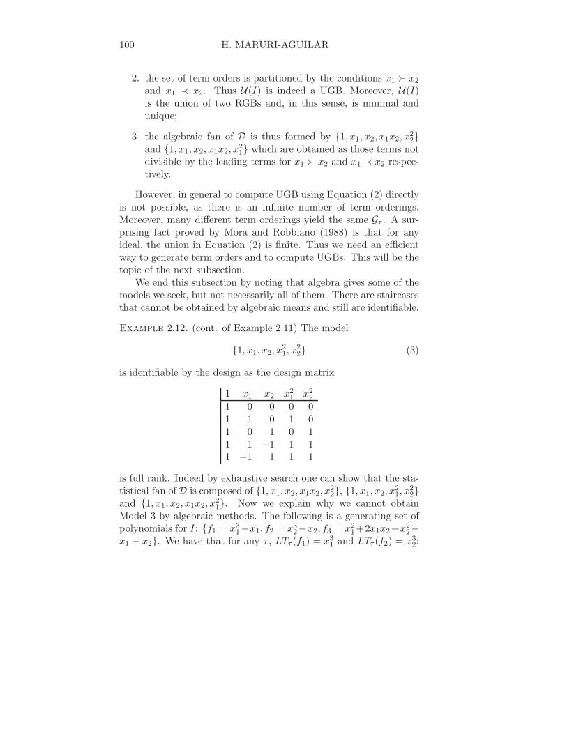
Example 3.4. (cont. of Example 2.10) The state polyhedron for thedesign ideal I is given by S(I) = conv

({(24

),(42

)})+ R

2+. We obtain

the sum(24

)as follows: the log of the model {1, x1, x2, x1x2, x

22}

gives the staircase{(0

0

),(10

),(01

),(11

),(02

)}, then the coordinate-wise

sum gives(24

). We have that

(42

)corresponds to {1, x1, x2, x1x2, x

21}

and we note that the model {1, x1, x2, x21, x

22} corresponds to the sum

(33

), which is an interior point of S(I). In Figure 3 we illustrate S(I)

and its normal fan composed of the cones C1 and C2. Now, we selectan integer vector in the interior of C1, e.g. w1 =

(21

)and obtain Gw1

which is the same RGB as in Example 2.10. We compute the UGBby repeating the computation with a vector w2 in C2 and unitingthe two RGBs as U(I) = Gw1 ∪ Gw2.

By using the state polyhedron S(I) we can obtain the adequateordering vectors w, one for every normal cone, and then computethe UGB using Equation (4). Up to this point, we have solved theinitial problem of selecting the right term orders to compute theUGB. However, we need to compute S(I) for every D. This is adisadvantage because the method has to deal with each specific casein a different way. Another disadvantage of this approach is theinherent complexity of the construction of S(I).


S(I)

C1

C2C1

C2

Figure 3: Picture of S(I) and the cones in N (S(I)).

For certain types of designs this disadvantage can be partly over-come. Onn and Sturmfels (1999) prove that if a design has a genericconfiguration (roughly a design whose points are at random), thenS(I) equals the corner cut polyhedron. They also prove that the listof models is enumerable in polytime for a generic design. They givea determinant-based formula to retrieve a model corresponding to avertex of S(I) for any vertex. For a random design, Caboara et al.

(1997) show that all models in(

Nd

n

)

stairare identifiable.

In the next section we introduce the Hilbert zonotope, whichovercomes the inherent difficulties of the state polyhedron.

4. Hilbert zonotope

We are now arriving at the main point of this paper in which theHilbert zonotope is the central feature. We follow the definition inOnn and Sturmfels (1999) and Babson et al. (2003). We constructthe zonotope and then list some of its main features.

Definition 4.1. The symmetrization of a finite set A ⊂ Zd is

sym(A) := {a − b : a ∈ A, b ∈ A\a} (5)

The following properties of sym(A) can be easily demonstrated:i) sym(A) is centrally symmetric, that is, if a ∈ sym(A) then −a ∈sym(A), and ii) 0 /∈ sym(A).

Definition 4.2. The primitive elements of a set A ⊂ Zd\{0} are

all the elements of A that are not non-negative integer multiples ofanother element of A. We call this set prim(A).


Figure 4: Symmetrization of V 25 (left), and D2

5 (right).

Definition 4.3. For n > 1 let Ddn be the set of primitive vectors of

the symmetrization of V dn , that is Dd

n := prim(sym(V dn )). For n = 1

let Dd1 := ±{e1, . . . , ed}, where ei is the i−th unit vector.

Example 4.4. Figure 4 gives the symmetrization of V 25 and its prim-

itives D25 .

When we compute the primitives of sym(V dn ), it is sufficient to

consider only those elements of sym(V dn ) where the greatest com-

mon divisor of its non-zero components is one. The set Ddn contains

vectors pointing in all directions of V dn . It has no zero vector and

has only one vector for each of the directions from the zero to apoint in sym(V d

n ). This is at the core of the definition of the Hilbertzonotope.

Definition 4.5. The Hilbert zonotope Hdn is the following Min- kowski

sum:

Hdn :=

∑

v∈Ddn

[0, 1] · v ⊂ Rd (6)

Clearly, Hdn is a zonotope. The Hilbert zonotope is a complicated

figure with many facets and vertices, even for small values of d, n (seefor example, Table 1 in the Appendix). Next we give two examplesand two propositions. Proposition 4.8 gives a recurrence relation


between Hilbert zonotopes, and Proposition 4.9 gives a refinementrelation between Hilbert zonotopes.

Example 4.6. For n = 1, Hd1 is the d−cube [−1, 1]d.

Example 4.7. The vertices of H25 are given by

H25 = ±

{(−2723

),(−27

25

),(−25

27

),(−23

27

),(−15

25

),(−9

23

),(−5

21

),( 117

),

( 911

),(11

9

),(17

1

),(21−5

),(23−9

),( 25−15

)}

On the left side of Figure 5 we present H25, which is a 28-gon.

Proposition 4.8. The Hilbert zonotope satisfies the following prop-erty: Hd

n ⊂ Hdn′ for n < n′.

Proof. For a fixed d, if n < n′ we have that V dn ⊂ V d

n′ , and thussym(V d

n ) ⊂ sym(V dn′), and Dd

n = prim(sym(V dn )) ⊂ prim(sym(V d

n′))= Dd

n′ , that is

Ddn′ = Dd

n

⋃

(Ddn′\Dd

n). (7)

Note that Ddn′\Dd

n is a non-empty set. Now we construct the zono-tope Hd

n′ by Minkowski-summing over v ∈ Ddn′ ,

Hdn′ =

∑

Ddn

[0, 1] · v +∑

Dd

n′\Ddn

[0, 1] · v = Hdn +

∑

Dd

n′\Ddn

[0, 1] · v ⊃ Hdn,

which completes the proof.

Proposition 4.9. The Hilbert zonotope Hdn′ is a refinement of Hd

n

for n < n′.

Proof. We construct the normal fan of Hdn′ using Theorem 3.3 and

Equation (7) from Proposition 4.8. The normal fan is then comprisedof two groups of hyperplanes. The first group is those hyperplanescorresponding to N (Hd

n) (i.e. those hyperplanes orthogonal to v ∈Dd

n); while the second group comprises the hyperplanes orthogonalto the vectors v ∈ Dd

n′\Ddn. As the set Dd

n′\Ddn is nonempty, the

second group of hyperplanes creates the refinement relation.


Figure 5: Picture of H25 with its normal cones (above), and the

normal fan N (H25) (below).


H22

C1

C2

C1

C2w2

w1

Figure 6: Picture of H22 with its normal fan (left). In the right side of

the figure, for every cone Ci we select the ordering vector wi (pointedin black). We added the vectors that generate Ci.

4.1. The Hilbert zonotope and UGB

In this subsection we illustrate the use of the zonotope to computeuniversal Grobner bases. First we recall the important result aboutthe universality of the zonotope.

Theorem 4.10. (Babson et al., 2003) The Hilbert zonotope Hdn is a

refinement of both the basis polytope B(I) and the state polyhedronS(I) of every member of the Hilbert scheme Hilbd

n.

The previous theorem is used to construct an efficient set of or-dering vectors, which is next described. For every vertex h of Hd

n weconstruct the corresponding normal cone Ch. Now let w(h) ∈ Z

d6=0

be the vector in the interior of the cone Ch with minimum normwith respect to the standard Euclidean distance. There is a uniquew(h) for every vertex h. Let W d

n be the set of all vectors w(h), thatis W d

n := {w(h) : h vertex of Hdn}. We are interested only in those

elements of W dn which are positive. Let W d

n+ ⊂ W dn be the subset of

vectors w(h) in the first orthant. This set of positive vectors W dn+

defines a universal set of term orders for Hilbdn, which can be com-

puted once and for all, and is independent of the configuration ofD. The set W d

n+ was proposed by Babson et al. as part of theirpolynomial time algorithm to compute UGB and the fan of a design.


Example 4.11. Consider H22. Of all the six cones of its normal fan,

we only consider the cones which lie in the positive orthant, whichare labelled C1 and C2 in Figure 6. The cone C1 is generated as thepositive hull of

{(01

),(11

)}, while C2 is generated by

{(10

),(11

)}. For

C1 we have w(1) =(01

)+

(11

)=

(12

)and thus W 2

2+ ={(

12

),(21

)}.

Example 4.12. For the values n = 5, d = 2, we have that W 25+ is

{(1

5

)

,

(2

7

)

,

(2

5

)

,

(3

5

)

,

(5

7

)

,

(4

5

)

,

(5

4

)

,

(7

5

)

,

(5

3

)

,

(5

2

)

,

(7

2

)

,

(5

1

)}

.

In the right side of Figure 5 we illustrate the complete normal fanN (H2

5). We compare the refinement given by the normal fan of H25

in Figure 5 (with 12 cones in the first orthant) against the normalfan of S(I) in Figure 3 (with only two cones in the first orthant).

5. Main theorem

Theorem 5.1 gives a fast method to compute the first orthant ofN (H2

n). The construction of Theorem 5.1 is intuitively more appeal-ing and easier than the usual construction of N (Hd

n). Unfortunately,it cannot be extended to d ≥ 3 as we shall see in the next section.

Theorem 5.1. The cones in the first orthant of N (H2n) are generated

by the set prim([0, n − 1]2\

{(00

)}), where [a, b] = {c ∈ Z, a ≤ c ≤ b}.

Proof. Using Definition 4.3, we have D2n = prim(±([−n + 1,−1] ×

[1, n− 1]))⋃

(±prim(V dn )). We must keep in mind that D2

n is the setof summands in the definition of H2

n. Next we shall apply Theorem3.3 to generate all the hyperplanes of the fan. For every vector(a

b

)∈ prim(±([−n+1,−1]×[1, n−1])), the corresponding orthogonal

hyperplane will be generated by(−ba

)∈ prim(±([1, n − 1]2)). This

last vector is orthogonal to(a

b

). We now have that the horizontal

and vertical axes are obtained by ±ei ∈ ±prim(V dn ). As we are only

concerned with the first orthant, we have that the fan is generated byprim([1, n − 1]2)

⋃{ei} = prim

([0, n − 1]2\

{(00

)}). The cardinality

of [0, n− 1]2\{(0

0

)}complies with the bound O(n2). Now, to obtain

the primitives we just need to screen out the non-primitive elementsand we can achieve all this with O(n2) operations.


Figure 7: Cones of N (H25).

Now we give two examples, the first shows the use of Theorem5.1 to obtain the ordering vectors, and the second the use of thevectors to obtain the algebraic fan of an experiment.

Example 5.2. For n = 5, we have that the cones in the first orthantare generated by the set prim

([0, 4]2\

{(00

)})=

{(01

),(14

),(13

),(12

),(23

),(34

),(11

),(43

),(32

),(21

),(31

),(41

),(10

)}.

We now explain the generation of the set of ordering vectors W 25+.

We start with the first cone in clockwise direction. For this cone, thegenerating vectors are

(01

)and

(14

), and the corresponding vector in

the interior of the cone is(01

)+

(14

)=

(15

). We proceed similarly with

the rest of the cones and we obtain W 25+ as in Example 4.12.

Example 5.3. Consider the experiment D ={(−1

−1

),(−1

1

),( 1−1

),(11

),

(00

)}, which is a factorial design with a central point. We now use the

ordering vectors W 25+ to compute UGB and obtain the algebraic fan.

For this case the algebraic fan has the models {1, x1, x2, x1x2, x21}

and {1, x1, x2, x1x2, x22} and coincides with the statistical fan, which

can be proved easily.

In the next proposition we identify commonly used term order-ings within the structure of N (H2

n). We omit the proof.


Proposition 5.4. i)For n > 1, the set W 2n+ includes the vectors

(1n

),

(n1

),(n−1

n

)and

( nn−1

).

ii) If we order the set V 2n using the vectors defined in i), we have

the following equivalence:(1n

)corresponds to a Lex ordering in which

x1 ≺ x2;(n1

)to Lex x1 ≻ x2;

(n−1n

)to DegLex x1 ≺ x2 and

( nn−1

)to

DegLex x1 ≻ x2.

6. Discussion

We presented Theorem 5.1, which gives the desired ordering vectorswithout having to actually compute the Hilbert zonotope and thussaving computational effort. The former methodology of Babson etal. (2003) constructs the vectors in O(n2(d−1)(log n))2(d−1)2) time,which for the case d = 2 is O(n2(log n)2), while our proposal inTheorem 5.1 is of order O(n2).

Our result for the bidimensional Hilbert zonotope can be easilyexplained in a graphical manner, as follows. The cones of N (H2

n)are generated by rotating D2

n by 90 degrees. In particular, the firstorthant of N (H2

n) is generated by vectors stemming from the originand pointing towards all possible the directions of the square grid[0, n − 1]2. See next example and Figure 10 in Appendix 7.3 for agraphical depiction of this idea.

Example 6.1. Consider the values d = 2, n = 5. The set D25 is

depicted in Figure 4. We generate the cones in N (H2n) by rotating

D25 , which we illustrate in Figure 7.

However, there is no immediate generalization for higher dimen-sions, and Theorem 5.1 and the graphical explanation will be validonly for d = 2.

Example 6.2. Consider the case d = 3, n = 3. A vector that gen-erates a cone in the first orthant is v = (1, 2, 4)T , but we have thatv /∈ prim([0, 2]3\{(0, 0, 0)T }).

6.1. Future work

Our problem is one of representation change for polytopes. Polytopeshave two representations: first as a set of vertices and secondly as


sets of inequalities. Being a zonotope, Hdn has a third representa-

tion: as a Minkowski sum. While computing the normal fan of Hdn,

we are changing from the third representation to the second. Weare interested in the normal fan of Hd

n, and more precisely, in thegenerating vectors for its normal cones. These generating vectorsare precisely the orthogonal vectors to the hyperplanes of the secondrepresentation. A difficulty is the complexity of the computation, asthe next example shows.

Example 6.3. Consider D33 = ±{(0, 0, 1)T , (0, 1, 0)T , (1, 0, 0)T , (0, 1,

−1)T , (1, 0,−1)T , (1,−1, 0)T , (0, 1,−2)T , (1, 0,−2)T , (1,−2, 0)T , (0,2,−1)T , (2, 0,−1)T , (2,−1, 0)T }. Now, to compute the generatingvectors of the fan, a rough approach is as follows: i) call the desiredset of generators F and initialize it to the empty set, ii) take aset of 3 linearly independent vectors of D3

3 and construct a 3 × 3matrix, iii) by gaussian elimination, we find the set of orthogonalinteger vectors which belong to the set of generators of the normalfan of H3

3, call this set V , iv) update F = F⋃

V and repeat fromi) until all possible linearly independent sets of three vectors havebeen processed. For the present example, steps i) to iii) would beiterated using all

(243

)= 2024 sets of three vectors to construct the

final set F of 50 generating vectors for N (H33). This proposal is of

order O(d2 ·(#Dd

n

d

)), with the cardinality of Dd

n having the bound

O(#Ddn) = O(n2(log n)2(d−1)) (Babson et al., 2003).

7. Appendix

7.1. Cardinality of the set of staircases

The formulas for the cardinality of the set of staircases have a longstory, stemming from Euler’s work in integer partitions, see Hardyand Wright (1975). The formulas are called after MacMahon, whostudied them in early 20th century. MacMahon’s formulas are

∞∑

n=0

#

(N

2

n

)

stair

·zn =

∞∏

k=1

1

1 − zk= 1+z+2z2 +3z3 +5z4 +7z5 + . . .

(8)


∞∑

n=0

#

(N

3

n

)

stair

· zn =

∞∏

k=1

1

(1 − zk)k= 1 + z + 3z2 + 6z3 + 13z4 + . . .

(9)

Next we show an example using MacMahon’s formulas. The numberof staircases with four elements (n = 4) in two dimensions (d = 2) is5, which is the coefficient of z4 in Equation 8. Finally, we see thatwe can express the number 4 as the following five integer partitions:4 = 3 + 1 = 2 + 2 = 2 + 1 + 1 = 1 + 1 + 1 + 1.

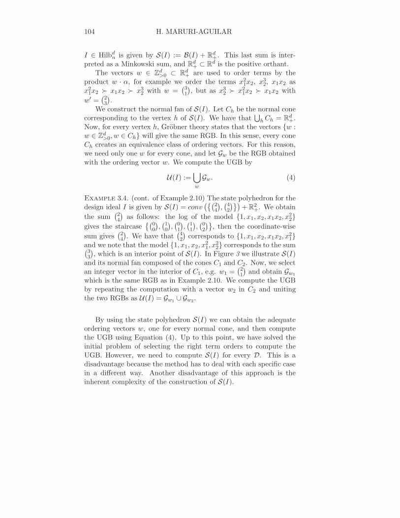
7.2. Complexity of the Hilbert zonotope

Table 1 lists the number of vertices, number of facets and numberof positive ordering vectors1 for various values of d and n. Theasymptotic order for the first two is discussed in Babson et al. (2003).The cardinality of W 2

n+ is listed on the sequence A049696 (Sloane,2004); and the following orders of magnitude are reported

#W 2n+ = 6n2/π2 + O(n log n),

and the refinement

#W 2n+ = 6n2/π2 + O(n(log n)2/3(log log n)4/3)

(Sloane, 2004).

n 1 2 3 4 5 6 7 8 9 10 11 12# of facets 4 6 10 20 28 48 56 84 100 128 144 192

#W2n+ 1 2 4 8 12 20 24 36 44 56 64 84

Table 1. Values for H2n.

n 1 2 3 4 5 6# of facets 6 14 50 458 1022 4970

# of vertices 8 24 84 720 1500 7320#W 2

n+ 1 6 24 192 456 1974

Table 1 (cont.). Values for H3n.

1See Appendix 7.4 for examples of W dn+. We have computed tables with the

vectors up to the following values (d, n): (2, 57), (3, 6), (4, 2), available from theauthor by request.


n 1 2# of facets 8 30

# of vertices 16 120#W 2

n+ 1 24

Table 1 (cont.). Values for H4n.

7.3. Pictures of zonotopes

We show several zonotopes in Figures 8 and 9. We give the generat-ing vectors for the cones of N (H2

n) in Figure 10.

Figure 8: Bidimensional Hilbert zonotopes for n = 1, . . . , 6 (startingfrom the centre).

7.4. Ordering vectors

We list some examples of ordering vectors. For other values d, n, seeNote 1.


Figure 9: Tridimensional Hilbert zonotope for n = 1, . . . , 5 (startingfrom top left).


Figure 10: Generating vectors for the cones of N (H2n) for n =

1, . . . , 10.


7.4.1. Bidimensional case

W 21+ =

{(11

)}

; W 22+ =

{(21

),(12

)}

; W 23+ =

{(31

),(32

),(23

),(13

)}

;

W 24+ =

{(14

),(25

),(35

),(34

),(43

),(53

),(52

),(41

)}

;

W 25+ =

{(15

),(27

),(25

),(35

),(57

),(45

),(54

),(75

),(53

),(52

),(72

),(51

)}

;

W 26+ =

{(16

),(29

),(27

),(38

),(37

),(47

),(58

),(57

),(79

),(56

),(65

),(97

),(75

),(85

),

(74

),(73

),(83

),(72

),(92

),(61

)}

;

W 27+ =

{(17

),( 211

),(29

),(27

),(38

),(37

),(47

),(58

),(57

),(79

),( 911

),(67

),(76

),

(119

),(97

),(75

),(85

),(74

),(73

),(83

),(72

),(92

),(11

2

),(71

)}

.

7.5. Three dimensional case

W 31+ = {(1, 1, 1)T };

W 32+ = {(1, 2, 3)T , (1, 3, 2)T , (2, 3, 1)T , (3, 2, 1)T , (3, 1, 2)T , (2, 1, 3)T }.

8. Acknowledgement

This work was partly supported with a scholarship by CONACYT(Science and Technology Council of Mexico).

References

[1] D. Avis and K. Fukuda, A pivoting algorithm for convex hulls andvertex enumeration of arrangements and polyhedra, Disc. Comput.Geom. 8 (1992), 295–313, in ACM Symposium on Computational Ge-ometry. Papers from the Seventh Annual Symposium

[2] D. Bayer and I. Morrison, Standard bases and geometric invarianttheory I. initial ideals and state polytopes, J. Symb. Comp. 6 (1988),209–217.

[3] B. Giglio, R.A. Bates and H.P. Wynn, A global selection proce-dure for polynomial interpolators, Technometrics (2003), 246–255.

[4] B. Grumbaum, Convex polytopes, ii ed., Springer-Verlag, New York,2003.

[5] G.H. Hardy and E.M. Wright, An introduction to the theory ofnumbers, Oxford Clarendon Press, 1975.

[6] J. Little, D. Cox and D. O’Shea, Ideals, varieties, and algo-rithms, ii ed., Springer-Verlag, New York, 1996.


[7] E. Miller and B. Sturmfels, Combinatorial commutative algebra,Graduate Texts in Math, vol. 227, Springer-Verlag, New York, 2004.

[8] T. Mora and L. Robbiano, The Grobner fan of an ideal, J. Symb.Comp. 6 (1988), 183–208.

[9] S. Onn, E. Bason and R. Thomas, The Hilbert zonotope and apolynomial time algorithm for universal Grobner bases, Adv. Appl.Math. 30 (2003), 529–544.

[10] S. Onn and B. Sturmfels, Cutting corners, Adv. Appl. Math. 623

(1999), 29–48.[11] J.L. Peixoto, A property of well-formulated polynomial regression

models, The American Statistician 44 (1990), no. 1, 26–30.[12] G. Pistone and H.P. Wynn, Generalised confounding with Grobner

bases, Biometrika 83 (1996), 653–666.[13] E. Riccomagno, M. Caboara, G. Pistone and H.P. Wynn, The

fan of an experimental design, SCU Research Report 10, Departmentof Statistics, University of Warwick, 1997.

[14] E. Riccomagno G. Pistone and H.P. Wynn, Algebraic statis-tics: Computational commutative algebra in statistics, Monographson Statistics and Applied Probability, Chapman & Hall/CRC Press,Boca Raton, 200.

[15] N.J.A. Sloane, Sequence a049696 in “the on-line en-cyclopedia of integer sequences.”, website, July 2005,http://www.research.att.com/∼njas/sequences/.

[16] B. Sturmfels, Grobner bases and convex polytopes, University Lec-ture Notes, vol. 8, American Mathematical Society, Providence, RI,1995.

[17] V. Weispfenning, Constructing universal Grobner bases, Ap-plied Algebra, Algebraic Algorithms and Error-Correcting Codes(L. Huguet, ed.), vol. 356, 1987, Proc. AAECC-5, pp. 408–417.

[18] G.M. Ziegler, Lectures on polytopes, Springer-Verlag, 1994.

Received December 6, 2005.

Universal Gr¶bner Bases for Designs of Experiments

Documents