Univariate Volatility Models: ARCH and GARCHdidattica.unibocconi.it/mypage/dwload.php?nomefile=... · Univariate Volatility Models: ARCH and GARCH Massimo Guidolin Dept. of Finance,

Univariate Volatility Models: ARCH andGARCH

Massimo Guidolin

Dept. of Finance, Bocconi University

1. Introduction

Because volatility is commonly perceived as a measure of risk, financial economists have been tra-

ditionally concerned with modeling the time variation in the volatility of (individual) asset and

portfolio returns. This is clearly crucial, as volatility, considered a proxy of risk exposure, leads

investors to demand a premium for investing in volatile assets. The time variation in the variance of

asset returns is also usually referred to as the presence of conditional heteroskedasticity in returns:

therefore the risk premia on conditionally heteroskedastic assets or portfolios may follow a dynamics

that depends on their time-varying volatility. The concept of conditional heteroskedasticity extends

in general to all patterns of time-variation in conditional second moments, i.e., not only to condi-

tional variances but also to conditional covariances and hence correlations. In fact, you will recall

that under the standard (conditional) CAPM, the risk of an asset or portfolio is measured by its

conditional beta vs. the returns on some notion of the market portfolio. Because a conditional

CAPM beta is defined as a ratio of conditional covariance with market portfolio returns and the

conditional variance of returns on the market itself, patterns of time-variation in covariances and

correlations also represent ways in which time-varying second moments affects investors’ perceptions

of risk exposure. Moreover, as already commented in chapter 1, banks and other financial institu-

tions apply risk management (e.g., value-at-risk, VaR) models to high frequency data to assess the

risks of their portfolios. In this case, modelling and forecasting volatilities and correlations becomes

a crucial task for risk managers.

The presence of conditional heteroskedastic patterns in financial returns is also intimately related

to the fact that there is overwhelming evidence that the (unconditional) distribution of realized

returns on most assets (not only stocks and bonds, but also currencies, real estate, commodities,

etc.) tends to display considerable departures from the classical normality assumption. We shall

document that conditional heteroskedasticity implies that the unconditional, long-run distribution of

asset returns is non-normal.1 This is well-known to be potentially responsible for strong departures

1We shall define the technical terms later on, but for the time being, the unconditional distribution of a time series

process is the overall, long-run distribution of the data generated by the process. Drawing on one familiar example,

if +1 = + +1 with +1 ∼ N (0 1) it is clear that the conditional distribution of +1 at time (i.e., given

information observed at time ) is N ( 1); however, in the long-run, when one averages over infinite draws from

of observed derivative prices from simple but still widely employed pricing frameworks that are built

on the classical results by Black and Scholes (1973) that rely on normality of financial returns.

Given these motivations, in this chapter we develop and compare alternative variance forecasting

models for each asset (or portfolio) individually and introduce methods for evaluating the perfor-

mance of these forecasts. In the following chapters, we extend these methods to a framework that

may capture any residual deviations of the distribution of asset returns from normality, after any

models of conditional heteroskedasticity have been applied. Additionally, we show how it is possible

to connect individual variance forecasts to covariance predictions within a correlation model. The

variance and correlation models together will yield a time-varying covariance model, which can be

used to calculate the variance of an aggregate portfolio of assets

This chapter has two crucial lessons that go over and above the technical details of each individual

volatility model or its specific performance. First, one should not be mislead by the naive notion that

because second moments change over time, this implies that the time series process characterized

by such moments becomes “wild”, in the sense of being non-stationary. On the contrary, under

appropriate technical conditions, one can prove that even though the conditional variance may

change in heteroskedastic fashion, the underlying time series process may still be stationary.2 In

practice, this means that even though the variance of a series may go through high and low periods,

the unconditional (long-run, average) variance may still exist and be actually constant.3 Second,

one can read this chapter as a detailed survey of a variety of alternative models used to forecast

variances. However, there is no logical contradiction in the fact that many different models have been

developed and compared in the literature: in the end we only care for their forecasting performance,

and it is possible that in alternative applications and sample periods, different models may turn out

to outperform the remaining ones.

Section 2 starts by offering a motivating example that connects conditional heteroskedasticity

to a few, easily checked and commonly observed empirical properties of financial returns. Section 3

introduces a few simple, in fact as simple as to be naive, variance models that have proven rather

resilient in the practice of volatility forecasting, in spite of their sub-optimality in a statistical

perspective. Section 4 represents the core of this chapter and contains material on forecasting

volatility that is tantamount to you having ever attended a financial econometrics course: we

introduce and develop several strands of the GARCH family. Section 5 presents a particularly

the process, because (under stationarity, i.e., || 1 ) [+1] = 0 and [+1] = 1(1 − 2) you know already

that +1 ∼ N (0 1(1− 2)) so that conditional and unconditional distributions will differ unless = 0.2Heuristically, stationarity of a stochastic process {} means that for every ≥ 0, {}∞= has the same dis-

tribution as {}∞=1. In words, this means that whatever is the point from which one starts sampling a time series

process, the resulting overall (unconditional) distribution is unaffected by the choice: under stationarity, the implied

distribution of returns over the last 20 years is the same as the distribution over 20 years of data to be sampled 10 years

from now, say. Intuitively, this is related to the concept that a stationary time series will display “stable” long-run

statistical properties–as summarized by its unconditional distribution–over time. Here the opposition between the

unconditional natural of a distribution and time-varying conditional variance is important.3However, if the unconditional variance of a time series is not constant, then the series is non-stationary.

2

useful and well-performing family of GARCH models that capture the evidence that past negative

(shocks to) returns tend to increase the subsequent predicted variance more than positive (shocks

to) returns do. Section 6 explains how models of conditional heteroskedasticity can be estimated

in practice and leads to review some basic notions concerning maximum likelihood estimation and

related inferential concepts and techniques. Section 7 explains how alternative conditional variance

models may be evaluated and, in some ways, compared to each other. This seems to be particularly

crucial because this chapter presents a range of different models, so that deciding whether a model

is “good” plays a crucial role. Section 8 closes by introducing a more advanced GARCH model

based on the intuition that the dynamics of variance in the short- vs. the long-run may be different.

The Appendix presents a fully worked set of examples in Matlab.

2. One Motivating Example: Easy Diagnostic of Conditional Heteroskedasticity

As a motivating example, consider the (dividend-adjusted) realized monthly returns on a value-

weighted index (hence, this is a portfolio) of all NYSE, AMEX, and NASDAQ stocks over the

sample period is January 1972 - December 2009.4 Even though this is not among the practice time

series to be used in this class, the series is similar to the typical ones that appear in most textbooks.5

Figure 1 plots the time series of the data.

‐20

‐15

‐10

‐5

0

5

10

15

72 75 78 81 84 87 90 93 96 99 02 05 08

Value‐Weighted NYSE/AMEX/NASDAQ Returns

Quiet period

Quiet period Quiet period

Turbulence Turbulence Turbulence Turbulence

Figure 1: Value-weighted U.S. CRSP monthly stock returns

Visibly, volatility “clusters” in time: high (low) volatility tends to be followed by high (low) volatility.

Casual inspection does have its perils, and formal testing is necessary to substantiate any first

impressions. In fact, our objective in this chapter is to develop models that can fit this typical

sequence of calm and turbulent periods. And especially forecast them.

4The data are compiled by the Center for Research in Security Prices (CRSP) and are available to the

general public from the data repository by Kenneth French, at http://mba.tuck.dartmouth.edu/pages/faculty

/ken.french/data library.html.5Do not worry: we shall take care of examining your typical class data during your MATLAB sessions as well as

at the end of this chapter.

3

Let’s now take this data a bit more seriously and apply the very methods of analysis that you

have learned over the initial 5 weeks of Financial Econometrics II. As you know, a good starting

point consists of examining the autocorrelogram of the series. Table 1 shows the autocorrelogram

function (ACF), the partial autocorrelogram function (PACF), as well as new statistics introduced

below, for the same monthly series in Figure 1.

Table 1: Serial correlation properties of value-weighted U.S. CRSP monthly stock returns

As you would expect of a series sampled at a relatively high frequency (such as monthly), there is

weak serial correlation in U.S. stock returns. This lack of correlation means that, given past returns,

the forecast of today’s expected return is unaffected by knowledge of the past. However, more

generally, the autocorrelation estimates from a standard ACF can be used to test the hypothesis that

the process generating observed returns is a series of independent and identically distributed (IID)

variables. The asymptotic (also called Bartlett’s) standard error of the autocorrelation estimator is

approximately 1√ , where is the sample size. In table 1, such a constant ±2

√ 95% confidence

interval boundary is represented as the short vertical lines that surround the bars that represent

the sample autocorrelation estimates also reported in the AC column of the table (these bars are

to the left of the vertical line representing the 0 in the case of negative autocorrelations and to the

right of the vertical zero-line in the case of positive autocorrelations).6 Visibly, there is only one

“bin”–in correspondence to the first lag, = 1 (an AC of 0.091)–that touches the vertical line

corresponding to the 2√ upper limit of the 95% confidence interval; also in this case, because the

upper limit is 0.094 and 0.091 fails to exceed it, the null hypothesis of 1 = 0 can in principle not be

rejected, although it is clear that we are close to the boundaries of the no-rejection area. However,

for all other values of between 2 and 12, the table emphasizes that all sample autocorrelations fall

inside the 95% confidence interval centered around a zero serial correlation, which is consistent with

the absence of any serial correlation and hence independence of the series of monthly stock returns.

6To be precise, the 2 in the confidence interval statement ±2√ should be replaced by 1.96:

Pr{−196√ ≤ ≤ 196

√} = 095

Notice that this confidence interval only obtains as an approximation, as →∞.

4

However, as we shall see, the absence of serial correlation is insufficient to establish independence.7

2.1. Testing the independence hypothesis and conditional heteroskedasticity

The independence hypothesis can also be tested using the Portmanteau Q-statistic of Box and Pierce

(1970), , calculated from the first autocorrelations of returns as:8

≡

X=1

2∼ 2 where ≡

P−=1 ( − )(+ − )P−

=1 ( − )2

(where 0). Here the notation∼ means that asymptotically, as → ∞, the distribution of

the statistic, under the null of an IID process (i.e., assuming that the null hypothesis holds), is

chi-square, with degrees of freedom.9 In fact, the last two columns of table 1 report both for

between 1 and 12 and the corresponding p-value under a 2 In this case, the availability of 456

monthly observations lends credibility to the claim that, at least as an approximation, ∼ 2. It

is typically suggested to use values for the upper limit up to 4, although here we have simply

set a maximum of = 12 to save space. Consistently with earlier evidence for 1 = 0091 the

table shows that none of the levels of experimented up to this point leads to rejecting the null

hypothesis of IIDness of U.S. stock returns.

Does this evidence allows us to conclude that stock returns are (approximately) IID? Unfortu-

nately not: it turns out that the squares and absolute values of stock and bond returns display high

and significant autocorrelations. Here the conceptual point is that while

is IID =⇒ ' 0 for all ≥ 1

the opposite does not hold:

' 0 for all ≥ 1 6=⇒ is IID.

The reason is that the definition of independence of a time series process has the following charac-

terization:10

is IID ⇐⇒ ' 0 for all ≥ 1

≡

X=1

( )2 ∼ 2 where ≡

P−=1 (()− ())((+ )− ())P−

=1 (()− ())

7Note that the fact that {} is independently distributed (over time) implies that the all autocorrelation coeffi-cients = 0, ∀ ≥ 1, does not imply the opposite: even though = 0, ∀ ≥ 1 independence does not follow. Weshall expand on this point below.

8We shall explain later the exact meaning of denoting portfolio returns as 9It is not surprising that the distribution of the test statistic () is derived assuming the null hypothesis holds:

the goal is indeed to find sample evidence in the data to reject such a null hypothesis. Therefore the logical background

is: are the data providing evidence inconsistent with the statistical properties that should possess under the null?10Technically, one could even state that [() (+ )] = 0 for any choice of sufficiently “smooth” functions

(·) and (·) and ∀ 6= 0.

5

and (·) is any (measurable) function that satisfies appropriate “smoothness” conditions. For in-stance, one may consider () = where is any positive integer and where 1 is admissible.

Another alternative mentioned above is the case of the function () = || the absolute valuetransformation that turns negative real numbers into positive ones (and leaves positive real num-

bers unchanged). In practice, independence implies not only the absence of any serial correlation

in the level of returns–i.e., in the first power of returns, ' 0 for all ≥ 1–but it is equivalentto the absence of any serial correlations in all possible functions of returns, ().

The high dependence in series of square and absolute returns proves that the returns process is

not made up of IID random variables: appropriate functions of past returns do give information on

appropriate functions of current and future returns. For instance, table 2 concerns the squares of

value-weighted monthly U.S. CRSP stock returns and shows that in this case the sample autocor-

relation coefficients of the squares are statistically significant (i.e., the null that these are zero can

be rejected) for = 1 3, 4, and 9.11

Table 2: Serial correlation properties of value-weighted squared U.S. monthly stock returns

Indeed implies p-values below 0.05 (and often below 0.01, indicating strong statistical signifi-

cance) for all values of and especially for ≥ 3 due to the large 3 = 011 (here the acronym

‘’ refers to the fact that we are considering () = 2). The evidence in table 2 implies that large

squared returns are more likely to be followed by large squared returns than small squared returns

are. The fact that past squared returns predict subsequent squared returns–for instance, this is

the meaning of 3 being high and statistically significant (as it exceeds the 95% confidence bound

threshold of 0.094)

3 ≡

P−=1 (

2 −2 )(

2+ −2 )P−

=1 (2 −2 )

(1)

–does not imply that past returns may predict subsequent returns: clearly, (1) may give a large

11The asymptotic distribution of the Box-Pierce statistic applies if and only if the returns themselves are serially

uncorrelated (in levels), i.e., if the null of = 0 cannot be rejected. This means that if one were to be uncertain

about the fact that the zero mean assumption is correctly specified in +1 = +1+1 this may imply that residuals

are not serially uncorrelated so that one cannot simply apply portmanteau tests to test for the presence of ARCH. As

stated, for most daily data series this does not represent a problem.

6

value even though

3 ≡P−

=1 ( −)(+ −)P−=1 ( −)

may be identically zero. This relates to a phenomenon that we have already commented in chapter 1:

at (relatively) high frequencies, it is possible that higher-order moments–in this case, the second–

may be strongly predictable even when the level of asset returns is not, so that they are well

approximated by the simple model

+1 = +1+1 +1 ∼ IID D(0 1)

where the fact that +1 changes over time captures the predictability in squared returns that we

have just illustrated.

At this point we face two challenges. First, and this is a challenge we are not about to pursue,

one wonders what type of economic phenomenon may cause the predictability in squares (or more

generally, in higher-order moments, as parameterized by a choice of ≥ 3 in () = ), commonly

referred to as volatility clustering, the fact that periods of high (low) squared returns tend to be

followed by other periods of high (low) squared returns. Providing an answer to such a question is

the subject of an exciting subfield of financial economics called asset pricing theory. In short, the

general consensus in this field is that changes in the speed of flow of relevant–concerning either

the exposures to risks or their prices–information to the market causes changes in price volatility

that creates clusters of high and low volatility. However, this just moves the question of what may

trigger such changes in the speed of information flows elsewhere. Although a range of explanations

have been proposed (among them, the effects of transaction costs when trading securities, the fact

that investors must learn the process of the fundamentals underlying asset prices in a complex and

uncertain world, special features of investors’ preferences such as habit formation and loss aversion,

etc.) we will drop the issue for the time being. Second, given this evidence of volatility clustering,

one feels a need to develop models in which volatility follows a stochastic process where today’s

volatility is positively correlated with the volatility of subsequent returns. This is what ARCH and

GARCH models are for and what we set out to present in the following section.

7

3. Naive Models for Variance Forecasting

Consider the simple model for one asset (or portfolio) returns:12

+1 = +1+1 +1 ∼ IID N (0 1) (2)

Note that if we compare this claim to Section 2, we have specified the generic distribution D to

be a normal distribution. We shall relax this assumption in the next chapter, but for the time

being this will do for our goals. Here +1 is a continuously compounded return: the notation

is to be opposed to the lowercase notation for returns that has appeared early on because we

want to emphasize that is generated by a model in which the expected return is zero: [+1] =

+1[+1] = +1 × 0 = 0. Equivalently, at high frequency, we can safely assume that the meanvalue of +1 is zero as it is dominated by the standard deviation of returns. In fact, not only +1

is a pure random “shock” to returns, but +1 also has another interesting interpretation that will

turn out to be useful later on:

+1 =+1

+1

which implies that +1 is also a standardized return.13 Note that in (??), +1 and

2+1 are assumed

to be statistically independent: this derives from the fact that 2+1 is a conditional variance function

that–at least in our treatment–only depends on past information, i.e., 2+1 ≡ [+1|F].A model in which [+1] = 0 is an acceptable approximation when applied to daily data.

Absent this assumption, a more realistic model would be instead

+1 = +1 + +1+1 +1 ∼ IID N (0 1)

where +1 ≡ [+1]. In this case, +1 = (+1 − +1)+1. This model will reappear in our

concerns in later chapters. How do you test whether +1 or, more concretely, = 0 or not? This

is a standard test of a mean, see your notes from any undergraduate statistics sequence.14

12We shall be modelling asset or portfolio returns, and never prices! This is important, because the absence of serial

correlation in returns means that a good model for returns is indeed (ignoring the mean and any dividends or interim

cash flows) +1 = log(+1) − log() = +1+1 which implies that log(+1) = log() + +1 i.e., (the log of )

prices tend to follow a random walk. Because (log-)asset prices are I(1) process, they contain a stochastic trend, to

analyze them without first removing the trend is always unwieldy and often plainly incorrect. Incorrect here means

that most of the tests and inferential procedures you have been taught apply only–except for major and complicated

corrections, if any–to stationary series, not to I(1) series. This also means that in most cases there is only one type

of econometrics that can be applied to the prices of assets or portfolios, the wrong one–the one we should never hear

about in MSc. theses, for instance.13You will recall that if is characterized by an expectation of [+1] and a variance of [+1] the stan-

dardized version of the variable is:+1 −[+1]

[+1]

Clearly, if [+1] = 0 the standardization simply involves scaling +1 by its standard deviation. Note that

standardization may also apply in conditional terms: if[+1] ≡ [+1|F] and [+1] ≡ [+1|F] whereF is the information set at time then the conditional standardized variable is: (+1 −[+1])

[+1].

14Right, you cannot find your notes or textbooks now. OK then: the null hypothesis is = 0 and the test statistic

8

3.1. Rolling window variance model

The easiest way to capture volatility clustering is by letting tomorrow’s variance be the simple

average of the most recent squared observations, as in

2+1 =1

X=1

2+1− =X

=1

1

2+1− (3)

This variance prediction function is simply a constant-weight sum of past squared returns.15

This is called a rolling window variance forecast model. However, the fact that the model puts equal

weights (equal to 1) on the past observations often yields unwarranted and hard to justify

results. Figure 2 offers a snapshot of the problems associated with rolling window variance models.

The figure concerns S&P 500 daily data and uses a rolling window of 25 observations, = 25.

The figure emphasizes that, when plotted over time, predicted rolling window variance exhibits

box-shaped patterns: An extreme return (positive or negative) today will bump up variance by

1 times the return squared for exactly periods after which variance immediately drops back

down.

Figure 2: Squared S&P500 returns with moving average variance estimate (bold), = 25

However, such extreme gyrations–especially the fact that predicted variance suddenly declines

after 25 periods–does not reflect the economics of the underlying financial market. It is instead

just caused by the mechanics of the volatility model postulated in (3). This brings us to the next

issue: given that has such a large impact on the dynamics of predicted variance, one wonders

how should be selected and whether any optimal choice may be hoped for. In particular, it is

(when the variance is unknown) is:

=2

∼ −1

where is the sample mean and 2 is the sample variance. Alternatively, simply estimate a regression of returns on

just an intercept and test whether the constant coefficient is statistically significant at a given, chosen size of the test.15Because we have assumed that returns have zero mean, note that when predicting variance we do not need to

worry about summing or weighing squared deviations from the mean, as in general the definition of variance would

require.

9

clear that a high will lead to an excessively smoothly evolving 2+1, and that a low will lead

to an excessively jagged pattern of 2+1. Unfortunately, in the financial econometrics literature no

compelling or persuasive answer has been yet reported.

3.2. Exponential variance smoothing: the RiskMetrics model

Another reason for dissatisfaction is that typically the sample autocorrelation plots/functions of

squared returns suggest that a more gradual decline is warranted in the effect of past returns on

today’s variance, see table 2.

Figure 3: Autocorrelation of squared daily S&P 500 returns

To make this point more persuasively (and waiting for our own evidence from the Matlab sessions),

observe now figure 3, concerning daily S&P 500 returns (table 2 concerned instead monthly value-

weighted U.S. stock returns). The sample underlying the sample calculations in the figure is January

1, 2010—December 31, 2010. Clearly, in the figure sample autocorrelations decline rather slowly (in

spite the inevitable sample variation of all estimators) from initial levels of of 0.25-0.30 for

small values of to values below 0.10 when exceeds 50. A more interesting model that takes this

evidence into account when computing forecasts of variance is JP Morgan’s RiskMetrics system:

2+1 = (1− )

∞X=1

−12+1− ∈ (0 1) (4)

In this model, the weight on past squared returns declines exponentially as we move backward in

time: 1, , 2, . . . 16 Because of this rather specific mathematical structure, the model is also called

the exponential variance smoother. Exponential smoothers have a long tradition in econometrics

16However, the weights do sum to 1, as you would expect them to do. In fact, this is the role played by the factor

(1 − ) that multiplies the infinite sum∞

=1 −12

+1− . Noting that because the sum of a geometric series is∞=0

= 1(1− ), we have

∞=1

=

∞=1

(1− )−1

= (1− )

∞=1

−1

= (1− )

∞=0

= (1− )

1

(1− )= 1

where ≡ (1− )−1 for ≥ 1.

10

and applied forecasting because they are known to provide rather accurate forecasts of the level

of time series. JP Morgan’s RiskMetrics desk was however rather innovative in thinking that such

a model could also provide good predictive accuracy when applied to second moments of financial

time series.

(4) does not represent either the most useful or the most common way in which the RiskMetrics

model is presented and used. Because for = 1 we have 0 = 1, it is possible to re-write it as:

2+1 = (1− )2 + (1− )

∞X=2

−12+1− = (1− )2 + (1− )

∞X=1

2−

Yet it is clear that

2 = (1− )

∞X=1

−12− =1

(1− )

∞X=1

2−

Substituting this expression into 2+1 = (1− )2 + (1− )P∞

=1 2− , gives

2+1 = (1− )2 +

(1− )

∞X=1

2−

= (1− )2 +

⎡⎢⎢⎢⎢⎢⎣1

(1− )

∞X=1

2−| {z }=2

⎤⎥⎥⎥⎥⎥⎦= (1− )2 + 2 (5)

(5) implies that forecasts of time +1 variance are obtained as a weighted average of today’s variance

and of today’s squared return, with weights and 1− , respectively.17 In particular, notice that

lim→1−

2+1 = 2

i.e., as → 1− (a limit from the left, given that we have imposed the restriction that ∈ (0 1))the process followed by conditional variance becomes a constant, in the sense that 2+1 = 2 =

2−1 = = 20 The naive idea that one can simply identify the forecast of time + 1 variance as

the squared return of corresponds instead to the case of → 0+.

The RiskMetrics model in (5) presents a number of important advantages:

1. (4) is a sensible formula as it implies that recent returns matter more for predicting tomorrow’s

variance than distant returns do; this derives from ∈ (0 1) so that gets smaller when the17One of your TAs has demanded that also the following, equivalent formulation be reported: 2+1| = (1−)2

+

2 where 2+1| emphasizes that this is the forecast of time + 1 variance given the time information set. This

notation will also appear later on in the chapter.

11

lag coefficient, , gets bigger. Figure 4 show the behavior of this weight as a function of .

Figure 4

2. (5) only contains one unknown parameter, that we will have to estimate. In fact, after

estimating on a large number of assets, RiskMetrics found that the estimates were quite

similar across assets, and therefore suggested to simply set for every asset and daily data

sets to a typical value of 0.94. In this case, no estimation is necessary.18

3. Little data need to be stored in order to calculate and forecast tomorrow’s variance; in fact,

for values of close to the 0.94 originally suggested by RiskMetrics, it is the case that after

including 100 lags of squared returns, the cumulated weight is already close to 100%. This is

of course due to the fact that, once 2 has been computed, past returns beyond the current

squared return 2 , are not needed. Figure 5 shows the behavior of the cumulative weight for

a fixed number of past observations as a function of .

Figure 5

Given all these advantages of the RiskMetrics model, why not simply end the discussion on

variance forecasting here?

18We shall see later in this chapter that maximum likelihood estimation of tends to provide estimates that hardly

fall very far from the classical RiskMetrics = 094

12

4. Generalized Autoregressive Conditional Heteroskedastic (GARCH) Variance

Models

The RiskMetrics model has a number of shortcomings, but these can be understood only after

introducing ARCH() models, where ARCH is the celebrated acronyms for Autoregressive Con-

ditional Heteroskedastic. Historically, ARCH models were the first-line alternative developed to

compete with exponential smoothers and one quick glance at their functional form reveals why. In

the zero-mean return case, their structure is very simple:

2+1 = + 2

In particular, this is a simple, plain-vanilla ARCH(1) process and it implies that

+1 =

µq + 2

¶+1 +1 ∼ IID N (0 1)

The intuition of this model is immediate: the appearance of 2 0 (if 0 as we shall impose

later) is what captures the clustering intuition that large movements in asset prices tend to follow

large movements, of either sign (as the square function only produces positive contributions). The

impact of past large movements in prices will be large if is large. In fact, as → 1− (from the

left, as we will see that 1), any return (shock) will cause an impact on subsequent variances

that is nearly permanent.

The differences vs. (5), 2+1 = (1 − )2 + 2 are obvious. On the one hand, RiskMetrics

can be taken as a special case of ARCH(1) in which = 0; on the other hand, it is clear that an

exponential smoother does not only attach a weight (1 − ) to current squared return, but also a

weight on current variance, 2 . The fact that the good performance of RiskMetrics mentioned

above is based on both 2 and 2 makes it less than surprising the fact that, historically, it became

soon obvious that just using one lag of past squared returns would not be sufficient to produce

accurate forecasts of variance: for most assets and sample periods there is indeed evidence that

one needs to use a large number 1 of lags on the right-hand side (RHS) of the ARCH()

representation:

2+1 = +

X=1

2+1− (6)

Yet, even though it is simple, in statistical terms ARCH() is not as innocuous as it may seem:

maximum likelihood estimation of models of the type (6) implies nonlinear parameter estimation,

on which some details will be provided later. It is easy to find the unconditional, long-run variance

under (6). Because (20) implies that [2+1] = [2+12+1] = [2+1][

2+1] = [2+1] × 1 =

13

[2+1] setting 2 ≡ [2+1] = [2+1−] ∀:19

2 = [2+1] = +

X=1

[2+1−] = +

X=1

2

= + 2X

=1

=⇒ 2 =

1−P=1

(7)

Because unconditional variance makes sense (technically, we say that it exists, i.e., it is defined)

only when 2 0, (7) implies that when 0, the condition

1−X

=1

0 =⇒X

=1

1

must hold. When the long-run, unconditional variance of a ARCH process exists, because in a

ARCH model the only source of time-variation in conditional moments comes from the variance,

we say that the ARCH process is stationary and we also refer to the conditionP

=1 1 as

a stationarity condition. Moreover, because also existence of conditional variances requires that

2+1 0 the additional restrictions that 0 and 1 2 0 are usually added both in

theoretical work and in applied estimation.

4.1. Inside the box: basic statistical properties of a simple AR(1)-ARCH(1) model

To get a concrete grip of the statistical implications of ARCH modelling and of the possible interac-

tions between conditional mean and conditional variance functions, consider the simplest possible

ARCH model with some structure in its conditional mean function, i.e., a Gaussian AR(1)-ARCH(1)

model:

+1 = [0 + 1] +£ + 2

¤12+1 +1 ∼ IID N (0 1)

where |1| 1, 0 1, while 0 keeps variance well-defined and

≡£ + 2−1

¤12

Notice that in this model we are temporarily removing the assumption that +1 = 0. In a way, this

is to show you why this assumption had been introduced in the first place: if +1 6= 0, even withvery simple conditional heteroskedastic models, things get considerably complicated. For instance,

the ARCH process is no longer simply defined in terms of one lag of returns, 2−1 but instead in

terms of 2−1. The Gaussian AR(1)-ARCH(1) model has to be compared with the homoskedastic

Gaussian AR(1)process

+1 = [0 + 1] + []12 +1 +1 ∼ IID N (0 1)

19[2+12+1] = [2+1][

2+1] derives from the fact that +1 and 2+1 are statistically independent. On its

turn, this derives from the fact that 2+1 is a conditional variance function that only depends on past information,

i.e., 2+1 ≡ [+1|F]. [2+1][2+1] = [2+1] comes then from the fact that if +1 ∼IID N (0 1) then

[2+1] = [+1] = 1

14

you are already familiar with from the first part of the course. Assume that is independent of

−1 −2 0.

Consider first the total residual of the process, i.e., ≡ =£ + 2−1

¤12. We show that

the process for the total residuals, denoted {} has zero mean and is serially uncorrelated at alllags > 1. This can be seen from

[] = h£ + 2−1

¤12

i=

from independence of from −1−20z }| {h£ + 2−1

¤12i []| {z }=0

= h£ + 2−1

¤12i0 = 0

[− ] = h£ + 2−1

¤12 £ + 2−1−

¤12−

i

=

from independence of from −1−20z }| {h£ + 2−1

¤12 £ + 2−1−

¤12i [− ]| {z }

=0 b/c +1∼ (01)

= h£ + 2−1

¤12 £ + 2−1−

¤12i0 = 0 ( > 1)

This property is important because it provides guarantees (necessary and sometimes sufficient con-

ditions) to proceed to the estimation of the conditional mean function using standard methods, such

as OLS. Yet, {} has a finite unconditional variance of (1− ). This can be seen from

£2¤=

£( + 2−1)

2

¤=

£ + 2−1

¤£2¤| {z }

=1

= + £2−1

¤= +

£2¤

£2¤= [] = (1− )

This iterates a point made above already: ARCH does not imply non-stationarity, and in fact a

finite long-run, average, unconditional variance exists, although it diverges to +∞ as → 1−. It

is also easy to prove that the conditional process for total residuals, {|−1 −2 }, has a zeroconditional mean and a conditional variance of + 2−1:

[|−1 ] = −1h£ + 2−1

¤12

i=

from independence of from −1−20z }| {−1

h£ + 2−1

¤12i−1 []

=£ + 2−1

¤120 = 0

£2 |−1

¤= −1

££ + 2−1

¤2¤=

from independence of from −1−20z }| {£ + 2−1

¤−1

£2¤| {z }

=1

=£ + 2−1

¤1 = + 2−1 = −1 []

This confirms what we have stated early on about the typical properties of financial data: under

ARCH, shocks may be serially uncorrelated as [− ] = 0 but they are not independent because

£2 |−1

¤= + 2−1.

15

Finally, let’s verify that the famous Wold’s representation theorem that you have encountered

in the first part of this course–by which any AR() process can be represented as an infinite MA

process–also applies to ARCH(1) models.20 By a process of recursive substitution, we have:

2 = + 2−1 + = +

from 2−1=+2−1+z }| {£

+ 2−2 + −1¤+ = (1 + ) + 22−2 +

£ + −1

¤=

¡1 + + 2

¢+ 32−3 +

£ + −1 + 2−2

¤=

= =

−1X=0

+ 20 +

−1X=0

−

This means that if the return series had started in the sufficiently “distant” past or, equivalently,

as +∞ this is indeed an (∞) process, 2 = [(1− )] + +−1+2−2+3−3+

Note that lim→∞ P−1

=0 = (1 − ) because for 1,

P∞=0

is a convergent geometric

series.

4.2. GARCH( ) models

Although you may not see that yet, (6) has the typical structure of a AR() model. To see this

note two simple facts. First given any random variable +1 notice that the variable can always

be decomposed as the sum of its conditional expectation plus a zero-mean white noise shock:

+1 = [+1] + +1

Hence applying this principle to square asset returns, one has 2+1 = [2+1]++1. Second, from

the definition of conditional variance and the fact that [+1] = 0 we have that 2+1 ≡ [+1]

= [2+1] Therefore, putting these two simple facts together, we have:

2+1 = [2+1] + +1 = 2+1 + +1

= +

X=1

2+1− + +1

Surprise: this is a standard AR() model for squared asset returns! At this point, if you have paid

some attention to what has happened in the last 5 weeks, you know where to look for when it comes

to generalize and improve the predictive performance of an AR() model: ARMA( ) models.

Before proceeding to that, we dig a bit deeper on this AR() characterization of ARCH by

showing–at least for the simple case of AR(1)-ARCH(1), when the algebra is relatively simple–

that the autocorrelogram of the series of squared shocks©2ªimplied by an ARCH(1) decays at

20Here we use a property that 2 = 2 + so that 2 = +1

2−1+ derived in next subsection. This just means

that in a ARCH model, squared shocks follow an AR(1) process (hence the “AR” in ARCH). Apologies for running

ahead, just take this property as a fact for the time being.

16

speed () . Note that under a ARCH(1), the forecast error when predicting squared residuals is

(note that = when the conditional mean is zero, i.e., 0 = 1 = 0):

= 2 −−1£2¤= 2 − 2 2 = + 1

2−1

Therefore 2 = 2 + or 2 = + 2−1 + which is an AR(1) process for squared innovations

to financial returns. This implies that the autocorrelogram for the series of squared shocks©2ª

from an ARCH(1) decays at speed () because of the properties of autoregressive processes

seen in the first part of the course. Here is the order of the autocorrelogram, i.e., the lag in

£2

2−¤

£2¤ the implication is that unless 1, the autocorrelogram of a ARCH(1)

will decay very quickly. See for instance the simulations below in figure 6.

Figure 6: Simulated sample autorecorrelation function for alternative choices of (0.1, 0.5, 0.9)

As far as the ARMA extensions are concerned, the simplest generalized autoregressive condi-

tional heteroskedasticity (GARCH(1,1)) model is:

2+1 = + 2 + 2 (8)

which yields a model for returns given by +1 = (p + 2 + 2 +1) where +1 ∼ IID N (0 1).

More generally, in the ARMA( ) case, we have:

2+1 = +

X=1

2+1− +

X=1

2+1− (9)

Similarly to the steps followed in the ARCH() case, setting 2 ≡ [2+1]:21

2 = [2+1] = +

X=1

[2+1−] +

X=1

[2+1− ] = +

X=1

2 +

X=1

2

= + 2

⎛⎝ X=1

+

X=1

⎞⎠ =⇒ 2 =

1−P=1 −

P=1

21The following derivation exploits the fact that 2 = [2+ ] ∀ ≥ 0 This is true of any stationary process: its

properties do not depend on the exact indexing of the time series under investigation.

17

Because unconditional variance exists only if 2 0, the equation above implies that when 0,

the condition

1−X

=1

−X

=1

0 =⇒X

=1

+

X=1

1

must hold. When the long-run (i.e. ergodic) variance of a GARCH process exists, because in a

GARCHmodel the only source of time-variation in conditional moments comes from the variance, we

say that the GARCH process is stationary and we also refer to the conditionP

=1 +P

=1 1

as a stationarity condition. Moreover, because also existence of conditional variances requires that

2+1 0 the additional restrictions that 0, 1 2 0 1 2 ..., 0 are usually

added both in theoretical work and in applied estimation. Of course in the = = 1 case, such

restrictions are simply 0, 0 0 and + 1.

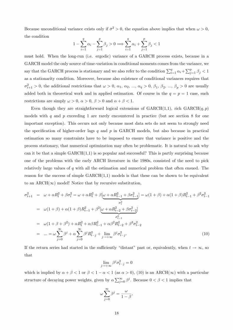
Even though they are straightforward logical extensions of GARCH(1,1), rich GARCH( )

models with and exceeding 1 are rarely encountered in practice (but see section 8 for one

important exception). This occurs not only because most data sets do not seem to strongly need

the specification of higher-order lags and in GARCH models, but also because in practical

estimation so many constraints have to be imposed to ensure that variance is positive and the

process stationary, that numerical optimization may often be problematic. It is natural to ask why

can it be that a simple GARCH(1,1) is so popular and successful? This is partly surprising because

one of the problems with the early ARCH literature in the 1980s, consisted of the need to pick

relatively large values of with all the estimation and numerical problem that often ensued. The

reason for the success of simple GARCH(1,1) models is that these can be shown to be equivalent

to an ARCH(∞) model! Notice that by recursive substitution,

2+1 = + 2 + 2 = + 2 + [ + 2−1 + 2−1| {z }2

] = (1 + ) + (1 + )2−1 + 22−1

= (1 + ) + (1 + )2−1 + 2[ + 2−2 + 2−2| {z }2−1

]

= (1 + + 2) + 2 + 2−1 + 22−2 + 32−2

= =

∞X=0

+

∞X=0

2− + lim→+∞

2− (10)

If the return series had started in the sufficiently “distant” past or, equivalently, when → ∞, sothat

lim→+∞

2− = 0

which is implied by + 1 or 1− 1 (as 0), (10) is an ARCH(∞) with a particularstructure of decaying power weights, given by

P∞=0

. Because 0 1 implies that

∞X=0

=

1−

18

(10) is then equivalent to

2+1 =

1− +ARCH(∞).

Therefore, because a seemingly innocuous GARCH(1,1) is in fact equivalent to a ARCH(∞) itsempirical power should be a little less than surprising.

There is another, useful way to re-write the GARCH(1,1) model (something similar applies to

the general ( ) case but the algebra is tedious) that becomes useful when it comes to investigate

variance predictions under GARCH. Because

2 =

1− − =⇒ = (1− − )2

substituting this expression into (8), we have:

2+1 = + 2 + 2 = (1− − )2 + 2 + 2

= 2 + (2 − 2) + (2 − 2) (11)

which means that under a GARCH(1,1), the forecast of tomorrow’s variance is the long-run average

variance, adjusted by:

• adding (subtracting) a term that measures whether today’s squared return is above (below)

its long-run average, and

• adding (subtracting) a term that measures whether today’s variance is above (below) its long-run average.

4.3. A formal (G)ARCH test

A more formal (Lagrange multiplier) test for (G)ARCH in returns/disturbances vs. the sample

autocorrelogram ones, has been proposed by Engle (1982). The methodology involves the following

two steps: First, use simple OLS to estimate the most appropriate regression equation or ARMA

model on asset returns and let {2 } denote the squares of the standardized returns (residuals), forinstance coming from a homoskedastic model, 2 = 2 ; Second, regress these squared residuals

on a constant and on lagged values 2−1, 2+2, ...,

2− ( is a white noise shock):

2 = 0 + 12−1 + 2

2−2 + +

2− + (12)

If there are no ARCH effects, the estimated values of 1 through should be zero, 1 = 2 = = .

Hence, this regression will have little explanatory power so that the coefficient of determination (i.e.,

the usual 2) will be quite low. Using a sample of standardized returns, under the null hypothesis

of no ARCH errors, the test statistic 2 converges to a 2 . If 2 is sufficiently large, rejection

of the null hypothesis that 1 through are jointly equal to zero is equivalent to rejection of the

19

null hypothesis of no ARCH errors. On the other hand, if 2 is sufficiently low, it is possible to

conclude that there are no ARCH effects.22

A straightforward extension of (12) can also be used to test alternative specifications of (G)ARCH

models. For instance, to test for ARCH(1) against ARCH(2), with 2 1 you simply estimate

(12) by regressing the standardized squared residuals from the ARCH(1) model on 2 lags of the

same squared residuals and then use an F-test for the null hypothesis that 1 = 1+1 = = 2

in:

2 = 0 + 1 2−1−1 + 1+1

2−1−2 + + 2

2−2 +

Note that these tests will be valid in small samples only if all the competing ARCH models have

been estimated on the same data sets, in the sense that the total number of observations should be

identical even though 2 1.

It is also possible to specifically test for GARCH effects by performing a Lagrange multiplier

regression-based test. For instance, if one has initially estimated a ARCH() model and wants to

test for generalized ARCH terms, then the needed auxiliary regression is:

2 = 0 + 12()−1 + 2

2()−2 + +

2()− +

where 2() is the time series of filtered, in-sample ARCH() conditional variances obtained in

the first-stage estimation. Also in this case, if there are no GARCH effects, the estimated values of

1 through should be zero, 1 = 2 = = . Hence, this regression will have little explanatory

power so that the coefficient of determination (i.e., the usual 2) will be quite low. Using a sample

of standardized returns, under the null hypothesis of no ARCH errors, the test statistic 2

converges to a 2 . As before, in small samples, an test may have superior power.

4.4. Forecasting with GARCH models

We have emphasized on several occasions that the point of GARCH models is more proposing

forecasts of subsequent future variance than telling or supporting some economic story for why

variance may be time-varying. It is therefore natural to ask how does one forecast conditional

variance with a GARCH model.23 At one level, the answer is very simple because the one-step

(one-day) ahead forecast of variance, 2+1|, is given directly by the model in (8):

2+1| = + 2 + 2

22With the small samples typically used in applied work, an F-test for the null hypothesis 1 = 2 = = has

been shown to be superior to a 2 test. In this case, we compare the sample value of F to the values in an F-table

with degrees of freedom in the numerator and − degrees of freedom in the denominator.23For concreteness, in what follows we focus on the case of a simple GARCH(1,1) model. All these results, at the

cost of tedious algebra, may be generalized to the GARCH( ) case. This may represent a useful (possibly, boring)

exercise.

20

where the notation 2+1| ≡ [

2+1] now stresses that such a prediction for time + 1 is obtained

on the basis of information up to time i.e., that 2+1| is a short-hand for [|F] = [2 |F],

where the equality derives from the fact that we have assumed +1 = 0.

However we are rarely interested in just forecasting one-step ahead. Consider a generic forecast

horizon, ≥ 1. In this case, it is easy to show that from (11),

2+| − 2 = [2+ ]− 2 = [

2+−1 − 2] + [

2+−1 − 2]

= ([2+−1]− 2) + ([

2+−1]− 2)

= (2+−1| − 2) + (2+−1| − 2) = (+ )(2+−1| − 2)

This establishes a recursive relationship: the predicted deviations of + forecasts from the un-

conditional, long-run variance on the left-hand side equal (+) 1 times the predicted deviations

of + − 1 forecasts from the unconditional, long-run variance. All the forecasts are computed

conditioning on time information. However, we know from the recursion that 2+−1| − 2 =

(+ )(2+−2| − 2), and

2+| − 2 = (+ )

⎡⎢⎢⎢⎣(+ )(2+−2| − 2)| {z }2+−1|−2

⎤⎥⎥⎥⎦ = (+ )2(2+−2| − 2)

Working backwards this way − 1 times, it is easy to see that

2+| − 2 = (+ )−1(2+1| − 2) (13)

or

2+| = 2 + (+ )−1(2+1 − 2) = 2 + (+ )−1[(2 − 2) + (2 − 2)]

This expression implies that as the forecast horizon grows, because for (+ ) 1 the limit of

(+ )−1 is 0, we obtain

lim→∞

2+| = 2

i.e., the very long horizon forecast from a stationary GARCH(1,1) model is the long-run variance

itself. Practically, this means that because stationary GARCH models are mean-reverting, any

long-run forecast will simply exploit this fact, i.e., use 2 as the prediction. Of course, for finite but

large it is easy to see that when ( + ) is relatively small, then 2+| will be close to 2 for

relatively modest values of ; when ( + ) is instead close to 1, 2+| will depart from 2 even

for large values of . (13) has another key implication: because in a GARCH we also restrict both

and to be positive, ( + ) ∈ (0 1) implies that ( + )−1 0 for all values of the horizon

≥ 1 Therefore it is clear that 2+| 2 when 2

+1| 2 and vice-versa. This means that

-step ahead forecasts of the variance will exceed long-run variance if 1-step ahead forecasts exceed

long-run variance, and vice-versa. As you have understood at this point, the coefficient sum (+)

21

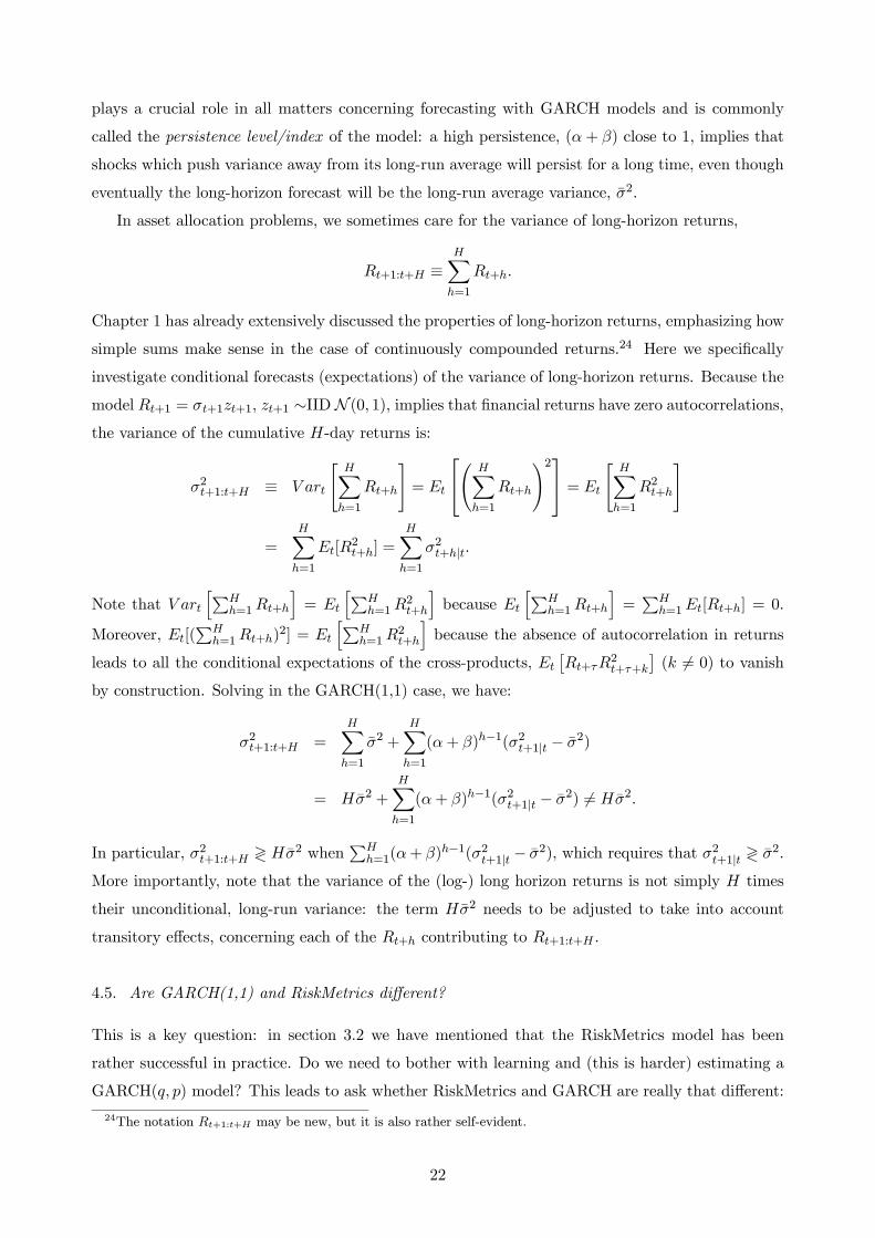
plays a crucial role in all matters concerning forecasting with GARCH models and is commonly

called the persistence level/index of the model: a high persistence, (+ ) close to 1, implies that

shocks which push variance away from its long-run average will persist for a long time, even though

eventually the long-horizon forecast will be the long-run average variance, 2.

In asset allocation problems, we sometimes care for the variance of long-horizon returns,

+1:+ ≡X=1

+

Chapter 1 has already extensively discussed the properties of long-horizon returns, emphasizing how

simple sums make sense in the case of continuously compounded returns.24 Here we specifically

investigate conditional forecasts (expectations) of the variance of long-horizon returns. Because the

model +1 = +1+1, +1 ∼IIDN (0 1), implies that financial returns have zero autocorrelations,the variance of the cumulative -day returns is:

2+1:+ ≡

"X=1

+

#=

⎡⎣Ã X=1

+

!2⎤⎦ =

"X=1

2+

#

=

X=1

[2+] =

X=1

2+|

Note that

hP=1+

i=

hP=1

2+

ibecause

hP=1+

i=P

=1[+] = 0

Moreover, [(P

=1+)2] =

hP=1

2+

ibecause the absence of autocorrelation in returns

leads to all the conditional expectations of the cross-products,

£+

2++

¤( 6= 0) to vanish

by construction. Solving in the GARCH(1,1) case, we have:

2+1:+ =

X=1

2 +

X=1

(+ )−1(2+1| − 2)

= 2 +

X=1

(+ )−1(2+1| − 2) 6= 2.

In particular, 2+1:+ ≷ 2 whenP

=1(+ )−1(2+1| − 2), which requires that 2

+1| ≷ 2.

More importantly, note that the variance of the (log-) long horizon returns is not simply times

their unconditional, long-run variance: the term 2 needs to be adjusted to take into account

transitory effects, concerning each of the + contributing to +1:+ .

4.5. Are GARCH(1,1) and RiskMetrics different?

This is a key question: in section 3.2 we have mentioned that the RiskMetrics model has been

rather successful in practice. Do we need to bother with learning and (this is harder) estimating a

GARCH( ) model? This leads to ask whether RiskMetrics and GARCH are really that different:

24The notation +1:+ may be new, but it is also rather self-evident.

22

as we shall see, they are indeed quite different statistical objects because they imply divergent

unconditional, long-run properties, even though in a small sample of data you cannot rule out

the possibility that their performance may be similar. Yet, especially in long-horizon forecasting

applications, the structural differences between the two ought to be kept in mind.

On the one hand, RiskMetrics and GARCH are not that radically different: comparing (8) with

(5) you can see that RiskMetrics is just a special case of GARCH(1,1) in which = 0 and = 1−so that, equivalently, (+ ) = 1. On the other hand, this simple fact has a number of important

implications:

1. Because = 0 and + = 1, under RiskMetrics the long-run variance does not exist as gives

an indeterminate ratio “0/0”:

2 =0

1− − =0

0

Therefore while RiskMetrics ignores the fact that the long-run, average variance tends to be

relatively stable over time, a GARCH model with ( + ) 1 does not. Equivalently, while

a GARCH with ( + ) 1 is a stationary process, a RiskMetrics model is not. This can

be seen from the fact that 2 does not even exist (do not spend much time trying to

figure out the value of 00).

2. Because under RiskMetrics (+ ) = 1, it follows that

(2+|) − 2 = (1)−1(2+1| − 2) = 2+1| − 2 =⇒ (2+|) = 2+1|

which means that any shock to current variance is destined to persist forever: If today is

a high (low)-variance day, then the RiskMetrics model predicts that all future days will be

high (low)- variance days, which is clearly rather unrealistic. In fact, this can be dangerous:

assuming the RiskMetrics model holds despite the data truly look more like GARCH will give

risk managers a false sense of the calmness of the market in the future, when the market is

calm today and 2+1| 2.25 A GARCH more realistically assumes that eventually, in the

future, variance will revert to the average value 2.

3. Under RiskMetrics, the variance of long-horizon returns is:

(2+1:+) =

X=1

2+| =X=1

2+1| = 2+1

= (1− )2 +2

which is just times the most recent forecast of future variance. Figure 7 illustrates this

25Clearly this point cannot be appreciated by such a risk-manager: under RiskMetrics 2 does not exist.

23

difference through a practical example in which for the RiskMetrics we set = 094

= 0.05,  = 0.90, 2 = 0.00014 

RiskMetrics

GARCH(1,1)

Figure 7: Variance forecasts as a function of horizon () under a GARCH(1,1) vs. RiskMetrics

5. Asymmetric GARCH Models (with Leverage) and Predetermined Variance

Factors

A number of empirical papers have emphasized that for many assets and sample periods, a negative

return increases conditional variance by more than a positive return of the same magnitude does,

the so-called leverage effect. Although empirical evidence exists that has shown that speaking of a

leverage effect with reference to corporate leverage may be slightly abusive of what the data show,

the underlying idea is that because, in the case of stocks, a negative equity return implies a drop

in the equity value of the company, this implies that the company becomes more highly levered

and thus riskier (assuming the level of debt stays constant). Assuming that on average conditional

variance represents an appropriate measure of risk–which, as we shall discuss, requires rather

precise assumptions within a formal asset pricing framework–the logical flow of ideas implies that

negative (shocks to) stock returns ought to be followed by an increase in conditional variance, or at

least that negative returns ought to affect subsequent conditional variance more than positive returns

do.26 More generally, even though a leverage-related story remains suggestive and a few researchers

in asset pricing have indeed tested this linkage directly, in what follows we shall write about an

asymmetric effect in conditional volatility dynamics, regardless of whether this may actually be a

leverage effect or not.

To quant experts, what matters is that returns on most assets seem to be characterized by an

26These claims are subject to a number of qualifications. First, this story for the existence of asymmetric effects in

conditional volatility only works in the case of stock returns, as it is difficult to imagine how leverage may enter the

picture in the case of bond, real estate, and commodities’ returns, not to mention currency log-changes. Second, the

story becomes fuzzy when one has to specify the time lag that would separate the negative shock to equity returns and

hence the capital structure and the (subsequent?) reaction of conditional volatility. Third, as acknowledged in the

main text, there are potential issue with identifying the (idiosyncratic) capital structure-induced risk of a company

with forecasts of conditional variance.

24

asymmetric news impact curve (NIC). The NIC measures how new information is incorporated into

volatility, i.e., it shows the relationship between the current return and conditional variance one

period ahead 2+1, holding constant all other past and current information.27 Formally, 2+1 =

(|2 = 2) means that one investigates the behavior of 2+1 as a function of the current

return, taking past variance as given. For instance, in the case of a GARCH(1,1) model we have:

(|2 = 2) = + 2 + 2 = + 2

where the constant ≡ + 2 and 0 is the convexity parameter. This function is a

quadratic function of 2 and therefore symmetric around 0 (with intercept ). Figure 8 shows such

a symmetric NIC from a GARCH(1,1) model.

Figure 8: Symmetric NIC from a GARCH model

However, from empirical work, we know that for most return series, the empirical NIC fails to

be symmetric. As already hinted at, there is now massive evidence that negative news increase

conditional volatility much more than positive news do.28 Figure 9 compares a symmetric GARCH-

induced NIC with an asymmetric one.

How do you actually test whether there are asymmetric effects in conditional heteroskedasticity?

The simplest and most common way consists of using (Lagrange multiplier) ARCH-type tests similar

to those introduced before. After having fitted to returns data either a ARCH or GARCH model,

call {} the corresponding time series of standardized residuals. Then simple regressions may be27In principle the NIC should be defined and estimated with reference to shocks to returns, i.e., news. In general

terms, news are defined as the unexpected component of returns. However, in this chapter we are working under the

assumption that +1 = 0 so that in our view, returns and news are the same. However, some of the language in the

text will still refer to news as this is the correct thing to do.28Intuitively, both negative and positive news should increase conditional volatility because they trigger trades by

market operators. This is another flaw of our earlier presentation of asymmetries in the NIC as leverage effects: in

this story, positive news ought to reduce company leverage, reduce risk, and volatility. In practice, all kinds of news

tend to generate trading and hence volatility, even though negative news often bump variance up more than positive

news do.

25

performed to assess whether the NIC is actually asymmetric.

GARCH

Asymmetric NIC

Figure 9: Symmetric and asymmetric NICs

If tests of the null hypothesis that the coefficients 1, 2, ..., , 1, 2, ..., are all equal to zero

(jointly or individually) in the regressions (10 is the notation for a dummy variable that takes a

value of 1 when the condition 0 is satisfied, and zero otherwise)

2 = 0 + 1−1 + 2−2 + + − +

or

2 = 0 + 11−10 + + 1−20 + 11−10−1 + + 1−0− +

lead to rejections, then this is evidence of the need of modelling asymmetric conditional variance

effects. This occurs because either the signed level of past estimated shocks (−1, −2, ..., −),

dummies that capture such signs, or the interaction between their signed level and dummies that

capture theirs signs, provide significant explanation for subsequent squared standardized returns.

Let’s keep in mind that this is not just semantics or a not better specified need to fit the data

by some geeky econometrician: market operators will care of the presence of any asymmetric effects

because this may massively impact their forecasts of volatility, depending on whether recent market

news have been positive or negative. Here the good news (to us) are that we can cheaply modify the

GARCH models introduced in section 4 so that the weight given to current returns when forecasting

conditional variance depends on whether past returns were positive or negative. In fact, this can be

done in some many effective ways to have sparked a proliferation of alternative asymmetric GARCH

models currently entertained by a voluminous econometrics literature. In the rest of this section we

briefly present some of these models, even though a Reader must be warned that several dozens of

them have been proposed and estimated on all kinds of financial data, often affecting applications,

such as option pricing.

The general idea is that–given that the NIC is asymmetric or displays other features of

interest–we may directly incorporate the empirical NIC as part of an extended GARCH model

specification according to the following logic:

Standard GARCH model + asymmetric NIC component.

26

where the NIC under GARCH (i.e., the standard component) is (|2 = 2) = + 2

= + 22 . In fact, there is an entire family of volatility models parameterized by 1, 2, and 3

that can be written as follows:

() = [| − 1|− 2( − 1)]23 (14)

One retrieves a standard, plain vanilla GARCH(1,1) by setting 1 = 0, 2 = 0, and 3 = 1. In

principle the game becomes then to empirically estimate 1, 2, and 3 from the data.

5.1. Exponential GARCH

EGARCH is probably the most prominent case of an asymmetric GARCH model. Moreover, the

use of EGARCH–where the “E” stands for exponential–is predicated upon the fact that while

in standard ARCH and GARCH estimation the need to impose non-negativity constraints on the

parameters often creates numerical as well as statistical (inferential, when the estimated parameters

fall on a boundary of the constraints) difficulties in estimation, EGARCH solves these problems by

construction in a very clever way: even though (θ) : R → R can take any real value (here θ is a

vector of parameters to be estimated and (·) some function, for instance predicted variance), it isobviously the case that

exp((θ)) 0 ∀θ ∈R

i.e., “exponentiating” any real number gives a positive real. Equivalently, one ought to model not

(θ) but directly log (θ) knowing that (θ) = exp(log (θ)): the model is written in log-linear

form.

Nelson (1990) has proposed such a EGARCH in which positivity of the conditional variance is

ensured by the fact that log 2+1 is modeled directly:29

log 2+1 = + log 2 + () () = + (||−||)

and recall that ≡ . The sequence of random variables { ()} is a zero-mean, IID stochasticprocess with the following features: (i) if ≥ 0, as () = +(−||) = −||+(+),

() is linear in with slope + ; (ii) if 0, as () = + (− − [−]) = −||+( − ), () is linear in with slope − . Thus, () is a function of both the magnitude

and the sign of and it allows the conditional variance process to respond asymmetrically to rises

and falls in stock prices. Indeed, () can be re-written as:

() = −||+ ( + )1≥0 + ( − )10

29This EGARCH(1,1) model may be naturally extended to a general EGARCH( ) case:

log2+1 = +

=1

log 2+1−+ ( −1 −) ( −1 − ) =

=1

[+1− + (|+1−|−|+1−|)]

However on a very few occasions these extended EGARCH( ) models have been estimated in the literature, although

their usefulness in applied forecasting cannot be ruled out on an ex-ante basis.

27

where 1≥0 is a standard dummy variable. The term (||−||) represents a magnitude effect:

• If 0 and = 0, innovations in the conditional variance are positive (negative) when the

magnitude of is larger (smaller) than its expected value;

• If = 0 and 0, innovations in the conditional variance are positive (negative) when

returns innovations are negative (positive), in accordance with empirical evidence for stock

returns.30

5.2. Threshold (GJR) GARCH model

Another way of capturing the leverage effect is to directly build a model that exploits the possibility

to define an indicator variable, , to take on the value 1 if on day the return is negative and zero

otherwise. For concreteness, in the simple (1,1) case, variance dynamics can now be specified as:

2+1 = + 2 + 2 + 2 ≡

(1 if 0

0 if ≥ 0or

2+1 =

( + (1 + )2 + 2 if 0

+ 2 + 2 if ≥ 0 (15)

A 0 will again capture the leverage effect. In fact, note that in (15) while the coefficient on

the current positive return is simply i.e., identical to a plain-vanilla GARCH(1,1) model when

≥ 0 this becomes (1 + ) when 0 just a simple and yet powerful way to capture

asymmetries in the NIC. This model is sometimes referred to as the GJR-GARCH model–from

Glosten, Jagannathan, and Runkle’s (1993) paper–or threshold GARCH (TGARCH) model. Also

in this case, extending the model to encompass the general ( ) case is straightforward:

2+1 = +

X=1

(1 + )2+1− +

X=1

2+1− .

In this model, because when 50% of the shocks are assumed to be negative and the other 50%

positive, so that [] = 12, the long-run variance equals:31

2 ≡ [2+1] = + [2 ] + [2 ] + [2 ] = + 2 + []

2 + 2

= + 2 +1

22 + 2 =⇒ 2 =

1− (1 + 05)−

Visibly, in this case the persistence index is (1 + 05) + . Formally, the NIC of a threshold

GARCH model is:

(|2 = 2) = + 2 + 2 + 2 = + (1 + )

2

30 () = 0 when 0 represents no problem thanks to the exponential transformation.31Obviously, this is the case in the model +1 = +1+1, +1 ∼IID N (0 1) as the density of the shocks is normal

and therefore symmetric around zero (the mean) by construction. However, this will also apply to any symmetric

distribution +1 ∼IID D(0 1) (e.g., think of a standard t-student). Also recall that [2+1] = [2 ] = 2 by the

definition of stationarity.

28

where the constant ≡ + 2 and 0 is a convexity parameter that is increased to (1 + )

for negative returns. This means that the NIC will be a parabola with a steeper left branch, to the

left of = 0.

5.3. NAGARCH model

One simple choice of parameters in the generalized NIC in (14) yields an increasingly common

asymmetric GARCH model: when 2 = 0 and 3 = 1, the NIC becomes () = (| − 1|)2 =( − 1)

2 and an asymmetry derives from the fact that when 1 0,32

( − 1)2 =

(( − 1)

2 2 if ≥ 0( − 1)

2 2 if 0

Written in extensive form that also includes the standard GARCH(1,1) component in (14), such a

model is called a Nonlinear (Asymmetric) GARCH, or N(A)GARCH:

2+1 = + ( − )2 + 2 = + 2 ( − )2 + 2

= + 2 2 + 22 − 22 + 2

= + 2 + ( + 2 − 2)2 = + 2 + 02 − 22

where 0 ≡ + 2 0 if 0. As you can see, NAGARCH(1,1) is:

• Asymmetric, because if 6= 0, then the NIC (for given 2 = 2) is: + 22 − 22which is no longer a simple, symmetric quadratic function of standardized residuals, as under a

plain-vanilla GARCH(1,1); equivalently, and assuming 0, while ≥ 0 impacts conditionalvariance only in the measure ( − )

2 2 , 0 impacts conditional variance in the

measure ( − )2 2 .

33

• Non-linear, because NAGARCH may be written in the following way:

2+1 = + 2 + [0 − 2]2 = + 2 + ()

2

where () ≡ 0 − 2 is a function that makes the beta coefficient of a GARCH dependon a lagged standardized residual.34 Here the claim of non-linearity follows from the fact that

32(| − 1|)2 = ( − 1)2 because squaring an absolute value makes the absolute value operator irrelavant, i.e.,

|()|2 = (())2.33When 0 the asymmetry remains, but in words it is stated as: while 0 impacts conditional variance

only in the measure ( − )2 2

, ≥ 0 impacts conditional variance in the measure ( − )2 2

. This

means that 0 captures a “left” asymmetry consistent with a leverage effect and in which negative returns increase

variance more than positive returns do; 0 captures instead a “right” asymmetry that is sometimes observed for

some commodities, like precious metals.34Some textbooks emphasize non-linearity in a different way: a NAGARCH implies

2+1 = +

2 ( − )

2+

2 = +

2

[ − ]

2+

2

where it is the alpha coefficient that now becomes a function of the last filtered conditional variance, 2 ≡ 2 0

29

all models that are written under a linear functional form (i.e., () = + ) but in which

some or all coefficients depend on their turn on the conditioning variables or information (i.e.,

() = + , in the sense that = () and/or = ()) is also a non-linear model.35

NAGARCH plays key role in option pricing with stochastic volatility because, as we shall see

later on, NAGARCH allows you to derive closed-form expressions for European option prices in

spite of the rich volatility dynamics. Because a NAGARCH may be written as

2+1 = + 2 ( − )2 + 2

and, if ∼IID N (0 1) is independent of 2 as 2 is only a function of an infinite numberof past squared returns, it is possible to easily derive the long-run, unconditional variance under

NAGARCH and the assumption of stationarity:36

[2+1] = 2 = + [2 ( − )2] + [2 ]

= + [2 ][2 + 2 − 2] + [2 ] = + 2(1 + 2) + 2

where 2 = [2 ] and [2 ] = [2+1] because of stationarity. Therefore

2[1− (1 + 2)− ] = =⇒ 2 =

1− (1 + 2)−

which is exists and positive if and only if (1 + 2) + 1. This has two implications: (i) the

persistence index of a NAGARCH(1,1) is (1+2)+ and not simply +; (ii) a NAGARCH(1,1)

model is stationary if and only if (1 + 2) + 1.

5.4. GARCH with exogenous (predetermined) factors

There is also a smaller literature that has connected time-varying volatility as well asymmetric NICs

not only to pure time series features, but to observable economic phenomena, especially at daily

frequencies. For instance, days where no trading takes place will affect the forecast of variance for

the days when trading resumes, i.e., days that follow a weekend or a holiday. In particular, because

information flows to markets even when trading is halted during weekends or holidays, a rather

popular model is

2+1 = + 2 + 2 + +1 = + 2 2 + 2 + +1

if 0. It is rather immaterial whether you want to see a NAGARCH as a time-varying coefficient model in which

0 depends on 2 or in which 0 depends on , although the latter view is more helpful in defining the NIC of the

model.35Technically, this is called a time-varying coefficient model. You can see that easily by thinking of what you expect

of a derivative to be in a linear model: () = , i.e., a constant indenpendent of In a time-varying coefficient

model this is potentially not the case as () = [()] +[()] ·+ () which is not a constant, at least

not in general. NAGARCH is otherwise called a time-varying coefficient GARCH model, with a special structure of

time-variation.36The claim that 2 is a function of an infinite number of past squared returns derives from the fact that under

GARCH, we know that the process of squared returns follows (under appropriate conditions) a stationary ARMA.

You know from the first part of your econometrics sequence that any ARMA has an autoregressive representation.

30

where is a dummy that takes a unit value in correspondence of a day that follows a weekend.

Note that in this model, the plain-vanilla GARCH(1,1) portion (i.e., + 2 + 2 ) has been re-

written in a different but completely equivalent way, exploiting the fact that 2 = 2 2 by definition.

Moreover, this variance model implies that it is +1 that affects 2+1 which is sensible because

is deterministic (we know the calendar of open business days on financial markets well in advance)

and hence clearly pre-determined. Obviously, many alternative models including predetermined

variables different from could have been proposed. Other predetermined variables could be

yesterday’s trading volume or pre-scheduled news announcement dates such as company earnings

and FOMC (Federal Open Market Committee at the U.S. Federal Reserve) meeting dates.37 For

example, suppose that you want to detect whether the terrorist attacks of September 11, 2001,

increased the volatility of asset returns. One way to accomplish the task would be to create a

dummy variable 0911 that equals 0 before September 11 and equals 1 thereafter. Consider the

following modification of the GARCH(1,1) specification:

2+1 = + 2 + 2 + 0911

If it is found that 0, it is possible to conclude that the terrorist attacks increased the mean of

conditional volatility.

More generally, consider the model

+1 = +1,

where +1 is IID D(0 1) and +1 is a random variable observable at time . Note that while if

= 0 0 ∀ ≥ 1, then [+1] = 20 [+1] = 20 · 1 = 20 and +1 is also D(0 20)so that returns are homoskedastic, when the realizations of the {} process are random, then [+1] = 2 ; because we can observe at time , one can forecast the variance of returns

conditioning on the realized value of . Furthermore, if {} is positively serially correlated, then theconditional variance of returns will exhibit positive serial correlation. The issue is what variable(s)

may enter the model with the role envisioned above. One approach is to try and empirically discover

what such a variable may be using standard regression analysis: you might want to modify the basic

model by introducing the coefficients 0 and 1 and estimate the regression equation in logarithmic

form as38

log(1 ++1) = 0 + 1 log + +1

This procedure is simple to implement since the logarithmic transformation results in a linear

regression equation; OLS can be used to estimate 0 and 1 directly. A major difficulty with this

strategy is that it assumes a specific cause for the changing variance. The empirical literature has

37See also the Spline-GARCH model with a deterministic volatility component in Engle and Rangel (2008).38Here +1 = ln +1 which will require however +1 0. Moreover, note that the left-hand side is now the log of

(1 ++1) to keep the logarithm well defined. If +1 is a net returns (i.e., +1 ∈ [−1+∞)), then (1 ++1) is a

gross returns, (1 ++1) ∈ [0+∞).

31

had a hard time coming up with convincing choices of variables capable to affect the conditional

variance of returns. For instance, was it the oil price shocks, a change in the conduct of monetary

policy, and/or the breakdown of the Bretton-Woods system that was responsible for the volatile

exchange rate dynamics during the 1970s?

Among the large number of predetermined variables that have been proposed in the empirical

finance literature, one (family) of them has recently acquired considerable importance in exercises

aimed at forecasting variance: option implied volatilities, and in particular the (square of the)

CBOE’s (Chicago Board Options Exchange) VIX as well as other functions and transformations of

the VIX. In general, models that use explanatory variables to capture time-variation in variance are

represented as:

2+1 = + (X) + 2 2 + 2

where X is a vector of predetermined variables that may as well include VIX. Note that

because this volatility model is not written in log-exponential form, it is important to ensure that

the model always generates a positive variance forecast, which will require that restrictions–either

of an economic type or to be numerically imposed during estimation–must be satisfied, such as

(X) 0 for all possible values of X, besides the usual , , 0.

5.4.1. One example with VIX predicting variances

Consider the model

+1 = +1+1 with +1 ∼ IID N (0 1)2+1 = + 2 + 2 +

where follows a stationary autoregressive process, = 0+1 −1+ with [] = 0

The expression for the unconditional variance remains easy to derive: if the process for is

stationary, we know that |1| 1 Moreover, from

[ ] = 0 + 1[ −1] =⇒ [ ] = [ −1] =0

1− 1

which is finite because |1| 1. Now

[2+1] = + [2 ] + [2 ] + [ ]

= + (+ )[2 ] + 0

1− 1=⇒ [2 ] =

+ 01−1

1− −

One may actually make more progress by imposing economic restrictions. For instance, taking

into account that, if the options markets are efficient, then [ ] = [2 ] may obtain, one can

32

establish a further connection between the parameters 0 and 1 and , and :39

[2+1] = + [2 ] + [2 ] + [ ]

= + (+ )[2 ] + [2 ] =⇒ [2 ] =

1− − −

Because [2 ] = 0(1− 1) and also [2 ] = (1− − − ) we derive the restriction that

0(1− 1) =

(1− − − )

should hold, which is an interesting and testable restriction.

In case you want to get “your hands dirty” with the data, we did that for you. We have asked

whether the VIX index, more precisely the logarithm of 2252 may be driving the variance of

US stock returns over the sample period February 1990 - February 2012. We have estimated an OLS

regression of log square returns on the scaled squared VIX to find (standard errors are reported in

parenthesis):

log(1 ++1)2 = 77125

(07193)+ 13097(00501)

log( 2

252)

Even though the coefficients are highly significant, the R-square of the regression is 106%, i.e., VIX

plays a role in determining the variance of returns (what a surprise!), it is clearly unable alone to

capture all the variance. Graphical results are plotted below in figure 10.

Figure 10: Estimation output from regression of squared log (gross) returns on the CBOE VIX index

39For the asset pricing buffs, [ ] = [2 ] may pose some problems, as VIX is normally calculated under the

risk-neutral measure while [2 ] refers to the physical measure. If this bothers you, please assume the two measures

are the same, which means you are assuming local risk-neutrality.

33

6. Estimation of GARCH Models

In a frequentist statistical perspective–which is the one adopted in most of your financial econo-

metrics sequence–to estimate the parameters of a GARCH model means that, given a random

sample of data on asset returns, one wants to select a vector of parameters θ ∈R in a way that

maximizes some criterion function that measures how plausible each possible value for θ is rela-

tive to the recorded sample.40 The parameters collected in θ ∈R are fixed, but they are also

unknown. is the number of parameters to be estimated. Frequentist inferential methods aim at

recovering θ from some sample of data, randomly obtained from an underlying population, the true

data generating process. The choice of the criterion and of a method to maximize it, defines the

estimation method and as such one specific type of estimator. This general principle will be made

clear later on. However, to gain some intuition, consider two examples. First, we may look for a

unique θ ∈R such that the probability that the observed data sample has been generated by the

assumed stochastic process is maximized when θ = θ. One such estimator will be the maximum

likelihood estimator. Second, we may look for a unique θ ∈R such that some features implied by

the data generating process–for instance, some interesting moments, such as unconditional means

and variances–are the same when computed from the assumed stochastic process when θ = θ as

in the observed data; one such estimator, based on matching sample with population moments, is

the method-of-moments estimator that we shall encounter in the following chapters. For the time

being, we focus on maximum likelihood estimators of θ. Here θ collects all the parameters of in-

terest, for instance , , and in the case of a plain-vanilla GARCH(1,1) Gaussian model. In this

case, = 3 in principle θ ≡ [ ]0∈R3, but we know already that positivity constraints will beimposed so that in fact θ ∈R3+ where R3+ is just the sub-set of strictly positive real numbers.41

As you may recall from your statistics sequence, given the need to choose some criterion function

to be “optimized” (often, maximized) and the fact that many alternative criteria can be proposed

(see our earlier example of two different types of criteria), to perform point estimation, you will

need not only to propose one estimator (or method of estimation) but also this estimator should

better have “good” properties.42 For GARCH models, maximum likelihood estimation (MLE) is

40Recall that in a frequentist framework, the data are fixed but are considered a realization (say, (1 2 ))

of a random sample from the stochastic process {}=1. Because in practice estimators will yield estimates thatare a function of the data (1 2 ) and these are from a random sample, the estimator will be a function of

the random sample, and as such itself a random variable (also called, a statistic). For instance, you will recall that

b = (X0X)−1X0y; because y collects realizations from a random sample, b itself is a random vector. Let’s

add that in fact, you have encountered a few occasional exceptions to the frequentist approach, for instance Black and

Littermmann’s methods in portfolio choice use a Bayesian approach to inference that differs from the frequentist one.41Of course, additional constraints, such as the stationarity restriction + 1, will impose further limitations to

the set to which may belong to, in which case we write ∈Θ⊆R3+.

42The typical properties of an estimator that are examined in a standard statistics course are: unibiasedness,

[ ] = ; consistency, in heuristic terms the fact that as →∞, converges to the true but unknown ; efficiency,the fact that among the estimators that are asymptotically unbiased, has the smallest possible (co)variance.

Notice that several alternative models of convergence may be employed to define consistency. Moreover, ruling out

pathological cases, it is clear that if [ ] = it will be easy to establish that as →∞, converges to the true

34

such a method.

6.1. Maximum likelihood estimation

MLE is based on knowledge of the likelihood function of the sample of data, which is affine (i.e., it

is not always identical, but for all practical purposes, it is) to the joint probability density function

(PDF) of the same data. In general, models that are estimated by maximum likelihood must be fully

specified parametric models, in the sense that once the parameter values are known, all necessary

information is available to simulate the (dependent) variable(s) of interest; yet, if one can simulate

the process of returns, this means that their PDF must be known, both for each observation as

a scalar random variable, and for the full sample as a vector random variable. The intuition of

ML estimation has been already illustrated above: to look for a unique θ ∈Θ (Θ is the space of

possible values of the parameters, to accommodate any restrictions or constraints) such that the

joint, total probability that the observed data sample has been generated by the assumed stochastic

process parameterized by θ is maximized when θ = θ. In what follows, for concreteness, we refer

to the MLE for a standard GARCH(1,1) model, when θ ≡ [ ]0. However, it will be clear that

these concepts easily generalize to all conditional heteroskedastic models covered in this chapter

and therefore to any possible structure for θ ∈Θ.The assumption of IID normal shocks (),

+1 = +1+1 +1 ∼ IID N (0 1)

implies (from normality and identical distribution of +1) that the density of the time observation

is:

≡ Pr(;θ) = 1

(θ)√2exp

µ−12

22 (θ)

¶

where the notation 2 (θ) emphasizes that conditional variance depends on θ ∈Θ. Because eachshock is independent of the others (from independence over time of +1), the total probability

density function (PDF) of the entire sample is then the product of such densities:

(1 2 ;θ) ≡Q=1

=Q=1

1

(θ)√2exp

µ−12

22 (θ)

¶ (16)

This is called the likelihood function. However, because it is more convenient to work–especially

when we are about to take the derivatives required by first-order conditions, and also to avoid nu-

merical problems when computers are involved–with sums than with products, we usually consider

the natural logarithm of the likelihood function,

L(1 2 ;θ) ≡ log(1 2 ;θ) = logQ=1

=

X=1

log

but unknown (e.g., a law of large numbers will be sufficient because in this case as as →∞, [ ]→ ).

35

=

X=1

∙− log (θ)− log

√2 − 1

2

22 (θ)

¸

= −2log 2 − 1

2

X=1

log 2 (θ)−1

2

X=1

22 (θ)

(17)

where we have used several obvious properties of natural logarithms, including the fact that log√ =

log 12 = 05 log and log (θ) = logp2 (θ) = 05 log 2 (θ). L(1 2 ;θ) is also called

log-likelihood function and the notation employed emphasizes that it is the log joint probability of

the sample of data, given a choice for the parameter vector θ ∈Θ However, nothing prevents youfrom seeing the log-likelihood as a function that simply depends on the unknown parameters in (say)

θ ≡ [ ]0. Note that whatever value of θ ∈Θ maximizes(17) will also maximize the likelihoodfunction (16), because L(1 2 ;θ) is just a monotonic transformation of (1 2 ;θ).

Therefore MLE is simply based on the idea that once the functional form of (17) has been written

down, for instance

L(1 2 ;θ) = −2log 2 − 1

2

X=1

log£ + 2−1 + 2−1

¤− 12

X=1

2 + 2−1 + 2−1

and initialized at

20 =

1− −

simply maximizing the log-likelihood to select the unknown parameters,

max∈Θ

(−2log 2 − 1

2

X=1

log£ + 2−1 + 2−1

¤− 12

X=1

2 + 2−1 + 2−1

)

will deliver the MLE, denoted as θ

, or

θ

= argmax∈Θ

(−2log 2 − 1

2

X=1

log£ + 2−1 + 2−1

¤− 12

X=1

2 + 2−1 + 2−1

)

Here the reference to some need to “initialize” 20 refers to the fact that the log-likelihood function

has a clear recursive structure: given 20 + 20 can be evaluated and therefore the = 1 term

of L can be numerically assessed for a given choice of and ;43 at this point, given the value of

21 +21+21 can be evaluated and therefore the = 2 term of L can be numerically assessedfor a given choice of , , and . The algorithm proceeds now iteratively until time when given

the value of 2−1 + 2−1 + 2−1 can be evaluated and therefore the = term of L canbe numerically assessed for a given choice of , and .

Another aspect needs some care: note that θ

is the maximizer of the log-likelihood function

for θ ∈Θ As already mentioned, this is a compact way to state that ML estimation may be per-formed subject to a number of constraints, such as positivity restrictions on the parameters and the

4320 does not appear because it is not available and it is implicitly set to zero, which in this corresponds to the

unconditional mean of the process. You know from your ML estimation theory for AR() models, that this is not an

innocent choice. However, asymptotically, for →∞ as it is frequently assumed in finance, such a short-cut will not

matter.

36

stationarity condition by which + 1. How do you do all this amazing amount of calculations?

Surely enough, not using paper and pencil. Note that even in our short description of the recursive

structure of the log-likelihood function calculation, that was done only for a given choice of the pa-

rameters θ ∈Θ: infinite such choices remain possible. Therefore, at least in principle, to maximizeL you will then need to repeat this operation an infinite number of times, to span all the vectorsof parameters in Θ. Needless to say, it takes an infinite amount time to span all of Θ. Therefore,

appropriate methods of numerical, constrained optimization need to be implemented: this is what

packages such as Matlab, Gauss or Stata are for.44

What about the desired good properties of the estimator? ML estimators have very strong

theoretical properties:

• They are consistent estimators: this means that as the sample size → ∞, the probabil-ity that the estimator θ

(in repeated samples) shows a large divergence from the true

(unfortunately unknown) parameter values θ, goes to 0.

• They are the most efficient estimators (i.e., those that give estimates with the smallest stan-dard errors, in repeated samples) among all the (asymptotically) unbiased estimators.45

The concept of efficiency begs the question of how does one compute standard errors for ML

estimates, in particular with reference to GARCH estimation. If the econometric model is correctly

specified, such an operation is based on the concept of information matrix, that under correct model

specification is given by:

I(θ) = lim→∞

−∙1

2L(θ)θθ0

¸ (18)

Correct specification means that the conditional mean and variance functions (i.e., +1 and 2+1)

should be correct and that the parametric distribution of the shocks (here, so far it was +1 ∼ IIDN (0 1)) is also correct. Visibly, the information matrix is based on the Hessian of the MLE prob-lem.46 In fact, under the assumption of correct specification, the result in (18) is called information

44For instance, Newton’s method makes use of the Hessian, which is a × matrix H() ≡ 2L()0 thatcollects second partial derivatives of the log-likelihood function with respect to each of the parameters in . Similarly

the gradient L() collects the first partial derivatives of the log-likelihood function with respect to each of theelements in . Let denote the value of the vector of estimates at step of the algorithm, and let L()and H() denote, respectively, the gradient and the Hessian evaluated at . Then the fundamental equation forNewton’s Method is +1 = −H−1()[L()]. Because the log-likelihood function is to be maximized, theHessian should be negative definite, at least when is sufficiently near . This ensures that this step is in an uphill

direction.45What does asymptotically unbiased mean? Something related to consistency (not exactly the same, but the

same for most cases) and for the time being, you may ignore the details of the technical differences between the two

concepts. One indirect but equivalent way to state that the MLE is the most efficient estimator is to state that “it

achieves the Cramer-Rao lower bound” for the variance of the estimator. Such famous bound represents the least

possible covariance matrix among all possible estimators, .46Wow, big words flying here... The Hessian is simply the matrix of second partial derivatives of the objective

function–here the log-likelihood function–and the vector of parameters ∈Θ. Let’s quickly review it with one

37

matrix equality (to the Hessian). In particular, it is the inverse of the information matrix, I−1(θ)that will provide the asymptotic covariance of the estimates:

√ (θ

− θ) → N ¡0I−1(θ)¢

where→ denotes convergence in distribution. Obviously, this result implies that θ

→ θ.47

Consistent estimates of the information matrix may be calculated from sample observations as:48

I (θ

) = − 1

X=1

∙2L(;θ)

θθ0

¯=

¸

where, for instance, in the GARCH(1,1) case the log-likelihood contribution L(;θ) is:

L(;θ) ≡ − log 2 − 12log£ + 2−1 + 2−1

¤− 12

2 + 2−1 + 2−1

The information matrix measures the average amount of information about the parameters that is

contained in the observations of the sample. As →∞ the asymptotic distribution of θ

allows

us to approximate its variance as:

[θ

] '(− 1

X=1

∙2L(;θ)

θθ0

¯=

¸)−1 (19)

The inverse of this matrix can be used for hypothesis testing by constructing the usual z-ratio

statistic. As usual, asymptotically valid tests of hypothesis are built as ratios that have a structure

similar to t-ratios, although their normal distribution obtains only asymptotically, as →∞. Forinstance, consider testing the null hypothesis that the parameter = ∗ (∗ is not necessarily zero,

but ∗ = 0 is very common) from a GARCH(1,1), i.e., 0 : = ∗. The first step is to find the

MLE estimate . Second, we compute an estimate of the covariance matrix, i.e.

e02

(− 1

X=1

∙2L(;θ)

θθ0

¯=

¸)−1e2

example: given the function L(1 2), the Hessian is:

2L()0

=

2L(12)21

2L(12)12

2L(12)21

2L(12)2

2

Clearly, the Hessian is a symmetric matrix because

2L(12)12

=2L(12)21

Also note that the main diagonal of the

Hessian collects second partial derivatives vs. the same variable (here, parameter), while the off-diagonal elements

collect the cross-partial derivatives.47Technically, under adequate assumptions, this may be stated as

converging to almost surely (a.s.), meaning

that the event in which asymptotically

6= has probability zero.48Probably you are wondering about the origin of the negative sign in the definition of the Hessian. Just think

about it: heuristically, you are maximizing the log-likelihood function, which is a function from Θ⊆R into R, ≥ 1;at any (also local) maximum a function that is being maximized will be concave; hence, in correspondence to = ,

the second derivative should be negative; but for a function from Θ⊆R into R such a second derivative is in fact

the Hessian; hence the Hessian is expected to be negative at = ; only taking the opposite of the negative definite

Hessian, one obtaines a positive definite covariance matrix, and we know that covariance matrix ought to be positive

definite by construction.

38

where e2 = [0 1 0]0 (because is the second element in θ ≡ [ ]0∈R3+). Third, we define theratio

( ;∗)≡

− ∗

e02n− 1

P=1

h2L(;)

0

¯=

io−1e2

and compare it with a chosen critical value under a N (0 1) , assuming ∗ belongs to the feasible

set, Θ⊆R .49

6.2. Quasi maximum likelihood (QML) estimation

One key aspect needs to be further emphasized: although the idea of trying and finding a unique

θ

∈ Θ that maximizes the joint probability that the sample of data actually came from the

process parameterized by θ ∈ Θ is highly intuitive–it answers the layman question “let’s rig theassumed model (e.g., a GARCH) to make it as consistent as possible to what we see out there in real

life and real financial markets”–one detail should not go unnoticed: the fact that MLE requires

knowledge of

+1 = +1+1 +1 ∼ IID N (0 1) (20)

In fact, as we have seen, both the IID nature of +1 and the fact that +1 ∼ N (0 1) has beenrepeatedly exploited in building the log-likelihood function. What if you are not positive about the

fact that (20) actually adequately describes the data? For instance, what if all you can say is that

+1 = +1+1 +1 ∼ IID D(0 1)

but it looks rather unlikely that D(0 1) may actually turn out to be a N (0 1)?50 Can we still

somehow do what we have described above and enjoy some of the good properties of MLE? The

answer is a qualified–i.e., that will hold subject to specific but possibly verifiable conditions–“yes”

and the resulting estimator is called a quasi (or pseudo) maximum likelihood estimator (QMLE).

Interestingly, the corresponding statistical result is one of the most useful and frequently exploited

finding in modern econometrics–in a way, as close to “magic” as econometrics can go.

The key finding concerning the QMLE estimator is that even though the conditional distribution

of the shocks is not normal (i.e., +1 ∼IID D(0 1) and D does not reduce to a N ), under someconditions, an application of MLE based on +1 ∼IID N (0 1) will yield estimators of the meanand variance parameters which converge to the true parameters as the sample gets infinitely large,

i.e. that are consistent.51 What are the conditions mentioned above? You will need that:

49For instance, if the test is based on a type I error of 5%, then if |( ;∗)| ' 196 the null hypothesis of

= ∗ is rejected; if instead |(

;∗)| 196 the null cannot be rejected. e02− 1

=1

2L(;)0

=

−1e2

is simply the matrix algebra operation that selects the second element on the diagonal of the approximate covariance

matrix of . You may find quicker ways to refer to this element of the main diagonal of the covariance matrix.50For instance, you may feel that in fact +1 ∼IID t-student(0 1) may be more sensible. We will deal with this

case extensively in the next chapter.51Such conditions and technical details are presented in Bollerslev and Wooldridge (1992).

39

• The conditional variance function, 2+1 seen as a function of the information at time F

must be correctly specified.

• The conditional mean function, +1 seen as a function of the information at time F mustbe correctly specified.

Two issues need to be clarified. First, “correctly specified” means that the mathematical, func-

tional specification of the models for the conditional mean and variance are “right”. In practice,

most of this chapter may be taken as a survey of alternative and increasingly complex conditional

variance functions. One example of what it means to mis-specify a model will help understand-

ing what correct specification means. Suppose the world as we know it, is actually ruled–as far

conditional variance of the market portfolio (say)– by a EGARCH(1,1) process:

log 2+1 = + log 2 + () () = + (||−||)

However, you do not know it (how could you, given that until a few hours ago you were healthy

and never heard of such a EGARCH gadget before?) and just out of sheer laziness you proceed to

estimate a plain-vanilla, off-the-shelf GARCH(1,1) model,

2+1 = + 2 + 2

Therefore the very functional form that you use, not to mention the fact that you should be paying

attention to 4 parameters ( , , and in the EGARCH) and not 3 ( , and in the GARCH)

will be a source of a violation of the needed assumptions to operationalize the QMLE. How would

you know in practice that you are making a mistake and using the wrong model for the conditional

variance? It is not easy and we shall return to this point, but one useful experiment would be:

simulate a long time series of returns from (20) under some EGARCH(1,1). Instead of estimating

such a EGARCH(1,1) model on the simulated data, estimate mistakenly a GARCH(1,1) model and

look at the resulting standardized residuals, +1 = +1+1 , where the hat alludes to the fact

that the GARCH standard deviations have been computed (filtered) under the estimated GARCH

model. Because the data came from (20), you know that in a long sample you should never reject

the (joint) null hypothesis that +1 ∼IID N (0 1). Trust me: if you performed this experiment,because you have incorrectly estimated a GARCH in place of a EGARCH, +1 ∼IID N (0 1) will beinstead rejected in most long samples of data.52 Second, note that the set of assumptions needed for

the properties of QMLE to obtain include the correct specification of the conditional mean function,

+1. Although technically this necessary and sufficient for the key QMLE result to obtain, clearly

in this chapter this is not strictly relevant because we have assumed from the very beginning that

52One good reason for that is that the data are simulated to include asymmetric effects that you would be instead

completely ignoring under a simpler, incorrect GARCH. Therefore +1 ∼IID N (0 1) will be rejected because thefiltered standard residuals will have an asymmetric distribution, which is inconsistent with the null of N (0 1)

40

+1 = 0 However, more generally, also the assumption that +1 has been correctly specified will

have to be tested.53

This may feel as the classical case of “Too good to be true”, and you would be right in your

instincts: QMLE methods do imply a precise cost, in a statistical sense as they will in general be less

efficient than ML estimators are. By using QMLE, we trade-off theoretical asymptotic parameter

efficiency for practicality.54

In short, the QMLE result says that we can still use MLE estimation based on normality as-

sumptions even when the shocks are not normally distributed, if our choices of conditional mean

and variance function are defendable, at least in empirical terms. However, because the maintained

model still has that +1 = +1+1 with +1 ∼ IID D(0 1) the shocks will have to be anyway IID:you can just do without normality, but the convenience of +1 ∼ IID D(0 1) needs to be preserved.In practice, QMLE buys us the freedom to worry about the conditional distribution later on, and

we shall, in the next chapter.

In this case, you will have to take our world for good, but it can be shown that although QMLE

yields an estimator that is as consistent as the true MLE one (i.e., they both converge to the same,

true θ ∈Θ), the covariance estimator of the QMLE needs to be adjusted with respect to (19). Inthe QMLE, the optimal estimator of [θ

] becomes:

[θ

] '(− 1

X=1

∙2L(;θ)

θθ0

¯=

¸)−1(− 1

X=1

∙L(;θ)

θ

¯=

¸)×

(− 1

X=1

∙L(;θ)

θ

¯=

¸)0(− 1

X=1

∙2L(;θ)

θθ0

¯=

¸)−1,

where the ×1 vector − 1

P=1

hL(;)

¯=

iis called the sum of the sample gradients of the log-

likelihood function, i.e., the first-partial derivative of the log-likelihood evaluated in correspondence

to θ = θ

. Such a vector is also called the sample score of the log-likelihood function.55

6.3. Sequential estimators as QMLEs

There is one special case in which we may indulge into QMLE estimation even though our key

problem is not really the correct specification of the joint density of the shocks to returns, i.e., we

53Notice that all misspecification tests that you have encountered in your econometrics sequence so far concerned

indeed tests of the correct specification of the conditional mean function, for instance when +1 was a simple

regression.54Equivalently, a QMLE fails to “achieve the Cramer-Rao lower bound” for the variance among all possible estima-

tors. Such lower bound is in fact attained by the MLE, which however requires that you can both correctly specify

the joint density of the data and that shocks are IID.55The elements of such a vector are because has elements and therefore the same holds for L(;)

Moreover, − 1

=1

L(;)

=

− 1

=1

L(;)

=

0

is a × square, symmetric matrix.

41

may need to invoke the QMLE result even though (20) actually holds. This occurs when estimation

of some vector of parameters θ ∈Θ⊆R is conveniently–this is only reason why we would do that,

because we now understand that QMLE implies costs–split up in a number of sequential estimation

stages. For instance, if θ ≡ [θ01 θ02]0 ∈ Θ, the idea is that one would first estimate by full MLE θ1

and then, conditional on the θ1 obtained during the first stage, estimate–again, at least in principle

by full MLE–θ2. Why would we do that? Sometimes because of practicality, because estimation

would be otherwise much harder; in other occasions, to avoid numerical optimization.

The problem with sequential estimation is simply defined: successive waves of (seemingly) partial

MLE that may even, at least on the surface, fully exploit (20) will not deliver the optimal statistical

properties and characterization of the MLE. On the contrary, a sequential ML-based estimator may

be characterized as a QMLE and as such it will be subject to the same limitations as all QMLEs

are: loss of asymptotic efficiency. Intuitively, this is due to the fact that when we split θ down into

[θ01 θ02]0 to separately estimate θ1 and θ2 this very separation in a sequential estimator will imply

that for all 1 ∈ θ1 and 2 ∈ θ2 [1 2 ] = 0 even though empirically there is no presumptionthat this should or might be the case. A few examples will help to clarify this point but also to

appreciate the potential advantages from sequential estimation.

6.3.1. Example 1 (OLS estimation of ARCH models)

Let’s go back to our AR(1)-ARCH(1) example. We know what the right estimation approach is:

MLE applied to full log-likelihood function, that in this case will take the form

L(1 2 ;0 1 ) = −

2log 2 − 1

2

X=1

log£ + 2−1

¤− 12

X=1

( − 0 − 1−1)2

+ 2−1

(21)

where −1 ≡ −1−0−1−2. Note that L(1 2 ;0 1 ) jointly and simultane-

ously depends on all the 4 parameters that characterize our AR(1)-ARCH(1) model. Yet, many of

you have been subject to a temptation that has started many pages ago (so I am afraid): why not

obtain the estimated OLS residuals from a simple regression as

= − 0 − 1−1

(which incidentally already gives estimates for 0 and 1) and then separately estimate and

from maximization of

L2(1 2 ; ) = −2log 2 − 1

2

X=1

log£ + 2−1

¤− 12

X=1

2

+ 2−1

where the {}=1 are considered as if they were data even though these are obtained conditional onthe OLS estimates of 0 and 1. In this case, given θ ≡ [θ01 θ02]0, we have θ1 ≡ [0 1]0 and θ2 ≡ []0 Clearly, there is no illusion: this is a QMLE and the loss of efficiency vs. maximization of (21)

may be dramatic. In fact, you even suspect that the very estimation of 0 and 1 by OLS in the

42

first stage may be problematic, as in the case of an AR() process, MLE does not correspond to

OLS. In short, OLS estimation of GARCH models should be avoided in favor of MLE.

6.3.2. Example 2 (variance targeting)

This is another common example of sequential estimation that frequently appears in practice. Be-

cause we know that the long-run (ergodic) variance from a GARCH(1,1) is 2 = (1 − − ),

instead of jointly estimating , , and you simply set

= (1− − )

"1

X=1

2

#for whatever values of and where the term in square brackets is simply the sample variance of

financial returns to be estimate beforehand, on the basis of the data. In this case, given θ ≡ [θ01 2]0,we have θ1 ≡ [ ]0 and 2 ≡ . Here the sample variance estimator for 2, 2 ≡ −1

P=1

2 , is

itself a first-step MLE. Of course, the fact that a pre-MLE run of estimation concerning the sample

variance to scale down the dimension of θ makes the resulting estimates of θ a QMLE. There are,

as usual, two obvious advantages from this approach: (i) you impose the long-run variance estimate

on the GARCH model directly and avoid that the model may yield nonsensical estimates;56 (ii) you

have reduced the number of parameters to be estimated in the model by one. These benefits must

be carefully contrasted with the well-known costs, the loss of efficiency caused by QMLE.

6.3.3. Example 3 (TARCH estimation in two steps or iteratively)

This is an academic example on which we shall follow through in our Matlab exercises. Given a

GJR model,

2+1 = + 2 + 2 + 2 ≡

(1 if 0

0 if ≥ 0

the idea is to first perform a round of plain-vanilla GARCH estimation via MLE, by setting = 0,

thus obtaining estimates of , , and .57 This also gives a filtered time series of GARCH variances,

2+1 = + 2 + 2

where , , and are first-round estimates.58 In the second step, one simply estimates a regression

2+1 − ( + 2 + 2 )

= (

2 ) + +1

56Note that MLE is not set up to match the sample moments of the data: this means that once

is obtained, if

the implied moments of the process–for instance, mean and variance–were computed, this may differ from those in

the data because of the structure of the log-likelihood function that in general weighs means and variances in a highly

non-linear fashion. We shall return on this distinction between MLE and method-of-moment estimators in the next

chapter.57We have changed the notation of the TARCH parameter that had been previously called to avoid confusion

with the new meaning that the vector has acquired in the meantime.58We call filtered GARCH variances those that are obtained from a conditional variance model when the estimates

of the parameters involved are plugged in the model and, given some starting condition 20, 2 is computed given the

information in the sample: 21 = + 20; 22 = + 2

1 + 21; ... 2 = + 2

−1 + 2−1.

43

to obtain a second-step estimate of . In this case, given θ ≡ [θ01 2]0, we have θ1 ≡ [ ]0 and

2 ≡ . One interesting idea is that the sequential estimation process does not stop at this stage:

instead, the algorithm proceeds now to re-apply MLE to estimate a modified GARCH(1,1) model

written as

(2+1 − 2 ) = + 2 + 2

to obtain new (Q)MLE estimates 0, 0, and 0, to be followed by a new regression estimate

0. The

algorithm may in principle be iterated until convergence, although this is rather rare in practice.

Clearly, the iterative nature hardly affects the fact that we are facing another QMLE.

7. Evaluating Conditional Variance Models

Let’s now move where the money is (or not): how can you tell whether a (univariate) volatility

model works in practice? A number of methods–called diagnostic or misspecification checks–

exist. In this concluding section, we simply discuss four among the many possible methods, even

though a few more ideas on how to test whether conditional variance models are correctly specified

will emerge in later chapters.

The first, rather simple (and already mentioned, to some extent) method consists of applying

standard univariate tests of normality, that aim at checking whether data from a given stochastic

process {} may have been generated by a normal random variable. In practice, if you have

estimated the parameters of a conditional volatility model by MLE and exploited the assumption

that +1 ∼ IID N (0 1) in (20), then this implies that the standardized model residuals defined as+1 ≡ +1+1 should have a normal distribution with zero mean and unit variance, where +1

denotes the time series of filtered standard deviations derived from the estimated volatility model.

Moreover, because a standard normal distribution is symmetric around 0 and the thickness of its

tails are used as benchmarks to measure tail thickness of all distributions (i.e., the excess kurtosis

of a normal is set to 0 by construction), the empirical (unconditional, overall) distribution of +1

should be characterized by zero skewness and zero excess kurtosis. At this point, a typical approach

consists of using Jarque and Bera’s (JB) test : JB proposed a test that measures departures from

normality in terms of the skewness and kurtosis of standardized residuals. Under the null hypothesis

of normally distributed errors, the JB statistic has a known asymptotic distribution:59

d() ≡

6

⎡⎢⎣ \()| {z }=0 under (01)

⎤⎥⎦2

+

24

⎡⎢⎣ [()− 3| {z }=0 under (01)

⎤⎥⎦2

∼ 22

59In the expression that follows, we define:

\() ≡

=1 3

=1 2

32 [() ≡

=1 4

=12

2 The intuition behind these scaled unconditional sample moments will be further explained in the next chapter.

44

where “hats” denote samples estimates of the moments under investigation. Clearly, d() = 0

under the null of normality; a large value of d() denotes a departure from normality, and JB

tests will formally reject the null of normality when d() exceeds the critical value under a 22

This means that when the null of normality is rejected, then there is evidence against +1 ∼ IIDN (0 1), which is an indication of model misspecification.

A second method echoes our earlier tests of time series independence of +1: this derives from

the fact that even though normality has not been assumed (this is the case of QMLE) so that the

assumed model for returns is +1 ∼ IID D(0 1) and D(0 1) is not N (0 1), a correctly specifiedanyway implies

+1 ∼ IID.

As we know, independence implies that () ' 0 for all ≥ 1 where

() ≡

X=1

( )2 ∼ 2 ≡

P−=1 (()− ())((+ )− ())P−

=1 (()− ())

and (·) is any (measurable) function. Because we are testing the correct specification of a condi-tional volatility model, it is typical to set () = 2 i.e., we test whether the squared standardized

residuals, 2+1 ≡ 2+12+1, display any systematic autocorrelation patterns. As it is now clear,

one often simply uses sample autocorrelations to test the null of IID standardized residuals, possibly

with tests based on the Bartlett’s asymptotic standard errors. For instance, figure 11 shows a case

in which there is little or no serial correlation in the levels of , but there is some serial correlation

left in the squares, at low orders: probably this means that one should build a different/better

volatility model.

Levels Squares

Figure 11: Sample autocorrelations for standardized residuals from a GARCH(1,1) for S&P 500 returns

However, the more informative way in which conditional volatility models are typically tested for

misspecification is by a smart use of so-called “variance regressions”. The idea is simply to regress

squared returns computed over a forecast period on the forecasts derived from the conditional

45

variance model under examination:60

2+1 = 0 + 12+1 + +1

where +1 follows a white noise process, i.e., +1 ∼ D(01). Estimation may be simply performedusing OLS, no sweat. Let’s first state how one proceeds to use such a regression to test whether the

conditional variance forecasts obtained from the model, 2+1, are consistent with the null hypothesis

of correct specification: in this case, 0 = 0 and 1 = 1. When 0 = 0, we say that the variance

model yields unbiased forecasts; 1 = 1 implies that the variance model is efficient. Our goal is

then to use standard OLS inference (as you have learned it from the first part of the Financial

Econometrics sequence) to test whether 0 = 0 and 1 = 1. The reason for why correct specification

is equivalent to 0 = 0 and 1 = 1 is that under these restrictions

2+1 = 2+1 + +1 ⇐⇒ [2+1] = 2+1 (22)

which is indeed what we expect of an unbiased and efficient forecast.

This variance forecast regression has however one problem: the squared returns are used as a

proxy (technically, estimator) for the true but unobserved variance in period + 1; one wonders,

whether this proxy for squared returns is any good. On the one hand, in principle we are fine because

from our model +1 = +1+1 with +1 ∼ IID D(0 1), so that [2+1] = 2+1[

2+1] = 2+1

because [2+1] = 1 = [

2+1]− {[+1]}2 = [

2+1] by assumption. [

2+1] = 2+1 means

that 2+1 is an unbiased estimator of conditional variance. On the other hand, you know better

than assessing estimators just on the basis of their being unbiased: the optimal estimator ought to

be also the most efficient one. Therefore one wonders what the variance of 2+1 as an estimator of

2+1 is:

[2+1] = [(

2+1 −[

2+1])

2] = [(2+1 − 2+1)

2] = [(2+1

2+1 − 2+1)

2]

= [2+1(

2+1 − 1)2] = 4+1[

4+1 − 22+1 + 1]

= 4+1{[4+1]| {z }

=

− 2[2+1]| {z }

=1

+ 1} = 4+1(− 1)

where is the kurtosis coefficient of +1.61 Because for typical (especially, daily) empirical

standardized residuals tends to be much higher than 3, the variance of the square return proxy

for realized variance is often very poor (i.e., imprecisely estimated), in the sense that [2+1]

60It just occured to me: 2+1 has nothing to do with the OLS coefficient of determination,

2, often also called

“R-square”!61Note that there is no contradiction between [

4+1] = and our general assumptions that +1 = +1+1 with

+1 ∼ IID D(0 1) Naturally, when +1 = +1+1 with +1 ∼ IID N (0 1) then [4+1] = 3 and [

2+1] =

24+1. As for the fact that [4+1] = is the kurtosis coefficient, note that

(+1) ≡ [4+1]

{[2+1]}2=

[4+1]

{1}2 = [4+1].

46

in excess of 10 times 4+1 emerges not infrequently. More generally, if we take the coefficient of

variation (defined as []

q []) as a measure of the variability of an estimator, then

[2+1]

[2+1]

=2+1q

4+1(− 1)=

1√− 1

and this coefficient declines as increases. Due to the high degree of noise in squared financial

returns, the fit of the variance regression as measured by the regression 2 (coefficient of determi-

nation) is typically very low, typically around 5 to 10%, even if the variance model used to forecast

is indeed the correctly specified one. Thus obtaining a low 2 in such regressions should not lead

one to reject a variance model even though the fact that variance regressions lead to a poor fit

is certainly not something that can be completely dismissed. What can be done about the fact

that (22) is based on an estimator of realized variance, 2+1, that is extremely inefficient? Simply

enough, to replace the estimator with a better estimator. How can that be done, will be analyzed

in later chapters.

Finally, alternative conditional heteroskedastic models can also be compared using penalized

measures of fit which trade-off in-sample fit with parsimony, i.e., whose value increases as the fit to

the data improves but also decreases as the number of estimated parameters increase. Since your

early age you have been familiar with one such measure, the adjusted2 (often denoted as 2) which,

indeed, penalizes the standard 2 with a measure of the parameter vector dimension to prevent

that big models have an unfair advantage over smaller, tightly parameterized ones. Why do we

value parsimony? Because in general terms the forecasting performance of a model improves as the

number of parameters used to fit the data in sample declines–i.e., smaller models tend to perform

better than bigger ones do. For instance, the general empirical finding is that, given an identical

in-sample fit, e.g., a GARCH(1,1) model will perform better than a GARCH(2,2) when it comes to

actual, out-of-sample volatility prediction because the latter implies two additional parameters to

be estimated. This is of course the forecasting analog of Occam’s razor. In a maximum likelihood

set up, the traditional concept of 2 is generalized to information criteria: in the same way in

which the 2 is based on the application of penalties to the classical coefficient of determination

(2), information criteria are based on the concept of applying additional penalty terms to the

maximized log-likelihood. Their general structure is:

−(Maximized Log-Lik) + ((θ))

where (·) is a penalty function, and (θ) is the notation for a counter of the number of differentparameters in to be estimated in θ ∈Θ (this was in our early treatment). You may wonder way

the maximized log-likelihood function enters information criteria with a negative sign: this is due to

the fact that, as we have seen, most numerical optimization software actually minimize the negative

of the log-likelihood function. Because the maximized log-likelihood is multiplied by −1 while the

47

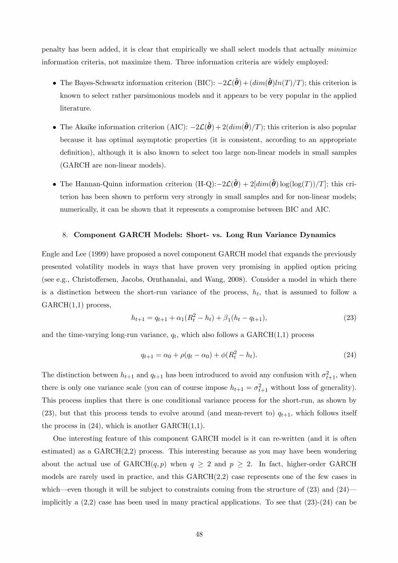
penalty has been added, it is clear that empirically we shall select models that actually minimize

information criteria, not maximize them. Three information criteria are widely employed:

• The Bayes-Schwartz information criterion (BIC): −2L(θ)+((θ)( ) ); this criterion isknown to select rather parsimonious models and it appears to be very popular in the applied

literature.

• The Akaike information criterion (AIC): −2L(θ)+2((θ) ); this criterion is also popularbecause it has optimal asymptotic properties (it is consistent, according to an appropriate

definition), although it is also known to select too large non-linear models in small samples

(GARCH are non-linear models).

• The Hannan-Quinn information criterion (H-Q):−2L(θ) + 2[(θ) log(log( )) ]; this cri-terion has been shown to perform very strongly in small samples and for non-linear models;

numerically, it can be shown that it represents a compromise between BIC and AIC.

8. Component GARCH Models: Short- vs. Long Run Variance Dynamics

Engle and Lee (1999) have proposed a novel component GARCH model that expands the previously

presented volatility models in ways that have proven very promising in applied option pricing

(see e.g., Christoffersen, Jacobs, Ornthanalai, and Wang, 2008). Consider a model in which there

is a distinction between the short-run variance of the process, , that is assumed to follow a

GARCH(1,1) process,

+1 = +1 + 1(2 − ) + 1( − +1) (23)

and the time-varying long-run variance, , which also follows a GARCH(1,1) process

+1 = 0 + ( − 0) + (2 − ) (24)

The distinction between +1 and +1 has been introduced to avoid any confusion with 2+1 when

there is only one variance scale (you can of course impose +1 = 2+1 without loss of generality).

This process implies that there is one conditional variance process for the short-run, as shown by

(23), but that this process tends to evolve around (and mean-revert to) +1 which follows itself

the process in (24), which is another GARCH(1,1).

One interesting feature of this component GARCH model is it can re-written (and it is often

estimated) as a GARCH(2,2) process. This interesting because as you may have been wondering

about the actual use of GARCH( ) when ≥ 2 and ≥ 2. In fact, higher-order GARCH

models are rarely used in practice, and this GARCH(2,2) case represents one of the few cases in

which–even though it will be subject to constraints coming from the structure of (23) and (24)–

implicitly a (2,2) case has been used in many practical applications. To see that (23)-(24) can be

48

re-written as a GARCH(2,2), note first that the process for long-run variance may be written as

+1 = (1− )0 + +(2 − ). At this point, plug the expression of +1 from (24) in (23):

+1 = (1− 1)+1 + 12 + (1 − 1)

= (1− 1)(1− )0 + (1− 1) + (1− 1)(2 − ) + 1

2 + (1 − 1)

= (1− 1)(1− )0 + (1− 1) + [(1− 1)+ 1]2 +

+[1 − 1 − (1− 1)]

= (1− 1)(1− 2)0 + (1− 1)2−1 + [(1− 1)+ 1]

2 + (1− 1)

2−1 +

+[1 − 1 − (1− 1)] − (1− 1)−1

= + 012 + 02

2−1 + 01 + 02−1

where we have exploited the fact that [−1] = 0 and set

= (1− 1)0 01 = (1− 1)+ 1

02 = (1− 1) 01 = [1 − 1 − (1− 1)]

02 = −(1− 1)

One example may help you familiarize with this new, strange econometric model. Suppose

that at time the long-run variance is 0.01 above short-run variance, it is equal to (0.15)2 and is

predicted to equal (0.16)2 at time . Yet, at time returns are subject to a large shock, = −02(i.e., a massive -20%). Can you find values for 1 ≥ 0 and 1 ≥ 0 such that you will forecast at time short-run variance of zero? Because we know that − = −001 +1 = 00225, and 2 = 004,

+1 = 00225 + 1(004− 00125) + 1(−001) = 00225 + 002751 − 0011

and we want to find a combination of 1 ≥ 0 and 1 ≥ 0 that solves

00225 + 002751 − 0011 = 0 or 1 = 225 + 2751

This means that such a value in principle exists but for 1 ≥ 0 this implies that 1 ≥ 225.Empirical, component GARCH models are useful because they capture the slow decay of auto-

correlations in squared returns that we found in section 2 and that we reinforce here (as well as in

the Matlab workout that follows). Consider for instance, the sample autocorrelogram obtained from

a long 1926-2009 daily data set on S&P 500 returns in Figure 12. Clearly, the rate of decay in the

level and significance of squared daily returns is very slow (technically, the literature often writes

about volatility processes with a long memory, in the sense that shocks take a very long time to be

re-absorbed). Component GARCH(1,1) models–also because of their (constrained) GARCH(2,2)

equivalence–have been shown to provide an excellent fit to data that imply long memory in the

49

variance process.

Figure 12: Sample autocorrelations for squared daily S&P 500 returns

Appendix – A Matlab Workout

Suppose you are a German investor. Unless it is otherwise specified, you evaluate the prop-

erties and risk of your equally weighted stock portfolio on a daily basis. Using daily data in the

file “data daily.txt”, construct daily portfolio returns. Please pay attention to the exchange rate

transformations required by the fact that you are a German investor who measures portfolio payoffs

in euros.62

1. For the sample period of 02/01/2006 - 31/12/2010 plot the time series of daily returns. Notice

that in what follows, you will use this sample until otherwise instructed. [Note: When you

run the code, you need to select the first time the file “data daily.txt”, and the second time

the file “data daily string.txt” that will import strings to identify the series.]

2. Compute and plot the autocorrelogram functions (for up to 60 lags) for the (i) level, (ii) the

square, and (iii) the absolute value of the equally weighted portfolio returns.

3. Plot the unconditional distribution of daily returns against a Gaussian (normal) density with

the same empirical moments, i.e., with the same mean and variance.

4. Estimate a GARCH(1,1) model for the daily returns and plot the fitted values for volatility:

(i) using the Matlab command garchfit,63 and (ii) computing 2 directly from

2 = + 2−1 + 2−1.

Compare the two series and verify whether these are identical; if they are not, explain why

they are different.

62In case there is any residual confusion: a portfolio is just a choice of weights (in this case, a 3×1 vector) summingto one. 3 × 1 implies that you should be investing 100% in stocks. Equivalently, we are dealing with an equity

diversification problem and not with a strategic asset allocation one. You can pick any real values, but it may be

wise, to keep the current lab session sufficiently informative, to restrict weights to (0 1) possibly avoiding zeroes.63Notice that the fitted volatility series automatically generated by this command corresponds to to the sigma

output as defined in the function help

50

5. Estimate a RiskMetrics exponential smoother (i.e., estimate the RiskMetrics parameter )

and plot the fitted conditional volatility series against those obtained from the GARCH(1,1).

6. Compute and plot daily one-day ahead recursive forecasts for the period 01/01/2011-31/01/2013

given the ML estimates for the parameters of the models in questions 4 and 5.

7. To better realize what the differences among GARCH(1,1) and RiskMetrics are when it comes

to forecast variances in the long term, proceed to a 300-day long simulation exercise for four

alternative GARCH(1,1) models: (i) with = 1, = 075, = 02; (ii) with = 1, = 02,

= 075; (iii) with = 2, = 075, = 02; (iv) with = 2, = 02, = 075. Plot

the process of the conditional variance under these alternative four models. In the case of

models 1 and 2 ((i) and (ii)), compare the behavior of volatility forecasts between forecast

horizons between 1- and 250-days ahead with the behavior of volatility forecasts derived from

a RiskMetrics exponential smoother.

8. Estimate the 1% Value-at-Risk under the alternative GARCH(1,1) and RiskMetrics models

with reference to the OOS period 01/01/2011-31/01/2013, given the ML estimates for the

parameters of the models in questions 4 and 5. Compute the number of violations of the VaR

measure. Which of the two models performed best and why?

9. Using the usual sample of daily portfolio returns, proceed to estimate the following three

“more advanced” and asymmetric GARCH models: NGARCH(1,1), GJR-GARCH(1,1), and

EGARCH(1,1). In all cases, assume that the standardized innovations follow an IID (0 1)

distribution. Notice that in the case of the NGARCH model, it is not implemented in the

Matlab garchfit toolbox and as a result you will have to develop and write the log-likelihood

function in one appropriate procedure. After you have performed the required print on the

Matlab screen all the estimates you have obtained and think about the economic and statistical

strength of the evidence of asymmetries that you have found. Comment on the stationarity

measure found for different volatility models. Finally, plot the dynamics of volatility over the

estimation sample implied by the three alternative volatility models.

10. For the sample used in questions 4, 5, and 9, use the fitted variances from GARCH(1,1),

RiskMetrics’ exponential smoothed, and a GJR-GARCH(1,1) to perform an out-of-sample

test for the three variance models inspired by the classical test that in the regression

2 = + b2−1 +

= 0 and = 1 to imply that −1[2 ] = 2 = b2−1, where b2−1 is the the time − 1conditional forecast of the variance from model ; moreover, as explained in the lectures,

we would expect the 2 of this regression to be high if model explains a large portion of

realized stock variance. In your opinion, which model performs best in explaining observed

variance (assuming that the proxies for observed variances are squared returns )?

51

11. Assume now you are a German investor. Perform an asset allocation exercise using a simple

Markowitz model using quarterly excess stock returns on three country price-indices: UK,

US, and Germany. Starting from March 1976 until the end of the available data set, compute

optimal weights, predicted (mean) returns and variances of your portfolio. Impose no short

sale constraints on the stock portfolios and no borrowing at the riskless rate. Notice that this

requires that you re-select your input data files: the first time the file “data quarterly.txt”,

and the second time the file “data quarterly string.txt” that will import strings to identify the

series. In particular, you are asked to compare three different mean and variance frameworks,

to be able to appreciate how and whether volatility models affect financial decisions:

(a) Variances: constant for all three indices; correlations: equal to the unconditional, con-

stant sample correlations for all three pairs of indices; means: constant. This is of course

a rather classical, standard Gaussian IID model in which means, variances, and covari-

ances are all constant.

(b) Variances: modeled as a GJR-GARCH(1,1) for all three indices; correlations: equal to the

unconditional, constant sample correlations for all three pairs of indices; mean: constant.

(c) Variances: modeled as a GJR-GARCH(1,1) for all three indices; correlations: equal to the

unconditional, constant sample correlations for all three pairs of indices; mean: assume

a model of the type

+1 =

0 +

1

+

+1 = 1 2 3

where +1is the log excess return on country

0s stock index, and is the log dividend

yield of country .

Notice that, just for simplicity (we shall relax this assumption later on), all models assume

a constant correlation among different asset classes. Plot optimal weights and the resulting

in-sample, realized Sharpe ratios of your optimal portfolio under each of the three different

frameworks. What is, in your opinion, the best-performing framework given a risk aversion

coefficient = 10 under a utility function of the type

( 2 ) = −

1

22 ?

[IMPORTANT: Use the toolboxes regression tool 1.m and mean variance multiperiod.m that

have been made available with this exercise set]

12. Compute the Value-at-Risk with a 95% confidence level and the resulting number of violations

for the optimal Markowitz portfolio derived under 11.c above, i.e., when both the mean and

the variance are predictable. Comment the results, and think about a better model to track

VaR. How could the model under 11.c be improved?

52

Solution

This solution is a commented version of the MATLAB code Ex GARCH 2012.m posted on the

course web site. Please make sure to use a “Save Path” to include jplv7 among the directories that

Matlab reads looking for usable functions. The loading of the data is performed by the lines of

code:

filename=uigetfile(‘*.txt’);

data=dlmread(filename);

The above two lines import only the numbers, not the strings, from a .txt file.64 The following

lines of the codes take care of the strings:

filename=uigetfile(‘*.txt’);

fid = fopen(filename);

labels = textscan(fid, ‘%s %s %s %s %s %s %s %s %s %s’);

fclose(fid);

1. The plot requires that the data are read in and transformed in euros using appropriate ex-

change rate log-changes, that need to be computed from the raw data, see the posted code for

details on these operations. The following lines proceed to convert Excel serial date numbers

into MATLAB serial date numbers (the function x2mdate( ·)), set the dates to correspond tothe beginning and the end of the sample, while the third and final dates are the beginning

and the end of the out-of-sample (OOS) period:

date=datenum(data(:,1));

date=x2mdate(date);

f=[‘02/01/2006’;‘31/12/2010’; ‘03/01/2013’];

date find=datenum(f,‘dd/mm/yyyy’);

ind=datefind(date find,date);

The figure is then produced using the following set of instructions, that shall not be commented

in detail because the structure of the plot should closely resemble many other plots proposed in the

first part of the course.65

figure(1);

t=ind(1):ind(2);

64The reason for loading from a .txt file in place of the usual Excel is to favor usage from Mac computers that

sometimes have issues with reading directly from Excel, because of copyright issues with shareware spreadsheets.65Those ‘...’ that are featured below represent the way in which you go to a new line in the text editor of a Matlab

code without actually breaking the line in the perspective of the compiler.

53

plot(t’, port ret(ind(1):ind(2),:),‘b’);

title(’Daily Portfolio Returns’,’fontname’,’Garamond’,’fontsize’,14);

set(gca,’fontname’,’garamond’,’fontsize’,12);

set(gca,’xtick’,index-1+ind(1)+5);

set(gca,’xticklabel’,’Jan2006|Jan2007|Jan2008|Jan2009|Jan2010|Jan2011||Dec2011’);ylabel(’% Returns’);

set(gcf,’color’,’w’);

set(gca,’Box’, ’off ’, ’TickDir’, ’out’, ’TickLength’, [.02 .02],’XMinorTick’,

’off ’,’YMinorTick’, ... ’off ’,’XColor’,[.3 .3 .3],’YColor’,[.3 .3 .3],’LineWidth’, 1,

’FontName’, ’Times’);

The resulting plot looks as follows and clearly shows the volatility outburst during the financial

crisis of the Summer 2008-Spring 2009, plus some further sovereign crisis jitters during the Summer

of 2010:

Figure A1:Daily Portfolio Returns

2. As already seen in the first part of the course, the Matlab functions that compute and plot

the autocorrelogram functions (for up to 60 lags) for the levels, squares, absolute values of

portfolio returns are:

sq port ret=port ret.ˆ2; %Squared daily returns

abs port ret=abs(port ret);

figure(2);

subplot(3,1,1)

autocorr(port ret(ind(1):ind(2),:),60,[],2);

title(‘ACF: Daily Returns’,‘fontname’,‘garamond’,‘fontsize’,16);

set(gcf,‘color’,‘w’);

subplot(3,1,2)

54

autocorr(sq port ret(ind(1):ind(2),:),60,[],2);

title(‘ACF: Daily Squared Returns’,‘fontname’,‘garamond’,‘fontsize’,16);

set(gcf,‘color’,’w’);

subplot(3,1,3)

autocorr(abs port ret(ind(1):ind(2),:),60,[],2);

title(‘ACF: Daily Absolute Returns’,‘fontname’,‘garamond’,‘fontsize’,16);

set(gcf,‘color’,‘w’);

The autocorr(Series,nLags,M,nSTDs) function computes and plots the sample ACF of a uni-

variate time series already complete with confidence bounds; the input argument nLags is a positive

scalar integer that indicates the number of lags of the ACF to compute;66 M is a nonnegative inte-

ger scalar indicating the number of lags beyond which the theoretical ACF is effectively 0; autocorr

assumes the underlying Series is an MA() process, and uses Bartlett’s approximation to compute

the large-lag standard error for lags greater than M;67 finally, nSTDs is a positive scalar indicating

the number of standard deviations of the sample ACF estimation error to compute; if nSTDs = []

or is unspecified, the default is 2 (that is, approximate 95 percent confidence interval). Note that

by using the command subplot divides the current figure into rectangular panes that are numbered

row-wise; each pane contains an axes object. Subsequent plots are output to the current pane. In

particular, subplot(m,n,p) breaks the figure window into an × matrix of small axes, selects the

th axes object for the current plot, and returns the axes handle. The axes are counted along the

top row of the figure window, then the second row, etc.

The resulting set of 3 plots in figure A2 shows the typical result already commented in section 2

of this chapter: while the level of financial returns hardly features any significant autocorrelations

(not even at the shortest lags), other functions ()–such as () = 2 and () = ||–arecharacterized by many statistically significant, when the Bartlett’s standard errors are used to form

confidence intervals, values and these values tend to decay rather slowly as the lag order increases

towards the bound of 60 that we have imposed. This is particularly visible in the case of the absolute

value of returns, and this is typical of all the literature. As commented in section 2, this evidence

allows us to conclude that our portfolio returns are not independently distributed over time and

that there is evidence of conditional heteroskedasticity because large past squared returns forecast

66If nLags = [] or is unspecified, the default is to compute the ACF at lags 0, 1, 2, ..., T, where = ([20

()− 1]).67If M = [] or is unspecified, the default is 0, and autocorr assumes that the Series is Gaussian white noise. If

Series is a Gaussian white noise process of length , the standard error is approximately 1√ . M must be less than

nLags.

55

subsequently large squared returns.

Figure A2:Sample Autocorrelations of a Range of Functions of Portfolio Returns

3. We use the lines of code

histfit(port ret(ind(1):ind(2),:),100);

to plot a histogram with Gaussian fit that matches the empirical moments, i.e., with the same

mean and variance. Note that here the 100 refers to the number of bins for the histogram.68 The

resulting histogram is shown in figure A3. The figure clearly shows that our portfolio returns

are highly non-normal. In particular, they are leptokurtic, in the sense that when compared to

a Gaussian density, there is excessive probability mass allocated to a neighborhood of the sample

mean and to both tails (in particular the left tail), while insufficient probability mass is allocated to

intermediate values in the support of the empirical distribution of returns, approximately around

± one empirical standard deviation.

4. We use the Matlab function garchfit to estimate a GARCH(1,1) model for daily returns,

spec=garchset(‘P’,1,‘Q’,1);

[coeff, errors,llf,innovation,sigma,summary]=garchfit(spec,port ret(ind(1):ind(2),:));

garchdisp(coeff,errors);

68histfit(data,nbins,dist) would instead plot a histogram with a density from the distribution specified by dist, one of

the following strings: ‘beta’, ‘birnbaumsaunders’, ‘exponential’, ‘extreme value’ or ‘ev’, ‘gamma’, ‘generalized extreme

value’ or ‘gev’, ‘generalized pareto’ or ‘gp’, ‘inversegaussian’, ‘logistic’, ‘loglogistic’, ‘lognormal’, ‘nakagami’, ‘negative

binomial’ or ‘nbin’, ‘normal’ (default), ‘poisson’, ‘rayleigh’, ‘rician’, ‘tlocationscale’, ‘weibull’ or ‘wbl’. The normal

distribution represents the default, used in the absence of other indications.

56

Figure A3:Unconditional distribution (histogram) of daily returns vs. matching Gaussian density

1. while the following computes the vector sigma step-by-step:

param(1:4,1)=[coeff.C;coeff.K;coeff.GARCH;coeff.ARCH];

init=param(2)/(1-param(3)-param(4));

cond var garch=zeros(rows(port ret(ind(1):ind(2))),1);

cond var garch(1)=init;

for i=1:ind(2)-ind(1)

cond var garch(i+1)=param(2)+param(3)*cond var garch(i)+param(4)*(innovation(i)ˆ2);

end

cond std garch=sqrt(cond var garch);

Here, ‘init=param(2)/(1-param(3)-param(4));’ initializes the first value of sigma to equal the

unconditional variance, which is a necessary choice. garchset sets the ARMAX/GARCH model

specification parameters; a GARCH specification structure includes these parameters: General

Parameters, Conditional Mean Parameters, Conditional Variance Parameters, Equality Constraint

Parameters, and Optimization Parameters, even though garchset sets all parameters you do not

specify to their respective defaults; among the Conditional Variance Parameters, there is the type

of model: ‘GARCH’, ‘EGARCH’, ‘GJR’, or ‘Constant’. The default is ‘GARCH’.

garchfit estimates the parameters of a conditional mean specification of ARMAX form, and con-

ditional variance specification of GARCH, EGARCH, or GJR form. The estimation process infers

the innovations (that is, residuals) from the return series. It then fits the model specification to the

return series by constrained maximum likelihood.69 The outputs include a GARCH specification

structure containing the estimated coefficients, where Coeff is of the same form as the Spec input

69garchfit performs the optimization using the Optimization Toolbox fmincon function. The constraints on the

parameters are the ones discussed in Sections 4-6.

57

structure given by garchset ; errors is a structure containing the estimation errors (that is, the stan-

dard errors) of the coefficients with the same form as the Spec and Coeff structures; LLF is the

optimized loglikelihood objective function value associated with the parameter estimates found in

Coeff; Innovations containts the residual time series column vector inferred from the data; Sigmas

collects the conditional standard deviation vector corresponding to Innovations; Summary includes

‘covMatrix ’, the Covariance matrix of the parameter estimates computed using the outer-product

method. Finally, garchdisp displays ARMAX/GARCH model parameters and statistics. The tabu-

lar display includes parameter estimates, standard errors, and t-statistics for each parameter in the

conditional mean and variance models.

Matlab prints at the screen the following information concerning estimation (we select the in-

formation to be printed to save space):

The first panel gives a number of technical information on the numerical optimization that Matlab

has performed. Although not directly useful, by clicking this information when possible, you will

get to know more about what Matlab is doing in the background of the numerical optimization

it is performing for you. The second panel details the 14 iterative steps followed by Matlab to

reach the optimum and how the value function () = L(θ)–in our case it is the log-likelihoodfunction–changes across different iterations. Notice that () obviously declines across iterations.

This is due to the fact that Matlab actually minimizes the opposite (i.e., ×−1) of the log-likelihoodfunction, because

θ ≡ argmax

L(θ) = argmin

(−L(θ)).

58

Visibly, after the 12th iteration, −L(θ) stabilizes to 1883.93 (i.e., L(θ) stabilizes to -1883.93)and this represents the optimum, in the sense that the objective function seems to have converged to

a stationary point (as signalled by “fmincon stopped because the predicted change in the objective

function is less than the selected value of the function tolerance and constraints were satisfied

to within the selected value of the constraint tolerance.”), even though Matlab warns you that

“Local minimum possible. Constraints satisfied.” In the case of parameter estimates, garchfit yields

point estimates (“Value”), the corresponding standard error, and the t-ratio. Obviously, ≡

q [] so that once you know the standard error, you could have derived

yourself; for

instance, 24445 ' 00645260026396. Note that given a non-zero mean model

+1 = + +1+1 +1 ∼ IID N (0 1)2 = + (−1 − )2 + 2−1,

Matlab calls the parameter and the parameter of the GARCH, i.e., +1 = + +1+1

and 2 = +(−1 − )2 + 2−1. The estimated GARCH model is clearly stationary as

+ ' 09821 1 and it implies a long-run, unconditional variance 2 = 002462(1 − 09821)

59

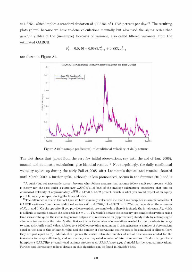
' 13754 which implies a standard deviation of √13754 of 1.1728 percent per day.70 The resultingplots (plural because we have re-done calculations manually but also used the sigma series that

garchfit yields) of the (in-sample) forecasts of variance, also called filtered variances, from the

estimated GARCH,

2 = 00246 + 009892−1 + 08832

2−1

are shown in Figure A4.

Figure A4:(In-sample predictions) of conditional volatility of daily returns

The plot shows that (apart from the very few initial observations, say until the end of Jan. 2006),

manual and automatic calculations give identical results.71 Not surprisingly, the daily conditional

volatility spikes up during the early Fall of 2008, after Lehmann’s demise, and remains elevated

until March 2009; a further spike, although it less pronounced, occurs in the Summer 2010 and is

70A quick (but not necessarily correct, because what follows assumes that variance follow a unit root process, which

is clearly not the case under a stationary GARCH(1,1)) back-of-the-envelope calculations transforms that into an

annualized volatility of approximately√252 × 11728 ' 1862 percent, which is what you would expect of an equity

portfolio mostly sampled during the financial crisis.71The difference is due to the fact that we have manually initialized the loop that computes in-sample forecasts of

GARCH variances from the unconditional variance 2 = 002462 (1−09821) ' 13754 that depends on the estimatesof, , and On the opposite, if you provide no explicit pre-sample data (here it is simply the intial return 0, which

is difficult to sample because the time scale is = 1 ), Matlab derives the necessary pre-sample observations using

time series techniques: the idea is to generate output with reference to an (approximate) steady state by attempting to

eliminate transients in the data. Matlab first estimates the number of observations needed for the transients to decay

to some arbitrarily small value, subject to a 10000-observation maximum; it then generates a number of observations

equal to the sum of this estimated value and the number of observations you request to be simulated or filtered (here

they are just equal to ). Matlab then ignores the earlier estimated number of initial observations needed for the

transients to decay sufficiently, and returns only the requested number of later observations. To do this, garchsim

interprets a GARCH( ) conditional variance process as an ARMA(max( ), ) model for the squared innovations.

Further and increasingly tedious details on this algorithm can be found in Matlab’s help.

60

probably related to the initial PIIGS sovereign debt crisis jitters. If you had any doubts volatility is

actually time-varying, this GARCH model shows that given a long-run average level that we know

to be at just above 1% per day, volatility rather often doubles up to almost touch 2% per day, while

spikes in excess of 3% per day may occur.

5. Here we proceed to estimate a RiskMetrics exponential smoother (i.e., estimate the RiskMet-

rics parameter ) by ML. Note that this is different from the simple approach mentioned in

the lectures where was fixed at the level suggested by RiskMetrics.

parm=0.1;

logL= maxlik(‘objfunction’,parm,[],port ret(ind(1):ind(2)+1));

lambda=logL.b;

disp(‘The estimated RiskMetrics smoothing coefficient is:’)

disp(lambda)

parm=0.1 sets an initial condition for the estimation (a weird one, indeed, but the point is to

show that in this case the data have such a strong opinion for what is the appropriate level of

that such an initial condition hardly matters; try to change it and see what happens). This maxlik

call is based on the maximization of the log-likelihood given in objfunction. That procedure reads

as

ret=y;

R=rows(ret);

C=cols(ret);

conditional var=NaN(R,C);

conditional var(1,1)=var(ret);

for i=2:R

conditional var(i,1)=(1-lambda)*ret(i-1,1).ˆ2+lambda*conditional var(i-1,1);

end

z=ret./sqrt(conditional var);

y=-sum(-0.5*log(2*pi)-0.5*log(conditional var)-0.5*(z.ˆ2));

In figure A5 we plot the fitted (also called in-sample filtered) conditional volatility series and

compare it to that obtained from the GARCH(1,1) in the earlier question. Clearly, the two models

behave rather differently and such divergencies were substantial during the financial crisis. This

61

may have mattered to financial institutions and their volatility traders and risk managers.

Figure A5:Comparing in-sample predictions of conditional volatility from GARCH vs. RiskMetrics

6. Using the following lines of code, we compute and plot daily one-day ahead, recursive out-

of-sample forecasts for the period 01/01/2011-01/01/2013 given the ML estimates for the

parameters of the models in questions 4,

spec pred=garchset(‘C’,coeff.C,‘K’,coeff.K,‘ARCH’,coeff.ARCH,‘GARCH’,coeff.GARCH);

garch pred=NaN(ind(3)-ind(2),1);

for i=1:(ind(3)-ind(2))

[SigmaForecast,MeanForecast,SigmaTotal,MeanRMSE] = ...

garchpred(spec pred,port ret(ind(1):ind(2)+i-1),1);

garch pred(i)=SigmaForecast(1);

end

and 5, using

for i=1:(ind(3)-ind(2)-1)

es pred(i+1)=lambda*es pred(i)+(1-lambda)*port ret(ind(2)+i)ˆ2;

end

es std pred=sqrt(es pred);

Here garchpred forecasts the conditional mean of the univariate return series and the standard

deviation of the innovations ind(3)-ind(2) into the future, a positive scalar integer representing

the forecast horizon of interest. It uses specifications for the conditional mean and variance of an

observed univariate return series as input. In both cases, note that actual returns realized between

2011 and early 2013 is fed into the models, in the form of series {(−1 − )2} sampled over time.

62

Figure A6 shows the results of this recursive prediction exercises and emphasizes once more the

existence of some difference across GARCH and RiskMetrics during the Summer 2011 sovereign

debt crisis.

Figure A6:Comparing out—of-sample predictions of conditional volatility from GARCH vs. RiskMetrics

7. To better realize what the differences among GARCH(1,1) and RiskMetrics are when it comes

to forecast variances in the long term, we proceed to a 300-day long simulation exercise for

four alternative GARCH(1,1) models, when the parameters are set by us instead of being

estimated: (i) = 1, = 075, = 02; (ii) = 1, = 02, = 075; (iii) with = 2,

= 075, = 02; (iv) with = 2, = 02, = 075. Importantly, forecasts under

RiskMetrics are performed using a value of that makes it consistent with the first variance

forecast from GARCH. For all parameterizations, this is done by the following lines of code:

for j=1:length(alpha)

for i=2:dim

epsilon=sqrt(garch(i-1,j))*ut(i);

garch(i,j)=omega(1)+alpha(j)*epsilonˆ2+beta(j)*garch(i-1,j);

end

end

for j=3:length(alpha)+length(omega)

for i=2:dim

epsilon=sqrt(garch(i-1,j))*ut(i);

garch(i,j)=omega(2)+alpha(j-2)*epsilonˆ2+beta(j-2)*garch(i-1,j);

end

end

63

Figure A7 presents simulation results. Clearly, the blue models imply generally low variance but

frequent and large spikes, while the green models imply considerably more conditional persistence

of past variance, but a smoother temporal path. Try and meditate on these two plots in relation to

the meaning of your MLE optimization setting the “best possible” values of and to fit the data.

Figure A7: Simulating 4 alternative GARCH models

The following code computes insteads true out-of-sample forecasts 250 periods ahead. Notice

that these forecasts are no long recursive, i.e., you do not feed the actual returns realized over the

out-of-sample periods, and this occurs for a trivial reason: you do not know them because this is a

truly out-of-sample exercise. Initialization is done with reference to the last shock obtained in the

previous run of simulations:

horz=250;

A=NaN(horz,1);

garch sigma sq t plus one a=omega(1)+alpha(1)*epsilonˆ2+beta(1)*garch(end,1);

garch sigma sq t plus one b=omega(1)+alpha(2)*epsilonˆ2+beta(2)*garch(end,2);

(%Derives forecasts under Model 1)

A(1)=garch sigma sq t plus one a;

uncond var=omega(1)/(1-alpha(1)-beta(1));

for i=2:horz

A(i)=uncond var+((alpha(1)+beta(1))ˆ(i-1))*(garch sigma sq t plus one a-

uncond var);

end

garch forecast a=sqrt(A);

lambda a=(garch sigma sq t plus one a-epsilonˆ2)/(garch(end,1)-epsilonˆ2);

es forecast a=lambda*garch forecast a(1)+(1-lambda)*epsilonˆ2;

64

es forecast a=sqrt(es forecast a).*ones(horz,1);

Here the initial value for the variance in the GARCHmodel is set to be equal to the unconditional

variance. The expression for lambda a sets a value for that makes it consistent with the first

variance forecast from GARCH. Figure A8 plots the forecasts between 1- and 250-periods ahead

obtained under models (i) and (ii) when the RiskMetrics is set in the way explained above. As

commented in the lectures, it is clear that while GARCH forecasts converge in the long-run to a

steady, unconditional variance value that by construction is common and equal to 4.5 in both cases,

RiskMetrics implies that the forecast is equal to the most recent variance estimate for all horizons

≥ 1.

Figure A8: Variance forecasts from two alternative GARCH models vs. RiskMetrics

8. We now estimate the 1% Value-at-Risk under the alternative GARCH(1,1) and RiskMetrics

models with reference to the OOS period 01/01/2011-31/01/2013, given the ML estimates for

the parameters of the models in questions 4 and 5. This is accomplished through the following

lines of code:

alpha=0.01;

Var garch=norminv(alpha,0,garch pred);

Var es=norminv(alpha,0,es std pred);

index garch=(port ret(ind(2)+1:ind(3))Var garch);

viol garch=sum(index garch);

index es=(port ret(ind(2)+1:ind(3))Var es);

viol es=sum(index es);

Figure A9 shows the results: because during parts of the Summer 2011 crisis, the RiskMetrics

one-step ahead variance forecast was below the GARCH(1,1), there are more violations of the 1%

65

VaR bound under the former model than under the second, 11 and 8, respectively.72 Also note

that if a volatility model is correctly specified, then we should find that in a recursive back testing

period of 524 days (which is the number of trading days between Jan. 1, 2011 and Jan. 31, 2013),

one ought to approximately observe 001× 524 = roughly 5 violations. Here we have instead 8 and11, and especially the latter number represents more than the double than the total number one

expects to see. This is an indication of misspecification of RiskMetrics and probably of the GARCH

model too. Even worse, most violations do occur in early August 2011, exactly when you would

have needed a more accurate forecasts of risk and hence of the needed capital reserves! However,

RiskMetrics also features occasional violations of the VaR bound in the Summer of 2012.

Figure A9: Daily 1% VaR bounds from GARCH vs. RiskMetrics

9. Next, we proceed to estimate three “more advanced” and asymmetric GARCHmodels: NGARCH

(1,1), GJR-GARCH(1,1), and EGARCH(1,1). While for GJR and EGARCH estimation pro-

ceeds again using the Matlab garchfit toolbox in the same way we have seen above, the

GJR(1,1) (also called threshold GARCH) model is estimated by MLE, using

GJRspec=garchset(‘VarianceModel’,‘GJR’,‘Distribution’,‘Gaussian’,‘P’,1,‘Q’,1);

[GJRcoeff, GJRerrors,GJRllf,GJRinnovation,GJRsigma,GJRsummary]=...

garchfit(GJRspec,port ret(ind(1):ind(2),:));

garchdisp(GJRcoeff,GJRerrors);

EGARCHspec=garchset(‘VarianceModel’,‘EGARCH’,‘Distribution’,‘Gaussian’,‘P’,1,‘Q’,1);

[EGARCHcoeff, EGARCHerrors,EGARCHllf,EGARCHinnovation,EGARCHsigma,EGARCHsummary]=...

garchfit(EGARCHspec,port ret(ind(1):ind(2),:));

garchdisp(EGARCHcoeff,EGARCHerrors);

In the case of the NGARCH model, estimation is not implemented through garchfit and as a

result you will have to develop and write the log-likelihood function in one appropriate procedure,

72These are easily computed simply using sum(viol garch) and sum(viol es) in Matlab.

66

which is the appropriate function ngarch, initialized at par initial(1:4,1)=[0.05;0.1;0.05;0.85]. This

procedure uses Matlab unconstrained optimization fminsearch (please press F1 over fminsearch and

read up on what this is):73

par initial(1:4,1)=[0.05;0.1;0.05;0.85];

function [sumloglik,z,cond var] = ngarch(par,y);

[mle,z ng,cond var ng]=ngarch(param ng,port ret(ind(1):ind(2),:));

ngarch takes as an input the 4x1 vector of NGARCH parameters (, , , and ) and the vector

y of returns and yields as an output sumloglik, the (scalar) value of likelihood function (under

a normal distribution), the vector of standardized returns z, and the conditional variance (note)

cond var. The various points requested by the exercise have been printed directly on the screen:

All volatility models imply a starionarity index of approximately 0.98, which is indeed typical of

daily data. The asymmetry index is large (but note that we have not yet derived standard errors,

which would not be trivial in this case) at 1.03 in the NAGARCH case, it is 0.14 with a t-stat of

73fminsearch finds the minimum of an unconstrained multi-variable function using derivative-free methods and

starting at a user-provided initial estimate.

67

7.5 in the GJR case, and it is -0.11 with a t-stat 9 in the EGARCH case: therefore in all cases

we know or we can easily presume that the evidence of asymmetries in these portfolio returns is

strong. Figure A10 plots the dynamics of volatility over the estimation sample implied by the three

alternative volatility models. As you can see, the dynamics of volatility models tends to be rather

homogeneous, apart from the Fall of 2008 when NAGARCH tends to be above the others while

simple GJR GARCH is instead below. At this stage, we have not computed VaR measures, but

you can easily figure out (say, under a simple Gaussian VaR such as the one presented in chapter

1) what these different forecasts would imply in risk management applications.

Figure A10: Comparing in-sample fitted volatility dynamics under GJR, EGARCH, and NAGARCH

10. We now compare the accuracy of the forecasts given by different volatility models. We use

the fitted/in-sample filtered variances from GARCH(1,1), RiskMetrics’ exponential smoother,

and a GJR-GARCH(1,1) to perform the out-of-sample test that is based on the classical test

that in the regression

2 = + b2−1 +

= 0 and = 1 to imply that −1[2 ] = 2 = b2−1, where b2−1 is the the time − 1conditional forecast of the variance from model . For instance, in the case of GARCH, the

lines of codes estimating such a regression and printing the relevant outputs are:

result = ols((port ret(ind(1):ind(2),:).ˆ2),[ones(ind(2)-ind(1)+1,1) (cond var garch)]);

disp(‘Estimated alpha and beta from regression test: GARCH(1,1) Variance forecast:’);

disp(result.beta’);

disp(‘With t-stats for the null of alpha=0 and beta=1 of:’);

disp([result.tstat(1) ((result.beta(2)-1)/result.bstd(2))]); fprintf(‘\n’);disp(‘and an R-square of:’);

disp(result.rsqr)

68

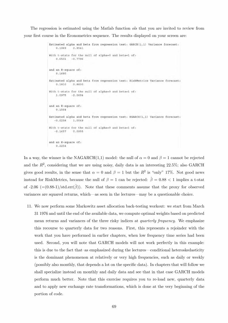
The regression is estimated using the Matlab function ols that you are invited to review from

your first course in the Econometrics sequence. The results displayed on your screen are:

In a way, the winner is the NAGARCH(1,1) model: the null of = 0 and = 1 cannot be rejected

and the 2 considering that we are using noisy, daily data is an interesting 22.5%; also GARCH

gives good results, in the sense that = 0 and = 1 but the 2 is “only” 17%. Not good news

instead for RiskMetrics, because the null of = 1 can be rejected: = 088 1 implies a t-stat

of -2.06 (=(0.88-1)/std.err()). Note that these comments assume that the proxy for observed

variances are squared returns, which–as seen in the lectures–may be a questionable choice.

11. We now perform some Markowitz asset allocation back-testing workout: we start from March

31 1976 and until the end of the available data, we compute optimal weights based on predicted

mean returns and variances of the three risky indices at quarterly frequency. We emphasize

this recourse to quarterly data for two reasons. First, this represents a rejoinder with the

work that you have performed in earlier chapters, when low frequency time series had been

used. Second, you will note that GARCH models will not work perfectly in this example:

this is due to the fact that—as emphasized during the lectures–conditional heteroskedasticity

is the dominant phenomenon at relatively or very high frequencies, such as daily or weekly

(possibly also monthly, that depends a lot on the specific data). In chapters that will follow we

shall specialize instead on monthly and daily data and see that in that case GARCH models

perform much better. Note that this exercise requires you to re-load new, quarterly data

and to apply new exchange rate transformations, which is done at the very beginning of the

portion of code.

69

In the case of the standard Gaussian IID model in which means, variances, and covariances

are all constant, the estimates are obtained with regression tool 1 which performs recursive

estimation.74 In the case in which the means are constant but the individual variances fol-

low a GJR-GARCH(1,1) and correlations are equal to the unconditional, constant sample

correlations for all three pairs of indices, the estimates displayed on the Matlab screen are:75

74The unconditional correlations are 0.73 between US and UK returns, 0.64 between US and German returns, and

0.60 between UK and German returns. You are also invited to inspect the structure and capabilities of regression tool 1,

which is provided for your use.75Such unconditional, constant correlations are 0.73 between US and UK returns, 0.60 between US and German

returns, and 0.57 between UK and German returns. As we shall see in due time, a multivariate model in which

the conditional variances follow a GARCH process but correlations are assumed to be constant over time is called a

Constant Conditional Correlation model, CCC.

70

Here please note that the user-provided toolbox regression tool 1 prints the constant uncon-

ditional mean parameter (previously called ) as Regress(1) because it is well known that

the estimate of a constant in a regression model can be obtained from a regressor that is the

unit vector of ones, as in this case. The estimates displayed are the ones corresponding to

last quarter in the sample, September 2012. Interestingly, there is little evidence of GARCH

and no evidence of an asymmetric in quarterly US and UK data (see comments made in the

lecture slides); there is instead strong evidence of GARCH as well as of asymmetric effects in

quarterly German stock returns, even though the leverage effect has a negative sign, differ-

ently from what one would expect ( = 016 with a t-stat of -2.2).76 The estimated values of

are positive as expected and also generally statistically significant.

We also estimate a fully conditional model in which both the conditional mean and conditional

variances are specified to be time-varying,:

+1 =

0 +

1

+

+1 = 1 2 3

where +1is the log excess return on country 0s stock index, and

is the log dividend yield

of country . However–just because at this point we do not know what else could be done–we

still assume that all correlations equal the unconditional, constant sample correlations for all three

pairs of indices. In this case, the unconditional, constant correlations are 0.73 between US and UK

returns, 0.60 between US and German returns, and 0.57 between UK and German returns.77 As

we shall see in due time, a multivariate model in which the conditional variances follow a GARCH

process but correlations are assumed to be constant over time is called a Constant Conditional

Correlation model, CCC.

In this case, a difference between the regression constant (i.e., 0, = 1 2 3) and the coefficient

attached to Regress(1), in this case the dividend-price ratio (i.e., 1, = 1 2 3) appears in the way

Matlab prints the estimated coefficients. There is now evidence of GARCH in US stock returns,

even though for this time series lagged dividend yields fail to forecast subsequent stock returns; in

the case of UK returns, it remains the case that the variance is homoskedastic, but there is evidence

that a high dividend yield ratio forecasts higher subsequent returns; finally, in the case of German

data, it remains the case that GARCH is strong (but with an odd negative leverage effect), but

the dividend-price ratio is not a strong predictor of subsequent returns. Therefore also in this third

and more complex model we are probably over-parameterizing the exercise: we are imposing GJR

GARCH on UK data when there seems to be evidence of homoskedasticity; we are also forcing a

predictive model from past dividend yields multiples to stock returns, when in the case of German

76Here it is clear that a decision to estimate a GJR GARCH(1,1) is either arbitrary or triggered by a need to at

least accommodate GARCH in German data. We leave it as an exercise to see what happens to optimal weights when

GJR GARCH is modelled only for German returns, while UK and US returns are simply taken to be homoskedastic.77I know, these seem to be the same estimates as in a previous footnote, but this is just because of the rounding,

see for yourself the differences between corr un1=corr(std resid1) and corr un2=corr(std resid2) in the code.

71

and possibly US data there is weak evidence of such a predictability pattern.

At this point, asset allocation is computed by the following lines of code that use the user-provided

procedure mean variance multiperiod. Risk aversion is assumed to be high, 10. Because the weights

computed are the weights of the risky assets, they might not sum up to 1, in which case what is

left of your wealth is invested in the risk-free asset.

gamma=10;

lower=0;

upper=10;

rskfree shortselling=0;

72

%Portfolio allocation with GARCH modelling and conditional mean (model 11.c)78

[w 11c,miu portf11c,sigma portf11c,act ret portf11c]=

mean variance multiperiod(cov mat con1,miu con1’,ret2,gamma,lower,upper,rskfree shortselling);

%Portfolio allocation with GARCH modelling and constant mean (model 11.b)

[w 11b,miu portf11b,sigma portf11b,act ret portf11b]=

mean variance multiperiod(cov mat con2,miu uncon1’,ret2,gamma,lower,upper,rskfree shortselling);

%Portfolio allocation without GARCH modelling and with constant mean (Gaussian

IID model, 11.a)

[w 11a,miu portf11a,sigma portf11a,act ret portf11a]=

mean variance multiperiod(cov mat uncon,miu uncon1’,ret2,gamma,lower,upper,rskfree shortselling);

Here lower=0 and upper=10 are the lower and upper bounds on the weights of risky assets.

rskfree shortselling=0 indicates the minimum weight of the risk-free asset and in this case the

zero derives from the requirement of no short-selling. Figure A11 plots the resulting portfolio

weights. Clearly, the Gaussian IID model implies constant weights over time, because there is

no predictability.79 Visibly, such a model favors UK stocks over US ones and especially German

stocks, which are never demanded. Under the remaining two models, recursive optimal portfolio

weights become time-varying because as the one-quarter ahead forecasts of variances (the second

plot) and of both variances and means (the third plot) change over time, the optimal Markowitz

portfolio changes too. Such a variation seems to be substantial and to come more from time-

variation in variances than in the means: this is visible from the fact that the second and third

plots are somewhat similar (but not identical, of course). This is not surprising also because the

predictability from the dividend-price ratio to subsequent stock returns is rather weak, over this

sample. In both the second and third plots, the weight attributed to UK stocks remains dominant,

but there are now occasional spells (in particular from early 1981 to 1982) in which the weight

to be assigned to German stocks is even larger. Moreover, the overall weight to stocks increases

somewhat when only predictability in variance is taken into account–it is on average in excess of

40% vs. just less than 40% when both conditional mean and variance are time-varying. Investors

may now time periods of favorable predicted moments (i.e., higher than average mean returns and

78Just a reminder: in Matlab, lines of codes preceded by a % are simply comments.79One could also have recursively re-estimated sample means and variances, but that would have been spurious

because their very variation over time indicates that the IID model should be rejected.

73

below-average variance, for all or most stock indices).

Figure A11: Recursive mean-variance portfolio weights under alternative econometric models

As far as the in-sample Sharpe ratios, because mean variance multiperiod automatically com-

putes and reports the mean and variance of the optimal portfolios over the asset allocation back-

testing sample, in the code it will be sufficient to use

sharpe ratios=[miu portf11c./sigma portf11c miu portf11b./sigma portf11b

miu portf11a./sigma portf11a];

to obtain the Sharpe ratios. Figure A11 plots such in-sample Sharpe ratios showing interesting

results. GARCH-based strategies have been most of the time better than classical IID strategies that

ignore predictability in variance between 1976 and the late 1990s (these produce a constant Sharpe

ratio just in excess of 0.23 that is rather typical at quarterly level). However, the variability has also

been substantial. Moreover, in this first part of the sample, to try and predict mean stock returns

besides predicting the variance, would have led to a loss in the Sharpe ratio. Starting in 1999, the

predictability-based strategies wildly fluctuate according to an easily interpretable pattern: during

good times, bull market states (as we known and interpret them ex-post), the predictability-based

strategies out-perform the IID strategy; however during bear markets (as identified ex-post), such

strategies are inferior vs. the IID one. For instance, during 2004-mid 2007, a strategy that “times”

both the conditional mean and the conditional variances, achieves a Sharpe ratio of 0.28 vs. 0.23 for

the IID case; however in 2008-2009, the realized Sharpe ratios decline to 0.15-0.18, with a strategy

just exploiting time variance in variance performing not as poorly as one instead based on predicting

74

the mean. Keep in mind however that in this exercise we have fixed all pairwise correlations to

correspond to their unconditional, full-sample estimates. Moreover, we have used a rather simple

GJR GARCH model. It remains to be seen whether jointly modelling all the stock indices–and

hence also trying to forecast their correlations–or by complicating the heteroskedastic model may

yield superior or more stable in-sample Sharpe ratios.

Figure A12: Recursive mean-variance portfolio weights under alternative econometric models

12. Finally, to close this long ride through the application of simple, univariate conditional het-

eroskedastic models in finance, we have computed the Value-at-Risk with a 95% confidence

level and the resulting number of violations for the optimal Markowitz portfolio derived under

question 11 above, when both the mean and the variance are predictable. This is performed

using the user-provided function VaR compute(confidence level, miu, sigma) that has the fol-

lowing structure:

VaR=NaN(size(miu));

for i=1:rows(VaR)

VaR(i)=norminv(1-confidence level,miu(i),sigma(i));

end

Figure A13 shows the results. As you can see there are several violations, although in the case

of a 95% VaR, 5% of them ought to be expected. Yet, we record 6.6% such violations and these are

once more frequent and rather painful in two quarters during the financial crisis. How to improve

the model to avoid this 1.6% excess of VaR violations is the objective of the next chapter.

75

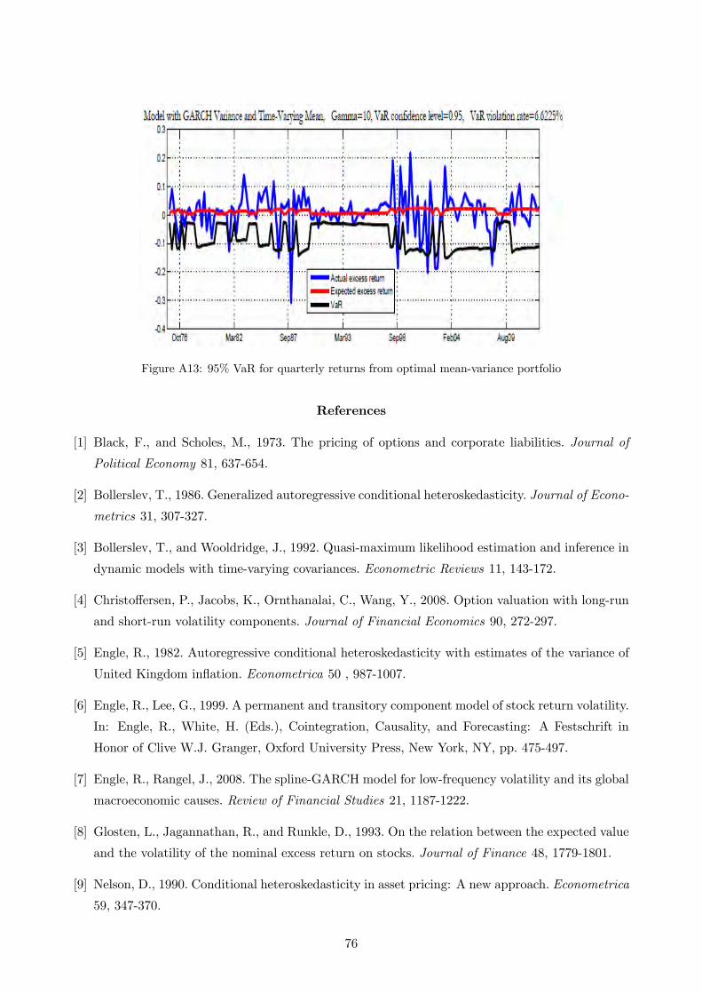
Figure A13: 95% VaR for quarterly returns from optimal mean-variance portfolio

References

[1] Black, F., and Scholes, M., 1973. The pricing of options and corporate liabilities. Journal of

Political Economy 81, 637-654.

[2] Bollerslev, T., 1986. Generalized autoregressive conditional heteroskedasticity. Journal of Econo-

metrics 31, 307-327.

[3] Bollerslev, T., and Wooldridge, J., 1992. Quasi-maximum likelihood estimation and inference in

dynamic models with time-varying covariances. Econometric Reviews 11, 143-172.

[4] Christoffersen, P., Jacobs, K., Ornthanalai, C., Wang, Y., 2008. Option valuation with long-run

and short-run volatility components. Journal of Financial Economics 90, 272-297.

[5] Engle, R., 1982. Autoregressive conditional heteroskedasticity with estimates of the variance of

United Kingdom inflation. Econometrica 50 , 987-1007.

[6] Engle, R., Lee, G., 1999. A permanent and transitory component model of stock return volatility.

In: Engle, R., White, H. (Eds.), Cointegration, Causality, and Forecasting: A Festschrift in

Honor of Clive W.J. Granger, Oxford University Press, New York, NY, pp. 475-497.

[7] Engle, R., Rangel, J., 2008. The spline-GARCH model for low-frequency volatility and its global

macroeconomic causes. Review of Financial Studies 21, 1187-1222.

[8] Glosten, L., Jagannathan, R., and Runkle, D., 1993. On the relation between the expected value

and the volatility of the nominal excess return on stocks. Journal of Finance 48, 1779-1801.

[9] Nelson, D., 1990. Conditional heteroskedasticity in asset pricing: A new approach. Econometrica

59, 347-370.

76

List of Errors of Previous Versions and Revisions

(May 20, 2013) Figure A11 has changed because a bug in mean variance multiperiod.m has been

fixed (thanks to Daniele Bianchi for finding it). Qualitative results are similar but the weigth of

stocks increase.

77