UNITED STATES MARINE CORPS;(USMC) KC-130J TANKER ...

NAVAL POSTGRADUATE SCHOOL

Monterey, California

THESIS 20000306 055 UNITED STATES MARINE CORPS; (USMC) KC-130J

TANKER REPLACEMENT REQUIREMENTS AND

COST / BENEFIT ANALYSIS

by

Mitchell J. McCarthy

December 1999

Thesis Advisor: Associate Advisor:

William Gates Keebom Kang

Approved for public release; distribution is unlimited.

miQ QUALm IEBF30EED 3

Public reporting burden for this collection of information is estimated to average 1 hour per response, including the time for reviewing instruction, searching existing data sources, gathering and maintaining the data needed, and completing and reviewing the collection of information. Send comments regarding this burden estimate or any other aspect of this collection of information, including suggestions for reducing this burden, to Washington headquarters Services, Directorate for Information Operations and Reports, 1215 Jefferson Davis Highway, Suite 1204, Arlington, VA 22202-4302, and to the Office of Management and Budget, Paperwork Reduction Project (0704-0188) Washington DC 20503.

REPORT DOCUMENTATION PAGE Form Approved OMB No. 0704-0188

i. AGENCY USE ONLY (Leave blank) 2. REPORT DATE December 1999

3. REPORT TYPE AND DATES COVERED Master's Thesis

4. TITLE AND SUBTITLE UNITED STATES MARINE CORPS' (USMC) KC-130J TANKER REPLACEMENT REQUIREMENTS AND COST / BENEFIT ANALYSIS

6. AUTHOR(S) McCarthy, Mitchell J.

5. FUNDING NUMBERS

7. PERFORMING ORGANIZATION NAME(S) AND ADDRESS(ES)

Naval Postgraduate School Monterey, CA 93943-5000

8. PERFORMING ORGANIZATION REPORT NUMBER

9. SPONSORING / MONITORING AGENCY NAME(S) AND ADDRESS(ES)

Commander, Naval Air Systems Command, AIR 4.4 Bldg. 2272, 47123 Buse Rd., Patuxent River, MD 20670

10.SPONSORING/MONITORING AGENCY REPORT NUMBER

II. SUPPLEMENTARY NOTES The views expressed in this thesis are those of the author and do not reflect the official policy or position of the Department of Defense or the U.S. Government.

12a. DISTRIBUTION / AVAILABILITY STATEMENT Approved for public release; distribution is unlimited.

12b. DISTRIBUTION CODE

13. ABSTRACT

NAVAIR funded a research project to answer the question: how many KC-130Js Aerial Refueling Tankers will the U.S. Marine Corps (USMC) need to meet their future wartime requirements? This thesis supports that study. Thesis results were incorporated into the recently completed Marine KC-130 Requirements Study, by Professors Gates, Kwon, Washburn, and Anderson.

Specifically, the thesis focuses on the tradeoffs the USMC faces between requirements, performance, and life-cycle costs. The KC-130J aerial refueling requirement must support expected USMC fixed-wing refueling demand during two nearly simultaneous major theater wars. Furthermore, refueling capacity must keep the average time an aircraft waits in the aerial refueling queue (CTq) below five minutes. To define the tradeoff between the KC-130J requirement and system performance (waiting time), the thesis develops a Simulation Model using the ARENA© simulation language. The simulation model highlights the impact of capacity failures (refueling drogues and hoses) and overlaps between KC-130J sorties, two potentially significant factors that can't be explored with standard static queuing theory models. Next, the thesis develops a Life Cycle Cost (LCC) Model that incorporates cost variability using the Crystal Ball EXCEL© spreadsheet add-on. The model defines the tradeoffs between LCC and KC-130J fleet size. The resulting analysis and conclusions specify a base-case KC-130J requirement and discuss the tradeoffs between the requirement, life-cycle cost and system performance. 14. SUBJECT TERMS

Queuing Theory, Simulation Model, Life Cycle Cost (LCC) Spreadsheet Model, KC-130J, Drogue, Cost / Benefit Analysis

15. NUMBER OF PAGES

114

16. PRICE CODE

17. SECURITY CLASSIFICATION OF REPORT

Unclassified

1. SECURITY CLASSIFICATION OF THIS PAGE

Unclassified

19. SECURITY CLASSIFICATION OF ABSTRACT

Unclassified

20. LIMITATION OF ABSTRACT

UL Standard Form 298(Rev. 2-89) Prescribed by ANSI Std 239-18

NSN 7540-01-280-5500

11

Approved for public release; distribution is unlimited.

UNITED STATES MARINE CORPS; (USMC) KC-130J TANKER REPLACEMENT REQUIREMENTS AND COST /

BENEFIT ANALYSIS

Mitchell J. McCarthy Major, United States Marine Corps

B.B.A., Texas A&M University, 1987

Submitted in partial fulfillment of the requirements for the degree of

MASTER OF SCIENCE IN MANAGEMENT

From the

NAVAL POSTGRADUATE SCHOOL December 1999

Author: /&y£2^*W£&Sys *_ MnTarthy

Approved by: SD^MkS^^^hnZZ- William Gates, Thesis Advisor

Teeböm Kang, Associate Advisor

[arris Depar/tme'nt of Systems M4^gement

111

IV

ABSTRACT

NAVAIR funded a research project to answer the question: how

many KC-130Js Aerial Refueling Tankers will the U.S. Marine Corps

(USMC) need to meet their future wartime requirements? This thesis

supports that study. Thesis results were incorporated into the recently

completed Marine KC-130 Requirements Study, by Professors Gates,

Kwon, Washburn, and Anderson.

Specifically, the thesis focuses on the tradeoffs the USMC faces

between requirements, performance, and life-cycle costs. The KC-130J

aerial refueling requirement must support expected USMC fixed-wing

refueling demand during two nearly simultaneous major theater wars.

Furthermore, refueling capacity must keep the average time an aircraft

waits in the aerial refueling queue (CTq) below five minutes. To define

the tradeoff between the KC-130J requirement and system performance

(waiting time), the thesis develops a Simulation Model using the

ARENA© simulation language. The simulation model highlights the

impact of capacity failures (refueling drogues and hoses) and overlaps

between KC-130J sorties, two potentially significant factors that can't be

explored with standard static queuing theory models. Next, the thesis

develops a Life Cycle Cost (LCC) Model that incorporates cost variability

using the Crystal Ball EXCEL© spreadsheet add-on. The model defines

the tradeoffs between LCC and KC-130J fleet size. The resulting analysis

and conclusions specify a base-case KC-130J requirement and discuss the

tradeoffs between the requirement, life cycle cost and system

performance.

v

VI

TABLE OF CONTENTS

I. INTRODUCTION 1

A. BACKGROUND 1

B. PURPOSE 1

C. SCOPE 1

D. METHODOLOGY 4

E. ORGANIZATION 5

II. STATIC QUEUING MODEL METHODOLOGY AND ASSUMPTIONS 7

A. INTRODUCTION 7

B. AERIAL REFUEL CONTROL POINT SCHEDULE EXPLANATION 8

1. What is the Mission Doctrine? 8

2. What is the Mission Schedule? 9

C. AERIAL REFUEL CONTROL POINT CAPACITY / ARRIVAL RATE / UTILIZATION DESCRIPTION 12

1. What is the Capacity of an Aerial Refuel Control Point? 12

2. Why does the Arrival rate at the Aerial Refuel Control Point matter? 14

3. What Utilization (p) is achieved by the Aerial Refuel Control Point given the Arrival Rate (X) driving the ARCP Capacity (Kji) Requirement? 16

D. AERIAL REFUEL CONTROL POINT QUEUING THEORY MODEL USING DETERMINISTIC INPUT 18

E. CHAPTER SUMMARY 21

III. AERIAL REFUELING CONTROL POINT SIMULATION MODEL METHODOLOGY AND ASSUMPTIONS 23

A INTRODUCTION 23

B. AERIAL REFUEL CONTROL POINT SIMPLE SIMULATION MODEL DESCRIPTION AND OUTPUT 24

1. How is the Simulation Model similar to the Static Queuing Theory Model?24

2. How does a Simulation Model differ from a static queuing model? 25

3. How does the output from the simulation model for INVq and CTq compare to the output from the static queuing theory output? 28

Vll

C. AERIAL REFUEL CONTROL POINT ENHANCED SIMULATION MODEL DESCRIPTION AND OUTPUT 31

1. How do we enhance the existing simulation model? 31

2. How and why do the simulation outputs differ between the two models? ..33

1. How does the Enhanced Simulation Model depict Utilization (p)? 36

2. How can we enhance this simulation model further to better depict how an ARCP would operate supporting a Major Theater War? 38

D. CHAPTER SUMMARY 40

TV. LIFE CYCLE COST MODEL METHODOLOGY AND ASSUMPTIONS 41

A. INTRODUCTION 41

B. SENSITIVITY ANALYSIS SHEET 42

1. Why is deriving a Procurement Schedule so critical to the development of the Life Cycle Cost Model? 42

2. Why are cost growth and discount rate important to the Life Cycle Cost Model? 43

3. Why would the probability of an MTW, potential attrition rates, and the service life of a KC-130J affect the Life Cycle Cost Model? 45

C. DEPLOYMENT AND ATTRITION SHEET 46

1. Why do we need to maintain accountability of the number of KC-130Js fielded and the number in the procurement inventory? 46

2. How does the attrition block make the model more realistic? 47

D. COST SCHEDULE SHEET 48

1. Why would the accountability of a particular fiscal year designator be important to the Life Cycle Cost Model 49

2. How are the costs accounted for in the Life Cycle Cost Model? ...49

E. SIMULATION INPUTS AND AFFECTS 53

F. CHART OUTPUTS SHEET 55

G. CHAPTER SUMMARY 56

V. COST / BENEFIT ANALYSIS: ALTERNATIVE FLEET SIZING OPTIONS 59

A. INTRODUCTION 59

B. KC-130J FLEET SIZING REQUIREMENTS FOR DAY OPERATIONS 60

Vlll

C. KC-130J FLEET SIZING REQUIREMENTS NIGHT OPERATIONS 65

D. KC-130J FLEET SIZING COSTS 68

E. KC-130J FLEET SIZING COST/BENEFIT ANALYSIS 71

F. CHAPTER SUMMARY 74

VI. KC-130J FLEET SIZE, CONCLUSIONS AND RECOMMENDATIONS 75

A. INTRODUCTION 75

B. KC-130J FLEET SIZE CONCLUSIONS 75

1. The Arrival Rate (A,) of Combat Aircraft to be refueled and the Aerial Refuel Control Point capacity (Ku\) in a particular theater are critical to the KC-130J Fleet sizing requirement 75

2. The Cycle Time of the Aerial Refuel Control Point Queue (CTq) provides the critical value that ultimately drives the KC-130J Fleet sizing requirement ..75

3. The refuel (process) time proves to be the crucial component that will drive the Aerial Refuel Control Point Capacity needed to meet future USMC requirements 76

C. KC-130J FLEET SIZE RECOMMENDATIONS 76

1. The KC-130J Fleet size of 72 Tankers currently meets the USMC aerial refueling requirements 76

2. The KC-130J Fleet size of 108 Tankers will meet future USMC aerial refueling requirements 77

3. The Fleet size of 108 KC-130J or KC-130J equivalents can meet future USMC aerial refueling requirements 77

D. OTHER ISSUES 77

1. The KC-130J could change current KC-130 Tactics, Technics, and Procedures 77

2. Tradeoff Analysis should be conducted between the KC-130J procurement program and other priority procurement programs 78

APPENDDC A. 24 HOUR AERIAL REFUEL CONTROL POINT SCHEDULE 79

APPENDIX B. KC-130J REQUIREMENTS - STATIC QUEUING MODEL SCHEDULES 81

APPENDIX C. LIFE CYCLE COST MODEL 83

IX

APPENDIX D. VARIABILITY CHART, CRYSTAL BALL DISTRIBUTION ASSUMPTIONS 89

LIST OF REFERENCES 93

INITIAL DISTRIBUTION LIST 95

LIST OF FIGURES Figure 1. Photograph of an ARCP 9

Figure 2. ARCP Model Assumptions 22

Figure 3. Simple Simulation Overview 26

Figure 4. ARENA Simulation Logic 28

Figure 5. Simple Simulation Model Outputs for INVq and CTq 30

Figure 6. Enhanced Simulation Logic 32

Figure 7. Enhanced Simulation Overview 32

Figure 8. Enhanced Simulation Model Outputs ..34

Figure 9. Visual depiction of a two division ARCP 36

Figure 10. Drogue Failure Generator 39

Figure 11. Enhanced Simulation Model Outputs w/Failures 39

Figure 12. Forecast: KC-130J Fleet NPV (LCC) 55

Figure 13. KC-130J Life Cycle Cost Breakdown 56

Figure 14. KC-130J LCC (Graph) Chart 57

Figure 15. Simulation Model CTq Outputs (Day) 63

Figure 16. Simulation Model (+10%) CTq Outputs (Day) 64

Figure 17. Simulation Model (Night) CTq Outputs 66

Figure 18. Forecast: KC-130J Fleet (72) NPV (LCC [in billions]) 68




Figure 22. LCC of different KC-130J Fleet Sizes 72

XI

Xll

LIST OF TABLES Table 1. Initial Columns of the ARCP Schedule 9

Table 2. Snapshot of the 24-Hour ARCP Schedule 10

Table 3. Spare KC-130J Tanker Turnaround Time 12

Table 4. Refuel Division Capacity (without Drogue Failure) 13

Table 5. Arrival Rates per Theater 15

Table 6. Deriving Utilization (p) 17

Table 7. Poisson / Exponential Probability distribution example 20

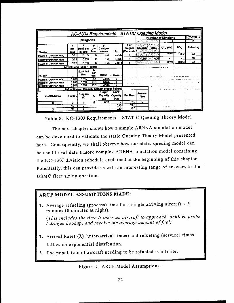
Table 8. KC-130J Requirements - STATIC Queuing Theory Model 22

Table 9. Static Queuing Model Results 29

Table 10. Snapshot of the 24 Hour ARCP Schedule 34

Table 11. Information used in Sensitivity Analysis 43

Table 12. O&M Costs per KC-130J 44

Table 13. Snapshot of the KC-130J Deployment / Phaseout Schedule 46

Table 14. Snapshot of the Life Cycle Cost Analysis 51

Table 15. O&M Difference Schedule 52

Table 16. Variability Chart 54

Table 17. KC-130J Requirements (Day) - STATIC Queuing Model Analysis 61

Table 18. KC-130J Requirements (Night) - STATIC Queuing Model Analysis 65

Table 19. KC-130J Requirements (Alternative) - STATIC Queuing Model Analysis .67

Table 20. Statistical Confidence Interval for Fleet Size of 72 vs.96 72

Table 21. Statistical Confidence Interval for Fleet Size of 96 vs.108 73

Xlll

XIV

LIST OF EQUATIONS

Equation 1. Capacity (fl) Equation 14

Equation 2. ARCP Capacity Equation 14

Equation 3. Arrival Rate Equation 15

Equation 4. Utilization Factor Equation 15

Equation 5. P0 Equation 19

Equation 6. Queue Size 19

Equation 7. Cycle Time of the Queue 19

Equati on 8. Future Value Equation 51

Equation 9. Present Value Equation 52

LIST OF SYMBOLS

ts

n K

ta

Po

P

Arrival Rate

Average Service Time

Capacity

Number of Channels

Inter-Arrival Rate

Probability that there are no units in the system

Utilization

LIST OF ACRONYMS

AR Aerial Refuel

ARCP Aerial Refuel Control Point

DASC(A) Direct Air Support Control (Air)

FMF Fleet Marine Force

LCC Life Cycle Costs

MTW Major Theater War

NPV Net Present Value

RGR Rapid Ground Refueling

xv

XVI

ACKNOWLEDGEMENTS:

I WOULD LIKE TO BEGIN BY THANKING MY WIFE, CINDY, FOR

THE UNWAVERING SUPPORT AND DEVOTION THROUGHOUT THIS

THESIS PROCESS. FURTHER, I APPRECIATE THE PATIENCE,

ENCOURAGEMENT, AND MENTORING GIVEN BY PROFESSORS

GATES AND KANG. FINALLY, I WOULD LIKE TO THANK THE LORD

JESUS CHRIST FOR WITHOUT HIM NONE OF THIS WOULD HAVE

BEEN POSSIBLE.

xvii

XV111

I. INTRODUCTION

A. BACKGROUND

In fiscal year 1998 (FY98), the United States Marine Corps (USMC)

began to transition to a newer re-engineered KC-130 platform, the KC-

130J, in order to replace its aging KC-130 F/R Aerial Refueling Tanker

Fleet. However, as the USMC began to make the transition, a question

arose concerning the KC-130J fleet size, particularly what fleet size the

USMC would need to support future aerial refueling (AR) mission

requirements. Hence, a study was directed to ascertain the requisite fleet

size the USMC would need to support a dual MTW.

B. PURPOSE

This study provides Marine planners with a decision making tool to

support the KC-130J fleet size decision. This decision making tool will

use two different simulation programs. One that simulates the physical

twenty-four hour a day refueling mission executed by a KC-130J Division

during a single MTW and the second, which applies variability to a KC-

130J Life Cycle Cost (LCC) EXCEL® spreadsheet. The combined output

of these two simulation models will provide the Marine planner with a

range of options concerning the fleet size requirement driven by the

physical simulation model and then ascribe cost as a factor ofthat fleet

size.

C. SCOPE

This study will provide insight into the size requirements for a

future USMC KC-130J fleet. This will not include the use of Joint or

Allied tanker aircraft. The exclusion of Joint and Allied aerial tanker

assets is deliberate, this study is intended to examine if the indigenous

USMC tanker fleet can meet the USMC aerial refueling requirements.

The use of Joint or Allied refueling platforms simply lies beyond the

scope of this study.

This study will begin by applying a simple queuing theory model to

the KC-130Js primary mission to provide tactical aerial refueling service

to Fleet Marine Force (FMF) in a particular theater of operation. We will

ascribe numerical values to certain variables, which have a dramatic

effect on how many aircraft may be waiting to be refueled (INVq) and / or

how long an aircraft may have to wait to be refueled (CTq)'. By capturing

these values we decide the number of KC-130J tankers we will need to

support the AR requirement in a certain theater. Secondly, a simulation

model will be created which will parallel the essential elements and

variables that effect a division of KC-130Js as they perform a twenty-four

hour a day refueling mission during a single Major Theater War (MTW)

scenario2.

This simulation model will glean three crucial variables: the

average number of aircraft waiting to be refueled (INVq), the average

time combat aircraft spend waiting to be refueled (CTq), and the average

number of KC-130Js actually performing the refueling mission. The fleet

sizing decision will be based on the target level for those variables

emphasizing the time aircraft spend waiting to be refueled. After

analyzing the results from the simulation model, the Marine planner can

derive a KC-130J Fleet size that will minimize the amount of time combat

aircraft spend waiting to be refueled. Once the fleet-size for an MTW

scenario is determined, simple multiplication can derive a fleet size which

1 Conventional notations depict INVq as Lq and CTq as Wq, the author chose to use

INVq (Inventory of the Queue) and CTq (Cycle Time of the Queue) because these

would more adequately describe the process. 2 KC-130 Tactical Manual NWP 3-22.5-KC-130. Volume I, NAVAIR 01-75GAA-IT,

May 1997, Department of the Navy, Office of the Chief of Naval Operations, pp. 3-35

- 3-39.

will support a near simultaneous dual MTW scenario. Now that the

Marine Planner has captured the number attributed to the fleet size, costs

can be ascribed to that number.

Thirdly, by plugging the fleet size number into the Life Cycle Cost

(LCC) spreadsheet, the LCC cost for the KC-130J fleet can be captured.

Variability will be embedded into both the simulation model and the LCC

spreadsheet in order to capture the uncertainty resident within any

decision process. These two models will work together to provide an

effective picture of how a future KC-130J Fleet might be sized and the

cost figure attributed to that size.

Fourthly, a chapter will be devoted to executing multiple iterations

of the simulation at the highest refueling usage rate, as estimated by a

Center for Naval Analysis (CNA) study, to obtain solid fleet size

numbers.3 Plugging those fleet size numbers into the LCC spreadsheet

will estimate the total cost for that fleet size. Thus, a range will be

derived ascribing fleet size to a cost figure, with the fleet size driven by

the required minimum time combat aircraft spend waiting to be refueled.

Other variables, such as refueling queue size or the average number of

KC-130Js actually performing the refuel mission, will help to validate the

model as well as better define the tradeoffs the Marine planner must make

(Cost / Benefit Analysis). Marine planners must balance the tradeoffs

between fleet size, costs, and the time a combat aircraft waits to be

refueled (CTq). Waiting time prevents combat aircraft from executing

their primary mission.

The fifth chapter will be devoted to a Cost / Benefit Analysis of the

data gathered from the simulations, providing some cogent conclusions

and recommendations to aid the USMC in arriving at the best value

3 Cox, Gregory, USN/USMC Tanking Requirements. Center for Naval Analysis, May

95, p.7.

decision. Finally, the last chapter will be dedicated to the study's

recommendations and conclusions based on the analysis in the previous

chapter.

D. METHODOLOGY

This thesis will mainly discuss the primary missions of the KC-

130J. The information will be drawn from a literature search of books,

magazine articles, and other library materials relevant to the subject.

Then, a static queuing theory model will be applied to the variables

derived from various expert sources on aerial refueling capacity

requirements and fleet sizing.

Next a simulation analysis, using the ARENA® simulation language,

shall be conducted to project the relationship between the number of KC-

130Js supporting an Aerial Refuel Control Point (ARCP) and the amount

of time combat aircraft spend waiting to be refueled.4 Subsequently, an

EXCEL® LCC spreadsheet of the relevant costs will be developed. This

spreadsheet will utilize some of the costs derived by Gates, Andersen,

Kwon, and Washburn (1999) in their KC-130J LCC spreadsheet.5

Variability will be included in the LCC model by capturing KC-130J

losses due to peace and wartime attrition. A discount rate will be

embedded into the LCC model. These features will provide a more

accurate depiction of the potential range of Net Present Value LCC in real

(FYS2000) dollars to make the fleet sizing decisions.

Finally, cost / benefit analysis will be conducted to provide the

USMC with a range of KC-130J fleet sizing options. The analysis will

4 Kelton, W. David, Sadowski, Randall P., Sadowski, Deborah A., Simulation with

ARENA, McGraw Hill, 1998. 5 Gates, William R., Young Kwon, Timothy Anderson, and Alan Washburn. Marine

KC-130 Requirements Study. Naval Postgraduate School, Monterey, CA. October

1999. Section #1, pp. 6-7.

weigh the tradeoffs between fleet size, LCC and the time the USMC is

willing to have combat aircraft waiting to be refueled (CTq) during a near

simultaneous dual MTW scenario. Balancing these tradeoffs will answer

the ultimate question: What KC-130J fleet size does the USMC need to

adequately support USMC aerial refueling'during a dual MTW.

E. ORGANIZATION

The reader now has been provided with the background, purpose,

scope, and methodology for this thesis. The following chapters will flow

as described in both the scope and methodology above. The study will be

organized into the format depicted below.

I. Introduction

II. Static Queuing Model Methodology and Assumptions

III. Aerial Refueling Control Point Simulation Model

Methodology and Assumptions

IV. LCC Model Methodology and Assumptions

V. Cost / Benefit Analysis: Alternative Fleet Sizing Options

VI. KC-130J Fleet Size, Conclusions and Recommendations

THIS PAGE WAS INTENTIONALLY LEFT BLANK

II. STATIC QUEUING MODEL METHODOLOGY AND

ASSUMPTIONS

A. INTRODUCTION

To build a model, one must understand the real world system that

needs to be simulated by the computer. In this case, an Aerial Refuel

Control Point (ARCP) needed to be simulated. An ARCP or the Aerial

Refueling (AR) requirement comprises sixty-seven percent of the KC-130J

Squadron mission in an MTW.6 The other main missions are Direct Air

Support Control (DASC), Rapid Ground Refuel (RGR), and Helicopter

Refueling operations.7 The purpose of this chapter is to describe the

many variables that affect a static queuing theory model which will enable

us to derive the USMC KC-130J Fleet size required for a certain theater.

This chapter is broken down into several parts, building upon each

other. First, the KC-130J Aircraft schedule to support an ARCP will be

described. Second, the ARCP's capacity (Kji) (i.e., maximum sustainable

throughput of aircraft that can be refueled per time), its interaction with

the particular arrival rate (k) used, and their combined effect on the

utilization factor (p) shall be discussed. With the given arrival rates (X),

the capacity (ji.) (maximum sustainable throughput of a single drogue),

and the number of operational drogues (K) will be inputs into the queuing

model equations. That will allow us to calculate the average number of

aircraft waiting in the queue (INVq) and the amount of time an aircraft

spends waiting to be refueled (CTq). Both INVq and CTq are crucial

6 Gates, William R., Young Kwon, Timothy Anderson, and Alan Washburn; Marine


1999. Section #1, p. 7. 7 KC-130 Tactical Manual NWP 3-22.5-KC-130. Volume I, NAVAIR 01-75GAA-IT,

May 1997, Department of the Navy, Office of the Chief of Naval Operations, p. 1-1.

factors in determining USMC KC-130J fleet sizing requirements. Finally,

the chapter will end with a review of the important highlights. The

chapter will be organized in the format depicted below:

A. Introduction

B. ARCP Schedule Explanation

C. ARCP Capacity (K\i)/ Arrival rate (X,) / Utilization (p)

Description

D. ARCP Queuing Model using Deterministic Input

E. Chapter Summary

B. AERIAL REFUEL CONTROL POINT SCHEDULE

EXPLANATION

1. What is the Mission Doctrine?

The ARCP mission doctrine states that a schedule shall be

established to provide tactical aerial refueling service to Fleet Marine

Force (FMF) squadrons. In our case, this is a 24-hour a day aerial

refueling capability during an MTW.8 Metaphorically speaking, an ARCP

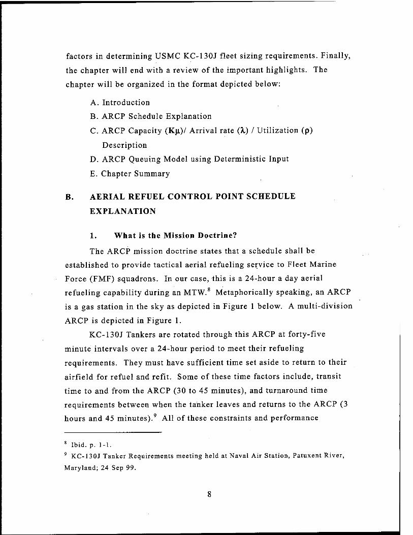
is a gas station in the sky as depicted in Figure 1 below. A multi-division

ARCP is depicted in Figure 1.

KC-130J Tankers are rotated through this ARCP at forty-five

minute intervals over a 24-hour period to meet their refueling

requirements. They must have sufficient time set aside to return to their

airfield for refuel and refit. Some of these time factors include, transit

time to and from the ARCP (30 to 45 minutes), and turnaround time

requirements between when the tanker leaves and returns to the ARCP (3

hours and 45 minutes).9 All of these constraints and performance

8 Ibid. p. 1-1. 9 KC-130J Tanker Requirements meeting held at Naval Air Station, Patuxent River,

Maryland; 24 Sep 99.

assumptions were incorporated into the 24-Hour ARCP Schedule

contained in Appendix A. Portions ofthat schedule will be explained

below.

Ci<: '•""• ""lauf i* f ;>...f.... 'IJ*Z

Figure 1. Photograph of an ARCP.

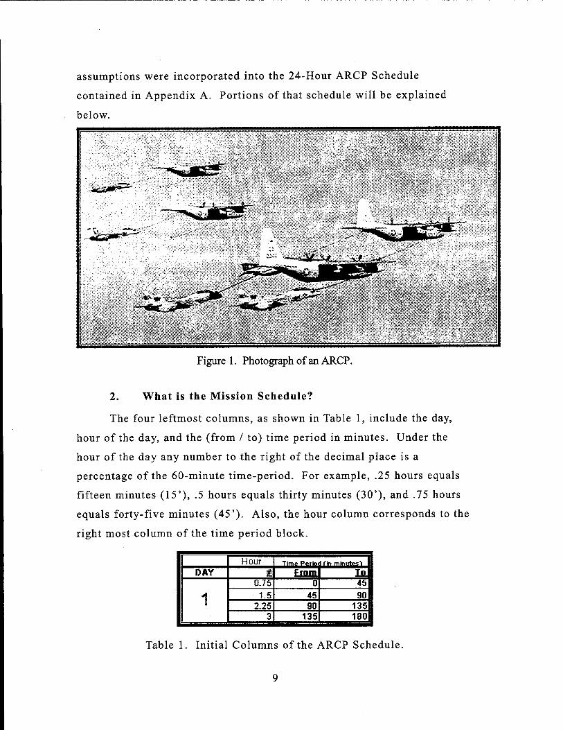
2. What is the Mission Schedule?

The four leftmost columns, as shown in Table 1, include the day,

hour of the day, and the (from / to) time period in minutes. Under the

hour of the day any number to the right of the decimal place is a

percentage of the 60-minute time-period. For example, .25 hours equals

fifteen minutes (15'), .5 hours equals thirty minutes (30'), and .75 hours

equals forty-five minutes (45'). Also, the hour column corresponds to the

right most column of the time period block.

Hour Time Porio I'm minutest H

DAY £ From IfiJ

1 0.75 0 451

1.5 45 901 2.25 90 1351

3 135 180(

Table 1. Initial Columns of the ARCP Schedule.

KC-130JA/CI Hour 1 2 3 4 5 6 7 8 9 to 11 12 13 14

* EBB I« E *£&*•&

1.S 45 90 0 2 45 ■■■■■-■ \- ■ \- • \ ''.' Z25

3 90

135 135 180

0 27 45 0

>K«0 '?W®V 2 45 sa

3.75 4.5

180

225

Us 270

0 2

0

4s' 2 46

♦ 0

5.25 6

270 315

315 360 0

0 2 JL

45 MB 2 45

6K 7.5

360

405

405"

450

2 0

& T ~45~ 0 I II

8.25 9

450 49G

495 540

o- ./'>i"i 2 I 45 I 0 I fomm 21 45 0 I. I

9.75

10.5

540

585

585

830

:,M4:»ä« 2 45 0

»fessl 2 I 45 ••7

°l -1

T ; '. ...:.... i ;. .;

11.25 12

630 675

675 720

kEteffi 2 45 ante»

0 2 *fe" ' ;,.-.

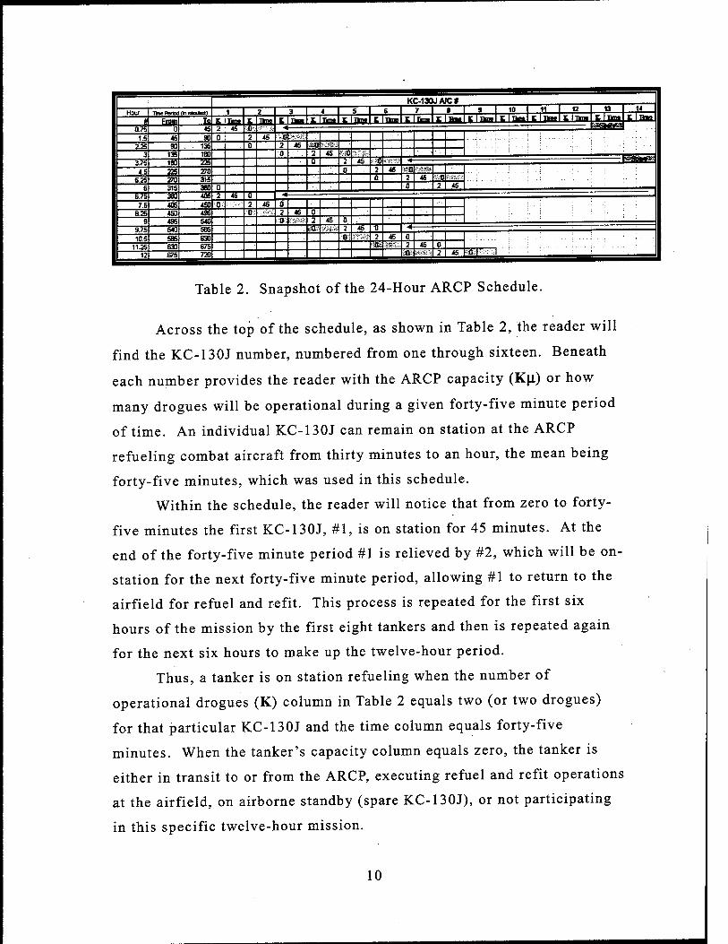
Table 2. Snapshot of the 24-Hour ARCP Schedule.

Across the top of the schedule, as shown in Table 2, the reader will

find the KC-130J number, numbered from one through sixteen. Beneath

each number provides the reader with the ARCP capacity (K\i) or how

many drogues will be operational during a given forty-five minute period

of time. An individual KC-130J can remain on station at the ARCP

refueling combat aircraft from thirty minutes to an hour, the mean being

forty-five minutes, which was used in this schedule.

Within the schedule, the reader will notice that from zero to forty-

five minutes the first KC-130J, #1, is on station for 45 minutes. At the

end of the forty-five minute period #1 is relieved by #2, which will be on-

station for the next forty-five minute period, allowing #1 to return to the

airfield for refuel and refit. This process is repeated for the first six

hours of the mission by the first eight tankers and then is repeated again

for the next six hours to make up the twelve-hour period.

Thus, a tanker is on station refueling when the number of

operational drogues (K) column in Table 2 equals two (or two drogues)

for that particular KC-130J and the time column equals forty-five

minutes. When the tanker's capacity column equals zero, the tanker is

either in transit to or from the ARCP, executing refuel and refit operations

at the airfield, on airborne standby (spare KC-130J), or not participating

in this specific twelve-hour mission.

10

Once another tanker relieves a tanker on station, its schedule

encompasses a five hour and fifteen minute period between the time the

tanker departs the ARCP and returns from the airfield to the ARCP. This

period includes: forty-five minutes to return to the airfield, three hours

and forty-five minutes at the airfield to refuel and refit, and another forty-

five minutes to return from the airfield to the ARCP. Again, this schedule

is repeated for the first eight KC-130J Tankers over the first twelve hours

of the schedule and then is repeated again over the next twelve hours

using tankers nine through sixteen, as shown in Appendix A.

A flight of more than two aircraft are considered a division of

aircraft.10 Thus, the schedule is broken down into three-hour periods with

a four-tanker division supporting the AR requirement over that period.

Further, in Table 2 a spare tanker is slated for each division of tankers.

These spare tankers remain available, prepared to assume the mission for

any one of the primary tankers to provide a buffer against primary tanker

- mechanical breakdown or failure.

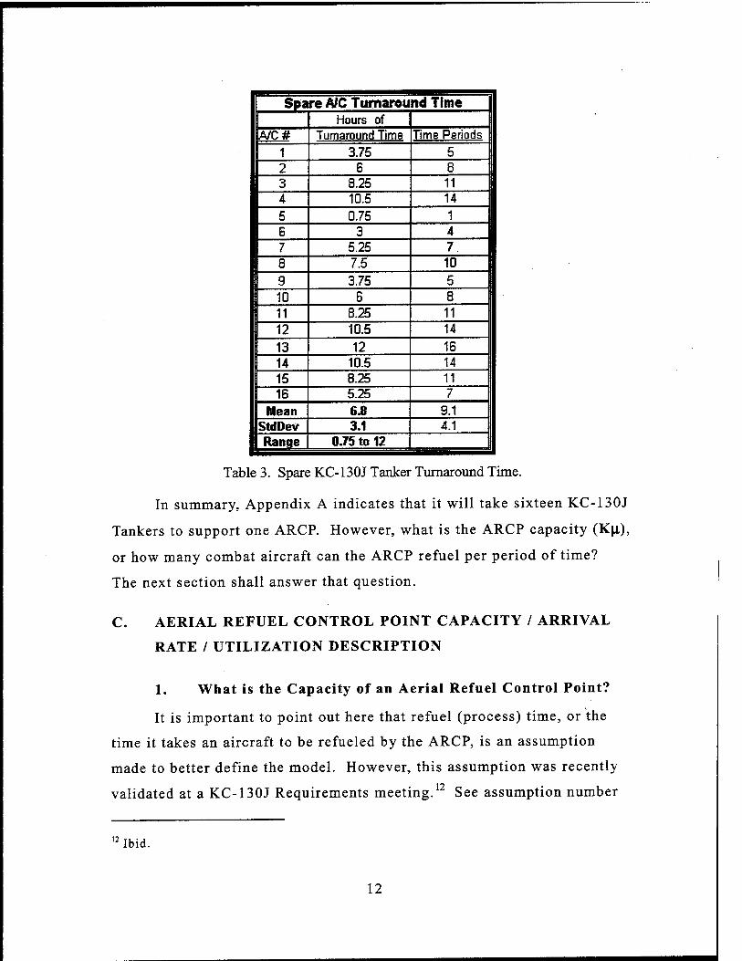
Table 3 (part of Appendix A) takes the turnaround time for all of

the KC-130Js being used as spare tankers over a two-day period, deriving

a mean, standard deviation, and range. The spare tanker turnaround time

or the time between when it completes a twelve hour mission and it is

slated as a spare tanker has a mean 6.8 hours or six hours and forty-eight

minutes as shown in Table 3. The standard deviation is plus or minus 3.1

or three hours and six minutes. The range spans from forty-five minutes

to twelve hours. The mean falls well within standard turnaround-time

established for aircraft11.

10 KC-130 Tactical Manual NWP 3-22.5-KC-130. Volume I, NAVAIR 01-75GAA-IT,

May 1997, Department of the Navy, Office of the Chief of Naval Operations, p. 5-2. 11 KC-130J Tanker Requirements meeting held at Naval Air Station, Patuxent River,


11

Spare A/C Turnaround Time Hours of

A/C# Turnaround Time Time Periods 1 3.75 5 2 6 8 3 8.25 11 4 10.5 14 5 0.75 1 6 3 4 7 5.25 7 8 7.5 10 9 3.75 5 10 6 8 11 8.25 11 12 10.5 14 13 12 16 14 10.5 14 15 8.25 11 16 5.25 7

Mean 6.8 9.1 StdDev 3.1 4.1 Range 0.75 to 12

Table 3. Spare KC-130J Tanker Turnaround Time.

In summary, Appendix A indicates that it will take sixteen KC-130J

Tankers to support one ARCP. However, what is the ARCP capacity (Ku.),

or how many combat aircraft can the ARCP refuel per period of time?

The next section shall answer that question.

C. AERIAL REFUEL CONTROL POINT CAPACITY / ARRIVAL

RATE / UTILIZATION DESCRIPTION

1. What is the Capacity of an Aerial Refuel Control Point?

It is important to point out here that refuel (process) time, or the

time it takes an aircraft to be refueled by the ARCP, is an assumption

made to better define the model. However, this assumption was recently

validated at a KC-130J Requirements meeting.12 See assumption number

12 Ibid.

12

one of Figure 2 at the end of this chapter; further, the other assumptions

made to formulate this model will be explained in the following chapters.

A combat aircraft is refueled on average ts units of time. As stated

above, one drogue can refuel one combat aircraft in five minutes (ts =5')

on average. Thus, we denote capacity (\i) as 1 / ts (see Equation 1), where

\i measures the maximum sustainable throughput of aircraft that need to

be refueled, per unit of time.13 As shown in the first row of Table 4, one

drogue on a KC-130J can refuel one aircraft every five minutes or twelve

per hour.

Combining the capacity of two drogues constitutes a single KC-

130J supporting an ARCP, the capacity of the ARCP (as shown in

Equation 2 and row two of Table 4) is 0.40 aircraft per minute or (60' X

0.40) twenty-four per hour. By adding another division to support the

ARCP, its capacity jumps to 0.80 aircraft per minute, or forty-eight per

hour, as shown in rows three and four of Table 4. Notice that as one adds

a division to the ARCP, the aircraft per minute raises by 0.40 or twenty-

four per hour. Thus, as divisions are added to support the AR

requirement, the ARCP capacity (Kji) increases significantly (see

Equation 2).

1 Refuel DM sion Capacity (without Droaue Failure)

# of Divisions #ofA/C Drogues ts

Drogue Capacity

to

ARCP Capacity Per Hour Process I

Time I

0 0 1 5 0.20 _ 12.0 5 1 16 2 - 0.40 24.0 2 32 4 - 0.80 48.0 3 48 6 - 1.20 72.0 • I

Table 4. Refuel Division Capacity (without Drogue Failure).

Adleman, Dan, Barnes-Schuster, Dawn, and Eisenstein, Don; Operations

Quadrangle: Business Process Fundamentals, The University of Chicago Graduate

School of Business, 1999, p. 39.

13

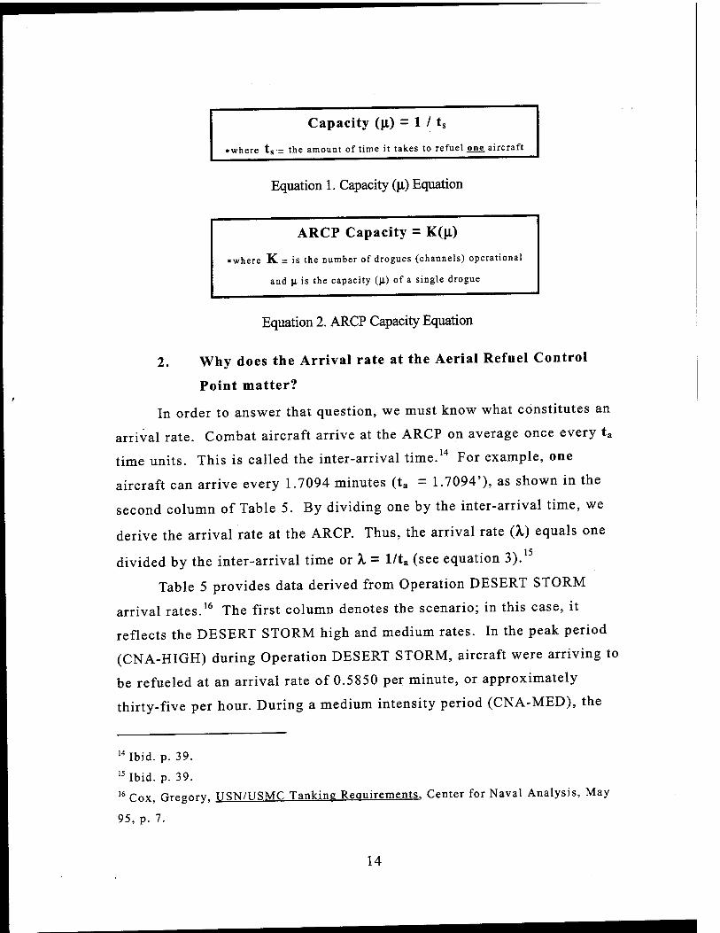
Capacity (\i) = 1 / ts

here ts _ the amount of time it takes to refuel one aircraft »wnere is

Equation 1. Capacity Qi) Equation

ARCP Capacity = K(^)

»where K = is the number of drogues (channels) operational

and \L is the capacity (ji) of a single drogue

Equation 2. ARCP Capacity Equation

2. Why does the Arrival rate at the Aerial Refuel Control

Point matter?

In order to answer that question, we must know what constitutes an

arrival rate. Combat aircraft arrive at the ARCP on average once every ta

time units. This is called the inter-arrival time.14 For example, one

aircraft can arrive every 1.7094 minutes (t. = 1.7094'), as shown in the

second column of Table 5. By dividing one by the inter-arrival time, we

derive the arrival rate at the ARCP. Thus, the arrival rate (X) equals one

divided by the inter-arrival time or A, = l/ta (see equation 3).

Table 5 provides data derived from Operation DESERT STORM

arrival rates.16 The first column denotes the scenario; in this case, it

reflects the DESERT STORM high and medium rates. In the peak period

(CNA-HIGH) during Operation DESERT STORM, aircraft were arriving to

be refueled at an arrival rate of 0.5850 per minute, or approximately

thirty-five per hour. During a medium intensity period (CNA-MED), the

14 Ibid. p. 39. 15 Ibid. p. 39. 16 Cox, Gregory, IJSN/USMC Tanking Requirements. Center for Naval Analysis, May

95, p. 7.

14

arrival rate was 0.3383 per minute, or approximately twenty per hour, as

shown in column 4 of Table 5.

Arrival Rates 1 W per Theater

Theater ta (X) Arrival Rate X

per hour

DESERT STORM (CNA-HIGH) 1.709402 0.5850 35.1 DESERT STORM (CNA-MED) 2.955665 0.3383 20.3

Table 5. Arrival Rates per Theater.

X - 1 / ta

»Where ta = the inter-arrival time between aircraft arrivals

Equation 3. Arrival Rate Equation

Having described capacity (jx), ARCP capacity (Kji), and arrival

rates (A,), it is important to discuss how they interact. Their interaction is

captured in the form of utilization (p). Utilization (p) is arrival rate (X)

divided by ARCP capacity or the number of channels (K) times capacity

per channel (|i); p = X I Kp, (see Equation 4)17. Utilization (p) is always

less than one (p < 1).

p = X I Kn

Equation 4. Utilization Factor Equation

As p gets closer to one, the aircraft queue waiting to be refueled

would grow until the entire population of USMC fixed wing (FW) aircraft

are in one of three places. The aircraft needing to be refueled will be

either waiting to be refueled, being refueled, or just departing the ARCP.

This occurs because the ARCP is refueling an infinite population of FW

17 Anderson, David R., Sweeney, Dennis J., and Williams, Thomas A.; An Introduction

to Management Science, 8th Edition, West Publishing Company, 1997, p. 506.

15

aircraft. However, the waiting line would increase indefinitely at some 1R point (depending on the system) as p gets closer to one .

An infinitely increasing queue does not realistically simulate the

real world ARCP procedures. Further, Marine planners will always ensure

there is enough ARCP capacity (Kji) to meet the requirements (X). Thus,

ARCP capacity must always be greater than the arrival rate (Kji > X) and

utilization (p) can never be greater than one.

The closer utilization (p) is to one the higher your ARCP utilization

and the less time your ARCP spends idle or not refueling any aircraft.

However, a tradeoff must be made because as p approaches one, there will

be a larger queue of aircraft waiting at the ARCP (INVq) and the aircraft

will wait longer to be refueled (CTq).

3. What Utilization (p) is achieved by the Aerial Refuel

Control Point given the Arrival Rate (X.) driving the ARCP

Capacity (Kn,) Requirement?

Combining Tables 4 and 5 determines how many divisions of KC-

130Js are needed to provide sufficient capacity to service the aircraft as

they arrive. Table 6 shows the tanker utilization factor (p), in the shaded

portion of Table 6, given the two DESERT STORM arrival rates, and the

number of divisions required to service each particular arrival rate.

DESERT STORM (CNA-HIGH), with an arrival rate (k) of 0.5850,

requires at least two divisions or four drogues with an ARCP capacity

(Kfi) of 0.80 to service the arriving aircraft without an infinitely

increasing queue. Using two divisions in this scenario prevents

utilization from peaking above one, which is necessary to meet planning

requirements.

Ibid. p. 506.

16

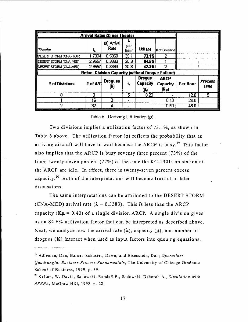
1 Arrival Rates tti per Theater

\Theater ta

pi) Arrival Rate

X

per hour Ui(P) # of Divisions

- -■

DESERT STORM (CNA-HGH) 1.7094 0.5850 35.1 73.1% 2 DESERT STORM (CNA-MED) 2.9557 0.3383 20.3 84.6% 1 PESERT STORM (CNA-MED) 2.9557 0.3383 20.3 423% 2 1 Refuel DM sion Capacity (without Droque Failure) I

# of Divisions #ofA/C Drogues

ts Drogue

Capacity ARCP

Capacity Per Hour Process

Tine

0 0 1 5 0.20 . 12.0 5 1 16 2 - 0.40 24.0 2 32 4 - 0.80 48.0

Table 6. Deriving Utilization (p).

Two divisions implies a utilization factor of 73.1%, as shown in

Table 6 above. The utilization factor (p) reflects the probability that an

arriving aircraft will have to wait because the ARCP is busy.19 This factor

also implies that the ARCP is busy seventy three percent (73%) of the

time; twenty-seven percent (27%) of the time the-KC-130Js on station at

the ARCP are idle. In effect, there is twenty-seven percent excess Of)

capacity. Both of the interpretations will become fruitful in later

discussions.

The same interpretations can be attributed to the DESERT STORM

(CNA-MED) arrival rate (k = 0.3383). This is less than the ARCP

capacity (Kjl = 0.40) of a single division ARCP. A single division gives

us an 84.6% utilization factor that can be interpreted as described above.

Next, we analyze how the arrival rate (A,), capacity (\i), and number of

drogues (K) interact when used as input factors into queuing equations.

Adleman, Dan, Barnes-Schuster, Dawn, and Eisenstein, Don; Operations



Kelton, W. David, Sadowski, Randall P., Sadowski, Deborah A., Simulation with

ARENA, McGraw Hill, 1998, p. 22.

20

17

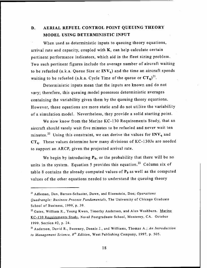
D. AERIAL REFUEL CONTROL POINT QUEUING THEORY

MODEL USING DETERMINISTIC INPUT

When used as deterministic inputs to queuing theory equations,

arrival rate and capacity, coupled with K, can help calculate certain

pertinent performance indicators, which aid in the fleet sizing problem.

Two such pertinent figures include the average number of aircraft waiting

to be refueled (a.k.a. Queue Size or INVq) and the time an aircraft spends

waiting to be refueled (a.k.a. Cycle Time of the queue or CTq) .

Deterministic inputs mean that the inputs are known and do not

vary; therefore, this queuing model possesses deterministic averages

containing the variability given them by the queuing theory equations.

However, these equations are more static and do not utilize the variability

of a simulation model. Nevertheless, they provide a solid starting point.

We now know from the Marine KC-130 Requirements Study, that an

aircraft should rarely wait five minutes to be refueled and never wait ten

minutes.22 Using this constraint, we can derive the values for INVq and

CTq. These values determine how many divisions of KC-130Js are needed

to support an ARCP, given the projected arrival rate.

We begin by introducing P0, or the probability that there will be no

units in the system. Equation 5 provides this equation.23 Column six of

table 8 contains the already computed values of P0 as well as the computed

values of the other equations needed to understand the queuing theory

21 Adleman, Dan, Barnes-Schuster, Dawn, and Eisenstein, Don; Operations


School of Business, 1999, p. 39. 22 Gates, William R., Young Kwon, Timothy Anderson, and Alan Washburn. Marine


1999. Section #2, p. 24. 23 Anderson, David R., Sweeney, Dennis J., and Williams, Thomas A.; An Introduction

to Management Science, 8,h Edition, West Publishing Company, 1997, p. 505.

18

model used. The equations are presented to aid the reader should he or

she desire a deeper understanding.

1 Pn = K-1

V(X/g)*% + (X/P)K / Kg \ ^ n! K! \ KB-X / n = 0

* Thus n begins with zero and extends to the number derived by K minus 1 in the summation, depending on the number of Drogues (K) are in use.

.24 Equation 5. Pn Equation

What queuing theory equations are used to derive numbers for INVq

and CTq? We must start by using an M / M / S queue. The first and

second M stand for (Markov) Poisson inter-arrival rates and (Markov)

Exponential service times, respectively. The S stands for the number of

servers used, which equates to the number of channels, in our case a KC-

130J with two drogues. The INVq and CTq equations are given by

Equations 6 and 7, respectively.

INVq(M/M/S) = (X/lLfXp.

(K-iy.(KiL-X)

Equation 6. Queue Size

CTq(M/M/S) = INVq

Equation 7. Cycle Time of the Queue

The Exponential service times are assumed when using the M / M /

S queuing equations as stated in Figure 2, at the end of the chapter. The

24 The term n!, factorial is'defined as n! = n (n-l)(n-2)...(2)(l). For example, 3!

(3)(2)(1) = 6. A special rule exists where n = 0, 0! = 1! by definition.

19

ARCP service time may or may not be exponential; however, the data is

currently unavailable to validate that assumption. Thus, in order to use

the static queuing theory model and later the simulation model the ARCP

exponential service time is assumed.

The Poisson probability distribution used for the arrival rate (A,) in

our queuing equation defines the probability distribution of arrivals

occurring over a specific period; the exponential probability distribution

models the time between arrivals. Both distributions are commonly used

in Queuing Theory Models. The Poisson and the exponential

distributions are mirrors of one another, metaphorically speaking of

course. For example, column two marked ta in Table 7 below, depicts

time between arrivals, an exponential distribution; one aircraft will arrive

every 1.7094 minutes. That same number can be converted into a Poisson

distribution (60' / 1.7094 = 35 per hour) to derive 35.1 arrivals per hour,

as in the last column of table 7.

| Arrival Rates X) per Theater I j

\Theater ta (X) Arrival Rate X

per hour I pESERT STORM (CNA-HIGH) 1.709402 0.5850 35.1 JDESERT STORM (CNA-MED) 2.955665 0.3383 20.3|

Table 7. Poisson / Exponential Probability distribution example

By plugging the information provided in Table 6, concerning arrival

rates (X), capacity (ji), and the number of drogues (K), into the queuing

theory equations above, one can derive the number of KC-130J divisions

necessary to support the projected arrival rate. The result is given in

Table 8 below. USMC will need two divisions of KC-I30Js to meet the

CNA-HIGH arrival rate (X) given in table 6. For reference, Table 6 is

25 Kelton, W. David, Sadowski, Randall P., Sadowski, Deborah A., Simulation with

ARENA, McGraw Hill, 1998, p. 22-23.

20

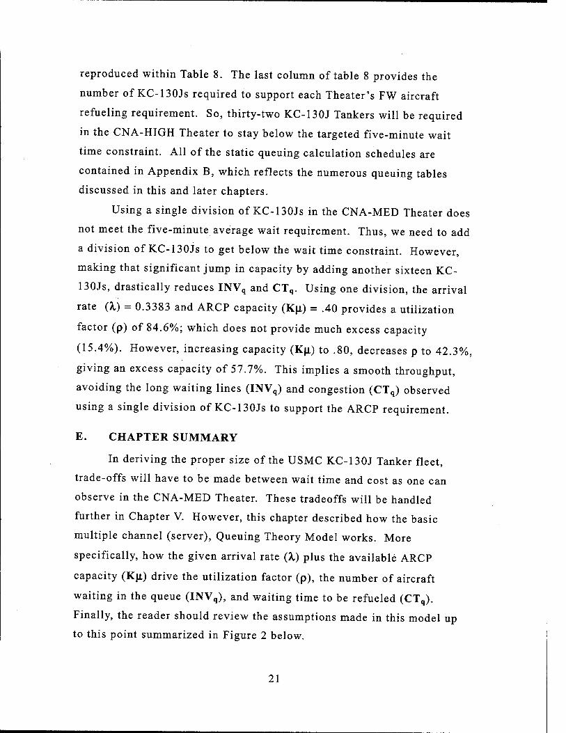
reproduced within Table 8. The last column of table 8 provides the

number of KC-130Js required to support each Theater's FW aircraft

refueling requirement. So, thirty-two KC-130J Tankers will be required

in the CNA-HIGH Theater to stay below the targeted five-minute wait

time constraint. All of the static queuing calculation schedules are

contained in Appendix B, which reflects the numerous queuing tables

discussed in this and later chapters.

Using a single division of KC-130Js in the CNA-MED Theater does

not meet the five-minute average wait requirement. Thus, we need to add

a division of KC-130Js to get below the wait time constraint. However,

making that significant jump in capacity by adding another sixteen KC-

130Js, drastically reduces INVq and CTq. Using one division, the arrival

rate (X) = 0.3383 and ARCP capacity (Kji) = .40 provides a utilization

factor (p) of 84.6%; which does not provide much excess capacity

(15.4%). However, increasing capacity (K\L) to .80, decreases p to 42.3%,

giving an excess capacity of 57.7%. This implies a smooth throughput,

avoiding the long waiting lines (INVq) and congestion (CTq) observed

using a single division of KC-130Js to support the ARCP requirement.

E. CHAPTER SUMMARY

In deriving the proper size of the USMC KC-130J Tanker fleet,

trade-offs will have to be made between wait time and cost as one can

observe in the CNA-MED Theater. These tradeoffs will be handled

further in Chapter V. However, this chapter described how the basic

multiple channel (server), Queuing Theory Model works. More

specifically, how the given arrival rate (X) plus the available ARCP

capacity (KJJ.) drive the utilization factor (p), the number of aircraft

waiting in the queue (INVq), and waiting time to be refueled (CTq).

Finally, the reader should review the assumptions made in this model up

to this point summarized in Figure 2 below.

21

KC-130J Reauirements - STATIC Queuing Mode! Categories

Number of Divisions KC-130JS

;,V . '■:•■■' 2 #

Theater

X per

hour

X (rate) per

minute per

hour (rate) per minute Po

#of Drogues

(Channels) or«,*»*») ;WVq CTq (Min) MV, Refueling

DESERT STORM (CNA-HGH) 35.1 0.585 12 0.20 0.0422 4 2.225 1.302 32

DESERT STORM (CNA-MED) 20.3 0.338 12 0.20 0.0835 2 1257 4.25 - - 16

DESERT STORM (CNA-MEO) 20.3 0.338 12 0.20 0.1811 4 0.232 0.078 32

Arrival Rates (k\ oer Theater

Theater U

(X) Arrival Rate

X per

hour tU(f>) # of Divisions

DESERT STORM (CMM*SH) 1.709 0.585 35.1 73.1% 2 DESERT STORM (CNA-MEO) 2.956 0.338 20.3 84.6% 1 DESERT STORM (CNAJ») 0.338 20.3 423% 2

1

— \ """ " ":" " Re fuel DM •ion Capacity (wii thout Dron ■a Failure»


(K) t>

Drogue Capacity

ARCP Capacity Per Hour Ik»

0 0 1 5 0.20 - 12.0 5

1 16 2 - 0.40 24.0

2 32 4 - 0.80 48.0

Table 8. KC-130J Requirements - STATIC Queuing Theory Model

The next chapter shows how a simple ARENA simulation model

can be developed to validate the static Queuing Theory Model presented

here. Consequently, we shall observe how our static queuing model can

be used to validate a more complex ARENA simulation model containing

the KC-130J division schedule explained at the beginning of this chapter.

Potentially, this can provide us with an interesting range of answers to the

USMC fleet sizing question.

ARCP MODEL ASSUMPTIONS MADE:

1. Average refueling (process) time for a single arriving aircraft = 5 minutes (8 minutes at night).

(This includes the time it takes an aircraft to approach, achieve probe / drogue hookup, and receive the average amount of fuel)

2. Arrival Rates (X) (inter-arrival times) and refueling (service) times

follow an exponential distribution.

3. The population of aircraft needing to be refueled is infinite.

Figure 2. ARCP Model Assumptions

22

III. AERIAL REFUELING CONTROL POINT

SIMULATION MODEL METHODOLOGY AND

ASSUMPTIONS

A. INTRODUCTION

The last chapter described a schedule for an Aerial Refuel Control

Point (ARCP) and that schedule captured a crucial element: the ARCP's

capacity (Kjj.). Then it discussed how a given arrival rate (X), coupled

with the ARCP's capacity (K(i), provided the utilization factor (p). This

utilization factor (p) ascertains how busy the ARCP is, given the

particular X. Further, we used these factors as inputs into a static queuing

model. This model estimates the number of aircraft waiting in the queue

(INVq) and the arriving aircraft's waiting time to be refueled (CTq).

However, this is a static queuing theory model. What can better reflect

the variability that an ARCP encounters in the real world?

A simulation model can emulate the assumptions mentioned in

Chapter II (see Figure 2) and apply a statistical distribution to the

refueling (process) time. This imbues our model with same variability

that an ARCP may realistically encounter. This chapter will introduce a

simple simulation model using the ARENA simulation program. The

outputs closely parallel those of the static queuing model. This serves to

validate the static model developed in Chapter II, but consistency between

models also allows the static queuing model to validate the simulation

model. Finally, we will enhance the simulation model to better emulate

the schedule described in Chapter II and contained in Appendix A.

23

The chapter will be organized in the format depicted below:

A. Introduction

B. ARCP Simple Simulation Model Description and Output

C. ARCP Enhanced Simulation Model Description and Output

D. Chapter Summary

B. AERIAL REFUEL CONTROL POINT SIMPLE SIMULATION

MODEL DESCRIPTION AND OUTPUT

1. How is the Simulation Model similar to the Static Queuing

Theory Model?

A simulation model uses mathematical expressions and logical

relationships to model real system behavior.26 Simply, the Static Queuing

Theory Model described in Chapter II "simulates" the steady-state of the

ARCP refueling sequence using predetermined distributions for X and [L to

obtain solutions for INVq and CTq. A simulation model uses the selected

statistical distribution to specify possible values for arrival rate (X) and

capacity (\i) which determine the outcome for both INVq and CTq. A

simulation model can do this over thousands of iterations. Again, the

outputs from the separate models can be used to cross validate each model

with the other.

For example, a simulation model can mimic an ARCP supporting a

MTW over a thirty-day period, as is done here. It applies the unique

statistical distribution to a given input, in our case arrival rate (X) and

capacity (jj.), and solves for INVq and CTq each time an aircraft arrives

and flows through the ARCP. By doing this, the ARENA program that

26 Anderson, David R., Sweeney, Dennis J., and Williams, Thomas A.; An Introduction

to Management Science, 8'k Edition, West Publishing Company, 1997, p. 535.

24

supports the simulation model can gather an average for INVq and CTq

over that thirty-day period. The results can help the analyst make policy

decisions, such as the KC-130J fleet sizing question.

This simulation model is not meant to provide the optimal solution

to a given question.27 However, it can help policy makers make cogent

decisions using variables like INVq and CTq. For example, decision-

makers can estimate how many KC-130Js the ARCP will require to hold

the INVq low and keep the CTq below five minutes. Thus, a simulation

model aids in understanding how a system (ARCP) realistically behaves

allowing policy makers to establish sound operating policies and make

informed decisions to achieve the desired system outcome. In our case,

this involves making the correct decision regarding the USMC KC-130J

fleet size.

2. How does a Simulation Model differ from a static queuing

model?

To answer this question, we must begin by developing a simple

simulation model in ARENA® involving a multi-channel server. Figure 3

provides an overview of the simulation model. We can use this simulation

model to derive all of the pertinent information gleaned from the static

queuing model. Notice that the upper left-hand corner of Figure 3

contains information on AIRCRAFT RECEIVING FUEL, to include the

number waiting to be refueled (INVq) and the time in the queue (CTq).

The right bottom corner contains KC-130J Division Utilization (p) output.

The real difference between this simple simulation model and the

static queuing theory model lies in the fact that a simulation model can

emulate the variability encountered in real life. For example, the mean

refuel (process) time for one drogue on a KC-130J is five minutes,

exponentially distributed; five minutes is the mean service time. The

25

Simulation generates random exponential variates around that mean of five

minutes. Every aircraft that arrives will be refueled with a mean time of

five minutes, but individual aircraft will be refueled in more or less time

than five minutes. This better simulates the variability that the ARCP

realistically encounters during an MTW.

Figure 3. Simple Simulation Overview

Essentially, the ARENA simulation language uses a mathematical

algorithm to decide which number to use from the exponential distribution

for the refueling (process) time when each aircraft arrives to be refueled.

An appropriate analogy would depict a computer with a set of dice with

all of the potential numeric possibilities from an exponential distribution

with a mean of five minutes. As an aircraft arrives the computer rolls the

dice (runs the algorithm) to decide how long it will take to refuel the

aircraft. This allows a simulation to effectively model what occurs in the

real system. Refueling (process) time (ts) or capacity (|i) and the ARCP's

total capacity (Kfi) are not static deterministic numbers but variates over

the range depicted by the distribution chosen.

27 Ibid. p. 535.

26

The exact same process is used to determine when an aircraft will

arrive to receive fuel. As explained in the last chapter, an exponential

distribution (time between arrivals) is equivalent to a Poisson distribution

(number of arrivals over a period of time).28 Since we run this simulation

over a varying time period, we want to choose the continuous statistical

equivalent to a (finite) Poisson distribution; thus, we selected an

Exponential distribution in ARENA to depict the inter-arrival time. Thus,

the inter-arrival time (ta) varies around the mean depending on the

number chosen by the algorithm (roll of our fictitious computer dice).

The variates derived by the computer for inter-arrival times (ta) and

refuel (process) time (ts) ultimately drive the variability of the arrival rate

(A,) and the refuel (process) time (\i) for the ARCP. Thus, enabling the

simulation model to solve the equations outlined in Chapter II, among

others, for each aircraft that flows through the ARCP. By doing this, the

simulation model can collect the average numbers for INVq and CTq over

the simulation period. A simulated thirty-day period or longer, can

provide the analyst with a better understanding of what INVq and CTq

will be for a given ARCP size in a MTW. This shall allow us to

realistically model ARCP behavior in MTW scenario.

The logic blocks of the simulation program are simple. Figure 4

below visually depicts the simulation logic. First, we begin with the

particular arrival rate used. The first simulation run, uses an exponential

(time between arrivals) arrival rate (X) with a mean of 1.7094. This

implies that 0.585 of an aircraft arrives per minute or 35.1 aircraft per

hour, the CNA-HIGH rate (refer to Table 9 below under Arrival Rates per

Theater). The incoming aircraft will either be immediately refueled or

enter the queue.

28 Ibid. p. 504.

27

Next, the aircraft enters the Refuel Division portion of the ARCP,

depicted by the Enter, Process, and Leave blocks in figure 4. These

blocks merely guide the arriving aircraft (entity) to the KC-130J currently

on station for the Refuel Division. Once the aircraft completes the probe

/ drogue hookup and begins refueling, it receives fuel using an

exponentially distributed refuel (process) time with a mean of five

minutes. As soon as the aircraft has completed refueling, it detaches from

the drogue and departs the ARCP.

Simulation Logic o

Arrive Enter Process Leave Depart

«nfvä RfijijalOjY Rfi!udO>fefcfi Bepatsi

Resource

KC130! 1

Figure 4. ARENA Simulation Logic

The KC-130J icon the reader sees in Figure 3 simulates a single

aircraft on station with two or four drogues (channels) operational. This

is intended to show the reader the base or simple simulation model; later

models add levels of sophistication to better depict the behavior of an

actual ARCP. This basic model simply introduces the simulation concept

and allows the simulation model results to cross-validate both the

simulation and static queuing models.

3. How does the output from the simulation model for INVq

and CTq compare to the output from the static queuing

theory output?

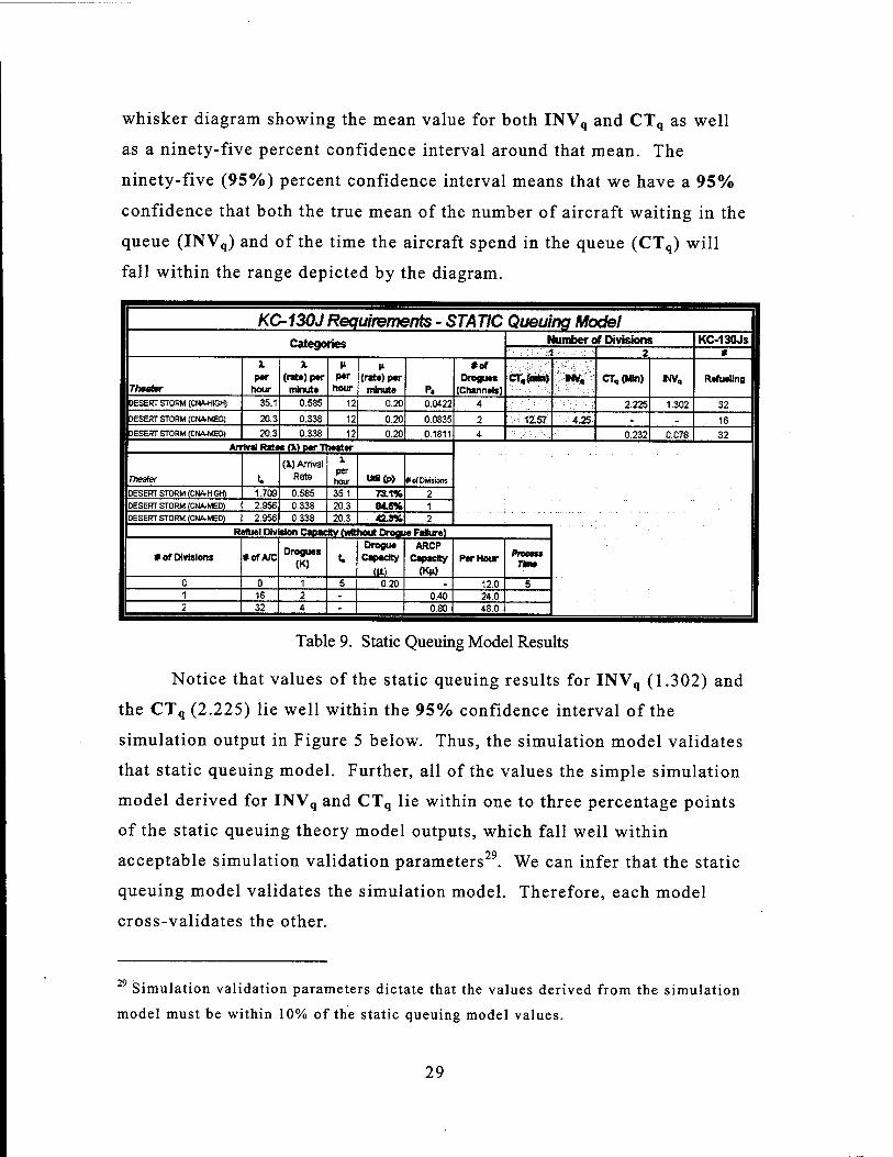
Table 9 below replicates Table 8 from Chapter II and also in

Appendix B; it is presented here to compare the output from the static

queuing and simulation models. Simulation results are presented in

Figure 5 below. The top portion of Figure 5 visually depicts a box and

28

whisker diagram showing the mean value for both INVq and CTq as well

as a ninety-five percent confidence interval around that mean. The

ninety-five (95%) percent confidence interval means that we have a 95%

confidence that both the true mean of the number of aircraft waiting in the

queue (INVq) and of the time the aircraft spend in the queue (CTq) will

fall within the range depicted by the diagram.

KC-130J Requirements - STATIC Queuing Model Categories Number of Divisions KC-130JS

i 2 *

Theatar

X

P»r hour

X (rate) per

minute

per hour

I» (rate) per

minute P.

#of Drogues

(Channels) CTa(mki) 1W« CT„(I&1) IW, Refueling

DESERT STORM (CNA-HIGH) 35.1 0.585 12 0.20 0.0422 4 2.225 1.302 32

DESERT STORM (CNA-MED) 20.3 0.338 12 0.20 0.0835 2 12.57 4.25 - . 16 DESERT STORM (CNA-MED) 20.3 0.338 12 0.20 0.1811 4 0.232 0.078 32

Arrival Rates (I) per Theater

Theater t. (1) Arrival

Rate

X per hour 1*8 ft» # of Divisions

DESERT STORM (CNA-HIGH) 1709 0.585 35.1 73.1% 2 DESERT STORM (CNA-MED) 2.956 0.338 20.3 84.8% 1 DESERT STORM (CNA-MED) 2.956 0.338 20.3 42.3% 2

Refuel Division Capacity (without Drogue Fature)

# of Divisions #OfA/C Drogues

(K) t.

Drogue Capacity

(U)

ARCP Capacity

(K|i) Per Hour

Tana

0 0 1 5 0.20 . 12.0 5 1 16 2 - 0.40 24.0 2 32 4 - 0.80 48.0

Table 9. Static Queuing Model Results

Notice that values of the static queuing results for INVq (1.302) and

the CTq (2.225) lie well within the 95% confidence interval of the

simulation output in Figure 5 below. Thus, the simulation model validates

that static queuing model. Further, all of the values the simple simulation

model derived for INVq and CTq lie within one to three percentage points

of the static queuing theory model outputs, which fall well within

acceptable simulation validation parameters29. We can infer that the static

queuing model validates the simulation model. Therefore, each model

cross-validates the other.

29 Simulation validation parameters dictate that the values derived from the simulation

model must be within 10% of the static queuing model values.

29

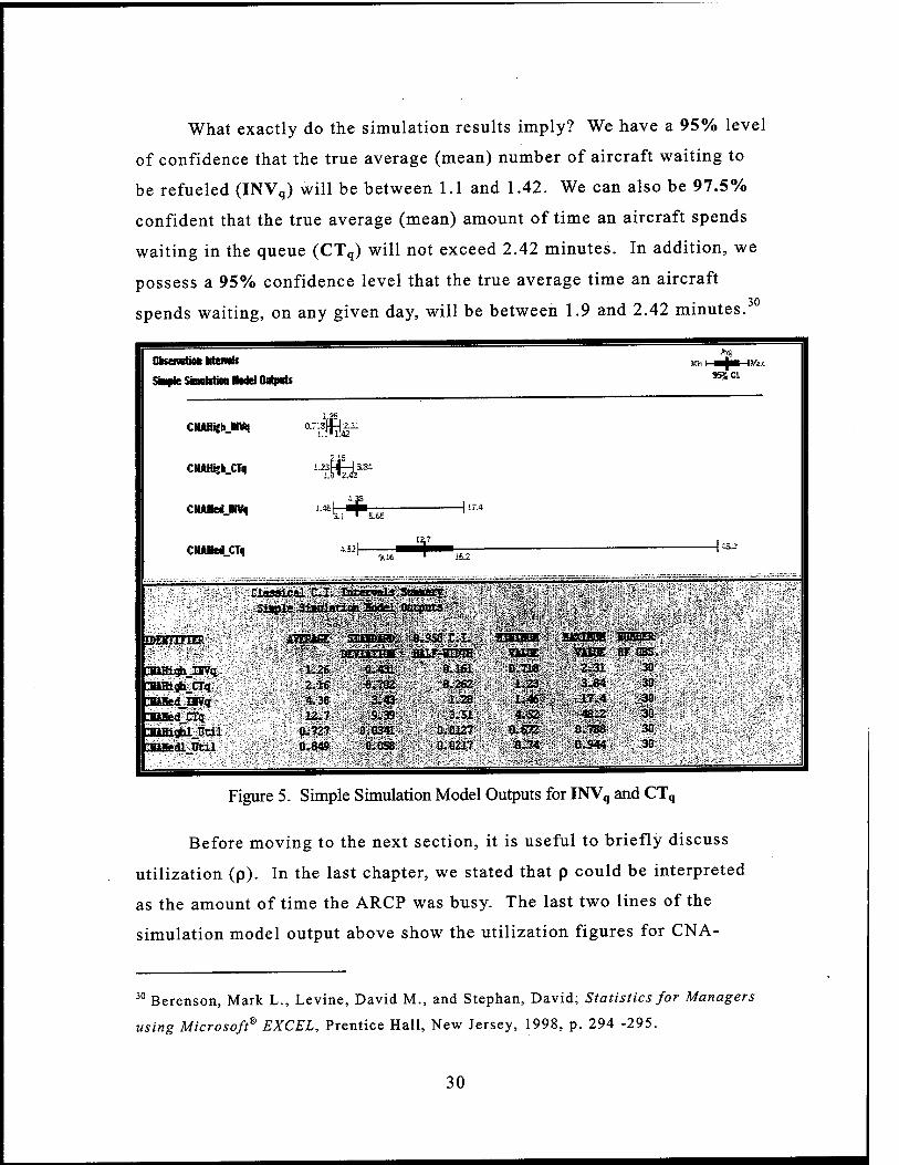
What exactly do the simulation results imply? We have a 95% level

of confidence that the true average (mean) number of aircraft waiting to

be refueled (INVq) will be between 1.1 and 1.42. We can also be 97.5%

confident that the true average (mean) amount of time an aircraft spends

waiting in the queue (CTq) will not exceed 2.42 minutes. In addition, we

possess a 95% confidence level that the true average time an aircraft 30

spends waiting, on any given day, will be between 1.9 and 2.42 minutes.

OtaemtiM Memb Av.J

Swpte Simulation IMd Oatpvti 95% Cl

CIUHi;b_inA| 0.71SJH 2.3J

CNAWjhCT« L?ÄiiSi

CNJUtalJNVi

CNJUWCTq

i-i £ In

|J&2 .i --A —

11--'

12,7 •k^\———wm

9.16 ■ 16.2

r-:^> ■%.■*,' '%*«pf :iB39ical C.I. Intervals Siaur; K.

i§t§ ||§äJä§llSsf **>>?¥ r bf *^ ' V ^

WXXIlXUäk'- ATOME SIWBM O.950 £.L ;': HISIBUH OKIBUB KHBER

ummor BUJMnWH : . mat . ;■'•. VilCE 0F OBS.

CBiEi#t H?<I 1.26 0.431' ' 0.161. 0.718 2.31 30 OBHigh CTq 2.16 0.702 0.262 l~Z3l: 3.84 30 uEUfed Wfq 4.38 3.4li 1.28 um Slllte 30 Sued CTq 12.7 9.Ä ii«ül|i|lp 4.52 48.2 30 f^^^'i^:tMi^£ä;-%:ft rmffi jii Ptii 0.727 0.0341 0.0127 îäjifip^ 0.-788 30 □BBedlJJtil 0.849 0.058 0.0217 \ tJ.74 0.944 30

. *'- "

Figure 5. Simple Simulation Model Outputs for INVq and CTq

Before moving to the next section, it is useful to briefly discuss

utilization (p). In the last chapter, we stated that p could be interpreted

as the amount of time the ARCP was busy. The last two lines of the

simulation model output above show the utilization figures for CNA-

30 Berenson, Mark L., Levine, David M., and Stephan, David; Statistics for Managers

using Microsoft® EXCEL, Prentice Hall, New Jersey, 1998, p. 294 -295.

30

HIGH and CNA-MED. Average utilization is listed in the first column.

We can interpret these numbers to mean that all of the ARCP's drogues are

busy 72.7% of the time with a CNA-HIGH arrival rate (X); they are busy

84.9% of the time for CNA-MED.

These two numbers are both within one percent of the static queuing

model (p) numbers contained in Table 9 above. These lie well within

acceptable validation parameters for each model, as discussed earlier.

These (p) values will become relevant as we enhance our simulation

model in the next section of this chapter.

Considering the range of the potential possibilities, the simulation

model better emulates the variability an ARCP realistically encounters.

Therein lies the critical difference between the simulation model and the

static queuing theory model. The simulation generates many variates that

are used to solve equations for INVq and CTq for many different aircraft

allowing for the gathering of data over a simulated period of time.

Nevertheless, the information gained from both models has enabled us to

cross-validate both models. Next, we will add an additional level of

sophistication to the simulation model.

C. AERIAL REFUEL CONTROL POINT ENHANCED

SIMULATION MODEL DESCRIPTION AND OUTPUT

1. How do we enhance the existing simulation model?

Appendix A contains the schedule of the 24-Hour ARCP Schedule.

In our simple simulation model, we have one KC-130J with two or four

drogues on station continually, depending on the number of KC-130J

Divisions supporting the ARCP. What information could we derive from

the simulation model by mimicking the ARCP Schedule to enhance our

simulation model? First, we would need to add three more KC-130J

31

Tankers, which are simply servers or resources in ARENA®, under the

Enter, Process, and Leave logic, as shown below in Figure 6.

Simulation Logic

Arrive Enter Process Leave Depart Arrival RtfoalDw

RdVielDr/BHi DepaHl

Resource Resource Resource Resource

KE1O0U 1 ■CCIQOU 2 KC130U a KC13U *

Figure 6. Enhanced Simulation Logic

Figure 7. Enhanced Simulation Overview

By doing so, our simulation model depicts the three additional KC-

130J Tankers that will support the ARCP, as shown in Figure 7. These

four aircraft simulate the sixteen aircraft that are required to support one

ARCP during a MTW. Further, if we need to increase ARCP capacity

(K\i) because the theater arrival rate (A,) is greater than the ARCP

32

capacity (Ä, > Kji), then each KC-130J icon can represent two or three KC-

130Js supporting two or three Refuel Divisions, respectively.

Given these enhancements, we can compare the enhanced simulation

output to the simple (base) simulation model and the basic queuing theory

model. Figure 8 below, contains the enhanced simulation model output.

Next we shall explore how and why the two models differ?

2. How and why do the simulation outputs differ between the

two models?

We have used four KC-130Js (resources) to simulate the sixteen

KC-130J schedule shown in Appendix A. The total number of KC-130Js

supporting the ARCP is divisible by four. Instead of making the

simulation exceedingly complicated, we simply used four KC-130Js to

depict the eight KC-130Js supporting the first twelve hour period, and

another four supporting the last twelve hour period of the twenty-four

hour day. Thus, four KC-130Js in the simulation depict sixteen KC-130Js

supporting a twenty-four hour ARCP schedule (see Appendix A). For

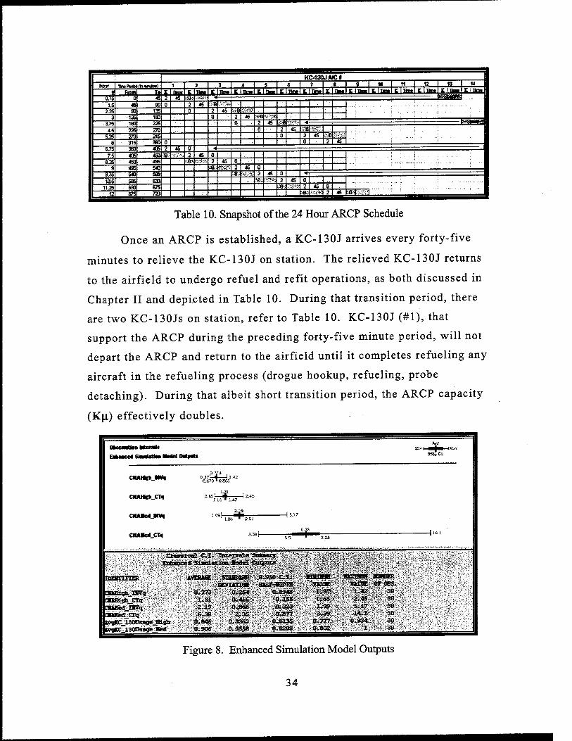
reference, a snapshot of this schedule is provided in table 10.

The first KC-130J in the simulation does not directly correspond to

the first in the schedule, it is merely a placeholder in the simulation.

Depending on the part of the schedule being simulated at any given time,

it could represent the first, fifth, ninth, or thirteenth KC-130J depicted in

the schedule, depending on the time frame being simulated by the model.

The results of the Enhanced Simulation Model are depicted in

Figure 8. By comparing the output from the different simulation or static

models, as shown in this chapter, some interesting results appear. It is

immediately obvious that there is a significant difference in the INVq and

CTq numbers contained in Table 9 and Figure 5 and those depicted in

Figure 8. This section asks what is the difference and why does it exist?

The difference lies in scheduling KC-130J aircraft to support the ARCP.

33

KC-130JMC! II Hour

—A Earn ̂ ^FT'rir-nrir—ir=iP™irir-nriF-inp,-«rir,*iniF—iriF—ii <IF-II «^ni «.-ii «JI -ii «-n 0.75

1.5 45 90 0 2 45 SBpf»! 2.25 90 135 0 2\ 45 »0

3 135 180 0 2 45 w4l &^S?

4.5 225 270 —j— 0 2 45 is!« ■:%?°^

5J25 270 315 I 0 2 45 SB 6 315 360 0 I 0 2 45

7.5 405 453 m 2 45 0 —T~ I I _..,. 625 490 495 ■iSi T-3>ft 2 45 0 I 1

9 495 5« m {fes| 2 45 o : : 9.75 10.5

540 595 630 —| ?-B;fcsl 2 45 0 1 i -- :

11.25 630 675 [ lm srsd 2 45 0

12 675 720 —I— —1—1— i^Jg sssai 21 45 ;*&5.«|

Table 10. Snapshot of the 24 Hour ARCP Schedule

Once an ARCP is established, a KC-130J arrives every forty-five

minutes to relieve the KC-130J on station. The relieved KC-130J returns

to the airfield to undergo refuel and refit operations, as both discussed in

Chapter II and depicted in Table 10. During that transition period, there

are two KC-130Js on station, refer to Table 10. KC-130J (#1), that

support the ARCP during the preceding forty-five minute period, will not

depart the ARCP and return to the airfield until it completes refueling any

aircraft in the refueling process (drogue hookup, refueling, probe

detaching). During that albeit short transition period, the ARCP capacity

(K|i) effectively doubles.

95% C3.

CN*Msb_IM|

CN*Mch_CT<l

0.37J I I 1A2 0.675 ■ o.aes

0.651—m i.uTi.i?

CNMfcCCTo -| ii.i

Classical C.I. Intervals aounrj financed Sianlatlnn Sodd Cutpots

WtXtLFIXR AVERAGE SXUBtHD BEnKim

CBtHi4b_ISVq

CUBed_IB7q - fled_CT<i

tggKC_130P3age_Hed ■•

0.773 1.31 2.19

0.846 0.906

0,254 0.41« 0.B66 2.35

0.0363 0 0558

0.950 C.X. BilF-WWH:

0.0948 o.ass:

0.877 0.0135 0.0206

-7JXDE 0.37

#l|w|i O 777 0.802

Y1E0X. 8T OBS. 1.42 30 2.45 5.17 14.1

0.934

30 30

pis 30

Ssol

Figure 8. Enhanced Simulation Model Outputs

34

The probability that the KC-130J on station will be busy when the

relief KC-130J arrives for CNA-HIGH arrival rate (X) is 72.7%, the

utilization factor (p) (refer to Figure 5 for the simple simulation p factor).

Remember we are using two divisions of KC-130Js to support that (X) or

AR requirement for the CNA-HIGH theater, refer to either Table 9 or

Figure 5. Thus, during 72.7% of the transition periods, or approximately

twelve times per day for the CNA-HIGH arrival rate (X), the ARCP

capacity (Kfi) doubles for a short period until the KC-130J on station can

complete refueling those aircraft actually in the process prior to its

departure.

Comparing the numbers for INVq and CTq between the simple and

the enhanced simulation model, the overlap between sorties causes

approximately a forty-percent reduction ([1.26 - .773] / 1.26 = .3865 ~

40%) in INVq and CTq for CNA-HIGH theater. The difference for CNA-

MED Theater is somewhat different. Comparing INVq and CTq between

the simple and enhanced simulation model, implies a difference of

approximately fifty-percent ([4.38 - 2.19] / 4.38 = .50 ~ 50%).

The difference can be best explained by using the utilization (p)

factors in Table 9. Two KC-130J Tanker divisions are supporting CNA-

HIGH, with four drogues on station at any one time (as depicted in Figure

9 below), and two drogues in the case of CNA-MED. This provides a

ARCP utilization (p) factor of 73.1% (Table 9), for CNA-HIGH and 84.6%

for CNA-MED.

Thus, CNA-HIGH has 26.9% excess capacity that can absorb

aircraft in the INVq, CNA-MED only has 15.4% excess capacity.

Therefore, during the transition period (spike in KJJ,), CNA-HIGH is likely

to have aircraft in the refueling queue. The added capacity can help clear

out INVq more quickly, because on average more drogues are available,

thereby reducing the CTq. The ARCP supporting CNA-MED does not

possess as much excess capacity and on average less drogues are

35

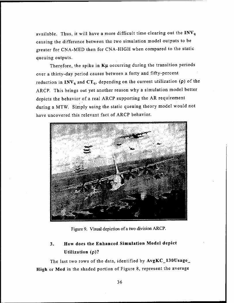
available. Thus, it will have a more difficult time clearing out the INVq

causing the difference between the two simulation model outputs to be

greater for CNA-MED then for CNA-HIGH when compared to the static

queuing outputs.

Therefore, the spike in Kji, occurring during the transition periods

over a thirty-day period causes between a forty and fifty-percent

reduction in INVq and CTq, depending on the current utilization (p) of the

ARCP. This brings out yet another reason why a simulation model better

depicts the behavior of a real ARCP supporting the AR requirement

during a MTW. Simply using the static queuing theory model would not

have uncovered this relevant fact of ARCP behavior.

Figure 9. Visual depiction of a two division ARCP.

3. How does the Enhanced Simulation Model depict

Utilization (p)?

The last two rows of the data, identified by AvgKC_130Usage_

High or Med in the shaded portion of Figure 8, represent the average

36

number of KC-130s being used over the thirty day simulation period.

This factor is similar to utilization (p), but it is not the same.

Since we used four KC-130Js (servers) to simulate the ARCP

schedule in the Enhanced Simulation Model, we cannot gather utilization

information on a single KC-130J (server) on station all the time, as we did

in the simple simulation model and the static queuing model. Instead, we

had four KC-130Js, in the enhanced simulation model, that are being

utilized approximately 25% of the time. Consider the other 75% of the

time, which accounts for the KC-130J in transit to or from the airfield, or

at the airfield being prepared to return to the ARCP. We also have spikes

in ARCP capacity (Kî). These facts combined together make it difficult

to ascertain an ARCP utilization factor (p).

To estimate how much the ARCP was being used, we simply

summed the utilization factors capture by ARENA for each KC-130J

(resource). This estimates the average number of KC-130Js supporting

the ARCP. However, we cannot call this utilization (p) because p is never

greater than one (p < 1); with four KC-130Js, this factor frequently peaks

above one, depending on the X used.31 However, we can use this number

to indicate if the theater arrival rate (X) is stressing the ARCP system.

For example, observe the ARCP p, in Figure 5, identified by

CNA_Medl_Util in the shaded area; this figure indicates that the ARCP

p is approximately 84.9%. This causes both the high INVq and CTq to

exceed the five-minute constraint. This indicates that we must increase

our K|x to bring CTq down to an acceptable level. Now look at the

Enhanced Simulation Model Output, specifically AVGKC_130Usage_

Med within the shaded area of Figure 8. Notice that its average runs

31 Adleman, Dan, Barnes-Schuster, Dawn, and Eisenstein, Don; Operations



37

around 90.6%, indicating we must increase Kî as above. Even though the

Enhanced Simulation Model Output does not give us p, it indicates the

same decisions: in this case add another Refuel Division to support the

ARCP in the CNA-MED Theater.

4. How can we enhance this simulation model further to

better depict how an ARCP would operate supporting a

Major Theater War?

One more aspect of the ARCP should be modeled to ensure that the

Enhanced Simulation Model adequately reflects the behavior and

variability of an ARCP supporting a MTW: drogue failures. Drogue

failures include any occurrence that may cause the KC-130J on station to

loose the use of a drogue and incur a reduction in ARCP capacity (Kji,).

Examples include, but are not restricted to, hydraulic, pump, or

mechanical failure, or even an inexperienced pilot damaging the drogue

through improper probe / drogue coupling procedures.

Fortunately, these occurrences are statistically rare, occurring on

average .025 (or 2.5%) of the time.32 However, it is appropriate to add

this sophistication (drogue failure) to the simulation.33 Figure 10 below,

provides a visual depiction of the logic surrounding the generation of

drogue failures.

Every forty-five minute period in the simulation model, a drogue

failure is created; this failure enters the chance block (i.e.; the second

block from the left). There the computer rolls a pair of dice,

metaphorically speaking, with all of the numerical possibilities between

zero and one. Every forty-five minutes the computer rolls the dice to

32 Interview with Major Patrick S. Flanery, USMC, Marine Aviation Weapons and

Tactics Squadron One (MAWTS-1) KC-130 Instructor, 28 Jul 99. 33 KC-130J Tanker Requirements meeting held at Naval Air Station, Patuxent River,


38

decide if a drogue failure occurs. If the computer's dice generate a

number less than or equal to .025, a failure will occur; if the number

generated is greater than .025, a failure will not occur. But, how does this

affect the enhanced simulation model outputs?

1 ' v:1'"."'^

Drogue Failure Generator

Create . ---,-• ■• - .- ■'-. ~ «Delay »■

>*—■•. .— ..Seizes --Assign H- ..~..~i- --:-- • ---' '45 R8fu«}Divistor»N«mberof FaiiOrogues

'Chance ; DrogueAvaii

•Release »■

RefuelOivisfon -■

Witb025 V™"-7"";? -r:'—r~—' - ——;- - Eis« *~.*-~-« Delay *

«Assign ,»»

( — ■~—L

.. .._ -.. -v. . .... -

Wumtterof FailDrogues DfogueAvail

Figure 10. Drogue Failure Generator

r-■ ■* rfiaii JaiTnii MM rial 4^^^^» ---^-^- ■ ■ urancM anunon MOOM mipw Nmin 99« CL

dUWckJWq

OWHKtl.CTq

CKMMJNVq

LCTq

D.486 086

1.486 h*—11 SI 0.74ST0.975

»h4» 1 1.27 T1£5

1.151—"i* 2m

355 h

-16.18

IS

5.47 7.7

JHWCH

fcjn:_13tB3»gelrt

■jit350;c^-.f-. icfiuüui mrâinH

0.86 0.308 AUS .£46 0 -SB6 (LIB 2.W UM <L38» C.5B i.99 1J2

4»>9B9 .- OvO«: .

S.4BS.'. Ul

1.15 ill us . a.*-

■0.804 0.925 «-« J.S2

30 iaoss

30 .

Figure 11. Enhanced Simulation Model Outputs w/Failures

Figure 11 shows the Enhanced Simulation Outputs with drogue

failures. As one might expect, the INVq, CTq and the average number of

KC-130Js being used will increase from two to ten percent in both the

39

CNA-HIGH and CNA-MED cases. This is within validation tolerances

discussed earlier. This modification, while not significantly affecting the

results, enables us to add another level of sophistication to the enhanced

simulation model to better replicate real world ARCP operations to

estimate the AR requirements in a MTW.

D. CHAPTER SUMMARY

As discussed in detail in this chapter, a simulation model can

provide superior insights into the real life behavior of the system being

studied, in our case an ARCP. In some cases, as in the case of utilization

(p), it cannot provide us with the exact information provided by the static

queuing model or the simple simulation model. Nevertheless, the

information gathered by modeling the real world ARCP will prove

invaluable in helping us develop a range of possible KC-130J Tanker fleet

sizing solutions. A better understanding of how the ARCP functions

during a MTW will help ferret out the most logical range of fleet sizing

solutions.

The next chapter will describe the Life Cycle Cost (LCC)

spreadsheet model for the KC-130J fleet. The analysis will use costs

derived from the cost study completed by Gates, Andersen, Kwon, and

Washburn (1999).34 By the end of the next chapter we shall be able to

ascribe a cost figure to a particular KC-130J fleet size that will enable us

to begin our Cost /Benefit Analysis, chapter five.



1999. Section #1, p. 7.

40

IV. LIFE CYCLE COST MODEL METHODOLOGY AND

ASSUMPTIONS

A. INTRODUCTION

To ascribe a cost figure to the fleet size, previously determined by

the simulation model, requires capturing the cost attributed to procuring,

operating, and maintaining a KC-130J. Professor Alan Washburn of the

Operations Research Department at the Naval Postgraduate School (NPS)

contributed to a Marine KC-130 Requirements study. He captured several

of the crucial KC-130J cost factors, including procurement, operations,

and maintenance (O&M) costs.35 Using these non-inflated real cost

figures as inputs to a Life Cycle Cost (LCC) spreadsheet determines a

total cost figure, in real dollars, of a particular fleet size.

This chapter will be broken up into several distinct sections

describing the LCC model. First, the Sensitivity Analysis sheet will be

described to indicate how variation in key variables affect the overall cost

of a given fleet size. Second, the Deployment and Attrition sheet will be

discussed showing how net fleet size and age is affected by the variables

input into the Sensitivity Analysis sheet. Thirdly, the cost schedule sheet

will be reviewed to explain all of the interactions between the pertinent

variables contained within the LCC model. Next, we discuss how another

simulation program can be added to imbue our LCC model with the cost

variability seen in the real world. Finally, the outputs from the charts'

sheet will be discussed to describe the charts reflecting the input variables

from the Sensitivity Analysis sheet. Appendix C contains all of the



1999. Section #1, p. 7.

41

schedules presented in this chapter as tables. The chapter outline is as

follows:

A. Introduction

B. Sensitivity Analysis Sheet

C. Deployment and Attrition Sheet

D. Cost Schedule Sheet

E. Simulation Inputs and Affects

F. Chart Outputs Sheet

G. Chapter Summary

B. SENSITIVITY ANALYSIS SHEET

1. Why is deriving a Procurement Schedule so critical to the

development of the Life Cycle Cost Model?

The factors which should be considered when conducting a cost

Sensitivity Analysis for procuring a major system are listed in the first

three lines of table 11; Number of KC-130Js Procured; Number of KC-

130Js per year; Years in Procurement Plan. By deriving the maximum

number of KC-130Js to be procured in any given year, the analyst can

develop a procurement schedule. In this case, the KC-130J Program

Manager provided this information. Lieutenant Colonel Isleib, USMC

stated that, at most, the USMC would procure an average of six KC-130Js 36 per year.

The fleet size is entered into the first line of Table 11, entitled

"number of KC-130Js procured." The number procured is divided by the

next line "number of KC-130Js [procured] per year." This results in the

third line, the "years in the procurement plan." These variables are

36 Telephone interview with LtCol Isleib, USMC; Program Manager, KC-130J; 19 July

99.

42

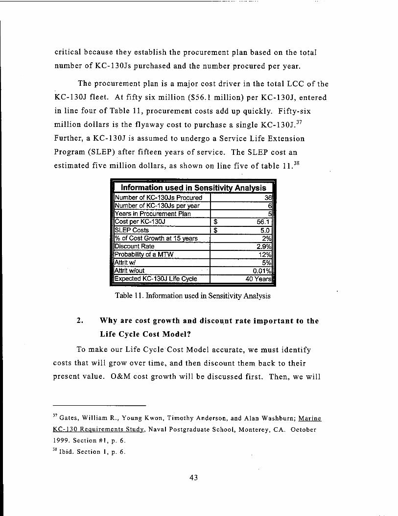
critical because they establish the procurement plan based on the total

number of KC-130Js purchased and the number procured per year.

The procurement plan is a major cost driver in the total LCC of the

KC-130J fleet. At fifty six million ($56.1 million) per KC-130J, entered

in line four of Table 11, procurement costs add up quickly. Fifty-six

million dollars is the flyaway cost to purchase a single KC-130J.37

Further, a KC-130J is assumed to undergo a Service Life Extension

Program (SLEP) after fifteen years of service. The SLEP cost an

estimated five million dollars, as shown on line five of table ll.38

Information used in Sensitivity Analysis Number of KC-130Js Procured 36 Number of KC-130Js per year 6 Years in Procurement Plan 5 Cost per KC-130J $ 56.1 SLEP Costs $ 5.0 % of Cost Growth at 15 years 2% Discount Rate 2.9% Probability of a MTW 12% Attritw/ 5% Attritw/out 0.01% Expected KC-130J Life Cycle 40 Years

Table 11. Information used in Sensitivity Analysis

2. Why are cost growth and discount rate important to the

Life Cycle Cost Model?

To make our Life Cycle Cost Model accurate, we must identify

costs that will grow over time, and then discount them back to their

present value. O&M cost growth will be discussed first. Then, we will



1999. Section #1, p. 6. 38 Ibid. Section 1, p. 6.

43

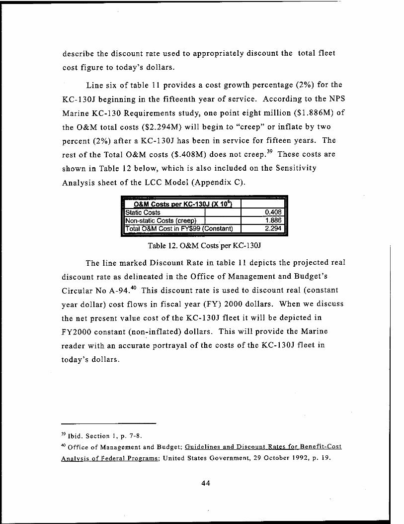
describe the discount rate used to appropriately discount the total fleet

cost figure to today's dollars.

Line six of table 11 provides a cost growth percentage (2%) for the

KC-130J beginning in the fifteenth year of service. According to the NPS

Marine KC-130 Requirements study, one point eight million (S1.886M) of

the O&M total costs ($2.294M) will begin to "creep" or inflate by two

percent (2%) after a KC-130J has been in service for fifteen years. The

rest of the Total O&M costs ($.408M) does not creep.39 These costs are

shown in Table 12 below, which is also included on the Sensitivity

Analysis sheet of the LCC Model (Appendix C).

O&M Costs per KC-130J (X 106) Static Costs 0.408 Non-static Costs (creep) | 1.886 Total O&M Cost in FY$99 (Constant) | 2.294

Table 12. O&M Costs per KC-130J

The line marked Discount Rate in table 11 depicts the projected real

discount rate as delineated in the Office of Management and Budget's

Circular No A-94.40 This discount rate is used to discount real (constant

year dollar) cost flows in fiscal year (FY) 2000 dollars. When we discuss

the net present value cost of the KC-130J fleet it will be depicted in

FY2000 constant (non-inflated) dollars. This will provide the Marine

reader with an accurate portrayal of the costs of the KC-130J fleet in

today's dollars.

39 Ibid. Section 1, p. 7-8. 40 Office of Management and Budget; Guidelines and Discount Rates for Benefit-Cost

Analysis of Federal Programs: United States Government, 29 October 1992, p. 19.

44

3. Why would the probability of an MTW, potential attrition

rates, and the service life of a KC-130J affect the Life

Cycle Cost Model?

The probability of an MTW, and the attrition factor account for the

number of KC-130Js lost during that MTW, can affect the KC-130J Fleet

LCC. Further, an attrition factor should be estimated for KC-130J Fleet

losses during normal peacetime operations. These factors will be

discussed below.

The line immediately below the discount rate is the probability that

an MTW occurs in any given year. This probability was derived from

discussion with Ambassador Rodney Minot of the National Security

Affairs Department NPS.41 A twelve-percent probability may seem rather

high; however, this variable can be changed to reveal its affect on the

LCC of the KC-130J fleet, if considered appropriate.

Finally, the last three lines of Table 11 portray the percentage of

KC130J losses occurring during an MTW (5%), the percentage of KC-130J

losses occurring during normal peacetime operations (.01%), and the

expected KC-130J Life Cycle (40 years). Certainly, some losses may

occur during an MTW and some do occur during peacetime operations.

These factors interact to affect the KC-130J Fleet LCC. For

example, if the probability of an MTW increases, one would incur a

higher LCC to replace the additional KC-130Js lost during the conflict.

The attrition factor for normal peacetime operations will also effect the

KC-130J Fleet LCC, but not significantly at its projected value.

The final line of table 11 contains the service life of a KC-130J.

The forty-year service life of a KC-130J is estimated from empirical

knowledge of the service life for the current KC-130F/R fleet. There are

41 Interview with Ambassador Rodney Minot, 28 September 99.

45

also O&M Difference and Variability schedules on the sensitivity analysis

sheet; each will be explained later in this chapter.

After discussing those factors unique to the sensitivity analysis

sheet (Appendix C), let's look at how they interact with the deployment

and attrition sheet (Appendix C).

C. DEPLOYMENT AND ATTRITION SHEET

The deployment and attrition sheet contains without attrition and

with attrition blocks. An attrition block was added to account for KC-

130Js lost in an MTW. This increases the number of KC-130Js procured

and reduces the number of KC-130Js in operation in a given year. Finally,

the last column depicts the phase-out of the KC-130J fleet, as the fleet

reaches the end of its useful life cycle beginning in the fortieth year.

Deployment / PhaseOut Ran

j KO130J Aerial Refueler without Attrition ^^^^^^^^S^B^^^^gMSMMSMM

PhaseOut Han Year

Reldinq Procurement KGUSÖcIs Vroasperrect KGim,[n ODS Ran Inv. ip^âjiiliiM^ i Losses i-v/Pösft- ■

1997 - - '0 ~o:o3% - - -

1998 2 2 0 000°.«, -■'- • ; _ T ■ - .- 3 W ' • 2 -

1999 3 5 0 0.00% - ' ■ 2 ;•■ "' "5 -

2000 2 7 i '5.00% - 6 - 7 -

2001 6 13 1 - 1PÜP M-.i-" '"t- 7 Ulli' 12 -

2002 6 19 001* tr i 6 "' : ; 19 -

2003 6 25 mm . 0.01% ^^;?ls^$i! 6 ,: ■■" ^ -

2004 6 31 1 *S00% T "" *Z msmm iillllllli -

2005 5 36 0 0LO1% 36 -

2006 - 36 0 0.01% - ^fli^t'S^ ■ 36j ~

Table 13. Snapshot of the KC-130J Deployment / Phaseout Schedule

1. Why do we need to maintain accountability of the number

of KC-130Js fielded and the number in the procurement

inventory?

It is critical to maintain accountability of our KC-130J inventory

net of attrition. We must always know how many KC-130Js we need to

meet the requirement discussed in Chapters II and III. For example, the

46

total number of KC130Js procured in line 1, Table 11, matches the number

of KC-130Js in table 13 in 2005 - 2006, after completing the initial

procurement process. Procurement numbers for years 1997 through 2000

represent actual numbers established prior to the beginning of this study.

One final point regarding the without attrition block. Observe that

five (5) procurement years past 2000 are included in Table 13. This

corresponds to the year's (5) in the procurement plan in table 11. This

can be used as an important validation tool and provides the required

flexibility to change the fleet size, as appropriate, to meet the

requirements identified in the simulation model. This will be explored

further in the next chapter.

2. How does the attrition block make the model more

realistic?

By employing an attrition block, we can model real world events

that may affect the total LCC of the KC-130J fleet. The main event that

could affect the total LCC would be an MTW. How can we model the

affect of an MTW?

This thesis uses the same principles described in the simulation

model in Chapter IV. The random number generator in the EXCEL©

spreadsheet program, along with the probability on the sensitivity analysis

sheet (12%) determines whether an MTW occurs or not. We again use the

computer's fictitious set of dice that contain all of the numerical

possibilities between zero and one, to decide whether we will have an

MTW.

Each time F9 is pressed on the computer keyboard, the computer

rolls the dice. Within this LCC spreadsheet model, one can watch the

estimated costs change by merely pressing F9 on the keyboard. If the

number rolled by our fictitious dice is 0.12 or less, an MTW will occur.

47

If the number derived is greater that 0.12, or twelve-percent, an MTW

will not occur.

Notice that MTW (column #4) and Attrition (column #5) correlate

with one another. If there is an MTW, attrition is 5%; without an MTW,

attrition stays at 0.01%. Again, the attrition percentages are drawn from

the sensitivity sheet outlined above. Further, when an MTW is predicted

KC-130J losses are depicted in column #6.

With attrition, more KC-130Js need to be procured in the year of

the MTW, as shown by procurement w/attrition (column #7). Observe that

the procurement schedule (column #7) is one year ahead of KC-130Js in

operation (column #8). The aircraft procured in any given year, for the

purposes of this model, do not enter operations until the following year.

Finally, the last column of Table 13 is the Deployment / PhaseOut

Schedule. This column contains the KC-130J fleet phase out plan. The

phase out plan reflects the procurement plan forty years later, except that

the USMC divests itself of KC-130Js. In other words, the USMC fielded

two KC-130Js in 1998; thus, forty-years later, in 2037, those two KC-

130Js will be retired and phased out of service. In the next section, we

will describe how the LCC schedule captures this information and allows

us to attribute a LCC to a particular fleet size.

D. COST SCHEDULE SHEET

Table 14 below is a snapshot of the LCC schedule contained in

Appendix C. The first column is the year of the LCC; the range of

different categories is spread across the second row. Each category will

be described in sufficient detail to provide a basic understanding of the

model.

48

1. Why would the accountability of a particular fiscal year

designator be important to the Life Cycle Cost Model.

The year designator (column #2) indicates the number of years in

the program from fiscal year (FY) 2000. The years before FY2000 are

identified by the number of years that separates them from FY2000. This

column is used in the net present value (discounting) calculations. As we

calculate the Net Present Value (Costs) of a particular KC-130J fleet size,

we must use the future value equation (equation 8 below) for those years

preceding FY2000. After FY2000, we must bring each year's costs back

to FY2000 (constant) dollars (equation 9 below). This is critical to

deriving an accurate cost estimate for the LCC of the particular KC-130J

fleet size in FY2000 dollars. When we begin discussing Costs (FY2000$)

this discussion will become more relevant.

2. How are the costs accounted for in the Life Cycle Cost

Model?

The columns in Table 14 that depict Procurement with attrition and

KC-130Js in operation (columns #3 and #4) are the same as those with the

same headings in table 13. Recall that the KC-130J we procure (pay for)

this year will not be in operations (fielded) until next year. Thus, they

will not incur O&M costs until the following year. Further, the cost of

KC-130Js (column #5) multiplies the number of aircraft procured that

year, after accounting for attrition, by the cost to procure the aircraft

($56.1 million), as shown in the sensitivity analysis schedule. The Static

and Non-static O&M cost categories without creeping (columns #6 and

#7) can be calculated in the similar way. By using the static and non-

static O&M cost figures contained in table 12 (page 44, above) and

multiplying them by the number of KC-130Js in operation.

Cost growth (column #8) delineates the costs associated with the

two percent "creep" as a KC-130J reaches its fifteenth year of service.

49

This model portrays the newest KC-130Js (having not reached 15 years of

service) being attrited first. By loosing newer KC-130Js, the two-percent

creep of KC-130Js is not postponed for another fifteen years; thus, the

two-percent creep will be incurred from the fifteenth year until

retirement.

lUfeCyc e Cost Analysis: KC-130JFlMtNPVfl.CC) $ 4.809.549.396

Year/ Year Designator

Procurement w/attrition

LC-130JS

in

Operation

Cost of

KC-130J

Static Costs

Non-Static Costs

Cost Growth (Lose New)

SLEP Costs

Costs (FY*2000$)

Cumulative (FY$2000$)

Costs

v'îJHTX;: 3 ■ 2 0 112.2 :"'.- '■: ■ . - 122.2 122.2

wmaem 2 3 2 168.3 0816 3.772 - 183.1 305.3

*mmm 1 2 ■5 112.2 2.040 9.430 -. 127.3 432.6

'■". 2000 ''"';: 0 6 7 336.6 2.856 13.202 ■-. 352.7 785.2

'200sfe" 1 6 13 336.6 5.304 24.518 ■:■■-. 356.1 1,141.3

... ^2002i«: 2 6 19 336.6 7.752 35.834 -■'■■ 359.1 1500.4

■":-.7BBSS:-f 3 6 •:-25 336.6 10.200 47:150 ■■":•', 351.6 1,861.9

i 2004 4 6 31 336.6 12.648 58.466 ■ ■ : -• 363.7 2225.6

:'^2006ft. 5 5 36 260.5 14.688 67.896 "..'.-■ 314.7 2540.3

•-.-SBOS?"- E 0 36 0.0 14.686 67.896 69.6 2509.9

'?'-:280rr-: 7 0 36 0.0 14.688 67.896 67.6 2,677.5 :3saao83ß' 8 0 36 0.0 14.688 67.896 - 65.7 2.743.2

mm&m 9 0 . ..36. ■. 0.0 14.688 67.896 '-': ■■- 63.8 2507.1

âowsf 10 2 34 112.2 13.872 64.124 - ■ 142.9 2350.0

' 2011 11 0 36 0.0 14.688 67596 - 60.3 3JD10.3

■.-.-■:aM2-'?;Ä 12 0 36 0.0 14.688 64.049 3347 10.000 65.7 3076.0

Table 14. Snapshot of the Life Cycle Cost Analysis

By doing this we build an LCC model that accounts for the highest

O&M costs because we do not defer the creeping cost affect for fifteen

years each time we loose a KC-130J. This was necessary to avoid undue

complications in the LCC model. Certainly, there is some probability that

the USMC will lose both older and newer KC-130Js during an MTW;

however, that calculation lies beyond the scope of this thesis.

To estimate the range of costs between losing new verses old KC-

130Js in an MTW, another sheet, LCC (2), and attrition schedule has been

developed. LCC (2) is the same as LCC except for the cost growth

column. The cost growth column in LCC (2) assures the USMC loses

older KC-130Js during an MTW. This was done to furnish a scaling

between the two extremes; Table 15 below depicts the numerical

differences. Thus, in this case the difference between losing new verses

50

old is about one hundred and eighty-nine million dollars. This represents

approximately four percent of the cost of losing new KC-130Js during an

MTW.

O&M Difference Schedule Cost Lose Newer Cost Lose Older Difference btwn losing old / new

% Difference of old

$ 4,809,549,396 $ 4,619,770,144

$ 189,779^53 3.95%

Table 15. O&M Difference Schedule

Finally, the second to the last column in Table 14 sums columns

four through eight and calculates the total annual costs in FY2000

(constant) dollars. The LCC model uses either equation 8 (future value)

or 9 (present value) below depending of the year being considered. Those

years prior to FY2000 will use the future value equation (equation #8) to

calculate costs for those years in FY2000 dollars; years following FY2000

will use the present value equation to bring each year's costs back to

FY2000 dollars.

Future Value = Cn X (1 + d) n

*Where C„ = cost incurred at the end of time period n.

d = Appropriate discount rate for the future cash flows

n = Time neriod when the cost occurs

Equation 8. Future Value Equation42

The last column calculates a cumulative total of the FY2000 dollar

costs for the KC-130J fleet, from the initial procurement until the last

KC-130J is phased out. The cumulative cost in this column measures the

final KC-130J Fleet Net Present Value (NPV) in any given year; the final

year is the overall cost of the program in FY2000 dollars. The next

42 Blanchard, Benjamin S.; Logistics Engineering and Management, 5th Edition,

Prentice Hall Publishing, Upper Saddle River, New Jersey; 1998, p. 490.

51

section explores how to make the LCC model more accurately reflect the

variability in LCC over the service life of our KC-130J Fleet.

Present Value = Cn X (1 + d) -n

*Where Cn = cost incurred at the end of time period n.

d = Appropriate discount rate for the future cash flows

n = Time period when the cost occur

Equation 9. Present Value Equation43

E. SIMULATION INPUTS AND AFFECTS

By using an EXCEL® spreadsheet - add on, called Crystal Ball©, we

can imbue the LCC Model with some realistic cost variability. The

factors that seem to possess the most significant uncertainty are SLEP

costs, % Cost Growth [in O&M Costs], discount rate, probability of an

MTW, and the attrition the KC-130J fleet would incur during an MTW.

These factors feed through the sensitivity analysis sheet and ultimately

affect the entire model to provide us with a NPV (Costs) of the fleet size

chosen.

Table 16 shows the distribution (column #5) around the mean or

average (column #2) value for each of the variables explored by Crystal

Ball©. The distribution is characterized by the parameters contained in

change and variability (columns #3 - #4). For example, the SLEP costs

use a normal distribution with a mean of five million and a standard

deviation of five hundred thousand. Alternatively, the probability of an

MTW assumes a triangular distribution with a mean of twelve percent, a

lower bound of five percent, and an upper bound of fourteen percent. A

visual depiction of the distributions for each of the Key External or Policy

variables shown in Table 16 is contained in Appendix D.

43 Maher, Michael; Cost Accounting: Creating Value for Management, McGraw-Hill

Companies, Inc.; 1997, p. 700.

52

Variability Chart Key External & Policy Variables Mean Change Variability Distribution

SLEP Costs 0.50 cr=+/-5 Normal

% of Cost Growth at 15 years 1% o=+/-1% Normal

Discount Rate 1% a=+/-1% Normal

Probability of a MTW from 5% to 14% Triangular Attritw/ 2% a=+/-2% Normal

Table 16. Variability Chart

Again, the computer has the set of dice with all of the numeric

values possible in the defined distribution. As the simulation model runs,

the computer rolls the dice over many trials (iterations). With each trial,

the value we are attempting to forecast is derived, in this case the KC-

130J Fleet NPV (LCC). Over numerous trials, a range of forecasted

values for NPV (LCC) will begin to develop. With sufficient trials, this

enables us to forecast the NPV (LCC) of a particular KC-130J fleet size

with a certain level of confidence (similar to the ARCP simulation). This

is illustrated in Figure 12.

3,000 Trials

.025-

.019

Forecast: KC-130J Fleet (36) NPV (LCC)

Frequency Chart

.a

o

.013^-

.006^

.000

49 Outliers

75

56.25

► i $3,500,000,000 $4,187,500,000 $4,875,000,000 $5,562,500,000 $6,250,000,000

Certainty is 95.00% from $3,665,000,000 to $5,800,833,333

Figure 12. Forecast: KC-130J Fleet NPV (LCC)

We now have a 95% confidence that a fleet size of thirty-six KC-

130Js will cost between 3.7 and 5.8 billion in FY2000 dollars, as depicted

53

in the last line of Figure 12. This provides a cost range coupled with a

level of confidence that the cost of a specified KC-130J fleet size will fall

within those parameters. The overall Project NPV (FY$2000 Costs) is

detailed visually in the chart sheet.

F. CHART OUTPUTS SHEET

The chart sheet provides two visual depictions that help the reader

understand where the dollars are spent on the KC-130J fleet. Figure 13

breaks down the Life Cycle Costs of the KC-130J fleet into procurement,

O&M, and SLEP Costs. O&M costs make up the majority (56%) of the

LCC for the KC-130J Fleet. This is consistant with most LCC 44 projections.

Figure 14 portrays the annual costs of the KC-130J fleet over the

entire life cycle. The peaks and valleys reflect the probabilistic MTW

during the KC-130J Life Cycle. Costs increase as the USMC replaces KC-

130Js lost in an MTW. Again, this graph is consistent with other LCC

projections.45

44 Ibid. p. 180.

45 Ibid. p. 180.

54

KC-130J Life Cycle Cost Breakdown

/^K" Figure 13. KC-130J Life Cycle Cost Breakdown

G. CHAPTER SUMMARY

We have developed a simple LCC Model that contains some realistic

cost variability. This model will allow us to attach a cost figure [KC-130J

Fleet NPV (LCC)] to a particular KC-130J fleet size. Ultimately, this will

enable us to conduct a Cost / Benefit Analysis (Chapter V). This will

combine fleet size, system performance figures derived from the ARENA®

Simulation Model reviewed in Chapter III, and the LCC values for the

fleet size estimated using the LCC model. Combining these outputs will

enable Marine planners to consider a range of KC-130J fleet sizing

possibilities, highlighting the tradeoffs between fleet size, system

performance, (waiting time ~ CTq), and LCC.

55

KC-130J LCC Chart 500.0

•Yearly Costs

50.0 --

liI i ii l l l l l II l l l l l ll i i i _i_

r^- o co co o o o o 05 o o o T- CM CM CM

O O CM

CM in co T- T- T- T- CM o o o o CM CM CM CM

CM O CM

N- O CM CO O O CM CM

CO «D 01 CM CO CO CO ^3" O O O O CM CM CM CM

Ift CO •"* ■* O O CM CM

r- Ta- in m o o CM CM

Figure 14. KC-130J LCC (Graph) Chart

56

V. COST / BENEFIT ANALYSIS: ALTERNATIVE FLEET

SIZING OPTIONS

A. INTRODUCTION

In the operations plans for two near simultaneous MTWs, the

critical point occurs when the USMC transitions its aviation assets from

one theater (western MTW) to the other (eastern MTW). This is when

USMC aerial refueling assets (KC-130Js) are most taxed.46 This

particular transition point drives the USMC KC-130J fleet size. Thus,

capturing the requirement for USMC aerial refueling assets at that point

provides the most accurate picture of the required USMC KC-130J fleet

size.

This chapter identifies the fleet size required to meet the aerial

refueling requirements for each MTW during both day and night ARCP

operations using the enhanced simulation model outlined in Chapter III.

Using the LCC Model, a KC-130J Fleet NPV (LCC) figure will be

defined. Finally, a cost / benefit analysis will be conducted to highlight

the tradeoffs between CTq and LCC of the particular KC-130J Fleet size.

The chapter outline is as follows.

A. Introduction

B. KC-130J Fleet Sizing Requirements for day operations

C. KC-130J Fleet Sizing Requirements for night operations

D. KC-130J Fleet Sizing Costs

E. KC-130J Fleet Sizing Cost / Benefit Analysis

F. Chapter Summary



1999. Section #2, p. 24.

57

B. KC-130J FLEET SIZING REQUIREMENTS FOR DAY

OPERATIONS

We can use the queuing theory spreadsheet from chapter II to define

the preliminary requirement for KC-130J divisions to meet the dual MTW

requirement. Table 17 (Appendix B) provides the starting point for the

simulation model. Also, recall that our daytime refuel (process) time for

one drogue is five minutes.

Notice that the arrival rate per hour (X) for East Surge (column #2)

is the same as the CNA-HIGH scenarios used in chapter II and III. Thus,

East Surge (MTW) requires two divisions of KC-130Js; anything less

would cause an unacceptable CTq for those aircraft waiting to be refueled.

In contrast, West-18 (MTW) falls into an indeterminate range where a

tradeoff must be considered.

Using the static queuing model as a benchmark, supporting West-18

with a single division implies a CTq of 6.43 minutes (the time aircraft

spend waiting to be refueled). Add another division to support West-18,

the ARCP CTq would drop dramatically to 0.149 minutes. Adding another

KC-130J Division to the ARCP mission provides a significant increase in

ARCP capacity (K|i), as discussed in Chapter II.

During a KC-130J requirements meeting held at Naval Air Station,

Patuxent River, the KC-130J community experts felt it relevant to

consider the affects of either Allied aircraft or MV-22 assets that may

require refueling during an MTW.47 Section two of the Marine KC-130

Requirements Study addresses these affects and includes a 10% increase in

the theater arrival rates (A,) in the base case.48 This thesis increases the

48

47 KC-130J Tanker Requirements meeting held at Naval Air Station, Patuxent River,


Gates, William R., Young Kwon, Timothy Anderson, and Alan Washburn; Marine


1999. Section #2, p. 40.

58

arrival rates for East Surge and West-18 by 10%, referred to as East Surge

(+10%) and West-18 (+10%) in table 17 (Appendix B). The resulting

tradeoff between one and two divisions supporting the West-18 Theater is

much greater; ARCP CTq is 12.57 minutes with a single division and

0.232 minutes with two KC-130J divisions.

Adding a second division to West-18 (+10%) enables the USMC to

meet the five-minute ARCP CTq constraint, but the ARCP utilization (p)

drops by 50%. This means that 42.3% of the time the ARCP is busy, but

the ARCP has 57.7% excess Kp, (ARCP Capacity). Excess capacity will

be discussed further in the Cost / Benefit Analysis section of this chapter.

KC-130J Requirements (Day) - STATIC Queuing Model Analysis Categories Number of Divisions KC-130JS

1 2 # Theater #

Theater per

hour

X (rate) per minute

per hour

(rate) per minute Po

#of Drogues

(Channels) CTq (min) INV„ CTq (Hin) IMV„ Refueling

Total Dual MTW East Surge 35.1 0.585 12 0.2000 0.0422 4 - ■ ■■-. 2.225 1.302 32 48 West -18 18 0.300 12 0.2000 0.1429 2 6.43 1.93 16 24 72 West -18 18 0.300 12 0.2000 0.2210 4 - ■ -. 0.149 0.045 32 48 96 East Surqe (♦ 10%) 38.6

20.3 0.644 12 0.2000 0.0265 4 ." . - 3.862 2.485 32 48

West-18 M0%) 0.338 12 0.2000 0.0835 2 12.57 4.25 16 24 72 West -18 (♦ 10%) 20.3 0.338 12 0.2000 0.1811 4 - - 0.232 0.078 32 48 96

Arrival Rates ft) per Theater Refuel Division Capacity (without Drogue Failure)

Theater U

(A) Arrival Rate

X per

hour use« »o»

Divisions of Division #ofA/C Drogu es(K) U

Drogue Capacit

yW

ARCP Capacity

(K>> Per Hour

Process Time

East Surge 1.709 0.585 35.1 73.1* 2 0 0 1 5 0.20 - 12.0 5 West -18 3.333 0.300 18 75.0% 1 1 16 2 - 0.40 24.0

West -18 3.333 0.300 18 375% 2 2 32 4 - 0.80 48.0

East Surge (♦ 10%) 1.554 0.643 38.6 «UK 2

West -18 (♦ 10%) 2.956 0.338 20.3 84.6% 1

West-18 r>10%) 2.956 0.338 20.3 423% 2

Table 17. KC-130J Requirements (Day) - STATIC Queuing Model Analysis

The last three columns in the top schedule of table 17 calculate the

number of KC-130Js required to support both the ARCP mission and the

other missions for which KC-130Js are tasked. These missions include

Direct Air Support Control (Air) [DASC(A)], cargo transport, rapid

ground refueling (RGR), and Airborne Standby.49 Marine Aviation

Weapons and Tactics Squadron One (MAWTS-1) projected that the ARCP

49 Ibid. Section #2, p. 22-24.

59

mission makes up 66.7% of the USMC KC-130J mission requirements;

this percentage is used here.50 Thus, DASC(A), Cargo Transport, RGR

and Airborne Standby make up 33.3% of the USMC KC-130J missions.

In table 17, the column titled KC-130J-Refueling shows the number

of KC-130Js required to support that theater's arrival rate (X) and meet

the minimum five-minute ARCP CTq constraint. The next column titled

"Total" divides the number of KC-130Js required to support the ARCP

requirement by 66.7%. This calculates the total number of KC-130Js

required to meet all assigned missions in that theater.

Thus, it takes forty-eight KC-130Js to meet the requirements of the

East Surge Theater using two KC-130J divisions (second to the last

column marked, "Total"). West-18 theater requires twenty-four KC-130Js,

if a single KC-130J division supports the ARCP Mission, and forty-eight

KC-130Js if two divisions are used. The same calculations are applied to

East Surge (+10%) and West-18 (+10%) in table 17.

The final column (Dual MTW) calculates the total number of KC-

130Js required to support both theaters, simultaneously. For example, the

value for West-18 (row #2) reveals that if the USMC supports East Surge

with two divisions and West-18 with one division, seventy-two KC-130Js

will be required for all missions in both theaters. If the USMC supports

the West-18 theater with two divisions, ninety-six KC-130Js would be

needed. Nevertheless, the larger requirement would enable the USMC to

meet its five-minute ARCP CTq constraint in both theaters. As stated

earlier, tradeoffs will have to be made.

Finally, the utilization factors (p) in the bottom left of the schedule

in table 17, marked as Arrival Rates (X) per Theater, provide a percentage

value showing the percentage of time the ARCP is serving a customer.

50 Ibid. Section #2, p. 37.

60

These factors will be useful later for discussing the tradeoffs between the

fleet size required to achieve a certain level of system performance, CTq

and the cost ofthat fleet. This is addressed in the cost / benefit analysis

section of this chapter.

These results can be compared to the ARCP CTq results from the

simulation model given the arrival rates (X) shown in table 17 for each

theater. Figure 15 below contains the simulation results for East Surge,

using two divisions to support the ARCP mission, and the results for one

and/or two divisions supporting the West-18 ARCP mission. Observe that

the simulation results are not the same as the static queuing model for

reasons discussed in chapter III. However, the conclusions in some cases

are similar to those derived using the static queuing model.

SäMU&M m»m CT< Oatputt 95% ci

EMtSai{e_CT4 o.s2s|—-afa— 1 z.n

«MjtMCT, o.°<f$ 0.O497JH 0.2Z6 0.107'du,

; Classical C.2. InteiwBls Su»ary -■.■■■:'.-■ '•„,'";.-'..'■ SJjulatloa Bodel CTq Ooqmts. '.-;"'./.•••", ''*'*?■„ ;.";'j.'fe'. ;',

EastSuxflejXtt J..« " QJS&.; ' ' gi3S$ 0.828% -1 2.*4 30. fest.182v.CTq -. ':4JWjÜ^:ffc5?v,-;.' ■ yfcsit'.)' i^*i%7<fclü ■' ■ -30 • fest.l8*:CTll : ' ■;■■ . • 0^3|trv. SK o'mX~ {- . ^8265 ' .0i84^|S{''U386-;" 30- brgKC_1300sage_East rO.»?.'•; !f8^B336,- * 0.0125 -0^884;;'A '.-'0.92S 30 LvgKC_1300saoe_182 0.821-0??Je639'. 0.0239 8:^^, ";B.«2S : :: 30 lwgKC_1300sage_184 0.478 ';. 0.8381., "fiU&42' •-:: Ö.39i;' "OiSSr. 30

Figure 15. Simulation Model CTq Outputs (Day)

The USMC still needs at least two divisions to support the ARCP

mission in the East Surge Theater. Further, a single KC-130J division

supporting the West-18 ARCP mission provides an average of 4.14

minutes CTq. With a 95% confidence level, the true mean ARCP CTq for

the West-18 will fall between 3.56 and 4.73 minutes. Thus, it appears the

61

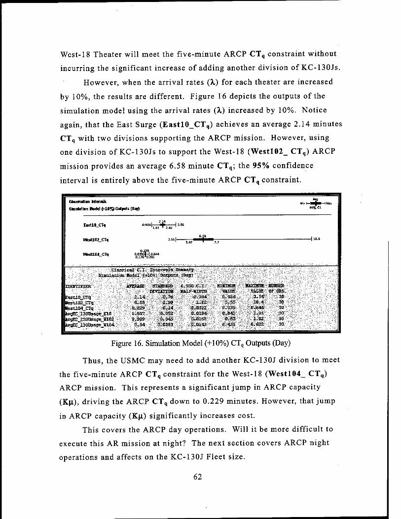
West-18 Theater will meet the five-minute ARCP CTq constraint without

incurring the significant increase of adding another division of KC-130Js.

However, when the arrival rates (X) for each theater are increased

by 10%, the results are different. Figure 16 depicts the outputs of the

simulation model using the arrival rates (X) increased by 10%. Notice

again, that the East Surge (EastlO_CTq) achieves an average 2.14 minutes

CTq with two divisions supporting the ARCP mission. However, using

one division of KC-130Js to support the West-18 (Westl02_ CTq) ARCP

mission provides an average 6.58 minute CTq; the 95% confidence

interval is entirely above the five-minute ARCP CTq constraint.

Observation Menials

Simulation Model (+10fi Outputs (Da?) »5%Cl

EastlO_CTq 0.9Z4I m 1 3.54 1.85^2.«

KVestl02_CTq 3.SS[- 6.5,8

5.47 " 7.7 1 1S.4

Wfcstl04_CTq 0.O39IIH 0.644 0.176 "0.281

Classical-C.I. mterrala Snnwiry .';.:.'. SlTtulairtrm Hoäal .<-HO%) Ontpacs

EDEHTinER AVERAGE :STM8MRI> - 0.950 C.I. jmYTwnff HUHtitk ■ PIINIHHH DEvifiTnar . -fiUF-uiinu: . VSHE, VMIffi orroBS.

EastlO CTq : 2.14 [-0.76: .0.284.'; 0.924 .■.-.'. 3.54 ,;.:.30 ■

iestl02 CTq • 6.S8 ■■:"■•.2.99 ■-■ .;■ 1.12. -■3.55 - •-...- 18.4. ■■-...;■ 30.;. v.;

BestltM CTq 0.229 , 0-i4 -. 0.0522, 0.039 0.644 . 30 ' -'■■ '"

ivgKC '13a0SageiE10 .- 0.937.: ■■■} 3J.052 .- '■;■■•■ 0.0194;:, ■ -; b.JS4i-- : ; ■ -v 1.05- . -30- .. .... tsnjlX I30üsagejö02 0.909 :fl.04S CtOlSS :0.82 1.02 30 tar&X 130Osagejn04 0..S4 0:0383 !0.i.bl43 -- ■ -■.-■Ö.-455 '■" 0.622 30,

Figure 16. Simulation Model (+10%) CTq Outputs (Day)

Thus, the USMC may need to add another KC-130J division to meet

the five-minute ARCP CTq constraint for the West-18 (Westl04_ CTq)

ARCP mission. This represents a significant jump in ARCP capacity

(KjLl), driving the ARCP CTq down to 0.229 minutes. However, that jump

in ARCP capacity (Kjl) significantly increases cost.

This covers the ARCP day operations. Will it be more difficult to

execute this AR mission at night? The next section covers ARCP night

operations and affects on the KC-130J Fleet size.

62

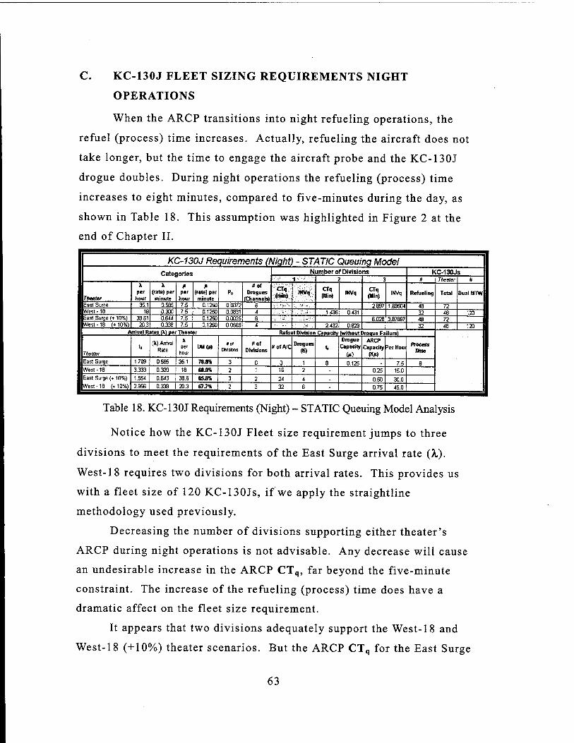
C. KC-130J FLEET SIZING REQUIREMENTS NIGHT

OPERATIONS

When the ARCP transitions into night refueling operations, the

refuel (process) time increases. Actually, refueling the aircraft does not

take longer, but the time to engage the aircraft probe and the KC-130J

drogue doubles. During night operations the refueling (process) time

increases to eight minutes, compared to five-minutes during the day, as

shown in Table 18. This assumption was highlighted in Figure 2 at the

end of Chapter II.

KC-130J Requirements (Night) - STATIC Queuinq Model Categories Number of Divisions KC-130JS

1 2 3 # Theater #

Theater

X per

hour

X (rate) per minute

per hour

(rate) per minute

Po #of

Drogues (Channels)

(mm) IHVq CTq (Hin)

INVq CTq (Min)

INVq Refueling Total Dual MTW

East Surqe 351 0.585 7.5 0.1250 0.0072 6 - -. ' . 2.897 1.69504 48 72 West -18 18 0.300 7.5 0.1250 0.0831 4 . . - 1.435 0.431 32 48 120 East Surge (+10%) 38.61 0.644 7.5 0.1250 0.0035 6 . . 6.028 3.87897 48 72 West-18 (+10%) 20.3 0.338 7.5 0.1250 0.0568 4 - ■- 2.432 0.823 32 48 120

Arrival Rales (X) per Theater Refuel Dnnsian Capacity (without Droque Failure)

Theater t.

(X) Arrival Rate

X Der

hour IHCP)

#ot Divisions

#of Divisions

#ofA/C Drogues

(K) t,

Drogue Capacity

to

ARCP Capacity

(K>)

3er Hour Process

Tkrn

East Surge 1.709 0.535 35.1 78JW 3 0 0 1 8 0.125 . 7.5 8 West -18 3.333 0.300 18 60.014 2 1 16 2 0.25 15.0

East Surge (♦ 10%)

West-18 (.10%)

1.554 0.643 38.6 85.8* 3 2 24 4 0.50 30.0 2.956 0.338 20.3 67.7« 2 3 32 6 • 0.75 45.0

Table 18. KC-130J Requirements (Night) - STATIC Queuing Model Analysis

Notice how the KC-130J Fleet size requirement jumps to three

divisions to meet the requirements of the East Surge arrival rate (X).

West-18 requires two divisions for both arrival rates. This provides us

with a fleet size of 120 KC-130Js, if we apply the straightline

methodology used previously.

Decreasing the number of divisions supporting either theater's

ARCP during night operations is not advisable. Any decrease will cause

an undesirable increase in the ARCP CTq, far beyond the five-minute

constraint. The increase of the refueling (process) time does have a

dramatic affect on the fleet size requirement.

It appears that two divisions adequately support the West-18 and

West-18 (+10%) theater scenarios. But the ARCP CTq for the East Surge

63

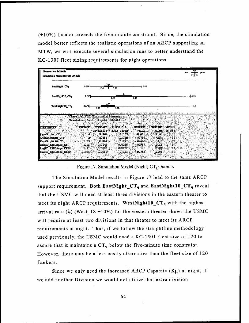
(+10%) theater exceeds the five-minute constraint. Since, the simulation

model better reflects the realistic operations of an ARCP supporting an

MTW, we will execute several simulation runs to better understand the

KC-130J fleet sizing requirements for night operations.

Obteniation Menials

Simulation Model (Ni£bt) Output» Min 1—>■ III 1 llto

85% CL

EaftNight_CT>

ErtNfehtULCTq

Wfc<tlU£htlO_CTq

0.696}- 1„4

1.2a ^> l.se 1 2.68

0.673|- l.}9

1.68 ■ 2.32

1.11 ■ 1.66

Claa Sum

normTER

EastSight_CTq eastiü^clOjCTq . ','■-. . JestEi^rclOjn'q lygKC_130PsageiEff ivc^Î30DsageJEB10 lvgKC_130tTsage_"i!H10

^cal.C.'l. Intervals $ lation Hodei' (Sighe) 0

ÄSEESGE , STAHMBD- MOTCtlOH ::

>i.4:;i;'';.Ö.:44l'._

was««».'■'■■"

qisso c;i. HSIT-TOBTH

0.165 : .;■'.:;■'.• 0.31S

; 0.271 G.*H65J

ilOi'0232; ■ ; ,v:'f ;o.023H

"VAHE V'2^68

:.'•■'•••ÄS«' ■ 4,6

-.■■;.:-lilfi >; '^24'

1.03

UIUU&K'' .or OBS,

38 . 30: .

■:■•' 30 V : 30

■yi>-' 30 :-■' : -: 30

:' '■ ':■ :' ■.■■■■■'

Binnrnrn' .7AHE

■'■ :0;S96'4 '■•'.: -OÜTIS ;'

•v-',0.673;v. ^'.V;0vS57l.

0.765

". 2 '■■ .1.39

-1.0S fyLii-'- B.885

■r.::i;ä.S54- s 0.727 0.0443 0.0623 0.0615>

Figure 17. Simulation Model (Night) CTq Outputs

The Simulation Model results in Figure 17 lead to the same ARCP

support requirement. Both EastNight_CTq and EastNightlO_CTq reveal

that the USMC will need at least three divisions in the eastern theater to

meet its night ARCP requirements. WestNightlO_CTq with the highest

arrival rate (A,) (West_18 +10%) for the western theater shows the USMC

will require at least two divisions in that theater to meet its ARCP

requirements at night. Thus, if we follow the straightline methodology

used previously, the USMC would need a KC-130J Fleet size of 120 to

assure that it maintains a CTq below the five-minute time constraint.

However, there may be a less costly alternative than the fleet size of 120

Tankers.

Since we only need the increased ARCP Capacity (Kjx) at night, if

we add another Division we would not utilize that extra division

64

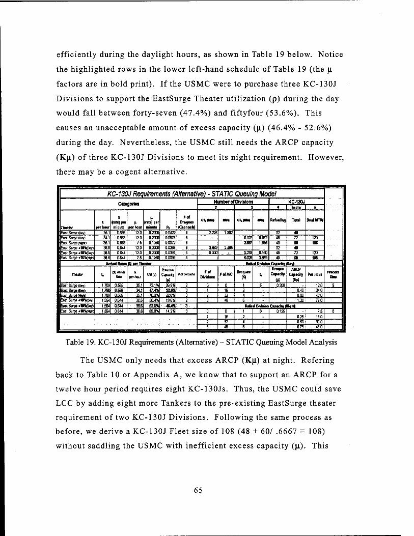
efficiently during the daylight hours, as shown in Table 19 below. Notice

the highlighted rows in the lower left-hand schedule of Table 19 (the (1

factors are in bold print). If the USMC were to purchase three KC-130J

Divisions to support the EastSurge Theater utilization (p) during the day

would fall between forty-seven (47.4%) and fiftyfour (53.6%). This

causes an unacceptable amount of excess capacity (\i) (46.4% - 52.6%)

during the day. Nevertheless, the USMC still needs the ARCP capacity

(KJJ.) of three KC-130J Divisions to meet its night requirement. However,

there may be a cogent alternative.

KC-130J Requirements (Alternative) - STATIC Queuing Model Categories Number of Divttlons KC-130J

2 3 # Theater #

Theater

X perhaur

X (rats) per minute

1» per hour

(rat*) par nMiwte Po

«of Drogues

(Caaonels)

CT.IMta) MN a,gm two. Ratuallruj Total DualkTTW

East Surqe (Day) 35.1 0.585 12.0 02000 0.0422 4 2225 1.302 32 48 East Surqe (Day) 34.1 0.568 12.0 0.2000 0.0576 6 - 0.127 0.072 48 72 120 East Surqe (Now) 35.1 0.585 7.5 0.1250 0.0072 6 1897 1.695 40 68 w East Surqe ♦MVDw) 38.6 0.644 12.0 0.2000 0.0265 4 1862 2.4S5 32 48 East Surqe »lOyttoy) 38.6 0.644 12.0 0.2000 0.0391 6 0.000 0233 0153 48 72 120 East Surge »10Vutft 38.6 0.644 7.5 0.1250 0.0D3S 6 6U28 3.879 40 68 108

Arrival Rate* U oar Th eatar Refa •IDivisloaCapacfcv Dav)

Theater t. (l)Arriv«

Rate X

per hour UtlM

Excess

Capacity

W fofOwhians

#ef

Divisions *0fA/C

Drogues

(K) t.

Drogue

CapacHy

(ID

ARCP Capacity

(M Per Hour

Pnctss

East Surqe (Day) 1.709 0.5B5 35.1 73.1% 26.9% 2 0 0 1 5 0.200 12.0 5 East Surge (Day) 1.760 0.5E8 34.1 47.4% S2Ä 3 1 16 2 0.40 24.0 East Surqe (NW) 1.709 0.585 35.1 78.0% 22.0% 3 2 32 4 - 0.80 49.0 East Surge ♦Wfcoay) 1.554 0.E44 33.6 80.4% 19.6% 2 3 48 6 - 1.20 72.0

East Surge »Wtoty) 1.554 0644 3B£ 516% «Su» '■■■■■.-3.' ■■ Refe rirXvialenCaBadWt HaM East Surge »10VN4* 1.554 0.644 38.6 85.8% 14.2% 3 0 0 1 8 0.125 7.51 8

1 16 2 0.25 15.0

2 32 4 . 0.50 30.0 3 48 6 075 45.0 I

Table 19. KC-130J Requirements (Alternative) - STATIC Queuing Model Analysis

The USMC only needs that excess ARCP (K|i) at night. Refering

back to Table 10 or Appendix A, we know that to support an ARCP for a

twelve hour period requires eight KC-130Js. Thus, the USMC could save

LCC by adding eight more Tankers to the pre-existing EastSurge theater

requirement of two KC-130J Divisions. Following the same process as

before, we derive a KC-130J Fleet size of 108 (48 + 60/ .6667 = 108)

without saddling the USMC with inefficient excess capacity (\i). This

65

alternative will enable the USMC to efficiently meet the five-minute CTq

constraint, without incurring excessive costs.

D. KC-130J FLEET SIZING COSTS

With a 95% confidence level, the costs to achieve an average ARCP

CTq of 1.46 minutes for East Surge and 4.14 minutes for West-18 will be

somewhere between $5.7 and $10.7 (mean = $8.4) billion dollars (FY2000

constant), see Figure 18. This represents the present value of the Life

Cycle Costs for a fleet of seventy-two KC-130Js as required to meet the

mission needs of both theaters. This fleet requirement uses the ARCP as

the primary mission driving the requirement. Yet, a 10% increase in

arrival rates (A,) is likely, considering the normal Allied participation in

an MTW as well as the influx of aerial refueling capable MV-22s.

3,000 Trials

.029


Frequency Chart 30 Outliers

87

5.000 6.750 8.500 10.250

Certainty is 95.00% from 5.700 to 10.693

12.000

Figure 18. Forecast: KC-130J Fleet (72) NPV (LCC [in billions])

The cost of a 10% increase in the East Surge and West-18 arrival

rates (A.) for daytime operations will depend on the tradeoffs made. If the

USMC is willing to accept a CTq exceeding the five-minute ARCP CTq

constraint (West-18 ARCP CTq = 6.58'), then the present value fleet LCC

will be the same as those in Figure 18. However, if the USMC considers

66

the five-minute ARCP CTq constraint inviolable (West-18 ARCP CTq

0.229'), then the costs will increase to between $6.7 and $14.0 (mean

$10.7) billion dollars (FY2000 constant), as shown in Figure 19.


3,000 Trials Frequency Chart

.030

33 Outliers

89

6.000 <

8.500 11.000 13.500


16.000



3,000 Trials Frequency Chart

.026

45 Outliers 79

7.000 10.000 13.000 16.000


19.000


67

The cost of sustaining CTq below the five-minute ARCP CTq

constraint during night operations will be considerable. At a minimum, a

KC-130J Fleet size of 120 tankers will be needed to sustain the CTq below

five-minutes. This fleet will cost the USMC between $8.7 and $17.6

(mean = $11.2) billion dollars (FY2000 constant), as shown in Figure 20.

Yet, this would be an inefficient use of resources, considering the

alternative KC-130J Fleet size of 108 tankers, which would still

efficiently meet the USMC requirement.

3,000 Trials


Frequency Chart 22 Outliers

90

.000

6.000 4

9.000 12.000 15.000


18.000


So, ultimately the cost of maintaining the ARCP CTq below the

five-minute constraint for both day and night operations in both theaters

would be a KC-130J Fleet size of 108 tankers. We can be 95% confident

the associated cost will be between $7.8 and $15.6 (mean = $11.7) billion

dollars (FY2000 constant), refer to Figure 21. The tradeoffs between the

various fleet size options can be shown visually to better highlight the

cost / benefit relationship.

68

E. KC-130J FLEET SIZING COST / BENEFIT ANALYSIS

Figure 21 below visually depicts this cost / benefit tradeoff between

the various options. With the arrival rates (X) for daytime operations of

35.1 per hour for East Surge and 18 per hour for West-18, no tradeoff is

necessary, unless the USMC wants to consider lowering the ARCP CTq

below four-minutes for day time operations. However, with Allied and

MV-22 demand, the arrival rates (X.) are increased by 10% to 38.6 per

hour for East Surge and 20.3 per hour for West-18 during daytime

operations. In this case, a tradeoff is implied.

The USMC must decide if the five-minute CTq constraint for the

West-18 Theater and night operations in both theaters is inviolable. To

reveal this difference, the cumulative probability density statistics output

report from the Crystal Ball® simulation was used. This generated Figure

21, which shows the difference in cost over the simulation runs for a fleet

size of 72, 96, and 108. Using the EXCEL® statistical formulas available,

Table 20 was derived to provide a 95% confidence interval around the

projected cost difference, assuming the sample derived is normally

distributed.

The resulting cost difference has a mean of approximately $2.31

billion dollars with a 95% confidence interval that the actual mean will be

between $2.1 and $2.6 billion dollars. Thus, it will cost approximately

$2.31 billion dollars to maintain the five-minute CTq constraint for the

ARCP serving the West-18 (+10%) Theater during daytime operations. Is

it worth $2.31 billion dollars to the USMC to ensure ARCP CTq for the

West-18 (+10%) Theater is less than five-minutes during daytime

operations?

69

Tradeoff in KC-130J Reet Size 100.00%

a> O) (0 c 0) u © a. >

£ 3 a

80.00%

60.00%

40.00%

20.00%

0.00% $5.0

—LCC Fleet Sze (72/VQ

—LCC Fleet Size (96 A/Q

—LCC Reet Size (106 A/Q

J $7.5 $10.0 $125 $150

Life Cycle Cost (in billions of dollars)

$17.5

Figure 22. LCC of different KC-130J Fleet Sizes

Between KC-130J F& Size of 72 vs 96 Statistical Com fidence Interval Mean $2.31 Std Dev 0.562 Conf. Int 95% Lower $2,066 Upper $2,558

Table 20. Statistical Confidence Interval for Fleet Size of 72 vs.96

The same concept was used to determine the cost between a KC-

130J Fleet size of 96 verses 108. The cost difference between the two has

a mean of approximately $1.1 billion dollars with a 95% confidence

interval that the actual mean will be between $0.9 and $1.2 billion

dollars. Thus, to sustain ARCP CTq below the five-minute constraint for

night operations will cost approximately $1.1 billion dollars more than the

KC-130J Fleet size of 96.

70

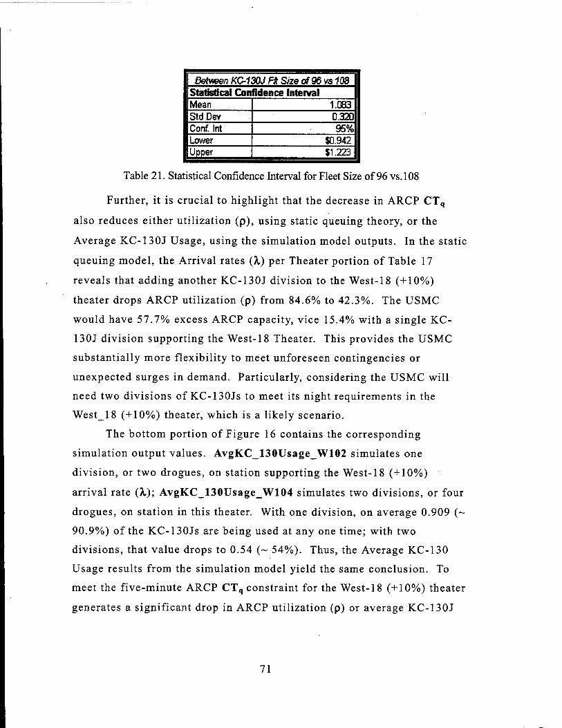
Between KC-130J Fit Size of 96 vs 108 Statistical Confidence Interval Mean 1.083 StdDev 0.320 Conf. Int 95% Lower $0,942 Upper $1,223

Table 21. Statistical Confidence Interval for Fleet Size of 96 vs. 108

Further, it is crucial to highlight that the decrease in ARCP CTq

also reduces either utilization (p), using static queuing theory, or the

Average KC-130J Usage, using the simulation model outputs. In the static

queuing model, the Arrival rates (X) per Theater portion of Table 17

reveals that adding another KC-130J division to the West-18 (+10%)

theater drops ARCP utilization (p) from 84.6% to 42.3%. The USMC

would have 57.7% excess ARCP capacity, vice 15.4% with a single KC-

130J division supporting the West-18 Theater. This provides the USMC

substantially more flexibility to meet unforeseen contingencies or

unexpected surges in demand. Particularly, considering the USMC will

need two divisions of KC-130Js to meet its night requirements in the

West_18 (+10%) theater, which is a likely scenario.

The bottom portion of Figure 16 contains the corresponding

simulation output values. AvgKC_130Usage_W102 simulates one

division, or two drogues, on station supporting the West-18 (+10%)

arrival rate (X); AvgKC_130Usage_W104 simulates two divisions, or four

drogues, on station in this theater. With one division, on average 0.909 (~

90.9%) of the KC-130Js are being used at any one time; with two

divisions, that value drops to 0.54 (~ 54%). Thus, the Average KC-130

Usage results from the simulation model yield the same conclusion. To

meet the five-minute ARCP CTq constraint for the West-18 (+10%) theater

generates a significant drop in ARCP utilization (p) or average KC-130J

71

usage on station. Again, this excess provides the USMC additional

flexibility for dealing with unexpected contingencies.

The utilization factors and average KC-130Js in use for ARCP night

operations are not as critical. Mainly, because a KC-130J fleet of 108

will enable the USMC to efficiently maintain ARCP CTq below five-

minutes. Any less than that will cause an unacceptable ARCP CTq far

above the five-minute constraint. Further, the utilization factor (p) in

Table 18 are higher than in most scenarios previously analyzed, the lowest

p for ARCP night operations is 60%.

F. CHAPTER SUMMARY

In this chapter, the ARCP requirement has been clearly defined,

focusing primarily on the ARCP CTq in a given theater. The critical point

occurs when US Armed Forces begin transitioning their aviation assets

from the western (West-18) to the eastern (East Surge) theater. The

analysis began by discussing purely USMC refueling needs, using the

ARCP requirement for day and night operations to define the total KC-

130J Fleet size. Further, we increased the arrival rate per theater by 10%

to account for potential Allied and MV-22 tanking requirements. Using

the LCC model, we calculated the (real) costs associated with the three

cases. Finally, we concluded with a cost / benefit analysis attributing a

KC-130J Life Cycle Cost to a particular ARCP CTq performance

achieved. The next chapter draws upon this analysis to state some

conclusions and provide some cogent recommendations.

72

VI. KC-130J FLEET SIZE, CONCLUSIONS AND

RECOMMENDATIONS

A. INTRODUCTION

This chapter culminates by defining the estimated KC-130J Fleet

size requirement. It draws on the analysis contained in the preceding

chapter in making the fleet sizing recommendation. This chapter also

includes the conclusions, recommendations, and further issues that should

be considered when making the KC-130J Fleet Sizing decision.

B. KC-130J FLEET SIZE CONCLUSIONS

1. The Arrival Rate (X) of Combat Aircraft to be refueled

and the Aerial Refuel Control Point capacity (Kji) in a

particular theater are critical to the KC-130J Fleet sizing

requirement.

The ARCP Capacity (KJI) must be large enough to handle the

theater arrival rate (X). As discussed in Chapter III, at some point as the

utilization factor (p = X I Kji) gets closer to one, the queue would increase

until all refueling capable aircraft are refueling, in the queue waiting to

be refueled, or just leaving the ARCP. Thus, the KC-130J Fleet must have

enough tankers continuously on station to ensure the Kji exceeds X; the

theater thereby avoids excessively large INVq and corresponding CTq for

the ARCP.

2. The Cycle Time of the Aerial Refuel Control Point Queue

(CTq) provides the critical value that ultimately drives the

KC-130J Fleet sizing requirement.

The KC-130J Fleet size must be large enough to keep the ARCP

CTq below five minutes, the defined constraint. Thus, K|i must be

73

sufficiently greater than X to meet the five-minute ARCP CTq. As clearly

defined in Chapter V, a KC-130J Fleet size of seventy-two is required to

meet this criteria for with two near simultaneous MTWs. If a 10%

increase in the arrival rate (X) for each theater is expected, the KC-130J

Fleet size requirement increases to ninety-six. Further, when the refuel

(process) time increases during ARCP night operations the fleet size

increases to one hundred and eight.

3. The refuel (process) time proves to be the crucial

component that will drive the Aerial Refuel Control Point

Capacity needed to meet future USMC requirements.

The aircraft refuel rate, approximately three minutes of the five

minute refuel (process) time, ultimately drives K\L. Any KC-130 platform

that on average can refuel combat aircraft in approximately two minutes,

subtracting the time it takes aircraft to attach and detach its probe from

the KC-130's drogue, provides capacity (]i) similar to a KC-130J. To

ensure adequate refueling capacity, the USMC can maintain KC-130

Tankers that provide the same aircraft refueling rate as the KC-130J. This

includes the KC-130 R/T variants.

C. KC-130J FLEET SIZE RECOMMENDATIONS

1. The KC-130J Fleet size of 72 Tankers currently meets the

USMC aerial refueling requirements.

Currently, a KC-130 Fleet size of seventy-two should be adequate to

meet current ARCP requirements, excluding Allied and MV-22 refueling

requirements. Based on the analysis in Chapter V, this fleet size is

adequate to meet the five-minute ARCP CTq constraint for day operations

only. However, projecting the aerial refuel requirement into the future

considering both day and night operations reveals the potential for those

requirements to increase.

74

2. The KC-130J Fleet size of 108 Tankers will meet future

USMC aerial refueling requirements.

Unclassified information received from the recent Kosovo conflict

showed a shortfall in aerial refueling assets.51 Further discussion with

KC-130 pilots who served in the Gulf War showed that Allied aircraft

often used the Marine KC-130 refueling assets.52 Thus, the KC-130 Fleet

size needed to support future MTW scenarios must increase to provide

sufficient ARCP capacity (K^l) to keep the ARCP CTq below five-minutes.

3. The Fleet size of 108 KC-130J or KC-130J equivalents can

meet future USMC aerial refueling requirements.

Since funds for starting up and sustaining a Major Defense

Acquisition Program (MDAP) are currently at a premium, the KC-130J

Fleet NPV (LCC) of between $7.9 and $15.6 billion dollars will not be

easy to justify. However, by procuring enough KC-130Js to retire the

older (slower refueling rate) KC-130F and increase the entire USMC fleet

of KC-130J/R/Ts to 108 tankers would be a reasonable alternative.

Currently, the USMC has fourteen KC-30R variants and twenty-two KC-

130T variants.

D. OTHER ISSUES

1. The KC-130J could change current KC-130 Tactics,

Technics, and Procedures.

Lieutenant Colonel (LtCol) Arien Rens, USMC (Ret), the Lockheed-

Martin's demonstration pilot for the KC-130J, introduced an interesting

51 Telephone interview with Major Patrick S. Flanery, USMC, MAWTS-1 KC-130

Instructor, 02 Sep 99. 52 Telephone interview with Lieutenant Colonel Arien Rens, USMC (Ret), former

Commanding Officer of the Composite KC-130 deployed in support of OPERATION

DESERT STORM, 27 Aug 99.

75

facet of the KC-130J that may affect the future Tactics, Techniques, and

Procedures of the KC-130 Fleet.53 The KC-130J possesses a probe that

makes the KC-130J aerial refueling capable. Currently, the KC-130Js

supporting an ARCP must return to their airfield to refuel and refit, taking

on average three and half-hours. Instead, the probe capable KC-130J

could simply fly to an Air Force KC-10 ARCP and completely refuel;

significantly reducing the turn around time required to refuel and refit a

KC-130J. This could drastically reduce the number of KC-130Js or KC-

130J equivalents necessary to support dual near simultaneous MTWs.

This is a potential subject for further analysis.

2. Tradeoff Analysis should be conducted between the KC-

130J procurement program and other priority

procurement programs.

Every even numbered year, the USMC submits its Program

Objective Memorandum (POM) outlining those programs that it requests

the Department of Defense to support through the Planning, Programming,

and Budgeting System (PPBS). As funding for Major Defense Acquisition

Programs (MDAP) becomes more austere, the need for thorough tradeoff

analysis between priority procurement programs will become more

critical. Certainly, this could be the subject of future research. In

particular, research could analyze the tradeoffs between the KC-130J and

other priority procurement programs.

53 Ibid.

76

APPENDIX A. 24 HOUR AERIAL REFUEL CONTROL POINT

SCHEDULE

77

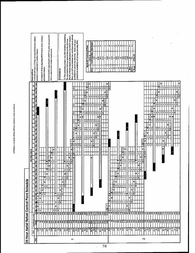
J — c T3 O

Si a, a

x S i »» x s s = s " s ■§ &! g S I | 3 E

' -' I« if '% I«

= s -a. s -o g — « < £ x 2 w • Ä o — ts -~ < «- C P1 - —

m

o

.1

1

i a

■a a> u

CO

o

C o Ü "3

CD

< 3 O X ^r CM

UJ o

<D So 2 » « — "in ; t» to *_ . S « £ S o SS

^ * j Ü <Q re >. — _ 01 of o -■2 £ < ® c "5 5 o 2 £ S E c £ — -o «5 s 5 « o c u 2

2.-Ö Ä § E & 5 .2 g Ä ■= <D > JE ~ C <D .G silISi

8 sr I S ° »

p as w « — JK

i i n" in eo ^ * - ■* *■

o m a> £ 5 <o it £ I-. oi ^

o

t-

(- 3 H

e

o r | 1

in CO

IO Ö d

« iri

»n r- CD

in d CN

m d CM

CO CM iri

0 « o m r- e

a c > &

i= ~ •- „. in <o ^. «o o> o ^ tv « ^1 m to

3 & Tl 5 a:

T

:i 6

a ^'

a~ .ässssssi

"«aw io w n i

ss s

I §s

L I I

i

I i

°SSS8

g

O CM O

78

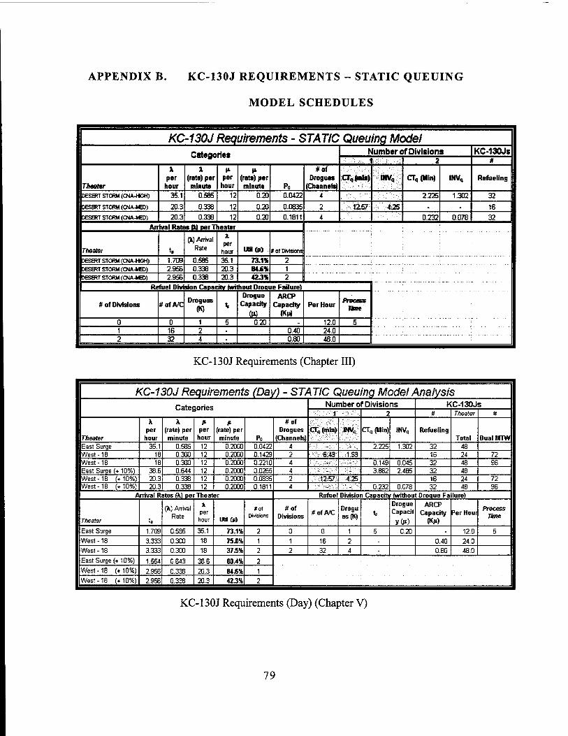
APPENDIX B. KC-130J REQUIREMENTS - STATIC QUEUING

MODEL SCHEDULES

KC-130J Requirements - STATIC Queuing Model Categories Number of Divisions KC-130JS

1 ■ 2 #

Thtattr

X per

hour

X (rate) per minute

per hour


#of Drogues

(Channels) CTq(mm) mv«, CTq (Min) INV„ Refueling

DESERT STORM (CNA-HGH) 35.1 0.585 12 0.20 0.0422 4 2.225 1.302 32

DESERT STORM (CNA-MED) 20.3 0.338 12 0.20 0.0835 2 1257 4.25 - - 16

DESERT STORM (CNA-MED) 20.3 0.338 12 0.20 0.1811 4 0.232 0.078 32 Arrival Rates Q) per Theater

Theater t.

(1) Arrival Rate

X per

hour UH(P) tot Divisions

DESERT STORM (CNA-HK3H) 1.709 0.585 35.1 73.1* 2 - ~| --; - ; - ■■

DESERT STORM (CNA-MED) 2.956 0.338 20.3 84-6% 1 DESERT STORM (CNA-MED) 2.956 0.338 20.3 423% 2

Refuel Division Capacity (without Droque Failure) -' ■ -■ - -- ,: -"-■-■ - - —


(K) t.

Drogue Capacity

(ID

ARCP Capacity

(Ku) Per Hour

Process One

0 0 1 5 0.20 . 12.0 5 1 16 2 - 0.40 24.0 2 32 4 - 0.80 48.0

KC-130J Requirements (Chapter III)

KC-130J Requirements (Day) - STATIC Queuing Model Analysis Categories Number of Divisions KC-130JS

1 . 2 # Theater #

Theater

k per

hour

X (rate) per minute

per hour


#of Drogues

(Channels) CTqOnin) INV, CTq (Min) INVq Refueling

Total DualMTW East Surqe 35.1 0.585 12 0.2000 0.0422 4 . -. . 2.225 1.302 32 48 West -18 18 0.300 12 0.2000 0.1429 2 6.43 1.93 16 24 72 West -18 18 0.300 12 0.2000 0.2210 4 ■'.':_ ■

■'■■- 0.149 0.045 32 48 96 East Surqe (♦ 10%) 38.6

20.3 0.644 12 0.2000 0.0265 4 ■: ■'■■-. 3.862 2.485 32 48

West-18 f*10%) 0.338 12 0.2000 0.0835 2 1257 425 16 24 72 West-18 (*10%) 20.3 0.338 12 0.200G 0.1811 4 - - 0.232 0.078 32 48 96

Arrival Rates ft) per Theater Refuel Division Capacity r fwithout Droque Failure)

Theater t>

(JL) Arrival Rate

X per

hour UBC«

«of Divisions

#of Divisions #ofA/C

Drogu es(K) W

Drogue Capach

ARCP Capacity

(K>) Per Horn Process

Time

East Surge 1.709 0.585 35.1 73.1* 2 0 0 1 5 0.20 - 12.0 5 West -18 3.333 0.300 18 75D% 1 1 16 2 - 0.40 24.0 West-18 3.333 0.300 18 375% 2 2 32 4 - 0.80 48.0

East Surge (♦ 10%) 1.554 0.643 38.6 804% 2 West-18 (*10%) 2.956 0.338 20.3 84.6% 1 West-18 (+10%) 2.956 0.338 20.3 423% 2

KC-130J Requirements (Day) (Chapter V)

79

KC-130J Requirements (Niqht) - STATIC Queuing Model Categories

Number of Divisions KC-130JS •";■ '1 2 3 tf Theater #

Theater

k per

hour

k (rate) per minute

per hour

(rate) per minute

Po

#of Drogues

(Channels)

CTq (min)

MVq CTq (Min)

INVq CTq (Min)

INVq Refueling Total DualMTW

East Surqe 35.1 0.585 7.5 0.1250 0.0072 6 ' ■ - •' 2.897 1.69504 48 72

West-18 18 0.300 7.5 0.1250 0.0831 4 -•:' •■•' -. - 1.435 0.431 32 48 120

East Surqe (+10%) 38.61 0.644 7.5 0.1250 0.0035 6 , .:- -' '. .' . . . 6.028 3.87837 48 72

West -18 (+10%) 21.3 0.338 7.5 0.1250 0.0568 4 ':--: 2.432 0.823 32 48 120

Arrival Rates ft) per Theater Refuel Division Capacity (without Droque Failure)

Theater ta

(X) Arrival Rate

1 per

hour Urjlu»

*0T

Divisions #of

Divisions ttoftJC Drogues

(K) t,

Drogue Capacity

ARCP Capacity Per Hour

(K>)

Process Tine

East Surge 1.709 0.585 35.1 78.0% 3 0 0 1 8 0.125 - 7.5 8

West -18 3.333 0.300 18 60.0% 2 1 16 2 - 0.25 15.0

East Surge (♦ 10%)

West -18 (+ 10%)

1.554 0.643 38.6 85.8% 3 2 24 4 - 0.50 30.0

2.956 0.338 20.3 67.7% 2 3 32 6 0.75 45.0

KC-130J Requirements (Night) (Chapter V)

KC-130J Requirements (Alternative) - STATIC Queuing Model Number of Divisions KC-130J 2 3 # Theater #

Theater k

per hour

\ (rate) per minute

ft per hour

r- (rate) per minute Po

#of Drogues

(Channels)

CTg(Mn) MVq CT,(Mn) MVq Refueling Total DualMTW

East Surqe (Day) 35.1 0.585 12.0 0.2000 0.0422 4 2.225 1.302 32 48

East Surge (Day) 34.1 0.568 12.0 0.2000 0.0576 6 - - 0.127 0.072 48 72 120

East Surqe (Wght) 35.1 0.585 7.5 0.1250 0.0072 6 2.897 1.695 40 60 108

East Surge ♦10%(Day) 38.6 0.644 12.0 0.2000 0.0265 4 3.862 2.485 32 48 East Surge ♦10%(Day) 38.6 0.644 12.0 0.2000 0.0391 6 0.000 - 0.233 0.150 48 72 120

East Surge +10%(Nie|ht 38.6 0.644 7.5 0.1250 0.0035 6 6.028 3.879 40 60 108

Arrival Rates ft) per Theater Refuel Division Capacity (Day)

Theater t> (Ik) Arrival

Rate 1

per hour Util(p)

Excess Capacity

W

toi Divisions #of

Divisions #ofA/C

Drogues

(K) U

Drogue Capacity

ARCP Capacity

m Per Hour

Process line

East Surqe (Day) 1.703 0.585 35.1 73.1% 26.9% 2 0 0 1 5 0.200 - 12.0 5

EastSurqe<Day) -■. .1.760 ■a568 ■"■ fr?, 34.1 -:::*rm ■:.iysün ;,-S.,-;=■>; 1 16 2 - 0.40 24.0

East Surge (Nghf) 1.709 0.585 35.1 78.0% 22.0% 3 2 32 4 - 0.80 48.0

East Surge +10%(Day) 1.554 0.644 38.6 80.4% 19.6% 2 3 48 6 - 1.20 72.0

EastSurge+10%(Pay) •:1:554 ■ 0.644 :: -,t.m& \::S3S% 464% i:::t:3":-JÄ> Refuel Division Capacity (Niqht)

East Surge ♦10%(Nigrt 1.554 0.644 38.6 85.8% 14.2% 3 0 0 1 8 0.125 - 7.5 8

1 16 2 - 0.25 15.0

2 32 4 - 0.50 30.0

3 48 6 - 0.75 45.0

KC-130J Requirements (Alternativ

80

e) (Chapter V)

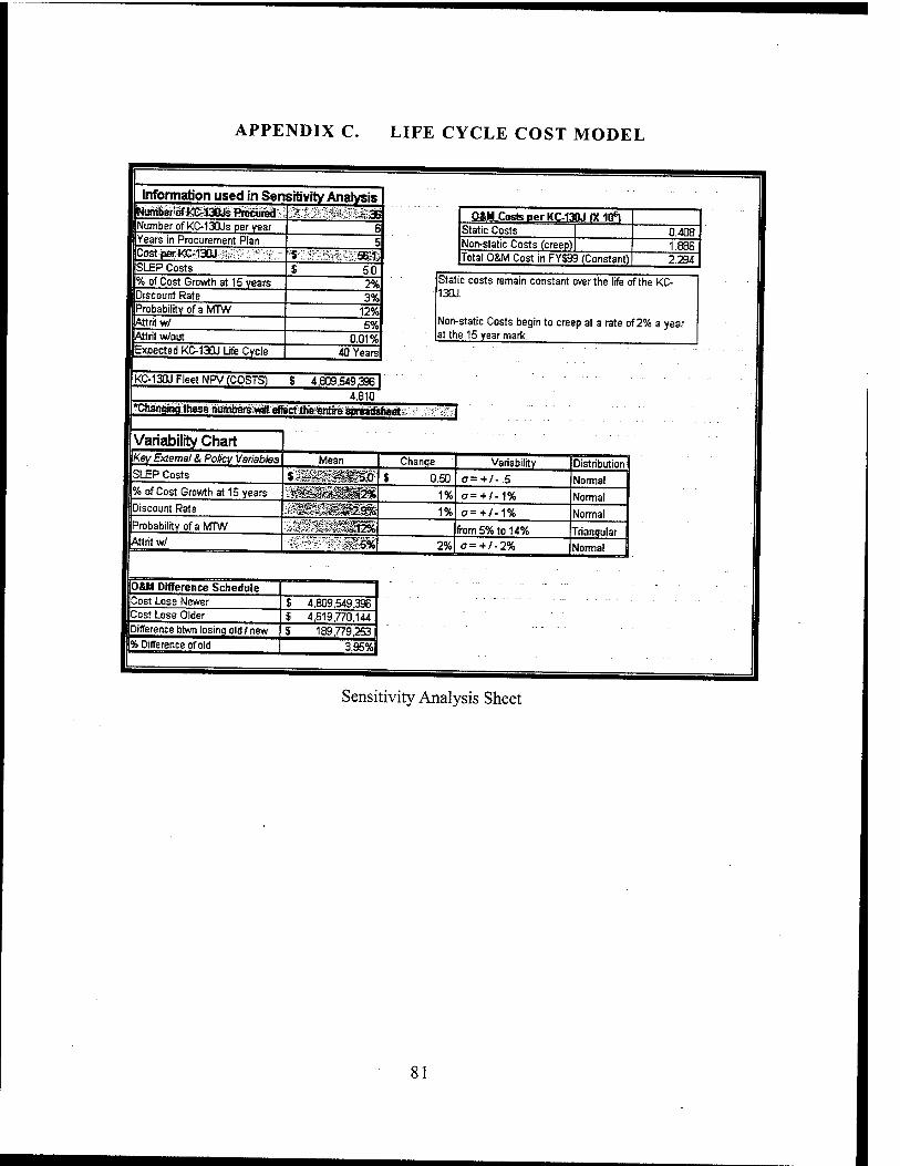
APPENDIX C. LIFE CYCLE COST MODEL

Information used in Sensitivity Analysis NuniteMKC^SaOÜS'Pfiiwaireä Number of KC-130Js per year

Cost pet: K&130Ü; Years in Procurement Plan

SLEP Costs % of Cost Growth at 15 years Discount Rate

Attritw/ Probability of a MTW

Altrit w/out Expected KC-130J Life Cycle

'^■c."e..:?'-i;g?Sja23!^B

:.-SE&S 5.0 2% 3%

12% 5%

0.01% 40 Years

O&M Costs Der KC-130J (X 1Q6) Static Costs I 0.408 Non-static Costs (creep) | 1.886 Total O&M Cost in FY$99 (Constant) 2.294

Static costs remain constant over the life of the KC- 130J.

Non-static Costs begin to creep at a rate of 2% a year at the 15 year mark.

KC-130J Fleet NPV (COSTS) $ 4,609,549361

4.810

'Changing these numbefsvwll effect the Bntro spreadsheet

Variability Chart Key External & Policy Variables

SLEP Costs

% of Cost Growth at 15 years

Discount Rate

Probability of a MTW

Attritw/

Mean

imms^®- Change

0.50

1% 1%

2%

Variability

o=+/-.5

CT=+/-1%

■+/-11

from 5% to 14%

=+/-2%

Distribution

Normal

Normal

Normal

Triangular

Normal

O&M Difference Schedule Cost Lose Newer Cost Lose Older Difference btwn losing old / new

% Difference of old

4,809,549,396 $ 4,619,770,1441

189,779,253 3.95%

Sensitivity Analysis Sheet

81

Deployment Attrition Sheet

82

Life Cycle Cost Analysis: KC-130J FlMt NPV (LCC) $ 4 .809.549.396

Year/ Category

Year Designator

Procurement w/ attrition

LC-130JS in

Operation

Cost of KC-130J

Static Costs

Non-Static Costs

Cost Growth (Lose New)

SLEP Costs

Costs <FY$2000$)


Costs

tsenr 3 2 0 112.2 - - - - 122.2 122.2

.1996 2 3 2 168.3 0.816 3.772 •- - 183.1 305.3

1999 1 2 5' 112.2 2.040 9.430 . - 127.3 432.6

2000 0 E 7 336.6 2.856 13.202 - ■ 352.7 785.2

2001 1 6 13 336.6 5.304 24.518 - . 356.1 1.141.3

2002 2 6 19 336.6 7.752 35.834 . - 359.1 1500.4

2003: 3 6 26 335.6 10.200 47.150 - - 361.6 1«61.9

2004 4 E 31 336.6 12.648 58.466 • - 363.7 2225.6

2006 5 5 36 280.5 14.688 67.896 - - 314.7 2540.3

2006 6 0 36 0.0 14.688 67.896 ■ - 69.6 2509.9

2007 7 0 36 ' 0.0 14.688 67.896 . - 67.6 2577.5

2008 e 0 36 0.0 14.686 67396 - - 65.7 2.743.2

2009 9 0 36 0.0 14.688 67.896 ■■ - - 63.8 2507.1

2010 10 2 34 112.2 13.872 64.124 - - 142.9 2550.0

2011 11 0 36 0.0 14.688 67.896 - - 60.3 3010.3

2012 12 0 36 0.0 14.688 64.049 3.847 101)00 65.7 3076.0

2013 13 0 36 0.0 14.688 5B.085 9.811 15.000 67.3 3,143.3

2014 14 2 34 112.2 13.872 50.114 14.010 10.000 134.2 3277.4

. 2016 15 0 36 0.0 14.688 41.357 26.539 30.000 73.3 3350.7

2016 16 0 36 0.0 14.688 28.332 39.564 30.000 71.3 3.422.0

2017 17 0 36 0.0 14.688 14.797 53.099 30.000 69.2 3/491.3

2018 18 0 36 0.0 14.686 0.737 67.159 30.000 67.3 3558.5

2019 19 0 36 0.0 14.688 .'■ 79.551 30.000 72.2 3530.7

2020 20 0 36 0.0 14.688 ■ . 81.142 25.000 68.2 3598.9

2021 21 0 36 0.0 14.688 - 82.765 0.000 53.5 3,752.4

2022 22 0 36 0.0 14.688 . 84.420 0.000 52.8 3505.2

2023 23 0 36 0.0 14.688 '-: 81.325 0.000 49.7 3555.0

2024 24 2 34 112.2 13.872 - 82.951 0.000 105.3 3360.2

2026 25 0 36 0.0 14.688 . 89.587 10.000 55.9 4016.2

2026 2E 0 36 0.0 14.688 - 91.379 0.000 50.4 4066.6

2027 27 0 36 0.0 14.688 . 93.207 0.000 49.9 4.116.5

2028 28 0 36 0.0 14.688 - 89.789 0.000 4B.9 4,163.4

'. 2ff2? 29 0 36 0.0 14.688 . 96.972 10.000 53.1 4 216.5

2030 30 0 36 0.0 14.688 ... 98.912 0.000 48.2 4264.7

3031 31 0 36 0.0 14.688 . 95.285 0.000 45.3 4310.0

2032 32 2 34 112.2 13.872 . 102.908 0.000 91.7 4.401.7

'2033' 33 0 36 0.0 14.688 . 104.966 0.000 4E.E 4,448.3

2034 34 0 36 ' 0.0 14.688 . 107.065 0.000 46.1 4.494.4

2036 35 0 36 0.0 14.688 - 109.206 0.000 45.6 45399

2036:"'' 35 2 34 11Z2 13.872 .. 111.391 0.000 84.8 4524.8

2037 37 0 34 0.0 13.872 . 107.306 0.000 42.1 4566.9

2038 38 0 31 0.0 12.648 . 99.795 0.000 37.9 4.704.8

2039 39 0 29 0.0 11.632 . 95.224 10.000 38.4 4.743.2

2040 40 0 23 0.0 9.384 - 77.033 0.000 27.5 4.770.7

2041 41 0 17 0.0 6.936 - 58.076 0.000 20.1 4.790.9

2042 42 0 11 0.0 4.488 . 38.330 0.000 12.9 4503.8

2043 43 0 5 0.0 2.040 . 17.771 0.000 5.8 4509.5

2044 44 0 0 0.0 - - - 0.000 - - 2046 45 0 0 0.0 - . - 0.OO0 - - 2046 : 46 0 0 on - - - 0.000 - - 2047 47 0 0 0.0 . ■ - 0.000 - - 2048 48 0 0 0.0 - - - 0.000 - - 2049 49 0 0 0.0 - -■■ - 0.000 - - 2060 50 0 0 0.0 . . - 0.000 - - 2061 51 0 0 0.0 - - - 0.000 '.■-.■ - 2062 52 0 0 0.0 . . . 0.000 - - 2063 S3 0 0 0.0 - - - 0.000 - -

• 2064 - . 54 0 0 0.0 - . . 0.000 - 2066 55 0 0 0.0 - . - 0.000 - - 2066 56 0 0 0.0 - - - 0.000 - -

Assumptions: 1) SUEP is done at the 15 year mark. 2) O&M Costs begin to creep at the 15 year mark. " Totals

Life Cycle Cost Sheet (Lose New)

83

Life Cycle Analysis: KC-130J Fleet NPV {FY$2O00tCOSTS) $ 4.619.770.144

Year/:

Category

Creep SLEP Time

Year Designator

Number Produced

#w/ Attrition from 15 yeare back

Number in Operation New

Attrition #s

Total H 15year replace

Cost of KC- 130J

Static Costs

Non- Static Costs

Cost Growth (Loose

Old)

SLEP Costs

Costs (FYJ2000$)


Costs

i«r 0

1

2

3

4

5

E

7

e 9

10

ii

12

13

14

15

3 2 0 0 0 0 112.2 - - 122.2 122.2

1998 ■,""■ 2 3 2 2 0 0 16S.3 0.816 3.772 - 183.1 305.3

■:■««■:; 1 2 5 5 0 0 112.2 2.040 9.430 - 127.3 432.6

2000 0 6 7 7 0 0 336.6 2.856 13.202 - 352.7 785.2

2001 1 E 13 13 0 0 336.6 5.304 24.518 - 356.1 1.141.3

2002 2 6 19 19 0 0 336.6 7.752 35.834 - 359.1 1500.4

2003 3 S 25 25 0 0 336.6 10.200 47.150 - 361.6 1.861.9

200« 4 E 31 31 0 0 336.6 12.648 S8.46E ■ 363.7 225.6

2006 5 5 36 36 0 0 260.5 14.688 67.896 - 314.7 2540.3

2006 6 0 36 36 0 0 0.0 14.688 67.896 • 69.6 2509.9

•';:"2007--' 7 0 36 36 0 0 0.0 14.698 67.896 • 67.6 2577.5

2008;;-" 8 0 36 36 0 0 0.0 14.683 67.896 - 65.7 2.743.2

2000 9 0 34 36 2 2 0.0 14.683 67.895 - 63.8 2507.1

2010- 10 2 34 34 0 2 112.2 13.872 64.124 - 142.9 2550.0

2011- 11 0 36 36 0 2 0.0 14.683 67.896 • 60.3 3510.3

ao»-.;. 12 0 35 36 0 2 0.0 14.683 60.468 7.428 10.000 65.7 3576.0

2013 16

17

18

19

20

21

13 0 35 36 0 2 0.0 14.688 53.824 14.072 15.000 67.3 3.143.3

20« ••>..• 14 2 34 34 0 2 112.2 13.872 43.146 20578 10.000 134.2 3577.4

2016/7 15 0 36 36 0 2 0.0 14.688 39.742 28.154 30.000 73.3 3350.7

201»-.:_ 16 0 35 36 0 2 0.0 14.688 32.287 35.609 30.000 71.3 3.422.0

■• 201T :"v: 17 0 34 36 2 4 0.0 14683 25.716 42.180 30.000 69.2 3.491.3

-2018::-,. 18 0 36 36 0 4 0.0 14.683 24.873 43.023 30.000 67.3 3558.5

2019.. 22

23

IS 0 36 36 0 4 0.0 14.633 24.012 43.884 30.000 65.4 3523.9

2020 20 0 36 36 0 4 0.0 14.688 23.135 44.761 25.000 60.7 3584.7

2021 24

25

26

27

28

29

30

31

32

33

34

35

36

37

36

39

40

41

42

43

44

45

46

47

48

49

50

51

52

S3

54

55

56

57

58

59

21 0 34 36 2 6 0.0 14.688 24.776 43.120 oooo 45.3 3730.0

2022 22 0 36 36 0 6 0.0 14.688 26.501 41.395 0.000 44.0 3.774.0

2023 ". 23 0 36 36 0 6 0.0 14.688 23.034 44.862 0.000 42.8 3516.8

2024 24 2 34 34 0 112/2 13.872 18.364 45.760 0.000 95.8 3512.6

2026 25 0 36 36 0 0.0 14.688 21.221 46.675 10.000 45.3 3557.9

.2609 - 26 0 36 36 0 0.0 14.688 23.088 44.80B 0000 39.3 3597.2

2027 27 0 36 36 0 0.0 14.683 19.336 48.560 0.000 38.2 4535.3

. .2029.T 28 0 36 36 0 0.0 14.688 18364 49.532 0.000 37.1 4572.4

2029 29 0 36 36 0 0.0 14.683 X.346 47.550 10.000 40.4 4.112.8

2030 30 0 36 36 0 0.0 14.683 19.395 48.501 0.000 35.0 4.147.9

'SBSfVi: 31 0 36 36 0 0.0 14.688 18.425 49.471 0.000 34.0 4.181.9

«32 32 2 34 34 0 2 112.2 13.872 13.663 50.461 0.000 76.2 4258.1

2033 33 0 36 36 0 2 0.0 14.688 19.643 48.253 0.000 32.2 430.2

2034 34 0 36 36 0 2 0.0 14.683 18.678 49.218 0.000 31.2 43215

2036 35 0 36 36 0 2 0.0 14.693 109.206 0.000 45.6 4367.0

2036. : 36 2 34 34 0 0 112.2 13.872 12.917 51.207 0.000 68.0 4,435.0

2037 < 37 0 34 34 0 0 0.0 13.872 - 107.305 oooo 42.1 4.477.1

2033 38 0 31 31 0 0 0.0 12.648 99.795 0.000 37.9 4515.0

2039 39 0 29 29 0 0 0.0 11.832 - 95.224 10.000 38.4 4.553.4

20*0 40 0 23 23 0 0 0.0 9.384 - 77.033 0.000 27.5 45B1.0

»HI ;, 41 0 17 17 0 0 0.0 6.936 58.076 0.000 20.1 4.601.1

' / '20*2 : 42 0 11 11 0 0 0.0 4.483 - 38.330 0.000 12.9 4514.0

2043 43 0 5 5 0 0 0.0 2040 - 17.771 oooo 5.8 4519.8

2044. 44 0 0 0 0 0 0.0 - - 0.000 - * ; 204R 45 0 0 0 0 0 0.0 - oooo - •

2046 46 0 0 0 0 0 0.0 - - 0.000 - 2047 47 0 0 0 0 0 0.0 - - 0.000 - 2048 48 0 0 0 0 0 0.0 - - - 0.000 " 2049 49 0 0 0 0 0 0.0 - O.O00 - "

. 2060:-:- 50 0 0 0 0 0 0.0 - - 0.000

2061 51 0 0 0 0 0 0.0 - - 0.000 • 2062 52 0 0 0 0 0 0.0 - - 0.000 • " 2063 53 0 0 0 0 0 0.0 - oooo ' 2064 54 0 0 0 0 0 0.0 - 0.000 - - 206» 55 0 0 0 0 0 0.0 - 0.000 - 2068 56 0 0 0 0 0 0.0 - - - O.O0O

Life Cycle Cost Sheet (Lose Old)

84

KC-130J Life Cycle Cost Breakdown

BOSM COSI5

!3SL£*» COSiS 3%

KC-130J Life Cycle Cost Breakdown (Chart Sheet)

85

KC-130J LCC Chart 450.0

-Yearly Costs

ll11 l l li

in m o o CM CM

KC-130K Life Cycle Cost Chart (Chart Sheet)

86

APPENDIX D. VARIABILITY CHART, CRYSTAL BALL

DISTRIBUTION ASSUMPTIONS

Assumption: SLEP Costs Cell: B22

$0L5

S6.0 158

Assumption: % of Cost Growth atl5 years

2% 1%

Cell: B23

2%

% of Cott Growth at 15 y*»r»

87

Assumption: Discount Rate Cell: B24

29% 10%

Assumption: Probability of a MTW Cell: B25

NHmm 5% 12% 14%

%t>M% 10%

Probability of a MTW

10% 12%

88

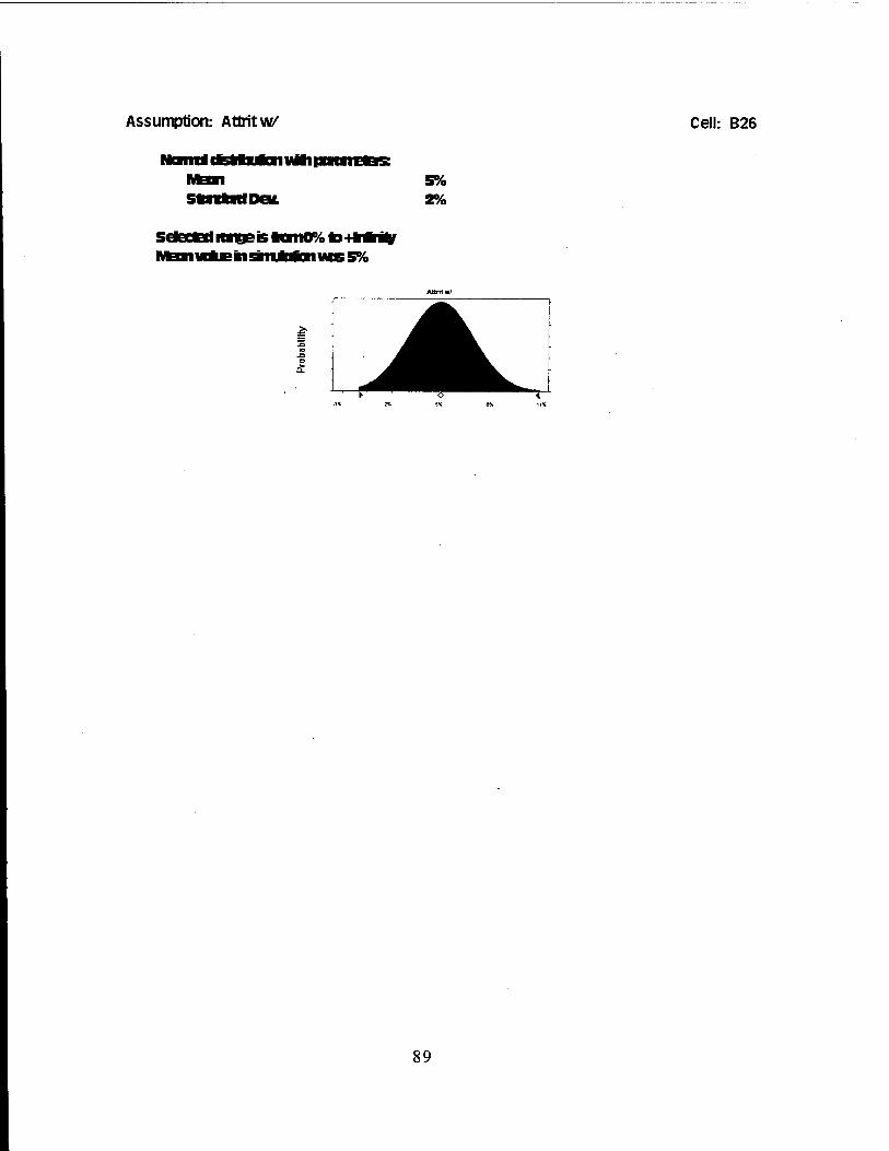
Assumption: Attritw Cell: B26

5% 2%

5%

89

THIS PAGE INTENTIONALLY LEFT BLANK

90

LIST OF REFERENCES

1. Adleman, Dan, Barnes-Schuster, Dawn, and Eisenstein, Don;

Operations Quadrangle: Business Process Fundamentals, The

University of Chicago Graduate School of Business, 1999.

2. Anderson, David R., Sweeney, Dennis J., and Williams, Thomas A.;

An Introduction to Management Science, 8th Edition, West

Publishing Company, 1997.

3. Blanchard, Benjamin S.; Logistics Engineering and Management,

5th Edition, F

Jersey; 1998.

5th Edition, Prentice Hall Publishing, Upper Saddle River, New

4. Cox, Gregory, USN/USMC Tanking Requirements. Center for Naval

Analysis, May 95.

5. Gates, William R., Young Kwon, Timothy Anderson, and Alan

Washburn; Marine KC-130 Requirements Study. Naval Postgraduate

School, Monterey, CA. October 1999.

6. KC-130 Tactical Manual NWP 3-22.5-KC-130. Volume I, NAVAIR

01-75GAA-IT, Department of the Navy, Office of the Chief of

Naval Operations, May 1997.

7. Kelton, W. David, Sadowski, Randall P., Sadowski, Deborah A.;

Simulation with ARENA, McGraw Hill, 1998.

91

8. Mäher, Michael; Cost Accounting: Creating Value for Management,

McGraw-Hill Companies, Inc.; 1997.

9. Office of Management and Budget; Guidelines and Discount Rates

for Benefit-Cost Analysis of Federal Programs; United States

Government, 29 October 1992.

92

INITIAL DISTRIBUTION LIST

No. of Copies

1. Defense Technical Information Center 2

8725 John J. Kingman Rdv Ste 0944

Ft. Belvoir, VA 22060-6218

2. Dudley Knox Library (Code 013) 2

Naval Postgraduate School

411 Dyer Road

Monterey, CA 93943

3. Headquarters, U.S. Marine Corps 1

Department of Aviation (APW-91)

1155 Defense Pentagon, Rm. 5D773

Washington, DC 20301-1155

4. Director, Training and Education 1

MCCDC Code 46

1019 Elliot Road

Quantico,VA 22134-5027

5. Director, Marine Corps Research Center '. 2

MCCDC Code C40RC

2040 Broadway Street


6. Director, Studies and Analysis Division 1

MCCDC Code C45

3300 Russell Road


93

7. Marine Corps Representative 1


Code 037, Bldg. 330, Ingersoll Hall, Room 116

555 Dyer Road

Monterey, CA 93940

8. Marine Corps Tactical Systems Support Activity 1

Technical Advisory Branch

Atta: Major J.C. Cummiskey

Box 555171

Camp Pendleton, CA 92055-5080

9. Chief of Naval Operations (N880G1) 1

Navy Department

Washington, DC 20350-2000

10. Commander 1

Naval Air Systems Command PMA207

Bldg. 419, 46990 Hinkle Rd., Unit 8

Patuxent River, MD 20670-1627

Attention: LtCol Doug Islieb

11. Naval Air Systems Command 1

PMA207 Detachment A

PSC Box 8026

Cherry Point, NC 28533-0026

Attention: Clark Hutchinson, Code PMA207.6B

12. Chief of Naval Operations (N-81) 1

Navy Department

Washington, DC 20350

94

13. Prof. Alan Washburn (Code OR/Ws) 1

Dept of Operations Research


Monterey, CA 93943-5000

14. Prof. William R. Gates (Code SM/Gt) 1

Dept of Systems Management



15. Prof Keebom Kang (Code SM/Kk) 1

Dept of Systems Management



16. Dr. Ira Lewis 1

Mail Code: SM/LE

Department of Systems Management


Monterey, CA 93943

17. LCDR John G. Meier III , 1

TCJ5-SC

USTRANSCOM

508 Scott Drive

Scott AFB, IL 62225-5357

18. Major Mitch J. McCarthy, USMC 2

601 Monticello Circle

Devine,TX 78016

95

UNITED STATES MARINE CORPS;(USMC) KC-130J TANKER ...

Documents