UNITED STATES DEPARTMENT OF THE INTERIOR GEOLOGICAL SURVEY INTERAGENCY REPORT: ASTROGEOLOGY 30 A TEST OF SELF-STATIONARITY By Robert D. Regan July 1971 Prepared under NASA Contract H-82013A This report is preliminary and has not been edited or reviewed for conformity with U.S. Geological Survey standards and nomenclature. Prepared by the Geological Survey for the National Aeronautics and Space Administration

Welcome message from author
This document is posted to help you gain knowledge. Please leave a comment to let me know what you think about it! Share it to your friends and learn new things together.
Transcript

UNITED STATES DEPARTMENT OF THE INTERIOR
GEOLOGICAL SURVEY
INTERAGENCY REPORT: ASTROGEOLOGY 30
A TEST OF SELF-STATIONARITY
By
Robert D. Regan
July 1971
Prepared under NASA Contract H-82013A
This report is preliminary and has not been edited or reviewed for conformity with U.S. Geological Survey standards
and nomenclature.
Prepared by the Geological Survey for the National Aeronautics and Space
Administration

INTERAGENCY REPORT: ASTROGEOLOGY 30
A TEST OF SELF-STATIONARITY
By
Robert D. Regan
July .1971
Prepared under NASA Contract H-82013A

The work presented in this report was accomplished as part of
a study investigating the analysis of traverse geophysics data.
The study was directed toward developing methods of extracting the
maximum amount of information from geophysical measurements ob
tained during proposed automated lunar vehicle traverses.
However, it became apparent that a computer program for test
ing stationarity would be of use in many fields of investigation.
Thus it was decided to publish this report separately.
i

CONTENTS Page
ABSTRACT ------------------------------------------------ 1
INTRODUCTION -------------------------------------------- 1
BRIEF THEORETICAL SUMMARY ------------------------------- 2
Time Series - Stochastic Process ----------------- 2
Stochastic Process Functions --------------------- 2
Stationarity ------------------------------------- 3
Ergodicity --------------------------------------- 4
STATIONARITY OF A SINGLE TIME SERIES -------------------- 4
TEST FOR SELF-STATIONARITY ------------------------------ 5
Bendat and Piersol Test -------------------------- 5
Bryan Test 5
Test Modifications ------------------------------- 6
SELF-STATIONARITY TEST ---------------------------------- 6
COMPUTER PROGRAM STEST ------ - --------------------------- 7
Program Input ------------------------------------ 7
Program Output ----------------------------------- 7
TEST CASES ---------------------------------------------- 8
APPENDIX ------------------------------------------------ 12
Computer Program STEST --------------------------- 13
Sample Input ------------------------------------- 27
Sample Output ------------------------------------ 29
REFERENCES ---------------------------------------------- 31
ii

A TEST OF SELF-STATIONARITY
by
Robert D. Regan
ABSTRACT
A method for testing the stationarity of a single time series has been devised. The method utilizes two pre-existing tests of stationarity. A computer program that permits routine testing of any time series has been developed, and the test has been successfully applied to several known series. In certain cases the selfstationarity determined can be equated to stationarity.
INTRODUCTION
In time-series analysis of any body of observational data,
the fundamental assumption is that of stationarity. Very little
work has been done with nonstationary time series, and the effects
of nonstationarity upon time-series analysis are little known. In
the practical application of time-series techniques the assumption
of stationarity is routinely invoked without adequate tests for
the validity of such an assumption. Yet the utilization of some
of the more essential techniques of time-series analysis, such as
the Wiener-Khintchine theorem in the indirect method of power
spectra computation, is valid only for stationary series.
This situation stems from the fact that, to date, no rapid,
accurate, routine method has been available to test the station
arity of a time series. Such a test is clearly required so that
stationarity or nonstationarity of a series can be routinely de
termined and the validity of the application of time-series anal
ysis be established. The method and computer program outlined in
this report is designed to fulfill this requirement.
Basically, the method outlined and programmed is a combina
tion of tests proposed by Bendat and Piersol (1966) and Bryan
(1967). Their tests and assumptions have been combined with some
additional logic to produce a computer test of the stationarity
of a single time series. The method has proved successful in sev
eral test cases.
1

BRIEF THEORETICAL SUMMARY
Before the test method and rationale are explained it is
essential to discuss some of the concepts and terms pertinent to
stationarity.
Time Series-Stochastic Process
A stochastic process can be considered as being composed of
a family of random variables, and viewed as a function of two
variables t and w. The sample space associated with this stoch
astic process is doubly infinite and the set of time functions
which can be defined on this space is called an ensemble.
A strict definition of a time series is that it is one reali-
zation (outcome) of a stochastic (random) process. A more popular
definition is that it is a set of observations of a parameter
arranged sequentially.
The label "time-series" is perhaps a misnomer, and is directly
applicable only when the observations are made chronologically.
However, for the independent variable, time, there may be substi
tuted any other parameter -e.g., distance.
The basic idea of the statistical theory of time series
analysis is to regard the time series as a set of observations
made on a family of random variables, i.e., for each tinT,
x (t) is an observed value of a random variable. The set of
observations { x (t); t E T } is called a time series.
Stochastic Process Functions
The basic process functions are
a) mean of the process OJ
~ (t) d
E {x(t)} = L J x f(x,t) X
-OJ
where:
LJ Lebesgue Integral
f (x, t) = Probability density
E Expectation operator
2
dx
function

In the general case the means are different at different
times and must be calculated for each t.
b) autocorrelation function of the process
where:
* x(t2
) = complex conjugate of x(t2
)
c) autocovariance function of the process
d * Cx(t1,t2 ) = E [[ x(t1)- ~x(t 1 )], [x(t2)- ~x<t2 )]}
In the general case these functions must be calculated for
each t1
, t2
combination.
Stationarity
In general the properties of a stochastic process will be
time dependent. A simplifying assumption which is often made is
that the series has reached some form of steady state in the sense
that the statistical properties of the series are independent of
absolute time. Stationarity can be pictured as the absence of any
time-varying change in the ensemble of member functions as a whole.
A sufficient degree of stationarity for most time-series
analysis is wide-sense stationarity. A process has wide-sense
stationarity if its expected value is a constant and its auto
correlation depends only on the time difference, t 1- t 2 = r, and
not on the absolute value of the respective times.
i.e.
and
E [x(t)} ~ · (t) = constant X
* E [x(t+ r), x(t)} = R ('T) X
Wide-sense stationarity is also termed stationarity of the second
order, i.e., the series is stationary through its second order
statistical moments. Stationarity of order n implies that all
statistical moments less than n depend only on the time differences.
3

Ergodicity
Ergodicity relates to the problem of determining the statis
tics of the stochastic process from the statistics of one time
series. A stochastic process for which the statistics are thus
determinable is said to be ergodic, and the single time series is
representative of the ensemble. The ensemble moments can then be
equated to the time moments.
For example the time average equals the ensemble average of
an ergodic process
fl. (t) X
1 T
T J x(t) dt E[x(t)}
-T
If a time series is ergodic we need only to measure the time
averages which are available rather than the postulated ensemble
averages. Since ergodicity is a subclass of stationarity, a time
series must be shown to be stationary before the question of
ergodicity can be considered,
STATIONARITY OF A SINGLE TIME SERIES
In the transformation from the theoretical to the empirical,
strict adherence to theory must be tempered with reasonable prac
tical considerations. In most practical applications the single
observed time series is the only information available on the
parent process. Hence ergodicity must be assumed and time-domain
statistics utilized. Also all analyses are performed on the
sample series and thus the stationarity of this series is of prime
interest. Bendat and Piersol (1966) have termed the concept of
stationarity of this one time series as self-stationarity. Thus
we speak of the series being stationary rather than the process
being stationary.
However, the concept of self-stationarity is not restrictive.
A necessary condition to extend this self-stationarity to station
arity is that the process be ergodic, i.e. that the series is
representative of the process. Ergodicity is impossible to prove
(except in special instances) when the entire process is not known.
4

Bendat and Piersol (1966, p. 12) state that "in actual practice,
random data representing stationary physical phenomena are gen
erally ergodic".
If the assumption of ergodicity is justified then self
stationarity becomes equivalent to stationarity, since the single
time series is representative of the ensemble·.
TEST FOR SELF-STATIONARITY
The test for self-stationarity is based on the methods pro
posed by Bendat and Piersol (1966) and Bryan (1967). The basis
of these methods is that in a stationary series certain statistical
properties of the time series are considered invariant with time.
The tests are for second order self-stationarity.
Bendat and Piersol Test
Bendat and Piersol (1966) suggest that the series be divided
into n equal time intervals (either contiguous or non-contiguous)
and that the mean and variance of these intervals be calculated.
The two series thus formed, composed of means and variances, are
then tested for underlying trends or variations by the Run test
and the Trend test, Bendat and Piersol (1966, p. 156). If no
trends or variations are suggested by the application of these
tests, the original series is assumed to be stationary.
Bryan Test
Basically, Bryan's test (1967) is quite similar in that he
tests the invariance of the means and variances obtained from in
dependent, equal time segments. Rather, than using the sample
mean and sample variance he constructs two combinations of the
data to serve as estimates of the population mean and population
variance. Those two estimates are independent, and independently
distributed.
Using these two variates, m, a linear function of the data
and an unbiased estimate of the population mean, and Q, a quad
ratic function of the data, he develops a test for the hypothesis
that the time series is stationary, and two test variables, L1
for
5

the Neyrnan-Pearson L test, and F for the F-distribution test.
Test modifications
The tables for the Run and Trend tests (Bendat and Piersol
1966, p. 170) were extrapolated to include the range n = 1 to
n = 200. With values of n less than 12 the results proved unre
liable. Hence a low limit cut off at n 12 is utilized, The
Acceptance region was extended to include the lower bound.
The Bryan test was extended to include the 97.5 percent con
fidence interval.
Self-Stationarity Test
In the proposed test both methods are combined and used with
some restrictions and modifications.
First the sampling interval for independent samples is deter
mined. If independent samples cannot be determined, i.e., the
autocorrelation function does not damp to zero, the test is aborted
and the series can be considered non-stationary if a reasonable
number of points has been used.
Once the sampling interval has been determined, the series
is segmented into independent samples of length N. Initially the
series is tested with N = 5, then N is increased to 10, and the
final test, if there are enough data points, is for N = 15.
The minimum test is for KK = N samples of length N. If there
are not enough data points for this number of samples, the re
quirement for independent samples is relaxed slightly (i.e. the
sample separation interval is steadily decreased to a limiting
value equal to the number of lags necessary for the autocorrelation
function to damp to .100). If at this sample interval there are
not N samples, the test is aborted. If this happens at N = 5, it
may be an indication of nonstationarity,
If we have KK independent samples of length N the series is
tested for stationarity at three confidence intervals (95%, 97.5%,
99%) in the following manner
a) if KK is greater than or equal to 12, the Bendat
6

and Piersol test statistics and the Bryan test
statistics are both utilized.
b) if KK is less than 12 only the Bryan test statistics
are utilized.
The series is considered stationary if both the Run and Trend
tests show no trends or variations for the mean and variance series
and if the two test statistics in the Bryan test indicate station
arity.
In the case where only one method is utilized (i.e. KK < 12)
stationarity is tested on the merits of the Bryan test statistics
alone.
It should be noted that the 95 percent confidence interval is
the most restrictive (i.e. the smallest acceptance region) and the
other confidence intervals progressively less restrictive.
Also results at the largest N used are preferable since more
data points are used in each sample to determine the test statis
tic and the assumption of normality in the Bryan test statistics
is more closely approximated.
COMPUTER PROGRAM STEST
The stationarity test has been programmed on an IBM 360/30 as
computer program STEST. A copy of the computer program is con
tained in the Appendix.
The program requires approximately 53,000 bytes of storage
and to test a series of 400 data points for all values of N re
quires approximately 2 minutes of computer time.
Program Input
The input to the program is simply the number of data points
in the series and the values of the data points. An example is
contained in the Appendix.
Program Output
The program output has several forms. Initially the lag re
quired for the autocorrelation function to damp to zero is indi
cated along with the value of the autocorrelation function at
7

that lag.
If the autocorrelation function does not damp to zero, a
statement is printed stating that this occurred and that it may be
indicative of non-stationarity.
The stationarity test is then conducted for values of N = 5,
10, 15. If at any value there are not at least N samples available
for testing, the sampling interval is progressively decreased to a
limiting value to obtain N values. If N values are obtained in
this manner a statement indicating that correlated samples are
being used along with the autocorrelation lag and value at this
sample interval is printed out. If N samples cannot be obtained
the test is aborted.
If there are KK samples (KK ~ N) of length N, the test re
sults are printed out for the 95%, 97.5%, and 99% confidence inter
vals.
A sample output is contained in the Appendix.
TEST CASES
Seven series that have been tested are series A-F as given
in Box and Jenkins (1970) and a second order auto regressive pro
cess as given in Jenkins (1968). The results are shown in Table 1.
In all cases except series A the test accurately indicated the
stationarity or non-stationarity of the series. The discrepancy
in series A may be attributable to the fact that correlated samples
were used.
It is interesting to note that the series generated from the
second order AR process is stationary and the process itself is
stationary. Thus, in this case self-stationarity is indicative
of stationarity.
8

Table 1
Series A - Non stationary
STEST Results
- Correlated samples used -
A) N = 5
95% confidence interval
97.5% confidence interval
99% confidence interval
B) N = 10
non stationary
stationary
stationary
Not enough data points for independent or
correlated samples.
Series B - Non stationary
STEST Results
A) N = 5
There are not enough data points for independent
or correlated samples. Since this occurred for
a sample of length 5 and the length of the in
put series is 369, this may be indicative of
non-stationarity.
Series C - Non stationary
STEST Results
A) N = 5
95% confidence interval
97.5 % confidence interval
99% confidence interval
B) N = 10
non stationary
non stationary
non stationary
Not enough data points for independent or cor
related samples.
9
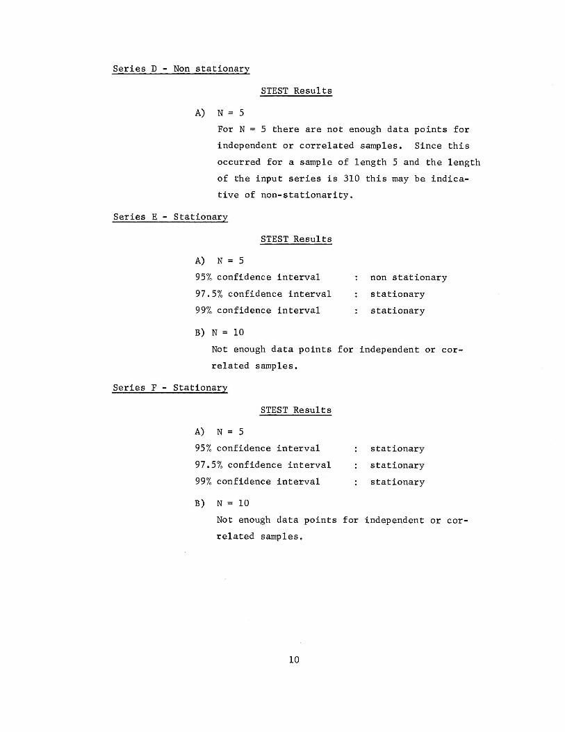
Series D - Non stationary
STEST Results
A) N = 5
For N = 5 there are not enough data points for
independent or correlated samples. Since this
occurred for a sample of length 5 and the length
of the input series is 310 this may be indica
tive of non-stationarity.
Series E - Stationary
STEST Results
A) N = 5
95% confidence interval
97.5% confidence interval
99% confidence interval
B) N = 10
non stationary
stationary
stationary
Not enough data points for independent or cor
related samples.
Series F - Stationary
STEST Results
A) N = 5
95% confidence interval
97.5% confidence interval
99% confidence interval
B) N = 10
stationary
stationary
stationary
Not enough data points for independent or cor
related samples.
10
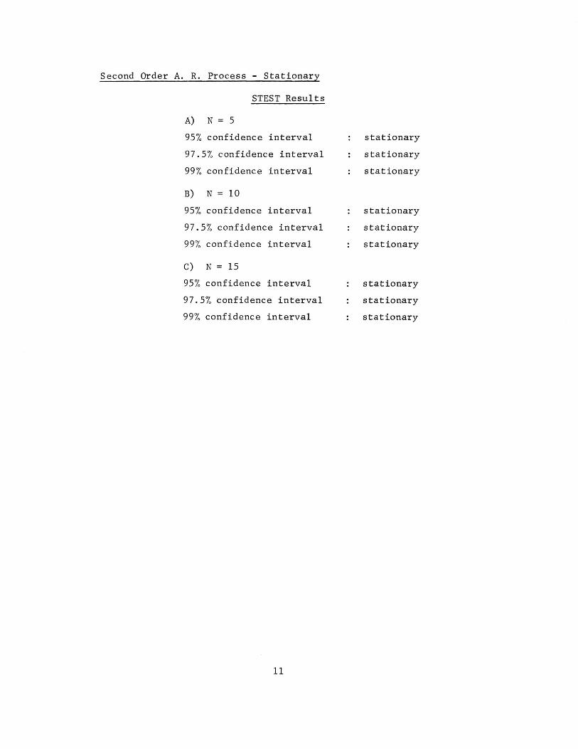
Second Order A. R. Process - Stationary
STEST Results
A) N = 5
95 % confidence interval
97.5% confidence interval
99% confidence interval
B) N = 10
95% confidence interval
97.5% confidence interval
99% confidence interval
C) N = 15
95 % con.fidence interval
97.5% confidence interval
99% confidence interval
11
stationary
stationary
stationary
stationary
stationary
stationary
stationary
stationary
stationary

Appendix
12

Computer Program STEST
13

..... .,.
DOS F O RT PA~ IV ~ ~n~- F Q-479 ~-4 ~~~I ~PGM DA Tl: 1)6 / 21/71 TI'1F 14.05.44
0001
000? 0003 0004 0005
0006 0007 000!1 000'1 0010 0011 001? non 001 4 0015 0016 0017 OOIA 0019
c oo0GRA'1 'TFST c ( TYI' oo nGRA'1 TF~TS A TTMF SERIES FOR WIDE SCNSF STAT IONARITY c c C THE PAnGRAM USES TWO TESTS r. r. c c c c
1 ) J.G. RAYA~--STATISTICAL TEST OF TH E HYPOTHESIS THAT A TIME SERIFS JS S TATIONARV---GFO PHYSIC S-V. 32-Nn.~
TIME SFRIES IS STATIONARY---GFOPHYSICSVOL.3 2---NO.~--P. 499
C 21 BENOA TT AND PIERSOL---MEASUREMENT AND ANALYSIS OF C RANDOM DATA---P. 219 c c C THF ~FRIES IS ~EAO INTO THE PROGRAM. THE ACF IS CALCULATED ANn C THE NUMRER OF LAG S NECESSARY EOR THE ACF TO DAMP TO ZERO IS C OETERMINFO. THF SERIFS IS THFN SAMPLE() AT INTERVALS SEPARATED C flY THIS LAS. THI S AS SllllES INDEPENDENCE. THE SAMPLED SERIES IS C TH EN TF,TEO FOR STATIONARITY. IF THE NUMBER GF SAMPLES IS G.F. C 12 f\ OTH TESTS a~r USEn, TF LT 12 ONLY BRYAN'S TEST IS USFO. c c C IIIJDUT DATA c c (
c c c
c
~Ill--LENGTH OF THE SERIES X---TIMF SERIES
OIMEIIJSIO~ XI1000l,RI300),WI300l,WXI100l,WWWI15,15l,RWI300l,NTESTI4 I l, JTESTI 4) ,NNTESTI 4)
PF ... DI I,t nO ) NIIJ 100 FDP'1<\T(I41
READI!,lnl)IXI li.I~1,NNI l Ot FnR'1ATIF12.4)
C NOW C,.,_LCl~4TF THE 'CF c
CJ\LL XV4ll(X , l,NN, XFlAR,V~RX l
TTI\U=n AN=NN "=0. ~*1\N '1(] 11 I P= 1, M IIJTP~'lN-ID
ASU'1~o.
DO 14 IN~1,N!P
14 A<;UM=ASll'-~+I(X(!Nl-XFlt.Rl*IXIIN+lPI-XR ,'\R))
R I I o 1 = I A S lJ I~ IN I P II VA P X !F(JThlJ.r,T.f)) Gf1 TO 12 JF( RI! P l.Lf:: .o.) !TAlJ~T?
J? '>II ( IP+t)= R( yo)
11 CrNTINUF
P<\(;E 0001

..... VI
OOS F O~T R A~ TV 3~0N-F0-479 3- 4 11A I NDG'1 DH E 06/? 3/71 Tl'11'
00 ?0 [1 0 21 0 0 ?? 002 3 0024 0025 00?6 00 27
00 28 0079 00 30 0031 fl0 3? "033 00 34 0035 00'1(, 00"'17 00'1 8
0039 004[1
0041 004 2 0043 0044 0045 0046 0047 fl04!1 0049 0050 0051 005 2 0053 0054 0055 00"16 0057 00"18 0059 0,060 0061 006 2 00 63 0064 0065 0066 ()0 6 7 0 068
l F ( l T A lJ • G T • 0 I \IR I T E ( 1 , 7 0 1 I 70 1 F O R '1 ~ T ( '1',40Xo' ***** LAG INFORMATIO N *****'o//)
TF( IU U. GT . 0 IW RTTF I 3 , 7001 ITAU,ITAU,RWI ITAU+l I 700 F ORM A TI 30X , ' I~ O EPEND EN T TAU = 1 ,!3 0 10X,•R(' 0 13 , 1 l =•,F7.4 , /I
RWIII = !. IFI ITAU. GT. OI GO TO 444 WRIT EI3o"'IO OIM
300 FOR'1ATI'1',5X,' THE AC F DIO NOT DAMP TO ZERO IN',I4, 1 LAGS---THIS lM~Y Rl' AN INDICATION OF A SIGNIFICANT TREND lN DATA 1
0 / 11 IMPLYING
2 N ~ N STATI ONARITY------ --T EST ABORTED'! GO T ~ 9'19
444 CONTI NUE DO :? 0 N = 5 ,1 5, 5 WR!TEI 3 ,70 2 1N
702 FORMATI// , 40 X,' ***** ST ATIONARITY TEST FO R N = 11 T3 1 1X 1 '*****' 1 /l
TCNT= O TSF G=N+TT All KK=NN/I SI'G IFIKK.L T.NI CALL PFIXIRW,ITAU,N,ISEG 0 KK,NNl TFIITAU.LE.OIWRITEI1,3041N
104 FOR'1ATI/f/olOX,°FOR N =',T3 0 ?X,'THERE ARE NOT ENOUGH DATA POINTS F lOR IN DI'PENDFNT OR CORRELATED ~AMPLES-----TEST ABORTEO.'I
IFIITAU.LE.O.ANO.N.E0.5lWRITEI3 1 3051NN 305 FORMATI//, 2X,'STNCE THIS OCCURED FOR A SAMPLF OF LENGTH 5 AND THE
!LENGTH OF THE INPUT SERIES TS 1 ,T5,1X, 1 THIS MAY RE INDICATIVE OF ?NON-STATIO~ARITY'I
IFIITA U.l E.OIGO TO 999 NFI=KK*ISFG 00 30 J=l,NFI,ISFG NIIIN=J M'1M=J+IN-ll 00 40 IJ=NNN,MM'1 ICNT= ICNT+l W!TCNT)=XIIJ) WX( T C ~TI=XI TJI
40 CONTINU E 30 CfJNTIIIIU E
TF(KK.LT.l21 GfJ TO 445 CALL RPTESTIKK,N,WX,NTESTI
44 5 Of) 6 0 J = 1 , N no 60 r = 1, ~ J I= J-1
1\fl WWW!T,Jl=W((Jl*NI+ll CALL BTESTIN,WWW,RW,JTESTl nrJ 10 00 11=1,3 IFIK K.LT.l 2 l NTI'ST!TTl=4 NNTEST!TII=NHSTIITI+JTFSTITTI GO TOI130,131,13 ZI 1 1T
130 cnNT= 95. 0 GO TO 133
131 CONT=97.5 Gn r n 11'3
11 :? CONT=99. 0 131 TF!NNTFSTITII.GE.5lWRTTEI1,788lCONT
14.05.44 PAGE 000 2

,_.
"'
DOS FrPT R A~ TV 3 60~-F0-479 1-4 MA I NPGM DATE 06/73/71 TIME
0069 0070 0071
0072
0073 0074 0075 0076
IF(NNTF ST !III.GE.51GO TO 1000 WRITE(1,789ICONI
78A FORMAT(20X,F5.t,lX,'PFRCENT CONFIDENCE TNTERVAL.•,lOX,~THE DATA TE 1STS STATIONARY',//)
789 FORMAT(20X,F5.1,1X,'PERCENT CONFIDFNCE INTERVAL.',lOX,'THE DATA TE lSTS NONSTATIONARY',//1
1000 CONTINUE 20 CONTINUE
999 STOP ENO
14.05.44 PAGE 0003

.... ....,
DOS FORTRAN IV ~60N-F0-479 3-4 BPTEST
0001 0002 0003 0004 0005 0006 0007 OOO'l 0009 0010 0011 0012 001'1 0014 0015 0016 0017 0()18 0019 0020 0021 0022 0021 0024 0025 0026 0027 0028 0029
SUBR OUTINF BPTESTIKK,N,WX,NTESTI DIMENSION WXIll,XMFI200),XXARI200) DIMENSION ITESTI41,MTFST14),NTESTI11 ICNT=O NFI=KK*III 00 40 J=1,N<=I,N ICNT=ICNT+I NNN=J "1MM=J+IN-ll CALL XVARIWX,NNN,MMM,XMN,VARI XMEI ICNTI=XMN XXAR I I CNTI=VAR
40 CONTINUE NNN=1 KJL=ICNT M'1'4=1CNT CALL XVARIX"1E,NNN,MMM,XMN,VARI CALL RTESTIXME,NNN,M"lM,X"lN,ITESTI DO 32 KK=1,3
32 MTESTIKKI=ITESTIKKI NNN=1 MM"1=KJL CALL XVARIXXAR,NNN,"1MM,XMN,VARI CALL RTESTCXXAR,NNN,MMM,XMN,ITESTI 00 90 IJK=l,3 N TE S Tl I JK) =MTE S T I I JK )+I TE S Tl I JK I
90 COIIITJI'Wf RFTURIII ENO
DATE 06/23/71 TIME 14.06.46 PAGE 0001

..... 00
DOS FORTRAN IV 360N-F0-479 3-4 XVAR
0001 0002 0003 0004 0005 0006 0007 0008 0009 0010 0011 0012 0013 0014
SUBR OU TIN E XVAR(X,NNN,MMM,XMN,VARl OIMENSION Xlll XSUM=O.O 00 244 K:NNN,MMM XSUM=XSUM+XIKI
244 CONTINUF AN=MMM-NNN+l.O XMN=XSUM/AN A:O .0 DO 220 l=NNN,MMM
220 A=A+(X(Il-XMNl**2 VAR=A/AN RETURN FND
DATE 06/23/71 TIME 14.07.19 PAGE 0001

.... "'
OOS FORTRA~ IV 360N-F0-479 1-4 •HE'ST 01\TF 06/ 23/71 TIME
0001 0002 0003 0004 0005
0006
SllBROUT INE R TEST I X,NNN, MMM, XM, I TESTI DIMENSION ITESTI11 DIMFNSION Xlll DIMENSION XXI10 0 ,6l,XXX1100,61 OAT A X X /1 • , 1. , 1 • , 1 • t 3. t 3 . , 4. , 5. , 6. t 6. t 7. , 8. , 9. t 10 • , 1 1 • , 11. , 12. , 13.
•,t4.,t5.,16.,t7.,17.,t8.,t9.,2o.,21.,22.,23.,24.,24.,25., 26.,27.,2 *8., 29.,30.,11.,3 2.,33.,31.,34.,35.,36.,37.,3A.,39.,40.,41.,42.,43. •,44.,45.,46.,46.,47.,48.,49.,50.,51 •• 52.,52.,53.,54.,56.,56.,57.,5 •8.,59.,60.,61.,62 .,63.,64.,65.,66.,67.,68.,69.,7o.,71.,7z.,73.,74. *t74.,75.,76.,77.,78.,79.,A0.,81.,82.,83.,84.,85.,86.,A7.,A8.,88.,1 •• ,1.,1.,1.,2.,3.,3.,4.,5.,6.,7.,7.,8.,9.,10.,11.,12.,12.,13.,14.,1 *5.,15.,16.,17.,18.,19.,20.,21.,22.,22 •• 23.,24.,25.,26.,27.,27.,28. *t29.,30.,31.,32.,33.,14.,35.,36.,37.,37.,38.,39.,40.,41.,42.,43.,4 *4.,45.,46.,46.,47.,48.,49.,50.,51 •• 52.,53.,54.,55.,56.,57.,58.,58. *t59.,60.,6t.,62.,63.,64.,65.,66.,67.,68.,69.,70.,7t.,72.,72.,73.,7 *4.,75.,76.,77.,78.,79.,80.,81.,82.,83.,94.,85.,86.,86.,1.,1.,1.,1. •,2.,2.,3.,4.,4.,5.,6.,7.,7.,8.,9.,10.,11.,11.,12.,13.,14.,15.,16., *17.,17.,!8.,!9.,20.,21 •• 21.,22.,23.,24.,25.,25.,26.,27.,28.,29.,30 •• ,31.,32.,33.,34.,34.,35.,36.,37.,38.,38.,39.,40.,41.,42.,43.,44., *45.,46.,47.,47.,48.,49.,50.,51.,52.,53.,54.,55.,56.,56.,57.,58.,59 •• ,60.,61.,62.,63.,64.,65.,65.,66.,67.,68.,69.,70.,71 •• 72.,73.,74., *74.,75.,76.,77.,78.,79.,80.,81.,82.,83.,84.,3.,5.,6.,8.,9.,11.,12. *, 13., I 5., 16., 17. , 18., 2 0., 21. , 22. , 23. ,2 5. , 26. , 27., 2 8., 29. , 31. , 32., 3 *3.,34.,35.,37.,18.,39.,40.,41.,4?.,43.,44.,46.,47.,48.,49.,50.,51. •,52.,54.,55.,56.,57.,58.,59.,60.,62.,63.,64.,65.,66.,67.,68.,69.,7 *0.,7?.,73.,74.,75.,76.,77.,78.,79.,80.,81.,82.,84.,85.,86.,87.,88. • ,A9.,90.,91.,92.,93.,94.,96.,97.,98.,99.,100.,101.,102.,103.,104., *105.,107.,108.,109.,110.,111.,112.,113.,114.,115.,116.,117.,3.,5., *6.,8.,9.,10.,12 •• 13.,14.,15.,16.,18.,19.,20.,21.,22.,23.,25.,26.,2 *7.,28.,29.,31.,12.,33.,34.,35.,37.,38.,39.,40.,41.,42.,43.,44.,45. *t46.,48.,49.,50.,51.,52.,53.,54.,55.,56.,58.,59.,60.,61.,62.,63.,6 *4.,65.,66.,68.,69.,70.,71.,72.,73.,74.,75.,76.,77.,78.,79.,80.,82. *tA3.,84.,85.,A6.,A7.,A8.,89.,90.,91.,92.,93.,94.,95.,97.,98.,99.,1 *00.,101.,102.,103.,104.,105.,106.,107.,108.,109.,110.,111.,113.,11 *4.,115.,3.,4.,6.,7.,8.,10.,11.,12.,13.,15.,16.,17.,18.,19.,20.,22 • • ,?1.,24.,25.,26.,27.,29.,30.,11.,32.,33.,34.,35.,36.,37.,38.,39.,4 *0.,41.,43.,44.,45.,46.,47.,48.,49.,50.,51.,53.,54.,55.,56.,57.,58. •,59., 60.,61.,63.,64.,65.,66.,67.,68.,69.,70.,71.,72.,73.,74.,75.,7 *6.,77.,79.,R0.,81.,92.,83.,84.,85.,86.,87.,88.,89.,90.,91.,92.,93. *,95.,96.,97.,98.,99.,100.,101.,102.,103.,104.,105.,106.,107.,108., *109.,110.,111.,113./
DATA XXX/1.,1.,2.,3.,4.,5.,6.,R.,10.,13.,18.,21.,25.,30.,35.,41.,4 * 7.,54.,61.,69.,80.,90.,100.,110.,120.,130.,140.,150.,160.,171.,190 •.,zoo.,?t5.,2?7.,240.,~58.,270.,290.,105.,320.,345.,360.,3so.,4oo. *t42'>.,445 . ,465.,485.,501.,514.,550.,570.,600.,610.,620.,665.,695., *710.,7 2?.,756.,ROO.,B30.,850.,880.,910.,940.,970.,1000.,1015.,1045 •.,109n.,1120.,1150.,l190.,1220.,1245.,l285.,1320.,1342.,l3B2.,1405 •• ,1440.,1495.,1515.~1550.,1600.,1640.,1690.,1710.,1766.,1800.,1830 •• ,1870.,)905.,1960.,2000.,2050.,2100.,2150.,2198.,1.,1.,1.,2.,3.,4 •.,5.,7.,9.,11.,15.,18.,22.,27.,31.,3B.,45.,50.,56.,64.,72.,82.,92. •,1oo.,110.,1zo.,t30.,140.,149.,162.,172.,182.,195.,210.,225.,240., * 255., 270., ? R5.,305.,1 20.,140.,350.,370.,3R5.,405.,422.,442.,465.,4 *9 5 .,515.,535.,560.,5A0.,600.,625.,650.,670.,700.,731.,742.,770.,80 *O.,A?O.,A'>0.,8A0.,910.,915.,960.,1014.,1030.,l050.,10R0.,1100.,114
14.07.48 PAGE 0001

N 0
OOS FORTRAN IV 160N-Frl-479 3-4 RTE ST DATF 06/23/71 TIME
0007 0008 0009 0010 0011 0012 0013 0014 0015 0016 0017 001R oo1q 0020 0021 0022 0023 0024 0025 0026
•o.,11qo.,1~05.,1240.,12B5.,1344.,1360.,t190.,1410.,1450.,150o.,t52
*5.,1570.,1600.,1650.,1721.,1750.,1770.,1AOO.,l840.,1B90.,1920.,199 * 0.' 2 00 5.' 2 060. ' 2 145. ' 1 • ' 1. '1 • ' 1 • '2. '3. '4. '6. '7. '9 • ' 12. ' 16. ' 20. ' 2 4. *•29.,34.,39.,45.,52.,59.,65.,73.,A0.,90.,l00.,110.,1~0.,130.,140., *152.,165.,180.,192.,205.,220.,232.,245.,261.,275.,290.,310.,325.,3 *40.,360.,375.,395.,410.,430.,450.,473.,500.,518.,530.,560.,580.,60 *5.,640.,650.,680.,702.,740.,760.,790.,810.,840.,870.,900.,930.,950 •.,977.,1010.,1045.,1070.,1100.,1130.,1160.,1200.,1230.,1266.,1299 • • ,1330.,1365.,1400.,1430 •• 1460.,1500.,1540.,1590.,1625.,1668.,1700. *•1710.,1765.,1800.,1850.,1900.,1950.,2000.,2040.,2083.,3.,4.,6.,8. *, 11., 1 5., 19. , 23. , 27. , 3 5. , 41. , 49. , 57. , 66. , 75. , A 5. , 95., 10 7., 116., 130 •• ,140.,155.,170.,180.,195.,215.,230.,245.,265.,282.,305.,322.,345. *,368.,385.,405.,425.,450.,465.,489.,515.,540.,560.,580.,610.,640., *660.,690.,720.,751.,780.,810.,840.,870.,905.,940.,970.,1000.,1030. •,1067.,1100.,1130.,1170.,1200.,1250.,1290.,1310.,1370.,1400.,1437. •,1460.,1500.,1560.,1600.,1650.,1680.,1705.,1750.,1800.,1860.,1880. *t1920.,1960.,2010.,2060.,2110.,2160.,2200.,2250.,2336.,2360.,2400. •,2450.,?500.,2560.,2620.,2680.,2730.,2800.,2866.,1.,5.,7.,8.,11.,1 *5.,18.,?2.,27.,33.,40.,47.,54.,~3.,74.,A1.,92.,102.,115.,125.,140.
*t158.,170.,180.,192 •• 208.,220.,240.,255.,272.,290.,305.,325.,345., *365.,385.,405.,430.,460.,474.,494.,518.,540.,560.,580.,610.,640.,6 *60.,690.,729.,740.,770.,800.,830.,860.,890.,920.,950.,9A0.,1038.,1 *060.,1100.,1140.,1170.,1200.,1230.,1270.,1305.,1350.,1400.,1420.,1 *465.,1500.,1530.,1580.,1605.,1660.,1700.,1740.,1815.,1840.,1900.,1 *930.,1960.,2010.,2050.,2105.,2160.,2200.,2283.,2310.,2350.,2400.,2 *450.,2500.,2550.,2600.,2680.,2710.,2804.,3.,4.,6.,8.,10.,13.,17.,2 *0.,25.,31.,36.,44.,52.,60.,68.,78.,86.,98.,110.,120.,135.,150.,165 •• ,180.,190.,200.,220.,235.,250.,263.,280.,300.,320.,330.,350.,375. *•390.,415.,440.,460.,490.,500.,530.,550.,570.,600.,630.,650.,670., *710.,730.,760.,780.,810.,840.,870.,900.,930.,960.,1013.,1040.,1080 •• ,1105.,1140.,1180.,1205.,1250.,1295.,1310.,1369.,1400.,1440.,1485 •• ,1510.,1550.,1600.,1650.,1680.,1705.,1777.,1800.,1830.,1870.,1920 •• ,1980 •• ~005.,2055.,2100.,2150.,2238.,2260.,2300 •• 2350.,2400.,2450 •• ,?500.,2550.,2600.,2680.,2751./ MNP~MMM
1F(MMM.GT.100IMMM~100.
N~MMM-NNN+1
CNT=O.O L~MMM-1
00 430 T=NNN,L on 431 J= r, L TFI XI I l .GT .X( J+l l lCNT=CNT+1.0
431 CONTINUE 430 CDNTINIJE
RIJN=1.0 IFIXINNN)-XMJ403,402,402
402 XINNNI~4.0 GO TO 404
40 3 XINNNl=3.0 404 CONTINUE
NJ=NNN+1 IF(MNP.GT.2001'1NP=?OO. Nt>l=MNP-NNN+1 00 433 JJ~NJ,MNP
14.07.48 PAGE 0002

N
005 FORTRAN IV 3~0~-Fn-479 1-4 RTF ST DATF 06/23/71
0077 00?11 0029 0010 00'11 0032 0033 0034 0035 0036 0037 0038 00'19 0040 0041 0042 0043 0044 0045 0046 0047 004~
'1049 0050 0051 0057 0053 0054 0055
XIJJI=XIJJI-XM IFIXIJJI.LT.O.OIGO TO 41A
419 IFIXIJJ-11-3.01900,421 7 420 421 RUN=RIIN+l.O 4?0 XIJJI=4.0
GO HJ 4'H 41B IFIXIJJ-11-3.01900 7 424,423 4::>3 RUN=R UN+ 1. 0 424 XIJJI=3.0
GO TO 433 433 CONTINUE
'4N=NN/2 GO TO 444
900 WRITFI3,5031 501 FOqMATI7H FRRI1RI 444 aCNT=CNT
IFIN.GT.100IRETURN 110 499 IJK = l,3 ITFSTI IJKI=O KJI=7-IJK TESTl=XXIMN,JJKI TEST2=XXIMN,KJII TESTA=XXXIN,IJKI TESTB=XXXIN,KJII IFIRUN.LE.TEST7.AND.RUN.GE.TEST111TEST(IJKI=ITESTIIJKI+1 IFIACNT.LE.TESTB.AND.ACNT.GE.TESTAIITESTIIJKI=ITFSTIIJKI+1
499 CONTINUE RETURN ENO
TIME 14.07.48 PAGE 0003

N N
OOS FORTRAN IV ~60N-F0-479 ~-4 RTF ST DATF 06/23/71 TI"1E
0001 0002 0003 0004 000'5 0006 0007
OOOR 0009 0010 01')11 0012 001":1 0014 not'5 0016 0017 0018
0019 0020 0021 0022
007.3
0024 002'5 0026 0027
00?8 0029 0030 0031 00~2
003~ 0034 0035
0036 003 7
c c
SUBROUTINE RTESTIN,X,WW,JTESTI DIMENSION Qll51,QQI15J,AMI1'51,ZZI2251,ZIII2251,ZII15,151 DIMENSION XI15,151,WWI15I,Zil5,151,r,(l51,Wil5l,Bil5,t5l,Yil5,t51 DIMENSION AAMil5l,JTESTill OIMENSION TEST313,3I,F313,31 DATA TEST3/.'59'51,.525,.483B,.822A,.795,.7791,.BA87,.868,.8562/ OATA F3/2.A7,3.51,4.43,1.99,?.31,2.615,t.739,1.929,2.16A/
C NOW CONSTRUCT THE AUTOCO~RELATION M~TRIX Z c
c
K~N
DO tO I~1,N
10 Z II, 11 = WW I I I 00 20 J=2,K J 1= J-1 DO 30 l=l,Jl Tl= 1-1
30 ZII,JI=WWIJ-Ill 00 40 I=J,N
40 Z(I,Jl=WWII-J1l ?0 CONTPWE
C CHANGE THE Z MATRIX TO MUL T!PLEXED FORM ZZ FOR INVERSION c
c
00 'iO J=1,K on so t=1,"l J1=J-1
'50 Zl I I Jl *N I+ I I= Z I I , J l
C NOW CALCULATE INVERSE OF AUTOCORRELATION MATRIX c
CALL MAINEIN,ZZ,ZIII c C TRANSFER INVERSF MULTIPLEXED Zll INTO REGULAR MATRIX ZI c c
c
c
c
DO 80 J=1,K DO 1!0 I= 1, N J l=J-1
An Zll I,Jl=71TIIJl*NI+II
on 90 I= 1, N GSUM=O.O 0'"1 500 J=1,K
500 GSUM=GSUM+ZIII,JI 90 GIII=GSUM
ASU"1=0.0 00 50 l I= l, N
'50\ AS!JM=ASUM+GI I I
00 502 I= 1, N 502 WIIl=GIII/ASUM
14.10.15
00000200 00000230 00000240 000002'50 00000260 00000270 00000280 00000290 00000300 00000310 00000320 00000330 00000340 00000350 00000360 000003 70 00000380 00000'\90 00000400 00000410 00000420 00000430 00000440 00000540 00000550 OOOOO'i60 0001)0570 000005!10 00000590 00000600 00000610 00000620 00000630 00000640 00000650 00000740 00000750 00000760 00000770 00000780 00000790 00000810 00000820 00000830 00000840 00000870 00000880
PAGE 0001

DOS FORTRAN IV 360N-F0-479 3-4 !HEST DATE 06/23/H TIME 14.10. 15 PAGE 0002
c 00000£190 r: 00000930 0038 DO '503 J=1,K 00000940 0039 DO '50~ I= l, N 00000950 0040 AI f,JI=ZJI I,JJ-GII I*WIJI 00000960 0041 <;O~ CONTINUE 00000970 c 00000980 c 00001190 0042 DO '504 J=1,K 00001200 0043 nn 504 1=1.N 00001210 0044 YSUM=O.O 00001220 004'5 00 50'5 KK=1 ,N 00001230 0046 50'5 YSUM=YSUM+BII,KKI*XIKK,JJ 00001240 0047 Y(I,JI=YSUM 00001250 0048 504 CONTINIJF 00001260 f. 00001270 c 00001300 0049 no 506 J= 1, K 00001310 0050 OSUM=O.O 00001320 0051 00 '507 l=l,N 00001330 00'52 507 QSUM=QSUM+X(f,JI*YII,JI 00001340 0053 QIJI=QSIJM 00001350 0054 '506 CONTINUE 00001360 c 00001370 c 00001380 005'; '508 CONTJNUf 00001480 c 00001490 c 00001530
N 0056 DO '509 1=1,K 00001540 "' 0057 IFIQIII.GT.O.IGO TO 900 00001550 0058 GO TO 999 00001580 0059 900 QQIII=ALOG101QII)J 00001590 0060 5()9 COIIIT INUJ= 00001600 c 00001610 c 00001620 0061 AK=K 00001630 006? AN=N 00001640 0061 QSUM=O.O 000016'50 00t>4 QQSUM=O.n 00001660 0065 on 510 I= 1, K 00001670 0066 QSUM=QSIJM+QI I I 00001680 0067 QOSUM=QQSUM+QQIII 00001690 0068 510 CONTlNUE 00001700 0069 OMN=QSUM/AK 00001710 0070 QQMN=QQSUM/AK 00001720 c 00001730 c FIND ANTILOG OF QQMN 00001740 r. 00001750 0071 ANOM=lO**QOMN 00001760 r: 00001770 0072 TESTl=ANOM/QMN 00001780 c 00001790 c 00001930 c SECOND PART OF TEST 00001940

noS FORTRAN IV 360N-F0-479 3-4 EIH: ST OATE 06/23/71 TIME 14.10.15 PAGE 0003
c 00001970 0073 no ., 11 J= 1, K 00001980 0074 SUMM=O.O 00001990 0075 DO 512 I= 1, N 00002000 0076 51 2 SUMM=SUMM+W(Il*XII,JI 00007.010 0077 <;11 AAMIJI=SUMM 00002020
c 00002030 c CALCULATION OF F 00002040
0078 SSSUM=O.O 00002050 0079 SMSUM=O.O 00002060 0080 on s2o J=1,K 00002070 0081 SMSUM=SMSUM+AAMIJI 000020AO OOA2 SSSUM=SSSUM+(AAMIJI*AAMIJII 00002090 0083 520 CONTINUE 00002100 .
c 00002110 c 00002120
0084 STAR1=1AK*ISSSUMI-ISMSUMI*ISMSUMII/AK 00002130 0085 STARM=ASUM*STAR 1 00002140
c 00002150 0086 IKI=K-1 00002160 0087 IK2=K*IN-ll 00002170 0088 AK1=IK1 00002180 0089 AK2= IK2 00002190
c 000027.00 0090 Fl=STARM/AK 1 00002210 0091 F2=QSUM/AK2 00002220 0092 F=F1/F2 00002230
c 00002240
"' 0093 t X= Ill/<; ... 0094 00 1000 I K I= 1, 3 0095 JTESTIIKI 1=0.0 0096 TEST2=TEST3(1KI,1Xl 0097 F2=F311Kt,IXl 0098 IFITEST1.GT.TEST2.AND.F.LT.F2lJTFSTIIKil=JTESTIIKil+1.0 0099 1000 CONTINUE 0100 999 RFTURN 00002340 0101 FNO 00002350

N U1
OOS FORTRAN IV 360N-F0-479 1-4 PFI X OATE 06/23/71 TIME
0001 0002 0003 0004
oooc; 0006 0007 0008 0009 0010 0011 0012
0013 0014
SUBROUTINE PFIXIPW,TTAU,N,ISFG,KK,NNI OIMENSION RWill WRTTEI3,600IITAU,N
600 FORMATI1SX,'WlTH TAU ='ol3,3X,'ANO N =•,t4,3Xo'THERE ARE NOT ENOUG lH DATA POINTS FOR INOEPF.NOENT SAMPLES',/!
1 JTAU= ITAU-1 IFIRWIITAU+11.GT.O.li!TAU=O ISEG=N+JTAU KK=NN/ISEG IFIITAU.LE.OIRETURN IFIKK.LT.NI GO TO 1 WRITEI3,6011ITAU,ITAU,RWIITAU+ll
601 FORMATI25X,'CORRELATEO SAMPLES USFO WITH TAU =',13,3X,'ANO R(',t3, 1'1 =•,F7.4 0 /)
RETURN FND
14.1l.22 PAGE 0001

DOS FORTRAN IV 3~0N-F0-479 3-4 Ml\ INE DATE 06/23/71 TI"'E 14.11.52 PAGE 0001
000 1 SUB ROUT I NE MAINE!N,A,BI c VER'ilON 1 OF SURROUTI NE MAINE c SYMMETRIC MATRIX INVERSION SY ESCALATOR METHOD
0002 DIMFNSION A!4001,8(4001 0003 Rl 11=1.0/A! 11 0004 I F ! N • E Q. 1 I R E T UP N 0005 NN=N*N ()006 00 5 T= Z ,NN 0007 5 R( I l=O.O 0008 00 '50 M=Z,N 0009 K=M-1 0010 MM=M+( M-ll*N 0011 EK=A! MM I 0012 00 10 I= 1 ,K 0013 DO 10 J=1 ,K 0014 MI=M+( 1-ll*N 00 15 IJ=I+!J-1l*N 0016 JM=J+ (M-ll*N 0017 10 EK=EK-A IMII*BIIJI*AIJMI 0018 EIIMM I= 1. 0/EK 0019 00 30 I= 1, K 0020 IM= I+! M-li*N 0021 00 20 J=l,K 0022 IJ=I+IJ-1l*N 0023 JM=J+(M-1l*N 0024 ;>O ElllMI=BIIMI-BIIJl*AIJMI/EK 0025 MI=.'H I I-ll *N 0026 30 B!Mil=BIIMI
N oon flO 40 I=1,K
"' 0028 IM=I+IM-1 l*N 0029 00 40 J=1, K 0030 MJ=M+IJ-1l*N 0031 IJ=I+IJ-11*111 0032 40 B!IJI=BIIJI+BIIMI*BIMJI*EK 0033 50 CONTINUE 0034 RETIIRN 0035 END

Sample Input
27

SAMPLE INPUT
(Series C - Box and Jenkins, 1970, p. 528)
0226 26.6 27.0 27.1 27.1 27.1 27.1 26.9 26.8 26.7 26.4
20.2 19.7 19.3 19.1 19.0 18.8
28

Sample Output
29

w 0
SAMPLE OUTPUT
''(-!d-Id LAG INFORMATION -!dnb'(-!(
INDEPENDENT TAU = 20 R( 20) = -0.0033
''dd(,'(-!( STATIONARITY TEST FOR N = 5 ''drl(-!(-J(
95.0 PERCENT CONFIDENCE INTERVAL. THE DATA TESTS NONSTATIONARY
97.5 PERCENT CONFIDENCE INTERVAL. THE DATA TESTS NONSTATIONARY
99.0 PERCENT CONFIDENCE INTERVAL. THE DATA TESTS NONSTATIONARY
-J(·k-J(-!(* STATIONARITY TEST FOR N = 10 -Jd<-!o'(-!(
WITH TAU = 20 AND N = 10 THERE ARE NOT ENOUGH DATA POINTS FOR INDEPENDENT SAMPLES
FOR N = 10 THERE ARE NOT ENOUGH DATA POINTS FOR INDEPENDENT OR CORRELATED SAMPLES----TEST ABORTED.

REFERENCES
Bendat, J. S., Piersol, A. G., 1966, Measurement and analysis of
random data: New York, Wiley.
Box, G. E. P., Jenkins, G. M., 1970, Time series analysis, fore
casting and control: San Francisco, Holden-Day.
Bryan, J. G., 1967, Statistical test of the hypothesis that a
time series is stationary: Geophysics, v. 22, p. 499-511.
Jenkins, G. M., Watts, D. G., 1968, Spectral analysis and its
applications: San Francisco, Holden-Day.
31

Related Documents