UNIT - V

Data Structures and Algorithms

UNIT - V

Snapshots Introduction Basic Concepts

Deterministic and Nondeterministic Algorithms The classes NP hard and NP complete

NP-Hard Graph Problems Clique decision Problem (CDP) Non-Cover Decision Problem Chromatic Number Decision Problem (CNDP) Directed Hamiltonian Cycle (DHC) Traveling Salesperson Decision Problem (TSP)

NP-Hard Scheduling Problems Scheduling Identical Processors Flow Shop Scheduling Job Shop Scheduling

NP-Hard Code Generation Problems Code Generation with Common Subexpressions Implementing Parallel Assignment Instructions

Introduction to Approximate Algorithms for NP-Hard Problems.

5.0 Introduction

The earlier chapters discussed about a variety of problems and algorithms. Some of them are straightforward, some are complicated and some are tricky, but virtually all of them have complexity in o(n3) where n is inexactly described as the input size. From this point of view, this chapter deals in accepting all algorithms studied so far as having low time requirements. Since many of these problems are optimization problems that arise repeatedly in applications, the need for an efficient algorithm is the actual significance.

5.1 ObjectiveThis chapter deals with the class of vital problems that have some annoying property of being efficiently solved. No reasonable fast algorithms for these problems have been found but no one has been able to prove that the algorithms require a lot of time. At end of this lesson you’ll able to sharp your skill and knowledge about NP-Hard Graph Problems, NP-Hard Code Generation Problems and NP-Hard Scheduling Problems.

Page 161


5.2 Content

5.2.1 Basic Concepts

The problems that can be solved by a polynomial time algorithm and problems for which no polynomial time algorithm is known should be a distinct. While the first group consists of problems whose solution times are bounded by polynomials of small degree, the second group is made up of problems whose best-known algorithms are non-polynomial.

Definition: The Class P

An algorithm is said to be polynomially bounded if its worst case complexity is bounded by a polynomial function of its input size.

Two classes of problems can be established namely NP-hard and NP-complete. A problem that is NP-complete has the property that it can be solved in polynomial time if and only if all other NP-complete problems can be solved in polynomial time. If an NP-hard problem can be solved in polynomial time, then all NP-complete problems can be solved in polynomial time. All NP-complete problems are NP-hard, but the reverse is not always true.

The relationship of these classes to non-deterministic computations together with the apparent power of non-determinism leads to the intuitive conclusion that no NP-complete or NP-hard problem is polynomially solvable.

Deterministic and Non-deterministic Algorithms

Algorithms, which use the property that the result of every operation is uniquely defined, are termed deterministic algorithms. Such algorithms agree with the way programs are executed on a computer. Algorithms contain operations whose outcomes are not uniquely defined but are limited to specified sets of possibilities. The machine executing such operations is allowed to choose any one of these outcomes subject to a termination condition to be defined later and this led to the concept of a non -deterministic algorithm.

New functions that are launched are given below:

1 Choice(s) arbitrarily chooses one of the elements of set S. 2 Failure() signals an unsuccessful completion.3 Success() signals a successful completion.

The assignment statement x:=Choice(1,n) could result in x being assigned any one of the integers in the range [1,n]. There is no rule specifying how this choice is to be made. The Failure() and Success() signals, used to define a computation of the algorithm, cannot be used to effect a return. A nondeterministic algorithm terminates unsuccessfully if and only if there exists no set of choices leading to a success signal. The computing

Page 162


times for Choice, Success and Failure are taken to be O(1). Nondeterministic machines provide strong intuitive reasons to conclude that fast deterministic algorithms cannot solve certain problems.

Example 1: Sorting: -

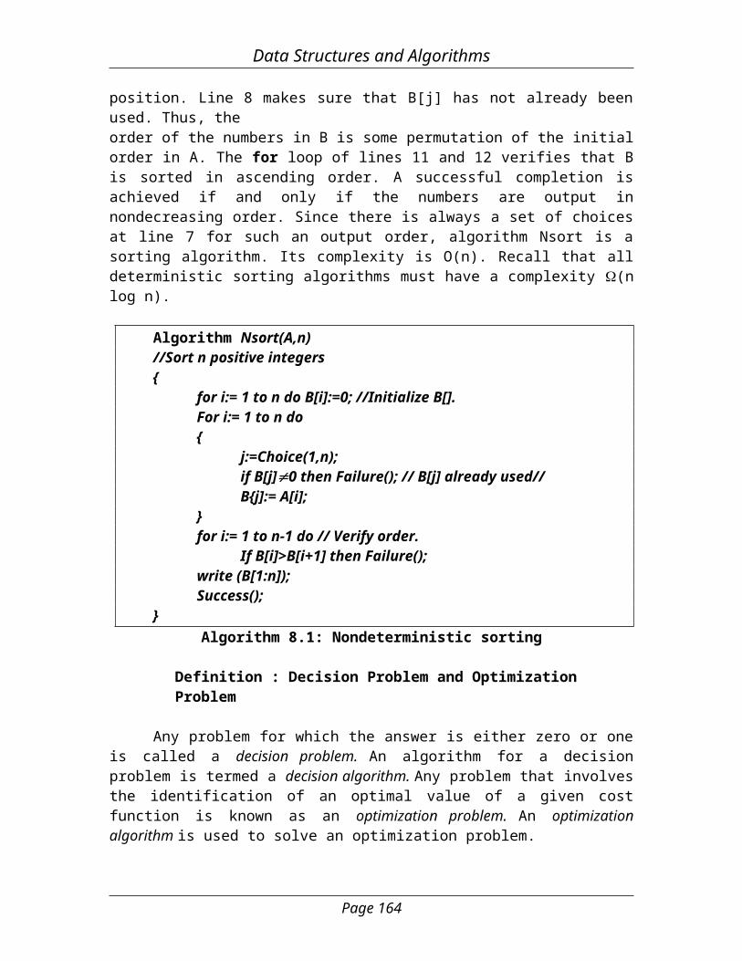
It sorts the numbers into ascending order and then outputs them in this order. An auxiliary array B[1:n] is used for convenience. Line 4 initializes B to zero. In the for loop of lines 5 to 10, each A[i] is assigned to a position in B. Line 7 non-deterministically determines this position. Line 8 makes sure that B[j] has not already been used. Thus, the order of the numbers in B is some permutation of the initial order in A. The for loop of lines 11 and 12 verifies that B is sorted in ascending order. A successful completion is achieved if and only if the numbers are output in nondecreasing order. Since there is always a set of choices at line 7 for such an output order, algorithm Nsort is a sorting algorithm. Its complexity is O(n). Recall that all deterministic sorting algorithms must have a complexity (n log n).

Algorithm Nsort(A,n)//Sort n positive integers{ for i:= 1 to n do B[i]:=0; //Initialize B[]. For i:= 1 to n do { j:=Choice(1,n); if B[j]0 then Failure(); // B[j] already used// B{j]:= A[i]; } for i:= 1 to n-1 do // Verify order. If B[i]>B[i+1] then Failure(); write (B[1:n]); Success();}

Algorithm 8.1: Nondeterministic sorting

Definition : Decision Problem and Optimization Problem

Any problem for which the answer is either zero or one is called a decision problem. An algorithm for a decision problem is termed a decision algorithm. Any problem that involves the identification of an optimal value of a given cost function is known as an optimization problem. An optimization algorithm is used to solve an optimization problem.

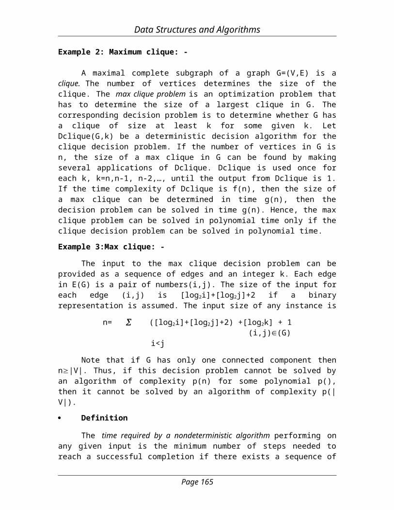
Example 2: Maximum clique: -

A maximal complete subgraph of a graph G=(V,E) is a clique. The number of vertices determines the size of the clique. The max clique problem is an optimization

Page 163


problem that has to determine the size of a largest clique in G. The corresponding decision problem is to determine whether G has a clique of size at least k for some given k. Let Dclique(G,k) be a deterministic decision algorithm for the clique decision problem. If the number of vertices in G is n, the size of a max clique in G can be found by making several applications of Dclique. Dclique is used once for each k, k=n,n-1, n-2,…, until the output from Dclique is 1. If the time complexity of Dclique is f(n), then the size of a max clique can be determined in time g(n), then the decision problem can be solved in time g(n). Hence, the max clique problem can be solved in polynomial time only if the clique decision problem can be solved in polynomial time.

Example 3:Max clique: -

The input to the max clique decision problem can be provided as a sequence of edges and an integer k. Each edge in E(G) is a pair of numbers(i,j). The size of the input for each edge (i,j) is [log2i]+[log2j]+2 if a binary representation is assumed. The input size of any instance is

n= ([log2i]+[log2j]+2) +[log2k] + 1 (i,j)(G)

i<j

Note that if G has only one connected component then n|V|. Thus, if this decision problem cannot be solved by an algorithm of complexity p(n) for some polynomial p(), then it cannot be solved by an algorithm of complexity p(|V|).

Definition

The time required by a nondeterministic algorithm performing on any given input is the minimum number of steps needed to reach a successful completion if there exists a sequence of choices leading to such a completion. In case successful completion is not possible, then the time required is O(1). A nondeterministic algorithm is of complexity O(f(n)) if for all inputs of size n, nn0 , that result in a successful completion, the time required is at most cf(n) for some constants c and n0.

Example 4: Satisfiability: -

Let x1, x2,… denote boolean variables (their value is either true or false). Let xi

denote the negation of xi. A literal is either a variable or its negation. A formula in the propositional calculus is an expression that can be constructed using literals and the operations and and or. Examples of such formulas are (x1x2) (x3x4) and (x3x4) (x1x2). The symbol denotes or and denotes and. A formula is in conjunctive normal form (CNF) if and only if it is represented as k

i=1 ci where ci are clauses each represented as lij .The lij are literals .It is in disjunctive normal form (DNF) if and only if it is represented as k

i=1 ci and each clause ci is represented as lij Thus (x1x2) (x3x4) is in DNF whereas (x3x4) (x1x2) is in CNF. The satisfiability problem is to determine whether a formula is true for some assignment of truth-values to the variables. CNF-satisfiability is the satisfiability problem for CNF formulas.

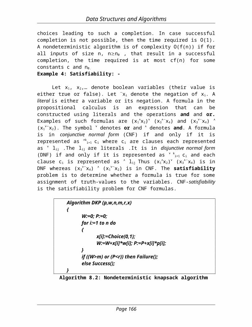
Algorithm DKP (p,w,n,m,r,x){

Page 164


W:=0; P:=0; for i:=1 to n do { x[i]:=Choice(0,1); W:=W+x[i]*w[i]; P:=P+x[i]*p[i]; } if ((W>m) or (P<r)) then Failure(); else Success();}

Algorithm 8.2: Nondeterministic knapsack algorithm

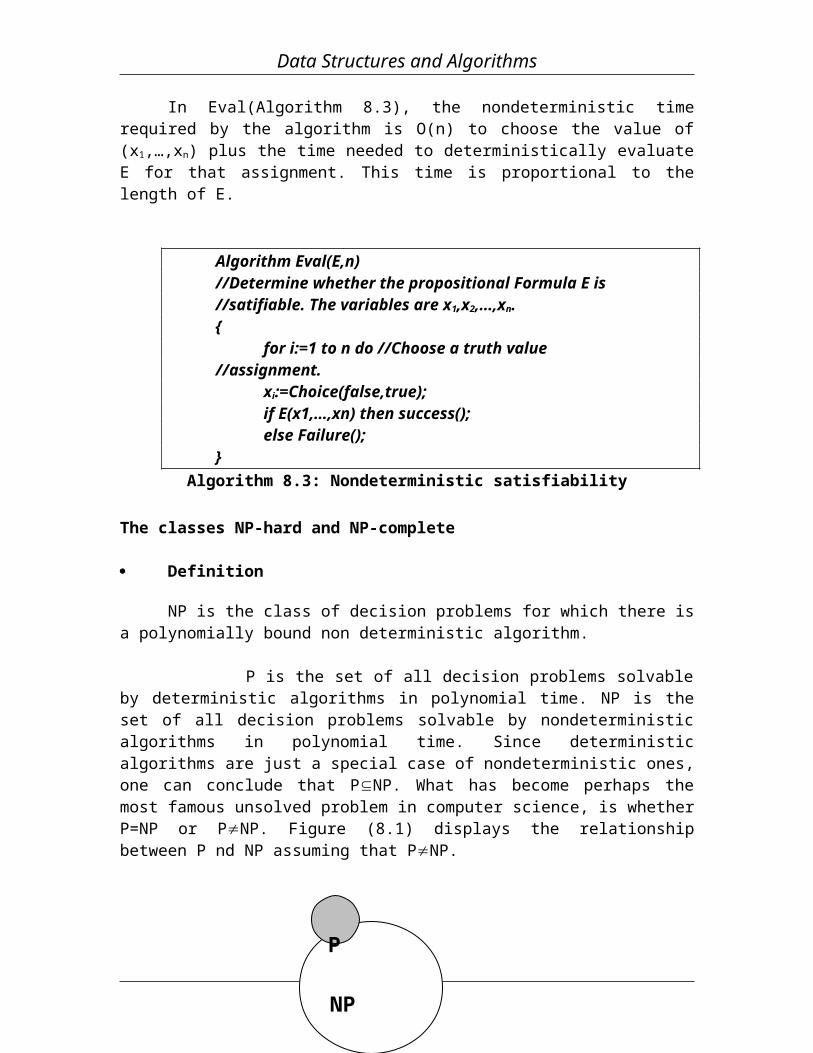
In Eval(Algorithm 8.3), the nondeterministic time required by the algorithm is O(n) to choose the value of (x1,…,xn) plus the time needed to deterministically evaluate E for that assignment. This time is proportional to the length of E.

Algorithm Eval(E,n)//Determine whether the propositional Formula E is//satifiable. The variables are x1,x2,…,xn.{ for i:=1 to n do //Choose a truth value //assignment.

xi:=Choice(false,true); if E(x1,…,xn) then success(); else Failure();}

Algorithm 8.3: Nondeterministic satisfiability

The classes NP-hard and NP-complete

Definition

NP is the class of decision problems for which there is a polynomially bound non deterministic algorithm.

P is the set of all decision problems solvable by deterministic algorithms in polynomial time. NP is the set of all decision problems solvable by nondeterministic algorithms in polynomial time. Since deterministic algorithms are just a special case of nondeterministic ones, one can conclude that PNP. What has become perhaps the most famous unsolved problem in computer science, is whether P=NP or PNP. Figure (8.1) displays the relationship between P nd NP assuming that PNP.

Page 165

NP

P


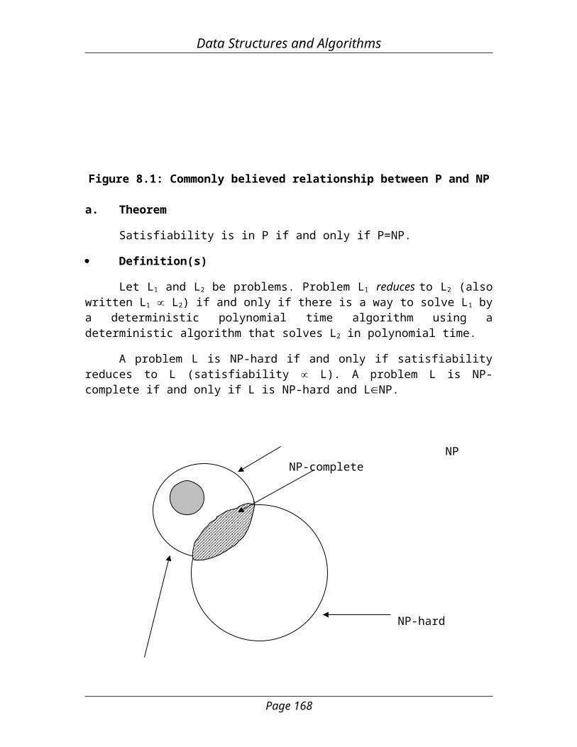
Figure 8.1: Commonly believed relationship between P and NP

a. Theorem

Satisfiability is in P if and only if P=NP.

Definition(s)

Let L1 and L2 be problems. Problem L1 reduces to L2 (also written L1 L2) if and only if there is a way to solve L1 by a deterministic polynomial time algorithm using a deterministic algorithm that solves L2 in polynomial time.

A problem L is NP-hard if and only if satisfiability reduces to L (satisfiability L). A problem L is NP-complete if and only if L is NP-hard and LNP.

NPNP-complete

NP-hard

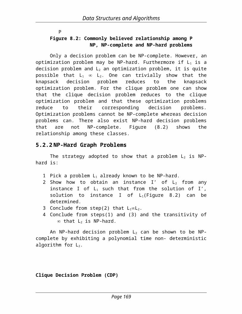
PFigure 8.2: Commonly believed relationship among P

NP, NP-complete and NP-hard problems

Only a decision problem can be NP-complete. However, an optimization problem may be NP-hard. Furthermore if L1 is a decision problem and L2 an optimization problem, it is quite possible that L1 L2. One can trivially show that the knapsack decision problem reduces to the knapsack optimization problem. For the clique problem one can show that the clique decision problem reduces to the clique optimization problem and that these optimization problems reduce to their corresponding decision problems.

Page 166


Optimization problems cannot be NP-complete whereas decision problems can. There also exist NP-hard decision problems that are not NP-complete. Figure (8.2) shows the relationship among these classes.

5.2.2 NP-Hard Graph Problems

The strategy adopted to show that a problem L2 is NP-hard is:

1 Pick a problem L1 already known to be NP-hard.2 Show how to obtain an instance I’ of L2 from any instance I of L1 such that from

the solution of I’, solution to instance I of L1(Figure 8.2) can be determined.3 Conclude from step(2) that L1L2.4 Conclude from steps(1) and (3) and the transitivity of that L2 is NP-hard.

An NP-hard decision problem L2 can be shown to be NP-complete by exhibiting a polynomial time nondeterministic algorithm for L2.

Clique Decision Problem (CDP)

According to the theorem, using the result, the transitivity of and the knowledge that satisfiability CNF-satisfiability, It can be established that satisfiability CDP. Hence, CDP is NP-hard. Since, CDPNP, CDP is also NP-complete.

b. Theorem

CNF-satisfiability clique decision problem. Example:

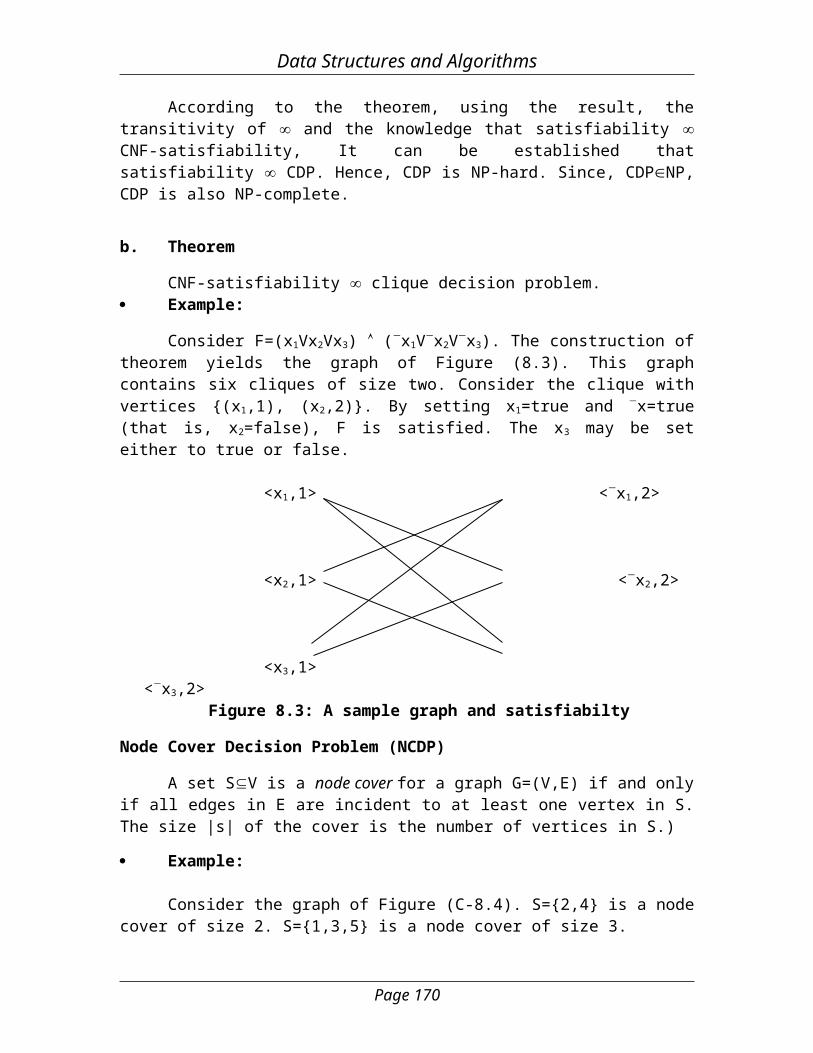
Consider F=(x1Vx2Vx3) (x1Vx2Vx3). The construction of theorem yields the graph of Figure (8.3). This graph contains six cliques of size two. Consider the clique with vertices {(x1,1), (x2,2)}. By setting x1=true and x=true (that is, x2=false), F is satisfied. The x3 may be set either to true or false.

<x1,1> <x1,2>

<x2,1> <x2,2>

<x3,1> <x3,2>Figure 8.3: A sample graph and satisfiabilty

Node Cover Decision Problem (NCDP)

Page 167


A set SV is a node cover for a graph G=(V,E) if and only if all edges in E are incident to at least one vertex in S. The size |s| of the cover is the number of vertices in S.)

Example:

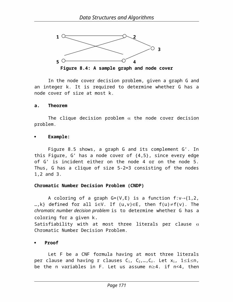
Consider the graph of Figure (C-8.4). S={2,4} is a node cover of size 2. S={1,3,5} is a node cover of size 3.

1 2

3

5 4Figure 8.4: A sample graph and node cover

In the node cover decision problem, given a graph G and an integer k. It is required to determine whether G has a node cover of size at most k.

a. Theorem

The clique decision problem the node cover decision problem.

Example:

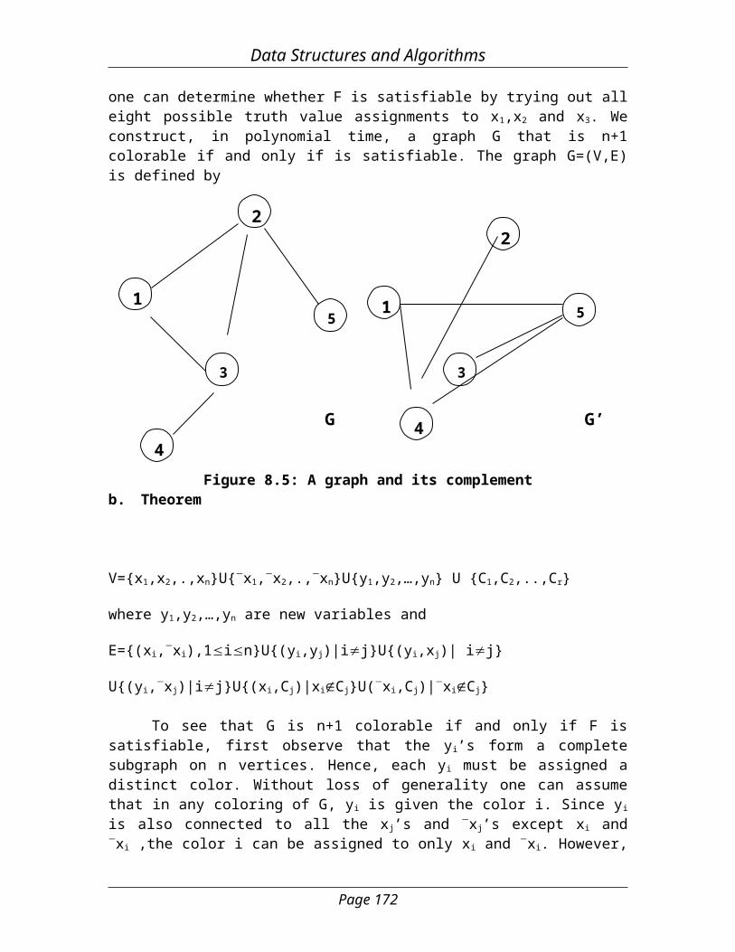
Figure 8.5 shows, a graph G and its complement G’. In this Figure, G’ has a node cover of {4,5}, since every edge of G’ is incident either on the node 4 or on the node 5. Thus, G has a clique of size 5-2=3 consisting of the nodes 1,2 and 3.

Chromatic Number Decision Problem (CNDP)

A coloring of a graph G=(V,E) is a function f:v{1,2,…,k} defined for all iV. If (u,v)E, then f(u)f(v). The chromatic number decision problem is to determine whether G has a coloring for a given k.Satisfiability with at most three literals per clause Chromatic Number Decision Problem.

Proof

Let F be a CNF formula having at most three literals per clause and having r clauses C1, C2,…,Cr. Let xi, 1in, be the n variables in F. Let us assume n4. if n<4, then one can determine whether F is satisfiable by trying out all eight possible truth value assignments to x1,x2 and x3. We construct, in polynomial time, a graph G that is n+1 colorable if and only if is satisfiable. The graph G=(V,E) is defined by

Page 1681

2

5


G G’

Figure 8.5: A graph and its complementb. Theorem

V={x1,x2,.,xn}U{x1,x2,.,xn}U{y1,y2,…,yn} U {C1,C2,..,Cr}

where y1,y2,…,yn are new variables and

E={(xi,xi),1in}U{(yi,yj)|ij}U{(yi,xj)| ij}

U{(yi,xj)|ij}U{(xi,Cj)|xiCj}U(xi,Cj)|xiCj}

To see that G is n+1 colorable if and only if F is satisfiable, first observe that the yi’s form a complete subgraph on n vertices. Hence, each yi must be assigned a distinct color. Without loss of generality one can assume that in any coloring of G, y i is given the color i. Since yi is also connected to all the xj’s and xj’s except xi and xi ,the color i can be assigned to only xi and xi. However, (xi, xi) E and so a new color, n+1, is needed for one of these vertices. The vertex that is assigned the new color n+1 is called a false vertex. The other vertex is a true vertex. The only way to color G using n+1 colors is to assign color n+1 to one of {xi,xi} for each i, 1in.

Under what conditions can the remaining vertices be colored using no new colors? Since n 4 and each clause has at most three literals, each Ci is adjacent to a pair of vertices xj,xj for at least one j. Consequently, no C i can be assigned the color n+1. Also, no Ci can be assigned a color corresponding to an xj or xj not in clause Ci. G is n+1 colorable if and only if there is a true vertex corresponding to each Ci.

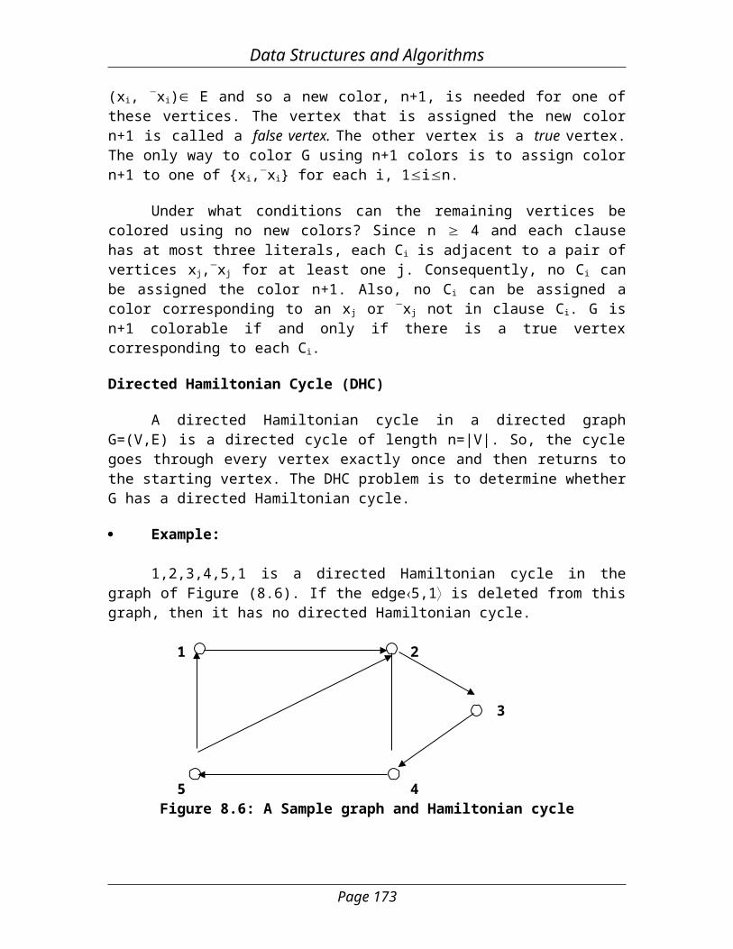
Directed Hamiltonian Cycle (DHC)

A directed Hamiltonian cycle in a directed graph G=(V,E) is a directed cycle of length n=|V|. So, the cycle goes through every vertex exactly once and then returns to the starting vertex. The DHC problem is to determine whether G has a directed Hamiltonian cycle.

Page 169

3

4

1

2

3

4

5


Example:

1,2,3,4,5,1 is a directed Hamiltonian cycle in the graph of Figure (8.6). If the edge5,1 is deleted from this graph, then it has no directed Hamiltonian cycle.

1 2

3

5 4

Figure 8.6: A Sample graph and Hamiltonian cycle

a. Theorem

CNF-satisfiability Directed Hamiltonian cycle.

Traveling Salesperson Decision Problem (TSP)

The corresponding decision problem is to determine whether a complete directed graph G=(V,E) with edge costs c(u,v) has a tour of cost at most M.

c. Theorem

Directed Hamiltonian cycle (DHC) the traveling salesperson decision problem (TSP).

5.2.3 NP-Hard Scheduling Problems

The NP-hard problem is called partition. This problem requires us to decide whether a given multiset A= {a1,a2,…,an} of n positive integers has a partition P such that ip ai=ip ai. In the sum of subsets problem, It has to be determined whether A={a1,a2,..,an} has a subset S that sums to a given integer M.

Theorem(s)

Exact cover sum of subsets. Sum of subsets partition.

Proof

Let A={a1,…,an} and M define an instance of the sum of subsets problem. Construct the set B={b1,b2,…,bn+2} with bi=ai, 1in, bn+1 = M+1, bn+2=(1in ai) +1-

Page 170


M. B has a partition if and only if A has a subset with sum M. Since B can be obtained from A and M in polynomial time, sum of subsets partition.

Scheduling Identical Processors

Let pi, 1im, be m identical processors (or machines). The pi could, for example, be line printers in a computer output room. Let Ji, 1in be n jobs. Let ti be the processing time required for Job Ji. A Schedule S assigns the jobs to processors. For each job Ji, S specifies the time intervals and the processor(s) on which this job is to be processed. More than one processor cannot process a job at any given time. Let f i be the time at which the processing of job Ji is completed. The mean finish time (MFT) of schedule S is

MFT(S)=1/nfi

1in

Let wi be a weight associated with each job Ji. The weighted mean finish time (WMFT) of schedule S is

WMFT(S)=1/nwifi

1in

Let Ti be the time at which Pi finishes processing all jobs (or job segments) assigned to it. The finish time (FT) of S is

FT(S)=max{Ti}1im

In a preemptive schedule each job need not be processed continuously to completion on one processor.

Obtaining minimum weighted mean finish time and minimum finish time non-preemptive schedules is NP-hard.a. Theorem

Partition minimum finish time non-preemptive schedule.

Example:Consider the following input to the partition problem: a1=2, a2=5, a3=6, a4=7 and

a5=10. The corresponding minimum finish time non-preemptive schedule problem has the input t1=2, t2=5, t3=6, t4=7 and t5=10. There is a non-preemptive schedule for this set of jobs with finish time 15: P1 takes the jobs t2 and t5; P2 takes the jobs t1,t3 and t4. This solution yields a solution for the partition problem also:{a2,a5}, {a1,a3,a4}.

b. Theorem

Page 171


Partition minimum WMFT non-preemptive schedule.

Proof

It is proved that this is for m=2 only. The extension to m>2 is trivial. Let ai, 1in, define an instance of the partition problem. Construct a two-processor scheduling problem with n jobs and wi=ti=ai, 1in. For this set of jobs there is a non-preemptive schedule S with weighted mean flow time at most 1/2 ai

2 + 1/4 ( ai)2 if and only if the ai’s have a partition. To see this, let the weights and times of jobs on P1 be = = = =(w1,t1),..,(wk,tk) and on P2 be (w1,t1),…,(w1,t1). Assume this is the order in which the jobs are processed on their respective processors. Then, for this schedule S we have

n*WMFT(S) = w1t1+w2(t1+t2)+……+wk(t1+…..tk)

= = = = = = = = + w1t1+w2(t1+t2)+….+w1(t1+….t1)

= 1/2 wi2 + 1/2 (wi)2 +1/2 (wi-wi)2

Thus, n*WMFT(S) (1/2) wi2 +(1/4)( wi)2.

Flow Shop Scheduling

When m=2, minimum finish time schedules can be obtained in O(n log n) time if n jobs are to be scheduled. When m=3, obtaining minimum finish time schedules is NP-hard. One proves the result for preemptive schedules. The proof one gives is also valid for the non-preemptive case where, a much simpler proof exists.

c. Theorem

Partition the minimum finish time preemptive flow shop schedule (m>2).

Proof

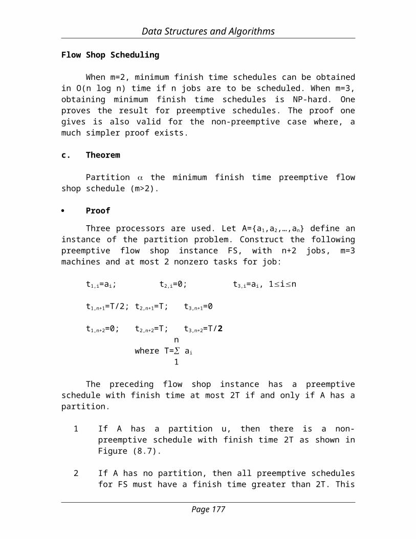
Three processors are used. Let A={a1,a2,…,an} define an instance of the partition problem. Construct the following preemptive flow shop instance FS, with n+2 jobs, m=3 machines and at most 2 nonzero tasks for job:

t1,i=ai; t2,i=0; t3,i=ai, 1in

t1,n+1=T/2; t2,n+1=T; t3,n+1=0

t1,n+2=0;t2,n+2=T; t3,n+2=T/2 n

where T= ai

1

Page 172


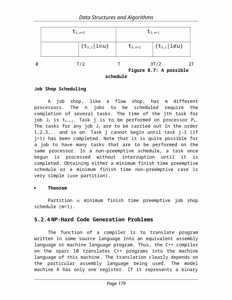
The preceding flow shop instance has a preemptive schedule with finish time at most 2T if and only if A has a partition.

1 If A has a partition u, then there is a non-preemptive schedule with finish time 2T as shown in Figure (8.7).

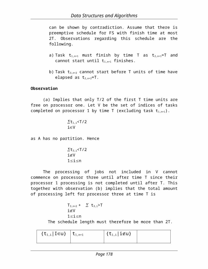
2 If A has no partition, then all preemptive schedules for FS must have a finish time greater than 2T. This can be shown by contradiction. Assume that there is preemptive schedule for FS with finish time at most 2T. Observations regarding this schedule are the following.

a) Task t1,n+1 must finish by time T as t2,n+1=T and cannot start until t1,n+1

finishes.

b) Task t3,n+2 cannot start before T units of time have elapsed as t2,n+2=T.

Observation

(a) Implies that only T/2 of the first T time units are free on processor one. Let V be the set of indices of tasks completed on processor 1 by time T (excluding task t1,n+1).

t1,i<T/2iV

as A has no partition. Hence

t3,i<T/2iV1in

The processing of jobs not included in V cannot commence on processor three until after time T since their processor 1 processing is not completed until after T. This together with observation (b) implies that the total amount of processing left for processor three at time T is

T3,n+2 + t3,i>TiV1in

The schedule length must therefore be more than 2T.

{t1,i|Iu} t1,n+1 {t1,i|iu}

t2,n+2 t2,n+1

Page 173


{t3,i|iu} t3,n+2 {t3,i|iu}

0 T/2 T 3T/2 2T Figure 8.7: A possible schedule

Job Shop Scheduling

A job shop, like a flow shop, has m different processors. The n jobs to be scheduled require the completion of several tasks. The time of the jth task for job J i is tk,i,j. Task j is to be performed on processor Pk. The tasks for any job Ji are to be carried out in the order 1,2,3,.. and so on. Task j cannot begin until task j-1 (if j>1) has been completed. Note that it is quite possible for a job to have many tasks that are to be performed on the same processor. In a non-preemptive schedule, a task once begun is processed without interruption until it is completed. Obtaining either a minimum finish time preemptive schedule or a minimum finish time non-preemptive case is very simple (use partition).

Theorem

Partition minimum finish time preemptive job shop schedule (m>1).

5.2.4 NP-Hard Code Generation Problems

The function of a compiler is to translate program written in some source language into an equivalent assembly language or machine language program. Thus, the C++ compiler on the sparc 10 translates C++ programs into the machine language of this machine. The translation clearly depends on the particular assembly language being used. The model machine A has only one register. If it represents a binary operator such as +, -, * and /, then the left operand must be in the accumulator.

The relevant assembly language instructions are:

LOAD X- load accumulator with contents of memory location X.STORE X- store contents of accumulator into memory location X.OP X OP may be ADD, SUB, MPY or DIV.

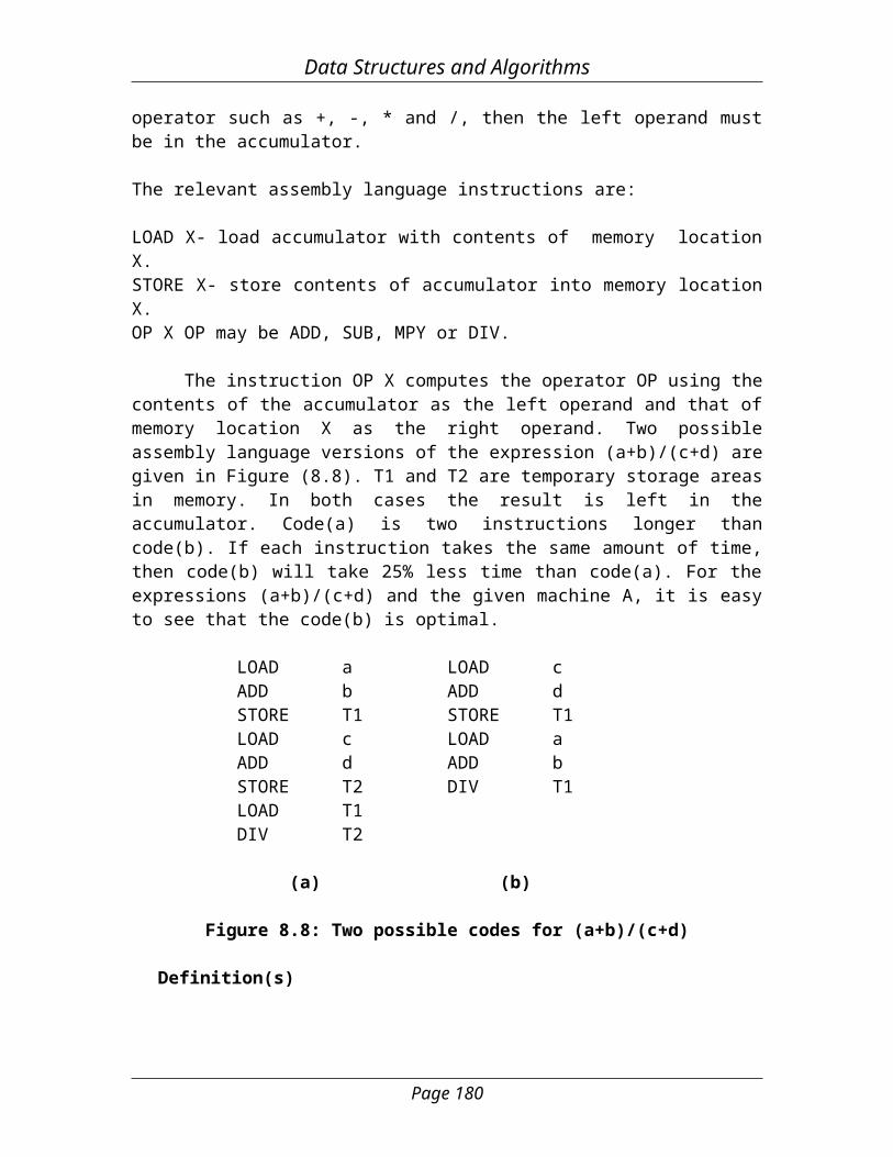
The instruction OP X computes the operator OP using the contents of the accumulator as the left operand and that of memory location X as the right operand. Two possible assembly language versions of the expression (a+b)/(c+d) are given in Figure (8.8). T1 and T2 are temporary storage areas in memory. In both cases the result is left in the accumulator. Code(a) is two instructions longer than code(b). If each instruction takes the same amount of time, then code(b) will take 25% less time than code(a). For the expressions (a+b)/(c+d) and the given machine A, it is easy to see that the code(b) is optimal.

LOAD a LOAD c

Page 174


ADD b ADD dSTORE T1 STORE T1LOAD c LOAD aADD d ADD bSTORE T2 DIV T1LOAD T1DIV T2

(a) (b)

Figure 8.8: Two possible codes for (a+b)/(c+d)

Definition(s)

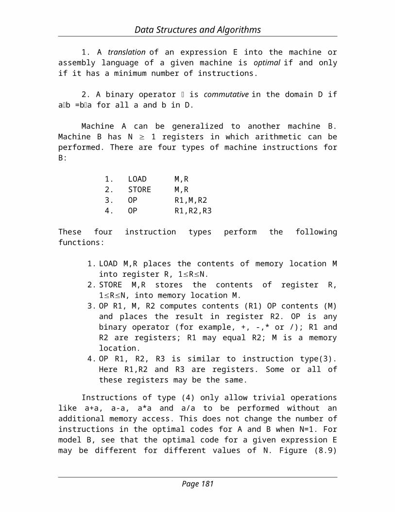
1. A translation of an expression E into the machine or assembly language of a given machine is optimal if and only if it has a minimum number of instructions.

2. A binary operator is commutative in the domain D if ab =ba for all a and b in D.

Machine A can be generalized to another machine B. Machine B has N 1 registers in which arithmetic can be performed. There are four types of machine instructions for B:

1. LOAD M,R2. STORE M,R3. OP R1,M,R24. OP R1,R2,R3

These four instruction types perform the following functions:

1. LOAD M,R places the contents of memory location M into register R, 1RN.

2. STORE M,R stores the contents of register R, 1RN, into memory location M.

3. OP R1, M, R2 computes contents (R1) OP contents (M) and places the result in register R2. OP is any binary operator (for example, +, -,* or /); R1 and R2 are registers; R1 may equal R2; M is a memory location.

4. OP R1, R2, R3 is similar to instruction type(3). Here R1,R2 and R3 are registers. Some or all of these registers may be the same.

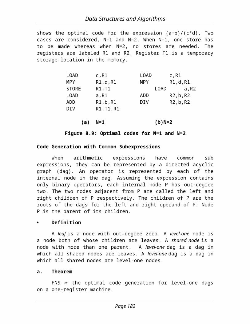
Instructions of type (4) only allow trivial operations like a+a, a-a, a*a and a/a to be performed without an additional memory access. This does not change the number of instructions in the optimal codes for A and B when N=1. For model B, see that the optimal code for a given expression E may be different for different values of N. Figure (8.9) shows the optimal code for the expression (a+b)/(c*d). Two cases are considered, N=1 and N=2. When N=1, one store has to be made whereas when N=2, no stores are

Page 175


needed. The registers are labeled R1 and R2. Register T1 is a temporary storage location in the memory.

LOAD c,R1 LOAD c,R1MPY R1,d,R1 MPY R1,d,R1STORE R1,T1 LOAD a,R2LOAD a,R1 ADD R2,b,R2ADD R1,b,R1 DIV R2,b,R2DIV R1,T1,R1

(a) N=1 (b)N=2

Figure 8.9: Optimal codes for N=1 and N=2

Code Generation with Common Subexpressions

When arithmetic expressions have common sub expressions, they can be represented by a directed acyclic graph (dag). An operator is represented by each of the internal node in the dag. Assuming the expression contains only binary operators, each internal node P has out-degree two. The two nodes adjacent from P are called the left and right children of P respectively. The children of P are the roots of the dags for the left and right operand of P. Node P is the parent of its children.

Definition

A leaf is a node with out-degree zero. A level-one node is a node both of whose children are leaves. A shared node is a node with more than one parent. A level-one dag is a dag in which all shared nodes are leaves. A level-one dag is a dag in which all shared nodes are level-one nodes.

a. Theorem

FNS the optimal code generation for level-one dags on a one-register machine.

Proof

Let G,k be an instance of FNS. Let n be the number of vertices in G. Dag A is constructed with the property that the optimal code for the expression corresponding to A has at most n+k LOADs if and only if G has a feedback node set of size at most R.

The dag A consists of three kinds of nodes namely, leaf nodes, chain nodes and tree nodes. All chain and tree nodes are internal nodes representing commutative operators. Leaf nodes represent distinct variables. dv denotes the out-degree of vertex v of G. Corresponding to each vertex v of G, there is a directed chain for v and is the parent of two leaf nodes vL and vR. Vertex v1 is the tail of the chain. From each of the chain nodes corresponding to vertex v, except the head node, there is one directed edge to the head node of one of the chains corresponding to a vertex w such that v,w is an edge in G. Each such edge goes to a distinct head. Since each chain node represents a commutative operator, it does not matter which of its two children is regarded as the left child.

Page 176


One has a dag in which the tail of every chain has in-degree zero. One needs n-1 tree nodes, since G has n vertices. These n-1 nodes are connected together to form a binary tree. In place of the external nodes we connect the tails of the n chains. This yields a dag A corresponding to an arithmetic expression.

Every optimal code for A will have exactly n LOADs of leaf nodes. There will be exactly one instruction of type for every chain node and tree node. Hence, the only variable is the number of LOADs and STOREs of chain and tree nodes. If G has no directed cycles, then its vertices can be arranged in topological order. Let v1,v2,…,vn be a topological ordering of the vertices in G. First computing all nodes on the chain for vn and storing the result of the tail node can compute the expression A using no LOADs of chain and tree nodes. All nodes on the chain for Vn-1 can be computed. We can also compute any nodes on the path from the tail for Vn-1 to the root for which both operands are available. Finally, one result needs to be stored. Next, the chain for Vn-2 can be computed. We can compute all nodes on the path from this chain tail to the root for which both operands are available. The entire expression can be computed in this way.

Suppose G contains at least one cycle v1,v2,…,vi,v1, then every code for A must contain at least one LOAD of a chain node on a chain for one of v1,v2,…,vi. Every optimal code for A contains exactly n+p LOADs. The p LOADs correspond to a combination of tail nodes corresponding to a minimum feedback node set and the siblings of these tail nodes. If non-commutative operators have been used for chain nodes and made each successor on a chain the left child of its parent, then the p LOADs would correspond to the tails of the chains of any minimum feedback set. Furthermore, if the optimal code contains p LOADs of chain nodes, then G has a feedback node set of size p.

Implementing Parallel Assignment Instructions

A parallel assignment instruction has the format (v1,v2,…,vn):=(e1,e2;,…,en) where the vi’s are distinct variable names and the ei’s are expressions. The semantics of this statement is that the value of vi is updated to be the value of the expression e i, 1in. The value of the expression ei is to be computed using the values the variables in ei have before this instruction is executed. Example:

Consider the statement (A,B,C) := (D,A+B,A-B); The 3!=6 different realizations and their costs are given in Figure (8.10). The realization 3,2,1 corresponding to the implementation C=A-B; B=A+B; A=D; needs no temporary stores (C(R)=0).

R C(R) 1,2,3 2 1,3,2 2 2,1,3 2 2,3,1 1 3,1,2 1 3,2,1 0

Figure 8.10: Realization for Example

Page 177


An optimal realization for a parallel assignment statement is one with minimum cost. When the expressions ei are all variable names or constants, an optimal realization can be found in linear time (O(n)). When the ei are allowed to be expressions with operators then finding an optimal realization is NP-Hard.

5.2.5 Introduction to Approximate Algorithms for NP-Hard Problems

The best-known algorithms for NP-hard problems have a worst-case complexity that is exponential in the number of inputs. O(2n/2) algorithm for the knapsack problem was developed. These algorithms can also be used for the partition, sum of subsets and exact cover problems. NP-hard problem increases the maximum problem size that can be solved. However, for large problem instances, even an O(n4) algorithm requires too much computational effort.

The use of heuristics in an existing algorithm may enable it to quickly solve a large instance of a problem provided the heuristic works on that instance. A heuristic does not work equally effectively on all problem instances. If one has to produce an algorithm of low polynomial complexity to solve an NP-hard optimization problem, then it is necessary to relax the meaning of “solve”. One removes the requirement that the algorithm that solves the optimization problem P must always generate an optimal solution. This requirement is replaced by the requirement that the algorithm for P must always generate a feasible solution with value close to the value of an optimal solution. A feasible solution with value close to the value of an optimal solution is called an appropriate solution. An appropriate algorithm for P is an algorithm that generates approximate solutions for P.

In the circumstance of NP-hard problems, approximate solutions have added importance, as exact solutions may not be obtainable in a feasible amount of computing time. An approximate solution may be all one can get using a reasonable amount of computing time.

Look for an algorithm for P that almost generates optimal solutions. Algorithms with this property are called probabilistically good algorithms.

Consider P is a problem of knapsack or the traveling salesperson problem, I is an instance of problem P and F*(I) is the value of an optimal solution to I. An approximation algorithm generally produces a feasible solution to I whose value F^(I) is less than F*(I) If P is a maximization (minimization) problem. Several categories of approximation algorithms can be defined.

Let A be an algorithm that generates a feasible solution to every instance I of a problem P. Let F*(I) be the value of an optimal solution to I and let F^(I) be the value of the feasible solution generated by A.

Page 178


Definition(s)

A is an absolute approximation algorithm for problem P if and only if for every instance I of P, |F*(I)-F^(I)| k for some constant k.

A is an f(n)-approximate algorithm if and only if for every instance I of size n, |F*(I)-F^(I)|/F*(I) f(n) for F*(I)>0.

An -approximate algorithm is an f(n)-approximate algorithm for which f(n) for some constant .

A() is an approximation scheme if and only if for every given >0 and problem instance I, A() generates a feasible solution such that |F*(I)-F^(I) / F*(I) . Again, we assume F*(I)>0.

An approximation scheme is a polynomial time approximation scheme if and only if for every fixed >0, it has a computing time that is polynomial in the problem size.

An approximation scheme whose computing time is a polynomial both in the problem size and in 1/ is a fully polynomial time approximation scheme.

The most attractive kind of approximation is an absolute approximation algorithm. Unfortunately, for most NP-hard problems it can be shown that fast algorithms of this type exist only if P=NP.

Based on absolute approximation algorithm and f(n)- approximate algorithm, one can define approximation problems in the obvious way. So, one can speak of k-absolute approximate problems and f(n)-approximate problems. The .5-approximate knapsack problem is to find any 0/1 feasible solution with |F*(I)-F^(I)|/F*(I).5.

Approximation algorithms only guarantee to generate feasible solutions with values within some constant or some factor of the optimal value. Being heuristic in nature, these algorithms are very much dependent on the individual problem being solved.

5.3 Revision Points

NP- Complete & NP – Hard ProblemA problem that is NP-complete has the property that it can be solved in polynomial time if and only if all other NP-complete problems can be solved in polynomial time. If an NP-hard problem can be solved in polynomial time, then all NP-complete problems can be solved in polynomial time. All NP-complete problems are NP-hard, but the reverse is not always true.

Page 179


Deterministic algorithmAlgorithms, which use the property that the result of every operation is uniquely defined, are termed deterministic algorithms

Non - Deterministic AlgorithmThe machine executing such operations is allowed to choose any one of these outcomes subject to a termination condition to be defined later and this led to the concept of a non -deterministic algorithm

5.4 Intext Questions

1. Discuss briefly Nondeterministic Algorithms.

2. Explain in detail NP-Hard Graph Problems.

3. Different NP-Hard Scheduling problems are to be explained in detail.

4. Explain the problems of NP-Hard Code Generation.

5. What are Approximate Algorithms used for?

5.5 Summary

Search, which necessitates the examination of every vertex in the object being searched, is called a traversal.

Algorithms, which use the property that the result of every operation is uniquely defined, are termed deterministic algorithms.

A nondeterministic algorithm terminates unsuccessfully if and only if there exists no set of choices leading to a success signal.

Any problem that involves the identification of an optimal value of a given cost function is known as an optimization problem.

The time required by a nondeterministic algorithm performing on any given input is the minimum number of steps needed to reach a successful completion if there exists a sequence of choices leading to such a completion.

An Algorithm A is polynomial complexity if there exists a polynomial p() such that the computing time of A is O(p(n)) for every input of size n.

The chromatic number decision problem is to determine whether G has a coloring for a given k.

Page 180


An approximation scheme is a polynomial time approximation scheme if and only if for every fixed >0, it has a computing time that is polynomial in the problem size.

5.6 Terminal Exercises

1. Define the classes NP-hard and NP-complete.

2. Define clique Decision problem.

3. Define node cover decision problem.

4. Define chromatic number decision problem.

5. Define Directed Hamiltonian Cycle.

5.7 Supplementary Materials

1. Ellis Horowitz, Sartaj Sahni, “Fundamentals of Computer Algorithms”,

Galgotia Publications, 1997.

2. Aho, Hopcroft, Ullman, “Data Structures and Algorithms”, Addison Wesley,

1987.

3. Jean Paul Trembly & Paul G.Sorenson, “An introduction to Data Structures

with Applications”, McGraw-Hill, 1984.

5.8 Assignments

Collect information on NP hard and NP Complete problems.

5.9 Suggested Reading/Reference Books/Set Books

1. Mark Allen Weiss, “Data Structures and Algorithm Analysis in C++”,

Addison Wesley, 1999.

2. Yedidyah Langsam, Moshe J.Augenstein, Aaron M. Tanenbaum, “Data

Structures Using C and C++”, Prentice-Hall, 1997.

Page 181


5.10 Learning Activities

Collect information on NP – Hard Code Generation Problems.

5.11 Keywords

NP- Complete & NP – Hard Problem

Deterministic algorithm

Non - Deterministic Algorithm

NP-Hard Graph

NP-Hard Scheduling

NP-Hard Code

Page 182

UNIT - V

Documents

hard scheduling problems

absolute approximation algorithm

termed deterministic algorithms

hard graph problems

feedback node set

max clique problem

clique decision problem

polynomial time algorithm