Doctoral Thesis Madrid, Spain 2014 Unit Commitment Computational Performance, System Representation and Wind Uncertainty Management Germán Andrés Morales-España

Welcome message from author
This document is posted to help you gain knowledge. Please leave a comment to let me know what you think about it! Share it to your friends and learn new things together.
Transcript
Doctoral ThesisMadrid, Spain 2014
Unit CommitmentComputational Performance, System Representation and
Wind Uncertainty Management
Germán Andrés Morales-España
Doctoral Thesis supervisors:
Prof.dr. Andrés Ramos, Universidad Pontificia Comillas, directorDr. Javier García-González, Universidad Pontificia Comillas, co-directorProf.dr.ir. Lennart Söder, Kungliga Tekniska Högskolan, supervisorProf.dr.ir. Paulien M. Herder, Technische Universiteit Delft, promotor
Members of the Examination Committee:
Prof.dr.ir. Francisco J. Prieto, Universidad Carlos III de Madrid, chairmanDr. Mohammad R. Hesamzadeh, Kungliga Tekniska HögskolanDr. Efraim Centeno, Universidad Pontificia ComillasDr.ir. Laurens J. de Vries, Technische Universiteit DelftProf.dr.ir. Benjamin F. Hobbs, Johns Hopkins University
This research was funded by the European Commission through the Erasmus MundusJoint Doctorate Program, and also partially supported by the Institute for Researchin Technology at Universidad Pontificia Comillas and the Cátedra Iberdrola de En-ergía e Innovación.
TRITA-EE 2014:041ISSN 1653-5146ISBN 978-84-697-1230-6
Copyright © 2014 by G. Morales-España.
Printed in Spain
Unit CommitmentComputational Performance, System Representation and
Wind Uncertainty Management
PROEFSCHRIFT
ter verkrijging van de graad van doctoraan de Technische Universiteit Delft,
op gezag van de Rector Magnificus prof. ir. K.C.A.M. Luyben,voorzitter van het College voor Promoties,
in het openbaar te verdedigenop woensdag 8 oktober 2014 om 13:00 uur
door
Germán Andrés MORALES-ESPAÑA
geboren te Florencia, Colombiain 1982
Dit proefschrift is goedgekeurd door de promotoren:
Prof.dr. Andrés Ramos, Universidad Pontificia Comillas, directorDr. Javier García-González, Universidad Pontificia Comillas, co-directorProf.dr.ir. Lennart Söder, Kungliga Tekniska Högskolan, supervisorProf.dr.ir. Paulien M. Herder, Technische Universiteit Delft, promotor
Samenstelling promotiecommissie:
Prof.dr.ir. Francisco J. Prieto, Universidad Carlos III de Madrid, voorzitterDr. Mohammad R. Hesamzadeh, Kungliga Tekniska HögskolanDr. Efraim Centeno, Universidad Pontificia ComillasDr.ir. Laurens J. de Vries, Technische Universiteit DelftProf.dr.ir. Benjamin F. Hobbs, Johns Hopkins University
ISBN 978-84-697-1230-6
Copyright © 2014 by G. Morales-España. Madrid, Spain. All rights reserved. Nopart of the material protected by this copyright notice may be reproduced or uti-lized in any form or by any means, electronic or mechanical, including photocopying,recording or by any information storage and retrieval system, without written per-mission from the author.
Printed in Spain

SETS Joint Doctorate
The Erasmus Mundus Joint Doctorate in Sustainable Energy Technologies andStrategies, SETS Joint Doctorate, is an international programme run by six insti-tutions in cooperation:
• Comillas Pontifical University, Madrid, Spain
• Delft University of Technology, Delft, the Netherlands
• Florence School of Regulation, Florence, Italy
• Johns Hopkins University, Baltimore, USA
• KTH Royal Institute of Technology, Stockholm, Sweden
• University Paris-Sud 11, Paris, France
The Doctoral Degrees issued upon completion of the programme are issued by Comil-las Pontifical University, Delft University of Technology, and KTH Royal Instituteof Technology.
The Degree Certificates are giving reference to the joint programme. The doctoralcandidates are jointly supervised, and must pass a joint examination procedure setup by the three institutions issuing the degrees.
This Thesis is a part of the examination for the doctoral degree.
The invested degrees are official in Spain, the Netherlands and Sweden respectively.
SETS Joint Doctorate was awarded the Erasmus Mundus excellence label by theEuropean Commission in year 2010, and the European Commission’s Education,Audiovisual and Culture Executive Agency, EACEA, has supported the fund-ing of this programme.
The EACEA is not to be held responsible for contents of the Thesis.


A Sandra Kempermanpor estar a mi lado y ser mi apoyo,
gracias por darme la estabilidad mentalque hizo posible esta tesis

Summary
In recent years, high penetration of variable generating sources, such as wind power, haschallenged independent system operators (ISO) in keeping a cheap and reliable powersystem operation. Any deviation between expected and real wind production must beabsorbed by the power system resources (reserves), which must be available and ready tobe deployed in real time. To guarantee this resource availability, the system resources mustbe committed in advance, usually the day-ahead, by solving the so-called unit commitment(UC) problem. If the quantity of committed resources is extremely low, there will bedevastating and costly consequences in the system, such as significant load shedding. Onthe other hand, if this quantity is extremely high, the system operation will be excessivelyexpensive, mainly because facilities will not be fully exploited.
This thesis proposes computationally efficient models for optimal day-ahead planning in(thermal) power systems to adequately face the stochastic nature of wind production inthe real-time system operation. The models can support ISOs to face the new challengesin short-term planning as uncertainty increases dramatically due to the integration ofvariable generating resources. This thesis then tackles the UC problem in the followingaspects:
• Power system representation: This thesis identifies drawbacks of the traditionalenergy-block scheduling approach, which make it unable to adequately prepare thepower system to face deterministic and perfectly known events. To overcome thosedrawbacks, we propose the ramp-based scheduling approach that more accuratelydescribes the system operation, thus better exploiting the system flexibility.
• UC computational performance: Developing more accurate models would be point-less if these models considerably increase the computational burden of the UC prob-lem, which is already a complex integer and non-convex problem. We then devisesimultaneously tight and compact formulations under the mixed-integer program-ming (MIP) approach. This simultaneous characteristic reinforces the convergencespeed by reducing the search space (tightness) and simultaneously increasing thesearching speed (compactness) with which solvers explore that reduced space.
• Uncertainty management in UC : By putting together the improvements in the previ-ous two aspects, this thesis contributes to a better management of wind uncertaintyin UC, even though these two aspects are in conflict and improving one often meansharming the other. If compared with a traditional energy-block UC model underthe stochastic (deterministic) paradigm, a stochastic (deterministic) ramp-based UCmodel: 1) leads to more economic operation, due to a better and more detailed sys-tem representation, while 2) being solved significantly faster, because the core ofthe model is built upon simultaneously tight and compact MIP formulations.
• To further improve the uncertainty management in the proposed ramp-based UC, weextend the formulation to a network-constrained UC with robust reserve modelling.Based on robust optimization insights, the UC solution guarantees feasibility forany realization of the uncertain wind production, within the considered uncertaintyranges. This final model remains as a pure linear MIP problem whose size does notdepend on the uncertainty representation, thus avoiding the inherent computationalcomplications of the stochastic and robust UCs commonly found in the literature.
i

Dissertation
This doctoral thesis includes an analysis of the unit commitment (UC) problemwith emphasis on three different aspects: computational performance, power systemrepresentation and wind uncertainty management. This thesis is based on the workof the following (JCR) journal papers [53, 91, 95, 97, 99, 100] which are included atthe end of this document (labelled Article I–VI) and listed as follows. The list ofpapers is separated on the different aspects of the thesis, but some of the papers fitin more than one. Further details of the thesis structure and roadmap are given insection 1.3.
Power System Representation
Article I G. Morales-España, J. M. Latorre, and A. Ramos, “Tight and compactMILP formulation of start-up and shut-down ramping in unit commitment,”IEEE Transactions on Power Systems, vol. 28, no. 2, pp. 1288–1296. May2013.
Article II G. Morales-España, A. Ramos, and J. García-González, “An MIP For-mulation for Joint Market-Clearing of Energy and Reserves Based on RampScheduling,” IEEE Transactions on Power Systems, vol. 29, no. 1, pp. 476–488, Jan. 2014.
UC Computational Performance
Article III G. Morales-España, J. M. Latorre, and A. Ramos, “Tight and compactMILP formulation for the thermal unit commitment problem,” IEEE Trans-actions on Power Systems, vol. 28, no. 4, pp. 4897–4908. Nov. 2013.
Article IV C. Gentile, G. Morales-España, and A. Ramos, “A Tight MIP For-mulation of the Unit Commitment Problem with Start-up and Shut-downConstraints,” Computers & Operations Research, paper under review.
Article V G. Morales-Espana, C. Gentile, and A. Ramos, “Tight MIP Formulationsof the Power-Based Unit Commitment Problem,” Optimization Letters, 2014,paper under review (Manuscript ID: OPTL-S-14-00348).
iii

Wind Uncertainty Management
Article VI G. Morales-Espana, R. Baldick, J. García-González, and A. Ramos,“Robust Reserve Modelling for Wind Power Integration in Ramp-Based UnitCommitment,” IEEE Transactions on Power Systems, 2014, paper under re-view.
The following two working papers are also result of this PhD research:Article VII “Comparison of Energy-Block and Ramp-Based Scheduling Approaches,”
Targeted Journal: IEEE Transactions on Power Systems. See chapter 3.Article VIII “The Worst-case Wind Scenario for Adaptive Robust Unit Commit-
ment Problems,” Targeted Journal: IEEE Transactions on Power Systems.See Appendix A.
Apart from this, during my four years as a PhD student I presented the relevantresults in several conferences [87–90, 92–94, 98, 114, 115] and I also co-authoredthree other (JCR) journal papers [85, 96, 122].
iv
Contents
Summary i
Dissertation iii
List of Acronyms ix
1. Introduction 11.1. Context . . . . . . . . . . . . . . . . . . . . . . . . . . . . . . . . . . 11.2. Objectives . . . . . . . . . . . . . . . . . . . . . . . . . . . . . . . . . 5
1.2.1. Main Objective . . . . . . . . . . . . . . . . . . . . . . . . . . 51.2.2. Specific Objectives . . . . . . . . . . . . . . . . . . . . . . . . 5
1.3. Thesis Outline . . . . . . . . . . . . . . . . . . . . . . . . . . . . . . . 6
2. Background 112.1. Short-Term Planning in the Electricity Sector . . . . . . . . . . . . . 11
2.1.1. Generic Formulation of the UC Problem . . . . . . . . . . . . 132.2. Power System Representation: Dealing with Certainty . . . . . . . . 14
2.2.1. Energy-Block: Scheduling vs. Real-time-operation . . . . . . . 152.2.2. Infeasible Power Delivery . . . . . . . . . . . . . . . . . . . . . 182.2.3. Startup and Shutdown Power Trajectories . . . . . . . . . . . 20
2.3. Performance of MIP Formulations . . . . . . . . . . . . . . . . . . . . 232.3.1. Good and Ideal MIP formulations . . . . . . . . . . . . . . . . 232.3.2. Tightness vs. Compactness . . . . . . . . . . . . . . . . . . . . 242.3.3. Improving UC formulations . . . . . . . . . . . . . . . . . . . 25
2.4. Modelling Wind Uncertainty . . . . . . . . . . . . . . . . . . . . . . . 262.4.1. Deterministic Paradigm . . . . . . . . . . . . . . . . . . . . . 272.4.2. Stochastic Paradigm . . . . . . . . . . . . . . . . . . . . . . . 282.4.3. Robust Paradigm . . . . . . . . . . . . . . . . . . . . . . . . . 29
2.5. Conclusions . . . . . . . . . . . . . . . . . . . . . . . . . . . . . . . . 31
3. Comparison of Energy-Block and Ramp-Based Scheduling Approaches 333.1. UC approaches and Power System . . . . . . . . . . . . . . . . . . . . 34
3.1.1. UC approaches . . . . . . . . . . . . . . . . . . . . . . . . . . 343.1.2. Power System . . . . . . . . . . . . . . . . . . . . . . . . . . . 34
3.2. UC Approach Analysis . . . . . . . . . . . . . . . . . . . . . . . . . . 353.2.1. Scheduling and Evaluation Stages . . . . . . . . . . . . . . . . 35
v
Contents
3.2.2. Performance Metrics . . . . . . . . . . . . . . . . . . . . . . . 363.3. Dealing with “Certainty” . . . . . . . . . . . . . . . . . . . . . . . . . 373.4. Dealing with Uncertainty . . . . . . . . . . . . . . . . . . . . . . . . . 40
3.4.1. Out-of-sample Evaluation . . . . . . . . . . . . . . . . . . . . 413.4.2. In-sample Evaluation . . . . . . . . . . . . . . . . . . . . . . . 43
3.5. Computational Performance . . . . . . . . . . . . . . . . . . . . . . . 443.5.1. EnSch vs. RmpSch . . . . . . . . . . . . . . . . . . . . . . . . 443.5.2. Tight and Compact EnSch . . . . . . . . . . . . . . . . . . . . 45
3.6. Conclusions . . . . . . . . . . . . . . . . . . . . . . . . . . . . . . . . 46
4. Conclusions, Contributions and Future Work 494.1. Conclusions . . . . . . . . . . . . . . . . . . . . . . . . . . . . . . . . 49
4.1.1. Power System Representation . . . . . . . . . . . . . . . . . . 504.1.2. UC Computational Performance . . . . . . . . . . . . . . . . . 514.1.3. Wind Uncertainty Management . . . . . . . . . . . . . . . . . 52
4.2. Scientific Contributions . . . . . . . . . . . . . . . . . . . . . . . . . . 544.2.1. Power System Representation . . . . . . . . . . . . . . . . . . 544.2.2. UC Computational Performance . . . . . . . . . . . . . . . . . 554.2.3. Wind uncertainty Management . . . . . . . . . . . . . . . . . 55
4.3. Future Work . . . . . . . . . . . . . . . . . . . . . . . . . . . . . . . . 564.3.1. Power system representation . . . . . . . . . . . . . . . . . . . 564.3.2. UC computational performance . . . . . . . . . . . . . . . . . 574.3.3. Uncertainty Management . . . . . . . . . . . . . . . . . . . . . 574.3.4. Analysis of Case Studies . . . . . . . . . . . . . . . . . . . . . 584.3.5. Pricing . . . . . . . . . . . . . . . . . . . . . . . . . . . . . . . 59
A. The Worst-case Wind Scenario for ARO-UC Problems 61A.1. Obtaining the Worst-case Wind Scenario . . . . . . . . . . . . . . . . 61
A.1.1. The Second Stage Problem . . . . . . . . . . . . . . . . . . . . 62A.1.2. Adaptive Robust Reformulation . . . . . . . . . . . . . . . . . 63
A.2. Illustrative Example . . . . . . . . . . . . . . . . . . . . . . . . . . . 64
B. Deterministic Network-Constrained UC Formulations 67B.1. Nomenclature . . . . . . . . . . . . . . . . . . . . . . . . . . . . . . . 67B.2. Traditional Energy-block UC . . . . . . . . . . . . . . . . . . . . . . . 69
B.2.1. System-wide Constraints . . . . . . . . . . . . . . . . . . . . . 70B.2.2. Individual Unit Constraints . . . . . . . . . . . . . . . . . . . 70
B.3. Ramp-Based UC . . . . . . . . . . . . . . . . . . . . . . . . . . . . . 71B.3.1. System-wide Constraints . . . . . . . . . . . . . . . . . . . . . 72B.3.2. Individual Unit Constraints . . . . . . . . . . . . . . . . . . . 72
C. IEEE-118 Bus System Data 75
D. Optimal Schedules of The Deterministic Case 87
vi

Contents
Bibliography 95
vii

List of Acronyms
AGC Automatic Generation Control
ARO Adaptive Robust Optimization
CE Continental Europe
DAM Day-Ahead Market
DRUC Day-Ahead Reliability Unit Commitment
ED Economic dispatch
HRUC Hourly Reliability Unit Commitment
IP Integer Programming
ISO Independent System Operator
LFC Load Frequency Control
LHS Latin hypercube sampling
LP Linear Programming
MIP Mixed-Integer (linear) Programming
RTM Real-Time Markets
RUC Reliability Unit Commitment
SO Stochastic Optimization
SRO Static Robust Optimization
UC Unit Commitment
ix

1. Introduction
Contents1.1. Context . . . . . . . . . . . . . . . . . . . . . . . . . . . . . 11.2. Objectives . . . . . . . . . . . . . . . . . . . . . . . . . . . . 5
1.2.1. Main Objective . . . . . . . . . . . . . . . . . . . . . . . . 51.2.2. Specific Objectives . . . . . . . . . . . . . . . . . . . . . . 5
1.3. Thesis Outline . . . . . . . . . . . . . . . . . . . . . . . . . 6
This Chapter introduces the context of this thesis, defines its main objectives, andpresents the structure of the document.
1.1. Context
Renewable energy plays a key role in tackling the challenges of global warming.The electricity sector, which significantly contributes to greenhouse emissions, hasbeen shifting toward a stronger presence of renewable energy sources. Wind powerproduction is the leading renewable technology in the electricity sector and it hasbeen firmly penetrating current power systems worldwide1. This is mainly due totechnological maturity, zero emissions, costless fuel resource and widespread avail-ability.Wind electricity production cannot be dispatched in a traditional manner becauseof its inherent randomness caused by the intrinsic chaotic nature of weather. Windis considered an intermittent resource due to its limited-controllable variability anduncertainty. As a result, wind generation constitutes a source of uncertainty in theplanning and operation of power systems. Power systems can accommodate someamount of intermittent generation with the current planning and operation practices.However, high penetration levels of intermittent generation considerably alter theusual system conditions which may endanger the security of the energy supply.Therefore, new procedures to plan and operate power systems are required in orderto deal with high penetration levels of intermittent generation, while maintainingthe security and reliability of the bulk power system [63, 104].
1In some power systems, hydropower is the leading renewable technology; however, its availabilityis not as widespread as wind.
1
Chapter 1 Introduction
The wind (un)predictability affects the power systems in different ways dependingon the time span. For example:
1. In long-term (years to decades) planning, the adequacy of the system is affectedbecause wind predictability influences the investments in generation capacityand thus the transmission (expansion) network capacity. The firm capacityof the system is the main factor that determines the adequacy level of thesystem. Wind power has been considered as an energy source rather than acapacity source [83], and the capacity credit of wind power plants is directlyaffected by its (un)predictability [3].
2. In medium-term (months to years) planning, the adequacy of the system isalso affected because wind power predictability influences the management,coordination and maintenance of components in power systems [148].
3. In short term (hours to days) planning, the security of the power system isaffected. The variability and uncertainty of wind power output is managedin short term scheduling, hence wind predictability influences the decision ofwhich generating units need to be committed to provide the energy and theextra capacity (reserves) available to respond to unforeseen wind productionchanges [126].
4. In real-time (seconds to minutes) operation, the security of the power system isdirectly affected. In real time, a perfect balance between supply and demandis always required to prevent the power system from collapsing. To avoiddevastating and costly consequences, any deviation between expected and realwind production must be absorbed by the power system resources (reserves),which must be available in real time.
To adequately face real-time wind uncertainty, enough system resources must beavailable and ready to be deployed. To guarantee this availability for real-timeoperations, these system resources must be scheduled and committed in advance,because a significant part of them may take few hours (or even days) to be broughtonline [128]. The day-ahead Unit Commitment (UC) is the short-term planningprocess that is commonly used to commit resources at minimum cost, while oper-ating the system and units within secure technical limits [60, 123]. These resourcesmust be enough to face expected (e.g., forecasted demand) and unexpected (e.g.,unforeseen wind) events.On the one hand, if the quantity of committed resources is extremely low, therewill be devastating and costly consequences in the system, such as significant loadshedding or startup of expensive fast-start units. For example, large industrial andcommercial electricity consumers were disconnected in Texas in February 2008 [41,79], due to an unexpected ramp-down of 1700 MW of wind generation that occurredwithin three hours. On the other hand, if the quantity of committed resources isextremely high, the system operation will be excessively expensive, mainly becausefacilities will not be fully exploited, and there may also be an excessive curtailmentof wind power that would lead to high fuel costs [31, 101].
2
1.1 Context
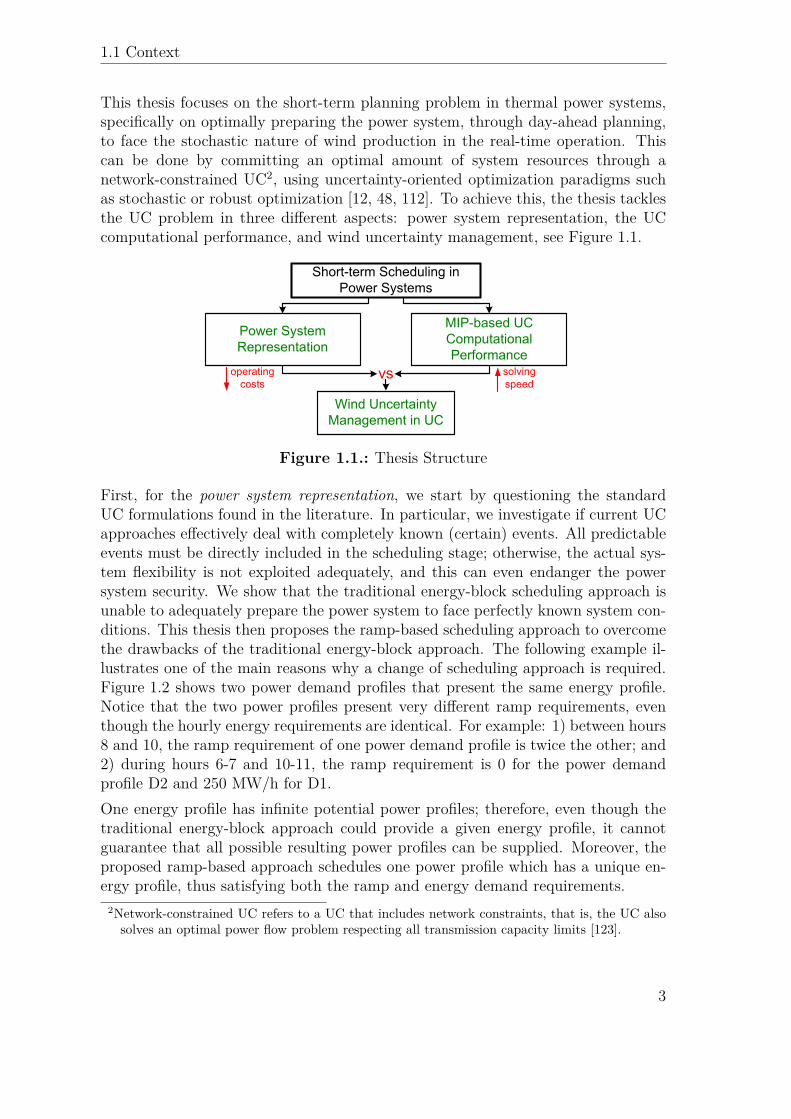
This thesis focuses on the short-term planning problem in thermal power systems,specifically on optimally preparing the power system, through day-ahead planning,to face the stochastic nature of wind production in the real-time operation. Thiscan be done by committing an optimal amount of system resources through anetwork-constrained UC2, using uncertainty-oriented optimization paradigms suchas stochastic or robust optimization [12, 48, 112]. To achieve this, the thesis tacklesthe UC problem in three different aspects: power system representation, the UCcomputational performance, and wind uncertainty management, see Figure 1.1.
Figure 1.1.: Thesis Structure
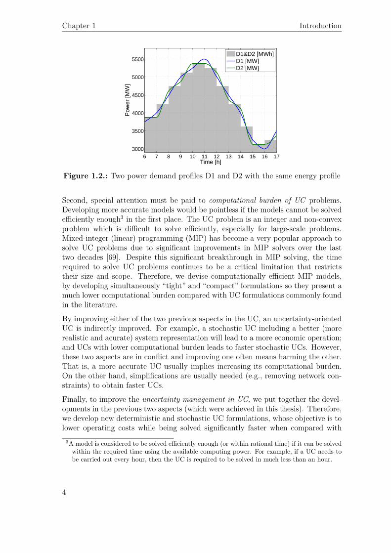
First, for the power system representation, we start by questioning the standardUC formulations found in the literature. In particular, we investigate if current UCapproaches effectively deal with completely known (certain) events. All predictableevents must be directly included in the scheduling stage; otherwise, the actual sys-tem flexibility is not exploited adequately, and this can even endanger the powersystem security. We show that the traditional energy-block scheduling approach isunable to adequately prepare the power system to face perfectly known system con-ditions. This thesis then proposes the ramp-based scheduling approach to overcomethe drawbacks of the traditional energy-block approach. The following example il-lustrates one of the main reasons why a change of scheduling approach is required.Figure 1.2 shows two power demand profiles that present the same energy profile.Notice that the two power profiles present very different ramp requirements, eventhough the hourly energy requirements are identical. For example: 1) between hours8 and 10, the ramp requirement of one power demand profile is twice the other; and2) during hours 6-7 and 10-11, the ramp requirement is 0 for the power demandprofile D2 and 250 MW/h for D1.One energy profile has infinite potential power profiles; therefore, even though thetraditional energy-block approach could provide a given energy profile, it cannotguarantee that all possible resulting power profiles can be supplied. Moreover, theproposed ramp-based approach schedules one power profile which has a unique en-ergy profile, thus satisfying both the ramp and energy demand requirements.
2Network-constrained UC refers to a UC that includes network constraints, that is, the UC alsosolves an optimal power flow problem respecting all transmission capacity limits [123].
3
Chapter 1 Introduction
Time [h]
Pow
er [M
W]
6 7 8 9 10 11 12 13 14 15 16 173000
3500
4000
4500
5000
5500D1&D2 [MWh]D1 [MW]D2 [MW]
Figure 1.2.: Two power demand profiles D1 and D2 with the same energy profile
Second, special attention must be paid to computational burden of UC problems.Developing more accurate models would be pointless if the models cannot be solvedefficiently enough3 in the first place. The UC problem is an integer and non-convexproblem which is difficult to solve efficiently, especially for large-scale problems.Mixed-integer (linear) programming (MIP) has become a very popular approach tosolve UC problems due to significant improvements in MIP solvers over the lasttwo decades [69]. Despite this significant breakthrough in MIP solving, the timerequired to solve UC problems continues to be a critical limitation that restrictstheir size and scope. Therefore, we devise computationally efficient MIP models,by developing simultaneously “tight” and “compact” formulations so they present amuch lower computational burden compared with UC formulations commonly foundin the literature.
By improving either of the two previous aspects in the UC, an uncertainty-orientedUC is indirectly improved. For example, a stochastic UC including a better (morerealistic and acurate) system representation will lead to a more economic operation;and UCs with lower computational burden leads to faster stochastic UCs. However,these two aspects are in conflict and improving one often means harming the other.That is, a more accurate UC usually implies increasing its computational burden.On the other hand, simplifications are usually needed (e.g., removing network con-straints) to obtain faster UCs.
Finally, to improve the uncertainty management in UC, we put together the devel-opments in the previous two aspects (which were achieved in this thesis). Therefore,we develop new deterministic and stochastic UC formulations, whose objective is tolower operating costs while being solved significantly faster when compared with
3A model is considered to be solved efficiently enough (or within rational time) if it can be solvedwithin the required time using the available computing power. For example, if a UC needs tobe carried out every hour, then the UC is required to be solved in much less than an hour.
4
1.2 Objectives
traditional UC models. In addition, based on robust optimization insights andtaking into account the wind generation flexibility, i.e., curtailment, we propose anetwork-constrained UC formulation with robust reserve modelling. Similarly to thestochastic and robust approaches, the proposed network-constrained UC formula-tion seeks to provide commitment (first-stage) decisions that give flexibility to thepower system to face wind uncertainty. This flexibility is provided by units andwind dispatch (second-stage). This final proposed model remains as a pure linearMIP problem, whose size does not depend on the uncertainty wind representation,unlike stochastic UCs whose size directly depends on of the quantity of scenariosconsidered. In comparison, the traditional robust UCs available in the literaturerequires solving an MIP together with a bilinear program, making the final problemconsiderably more complex to solve than a pure linear MIP.
In summary, this thesis proposes computationally efficient tools to optimally committhe required power-system resources to face wind uncertainty in real time, henceallowing power systems to deal with high penetration levels of wind production inan efficient manner. These tools can support ISOs to face the new challenges inday-ahead planning as uncertainty increases dramatically due to the integration ofvariable and uncertain generation resources, such as wind and solar power.
1.2. Objectives
1.2.1. Main Objective
The main objective of this research is to propose computationally efficient modelsfor day-ahead planning in power systems to adequately prepare the system to facethe stochastic nature of wind production in the real-time operation.
1.2.2. Specific Objectives
The main objective can be broken down in the following specific objectives:
Obj1. To develop new day-ahead UC formulations that are able to describe moreaccurately the system’s real-time operation.
Obj2. To devise computationally efficient UC formulations under the MIP approach,by identifying and taking into account the key features that affects the com-putational burden of MIP formulations.
Obj3. To propose network-constrained UC formulations to optimally schedule gen-erating resources to deal with the stochastic nature of wind production.
5
Chapter 1 Introduction
1.3. Thesis Outline
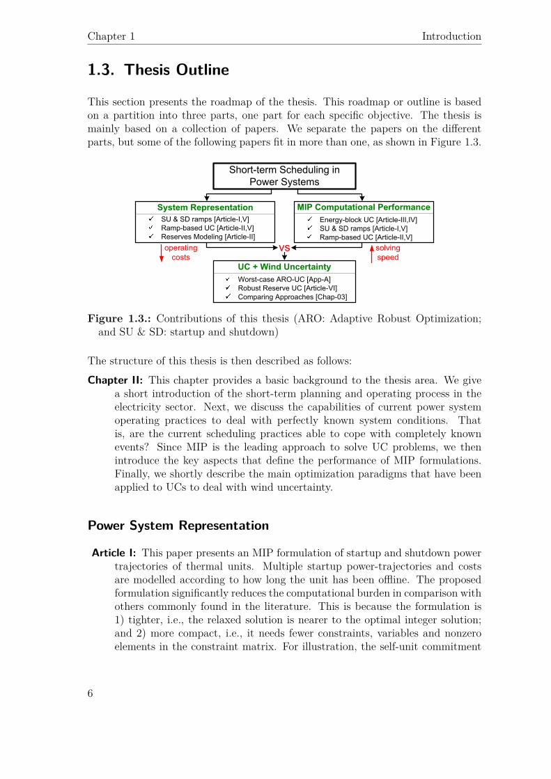
This section presents the roadmap of the thesis. This roadmap or outline is basedon a partition into three parts, one part for each specific objective. The thesis ismainly based on a collection of papers. We separate the papers on the differentparts, but some of the following papers fit in more than one, as shown in Figure 1.3.
Figure 1.3.: Contributions of this thesis (ARO: Adaptive Robust Optimization;and SU & SD: startup and shutdown)
The structure of this thesis is then described as follows:Chapter II: This chapter provides a basic background to the thesis area. We give
a short introduction of the short-term planning and operating process in theelectricity sector. Next, we discuss the capabilities of current power systemoperating practices to deal with perfectly known system conditions. Thatis, are the current scheduling practices able to cope with completely knownevents? Since MIP is the leading approach to solve UC problems, we thenintroduce the key aspects that define the performance of MIP formulations.Finally, we shortly describe the main optimization paradigms that have beenapplied to UCs to deal with wind uncertainty.
Power System Representation
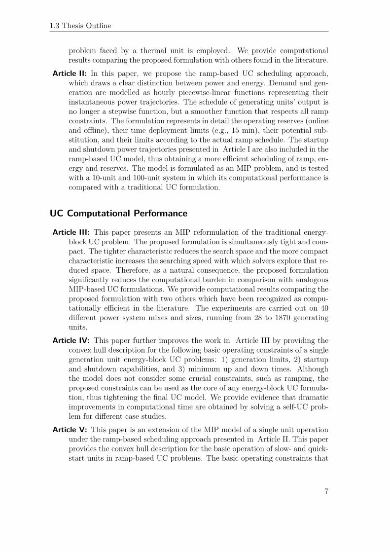
Article I: This paper presents an MIP formulation of startup and shutdown powertrajectories of thermal units. Multiple startup power-trajectories and costsare modelled according to how long the unit has been offline. The proposedformulation significantly reduces the computational burden in comparison withothers commonly found in the literature. This is because the formulation is1) tighter, i.e., the relaxed solution is nearer to the optimal integer solution;and 2) more compact, i.e., it needs fewer constraints, variables and nonzeroelements in the constraint matrix. For illustration, the self-unit commitment
6
1.3 Thesis Outline
problem faced by a thermal unit is employed. We provide computationalresults comparing the proposed formulation with others found in the literature.
Article II: In this paper, we propose the ramp-based UC scheduling approach,which draws a clear distinction between power and energy. Demand and gen-eration are modelled as hourly piecewise-linear functions representing theirinstantaneous power trajectories. The schedule of generating units’ output isno longer a stepwise function, but a smoother function that respects all rampconstraints. The formulation represents in detail the operating reserves (onlineand offline), their time deployment limits (e.g., 15 min), their potential sub-stitution, and their limits according to the actual ramp schedule. The startupand shutdown power trajectories presented in Article I are also included in theramp-based UC model, thus obtaining a more efficient scheduling of ramp, en-ergy and reserves. The model is formulated as an MIP problem, and is testedwith a 10-unit and 100-unit system in which its computational performance iscompared with a traditional UC formulation.
UC Computational Performance
Article III: This paper presents an MIP reformulation of the traditional energy-block UC problem. The proposed formulation is simultaneously tight and com-pact. The tighter characteristic reduces the search space and the more compactcharacteristic increases the searching speed with which solvers explore that re-duced space. Therefore, as a natural consequence, the proposed formulationsignificantly reduces the computational burden in comparison with analogousMIP-based UC formulations. We provide computational results comparing theproposed formulation with two others which have been recognized as compu-tationally efficient in the literature. The experiments are carried out on 40different power system mixes and sizes, running from 28 to 1870 generatingunits.
Article IV: This paper further improves the work in Article III by providing theconvex hull description for the following basic operating constraints of a singlegeneration unit energy-block UC problems: 1) generation limits, 2) startupand shutdown capabilities, and 3) minimum up and down times. Althoughthe model does not consider some crucial constraints, such as ramping, theproposed constraints can be used as the core of any energy-block UC formula-tion, thus tightening the final UC model. We provide evidence that dramaticimprovements in computational time are obtained by solving a self-UC prob-lem for different case studies.
Article V: This paper is an extension of the MIP model of a single unit operationunder the ramp-based scheduling approach presented in Article II. This paperprovides the convex hull description for the basic operation of slow- and quick-start units in ramp-based UC problems. The basic operating constraints that
7
Chapter 1 Introduction
are modelled for both types of units are: 1) generation limits and 2) minimumup and down times. Apart from this, the startup and shutdown processesare also included, by using 3) startup and shutdown power trajectories forslow-start units, and 4) startup and shutdown ramps for quick-start units.The proposed constraints can be used as the core of any ramp-based UCformulation, thus tightening the final MIP problem. We provide evidencethat dramatic improvements in computational time are obtained by solving aself-UC problem for different case studies.
Wind Uncertainty Management
Article VI: This paper proposes a robust reserve-based network-constrained UCformulation as an alternative to traditional robust and stochastic UC formu-lations under wind generation uncertainty. The formulation draws a cleardistinction between power-capacity and ramp-capability reserves to deal withwind production uncertainty. These power and ramp requirements can beobtained from wind forecast information. Using the solution of the worst-case wind scenario (see Appendix A) the formulation guarantees feasibility forany realization of the wind uncertainty. The model is formulated under theramp-based scheduling approach ( Article II), this allows a correct represent-ation of unit’s ramp schedule which define their ramp availability for reserves.The core of the proposed MIP formulation is built upon 1) the convex hulldescription of slow- and quick-start units ( Article V), and 2) the tight andcompact formulation for multiple startup power-trajectories and costs ( Art-icle I), thus taking advantage of their mathematical properties. Furthermore,the proposed formulation significantly decreases operation costs if compared totraditional deterministic and stochastic UC formulations while simultaneouslylowering the computational burden. The operation cost comparison is madethrough 5-min economic dispatch simulation under hundreds of out-of-samplewind-power scenarios.
Chapter III: This chapter presents case studies where the traditional energy-blockscheduling approach is compared with the ramp-based one proposed in thisthesis. We compare the different commitment policies using a 5-min economicdispatch simulation. We assess the performance of the two approaches un-der certain and uncertain events. To observe how the approaches deal withcertainty, we compare the two approaches using completely known demandprofiles. To assess the performance of the two approaches under uncertainty,the two scheduling approaches are implemented under different uncertainty-oriented optimization paradigms (e.g., deterministic, stochastic) and they arecompared through an out-of-sample evaluation stage.
8

1.3 Thesis Outline
Chapter IV: In this, the last chapter of the thesis, conclusions are drawn andguidelines for future work are outlined.
9

2. Background
Contents2.1. Short-Term Planning in the Electricity Sector . . . . . . 11
2.1.1. Generic Formulation of the UC Problem . . . . . . . . . . 132.2. Power System Representation: Dealing with Certainty . 14
2.2.1. Energy-Block: Scheduling vs. Real-time-operation . . . . 152.2.2. Infeasible Power Delivery . . . . . . . . . . . . . . . . . . 182.2.3. Startup and Shutdown Power Trajectories . . . . . . . . . 20
2.3. Performance of MIP Formulations . . . . . . . . . . . . . 232.3.1. Good and Ideal MIP formulations . . . . . . . . . . . . . 232.3.2. Tightness vs. Compactness . . . . . . . . . . . . . . . . . 242.3.3. Improving UC formulations . . . . . . . . . . . . . . . . . 25
2.4. Modelling Wind Uncertainty . . . . . . . . . . . . . . . . 262.4.1. Deterministic Paradigm . . . . . . . . . . . . . . . . . . . 272.4.2. Stochastic Paradigm . . . . . . . . . . . . . . . . . . . . . 282.4.3. Robust Paradigm . . . . . . . . . . . . . . . . . . . . . . . 29
2.5. Conclusions . . . . . . . . . . . . . . . . . . . . . . . . . . . 31
This chapter presents the basic theoretical background of the thesis research topics.We first provide an overview of the short-term planning process in the electricitysector. Next, we discuss the capabilities of current power system operating practicesto deal with perfectly known system conditions. We then introduce the key aspectsthat define the performance of MIP formulations. Last, we shortly describe the mainoptimization paradigms that have been applied to UCs to deal with wind uncertainty.
2.1. Short-Term Planning in the Electricity Sector
In recent years, large-scale integration of wind generation in power systems haschallenged system operators in keeping a reliable power system operation, due tothe unpredictable and highly variable pattern of wind. Uncertainty in power systemoperations is commonly classified in discrete and continuous disturbances. Discrete
11
Chapter 2 Background
disturbances are mainly due to transmission and generation outages. Continuousdisturbances mostly result from stochastic fluctuations in electricity demand andrenewable energy sources, such as wind and solar energy production.
The appearance of these disturbances in real-time operation results in an imbalancebetween supply and demand. A perfect balance between supply and demand isalways required in real time to prevent the power system from collapsing. Anyimbalance must be absorbed by the power system resources (reserves), which mustbe available and ready to be deployed in real time. To guarantee this availability, thesystem resources must be committed in advance, usually the day-ahead, by solvingthe so-called unit commitment (UC) problem.
In many electricity markets, the market operator or Independent System Operator(ISO) is in charge of performing the market clearing in order to determine the setof accepted bids (supply and demand), and the prices to be used in the resultingeconomic transactions. The electricity market is usually structured as day-aheadmarkets (DAM) and a sequence of real-time markets (RTM), or intra-day markets.There are many electricity markets, such as those in USA, where the DAM is basedon UC formulations, then commitment decisions and market clearing prices for thenext 24 hours are computed by solving an UC problem. The objective of this UCis to make the unit’s on/off (commitment) decisions to ensure that enough unitsare online to meet the demand at minimum cost. In RTM, the clearing prices andquantities are commonly obtained by using an optimal economic dispatch (ED).The objective of the ED is to optimally manage the online units to meet demandat minimum cost. The market settlement is usually based on deviations betweenDAM and RTM [136]. As stated in chapter 1, this thesis is focused on schedulingquantities, and the problem of determining the prices that will allow generators torecover their non-convex costs is beyond the scope of this work.
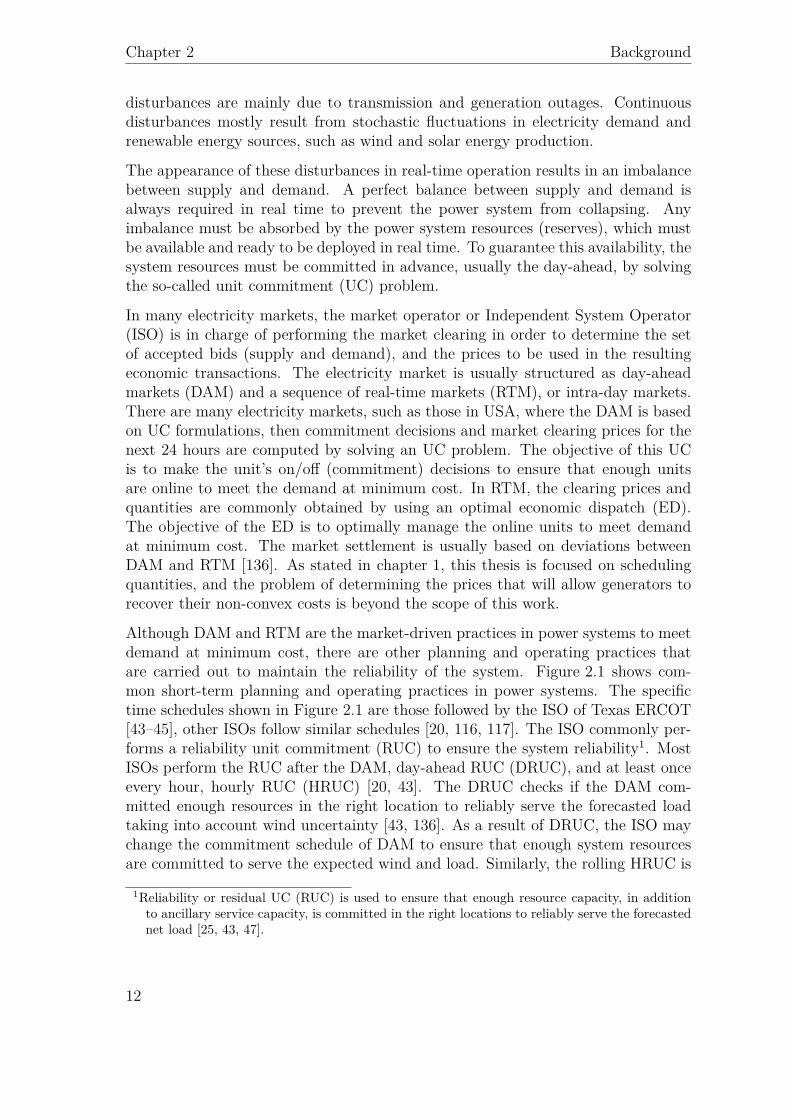
Although DAM and RTM are the market-driven practices in power systems to meetdemand at minimum cost, there are other planning and operating practices thatare carried out to maintain the reliability of the system. Figure 2.1 shows com-mon short-term planning and operating practices in power systems. The specifictime schedules shown in Figure 2.1 are those followed by the ISO of Texas ERCOT[43–45], other ISOs follow similar schedules [20, 116, 117]. The ISO commonly per-forms a reliability unit commitment (RUC) to ensure the system reliability1. MostISOs perform the RUC after the DAM, day-ahead RUC (DRUC), and at least onceevery hour, hourly RUC (HRUC) [20, 43]. The DRUC checks if the DAM com-mitted enough resources in the right location to reliably serve the forecasted loadtaking into account wind uncertainty [43, 136]. As a result of DRUC, the ISO maychange the commitment schedule of DAM to ensure that enough system resourcesare committed to serve the expected wind and load. Similarly, the rolling HRUC is
1Reliability or residual UC (RUC) is used to ensure that enough resource capacity, in additionto ancillary service capacity, is committed in the right locations to reliably serve the forecastednet load [25, 43, 47].
12
2.1 Short-Term Planning in the Electricity Sector
performed with updated demand and wind power forecasts to provide more accur-ate information, thus permanently checking and ensuring that enough resources areavailable to face demand and wind uncertainties in real time.
Figure 2.1.: Short-term planning and operating practices in power systems.
Apart from the day-ahead (DAM and DRUC) and hourly scheduling practices(HRUC) the ED is usually executed every 5 minutes to economically dispatch theunits. Finally, in even shorter time frames, a load frequency control (LFC) keepsthe supply and load balance in real time, by maintaining the system frequency onits nominal value through control strategies without cost optimization functions[37, 106]. These control strategies are usually composed 1) by an Automatic Gen-eration Control (AGC), whose response is between seconds and minutes; and 2)by a primary frequency control, whose response is within few seconds. The formercontrol mainly responds to smooth changes and the latter to more sudden changesof frequency.
It is important to highlight that the ED and LFC are the strategies that finallymatches demand and supply. However, they only manage the committed resourcesthat are available in real time. If there are not enough resources available, theISO needs to take expensive emergency actions to maintain system security andavoid devastating consequences (e.g. blackout). These emergency actions includedispatching fast-start units, voltage reduction, or load shedding [37, 106]. To avoidthese emergency actions, ISOs frequently monitor the system condition by usingrolling DRUC and HRUC, thus ensuring that enough system resources are alwayscommitted to face unexpected events in real time.
2.1.1. Generic Formulation of the UC Problem
Efficient resource scheduling is necessary in power systems to achieve an economicaland reliable energy production and system operation, either under centralized orcompetitive environments. This can be achieved by solving the UC problem, asdiscussed above.
13
Chapter 2 Background
The UC main objective is to meet demand at minimum cost while operating thesystem and units within secure technical limits [61, 111, 127, 149]. Here, we presenta compact matrix formulation:
minx,p,w
(b>x+ c>p+ d>w
)s.t. Fx ≤ f , x is binary (2.1)
Hp+ Jw ≤ h (2.2)Ax+ Bp+ Cw ≤ g (2.3)w ≤W (2.4)
where x,p and w are decision variables. The binary variable x is a vector ofcommitment related decisions (e.g., on/off and startup/shutdown) of each generationunit for each time interval over the planning horizon. The continuous variable p is avector of each unit dispatch decision for each time interval. The continuous variablew is a vector of wind dispatch decision for each time interval at each node wherewind is injected.
The objective function is to minimize the sum of the commitment cost b>x (includ-ing non-load, start-up and shut-down costs), dispatch cost c>p and wind dispatchcost d>w over the planning horizon. Wind dispatch cost is usually considered tobe zero. However, the parameter d is explicitly included to consider the possibilitywhere this cost is different than zero (in some power systems, this cost can even benegative reflecting opportunity costs, e.g., -40 $/MWh in ERCOT [7])
Constraint (Equation 2.1) involves only commitment-related variables, e.g., min-imum up and down times, startup and shutdown constraints, variable startup costs.Constraint (Equation 2.2) contains dispatch-related constraints, e.g., energy balance(equality can always be written as two opposite inequalities), reserve requirements,transmission limits, ramping constraints. Constraint (Equation 2.3) couples thecommitment and dispatch decisions. e.g., minimum and maximum generation capa-city constraints. Constraint (Equation 2.4) empathizes that wind dispatch cannotexceed its forecasted values W. The reader is referred to [61], Morales-Espana et al.[91, 99] and Appendix B for more detailed UC formulations.
2.2. Power System Representation: Dealing withCertainty
This section illustrates how the traditional energy-block scheduling approach is un-able to adequately prepare the power system to face perfectly known system condi-tions. This section is mainly based on the work in Morales-Espana et al. [88].
14
2.2 Power System Representation: Dealing with Certainty
2.2.1. Energy-Block: Scheduling vs. Real-time-operation
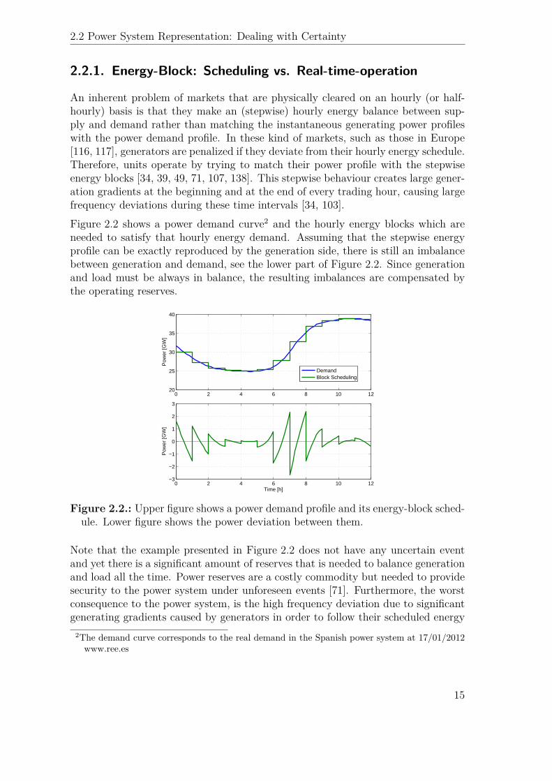
An inherent problem of markets that are physically cleared on an hourly (or half-hourly) basis is that they make an (stepwise) hourly energy balance between sup-ply and demand rather than matching the instantaneous generating power profileswith the power demand profile. In these kind of markets, such as those in Europe[116, 117], generators are penalized if they deviate from their hourly energy schedule.Therefore, units operate by trying to match their power profile with the stepwiseenergy blocks [34, 39, 49, 71, 107, 138]. This stepwise behaviour creates large gener-ation gradients at the beginning and at the end of every trading hour, causing largefrequency deviations during these time intervals [34, 103].Figure 2.2 shows a power demand curve2 and the hourly energy blocks which areneeded to satisfy that hourly energy demand. Assuming that the stepwise energyprofile can be exactly reproduced by the generation side, there is still an imbalancebetween generation and demand, see the lower part of Figure 2.2. Since generationand load must be always in balance, the resulting imbalances are compensated bythe operating reserves.
0 2 4 6 8 10 1220
25
30
35
40
Pow
er [G
W]
DemandBlock Scheduling
0 2 4 6 8 10 12−3
−2
−1
0
1
2
3
Pow
er [G
W]
Time [h]
Figure 2.2.: Upper figure shows a power demand profile and its energy-block sched-ule. Lower figure shows the power deviation between them.
Note that the example presented in Figure 2.2 does not have any uncertain eventand yet there is a significant amount of reserves that is needed to balance generationand load all the time. Power reserves are a costly commodity but needed to providesecurity to the power system under unforeseen events [71]. Furthermore, the worstconsequence to the power system, is the high frequency deviation due to significantgenerating gradients caused by generators in order to follow their scheduled energy
2The demand curve corresponds to the real demand in the Spanish power system at 17/01/2012www.ree.es
15
Chapter 2 Background
blocks. Such frequency deviations have been observed in the Continental Europe(CE) power system, see in Figure 2.3.
Frequency Quality Investigation EXCERPT OF FINAL REPORT Page 2/4
Evening frequency average profile - winters 2003 to 2008 (November to March - Monday to Friday)
49,92
49,94
49,96
49,98
50,00
50,02
50,04
50,0619:00
19:30
20:00
20:30
21:00
21:30
22:00
22:30
23:00
23:30
00:00
Fre
qu
en
cy
(H
z)
2002-2003 2003-2004 2004-2005 2005-2006 2006-2007 2007-2008
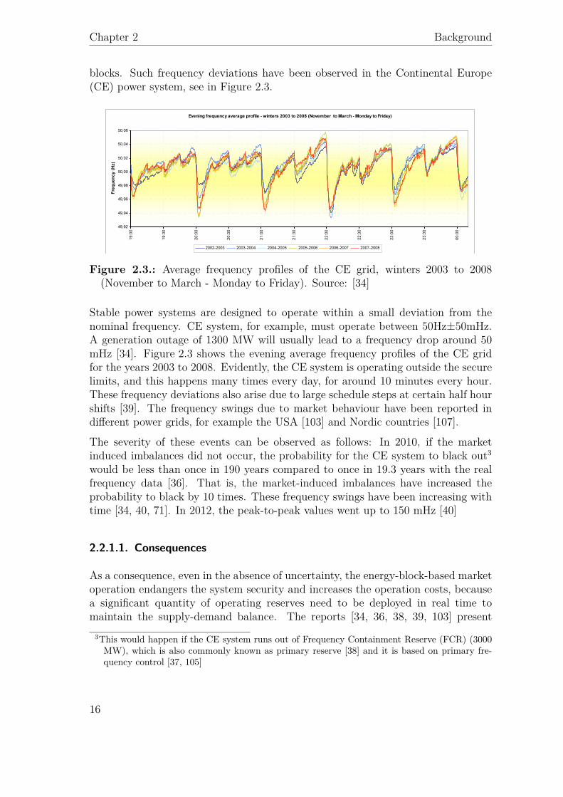
Figure 2.3.: Average frequency profiles of the CE grid, winters 2003 to 2008(November to March - Monday to Friday). Source: [34]
Stable power systems are designed to operate within a small deviation from thenominal frequency. CE system, for example, must operate between 50Hz±50mHz.A generation outage of 1300 MW will usually lead to a frequency drop around 50mHz [34]. Figure 2.3 shows the evening average frequency profiles of the CE gridfor the years 2003 to 2008. Evidently, the CE system is operating outside the securelimits, and this happens many times every day, for around 10 minutes every hour.These frequency deviations also arise due to large schedule steps at certain half hourshifts [39]. The frequency swings due to market behaviour have been reported indifferent power grids, for example the USA [103] and Nordic countries [107].
The severity of these events can be observed as follows: In 2010, if the marketinduced imbalances did not occur, the probability for the CE system to black out3
would be less than once in 190 years compared to once in 19.3 years with the realfrequency data [36]. That is, the market-induced imbalances have increased theprobability to black by 10 times. These frequency swings have been increasing withtime [34, 40, 71]. In 2012, the peak-to-peak values went up to 150 mHz [40]
2.2.1.1. Consequences
As a consequence, even in the absence of uncertainty, the energy-block-based marketoperation endangers the system security and increases the operation costs, becausea significant quantity of operating reserves need to be deployed in real time tomaintain the supply-demand balance. The reports [34, 36, 38, 39, 103] present
3This would happen if the CE system runs out of Frequency Containment Reserve (FCR) (3000MW), which is also commonly known as primary reserve [38] and it is based on primary fre-quency control [37, 105]
16
2.2 Power System Representation: Dealing with Certainty
detailed consequences of the frequency swings. We summarize and classify them asfollows:
Operational risks
• Insufficient primary reserve leaves the power system unprotected to face gen-eration and demand outages. This endangers the security supply.
• Frequency oscillations can lead into uncontrollable operational situation, whichmay cause the loss of generation or demand units. This may cause a snowballeffect leading to a blackout.
• Power flow variations cause overload which may lead to tripping in systemsoperating close to their limits. As the previous consequence, this may alsolead to a blackout.
Economic impact
• Unnecessary use of primary reserves, which is repeatedly used during a day,results in higher power plant stress. This has a direct impact on the lifetime ofthe units and inevitably increases the cost of providing this reserve. Besides,more primary reserve must be scheduled for not leaving the system unprotectedduring the inter-hour periods.
• Unnecessary use of secondary reserves, which are needed to restore the primaryreserves, hence increasing the operation costs of the system. In addition, morereserves must then be scheduled to deal with this issue. For example, the costsassociated to the overuse of secondary reserves due to the block scheduled inSpain in 2010 was calculated on 17.5 millions of Euros4 [33].
• Generators following the stepwise energy profiles and also providing reservespresent a high ramp use during the changing hours, for around 10 minutes,and thus decreasing their possibility to provide reserves [118].
2.2.1.2. Actions to take
Many measures have been proposed to diminish the previously mentioned con-sequences [33, 34, 39, 40, 49, 71, 103, 107, 138], from an extremely centralized pointof view, e.g. unilateral control of the generation output by ISOs; to very decent-ralized one, e.g. generation unit must incorporate the ramping costs then avoidingsudden output changes. Here, we summarize some of the outstanding measures.
4Egido et al. [33] presented that savings of about 14.5 millions of Euros, for Spain in 2010, couldhave been obtained by changing the dispatch of units to a half an hour basis and followingpiecewise power patterns even thought the scheduling was stepwise-based.
17
Chapter 2 Background
• Implement shorter trading periods. The shorter the periods, the smaller theimpact on frequency. This is because the resulting energy blocks will be moresimilar to the smoother continuous demand profile. This will inevitably in-crease transaction costs.
• Imposing maximum ramp rates on generators during short time periods (minutes).That way, their power profiles will be smoother. This measure constrains thefreedom and technical flexibility of generators.
• Dispatching with smooth profiles although the scheduling is made in hourlyblocks. This measure is similar to the previous one, with the difference thata constant ramp rate must be followed during the operation stage. The maindisadvantage of this solution is that once the energy blocks are fixed, theplausible power profiles of generators may oscillate, besides generators nothaving the incentives to do so. This problem can be diminished by consideringshorter trading periods.
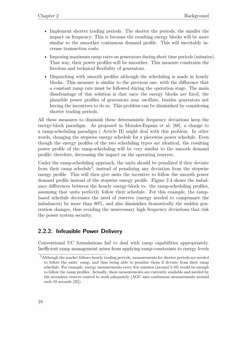
All these measures to diminish these deterministic frequency deviations keep theenergy-block paradigm. As proposed in Morales-Espana et al. [88], a change toa ramp-scheduling paradigm ( Article II) might deal with this problem. In otherwords, changing the stepwise energy schedule for a piecewise power schedule. Eventhough the energy profiles of the two scheduling types are identical, the resultingpower profile of the ramp-scheduling will be very similar to the smooth demandprofile; therefore, decreasing the impact on the operating reserves.Under the ramp-scheduling approach, the units should be penalized if they deviatefrom their ramp schedule5, instead of penalizing any deviation from the stepwiseenergy profile. This will then give units the incentive to follow the smooth powerdemand profile instead of the stepwise energy profile. Figure 2.4 shows the imbal-ance differences between the hourly energy-block vs. the ramp-scheduling profiles,assuming that units perfectly follow their schedule. For this example, the ramp-based schedule decreases the need of reserves (energy needed to compensate theimbalances) by more than 80%, and also diminishes dramatically the sudden gen-eration changes, thus avoiding the unnecessary high frequency deviations that riskthe power system security.
2.2.2. Infeasible Power Delivery
Conventional UC formulations fail to deal with ramp capabilities appropriately.Inefficient ramp management arises from applying ramp-constraints to energy levels
5Although the market follows hourly trading periods, measurements for shorter periods are neededto follow the units’ ramp, and thus being able to penalize them if deviate from their rampschedule. For example, energy measurements every few minutes (around 5-10) would be enoughto follow the ramp profiles. Actually, these measurements are currently available and needed bythe secondary reserve control to work adequately (AGC uses continuous measurements aroundeach 10 seconds [35]).
18
2.2 Power System Representation: Dealing with Certainty
0 2 4 6 8 10 1220
25
30
35
40
Pow
er [G
W]
DemandBlock SchedulingRamp Scheduling
0 2 4 6 8 10 12−3
−2
−1
0
1
2
3P
ower
[GW
]
Time [h]
Figure 2.4.: Energy-blocks vs. ramp scheduling and their impact on reserves. Up-per figure shows a power demand profile and its energy-block/ramp-based sched-ules. Lower figure shows the power deviation between the schedules and thedemand.
or (hourly) averaged generation levels, which is a standard practice in traditionalUC models [28, 51, 60, 123]. As a result, energy schedules may not be feasible [57].
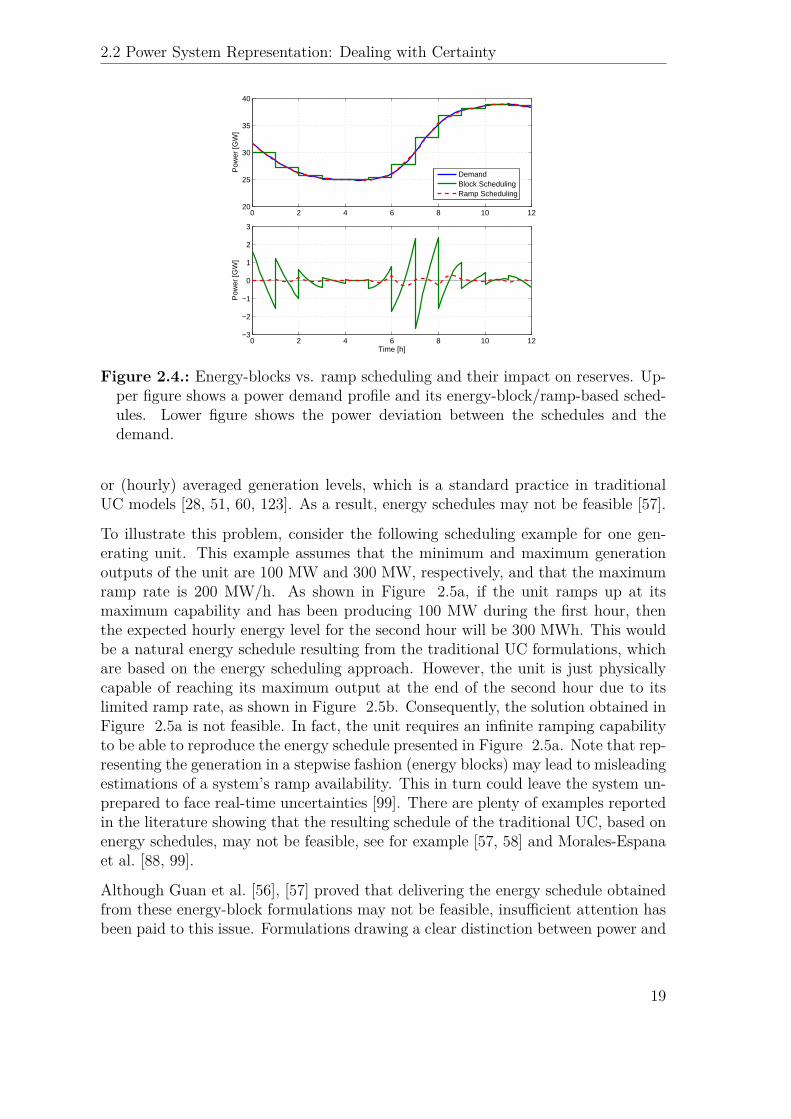
To illustrate this problem, consider the following scheduling example for one gen-erating unit. This example assumes that the minimum and maximum generationoutputs of the unit are 100 MW and 300 MW, respectively, and that the maximumramp rate is 200 MW/h. As shown in Figure 2.5a, if the unit ramps up at itsmaximum capability and has been producing 100 MW during the first hour, thenthe expected hourly energy level for the second hour will be 300 MWh. This wouldbe a natural energy schedule resulting from the traditional UC formulations, whichare based on the energy scheduling approach. However, the unit is just physicallycapable of reaching its maximum output at the end of the second hour due to itslimited ramp rate, as shown in Figure 2.5b. Consequently, the solution obtained inFigure 2.5a is not feasible. In fact, the unit requires an infinite ramping capabilityto be able to reproduce the energy schedule presented in Figure 2.5a. Note that rep-resenting the generation in a stepwise fashion (energy blocks) may lead to misleadingestimations of a system’s ramp availability. This in turn could leave the system un-prepared to face real-time uncertainties [99]. There are plenty of examples reportedin the literature showing that the resulting schedule of the traditional UC, based onenergy schedules, may not be feasible, see for example [57, 58] and Morales-Espanaet al. [88, 99].
Although Guan et al. [56], [57] proved that delivering the energy schedule obtainedfrom these energy-block formulations may not be feasible, insufficient attention hasbeen paid to this issue. Formulations drawing a clear distinction between power and
19
Chapter 2 Background
(a) Traditional Energy Schedule (b) Actual Deployment
Figure 2.5.: Scheduling vs. Deployment
energy have been proposed, guaranteeing that stepwise energy schedules can be real-ized [26, 52, 58, 144, 150]. Guan et al. [58] proposes a smooth nonlinear programmingproblem which does not take into account discrete decisions (e.g. commitment). Wuet al. [144] presents a formulation with feasible energy delivery constraints, whichis further extended in Yang et al. [150], where a sub-hourly UC is formulated. Thework in [26, 52] use power profiles to guarantee that the scheduled energy can beprovided. These formulations are focused on feasible energy schedules rather thanon matching generation and demand power profiles. In fact, these formulationssupply hourly energy demand with power profiles that vary from stepwise [150] tooscillating power trajectories [26, 52, 118], which are far from matching the instant-aneous power demand forecast. This indiscriminate use of ramping resources fromthe scheduling stage does not permit the effective management of the system rampcapabilities to face real-time uncertainties.
2.2.3. Startup and Shutdown Power Trajectories
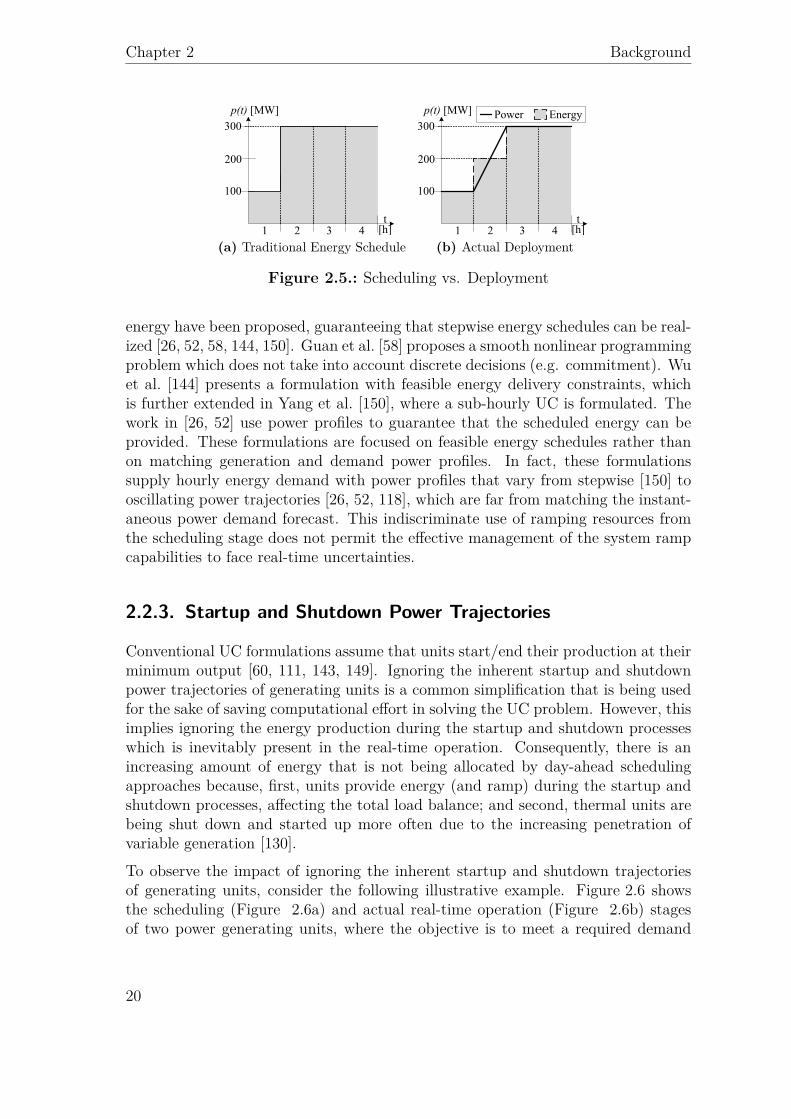
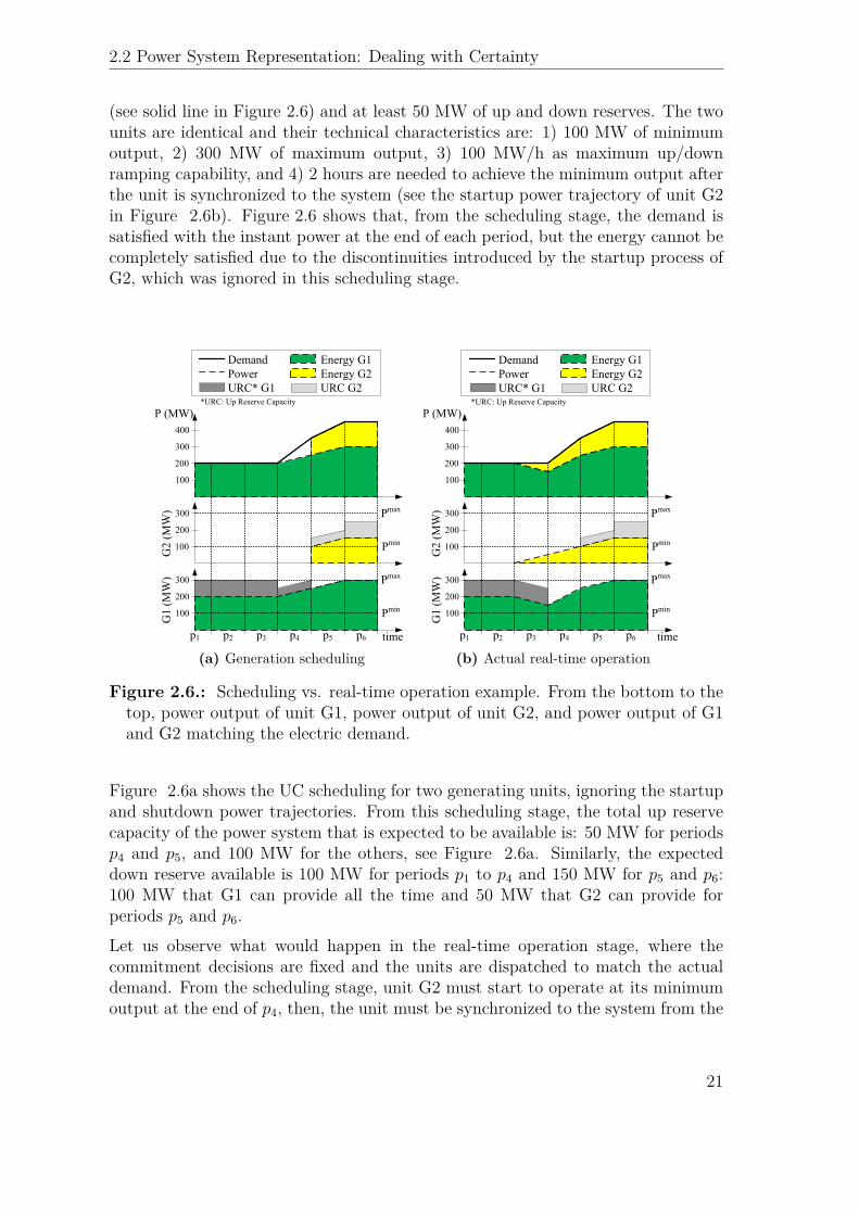
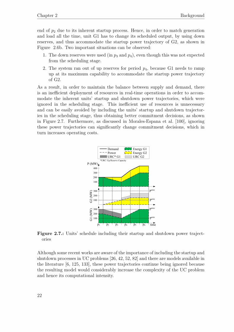
Conventional UC formulations assume that units start/end their production at theirminimum output [60, 111, 143, 149]. Ignoring the inherent startup and shutdownpower trajectories of generating units is a common simplification that is being usedfor the sake of saving computational effort in solving the UC problem. However, thisimplies ignoring the energy production during the startup and shutdown processeswhich is inevitably present in the real-time operation. Consequently, there is anincreasing amount of energy that is not being allocated by day-ahead schedulingapproaches because, first, units provide energy (and ramp) during the startup andshutdown processes, affecting the total load balance; and second, thermal units arebeing shut down and started up more often due to the increasing penetration ofvariable generation [130].To observe the impact of ignoring the inherent startup and shutdown trajectoriesof generating units, consider the following illustrative example. Figure 2.6 showsthe scheduling (Figure 2.6a) and actual real-time operation (Figure 2.6b) stagesof two power generating units, where the objective is to meet a required demand
20
2.2 Power System Representation: Dealing with Certainty
(see solid line in Figure 2.6) and at least 50 MW of up and down reserves. The twounits are identical and their technical characteristics are: 1) 100 MW of minimumoutput, 2) 300 MW of maximum output, 3) 100 MW/h as maximum up/downramping capability, and 4) 2 hours are needed to achieve the minimum output afterthe unit is synchronized to the system (see the startup power trajectory of unit G2in Figure 2.6b). Figure 2.6 shows that, from the scheduling stage, the demand issatisfied with the instant power at the end of each period, but the energy cannot becompletely satisfied due to the discontinuities introduced by the startup process ofG2, which was ignored in this scheduling stage.
(a) Generation scheduling (b) Actual real-time operation
Figure 2.6.: Scheduling vs. real-time operation example. From the bottom to thetop, power output of unit G1, power output of unit G2, and power output of G1and G2 matching the electric demand.
Figure 2.6a shows the UC scheduling for two generating units, ignoring the startupand shutdown power trajectories. From this scheduling stage, the total up reservecapacity of the power system that is expected to be available is: 50 MW for periodsp4 and p5, and 100 MW for the others, see Figure 2.6a. Similarly, the expecteddown reserve available is 100 MW for periods p1 to p4 and 150 MW for p5 and p6:100 MW that G1 can provide all the time and 50 MW that G2 can provide forperiods p5 and p6.Let us observe what would happen in the real-time operation stage, where thecommitment decisions are fixed and the units are dispatched to match the actualdemand. From the scheduling stage, unit G2 must start to operate at its minimumoutput at the end of p4, then, the unit must be synchronized to the system from the
21
Chapter 2 Background
end of p2 due to its inherent startup process. Hence, in order to match generationand load all the time, unit G1 has to change its scheduled output, by using downreserves, and thus accommodate the startup power trajectory of G2, as shown inFigure 2.6b. Two important situations can be observed:
1. The down reserves were used (in p3 and p4), even though this was not expectedfrom the scheduling stage.
2. The system ran out of up reserves for period p4, because G1 needs to rampup at its maximum capability to accommodate the startup power trajectoryof G2.
As a result, in order to maintain the balance between supply and demand, thereis an inefficient deployment of resources in real-time operations in order to accom-modate the inherent units’ startup and shutdown power trajectories, which wereignored in the scheduling stage. This inefficient use of resources is unnecessaryand can be easily avoided by including the units’ startup and shutdown trajector-ies in the scheduling stage, thus obtaining better commitment decisions, as shownin Figure 2.7. Furthermore, as discussed in Morales-Espana et al. [100], ignoringthese power trajectories can significantly change commitment decisions, which inturn increases operating costs.
Figure 2.7.: Units’ schedule including their startup and shutdown power traject-ories
Although some recent works are aware of the importance of including the startup andshutdown processes in UC problems [26, 42, 52, 82] and there are models available inthe literature [6, 125, 133], these power trajectories continue being ignored becausethe resulting model would considerably increase the complexity of the UC problemand hence its computational intensity.
22
2.3 Performance of MIP Formulations
An adequate day-ahead schedule not only must take into account these startup andshutdown power trajectories, but also must optimally schedule them to avoid theaforementioned drawbacks.
2.3. Performance of MIP Formulations
Mixed-integer (linear) programming (MIP) has become a very popular approachto solving UC problems due to significant improvements in off-the-shelf MIP solv-ers, based on the branch-and-cut algorithm. The combination of pure algorithmicspeedup and the progress in computer machinery has meant that solving MIPs hasbecome 100 million times faster over the last 20 years [69]. Recently, the world’slargest competitive wholesale market, PJM, changed from Lagrangian Relaxationto MIP to tackle its UC-based scheduling problems [46, 110]. There is extensiveliterature comparing the pros and cons of MIP with its competitors, see for example[61] and [72].
Despite the significant improvements in MIP solving, the time required to solve UCproblems continues to be a critical limitation that restricts the size and scope ofUC models. Nevertheless, improving an MIP formulation can dramatically reduceits computational burden and so allow the implementation of more advanced andcomputationally demanding problems, such as stochastic formulations [22, 23, 112],accurate modelling of different types of (online and offline) reserves Morales-Espanaet al. [99], transmission switching [59], or detailed modelling of combined-cycle gen-erating units [24, 72, 74, 78].
2.3.1. Good and Ideal MIP formulations
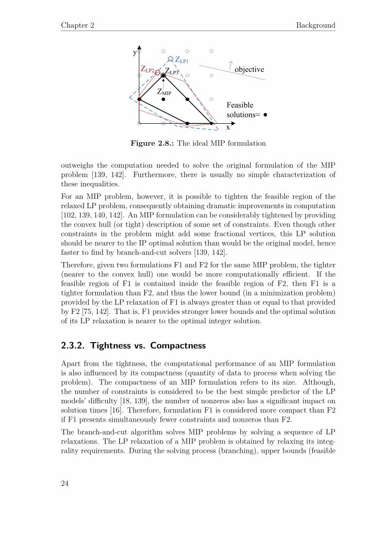
Figure 2.8 shows three different linear programming (LP) formulations (LP1, LP2and LP3) of the same integer programming (IP) problem. Geometrically we canobserve that there is actually an infinite number of LP formulations for the same in-teger problem, so the next question that could be raised: which of these formulationsis the most computationally efficient?
Formulation LP3 (solid line in Figure 2.8) is ideal, because each vertex is an integerso the optimal LP solution (which lies in a vertex) is optimal for the correspondingIP. In general, for every MIP problem there is only one ideal formulation calledconvex hull, defined as the smallest convex feasible region containing all the feasibleinteger points [142]. Each vertex of this unique formulation is a point satisfying theintegrality constraints, hence it allows solving the IP (non-convex) problem as anLP (convex-problem).
Unfortunately, in many practical problems there is an enormous number of inequal-ities needed to describe the convex hull, and the effort required to obtain them
23
Chapter 2 Background
Figure 2.8.: The ideal MIP formulation
outweighs the computation needed to solve the original formulation of the MIPproblem [139, 142]. Furthermore, there is usually no simple characterization ofthese inequalities.For an MIP problem, however, it is possible to tighten the feasible region of therelaxed LP problem, consequently obtaining dramatic improvements in computation[102, 139, 140, 142]. An MIP formulation can be considerably tightened by providingthe convex hull (or tight) description of some set of constraints. Even though otherconstraints in the problem might add some fractional vertices, this LP solutionshould be nearer to the IP optimal solution than would be the original model, hencefaster to find by branch-and-cut solvers [139, 142].Therefore, given two formulations F1 and F2 for the same MIP problem, the tighter(nearer to the convex hull) one would be more computationally efficient. If thefeasible region of F1 is contained inside the feasible region of F2, then F1 is atighter formulation than F2, and thus the lower bound (in a minimization problem)provided by the LP relaxation of F1 is always greater than or equal to that providedby F2 [75, 142]. That is, F1 provides stronger lower bounds and the optimal solutionof its LP relaxation is nearer to the optimal integer solution.
2.3.2. Tightness vs. Compactness
Apart from the tightness, the computational performance of an MIP formulationis also influenced by its compactness (quantity of data to process when solving theproblem). The compactness of an MIP formulation refers to its size. Although,the number of constraints is considered to be the best simple predictor of the LPmodels’ difficulty [18, 139], the number of nonzeros also has a significant impact onsolution times [16]. Therefore, formulation F1 is considered more compact than F2if F1 presents simultaneously fewer constraints and nonzeros than F2.The branch-and-cut algorithm solves MIP problems by solving a sequence of LPrelaxations. The LP relaxation of a MIP problem is obtained by relaxing its integ-rality requirements. During the solving process (branching), upper bounds (feasible
24
2.3 Performance of MIP Formulations
integer solutions) and lower bounds (LP relaxations) are computed. The quality ofa feasible integer solution is measured with the optimality tolerance, which is thedifference between upper and lower bounds. In order to reduce this difference, upperbounds are decreased by finding better integer solutions (e.g. by using heuristics)and lower bounds are increased by strengthening the LP relaxation (e.g. by addingcutting planes) [16]. Providing an MIP formulation with strong lower bounds (LPrelaxation near to the optimal integer solution) can dramatically reduce the lengthof the search for optimality [102, 132, 139, 142]. In addition, strong lower boundseffectively guide the search for better upper bounds (i.e. heuristics explore theneighbourhood of the LP relaxation to find potentially better integer solutions).In short, the tightness of an MIP formulation defines the search space (relaxedfeasible region) that the solver needs to explore in order to find the (optimal integer)solution. On the other hand, the compactness of an MIP formulation refers to itssize and defines the searching speed that the solver takes to find the optimal solution,since during the process many LP relaxations are repeatedly solved.Off-the-shelf MIP solvers fully exploit tightening and compacting strategies. Eventhough solvers’ breakthrough is due to the synergy between different strategies (e.g.heuristics, cuts, node presolve), introducing cutting planes has been recognized asthe most effective strategy, followed by root presolve [16, 17, 19, 119]. The formerstrategy dynamically tightens the formulation around the integer feasible solutionpoint. The latter makes the initial problem formulation more compact (by removingredundant variables and constraints) and also tighter (by strengthening constraintsand variable bounds).Research on improving MIP formulations is usually focused on tightening rather thanon compacting. An MIP formulation is typically tightened by adding a huge numberof constraints, which increases the problem size [64, 109]. Although this tighteningreduces the search space, solvers may take more time exploring it because they arenow required to repeatedly solve larger LPs. Consequently, when a formulation istightened while significantly affecting its compactness, a more compact and less tightformulation may be solved faster, because the solver is able to explore the largerfeasible region more rapidly [64]. On the other hand, compact formulations usuallyprovide weak (not strong) lower bounds.In conclusion, creating tight or compact computationally efficient formulations is anon trivial task because the obvious formulations are very weak (not tight) or verylarge, and trying to improve the tightness (compactness) usually means harming thecompactness (tightness).
2.3.3. Improving UC formulations
Improving MIP formulations, especially the tightness, has been widely researched.In fact, all the cutting plane theory, which has meant the breakthrough in MIPsolving, is about tightening the formulations [16, 17, 69, 140, 140, 141]. In the
25
Chapter 2 Background
case of UC problems, there have been efforts affecting single sets of constraints[48, 70, 109, 113]. Lee et al. [70] and Rajan and Takriti [113] describe the convexhull of the minimum up/down time constraints for the 1-binary (only modellingcommitment binary variables) and 3-binary format (modelling commitment, startupand shutdown binary variables), respectively. Although both formulations are idealin terms of tightness, the formulation in [113] is considerably more compact whichresults in a much lower computational burden.
Apart from convex hulls, some contributions seek to find stronger MIP formulations.Frangioni et al. [48] proposes a tighter linear approximation for quadratic generationcosts; Ostrowski et al. [109] presents a new class of valid inequalities (cuts) to tightenramping constraints.
2.4. Modelling Wind Uncertainty
The high penetration of uncertain generation sources, such as wind and solar power,in power systems have posed new challenges to the UC process. The deviationbetween expected and real wind production must be absorbed by the power systemresources (reserves), which must be available and ready to be deployed in real time.To guarantee that enough system resources are available to face real-time uncer-tainty, the system resources must be committed in advance, usually the day-ahead,by solving the so-called UC problem. It is imperative for ISOs to have an adequatemethodology to schedule an efficient amount of system resources (reserves) to facethe increasing amount of real-time uncertainty.
The short-term decision process for power systems operations (see section 2.1) isconceptually a two-stage problem [143]. In the first-stage, the unit commitmentdecision takes places hours to days ahead of the actual operation, where units arecommitted to meet an expected power demand for each hour, based on the units’costs and constraints. In the second-stage, after the uncertainty (e.g. wind) hasbeen realized, the power outputs of committed units are decided to meet the real-time load. These dispatch decisions take place between minutes to seconds aheadof the time implementation.
Let us consider the second-stage of the UC optimization problem (Equation 2.1)-(Equation 2.4), which is obtained by fixing the first-stage variable x:
minp,w
c>p+ d>w
s.t. Hp+ Jw ≤ h (2.5)Bp+ Cw ≤ g (2.6)w ≤W (2.7)
where g = g−Ax.
26
2.4 Modelling Wind Uncertainty
The optimal solution of this LP problem will always be at a vertex of the feasibleregion, because the objective function is linear and the feasible region is convex.Therefore, the optimal solution is always at the very boundary of the feasible region,which is also the boundary of feasibility. This solution is then by nature not designedto be robust against perturbations in the feasible region.In fact, Ben-Tal and Nemirovski [9],[10] reported that for many real LP problems,the optimal solutions presented more than 50% violations of some of the constraintsdue to small perturbations (0.01%) of uncertain data. These “optimal” solutionsbecome meaningless, especially if the constraints of the optimization problem arehard constraints that cannot be violated. Similarly, under the stochastic paradigm,it has been observed that using a single deterministic value (usually the mean value)instead of uncertain parameters lead to very poor solutions (see, e.g., [15, 124]).A reasonable strategy to overcome this problem is then to find a solution away fromthe boundary (of feasibility), sacrificing optimality for some robustness. This can beachieved by modifying the optimization problem to somehow consider a given level ofuncertainty. There are different strategies for modelling uncertainty in optimizationproblems. These strategies define how much and where to move in the interior ofthe feasible region.For the case of the UC problem, there are mainly three different paradigms formodelling uncertainty: deterministic, stochastic and robust. In the deterministicparadigm, reserve levels must be given and they define how much the solution mustbe away from the boundary of some constraints (usually the units’ generation lim-its). The other two paradigms rely on uncertainty-oriented optimization techniques,stochastic and robust programming, and they optimize the reserve levels endogen-ously. In order to ensure feasibility, the stochastic and robust paradigms may movethe solution away from the boundary of all constraints if necessary.The following three subsections provide an overview of all three paradigms. Forother methodologies, like chance-constrained optimization, the reader is referred to[128] and references therein.
2.4.1. Deterministic Paradigm
The deterministic paradigm has been the most common practice used for dealingwith uncertainty in the power industry, and it has been widely studied in the UCliterature, see for example [60, 123], Morales-Espana et al. [91, 99] and referencestherein. A deterministic UC solves the problem (Equation 2.1)-(Equation 2.4), thuscommitting and dispatching generating units to meet a deterministic expected load.The uncertainty is handled by including (capacity) reserve constraints that imposegiven reserve levels, e.g., the total capacity of committed units exceed the forecastedload.The reserve sizing is usually based on deterministic rule-of-thumb criteria. A com-mon practice is to determine the level of reserve to cover the loss of the largest
27
Chapter 2 Background
generator, known as the N − 1 criterion, or a fraction of the hourly demand [116].To consider different sources of uncertainty, the N − 1 criterion is commonly mixedwith a number of standard deviations of the error in uncertainty introduced by loadand wind. Some ISOs require enough power reserves to cover at least three times thestandard deviation of the net-load (forecast load minus forecast wind generation)error prediction [54, 62]. Although probabilistic methods have been proposed to sizethe level of reserves [2, 5, 32, 81, 108], the deterministic rule-of-thumb criteria arestill very popular in the electricity sector due to their simplicity.The deterministic paradigm remains the most common paradigm in the power in-dustry, because it is easy to implement in practice. However, the deterministicparadigm usually leads to an over-scheduling of resources resulting in an econom-ically inefficient way to handle uncertainty, especially when the reserve sizing isdetermined by rule-of-thumb rules. This can be illustrated with the following ex-ample. Suppose that an ISO wants to schedule enough reserves to cope with theuncertainty range of a wind farm. This uncertainty range is between 100 and 200MW, hence 100 MW of reserves (up and down together) is then required. Now,suppose that the wind farm is only connected to a power line with transmission ca-pacity of 75 MW, then a maximum wind production of 75 MW can be dispatched,regardless of the possible realization of uncertainty. Consequently, the actual reserverequirement is zero due to the transmission limit.Although for this illustrative example it was easy to readjust the reserve levels, realpower systems are considerably more complex and it is not possible to perform thisreserve adjustment a priori. Furthermore, since a deterministic UC only considersone expected deterministic condition, even with enough reserve levels, the powersystem may not be able to deploy the reserves if the real-time condition deviatessignificantly from the expected value. This has been confirmed by ISO’s operationalexperience [84] as well as by numerical simulations shown in [12], [95] and chapter 3.Uncertainty-oriented optimization methods, such as stochastic and robust program-ming, seek to overcome these weaknesses, as described in the following sections.
2.4.2. Stochastic Paradigm
Stochastic optimization has gained substantial popularity for UC optimization underparameter uncertainty. In the stochastic optimization approach, different (stochastic)conditions can be considered through an explicit description of scenarios and theirassociated probability [112, 121, 124].Here, we provide an overview of the generic two-stage stochastic UC problem. Muchwork has been done in various aspects of stochastic optimization. The reader isreferred to [15, 68, 124] and references therein for a more comprehensive picture ofstochastic optimization (including multi-stage stochastic problems).In the two-stage stochastic problem, the uncertainty is realized after the first-stagedecisions must be implemented, but before the implementation of the second-stage
28
2.4 Modelling Wind Uncertainty
decisions. Thus, the second-stage decisions are the actions implemented to face theunexpected realization of the uncertainty.
The two-stage UC problem (Equation 2.1)-(Equation 2.4) under the stochastic paradigm,only considering wind uncertainty, can be represented as follows:
minx,pς ,wς
(b>x+ E
[c>pς + d>wς
])s.t. Fx ≤ f , x is binary (2.8)
Hpς + Jwς ≤ h, ∀ς ∈ Z (2.9)Ax+ Bpς + Cwς ≤ g, ∀ς ∈ Z (2.10)wς ≤Wς , ∀ς ∈ Z (2.11)
where the objective is usually to minimize the expected generation cost consideringthe occurrence probability of each scenario. The variables x represent the first-stagedecisions, pς and wς the second-stage decisions, Wς the uncertain wind realizationfor scenario ς, and Z the set of scenarios. The operating constraints involving thesecond-stage variables (Equation 2.9)-(Equation 2.11) are enforced for all scenarios.
Much research along the stochastic UC has been done. Takriti et al. [129] pro-poses one of the first UC under the stochastic paradigm, where uncertain demandwas considered. Bouffard et al. [22],[23] introduces uncertain generation outages.Wu et al. [145] models outages of generation units and transmission lines as wellas uncertain demand. Ruiz et al. [120] also incorporates two different sources ofuncertainty, generation unreliability and deviations from the load forecast. Someother works have focused on modelling wind generation uncertainty, see for example[21, 86, 112, 131, 134].
Although the stochastic paradigm overcomes the main drawbacks of the determin-istic paradigm, it presents however some practical limitations: 1) a large number ofscenario samples is required to obtain robust solutions (i.e. feasible solutions for anywind uncertainty realization), which results in a computationally intensive problem(often intractable); and 2) it may be difficult to obtain an accurate probability dis-tribution of the uncertainty, this could considerably affect the efficiency of the finaldecisions [14].
2.4.3. Robust Paradigm
Here we present the two-stage adaptive robust UC problem. For adaptive-multi-stage and static robust problems as well as details about different uncertainty sets,the reader is referred to [10, 14, 27] and references therein.
The two-stage adaptive UC problem, only considering wind uncertainty, can be
29
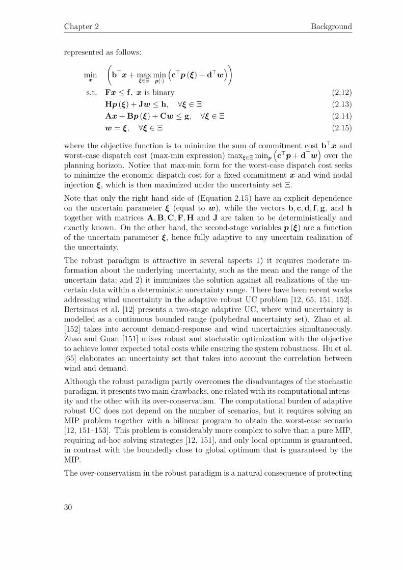
Chapter 2 Background
represented as follows:
minx
(b>x+ max
ξ∈Ξminp(·)
(c>p (ξ) + d>w
))s.t. Fx ≤ f , x is binary (2.12)
Hp (ξ) + Jw ≤ h, ∀ξ ∈ Ξ (2.13)Ax+ Bp (ξ) + Cw ≤ g, ∀ξ ∈ Ξ (2.14)w = ξ, ∀ξ ∈ Ξ (2.15)
where the objective function is to minimize the sum of commitment cost b>x andworst-case dispatch cost (max-min expression) maxξ∈Ξ minp
(c>p+ d>w
)over the
planning horizon. Notice that max-min form for the worst-case dispatch cost seeksto minimize the economic dispatch cost for a fixed commitment x and wind nodalinjection ξ, which is then maximized under the uncertainty set Ξ.Note that only the right hand side of (Equation 2.15) have an explicit dependenceon the uncertain parameter ξ (equal to w), while the vectors b, c,d, f ,g, and htogether with matrices A,B,C,F,H and J are taken to be deterministically andexactly known. On the other hand, the second-stage variables p (ξ) are a functionof the uncertain parameter ξ, hence fully adaptive to any uncertain realization ofthe uncertainty.The robust paradigm is attractive in several aspects 1) it requires moderate in-formation about the underlying uncertainty, such as the mean and the range of theuncertain data; and 2) it immunizes the solution against all realizations of the un-certain data within a deterministic uncertainty range. There have been recent worksaddressing wind uncertainty in the adaptive robust UC problem [12, 65, 151, 152].Bertsimas et al. [12] presents a two-stage adaptive UC, where wind uncertainty ismodelled as a continuous bounded range (polyhedral uncertainty set). Zhao et al.[152] takes into account demand-response and wind uncertainties simultaneously.Zhao and Guan [151] mixes robust and stochastic optimization with the objectiveto achieve lower expected total costs while ensuring the system robustness. Hu et al.[65] elaborates an uncertainty set that takes into account the correlation betweenwind and demand.Although the robust paradigm partly overcomes the disadvantages of the stochasticparadigm, it presents two main drawbacks, one related with its computational intens-ity and the other with its over-conservatism. The computational burden of adaptiverobust UC does not depend on the number of scenarios, but it requires solving anMIP problem together with a bilinear program to obtain the worst-case scenario[12, 151–153]. This problem is considerably more complex to solve than a pure MIP,requiring ad-hoc solving strategies [12, 151], and only local optimum is guaranteed,in contrast with the boundedly close to global optimum that is guaranteed by theMIP.The over-conservatism in the robust paradigm is a natural consequence of protecting
30
2.5 Conclusions
the solution against each uncertainty realization within the uncertainty set, regard-less of its probability. The solution is especially protected against the worst casescenario which may be fictitious and very unlikely to occur. To deal with the over-conservatism, parameters (like the budget-of-uncertainty [13]) are introduced in theoptimization problem to control the level of conservatism of the robust solution[12, 65, 151, 152]. However, tuning these parameters is a far from trivial task [128]and highly dependent on the specific study case [12, 151].
In addition, and to the best of our knowledge, all the work introducing wind uncer-tainty into adaptive robust UCs does not allow wind to have any flexibility because(Equation 2.15) imposes that w takes a fixed wind realization. However, wind hassome flexibility because it can be curtailed. Therefore, what is uncertain is not thewind production range but rather the upper bound of the possible wind dispatch.
2.5. Conclusions
The traditional energy-block scheduling approach is unable to adequately preparethe power system to face perfectly known system conditions. We identified threemain drawbacks of the traditional energy-block scheduling approach that lead to anunnecessary and inefficient use of system resources (reserves) and can even comprom-ise the power system security. These drawbacks can be overcome 1) by schedulingthe power generation in a piecewise-linear fashion to follow a forecasted smoothpower demand profile; 2) by modelling the ramp constraints, in UCs, based onpower production instead of energy, then respecting all ramping constraints; and3) by explicitly scheduling the intrinsic startup and shutdown power trajectories ofgenerating units, i.e., introducing these constraints in the UC formulations. Con-sequently, it is imperative to develop more adequate and accurate models.
Developing more accurate models would be pointless if the models cannot be solvedefficiently enough in the first place. The UC problem is an integer and non-convexproblem which is difficult to solve efficiently, especially for large-scale problems.Mixed-integer (linear) programming (MIP) has become a very popular approach tosolve UC problems due to significant improvements in MIP solvers over the lasttwo decades. Despite this significant breakthrough, the time required to solve UCproblems continues to be a critical limitation that restricts its size and scope. Thischapter identified the key features that affects the computational burden of MIPformulations: the tightness and compactness. Therefore, to develop computationallyefficient MIP models, it is neccesary to devise tight and preferably simultaneouslycompact MIP formulations. This is, however, a non trivial task because the obviousformulations are very weak (not tight) or very large, and trying to improve thetightness (compactness) usually means harming the compactness (tightness).
UC formulations can be further extended to deal with uncertainty. This chapter alsogave an overview of the the three main paradigms used to deal with wind uncertainty
31
Chapter 2 Background
in UC problems: deterministic, stochastic and robust. The deterministic paradigm,based on reserve levels, is the most common in the power industry because it iseasy to implement in practice and it is not as computationally intensive as the otherparadigms. However, the deterministic paradigm usually leads to an over-schedulingof resources resulting in an economically inefficient way to handle uncertainty. Fur-thermore, a deterministic UC only considers one expected deterministic condition,even with enough reserve levels, the power system may not be able to deploy thereserves if the real-time condition deviates significantly from the expected value.Uncertainty-oriented optimization methods, such as stochastic and robust program-ming, seek to overcome the weaknesses of the deterministic paradigm. However,there is a price to pay in order to better tackle uncertainty:
• The stochastic approach presents some practical limitations: 1) a large numberof scenario samples is required to obtain robust solutions, which results ina computationally intensive problem (often intractable); and 2) it may bedifficult to obtain an accurate probability distribution of the uncertainty.
• Although the robust paradigm partly overcomes the disadvantages of thestochastic one, it presents two main drawbacks: 1) it requires solving an MIPproblem together with a bilinear program to obtain the worst-case scenario,this problem is considerably more complex to solve than a pure MIP. 2) Theover-conservatism in the robust paradigm is a natural consequence of protect-ing the solution against each uncertainty realization within the uncertaintyset, regardless of its probability. The solution is especially protected againstthe worst-case scenario which may be fictitious and very unlikely to occur.
32
3. Comparison of Energy-Block andRamp-Based SchedulingApproaches
Contents3.1. UC approaches and Power System . . . . . . . . . . . . . 34
3.1.1. UC approaches . . . . . . . . . . . . . . . . . . . . . . . . 34
3.1.2. Power System . . . . . . . . . . . . . . . . . . . . . . . . . 34
3.2. UC Approach Analysis . . . . . . . . . . . . . . . . . . . . 35
3.2.1. Scheduling and Evaluation Stages . . . . . . . . . . . . . 35
3.2.2. Performance Metrics . . . . . . . . . . . . . . . . . . . . . 36
3.3. Dealing with “Certainty” . . . . . . . . . . . . . . . . . . . 37
3.4. Dealing with Uncertainty . . . . . . . . . . . . . . . . . . . 40
3.4.1. Out-of-sample Evaluation . . . . . . . . . . . . . . . . . . 41
3.4.2. In-sample Evaluation . . . . . . . . . . . . . . . . . . . . . 43
3.5. Computational Performance . . . . . . . . . . . . . . . . . 44
3.5.1. EnSch vs. RmpSch . . . . . . . . . . . . . . . . . . . . . . 44
3.5.2. Tight and Compact EnSch . . . . . . . . . . . . . . . . . 45
3.6. Conclusions . . . . . . . . . . . . . . . . . . . . . . . . . . . 46
This Chapter presents a comparison between the traditional energy-block schedulingapproach and the ramp-based scheduling approach proposed in this thesis. In the firstsection, we introduce the two approaches and the models used to represent them, andwe also present the power system used to perform the comparisons. Then, we describethe procedure used to assess their performance. The last two sections analyse thecases where scheduling is performed under certain and uncertain system conditions,where the latter only considers wind uncertainty.
33
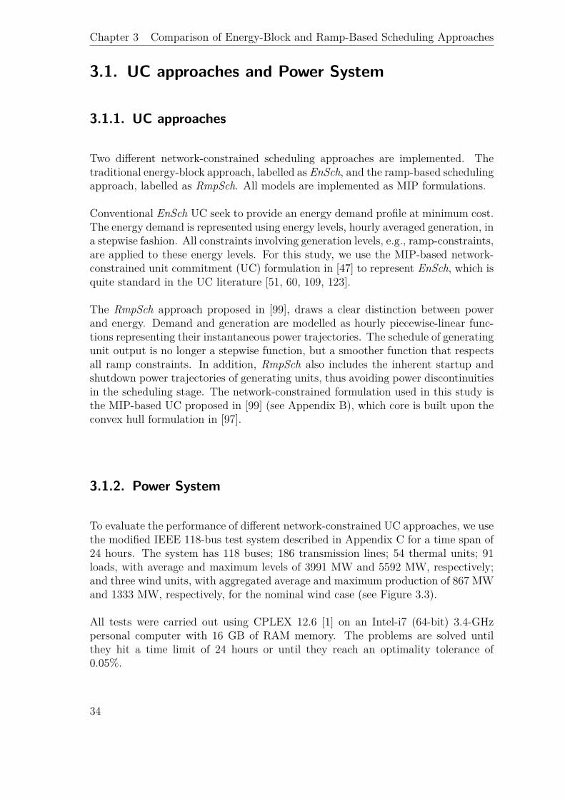
Chapter 3 Comparison of Energy-Block and Ramp-Based Scheduling Approaches
3.1. UC approaches and Power System
3.1.1. UC approaches
Two different network-constrained scheduling approaches are implemented. Thetraditional energy-block approach, labelled as EnSch, and the ramp-based schedulingapproach, labelled as RmpSch. All models are implemented as MIP formulations.
Conventional EnSch UC seek to provide an energy demand profile at minimum cost.The energy demand is represented using energy levels, hourly averaged generation, ina stepwise fashion. All constraints involving generation levels, e.g., ramp-constraints,are applied to these energy levels. For this study, we use the MIP-based network-constrained unit commitment (UC) formulation in [47] to represent EnSch, which isquite standard in the UC literature [51, 60, 109, 123].
The RmpSch approach proposed in [99], draws a clear distinction between powerand energy. Demand and generation are modelled as hourly piecewise-linear func-tions representing their instantaneous power trajectories. The schedule of generatingunit output is no longer a stepwise function, but a smoother function that respectsall ramp constraints. In addition, RmpSch also includes the inherent startup andshutdown power trajectories of generating units, thus avoiding power discontinuitiesin the scheduling stage. The network-constrained formulation used in this study isthe MIP-based UC proposed in [99] (see Appendix B), which core is built upon theconvex hull formulation in [97].
3.1.2. Power System
To evaluate the performance of different network-constrained UC approaches, we usethe modified IEEE 118-bus test system described in Appendix C for a time span of24 hours. The system has 118 buses; 186 transmission lines; 54 thermal units; 91loads, with average and maximum levels of 3991 MW and 5592 MW, respectively;and three wind units, with aggregated average and maximum production of 867 MWand 1333 MW, respectively, for the nominal wind case (see Figure 3.3).
All tests were carried out using CPLEX 12.6 [1] on an Intel-i7 (64-bit) 3.4-GHzpersonal computer with 16 GB of RAM memory. The problems are solved untilthey hit a time limit of 24 hours or until they reach an optimality tolerance of0.05%.
34
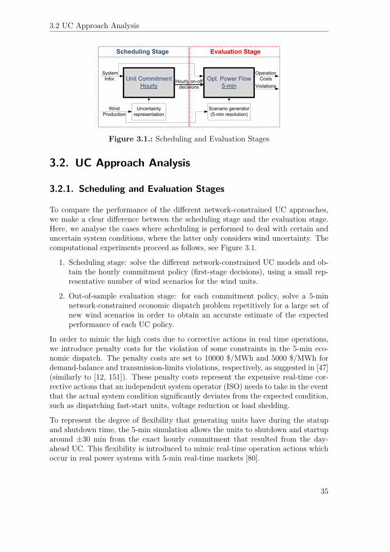
3.2 UC Approach Analysis
Figure 3.1.: Scheduling and Evaluation Stages
3.2. UC Approach Analysis
3.2.1. Scheduling and Evaluation Stages
To compare the performance of the different network-constrained UC approaches,we make a clear difference between the scheduling stage and the evaluation stage.Here, we analyse the cases where scheduling is performed to deal with certain anduncertain system conditions, where the latter only considers wind uncertainty. Thecomputational experiments proceed as follows, see Figure 3.1.
1. Scheduling stage: solve the different network-constrained UC models and ob-tain the hourly commitment policy (first-stage decisions), using a small rep-resentative number of wind scenarios for the wind units.
2. Out-of-sample evaluation stage: for each commitment policy, solve a 5-minnetwork-constrained economic dispatch problem repetitively for a large set ofnew wind scenarios in order to obtain an accurate estimate of the expectedperformance of each UC policy.
In order to mimic the high costs due to corrective actions in real time operations,we introduce penalty costs for the violation of some constraints in the 5-min eco-nomic dispatch. The penalty costs are set to 10000 $/MWh and 5000 $/MWh fordemand-balance and transmission-limits violations, respectively, as suggested in [47](similarly to [12, 151]). These penalty costs represent the expensive real-time cor-rective actions that an independent system operator (ISO) needs to take in the eventthat the actual system condition significantly deviates from the expected condition,such as dispatching fast-start units, voltage reduction or load shedding.
To represent the degree of flexibility that generating units have during the statupand shutdown time, the 5-min simulation allows the units to shutdown and startuparound ±30 min from the exact hourly commitment that resulted from the day-ahead UC. This flexibility is introduced to mimic real-time operation actions whichoccur in real power systems with 5-min real-time markets [80].
35
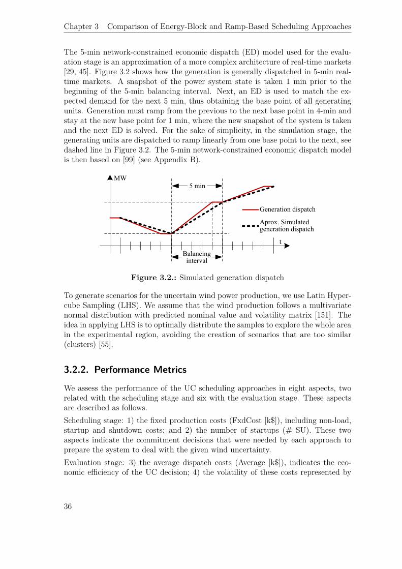
Chapter 3 Comparison of Energy-Block and Ramp-Based Scheduling Approaches
The 5-min network-constrained economic dispatch (ED) model used for the evalu-ation stage is an approximation of a more complex architecture of real-time markets[29, 45]. Figure 3.2 shows how the generation is generally dispatched in 5-min real-time markets. A snapshot of the power system state is taken 1 min prior to thebeginning of the 5-min balancing interval. Next, an ED is used to match the ex-pected demand for the next 5 min, thus obtaining the base point of all generatingunits. Generation must ramp from the previous to the next base point in 4-min andstay at the new base point for 1 min, where the new snapshot of the system is takenand the next ED is solved. For the sake of simplicity, in the simulation stage, thegenerating units are dispatched to ramp linearly from one base point to the next, seedashed line in Figure 3.2. The 5-min network-constrained economic dispatch modelis then based on [99] (see Appendix B).
Figure 3.2.: Simulated generation dispatch
To generate scenarios for the uncertain wind power production, we use Latin Hyper-cube Sampling (LHS). We assume that the wind production follows a multivariatenormal distribution with predicted nominal value and volatility matrix [151]. Theidea in applying LHS is to optimally distribute the samples to explore the whole areain the experimental region, avoiding the creation of scenarios that are too similar(clusters) [55].
3.2.2. Performance Metrics
We assess the performance of the UC scheduling approaches in eight aspects, tworelated with the scheduling stage and six with the evaluation stage. These aspectsare described as follows.Scheduling stage: 1) the fixed production costs (FxdCost [k$]), including non-load,startup and shutdown costs; and 2) the number of startups (# SU). These twoaspects indicate the commitment decisions that were needed by each approach toprepare the system to deal with the given wind uncertainty.Evaluation stage: 3) the average dispatch costs (Average [k$]), indicates the eco-nomic efficiency of the UC decision; 4) the volatility of these costs represented by
36
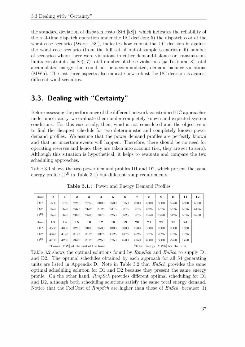
3.3 Dealing with “Certainty”
the standard deviation of dispatch costs (Std [k$]), which indicates the reliability ofthe real-time dispatch operation under the UC decision; 5) the dispatch cost of theworst-case scenario (Worst [k$]), indicates how robust the UC decision is againstthe worst-case scenario (from the full set of out-of-sample scenarios); 6) numberof scenarios where there were violations in either demand-balance or transmission-limits constraints (# Sc); 7) total number of these violations (# Tot); and 8) totalaccumulated energy that could not be accommodated, demand-balance violations(MWh). The last three aspects also indicate how robust the UC decision is againstdifferent wind scenarios.
3.3. Dealing with “Certainty”
Before assessing the performance of the different network-constrained UC approachesunder uncertainty, we evaluate them under completely known and expected systemconditions. For this case study, then, wind is not considered and the objective isto find the cheapest schedule for two deterministic and completely known powerdemand profiles. We assume that the power demand profiles are perfectly knownand that no uncertain events will happen. Therefore, there should be no need foroperating reserves and hence they are taken into account (i.e., they are set to zero).Although this situation is hypothetical, it helps to evaluate and compare the twoscheduling approaches.Table 3.1 shows the two power demand profiles D1 and D2, which present the sameenergy profile (DE in Table 3.1) but different ramp requirements.
Table 3.1.: Power and Energy Demand Profiles
Hour 0 1 2 3 4 5 6 7 8 9 10 11 12
D1∗ 1500 1750 2250 2750 3000 3500 3750 4000 4500 5000 5250 5500 5000
D2∗ 1625 1625 2375 2625 3125 3375 3875 3875 4625 4875 5375 5375 5125
DE† 1625 1625 2000 2500 2875 3250 3625 3875 4250 4750 5125 5375 5250
Hour 13 14 15 16 17 18 19 20 21 22 23 24
D1∗ 4500 4000 3250 3000 3500 4000 5000 4500 3500 2500 2000 1500
D2∗ 4375 4125 3125 3125 3375 4125 4875 4625 3375 2625 1875 1625
DE† 4750 4250 3625 3125 3250 3750 4500 4750 4000 3000 2250 1750∗Power [MW] at the end of the hour †Total Energy [MWh] for the hour
Table 3.2 shows the optimal solutions found by RmpSch and EnSch to supply D1and D2. The optimal schedules obtained by each approach for all 54 generatingunits are listed in Appendix D. Note in Table 3.2 that EnSch provides the sameoptimal scheduling solution for D1 and D2 because they present the same energyprofile. On the other hand, RmpSch provides different optimal scheduling for D1and D2, although both scheduling solutions satisfy the same total energy demand.Notice that the FxdCost of RmpSch are higher than those of EnSch, because: 1)
37
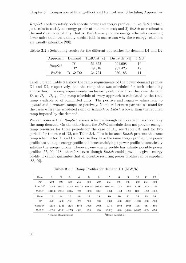
Chapter 3 Comparison of Energy-Block and Ramp-Based Scheduling Approaches
RmpSch needs to satisfy both specific power and energy profiles, unlike EnSch whichjust seeks to satisfy an energy profile at minimum cost; and 2) EnSch overestimatesthe units’ ramp capability, that is, EnSch may produce energy schedules requiringfewer units than are actually needed (this is one reason why these energy schedulesare usually infeasible [99]).
Table 3.2.: Scheduling results for the different approaches for demand D1 and D2
Approach Demand FxdCost [k$] Dispatch [k$] # SU
RmpSch D1 51.352 901.908 16D2 49.618 907.425 19
EnSch D1 & D2 34.724 930.185 11
Table 3.3 and Table 3.4 show the ramp requirements of the power demand profilesD1 and D2, respectively, and the ramp that was scheduled for both schedulingapproaches. The ramp requirements can be easily calculated from the power demandDt as Dt − Dt−1. The ramp schedule of every approach is calculated as the totalramp available of all committed units. The positive and negative values refer toupward and downward ramps, respectively. Numbers between parenthesis stand forthe cases where the scheduled ramp of RmpSch or EnSch is lower than the requiredramp imposed by the demand.We can observe that RmpSch always schedule enough ramp capabilities to supplythe ramp demand. On the other hand, the EnSch schedule does not provide enoughramp resources for three periods for the case of D1, see Table 3.3, and for twoperiods for the case of D2, see Table 3.4. This is because EnSch presents the sameramp schedule for D1 and D2, because they have the same energy profile. One powerprofile has a unique energy profile and hence satisfying a power profile automaticallysatisfies the energy profile. However, one energy profile has infinite possible powerprofiles [57, 99, 118]; therefore, even though EnSch could provide a given energyprofile, it cannot guarantee that all possible resulting power profiles can be supplied[88, 99].
Table 3.3.: Ramp Profiles for demand D1 (MW/h)
Hour 1 2 3 4 5 6 7 8 9 10 11 12
D1∗ 250 500 500 250 500 250 250 500 500 250 250 -500
RmpSch† 935.6 960.6 552.5 696.75 981.75 994.25 1006.75 1033 1103 1138 1138 -1138
EnSch† 1045.6 727.5 900.5 923 1058 1058 1083 1083 1098 1098 1098 -1098
Hour 13 14 15 16 17 18 19 20 21 22 23 24
D1∗ -500 -500 -750 -250 500 500 1000 -500 -1000 -1000 -500 -500
RmpSch† -1138 -1143 -1128 -1078 1078 1078 1078 -1078 -1088 -1063 -983 -808
EnSch† -1098 -1108 -1073 -998 998 998 (998) -998 (-998) (-983) -983 -958∗ Ramp Requirement †Ramp Available
38
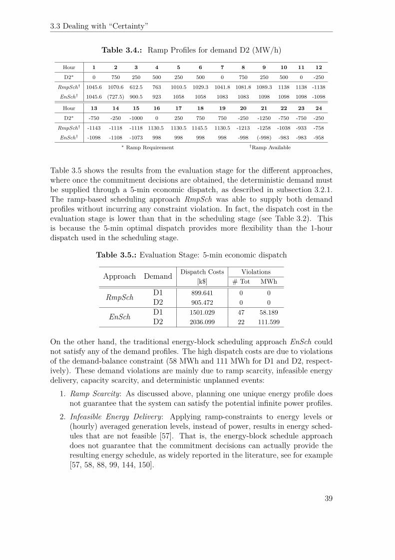
3.3 Dealing with “Certainty”
Table 3.4.: Ramp Profiles for demand D2 (MW/h)
Hour 1 2 3 4 5 6 7 8 9 10 11 12
D2∗ 0 750 250 500 250 500 0 750 250 500 0 -250
RmpSch† 1045.6 1070.6 612.5 763 1010.5 1029.3 1041.8 1081.8 1089.3 1138 1138 -1138
EnSch† 1045.6 (727.5) 900.5 923 1058 1058 1083 1083 1098 1098 1098 -1098
Hour 13 14 15 16 17 18 19 20 21 22 23 24
D2∗ -750 -250 -1000 0 250 750 750 -250 -1250 -750 -750 -250
RmpSch† -1143 -1118 -1118 1130.5 1130.5 1145.5 1130.5 -1213 -1258 -1038 -933 -758
EnSch† -1098 -1108 -1073 998 998 998 998 -998 (-998) -983 -983 -958∗ Ramp Requirement †Ramp Available
Table 3.5 shows the results from the evaluation stage for the different approaches,where once the commitment decisions are obtained, the deterministic demand mustbe supplied through a 5-min economic dispatch, as described in subsection 3.2.1.The ramp-based scheduling approach RmpSch was able to supply both demandprofiles without incurring any constraint violation. In fact, the dispatch cost in theevaluation stage is lower than that in the scheduling stage (see Table 3.2). Thisis because the 5-min optimal dispatch provides more flexibility than the 1-hourdispatch used in the scheduling stage.
Table 3.5.: Evaluation Stage: 5-min economic dispatch
Approach Demand Dispatch Costs Violations[k$] # Tot MWh
RmpSch D1 899.641 0 0D2 905.472 0 0
EnSch D1 1501.029 47 58.189D2 2036.099 22 111.599
On the other hand, the traditional energy-block scheduling approach EnSch couldnot satisfy any of the demand profiles. The high dispatch costs are due to violationsof the demand-balance constraint (58 MWh and 111 MWh for D1 and D2, respect-ively). These demand violations are mainly due to ramp scarcity, infeasible energydelivery, capacity scarcity, and deterministic unplanned events:
1. Ramp Scarcity: As discussed above, planning one unique energy profile doesnot guarantee that the system can satisfy the potential infinite power profiles.
2. Infeasible Energy Delivery: Applying ramp-constraints to energy levels or(hourly) averaged generation levels, instead of power, results in energy sched-ules that are not feasible [57]. That is, the energy-block schedule approachdoes not guarantee that the commitment decisions can actually provide theresulting energy schedule, as widely reported in the literature, see for example[57, 58, 88, 99, 144, 150].
39
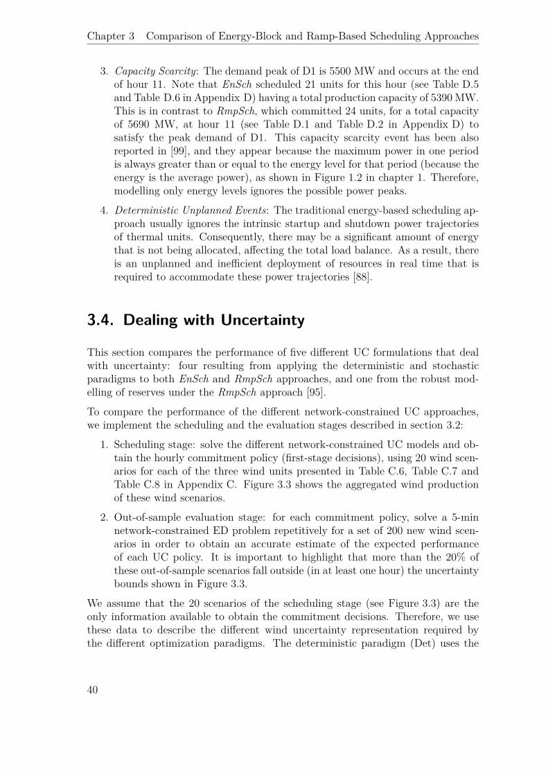
Chapter 3 Comparison of Energy-Block and Ramp-Based Scheduling Approaches
3. Capacity Scarcity: The demand peak of D1 is 5500 MW and occurs at the endof hour 11. Note that EnSch scheduled 21 units for this hour (see Table D.5and Table D.6 in Appendix D) having a total production capacity of 5390 MW.This is in contrast to RmpSch, which committed 24 units, for a total capacityof 5690 MW, at hour 11 (see Table D.1 and Table D.2 in Appendix D) tosatisfy the peak demand of D1. This capacity scarcity event has been alsoreported in [99], and they appear because the maximum power in one periodis always greater than or equal to the energy level for that period (because theenergy is the average power), as shown in Figure 1.2 in chapter 1. Therefore,modelling only energy levels ignores the possible power peaks.
4. Deterministic Unplanned Events: The traditional energy-based scheduling ap-proach usually ignores the intrinsic startup and shutdown power trajectoriesof thermal units. Consequently, there may be a significant amount of energythat is not being allocated, affecting the total load balance. As a result, thereis an unplanned and inefficient deployment of resources in real time that isrequired to accommodate these power trajectories [88].
3.4. Dealing with Uncertainty
This section compares the performance of five different UC formulations that dealwith uncertainty: four resulting from applying the deterministic and stochasticparadigms to both EnSch and RmpSch approaches, and one from the robust mod-elling of reserves under the RmpSch approach [95].
To compare the performance of the different network-constrained UC approaches,we implement the scheduling and the evaluation stages described in section 3.2:
1. Scheduling stage: solve the different network-constrained UC models and ob-tain the hourly commitment policy (first-stage decisions), using 20 wind scen-arios for each of the three wind units presented in Table C.6, Table C.7 andTable C.8 in Appendix C. Figure 3.3 shows the aggregated wind productionof these wind scenarios.
2. Out-of-sample evaluation stage: for each commitment policy, solve a 5-minnetwork-constrained ED problem repetitively for a set of 200 new wind scen-arios in order to obtain an accurate estimate of the expected performanceof each UC policy. It is important to highlight that more than the 20% ofthese out-of-sample scenarios fall outside (in at least one hour) the uncertaintybounds shown in Figure 3.3.
We assume that the 20 scenarios of the scheduling stage (see Figure 3.3) are theonly information available to obtain the commitment decisions. Therefore, we usethese data to describe the different wind uncertainty representation required bythe different optimization paradigms. The deterministic paradigm (Det) uses the
40
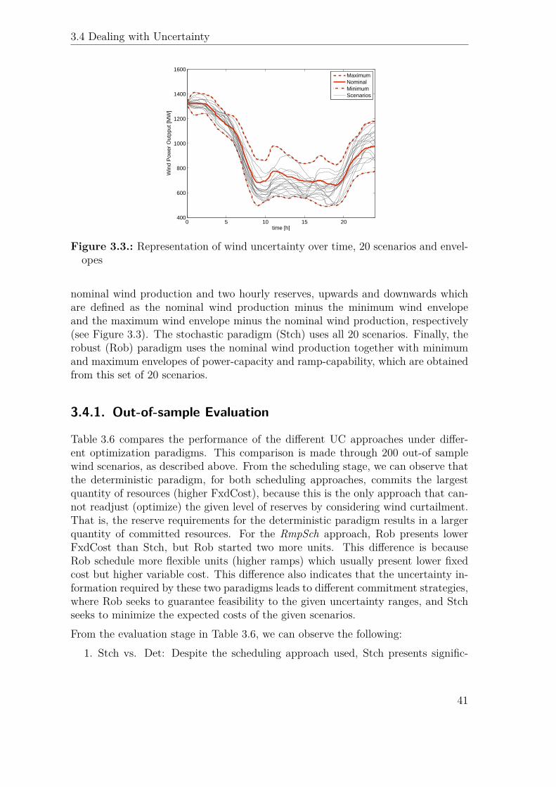
3.4 Dealing with Uncertainty
0 5 10 15 20400
600
800
1000
1200
1400
1600
time [h]
Win
d P
ower
Out
pput
[MW
]
MaximumNominalMinimumScenarios
Figure 3.3.: Representation of wind uncertainty over time, 20 scenarios and envel-opes
nominal wind production and two hourly reserves, upwards and downwards whichare defined as the nominal wind production minus the minimum wind envelopeand the maximum wind envelope minus the nominal wind production, respectively(see Figure 3.3). The stochastic paradigm (Stch) uses all 20 scenarios. Finally, therobust (Rob) paradigm uses the nominal wind production together with minimumand maximum envelopes of power-capacity and ramp-capability, which are obtainedfrom this set of 20 scenarios.
3.4.1. Out-of-sample Evaluation
Table 3.6 compares the performance of the different UC approaches under differ-ent optimization paradigms. This comparison is made through 200 out-of samplewind scenarios, as described above. From the scheduling stage, we can observe thatthe deterministic paradigm, for both scheduling approaches, commits the largestquantity of resources (higher FxdCost), because this is the only approach that can-not readjust (optimize) the given level of reserves by considering wind curtailment.That is, the reserve requirements for the deterministic paradigm results in a largerquantity of committed resources. For the RmpSch approach, Rob presents lowerFxdCost than Stch, but Rob started two more units. This difference is becauseRob schedule more flexible units (higher ramps) which usually present lower fixedcost but higher variable cost. This difference also indicates that the uncertainty in-formation required by these two paradigms leads to different commitment strategies,where Rob seeks to guarantee feasibility to the given uncertainty ranges, and Stchseeks to minimize the expected costs of the given scenarios.From the evaluation stage in Table 3.6, we can observe the following:
1. Stch vs. Det: Despite the scheduling approach used, Stch presents signific-
41
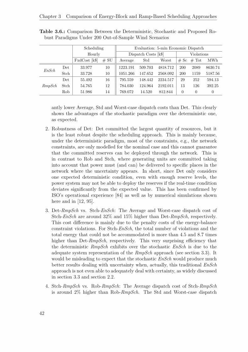
Chapter 3 Comparison of Energy-Block and Ramp-Based Scheduling Approaches
Table 3.6.: Comparison Between the Deterministic, Stochastic and Proposed Ro-bust Paradigms Under 200 Out-of-Sample Wind Scenarios
Scheduling Evaluation: 5-min Economic DispatchHourly Dispatch Costs [k$] Violations
FxdCost [k$] # SU Average Std Worst # Sc # Tot MWh
EnSchDet 33.977 10 1223.191 509.703 4818.712 200 2089 8630.74Stch 33.728 10 1051.266 147.652 2568.092 200 1159 5187.56
RmpSchDet 55.492 16 795.559 148.442 2234.517 29 252 594.13Stch 54.765 12 784.030 124.964 2192.011 13 126 392.25Rob 51.986 14 769.072 14.520 812.844 0 0 0
antly lower Average, Std and Worst-case dispatch costs than Det. This clearlyshows the advantages of the stochastic paradigm over the deterministic one,as expected.
2. Robustness of Det: Det committed the largest quantity of resources, but itis the least robust despite the scheduling approach. This is mainly because,under the deterministic paradigm, most of the constraints, e.g., the networkconstraints, are only modelled for the nominal case and this cannot guaranteethat the committed reserves can be deployed through the network. This isin contrast to Rob and Stch, where generating units are committed takinginto account that power must (and can) be delivered to specific places in thenetwork where the uncertainty appears. In short, since Det only considersone expected deterministic condition, even with enough reserve levels, thepower system may not be able to deploy the reserves if the real-time conditiondeviates significantly from the expected value. This has been confirmed byISO’s operational experience [84] as well as by numerical simulations shownhere and in [12, 95].
3. Det-RmpSch vs. Stch-EnSch: The Average and Worst-case dispatch cost ofStch-EnSch are around 32% and 15% higher than Det-RmpSch, respectively.This cost difference is mainly due to the penalty costs of the energy-balanceconstraint violations. For Stch-EnSch, the total number of violations and thetotal energy that could not be accommodated is more than 4.5 and 8.7 timeshigher than Det-RmpSch, respectively. This very surprising efficiency thatthe deterministic RmpSch exhibits over the stochastic EnSch is due to theadequate system representation of the RmpSch approach (see section 3.3). Itwould be misleading to expect that the stochastic EnSch would produce muchbetter results dealing with uncertainty when, actually, this traditional EnSchapproach is not even able to adequately deal with certainty, as widely discussedin section 3.3 and section 2.2.
4. Stch-RmpSch vs. Rob-RmpSch: The Average dispatch cost of Stch-RmpSchis around 2% higher than Rob-RmpSch. The Std and Worst-case dispatch
42
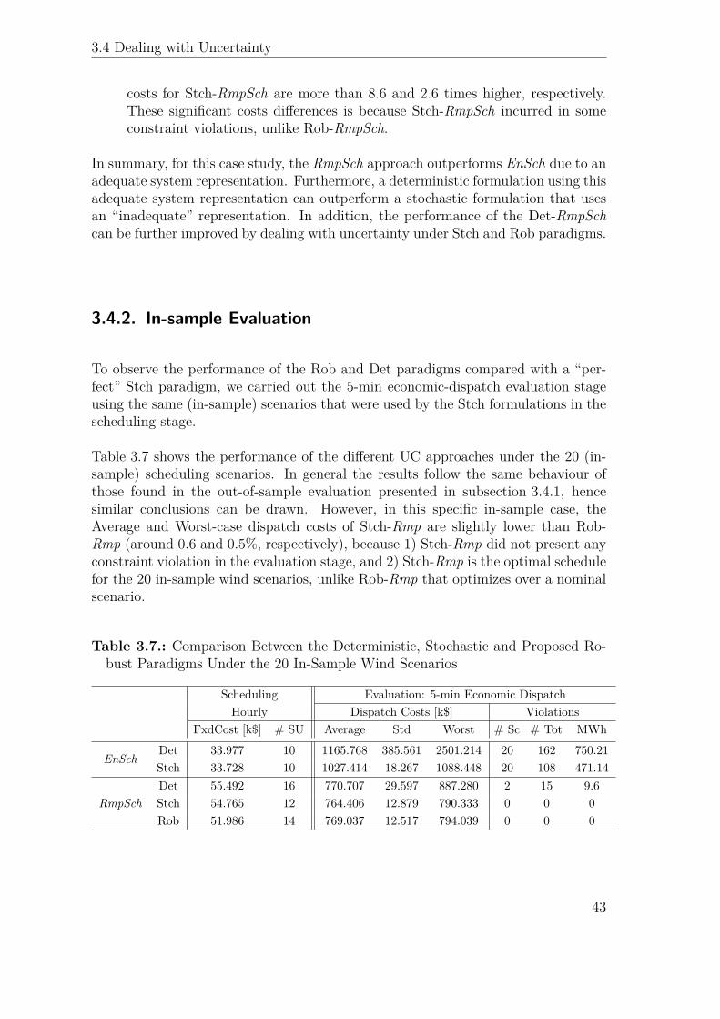
3.4 Dealing with Uncertainty
costs for Stch-RmpSch are more than 8.6 and 2.6 times higher, respectively.These significant costs differences is because Stch-RmpSch incurred in someconstraint violations, unlike Rob-RmpSch.
In summary, for this case study, the RmpSch approach outperforms EnSch due to anadequate system representation. Furthermore, a deterministic formulation using thisadequate system representation can outperform a stochastic formulation that usesan “inadequate” representation. In addition, the performance of the Det-RmpSchcan be further improved by dealing with uncertainty under Stch and Rob paradigms.
3.4.2. In-sample Evaluation
To observe the performance of the Rob and Det paradigms compared with a “per-fect” Stch paradigm, we carried out the 5-min economic-dispatch evaluation stageusing the same (in-sample) scenarios that were used by the Stch formulations in thescheduling stage.
Table 3.7 shows the performance of the different UC approaches under the 20 (in-sample) scheduling scenarios. In general the results follow the same behaviour ofthose found in the out-of-sample evaluation presented in subsection 3.4.1, hencesimilar conclusions can be drawn. However, in this specific in-sample case, theAverage and Worst-case dispatch costs of Stch-Rmp are slightly lower than Rob-Rmp (around 0.6 and 0.5%, respectively), because 1) Stch-Rmp did not present anyconstraint violation in the evaluation stage, and 2) Stch-Rmp is the optimal schedulefor the 20 in-sample wind scenarios, unlike Rob-Rmp that optimizes over a nominalscenario.
Table 3.7.: Comparison Between the Deterministic, Stochastic and Proposed Ro-bust Paradigms Under the 20 In-Sample Wind Scenarios
Scheduling Evaluation: 5-min Economic DispatchHourly Dispatch Costs [k$] Violations
FxdCost [k$] # SU Average Std Worst # Sc # Tot MWh
EnSchDet 33.977 10 1165.768 385.561 2501.214 20 162 750.21Stch 33.728 10 1027.414 18.267 1088.448 20 108 471.14
RmpSchDet 55.492 16 770.707 29.597 887.280 2 15 9.6Stch 54.765 12 764.406 12.879 790.333 0 0 0Rob 51.986 14 769.037 12.517 794.039 0 0 0
43
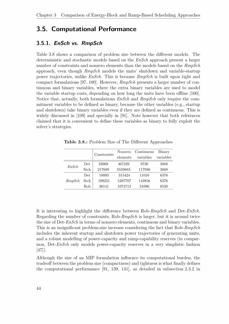
Chapter 3 Comparison of Energy-Block and Ramp-Based Scheduling Approaches
3.5. Computational Performance
3.5.1. EnSch vs. RmpSch
Table 3.8 shows a comparison of problem size between the different models. Thedeterministic and stochastic models based on the EnSch approach present a largernumber of constraints and nonzero elements than the models based on the RmpSchapproach, even though RmpSch models the units’ shutdown and variable-startuppower trajectories, unlike EnSch. This is because RmpSch is built upon tight andcompact formulations [97, 100]. However, RmpSch presents a larger number of con-tinuous and binary variables, where the extra binary variables are used to modelthe variable startup costs, depending on how long the units have been offline [100].Notice that, actually, both formulations EnSch and RmpSch only require the com-mitment variables to be defined as binary, because the other variables (e.g., startupand shutdown) take binary variables even if they are defined as continuous. This iswidely discussed in [109] and specially in [91]. Note however that both referencesclaimed that it is convenient to define these variables as binary to fully exploit thesolver’s strategies.
Table 3.8.: Problem Size of The Different Approaches
ConstraintsNonzero Continuous Binaryelements variables variables
EnSchDet 33969 467329 9720 3888Stch 217689 5559883 117936 3888
RmpSchDet 18093 315424 11016 6376Stch 199221 5497707 143856 6376Rob 36141 1074712 21096 6520
It is interesting to highlight the difference between Rob-RmpSch and Det-EnSch.Regarding the number of constraints, Rob-RmpSch is larger, but it is around twicethe size of Det-EnSch in terms of nonzero elements, continuous and binary variables.This is an insignificant problem-size increase considering the fact that Rob-RmpSchincludes the inherent startup and shutdown power trajectories of generating units,and a robust modelling of power-capacity and ramp-capability reserves (in compar-ison, Det-EnSch only models power-capacity reserves in a very simplistic fashion[47]).Although the size of an MIP formulation influence its computational burden, thetradeoff between the problem size (compactness) and tightness is what finally definesthe computational performance [91, 139, 141], as detailed in subsection 2.3.2 in
44
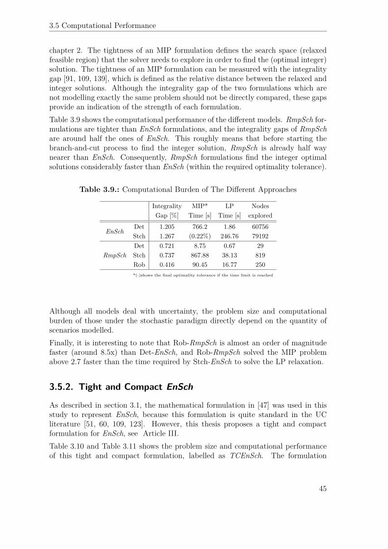
3.5 Computational Performance
chapter 2. The tightness of an MIP formulation defines the search space (relaxedfeasible region) that the solver needs to explore in order to find the (optimal integer)solution. The tightness of an MIP formulation can be measured with the integralitygap [91, 109, 139], which is defined as the relative distance between the relaxed andinteger solutions. Although the integrality gap of the two formulations which arenot modelling exactly the same problem should not be directly compared, these gapsprovide an indication of the strength of each formulation.Table 3.9 shows the computational performance of the different models. RmpSch for-mulations are tighter than EnSch formulations, and the integrality gaps of RmpSchare around half the ones of EnSch. This roughly means that before starting thebranch-and-cut process to find the integer solution, RmpSch is already half waynearer than EnSch. Consequently, RmpSch formulations find the integer optimalsolutions considerably faster than EnSch (within the required optimality tolerance).
Table 3.9.: Computational Burden of The Different Approaches
Integrality MIP* LP NodesGap [%] Time [s] Time [s] explored
EnSchDet 1.205 766.2 1.86 60756Stch 1.267 (0.22%) 246.76 79192
RmpSchDet 0.721 8.75 0.67 29Stch 0.737 867.88 38.13 819Rob 0.416 90.45 16.77 250*(·)shows the final optimality tolerance if the time limit is reached
Although all models deal with uncertainty, the problem size and computationalburden of those under the stochastic paradigm directly depend on the quantity ofscenarios modelled.Finally, it is interesting to note that Rob-RmpSch is almost an order of magnitudefaster (around 8.5x) than Det-EnSch, and Rob-RmpSch solved the MIP problemabove 2.7 faster than the time required by Stch-EnSch to solve the LP relaxation.
3.5.2. Tight and Compact EnSch
As described in section 3.1, the mathematical formulation in [47] was used in thisstudy to represent EnSch, because this formulation is quite standard in the UCliterature [51, 60, 109, 123]. However, this thesis proposes a tight and compactformulation for EnSch, see Article III.Table 3.10 and Table 3.11 shows the problem size and computational performanceof this tight and compact formulation, labelled as TCEnSch. The formulation
45
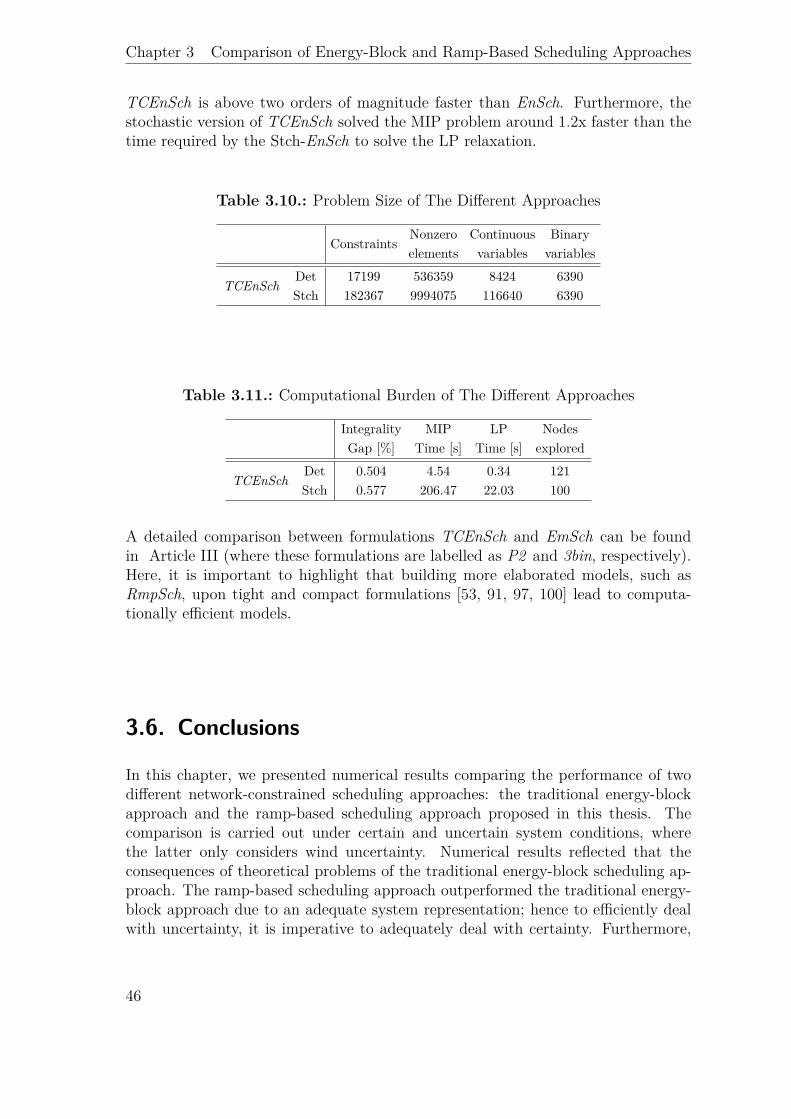
Chapter 3 Comparison of Energy-Block and Ramp-Based Scheduling Approaches
TCEnSch is above two orders of magnitude faster than EnSch. Furthermore, thestochastic version of TCEnSch solved the MIP problem around 1.2x faster than thetime required by the Stch-EnSch to solve the LP relaxation.
Table 3.10.: Problem Size of The Different Approaches
ConstraintsNonzero Continuous Binaryelements variables variables
TCEnSchDet 17199 536359 8424 6390Stch 182367 9994075 116640 6390
Table 3.11.: Computational Burden of The Different Approaches
Integrality MIP LP NodesGap [%] Time [s] Time [s] explored
TCEnSchDet 0.504 4.54 0.34 121Stch 0.577 206.47 22.03 100
A detailed comparison between formulations TCEnSch and EmSch can be foundin Article III (where these formulations are labelled as P2 and 3bin, respectively).Here, it is important to highlight that building more elaborated models, such asRmpSch, upon tight and compact formulations [53, 91, 97, 100] lead to computa-tionally efficient models.
3.6. Conclusions
In this chapter, we presented numerical results comparing the performance of twodifferent network-constrained scheduling approaches: the traditional energy-blockapproach and the ramp-based scheduling approach proposed in this thesis. Thecomparison is carried out under certain and uncertain system conditions, wherethe latter only considers wind uncertainty. Numerical results reflected that theconsequences of theoretical problems of the traditional energy-block scheduling ap-proach. The ramp-based scheduling approach outperformed the traditional energy-block approach due to an adequate system representation; hence to efficiently dealwith uncertainty, it is imperative to adequately deal with certainty. Furthermore,
46

3.6 Conclusions
numerical results showed that a deterministic formulation using this adequate sys-tem representation can outperform a stochastic formulation that uses an “inad-equate” representation. In addition, the performance of the deterministic ramp-based scheduling approach was further improved by dealing with uncertainty understochastic and robust paradigms.
47

4. Conclusions, Contributions andFuture Work
Contents4.1. Conclusions . . . . . . . . . . . . . . . . . . . . . . . . . . . 49
4.1.1. Power System Representation . . . . . . . . . . . . . . . . 504.1.2. UC Computational Performance . . . . . . . . . . . . . . 514.1.3. Wind Uncertainty Management . . . . . . . . . . . . . . . 52
4.2. Scientific Contributions . . . . . . . . . . . . . . . . . . . . 544.2.1. Power System Representation . . . . . . . . . . . . . . . . 544.2.2. UC Computational Performance . . . . . . . . . . . . . . 554.2.3. Wind uncertainty Management . . . . . . . . . . . . . . . 55
4.3. Future Work . . . . . . . . . . . . . . . . . . . . . . . . . . 564.3.1. Power system representation . . . . . . . . . . . . . . . . 564.3.2. UC computational performance . . . . . . . . . . . . . . . 574.3.3. Uncertainty Management . . . . . . . . . . . . . . . . . . 574.3.4. Analysis of Case Studies . . . . . . . . . . . . . . . . . . . 584.3.5. Pricing . . . . . . . . . . . . . . . . . . . . . . . . . . . . 59
In this last chapter of the thesis, the main conclusions are drawn, the most relevantcontributions are presented, and some guidelines for future work are outlined.
4.1. Conclusions
This thesis proposes computationally efficient models for day-ahead planning inthermal power systems to adequately face the stochastic nature of wind productionin the real-time system operation. These models can support ISOs to face the newchallenges in day-ahead planning as uncertainty increases dramatically due to theintegration of variable and uncertain generation resources, such as wind and solarpower.The following subsections expose the conclusions in three parts: power system rep-resentation, UC computational performance, and wind uncertainty management. A
49
Chapter 4 Conclusions, Contributions and Future Work
list of specific contributions for each of these parts can be found in section 4.2 inchapter 1.
4.1.1. Power System Representation
Even in the absence of uncertainty, current day-ahead scheduling practices do notexploit the real flexibility of power systems, this increases operation costs and mayeven endanger the power system security. In this thesis, we have identified four maindrawbacks of current energy-block scheduling practices that lead to an unnecessaryand inefficient use of system resources (reserves):
1. In markets that are physically cleared on an hourly (or half-hourly) basis, suchas those in Europe, generators are penalized if they deviate from their hourlyenergy schedule. In practice, units operate by trying to match their powerprofile with the stepwise energy blocks. This stepwise behaviour creates largegeneration gradients at the beginning and at the end of every trading hour,causing large frequency deviations during these time intervals.
2. In the traditional energy-block UC formulations, generation production levelsare taken as stepwise energy blocks and ramp constraints are then appliedto the inter-hour changes between these energy blocks. Although it has beenproven that the energy delivery obtained from these energy-block formulationsmay not be feasible, insufficient attention has been paid to this issue in theliterature. Consequently, generating units cannot follow their scheduled powerprofile causing an overuse of other system resources to supply the demand.
3. Traditional UC formulations do not consider the intrinsic startup and shut-down power trajectories of thermal units. Ignoring these trajectories at thescheduling stage inevitably leads to an unnecessary deployment of resources inreal-time, which are needed to accommodate the energy produced by the unitsduring their startup and shutdown processes. Although some recent works areaware of this problem, these power trajectories continue being ignored mainlybecause the resulting model would considerably increase the complexity of theproblem and hence its computational intensity.
4. Traditional short-term scheduling approaches seek to supply an energy-block(stepwise) demand profile. One energy profile has infinite possible power pro-files; therefore, even though the traditional energy-block scheduling approachcould provide a given energy profile, it cannot guarantee that the final profilecan be supplied.
To overcome all these drawbacks and to better exploit the power system flexibility,this thesis proposes the ramp-based scheduling approach. Demand and generationare modelled as hourly piecewise-linear functions representing their instantaneouspower trajectories. The schedule of generating units output is no longer a step-wise function, but a smoother function that respects all ramp constraints. As aconsequence:
50
4.1 Conclusions
• The first two drawbacks are then overcome by scheduling the power genera-tion in a piecewise-linear fashion to follow a forecasted smooth power demandprofile.
• The third drawback is tackled by explicitly scheduling the startup and shut-down power trajectories of generating units. That is, these trajectories areincluded in the ramp-based UC formulation.
• The last drawback is overcome by directly scheduling a power profile, whichautomatically satisfies the energy profile (since one power profile only has anunique energy profile).
4.1.2. UC Computational Performance
Developing more accurate models would be pointless if the models cannot be solvedwithin rational time1. The UC problem is an integer and non-convex problem whichis difficult to solve efficiently, especially for large-scale problems. Mixed-integer (lin-ear) programming (MIP) has become a very popular approach to solve UC problemsdue to significant improvements in MIP solvers over the last two decades. Despitethis significant breakthrough in MIP solving, the time required to solve UC problemscontinues to be a critical limitation that restricts its size and scope.
This thesis identifies and takes into account the key features that affects the com-putational burden of MIP formulations. These key features are the tightness andthe compactness: the tightness of an MIP problem defines the search space that thesolver needs to explore in order to find the optimal (integer) solution; the compact-ness of an MIP problem refers to its size and defines the searching speed that thesolver takes to find the optimal solution. Creating tight or compact computationallyefficient formulations is a nontrivial task because the obvious formulations are veryweak (not tight) or very large, and trying to improve the tightness (compactness)usually means harming the compactness (tightness).
Although much work has been done in developing tight generic constraints, especiallyto improve MIP solvers, little has been done in improving the computational burdenof UC formulations. This thesis also contributes to improving the performance ofMIP-based UC formulations. We provide the convex hulls descriptions for the basicoperating constraints (without ramp constraints) of slow- and quick-start units, forboth the energy-block and ramp-based scheduling approaches. Using these convexhulls as the core of energy-block or ramp-based UC models lead to simultaneouslytight and compact MIP formulations. This simultaneous characteristic reinforcesthe convergence speed by reducing the search space (tightness) and at the same
1As stated in chapter 1, a model is considered to be solved within rational time (or efficientlyenough) if it can be solved within the required time using the available computing power. Forexample, if an UC needs to be carried out every hour, then the UC is required to be solved inmuch less than an hour.
51
Chapter 4 Conclusions, Contributions and Future Work
time by increasing the searching speed (compactness) with which solvers explorethat reduced space.As a consequence, although the proposed ramp-based UC model contains moredetailed features than a traditional energy-block UC model, it solves significantlyfaster, because it is based on tight and compact MIP formulations.
4.1.3. Wind Uncertainty Management
Introducing uncertainty management to a given UC model inevitably increases itscomputational burden. There are three main paradigms to deal with wind uncer-tainty in UC:
1. The deterministic paradigm, based on reserve levels, is the most commonpractice in the power industry nowadays, because it is simple and presents alow computational burden. However, it is one of the least robust paradigmsand it usually needs an over-dimension of reserve requirements to improveits robustness, this over-dimension increases operating costs. Furthermore,since a deterministic UC only considers one expected deterministic condition,even with enough reserve levels, the power system may not be able to deploythe reserves if the real-time condition deviates significantly from the expectedvalue.
2. The stochastic paradigm overcomes the disadvantages of the deterministicparadigm. Unfortunately, there is a “price to pay” for this. The stochasticparadigm presents some practical limitations: 1) it may be difficult to obtainan accurate probability distribution of the uncertainty; and 2) a large numberof scenarios is required to obtain robust solutions, which results in a computa-tionally intensive problem (often intractable). Therefore, many simplificationsare usually employed to make the problem tractable, e.g., fewer scenarios areconsidered and many crucial constraints (e.g., network constraints) are usuallyneglected.
3. The robust optimization paradigm partly overcomes these disadvantages 1) byrequiring moderate information about the underlying uncertainty, such as themean and the range of the uncertain data; and 2) by immunizing the solutionagainst all realizations of the data within the uncertainty range. However, thisparadigm may be too conservative, since the objective function is to minimizethe worst-case cost scenario, which may be fictitious and never be realized inpractice. Although a robust UC may not be as computationally intensive asa stochastic one, it requires solving an MIP problem together with a bilin-ear problem. This is considerably more complex to solve than a pure MIP,requiring ad-hoc solving strategies, and only local optimum is guaranteed.
Although the main objective of this thesis is wind uncertainty management in UCmodels, we first focused on dealing adequately with certainty (power system repres-entation) and the UC computational performance. These two aspects are in conflict
52
4.1 Conclusions
and improving one usually means harming the other. By putting together improve-ments in the previous two aspects, this thesis contributes to a better managementof wind uncertainty in UC. Therefore, as a natural consequence, if compared with atraditional energy-block UC model under the stochastic (deterministic) paradigm, astochastic (deterministic) ramp-based UC model 1) leads to more economic opera-tion, due to a better and more detailed system representation, while 2) being solvedsignificantly faster, because the core of the model is built upon simultaneously tightand compact MIP formulations.This thesis also proposes a methodology to assess the performance of a given UCsolution, which helps to perform comparisons between different commitment strategies.We then make a clear difference between the scheduling stage and the evaluationstage, where the commitment decisions obtained from the scheduling stage, are eval-uated using a 5-min optimal dispatch simulation. This evaluation stage mimics theactual real-time system operation where generating units are dispatched to supplythe demand every instant. To the best of our knowledge, there are previous worksthat only uses hourly simulation as evaluation procedure. In this thesis, we pro-pose to increase the granularity of the simulation stage up to 5 min in order tomimic the actual real-time system operation (where generating units are dispatchedto supply the demand at every instant). Consequently, as shown in the differentcase studies, this 5-min evaluation stage helped to unveil drawbacks of traditionalenergy-block UC approaches, which are not possible to be identified by using 1-hourperiod simulation.In addition, based on robust optimization insights and taking into account the windgeneration flexibility (i.e., curtailment), we propose a network-constrained UC for-mulation with robust reserve modelling, which main characteristics as listed as fol-lows:
• The model is formulated under the ramp-based scheduling approach and builtupon thigh and compact MIP formulations, hence taking complete advant-age of putting together the improvements in these two aspects (power systemrepresentation and UC computational performance).
• To guarantee that the UC solution is feasible for any realization of the un-certain wind production within the considered uncertainty ranges, the modelincludes the worst-case wind power scenario provided by the adaptive robustoptimization problem. We show that by allowing wind curtailment, the worst-case scenario can be obtained a priori, and thus the robust UC becomes asingle-scenario UC. That is, the final proposed model remains as a pure MIPproblem.
• To correctly represent wind uncertainty, the model distinguishes between power-capacity and ramp-capability reserve requirements. This is aligned with acurrent trend of defining new products in electricity markets to increase itsflexibility in real-time operation.
• The final UC model remains as a pure MIP problem, which size does not
53
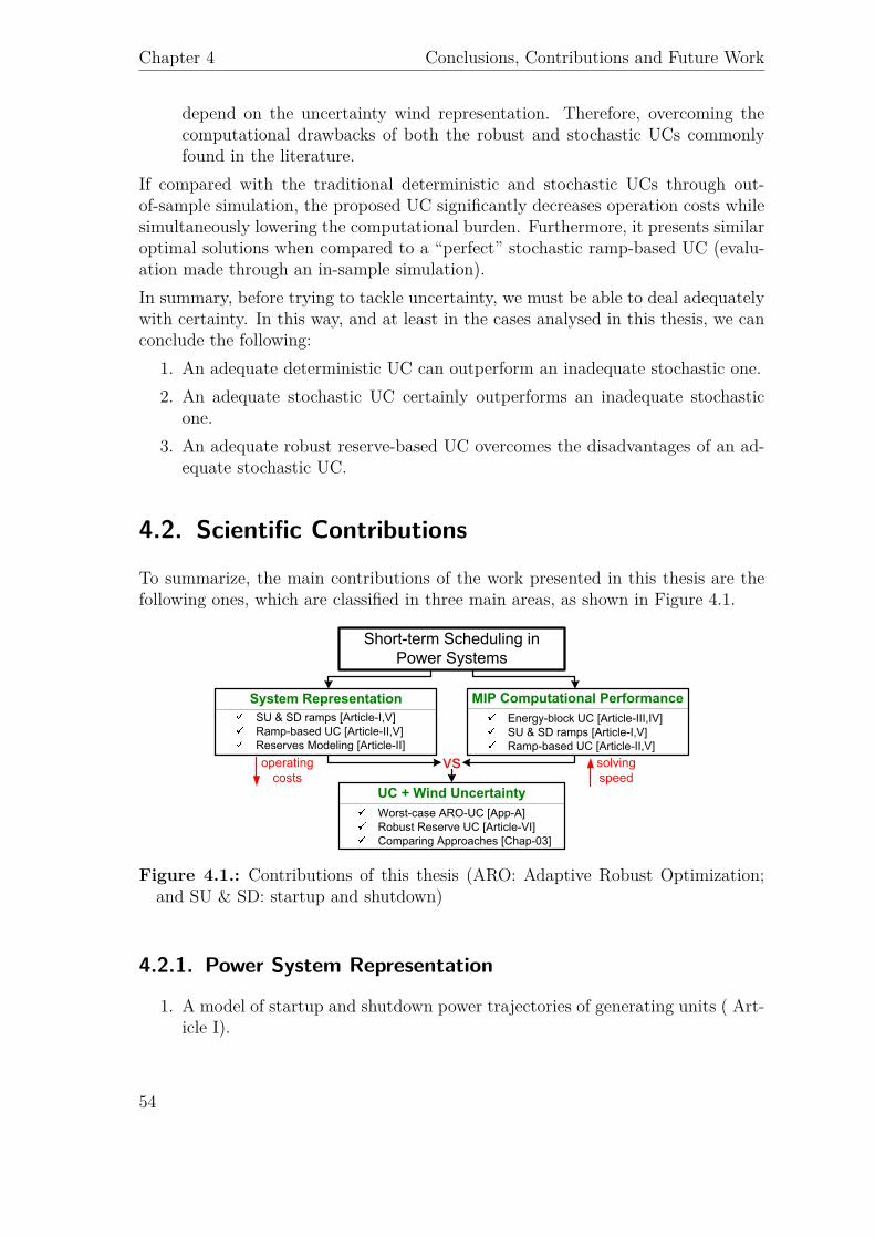
Chapter 4 Conclusions, Contributions and Future Work
depend on the uncertainty wind representation. Therefore, overcoming thecomputational drawbacks of both the robust and stochastic UCs commonlyfound in the literature.
If compared with the traditional deterministic and stochastic UCs through out-of-sample simulation, the proposed UC significantly decreases operation costs whilesimultaneously lowering the computational burden. Furthermore, it presents similaroptimal solutions when compared to a “perfect” stochastic ramp-based UC (evalu-ation made through an in-sample simulation).In summary, before trying to tackle uncertainty, we must be able to deal adequatelywith certainty. In this way, and at least in the cases analysed in this thesis, we canconclude the following:
1. An adequate deterministic UC can outperform an inadequate stochastic one.2. An adequate stochastic UC certainly outperforms an inadequate stochastic
one.3. An adequate robust reserve-based UC overcomes the disadvantages of an ad-
equate stochastic UC.
4.2. Scientific Contributions
To summarize, the main contributions of the work presented in this thesis are thefollowing ones, which are classified in three main areas, as shown in Figure 4.1.
Figure 4.1.: Contributions of this thesis (ARO: Adaptive Robust Optimization;and SU & SD: startup and shutdown)
4.2.1. Power System Representation
1. A model of startup and shutdown power trajectories of generating units ( Art-icle I).
54
4.2 Scientific Contributions
2. A ramp-based scheduling approach ( Article II), which schedules piecewisepower profiles instead of the traditional stepwise energy blocks.
3. Ramp-based models for slow- and quick-start units ( Article V), includingdifferent operating reserves (online and offline) and their time deploymentlimits, e.g., 15 min, (section II-B and II-C in Article II).
4.2.2. UC Computational Performance
1. Convex hull of the energy-block scheduling approach for quick-start units ( Art-icle IV). To model slow-start units, the startup and shutdown energy traject-ories presented in Article V (see equation (10) in section 3.2) can be added tothe convex hull in Article IV where the resulting enlarged formulation is stilla convex hull. This is because the startup and shutdown energy trajectoriesin Article V are equalities that add new variables, so they do not add anyfractional vertex to the previous formulation (see Lemma 7 in Article IV). Us-ing these convex hulls as the core of any energy-block UC formulation yieldssimultaneously tight and compact formulations, as presented in Article III.
2. Convex hull of the proposed ramp-based scheduling approach for both slow-and quick-start units ( Article V). When used as the core of any UC problemmodelling startup and shutdown power trajectories, the proposed model con-siderably outperforms other analogous formulations (section II-B in Article I).If compared with simpler energy-block UC formulations commonly found inthe literature, which do not include these startup and shutdown power tra-jectories, the proposed model still reduces the computational burden (sectionII-C in Article II, section 5 in Article V, and section 3.5 in chapter 3).
3. Tight and compact MIP formulation for variable startup costs (section II-A-2in Article III), according to how long a unit has been offline. This formulationallows a straightforward introduction of different startup power trajectoriesinto UC models (section II-A-5 in Article II, and section II-A-7 in Article I).
4.2.3. Wind uncertainty Management
1. Using the ramp-based approach, we produce deterministic and stochastic UCformulations to deal with wind uncertainty. If compared with traditionalenergy-block UCs commonly found in the literature, the proposed ramp-basedformulations: 1) lower operating costs due to a better system representation;while 2) being solved significantly faster, because the models are built upontight and compact MIP formulations ( Article VI and chapter 3).
2. A linear MIP formulation for the worst-case wind power scenario for adaptiverobust UC problems (Appendix A).
55
Chapter 4 Conclusions, Contributions and Future Work
3. A robust network-constrained UC formulation based on the ramp-based schedul-ing approach ( Article VI). The model distinguishes between power-capacityand ramp-capability reserve requirements to correctly represent wind uncer-tainty ( Article VI). In addition, by including the worst-case wind scenario(Appendix A), the formulation ensures feasibility for any wind uncertaintyrealization. If compared with a traditional energy-block stochastic UC, theproposed approach lowers operating costs while being solved significantly faster(chapter 3).
4. To assess the performance of the different UC approaches, this thesis alsoproposes to make a clear difference between the scheduling and the evaluationstages (Section III-A in Article VI and section 3.2 in chapter 3). The commit-ment decisions, obtained from the scheduling stage, are evaluated through a 5-min optimal dispatch simulation. To the best of our knowledge, there are worksthat uses hourly simulation as evaluation stage, but not a more detailed 5-minsimulation to mimic the actual real-time system operation (where generatingunits are dispatched to supply the demand at every instant). Consequently,this evaluation stage helped to unveil drawbacks of traditional energy-blockUC approaches, which are not possible to be identified by just using an hourlysimulation.
4.3. Future Work
The main work presented in this thesis is a novel scheduling approach to betterrepresent and exploit the power system flexibility. This opens many new questionsand possible steps for further research, some of which are listed below:
4.3.1. Power system representation
The proposed ramp-based scheduling approach implies that all technologies thatprovide (or consume) power must be modelled using piecewise power trajectories,instead of the traditional stepwise energy blocks. This thesis has only modelledthermal units. Although many technologies can be formulated in a similar way, theymust be carefully modelled respecting all their technical characteristics. Therefore,all technologies that have been already modelled using the traditional energy-blockapproach should now be modelled under the ramp-based scheduling approach, mak-ing a clear distinction between their power and energy production levels.Some of the technologies that need to be modelled following the ramp-based schedul-ing approach, which were not included in this thesis, are: 1) hydropower plants,with and without pumped storage; 2) plug-in electric vehicles; and 3) multi-modecombined-cycle units (which present different operating modes or states with differ-ent technical parameters).
56
4.3 Future Work
There are also some specific set of constraints that may apply to different technolo-gies and should be remodelled under the ramp-scheduling approach, such as dynamicramping2.
4.3.2. UC computational performance
The UC problem involves binary variables by definition. Therefore, it will always bechallenging to build MIP-based computationally efficient models. Therefore, muchresearch is needed in developing “tight” and, if possible, simultaneously “compact”models so they can be solved within rational time.
The previous section mentioned some of the models that need to be formulatedunder the ramp-based scheduling approach, these models should be carefully craftedto achieve tight and compact MIP formulations. This can be done with the help ofspecialized computational software (e.g., PORTA [30]).
Some models, which are already available in the literature, require further improve-ments, for example:
1. Further tightening the complete UC models under the deterministic, stochasticand robust paradigms. For example, proposing the convex hull or tighterformulations for a single unit taking into account the ramping constraints.
2. Developing compact stochastic UCs without loosing accuracy in the solution.That is, identify or develop dominating constraints that allows removing pos-sible redundant constraints, especially when introducing network constraints.
3. Proposing tight and compact MIP formulations for cumbersome (energy-based)UC problems that involve many binary variables, e.g., dynamic ramping,multi-mode combined-cycle units.
4.3.3. Uncertainty Management
As widely discussed in this thesis, any improvement in either of the two previousfields will naturally yield to UC models that can better deal with uncertainty. Onthe one hand, by better representing the power system, lower operating costs willbe expected when dealing with uncertainty, since the deterministic and completelyknown events will be optimally scheduled. On the other hand, by improving thecomputational performance of UC models, stochastic and robust UCs will be solvedfaster then less simplifications will be needed.
This thesis proposes a linear MIP formulation for the worst-case adaptive-robustUC problem. Although this worst-case scenario ensures feasibility, further research
2Dynamic ramping refers to the unit’s variable ramp capability, which numerical value dependson the unit’s production level.
57
Chapter 4 Conclusions, Contributions and Future Work
is needed to obtain deterministic formulations that control the level of conservat-ism of the adaptive-robust optimal solution, avoiding the bilinear problem and itsassociated disadvantages.This thesis focused on dealing with wind uncertainty and introducing of any source ofuncertainty that can be curtailed is straightforward, but other sources of uncertaintyshould be included in the future, such as demand-response, hydro inflows, generatorsand line outages. Furthermore, possible correlations (e.g. temporal and spacialcorrelations) should also be considered.We proposed a deterministic ramp-based approach that includes different types ofreserves depending on their time-deployment requirements (e.g., 15 mins, 30 mins).The robust reserve-based approach proposed in this thesis can be further exten-ded to consider these different time-dependent reserves, thus dealing simultaneouslywith inter- and intra-hourly wind power fluctuations (which have different stochasticcharacteristics).
4.3.4. Analysis of Case Studies
One of the main objectives of this thesis was to propose new formulations to dealwith wind uncertainty. The case studies were carried out for illustrative purposes;they were not based on real power systems, but rather based on benchmark studycases widely used in the UC literature. Much more work can be done in this vein,for example:
• The experiments performed in this thesis can be replicated in real and largerpower systems. By using a specific real power systems, we can observe towhat extend the proposed formulation can further improve the current oper-ating practices in that system, so conclusions and advice for the specific powersystems can be outlined.
• Many studies have been performed for integrating renewable energy sources inpower systems, using the traditional energy-block approach. Similar studiescan be done using the proposed ramp-based scheduling approach and perhapsdifferent conclusions could be achieved.
• Different commitment strategies can be implemented, e.g., multi-stage or rollingUC, and they can be evaluated using more detailed real-time simulations ofpower systems. These real-time simulations can be tailored considering specificcharacteristics of different real power systems.
Other case studies can be carried out focused on markets that are physically clearedon an hourly (or half-hourly) basis, such as those in Europe. These markets arepresenting large deterministic frequency deviations. A change of market approachfrom the energy-block to the ramp-based scheduling may contribute to diminish thisproblem. Generators should be penalized if they deviate from their power sched-ule, which satisfies the energy and ramp schedule. Although these markets follow
58
4.3 Future Work
hourly trading periods, measurements for shorter periods are needed to measurethe ramp, and thus being able to penalize deviations from the power schedule. En-ergy measurements every few minutes (around 5-10) would be enough to monitorthe ramp profiles. Actually, these measurements are usually available and neededby the secondary reserve control to work adequately (AGC usually uses continu-ous measurements every few seconds). Consequently, generators would have theincentive to follow their smooth power profile, thus considerably diminishing thesedeterministic frequency deviations.
4.3.5. Pricing
The ramp-based scheduling approach proposed in this thesis should be further ex-tended to obtain a complete UC-based market-clearing mechanism. So apart fromusing this approach to schedule optimal quantities, as done in this thesis, it couldbe also used to determine the prices that allows the different parties to recover theirproduction costs.As a possible starting point, one can use the pricing mechanisms implemented bythe current UC-based markets (e.g., those in USA). However, the proposed approachprovides a power price $/MW (which is the dimension of the shadow price of thedemand-balance constraint) instead of the traditional energy price $/MWh. Thispower price needs to be completely understood since it reflects the need of a givenenergy profile together with a given power profile, hence a unique ramp profile. Incomparison, the energy price that results from the traditional energy-block approachjust reflects an energy requirement, but not a ramp requirement, then the pureenergy pricing cannot provide the right signal to avoid ramping scarcity events.Furthermore, to introduce price-sensitive demand, a new trading product must bedefined since the traditional energy-block bidding from the demand side is not validunder the proposed ramp-scheduling approach. Therefore, extending the ideas ofthe piecewise-linear formulation to the demand side would require a deeper analysisand further research. One possible solution could be to change from the squaredenergy blocks to piecewise-linear (or triangular shape) functions, which reflects boththe energy and ramping requirements. That is, the demand can be modelled as agenerator, so it can be included in the demand power-balance equation as if it were anegative generator, and the energy payment can be added in the objective functionhaving only variable cost (the price assigned to each one of the energy blocks).Apart from this, many questions have not been (completely) answered about pricingthe stochastic paradigm yet, which also apply to the proposed robust reserve-basedparadigm. If a stochastic UC is used as a market-clearing mechanism, how shouldthe prices be calculated? Because a stochastic UC produces as part of its solutionmany shadow prices (e.g., one per energy-balance constraint scenario), instead ofthe traditional single set of deterministic shadow prices for energy at each location.Perhaps, a multi-price commodity can then be derived, similar to those traditional
59

Chapter 4 Conclusions, Contributions and Future Work
joint reserve-energy markets (based on the deterministic paradigm). In those jointmarkets, the reserve price compensates the units for not exploiting their maximumcapacity in the energy market, thus guaranteeing that the units have some reserveavailable in case it is needed later.
60
A. The Worst-case Wind PowerScenario for Adaptive RobustUnit Commitment Problems
ContentsA.1. Obtaining the Worst-case Wind Scenario . . . . . . . . . 61
A.1.1. The Second Stage Problem . . . . . . . . . . . . . . . . . 62A.1.2. Adaptive Robust Reformulation . . . . . . . . . . . . . . . 63
A.2. Illustrative Example . . . . . . . . . . . . . . . . . . . . . . 64
This appendix presents a simple deterministic formulation for the unit commitment(UC) problem under the adaptive robust optimization (ARO) paradigm for the caseof wind production uncertainty. We show that the worst-case wind power scenariocan be obtained before solving the UC. This way the ARO-UC problem becomes asimple single-scenario deterministic UC, avoiding the bilinear optimization problemassociated with the second-stage dispatch actions in traditional ARO formulations.
A.1. Obtaining the Worst-case Wind Scenario
The two-stage adaptive robust UC seeks to minimize the worst-case dispatch costconsidering any possible realization of wind nodal injection ξ within the determ-inistic uncertainty set Ξ (or uncertainty range). In the adaptive robust UC, thefirst-stage commitment decisions and the second-stage dispatch decisions are robustagainst all uncertain wind nodal injection realizations. Furthermore, the second-stage dispatch solutions are fully adaptable to the uncertainty [8, 10, 12]. Here, wepresent a compact matrix formulation:
minx
(b>x+ max
ξ∈Ξmin
p(·),w(·)
(c>p (ξ) + d>w (ξ)
))s.t. Fx ≤ f , x is binary (A.1)
Hp (ξ) + Jw (ξ) ≤ h, ∀ξ ∈ Ξ (A.2)Ax+ Bp (ξ) + Cw (ξ) ≤ g, ∀ξ ∈ Ξ (A.3)w (ξ) ≤ ξ, ∀ξ ∈ Ξ (A.4)
61
Appendix A The Worst-case Wind Scenario for ARO-UC Problems
where x,p and w are variables. The binary variable x is a vector of commitmentrelated decisions (e.g., on/off and startup/shutdown) of each generation unit for eachtime interval over the planning horizon. The continuous variable p is a vector of eachunit dispatch decision for each time interval. The continuous variable w is a vectorof each wind production dispatch decision for each node and for each time interval.The parameter ξ is a vector of each uncertain maximum wind nodal injection foreach time interval, and the set of uncertainty Ξ is defined by the continuous intervalξbt = [wbt,wbt] for all t ∈ T , b ∈ Bw, where t is the time index in the planninghorizon T , b is the index representing buses and Bw is the set of buses that haveuncertain wind power injections.
Constraint (Equation A.1) involves only commitment-related constraints, e.g., min-imum up and down. Constraint (Equation A.2) contains dispatch-related con-straints, e.g., energy balance (equality can always be written as two opposite inequal-ities), transmission limit constraints, ramping constraints. Constraint (Equation A.3)couples the commitment and dispatch decisions, e.g., minimum and maximum gen-eration capacity constraints. Finally, (Equation A.14) guarantees that the winddispatch cannot exceed the available wind power. The reader is referred to [91] fora detailed UC formulation.
Note that only the right hand side of (Equation A.4) have an explicit dependenceon the uncertain parameter ξ, while the vectors b, c,d, f ,h, and g together withmatrices A,B,C,F,H and J are taken to be deterministically and exactly known.On the other hand, the second-stage variables p (ξ) and w (ξ) are a function of theuncertain parameter ξ, hence fully adaptive to any realization of the uncertainty.
Wind dispatch cost is usually considered to be zero. However, the parameter d isexplicitly included to consider the possibility where this cost is different than zero(in some power systems, this cost can even be negative, e.g. -40 $/MWh in ERCOT[7]). Defining negative values for parameter d is equivalent to penalize curtailmentsin the objective function.
The objective function is to minimize the sum of commitment cost b>x and worst-case dispatch cost (max-min expression) maxξ∈Ξ miny,w
(c>p+ d>w
)over the plan-
ning horizon. Notice that the max-min form for the worst-case dispatch cost seeksto minimize the economic dispatch costs for a fixed commitment x and wind nodalinjection ξ, which is then maximized under the uncertainty set Ξ.
A.1.1. The Second Stage Problem
The second stage optimization problem of (Equation A.1)-(Equation A.4) can bereformulated as a single stage optimization problem with adaptability. This corres-ponds to the single-stage problem once the first-stage variables x have been fixed.
62
A.1 Obtaining the Worst-case Wind Scenario
The completely adaptive linear formulation of this second-stage problem is now:
maxξ∈Ξ
minp(·),w(·)
c>p (ξ) + d>w (ξ)
s.t. Hp (ξ) + Jw (ξ) ≤ h, ∀ξ ∈ Ξ (A.5)Bp (ξ) + Cw (ξ) ≤ g, ∀ξ ∈ Ξ (A.6)w (ξ) ≤ ξ, ∀ξ ∈ Ξ (A.7)
where g = g−Ax.
Note that the uncertainty affecting every one of the constraints (Equation A.7)is independent of each other (i.e., no correlations are considered). As mentionedbefore, the uncertainty set Ξ is defined by the continuous interval ξbt = [wbt,wbt]for all t ∈ T , b ∈ Bw. Due to this special characteristic of the uncertainty setin LP problems, the adaptive and static (or non-adaptive) robust formulations areequivalent, as proven in [8] and further discussed in [27]. That is, we can obtainthe solution of the adaptive robust model by finding the static robust formulationof (Equation A.5)-(Equation A.7).
It can be easily observed that the solution of the adaptive (and static) robust formu-lation of the LP problem (Equation A.5)-(Equation A.7) can be obtained by solvingthe following LP reformulation [10]:
minp(·),w(·)
c>p+ d>w
s.t. Hp+ Jw ≤ h (A.8)Bp+ Cw ≤ g (A.9)w ≤ w (A.10)
notice that (Equation A.10) only includes the lowest bound of the uncertainty set.
To the best of our knowledge, all the ARO UCs models introducing wind uncer-tainty in the formulation consider (Equation A.4) and (Equation A.7) as equalities.Therefore, wind production is not allowed to have any flexibility because modelling(Equation A.4) and (Equation A.7) as equalities impose that w takes a fixed windrealization. However, wind has some flexibility because it can be curtailed. There-fore, what is uncertain is not the wind production range but rather the upper boundof the possible wind dispatch. Furthermore, if (Equation A.4) and (Equation A.7)are modelled as equalities, the second-stage adaptive problem requires solving abilinear problem which further complicate the MIP problem [12, 151].
A.1.2. Adaptive Robust Reformulation
The adaptive robust problem (Equation A.1)-(Equation A.4) can be easily reformu-lated by replacing the max-min second-stage problem by its LP equivalent (Equation A.8)-
63
Appendix A The Worst-case Wind Scenario for ARO-UC Problems
(Equation A.10):
minx,p,w
b>x+ c>p+ d>w
s.t. Fx ≤ f , x is binary (A.11)Hp+ Jw ≤ h (A.12)Ax+ Bp+ Cw ≤ g (A.13)w ≤ w (A.14)
Therefore, a two-stage ARO MIP problem presents the same solution as a staticrobust problem if 1) the uncertainty affecting every one of the constraints is inde-pendent of each other, and 2) the second-stage (adaptive) variables are all continu-ous, i.e., the integer variables only appear as first-stage (non-adjustable) decisionvariables [11].It is important to highlight that this is a deterministic formulation where the onlyscenario that is needed to solve the ARO UC problem is the lowest expected boundof wind w within the uncertainty set Ξ. If this formulation has a feasible optimalsolution w∗ then it guarantees that all other possible wind realizations within theuncertainty set are feasible. That is, all scenarios can become w∗ by curtailment.Consequently, all scenarios can be dispatched and, in the worst case, the maximumquantity of wind that can be dispatched for any scenario would be w∗.In short, w is the worst-case scenario for the ARO UC problem, which ensuresfeasibility, but it may be too conservative because it does not guarantee that windscenarios above w can be dispatched.
A.2. Illustrative Example
Not allowing wind curtailment in the ARO UC formulation leads to misleading solu-tions. To illustrate this, consider the following example for an one-period ARO UCproblem, where a first-stage (binary) commitment decision needs to be taken (thisinteger decision only appears in the first-stage). We compare two ARO UC formula-tions: 1) the traditional ARO-UC, presented in [12, 151], which does not allow cur-tailment, and 2) the ARO UC formulation that allows curtailment (Equation A.1)-(Equation A.4). They are labelled as NotCurt. and WithCurt., respectively.A fixed demand of 45 MWh needs to be supplied by one thermal and one windgenerating units. The thermal unit has 20 and 40 MW as min and max generationcapacity, respectively. The wind production is within the uncertainty range [40, 70]MWh. To provide the demand, it is necessary to maintain an energy balance.Figure A.1 shows the demand-balance deviations (shortage/surplus) for every valueof wind within its uncertainty range. Notice that for a given value of wind, thedeviations are always lower if the thermal unit is offline. Following the NotCurt
64
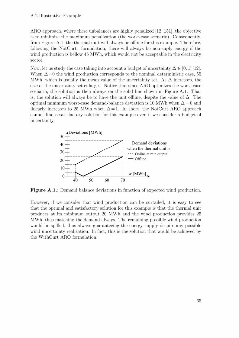
A.2 Illustrative Example
ARO approach, where these unbalances are highly penalized [12, 151], the objectiveis to minimize the maximum penalization (the worst-case scenario). Consequently,from Figure A.1, the thermal unit will always be offline for this example. Therefore,following the NotCurt. formulation, there will always be non-suply energy if thewind production is bellow 45 MWh, which would not be acceptable in the electricitysector.Now, let us study the case taking into account a budget of uncertainty ∆ ∈ [0, 1] [12].When ∆=0 the wind production corresponds to the nominal deterministic case, 55MWh, which is usually the mean value of the uncertainty set. As ∆ increases, thesize of the uncertainty set enlarges. Notice that since ARO optimizes the worst-casescenario, the solution is then always on the solid line shown in Figure A.1. Thatis, the solution will always be to have the unit offline, despite the value of ∆. Theoptimal minimum worst-case demand-balance deviation is 10 MWh when ∆ = 0 andlinearly increases to 25 MWh when ∆=1. In short, the NotCurt ARO approachcannot find a satisfactory solution for this example even if we consider a budget ofuncertainty.
Figure A.1.: Demand balance deviations in function of expected wind production.
However, if we consider that wind production can be curtailed, it is easy to seethat the optimal and satisfactory solution for this example is that the thermal unitproduces at its minimum output 20 MWh and the wind production provides 25MWh, thus matching the demand always. The remaining possible wind productionwould be spilled, thus always guaranteeing the energy supply despite any possiblewind uncertainty realization. In fact, this is the solution that would be achieved bythe WithCurt ARO formulation.
65

B. DeterministicNetwork-Constrained UCFormulations
ContentsB.1. Nomenclature . . . . . . . . . . . . . . . . . . . . . . . . . . 67B.2. Traditional Energy-block UC . . . . . . . . . . . . . . . . 69
B.2.1. System-wide Constraints . . . . . . . . . . . . . . . . . . . 70B.2.2. Individual Unit Constraints . . . . . . . . . . . . . . . . . 70
B.3. Ramp-Based UC . . . . . . . . . . . . . . . . . . . . . . . . 71B.3.1. System-wide Constraints . . . . . . . . . . . . . . . . . . . 72B.3.2. Individual Unit Constraints . . . . . . . . . . . . . . . . . 72
This appendix presents the basic set of constraints for the proposed UC formula-tions under the traditional-energy-block and the proposed-ramp-based scheduling ap-proaches.Here, we present the set of constraints for quick-start units (which can startupwithin one hour) and single-startup costs. The proposed formulations also take intoaccount slow-start units and variable startup costs, which depend on how long theunit have been offline. The reader is referred to [53, 91, 97, 99, 100] for furtherdetails.
B.1. Nomenclature
Upper-case letters are used for denoting parameters and sets. Lower-case lettersdenote variables and indexes.
Indexes and Sets
g ∈ G Generating units, running from 1 to G.b ∈ B Buses, running from 1 to B.
67
Appendix B Deterministic Network-Constrained UC Formulations
l ∈ L Transmission lines, running from 1 to L.
t ∈ T Hourly periods, running from 1 to T hours.
System Parameters
DEbt Energy demand on bus b for hour t [MWh].
DPbt Power demand on bus b at the end of hour t [MW].
D−t System requirements for downward reserve for hour t [MW].
D+t System requirements for upward reserve for hour t [MW].
F l Power flow limit on transmission line l [MW].
Γlb Shift factor for line l associated with bus b [p.u.].
ΓGlg Shift factor for line l associated with unit g [p.u.].
WEbt Nominal forecasted wind energy for hour t [MWh].
WPbt Nominal forecasted wind power at end of hour t [MW].
Unit’s Parameters
CLVg Linear variable production cost [$/MWh].
CNLg No-load cost [$/h].
CSDg Shutdown cost [$].
CSUg Startup cost [$].
P g Maximum power output [MW].
P g Minimum power output [MW].
RDg Ramp-down capability [MW/h].
RUg Ramp-up capability [MW/h].
SDg Shutdown ramping capability [MW/h].
SUg Startup ramping capability [MW/h].
TDg Minimum down time [h].
TUg Minimum up time [h].
68
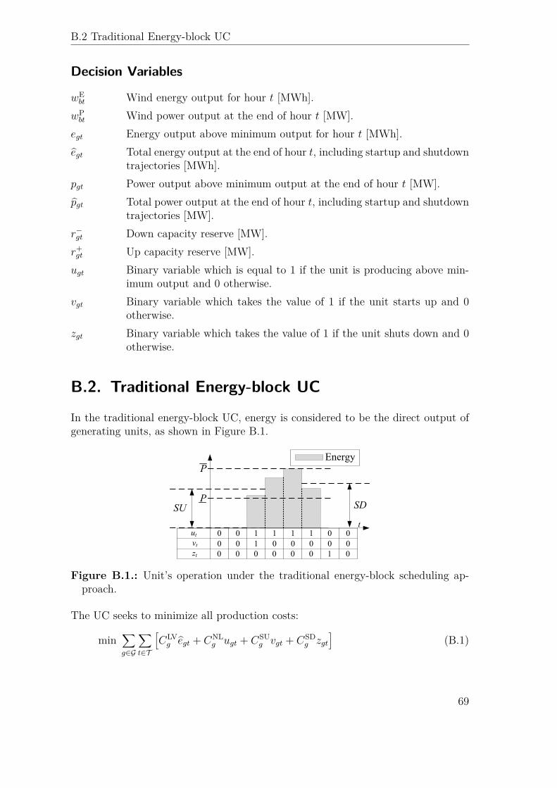
B.2 Traditional Energy-block UC
Decision Variables
wEbt Wind energy output for hour t [MWh].
wPbt Wind power output at the end of hour t [MW].
egt Energy output above minimum output for hour t [MWh].egt Total energy output at the end of hour t, including startup and shutdown
trajectories [MWh].pgt Power output above minimum output at the end of hour t [MW].pgt Total power output at the end of hour t, including startup and shutdown
trajectories [MW].r−gt Down capacity reserve [MW].r+
gt Up capacity reserve [MW].ugt Binary variable which is equal to 1 if the unit is producing above min-
imum output and 0 otherwise.vgt Binary variable which takes the value of 1 if the unit starts up and 0
otherwise.zgt Binary variable which takes the value of 1 if the unit shuts down and 0
otherwise.
B.2. Traditional Energy-block UC
In the traditional energy-block UC, energy is considered to be the direct output ofgenerating units, as shown in Figure B.1.
Figure B.1.: Unit’s operation under the traditional energy-block scheduling ap-proach.
The UC seeks to minimize all production costs:
min∑g∈G
∑t∈T
[CLV
g egt + CNLg ugt + CSU
g vgt + CSDg zgt
](B.1)
69
Appendix B Deterministic Network-Constrained UC Formulations
B.2.1. System-wide Constraints
Energy demand balance for hour t and reserves requirements are guaranteed asfollows:∑
g∈Gegt =
∑b∈B
(DE
bt − wEbt
)∀t (B.2)
∑g∈G
r+gt ≥ D+
t ∀t (B.3)∑g∈G
r−gt ≥ D−t ∀t (B.4)
and power-flow transmission limits are ensured with:
−F l ≤∑g∈G
ΓGlgegt +
∑b∈B
Γlb
(wE
bt −DEbt
)≤ F l ∀l, t (B.5)
B.2.2. Individual Unit Constraints
The commitment, startup/shutdown logic and the minimum up/down times areguaranteed with:
ugt − ug,t−1 = vgt − zgt ∀g, t (B.6)t∑
i=t−T Ug+1vgi ≤ ugt ∀g, t ∈ [TUg, T ] (B.7)
t∑i=t−T Dg+1
zgi ≤ 1− ugt ∀g, t ∈ [TDg, T ] (B.8)
Power production and reserves must be within the power capacity limits:
egt + r+gt ≤
(P g − P g
)ugt −
(P g − SDg
)zg,t+1
−max (SDg−SUg, 0) vg,t ∀g∈G1, t (B.9)egt + r+
gt ≤(P g − P g
)ugt −
(P g − SUg
)vgt
−max (SUg−SDg, 0) zg,t+1 ∀g∈G1, t (B.10)egt + r+
gt ≤(P g − P g
)ugt −
(P g − SUg
)vgt
−(P g − SDg
)zg,t+1 ∀g /∈G1, t (B.11)
egt − r−gt ≥ 0 (B.12)
where G1 is defined as the units in G with TUg =1.
70
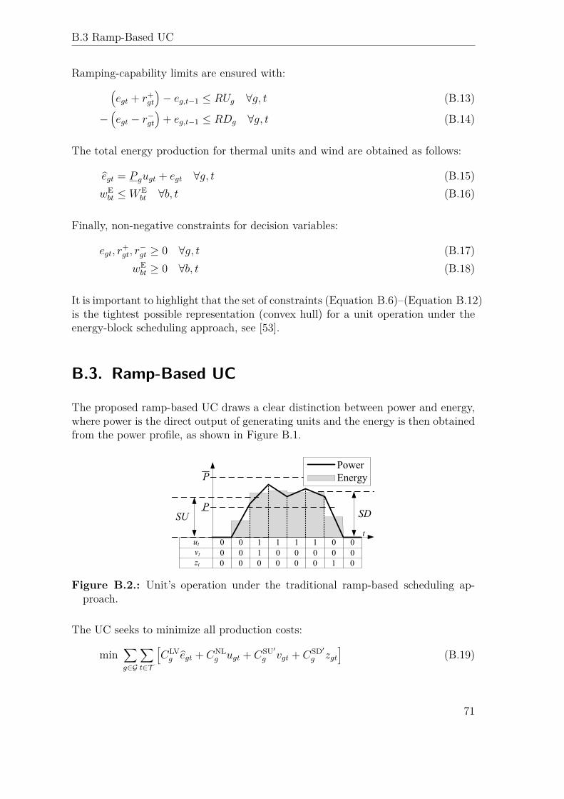
B.3 Ramp-Based UC
Ramping-capability limits are ensured with:(egt + r+
gt
)− eg,t−1 ≤ RUg ∀g, t (B.13)
−(egt − r−gt
)+ eg,t−1 ≤ RDg ∀g, t (B.14)
The total energy production for thermal units and wind are obtained as follows:
egt = P gugt + egt ∀g, t (B.15)wE
bt ≤ WEbt ∀b, t (B.16)
Finally, non-negative constraints for decision variables:
egt, r+gt, r
−gt ≥ 0 ∀g, t (B.17)
wEbt ≥ 0 ∀b, t (B.18)
It is important to highlight that the set of constraints (Equation B.6)–(Equation B.12)is the tightest possible representation (convex hull) for a unit operation under theenergy-block scheduling approach, see [53].
B.3. Ramp-Based UC
The proposed ramp-based UC draws a clear distinction between power and energy,where power is the direct output of generating units and the energy is then obtainedfrom the power profile, as shown in Figure B.1.
Figure B.2.: Unit’s operation under the traditional ramp-based scheduling ap-proach.
The UC seeks to minimize all production costs:
min∑g∈G
∑t∈T
[CLV
g egt + CNLg ugt + CSU′
g vgt + CSD′g zgt
](B.19)
71
Appendix B Deterministic Network-Constrained UC Formulations
Note that the no-load cost (CNLg ) in (Equation B.19) ignores the startup and shut-
down periods, see Figure B.2. This is because the CNLg only multiplies the commit-
ment during the up state ugt. In order to take into account the no-load cost duringthe startup and shutdown periods, CSU′ and CSD′ are introduced in (Equation B.19)and defined as:
CSU′ = CSU + CNL (B.19a)CSD′ = CSD + CNL (B.19b)
B.3.1. System-wide Constraints
Power demand balance at the end of hour t and reserves requirements are guaranteedas follows:∑
g∈Gpgt =
∑b∈B
(DP
bt − wPbt
)∀t (B.20)
∑g∈G
r+gt ≥ D+
t ∀t (B.21)∑g∈G
r−gt ≥ D−t ∀t (B.22)
where (Equation B.20) is a power balance at the end of hour t. Be aware that theenergy balance for the whole hour is automatically achieved by satisfying the powerdemand at the beginning and end of each hour, and by considering a piecewise-linearpower profile for demand and generation [99].
Power-flow transmission limits are ensured with:
−F l ≤∑g∈G
ΓGlgpgt +
∑b∈B
Γlb
(wP
bt −DPbt
)≤ F l ∀l, t (B.23)
B.3.2. Individual Unit Constraints
The commitment, startup/shutdown logic and the minimum up/down times areguaranteed with:
ugt − ug,t−1 = vgt − zgt ∀g, t (B.24)t∑
i=t−T Ug+1vgi ≤ ugt ∀g, t ∈ [TUg, T ] (B.25)
t∑i=t−T Dg+1
zgi ≤ 1− ugt ∀g, t ∈ [TDg, T ] (B.26)
72
B.3 Ramp-Based UC
Power production and reserves must be within the power capacity limits:
pgt + rgt ≤(P g − P g
)ugt −
(P g − SDg
)zg,t+1
+(SUg − P g
)vg,t+1 ∀g, t (B.27)
pgt − r−gt ≥ 0 ∀g, t (B.28)
Ramping-capability limits are ensured with:(pgt + r+
gt
)− pg,t−1 ≤ RUg ∀g, t (B.29)
−(pgt − r−gt
)+ pg,t−1 ≤ RDg ∀g, t (B.30)
The total power and energy production for thermal units are obtained as follows:
pgt = P g (ugt + vg,t+1) + pgt ∀g, t (B.31)
egt = pg,t−1 + pgt
2 ∀g, t (B.32)
wPbt ≤ WP
bt ∀b, t (B.33)
wEbt =
wPbt + wP
b,t−1
2 ∀b, t (B.34)
Finally, non-negative constraints for decision variables:
pgt, r+gt, r
−gt ≥ 0 ∀g, t (B.35)
wPbt ≥ 0 ∀b, t (B.36)
It is interesting to note that even though SUg, SDg ≥ P g (by definition), the result-ing energy from (Equation B.32) from the ramp-based UC may take values belowP g during the startup and shutdown processes, see Figure B.2, unlike the traditionalenergy-block UC.It is important to highlight that the set of constraints (Equation B.24)–(Equation B.28)together with (Equation B.31) and (Equation B.32) is the tightest possible repres-entation (convex hull) for a unit operation under the ramp-based scheduling ap-proach, see [97].
73

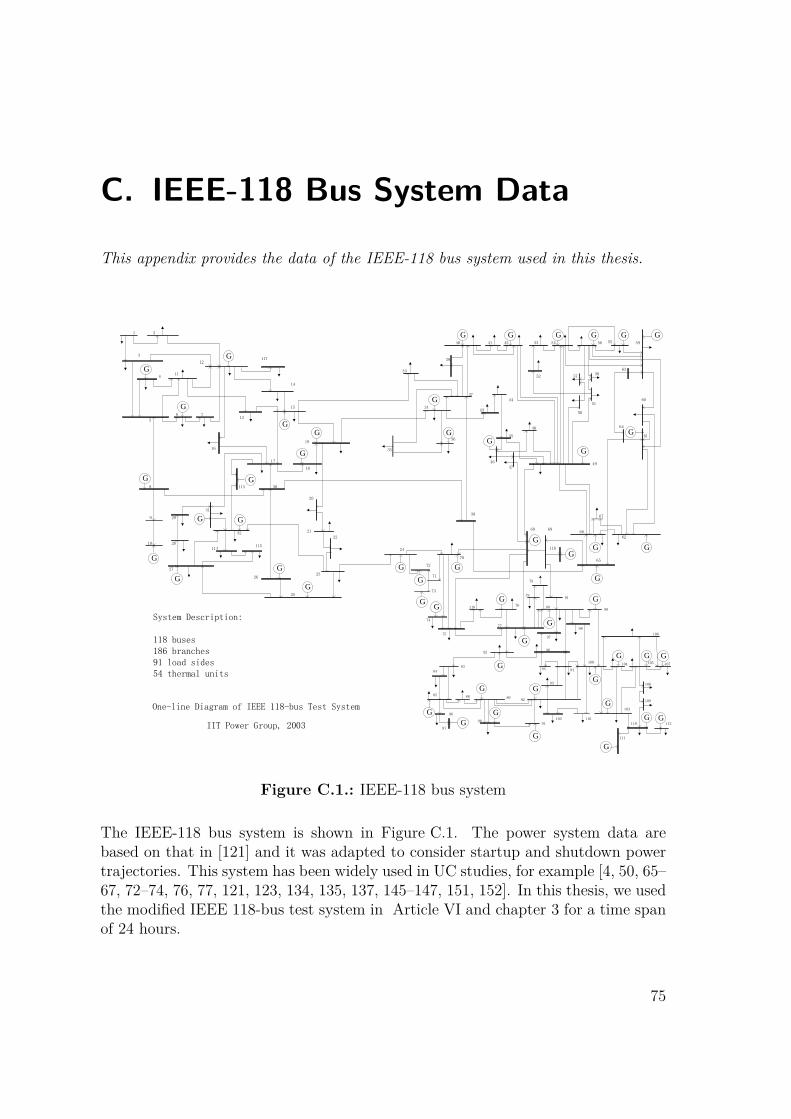
C. IEEE-118 Bus System Data
This appendix provides the data of the IEEE-118 bus system used in this thesis.
1 2
4
5
6 7
8
9
10
11
12
13
14
117
15
16
17
18
19
20
21
22
23
25
26
27
28
29
113 30
31
32
114115
33
34
35
36
37
38
39
40 41 42
43
44
45
4746
48
49
50
51
52
53 54 5556
5758
59
60
61
62
63
64
65
66
67
68
116
69
70
71
72
73
24
74
75
118 76
77
78
79
80
81
82
8384
85
86
87
88 89
9091
92
93
9495
96
97
98
99
100
101102
103
104 105
106
107
108
109
110
111
112
G
G
G
G
G G
G
G
GG
G
GG
G
G
G
G G
G
G
G
G
G G
G G
G
G G
G
G
G
G
G G G G G
G
G
3
G
G
G
G
G
G
G
G
G
G
G
G
G
G
One-line Diagram of IEEE 118-bus Test System
IIT Power Group, 2003
System Description:
118 buses186 branches91 load sides54 thermal units
Figure C.1.: IEEE-118 bus system
The IEEE-118 bus system is shown in Figure C.1. The power system data arebased on that in [121] and it was adapted to consider startup and shutdown powertrajectories. This system has been widely used in UC studies, for example [4, 50, 65–67, 72–74, 76, 77, 121, 123, 134, 135, 137, 145–147, 151, 152]. In this thesis, we usedthe modified IEEE 118-bus test system in Article VI and chapter 3 for a time spanof 24 hours.
75
Appendix C IEEE-118 Bus System Data
The IEEE-118 bus system has 118 buses; 186 transmission lines; 54 thermal units;91 loads, with average and maximum levels of 3991 MW and 5592 MW, respectively;and three wind units, with aggregated average and maximum production of 867 MWand 1333 MW, respectively, for the nominal wind case (see Figure 3.3).
Table C.1 and Table C.2 provide the generator data. Table C.3 and Table C.4 showthe transmission network technical data. The load distribution profile and totalsystem-wide power demand is given in Table C.6 and Table C.5, respectively. The20 scenarios for wind power injection in three different buses are given in Table C.6,Table C.7 and Table C.8. Notice that the demand and wind data are given aspower profiles (in MW) rather than the commonly used energy profiles (in MWh).However, obtaining the energy profiles is straightforward, for example, the energyprofile for the demand is obtained as DE = DP
t +DPt−1
2 .
The symbols that appear in the header of Table C.1 to Table C.4 are defined asfollows (in the same order as they appear in the tables):
Generator Data:
P Maximum power output [MW].
P Minimum power output [MW].
P0 Initial power output [MW].
State0 Initial state: hours that the unit has been online (+) or offline (-) priorto the first period of the time span.
RU Ramp-up capability [MW/h].
RD Ramp-down capability [MW/h].
CNL No-load cost [$/h].
CLV Linear variable production cost [$/MWh].
TU Minimum up time [h].
TD Minimum down time [h].
CSD Shutdown cost [$].
SDD Duration of the shutdown process [h].
CSUh Hot-startup cost [$].
SUDh Duration of the hot-startup process[h].
CSUc Cold-startup cost [$].
SUDc Duration of the cold-startup process[h].
76
IEEE-118 Bus System Data
T SUc Time defining the interval limit of the cold startup segment [h]. That is,
the unit has a hot startup if it has been offline for less than T SUc hours,
and it has a cold startup if it has been offline for more than or equal toT SU
c hours.SU Shutdown ramping capability [MW/h].SD Startup ramping capability [MW/h].
Network Data:
R Resistance of transmission line (per unit).X Reactance of transmission line (per unit).F Flow limit on transmission line [MW].
77
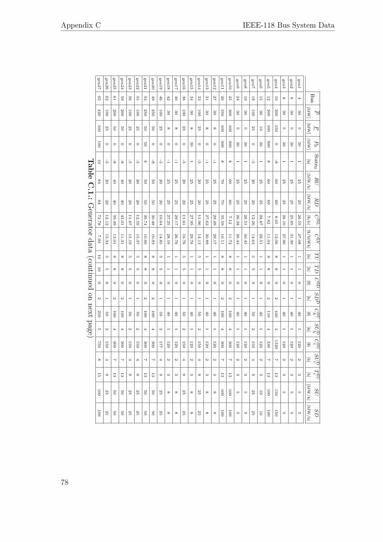
Appendix C IEEE-118 Bus System Data
Bus
PP
P0
State0R
UR
DC
NL
CLV
TU
TD
CSD
SD
DC
SUh
SU
DhC
SUc
SU
DcT
SUc
SU
SD
[MW]
[MW]
[MW]
[h][M
W/h]
[MW/h]
[$/h][$/M
Wh]
[h][h]
[$][h]
[$][h]
[$][h]
[h][M
W/h]
[MW/h]
gen14
305
301
2525
26.5527.08
11
01
401
1202
35
5
gen26
305
301
2525
25.8531.30
11
01
401
1202
35
5
gen38
305
301
2525
26.1027.90
11
01
401
1202
35
5
gen410
300150
0-8
6060
8.0512.06
88
02
4404
13207
13150
150
gen512
300100
3008
6060
7.8211.04
88
02
1104
3307
13100
100
gen615
3010
301
2525
28.8728.51
11
01
401
1202
310
10
gen718
10025
0-5
2020
12.2614.64
55
01
502
1504
925
25
gen819
305
301
2525
28.5130.45
11
01
401
1202
35
5
gen924
305
301
2525
26.3826.44
11
01
401
1202
35
5
gen1025
300100
3008
6060
7.1211.72
88
02
1004
3007
13100
100
gen1126
350100
3008
7070
35.5910.11
88
02
1004
3007
13100
100
gen1227
308
0-1
2525
29.4929.17
11
01
401
1202
38
8
gen1331
308
0-1
2525
27.6230.89
11
01
401
1202
38
8
gen1432
10025
0-5
2020
11.9614.13
55
01
502
1504
925
25
gen1534
308
301
2525
27.9529.76
11
01
401
1202
38
8
gen1636
10025
0-5
2020
11.6116.76
55
01
502
1504
925
25
gen1740
308
0-1
2525
29.1726.76
11
01
401
1202
38
8
gen1842
308
0-1
2525
27.2528.10
11
01
401
1202
38
8
gen1946
10025
0-5
2020
10.6414.85
55
01
592
1774
925
25
gen2049
25050
0-8
5050
30.4810.83
88
02
1004
3007
1350
50
gen2154
25050
508
5050
30.7410.60
88
02
1004
3007
1350
50
gen2255
10025
0-5
2020
12.5915.37
55
01
502
1504
925
25
gen2356
10025
0-5
2020
11.8715.19
55
01
502
1504
925
25
gen2459
20050
0-8
4040
43.0111.31
88
02
1004
3007
1350
50
gen2561
20050
0-8
4040
39.4913.01
88
02
1004
3007
1350
50
gen2662
10025
0-5
2020
12.1215.34
55
01
502
1504
925
25
gen2765
420100
10010
8484
72.787.93
1010
02
2505
7508
15100
100
Table
C.1.:G
eneratordata
(continuedon
nextpage)
78
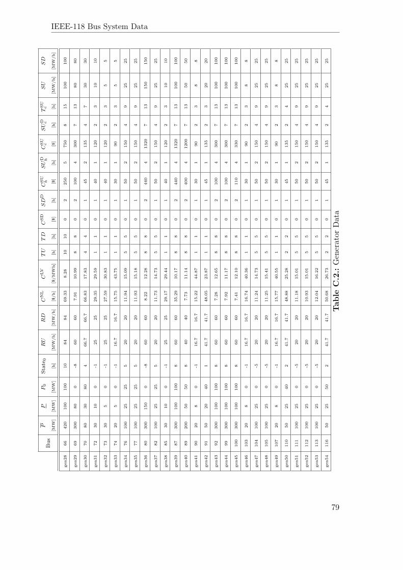
IEEE-118 Bus System Data
Bus
PP
P0
Stat
e 0R
UR
DC
NL
CLV
TU
TD
CSD
SD
DC
SU hS
UD h
CSU c
SU
D cT
SU cS
US
D
[MW]
[MW]
[MW]
[h]
[MW/h
][M
W/h
][$/h
][$/M
Wh]
[h]
[h]
[$]
[h]
[$]
[h]
[$]
[h]
[h]
[MW/h
][M
W/h
]
gen2
866
420
100
100
1084
8469.33
8.28
1010
02
250
5750
815
100
100
gen2
969
300
800
-860
607.91
10.99
88
02
100
4300
713
8080
gen3
070
8030
804
66.7
66.7
66.83
17.83
44
01
452
135
47
3030
gen3
172
3010
0-1
2525
29.35
29.59
11
01
401
120
23
1010
gen3
273
305
0-1
2525
27.59
30.83
11
01
401
120
23
55
gen3
374
205
0-1
16.7
16.7
15.75
43.75
11
01
301
902
35
5
gen3
476
100
2525
520
2011.94
15.09
55
01
502
150
49
2525
gen3
577
100
2525
520
2011.93
15.18
55
01
502
150
49
2525
gen3
680
300
150
0-8
6060
8.22
12.28
88
02
440
41320
713
150
150
gen3
782
100
2525
520
2011.73
14.73
55
01
502
150
49
2525
gen3
885
3010
0-1
2525
29.17
29.44
11
01
401
120
23
1010
gen3
987
300
100
100
860
6035.29
10.17
88
02
440
41320
713
100
100
gen4
089
200
5050
840
407.73
11.14
88
02
400
41200
713
5050
gen4
190
208
0-1
16.7
16.7
15.22
44.87
11
01
301
902
38
8
gen4
291
5020
401
41.7
41.7
48.05
23.87
11
01
451
135
23
2020
gen4
392
300
100
100
860
607.28
12.65
88
02
100
4300
713
100
100
gen4
499
300
100
100
860
607.92
11.17
88
02
100
4300
713
100
100
gen4
5100
300
100
100
860
607.41
12.10
88
02
110
4330
713
100
100
gen4
6103
208
0-1
16.7
16.7
16.74
40.36
11
01
301
902
38
8
gen4
7104
100
250
-520
2011.24
14.73
55
01
502
150
49
2525
gen4
8105
100
250
-520
2011.25
15.41
55
01
502
150
49
2525
gen4
9107
208
0-1
16.7
16.7
15.77
40.55
11
01
301
902
38
8
gen5
0110
5025
402
41.7
41.7
48.88
25.28
22
01
451
135
24
2525
gen5
1111
100
250
-520
2011.18
15.01
55
01
502
150
49
2525
gen5
2112
100
250
-520
2010.93
15.01
55
01
502
150
49
2525
gen5
3113
100
250
-520
2012.04
16.22
55
01
502
150
49
2525
gen5
4116
5025
502
41.7
41.7
50.68
26.73
22
01
451
135
24
2525
Tab
leC
.2.:
Generator
Data
79
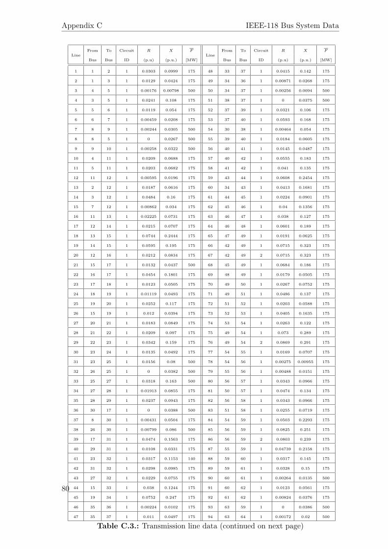
Appendix C IEEE-118 Bus System Data
LineFrom To Circuit R X F
LineFrom To Circuit R X F
Bus Bus ID (p.u) (p.u.) [MW] Bus Bus ID (p.u) (p.u.) [MW]
1 1 2 1 0.0303 0.0999 175 48 33 37 1 0.0415 0.142 175
2 1 3 1 0.0129 0.0424 175 49 34 36 1 0.00871 0.0268 175
3 4 5 1 0.00176 0.00798 500 50 34 37 1 0.00256 0.0094 500
4 3 5 1 0.0241 0.108 175 51 38 37 1 0 0.0375 500
5 5 6 1 0.0119 0.054 175 52 37 39 1 0.0321 0.106 175
6 6 7 1 0.00459 0.0208 175 53 37 40 1 0.0593 0.168 175
7 8 9 1 0.00244 0.0305 500 54 30 38 1 0.00464 0.054 175
8 8 5 1 0 0.0267 500 55 39 40 1 0.0184 0.0605 175
9 9 10 1 0.00258 0.0322 500 56 40 41 1 0.0145 0.0487 175
10 4 11 1 0.0209 0.0688 175 57 40 42 1 0.0555 0.183 175
11 5 11 1 0.0203 0.0682 175 58 41 42 1 0.041 0.135 175
12 11 12 1 0.00595 0.0196 175 59 43 44 1 0.0608 0.2454 175
13 2 12 1 0.0187 0.0616 175 60 34 43 1 0.0413 0.1681 175
14 3 12 1 0.0484 0.16 175 61 44 45 1 0.0224 0.0901 175
15 7 12 1 0.00862 0.034 175 62 45 46 1 0.04 0.1356 175
16 11 13 1 0.02225 0.0731 175 63 46 47 1 0.038 0.127 175
17 12 14 1 0.0215 0.0707 175 64 46 48 1 0.0601 0.189 175
18 13 15 1 0.0744 0.2444 175 65 47 49 1 0.0191 0.0625 175
19 14 15 1 0.0595 0.195 175 66 42 49 1 0.0715 0.323 175
20 12 16 1 0.0212 0.0834 175 67 42 49 2 0.0715 0.323 175
21 15 17 1 0.0132 0.0437 500 68 45 49 1 0.0684 0.186 175
22 16 17 1 0.0454 0.1801 175 69 48 49 1 0.0179 0.0505 175
23 17 18 1 0.0123 0.0505 175 70 49 50 1 0.0267 0.0752 175
24 18 19 1 0.01119 0.0493 175 71 49 51 1 0.0486 0.137 175
25 19 20 1 0.0252 0.117 175 72 51 52 1 0.0203 0.0588 175
26 15 19 1 0.012 0.0394 175 73 52 53 1 0.0405 0.1635 175
27 20 21 1 0.0183 0.0849 175 74 53 54 1 0.0263 0.122 175
28 21 22 1 0.0209 0.097 175 75 49 54 1 0.073 0.289 175
29 22 23 1 0.0342 0.159 175 76 49 54 2 0.0869 0.291 175
30 23 24 1 0.0135 0.0492 175 77 54 55 1 0.0169 0.0707 175
31 23 25 1 0.0156 0.08 500 78 54 56 1 0.00275 0.00955 175
32 26 25 1 0 0.0382 500 79 55 56 1 0.00488 0.0151 175
33 25 27 1 0.0318 0.163 500 80 56 57 1 0.0343 0.0966 175
34 27 28 1 0.01913 0.0855 175 81 50 57 1 0.0474 0.134 175
35 28 29 1 0.0237 0.0943 175 82 56 58 1 0.0343 0.0966 175
36 30 17 1 0 0.0388 500 83 51 58 1 0.0255 0.0719 175
37 8 30 1 0.00431 0.0504 175 84 54 59 1 0.0503 0.2293 175
38 26 30 1 0.00799 0.086 500 85 56 59 1 0.0825 0.251 175
39 17 31 1 0.0474 0.1563 175 86 56 59 2 0.0803 0.239 175
40 29 31 1 0.0108 0.0331 175 87 55 59 1 0.04739 0.2158 175
41 23 32 1 0.0317 0.1153 140 88 59 60 1 0.0317 0.145 175
42 31 32 1 0.0298 0.0985 175 89 59 61 1 0.0328 0.15 175
43 27 32 1 0.0229 0.0755 175 90 60 61 1 0.00264 0.0135 500
44 15 33 1 0.038 0.1244 175 91 60 62 1 0.0123 0.0561 175
45 19 34 1 0.0752 0.247 175 92 61 62 1 0.00824 0.0376 175
46 35 36 1 0.00224 0.0102 175 93 63 59 1 0 0.0386 500
47 35 37 1 0.011 0.0497 175 94 63 64 1 0.00172 0.02 500
Table C.3.: Transmission line data (continued on next page)
80
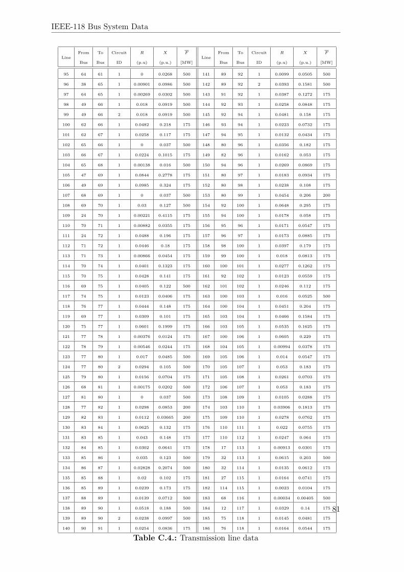
IEEE-118 Bus System Data
LineFrom To Circuit R X F
LineFrom To Circuit R X F
Bus Bus ID (p.u) (p.u.) [MW] Bus Bus ID (p.u) (p.u.) [MW]
95 64 61 1 0 0.0268 500 141 89 92 1 0.0099 0.0505 500
96 38 65 1 0.00901 0.0986 500 142 89 92 2 0.0393 0.1581 500
97 64 65 1 0.00269 0.0302 500 143 91 92 1 0.0387 0.1272 175
98 49 66 1 0.018 0.0919 500 144 92 93 1 0.0258 0.0848 175
99 49 66 2 0.018 0.0919 500 145 92 94 1 0.0481 0.158 175
100 62 66 1 0.0482 0.218 175 146 93 94 1 0.0223 0.0732 175
101 62 67 1 0.0258 0.117 175 147 94 95 1 0.0132 0.0434 175
102 65 66 1 0 0.037 500 148 80 96 1 0.0356 0.182 175
103 66 67 1 0.0224 0.1015 175 149 82 96 1 0.0162 0.053 175
104 65 68 1 0.00138 0.016 500 150 94 96 1 0.0269 0.0869 175
105 47 69 1 0.0844 0.2778 175 151 80 97 1 0.0183 0.0934 175
106 49 69 1 0.0985 0.324 175 152 80 98 1 0.0238 0.108 175
107 68 69 1 0 0.037 500 153 80 99 1 0.0454 0.206 200
108 69 70 1 0.03 0.127 500 154 92 100 1 0.0648 0.295 175
109 24 70 1 0.00221 0.4115 175 155 94 100 1 0.0178 0.058 175
110 70 71 1 0.00882 0.0355 175 156 95 96 1 0.0171 0.0547 175
111 24 72 1 0.0488 0.196 175 157 96 97 1 0.0173 0.0885 175
112 71 72 1 0.0446 0.18 175 158 98 100 1 0.0397 0.179 175
113 71 73 1 0.00866 0.0454 175 159 99 100 1 0.018 0.0813 175
114 70 74 1 0.0401 0.1323 175 160 100 101 1 0.0277 0.1262 175
115 70 75 1 0.0428 0.141 175 161 92 102 1 0.0123 0.0559 175
116 69 75 1 0.0405 0.122 500 162 101 102 1 0.0246 0.112 175
117 74 75 1 0.0123 0.0406 175 163 100 103 1 0.016 0.0525 500
118 76 77 1 0.0444 0.148 175 164 100 104 1 0.0451 0.204 175
119 69 77 1 0.0309 0.101 175 165 103 104 1 0.0466 0.1584 175
120 75 77 1 0.0601 0.1999 175 166 103 105 1 0.0535 0.1625 175
121 77 78 1 0.00376 0.0124 175 167 100 106 1 0.0605 0.229 175
122 78 79 1 0.00546 0.0244 175 168 104 105 1 0.00994 0.0378 175
123 77 80 1 0.017 0.0485 500 169 105 106 1 0.014 0.0547 175
124 77 80 2 0.0294 0.105 500 170 105 107 1 0.053 0.183 175
125 79 80 1 0.0156 0.0704 175 171 105 108 1 0.0261 0.0703 175
126 68 81 1 0.00175 0.0202 500 172 106 107 1 0.053 0.183 175
127 81 80 1 0 0.037 500 173 108 109 1 0.0105 0.0288 175
128 77 82 1 0.0298 0.0853 200 174 103 110 1 0.03906 0.1813 175
129 82 83 1 0.0112 0.03665 200 175 109 110 1 0.0278 0.0762 175
130 83 84 1 0.0625 0.132 175 176 110 111 1 0.022 0.0755 175
131 83 85 1 0.043 0.148 175 177 110 112 1 0.0247 0.064 175
132 84 85 1 0.0302 0.0641 175 178 17 113 1 0.00913 0.0301 175
133 85 86 1 0.035 0.123 500 179 32 113 1 0.0615 0.203 500
134 86 87 1 0.02828 0.2074 500 180 32 114 1 0.0135 0.0612 175
135 85 88 1 0.02 0.102 175 181 27 115 1 0.0164 0.0741 175
136 85 89 1 0.0239 0.173 175 182 114 115 1 0.0023 0.0104 175
137 88 89 1 0.0139 0.0712 500 183 68 116 1 0.00034 0.00405 500
138 89 90 1 0.0518 0.188 500 184 12 117 1 0.0329 0.14 175
139 89 90 2 0.0238 0.0997 500 185 75 118 1 0.0145 0.0481 175
140 90 91 1 0.0254 0.0836 175 186 76 118 1 0.0164 0.0544 175
Table C.4.: Transmission line data
81
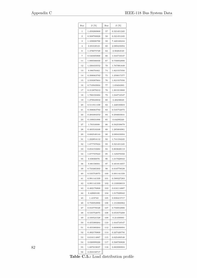
Appendix C IEEE-118 Bus System Data
Bus D [%] Bus D [%]
1 1.450280868 57 0.321451245
2 0.568700828 58 0.321451245
3 1.109006796 59 7.420166244
4 0.85318518 60 2.089433094
6 1.478675728 62 2.06264549
7 0.540305968 66 1.044716547
11 1.990586836 67 0.750052906
12 1.336433552 70 1.767981849
13 0.96676462 74 1.821557056
14 0.398063792 75 1.259017377
15 2.559287664 76 1.821557056
16 0.710943004 77 1.63404383
17 0.312879212 78 1.901919868
18 1.706102484 79 1.044716547
19 1.279643832 80 3.48238849
20 0.511911108 82 1.446530603
21 0.398063792 83 0.535752075
22 0.284484352 84 0.294663641
23 0.199031896 85 0.64290249
27 1.76316008 86 0.562539679
28 0.483516248 88 1.285804981
29 0.682548144 90 2.089433094
31 1.222854112 92 1.741194245
32 1.677707624 93 0.321451245
33 0.654153284 94 0.803628113
34 1.677707624 95 1.125079358
35 0.93836976 96 1.017928943
36 0.88158004 97 0.401814057
39 0.723265302 98 0.910778528
40 0.535752075 100 0.991141339
41 0.991141339 101 0.589327283
42 0.991141339 102 0.133938019
43 0.482176868 103 0.616114887
44 0.42860166 104 1.017928943
45 1.419743 105 0.830415717
46 0.750052906 106 1.151866962
47 0.910778528 107 0.750052906
48 0.535752075 108 0.053575208
49 2.330521528 109 0.21430083
50 0.455389264 110 1.044716547
51 0.455389264 112 0.669690094
52 0.482176868 114 0.227426756
53 0.616114887 115 0.625490548
54 3.026999226 117 0.568700828
55 1.687619037 118 0.883990924
56 2.250158717
Table C.5.: Load distribution profile
82
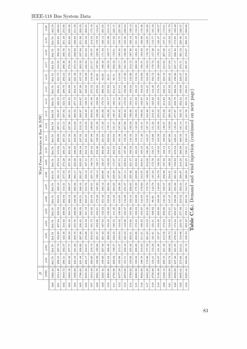
IEEE-118 Bus System Data
DW
ind
Pow
erSc
enar
ios
atB
us36
[MW
][M
W]
sc01
sc02
sc03
sc04
sc05
sc06
sc07
sc08
sc09
sc10
sc11
sc12
sc13
sc14
sc15
sc16
sc17
sc18
sc19
sc20
h00
3466.24
304.79
304.79
304.79
304.79
304.79
304.79
304.79
304.79
304.79
304.79
304.79
304.79
304.79
304.79
304.79
304.79
304.79
304.79
304.79
304.79
h01
3314.40
298.35
287.74
324.89
307.64
328.93
303.61
308.10
291.12
279.94
310.82
296.89
287.01
330.87
326.55
300.81
321.75
313.94
306.22
283.85
286.84
h02
3010.72
286.41
292.37
323.46
310.82
308.08
292.58
310.31
277.03
273.28
293.47
287.24
273.15
307.94
325.72
289.70
293.24
290.30
290.78
291.49
272.86
h03
2403.36
262.36
277.77
306.50
285.49
294.79
266.12
298.57
266.72
257.30
262.40
257.50
237.26
281.61
309.55
264.09
261.70
270.56
270.57
265.66
245.38
h04
1036.80
245.34
241.20
293.76
255.70
238.90
248.20
265.92
264.17
235.98
240.94
224.09
214.84
269.52
277.13
252.47
221.39
274.19
249.82
246.83
211.59
h05
1796.00
241.48
236.80
287.98
236.45
200.39
249.51
246.10
261.67
223.05
248.44
247.95
212.10
262.97
244.87
287.28
197.19
263.32
237.94
251.90
202.33
h06
2555.20
236.17
254.91
278.88
219.18
181.18
250.27
219.76
239.12
187.31
252.19
241.82
218.03
240.38
198.55
303.05
166.28
244.84
231.84
239.32
206.65
h07
3314.40
206.80
218.10
252.93
191.73
123.95
221.63
190.91
201.73
146.78
225.43
207.98
189.60
202.64
161.99
275.32
116.50
211.57
195.07
214.54
173.18
h08
3921.76
189.99
190.00
221.37
183.66
103.61
179.22
189.30
199.14
120.17
234.36
199.34
161.56
196.09
158.00
270.04
82.66
197.83
169.96
179.70
154.81
h09
4225.44
199.06
207.58
201.42
187.53
132.52
161.42
240.12
203.80
128.47
262.30
221.65
171.30
201.08
178.73
268.10
92.00
186.44
171.44
166.14
201.65
h10
4680.96
201.84
208.49
209.30
194.32
130.56
150.84
262.94
197.81
142.68
254.91
202.84
178.11
182.29
185.77
237.62
82.91
180.55
169.77
165.98
215.14
h11
4756.88
200.22
198.57
224.45
186.55
141.36
144.32
264.65
205.93
175.07
262.33
183.94
191.47
180.47
182.11
214.21
95.51
202.32
178.61
151.82
225.17
h12
4377.28
193.86
213.47
243.64
144.02
136.68
143.05
238.39
217.87
207.51
235.65
181.36
197.66
204.82
161.36
217.01
113.64
220.17
185.45
156.75
227.93
h13
4073.60
191.51
232.44
225.23
143.88
156.37
144.96
231.07
235.14
222.84
197.96
158.38
207.90
209.43
170.93
189.88
137.98
231.78
196.06
165.56
236.64
h14
3769.92
183.06
225.40
204.21
172.60
165.06
150.16
206.65
225.38
221.37
166.58
145.44
182.56
198.86
194.41
169.24
143.96
212.15
187.96
186.18
198.14
h15
4680.96
180.04
208.68
204.86
172.43
168.04
160.88
175.39
229.66
233.62
162.45
149.53
143.32
192.05
191.08
182.15
134.54
206.34
184.45
191.49
152.85
h16
4832.80
188.70
210.83
211.61
180.23
194.87
143.03
178.60
213.55
244.61
185.33
171.46
155.41
196.04
192.87
184.33
152.66
190.51
184.92
180.98
170.28
h17
4453.20
172.98
177.32
201.23
153.53
213.26
119.35
170.79
188.99
212.00
190.20
143.27
137.19
210.48
187.53
156.21
164.08
193.53
176.76
124.97
165.20
h18
4756.88
150.41
155.56
181.91
125.41
188.92
96.66
142.76
161.34
172.76
156.77
143.86
151.23
219.45
165.82
144.40
183.72
178.74
157.28
110.77
161.34
h19
5136.48
168.07
191.36
197.27
133.39
209.99
109.56
140.05
184.79
166.90
149.03
163.39
165.58
235.62
165.03
178.79
194.20
190.05
176.21
126.47
169.57
h20
5440.16
209.10
231.40
213.58
173.04
259.66
140.33
169.57
232.88
187.42
168.14
190.94
148.07
273.98
214.84
222.41
204.19
213.05
207.20
157.31
173.01
h21
5592.00
222.74
226.62
248.73
153.03
272.61
147.47
204.92
234.41
186.20
178.77
207.86
133.09
285.32
219.29
237.93
203.41
217.04
213.71
145.63
181.73
h22
4832.80
237.36
221.95
278.94
174.34
259.27
196.58
255.22
261.23
194.83
219.54
246.21
133.21
277.87
238.79
282.54
190.40
237.17
226.45
175.85
182.42
h23
4605.04
273.69
253.21
319.88
233.70
277.89
253.52
302.24
288.87
218.20
288.99
300.59
181.14
328.75
292.24
339.08
229.37
279.71
261.52
229.90
220.57
h24
4225.44
300.66
281.72
339.34
282.23
276.11
265.34
314.75
286.24
243.25
330.21
323.10
252.13
341.56
305.10
350.61
253.27
291.67
278.87
266.57
269.60
Tab
leC
.6.:
Dem
andan
dwindinjection(con
tinuedon
next
page)
83
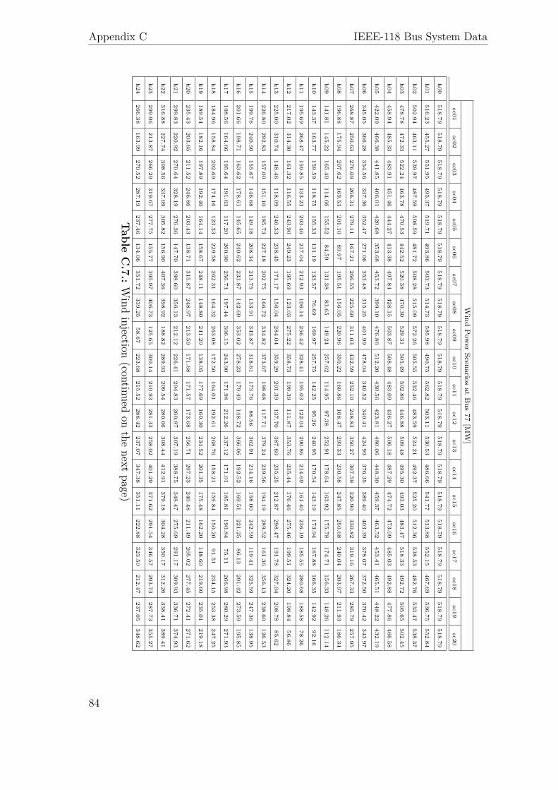
Appendix C IEEE-118 Bus System Data
Wind
Pow
erScenarios
atB
us77
[MW
]sc01
sc02sc03
sc04sc05
sc06sc07
sc08sc09
sc10sc11
sc12sc13
sc14sc15
sc16sc17
sc18sc19
sc20
h00518.79
518.79518.79
518.79518.79
518.79518.79
518.79518.79
518.79518.79
518.79518.79
518.79518.79
518.79518.79
518.79518.79
518.79
h01516.23
455.27551.95
495.37519.71
493.86503.73
514.73585.98
490.75562.82
503.11530.53
486.66541.77
513.88552.15
467.69536.75
552.84
h02502.94
463.11539.97
487.59508.59
481.72508.28
515.09572.26
505.55532.46
483.59524.21
492.37525.20
512.36538.53
482.76533.47
538.37
h03478.78
472.33522.24
463.78470.53
442.52520.38
470.30529.31
505.49502.86
446.88509.48
495.30493.03
483.47518.33
492.72505.65
502.45
h04458.94
485.33483.91
451.46444.27
413.38497.84
428.15503.87
508.48483.09
436.27506.18
487.29474.72
473.09485.03
492.88477.86
466.58
h05422.09
466.38441.85
406.01420.68
353.68453.72
399.10476.86
512.20430.56
423.81480.06
448.30459.37
463.52453.41
465.51448.22
432.19
h06345.05
366.28354.56
337.36352.47
271.06353.48
315.25401.99
478.04340.52
340.41424.99
376.35389.40
403.39378.07
372.50370.42
343.97
h07268.87
250.63276.09
266.31279.11
167.21266.55
225.60311.03
432.59252.10
248.83350.27
307.59320.90
330.82319.16
267.33285.79
257.95
h08196.88
175.94207.62
169.53201.10
89.97195.51
156.05220.96
350.22160.86
168.47293.33
230.58247.85
250.68240.04
203.97211.93
186.34
h09141.81
145.22165.40
114.66155.52
84.59131.38
83.65149.24
257.62114.95
97.38252.91
178.64163.92
175.78174.71
156.33148.26
112.14
h10143.37
163.77159.59
118.75155.33
131.19133.57
76.69169.97
257.75142.25
95.26240.95
170.54143.19
173.94167.88
166.35142.92
92.16
h11195.69
268.47159.85
133.23203.46
217.04212.93
106.14256.42
328.41195.03
122.04290.86
214.69161.40
236.19185.55
280.68188.58
78.26
h12217.02
314.30161.32
116.55243.90
249.23195.69
123.03275.22
358.73199.39
111.87353.76
235.44176.46
275.46199.51
324.20198.84
56.86
h13225.00
310.74148.46
118.09246.33
238.45171.17
156.04284.04
359.29201.39
137.70387.60
235.25212.87
298.47191.78
327.04208.78
85.62
h14226.80
292.83157.00
151.10185.73
227.18202.75
166.72334.82
373.67198.68
117.71379.24
239.56194.19
289.52161.36
356.13238.60
126.53
h15199.76
240.50155.67
146.68149.18
208.34213.75
133.91343.87
318.61173.76
88.56362.91
214.16158.00
242.59119.41
325.59247.36
138.95
h16201.66
198.71163.62
178.61145.65
240.62233.87
142.69353.02
278.23179.49
148.72366.06
192.52169.51
221.2586.13
291.42273.59
195.85
h17198.56
164.66195.64
191.63117.20
260.90256.73
197.44306.15
243.90171.98
212.26337.12
171.01185.81
190.8475.11
266.98280.29
271.93
h18184.96
158.84202.69
174.16123.33
229.58262.31
164.32263.08
172.50164.01
192.61268.76
158.21159.84
150.2091.51
234.15253.38
247.25
h19189.54
182.16197.89
192.40164.14
158.67248.11
148.80241.20
138.05177.69
160.30234.52
201.35175.48
162.20148.60
219.60235.01
219.18
h20235.43
203.65211.52
246.86203.43
138.71315.87
248.97213.59
171.68171.57
173.68256.71
297.23240.48
211.49205.02
277.45272.41
271.62
h21299.83
220.92270.64
328.19276.36
147.70398.60
356.13212.12
226.41204.83
260.87307.19
388.75348.47
275.69291.17
309.93336.71
374.93
h22316.88
227.74308.56
337.09305.82
156.90407.36
398.92188.82
289.93209.54
280.66308.44
412.91379.18
304.28350.17
312.26338.41
389.41
h23299.96
213.87266.29
319.67277.75
155.77395.97
406.73125.65
300.14210.93
281.33258.02
401.29371.62
291.54346.57
293.73287.73
355.27
h24266.38
163.99270.52
287.19237.46
134.06351.72
339.2558.67
223.68215.52
288.42237.07
347.38351.11
222.88323.50
212.47237.05
348.62
Table
C.7.:W
indinjection
(continuedon
thenext
page)
84
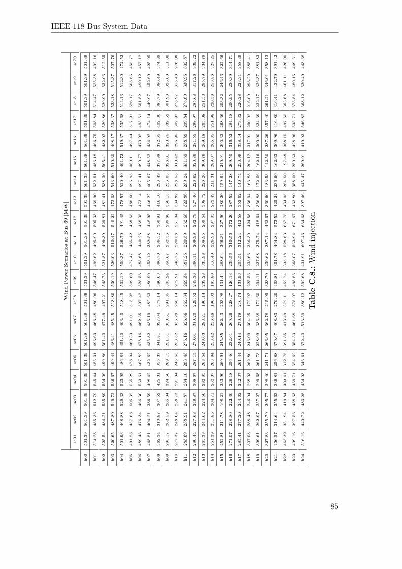
IEEE-118 Bus System Data
Win
dP
ower
Scen
ario
sat
Bus
69[M
W]
sc01
sc02
sc03
sc04
sc05
sc06
sc07
sc08
sc09
sc10
sc11
sc12
sc13
sc14
sc15
sc16
sc17
sc18
sc19
sc20
h00
501.39
501.39
501.39
501.39
501.39
501.39
501.39
501.39
501.39
501.39
501.39
501.39
501.39
501.39
501.39
501.39
501.39
501.39
501.39
501.39
h01
514.28
485.36
512.79
545.44
483.31
496.63
466.48
480.06
546.47
499.62
495.90
505.33
469.90
532.51
486.18
466.75
508.84
514.47
525.38
492.16
h02
525.54
484.21
535.89
554.09
499.86
501.40
477.49
497.21
545.73
521.87
499.39
529.81
481.41
538.30
505.41
482.02
529.86
529.90
532.03
512.55
h03
520.65
487.80
549.72
536.67
499.44
486.41
485.45
513.80
530.19
526.03
510.47
540.22
472.03
543.60
510.30
498.17
538.37
523.18
515.37
507.76
h04
501.93
468.88
529.33
523.95
486.84
451.40
493.40
518.45
502.19
509.37
526.70
491.45
478.57
520.40
491.72
519.37
535.68
514.13
512.30
472.52
h05
491.28
457.68
505.32
535.29
478.94
460.33
491.01
513.92
509.60
477.47
485.42
458.55
488.60
496.95
480.11
497.44
517.91
526.17
505.65
455.77
h06
489.43
476.34
466.30
533.61
467.82
478.16
462.35
507.42
528.56
485.68
440.25
468.35
473.14
497.41
499.77
470.02
493.51
501.82
490.12
457.12
h07
448.81
404.21
386.59
498.42
432.62
435.82
435.19
482.63
480.90
458.12
382.58
448.95
446.22
405.67
448.52
434.92
474.14
449.97
452.69
425.95
h08
362.34
310.87
307.52
425.31
355.37
341.81
397.04
377.14
380.63
390.70
286.32
360.91
416.10
293.49
377.88
372.65
402.30
383.79
386.49
374.89
h09
295.17
262.59
265.34
324.56
269.13
251.31
350.51
291.85
305.24
350.67
232.36
299.88
366.15
236.03
328.01
320.75
332.52
301.93
325.03
311.00
h10
277.37
248.04
238.73
291.34
245.53
253.52
335.29
268.14
272.91
348.75
220.58
261.04
334.82
228.55
310.42
296.95
302.97
275.97
315.43
276.08
h11
283.69
238.91
241.87
284.10
283.43
276.16
326.66
262.34
269.34
387.25
220.59
252.68
323.86
239.24
331.69
288.89
299.84
275.69
330.95
302.87
h12
280.44
227.68
249.87
308.67
287.15
270.01
310.20
229.52
249.36
360.11
209.99
282.79
327.40
226.62
320.86
281.55
298.97
285.68
317.26
339.22
h13
265.38
244.02
224.50
292.85
268.54
249.63
283.21
190.14
239.28
333.98
208.95
269.54
308.72
226.26
309.76
269.18
265.08
251.53
295.79
334.79
h14
251.39
231.85
204.71
262.37
263.94
253.42
236.48
196.03
183.80
316.40
226.93
297.03
272.49
211.31
289.07
265.85
251.98
220.38
258.86
327.25
h15
252.81
211.78
198.21
233.90
260.91
245.85
262.43
203.98
131.44
288.04
266.31
327.90
280.20
159.94
240.91
290.33
268.36
203.32
246.43
322.66
h16
271.07
228.80
222.30
226.18
256.46
232.61
269.26
228.27
126.13
239.56
310.56
372.20
287.52
147.28
209.50
316.52
284.18
200.95
230.39
314.71
h17
285.41
277.20
244.62
242.07
261.44
240.14
270.78
216.74
131.96
205.51
312.24
412.58
352.62
140.74
230.99
338.44
273.32
220.28
223.31
358.39
h18
307.08
288.48
246.94
268.03
262.80
246.09
304.25
172.92
225.53
233.66
356.30
424.58
366.94
163.88
204.12
317.01
290.92
216.09
293.20
388.41
h19
309.61
262.97
257.27
299.68
261.73
228.99
336.38
172.60
294.11
227.98
375.74
418.64
356.88
172.06
162.16
300.00
324.39
232.17
326.37
381.83
h20
327.83
255.79
295.77
298.40
241.71
266.95
362.78
215.95
323.70
239.62
387.14
462.67
360.60
183.53
142.50
287.26
357.40
261.21
346.01
358.13
h21
406.57
314.64
355.63
339.81
256.88
379.67
408.83
279.20
403.81
301.78
464.84
573.52
425.24
236.60
162.63
309.96
416.80
316.41
432.79
391.42
h22
463.39
331.94
419.84
403.41
312.75
391.85
413.49
372.11
452.74
335.18
528.63
657.75
434.05
284.50
197.48
368.15
497.55
363.68
461.11
426.00
h23
499.16
397.56
458.63
459.71
324.62
354.33
461.68
378.07
498.83
368.07
563.94
671.67
433.80
358.00
250.63
428.96
535.71
373.84
480.15
449.31
h24
516.16
440.72
483.28
454.93
346.61
372.40
513.59
380.12
592.68
431.91
607.43
634.63
397.46
445.47
269.01
419.93
546.82
368.12
530.49
443.68
Tab
leC
.8.:
Windinjection
85


D. Optimal Schedules of TheDeterministic Case
This appendix presents the optimal unit schedules of the EnSch and RmpSch ap-proaches for the deterministic study case presented in section 3.3 in chapter 3.chapter 3, section 3.3 describes the deterministic case study for two different powerdemand profiles D1 and D2 (in MW), which present the same energy profile DE (inMWh). The IEEE-118 bus system (see Appendix C) is used for this case study,where we assumed that the power demand profiles are perfectly known and given inTable 3.1, without uncertain events (i.e., no wind).Table D.1 and Table D.2 show the optimal power schedules of the RmpSch approachfor D1. Table D.3 and Table D.4 list the optimal power schedules of the RmpSchapproach for D2; and Table D.5 and Table D.6 show the optimal energy schedulesobtained by the EnSch approach for the energy profile DE. Numbers between par-enthesis indicate that the unit is either starting up or shutting down (productionswhich are bellow the unit’s minimum output). Note that all these tables containthe initial conditions for the case studies.
87

Appendix D Optimal Schedules of The Deterministic Case
State0h00
h01h02
h03h04
h05h06
h07h08
h09h10
h11h12
h13h14
h15h16
h17h18
h19h20
h21h22
h23h24
gen11
305
5.
..
..
..
..
..
..
..
..
..
..
.
gen21
305
5.
..
..
..
..
..
..
..
..
..
..
.
gen31
305
5.
..
..
..
..
..
..
..
..
..
..
.
gen4-8
.(37.5)
(75)(112.5)
150210
150180
240300
300300
240180
210150
150150
210270
210150
(75).
.
gen58
100160
220280
250300
300300
300300
300300
300300
240180
120180
240300
300240
180120
100
gen61
3010
10.
..
..
..
..
..
..
..
..
..
..
.
gen7-5
..
..
..
(6.25)(12.5)
(18.75)25
4565
4525
25.
..
..
..
..
.
gen81
305
5.
..
..
..
..
..
..
..
..
..
..
.
gen91
305
5.
..
..
..
..
..
..
..
..
..
..
.
gen108
200140
100160
113.75173.75
233.75180
240300
300300
240180
160100
100160
220280
220160
100(50)
.
gen118
200270
300.5350
350350
350350
350350
350350
350350
350295
350350
280350
350280
210207
137
gen12-1
..
..
..
..
..
..
..
..
..
..
..
..
.
gen13-1
..
..
..
..
..
..
..
..
..
..
..
..
.
gen14-5
..
..
(6.25)(12.5)
(18.75)25
4060
80100
8060
4025
2525
4565
4525
..
.
gen151
308
8.
..
..
..
..
..
..
..
..
..
..
.
gen16-5
..
..
..
..
..
..
..
..
..
..
..
..
.
gen17-1
..
..
..
..
..
..
..
..
..
..
..
..
.
gen18-1
..
..
..
..
..
..
..
..
..
..
..
..
.
gen19-5
..
..
..
(6.25)(12.5)
(18.75)25
4565
4525
2525
2525
2545
25.
..
.
gen20-8
.(12.5)
(25)(37.5)
50100
150200
250250
250250
250250
235185
135150
200250
250200
150100
50
gen218
50100
150200
250250
250250
250250
250250
250250
250200
150150
200250
250200
150100
50
gen22-5
..
..
..
..
..
..
..
..
..
..
..
..
.
gen23-5
..
..
..
..
..
..
..
..
..
..
..
..
.
gen24-8
.(12.5)
(25)(37.5)
5090
130120
160200
200200
180160
12080
80120
160200
160120
8050
50
gen25-8
.(12.5)
(25)(37.5)
5050
5050
80120
160200
160120
8050
5050
90130
9050
(25).
.
gen26-5
..
..
..
..
..
..
..
..
..
..
..
..
.
gen2710
100184
268352
420420
420420
420420
420420
420420
420420
420420
414420
420420
336420
420
Table
D.1.:O
ptimalPower
Schedulesofthe
RmpSch
approachfor
D1[M
W](continued
onnext
page)
88
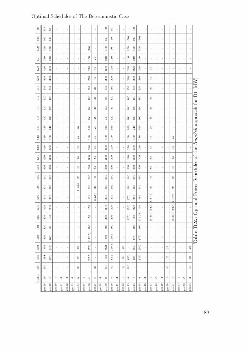
Optimal Schedules of The Deterministic Case
State 0
h00
h01
h02
h03
h04
h05
h06
h07
h08
h09
h10
h11
h12
h13
h14
h15
h16
h17
h18
h19
h20
h21
h22
h23
h24
gen2
810
200
284
368
420
420
420
420
420
420
420
420
420
420
420
420
420
420
420
336
420
420
340
319
403
363
gen2
9-8
.(20)
(40)
(60)
80140
200
260
300
300
300
300
300
300
240
180
120
180
240
300
300
240
180
140
80
gen3
0-4
..
..
..
..
..
..
..
..
..
..
..
..
.
gen3
1-1
..
..
..
..
..
..
..
..
..
..
..
..
.
gen3
2-1
..
..
..
..
..
..
..
..
..
..
..
..
.
gen3
3-1
..
..
..
..
..
..
..
..
..
..
..
..
.
gen3
45
3525
25.
..
..
(12.5)
2545
6545
2525
..
..
..
..
..
gen3
5-5
..
..
..
..
..
..
..
..
..
..
..
..
.
gen3
6-8
.(37.5)
(75)
(112.5)
150
150
150
160
220
280
290
300
240
180
150
150
150
150
210
270
210
150
(75)
..
gen3
75
25.
..
..
.(12.5)
2545
6585
6545
2525
2525
2545
4525
..
.
gen3
8-1
..
..
..
..
..
..
..
..
..
..
..
..
.
gen3
98
100
160
220
280
300
300
300
300
300
300
300
300
300
300
300
240
255
300
240
300
300
240
180
160
100
gen4
08
5081.5
120.5
160.5
160
200
200
200
200
200
200
200
200
200
160
120
80120
160
200
170
130
9050
50
gen4
1-1
..
..
..
..
..
..
..
..
..
..
..
..
.
gen4
21
4020
20.
..
..
..
..
..
..
..
..
..
..
.
gen4
38
100
(50)
..
.(25)
(50)
(75)
100
160
220
280
220
160
100
100
100
160
220
280
220
160
100
(50)
.
gen4
4-8
.(25)
(50)
(75)
100
160
220
255
265
300
300
300
300
300
240
180
120
180
240
300
270
210
150
100
100
gen4
5-8
.(25)
(50)
(75)
100
136.25
120
180
240
300
300
300
240
180
160
100
100
160
220
280
220
160
100
(50)
.
gen4
6-1
..
..
..
..
..
..
..
..
..
..
..
..
.
gen4
7-5
..
..
.(6.25)
(12.5)
(18.75)
2545
6585
6545
2525
2525
2545
25.
..
.
gen4
8-5
..
..
..
..
..
..
..
..
..
..
..
..
.
gen4
9-1
..
..
..
..
..
..
..
..
..
..
..
..
.
gen5
02
4025
25.
..
..
..
..
..
..
..
..
..
..
.
gen5
1-5
..
..
.(6.25)
(12.5)
(18.75)
2525
4565
4525
..
..
..
..
..
.
gen5
2-5
..
..
..
..
..
..
..
..
..
..
..
..
.
gen5
3-5
..
..
..
..
..
..
..
..
..
..
..
..
.
gen5
42
5025
25.
..
..
..
..
..
..
..
..
..
..
.
Tab
leD
.2.:
Optim
alPo
werSchedu
lesof
theRm
pSch
approach
forD1[M
W]
89
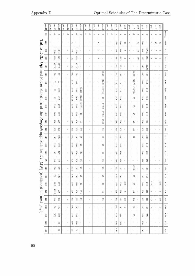
Appendix D Optimal Schedules of The Deterministic Case
State0h00
h01h02
h03h04
h05h06
h07h08
h09h10
h11h12
h13h14
h15h16
h17h18
h19h20
h21h22
h23h24
gen11
305
5.
..
..
..
..
..
..
..
(2.5)5
305
..
.
gen21
305
5.
..
..
..
..
..
..
..
..
..
..
.
gen31
305
5.
..
..
..
..
..
..
..
(2.5)5
225
..
.
gen4-8
.(37.5)
(75)(112.5)
150150
210150
210240
300300
300240
210150
150150
210270
210150
(75).
.
gen58
200140
200240
300300
300240
300300
300300
300240
240180
120180
240300
300240
180120
100
gen61
3010
10.
..
..
..
..
..
..
..
..
..
..
.
gen7-5
..
..
(6.25)(12.5)
(18.75)25
2545
6545
25.
..
(12.5)25
2545
5333
25.
.
gen81
305
5.
..
..
..
..
..
..
..
..
..
..
.
gen91
305
5.
..
..
..
..
..
..
..
(2.5)5
305
..
.
gen108
200140
199.5139.5
168110
170230
290240
300300
300240
180120
100160
220280
220160
100(50)
.
gen118
200210
280350
350350
350350
350350
350350
350350
350280
350280
350350
350280
210140
205
gen12-1
..
..
..
..
..
..
..
..
..
..
..
..
.
gen13-1
..
..
..
..
..
..
..
..
..
..
..
..
.
gen14-5
..
..
(6.25)(12.5)
(18.75)25
37.9357.93
77.9365
4525
4525
2525
2545
25.
..
.
gen151
308
8.
..
..
..
..
..
..
..
..
..
..
.
gen16-5
..
..
..
..
..
..
..
..
..
..
..
..
.
gen17-1
..
..
..
..
..
..
..
..
..
..
..
..
.
gen18-1
..
..
..
..
..
..
..
..
..
..
..
..
.
gen19-5
..
..
..
(6.25)(12.5)
(18.75)25
4560
4025
2525
2525
2537.5
25.
..
.
gen20-8
.(12.5)
(25)(37.5)
50100
150200
250250
250250
250200
250200
150150
200250
250200
150100
50
gen218
5050
100150
200250
250206.68
250250
250250
250250
250200
152.5200
250250
250200
150100
50
gen22-5
..
..
..
..
..
..
..
..
..
..
..
..
.
gen23-5
..
..
..
..
..
..
..
..
..
..
..
..
.
gen24-8
.(12.5)
(25)(37.5)
5090
130160
200180
200200
200160
12080
80120
160200
200160
12080
50
gen25-8
.(12.5)
(25)(37.5)
5050
5080
120160
200200
160120
9050
5050
62.5102.5
9050
(25).
.
gen26-5
..
..
..
..
..
..
..
..
..
..
..
..
.
gen2710
225309
393420
420420
420420
420420
420420
420420
420354
420420
420420
420336
420420
420
Table
D.3.:O
ptimalPower
Schedulesofthe
RmpSch
approachfor
D2[M
W](continued
onnext
page)
90
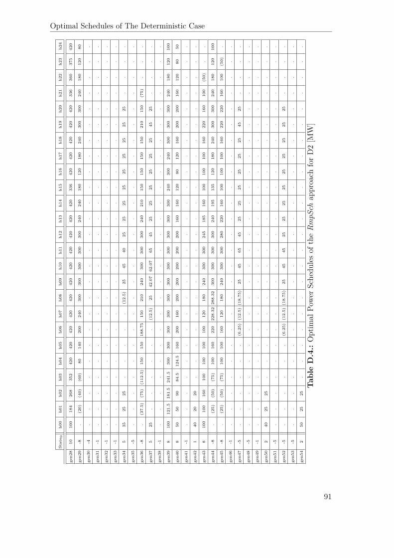
Optimal Schedules of The Deterministic Case
State 0
h00
h01
h02
h03
h04
h05
h06
h07
h08
h09
h10
h11
h12
h13
h14
h15
h16
h17
h18
h19
h20
h21
h22
h23
h24
gen2
810
100
184
268
352
420
420
420
420
420
420
420
420
420
420
420
336
420
420
420
420
420
336
360
375
420
gen2
9-8
.(20)
(40)
(60)
80140
200
240
300
300
300
300
300
240
240
180
120
180
240
300
300
240
180
120
80
gen3
0-4
..
..
..
..
..
..
..
..
..
..
..
..
.
gen3
1-1
..
..
..
..
..
..
..
..
..
..
..
..
.
gen3
2-1
..
..
..
..
..
..
..
..
..
..
..
..
.
gen3
3-1
..
..
..
..
..
..
..
..
..
..
..
..
.
gen3
45
3525
25.
..
..
(12.5)
2545
4025
2525
2525
2525
2525
..
..
gen3
5-5
..
..
..
..
..
..
..
..
..
..
..
..
.
gen3
6-8
.(37.5)
(75)
(112.5)
150
150
188.75
150
210
240
300
300
300
240
210
150
150
150
150
210
150
(75)
..
.
gen3
75
25.
..
..
.(12.5)
2542.07
62.07
6545
2525
2525
2525
4525
..
..
gen3
8-1
..
..
..
..
..
..
..
..
..
..
..
..
.
gen3
98
100
121.5
181.5
241.5
300
300
300
300
300
300
300
300
300
300
300
240
300
240
300
300
300
240
180
120
100
gen4
08
5050
9084.5
124.5
160
200
160
200
200
200
200
200
160
160
120
80120
160
200
200
160
120
8050
gen4
1-1
..
..
..
..
..
..
..
..
..
..
..
..
.
gen4
21
4020
20.
..
..
..
..
..
..
..
..
..
..
.
gen4
38
100
100
160
100
100
100
100
120
180
240
300
300
245
185
160
100
100
100
160
220
160
100
(50)
..
gen4
4-8
.(25)
(50)
(75)
100
160
220
228.32
288.32
300
300
300
300
240
195
135
120
180
240
300
300
240
180
120
100
gen4
5-8
.(25)
(50)
(75)
100
100
160
120
180
240
300
300
280
220
160
100
100
100
160
220
220
160
100
(50)
.
gen4
6-1
..
..
..
..
..
..
..
..
..
..
..
..
.
gen4
7-5
..
..
..
(6.25)
(12.5)
(18.75)
2545
6545
2525
2525
2525
4525
..
..
gen4
8-5
..
..
..
..
..
..
..
..
..
..
..
..
.
gen4
9-1
..
..
..
..
..
..
..
..
..
..
..
..
.
gen5
02
4025
25.
..
..
..
..
..
..
..
..
..
..
.
gen5
1-5
..
..
..
..
..
..
..
..
..
..
..
..
.
gen5
2-5
..
..
..
(6.25)
(12.5)
(18.75)
2545
4525
2525
2525
2525
2525
..
..
gen5
3-5
..
..
..
..
..
..
..
..
..
..
..
..
.
gen5
42
5025
25.
..
..
..
..
..
..
..
..
..
..
.
Tab
leD
.4.:
Optim
alPo
werSchedu
lesof
theRm
pSch
approach
forD2[M
W]
91
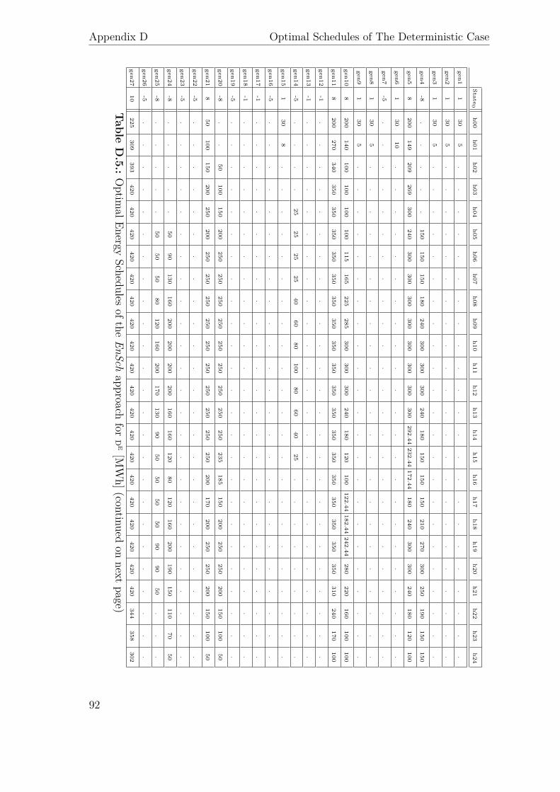
Appendix D Optimal Schedules of The Deterministic Case
State0h00
h01h02
h03h04
h05h06
h07h08
h09h10
h11h12
h13h14
h15h16
h17h18
h19h20
h21h22
h23h24
gen11
305
..
..
..
..
..
..
..
..
..
..
..
.
gen21
305
..
..
..
..
..
..
..
..
..
..
..
.
gen31
305
..
..
..
..
..
..
..
..
..
..
..
.
gen4-8
..
..
.150
150150
180240
300300
300240
180150
150150
210270
300250
190150
150
gen58
200149
209269
300240
300300
300300
300300
300300
292.44232.44
172.44180
240300
300240
180120
100
gen61
3010
..
..
..
..
..
..
..
..
..
..
..
.
gen7-5
..
..
..
..
..
..
..
..
..
..
..
..
.
gen81
305
..
..
..
..
..
..
..
..
..
..
..
.
gen91
305
..
..
..
..
..
..
..
..
..
..
..
.
gen108
200140
100100
100100
115165
225285
300300
300240
180120
100122.44
182.44242.44
280220
160100
100
gen118
200270
340350
350350
350350
350350
350350
350350
350350
350350
350350
350310
240170
100
gen12-1
..
..
..
..
..
..
..
..
..
..
..
..
.
gen13-1
..
..
..
..
..
..
..
..
..
..
..
..
.
gen14-5
..
..
2525
2525
4060
80100
8060
4025
..
..
..
..
.
gen151
308
..
..
..
..
..
..
..
..
..
..
..
.
gen16-5
..
..
..
..
..
..
..
..
..
..
..
..
.
gen17-1
..
..
..
..
..
..
..
..
..
..
..
..
.
gen18-1
..
..
..
..
..
..
..
..
..
..
..
..
.
gen19-5
..
..
..
..
..
..
..
..
..
..
..
..
.
gen20-8
..
50100
150200
250250
250250
250250
250250
250235
185150
200250
250200
150100
50
gen218
50100
150200
250200
250250
250250
250250
250250
250250
200170
200250
250200
150100
50
gen22-5
..
..
..
..
..
..
..
..
..
..
..
..
.
gen23-5
..
..
..
..
..
..
..
..
..
..
..
..
.
gen24-8
..
..
.50
90130
160200
200200
200160
160120
80120
160200
190150
11070
50
gen25-8
..
..
.50
5050
80120
160200
170130
9050
5050
5090
9050
..
.
gen26-5
..
..
..
..
..
..
..
..
..
..
..
..
.
gen2710
225309
393420
420420
420420
420420
420420
420420
420420
420420
420420
420420
344358
302
Table
D.5.:O
ptimalEnergy
Schedulesofthe
EnSchapproach
forD
E[M
Wh](continued
onnext
page)
92

Optimal Schedules of The Deterministic Case
State 0
h00
h01
h02
h03
h04
h05
h06
h07
h08
h09
h10
h11
h12
h13
h14
h15
h16
h17
h18
h19
h20
h21
h22
h23
h24
gen2
810
100
184
268
352
420
420
420
420
420
420
420
420
420
420
420
420
420
420
420
420
420
420
336
252
168
gen2
9-8
..
80140
200
180
240
300
300
300
300
300
300
300
300
240
180
180
240
300
300
240
180
120
80
gen3
0-4
..
..
..
..
..
..
..
..
..
..
..
..
.
gen3
1-1
..
..
..
..
..
..
..
..
..
..
..
..
.
gen3
2-1
..
..
..
..
..
..
..
..
..
..
..
..
.
gen3
3-1
..
..
..
..
..
..
..
..
..
..
..
..
.
gen3
45
3525
..
..
..
2545
6585
6545
25.
..
..
..
..
.
gen3
5-5
..
..
..
..
..
..
..
..
..
..
..
..
.
gen3
6-8
..
..
.150
150
150
150
210
270
300
300
240
180
150
150
150
180
240
300
240
180
150
150
gen3
75
2525
2525
2525
2525
4060
80100
8060
4025
..
..
..
..
.
gen3
8-1
..
..
..
..
..
..
..
..
..
..
..
..
.
gen3
98
100
160
220
280
300
300
300
300
300
300
300
300
300
300
300
300
280
300
250
300
300
280
220
160
100
gen4
08
5050
6564
104
65105
145
185
200
200
200
200
200
160
120
80120
160
200
200
160
120
8050
gen4
1-1
..
..
..
..
..
..
..
..
..
..
..
..
.
gen4
21
4020
..
..
..
..
..
..
..
..
..
..
..
.
gen4
38
100
100
100
100
100
100
100
100
120
180
240
300
285
225
165
105
100
100
100
160
220
160
100
100
100
gen4
4-8
..
.100
106
100
160
220
275
300
300
300
300
260
227.56
167.56
107.56
167.56
227.56
287.56
300
240
180
120
100
gen4
5-8
..
..
.100
100
100
140
200
260
300
300
240
180
120
100
100
160
220
280
220
160
100
100
gen4
6-1
..
..
..
..
..
..
..
..
..
..
..
..
.
gen4
7-5
..
..
2525
2525
4060
80100
8060
4025
..
..
..
..
.
gen4
8-5
..
..
..
..
..
..
..
..
..
..
..
..
.
gen4
9-1
..
..
..
..
..
..
..
..
..
..
..
..
.
gen5
02
4025
..
..
..
..
..
..
..
..
..
..
..
.
gen5
1-5
..
..
..
..
..
..
..
..
..
..
..
..
.
gen5
2-5
..
..
..
..
..
..
..
..
..
..
..
..
.
gen5
3-5
..
..
..
..
..
..
..
..
..
..
..
..
.
gen5
42
5025
..
..
..
..
..
..
..
..
..
..
..
.
Tab
leD
.6.:
Optim
alEn
ergy
Schedu
lesof
theEn
Schap
proach
for
DE[M
Wh]
93

Bibliography[1] “CPLEX 12,” IBM ILOG CPLEX, User’s Manual, 2013. [Online]. Available: http:
//gams.com/dd/docs/solvers/cplex.pdf[2] A. Abiri-Jahromi, M. Fotuhi-Firuzabad, and E. Abbasi, “Optimal scheduling of spinning
reserve based on well-being model,” Power Systems, IEEE Transactions on, vol. 22, no. 4,pp. 2048–2057, 2007.
[3] M. Amelin, “Comparison of capacity credit calculation methods for conventional power plantsand wind power,” Power Systems, IEEE Transactions on, vol. 24, no. 2, pp. 685–691, 2009.
[4] F. Aminifar, M. Fotuhi-Firuzabad, and M. Shahidehpour, “Unit commitment with proba-bilistic spinning reserve and interruptible load considerations,” Power Systems, IEEE Trans-actions on, vol. 24, no. 1, pp. 388–397, 2009.
[5] L. T. Anstine, R. E. Burke, J. E. Casey, R. Holgate, R. S. John, and H. G. Stewart, “Appli-cation of probability methods to the determination of spinning reserve requirements for thepennsylvania-new jersey-maryland interconnection,” IEEE Transactions on Power Appara-tus and Systems, vol. 82, no. 68, pp. 726–735, Oct. 1963.
[6] J. M. Arroyo and A. Conejo, “Modeling of start-up and shut-down power trajectories ofthermal units,” IEEE Transactions on Power Systems, vol. 19, no. 3, pp. 1562–1568, Aug.2004.
[7] R. Baldick, “Wind and energy markets: A case study of texas,” IEEE Systems Journal,vol. 6, no. 1, pp. 27–34, Mar. 2012.
[8] A. Ben-Tal, A. Goryashko, E. Guslitzer, and A. Nemirovski, “Adjustable robust solutions ofuncertain linear programs,” Mathematical Programming, vol. 99, no. 2, pp. 351–376, Mar.2004.
[9] A. Ben-Tal and A. Nemirovski, “Robust solutions of linear programming problemscontaminated with uncertain data,” Mathematical Programming, vol. 88, no. 3, pp.411–424, Sep. 2000. [Online]. Available: http://link.springer.com.focus.lib.kth.se/article/10.1007/PL00011380
[10] A. Ben-Tal, L. E. Ghaoui, and A. Nemirovski, Robust Optimization. Princeton UniversityPress, Aug. 2009.
[11] A. Ben-Tal, A. Nemirovski, and D. den Hertog, “ARO MIP problems,” 2014, personal cor-respondence.
[12] D. Bertsimas, E. Litvinov, X. A. Sun, J. Zhao, and T. Zheng, “Adaptive robust optimiza-tion for the security constrained unit commitment problem,” IEEE Transactions on PowerSystems, vol. 28, no. 1, pp. 52–63, Feb. 2013.
[13] D. Bertsimas and M. Sim, “The price of robustness,” Operations Research, vol. 52, no. 1,pp. 35 –53, Jan. 2004. [Online]. Available: http://or.journal.informs.org/content/52/1/35.abstract
[14] D. Bertsimas, D. B. Brown, and C. Caramanis, “Theory and applications of robustoptimization,” SIAM Review, vol. 53, no. 3, pp. 464–501, Jan. 2011. [Online]. Available:http://epubs.siam.org/doi/abs/10.1137/080734510
95
Bibliography
[15] J. R. Birge and F. Louveaux, Introduction to Stochastic Programming, corrected ed.Springer, Jul. 1997.
[16] R. Bixby, M. Fenelon, Z. Gu, E. Rothberg, and R. Wunderling, “MIP: theory and prac-tice–closing the gap,” in System Modelling and Optimization: Methods, Theory and Appli-cations, M. J. D. Powell and S. Scholtes, Eds. Boston: Kluwer Academic Publishers, 2000,vol. 174, p. 19–49.
[17] R. Bixby and E. Rothberg, “Progress in computational mixed integer programming—A lookback from the other side of the tipping point,” Annals of Operations Research, vol. 149, no. 1,pp. 37–41, Jan. 2007.
[18] R. E. Bixby, “Solving real-world linear programs: A decade and more of progress,” OperationsResearch, vol. 50, no. 1, pp. 3–15, Jan. 2002.
[19] R. E. Bixby, M. Fenelon, Z. Gu, E. Rothberg, and R. Wunderling, “Mixed-integer program-ming: A progress report,” in The Sharpest Cut: The Impact of Manfred Padberg and hisWork, ser. MPS-SIAM Series on Optimization, M. Grötschel, Ed. 3600 Market Street, 6thFloor Philadelphia, PA 19104-2688: SIAM, Jan. 2004, pp. 309—325.
[20] A. Botterud, J. Wang, V. Miranda, and R. J. Bessa, “Wind power forecasting in U.S.electricity markets,” The Electricity Journal, vol. 23, no. 3, pp. 71–82, Apr. 2010. [Online].Available: http://www.sciencedirect.com/science/article/pii/S104061901000062X
[21] F. Bouffard and F. Galiana, “Stochastic security for operations planning with significantwind power generation,” Power Systems, IEEE Transactions on, vol. 23, no. 2, pp. 306–316,2008.
[22] F. Bouffard, F. Galiana, and A. Conejo, “Market-clearing with stochastic security-part i:formulation,” IEEE Transactions on Power Systems, vol. 20, no. 4, pp. 1818–1826, Nov.2005.
[23] ——, “Market-clearing with stochastic security-part II: case studies,” Power Systems, IEEETransactions on, vol. 20, no. 4, pp. 1827–1835, 2005.
[24] CAISO, “Multi-stage generator unit modeling enhancements,” Tech.Rep., Sep. 2011. [Online]. Available: http://www.caiso.com/Documents/DraftFinalProposal-Multi-StageGenerationEnhancements.pdf
[25] ——, “White paper - integrated day-ahead market: Technical description forflexible ramping product,” Midwest Independent Transmission System Operator,USA, Tech. Rep., Sep. 2012. [Online]. Available: http://www.caiso.com/Documents/IntegratedDay-AheadMarketDraftTechnicalDescription-FlexibleRampingProduct.pdf
[26] F. Campos, “Modelos de evaluación de reservas de generación en el mercado eléctrico es-pañol,” Institute for Research in Technology (IIT), Technical Report, 2002.
[27] C. C. M. Caramanis, “Adaptable optimization: theory and algorithms,” Thesis,Massachusetts Institute of Technology, 2006, thesis (Ph. D.)–Massachusetts Instituteof Technology, Dept. of Electrical Engineering and Computer Science, 2006. [Online].Available: http://dspace.mit.edu/handle/1721.1/38301
[28] M. Carrion and J. Arroyo, “A computationally efficient mixed-integer linear formulationfor the thermal unit commitment problem,” IEEE Transactions on Power Systems, vol. 21,no. 3, pp. 1371–1378, 2006.
[29] H. Chavez, R. Baldick, and S. Sharma, “Regulation adequacy analysis under high windpenetration scenarios in ERCOT nodal,” IEEE Transactions on Sustainable Energy, vol. 3,no. 4, pp. 743 –750, Oct. 2012.
96
Bibliography
[30] T. Christof and A. Löbel, “PORTA: POlyhedron representation transformation algorithm,version 1.4.1,” Konrad-Zuse-Zentrum für Informationstechnik Berlin, Germany, 2009.[Online]. Available: http://typo.zib.de/opt-long_projects/Software/Porta/
[31] E. DeMeo, G. Jordan, C. Kalich, J. King, M. Milligan, C. Murley, B. Oakleaf, andM. Schuerger, “Accommodating wind’s natural behavior,” Power and Energy Magazine,IEEE, vol. 5, no. 6, pp. 59–67, 2007.
[32] R. Doherty and M. O’Malley, “A new approach to quantify reserve demand in systems withsignificant installed wind capacity,” Power Systems, IEEE Transactions on, vol. 20, no. 2,pp. 587–595, 2005.
[33] I. Egido, L. Rouco, J. Alonso, E. Porras, and J. Ruiz, “Impacto en regulación frecuencia-potencia de los cambios de programa en escalón de las unidades generadoras,” Anales deMecánica y Electricidad, vol. LXXXVIII, no. 3, pp. 26—32, May 2011.
[34] ENTSO-e, “Frequency quality investigation, excerpt of the final report,” UCTE AD-HOC,Report, Aug. 2008. [Online]. Available: www.entsoe.eu/fileadmin/user_upload/_library/publications/ce/otherreports/090330_UCTE_FrequencyInvestigationReport_Abstract.pdf
[35] ——, “Operation handbook, P1–Policy 1: Load-frequency control and performance [c],”European Network of Transmission Systems Operators for Electricity (ENTSO-e), Tech.Rep., Apr. 2009. [Online]. Available: https://www.entsoe.eu/nc/resources/publications/former-associations/ucte/operation-handbook
[36] ——, “Operational reserve ad hoc team report (AHT-Report),” European Network ofTransmission Systems Operators for Electricity (ENTSO-e), Tech. Rep., May 2012.[Online]. Available: https://www.entsoe.eu/fileadmin/user_upload/_library/consultations/Network_Code_OR/2012-06-14_SOC-AhT-OR_Report_final_V9.pdf
[37] ——, “Network code on load-frequency control and reserves,” European Network ofTransmission Systems Operators for Electricity (ENTSO-e), Tech. Rep., Jun. 2013.[Online]. Available: https://www.entsoe.eu/major-projects/network-code-development/load-frequency-control-reserves/
[38] ——, “Supporting document for the network code on load-frequency control and reserves,”European Network of Transmission Systems Operators for Electricity (ENTSO-e), Tech.Rep., Jun. 2013. [Online]. Available: https://www.entsoe.eu/fileadmin/user_upload/_library/resources/LCFR/130628-NC_LFCR-Supporting_Document-Issue1.pdf
[39] ENTSO-e and Eurelectric, “Deterministic frequency deviations – root causes andproposals for potential solutions,” ENTSO-e, Report, Dec. 2011. [Online]. Available:https://www.entsoe.eu/fileadmin/user_upload/_library/publications/entsoe/120222_Deterministic_Frequency_Deviations_joint_ENTSOE_Eurelectric_Report__Final_.pdf
[40] ——, “Deterministic frequency deviations: 2nd stage impact analysis,” ENTSO-e, Report,Dec. 2012. [Online]. Available: https://www.entsoe.eu/fileadmin/user_upload/_library/publications/entsoe/130325_Deterministic_Frequency_Deviations_Final_Report.pdf
[41] ERCOT, “ERCOT operations report on the EECP event of february 26, 2008,”Electric Reliability Council of Texas (ERCOT), Texas - USA, Tech. Rep., Jul.2008. [Online]. Available: http://www.ercot.com/meetings/ros/keydocs/2008/0313/07._ERCOT_OPERATIONS_REPORT_EECP022608_public.doc
[42] ——, “White paper functional description of core market management system(MMS) applications for "Look-Ahead SCED", version 0.1.2,” Electric ReliabilityCouncil of Texas (ERCOT), Texas - USA, Tech. Rep., Nov. 2011. [Online].Available: http://www.ercot.com/content/meetings/metf/keydocs/2012/0228/04_white_paper_funct_desc_core_mms_applications_for_la_sced.doc
97
Bibliography
[43] ——, “ERCOT nodal protocols: Transmission security analysis and reliability unitcommitment,” Electric Reliability Council of Texas (ERCOT), Texas - USA, Tech. Rep.,Mar. 2014. [Online]. Available: http://ercot.com/content/mktrules/nprotocols/current/05-050114_Nodal.doc
[44] ——, “ERCOT nodal protocols: Day-ahead operations,” Electric Reliability Councilof Texas (ERCOT), Texas - USA, Tech. Rep., Mar. 2014. [Online]. Available:http://ercot.com/content/mktrules/nprotocols/current/04-030114_Nodal.doc
[45] ——, “ERCOT nodal protocols: Adjustment period and real-time operations,” ElectricReliability Council of Texas (ERCOT), Texas - USA, Tech. Rep., May 2014. [Online].Available: http://ercot.com/content/mktrules/nprotocols/current/06-050114_Nodal.doc
[46] FERC, “Recent ISO software enhancements and future software and modeling plans,”Federal Energy Regulatory Commission, Staff Report, Nov. 2011. [Online]. Available:http://www.ferc.gov/industries/electric/indus-act/rto/rto-iso-soft-2011.pdf
[47] ——, “RTO unit commitment test system,” Federal Energy and Regulatory Commission,Washington DC, USA, Tech. Rep., Jul. 2012.
[48] A. Frangioni, C. Gentile, and F. Lacalandra, “Tighter approximated MILP formulationsfor unit commitment problems,” IEEE Transactions on Power Systems, vol. 24, no. 1, pp.105–113, Feb. 2009.
[49] J. Frunt, I. Lampropoulos, and W. L. Kling, “The impact of electricity market design onperiodic network frequency excursions,” in Energy Market (EEM), 2011 8th InternationalConference on the European. IEEE, May 2011, pp. 550–555.
[50] Y. Fu, M. Shahidehpour, and Z. Li, “AC contingency dispatch based on security-constrainedunit commitment,” Power Systems, IEEE Transactions on, vol. 21, no. 2, pp. 897–908, 2006.
[51] F. Galiana, F. Bouffard, J. Arroyo, and J. Restrepo, “Scheduling and pricing of coupledenergy and primary, secondary, and tertiary reserves,” Proceedings of the IEEE, vol. 93,no. 11, pp. 1970–1983, 2005.
[52] J. Garcia-Gonzalez, A. San Roque, F. Campos, and J. Villar, “Connecting the intradayenergy and reserve markets by an optimal redispatch,” IEEE Transactions on Power Systems,vol. 22, no. 4, pp. 2220–2231, Nov. 2007.
[53] C. Gentile, G. Morales-Espana, and A. Ramos, “A tight MIP formulation of the unit commit-ment problem with start-up and shut-down constraints,” European Journal of OperationalResearch, 2014, under Review.
[54] A. Gil, M. de la Torre, T. Dominguez, and R. Rivas, “Influence of wind energy forecast indeterministic and pobabilistic sizing of reserves,” Quebec, Canada, Oct. 2009, p. 6.
[55] P. Glasserman, Monte Carlo methods in financial engineering. New York: Springer, 2003.[56] X. Guan, F. Gao, and A. Svoboda, “Energy delivery scheduling and realizability in deregu-
lated electric energy market,” in Proceedings of the 32nd Annual Hawaii International Con-ference on System Sciences, 1999. HICSS-32, vol. Track3. IEEE, 1999.
[57] ——, “Energy delivery capacity and generation scheduling in the deregulated electric powermarket,” IEEE Transactions on Power Systems, vol. 15, no. 4, pp. 1275–1280, Nov. 2000.
[58] X. Guan, Q. Zhai, Y. Feng, and F. Gao, “Optimization based scheduling for a class ofproduction systems with integral constraints,” Science in China Series E: TechnologicalSciences, vol. 52, no. 12, pp. 3533–3544, Dec. 2009.
[59] K. Hedman, M. Ferris, R. O’Neill, E. Fisher, and S. Oren, “Co-optimization of generationunit commitment and transmission switching with n-1 reliability,” Power Systems, IEEETransactions on, vol. 25, no. 2, pp. 1052 –1063, May 2010.
98
Bibliography
[60] B. F. Hobbs, M. H. Rothkopf, R. P. O’Neill, and H.-p. Chao, Eds., The Next Generation ofElectric Power Unit Commitment Models, 1st ed. Springer, 2001.
[61] B. F. Hobbs, W. R. Stewart, R. E. Bixby, M. H. Rothkopf, R. P. O’Neill, and H.-p. Chao,“Why this book? new capabilities and new needs for unit commitment modeling,” in TheNext Generation of Electric Power Unit Commitment Models, B. F. Hobbs, M. H. Rothkopf,R. P. O’Neill, and H.-p. Chao, Eds. Boston: Kluwer Academic Publishers, 2002, vol. 36,pp. 1–14.
[62] H. Holttinen, M. Milligan, B. Kirby, T. Acker, V. Neimane, and T. Molinski, “Usingstandard deviation as a measure of increased operational reserve requirement for windpower,” Wind Engineering, vol. 32, no. 4, pp. 355–377, Jun. 2008. [Online]. Available:http://dx.doi.org/10.1260/0309-524X.32.4.355
[63] H. Holttinen, P. Meibom, A. Orths, B. Lange, M. O’Malley, J. O. Tande, A. Estanqueiro,E. Gomez, L. Söder, G. Strbac, J. C. Smith, and F. van Hulle, “Impacts of largeamounts of wind power on design and operation of power systems, results of IEAcollaboration,” Wind Energy, vol. 14, no. 2, pp. 179–192, Mar. 2011. [Online]. Available:http://onlinelibrary.wiley.com/doi/10.1002/we.410/abstract
[64] J. Hooker, Logic-Based Methods for Optimization: Combining Optimization and ConstraintSatisfaction, 1st ed. Wiley-Interscience, May 2000.
[65] B. Hu, L. Wu, and M. Marwali, “On the robust solution to SCUC with load and winduncertainty correlations,” IEEE Transactions on Power Systems, vol. Early Access Online,2014.
[66] R. Jiang, J. Wang, M. Zhang, and Y. Guan, “Two-stage minimax regret robust unit com-mitment,” IEEE Transactions on Power Systems, vol. Early Access Online, 2013.
[67] R. Jiang, M. Zhang, G. Li, and Y. Guan, “Two-stage network constrained robust unitcommitment problem,” European Journal of Operational Research, vol. 234, no. 3, pp.751–762, May 2014. [Online]. Available: http://www.sciencedirect.com/science/article/pii/S0377221713007832
[68] P. Kall and S. W. Wallace, Stochastic programming, 2nd ed., ser. Wiley-Interscience Seriesin Systems and Optimization. Chichester: John Wiley & Sons, Ltd., 1994. [Online].Available: http://stoprog.org/index.html?introductions.html
[69] T. Koch, T. Achterberg, E. Andersen, O. Bastert, T. Berthold, R. E. Bixby, E. Danna,G. Gamrath, A. M. Gleixner, S. Heinz, A. Lodi, H. Mittelmann, T. Ralphs, D. Salvagnin,D. E. Steffy, and K. Wolter, “MIPLIB 2010,” Mathematical Programming Computation,vol. 3, no. 2, pp. 103–163, Jun. 2011.
[70] J. Lee, J. Leung, and F. Margot, “Min-up/min-down polytopes,” Discrete Optimization,vol. 1, no. 1, pp. 77–85, Jun. 2004.
[71] K. Leuven and T. Engineering, “Study of the interactions and dependencies ofbalancing markets, intraday trade and automatically activated reserves,” KatholiekeUniversiteit Leuven (KULeuven) and Tractebel Engineering, Tech. Rep., 2009.[Online]. Available: http://ec.europa.eu/energy/gas_electricity/studies/doc/electricity/2009_balancing_markets.pdf
[72] T. Li and M. Shahidehpour, “Price-based unit commitment: a case of lagrangian relaxationversus mixed integer programming,” IEEE Transactions on Power Systems, vol. 20, no. 4,pp. 2015–2025, Nov. 2005.
[73] Z. Li and M. Shahidehpour, “Security-constrained unit commitment for simultaneous clearingof energy and ancillary services markets,” Power Systems, IEEE Transactions on, vol. 20,no. 2, pp. 1079–1088, 2005.
99
Bibliography
[74] C. Liu, M. Shahidehpour, Z. Li, and M. Fotuhi-Firuzabad, “Component and mode models forthe short-term scheduling of combined-cycle units,” IEEE Transactions on Power Systems,vol. 24, no. 2, pp. 976 –990, May 2009.
[75] A. Lodi, “Mixed integer programming computation,” in 50 Years of Integer Programming1958-2008, M. Jünger, T. M. Liebling, D. Naddef, G. L. Nemhauser, W. R. Pulleyblank,G. Reinelt, G. Rinaldi, and L. A. Wolsey, Eds. Berlin, Heidelberg: Springer Berlin Heidel-berg, 2010, pp. 619–645.
[76] A. Lotfjou, M. Shahidehpour, Y. Fu, and Z. Li, “Security-constrained unit commitment withAC/DC transmission systems,” Power Systems, IEEE Transactions on, vol. 25, no. 1, pp.531–542, 2010.
[77] B. Lu and M. Shahidehpour, “Unit commitment with flexible generating units,” Power Sys-tems, IEEE Transactions on, vol. 20, no. 2, pp. 1022–1034, 2005.
[78] ——, “Short-term scheduling of combined cycle units,” IEEE Transactions on Power Sys-tems, vol. 19, no. 3, pp. 1616 – 1625, Aug. 2004.
[79] S. Lu, C. A. McKinstry, A. J. Brothers, and S. Jin, “Low probability tailevent analysis and mitigation in the BPA control area,” Pacific Northwest NationalLaboratory, Texas - USA, Tech. Rep., Oct. 2010. [Online]. Available: http://www.pnl.gov/main/publications/external/technical_reports/PNNL-20120.pdf
[80] J. Matevosyan, “Real-time operations in ERCOT,” 2014, personal correspondence.
[81] M. Matos, J. P. Lopes, M. Rosa, R. Ferreira, A. Leite da Silva, W. Sales,L. Resende, L. Manso, P. Cabral, M. Ferreira, N. Martins, C. Artaiz, F. Soto, andR. López, “Probabilistic evaluation of reserve requirements of generating systems withrenewable power sources: The portuguese and spanish cases,” International Journalof Electrical Power & Energy Systems, vol. 31, no. 9, pp. 562–569, Oct. 2009.[Online]. Available: http://www.sciencedirect.com/science/article/B6V2T-4W73H68-2/2/05a6af8b1097af984d9a5e2f96a89744
[82] P. Meibom, R. Barth, B. Hasche, H. Brand, C. Weber, and M. O’Malley, “Stochastic op-timization model to study the operational impacts of high wind penetrations in ireland,”IEEE Transactions on Power Systems, vol. 26, no. 3, pp. 1367–1379, Aug. 2011.
[83] M. Milligan, K. Porter, E. DeMeo, P. Denholm, H. Holttinen, B. Kirby, N. Miller,A. Mills, M. O’Malley, M. Schuerger, and L. Soder, “Wind power myths debunked,”Power and Energy Magazine, IEEE, vol. 7, no. 6, pp. 89–99, 2009. [Online]. Available:10.1109/MPE.2009.934268
[84] MISO, “Ramp capability for load following in the MISO markets,” Midwest IndependentTransmission System Operator, USA, Tech. Rep., Jul. 2011. [Online]. Available:https://www.midwestiso.org/_layouts/MISO/ECM/Redirect.aspx?ID=112806
[85] I. Momber, G. Morales-Espana, A. Ramos, and T. Gomez, “PEV storage in multi-busscheduling problems,” IEEE Transactions on Smart Grid, vol. 5, no. 2, pp. 1079–1087, Mar.2014.
[86] J. Morales, A. Conejo, and J. Perez-Ruiz, “Economic valuation of reserves in power systemswith high penetration of wind power,” Power Systems, IEEE Transactions on, vol. 24, no. 2,pp. 900–910, 2009.
[87] G. Morales-España, J. M. Latorre, and A. Ramos, “Modeling start-up & shut-down rampsof thermal units in unit-commitment formulations,” in Workshop on Advanced OptimisationMethods and their Applications to Unit Commitment in Energy Management, Paris, France,Nov. 2011, pp. 1–4.
100
Bibliography
[88] G. Morales-Espana, J. Garcia-Gonzalez, and A. Ramos, “Impact on reserves and energydelivery of current UC-based market-clearing formulations,” in European Energy Market(EEM), 2012 9th International Conference on the, Florence, Italy, May 2012, pp. 1–7.
[89] G. Morales-España, J. Garcia-Gonzalez, and A. Ramos, “Tight and compact MILP formu-lation for the thermal unit commitment problem,” in PowerTech 2013, Grenoble, Francia,Jun. 2013, (Invited Presentation).
[90] G. Morales-España, J. M. Latorre, J. Garcia-Gonzalez, and A. Ramos, “Tight and com-pact MILP formulations for unit commitment problems,” in FERC Technical Conference onIncreasing Real-Time And Day-Ahead Market Efficiency Through Improved Software, Wash-ington D.C., USA, Jun. 2013, (Invited Presentation).
[91] G. Morales-Espana, J. M. Latorre, and A. Ramos, “Tight and compact MILP formulationfor the thermal unit commitment problem,” IEEE Transactions on Power Systems, vol. 28,no. 4, pp. 4897–4908, Nov. 2013.
[92] G. Morales-España, J. M. Latorre, and A. Ramos, “Tight and compact MILP formulationof start-up and shut-down ramping in unit commitment,” in 2013 IEEE Power and EnergySociety General Meeting, Vancouver, Canada, Jul. 2013.
[93] G. Morales-España, R. Baldick, J. Garcia-Gonzalez, and A. Ramos, “Robust reserve model-ing for wind power integration in day-ahead unit commitment,” in FERC Technical Confer-ence on Increasing Real-Time And Day-Ahead Market Efficiency Through Improved Software,Washington D.C., USA, Jun. 2014, (Invited Presentation).
[94] ——, “Robust reserve modeling for wind power integration in ramp-based unit commitment,”in ERCOT: KERMIT Summit, Austin-Texas, USA, Mar. 2014, (Invited Presentation).
[95] G. Morales-Espana, R. Baldick, J. Garcia-Gonzalez, and A. Ramos, “Robust reserve mod-elling for wind power integration in ramp-based unit commitment,” IEEE Transactions onPower Systems, 2014, under review.
[96] G. Morales-Espana, C. M. Correa-Posada, and A. Ramos, “Tight and compact MIP formu-lation of configuration-based combined-cycle units,” IEEE Transactions on Power Systems,2014, to be submitted.
[97] G. Morales-Espana, C. Gentile, and A. Ramos, “Tight MIP formulations of the power-basedunit commitment problem,” Optimization Letters, 2014, under Review. [Online]. Available:http://www.iit.upcomillas.es/aramos/papers/Power-UC_ConvexHull.pdf
[98] G. Morales-España, C. Gentile, and A. Ramos, “Accelerating the convergence of stochasticunit-commitment problems by using a tight and compact MIP formulation,” in 20th Con-ference of The International Federation of Operational Research Societies, Barcelona, Spain,Jul. 2014.
[99] G. Morales-Espana, A. Ramos, and J. Garcia-Gonzalez, “An MIP formulation for jointmarket-clearing of energy and reserves based on ramp scheduling,” IEEE Transactions onPower Systems, vol. 29, no. 1, pp. 476–488, 2014.
[100] G. Morales-Espana, J. M. Latorre, and A. Ramos, “Tight and compact MILP formulationof start-up and shut-down ramping in unit commitment,” IEEE Transactions on PowerSystems, vol. 28, no. 2, pp. 1288–1296, 2013.
[101] Morales Juan Miguel, “Impact on system economics and security economics of a highpenetration of wind power,” Ph.D. dissertation, University of Castilla - La Mancha,Ciudad Real, Spain, Dec. 2010. [Online]. Available: www.uclm.es/area/gsee/tesis/Tesis_JMMorales.pdf
[102] G. L. Nemhauser and L. A. Wolsey, Integer and combinatorial optimization. New York:John Wiley and Sons, 1999.
101
Bibliography
[103] NERC, ““22:00” frequency excursion (final report),” NERC, Report 20020828, Aug. 2002.[Online]. Available: www.nerc.com/docs/oc/rs/FETF-Report_20020828.doc
[104] ——, “Accommodating high levels of variable generation,” North American ElectricReliability Corporation, Tech. Rep., 2010. [Online]. Available: http://www.nerc.com/files/IVGTF_Report_041609.pdf
[105] ——, “Balancing and frequency control,” North American Electric Reliability Corporation,Tech. Rep., Jan. 2011. [Online]. Available: http://www.nerc.com/docs/oc/rs/NERC%20Balancing%20and%20Frequency%20Control%20040520111.pdf
[106] ——, “Reliability standards for the bulk electric systems in north america,” NorthAmerican Electric Reliability Corporation, Tech. Rep., May 2011. [Online]. Available:http://www.nerc.com/files/Reliability_Standards_Complete_Set.pdf
[107] G. Nilssen, “Planned actions to remedy the weakning nordic frequency quality,” StrategicSystem Operation Development, Tech. Rep. Cokument ID 1438187, Jun. 2010.
[108] M. Ortega-Vazquez and D. Kirschen, “Estimating the spinning reserve requirements in sys-tems with significant wind power generation penetration,” Power Systems, IEEE Transac-tions on, vol. 24, no. 1, pp. 114–124, 2009.
[109] J. Ostrowski, M. F. Anjos, and A. Vannelli, “Tight mixed integer linear programming formu-lations for the unit commitment problem,” IEEE Transactions on Power Systems, vol. 27,no. 1, pp. 39–46, Feb. 2012.
[110] A. L. Ott, “Evolution of computing requirements in the PJM market: Past and future,” in2010 IEEE Power and Energy Society General Meeting. IEEE, Jul. 2010, pp. 1–4.
[111] N. Padhy, “Unit commitment-a bibliographical survey,” IEEE Transactions on Power Sys-tems, vol. 19, no. 2, pp. 1196–1205, May 2004.
[112] A. Papavasiliou, S. S. Oren, and R. P. O’Neill, “Reserve requirements for wind power integra-tion: A scenario-based stochastic programming framework,” IEEE Transactions on PowerSystems, vol. 26, no. 4, pp. 2197–2206, Nov. 2011.
[113] D. Rajan and S. Takriti, “Minimum Up/Down polytopes of the unitcommitment problem with start-up costs,” IBM, Research Report RC23628,Jun. 2005. [Online]. Available: http://domino.research.ibm.com/library/cyberdig.nsf/1e4115aea78b6e7c85256b360066f0d4/cdcb02a7c809d89e8525702300502ac0?OpenDocument
[114] A. Ramos, J. M. Latorre, F. Báñez, Á. Hernández, G. Morales-Espana, K. Dietrich, andL. Olmos, “Modeling the operation of electric vehicles in an operation planning model,” in17th Power Systems Computation Conference (PSCC’11), Stockholm, Sweden, Aug. 2011,pp. 1–7.
[115] A. Ramos, G. Morales-España, J. Garcia-Gonzalez, and M. Rivier, “Operation reserve usagefor different unit time periods of a stochastic unit commitment,” in 20th Conference of TheInternational Federation of Operational Research Societies, Barcelona, Spain, Jul. 2014.
[116] Y. G. Rebours, D. S. Kirschen, M. Trotignon, and S. Rossignol, “A survey of frequencyand voltage control ancillary Services—Part i: Technical features,” Power Systems, IEEETransactions on, vol. 22, no. 1, pp. 350–357, 2007.
[117] ——, “A survey of frequency and voltage control ancillary Services—Part II: economic fea-tures,” Power Systems, IEEE Transactions on, vol. 22, no. 1, pp. 358–366, 2007.
[118] G. Relaño, J. I. de la Fuente, T. Gómez, D. Soler, O. Largo, R. Martínez, and F. Apartero,“A linearization algorithm for hourly power scheduling in a competitive framework,” inUniversities Power Engineering Conference (UPEC), Belfast, September, 2000.
102
Bibliography
[119] E. Rothberg, “The CPLEX library: Presolve and cutting planes,” in 4th Max-Planck Ad-vanced Course on the Foundations of Computer Science (ADFOCS), Saarbrücken, Germany,Sep. 2003, pp. 1–17.
[120] P. A. Ruiz, C. R. Philbrick, E. Zak, K. W. Cheung, and P. W. Sauer, “Uncertainty man-agement in the unit commitment problem,” Power Systems, IEEE Transactions on, vol. 24,no. 2, pp. 642–651, May 2009.
[121] C. Sahin, M. Shahidehpour, and I. Erkmen, “Allocation of hourly reserve versus demandresponse for security-constrained scheduling of stochastic wind energy,” IEEE Transactionson Sustainable Energy, vol. 4, no. 1, pp. 219–228, 2013.
[122] P. Sanchez-Martin, G. Sanchez, and G. Morales-Espana, “Direct load control decision modelfor aggregated EV charging points,” IEEE Transactions on Power Systems, vol. 27, no. 3, pp.1577–1584, Aug. 2012. [Online]. Available: http://dx.doi.org/10.1109/TPWRS.2011.2180546
[123] M. Shahidehpour, H. Yamin, and Z. Li, Market Operations in Electric Power Systems: Fore-casting, Scheduling, and Risk Management, 1st ed. Wiley-IEEE Press, Mar. 2002.
[124] A. Shapiro, D. Dentcheva, and A. Ruszczynski, Lectures on Stochastic Programming: Mod-eling and Theory. SIAM-Society for Industrial and Applied Mathematics, Sep. 2009.
[125] C. Simoglou, P. Biskas, and A. Bakirtzis, “Optimal self-scheduling of a thermal producerin short-term electricity markets by MILP,” IEEE Transactions on Power Systems, vol. 25,no. 4, pp. 1965–1977, Nov. 2010.
[126] J. Smith, M. Milligan, E. DeMeo, and B. Parsons, “Utility wind integration and operatingimpact state of the art,” Power Systems, IEEE Transactions on, vol. 22, no. 3, pp. 900–908,2007. [Online]. Available: 10.1109/TPWRS.2007.901598
[127] S. Stoft, Power System Economics: Designing Markets for Electricity, 1st ed. Wiley-IEEEPress, May 2002.
[128] M. Tahanan, W. van Ackooij, A. Frangioni, and F. Lacalandra, “Large-scaleunit commitment under uncertainty: a literature survey,” University of Pisa,Pisa, Italy, Technical Report TR-14-01, Jan. 2014. [Online]. Available: http://compass2.di.unipi.it/TR/Files/TR-14-01.pdf.gz
[129] S. Takriti, J. Birge, and E. Long, “A stochastic model for the unit commitment problem,”Power Systems, IEEE Transactions on, vol. 11, no. 3, pp. 1497–1508, 1996.
[130] N. Troy, E. Denny, and M. O’Malley, “Base-load cycling on a system with significant windpenetration,” IEEE Transactions on Power Systems, vol. 25, no. 2, pp. 1088–1097, May2010.
[131] A. Tuohy, P. Meibom, E. Denny, and M. O’Malley, “Unit commitment for systems withsignificant wind penetration,” Power Systems, IEEE Transactions on, vol. 24, no. 2, pp.592–601, 2009.
[132] F. Vanderbeck and L. A. Wolsey, “Reformulation and decomposition of integer programs,”in 50 Years of Integer Programming 1958-2008, M. Jünger, T. M. Liebling, D. Naddef, G. L.Nemhauser, W. R. Pulleyblank, G. Reinelt, G. Rinaldi, and L. A. Wolsey, Eds. Berlin,Heidelberg: Springer Berlin Heidelberg, 2010, pp. 431–502.
[133] C. Wang and S. M. Shahidehpour, “Effects of ramp-rate limits on unit commitment andeconomic dispatch,” IEEE Transactions on Power Systems, vol. 8, no. 3, pp. 1341–1350,Aug. 1993.
[134] J. Wang, M. Shahidehpour, and Z. Li, “Security-constrained unit commitment with volatilewind power generation,” Power Systems, IEEE Transactions on, vol. 23, no. 3, pp. 1319–1327, 2008.
103
Bibliography
[135] ——, “Contingency-constrained reserve requirements in joint energy and ancillary servicesauction,” Power Systems, IEEE Transactions on, vol. 24, no. 3, pp. 1457–1468, 2009.
[136] J. Wang, J. Valenzuela, A. Botterud, H. Keko, R. Bessa, and V. Miranda, “Reliabilityassessment unit commitment with uncertain wind power,” in Handbook of Wind PowerSystems, ser. Energy Systems, P. M. Pardalos, S. Rebennack, M. V. F. Pereira, N. A.Iliadis, and V. Pappu, Eds. Springer Berlin Heidelberg, Jan. 2013, pp. 3–20. [Online].Available: http://link.springer.com.focus.lib.kth.se/chapter/10.1007/978-3-642-41080-2_1
[137] Q. Wang, J.-P. Watson, and Y. Guan, “Two-stage robust optimization for n -k contingency-constrained unit commitment,” IEEE Transactions on Power Systems, vol. Early AccessOnline, 2013.
[138] T. Weissbach and E. Welfonder, “High frequency deviations within the european power sys-tem: Origins and proposals for improvement,” in Power Systems Conference and Exposition,2009. PSCE ’09. IEEE/PES. IEEE, Mar. 2009, pp. 1–6.
[139] H. P. Williams, Model Building in Mathematical Programming, 5th ed. John Wiley & SonsInc, Feb. 2013.
[140] L. Wolsey, “Strong formulations for mixed integer programs: valid inequalities and extendedformulations,” Mathematical programming, vol. 97, no. 1, p. 423–447, 2003.
[141] ——, “Strong formulations for mixed integer programming: A survey,” Mathematical Pro-gramming, vol. 45, no. 1-3, pp. 173–191, Aug. 1989.
[142] ——, Integer Programming. Wiley-Interscience, 1998.[143] A. J. Wood and B. F. Wollenberg, Power Generation, Operation, and Control, 2nd ed.
Wiley-Interscience, Jan. 1996.[144] H. Wu, Q. Zhai, X. Guan, F. Gao, and H. Ye, “Security-constrained unit commitment based
on a realizable energy delivery formulation,” Mathematical Problems in Engineering, vol.2012, pp. 1–22, 2012.
[145] L. Wu, M. Shahidehpour, and T. Li, “Stochastic security-constrained unit commitment,”IEEE Transactions on Power Systems, vol. 22, no. 2, pp. 800–811, May 2007.
[146] ——, “Cost of reliability analysis based on stochastic unit commitment,” Power Systems,IEEE Transactions on, vol. 23, no. 3, pp. 1364–1374, 2008.
[147] L. Wu, M. Shahidehpour, and Z. Li, “Comparison of scenario-based and interval optimizationapproaches to stochastic SCUC,” Power Systems, IEEE Transactions on, vol. 27, no. 2, pp.913 –921, May 2012.
[148] L. Xie, P. Carvalho, L. Ferreira, J. Liu, B. Krogh, N. Popli, and M. Ilic, “Wind integrationin power systems: Operational challenges and possible solutions,” Proceedings of the IEEE,vol. 99, no. 1, pp. 214–232, 2011.
[149] H. Y. Yamin, “Review on methods of generation scheduling in electric power systems,”Electric Power Systems Research, vol. 69, no. 2-3, pp. 227–248, May 2004.
[150] Y. Yang, J. Wang, X. Guan, and Q. Zhai, “Subhourly unit commitment with feasible energydelivery constraints,” Applied Energy, 2012, to be published.
[151] C. Zhao and Y. Guan, “Unified stochastic and robust unit commitment,” IEEE Transactionson Power Systems, vol. 28, no. 3, pp. 3353–3361, Aug. 2013.
[152] C. Zhao, J. Wang, J.-P. Watson, and Y. Guan, “Multi-stage robust unit commitment con-sidering wind and demand response uncertainties,” IEEE Transactions on Power Systems,vol. Early Access Online, 2013.
[153] L. Zhao and B. Zeng, “Robust unit commitment problem with demand response and windenergy,” in 2012 IEEE Power and Energy Society General Meeting, Jul. 2012, pp. 1–8.
104

For KTH Royal Institute of Technology:DOCTORAL THESIS IN ELECTRICAL ENGINEERINGTRITA-EE 2014:041www.kth.se
ISNN 1653-5146ISBN 978-84-697-1230-6
Related Documents


![Commitment Issues 20160603 - DiVA portalmdh.diva-portal.org/smash/get/diva2:957148/FULLTEXT01.pdf · Bilaga 1 - Deskriptiv statistik ..... commitment, n. [kəˈmɪtm(ə)nt] 1) An](https://static.cupdf.com/doc/110x72/5a75c8ef7f8b9a93088ca62c/commitment-issues-20160603-diva-957148fulltext01pdf-bilaga-1-deskriptiv.jpg)


