Unit 8: Robust Parameter Design - ISyE Home | ISyE ...jeffwu/isye6413/unit_08_12spring.pdf · Unit 8: Robust Parameter Design Source : Chapter 11 (sections 11.1 - 11.6, part of sections

Unit 8: Robust Parameter Design

Source : Chapter 11 (sections 11.1 - 11.6, part of sections 11.7 -11.8 and 11.9).

• Revisiting two previous experiments.

• Strategies for reducing variation.

• Types of noise factors.

• Variation reduction through robust parameter design.

• Cross array, location-dispersion modeling, response modeling.

• Single arrays vs cross arrays.

• Signal-to-noise ratios and limitations.

1

Robust Parameter Design

• Statistical/engineering method for product/process improvement (G.

Taguchi).

• Two types of factors in a system (product/process):

– control factors: once chosen, values remain fixed.

– noise factors: hard-to-control during normal process or usage.

• Robust Parameter design(RPD or PD): choose control factor settings to

make response less sensitive (i.e.more robust) to noise variation; exploiting

control-by-noise interactions.

2

A Robust Design Perspective of Layer-growth and

Leaf Spring Experiments

• The original AT & T layer growth experiment had 8 control factors, 2 noise

factors (location and facet). Goal was to achieveuni f ormthickness around

14.5µm over the noise factors. See Tables 1 and 2.

• The original leaf spring experiment had 4 control factors, 1noise factor

(quench oil temperature). The quench oil temperature is notcontrollable;

with efforts it can be set in two ranges of values 130-150, 150-170. Goal is

to achieveuniformfree height around 8 inches over the range of quench oil

temperature. See Tables 3 and 4.

• Must understand the role ofnoise factorsin achieveingrobustness.

3

Layer Growth Experiment: Factors and Levels

Table 1: Factors and Levels, Layer Growth Experiment

Level

Control Factor − +

A. susceptor-rotation method continuous oscillating

B. code of wafers 668G4 678D4

C. deposition temperature(◦C) 1210 1220

D. deposition time short long

E. arsenic flow rate(%) 55 59

F. hydrochloric acid etch temperature(◦C) 1180 1215

G. hydrochloric acid flow rate(%) 10 14

H. nozzle position 2 6

Level

Noise Factor − +

L. location bottom top

M. facet 1 2 3 4

4

Layer Growth Experiment: Thickness Data

Table 2: Cross Array and Thickness Data, Layer Growth Experiment

Noise Factor

Control Factor L-Bottom L-Top

A B C D E F G H M-1 M-2 M-3 M-4 M-1 M-2 M-3 M-4

− − − + − − − − 14.2908 14.1924 14.2714 14.1876 15.3182 15.4279 15.2657 15.4056

− − − + + + + + 14.8030 14.7193 14.6960 14.7635 14.9306 14.8954 14.9210 15.1349

− − + − − − + + 13.8793 13.9213 13.8532 14.0849 14.0121 13.9386 14.2118 14.0789

− − + − + + − − 13.4054 13.4788 13.5878 13.5167 14.2444 14.2573 14.3951 14.3724

− + − − − + − + 14.1736 14.0306 14.1398 14.0796 14.1492 14.1654 14.1487 14.2765

− + − − + − + − 13.2539 13.3338 13.1920 13.4430 14.2204 14.3028 14.2689 14.4104

− + + + − + + − 14.0623 14.0888 14.1766 14.0528 15.2969 15.5209 15.4200 15.2077

− + + + + − − + 14.3068 14.4055 14.6780 14.5811 15.0100 15.0618 15.5724 15.4668

+ − − − − + + − 13.7259 13.2934 12.6502 13.2666 14.9039 14.7952 14.1886 14.6254

+ − − − + − − + 13.8953 14.5597 14.4492 13.7064 13.7546 14.3229 14.2224 13.8209

+ − + + − + − + 14.2201 14.3974 15.2757 15.0363 14.1936 14.4295 15.5537 15.2200

+ − + + + − + − 13.5228 13.5828 14.2822 13.8449 14.5640 14.4670 15.2293 15.1099

+ + − + − − + + 14.5335 14.2492 14.6701 15.2799 14.7437 14.1827 14.9695 15.5484

+ + − + + + − − 14.5676 14.0310 13.7099 14.6375 15.8717 15.2239 14.9700 16.0001

+ + + − − − − − 12.9012 12.7071 13.1484 13.8940 14.2537 13.8368 14.1332 15.1681

+ + + − + + + + 13.9532 14.0830 14.1119 13.5963 13.8136 14.0745 14.4313 13.6862

5

Leaf Spring Experiment

Table 3: Factors and Levels, Leaf Spring Experiment

Level

Control Factor − +

B. high heat temperature (◦F) 1840 1880

C. heating time (seconds) 23 25

D. transfer time (seconds) 10 12

E. hold down time (seconds) 2 3

Level

Noise Factor − +

Q. quench oil temperature (◦F) 130-150 150-170

Table 4: Cross Array and Height Data, Leaf Spring Experiment

Control Factor Noise Factor

B C D E Q− Q+

− + + − 7.78 7.78 7.81 7.50 7.25 7.12

+ + + + 8.15 8.18 7.88 7.88 7.88 7.44

− − + + 7.50 7.56 7.50 7.50 7.56 7.50

+ − + − 7.59 7.56 7.75 7.63 7.75 7.56

− + − + 7.94 8.00 7.88 7.32 7.44 7.44

+ + − − 7.69 8.09 8.06 7.56 7.69 7.62

− − − − 7.56 7.62 7.44 7.18 7.18 7.25

+ − − + 7.56 7.81 7.69 7.81 7.50 7.59

6

Strategies for Variation Reduction

• Sampling inspection: passive, sometimes last resort.

• Control charting and process monitoring: can remove special causes. If

the process is stable, it can befollowedby using adesigned experiment.

• Blocking, covariate adjustment: passive measures but useful in reducing

variability, not for removing root causes.

• Reducing variation in noise factors: effective as it may reduce variation in

the response but can be expensive. Better approach is to change control

factor settings (cheaperandeasierto do) by exploiting control-by-noise

interactions, i.e., use robust parameter design!

7

Types of Noise Factors

1. Variation in process parameters.

2. Variation in product parameters.

3. Environmental variation.

4. Load Factors.

5. Upstream variation.

6. Downstream or user conditions.

7. Unit-to-unit and spatial variation.

8. Variation over time.

9. Degradation.

• Traditional design uses 7 and 8.

8

Variation Reduction Through RPD

• Supposey = f (x,z), x control factors andz noise factors. Ifx andz interact

in their effects ony, then thevar(y) can be reduced either by reducing

var(z) (i.e. method 4 on p.7) or by changing thex values (i.e., RPD).

• An example:

y = µ+αx1 +βz+ γx2z+ ε,

= µ+αx1 +(β+ γx2)z+ ε.

By choosing an appropriate value ofx to reduce the coefficientβ+ γx2, the

impact ofz ony can be reduced. Sinceβ andγ are unknown, this can be

achieved by using the control-by-noise interaction plots or other methods to

be presented later.

9

Exploitation of Nonlinearity

• Nonlinearity betweeny andx can be exploited for robustness ifx0, nominal values

of x, are control factors and deviations ofx aroundx0 are viewed as noise factors

(calledinternal noise). Expandy = f (x) aroundx0,

y≈ f (x0)+∑i

∂ f∂xi

∣

∣

∣

∣

xi0

(xi −xi0).

(1)

This leads to

σ2≈ ∑

i

(

∂ f∂xi

∣

∣

∣

∣

xi0

)2

σ2i ,

whereσ2 = var(y), σ2i = var(xi), each componentxi has meanxi0 and varianceσ2

i .

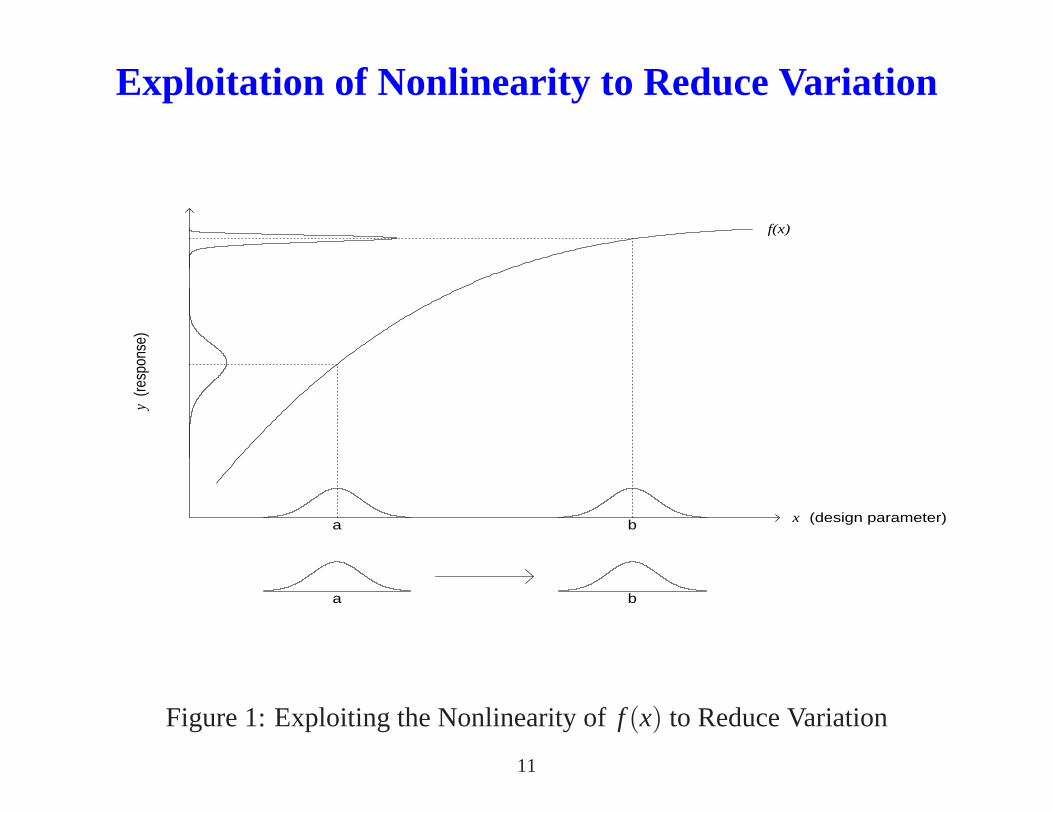
• From (1), it can be seen thatσ2 can be reduced by choosingxi0 with a smaller slope∂ f∂xi

∣

∣

∣

xi0

. This is demonstrated in Figure 1. Moving the nominal valuea to b can

reducevar(y) because the slope atb is more flat. This is aparameter designstep.

On the other hand, reducing the variation ofx arounda can also reducevar(y). This

is atolerance designstep.10

Exploitation of Nonlinearity to Reduce Variation

f(x)

x (design parameter)

y(re

spon

se)

a b

a b

Figure 1: Exploiting the Nonlinearity off (x) to Reduce Variation

11

Cross Array and Location-Dispersion Modeling

• Cross array = control array× noise array,

control array = array for control factors,

noise array = array for noise factors.

• Location-dispersion modeling

– compute ¯yi ,s2i based on the noise settings for theith control setting,

– analyze ¯yi (location), and lns2i (dispersion), identify significant location

and dispersion effects.

12

Two-step Procedures for Parameter Design

Optimization

• Two-Step Procedure for Nominal-the-Best Problem

(i) select the levels o f the dispersion f actors to minimize dispersion,

(ii) select the level o f the ad justment f actor to bring the location on target.(2)

• Two-Step Procedure for Larger-the-Better and Smaller-the-Better Problems

(i) select the levels o f the location f actors to maximize(or minimize)

the location,

(ii) select the levels o f the dispersion f actors that are not location

f actors to minimize dispersion.

(3)

Note that the two steps in (3) are in reverse order from those in (2).

Reason: It is usually harder to increase or decrease the responsey in the latter

problem, so this step should be the first to perform.

13

Analysis of Layer Growth Experiment

• From the ¯yi and lns2i columns of Table 5, compute the factorial effects for

location and dispersion respectively. (These numbers are not given in the

book.) From the half-normal plots of these effects (Figure 2), D is

significant for location andH, A for dispersion.

y = 14.352+0.402xD,

z = −1.822+0.619xA−0.982xH .

• Two-step procedure:

(i) chooseA at the “−” level (continuous rotation) andH at the “+” level

(nozzle position 6).

(ii) By solving

y = 14.352+0.402xD = 14.5,

choosexD= 0.368.14

Layer Growth Experiment: Analysis Results

Table 5: Means, Log Variances and SN Ratios, Layer Growth Experiment

Control Factor

A B C D E F G H yi lns2i ln y2i ηi

− − − + − − − − 14.79 -1.018 5.389 6.41

− − − + + + + + 14.86 -3.879 5.397 9.28

− − + − − − + + 14.00 -4.205 5.278 9.48

− − + − + + − − 13.91 -1.623 5.265 6.89

− + − − − + − + 14.15 -5.306 5.299 10.60

− + − − + − + − 13.80 -1.236 5.250 6.49

− + + + − + + − 14.73 -0.760 5.380 6.14

− + + + + − − + 14.89 -1.503 5.401 6.90

+ − − − − + + − 13.93 -0.383 5.268 5.65

+ − − − + − − + 14.09 -2.180 5.291 7.47

+ − + + − + − + 14.79 -1.238 5.388 6.63

+ − + + + − + − 14.33 -0.868 5.324 6.19

+ + − + − − + + 14.77 -1.483 5.386 6.87

+ + − + + + − − 14.88 -0.418 5.400 5.82

+ + + − − − − − 13.76 -0.418 5.243 5.66

+ + + − + + + + 13.97 -2.636 5.274 7.91

15

Layer Growth Experiment: Plots

• • • • • • • • • • • • ••

•

half-normal quantiles

abso

lute e

ffects

0.0 0.5 1.0 1.5 2.0 2.50.0

0.20.4

0.60.8

G C

H

D

location

• •• • • • • • • • •

••

•

•

half-normal quantiles

abso

lute e

ffects

0.0 0.5 1.0 1.5 2.0 2.5

0.00.5

1.01.5

2.0

AED

A

H

dispersion

Figure 2:Half-Normal Plots of Location and Dispersion Effects, Layer Growth Experiment

16

Analysis of Leaf Spring Experiment

• Based on the half-normal plots in Figure 3,B, C andE are significant for

location,C is significant for dispersion:

y = 7.6360+0.1106xB +0.0881xC +0.0519xE,

z = −3.6886+1.0901xC.

• Two-step procedure:

(i) chooseC at−.

(ii) With xC = −1, y = 7.5479+0.1106xB +0.0519xE.

To achieve ˆy = 8.0, xB andxE must be chosen beyond+1, i.e.,

xB = xE = 2.78. This is too drastic, and not validated by current data. An

alternative is to selectxB = xE = xC = +1 (not to follow the two-step

procedure), then ˆy=7.89 is closer to 8. (Note that ˆy = 7.71 withB+C−E+.)

Reason for the breakdown of the 2-step procedure: its secondstep cannot

achieve the target 8.0.17

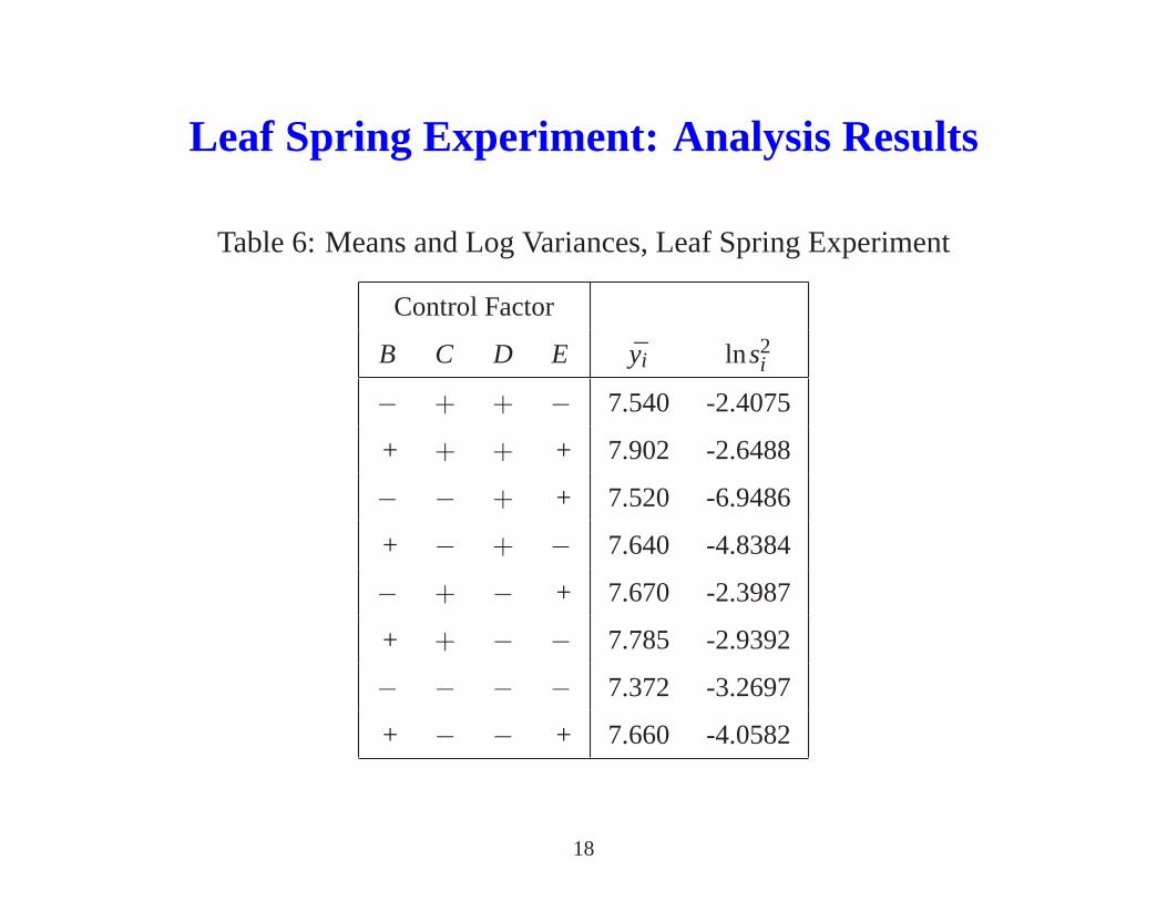
Leaf Spring Experiment: Analysis Results

Table 6: Means and Log Variances, Leaf Spring Experiment

Control Factor

B C D E yi lns2i

− + + − 7.540 -2.4075

+ + + + 7.902 -2.6488

− − + + 7.520 -6.9486

+ − + − 7.640 -4.8384

− + − + 7.670 -2.3987

+ + − − 7.785 -2.9392

− − − − 7.372 -3.2697

+ − − + 7.660 -4.0582

18

Leaf Spring Experiment: Plots

• • • •

•

•

•

half-normal quantiles

abso

lute e

ffects

0.0 0.5 1.0 1.5 2.00.0

50.1

5

BC BDD CD

E

C

B

location

•

••

••

•

•

half-normal quantiles

abso

lute e

ffects

0.0 0.5 1.0 1.5 2.0

0.51.0

1.52.0

B

BCE

BD

DCD

C

dispersion

Figure 3:Half-Normal Plots of Location and Dispersion Effects, LeafSpring Experiment

19

Response Modeling and Control-by-Noise

Interaction Plots

• Response Model: modelyi j directly in terms of control, noise effects and

control-by-noise interactions.

– half normal plot of various effects.

– regression model fitting, obtaining ˆy.

• Make control-by-noise interaction plots for significant effects iny, choose

robust control settings at which y has a flatter relationship with noise.

• ComputeVar(y) with respect to variation in the noise factors. CallVar(y)

thetransmitted variance model. Use it to identify control factor settings

with small transmitted variance.

20

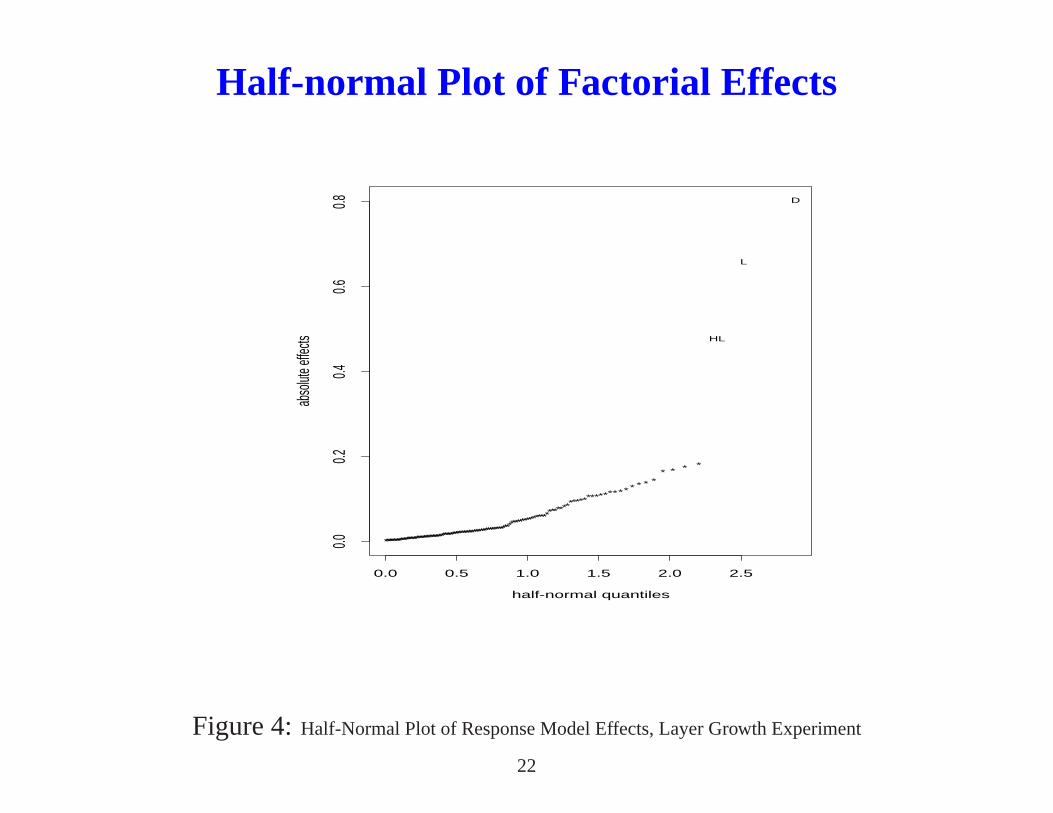
Half-normal Plot, Layer Growth Experiment

• Define

Ml = (M1 +M2)− (M3 +M4),

Mq = (M1 +M4)− (M2 +M3),

Mc = (M1 +M3)− (M2 +M4),

• From Figure 4, selectD, L, HL as the most significant effects.

• How to deal with the next cluster of effects in Figure 4? Usestep-downmultiple comparisons.

• After removing the top three points in Figure 4, make a half-normal plot

(Figure 5) on the remaining points. The cluster of next four effects

(Ml ,H,CMl ,AHMq) appear to be significant.

21

Half-normal Plot of Factorial Effects

half-normal quantiles

abso

lute e

ffects

0.0 0.5 1.0 1.5 2.0 2.5

0.00.2

0.40.6

0.8

********************************************************

***********************

****************

************

********** * * *

* * * *

HL

L

D

Figure 4:Half-Normal Plot of Response Model Effects, Layer Growth Experiment

22

Second Half-normal Plot of Factorial Effects

0.0 0.5 1.0 1.5 2.0 2.5

0.00

0.05

0.10

0.15

half−normal quantiles

abso

lute

effe

cts

AHMqCMl

HMl

Figure 5:Second Half-Normal Plot of Response Model Effects, Layer Growth Experiment

23

Control-by-noise Interaction Plots

L

13.8

14.2

14.6

-- +

H--

H+

M

14.1

14.3

14.5

1 2 3 4

C--

C+

Figure 6:H ×L andC×M Interaction Plots, Layer Growth Experiment

24

A×H ×M Plot

M

14.0

14.2

14.4

14.6

1 2 3 4

A--H--

A--H+

A+H--

A+H+

Figure 7:A×H ×M Interaction Plot, Layer Growth Experiment

25

Response Modeling, Layer Growth Experiment

• The following model is obtained:

y = 14.352+0.402xD +0.087xH +0.330xL −0.090xMl

−0.239xHxL −0.083xCxMl −0.082xAxHxMq. (4)

• Recommendations:

H: − (position 2) to+ (position 6)

A: + (oscillating) to− (continuous)

C: + (1210) to− (1220)

resulting in 37% reduction of thickness standard variation.

26

Predicted Variance Model• AssumeL, Ml andMq are random variables, taking−1 and+1 with equal

probabilities. This leads to

x2L = x2

Ml= x2

Mq= x2

A = x2C = x2

H = 1,

E(xL) = E(xMl ) = E(xMq) = 0,

Cov(xL,xMl ) = Cov(xL,xMq) = Cov(xMl ,xMq) = 0.

(5)

• From (4) and (5), we have

Var(y) = (.330− .239xH)2Var(xL)+(−.090− .083xC)2Var(xMl )

+(.082xAxH)2Var(xMq)

= constant+(.330− .239xH)2 +(−.090− .083xC)2

= constant−2(.330)(.239)xH +2(.090)(.083)xC

= constant− .158xH + .015xC.

• ChooseH+ andC−. But factorA is not present here. (Why? Seeexplanation on p. 532).

27

Estimation Capacity for Cross Arrays

• Example 1. Control array is a 23−1III design withI = ABC and the noise array

is a 23−1III design withI = abc. The resulting cross array is a 16-run 26−2

III

design withI = ABC = abc= ABCabc. Easy to show that all 9

control-by-noise interactions are clear, (but not the 6 main effects). This is

indeed a general result stated next.

Theorem: Suppose a 2k−p designdC is chosen for the control array, a 2m−q

designdN is chosen for the noise array, and a cross array, denoted by

dC⊗dN, is constructed fromdC anddN.

(i) If α1, . . . ,αA are the estimable factorial effects (among the control

factors) indC andβ1, . . . ,βB are the estimable factorial effects (among the

noise factors) indN, thenαi ,β j ,αiβ j for i = 1, . . . ,A, j = 1, . . . ,B are

estimable indC⊗dN.

(ii) All the kmcontrol-by-noise interactions (i.e., two-factor interactions

between a control factor main effect and a noise factor main effect) are clear

in dC⊗dN.

28

Cross Arrays or Single Arrays?

• Three control factorsA, B, C two noise factorsa, b: 23×22 design, allowing

all main effects and two-factor interactions to be clearly estimated.

• Use a single array with 16 runs for all five factors: a resolution V 25−1

design withI = ABCabor I = −ABCab, all main effects and two-factor

interactions are clear. (See Table 7)

• Single arrays can have smaller runs, but cross arrays are easier to use and

interpret.

29

32-run Cross Array and 16-run Single Arrays

Table 7: 32-Run Cross Array

a + + − −

b + − + −

Runs A B C

1–4 + + + • ◦ ◦ •

5–8 + + − ◦ • • ◦

9–12 + − + ◦ • • ◦

13–16 + − − • ◦ ◦ •

17–20 − + + ◦ • • ◦

21–24 − + − • ◦ ◦ •

25–28 − − + • ◦ ◦ •

29–32 − − − ◦ • • ◦

• : I = ABCab, ◦ : I = −ABCab,30

Comparison of Cross Arrays and Single Arrays

• Example 1 (continued) An alternative is to choose a single array 26−2IV design

with I = ABCa = ABbc = abcC. This is not advisable because no 2fi’s are

clear and only main effects are clear. (Why? We need to have some clear

control-by-noise interactions for robust optimization.) Abetter one is to use

a 26−2III design withI = ABCa = abc= ABCbc. It has 9 clear effects:

A,B,C,Ab,Ac,Bb,Bc,Cb,Cc (3 control main effects and 6 control-by-noise

interactions).

31

Signal-to-Noise Ratio

• Taguchi’s SN ratioη = ln y2

s2

• Two-step procedure:

1. Select control factor levels to maximize SN ratio,

2. Use an adjustment factor to move mean on target.

• Limitations

– maximizingy2 not always desired.

– little justification outside linear circuitry.

– statistically justifiable only whenVar(y) is proportional toE(y)2

• Recommendation: Use SN ratio sparingly. Better to use the

location-dispersion modeling or the response modeling. The latter strategies

can do whatever SN ratio analysis can achieve.

32

Half-normal Plot for S/N Ratio Analysis

• •

• ••

•• • • •

•

• •

•

•

half-normal quantiles

abso

lute

effe

cts

0.0 0.5 1.0 1.5 2.0 2.5

0.0

0.2

0.4

0.6

0.8

1.0

AED

A

H

Figure 8: Half-Normal Plots of Effects Based on SN Ratio, Layer Growth Exper-

iment

33

S/N Ratio Analysis for Layer Growth Experiment

• Based on theηi column in Table 5, compute the factorial effects using SN

ratio. From Figure 7, the conclusion is similar to location-dispersion

analysis. Why? Using

ηi = ln yi2− lns2

i ,

and from Table 5, the variation among lns2i is much larger than the variation

among ln ¯yi2; thus maximizing SN ratio is equivalent to minimizing lns2

i in

this case.

34

Comments on Board

35