Unit 29: Inference for Two-Way Tables - learner.org · Unit 29: Inference for Two-Way Tables | Faculty Guide | Page 1 Prerequisites Unit 13, Two-Way Tables is a prerequisite for this

Unit 29: Inference for Two-Way Tables | Faculty Guide | Page 1

PrerequisitesUnit 13, Two-Way Tables is a prerequisite for this unit. In addition, students need some background in significance tests, which was introduced in Unit 25.

Additional Topic CoverageAdditional coverage of inference for two-way tables can be found in The Basic Practice of Statistics, Chapter 23, Two Categorical Variables: The Chi-Square Test.

Activity DescriptionStudents should work in small groups on this activity. The activity consists of three parts. The first part provides a justification for the formula for computing the expected cell counts for chi-square tables. Students can work on Part I on their own or it could be part of a lecture/class discussion. Parts II and III involve two different structures for datasets, both of which are appropriate for the chi-square analysis covered in this unit.

Here are the two data structures: (1) subjects from a single sample are classified according to two categorical variables and (2) subjects from multiple samples (drawn from different populations) are classified according to a single categorical variable. In the latter case, “which sample” can be thought of as the second categorical variable. In the first case, a chi-square test for independence is performed; in the second case, a chi-square test for homogeneity is performed. The chi-square test statistics and the analyses are the same for both situations. So, in this unit, we have put little emphasis on distinguishing between these two situations.

Unit 29: Inference for Two-Way Tables

Unit 29: Inference for Two-Way Tables | Faculty Guide | Page 2

MaterialsFor Part III, bags of at least two different types of M&Ms are needed. Large-sized bags were used for the sample data, with the exception of the M&Ms minis, for which a medium bag was purchased. In addition, students will need paper plates or bowls to contain the M&Ms while they are being counted.

Part I: Introduction – Assumption of Independence and Expected Count Formula

Part I provides an explanation of the expected counts formula used in a chi-square test of independence. Students need to be familiar with the Multiplication Rule from Unit 19, Probability Models. This part could be approached either as an activity or as part of an informal lecture that introduces the topic of this activity. It could also be skipped and students could move directly to Part II.

Part II: Single Sample, Classified on Two Categorical Variables

For this part, students will need to collect data from people. The class could serve as the sample, or perhaps combine this class with another class, or have students add their friends to the sample. Students will need to classify each individual in the sample by gender and eye color. An easy way to collect the data is to draw a table on the board. Each student should come up to the board and put a tally line in the appropriate box for gender and eye color. After students have completed their entries, numbers can replace the tally marks. Students can then copy the table from the board and begin work on Part II.

Part III: Multiple Samples, Classified on One Categorical Variable

Students should work in groups to collect the data on the M&Ms colors. Again, you may want to put a chart on the board and have students enter their results for each color as they finish sorting their M&Ms into colors. Once the data are collected, groups will need a copy of the class data. Since the resulting two-way table is quite large, group members should be encouraged to divide up the work of computing the expected cell counts.

The color distribution of M&Ms differs by types and has changed over the years. You can write to Mars, the makers of M&Ms, for the latest color distribution in its candies.

Unit 29: Inference for Two-Way Tables | Faculty Guide | Page 3

The Video Solutions

1. Dr. Pardis Sabeti investigates the nonstop evolutionary arms race between our bodies and the infectious microorganisms that invade and inhabit them. In other words, she investigates connections between genotypes and protections from infectious diseases. Her work on Lassa fever is still in its early stages.

2. Sickle cell anemia hemoglobin mutation, HbS.

3. 0 : No association betweeen malaria and HbS.: Association between malaria and HbS. a

HH

4. Expected count = (row total)(column total)grand total

.

5. We reject the null hypothesis and conclude that there is an association between the HbS gene and malaria.

Unit 29: Inference for Two-Way Tables | Faculty Guide | Page 4

Unit Activity: Associations With Color Solutions

Part I: Introduction – Assumption of Independence and Expected Count Formula

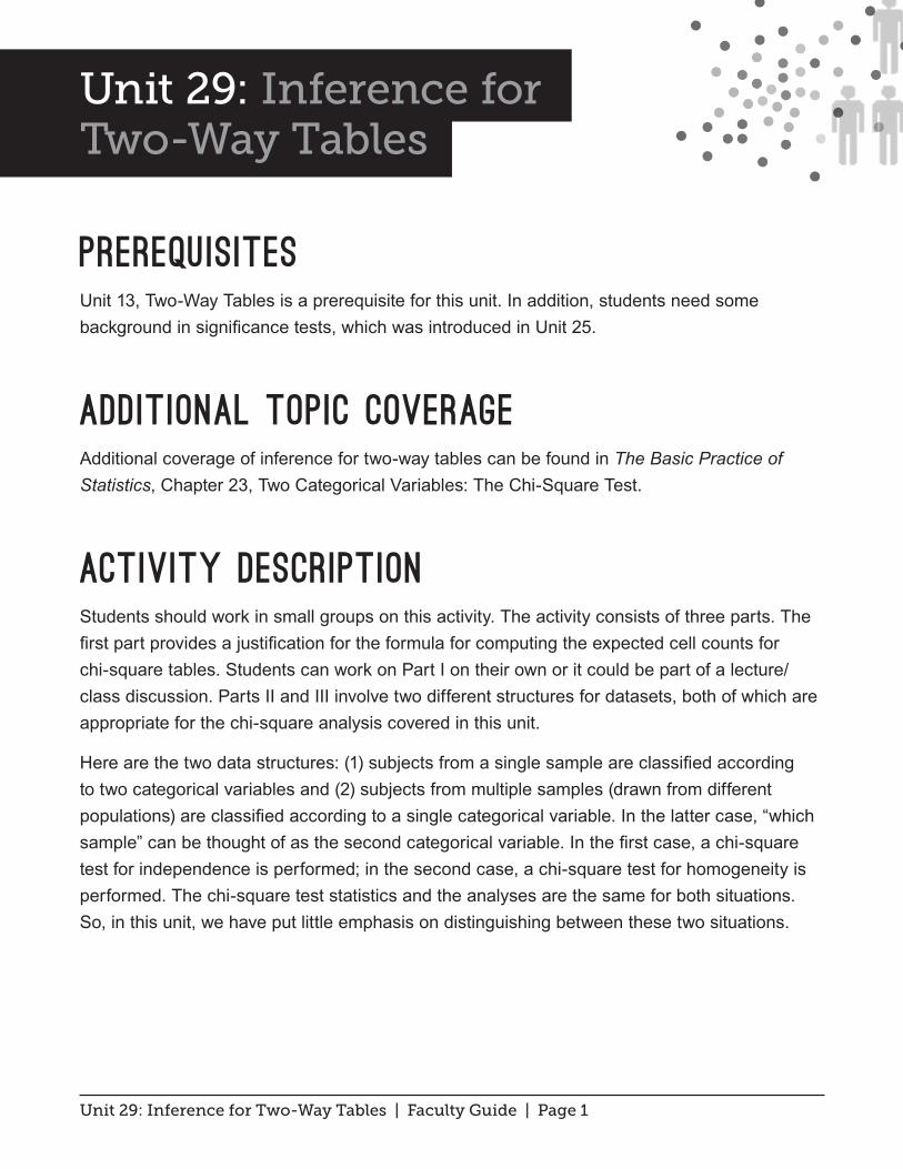
1. a. P(DEM and female) = P(DEM) P(female) = 196 246 0.1929500 500

≈

b. Expected number = 196500

⎛⎝⎜

⎞⎠⎟246500

⎛⎝⎜

⎞⎠⎟500( ) = 196( ) 246( )

500≈ 96.432

c. Expected count = (196)(246)500

» 96.432

d. P(DEM and male) = P(DEM)P(male) =196 254 0.1991500 500

≈

Expected number =196500

⎛⎝⎜

⎞⎠⎟254500

⎛⎝⎜

⎞⎠⎟500( ) = (196)(254)500

≈ 99.57

Expected count = (196)(254)500

» 99.57

2. a.

b. χ 2 = +107 − 96.43( )2

96.43+89 − 99.57( )2

99.57+ . . . +

56 − 60.45( )260.45

≈ 7.825

df = (3 – 1)(2 – 1) = 2; p ≈ 0.02

Expected Male Female Total Political DEM (Blue) 96.43 99.57 196 Preference GOP (Red) 91.02 93.98 185 Color IND (White) 58.55 60.45 119

Total 246 254 500

Activity  Solutions  2a

Unit 29: Inference for Two-Way Tables | Faculty Guide | Page 5

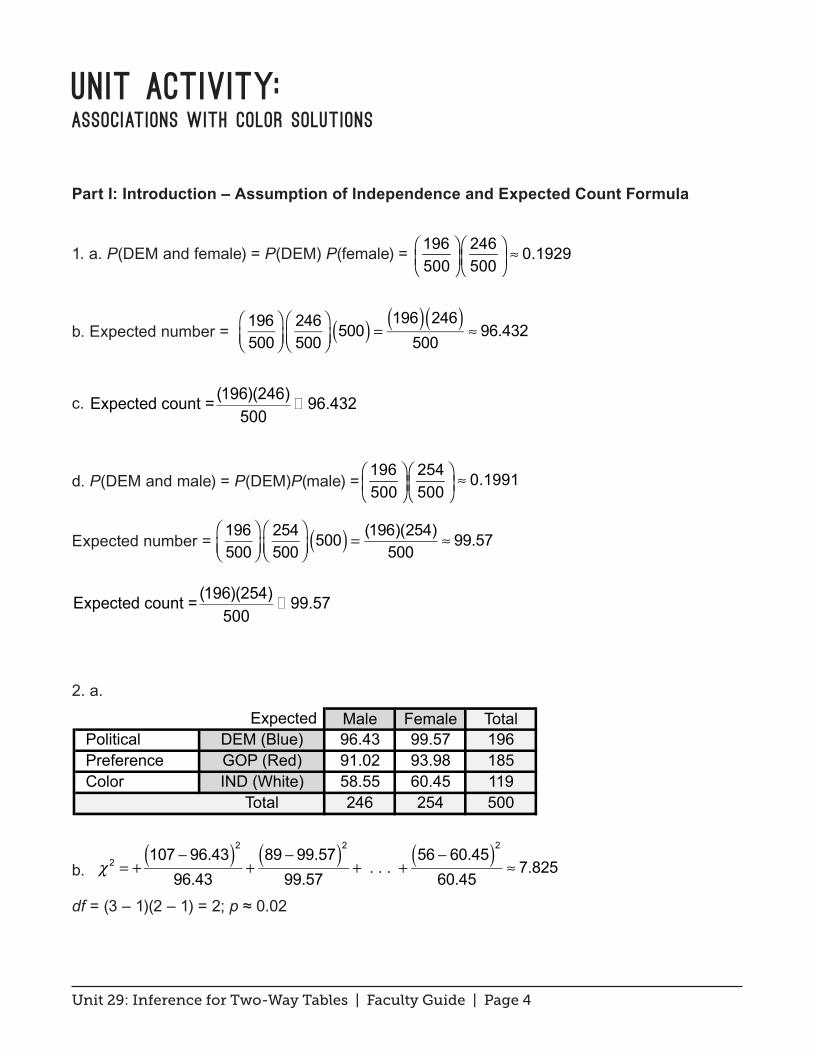
c. There is sufficient evidence to reject the null hypothesis. There is association between these two variables. In other words, they are dependent.

3. a. Sample data will be used to provide sample answers.

b. 0 : No association between gender and eye color.: Association between gender and eye color.a

HH

c. Sample answer:

d. Sample answer:

χ 2 =8 − 6.18( )26.18

+20 −18.55( )2

18.55+ . . . +

12− 8.73( )28.73

≈ 3.72 ; df = 2

p ≈ 0.151. There is insufficient evidence to reject the null hypothesis. In other words, there is no strong evidence to suggest that there is an association between eye color and gender.

4. a. Sample data (will be used for sample answers) (See next page...):

Count Blue Brown Other

Total 12 36 18 66

Activity  Solutions  3a

324 16 12

Male

FemaleGender

Eye Color Total

346208

Eye ColorCount Blue Brown Other Total

Gender Male 8 20 6 346.18 18.55 9.27

Female 4 16 12 325.82 17.45 8.73

Total 12 36 18 66

Activity  Solutions  3c

Unit 29: Inference for Two-Way Tables | Faculty Guide | Page 6

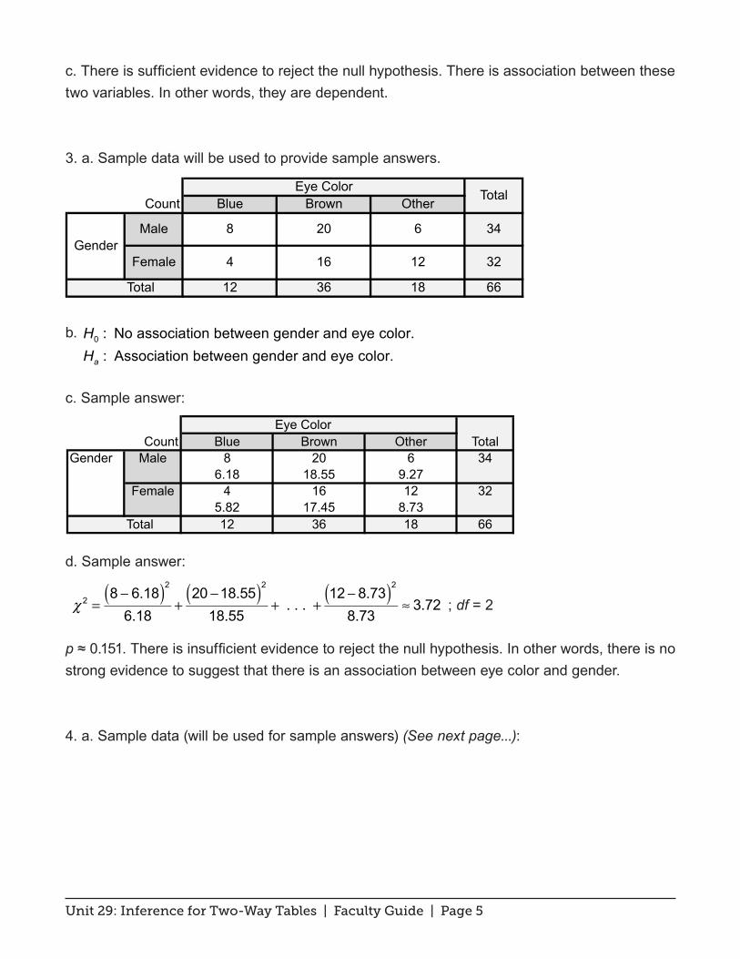
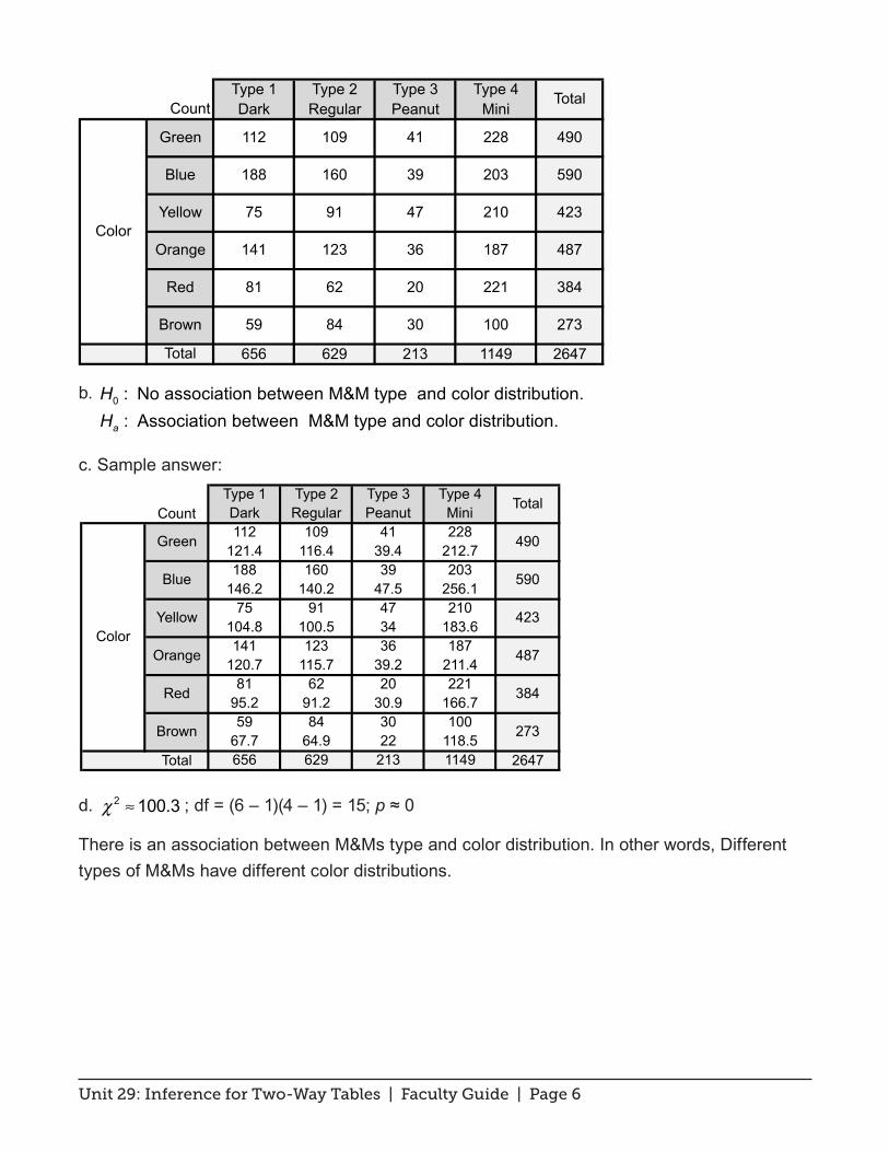
b. 0 : No association between M&M type and color distribution.: Association between M&M type and color distribution.a

HH

c. Sample answer:

d. χ 2 ≈100.3 ; df = (6 – 1)(4 – 1) = 15; p ≈ 0

There is an association between M&Ms type and color distribution. In other words, Different types of M&Ms have different color distributions.

Type 1 Type 2 Type 3 Type 4Count Dark Regular Peanut Mini

Total 656 629 213 1149 2647

Activity  Solutions  4a

Total

141

81 62 20 221

30 1008459

91 47 210

18736123Color

112 109 41 228

20339160188

75

Green

Blue

Yellow

Orange

Red

Brown

490

590

423

487

384

273

Type 1 Type 2 Type 3 Type 4Count Dark Regular Peanut Mini

112 109 41 228121.4 116.4 39.4 212.7188 160 39 203

146.2 140.2 47.5 256.175 91 47 210

104.8 100.5 34 183.6141 123 36 187

120.7 115.7 39.2 211.481 62 20 221

95.2 91.2 30.9 166.759 84 30 100

67.7 64.9 22 118.5Total 656 629 213 1149 2647

Activity  Solutions  4c

Color

273

Green

Blue

Yellow

Orange

Red

Brown

490

590

423

487

Total

384

Unit 29: Inference for Two-Way Tables | Faculty Guide | Page 7

Exercise Solutions

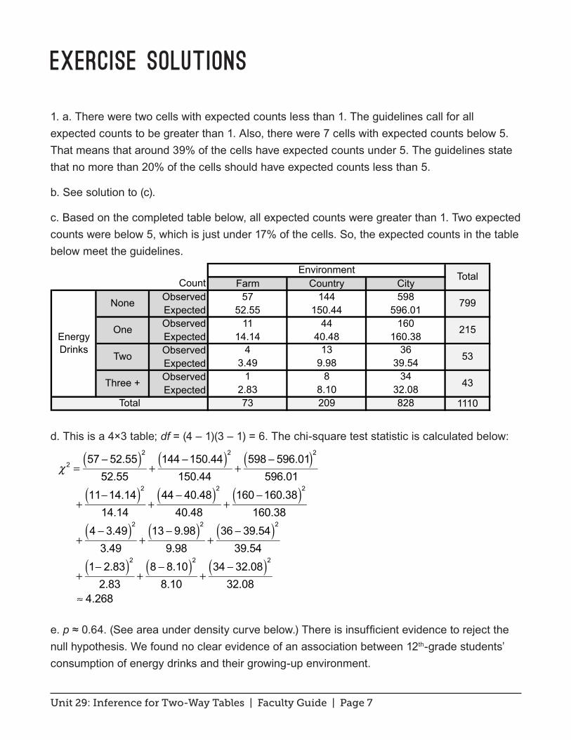
1. a. There were two cells with expected counts less than 1. The guidelines call for all expected counts to be greater than 1. Also, there were 7 cells with expected counts below 5. That means that around 39% of the cells have expected counts under 5. The guidelines state that no more than 20% of the cells should have expected counts less than 5.

b. See solution to (c).

c. Based on the completed table below, all expected counts were greater than 1. Two expected counts were below 5, which is just under 17% of the cells. So, the expected counts in the table below meet the guidelines.

d. This is a 4×3 table; df = (4 – 1)(3 – 1) = 6. The chi-square test statistic is calculated below:

χ 2 =57 − 52.55( )252.55

+144 −150.44( )2150.44

+598 − 596.01( )2

596.01

+11−14.14( )214.14

+44 − 40.48( )240.48

+160 −160.38( )2

160.38

+4 − 3.49( )23.49

+13 − 9.98( )29.98

+36 − 39.54( )2

39.54

+1− 2.83( )22.83

+8 − 8.10( )28.10

+34 − 32.08( )2

32.08 ≈ 4.268

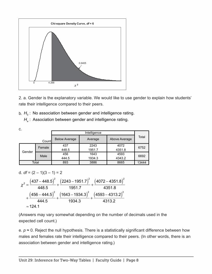
e. p ≈ 0.64. (See area under density curve below.) There is insufficient evidence to reject the null hypothesis. We found no clear evidence of an association between 12th-grade students’ consumption of energy drinks and their growing-up environment.

Count Farm Country CityObserved 57 144 598Expected 52.55 150.44 596.01Observed 11 44 160Expected 14.14 40.48 160.38Observed 4 13 36Expected 3.49 9.98 39.54Observed 1 8 34Expected 2.83 8.10 32.08

73 209 828 1110

Ex.  Solution  1(c  )

Energy Drinks

None

One

Two

Three +

Total

Environment Total

799

215

53

43

Unit 29: Inference for Two-Way Tables | Faculty Guide | Page 8

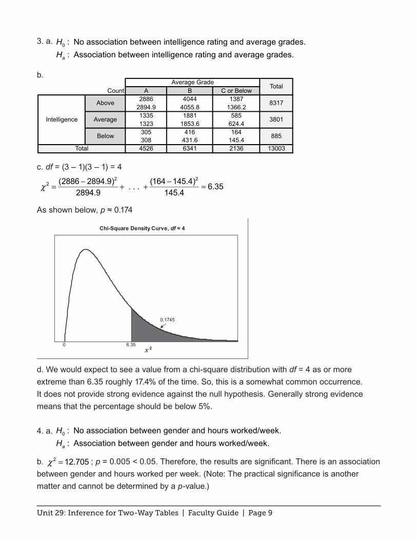
2. a. Gender is the explanatory variable. We would like to use gender to explain how students’ rate their intelligence compared to their peers.

b. 0 : No association between gender and intelligence rating.: Association between gender and intelligence rating. a

HH

c.

d. df = (2 – 1)(3 – 1) = 2

χ 2 =437 − 448.5( )2

448.5+2243 −1951.7( )2

1951.7+4072− 4351.8( )2

4351.8

+456 − 444.5( )2

444.5+1643 −1934.3( )2

1934.3+4593 − 4313.2( )2

4313.2 ≈124.1

(Answers may vary somewhat depending on the number of decimals used in the expected cell count.)

e. p ≈ 0. Reject the null hypothesis. There is a statistically significant difference between how males and females rate their intelligence compared to their peers. (In other words, there is an association between gender and intelligence rating.)

Χ4.268

0.6405

0

Chi-square Density Curve, df = 6

2

Count437 2243 4072

448.5 1951.7 4351.8456 1643 4593

444.5 1934.3 4343.2893 3886 8665 13444

Ex.  Solution  2c

6692

Female

MaleGender

Total

Below Average Average Above Average

IntelligenceTotal

6752

Unit 29: Inference for Two-Way Tables | Faculty Guide | Page 9

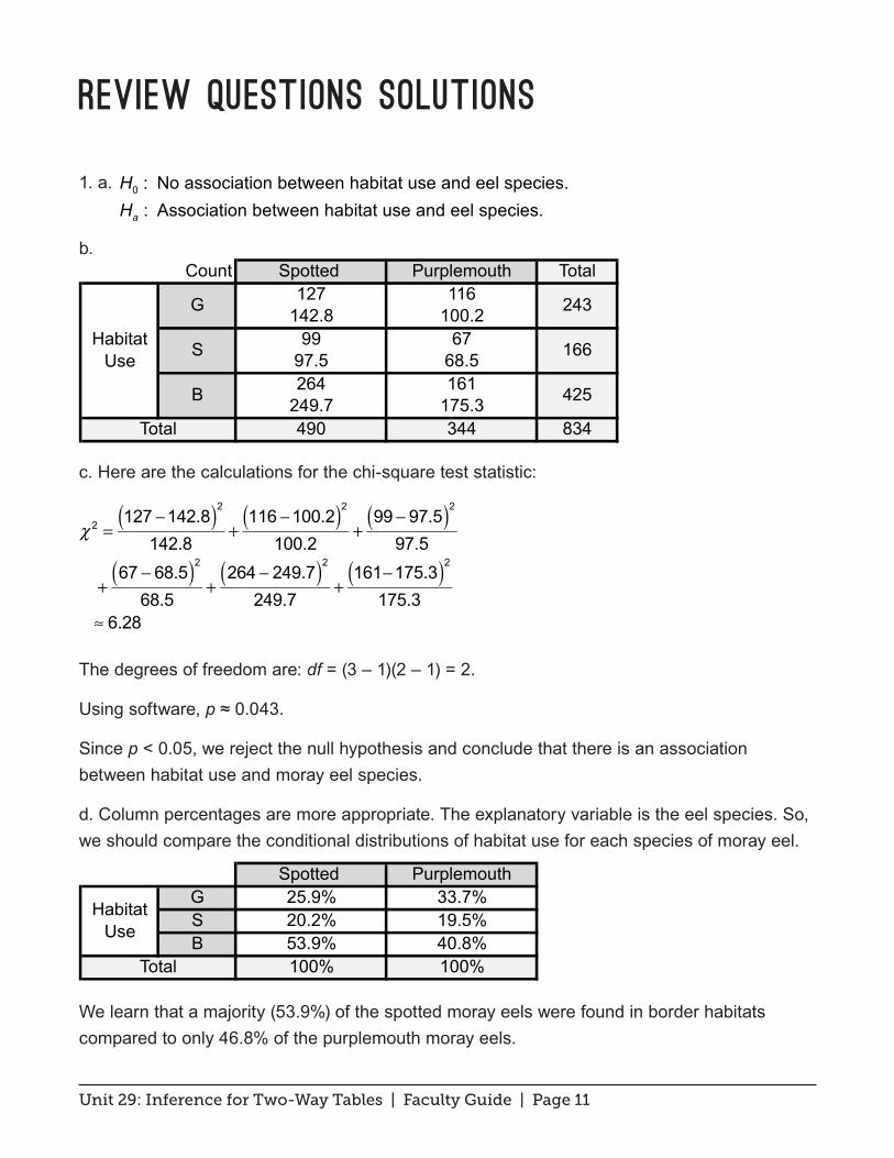
3. a. 0 : No association between intelligence rating and average grades.: Association between intelligence rating and average grades.a

HH

b.

c. df = (3 – 1)(3 – 1) = 4

χ 2 = (2886 − 2894.9)2

2894.9+ . . . + (164 −145.4)2

145.4≈ 6.35

As shown below, p ≈ 0.174

d. We would expect to see a value from a chi-square distribution with df = 4 as or more extreme than 6.35 roughly 17.4% of the time. So, this is a somewhat common occurrence. It does not provide strong evidence against the null hypothesis. Generally strong evidence means that the percentage should be below 5%.

4. a. 0 : No association between gender and hours worked/week.: Association between gender and hours worked/week.a

HH

b. χ 2 = 12.705 ; p = 0.005 < 0.05. Therefore, the results are significant. There is an association between gender and hours worked per week. (Note: The practical significance is another matter and cannot be determined by a p-value.)

Χ6.350

0.1745

Chi-Square Density Curve, df = 4

2

Count A B C or Below2886 4044 1387

2894.9 4055.8 1366.21335 1881 5851323 1853.6 624.4305 416 164308 431.6 145.44526 6341 2136 13003

Exercise Solution 3b

Intelligence

Total

Average Grade Total

8317

3801

885

Above

Average

Below

Unit 29: Inference for Two-Way Tables | Faculty Guide | Page 10

c. The biggest discrepancy in work patterns is that a higher percentage of males did not work (43.52%) compared to females (40.59%). Furthermore, in every category of hours worked/week, there is a higher percentage of females than males.

Unit 29: Inference for Two-Way Tables | Faculty Guide | Page 11

Review Questions Solutions

1. a. 0 : No association between habitat use and eel species.: Association between habitat use and eel species.a

HH

b.

c. Here are the calculations for the chi-square test statistic:

χ 2 =127 −142.8( )2142.8

+116 −100.2( )2100.2

+99 − 97.5( )2

97.5

+67 − 68.5( )268.5

+264 − 249.7( )2

249.7+161−175.3( )2

175.3 ≈ 6.28

The degrees of freedom are: df = (3 – 1)(2 – 1) = 2.

Using software, p ≈ 0.043.

Since p < 0.05, we reject the null hypothesis and conclude that there is an association between habitat use and moray eel species.

d. Column percentages are more appropriate. The explanatory variable is the eel species. So, we should compare the conditional distributions of habitat use for each species of moray eel.

We learn that a majority (53.9%) of the spotted moray eels were found in border habitats compared to only 46.8% of the purplemouth moray eels.

Count Spotted Purplemouth Total127 116

142.8 100.299 67

97.5 68.5264 161

249.7 175.3490 344 834

Review  Questions  Solutions  1b

Total

Habitat Use

G

S

B

243

166

425

Spotted PurplemouthG 25.9% 33.7%S 20.2% 19.5%B 53.9% 40.8%

100% 100%

Review  Questions  Solutions  1d

Habitat Use

Total

Unit 29: Inference for Two-Way Tables | Faculty Guide | Page 12

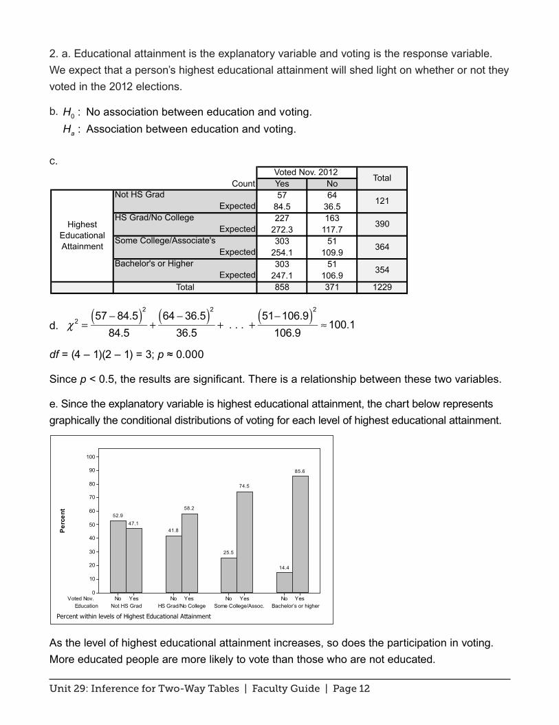
2. a. Educational attainment is the explanatory variable and voting is the response variable. We expect that a person’s highest educational attainment will shed light on whether or not they voted in the 2012 elections.

b. 0 : No association between education and voting.: Association between education and voting.a

HH

c.

d. χ 2 =57 − 84.5( )284.5

+64 − 36.5( )2

36.5+ . . . +

51−106.9( )2106.9

≈100.1

df = (4 – 1)(2 – 1) = 3; p ≈ 0.000

Since p < 0.5, the results are significant. There is a relationship between these two variables.

e. Since the explanatory variable is highest educational attainment, the chart below represents graphically the conditional distributions of voting for each level of highest educational attainment.

As the level of highest educational attainment increases, so does the participation in voting. More educated people are more likely to vote than those who are not educated.

Count Yes NoNot HS Grad 57 64

Expected 84.5 36.5HS Grad/No College 227 163

Expected 272.3 117.7Some College/Associate's 303 51

Expected 254.1 109.9Bachelor's or Higher 303 51

Expected 247.1 106.9Total 858 371 1229

Review Questions Solutions 2c

Highest Educational Attainment

Voted Nov. 2012 Total

121

390

364

354

EducationVoted Nov.

Bachelor’s or higherSome College/Assoc.HS Grad/No College Not HS GradYesNoYesNoYesNoYesNo

100

90

80

70

60

50

40

30

20

10

0

Perc

ent

85.6

14.4

74.5

25.5

58.2

41.847.1

52.9

Percent within levels of Highest Educational Attainment

Unit 29: Inference for Two-Way Tables | Faculty Guide | Page 13

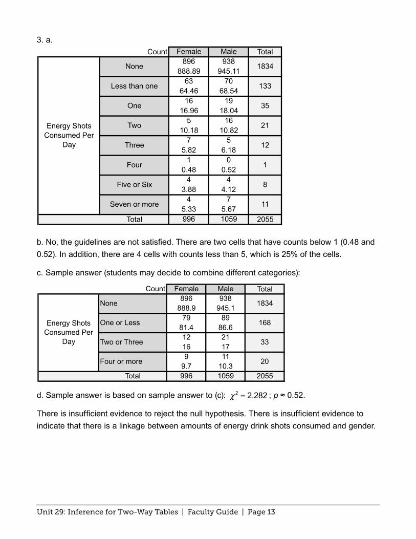
3. a.

b. No, the guidelines are not satisfied. There are two cells that have counts below 1 (0.48 and 0.52). In addition, there are 4 cells with counts less than 5, which is 25% of the cells.

c. Sample answer (students may decide to combine different categories):

d. Sample answer is based on sample answer to (c): χ 2 = 2.282 ; p ≈ 0.52.

There is insufficient evidence to reject the null hypothesis. There is insufficient evidence to indicate that there is a linkage between amounts of energy drink shots consumed and gender.

Count Female Male Total896 938

888.89 945.1163 70

64.46 68.5416 19

16.96 18.045 16

10.18 10.827 5

5.82 6.181 0

0.48 0.524 4

3.88 4.124 7

5.33 5.67Total 996 1059 2055

Review Questions Solutions 3a

8

11

1834

133

35

21

12

1

Energy Shots Consumed Per

Day

None

Less than one

One

Two

Three

Four

Five or Six

Seven or more

Count Female Male Total896 938

888.9 945.179 89

81.4 86.612 2116 179 11

9.7 10.3Total 996 1059 2055

Review  Questions  Solutions  3c

Energy Shots Consumed Per

Day

None

One or Less

Two or Three

Four or more

1834

168

33

20