Unified Multi-domain Decision Making: Cognitive Radio and Autonomous Vehicle Convergence Alexander Rian Young Dissertation submitted to the Faculty of the Virginia Polytechnic Institute and State University in partial fulfillment of the requirements for the degree of Doctor of Philosophy in Electrical Engineering Charles W. Bostian, Chair Kathleen Meehan Timothy Pratt Jeffrey H. Reed Craig A. Woolsey 7 December, 2012 Blacksburg, Virginia Keywords: Cognitive Radio, Autonomous Vehicles, Multi-domain Decision Making, Multi-objective Optimization Copyright c 2012 Alexander Rian Young

Welcome message from author
This document is posted to help you gain knowledge. Please leave a comment to let me know what you think about it! Share it to your friends and learn new things together.
Transcript

Unified Multi-domain Decision Making: CognitiveRadio and Autonomous Vehicle Convergence
Alexander Rian Young
Dissertation submitted to the Faculty of theVirginia Polytechnic Institute and State University
in partial fulfillment of the requirements for the degree of
Doctor of Philosophyin
Electrical Engineering
Charles W. Bostian, ChairKathleen MeehanTimothy PrattJeffrey H. ReedCraig A. Woolsey
7 December, 2012Blacksburg, Virginia
Keywords: Cognitive Radio, Autonomous Vehicles, Multi-domain Decision Making,Multi-objective Optimization
Copyright c©2012 Alexander Rian Young

Unified Multi-domain Decision Making: Cognitive Radio and AutonomousVehicle Convergence
Alexander Rian Young
(ABSTRACT)
This dissertation presents the theory, design, implementation and successful deployment of
a cognitive engine decision algorithm by which a cognitive radio-equipped mobile robot may
adapt its motion and radio parameters through multi-objective optimization. This provides a
proof-of-concept prototype cognitive system that is aware of its envirionment, its user’s needs,
and the rules governing its operation. It is to take intelligent action based on this awareness
to optimize its performance across both the mobility and radio domains while learning from
experience and responding intelligently to ongoing environmental mission changes. The
prototype combines the key features of cognitive radios and autonomous vehicles into a
single package whose behavior integrates the essential features of both.
The use case for this research is a scenario where a small unmanned aerial vehicle (UAV) is
traversing a nominally cyclic or repeating flight path (an “orbit”) seeking to observe targets
and where possible avoid hostile agents. As the UAV traverses the path, it experiences
varying RF effects, including multipath propagation and terrain shadowing. The goal is to
provide the capability for the UAV to learn the flight path with respect both to motion
and RF characteristics and modify radio parameters and flight characteristics proactively
to optimize performance. Using sensor fusion techniques to develop situaitonal awareness,
the UAV should be able to adapt its motion or communication based on knolwedge of (but
not limited to) physical location, radio performance, and channel conditions. Using sensor
information from RF and mobility domains, the UAV uses the mission objectives and its
knowledge of the world to decide on a course of action. The UAV develops and executes a
multi-domain action; action that crosses domains, such as changing RF power and increasing

its speed.
This research is based on a simple observation, namely that cognitive radios and autonomous
vehicles perform similar tasks, albeit in different domains. Both analyze their environment,
make and execute a decision, evaluate the result (learn from experience), and repeat as
required. This observation led directly to the creation of a single intelligent agent combining
cognitive radio and autonomous vehicle intelligence with the ability to leverage flexibility in
the radio frequency (RF) and motion domains. Using a single intelligent agent to optimize
decision making across both mobility and radio domains is unified multi-domain decision
making (UMDDM).
iii

Acknowledgments
This dissertation is the culmination of years of work. I have not been alone in this work,
but any attempt to thank those involved will be incomplete. Thank you to everyone.
I wish to thank Charles Bostian for all the opportunities and challenges, the gentle guidance
and the hard questions.
I have sorely missed Judy Hood over these past two years. While Judy was an administrator
nonpareil, Judy was also a friend and mentor, an excellent guide through the maze of graduate
school regulations, a sounding board for new ideas, and friendly ear when I just couldn’t
figure out how to deal with a confusing situation. I miss our discussions of books and art
and music and life. Thank you Judy.
Thank you to all the members of CWT, past and present. We made great things together,
and I am glad to have been part of so many compelling (neat!) projects. We challenged each
other, collaborated and competed, alternately working together smoothly and driving each
other crazy. But I wouldn’t change it.
Nick: hockey.py. Wow. This may not have started there, but that’s probably when I first
realized it was actually possible. Al: sometimes you drive me absolutely nuts. But if I can
explain something to your satisfaction, I’ve probably got it covered. Thank you to both of
you.
iv

I would like to thank my parents and siblings for all the love and support over many many
years.
Amanda, my wife, I thank you for everything. The promise of our future together and our
family has driven me forward, pulled me through to the end. Thank you, and yes.
Max, your wonder and excitement about the world, math, robots, the lab, about every-
thing. . . . You’ve opened my eyes once again to the wonders in the world around me.
Unless otherwise noted, all figures are the work of the author.
v

Grant Information
This material is based upon work supported by the National Science Foundation under Grant
No. CNS-0519959. Any opinions, findings, and conclusions or recommendations expressed
in this material are those of the author(s) and do not necessarily reflect the views of the
National Science Foundation (NSF).
This material is based on research sponsored by Air Force Research Laboratory under Agree-
ment # FA8750-11-2-0014. The views and conclusions contained herein are those of the
authors and should not be interpreted as necessarily representing the official policies or
endorsements, either expressed or implied, of Air Force Research Laboratory or the U.S.
Government.
vi

Contents
List of Figures xiv
List of Tables xviii
Acronyms xxi
1 Introduction 1
1.1 Summary and Overview . . . . . . . . . . . . . . . . . . . . . . . . . . . . . 1
1.2 Problem of Interest . . . . . . . . . . . . . . . . . . . . . . . . . . . . . . . . 5
1.3 Contributions . . . . . . . . . . . . . . . . . . . . . . . . . . . . . . . . . . . 8
1.4 This Work in the Context of My Research Assignment . . . . . . . . . . . . 8
1.5 Desired Results from this Research . . . . . . . . . . . . . . . . . . . . . . . 10
2 Literature Review 12
2.1 Introduction . . . . . . . . . . . . . . . . . . . . . . . . . . . . . . . . . . . . 12
2.2 Cognitive Radio . . . . . . . . . . . . . . . . . . . . . . . . . . . . . . . . . . 13
vii

2.3 Autonomous Vehicles . . . . . . . . . . . . . . . . . . . . . . . . . . . . . . . 19
2.4 CR/AV Convergence . . . . . . . . . . . . . . . . . . . . . . . . . . . . . . . 22
2.4.1 AVs with CR . . . . . . . . . . . . . . . . . . . . . . . . . . . . . . . 23
2.5 Conclusion . . . . . . . . . . . . . . . . . . . . . . . . . . . . . . . . . . . . . 26
3 Experiment Design and Philosophy 27
3.1 Introduction . . . . . . . . . . . . . . . . . . . . . . . . . . . . . . . . . . . . 27
3.2 Experimental Intent . . . . . . . . . . . . . . . . . . . . . . . . . . . . . . . 28
3.3 Experimental Design . . . . . . . . . . . . . . . . . . . . . . . . . . . . . . . 28
3.4 Evaluation of Test Results . . . . . . . . . . . . . . . . . . . . . . . . . . . . 29
3.5 Experimental Components . . . . . . . . . . . . . . . . . . . . . . . . . . . . 31
3.5.1 AVEP . . . . . . . . . . . . . . . . . . . . . . . . . . . . . . . . . . . 31
3.5.2 Node B Radio . . . . . . . . . . . . . . . . . . . . . . . . . . . . . . . 31
3.5.3 AVEP Test Bed . . . . . . . . . . . . . . . . . . . . . . . . . . . . . . 33
3.6 Experimental Procedure . . . . . . . . . . . . . . . . . . . . . . . . . . . . . 35
3.6.1 Experimental Data . . . . . . . . . . . . . . . . . . . . . . . . . . . . 35
3.6.2 Software Simulation . . . . . . . . . . . . . . . . . . . . . . . . . . . 36
3.6.3 Live Testing . . . . . . . . . . . . . . . . . . . . . . . . . . . . . . . . 36
3.7 Conclusion . . . . . . . . . . . . . . . . . . . . . . . . . . . . . . . . . . . . . 36
4 Hardware and Software Choices for System Implementation 38
viii

4.1 Introduction . . . . . . . . . . . . . . . . . . . . . . . . . . . . . . . . . . . . 38
4.2 Hardware Systems for Cognitive Radio . . . . . . . . . . . . . . . . . . . . . 39
4.2.1 Hardware Overview . . . . . . . . . . . . . . . . . . . . . . . . . . . . 39
4.2.2 Dispensing with SDR . . . . . . . . . . . . . . . . . . . . . . . . . . . 39
4.2.3 RFIC-Based RF Platforms for CR . . . . . . . . . . . . . . . . . . . . 41
4.2.4 Computational Platforms for Low Cost CR . . . . . . . . . . . . . . . 42
4.2.5 RF Hardware Selection . . . . . . . . . . . . . . . . . . . . . . . . . . 43
4.3 Robotics Hardware Systems Suitable for the Topic of this Dissertation . . . . 43
4.4 Research Hardware Platform: AVEP . . . . . . . . . . . . . . . . . . . . . . 44
4.4.1 Physical Components: SKIRL Radio Platform . . . . . . . . . . . . . 44
4.4.1.1 BeagleBoard-xM . . . . . . . . . . . . . . . . . . . . . . . . 44
4.4.1.2 Hope RF RFM22B . . . . . . . . . . . . . . . . . . . . . . . 47
4.4.1.3 Trainer Board . . . . . . . . . . . . . . . . . . . . . . . . . . 53
4.4.2 SKIRL Integration . . . . . . . . . . . . . . . . . . . . . . . . . . . . 54
4.4.3 Physical Components: NXT Brick and Chassis . . . . . . . . . . . . . 55
4.4.3.1 Sensors . . . . . . . . . . . . . . . . . . . . . . . . . . . . . 57
4.5 System Software . . . . . . . . . . . . . . . . . . . . . . . . . . . . . . . . . . 58
4.5.1 Software Options and Choices . . . . . . . . . . . . . . . . . . . . . . 58
4.5.2 System Architecture . . . . . . . . . . . . . . . . . . . . . . . . . . . 59
4.5.3 Radio Software . . . . . . . . . . . . . . . . . . . . . . . . . . . . . . 60
ix

4.5.3.1 Radio Driver . . . . . . . . . . . . . . . . . . . . . . . . . . 62
4.5.3.2 Radio API . . . . . . . . . . . . . . . . . . . . . . . . . . . 62
4.5.3.2.1 Listen Function . . . . . . . . . . . . . . . . . . . . 63
4.5.3.2.2 Receive Function . . . . . . . . . . . . . . . . . . . 64
4.5.3.2.3 Transmit Function . . . . . . . . . . . . . . . . . . 64
4.5.4 Motion Software . . . . . . . . . . . . . . . . . . . . . . . . . . . . . 66
4.5.4.1 Motion API . . . . . . . . . . . . . . . . . . . . . . . . . . . 68
4.6 Conclusion . . . . . . . . . . . . . . . . . . . . . . . . . . . . . . . . . . . . . 68
5 Algorithms and Software Development 70
5.1 Introduction . . . . . . . . . . . . . . . . . . . . . . . . . . . . . . . . . . . . 70
5.2 Operation and Control . . . . . . . . . . . . . . . . . . . . . . . . . . . . . . 71
5.2.1 Controller . . . . . . . . . . . . . . . . . . . . . . . . . . . . . . . . . 71
5.2.1.1 Controller Finite State Machine . . . . . . . . . . . . . . . . 71
5.2.1.1.1 FSM State: first time . . . . . . . . . . . . . . . . 71
5.2.1.1.2 FSM State: before traverse . . . . . . . . . . . . . 73
5.2.1.1.3 FSM State: traverse path . . . . . . . . . . . . . . 73
5.2.1.1.4 FSM State: after traverse . . . . . . . . . . . . . . 75
5.2.1.1.5 FSM State: go to beginning . . . . . . . . . . . . . 75
5.2.2 Sensors . . . . . . . . . . . . . . . . . . . . . . . . . . . . . . . . . . . 75
x

5.2.2.1 NXT Light Sensor . . . . . . . . . . . . . . . . . . . . . . . 76
5.2.2.2 NXT Color Sensor . . . . . . . . . . . . . . . . . . . . . . . 76
5.2.2.3 Barcode Reader . . . . . . . . . . . . . . . . . . . . . . . . . 77
5.2.3 Radio Subsystem . . . . . . . . . . . . . . . . . . . . . . . . . . . . . 78
5.2.3.1 Radio Subsystem Finite State Machine . . . . . . . . . . . . 78
5.2.3.2 Packet Structure . . . . . . . . . . . . . . . . . . . . . . . . 79
5.2.4 Motion Subsystem . . . . . . . . . . . . . . . . . . . . . . . . . . . . 82
5.2.4.1 Motion Subsystem Finite State Machine . . . . . . . . . . . 82
5.2.5 Motion Behavior: Follow The Line . . . . . . . . . . . . . . . . . . . 82
5.3 Path Data Structure . . . . . . . . . . . . . . . . . . . . . . . . . . . . . . . 83
5.4 Node B Radio Architecture . . . . . . . . . . . . . . . . . . . . . . . . . . . 86
5.5 Conclusion . . . . . . . . . . . . . . . . . . . . . . . . . . . . . . . . . . . . . 89
6 Learning and Decision Making 90
6.1 Introduction . . . . . . . . . . . . . . . . . . . . . . . . . . . . . . . . . . . . 90
6.2 Learn The Environment . . . . . . . . . . . . . . . . . . . . . . . . . . . . . 92
6.3 Decision Making . . . . . . . . . . . . . . . . . . . . . . . . . . . . . . . . . 93
6.3.1 Objective Functions . . . . . . . . . . . . . . . . . . . . . . . . . . . 94
6.3.1.1 Target/Anti-target Score . . . . . . . . . . . . . . . . . . . . 95
6.3.1.2 Time . . . . . . . . . . . . . . . . . . . . . . . . . . . . . . . 99
xi

6.3.1.3 Bit Error Rate . . . . . . . . . . . . . . . . . . . . . . . . . 104
6.3.1.4 Packet Delivery . . . . . . . . . . . . . . . . . . . . . . . . . 110
6.3.2 Decision Making Process . . . . . . . . . . . . . . . . . . . . . . . . . 113
6.4 Learn From Experience . . . . . . . . . . . . . . . . . . . . . . . . . . . . . . 115
6.5 Conclusion . . . . . . . . . . . . . . . . . . . . . . . . . . . . . . . . . . . . . 118
7 Experimental Results 119
7.1 Introduction . . . . . . . . . . . . . . . . . . . . . . . . . . . . . . . . . . . . 119
7.2 Simulation Results . . . . . . . . . . . . . . . . . . . . . . . . . . . . . . . . 120
7.2.1 Individual Objective Functions . . . . . . . . . . . . . . . . . . . . . 120
7.2.2 Multi-domain Decision Making in a Static Environment . . . . . . . . 123
7.2.3 Multi-domain Decision Making in a Simple Dynamic Environment . . 129
7.2.4 Multi-domain Decision Making in a Highly Dynamic Environment . . 132
7.3 Live Test Results . . . . . . . . . . . . . . . . . . . . . . . . . . . . . . . . . 136
7.3.0.1 Live Multi-domain Decision Making in a Static Environment 136
7.3.0.2 Live Multi-domain Decision Making in a Simple Dynamic
Environment . . . . . . . . . . . . . . . . . . . . . . . . . . 141
7.3.0.3 Live Multi-domain Decision Making in a Highly Dynamic
Environment . . . . . . . . . . . . . . . . . . . . . . . . . . 144
7.4 Conclusion . . . . . . . . . . . . . . . . . . . . . . . . . . . . . . . . . . . . . 148
xii

8 Conclusions 150
8.1 Summary . . . . . . . . . . . . . . . . . . . . . . . . . . . . . . . . . . . . . 150
8.2 Contributions . . . . . . . . . . . . . . . . . . . . . . . . . . . . . . . . . . . 153
8.3 Future Research . . . . . . . . . . . . . . . . . . . . . . . . . . . . . . . . . . 154
Bibliography 157
xiii

List of Figures
1.1 Conceptional representation of multi-domain action implemented by proof-of-
concept prototype mobile robot. . . . . . . . . . . . . . . . . . . . . . . . . . 2
1.2 xkcd comic that initiated my interest in CR and AV integration. R. Munroe,
New pet, http://xkcd.com/413/, Apr. 2008. [Online]. Available: http://xkcd.com/413/
Used under a Creative Commons Attribution-NonCommercial license. . . . . 3
1.3 UAV on SAR search mission using RF and motion flexibility to maintain
connectivity and ensure mission success. This UAV is part of a proposal that
extends the research in this dissertation. . . . . . . . . . . . . . . . . . . . . 11
3.1 Autonomous vehicle experiment platform . . . . . . . . . . . . . . . . . . . . 32
3.2 Photograph of AVEP test bed. . . . . . . . . . . . . . . . . . . . . . . . . . . 33
3.3 The central aspect of test bed graph is three paths (edges) that diverge from
the decision point at Node 1 and converge again at Node 2. . . . . . . . . . . 34
4.1 Autonomous vehicle experiment platform . . . . . . . . . . . . . . . . . . . . 45
4.2 BeagleBoard-xM single board computer. c©2013 IEEE, used with permission. 46
4.3 Hope RF RFM22B FSK RFIC. c©2013 IEEE, used with permission. . . . . . 47
xiv

4.4 CW power delivered to a 50 ohm load as a function of carrier frequency for a
stock 433 MHz RFM22B and for the same module with the output networks
removed. c©2013 IEEE, used with permission. . . . . . . . . . . . . . . . . . 48
4.5 RFM22B reference implementation. Hope Microelectronics Co., RFM22B
FSK transceiver - FSK modules - HOPE microelectronics, 2012. [Online].
Available http://www.hoperf.com. Used with permission. . . . . . . . . . . . 49
4.6 RFM22B transmit filter network. . . . . . . . . . . . . . . . . . . . . . . . . 49
4.7 RFM22B transmit filter network with bypass. The dotted line show the im-
plemented short circuit used to bypass the filter network. . . . . . . . . . . . 49
4.8 RSSI values as a function of CW RF power at the antenna terminal. c©2013
IEEE, used with permission. . . . . . . . . . . . . . . . . . . . . . . . . . . . 50
4.9 Receiver’s passband characteristics. c©2013 IEEE, used with permission. . . 51
4.10 Sample of memory registers set and read on the RFM22B. Hope Microelec-
tronics Co., RFM22B FSK transceiver - FSK modules - HOPE microelectron-
ics, 2012. [Online]. Available http://www.hoperf.com. Used with permission. 52
4.11 BeagleBoard-xM trainer board. . . . . . . . . . . . . . . . . . . . . . . . . . 53
4.12 SKIRL radio package, showing BeagleBoard-xM, trainer board, and RFM22B. 54
4.13 SKIRL schematic showing individual components along with their functions.
c©2013 IEEE, used with permission. . . . . . . . . . . . . . . . . . . . . . . . 55
4.14 NXT Brick and chassis. . . . . . . . . . . . . . . . . . . . . . . . . . . . . . . 56
4.15 Conceptual AVEP system architecture showing components and process flow. 59
4.16 High-layer software organization of AVEP system. . . . . . . . . . . . . . . . 60
xv

4.17 AVEP radio software stack. c©2013 IEEE, used with permission. . . . . . . . 61
4.18 Radio software stack compared to SKIRL hardware components. c©2013
IEEE, used with permission. . . . . . . . . . . . . . . . . . . . . . . . . . . . 61
4.19 Flow chart showing logic and flow of API’s listen function. . . . . . . . . . . 65
4.20 Flow chart showing logic and flow of API’s receive function. . . . . . . . . . 66
4.21 Flow chart showing logic and flow of API’s transmit function. . . . . . . . . 67
5.1 AVEP controller finite state machine. . . . . . . . . . . . . . . . . . . . . . . 72
5.2 RF subsystem packet structure. . . . . . . . . . . . . . . . . . . . . . . . . . 80
5.3 Organization of flags field in RF subsystem packet. This figure shows the flags
available to a Node A radio. . . . . . . . . . . . . . . . . . . . . . . . . . . . 81
5.4 The test bed graph contains three separate paths between Node 1 and Node 2. 84
5.5 A more complicated test bed layout with additional nodes and edges, and
their attendant paths. . . . . . . . . . . . . . . . . . . . . . . . . . . . . . . 86
5.6 Organization of flags field in RF subsystem packet. This figure shows the flags
available to a Node B radio for communication with a Node A radio. . . . . 88
6.1 The ODA loop applied to CR and AV scenarios. . . . . . . . . . . . . . . . . 91
6.2 The cognition cycle used by the AVEP. . . . . . . . . . . . . . . . . . . . . . 92
6.3 Graphical representation of Z objective function as a function of targets and
anti-targets. . . . . . . . . . . . . . . . . . . . . . . . . . . . . . . . . . . . . 98
6.4 Experimentally recorded values of time (to travel a fixed-length path) and
requisite AVEP rotor power values, with 3rd order polynomial fit. . . . . . . 100
xvi

6.5 Graphical representation of T objective function as a function of path distance
and rotor power. . . . . . . . . . . . . . . . . . . . . . . . . . . . . . . . . . 103
6.6 BER waterfall curve for noncoherent FSK. . . . . . . . . . . . . . . . . . . . 107
6.7 Eb/N0 values as a function of SNR and Rs. . . . . . . . . . . . . . . . . . . . 108
6.8 Graphical representation of B objective function as a function of SNR and Rs. 109
6.9 Graphical representation of G objective function as a function of time and bit
rate. . . . . . . . . . . . . . . . . . . . . . . . . . . . . . . . . . . . . . . . . 112
7.1 AVEP in operation during a live test experiment. . . . . . . . . . . . . . . . 136
xvii

List of Tables
3.1 Path length (in meters) of each path in the test bed. . . . . . . . . . . . . . 34
5.1 Values returned by the NXT color sensor and their associated colors. . . . . 76
5.2 Knobs and meters available stored in path data structure. . . . . . . . . . . 85
6.1 Rotor power and time measurements for AVEP, used to determine AVEP
velocity. . . . . . . . . . . . . . . . . . . . . . . . . . . . . . . . . . . . . . . 99
7.1 Environmental parameters (meters) used in evaluating UMDDM in a static
environment. . . . . . . . . . . . . . . . . . . . . . . . . . . . . . . . . . . . 123
7.2 Results of UMDDM decision making simulation in a static environment over
20 iterations. . . . . . . . . . . . . . . . . . . . . . . . . . . . . . . . . . . . 124
7.3 Solutions generated by decision maker on iterations 4, 5, and 10, and the
scores associated with each solution. . . . . . . . . . . . . . . . . . . . . . . 125
7.4 Parameters associated with solutions shown in Table 7.3. . . . . . . . . . . . 125
7.5 Results of UMDDM decision making simulation in a static environment with
N = −82 dBm. . . . . . . . . . . . . . . . . . . . . . . . . . . . . . . . . . . 127
xviii
7.6 Solutions generated by decision maker for simulated environment where N =
−82 dBm. . . . . . . . . . . . . . . . . . . . . . . . . . . . . . . . . . . . . . 128
7.7 Parameters associated with solutions shown in Table 7.6. . . . . . . . . . . . 128
7.8 Environmental parameters (meters) used in evaluating UMDDM in a simple
dynamic environment. . . . . . . . . . . . . . . . . . . . . . . . . . . . . . . 129
7.9 Results of UMDDM decision making simulation in a simple dynamic environ-
ment over 20 iterations. . . . . . . . . . . . . . . . . . . . . . . . . . . . . . 130
7.10 Solutions generated by decision maker in a simple dynamic environment, and
the scores associated with each solution. . . . . . . . . . . . . . . . . . . . . 131
7.11 Parameters associated with solutions shown in Table 7.10. . . . . . . . . . . 131
7.12 Environmental parameters (meters) used in evaluating UMDDM in a highly
dynamic environment. . . . . . . . . . . . . . . . . . . . . . . . . . . . . . . 133
7.13 Results of UMDDM decision making simulation in a highly dynamic environ-
ment over 10 iterations. . . . . . . . . . . . . . . . . . . . . . . . . . . . . . 134
7.14 Solutions generated by decision maker in a highly dynamic environment, and
the scores associated with each solution. . . . . . . . . . . . . . . . . . . . . 135
7.15 Parameters associated with solutions shown in Table 7.14. . . . . . . . . . . 135
7.16 Environmental parameters (meters) used in evaluating live UMDDM in a
static environment. . . . . . . . . . . . . . . . . . . . . . . . . . . . . . . . . 137
7.17 Results of live UMDDM in a static environment over 10 iterations. . . . . . . 137
7.18 Solutions generated by decision maker during live tests in a static environment.138
7.19 Parameters associated with solutions shown in Table 7.18. . . . . . . . . . . 139
xix

7.20 Results of live UMDDM in a static environment over 10 iterations using higher
noise floor. . . . . . . . . . . . . . . . . . . . . . . . . . . . . . . . . . . . . . 139
7.21 Solutions generated by decision maker during live tests in a static environment
with higher noise floor. . . . . . . . . . . . . . . . . . . . . . . . . . . . . . . 139
7.22 Parameters associated with solutions shown in Table 7.18. . . . . . . . . . . 140
7.23 Environmental parameters (meters) used in evaluating UMDDM in a simple
dynamic environment during a live experiment. . . . . . . . . . . . . . . . . 141
7.24 Results of live UMDDM in a simple dynamic environment over 10 iterations
in a live experiment. . . . . . . . . . . . . . . . . . . . . . . . . . . . . . . . 142
7.25 Solutions generated by decision maker during live tests in a simple dynamic
environment. . . . . . . . . . . . . . . . . . . . . . . . . . . . . . . . . . . . 143
7.26 Parameters associated with solutions shown in Table 7.25. . . . . . . . . . . 143
7.27 Environmental parameters (meters) used in evaluating UMDDM in a highly
dynamic environment during a live experiment. . . . . . . . . . . . . . . . . 145
7.28 Results of live UMDDM in a simple dynamic environment over 10 iterations
in a live experiment. . . . . . . . . . . . . . . . . . . . . . . . . . . . . . . . 146
7.29 Solutions generated by decision maker in a highly dynamic environment during
a live experiment. . . . . . . . . . . . . . . . . . . . . . . . . . . . . . . . . . 146
7.30 Parameters associated with solutions shown in Table 7.29. . . . . . . . . . . 147
xx

Acronyms
ABM agent based modeling.
AFRL Air Force Research Lab.
AI artificial intelligence.
API application programming interface.
ASIC application-specific integrated circuit.
AV autonomous vehicle.
AVEP autonomous vehicle experimental platform.
AWGN additive white gaussian noise.
BAA broad agency announcement.
BER bit error rate.
CAM communication-aware motion.
CE cognitive engine.
CN cognitive network.
CNI Communication Networks Insittute.
CORNET Cognitive Radio Network Testbed.
CR cognitive radio.
xxi

CRC cyclic redundancy check.
CRE cognitive radio engine.
CRS cognitive radio system.
CSERE Cognitive System Enabling Radio Evolution.
CW continuous wave.
CWT Center for Wireless Telecommunications.
DARPA Defense Advanced Research Projects Agency.
DGC DARPA Grand Challenge.
DRC DARPA Robotics Challenge.
DS dynamic spectrum.
DSA dynamic spectrum access.
DSP digital signal processing.
DSS dynamic spectrum sharing.
DUC DARPA Urban Challenge.
EIRP equivalent isotropically radiated power.
EM electromagnetic radiation.
FIFO first in first out.
FSK frequency shift keying.
FSM finite state machine.
GA genetic algorithm.
GFSK gassian frequency shift keying.
xxii

GPIO general purpose I/O.
GPS global positioning system.
I/O input/output.
I2C inter-integrated circuit.
LBT listen before talk.
MAC media access control.
MAV micro air vehicle.
MCDM multiple criteria decision making.
MCU microcontroller unit.
MDDM multi-domain decision making.
MDF mission data file.
MoE measure of effectiveness.
MOO multi-objective optimization.
MOT motion.
MUAV micro unmanned aerial vehicle.
NAR Node A radio.
NBR Node B radio.
NSGA nondominated sorting genetic algorithm.
ODA observe, decide, and act.
OE Open Embedded.
xxiii

OOK on-off keying.
OS operating system.
OTA over the air.
P/MAC position/motion-aware communication.
PDS path data structure.
PHY physical layer.
POMDP partially observed Markov decision process.
PU primary user.
QoS quality of service.
RCR railway cognitive radio.
RF radio frequency.
RFIC radio frequency integrated circuit.
RNDF route network definition file.
RSSI received signal strength indicator.
RX receive.
SDR software define radio.
SNR signal-to-noise ratio.
SPI serial peripheral interface.
SU secondary user.
T/R transmit/receive.
xxiv

TCP transmission control protocol.
TX transmit.
UAV unmanned aerial vehicle.
UGV unmanned ground vehicle.
UMDDM unified multi-domain decision making.
USB universal serial bus.
USRP Universal Software Radio Peripheral.
USV unmanned surface vehicle.
V2I vehicle-to-infrastructure.
V2V vehicle-to-vehicle.
VN vehicular network.
VT Virginia Tech.
WARP Wireless Open-Access Research Platform.
WNaN Wireless Network after Next.
XG neXt Generation.
xxv

Chapter 1
Introduction
1.1 Summary and Overview
This dissertation deals with cognitive radios (CRs)—intelligent radio frequency (RF) com-
munication systems—and autonomous vehicles (AVs)—vehicles capable of intelligent and
independent motion. In this research, I present the first true integration of AV and CR,
combining radio learning and environmental learning into a single intelligent agent: a proof-
of-concept prototype mobile robot that can adapt its motion and radio parameters through
multi-objective optimization. Using sensor information from RF and mobility domains, the
robot uses mission objectives and its knowledge of the world to decide on a course of action.
The robot develops and executes a multi-domain action; action that crosses domains, such
as changing RF power and increasing its speed. A conceptual representation of this process
is shown in Figure 1.1.
The idea for this dissertation began with a small seed, a kernel of thought planted by a web
comic. The xkcd web comic called “New Pet,” shown in Figure 1.2 [1], shows a small robot
1

2
Figure 1.1: Conceptional representation of multi-domain action implemented by proof-of-concept prototype mobile robot.
built using a net book computer, and using Python [2] to provide the robot with a soul. While
this is clearly a joke, Python is very flexible and powerful. Python has been used repeatedly
and successfully to build and control robots. When I read the web comic, I realized that in
our research at the Virginia Tech (VT) Center for Wireless Telecommunications (CWT), we
were already using Python to build software define radio (SDR) and CR applications using
GNU Radio [3]. This idea developed further with the simple but fundamental observation
that CRs and AVs perform similar tasks, albeit in different domains:
• Analyze their environment,
• Make and execute a decision,
• Evaluate the result (learn from experience), and
• Repeat as required.
CR and AV research highlights the limitations of current systems. While visiting an un-
3
Figure 1.2: xkcd comic that initiated my interest in CR and AV integration. R. Munroe,New pet, http://xkcd.com/413/, Apr. 2008. [Online]. Available: http://xkcd.com/413/Used under a Creative Commons Attribution-NonCommercial license.

4
manned aerial vehicle (UAV) lab, I observed a simulation that replayed results obtained
during live flight UAV tests. The UAV under test flew a nominally repeating flight path over
a large field, while transmitting and receiving RF data packets. Every time the UAV passed
over a certain corner of the field, the UAV experienced poor RF performance. Yet the UAV
continued to fly the same path on every iteration, making no change in RF parameters or
motion behavior.
As mobile sensor platforms, AVs are the perfect example of agents that must operate in
both the RF and physical domains, maintaining mission and communications situational
awareness based on input from a variety of sensors and making intelligent decisions based
on this awareness. This research is based on two fundamental assumptions:
1. The need to move affects AV communication, and
2. The need to communicate affects AV motion.
The first point is known by everyone who uses a cell phone; everyone has a story to tell about
a certain part of their commute where their cell phone coverage always drops out. Com-
munications researchers know that shadowing and multipath are highly location dependent,
and can vary greatly over very short distances.
To illustrate the second, consider that AVs are effectively mobile sensor platforms. AVs are
used as data collection platforms across a wide variety of application domains, including
tactical [4], disaster response [5, 6], and environmental and wildlife management [7, 8] oper-
ations. In all these cases, the collection of information, and subsequent relay of the same to
those who need the information, is critical to AV mission success.
Faced with the above, a scenario in which an AV requires effective communications, and
where the vehicle’s inherent motion and mobility intrinsically affect that same communica-
tions, it becomes imperative to consider motion and communications together, a coupled

5
problem with a coupled solution.
1.2 Problem of Interest
Currently autonomous vehicles do not use RF information in their decision making process;
that is, no AV uses RF information for unified multi-domain decision making. From the
perspective of an operational AV, possible courses of action that could improve the RF
environment do not exist and are not considered in any decision making process.
The intent of this research is to combine RF and other information for a unified decision
making progress. I expect to improve mission performance by potentially trading off RF
with other mission parameters. The result is a system with two equally important degrees
of freedom:
• RF agility, and
• Physical mobility (motion).
Although CRs and AVs are very similar, the two research fields have essentially no crossover
or shared experience: each field of research has developed independent of the other. Any
attempt to combine the two fields will necessarily run into challenges and constraints from
both. The development of a suitable experimental platform is one such challenge, one that
presents challenges in traditional AV research topics such as motion planning, route planning,
and positioning, as well as radio and CR topics like physical layer (PHY) adaptation, media
access control (MAC) protocols, data packet structure, and synchronization. However, in
both domains, these are well developed fields of research and many good solutions have been
presented already. This research will build that work, abstracting out the complexity of
the underlying issues involved in platform development to focus on the true topic of this

6
research. Specifically, simplified methods of motion planning, route planning, positioning,
PHY reconfiguration, and media access have been implemented, resulting in a platform that
focuses on the areas where CR and AV cognition come together, and not the details of CR
and AV implementation.
These ideas ultimately led to the work described in detail here: an implementation of the
VT cognitive engine (CE) on a BeagleBoard-xM single board computer based on the Texas
Instruments DM3730 processor and its successful use to provide simultaneous intelligent
control of a frequency-agile and mode-agile radio and an autonomous vehicle. This provides
a proof-of-concept prototype of a cognitive system that is aware of its environment, its users
needs, and the rules governing its operation, and able to take intelligent action based on
this awareness to optimize its performance across both the mobility and radio domains while
learning from experience and responding intelligently to ongoing environmental and mission
changes. It combines the key features of CRs and AVs into a single package whose behavior
integrates the essential aspects of both.
The use case for this research is a scenario where a small UAV is traversing a nominally
cyclic or repeating flight path (an orbit) seeking to observe targets and where possible avoid
hostile agents. As the UAV traverses the path, it experiences varying RF effects, including
multipath propagation and terrain shadowing. The goal is to provide the capability for the
UAV to learn the flight path with respect both to motion and RF characteristics and modify
radio parameters and flight characteristics proactively to optimize performance. Using sensor
fusion techniques to develop situational awareness, the UAV should be able to adapt its
motion or communication based on knowledge of (but not limited to) physical location,
radio performance, and channel conditions. Using sensor information from RF and motion
(MOT) domains, the UAV uses the mission objectives and its knowledge of the world, to
decide on a course of action. The UAV develops and executes a multi-domain action; action

7
that crosses domains, such as changing the RF power and increasing its speed.
I present in detail the design of a low-cost (less than $250) package called SKIRL, based
on the BeagleBoard-XM computer and the Hope RF RFM22B RF integrated circuit that
is suitable for installation in the small experimental UAVs flown by USAFRL. In the work
documented here, SKIRL is integrated with a set of target, navigational, and environmental
sensors mounted on a LEGO wheeled vehicle that executes a hypothetical two-dimensional
mission based on the UAV use case while avoiding the costs and potential security problems
associated with a flight test. Experiments with the system demonstrate its ability to explore
and learn a multidimensional environment that combines changing RF, location, and mission
data and to optimize its mission performance intelligently. So far as I am aware, this is the
first successful demonstration of its kind.
Beginning with a review of the literature of CR cognitive radio and AV research, I discuss
the rationale for combining the two technologies and move through the practical steps of
designing, building, and testing a prototype. I show how the architecture of a typical CR
(consisting of a CE and a programmable RF unit) can be expanded to include the sensors and
actuators associated with an autonomous vehicles and provide the software and hardware
details necessary for implementation. This includes possibly the first development of a low-
cost cognitive radio platform based on a low-cost RF integrated circuit instead of a SDR.
I explore the issues associated with testing and evaluating a cognitive device and develop
an appropriate test procedure for the prototype considered here. The test results clearly
demonstrate that the vehicle is capable of exploring and learning a complex environment
and meeting the intended objectives.
Sections of this dissertation have been previously published as separate articles [9,10]. Where
I include material from these papers, I make an explicit note and include the appropriate
citation.

8
1.3 Contributions
This dissertation contributes both to the conceptual side of combining CR and AV intelli-
gence into a single intelligent agent, with the ability to leverage flexibility in the RF and
MOT domains as well as to practical implementation issues. I call the underlying theory
unified multi-domain decision making (UMDDM). After reviewing its origins in the liter-
ature of CRs and AVs (Chapter 2), I the explore the development and implementation of
UMDDM as cognitive engine decision algorithms by which a CR-equipped mobile robot—in
this case the autonomous vehicle experimental platform (AVEP)—may adapt its motion and
radio parameters through multi-objective optimization (Chapter 6). I discuss the design and
implementation of a platform combining CR and AV intelligence, the AVEP test platform,
a working proof of concept prototype that deploys UMDDM on a live system. In the pro-
cess I design and deploy a wholly new inexpensive CR platform using commercial off the
shelf (COTS) hardware and free and open source software (Chapters 4 and 5). I review the
philosophical and practical issues associated with testing intelligent machines and develop
a test procedure for the prototype system (Chapter 3). Using this procedure I evaluate its
performance and report the results (Chapter 7).
1.4 This Work in the Context of My Research Assign-
ment
My research has been funded by the Air Force Research Lab (AFRL) in Rome, NY. Current
and previous rounds of funding have focused on AVs (specifically UAVs) and CR.
The proposal for the first round of this work was titled “The Application of Cognitive Ra-
dio for Coordinated UAV Missions” and this title is a good description of the work. UAVs

9
support many types of missions, ranging from tactical surveillance and reconnaissance to
humanitarian. Reliable communications is critical. For this project we developed a system
that provides reliable back haul communications for a small network of UAVs. The opera-
tional scenario assumes that several UAVs are conducting a surveillance mission, gathering
photographic data and analyzing the images for the presence of a high value target. UAVs
are connected to each other using an ad-hoc 802.11g wifi network for intra-UAV commu-
nications. Communications between the UAV swarm and a headquarters node is over a
high-power back haul hosted by one of the UAVs. To conserve mission resources, individual
UAVs share responsibility for the back haul; UAVs host the back haul link in turn, sharing
responsibility in round robin fashion. UAVs that are not currently hosting the back haul
forward their captured images to the gateway node, the one hosting the back haul. The
gateway node then sends all images on to the headquarters system. Mission resources are
additionally conserved by adjusting the rate of intra-UAV communications to accommodate
high priority traffic. As each UAV is gathering its photographic data, it is analyzing the
image for the presence of a high value target. If it determines it has found such a target, it
increases its image capture rate and its intra-UAVs data transfer rate. At the same time,
it sends out a message to all the other UAVs in the swarm indicating that it has found a
target. The other UAVs accommodate the higher data rate associated with the finding of a
target by reducing their own intra-UAV data transfer rate.
The second research project was titled “Low-cost Electronics Technology for Enhanced Com-
munications and Situational Awareness for Networks of Small UAVs”. The research deals
with a scenario where a UAV is flying an nominally cyclic or repeating flight path. As the
UAV traverses the path, it experiences varying RF effects, including multipath propagation
and terrain shadowing. The goal is to provide the capability for the UAV to learn the flight
path with respect to motion and RF characteristics, and modify radio parameters and/or

10
motion behavior proactively to mitigate deleterious effects. Using sensor fusion techniques
to develop situational awareness, the UAV should be able to adapt its motion or communica-
tion based on knowledge of (but not limited to) physical location, antenna orientation, radio
performance, and channel conditions. Using sensor information from RF and MOT (MOT
for physical motion) domains, the UAV uses the mission objectives and its knowledge of
the world, to decide on a course of action. The UAV develops and executes a multi-domain
action; action that crosses domains, such as changing the RF power and increasing its speed.
1.5 Desired Results from this Research
The “blue sky” vision for this research takes a few different forms: emergency response
robots exploring harsh (e.g. radioactive) environments looking for signs of life on behalf of
susceptible human emergency responders; mobile robots dropped into a post-Katrina New
Orleans that adjust their position and RF parameters to create a self-organizing network for
replacement communications infrastructure; swarms of UAVs, unmanned ground vehicles
(UGVs), and unmanned surface vehicles (USVs) that can communicate with each other and
use their full degrees of freedom—both RF and motion—to cooperatively ensure mission
success; even rovers that can intelligently explore new worlds, where RF and motion flexibility
can be traded off against each other to fulfill the mission.
A more practical goal for this research differs only in scope: design, develop, and deploy
a vehicle capable of carrying out a mission (e.g. explore a test environment, track targets,
and relay data to base), while operating within predefined bounds (e.g. minimum speed,
maximum mission duration, minimum quality of service (QoS)), and leveraging degrees of
freedom in the RF domain and the physical mobility domain (hereafter referred to as MOT).
The research described in this dissertation will serve as a basis for future tactical and emer-

11
gency response AV research. I have already submitted a proposal to extend my research to a
fully mobile prototype based on a quadrocopter aerial vehicle, with the CE interfacing with
both the quadrocopter’s autopilot and the communication subsystem. The proposed UAV
will carry out an appropriate public safety mission, such as SAR search, while using motion
and RF flexibility to maintain connectivity and ensure mission success. Figure 1.3 shows the
proposed quadrocopter conducting a SAR search mission.
Figure 1.3: UAV on SAR search mission using RF and motion flexibility to maintain connec-tivity and ensure mission success. This UAV is part of a proposal that extends the researchin this dissertation.
The next chapter presents the current state of research on CRs and AVs, including a brief
history of both CR and AV research. I also survey the limited scope of current research that
combines RF adaptability with robotic motion.

Chapter 2
Literature Review
2.1 Introduction
The literatures of cognitive radio and autonomous vehicles are both large and comprehensive.
In this chapter I will identify and describe the founding writings and key literature that
relates to my work. The central aspect of this research presented in this dissertation is the
convergence of CR and AV technologies, and as such, I look to current research in both fields,
to provide a foundation of understanding upon which to build. As flexible adaptable systems
that operate independently and intelligently, CRs and AVs share many characteristics. In
this chapter, I attempt to look at both fields from a historical perspective, and highlight
current trends that relate to ongoing efforts to bring the fields closer together.
12

13
2.2 Cognitive Radio
The field of CR is a wide one, covering many diverse sub-areas. Many different groups have
tried to define CR, and these definitions vary according to the group and their interests
and requirements. The IEEE [11], Wireless Innovation Forum (formerly SDR Forum) [12],
ITU-R [13], and FCC [14] each have their own somewhat different definitions for CR. In
“Essentials of Cognitive Radio”, Linda Doyle writes, “In very simple terms, a cognitive
radio is a very smart radio,” [15]. This definition is very appealing in its simplicity. Because
of the multiplicity of (completely valid) definitions, I have chosen to adopt a broad definition
of CR for this work, focusing on system’s ability to learn from experience. Thus: A cognitive
radio is a radio that is able to adapt its behavior based on changes in its environment, and
is able to learn from previous experiences.
Radio technology has a long history going back to the late 19th century. For much of that
time radio transmitters and receivers were defined by their hardware, at best allowing their
user to select from a limited range of operating frequencies and a few modulation types.
Design focused on efficiency and power consumption.
Things began to change in the late 1980s when researchers recognized that transmitters and
receivers were really cascaded analog signal processing blocks performing well defined math-
ematical operations. These could be replaced by software driven digital signal processing
blocks, leading in principle to software radios.
Joseph Mitola is credited with inventing the term “software radio” to describe a radio imple-
mentation wherein the individual radio components such as mixers, filters, and amplifiers,
are implemented as software function blocks and the RF signal is a data stream that is acted
upon by each function block in turn [16]. A software radio performs all signal processing
functions digitally; a software defined radio retains some analog components at its front

14
(antenna) end. The distinction is somewhat arbitrary. Here I use the term “software radio”
to apply to both. Software radio offers important capabilities for radio design, including
potentially unlimited reconfigurability and the ability to build and deploy new components.
Software radio is the core technology behind the US military Joint Tactical Radio System
(JTRS). Based on open standards, JTRS is intended to reuse existing system configurations
while allowing evolving technologies to build a family of software programmable and modular
communications systems aimed at communications connectivity for warfighters in the digital
battlefield environment [17]. Software radio is also a promising technology for public safety
and emergency response communications. A flexible and adaptable radio architecture can
overcome the inherent incompatibilities that are highlighted when multiple public safety
and emergency response agencies mobilize in the face of large-scale disaster [18, 19]. For a
thorough analysis of both software radio theory and representative applications, see [20,21].
Mitola also introduced the phrase and concept of CR, a logical extension of the flexibility
embodied by software radio [22].1 CR builds on the flexibility of radio components written
and deployed in software, incorporating knowledge of the radio’s capabilities and current
configuration into an adaptive decision making process that seeks to optimize the radio’s
performance. Mitola’s CR prototype is smart communication device that adapts to a user’s
needs and changes in the environment. Mitola focused on high-level intelligence in the form
of a PDA-like device that communicated conversationally with the user to determine the
user’s needs and to relay information to the user [22].
Simon Haykin was one of the first to realize the potential of CR. In his highly influential
1The golden age actress Hedy Lamarr may have developed one of the first cognitive communicationsystems. In 1942, Lamarr and George Antheil received a patent for a “Secret Communication System”that used preemptive adaptation in the form of frequency hopping to maintain secret communications forthe purpose remote control of aircraft. Player piano rolls allowed a transmitter and receiver to synchronizetheir tuning adaptations [23]. This work presages the preemptive adaptation techniques of communicationsystems such as Bluetooth.

15
paper [24], Haykin identified the “promise of a new frontier in wireless communications.” CR
would improve spectrum utilization through dynamic coordination of the spectrum sharing
process, focusing on interference between radio nodes, and awareness of and adaptation to
the RF environment.
Other researchers realized that CR could be applied to lower layers of the radio “stack”. CR
could be applied to the physical layer, as in [25]. CR research has since grown to cover an
extremely wide range of topics, including (but not limited to), spectrum sensing, situational
awareness, smart antenna techniques, signal classification, spectrum management, PHY and
MAC layer adaptation, network optimization, cooperative relay, rendezvous methods, proto-
col schemes, network stack adaptation, artificial intelligence, waveform design, primary user
detection, and ontology.
Managing radio and spectral resources for effective operations has long been and continues
to be a major concern both to military and civilian authorities [26]. The proliferation of
mobile devices capable of receiving and sending massive amounts of data (e.g. streaming
video from mobile handsets) has cellular communications providers concerned with balancing
limited network resources and high user demand.
Dynamic spectrum access (DSA) has been seen as the answer to the problem of spectrum
scarcity, and was the first practical application of CR; the first economically viable use
case. Dynamic spectrum access deals with management and sharing of spectrum from the
perspective of a limited resource. DSA continues to capture the attention of CR researchers,
to the extent that there have been limited advances in other applications.
Much of the current research in DSA is theoretical and does not account for real world
implementation issues. However, an early practical DSA demonstration showed a network
of six DARPA neXt Generation (XG) radio nodes capable of using spectrum over a wide

16
range of frequencies as opportunistic secondary users [27]. Shortly thereafter, Nolan et al.
presented a live system capable of identifying holes in the RF spectrum and configuring a
radio link to exploit those holes. Further, the system showed that it was repeatedly able
to reconfigure the link as the spectrum occupancy changed over time [28]. In [29], Preston
Marshall notes that there has been significant research into the mechanics underlying effective
DSA, including spectrum brokers utilizing spectrum databases, and methods of distributed
and fused spectrum sensing. However, Marshall notes that there has been little investigation
of RF signal metrics such as adjacent channel energy in DSA scenarios. Marshall himself
addressed this deficiency in [30].
The first successful cognitive radio architecture consists of an intelligent software package
called a CE directing an electronically controlled mode-agile and frequency-agile RF plat-
form. This is commonly, but not necessarily, a SDR [9].
The first prototype cognitive radios, employing the VT cognitive engine and genetic algo-
rithms, were built by Rieser et al., in 2004. The RF unit was a 5.8 GHz Proxim Tsunami
radio with the following electronically settable knobs: transmitter power, modulation type
and index, forward error correction (FEC), uplink/downlink time slot ratio (fibs), and cen-
ter frequency. The test radios established a video link on a fixed frequency and a jammer
was then turned on. The radios were not allowed to change frequency but cooperatively
adjusted all of the other knobs to minimize the effect of the jammer. If the jammer went
away and subsequently returned, the radios remembered their earlier settings and returned
immediately to them [9].
The concept of a CE as an intelligent software package that “turns the knobs” and “reads
the meters” of an electronically configurable radio transceiver is now over ten years old [31].
The first successful cognitive engines were highly complex, with a steep learning curve, and
difficult to port from one host computer to another [32]. As a result, my laboratory colleagues
17
and I developed Cognitive System Enabling Radio Evolution (CSERE), a flexible and user
friendly CE. CSERE is written in Python for universal porting, and capable of run-time
evolution by hot-swapping modules (optimizers, for example) as its operating environment
and mission evolve.
Based on our experience with previous software-based, adaptive, and cognitive radio systems,
we developed a road map for development that was based on three key principles:
• Extremely modular architecture;
• High level of data introspection; and,
• Easy to use when installing, modifying or running in an experiment.
By modularity, we wanted to develop a system that was built of reusable blocks that could
be integrated to form a complete cognitive engine, but where the individual blocks could
be easily modified or in fact entirely removed and replaced with other blocks. We also
wanted the blocks to be usable by other code so that individual blocks could be integrated
into other projects without requiring the full functionality of the cognitive engine or the
other components. “Data introspection” means that we wanted to develop software that
offered easy access any of the intermediate data or final results that the cognitive engine’s
components generated during run time operation. And perhaps most importantly, we wanted
a cognitive engine that was simple to install and operate, and simple to experiment with and
modify.
Further information on CSERE, including system organization and architecture, run time
details, and application programming interface (API), are available in [33].
The most widely deployed DSA radios are those using the Defense Advanced Research
Projects Agency (DARPA) sponsored XG technology [27] discussed above. An advanced
hand-held prototype incorporating XG and an excellent platform for implementing a va-

18
riety of cognitive radio applications is the DARPA Wireless Network after Next (WNaN)
radio [34,35]. Researchers at the Canadian Communications Research Centre have developed
an 802.11 based prototype cognitive radio called both the WiFi CR and CORAL which they
describe as a building block for building cognitive radios and networks capable of performing
DSA and other cognitive functions [36, 37]. Virginia Tech researchers have set up what is
probably the first permanently deployed, large-scale cognitive and software defined radio net-
work test bed emphasizing PHY and MAC reconfigurability. With 48 nodes, the Cognitive
Radio Network Testbed (CORNET) covers 100 MHz to 4 GHz, and is based primarily on
the Ettus Universal Software Radio Peripheral (USRP) [38] with a Motorola RFIC4 daugh-
terboard. Code for each node runs on its own Intel Xeon processor-based server. While used
primarily for DSA to date, it offers users a large and flexible test bed on which researchers
can try out almost any proposed cognitive radio code [39].
Academic CR development has focused primarily on two radio platforms: the USRP and
the Wireless Open-Access Research Platform (WARP) from Rice University [40]. A high-
performance laptop typically runs much or all of the associated software. A brand new entry
in the RF platform market is the Phi from Per Vices [41]. The Phi is a PCI Express card
platform that installs directly into a computer chassis. This integration eliminates any wire
interconnect, allowing extremely high transfer rates, up to 8 Gbps. The Phi covers 100 kHz
to 4 GHz with up to 200 MHz bandwidth, and like the USRP, works with GNU Radio [42].
Christodoulou, Tawk, and Jayaweera have revisited Rieser’s and Rondeau’s vision of a cog-
nitive radio engine (CRE) that “does not have to be limited to dynamic spectrum sharing
(DSS), to simply an upgraded version of SDR, or even to a number-crunching machine
that can perform pre-defined cross-layer optimizations.” The researchers emphasize self-
management, self-reconfiguration, and self-learning in their system which they call Radiobot.
They have developed an architecture wherein a CE controls a reconfigurable hardware plat-

19
form (in this case a reconfigurable antenna), and fabricated a proof-of-concept RF front-end
featuring said reconfigurable antenna, but missing any CE) or CR component. In fact, they
may have missed their own point, by talking up wide-open learning and adaptation potential,
and then limiting themselves to reconfigurable antennas [43].
Recent work on mobile and portable applications employs CEs and software that run on
single-board computers like the BeagleBoard [44]. While SDRs dominated the early years of
cognitive radio building, this is changing in response to the availability of low-cost CMOS
transceiver chips like the Motorola RFIC series and the Hope RF RFM22B [45]. A cognitive
engine can reconfigure these rapidly by loading new values into registers, and the development
time and cost and the power consumption are a small fraction of that for an SDR with similar
capabilities. For more information on RF platforms for CE, see [9, 10]. The work in this
dissertation extends the research area of building practical cognitive radios in small low-cost
packages.
2.3 Autonomous Vehicles
As with CRs, the field of AV is a wide one. However, unlike CR, the phrase “autonomous
vehicle” has not been defined by multiple standards committees. The Oxford English Dic-
tionary defines “autonomous” as “Of a machine, apparatus, etc.: capable of carrying out,
without supervision, tasks typically performed by humans,” [46]. Conner [47] provides pro-
vides the following definition of an AV:
1. It is a machine that can move,
2. It reacts autonomously, and
3. It reacts in an apparently intelligent manner.

20
This definition of an AV is compelling in its clear simplicity. Thus, following the simplicity
of the example set by the CR definition above, and guided by the definition provided by
Conner, I have chosen the follwoing broad definition for AVs: an autonomous vehicle is a
machine that is capable of independent motion, can act and react autonomously in order to
carry out a defined mission, and is capable of learning.
The history of AVs is closely entwined with the history of robotics. In their discussion on
the origin of robots, Asimov and Frenkel start off with Monster in Shelley’s “Frankenstein”,
an autonomous and mobile organic agent capable of exploring and interacting with its en-
vironment, and capable of learning as well [48, 49]. For Asimov and Frankel, Shelley’s book
appeared at an appropriate time, in the midst of the scientific and technological advances
industrial revolution. However the term “robot” did not appear until 1920, in Capek’s play
“R.U.R.: Rossum’s Universal Robots” [50, 51]. The formalization of methods dealing with
control and communication processes as statistical information was laid forth by Wiener
in his influential book “Cybernetics”, where he drew connections between the human ner-
vous system, computers, control systems, and communication systems [52]. Wiener was
a key participant in the Macy Conferences, a series of meetings between scholars from a
variety of fields including mathematics, psychology, sociology, statistics, logic, and anthro-
pology. These conferences explored topics such as neural networks, feedback mechanisms,
information theory and decision theory. All these topics are fundamental to the design and
development aspects of the systems we call robots or autonomous vehicles.
The idea of robotic systems and autonomous vehicles has been evolving for several decades
[53], with significant advancements occurring in recent years. Conner provides a very thor-
ough discussion of robotics and autonomous vehicles from both a historical and philosophical
perspective in [47], while Vanderbilt highlights some of the more recent advancements [54].

21
The DARPA Grand Challenge (DGC) is an autonomous vehicle research and development
program with the goal of developing technology that will keep war fighters off the battlefield
and out of harm’s way. The 2007 DARPA Urban Challenge (DUC) was designed to accel-
erate the development of autonomous ground vehicle technology for operations in an urban
environment. The vehicles faced a series of driving challenges, while obeying the rules of the
road [55].
To meet the objectives for the DUC, teams’ vehicles were required to complete multiple
missions over a defined course. The course itself and the missions were defined using route
network definition file (RNDF) and mission data file (MDF) formats, respectively [56]. The
course was defined as a set of accessible roads and areas in which an autonomous vehicle
was permitted to travel. The MDF provided a series of checkpoints that had to be visited in
sequence by a vehicle. While vehicles were required to travel to each of the checkpoints in
order, and stay within the bounds defined by the RNDF, the manner in which they might do
so was unspecified. While completing the challenge missions, vehicles had to contend with
and accommodate various challenges, including static obstacles, other moving vehicles and
varying course conditions.
One of the most exciting and visible examples of AV technology and research in the past
several years is the Google car [57], a project led by Sebastian Thrun, formerly part of
Stanford’s DARPA Grand Challenge and Urban Challenge teams. There has been very
little published that directly addresses the car’s technological innovations; in fact the biggest
topic of discussion surrounding the Google car is legal, dealing with motor vehicle regulations
[58, 59].
22
2.4 CR/AV Convergence
The central aspect of this research is the convergence of CR and AV technologies. Railway
cognitive radio (RCR) appears to be one of the first efforts to integrate SDR and CR plat-
forms into a vehicle. RCR seeks to condense multiple radios into a single unit, for flexible
adaptability [60]. RCR offers the potential for interoperability between otherwise incompat-
ible systems, an important factor that drives CR research in public safety as well [61, 62].
Amanna et al. highlight the potential for CR to use global positioning system (GPS) to
provide intelligent spectrum policy adaptation based on location. For example, a train that
crosses international borders must adhere to the mandated spectrum policies of both na-
tions to avoid conflicts with other railroads. However, Amanna et al. don’t explore any
other possibilities to adapt radio operation performance based on location information [60].
Troxel et al. also look at applications of CR in mobile scenarios. Using a team of mobile radio
nodes, they constructed a system that used learning to optimize network performance. They
sought to have the nodes cooperate to improve the team’s performance, rather than have
each node optimize local performance. Using neural networks and multiple runs, they found
that the radio teams could show improvement from one run to the next. Interestingly, while
location information is recorded by the mobile radio nodes, it is not used in the adaptation
process. The measurement and communication software remained unaware of the paths
taken by the radio node [63].
Vehicular networking, an active new research area [64,65] also leads logically to the combina-
tion of CR with AVs. Vehicular networks (VNs) offer the potential for increased safety and
reduced resource consumption through vehicle-to-vehicle (V2V) and vehicle-to-infrastructure
(V2I) communications. However, VNs still have to deal with limited spectrum resources, and
in fact have to share that same spectrum with non-mobile radio communication systems.

23
DSA is seen as the de-facto solution to this problem, using spectrum holes opportunistically
to provide necessary bandwidth [64, 66]. In their VN overview, Di Felice et al. discuss the
potential for vehicles to tap into national spectrum databases, such as those compiled by
Shared Spectrum [67]. Using location information as provided by GPS in conjunction with
a geolocation database can provide information about the bands and primary users (PUs),
allowing vehicles to adjust their radio operation to avoid interference with licensed users
without resorting to spectrum sensing. Di Felice et al. also identify the possibility of “future
route-determining software” that could use RF information to “identify the regions where
the user may have the best travel experience, going beyond the shortest distance alone.”
This is a key observation. The possibilities extend far beyond simple DSA and spectrum
holes, as this dissertation will show.
2.4.1 AVs with CR
None of the above research actually deal with AVs. The concept of combining CR and AV
technology seemed to originate with Hauris [68], who simply recast the work of Rieser et
al. [69, 70] in an AV scenario. And while Hauris specifically addresses optimization of RF
parameters for a “geographically varying wireless network” in the introduction, no effort is
made to consider geographic information (i.e. position) in the optimization process.
Angermann, Frassl and Lichtenstern take a step closer to CR/AV convergence with a com-
munication relay chain based on quadrocopter micro air vehicles (MAVs) [71]. A central
node calculates position for each MAV node based on simple geometry, dividing the end-to-
end link into equally spaced relays based on the number of nodes present. The central node
pushes the position information out to each node, who attempt to perform station keeping
without any onboard positioning information. The non-distributed nature of the decision

24
making limits the potential of the system, as does the lack of onboard positioning on each
node.
Communication-aware motion (CAM) is where we start to see CR and AV systems come
together. CAM refers to mobile nodes that are capable of taking communication parameters
into account when planning and executing motion. Mostofi notes that “a mobile network
that is deployed in an outdoor environment can experience uncertainty in communication,
navigation and sensing.” In this situation, “optimum motion-planning decisions considering
only sensing and navigation may not be the best for communication, resulting in communi-
cation and sensing trade offs,” [72]. While Mostofi presents a method of using noise variance,
signal-to-noise ratio (SNR), and statistical channel models to plan and adapt motion, Mostofi
limits his work to one perspective. His observation quoted above opens the door to much
more: the possible benefits of adapting RF operation as well.
Hager, Burdin, and Landry explore emergent behavior in tactical networks using agent based
modeling (ABM) [73]. As the number of interactions in tactical wireless networks increases,
the risk of emergent misbehavior or emergent failure also increases. The researchers believe
that the opportunity for emergent successes should also be considered for tactical applica-
tions. And while they don’t explicitly address CAM, they do in fact make use of some CAM
behaviors in their simulation with their empty-buffer behavior. But again, they do not look
into the possibilities that come with the ability to adapt RF operation.
CAM has been seen as a solution to propagation problems. While traditional CR designers
may change frequencies, data rate, modulation, or encoding to compensate for poor channel
conditions [70], Lindhe and Johansson have identified CAM as a method to increase average
communication throughput [74]. In a multipath fading environment, robots can measure the
SNR and adapt their motion to maximize communication performance. Allowing a robot
to “spend slightly more time at positions where the channel is good” ensures that network

25
performance improved over scenarios where the robots did not stop at all.
A team of researchers at the Communication Networks Insittute (CNI) of the Dortmund
University of Technology have explored CAM in their effort to build a micro unmanned aerial
vehicle (MUAV) system targeted at disaster response [75]. A series of publications detail the
team’s efforts to design the system from the ground up [76–79], but the most relevant is [80].
The CNI team develop motion control algorithms that balance the competing needs of spatial
coverage and connectivity between nodes. The result is a “clusterbreathing” algorithm based
on received signal strength indicator (RSSI). Specifically, swarms of MUAV nodes perform
station keeping based on maximum and minimum values of RSSI. The result is a swarm that
seems to breathe, as the swarm expands and contracts in order to ensure that RSSI levels
remain within limits.
The research discussed here, as well as other CAM research efforts, all seem to miss one
major point: while motion can be modified based on communication performance, so can
radio operation be adapted based on location and motion. As mentioned at the beginning
of this section, all this research approaches the same problem from only one perspective.
The other perspective, the opposite side of CAM, is position/motion-aware communication
(P/MAC). And there is very little research in this area. Amanna et al. briefly allude to
P/MAC, but limit possibilities to matters of policy, that which is required by regulations. Di
Felice et al. also seem to flirt with the idea of P/MAC, in the form of geolocation and national
spectrum databases that vehicles can access in order to more easily perform vehicle-based
DSA [64]. But again, Di Felice et al. seem to miss the potential that exists; the concept of
extending location based decision-making beyond DSA completely lost.

26
2.5 Conclusion
Both cognitive radio and autonomous vehicle technology are logical extensions of trends that
began with making communications systems and vehicles more reliable and flexible and now
are focused on removing their need for human operators. Bringing them together is an idea
whose time has come. Insufficient time has elapsed for it to have much literature of its own.
In this chapter I have tried to trace the development of both fields and to report on early
efforts to bring them together.
The next chapter opens the discussion on UMDDM with an overview of the experimental
procedure I developed to showcase the possibilities of UMDDM. I discuss the intent and the
design philosophy of the experimental process I developed for this research.
Chapter 3
Experiment Design and Philosophy
3.1 Introduction
As discussed in Chapter 1, the use case for this research is a scenario where a UAV is flying
an nominally cyclic or repeating flight path. As the UAV traverses the path, it experiences
varying RF effects, including multipath propagation and terrain shadowing. The goal is to
provide the capability for the UAV to learn the flight path with respect to motion and RF
characteristics, and modify radio parameters and/or motion behavior proactively to mitigate
deleterious effects.
Experiments and the resultant data are fundamental requirements for new research. This
chapter starts the discussion and exploration of UMDDM, discussing the experiments that
support the research presented in this dissertation. The remainder of this chapter is or-
ganized as follows. Section 3.2 lays out the intent and high level goals of the research
experiments. Section 3.3 discusses the design of the experiments in order to achieve the high
level goals. Section 3.6 discusses the implementation details of the experimental process.
27

28
Section 3.4 discusses how the experimental results are to be evaluated. I conclude with some
summarizing comments in Section 3.7.
3.2 Experimental Intent
This research explores the convergence of CRs and AVs, leveraging UMDDM. UMDDM is
a natural extension of multi-objective optimization, and has precedent in cognitive network
(CN) research, which seeks to optimize multiple aspects of the network stack, not just
the PHY layer. UMDDM extends these concepts beyond the communication world into
the physical motion-based world. This research is explicitly concerned with RF and MOT
parameters. Thus any experiment must clearly show the choices and trade-offs the system
makes in the RF and MOT domains.
I have developed a test scenario that specifically targets the use case and the UMDDM ideas
I developed in this research. I use a combination of software simulation and live testing. Live
testing in this case means over the air (OTA) transmission combined with actual motion.
3.3 Experimental Design
The experiment is based on the use case developed for my AFRL funded work. Resource
and space limitations preclude the use of actual UAVs. I have instead used a ground robot
and designed an indoor test track which is presented in Section 3.5.3.
The experimental procedure has been developed to specifically target RF and MOT param-
eters. The experimental procedure consists of two major components: software simulation,
and live testing.

29
The core of the system is the decision making component. The decision maker uses data
from the system’s sensors to generate solutions that the system uses to implement action.
The simulation is a software analysis of the system’s core decision making component. For
the live system testing, I built a robotic component, called the AVEP. The decision making
code that is analyzed in the simulation is implemented as part of the AVEP, which is then
deployed on the testbed described below in Section 3.5.3. (The decision maker itself is
discussed in further detail in Section 6.3.)
3.4 Evaluation of Test Results
Traditionally the performance of a CR has been measured using various figures of merit in-
cluding throughput/goodput, network stability, and spectrum utilization [70, 81, 82]. These
metrics are very appealing due to there familiarity to RF engineers, and their representation
of real RF channel and network characteristics. However, many CR researchers are inter-
ested not only in RF metrics, but in the performance of the cognition process itself, the
ability to determine whether a given solution applied during the cognition process is in fact
suitable to the present scenario. Zhao et al. provide an overview of performance metrics,
“from node-level to network-level and application level.” While they also used a CR testbed
for evaluating the process of selecting, incorporating, and evaluating performance metrics
and utility functions, they limited themselves to traditional RF metrics: QoS, spectral effi-
ciency, power efficiency, and time of solution adaptation [83]. Dietrich, Wolfe,and Vanhoy
have proposed a method of evaluating CR performance using psychometric approaches, i.e.,
psychological measurement models that are used in testing of humans, [84]. Kaminski has
proposed the use of measure of effectivenesss (MoEs) two evaluate CR performance using a
two stage algorithm based on neural networks [85]. Clearly, there is not current consensus

30
for a standard method of measuring and evaluating CR performance.
AV performance is primarily evaluated an AV’s ability to perform its intended task. Techy
et al. note “UAVs hold the desired altitude with high precision and converge to a phase-
synchronized state” in [7]. The rules for the DUC state that vehicles must demonstrate the
ability to “Complete a mission defined by an ordered series of checkpoints in a complex route
network,” while observing standard traffic etiquette and regulations [55]. The rules for the
2012 RoboCup state simply “The team scoring the greater number of goals during a match
is the winner,” [86]. DARPA has recently announced a new robotics challenge seeking to
foster innovative research in the area of robotics for disaster response. The broad agency
announcement (BAA) indicates that the scoring criteria and competition rules “have not
yet been defined,” but that candidate scoring criteria includes “successful event completion,
completion time, data rate, and energy consumption,” [87]. Similar the the CR situation
described above, there does not appear to be a standard method for measuring and evaluating
AV performance.
Evaluating the performance of the AVEP is not straight forward. CR researchers have
proposed methods of evaluating the cognitive aspects of CRs, but there are no standards,
nor are there even fully implemented prototypes. Methods for evaluating performance of
AVs focus primarily on whether the AV in question can successfully complete its assigned
task. In light of this, I have followed the example set by DARPA in the DARPA Robotics
Challenge (DRC). I will evaluate the AVEP on a variety of factors, including mission success
and completion time. Additionally, I will consider two common RF metrics: bit error rate
(BER) and packet delivery.

31
3.5 Experimental Components
There are three major components used in the experimental testing, the AVEP, the Node B
radio (NBR), and AVEP test bed. This section describes their capability and their missions;
technical details appear later.
3.5.1 AVEP
The research in this dissertation includes software algorithms as well as a physical compo-
nent; a robotic/RF hybrid system that implements the software algorithms in a laboratory
environment. The AVEP, shown in Figure 4.1 is the hardware and software platform that I
developed to deploy the UMDDM algorithms. The AVEP consists of two distinct physical
subsystems, the computational platform and the chassis. The chassis provides the mobility
capability, while the computational platform runs all system and control software, as well
as the algorithms developed for this research. The AVEP is discussed in greater detail in
Section 4.4.
3.5.2 Node B Radio
While the AVEP consists of an RF component and a MOT component, the NBR consists
simply of an RF component, as a stand alone radio. However, it is the radio system with
which the AVEP communicates when the AVEP is employing its RF capabilities. The NBR
is discussed in greater detail in Section 5.4.

32
Figure 3.1: Autonomous vehicle experiment platform

33
Figure 3.2: Photograph of AVEP test bed.
3.5.3 AVEP Test Bed
The AVEP test bed is used as the testing ground for the physical AVEP implementation.
The test bed represents a single section of the UAV flight path; one critical point where the
AVEP must make a choice. A picture of the test bed is shown in Figure 3.2.
The central aspect of the test bed (Figure 3.3 is three paths that diverge from the decision
point at Node 1 and converge again at Node 2. Both Node 1 and Node 2 have barcodes
marking their position, and a barcode reader is used by the AVEP to determine position, as
discussed in Sections 4.4.3.1 and 5.2.2.3.
The test bed has been designed so that each path has a different length, enough of a length
difference to ensure that travel along each path by the AVEP is a different experience. Table
3.1 lists the path length (in meters) of each path in the test bed.

34
Figure 3.3: The central aspect of test bed graph is three paths (edges) that diverge from thedecision point at Node 1 and converge again at Node 2.
Table 3.1: Path length (in meters) of each path in the test bed.
Path Length (m)
1 1.5752 1.2193 2.223

35
3.6 Experimental Procedure
This section discusses the experimental research, both the data generated, and the processes
used. The decision making component that uses and generates the experimental data is
written in Python, and the same code/module is used in the software simulation as well as
the live test system on the AVEP.
3.6.1 Experimental Data
Data is at the heart of the decision making process. Sensor data provides the input to the
decision maker. The decision maker uses several objective functions in its decision making
process. The individual objective functions represent both the RF and MOT domains, and
are:
• Z, Target/Anti-target Value,
• T , Time,
• B, Bit Error Rate, and
• G, Packet Delivery.
In this system, I wish to minimize the bit error rate and the time of travel along a path,
and maximize the packet delivery and target/anti-target value. I use a nondominated sort
to determine the final solution [Z, T , B, G] that the AVEP will implement. The decision
making process, and the objective functions and their supporting algorithms are discussed
in depth in Chapter 6.

36
3.6.2 Software Simulation
Software simulation focuses on the decision making component, Running the decision making
module through multiple iterations with inputs simulating actual environments the AVEP
would encounter. I first evaluate each objective function individually, as in [88]. I then
observe the output of the decision maker when it evaluates all the objective functions together
and generates a single multi-domain solution.
3.6.3 Live Testing
For live testing, I integrate the decision maker into the full AVEP system, and run a series
of experiments on the AVEP test bed. These live experiments validate the operation of the
decision making module, but also demonstrate the operation of the full AVEP. During tests,
the AVEP navigates the AVEP test bed, while communicating with the NBR. Each action
the AVEP executes during operation is generated by the decision maker.
3.7 Conclusion
In this chapter, I presented the experiments that support the research presented in this
dissertation. I laid out the intent and high level goals of the research experiments, then
discussed the design of the experiments in order to achieve the high level goals. I discussed
the difficulties in evaluating the performance of CR and AV systems in isolation, a problem
that is compounded when I combine CR and AV systems. However, I developed a plan based
on recent DARPA challenges, and presented a plan for evaluating the AVEP.
The next chapter presents the hardware and software components that I built to support
the research in this dissertation. I describe the hardware and software components from a

37
high level system perspective, and attempt to provide a framework of understanding for a
more detailed discussion of my research in subsequent chapters, where I describe the AVEP
operational algorithms and the UMDDM decision making and learning algorithms.

Chapter 4
Hardware and Software Choices for
System Implementation
4.1 Introduction
This chapter presents the hardware and software components that I designed and built to
support the research in this dissertation. I will describe the systems themselves, and highlight
some of the choices made as well as the reasoning behind those choices.1
The software discussion will cover architecture and organization, but any discussion of the
algorithms involved will be held until Chapter 5.
The remainder of this chapter is organized as follows. Section 4.2 discusses hardware options
and selection of hardware components for CR systems, while Section 4.3 discusses the same
for robotic systems. Section 4.4 presents the details of the hardware components for the
research platform.
1Much of the material in this chapter is taken from [10].
38

39
4.2 Hardware Systems for Cognitive Radio
4.2.1 Hardware Overview
For the purpose of this research, the hardware parts of a CR system consist of a computa-
tional platform and a radio platform. (In some circumstances these may reside on a single
circuit board.) The computational platform (usually) supports both the CE and either some
of the DSP functions required by an SDR—SDR designs differ in how their internal signal
processing functions are divided between software and hardware—or the control functions
required by an RF application-specific integrated circuit (ASIC). An ASIC may eliminate the
need for some or all digital signal processing (DSP) operations on the computational plat-
form. The radio platform provides the remaining analog and digital RF functions required
to transmit and receive communications signals.
A CR must sense its environment with sufficient sensitivity and fidelity, and reconfigure itself
appropriately to accomplish its mission. To the usual specifications like receiver sensitivity
and dynamic range, transmitter output power, and data rate, a CR adds frequency, waveform
and output power agility requirements.
4.2.2 Dispensing with SDR
Engineers’ perceptions of software defined radios and their approach to designing them differs
somewhat according to their backgrounds and experience. Communications theorists may
view a radio as a series of blocks performing ideal mathematical operations, perhaps unaware
of issues like spurious response, dynamic range, bandwidth, etc., that do not arise in ideal
cases. RF engineers may not initially appreciate that an SDR is really a computer system
that must perform real time calculations in a way that mimics the pipeline processing of

40
analog radios, where a continuous sequence of signal values works its way through a chain.
The difficulty of processing the current block of signal samples in time to be ready for the
next block can be a challenge for SDRs running on a single-board computer.
Software radio offers important capabilities for CR design, including potentially unlimited
reconfigurability and the ability to build new components, but it also brings problems like
overhead, resource consumption, and time delays associated with reconfiguration. These
issues are nontrivial. For many practical applications, SDRs are inherently embedded real-
time systems, requiring hardware platforms and tools and expertise that engineers focusing
on the applications of CR may well lack. Hardware and software issues can severely limit the
performance of real SDR-based CR which, instead of having infinite configurability, when
deployed may simply select from a relatively small set of pre-programmed modulations and
modulation parameters. For many CR researchers, the net result may be a radio whose cost,
reliability, and RF capabilities are comparable to those of an off-the-shelf radio frequency
integrated circuit (RFIC) or single-board transceiver. Consequently, for some applications
requiring low cost and small form factor CRs, there is now interest in CR designs that
leverage WiFi and cellular chip sets and general purpose RFICs.
None of the above is meant to downplay the power and almost unlimited freedom that
baseband processing of RF and microwave signals offers for the implementation of CR, as
well as its widespread use of SDR for many applications. An excellent tutorial on RF
baseband signal processing and its practical implementation in USRPs can be found in [21].
This discussion addresses the need to build a small form factor cognitive radio that will run
on a modest single-board computer rather than, for example, on a desktop or laptop running
LabVIEW. As in many designs for practical applications, trade offs between flexibility and
cost, power consumption, and size apply.

41
4.2.3 RFIC-Based RF Platforms for CR
“A key bottleneck in CR experimentation has always been (and we believe continues to be)
the availability of appropriate frequency-agile RF front-ends that can easily be coupled with
the parts of the CR that carry out the digital processing,” [89]. The recent availability of
low-cost RFIC modules with reasonable performance which can take over the RF platform’s
tasks alleviates this problem. Their use represents a change from familiar designs employing
the widely used USRP family of products. Typically a USRP is responsible for relatively few
steps in the communications chain, and much of the processing is done elsewhere. RFICs
remove this processing load from the computational platform.
As alternatives to SDR, I am interested in frequency agile electronically controllable full RF
solutions in low-cost small form factor packages. Currently available products are capable
of transmitting and receiving a variety of frequency shift keying (FSK)-based modulations
in multiple bands, typically between 200-900 MHz, or in the 2.4 GHz band. Data rates can
vary between 1-600 kbps. While these are low for commercial applications, they are adequate
for CR experimentation. Frequency, transmit power, data rate, and modulation type are all
user configurable, and the modules provide information about RSSI, link quality, and cyclic
redundancy check (CRC) status. Additionally, users can customize the data packet structure.
One example of these flexible and reconfigurable RFIC-based RF platforms is the RFM22B
from Hope RF Electronics [45], which is discussed in Section 4.4.1.2. Others include the
Maxim 7032 [90] and the Motorola RFIC4 and RFIC5, which offer higher performance but
which are not commercially available [91].
In contrast to SDR systems, where radio operation is determined by software blocks, an
RFIC is controlled by reading from and writing into memory registers within the device
itself. Instead of generating a software emulation of a radio communication chain that

42
implements data sources, mixers, filters and modulators, the cognitive engine writes control
bits into registers to set the desired communication parameters. Radio reconfiguration is a
simple matter of changing a few register values. In contrast, for radio reconfiguration, SDR
platforms must build and load new software blocks or radio chains.
4.2.4 Computational Platforms for Low Cost CR
As discussed above, the computational platform usually supports both the CE and either the
DSP functions required by an SDR or the control functions required by an RF ASIC. Moving
away from SDR and employing a RF platform like the RFM22B reduces the computational
load. No DSP intensive calculations are required; the computational platform needs only
support the high-level cognition functionality and RFIC configuration and control. High end
laptops are no longer required.
Microcontroller-based platforms like the Arduino [92], and chipKIT [93] are the lowest-end
option for RFIC based cognitive radios. These boards generally have the same form factor or
footprint, but vary widely in types of microcontroller chips, and target applications ranging
from robotics to home automation to remote sensing. They are popular due to their low
cost (the Arduino itself is less than $30 USD), and the ease with which users can jump in
and build working projects very quickly.
Single board computers are the next level above microcontroller chips. These are often
designed as development platforms for set-top boxes (cable boxes) and mobile systems. They
feature small form factors, low power consumption, and a wealth of input/output (I/O)
options, as well as the processing power to support intensive graphics operations. Unlike
the microcontroller-based platforms discussed above, these platforms are full computers.
Their operating system provides file management, task scheduling, and drivers for I/O and

43
peripherals. Current choices include Raspberry Pi [94], BeagleBone [95], PandaBoard [96],
and Gumstix Overo [97]. The Raspberry Pi is notable because of its extreme low cost ($35
USD).
4.2.5 RF Hardware Selection
The hardware I chose to use in this research includes the Hope RF RFM22B RFIC and
BeagleBoard-xM. I alluded to reasons for choosing the RFIC above; cost, reduced computa-
tional complexity, and sufficient RF flexibility for this research. Additionally, the RFM22B
has a selection of example applications that helped to guide development efforts [98, 99].
The choice of the BeagleBoard-xM was motivated largely by the wealth of pre-existing in-
stitutional knowledge; previous research by CWT and others at Virginia Tech leveraged the
BeagleBoard [44,100,101]. Furthermore, the size of the BeagleBoard-xM-based RF platform
(described in Section 4.4.1) is perfect for deployment on AFRL UAVs.
4.3 Robotics Hardware Systems Suitable for the Topic
of this Dissertation
There are a wealth of robotics platforms around, including iRobot’s Roomba-based Create
[102] as well as their industrial platforms [103], Aldebaran’s humanoid Nao [104], platforms
designed for use with Arduinos [105], and Lego’s Mindstorms NXT 2.0 robotics kit [106], and
more besides. They range from providing the bare minimum (wheels and a level platform for
the 2WD Arduino compatible Mobile platform) to fully articulated turn-key systems (Nao
robot), and their respective costs are commensurate with their capabilities.
I chose to use the Lego Mindstorms toolkit as the robotics platform, due to the comparatively

44
low cost (> $ 600 USD for all the required components), and its form flexibility; I could
customize the form factor as required to accommodate the RF platform.
4.4 Research Hardware Platform: AVEP
The AVEP, shown in Figure 4.1 is the hardware and software platform that I developed to
deploy and test the UMDDM algorithms presented in this dissertation. It is a robotic line
follower with integrated RF communication system. The AVEP is composed of two distinct
physical subsystems, the SKIRL radio platform, and the NXT brick and chassis. SKIRL
is the major computational component of the system, while the NXT brick and chassis
enable AVEP MOT capability and select environmental sensing capabilities. The AVEP
components are discussed in greater detail below.
4.4.1 Physical Components: SKIRL Radio Platform
As noted above, SKIRL is the major computational component of the system, and is respon-
sible for running all the control software, as well as radio operation. SKIRL comprises three
components discussed below: BeagleBoard-xM single board computer, Hope RF RFM22B
RFIC, and trainer board.
4.4.1.1 BeagleBoard-xM
The BeagleBoard-xM is a low-power, low-cost, single-board computer, using Texas Instru-
ments components. The BeagleBoard-xM features a TI DM3730 with 1 GHz ARM Cortex
A8, onboard Ethernet and 4 port USB hub, with a small footprint (8.26 cm x 8.26 cm). De-
signed and built to target mobile and video applications, the BeagleBoard-xM supports the

45
Figure 4.1: Autonomous vehicle experiment platform

46
Figure 4.2: BeagleBoard-xM single board computer. c©2013 IEEE, used with permission.
addition of expansion boards that can provide additional functionality. The BeagleBoard-xM
fully supports Linux and the attendant free and open source tool chains and development
environments such as gcc, Python, Emacs, Subversion, etc. The BeagleBoard-xM also has
many I/O ports available for interfacing with other components, using serial peripheral in-
terface (SPI) or inter-integrated circuit (I2C), in addition to standard general purpose I/O
(GPIO).

47
Figure 4.3: Hope RF RFM22B FSK RFIC. c©2013 IEEE, used with permission.
4.4.1.2 Hope RF RFM22B
The Hope RF RFM22B [45] shown in Figure 4.3 is a low cost highly configurable transceiver
capable of transmitting and receiving FSK, gaussian frequency shift keying (GFSK), and on-
off keying (OOK) waveforms between 240 MHz and 930 MHz with a maximum transmitter
output power of +13 dBm. Advertised receiver sensitivity ranges from -121 dBm to -101
dBm, depending on data rate and modulation used. The module is marketed as a fully
contained radio solution, providing all the necessary mixing, filtering, tuning, and A/D
components to transmit and receive packetized bit data.
While the data sheet might be read to imply continuous 240 MHz – 930 MHz, the RFM22B
is sold in three versions designed for operation in the 433, 868, and 915 MHz bands. These
differ in their output impedance matching and filter networks. For experimental transceivers
operating in closed RF environments, removing the output networks allows satisfactory op-
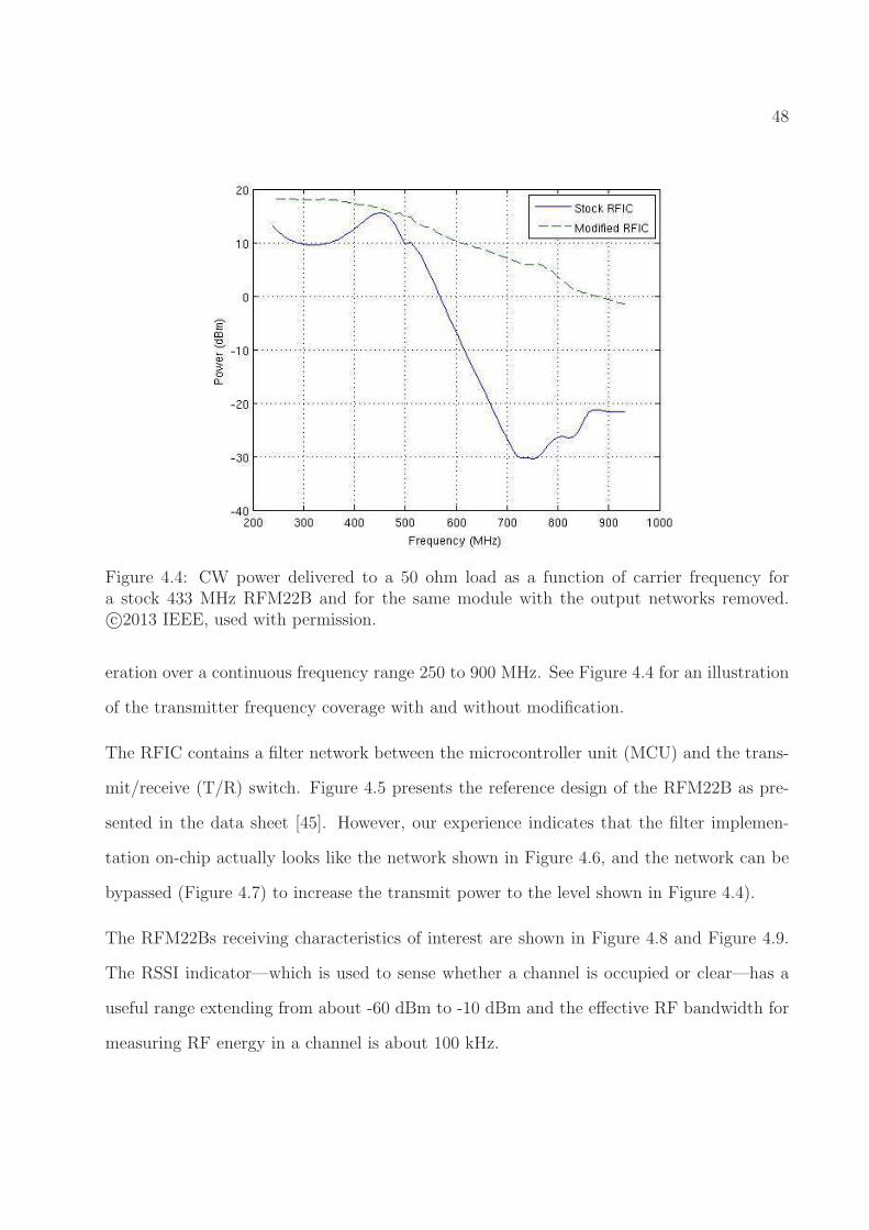
48
Figure 4.4: CW power delivered to a 50 ohm load as a function of carrier frequency fora stock 433 MHz RFM22B and for the same module with the output networks removed.c©2013 IEEE, used with permission.
eration over a continuous frequency range 250 to 900 MHz. See Figure 4.4 for an illustration
of the transmitter frequency coverage with and without modification.
The RFIC contains a filter network between the microcontroller unit (MCU) and the trans-
mit/receive (T/R) switch. Figure 4.5 presents the reference design of the RFM22B as pre-
sented in the data sheet [45]. However, our experience indicates that the filter implemen-
tation on-chip actually looks like the network shown in Figure 4.6, and the network can be
bypassed (Figure 4.7) to increase the transmit power to the level shown in Figure 4.4).
The RFM22Bs receiving characteristics of interest are shown in Figure 4.8 and Figure 4.9.
The RSSI indicator—which is used to sense whether a channel is occupied or clear—has a
useful range extending from about -60 dBm to -10 dBm and the effective RF bandwidth for
measuring RF energy in a channel is about 100 kHz.

49
Figure 4.5: RFM22B reference implementation. Hope Microelectronics Co., RFM22BFSK transceiver - FSK modules - HOPE microelectronics, 2012. [Online]. Availablehttp://www.hoperf.com. Used with permission.
Figure 4.6: RFM22B transmit filter network.
Figure 4.7: RFM22B transmit filter network with bypass. The dotted line show the imple-mented short circuit used to bypass the filter network.

50
Figure 4.8: RSSI values as a function of CW RF power at the antenna terminal. c©2013IEEE, used with permission.

51
Figure 4.9: Receiver’s passband characteristics. c©2013 IEEE, used with permission.
The module’s operation is configured (and reconfigured) by values stored in its internal
registers. Figure 4.10 shows some of the memory registers on the RFM22B that can be
set to configure the radio operation (and subsequently read to determine what the current
configuration is).
As an example of how the radio is controlled, the two lines below set the data rate by writing
values (txdr1 and txdr0) to the upper and lower transmit data rate registers TX Data Rate
1 and TX Data Rate 0. The data rate value is a 16 bit value, and TX Data Rate 1 holds
the upper 8 bits of the value, while TX Data Rate 0 holds the lower 8 bits.
self._set_reg_tx_rate_1(txdr1)
self._set_reg_tx_rate_0(txdr0)
The primary I/O mechanism for the RF module is a first in first out (FIFO) buffer. Serial

52
Figure 4.10: Sample of memory registers set and read on the RFM22B. Hope MicroelectronicsCo., RFM22B FSK transceiver - FSK modules - HOPE microelectronics, 2012. [Online].Available http://www.hoperf.com. Used with permission.
data bytes are written to the transmit (TX) FIFO buffer in succession for transmission.
When the buffer is full, the accumulated bytes are transmitted. Received data is likewise
stored serially in the receive (RX) FIFO buffer. Continued reads will transfer all the data
out of the buffer to the user. From the user perspective, it appears that the TX and RX
FIFO buffers are one and the same, as they are both accessed through writing to and reading
from the same register address, however there are in fact two FIFO buffers, one for TX and
one for RX and internal RFIC controls ensure proper access to the appropriate FIFO.
A SPI bus is the primary method of interaction with the RFM22B, and four SPI lines are
used to send and receive data to and from the module. GPIO is used for secondary signaling;
controlling a T/R switch and providing a path for reading hardware interrupts.

53
Figure 4.11: BeagleBoard-xM trainer board.
4.4.1.3 Trainer Board
There are minor issues to be resolved in interfacing the radio platform and the BeagleBoard-
xM. The trainer board shown in Figure 4.11 and available from Tin Can Tools [107] solves
these problems while providing access to SPI, I2C, and GPIO interfaces, a circuit prototyping
area, and an onboard ATMEL ATmega328 processor. It provides level translators that
convert the 1.8 V signals from the BeagleBoard-xM to 3.3 V for serial communication with
the radio module, and it converts the radio module signals from 3.3 V to 1.8 V for serial
communication in the opposite direction.

54
Figure 4.12: SKIRL radio package, showing BeagleBoard-xM, trainer board, and RFM22B.
4.4.2 SKIRL Integration
Fully integrated, the SKIRL radio platform components stack to make a single package, as
shown in Figure 4.12. The system schematic in Figure 4.13 shows the components and their
functions. The radio module provides FSK-based radio communications and the trainer
board provides logic level translation for serial communications. The BeagleBoard-xM con-
tains a Linux kernel and Ubuntu operating system. The BeagleBoard-xM also contains the
software that operates the radio, from the users perspective. While all the radio operations
actually take place on the radio module itself, the software on the BeagleBoard-xM initializes
the radio module and controls its operation by reading values from and writing values to the
radio module’s registers. Communication between the radio module and the BeagleBoard-
xM is achieved using four SPI communication lines, and three GPIO lines. In addition to
the signaling lines, the BeagleBoard-xM also provides power and ground to the trainer board
and—indirectly via the trainer board—to the radio module.

55
Figure 4.13: SKIRL schematic showing individual components along with their functions.c©2013 IEEE, used with permission.
4.4.3 Physical Components: NXT Brick and Chassis
The NXT brick and chassis form (Figure 4.14) the motion platform of the AVEP. Both the
brick and the chassis come from the Lego Mindstorms NXT robotics toolkit [106]. The chassis
features wheels and rotors for locomotion, as well as various sensors used by the system. The
NXT brick forms the structural core of the chassis; the rotors, sensors, and Lego interconnect
pieces all connect to the NXT brick, and the SKIRL platform rests physically on the brick.
The NXT brick contains an ARM processor and integrated LCD for display. The brick
contains 3 rotor connector ports and 4 sensor connector ports. The ARM processor on the
brick natively supports 2 languages (the graphical NXT-G language and NI’s LabVIEW for
Lego Mindstorms), and with minimal effort is capable of running programs written in many
more languages.

56
Figure 4.14: NXT Brick and chassis.

57
4.4.3.1 Sensors
The chassis currently carries three sensors, a light sensor, color sensor, and barcode reader.
The light and color sensors are NXT native sensors, and connect to the brick. The light
sensor responds to reflected light and measures the intensity of the reflected light. This
functionality is used in the AVEP line following algorithm. The color sensor also responds
to reflected light, but in contrast to the light sensor, the color sensor analyzes the reflected
light to determine the light color. The color sensor is used in the AVEP target/anti-target
detection algorithm. Unlike the light and color sensors, the barcode reader is not an NXT
native sensor, nor is it connected to the NXT brick. While the barcode sensor is mounted on
the chassis, it connects directly to the SKIRL radio platform. The NXT sensors were chosen
due to their capability to integrate with the NXT brick, and for their relatively low cost.
The barcode reader is used in the position/location algorithm. The barcode was chosen as the
method of position/location determination due to its simplicity and low cost. The testbed is
set up indoors, and GPS works very poorly (if at all) indoors. As well, standard GPS does
not have sufficient resolution to be useful at the scale used by the testbed. Other indoor
positioning systems that use infrared [108] are prohibitively expensive for this research. The
barcode is a hand held laser scanner similar to those use in retail point-of-sale systems. The
barcode scanner has a trigger button to activate the laser, but for this research, I configured
the laser to remain on continuously, allowing the scanner automatically to read any barcode
that the laser passes over. Modern smart phones such as the iPhone or Android based phones
can take a picture of a barcode with their integrated cameras and then use image recognition
software to read the value embedded in the barcode image. However, I found the time to
take a picture and analyze the barcode took too long to be practical; while the hand held
scanner can read and decode a barcode in less than 1 second, the smart phone method often
took up to 5 seconds to return a result.

58
The sensors and the algorithm they support are discussed in further detail in Chapter 5.
4.5 System Software
4.5.1 Software Options and Choices
The recommended operating system for the BeagleBoard-xM is Angstrom [109], and it is
used in the board validation process [110]. Angstrom is configured using the Open Embedded
(OE) embedded development framework [111]. OE allows users to deploy a full operating
environment for the BeagleBoard-xM, including operating system (OS) and tool chains. OE
builds the operating environment on a separate system, cross compiled for the BeagleBoard-
xM platform. For a more detailed discussion of development for the BeagleBoard, see [112].
OE allows completely custom distribution builds for the BeagleBoard, at the expense of
having to build every aspect of that custom distribution. Alternatives to Angstrom and
OE include OS and tools from the Linaro project [113] and the Ubuntu ARM project [114].
Ubuntu has a history of stable operation and a large selection of available packages. As our
laboratory uses Ubuntu on all research and development workstations, I decided to leverage
the wealth of institutional knowledge with regards to system installation and support and
chose the Ubuntu ARM as the OS for the SKIRL computational platform.
For cognitive engine code and control software for SKIRL, Python [2] was the obvious choice
for this work. Python is easy to read and code, and Python applications are readily ported
to multiple platforms. As with other choices, our institutional knowledge of Python helped
make the choice; the CSERE cognitive engine [33] is implemented entirely in Python, and
GNU Radio [3] makes heavy use of Python as well.

59
Figure 4.15: Conceptual AVEP system architecture showing components and process flow.
4.5.2 System Architecture
The concept for the AVEP system architecture is presented in Figure 4.15. The architecture
is inspired by the work of DARPA Grand Challenge (DGC) and DUC competitors.
Figure 4.16 shows the software organization of the AVEP as implemented. The controller
is computational and functional core of the system, and is responsible for starting the radio
and motion software, as well as integrating the cognition, route planning, positioning, and
other sensor information.
All system software for SKIRL runs on the BeagleBoard-xM. While the microcontroller on
the trainer board is capable of hosting and running programs written in C or assembly, the
microcontroller is currently unused. The radio module itself is effectively a closed system;
while I can interact with it at some level using its readable and writable registers, its internal
operation is hidden. The AVEP system is written entirely in Python. Python provides cross-

60
Figure 4.16: High-layer software organization of AVEP system.
platform functionality and is easy to read and code, with its similarity to pseudo-code.
4.5.3 Radio Software
The radio software is written and organized as a stack (Figure 4.17), with each layer providing
functionality to the layer above and built on the layer below.
An application is built on top of the API which is in turn built on top of the driver. Figure
shows how the radio software stack corresponds to SKIRL hardware. Applications and the
API correspond to the GPP component in the hardware stack, while the driver crosses the
divide between the RF module and the GPP component. The register access functions
correspond directly to the RF module, while the drivers helper functions correspond to the
GPP component.

61
Figure 4.17: AVEP radio software stack. c©2013 IEEE, used with permission.
Figure 4.18: Radio software stack compared to SKIRL hardware components. c©2013 IEEE,used with permission.

62
4.5.3.1 Radio Driver
The radio driver is the base interface for all interaction with the RF module. The radio
drive uses the Python SPI driver to enable the bit-level communication with the RF module,
and provides direct access to the RF modules configuration registers using register-specific
functions. An example is:
_set_reg_operating_mode_1(0x01)
The function sets the value of register 0x07, Operating Mode and Function Control 1, writing
the hexadecimal value 0x01 into the register. The leading underscore (‘ ’) indicates that the
function is intended to be a private function, used only by other functions provided by the
driver. These other functions are publicly accessible helper functions, such as:
set_op_mode(ready)
The publicly accessible functions are designed to be more user-friendly, using strings for input
rather than hexadecimal values. This improves code readability and eases debugging. Many
radio operations such as setting the frequency require reading and setting multiple registers,
and the helper functions consolidate these multiple operations into a single function.
4.5.3.2 Radio API
The radio API is the interface for operating the radio module. It provides:
• Radio initialization,
• RF front end T/R switch control,
• Access to the air interface for listen, receive, and transmit operations,
63
• Timeout and random back-off, and
• Interrupt monitoring.
The radio API provides an initialization function that is responsible for setting up GPIO-
based communication lines and configuring the radio module in a default mode. This allows
a user to start using the radio module quickly with little effort. The default configuration
enables radio operation at 434 MHz using GFSK at 4.8 kbps. Default payload length is 17
bytes. This default configuration is based on sample code provided by Hope RF [98].
The GPIO-based communication lines are used by the API’s T/R switch to control the
transmit and receive antennas. Each antenna is controlled by a single GPIO line, switching
the antenna on or off. The T/R switch function has three states tx, rx, and off. Internally,
the T/R switch always disables one antenna before enabling the other.
Hardware interrupts are used to indicate that certain events have occurred, including when
a packet has been received and a packet has been sent. The system enables the specific
interrupt for a particular event, and then loops to perform an action until the interrupt
occurs. In this case, the interrupt port is tied to a GPIO line. When the radio module
generates an interrupt, the GPIO line is driven low and the value GPIO line can be read by
software.
A central service provided by the API is access to the air interface, using the listen, receive
and transmit functions.
4.5.3.2.1 Listen Function The listen function provides carrier sense or listen before
talk (LBT) capability, using RSSI. The radio module is put into receive mode, and the RSSI
level is checked by reading register 0x26 Received Signal Strength Indicator. If this value
is above a user indicated threshold, the listen function returns clear to the calling function.

64
It the RSSI value is not above the user indicated threshold, the listen function goes into
a random back off period before checking the RSSI level again. This behavior is repeated
a finite number of times, until the listen function either returns clear indicating a clear
channel, or the maximum number of iterations is exceeded and the listen function returns
busy indicating the channel is not clear. The logic for the listen function is shown in Figure
4.19.
4.5.3.2.2 Receive Function The receive function is used to receive a packet over the
air. The receiver uses two modes, with timeout and without, as shown in Figure 4.20. The
receive process involves waiting for a hardware interrupt to signal that a packet has been
received, then reading the received packet from the radio modules RX FIFO buffer. It is
important, therefore to have a method to interrupt the waiting action. A timer can be started
in an independent thread, and a flag is set when the timer expires. Periodically checking for
this timeout flag allows the packet receiver process to escape its wait loop, and return to its
parent process. This is useful behavior for a radio node that wishes both to transmit and
receive data regularly. However, some radio nodes’ primary function is to receive data, and
for this a receive timeout is unnecessary. In this situation, the timeout timer is not enabled,
and the process continuously waits for a hardware interrupt, indicating that a packet has
been received, returning to the parent process only when the packet has been read from the
RX FIFO buffer.
4.5.3.2.3 Transmit Function The transmit function (Figure 4.21) is used to transmit
packets over the air. Packets are loaded into the radio modules TX FIFO buffer. When the
transmitter function sets the operational mode of the radio module to transmit, the radio
automatically transmits all the data in the FIFO buffer, raising an interrupt when it is done.
After setting the operational mode to transmit, the receive process loops until the interrupt

65
Figure 4.19: Flow chart showing logic and flow of API’s listen function.

66
Figure 4.20: Flow chart showing logic and flow of API’s receive function.
is raised to ensure that all data has been sent, before returning to the parent process.
4.5.4 Motion Software
As with the radio software, the motion software operates on-board SKIRL, but is responsible
for communicating with and controlling an off-board component, in this case the NXT brick.
While the NXT brick is capable of running programs on its ARM processor, I have instead
chosen to control the sensors directly from SKIRL, effectively using the brick as a pipe
through which to control the sensors and rotors. I am using a Python library called nxt-
python that provides direct access to the brick and its components over universal serial
bus (USB). Unlike the radio software, there is no explicit motion driver. Where the radio
driver provides basic connectivity to the RFIC, connectivity to the brick is provided by the
nxt-python library.

67
Figure 4.21: Flow chart showing logic and flow of API’s transmit function.

68
4.5.4.1 Motion API
The motion API the core of the AVEP motion system, and is the interface for operating the
motion module. It provides:
• Rotor and sensor initialization,
• Rotor state information,
• Motion actions such as “go forward”, “halt motion”, and “find line”.
The AVEP system uses a single connection to the NXT brick for all communication and
control. This connection is established at the highest level, and passed to the motion API
by the controller. The motion API uses the connection to initialize the AVEP rotors and
sensors.
The simple “go forward” function is the basis of all AVEP forward motion. The left and
right rotors are engaged and allowed to run until the “halt motion” function is called, which
applies a braking function to the rotors. The “find line” function turns the AVEP in place
about its vertical axis until a line is detected. The AVEP turns first clockwise then anti-
clockwise, sweeping out increasing arcs until the light sensor detects a line beneath it. These
three functions combine to provide a more sophisticated motion algorithm. The algorithm
is used by the motion subsystem and is discussed in further detail in Chapter 5.
4.6 Conclusion
This chapter has discussed the hardware and software components that I built to support
the research in this dissertation, in the form of the AVEP. The AVEP is a prototype robotic
platform that integrates RF and MOT decision making and flexibility into a single system.
The AVEP is capable of autonomous motion using a line following algorithm. A new RF

69
and computational platform called SKIRL provides integrated system control and RF com-
munication capabilities. SKIRL and the AVEP use a low cost RFIC, in contrast to the
SDR systems often used in CR research. The AVEP hosts a number of sensors that provide
environmental information to aid in positioning, motion planning, and target detection. The
AVEP is programmed entirely in easy-to-read, easy-to-debug Python.
In discussing the hardware and software components of the AVEP, I have tried to paint a
clear picture of all the components from a system level. This should provide a framework
of understanding for the next two chapters, which present and discuss the algorithms I
developed to implement UMDDM.
The next chapter presents the AVEP operational and control algorithms. In it, I present
details of the various finite state machines (FSMs) that control the AVEP and the MOT
and RF subsystems, as well as the sensor algorithms that read sensor raw data and generate
useful information for the system. I also provide details on the path data structure (PDS),
the graph-based data structure that the AVEP uses as its data storage mechanism.

Chapter 5
Algorithms and Software
Development
5.1 Introduction
This chapter presents the AVEP operational and control algorithms. These are the algo-
rithms that govern the operation of the AVEP; how it moves and communicates and how
the sensors operate. This chapter builds on the discussion of the last chapter, which pro-
vided information on hardware and system software. This chapter discusses the algorithms
that run on that hardware, integrating all the separate hardware components into a single
system capable of autonomous operation leveraging RF and MOT flexibility. This chapter
also presents details of the NBR, the node on the other end of the AVEP communication
link.
In the material which follows, Section 5.2 discusses the run-time and operational aspects of
the AVEP. Section 5.3 presents the PDS, a new and innovative method for organizing and
70

71
storing multi-domain environmental information. Section 5.4 discusses the operation of the
NBR, while Section 5.5 provides a summary with concluding remarks.
5.2 Operation and Control
This section presents the algorithms that provide the operational logic for the AVEP; the
logic flow of the controller, the data collection algorithms used by the sensors, and the logic
flows of the RF and MOT subsystems.
5.2.1 Controller
The controller is the central system component, and the hierarchical top layer of the system.
The controller starts and manages the other modules, coordinating interactions between all
the various subsystems.
5.2.1.1 Controller Finite State Machine
As the controller is the core of the AVEP system, so the FSM (shown in Figure 5.1) is
the heart of the controller. The FSM consists of five states (“first time”, “before traverse”,
“traverse path”, “after traverse”, “return to beginning”) and these five states handle all
the functions of the AVEP after initialization. The FSM uses the “fsm state” variable to
determine the current state.
5.2.1.1.1 FSM State: first time The “first time” state is entered only once, when the
controller FSM is first started. This state uses default motion parameters to move the AVEP
to the first barcode location, where it stops. Finally, the state variable “fsm state” is set to

72
Figure 5.1: AVEP controller finite state machine.

73
“before traverse”, indicating the next FSM state.
5.2.1.1.2 FSM State: before traverse The “before traverse” state is entered every
time the AVEP reaches the first barcode location. This state uses the decision making
module to determine which path to traverse. The decision making module and the decision
making process are explored in detail in Section 6.3. This state is responsible for setting the
parameters for the radio and motion subsystems before the AVEP traverses its chosen path.
In order to ensure that the radio is properly configured and that the NBR can receive the
AVEP RF transmissions, this state sends a data packet to the NBR containing the radio
parameters that the AVEP will use during its path traversal. To ensure that communication
is always possible, the AVEP transmits the reconfiguration information to the NBR before
it reconfigures its radio. When the AVEP receives an acknowledgment from the NBR, the
AVEP reconfigures its radio and motion subsystems with the predetermined parameters
as determined by the decision making module. If the reconfiguration was faulty or the
AVEP could not reestablish communication with the NBR, the AVEP could fall back to a
default configuration or use a control channel to reestablish communication. This feature
is not currently implemented, however. Finally, the state variable “fsm state” is set to
“traverse path”, indicating the next FSM state.
5.2.1.1.3 FSM State: traverse path The “traverse path” state is entered every time
the AVEP traverses its chosen path. There are two possible behaviors the AVEP can employ
during this state, dependent on whether or not the path has been previously explored.
If the path is unexplored, the AVEP sets the state of the radio subsystem to “listen”, causing
the radio subsystem to record the RSSI of a continuous wave (CW) signal transmitted by
the NBR. A CW signal is used to simplify the process of determining the RSSI. The RFIC

74
operates as a black box with respect to many of its functions, including the way it samples the
RSSI. Sampling the RSSI for an incoming modulated signal results in widely varying RSSI
results. No doubt, the RFIC sometimes samples RSSI during a break in the transmission,
and samples on the rising of falling edge of the waveform as well as sampling during the peak
transmission. However, recording the RSSI of a CW signal provides much more consistent
results. The RSSI information is used by the decision making module to determine some
RF path characteristics (see Section 6.3). The AVEP sets the state of the motion subsystem
to “go”, engaging actual forward motion of the AVEP along its chosen path. As the AVEP
moves along the path, it records the time it takes to travel the length of the path, and the
number of targets and anti-targets encountered along the path. Targets and anti-targets are
discussed further in Sections 5.2.2 and 6.3.1.1, but for ease of discussion in this chapter, a
target is an object the AVEP wishes to find and record, while an anti-target is something it
wishes to avoid.
If the path has been previously explored, the AVEP sets the state of the radio subsystem to
“stream”, causing the radio subsystem to transmit data packets to the NBR, using the radio
parameters as determined and set during the previous “before traverse” FSM state. As in
the “listen” mode described directly above, the AVEP sets the motion subsystem state to
“go”, and the AVEP traverses its chosen path, again recording the time of traversal, and
number of targets and anti-targets along the path.
In either case, When the AVEP reaches the end of the path, indicated by the second location
barcode, and recorded by the barcode sensor, the AVEP halts its motion by setting the
motion subsystem state to “stop”, and stores the time, target, and anti-target information
in the PDS. Obviously an airplane style UAV could not stop in midflight, and while a
helicopter style could pause in midair, this is not ideal operation. In practice, the duration
for which the AVEP is halted is not observable; the housekeeping operations the AVEP

75
conducts in this period are concluded very quickly. Additionally, the halt of motion provides
an easy way to differentiate between different stages of operation while performing tests.
The PDS is discussed further in Section 5.3. Finally, the state variable “fsm state” is set to
“after traverse”, indicating the next FSM state.
5.2.1.1.4 FSM State: after traverse The “after traverse” state is entered every time
the AVEP reaches the second barcode location. During this state, the AVEP updates pa-
rameter information in the path data structure for the current path. Specifically, the knobs
and meters from the just completed traverse are recorded in a historical manner, as “previ-
ous knobs” and “previous meters”. Additionally, the path is now recorded as having been
explored. The AVEP again communicates with the NBR, requesting an update. This update
includes the number of packets received by the NBR. Finally, the state variable “fsm state”
is set to “go to beginning”, indicating the next FSM state.
5.2.1.1.5 FSM State: go to beginning The “go to beginning” state is used by the
AVEP every time it finishes a path traversal (including the “after traverse” state) and needs
to return to the start of the test course. The AVEP leaves the radio subsystem off, but
engages the motion subsystem. The AVEP then follows the return path until it arrives back
at the beginning, as indicated by the first location barcode.
5.2.2 Sensors
The AVEP uses three sensors for data collection: NXT light sensor, NXT color sensor, and
barcode reader.

76
5.2.2.1 NXT Light Sensor
As mentioned preciously, the NXT light sensor is used in the motion control algorithm. The
light sensor is a NXT native sensor that is connected to the NXT brick, and the AVEP uses
the nxt-python library to control it. The light sensor uses reflected light to determine the
presence of the test track line beneath it. The threshold value for the light sensor for the
test track line is 500. If the light sensor reads a value above the threshold, the test track line
is not present beneath the light sensor, and if the sensor reads a value below the threshold,
the test track line is present beneath the light sensor.
5.2.2.2 NXT Color Sensor
The NXT color sensor is used in the target tracking algorithm. As with the light sensor, the
color sensor is a NXT native sensor that is connected to the NXT brick, and the AVEP uses
the nxt-python library to control it. The color sensor uses reflected light to determine the
color of an object below the sensor. The sensor returns a value which indicates the specific
color of the object (Table 5.1).
Table 5.1: Values returned by the NXT color sensor and their associated colors.
Color Black Blue Green Yellow Red WhiteValue 1 2 3 4 5 6
A different color is used to represent the targets and anti-targets; in this case, yellow repre-
sents a target, and red represents an anti-target. These values were chosen to minimize false
positive cases. During a path traversal, every value recorded by the color sensor is stored in
a single vector. After the path has been traversed, the results are processed in the following
manner. The single vector is copied so that there are now two identical vectors. The two
vectors are processes in a similar manner, although one of the vectors is analyzed to find the

77
number of targets, while the other vector is analyzed to find the number of anti-targets. In
the target vector, every vector element that is not equal to the target color value is set to 0.
Likewise, in the anti-target vector, every vector element that is not equal to the anti-target
color value is set to 0. Each vector is then processed to determine the number of transitions,
that is, the number of times that an element is zero while the two following elements are non-
zero. The number of transitions accurately indicates the number of targets (or anti-targets
as appropriate) observed along the path just traversed.
5.2.2.3 Barcode Reader
The barcode sensor is used to determine the AVEPs position. My advisor, Charles Bostian,
noted that in an indoor scenario, a simple, cheap and accurate method of determining
position is to reference it to an object with known location. This led to the idea of using
barcodes at specific locations to fix a position, and using a barcode reader to determine the
presence of a barcode, thus indicating current position [115].
As mentioned previously, despite being mounted on the chassis, the barcode reader connects
directly to the SKIRL platform over USB. The barcode reader is accessible through the
SKIRL OS device driver interface /dev. The specific interface for the barcode reader is
/dev/hidraw0. The barcode reader itself operates in a mode that continually scans for
barcodes, and once it scans one, the data embedded in the barcode is immediately available
for decoding. Using the information available from [116], a barcode can be translated into a
number, indicating a specific location on the test track.
The barcode reader is a threaded module, running in a continuous loop separate from (but
started by) the controller. The value encoded in the barcode is relayed to the controller
using a callback passed to the barcode reader when it is instantiated.
78
5.2.3 Radio Subsystem
The radio subsystem is responsible for all AVEP communications operation. The radio
subsystem runs in its own thread, allowing it to run concurrently with, but independent of
the main process. The radio subsystem is originally instantiated by the AVEP controller,
after which the radio subsystem FSM takes over.
5.2.3.1 Radio Subsystem Finite State Machine
The radio subsystem FSM is responsible for all AVEP RF operations. The acAVEP con-
troller uses the subsystem function set_state(current_state) to set the radio subsystem
state of operation. The controller consists of of five states: “stop”, “stream”, “update”,
“reconfigure”, and “listen”. Each FSM state is responsible for a different aspect of RF
operations.
The “stop” state is the default state of operation for the radio subsystem FSM. When the
controller starts the radio subsystem, the FSM drops into this state, as it does when it
completes any of its operations, represented by the other FSM states.
The “stream” state is used to stream data from the AVEP to a NBR. While the AVEP
traverses a path, it transmits data packets to the NBR. The data payload inside the packet
is not a significant aspect of this research, but payloads could include any type of operational
data as required by the mission. (In my first round of AFRL funded research, payload data
included video images captured by network nodes [117].)
The “update” state is used by the AVEP to request updates from the NBR. Each time the
AVEP completes a path traversal, it sends a request to the NBR for an update. When
the NBR receives the request, it replies by transmitting a packet containing information

79
on the number of packets that the NBR received from the AVEP while the AVEP was
traversing its selected test bed path. This information can be used by the AVEP to improve
its understanding of the RF environment.
The “reconfigure” state is used by the AVEP to notify the NBR of a new RF configuration.
Every time the AVEP reaches Node 1 on the test bed, the AVEP makes a decision about
how to operate. The solution generated by the decision maker at this point can include a
new RF operational profile: frequency, modulation, bit rate, etc. However, If the AVEP
unilaterally changes its operational profile, the receiving NBR won’t be able to receive the
data, as it is still operating using an old profile. For this reason, using the original operational
parameters, the AVEP notifies the NBR of the new operational profile, and waits for the
NBR acknowledgment. When the AVEP receives the reconfiguration acknowledgment, it
then reconfigures its own radio using the new parameters, knowing that the NBR has done
the same, and that both RF systems are ready to start communicating using the new RF
profile.
The “listen” state is used by the AVEP for RF sensing. In its initial iterations of operation,
the AVEP explores its environment. During this exploration, the AVEP controller sets the
state of the radio subsystem to “listen”, causing the radio subsystem to record RSSI along
the path. This RSSI information is used by the decision making module to determine some
RF path characteristics (see Section 6.3).
5.2.3.2 Packet Structure
The RFM22B RFIC provides a very flexible platform for RF applications, but the downside
to the flexibility is that it does not provide pre-existing support for packet structure or
protocols above the PHY. To support AVEP operation, I developed a packet structure based

80
on the transmission control protocol (TCP) standard [118]. The packet structure is shown
in Figure 5.2.
Figure 5.2: RF subsystem packet structure.
Most of the header fields are self explanatory. The “packet number” field contains a three
byte integer indicating the number of the current packet. The “time stamp” contains an
eight byte value indicating the time the packet header was packed, or put together. The
“location” field contains a two byte integer that corresponds to the most recent location of
the radio node. For the AVEP, this corresponds to the last barcode the AVEP recorded.
The “flags” field is used to provide control information for coordination between transmitter
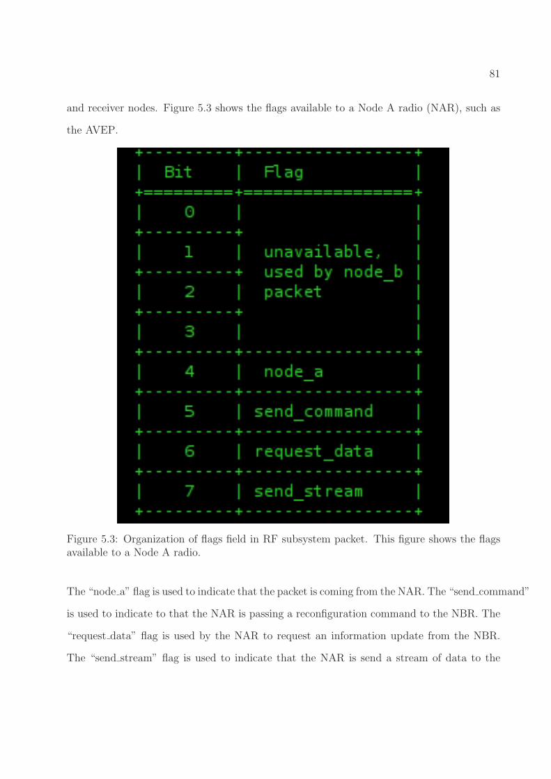
81
and receiver nodes. Figure 5.3 shows the flags available to a Node A radio (NAR), such as
the AVEP.
Figure 5.3: Organization of flags field in RF subsystem packet. This figure shows the flagsavailable to a Node A radio.
The “node a” flag is used to indicate that the packet is coming from the NAR. The “send command”
is used to indicate to that the NAR is passing a reconfiguration command to the NBR. The
“request data” flag is used by the NAR to request an information update from the NBR.
The “send stream” flag is used to indicate that the NAR is send a stream of data to the

82
NBR while the AVEP is traversing a path.
5.2.4 Motion Subsystem
Similar to the radio subsystem, the motion subsystem is responsible for all AVEP motion.
The motion subsystem also runs in its own thread, again for concurrent but independent.
The motion subsystem is originally instantiated by the AVEP controller, after which the
motion subsystem FSM takes over.
5.2.4.1 Motion Subsystem Finite State Machine
The motion subsystem FSM is responsible for all AVEP motion operations. The acAVEP
controller uses the subsystem function set_state(current_state) to set the motion sub-
system state of operation. The controller implements only two states: “stop”, and “go”.
The “stop” state is the default state of operation for the motion subsystem FSM. When the
controller starts the motion subsystem, the FSM drops into this state, as it does when it
completes its actual motion operation, as represented by the “go” state.
The “go” state is used by the AVEP controller to initiate operational motion. This the
motion operation is governed by a motion behavior described below in Section 5.2.5. The
behavior is employed until the AVEP reaches the end of its chosen test bed path, indicated
by arrival at test bed Node 2.
5.2.5 Motion Behavior: Follow The Line
The motion subsystem uses a line-following algorithm. This is a simplistic method of im-
plementing robot motion, where the robot uses a sensor to detect a line on the ground, and

83
the robot follows the line as it moves forward [119]. The algorithm trades off between two
sub-behaviors, “follow the line” and “find the line”. The “follow the line” state causes the
AVEP to move forward in a straight line until the light sensor (Section 5.2.2.1) indicates
that the AVEP is no longer following the line. At this point, forward motion is halted and
the AVEP proceeds to “find the line”. The AVEP starts to turn in place about its z-axis,
sweeping out larger and larger arcs as it seeks to find the test bed path—the line—with the
light sensor. When the path has been found, turning motion is halted, and forward motion
is again commenced via the “follow the line” behavior. Using the “follow the line” and “find
the line” sub-behaviors, the AVEP is able to move effective along test bed paths by following
the black lines marked out on the test bed.
5.3 Path Data Structure
CRs and AVs both require relevant and up-to-date information on their environment to
operate effectively. AVs often use evidence grids to represent environmental data [47], while
CRs commonly use internal or external databases to store RF information [19, 62]. I have
developed a method inherently suited to multi-domain knowledge storage that uses graph
structures to represent environmental data. The PDS is the system’s central data storage
component, labeled as “(Multi-Domain) World View” in Figure 4.16.
A single PDS is a software object that represents a graph edge, specifically a single test bed
path. It can be instantiated multiple times to represent multiple paths. As shown in Figure
5.4, the test bed graph —originally presented in Figure 3.3—contains three individual paths
between Node 1 and Node 2. Each path is a route that the AVEP can traverse as it moves
from Node 1 to Node 2, and each path is represented by a single PDS.
The PDS extends the concept of a weighted graph [120], or more specifically a weighted edge.

84
Figure 5.4: The test bed graph contains three separate paths between Node 1 and Node 2.

85
Table 5.2: Knobs and meters available stored in path data structure.
Knob Name Knob SettingsBitrate 2.0, 2.4, 4.8, 9.6, 19.2, 38.4, 57.6, 125.0 (kbps)Transmit Power 8.0, 11.0, 14.0, 17.0 (dBm)Rotor Power 25.0 - 80.0, steps of 5.0
MetersTargetsAnti-targetsRSSI
Weighted graphs use weight to represent some cost associated with a particular graph edge,
such as the distance between two cities in the traveling salesman problem, or the distance
between two routers in a network. The PDS builds on the concept of an edge weight by using
the weight as a data storage mechanism. The edge weight becomes multiple weights, each
one representing a particular environmental characteristic, and all describing that particular
graph edge.
For this research, each of the three instantiated PDS objects maintains physical and RF
characteristics of a particular test bed path, such as path name, path distance or length,
whether the path has been explored or not, and system knobs and meters along the path.
Table 5.2 shows the knobs and meters stored in the PDS. Additionally, each PDS maintains
a record of the most recent system solution for the path, as determined by the decision
making module. Further solution details are presented in Section 6.3.
Currently the experimental test bed contains only three paths, each of which connects the
same two nodes, Node 1 and Node 2. However, in a more complicated test bed layout, there
would be additional nodes with additional edges and their attendant paths. An example is
shown in Figure 5.5. In such a scenario, path search algorithms such as Dijkstra’s algorithm
[121] or D* Lite [122] can be used to determine a path of travel for the AVEP that spans
multiple edges. The path search algorithm would use the data stored in each PDS object to

86
evaluate each possible route.
Figure 5.5: A more complicated test bed layout with additional nodes and edges, and theirattendant paths.
5.4 Node B Radio Architecture
The NBR is a stand alone radio node based on the SKIRL radio platform described in Section
4.4.1. It is based on the same RF stack that provides radio functionality in the AVEP, but
has no motion capabilities, in hardware or in software. The primary function of the NBR is
to provide a node with which the AVEP can communicate during its operation.
The NBR uses a FSM to switch between three states : “listen”, “receive”, and “transmit”.
The default state is “receive”, where it waits to receive a transmission from the AVEP. When
it receives a packet from the AVEP, it parses the packet header, reading the value of the
flags in the “flags” field, and sending an appropriate reply as necessary. Figure 5.6 shows
the flags available to a NBR in replying to control flags from a NAR.

87
If an incoming packet contains the “send stream” flag, the NBR records the packet number
of the incoming packet, and then returns to “receive” state to await another packet. If an
incoming packet contains the “request data” flag, the NBR calculates the total number of
data stream packets it has received since the last update. Before it transmits this informa-
tion back to the NAR, it enters the “listen” state to implement LBT as described in Section
4.5.3.2. When the channel is clear, the NAR enters the “transmit” state and transmits
the data back to the NAR, using the “send data” flag, and returns to the “receive” state.
If an incoming packet contains the “send command” flag, the NBR parses the packet to
determine the new radio configuration to implement. It then enters “listen” before trans-
mitting an acknowledgment to the NAR using the using the “ack command” flag. The NBR
then reconfigures its radio parameters and once again enters the “receive” state to await
communications from the NAR.

88
Figure 5.6: Organization of flags field in RF subsystem packet. This figure shows the flagsavailable to a Node B radio for communication with a Node A radio.

89
5.5 Conclusion
This chapter discussed the AVEP operational and control algorithms. I presented the details
of the FSM that controls the overall operation of the AVEP as well as the FSMs that control
the radio and motion subsystems. I also introduced and described the PDS, a graph-based
method for storing data on the AVEP that is particularly suited to multi-domain information.
In this chapter, I tried to fill out the operational details of the AVEP, building on the high
level discussion of hardware and software components in the last chapter. I described in
detail the operation and flow of all aspects of the AVEP, with the intention of providing
insight into how the AVEP was implemented and how it operates. This chapter, when
combined with the last chapter and the information provided in the next chapter, should
provide a comprehensive view of UMDDM, in both theory and application.
The next chapter presents the learning and decision making algorithms that underpin UMDDM.
I discuss the development of the decision making algorithm and its objective functions. I
present two stages of learning, learning the environment, and learning from experience. I
also show how all the steps fit together to provide true UMDDM.

Chapter 6
Learning and Decision Making
6.1 Introduction
This chapter discusses the learning and decision making aspects of this research. The learning
and decision making processes make up the cognitive core of this research, providing intelli-
gent action and introspection for the AVEP. Learning and decision making in the AVEP are
closely entwined; learning feeds decision making, and decision making feeds learning. The
learning and decision making processes presented here are the essence of UMDDM.
Decision making “is the process of selecting a possible course of action from all the available
alternatives,” [123]. Sometimes this is also referred to as reasoning [124]. Clearly the ultimate
point of making a decision—selecting a possible course of action—is actually to act. Decision
making is the process of deciding on a course of action, which is passed to the RF and MOT
subsystems, the system’s actuators.
The Oxford English Dictionary defines the verb “learn” as “to acquire knowledge” specifically
“ as a result of study, experience, or teaching” [125]. However, the concept of what is machine
90

91
learning is a moving target. Machine learning is closely tied to artificial intelligence (AI), and
therefore subject to the “odd paradox”, the concept that once AI has solved a problem, that
problem and the corresponding solution no longer belong to the domain of AI [126, 127].
Karen Haigh differentiates between adaptation, where a system can change its behavior
based on current conditions; and learning, wherein a system uses its experience to change
its adaptation methods, effectively adaptive adaptation [127]. In this research, learning is
used in two distinct ways, learning the environment, and learning from experience. Learning
the environment provides information for decision making, while learning from experience
evaluates the decisions and provides feedback to the decision maker.
The AVEP cognitive process implements a cycle similar to Mitola’s cognition cycle [22], and
the observe, decide, and act (ODA) loop [15], and brings to bear the observation noted in
Section 1.1, namely that CRs and AVs perform similar tasks, albeit in different domains:
• Analyze their environment,
• Make and execute a decision,
• Evaluate the result (learn from experience), and
• Repeat as required.
The ODA loop and the observations above are so similar that they can be effectively com-
bined into a single loop, shown in Figure 6.1. The specific cognition process the AVEP uses
Figure 6.1: The ODA loop applied to CR and AV scenarios.
is shown in Figure 6.2.
The remainder of this chapter is organized as follows. Section 6.2 discusses the first aspect

92
of learning, learning the environment. Section 6.3 discusses decision making, while Section
6.4 presents the second aspect of learning, learning from experience. Section 6.5 contains
some concluding remarks with a look ahead to the next chapter.
6.2 Learn The Environment
There is a significant body of research that deals with decision making and learning, from
perspectives that include pure AI, economics, child development, CR, and AVs. Much of
what is published deals with the decision making and learning processes themselves, skipping
right over the acquisition of information that supports these processes. The AVEP learn the
environment process is responsible for gathering this information, collecting meter values
during AVEP operation.
The AVEP uses its sensor systems to learn the environment. The AVEP is programmed with
some initial information to jump-start the learning process. This includes path length for
individual paths in the test bed. In the AFRL systems that this research supports, UAVs fly
preprogrammed flight paths, and the AVEP emulates this setup with a priori knowledge of
the test bed paths. Information such as number of targets and anti-targets along the path as
well as RF noise are sensed and stored as the AVEP actually travels the test bed paths. The
mechanics of the environmental learning process are discussed in Section 5.2.1.1, while the
individual sensors used to gather the information are presented in Section 5.2.2. It should
be noted that while the AVEP gathers its initial information during an exploration phase,
Figure 6.2: The cognition cycle used by the AVEP.

93
and then moves into an “exploitation” phase (using the information it has obtained to carry
out its operational duties), the AVEP continues to gather environmental information about
its current path of travel during operation. Additionally, the AVEP maintains a record
of the last time it received information about a given path. If the meters corresponding
to a given path have not been updated within a certain number of iterations, the AVEP
switches from operational (or “exploit”) mode to exploration mode, and explores that path
to updates its internal path data. In this manner, the AVEP is able to maintain up-to-date
information about its changing environment, ensuring effective decision making with relevant
information.
6.3 Decision Making
Decision making is the process of choosing an action or outcome from a set of possible ac-
tions or outcomes. Optimization theory often refers to multiple criteria decision making
(MCDM), while CR research often uses multi-objective optimization (MOO), but they both
refer to decision and planning involving multiple conflicting criteria that should be consid-
ered simultaneously [128]. Rondeau uses evolutionary based genetic algorithms (GAs) to
address his MOO problems [70], and this approach has been embraced by researchers in a a
wide variety of application domains, including economics, mechanical engineering, and cryp-
tography [129–131]. Guided search algorithms like GAs are well suited to finding solutions
in large search spaces. Additional techniques that have been investigated for guided search
include simulated annealing [124] and swarming algorithms [132].
Zitzler and Theile present a general formulation for multiple objective optimization problems
in [133], shown in (6.1).

94
min/max y = f(x) = (f1(x), . . . , f1(x))
subject to x = (x1, x2, . . . , xm) ∈ X
y = (y1, y2, . . . , yn) ∈ Y (6.1)
That is, we seek to minimize (or maximize) a vector function f that maps a tuple of m input
parameters to a tuple of n output parameters, or objectives. The set x is the set of input
parameters, and y is the of objective values determined by the objective functions. The
set of solutions to a multi-objective problem lie on the Pareto front, which consists of all
the solution sets y which are non-dominated, that is, those sets that cannot be improved in
some dimension without a decrease in some other dimension. Multi-objective optimization
problems are naturally problems in balancing trade-offs [134]. Attempting to minimize both
BER and equivalent isotropically radiated power (EIRP) in the RF domain is a perfect
example. With all other factors held constant, minimizing BER requires increased transmit
power, while reducing transmit power correspondingly drives an increase in BER. In the
MOT domain, for a given travel distance, attempting to minimize both travel time and
vehicle velocity results in the same interplay. Multi-objective optimization balances the
trade-offs, and provides decision making capability in the face of multiple competing decision
criteria.
6.3.1 Objective Functions
This work is the first to combine flexibility in the RF with flexibility in the MOT domain.
To implement this flexibility, any decision making process must take into account both
domains in the objective functions used. In order to clearly show the concept of UMDDM,

95
the proof of concept prototype AVEP implements only a few objective functions in total.
As mentioned in Chapter 3, I have chosen to follow the example set by DARPA in the
DRC. Decision making will be based on a variety of factors, including mission success and
completion time. For the RF domain, I have chosen to BER as one objective. BER is a
commonly used metric for evaluating wireless communication systems. I also chose packet
delivery to evaluate RF performance. Packet delivery is based on the concept of goodput
or throughput, and integrates consideration of the chosen MOT metric. The single chosen
MOT objective function is time, the time it takes the AVEP to traverse a single test bed
path. In addition to the RF and MOT objective functions, the AVEP also uses a target/anti-
target objective function to evaluate mission based parameters. The objective functions are
explored in greater detail below.
This section presents the four objective functions used in the AVEP decision making process.
I use the same format used in [70]. For each objective, I list the required knobs, meters, and
other objective functions used in the objective function calculation.
6.3.1.1 Target/Anti-target Score
Dependencies
Knobs: None
Meters: Targets, anti-targets
Objectives: None
I developed the target/anti-target score to incorporate consideration of mission success into
the decision making process. While this work is modeled on AFRL UAV scenarios, I am not
privy to the missions the United States Air Force (USAF) is flying. And although it likely
goes with out saying, I will explicitly state that I do not have access to USAF or AFRL

96
UAV mission parameters. As a result, I developed the details of this objective function to
model a plausible UAV mission objective, namely tracking and observing some target while
avoiding some other anti-target. Further, I wished to show a reasonable trade off between the
desirable aspects of the mission (finding targets) and the undesirable aspects of the mission
(encountering anti-targets). Clearly, if the USAF uses a mission objective like this, the
weightings would change based on the specific mission. The risk inherent in encountering a
large number of anti-targets may be considered acceptable in order to complete a high value
mission.
Targets (X) and anti-targets (Y ) are mission-based parameters. They attempt to model
mission priorities. Targets are objects that the AVEP should track, while anti-targets are
objects that the AVEP should avoid, in the course of its mission. During AVEP operation,
targets and anti-targets are represented by colored pieces of cardboard placed along the test
bed paths. As the AVEP travels the path, it records the presence of the targets and anti-
targets as described in Section 5.2.2.2. The target/anti-target score (Z) is an objective that
is used to incorporate mission information into the decision making process. In the scenario
presented in Section 1.4 (second research project), a UAV carrying out a mission might
reasonably be required to find and track a number of targets, while avoiding or minimizing
detection by hostile entities (anti-targets). The Z function (6.2) defines a series of cases for
possible values of X and Y , with instances where X > Y given greater value. Note that
where X ≤ Y , Z ← 0. This incorporates the mission directive to avoid anti-targets. A
graphical representation of the objective function is shown in Figure 6.3, where Z ∼ f(X, Y )
and X ∈ Z, X = {x | 0 ≤ x ≤ 20}, Y ∈ Z, Y = {y | 0 ≤ y ≤ 20}.

97
Z =
0 if X = 0 or X < Y ,
0.2 if X = 1 and Y = 0,
0.2*(X - Y) if 1 < X <= 3 and Y <= (X − 2),
0.15*(X - Y) if 4 < X <= 6 and Y <= (X − 3),
0.2*(X - Y) if 4 < X <= 6 and Y <= (X − 2),
0.2*(X - Y) if X > 6, Y <= (X − 4), and 0.2 ∗ (X − Y ) <= 1.0,
1.0 if X > 6 and, Y <= (X − 4), and 0.2 ∗ (X − Y ) > 1.0,
0.15*(X - Y) if X > 6 and Y <= (X − 3),
0.1*(X - Y) if X > 6 and Y <= (X − 2),
0 otherwise.
(6.2)

98
Figure 6.3: Graphical representation of Z objective function as a function of targets andanti-targets.

99
6.3.1.2 Time
Dependencies
Knobs: Rotor power
Meters: None
Objectives: None
Time refers to the length of time required for the AVEP to traverse a given path. The time
required to travel a given distance at constant velocity is given by a standard first semester
physics equation: (6.3):
T = d/v (6.3)
where T is time, d is the distance traveled, and v is the velocity. However in this case,
while the distance traveled along a given path is known, AVEP velocity is not known. The
available system knob is rotor power, and rotor power is controlled through a unitless number
{Protor : 64 > Protor 6 128}. Without further exploration, there is no indication how this
value relates to velocity. I ran repeated tests of the AVEP, driving it along a fixed length
(0.762 meter) path using various rotor power values. Table 6.1 shows the values gathered
during these experiments.
Table 6.1: Rotor power and time measurements for AVEP, used to determine AVEP velocity.
Rotor power Time (sec)
25 6.636803 7.384832 6.820400 7.033324 6.61556235 6.011670 5.473605 5.078091 4.992305 5.96381845 4.268262 4.179882 3.975959 4.217389 4.03778955 4.829124 4.848656 3.488006 3.301235 4.72786565 4.387924 5.452579 6.348041 6.948240 4.47474875 5.597478 4.591388 6.627983 6.298144 7.116761
I generated a 3rd-order polynomial equation to fit the data, and a plot of the experimental
data and a 3rd-order polynomial are shown in Figure 6.4. Using the now generated polyno-

100
mial, I can determine the expected time to traverse a given distance with using a particular
value of rotor power as input.
20 30 40 50 60 70 802
3
4
5
6
7
8
9
10
Rotor Power (unitless)
Tim
e (s
ec)
Experimentally recorded values3rd order polynomial fit
Figure 6.4: Experimentally recorded values of time (to travel a fixed-length path) and req-uisite AVEP rotor power values, with 3rd order polynomial fit.
While the experimental data and plotted data are valid for a path distance of 0.762 meters
(30 inches), the calculation of the polynomial used in the calculation of objective function
includes some additional steps. Knowing that the distance in the experiment is 0.762 meters,
I divide the experimentally generated time results by the distance to come up with a unit
time value, the time it takes the AVEP to travel a meter using the rotor power value currently
under test (6.4).
t = texp/d (6.4)

101
Multiple mathematical calculation packages provide the functionality for generating polyno-
mial fits to data. The numerical Python package NumPy [135] provides the olyfit\end{verb} and \begin{verb}
functions for fitting data with polynomials. The Python code listing below shows how the
polynomial is generated.
import numpy as np
distance = 0.762
t_total = np.array([6.636803, 7.384832, 6.820400, 7.033324, 6.615562,
6.011670, 5.473605, 5.078091, 4.992305, 5.963818,
4.268262, 4.179882, 3.975959, 4.217389, 4.037789,
4.829124, 4.848656, 3.488006, 3.301235, 4.727865,
4.387924, 5.452579, 6.348041, 6.948240, 4.474748,
5.597478, 4.591388, 6.627983, 6.298144, 7.116761])
unit_t = t_total / distance
power = [25, 25, 25, 25, 25,
35, 35, 35, 35, 35,
45, 45, 45, 45, 45,
55, 55, 55, 55, 55,
65, 65, 65, 65, 65,
75, 75, 75, 75, 75]
z3 = np.polyfit(power, unit_t, 3)
poly3 = np.poly1d(z3)
Using the polynomial generated, a simple function can provide the expected time the AVEP
will require to travel a given distance with specified rotor power:
def calculate_time(self, rotor_power, distance):

102
unit_time_given_power = self.poly3(rotor_power)
total_time = unit_time_given_power * distance
return total_time
where self.poly3 is the same polynomial calculated previously.
Note that as rotor power increases, the corresponding time first decreases, then starts to
increase again. This is an artifact of the AVEP line-following motion algorithm. High
rotor power causes high AVEP velocity for a very short period of time, but this velocity
immediately goes to 0 when the AVEP moves off the line it follows. The AVEP must stop
and reacquire the line, before starting to move forward again. And because the AVEP is
moving faster when it diverges from its path, it travels farther from the path before stopping,
and takes longer to reacquire the line.
Figure 6.5 shows a graphical representation of the objective function, where T ∼ f(D,Protor)
and D = {1.575, 1.219, 2.223} (m), Protor ∈ Z, Protor = {p | 5 ≤ p ≤ 80}.

103
1
1.5
2
2.5
020
4060
800
10
20
30
40
50
Path length (m)Rotor power)
Tim
e (s
ec)
Figure 6.5: Graphical representation of T objective function as a function of path distanceand rotor power.

104
6.3.1.3 Bit Error Rate
Dependencies
Knobs: Bit rate, EIRP
Meters: RSSI
Objectives: None
BER is a metric that is commonly used to evaluate the performance of communication
systems. Equations for calculating BER vary according to the type of modulation employed,
as well as the type of channel in use. For the purpose of this research, I have assumed an
additive white gaussian noise (AWGN). The type of modulation employed is dictated by my
choice of the RFM22B RFIC. While the RFIC can use FSK, GFSK, or OOKmodulations, the
AVEP currently only uses FSK. The RFIC data sheet does not provide many details about
the inner workings of the RF modem, therefore in the absence of additional information, I
have assumed that based on the low cost of the RFIC, it employs noncoherent detection.
Sklar [136] provides an equation for calculating BER for noncoherently detected FSK (6.5):
B =
(
1
2
)
e−
1
2
EbN0 (6.5)
where B is the BER, and Eb/N0 is the energy per bit to noise power spectral density ratio.
While Eb/N0 is commonly used in textbooks and theoretical research, it is a difficult con-
cept to use in practical applications and implementations where SNR is easily and readily
determined. Fortunately Sklar [136] also presents the relationship between Eb/N0 and SNR
for binary signals (6.6):
Eb
N0
=s
n
(
Bw
Rs
)
(6.6)
where s/n is the (linear, non-dB) signal to noise ratio, Bw is the signal bandwidth, and Rs

105
is the bit rate.
Due to the non-linear nature of FSK, analysis of FSK spectrum is non-trivial [137], however
one source [138] provides (6.7) for calculating the bandwidth of binary FSK:
Bw = 2
(
fdev +Rs
2
)
(6.7)
where fdev is the maximum frequency deviation, which can be read from a register on the
RFIC. Through repeated measurements on spectrum analyzer, I found that the bandwidth
can be approximated as Bw = 100 kHz across the full range of RFIC data rates.
A link power budget is used to calculate the received power at a receiving terminal (6.8):
PR = PT +Gantenna − Lp − Lmisc (6.8)
where PR is the power level at the receiver, PT is the power level at the transmitter or EIRP,
Gantenna is the antenna gain, Lp is the path loss, and Lmisc represents miscellaneous losses
not accounted for elsewhere. In this work, I have assumed that Gantenna = 0 and Lmisc = 0.
The modified link budget is shown in (6.9).
PR = PT − Lp (6.9)
Pratt, Bostian, and Allnutt present a detailed discussion of path loss in [139]. Path loss
is dependent on both frequency and distance, and it would be difficult to calculate path
loss with any degree of accuracy without knowing if mulitpath or shadowing are present.
However, I can empirically determine a value for path loss in the test bed experiments
through repeated measurements. I determined that the path loss experienced by the AVEP
is Lp ≈ 90 dB.

106
A noise power budget can be used to calculate noise power; however I have approximated
the noise power using RSSI measurements. RSSI can be read from a register on the RFIC.
The RFIC data sheet provides a figure that graphs the relationship between input power in
dBm and RSSI [45]. Using the table, I derived a simple linear equation for input power and
RSSI (6.10).
Pin =
(
RSSI − 125.0
2.0
)
− 60.0 (6.10)
Using (6.10), and reading RSSI values in the absence of any input signal, I have approximated
the noise power as N = −92 dBm.
With all the pieces now in place, I can calculate the BER the AVEP can expect to experience
along a particular path in the test bed, as shown in the code listing below:
def calculate_ber(self, EIRP, Rs, Noise, Lp):
rate_list = [2e3, 2.4e3, 4.8e3, 9.6e3, 19.2e3, 38.4e3, 57.6e3, 125e3]
idx = rate_list.index(Rs)
fd_list = [2e3, 2.4e3, 4.8e3, 9.6e3, 19.2e3, 38.4e3, 57.6e3, 125e3]
fd = fd_list[idx]
Bw = 2*(fd + Rs/2)
SNR = EIRP - Lp - Noise
snr = 10.0**(SNR/10.0)
ebn0 = snr*Bw/Rs
Pb = (0.5)*np.exp((-0.5*ebn0))
return Pb
Figure 6.6 shows the standard BER vs. Eb/N0 curve for noncoherent FSK, called a waterfall
curve. Figure 6.7 shows the resultant Eb/N0 values as a function of SNR in dB and Rs in
kbps.

107
0 2 4 6 8 10 12 14 16 18 2010
−25
10−20
10−15
10−10
10−5
100
Eb/N0 (dB)
Pro
babi
lity
of b
it er
ror
Figure 6.6: BER waterfall curve for noncoherent FSK.

108
12
34
50
50100
150
0
5
10
15
20
25
Rs (kbps)SNR (dB)
Eb/
N0
(dB
)
Figure 6.7: Eb/N0 values as a function of SNR and Rs.

109
Combining Figures 6.6 and 6.7 into a single plot, Figure 6.8 where B ∼ f(SNR, Rs) and
SNR ∈ R, SNR = {x | 1 ≤ x ≤ 15} (dB), Rs = {2.4, 4.8, 9.6, 19.2, 38.4, 57.6, 125} (kbps).
0
5
10
15
0
50
100
150
0
0.1
0.2
0.3
0.4
SNR (dB)
Rs (kbps)
B
Figure 6.8: Graphical representation of B objective function as a function of SNR and Rs.

110
6.3.1.4 Packet Delivery
Dependencies
Knobs: Bit rate
Meters: None
Objectives: Time
Packet delivery measures the number of packets that can be transmitted by the AVEP while
it traverses a single test bed path. The time it takes for a single packet to be transmitted
and arrive at the other end of a link is given by (6.11):
tpacket =dpropc
+lpktRs
(6.11)
where dprop is the propagation distance, c is the speed of light, , lpkt is the length of the
transmitted packet (number of bits) and Rs is the bit rate. The term dprop/c represents the
propagation delay, or the time it takes a signal to travel from one point to another through
the air. The term lpkt/Rs represents the transmission delay, or the amount of time it takes
to transfer all the bits of a packet on to the medium. Leon-Garcia and Widjaja refer to this
as block transmission time [140].
In the case of repeated transmissions, system latency must be considered. System latency
is the delay that occurs before the system can send another packet after it has completed
transmitting a packet. System latency arises when the system must handle other tasks before
it can resume sending packets. In the case of the AVEP, the system is managing sensor
information as well as the MOT subsystem in addition to the RF subsystem, so system
latency is nontrivial. However, I have defined packet delivery as the number of packets that
can be transmitted by the AVEP while it traverses a single test bed path. This definition

111
allows me to remove the time it takes to receive the packet from the calculation. In fact,
the time required to transmit packets is simply a function of the transmitter: how fast it
can move the bits on to the medium, and how long it takes before it can repeat the process.
Therefore, the total number of packets the AVEP can transmit during a single path traverse
is equal to the time it takes to traverse the path divide by the time it takes the AVEP to
transmit the packets (6.12):
G =T
tsys +lpktRs
(6.12)
where G is packet delivery, T is time, as calculated in 6.3.1.2, and tsys is the system latency.
Packet delivery is similar to throughput or goodput, common metrics used to evaluate wire-
less network performance. While BER is a measure of RF performance in a particular
channel, packet delivery formulated in this manner implicitly ties together MOT and RF
parameters.
Figure 6.9 shows a graphical representation of the G objective function, where G ∼ f(T,Rs)
and T ∈ R, T = {t | 0 < t ≤ 50}, Rs = {2.4, 4.8, 9.6, 19.2, 38.4, 57.6, 125} (kbps).

112
010
2030
4050
0
50
100
1500
50
100
150
Time (sec)Bitrate (kbps)
Num
ber
of p
acke
ts d
eliv
ered
Figure 6.9: Graphical representation of G objective function as a function of time and bitrate.

113
6.3.2 Decision Making Process
The decision making process starts off with generating a solution space. This solution space
contains all the possible solutions the AVEP can implement at a given moment.
The decision maker module uses the system knobs and meters to calculate the objectives
according to the equations in 6.3.1. A complete solution space is a list of solutions, where
each element in the list is itself a list with objective values as elements (6.13),
S = [[Z1, T1, B1, G1],
[Z2, T2, B2, G2],
......
......
[Zn, Tn, Bn, Gn]]
(6.13)
where S is the solution space, and Si = [Zi, Ti, Bi, Gi] is an individual solution. The solution
space is generated by looping through all possible values of the input parameters, including
the knobs and meters, and calculating each objective value in turn. This is feasible because
the solution space is rather small in this case, only 1152 solutions. At the same time that
the decision maker generates the solution space, it also creates a corresponding parameter
space param, where parami is a Python dictionary containing the input parameters that
result in solution Si.
The decision maker uses a nondominated sort to generate a population of suitable solutions.
A vector x dominates vector y if no value of x is less than y and one value of x is strictly
greater than y. In a collection of vectors, any one vector that is not dominated by any other
vector in the collection is nondominated. The optimal solutions to a MOO problem are the
nondominated solutions, also known as the Pareto-optimal solutions [141]. A nondominated
sort is a tool used in MOO to determine which members of a population best satisfy a

114
MOO problem. A large number of MOO problems are not expressed in terms of a common
metric. Rapoport discusses the difficulty of dealing with multifaceted problems even when
the problem can be expressed in terms of a single parameter, let alone problems that can not
be boiled down to a common metric [134]. Nondominated sort is one effective way for dealing
with exactly these types of complex problems, by ranking populations according to how the
components of individual members compare to the same components of other members in
the population. The nondominated sorting method is used in the nondominated sorting
genetic algorithm (NSGA) presented by Srinivas and Deb in [141]. As noted previously, the
decision making solution space is relatively small, and a guided search method such as a
GA is not required for effective search. Shi, Chen, and Shi isolated the nondominated sort
algorithm in the NSGA [142], and I have used it to do a population based multi-objective
sort on the search space.
The nondominated sort algorithm generates a list of nondominated results, as shown in
[141, 142], from which a single solution is randomly selected for implementation by the
AVEP. However nondominated does not necessarily mean “good”. Controlled experiments
have shown that, given the right objective function inputs, is possible that one or more
nondominated solution exist where Z = 0 or B ≈ 0.5. Clearly, these are not “good” values.
And yet, in certain cases, these values show up in the nondominated results. This is where
system policy comes into play.
Policy is often used to implement legal or procedural limits on CR operation [60, 143]. In
this case, policy is used to indicate minimum and maximum desired values for individual
solution objectives. The policy file contains the following lines:
min_z = 0.1
max_ber = 0.25

115
notifying the decision maker it is to select solutions that have a minimum Z value of 0.1,
and a maximum B value of 0.25. When the decision maker selects a value at random from
the current Pareto front, it checks the solution against the policy. If an objective value does
not satisfy the policy, the decision maker chooses another solution and repeats the check.
The first nondominated solution that satisfies the policy is the solution that the AVEP will
implement. The decision maker returns the solution and the corresponding parameters to
the AVEP controller for implementation. If the decision maker is unable to select a solution
that meets the AVEP requirements and policy restrictions, the AVEP will use a solution
that is not fully compliant with the policy generate a new solution on the next iteration.
6.4 Learn From Experience
The second aspect of learning is to learn from experience, where the AVEP modifies its
current behavior based on its previous behavior. The decision maker calculates a score for
each solution in the solution space. The score is a weighted sum of the objective values in
a single solution, resulting in a single value for each solution in the solution space. Ron-
deau mentions several scoring methods for multi-objective optimization problems, including
the weighted-sum approach, the linear-logarithmic function, and the constant-elasticity-of-
substitution function. Considerable work can go into choosing the coefficients that weight
individual scores in each method [70]. For the sake of simplicity, I have chosen to use a
weighted-sum approach, described below, where the weights for each value to be summed
are equal to 1. While the weight value was also chosen for the sake of simplicity, the ulti-
mate justification is that the weighted-sum method using unity weights achieves the desired
results, as shown in Chapter 7.
For a solution space, the scoring function normalizes objective values in the solution space

116
so that they are each scaled (0, 1), that is, F = {f | 0 ≤ f ≤ 1}, where F is an objective
value in the solution space. (This scaling process is not actually performed on the Z values,
as the Z objective function is defined such that Z = {z | 0 ≤ z ≤ 1}.)
With all the values in the solution space normalized, a single score for a solution [Z, T , B,
G] can be generated. Recalling that I wish to minimize the bit error rate and the time of
travel along a path, and maximize the packet delivery and target/anti-target value, (6.14)
is a reasonable and simple method of scoring the solutions in the solution space:
S = Z − T − B +G (6.14)
where S is the solution score. This score is returned to the AVEP along with the solution
itself and the solution parameters, where it is used in the second stage of the learning
process. The second stage learning process is designed to provide AVEP learning in the
mode of machine learning or cognition. While the decision maker provides decision and
action functions, the second stage learning provides context to the decisions. Second stage
learning provides the adaptive adaptation that differentiates cognitive systems from simply
adaptive systems according to Haigh [127].
The second stage learning process uses the solution score to determine whether to apply
the current solution, or use a different solution. The nondominated sort generates a set of
nondominated solutions, any of which may be suitable for AVEP operation. The solution
score attempts to provide so method of comparing solutions from one iteration to the next.
When the decision maker returns a solution and a score, the AVEP controller compares
the current score with the score associated with the most recently implemented solution.
If the current score is higher than the previous score, or if there is no previous score, then
the AVEP implements the current solution. But if the current score is not higher than

117
the previous score, and the previous solution is still valid (that is, if the environment in
which the previous solution was generated has not changed), then the AVEP will reuse the
previously generated solution. Thus the AVEP can choose to implement a solution returned
by the decision maker if the solution provides an improvement in performance as indicated
by the solution score, or the AVEP can choose to use a solution that provided satisfactory
performance previously.
In addition to allowing the AVEP to incrementally increase the effectiveness of AVEP per-
formance, the second stage learning process provides a level of persistence to the decision
making process. The decision maker operates only on the information it has on hand, the
meters recorded as the AVEP traverses each path. But the second stage learning provides
context for those decisions. The AVEP can compare solutions from different iterations,
different points in time, and choose which one to ultimately implement.
However, there is a risk associated with using the previous solution if the current solution
does not have a high score. The AVEP reads environmental meters as it traverses a path. If
the AVEP continually uses the previous solution, it is continually traversing the same path,
and any changes occuring on other paths remain unobserved. Therefore, the AVEP keeps
track of the number of times it dispenses with the current solution in favor of the previous
solution. When this occurs a certain number of times (currently the threshold is set at 5),
the AVEP automatically explores the other paths to record the path meters. After this
re-exploration process, the AVEP goes back to generating and implementing solutions, now
with up to date information.

118
6.5 Conclusion
This chapter presented the learning and decision making algorithms I implemented for
UMDDM. The learning and decision making processes make up the cognitive core of this
research, providing intelligent action and introspection for the AVEP. I discussed the manner
in which the AVEP learns the environment, which provides information used in the decision
making process. The decision maker generates solutions for the AVEP to implement, and
provides a solution score that the AVEP uses for a second stage of learning, learning from
experience. This second stage of learning provides the AVEP with the capabilities to modify
its behavior based on its current and previous performance.
This chapter concludes the discussion of UMDDM algorithms and AVEP implementation
details. I have attempted to provide a comprehensive discussion of the ideas behind this
research, through a detailed presentation of the AVEP system components, the AVEP control
algorithms, and the UMDDM learning and decision making algorithms.
The next chapter presents experimental results in two sections, software-based simulation,
and robot-deployed live tests. I will verify that the decision making process works for individ-
ual objective functions, then verify the results when considering all four objective functions
together. I will conduct the tests first by software simulation, then again in live tests.

Chapter 7
Experimental Results
7.1 Introduction
This chapter presents AVEP experimental tests and results. The experiments are divided
into two sections, software-based simulation, and robot-deployed live tests.
As noted previously in this dissertation as well as by others [70, 85], there is a lack of
standardized experimental procedures or metrics for CR. My work combining CR and AV
research further highlights this situation. In order to validate the experimental results, I will
start simply and build up. As noted in 3.6, the AVEP objective functions are target/anti-
target score (Z), travel time (T ), bit error rate (B), and packet delivery (G). I will verify
that the decision making process works for individual objective functions; that is, I will
isolate an individual objective function and show that the decision making process returns a
solution that makes sense when the objective function is the only one considered [88]. The
next step is to evaluate the results when considering all four objective functions together. I
will evaluate the full decision making process over many iterations, in scenarios representing
119

120
static environments, a simple dynamic environment (environment changes once during the
scenario), and rapidly changing dynamic environments (values can change dramatically from
iteration to iteration).
The remainder of this chapter is organized as follows. Section 7.2 presents the details of
software simulation, while Section 7.3 deals with the results from the live tests. Section 7.4
summarizes and presents concluding remarks.
7.2 Simulation Results
The simulation results are generated in software. I use the same modules for simulation
as those deployed on the AVEP. The simulation controller employs the same FSM as the
AVEP controller (Section 5.2.1.1), but while the AVEP employs actual environmental and
RF sensing, the simulation uses a pre-generated set of environmental parameters (X, Y ,
and Noise) that are fed to the simulation controller during every iteration. The simulation
controller feeds the values to the decision maker, which generates a solution space and returns
a solution to the simulation controller. The simulation controller also implements the second
stage learning process, as discussed in Section 6.4.
7.2.1 Individual Objective Functions
I first demonstrated the effectiveness of the decision making process in [88]. I isolated a
single objective and showed that the system was able to make an appropriate choice, and I
reproduce the results here.
The three lines below reproduce the Python dictionaries that store the solution parameters
generated during the decision making process.

121
{’dist’:62.0, ..., ’Z’: 0.0, ...}
{’dist’:48.0, ..., ’Z’: 0.40, ...}
{’dist’:87.5, ..., ’Z’: 0.599, ...}
These results were generated when the decision maker was asked to choose a solution that
maximizes the Z score. Each dictionary represents a different test bed path, and the RF
and MOT parameters the AVEP would implement while traversing the path. Of the three
possible paths, the decision making process chose the third, the path with the highest Z
score.
When the decision maker was asked to choose a solution that minimized the time, T , the
second path was chosen. Clearly, in the absence of any other considerations, the path with
the shortest length will result in the shortest travel time.
{’dist’:62.0, ’T’:8.967, ..., ’rotor power’: 50.0, ...}
{’dist’:48.0, ’T’:6.942, ..., ’rotor power’: 50.0, ...}
{’dist’:87.5, ’T’:12.655, ..., ’rotor power’: 50.0, ...}
Tasked with minimizing the B objective, BER, the decision maker selected a solution that
uses high transmit power and low data rate. This is a “pure” RF solution, i.e., the choice of
solution in this case requires no consideration of MOT parameters. In this case, the choice of
path has no impact, as the solution parameters are the same for each path, and the decision
maker selected the first path.
{..., ’Rs’:2000.0, ’B’:0.0, ..., ’EIRP’:17.0, ...}
{..., ’Rs’:2000.0, ’B’:0.0, ..., ’EIRP’:17.0, ...}
{..., ’Rs’:2000.0, ’B’:0.0, ..., ’EIRP’:17.0, ...}
The final objective function the decision maker optimized in isolation was packet delivery,

122
maximizing G. The decision maker used a high bit rate while driving the rotor power (and
therefore the AVEP speed) down to increase the time available to transmit the packets. This
combination of RF and MOT parameters, implemented on the longest path in the test bed
(the third path) resulted in the best results for G. This clearly shows the coupled nature of
RF and MOT parameters, and is a simple example of why I am considering RF and MOT
together.
{’dist’:62.0, ’T’:14.5, ’Rs’:57600.0, ..., ’rotor power’: 25.0, ’G’:45}
{’dist’:48.0, ’T’:11.2, ’Rs’:57600.0, ..., ’rotor power’: 25.0, ’G’:35}
{’dist’:87.5, ’T’:20.4, ’Rs’:57600.0, ..., ’rotor power’: 25.0, ’G’:64}

123
7.2.2 Multi-domain Decision Making in a Static Environment
The next step is to evaluate the full UMDDM process in a static environment, i.e., an
environment that does not change from iteration to iteration. The environment for an
iteration is established by fixing the meters for each path that the decision maker will use
in the decision making process. The parameters used for this analysis are shown in Table
7.1. The X and Y are values that are reproducible in the test bed, while the Noise value
represents the empirically determined value as discussed in Section 6.3.1.3.
Table 7.1: Environmental parameters (meters) used in evaluating UMDDM in a static envi-ronment.
Path Targets X Anti-targets Y Noise (dBm)
A 5 1 -92B 3 0 -92C 5 3 -92
I ran the decision maker through 20 iterations, simulating the choices the AVEP would make
if it traveled around the test bed 20 times. The results are shown in Table 7.2. The table
highlights several different aspects of the decision making and learning process. The “Mode”
column shows whether the AVEP is actively communicating while traversing its chosen path
(“Exploit”), or whether it is exploring the path environment to ensure up-to-date meter
values (“Explore”). Notice that the second stage learning process ensures that the AVEP
does not spend all its time exploiting the best path at the expense of exploring the other
paths. Rather, the second stage learning process ensures that the AVEP does maintain up-
to-date meter readings by periodically re-exploring other paths. Also note that the solution
scores never decrease. Over the course of an entire operational session, the score increases,
indicating that the AVEP is incrementally improving its performance over the long term.
The first three iterations of the operational session are used to explore each of the three
paths. Iteration four is the first time the decision maker must generate a solution and

124
Table 7.2: Results of UMDDM decision making simulation in a static environment over 20iterations.
Iteration Path traversed Mode New/Prev solution Solution score
1 A Explore N/A N/A2 B Explore N/A N/A3 C Explore N/A N/A4 C Exploit New solution 0.23195 A Exploit New solution 0.58746 A Exploit Prev solution 0.58747 A Exploit Prev solution 0.58748 A Exploit Prev solution 0.58749 A Exploit Prev solution 0.587410 B Exploit New solution 0.601311 B Exploit Prev solution 0.601312 A Explore N/A N/A13 C Explore N/A N/A14 B Exploit Prev solution 0.601315 B Exploit Prev solution 0.601316 B Exploit Prev solution 0.601317 B Exploit Prev solution 0.601318 B Exploit Prev solution 0.601319 A Explore N/A N/A20 C Explore N/A N/A

125
parameters to implement. While new solutions are generated each iteration that the AVEP
is not exploring, in this scenario, the AVEP implements the new solutions on iterations 4, 5,
and 10. Table 7.3 shows the solutions generated by the decision maker for those iterations.
The trade-offs inherent in choosing one nondominated solution over another are clear. From
iterations 4 to iteration 5, T is decreased as desired, and Z is increased (also desirable), but
at the cost of a decrease in G.
Table 7.3: Solutions generated by decision maker on iterations 4, 5, and 10, and the scoresassociated with each solution.
Iteration Z T B G Score
4 0.4000 13.0587 0 31 0.23195 0.5999 9.2530 0 29 0.587410 0.6000 7.4189 0 24 0.6013
Table 7.4 shows the parameters that AVEP uses to implement the solutions shown in Table
7.3 above. The differences and trade-offs between solutions are more obvious here. The
AVEP starts out on the longest path, but as it switches to shorter paths, it increases the bit
rate and reduces its motive power slightly to maintain a reasonable value for packet delivery.
This scenario is a perfect example of how MOT and RF parameters can be exchanged to
ensure mission success.
Table 7.4: Parameters associated with solutions shown in Table 7.3.
Iteration Path Length (m) Rs (kbps) EIRP (dBm) Rotor power
4 C 2.223 9.6 17.0 555 A 1.575 57.6 17.0 5510 B 1.219 125.0 17.0 40
The nondominated sort algorithm generates a front with 154 members (out of a solution
space with 1152 members). Using UMDDM, the AVEP uses an optimal solution every time
it must make a decision. For comparison, I used Python’s random number generator to gen-
erate 50 uniformly distributed samples from the solution space, and none of the randomly

126
selected solutions was present in the nondominated solution set.1 Clearly UMDDM provides
better results than selecting operational parameters at random. UMDDM also implements
intelligent adaptation, using the second stage learning, which provides incremental improve-
ment in operational performance over time. This is highlighted by the increasing score,
recorded in Tables 7.2 and 7.3.
It should be noted with that with the environmental parameters set as noted in Table 7.1,
and with the available set of knobs, the BER will always be 0. Figure 6.8 shows that for a
wide range of RS values, the B value (BER) is effectively 0 for SNR values greater than 5
dB. If I increase the Noise value in the simulated environment to −82 dBm, this will generate
some variability in B values in the solutions space generated by the decision maker. Table
7.5 shows the results of running the simulation again with the higher noise value. There is
nothing significant to observe in this table as compared to Table 7.2, but I have included the
information for the sake of completeness.
Table 7.6 shows the solutions generated by the decision maker and implemented by the
AVEP in the scenario where the simulated environment has noise N = −82 dBm. Note
that the higher noise does result in variability in the B values. Again, the trade-offs are
clear when choosing one nondominated solution over another. For example, from iteration
6 to 10, the T value worsens (time increases) while the B value improves (BER decreases).
From iteration 10 to 14, the T value improves, while the B value worsens. Table 7.7 shows
the parameters used to implement the solutions in this scenario. As in the previous static
scenario, the decision maker generates solution with maximum EIRP. The decision maker
seeks to minimize B, and this can be done by driving the transmit power up. In this
working proof of concept prototype, I implemented only 4 objective functions that clearly
1I used the “random” module from the Python Standard Library. I used a seed of 0 for repeatability,and generated a list of 20 values using the following code: [random.randint(0, 1151) for i in range(50)]. Icompared each of the values in the list with the values in the nondominated solution and recorded whichones, if any, were common in both. There were no common values.

127
Table 7.5: Results of UMDDM decision making simulation in a static environment withN = −82 dBm.
Iteration Path traversed Mode New/Prev solution Solution score
1 A Explore N/A N/A2 B Explore N/A N/A3 C Explore N/A N/A4 B Exploit New solution 0.42565 B Exploit Prev solution 0.42566 B Exploit New solution 0.52957 B Exploit Prev solution 0.52958 B Exploit Prev solution 0.52959 B Exploit Prev solution 0.529510 B Exploit New solution 0.572611 B Exploit Prev solution 0.572612 A Explore N/A N/A13 C Explore N/A N/A14 B Exploit New solution 0.575015 B Exploit New solution 0.584616 B Exploit Prev solution 0.584617 B Exploit Prev solution 0.584618 B Exploit Prev solution 0.584619 B Exploit Prev solution 0.584620 B Exploit Prev solution 0.5846

128
show the multi-domain aspects of UMDDM. There are methods to reduce the tendency to
drive input parameters to their maximum values, such as including the parameter as an
objective function [70,144] or penalizing solutions that result in high transmit power [145].
Table 7.6: Solutions generated by decision maker for simulated environment where N = −82dBm.
Iteration Z T B G Score
4 0.6000 8.2233 0 15 0.42566 0.6000 9.4762 0.0209 30 0.529510 0.6000 9.8670 1.6111e-5 30 0.572614 0.6000 9.4762 5.0631e-4 29 0.575015 0.6000 7.4189 5.0631e-4 23 0.5846
Table 7.7: Parameters associated with solutions shown in Table 7.6.
Iteration Path Length (m) Rs (kbps) EIRP (dBm) Rotor power
4 B 1.219 4.8 17.0 356 B 1.219 125 17.0 3010 B 1.219 38.4 17.0 7514 B 1.219 57.6 17.0 3015 B 1.219 57.6 17.0 40

129
7.2.3 Multi-domain Decision Making in a Simple Dynamic Envi-
ronment
To evaluate UMDDM in a simple dynamic environment, I generated a scenario that changed
the parameters of Path B at iteration 10, as noted in Table 7.8.
Table 7.8: Environmental parameters (meters) used in evaluating UMDDM in a simpledynamic environment.
Iterations Path Targets X Anti-targets Y Noise (dBm)
A 5 1 -821-10 B 3 0 -82
C 5 3 -82A 5 1 -82
11-20 B 0 0 -82C 5 3 -82
The results of this test scenario are shown in Table 7.9. The AVEP uses the second stage
learning to increase the score on iterations 4 and 6, but the score drops again on iteration 13.
This reflects the change in the environment that occurs on iteration 11; however, this change
is not registered until iteration 13. During iteration 13, the AVEP traverses path B and
updates its internal information. This updated information is incorporated into the learning
process, and a new solution space is generated. The selected solution has a lower score
than the previously implemented solution, but the AVEP recognizes that the environment
in which the previous solution was generated no longer exists, and the previous solution is
not relevant. As before, the AVEP periodically re-explores paths that have not been recently
traversed, in order to maintain up to date information for effective decision making.
Table 7.10 shows the solutions generated by the decision maker and implemented by the
AVEP in this scenario, which simulates a slowly changing dynamic environment. Once
again, it is possible observe the trade-offs associated with selecting a solution from multiple

130
Table 7.9: Results of UMDDM decision making simulation in a simple dynamic environmentover 20 iterations.
Iteration Path traversed Mode New/Prev solution Solution score
1 A Explore N/A N/A2 B Explore N/A N/A3 C Explore N/A N/A4 B Exploit New solution 0.52115 B Exploit Prev solution 0.52116 B Exploit New solution 0.58197 B Exploit Prev solution 0.58198 B Exploit Prev solution 0.58199 B Exploit Prev solution 0.581910 B Exploit Prev solution 0.581911 A Explore N/A N/A12 C Explore N/A N/A13 B Exploit Prev solution 0.581914 A Exploit New solution 0.540815 A Exploit Prev solution 0.540816 A Exploit Prev solution 0.540817 A Exploit Prev solution 0.540818 A Exploit Prev solution 0.540819 B Explore N/A N/A20 C Explore N/A N/A

131
nondominated solutions. From iteration 4 to iteration 6, the T value is improved, while
the B and G values decline (BER increases and packet delivery is reduced). From iteration
6 to iteration 10, the T and B values improve, while the G value again decreases. Table
7.11 shows the parameters associated with each implemented, and a corresponding trade-off
between parameters can also be observed.
Table 7.10: Solutions generated by decision maker in a simple dynamic environment, andthe scores associated with each solution.
Iteration Z T B G Score
4 0.6000 11.2310 5.1918e-10 31 0.52116 0.6000 7.4189 5.0631e-4 28 0.581914 0.5999 8.2233 5.1918e-10 25 0.5408
Table 7.11: Parameters associated with solutions shown in Table 7.10.
Iteration Path Length (m) Rs (kbps) EIRP (dBm) Rotor power
4 B 1.219 19.2 17.0 256 B 1.219 57.6 17.0 7014 A 1.575 19.2 17.0 50

132
7.2.4 Multi-domain Decision Making in a Highly Dynamic Envi-
ronment
I created a randomly generated scenario to test the AVEP decision making and learning
performance in a highly dynamic environment. Table 7.12 shows the meters for the first 10
iterations of this scenario. This scenario represents situations where the AVEP encounters a
rapidly changing environment. Such situations might arise as a result of high speed operation
or extremely hostile environments.
The results of this test scenario are shown in Table 7.13. In this scenario where the environ-
ment changes dramatically with every iteration, the AVEP implements a new solution every
iteration and is unable to use previous solutions in a attempt to increase its performance
from one iteration to the next, as indicated by the solution score. While the AVEP does
seek to maintain high performance by selecting nondominated solutions from the solution
space generated by the decision maker, the AVEP does not “chase” a single best solution.
Newman et al. have shown that a system which changes operationally parameters in re-
sponse to environmental cues too readily can be “herded” or exploited, guided to operate
in a manner beneficial to external agents [146]. As the AVEP makes decisions based only
on the information is has gathered, it is possible that in a highly dynamic environment, the
AVEP will miss some opportunities, such as the extremely beneficial environment offered by
path C on iteration 9. On the other hand, the AVEP continues to operate even while in
a hostile environment, such as that of path C on iteration 4. The AVEP seeks to improve
performance after every iteration, whether in a favorable or hostile environment.
Table 7.14 shows the solutions generated by the decision maker and implemented by the
AVEP in this scenario, which simulates a rapidly changing dynamic environment. Once
again, it is possible observe the trade-offs associated with selecting a solution from multiple

133
Table 7.12: Environmental parameters (meters) used in evaluating UMDDM in a highlydynamic environment.
Iterations Path Targets X Anti-targets Y Noise (dBm)
A 6 7 -87.11 B 8 7 -83.1
C 3 0 -76.7A 3 8 -75.5
2 B 10 3 -71.5C 1 1 -83.1A 6 4 -90.7
3 B 5 6 -68.3C 6 8 -98.2A 9 10 -85.5
4 B 9 6 -86.5C 0 7 -60.11A 9 2 -78.6
5 B 5 3 -76.0C 9 4 -87.6A 0 5 -77.7
6 B 9 6 -77.8C 9 2 -98.2A 6 1 -86.9
7 B 2 3 -81.8C 5 4 -76.9A 0 6 -81.6
8 B 1 1 -82.3C 3 5 -76.9A 1 6 -80.0
9 B 7 5 -69.5C 10 2 -86.8A 4 2 -81.6
10 B 5 5 -91.7C 10 7 -85.0

134
Table 7.13: Results of UMDDM decision making simulation in a highly dynamic environmentover 10 iterations.
Iteration Path traversed Mode New/Prev solution Solution score
1 A Explore N/A N/A2 B Explore N/A N/A3 C Explore N/A N/A4 C Exploit New solution 0.00025 A Exploit New solution -0.03726 A Exploit New solution 0.75397 B Exploit New solution 0.79018 A Exploit New solution -0.10519 A Exploit New solution -0.258810 B Exploit New solution -0.2849
nondominated solutions. This scenario presents instances where selected solutions are not
fully policy compliant (Z < 0.1 for iterations 4, 5, 6, 8, and 9). While the decision maker
does generate every possible solution in the solution space, it does not exhaustively search
the solution space for a solution. Instead, the decision maker uses the nondominated sort to
select a suitable subsection of the entire population, and makes an effort to choose a solution
that satisfies policy. But if the decision maker is unable to find a compliant solution, the
decision maker will return a solution that is not compliant with policy. This avoids a deadlock
state, searching for a nondominated solution that satisfies policy which may not exist. On
the other hand, the decision maker may miss solutions that are compliant and return a
non-complaint solution. I have chosen to accept this trade off, as the result is a system that
is robust and stable in the face of hostile environments with limited solution possibilities:
implementing a non-compliant solution ensures that AVEP operation actually continues, and
with limited delay.
In this highly dynamic environment, the second stage learning process is unable to improve
performance from one iteration to the next through the use of previously implemented so-
lutions; in this scenario, previous solutions are never applicable as the environment along

135
every path changes with every iteration. In this case, the AVEP is intelligent enough not to
use previous results while the environment is rapidly changing. Yet if the environment were
to settle, the AVEP would then apply the second stage learning process and seek iterative
improvement using previously implemented solutions. Table 7.15 shows the parameters that
correspond to the solutions generated and implemented in this scenario.
Table 7.14: Solutions generated by decision maker in a highly dynamic environment, andthe scores associated with each solution.
Iteration Z T B G Score
4 0.0 17.9867 0 58 -0.12085 0.0 12.2401 0 37 -0.02286 0.0 13.8606 1.6038e-5 44 0.25997 1.0 9.8670 3.3715e-4 18 -0.03728 0.0 14.5068 8.8464e-11 48 -0.03939 0.0 12.7449 0 24 -0.005710 1.0 9.8670 2.2734e-7 13 -0.1060
Table 7.15: Parameters associated with solutions shown in Table 7.14.
Iteration Path Length (m) Rs (kbps) EIRP (dBm) Rotor power
4 C 2.223 125.0 17.0 755 A 1.575 38.4 17.0 306 A 1.575 125.0 17.0 807 B 1.219 4.8 17.0 758 A 1.575 57.6 17.0 259 A 1.575 4.8 17.0 7510 A 1.575 2.4 17.0 75

136
7.3 Live Test Results
In this section, I present the results from the live tests conducted using the AVEP on the
test bed. I will evaluate the full decision making process over many iterations, in scenarios
representing static environments, a simple dynamic environment (environment changes once
during the scenario), and rapidly changing dynamic environments (values can change dra-
matically from iteration to iteration). Figure 7.1 shows the AVEP in operation during one
of the live test experiments.
Figure 7.1: AVEP in operation during a live test experiment.
7.3.0.1 Live Multi-domain Decision Making in a Static Environment
This scenario mirrors the software simulation of the full UMDDM process in a static envi-
ronment. The environment for an iteration is established by fixing the meters for each path

137
that the decision maker will use in the decision making process. The parameters used for
this analysis are shown in Table 7.16. Notice that these are the same values as in Table
7.1. The X and Y are values that fixed by using pieces of colored paper on a given test bed
path. The Noise value is a close approximation of the Noise value seen by the receiver while
operating in the test bed.
Table 7.16: Environmental parameters (meters) used in evaluating live UMDDM in a staticenvironment.
Path Targets X Anti-targets Y Noise (dBm)
A 5 1 -92B 3 0 -92C 5 3 -92
Test bed experiments are run in real time in the test bed, and as a result take much longer
to complete than the software simulations. I ran the test bed experiments for 10 iterations,
and changed the threshold that controls the re-exploration of alternative paths from 5 to
3. In this manner, I still show all the details of the decision making and learning processes,
while completing the experiments in a reasonable time. Table 7.17 shows the results from a
live test bed experiment in a static environment.
Table 7.17: Results of live UMDDM in a static environment over 10 iterations.
Iteration Path traversed Mode New/Prev solution Solution score
1 A Explore N/A N/A2 B Explore N/A N/A3 C Explore N/A N/A4 C Exploit New solution 0.36485 A Exploit New solution 0.57136 A Exploit Prev solution 0.57137 A Exploit Prev solution 0.57138 A Exploit Prev solution 0.57139 B Explore N/A N/A10 C Explore N/A N/A
During live tests, the AVEP uses the first three iterations to explore the environment, record-

138
ing the number of targets and anti-targets along each path, and recording the noise level
observed by the RFIC while traversing each path. As with the software simulations above,
the decision maker generates a new solution on iteration 4. On iteration 5, the AVEP again
uses a new solution, but continues to use that solution on iterations 6, 7, and 8. From
iteration 4 to 5, the score increases, indicating that the AVEP is incrementally improving its
performance over the long term. The second stage learning process ensures that the AVEP
maintains up to date information. After three iterations using the same previous solution,
the AVEP switches from “Exploit” to “Explore” mode and re-explores paths B and C to
obtain up to date information.
Table 7.18 shows the solutions generated by the decision maker and implemented by the
AVEP on iterations 4 and 5 during the live experiments in a static environment. As men-
tioned previously, the noise in the test bed environment is approximately N = −92 dBm as
observed by the RFIC. At this level and for a wide range of RS values, the B value (aka
BER) is effectively 0 for SNR values greater than 5 dB. This can be observed in the table.
The trade-offs associated with selecting a solution among nondominated candidates is again
observable. From iteration 4 to 5, the Z and T values at the expense of reduced packet
delivery. Table 7.19 shows the corresponding trade-offs in parameters: Rs is reduced, while
the AVEP rotor power is increased.
Table 7.18: Solutions generated by decision maker during live tests in a static environment.
Iteration Z T B G Score
4 0.4000 14.9903 0 46 0.36485 0.5999 9.5827 0 29 0.5713
By transmitting a broadband signal on the frequency that the AVEP uses, and by trans-
mitting at very low power, it is possible to simulate a higher noise floor in the test bed
environment. Using this method, I was able to raise the noise to approximately N = −83

139
Table 7.19: Parameters associated with solutions shown in Table 7.18.
Iteration Path Length (m) Rs (kbps) EIRP (dBm) Rotor power
4 C 2.223 57.6 17.0 355 A 1.575 38.4 17.0 55
dBm, which resulted in some variability in the B values generated by the decision maker. I
re-ran the static environment test bed experiment using the broadband signal to raise the
noise floor. The results are shown in Table 7.20.
Table 7.20: Results of live UMDDM in a static environment over 10 iterations using highernoise floor.
Iteration Path traversed Mode New/Prev solution Solution score
1 A Explore N/A N/A2 B Explore N/A N/A3 C Explore N/A N/A4 A Exploit New solution 0.31695 B Exploit New solution 0.46656 A Exploit New solution 0.96707 A Exploit Prev solution 0.96708 A Exploit Prev solution 0.96709 A Exploit Prev solution 0.967010 B Explore N/A N/A
Table 7.21 shows the solutions generated by the decision maker in this re-run test bed
experiment. Note the value of B on iteration 6. This is a result of the increased noise floor,
and the higher data rate shown in Table 7.22. I conducted the remaining experiments in
this chapter using the broadband signal to increase the noise floor observed the RFIC.
Table 7.21: Solutions generated by decision maker during live tests in a static environmentwith higher noise floor.
Iteration Z T B G Score
4 0.5999 13.8606 0 26 0.31695 0.6000 9.8670 0 23 0.46656 0.5999 12.2401 1.7094e-4 39 0.9670
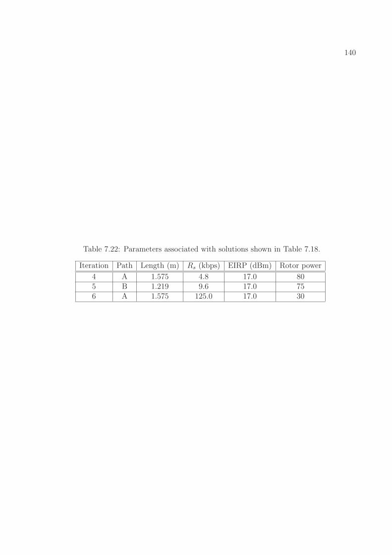
140
Table 7.22: Parameters associated with solutions shown in Table 7.18.
Iteration Path Length (m) Rs (kbps) EIRP (dBm) Rotor power
4 A 1.575 4.8 17.0 805 B 1.219 9.6 17.0 756 A 1.575 125.0 17.0 30

141
7.3.0.2 Live Multi-domain Decision Making in a Simple Dynamic Environment
Having now shown that the AVEP can learn its surroundings by exploring the paths during
test bed experiments, I inteintionally bypassed the initial exploration process for this exper-
iment. By pre-loading the AVEP with the information that would have been learned during
the initial path explorations, I can focus on the showing how the AVEP uses decision making
and the second stage learning process during the test bed experiment.
This experiment shows the operation of the AVEP in a simple dynamic environment, as in
Section 7.2.3. Table 7.23 shows the changes in the number of target and anti-targets pieces
on paths A and B from iterations 1-5 to iterations 6-10.
Table 7.23: Environmental parameters (meters) used in evaluating UMDDM in a simpledynamic environment during a live experiment.
Iterations Path Targets X Anti-targets Y Noise (dBm)
A 5 1 -821-5 B 3 0 -82
C 5 3 -82A 3 1 -82
6-10 B 0 0 -82C 5 3 -82
Table 7.24 shows the experimental results for this live test bed experiment in a simple
dynamic environment. As in the simulations, the AVEP seeks to maintain or increase per-
formance, as indicated by the solution score. In the simulations, the only time that the score
decreased was when the environment changed from one iteration to the next. Note that
the score does drop on iteration 3, when the environment has not in fact changed. This is
due to sensor jitter; during live tests, the chassis mounted sensors will occasionally register
more targets or anti-targets than actually exist due to the motion of the AVEP itself. This
could be fixed with a more sophisticated sensing algorithm, but that is outside the scope of
this work. On iteration 6, the target and anti-target values do change, and this is correctly

142
observed by the AVEP. On iteration 6, the AVEP traverse path B using a previously de-
veloped solution, but observes that the environment has changed and discards the solution.
The AVEP selects path A for the next iteration, and develops a solution based on expired
data. As soon as the AVEP traverses path A, it observers that path A has also changed,
and discards the expired solution for path A as well. On iteration 8, the AVEP implements
a solution that corresponds to the current path environment, and uses this solution for the
remaining iterations of the experiment.
Table 7.24: Results of live UMDDM in a simple dynamic environment over 10 iterations ina live experiment.
Iteration Path traversed Mode New/Prev solution Solution score
1 A Exploit New solution 0.58742 A Exploit New solution 0.63013 C Exploit New solution -0.00574 A Exploit New solution 0.28505 B Exploit New solution 0.59816 B Exploit Prev solution 0.59817 A Exploit New solution 0.26308 A Exploit New solution 0.12869 A Exploit Prev solution 0.128610 A Exploit Prev solution 0.1286
Table 7.25 shows the solutions generated by the decision maker and implemented by the
AVEP during the live experiment in a simple dynamic environment. As directly above,
this table also show the results of the changing environment and the solutions generated in
iterations 7 and 8 to accommodate the changes. Table 7.26 shows the parameters associated
with each solution.

143
Table 7.25: Solutions generated by decision maker during live tests in a simple dynamicenvironment.
Iteration Z T B G Score
1 0.5999 14.5067 1.7094e-4 46 0.58742 0.5999 8.9673 0 21 0.63013 0.4000 13.8907 0 18 -0.00574 0.5999 13.8606 0.1709e-4 44 0.28505 0.6000 9.0251 0.1709e-4 29 0.59817 0.5999 10.6217 0 12 0.26308 0.5999 8.9673 0 11 0.1286
Table 7.26: Parameters associated with solutions shown in Table 7.25.
Iteration Path Length (m) Rs (kbps) EIRP (dBm) Rotor power
1 A 1.575 125.0 17.0 252 A 1.575 9.6 17.0 503 C 2.223 2.4 17.0 604 A 1.575 125.0 17.0 805 B 1.219 125.0 17.0 707 A 1.575 2.0 17.0 358 A 1.575 2.4 17.0 50

144
7.3.0.3 Live Multi-domain Decision Making in a Highly Dynamic Environment
For this live experiment, I again created a randomly generated scenario to test the AVEP
decision making and learning performance in a highly dynamic environment. Using the
randomly generated environmental parameters , I was able to implement the experiment
by changing the target and anti-target parameters along each path between every iteration
of the experiment. While I did conduct this experiment while transmitting a broadband
signal to raise the noise floor, further refinements to the test bed’s RF environment are not
practical. Table 7.27 shows the meters for 10 iterations.
The results of this live test experiment are shown in Table 7.28. As in the highly dynamic
tests scenario simulation, in this experiment where the environment changes dramatically
with every iteration, the AVEP implements a new solution every iteration and is unable to
use previous solutions in a attempt to increase its performance from one iteration to the
next, as indicated by the solution score. The AVEP makes decisions based only on the
information is has gathered. While it is possible that in a highly dynamic environment the
AVEP will miss some opportunities, in this experiment the AVEP manages to exploit some
of the better path environments, such as path B on iteration 3, path C on iteration 8, and
path A on iteration 10.
Table 7.29 shows the solutions generated by the decision maker and implemented by the
AVEP in this experiment. As mentioned in previous experiment, I transmitted a broadband
signal to increase the noise as observed by the RFIC. Even with this signal raising the
noise floor, there is very little variability in the B values of the solutions generated by the
decision maker. This is due to the nature of the B objective function. Figure 6.8 shows
that for a wide range of RS values, the B value (aka BER) is effectively 0 for SNR values
greater than 5 dB. In live experiments, it is difficult to fix the laboratory RF environment, as

145
Table 7.27: Environmental parameters (meters) used in evaluating UMDDM in a highlydynamic environment during a live experiment.
Iterations Path Targets X Anti-targets Y Noise (dBm)
A 1 3 -821 B 1 2 -82
C 3 3 -82A 0 3 -82
2 B 0 1 -82C 3 5 -82A 0 5 -82
3 B 5 0 -82C 2 2 -82A 1 5 -82
4 B 3 4 -82C 0 2 -82A 5 2 -82
5 B 3 5 -82C 3 4 -82A 3 3 -82
6 B 1 4 -82C 1 4 -82A 2 3 -82
7 B 3 4 -82C 0 0 -82A 4 4 -82
8 B 1 2 -82C 2 0 -82A 2 3 -82
9 B 4 1 -82C 3 2 -82A 5 1 -82
10 B 3 4 -82C 3 1 -82

146
Table 7.28: Results of live UMDDM in a simple dynamic environment over 10 iterations ina live experiment.
Iteration Path traversed Mode New/Prev solution Solution score
1 C Exploit New solution 0.29332 A Exploit New solution 0.58643 B Exploit New solution 0.37934 B Exploit New solution 0.57095 B Exploit New solution -0.02906 C Exploit New solution -0.10667 C Exploit New solution -0.48538 C Exploit New solution -0.24339 C Exploit New solution 0.139610 A Exploit New solution -0.2701
opposed to simulations, where the noise value can be fixed to a specific value to ensure that
the decision maker generates solutions with variability in the B values. Still, it is possible
observe the trade-offs made between solutions from one iteration to the next. For example,
from iteration 5 to iteration 6, the Z and T values degrade (Z goes down, T goes up), but
the G value improves by more than double. Table 7.30 shows the parameters associated with
the solutions generated by the decision maker and implemented by the AVEP in this live
experiment.
Table 7.29: Solutions generated by decision maker in a highly dynamic environment duringa live experiment.
Iteration Z T B G Score
1 0.4000 16.4519 0 46 0.29332 0.5999 9.5827 1.5031e-8 30 0.58643 0.6000 7.6200 0 10 0.37934 0.6000 7.4189 0 22 0.57095 0.6000 7.4189 0 22 -0.02906 0.4000 16.4519 0 46 -0.10667 0.4000 16.4519 0 21 -0.48538 0.4000 19.5613 0 47 -0.24339 0.4000 17.9867 0 54 0.139610 0.5999 9.2530 0 12 -0.2701

147
Table 7.30: Parameters associated with solutions shown in Table 7.29.
Iteration Path Length (m) Rs (kbps) EIRP (dBm) Rotor power
1 C 2.223 192.0 17.0 70.02 A 1.575 57.6 17.0 40.03 B 1.219 2.4 17.0 60.04 B 1.219 38.4 17.0 40.05 B 1.219 38.4 17.0 40.06 C 2.223 19.2 17.0 70.07 C 2.223 2.4 17.0 70.08 C 2.223 9.6 17.0 80.09 C 2.223 38.4 17.0 75.010 A 1.575 2.4 17.0 55.0

148
7.4 Conclusion
This chapter presented AVEP experimental tests and results, both in software simulation
and in live tests. I verified that the decision making process works for individual objective
functions by isolating an individual objective function and showing that the decision making
process returned a solution that made sense when the objective function is the only one
considered [88]. I next evaluated the results when considering all four objective functions
together. I evaluated the full decision making process over many iterations, in scenarios
representing static environments, a simple dynamic environment (environment changes once
during the scenario), and rapidly changing dynamic environments (values can change dra-
matically from iteration to iteration).
In static and simple dynamic environments, the second stage learning process ensures that
the AVEP does not spend all its time exploiting the best path at the expense of exploring the
other paths. Rather, the second stage learning process ensures that the AVEP does main-
tain up-to-date meter readings by periodically re-exploring other paths. In highly dynamic
environment, the second stage learning process is unable improve performance from one it-
eration to the next through the use of previously implemented solutions; previous solutions
are never applicable as the environment along every path changes with every iteration. In
these cases, the AVEP is intelligent enough not to use previous results while the environment
is rapidly changing. Yet if the environment were to settle, the AVEP would then apply the
second stage learning process and seek iterative improvement using previously implemented
solutions.
This chapter concludes the description of UMDDM and the design, development, implemen-
tation, and deployment of the AVEP and the UMDDM algorithms. I have shown that the
AVEP can learn the RF and MOT parameters of the environment, choose a solution that

149
maximizes the objective functions, and implement the solution to ensure mission success.
I have also shown that AVEP is also capable of learning from experience, modifying its
behavior over time increase its performance.

Chapter 8
Conclusions
This chapter presents a summary of the research in this dissertation, lists my research con-
tributions, and discusses areas for future research.
8.1 Summary
This research started several years ago with a simple observation, namely that CRs and AVs
perform similar tasks, albeit in different domains:
• Analyze their environment,
• Make and execute a decision,
• Evaluate the result (learn from experience), and
• Repeat as required.
This observation led to try to combine CR and AV intelligence into a single intelligent agent,
with the ability to leverage flexibility in the RF and motion (MOT) domains. I call this idea
unified multi-domain decision making (UMDDM).
150

151
This dissertation has presented my work on UMDDM, the development of UMDDM al-
gorithms and the implementation of the AVEP test platform, a working proof of concept
prototype that deploys UMDDM on a live system.
Chapter 1 introduced the concept of UMDDM and discussed the conception of my research
idea: combining CR and AV decision making into a single intelligent agent. My previous
research, funded by AFRL, has dealt with exploring CR applications for UAVs, and has led
directly to the research I presented in this dissertation.
Chapter 2 provided an overview of current CR and AV research, looking in particular at
efforts to combine CRs and AVs. However, few people are looking at combined CR and
AV solutions, and those that are do so from one perspective only. No one else is looking at
unified solutions, solutions that leverage flexibility in both RF and MOT domains.
Chapter 3 presents an overview of the experimental procedure used to develop and verify
UMDDM as well as the underlying experimental philosophy. I highlighted all the components
involved in developing and testing the UMDDM algorithms, including the experimental test
bed, the autonomous robotic AVEP, and the stand alone NBR. I highlighted an experimental
procedure that relies on software simulation combined with live tests to show the capabilities
of UMDDM.
Chapters 4, 5, and 6 lay out the details of the AVEP, a working proof of concept prototype
that implements UMDDM. Chapter 4 is a high level system overview, presenting the hard-
ware and software components that I designed and built to support my research in UMDDM.
The AVEP is an autonomous robotic platform capable of making and executing decisions
that leverage flexibility and intelligent adaptation in both RF and MOT domains.
Chapter 5 presents the AVEP operational and control algorithms. I stepped through the
AVEP FSM which provides top level control, pulling all the subcomponents and sensors to-

152
gether into a single integrated system. I also stepped through the RF and MOT subsystems,
giving the operational details of the communication system as well as the motion algorithm.
Chapter 6 discusses the learning and decision making aspects of this research. The learning
and decision making algorithms make up the cognitive core of this research, providing intelli-
gent action and introspection for the AVEP. UMDDM uses two stages of learning. The first
stage of learning provide environmental awareness through sensor data acquisition, and feeds
the decision making process. The decision maker uses the sensor data (meters) along with
knowledge of its own capabilities (knobs) to generate possible solutions for the AVEP to im-
plement. The second stage of learning provides intelligent adaptation based on the system’s
experiences, allowing it to implement a new solution or use a previous solution that may
provide better performance in the current environment. The two stages of learning combine
with the decision making process to implement UMDDM. As a result, the working proof
of concept prototype AVEP is able to leverage flexibility in both RF and MOT domains to
ensure mission success.
Chapter 7 presents the experimental tests and results that I used to validate my UMDDM
research. I divided the experiments into two section, software-based simulation and robot-
deployed live tests. I verified that the decision making process works for individual objective
functions by isolating an individual objective function and showing that the decision mak-
ing process returns a solution that makes sense when the objective function is the only
one considered. I then evaluated the results when considering all four objective functions
together, with scenarios representing static environments, slowly changing dynamic envi-
ronments (values change a small amount from iteration to iteration), and rapidly changing
dynamic environments (values can change dramatically from iteration to iteration). The
software simulations allowed me to highlight the details of the decision making and learning
UMDDM algorithms, while the live tests showed that I was able to implement my ideas in

153
a working proof of concept prototype.
8.2 Contributions
This research has made the following contributions to knowledge:
• I have initiated the exploration of unified multi-domain decision making (UMDDM). As
mentioned several times through this dissertation, CRs and AVs perform similar tasks in
order to fulfill their intended missions. They both analyze their environment, make and
execute a decision, evaluate the result (learn from their actions) and repeat the process as
required. AVs are increasingly present in tactical and public safety roles, and both motion
and communication are fundamental aspects of AV operation. Knowing that need to move
affects communication, and the need to communicate affects motion, it not only makes
sense but becomes increasingly imperative that RF and MOT be considered together in
AV research. This dissertation presents the first work in UMDDM, where flexibility in RF
and MOT domains are considered with equal importance.
• I have designed and implemented a working proof of concept prototype AV with UMDDM.
This autonomous robotic platform AVEP is able to leverage flexibility in both RF and
MOT domains to ensure mission success. The AVEP performs live tests in a laboratory
test bed, showing the real life capabilities of UMDDM. Further, the controller software
is written in such a way that it can be ported to other AV platforms, such as the UAVs
used by AFRL in Rome, NY.
• I have developed and implemented an experimental procedure based on both software
simulation and live (non-simulation) tests. Further, I have provided the experimental
results that show UMDDM in use on a working proof of concept prototype AV.
• I have designed and deployed a wholly new inexpensive CR platform using commercial

154
off the shelf (COTS) hardware and free and open source software. The radio platform,
called SKIRL, is based on the BeagleBoard-xM single board computer and the Hope RF
RFM22B RFIC. It is ideally suited for low cost CR experimentation and deployment. An
overview of SKIRL with an example application is available in [10].
• I have advanced the state of CR for mobile applications. I have developed, implemented,
and tested new hardware, software, and algorithms for mobile CR. My SKIRL radio plat-
form is a low cost low power system ideally suited to mobile CR and intelligent sensor
networks. While UMDDM is intended for AV deployment, it is also ideally suited for sit-
uational awareness in mobile CR applications. My dissertation provides extensive details
on the software algorithms, and control and data structures I implemented to support
UMDDM, and these are all applicable to mobile CR research.
• I have provided an introduction to CR concepts and methods for the AV research com-
munity. At the same time, I have provided an introduction to AV concepts and methods
for the CR community. This dissertation itself opens the doors to the possibilities of
crossover between CR and AV research. I have shown the possibility of combined CR
and AV decision making in a single intelligent agent, showcased by my working proof of
concept prototype AVEP.
8.3 Future Research
This dissertation is the first step in UMDDM, and provides a foundation for future work. I
have implemented decision making and learning algorithms that leverage flexibility in both
RF and MOT. I have also designed and deployed a working proof of concept prototype
robotic platform that implements my UMDDM algorithms in live tests.
My research focuses on a limited set of controllable RF and MOT parameters. The most

155
obvious next step to expand the set of controllable parameters: a quadrocopter or airplane-
based UAV provide much more flexibility in the MOT domain, capable of movement in three
dimensions. RF considerations can be extended to a full set of PHY parameters, and recon-
figurability can be extended up the network stack. While this provides additional flexibility,
additional RF and MOT parameters do not push this research forward significantly.
Deploying UMDDM on multiple platforms opens the doors to the new ideas in swarming,
both from the physical and RF perspective. UMDDM can also be extended to additional
domains, beyond RF and MOT. Weather is capable of affecting movement and communi-
cation significantly; a torrential rain storm increases RF attenuation dramatically, and may
inhibit motion of vehicles via strong winds or muddy ground. These considerations could be
integrated into the decision making process with the development of appropriate objective
functions.
UMDDM currently uses a population based nondominated sort method to implement de-
cision making, but decision making research can provide more sophisticated decision mak-
ing options. Case based decision making and recognition primed decision making are two
methods that are used to model the way humans make decisions. However, researchers are
currently exploring other biologically inspired decision making methods, such as emulating
the way the human body makes decisions in the healing process [147]. These methods have
the potential to extend UMDDM into new application areas.
I believe that my research into UMDDM is just the beginning. The future of RF commu-
nications needs to take into account the totality of the environment, and the future of AV
research needs to enable flexibility in multiple domains to ensure mission success. While I
have outlined a few areas where I believe that my research can be extended, I feel that the
next step in UMDDM will be in a direction that is completely unexpected, an advancement
that I could not predict. But the next step will move UMDDM forward for the benefit of

156
all.

Bibliography
[1] R. Munroe, “New pet,” Apr. 2008. [Online]. Available: http://xkcd.com/413/
[2] Python Software Foundation, “Python programming language official website,” 2012.[Online]. Available: http://www.python.org/
[3] T. W. Rondeau, “GNU radio - WikiStart - gnuradio.org,” 2012. [Online]. Available:http://gnuradio.org/redmine/projects/gnuradio/wiki
[4] N. R. C. Committee on Autonomous Vehicles in Support of Naval Operations,Autonomous Vehicles in Support of Naval Operations. National Academies Press, 2005.[Online]. Available: http://www.nap.edu/openbook.php?record id=11379&page=135
[5] G. Anthes, “Robots gear up for disaster response,” Commun. ACM, vol. 53, no. 4, p.1516, Apr. 2010. [Online]. Available: http://doi.acm.org/10.1145/1721654.1721662
[6] A. Birk, S. Schwertfeger, and K. Pathak, “A networking framework for teleoperation insafety, security, and rescue robotics,” IEEE Wireless Communications, vol. 16, no. 1,pp. 6 –13, Feb. 2009.
[7] L. Techy, D. G. Schmale III, and C. A. Woolsey, “Coordinated aerobiological samplingof a plant pathogen in the lower atmosphere using two autonomous unmanned aerialvehicles,” Journal of Field Robotics, vol. 27, no. 3, pp. 335–343, May 2010. [Online].Available: http://onlinelibrary.wiley.com/doi/10.1002/rob.20335/abstract
[8] A. Posch and S. Sukkarieh, “UAV based search for a radio tagged animal using particlefilters,” in In Proceedings of 2009 Australasian Conference on Robotics and Automa-tion, 2009.
[9] C. W. Bostian and A. R. Young, “Cognitive radio: A practical review for the radioscience community,” Radio Science Bulletin, no. 342, pp. 16–25, Sep. 2012.
[10] A. R. Young and C. W. Bostian, “Simple and low cost platforms for cognitive radioexperiments,” Microwave Magazine, IEEE, vol. 14, no. 1, pp. 146 –157, Jan.-Feb. 2013.
[11] IEEE-SA, “IEEE DySPAN standards committee,” 2008. [Online]. Available:http://www.dyspan-sc.org/
157

158
[12] SDR Forum, “SDRF cognitive radio definitions: Working document SDRF-06-R-0011-V1.0.0,” 2007. [Online]. Available: http://www.sdrforum.org/pages/documentLibrary/documents/SDRF-06-R-0011-V1 0 0.pdf
[13] S. Pastukh, “Software-defined radio and cognitive radio systems |ITU news,” Jun. 2012. [Online]. Available: https://itunews.itu.int/En/2076-Software-defined-radio-and-cognitive-radio-systems.note.aspx
[14] FCC, “Notice of proposed rule making and order, in the matter of: Facilitatingopportunities for flexible, efficient, and reliable spectrum use employing cognitiveradio technologies; authorization and use of software defined radios,” 2003. [Online].Available: http://hraunfoss.fcc.gov/edocs public/attachmatch/FCC-03-322A1.pdf
[15] L. Doyle, Essentials of Cognitive Radio, ser. The Cambridge wireless essentials series.Cambridge: Cambridge University Press, 2009.
[16] J. Mitola, “Software radios: Survey, critical evaluation and future directions,”Aerospace and Electronic Systems Magazine, IEEE, vol. 8, no. 4, pp. 25 –36, april1993.
[17] J. Melby, “JTRS and the evolution toward software-defined radio,” in MILCOM 2002.Proceedings, vol. 2, Oct. 2002, pp. 1286 – 1290 vol.2.
[18] S. Chen et al., “Genetic algorithm-based optimization for cognitive radio networks,”in 2010 IEEE Sarnoff Symposium, Apr. 2010, pp. 1 –6.
[19] B. Le et al., “A public safety cognitive radio node,” in 2007 SDR Forum TechnicalConference, Denver, CO, 2007. [Online]. Available: http://cognitiveradiotechnologies.com/files/LeB 1.pdf
[20] J. H. Reed, Software Radio: A Modern Approach to Radio Engineering. Upper SaddleRiver, N.J.: Prentice Hall, 2002.
[21] G. Kolumban, T. Krebesz, and F. Lau, “Theory and application of software definedelectronics: Design concepts for the next generation of telecommunications and mea-surement systems,” IEEE Circuits and Systems Magazine, vol. 12, no. 2, pp. 8 –34,2012.
[22] J. Mitola, “Cognitive radio an integrated agent architecture for software defined radio,”PhD Dissertation, KTH, Sweden, 2000.
[23] H. K. Markey and G. Antheil, “Secret communication system,” U.S. Patent2 292 387, Aug., 1942, U.S. Classification: 380/34. [Online]. Available: http://www.google.com/patents?id=R4BYAAAAEBAJ

159
[24] S. Haykin, “Cognitive radio: brain-empowered wireless communications,” SelectedAreas in Communications, IEEE Journal on, vol. 23, no. 2, p. 201220, 2005. [Online].Available: http://ieeexplore.ieee.org/xpls/abs all.jsp?arnumber=1391031
[25] C. Rieser et al., “Cognitive radio testbed: further details and testing of a distributedgenetic algorithm based cognitive engine for programmable radios,” in 2004 IEEEMilitary Communications Conference, 2004. MILCOM 2004, vol. 3, Nov. 2004, pp.1437 – 1443 Vol. 3.
[26] Federation of American Scientists, United States Air Force Unmanned AircraftSystems Flight Plan 2009-2047. Headquarters, United States Air Force, 2009.[Online]. Available: http://www.govexec.com/pdfs/072309kp1.pdf
[27] F. Seelig, “A description of the august 2006 XG demonstrations at Fort A.P. Hill,”in 2nd IEEE International Symposium on New Frontiers in Dynamic Spectrum AccessNetworks, 2007. DySPAN 2007, Apr. 2007, pp. 1 –12.
[28] K. Nolan et al., “Dynamic spectrum access and coexistence experiences involving twoindependently developed cognitive radio testbeds,” in New Frontiers in Dynamic Spec-trum Access Networks, 2007. DySPAN 2007. 2nd IEEE International Symposium on,april 2007, pp. 270 –275.
[29] P. Marshall, “Extending the reach of cognitive radio,” Proceedings of the IEEE, vol. 97,no. 4, pp. 612 –625, april 2009.
[30] ——, Quantitative Analysis of Cognitive Radio and Network Performance. Boston:Artech House, 2010.
[31] T. W. Rondeau and C. W. Bostian, Artificial Intelligence in Wireless Communications,1st ed. Boston: Artech House, Jun. 2009.
[32] T. W. Rondeau et al., “Cognitive radio formulation and implementation,”in Cognitive Radio Oriented Wireless Networks and Communications, 2006.1st International Conference on, 2006, p. 110. [Online]. Available: http://ieeexplore.ieee.org/xpls/abs all.jsp?arnumber=4211156
[33] A. R. Young et al., “CSERE (Cognitive system enabling radio evolution): A modularand user-friendly cognitive engine,” in 2012 IEEE Symposium on New Frontiers inDynamic Spectrum Access Networks (DySPAN), Bellevue, WA, Oct. 2012.
[34] P. Marshall, “DARPA progress towards affordable, dense, and content focused tacticaledge networks,” in IEEE Military Communications Conference, 2008. MILCOM 2008,Nov. 2008, pp. 1 –7.
[35] J. Redi and R. Ramanathan, “The DARPA WNaN network architecture,” in IEEEMilitary Communications Conference, 2009. MILCOM 2009, Nov. 2011, pp. 2258 –2263.

160
[36] J. Sydor, “CORAL: a WiFi based cognitive radio development platform,” in 2010 7thInternational Symposium on Wireless Communication Systems (ISWCS), Sep. 2010,pp. 1022 –1025.
[37] J. Sydor et al., “A generic cognitive radio based on commodity hardware,”in Computer Communications Workshops (INFOCOM WKSHPS), 2011 IEEEConference on, 2011, p. 16. [Online]. Available: http://ieeexplore.ieee.org/stamp/stamp.jsp?tp=&arnumber=5928808
[38] Ettus Research, “Ettus research,” 2012. [Online]. Available: http://www.ettus.com/
[39] T. Newman and T. Bose, “A cognitive radio network testbed for wireless communica-tion and signal processing education,” in Digital Signal Processing Workshop and 5thIEEE Signal Processing Education Workshop, 2009. DSP/SPE 2009. IEEE 13th, Jan.2009, pp. 757 –761.
[40] Rice University, “Rice university WARP - wireless open-access research platform,”2012. [Online]. Available: http://warp.rice.edu/trac
[41] T. B. Lee, “How software-defined radio could revolutionize wireless,”Jul. 2012. [Online]. Available: http://arstechnica.com/tech-policy/2012/07/how-software-defined-radio-could-revolutionize-wireless/
[42] Per Vices, “Per vices,” 2012. [Online]. Available: http://www.pervices.com/index.html
[43] C. Christodoulou, Y. Tawk, and S. Jayaweera, “Cognitive radio, reconfigurable anten-nas, and radiobots,” in 2012 IEEE International Workshop on Antenna Technology(iWAT), Mar. 2012, pp. 16 –19.
[44] A. S. Fayez et al., “Leveraging embedded heterogeneous processors for softwaredefined radio applications,” in 2010 SDR Forum Technical Conference, Arlington, VA,Dec. 2010, pp. 490–495. [Online]. Available: http://groups.winnforum.org/d/do/3704
[45] L. Hope Microelectronics Co., “RFM22B FSK transceiver - FSK modules -HOPE microelectronics,” 2012. [Online]. Available: http://www.hoperf.com/rf fsk/fsk/RFM22B.htm
[46] Oxford English Dictionary, “”autonomous, adj.”.” 2012. [Online]. Available:http://www.oed.com/viewdictionaryentry/Entry/13498
[47] D. C. Conner, “Sensor fusion, navigation, and control of autonomous vehicles,”Masters Thesis, Virginia Polytechnic Institute and State University, Aug. 2000. [On-line]. Available: http://scholar.lib.vt.edu/theses/available/etd-08112000-13580038/unrestricted/DCCthesis.pdf
[48] I. Asimov and K. A. Frenkel, Robots, Machines in Man’s Image, 1st ed. New York:Harmony Books, 1985.

161
[49] M. W. Shelley, Frankenstein, or, The Modern Prometheus: With Supplementary Essaysand Poems from the Twentieth Century. Washington, D.C: Orchises, 1988.
[50] Oxford English Dictionary, “”robot, n.2”.” 2012. [Online]. Available: http://www.oed.com/view/Entry/166641
[51] K. Capek, P. Selver, and N. Playfair, R.U.R. (Rossum’s Universal Robots): A FantasticMelodrama in Three Acts and an Epilogue. New York: S. French, 1923.
[52] N. Wiener, Cybernetics; or, Control and Communication in the Animal and the Ma-chine. New York: J. Wiley, 1948.
[53] C. A. Woolsey, “Autonomous vehicles,” private communication, Aug. 2012.
[54] T. Vanderbilt, “Autonomous cars through the ages,” Feb. 2012. [Online]. Available:http://www.wired.com/autopia/2012/02/autonomous-vehicle-history/
[55] DARPA, “Urban challenge rules,” 2007. [Online]. Available: http://archive.darpa.mil/grandchallenge/docs/Urban Challenge Rules 102707.pdf
[56] ——, Urban Challenge Route Network Definition File (RNDF) and Mission Data File(MDF) Formats, Mar. 2007.
[57] T. Vanderbilt, “Let the robot drive: The autonomous car of the future ishere | wired magazine | wired.com,” Jan. 2012. [Online]. Available: http://www.wired.com/magazine/2012/01/ff autonomouscars/
[58] ——, “Navigating the legality of autonomous vehicles | autopia |wired.com,” Feb. 2012. [Online]. Available: http://www.wired.com/autopia/2012/02/autonomous-vehicle-legality/
[59] C. Pinto, “How autonomous vehicle policy in California and Nevada addressestechnological and non-technological liabilities,” Intersect: The Stanford Journalof Science, Technology and Society, vol. 5, 2012. [Online]. Available: http://ojs.stanford.edu/ojs/index.php/intersect/article/view/361
[60] A. Amanna et al., “Railway cognitive radio,” IEEE Vehicular Technology Magazine,vol. 5, no. 3, pp. 82–89, Sep. 2010.
[61] D. Scaperoth et al., “Cognitive radio platform development for interoperability,”in Military Communications Conference, 2006. MILCOM 2006. IEEE, 2006, p. 16.[Online]. Available: http://ieeexplore.ieee.org/xpls/abs all.jsp?arnumber=4086554
[62] F. Ge et al., “Cognitive radio: from spectrum sharing to adaptive learning andreconfiguration,” in Aerospace Conference, 2008 IEEE, 2008, p. 110. [Online].Available: http://ieeexplore.ieee.org/xpls/abs all.jsp?arnumber=4526372

162
[63] G. D. Troxel et al., “Cognitive adaptation for teams in ADROIT,” in IEEE GlobalTelecommunications Conference, 2007. GLOBECOM ’07. IEEE, Nov. 2007, pp. 4868–4872.
[64] M. Di Felice et al., “Smart radios for smart vehicles: Cognitive vehicular networks,”IEEE Vehicular Technology Magazine, vol. 7, no. 2, pp. 26 –33, Jun. 2012.
[65] H. Hartenstein and K. Laberteaux, “A tutorial survey on vehicular ad hoc networks,”IEEE Communications Magazine, vol. 46, no. 6, pp. 164 –171, Jun. 2008.
[66] S. Chen et al., “On optimizing vehicular dynamic spectrum access networks: Automa-tion and learning in mobile wireless environments,” in 2011 IEEE Vehicular NetworkingConference (VNC), Nov. 2011, pp. 39 –46.
[67] M. A. McHenry et al., “Chicago spectrum occupancy measurements & analysis anda long-term studies proposal,” in Proceedings of the First International Workshopon Technology and Policy for Accessing Spectrum, 2006, p. 1. [Online]. Available:http://dl.acm.org/citation.cfm?id=1234389
[68] J. F. Hauris, “Genetic algorithm optimization in a cognitive radio for autonomousvehicle communications,” in International Symposium on Computational Intelligencein Robotics and Automation, 2007. CIRA 2007. IEEE, Jun. 2007, pp. 427–431.
[69] C. J. Rieser et al., “Cognitive radio engine based on genetic algorithms in a network,”U.S. Patent 7 289 972, Oct., 2007, U.S. Classification: 706/13. [Online]. Available:http://www.google.com/patents/US7289972
[70] T. W. Rondeau, “Application of artificial intelligence to wireless communications,”PhD Dissertation, Virginia Polytechnic Institute and State University, Oct. 2007.[Online]. Available: http://scholar.lib.vt.edu/theses/available/etd-10052007-081332/
[71] M. Angermann, M. Frassl, and M. Lichtenstern, “Autonomous formation flying ofmicro aerial vehicles for communication relay chains,” San Diego, CA, Jan. 2011.
[72] Y. Mostofi, “Communication-aware motion planning in fading environments,” in IEEEInternational Conference on Robotics and Automation, 2008. ICRA 2008, May 2008,pp. 3169 –3174.
[73] C. Hager, J. Burdin, and R. Landry, “Modeling emergent behavior in tactical wirelessnetworks,” in IEEE Military Communications Conference, 2009. MILCOM 2009, Oct.2009, pp. 1 –7.
[74] M. Lindhe and K. Johansson, “Using robot mobility to exploit multipath fading,”IEEE Wireless Communications, vol. 16, no. 1, pp. 30 –37, Feb. 2009.

163
[75] K. Daniel et al., “AirShield: a system-of-systems MUAV remote sensing architecturefor disaster response,” in 2009 3rd Annual IEEE Systems Conference, Mar. 2009, pp.196 –200.
[76] ——, “Three dimensional channel characterization for low altitude aerial vehicles,”in 2010 7th International Symposium on Wireless Communication Systems (ISWCS),Sep. 2010, pp. 756 –760.
[77] K. Daniel, A. Wolff, and C. Wietfeld, “Protocol design and delay analysis for a MUAV-Based aerial sensor swarm,” in 2010 IEEE Wireless Communications and NetworkingConference (WCNC), Apr. 2010, pp. 1 –6.
[78] K. Daniel et al., “Fading countermeasures with cognitive topology management foraerial mesh networks,” in 2010 IEEE International Conference on Wireless Informa-tion Technology and Systems (ICWITS), Sep. 2010, pp. 1 –4.
[79] ——, “Cognitive agent mobility for aerial sensor networks,” IEEE Sensors Journal,vol. 11, no. 11, pp. 2671 –2682, Nov. 2011.
[80] ——, “A communication aware steering strategy avoiding self-separation of flying robotswarms,” in Intelligent Systems (IS), 2010 5th IEEE International Conference, Jul.2010, pp. 254 –259.
[81] M. D. Silvius, “Building a dynamic spectrum access smart radio with applicationto public safety disaster communications,” PhD Dissertation, Virginia PolytechnicInstitute and State University, Blacksburg, Va, Sep. 2009. [Online]. Available:http://scholar.lib.vt.edu/theses/available/etd-08272009-000216/
[82] T. R. Newman et al., “Cognitive engine implementation for wireless multicarriertransceivers,” Wirel. Commun. Mob. Comput., vol. 7, no. 9, p. 11291142, Nov. 2007.[Online]. Available: http://dx.doi.org/10.1002/wcm.v7:9
[83] Y. Zhao et al., “Performance evaluation of cognitive radios: Metrics, utility functions,and methodology,” Proceedings of the IEEE, vol. 97, no. 4, pp. 642–659, 2009.
[84] C. B. Dietrich, E. W. Wolfe, and G. M. Vanhoy, “Cognitive radio testingusing psychometric approaches: applicability and proof of concept study,” AnalogIntegrated Circuits and Signal Processing, p. 110, 2012. [Online]. Available:http://www.springerlink.com/index/vg022u1330277056.pdf
[85] N. J. Kaminski, “Performance evaluation of cognitive radios,” Masters Thesis,Virginia Polytechnic Institute and State University, Blacksburg, Va, May 2012.[Online]. Available: http://scholar.lib.vt.edu/theses/available/etd-05012012-135634/
[86] RoboCup, “RoboCup soccer humanoid league rules and setup,”2012. [Online]. Available: http://www.tzi.de/humanoid/pub/Website/Downloads/HumanoidLeagueRules2012-06-07.pdf

164
[87] DARPA, “DARPA robotics challenge - DARPA-BAA-12-39 - federal businessopportunities: Opportunities,” 2012. [Online]. Available: https://www.fbo.gov/index?s=opportunity\&mode=form\&id=ee8e770bcfe1fe217472342c67d6bd5a
[88] A. R. Young and C. W. Bostian, “A low-cost cognitive radio for UAVs that implementsmulti-domain decision making,” in 2012 AFRL Cognitive RF Workshop, Kirtland AirForce Base, Albuquerque, NM, Sep. 2012.
[89] P. Pawelczak et al., “Cognitive radio: Ten years of experimentation and development,”Communications Magazine, IEEE, vol. 49, no. 3, pp. 90 –100, Mar. 2011.
[90] Maxim Integrated, “MAX7032 low-cost, crystal-based, programmable, ASK/FSKtransceiver with fractional-n PLL - overview,” 2012. [Online]. Available: http://www.maximintegrated.com/datasheet/index.mvp/id/4755
[91] S. M. S. Hasan and S. W. Ellingson, “Multiband public safety radio usinga multiband RFIC with an RF multiplexer-based antenna interface,” SoftwareDefined Radio (SDR)’08, Washington DC, 2008. [Online]. Available: http://www.ece.vt.edu/swe/mypubs/Hasan VT SDR08 Final.pdf
[92] Arduino, “Arduino - HomePage,” 2012. [Online]. Available: http://www.arduino.cc/
[93] Digilent, Inc., “Digilent inc. - digital design engineer’s source,” 2012. [Online]. Avail-able: http://www.digilentinc.com/Products/Catalog.cfm?NavPath=2,892&Cat=18
[94] The Raspberry Pi Foundation, “Raspberry pi | an ARM GNU/Linux box for \$25.take a byte!” 2012. [Online]. Available: http://www.raspberrypi.org/
[95] BeagleBoard.org, “BeagleBoard.org - bone,” 2012. [Online]. Available: http://beagleboard.org/bone
[96] pandaboard.org, “Pandaboard,” 2012. [Online]. Available: http://pandaboard.org/
[97] Gumstix inc., “Gumstix overo COMS open source products,” 2012. [Online].Available: https://gumstix.com/store/index.php?cPath=33
[98] Baigung, “RFM22B transciever simple example in FIFO mode - application notes- HOPE microelectronics,” 2011. [Online]. Available: http://www.hoperf.com/docs/guide/185.htm
[99] M. McCauley, “RF22: RF22 library for arduino,” 2012. [Online]. Available:http://www.open.com.au/mikem/arduino/RF22/
[100] A. S. Fayez, “Designing a software defined radio to run on a heterogeneousprocessor,” Masters Thesis, Virginia Polytechnic Institute and State University,Blacksburg, Va, Apr. 2011. [Online]. Available: http://scholar.lib.vt.edu/theses/available/etd-05042011-190721/unrestricted/Fayez AS T 2011 1.pdf

165
[101] C. R. Anderson, E. G. Schaertl, and P. Balister, “A low-cost embedded sdr solutionfor prototyping and experimentation,” in SDR’09: Proceedings of the Software DefinedRadio Technical and Product Exposition, 2009.
[102] iRobot, “iRobot create programmable robot - overview,” 2012. [Online]. Available:http://www.irobot.com/us/robots/Educators/Create.aspx
[103] ——, “iRobot: robots for defense and public safety,” 2012. [Online]. Available:http://www.irobot.com/en/us/robots/defense.aspx
[104] Aldebaran Robotics, “Home - corporate - aldebaran robotics | accueil,” 2012. [Online].Available: http://www.aldebaran-robotics.com/en/#
[105] Seeed Studio, “2WD arduino compatible mobile platform [ROB102F3M]- \$36.00 : Seeed studio bazaar, boost ideas, extend thereach,” 2012. [Online]. Available: http://www.seeedstudio.com/depot/2wd-arduino-compatible-mobile-platform-p-657.html?cPath=170
[106] The LEGO Group, “LEGO.com MINDSTORMS : Home,” 2012. [Online]. Available:http://mindstorms.lego.com/en-us/Default.aspx
[107] Tin Can Tools, “Tin can tools :: All products :: Trainer-xM board,”2012. [Online]. Available: http://www.tincantools.com/product.php?productid=16151&cat=0&page=2&featured
[108] “Hagisonic StarGazer robot localization system - RobotShop,” 2012. [Online]. Avail-able: http://www.robotshop.com/hagisonic-stargazer-localization-system-2.html
[109] “The angstrom distribution | embedded power,” 2012. [Online]. Available:http://www.angstrom-distribution.org/
[110] “BeagleboardRevCValidation - beagleboard - beagle board diagnostic toolsand procedure - low-cost, low-power single-board computer - google projecthosting,” 2012. [Online]. Available: http://code.google.com/p/beagleboard/wiki/BeagleboardRevCValidation
[111] “Main page - openembedded.org,” 2012. [Online]. Available: http://www.openembedded.org/wiki/Main Page
[112] A. S. Fayez et al., “Embedded SDR system design case study: An implmentationperspective,” Washington, D.C, 2012.
[113] Linaro, “Linaro: open source software for ARM SoCs,” 2012. [Online]. Available:http://www.linaro.org/
[114] “ARM - ubuntu wiki,” 2012. [Online]. Available: https://wiki.ubuntu.com/ARM

166
[115] C. W. Bostian, private communication, Aug. 2011.
[116] “Scan codes demystified.” [Online]. Available: http://www.quadibloc.com/comp/scan.htm
[117] C. W. Bostian and A. R. Young, “The application of cognitive radio to coordinatedunmanned aerial vehicle (UAV) missions,” DTIC Document, Tech. Rep., 2011.[Online]. Available: http://oai.dtic.mil/oai/oai?verb=getRecord&metadataPrefix=html&identifier=ADA546145
[118] IETF, “RFC: 793 transmission control protocol,” 1981. [Online]. Available:http://www.ietf.org/rfc/rfc793.txt
[119] M. Pakdaman and M. Sanaatiyan, “Design and implementation of line follower robot,”in Second International Conference on Computer and Electrical Engineering, 2009.ICCEE ’09, vol. 2, Dec. 2009, pp. 585 –590.
[120] S. S. Epp, Discrete mathematics with applications. Belmont, CA: Thomson-Brooks/Cole, 2004.
[121] E. W. Dijkstra, “A note on two problems in connexion with graphs,”Numerische Mathematik, vol. 1, no. 1, pp. 269–271, 1959. [Online]. Available:http://www.springerlink.com/content/uu8608u0u27k7256/abstract/
[122] S. Koenig and M. Likhachev, “Dˆ* lite,” in Proceedings of the nationalconference on artificial intelligence, 2002, p. 476483. [Online]. Available: http://www.aaai.org/Library/AAAI/2002/aaai02-072.php
[123] C. L. Hwang and A. S. M. Masud, Multiple objective decision making, methods and ap-plications: a state-of-the-art survey, ser. Lecture notes in economics and mathematicalsystems. Berlin ; New York: Springer-Verlag, 1979, no. 164.
[124] A. He et al., “A survey of artificial intelligence for cognitive radios,” Vehicular Tech-nology, IEEE Transactions on, vol. 59, no. 4, p. 15781592, 2010.
[125] Oxford English Dictionary, “”learn, v.”.” 2012. [Online]. Available: http://oed.com/viewdictionaryentry/Entry/106716
[126] P. McCorduck, Machines Who Think: A Personal Inquiry into the History andProspects of Artificial Intelligence, 2nd ed. A K Peters/CRC Press, Mar. 2004.
[127] K. Z. Haigh, “Can artificial intelligence meet the cognitive networking challenge?”Dayton, OH, Sep. 2011. [Online]. Available: http://www.cs.cmu.edu/∼khaigh/papers/2011-haigh-AI-in-MANET.pdf

167
[128] L. Thiele et al., “A preference-based evolutionary algorithm for multi-objectiveoptimization,” Evolutionary Computation, vol. 17, no. 3, pp. 411–436, Sep. 2009.[Online]. Available: http://dx.doi.org/10.1162/evco.2009.17.3.411
[129] K. M. Nelson, “Applications of evolutionary algorithms in mechanical engineering,”Tech. Rep., 1997. [Online]. Available: http://digitalcommons.fau.edu/dissertations/AAI9735642
[130] J. Arifovic, “Genetic algorithm learning and the cobweb model,” Journal of EconomicDynamics and Control, vol. 18, no. 1, pp. 3–28, Jan. 1994. [Online]. Available:http://www.sciencedirect.com/science/article/pii/0165188994900671
[131] D. Sahoo, S. Rai, and S. Pradhan, “Threshold cryptography #x00026; genetic algo-rithm based secure key exchange for mobile hosts,” in Advance Computing Conference,2009. IACC 2009. IEEE International, Mar. 2009, pp. 1297 –1302.
[132] J. F. Kennedy, R. C. Eberhart, and Y. Shi, Swarm intelligence. San Francisco: MorganKaufmann Publishers, 2001.
[133] E. Zitzler and L. Thiele, “Multiobjective evolutionary algorithms: a comparative casestudy and the strength pareto approach,” IEEE Transactions on Evolutionary Com-putation, vol. 3, no. 4, pp. 257 –271, Nov. 1999.
[134] A. Rapoport, Decision Theory and Decision Behaviour, 2nd ed. Basingstoke: Macmil-lan, 1998.
[135] “Scientific computing tools for python numpy,” 2012. [Online]. Available:http://numpy.scipy.org/
[136] B. Sklar, Digital Communications: Fundamentals and Applications, 2nd ed. UpperSaddle River, N.J: Prentice Hall, Jan. 2001.
[137] T. Hooper, “Communication systems modelling with TIMS:Volume d1 fudamentaldigital experiments,” 2012. [Online]. Available: http://www.eng.auburn.edu/∼troppel/courses/TIMS-manuals-r5/
[138] “Question about bandwidth of FSK,” 2009. [Online]. Available: http://www.edaboard.com/thread24570.html
[139] T. Pratt, C. W. Bostian, and J. E. Allnutt, Satellite Communications, 2nd ed. Wiley,Oct. 2002.
[140] A. Leon-Garcia and I. Widjaja, Communication networks : fundamental concepts andkey architectures. Boston: McGraw-Hill, 2004.

168
[141] N. Srinivas and K. Deb, “Muiltiobjective optimization using nondominated sorting ingenetic algorithms,” Evolutionary Computation, vol. 2, no. 3, pp. 221–248, Sep. 1994.[Online]. Available: http://dx.doi.org/10.1162/evco.1994.2.3.221
[142] C. Shi, M. Chen, and Z. Shi, “A fast nondominated sorting algorithm,” in 2005 In-ternational Conference on Neural Networks and Brain, vol. 3. IEEE, Jan. 2005, pp.1605–1610.
[143] B. A. Fette, Ed., Cognitive Radio Technology, 1st ed. Newnes, Aug. 2006.
[144] D. Goodman and N. Mandayam, “Power control for wireless data,” IEEE PersonalCommunications, vol. 7, no. 2, pp. 48 –54, Apr. 2000.
[145] R. Kazemi et al., “Inter-network interference mitigation in wireless body area networksusing power control games,” in 2010 International Symposium on Communications andInformation Technologies (ISCIT), Oct. 2010, pp. 81 –86.
[146] T. Newman et al., “Case study: Security analysis of a dynamic spectrum access radiosystem,” in 2010 IEEE Global Telecommunications Conference (GLOBECOM 2010),Dec. 2010, pp. 1 –6.
[147] M. A. Johnson, “Personal communication,” Sep. 2012.
Related Documents