On Unicast QoS Routing in Overlay Networks Dragos Ilie October 2008 Department of Telecommunication Systems, School of Engineering, Blekinge Institute of Technology

Welcome message from author
This document is posted to help you gain knowledge. Please leave a comment to let me know what you think about it! Share it to your friends and learn new things together.
Transcript
On Unicast QoS Routing
in Overlay Networks
Dragos Ilie
October 2008
Department of Telecommunication Systems,
School of Engineering,
Blekinge Institute of Technology
A dissertation submitted in partial fulfillmentof the requirements for the degree of
Doctor of Philosophy in Telecommunication Systemsat the Blekinge Institute of Technology (BTH), Karlskrona, Sweden
2008
Thesis adviser: Prof. Adrian PopescuThesis co-adviser: Prof. Arne A. Nilsson
Doctoral committee:Prof. Zhili SunProf. Demetres KouvatsosProf. Do van ThanhProf. Micha l PioroAssoc. Prof. Markus Fiedler (substitute)
c© 2008 Dragos IlieAll rights reserved
Blekinge Institute of TechnologyDoctoral Dissertation Series No. 2008:13ISSN 1653-2090ISBN 978-91-7295-150-1
Published 2008Printed by Printfabriken, Karlskrona Sweden
This publication was typeset using LATEX

To my parents
“I do not know what I may appear to the world; but to myself I seem to havebeen only like a boy playing on the seashore, and diverting myself in now andthen finding a smoother pebble or a prettier shell than ordinary, whilst the greatocean of truth lay all undiscovered before me.”
Isaac Newton (1642–1727)


Abstract
In the last few years the Internet has witnessed a tremendous growth in the areaof multimedia services. For example YouTube, used for videosharing [1] andSkype, used for Internet telephony [2], enjoy a huge popularity, counting theirusers in millions. Traditional media services, such as telephony, radio and TV,once upon a time using dedicated networks are now deployed over the Internetat an accelerating pace. The triple play and quadruple play business models,which consist of combined broadband access, (fixed and mobile) telephony andTV over a common access medium, are evidence for this development.
Multimedia services often have strict requirements on quality of service(QoS) metrics such as available bandwidth, packet delay, delay jitter and packetloss rate. Existing QoS architectures (e. g. , IntServ and DiffServ) are typicallyused within the service provider network, but have not seen a wide Internetdeployment. Consequently, Internet applications are still forced to rely on theInternet Protocol (IP)’s best-effort service.
Furthermore, wide availability of computing resources at the edge of the net-work has lead to the appearance of services implemented in overlay networks.The overlay networks are typically spawned between end-nodes that share re-sources with each other in a peer-to-peer (P2P) fashion. Since these servicesare not relying on dedicated resources provided by a third-party, they can bedeployed with little effort and low cost. On the other hand, they require mecha-nisms for handling resource fluctuations when nodes join and leave the overlay.
This dissertation addresses the problem of unicast QoS routing implementedin overlay networks. More precisely, we are investigating methods for providinga QoS-aware service on top of IP’s best-effort service, with minimal changes to

existing Internet infrastructure. A framework named Overlay Routing Protocol(ORP) was developed for this purpose. The framework is used for handlingQoS path discovery and path restoration. ORP’s performance was evaluatedthrough a comprehensive simulation study. The study showed that QoS pathscan be established and maintained as long as one is willing to accept a protocoloverhead of maximum 1.5 % of the network capacity.
We studied the Gnutella P2P network as an example of overlay network. An11-days long Gnutella link-layer packet trace collected at Blekinge Institute ofTechnology (BTH) was systematically decoded and analyzed. Analysis resultsinclude various traffic characteristics and statistical models. The emphasis forthe characteristics has been on accuracy and detail, while for the traffic modelsthe emphasis has been on analytical tractability and ease of simulation. To theauthor’s best knowledge this is the first work on Gnutella that presents statisticsdown to message level. The models for Gnutella’s session arrival rate and sessionduration were further used to generate churn within the ORP simulations.
Finally, another important contribution is the evaluation of GNU Linear Pro-gramming Toolkit (GLPK)’s performance in solving linear optimization prob-lems for flow allocation with the simplex method and the interior point method,respectively. Based on the results of the evaluation, the simplex method wasselected to be integrated with ORP’s path restoration capability.

Acknowledgments
The five-year long journey towards completing my Ph.D. education has beena most rewarding experience. Many of my research achievements during thisperiod would not have been possible without the direct or indirect support froma number of people.
First and foremost, I would like to express my gratitude and appreciationto Prof. Adrian Popescu from Blekinge Institute of Technology (BTH). Alreadywhile I was a M.Sc. student, he encouraged me to pursue graduate studies. Histenacity, enthusiasm and belief in my capacity to get the job done were keyelements in finalizing this thesis.
My colleagues and friends, David Erman and Doru Constantinescu, werealways there to challenge new ideas, ask difficult questions and encourage meto move forward. Discussions with them over research topics often resulted infresh, new insights. Additionally, I am grateful for their help with carrying theheavy furniture every time when I changed apartment.
I am indebted to Karel De Vogeleer for his invaluable help with the im-plementation of the RDP simulator and for numerous suggestions on how toimprove the protocol.
Prof. Arne Nilsson has my gratitude for accepting me as a Ph.D. student atthe department and for being my secondary adviser.
I have benefited from several interesting discussions with Dr. Markus Fiedler.For this, I thank him very much.
My fellow graduate students Stefan Chevul, Lennart Isaksson, Patrik Arlosand Henric Johnson deserve acknowledgments for encouragement and manyinteresting discussions.

I would like to thank our head of department, Civ. Eng. Anders Nelsson,and our department economist, Eva-Lotta Runesson, who dealt admirably withpractical issues related to my studies, such as literature, equipment and confer-ence travel.
Dr. Parag Pruthi, CEO of Niksun Inc., has my gratitude for helping mewith the transition from being a software engineer in his company to becominga Ph.D. student at BTH.
Much of my early scientific skills were trained by Dr. T. V. Kurien, now withMicrosoft Corp. He often reminded me that if I do not start graduate studiesbefore the age of 30, I probably never will. Looking back, I know he was right.
My dear friends, Bob & Hana Pruthi, Zohra Yermeche, Alina Tatu, GabrielaSerban and Mihaela Chirila, deserve huge recognition for help, encouragementand advices during my studies.
I would like to express my deep gratitude to my parents who were alwaysthere for me. Without their love, help and encouragement I would not havemade it this far.
My late grandfather Constantin is responsible for cultivating my interesttowards science and discovery during my childhood, through careful selection ofbooks to read. I will always remember him as the man who taught me to lovebooks.
Dragos IlieKarlskrona, September 2008

Contents
Page
1 Introduction 1
1.1 QoS . . . . . . . . . . . . . . . . . . . . . . . . . . . . . . . . . . 1
1.2 Motivation . . . . . . . . . . . . . . . . . . . . . . . . . . . . . . 4
1.3 Related Work . . . . . . . . . . . . . . . . . . . . . . . . . . . . . 8
1.3.1 Gnutella Traffic Measurements and Models . . . . . . . . 8
1.3.2 Overlay Networks for QoS . . . . . . . . . . . . . . . . . . 10
1.4 Main Contributions . . . . . . . . . . . . . . . . . . . . . . . . . . 12
1.5 Thesis Outline . . . . . . . . . . . . . . . . . . . . . . . . . . . . 13
1.6 Publications . . . . . . . . . . . . . . . . . . . . . . . . . . . . . . 14
2 Graph Algorithms 17
2.1 Definitions and Notation . . . . . . . . . . . . . . . . . . . . . . . 17
2.2 Network Models . . . . . . . . . . . . . . . . . . . . . . . . . . . 20
2.3 Algorithms . . . . . . . . . . . . . . . . . . . . . . . . . . . . . . 22
2.4 Algorithm Efficiency . . . . . . . . . . . . . . . . . . . . . . . . . 26
2.5 Shortest-Path Algorithms . . . . . . . . . . . . . . . . . . . . . . 29
2.5.1 The Bellman-Ford Algorithm . . . . . . . . . . . . . . . . 31
2.5.2 Dijkstra’s Algorithm . . . . . . . . . . . . . . . . . . . . . 33
2.5.3 Breadth-First Search (BFS) . . . . . . . . . . . . . . . . . 34
2.5.4 Yen’s K Shortest Paths Algorithm . . . . . . . . . . . . . 35

2.6 Summary . . . . . . . . . . . . . . . . . . . . . . . . . . . . . . . 38
3 Optimization Algorithms 39
3.1 Linear Programming . . . . . . . . . . . . . . . . . . . . . . . . . 40
3.2 Optimization Models . . . . . . . . . . . . . . . . . . . . . . . . . 42
3.2.1 Multi-Constrained Path Selection . . . . . . . . . . . . . . 43
3.2.2 Flow Allocation . . . . . . . . . . . . . . . . . . . . . . . . 44
3.3 Performance Testbed . . . . . . . . . . . . . . . . . . . . . . . . . 46
3.4 Experiment Setup and Results . . . . . . . . . . . . . . . . . . . 50
3.5 Summary . . . . . . . . . . . . . . . . . . . . . . . . . . . . . . . 66
4 Gnutella Traffic Models 69
4.1 The Gnutella Protocol . . . . . . . . . . . . . . . . . . . . . . . . 69
4.1.1 Bootstrap . . . . . . . . . . . . . . . . . . . . . . . . . . . 70
4.1.2 Connection Establishment . . . . . . . . . . . . . . . . . . 71
4.1.3 Messages . . . . . . . . . . . . . . . . . . . . . . . . . . . 71
4.1.4 Topology Exploration . . . . . . . . . . . . . . . . . . . . 72
4.1.5 Resource Discovery . . . . . . . . . . . . . . . . . . . . . . 73
4.1.6 Other Features . . . . . . . . . . . . . . . . . . . . . . . . 74
4.1.7 Example of a Gnutella Session . . . . . . . . . . . . . . . 75
4.2 Measurement Infrastructure . . . . . . . . . . . . . . . . . . . . . 77
4.3 Methodology for Statistical Modeling . . . . . . . . . . . . . . . . 81
4.3.1 Exploratory Data Analysis . . . . . . . . . . . . . . . . . 82
4.3.2 Parameter Estimation . . . . . . . . . . . . . . . . . . . . 87
4.3.3 Fitness Assessment . . . . . . . . . . . . . . . . . . . . . . 90
4.3.4 Finite Mixture Distributions . . . . . . . . . . . . . . . . 92
4.3.5 Methodology Review . . . . . . . . . . . . . . . . . . . . . 94
4.3.6 Numerical Software and Methods . . . . . . . . . . . . . . 96
4.4 Characteristics and Statistical Models . . . . . . . . . . . . . . . 96
4.4.1 Ultrapeer Settings and Packet-Trace Statistics . . . . . . 97
4.4.2 Session Characteristics . . . . . . . . . . . . . . . . . . . . 98

4.4.3 Session Interarrival and Interdeparture Times . . . . . . . 100
4.4.4 Session Size and Duration . . . . . . . . . . . . . . . . . . 103
4.4.5 Message Characteristics . . . . . . . . . . . . . . . . . . . 104
4.4.6 Transfer Rate Characteristics . . . . . . . . . . . . . . . . 110
4.5 Summary . . . . . . . . . . . . . . . . . . . . . . . . . . . . . . . 115
5 Overlay Routing Protocol 117
5.1 Elements of QoS Routing . . . . . . . . . . . . . . . . . . . . . . 118
5.2 Design Assumptions . . . . . . . . . . . . . . . . . . . . . . . . . 121
5.3 Route Discovery Protocol . . . . . . . . . . . . . . . . . . . . . . 123
5.3.1 Protocol Elements . . . . . . . . . . . . . . . . . . . . . . 124
5.3.2 Path Discovery Procedure . . . . . . . . . . . . . . . . . . 128
5.3.3 Implementation . . . . . . . . . . . . . . . . . . . . . . . . 131
5.3.4 Simulator Validation . . . . . . . . . . . . . . . . . . . . . 132
5.3.5 Experiment Setup . . . . . . . . . . . . . . . . . . . . . . 134
5.3.6 Performance Results . . . . . . . . . . . . . . . . . . . . . 137
5.4 Route Maintenance Protocol . . . . . . . . . . . . . . . . . . . . 146
5.4.1 Protocol Description . . . . . . . . . . . . . . . . . . . . . 147
5.4.2 Implementation and Validation . . . . . . . . . . . . . . . 151
5.4.3 Experiment Setup . . . . . . . . . . . . . . . . . . . . . . 154
5.4.4 Performance Results . . . . . . . . . . . . . . . . . . . . . 157
5.5 Summary . . . . . . . . . . . . . . . . . . . . . . . . . . . . . . . 163
6 Conclusions and Future Work 165
6.1 Contributions of the Thesis . . . . . . . . . . . . . . . . . . . . . 165
6.2 Future Directions and Research . . . . . . . . . . . . . . . . . . . 166
A Acronyms 169
B Notation 173
B.1 Graph Theory . . . . . . . . . . . . . . . . . . . . . . . . . . . . . 173
B.2 Probability and Statistics . . . . . . . . . . . . . . . . . . . . . . 174
C Probability Distributions 175
C.1 Uniform Distribution, U[a,b] . . . . . . . . . . . . . . . . . . . . . 175C.2 Poisson Distribution, PO[λ] . . . . . . . . . . . . . . . . . . . . . 176C.3 Exponential Distribution, EXP[λ] . . . . . . . . . . . . . . . . . . 176C.4 Normal Distribution, N[µ, σ2] . . . . . . . . . . . . . . . . . . . . 176C.5 Lognormal Distribution, LN[µ, σ2] . . . . . . . . . . . . . . . . . 176C.6 Pareto Distributions . . . . . . . . . . . . . . . . . . . . . . . . . 177

List of Figures
Figure Page
1.1 ROVER architecture. . . . . . . . . . . . . . . . . . . . . . . . . 7
1.2 Overlay network. . . . . . . . . . . . . . . . . . . . . . . . . . . . 10
2.1 Asymptotic worst-case complexity. . . . . . . . . . . . . . . . . . 28
2.2 Complexity classes. . . . . . . . . . . . . . . . . . . . . . . . . . . 28
3.1 Yen’s 3SPs. . . . . . . . . . . . . . . . . . . . . . . . . . . . . . . 52
3.2 Yen’s 5SPs. . . . . . . . . . . . . . . . . . . . . . . . . . . . . . . 53
3.3 Yen’s 7SPs. . . . . . . . . . . . . . . . . . . . . . . . . . . . . . . 53
3.4 KSP user-space time comparison. . . . . . . . . . . . . . . . . . . 54
3.5 Solver init() subroutine with 3SPs. . . . . . . . . . . . . . . . . 55
3.6 Solver init() subroutine with 5SPs. . . . . . . . . . . . . . . . . 56
3.7 Solver init() subroutine with 7SPs. . . . . . . . . . . . . . . . . 57
3.8 Solver solve() subroutine with 3SPs, 20 % demands. . . . . . . 60
3.9 Solver solve() subroutine with 5SPs, 20 % demands. . . . . . . 61
3.10 Solver solve() subroutine with 7SPs, 20 % demands. . . . . . . 62
3.11 Solver solve() subroutine with 3SPs, 80 % demands. . . . . . . 63
3.12 Solver solve() subroutine with 5SPs, 80 % demands. . . . . . . 64
3.13 Solver solve() subroutine with 7SPs, 80 % demands. . . . . . . 65
4.1 The Gnutella header. . . . . . . . . . . . . . . . . . . . . . . . . . 72
4.2 Example of a Gnutella session. . . . . . . . . . . . . . . . . . . . 76
4.3 Measurement network infrastructure. . . . . . . . . . . . . . . . . 78
4.4 Measurement process. . . . . . . . . . . . . . . . . . . . . . . . . 79
4.5 Poisson distribution with λ = 400: histogram for 2000 samplesand superimposed density function. . . . . . . . . . . . . . . . . . 85
4.6 Probability integral transform (PIT). . . . . . . . . . . . . . . . . 92
4.7 Gnutella session interarrival and interdeparture times (s). . . . . 101
4.8 Gnutella (valid and invalid) session interarrival times and incom-ing session rate. . . . . . . . . . . . . . . . . . . . . . . . . . . . . 102
4.9 Gnutella (valid and invalid) session interdeparture times (s). . . . 103
4.10 Gnutella session size and duration. . . . . . . . . . . . . . . . . . 104
4.11 Message interarrival and interdeparture times. . . . . . . . . . . . 108
4.12 Gnutella message size (bytes) and bulk distribution. . . . . . . . 109
4.13 Gnutella (ALL) byte rates (bytes/s) models. . . . . . . . . . . . . 114
4.14 Comparison of compressed and decompressed traffic. . . . . . . . 114
5.1 ORP generic packet header. . . . . . . . . . . . . . . . . . . . . . 124
5.2 QoS map. . . . . . . . . . . . . . . . . . . . . . . . . . . . . . . . 127
5.3 Topology for validation of RDP simulator. . . . . . . . . . . . . . 132
5.4 Call blocking ratio. . . . . . . . . . . . . . . . . . . . . . . . . . . 138
5.5 Low-TTL blocking ratio. . . . . . . . . . . . . . . . . . . . . . . . 140
5.6 Call blocking ratio with confidence intervals. . . . . . . . . . . . 141
5.7 RDP bandwidth. . . . . . . . . . . . . . . . . . . . . . . . . . . . 142
5.8 Path stretch. . . . . . . . . . . . . . . . . . . . . . . . . . . . . . 143
5.9 Call blocking. . . . . . . . . . . . . . . . . . . . . . . . . . . . . . 144
5.10 RDP bandwidth overhead. . . . . . . . . . . . . . . . . . . . . . . 145
5.11 Path stretch. . . . . . . . . . . . . . . . . . . . . . . . . . . . . . 145
5.12 Sequence of link-state updates. . . . . . . . . . . . . . . . . . . . 149
5.13 Topology for RMP simulator validation. . . . . . . . . . . . . . . 153
5.14 RMP path restoration. . . . . . . . . . . . . . . . . . . . . . . . . 158
5.15 RMP restored paths ratio. . . . . . . . . . . . . . . . . . . . . . . 160
5.16 RMP bandwidth utilization. . . . . . . . . . . . . . . . . . . . . . 1615.17 RMP bandwidth overhead. . . . . . . . . . . . . . . . . . . . . . 162

List of Tables
Table Page
3.1 Linear optimization problem in general form. . . . . . . . . . . . 40
3.2 Linear optimization problem in standard form. . . . . . . . . . . 41
3.3 Multi-constrained path selection problem (MCP). . . . . . . . . . 43
3.4 Multi-constrained optimal path selection problem (MCOP). . . . 44
3.5 Pure allocation problem (PAP). . . . . . . . . . . . . . . . . . . . 45
3.6 PAP with modified link-path formulation (PAP-MLPF). . . . . . 46
3.7 PAP in detail for a network with 10 nodes. . . . . . . . . . . . . 49
4.1 Various rules for choosing histogram bin width. . . . . . . . . . . 86
4.2 Quality-of-fit mapping. . . . . . . . . . . . . . . . . . . . . . . . . 92
4.3 Model notation. . . . . . . . . . . . . . . . . . . . . . . . . . . . . 97
4.4 Incoming session statistics. . . . . . . . . . . . . . . . . . . . . . 99
4.5 Outgoing session statistics. . . . . . . . . . . . . . . . . . . . . . 99
4.6 Incoming and outgoing session statistics. . . . . . . . . . . . . . . 99
4.7 Session interarrival and interdeparture times statistics (s). . . . . 101
4.8 Models for session interarrival and interdeparture times (s). . . . 101
4.9 Gnutella (valid and invalid) session interarrival times. . . . . . . 102
4.10 Session size and duration models. . . . . . . . . . . . . . . . . . . 104
4.11 Message interarrival time statistics (s). . . . . . . . . . . . . . . . 106
4.12 Message interdeparture time statistics (s). . . . . . . . . . . . . . 106
4.13 Models for message interarrival and interdeparture times (s). . . 1074.14 Probability mass points for message interdeparture times (s). . . 1074.15 Message size statistics (bytes). . . . . . . . . . . . . . . . . . . . 1084.16 Message size (bytes) and bulk size distribution. . . . . . . . . . . 1094.17 Probability mass points for message bulk size. . . . . . . . . . . . 1094.18 Message duration statistics (s). . . . . . . . . . . . . . . . . . . . 1104.19 Gnutella (ALL) message rate (msg/s) statistics. . . . . . . . . . . 1114.20 Gnutella (ALL) byte rate (bytes/s) statistics. . . . . . . . . . . . 1114.21 Gnutella (ALL) byte rate (bytes/s) modeling results. . . . . . . . 1114.22 Message rate (msg/s) statistics. . . . . . . . . . . . . . . . . . . . 1124.23 Message byte rate (bytes/s) statistics. . . . . . . . . . . . . . . . 1134.24 IP layer byte rate (bytes/s) statistics. . . . . . . . . . . . . . . . 113
5.1 Topology parameters for validation of RDP simulator. . . . . . . 1335.2 Parameters for the first set of experiments. . . . . . . . . . . . . 1375.3 Parameters for the second set of experiments. . . . . . . . . . . . 137

List of Algorithms
1 Initialize. . . . . . . . . . . . . . . . . . . . . . . . . . . . . . . . 312 Relax. . . . . . . . . . . . . . . . . . . . . . . . . . . . . . . . . . 313 The Bellman-Ford algorithm. . . . . . . . . . . . . . . . . . . . . 324 Dijkstra’s algorithm. . . . . . . . . . . . . . . . . . . . . . . . . . 335 Breadth-first search (BFS). . . . . . . . . . . . . . . . . . . . . . 346 Yen’s K shortest paths algorithm. . . . . . . . . . . . . . . . . . 367 Calculate error percentage. . . . . . . . . . . . . . . . . . . . . . 918 Methodology for statistical modeling. . . . . . . . . . . . . . . . . 95

Chapter 1
Introduction
Multimedia services such as voice over IP (VoIP), IP Television (IPTV), video-conferencing, and video on demand (VoD) have progressed considerably duringthe last decade in replacing similar functionality offered by traditional analognetworks. These IP-based services have strict requirements on how the mediastreams must be handled during transit in the network. The requirements aretypically expressed in the form of constraints on bandwidth1, packet delay, de-lay jitter and packet loss. Consequently, multimedia traffic must be transferredover network paths selected such that the media stream requirements are sat-isfied. This can be done by QoS routing, which is a mechanism for optimizingnetwork performance by a combination of constrained-path selection and trafficflow allocation.
This thesis is about unicast QoS routing in overlay networks. More precisely,we are investigating methods for providing a QoS-aware service on top of IP’sbest-effort service, with minimal changes to existing Internet infrastructure.
1.1 QoS
The term QoS can be interpreted intuitively as an indication for how well aservice performs. In reality, QoS is an overloaded term and, when used outside
1In the field of computer networking, the term bandwidth is used to denote data rate or
capacity, unless specified otherwise.
1

CHAPTER 1. INTRODUCTION
a specific context, it can refer to a quantitative metric related to the “wellness”of the network (or service) or to a mechanism or architecture aimed at improvingthe well-being of the network (or service). Out of several definitions, we haveselected the following two which we consider best at capturing the notion ofQoS:
• “The capability to provide resource assurance and service differentiationin a network is often referred to as quality of service (QoS)” [3].
• “Quality of Service (QoS) refers to the capability of a network to pro-vide better service to selected network traffic over various technologies,including Frame Relay, Asynchronous Transfer Mode (ATM), Ethernetand 802.1 networks, SONET, and IP-routed networks that may use anyor all of these underlying technologies. The primary goal of QoS is toprovide priority including dedicated bandwidth, controlled jitter and la-tency (required by some real-time and interactive traffic), and improvedloss characteristics. Also important is making sure that providing priorityfor one or more flows does not make other flows fail” [4].
Consider the following scenario that attempts to illustrate the necessity toimplement QoS support in networks and services. Two nodes engage in a voiceconversation over a computer network. At each node the continuous voice signalis sampled into a digital signal. The digital signal is compressed and encodedby a codec into a sequence of packets that are sent over the network. In apacket-switched network, individual packets may reach the destination over dif-ferent paths, within different time durations, possibly arriving out-of-order ornot at all. The receiver attempts to cope with these limitations by using forexample a playback buffer and error correcting codes. However, each codec hasa number of requirements, e. g. , bitrate, delay, delay jitter, that must be met ifthe signal is to be decoded successfully. Additionally, if the packet delay growstoo large it gravely affects the interactivity between the speakers, thus render-ing the conversation useless. When the network load increases from mediumto high, packet queues start building up. This increases the packet delay andalso the number of Transmission Control Protocol (TCP) retransmissions, andnodes where the queues reach critical length start dropping packets. Clearly,in this scenario it becomes difficult to guarantee that codec requirements are
2
1.1. QOS
maintained, unless care is taken to prevent multimedia flows from being affectedby these conditions.
Pure IP-based networks offer the weakest form of QoS, namely best-effortservice. In best-effort service no guarantees are provided. The network tries totransport the data to the destination, but sometimes may fail to do even that.Perhaps “poor-effort service” is a more accurate name, but the terminology istoo entrenched to be changed.
With the increased popularity of multimedia services, the ability to providebetter than best-effort service gained importance. In this context, work begunon architectures for QoS.
The first proposed QoS architectures used on top of IP is called IntegratedServices (IntServ) [5]. In IntServ, resources are allocated along the path by usingthe Resource Reservation Protocol (RSVP) [6, 7]. IntServ performs per-flowresource management. This has led to skepticism towards IntServ’s ability toscale, since core routers in the Internet must handle several hundred thousandsflows simultaneously [8]. A newer report [9] corroborates this number. However,the authors of the report argue that per-flow management is feasible in theseconditions due to advances in network processors, which allow over a millionconcurrent flows to be handled simultaneously.
A new architecture called Differentiated Services (DiffServ) [10] was devel-oped, due to concerns about IntServ’s scalability. DiffServ attempts to solvethe scalability problem by dividing the traffic into separate forwarding classes.Each forwarding class is allocated resources as stipulated in the service levelagreement (SLA) between provider and customer. Packets are classified andmapped to a specific forwarding class at the edge of the network. Inside the core,routers handle the packets according to their forwarding class. Since routers donot have to store state information for every flow, but only have to inspectcertain fields in the packet header, it is expected that DiffServ scales much bet-ter than IntServ. A major problem with the DiffServ architecture has to dowith end-to-end QoS provisioning over multiple DiffServ domains. Premiumservices cannot be offered unless bilateral SLAs exist between peering domainsover the entire end-to-end path. Currently, technical difficulties coupled withthe providers’ lack of incentive to engage in bilateral SLAs has prevented wide-spread deployment of DiffServ [3, 11].
3
CHAPTER 1. INTRODUCTION
Generally, a QoS architecture must address two issues: resource allocationand performance optimization.
Resource allocation is responsible for the reservation and maintenance of QoSresources, foremost bandwidth, but in some cases also host memory buffers andCPU utilization. In IntServ this is achieved by RSVP, while DiffServ relies onbandwidth provisioning.
Efficient resource allocation is important in order to minimize the costs to runthe network. By minimizing costs we do not mean solely lowering the monetaryvalue, but also reducing the number of flows for which no QoS commitmentscan be made because of wasted resources. This is the goal of performanceoptimization. Optimizing the performance of a network implies taking controlover how individual flows are allocated to paths in the network. This is theproblem of QoS routing [3].
Routing is the process of finding a path between two hosts in a network. InQoS routing, the path must be selected such that QoS metrics of interest willstay within specific bounds. Such a path is called a feasible path. A networkthat has the ability to keep the QoS metrics within bounds is said to be ableto provide QoS guarantees. In the case when the guarantees are of statisticalnature (i. e. , for brief periods of time the bounds do not hold) it is said thatthe system provides soft QoS. If the bounds hold at all time, then the systemis said to provide hard QoS.
1.2 Motivation
The predominant form of Internet routing is a combination of shortest-pathrouting for intradomain environments coupled with policy-based routing forinterdomain communication. For the past ten years it has been argued thatInternet routing must incorporate elements of QoS in order for the Internetto be used as platform for multimedia distribution. This argument is in partmotivated by difficulties in providing a pleasant user experience with multimediaservices when relying solely on a best-effort datagram service.
The term quality of experience (QoE) is used to capture the notion of sub-jective user experience. A typical way to quantify the QoE is through the use ofmean opinion scores (MOSs) [12–15]. Contrary to QoE, the QoS term denotes
4

1.2. MOTIVATION
an objective performance level based on various metrics at the network layer,e. g. , bit rate, jitter, packet loss. Lately, QoS has been extended to includeapplication-layer metrics related to call signaling and media handling [16]. QoEis related to QoS in the sense that a desired QoE level can be used to determinevalues for end-to-end QoS parameters.
Large network operators configure their networks to supply a specific QoSlevel in order to achieve good QoE and consequently high customer satisfaction.The configuration aspect incorporates techniques such as service prioritization,packet marking, rate control, load balancing and path protection and restora-tion. Network operators can also choose to implement their services on topof a specific QoS architecture such as IntServ or DiffServ [5, 7, 10]. However,these approaches are of benefit to services and users located in the same network(e. g. , the corporate network), but fail to address a more heterogeneous scenario,where the service provider and users are scattered across the Internet. The mainreason for this situation is because of the lack of interaction between networkproviders or difficulties to align premium services to a common denominatoramong the providers [17–19].
QoS is one of the most debated topics in the areas of computer networkengineering and research. It is generally understood that a network providingQoS has the ability to allocate resources for the purpose of implementing servicesbetter than best-effort. The major source of debate is on how to provide QoSin IP-based networks [3, 20].
The debate is characterized by two opposing camps. One of them arguesthat no new mechanisms are required to provide QoS in the Internet, and simplyincreasing the amount of available bandwidth will suffice. The members of theother camp express their doubts over the idea that bandwidth over-provisioningalone can take care of QoS issues such as packet loss and delay. History hasshown that whenever bandwidth has been added to the networks, new “killer”applications were developed to use most of it. Furthermore, over-provisioningmay not be an economically viable solution for developing countries and in thelong run it may prove to be very expensive even for developed countries. It isalso well worth considering the case of mobile networks, e. g. , ad-hoc networksor the Universal Mobile Telecommunications System (UMTS), where not onlybandwidth is a scarce resource, but additional challenges in the form of powerconsumption, mobility prediction and handover must be considered.
5
CHAPTER 1. INTRODUCTION
From a hierarchical point of view, Internet consists of several autonomoussystems (ASs). Each AS consists of a number of interconnected networks ad-ministered by the same authority. Within an AS routing is performed by usingintradomain routing protocols such as Routing Information Protocol (RIP) [21]and Open Shortest Path First (OSPF) [22]. Interconnected ASs exchange rout-ing information using Border Gateway Protocol (BGP) [23]. An AS connectsto other ASs through peering agreements. A peering agreement is typically abusiness contract stipulating the cost of routing traffic across an AS along withother policies to be maintained. When there are several routes to a destinationthe peering agreements force an AS to prefer certain routes over others. Forexample, given two paths to a destination where the first one is shorter (in termsof hops) and the second one is cheaper, the AS will tend to select the cheaperpath. This is called policy routing and is one of the reasons for suboptimalrouting [24, 25]. With the commercialization of the Internet it is unlikely thatproblems related to policy routing will disappear in the near future.
There seems to be little hope for wide Internet deployment of QoS at networklayer, at least in the near future. To cope with this problem several researchershave investigated the possibility to deploy QoS in overlay networks on top ofIP [26–30]. This is also the direction chosen for the research presented in thisthesis.
At BTH, we are working towards an architecture for multimedia distributionin overlay networks. The work includes evaluation and enhancement of variousparts required by the targeted architecture. An important such part is QoSrouting in overlay networks. Under the Routing in Overlay Networks (ROVER)project we are developing a platform to facilitate development, testing, evalu-ation and performance analysis of different solutions for overlay routing, whilerequiring minimal changes to the applications making use of the platform [31].The project aims to do this by implementing a middleware system, and expos-ing two set of application programming interfaces (APIs) – one for applicationwriters, and one for interfacing various overlay solutions.
Overlay routing frameworks have been been the subject of much research inrecent years. Systems such as Chord [32], i3 [33], and Kademlia [34] have beenproposed and studied from various aspects. The similarities in the functionalityof these and other structured overlay routing systems have resulted in a sug-gestion for a common API for structured overlays [35]. The ROVER research
6

1.2. MOTIVATION
ROVER Middleware
Gnutella Kademlia
TCP/IP TCP/IP
TCP/IP
Multicast/QoSORP
Unicast/QoS
Figure 1.1: ROVER architecture.
group uses this API as a starting point for the development of the ROVERmiddleware.
The common API is designed to abstract structured overlays, which are over-lays with topologies that follow a specific geometry imposed by the distributedhash table (DHT) they use. These overlays are in contrast with unstructuredoverlays, in which there is no internal structure, and the system can be viewedas emergent. An important goal of the ROVER middleware is to abstract bothstructured and unstructured overlays.
The ROVER architecture is shown in Fig. 1.1. The top layer represents var-ious protocols and applications using the ROVER API. The middle layer is theROVER middleware with associated API. Finally, the bottom layer representsvarious transport protocols that can be used by the ROVER middleware. Onlythe left box, denoted ORP, in the top layer in the figure is within the scope ofthis thesis. ORP is a framework that allows us to study specific problems andsolutions related to unicast QoS routing [31]. The details of ORP are presentedin Chapter 5.
The long term goal is to combine ORP together with additional QoS mech-anisms, such as resource reservation and admission control, into a QoS layer.User applications that use the QoS layer can thus obtain soft QoS guarantees.These applications run on end-hosts without any specific privileges such as the
7

CHAPTER 1. INTRODUCTION
ability to control the internals of TCP/IP stack, the operating system, or otherapplications that do not use the QoS layer. In terms of the OSI protocol stack,the QoS layer is a sub-layer of the application layer. Applications may chooseto use it or to bypass it.
We consider that a QoS routing application based on the architecture de-scribed here can be deployed efficiently since it requires no changes to existingIP routers and it relies solely on resource management on end-nodes.
1.3 Related Work
In this section we discuss related work in the area of measurement and mod-eling of Gnutella traffic and in the area of overlay-based QoS routing. Theselection criteria for related work is that it should either have produced strongcontributions or influenced our own work, preferably both.
1.3.1 Gnutella Traffic Measurements and Models
Perhaps the oldest and most cited paper on Gnutella measurements is [36], whichlooks into the social aspects of the Gnutella network. The authors instrumenteda Gnutella client to log protocol events. The main contribution of the paper wasto show that only a few peers contribute with hosting or adding new contentto the Gnutella network, whereas the majority of nodes would retrieve contentwithout sharing any. The authors used the term free-riding to describe thisbehavior and showed that it was just another form of the tragedy of the commonsphenomenon described more than three decades earlier [37]. The conclusion ofthe paper was that the common belief in Gnutella network being more resilientto shutdowns due to distributed control does not hold very well when only fewnodes host the majority of content.
A dooms-day prediction was made by [38]. Through mathematical anal-ysis, the author argued that due to its architectural design, in particular thevolume of signaling traffic, the Gnutella network will not be able to scale tomore than a few hundred users. Enhancements in message caching, flow controland dynamic hierarchical routing implemented by major Gnutella vendors havehowever rendered most of the conclusions in [38] obsolete.
8

1.3. RELATED WORK
In [39] the authors created crawlers for Napster and Gnutella networks. Acrawler is a special purpose software agent, which discovers and records thenetwork topology through an automated, iterative process. The authors usedinformation from crawlers to measure properties of individual peers (e. g. , band-width and latency). The data from their measurements indicated that bothGnutella and Napster exhibit highly heterogeneous properties, e. g. , in connec-tivity, speed, shared data. This is contrary to the design assumptions used whenthose systems were built. Another important finding is that users are typicallyunwilling to cooperate with each other, few of them acting as servers and theremaining majority acting as clients.
A different approach was taken in [40]. The authors performed non-intrusiveflow measurements at a large Internet service provider (ISP) instead of using acrawler. The goal was to analyze FastTrack2, Gnutella and DirectConnect net-works. Flows belonging to any of these networks were identified by well-knownport numbers. The major findings in the paper are that all three networksshowed increases in the traffic volume across consecutive months, skewed distri-butions for traffic volume, connectivity and average bandwidth, few hosts witha long uptime, and uniformity in terms of number of P2P nodes from individualnetwork address prefixes.
Measurements from a 1 Gbps link in the France Telecom IP backbone [41]network revealed that almost 80 % of traffic on the link in question was producedby P2P applications. Further, the authors showed that flows were partitionedinto “mice” — short flows, mostly due to signaling, and “elephants” — longflows due to data transfers.
The P2P traffic identification in [40, 41] assumes that applications use well-known ports. This assumption rarely holds nowadays, when P2P applicationsuse dynamic ports in order to camouflage themselves. Karagiannis et al. [42–44] used better heuristics to detect P2P traffic. Their measurement resultsshowed that, if anything, P2P traffic was not declining in volume. Further, theyshowed that P2P traffic is predominantly using dynamic ports. Applicationsthat currently use or will use encrypted connections would make the P2P flowidentification task even harder, if not impossible.
2FastTrack is a protocol used by Kazaa and Grokster.
9

CHAPTER 1. INTRODUCTION
AS 1 AS 3
AS 2
Physical Network
Overlay Network
Figure 1.2: Overlay network.
1.3.2 Overlay Networks for QoS
An overlay network utilizes the services of an existing network in an attemptto implement new or better services. An example of an overlay network isshown in Figure 1.2. The physical interconnections of three ASs are depictedat the bottom of the figure. The grey circles denote nodes that use the physicalinterconnections to construct virtual paths used by the overlay network at thetop of the figure.
The nodes participating in the overlay network perform active measurementsto discover the QoS metrics associated with the virtual paths. Assume that anoverlay node in AS1 wishes to communicate with another overlay node in AS2.Assume further that AS1 always routes packets to AS2 by using the direct linkbetween them, due to some policy or performance metric. The overlay node inAS1 may discover through active measurements that the path crossing AS3 canactually provide better QoS (e. g. , smaller delay), than the direct link to AS2.In this specific case, the AS1 node forwards its traffic to the AS3 node, which inturn forwards the traffic to the destination node (or to the next node on the pathif multiple hops are necessary). This is the basic idea behind QoS routing in
10
1.3. RELATED WORK
overlays. Examples of such overlays are the Resilient Overlay Network (RON),OverQoS, the QoS-aware routing protocol for overlay networks (QRON) andthe QoS overlay network (QSON).
In RONs [26], strategically placed nodes in the Internet are organized inan application-layer overlay. Nodes belonging to the overlay aid each other inrouting packets in such a way as to avoid path failures in the Internet. EachRON node carefully monitors the quality of Internet paths to his neighboursthrough active measurements. In order to discover the RON topology, RON-nodes exchange routing tables and various quality metrics, e. g. , latency, packetloss rate, throughput, using a link-state routing protocol. The path selectionis done at the source, which signals to nodes downstream the chosen path.Nodes along the path signal to the source nodes information about link failurespertaining to the selected path. Results involving thirteen sites scattered widelyover Internet showed the feasibility of this solution. RON’s routing mechanismwas able to detect and route around all 32 outages that occurred during the timeframe for the experiment, 1 % of the transfers doubled their TCP throughputand 5 % had their loss rate reduced with 5 %.
Following the success of RONs, the authors of [30] propose OverQoS, anoverlay-based QoS architecture for enhancing Internet QoS. The key part ofthe architecture is the controlled-loss virtual link (CLVL) abstraction, whichprovides statistical loss guarantees to a traffic aggregate between two overlaynodes in the presence of changing traffic dynamics. They demonstrate thattheir architecture can supply the following QoS enhancements with as littleas 5 % bandwidth overhead: smoothing losses, packet prioritization, as well asstatistical bandwidth and loss guarantees.
Another approach involving strategically placed nodes in the Internet is pre-sented in [29]. The authors propose an architecture where each AS has one ormore overlay brokers. The overlay brokers are organized into clusters that inter-connect with each other to form an overlay service network that runs a QRON.The purpose of QRON is to find an overlay path satisfying a bandwidth con-straint. QRON nodes use source routing and a number of backup paths to copewith bandwidth fluctuations. The authors were able to show that the QRONalgorithms perform well under a variety of traffic loads while balancing the loadamong overlay brokers.
11
CHAPTER 1. INTRODUCTION
In a similar spirit, the QSON architecture [45] advocates a backbone overlaynetwork for QoS routing. This architecture relies on well-established businessrelationships of two kinds. The first type of business relationships is definedby end-users who purchase QoS services from the QSON provider. The QSONprovider is able to supply these services by engaging in SLAs with several ISPs.This is the second kind of business relationships. The QSON overlay is spannedby QSON proxies located between ISP domains. Each proxy stores a list of pathsto the other proxies. The proxies use probes to reserve bandwidth and to informeach other about changes in available bandwidth. Simulation results have shownthat QSON is able to provide bandwidth reservation with low control overhead.
1.4 Main Contributions
In this thesis we investigate the possibility of providing QoS-aware routing forend-users on top of IP’s best-effort service. We focus on bandwidth manage-ment, but our framework is applicable to other QoS parameters as well. Oursolution is based on using an overlay network for QoS routing that combinesconstrained-path discovery with flow allocation. In this context we present thefollowing contributions:
• Highly detailed statistical models and characteristics for Gnutella trafficcrossing an ultrapeer.
• The Route Discovery Protocol (RDP), which is used for constrained-pathdiscovery by selective diffusion.
• The Route Management Protocol (RMP), which is used to handle nodechurn in the overlay.
• A software library based on the GLPK for solving network flow problems.
• A performance testbed for network flow algorithms utilizing the solverlibrary above.
• Performance results for the simplex method and the interior point methodon linear problems of network flow allocation.
• A flexible software library for P2P traffic decoding, based on tcptrace.
12
1.5. THESIS OUTLINE
1.5 Thesis Outline
The thesis is organized as follows. In the current chapter we described themotivation for this thesis. Additionally, we presented related research work andan outline of our own main research results.
In the next chapter we lay the theoretical ground for the reminder of thethesis. In particular, we define notation and terminology for elements of graphtheory and discuss algorithms and complexity. This is followed by a brief pre-sentation of shortest-path algorithms, which are used by ORP.
Chapter 3 begins with a short overview of notation and terminology forlinear optimization problems involving network flows. This is followed by apresentation of our performance testbed for algorithms used in solving networkflow problems. The remainder of the chapter describes performance results forthe simplex method and the interior point method. Based on these results weselected the simplex method for solving the optimization problems in Chapter 5.
The Gnutella P2P protocol is presented in Chapter 4. In addition, we de-scribe the measurement infrastructure used to capture Gnutella traffic and oursoftware library for P2P traffic decoding. The chapter reports on the modelsand characteristics obtained from the recorded traffic. The statistical modelsfor session duration and session interarrival time are further used to generatechurn for our ORP simulations presented in Chapter 5.
The subject of Chapter 5 is the ORP framework, which is composed of twoprotocols: Route Discovery Protocol (RDP) and Route Management Protocol(RMP). We describe their design and implementation and present performanceresults based on simulations.
In Chapter 6 we share our conclusions and ideas for future work.There are a number of appendixes at the end of the thesis. In Appendix A
we provide a list with acronyms encountered throughout the text. The nextappendix summarizes the notation used in preceding chapters. Appendix Coutlines the probability distributions relevant for this work.
13

CHAPTER 1. INTRODUCTION
1.6 Publications
The thesis reports on the author’s research activities in the areas of QoS routing,applied optimization algorithms and P2P traffic measurements and analysis.The work was done at the Department of Telecommunication Systems (ATS) atBlekinge Institute of Technology (BTH) in the context of the following researchprojects:
• Internet Next Generation Analysis (INGA), funded by the Swedish Agencyfor Innovation Systems (VINNOVA), 2003–2005.
• Routing in Overlay Networks (ROVER), funded by the European NextGeneration Internet (EuroNGI)-Network of Excellence (NoE), 2006.
• ROVER, funded by the Swedish Foundation for Internet Infrastructure(IIS), 2007–2008.
Parts of this thesis are based on the following previously published material:
1. K. De Vogeleer, D. Ilie, and A. Popescu, “Constrained-path discovery byselective diffusion,” in Proceedings of HET-NETs, Karlskrona, Sweden,Feb. 2008.
2. D. Ilie, D. Erman, and A. Popescu, “Passive application layer measure-ments,” Communications of the ACM, Submitted for publication.
3. D. Ilie and A. Popescu, “Statistical models for Gnutella signaling traffic,”Journal of Computer Networks, vol. 51, no. 17, pp. 4816–4835, Dec. 2007.
4. D. Ilie, “Optimization algorithms with applications to unicast QoS rout-ing in overlay networks,” Blekinge Institute of Technology, Karlskrona,Sweden, Research Report 2007:09, Sep. 2007.
5. D. Erman, D. Ilie, and A. Popescu, “BitTorrent Session Characteristicsand Models,” to appear in the Journal of Computer Communications,COMCOM HET-NETs Special Journal Issue 2.
6. D. Ilie and A. Popescu, “A framework for overlay QoS routing,” in Pro-ceedings of 4th Euro-FGI Workshop, Ghent, Belgium, May 2007.
14

1.6. PUBLICATIONS
7. A. Popescu, D. Constantinescu, D. Erman, and D. Ilie, “A Survey ofReliable Multicast Communication,” in Proceedings of Euro-NGI NGI,Trondheim, Norway, May 2007.
8. D. Ilie and D. Erman, “Peer-to-Peer Traffic Measurements,” Researchreport No. 2007:02, Blekinge Institute of Technology. Feb. 2007.
9. D. Constantinescu, D. Erman, D. Ilie, and A. Popescu, “Congestion andError Control in Overlay Networks,” Research report No. 2007:01, BlekingeInstitute of Technology, Jan. 2007.
10. A. Popescu, D. Erman, D. Ilie, D. Constantinescu, and A. Popescu, “Inter-net Content Distribution: Developments and Challenges,” in Proceedingsof SNCNW, Lulea, Sweden, Oct. 2006.
11. D. Erman, D. Ilie, and A. Popescu, “BitTorrent Traffic Characteristics,”in Proceedings of IEEE ICCGI, Bucharest, Romania, Aug. 2006.
12. D. Ilie, “Gnutella network traffic: Measurements and characteristics,”Licentiate Dissertation, Blekinge Institute of Technology (BTH), Karl-skrona, Sweden, Apr. 2006, ISBN: 91-7295-084-6.
13. D. Ilie, D. Erman, and A. Popescu, “Transfer rate models for Gnutellasignaling traffic,” in Proceedings of ICIW, Guadeloupe, French Caribbean,Feb. 2006.
14. D. Erman, D. Ilie, and A. Popescu, “BitTorrent Session Characteristicsand Models,” in Proceedings of HET-NETs, Ilkley, United Kingdom, Jul.2005.
15. D. Ilie, D. Erman, A. Popescu, and A. A. Nilsson, “Traffic measurementsof P2P systems,” in Proceedings of SNCNW, Karlstad, Sweden, Nov. 2004,pp. 25–29.
16. D. Ilie, D. Erman, A. Popescu, and A. A. Nilsson, “Measurement andanalysis of Gnutella signaling traffic,” in Proceedings of IPSI, Stockholm,Sweden, Sep. 2004.
15

CHAPTER 1. INTRODUCTION
17. D. Erman, D. Ilie, A. Popescu, and A. A Nilsson, “Measurement andAnalysis of BitTorrent Signaling Traffic,” in Proceedings of NTS, Oslo,Norway, Aug. 2004.
18. P. Pruthi, D. Ilie, and A. Popescu, “Application Level Performance ofMultimedia Services,” in Proceedings of SPIE International Conferenceon Quality of Service Issues Related to Internet, Boston, USA, Sep. 1999.
The origin of ORP can be traced back to an unpublished design docu-ment [46]. High-level details were presented for the first time at the 4th Euro-FGI workshop in Ghent and more details were included in Karel De Vogeleer’sM.Sc. thesis “QoS Routing in Overlay Networks [47], for which I acted as mainadviser.
16
Chapter 2
Graph Algorithms
The goal of this chapter is to introduce theoretical elements, terminology andnotation that will be used in the reminder of the thesis. In the first part of thechapter we focus on graph theory and graph algorithms. QoS with emphasis onQoS routing is the subject of the second part of the chapter.
2.1 Definitions and Notation
Routing and network flow problems can be defined rigorously using graph theorynotation. This allows in turn concise, non-ambiguous specification of algorithmsthat can solve such problems. We use therefore this opportunity to introducebasic graph theory definitions.
Definition 2.1 (Undirected graph). An undirected graph G(V, E) consists ofa nonempty set V of vertices (also called nodes) and a collection E of pairs ofdistinct vertices from the set V. The elements of E are called edges, links orarcs. In an undirected graph the edge (u, v) between node u and node v isindistinguishable from the edge (v, u).
Sometimes, in the interest of brevity we write G instead of G(V, E). Wedenote by the V number of vertices in G and similarly we denote by E thenumber of graph edges.
Definition 2.2 (Directed graph). In the case of a directed graph (also called
17

CHAPTER 2. GRAPH ALGORITHMS
digraph) the edges (u, v) and (v, u) are distinct [48–50]. For the directed edge(u, v) we say that the edge is outgoing from the perspective of node u andincoming for node v.
In a computer network vertices represent hosts, also called nodes, while edgesrepresent communication links connecting two hosts. Since various networktraffic characteristics are dependent upon the direction in which the traffic flows,we focus exclusively on digraphs. An undirected graph can be converted to adigraph by replacing each undirected link with a pair of directed links, each ofthem pointing in the opposite direction of the other.
If (u, v) is an edge in G(V, E) then we say that edge (u, v) is incident to nodeu and v. Additionally, we say that u and v are adjacent nodes (or neighbors).
The number of outgoing edges (u, v) is called the outdegree of node u. Sim-ilarly, the indegree of node v is defined as the number of incoming edges at vfrom various nodes u. When edge direction is not relevant, the term degreedenotes the number di of links associated with a node u.
A graph has two basic forms of representation. Adjacency-list representationconsists of an array of elements Adj[v], one for each vertex v in the graph. Eachelement Adj[v] is a list consisting of nodes adjacent to v. In adjacency-matrixrepresentation the graph is represented by a V ×V matrix A, where each elementau,v is equal to one if the nodes u and v are adjacent (i. e. , the edge (u, v) ∈ E)and zero otherwise. The adjacency list representation is preferred when thegraph is sparse (i. e. , when having a graph where V 2 � E) since it requires lessmemory than the adjacency-matrix representation. For a dense graph (i. e. , agraph where V 2 ≈ E) the adjacency-matrix representation tends to be morecomputationally efficient when searching for the existence of an edge (u, v) inthe graph, but has higher memory requirements [51].
Definition 2.3 (Weighted graph). In a weighted graph G(V, E) all edges havean associated number w ∈ R called the weight, which represents a metric ofinterest, e. g. , cost, bandwidth, delay. Clearly, if we consider n > 1 metricssimultaneously, the weight is a vector w = [w1, . . . wn]. The link weights in aweighted graph can be represented by a symmetric matrix W =
[wu,v
], where
wu,v is set to a suitable value (e. g. , 0 or ∞) if there is no edge (u, v) in E.
We use the terms graph and topology to denote the same thing, which is
18

2.1. DEFINITIONS AND NOTATION
a complete network description that includes nodes and links along with addi-tional properties.
Definition 2.4 (Path). A path P (v1, vk) in a directed graph G(V, E) is a se-quence of vertices (v1, v2, . . . , vk) with k ≥ 2. This definition is equivalent tosaying that the path P is a sequence of (k−1) links (e1, . . . , ek−1). The numberof edges in a path P defines the length of the path, which is (k − 1) in thiscase.
A graph G(V, E) is said to be connected if, for each pair of vertices u, v ∈ Vand u 6= v, there is a path P (u, v). If each vertex pair is connected also by apath P (v, u), the graph is said to be strongly connected.
In a path P (v1, vk), the node v1 is called the source or origin node and vkis called the destination node. For a node vi in P , all nodes {vj : 1 ≤ j < i}(if any) are called upstream nodes and all nodes {vm : i < m ≤ k} (if any) arecalled downstream nodes.
A simple path P (v1, vk) is a path without loops (cycles), meaning that eachelement in the sequence (v1, v2, . . . , vk) is distinct.
We denote a path by a single italic letter P when the node sequence isimplicitly defined or when it is irrelevant to the context.
Definition 2.5 (Characteristic path length). The characteristic path length, L,of the graph G is the number of edges in the shortest path between two nodes,averaged1 over all pairs of nodes in the graph [53, 54].
Definition 2.6 (Clustering coefficient). Let a node i have k neighbours. Theseneighbours share at most k(k − 1)/2 links. Denote by Ci the fraction of linksthat actually exist. The clustering coefficient, C, of the graph G is the averagevalue of Ci taken over all nodes with degree larger than one [53, 54].
Definition 2.7 (Node rank). The rank ri of a node v is the index of the nodev in a node list sorted by node degree in decreasing order.
1In [52], L is defined as the median of the means of the shortest paths from each node to
the other nodes in the graph.
19
CHAPTER 2. GRAPH ALGORITHMS
2.2 Network Models
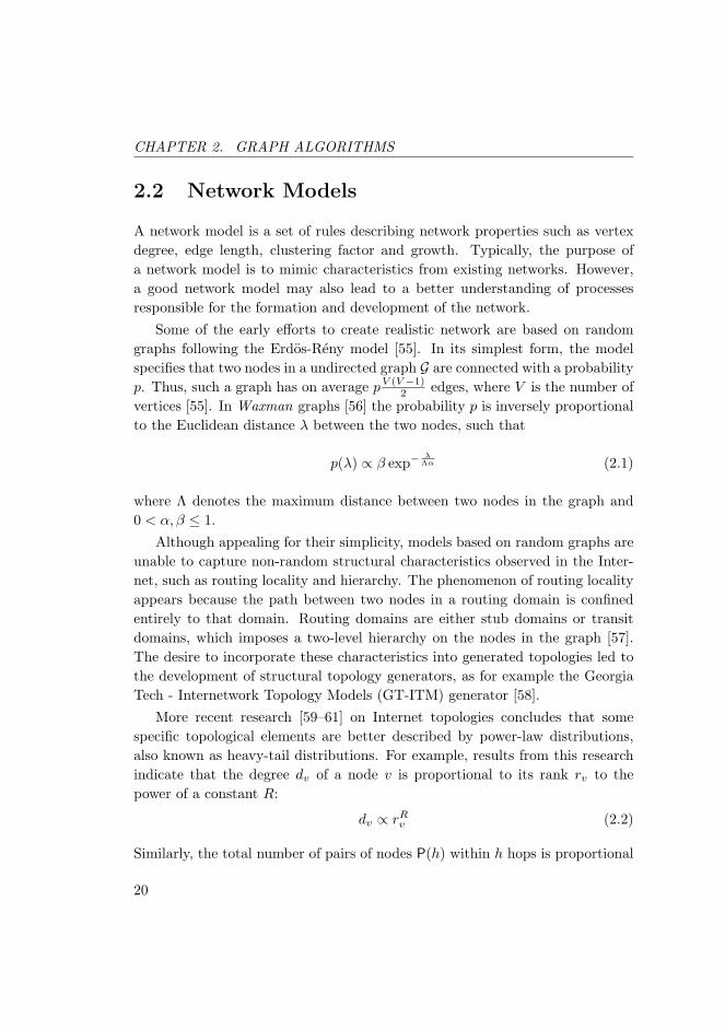
A network model is a set of rules describing network properties such as vertexdegree, edge length, clustering factor and growth. Typically, the purpose ofa network model is to mimic characteristics from existing networks. However,a good network model may also lead to a better understanding of processesresponsible for the formation and development of the network.
Some of the early efforts to create realistic network are based on randomgraphs following the Erdos-Reny model [55]. In its simplest form, the modelspecifies that two nodes in a undirected graph G are connected with a probabilityp. Thus, such a graph has on average pV (V−1)
2 edges, where V is the number ofvertices [55]. In Waxman graphs [56] the probability p is inversely proportionalto the Euclidean distance λ between the two nodes, such that
p(λ) ∝ β exp−λ
Λα (2.1)
where Λ denotes the maximum distance between two nodes in the graph and0 < α, β ≤ 1.
Although appealing for their simplicity, models based on random graphs areunable to capture non-random structural characteristics observed in the Inter-net, such as routing locality and hierarchy. The phenomenon of routing localityappears because the path between two nodes in a routing domain is confinedentirely to that domain. Routing domains are either stub domains or transitdomains, which imposes a two-level hierarchy on the nodes in the graph [57].The desire to incorporate these characteristics into generated topologies led tothe development of structural topology generators, as for example the GeorgiaTech - Internetwork Topology Models (GT-ITM) generator [58].
More recent research [59–61] on Internet topologies concludes that somespecific topological elements are better described by power-law distributions,also known as heavy-tail distributions. For example, results from this researchindicate that the degree dv of a node v is proportional to its rank rv to thepower of a constant R:
dv ∝ rRv (2.2)
Similarly, the total number of pairs of nodes P(h) within h hops is proportional
20
2.2. NETWORK MODELS
to the power of a constant H:
P(h) ∝ hH , h� δ (2.3)
where δ is the diameter of the graph.Barabasi and Albert [62] showed that two generic mechanisms can be hold
responsible for the appearance of power-law distributions: incremental growthand preferential connectivity. Incremental growth refers to continuous expansionof the network by adding new nodes to existing ones. This is in sharp contrastto Erdos-Reny and Waxman networks, where the number of nodes is kept un-changed and new links are added or old links are rewired. On the other hand,preferential connectivity denotes the tendency of new nodes to be connected toexisting high-degree nodes [60].
Incremental growth and preferential connectivity together lead to the ap-pearance of what is called small-world networks [53]. These networks are char-acterized by short paths lengths between arbitrary pairs of nodes and by strongclustering behavior. Compared to random graphs, small-world graphs tend tohave shorter characteristic path length and a much larger clustering coefficient(see Def. 2.5 and Def. 2.6 in Section 2.1) [54].
We have used the BRITE [63] software to generate network models accordingto the Barabasi-Albert model. BRITE is a topology generator developed atBoston University, designed to be flexible, extensible, interoperable, portableand user friendly. We have chosen BRITE because:
i) it has supports for realistic topology models based on power-law distribu-tions,
ii) it can generate router level topologies,
iii) it is supported under OMNeT++, and
iv) the source code is freely available.
Each BRITE topology is embedded on a two-dimensional Euclidean planedivided into HS ×HS high-level squares, where HS is a configurable BRITEparameter. Each high-level square is divided into LS × LS low-level squares,where LS is also configurable. A low-level square can be occupied by at most
21

CHAPTER 2. GRAPH ALGORITHMS
one node. BRITE has two modes of laying out nodes: random and heavy-tailed. In random mode, BRITE assigns each node to a random low-level squarewhile avoiding collisions. In heavy-tailed mode, BRITE selects the number ofnodes in a high-level square according to the bounded Pareto probability densityfunction [60]
f(x) =aκx−a−1
1− (κ/P )a. (2.4)
These nodes are then distributed randomly within the high-level square, suchthat each node occupies exactly one low-level square.
We have configured BRITE to use both incremental growth and preferentialconnectivity. With this configuration, BRITE starts with an initial set of m0
randomly connected nodes2. The remaining nodes are added to the graph, oneby one. Each of these nodes selects an existing node u with probability
du∑v∈C dv
(2.5)
where C is the set of nodes already added to the network and di and dv are theoutdegree of node u and v, respectively. This process is repeated m times toconnect node u to m other nodes. The parameter m is configurable.
2.3 Algorithms
Many problems can be converted to analytical expressions suitable for directcalculation. However, a significant amount of problems are either too large ortoo complex to be solved analytically. In this case it is more reasonable toattempt a computer-based algorithmic approach to find the solution.
Definition 2.8 (Algorithm). An algorithm is a well-defined step-by-step pro-cedure to solve a problem [51, 64, 65].
We differentiate between a problem and a problem instance. The first casedenotes a general inquiry with some parameters left unspecified (e. g. , “What isthe shortest path between two nodes in a graph?”). An instance of this problemrequires complete specification of the nodes, edges and edge weights contained
2In BRITE’s source code m0 = m.
22

2.3. ALGORITHMS
in the graph as well as specification of the two nodes we are interested in. Analgorithm can solve either all instances of a problem or only some subset ofthem. For example, Dijkstra’s shortest path algorithm can solve only probleminstances where all edge weights are non-negative.
For computer algorithms, the problem instance must be encoded into a stringω that serves as input to the algorithm. In the case of problem instances withparameters defined on a continuous space, the encoding process involves inputconversion to a discrete space. In some cases the conversion can introduce anerror called discretization error. It may be possible to reduce the discretiza-tion error by making the conversion more “fine-grained”, albeit at an increasedcomputational cost.
The general form of an algorithm is
x = f (ω) (2.6)
where f denotes the algorithm and x is the result.Algorithms can often be classified either as direct methods or as iterative
methods. A direct method finds the solution in a finite number of steps whereasan iterative method converges asymptotically to the solution. Typically, aniterative method searches some space X defined by ω in order to find the solu-tion. The simplex algorithm and Newton’s method for unconstrained optimiza-tion [66] are examples of a direct and a iterative method, respectively.
An iterative method can be specified as
xk+1 = f (xk) for xk ∈ X (2.7)
where X is the space to be explored by the algorithm, xk denotes the positionin the search space at step k and the algorithm f is a mapping from X to X .When applied to a vector x ∈ X , f produces another vector y ∈ X .
Another way to classify algorithms is to place them in one of the followingfour classes:
i) numerical methods,
ii) exact algorithms,
iii) heuristics,
23
CHAPTER 2. GRAPH ALGORITHMS
iv) meta-heuristics.
Numerical methods solve problems by using function approximation, finitedifferential calculus or a combination thereof [67, 68]. For example, Newton’smethod for unconstrained optimization approximates a function g in the neigh-bourhood of a point x with the polynomial generated by the second-degreeTaylor series [66]. The first and second order derivatives from the series allowNewton’s method to estimate the direction towards the optimum. Numericalmethods require that certain conditions apply to functions involved in solvingthe problem or else the methods may not converge to the solution [69]. They aresusceptible to round-off and truncation errors and to stability problems relatedto the feedback loop in Equation 2.7 [67]. It is worth noting that algorithms inthe remaining three classes may be susceptible to these problems as well. Thesteepest descent and Newton’s method are examples of numerical methods forunconstrained optimization [66].
Exact algorithms are iterative procedures that always find the correct so-lution, provided there is one. They are different from numerical methods inthe sense that they do not require function approximation or finite differentialcalculus, but rely instead on properties specific to the problem they solve. Forexample, the Bellman-Ford shortest path algorithm and Dijkstra’s shortest pathalgorithm, both described in Section 2.5, are exact algorithms that rely on theproperty that sub-paths of shortest paths in one dimension are also shortestpaths [55].
If numerical methods or exact algorithms do not work well on the problemat hand, it may be possible to apply a heuristic [69]. Heuristics are algorithmsthat explore the search space in an intelligent way, albeit without guaranteesfor convergence to the correct solution. Often, they involve a trade-off betweencomputation time and accuracy: fast heuristics sometimes cannot find the op-timal solution and accurate heuristics always find the optimal solution, but forsome problem instances they can take an unreasonable amount of time to finish.Local search [50, 70] is an example of optimization heuristic.
Metaheurstics are algorithms that combine various heuristics in an effort toobtain an approximate solution even in the case of difficult problem instances[69, 71]. They often employ a probabilistic element in order to avoid beingtrapped in a local minimum. The particle swarm optimization (PSO) method
24
2.3. ALGORITHMS
described in [72] is an example of metaheuristic.Direct methods find the solution to a problem instance in a finite number
of steps, but iterative algorithms require some form of convergence criteria.Intuitively, we say that an algorithm has converged when xk+1 = xk or whenf (xk+1) = f (xk). However, this may not happen at all when the algorithm isexecuted on a computer. Since computers are finite-state machines, they havefinite precision in representing real numbers i. e. , they allocate a finite numberof bits to represent numbers. This implies that numbers are rounded off, whichleads to round-off errors. In practice, it means that the solution found by thealgorithm approaches the true solution x∗ in an ε-neighborhood dictated by theunit round-off (machine precision) for floating-point numbers. Therefore, theconvergence criteria should be of one of the formulas shown below [72]:
1. f (xk+1)− f (xk) < ε(1 + |f (xk+1) |),
2. ‖xk − xk+1‖ <√ε(1 + ‖xk+1‖),
3. ‖∇f (xk+1)‖ < ε1/3(1 + |f (xk+1) |.
The unit round-off is defined as the difference between 1 and the least valuegreater than 1 on a specific computer architecture. On a 32-bit Pentium/Athlonarchitecture a float data type uses 32 bits with 1.19209× 10⁻⁷ unit round-off,while a double uses 64 bits with 2.22045× 10⁻¹⁶ unit round-off.
The use of the name iterative methods (algorithms) is perhaps unfortunatesince direct methods can rely on iterations as well. The difference is that directmethods find the exact solution, whereas iterative methods find the solution inthe limit. Nonetheless, the name is well established and we will continue usingit.
Algorithms require also a stopping condition. Obviously if the algorithm con-verges according to one of the criteria above, then it can stop. Otherwise, oneneeds an upper bound ζ on the number of steps k performed by the algorithm.If the k = ζ the algorithm stops. Clearly, the choice of ζ is very important sincesetting the value too low causes the algorithm to stop prematurely when prob-lems do actually have a solution, whereas if the value is too high the algorithmswill run for a long time, even when no solution exists.
25

CHAPTER 2. GRAPH ALGORITHMS
2.4 Algorithm Efficiency
A critical aspect in using algorithms is understanding how efficient they are atfinding the solution for the problem at hand. Information about their efficiencyhelps not only in estimating the computational resources required, but can alsobe used as a decision factor in selecting one out of several algorithms that cansolve the same problem.
For direct methods the efficiency is typically expressed as a function of theinput size and it is called computational complexity. The complexity referseither to the space (e. g. , memory) required to store the input data, to thetime required to run the algorithm until a solution is found3, or, in the caseof a distributed system, to the communication volume required by the systemto perform its function. In the reminder of this thesis we will focus on timecomplexity. The word “complexity” will therefore refer to “time complexity”unless stated otherwise.
The goal is to obtain a complexity estimate, which is unaffected by variationsin underlying hardware and software (i. e. , the computer and operating systemrunning the algorithm) or by variations in the contents of the input. This isachieved by assuming that the algorithm runs inside a mathematical model ofa computer instead of a real computer. The mathematical model is typically aTuring machine or a random-access machine [51, 65, 73]. The details of thesemathematical models are not directly significant for this thesis. It is sufficientto say that there are several variants of Turing machines, the most importantones being the deterministic Turing machine and the non-deterministic Turingmachine. All computers in use today work according to the principles of a de-terministic Turing machine or of a random-access machine. Non-deterministicTuring machines have the ability to clone themselves into multiple copies run-ning simultaneously.
We are foremost interested in worst-case complexity, which is an asymptoticupper bound on the number of elementary operations required by the algorithmto complete. In general, the elementary operations include arithmetic opera-tions, comparisons, jumps and subroutine calls. The asymptotic upper boundis a function of the size of the input ω. It is customary to make the simplifying
3We assume ζ = ∞ in this case.
26

2.4. ALGORITHM EFFICIENCY
assumption that each elementary instruction, with the exception of subroutinecalls, requires unit time for execution [50]. The time required by a subroutinecall depends on the elementary instructions inside the subroutine.
Definition 2.9 (Asymptotic upper bound O (·) for worst-case run time). Givena function f(n) that estimates the run time of an algorithm, where n is the size ofthe input ω, f(n) has an asymptotic upper bound O (g(n)) if 0 ≤ f(n) ≤ cg(n)for all n ≥ n0 and provided that the positive constants c and n0 exist [51]. Inpractice, g(n) is obtained by removing from f(n) the low order terms and thepreceding constant of the high order term.
If the algorithm scales as a constant, then it means that the algorithm isindependent of the size of the input, and we write O (1). Polynomial-time algo-rithms are denoted by O (nx), where x is an integer constant. These algorithmsare considered tractable methods to solve the problem. On the other hand, al-gorithms belonging to the family of exponential time complexity (e. g. ,, O (n!)and O (kn) for k ∈ Z) are generally regarded as intractable since they tend to re-quire prohibitive amounts of computation resources [50]. In Figure 2.1 we haveplotted several types of asymptotic growth functions. The common elementbetween Figure 2.1(a) and Figure 2.1(b) is the linear function O(n), which actsas a border between the regions of sublinear complexity and superlinear com-plexity. Note that we intentionally use a logarithmic y-axis in Figure 2.1(b) inorder to emphasize the growth explosion occurring with superlinear complexity.
Many problems can be rephrased in the form of a decision problem, that is aproblem which has a “yes” or “no” answer. Most graph optimization problemsare of this type. The set of decision problems can be divided into two classes, Pand NP. The class P contains decision problems that can be solved in polyno-mial time on a deterministic Turing machine. Similarly, the class NP containsdecision problems that can be solved in polynomial time on a non-deterministicTuring machine using a non-deterministic algorithm [70]. An alternative defi-nition states that the class NP contains decision problems, whose solution canbe verified in polynomial time [50, 73]. Problems belonging to the class NP aregenerally regarded as intractable (i. e. , it is expected that algorithms solvingthem will have exponential worst-case complexity). One of the most interestingopen questions in computer science is whether P = NP or not. In the absence
27

CHAPTER 2. GRAPH ALGORITHMS
0 5 10 15 20 25 30
12
34
5
Input size
Com
plex
ity O(n)O(( n))O(lg n)O(1)
(a) Sublinear complexity.
0 5 10 15 20 25 30
1e+
001e
+03
1e+
061e
+09
Input size
Com
plex
ity
O(n!)O((n2n))O((2n))O((n3))O((n2))O(n)
(b) Superlinear complexity.
Figure 2.1: Asymptotic worst-case complexity.
of a proof, the empirical evidence seems to indicate that this is not the case andthat instead P ⊆ NP, as shown in Figure 2.2.
NP
NPCP
Figure 2.2: Complexity classes.
Some problems in NP are called NP-complete (NPC) because they hold aspecial status. If a polynomial-time algorithm is found to solve one of theseproblems, the theory states that all problems in the class NP will be solvable inpolynomial time. Should this occur, it would constitute proof that our currentview of the complexity classes is wrong, and in fact P = NP . The interestedreader can find more information in [65, 74].
28

2.5. SHORTEST-PATH ALGORITHMS
In terms of the problems described in Chapter 3, the multi-constrained path(MCP) and multi-constrained optimal path (MCOP) problems are NP-complete[75]. However, Kuipers and Van Mieghem have shown [76] that NP-completebehavior is unlikely to occur in realistic communication networks.
The concept of computational complexity is not easily applied to iterativemethods [48]. In particular, the computational complexity can be strongly in-fluenced by the convergence criteria used. Some results are provided in [77]for the case of optimization algorithms, although they require strict technicalconditions (e. g. , Lipschitz-continuity) to apply to the objective function. Foriterative algorithms it can be more interesting to examine the rate of conver-gence.
Definition 2.10 (Rate of convergence). For an algorithm that converges througha series of intermediate steps xk ∈ R to a point x∗ ∈ R in the search space, thealgorithm’s rate of convergence is given by
limk→∞
‖xk+1 − x∗‖‖xk − x∗‖p
= α (2.8)
provided the number p exists and α 6= 0. The number p is called order ofconvergence. When p = 1 the algorithm is said to have linear convergence [66,78]. Sometimes linear convergence is also called geometric convergence. Ingeneral, the case p > 1 denotes superlinear convergence, whereas the specificcase p = 2 is called quadratic convergence.
2.5 Shortest-Path Algorithms
In this section we review various shortest-path algorithms. The selection isbased on algorithms developed and used in the context of the ORP framework.More specifically, we describe Bellman-Ford and Dijkstra’s shortest path algo-rithms, breadth-first-search (BFS) and Yen’s K shortest paths (KSP). Most ofthe material and notation presented here is based on [51]. In some cases [64]was consulted as well. The description of Yen’s KSP is based entirely on hisarticle [79].
Definition 2.11 (Shortest-path problem). Let G(V, E) be a weighted graph,where the scalar w(u, v) denotes the weight of the link connecting node u and
29
CHAPTER 2. GRAPH ALGORITHMS
node v. If there is no link connecting node u and v, then w(u, v) = ∞. Givena pair of nodes s, d ∈ V , solving the shortest-path problem requires finding apath P ∗ with the path weight
w(P ∗) =∑
(u,v)∈P∗
w(u, v) (2.9)
such that w(P ∗) ≤ w(P ), for all possible paths P . The path weight w(P ) issometimes referred to as the distance between node s and node d over the pathP .
The algorithmic approaches for solving shortest-path problems can be di-vided into two categories: label-setting algorithms and label-correcting algo-rithms. The label denotes an estimated distance assigned to a node at somestep in the algorithm. A label-setting algorithm assigns one label at each iter-ation and does not change it afterwards. This is the same as saying that thealgorithm finds the shortest-path to a node at each iteration. A label-correctingalgorithm can change assigned labels several times before the algorithm finishes.Dijkstra’s shortest-path algorithm is a label-setting algorithm. The Bellman-Ford algorithm and BFS are label-correcting algorithms.
Yen’s KSP algorithm does not belong to any labeling class. This algorithmbelongs instead to a class of deviation algorithms used to solve ranking problems[80]. Solutions produced by deviation algorithms take the form of a tree wherethe root is the source node. Each branch of the tree constitutes a path fromthe source node to the destination node, obtained by a deviation in one of theprevious paths, e. g. , the initial path used to bootstrap the algorithm. Yen’sKSP relies internally on a shortest-path algorithm. Our implementation usesDijkstra’s shortest path algorithm.
Both Dijkstra’s algorithm and the Bellman-Ford algorithm manage a list πwith predecessor nodes and a second list d with distances to various verticesin the graph. Each list, when indexed by a node name (or other form of nodeidentification), allows retrieval of or changes to the entry corresponding to thenode. The purpose of the subroutine Initialize shown in Algorithm 1 is toinitialize these lists. The subroutine requires as input the graph correspondingto the problem instance, a source node s where from the shortest-path beginsand the two (uninitialized) lists, π and d. Initialize sets each entry in the
30
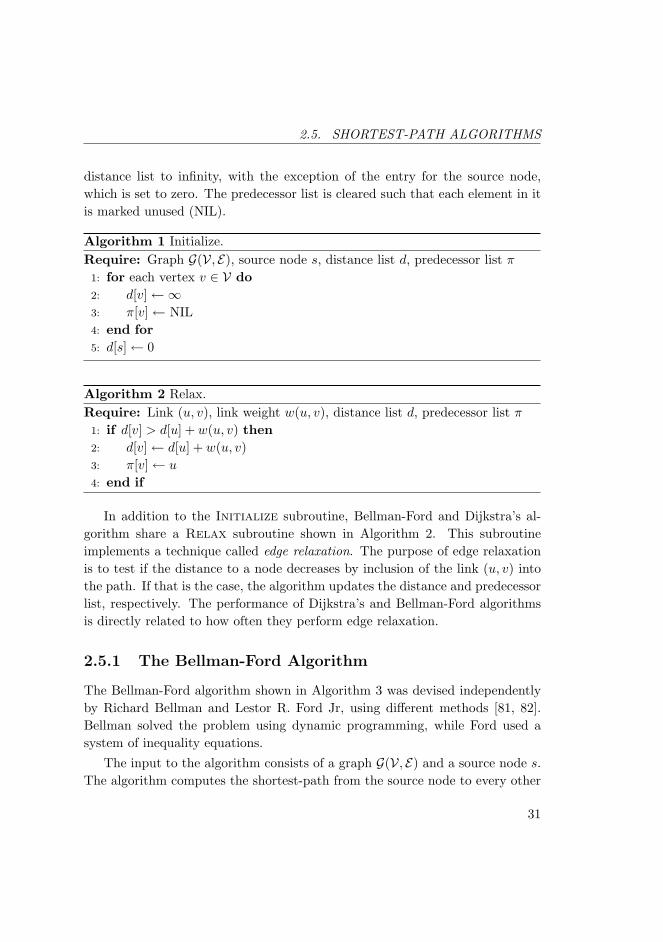
2.5. SHORTEST-PATH ALGORITHMS
distance list to infinity, with the exception of the entry for the source node,which is set to zero. The predecessor list is cleared such that each element in itis marked unused (NIL).
Algorithm 1 Initialize.Require: Graph G(V, E), source node s, distance list d, predecessor list π
1: for each vertex v ∈ V do2: d[v]←∞3: π[v]← NIL4: end for5: d[s]← 0
Algorithm 2 Relax.Require: Link (u, v), link weight w(u, v), distance list d, predecessor list π
1: if d[v] > d[u] + w(u, v) then2: d[v]← d[u] + w(u, v)3: π[v]← u
4: end if
In addition to the Initialize subroutine, Bellman-Ford and Dijkstra’s al-gorithm share a Relax subroutine shown in Algorithm 2. This subroutineimplements a technique called edge relaxation. The purpose of edge relaxationis to test if the distance to a node decreases by inclusion of the link (u, v) intothe path. If that is the case, the algorithm updates the distance and predecessorlist, respectively. The performance of Dijkstra’s and Bellman-Ford algorithmsis directly related to how often they perform edge relaxation.
2.5.1 The Bellman-Ford Algorithm
The Bellman-Ford algorithm shown in Algorithm 3 was devised independentlyby Richard Bellman and Lestor R. Ford Jr, using different methods [81, 82].Bellman solved the problem using dynamic programming, while Ford used asystem of inequality equations.
The input to the algorithm consists of a graph G(V, E) and a source node s.The algorithm computes the shortest-path from the source node to every other
31
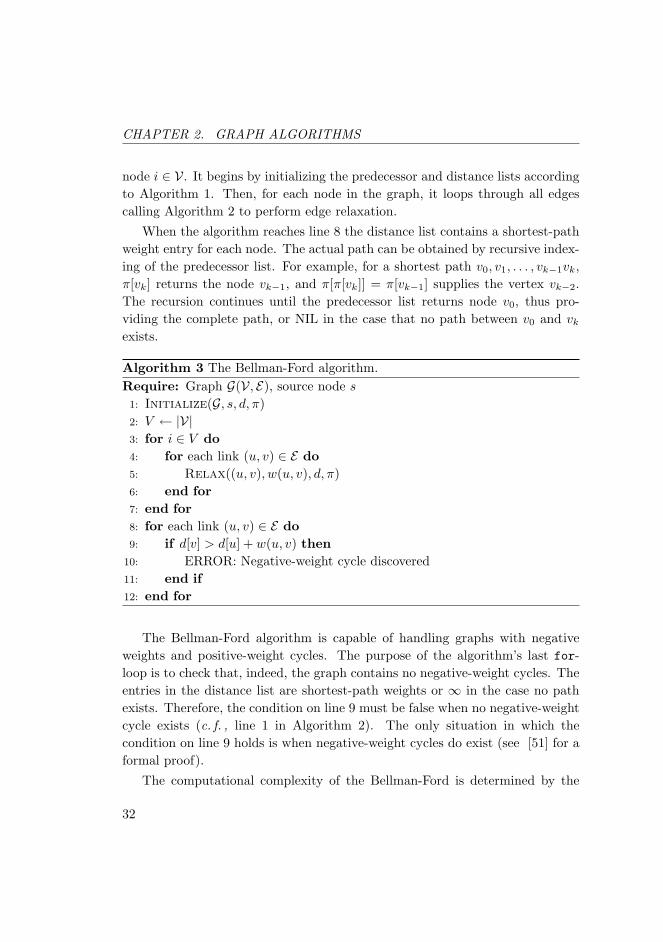
CHAPTER 2. GRAPH ALGORITHMS
node i ∈ V. It begins by initializing the predecessor and distance lists accordingto Algorithm 1. Then, for each node in the graph, it loops through all edgescalling Algorithm 2 to perform edge relaxation.
When the algorithm reaches line 8 the distance list contains a shortest-pathweight entry for each node. The actual path can be obtained by recursive index-ing of the predecessor list. For example, for a shortest path v0, v1, . . . , vk−1vk,π[vk] returns the node vk−1, and π[π[vk]] = π[vk−1] supplies the vertex vk−2.The recursion continues until the predecessor list returns node v0, thus pro-viding the complete path, or NIL in the case that no path between v0 and vkexists.
Algorithm 3 The Bellman-Ford algorithm.Require: Graph G(V, E), source node s
1: Initialize(G, s, d, π)2: V ← |V|3: for i ∈ V do4: for each link (u, v) ∈ E do5: Relax((u, v), w(u, v), d, π)6: end for7: end for8: for each link (u, v) ∈ E do9: if d[v] > d[u] + w(u, v) then
10: ERROR: Negative-weight cycle discovered11: end if12: end for
The Bellman-Ford algorithm is capable of handling graphs with negativeweights and positive-weight cycles. The purpose of the algorithm’s last for-loop is to check that, indeed, the graph contains no negative-weight cycles. Theentries in the distance list are shortest-path weights or ∞ in the case no pathexists. Therefore, the condition on line 9 must be false when no negative-weightcycle exists (c. f. , line 1 in Algorithm 2). The only situation in which thecondition on line 9 holds is when negative-weight cycles do exist (see [51] for aformal proof).
The computational complexity of the Bellman-Ford is determined by the
32
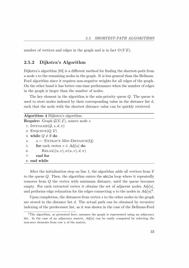
2.5. SHORTEST-PATH ALGORITHMS
number of vertices and edges in the graph and is in fact O (V E).
2.5.2 Dijkstra’s Algorithm
Dijkstra’s algorithm [83] is a different method for finding the shortest-path froma node s to the remaining nodes in the graph. It is less general than the Bellman-Ford algorithm since it requires non-negative weights for all edges of the graph.On the other hand it has better run-time performance when the number of edgesin the graph is larger than the number of nodes.
The key element in the algorithm is the min-priority queue Q. The queue isused to store nodes indexed by their corresponding value in the distance list d,such that the node with the shortest distance value can be quickly retrieved.
Algorithm 4 Dijkstra’s algorithm.Require: Graph G(V, E), source node s
1: Initialize(G, s, d, π)2: Enqueue(Q,V)3: while Q 6= ∅ do4: u← Extract-Min-Distance(Q)5: for each vertex v ∈ Adj[u] do6: Relax((u, v), w(u, v), d, π)7: end for8: end while
After the initialisation step on line 1, the algorithm adds all vertices from Vto the queue Q. Then, the algorithm enters the while loop where it repeatedlyremoves from Q the vertex with minimum distance, until the queue becomesempty. For each extracted vertex it obtains the set of adjacent nodes Adj[u],and performs edge relaxation for the edges connecting u to the nodes in Adj[u]4.
Upon completion, the distances from vertex s to the other nodes in the graphare stored in the distance list d. The actual path can be obtained by recursiveindexing of the predecessor list, as it was shown in the case of the Bellman-Ford
4The algorithm, as presented here, assumes the graph is represented using an adjacency
list. In the case of an adjacency matrix, Adj[u] can be easily computed by selecting the
non-zero elements from row u of the matrix.
33

CHAPTER 2. GRAPH ALGORITHMS
algorithm. Dijkstra’s algorithm has O(V 2)
computational complexity. It ispossible to achieve a O (V log2 V + E) complexity if the algorithm is modifiedto use a more sophisticated min-priority queue based on Fibonacci heaps [84].However, our implementation follows the original algorithm.
2.5.3 Breadth-First Search (BFS)
BFS is typically presented as a method to explore graphs rather than a tradi-tional shortest-path algorithm. This is because BFS implicitly assumes that alllinks have equal weights, which can be seen on line 14 in Algorithm 5. There-fore, this method can be used only in the case where our interpretation of ashortest-path is that of a path with minimum number of hops (i. e. , a pathwith minimum length according to Definition 2.4 on page 19).
Algorithm 5 Breadth-first search (BFS).Require: Graph G(V, E), source node s
1: for each vertex v ∈ V do2: c[v]← WHITE3: d[v]←∞4: π[v]← NIL5: end for6: c[s]← GREY7: d[s]← 08: Enqueue(Q, s)9: while Q 6= ∅ do
10: u← Dequeue(Q)11: for each v ∈ Adj[u] do12: if c[v] = WHITE then13: c[v]← GREY14: d[v]← d[u] + 115: π[v]← u
16: Enqueue(Q,n)17: end if18: end for19: end while
34
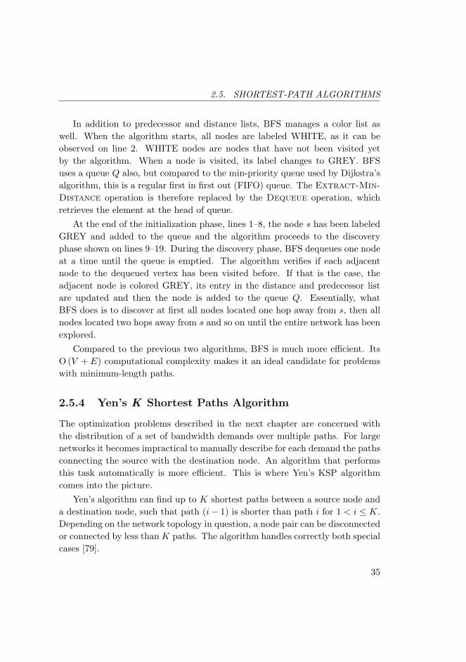
2.5. SHORTEST-PATH ALGORITHMS
In addition to predecessor and distance lists, BFS manages a color list aswell. When the algorithm starts, all nodes are labeled WHITE, as it can beobserved on line 2. WHITE nodes are nodes that have not been visited yetby the algorithm. When a node is visited, its label changes to GREY. BFSuses a queue Q also, but compared to the min-priority queue used by Dijkstra’salgorithm, this is a regular first in first out (FIFO) queue. The Extract-Min-
Distance operation is therefore replaced by the Dequeue operation, whichretrieves the element at the head of queue.
At the end of the initialization phase, lines 1–8, the node s has been labeledGREY and added to the queue and the algorithm proceeds to the discoveryphase shown on lines 9–19. During the discovery phase, BFS dequeues one nodeat a time until the queue is emptied. The algorithm verifies if each adjacentnode to the dequeued vertex has been visited before. If that is the case, theadjacent node is colored GREY, its entry in the distance and predecessor listare updated and then the node is added to the queue Q. Essentially, whatBFS does is to discover at first all nodes located one hop away from s, then allnodes located two hops away from s and so on until the entire network has beenexplored.
Compared to the previous two algorithms, BFS is much more efficient. ItsO (V + E) computational complexity makes it an ideal candidate for problemswith minimum-length paths.
2.5.4 Yen’s K Shortest Paths Algorithm
The optimization problems described in the next chapter are concerned withthe distribution of a set of bandwidth demands over multiple paths. For largenetworks it becomes impractical to manually describe for each demand the pathsconnecting the source with the destination node. An algorithm that performsthis task automatically is more efficient. This is where Yen’s KSP algorithmcomes into the picture.
Yen’s algorithm can find up to K shortest paths between a source node anda destination node, such that path (i− 1) is shorter than path i for 1 < i ≤ K.Depending on the network topology in question, a node pair can be disconnectedor connected by less than K paths. The algorithm handles correctly both specialcases [79].
35

CHAPTER 2. GRAPH ALGORITHMS
Algorithm 6 Yen’s K shortest paths algorithm.Require: Graph G(V, E), source vs and destination vd, K
1: P 1 ← DIJKSTRA(G, vs, vd)2: for k ← 2, . . . ,K do3: for vi ← vs, v
k−12 , . . . , vk−1
d−1 do4: for j ← 1, 2, . . . , (k − 1) do5: if Rk−1
vi ≡ Rjvi then6: w(vji , v
ji+1)←∞ in the graph G
7: end if8: end for9: Skvi ← DIJKSTRA(G, vi, vd)
10: if Skvi 6= ∅ then11: P kvi ← Rk−1
vi
⋃Skvi
12: C⋃P kvi
13: if C contains K − k + 1 paths then14: break15: end if16: end if17: end for18: P k ← min C19: restore all changed weights w to original values20: end for
36
2.5. SHORTEST-PATH ALGORITHMS
The pseudo-code for Yen’s KSP is shown in Algorithm 6. The algorithmrequires a graph description, G(V, E), a source node vs, a destination node vdand the desired number of shortest paths, K. We denote the kth shortestpath between vs and vd by P k. Furthermore, the ith node (vertex) on the kthpath is denoted by vki . For k > 1, each path P k consists of a root Rkvi thatextends from the source node vs to an intermediate node vki and of a spur Skvifrom node vki to the destination node vd. A candidate path P kvi coincides withthe (k − 1)st shortest path, P k−1, in nodes vs, . . . , vk−1
i and differs from theremaining portion of P k−1 that consists of nodes vk−1
i , . . . , vk−1d−1 , vd. Node vk−1
d−1
is the predecessor of the destination node on path P k−1. The candidate pathP kvi is also called a deviation from the path P k−1 at the node vi.
The first shortest path P 1 is computed using Dijkstra’s shortest path al-gorithm [83], as shown on line 1. Subsequent shortest paths are computediteratively. The idea is to find new deviations, searching from the source nodetowards the destination node. The for-loop on line 3 computes the root Rk−1
vi
of the shortest path P k−1. On each loop iteration, the root is allowed to extendone node further towards the destination, up to the node vd−1 preceding thedestination. During each iteration this root is compared to the roots of equallength for all shortest paths computed so far, as shown on lines 4–5.
If the compared roots consist of the exact same sequence of nodes, then thealgorithm removes the link connecting the nodes vji and vji+1 from the graph.This is shown on line 6, where the algorithm sets the link weight w to infinity.This has the effect of forcing Dijkstra’s algorithm on the next line to find a newshortest path from vi to vd, different from Rk−1
vi (note that nodes vji and vi arethe same at this point). If Dijkstra’s algorithm is successful in finding a shortestpath, then we concatenate the path to the root Rk−1
vi and save that in the listC with candidate paths, as shown on lines 11–12. Since it is not necessary tostore more than (K − k + 1) paths in the candidate list [79], we terminate thefor-loop started on line 3 when the list grows to this size.
On line 18 Yen’s KSP extracts the shortest path from the candidate listand this becomes our kth shortest path. Before starting a new iteration, thealgorithm restores the weights in the graph as shown on the next line.
Yen’s KSP algorithm has O(KV 3
)worst-case time complexity. In the case
when Dijkstra’s algorithm uses Fibonacci heaps the complexity is reduced to
37

CHAPTER 2. GRAPH ALGORITHMS
O (KV (V log2 V + E)) [80]. There have been reports [80, 85] of newer imple-mentations that share the same worst-case complexity, but with the claim thatin practice they perform better than Yen’s KSP.
2.6 Summary
In this chapter we established graph theoretical notation and terminology. Weprovided also a brief overview of various graph models used to represent realnetworks and a short description of the BRITE topology generator. Further-more, we discussed different classes of algorithms and methods used to quantifyalgorithmic efficiency.
In the final part of the chapter our attention was focused on shortest pathalgorithms, which are used in our ORP framework. We provided algorithmicformulation and worst-case run-time estimates for the Bellman-Ford algorithm,Dijkstra’s algorithm, breadth-first search and Yen’s K shortest paths algorithm.
38
Chapter 3
Optimization Algorithms
The ORP framework described in Chapter 5 relies on three different types ofoptimization algorithms:
i) path selection,
ii) K shortest paths,
iii) flow allocation.
The purpose of the path selection algorithm is to find a path from a sourcenode s to a destination node d, subject to a number of QoS constraints. In theevent that one or more paths are no longer able to satisfy the QoS constraints,the K shortest paths algorithm is used to discover multiple backup paths. Theflow allocation algorithm is then used to distribute the affected flows over thebackup paths, such that the traffic volumes are accommodated [86].
To quantify the time and memory requirements for this type of computationswe have implemented a performance tested for network flow algorithms. Usingthis testbed we have analyzed the performance of Yen’s K shortest paths (KSP)algorithm [79] as well as the performance of linear optimization methods (i. e. ,the simplex method and the interior point method) in conjunction with the pureallocation problem (PAP) and the PAP with modified link-path formulation(PAP-MLPF) [70]. These problems are described in Section 3.2. The end goalin this chapter is to select, based on empirical data provided by the testbed, anoptimization algorithm suitable for use with ORP.
39

CHAPTER 3. OPTIMIZATION ALGORITHMS
In the next section we describe linear programming terminology and thenproceed to outline optimization problems related to path selection and flowallocation. The remaining part of the chapter describes the performance testbedand the performance results obtained with it.
3.1 Linear Programming
The expression linear programming refers to the design and analysis of algo-rithms for solving linear optimization problems [87]. The general form of alinear optimization problem is shown in Table 3.1.
minimize f (x) = cTx
subject to Ex = p (1)Gx ≥ s (2)Hx ≤ t (3)xi ∈ R for i = 1, . . . , n
Table 3.1: Linear optimization problem in general form.
The function f (x) is called the objective function. The unknown variablesare denoted by the column vector x with n elements. The vector cT holds thecoefficients for the unknown variables. The matrix E contains the coefficientsfor the equality constraints. Similarly, the matrices G and H represent thecoefficients for the inequality constraints. The vectors p,s and t contain theconstants on the right hand side of the equalities and inequalities, respectively.Solving this problem, implies finding an optimal point x∗ (also called optimalsolution) such that the optimal value f (x∗) is a minimum and all constraintsare satisfied. In the description of the linear problem any combination of theconstraints (1)–(3) may appear. If there are no constraints of the type (1)–(3),then the linear problem is unconstrained.
Optimization algorithms (e. g. , the simplex method) require the problemdescription to be converted from the general form to the standard form shownin Table 3.2. To do that, the inequality constraints (2) and (3) are changed toequality constraints and are stored together with (1) in matrix A [66].
40

3.1. LINEAR PROGRAMMING
minimize f (x) = cTx
subject to Ax = b
xi ≥ 0 and bi > 0 for i = 1, . . . , N
Table 3.2: Linear optimization problem in standard form.
Inequality constraints can be changed to equality constraints by adding slackor surplus variables to the problem. For example, given the constraint row i inmatrix G
gi1x1 + gi2x2 + · · ·+ ginxn ≥ si (3.1)
this row can be converted into standard form by subtracting from it a surplusvariable y1 such that
gi1x1 + gi2x2 + · · ·+ ginxn − yi = s1. (3.2)
There are just as many surplus variables as rows in the matrix G. Similarly, forthe constraints row i in matrix H
hi1x1 + hi2x2 + · · ·+ hinxn ≤ ti (3.3)
we add a slack variable wi on the right side of the equality sign such that
hi1x1 + hi2x2 + · · ·+ hinxn + wi = ti. (3.4)
Geometrically, the feasible region of the problem described in Table 3.2 isalways a convex polytope, also called simplex. The vertices of the simplex con-stitute feasible solutions to the optimization problem. For a problem with n
variables and m constraints there are(n
m
)=
n!m!(n−m)!
(3.5)
feasible solutions.The simplex method, which is the classical algorithm for solving linear op-
timization problems, attempts to find the optimal solution by searching thevertices of the polytope in an efficient manner. The algorithm starts in one ofthe simplex vertices, and it evaluates how the objective function changes if it
41
CHAPTER 3. OPTIMIZATION ALGORITHMS
were to “move” into one of the (n−m) neighboring vertices. The move is alwaysalong the edges of the simplex. Although in practice the simplex method ap-pears to have O (m+ n) computational complexity, it can approach exponentialcomplexity on some specific problems [50, 70, 87].
A newer class of optimization algorithms, called interior point methods(IPMs), has O (n log 1/ε) theoretical worst-case complexity, where ε > 0 is asmall tolerance factor. Contrary to the simplex method, IPMs approach thesolution asymptotically from the interior or exterior of the polytope. Manypractical IPM implementations, including the one used here, are based on tech-niques suggested by Mehrotra [88]. These techniques are aimed at improvingthe performance of the algorithm. Their side effect is that certain theoretical as-pects of the algorithm are modified. Hence, it is not yet known if the complexityestimate apply to Mehrotra-based implementations [87].
3.2 Optimization Models
In this section we focus on optimization models that are used within the ORPframework to solve multi-constrained path (MCP) and multi-constrained opti-mal path (MCOP) selection problems [89] as well as flow allocation problems.Comprehensive surveys on additional types of optimization models and algo-rithms are available in [64, 69, 70].
The starting assumption is that information about network topology is avail-able in the form of a weighted digraph G(V, E). The weight of each link repre-sents a set of metrics of interest, such as bandwidth, delay, jitter, packet lossand cost. In addition to the graph and link weights, information about the flowdemands is available as well. A flow demand is a set of path constraints forthe path P (s, d), where s ∈ V is the source node and d ∈ V is the destination(sink) node. In its simplest form, the flow demand contains only the bandwidthrequired to transfer data from s to d. In our implementation, the flow demandsare tied to the direction of the path.
42

3.2. OPTIMIZATION MODELS
3.2.1 Multi-Constrained Path Selection
In the case of a MCP problem we attempt to find one constrained path at atime. This is a feasibility problem. Each link weight in G(V, E) is a vector ofQoS metrics, where each metric belongs to one of the following types:
additive: delay, jitter, cost
multiplicative: packet loss
min-max: bandwidth, policy flags
Multiplicative weights can be turned into additive weights by taking the loga-rithm of their product. The constraints on min-max metrics can be dealt withby pruning the links of the graph that do not satisfy the constraints [89, 90].Therefore, in the remainder of this section we focus on additive link weightsonly.
For i = 1, . . . ,m we denote by wi(u, v) the ith additive metric for the link(u, v) between nodes u and v such that (u, v) ∈ E . The MCP optimizationproblem for m additive constraint values Li on the requested path is shown inTable 3.3.
find path P
subject to wi(P ) =∑
(u,v)∈P
wi(u, v) ≤ Li for i = 1, . . . ,m and (u, v) ∈ E
Table 3.3: Multi-constrained path selection problem (MCP).
The MCP selection problem problem can be converted to a multi-constrainedoptimal path (MCOP) selection problem by minimizing or maximizing over oneof the metrics wi. It is also possible to define a path-weight function f over allmetrics [89, 90] and to optimize over the path-weight function itself, as shownin Table 3.4.
Wang and Crowcroft proved in [75] that MCP problems with two or moreconstraints are NP-complete. By extension, MCOP problems with two or moreconstraints are NP-complete as well. The apparent intractability of these prob-lems suggests abandoning the search for exact solutions in the favour of heuris-
43
CHAPTER 3. OPTIMIZATION ALGORITHMS
minimize f (w(P ))subject to wi(P ) =
∑(u,v)∈P
wi(u, v) ≤ Li for i = 1, . . . ,m and (u, v) ∈ E
Table 3.4: Multi-constrained optimal path selection problem (MCOP).
tics that have a better chance of running in polynomial time. Chen and Nahrst-edt suggest a O (2L) heuristic [91] for the MCP problem, where L is the lengthof the feasible path. The path selection algorithm in ORP is based on thisheuristic.
The results of a study [76] on the NP-complexity of QoS routing found fourconditions leading to its appearance:
i) graphs with long paths (large hop-count),
ii) link weights with infinite granularity, or excessively large or small linkweights,
iii) strong negative correlation among link weights,
iv) “critically constrained” problems, which are problems with constraint val-ues close to the center of the feasible region.
The authors of the study consider that these conditions are unlikely to occurin typical networks. If they are right, the consequence is that the exponen-tial run time behavior of exact algorithms is bound to occur only in some fewpathological cases.
3.2.2 Flow Allocation
In the flow allocation problem, it is assumed that we know about one or moredirected paths connecting a source node s and a destination node d. Thesepaths can be discovered automatically, for example with a K shortest pathsalgorithm. We consider the following type of optimization problems: given adigraph G(V, E), a set P of directed paths and a set D of flow demands forbandwidth, we would like to allocate bandwidth on the paths in P such as tosimultaneously satisfy all demands.
44

3.2. OPTIMIZATION MODELS
If the traffic volume pertaining to a specific flow is allowed to be distributedover several paths to the destination, this is said to be a feasibility problem forbifurcated flows. This is the flow allocation problem that we are interested in.
On the other hand, if the problem includes the requirement that the entiretraffic flow between two nodes must be transmitted on a single path, insteadof being spread across several, we have a feasibility problem for non-bifurcatedflows. This problem is known to be computationally intractable [70] for largenetworks (it is in fact NP-complete). Hence, it will not be considered here.
We adopt a notation called link-path formulation [70] to formalize our prob-lem statement. Using this notation, we let the variable xdp denote bandwidthallocated to demand d on path p. Recall that a demand is a request for a spe-cific amount of bandwidth, hd, from a source node to a destination node. Thesource node and the destination node can be connected by more than one path,which explains the use of the index variable p. We use the variables D and E todenote the number of demands in the demand set D and the number of edges(links) in the set E , respectively. Further, the capacity of a link e is denoted byce. The indicator variable δedp is defined as
δedp =
{1 if link e is used by demand d on path p,
0 otherwise.(3.6)
Our problem statement can now be written as shown in Table 3.5.
find xdp for all d ∈ D, p ∈ Psubject to
∑p xdp = hd, d = 1, 2, . . . , D∑d
∑p δedpxdp ≤ ce, e = 1, 2, . . . , E
Table 3.5: Pure allocation problem (PAP).
PAP is a linear feasibility problem. Finding a solution to it entails solving asystem of linear equations of the type Ax = b. If the number of variables equalsthe number of equations we can use LU-decomposition or the conjugate gradientmethod [92] to solve the system of equations. If there are fewer equations thanvariables, then the system is underdetermined and has an infinity of solutionsor no solution at all. In the first case, this type of systems can be solved
45

CHAPTER 3. OPTIMIZATION ALGORITHMS
with singular value decomposition (SVD). Overdetermined systems of linearequations (i. e. , systems with more equations than variables) in general lack anexact solution. In this case, one can transform the system into a linear least-square optimization problem to obtain an approximation of the true solution.The goal of the least-square problem is to minimizes the residual error ‖Ax− b‖due to the approximation. The least square problem can be solved for examplewith SVD or with QR-decomposition [68, 93].
The first phase (phase I) of the simplex method is another approach forsolving the system of linear equations. The purpose of phase I is to obtain aninitial feasible solution from which the simplex method can start. This involvesaugmenting the original system Ax = b with a set of artificial variables y andusing the simplex method to solve the modified system Ax + y = b [66, 86, 87].
In [70], it is suggested that the PAP described in Table 3.5 can be reformu-lated in the form of the linear optimization problem shown in Table 3.6. Thenew problem, PAP with modified link-path formulation (PAP-MLPF), has anadditional variable z to be modified. Unlike the PAP, this problem always has afeasible solution in the sense that a minimum value for z can be found. If z < 0in the solution, we have a successful bandwidth allocation. Otherwise the valueof z indicates how much additional bandwidth is required to obtain feasibility.
minimize z for all d ∈ D, p ∈ Psubject to
∑p xdp = hd, d = 1, 2, . . . , D∑d
∑p δedpxdp ≤ z + ce, e = 1, 2, . . . , E
Table 3.6: PAP with modified link-path formulation (PAP-MLPF).
The PAP-MLPF can be solved with the linear programming algorithms pre-sented in Section 3.1.
3.3 Performance Testbed
The performance testbed for network flow algorithms consists of five main parts:
i) network topology parser,
46

3.3. PERFORMANCE TESTBED
ii) flow demands module,
iii) graph data types and algorithms,
iv) optimization methods,
v) resource utilization counters.
Currently, the topology parser is able to read network graphs created withthe BRITE [63] topology generator. BRITE uses a simple text-based file format,which allows users to define their own topologies using a text editor.
The flow demand module is used to either randomly generate flow demandsor to read demands from a file. A flow demand consists of a source node iden-tifier, a destination node identifier and a set of QoS values: bandwidth (i. e. ,bit rate or throughput), delay and loss. The set of QoS values can be easilyextended to incorporate other metrics. A collection of flow demands is tied toa specific topology since the source and destination nodes must have the sameidentifier as in the corresponding graph. For random flow demands the value ofeach component (i. e. , node identifiers and QoS parameters) is chosen accordingto an uniform distribution. We are using for this purpose the Mersenne-Twisterrandom number generator [94] from the GNU Scientific Library (GSL) version1.9 [95]. The user can choose to initialize the random number generator usingthe default seed or with a seed from device /dev/urandom [96]. The Linux kernelmaintains an entropy pool containing environmental noise from device driversand other sources. The entropy pool is used to create random numbers that canbe accessed via /dev/urandom.
We have implemented a number of graph algorithms for performing variousoperations on Graph objects. The Graph object is used to store data importedfrom a BRITE topology file. Additionally, it provides various methods to obtaininformation about or modify the contents of Graph objects (e. g. , finding the linkconnecting a pair of nodes if one exists, adding and removing nodes and links).A summary of the implemented graph algorithms consists of: BFS, depth-first-search (DFS), topology closure, connectivity map, Bellman-Ford shortest-path,Dijkstra’s shortest-path and Yen’s KSP [51, 79, 81–83].
There can be several optimization algorithms that are able solve the sametype of optimization problem. Furthermore, an optimization algorithm may
47
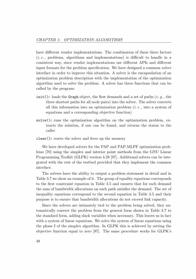
CHAPTER 3. OPTIMIZATION ALGORITHMS
have different vendor implementations. The combination of these three factors(i. e. , problems, algorithms and implementations) is difficult to handle in aconsistent way, since vendor implementations use different APIs and differentinput formats for the problem specification. We have designed a common solverinterface in order to improve this situation. A solver is the encapsulation of anoptimization problem description with the implementation of the optimizationalgorithm used to solve the problem. A solver has three functions that can becalled by the program:
init(): loads the Graph object, the flow demands and a set of paths (e. g. , thethree shortest paths for all node pairs) into the solver. The solver convertsall this information into an optimization problem (i. e. , into a system ofequations and a corresponding objective function)
solve(): runs the optimization algorithm on the optimization problem, ex-tracts the solution, if one can be found, and returns the status to thecaller
clear(): resets the solver and frees up the memory
We have developed solvers for the PAP and PAP-MLPF optimization prob-lems [70] using the simplex and interior point methods from the GNU LinearProgramming Toolkit (GLPK) version 4.28 [97]. Additional solvers can be inte-grated with the rest of the testbed provided that they implement the commoninterface.
The solvers have the ability to output a problem statement in detail and inTable 3.7 we show an example of it. The group of equality equations correspondsto the first constraint equation in Table 3.5 and ensures that for each demandthe sum of bandwidth allocations on each path satisfies the demand. The set ofinequality equations correspond to the second equation in Table 3.5 and theirpurpose is to ensure that bandwidth allocations do not exceed link capacity.
Since the solvers are intimately tied to the problem being solved, they au-tomatically convert the problem from the general form shown in Table 3.7 tothe standard form, adding slack variables when necessary. This leaves us in factwith a system of linear equations. We solve the system of linear equations usingthe phase I of the simplex algorithm. In GLPK this is achieved by setting theobjective function equal to zero [97]. The same procedure works for GLPK’s
48

3.3. PERFORMANCE TESTBED
find xdp for all d ∈ D, p ∈ Psubject to x0,0 + x0,1 + x0,2 = 289.401
x1,0 + x1,1 + x1,2 = 496.613x2,0 + x2,1 + x2,2 = 553.005
x1,2 ≤ 9269.23x0,1 ≤ 899.3x1,1 ≤ 402.51x2,2 ≤ 6661.46x0,2 ≤ 2505.57x0,2 + x2,2 ≤ 8457.03x1,1 + x2,0 ≤ 902.17x0,0 + x1,0 + x1,2 + x2,1 ≤ 213.26x0,1 ≤ 5685.38x1,2 ≤ 9323.55x0,0 ≤ 3240.66x1,0 ≤ 3220.41x2,2 ≤ 5912.13x2,1 ≤ 5482.41
Table 3.7: PAP in detail for a network with 10 nodes.
49
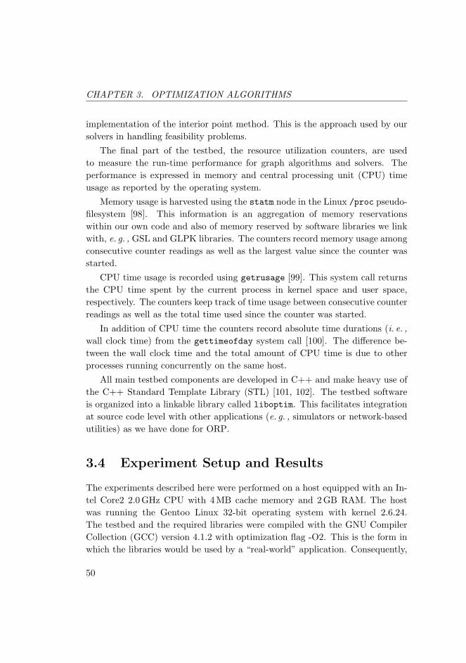
CHAPTER 3. OPTIMIZATION ALGORITHMS
implementation of the interior point method. This is the approach used by oursolvers in handling feasibility problems.
The final part of the testbed, the resource utilization counters, are usedto measure the run-time performance for graph algorithms and solvers. Theperformance is expressed in memory and central processing unit (CPU) timeusage as reported by the operating system.
Memory usage is harvested using the statm node in the Linux /proc pseudo-filesystem [98]. This information is an aggregation of memory reservationswithin our own code and also of memory reserved by software libraries we linkwith, e. g. , GSL and GLPK libraries. The counters record memory usage amongconsecutive counter readings as well as the largest value since the counter wasstarted.
CPU time usage is recorded using getrusage [99]. This system call returnsthe CPU time spent by the current process in kernel space and user space,respectively. The counters keep track of time usage between consecutive counterreadings as well as the total time used since the counter was started.
In addition of CPU time the counters record absolute time durations (i. e. ,wall clock time) from the gettimeofday system call [100]. The difference be-tween the wall clock time and the total amount of CPU time is due to otherprocesses running concurrently on the same host.
All main testbed components are developed in C++ and make heavy use ofthe C++ Standard Template Library (STL) [101, 102]. The testbed softwareis organized into a linkable library called liboptim. This facilitates integrationat source code level with other applications (e. g. , simulators or network-basedutilities) as we have done for ORP.
3.4 Experiment Setup and Results
The experiments described here were performed on a host equipped with an In-tel Core2 2.0 GHz CPU with 4 MB cache memory and 2 GB RAM. The hostwas running the Gentoo Linux 32-bit operating system with kernel 2.6.24.The testbed and the required libraries were compiled with the GNU CompilerCollection (GCC) version 4.1.2 with optimization flag -O2. This is the form inwhich the libraries would be used by a “real-world” application. Consequently,
50
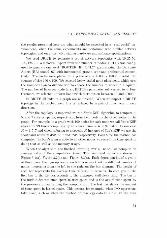
3.4. EXPERIMENT SETUP AND RESULTS
the results presented here are what should be expected in a “real-world” en-vironment, when the same experiments are performed with similar networktopologies, and on a host with similar hardware and software specifications.
We used BRITE to generate a set of network topologies with 10, 25, 50,100, 125, . . . , 300 nodes. Apart from the number of nodes, BRITE was config-ured to generate one level “ROUTER (IP) ONLY” graphs using the Barabasi-Albert (BA) model [62] with incremental growth type and preferential connec-tivity. The nodes were placed on a plane of size 10000 × 10000 divided intosquares of size 100× 100. We selected heavy-tailed node placement, which usesthe bounded Pareto distribution to choose the number of nodes in a square.The number of links per node (i. e. , BRITE’s parameter m) was set to 4. Fur-thermore, we selected uniform bandwidth distribution between 10 and 10000.
In BRITE all links in a graph are undirected. When we import a BRITEtopology in the testbed each link is replaced by a pair of links, one in eachdirection.
After the topology is imported we run Yen’s KSP algorithm to compute 3,5, and 7 shortest paths, respectively, from each node to the other nodes in thegraph. For example, in a graph with 100 nodes for each node we call Yen’s KSPalgorithm 99 times computing up to a maximum of K × 99 paths. In our caseK = 3, 5, 7 and when referring to a specific K instance of Yen’s KSP we use theshorthand notation 3SP, 5SP and 7SP, respectively. Each time the testbed hascomputed the KSPs from a node to all other nodes we record the time spent indoing that as well as the memory usage.
When the algorithm has finished iterating over all nodes, we compute anaverage value of the computation time. The computed values are shown inFigure 3.1(a), Figure 3.2(a) and Figure 3.3(a). Each figure consist of a groupof three bars. Each group corresponds to a network with a different number ofnodes, increasing from the left to the right on the bar diagram. The height ofeach bar represents the average time duration in seconds. In each group, thefirst bar to the left corresponds to the measured wall-clock time. The bar inthe middle denotes time spent in user space and is the actual time spent bythe processor in performing the computation. The last bar shows the amountof time spent in kernel space. This occurs, for example, when I/O operationstake place, such as when the testbed process logs data to a file. In the tests
51
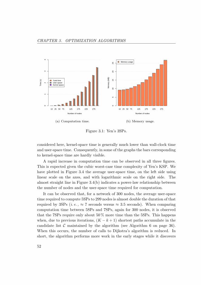
CHAPTER 3. OPTIMIZATION ALGORITHMS
10 25 50 75 125 175 225 275
Number of nodes
Tim
e (s
)
01
23
4
Total timeUser spaceKernel space
(a) Computation time.
10 25 50 75 125 175 225 275
Number of nodes
Mem
ory
(MB
)
05
1015
2025
Memory usage
(b) Memory usage.
Figure 3.1: Yen’s 3SPs.
considered here, kernel-space time is generally much lower than wall-clock timeand user-space time. Consequently, in some of the graphs the bars correspondingto kernel-space time are hardly visible.
A rapid increase in computation time can be observed in all three figures.This is expected given the cubic worst-case time complexity of Yen’s KSP. Wehave plotted in Figure 3.4 the average user-space time, on the left side usinglinear scale on the axes, and with logarithmic scale on the right side. Thealmost straight line in Figure 3.4(b) indicates a power-law relationship betweenthe number of nodes and the user-space time required for computation.
It can be observed that, for a network of 300 nodes, the average user-spacetime required to compute 5SPs to 299 nodes is almost double the duration of thatrequired by 3SPs (i. e. , ≈ 7 seconds versus ≈ 3.5 seconds). When comparingcomputation time between 5SPs and 7SPs, again for 300 nodes, it is observedthat the 7SPs require only about 50 % more time than the 5SPs. This happenswhen, due to previous iterations, (K − k + 1) shortest paths accumulate in thecandidate list C maintained by the algorithm (see Algorithm 6 on page 36).When this occurs, the number of calls to Dijkstra’s algorithm is reduced. Inshort, the algorithm performs more work in the early stages while it discovers
52
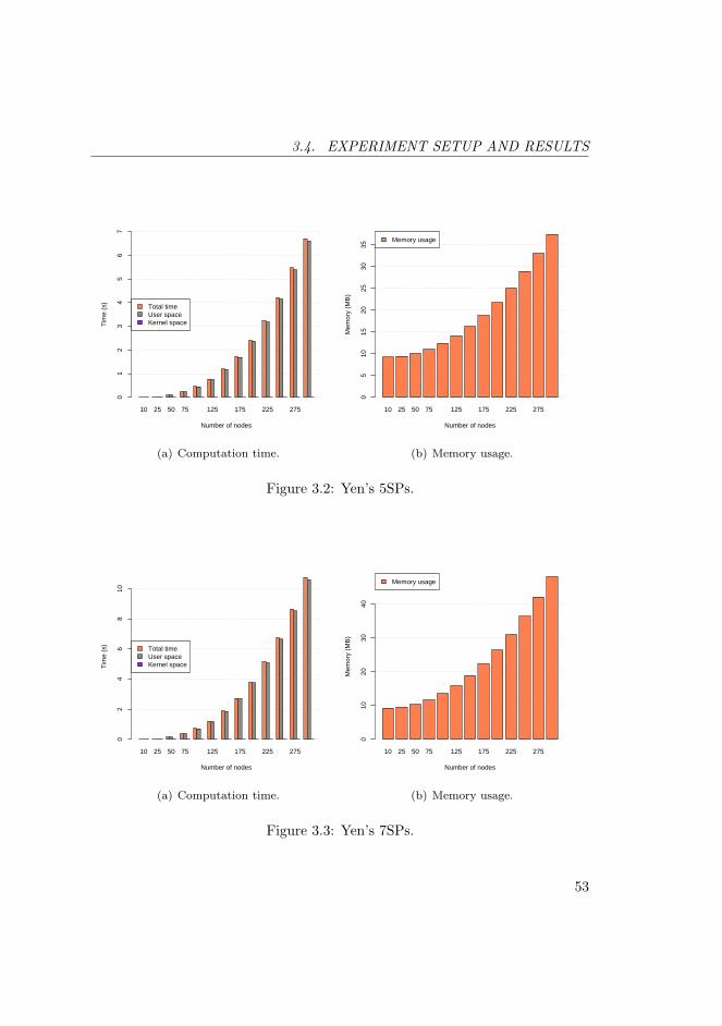
3.4. EXPERIMENT SETUP AND RESULTS
10 25 50 75 125 175 225 275
Number of nodes
Tim
e (s
)
01
23
45
67
Total timeUser spaceKernel space
(a) Computation time.
10 25 50 75 125 175 225 275
Number of nodes
Mem
ory
(MB
)
05
1015
2025
3035
Memory usage
(b) Memory usage.
Figure 3.2: Yen’s 5SPs.
10 25 50 75 125 175 225 275
Number of nodes
Tim
e (s
)
02
46
810
Total timeUser spaceKernel space
(a) Computation time.
10 25 50 75 125 175 225 275
Number of nodes
Mem
ory
(MB
)
010
2030
40
Memory usage
(b) Memory usage.
Figure 3.3: Yen’s 7SPs.
53
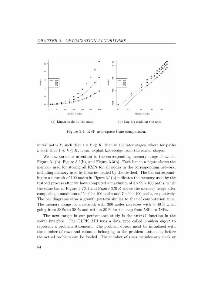
CHAPTER 3. OPTIMIZATION ALGORITHMS
● ● ●●
●
●
●
●
●
●
●
●
●
0 50 100 150 200 250 300
02
46
810
Number of nodes
Tim
e (s
)
● ● ●●
●●
●
●
●
●
●
●
●
● ● ● ● ●●
●●
●
●
●
●
●
3SP5SP7SP
(a) Linear scale on the axes.
●
●
●
●
●
●
●
●
●
●
●●
●
10 20 50 100 200
Number of nodes
Tim
e (s
)
0.00
50.
050.
55
10
●
●
●
●
●
●
●
●
●
●
●●
●
●
●
●
●
●
●
●
●
●
●
●●
●
3SP5SP7SP
(b) Log-log scale on the axes.
Figure 3.4: KSP user-space time comparison.
initial paths k, such that 1 ≤ k � K, than in the later stages, where for pathsk such that 1� k ≤ K, it can exploit knowledge from the earlier stages.
We now turn our attention to the corresponding memory usage shown inFigure 3.1(b), Figure 3.2(b), and Figure 3.3(b). Each bar in a figure shows thememory used for storing all KSPs for all nodes in the corresponding network,including memory used by libraries loaded by the testbed. The bar correspond-ing to a network of 100 nodes in Figure 3.1(b) indicates the memory used by thetestbed process after we have computed a maximum of 3×99×100 paths, whilethe same bar in Figure 3.2(b) and Figure 3.3(b) shows the memory usage aftercomputing a maximum of 5×99×100 paths and 7×99×100 paths, respectively.The bar diagrams show a growth pattern similar to that of computation time.The memory usage for a network with 300 nodes increases with ≈ 40 % whengoing from 3SPs to 5SPs and with ≈ 30 % for the step from 5SPs to 7SPs.
The next target in our performance study is the init() function in thesolver interface. The GLPK API uses a data type called problem object torepresent a problem statement. The problem object must be initialized withthe number of rows and columns belonging to the problem statement, beforethe actual problem can be loaded. The number of rows includes any slack or
54

3.4. EXPERIMENT SETUP AND RESULTS
10 25 50 75 125 175 225 275
Number of nodes
Tim
e (s
)
0.0
0.1
0.2
0.3
0.4
Total timeUser spaceKernel space
Eq: 13 32 73 105 149 167 216 247 268 307 375 399 425
Var: 6 15 30 45 60 75 90 105 120 135 150 165 180
(a) Computation time, 20 % demands.
10 25 50 75 125 175 225 275
Number of nodes
Mem
ory
(MB
)
010
2030
40
Memory usage
Eq: 13 32 73 105 149 167 216 247 268 307 375 399 425
Var: 6 15 30 45 60 75 90 105 120 135 150 165 180
(b) Memory usage, 20 % demands.
10 25 50 75 125 175 225 275
Number of nodes
Tim
e (s
)
0.0
0.5
1.0
1.5
2.0
Total timeUser spaceKernel space
Eq: 46 104 218 323 450 480 625 713 846 937 1135 1206 1267
Var: 24 60 120 180 240 300 360 420 480 540 600 660 720
(c) Computation time, 80 % demands.
10 25 50 75 125 175 225 275
Number of nodes
Mem
ory
(MB
)
010
2030
40
Memory usage
Eq: 46 104 218 323 450 480 625 713 846 937 1135 1206 1267
Var: 24 60 120 180 240 300 360 420 480 540 600 660 720
(d) Memory usage, 80 % demands.
Figure 3.5: Solver init() subroutine with 3SPs.
55
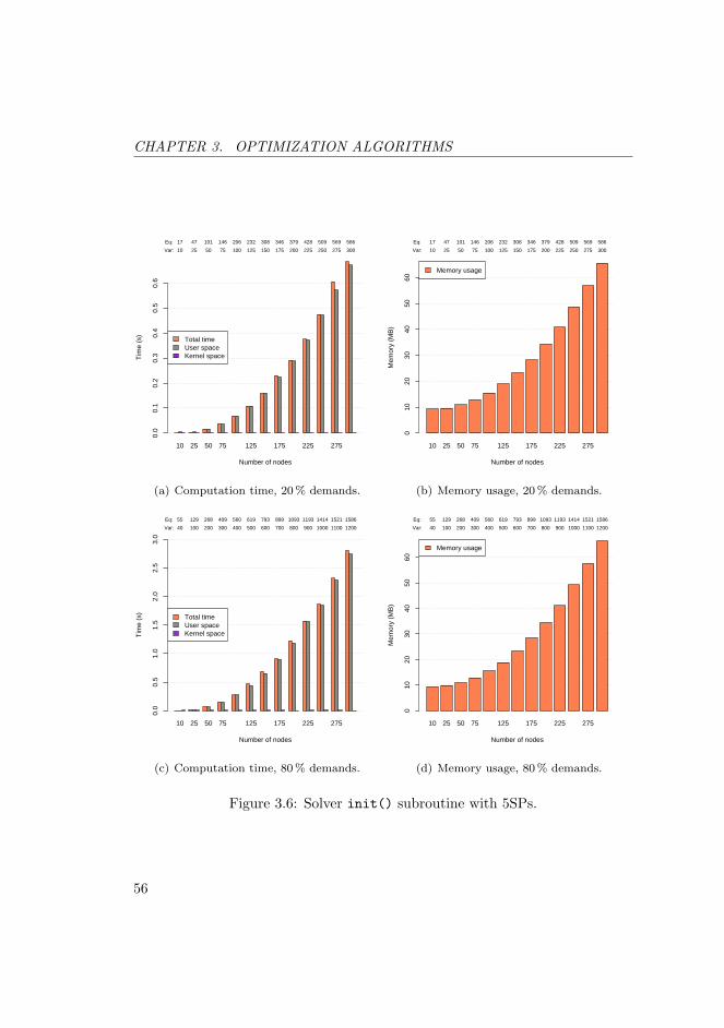
CHAPTER 3. OPTIMIZATION ALGORITHMS
10 25 50 75 125 175 225 275
Number of nodes
Tim
e (s
)
0.0
0.1
0.2
0.3
0.4
0.5
0.6
Total timeUser spaceKernel space
Eq: 17 47 101 146 206 232 308 346 379 428 509 569 586
Var: 10 25 50 75 100 125 150 175 200 225 250 275 300
(a) Computation time, 20 % demands.
10 25 50 75 125 175 225 275
Number of nodes
Mem
ory
(MB
)
010
2030
4050
60
Memory usage
Eq: 17 47 101 146 206 232 308 346 379 428 509 569 586
Var: 10 25 50 75 100 125 150 175 200 225 250 275 300
(b) Memory usage, 20 % demands.
10 25 50 75 125 175 225 275
Number of nodes
Tim
e (s
)
0.0
0.5
1.0
1.5
2.0
2.5
3.0
Total timeUser spaceKernel space
Eq: 55 129 268 409 560 619 793 899 1093 1193 1414 1521 1586
Var: 40 100 200 300 400 500 600 700 800 900 1000 1100 1200
(c) Computation time, 80 % demands.
10 25 50 75 125 175 225 275
Number of nodes
Mem
ory
(MB
)
010
2030
4050
60
Memory usage
Eq: 55 129 268 409 560 619 793 899 1093 1193 1414 1521 1586
Var: 40 100 200 300 400 500 600 700 800 900 1000 1100 1200
(d) Memory usage, 80 % demands.
Figure 3.6: Solver init() subroutine with 5SPs.
56

3.4. EXPERIMENT SETUP AND RESULTS
10 25 50 75 125 175 225 275
Number of nodes
Tim
e (s
)
0.0
0.2
0.4
0.6
0.8
Total timeUser spaceKernel space
Eq: 18 63 127 176 251 287 366 415 447 523 603 692 714
Var: 14 35 70 105 140 175 210 245 280 315 350 385 420
(a) Computation time, 20 % demands.
10 25 50 75 125 175 225 275
Number of nodes
Mem
ory
(MB
)
020
4060
80
Memory usage
Eq: 18 63 127 176 251 287 366 415 447 523 603 692 714
Var: 14 35 70 105 140 175 210 245 280 315 350 385 420
(b) Memory usage, 20 % demands.
10 25 50 75 125 175 225 275
Number of nodes
Tim
e (s
)
01
23
4
Total timeUser spaceKernel space
Eq: 56 150 304 452 630 711 898 1026 1217 1348 1570 1674 1801
Var: 56 140 280 420 560 700 840 980 1120 1260 1400 1540 1680
(c) Computation time, 80 % demands.
10 25 50 75 125 175 225 275
Number of nodes
Mem
ory
(MB
)
020
4060
80
Memory usage
Eq: 56 150 304 452 630 711 898 1026 1217 1348 1570 1674 1801
Var: 56 140 280 420 560 700 840 980 1120 1260 1400 1540 1680
(d) Memory usage, 80 % demands.
Figure 3.7: Solver init() subroutine with 7SPs.
57

CHAPTER 3. OPTIMIZATION ALGORITHMS
surplus variables required to bring the problem into standard form. This allowsGLPK to reserve enough memory for the problem object. Consequently, theinit() function performs two passes. During the first pass we iterate throughthe flow demands and through the KSPs and compute the amount of memoryneeded. During the second pass we iterate again through the same items andload the variable coefficients, the constraint values and the objective functioninto the reserved memory. The time spent in init() is computed over bothpasses.
There are several factors that decide the number of equations and the numberof variables in a problem statement:
i) amount of flow demands,
ii) number of paths associated with each flow demand,
iii) number of links traversed by the flow demand paths.
Item ii) can be controlled loosely by a suitable choice of K for Yen’s KSP. Itemiii) is indirectly decided by the choices in i) and iii). To test the influence ofitem i) on the problem statement we have created two scenarios correspondingroughly to a quiescent network and to a busy network, respectively. In thequiescent network scenario we create d0.2V e demands, where V is the numberof nodes in the graph1. We call this the “20 % demands” scenario. In the busynetwork scenario we let the number of demands go up to d0.8V e and we call it the“80 % demands” scenario. For each demand, we randomly choose the bandwidthrequired, the source and the destination nodes. The only requirement is that thesource and the destination nodes are distinct from each other. The bandwidthvalues are selected from a uniform distribution on the half-open segment (0, 256].
Figures 3.5–3.7 show each a group of bar diagrams for the run-time behaviorand memory usage of the init() function in the case of 3SPs, 5SPs and 7SPs,respectively. In each group we show the 20 % demands and 80 % demandsscenarios on top of each other. At the top of each bar diagram there are tworows with numbers aligned to the bars. The first row shows the number ofequations corresponding to the bar in question and the second line shows thenumber of variables. We want to emphasize that the number of variables on
1The notation dxe denotes that x is rounded upwards to the nearest larger integer.
58
3.4. EXPERIMENT SETUP AND RESULTS
top of the diagrams does not include slack variables. To compute the number ofslack variables we can use the property that for a PAP problem with n demands,n of the equations are equality equations for satisfying the demands, and thereminder are inequality equations for satisfying link capacity constraints. Theinequality equations require a slack variable each. The largest system of linearequations encountered in our test is shown in Figure 3.7(c) and Figure 3.7(d) andcontains 1801 equations and 1680 variables. In addition, this system includesalso 1801− (0.8× 300) = 1561 slack variables.
We can observe that the computation time for init() is directly proportionalto the number of demands: when the number of demands grows four times (i. e. ,from 20 % to 80 % demands) so does the computation time. The same relationholds between computation time and number of variables. This is expectedbecause the number of variables is equal to the number of demands multipliedby the number of paths used by all demands. The BRITE topologies are stronglyconnected, which allows Yen’s KSP to always find K paths between a pair ofnodes. This keeps the number of paths per demand constant (i. e. , 3, 5, and 7).
The memory usage displayed in the diagrams is constituted of the followingcomponents:
• memory used for storing all KSPs as shown in Figure 3.1(b), Figure 3.2(b),and Figure 3.3(b),
• memory reserved for all flow demands,
• memory reserved for GLPK’s problem object.
In all diagrams the memory usage shows roughly 20 MB increase for networkswith 250–300 nodes, when compared to the memory used for storing KSPs. Forsmaller networks the increase is smaller because the STL data types allocatea reasonable amount of memory from the start. Additionally, /proc/statm
reports memory usage in terms 4 KB pages reserved by the Linux kernel. Whenthe testbed is started a number of pages are automatically reserved, which canbe enough to hold our data for small networks.
The next six groups of graphs, Figure 3.8–3.13, show the computation timerequired to solve the PAP and PAP-MLPF problems using the simplex methodand the interior point method (IPM), respectively. Some of the bars displaying
59

CHAPTER 3. OPTIMIZATION ALGORITHMS
10 25 50 75 125 175 225 275
Number of nodes
Tim
e (s
)
0.00
00.
002
0.00
40.
006
0.00
8
Total timeUser spaceKernel space
Eq: 13 32 73 105 149 167 216 247 268 307 375 399 425
Var: 6 15 30 45 60 75 90 105 120 135 150 165 180
(a) PAP-IPM computation time.
10 25 50 75 125 175 225 275
Number of nodes
Tim
e (s
)
0.0
0.1
0.2
0.3
0.4
Total timeUser spaceKernel space
Eq: 13 32 73 105 149 167 216 247 268 307 375 399 425
Var: 7 16 31 46 61 76 91 106 121 136 151 166 181
(b) PAP-MLPF-IPM computation time.
10 25 50 75 125 175 225 275
Number of nodes
Tim
e (s
)
0.00
00.
005
0.01
00.
015
Total timeUser spaceKernel space
Eq: 13 32 73 105 149 167 216 247 268 307 375 399 425
Var: 6 15 30 45 60 75 90 105 120 135 150 165 180
(c) PAP-SIMPLEX computation time.
10 25 50 75 125 175 225 275
Number of nodes
Tim
e (s
)
0.00
00.
001
0.00
20.
003
0.00
4
Total timeUser spaceKernel space
Eq: 13 32 73 105 149 167 216 247 268 307 375 399 425
Var: 7 16 31 46 61 76 91 106 121 136 151 166 181
(d) PAP-MLPF-SIMPLEX computation time.
Figure 3.8: Solver solve() subroutine with 3SPs, 20 % demands.
60

3.4. EXPERIMENT SETUP AND RESULTS
10 25 50 75 125 175 225 275
Number of nodes
Tim
e (s
)
0.00
00.
005
0.01
00.
015
0.02
0
Total timeUser spaceKernel space
Eq: 17 47 101 146 206 232 308 346 379 428 509 569 586
Var: 10 25 50 75 100 125 150 175 200 225 250 275 300
(a) PAP-IPM computation time.
10 25 50 75 125 175 225 275
Number of nodes
Tim
e (s
)
0.0
0.5
1.0
1.5
2.0
2.5
3.0
Total timeUser spaceKernel space
Eq: 17 47 101 146 206 232 308 346 379 428 509 569 586
Var: 11 26 51 76 101 126 151 176 201 226 251 276 301
(b) PAP-MLPF-IPM computation time.
10 25 50 75 125 175 225 275
Number of nodes
Tim
e (s
)
0.00
00.
001
0.00
20.
003
0.00
40.
005
Total timeUser spaceKernel space
Eq: 17 47 101 146 206 232 308 346 379 428 509 569 586
Var: 10 25 50 75 100 125 150 175 200 225 250 275 300
(c) PAP-SIMPLEX computation time.
10 25 50 75 125 175 225 275
Number of nodes
Tim
e (s
)
0.00
00.
001
0.00
20.
003
0.00
40.
005
0.00
6
Total timeUser spaceKernel space
Eq: 17 47 101 146 206 232 308 346 379 428 509 569 586
Var: 11 26 51 76 101 126 151 176 201 226 251 276 301
(d) PAP-MLPF-SIMPLEX computation time.
Figure 3.9: Solver solve() subroutine with 5SPs, 20 % demands.
61
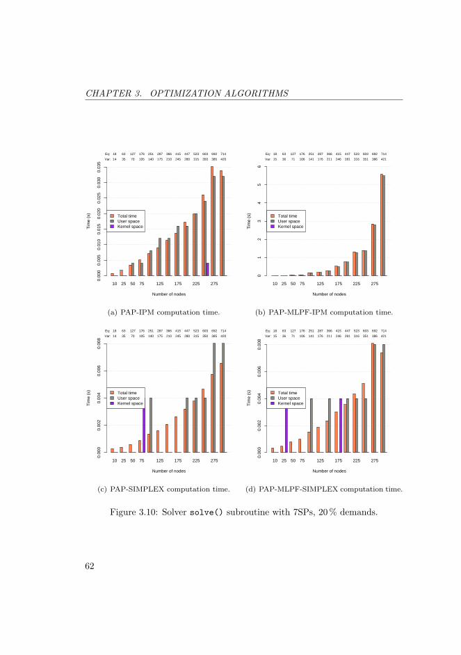
CHAPTER 3. OPTIMIZATION ALGORITHMS
10 25 50 75 125 175 225 275
Number of nodes
Tim
e (s
)
0.00
00.
005
0.01
00.
015
0.02
00.
025
0.03
00.
035
Total timeUser spaceKernel space
Eq: 18 63 127 176 251 287 366 415 447 523 603 692 714
Var: 14 35 70 105 140 175 210 245 280 315 350 385 420
(a) PAP-IPM computation time.
10 25 50 75 125 175 225 275
Number of nodes
Tim
e (s
)
01
23
45
6
Total timeUser spaceKernel space
Eq: 18 63 127 176 251 287 366 415 447 523 603 692 714
Var: 15 36 71 106 141 176 211 246 281 316 351 386 421
(b) PAP-MLPF-IPM computation time.
10 25 50 75 125 175 225 275
Number of nodes
Tim
e (s
)
0.00
00.
002
0.00
40.
006
0.00
8
Total timeUser spaceKernel space
Eq: 18 63 127 176 251 287 366 415 447 523 603 692 714
Var: 14 35 70 105 140 175 210 245 280 315 350 385 420
(c) PAP-SIMPLEX computation time.
10 25 50 75 125 175 225 275
Number of nodes
Tim
e (s
)
0.00
00.
002
0.00
40.
006
0.00
8
Total timeUser spaceKernel space
Eq: 18 63 127 176 251 287 366 415 447 523 603 692 714
Var: 15 36 71 106 141 176 211 246 281 316 351 386 421
(d) PAP-MLPF-SIMPLEX computation time.
Figure 3.10: Solver solve() subroutine with 7SPs, 20 % demands.
62
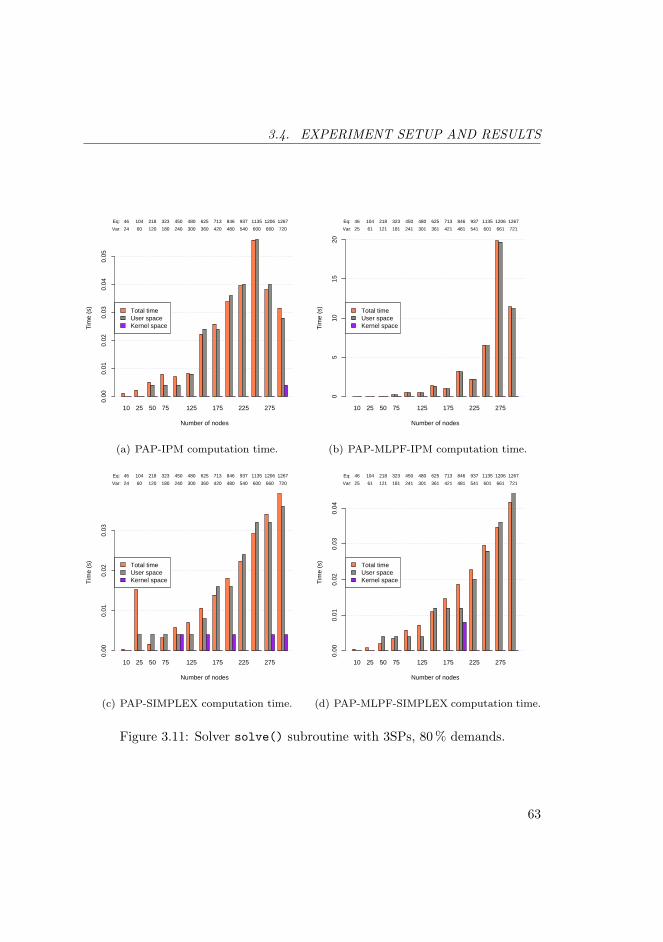
3.4. EXPERIMENT SETUP AND RESULTS
10 25 50 75 125 175 225 275
Number of nodes
Tim
e (s
)
0.00
0.01
0.02
0.03
0.04
0.05
Total timeUser spaceKernel space
Eq: 46 104 218 323 450 480 625 713 846 937 1135 1206 1267
Var: 24 60 120 180 240 300 360 420 480 540 600 660 720
(a) PAP-IPM computation time.
10 25 50 75 125 175 225 275
Number of nodes
Tim
e (s
)
05
1015
20
Total timeUser spaceKernel space
Eq: 46 104 218 323 450 480 625 713 846 937 1135 1206 1267
Var: 25 61 121 181 241 301 361 421 481 541 601 661 721
(b) PAP-MLPF-IPM computation time.
10 25 50 75 125 175 225 275
Number of nodes
Tim
e (s
)
0.00
0.01
0.02
0.03
Total timeUser spaceKernel space
Eq: 46 104 218 323 450 480 625 713 846 937 1135 1206 1267
Var: 24 60 120 180 240 300 360 420 480 540 600 660 720
(c) PAP-SIMPLEX computation time.
10 25 50 75 125 175 225 275
Number of nodes
Tim
e (s
)
0.00
0.01
0.02
0.03
0.04
Total timeUser spaceKernel space
Eq: 46 104 218 323 450 480 625 713 846 937 1135 1206 1267
Var: 25 61 121 181 241 301 361 421 481 541 601 661 721
(d) PAP-MLPF-SIMPLEX computation time.
Figure 3.11: Solver solve() subroutine with 3SPs, 80 % demands.
63
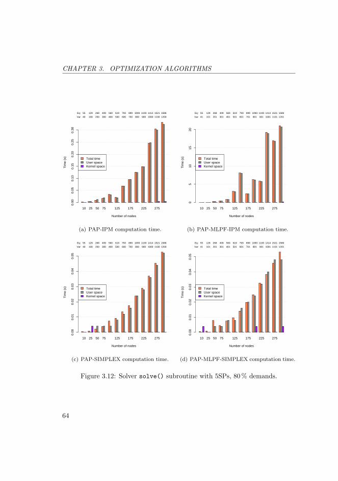
CHAPTER 3. OPTIMIZATION ALGORITHMS
10 25 50 75 125 175 225 275
Number of nodes
Tim
e (s
)
0.00
0.05
0.10
0.15
0.20
0.25
0.30
Total timeUser spaceKernel space
Eq: 55 129 268 409 560 619 793 899 1093 1193 1414 1521 1586
Var: 40 100 200 300 400 500 600 700 800 900 1000 1100 1200
(a) PAP-IPM computation time.
10 25 50 75 125 175 225 275
Number of nodes
Tim
e (s
)
05
1015
20
Total timeUser spaceKernel space
Eq: 55 129 268 409 560 619 793 899 1093 1193 1414 1521 1586
Var: 41 101 201 301 401 501 601 701 801 901 1001 1101 1201
(b) PAP-MLPF-IPM computation time.
10 25 50 75 125 175 225 275
Number of nodes
Tim
e (s
)
0.00
0.01
0.02
0.03
0.04
0.05
Total timeUser spaceKernel space
Eq: 55 129 268 409 560 619 793 899 1093 1193 1414 1521 1586
Var: 40 100 200 300 400 500 600 700 800 900 1000 1100 1200
(c) PAP-SIMPLEX computation time.
10 25 50 75 125 175 225 275
Number of nodes
Tim
e (s
)
0.00
0.01
0.02
0.03
0.04
0.05
Total timeUser spaceKernel space
Eq: 55 129 268 409 560 619 793 899 1093 1193 1414 1521 1586
Var: 41 101 201 301 401 501 601 701 801 901 1001 1101 1201
(d) PAP-MLPF-SIMPLEX computation time.
Figure 3.12: Solver solve() subroutine with 5SPs, 80 % demands.
64
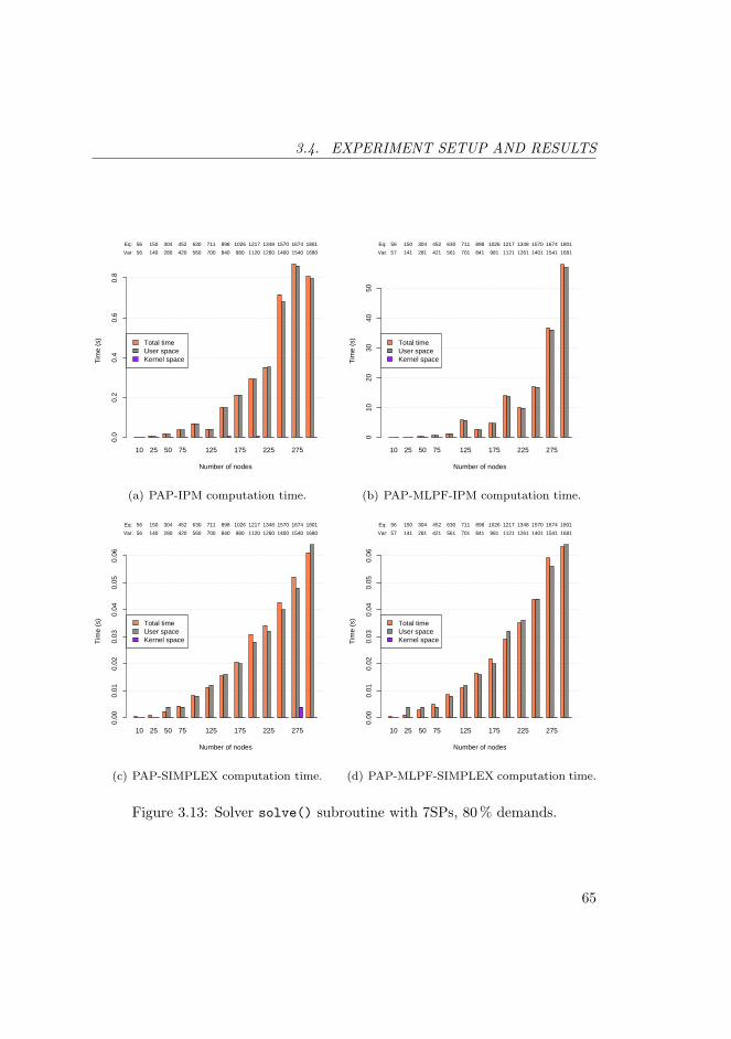
3.4. EXPERIMENT SETUP AND RESULTS
10 25 50 75 125 175 225 275
Number of nodes
Tim
e (s
)
0.0
0.2
0.4
0.6
0.8
Total timeUser spaceKernel space
Eq: 56 150 304 452 630 711 898 1026 1217 1348 1570 1674 1801
Var: 56 140 280 420 560 700 840 980 1120 1260 1400 1540 1680
(a) PAP-IPM computation time.
10 25 50 75 125 175 225 275
Number of nodes
Tim
e (s
)
010
2030
4050
Total timeUser spaceKernel space
Eq: 56 150 304 452 630 711 898 1026 1217 1348 1570 1674 1801
Var: 57 141 281 421 561 701 841 981 1121 1261 1401 1541 1681
(b) PAP-MLPF-IPM computation time.
10 25 50 75 125 175 225 275
Number of nodes
Tim
e (s
)
0.00
0.01
0.02
0.03
0.04
0.05
0.06
Total timeUser spaceKernel space
Eq: 56 150 304 452 630 711 898 1026 1217 1348 1570 1674 1801
Var: 56 140 280 420 560 700 840 980 1120 1260 1400 1540 1680
(c) PAP-SIMPLEX computation time.
10 25 50 75 125 175 225 275
Number of nodes
Tim
e (s
)
0.00
0.01
0.02
0.03
0.04
0.05
0.06
Total timeUser spaceKernel space
Eq: 56 150 304 452 630 711 898 1026 1217 1348 1570 1674 1801
Var: 57 141 281 421 561 701 841 981 1121 1261 1401 1541 1681
(d) PAP-MLPF-SIMPLEX computation time.
Figure 3.13: Solver solve() subroutine with 7SPs, 80 % demands.
65
CHAPTER 3. OPTIMIZATION ALGORITHMS
entries in the millisecond range show user-space time or kernel-space time largerthan the total time value. This pathological behavior is caused by the getrusagesystem call, which uses the system timer that runs at a frequency of 250 Hz.The time reported by getrusage is consequently incremented by 4 ms units.The total time provided by the gettimeofday system call has microsecondaccuracy [103].
The name in the caption of each graph denote the type of problem and solvedand the algorithm used:
PAP-IPM: pure allocation problem solved with the IPM,
PAP-MLPF-IPM: pure allocation problem with modified link-path formula-tion solved with the IPM,
PAP-SIMPLEX: pure allocation problem solved with the simplex method,
PAP-MLPF-SIMPLEX: pure allocation problem with modified link-pathformulation solved with the simplex method.
The obvious observation is that the simplex method outperforms the IPMin every tested scenario. We suspect that this happens because GLPK’s imple-mentation of the interior point method is not as mature as the implementationof the simplex method. In particular, there is a huge difference, almost twoorders of magnitude in some scenarios, between the IPM’s computation timefor the feasibility problem, PAP, and the computation time for the optimizationproblem, PAP-MLPF. When the simplex method is used to solve these prob-lems, the diagrams show minor differences (1–20 ms) between the computationtime of the feasibility problem versus the computation time of the optimizationproblem.
We show no corresponding memory graphs since any fluctuations in thememory usage while solving the problems are too small to distinguish from thememory usage displayed in Figure 3.8–3.13.
3.5 Summary
The chapter started with a brief overview of linear programming notation. Usingthis notation, we formulated optimization problems concerning path selection
66

3.5. SUMMARY
and flow allocation. Furthermore, we described the performance testbed formethods used in solving network flow problems.
We used the testbed to obtain empirical results for the performance of Yen’sKSP, the simplex method, and the IPM. The purpose for obtaining these resultswas two-fold. First, we wanted to know the cost in terms of resource usageassociated with running these algorithms. Secondly, but no less important, thetest results provided guidance for choosing an optimization algorithm for theORP framework presented in Chapter 5.
Based on the results in final part of Section 3.4 we selected the simplexalgorithm to be used in ORP because it showed consistent good performancewhen compared to the performance of the IPM.
67

CHAPTER 3. OPTIMIZATION ALGORITHMS
68
Chapter 4
Gnutella Traffic Models
In the design of the ORP framework described in Chapter 5 it is assumedthat implementations run on top of existing overlay networks spawned by end-nodes. The Gnutella P2P network is a typical example of this type of overlays.Consequently, Gnutella’s traffic characteristics were the subject of a detailedstudy [104, 105].
The goal in studying the characteristics of Gnutella traffic was to obtaina better understanding of P2P dynamics and to construct simple statisticalmodels that can be used for synthetic traffic generation.
In Section 4.1 we describe the Gnutella protocol with emphasis on messageformat, bootstrap, connection establishment, topology exploration and resourcediscovery. The infrastructure for measuring Gnutella traffic is described in Sec-tion 4.2, which is followed by a presentation of the methodology for constructingstatistical models in Section 4.3. Section 4.4 presents the characteristics andmodels obtained from the recorded traffic.
4.1 The Gnutella Protocol
Gnutella is a heavily decentralized P2P system. Nodes1 can share any type ofresources, although the currently available specification covers only computer
1A Gnutella node is also called a servent, which is a combination of the words server and
client.
69
CHAPTER 4. GNUTELLA TRAFFIC MODELS
files [106].The network spawned by Gnutella nodes consists of an unstructured topol-
ogy with a two-level hierarchy: ultrapeers (UPs) and leaf nodes (LNs). UPs arefaster nodes in the sense that they are connected to high-capacity links and havea large amount of processing power available. LNs maintain a single connectionto their UP. An UP maintains 10-100 connections, one for each LN and 1-10connections to other UPs [107]. The UPs perform signaling on behalf of theLNs, thus shielding them from large volumes of signaling traffic. An UP doesnot necessarily have LNs, in which case it works standalone.
The activities of Gnutella peers can be divided into two main categories:signaling and user-data transfer (further referred to as data transfer). Signal-ing activities are concerned with peer discovery, overlay topology maintenance,content search and other management functions. Data transfer occurs when apeer has localized during content search one or more files of interest.
According to the Gnutella Development Forum (GDF) mailing list, theGnutella community has recently adopted what is called support for high out-degree [108]. This implies that UPs maintain at least 32 connections to otherUPs and 100–300 connections to different lead nodes. LNs are recommended tomaintain approximately 4 connections to UPs. The numbers may slightly differbetween different Gnutella vendors. The claim is that high outdegree supportallows a peer to connect to the majority of Gnutella peers in 4 hops or less [109].
4.1.1 Bootstrap
A Gnutella node that attempts to join the overlay for the first time must boot-strap itself into the overlay. This implies finding and connecting to one orseveral peers that are already part of the overlay. A list of active servents canbe obtained from a Gnutella Web Cache (GWC) [110] server. A GWC serveris essentially an Hypertext Transfer Protocol (HTTP) server maintaining a listof active peers with associated listening sockets. A listening socket is an IPaddress and port number pair that can be used to connect to the correspondingservent. UPs update the list continuously, ensuring that new peers can alwaysjoin the overlay.
Once the node joins the overlay, additional peers can be found through the
70
4.1. THE GNUTELLA PROTOCOL
exchange of PING and PONG messages. The servent saves peer addresses in alocal host cache in order to avoid connecting to a GWC server upon restart. Thelocal host cache is used also if the servent supports the UDP Host Cache (UHC)protocol. The protocol works as a distributed bootstrap system, transformingUHC-enabled servents into GWC-like servers [111] and off-loading the actualGWC servers.
4.1.2 Connection Establishment
Peer signaling occurs over TCP connections. Once a TCP connection has beensetup, the peers at each end of the TCP connection perform a three-way Gnutellahandshake. The Gnutella handshake allows the negotiation of a common set ofcapabilities to be used during the session. The type of capabilities negotiatedare UP - LN relationship, support for high outdegree, traffic compression, etc.
If the handshake fails the TCP connections is teared down. Otherwise,the client and the server start exchanging binary Gnutella messages over theexisting TCP connection. The connection lasts until one of the peers decidesto terminate the session. At that point the node ending the connection canoptionally send a BYE message to notify its peer of its departure. The TCPconnection will then be closed.
If the capability set used by the peers includes stream compression [112],then all data on the TCP connection is compressed, with the exception of theinitial Gnutella handshake. The type of compression algorithm can be selectedduring the handshake, but the currently supported algorithm is deflate, whichis implemented in zlib [113].
4.1.3 Messages
Each Gnutella message starts with a generic header that contains the fieldsshown in Figure 4.1 (the numbers in the figure denote bytes):
• message ID using a globally unique identifier (GUID), to uniquely identifymessages on the Gnutella network [114],
• payload type code, denoted by P in Figure 4.1, which identifies the type ofGnutella message. The currently supported messages are: PING, PONG,
71

CHAPTER 4. GNUTELLA TRAFFIC MODELS
GUID P T H Length
15 17 19 220
Figure 4.1: The Gnutella header.
BYE, QRP, VEND, STDVEND, PUSH, QUERY, QUERY HIT and HSEP,
• time-to-live (TTL), to limit the signaling radius and its adverse impact onthe network. Messages with TTL > 15 are dropped2. This field is denotedby T in Figure 4.1,
• hop count to inform receiving peers how far the message has traveled,denoted by H in Figure 4.1,
• payload length in bytes to describe the length of the message, not includingthe header. The payload length indicates where in the byte stream thenext Gnutella generic message header can be found.
The generic Gnutella header is followed by the actual message, which mayhave own headers. Also, the message may contain vendor extensions. Vendorextensions are used when a specific type of servent wants to implement experi-mental functionality not covered by the standard specifications.
4.1.4 Topology Exploration
Each successfully connected servent periodically sends PING messages to itsneighbors. The receiver of a PING message decrements the TTL in the Gnutellaheader. If the TTL is greater than zero the node increments the hop counter inthe message header and then forwards the message to all its directly connectedpeers, with the exception of the one from where the message came. PINGmessages do not carry any user data, not even the sender’s listening socket.This means that the payload length field in the Gnutella header is set to zero.
PONG messages are sent only in response to PING messages. More thanone PONG message can be sent in response to one PING. The PONG messagetravels in the reverse direction on the path used by the corresponding PING
2Nodes that support high outdegree drop messages with TTL > 4.
72

4.1. THE GNUTELLA PROTOCOL
message. Each PONG message contains detailed information about one activeGnutella peer. It also contains the same GUID as the PING message thattriggered it.
UPs use the same scheme, however they do not forward PINGs and PONGsto and from the LNs attached to them.
Gnutella peers are required to implement some form of flow control in aneffort to prevent PING-PONG traffic generated by malfunctioning servents fromswamping the network. A simple flow control mechanism is specified in [115].
The BYE message is an optional message used when a peer wants to informits neighbors that it will close the signaling connection. The message is sentonly to hosts that have indicated during handshake that they support BYEmessages.
4.1.5 Resource Discovery
Gnutella peers use QUERY messages to search for files. The message payloadconsists of a text string, information about the minimum speed (i. e. , uploadrate) of servents that should respond to this message, and in some cases addi-tional extensions that are not within the scope of this work. The most importantpart of the query is the text string, which is used to match files on the nodesreceiving the message.
Gnutella v0.6 sends QUERY messages through a form of selective forwardingcalled dynamic query [108]. A dynamic query first probes how popular thetargeted content is. This is done by using a low TTL value in the QUERYmessage that is sent to a small set of directly connected peers. A large numberof replies indicate popular content, whereas a low number of replies imply rarecontent. For rare content, the QUERY TTL value and the number of directlyconnected peers receiving the message are gradually increased. This procedure isrepeated until enough results are received or until an upper bound on the numberof QUERY receivers is reached. This form of resource discovery requires all LNsto rely on UPs for their queries (i. e. , LNs do not perform dynamic queries).
If a peer that has received the QUERY message is able to serve the resource,it responds with a QUERY HIT message. The GUID for the QUERY HIT mes-sage must be the same as the one in the QUERY message that triggered the
73
CHAPTER 4. GNUTELLA TRAFFIC MODELS
response. The QUERY HIT message lists all file names that match the textstring from the QUERY message, their size in bytes and some other informa-tion [106]. In addition, the QUERY HIT messages contain the listening socketto be used by the message receiver when it wants to download the matched files.The Gnutella specification discourages the use of messages with size greater than4 KB. Consequently, several QUERY HIT messages may be issued by the sameservent in response to a single QUERY message.
4.1.6 Other Features
The Query Routing Protocol (QRP) was introduced in order to mitigate theadverse effects of flooding used by the Gnutella file queries [116]. QRP is basedon a modified version of Bloom filters [117]. The idea is to break a query intoindividual keywords and have a hash function applied to each keyword. Givena keyword, the hash function returns an index to an element in a finite discretevector. Each entry in the vector is the minimum distance (i. e. , number of hops)to a peer holding a resource that matches the keyword in the query. Queries areforwarded only to leaf nodes that have resources that match all the keywords.This procedure substantially limits the bandwidth used by queries. Peers runthe hash algorithm over the resources they share and exchange the routing tables(i. e. , hop vectors) at regular intervals.
LNs send route table updates only to UPs and the UPs propagate thesetables only to directly connected UPs [118].
Data exchange takes place over a direct HTTP connection initiated by thereceiver of a QUERY HIT message. Both HTTP 1.0 and HTTP 1.1 are sup-ported but use of HTTP 1.1 is strongly recommended [106].
PUSH messages can be used when the file owner is protected by a firewallthat does not allow incoming TCP connections or if the host is behind a NetworkAddress Translation (NAT) device. In that specific case, the file requester opensa listening socket and puts information about the socket in a PUSH message.The PUSH message is sent over the signaling path to the file owner who, uponmessage reception, is able to open a TCP connection to the file requester. Atthat point the HTTP transfer can be performed. The PUSH message does nothelp if both peers are protected by firewalls or NAT devices that block incomingTCP connections.
74
4.1. THE GNUTELLA PROTOCOL
The Horizon Size Estimation Protocol (HSEP) [119] is used to obtain es-timates on the number of reachable resources (e. g. , nodes, shared files andshared kilobytes of data). Hosts that support HSEP announce this as part ofthe capability set exchange during the Gnutella handshake. If the hosts oneach side of a connection support HSEP, they start exchanging HSEP messageapproximately every 30 seconds. The HSEP message consists of n max triples.Each triple describes the number of nodes, files and kilobytes of data estimatedat the corresponding number of hops from the node sending the message. Then max values is the maximum number of hops supported by the protocol and itsrecommended value is 10 hops [119]. The horizon size estimation can be used toquantify the quality of a connection (e. g. , the higher the number of reachableresources, the higher the quality of the connection).
4.1.7 Example of a Gnutella Session
Figure 4.2 shows a simple Gnutella scenario, involving three peers. It is assumedthat Peer A has obtained the listening socket of Peer B from a GWC server.Using the socket descriptor, Peer A attempts to connect to Peer B. In thisparticular example, Peer B already has a signaling connection to Peer C.
The first three messages between Peer A and Peer B illustrate the establish-ment of the signaling connection between the two peers. The two peers mayexchange capabilities during this phase as well.
The next phase encompasses the exchange of network topology informationwith the help of PING and PONG messages. The messages are sent over theTCP connection established previously (i.e., during the peer handshake). It isobserved that PING messages are forwarded by Peer B from Peer A to Peer Cand in the opposite direction. Also, it can be observed that PONG messagesfollow the reverse path taken by the corresponding PING message.
At a later time the Peer A sends a QUERY message, which is forwardedby Peer B to Peer C. In this example, only Peer C is able to serve the re-source, which is illustrated by the QUERY HIT message. The QUERY andQUERY HIT messages use the existing TCP connection, just like the PINGand PONG messages. Again, it is observed that the QUERY HIT messagefollows the reverse path taken by the corresponding QUERY message.
75

CHAPTER 4. GNUTELLA TRAFFIC MODELS
Gnutella message over
Separate HTTP connection
established TCP connection
TCP connection
PONG
PING
PING
PONG
PONGQUERY
QUERY
QUERY HIT
QUERY HIT
PONG
PONG
PING
PING
HTTP response
HTTP GET
Peer A Peer CPeer B
GNUTELLA CONNECT/0.6
GNUTELLA/0.6 200 OK
GNUTELLA/0.6 200 OK
Figure 4.2: Example of a Gnutella session.
76
4.2. MEASUREMENT INFRASTRUCTURE
Finally, Peer A opens a direct HTTP connection to Peer C and downloads theresource by using the HTTP GET method. The resource contents are returnedin the HTTP response message.
The exchange of PING-PONG and QUERY-QUERY HIT messages contin-ues until one of the peers tears down the TCP connection. A Gnutella BYEmessage may be sent as notification that the signaling connection will be closed.
4.2 Measurement Infrastructure
Network traffic measurements can be generally divided into active and passivemeasurements. The main difference between the two is that in active measure-ments specific patterns of traffic are injected into the network and analyzedwhen they exit the network. Changes in the injected traffic pattern are usedto draw inferences about various properties of the network. In the case of pas-sive measurements, traffic flows seen at specific nodes are observed or recorded,without sending any additional traffic in the network. In general, when thefocus is on the characteristics of traffic crossing a single network element, thepassive method is more appropriate [120]. This was our choice as well, since wewere interested only in the traffic crossing the BTH ultrapeer.
There are two main approaches to perform passive application layer mea-surements: application logging or link-layer packet capture with application flowreassembly [104]. An important advantage of the link-layer packet capture isthat it allows for traffic analysis at any layer in the TCP/IP stack. This enablesa more accurate view of how the application affects the network and vice-versa.Another advantage is that packet timestamping is performed in the kernel andnot in user space as is the case of application logging [103]. This means thatpacket timestamps are less affected by, e. g. , process preemption due to schedul-ing in the operating system and queuing and scheduling in the TCP/IP stack.Given these advantages, we use link-layer packet capture with application flowreassembly.
A measurement infrastructure dedicated to P2P measurement has been de-veloped at BTH [121]. It consists of peer nodes and protocol decoding software.Tcpdump [122] and tcptrace [123] are used for traffic recording and protocol de-coding. Although the infrastructure is currently geared towards P2P protocols,
77

CHAPTER 4. GNUTELLA TRAFFIC MODELS
Switch 10/100 Mbit
BTH router
BitTorrent
Internet
Gnutellanodenode
Figure 4.3: Measurement network infrastructure.
it can be easily extended to measure other protocols running over TCP. Themeasurement infrastructure has been successfully used for Gnutella [104, 124]and BitTorrent measurements [125, 126].
The BTH measurement nodes run the Gentoo Linux 1.4 operating system,with kernel version 2.6.5. Each node is equipped with an Intel Celeron 2.4 GHzprocessor, 1 GB RAM, 120 GB hard drive, and 10/100 Mbps Ethernet networkinterface. The network interface is connected to a 100 Mbps switch in the labo-ratory at the Department of Telecommunication Systems, which is further con-nected through a router to the GigaSUNET backbone, as shown in Figure 4.3.
Figure 4.4 shows the measurement process flow, which consists of six stages.The data enters each stage sequentially, from top to bottom.
Each measurement node has tcpdump 3.8.3 installed on it. When the node isrunning measurements, tcpdump is started before the Gnutella servent to avoidmissing any connections. Tcpdump collects Ethernet frames from the switch portwhere the ultrapeer node is connected. The collected data is saved in packetcapture (PCAP) format [122]. Since P2P applications tend to use dynamicports, all traffic reaching the switch port must be collected. In addition, Ether-net frames cannot be truncated since we need the entire payload to decode thesignaling traffic.
78
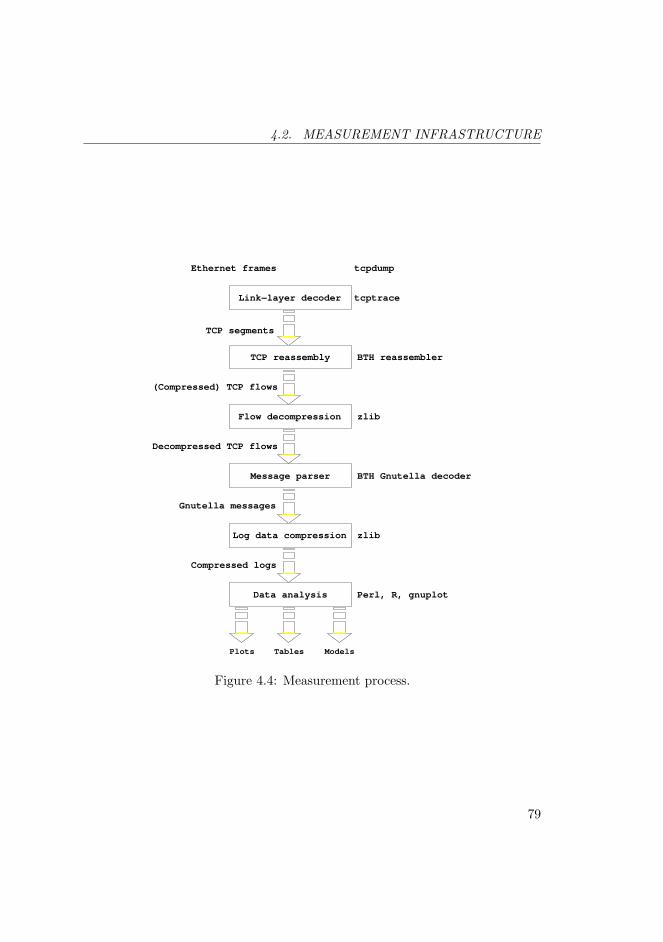
4.2. MEASUREMENT INFRASTRUCTURE
Plots Models
BTH reassembler
Perl, R, gnuplot
zlib
zlib
tcptrace
TCP segments
Tables
Link−layer decoder
TCP reassembly
Flow decompression
Message parser
Log data compression
Ethernet frames tcpdump
(Compressed) TCP flows
Decompressed TCP flows
Gnutella messages
Compressed logs
BTH Gnutella decoder .
Data analysis
Figure 4.4: Measurement process.
79

CHAPTER 4. GNUTELLA TRAFFIC MODELS
During the first stage of the measurement process, we use tcptrace to ex-tract TCP segments from the Ethernet frames.
The TCP segments are then sent to the next stage, whose task is to reassem-ble them to a flow of ordered bytes. The TCP reassembly module developedat BTH [104] builds on the TCP engine available in tcptrace and is similarto the one used by the FreeBSD TCP/IP stack [127]. The reassembly engineis capable of handling out-of-order segments as well as forward and backwardoverlapping between segments.
When a new Gnutella connection is found, the application reassembly mod-ule first waits for the handshake phase to begin. If the handshake fails, theconnection is marked invalid and it is eventually discarded by the memory man-ager.
If the handshake is successful, the application reassembly module scans thecapability lists sent by the nodes involved in the TCP connection. If the nodeshave agreed to compress the data, the connection is marked as compressed. Sub-sequent segments received from the TCP reassembly module for this connectionare first sent to the decompresser, before being appended to previous data thathas not been consumed yet.
The decompresser uses zlib’s inflate() function to decompress the dataavailable in the new segment [113]. Upon successful decompression the de-compressed data is appended to the data buffer.
Immediately after the handshake phase, the application reassembly moduleattempts to find the Gnutella message header of the first message. Using thepayload length field, it is able to discover the beginning of the next message.This is the only way to discover message boundaries in the Gnutella protocoland thus track application state changes [104]. Based on the message type fieldin the message header, the corresponding decoding function is called, whichoutputs a message record to the log file. The message records follow a specificformat required by the post-processing stage [104].
Since the logs can grow quite large, they can be processed through an op-tional stage of data compression. The compression is achieved by using theon-the-fly deflate compression offered by zlib. Additional data reduction canbe achieved if the user is willing to sacrifice some detail by aggregating dataover time.
80
4.3. METHODOLOGY FOR STATISTICAL MODELING
The data analysis module interprets the (optionally compressed) log dataand it is able to demultiplex it based on different types of constraints: messagetype, IP address, port number, etc. The data output format of this stage issuitable for input to numerical computation software such as MATLAB andstandard UNIX text processing software such as sed, awk and perl.
4.3 Methodology for Statistical Modeling
The measurement infrastructure described in the previous section was used tocollect Gnutella traffic crossing the BTH ultrapeer. By decoding the recordedtraffic data, flows were recreated at several layers in the TCP/IP stack. Theflows consist of discrete protocol data units: IP datagrams at the network layer,TCP segments at the transport layer, and finally, Gnutella messages at theapplication layer. The Gnutella messages are logically grouped in peer sessions.The time when the protocol data units reached the link layer was recordedtogether with their size. For peer sessions, the session duration was recorded aswell. Due to the complexity of the protocol we used a statistical approach [104,125] to describe the quantities of interest, which is similar to the methodologyintroduced by Paxson in [128].
Each quantity of interest is modeled by a random variable X that changes itsvalue whenever a new protocol data unit (or session) is considered. The actualvalues taken by X are denoted by the small letter x. The random variable X isassumed to have a theoretical cumulative distribution function (cdf) FX(x; θ).
Definition 4.1. The theoretical cdf FX(x; θ) of a random variable X is definedas
FX(x; θ) , P [X ≤ x], (4.1)
where , is the equality by definition operator, x is some value on the real lineand θ is a set of one or more parameters that control the distribution functione. g. , θ = {µ, σ} in the case of the normal distribution.
Definition 4.2. It is assumed that a cdf FX(x; θ) has a corresponding proba-bility density function (pdf) fX(x; θ) defined as
fX(x; θ) ,dFX(x; θ)
dx. (4.2)
81

CHAPTER 4. GNUTELLA TRAFFIC MODELS
The derivative must exist at all points of interest otherwise impulse functionsare required like in the case of discrete distributions [129].
It is often useful to observe how fast the cdf decays for large values of x.For that particular purpose it is better to use the complementary cumulativedistribution function (ccdf) function.
Corollary 4.1. Assuming a cdf function FX(x; θ), the corresponding ccdf func-tion is:
FX(x; θ) , 1− FX(x; θ) = P [X > x] (4.3)
For each quantity of interest, the set of values extracted from the recordedtraffic is considered to be a random sample from the population of the randomvariable X. The elements of the random sample are denoted by X1, X2, . . . , Xn
and the actual recorded values (data sample) by x1, x2, . . . , xn. The index n isthe number of available values from the measurement.
The modeling methodology employed in this chapter involves three phases:
i) identify a distribution family F (·) through exploratory data analysis (EDA),
ii) using the available data, estimate the parameter(s) θ of the distributionfrom the previous step. Denote the estimated parameter(s) by θ and theestimated distribution by FX(x; θ),
iii) quantify the quality of the fit.
4.3.1 Exploratory Data Analysis
The first step in the modeling methodology is to identify a distribution familyFX(x, θ). This is done through an EDA approach that combines graphs of thedata such as histograms and distribution plots and summary statistics e. g. ,mean, median and standard deviation [130, 131].
The histograms and distribution plots are the main EDA tools. Using them,the EDA user is aided in recognizing a family of distributions that provides goodmatch for the data. The summary statistics provide some quantitative supportin the selection of a distribution family.
82
4.3. METHODOLOGY FOR STATISTICAL MODELING
When unknown parameters of the distribution family are estimated, thecandidate distribution is fully specified. At that point the quality of the fit canbe assessed by formal numerical methods, as described in Section 4.3.3.
Summary Statistics
Five different types of statistics can be used to summarize a random sample:maximum, minimum, mean, median and standard deviation. All definitions inthis section assume a random sample X1, X2, . . . , Xn of length n > 1. Thecorresponding order statistics are X(1) ≤ X(2) ≤ · · · ≤ X(n).
Definition 4.3. The largest and smallest value of the random sample are de-noted by X(n) = max[X1, . . . , Xn] and X(1) = min[X1, . . . , Xn], respectively.The difference
(X(n) −X(1)
)defines the range of the data sample.
Definition 4.4. The sample mean X is defined as
µ = X =1n
n∑i=1
Xi (4.4)
X is an unbiased estimator of the first population moment, that is of theexpected value E[X]. For a symmetric distribution the actual value of X rep-resents the “center” of the data range. For a skewed distribution, the medianstatistic is a more appropriate representation of centricity.
Definition 4.5. If the sample size is odd, i. e. , n = 2k+ 1, the sample medianis the middle order statistic X(k+1). If the sample size is even, i. e. , n = 2k, thesample median is the average of the two middle order statistics
median =X(k) +X(k+1)
2(4.5)
Definition 4.6. The sample standard deviation is defined as
σ =
√√√√ 1n− 1
n∑i=1
(Xi −X)2 (4.6)
83
CHAPTER 4. GNUTELLA TRAFFIC MODELS
Histogram Plots
A histogram plot is a graph of tabulated frequencies for an univariate datasample x1, x2, . . . , xn of length n. If the frequencies are normalized such thatthe area below the histogram is equal to one, then the histogram can be viewedas a rough estimate of the probability density function.
In order to build a histogram one must begin by dividing the range r of thedata into a number of m contiguous bins. Each bin i covers a portion of length3
L of the data range. The boundaries of the bin i are denoted by bi and bi+1.Next, the data values are sorted and placed into bins that correspond to theirvalue. The number of entries in each bin represents the frequency fi of the bini. To obtain the probability of each bin, the frequencies fi are normalized suchthat the probability pi of bin i is:
pi =fin
(4.7)
It follows that the probability of the bin i is [132]
pi ≈ P [bi < X ≤ bi+1] =
bi+1∫bi
fX(x) dx = fX(y)L for some y ∈ (bi, bi+1)
(4.8)An important question is how to choose the bin length L or equivalently the
number of bins m. Histograms using bins that are too wide fail to reveal specificcharacteristics of the data such as multi-modality (i. e. , mixture of distributions)or impulses at the origin. These are called undersmoothed histograms. Onthe other hand, if the bin width is too small the histogram is likely have ajagged appearance that could complicate the identification of the underlyingdistribution or even worse, it may present false evidence of multi-modality. Inthis case the histogram is called an oversmoothed histogram. Research intooptimal bin width has lead to the thumb rules [133, 134] presented in Table 4.1.
The terms σ, q.75 and q.25 denote the estimated standard deviation, the0.75-quantile, and the 0.25-quantile, respectively. Figure 4.5 shows an exampleof how the histogram of specific data can look like when the bin width is toolarge, too small and when it is chosen by using the Friedman-Diaconis method.
3Bins of equal length are assumed.
84
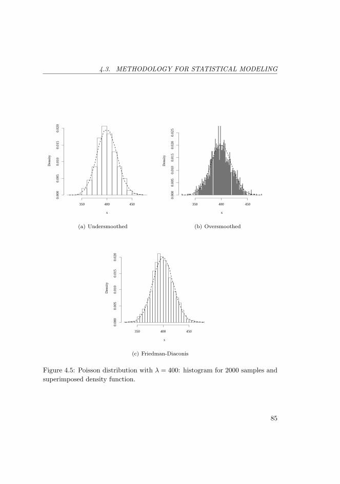
4.3. METHODOLOGY FOR STATISTICAL MODELING
x
Den
sity
350 400 450
0.00
00.
005
0.01
00.
015
0.02
0
(a) Undersmoothed
x
Den
sity
350 400 450
0.00
00.
005
0.01
00.
015
0.02
00.
025
(b) Oversmoothed
x
Den
sity
350 400 450
0.00
00.
005
0.01
00.
015
0.02
0
(c) Friedman-Diaconis
Figure 4.5: Poisson distribution with λ = 400: histogram for 2000 samples andsuperimposed density function.
85

CHAPTER 4. GNUTELLA TRAFFIC MODELS
Name Bin width
Sturges’ formula L = r/(1 + log2 n)Scott’s rule L = 3.49σ n−1/3
Friedman-Diaconis L = 2 (q.75 − q.25)n−1/3
Table 4.1: Various rules for choosing histogram bin width.
The rules in Table 4.1 work well in many situations. Unfortunately, none ofthem is a panacea. In fact, for some distributions it is necessary to manuallyadjust the number of bins in order to obtain a smooth histogram [133].
Edf Plots
The empirical distribution function (edf) Fn(x)4 of a random sample is an ap-proximated representation of the true cdf for the population from which thesample is drawn.
Definition 4.7. Given a random sample X1, X2, ..., Xn of length n drawn froma distribution FX(x), denote the corresponding order statistics byX(1) ≤ X(2) ≤· · · ≤ X(n). Then, Fn(x) is defined as
Fn(x) ,
0 x < X(1)
i
nX(i) ≤ x < X(i+1)
1 X(n) ≤ x.
(4.9)
For large samples, Fn(x) converges uniformly to the population FX(x) forall x-values [130].
Corollary 4.2. Assuming an edf Fn(x), then
Fn = 1−Fn (4.10)
is the corresponding complementary empirical distribution function (cedf).4Normally, the notation Fn(x) is used to denote an edf. However, this notation could
conflict here with the notation used for a cdf and it is therefore written using a calligraphic
letter: Fn(x).
86
4.3. METHODOLOGY FOR STATISTICAL MODELING
The histogram, the edf and the cedf are complementary views of the sam-ple distribution. The terminology used for ccdf and cedf plots is to denote as“body” the values of Fn(x) for x ≤ ξ and as “tail” the values of Fn(x) forx > ξ. The point ξ on the x-axis is in general dictated by the type of dataanalysis performed, but tends to be selected such that for large x-values thecorresponding ccdf values are very small, but non-negligible. The decay of thetail allows us to assign the empirical distribution to a particular distributionclass.
The subexponential or long-tailed class contains distributions that decayslower than the exponential distributions. The class of heavy-tailed distribu-tions is a more restrictive subclass, since they require infinite variance. A ran-dom variable X has a heavy-tailed distribution if:
limx→∞
FX(x) = limx→∞
P [X > x] = cx−α, 0 < α < 2, c > 0 (4.11)
When the tail index α is 0 < α < 1, the heavy-tailed distribution has infinitemean in addition to infinite variance. This is in contrast with the larger classof long-tailed distributions with finite moments [135].
The Pareto distribution is a good example of heavy-tailed distribution. Thelognormal and Weibull distributions are subexponential, but not heavy-tailed.In particular, the Weibull distribution has finite variance [135]. Paxson andFloyd provide proof that the lognormal distribution is not heavy-tailed [136].Gaussian or Gamma and exponential distributions are called light-tailed dis-tributions and are not part of the subexponential class [135]. For light-taileddistributions the ccdf values in the tail are negligible.
4.3.2 Parameter Estimation
Parameter estimation is the second phase of the modeling methodology usedin this thesis. It is assumed that a distribution family FX(x; θ) with a set ofunknown parameters θ has been identified as described in Section 4.3.1. The goalis to estimate the parameters by using point estimators Θ = E(X1, X2, . . . , Xn),where E is a function of the random sample. Point estimates θ are obtained byreplacing the random variables in Θ with observed values.
The optimality of point estimators is decided by concepts such as bias, ef-ficiency, consistency and sufficiency. An unbiased estimator is one for which
87
CHAPTER 4. GNUTELLA TRAFFIC MODELS
E[Θ] = θ [137]. Furthermore, an estimator Θ1 is more efficient than an estima-tor Θ2 if Var
[Θ1
]< Var
[Θ2
]. By consistency it is meant that a sequence of
estimators converges towards the “true” value of the parameter. Sufficiency isconcerned with the amount of information intrinsic to the sample, which is lostor kept when a particular estimator is used [137, 138]. These are large topicsoutside the scope of this thesis. It is sufficient to mention that maximum like-lihood estimators are in general at least as good as other estimators for largesample sizes. However, the equations that appear in the course of using themethod can be non-linear and difficult to solve. In this case numerical solu-tions are required [137–139]. Similar problems appear when the method is usedwith mixture distributions. Therefore, a secondary method, denoted minimum-absolute-error, is introduced as well. In addition for providing point estimates,the minimum-absolute-error method is used as goodness-of-fit measure, as de-scribed in Section 4.3.3.
Maximum Likelihood Method
The maximum likelihood (ML) method is based on the concept of likelihoodfunction, which is defined as the joint pdf of a number of random variables [138].
Definition 4.8. Given n random variables X1, X2, . . . , Xn drawn from a dis-tribution FX(x; θ), and the corresponding observed values x1, x2, . . . , xn, thelikelihood function L(θ) is defined as
L(θ) , fX1,X2,...,Xn(x1, x2, . . . , xn; θ) (4.12)
which is the joint distribution of X1, X2, . . . , Xn.
Corollary 4.3. For a random sample X1, X2, . . . , Xn with common distributionFX(x; θ)
L(θ) =n∏i=1
fX(xi; θ), (4.13)
which follows from the definition of a random sample.
Intuitively, the likelihood function L(θ) for a random sample drawn from adiscrete pdf is the probability that the random sample will assume the observedvalues [139]:
88
4.3. METHODOLOGY FOR STATISTICAL MODELING
L(θ) = P [X1 = x1; θ]P [X2 = x2; θ] . . . P [Xn = xn; θ] (4.14)
It becomes evident that the optimal θ is the value that maximizes L(θ).This idea can be applied in a similar manner to random samples from a con-tinuous pdf. Assuming certain regularity conditions [138], the solution Θ =E(X1, X2, . . . , Xn) to the equation
dL(θ)dθ
= 0 (4.15)
is the ML estimator. When the random variables are replaced with the actualobserved values, one obtains the ML estimate θ = E(x1, x2, . . . , xn). Sometimesit is easier to solve the equation
d ln [L(θ)]dθ
= 0 (4.16)
instead of Equation 4.15 [138].
Minimum-Absolute-Error Method
The minimum-absolute-error method seeks to find an estimate θ that minimizesthe difference between the edf, Fn(x), and the estimated cdf, FX(x; θ), over allx.
Definition 4.9. For a data sample x1, x2, . . . , xn, the difference between Fn(x)and FX(x; θ) is defined as the cumulative absolute error ε(θ), such that
ε(θ) ,n∑i=1
∣∣∣FX(xi; θ)−Fn(xi)∣∣∣ (4.17)
The estimate θ is the θ-value that minimizes ε(θ). .
Since this method relies on the edf, θ cannot be solved analytically. Numer-ical algorithms to obtain solutions for it are discussed in Section 4.3.5.
89
CHAPTER 4. GNUTELLA TRAFFIC MODELS
4.3.3 Fitness Assessment
After a probability distribution has been fitted to the data as described in theprevious section, the next step is to estimate the quality of the fit. A varietyof goodness-of-fit tests can be used for this purpose, e. g. , the χ2, Kolmogorov-Smirnov and Anderson-Darling tests. Their common denominator is the test ofthe null hypothesis:
H0 : The random sample X1 . . . Xn is drawn from
the distribution F (x, θ)
Unfortunately, these tests tend to erroneously reject the null hypothesis whenthe number of samples is large (Type 1 error) [132, 140, 141], which is the casefor our data. Therefore, a different approach is used in which the hypothesistest is avoided.
A goodness-of-fit measure called error-percentage measure (E%) was intro-duced in [126] and used later in [125, 142]. The method is based on the proba-bility integral transform (PIT).
Definition 4.10 (Probability integral transform). Given a continuous randomvariable R with cdf FX(x) and P [Y ≤ y] d= U [0, 1], the transformation
FX(R) = P [X ≤ R] = Y (4.18)
is called the probability integral transform [132, 138]. The symbol d= denotesequality in distribution and U [0, 1] denotes the uniform distribution betweenzero and one.
The algorithm to compute E% is shown in Algorithm 7. If the distribu-tion F is a perfect fit, then the PIT transforms the random sample to an uni-form distribution, U [0, 1]. However, since perfect fittings rarely occur in reality,the transformed distribution, U , is an approximate of the uniform distribution.The discrepancies between U and U are computed and their average is normal-
90

4.3. METHODOLOGY FOR STATISTICAL MODELING
ized [125] to the highest possible error Emax for the distribution U [0, 1] where,
Emax =
1∫0
sup {U(x), 1− U(x)} dx
=
1/2∫0
[1− U(x)] dx+
1∫1/2
U(x) dx =34
(4.19)
Algorithm 7 Calculate error percentage.
Fit a distribution FX(x; θ) to the random sample X1, X2, . . . , Xn
Obtain the order statistics X(1), X(2), . . . , X(n)
Transform the random sample with PIT: Ui = FX(X(i); θ), i = 1, . . . , n
E% = 100
∑ni=1
∣∣∣Ui − Ui∣∣∣nEmax
, where Ui =i
n
d= U [0, 1]
return E%
Figures 4.6(a)–4.6(b) provide additional visual clues on how the E%-methodworks. Figure 4.6(a) shows a hypothetical edf for a random sample transformedwith the PIT, i. e. , the diagonal straight line. The blue shaded area representsthe error (discrepancy) when the edf is compared to the ideal U [0, 1] distribution.The size of that area is the E% score. The size of the shaded area in Figure 4.6(b)is the maximum error Emax that can occur when the PIT is applied to a randomsample. This is the value that is used to normalize the E% score.
E% is expressed in the form of a percentage. The criteria used here toaccept a candidate distribution is that E% < 6. We call this value the acceptederror percentage. The accepted error percentage was decided experimentally byobserving that most distributions that provide a visually acceptable fit in bothbody and tail have E% < 6. Table 4.3.3 presents a mapping between variousE% ranges and qualitative statements about the fit.
The main disadvantage of the E%-method is that it cannot be used withdiscrete distributions. The reason is that when the PIT method is appliedto a discontinuous distribution, the transformed variable is not uniformly dis-tributed [143].
91

CHAPTER 4. GNUTELLA TRAFFIC MODELS
��������������������������������������������������������������������������������������������������������������������������������������������������������������������������������������������������������������������������������������������������������������������������������������������������������������������������������������������������������������������������������������������������������������������������������������������������������������������������������������������������������������������������������������������������������������������������������������������������
��������������������������������������������������������������������������������������������������������������������������������������������������������������������������������������������������������������������������������������������������������������������������������������������������������������������������������������������������������������������������������������������������������������������������������������������������������������������������������������������������������������������������������������������������������������������������������������������������
1
1
x0
U(x)
(a) Error in transformed random sample.
0 1
1
U(x)
x
(b) Maximum error for a PIT transforma-
tion.
Figure 4.6: Probability integral transform (PIT).
Range 0 ≤ E% < 2 2 ≤ E% < 4 4 ≤ E% < 6 E% ≥ 6
Quality Excellent Good Acceptable Unacceptable
Table 4.2: Quality-of-fit mapping.
4.3.4 Finite Mixture Distributions
Sometimes a single cdf cannot accurately describe the distribution of the randomvariables of interest e. g. , the E%-method yields an unacceptable score. A moreaccurate model may be constructed by using a mixture of two distributionsor more. In the case of a mixture of two distributions one component of themixture accounts for the main body of the empirical distribution and a differentone describes the behavior in the tail. In the case of more than two components,each cdf accounts for specific modality found in the data. The crux of theproblem becomes to find a way to combine the two distributions in a meaningfulway. The method used here is based on finite mixture distributions as describedin [144]
A mixture distribution FX(x) with n components has the following distri-
92

4.3. METHODOLOGY FOR STATISTICAL MODELING
bution function:
FX(x) =n∑i=1
πiGi(x) π1 + π2 + · · ·+ πn = 1 (4.20)
where Gi(x) is the ith distribution in the mixture and each πi is a constantcalled mixing weight. The mixing weight πi is selected such that 0 < πi < 1and it decides how much each component is allowed to influence the distributionFX(x).
The first step in building a mixture distribution with two components is toidentify a distribution familyG1(·) that matches the body of the data, preferablythe tail as well. This is done by using the EDA approach, as explained inSection 4.3.1. The parameters of the distribution are estimated, yielding aspecific distribution function G1(x; θ1). G1(x; θ1) is then visually comparedto the true distribution to asses the fit in the tail. If the fit appears good,then the goodness-of-fit measure E% is computed as explained in Section 4.3.3.Otherwise, it is necessary to find the cutoff point xc and the corresponding cutoffquantile qc, where G1 diverges from the true distribution. The probability massbetween qc and 1 is used to identify the distribution family G2(·) that matchesthe tail. The parameters of the new distribution must be estimated as well,yielding θ2. Then, a finite mixture distribution
F (x; θ) = πG1(x; θ1) + (1− π)G2(x; θ2) (4.21)
is assembled, where π = qc. Since the single distributions, G1 and G2, are nowcombined in a finite mixture, the parameters θ1 and θ2 must be recomputed5.Their original values may be used as a starting point. An optimal value for πmust be computed as well. The parameter set θ in F (x; θ) is the set containingthe parameters for both distributions and π, i. e. , θ = {θ1, θ2, π}. Numeri-cal methods for computing the set of optimal parameters θ are presented inSection 4.3.6.
It is often the case that a mixture distribution (in particular one with onlytwo components) still cannot describe the data accurately enough. This maybe further improved by increasing the number of components in the mixturedistribution at the expense of an increase in the number of parameters. However,a different approach was used here.
5Recall that G1 was estimated using the entire probability mass.
93

CHAPTER 4. GNUTELLA TRAFFIC MODELS
Typically, the major discrepancies between the estimated distribution andthe true one appear either in the body or in the tail. If, for example, the dis-crepancies appear in the tail, one can attempt to improve the model accuracyby adjusting the values of the distribution parameters. However, our experi-ence was that this is likely to decrease the accuracy of the model in the body.Similarly, attempts to increase the accuracy in the body may lead to (higher)discrepancies in the tail. Thus, a trade-off is required, accuracy in the body ver-sus accuracy in the tail [104]. Accordingly, a decision must be taken on whichpart of the distribution (body or tail) is more important to model accurately.
For example, in the case of transfer rates the tail of the distribution modelshigh rates of traffic (bursts) that occur rarely. On the other hand, the bodyof the distribution models the “average” size of transfer rates. For message orpacket size the body accounts for small packets or messages and the tail for largeones. In the case of interarrival and interdeparture times the body accounts for“dense” traffic and the tail for “sparse” traffic. In our models, when a trade-offwas required, we favored to accurately model bursty, dense traffic with largepackets (messages).
4.3.5 Methodology Review
The goal of this section is to present a formal process for the modeling method-ology discussed in the previous sections. The process assumes that the variableof interest has been measured (sampled) n times. The values x1, x2, . . . , xnresulting from the n measurements are assumed to be the result of a randomsample X1, X2, . . . , Xn. The complete process for building the statistical modelsis presented in Algorithm 8 [104].
Step 14–15 in Algorithm 8 may be confusing since no criteria has been pro-vided on how to decide to either select a different quantile or to start over. Tosolve this, the quantile was changed in increments of 0.05 to either sides of theoriginal value. If this did not result in any improvement, the decision was tostart over.
94

4.3. METHODOLOGY FOR STATISTICAL MODELING
Algorithm 8 Methodology for statistical modeling.1: Use EDA visual tools, i. e. , histogram, edf and cedf plots, to explore the
data. The summary statistics provide hints about range, skewness andspread
2: Select a distribution family G1, which appears to provide a good fit3: Estimate the unknown parameters θ1 using ML estimation to obtain a can-
didate distribution G1X(x, θ1)4: Compare the plots of g1X(x; θ1), G1X(x; θ1), and G1X(x; θ1) to the his-
togram, edf, and cedf plots obtained in Step 15: if high visual discrepancy then6: Go back to Step 17: end if8: Compute E% for G1X(x; θ1) using x1, x2, . . . , xn9: if E% < 6 then return E% and G1X(x, θ1)
10: end if11: Identify the cutoff quantile qc12: Fit a distribution G2(·) to the probability mass (1−qc) as outlined in Step 1–
813: if E% > 6 then14: Either go back to Step 11 and select a different quantile qc or,15: Go back to Step 1. This is equivalent to starting over. Try using a
different distribution family G1(·)16: end if17: Assemble the mixture distribution F (·) = πG1(·) + (1− π)G2(·)18: Estimate the unknown parameters θ = {θ1, θ2, π} using E% method. Use
the estimated values from previous steps as initial values19: if E% < 6 then return E% and FX(x; θ)20: else21: Go back to step 122: end if
95

CHAPTER 4. GNUTELLA TRAFFIC MODELS
4.3.6 Numerical Software and Methods
The process presented here was implemented by using the statistical softwarepackage R [145]. R is an interpreted computer language with syntax similar to S
and S-PLUS [133]. The software package contains in addition to the language, arun-time environment with graphics, a debugger and a large library of functions.
As mentioned in Section 4.3.4, the E%-method relies on numerical optimiza-tion for finding a minimum. ML estimation requires also numerical optimiza-tion in many cases where no closed form ML estimators exist. The R-functionsoptimize() and optim() have been used for numerical optimization.
The function optimize() performs optimization in one dimension. Theunderlying algorithm is a combination of golden section search and successiveparabolic interpolation [93, 145]
General purpose multi-dimensional optimization is performed by the optim()function. The function has support for several optimization algorithms. Thedefault algorithm, Nelder-Mead [93, 146, 147], is primarily used. The algorithmdoes not require any derivatives, and it is quite stable although not very efficientin terms of number of iterations.
When the Nelder-Mead algorithm fails to converge to a solution, the L-BFGS-B [148] algorithm is used instead. This algorithm requires a lower andan upper bound for each variable. The thumb rule used to provide the boundsis to allow variables with initial values m0 ≥ 1 a range of 0.2m0 between theupper and lower bound. For variables with initial values m0 < 1 the rangebetween bounds was 0.1m0. This thumb rule was designed empirically and itis by no means optimal in any way. In fact, from our experience, the boundsoften needed additional adjustment to obtain convergence.
4.4 Characteristics and Statistical Models
In order to keep the mathematical formulas brief we use the following conven-tions. Cdfs are denoted by capital letters and pdfs by lower case letters, asshown in Table 4.3. The parameters are as follows: µ and σ are related tothe distribution mean and standard deviation, while α, β and κ are the shape,scale and location parameters. For the uniform distribution, a and b are the
96

4.4. CHARACTERISTICS AND STATISTICAL MODELS
Uniform uX(x; a, b) UX(x; a, b)Poisson poX(x;µ) POX(x;µ)Exponential expX(x;µ) EXPX(x;µ)Normal (Gaussian) nX(x;µ, σ) NX(x;µ, σ)Log-normal lnX(x;µ, σ) LNX(x;µ, σ)Generalized Pareto paX(x;α, κ, β) PAX(x;α, κ, β)
Table 4.3: Model notation.
lower and upper boundary, respectively, of the range of x-values for which thedistribution is valid. In particular, the parameter a is equivalent to a locationparameter, while (b−a) is equivalent to a scale parameter [132]. All logarithmicedf plots use log10-transformations for both axes.
The generalized Pareto distribution [149] and the corresponding densityfunction are defined as
FX(x;α, κ, β) = 1−[1 +
α(x− κ)β
]− 1α
(4.22)
fX(x;α, κ, β) =1β
[1 +
α(x− κ)β
]− 1α−1
(4.23)
where α 6= 0 is the shape parameter, κ ≤ x is the location parameter, and β > 0is the scale parameter.
4.4.1 Ultrapeer Settings and Packet-Trace Statistics
The results reported here were obtained from an 11-days long link-layer packettrace collected from the BTH network with the methods described in Section 4.2.The gtk-gnutella servent at BTH was configured to run as ultrapeer and tomaintain 32–40 connections to other ultrapeers and approximately 100 connec-tions to leaf nodes. The number of connections is a vendor preconfigured value,which is close to the suggested values [107, 108]. Although gtk-gnutella cancommunicate using the User Datagram Protocol (UDP), this functionality wasturned off. Consequently, the ultrapeer used only TCP for its traffic. No otherapplications, with the exception of a Secure Shell (SSH) daemon, were running
97
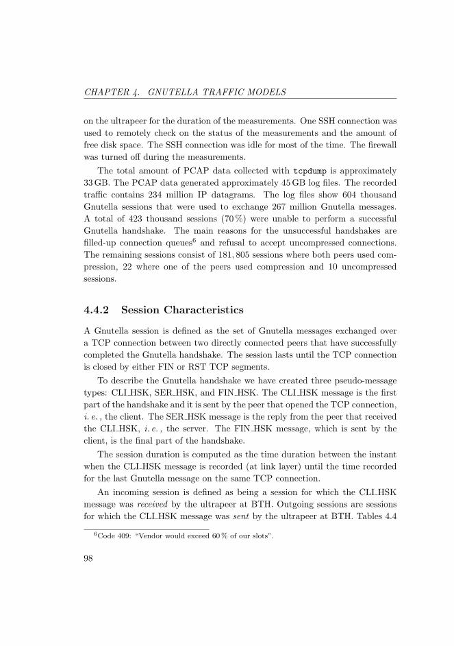
CHAPTER 4. GNUTELLA TRAFFIC MODELS
on the ultrapeer for the duration of the measurements. One SSH connection wasused to remotely check on the status of the measurements and the amount offree disk space. The SSH connection was idle for most of the time. The firewallwas turned off during the measurements.
The total amount of PCAP data collected with tcpdump is approximately33 GB. The PCAP data generated approximately 45 GB log files. The recordedtraffic contains 234 million IP datagrams. The log files show 604 thousandGnutella sessions that were used to exchange 267 million Gnutella messages.A total of 423 thousand sessions (70 %) were unable to perform a successfulGnutella handshake. The main reasons for the unsuccessful handshakes arefilled-up connection queues6 and refusal to accept uncompressed connections.The remaining sessions consist of 181, 805 sessions where both peers used com-pression, 22 where one of the peers used compression and 10 uncompressedsessions.
4.4.2 Session Characteristics
A Gnutella session is defined as the set of Gnutella messages exchanged overa TCP connection between two directly connected peers that have successfullycompleted the Gnutella handshake. The session lasts until the TCP connectionis closed by either FIN or RST TCP segments.
To describe the Gnutella handshake we have created three pseudo-messagetypes: CLI HSK, SER HSK, and FIN HSK. The CLI HSK message is the firstpart of the handshake and it is sent by the peer that opened the TCP connection,i. e. , the client. The SER HSK message is the reply from the peer that receivedthe CLI HSK, i. e. , the server. The FIN HSK message, which is sent by theclient, is the final part of the handshake.
The session duration is computed as the time duration between the instantwhen the CLI HSK message is recorded (at link layer) until the time recordedfor the last Gnutella message on the same TCP connection.
An incoming session is defined as being a session for which the CLI HSKmessage was received by the ultrapeer at BTH. Outgoing sessions are sessionsfor which the CLI HSK message was sent by the ultrapeer at BTH. Tables 4.4
6Code 409: “Vendor would exceed 60 % of our slots”.
98
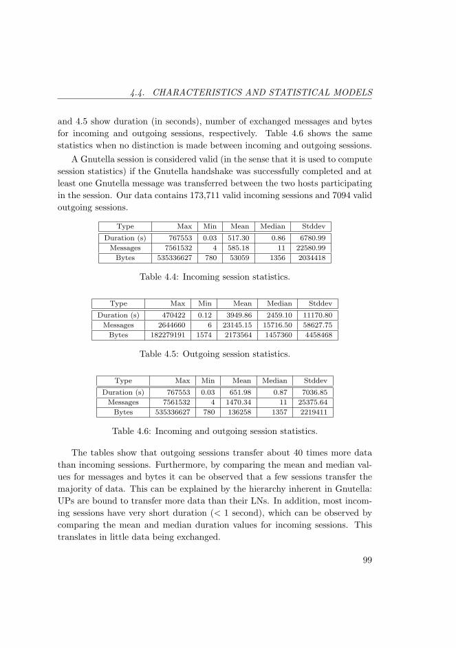
4.4. CHARACTERISTICS AND STATISTICAL MODELS
and 4.5 show duration (in seconds), number of exchanged messages and bytesfor incoming and outgoing sessions, respectively. Table 4.6 shows the samestatistics when no distinction is made between incoming and outgoing sessions.
A Gnutella session is considered valid (in the sense that it is used to computesession statistics) if the Gnutella handshake was successfully completed and atleast one Gnutella message was transferred between the two hosts participatingin the session. Our data contains 173,711 valid incoming sessions and 7094 validoutgoing sessions.
Type Max Min Mean Median Stddev
Duration (s) 767553 0.03 517.30 0.86 6780.99
Messages 7561532 4 585.18 11 22580.99
Bytes 535336627 780 53059 1356 2034418
Table 4.4: Incoming session statistics.
Type Max Min Mean Median Stddev
Duration (s) 470422 0.12 3949.86 2459.10 11170.80
Messages 2644660 6 23145.15 15716.50 58627.75
Bytes 182279191 1574 2173564 1457360 4458468
Table 4.5: Outgoing session statistics.
Type Max Min Mean Median Stddev
Duration (s) 767553 0.03 651.98 0.87 7036.85
Messages 7561532 4 1470.34 11 25375.64
Bytes 535336627 780 136258 1357 2219411
Table 4.6: Incoming and outgoing session statistics.
The tables show that outgoing sessions transfer about 40 times more datathan incoming sessions. Furthermore, by comparing the mean and median val-ues for messages and bytes it can be observed that a few sessions transfer themajority of data. This can be explained by the hierarchy inherent in Gnutella:UPs are bound to transfer more data than their LNs. In addition, most incom-ing sessions have very short duration (< 1 second), which can be observed bycomparing the mean and median duration values for incoming sessions. Thistranslates in little data being exchanged.
99

CHAPTER 4. GNUTELLA TRAFFIC MODELS
These observations confirm earlier results reported in [40, 41, 150]. Followingthe taxonomy used in [41, 151], we observe that, although we analyze onlysignaling traffic without considering data transfers, the sessions can be dividedinto “mice” (i. e. , sessions carrying small amounts of data), and “elephants”(i. e. , sessions responsible for large volumes of traffic).
The same type of heterogeneity appears when we consider session duration.We observe both “dragonflies”, which are very short sessions and “tortoises”,which are sessions with very long duration.
4.4.3 Session Interarrival and Interdeparture Times
The statistics and models for session interarrival and interdeparture times areshown in Table 4.7 and Table 4.8. It is observed that interarrival times can bemodeled by the lognormal distribution, which is subexponential. In contrast,session interdeparture times require a mixture distribution with a heavy-tailedcomponent (Pareto distribution) to provide an acceptable fit.
A possible explanation for the appearance of the heavy-tailed component isgiven by the connection cap described in Section 4.4.1. When a Gnutella peerreaches the preset number of connections it does not attempt to establish moreconnections until existing connections are terminated. This leads to large sessioninterdeparture times that have a non-negligible probability of occurrence.
The absence of the heavy-tailed component from the session interarrivaltimes distribution can be explained as follows. We noticed that many of theshort duration (< 1 second) incoming sessions presented in Section 4.4.2 transferone BYE message and are then terminated. This behavior cannot be traced toany of the Gnutella specifications. We assume that the behavior is due to thegtk-gnutella implementation, but further study is required to confirm. Itappears that gtk-gnutella discovers that the connection cap is reached afterthe handshake is completed. Only then it sends the BYE message to terminatethe connection. Normally, this connection should have been aborted duringhandshake. Nonetheless, since these sessions are considered valid according toour criteria, the session interarrival times are shorter and we can model themwithout introducing a heavy-tailed component.
An interesting characteristic was observed when all session interarrival times
100
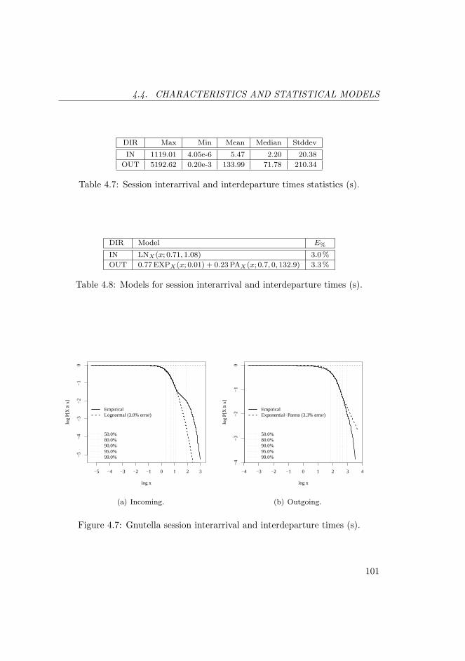
4.4. CHARACTERISTICS AND STATISTICAL MODELS
DIR Max Min Mean Median Stddev
IN 1119.01 4.05e-6 5.47 2.20 20.38
OUT 5192.62 0.20e-3 133.99 71.78 210.34
Table 4.7: Session interarrival and interdeparture times statistics (s).
DIR Model E%
IN LNX(x; 0.71, 1.08) 3.0 %
OUT 0.77 EXPX(x; 0.01) + 0.23 PAX(x; 0.7, 0, 132.9) 3.3 %
Table 4.8: Models for session interarrival and interdeparture times (s).
log x
log
P[X
≥x]
−5
−4
−3
−2
−1
0
−5 −4 −3 −2 −1 0 1 2 3
50.0%80.0%90.0%95.0%99.0%
EmpiricalLognormal (3.0% error)
(a) Incoming.
log x
log
P[X
≥x]
−4
−3
−2
−1
0
−4 −3 −2 −1 0 1 2 3 4
50.0%80.0%90.0%95.0%99.0%
EmpiricalExponential−Pareto (3.3% error)
(b) Outgoing.
Figure 4.7: Gnutella session interarrival and interdeparture times (s).
101

CHAPTER 4. GNUTELLA TRAFFIC MODELS
Statistic Model E%
Interarrival times (s) EXPX(x; 0.58) 1.7 %
Rate (sessions/s) POX(x; 0.58) N/A
Table 4.9: Gnutella (valid and invalid) session interarrival times.
log x
log
P[X
≥x]
−5
−4
−3
−2
−1
0
−6 −5 −4 −3 −2 −1 0 1
50.0%80.0%90.0%95.0%99.0%
EmpiricalExponential (1.7% error)
(a) Interarrival times (s).
0 2 4 6 8 10
0.0
0.1
0.2
0.3
0.4
x
P[X
≥x]
50.0%80.0%90.0%95.0%99.0%
EmpiricalPoisson
(b) Incoming session rate (sessions/s).
Figure 4.8: Gnutella (valid and invalid) session interarrival times and incomingsession rate.
were considered, that is, even those for invalid sessions. This is equivalent tointerarrival times for incoming requests to open a session (incoming CLI HSKmessages). It turns out that the set of all interarrival times is exponentiallydistributed with parameter λ = 0.58, as shown in Figure 4.8(a) and Table 4.9.The session arrival rate was analyzed to verify that this is not a measurementerror. It is well-known that exponentially distributed interarrival times implya Poisson arrival rate [129]. As it can be observed in Figure 4.8(b), a Pois-son distribution POX(x; 0.58) fits well, at least visually. Unfortunately, no E%
measure can be provided since the method does not work with discrete distribu-tions. However, the edf should leave little doubt that the data is indeed Poissondistributed. The edf is plotted without log-scaled axes, since most of the data,99.9 % of the probability mass, is clustered around the values 0, 1, . . . , 4.
102
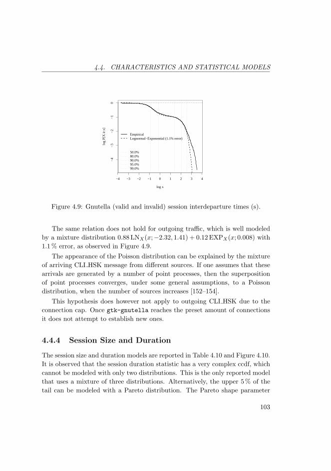
4.4. CHARACTERISTICS AND STATISTICAL MODELS
log x
log
P[X
≥x]
−4
−3
−2
−1
0
−4 −3 −2 −1 0 1 2 3 4
50.0%80.0%90.0%95.0%99.0%
EmpiricalLognormal−Exponential (1.1% error)
Figure 4.9: Gnutella (valid and invalid) session interdeparture times (s).
The same relation does not hold for outgoing traffic, which is well modeledby a mixture distribution 0.88 LNX(x;−2.32, 1.41) + 0.12 EXPX(x; 0.008) with1.1 % error, as observed in Figure 4.9.
The appearance of the Poisson distribution can be explained by the mixtureof arriving CLI HSK message from different sources. If one assumes that thesearrivals are generated by a number of point processes, then the superpositionof point processes converges, under some general assumptions, to a Poissondistribution, when the number of sources increases [152–154].
This hypothesis does however not apply to outgoing CLI HSK due to theconnection cap. Once gtk-gnutella reaches the preset amount of connectionsit does not attempt to establish new ones.
4.4.4 Session Size and Duration
The session size and duration models are reported in Table 4.10 and Figure 4.10.It is observed that the session duration statistic has a very complex ccdf, whichcannot be modeled with only two distributions. This is the only reported modelthat uses a mixture of three distributions. Alternatively, the upper 5 % of thetail can be modeled with a Pareto distribution. The Pareto shape parameter
103
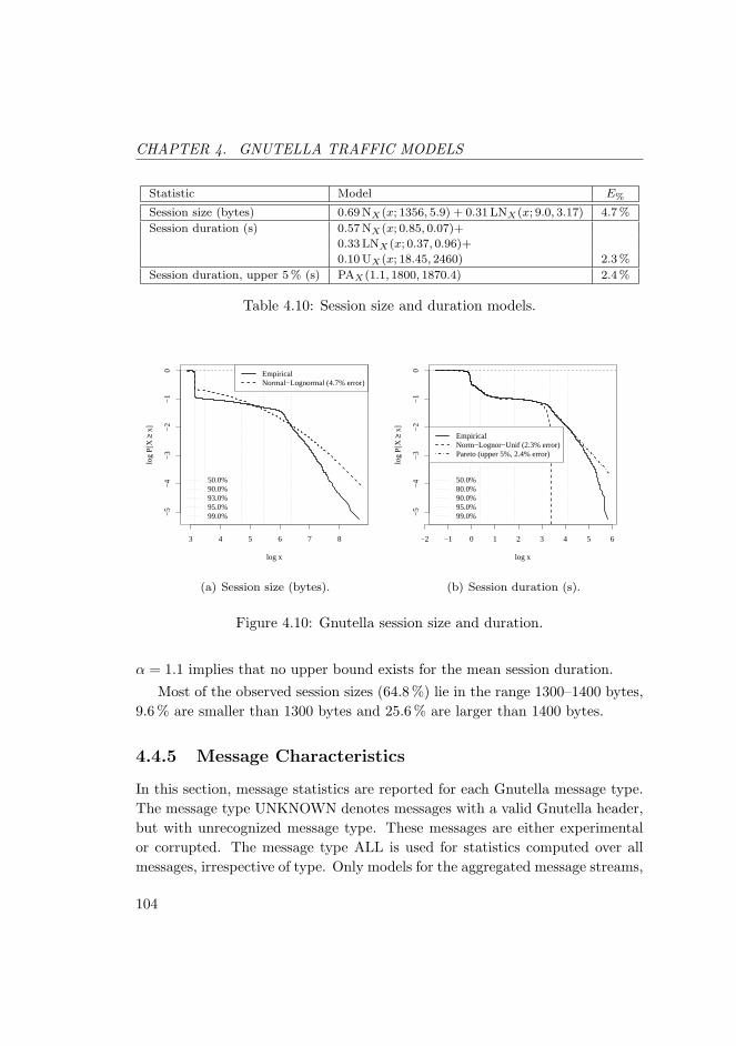
CHAPTER 4. GNUTELLA TRAFFIC MODELS
Statistic Model E%
Session size (bytes) 0.69 NX(x; 1356, 5.9) + 0.31 LNX(x; 9.0, 3.17) 4.7 %
Session duration (s) 0.57 NX(x; 0.85, 0.07)+
0.33 LNX(x; 0.37, 0.96)+
0.10 UX(x; 18.45, 2460) 2.3 %
Session duration, upper 5 % (s) PAX(1.1, 1800, 1870.4) 2.4 %
Table 4.10: Session size and duration models.
log x
log
P[X
≥x]
−5
−4
−3
−2
−1
0
3 4 5 6 7 8
50.0%90.0%93.0%95.0%99.0%
EmpiricalNormal−Lognormal (4.7% error)
(a) Session size (bytes).
log x
log
P[X
≥x]
−5
−4
−3
−2
−1
0
−2 −1 0 1 2 3 4 5 6
50.0%80.0%90.0%95.0%99.0%
EmpiricalNorm−Lognor−Unif (2.3% error)Pareto (upper 5%, 2.4% error)
(b) Session duration (s).
Figure 4.10: Gnutella session size and duration.
α = 1.1 implies that no upper bound exists for the mean session duration.Most of the observed session sizes (64.8 %) lie in the range 1300–1400 bytes,
9.6 % are smaller than 1300 bytes and 25.6 % are larger than 1400 bytes.
4.4.5 Message Characteristics
In this section, message statistics are reported for each Gnutella message type.The message type UNKNOWN denotes messages with a valid Gnutella header,but with unrecognized message type. These messages are either experimentalor corrupted. The message type ALL is used for statistics computed over allmessages, irrespective of type. Only models for the aggregated message streams,
104

4.4. CHARACTERISTICS AND STATISTICAL MODELS
i. e. , message type ALL are presented.Table 4.11 shows interarrival times for messages received by the BTH ultra-
peer and Table 4.12 shows interdeparture times for messages sent by the BTHultrapeer. Although the PCAP timestamps have microsecond resolution [103],the times presented here have only 100µs precision. This is due to memorylimitations in the post-processing software.
Summing over the number of samples for each message type does not addup to the value shown in the number of samples for message type ALL. Thisis caused by the analysis software, which ignores messages that generate nega-tive interarrival and interdeparture times. Negative times appear because theapplication flow reassembly handles several (typically more than a hundred)connections at the same time. On each connection the timestamp for arrivingpackets is monotonically increasing. However, the interarrival and interdepar-ture statistics are computed across all connections. To ensure monotonicallyincreasing timestamps even in this case, new messages from arbitrary connec-tions are stored in a buffer, where they are sorted by timestamp. The size of thebuffer is limited to 500, 000 entries due to memory management issues. By sum-ming the entries in the “Mean” column in Table 4.19 it can be observed that, onaverage, there are 280 incoming and outgoing messages per second. This meansthat the buffer can store about 30 minutes of average traffic and much less dur-ing traffic bursts. If there are delayed messages due to TCP retransmissions orother events, they reach the buffer too late and are discarded.
The large interarrival and interdeparture times in handshake messages (CLI -HSK, SER HSK, FIN HSK) observed in Table 4.11 and Table 4.12 occur becauseonce a servent reaches the preset amount of connections, it no longer accepts orattempts to open new connections until one or more of the existing connectionsis closed. This behavior also explains the large interarrival and interdeparturetimes for BYE messages.
It is interesting to see that interarrival times are exponentially distributed asshown in Table 4.13 and Figure 4.11. Analysis of the arrival process reveals thatthis is is not a pure Poisson process, but rather a compound Poisson process [129,155, 156] since simultaneous message arrivals do occur. To understand why thishappens, recall that before the messages can be extracted from the TCP flows,these flows pass through a decompression layer. Typically, a single TCP segment
105

CHAPTER 4. GNUTELLA TRAFFIC MODELS
Type Max Min Mean Median Stddev Samples
CLI HSK 28.4591 0.0001 1.7246 1.1256 1.8644 551148
SER HSK 5185.0490 0.0001 19.6294 0.2090 92.1849 48432
FIN HSK 1118.9920 0.0001 5.3165 2.1942 19.4800 178783
PING 13.5871 0.0001 0.2762 0.1931 0.2726 3457169
PONG 2.2624 0.0001 0.1404 0.0979 0.1383 9086918
QUERY 1.4514 0.0001 0.0343 0.0240 0.0340 59010007
QUERY HIT 19.2778 0.0001 0.1842 0.0976 0.2661 6932327
QRP 50.0632 0.0001 2.0475 1.0534 2.8707 478451
HSEP 1780.4420 0.0003 6.1560 4.3834 8.4758 154742
PUSH 40.1396 0.0001 0.0677 0.0405 0.1157 24934450
BYE 1119.5930 0.0001 5.9160 2.3591 22.3494 160695
VENDOR 30.8037 0.0001 0.4346 0.2207 0.5993 9669915
UNKNOWN 51576.8600 3.0680 2075.3190 6.9379 9298.3600 35
ALL 9.8299 0.0001 0.02436 0.0169 0.0243 114663084
Table 4.11: Message interarrival time statistics (s).
Type Max Min Mean Median Stddev Samples
CLI HSK 5189.2340 0.0002 17.9655 0.1273 88.8506 52902
SER HSK 28.4595 0.0003 1.7298 1.1287 1.8712 549456
FIN HSK 5185.5150 0.0006 28.4784 0.3305 110.2372 33373
PING 20.5910 0.0001 1.3773 0.5077 2.1342 694550
PONG 2.7215 0.0001 0.1573 0.1012 0.1682 34639367
QUERY 12.1151 0.0001 0.0295 0.0003 0.0541 70066326
QUERY HIT 19.2818 0.0001 0.2188 0.1285 0.2885 6309719
QRP 603.3599 0.0001 2.6350 0.0004 19.8572 680103
HSEP 358.3067 0.0001 2.5020 1.4089 5.8293 384084
PUSH 76.5303 0.0001 0.0429 0.0003 0.1713 38105019
BYE 3849.4550 0.0001 134.8121 77.2090 187.7784 7033
VENDOR 64.6689 0.0001 1.8253 1.1124 2.4838 525269
UNKNOWN N/A N/A N/A N/A N/A 1
ALL 1.5450 0.0001 0.0178 0.0003 0.0353 152047214
Table 4.12: Message interdeparture time statistics (s).
106

4.4. CHARACTERISTICS AND STATISTICAL MODELS
DIR Message Model E%
IN ALL EXPX(x; 40.96) 0.16 %
OUT ALL 0.261 EXPX(x; 20.23) 3.8 %
(upper 26.1 %) (see Table 4.14 for the body)
Table 4.13: Models for message interarrival and interdeparture times (s).
Interdeparture times 0.0001 0.0002 0.0003 0.0004 0.0005
Probability 0.024 0.515 0.155 0.033 0.012
Table 4.14: Probability mass points for message interdeparture times (s).
carries several Gnutella messages. All of them receive the same timestamp, sincethey traveled in bulk all the way from the source to the destination. Models forthe bulk-size distributions are provided in Table 4.16 and Table 4.17.
The appearance of the Poisson distribution can be explained by argumentssimilar to those considered in Section 4.4.3.
Message interdeparture times have an interesting distribution. As it can beobserved in Table 4.14, approximately 73.9 % of the probability mass is clusteredaround the values 0.0001–0.0005. The remaining 26.1 % of the probability masscan be modeled by an exponential distribution (λ = 20.23) with 3.8 % error.
Table 4.15 shows the message size statistics for each Gnutella message type.In contrast to the other tables, messages are not classified by direction (incomingor outgoing). The rationale is that the message size is independent of messagedirection. It can be observed that, on average, QUERY HIT and QRP messageshave the largest size. They are closely followed by handshake messages, wherethe capability headers account for most of the data. It is interesting to noticethat the maximum size of QUERY HIT messages is 39 KB, which is an order ofmagnitude larger than the 4 KB specified in [106].
The model for the message bulk size is reported in Tables 4.16–4.17. Bulksof size 1–15 use 99.7 % of the probability mass. The remaining 0.3 % of theprobability mass is modeled with a Pareto distribution.
The message duration statistic can be useful to infer waiting times at theapplication layer, when a message is transported in two or more TCP segments.The statistic is defined as the time difference between the first and last TCP
107
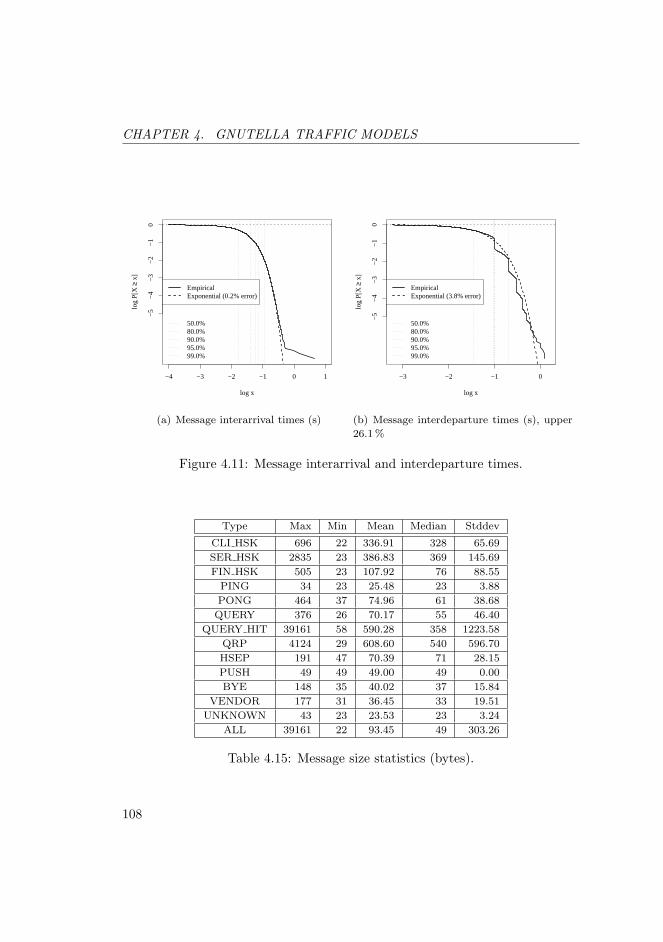
CHAPTER 4. GNUTELLA TRAFFIC MODELS
log x
log
P[X
≥x]
−5
−4
−3
−2
−1
0
−4 −3 −2 −1 0 1
50.0%80.0%90.0%95.0%99.0%
EmpiricalExponential (0.2% error)
(a) Message interarrival times (s)
log x
log
P[X
≥x]
−5
−4
−3
−2
−1
0−3 −2 −1 0
50.0%80.0%90.0%95.0%99.0%
EmpiricalExponential (3.8% error)
(b) Message interdeparture times (s), upper
26.1 %
Figure 4.11: Message interarrival and interdeparture times.
Type Max Min Mean Median Stddev
CLI HSK 696 22 336.91 328 65.69
SER HSK 2835 23 386.83 369 145.69
FIN HSK 505 23 107.92 76 88.55
PING 34 23 25.48 23 3.88
PONG 464 37 74.96 61 38.68
QUERY 376 26 70.17 55 46.40
QUERY HIT 39161 58 590.28 358 1223.58
QRP 4124 29 608.60 540 596.70
HSEP 191 47 70.39 71 28.15
PUSH 49 49 49.00 49 0.00
BYE 148 35 40.02 37 15.84
VENDOR 177 31 36.45 33 19.51
UNKNOWN 43 23 23.53 23 3.24
ALL 39161 22 93.45 49 303.26
Table 4.15: Message size statistics (bytes).
108

4.4. CHARACTERISTICS AND STATISTICAL MODELS
DIR Message Model E%
IN/OUT ALL 0.81 LNX(x; 3.94, 0.23)+ 4.3 %
0.19 LNX(x; 5.14, 1.24)
IN/OUT Bulk size 0.003 PAX(x; 0.42, 15, 9.6) 5.0 %
Table 4.16: Message size (bytes) and bulk size distribution.
Bulk size (messages) 1 2 3 4 5
Probability 0.586 0.173 0.082 0.049 0.031
Bulk size (messages) 6 7 8 9 10
Probability 0.020 0.012 0.008 0.005 0.003
Bulk size (messages) 11 12 13 14 15
Probability 0.019 0.005 0.002 0.001 0.001
Table 4.17: Probability mass points for message bulk size.
log x
log
P[X
≥x]
−5
−4
−3
−2
−1
0
2 3 4
50.0%80.0%90.0%95.0%99.0%
EmpiricalLognorm−Lognorm (4.3% error)
(a) Message size distribution
log x
log
P[X
≥x]
−5
−4
−3
−2
−1
0 1 2 3
50.0%90.0%95.0%99.0%99.9%
EmpiricalPareto (upper 0.3%, 5.0% error)
(b) Message bulk size distribution (upper
0.3 %)
Figure 4.12: Gnutella message size (bytes) and bulk distribution.
109

CHAPTER 4. GNUTELLA TRAFFIC MODELS
Type Max Min Mean Median Stddev Samples
CLI HSK 349.3015 0 0.0308 0 1.0412 604072
SER HSK 52.2645 0 0.0032 0 0.1350 597896
FIN HSK 68.6295 0 0.0057 0 0.2838 212162
PING 251.2914 0 0.0273 0 0.6309 4151799
PONG 2355.8650 0 0.0077 0 0.5881 43727188
QUERY 2355.8650 0 0.0035 0 1.3271 129078986
QUERY HIT 480.8159 0 0.0243 0 1.0260 13242329
QRP 753.1904 0 0.1883 0 1.6019 1158596
HSEP 74.0482 0 0.0017 0 0.2186 538834
PUSH 135.5155 0 0.0023 0 0.2017 63040718
BYE 148.7292 0 0.0386 0 0.5194 167726
VENDOR 391.3439 0 0.0117 0 0.2451 10195389
UNKNOWN 1.0418 0 0.2995 0 0.4294 38
ALL 2355.8650 0 0.0065 0 0.9968 266715733
Table 4.18: Message duration statistics (s).
segments that were used to transport the message. When a message uses onlyone TCP segment the time duration for that specific message is zero.
From the median column in Table 4.18 it can be observed that at least 50 %of the messages require just one TCP segment. The PONG and QUERY HITmessage rows contain extreme values for the maximum duration, namely 2355.9seconds (≈ 39 minutes). These values are most likely the result of malfunction-ing or experimental Gnutella servents.
4.4.6 Transfer Rate Characteristics
This section reports on transfer rates in bytes per second and in messages persecond for each Gnutella message types. All statistics are computed over 950,568samples. The number of samples is equal to the time duration expressed inseconds (approximately 11 days) for the available measurement data. Modelsare reported only for aggregate message flows, i. e. , type ALL messages. As itcan be observed in Table 4.21 both incoming and outgoing transfer rates areheavy-tailed. In terms of specific message types, QUERY and QUERY HITmessages dominate incoming and outgoing streams, both in terms of averagemessage rate and of average byte rates. This is expected since the Gnutella
110
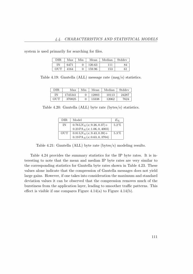
4.4. CHARACTERISTICS AND STATISTICAL MODELS
system is used primarily for searching for files.
DIR Max Min Mean Median Stddev
IN 6471 0 120.63 111 84
OUT 4164 0 159.96 153 61
Table 4.19: Gnutella (ALL) message rate (msg/s) statistics.
DIR Max Min Mean Median Stddev
IN 1745341 0 12883 10113 24287
OUT 370825 0 13338 12062 7624
Table 4.20: Gnutella (ALL) byte rate (bytes/s) statistics.
DIR Model E%
IN 0.76 LNX(x; 9.26, 0.37)+ 5.2 %
0.23 PAX(x; 1.06, 0, 4003)
OUT 0.81 LNX(x; 9.43, 0.39)+ 5.3 %
0.19 PAX(x; 0.63, 0, 3704)
Table 4.21: Gnutella (ALL) byte rate (bytes/s) modeling results.
Table 4.24 provides the summary statistics for the IP byte rates. It is in-teresting to note that the mean and median IP byte rates are very similar tothe corresponding statistics for Gnutella byte rates shown in Table 4.23. Thesevalues alone indicate that the compression of Gnutella messages does not yieldlarge gains. However, if one takes into consideration the maximum and standarddeviation values it can be observed that the compression removes much of theburstiness from the application layer, leading to smoother traffic patterns. Thiseffect is visible if one compares Figure 4.14(a) to Figure 4.14(b).
111

CHAPTER 4. GNUTELLA TRAFFIC MODELS
Type DIR Max Min Mean Median Stddev
CLI HSK IN 12 0 0.58 0 0.79
CLI HSK OUT 30 0 0.06 0 0.56
SER HSK IN 20 0 0.05 0 0.48
SER HSK OUT 12 0 0.58 0 0.79
FIN HSK IN 9 0 0.19 0 0.46
FIN HSK OUT 18 0 0.04 0 0.34
PING IN 72 0 3.64 3 1.94
PING OUT 17 0 0.73 0 1.56
PONG IN 130 0 9.56 9 4.33
PONG OUT 433 0 36.44 36 19.12
QUERY IN 347 0 62.08 60 19.64
QUERY OUT 875 0 73.71 69 34.08
QUERY HIT IN 531 0 7.29 5 9.82
QUERY HIT OUT 272 0 6.64 5 7.39
QRP IN 45 0 0.50 0 0.98
QRP OUT 283 0 0.72 0 7.18
HSEP IN 20 0 0.16 0 0.41
HSEP OUT 23 0 0.40 0 0.68
PUSH IN 1068 0 26.23 23 19.34
PUSH OUT 4091 0 40.09 32 37.32
BYE IN 40 0 0.17 0 0.43
BYE OUT 118 0 0.01 0 0.15
VENDOR IN 6385 0 10.17 1 76.17
VENDOR OUT 24 0 0.55 0 0.80
UNKNOWN IN 1 0 0.00 0 0.01
UNKNOWN OUT 1 0 0.00 0 0.00
Table 4.22: Message rate (msg/s) statistics.
112

4.4. CHARACTERISTICS AND STATISTICAL MODELS
Type DIR Max Min Mean Median Stddev
CLI HSK IN 4126 0 187 0 258
CLI HSK OUT 14519 0 27 0 273
SER HSK IN 12507 0 31 0 289
SER HSK OUT 4001 0 212 0 306
FIN HSK IN 982 0 15 0 42
FIN HSK OUT 4474 0 9 0 94
PING IN 1665 0 92 92 50
PING OUT 503 0 19 0 45
PONG IN 17043 0 1213 1173 541
PONG OUT 26050 0 2235 2162 1179
QUERY IN 24101 0 4441 4317 1426
QUERY OUT 46424 0 5088 4702 2511
QUERY HIT IN 1736791 0 4868 1912 23917
QUERY HIT OUT 360235 0 3355 1837 5229
QRP IN 47340 0 389 0 1408
QRP OUT 152820 0 353 0 3660
HSEP IN 940 0 8 0 21
HSEP OUT 2185 0 32 0 58
PUSH IN 52332 0 1285 1127 948
PUSH OUT 200459 0 1964 1568 1829
BYE IN 1720 0 6 0 16
BYE OUT 4956 0 1 0 11
VENDOR IN 210702 0 347 33 2514
VENDOR OUT 2197 0 44 0 81
UNKNOWN IN 23 0 0 0 0.1
UNKNOWN OUT 43 0 0 0 0.1
ALL IN 1745341 0 12883 10113 24287
ALL OUT 370825 0 13338 12062 7624
Table 4.23: Message byte rate (bytes/s) statistics.
DIR Max Min Mean Median Stddev
IN 249522 0 11536 10961 4075
OUT 176986 0 12668 12037 5722
Table 4.24: IP layer byte rate (bytes/s) statistics.
113
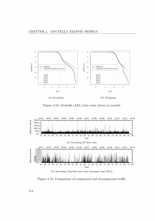
CHAPTER 4. GNUTELLA TRAFFIC MODELS
log x
log
P[X
≥x]
−5
−4
−3
−2
−1
0
2 3 4 5 6
50.0%80.0%90.0%95.0%99.0%
EmpiricalLognormal−Pareto (5.2% error)
(a) Incoming
log x
log
P[X
≥x]
−5
−4
−3
−2
−1
02 3 4 5
50.0%80.0%90.0%95.0%99.0%
EmpiricalLognormal−Pareto (5.3% error)
(b) Outgoing
Figure 4.13: Gnutella (ALL) byte rates (bytes/s) models.
0.0
50.0 k
100.0 k
150.0 k
200.0 k
250.0 k
12 00 12 00 12 00 12 00 12 00 12 00 12 00 12 00 12 00 12 00 12 00 12 00
Jul 01 Jul 02 Jul 03 Jul 04 Jul 05 Jul 06 Jul 07 Jul 08 Jul 09 Jul 10 Jul 11 Jul 12 Jul 13
Byt
es p
er s
econ
d
Time
(a) Incoming IP byte rate.
0.0 200.0 k400.0 k600.0 k800.0 k
1.0 M1.2 M1.4 M1.6 M1.8 M
12 00 12 00 12 00 12 00 12 00 12 00 12 00 12 00 12 00 12 00 12 00 12 00
Jul 01 Jul 02 Jul 03 Jul 04 Jul 05 Jul 06 Jul 07 Jul 08 Jul 09 Jul 10 Jul 11 Jul 12 Jul 13
Byt
es p
er s
econ
d
Time
(b) Incoming Gnutella byte rate (message type ALL).
Figure 4.14: Comparison of compressed and decompressed traffic.
114

4.5. SUMMARY
4.5 Summary
In this chapter we examined the characteristics of Gnutella traffic. An 11-dayslong Gnutella link-layer packet trace collected at BTH was systematically de-coded and analyzed. We extracted several traffic characteristics and constructedstatistical models for some of them. The emphasis for the characteristics hasbeen on accuracy and detail, while for the traffic models the emphasis has beenon analytical tractability and ease of simulation. To the author’s best knowl-edge this is the first work on Gnutella that presents statistics down to messagelevel.
The results show that incoming requests to open a session follow a Poissondistribution. Incoming messages of mixed types can be described by a compoundPoisson distribution. Mixture distribution models for message transfer ratesinclude a heavy-tailed component.
115

CHAPTER 4. GNUTELLA TRAFFIC MODELS
116
Chapter 5
Overlay Routing Protocol
In this chapter we present the current implementation of the ORP frameworkand the associated performance results. ORP consists of two protocols: theRoute Discovery Protocol (RDP) and the Route Management Protocol (RMP).
RDP is used to find network paths subject to various QoS constraints [46, 47].To achieve this goal, RDP uses a form of selective diffusion in which a node thatreceives a path request forwards the request only on outgoing links that do notviolate the QoS constraints. Eventually, the request arrives at the destinationnode if there is at least one path satisfying the constraints. At that point, areply message containing information about the complete path is sent back tothe requesting node. RDP is based on ideas presented in [91, 157, 158].
The purpose of RMP is to alleviate changes in the path QoS metrics, dueto node and traffic dynamics. This is done through a combination of pathrestoration and optimization algorithms for traffic flow allocation on bifurcatedpaths. The purpose of the flow allocation is to spread the demand on multiplepaths towards the destination [86]. The design of RMP is influenced by ideaspresented in [159, 160].
In Section 5.1 we give a brief overview of fundamental elements of QoS rout-ing. Based on this, we discuss in Section 5.2 a number of assumptions usedin the design of RDP and RMP. The protocol specification and the perfor-mance results for RDP and RMP are presented in Section 5.3 and Section 5.4,respectively.
117
CHAPTER 5. OVERLAY ROUTING PROTOCOL
5.1 Elements of QoS Routing
In QoS networks every link and every node has a state described by specificQoS metrics. The link state can consist of available bandwidth, delay andcost whereas the node state can be a combination of available memory, CPUutilization and harddisk storage. The link state and the node state may beconsidered separately or they may be combined. The focus in the reminder ofthis thesis is on link state.
Recall from Section 1.1 that routing is the process of finding a path betweentwo hosts in a network. In QoS routing, the path must be selected such thatQoSmetrics of interest stay within specific bounds. The routing process relies ona routing algorithm for computing constrained paths and on a routing protocolfor distributing state information.
There are three basic forms of storing state information: local state, globalstate and aggregated (partial) state [161].
When a node keeps local state, it maintains information about its outgoinglinks only. No information about the rest of the network is available.
A global state is the combination of local states for all nodes in a graph.Global states are imprecise (i. e. , they are merely approximations of the globalstate) due to non-negligible delay in propagating information about local states.When the network size grows, the imprecision grows as well. This makes it hardto maintain an accurate picture about resource availability in the network andit has severe impact on QoS routing.
Aggregated state aims to solve scalability issues in large networks. The basicidea is to group together adjacent nodes into a single logical node. The localstate of a logical node is the aggregation of local states for physical nodes thatare part of the logical node. Similar to the case of global state, this leads toimprecision that grows with the amount of state information aggregated in thelogical node.
Imprecision, also called uncertainty [162], is not generated by aggregationonly. Other sources of uncertainty are network dynamics (churn), informationkept secret by ISPs due to business reasons, as well as approximate state infor-mation due to systematic or random errors in the measurement process [162].An interesting solution suggested for mitigating these problems is to replace
118
5.1. ELEMENTS OF QOS ROUTING
the deterministic state information metrics with random variables. In this case,the routing algorithm must be changed such as to select feasible paths on aprobabilistic basis, with the result that the selected paths are those most likelyto satisfy the QoS constraints [163, 164]. However, a non-trivial problem withthis approach lies in the estimation of the probability distributions for statevariables [165].
There are three different classes of routing strategies, each correspondingroughly to one form of maintaining state information: source routing, (flat)distributed routing and hierarchical routing [166].
In source routing the nodes are required to keep global state and the fea-sible path is computed at the source node. The main advantage in this caseis that route computation is performed in a centralized fashion, avoiding someof the problems associated with distributed computation. The centralized com-putation can guarantee loop-free routes. One disadvantage of source routing isbecause of the requirement to maintain global state. In a network where theQoS metrics often change, this requires large communication overhead in orderto keep the state information updated. Additionally, due to the propagationdelay, the state information may become stale before reaching the destination.This leads to imprecise state information, as explained above. Furthermore,depending on the network size and the number of paths to compute, the sourcerouting algorithm can result in very high computational overhead [166].
Distributed routing, typically, also relies on nodes maintaining global states,but the path computation is performed in a distributed fashion. This diminishescomputational overhead and also allows concurrent computation of multipleroutes in search for a feasible path. Distributed computation suffers from prob-lems related to distributed state snapshot, deadlock and loop occurrence [161].Additionally, when global state is maintained, distributed routing shares withsource routing the problems related to imprecise state information.
Some suggestions on using flooding-based algorithms, require nodes to main-tain local state only [91, 167]. This mitigates problems related to imprecise stateinformation. However, flooding-based algorithms tend to generate large volumesof traffic compared to the other forms of routing.
In hierarchical routing, the network is divided into groups of nodes and thestate information is aggregated for the nodes participating in a group. With
119

CHAPTER 5. OVERLAY ROUTING PROTOCOL
this form of aggregation, a group appears as a logical node. One node in thegroup is designated leader or border node and acts as a gateway for the com-munication with other logical nodes. Each group can in turn be divided intosmaller groups. Using this form of recursion, several hierarchical levels can becreated. Nodes maintain global state information for peers within a group andaggregated state information about the other groups. The major advantage ofhierarchical routing is scalability [159, 166]. In particular, since nodes maintainaggregated state information there is less state information to be transmittedto other nodes, hence less communication overhead. For the same reason, thereis also less computational overhead. However, each level of hierarchy inducesadditional uncertainty in the state information. This problem becomes more dif-ficult when several QoS metrics must be aggregated, since for some topologiesthere can be no meaningful way to combine the metrics [161]. Some solutionsfor topology aggregation are presented in [168, 169].
The networks considered here rely on end-nodes. Since end-nodes are underthe control of their users, they tend to be an unreliable infrastructure. By this,we mean that end-nodes can be turned off by their users, effectively removingthem from the network. This type of node churn is similar to the topologydynamics occurring in mobile ad-hoc networks, when stations move out of radiorange. Routing protocols that handle topology dynamics can be classified asproactive or reactive protocols.
Proactive protocols, such as destination sequence distance vector (DSDV)periodically update the routing tables [170]. In contrast, reactive protocols(e. g. , dynamic source routing (DSR) and ad-hoc on-demand distance vector(AODV)) update the routing tables only when routes need to be created oradjusted due to changes to topology [170]. Proactive protocols are in generalbetter at providing QoS guarantees for real-time traffic such as multimedia.Their disadvantage lies in the traffic volume overhead generated by the pro-tocol itself. Reactive protocols scale better than proactive protocols, but willexperience higher latency when setting up a new route [170].
120
5.2. DESIGN ASSUMPTIONS
5.2 Design Assumptions
In this section are discussed a number of assumptions that have influenced thedesign of RDP and RMP. These assumptions pertain to the environments inwhich the protocols are running and to the type of media being routed.
The first assumption is that ORP is executed on end-nodes consisting of off-the-shelf hardware (e. g. , PC, Macintosh) running a general purpose operatingsystem (e. g. , Linux-based operating systems, Mac OS X, Microsoft Windows).ORP runs in unprivileged mode accessing peripheral devices through standardcalls to the operating system API.
ORP requires that nodes interested in performing QoS routing form anapplication-layer overlay. The overlay may be structured (i. e. , a DHT) orunstructured. The only requirements for it are the ability to forward mes-sages and to address individual nodes through some form of universally uniqueidentifier (UUID) [114]. In the simulations we assumed that ORP runs on topof a Gnutella-like topology.
The type of services considered for the QoS layer are currently restrictedto those that require interactive and non-interactive live unicast multimediastreams only.
Multimedia stream refers to a stream containing audio, video, text (e. g. ,subtitles or Text-TV), control data (e. g. , synchronization data), or a combina-tion thereof. If an application chooses to use several media streams (e. g. , onestream per media type), the QoS routing protocol treats them independently ofeach other and assumes that the application is capable on its own of performingsynchronization or any other type of stream merging processing.
The multimedia streams within the scope of ORP are of unicast type (one-to-one). Multicast streams (one-to-many) are not withing the scope of thisthesis. Furthermore, the streams are considered to be live, which means thatthe receiver is not willing to wait until the whole stream data is received, butwould rather start watching and listening to the contents as soon as enoughdata is available for rendering.
Interactive multimedia streams refers to streams generated by user inter-action as in a video conference or a VoIP call. Conversely, non-interactivemultimedia streams do not involve any interaction between users as is the case
121

CHAPTER 5. OVERLAY ROUTING PROTOCOL
of IPTV or music streaming.Applications using ORP request overlay paths from the node where they are
running to specific destinations, along with constraints attached to each path.The path is discovered using RDP as described in Section 5.3.
It is assumed that each node is capable of estimating the available hostresources (e. g. , RAM, storage) as well as link properties (e. g. , residual band-width, round-trip time (RTT), loss rate) to its one-hop neighbors in the over-lay. The amount of available host resources can be obtained using calls to theoperating system API. Link properties can be estimated using active measure-ments [171–175]. Nodes are expected to exchange this information using RMP,as described in Section 5.4.
Furthermore, it is assumed that ORP-enabled software cannot interfere withresources used by processes outside ORP’s scope. In other words, ORP can-not perform resource reservation other than on residual resources, which areresources currently unused by other applications running simultaneously on thenode. Consequently, it is expected that the volume of available resources willfluctuate.
Large fluctuations can drive the node into resource starvation. During re-source starvation the node is unable to honor some or all of the QoS constraints.This type of events can lead to degradation in the quality of rendered media(e. g. , MPEG frames that are lost, garbled, or arrive too late). Applicationsmay be able to tolerate quality degradation for very short periods of time oreven recover from brief degradation by using forward error correction (FEC)codes or retransmissions. However, prolonged quality degradation may even-tually lead to user dissatisfaction with the quality of the service. Each nodemust therefore carefully monitor the link properties to each of its immediateneighbors. If resource starvation is detected, or anticipated, then a new feasiblepath should be found and traffic re-routed on it. It is clear that the latencyexperienced in obtaining measurement results is in fact an upper bound on howfast ORP can react to changes. Estimating the effect of the upper bound onthe performance of ORP has not been studied yet, but is planned as an itemfor future work.
122
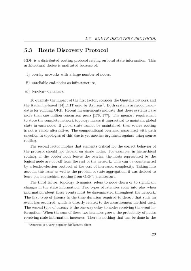
5.3. ROUTE DISCOVERY PROTOCOL
5.3 Route Discovery Protocol
RDP is a distributed routing protocol relying on local state information. Thisarchitectural choice is motivated because of:
i) overlay networks with a large number of nodes,
ii) unreliable end-nodes as infrastructure,
iii) topology dynamics.
To quantify the impact of the first factor, consider the Gnutella network andthe Kademlia-based [34] DHT used by Azureus1. Both systems are good candi-dates for running ORP. Recent measurements indicate that these systems havemore than one million concurrent peers [176, 177]. The memory requirementto store the complete network topology makes it impractical to maintain globalstate in each node. If global state cannot be maintained, then source routingis not a viable alternative. The computational overhead associated with pathselection in topologies of this size is yet another argument against using sourcerouting.
The second factor implies that elements critical for the correct behavior ofthe protocol should not depend on single nodes. For example, in hierarchicalrouting, if the border node leaves the overlay, the hosts represented by thelogical node are cut-off from the rest of the network. This can be counteractedby a leader-election protocol at the cost of increased complexity. Taking intoaccount this issue as well as the problem of state aggregation, it was decided toleave out hierarchical routing from ORP’s architecture.
The third factor, topology dynamics, refers to node churn or to significantchanges in the state information. Two types of latencies come into play wheninformation about these events must be disseminated throughout the network.The first type of latency is the time duration required to detect that such anevent has occurred, which is directly related to the measurement method used.The second type of latency is the one-way delay to nodes receiving the event in-formation. When the sum of these two latencies grows, the probability of nodesreceiving stale information increases. There is nothing that can be done in the
1Azureus is a very popular BitTorrent client.
123
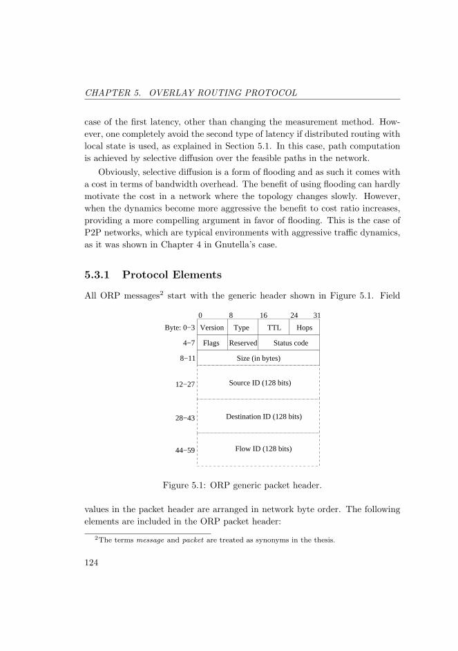
CHAPTER 5. OVERLAY ROUTING PROTOCOL
case of the first latency, other than changing the measurement method. How-ever, one completely avoid the second type of latency if distributed routing withlocal state is used, as explained in Section 5.1. In this case, path computationis achieved by selective diffusion over the feasible paths in the network.
Obviously, selective diffusion is a form of flooding and as such it comes witha cost in terms of bandwidth overhead. The benefit of using flooding can hardlymotivate the cost in a network where the topology changes slowly. However,when the dynamics become more aggressive the benefit to cost ratio increases,providing a more compelling argument in favor of flooding. This is the case ofP2P networks, which are typical environments with aggressive traffic dynamics,as it was shown in Chapter 4 in Gnutella’s case.
5.3.1 Protocol Elements
All ORP messages2 start with the generic header shown in Figure 5.1. Field
Type
0 8 16 24 31
0−3Byte: HopsTTL
ReservedFlags Status code
Version
Flow ID (128 bits)
Size (in bytes)
4−7
8−11
12−27
28−43
44−59
Source ID (128 bits)
Destination ID (128 bits)
Figure 5.1: ORP generic packet header.
values in the packet header are arranged in network byte order. The followingelements are included in the ORP packet header:
2The terms message and packet are treated as synonyms in the thesis.
124

5.3. ROUTE DISCOVERY PROTOCOL
Version ORP protocol version. At the moment of writing the protocol is atversion 1.
Type ORP packet type, showed below.
Field value Packet type
0 reserved1 control packet (CP)2 acknowledgement packet (AP)3 data packet (DP)4 used by RMP
TTL time-to-live, denoting how many overlay hops the packet is allowed totravel.
Hops indicates the amount of links the packet already has passed. If the valuein the Hops field equals the value in the TTL field the packet is dropped.
Flags bitfield arranged as |0|0|E|0|D|C|B|R|, where 0 denotes unused bits.
E indicates that the node is leaving the overlay and all routesassociated with Source Id should be rerouted or deleted.
D indicates that the path associated with the Flow Idshould be deleted.
C denotes a route change.B denotes a bidirectional route request.R indicates a redundant AP.
Reserved For future use.
Status code Used to exchange status codes among nodes.
Size Packet size in bytes excluding the generic header.
Source ID UUID denoting the source node of the packet3, also abbreviated asSrcID.
3ORP UUIDs are defined as specified in [114].
125

CHAPTER 5. OVERLAY ROUTING PROTOCOL
Destination ID UUID denoting the destination node of the packet, also ab-breviated as DstID.
Flow ID UUID of the flow to which this packet belongs, also abbreviated asFlowID.
RDP uses both a TTL field and a hops field. This is in contrast with, e. g. ,IP, where only TTL is available. The reason for using both fields is that the hopsfield can relay distance information, which can be useful for selecting a properTTL value. Consider for example a network where each node can be reached inN hops or less. In the absence of any information, nodes use TTL=N . Supposethat a node v0 forwarding control traffic learns from the hops field that anothernode v1 is M < N hops away. Based on this information, if node v0 wants toopen a route to v1 it can set the TTL field to M in order to reduce the flooding,thus saving bandwidth and CPU utilization.
The use of 128-bit identifiers is mandated by the UUID specification [114].Even if direct use of UUIDs is not desired, a 128-bit large field offers the followingadvantages:
• IPv6 addresses can be mapped directly on this field,
• IPv4 addresses can be mapped on this field, provided padding is used, orby using IPv6 mapping,
• addressing used by other systems can be directly mapped on this fieldsif the address length is equal or smaller than 128 bits, as in the case ofGnutella, or mapped by truncating the address space when it exceeds 128bits.
RDP uses two different kinds of packets: control packets (CPs) and acknowl-edgement packets (APs).
A CP begins with the generic header followed by a data structure calledQoS map, as shown in Figure 5.2. The QoS map starts with the flow demand,i. e. , with the QoS constraints for the requested path. ORP currently supportstwo type of QoS constraints: minimum bandwidth specified in kilobytes persecond and the maximum path delay, specified in milliseconds. We plan tointegrate additional constraint types in future ORP versions. The timestamp,
126
5.3. ROUTE DISCOVERY PROTOCOL
ReservedLoss rate
DelayBandwidth
ReservedLoss rate
DelayBandwidth
Max delayMin bandwidth
Timestamp
Hop 1 UUID
32160
Hop N UUID
Feasible Path
QoS constraints
Figure 5.2: QoS map.
in Coordinated Universal Time (UTC) format, indicates the time when the QoSmap was sent to the next hop.
Following the path QoS constraints comes the feasible path explored so farby the CP in question. Each node that forwards the CP appends an entry tothe feasible path. The entry consists of the UUID of the downstream node anda set of QoS metrics associated with the link on which the packet is forwarded.Metrics currently supported by ORP are bandwidth (expressed in kilobytes persecond), delay (expressed in milliseconds) and packet loss rate. The packet lossrate is a fraction with the accuracy 1/(216 − 1). A loss rate of 0 indicates thatno packets are lost whereas a loss rate of 216 − 1 denotes that all packets arelost. The use of the last field is not defined yet. The manner in which theQoS metrics are computed is not within the scope of the thesis, as stated inSection 5.2.
127
CHAPTER 5. OVERLAY ROUTING PROTOCOL
When the destination node receives a CP it assembles an AP by copying thetriple (SrcID, DstID, FlowID) and feasible path from the CP. Then, the APis sent back to the source node over the reverse feasible path4. The purposeof APs is to inform nodes on the feasible path that a complete route to thedestination has been found.
After a route has been established between two nodes, the source node canstart sending data. Data (payload) is transported in data packets (DPs). DPsusing the same FlowID are said to form a flow. The actual format of thesepackets is left open. The only requirement is that they begin with the genericheader. The simulations presented in the reminder of this chapter are concernedwith control traffic (i. e. , CPs and APs) and do not include DPs.
Each node maintains a number of flow relays (FRs). A FR is an abstractdata type associated with a single flow or a group of flows (flow bundle) sharingcommon characteristics (e. g. , the same QoS constraints). The information inthe FRs is updated by CPs and APs associated with the flows and by QoSmeasurements performed by the node in question.
At each node a list of active CPs is maintained. Each entry in the list consistsof a copy of the triple (SrcID, DstID, FlowID) from the corresponding CP. ACP is considered active from the time it is forwarded towards the destinationuntil a corresponding AP is received or a timeout occurs. Further, a timerTout is associated with every entry in the list. When the timer expires thecorresponding entry is removed from the list.
5.3.2 Path Discovery Procedure
When a node in the overlay wants to open a route to another overlay nodeit assembles a CP with the desired QoS constraints. The requesting node,also called source node, sends the CP to all adjacent nodes connected by linkssatisfying the QoS constraints. If at least one feasible link is found, the CP isadded to the list of active CPs and a timer is started accordingly. If after Toutseconds no information is received, the CP is considered lost and it is removedfrom the active CP list.
4Traveling on the reverse feasible path between node v1 and node vN means traveling in
the opposite direction on the feasible path (i. e. , over hops vN , vN−1, . . . , v1).
128
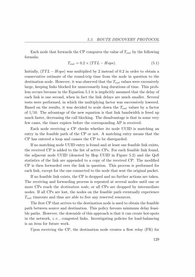
5.3. ROUTE DISCOVERY PROTOCOL
Each node that forwards the CP computes the value of Tout by the followingformula:
Tout = 0.2× (TTL−Hops). (5.1)
Initially, (TTL−Hops) was multiplied by 2 instead of 0.2 in order to obtain aconservative estimate of the round-trip time from the node in question to thedestination node. However, it was observed that the Tout values were excessivelylarge, keeping links blocked for unnecessarily long durations of time. This prob-lem occurs because in the Equation 5.1 it is implicitly assumed that the delay ofeach link is one second, when in fact the link delays are much smaller. Severaltests were performed, in which the multiplying factor was successively lowered.Based on the results, it was decided to scale down the Tout values by a factorof 1/10. The advantage of the new equation is that link bandwidth is freed upmuch faster, decreasing the call blocking. The disadvantage is that in some veryfew cases, the timer expires before the corresponding AP is received.
Each node receiving a CP checks whether its node UUID is matching anentry in the feasible path of the CP or not. A matching entry means that theCP has entered a loop and causes the CP to be disregarded.
If no matching node UUID entry is found and at least one feasible link exists,the received CP is added to the list of active CPs. For each feasible link found,the adjacent node UUID (denoted by Hop UUID in Figure 5.2) and the QoSstatistics of the link are appended to a copy of the received CP. The modifiedCP is then forwarded over the link in question. This process is performed foreach link, except for the one connected to the node that sent the original packet.
If no feasible link exists, the CP is dropped and no further actions are taken.The receiving and forwarding process is repeated at several nodes until one ormore CPs reach the destination node, or all CPs are dropped by intermediatenodes. If all CPs are lost, the nodes on the feasible path eventually experienceTout timeouts and thus are able to free any reserved resources.
The first CP that arrives to the destination node is used to obtain the feasiblepath between source and destination. This policy favours minimum delay feasi-ble paths. However, the downside of this approach is that it can create hot-spotsin the network, i. e. , congested links. Investigating policies for load-balancingis an item for future work.
Upon receiving the CP, the destination node creates a flow relay (FR) for
129
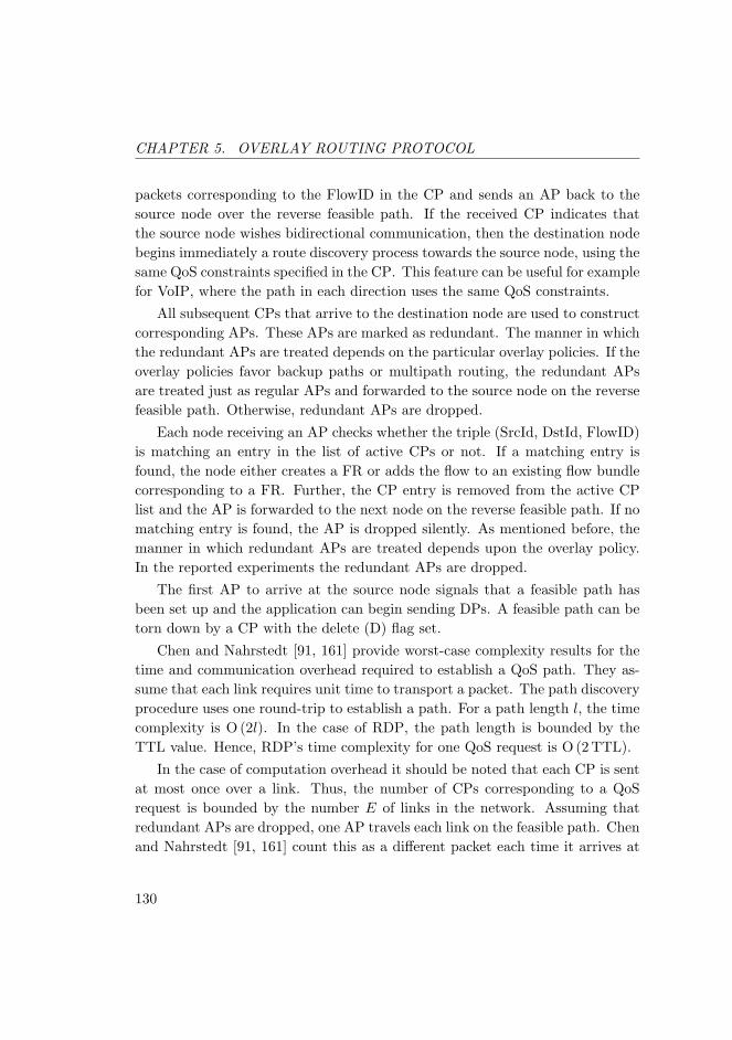
CHAPTER 5. OVERLAY ROUTING PROTOCOL
packets corresponding to the FlowID in the CP and sends an AP back to thesource node over the reverse feasible path. If the received CP indicates thatthe source node wishes bidirectional communication, then the destination nodebegins immediately a route discovery process towards the source node, using thesame QoS constraints specified in the CP. This feature can be useful for examplefor VoIP, where the path in each direction uses the same QoS constraints.
All subsequent CPs that arrive to the destination node are used to constructcorresponding APs. These APs are marked as redundant. The manner in whichthe redundant APs are treated depends on the particular overlay policies. If theoverlay policies favor backup paths or multipath routing, the redundant APsare treated just as regular APs and forwarded to the source node on the reversefeasible path. Otherwise, redundant APs are dropped.
Each node receiving an AP checks whether the triple (SrcId, DstId, FlowID)is matching an entry in the list of active CPs or not. If a matching entry isfound, the node either creates a FR or adds the flow to an existing flow bundlecorresponding to a FR. Further, the CP entry is removed from the active CPlist and the AP is forwarded to the next node on the reverse feasible path. If nomatching entry is found, the AP is dropped silently. As mentioned before, themanner in which redundant APs are treated depends upon the overlay policy.In the reported experiments the redundant APs are dropped.
The first AP to arrive at the source node signals that a feasible path hasbeen set up and the application can begin sending DPs. A feasible path can betorn down by a CP with the delete (D) flag set.
Chen and Nahrstedt [91, 161] provide worst-case complexity results for thetime and communication overhead required to establish a QoS path. They as-sume that each link requires unit time to transport a packet. The path discoveryprocedure uses one round-trip to establish a path. For a path length l, the timecomplexity is O (2l). In the case of RDP, the path length is bounded by theTTL value. Hence, RDP’s time complexity for one QoS request is O (2 TTL).
In the case of computation overhead it should be noted that each CP is sentat most once over a link. Thus, the number of CPs corresponding to a QoSrequest is bounded by the number E of links in the network. Assuming thatredundant APs are dropped, one AP travels each link on the feasible path. Chenand Nahrstedt [91, 161] count this as a different packet each time it arrives at
130
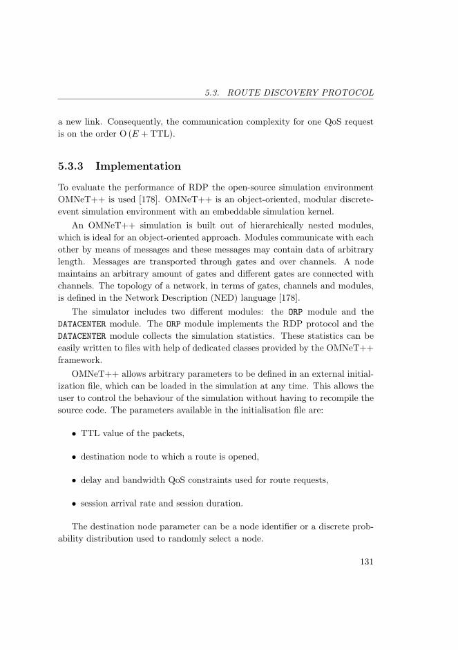
5.3. ROUTE DISCOVERY PROTOCOL
a new link. Consequently, the communication complexity for one QoS requestis on the order O (E + TTL).
5.3.3 Implementation
To evaluate the performance of RDP the open-source simulation environmentOMNeT++ is used [178]. OMNeT++ is an object-oriented, modular discrete-event simulation environment with an embeddable simulation kernel.
An OMNeT++ simulation is built out of hierarchically nested modules,which is ideal for an object-oriented approach. Modules communicate with eachother by means of messages and these messages may contain data of arbitrarylength. Messages are transported through gates and over channels. A nodemaintains an arbitrary amount of gates and different gates are connected withchannels. The topology of a network, in terms of gates, channels and modules,is defined in the Network Description (NED) language [178].
The simulator includes two different modules: the ORP module and theDATACENTER module. The ORP module implements the RDP protocol and theDATACENTER module collects the simulation statistics. These statistics can beeasily written to files with help of dedicated classes provided by the OMNeT++framework.
OMNeT++ allows arbitrary parameters to be defined in an external initial-ization file, which can be loaded in the simulation at any time. This allows theuser to control the behaviour of the simulation without having to recompile thesource code. The parameters available in the initialisation file are:
• TTL value of the packets,
• destination node to which a route is opened,
• delay and bandwidth QoS constraints used for route requests,
• session arrival rate and session duration.
The destination node parameter can be a node identifier or a discrete prob-ability distribution used to randomly select a node.
131

CHAPTER 5. OVERLAY ROUTING PROTOCOL
5.3.4 Simulator Validation
The simulation model for RDP was primarily developed for assessing the per-formance of the protocol under different workloads. Ideally, a simulator shouldbe validated against an existing system or against a mathematical model [132].Since RDP is a prototype for a new system, the first form of validation cannotbe applied. Also, due to the complexity of the protocol it is difficult to con-struct an accurate mathematical model. This is however left for future work. Inorder to circumvent these hurdles and still provide some validation, a numberof scenarios with known correct outcome, called sanity tests, were considered:
i) one feasible path only,
ii) no feasible paths,
iii) multiple feasible paths.
Figure 5.3: Topology for validation of RDP simulator.
132

5.3. ROUTE DISCOVERY PROTOCOL
Link-state class Capacity (Kbps) Delay (ms)
1 64 1000
2 500 5
3 500 35
Table 5.1: Topology parameters for validation of RDP simulator.
The sanity tests are executed in a network with 11 nodes, shown in Fig-ure 5.3. The network with the corresponding scenarios, is small enough to allowinspection of each event occurring in the simulator. In each scenario, the goal isto find paths from node 0 to node 6, such that the maximum end-to-end delaydoes not exceed 100 ms and the available bandwidth is at least 64 Kbps. Thepath computation is initiated from node 0. For each link, the link state is de-terministically set to one of the link-state classes shown in Table 5.1. The linksare error-free. It should be noted that links with link-state class 1 are alwaysinfeasible due to excessive delay. For class 2 and 3, the path feasibility dependson its length.
In the first scenario, links have either link-state class 1 or link state class 2.In Figure 5.3, links with link state class 1 are colored red and links with link-state class 2 are colored green. If correctly implemented, RDP finds a singlefeasible path 0→ 1→ 5→ 3→ 6. CPs traveling over the path 0→ 8→ 2→ 1are dropped when reaching node 1. This happens because node 1 has alreadyreceived a CP from node 0, since a CP requires only 5 ms over the path 0→ 1compared to 15 ms over the path 0→ 8→ 2→ 1.
In the second scenario, the network shown in Figure 5.3 was modified bychanging the state of the links (6, 3) and (3, 6) to link-state class 1. In this case,a valid RDP implementation finds no feasible path between node 0 and node 6.
The network shown in Figure 5.3 was changed once more for the third sce-nario. In this scenario, all links in the network have link-state class 2, with theexception of the links (1, 4), (4, 1), (4, 7) and (7, 4), which have link-state class 3.These changes prevent node 4 from being used as intermediate node on the path.A valid RDP implementation finds two feasible paths: 0→ 1→ 5→ 3→ 6 and0→ 10→ 7→ 6.
133

CHAPTER 5. OVERLAY ROUTING PROTOCOL
The sanity tests above are based on modifying the delay of various links.Similar tests were performed with regards to the link bandwidth and error rate.Additional validation tests were performed on the output of the simulator, e. g. ,controlling that measured bitrates are proportional to the number of exchangedmessages.
5.3.5 Experiment Setup
The purpose of the experiments is to evaluate the performance of RDP fordifferent workloads. The experiments are divided into two sets. In the first setof experiments, the network size is increased from 10 to 1000 nodes and variousperformance metrics are computed. In the second set of experiments, the samemetrics are observed when the network utilization increases in a network of 100nodes. The network size in the two experiments was limited by the amount ofmemory required. In particular, high network utilization results in high memoryusage in the simulator.
In the experiments the focus was entirely on bandwidth reservations. Theterm QoS session is used to denote a request for a directed path with a con-straint on minimum available bandwidth. Each session has an associated sessionduration, which specifies the life length of the path. If a path is successfully es-tablished, the amount of bandwidth specified by the path constraint is reservedfor the entire session duration. The links in these experiments are error-free andno churn occurs.
During simulation data has been collected for the following metrics:
call blocking ratio: ratio between the number of infeasible QoS sessions andthe total number of QoS sessions arrived at the network,
low-TTL blocking ratio: ratio between infeasible sessions due to low TTLvalue and the total number of infeasible sessions,
bandwidth utilization: average number of bytes per second due to RDP con-trol information,
bandwidth overhead: ratio between the average number of RDP bytes persecond and network capacity (i. e. , the aggregated volume of every linkin the network),
134

5.3. ROUTE DISCOVERY PROTOCOL
path stretch: average value for the ratio between feasible path length to short-est path length.
The call blocking ratio metric is a good indicator of the overall success orfailure of the protocol in establishing QoS paths. When the call blocking ratio ishigh, it is important to diagnose the root cause of the failures. In this context,the low-TTL blocking ratio metric can help in deciding if failures occur becausebandwidth requests cannot be satisfied or because CPs are hindered in findinga feasible due to the TTL value used.
The bandwidth metrics provide information about the cost of using RDPexpressed in terms of protocol overhead. The utilization metric can be used tocompare the required bandwidth per second with that used by other protocols.On the other hand, the overhead metric reflects how much of the entire networkcapacity is dedicated to RDP.
Finally, path stretch is also a way of estimating the cost of using RDP. Whenthe path stretch is higher than 1, a penalty is payed in terms of bandwidth anddelay. The bandwidth penalty has to do with reserved bandwidth on additionallinks compared to the case of the shortest-path. Since more links are used, theone-way delay of packets sent over feasible paths increases as well.
In the first set of experiments, the sessions arrive at the network according toa Poisson distribution with parameter λ = 1. The session duration is drawn froma generalized Pareto distribution with mean 180 seconds. This value reflects theaverage duration of a voice conversation [29, 179, 180]. The Pareto distributionis used to model the effect of long-tails and heavy-tails. The existence of long-tails in the distribution of session duration in wide-area networks is supportedby empirical evidence from several studies [179, 181, 182].
The bandwidth requested for a QoS session is uniformly distributed overthree different ranges: 16–64 Kbps, 128–512 Kbps and 1–2 Mbps. These rangesroughly represent low-to-high quality audio, streaming music or low qualityvideo, and high quality video, respectively. The network topologies are cre-ated with the same settings as described in Section 3.4. The bandwidth in thetopologies generated with BRITE is uniformly distributed between 10 Kbps and10 Mbps. The upper bound of the distribution represents an average value forthe maximum connection capacity offered to residential users by ISPs in Swe-
135

CHAPTER 5. OVERLAY ROUTING PROTOCOL
den5. Links with less than 10 Kbps are not considered useful. The link delayconstraint is set to 10000 seconds. This value is several orders of magnitudehigher than the link delay, thus the delay constraint is always satisfied.
Preliminary results [183] indicate that RDP’s performance is strongly influ-enced by the TTL value in use. Consequently, the performance of the protocol iscompared for the following TTL values: 4, 8 and 250. For brevity, these valuesare denoted by TTL=4, TTL=8, and TTL=250, respectively.
In the second set of experiments, the metrics are observed in terms of in-creasing network utilization. The network utilization, ρ, is defined as [29, 181]
ρ =λTQH∑e∈E
be(5.2)
where T is the average session duration, Q is the average amount of QoS (band-width) requested, H is the average path length across all node pairs, and be isthe available bandwidth on link e.
The session duration is selected from a generalized Pareto distribution withmean 180 seconds, as in the first set of the experiments. Additionally, theseexperiments include Pareto distributed sessions with a mean of 600 seconds.This value was selected to explore the effect of longer sessions on the performanceof the protocol.
The amount of bandwidth requested by each QoS is defined exactly as inthe case of the first set of experiments.
The network utilization variable, ρ, was allowed to assume values from the set{0.1, 0.25, 0.50, 0.75, 1.00}. This is accomplished by correspondingly adjustingthe arrival rate variable, λ, in Equation 5.2, while the remaining variable werekept fixed.
For the second set of experiments a single BRITE topology is used, whichconsists of 100 nodes. The topology is generated with the configuration param-eters described for the first set of experiments.
The TTL value is set to 8, based on results from the first set of experiments.Redundant APs are dropped.
Both sets of experiments are executed 30 times for each parameter combi-5This was estimating by comparing the current offers from ISPs in Sweden.
136
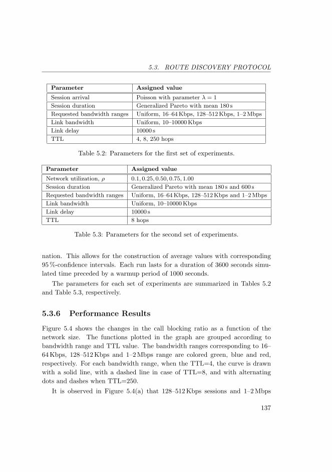
5.3. ROUTE DISCOVERY PROTOCOL
Parameter Assigned value
Session arrival Poisson with parameter λ = 1
Session duration Generalized Pareto with mean 180 s
Requested bandwidth ranges Uniform, 16–64 Kbps, 128–512 Kbps, 1–2 Mbps
Link bandwidth Uniform, 10–10000 Kbps
Link delay 10000 s
TTL 4, 8, 250 hops
Table 5.2: Parameters for the first set of experiments.
Parameter Assigned value
Network utilization, ρ 0.1, 0.25, 0.50, 0.75, 1.00
Session duration Generalized Pareto with mean 180 s and 600 s
Requested bandwidth ranges Uniform, 16–64 Kbps, 128–512 Kbps and 1–2 Mbps
Link bandwidth Uniform, 10–10000 Kbps
Link delay 10000 s
TTL 8 hops
Table 5.3: Parameters for the second set of experiments.
nation. This allows for the construction of average values with corresponding95 %-confidence intervals. Each run lasts for a duration of 3600 seconds simu-lated time preceded by a warmup period of 1000 seconds.
The parameters for each set of experiments are summarized in Tables 5.2and Table 5.3, respectively.
5.3.6 Performance Results
Figure 5.4 shows the changes in the call blocking ratio as a function of thenetwork size. The functions plotted in the graph are grouped according tobandwidth range and TTL value. The bandwidth ranges corresponding to 16–64 Kbps, 128–512 Kbps and 1–2 Mbps range are colored green, blue and red,respectively. For each bandwidth range, when the TTL=4, the curve is drawnwith a solid line, with a dashed line in case of TTL=8, and with alternatingdots and dashes when TTL=250.
It is observed in Figure 5.4(a) that 128–512 Kbps sessions and 1–2 Mbps
137
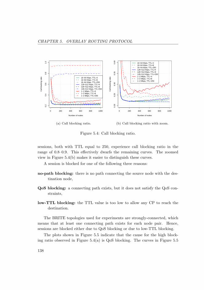
CHAPTER 5. OVERLAY ROUTING PROTOCOL
0 200 400 600 800 1000
0.2
0.4
0.6
0.8
1.0
Number of nodes
Cal
l blo
ckin
g ra
tio 16−64 Kbps, TTL=416−64 Kbps, TTL=816−64 Kbps, TTL=250128−512 Kbps, TTL=4128−512 Kbps, TTL=8128−512 Kbps, TTL=2501−2 Mbps, TTL=41−2 Mbps, TTL=81−2 Mbps, TTL=250
(a) Call blocking ratio.
0 200 400 600 800 1000
0.20
0.25
0.30
0.35
0.40
Number of nodes
Cal
l blo
ckin
g ra
tio
16−64 Kbps, TTL=416−64 Kbps, TTL=816−64 Kbps, TTL=250128−512 Kbps, TTL=4128−512 Kbps, TTL=8128−512 Kbps, TTL=2501−2 Mbps, TTL=41−2 Mbps, TTL=81−2 Mbps, TTL=250
(b) Call blocking ratio with zoom.
Figure 5.4: Call blocking ratio.
sessions, both with TTL equal to 250, experience call blocking ratio in therange of 0.8–0.9. This effectively dwarfs the remaining curves. The zoomedview in Figure 5.4(b) makes it easier to distinguish these curves.
A session is blocked for one of the following three reasons:
no-path blocking: there is no path connecting the source node with the des-tination node,
QoS blocking: a connecting path exists, but it does not satisfy the QoS con-straints,
low-TTL blocking: the TTL value is too low to allow any CP to reach thedestination.
The BRITE topologies used for experiments are strongly-connected, whichmeans that at least one connecting path exists for each node pair. Hence,sessions are blocked either due to QoS blocking or due to low-TTL blocking.
The plots shown in Figure 5.5 indicate that the cause for the high block-ing ratio observed in Figure 5.4(a) is QoS blocking. The curves in Figure 5.5
138
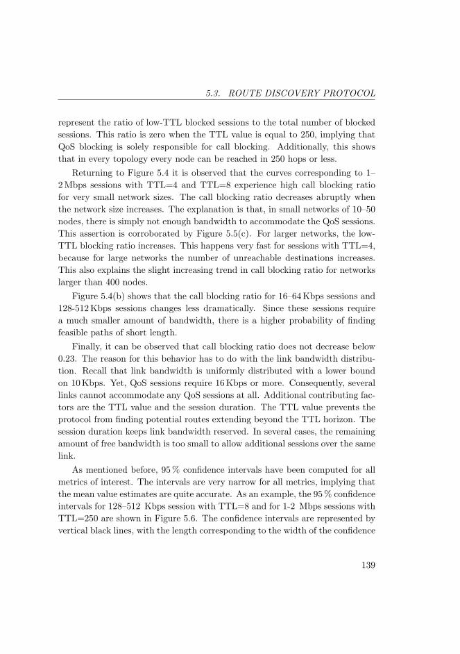
5.3. ROUTE DISCOVERY PROTOCOL
represent the ratio of low-TTL blocked sessions to the total number of blockedsessions. This ratio is zero when the TTL value is equal to 250, implying thatQoS blocking is solely responsible for call blocking. Additionally, this showsthat in every topology every node can be reached in 250 hops or less.
Returning to Figure 5.4 it is observed that the curves corresponding to 1–2 Mbps sessions with TTL=4 and TTL=8 experience high call blocking ratiofor very small network sizes. The call blocking ratio decreases abruptly whenthe network size increases. The explanation is that, in small networks of 10–50nodes, there is simply not enough bandwidth to accommodate the QoS sessions.This assertion is corroborated by Figure 5.5(c). For larger networks, the low-TTL blocking ratio increases. This happens very fast for sessions with TTL=4,because for large networks the number of unreachable destinations increases.This also explains the slight increasing trend in call blocking ratio for networkslarger than 400 nodes.
Figure 5.4(b) shows that the call blocking ratio for 16–64 Kbps sessions and128-512 Kbps sessions changes less dramatically. Since these sessions requirea much smaller amount of bandwidth, there is a higher probability of findingfeasible paths of short length.
Finally, it can be observed that call blocking ratio does not decrease below0.23. The reason for this behavior has to do with the link bandwidth distribu-tion. Recall that link bandwidth is uniformly distributed with a lower boundon 10 Kbps. Yet, QoS sessions require 16 Kbps or more. Consequently, severallinks cannot accommodate any QoS sessions at all. Additional contributing fac-tors are the TTL value and the session duration. The TTL value prevents theprotocol from finding potential routes extending beyond the TTL horizon. Thesession duration keeps link bandwidth reserved. In several cases, the remainingamount of free bandwidth is too small to allow additional sessions over the samelink.
As mentioned before, 95 % confidence intervals have been computed for allmetrics of interest. The intervals are very narrow for all metrics, implying thatthe mean value estimates are quite accurate. As an example, the 95 % confidenceintervals for 128–512 Kbps session with TTL=8 and for 1-2 Mbps sessions withTTL=250 are shown in Figure 5.6. The confidence intervals are represented byvertical black lines, with the length corresponding to the width of the confidence
139
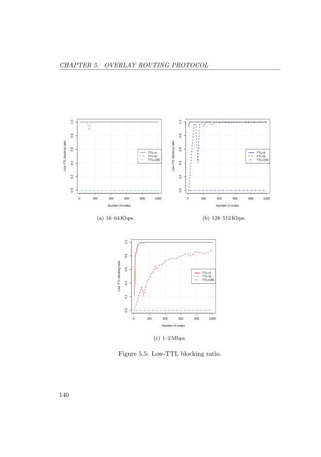
CHAPTER 5. OVERLAY ROUTING PROTOCOL
0 200 400 600 800 1000
0.0
0.2
0.4
0.6
0.8
1.0
Number of nodes
Low
−T
TL
bloc
king
rat
io
TTL=4TTL=8TTL=250
(a) 16–64 Kbps.
0 200 400 600 800 1000
0.0
0.2
0.4
0.6
0.8
1.0
Number of nodes
Low
−T
TL
bloc
king
rat
io
TTL=4TTL=8TTL=250
(b) 128–512 Kbps.
0 200 400 600 800 1000
0.0
0.2
0.4
0.6
0.8
1.0
Number of nodes
Low
−T
TL
bloc
king
rat
io
TTL=4TTL=8TTL=250
(c) 1–2 Mbps.
Figure 5.5: Low-TTL blocking ratio.
140
5.3. ROUTE DISCOVERY PROTOCOL
0 200 400 600 800 1000
0.22
0.24
0.26
0.28
0.30
Number of nodes
Cal
l blo
ckin
g ra
tio
128−512 Kbps, TTL=8
(a) 95 % confidence interval.
0 200 400 600 800 1000
0.92
50.
930
0.93
50.
940
0.94
50.
950
Number of nodes
Cal
l blo
ckin
g ra
tio
1−2 Mbps, TTL=250
(b) 95 % confidence interval.
Figure 5.6: Call blocking ratio with confidence intervals.
interval. It can be observed that all confidence intervals are within the rangeof 0.005. The intervals are so small, that in fact it was required to zoom inthe plot to make them visible. If they would be drawn on top of the curves inFigure 5.4 they would not show at all. This is a recurring observation for allmetrics. Hence, additional confidence interval plots are not shown.
As stated in Section 5.3, RDP’s foremost disadvantage is its cost in terms ofbandwidth. Figure 5.7(a) shows the RDP bandwidth utilization in Kbps, as aform of quantitative estimate of the cost. However, Figure 5.7(b) showing thebandwidth utilization normalized by network capacity, is a better indication ofhow much capacity is wasted by the path discovery process6.
The upper bound on RDP’s bandwidth utilization is decided by two factors:the number of feasible links in the network and the TTL value used. In Fig-ure 5.7 it can be observed that 128–512 Kbps sessions and 1–2 Mbps sessionswith TTL=250 consume the least amount of bandwidth. This happens becausemost sessions of this type experience QoS blocking as it can be observed inFigure 5.4(a) and in Figure 5.5.
6The legend shown in Figure 5.7(a) applies to Figure 5.7(b) as well.
141
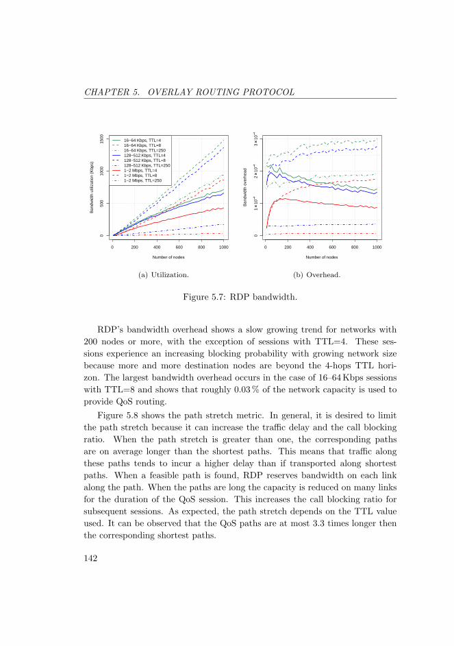
CHAPTER 5. OVERLAY ROUTING PROTOCOL
0 200 400 600 800 1000
050
010
0015
00
Number of nodes
Ban
dwid
th u
tiliz
atio
n (K
bps)
16−64 Kbps, TTL=416−64 Kbps, TTL=816−64 Kbps, TTL=250128−512 Kbps, TTL=4128−512 Kbps, TTL=8128−512 Kbps, TTL=2501−2 Mbps, TTL=41−2 Mbps, TTL=81−2 Mbps, TTL=250
(a) Utilization.
0 200 400 600 800 1000
Number of nodes
Ban
dwid
th o
verh
ead
01
××10
−−42
××10
−−43
××10
−−4
(b) Overhead.
Figure 5.7: RDP bandwidth.
RDP’s bandwidth overhead shows a slow growing trend for networks with200 nodes or more, with the exception of sessions with TTL=4. These ses-sions experience an increasing blocking probability with growing network sizebecause more and more destination nodes are beyond the 4-hops TTL hori-zon. The largest bandwidth overhead occurs in the case of 16–64 Kbps sessionswith TTL=8 and shows that roughly 0.03 % of the network capacity is used toprovide QoS routing.
Figure 5.8 shows the path stretch metric. In general, it is desired to limitthe path stretch because it can increase the traffic delay and the call blockingratio. When the path stretch is greater than one, the corresponding pathsare on average longer than the shortest paths. This means that traffic alongthese paths tends to incur a higher delay than if transported along shortestpaths. When a feasible path is found, RDP reserves bandwidth on each linkalong the path. When the paths are long the capacity is reduced on many linksfor the duration of the QoS session. This increases the call blocking ratio forsubsequent sessions. As expected, the path stretch depends on the TTL valueused. It can be observed that the QoS paths are at most 3.3 times longer thenthe corresponding shortest paths.
142

5.3. ROUTE DISCOVERY PROTOCOL
0 200 400 600 800 1000
1.5
2.0
2.5
3.0
Number of nodes
Pat
h st
retc
h
16−64 Kbps, TTL=416−64 Kbps, TTL=816−64 Kbps, TTL=250128−512 Kbps, TTL=4128−512 Kbps, TTL=8128−512 Kbps, TTL=2501−2 Mbps, TTL=41−2 Mbps, TTL=81−2 Mbps, TTL=250
Figure 5.8: Path stretch.
This concludes the first set of experiments. Based on the results it wasdecided to use a TTL value of 8 for the second set of experiments. The mainreasons for this decision is the combination of low call blocking ratio and mediumpath stretch.
For the second set of experiments, the same metrics as in the first set areobserved while the network utilization increases. The blue color is used forsessions with mean duration of 180 seconds, while red color denotes sessionswith mean duration of 600 seconds. Plots for 16-64 Kbps sessions are drawn withsolid lines, those for 128–512 Kbps are drawn with dashed lines, and 1-2 Mbpssession plots use alternating dots and dashes. Each hollow circle indicates thesimulated utilization factor pertaining to the value on the y-axis.
The call blocking ratio and the low-TTL blocking ratio are shown side byside in Figure 5.9. The first thing to notice in Figure 5.9(a) is that 180 secondssessions consistently experience higher call blocking ratio than 600 seconds ses-sions. The explanation is found in Equation 5.2. This equation is used tocompute the utilization factor, ρ, by adjusting the arrival rate, λ, while theother parameters are kept fixed. For a given ρ value, the arrival rate must behigher for short sessions than for long sessions. A higher arrival rate implies thatmore feasible paths must be found. This leads to higher bandwidth overhead
143

CHAPTER 5. OVERLAY ROUTING PROTOCOL
●
●
●
●
●
0.2 0.4 0.6 0.8 1.0
0.2
0.3
0.4
0.5
0.6
0.7
0.8
Utilization factor, ρρ
Cal
l blo
ckin
g ra
tio
●
●
●
●
●
●
●
●
●
●
● ●
●
●
●
● ●
●
●
●
●
●
●
●
●
16−64 Kbps, 180s128−512 Kbps, 180s1−2 Mbps, 180s16−64 Kbps, 600s128−512 Kbps, 600s1−2 Mbps, 600s
(a) Call blocking ratio.
●
●●
●●
0.2 0.4 0.6 0.8 1.0
0.3
0.4
0.5
0.6
0.7
0.8
0.9
1.0
Utilization factor, ρρ
Low
−T
TL
bloc
king
rat
io
●
●●
●●
●
●●
●●
●
●
● ●●
●
●
● ●●
●
●
● ●●
16−64 Kbps, 180s128−512 Kbps, 180s1−2 Mbps, 180s16−64 Kbps, 600s128−512 Kbps, 600s1−2 Mbps, 600s
(b) Low-TTL blocking ratio.
Figure 5.9: Call blocking.
since more CPs are in the network, as it can be observed in Figure 5.10. Sinceless network capacity is available in this case than in the case of low arrival rate,the call blocking ratio is higher. Further support for this assertion is found inFigure 5.9(b), where it can be observed that, when the utilization factor exceeds0.25, most call blocking is due to QoS blocking.
Two different graphs are used in Figure 5.10 to show the RDP bandwidthoverhead. This is done because in the case of a single graph, the high band-width overhead of 16-64 Kbps sessions would make it hard to distinguish thebandwidth overhead of the remaining sessions. Indeed, for 16-64 Kbps sessionsthe bandwidth overhead is 40–80 times higher than that of 1–2 Mbps sessions.
Figure 5.11 shows the path stretch metric as a function of the utilizationfactor. The figure shows that when the utilization factor is below 0.75 thepath stretch is higher for 180 second sessions. When the path stretch increasesbeyond 0.75 the situation is reversed. Unfortunately, there are currently noresults available for intermediate ρ values between 0.75 and 1. In their absence,the hypothesis is that, at high network utilization, the session duration has moreinfluence over the path stretch. Long sessions keep the links occupied forcingRDP to search longer feasible paths.
144
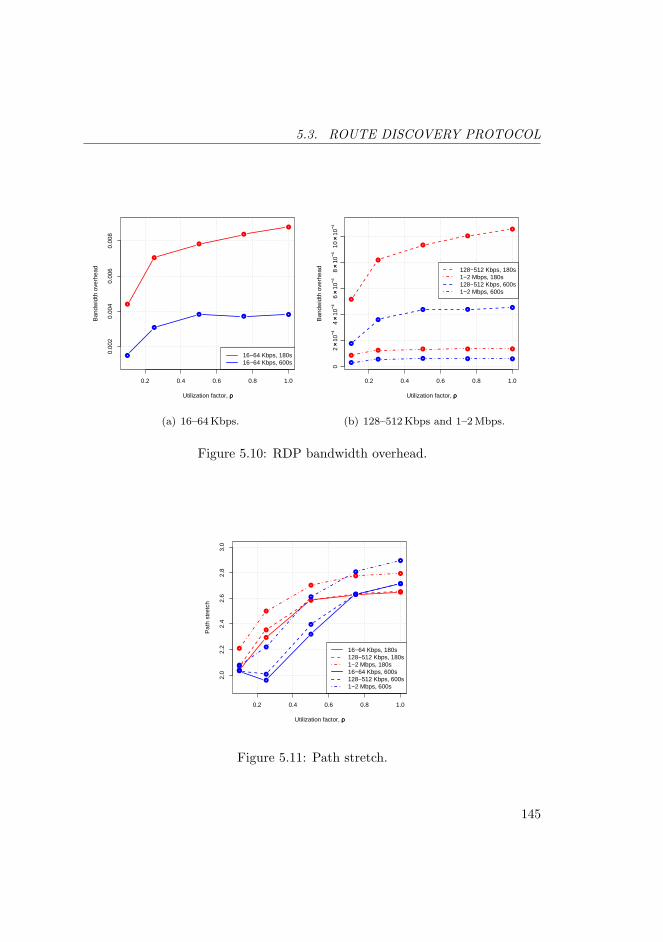
5.3. ROUTE DISCOVERY PROTOCOL
●
●
●
●
●
0.2 0.4 0.6 0.8 1.0
0.00
20.
004
0.00
60.
008
Utilization factor, ρρ
Ban
dwid
th o
verh
ead
●
●
●● ●
16−64 Kbps, 180s16−64 Kbps, 600s
(a) 16–64 Kbps.
●
●
●
●
●
0.2 0.4 0.6 0.8 1.0
Utilization factor, ρρ
Ban
dwid
th o
verh
ead
02
××10
−−44
××10
−−46
××10
−−48
××10
−−410
××10
−−4
●
●
● ●●
●
● ● ● ●
●● ● ● ●
128−512 Kbps, 180s1−2 Mbps, 180s128−512 Kbps, 600s1−2 Mbps, 600s
(b) 128–512 Kbps and 1–2 Mbps.
Figure 5.10: RDP bandwidth overhead.
●
●
●
●●
0.2 0.4 0.6 0.8 1.0
2.0
2.2
2.4
2.6
2.8
3.0
Utilization factor, ρρ
Pat
h st
retc
h
●
●
●
●●
●
●
●
●●
●
●
●
●
●
●●
●
●
●
●
●
●
●
●
16−64 Kbps, 180s128−512 Kbps, 180s1−2 Mbps, 180s16−64 Kbps, 600s128−512 Kbps, 600s1−2 Mbps, 600s
Figure 5.11: Path stretch.
145
CHAPTER 5. OVERLAY ROUTING PROTOCOL
5.4 Route Maintenance Protocol
The paths established with RDP must satisfy the QoS constraints (i. e. , theflow demand) in the face of resource fluctuations, as explained in Section 5.2.Applications are expected to cope with resource starvation during short dura-tions of time. However, prolonged resource outage can have a serious adverseimpact on the QoE. When resource starvation is detected it is necessary tore-route the flows such that the QoS constraints can still be satisfied. RMPcombines path restoration and flow allocation to achieve this goal. In this thesisthe focus is on bandwidth constraints, but the protocol as such has support fordifferent types of QoS constraints.
The factors that influence the design of RDP are also responsible for thedesign of RMP. They were introduced in Section 5.3:
i) overlay networks with a large number of nodes,
ii) unreliable end-nodes as infrastructure,
iii) topology dynamics.
The use of traditional routing algorithms based on link state or distance vec-tors in an environment with a large number of nodes is problematic at best [159].In particular, the reliable flooding required by link-state algorithms presents se-rious scalability issues. If the link-state updates are triggered by changes in thelink-state information in an environment with unreliable network infrastructureand aggressive topology dynamics, the scalability problem becomes even moreserious. On the other hand, if the updates are periodic, nodes are likely to actupon stale information. In the same type of environment, distance-vectors al-gorithms suffer from problems related to routing loops and explosion in the sizeof the routing table when multiple QoS constraints are maintained [159, 184].
To alleviate the scalability problem it is necessary to drastically reduce thecommunication requirements. This entails to reducing the number of source-destination pairs for which link state or distance vectors must be maintained.Simultaneously, care must be taken such that QoS information is maintainedfresh.
If one considers the typical applications of unicast QoS routing (e. g. , VoIP,videoconferencing) it becomes clear that maintaining information about all
146
5.4. ROUTE MAINTENANCE PROTOCOL
source-destination pairs in each node is unnecessary. For example, most peoplehave voice conversations with a limited number of other people, who add upto just a tiny fraction of the entire population. In the VoIP scenario, this im-plies that a source needs to maintain only topology information that describespotential paths to its preferred destination nodes.
The solution proposed here assumes that source nodes establish QoS pathsusing RDP. Neighbouring nodes share link-state information about establishedpaths among themselves. Contrary to the approach used by traditional link-state protocols where complete topology information is flooded over the wholenetwork, the solution presented here exchanges specific topology informationby using selective diffusion. When an intermediate node on the path detectsthat the QoS constraints of its outgoing link can no longer be maintained, itenters restoration mode. A node in restoration mode computes a number ofbackup paths based on the available link-state information. Traffic flows over thebroken path are reallocated to the backup paths using the techniques explainedin Chapter 3. Additionally, the intermediate node sends a message to the sourceof each affected flow, informing it that backup paths are maintained until thecorresponding source node finds a new QoS path to the destination. In the casewhen a link fails at the source node, the same actions are taken as in the case ofan intermediate node. Destination nodes are not required to do anything otherthan to exchange link-state information.
5.4.1 Protocol Description
RMP relies on two main components: an algorithm for distributing link-stateinformation and an optimization algorithm for flow allocation.
Link-state information is distributed using the link vector algorithm pro-posed by Behrens and Garcia-Luna-Aceves [159]. The difference between alink-state algorithm and a link vector algorithm is that the link-state algorithmis require to broadcast complete topology information. When a link vectoralgorithm is used, a node uses selective diffusion to disseminate link-state infor-mation pertaining only to its preferred paths. This reduces the communicationoverhead associated with traditional link-state algorithms.
In the case of RMP, the preferred paths are setup using RDP. The QoSinformation provided by RDP ensures that a node has link-state information
147

CHAPTER 5. OVERLAY ROUTING PROTOCOL
about each link in each of its preferred paths. The set of links belonging to anode’s preferred paths is called the source graph of that node. Nodes exchangesource graph information with their neighbours. Additionally, nodes have link-state information about their own outgoing links. The topology informationknown to a node consists of its own links, its own source graph and the sourcegraphs reported by its neighbours [159].
Nodes report incremental source graph information to their neighbours. Ob-viously, when a node joins the overlay it receives complete source graphs fromits neighbours. Beyond that, information is transmitted only if the link-statechanges, i. e. , triggered updates.
There are two type of updates: add update and delete update. In RMPparlance they are called LS ADD and LS DEL update, respectively. The prefixLS is an abbreviation for link-state. A node sends an LS ADD update when anew link is added to its source graph or when updated link-state information isavailable for a link in its source graph. A LS DEL update is sent when a nodediscards a link from its source graph.
A RMP message begin with the generic ORP header shown in Figure 5.1.The type field in the header uses a value of 4. The generic header can befollowed by multiple LS ADD and LS DEL updates. The format of a sequenceof link-state updates is shown in Figure 5.12.
The bandwidth, delay and loss rate fields have the same meaning as in thecase of RDP. A value of one in the type field indicates a LS ADD update anda value of two indicates a LS DEL update, respectively. The link source UUIDdenotes the head node of a link. Similarly, the link destination UUID denotesthe tail node of a link.
Nodes receiving link-state updates must be guarded against the possibility ofprocessing stale information. Therefore, each node maintains a sequence numbercounter that is updated by changes occurring to its topology table. Only thehead node of a link is allowed to change the sequence number and the link-stateinformation (i. e. , the QoS metrics) associated with the link in question. Whena node receives a link-state update for a link already available in its topologytable, it compares the sequence number of the update with the sequence numberstored in the topology table. If the sequence number of the update is higher,the contents of the topology table are updated with the information from the
148
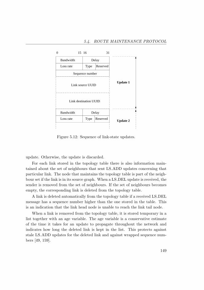
5.4. ROUTE MAINTENANCE PROTOCOL
3115 160
Bandwidth Delay
Loss rate
Bandwidth Delay
Loss rate
Link destination UUID
Link source UUID
Sequence number
Update 2
Update 1
Reserved
ReservedType
Type
Figure 5.12: Sequence of link-state updates.
update. Otherwise, the update is discarded.For each link stored in the topology table there is also information main-
tained about the set of neighbours that sent LS ADD updates concerning thatparticular link. The node that maintains the topology table is part of the neigh-bour set if the link is in its source graph. When a LS DEL update is received, thesender is removed from the set of neighbours. If the set of neighbours becomesempty, the corresponding link is deleted from the topology table.
A link is deleted automatically from the topology table if a received LS DELmessage has a sequence number higher than the one stored in the table. Thisis an indication that the link head node is unable to reach the link tail node.
When a link is removed from the topology table, it is stored temporary in alist together with an age variable. The age variable is a conservative estimateof the time it takes for an update to propagate throughout the network andindicates how long the deleted link is kept in the list. This protects againststale LS ADD updates for the deleted link and against wrapped sequence num-bers [49, 159].
149
CHAPTER 5. OVERLAY ROUTING PROTOCOL
Upon receiving a stale update, the receiver uses information from its topol-ogy table to prepare an update for sender. If the stale information describesa link present in the receiver’s source graph, the prepared update is of typeLS ADD. Otherwise, a LS DEL update is prepared to inform the sender thatthe link in question is not in the receiver’s source graph.
A node enters restoration mode when a path is broken, i. e. , when one orseveral links are deleted from the source graph or when their updated state infor-mation makes it impossible to satisfy the path QoS constraints. In restorationmode the following actions are taken:
i) an AP is sent to the source node of each affected flow, with the status codeset to indicate path error,
ii) Yen’s KSP algorithm is executed to find the K backup paths to the desti-nations affected by the topology updates,
iii) the corresponding flow demands and the backup paths are used to constructa PAP-MLPF optimization problem as described in Section 3.2.2,
iv) the simplex method is used to solve the PAP-MLPF problem as describedin Section 3.1 and Section 3.3,
v) if the simplex method is successful, the links on the new paths are addedto the source graph; otherwise the affected flows are dropped (i. e. , packetsbelonging to them are not forwarded further).
In restoration mode, RMP exploits path diversity in order to keep trafficflowing when the main route is failing. A strongly-connected topology (e. g. ,a graph with high outdegree) is a key element for creating high path diversity.Path diversity is also dependent upon the number of constraints. In particular,finding several backup paths can be more difficult if several QoS constraintsmust be satisfied simultaneously. The focus here is on bandwidth management,but it is theoretically possible to replace Yen’s algorithm with the Self-AdaptiveMultiple Constraints Routing Algorithm (SAMCRA), which allows for pathselection with multiple constraints [55, 185].
As stated above, if the simplex method fails, then path failure occurs andthe node drops the concerned flows. An alternative approach is to drop one flow
150
5.4. ROUTE MAINTENANCE PROTOCOL
demand at a time and rerun the simplex method. This can improve the successratio for the flow allocation, albeit at a higher computational cost. Only thefirst approach is used in the implementation reported here.
The following actions [159] are taken by a node if its topology table is up-dated in response to a received RMP message:
i) a new source graph is constructed using the updated information,
ii) the new source graph is compared to the old source graph and based ontheir differences a set of LS ADD and LS DEL updates is created,
iii) the set of updates from the previous step is used to construct a RMPmessages that is sent to all neighbours,
iv) aged links are removed from the deleted links list,
v) the sequence number counter is incremented.
The time complexity of the link vector algorithm after a single link changeis O (n), where n is the number of nodes affected by the change. The upperbound for n is given by the length of the longest path in the network. Thecommunication complexity O (E) is asymptotic in the number of links in thenetwork [159].
5.4.2 Implementation and Validation
The OMNeT++ simulator [178] environment is used to test the performanceof RMP under various levels of churn. The simulator consists of two modules:ORPNODE and WORLD.
The ORPNODE module is the actual RMP implementation. It should be notedthat the module is as close to a real implementation as it can be done in OM-NeT++. This statement applies to the datatypes used, the function calls,the message format and the optimization algorithms. In fact, the simulatoris linked with the liboptim software library presented in Chapter 3. If themessage-passing layer in OMNeT++ is replaced with a TCP/IP-based layer,then minimal changes to ORPNODE are required in order to make it work over areal network. Suggestions for enabling network communication in OMNeT++can be found in [186].
151

CHAPTER 5. OVERLAY ROUTING PROTOCOL
Given that RMP depends on RDP for obtaining preferred paths, it shouldideally use the RDP implementation described in Section 5.3.3. However, em-pirical evidence from the experiments with RDP suggested that this approach islikely to result in extremely long simulation times. Instead, the RMP simulatoruses a bootstrap phase to setup preferred routes.
The bootstrap phase is implemented in the WORLD module. This phase isinitiated with a set of randomly generated flow demands and with a BRITEtopology object. For each flow demand, a path is computed with Yen’s KSPalgorithm, where K = 5. The reason for using Yen’s KSP is to induce pathstretch as observed in the performance results for RDP. The bandwidth isadjusted for each link on every 5SP7 in order to satisfy the flow demand. Thisconcludes the bootstrap phase.
It should also be noted that because RDP is not used, when a node entersrestoration mode no AP message is sent to the source node of each broken flow.
In addition to the bootstrap phase, the WORLD module is responsible forgenerating link churn. Each connected pair of nodes shares a pair of links, witheach link going in the opposite direction of the other. Every link pair in thenetwork has an associated session duration variable, which is used to schedulea session termination event. The value for the session duration is drawn from auser-configurable probability distribution. When the session termination eventoccurs, the node pair is disconnected. Nodes are assigned a session arrivalvariable, also drawn from a user-selectable probability distribution. The sessionarrival variable is used to schedule a session arrival event. Furthermore, eachnode has a fixed degree, which is an upper bound on the number of nodes it canbe connected with. A node can be in three states: full, active or idle. A fullnode has all its links in use and ignores any session arrivals. Active nodes haveone or more unused links, while idle nodes are completely disconnected from thenetwork. When a session arrival event occurs, the node in question is selectedas destination node. If idle nodes are available, the simulator randomly selectsone of them as source node. Otherwise, an active node is selected. If only fullnodes are available, the session arrival is ignored. When the simulator is able tofind both a source and a destination node, two links are created: one from thesource node to the destination node and another one in the opposite direction.
7Using the notation from Chapter 3, a 5SP denotes a path computed with Yen’s KSP
algorithm for K = 5.
152

5.4. ROUTE MAINTENANCE PROTOCOL
The link pair is assigned a session duration and a corresponding session durationevent is scheduled.
Figure 5.13: Topology for RMP simulator validation.
Validation methods similar to those used for RDP are used in the case ofRMP as well. The topology shown in Figure 5.13 has been extensively usedsince it is simple enough both for calculating the outcome for the validationtests and also for inspecting each event that occurs in the simulator. The testsperformed cover the following aspects of the protocol:
• Yen’s KSP algorithm,
• flow allocation,
• link vector algorithm.
The liboptim implementation of Yen’s KSP algorithm was executed to com-pute up to the first seven shortest paths (7SPs), from each node to the remainingnodes shown in Figure 5.13. For example, when the algorithm is searching pathsfrom from node 0 to node 4, only the following four paths must be found if thealgorithm works correctly:
i) 0→ 1→ 3→ 4,
153

CHAPTER 5. OVERLAY ROUTING PROTOCOL
ii) 0→ 2→ 3→ 4,
iii) 0→ 1→ 2→ 3→ 4,
iv) 0→ 2→ 1→ 3→ 4.
In one of the flow allocation tests the bandwidth is forced to zero on all linksexcept for the links on the path 0 → 1 → 3 → 4, where each link is assignedenough bandwidth to satisfy the demand from node 0 to node 4. A correctimplementation allocates the entire demand to the path 0→ 1→ 3→ 4, whenno other demands exist. In another test, bandwidth is allocated to the paths0 → 1 → 3 → 4 and 0 → 2 → 3 → 4, such that the demand from node 0 tonode 4 can be evenly distributed. Error conditions are tested also, for example,by setting the bandwidth on the link (3, 4) to a value below that of the demandfrom node 0 to node 4. In this case no path from node 0 to node 4 can be found.
The link vector algorithm is tested by removing specific links and tracing theupdates generated. Also, an important test is to turn off the churn completelyafter a number a link changes occurs. A valid implementation converges to astable state in these conditions.
Although each test described here validates only small aspects of the proto-col, together they provide an indication that the protocol as a whole works asintended.
5.4.3 Experiment Setup
The purpose of the experiments is to evaluate RMP’s performance for differentlevels of churn. In the experiments we focus entirely on bandwidth reservations.A network topology with 100 nodes and a maximum of 780 links is used for allexperiments. The links in these experiments are error-free.
The simulation time is divided into non-overlapping intervals that are oneminute long each. Within each interval, the simulator keeps track of the flowsthat are affected by link churn. A path affected by churn is referred to as abroken path. If the flow over a broken path can be allocated to a set of backuppaths, the path status is set to restored. Otherwise, the path status is set tofailure. A link that is down during consecutive minute intervals contributes
154
5.4. ROUTE MAINTENANCE PROTOCOL
only during the first interval to the number of path failures or to the number ofrestored paths.
We denote by pt the total number of preferred paths, by pr the numberof restored paths, and finally by pf the number of path failures. The relation0 ≤ pr + pf ≤ pt always holds. At the beginning of each interval the variablespr and pd are reset to zero.
During simulation the following averages are computed:
path failure ratio: ratio between the number of path failures and the totalnumber of preferred paths in the network, pf/pt,
restored paths ratio: ratio between the number of restored paths and thenumber of broken paths, pr/(pr + pf ) for pr + pf > 08,
bandwidth utilization: average number of bytes per second due to RMP con-trol information,
bandwidth overhead: ratio between the average number of RDP bytes persecond and network capacity (i. e. , the aggregated volume of every linkin the network),
There are 50 random flow demands in each simulation, i. e. , pt = 50. Thisvalue of pt provides an acceptable trade-off between link utilization and the timerequired to run the simulations. The flow demand bandwidth is uniformly dis-tributed over three different ranges: 16–164 Kbps, 128–512 Kbps and 1–2 Mbps,as in the case of RDP. The source and destination node are selected randomlyas described in Section 3.3.
In these experiments, link bandwidth is interpreted as residual capacity afterbandwidth is reserved on preferred paths. The residual capacity determines theamount of path diversity within the network. Here, the residual capacity isexponentially distributed with mean value equal to the maximum bandwidthdemand multiplied by an integer scaling factor. For example, for the bandwidthrange 1–2 Mbps and a scaling factor of 2, the link bandwidth is exponentiallydistributed with mean value 4 Mbps. This means that, on the average, each linkin the network can accommodate two flows or more.
8Intervals where pr + pf = 0 are not used in computing the average.
155

CHAPTER 5. OVERLAY ROUTING PROTOCOL
The following scaling factors are used: 1, 2, 3, 4, and 5. The use of exponen-tial distribution with mean value based on the maximum bandwidth demandresults in a good mix of links with very little bandwidth as well as links with lotsof residual capacity. Using the upper bound of the bandwidth range is a matterof preference. In fact, any value within the bandwidth range can be selected andthe mean link bandwidth is scaled accordingly. The residual network capacityincreases proportionally with the integer multiple value.
Four different levels of churn are simulated: one based on the Gnutella sessionduration model from Table 4.10, and the remaining three based on exponentialsession duration with mean 10 seconds, 30 seconds and 300 seconds respectively.The last three types of churn are referred to as exponential churn for the re-mainder of the thesis. They are denoted by Exp(T), where T is mean sessionduration.
The four types of churn correspond roughly to the following scenarios:
Gnutella churn: general purpose P2P overlay network,
Exp(300 s): a more reliable general purpose network,
Exp(30 s): wireless network with slowly moving stations,
Exp(10 s): wireless network with rapid moving stations.
The Gnutella mean session duration is approximately 130 seconds, since inthe model equation from Table 4.10
0.57 NX(x; 0.85, 0.07) + 0.33 LNX(x; 0.37, 0.96) + 0.10 UX(x; 18.45, 2460)
the largest contribution comes from the uniform distribution term. The sessioninterarrival time for Gnutella churn is modeled by the equation LNX(x; 0.71, 1.08),as shown in Table 4.8 on page 101. From [138], the expected value for a randomvariable X following the lognormal distribution LNX(x;µ, σ) is E[X] = eµ+σ2/2.Hence, the Gnutella mean session interarrival time is 3.6 seconds.
For the remaining cases of churn, the Gnutella mean session interarrival timewith an exponential distribution time is used.
RMP is configured to use 3, 5, and 7 backup paths, respectively. A highernumber of backup paths increases the chances for successful flow allocation insituations with low residual network capacity.
156

5.4. ROUTE MAINTENANCE PROTOCOL
Each experiment is executed 30 times for each parameter combination. Thisallows the construction of average values with corresponding 95 % confidenceintervals. As in the case of RMP, the confidence intervals are very narrow,implying that the estimated average values are statistically sound. For ratiometrics in particular, the width of a 95 %-confidence interval is in the range0.001.
In each run the duration of simulated time is 3600 seconds. Analysis ofsimulation output by means of Welch’s procedure [132, 140] revealed that RMPhas a longer initial transient than RDP. A 2000 second warmup period wasrequired for removing the transient, which is twice as long as the warmup periodused in the case of RDP.
5.4.4 Performance Results
Figure 5.14 shows the performance of path restoration for each type of churn.The solid black line at the top of each subfigure indicates the ratio of pathfailures to the total number of paths (pt = 50) when no path restoration is in use.It can be observed that the shorter the mean session duration is, the higher thepath failure ratio becomes. The minimum path failure ratio occurs in the caseof exponential churn with 300 seconds mean session duration. The maximumpath failure ratio is registered for scenarios with Exp(30 s) and Exp(10 s) churn.These two scenario types show similar path failure ratio because 20 secondsdifference in the mean session duration is not enough to affect significantlymore links in the preferred paths.
Colored lines are used to plot the path failure ratio when RMP is used. Lowerpath failure ratio values indicate higher RMP success in restoring paths. Thecolors green, blue and red are used for curves belonging to bandwidth ranges 16–64 Kbps, 128–512 Kbps and 1–2 Mbps, respectively. Solid lines denote scenarioswith 3SPs, dashed lines are used for scenarios with 5SPs and and alternatingdots and dashes are used for scenarios with 7SPs.
In all four cases of churn, the path failure ratio decreases when RMP isused. Clearly, RMP’s success is directly proportional to the amount of residualcapacity. In terms of reduced path failure ratio, the largest gains are registeredfor Exp(30 s) scenarios. In these scenarios, the path failure ratio is very high inthe absence of RMP, which means that there is a lot of room for improvement.
157
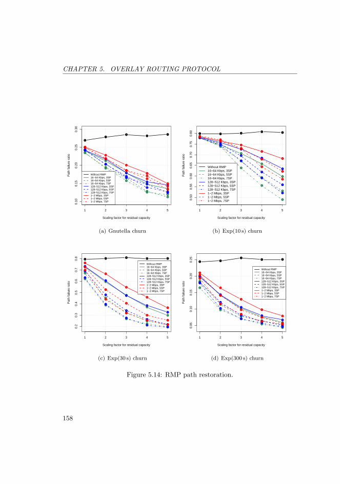
CHAPTER 5. OVERLAY ROUTING PROTOCOL
●
●
●●
●
1 2 3 4 5
0.10
0.15
0.20
0.25
0.30
Scaling factor for residual capacity
Pat
h fa
ilure
rat
io
●
●
●
●
●
●
●
●
●
●
●
●
●
●●
●
●
●
●
●
●
●
●
●
●
●
●
●
●
●
●
●
●
●
●
●
●
●
●
●
●
●
●
●
●
Without RMP16−64 Kbps, 3SP16−64 Kbps, 5SP16−64 Kbps, 7SP128−512 Kbps, 3SP128−512 Kbps, 5SP128−512 Kbps, 7SP1−2 Mbps, 3SP1−2 Mbps, 5SP1−2 Mbps, 7SP
(a) Gnutella churn
● ● ●● ●
1 2 3 4 5
0.50
0.55
0.60
0.65
0.70
0.75
0.80
Scaling factor for residual capacity
Pat
h fa
ilure
rat
io
●
●
●
●
●
●
●
●
●
●
●
●
●
●
●
●
●
●
●
●
●
●
●
●
●
●
●
●
●
●
●
●
●
●
●
●
●
●
●
●
●
●
●
●
●
Without RMP16−64 Kbps, 3SP16−64 Kbps, 5SP16−64 Kbps, 7SP128−512 Kbps, 3SP128−512 Kbps, 5SP128−512 Kbps, 7SP1−2 Mbps, 3SP1−2 Mbps, 5SP1−2 Mbps, 7SP
(b) Exp(10 s) churn
● ● ● ● ●
1 2 3 4 5
0.2
0.3
0.4
0.5
0.6
0.7
0.8
Scaling factor for residual capacity
Pat
h fa
ilure
rat
io
●
●
●
●
●
●
●
●
●
●
●
●
●
●
●
●
●
●
●
●
●
●
●
●
●
●
●
●
●●
●
●
●
●
●
●
●
●
●
●
●
●
●
●
●
Without RMP16−64 Kbps, 3SP16−64 Kbps, 5SP16−64 Kbps, 7SP128−512 Kbps, 3SP128−512 Kbps, 5SP128−512 Kbps, 7SP1−2 Mbps, 3SP1−2 Mbps, 5SP1−2 Mbps, 7SP
(c) Exp(30 s) churn
● ●
●● ●
1 2 3 4 5
0.05
0.10
0.15
0.20
0.25
Scaling factor for residual capacity
Pat
h fa
ilure
rat
io
●
●
●
●
●
●
●
●
●
●
●
●
●
●
●
●
●
●
●
●
●
●
●
●
●
●
●
●
●
●
●
●
●
●
●
●
●
●
●
●
●
●
●
●
●
Without RMP16−64 Kbps, 3SP16−64 Kbps, 5SP16−64 Kbps, 7SP128−512 Kbps, 3SP128−512 Kbps, 5SP128−512 Kbps, 7SP1−2 Mbps, 3SP1−2 Mbps, 5SP1−2 Mbps, 7SP
(d) Exp(300 s) churn
Figure 5.14: RMP path restoration.
158

5.4. ROUTE MAINTENANCE PROTOCOL
At the same time, the churn is less aggressive than in the case of Exp(10 s)scenarios. Hence, path diversity is less affected and backup paths are morestable.
Using more backup paths (i. e. , 5SPs or 7SPs) shows most gain in the case ofExp(30 s) scenarios for bandwidth range 1–2 Mbps. With less aggressive churn,the usefulness of additional backup paths decreases.
A complementary view of RMP’s path restoration success is shown in Fig-ure 5.15 in terms of the ratio of number of restored paths to the number ofbroken paths. RMP’s largest success in restoring broken paths is experienced inthe case of 16-64 Kbps scenarios, in each scenario. In Figure 5.15(c) for scalingfactor 4 and 5, the restored paths ratio for 128-512 Kbps scenarios with 7SPsis slightly higher than the restored path ratio for 16-64 Kbps scenarios with7SPs. These minimal differences are due to the random selection of source anddestination node for each flow demand.
The worst path restored ratio is observed in the case of 1–2 Mbps scenarioswith 3SPs. This is consistent across all subfigures in Figure 5.15 and is a directresult of lack of path diversity. In order to allocated 1–2 Mbps flow to a smallnumber of paths, those particular paths must have high residual capacity. Forthe topologies used, it is more likely to find a large number of paths with lowresidual capacity that together can accommodate the 1-2 Mbps broken flows.
As in case of RDP, the cost for using RMP is assessed in terms of bandwidthutilization and bandwidth overhead, as shown in Figure 5.16 and Figure 5.17,respectively.
Since RMP’s link vector algorithm uses triggered updates, it is no surprisethat the highest bandwidth utilization occurs in the case of aggressive churn asit can be observed in Figure 5.16(b) and Figure 5.16(c).
It should be recalled from Section 5.4.1 that RMP sends updates in re-sponse to changes in the topology table. The topology table stored at a nodeconsists of the node’s outgoing links, its source graph and the source graphs ofits neighbours. It should be clear that, with increasing number of backup paths,the number of links stored in the topology table grows as well. Consequently,changes to links in the network is more likely to trigger the node to send updatemessages. This behavior is observed in Figure 5.16 for 5SPs and 7SPs scenarios.
The bandwidth overhead shown in Figure 5.17 is computed by dividing the
159

CHAPTER 5. OVERLAY ROUTING PROTOCOL
●
●
●
●
●
1 2 3 4 5
0.0
0.1
0.2
0.3
0.4
0.5
0.6
Scaling factor for residual capacity
Res
tore
d pa
ths
ratio
●
●
●
●
●
●
●
●
●●
●
●
●
●
●
●
●
●
●
●
●
●
●
●
●
●
●
●
●
●
●
●
●
●
●
●
●
●
●
●
16−64 Kbps, 3SP16−64 Kbps, 5SP16−64 Kbps, 7SP128−512 Kbps, 3SP128−512 Kbps, 5SP128−512 Kbps, 7SP1−2 Mbps, 3SP1−2 Mbps, 5SP1−2 Mbps, 7SP
(a) Gnutella churn
●
●
●
●
●
1 2 3 4 5
0.0
0.1
0.2
0.3
0.4
Scaling factor for residual capacity
Res
tore
d pa
ths
ratio
●
●
●
●
●
●
●
●
●
●
●
●
●
●
●
●
●
●
●
●
●
●
●
●
●
●
●
●
●
●
●
●
●
●
●
●
●
●
●
●
16−64 Kbps, 3SP16−64 Kbps, 5SP16−64 Kbps, 7SP128−512 Kbps, 3SP128−512 Kbps, 5SP128−512 Kbps, 7SP1−2 Mbps, 3SP1−2 Mbps, 5SP1−2 Mbps, 7SP
(b) Exp(10 s) churn
●
●
●
●
●
1 2 3 4 5
0.0
0.2
0.4
0.6
0.8
Scaling factor for residual capacity
Res
tore
d pa
ths
ratio
●
●
●
●
●
●
●
●
●
●
●
●
●
●
●
●
●
●
●
●
●
●
●
●●
●
●
●
●
●
●
●
●
●
●
●
●
●
●
●
16−64 Kbps, 3SP16−64 Kbps, 5SP16−64 Kbps, 7SP128−512 Kbps, 3SP128−512 Kbps, 5SP128−512 Kbps, 7SP1−2 Mbps, 3SP1−2 Mbps, 5SP1−2 Mbps, 7SP
(c) Exp(30 s) churn
●
●
●
●
●
1 2 3 4 5
0.0
0.2
0.4
0.6
0.8
Scaling factor for residual capacity
Res
tore
d pa
ths
ratio
●
●
●
●
●
●
●
●
●
●
●
●
●
●
●
●
●
●
●
●
●
●
●
●
●
●
●
●
●
●
●
●
●
●
●
●
●
●
●●
16−64 Kbps, 3SP16−64 Kbps, 5SP16−64 Kbps, 7SP128−512 Kbps, 3SP128−512 Kbps, 5SP128−512 Kbps, 7SP1−2 Mbps, 3SP1−2 Mbps, 5SP1−2 Mbps, 7SP
(d) Exp(300 s) churn
Figure 5.15: RMP restored paths ratio.
160
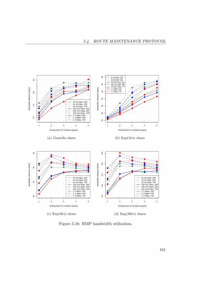
5.4. ROUTE MAINTENANCE PROTOCOL
●
●
● ●
●
1 2 3 4 5
7.0
7.5
8.0
8.5
Scaling factor for residual capacity
Ban
dwid
th u
tiliz
atio
n (K
bps)
●
●
●
●
●
●
●
●●
●
●
●
●
●
●
●
●
●
● ●
●
●
●
● ●
●
●
●
●
●
●
●
●●
●
●
●
●
●
●
16−64 Kbps, 3SP16−64 Kbps, 5SP16−64 Kbps, 7SP128−512 Kbps, 3SP128−512 Kbps, 5SP128−512 Kbps, 7SP1−2 Mbps, 3SP1−2 Mbps, 5SP1−2 Mbps, 7SP
(a) Gnutella churn
●
●
●
●
●
1 2 3 4 5
3436
3840
4244
46
Scaling factor for residual capacity
Ban
dwid
th u
tiliz
atio
n (K
bps)
●
●
●
●
●
●
●
●
●
●
●
●
●
●
●
●
●
●
●
●
●
●
●
●
●
●
●
●
●
●
●
●
●
●
●
●
●
●
●
●
16−64 Kbps, 3SP16−64 Kbps, 5SP16−64 Kbps, 7SP128−512 Kbps, 3SP128−512 Kbps, 5SP128−512 Kbps, 7SP1−2 Mbps, 3SP1−2 Mbps, 5SP1−2 Mbps, 7SP
(b) Exp(10 s) churn
●
●
● ● ●
1 2 3 4 5
3035
4045
Scaling factor for residual capacity
Ban
dwid
th u
tiliz
atio
n (K
bps)
●
● ●●
●
●
●
●
●
●
●
●
●● ●
●
●
●
●
●
●
●
●
●
●
●
●
●
● ●
●
●●
●
●
●
●
●
●●
16−64 Kbps, 3SP16−64 Kbps, 5SP16−64 Kbps, 7SP128−512 Kbps, 3SP128−512 Kbps, 5SP128−512 Kbps, 7SP1−2 Mbps, 3SP1−2 Mbps, 5SP1−2 Mbps, 7SP
(c) Exp(30 s) churn
●
●
● ●●
1 2 3 4 5
4.5
5.0
5.5
6.0
6.5
Scaling factor for residual capacity
Ban
dwid
th u
tiliz
atio
n (K
bps)
●
● ●● ●
●
●●
●
●
●
●
●●
●
●
●
●●
●●
●
●
●
●
●
●
●
●●
●
● ●
●
●
●
●
●
●
●
16−64 Kbps, 3SP16−64 Kbps, 5SP16−64 Kbps, 7SP128−512 Kbps, 3SP128−512 Kbps, 5SP128−512 Kbps, 7SP1−2 Mbps, 3SP1−2 Mbps, 5SP1−2 Mbps, 7SP
(d) Exp(300 s) churn
Figure 5.16: RMP bandwidth utilization.
161

CHAPTER 5. OVERLAY ROUTING PROTOCOL
●
●
●
●
●
1 2 3 4 5
Scaling factor for residual capacity
Ban
dwid
th o
verh
ead
02
××10
−−44
××10
−−46
××10
−−48
××10
−−410
××10
−−4
●
●
●
●
●
●
●
●
●
●
●
●● ● ●
●
●● ● ●
●
●● ● ●● ● ● ● ●
● ● ● ● ●● ● ● ● ●
16−64 Kbps, 3SP16−64 Kbps, 5SP16−64 Kbps, 7SP128−512 Kbps, 3SP128−512 Kbps, 5SP128−512 Kbps, 7SP1−2 Mbps, 3SP1−2 Mbps, 5SP1−2 Mbps, 7SP
(a) Gnutella churn
●
●
●
●
●
1 2 3 4 5
0.00
00.
001
0.00
20.
003
0.00
40.
005
Scaling factor for residual capacity
Ban
dwid
th o
verh
ead
●
●
●
●
●
●
●
●
●
●
●
●● ● ●
●
●● ● ●
●
●● ● ●●
● ● ● ●●
● ● ● ●●
● ● ● ●
16−64 Kbps, 3SP16−64 Kbps, 5SP16−64 Kbps, 7SP128−512 Kbps, 3SP128−512 Kbps, 5SP128−512 Kbps, 7SP1−2 Mbps, 3SP1−2 Mbps, 5SP1−2 Mbps, 7SP
(b) Exp(10 s) churn
●
●
●
●
●
1 2 3 4 5
0.00
00.
001
0.00
20.
003
0.00
40.
005
0.00
6
Scaling factor for residual capacity
Ban
dwid
th o
verh
ead
●
●
●
●
●
●
●
●
●
●
●
●● ● ●
●
●● ● ●
●
●● ● ●● ● ● ● ●
● ● ● ● ●● ● ● ● ●
16−64 Kbps, 3SP16−64 Kbps, 5SP16−64 Kbps, 7SP128−512 Kbps, 3SP128−512 Kbps, 5SP128−512 Kbps, 7SP1−2 Mbps, 3SP1−2 Mbps, 5SP1−2 Mbps, 7SP
(c) Exp(30 s) churn
●
●
●
●
●
1 2 3 4 5
Scaling factor for residual capacity
Ban
dwid
th o
verh
ead
02
××10
−−44
××10
−−46
××10
−−48
××10
−−4
●
●
●
●
●
●
●
●
●
●
●
●● ● ●
●
●● ● ●
●
●●
● ●● ● ● ● ●● ● ● ● ●● ● ● ● ●
16−64 Kbps, 3SP16−64 Kbps, 5SP16−64 Kbps, 7SP128−512 Kbps, 3SP128−512 Kbps, 5SP128−512 Kbps, 7SP1−2 Mbps, 3SP1−2 Mbps, 5SP1−2 Mbps, 7SP
(d) Exp(300 s) churn
Figure 5.17: RMP bandwidth overhead.
162

5.5. SUMMARY
bandwidth utilization with the network capacity, i. e. , the sum of residual ca-pacity and used capacity. In contrast to RDP’s bandwidth overhead, the RMPbandwidth overhead is biased. For example, the 16–64 Kbps scenarios dominatein each of the churn scenarios. This happens because the amount of averageresidual capacity per link is determined by the product between the scaling fac-tor in use and the upper bound of the bandwidth range. Hence, the networkcapacity for 16–64 Kbps scenarios is always lower than for the other two band-width ranges. Comparison of bandwidth overhead is fair only for graphs withinthe same bandwidth range.
For each bandwidth range, the largest bandwidth overhead occurs in 7SPsscenarios with Exp(30 s) churn when the scaling factor is equal to one: 0.6 %in the case of 16–64 Kbps scenarios, 0.07 % in the case of 128–512 Kbps scenar-ios, and 0.02 % in the case of 1–2 Mbps scenarios. RMP is less successful inestablishing backup paths for Exp(10 s) scenarios. This explains why Exp(10 s)scenarios show lower bandwidth overhead than Exp(30 s) scenarios. The low-est bandwidth overhead occurs in the case of Exp(300 s) scenarios where it isapproximately one magnitude lower than in the other scenarios.
5.5 Summary
At the beginning of this chapter a brief overview of QoS routing was provided.This was followed by a discussion about the design assumptions used in thedesign of ORP. The discussion included the type of underlying environmentand the targeted multimedia applications. The remaining part of the chapterdescribed RDP and RMP, the simulations performed for each protocol, and theperformance results obtained from the simulations.
RDP is used to select a path between two nodes subject to a number ofQoS constraints. Results from the RDP simulations indicate that the protocolcan find bandwidth-constrained paths with no more than 0.03 % overhead ina network with 1000 nodes when TTL=8. The call blocking ratio depends onthe amount of available bandwidth in the network, but it is also sensitive tothe TTL value in use. When the utilization factor increases, the bandwidthoverhead increases as well, especially in the case of 16–64 Kbps flow demands.Also, as the utilization increases, the call blocking ratio becomes increasingly
163
CHAPTER 5. OVERLAY ROUTING PROTOCOL
sensitive to the amount of available bandwidth in the network.RMP is used to restore RDP paths when the original paths are broken. This
includes the case when the path QoS constraints can no longer be satisfied. Alink vector algorithm is used to share link state information among neighbouringnodes. When path needs to be restored, Yen’s KSP is used to compute backuppaths and the affected flows are allocated to them. RMP can be quite efficientin restoring broken paths provided enough residual capacity is available. Forexample in Exp(30 s) scenarios, in spite of aggressive churn, RMP is able torestore up to 40 % of broken paths used for transporting 1–2 Mbps flows, withapproximately 0.02 % bandwidth overhead.
The worst-case cost in the case of RDP, namely 0.9 % bandwidth overhead,occurs for 16–64 Kbps flow demands with 180 seconds mean session durationwhen the utilization factor is one. For RMP, the worst-case cost, 0.6 %, occursin Exp(30 s) scenarios with 16-64 Kbps flow demands, 7SPs and scaling factorone for residual capacity. Assuming an additive cost when RDP and RMP arebeing used together, the worst-case cost is estimated to be as high as 1.5 %protocol overhead in terms of bandwidth.
164
Chapter 6
Conclusions and Future Work
Wide availability of computing resources at the edge of the network has leadto the appearance of services implemented in overlay networks. These applica-tions often utilize end-node resources as infrastructure rather than relying ondedicated resources. This approach greatly reduces the deployment effort andthe cost for the service in question.
The dissertation addresses the problem of unicast QoS routing in overlaynetworks. More precisely, the emphasis is on methods for providing a QoS-aware service on top of IP’s best-effort service, with minimal changes to existingInternet infrastructure.
6.1 Contributions of the Thesis
The ORP framework for QoS routing is proposed along with a set of de-sign assumptions on the environment and multimedia application for whichORP can be used. The framework consists of two protocols: Route DiscoveryProtocol (RDP) and Route Management Protocol (RMP). RDP is used to findpaths subject to a number of QoS constraints and RMP’s task is to maintainthem when churn occurs. The design and implementation of both protocols ispresented and their performance is evaluated through an extensive simulationstudy. The study is focused on several parameters that capture the success offinding and maintaining QoS paths along with the cost in terms of bandwidth
165

CHAPTER 6. CONCLUSIONS AND FUTURE WORK
overhead for using these protocols.A Gnutella study was performed in order to gain a better understanding of
the dynamics that occur in an overlay network. The study resulted in highlydetailed statistical models and characteristics for Gnutella traffic crossing anultrapeer. The models for session arrival and session duration were later usedto generate churn in the ORP simulations. An additional contribution is thedesign and implementation of a flexible software library for P2P traffic decoding,based on tcptrace.
An important part of RMP’s operation involves solving linear optimiza-tion problems for flow allocation. A software library for solving network flowproblems was designed, based on the GLPK implementation of the simplexmethod and interior point method. The software library implementation, calledliboptim, can be relatively easy extended to include additional flow problemsand algorithms.
The liboptim library was essential for the implementation of a performancetestbed for network flow algorithms. The testbed was used for performancemeasurements of the simplex method and interior point method as implementedby GLPK. Based on these measurements the simplex method was selected foruse in RMP.
6.2 Future Directions and Research
The results of the performance study reported in the previous chapter indicatethat ORP is a viable solution for QoS routing. The intention is to run similartests in a more realistic environment, such as PlanetLab. However, a realis-tic PlanetLab implementation requires that ORP is extended to include twoimportant elements: an overlay network that organizes nodes and transportsORP messages and the ability to measure link-state variables (e. g. , availablebandwidth, delay and loss).
ORP’s initial design envisioned the Gnutella network as the overlay of choicefor ORP. In fact, the CPs and APs used by RDP can be directly mapped onGnutella’s QUERY and QUERY HIT messages. For DPs and RMP link-stateupdates, either a new message type can be created or a existing message type(e. g. , QUERY HIT) can be extended to include ORP data. However, ORP can
166
6.2. FUTURE DIRECTIONS AND RESEARCH
use any overlay that can forward message and address individual nodes.Several methods for active measurement [171–175] exist already. It is im-
portant that these methods are evaluated and a subset suitable for ORP isselected.
There is a certain latency involved in obtaining link-state information viaactive measurements, as it was explained in Section 5.2. An interesting item forfuture work involves estimating the extent of this latency, its effect on ORP’sability to react to changes in the link-state, and finding methods to reduce it.
RDP’s current path-selection policy is to use the path determined by thefirst CP arriving at the destination node. This policy favours paths with shortone-way delay but can create hot-spots in the network. Future research shouldtherefore also focus on designing policies for load-balancing in order to improvethe utilization of network resources.
All experiments presented here focus on a single QoS metric: bandwidth.Additional experiments should be performed to evaluate ORP’s performancewhen several QoS metrics are used. For RMP, this requires that Yen’s KSPalgorithm is replaced by SAMCRA or a similar algorithm.
167

CHAPTER 6. CONCLUSIONS AND FUTURE WORK
168
Appendix A
Acronyms
ccdf complementary cumulative
distribution function
cdf cumulative distribution
function
cedf complementary empirical
distribution function
edf empirical distribution
function
pdf probability density function
AODV ad-hoc on-demand distance
vector
AP acknowledgement packet
API application programming
interface
AS autonomous system
BFS breadth-first-search
BGP Border Gateway Protocol
BTH Blekinge Institute of
Technology
CLVL controlled-loss virtual link
CP control packet
CPU central processing unit
DFS depth-first-search
DHT distributed hash table
DiffServ Differentiated Services
DP data packet
DSDV destination sequence
distance vector
DSR dynamic source routing
EDA exploratory data analysis
FEC forward error correction
FIFO first in first out
169
APPENDIX A. ACRONYMS
FR flow relay
GCC GNU Compiler Collection
GLPK GNU Linear Programming
Toolkit
GSL GNU Scientific Library
GT-ITM Georgia Tech - Internetwork
Topology Models
GUID globally unique identifier
GWC Gnutella Web Cache
HSEP Horizon Size Estimation
Protocol
HTTP Hypertext Transfer
Protocol
IP Internet Protocol
IPM interior point method
ISP Internet service provider
IPTV IP Television
IntServ Integrated Services
KSP K shortest paths
LN leaf node
MCP multi-constrained path
MCOP multi-constrained optimal
path
ML maximum likelihood
MOS mean opinion score
NAT Network Address
Translation
NED Network Description
ORP Overlay Routing Protocol
OSPF Open Shortest Path First
P2P peer-to-peer
PAP pure allocation problem
PAP-MLPF PAP with modified
link-path formulation
PCAP packet capture
PIT probability integral
transform
PSO particle swarm optimization
QoE quality of experience
QoS quality of service
QRON QoS-aware routing protocol
for overlay networks
QRP Query Routing Protocol
QSON QoS overlay network
RDP Route Discovery Protocol
RIP Routing Information
Protocol
RMP Route Management
Protocol
RON Resilient Overlay Network
ROVER Routing in Overlay
Networks
170
RSVP Resource Reservation
Protocol
RTT round-trip time
SAMCRA Self-Adaptive Multiple
Constraints Routing
Algorithm
SLA service level agreement
SSH Secure Shell
STL Standard Template Library
SVD singular value
decomposition
TCP Transmission Control
Protocol
TTL time-to-live
UDP User Datagram Protocol
UHC UDP Host Cache
UMTS Universal Mobile
Telecommunications System
UTC Coordinated Universal
Time
UUID universally unique identifier
UP ultrapeer
VoD video on demand
VoIP voice over IP
171

APPENDIX A. ACRONYMS
172
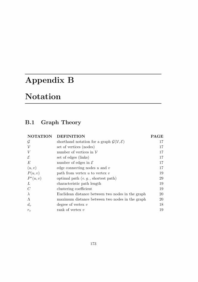
Appendix B
Notation
B.1 Graph Theory
NOTATION DEFINITION PAGEG shorthand notation for a graph G(V, E) 17V set of vertices (nodes) 17V number of vertices in V 17E set of edges (links) 17E number of edges in E 17(u, v) edge connecting nodes u and v 17P (u, v) path from vertex u to vertex v 19P ∗(u, v) optimal path (e. g. , shortest path) 29L characteristic path length 19C clustering coefficient 19λ Euclidean distance between two nodes in the graph 20Λ maximum distance between two nodes in the graph 20dv degree of vertex v 18rv rank of vertex v 19
173

APPENDIX B. NOTATION
B.2 Probability and Statistics
NOTATION DEFINITION PAGEθ distribution parameter 81θ point estimate of θ 87fX (x; θ) pdf for the random variable X 81FX (x; θ) cdf for the random variable X 81FX (x; θ) ccdf for the random variable X 82FX (x; θ) edf for the random variable X 86FX (x; θ) cedf for the random variable X 86Xn nth element of a random sample 82X(n) nth order statistic 83E[X] expected value of the random variable X 83Var[X] variance of the random variable X 87µ = X sample mean (point estimate) 83σ sample standard deviation (point estimate) 83
174
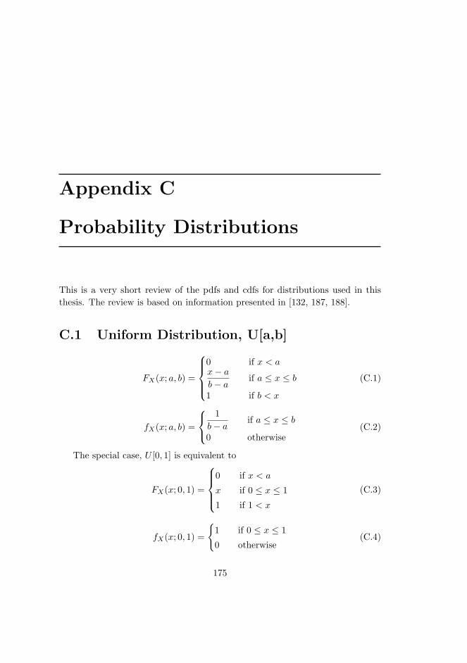
Appendix C
Probability Distributions
This is a very short review of the pdfs and cdfs for distributions used in thisthesis. The review is based on information presented in [132, 187, 188].
C.1 Uniform Distribution, U[a,b]
FX(x; a, b) =
0 if x < ax− ab− a
if a ≤ x ≤ b
1 if b < x
(C.1)
fX(x; a, b) =
1
b− aif a ≤ x ≤ b
0 otherwise(C.2)
The special case, U [0, 1] is equivalent to
FX(x; 0, 1) =
0 if x < a
x if 0 ≤ x ≤ 1
1 if 1 < x
(C.3)
fX(x; 0, 1) =
{1 if 0 ≤ x ≤ 1
0 otherwise(C.4)
175
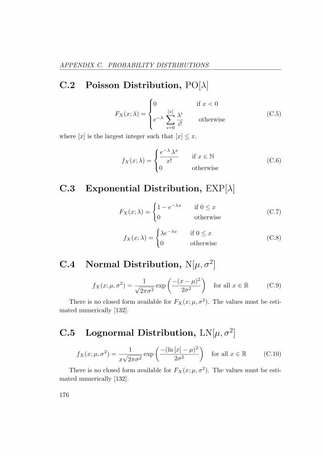
APPENDIX C. PROBABILITY DISTRIBUTIONS
C.2 Poisson Distribution, PO[λ]
FX(x;λ) =
0 if x < 0
e−λ[x]∑i=0
λi
i!otherwise
(C.5)
where [x] is the largest integer such that [x] ≤ x.
fX(x;λ) =
e−λ λx
x!if x ∈ N
0 otherwise(C.6)
C.3 Exponential Distribution, EXP[λ]
FX(x;λ) =
{1− e−λx if 0 ≤ x0 otherwise
(C.7)
fX(x;λ) =
{λe−λx if 0 ≤ x0 otherwise
(C.8)
C.4 Normal Distribution, N[µ, σ2]
fX(x;µ, σ2) =1√
2πσ2exp
(−(x− µ)2
2σ2
)for all x ∈ R (C.9)
There is no closed form available for FX(x;µ, σ2). The values must be esti-mated numerically [132].
C.5 Lognormal Distribution, LN[µ, σ2]
fX(x;µ, σ2) =1
x√
2πσ2exp
(−(ln [x]− µ)2
2σ2
)for all x ∈ R (C.10)
There is no closed form available for FX(x;µ, σ2). The values must be esti-mated numerically [132].
176
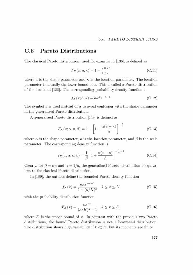
C.6. PARETO DISTRIBUTIONS
C.6 Pareto Distributions
The classical Pareto distribution, used for example in [136], is defined as
FX(x; a, κ) = 1−(κx
)a(C.11)
where a is the shape parameter and κ is the location parameter. The locationparameter is actually the lower bound of x. This is called a Pareto distributionof the first kind [188]. The corresponding probability density function is
fX(x; a, κ) = aκax−a−1 (C.12)
The symbol a is used instead of α to avoid confusion with the shape parameterin the generalized Pareto distribution.
A generalized Pareto distribution [149] is defined as
FX(x;α, κ, β) = 1−[1 +
α(x− κ)β
]− 1α
(C.13)
where α is the shape parameter, κ is the location parameter, and β is the scaleparameter. The corresponding density function is
fX(x;α, κ, β) =1β
[1 +
α(x− κ)β
]− 1α−1
(C.14)
Clearly, for β = ακ and α = 1/a, the generalized Pareto distribution is equiva-lent to the classical Pareto distribution.
In [189], the authors define the bounded Pareto density function
fX(x) =aκx−a−1
1− (κ/K)ak ≤ x ≤ K (C.15)
with the probability distribution function
FX(x) =κx−a
(κ/K)a − 1k ≤ x ≤ K. (C.16)
where K is the upper bound of x. In contrast with the previous two Paretodistributions, the bound Pareto distribution is not a heavy-tail distribution.The distribution shows high variability if k � K, but its moments are finite.
177

APPENDIX C. PROBABILITY DISTRIBUTIONS
178
BIBLIOGRAPHY
Bibliography
[1] Google Inc., “Youtube,” 2008. [Online]. Available: http://www.youtube.com
[2] Skype Communications, “Skype,” Mar. 2006. [Online]. Available:http://www.skype.com
[3] Z. Wang, Internet QoS: Architectures and Mechanisms for Quality of Ser-vice. San Francisco, CA, USA: Morgan Kaufman Publishers, 2000, ISBN:1-55860-608-4.
[4] Cisco Systems, Internetworking Technologies Handbook. Cisco Press,2003, ch. Quality of Service (QoS). [Online]. Available: http://www.cisco.com/en/US/docs/internetworking/technology/handbook/QoS% .html
[5] R. Braden, D. D. Clark, and S. Shenker, RFC 1633: Integrated Servicesin the Internet Architecture: an Overview, IETF, Jun. 1994, category:Informational. [Online]. Available: http://www.ietf.org/ietf/rfc1633.txt
[6] L. Zhang, S. Deering, D. Estrin, S. Shenker, and D. Zappala, “RSVP: Anew resource reservation protocol,” IEEE Network, vol. 7, no. 5, pp. 8–18,Sep. 1993.
[7] J. Wroclawski, RFC 2210: The Use of RSVP with IETF IntegratedServices, IETF, Sep. 1997, category: Standards Track. [Online].Available: http://www.ietf.org/ietf/rfc2210.txt
179
BIBLIOGRAPHY
[8] K. Thompson, G. J. Miller, and R. Wilder, “Wide-area Internet trafficpatterns and characteristics,” IEEE Network, vol. 11, no. 6, pp. 10–23,Nov. 1997.
[9] C. Fraleigh, S. Moon, B. Lyles, C. Cotton, M. Khan, D. Moll, R. Rockell,T. Seely, and C. Diot, “Packet-level traffic measurements from the SprintIP backbone,” IEEE Network, vol. 17, no. 6, pp. 6–16, Nov. 2003.
[10] S. Blake, D. L. Black, M. A. Carlson, E. Davies, Z. Wang, and W. Weiss,“An architecture for differentiated services,” RFC 2475, Dec. 1998.[Online]. Available: http://www.ietf.org/ietf/rfc2475.txt
[11] C. Bouras and A. Sevasti, “Service level agreements for DiffServ-basedservices’ provisioning,” Journal of Computer Networks, vol. 28, no. 4, pp.285–302, Nov. 2005.
[12] T. Hoßfeld, P. Tran-Gia, and M. Fiedler, “Quantification of quality ofexperience for edge-based applications,” in Proceedings of ITC, Ottawa,Canada, Jun. 2007, pp. 361–373.
[13] S. Winkler and C. Faller, “Perceived audiovisual quality of low-bitratemultimedia content,” IEEE Transactions on Multimedia, vol. 8, no. 5, pp.973–980, Oct. 2006.
[14] L. Ding, Z. Lin, A. Radwan, M. S. El-Hennawey, and R. A. Goubran,“Non-intrusive single ended speech quality assessment in VoIP,” Journalof Speech Communication, vol. 49, pp. 477–489, Apr. 2007.
[15] V. Grancharov, D. Y. Zhao, J. Lindblom, and W. B. Kleijn, “Low-complexity, nonintrusive speech quality assessment,” IEEE Transactionson Audio, Speech, and Language Processing, vol. 14, no. 6, pp. 1948–1956,Nov. 2006.
[16] T. M. O’Neil, “Quality of experience and quality of service for IP videoconferencing,” Polycom Video Communications, Milpitas, CA, USA,White paper, 2002.
[17] G. J. Armitage, “Revisiting IP QOS,” ACM SIGCOMM Computer Com-munications Review, vol. 33, no. 5, pp. 81–88, Oct. 2003.
180
BIBLIOGRAPHY
[18] G. Bell, “Failure to thrive: QoS and the culture of operational network-ing,” in Proceedings ot the ACM SIGCOMM Workshops, Karlsruhe, Ger-many, Aug. 2003, pp. 115–120.
[19] L. Burgsthaler, K. Dolzer, C. Hauser, J. Jahnert, S. Junghans, C. Macian,and W. Payer, “Beyond technology: The missing pieces for QoS success,”in Proceedings ot the ACM SIGCOMM Workshops, Karlsruhe, Germany,Aug. 2003, pp. 121–130.
[20] L. L. Peterson and B. S. Davie, Computer Networks: A Systems Approach,2nd ed. San Francisco, CA, USA: Morgan Kaufman Publishers, 2000,ISBN: 1-55860-514-2.
[21] G. Malkin, RFC 2453: RIP Version 2, IETF, Nov. 1998, category:Standards Track. [Online]. Available: http://www.ietf.org/ietf/rfc2453.txt
[22] J. Moy, RFC 2328: OSPF Version 2, IETF, Apr. 1998. [Online].Available: http://www.ietf.org/ietf/rfc2328.txt
[23] Y. Rekhter, T. Li, and S. Hares, RFC 4271: A Border GatewayProtocol 4 (BGP-4), IETF, Jan. 2006. [Online]. Available: http://www.ietf.org/ietf/rfc4271.txt
[24] C. Huitema, Routing in the Internet, 2nd ed. Upper Saddle River, NJ,USA: Prentice Hall, 2000, ISBN: 0-13-022647-5.
[25] J. F. Kurose and K. W. Ross, Computer Networking: A Top-Down Ap-proach Featuring the Internet. Boston, MA, USA: Addison Wesley Long-man, 2001, ISBN: 0-201-47711-4.
[26] D. G. Andersen, “Resilient overlay networks,” Master’s thesis, Dept. ofElectrical Engineering and Computer Science, Massachusetts Institute ofTechnology, May 2001.
[27] M. Castro, P. Druschel, A.-M. Kermarrec, A. Nandi, A. Rowstron, andA. Singh, “Splitstream: High-bandwidth multicast in a cooperative envi-ronment,” in Proceeding of IPTPS, Berkeley, CA, USA, Feb. 2003.
181
BIBLIOGRAPHY
[28] Y. Cui, B. Li, and K. Nahrstedt, “oStream: Asynchronous streaming mul-ticast in application-layer overlay networks,” IEEE Journal on SelectedAreas in Communications, vol. 22, no. 1, pp. 91–106, Jan. 2004.
[29] Z. Li and P. Mohapatra, “QRON: QoS-aware routing in overlay networks,”IEEE Journal on Selected Areas in Communications, vol. 22, no. 1, pp.29–40, Jan. 2004.
[30] L. Subramanian, I. Stoica, H. Balakrishnan, and R. Katz, “OverQoS: Anoverlay based architecture for enhancing Internet QoS,” in Proceedings ofNSDI, San Francisco, CA, USA, Mar. 2004.
[31] D. Ilie and A. Popescu, “A framework for overlay QoS routing,” in Pro-ceedings of 4th Euro-FGI Workshop, Ghent, Belgium, May 2007.
[32] I. Stoica, R. Morris, D. Karger, F. Kaashoek, and H. Balakrishnan,“Chord: A scalable peer-to-peer lookup service for internet applications,”in Proceedings of ACM SIGCOMM, San Diego, CA, USA, Aug. 2001, pp.149–160.
[33] I. Stoica, D. Adkins, S. Zhuang, S. Shenker, and S. Surana, “Internet in-direction infrastructure,” in Proceedings of ACM SIGCOMM, Pittsburgh,PA, USA, Aug. 2002, pp. 73–88.
[34] P. Maymounkov and D. Mazieres, “Kademlia: A peer-to-peer informationsystem based on the xor metric,” in Proceedings of IPTPS, Berkeley, CA,USA, Mar. 2002.
[35] F. Dabek, B. Zhao, P. Druschel, J. Kubiatowicz, and I. Stoica, “Towardsa common API for structured peer-to-peer overlays,” in Proceedings ofIPTPS, Berkeley, CA, USA, Feb. 2003.
[36] E. Adar and B. A. Huberman, “Free riding on gnutella,” FirstMonday, vol. 5, no. 10, Oct. 2000. [Online]. Available: http://www.firstmonday.org/issues/issue5\ 10/adar/index.html
[37] G. Hardin, “The tragedy of the commons,” Science, vol. 162, pp.1243–1248, Dec. 1968. [Online]. Available: http://www.sciencemag.org/cgi/content/full/162/3859/1243
182

BIBLIOGRAPHY
[38] J. Ritter, Why Gnutella Can’t Scale. No, Really., Feb. 2001. [Online].Available: http://www.darkridge.com/∼jpr5/doc/gnutella.html
[39] S. Saroiu, P. K. Gummadi, and S. D. Gribble, “A measurement studyof peer-to-peer file sharing systems,” in Proceedings of MMCN, San Jose,CA, USA, Jan. 2002.
[40] S. Sen and J. Wang, “A measurement study of peer-to-peer file sharingsystems,” in Proceedings of the 2nd ACM SIGCOMM Workshop on In-ternet measurment, Marseille, France, Nov. 2002, pp. 137–150.
[41] N. B. Azzouna and F. Guillemin, “Experimental analysis of the impact ofpeer-to-peer applications on traffic in commercial IP networks,” EuropeanTransactions on Telecommunications: Special Issue on P2P Networkingand P2P Services, 2004.
[42] T. Karagiannis, A. Broido, N. Brownlee, K. Claffy, and M. Faloutsos,“File-sharing in the internet: A characterization of P2P traffic in thebackbone,” University of California, Riverside, Tech. Rep., Nov. 2003.
[43] ——, “Is P2P dying or just hiding?” in Proceedings of IEEE Globecom,Dallas, TX, USA, Dec. 2004.
[44] T. Karagiannis, A. Broido, M. Faloutsos, and K. Claffy, “Transport layeridentification of P2P traffic,” in Proceedings of IMC, Taormina, Sicily,Italy, Oct. 2004.
[45] L. Lao, S. S. Gokhale, and J.-H. Cui, “Distributed QoS routing for back-bone overlay networks,” in Proceedings of IFIP Networking, Coimbra, Por-tugal, May 2006.
[46] D. Ilie, “Overlay routing protocol (ORP),” Dec. 2004, unpublished archi-tecture and design document.
[47] K. De Vogeleer, “QoS routing in overlay networks,” Master’s thesis,Blekinge Institute of Technology (BTH), Karlskrona, Sweden, Jun. 2007,MEE07:24.
183

BIBLIOGRAPHY
[48] D. P. Bertsekas and J. N. Tsitsiklis, Parallel and Distributed Computation:Numerical Methods. Belmont, MA, USA: Athena Scientific, 1997, ISBN:1-886529-01-9.
[49] D. P. Bertsekas and R. G. Gallager, Data Networks, 2nd ed. UpperSaddle River, NJ, USA: Prentice Hall, 1991, ISBN: 0-13-200916-1.
[50] C. H. Papadimitriou and K. Steiglitz, Combinatorial Optimization: Algo-rithms and Complexity. Mineola, NY, USA: Dover Publications, 1998,ISBN: 0-486-40258-4.
[51] T. H. Cormen, C. E. Leiserson, and R. L. Rivest, Introduction to Algo-rithms, 2nd ed. Cambridge, MA, USA: The MIT Press, 2001, ISBN:0-262-53196-8.
[52] T. Bu and D. Towsley, “On distinguishing between Internet power lawtopology generators,” in Proceedings of IEEE INFOCOM, Amherst, MA,USA, Jun. 2002.
[53] D. J. Watts and S. H. Strogatz, “Collective dynamics of ’small-world’networks,” Nature, vol. 393, no. 6684, pp. 440–442, Jun. 1998.
[54] S. Jin and A. Bestavros, “Small-world characteristics of Internet topologiesand implications on multicast scaling,” Journal of Computer Networks,vol. 50, no. 5, pp. 648–666, Apr. 2006.
[55] F. A. Kuipers, “Quality of service routing in the internet: Theory, com-plexity and algorithms,” Ph.D. dissertation, Delft University, Delft, TheNetherlands, 2004, ISBN: 90-407-2523-3.
[56] B. M. Waxman, “Routing of multipoint connections,” IEEE Journal onSelected Areas in Communications, vol. 6, no. 9, pp. 1617–1622, Dec. 1988.
[57] E. W. Zegura, K. L. Calvert, and M. J. Donahoo, “A quantitative com-parison of graph-based models for Internet topology,” IEEE/ACM Trans-actions on Networking, vol. 5, no. 6, pp. 770–783, Dec. 1997.
[58] “GT-ITM: Georgia Tech internetwork topology models,” 1997. [Online].Available: http://www.cc.gatech.edu/projects/gtitm
184
BIBLIOGRAPHY
[59] M. Faloutsos, P. Faloutsos, and C. Faloutsos, “On power-law relationshipsof the internet topology,” in Proceedings of SIGCOMM, Cambridge, MA,USA, Aug. 1999, pp. 251–262.
[60] A. Medina, I. Matta, and J. Byers, “On the origin of power laws in In-ternet topologies,” ACM SIGCOMM Computer Communications Review,vol. 30, no. 2, pp. 18–28, Apr. 2000.
[61] G. Siganos, M. Faloutsos, P. Faloutsos, and C. Faloutsos, “Power laws andthe AS-level Internet topology,” IEEE/ACM Transactions on Networking,vol. 11, no. 4, pp. 514–524, Aug. 2003.
[62] A.-L. Barabasi and R. Albert, “Emergence of scaling in random networks,”Science, vol. 286, pp. 509–512, Oct. 1999.
[63] A. Medina, A. Lakhina, I. Matta, and J. Byers, “BRITE: Universaltopology generation from a user’s perspective,” Boston University,Boston, MA, USA, Tech. Rep. BUCS-TR-20001-03, Apr. 2001. [Online].Available: http://www.cs.bu.edu/brite
[64] R. K. Ahuja, T. L. Magnanti, and J. B. Orlin, Network Flows: Theories,Algorithms, and Applications. Upper Saddle River, NJ, USA: PrenticeHall, 1993, ISBN: 0-13-617549-X.
[65] M. R. Garey and D. S. Johnson, Computers and Intractability: A Guideto the Theory of NP-Completness. New York, NY, USA: W. H. Freemanand Company, 1979, ISBN: 0-7167-1045-5.
[66] D. G. Luenberger, Linear and Nonlinear Programming. Norwell, MA,USA: Kluwer Academic Publishers, 2004, ISBN: 1-4020-7593-6.
[67] R. W. Hamming, Numerical Methods for Scientists and Engineers. Mi-neola, NY, USA: Dover Publications, 1986, ISBN: 0-486-65241-6.
[68] G. H. Golub and C. F. Van Loan, Matrix Computations, 3rd ed. Bal-timore, MD, USA: The Johns Hopkins University Press, 1996, ISBN: 0-8018-5414-8.
185
BIBLIOGRAPHY
[69] Y. Donoso and R. Fabregat, Multi-Objective Optimization in ComputerNetworks Using Metaheuristics. Boca Raton, FL, USA: Auerbach Pub-lications, 2007, ISBN: 0-8493-8084-7.
[70] M. Pioro and D. Medhi, Routing, Flow, and Capacity Design in Com-munication and Computer Networks. San Francisco, CA, USA: MorganKaufman Publishers, 2004, ISBN: 0-12-557189-5.
[71] C. Blum and A. Roli, “Metaheuristics in combinatorial optimization:Overview and conceptual comparison,” ACM Computing Surveys, vol. 35,no. 3, pp. 268–308, Sep. 2003.
[72] A. P. Engelbrecht, Fundamentals of Computational Swarm Intelligence.Chichester, West Sussex, England: John Wiley & Sons, 2006, ISBN: 0-470-09191-6.
[73] M. Sipser, Introduction to the Theory of Computation. Boston, MA,USA: PWS Publishing Company, 1997, ISBN: 981-240-226-8.
[74] S. A. Cook, “An overview of computational complexity,” Communicationsof the ACM, vol. 26, no. 6, pp. 400–408, Jun. 1983.
[75] Z. Wang and J. Crowfort, “Quality-of-service routing for supporting multi-media applications,” IEEE Journal on Selected Areas in Communications,vol. 14, no. 7, pp. 1228–1234, Sep. 1996.
[76] F. A. Kuipers and P. F. A. Van Mieghem, “Conditions that impact thecomplexity of QoS routing,” IEEE/ACM Transactions on Networking,vol. 13, no. 4, pp. 717–730, Aug. 2005.
[77] S. A. Vavasis, Nonlinear Optimization: Complexity Issues. Oxford, UK:Oxford University Press, 1991, ISBN: 0-19-507208-1.
[78] M. Avriel, Nonlinear Programming: Analysis and Methods. Mineola, NY,USA: Dover Publications, 2003, ISBN: 0-486-43227-0.
[79] J. Y. Yen, “Finding the k shortest loopless paths in a network,” Manage-ment Science, vol. 17, no. 11, pp. 712–716, Jul. 1971.
186
BIBLIOGRAPHY
[80] E. Q. V. Martins and M. M. B. Pascoal, “A new implementation ofYen’s ranking loopless paths algorithms,” Quarterly Journal of the Bel-gian, French and Italian Operations Research Societies, vol. 1, no. 2, pp.121–133, 2003.
[81] R. Bellman, “On a routing problem,” Quarterly of Applied Mathematics,vol. 16, no. 1, pp. 87–90, 1958.
[82] R. L. Ford, Jr. and D. R. Fulkerson, Flows in Networks. Princeton, NJ,USA: Princeton University Press, 1962, ISBN: 0-691-07962-5.
[83] E. W. Dijkstra, “A note on two problems in connection with graphs,”Numerische Mathematik, vol. 1, pp. 269–271, 1959.
[84] M. L. Fredman and R. E. Tarjan, “Fibonacci heaps and their uses inimproved network optimization algorithms,” Journal of the ACM, vol. 34,no. 3, pp. 596–615, Jul. 1987.
[85] J. Hershberger, M. Maxel, and S. Suri, “Finding the k shortest simplepaths: A new algorithm and its implementation,” ACM Transactions onAlgorithms, vol. 3, no. 4, pp. 45:1–45:19, 2007.
[86] D. Ilie, “Optimization algorithms with applications to unicast QoS rout-ing in overlay networks,” Blekinge Institute of Technology, Karlskrona,Sweden, Research Report 2007:09, Sep. 2007, ISSN: 1103-1581.
[87] J. Nocedal and J. S. Wright, Numerical Optimization, 2nd ed. New York,NY, USA: Springer Science+Business Media, 2006, ISBN: 0-387-30303-0.
[88] S. Mehrotra, “On the implementation of a primal-dual interior pointmethod,” SIAM Journal on Optimization, vol. 2, no. 4, pp. 575–601, Nov.1992.
[89] P. Van Mieghem and F. A. Kuipers, “Concepts of exact QoS routingalgorithms,” IEEE/ACM Transactions on Networking, vol. 12, no. 5, pp.851–864, Oct. 2004.
[90] F. Kuipers, P. Van Mieghem, T. Korkmaz, and M. Krunz, “An overview ofconstraint-based path selection algorithms for QoS routing,” IEEE Com-munications Magazine, vol. 40, no. 2, pp. 50–55, Dec. 2002.
187
BIBLIOGRAPHY
[91] S. Chen and K. Nahrstedt, “Distributed quality-of-service routing in high-speed networks based on selective probing,” in Proceedings of LCN, Lowell,MA, USA, Oct. 1998, pp. 80–89.
[92] M. R. Hestenes and E. Stiefel, “Methods of conjugate gradients for solvinglinear systems,” Journal of Research of the National Bureau of Standards,vol. 49, no. 6, pp. 409–436, Dec. 1952.
[93] W. H. Press, S. A. Teukolsky, W. T. Vettering, and B. P. Flannery, Nu-merical Recipes in C++: The Art of Scientific Computing, 2nd ed. Cam-bridge, UK: Cambridge University Press, 2002, ISBN: 0-521-75033-4.
[94] M. Matsumoto and T. Nishimura, “Mersenne Twister: A 623-dimensionally equidistributed uniform pseudo-random number genera-tor,” ACM Transactions on Modeling and Computer Simulation, vol. 8,no. 1, pp. 3–30, jan 1998.
[95] M. Galassi, J. Davies, J. Theiler, B. Gough, G. Jungman, M. Booth, andF. Rossi, GNU Scientific Library Reference Manual, 2nd ed. Bristol, UK:Network Theory Limited, 2006, ISBN: 0-9541617-3-4. [Online]. Available:http://www.gnu.org/software/gsl
[96] GNU Linux, “random, urandom — kernel random number sourcedevices,” in Linux Programmer’s Manual, Jan. 2008, RANDOM(4).[Online]. Available: http://www.kernel.org/doc/man-pages
[97] A. Makhorin, GNU Linear Programming Kit: Reference Manual version4.24, Moscow Aviation Institute, Moscow, Russia, Nov. 2007. [Online].Available: http://www.gnu.org/software/glpk
[98] GNU Linux, “proc — process information pseudo-filesystem,” inLinux Programmer’s Manual, Jan. 2008, PROC(5). [Online]. Available:http://www.kernel.org/doc/man-pages
[99] ——, “getrusage — get resource usage,” in Linux Programmer’sManual, Jan. 2008, GETRUSAGE(2). [Online]. Available: http://www.kernel.org/doc/man-pages
[100] ——, “gettimeofday, settimeofday — get / set time,” in Linux Program-mer’s Manual, 2008, GETTIMEOFDAY(2).
188

BIBLIOGRAPHY
[101] N. M. Josuttis, The C++ Standard Library: A Tutorial and Reference.Boston, MA, USA: Addison Wesley, 1999, ISBN: 0-201-37926-0.
[102] S. Meyers, Effective STL. Boston, MA, USA: Addison Wesley, 2001,ISBN: 0-201-74962-9.
[103] L. Torvalds, “do gettimeofday(),” Linux 2.6.14 Kernel Sources, 2005,arch/i386/kernel/time.c.
[104] D. Ilie, “Gnutella network traffic: Measurements and characteristics,”Licentiate Dissertation, Blekinge Institute of Technology (BTH), Karl-skrona, Sweden, Apr. 2006, ISBN: 91-7295-084-6.
[105] D. Ilie and A. Popescu, “Statistical models for Gnutella signaling traffic,”Journal of Computer Networks, vol. 51, no. 17, pp. 4816–4835, Dec. 2007.
[106] T. Klingberg and R. Manfredi, Gnutella 0.6, The Gnutella DeveloperForum (GDF), Jun. 2002. [Online]. Available: http://groups.yahoo.com/group/the gdf/files/Development
[107] A. Singla and C. Rohrs, Ultrapeers: Another Step Towards GnutellaScalability, 1st ed., Lime Wire LLC, Nov. 2002. [Online]. Available:http://groups.yahoo.com/group/the gdf/files/Development
[108] A. A. Fisk, Gnutella Dynamic Query Protocol, 0th ed., LimeWire LLC,May 2003. [Online]. Available: http://groups.yahoo.com/group/the gdf/files/Proposals/Working Proposals/search/Dynamic Querying
[109] P. Verdy, “Gnutella topology,” The Gnutella Developer Forum (GDF),Jan. 2006, http://groups.yahoo.com/group/the gdf/message/22187.
[110] Gnucleus, “Gnutella web cache,” Jun. 2006, http://www.gnucleus.com/gwebcache.
[111] GDF, “Gnutella protocol development,” Dec. 2005, http://www.the-gdf.org.
[112] R. Manfredi, Gnutella Traffic Compression, The Gnutella DeveloperForum (GDF), Jan. 2003. [Online]. Available: http://groups.yahoo.com/group/the gdf/files/Proposals/Working Proposals/Gnet Compression
189
BIBLIOGRAPHY
[113] J.-l. Gailly and M. Adler, “zlib,” Dec. 2005, http://www.gzip.org/zlib.
[114] P. Leach, M. Mealling, and R. Salz, RFC 4122: A Universally UniqueIDentifier (UUID) URN Namespace, Jul. 2005, category: StandardsTrack. [Online]. Available: http://www.ietf.org/ietf/rfc4122.txt
[115] C. Rohrs, SACHRIFC: Simple Flow Control for Gnutella, Lime Wire LLC,Mar. 2002.
[116] ——, Query Routing for the Gnutella Network, 1st ed., Lime Wire LLC,May 2002. [Online]. Available: http://groups.yahoo.com/group/the gdf/files/Development
[117] B. H. Bloom, “Space/time trade-offs in hash coding with allowable errors,”Communication of the ACM, vol. Volume 13, no. Number 7, pp. p. 422–426, July 1970, iSSN:0001-0782.
[118] A. A. Fisk, Gnutella Ultrapeer Query Routing, 0th ed., Lime Wire LLC,May 2003. [Online]. Available: http://groups.yahoo.com/group/the gdf/files/Proposals/Working Proposals/search/Ultrapeer QRP
[119] T. Schurger, Horizon size estimation on the Gnutella network v0.2, Mar.2004. [Online]. Available: http://www.menden.org/gnutella/hsep.html
[120] F. Michaut and F. Lepage, “Application-oriented network metrology:Metrics and active measurement tools,” IEEE Communications Surveys& Tutorials, vol. 7, no. 2, pp. 2–24, 2005.
[121] D. Ilie, D. Erman, A. Popescu, and A. A. Nilsson, “Traffic measurementsof P2P systems,” in Proceedings of SNCNW, Karlstad, Sweden, Nov. 2004,pp. 25–29.
[122] V. Jacobsen, C. Leres, and S. McCanne, “Tcpdump/libpcap,” http://www.tcpdump.org, Aug. 2005.
[123] S. Ostermann, “Tcptrace,” http://www.tcptrace.org, Aug. 2005.
[124] D. Ilie, D. Erman, A. Popescu, and A. A. Nilsson, “Measurement andanalysis of Gnutella signaling traffic,” in Proceedings of IPSI, Stockholm,Sweden, Sep. 2004.
190

BIBLIOGRAPHY
[125] D. Erman, “Bittorrent traffic measurements and models,” Licentiate Dis-sertation, Blekinge Institute of Technology (BTH), Karlskrona, Sweden,Oct. 2005, iSBN: 91-7295-071-4.
[126] D. Erman, D. Ilie, and A. Popescu, “BitTorrent session characteristics andmodels,” in Proceedings of HET-NETs, D. Kouvatsos, Ed., Ilkley, WestYorkshire, UK, Jul. 2005, pp. P30/1–P30/10.
[127] G. R. Wright and W. R. Stevens, TCP/IP Illustrated: The Implementa-tion. Boston, MA, USA: Addison Wesley, 1995, ISBN: 0-201-63354-X.
[128] V. Paxson, “Empirically derived analytic models for wide-area tcp con-nections,” IEEE/ACM Transactions on Networking, vol. 2, no. 4, pp.316–336, Aug. 1994.
[129] L. Kleinrock, Queueing Systems Volume 1: Theory. Hoboken, NJ, USA:John Wiley & Sons, 1975, ISBN: 0-471-49110-1.
[130] R. B. D’Agostino and M. A. Stephens, Goodness-of-Fit Techniques. NewYork, NY, USA: Marcel Dekker, Inc., 1986, ISBN: 0-8247-7487-6.
[131] J. Maindonald and J. Braun, Data Analysis and Graphics using R: AnExample-based Approach. Cambridge, UK: Cambridge University Press,2003, ISBN: 0-521-81336-0.
[132] A. M. Law and W. D. Kelton, Simulation Modeling and Analysis, 3rd ed.New York, NY, USA: McGraw-Hill, 2000, ISBN: 0-07-059292-6.
[133] W. N. Venables and B. D. Ripley, Modern Applied Statistics with S-PLUS,3rd ed. New York, NY, USA: Springer-Verlag, 1999, ISBN: 0-387-98825-4.
[134] M. P. Wand, “Data-based choice of histogram bin width,” The AmericanStatistician, vol. 51, pp. 59–64, 1997.
[135] K. Park and W. Willinger, Self-Similar Network Traffic and PerformanceEvaluation. Hoboken, NJ, USA: John Wiley & Sons, 2000, ch. 1: Self-Similar Network Traffic: An Overview, pp. 1–38, ISBN: 0-471-31974-0.
[136] V. Paxson and S. Floyd, “Wide area traffic: The failure of the poissonmodeling,” IEEE/ACM Transactions on Networking, vol. 3, no. 3, pp.226–244, Jun. 1995.
191
BIBLIOGRAPHY
[137] R. J. Larsen and M. L. Marx, An Introduction to Mathematical Statisticsand Its Applications, 2nd ed. Englewood Cliffs, NJ, USA: Prentice Hall,1986, ISBN: 0-13-487174-X.
[138] A. M. Mood, F. A. Graybill, and D. C. Boes, Introduction to the Theoryof Statistics, 3rd ed. New York, NY, USA: McGraw-Hill, 1974, ISBN:0-07-085465-3.
[139] D. C. Montgomery and G. C. Runger, Applied Statistics and Probabilityfor Engineers, 2nd ed. Hoboken, NJ, USA: John Wiley & Sons, 1999,ISBN: 0-471-17027-5.
[140] J. Banks, J. S. Carson II, B. L. Nelson, and D. M. Nicol, Discrete-EventSystem Simulation, 3rd ed. Upper Saddle River, NJ, USA: Prentice Hall,2001, ISBN: 0-13-088702-1.
[141] J. Beran, Statistics for Long-Memory Processes. New York, NY, USA:Chapman & Hall, 1994, ISBN: 0-412-04901-5.
[142] D. Ilie, D. Erman, and A. Popescu, “Transfer rate models for Gnutellasignaling traffic,” in Proceedings of ICIW, Guadeloupe, French Caribbean,Feb. 2006.
[143] F. N. David and N. L. Johnson, “The probability integral transform whenthe variable is discontinuous,” Biometrika, vol. 37, no. 1–2, pp. 42–49,Jun. 1950.
[144] D. M. Titterington, A. F. M. Smith, and U. E. Makov, Statistical Analysisof Finite Mixture Distributions. John Wiley & Sons, 1985, ISBN: 0-471-90763-4.
[145] R Development Core Team, R: A Language and Environment for Statisti-cal Computing, R Foundation for Statistical Computing, Vienna, Austria,2005, ISBN 3-900051-07-0http://www.R-project.org.
[146] J. C. Lagarias, J. A. Reeds, M. H. Wright, and W. P. E., “Convergenceproperties of the Nelder-Mead simplex algorithm in low dimensions,”SIAM Journal on Optimization, vol. 9, no. 1, pp. 112–147, 1998.
192
BIBLIOGRAPHY
[147] J. H. Mathews and K. K. Funk, Numerical Methods using Matlab, 4th ed.Upper Saddle River, NJ, USA: Prentice Hall, 2004, ch. 8: NumericalOptimization, pp. 430–436, ISBN: 0-13-065248-2.
[148] R. H. Byrd, P. Lu, J. Nocedal, and C. Zhu, “A limited memory algorithmfor bound constrained optimization,” Northwestern University, Evanston,IL, USA, Tech. Rep. NAM-08, May 1994.
[149] S. Coles, An Introduction to Statistical Modeling of Extreme Values, ser.Springer Series in Statistics. London, UK: Springer-Verlag, 2001, ISBN:1-85233-459-2.
[150] S. Saroiu, P. K. Gummadi, and S. D. Gribble, “A measurement study ofpeer-to-peer file sharing systems,” Deparment of Computer Science andEngineering, University of Washington, Seattle, WA, USA, Tech. Rep.UW-CSE-01-06-02, Jul. 2001.
[151] N. Brownlee and K. C. Claffy, “Understanding internet traffic streams:Dragonflies and tortoises,” IEEE Communications Magazine, pp. 110–117, Oct. 2002.
[152] J. Cao, W. S. Cleveland, D. Lin, and D. X. Sun, Nonlinear Estimationand Classification, ser. Lecture Notes in Statistics. New York, NY, USA:Springer-Verlag, 2003, vol. 171, ch. Internet Traffic Tends Toward Poissonand Independent as the Load Increases, pp. 83–110, ISBN: 0-387-95471-6.
[153] J. Cao and K. Ramanan, “A Poisson limit for buffer overflow probabili-ties,” in Proceedings of IEEE Infocom, no. 1, Jun. 2002, pp. 994–1003.
[154] K. Sriram and W. Whitt, “Characterizing superposition arrival processesin packet multiplexers for voice and data,” IEEE Journal on Selected Areasin Communications, vol. SAC-4, no. 6, pp. 833–846, Sep. 1986.
[155] D. R. Cox and H. D. Miller, The Theory of Stochastic Processes. London,UK: Chapman & Hall, 1965, ISBN: 0-412-15170-7.
[156] S. M. Ross, Applied Probability Models With Optimization Applications,ser. Dover Books On Mathematics. Mineola, NY, USA: Dover Publica-tions, 1992, ISBN: 0-486-67314-6.
193

BIBLIOGRAPHY
[157] E. Gelenbe, M. Gellman, R. Lent, P. Lei, and P. Su, “Autonoumous smartrouting for network QoS,” in Proceedings of ICAC, New York, NY, May2004, pp. 232–239.
[158] E. Gelenbe, R. Lent, A. Montuori, and Z. Xu, “Cognitive packet networks:QoS and performance,” in Proceedings of IEEE MASCOTS, Ft. Worth,TX, USA, Oct. 2002, pp. 3–12.
[159] J. Behrens and J. J. Garcia-Luna-Aceves, “Distributed, scalable routingbased on link-state vectors,” in Proceedings of SIGCOMM, London, UK,Aug. 1994, pp. 136–147.
[160] J. J. Garcia-Luna-Aceves, “Loop-free routing using diffusing computa-tions,” IEEE/ACM Transactions on Networking, vol. 1, no. 1, pp. 130–141, Feb. 1993.
[161] S. Chen, “Routing support for providing guaranteed end-to-end quality-of-service,” Ph.D. dissertation, Engineering College of the University ofIllinois, Urbana, IL, USA, 1999.
[162] D. H. Lorenz, “QoS routing and partitioning in networks with per-link performance-dependent costs,” Ph.D. dissertation, Israel Institute ofTechnology, Haifa, Israel, 2004.
[163] R. Guerin and A. Orda, “QoS-based routing in networks with inaccurateinformation: Theory and algorithms,” in Proceedings of INFOCOM, vol. 1,Kobe, Japan, Apr. 1997, pp. 75–83.
[164] D. H. Lorenz and A. Orda, “QoS routing in networks with uncertainparameters,” IEEE/ACM Transactions on Networking, vol. 6, no. 6, pp.768–778, Dec. 1998.
[165] S. Chen and K. Nahrstedt, “Distributed QoS routing with imprecise stateinformation,” in Proceedings of ICCCN, Lafayette, LA, USA, Oct. 1998.
[166] ——, “An overview of quality of service routing for the next generationhigh-speed networks: Problems and solutions,” IEEE Network, vol. 12,no. 6, pp. 64–79, Nov. 1998.
194

BIBLIOGRAPHY
[167] E. Gelenbe, R. Lent, and A. Nunez, “Self-aware networks and QoS,” inProceedings of the IEEE, vol. 92, Sep. 2004, pp. 1478–1489.
[168] W. C. Lee, “Topology aggregation for hierarchical routing in ATM net-works,” ACM SIGCOMM Computer Communications Review, vol. 25,no. 2, pp. 82–92, Apr. 1995.
[169] K.-S. Lui, K. Nahrstedt, and S. Chen, “Routing with topology aggrega-tion in delay-bandwith sensitive networks,” IEEE/ACM Transactions onNetworking, vol. 12, no. 1, pp. 17–29, Feb. 2004.
[170] J. Schiller, Mobile Communications, 2nd ed. Boston, MA, USA: AddisonWesley, 2003, ISBN: 0-321-12381-6.
[171] K. P. Gummadi, S. Saroiu, and S. D. Gribble, “King: Estimating latencybetween arbitrary internet end hosts,” in Proceedings of IMW, Marseille,France, Nov. 2002.
[172] K. G. Anagnostakis, M. Greenwald, and R. S. Ryger, “cing: Measuringnetwork-internal delays using only existing infrastructure,” in Proceedingsof INFOCOM, San Francisco, CA, USA, Apr. 2003.
[173] R. Prasad, C. Dovrolis, M. Murray, and K. C. Claffy, “Bandwidth es-timation: Metrics, measurement techniques, and tools,” IEEE Network,vol. 17, no. 6, pp. 27–35, Nov. 2003.
[174] J. Sommers, P. Barford, and W. Willinger, “Laboratory-based calibrationof available bandwidth estimation tools,” Microprocessors and Microsys-tems, vol. 31, no. 4, pp. 225–235, Jun. 2007.
[175] J. Sommers, P. Barford, N. Duffield, and A. Ron, “A geometric approachto improving active packet loss measurement,” IEEE/ACM Transactionson Networking, vol. 16, no. 2, pp. 307–320, Apr. 2008.
[176] J. Falkner, M. Piatek, J. P. John, A. Krishnamurthy, and T. Anderson,“Profiling a million user DHT,” in Proceedings of IMC, San Diego, CA,USA, Oct. 2007.
195
BIBLIOGRAPHY
[177] D. Stutzbach, R. Rejaie, and S. Sen, “Characterizing unstructured overlaytopologies in modern P2P file-sharing systems,” IEEE/ACM Transactionson Networking, vol. 16, no. 2, pp. 267–280, Apr. 2008.
[178] A. Varga, “OMNeT++,” Mar. 2006. [Online]. Available: http://www.omnetpp.org
[179] V. A. Bolotin, “Modeling call holding time distributions for CCS networkdesign and performance analysis,” IEEE Journal on Selected Areas inCommunications, vol. 12, no. 3, pp. 433–438, Apr. 1994.
[180] Q. Ma and P. Steenkiste, “On path selection for traffic with bandwidthguarantees,” in Proceedings of ICNP, Atlanta, GA, USA, Oct. 1997.
[181] A. A. Shaikh, “Efficient dynamic routing in wide-area networks,” Ph.D.dissertation, University of Michigan, Ann Arbor, MI, USA, 1999.
[182] S. Floyd and V. Paxon, “Difficulties in simulating the internet,”IEEE/ACM Transactions on Networking, vol. 9, no. 4, pp. 392–403, Aug.2001.
[183] K. De Vogeleer, D. Ilie, and A. Popescu, “Constrained-path discovery byselective diffusion,” in Proceedings of HET-NETs, Karlskrona, Sweden,Feb. 2008.
[184] J. M. Jaffe, “Algorithms for finding paths with multiple constraints,” Net-works, vol. 14, no. 1, pp. 95–116, Apr. 1984.
[185] F. A. Kuipers, T. Korkmaz, M. Krunz, and P. Van Mieghem, “Perfor-mance evaluation of constrained-based path selection algorithms,” IEEENetwork, vol. 18, no. 5, pp. 16–23, Sep. 2004.
[186] C. P. Mayer and T. Gamer, “Integrating real world applications intoOMNeT++,” Institute of Telematics, University of Karlsruhe, Karlsruhe,Germany, Tech. Rep. TM-2008-2, Feb. 2008, ISSN: 1613-849X.
[187] S. Ghahramani, Fundamentals of Probability with Stochastic Processes,3rd ed. Upper Saddle River, NJ, USA: Pearson Prentice Hall, 2005,ISBN: 0-13-145340-8.
196

BIBLIOGRAPHY
[188] N. L. Johnson, S. Kotz, and N. Balakrishnan, Continuous Univariate Dis-tributions, Vol. 1, 2nd ed., ser. Wiley Series in Probability and Mathe-matical Statistics. Hoboken, NJ, USA: John Wiley & Sons, 1994, ISBN:0-471-58495-9.
[189] M. Harchol-Balter, M. Crovella, and C. Murta, “On choosing a task as-signment policy for a distributed server system,” Journal of Parallel andDistributed Computing, vol. 59, no. 2, pp. 204–228, Nov. 1999.
197
Related Documents