Unequal pay or unequal employment? A cross-country - LSE

Unequal pay or unequal employment?A cross-country analysis of gender gaps∗

Claudia OlivettiBoston University

Barbara PetrongoloLondon School of Economics

CEP, CEPR and IZA

January 2008

Abstract

We analyze gender wage gaps correcting for sample selection induced by nonemployment.We recover wages for the nonemployed using alternative imputation techniques, simply requir-ing assumptions on the position of imputed wages with respect to the median. We obtainhigher median wage gaps on imputed rather than actual wage distributions for several OECDcountries. However, this difference is small in the US, the UK and most central and northernEU countries, and becomes sizeable in southern EU, where gender employment gaps are high.Selection correction explains nearly one half of the observed negative correlation between wageand employment gaps.Keywords: median gender gaps, sample selection, wage imputation.JEL classification: E24, J16, J31

∗We wish to thank Ivan Fernandez-Val, Richard Freeman, Larry Katz, Kevin Lang, Alan Manning, Steve Pischke,Chris Taber and an anonymous referee for their very helpful suggestions. We also acknowledge comments fromseminars at several institutions, as well as from presentations at the Bank of Portugal Annual Conference 2005, theSOLE/EALE Conference 2005, the Conference in Honor of Reuben Gronau 2005 and the NBER Summer Institute2006. Olivetti aknowledges the Radcliffe Institute for Advanced Studies for financial support during the early stagesof the project. Petrongolo aknowledges the ESRC for financial support to the Centre for Economic Performance.Email addresses for correspondence: [email protected]; [email protected].

1

1 Introduction

There is substantial international variation in gender pay gaps, from around 30 log points in the US

and the UK, to between 10-25 log points in a number of central and northern European countries,

down to an average below 10 log points in southern Europe. International differences in overall wage

dispersion are typically found to play a role in explaining the variation in gender pay gaps (Blau

and Kahn 1996, 2003). The idea is that a given level of dissimilarities between the characteristics

of working men and women translates into a higher gender wage gap the higher the overall level

of wage inequality. However, OECD (2002, chart 2.7) shows that, while differences in the wage

structure do explain an important portion of the international variation in gender wage gaps, the

inequality-adjusted wage gap in southern Europe remains substantially lower than in the rest of

Europe and in the US.

In this paper we argue that, besides differences in wage inequality and therefore in the returns

associated to characteristics of working men and women, a significant portion of the international

variation in gender wage gaps may be explained by differences in characteristics themselves, whether

observed or unobserved. This idea is supported by the striking international variation in employ-

ment gaps, ranging from 10 percentage points in the US, UK and Scandinavian countries, to 15-25

points in northern and central Europe, up to 30-40 points in southern Europe and Ireland (see

Figure 1). If selection into employment is non-random, it makes sense to worry about the way in

which selection may affect the resulting gender wage gap. In particular, if women who are em-

ployed tend to have relatively high-wage characteristics, low female employment rates may become

consistent with low gender wage gaps simply because low-wage women would not feature in the

observed wage distribution. This idea could thus be well suited to explain the negative correlation

between gender wage and employment gaps that we observe in the data.

Different patterns of employment selection across countries may in turn stem from a number

of factors. First, there may be international differences in labor supply behavior and in particular

in the role of household composition and/or social norms in affecting participation. Second, labor

demand mechanisms, including social attitudes towards female employment and their potential

effects on employer choices, may be at work, affecting both the arrival rate and the level of wage

offers of the two genders. Finally, institutional differences in labor markets regarding unionization

and minimum wages may truncate the wage distribution at different points in different countries,

affecting both the composition of employment and the observed wage distribution. In this paper

we will be agnostic as regards the separate role of these factors in shaping gender gaps, and aim at

recovering alternative measures of selection-corrected gender wage gaps.

Although there exist substantial literatures on gender wage gaps on one hand, and gender

2

employment, unemployment and participation gaps on the other hand,1 to our knowledge the

variation in both quantities and prices in the labor market has not been simultaneously exploited

to understand important differences in gender gaps across countries. In this paper we claim that the

international variation in gender employment gaps can indeed shed some light on well-known cross-

country differences in gender wage gaps. We will explore this view by estimating selection-corrected

wage gaps.

To analyze gender wage gaps across countries, allowing for sample selection induced by non-

employment, we recover information on wages for those not in work in a given year using alternative

imputation techniques.2 Our approach is closely related to that of Johnson, Kitamura and Neal

(2000) and Neal (2004), and simply requires assumptions on the position of the imputed wage

observations with respect to the median. Importantly, it does not require assumptions on the actual

level of missing wages, as typically required in the matching approach, nor it requires arbitrary

exclusion restrictions often invoked in two-stage Heckman sample selection correction models.

We then estimate median wage gaps on the sample of employed workers and on a sample

enlarged with wage imputation for the non-employed, in which selection issues are alleviated. The

impact of selection into work on estimated wage gaps is assessed by comparing estimates obtained

under alternative sample inclusion rules. The attractive feature of median regressions is that the

results are only affected by the position of wage observations with respect to the median, and not

by specific values of imputed wages. If missing wage observations are correctly imputed on the side

of the median where they belong, then median regressions retrieve the true parameter of interest.

Imputation can be performed in several ways, and our alternative imputation methods will

address slightly different economic mechanisms of selection. First, we use panel data and, for all

those not in work in some base year, we search backward and forward to recover wage observations

from the nearest wave in the sample. This implicitly assumes that an individual’s position with

respect to the base-year median can be signalled by her wage from the nearest wave. As imputation

is simply driven by wages observed in other waves, we are in practice allowing for selection on

unobservables. Estimates based on this procedure tell what level of the gender wage gap we would

observe if the non-employed earned “similar” wages to those earned when they were employed,

where “similar” here means on the same side of the base-year median.

While this imputation method arguably uses the minimum set of potentially arbitrary assump-

tions, it cannot provide wage information on individuals who never work during the sample period.

In order to recover wages also for those never observed in work, we use observable characteristics of

1See Altonji and Blank (1999) for an overall survey on both employment and gender gaps for the US, Blauand Kahn (2003) for international comparisons of gender wage gaps and Azmat, Güell and Manning (2006) forinternational comparisons of unemployment gaps.

2We do not attempt to provide a structural model of wage determination that would in principle characterizegeneral equilibrium effects of sample selection, at the cost of making assumptions on production technologies involvingmale and female work. We are simply trying to estimate the gender wage gap correcting for sample selection.

3

the non-employed to make educated guesses concerning their position with respect to the median.

In this case we are allowing for selection on observable characteristics only, assuming that the non-

employed would earn wages “similar” to the wages of the employed with matching characteristics,

where again “similar” means on the same side of the base-year median. Having done this, earlier

or later wage observations for those with imputed wages in the base year can shed light on the

goodness of our imputation methods.

We next use probability models for assigning individuals on either side of the median of the

wage distribution for given observable characteristics. We then use a statistical repeated-sampling

model (Rubin, 1987) to obtain estimates of the median gender wage gap on the imputed sample.

This method has the advantage of using all available information on the characteristics of the non-

employed and of taking into account uncertainty about the reason for missing wage information.

We finally complete our set of results by estimating bounds to the distribution of wages (see

Manski, 1994), using either the actual or the imputed wage distribution in turn. Bounds computed

using the observed wage distribution are interesting because they show that all our wage gap

estimates based on imputation do fall within these bounds. When the imputed wage distribution

is used, the increase in the proportion of individuals with a wage (actual or imputed) allows us to

tighten the bounds, as predicted by the theory.

In our study we use panel data sets that are as comparable as possible across countries, namely

the Panel Study of Income Dynamics (PSID) for the US and the European Community Household

Panel Survey (ECHPS) for Europe. We consider the period 1994-2001, which is the longest time

span for which data are available for all countries. Our estimates on these data deliver higher

median wage gaps on imputed rather than actual wage distributions for most countries, and across

alternative imputation methods. This implies, as one would have expected, that women tend on

average to be more positively selected into work than men. However, the difference between actual

and potential wage gaps is small in the US, the UK and most central and northern European

countries, and becomes sizeable in southern Europe, where the gender employment gap is highest.

Under our most conservative correction, sample selection into employment explains nearly one half

of the observed negative correlation between gender wage and employment gaps. In particular, in

Spain, Italy, Portugal and Greece the median wage gap on the imputed wage distribution reaches

closely comparable levels to those of the US and of other central and northern European countries.

Our results thus show that, while the raw wage gap is much higher in Anglo Saxon countries than

in southern Europe, the reason is probably not to be found in more equal pay treatment for women

in the latter group of countries, but mainly in a different process of selection into employment.

Female participation rates in catholic countries and Greece are low and concentrated among high-

wage women. Having corrected for lower participation rates, the wage gap there widens to similar

levels to those of other European countries and the US.

4

The paper is organized as follows. Section 2 discusses the related literature. Section 3 describes

the data sets used and presents descriptive evidence on gender gaps. Section 4 describes our

imputation methodologies. Section 5 estimates raw median gender wage gaps on actual and imputed

wage distributions, to illustrate how alternative sample selection rules affect the estimated gaps.

Conclusions are brought together in Section 6.

2 Related work

The importance of selectivity biases in making wage comparisons has long been recognized since

seminal work by Gronau (1974) and Heckman (1974, 1979, 1980). The current literature contains

a number of country-level studies that estimate selection-corrected wage gaps across genders or

ethnic groups, based on a variety of correction methodologies. Among studies that are more closely

related to our paper, Neal (2004) estimates the gap in potential earnings between black and white

women in the US by fitting median regressions on imputed wage distributions, using alternative

methods of wage imputation for women non employed in 1990. He finds that the gap between

potential earnings of white and black women is at least 60 percent higher than the gap in actual

earnings, thus revealing that black women are more positively selected into work. Using both wage

imputation and matching techniques, Chandra (2003) finds that the wage gap between black and

white US males is also understated, due to selective withdrawal of black men from the labor force

during the 1970s and 1980s.3

Turning to gender wage gaps, Blau and Kahn (2006) study changes in the US gender wage gap

between 1979 and 1998 and find that sample selection implies that the 1980s gains in women’s

relative wage offers were overstated, and that selection may also explain part of the slowdown

in convergence between male and female wages in the 1990s. Their approach is based on wage

imputation for those not in work, along the lines of Neal (2004). Mulligan and Rubinstein (2005)

also argue that the narrowing of the gender wage gap in the US during 1975-2001 may be a direct

impact of progressive selection into employment of high-wage women, in turn attracted by widening

within-gender wage dispersion. Correction for selection into work is implemented here using a two-

stage Heckman (1979) selection model. The authors show that while in the 1970s the gender

selection bias was negative, i.e. non-employed women had higher earnings potential than working

women, it became positive in the mid 1980s.4

Related work on European countries includes Blundell, Gosling, Ichimura and Meghir (2007),

Albrecht, van Vuuren and Vroman (2004) and Beblo, Beninger, Heinze and Laisney (2003). Blundell

3See also Blau and Beller (1992) and Juhn (2003) for earlier use of matching techniques in the study of selection-corrected race gaps.

4Earlier studies that discuss the importance of changing characteristics of the female workforce in explaining thedynamics of the gender wage gap in the US include O’Neil (1985), Smith and Ward (1989) and Goldin (1990).

5

et al. examine changes in the distribution of wages in the UK during 1978-2000. They allow for the

impact of non-random selection into work by using bounds to the latent wage distribution according

to the procedure proposed by Manski (1994). Bounds are first constructed based on the worst case

scenario and then progressively tightened using restrictions motivated by economic theory. Features

of the resulting wage distribution are then analyzed, including overall wage inequality, returns to

education, and gender wage gaps. Albrecht et al. estimate gender wage gaps in the Netherlands

having corrected for selection of women into market work according to the Buchinsky’s (1998)

semi-parametric method for quantile regressions, and find evidence of strong positive selection

into full-time employment. Finally, Beblo et al. show selection corrected wage gaps for Germany

using both the Heckman (1979) and the Lewbel (2007) two-stage selection models. They find that

correction for selection has an ambiguous impact on gender wage gaps in Germany, depending on

the method used.

Interestingly, most studies find that correction for selection has important consequences for our

assessment of gender wage gaps. At the same time, none of these studies use data for southern

European countries, where employment rates of women are lowest, and thus the selection issue

should be most relevant. In this paper we use data for the US and for a representative group of

European countries to investigate how non-random selection into work may affect international

comparisons of gender wage gaps.

3 Data

3.1 The PSID

Our analysis for the US is based on the Michigan Panel Study of Income Dynamics (PSID). This

is a longitudinal survey of a representative sample of US individuals and their households. It has

been ongoing since 1968. The data were collected annually through 1997 and every other year after

1997. In order to ensure consistency with European data, we use six waves from the PSID, from

1994 to 2001. We restrict our analysis to individuals aged 25-54, having excluded the self-employed,

full-time students, and individuals in the armed forces.5

The wage concept that we use throughout the analysis is the gross hourly wage. This is given

by annual labor income divided by annual hours worked in the calendar year before the interview

date. Employed workers are defined as those with positive hours worked in the previous year.

The characteristics that we exploit for wage imputation for the non-employed are human capital

variables, spouse income and non-employment status, i.e. unemployed versus out of the labor force.5The exclusion of self-employed individuals may require some justification, in so far the incidence of self employment

varies importantly across genders and countries, as well as the associated earnings gap. However, the availabledefinition of income for the self employed is not comparable to the one we are using for the employees and thenumber of observations for the self employed is very limited for European countries. Both these factors prevent usfrom including the self-employed in our analysis.

6

Human capital is proxied by education and work experience controls. Ethnic origin is not included

here as information on ethnicity is not available for the European sample. We consider three broad

educational categories: less than high school, high school completed, and college completed. They

include individuals who have completed less than twelve years of schooling, between twelve and

fifteen years of schooling, and at least sixteen years of schooling, respectively. This categorization

of the years of schooling variable is chosen for consistency with the definition of education in the

ECHPS, which does not provide information on completed years of schooling, but only on recognized

qualifications.

Information on work experience refers to years of actual labor market experience (either full-

or part-time) since the age of 18. When individuals first join the PSID sample as a head or a

wife (or cohabitor), they are asked how many years they worked since age 18, and how many of

these years involved full-time work. These two questions are also asked retrospectively in 1974 and

1985, irrespective of the year in which respondents had joined the sample. The answers to these

questions are used to construct a measure for actual work experience, following the procedure of

Blau and Kahn (2006). Given the initial values reported, we update work experience information

for the years of interest using the longitudinal work history file from the PSID. For example, in

order to construct the years of actual experience in 1994 for an individual who was in the survey in

1985, we add to the number of years of experience reported in 1985 the number of years between

1985 and 1994 during which they worked a positive number of hours.6 This procedure allows us

to construct the full work experience in each year until 1997. As the survey became biannual after

1997, there is no information on the number of hours worked by individuals between 1997 and 1998

and between 1999 and 2000. We fill missing work experience information for 1998 following again

Blau and Kahn (2006). In particular, we use the 1999 sample to estimate logit models for positive

hours in the previous year and in the year preceding the 1997 survey, separately for males and

females. The explanatory variables are race, schooling, experience, a marital status indicator and

variables for the number of children aged 0-2, 3-5, 6-10, and 11-15, who are living in the household

at the time of the interview. Work experience in the missing year is obtained as the average of the

predicted values in the 1999 logit and the 1997 logit. We repeat the same steps for filling missing

work experience information in 2000.

Spouse income is constructed as the sum of total labor and business income in unincorporated

enterprises both for spouses and cohabitors of respondents. Finally, the reason for non-employment,

i.e. unemployment versus inactivity, is given by self-reported information on employment status.

6The measure of actual experience used here includes both full-time and part-time work experience, as this isbetter comparable to the measure of experience available from the ECHPS.

7

3.2 The ECHPS

Data for European countries are drawn from the European Community Household Panel Survey.

This is an unbalanced household-based panel survey, containing annual information on a few thou-

sands households per country during the period 1994-2001.7 The ECHPS has the advantage that

it asks a consistent set of questions across the 15 members states of the pre-enlargement EU. The

Employment section of the survey contains information on the jobs held by members of selected

households, including wages and hours of work. The household section allows to obtain information

on the family composition of respondents. We exclude Sweden and Luxembourg from our country

set, as wage information is unavailable for Sweden in all waves, and unavailable for Luxembourg

after 1996.

As for the US, we restrict our analysis of wages to individuals aged 25-54 as of the survey date,

and exclude the self-employed, those in full-time education and the military. The definition of

variables used replicates quite closely that used for the US.

Hourly wages are computed as gross weekly wages divided by weekly usual working hours.

The education categories used are: less than upper secondary high school, upper secondary school

completed, and higher education. These correspond to ISCED 0-2, 3, and 5-7, respectively. Unfor-

tunately, no information on actual experience is available in the ECHPS, and we use a measure of

potential work experience, obtained as the current age of respondents, minus the age at which they

started their working life. Spouse income is computed as the sum of labor and non-labor annual

income for spouses or cohabitors of respondents. Finally, unemployment status is determined using

self-reported information on the main activity status.

Descriptive statistics for both the US and the EU samples are reported in Table A1.

3.3 Descriptive evidence on gender gaps

Figure 1 plots raw gender gaps in log gross hourly wages and employment rates for all countries in

our sample. All estimates refer to 1999, which will be the base year in our analysis. At the risk

of some oversimplification, one can classify countries in three broad categories according to their

levels of gender wage gaps. In the US and the UK men’s hourly wages are between 27 and 33 log

points higher than women’s hourly wages. Next, in northern and central Europe the gender wage

gap in hourly wages is between 11 and 25 log points, from a minimum of 11 log points in Belgium,

to a maximum of 25 log points in the Netherlands. Finally, in southern European countries the

gender wage gap is on average below 9 log points, from 5 in Italy to 11 in Spain. Such gaps in

7The initial sample sizes are as follows. Austria: 3,380; Belgium: 3,490; Denmark: 3,482; Finland: 4,139; France:7,344; Germany: 11,175; Greece: 5,523; Ireland: 4,048; Italy: 7,115; Luxembourg: 1,011; Netherlands: 5,187;Portugal: 4,881; Spain: 7,206; Sweden: 5,891; U.K.: 10,905. These figures are the number of households included inthe first wave for each country, which corresponds to 1995 for Austria, 1996 for Finland, 1997 for Sweden, and 1994for all other countries.

8

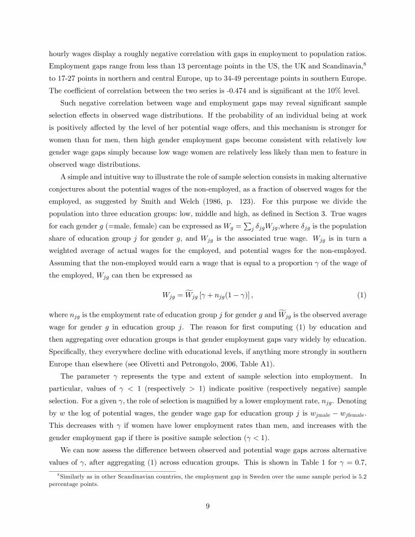
hourly wages display a roughly negative correlation with gaps in employment to population ratios.

Employment gaps range from less than 13 percentage points in the US, the UK and Scandinavia,8

to 17-27 points in northern and central Europe, up to 34-49 percentage points in southern Europe.

The coefficient of correlation between the two series is -0.474 and is significant at the 10% level.

Such negative correlation between wage and employment gaps may reveal significant sample

selection effects in observed wage distributions. If the probability of an individual being at work

is positively affected by the level of her potential wage offers, and this mechanism is stronger for

women than for men, then high gender employment gaps become consistent with relatively low

gender wage gaps simply because low wage women are relatively less likely than men to feature in

observed wage distributions.

A simple and intuitive way to illustrate the role of sample selection consists in making alternative

conjectures about the potential wages of the non-employed, as a fraction of observed wages for the

employed, as suggested by Smith and Welch (1986, p. 123). For this purpose we divide the

population into three education groups: low, middle and high, as defined in Section 3. True wages

for each gender g (=male, female) can be expressed asWg =P

j δjgWjg,where δjg is the population

share of education group j for gender g, and Wjg is the associated true wage. Wjg is in turn a

weighted average of actual wages for the employed, and potential wages for the non-employed.

Assuming that the non-employed would earn a wage that is equal to a proportion γ of the wage of

the employed, Wjg can then be expressed as

Wjg = fWjg [γ + njg(1− γ)] , (1)

where njg is the employment rate of education group j for gender g and fWjg is the observed average

wage for gender g in education group j. The reason for first computing (1) by education and

then aggregating over education groups is that gender employment gaps vary widely by education.

Specifically, they everywhere decline with educational levels, if anything more strongly in southern

Europe than elsewhere (see Olivetti and Petrongolo, 2006, Table A1).

The parameter γ represents the type and extent of sample selection into employment. In

particular, values of γ < 1 (respectively > 1) indicate positive (respectively negative) sample

selection. For a given γ, the role of selection is magnified by a lower employment rate, njg. Denoting

by w the log of potential wages, the gender wage gap for education group j is wjmale − wjfemale.

This decreases with γ if women have lower employment rates than men, and increases with the

gender employment gap if there is positive sample selection (γ < 1).

We can now assess the difference between observed and potential wage gaps across alternative

values of γ, after aggregating (1) across education groups. This is shown in Table 1 for γ = 0.7,

8Similarly as in other Scandinavian countries, the employment gap in Sweden over the same sample period is 5.2percentage points.

9

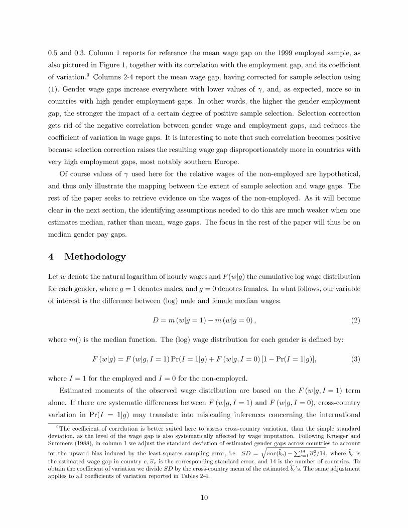
0.5 and 0.3. Column 1 reports for reference the mean wage gap on the 1999 employed sample, as

also pictured in Figure 1, together with its correlation with the employment gap, and its coefficient

of variation.9 Columns 2-4 report the mean wage gap, having corrected for sample selection using

(1). Gender wage gaps increase everywhere with lower values of γ, and, as expected, more so in

countries with high gender employment gaps. In other words, the higher the gender employment

gap, the stronger the impact of a certain degree of positive sample selection. Selection correction

gets rid of the negative correlation between gender wage and employment gaps, and reduces the

coefficient of variation in wage gaps. It is interesting to note that such correlation becomes positive

because selection correction raises the resulting wage gap disproportionately more in countries with

very high employment gaps, most notably southern Europe.

Of course values of γ used here for the relative wages of the non-employed are hypothetical,

and thus only illustrate the mapping between the extent of sample selection and wage gaps. The

rest of the paper seeks to retrieve evidence on the wages of the non-employed. As it will become

clear in the next section, the identifying assumptions needed to do this are much weaker when one

estimates median, rather than mean, wage gaps. The focus in the rest of the paper will thus be on

median gender pay gaps.

4 Methodology

Let w denote the natural logarithm of hourly wages and F (w|g) the cumulative log wage distributionfor each gender, where g = 1 denotes males, and g = 0 denotes females. In what follows, our variable

of interest is the difference between (log) male and female median wages:

D = m (w|g = 1)−m (w|g = 0) , (2)

where m() is the median function. The (log) wage distribution for each gender is defined by:

F (w|g) = F (w|g, I = 1)Pr(I = 1|g) + F (w|g, I = 0) [1− Pr(I = 1|g)], (3)

where I = 1 for the employed and I = 0 for the non-employed.

Estimated moments of the observed wage distribution are based on the F (w|g, I = 1) termalone. If there are systematic differences between F (w|g, I = 1) and F (w|g, I = 0), cross-countryvariation in Pr(I = 1|g) may translate into misleading inferences concerning the international

9The coefficient of correlation is better suited here to assess cross-country variation, than the simple standarddeviation, as the level of the wage gap is also systematically affected by wage imputation. Following Krueger andSummers (1988), in column 1 we adjust the standard deviation of estimated gender gaps across countries to account

for the upward bias induced by the least-squares sampling error, i.e. SD = var(bc)− 14c=1 σ

2c/14, where bc is

the estimated wage gap in country c, σc is the corresponding standard error, and 14 is the number of countries. Toobtain the coefficient of variation we divide SD by the cross-country mean of the estimated bc’s. The same adjustmentapplies to all coefficients of variation reported in Tables 2-4.

10

variation in the distribution of potential wage offers. This problem typically affects estimates of

female wage offer distributions; even more so when one is interested in cross-country comparisons of

gender wage gaps, given the cross-country variation in Pr(I = 1|g = male)−Pr(I = 1|g = female),measuring the gender employment gap. But F (w|g), the term of interest, is not identified, becausedata provide information on F (w|g, I = 1) and Pr(I = 1|g), but clearly not on F (w|g, I = 0) , aswages are only observed for those who are in work.

In particular, using (3), the median log wage for each gender, m, is defined by

F (m|g, I = 1)Pr(I = 1|g) + F (m|g, I = 0) [1− Pr(I = 1|g)] = 1

2. (4)

Our goal is to retrieve gender gaps in median (potential) wages, as illustrated in equation (2),

with gender medians defined in equation (4). To do this we need to retrieve information on

F (m|g, I = 0), representing the probability that non-employed individuals have potential wagesbelow the median.

It can be shown that knowledge of F (m|g, I = 0) allows to identify the median wage gap inpotential wages using median wage regressions, as a simpler alternative to numerically solving (4).

Let’s consider the linear wage equation

wi = β0 + β1gi + εi, (5)

where wi denotes (log) potential wages, β0 is a constant term, β1 is the parameter of interest, and

εi is an error term such that m (εi|gi) = 0. Denote by β the hypothetical LAD estimator based onpotential wages, i.e. β ≡ argminβ

PNi=1 |wi − β0 − β1gi|, where β ≡ [β0 β1]

0.

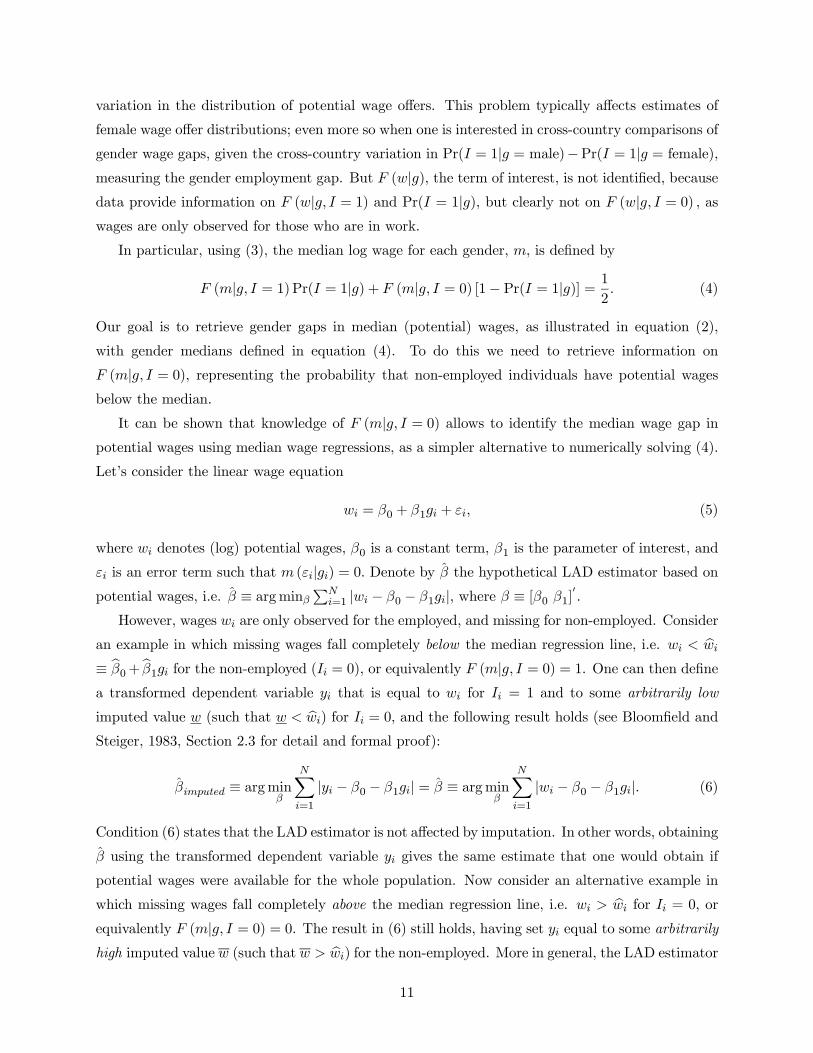
However, wages wi are only observed for the employed, and missing for non-employed. Consider

an example in which missing wages fall completely below the median regression line, i.e. wi < bwi

≡ bβ0+ bβ1gi for the non-employed (Ii = 0), or equivalently F (m|g, I = 0) = 1. One can then definea transformed dependent variable yi that is equal to wi for Ii = 1 and to some arbitrarily low

imputed value w (such that w < bwi) for Ii = 0, and the following result holds (see Bloomfield and

Steiger, 1983, Section 2.3 for detail and formal proof):

βimputed ≡ argminβ

NXi=1

|yi − β0 − β1gi| = β ≡ argminβ

NXi=1

|wi − β0 − β1gi|. (6)

Condition (6) states that the LAD estimator is not affected by imputation. In other words, obtaining

β using the transformed dependent variable yi gives the same estimate that one would obtain if

potential wages were available for the whole population. Now consider an alternative example in

which missing wages fall completely above the median regression line, i.e. wi > bwi for Ii = 0, or

equivalently F (m|g, I = 0) = 0. The result in (6) still holds, having set yi equal to some arbitrarilyhigh imputed value w (such that w > bwi) for the non-employed. More in general, the LAD estimator

11

is not affected by imputation when the missing wage observations are imputed “so as to maintain

the same sign of the residual” (Bloomfield and Steiger, 1983 p. 52). That is, (6) is valid whenever

missing wage observations are imputed on the “correct” side of the median. As a further example,

suppose that the potential wages of the non-employed could be classified in two groups, L and U ,

such that wi < bwi for i ∈ L and wi > bwi for i ∈ U . One can define yi as a transformed variable

such that yi = wi for Ii = 1, yi = w for Ii = 0 and i ∈ L, and yi = w for Ii = 0 and i ∈ U ; and

LAD inference is still valid.

Using this result one can estimate median wage gaps, based on wage imputation for the non-

employed that simply requires assumptions on the position of the imputed wage observations with

respect to the median of the wage distribution, as done in Johnson et al. (2000) and Neal (2004).

The attractive feature of median regressions is that results are only affected by the position of

imputed wage observations with respect to the median, and not by specific values of imputed

wages, as it would be in the matching approach. In this paper we will estimate median wage gaps

under alternative imputation rules, i.e. under alternative conjectures over F (m|g, I = 0). Theseimputation rules are described in detail below.

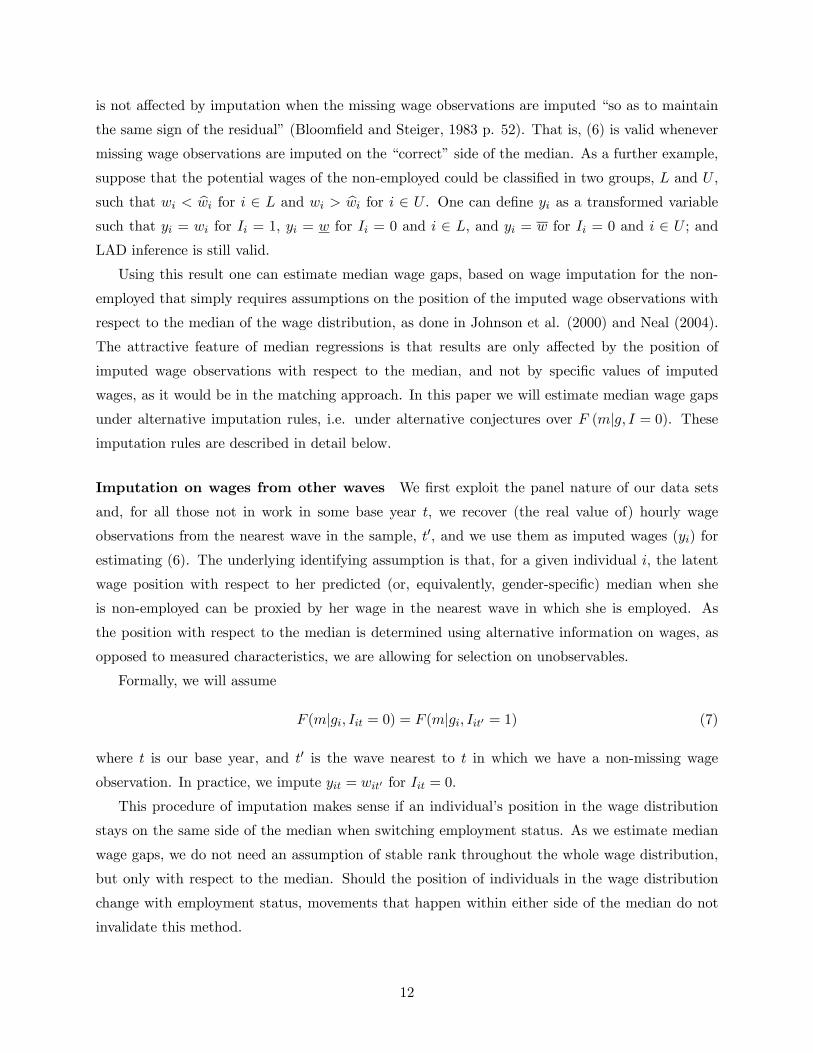
Imputation on wages from other waves We first exploit the panel nature of our data sets

and, for all those not in work in some base year t, we recover (the real value of) hourly wage

observations from the nearest wave in the sample, t0, and we use them as imputed wages (yi) for

estimating (6). The underlying identifying assumption is that, for a given individual i, the latent

wage position with respect to her predicted (or, equivalently, gender-specific) median when she

is non-employed can be proxied by her wage in the nearest wave in which she is employed. As

the position with respect to the median is determined using alternative information on wages, as

opposed to measured characteristics, we are allowing for selection on unobservables.

Formally, we will assume

F (m|gi, Iit = 0) = F (m|gi, Iit0 = 1) (7)

where t is our base year, and t0 is the wave nearest to t in which we have a non-missing wage

observation. In practice, we impute yit = wit0 for Iit = 0.

This procedure of imputation makes sense if an individual’s position in the wage distribution

stays on the same side of the median when switching employment status. As we estimate median

wage gaps, we do not need an assumption of stable rank throughout the whole wage distribution,

but only with respect to the median. Should the position of individuals in the wage distribution

change with employment status, movements that happen within either side of the median do not

invalidate this method.

12

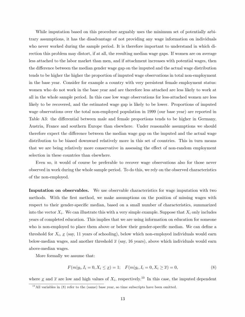
While imputation based on this procedure arguably uses the minimum set of potentially arbi-

trary assumptions, it has the disadvantage of not providing any wage information on individuals

who never worked during the sample period. It is therefore important to understand in which di-

rection this problem may distort, if at all, the resulting median wage gaps. If women are on average

less attached to the labor market than men, and if attachment increases with potential wages, then

the difference between the median gender wage gap on the imputed and the actual wage distribution

tends to be higher the higher the proportion of imputed wage observations in total non-employment

in the base year. Consider for example a country with very persistent female employment status:

women who do not work in the base year and are therefore less attached are less likely to work at

all in the whole sample period. In this case low wage observations for less-attached women are less

likely to be recovered, and the estimated wage gap is likely to be lower. Proportions of imputed

wage observations over the total non-employed population in 1999 (our base year) are reported in

Table A3: the differential between male and female proportions tends to be higher in Germany,

Austria, France and southern Europe than elsewhere. Under reasonable assumptions we should

therefore expect the difference between the median wage gap on the imputed and the actual wage

distribution to be biased downward relatively more in this set of countries. This in turn means

that we are being relatively more conservative in assessing the effect of non-random employment

selection in these countries than elsewhere.

Even so, it would of course be preferable to recover wage observations also for those never

observed in work during the whole sample period. To do this, we rely on the observed characteristics

of the non-employed.

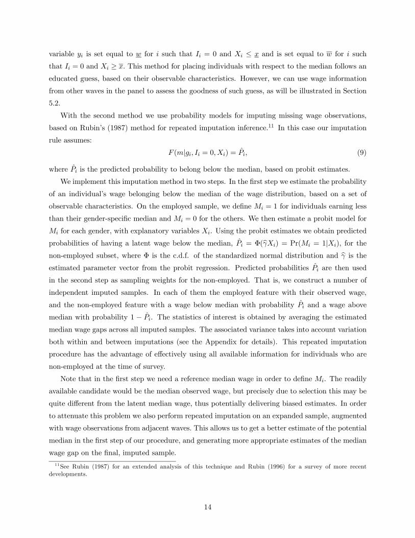
Imputation on observables. We use observable characteristics for wage imputation with two

methods. With the first method, we make assumptions on the position of missing wages with

respect to their gender-specific median, based on a small number of characteristics, summarized

into the vectorXi. We can illustrate this with a very simple example. Suppose thatXi only includes

years of completed education. This implies that we are using information on education for someone

who is non-employed to place them above or below their gender-specific median. We can define a

threshold for Xi, x (say, 11 years of schooling), below which non-employed individuals would earn

below-median wages, and another threshold x (say, 16 years), above which individuals would earn

above-median wages.

More formally we assume that:

F (m|gi, Ii = 0,Xi ≤ x) = 1; F (m|gi, Ii = 0,Xi ≥ x) = 0, (8)

where x and x are low and high values of Xi, respectively.10 In this case, the imputed dependent

10All variables in (8) refer to the (same) base year, so time subscripts have been omitted.

13

variable yi is set equal to w for i such that Ii = 0 and Xi ≤ x and is set equal to w for i such

that Ii = 0 and Xi ≥ x. This method for placing individuals with respect to the median follows an

educated guess, based on their observable characteristics. However, we can use wage information

from other waves in the panel to assess the goodness of such guess, as will be illustrated in Section

5.2.

With the second method we use probability models for imputing missing wage observations,

based on Rubin’s (1987) method for repeated imputation inference.11 In this case our imputation

rule assumes:

F (m|gi, Ii = 0,Xi) = Pi, (9)

where Pi is the predicted probability to belong below the median, based on probit estimates.

We implement this imputation method in two steps. In the first step we estimate the probability

of an individual’s wage belonging below the median of the wage distribution, based on a set of

observable characteristics. On the employed sample, we define Mi = 1 for individuals earning less

than their gender-specific median and Mi = 0 for the others. We then estimate a probit model for

Mi for each gender, with explanatory variables Xi. Using the probit estimates we obtain predicted

probabilities of having a latent wage below the median, Pi = Φ(bγXi) = Pr(Mi = 1|Xi), for the

non-employed subset, where Φ is the c.d.f. of the standardized normal distribution and bγ is theestimated parameter vector from the probit regression. Predicted probabilities Pi are then used

in the second step as sampling weights for the non-employed. That is, we construct a number of

independent imputed samples. In each of them the employed feature with their observed wage,

and the non-employed feature with a wage below median with probability Pi and a wage above

median with probability 1 − Pi. The statistics of interest is obtained by averaging the estimated

median wage gaps across all imputed samples. The associated variance takes into account variation

both within and between imputations (see the Appendix for details). This repeated imputation

procedure has the advantage of effectively using all available information for individuals who are

non-employed at the time of survey.

Note that in the first step we need a reference median wage in order to define Mi. The readily

available candidate would be the median observed wage, but precisely due to selection this may be

quite different from the latent median wage, thus potentially delivering biased estimates. In order

to attenuate this problem we also perform repeated imputation on an expanded sample, augmented

with wage observations from adjacent waves. This allows us to get a better estimate of the potential

median in the first step of our procedure, and generating more appropriate estimates of the median

wage gap on the final, imputed sample.

11See Rubin (1987) for an extended analysis of this technique and Rubin (1996) for a survey of more recentdevelopments.

14

Discussion of imputation methodology We discuss here the main differences between alter-

native imputation methods, to ease the interpretation of the results presented in the next section.

The three methods described differ in terms of the underlying identifying assumptions and of result-

ing imputed samples. The first method, where missing wages are imputed using wage information

from other waves, implicitly assumes that an individual’s position with respect to the median can be

proxied by their wage in the nearest wave in the panel. With this procedure one can recover at best

individuals who worked at least once during the eight-year sample period. We thus emphasize that

this is a fairly conservative imputation procedure, in which we impute wages for individuals who are

relatively weakly attached to the labor market, but not for those who are completely unattached

and thus never observed in work. This procedure has the advantage of restricting imputation to

a relatively “realistic” set of potential workers, and thus is the one we mostly rely upon to make

quantitative statements.

In the second and third imputation methods, we assume instead that an individual’s position

with respect to the median can be proxied by some of their observable characteristics. In the second

method, we use characteristics to take educated guesses regarding the position of missing wages.

Clearly this procedure is more accurate for values of the observables in the tails than in the middle

of the distribution. For example, guessing the position with respect to the median for individuals

with either college or no education at all is safer than doing it for secondary school graduates, who

are thus best left without an imputed wage. In doing this, our imputed sample is typically larger

than the one obtained with the first method, although still substantially smaller than the existing

population. Finally, with the third method, we estimate the probability of belonging above the

median for the whole range of our vector of characteristics, thus recovering predicted probabilities

and imputed wages for the whole existing population.

Different imputed samples will have an impact on our estimated median wage gaps. In so far

women tend to be more positively selected into employment than men, the larger the imputed

sample with respect to the actual sample of employed workers, the larger the estimated correction

for selection.

Having said this, it is important to stress that with all three imputation methods used we

never impose positive selection ex-ante (except in a benchmark example), and thus there is nothing

that would tell a priori which way correction for selection is going to affect the results. This is

ultimately determined by the wages that the non-employed earned when they were previously (or

later) employed, and by their observable characteristics, depending on methods.

Before moving on to the discussion of our estimates, it is worthwhile to motivate our choice of

selection correction methodology and to frame it in the context of the existing literature on sample

selection. A number of approaches can be used to correct for non-random sample selection in wage

equations and/or recover the distribution in potential wages. The seminal approach suggested

15

by Heckman (1974, 1979) consists in allowing for selection on unobservables, i.e. on variables

that do not feature in the wage equation but that are observed in the data.12 Heckman’s two-

stage parametric specifications have been used extensively in the literature in order to correct

for selectivity bias in female wage equations. More recently, these have been criticized for lack

of robustness and distributional assumptions (see Manski, 1989). Approaches that circumvent

most of the criticism include semi-parametric selection correction models that appeared in the

literature since the early 1980s (see Vella, 1998, for an extensive survey of both parametric and

non-parametric sample selection models). Two-stage nonparametric methods allow in principle to

approximate the bias term by a series expansion of propensity scores from the selection equation,

with the qualification that the term of order zero in the polynomial is not separately identified

from the constant term in the wage equation, unless some additional information is available (see

Buchinski, 1998). Usually, the constant term in the wage regression is identified from a subset of

workers for which the probability of work is close to one, but in our case this route is not feasible

since for no type of women is the probability of working close to one in all countries.

Selection on observed characteristics is instead exploited in the matching approach, which con-

sists in imputing wages for the non-employed by assigning them the observed wages of the employed

with matching characteristics (see Blau and Beller, 1992, and Juhn, 1992, 2003). The approach

of our paper is also based on some form of wage imputation for the non-employed, but it simply

requires assumptions on the position of the imputed wage observations with respect to the me-

dian of the wage distribution. Importantly, it does not require assumptions on the actual level of

missing wages, as typically required in the matching approach, nor it requires arbitrary exclusion

restrictions often invoked in two-stage Heckman sample selection correction models.

Bounds As discussed above, each imputation method is based on identifying assumptions that

are largely untested. In order to illustrate that results delivered by our imputation methods are

reasonable, we also provide “worst case” bounds to the gap in potential median wages that do not

require any identifying assumption, as shown by Manski (1994) and Blundell et. al. (2007). We

will then check that our estimated wage gaps on imputed wage distributions fall into these bounds.

Manski notes that substituting the inequality 0 ≤ F (w|g, I = 0) ≤ 1 into (3) we obtain thefollowing bounds for the true cumulative distribution

F (w|g, I = 1)Pr(I = 1|g) ≤ F (w|g) ≤ F (w|g, I = 1)Pr(I = 1|g) + [1− Pr(I = 1|g)]. (10)

12 In this framework, wages of employed and nonemployed would be recovered as

E (w|Zw, I = 1) = Zwδw +E (εw|εI > −ZIδI)E (w|Zw, I = 0) = Zwδw +E (εw|εI < −ZIδI) ,

respectively, where Zw and ZI are the set of covariates included in the wage and selection equations, respectively,with associated parameters δw and δI , and εw and εI are the respective error terms.

16

If one is interested in the median of F (), denoted by m, (3) implies

F (m|g, I = 1)Pr(I = 1|g) ≤ 12≤ F (m|g, I = 1)Pr(I = 1|g) + [1− Pr(I = 1|g)]. (11)

These bounds on F () deliver the following worst case bounds on the gender-specific median

ml (w|g) ≤ m (w|g) ≤ mu (w|g) , (12)

such that:1

2= F

³ml|g, I = 1

´Pr(I = 1|g) + [1− Pr(I = 1|g)] (13)

and1

2= F (mu|g, I = 1)Pr(I = 1|g). (14)

Bounds on the gender specific median can be obtained solving (13) and (14), using data on the

observed wage distribution and employment rates. Note that Conditions (13) and (14) imply that

one can only identify bounds for the median if Pr(I = 1|g) ≥ 12 . Hence we will not be able to obtain

such bounds for the female median wage (and therefore, for the gender wage gap) in countries

where less than 50% of the women have a wage observation.

Having said this, the bounds for the median gender wage gap D defined in (2) are obtained as

follows:

ml (w|g = male)−mu (w|g = female) ≤ D ≤ mu (w|g = male)−ml (w|g = female) . (15)

5 Results

5.1 Imputation on wages from adjacent waves

In our first set of estimates, an individual’s position with respect to the median of the wage distri-

bution in the base year is proxied by the position of their wage obtained from the nearest available

wave. The kind of imputation made here requires that individuals stay on the same side of their

gender median across different waves in the panel (see equation (7)). Results obtained with this

method are reported in Table 2.

Column 1 reports the actual wage gap for reference: this is the median wage gaps for individuals

with an hourly wage in 1999, which is our base year. Wage gaps of column 1 replicate very closely

those plotted in Figure 1, with the only difference that Figure 1 plotted mean as opposed to median

wage gaps.13 As in Figure 1, the US and the UK stand out as the countries with the highest wage

gaps, followed by central and northern Europe, and finally Scandinavia and Southern Europe.13The absence of any important difference between mean and median wage gaps on the observed wage distribution

is good news for our approach, based on the recovery of selection-corrected median wage gaps.

17

In column 2 missing wage observations in 1999 are replaced with the real value of the nearest

wage observation in a 2-year window, while in column 3 they are replaced with the real value of

the nearest wage observation in the whole sample period, meaning a maximum window of [-5, +2]

years. Moving across from column 1 to column 3, gender wage gaps tend to increase as more wage

observations are included into the imputed sample. This is indicative of positive sample selection,

or, in other words, estimated wage gaps on the observed wage distribution are downward biased

due to non-random sample selection into employment because low-wage women are less likely to

feature in the observed wage distribution.

But there is important cross-country variation in the role of selection. In particular, one can see

that the median wage gap remains substantially unaffected or marginally affected in the US, the

UK, Scandinavia, Germany and the Netherlands; it increases by around 25% in Austria, Ireland,

Italy and Portugal; by 40% in Belgium; and by more than 60% in France, Spain and Greece. As

expected, gender wage gaps tend to respond more strongly to selection correction in countries with

high employment gaps. This can be clearly grasped by looking at the cross-country correlation

between employment and wage gaps. In column 1 such correlation is -0.329, and it falls by 45%

in column 3. Employment selection thus explains nearly a half of the observed correlation between

wage and employment gaps. Another indicative cross-country statistics is the coefficient of variation

in the gender wage gap: this falls by 31% between column 1 and column 3, thus selection explains

almost one third of the observed cross-country variation of wage gaps.

For each sample inclusion rule in column 1-3 one can compute the adjusted employment rate for

each gender, i.e. the proportion of the adult population that is either working or has an imputed

wage. These proportions are reported in columns 1-3 of Table A2. When moving from column 1 to

3, the fraction of women included increases substantially in most countries, including some countries

where the estimated wage gap is not greatly affected by the sample inclusion rules. Moreover, the

fraction of men included in the sample also increases, albeit less than for women. It is thus not

simply the lower female employment rate in several countries that drives our findings, it is also the

fact that in some countries selection into work seems to be less correlated to wage characteristics

than in others.

The estimates of columns 2 and 3 do not control for aggregate wage growth over time. If

aggregate wage growth were homogeneous across genders and countries, then estimated wage gaps

based on wage observations for other waves in the panel would not be not affected. But if there

is a gender differential in wage growth, and if such differential varies across countries, then simply

using earlier (later) wage observations would deliver a higher (lower) median wage gap in countries

where wage growth for women is lower than for men.14 We thus estimate real wage growth by

14Note however that, even if real wage growth were homogeneous across genders, imputation based on wageobservations from adjacent waves would not be affected only if the proportion of men and women in the sample

18

regressing log real hourly wages for each country and gender on a linear trend.15 The resulting

coefficients are reported in Table A4. These are then used to adjust real wage observations outside

the base year and re-estimate median wage gaps. The resulting median wage gaps on the imputed

wage distribution are reported in column 4 and 5 of Table 2. Despite some differences in real wage

growth rates across genders and countries, adjusting estimated median wage gaps does not produce

any appreciable change in the results reported in columns 2 and 3, which do not control for real

wage growth.

Note finally that in Table 2 we are only recovering wages for a quarter, on average, of non-

employed women in the four southern European countries, as opposed to more than a half in the

rest of countries (see Table A3). For men, cross country differences are less marked, as respective

proportions are 57% and 63%. Such differences happen because (non)employment status tends to

be relatively more persistent in southern Europe than elsewhere, and much more so for women

than for men. As noted in Section 4, given that we recover relatively fewer less-attached women in

southern Europe, we are being relatively more conservative in assessing the effect of non-random

employment selection in southern Europe than elsewhere. For this reason it is important to try to

recover wage observations also for those never observed in work in any wave of the sample period,

as explained in the next subsection.

5.2 Imputation on observables

In Table 3 we exploit some observable characteristics of the non-employed for assigning them on

one or the other side of their gender median (equation (8) gives the formal identifying assumption).

Column 1 reports for reference the median wage gap on the base sample, which is the same as the

one reported in column 1 of Table 2. In column 2 we assume that all those not in work in 1999

would have wage offers below the median for their gender.16 This is an extreme assumption, and

the only case in which we impose ex ante positive sample selection. This assumption is clearly

violated for countries like Italy, Spain and Greece, in which more than a half of the female sample

is not in work in 1999, and thus estimates are not reported for these three countries. However, also

for other countries there are reasons to believe that not all non-employed individuals would have

wage offers below their gender mean.

Of course, one cannot know exactly what wages these individuals would have received, had

they worked in 1999. But we can form an idea of the goodness of this assumption by looking again

at wage observations (if any) for these individuals in all other waves in the panel. This allows us

remained unchanged after imputation.15Of course, for our estimated rates of wage growth to be unbiased, this procedure requires that participation into

employment be unaffected by wage growth, which may not be the case.16 In the practice, whenever we assign someone a wage below the median we pick wi = −5, this value being lower

than the minimum observed (log) wage for all countries, and thus lower than the median. Similarly, whenever weassign someone a wage above the median we pick wi = 20.

19

to see whether an imputed observations had a wage that was indeed below their predicted gender

median at the time he/she was observed working. Specifically, we take all imputed observations in

1999. Among these, we select those who ever worked at some time in the sample period. Out of

this subset we compute the proportion of observations who had wages below the predicted gender

median. Such proportions are computed for men and women and reported in columns headed

"M" and "F". They are fairly high for men, but sensibly lower for women, which makes the

estimates based on this extreme imputation case a benchmark rather than a plausible measure for

the gender wage gap. Having said this, estimated median wage gaps increase substantially for most

countries, except Denmark and Finland. The correlation with employment gaps turns positive and

quite strong, because the wage gap in high employment-gap countries increase disproportionately

relative to other countries.

In column 3 we impute a wage below the median to all those who are unemployed (as opposed

to non participants) in 1999. The unemployed by definition are receiving wage offers (if any)

below their reservation wage, while the employed have received at least one wage offer above their

reservation wage. At constant reservation wages, the unemployed have lower potential wages than

the observed wages of the employed, and are thus assigned an imputed wage value below the median.

This imputation leaves the median wage gap roughly unchanged with respect to the base sample in

the US, the UK, Scandinavia, Germany, Austria and Ireland, and raises it substantially elsewhere,

especially in southern Europe. Also, the proportion of “correctly” imputed observations, computed

as for the previous imputation case, is now much higher. Those who do not work because they

are unemployed are thus relatively more likely to be over-represented in the lower half of the wage

distribution. Selection now explains 64% of the correlation between wage and employment gaps,

and 32% of the cross-country variation.

In column 4 we follow standard human capital theory and assume that all those with less

than upper secondary education and less than 10 years of potential labor market experience have

wage observations below the median for their gender. Those with at least higher education and at

least 10 years of labor market experience are instead placed above the median. In the four southern

European countries the gender wage gap increases enormously with respect to the actual wage gap of

column 1, and as a consequence the correlation with employment gaps turns positive. Interestingly,

the proportion of correctly imputed observations is high in Ireland, France and southern Europe,

but not so much in other countries, where imputation based on unemployment works better than

imputation based on human capital components.

The imputation method of column 5 is implicitly based on the assumption of assortative mating

along wage attributes and consists in assigning wages below the median to those whose partners

have total income in the bottom quartile of the gender-specific distribution. The assumption is that

individuals married to low-productivity spouses are also low productivity, and thus the spouse’s

20

wage is taken as a proxy for an individual’s potential wage offer. The results are qualitatively

similar to those of column 3, with the wage gap being mostly affected in southern Europe, but

on average the wage gap is less affected by imputation than in other imputation examples. It

would be natural to perform a similar exercise at the top of the distribution, by assigning a wage

above the median to those whose partner earns income in the top quartile. However, in this case

the proportion of correctly imputed observations was too low to rely on the assumption used for

imputation. We have also considered imputation based on low spouse education, obtaining very

similar results as with low spouse income. Finally, we considered imputation based on high spouse

education, and similarly as for imputation based on high spouse income the goodness of imputation

turned out worse.

We also combine imputation methods by using first wage observations available from other

waves, and then imputing the remaining missing ones using education and experience information

as done in column 4. The results, reported in column 6, show again a much higher gender gap in

France, and southern Europe, and not much of a change elsewhere with respect to the base sample

of column 1.

Similarly as with the previous imputation method, we report in columns 4-8 of Table A2 the

proportion of men and women included in our imputed samples. As expected, we are now able to

recover wage information for a higher fraction of the adult population. In column 4 such proportions

are generally not equal to 100% because we did not impute wages to those who are employed but

have missing information on hourly wages due to non-response, as the selection mechanism driving

non-response is clearly different from that driving nonemployment.

We finally report estimates based on a probabilistic, two-step imputation technique, summarized

in equation (9). In the first step we use the 1999 base sample to estimate a probit model for

the probability of belonging above the gender-specific median, controlling for education (upper

secondary and higher education), experience and its square.17 The estimated coefficients for the

first-stage probit regression (not reported) conform to standard economic theory: individuals with

higher levels of educational attainment and/or of labor market experience are more likely to feature

in the top half of the wage distribution. These estimates are used as sampling weights in the second

step to construct 20 independent imputed samples. For each of these we estimate the median gender

wage gap and the corresponding bootstrapped standard error.18 The median wage gaps reported

are averages across the 20 rounds of imputation.

The results of this exercise are summarized in Table 4. Column 1 reports the median wage gap

17We also estimated a more general specification that also controls for marital status, the number of children ofdifferent ages and the position of the spouse in their gender specific distribution of total income. Since the results ofthe exercise do not vary in any meaningful way across specifications, we only report findings for the human capitalspecification.18We use the STATA command bsqreg where we set the number of replications to 200.

21

for the base sample, which is the same as the one reported in column 1 of Tables 2 and 3. Column

2 reports the estimated median wage gap obtained from the probabilistic model described, having

used the observed 1999 median as the reference median for our probit estimates. As fewer than

50% of women are employed in Italy, Spain and Greece, we cannot credibly estimate a probit model

where Mi = 1 for workers earning less than the median for these countries. In Column 3 we use as

the reference median the one obtained on a wage distribution enlarged with wage imputation from

all other waves, and in this the fraction of missing wages is below 50% for men and women in all

countries. If wage imputation is correct this procedure delivers a reference median that is closer

to the latent median than the observed median. Comparing column 1 to columns 2 and 3 shows

that the median wage gap on imputed wage distributions increases mildly in most countries down

to Austria, but rises substantially in Ireland, France and Portugal, and enormously in Italy, Spain

and Greece, which are the countries with the highest employment gaps.

To broadly summarize our findings, one could note that whether one corrects for selection on

unobservables (Table 2) or on observables (Table 3 and 4), our results are qualitatively consistent in

identifying a clear role of sample selection in countries with high employment gaps, and especially

France and southern Europe.19 Quantitatively, the correction for sample selection is smallest when

wage imputation is performed using wage observation from other waves in the panel, and increases

when it is instead performed using observed characteristics of the non-employed. As argued above,

this is mainly due to different sizes of the imputed samples. While only individuals with some

degree of labor market attachment feature in the imputed wage distribution in the first case, the

use of observed characteristics may in principle allow wage imputation for the whole population,

thus including individuals with no labor market attachment at all. Interestingly, the fact that

controlling for unobservables does not greatly change the picture obtained when controlling for a

small number of observables alone (education, experience and spouse income) implies that most of

the selection role can indeed be captured by a set of observable individual characteristics.20

19Our selection-corrected estimates for the gender wage gap are consistent with evidence of glass-ceilings in mostEuropean country but of sticky floor for France, Italy and Spain (see Arulampalan, Booth and Bryan, 2007). De LaRica, Dolado and Llorens (2008) also find evidence of sticky floors for low-educated Spanish women.20We have performed a number of robustness tests and more disaggregate analyses on the results reported in Tables

2 to 4. First, we repeated all estimates using a common set of age weights (obtained from the US 1999 sample) for allcountries. Results using such weights were virtually identical to those obtained without weights, and thus variation inthe age structure across countries does not seem to explain much of the observed variation in gender pay gaps. Second,for the imputation rules reported in Table 2 and 3, we have repeated our estimates separately for three educationgroups (less than upper secondary education, upper secondary education, and higher education), and we found thatmost of the selection occurs between rather than within groups, as median wage gaps disaggregated by education aremuch less affected by sample inclusion rules than in the aggregate. Finally, we have repeated our estimates separatelyfor three demographic groups: single individuals without kids in the household, married or cohabiting without kids,and married or cohabiting with kids. We found evidence of a strong selection effect in France and southern Europeamong those who are married or cohabiting, especially when they have kids, and much less evidence of selectionamong single individuals without kids.

22

5.3 Bounds

Each imputation rule requires assumptions about the position of the non-employed relative to the

median of the potential wage distribution. In order to show that we obtain reasonable estimates

for the median wage gap under each specification, we compute bounds following the procedure

discussed in Section 4. Table 5 reports “worst case” bounds to the potential distribution for the

base sample and for a subset of our wage imputation rules.

Column 1 reports bounds using the actual wage distribution to obtain the F () terms in condi-

tions (13) and (14). All estimates for the median wage gap obtained with alternative imputation

methods and reported in Table 2 to 4 lye within the bounds to the potential distribution reported in

column 1. Note that, mechanically, the bounds for the gender-specific median are tighter the higher

the employment rate for that gender. Since variation in male employment rates is low relative to

variation in female rates, cross-country differences in the tightness of the bounds mostly stem from

differences in women’s employment selection across countries. Bounds for the median gender wage

gap are thus much tighter for the US, the UK and countries all the way down to Austria than they

are for Ireland, France and Portugal - for which they are so large to be completely uninformative.

Indeed, we cannot even obtain bounds to the median wage gap for Italy, Spain and Greece on the

base sample because less than 50% of women are employed.

A restriction typically used to tighten such bounds is that of stochastic dominance (see Blundell

et al., 2007), which assumes various forms of positive selection into employment. As this is precisely

something that our paper is supposed to investigate we cannot use it as an identifying assumption.

But we can instead compute bounds after wage imputation (i.e. using imputed wage distributions

to compute the F () terms in (13) and (14)). These estimated bounds are reported in columns

2-4 of Table 5. This procedure has the advantage of tightening the bounds without assuming

positive sample selection ex ante. In column 2 the wage distribution used is one in which missing

wage observations are replace by observed wages in the nearest available wave (as in column 2 of

Table 2). In column 3, missing wage observations are imputed below the median if an individual

is unemployed (as in column 3 of Table 3). In column 4, they are imputed using education and

experience levels of the non-employed (as in column 4 of Table 3). As employment rates are higher

in columns 2-4 than in column 1, bounds do become tighter. However, they still remain relatively

large in southern Europe, where employment rates remain relatively low even after wage imputation.

6 Conclusions

Gender wage gaps in the US and the UK are much higher than in other European countries, and

especially so with respect to France and southern Europe. Although at first glance this fact may

suggest evidence of a more equal pay treatment across genders in the latter group of countries,

23

appearances can be deceptive.

In this paper we note that gender wage gaps across countries are negatively correlated with

gender employment gaps, and illustrate the importance of non random selection into work in

understanding the observed international variation in gender wage gaps. To do this, we perform

wage imputation for those not in work, by simply making assumptions on the position of the imputed

wage observations with respect to the median. Imputation is performed according to different

methodologies based on observable or unobservable characteristics of missing wage observations.

We find higher median wage gaps on imputed rather than actual wage distributions for most

countries in the sample, meaning that, as one would have expected, women tend on average to

be more positively selected into work than men. However, this difference is small in the US, the

UK and in a number of central and northern European countries, and it is sizeable in France and

southern Europe, i.e. countries in which the gender employment gap is particularly high. Our

(most conservative) estimates suggest that correction for employment selection explains about 45%

of the observed negative correlation between wage and employment gaps. In Italy, Spain, Portugal

and Greece the median wage gap on the imputed wage distribution ranges between 20 and 30 log

points across specifications. These are closely comparable levels to those of the US and of other

central and northern European countries.

Another interesting result is that we obtain qualitatively similar estimates whether we impute

missing wages using available wage information from other waves in the panel or whether we use

observable characteristics of the non-employed. This implies that employment selection mostly

takes place along a small number of measurable characteristics.

Our analysis identifies a clear direction for future work. As we argue in this paper, gender

employment gaps are important in understanding cross-country differences in gender wage gaps.

Hence, the current work may be used to ultimately assess the importance of demand and supply

factor in explaining variation in these gaps. As emphasized in recent work by Fernández and Fogli

(2005) and by Fortin (2005, 2006), “soft variables” such as cultural beliefs about gender roles

and family values and individual attitudes towards greed, ambition and altruism are important

determinants of women’s employment decisions as well as of gender wage differentials. Cross-

country differences in these “fuzzy” variables, as well as differences in labor market and financial

institutions, might contribute to explain the cross-country patterns of women’s selection into the

labor force discussed in this paper and hence the international variation in gender pay gaps.

References

[1] Albrecht, J., A. van Vuuren and S. Vroman (2004), “Decomposing the Gender Wage Gap inthe Netherlands with Sample Selection Adjustment,” IZA DP No. 1400.

24

[2] Altonji, J. and R. Blank (1999), “Race and Gender in the Labor Market”, in O. Ashenfelterand D. Card (eds.) Handbook of Labor Economics, North-Holland, volume 3C: 3141-3259.

[3] Arulampalan, W., A. Booth and M. Bryan (2007), “Is There a Glass Ceiling over Europe?Exploring the Gender Pay Gap across the Wage Distribution”, Industrial and Labor RelationsReview, 60 (2): 163-186.

[4] Azmat, G., M. Güell and A. Manning (2006), “Gender Gaps in Unemployment Rates in OECDCountries,” Journal of Labor Economics 24: 1-37.

[5] Beblo, M., D. Beninger, A. Heinze and F. Laisney (2003), “Measuring Selectivity-correctedGender Wage Gaps in the EU,” ZEW DP No. 03-74, Mannheim.

[6] Blau, F. and A. H. Beller (1992), “Black-White Earnings over the 1970s and 1980s: GenderDifferences in Trends,” Review of Economics and Statistics 72(2): 276-286.

[7] Blau, F. and L. Kahn (1996), “Wage Structure and Gender Earnings Differentials: An Inter-national Comparison,” Economica 63: S29-S62.

[8] Blau, F. and L. Kahn (1997), “Swimming Upstream: Trends in the Gender Wage Differentialsin the 1980s,” Journal of Labor Economics 15: 1-42.

[9] Blau, F. and L. Kahn (2003), “Understanding International Differences in the Gender PayGap,” Journal of Labor Economics 21: 106—144.

[10] Blau, F. and L. Kahn (2006), “The US Gender Pay Gap in the 1990s: Slowing Convergence?”Industrial and Labor Relations Review 60: 45-66.

[11] Bloomfield, P. and W. Staiger (1983), Least Absolute Deviations: Theory, Applications andAlgorithms. Boston, MA: Birkhauser.

[12] Blundell, R., A. Gosling, H. Ichimura and C. Meghir (2007), “Changes in the Distribution ofMale and Female Wages Accounting for Employment Composition Using Bounds,” Economet-rica, 75 (2): 323—363.

[13] Buchinsky, M. (1998), “The Dynamics of Changes in the Female Wage Distribution in theUSA: A Quantile Regression Approach,” Journal of Applied Econometrics 13, 1-30.

[14] Chandra, A. (2003), “Is the Convergence in the Racial Wage Gap Illusory?”, NBER WP No.9476.

[15] De la Rica, S., J. Dolado and V. Llorens (2008), “Ceilings and Floors: Gender Wage Gaps byEducation in Spain,” Journal of Population Economics, forthcoming.

[16] Fernández, R. and A. Fogli (2005), “Culture: An Empirical Investigation of Beliefs, Work, andFertility,” NBER Working Paper No. 11268.

[17] Fortin N. (2006), “Greed, Altruism, and the Gender Wage Gap,” Manuscript, University ofBritish Columbia.

[18] Fortin N. (2005), “Gender Role Attitudes and the Labour Market Outcomes of Women AcrossOECD Countries,” Oxford Review of Economic Policy 21, 416-438.

25

[19] Fortin, N. and T. Lemieux (1998), “Rank Regressions, Wage Distributions, and the GenderGap,” Journal of Human Resources 33, 610-643.

[20] Goldin C., 1990, Understanding the Gender Gap: An Economic History of American Women,New York: Oxford University Press.

[21] Gronau, R. (1974), “Wage Comparison - A Selectivity Bias,” Journal of Political Economy,82, 1119-1143.

[22] Heckman, J. (1974), “Shadow Prices, Gender Differenced and Labor Supply,” Econometrica42, 679-694.

[23] Heckman, J. (1979), “Sample Selection Bias as a Specification Error,” Econometrica 47, 153-163.

[24] Heckman, J. (1980), “Addendum to Sample Selection Bias as a Specification Error”. In E.Stromsdorfer and G Ferkas (eds.) Evaluation Studies. San Francisco: Sage, Volume 5.

[25] Johnson, W., Y. Kitamura and D. Neal (2000), “Evaluating a Simple Method for EstimatingBlack-White Gaps in Median Wages,” American Economic Review 90, 339-343.

[26] Juhn, C. (1992), “Decline of Labor Market Participation: The Role of Declining Market Op-portunities,” Quarterly Journal of Economics 107, 79-122.

[27] Junh, C. (2003), “Labor Market Dropouts and Trends in the Wages of Black and White Men,”Industrial and Labor Relations Review 56, 643-662.

[28] Juhn, C., K. Murphy and B. Pierce (1991), “Accounting for the Slowdown in Black-whiteWage Convergence.” In Workers and Their Wages, by M. Kosters (ed.), 107—43. Washington,DC: AEI Press, 1991.

[29] Krueger, A. B. and L. H. Summers (1988), “Efficiency Wages and the Inter-Industry WageStructure,” Econometrica, 56 (2): 259-293.

[30] Lewbel, A. (2007), “Endogenous Selection or Treatment Model Estimation,” Journal of Econo-metrics, 141: 777-806.

[31] Manski, C. F. (1989), “Anatomy of the Selection Problem,” Journal of Human Resources 24,343-360.

[32] Manski, C. F. (1994), “The Selection Problem,” in Advances in Econometrics, Sixth WorldCongress vol. 1, C. Sims (ed.), Cambridge University Press.

[33] Mulligan, C. and Y. Rubinstein (2005), “Selection, Investment, and Women’s Relative WagesSince 1975,” NBER WP No. 11159.

[34] Oaxaca R. L. (1973), “Male-Female Wage Differentials in Urban Labor Markets,” InternationalEconomic Review 14, 693-709.

[35] Olivetti, C. and B. Petrongolo (2006), “Unequal Pay or Unequal Employment? A Cross-Country Analysis of Gender Gaps”, CEPR Discussion Paper No. 5506.

26

[36] O’Neill J., (1985), “The Trend in the Male-Female Wage Gap in the United States,” Journalof Labor Economics 3, 91-116.

[37] Neal, D. (2004), “The Measured Black-white Wage Gap Among Women is Too Small,” Journalof Political Economy 112, S1-S28.

[38] OECD (2002), Employment Outlook, Paris.

[39] Rubin, Donald B. (1996), “Multiple Imputation After 18+ Years,” Journal of the AmericanStatistical Association 91, 473-489.

[40] Rubin, Donald B. (1987), Multiple Imputation for Nonresponse in Surveys, Wiley Series inProbability and Mathematical Statistics, Wiley & Sons, New York.

[41] Smith J.P. and M.P. Ward (1989), “Women in the Labor Market and in the Family,” Journalof Economic Perspective 3, 9-24.

[42] Smith J.P. and F. Welch (1986), Closing the Gap. Forty Years of Economic Progress for Blacks,The RAND Corporation, R-3330-DOL, Santa Monica, CA.

[43] Vella, F. (1998), “Estimating Models with Sample Selection Bias: A Survey”, Journal ofHuman Resources 33, 127-169.

7 Appendix. Rubin’s (1987) repeated imputation methodology

We are interested in estimating the median β of the distribution of (log) wages w. However, partof the wages are observed wobs and part of the wages are missing wmis. If wages where availablefor everyone in the sample we would have β = β (wobs, wmis) , our statistic of interest. In theabsence of wmis suppose that we have a series of L > 1 repeated imputations of the missingwages, w1mis, ..., w

Lmis. From this expanded data set we can calculate the imputed-data estimates

of the median of the wage distribution β = β¡wobs, wmis

¢as well as their estimated variances

U = U¡wobs, wmis

¢for each round of imputation = 1, .., L. The overall estimate of β is simply

the average of the L estimates so obtained, that is: β = 1L

PL=1 β . The estimated variance for

β is given by T = (1 + 1L)B + U where B =

L=1(β −β)2(L−1) is the between-imputation variance and

U = 1L

PL=1 U is the within-imputation variance. Test and confidence interval for the statistics

are based on a Student’s t-approximation (β−β)/√T with degrees of freedom given by the formula:

(L− 1)h1 + U

(1+ 1L)B

i2. As discussed in Rubin (1987) with a 50% missing observations, an estimate

based on 5 repeated imputation has a standard deviation that is only about 5% wider than onebased on an infinite number of repeated imputations. Since in some of our countries we have morethan 50% missing observations we use L = 20 in our repeated imputation methodology.21 Notethat this methodology requires that

³β − β

´/√U follows a standard Normal distribution. That is,

β is a consistent estimator of β with a limiting Normal distribution. The LAD estimation propertythat we discussed above ensure that this is the case.

21This choice is quite conservative. Schafer (1999) suggests that there is little benefit to choose L bigger than 10.

27

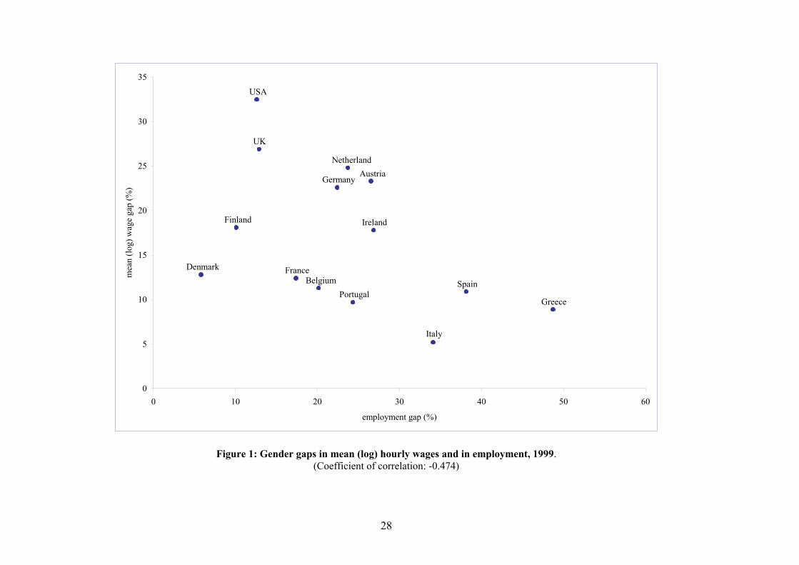
28

GreecePortugal

Spain

Italy

France

Ireland

Austria

Belgium

Netherland

Germany

Denmark

Finland

UK

USA

0

5

10

15

20

25

30

35

0 10 20 30 40 50 60

employment gap (%)

mea

n (lo

g) w

age

gap

(%)

Figure 1: Gender gaps in mean (log) hourly wages and in employment, 1999. (Coefficient of correlation: -0.474)

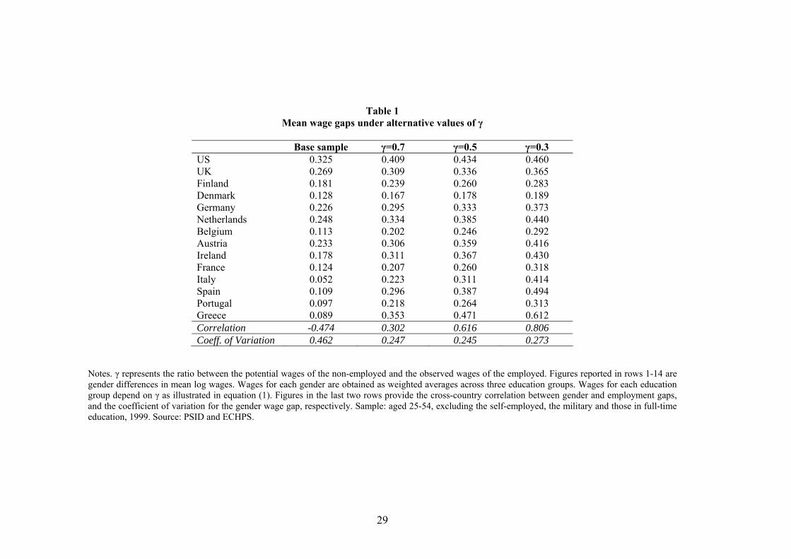
29

Table 1 Mean wage gaps under alternative values of γ

Base sample γ=0.7 γ=0.5 γ=0.3 US 0.325 0.409 0.434 0.460 UK 0.269 0.309 0.336 0.365 Finland 0.181 0.239 0.260 0.283 Denmark 0.128 0.167 0.178 0.189 Germany 0.226 0.295 0.333 0.373 Netherlands 0.248 0.334 0.385 0.440 Belgium 0.113 0.202 0.246 0.292 Austria 0.233 0.306 0.359 0.416 Ireland 0.178 0.311 0.367 0.430 France 0.124 0.207 0.260 0.318 Italy 0.052 0.223 0.311 0.414 Spain 0.109 0.296 0.387 0.494 Portugal 0.097 0.218 0.264 0.313 Greece 0.089 0.353 0.471 0.612 Correlation -0.474 0.302 0.616 0.806 Coeff. of Variation 0.462 0.247 0.245 0.273

Notes. γ represents the ratio between the potential wages of the non-employed and the observed wages of the employed. Figures reported in rows 1-14 are gender differences in mean log wages. Wages for each gender are obtained as weighted averages across three education groups. Wages for each education group depend on γ as illustrated in equation (1). Figures in the last two rows provide the cross-country correlation between gender and employment gaps, and the coefficient of variation for the gender wage gap, respectively. Sample: aged 25-54, excluding the self-employed, the military and those in full-time education, 1999. Source: PSID and ECHPS.

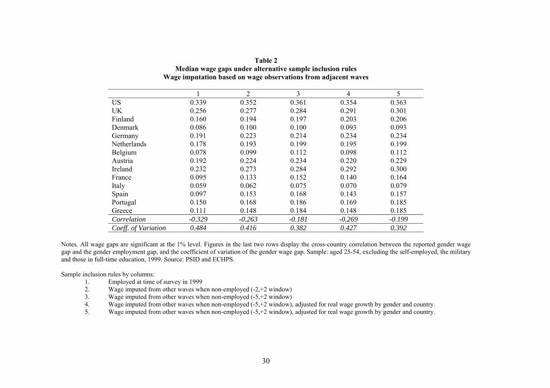
30

Table 2 Median wage gaps under alternative sample inclusion rules

Wage imputation based on wage observations from adjacent waves

1 2 3 4 5 US 0.339 0.352 0.361 0.354 0.363 UK 0.256 0.277 0.284 0.291 0.301 Finland 0.160 0.194 0.197 0.203 0.206 Denmark 0.086 0.100 0.100 0.093 0.093 Germany 0.191 0.223 0.214 0.234 0.234 Netherlands 0.178 0.193 0.199 0.195 0.199 Belgium 0.078 0.099 0.112 0.098 0.112 Austria 0.192 0.224 0.234 0.220 0.229 Ireland 0.232 0.273 0.284 0.292 0.300 France 0.095 0.133 0.152 0.140 0.164 Italy 0.059 0.062 0.075 0.070 0.079 Spain 0.097 0.153 0.168 0.143 0.157 Portugal 0.150 0.168 0.186 0.169 0.185 Greece 0.111 0.148 0.184 0.148 0.185 Correlation -0.329 -0.263 -0.181 -0.269 -0.199 Coeff. of Variation 0.484 0.416 0.382 0.427 0.392

Notes. All wage gaps are significant at the 1% level. Figures in the last two rows display the cross-country correlation between the reported gender wage gap and the gender employment gap, and the coefficient of variation of the gender wage gap. Sample: aged 25-54, excluding the self-employed, the military and those in full-time education, 1999. Source: PSID and ECHPS. Sample inclusion rules by columns:

1. Employed at time of survey in 1999 2. Wage imputed from other waves when non-employed (-2,+2 window) 3. Wage imputed from other waves when non-employed (-5,+2 window) 4. Wage imputed from other waves when non-employed (-5,+2 window), adjusted for real wage growth by gender and country. 5. Wage imputed from other waves when non-employed (-5,+2 window), adjusted for real wage growth by gender and country.

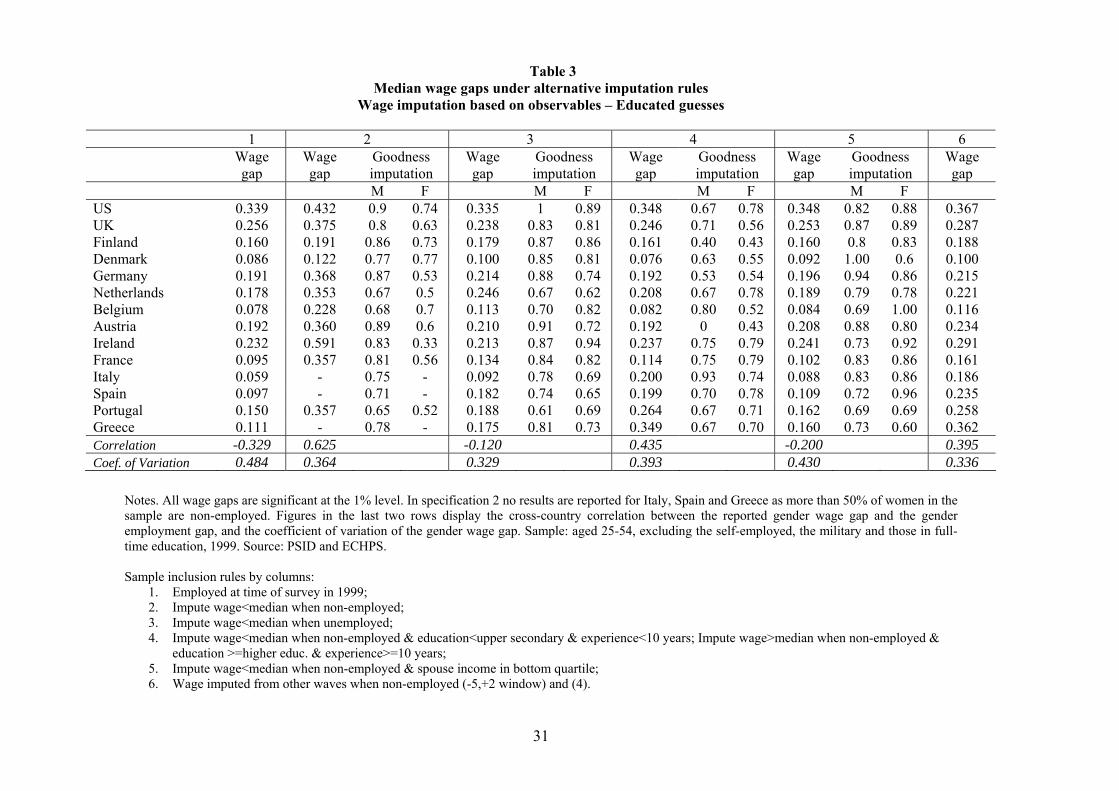
31

Table 3

Median wage gaps under alternative imputation rules Wage imputation based on observables – Educated guesses

1 2 3 4 5 6 Wage

gap Wage gap

Goodness imputation

Wage gap

Goodness imputation

Wage gap

Goodness imputation

Wage gap

Goodness imputation

Wage gap

M F M F M F M F US 0.339 0.432 0.9 0.74 0.335 1 0.89 0.348 0.67 0.78 0.348 0.82 0.88 0.367 UK 0.256 0.375 0.8 0.63 0.238 0.83 0.81 0.246 0.71 0.56 0.253 0.87 0.89 0.287 Finland 0.160 0.191 0.86 0.73 0.179 0.87 0.86 0.161 0.40 0.43 0.160 0.8 0.83 0.188 Denmark 0.086 0.122 0.77 0.77 0.100 0.85 0.81 0.076 0.63 0.55 0.092 1.00 0.6 0.100 Germany 0.191 0.368 0.87 0.53 0.214 0.88 0.74 0.192 0.53 0.54 0.196 0.94 0.86 0.215 Netherlands 0.178 0.353 0.67 0.5 0.246 0.67 0.62 0.208 0.67 0.78 0.189 0.79 0.78 0.221 Belgium 0.078 0.228 0.68 0.7 0.113 0.70 0.82 0.082 0.80 0.52 0.084 0.69 1.00 0.116 Austria 0.192 0.360 0.89 0.6 0.210 0.91 0.72 0.192 0 0.43 0.208 0.88 0.80 0.234 Ireland 0.232 0.591 0.83 0.33 0.213 0.87 0.94 0.237 0.75 0.79 0.241 0.73 0.92 0.291 France 0.095 0.357 0.81 0.56 0.134 0.84 0.82 0.114 0.75 0.79 0.102 0.83 0.86 0.161 Italy 0.059 - 0.75 - 0.092 0.78 0.69 0.200 0.93 0.74 0.088 0.83 0.86 0.186 Spain 0.097 - 0.71 - 0.182 0.74 0.65 0.199 0.70 0.78 0.109 0.72 0.96 0.235 Portugal 0.150 0.357 0.65 0.52 0.188 0.61 0.69 0.264 0.67 0.71 0.162 0.69 0.69 0.258 Greece 0.111 - 0.78 - 0.175 0.81 0.73 0.349 0.67 0.70 0.160 0.73 0.60 0.362 Correlation -0.329 0.625 -0.120 0.435 -0.200 0.395 Coef. of Variation 0.484 0.364 0.329 0.393 0.430 0.336

Notes. All wage gaps are significant at the 1% level. In specification 2 no results are reported for Italy, Spain and Greece as more than 50% of women in the sample are non-employed. Figures in the last two rows display the cross-country correlation between the reported gender wage gap and the gender employment gap, and the coefficient of variation of the gender wage gap. Sample: aged 25-54, excluding the self-employed, the military and those in full-time education, 1999. Source: PSID and ECHPS. Sample inclusion rules by columns:

1. Employed at time of survey in 1999; 2. Impute wage<median when non-employed; 3. Impute wage<median when unemployed; 4. Impute wage<median when non-employed & education<upper secondary & experience<10 years; Impute wage>median when non-employed &

education >=higher educ. & experience>=10 years; 5. Impute wage<median when non-employed & spouse income in bottom quartile; 6. Wage imputed from other waves when non-employed (-5,+2 window) and (4).

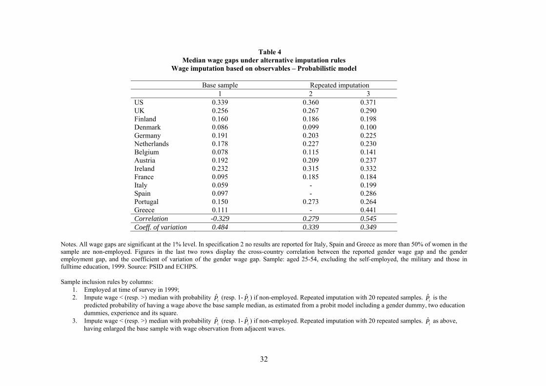
32

Table 4 Median wage gaps under alternative imputation rules

Wage imputation based on observables – Probabilistic model

Base sample Repeated imputation 1 2 3 US 0.339 0.360 0.371 UK 0.256 0.267 0.290 Finland 0.160 0.186 0.198 Denmark 0.086 0.099 0.100 Germany 0.191 0.203 0.225 Netherlands 0.178 0.227 0.230 Belgium 0.078 0.115 0.141 Austria 0.192 0.209 0.237 Ireland 0.232 0.315 0.332 France 0.095 0.185 0.184 Italy 0.059 - 0.199 Spain 0.097 - 0.286 Portugal 0.150 0.273 0.264 Greece 0.111 - 0.441 Correlation -0.329 0.279 0.545 Coeff. of variation 0.484 0.339 0.349

Notes. All wage gaps are significant at the 1% level. In specification 2 no results are reported for Italy, Spain and Greece as more than 50% of women in the sample are non-employed. Figures in the last two rows display the cross-country correlation between the reported gender wage gap and the gender employment gap, and the coefficient of variation of the gender wage gap. Sample: aged 25-54, excluding the self-employed, the military and those in fulltime education, 1999. Source: PSID and ECHPS. Sample inclusion rules by columns:

1. Employed at time of survey in 1999; 2. Impute wage < (resp. >) median with probability iP (resp. 1- iP ) if non-employed. Repeated imputation with 20 repeated samples. iP is the

predicted probability of having a wage above the base sample median, as estimated from a probit model including a gender dummy, two education dummies, experience and its square.

3. Impute wage < (resp. >) median with probability iP (resp. 1- iP ) if non-employed. Repeated imputation with 20 repeated samples. iP as above, having enlarged the base sample with wage observation from adjacent waves.

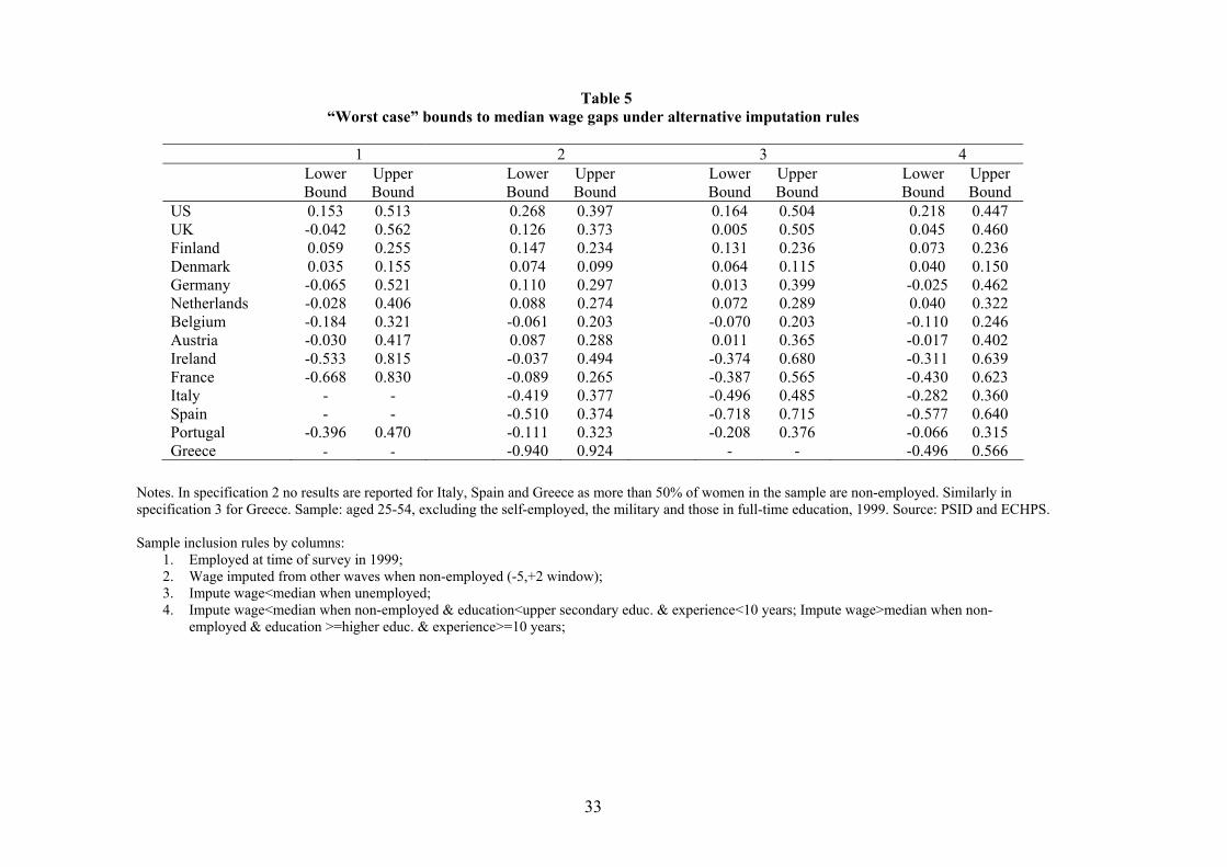
33

Table 5 “Worst case” bounds to median wage gaps under alternative imputation rules

1 2 3 4 Lower

Bound Upper Bound

Lower Bound

Upper Bound

Lower Bound

Upper Bound

Lower Bound

Upper Bound

US 0.153 0.513 0.268 0.397 0.164 0.504 0.218 0.447 UK -0.042 0.562 0.126 0.373 0.005 0.505 0.045 0.460 Finland 0.059 0.255 0.147 0.234 0.131 0.236 0.073 0.236 Denmark 0.035 0.155 0.074 0.099 0.064 0.115 0.040 0.150 Germany -0.065 0.521 0.110 0.297 0.013 0.399 -0.025 0.462 Netherlands -0.028 0.406 0.088 0.274 0.072 0.289 0.040 0.322 Belgium -0.184 0.321 -0.061 0.203 -0.070 0.203 -0.110 0.246 Austria -0.030 0.417 0.087 0.288 0.011 0.365 -0.017 0.402 Ireland -0.533 0.815 -0.037 0.494 -0.374 0.680 -0.311 0.639 France -0.668 0.830 -0.089 0.265 -0.387 0.565 -0.430 0.623 Italy - - -0.419 0.377 -0.496 0.485 -0.282 0.360 Spain - - -0.510 0.374 -0.718 0.715 -0.577 0.640 Portugal -0.396 0.470 -0.111 0.323 -0.208 0.376 -0.066 0.315 Greece - - -0.940 0.924 - - -0.496 0.566

Notes. In specification 2 no results are reported for Italy, Spain and Greece as more than 50% of women in the sample are non-employed. Similarly in specification 3 for Greece. Sample: aged 25-54, excluding the self-employed, the military and those in full-time education, 1999. Source: PSID and ECHPS. Sample inclusion rules by columns:

1. Employed at time of survey in 1999; 2. Wage imputed from other waves when non-employed (-5,+2 window); 3. Impute wage<median when unemployed; 4. Impute wage<median when non-employed & education<upper secondary educ. & experience<10 years; Impute wage>median when non-

employed & education >=higher educ. & experience>=10 years;

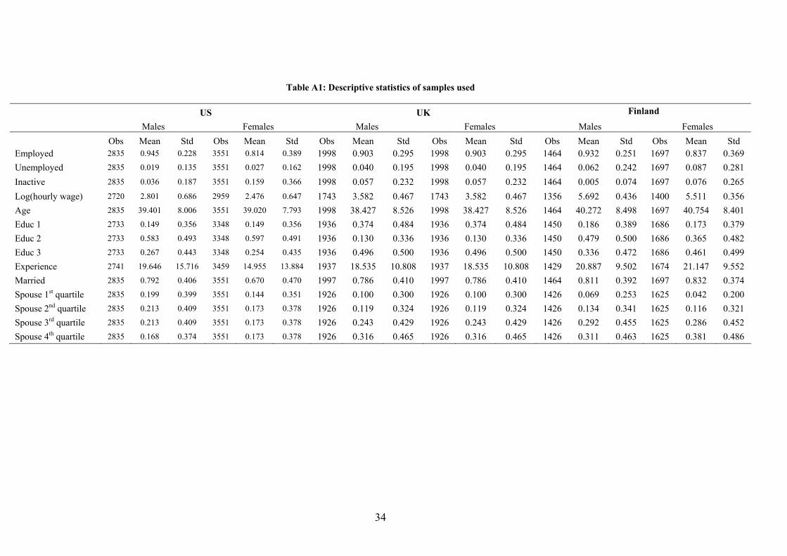
34

Table A1: Descriptive statistics of samples used

US UK Finland Males Females Males Females Males Females Obs Mean Std Obs Mean Std Obs Mean Std Obs Mean Std Obs Mean Std Obs Mean Std Employed 2835 0.945 0.228 3551 0.814 0.389 1998 0.903 0.295 1998 0.903 0.295 1464 0.932 0.251 1697 0.837 0.369 Unemployed 2835 0.019 0.135 3551 0.027 0.162 1998 0.040 0.195 1998 0.040 0.195 1464 0.062 0.242 1697 0.087 0.281 Inactive 2835 0.036 0.187 3551 0.159 0.366 1998 0.057 0.232 1998 0.057 0.232 1464 0.005 0.074 1697 0.076 0.265 Log(hourly wage) 2720 2.801 0.686 2959 2.476 0.647 1743 3.582 0.467 1743 3.582 0.467 1356 5.692 0.436 1400 5.511 0.356 Age 2835 39.401 8.006 3551 39.020 7.793 1998 38.427 8.526 1998 38.427 8.526 1464 40.272 8.498 1697 40.754 8.401 Educ 1 2733 0.149 0.356 3348 0.149 0.356 1936 0.374 0.484 1936 0.374 0.484 1450 0.186 0.389 1686 0.173 0.379 Educ 2 2733 0.583 0.493 3348 0.597 0.491 1936 0.130 0.336 1936 0.130 0.336 1450 0.479 0.500 1686 0.365 0.482 Educ 3 2733 0.267 0.443 3348 0.254 0.435 1936 0.496 0.500 1936 0.496 0.500 1450 0.336 0.472 1686 0.461 0.499 Experience 2741 19.646 15.716 3459 14.955 13.884 1937 18.535 10.808 1937 18.535 10.808 1429 20.887 9.502 1674 21.147 9.552 Married 2835 0.792 0.406 3551 0.670 0.470 1997 0.786 0.410 1997 0.786 0.410 1464 0.811 0.392 1697 0.832 0.374 Spouse 1st quartile 2835 0.199 0.399 3551 0.144 0.351 1926 0.100 0.300 1926 0.100 0.300 1426 0.069 0.253 1625 0.042 0.200 Spouse 2nd quartile 2835 0.213 0.409 3551 0.173 0.378 1926 0.119 0.324 1926 0.119 0.324 1426 0.134 0.341 1625 0.116 0.321 Spouse 3rd quartile 2835 0.213 0.409 3551 0.173 0.378 1926 0.243 0.429 1926 0.243 0.429 1426 0.292 0.455 1625 0.286 0.452 Spouse 4th quartile 2835 0.168 0.374 3551 0.173 0.378 1926 0.316 0.465 1926 0.316 0.465 1426 0.311 0.463 1625 0.381 0.486

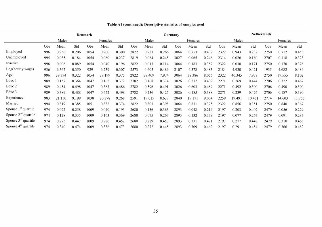
35

Table A1 (continued): Descriptive statistics of samples used

Denmark Germany Netherlands Males Females Males Females Males Females Obs Mean Std Obs Mean Std Obs Mean Std Obs Mean Std Obs Mean Std Obs Mean Std Employed 996 0.956 0.206 1054 0.900 0.300 2822 0.923 0.266 3064 0.753 0.432 2322 0.943 0.232 2750 0.712 0.453 Unemployed 995 0.035 0.184 1054 0.060 0.237 2819 0.064 0.245 3027 0.065 0.246 2314 0.026 0.160 2707 0.118 0.323 Inactive 996 0.008 0.089 1054 0.040 0.196 2822 0.013 0.114 3064 0.183 0.387 2322 0.030 0.171 2750 0.170 0.376 Log(hourly wage) 936 6.367 0.350 929 6.239 0.307 2573 4.605 0.486 2107 4.378 0.483 2184 4.930 0.421 1935 4.682 0.484 Age 996 39.394 8.322 1054 39.199 8.375 2822 38.409 7.974 3064 38.386 8.056 2322 40.345 7.978 2750 39.555 8.102 Educ 1 989 0.157 0.364 1047 0.165 0.372 2782 0.168 0.374 3026 0.212 0.409 2271 0.269 0.444 2706 0.322 0.467 Educ 2 989 0.454 0.498 1047 0.383 0.486 2782 0.596 0.491 3026 0.603 0.489 2271 0.492 0.500 2706 0.490 0.500 Educ 3 989 0.389 0.488 1047 0.452 0.498 2782 0.236 0.425 3026 0.185 0.388 2271 0.239 0.426 2706 0.187 0.390 Experience 983 21.150 9.199 1038 20.378 9.268 2591 19.015 8.637 2840 19.171 9.004 2259 19.491 10.431 2714 14.603 11.755 Married 994 0.819 0.385 1051 0.832 0.374 2822 0.803 0.398 3064 0.831 0.375 2322 0.856 0.351 2750 0.840 0.367 Spouse 1st quartile 974 0.072 0.258 1009 0.040 0.195 2680 0.156 0.363 2893 0.048 0.214 2197 0.203 0.402 2479 0.056 0.229 Spouse 2nd quartile 974 0.128 0.335 1009 0.163 0.369 2680 0.075 0.263 2893 0.132 0.339 2197 0.077 0.267 2479 0.091 0.287 Spouse 3rd quartile 974 0.275 0.447 1009 0.286 0.452 2680 0.289 0.453 2893 0.331 0.471 2197 0.277 0.448 2479 0.310 0.463 Spouse 4th quartile 974 0.340 0.474 1009 0.336 0.473 2680 0.272 0.445 2893 0.309 0.462 2197 0.291 0.454 2479 0.366 0.482

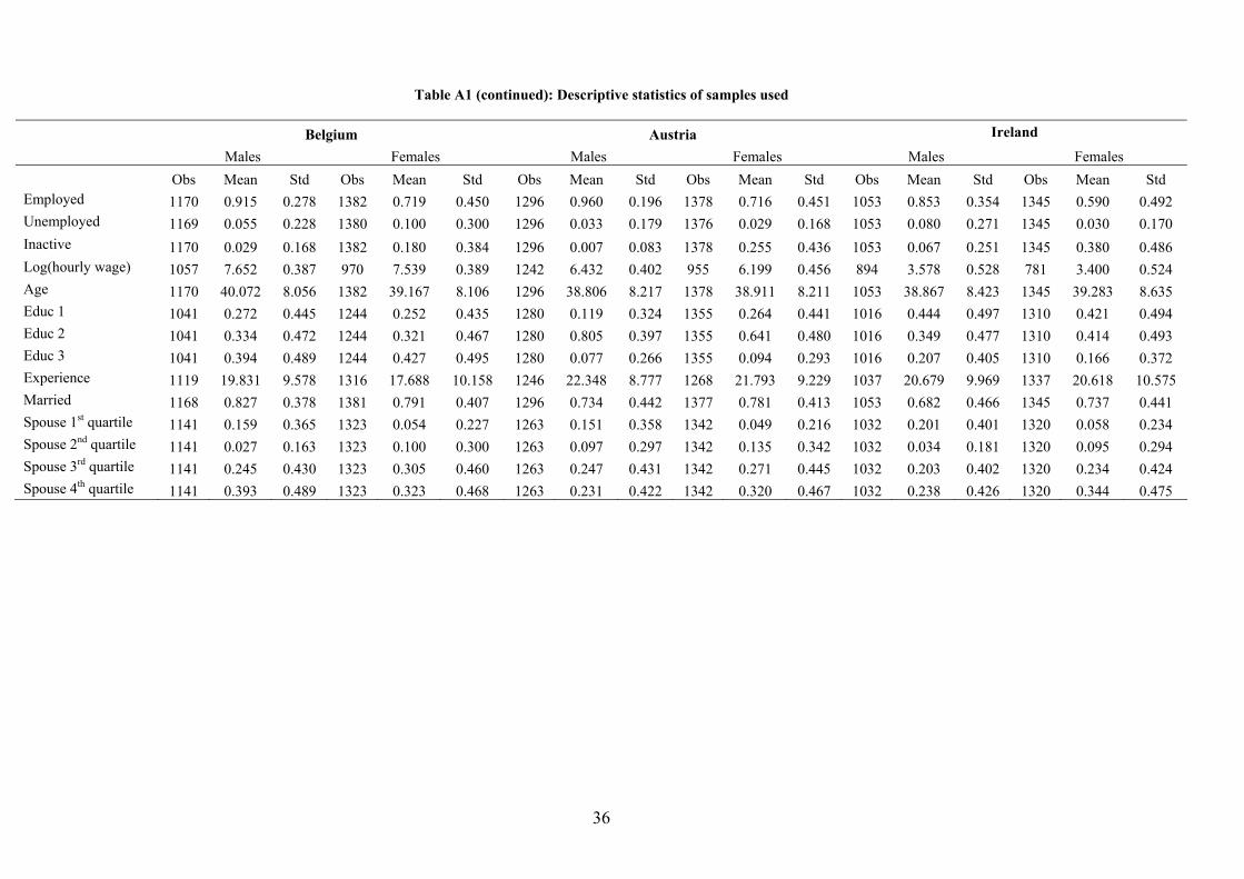
36

Table A1 (continued): Descriptive statistics of samples used

Belgium Austria Ireland Males Females Males Females Males Females Obs Mean Std Obs Mean Std Obs Mean Std Obs Mean Std Obs Mean Std Obs Mean Std Employed 1170 0.915 0.278 1382 0.719 0.450 1296 0.960 0.196 1378 0.716 0.451 1053 0.853 0.354 1345 0.590 0.492 Unemployed 1169 0.055 0.228 1380 0.100 0.300 1296 0.033 0.179 1376 0.029 0.168 1053 0.080 0.271 1345 0.030 0.170 Inactive 1170 0.029 0.168 1382 0.180 0.384 1296 0.007 0.083 1378 0.255 0.436 1053 0.067 0.251 1345 0.380 0.486 Log(hourly wage) 1057 7.652 0.387 970 7.539 0.389 1242 6.432 0.402 955 6.199 0.456 894 3.578 0.528 781 3.400 0.524 Age 1170 40.072 8.056 1382 39.167 8.106 1296 38.806 8.217 1378 38.911 8.211 1053 38.867 8.423 1345 39.283 8.635 Educ 1 1041 0.272 0.445 1244 0.252 0.435 1280 0.119 0.324 1355 0.264 0.441 1016 0.444 0.497 1310 0.421 0.494 Educ 2 1041 0.334 0.472 1244 0.321 0.467 1280 0.805 0.397 1355 0.641 0.480 1016 0.349 0.477 1310 0.414 0.493 Educ 3 1041 0.394 0.489 1244 0.427 0.495 1280 0.077 0.266 1355 0.094 0.293 1016 0.207 0.405 1310 0.166 0.372 Experience 1119 19.831 9.578 1316 17.688 10.158 1246 22.348 8.777 1268 21.793 9.229 1037 20.679 9.969 1337 20.618 10.575 Married 1168 0.827 0.378 1381 0.791 0.407 1296 0.734 0.442 1377 0.781 0.413 1053 0.682 0.466 1345 0.737 0.441 Spouse 1st quartile 1141 0.159 0.365 1323 0.054 0.227 1263 0.151 0.358 1342 0.049 0.216 1032 0.201 0.401 1320 0.058 0.234 Spouse 2nd quartile 1141 0.027 0.163 1323 0.100 0.300 1263 0.097 0.297 1342 0.135 0.342 1032 0.034 0.181 1320 0.095 0.294 Spouse 3rd quartile 1141 0.245 0.430 1323 0.305 0.460 1263 0.247 0.431 1342 0.271 0.445 1032 0.203 0.402 1320 0.234 0.424 Spouse 4th quartile 1141 0.393 0.489 1323 0.323 0.468 1263 0.231 0.422 1342 0.320 0.467 1032 0.238 0.426 1320 0.344 0.475

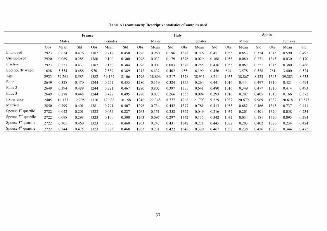
37

Table A1 (continued): Descriptive statistics of samples used

France Italy Spain Males Females Males Females Males Females Obs Mean Std Obs Mean Std Obs Mean Std Obs Mean Std Obs Mean Std Obs Mean Std Employed 2923 0.654 0.476 1382 0.719 0.450 1296 0.960 0.196 1378 0.716 0.451 1053 0.853 0.354 1345 0.590 0.492 Unemployed 2920 0.089 0.285 1380 0.100 0.300 1296 0.033 0.179 1376 0.029 0.168 1053 0.080 0.271 1345 0.030 0.170 Inactive 2923 0.257 0.437 1382 0.180 0.384 1296 0.007 0.083 1378 0.255 0.436 1053 0.067 0.251 1345 0.380 0.486 Log(hourly wage) 1628 5.554 0.488 970 7.539 0.389 1242 6.432 0.402 955 6.199 0.456 894 3.578 0.528 781 3.400 0.524 Age 2923 39.261 8.585 1382 39.167 8.106 1296 38.806 8.217 1378 38.911 8.211 1053 38.867 8.423 1345 39.283 8.635 Educ 1 2649 0.328 0.470 1244 0.252 0.435 1280 0.119 0.324 1355 0.264 0.441 1016 0.444 0.497 1310 0.421 0.494 Educ 2 2649 0.394 0.489 1244 0.321 0.467 1280 0.805 0.397 1355 0.641 0.480 1016 0.349 0.477 1310 0.414 0.493 Educ 3 2649 0.278 0.448 1244 0.427 0.495 1280 0.077 0.266 1355 0.094 0.293 1016 0.207 0.405 1310 0.166 0.372 Experience 2405 16.177 12.295 1316 17.688 10.158 1246 22.348 8.777 1268 21.793 9.229 1037 20.679 9.969 1337 20.618 10.575 Married 2850 0.799 0.401 1381 0.791 0.407 1296 0.734 0.442 1377 0.781 0.413 1053 0.682 0.466 1345 0.737 0.441 Spouse 1st quartile 2722 0.042 0.201 1323 0.054 0.227 1263 0.151 0.358 1342 0.049 0.216 1032 0.201 0.401 1320 0.058 0.234 Spouse 2nd quartile 2722 0.098 0.298 1323 0.100 0.300 1263 0.097 0.297 1342 0.135 0.342 1032 0.034 0.181 1320 0.095 0.294 Spouse 3rd quartile 2722 0.305 0.460 1323 0.305 0.460 1263 0.247 0.431 1342 0.271 0.445 1032 0.203 0.402 1320 0.234 0.424 Spouse 4th quartile 2722 0.344 0.475 1323 0.323 0.468 1263 0.231 0.422 1342 0.320 0.467 1032 0.238 0.426 1320 0.344 0.475

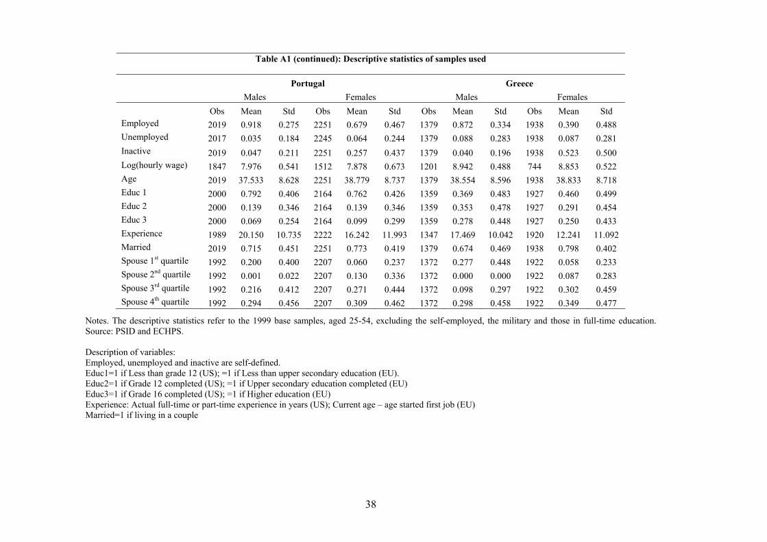
38

Notes. The descriptive statistics refer to the 1999 base samples, aged 25-54, excluding the self-employed, the military and those in full-time education. Source: PSID and ECHPS. Description of variables: Employed, unemployed and inactive are self-defined. Educ1=1 if Less than grade 12 (US); =1 if Less than upper secondary education (EU). Educ2=1 if Grade 12 completed (US); =1 if Upper secondary education completed (EU) Educ3=1 if Grade 16 completed (US); =1 if Higher education (EU) Experience: Actual full-time or part-time experience in years (US); Current age – age started first job (EU) Married=1 if living in a couple

Table A1 (continued): Descriptive statistics of samples used

Portugal Greece Males Females Males Females Obs Mean Std Obs Mean Std Obs Mean Std Obs Mean Std Employed 2019 0.918 0.275 2251 0.679 0.467 1379 0.872 0.334 1938 0.390 0.488 Unemployed 2017 0.035 0.184 2245 0.064 0.244 1379 0.088 0.283 1938 0.087 0.281 Inactive 2019 0.047 0.211 2251 0.257 0.437 1379 0.040 0.196 1938 0.523 0.500 Log(hourly wage) 1847 7.976 0.541 1512 7.878 0.673 1201 8.942 0.488 744 8.853 0.522 Age 2019 37.533 8.628 2251 38.779 8.737 1379 38.554 8.596 1938 38.833 8.718 Educ 1 2000 0.792 0.406 2164 0.762 0.426 1359 0.369 0.483 1927 0.460 0.499 Educ 2 2000 0.139 0.346 2164 0.139 0.346 1359 0.353 0.478 1927 0.291 0.454 Educ 3 2000 0.069 0.254 2164 0.099 0.299 1359 0.278 0.448 1927 0.250 0.433 Experience 1989 20.150 10.735 2222 16.242 11.993 1347 17.469 10.042 1920 12.241 11.092 Married 2019 0.715 0.451 2251 0.773 0.419 1379 0.674 0.469 1938 0.798 0.402 Spouse 1st quartile 1992 0.200 0.400 2207 0.060 0.237 1372 0.277 0.448 1922 0.058 0.233 Spouse 2nd quartile 1992 0.001 0.022 2207 0.130 0.336 1372 0.000 0.000 1922 0.087 0.283 Spouse 3rd quartile 1992 0.216 0.412 2207 0.271 0.444 1372 0.098 0.297 1922 0.302 0.459 Spouse 4th quartile 1992 0.294 0.456 2207 0.309 0.462 1372 0.298 0.458 1922 0.349 0.477

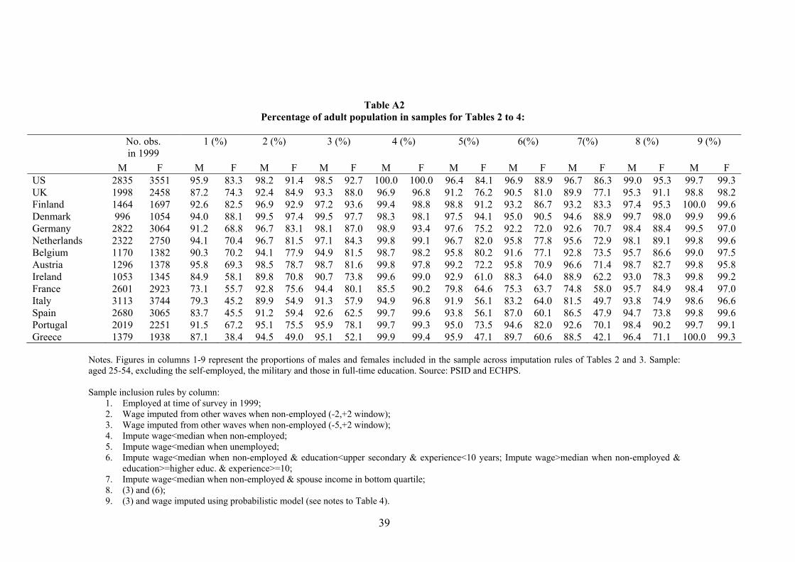
39

Table A2

Percentage of adult population in samples for Tables 2 to 4:

No. obs. in 1999

1 (%) 2 (%) 3 (%) 4 (%) 5(%) 6(%) 7(%) 8 (%) 9 (%)

M F M F M F M F M F M F M F M F M F M F US 2835 3551 95.9 83.3 98.2 91.4 98.5 92.7 100.0 100.0 96.4 84.1 96.9 88.9 96.7 86.3 99.0 95.3 99.7 99.3 UK 1998 2458 87.2 74.3 92.4 84.9 93.3 88.0 96.9 96.8 91.2 76.2 90.5 81.0 89.9 77.1 95.3 91.1 98.8 98.2 Finland 1464 1697 92.6 82.5 96.9 92.9 97.2 93.6 99.4 98.8 98.8 91.2 93.2 86.7 93.2 83.3 97.4 95.3 100.0 99.6 Denmark 996 1054 94.0 88.1 99.5 97.4 99.5 97.7 98.3 98.1 97.5 94.1 95.0 90.5 94.6 88.9 99.7 98.0 99.9 99.6 Germany 2822 3064 91.2 68.8 96.7 83.1 98.1 87.0 98.9 93.4 97.6 75.2 92.2 72.0 92.6 70.7 98.4 88.4 99.5 97.0 Netherlands 2322 2750 94.1 70.4 96.7 81.5 97.1 84.3 99.8 99.1 96.7 82.0 95.8 77.8 95.6 72.9 98.1 89.1 99.8 99.6 Belgium 1170 1382 90.3 70.2 94.1 77.9 94.9 81.5 98.7 98.2 95.8 80.2 91.6 77.1 92.8 73.5 95.7 86.6 99.0 97.5 Austria 1296 1378 95.8 69.3 98.5 78.7 98.7 81.6 99.8 97.8 99.2 72.2 95.8 70.9 96.6 71.4 98.7 82.7 99.8 95.8 Ireland 1053 1345 84.9 58.1 89.8 70.8 90.7 73.8 99.6 99.0 92.9 61.0 88.3 64.0 88.9 62.2 93.0 78.3 99.8 99.2 France 2601 2923 73.1 55.7 92.8 75.6 94.4 80.1 85.5 90.2 79.8 64.6 75.3 63.7 74.8 58.0 95.7 84.9 98.4 97.0 Italy 3113 3744 79.3 45.2 89.9 54.9 91.3 57.9 94.9 96.8 91.9 56.1 83.2 64.0 81.5 49.7 93.8 74.9 98.6 96.6 Spain 2680 3065 83.7 45.5 91.2 59.4 92.6 62.5 99.7 99.6 93.8 56.1 87.0 60.1 86.5 47.9 94.7 73.8 99.8 99.6 Portugal 2019 2251 91.5 67.2 95.1 75.5 95.9 78.1 99.7 99.3 95.0 73.5 94.6 82.0 92.6 70.1 98.4 90.2 99.7 99.1 Greece 1379 1938 87.1 38.4 94.5 49.0 95.1 52.1 99.9 99.4 95.9 47.1 89.7 60.6 88.5 42.1 96.4 71.1 100.0 99.3

Notes. Figures in columns 1-9 represent the proportions of males and females included in the sample across imputation rules of Tables 2 and 3. Sample: aged 25-54, excluding the self-employed, the military and those in full-time education. Source: PSID and ECHPS. Sample inclusion rules by column:

1. Employed at time of survey in 1999; 2. Wage imputed from other waves when non-employed (-2,+2 window); 3. Wage imputed from other waves when non-employed (-5,+2 window); 4. Impute wage<median when non-employed; 5. Impute wage<median when unemployed; 6. Impute wage<median when non-employed & education<upper secondary & experience<10 years; Impute wage>median when non-employed &

education>=higher educ. & experience>=10; 7. Impute wage<median when non-employed & spouse income in bottom quartile; 8. (3) and (6); 9. (3) and wage imputed using probabilistic model (see notes to Table 4).

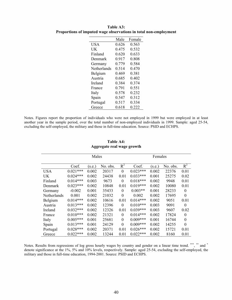
40

Table A3: Proportions of imputed wage observations in total non-employment

Notes. Figures report the proportion of individuals who were not employed in 1999 but were employed in at least another year in the sample period, over the total number of non-employed individuals in 1999. Sample: aged 25-54, excluding the self-employed, the military and those in full-time education. Source: PSID and ECHPS.

Table A4: Aggregate real wage growth

Notes. Results from regressions of log gross hourly wages by country and gender on a linear time trend. ***, ** and * denote significance at the 1%, 5% and 10% levels, respectively. Sample: aged 25-54, excluding the self-employed, the military and those in full-time education, 1994-2001. Source: PSID and ECHPS.

Male FemaleUSA 0.626 0.563 UK 0.475 0.532 Finland 0.620 0.633 Denmark 0.917 0.808 Germany 0.779 0.584 Netherlands 0.514 0.470 Belgium 0.469 0.381 Austria 0.685 0.402 Ireland 0.384 0.374 France 0.791 0.551 Italy 0.578 0.232 Spain 0.547 0.312 Portugal 0.517 0.334 Greece 0.618 0.222

Males Females

Coef. (s.e.) No. obs. R2 Coef. (s.e.) No. obs. R2 USA 0.021*** 0.002 20317 0 0.023*** 0.002 22376 0.01UK 0.024*** 0.002 24438 0.01 0.033*** 0.001 25275 0.02Finland 0.014*** 0.003 9673 0 0.018*** 0.002 9948 0.01Denmark 0.023*** 0.002 10848 0.01 0.019*** 0.002 10080 0.01Germany -0.002 0.001 35433 0 0.003** 0.001 28233 0 Netherlands 0.001 0.002 21032 0 0.002 0.002 17695 0 Belgium 0.014*** 0.002 10616 0.01 0.014*** 0.002 9051 0.01Austria 0.013*** 0.002 12396 0 0.010*** 0.003 9091 0 Ireland 0.032*** 0.002 12326 0.01 0.039*** 0.003 9607 0.02France 0.010*** 0.002 21321 0 0.014*** 0.002 17824 0 Italy 0.005*** 0.001 25681 0 0.009*** 0.001 16744 0 Spain 0.013*** 0.001 24129 0 0.009*** 0.002 14255 0 Portugal 0.028*** 0.002 20371 0.01 0.026*** 0.002 15721 0.01Greece 0.022*** 0.002 13244 0.01 0.022*** 0.002 8160 0.01