Unemployment vs. Mismatch of Talents: Reconsidering Unemployment Benefits

6HPLQDU 3DSHU 1Rï ççì

81(03/2<0(17 96ï 0,60$7&+ 2) 7$/(176ã

5(&216,'(5,1* 81(03/2<0(17 %(1(),76

E\

5DPRQ 0DULPRQ DQG )DEUL]LR =LOLERWWL

,167,787( )25 ,17(51$7,21$/ (&2120,& 678',(66WRFNKROP 8QLYHUVLW\

,661 íêéæðåæçä

6HPLQDU 3DSHU 1Rï ççì

81(03/2<0(17 96ï 0,60$7&+ 2) 7$/(176ã5(&216,'(5,1* 81(03/2<0(17 %(1(),76

E\

5DPRQ 0DULPRQ DQG )DEUL]LR =LOLERWWL

3DSHUV LQ WKH VHPLQDU VHULHV DUH DOVR SXEOLVKHG RQ LQWHUQHWLQ SRVWVFULSW DQG $GREH $FUREDW õ3')ô IRUPDWVï'RZQORDG IURP KWWSãîîZZZïLLHVïVXïVHî

6HPLQDU 3DSHUV DUH SUHOLPLQDU\ PDWHULDO FLUFXODWHG WRVWLPXODWH GLVFXVVLRQ DQG FULWLFDO FRPPHQWï

1RYHPEHU ìääå

,QVWLWXWH IRU ,QWHUQDWLRQDO (FRQRPLF 6WXGLHV6ðìíç äì 6WRFNKROP6ZHGHQ

Unemployment vs. mismatch of talents:Reconsidering unemployment bene¯ts.¤

Ramon MarimonEuropean University Institute,

Universitat Pompeu Fabra, NBER and CEPR

Fabrizio ZilibottiInstitute for International Economic Studies,Universitat Pompeu Fabra and CEPR

November 20, 1998

AbstractWe develop an equilibrium search-matching model with risk-neutral agents

and two-sided ex-ante heterogeneity. Unemployment insurance has the stan-dard e®ect of reducing employment, but also helps workers to get a suitablejob. The predictions of our simple model are consistent with the contrastingperformance of the labor market in Europe and US in terms of unemploy-ment, productivity growth and wage inequality. To show this, we constructtwo ¯ctitious economies with calibrated parameters which only di®er by thedegree of unemployment insurance and assume that they are hit by a commontechnological shock which enhances the importance of mismatch. This shockreduces the proportion of jobs which workers regards as acceptable in theeconomy with unemployment insurance (Europe). As a result, unemploymentdoubles in this economy. In the laissez-faire economy (US), unemploymentremains constant, but wage inequality increases more and productivity growsless due to larger mismatch. The model is used to address some politicaleconomy issues.

Keywords: Unemployment, Productivity, Mismatch, Ex-ante heterogeneity,Search, Unemployment bene¯ts, E±ciency, Inequality.JEL Classi¯cation: J64, J65, D33.

¤We wish to thank Daron Acemoglu, Dale Mortensen and two referees for their comments andChristina Loennblad and Marcia Gastaldo for their editorial assistance. Zilibotti acknowledges theCentre de Recerca en Economia Internacional for ¯nancial support and the European Forum ofthe EUI for kind hospitality.

1

1 Introduction.

In this paper we present a simple equilibrium search-matching model of the labormarket with two-sided ex-ante heterogeneity. The predictions of this model areshown to be consistent with some salient features of the contrasting evolution oflabor markets in ContinentalWestern Europe and the US. In particular, we focus onthree observations. First, unemployment has risen dramatically in Europe, whereasit exhibits no such trend in the United States. Second, the productivity per workerhas increased much faster in Europe than in the US. Third, wage inequality hasincreased to a much larger extent in the US than in Europe.European unemployment increased, from an average of 4% in the early 70's to

more than 11% in the mid 80's and, then, persistently remained very high. In theUS the unemployment rate was around 5% in 1975, and around 6% in 1994. Therising level of unemployment in Europe has been associated with decreasing ratesof exit from unemployment (and fairly stationary rates of entry), longer duration ofunemployment, and growing incidence of long-term unemployment (see, for example,Alogoskou¯s et al. 1995). In the US, instead, both the in°ows and out°ows arestationary and unemployment spells tend to be short. The unemployment gapnotwithstanding, the total GDP growth in Europe has been similar to that in theUS over the last 25 years. In the period 1975-93, the GDP growth rate of the US was2.6% per year, that is about the same as that of Germany (2.5%), France (2.4%),Italy (2.8%) and Spain (2.5%). Di®erent employment growth rates and similar GDPgrowth rates imply large di®erences in productivity growth; in the period 1975-94the average gap between the growth rate of output per worker in the EuropeanUnion and the United States was above one per cent per year.While unemployment has been the main social concern in Europe, wage inequal-

ity, and the raise of the so-called \class of working-poor" which has been associatedwith it, has been the \big issue" in the US. Although part of this inequality originatesfrom the increasing gap between the earnings of quali¯ed groups (college graduates,experienced workers) vs. non-quali¯ed groups, it is now well-documented that, inthe US, wage di®erences have grown not only across groups, i.e. between work-ers with di®erent quali¯cations, but also within groups, i.e. among observationallyidentical workers (Gottschalk, 1998; Levy and Murnane, 1992). Within group wageinequality accounts for at least 50% of the total increase in inequality for men andis, therefore, a very substantial part of the change that needs to be explained by

2

economic theory. Moreover, historically, it was within group inequality which led,in the 70's, the upwards trend of earning inequality. An additional important ob-servation is that a signi¯cant component of the increase in the variance of wages isdue to the increase in the transitory movements in the earnings of individual work-ers. Quantitatively, Gottschalk and Mo±tt (1994) document that one third of thewidening of the earnings distribution originates from an increase in the instabilityof earnings. This evidence suggests that, in the 90's more than in the 70's, workersin the US are frequently employed in technologies where they do not fully bene¯tfrom their speci¯c skills. In other words, this suggests that the extent of mismatchhas increased substantially in the US.Wage inequality has increased less dramatically, and, in some cases, not at all, in

other OECD countries. In particular, within group wage inequality has remained,overall, stationary in Continental Europe. Although the results vary across studies,to some extent, this type of inequality seems to have remained practically unchangedthroughout the 80's in Finland, France, Germany and Italy, and to have only mar-ginally increased in The Netherlands (see Bertola and Ichino, 1995; Gottschalk andSmeeding, 1998). The only major exception is Sweden (Edin and Holmlund, 1995),a country which started from a very low level of inequality, however.1

The focus of our analysis is on unemployment bene¯ts. For this purpose, weabstract from other important factors (labor market regulations, nominal rigidities,etc.) which are likely to have played an important role in determining the con-trasting evolution of the labor market experiences on the two sides of the Ocean(see, among others, Bean, 1994). Our paper adopts a \minimalist strategy" (i.e.,abstract from other institutional di®erences) with the aim of enlightening one of thepossible factors which can contribute to explain the evidence. Previous papers havestressed a variety of channels through which high replacement ratios can cause highand persistent unemployment. Here we stress an observation which has been to alarge extent neglected by the recent literature. Unemployment bene¯ts provide a\search subsidy" (Burdett, 1979) for giving the unemployed time to ¯nd, not justa job, but the right job. In a labor market with search frictions, the existence ofunemployment bene¯ts tends to reduce job mismatches. In particular, unemployedworkers without a \safety net" might accept unsuitable jobs and form what can be

1In the case of Germany, we are not aware of any direct evidence, but we infer the claim in thetext from the fact that neither overall nor across groups inequality has increased. Within-groupinequality has instead increased substantially in Australia, Canada and the UK.

3

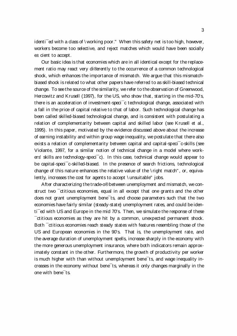
identi¯ed with a class of \working poor." When this safety net is too high, however,workers become too selective, and reject matches which would have been sociallye±cient to accept.Our basic idea is that economies which are in all identical except for the replace-

ment ratio may react very di®erently to the occurrence of a common technologicalshock, which enhances the importance of mismatch. We argue that this mismatch-biased shock is related to what other papers have referred to as skill-biased technicalchange. To see the source of the similarity, we refer to the observation of Greenwood,Hercowitz and Krusell (1997), for the US, who show that, starting in the mid-70's,there is an acceleration of investment-speci¯c technological change, associated witha fall in the price of capital relative to that of labor. Such technological change hasbeen called skilled-biased technological change, and is consistent with postulating arelation of complementarity between capital and skilled labor (see Krusell et al.,1995). In this paper, motivated by the evidence discussed above about the increaseof earning instability and within group wage inequality, we postulate that there alsoexists a relation of complementarity between capital and capital-speci¯c-skills (seeViolante, 1997, for a similar notion of technical change in a model where work-ers' skills are technology-speci¯c). In this case, technical change would appear tobe capital-speci¯c-skilled-biased. In the presence of search frictions, technologicalchange of this nature enhances the relative value of the \right match", or, equiva-lently, increases the cost for agents to accept \unsuitable" jobs.After characterizing the trade-o® between unemployment and mismatch, we con-

struct two ¯ctitious economies, equal in all except that one grants and the otherdoes not grant unemployment bene¯ts, and choose parameters such that the twoeconomies have fairly similar (steady-state) unemployment rates, and could be iden-ti¯ed with US and Europe in the mid 70's. Then, we simulate the response of these¯ctitious economies as they are hit by a common, unexpected permanent shock.Both ¯ctitious economies reach steady states with features resembling those of theUS and European economies in the 90's. That is, the unemployment rate, andthe average duration of unemployment spells, increase sharply in the economy withthe more generous unemployment insurance, where both indicators remain approx-imately constant in the other. Furthermore, the growth of productivity per workeris much higher with than without unemployment bene¯ts, and wage inequality in-creases in the economy without bene¯ts, whereas it only changes marginally in theone with bene¯ts.

4

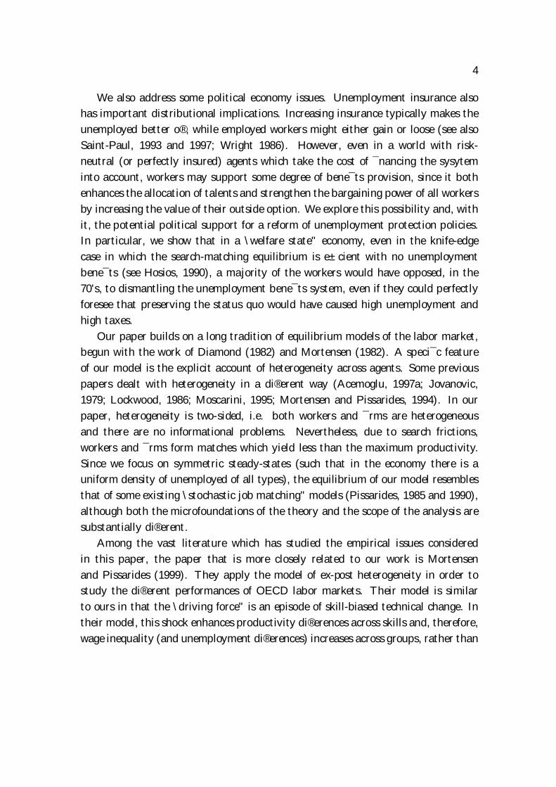
We also address some political economy issues. Unemployment insurance alsohas important distributional implications. Increasing insurance typically makes theunemployed better o®, while employed workers might either gain or loose (see alsoSaint-Paul, 1993 and 1997; Wright 1986). However, even in a world with risk-neutral (or perfectly insured) agents which take the cost of ¯nancing the sysyteminto account, workers may support some degree of bene¯ts provision, since it bothenhances the allocation of talents and strengthen the bargaining power of all workersby increasing the value of their outside option. We explore this possibility and, withit, the potential political support for a reform of unemployment protection policies.In particular, we show that in a \welfare state" economy, even in the knife-edgecase in which the search-matching equilibrium is e±cient with no unemploymentbene¯ts (see Hosios, 1990), a majority of the workers would have opposed, in the70's, to dismantling the unemployment bene¯ts system, even if they could perfectlyforesee that preserving the status quo would have caused high unemployment andhigh taxes.Our paper builds on a long tradition of equilibrium models of the labor market,

begun with the work of Diamond (1982) and Mortensen (1982). A speci¯c featureof our model is the explicit account of heterogeneity across agents. Some previouspapers dealt with heterogeneity in a di®erent way (Acemoglu, 1997a; Jovanovic,1979; Lockwood, 1986; Moscarini, 1995; Mortensen and Pissarides, 1994). In ourpaper, heterogeneity is two-sided, i.e. both workers and ¯rms are heterogeneousand there are no informational problems. Nevertheless, due to search frictions,workers and ¯rms form matches which yield less than the maximum productivity.Since we focus on symmetric steady-states (such that in the economy there is auniform density of unemployed of all types), the equilibrium of our model resemblesthat of some existing \stochastic job matching" models (Pissarides, 1985 and 1990),although both the microfoundations of the theory and the scope of the analysis aresubstantially di®erent.Among the vast literature which has studied the empirical issues considered

in this paper, the paper that is more closely related to our work is Mortensenand Pissarides (1999). They apply the model of ex-post heterogeneity in order tostudy the di®erent performances of OECD labor markets. Their model is similarto ours in that the \driving force" is an episode of skill-biased technical change. Intheir model, this shock enhances productivity di®erences across skills and, therefore,wage inequality (and unemployment di®erences) increases across groups, rather than

5

within groups, as in our model. Accordingly, their work and our work (which havebeen developed independently) complement each other, by showing that the basicequilibrium-search matching model can be extended to account for di®erent perfor-mances of labor markets (say, US vs. continental Europe) and that this frameworkcan be of use to analyze the e®ects of di®erent labor policies.Ljungqvist and Sargent (1998) is also similar in scope and to some extent com-

plementary to our work. They stress the distortion on the incentives to search dueto unemployment bene¯ts in a model where job creation as exogenous. A calibra-tion of the model shows that although unemployment bene¯ts have moderate e®ectson the aggregate unemployment rate in a situation of \low economic turbulence"(the 60's) it can have larger e®ects as this turbulence increases (the 80's). A thirdpaper closely related to our work is Acemoglu (1997b), which constructs a modelwith one-sided heterogeneity, where ¯rms open jobs of di®erent \qualities". The sizeof unemployment bene¯ts and minimum wages a®ects the equilibrium compositionof jobs in term of good vs. bad jobs. This paper, like ours and in contrast withLjungqvist and Sargent (1998), stresses the existence of channels through which togive workers some social insurance can be welfare-improving (see also Acemoglu,1997c).The paper is organized as follows. Section 2 presents the model. Section 3

characterizes the equilibrium. Section 4 discusses political economy issues. Section5 presents the results of a calibration of the model, intended to reproduce the recentexperience of Europe and the US. Section 6 concludes. An appendix contains thetechnical details.

2 The model

2.1 Ex-ante heterogeneity and search frictions.

We consider an economy populated by a continuum of ¯rms, workers and rentiers,where both ¯rms and workers are heterogeneous. In particular, each worker hasa di®erent productivity depending on in which ¯rm he his employed. Workers areuniformly distributed along a circle of unit length and the total measure of workersis one. At each moment in time a worker can be either employed in a certain ¯rm orunemployed. All unemployed workers search for a job, and search e®ort is costless.Employed workers cannot change job without going through unemployment (no on-

6

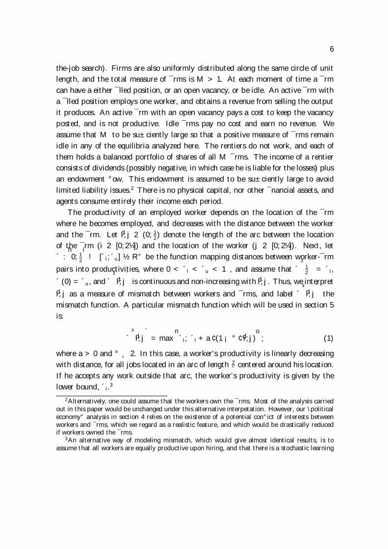
the-job search). Firms are also uniformly distributed along the same circle of unitlength, and the total measure of ¯rms is M > 1. At each moment of time a ¯rmcan have a either ¯lled position, or an open vacancy, or be idle. An active ¯rm witha ¯lled position employs one worker, and obtains a revenue from selling the outputit produces. An active ¯rm with an open vacancy pays a cost to keep the vacancyposted, and is not productive. Idle ¯rms pay no cost and earn no revenue. Weassume that M to be su±ciently large so that a positive measure of ¯rms remainidle in any of the equilibria analyzed here. The rentiers do not work, and each ofthem holds a balanced portfolio of shares of all M ¯rms. The income of a rentierconsists of dividends (possibly negative, in which case he is liable for the losses) plusan endowment °ow. This endowment is assumed to be su±ciently large to avoidlimited liability issues.2 There is no physical capital, nor other ¯nancial assets, andagents consume entirely their income each period.The productivity of an employed worker depends on the location of the ¯rm

where he becomes employed, and decreases with the distance between the workerand the ¯rm. Let di; j 2 (0; 12) denote the length of the arc between the locationof the ¯rm (i 2 [0; 2¼]) and the location of the worker (j 2 [0; 2¼]). Next, let´ :

h0; 12

i! [´l; ´u] ½ R+ be the function mapping distances between worker-¯rm

pairs into productivities, where 0 < ´l < ´u < 1, and assume that ´³12

´= ´l,

´ (0) = ´u, and ´³di; j

´is continuous and non-increasing withdi; j. Thus, we interpret

di; j as a measure of mismatch between workers and ¯rms, and label ´³di; j

´the

mismatch function. A particular mismatch function which will be used in section 5is:

´³di; j

´= max

n´l; ´l + a ¢ (1¡ ° ¢ di; j)

o; (1)

where a > 0 and ° ¸ 2. In this case, a worker's productivity is linearly decreasingwith distance, for all jobs located in an arc of length 2

° centered around his location.If he accepts any work outside that arc, the worker's productivity is given by thelower bound, ´l.3

2Alternatively, one could assume that the workers own the ¯rms. Most of the analysis carriedout in this paper would be unchanged under this alternative interpetation. However, our \politicaleconomy" analysis in section 4 relies on the existence of a potential con°ict of interests betweenworkers and ¯rms, which we regard as a realistic feature, and which would be drastically reducedif workers owned the ¯rms.

3An alternative way of modeling mismatch, which would give almost identical results, is toassume that all workers are equally productive upon hiring, and that there is a stochastic learning

7

Next, we describe the matching technology. Firms do not sort workers ex-anteby specifying personal requirements when posting vacancies. This implies that anyunemployed worker can meet and interview with any ¯rm located at any pointalong the circle, with the same probability. The density of interviews between ¯rmslocated at i and workers located at j is an increasing function of the density ofvacancies posted at location i and the density of unemployment at location j. Moreformally, let v : [0; 2¼] ! <+ denote the density of vacancies at location i andlet u : [0; 2¼] ! [0; 1] denote the density of unemployment at location j. Thematching function, m : <+ £ [0; 1]! <+, speci¯es the °ow of \interviews" between¯rms located at i and workers located at j and depends positively on v(i) andu(j). As is standard, m(v(i); u(j)) is assumed to be constant returns to scale. Letq(v(i); u(j)) = m(v(i);u(j))

v(i) ´ q(i; j) and µ(v(i); u(j)) = v(i)u(j) ´ µ(i; j). We make the

following standard assumptions:

q(i; j) = q [µ(i; j)] ; q0 [µ(i; j)] < 0; ²µ(i;j) ´dq(i; j)dµ(i; j)

µ(i; j)q(i; j

< 1;

limµ(i;j)!0 q0 [µ(i; j)] = 1; limµ(i;j)!1 q0 [µ(i; j)] = 0:

q(i; j) represents the Poisson probability for a ¯rm posting a vacancy at i to inter-view an unemployed worker located at j, and µ(i; j)q(i; j) represents the Poissonprobability for an unemployed worker located at j to have an interview with a ¯rmposting a vacancy at i. Note that neither of these probabilities depend on di; j. Dueto ex-ante heterogeneity, only a fraction of the interviews which take place at eachmoment will be regarded as acceptable by workers and ¯rms. The determination ofthis fraction will constitute part of the characterization of the equilibrium.Finally, we introduce the following standard notation:

d is the exogenous arrival rate of job separation, which is assumed to be the samefor all matches. Once a job is terminated, the worker returns to the pool ofunemployed (at his original location), and his productivity in the previousjob is irrelevant to the e®ects of his future employment. The ¯rm, in turn,becomes idle, and can decide whether or not to open a new vacancy;

process which, at each moment, turns some employed worker into high productivity `quali¯ed'workers. The learning event is modeled as a Poisson process, whose arrival rate is a decreas-ing function of the distance between each worker-¯rm pair. Note that an increase in relativeproductivity of `quali¯ed' vs. `unquali¯ed' workers in that version of the model (i.e., a capital-speci¯c-technological-change) is isomorphic to an increase in the parameter a in equation (1).

8

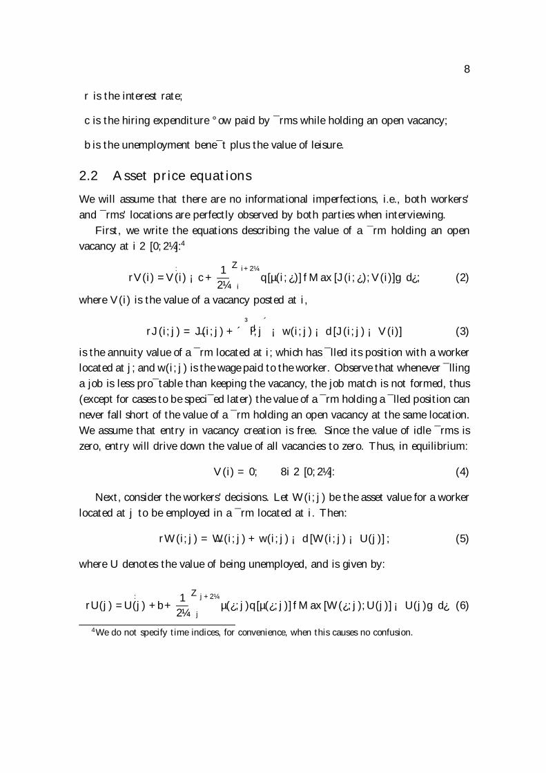
r is the interest rate;

c is the hiring expenditure °ow paid by ¯rms while holding an open vacancy;

b is the unemployment bene¯t plus the value of leisure.

2.2 Asset price equations

We will assume that there are no informational imperfections, i.e., both workers'and ¯rms' locations are perfectly observed by both parties when interviewing.First, we write the equations describing the value of a ¯rm holding an open

vacancy at i 2 [0; 2¼]:4

rV (i) =:

V (i) ¡c+12¼

Z i+2¼

iq [µ(i; ¿)] fMax [J(i; ¿); V (i)]g d¿; (2)

where V (i) is the value of a vacancy posted at i,

rJ(i; j) = _J(i; j) + ´³di; j

´¡ w(i; j)¡ d [J(i; j)¡ V (i)] (3)

is the annuity value of a ¯rm located at i; which has ¯lled its position with a workerlocated at j; and w(i; j) is the wage paid to the worker. Observe that whenever ¯llinga job is less pro¯table than keeping the vacancy, the job match is not formed, thus(except for cases to be speci¯ed later) the value of a ¯rm holding a ¯lled position cannever fall short of the value of a ¯rm holding an open vacancy at the same location.We assume that entry in vacancy creation is free. Since the value of idle ¯rms iszero, entry will drive down the value of all vacancies to zero. Thus, in equilibrium:

V (i) = 0; 8i 2 [0; 2¼]: (4)

Next, consider the workers' decisions. Let W (i; j) be the asset value for a workerlocated at j to be employed in a ¯rm located at i. Then:

rW (i; j) = _W (i; j) + w(i; j)¡ d [W (i; j)¡ U(j)] ; (5)

where U denotes the value of being unemployed, and is given by:

rU(j) =:

U(j) +b+12¼

Z j+2¼

jµ(¿; j)q [µ(¿; j)]fMax [W (¿; j); U (j)]¡ U(j)g d¿ (6)

4We do not specify time indices, for convenience, when this causes no confusion.

9

An acceptable job match generates a rent. We assume that if this rent is positive,it is shared between the ¯rm and the worker, according to the Nash bargainingsolution. The total surplus is given by S(i; j) = [J(i; j) ¡ V (i) +W (i; j)¡ U (j)],and the Nash solution implies that:

W (i; j)¡ U(j) =¯

1¡ ¯[J(i; j)¡ V (i)] (7)

where ¯ is a parameter representing the bargaining power of the workers, and werecall that V (i) = 0 due to free entry. Note that (7) ensures that if a worker ¯ndsa particular match to be acceptable, so will the ¯rm, and viceversa (i.e., J(i; j) ¸V (i) ,W (i; j) ¸ U(j)).Using the set of equations from (2) to (7), we can obtain the following expression

for the wage rate paid to a worker in the accepted match i; j.

w(i; j) = ¯h´

³di; j

´+©(j)

i+ (1¡ ¯)b; (8)

where ©(j) ´ 12¼

R j+2¼j µ(¿; j)q [µ(¿; j)] J(¿; j) d¿ .

3 Equilibrium.

In this section, we will characterize the equilibrium. We restrict attention to ini-tial distributions such that the same proportion of workers are unemployed at alllocations j 2 [0; 2¼]. We will start by showing that if a stationary equilibrium, itmust have a uniform distribution of vacancies at all locations. We then proceedto characterize the equilibrium, its dynamics and e®ects of paramater changes; inparticular, employment bene¯ts.

Lemma 1 Assume u(j) = u for all j 2 [0; 2¼]. Then, a stationary equilibrium musthave v(i) = v for all i 2 [0; 2¼] :

Proof. (see Appendix)This Lemma implies that, 8(i; j) 2 [0; 2¼]2, we have µ(i; j) = µ, and that the

Poisson arrival rate of interviews is the same for all unemployed workers (as well asfor all ¯rms posting a vacancy), irrespective of their location.

10

3.1 Allocation of talents and vacancy creation .

A preliminary important observation which descends from Lemma 1 is that, in astationary equilibrium (whereby

:V (i)=

:J(i; j)=

:W (i; j)=

:U (j)= 0), for all (i; j) 2

[0; 2¼]2 ; we have:

©(j) = cµ; J(i; j) = J(x); W (i; j) =W (x); U(j) = U; and w(i; j) = w(x); (9)

where x ´ di; j: In words, the value of a ¯rm with a ¯lled position, J(i; j), onlydepends on the distance between i and j (since this determines the productivity ofthe match, ´(x)), but not the speci¯c location of i and j along the circle. The sameapplies to the value of a job for an employed worker, W (i; j). Furthermore, thevalue of unemployment is independedent of j, as all workers face the same expectedgain from getting a job in the future.Recall, next, that Nash bargainin implies that a ¯rm and a worker always agree,

at the interview, on whether the match is pro¯table. Formally, a job is formedwhenever J(x) ¸ 0, which implies, by (7), that W (x) ¸ U . There are two possiblealternative cases. In the former case, J (x) > 0 for all x 2 [0; 12 ]; and all matchesare considered as acceptable. In the latter case, there exists a threshold distance,

¹x, such that J(¹x) = 0 (hence, W (¹x) = U). De¯ne ´ (x) ´R x0´(x)dxx , i.e. ´ is the

average productivity of acceptable matches. Then, the threshold distance satis¯esthe following condition:

[´(x)¡ b]¡2¯ x µq(µ)

r + d+ 2¯ x µq(µ)

h´ (x)¡ b

i¸ 0 (10)

or, equivalently:

(1¡ ¯) [´(x)¡ b]¡ ¯cµ ¸ 0 (11)

Both (10) and (11) hold with equality if ¹x < 12 .

The algebraic derivation of these conditions is in the Appendix. Equation (10)has the intuitive economic interpretation of a comparative advantage condition. Thereservation distance is such that the value for a worker to accept a type x job isequal to the value of waiting, i.e. the present discounted expected value of a futurematch (when ¹x = 1

2 waiting is always a dominated option). Equation (11) statesthe equivalent condition that the marginal match makes non-negative pro¯ts.

11

Next, we characterize the set of pairs (µ; ¹x) which are consistent with the freeentry condition in vacancy creation (V = 0). In particular, we have:

¡c+(1¡ ¯)2 x q(µ)r + d+ ¯2 x µq(µ)

h´ (x)¡ b

i= 0; (12)

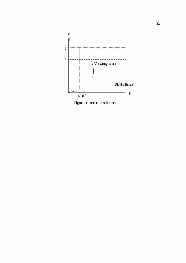
which states that the cost for a ¯rm of holding an open vacancy must be equal tothe expected pro¯t from ¯lling the position.Figure 1 geometrically represents the equilibrium conditions implied by equa-

tions (11)-(12), when they both hold with equality {. In particular, equation (11)corresponds to the skill allocation, (SA), while equation (12) corresponds to thevacancy creation, (V C), schedule.First, consider the skill allocation schedule. The more frequently matches occur

(high µ), the more easily unemployed workers expect to get good job opportunitiesin the future, and the less eager they are to accept low-productivity jobs with lowwages (small x). Thus, in tight labor markets, people seeking employment tend tobe very choosy, and to only accept highly suitable jobs. Since ´(x) is continuous andbounded, the range of values of µ which satisfy (11) is also bounded. Provided that´l > b; there exists µ¤ > 0 such that (1 ¡ ¯) (´l ¡ b) = ¯cµ¤; namely, there existsa su±ciently low matching rate, such that all jobs, even those implying the largestmismatch, are considered as acceptable. The particular skill allocation schedulein Figure 1 corresponds to the piece-wise linear productivity function of equation(1). In this case, the schedule becomes vertical at µ¤; corresponding to values of xexceeding 1

° , since all \bad" jobs located at a distance longer than1° have the same

low productivity. Thus, workers accept jobs along the whole circle (i.e. they setx= 1

2) if µ < µ¤, and set the cut-o® distance below 1

° ; if µ > µ¤:

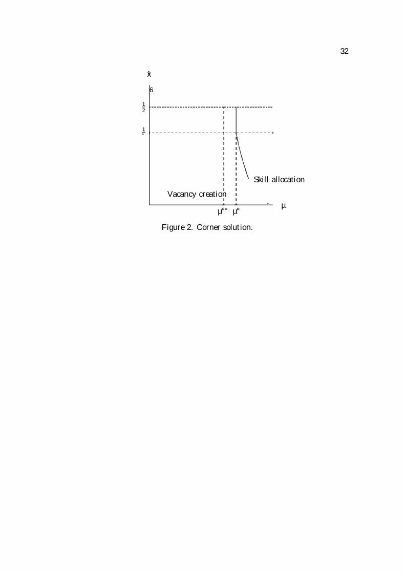
Consider, next, the vacancy creation, schedule, (12). Determining the slope ofthis schedule is less straightforward, as the partial derivative of the left hand side of(12) with respect to ¹x has an ambiguous sign. We will prove below (see the proofof Proposition 1) that this schedule is either backward bending, as in Figure 1, ormonotonically increasing, as in Figure 2. Parallel to the de¯nition of µ¤ providedabove, we can de¯ne µ¤¤ as the matching rate such that c = (1¡¯)q(µ¤¤)

r+d+¯µq(µ¤¤)

h¹

³12

´¡ b

i,

namely µ¤¤ is the labor market tightness which is consistent with free entry in va-cancy creation, when all interviews lead to employment.

[Figures 1&2 around here]

12

The following proposition establishes the properties of the steady-state equilib-rium of the model.

Proposition 1 Assume ´u > b. Then:

a) There exists, for generic economies, a unique stationary equilibrium pair (xe; µe):Multiple equilibria can only exist for non-generic economies, whose parametersare such that µ¤ = µ¤¤.

b) (i) If µ¤ < µ¤¤, then 0 < ¹xe < 12, and the equilibrium pair (x

e; µe) is as determinedby (11) and (12); (ii) if µ¤ > µ¤¤, then ¹xe = 1

2 and µe = µ¤¤.

Proof. (see Appendix)Proposition 1 rules out the possibility of multiple equilibria (except for non-

generic cases). If the two schedules cross, then we have the unique interior equilib-rium described by Figure 1. If they do not cross, then the vacancy creation scheduleis positively sloped everywhere, and we have a corner solution, like in Figure 2.

3.2 The dynamics of unemployment, output and productiv-ity.

Given, ¹x and µe, unemployment has the following law of motion:

_ut = d(1¡ ut)¡ 2 xe µeq(µe)ut: (13)

The linear di®erential equation (13) has a standard interpretation. The °owinto unemployment is given by the exogenous separations, d(1¡ ut), while the °owout of unemployment is given by the probability that an unemployed worker ¯ndsan acceptable match, 2 xe µeq(µe), times the mass of unemployed at time t. Itimmediately becomes evident that if the initial distribution of unemployment isuniform, it remains uniform over time. The solution to the di®erential equation(13) is ut = u¤ + (u0 ¡ u¤)e¡[2x

eµeq(µe)+d]t; where u¤ = dd+2xeµeq(µe) is the steady-state

unemployment rate to which unemployment monotonically converges.Next, consider, the dynamics of output. De¯ne gross production at time t as yt.5

Gross output has the following law of motion::yt=´ (xe)2 xe µeq(µe)ut ¡ dyt; (14)

5We de¯ne as net production the production °ow generated by ¯rms holding a ¯lled positionminus the hiring expenditure °ow su®ered by ¯rms holding a vacant position. Gross production isequal to net production plus hiring expenditure.

13

where y0 is predetermined. To understand (14), observe that the average produc-tivity of new jobs at t will in general di®er from that of the jobs terminated at t. Inparticular, the average productivity of the employed workers at t (thus, the produc-tivity of jobs which are terminated) is a predetermined variable which depends onpast hiring decisions, while the average productivity of new matches is not prede-termined. The latter is equal to ´ (xe), and the output °ow from newly created jobsis, therefore, equal to this average productivity times the °ow of successful matches,2 xe µeq(µe)ut. The solution to (14) is given by:

yt = y¤ +h(y0 ¡ y¤)+ ´ (xe)(u0 ¡ u¤)

ie¡dt¡ ´ (xe)(u0 ¡ u¤)e¡[2x

eµeq(µe)+d]t; (15)

where y¤ = ´ (xe) 2¹xeµeq(µe)d+2¹xeµeq(µe) is the steady-state equilibrium gross production levels.

The dynamic system is globally stable, thus the economy converges to y¤; u¤ startingfrom any pair of initial conditions u0; y0: To determine net production, ¯nally, observethat the aggregate hiring expenditure in the economy is given by cvt = cµut. Thus,net production is equal to zt = yt ¡ cµeut.We conclude with an important remark. Irrespective of the initial distribution

of existing matches, the equilibrium converges over time to a stationary uniformdistribution of jobs. More precisely, the steady-state will, at every location i 2[0; 2¼], have a density 1¡u¤ of ¯rms with a ¯lled position and a uniform distributionof ¯lled job (productivities) over the interval x 2 [0; ¹x]. In other words, the extent ofmismatch will be independent and identically distributed with respect to the locationof workers and ¯rms. This feature will be important in the following sections, whenwe study the e®ect of parameter changes.

3.3 An unexpected change of unemployment bene¯ts.

We will now discuss an important result of comparative statics: the e®ect of anunanticipated increase in unemployment bene¯ts. We assume that the shock occurswhen the economy is in a steady-state as characterized by the previous subsection.When b increases, both curves in Figures 1 and 2 will shift to the left, and thegeometrical analysis followed so far is inconclusive. It can be shown, however, thatwhen b increases, both the threshold distance and the tightness of the labor marketfall. To see this, we ¯rst rearrange (10) as follows:

h´ (x)¡ b

i=[r + d+ 2¯ x µq(µ)]

h´ (x)¡ ´(x)

i

r + d: (16)

14

Next, replacing the left hand-side of (16) into (12), we obtain:

1q(µ)

¡

8<

:

(1¡ ¯)2 xh´ (x)¡ ´(x)

i

(r + d)c

9=

; = 0 (17)

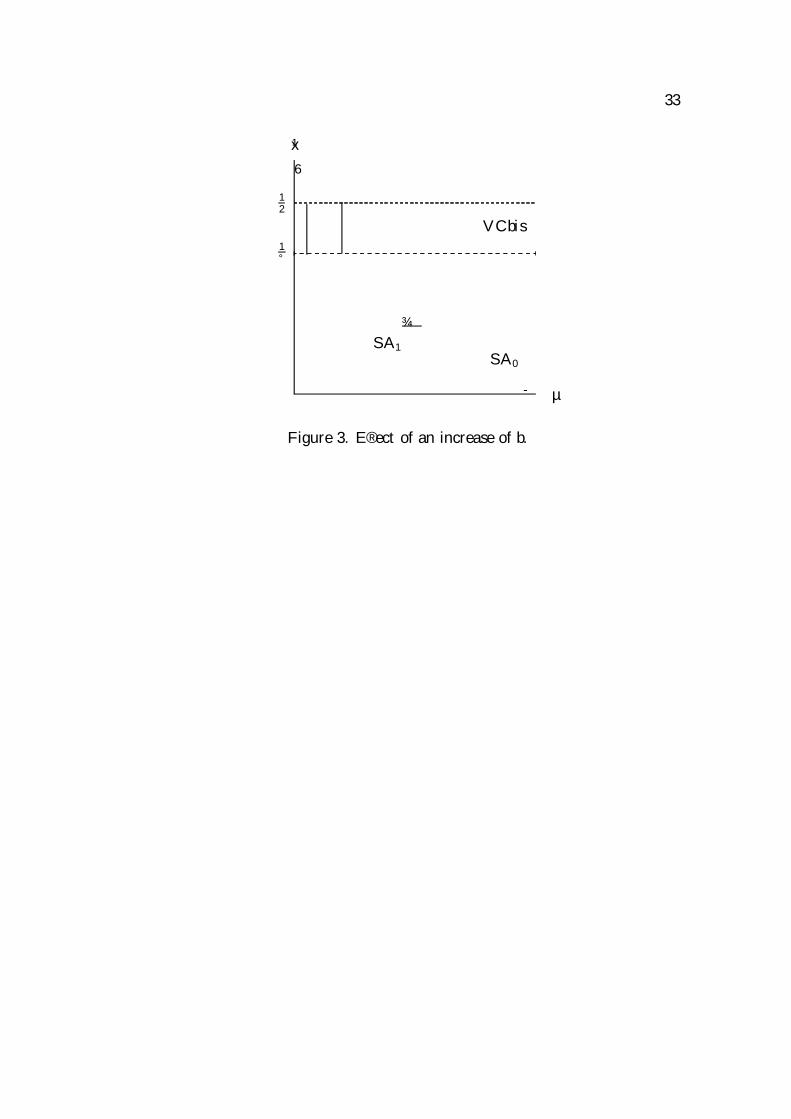
Equations (11) and (17) provide an alternative characterization of a(n interior) equi-librium. The advantage of this formulation is that only (11) is dependent on b,and this facilitates the geometrical analysis of the comparative statics. Equation(17) de¯nes a positively sloped locus { labeled VCbis in Figure 3 { in the plane(µ; ¹x). This can be shown by observing that 1

q(µ) is an increasing function of µ, whileddx

nh´ (x)¡ ´(x)

i¹xo= ¡ x ´0(x) > 0 and using standard di®erentiation. When

b grows, the skill allocation schedule shifts to the left, and the equilibrium has alower threshold distance as well as a less tight labor market. The more generousinsurance, the lower is the mismatch and the higher the productivity per worker inequilibrium. But, at the same time, unemployment insurance reduces job creationand employment.

[Figure 3 around here]

3.4 Transitional dynamics after a shock.

When the value of some parameter of the model changes unexpectedly (e.g., anincrease in b), the rents generated by some of the existing matches, which werepro¯table before the shock, might turn negative. We must therefore clarify whathappens to the matches which become unpro¯table. One could assume that workersand ¯rms split the losses associated with the continuation of unpro¯table matches(equation (8) extends to cases in which surplus is negative). We ¯nd this optionrather unplausible. In particular, it seems unrealistic that some employed workershave lower welfare than the unemployed. These workers would prefer to quit theirjob, and postulating that they are not allowed to quit is equivalent to introducingsome \slavery-type" condition.There are other possible solutions. For example, assuming that separation is par-

tially endogenous, i.e., that a job can be destroyed at no cost whatsoever, as soon asit ceases to be pro¯table. In this case, unemployment would become a \quasi-state"variable, which jumps discontinuously in case of unexpected parameter changes. Forinstance, after an increase of b, the unemployment rate would instantaneously jumpupwards, from u¤ to u¤ + 2(¹xe0 ¡ ¹xe1)(1 ¡ u¤), where ¹xe0, ¹xe1 denote the equilibrium

15

threshold distances before and after the shock respectively (note that, on the con-trary, a decrease of b does not cause any discontinuous jump in unemployment).Our formulation is consistent with this assumption, although the event of a sud-den increase of unemployment due to massive job destruction seems, also, ratherunrealistic.Another alternative is to introduce dismissal costs.6 To capture employment

protection constraints in a reduced-form fashion, we introduce the alternative as-sumption that, while job termination remains exogenous, whenever the surplus gen-erated by a job turns negative, the ¯rm must bear the entire loss, and pay theworker a salary granting him the same utility which he would receive if unemployed.Formally, this implies modifying (8) as follows:

w(x) = max [rU; ¯ [´(x) + cµ] + (1¡ ¯)b] : (18)

In words, the worker receives the reservation wage whenever the match generatea non-positive surplus in an existing job. Under this assumption, unemploymentremains strictly predetermined, and the model predicts more realistic transitionaldynamics.7 Although we will stress this last interpretation of the model when dis-cussing transitional dynamics, most of our results, and in particular the steady-stateanalysis, which is the main focus of this paper, are identical in the two cases.

4 The political economy of unemployment bene-¯ts.

The purpose of this section is to analyze how gains and losses from policy changesare distributed among di®erent agents when the unemployment bene¯t system ischanged. We start by stating a standard e±ciency result. Consider a social plannerwho is only subject to the search frictions and can costlessly redistribute incomeamong agents (or, alternatively, the planner has no egalitarian concern). The plan-ner maximizes the present discounted value of the output stream plus leisure, giveninitial conditions. The following result can be established.

6This is also the approach followed by Mortensen and Pissarides (1999), although their modelhas di®erent features.

7A third alternative, following Shaked and Sutton (1983), is to assume that wages are deter-mined according to w(x) = max [rU; ¯´(x)], derive the equation corresponding to (10) and showthat in that corresponding equation b plays a similar role than under our Nash bargaing wagedetermination. With this formulation, wages obey the same contracting rule after a shock.

16

Proposition 2 The competitive search-matching equilibrium with no unemploymentbene¯ts is e±cient, both in terms of job creation and assignments, if and only if® = ¯.

The proof of this Proposition is provided in Marimon and Zilibotti (1997). Propo-sition 2 generalizes the well-known result that the equilibrium rate of job creationis ine±cient when there are search frictions in the labor market, except for the non-generic case when the elasticity of the matching function is equal to the bargainingpower of workers (Hosios, 1990; Pissarides, 1990; Mortensen (1996a)). In particular,it establishes that mismatch is generically suboptimal in a decentralized equilibrium(being either too large or too small) with exogeneous bargaining powers, but whenthe Hosios-Pissarides condition is satis¯ed workers are e±ciently assigned to jobs.We now turn to the distributional e®ects of changing unemployment bene¯ts.

Consider an economy where the unemployed receive a provision equal to b0. Unem-ployment and output are at the corresponding steady-state, u0(b0); y0(b0). Given thissteady state, ¯lled positions are uniformly distributed over the interval [0; xe0 (b0)].Without much loss of generality, assume ´0(x) < 0 for all x. The following lemmais a ¯rst step towards accounting for distributional e®ects.

Lemma 2 Let b > b0 and 0:5 ¸xe (b0) >xe (b). Then:

1. For all x ·xe (b0); we have J(x; b) < J(x; b0);W (x; b) > W (x; b0); U(b) >U(b0):

2. For all x ·xe0 (b0), U(b)¡ U(b0) ¸ W (x; b)¡W (x; b0).

3. Let x > x0. Then: W (x; b)¡W (x; b0) ¸W (x0; b)¡W (x0; b0). In particular:

a) If both x; x0 2 [0; xe (b)], then W (x; b)¡W (x; b0) = W (x0; b)¡W (x0; b0);

b) If x 2 [xe (b); xe0 (b0)] and x0 2 [0; xe0 (b0)] ; then W (x; b) ¡ W (x; b0) >W (x0; b)¡W (x0; b0):

That is, raising b (ignoring the costs of ¯nancing it) increases the reservationwage of workers and the value of the human assets of all workers (both employedand unemployed), whereas it decreases the value of ¯rms (part 1). However, thee®ects are not symmetric. Unemployed workers makes the largest gains (part 2).Furthermore, some richer employed workers bene¯t less than some poorer co-workers

17

(part 3). To understand why, observe that a group of relatively poor workers, namelythose whose mismatch ranges in the interval x 2 [xe (b); xe0 (b0)] ; are employed injobs which turn non-pro¯table when the bene¯ts go up to b: These workers bene-¯t from the change.8 These poor workers therefore receive an implicit or explicitpremium over the wage increase which accrues to their richer, better-matched col-leagues (part 3b). The welfare gains of all workers belonging to this richer group areinstead equal, irrespective of x (part 3a).Next, we consider the cost of ¯nancing the system. Assume that the system

is ¯nanced through lump sum taxes, levied on all workers (both employed andunemployed), and that, at each t; all workers (both employed and unemployed)have to pay a tax equal to ¿ = but. Let T denote the asset value of `being atax-payer' of a country in which the unemployed receive the gross bene¯t b: Then:

T (b; u0) = ¡bZ 1

0e¡rtut(b; u0)dt: (19)

T (b; u0) is a decreasing function of b; since the higher b the larger the ¯scal burdento ¯nance the provision. Since all workers are subject to the same tax burden, whilethe gains from raising unemployment bene¯ts depend on their employment status(Lemma 2), we can state the following Proposition.

Proposition 3 Let b > b0. Assume that, at t = 0; u0 = u¤(b0) and y0 = y¤(b0)(where stars denote steady-states). Then (unless all workers unanimously prefer bto b0 or b0 to b), 9 ^x2 [xe (b); xe0 (b0)] such that all the unemployed and all workersemployed at a distance x ¸ x prefer b to b0, while all workers employed at a distancex < x prefer b0 to b:

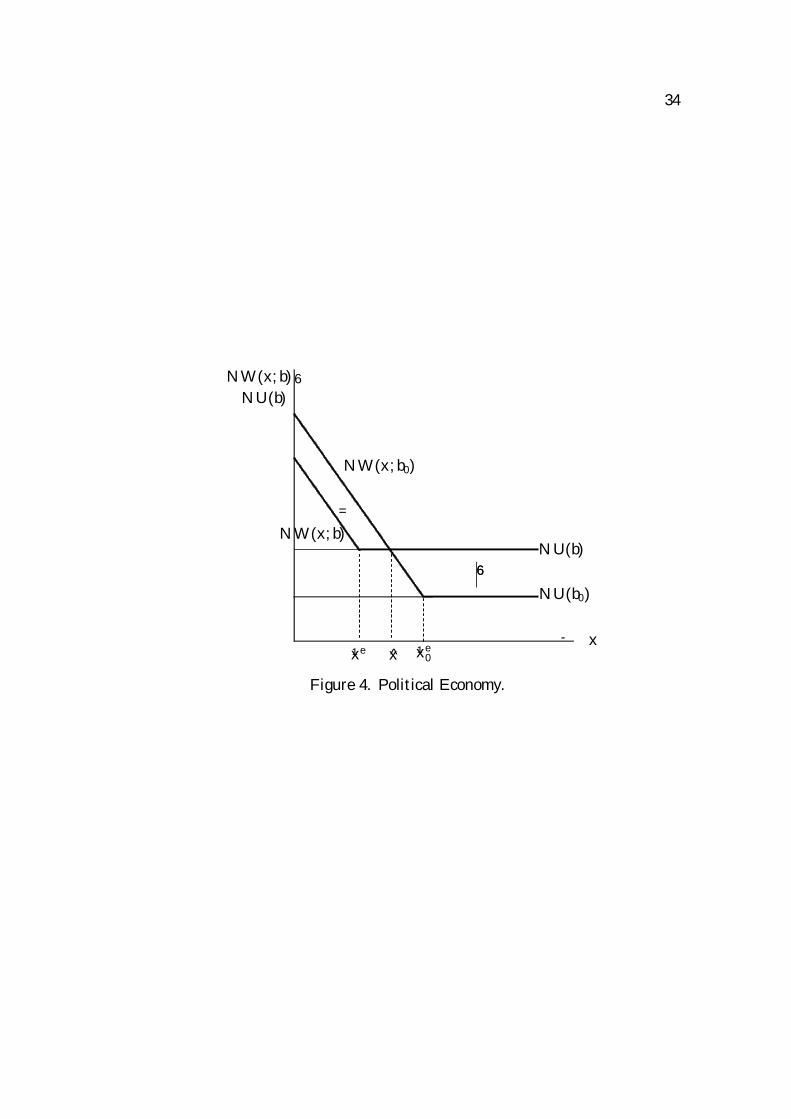
Proposition 3 establishes that, unless workers have unanimous views, there isa con°ict of interests between workers with the option of increasing bene¯ts gath-ering the support of the unemployed and the \poorer" employed workers, and theopposition of the \richer" employed workers. This case is represented by Figure 4(where NW (x; b) = W (x; b)+T (b) and NU(b) = U(b)+T (b)). In this case, althoughharmful to well-matched workers (the NW schedule shifts to the left), the increase of

8If, on the one hand, ¯rms can lay-o® workers at no cost, these workers will become unemployed.However, the entitlements to receive bene¯ts plus the perspective of getting a better job in futuremake these \poor" workers better o®. If, on the other end, there are ¯ring restrictions and workersare entitled to earn more than what the Nash rule would grant them (according to equation (18)),the improvement takes the form of a higher wage.

18

the unemployment bene¯ts from b0 to b increases the welfare of the \poor" workersholding a job in the range [x; ¹xe0], as well as of all the unemployed.

[Figure 4 around here]

Note, to conclude, that if bene¯ts were ¯nanced, more realistically, by linear (orprogressive) income taxation, or pay-roll taxes, this would reinforce the alignmentof interests between the \working poor" and unemployed workers.

5 Calibration: US vs. Europe.

5.1 Unemployment, output growth and inequality: the 70'svs. the 90's.

In this section, we present the result of a numerical solution of the model withcalibrated parameters, which illustrates how the model can successfully mimic somekey features of the contrasting behavior of the labor markets in Western Europe andthe United States in the last two decades.In order to obtain numbers comparable with the data, we introduce a trend of

neutral technical change. More precisely, we assume that b, c, and ´(x) grow atthe exogenous rate g. It is easily shown that the steady-state equilibrium in thepresence of neutral technical change is given by a simple modi¯cation of (10) and(12), whereby the interest rate (r) is replaced by the di®erence between the interestrate and the rate of technical change (r¡g). In particular, the solution characterizedby Proposition 1 remains true up to replacing r by r ¡ g, and neither the tightnessof the labor market nor the reservation distance changes over time. Note that fortechnical progress to be neutral, the productivity of all matches must grow at thesame rate, i.e. ´t+k(x) = egk´t(x) for all x: If technical progress is non-neutral, theimportance of mismatch changes over time, and this a®ects the agents' equilibriumbehavior.We will consider two hypothetical economies which only di®er by the extent of

unemployment insurance, b. One economy, denoted by U , will be assumed to haveno unemployment insurance (b = 0), and will be interpreted as a US-type laissezfaire economy9. The other economy, denoted by E, provides the unemployed with

9Here we follow Mortensen (1996b) who argues that the limited extent of unemployment bene¯tsin most states of US results in a non-positive e®ect of bene¯ts on reservation wages.

19

bene¯ts of unlimited duration (b > 0, ¯nanced by lump sum taxes charged fromall workers, both employed and unemployed), and can be interpreted as a typicalwelfare state European country. The two economies will be identical in all otherparameters.We assume that the two countries are initially at their respective steady-states,

which we interpret as the situation in the early 70's. Then, both economies arehit by a common, unanticipated shock increasesing the importance of mismatch, bywidening the productivity gap between the best (x = 0) and the worst (x = 1

2) jobthat a worker can perform. The new steady state will be interpreted as the situationin the nineties.We calibrate the parameters as follows. We interpret a time period of unit length

to be one quarter, and set the interest rate equal to 0:01125, implying an annualinterest rate of 4:5%. The rate of neutral technical change is assumed to be 1% peryear (thus, g = 0:0025). The separation rate is set equal to d = 0:04, implying anaverage duration of a match of about six years. Although this duration might seemfairly long { especially for the US { it should be noticed that we are here consideringthe duration of employment spells, not of jobs (i.e, we ignore job-to-job movements).Since in this experiment we do not want to introduce exogenous di®erences betweenEurope and the US other than b, we ¯nd that this ¯gure is reasonable. We parame-terize the mismatch function according to the linear speci¯cation given by equation(1), and set the initial minimum productivity (´l;0) equal to 2:25, a normalizationwithout any particular importance. Furthermore, we set a0 = 0:5 implying thateach agent is 22% more productive in his best than in his worst possible occupation,and let ° = 4, implying that each worker is, to some extent, skilled in 50% of thepossible employments. The bargaining power of both parties is equal, so ¯ = 0:5;corresponding to the symmetric Nash solution, and the elasticity of the matchingfunction is constant with ® = 0:5. Recall that when ® = ¯ the equilibrium with nobene¯ts is e±cient. The hiring cost is assumed to be equal to foregoing the produc-tion °ow of one low-productivity worker, i.e. c0 = 2:25. Leisure is assumed to beworthless. In E, the welfare state economy, unemployed workers receive a subsidyequal to 50% of the wage paid to the worst paid workers (in both the initial and¯nal period). Although this is less than the average subsidy granted to unemployedworkers in many European countries, in reality bene¯ts have usually a limited du-ration. Moreover, accepting a job has normally a positive in°uence on the levelof future bene¯ts, hence we regard this ¯gure as a realistic approximation of the

20

impact of the bene¯ts on the reservation wages.The skill-biased technical change shock is captured by an increase in the parame-

ter a above its trend in both countries. In particular, a is assumed to increase froma0 = 0:5 to a1 = 0:85. As a result, in the ¯nal steady-state the best matched work-er's productivity exceeds the worst matched worker's productivity by about 38%:Table 1 summarizes the results, by comparing the steady-states of the two economiesbefore (steady-state 1) and after (steady-state 2) the shock. We will regard the timeelapsed between the initial and ¯nal situation as approximately twenty years. In theinitial period, all workers in both economies accept matches along the entire circle,i.e. x= 1

2 . The resulting unemployment rates do not di®er a great deal, although,not surprisingly, unemployment is higher in E (5.5%) than in U (3.9.%). The av-erage duration of unemployment is about four months in U , and 5.7 months in E.The wage distribution is very similar in the two countries, and so are output andproductivity. Note that total output is initially slightly larger in U than in E. Inthe ¯nal steady-state, the situation looks dramatically di®erent. The unemploymentrate remains almost the same in U (3.8%) but increases substantially in E (11%).The explanation of this diverging behavior is that in E, where the cost of unemploy-ment is lower due to insurance, the optimal search behavior changes. In responseto the shock which increases the gap between their productivity in suitable andunsuitable occupations, they become more selective and lower the cut-o® distanceto ¹x = 0:219. In U , instead, where unemployment is a more painful experience,agents continue to rush into any employment. As a result, although the vacancy-to-unemployment ratio does not change signi¯cantly in either country, the averageduration of unemployment, stable in country 1, doubles in country 2, increasing toover one year. For the same reason, the share of long-term unemployment growssubstantially in E, where, after the shock, it takes more than six months for morethan half of the unemployed workers to exit unemployment, while, for almost 30%,it takes more than a year.10

10The predictions of the model as to the change in the share of long-term unemployment areconsistent with the evidence that this share has increased substantially in Europe, whereas therehas hardly been any change in the United States. On the other hand, the model is not entirelysuccessful in some of its quantitative predictions. First, it predicts a lower share of long termunemployment in Europe than what we observe. Second, and more important, it fails to recognizethat long-term unemployment was already high in Europe during the 70's. In 1989, about 70% ofthe unemployed in Europe had to wait more than six months before ¯nding employment (vs. 53%in our model), and about 50% had to wait for more than one year.

21

Table 1. Comparison between steady-states.steady-state 1 steady-state 2 % change

Cut-o®, ¹x U 0.5 0.5E 0.5 0.218

Unemployment rate U 3.9 3.8E 5.5 11.1

Average duration of U 4.1 4.0unemployment (months) E 5.8 12.5Average productivity U 2.29 2.89 23.6per employed E 2.31 3.15 30.8Total output U 2.20 2.78 23.6

E 2.19 2.80 24.6Percentage of unemployed U 14.1 13.6with duration ¸ 6 months E 25.1 52.8Percentage of unemployed U 2.0 1.8with duration ¸ 12 months E 6.3 27.9Ratio between U 1.107 1.173 6.6highest lowest wage E 1.133 1.146 1.2Ratio between U 1.087 1.142 5.590th-10th wage percentile E 1.086 1.116 3.1

Although workers experience longer unemployment spells in the welfare stateeconomy, they are on average better assigned to jobs. As a result, productivitygrowth is higher in E (+31%) than in U (+24%). If we interpret the period lengthas twenty years, this translates into average yearly growth rates of 1.18% and 1.54%,respectively. The productivity gap is of the order of 0.4% per year. The observeddi®erential of productivity growth between the US and Europe is about 1.1% peryear, so this speci¯cation of the model predicts more than one third of the observeddi®erence. Furhtermore, note that total output growth is larger in country 2 thanin country 1. Remarkably, the model predicts that with standard parameters aneconomy with 11% unemployment rate can be more productive than an economywith 4% unemployment rate, since very high employment is obtained in U at thecost of larger mismatch.The transitional dynamics of unemployment and output depends on whether

unproductive matches can be costlessly destroyed. If we rule out the possibility ofinstantaneous distraction, we have the following patterns. In the economy withoutinsurance, unemployment is almost constant, whereas in the economy with insur-ance the unemployment rate ¯rst grows rapidly and, then, settles down at the new

22

steady-state level. As far as output is concerned, the two economies start from verysimilar levels, and the economy with welfare state reaches some higher output levelat the new steady-state. However, the cost of this better performance in the long runis a sharp initial recession. The output in the economy with welfare state remainsbelow that of the economy without insurance for about ten years. Twenty yearsafter the shock, all variables in both economies are very close to their respectivesteady-state, and this justi¯es our interpretation of the steady-state ¯gures of Table1 as the situation prevailing in the 70's and the 90's. If ¯rms could instead exit atno cost, unemployment in E would jump upwards upon the occurrence of the shock,overshooting the steady-state level. In particular, more than half of the existingjobs would suddenly be destroyed, causing a dramatic boom of unemployment. Un-employment would then gradually fall to its new steady-state level, which would bethe same as steady-state 2 in Table 1.Table 1 also shows that the model correctly predicts the qualitative changes in

wage inequality, although the quantitative e®ects are fairly small. As noticed earlier,the model has predictions about within group wage inequality, which, as shown inthe Introduction, has grown in the US more than in Europe. As shown in thetwo last raws of Table 1, our model predicts a signi¯cantly larger increase in wageinequality in the economy without unemployment insurance than in the one withinsurance, and this is valid for both the ratio between the highest and the lowestwage and the ratio between the 90th and the 10th percentile. The explanation of thisdi®erence is that while many workers in U accept jobs which are highly unsuitableto their characteristics, and therefore receive a low wage, poor matches are notformed in E. This reduces the spread of the wage distribution. Thus, althoughboth economies were hit by an intrinsically unequalising shock, this is partiallyo®set, in the welfare state economy, by the change of attitudes of the unemployed.On the contrary, in E, the increase of the productivity di®erentials between goodand bad matches is entirely passed through to increasing wage di®erentials between\lucky" well-matched workers and \unlucky" badly matched workers.

5.2 The welfare state dilemma: winners and loosers.

The calibrated version of the model presented above can also be used for assessingsome of the distributional e®ects discussed in section 3. Consider country E, andassume that, when the mismatch biased technological shock occurs, the agents living

23

in E can choose whether to keep the status quo (unemployment insurance), ordismantling the system of bene¯t provision (like in country U) in order to avoid theincrease of unemployment. As we will see, this choice will raise a con°ict of interestsbetween agents with di®erent employment status.Recall that, when the shock occurs, the economy is in a steady-state, where the

unemployment rate is 5.5%. We assume, here, that ¯rms cannot lay o® workerswhen matches turn unpro¯table, but, according to equation (18), existing jobs mustbe continued and workers paid no less than their reservation wage. First, considerthe \rich", well-matched workers whose jobs remain pro¯table after the shock (i.e.,x 2 [0; 0:219]). If unemployment bene¯ts were abolished, these workers would su®era wage cut (compared with the status quo) due to the loss of bargaining power inthe wage negotiation (outside option e®ect). In our calibrated economy, the loss, asmeasured by the asset value di®erence between being employed in a match x withand without bene¯ts is equal to W (x; b)¡W (x; 0) = 12:0 (recall that, by Lemma 2,the welfare change is identical for all well-matched workers, such that x 2 [0; 0:219]).Consider, next, the unemployed. We expect that the unemployed would loose morethan the employed workers from cutting bene¯ts to zero. In fact, the measured lossis, in their case, equal to U(b) ¡ U(0) = 13:2. The loss of the \poor" employedworkers (such that x 2 [0:219; 0:5]) is bounded between the loss of the rich workersand that of the unemployed. All agents, however, would gain from tax reduction.Since we assume uniform lump sum taxes, this gain is the same for all workers, bothemployed and unemployed. The present discounted cost of ¯nancing the existingbene¯t system with the perspective of growing unempoyment (see equation (19)) isT (b) = 13:0.As these numbers immediately show, the unemployed are better o® with than

without bene¯ts (since 13:2 > 13:0), while well-matched workers would prefer ano-insurance system (12:0 < 13:0). A large share of the working poor, however willalso gain from the provision of bene¯ts. In particular, it turns out that all employedworkers with x > 0:242 will be better o® with than without insurance, whereasall `richer' workers with x < 0:249 are worse o® without insurance. Since employedworkers are initially homogeneously distributed in the interval x 2 [0; 0:5] this meansthat about 50% the employed workers, together with all the unemployed (5.5% ofthe working population), would prefer to preserve the welfare state, even though thee®ects on unemployment are perfectly predicted. Note that the results change if weassume that unproductive matches can be terminated. In this case, unemployment

24

would have boomed upon the occurrence of the technological shock, and the costof keeping the existing welfare state system would have become prohibitively high.In this case, all workers (including the unemployed) would support a laissez-faireoriented reform.

6 Conclusions

In this paper we have shown how a search equilibrium model, where agents havedi®erently skills for performing di®erent tasks, can capture the main facts regardingthe contrasting performances of the US and Continental European labor markets. Inour simulated results, the contrast arises from the di®erent responses to a mismatch-biased technological shock, which are the result of di®erences in unemploymentinsurance (or social norms regarding unemployment protection). Although the scopeof our \calibration" is mainly illustrative, we believe that the results are insightfulto assess the trade-o® involved in unemployment protection policies (unemploymentvs. mismatch). Our results complement other explanations of the \contrastingperformance of US and European labor markets" that explore alternative mechanimsand that may also be at work.We believe that the theoretical model which we have constructed is of indepen-

dent theoretical interest, and is suitable to study a number of positive or normativeissues which have been ignored in this paper. Among them, the impact of otherlabor policies; the transitional e®ects of sectorial reallocations; the relation beweeneconomic °uctuations and employment mismatches, etc. In the current develop-ment of the model, we have made restrictive simplifying assumptions that shouldbe reassessed in the future. For instance, we have ruled out on-the-job search,while mismatched workers have substantial incentives to look for better matcheswhile employed. Furthermore, the assumption of uniform initial distributions ofunemployment needs to be addressed in more detail by future work, by focussingon the stability property of the uniform steady-state distribution considered here,and extending attention to non-stationary solutions when the entire distribution ofunemployment is the state variable of the economy.

Appendix.

Proof of Lemma 1

25

Stationarity implies that, for all (i; j) 2 [0; 2¼]2 ; _J(i; j) = _V (i) = 0. Imagine that,in contradiction with the Lemma, v(i) < v(i0) for some i; i0. Then, equation (2) impliesthat:

V (i) = ¡c+ 12¼ q

³v(i)u

´ R i+2¼i (J(i; ¿)) d¿

V (i0) = ¡c+ 12¼q

³v(i0)u

´ R i0+2¼i0 (J(i0; ¿ )) d¿

(20)

Equations (3)-(8), in turn, imply that:

J(i; j) = (r + d)¡1³(1¡ ¯)

³´(di; j)¡ b

´´¡ ¯©(j)

Hence, for any · 2 [0; 2¼]:Z ·+2¼

·(J(i; ¿ )) d¿ = (r + d)¡1 ((1¡ ¯) (^¡ b)) ¡ ¯© = J

where ^ =R ·+2¼· ´(d·; ¿)d¿ and © =

R ·+2¼· ©(¿ )d¿: Thus:

V (i) = ¡c+12¼q

Ãv(i)u

!

J > ¡c+12¼q

Ãv(i0)u

!

J = V (i0) (21)

where the sign of the inequality follows from the properties of the matching function, q(:).But (21) contradicts the assumption of free-entry, which implies that V (i) = V (i0) = 0:Thus, v(i) must be equal to v(i0). QED.

Proof of Proposition 1We prove the Proposition through simple geometrical arguments.To prove existence, we will ¯rst establish that either the Vacancy creation schedule

(V C) lies entirely to the left of the Skill allocation schedule (SA), or the two schedulescross; we then establish that in both cases an equilibrium exists. To rule out that V Cis entirely to the right of SA, observe that (a) from (11), the SA schedule intersects thehorizontal axis in correspondence of µ = (1¡¯)

¯c (´u ¡ b) > 0; (b) for (12) to be satis¯ed,it must be the case that as ¹x ! 0, µ ! 0 (which implies that q(µ) ! 1), thereforethe V C schedule starts from the origin. Hence, at x= 0; V C is always to the left ofSA. Assume that V C is entirely to the left of SA. Then, it is easy to check that thesolution

³µe = µ¤¤; xe= 1

2

´satis¯es the conditions (10) (or, alternatively, (11)) and (12)

{ the former holding with strict inequality { and is, therefore, an equilibrium. Assume,instead, that V C and SA intersect. Then, it is immediate to show that any intersectionpoint identi¯es an equilibrium.

To prove uniqueness, we show that the two schedules can cross at most once, exceptfor non-generic parameter con¯gurations. De¯ne:

`p(µ; ¹x) ´ (1¡ ¯)(´(x)¡ b)¡ ¯cµ;

26

`v(µ; x) ´ ¡c (r + d+ ¯2 x µq(µ)) + (1¡ ¯)2 x q(µ)³´ (x)¡ b

´;

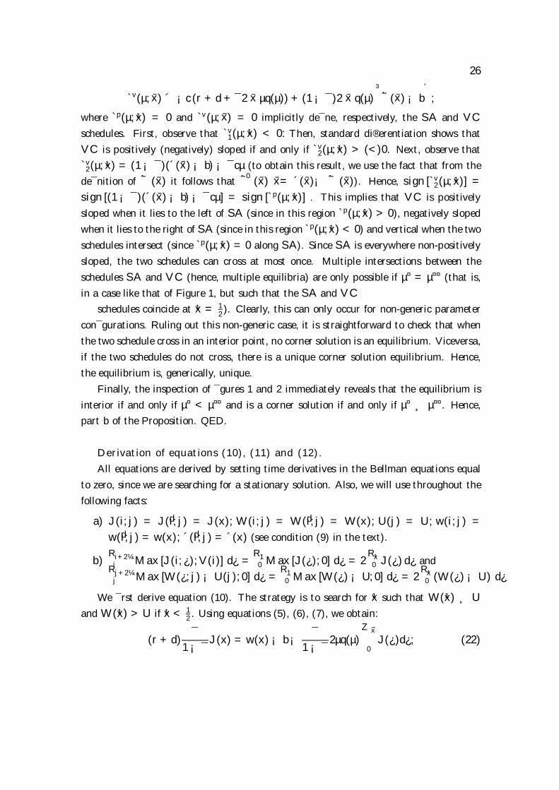
where `p(µ; ¹x) = 0 and `v(µ; x) = 0 implicitly de¯ne, respectively, the SA and V Cschedules. First, observe that `v1(µ; ¹x) < 0: Then, standard di®erentiation shows thatV C is positively (negatively) sloped if and only if `v2(µ; ¹x) > (<)0. Next, observe that`v2(µ; ¹x) = (1¡ ¯)(´(x)¡ b) ¡ ¯cµ (to obtain this result, we use the fact that from thede¯nition of ´ (x) it follows that ´0 (x) x= ´(x)¡ ´ (x)). Hence, sign [`v2(µ; ¹x)] =sign [(1¡ ¯)(´(x)¡ b)¡ ¯cµ] = sign [`p(µ; ¹x)] . This implies that V C is positivelysloped when it lies to the left of SA (since in this region `p(µ; ¹x) > 0), negatively slopedwhen it lies to the right of SA (since in this region `p(µ; ¹x) < 0) and vertical when the twoschedules intersect (since `p(µ; ¹x) = 0 along SA). Since SA is everywhere non-positivelysloped, the two schedules can cross at most once. Multiple intersections between theschedules SA and V C (hence, multiple equilibria) are only possible if µ¤ = µ¤¤ (that is,in a case like that of Figure 1, but such that the SA and V C

schedules coincide at ¹x = 12 ). Clearly, this can only occur for non-generic parameter

con¯gurations. Ruling out this non-generic case, it is straightforward to check that whenthe two schedule cross in an interior point, no corner solution is an equilibrium. Viceversa,if the two schedules do not cross, there is a unique corner solution equilibrium. Hence,the equilibrium is, generically, unique.

Finally, the inspection of ¯gures 1 and 2 immediately reveals that the equilibrium isinterior if and only if µ¤ < µ¤¤ and is a corner solution if and only if µ¤ ¸ µ¤¤. Hence,part b of the Proposition. QED.

Derivation of equations (10), (11) and (12).All equations are derived by setting time derivatives in the Bellman equations equal

to zero, since we are searching for a stationary solution. Also, we will use throughout thefollowing facts:

a) J(i; j) = J(di; j) = J(x); W (i; j) = W (di; j) = W (x); U(j) = U ; w(i; j) =w(di; j) = w(x); ´(di; j) = ´(x) (see condition (9) in the text).

b)R i+2¼i Max [J(i; ¿ ); V (i)] d¿ =

R 10 Max [J(¿ ); 0] d¿ = 2

R ¹x0 J(¿ ) d¿ and

R j+2¼j Max [W (¿; j)¡ U(j); 0] d¿ =

R 10 Max [W (¿ )¡ U; 0] d¿ = 2

R ¹x0 (W (¿ )¡ U) d¿

We ¯rst derive equation (10). The strategy is to search for ¹x such that W (¹x) ¸ Uand W (¹x) > U if ¹x < 1

2 . Using equations (5), (6), (7), we obtain:

(r + d)¯

1¡ ¯J(x) = w(x)¡ b¡

¯1¡ ¯

2µq(µ)Z x

0J(¿ )d¿; (22)

27

Next, we use (3) to obtain the following expression for the . This gives the followingexpression for the wage schedules:

w(x) = (1¡ ¯)b+ ¯´(x) + 2¯µq(µ)Z x

0J(¿ )d¿ : (23)

>From replacing (23) into (22), and simplifying terms, we obtain:

(r + d)J(x) = (1¡ ¯) (´(x)¡ b)¡ ¯2µq(µ)Z x

0J(¿)d¿: (24)

Integrating on both sides of (24) gives:Z ¹x

0J(¿ )d¿ = (r + d+ ¯2¹xµq(µ))¡1 (1¡ ¯)

µZ ¹x

0´(¿ )d¿ ¡ b¹x

¶(25)

Finally, we substitute (25) into (24) and obtain:

(r + d)J(x) = (1¡ ¯) (´(x)¡ b)¡(1¡ ¯)¯2µq(µ)¹xr + d + ¯2¹xµq(µ)

³´ (x)¡ b

´(26)

where ´ is de¯ned in the text. Recall that Nash bargaining implies that, if ¹x < 12 ,

W (¹x)¡U , J(¹x) = 0: If, instead, we have a corner solution, however, J(x) > 0 for allx (and ¹x = 1

2 ). Thus, the general condition is:

(´(x)¡ b)¡¯2µq(µ)¹x

r + d+ ¯2¹xµq(µ)

³´ (x)¡ b

´¸ 0

which is the same as equation (10) in the text.Next, we derive equation (11). Equations (3) and (8) imply (recalling that ©(j) = cµ

for all j's) that (r + d)J(x) = (1¡ ¯)´(x) ¡ ¯cµ ¸ 0, and this establishes the result.QED.

To obtain equation (12), ¯nally, observe that equation (2) implies (given µ(i; ¿ ) = µ)that c = 2

R ¹x0 J(¿ ) d¿ . Substituting away

R ¹x0 J(¿) d¿ using equation (25) yields equation

(12). QED.

Proof of Lemma 3. Part 1.From (3) and (8) we have, for all x 2 [0; xe (b)], J(x; b) ¡J(x; b0) = w(x; b0)¡w(x; b) = (1¡¯)(b0¡ b)+¯c(µ(b0)¡ µ(b)) = (1¡¯)[´(x (b0))¡´(x

(b))] < 0: (Note that this expression is independent of x; this observation will be useful inthe proof of part 3). This inequality holds true, a fortiori, for x >xe (b). Also, from (2), (4),(6), (7) and (8) we have U(b)¡U(b0) = (1¡¯)(b¡b0)¡ ¯

1¡¯ [J(x; b) ¡ J(x; b0)] < 0. Finally,from (5) we have that W (x; b) ¡ W (x; b0) = w(x; b) ¡ w(x; b0) + d [U(b) ¡ U(b0)] > 0.

28

Part 2. From (7), we have that, for all x 2 [0; xe (b)] W (x; b) ¡ W (x; b0) = U(b) ¡U(b0) + ¯

1¡¯ [J(x; b) ¡ J(x; b0)]. Since, from part 1, J(x; b) ¡ J(x; b0) < 0, then W (x; b) ¡W (x; b0) < U(b) ¡ U(b0). Next, consider the range x 2 [xe (b0); x

e (b)] : In this range,(5) and (18), imply that W (x; b) = U(b). But, since W (x; b0) > U(b0), then W (x; b) ¡W (x; b0) < U(b) ¡ U(b0) also in this range of x's.

Part 3. The proof of part 1 shows that in the range x 2 [0; xe (b)], J(x; b) ¡ J(x; b0)is independent of x. But, then, from (7), W (x; b) ¡ W (x; b0) is also independent of x,and this proves part (a). To prove part (b) we consider ¯rst the case in which x0 2[0; xe (b)], and then the case in which x0 2 [xe (b); xe (b0)]. In the former case: W (x; b) ¡W (x; b0) = U(b) ¡ W (x; b0) > U(b) ¡ U(b0) + ¯

1¡¯ [J(x; b) ¡ J(x; b0)] = U(b) ¡ U(b0) +¯1¡¯ [J(x0; b) ¡ J(x0; b0)] = W (x0; b) ¡ W (x0; b0) . In the latter case: W (x; b) ¡ W (x; b0) =U(b) ¡ W (x; b0) > U(b) ¡ W (x0; b0) = W (x0; b) ¡ W (x0; b0). QED.

References[1] Acemoglu, D., (1997a). `Matching, Heterogeneity and the Evolution of Income Dis-

tribution.' Journal of Economic Growth, vol. 2, pp. 61-92.

[2] Acemoglu, D. (1997b). `Good Jobs versus Bad Jobs.' CEPR Discussion Paper No.1588.

[3] Acemoglu, D. (1997c). `Changes in Unemployment and Wage Inequality: An Alter-native Theory and Some Evidence.' NBER Discussion Paper No. 6658.

[4] Alogoskou¯s, G., Bean, C., Bertola, G., Cohen, D., Dolado, J. and Saint-Paul, G.(1995). European Unemployment; Choices for Europe. Centre for Economic PolicyResearch Monitoring European Integration 5, London.

[5] Bean, C. (1994). `European Unemployment: A Survey'. Journal-of-Economic-Literature, vol. 32, pp. 573-69.

[6] Bertola, G. and Ichino A. (1995). ` Wage Inequality and Unemployment: UnitedStates vs. Europe'. NBER Macroeconomic Annual, pp. 13-54

[7] Burdett, K. (1979). `Unemployment Insurance Payments as a Search Subsidy: ATheoretical Analysis.' Economic Inquiry, vol. 42, pp. 333-43.

[8] Diamond, P. (1981).`Mobility Costs, Frictional Unemployment, and E±ciency'. Jour-nal of Political Economy, 89, 798-812.

[9] Gottschalk, P. (1998). `Inequality, Income Growth and Mobility: The Basic Facts.'Journal of Economic Perspectives, vol. 11, pp. 21-40.

[10] Gottschalk, P. and Mo±tt R. (1994). `The Growth of Earnings Instability in the USLabor Market.' Brooking Papers on Economic Activity, pp. 217-272.

[11] Gottschalk, P. and Smeeding T. (1997). `Cross-National Comparisons of Earningsand Income Inequality.' Journal of Economic Literature, vol. 35, pp. 633-88.

29

[12] Greenwood, J., Hercowitz, Z. and Krusell, P. (1997). `Long-Run Implicationsof Investment-Speci¯c Technological Change'. American Economic Review, 87,3,pp.342-362.

[13] Hosios, A. (1990).`On the e±ciency of Matching and Related Models of Search andUnemployment.' Review of Economic Studies, 57.

[14] Jovanovic, B. (1979). `Job Matching and the Theory of Turnover.' Journal of PoliticalEconomy, 87, 972-990.

[15] Krusell, P., Ohanian, L., Rios Rull, V. and Violante, G. (1995).`Capital-Skill Com-plementarity and Inequality'. Mimeo, University of Pennsylvania.

[16] Levy, F. and Murnane R. (1992).`U.S. earnings levels and earnings inequality: Areview of recent trends and proposed explanations.' Journal of Economic Literature,30, 1333-1381.

[17] Ljungqvist, L. and Sargent, T. (1998). `The European Unemployment Dilemma.'Journal of Political Economy, vol. 106, pp. 514-50.

[18] Lockwood,B. (1986). `Transferable Skills, Job Matching, and the Ine±ciency of theNatural Rate of Unemployment' Economic-Journal, vol. 96, pp. 961-74.

[19] Marimon, R. and Zilibotti, F. (1997). `Unemployment vs. Mismatch of Talents. Re-considering Unemployment Bene¯ts.' NBER Working Paper No. 6038.

[20] Moen, E.R. (1995). `A Search Model with Wage Announcement.' London School ofEconomics, Theoretical Economics Disc. Papers TE/95/280

[21] Mortensen, D. (1982). `Property Rights and E±ciency in Mating, Racing, and Re-lated Games.' American-Economic-Review, vol. 72, pp. 968-79.

[22] Mortensen, D. (1996a). `Equilibrium Unemployment Theory: Determinants of theNatural Rate.' (mimeo) Northwestern University.

[23] Mortensen, D. (1996b). `Employment and Wage Responses to Economic Fluctuationsand Growth.' (mimeo) Northwestern University.

[24] Mortensen, D. and Pissarides, C. (1994). `Job Creation and Job Destruction in theTheory of Unemployment.' Review of Economic Studies, 61, 397-415.

[25] Mortensen, D. and Pissarides, C. (1999) `Unemployment response to \skill-biased"shocks: the role of labor market policies." Economic Journal, this issue.

[26] Moscarini, G., (1995). `Fattening Economies.' Mimeo, MIT.

[27] Pissarides, C. (1985). `Short-run Equilibrium Dynamics of Unemployment Vacancies,and Real Wages.' American-Economic-Review, vol. 75, pp. 676-90.

[28] Pissarides, C. (1990). Equilibrium Unemployment Theory. Basil Blackwell, London.

[29] Saint-Paul, G. (1993). `On the Political Economy of Labor Market Flexibility.' NBERMacroeconomics Annual 1993, pp.151-87.

30

[30] Saint-Paul, G. (1997).`Voting for Jobs: Policy Persistence and Unemployment'.CEPR Discusison Paper No. 1428.

[31] Violante G. (1997). `"Technological progress and skill dynamics: a solution to thewage dispersion puzzle?".' Mimeo. University College, London.

[32] Wright, R. (1986). `The Redistributive Role of Unemployment Insurance and theDynamics of Voting.' Journal of Public Economics, 31, 377-399.

31

- µ

Figure 1. Interior solution.

6

12

1°

µ¤ µ¤¤

¹x

Skill allocation

Vacancy creation

32

- µ

Figure 2. Corner solution.

6

¹x

12

1°

µ¤¤ µ¤

Skill allocation

Vacancy creation

33

- µ

Figure 3. E®ect of an increase of b.

6

12

1°

¹x

SA0

V Cbis

SA1¾

34

- x

Figure 4. Political Economy.

6

¹xe x ¹xe0

NU (b0)

NU(b)66

=

NW (x; b0)

NW (x; b)

NW (x; b)NU (b)

6(0,1$5 3$3(5 6(5,(6

7KH 6HULHV ZDV LQLWLDWHG LQ ìäæìï )RU D FRPSOHWH OLVW RI 6HPLQDU 3DSHUVñ SOHDVH FRQWDFW WKH ,QVWLWXWHï

ìääç

çíéï $VVDU /LQGEHFNã ,QFHQWLYHV LQ WKH :HOIDUHð6WDWH ð /HVVRQV IRUZRXOGðEH ZHOIDUH VWDWHVï êì SSï

çíèï $VVDU /LQGEHFN DQG 5HRUJDQL]DWLRQ RI )LUPV DQG /DERU 0DUNHW'HQQLV -ï 6QRZHUã ,QHTXDOLW\ï ìé SSï

çíçï 7KRUYDOGXU *\OIDVRQã 2XWSXW *DLQV IURP (FRQRPLF 6WDELOL]DWLRQï êí SSï

çíæï 'DURQ $FHPRJOX DQG $JHQF\ &RVWV LQ WKH 3URFHVV RI 'HYHORSPHQWï éí SSï)DEUL]LR =LOLERWWLã

çíåï $VVDU /LQGEHFNñ 6RFLDO 1RUPVñ WKH :HOIDUH 6WDWHñ DQG 9RWLQJï êê SSï6WHQ 1\EHUJ DQG-|UJHQ :ï :HLEXOOã

çíäï -RKQ +DVVOHU DQG 2SWLPDO $FWXDULDO )DLUQHVV LQ 3HQVLRQ 6\VWHPV ð D 1RWHï$VVDU /LQGEHFNã ìè SSï

çìíï -DFRE 6YHQVVRQã &ROOXVLRQ $PRQJ ,QWHUHVW *URXSVã )RUHLJQ $LG DQG5HQWð'LVVLSDWLRQï êì SSï

çììï -HIIUH\ $ï )UDQNHO DQG (FRQRPLF 6WUXFWXUH DQG WKH 'HFLVLRQ WR $GRSW D &RPPRQ$QGUHZ .ï 5RVHã &XUUHQF\ï èäSSï

çìëï 7RUVWHQ 3HUVVRQñ *HUDUG 6HSDUDWLRQ RI 3RZHUV DQG $FFRXQWDELOLW\ã 7RZDUGV D5RODQG DQG *XLGR 7DEHOOLQLã )RUPDO $SSURDFK WR &RPSDUDWLYH 3ROLWLFVï éí SSï

çìêï 0DWV 3HUVVRQñ 7RUVWHQ 'HEWñ &DVK )ORZ DQG ,QIODWLRQ ,QFHQWLYHVã $ 6ZHGLVK3HUVVRQ DQG /DUV (ï2ï 0RGHOï éì SSï6YHQVVRQã

çìéï /DUV (ï2ï 6YHQVVRQã 3ULFH /HYHO 7DUJHWLQJ YVï ,QIODWLRQ 7DUJHWLQJã $ )UHH/XQFK" ëä SSï

çìèï /DUV (ï2ï 6YHQVVRQã ,QIODWLRQ )RUHFDVW 7DUJHWLQJã ,PSOHPHQWLQJ DQG 0RQLWRULQJ,QIODWLRQ 7DUJHWVï êç SSï

çìçï $VVDU /LQGEHFNã 7KH :HVW (XURSHDQ (PSOR\PHQW 3UREOHPï êì SSï

çìæï $VVDU /LQGEHFNã )XOO (PSOR\PHQW DQG WKH :HOIDUH 6WDWHï ëë SSï

çìåï -DYLHU 2UWHJDã +RZ õ*RRGô ,PPLJUDWLRQ ,Vã $ 0DWFKLQJ $QDO\VLVïêí SSï

çìäï -RDNLP 3HUVVRQ DQG +XPDQ &DSLWDOñ 'HPRJUDSKLFV DQG *URZWK $FURVV%R 0DOPEHUJã WKH 86 6WDWHV ìäëíðìääíï ëì SSï

çëíï $VVDU /LQGEHFN DQG &HQWUDOL]HG %DUJDLQLQJñ 0XOWLð7DVNLQJñ DQG :RUN'HQQLV -ï 6QRZHUã ,QFHQWLYHVï éê SSï

çëìï 3DXO 6|GHUOLQG DQG 1HZ 7HFKQLTXHV WR ([WUDFW 0DUNHW ([SHFWDWLRQV IURP/DUV (ï2ï 6YHQVVRQã )LQDQFLDO ,QVWUXPHQWVï éæ SS

ìääæ

çëëï $VVDU /LQGEHFNã ,QFHQWLYHV DQG 6RFLDO 1RUPV LQ +RXVHKROG %HKDYLRUïìë SSï

çëêï -RKQ +DVVOHU DQG (PSOR\PHQW 7XUQRYHU DQG 8QHPSOR\PHQW ,QVXUDQFHï-RVp 9LFHQWH 5RGULJXH] êç SSï0RUDã

çëéï 1LOVð3HWWHU /DJHUO|Iã 6WUDWHJLF 6DYLQJ DQG 1RQð1HJDWLYH *LIWVï ëí SSï

çëèï /DUV (ï2ï 6YHQVVRQã ,QIODWLRQ 7DUJHWLQJã 6RPH ([WHQVLRQVï éê SSï

çëçï -DPHV (ï $QGHUVRQã 5HYHQXH 1HXWUDO 7UDGH 5HIRUP ZLWK 0DQ\+RXVHKROGVñ 4XRWDV DQG 7DULIIVï êç SSï

çëæï 0nUWHQ %OL[ã 5DWLRQDO ([SHFWDWLRQV LQ D 9$5 ZLWK 0DUNRY6ZLWFKLQJï êæ SSï

çëåï $VVDU /LQGEHFN DQG 7KH 'LYLVLRQ RI /DERU :LWKLQ )LUPVï ìë SSï'HQQLV -ï 6QRZHUã

çëäï (WLHQQH :DVPHUã &DQ /DERXU 6XSSO\ ([SODLQ WKH 5LVH LQ 8QHPSOR\PHQW DQG,QWHUð*URXS :DJH ,QHTXDOLW\ LQ WKH 2(&'" çé SSï

çêíï 7RUVWHQ 3HUVVRQ DQG 3ROLWLFDO (FRQRPLFV DQG 0DFURHFRQRPLF 3ROLF\ïìíí SSï*XLGR 7DEHOOLQLã

çêìï -RKQ +DVVOHU DQG ,QWHUJHQHUDWLRQDO 5LVN 6KDULQJñ 6WDELOLW\ DQG 2SWLPDOLW\$VVDU /LQGEHFNã RI $OWHUQDWLYH 3HQVLRQ 6\VWHPVï êå SSï

çêëï 0LFKDHO :RRGIRUGã 'RLQJ :LWKRXW 0RQH\ã &RQWUROOLQJ ,QIODWLRQ LQ D 3RVWð0RQHWDU\:RUOGï çë SSï

çêêï 7RUVWHQ 3HUVVRQñ &RPSDUDWLYH 3ROLWLFV DQG 3XEOLF )LQDQFHï èè SSï*pUDUG 5RODQG DQG*XLGR 7DEHOOLQLã

çêéï -RKDQ 6WHQQHNã &RRUGLQDWLRQ LQ 2OLJRSRO\ï ìé SSï

ìääå

çêèï -RKQ +DVVOHU DQG ,4ñ 6RFLDO 0RELOLW\ DQG *URZWKï êé SSï-RVp 9ï 5RGUtJXH] 0RUDã

çêçï -RQ )DXVW DQG 7UDQVSDUHQF\ DQG &UHGLELOLW\ã 0RQHWDU\ 3ROLF\/DUV (ï 2ï 6YHQVVRQã ZLWK 8QREVHUYDEOH *RDOVï éí SSï

çêæï *OHQQ 'ï 5XGHEXVFK DQG 3ROLF\ 5XOHV IRU ,QIODWLRQ 7DUJHWLQJï èì SSï/DUV (ï 2ï 6YHQVVRQã

çêåï /DUV (ï 2ï 6YHQVVRQã 2SHQð(FRQRP\ ,QIODWLRQ 7DUJHWLQJï èì SSï

çêäï /DUV &DOPIRUVã 8QHPSOR\PHQWñ /DERXUð0DUNHW 5HIRUP DQG 0RQHWDU\ 8QLRQïêè SS

çéíï $VVDU /LQGEHFNã 6ZHGLVK /HVVRQV IRU 3RVWð6RFLDOLVW &RXQWULHVï êæ SSï

çéìï 'RQDOG %UDVKã ,QIODWLRQ 7DUJHWLQJ LQ 1HZ =HDODQGã ([SHULHQFH DQG 3UDFWLFHïìì SSï

çéëï &ODHV %HUJ DQG 3LRQHHULQJ 3ULFH /HYHO 7DUJHWLQJã 7KH 6ZHGLVK/DUV -RQXQJã ([SHULHQFH ìäêìðìäêæï èí SSï

çéêï -�UJHQ YRQ +DJHQã 0RQH\ *URZWK 7DUJHWLQJï êé SSï

çééï %HQQHWW 7ï 0F&DOOXP DQG 1RPLQDO ,QFRPH 7DUJHWLQJ LQ DQ 2SHQð(FRQRP\(GZDUG 1HOVRQã 2SWLPL]LQJ 0RGHOï éå SSï

çéèï $VVDU /LQGEHFNã 6ZHGLVK /HVVRQV IRU 3RVWð6RFLDOLVW &RXQWULHVïéë SSï

çéçï /DUV (ï2ï 6YHQVVRQã ,QIODWLRQ 7DUJHWLQJ DV D 0RQHWDU\ 3ROLF\ 5XOHïèì SSï

çéæï -RQDV $JHOO DQG 7D[ $UELWUDJH DQG /DERU 6XSSO\ï êè SSï0DWV 3HUVVRQã

çéåï )UHGHULF 6ï 0LVKNLQã ,QWHUQDWLRQDO ([SHULHQFHV :LWK 'LIIHUHQW0RQHWDU\ 3ROLF\ 5HJLPHVï éæ SSï

çéäï -RKQ %ï 7D\ORUã 7KH 5REXVWQHVV DQG (IILFLHQF\ RI 0RQHWDU\3ROLF\ 5XOHV DV *XLGHOLQHV IRU ,QWHUHVW 5DWH 6HWWLQJE\ 7KH (XURSHDQ &HQWUDO %DQNï êä SSï

çèíï &KULVWRSKHU -ï (UFHJñ 7UDGHRIIV %HWZHHQ ,QIODWLRQ DQG 2XWSXWð*DS'DOH :ï +HQGHUVRQ DQG 9DULDQFHV LQ DQ 2SWLPL]LQJð$JHQW 0RGHOï éê SSï

$QGUHZ 7ï /HYLQã

çèìï (WLHQQH :DVPHUã /DERU 6XSSO\ '\QDPLFVñ 8QHPSOR\PHQW DQG+XPDQ &DSLWDO ,QYHVWPHQWVï êç SSï

çèëï 'DURQ $FHPRJOX DQG ,QIRUPDWLRQ $FFXPXODWLRQ LQ 'HYHORSPHQWï éê SSï)DEUL]LR =LOLERWWLã

çèêï $UJLD 6ERUGRQHã 3ULFHV DQG 8QLW /DERU &RVWVã $ 1HZ 7HVW RI3ULFH 6WLFNLQHVVï êê SSï

çèéï 0DUWLQ )ORGpQ DQG ,GLRV\QFUDWLF 5LVN LQ WKH 8ï6ï DQG 6ZHGHQã ,V WKHUH-HVSHU /LQGpã D 5ROH IRU *RYHUQPHQW ,QVXUDQFH" êí SSï

çèèï 7KRPDV 3ï 7DQJHUnVã 2Q WKH 5ROH RI 3XEOLF 2SLQLRQ 3ROOV LQ 3ROLWLFDO&RPSHWLWLRQï êç SSï

çèçï 3HWHU 6YHGEHUJã åéì 0LOOLRQ 8QGHUQRXULVKHG" 2Q WKH 7\UDQQ\ RI'HULYLQJ D 1XPEHUï êä SSï

çèæï /DUV &DOPIRUVã 0DFURHFRQRPLF 3ROLF\ñ :DJH 6HWWLQJ DQG (PSOR\PHQW ¤ :KDW'LIIHUHQFH 'RHV WKH (08 0DNH" èë SSï

çèåï 7RUVWHQ 3HUVVRQ DQG 7KH 6L]H DQG 6FRSH RI *RYHUQPHQWã &RPSDUDWLYH 3ROLWLFV*XLGR 7DEHOOLQLã ZLWK 5DWLRQDO 3ROLWLFLDQVï éæ SSï

çèäï /DUV &DOPIRUVã 0RQHWDU\ 8QLRQ DQG 3UHFDXWLRQDU\ /DERXUð0DUNHW 5HIRUPïìí SSï

ççíï 'DURQ $FHPRJOX DQG 3URGXFWLYLW\ 'LIIHUHQFHVï éå SSïï )DEUL]LR =LOLERWWLã

ççìï 5DPRQ 0DULPRQ DQG 8QHPSOR\PHQW YVï 0LVPDWFK RI 7DOHQWVã 5HFRQVLGHULQJ)DEUL]LR =LOLERWWLã 8QHPSOR\PHQW %HQHILWVï êè SSï