Welcome message from author
This document is posted to help you gain knowledge. Please leave a comment to let me know what you think about it! Share it to your friends and learn new things together.
Transcript

Understanding Travel Behavior – Data Availability and Gaps Scan | ii
UNDERSTANDING TRAVEL BEHAVIOR Data Availability and Gaps Scan
Authors
Aly Tawfik and Ismail Zohdy
Research Team
Elliot Martin, Susan Shaheen, Balaji Yelchuru, and Rachel Finson
Prepared By
Booz Allen Hamilton California State University, Fresno
NOTICE This document is disseminated under the sponsorship of the Department of Transportation in the interest of information exchange. The United States Government assumes no liability for its contents or use thereof. The U.S. Government is not endorsing any manufacturers, products, or services cited herein and any trade name that may appear in the work has been included only because it is essential to the contents of the work.

Understanding Travel Behavior – Data Availability and Gaps Scan | iii
TABLE OF CONTENTS EXECUTIVE SUMMARY ........................................................................................................................ 1
CHAPTER 1.0. INTRODUCTION ........................................................................................................... 4
CHAPTER 2.0. TRADITIONAL DATA SOURCES .............................................................................. 7
INTRODUCTION .................................................................................................................................................... 7
NATIONAL HOUSEHOLD TRAVEL SURVEY (NHTS) .......................................................................................... 8 Introduction ............................................................................................................................................... 8 Strengths and Benefits ........................................................................................................................... 12 Limitations and Possible Extensions ...................................................................................................... 13
HIGHWAY PERFORMANCE MONITORING SYSTEM (HPMS) .......................................................................... 15 Introduction ............................................................................................................................................. 15 Strengths and Benefits ........................................................................................................................... 17 Limitations and Possible Extensions ...................................................................................................... 20
AMERICAN COMMUNITY SURVEY (ACS) ......................................................................................................... 25 Introduction ............................................................................................................................................. 25 Strengths and Benefits ........................................................................................................................... 30 Limitations and Possible Extensions ...................................................................................................... 31
OTHER TRAVEL SURVEYS AND DATA REPOSITORIES ................................................................................. 32 OTHER TRAVEL SURVEYS ................................................................................................................................ 32
GPS- and Cellphone-Based Travel Surveys .......................................................................................... 32 Travel Data Repositories ........................................................................................................................ 34
SUMMARY............................................................................................................................................................ 37 REFERENCES ..................................................................................................................................................... 38
CHAPTER 3.0. CHAPTER 3: NICHE AND OTHER POTENTIAL DATA SOURCES ................. 40
INTRODUCTION .................................................................................................................................................. 40
NICHE DATA SOURCES ..................................................................................................................................... 41 Trace Data .............................................................................................................................................. 41 American Timeuse Travel Survey (ATUS) .............................................................................................. 46 National Transit Database (NTD) ........................................................................................................... 51 SHRP2’s Naturalistic Driving Study Dataset (NDS) ................................................................................ 52 Travel Apps Data .................................................................................................................................... 55
OTHER POTENITAL DATA SOURCES ............................................................................................................... 63 Introduction ............................................................................................................................................. 63 Department of Motor Vehicles (DMV) and Insurance Data ..................................................................... 63 Highway Statistics Series ....................................................................................................................... 64

Understanding Travel Behavior – Data Availability and Gaps Scan | iv
National Transportation Statistics ........................................................................................................... 65 AHS ........................................................................................................................................................ 66 Social Network Data ............................................................................................................................... 69 Omnibus Surveys ................................................................................................................................... 71 USPS Mail Survey .................................................................................................................................. 75 ITS/RIITS ................................................................................................................................................ 76 The Research Data Exchange (RDE) ..................................................................................................... 77
SUMMARY............................................................................................................................................................ 78 REFERENCES ..................................................................................................................................................... 78
CHAPTER 4.0. DATA CHARACTERIZATION FOR HIGH-PRIORITY INFORMATION NEEDS ....................................................................................................................................................... 81
INTRODUCTION .................................................................................................................................................. 81
HIGH PRIORITY INFORMATION NEEDS AND DATA SOURCES ...................................................................... 82 High Priority Information Needs .............................................................................................................. 82 Data Sources .......................................................................................................................................... 83
PROMISING DATA SOURCES ............................................................................................................................ 84 Step 1: Collective Characterization of the Data Sources Against the HPINs .......................................... 85 Step 2: Further Characterization of the Data Sources Against the HPINs .............................................. 85 Step 3: Identifying the Most Promising Data Sources ............................................................................. 86
SUMMARY............................................................................................................................................................ 87
CHAPTER 5.0. EVALUATION AND RANKING OF DATA SOURCES ....................................... 106
INTRODUCTION ................................................................................................................................................ 106
RATING SCHEME .............................................................................................................................................. 107
RANKING OF DATA SOURCES ........................................................................................................................ 109 First Evaluation ..................................................................................................................................... 109 Ranking of Data Sources ...................................................................................................................... 115 Second Evaluation ................................................................................................................................ 116 Third Evaluation .................................................................................................................................... 119 Fourth Evaluation ................................................................................................................................. 122 Fifth Evaluation ..................................................................................................................................... 123
SENSITIVITY ANALYSIS ................................................................................................................................... 124 SUMMARY.......................................................................................................................................................... 125
CHAPTER 6.0. DATABASE ................................................................................................................. 127
INTRODUCTION ................................................................................................................................................ 127
DATA SOURCES ................................................................................................................................................ 127
DATA SOURCE ATTRIBUTES ........................................................................................................................... 128

Understanding Travel Behavior – Data Availability and Gaps Scan | v
SUMMARY.......................................................................................................................................................... 130
CHAPTER 7.0. SUMMARY, KEY FINDINGS, AND FUTURE WORK......................................... 131
INTRODUCTION ................................................................................................................................................ 131
SUMMARY.......................................................................................................................................................... 132
KEY FINDINGS ................................................................................................................................................... 133
FUTURE WORK ................................................................................................................................................. 134
ACKNOWLEDGMENT ........................................................................................................................ 136
LIST OF FIGURES AND TABLES Figure 1. Content Flow of Chapter 2 ............................................................................................................................................... 7 Figure 2. 2009 NHTS Subsets and Overlapping Relationships .................................................................................................... 11 Figure 3. 2009 NHTS Geographic Regions .................................................................................................................................. 14 Figure 4. HPMS Data Reporting Flow Chart ................................................................................................................................. 16 Figure 5. HPMS Data Reporting Sample ...................................................................................................................................... 17 Figure 6. Cover Page of the March 2016 TVT Report .................................................................................................................. 19 Figure 7. Combined U.S. 2013 GIS HPMS Map ........................................................................................................................... 20 Figure 8. Highway Segments at Varying Levels of Scale in the 2013 HPMS Combined U.S. GIS Map ...................................... 22 Figure 9. Sample of 2013 Illinois GIS Data Set ............................................................................................................................ 24 Figure 10. Census Data Structure 1970-Present .......................................................................................................................... 26 Figure 11. 1960 Census Long Form Journey-to-Work Questions ................................................................................................ 27 Figure 12. Journey to Work Questions 2000 Census Long Form ................................................................................................. 28 Figure 13. JTW Questions from the ACS ...................................................................................................................................... 29 Figure 14. Structure and Products of the ACS Datasets .............................................................................................................. 30 Figure 15. Editing Data to Create One Activity-Based Tour from Three Trip-Based Trips ........................................................... 34 Figure 16. Classification of Travel Datasets at the MTSA by Year and Agency ........................................................................... 37 Figure 17. Content Flow of Chapter 3 ........................................................................................................................................... 41 Figure 18. NPMRDS National Highway System ........................................................................................................................... 42 Figure 19. A Comparison of Estimated and Observed Speeds on Different Highway Segments in Atlanta Before
and After Using the NPMRDS ............................................................................................................................................... 45 Figure 20. AirSage Graphical Visualization of Trace Data of 24-hour Trips in the Lexington, KY Metro Area ............................. 46 Figure 21. The Five Main Topics of the ATUS .............................................................................................................................. 48 Figure 22. Coding of Trip Purpose in ATUS ................................................................................................................................. 50 Figure 23. National Unlinked Passenger Trips (UPT) in Millions per Year per Transit Agency .................................................... 52 Figure 24. Sample Images of Differences between Drivers Commute Route Choice Behavior: Number of
Commute Routes and Frequency of Route Choice Switching .............................................................................................. 54 Figure 25. Traversal Density of Recorded Trips Data in Tampa, FL ............................................................................................ 55 Figure 26. Snapshot of Waze Route Guidance Screen ................................................................................................................ 57 Figure 27. Snapshots of Waze Tasks and User Levels ................................................................................................................ 58 Figure 28. Metropia Displays of Alternative Departure Times and CO2 Savings ............................ Error! Bookmark not defined. Figure 29. Screenshots of Uber Services in San Francisco and Fresno Cities in CA .................................................................. 61
Understanding Travel Behavior – Data Availability and Gaps Scan | vi
Figure 30. Screenshots of Ridescout Services ............................................................................................................................. 62 Figure 31. AHS Transportation Alternatives Infographic Depicting Transportation Mode Choices, Costs, and
Accessibility Statistics in Several Regions in the United States ........................................................................................... 68 Figure 32. Gowalla Location Based Social Networking Data of Five Individuals .......................................................................... 71 Figure 33. Driving Attitudes from Pew Research Center’s 2006 Work/Optimism/Cars Omnibus Survey. ................................... 74 Figure 34. Screenshot of Information Collected and Shared on RIITS ......................................................................................... 77 Figure 35. Content Flow of Chapter 4 ........................................................................................................................................... 82 Figure 36. Collective Sum of Data Source Rankings .................................................................................................................. 105 Figure 37. Content Flow of Chapter 5 ......................................................................................................................................... 107 Figure 38. Frequency Distribution of Travel Survey Datasets of the Metropolitan Travel Survey Archive by Year .................... 115 Figure 39. Sensitivity of Results of First Evaluation to a One-Unit Unilateral Change in Data Scores ....................................... 125 Figure 40: Content Flow of Chapter 6 ......................................................................................................................................... 127 Figure 41. Content Flow of Chapter 7 ......................................................................................................................................... 132 Table 1. Traditional Data Sources .................................................................................................................................................. 2 Table 2. Niche Data Sources .......................................................................................................................................................... 2 Table 3. Other Potential Data Sources ........................................................................................................................................... 2 Table 4. HPINs and HPIN Data Gaps ............................................................................................................................................. 1 Table 5. Most Promising Data Sources for Addressing Identified HPINs ....................................................................................... 2 Table 6. Changes over Time in the NHTS Dataset Size ................................................................................................................. 8 Table 7. 2009 NHTS Subsets Information Details .......................................................................................................................... 9 Table 8. Research Papers that Used the NHTS in 2015 .............................................................................................................. 13 Table 9. Comparison of GIS Records to Miles of Public Roads, 2013 HPMS U.S. GIS Data ...................................................... 23 Table 10. Geographic Aggregation Units of the ACS 1-, 3- and 5- Year Datasets ....................................................................... 31 Table 11. Description of Datasets Currently Available at NREL’s TSDC ...................................................................................... 35 Table 12. Sample of a TMC Definition File ................................................................................................................................... 43 Table 13. Sample of a Data File ................................................................................................................................................... 43 Table 14. Locations of SHRP2 NDS and Recorded Number of Participant Vehicles, Drivers, and Trips per
Location ................................................................................................................................................................................ 53 Table 15. Datasets of DMV and Vehicle Insurance Agencies ...................................................................................................... 64 Table 16. Summary of Data Included in the 2013 Highway Statistics Series Data ....................................................................... 65 Table 17. Summary of Data Included in the July 2015 National Transportation Statistics ........................................................... 66 Table 18. Gowalla Location Based Social Network Data .............................................................................................................. 69 Table 19. ICPSR Sample Search Results for Travel and Transportation Related Datasets ........................................................ 75 Table 20. Mail Volume and Demographics Average Annual Growth 1981 – 2012 ....................................................................... 76 Table 21. Identified High Priority Information Needs .................................................................................................................... 82 Table 22. Presented Data Sources. Source: Chapters 2 and 3 of this Report ............................................................................. 84 Table 23. Step 1 – Collective Classification of Data Sources against HPINs. .............................................................................. 88 Table 24a.i. Step 2 – Further Characterization of Data Sources against VMT ............................................................................. 89 Table 24a-ii. Step 2 – Expanded Explanations of Further Characterization of Data Sources against VMT….............................. 88 Table 24b. Step 2 – Further Characterization of Data Sources against PMT Frequency… ......................................................... 93 Table 24c. Step 2 – Further Characterization of Data Sources against MS Frequency… ............................................................ 94 Table 24d. Step 2 – Further Characterization of Data Sources against MS Spatial Resolution… ............................................... 95

Understanding Travel Behavior – Data Availability and Gaps Scan | vii
Table 24e. Step 2 – Further Characterization of Data Sources against Telecommuting… .......................................................... 96 Table 24f. Step 2 – Further Characterization of Data Sources against TP & Characteristics.. ..................................................... 98 Table 24g. Step 2 – Further Characterization of Data Sources against Trip Demographics.. ...................................................... 99 Table 24h. Step 2 – Further Characterization of Data Sources against Public Attitudes… ........................................................ 100 Table 24i. Step 2 – Further Characterization of Data Sources against Vehicle Occupancy… ................................................... 101 Table 25. Step 3 – Identifying Promising Data Sources ............................................................................................................. 104 Table 26. Defined Evaluation Criteria for the 1st Evaluation ....................................................................................................... 110 Table 27. Identified Criteria Weight for the 1st Evaluation ........................................................................................................... 111 Table 28a. Determined Data Scores for the 1st Evaluation ......................................................................................................... 112 Table 28b. Expanded Explanation of Determined Data Scores for the 1st Evaluation… ........................................................... 111 Table 29. Normalized Data Scores, Data Ranking Scores, and Ranked Data Sources for the 1st Evaluation ........................... 116 Table 30. Defined Evaluation Criteria for the 2nd Evaluation ....................................................................................................... 117 Table 31. Identified Criteria Weight for the 2nd Evaluation .......................................................................................................... 118 Table 32. Normalized Data Scores, Data Ranking Scores, and Ranked Data Sources for the 2nd Evaluation .......................... 119 Table 33. Defined Evaluation Criteria for the 3rd Evaluation ....................................................................................................... 120 Table 34. Normalized Data Scores, Data Ranking Scores, and Ranked Data Sources for the 3rd Evaluation ........................... 122 Table 35. Normalized Data Scores, Data Ranking Scores, and Ranked Data Sources for the 5th Evaluation ........................... 123 Table 36. Data Sources Included in the Excel Database ............................................................................................................ 128 Table 37. Data Source Attributes Included in the Excel Database ............................................................................................. 129 Table 38. Traditional, Niche, and Other Potentially Relevant Data Sources Reviewed in Chapters 2 and 3 ............................ 132
Understanding Travel Behavior – Data Availability and Gaps Scan | 1
EXECUTIVE SUMMARY
Recent travel behavior trends in the United States reveal significant and unprecedented shifts. While factors causing these shifts are probably abundant and diverse in nature, it is alarming that these changes were not forecasted. Even more troubling, these significant shifts are continue to occur with no considerable improvement in our ability to forecast these changes. However, it has become clear that we have a dire need to identify and develop new sources of travel information to improve our ability to understand and forecast recent travel behavior trends. Naturally, different transportation agencies have different information needs and every agency is interested in identifying the best methods suitable for addressing their specific set of information needs. Typically, a transportation agency relies on one of two tools in their toolbox: transportation data or travel models. In general, this report intends to provide transportation agencies with additional tools (both models and data) that could enable them identify more efficient means for addressing their specific needs. This work develops and presents a methodology to demonstrate how different and diverse data sources could be evaluated and ranked to answer travel behavior information needs. In order to assess the suitability and potential of existing data sources for addressing a specific set of eight High Priority Information Needs (HPINs), this document (Understanding Travel Behavior: Data Availability and Gaps Scan) provides an inventory and assessment of current and potential data sources that can be used to identify and quantify emerging trends in travel behavior. In this report, 23 different data sources –representing a diverse array travel data sources, including traditional, niche, and other potential data sources – are assessed and ranked for addressing a specific set of eight HPINs. The results of the work yield a number of observations and lead to a number of potentially valuable future research directions. The report is divided into the following seven chapters. Chapter 1 is an introduction to the report. It introduces and summarizes the succeeding chapters of this report. Chapter 2, “Traditional Data Sources,” provides an overview of the major traditional data sources currently used to identify and quantify travel behavior trends. It provides brief discussions on the characteristics of these data sources, their primary uses, their benefits and limitations, and possible extensions underway for these data sources. Table 1 shows the data sources that are presented in this chapter.

Understanding Travel Behavior – Data Availability and Gaps Scan | 2
Table 1. Traditional Data Sources
# Traditional Data Sources 1 National Household Travel Survey (NHTS) 2 Highway Performance Monitoring System (HPMS) and Traffic Volume Trends
(TVT) 3 American Community Survey (ACS) and Census Transportation Planning Package
(CTPP) 4 Other travel surveys
− GPS- and cellphone- based travel surveys − Activity-based surveys
5 Travel survey repositories (Local Surveys) − NREL’s Transportation Secure Data Center (TSDC) − Metropolitan Travel Survey Archive (MTSA)
Chapter 3, “Niche and Other Potential Data Sources,” identifies niche and other relevant data sources that could contribute to the understanding of emerging trends in travel behavior. This chapter provides a brief outline of the main characteristics of these data sources and explains their potential relevance to travel behavior and travel behavior models. Table 2 and Table 3 list the niche and other potential data sources that are presented in this chapter.
Table 2. Niche Data Sources # Niche Data Sources 1 Trace Data
− GPS-Trace Data: National Performance Management Research Data Set (NPMRDS/HERE)
− Cellphone Trace Data: AirSage 2 American Time Use Survey (ATUS) 4 National Transit Database (NTD) 5 Strategic Highway Research Program
(SHRP2) Naturalistic Driving Study (NDS)
6 Travel Apps − Gamification
• Waze • Metropia
− Ridesourcing • Uber
− Alt. Transp • RideScout
Table 3. Other Potential Data Sources # Other Potential Data Sources 1 Department of Motor Vehicles (DMV) and
Insurance 2 Highway Statistics Series (HSS) 3 National Transportation Statistics (NTS) 4 American Housing Survey (AHS) 5 Location Based Social Network Data
(LBSND) 6 Omnibus surveys
− Bureau of Transportation Statistics Omnibus Surveys
− Pew Research Center − University of Michigan’s Inter-
university Consortium for Political and Social Research (ICPSR)
− Other Omnibus Surveys 7 USPS Mail Survey 8 ITS/RIITS (Los Angeles County
Metropolitan Transportation Authority’s Regional Integration of Intelligent Transportation Systems)
9 Research Data Exchange (RDE)

Understanding Travel Behavior – Data Availability and Gaps Scan | 1
Chapter 4, “Data Characterization for High Priority Information Needs,“ assesses all traditional, niche, and other potential data sources, presented in Chapters 2 and 3, with respect to their suitability for addressing the eight HPINs identified in the Research Scan. Based on this assessment, the chapter identifies seven most promising data sources for addressing these eight HPINS, so that these data sources can be formally ranked in the succeeding chapter. The chapter provides a brief review of the eight identified HPINs and the 23 data sources presented in Chapters 2 and 3. The eight HPINs and HPIN data gaps identified in the Research Scan are summarized in the following table.
Table 4. HPINs and HPIN Data Gaps
# INFORMATION GAP / HPIN HPIN DATA GAP
1 Vehicle Miles Traveled (VMT): VMT is currently tracked through an estimation derived from HPMS reports and variations in counts from highway detectors. It misses activity on local roads and may have other measurement errors. Through sensor counts it is measured frequently (monthly), but its estimation procedure may be in accurate.
HPIN 1: VMT • Improve measurement • Better accuracy
2 Person Miles Traveled (PMT): PMT is currently measured mostly through surveys such as the NHTS and regional travel surveys. These surveys provide important insights into travel across modes. PMT measurements are snapshots of activity, and because of the large effort required to undertake such surveys, are infrequently done.
HPIN 2: PMT Frequency (PMT Freq) • More frequent intervals
3 Mode Share (MS): Related to gaps in PMT, information on mode share is derived from regional travel surveys and the ACS journey to work data. The journey to work data provides the most frequent measurement change in mode share. Better understanding of overall changes in mode share is needed on more frequent time intervals and at better spatial resolution.
HPIN 3a: MS Frequency (MS Freq) • More frequent intervals HPIN 3b: MS Resolution (MS Res.) • Better spatial resolution
4 Telecommuting (Telecom): Telecommuting is a challenging mode to define and to measure. Yet it is becoming an exceedingly important mode. Better measurement of the share of telecommuting (avoided commuting) is needed.
HPIN 4: Telecommuting (Telecom) • Better measurements
5 Trip Purpose (TP Char) Work v. Non-work: Similar to the gaps in PMT and mode share, trip purpose is an infrequently measured data point for travel. This data is currently supplied by surveys, and it is difficult to understand evolving distinctions between work and non-work travel, including distinctions in mode share, distance, time of day, discretionary nature, and other attributes on a timely basis. Better spatial and temporal information is needed.
HPIN 5: TP & Characteristics (TP Char) • Better understanding of travel
characteristics (mode share, distance, …)
• Better spatial resolution • More frequent intervals
6 Demographics as crossed with Travel Metrics (Tr. Demog.): The association of demographic distributions with data as related to other measurements of travel (mode split, VMT, PMT) is limited, and only supplied by NHTS and other regional travel surveys.
HPIN 6: Trip Demographics (Tr. Demog) • Association of demographic
distributions with travel data (mode split, VMT, PMT)
7 Attitudes & Public Perceptions (Tr. Demog): Attitudes towards mobility have shifted across generations, which impacts the choices made by travelers in different situations. There is limited information on how those attitudes change and limited abilities to forecast attitude changes.
HPIN 7: Public Attitudes (Tr. Demog) • Attitudes towards mobility across
generations • Effect of attitude changes

Understanding Travel Behavior – Data Availability and Gaps Scan | 2
# INFORMATION GAP / HPIN HPIN DATA GAP
8 Vehicle Occupancy (Veh. Occ.): Vehicle occupancy is a difficult data point to obtain, yet would be critical for better HOV enforcement, and for better understanding the impacts of ridesharing services. Ways to identify real-time vehicle occupancy and measure historical vehicle occupancy would be very useful.
HPIN 8: Vehicle Occupancy (Veh. Occ.) • Identify real-time vehicle occupancy • Measure historical vehicle occupancy
Chapter 4, then, characterizes each of these eight HPINs against the 23 traditional, niche, and other potential data sources presented in Chapters 2 and 3. It examines the potential of these data sources to address the identified HPINs. It also examines the extent to which these data sources may contribute to the overall understanding of emerging travel behavior trends, the current impacts of those trends, and future impacts. By aggregating the individual characterizations, the chapter identifies the seven most promising data sources suitable for addressing this set of HPINs. These promising data sources span over all three groups of data, traditional, niche, and other potential ones.
Table 5. Most Promising Data Sources for Addressing Identified HPINs
Type of Data Source Promising Data Sources
Traditional Data Sources
1. National Household Travel Survey (NHTS) 2. American Community Survey (ACS) and Census Transportation Planning
Package (CTPP) 3. Local Surveys
Niche Data Sources 4. Cellphone Trace Data: AirSage 5. American Time Use Survey (ATUS)
Other Potential Data Sources
6. American Housing Survey (AHS) 7. Omnibus Surveys
Chapter 5, “Evaluation and Ranking of Data Sources,” develops and implements a rating scheme to evaluate and rank the seven most promising data sources, with respect to their prospects for addressing the eight identified HPINs. The chapter describes a multi-attribute decision making (MADM) model that was used to evaluate and rank the data sources. The chapter presents five different evaluations based on various combinations of evaluation criteria, criteria weights, and data sources to examine the robustness of the produced evaluation and ranking. Chapter 5 concludes with a sensitivity analysis to examine the sensitivity of the ranking of the identified data scores in the MADM model. In general, the results of the MADM model seem generally consistent, where a continuous NHTS received the highest score/ranking; followed by ATUS and omnibus surveys; then the existing NHTS, ACS, and local surveys. AirSage and AHS received the lowest score/ranking. Results indicate that a continuous NHTS would be valuable for addressing the identified set of HPINs. The results also point out the potential value from capitalizing on niche and other potential data sources, such as ATUS and omnibus surveys for addressing the HPINs. Additionally, the results indicate there are potential benefits from fusing data from a number of data sources.

Understanding Travel Behavior – Data Availability and Gaps Scan | 3
Chapter 6, “Database,” presents the Microsoft (MS) Excel database that houses the detailed metadata of the data sources. It presents the data sources included in the database, and identifies and explains the data source attributes included in the database. The final chapter of this report – Chapter 7. “Summary, Key Findings and Future Work” – provides a summary of the report, presents key findings of the data scan, and identifies possible future research directions. The work presented in this report reveals a number of interesting insights and potentially beneficial findings, including: Niche and other potential data sources: The analysis conducted in this report showed that the
two top ranking data sources (ATUS, from the niche group, and omnibus surveys) are not traditionally used for understanding or modeling travel behavior.
o ATUS: Since ATUS consistently ranked at the top of the evaluated data sources, it seems particularly promising to capitalize on the existence of this data source to address some of the existing data gaps. It could be specifically beneficial to perform a research project to assess the quality of the ATUS’s travel behavior data and identify all potential travel-behavior-related uses of the dataset.
o Omnibus Surveys: Similarly, since omnibus surveys persistently ranked at the top of the evaluated data sources, it would be beneficial to conduct a comprehensive research project to identify particular travel behavior trends that would be most suitable for this data source.
Data Fusion: While none of the assessed data sources was found to be completely and independently capable of addressing all eight HPINs, different data sources exhibited different levels of strengths with different HPINs. Accordingly, it could be highly beneficial to build data fusion models that capitalize on the strengths of the different data sources to find better and more accurate answers to travel behavior questions.
Continuous NHTS Solution: Since a continuous NHTS ranked highest in terms of its potential to address the eight HPINs, it would be beneficial to perform a more comprehensive research that identifies and quantifies potential costs, benefits, and limitations associated with a continuous NHTS.
Understanding of travel behavior represents a critical foundation for efficient planning, design, operation, maintenance, and management of our transportation systems. Acquiring travel behavior trends is considered a challenging task for transportation professionals. Especially since different transportation agencies have different information needs and data availability. Consequently, the work presented in this report enables travel behavior understanding by providing a methodology to evaluate and rank diverse data sources in order to answer a specific set of information needs.
Understanding Travel Behavior – Data Availability and Gaps Scan | 4
CHAPTER 1.0. INTRODUCTION
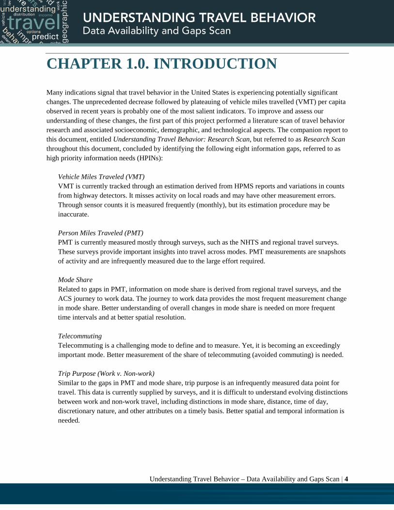
Many indications signal that travel behavior in the United States is experiencing potentially significant changes. The unprecedented decrease followed by plateauing of vehicle miles travelled (VMT) per capita observed in recent years is probably one of the most salient indicators. To improve and assess our understanding of these changes, the first part of this project performed a literature scan of travel behavior research and associated socioeconomic, demographic, and technological aspects. The companion report to this document, entitled Understanding Travel Behavior: Research Scan, but referred to as Research Scan throughout this document, concluded by identifying the following eight information gaps, referred to as high priority information needs (HPINs):
Vehicle Miles Traveled (VMT) VMT is currently tracked through an estimation derived from HPMS reports and variations in counts from highway detectors. It misses activity on local roads and may have other measurement errors. Through sensor counts it is measured frequently (monthly), but its estimation procedure may be inaccurate. Person Miles Traveled (PMT) PMT is currently measured mostly through surveys, such as the NHTS and regional travel surveys. These surveys provide important insights into travel across modes. PMT measurements are snapshots of activity and are infrequently measured due to the large effort required. Mode Share Related to gaps in PMT, information on mode share is derived from regional travel surveys, and the ACS journey to work data. The journey to work data provides the most frequent measurement change in mode share. Better understanding of overall changes in mode share is needed on more frequent time intervals and at better spatial resolution. Telecommuting Telecommuting is a challenging mode to define and to measure. Yet, it is becoming an exceedingly important mode. Better measurement of the share of telecommuting (avoided commuting) is needed. Trip Purpose (Work v. Non-work) Similar to the gaps in PMT and mode share, trip purpose is an infrequently measured data point for travel. This data is currently supplied by surveys, and it is difficult to understand evolving distinctions between work and non-work travel, including distinctions in mode share, distance, time of day, discretionary nature, and other attributes on a timely basis. Better spatial and temporal information is needed.

Understanding Travel Behavior – Data Availability and Gaps Scan | 5
Demographics and Travel Metrics The association of demographic distributions with data related to other measurements of travel (mode split, VMT, PMT) is limited, and only supplied by NHTS and other regional travel surveys. Attitudes & Public Perceptions Attitudes towards mobility have shifted across generations, which impacts the choices made by travelers in different situations. There is limited information on how those attitudes change and limited abilities to forecast attitude changes Vehicle Occupancy Vehicle occupancy data is difficult to obtain, yet is critical for better HOV enforcement and better understanding of the impacts of ridesharing services. The ability to identify real-time vehicle occupancy and measure historical vehicle occupancy would be very useful.
For further information about these HPINs, the reader is referred to the “Research Scan” report. In order to assess the suitability and potential of existing data sources for addressing these eight HPINs, this document (Understanding Travel Behavior: Data Availability and Gaps Scan) provides an inventory and assessment of current and potential data sources that can be used to identify and quantify emerging trends in travel behavior. This report identifies and reviews existing traditional, niche, and potentially beneficial travel behavior and travel-behavior-related data sources. In total, this report identifies and reviews 23 data sources. The 23 data sources are then characterized against these 8 HPINs. Based on the characterization results, seven data sources are recognized as most promising for addressing the data gaps. In order to assess and rank the seven data sources, a rating scheme is developed and applied. Results of the data assessment and ranking lead to conclusions about the suitability of these data sources for addressing the HPINs and development of recommendations to address existing travel behavior data gaps. In summary, this Data Scan is divided into seven chapters, the outline of which is as follows: Chapter 1: Introduction This chapter presents the project background and an overview for the chapters on existing travel behavior data sources, and assessment and ranking scheme. Chapter 2: Traditional Data Sources Chapter 2 provides an overview of the major traditional data sources currently used to identify and quantify travel behavior trends. It provides brief discussions of the characteristics of these data sources, their primary uses, and their benefits and limitations, as well as possible extensions underway for these data sources.
Understanding Travel Behavior – Data Availability and Gaps Scan | 6
Chapter 3: Niche and Other Potential Data Sources Chapter 3 identifies niche and other relevant data sources that could contribute to the understanding of emerging trends in travel behavior. The chapter provides a brief overview of the main characteristics of these data sources and explains their potential relevance to travel behavior and travel behavior models. Chapter 4: Data Characterization for High-Priority Information Needs Chapter 4 builds on the primary findings of Task 2 of this project, Travel Behavior Research Scan, and augments them with major recommendations from the travel behavior literature to identify the high-priority travel behavior data gaps and information needs. The chapter examines the potential of traditional, niche, and other relevant data sources for addressing the identified high-priority data gaps and information needs. It examines the extent to which these data sources may contribute to the overall understanding of emerging travel behavior trends, inform on the current impacts of those trends, and allow for understanding of future impacts. Chapter 5: Evaluation and Ranking of Data Sources Chapter 5 identifies criteria to evaluate the most promising data sources for addressing the high-priority data gaps and information needs, develops a scheme for rating these data sources, and applies the developed scheme to rank the data sources according to their potential for filling data gaps and satisfying high-priority information needs. Chapter 6: Database Chapter 6 presents the formal database that will house the detailed metadata of the promising data sources. It presents the design and construction of the database, identifies the data sources that will be included in the database, identifies and presents the attributes that will be included in the database, and provides snapshots of the database. Chapter 7: Summary and Conclusions Chapter 7 presents a summary of this report and provides a synthesis of the conclusions and recommendations for future work.

Understanding Travel Behavior – Data Availability and Gaps Scan | 7
CHAPTER 2.0. TRADITIONAL DATA SOURCES
INTRODUCTION
Understanding, modeling, and forecasting travel behavior is highly dependent on the ability to collect, store, and analyze frequent, widely varied, and high quality data. This chapter presents the traditional and major data sources that have represented the cornerstone of understanding and modeling travel behavior in the United States. All datasets presented in this chapter have a long established history and a diversified profile of areas of application. Accordingly, literature on these datasets is abundant. Using a simple search, the reader should have no trouble locating numerous resources and references for each of the presented datasets. The objective of this chapter, however, focuses on providing the reader with an overview for each of these datasets, and presenting a short synthesized summary of some of the major uses, strengths, and limitations of each of these datasets – within the context of passenger travel research. This chapter is divided into six sections. Section 1, this introduction, presents a brief overview of the chapter and the most prominent transportation data sources, including: National Household Travel Survey (NHTS), Highway Performance Monitoring System (HPMS), the American Community Survey (ACS), and other travel surveys and data repositories (e.g., GPS- and cellphone- based travel surveys). Section 2, Section 3, Section 4, and Section 5 present a detailed discussion of the aforementioned list of transportation data sources, respectively. Section 6 presents the summary and key takeaways, which provide a segue into subsequent chapters. Figure 1 depicts the graphical flow of Chapter 2.
Figure 1. Content Flow of Chapter 2

Understanding Travel Behavior – Data Availability and Gaps Scan | 8
At the end of Chapter 2, the reader is expected to have a general understanding of the most prominent travel survey data sources traditionally used in modeling of travel behavior, along with their major characteristics, strengths, usages, and limitations. In addition, the reader is expected to realize recent movements towards newer data collection technologies and approaches and major efforts towards the creation of open access travel data repositories.
NATIONAL HOUSEHOLD TRAVEL SURVEY (NHTS)
Introduction The National Household Travel Survey (NHTS) is undoubtedly the most widely used household travel data in both research and application, due to both the size and the depth of the dataset. The NHTS is a travel survey that is conducted nationally every 5 to 7 years. The survey was conducted in 1969, 1977, 1983, 1990, 1995, 2001, 2009, and 2016 (ongoing). The first NHTS dataset was collected in 1969. At that time and until the dataset collection in 1995, the NHTS was referred to as the Nationwide Personal Transportation Survey (NPTS). In 2001, and in order to build a more comprehensive picture of household travel and at the same time reduce cost and respondent burden, the NPTS was redesigned to combine the NPTS with a long-distance travel survey (called the American Travel Survey, ATS) that was conducted only once in 1995 (Sharp & Murakami, 2005). Hence, the new term NHTS was coined only in 2001 when the sixth NHTS dataset was collected (Federal Highway Administration, 2009). While the seventh NHTS dataset was collected in 2009, data collection of the eighth and latest is currently ongoing in 2016. Table 6 presents the change over time in the NHTS dataset size (Federal Highway Administration, 2004).
Table 6. Changes over Time in the NHTS Dataset Size
NHTS YEAR
NUMBER OF SURVEYED HOUSEHOLDS (HHS)
1969 15,000 HHs
1977 18,000 HHs
1983 6,500 HHs
1990 22,317 HHs (approximately 18,000 national and 4,300 add-ons)
1995 42,033 HHs (approximately 21,000 national and 21,033 add-ons + 80,000 HHs ATS)
2001 69,817 HHs (approximately 26,038 national and 43,779 add-ons)
2009 150,147 HHs (approximately 25,510 national and 124,637 add-ons)
2016 129,112 HHs (approximately 26,000 national and 103,112 add-ons) Source: Generated by California State University, Fresno

Understanding Travel Behavior – Data Availability and Gaps Scan | 9
The NHTS is a trip-based, self-reported, 24-hour household travel survey that is conducted nationally every 5 to 7 years. The survey collects information across all regions of the United States. It records data on all trips, all modes, all trip lengths, and all trip purposes. The 2009 NHTS data collection included three stages. Stage 1 was a phone interview, stage 2 included a mail-in travel diary, and stage 3 was an extended follow-up phone interview (Federal Highway Administration, 2009). The trip data is collected via travel diaries that are self-reported by all eligible individuals within a household for a designated travel day. While designated travel days are any of the 7 days in a week, a weekday travel day encompasses the 24-hour period starting at 4 am of the travel day, and the travel for the weekend is grouped into a single reporting period that goes from 6 pm on Friday to midnight on Sunday (i.e., a 54-hour period). The survey collection method was changed from a one-stage survey in 1990 (with retrospective collection of travel day trips) to a two-stage survey with a travel diary in 1995 and later (Federal Highway Administration, 2011). In general, the NHTS dataset is divided into four independent subsets of information: 1) household characteristics, 2) traveler characteristics, 3) trip information, and 4) vehicle ownership and usage information. Details about the types of data included and the number of records in each of these subsets in the 2009 NHTS are presented in Table 7. Although each of the four subsets is independent, overlaps exist between the different subsets. In the 2009 NHTS dataset, there are 32 variables that are common among all 4 subsets. These variables maintain the hierarchical relationships between the four subsets and prevent loss of information, yet at the same time allow for independent analyses and usage of the individual subsets. Figure 2 depicts the size of the 2009 NHTS subsets and the overlapping nature between the 4 subsets.
Table 7. 2009 NHTS Subsets Information Details
SUBSET/ SECTION
DESCRIPTION APPROXIMATE SECTION SIZE
Households HH-level data such as housing type, whether it is owned or rented, number of people in HH, drivers, workers and vehicles in the household, and other demographic data.
150,000 HHs
Individuals Individual-specific with data on age, sex, education level and relation to the reference individual, as well as number of trips taken by different modes in the last month, and other personal information.
308,000 Persons
Trips Provides detailed information about each trip that was taken by all eligible members of the household during the 24-hour sampling period. This data contains information on the time each trip started and ended, the distance, and detailed purpose of the trip, as well as what vehicle or transit type was used for the trip. The 2009 NHTS contains more than 1,000,000 entries in this database.
1,040,000 Trips

Understanding Travel Behavior – Data Availability and Gaps Scan | 10
SUBSET/ SECTION
DESCRIPTION APPROXIMATE SECTION SIZE
Vehicles Provides details about all vehicles at the residence. This data includes year, make, and model, registration and odometer information, and annual miles driven.
309,000 Vehicles
Source: Generated by California State University, Fresno The 2009 NHTS contains travel information from a national sample of 25,510 households. In addition to the national sample, 20 add-on regions sponsored the surveying of additional households. These 20 regions are made up of 14 State Departments of Transportations and 6 metropolitan planning organizations (MPOs). The add-on regions account for nearly 124,637 additional surveys. The 2001 NHTS was the first in the series to have a majority of the total surveys sponsored by the add-on partners (Federal Highway Administration, 2009). The NHTS is a comprehensive survey that boasted an impressive 100% eligible member interview rate for 87% of the households surveyed. Overall, 93% of all eligible members of the surveyed households were interviewed.

Understanding Travel Behavior – Data Availability and Gaps Scan | 11
Figure 2. 2009 NHTS Subsets and Overlapping Relationships
Source: Generated by California State University, Fresno
Understanding Travel Behavior – Data Availability and Gaps Scan | 12
Strengths and Benefits The NHTS is beyond doubt the most comprehensive and valuable travel behavior survey and dataset in the United States. It serves as the nation’s inventory for travel behavior; collecting extensive information about households, individuals, trips, and vehicles from a large dataset covering the whole country (urban and rural). As mentioned earlier, the NHTS collects information about all trips, performed by all members of a household, using all transportation modes during a 24-hour weekday period (or a 54-hour weekend period). While the NHTS data is collected by the U.S. Department of Transportation (USDOT), primarily to “assist transportation planners and policy makers who need comprehensive data on travel and transportation patterns in the United States”, its usage and users are rather diverse. Every year, the USDOT publishes a “Compendium of Uses” of the NHTS. These compendiums demonstrate the diversity of these applications and represent clear evidence about the significant value of the NHTS. The 2014 compendium, lists 323 published research papers and articles covering 11 different areas of application. Other areas, besides the transportation-focused areas of application, include demographic trends, environment, energy, and special population groups. Following is a list of a few of the most prominent strengths and benefits of the NHTS: Following is a list of a few of the most prominent strengths and benefits of the NHTS: Size and geographic distribution: the NHTS is undoubtedly the largest and most comprehensive
travel dataset in the United States, sampling household travel behavior of hundreds of thousands of individuals across the entire nation as well as major metropolitan regions across the country.
Temporal coverage: while the NHTS collects travel data of a specific household during a 24-hour weekday period (or a 54-hour weekend period), the combined data from all households presents travel information over all weekdays, seasons and months in a year. Accordingly, this presents a rich data source for understanding temporal variations in travel behavior.
Breadth and scope: the NHTS is a comprehensive travel survey that covers a multitude of travel variables and factors. It collects comprehensive information about HH characteristics, individual travel, trip characteristics and vehicle ownership and usage information. The breadth of the collected data enables for addressing and answering multitudes of questions and figuring plethora of relationships that are not possible otherwise.
Time range and consistency: while the survey has been conducted seven times since 1969, the general structure of the survey and the data has been largely consistent. Hence, allowing for temporal analysis of trends and comparisons for a long time period.
Reliability: the collected data is processed via rigorous well-designed algorithms. It is also validated against results of other national well-established datasets, such as the Census and Census Transportation Planning Package (CTPP) and the Highway Performance Monitoring System (HPMS). This ensures the reliability and the quality of the dataset as well as the concluded statistics, trends and inferences.
Usage: the NHTS dataset is widely used in many areas of transportation research, such as travel behavior, characteristics of travel, relationships of demographics to travel, and the public’s perception of the transportation system. The National Household Travel Survey Compendium of Uses lists 323 research papers across 11 subject areas using the NHTS only in 2014. Important to

Understanding Travel Behavior – Data Availability and Gaps Scan | 13
note is the 25 research papers regarding travel behavior that were written in 2014 alone (Federal Highway Administration, 2015). Table 8 presents the number of papers published in 2015 by subject area. Furthermore, data from the NHTS is used by the the Federal Highway Administration (FHWA) in the completion of the biennial Conditions and Performance Report given to Congress.
Table 8. Research Papers that Used the NHTS in 2015
SUBJECT AREA NUMBER OF PAPERS
Energy Consumption 74
Trend Analysis and Market Segmentation 51
Bicycle and Pedestrian Studies 46
Policy and Mobility 42
Travel Behavior 38
Survey, Data Synthesis, and Other Applications 35
Special Population Groups 29
Environment 29
Traffic Safety 15
Transit Planning 13
Demographic Trends 5
Total Papers 377
Limitations and Possible Extensions While there is no doubt about the usefulness and value of the NHTS, there are limitations to the data. Following are the most salient limitations associated with the NHTS dataset and possible extensions discussed in the literature (Saphores, National Research, Transportation Research, & Task Force on Understanding New Directions for the National Household Travel, 2013). Sample size limitations: the geographic distribution of the surveyed HHs represents one of the
issues associated with the NHTS. Out of the more than 150,000 surveyed HHs, only about 25,510 are part of the national sample. This sample is used to represent millions of HHs across the United States that are not part of the add-on surveys, broken down into nine geographic regions – the Census division classification. The nine regions are depicted in Figure 3. While additional surveys were conducted as part of the add-on surveys, the data in these surveys are weighted based on oversampling of their respective geographic locations. Sample sizes in areas that are not part of the add-ons surveys are limited in size; hence, limiting possible analyses of low-density

Understanding Travel Behavior – Data Availability and Gaps Scan | 14
rural areas, as well as analyses of differences between urban, suburban, and rural travel behaviors in some areas.
Figure 3. 2009 NHTS Geographic Regions
Source: generated by California State University, Fresno and Booz Allen Hamilton Geographic comparisons at local levels: While data about the exact address – and dependent
transportation analysis zone (TAZ) – of every surveyed HH is collected, this information is stripped out (for privacy reasons) from the dataset. Instead, information about only the geographic region (Figure 3) is included for the national dataset – 25,510 HHs. On the other hand, the add-on data includes additional information about its Census metropolitan statistical area – 49 MSAs. This limits the suitability of the dataset for some geographic comparisons in travel behavior. In essence, due to the sample size, the NHTS dataset may have limited applications to support state level analyses – especially these states that are not participating with add-on samples.
Susceptibility to anomalies: While the NHTS is a huge undertaking, the fact that the data is cross-sectional, collected only once every 5-8 years, prevents the possibility of capturing smaller, short-term changes in travel behavior. Allowing a number of years in between surveys do not account for non-recurring outside influences. External factors such as extreme weather, changes in gas prices, and incidents can affect travel behavior on the short term. An example of this type of travel behavior change was captured in the 2001 NHTS. During the interview/survey timeframe,

Understanding Travel Behavior – Data Availability and Gaps Scan | 15
the 9/11 attacks on the World Trade Center occurred. This drastically changed travel behavior for at least a short amount of time, leading to data that is possibly inconsistent with normal travel behavior (Westat, 2007). Similarly, the 2009 (and possibly other iterations of the) NHTS was conducted during an economic recession, and captured behaviors that are inconsistent with normal travel behavior.
Inconsistency of periodicity: It may be true that travel does not change fast enough to warrant annual measurement of household travel. However, from a data perspective, the non-uniform periodicity of a dataset (in addition to its low frequency) can have negative impacts on its utility. Much work in performance measurement and other applications (e.g., FHWA’s Conditions and Performance, C&P, Report) require annual or biennial reporting.
Underreporting of short trips: Since the NHTS is a self-reporting, diary-based survey, surveyed individuals are required to keep track and record their travel activities during a designated trip day. Under reporting of short trips and respective information is a common limitation of the NHTS.
Repeated cross-sectional dataset: Since the NHTS is a repeated cross-sectional survey, it does not allow for the tracking of travel behavior changes within a single household over time.
Less frequent travel: The 2009 NHTS is a single-day survey. It captures individual travel behavior over a 24-hour period weekday and a 54-hour weekend period. This limits the possibility of capturing variations in household weekly trip plans. Additionally, it limits the ability of the dataset to capture less frequent travel, such as air and vacation.
Other survey design data: Some of other travel variables that are not captured by the NHTS include costs of travel, reasons of mode choices, route choices, newer modes of transportation such as ride sourcing services like Uber, Lyft and bus rapid transit (BRT) systems, and health information that could enable understanding the effects of travel on human health.
Nonetheless, even with the limitations and potential extensions listed above, the NHTS remains to be the most powerful, valuable and widely used travel dataset in the nation. Its value and significance in understanding travel behavior and in shaping national and regional policies is beyond description. The following section presents and discusses another highly valuable dataset, the HPMS.
HIGHWAY PERFORMANCE MONITORING SYSTEM (HPMS)
Introduction The Highway Performance Monitoring System (HPMS) provides a database of information on the public roads and highways in the United States. It was established in 1978, with the primary function of establishing a consistent method for determining annual Vehicle Miles Traveled (VMT) on all public highways in the United States (Federal Highway Administration, 2008). However, the HPMS database has continued to expand over the years and nowadays includes additional infrastructure, geometric, and traffic information.

Understanding Travel Behavior – Data Availability and Gaps Scan | 16
The HPMS dataset contains detailed data on selected sample sections of major arterial and collector sections across the United States, as well as a variety of limited data on all public roads in the country, as explained further below. Every state bears the responsibility of assembling the data both from the highways under their control as well as from the various local entities (e.g., local governments and MPOs) in the state. States are required to submit the data to the FWHA by June of each year covering the information collected during the previous year. Figure 4 shows an example of a typical data collection and reporting flow from the 2014 HPMS Field Manual.
Figure 4. HPMS Data Reporting Flow Chart
Source: (Federal Highway Administration, 2014) While state transportation agencies are responsible for data collection and reporting, the FWHA has set minimum data requirements for all public roads eligible for federal funding. Data requirements define three different scales of data collection and reporting; namely, Full Extent, Sample Panel and Summary, as depicted in Figure 5. The Full Extent scale includes length, lane-miles, pavement quality (International Roughness Index, IRI) and traffic (total and truck VMT). The Sample Panel provides more detailed statistical data on a set of randomly selected roadway segments. In addition to the Full Extent data, these Sample segments include additional information in the categories of traffic, geometric, and pavement data. Last, the Summary scale provides aggregate-scale data for the lower functional highways such as the non-Federal funded roads and local roads in an entire administrative or geographic region, where data collection availability and methods are not prevalent (Federal Highway Administration, 2014).

Understanding Travel Behavior – Data Availability and Gaps Scan | 17
Figure 5. HPMS Data Reporting Sample
Source: (Federal Highway Administration, 2014)
Strengths and Benefits The data compiled in the HPMS is used by the FHWA in a variety of ways. Particularly, it represents the basis for the biennial Conditions and Progress (C&P) report to Congress, as well as the annual Highway Statistics report. In addition, the FWHA uses the information in the HPMS to assist in calculating the apportionment of Federal Highway funds. The traffic data gathered for the HPMS is also used, along with additional data collected monthly from each state, to produce the monthly Traffic Volume Trends (TVT) report. While the HPMS data reports absolute values of VMT on different highway segments, the TVT

Understanding Travel Behavior – Data Availability and Gaps Scan | 18
focuses more on the temporal variations of these values. The TVT calculates and reports variations in VMT over varying temporal spans. For example, it reports the annual monthly variation in VMT, month to month within a year. It also reports the monthly annual variation, showing the variation of a month within a year to the same month the following year. Figure 6 depicts a couple of VMT variations calculated in the January 2012 TVT report. Another salient different between the HPMS and the TVT involves that the HPMS calculates annual VMT, while the TVT estimates monthly VMT. The HPMS data is a unique and valuable dataset. It is used in a wide variety of areas and its applications are numerous. In addition to the Congressional C&P report, the TVT report, and the apportionment of Federal Highway funds, the HPMS is used in the following ways: The National Highway Traffic and Safety Administration (NHTSA) uses the VMT in
determination of their statistics on fatality and injury rates by road class (Transportation Research Board, 2011).
The Texas Transportation Institute uses the HPMS to assist in producing the annual Urban Mobility Report, which addresses congestion across the nation.
Many local governments use the data from the HPMS to develop Air Quality reports and planning.
The Transportation Research Board uses the information in planning and policy analysis (Federal Highway Administration, 2008).
The Environmental Protections Agency (EPA) uses the dataset for its Air Quality Report. The Department of Defense uses the HPMS dataset because it covers the Strategic Highway
Network (STRAHNET). “STRAHNET includes highways that are important to the United States strategic defense policy and which provide defense access, continuity, and emergency capabilities for the movement of personnel, materials, and equipment in both peacetime and war time” (Federal Highway Administration, 2014).
Due to its value and diversity of applications, the HPMS dataset has continued to develop and grow. Over the years, agencies have been submitting requests to expand the dataset and include additional variables that would benefit these agencies. Digitization of the HPMS dataset in a GIS format was one of the improvement suggestions in the 2008 report, “HPMS Reassessment 2010+” (Federal Highway Administration, 2008). Since 2009, the HPMS has been annually released in the form of a GIS file or geospatial database. This strengthens the HPMS by taking full advantage of the spatial relationships that exist between the vast amounts of data both internal and external to the HPMS (Federal Highway Administration, 2014). Figure 7 shows the 2013 HPMS GIS shapefiles from all 50 states combined together into a single map.

Understanding Travel Behavior – Data Availability and Gaps Scan | 19
Figure 6. Cover Page of the March 2016 TVT Report

Understanding Travel Behavior – Data Availability and Gaps Scan | 20
Figure 7. Combined U.S. 2013 GIS HPMS Map
Source: Generated by California State University, Fresno Another strength of the HPMS includes the variety and amount of data that it encompasses, where almost all roads have total VMT and truck VMT data, AADT as well as total lane-miles. Furthermore, the Sample Panel sections includes additional data on signalization, k factors, directional splits, lane and shoulder types and widths, pavement types and conditions, pavement base types and thicknesses, and soil types (Federal Highway Administration, 2014).
Limitations and Possible Extensions While the HPMS is comprised of a massive amount of information that provides a representation of the vehicular transportation network across the nation, several limitations and potential extensions are reported in the literature. The most prevalent of these issues pertains to the uniformity of data. While the FWHA requires each state transportation agency to provide certain types of data, the guidelines for data collection and packaging have been flexible and much freedom has been left to the individual state agencies. It has been the FHWA’s policy to collect data from across the nation, while at the same time minimizing burden on the individual states – given the massive differences between states in terms of size, highway miles, infrastructure, technologies, resources, and personnel. Nonetheless, this freedom has resulted in discrepancies between data collected at different states.

Understanding Travel Behavior – Data Availability and Gaps Scan | 21
Inspecting Figure 7 reveals that states have different densities of reporting of road sections. Figure 8b and 8c show a more detailed view of a section of the 2013 combined GIS map, at varying levels of scale. Scales of Figures 8a, 8b, and 8c show highway segments in eight, four, and two states, respectively. Upon closer inspection of the combined GIS map, the large

Understanding Travel Behavior – Data Availability and Gaps Scan | 22
differences in the density of reported roadway sections between states become more apparent.
Figure 8a. Highway Segments in 8 States of the 2013 HPMS Combined U.S. GIS Map
Figure 8. Highway Segments at Varying Levels of Scale in the 2013 HPMS Combined U.S. GIS
Map
Source: Generated by California State University, Fresno

Understanding Travel Behavior – Data Availability and Gaps Scan | 23
Table 9 presents examples of the differences between the number of records included with each
state’s GIS file compared to the actual miles of public roads within that state. It can be seen that while some states have several records for every mile of public road (e.g., Maryland: around 3.85 records per mile), others have only one record for a number of public miles (e.g., California: 0.43 records per mile).
Table 9. Comparison of GIS Records to Miles of Public Roads, 2013 HPMS U.S. GIS Data
STATE NUMBER OF RECORDS IN 2013 GIS FILE
MILES OF PUBLIC ROAD
California 75,684 174,989
Illinois 158,797 145,708
Indiana 301,113 97,553
Maryland 124,630 32,422
Texas 343,283 313,228 The differences in number of records as compared to miles of public roadway are a direct result
of the length of sections and number of roads accounted for in each state. Illinois’ nearly 159,000 records are made up of only 12,120 different roadways, as compared to Indiana’s 300,000 records covering 130,998 roadways (this was determined by dissolving route ID’s for each GIS file). It is also of importance to note that much of the data for Illinois and Indiana is collected in an average of 0.1-mile increments, while West Virginia’s data is often in several-mile increments, as shown in Figure 9.

Understanding Travel Behavior – Data Availability and Gaps Scan | 24
Figure 9. Sample of 2013 Illinois GIS Data Set
Source: Generated by California State University, Fresno
Other examples of concerns and possible extensions for the HPMS data discussed in the literature include the following: VMT forecasts: Several publications expressed concerns with accuracies of and difference
between the VMT models used by the FHWA, states, and local agencies. An example of this is shown in concerns raised by the Illinois Department of Transportation (IDOT). IDOT uses the same system to collect data for all roads in the state. However, they have seen that the VMT estimations from this system and the Chicago Area Transportation Study (CATS) are vastly different from the VMT estimations that are produced by the HPMS. While research is being done, the reason for the difference in VMT for the cities of Chicago and the Illinois portion of St Louis is still unknown (Federal Highway Administration, 2008).
Sample sections: Use of sample sections has been discussed in the literature. While sample sections are meant to provide an accurate picture of the highway system across the United States as a whole, without over-burdening states with costly data collection, sample size versus state burden will always be an issue of debate. The 2006 HPMS data on Interstate through Major Collector roadways was made up of approximately 120,000 sample sections – totaling 137,000 miles (i.e., each section representing about 1.14 miles). This represents only 14% of the total 980,000 miles of these types of roads in the United States (Federal Highway Administration, 2008).
Segment lengths: Following the same argument presented in the preceding point (sample sections set size), lengths of roadway segments was another similar point discussed in the literature. Lengths of segment sections decrease with an increase in number of sections (i.e., increased burden and costs to states). The 2006 HPMS data consisted of 1.13 million sections representing 4.01 million miles of public roads. This means that the average section is about 4 miles long.
Understanding Travel Behavior – Data Availability and Gaps Scan | 25
Other variables / more data: Publications and surveys included several other requests, many involving increasing the number of variables collected in the HPMS. Requests included collecting additional information that reflects time of day variation in volumes and speeds, supplementing the HPMS data with speed data (possibly from private, commercial data sources), involving cities and local agencies in the choice of the highway data collection points, and paying particular attention to data collection in non-attainment zones.
AMERICAN COMMUNITY SURVEY (ACS)
Introduction The United States Constitution requires that a comprehensive Census of all households be conducted every 10 years. The 1960 Census was the first to be mailed out, marking the modern age of the Census. During every Census, data is collected by survey from every household, and subsequently every individual in the United States. The survey given to every household, called the Short Form, collects limited data. This data includes age, sex, race, and relationship to the person filling out the survey. Another longer survey that asked additional questions from each member of the household, called the Long Form, was given only to a sample of the population. In the 2000 Census, approximately 1 in 6 households received the Long Form survey. The additional questions ranged from marital status, education, and earnings information, to journey to work (JTW) information – which is used extensively in transportation research and modeling. For the 2000 Census and prior, the information collected from the Long Form survey was used to estimate general data for each of the Census tracts. This data is available in many forms and contains basic demographic data, as well as average household income, and a variety of other statistics. The 2000 Census was the last to include the Long Form survey. In 2006, the Census Bureau created the ongoing American Community Survey (ACS). This new survey was designed to replace the Census Long Form survey. However, while the Long Form data was collected with the Census (i.e., once every 10 years) the ACS is collected annually. Figure 10 represents the hierarchy of data collection for the Census. Figure 10a shows the structure from 1970-2000, and Figure 10b shows the structure since 2006.

Understanding Travel Behavior – Data Availability and Gaps Scan | 26
Figure 10. Census Data Structure 1970-Present
Source: Generated by California State University, Fresno The 1960 Census Long Form was the first census survey to collect information about the JTW. It asked any worker over the age of 14 if their work was in the city they lived, another city, or not in any city, and the name of the county where the work exists. Then, the individual was asked to give the mode of transportation used to make the trip to work. In the 1960 Census, there were only eight modes of transportation listed. Figure 11 shows the questions as they appeared in the 1960 U.S. Census.

Understanding Travel Behavior – Data Availability and Gaps Scan | 27
Figure 11. 1960 Census Long Form Journey-to-Work Questions
Source: U.S. Bureau of the Census. U.S. Census of Population: 1960. Subject Reports, Journey to Work. Final Report PC(2)-6B. U.S. Government Printing Office, Washington, D.C. 1963. In the Census Long Forms that followed, questions were modified and additional questions were added. The eligible workers age changed to be 16 years old, additional modes of transportation were added and departure time and travel time questions were added. As mentioned above, the 2000 Census was the last to use the sampled Long Form format. This long form contained five questions for each eligible worker relating to their journey to work. Questions 21 to 24 on Figure 12 show the questions as they appeared on the 2000 Census long form. It is from the Census Long Form questions that the first transportation statistics were created and sold to 112 separate buyers in 1970. These buyers were mostly Metropolitan Planning Organizations (MPOs). For the 1990 and 2000 census, many states and MPO’s pooled funds to purchase the data, and cover the additional costs required for data gathering and information processing. For 1970 and 1980, the processed information package was called the Urban Transportation Planning Package (UTPP). Starting with the 1990 census, it became the Census Transportation Planning Package (CTPP). The largest change in the planning package was the ability to break down the JTW information by transportation defined geographic Travel Analysis Zones (TAZs). Out of the 340 MPOs that purchased the CTPP in 2000, 282 defined their own TAZs. The questions concerning JTW, formerly on the Census Long Form, could now be found on the new ACS. Questions 29 to 34 from Figure 12 show the JTW questions contained on the ACS. Figures 11, 12, and 13 demonstrate how the JTW questions have been evolving to capture more information and become more valuable in understanding and answering travel behavior in the United States.

Understanding Travel Behavior – Data Availability and Gaps Scan | 28
Figure 12. Journey to Work Questions 2000 Census Long Form

Understanding Travel Behavior – Data Availability and Gaps Scan | 29
Figure 13. JTW Questions from the ACS
This new survey (the ACS) is able to produce the same estimated data as the former decennial survey (Census Long Form), but now on a yearly basis. This data includes population estimates, education statistics, income and poverty statistics, and economy statistics. This data is readily available in the most recent one-, three-, and five-year estimates. The data is formatted into two different datasets: summary data, and Public Use Microdata Samples (PUMS).

Understanding Travel Behavior – Data Availability and Gaps Scan | 30
The summary data represents data that has already been tabulated for specific geographic areas. This data can be broken down geographically as far as block groups, but can also be viewed by cities, counties, census tracts, and congressional districts. On the other hand, the PUMS dataset contains information on responses to all of the survey questions from each individual. This data is available in a non-restricted form to the general public, which has the identifiable data removed. Yet, under specific circumstances, the full, unrestricted PUMS data can be obtained. Figure 14 depicts the structure and products of these two datasets.
Figure 14. Structure and Products of the ACS Datasets
Source: Generated by California State University, Fresno
Strengths and Benefits While the ACS survey collects much information and is not limited to transportation or travel behavior, it provides information that is of significant value for understanding and modeling of travel behavior and planning of transportation systems. The ability to collect and analyze data at the TAZ level is particularly useful and beneficial for MPOs. As a result, states, MPOs, and local agencies have been keen for funding and purchasing the ACS products, especially the CTPP (UTPP, formerly). Typically, states, MPOs, and local planning agencies use this data in their long-range planning and forecasting models, environmental and project analyses and descriptive statistics. Furthermore, the Commuting in America report is possibly one of the most prominent passenger travel publications, and it relies on the ACS (and NHTS) datasets.
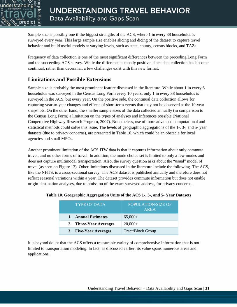
Understanding Travel Behavior – Data Availability and Gaps Scan | 31
Sample size is possibly one if the biggest strengths of the ACS, where 1 in every 38 households is surveyed every year. This large sample size enables slicing and dicing of the dataset to capture travel behavior and build useful models at varying levels, such as state, county, census blocks, and TAZs. Frequency of data collection is one of the most significant differences between the preceding Long Form and the succeeding ACS survey. While the difference is mostly positive, since data collection has become continual, rather than decennial, a few challenges exist with this new format.
Limitations and Possible Extensions Sample size is probably the most prominent feature discussed in the literature. While about 1 in every 6 households was surveyed in the Census Long Form every 10 years, only 1 in every 38 households is surveyed in the ACS, but every year. On the positive side, the continual data collection allows for capturing year-to-year changes and effects of short-term events that may not be observed at the 10-year snapshots. On the other hand, the smaller sample sizes of the data collected annually (in comparison to the Census Long Form) a limitation on the types of analyses and inferences possible (National Cooperative Highway Research Program, 2007). Nonetheless, use of more advanced computational and statistical methods could solve this issue. The levels of geographic aggregations of the 1-, 3-, and 5- year datasets (due to privacy concerns), are presented in Table 10, which could be an obstacle for local agencies and small MPOs. Another prominent limitation of the ACS JTW data is that it captures information about only commute travel, and no other forms of travel. In addition, the mode choice set is limited to only a few modes and does not capture multimodal transportation. Also, the survey question asks about the “usual” model of travel (as seen on Figure 13). Other limitations discussed in the literature include the following. The ACS, like the NHTS, is a cross-sectional survey. The ACS dataset is published annually and therefore does not reflect seasonal variations within a year. The dataset provides commute information but does not enable origin-destination analyses, due to omission of the exact surveyed address, for privacy concerns.
Table 10. Geographic Aggregation Units of the ACS 1-, 3-, and 5- Year Datasets
TYPE OF DATA POPULATION/SIZE OF AREA
1. Annual Estimates 65,000+
2. Three-Year Averages 20,000+
3. Five-Year Averages Tract/Block Group It is beyond doubt that the ACS offers a treasurable variety of comprehensive information that is not limited to transportation modeling. In fact, as discussed earlier, its value spans numerous areas and applications.

Understanding Travel Behavior – Data Availability and Gaps Scan | 32
The following section presents other travel survey technologies and approaches, and open access data repositories.
OTHER TRAVEL SURVEYS AND DATA REPOSITORIES
GPS- and cell-phone- based travel surveys, and activity-based travel surveys are two of the main alternative technologies for surveying and modeling travel behavior. These two survey types have received particularly high attention in the past couple of decades. The first part of this section introduces these two technologies. The second part of this section introduces two travel survey repositories, NREL’s Transportation Secure Data Center (TSDC) and the Metropolitan Travel Survey Archive (MTSA). These two repositories house many of the state and local travel and GPS surveys. It is worth noting that the number of local and regional travel surveys that have been conducted in the United States is much larger than the ones housed at these two repositories. While attempts continue to assemble these datasets into regional and/or national clearinghouses, it seems that many of the surveys are still missing; either being kept at the local agencies, possibly damaged, or lost. Some of these surveys (missing from these two repositories) are available at the Inter-university Consortium for Political and Social Research (ICPSR), as discussed later in the omnibus surveys section of Chapter 3.
OTHER TRAVEL SURVEYS
This section provides a brief introduction for GPS- and cellphone- based travel surveys, and activity-based travel surveys.
GPS- and Cellphone-Based Travel Surveys Travel survey technologies have been continuously progressing. However, GPS- and cellphone- based survey technologies represent a significant development in travel data collection. Examples of the different survey technologies used for travel data collection include travel questionnaires and diaries; in-person interviews, mail-in forms; phone interviews; and recall aids, among many other combinations, such as the NHTS’s multi-stage design. Because most travel surveys are based on self-reporting of personal trips, either by responding to interview questions or keeping a personal travel diary for a period of time, underreporting of trips has always been a characteristic of travel-survey based data (Bricka & Bhat, 2006). During the past decade, numerous studies have been performed to evaluate the effectiveness of different GPS-based surveys in capturing underreported travel. Examples of the different GPS-based approaches in these surveys include the role of the gathered GPS data. While many surveys passively use GPS data to help the traveler check their reported trips and improve the accuracy of the diary, other studies actively use GPS data to interact with and prompt the traveler to enter travel information on the go (e.g., via a smartphone) (Sharp & Murakami, 2005; Zmud, Lee-Gosselin, & Carrasco, 2013).

Understanding Travel Behavior – Data Availability and Gaps Scan | 33
It seems logical that contemporary travel survey approaches are moving in a direction that integrates and capitalizes on the capabilities of GPS-technologies, smartphone abilities, and machine learning algorithms. It appears that most of the recent and visible travel surveys are using utilizing these three attributes in different formats, yet with similar capacities. While SMART’s Future Mobility Survey, a national smartphone-based prompted-recall travel survey, is perhaps one of the most advanced travel survey designs of this time (Cottrill et al., 2013), many states and local agencies in the United States have conducted GPS-based travel surveys. As presented later in this chapter, a couple of these datasets are housed at NREL’s TSDC.
Activity-Based Travel Surveys
In recent years, activity-based travel surveys (sometimes referred to as time-use travel surveys) and dependent activity-based models have been gaining much traction, primarily because of their ability to address several of the limitations of the trip-based travel surveys and dependent trip-based models. Perhaps the most salient limitation of trip-based models involves the inherent assumption that all trips are made independently. It does not recognize the geographical, temporal, and social relationships between trips. For example, a trip-based model would not capture ride or carpooling arrangements between household members. Instead, it would model these trips independently. Another advantage of activity-based models over trip-based models includes its ability to answer more detailed policy questions, such as evaluation of time-based tolling scenarios, and the effect of different policies on different population groups (Castiglione et al., 2015). While the literature is rich with local, regional, national, and international studies and reports discussing the advantages and usefulness of activity-based travel models over travel-based ones, discussions about differences between activity- and trip- based surveys is not equally abundant. This is probably because, with data editing, trip-based datasets can be used to develop activity-based models and answer many of the previously challenging policy questions. Data editing involves developing trip chains from individual trip segments; hence, allowing the creation of individual full-day activities and travel patterns. Figure 15 depicts three independent trips that represent only one tour.

Understanding Travel Behavior – Data Availability and Gaps Scan | 34
Figure 15. Editing Data to Create One Activity-Based Tour from Three Trip-Based Trips
Figure from (Castiglione et al., 2015) It should be noted that activity-based travel surveys (in comparison to travel surveys) enable, in general, more detailed analyses and could improve the quality of the collected data (Pendyala, 2003).
Travel Data Repositories This section provides a brief introduction for two travel data repositories; namely, NREL’s TSDC, and the Metropolitan Travel Survey Archive (MTSA).
NREL’s Transportation Secure Data Center (TSDC)
NREL’s TSDC functions as a free access repository of primarily GPS-based travel datasets collected by different states and agencies. According to NREL’s website, TSDC “provides free access to detailed transportation data from a variety of travel surveys and studies. While preserving the privacy of survey participants, this repository makes vital transportation data broadly available to users from the comfort of their own desks via a secure online connection. Maintained by NREL in partnership with the USDOT and the U.S. Department of Energy, this centralized repository relieves individual agencies from the burden of fielding numerous data-access requests and provides additional features such as linked reference layers, data filtering, road grade and road network matching, summary statistics, and data set comparisons” (Castiglione et al., 2015). Table 11 provides a brief description of the nine datasets currently available at NREL’s TSDC.

Understanding Travel Behavior – Data Availability and Gaps Scan | 35
Table 11. Description of Datasets Currently Available at NREL’s TSDC
# DATASET NAME DESCRIPTION
1 California DOT 2010-2012 Household Travel Survey (CHTS)
Household travel survey of 42,500 households using “multiple data-collection methods, including computer-assisted telephone interviewing, online and mail surveys, wearable and in-vehicle global positioning system (GPS) devices, and on-board diagnostic (OBD) sensors that gathered data directly from a vehicle's engine.”
2 USDOT 2011 Tolling Impact Survey Conducted for the USDOT and the Urban Partnership Agreement
Before and after tolling impact survey of “drivers, public transportation users, carpoolers, and vanpoolers using the I-85 corridor in Atlanta, Georgia, and the SR-520 corridor in Seattle, Washington ... [to measure] route changes, trip timing, trip purpose, and travel mode [choices].”
3 Atlanta Regional Commission 2011 Regional Travel Survey
Regional travel survey of 20 counties in and around Atlanta, GA. The GPS part includes 1,325 households belonging to two groups. Group 1 had GPS devices installed in their personal vehicles during an assigned study period, and group 2 members (selected for being transit users) wore a GPS device that collected their individual movements during an assigned study period.
4 Texas DOT 2002-2011 Regional Travel Surveys
Nine GPS-based travel diary studies of 3,404 vehicles in Texas. The 9 cities and regions are Abilene, Austin, El Paso, Houston/Galveston, San Antonio, Wichita Falls, Rio Grande Valley, Tyler/Longview, and Laredo.
5 Metropolitan Council of Minneapolis/St. Paul 2010 Travel Behavior Inventory
While the inventory consists of a paper-based survey and a wearable GPS survey, these two surveys are independent. The wearable GPS sample includes data collected from 279 individuals.
6 Chicago 2007 Regional Household Travel Inventory
The inventory surveyed travel data from eight counties in Illinois and three in Indiana, and it featured a subsample of households collecting data via GPS devices. The GPS add-on included four stages: Stage 1 focused on in-vehicle deployments to households with significant travel requirements. Data collection occurred on the same day that the household members recorded travel. Stage 2 focused on households with at least one member with significant daily automobile travel. Stage 3 continued to focus on high-volume travelers with the deployment period for the in-vehicle component extended from one to seven days. Stage 4 involved participants in Stage 3 wearing a GPS device for seven days.
7 Puget Sound Regional Council 2004–2006 Traffic Choices Study
Pilot study to test whether time-of-day variable road tolling can reduce traffic congestion and generate revenue. Involves GPS-based vehicle travel data of 275 households using more than 400 vehicles over a period of 18 months (where the tolling lasted for only 32 weeks, i.e., about 7 months) in the Seattle metropolitan area.
8 Mid-America Regional Council — 2004 Regional Travel Study
GPS-based one-day travel data of a sample of 408 vehicles around Kansas city, Missouri.

Understanding Travel Behavior – Data Availability and Gaps Scan | 36
# DATASET NAME DESCRIPTION
9 Southern California Association of Governments — 2001–2002 Regional Travel Survey
GPS-based sample taken for the purpose of auditing self-reported travel diaries that were collected using computer-assisted telephone interviewing (CATI) and travel diaries in the six-county SCAG region: Imperial, Los Angeles, Orange, Riverside, San Bernardino, and Ventura. The GPS data includes roughly 1,200 vehicle-days of driving representing about 450 households (with one or more vehicles and one or more driving days for each household).
Metropolitan Travel Survey Archive (MTSA)
As part of a grant provided by the Bureau of Transportation Statistics and the FHWA in the early years of the 21st century, a team at the University of Minnesota created the and continues to host the MTSA website – where the last reported update to the website appears to have happened in September 2012. The objective of the grant was to “store, preserve, and make publicly available, via the internet, travel surveys conducted by metropolitan areas, states, and localities”. At the moment, the MTSA houses 84 datasets, spanning from 1960 to 2011. Figure 16 depicts the classification of the housed datasets by year and agency (state DOTs and MPOs or COGs). The figure demonstrates that the bulk of the datasets span between the years 1996 and 2008, and that while the majority (87%) of the datasets belong to MPOs and local agencies, only 13% are state DOT datasets. In addition to the collection and housing of the datasets, the grant intended “to make the available datasets compatible with the Survey Documentation and Analysis (SDA) software to enable online analysis of dataset.”

Understanding Travel Behavior – Data Availability and Gaps Scan | 37
Figure 16. Classification of Travel Datasets at the MTSA by Year and Agency
Source: Generated by California State University, Fresno
SUMMARY
This chapter provides a brief overview of the traditional and major datasets that are traditionally utilized by transportation planning agencies in the United States for understanding and modeling travel behavior. The chapter presented three major datasets: the NHTS, the HPMS, and the ACS. In addition, the chapter presented a brief discussion of the emerging GPS- and cellphone- based travel survey technologies, and the activity-based travel survey and modeling approach. The chapter ended with brief introductions to two prominent travel data repositories: NREL’s TSDC, which houses 9 major datasets (mostly GPS-based datasets); and the Metropolitan Travel Survey Archive, which houses 84 datasets from state DOTs and MPOs across the country, spanning from 1996 to 2011. All the datasets presented in this chapter have a long history of established use and application and are characterized with a comprehensive literature. Accordingly, presenting a thorough discussion of these datasets in such a limited space is quite challenging. Therefore, while the chapter provided only brief introductions and discussions, the reader is encouraged to pursuit the provided references for further details and information. Because none of the existing travel behavior models was able to capture recent trends in travel behavior (e.g., plateauing of national and individual VMT), it is expected that other and newer sources of travel

Understanding Travel Behavior – Data Availability and Gaps Scan | 38
data will be needed for the explanation of these trends. Accordingly, the following chapter, Chapter 3, presents a brief discussion of the most prominent niche and potentially relevant travel data sources.
REFERENCES
Bricka, S., & Bhat, C. R. (2006). Comparative analysis of Global Positioning System-based and travel survey-based data. Transportation research record.(1972), 9-20.
Castiglione, J., Bradley, M. A., Gliebe, J., National Research, C., Transportation Research, B., & Second Strategic Highway Research, P. (2015). Activity-based travel demand models : a primer.
Cottrill, C., Pereira, F., Zhao, F., Dias, I., Lim, H., Ben-Akiva, M., & Zegras, P. (2013). Future Mobility Survey. Transportation Research Record: Journal of the Transportation Research Board, 2354, 59-67. doi: doi:10.3141/2354-07
Federal Highway Administration. Non-Federal Applications of the Highway Performance Monitoring System (HPMS). Retrieved Jult 21, 2015, from http://www.fhwa.dot.gov/policyinformation/hpms/nahpms.cfm
Federal Highway Administration. (2004). 2001 National Household Travel Survey User's Guide (Version 3). Washington, DC.
Federal Highway Administration. (2008). HPMS Reassessment 2010+ (O. o. H. P. Information, Trans.). Washington, D.C.
Federal Highway Administration. (2009). 2009 National Household Travel Survey User's Guide (Version 2). Washington, DC.
Federal Highway Administration. (2011). Summary of Travel Trends: 2009 National Household Travel Survey. Washington, D.C.
Federal Highway Administration. (2014). Highway Performance Monitoring System: Field Manual (F. H. Administration, Trans.).
Federal Highway Administration. (2015). National Household Travel Survey Compendium of Uses. Washington, DC.
National Cooperative Highway Research Program. (2007). Report 588: A guidebook for using American Community Survey data for transportation planning. Washington, D.C.: Transportation Research Board.
Pendyala, R. (2003). Quality and Innovation in Time Use and Activity Surveys. In P. Stopher & P. Jones (Eds.), Transport survey quality and innovation. Amsterdam, The Netherlands: Pergamon Press.
Saphores, J. D., National Research, C., Transportation Research, B., & Task Force on Understanding New Directions for the National Household Travel, S. (2013). Exploring new directions for the National Household Travel Survey : phase one report of activities. from http://onlinepubs.trb.org/onlinepubs/circulars/ec178.pdf
Sharp, J., & Murakami, E. (2005). Travel surveys : methodological and technology-related considerations. Journal of transportation and statistics., 8(3), 97-113.
Transportation Research Board. (2011). How we travel: a sustainable national program for travel data. Washington, D.C.
Transportation Secure Data Center. (2015). National Renewable Energy Laboratory. Retrieved July 20, 2015, from www.nrel.gov/tsdc

Understanding Travel Behavior – Data Availability and Gaps Scan | 39
Westat. (2007). Gaps and Strategies for Improving AI/AN/NA Data. Rockville, MD. Zmud, J., Lee-Gosselin, M., & Carrasco, J. A. (2013). Transport Survey Methods Best Practice
for Decision Making. from http://public.eblib.com/choice/publicfullrecord.aspx?p=1123223

Understanding Travel Behavior – Data Availability and Gaps Scan | 40
CHAPTER 3.0. CHAPTER 3: NICHE AND OTHER POTENTIAL DATA SOURCES
INTRODUCTION
Recent travel patterns have demonstrated unprecedented trends. While the plateauing of national VMT is probably the most significant of these trends, other significant shifts in travel behavior are occurring. The suitability of the traditional datasets in explaining these unprecedented and unpredicted trends could be limited. Hence, identifying other data sources could be particularly beneficial. While Chapter 2 provided an overview of many datasets that have been traditionally used to understand, model, and forecast travel behavior, this chapter introduces other niche and potential data sources that could help improve our understanding and forecasting of U.S. travel behavior at local, regional, state, and national levels. Some of the datasets presented in this chapter have a long established history and a diversified profile of areas of application. However, others are more recent, proprietary, and/or have received much less attention in research and application. Accordingly, the objective of this chapter focuses on providing the reader with an overview for each of these datasets, and presenting a short synthesized summary of some of their major uses, strengths and limitations. This chapter is divided into four sections. While Section 1 is this Introduction, Section 2 presents a brief overview of five of the most relevant niche travel datasets: Trace Data (e.g., NPMRDS/Here, INRIX, AirSage), American Time Use Survey (ATUS), National Transit Dataset (NTD), Strategic Highway Research Program (SHRP2) Naturalistic Driving Study (NDS), and 4 Travel Apps (Gamification: Waze and Metropia, Ride Sourcing: Uber, and Alternative Transportation: RideScout). Section 3 presents a brief overview of nine other potentially relevant datasets: DMV and Insurance, American Housing Survey (AHS), National Transportation Statistics, omnibus surveys (e.g., Pew, U Michigan), Social Network Data, Mail Data, ITS, and the Research Data Exchange (RDE). Section 4 presents the summary and key takeaways that provide a segue into the subsequent chapters. Figure 17 depicts the graphical flow of Chapter 3. At the end of Chapter 3, the reader is expected to have a general understanding of some of the most prominent niche datasets and other potentially relevant ones. These datasets could potentially help improve our understanding and modeling of current and future travel behavior and trends.
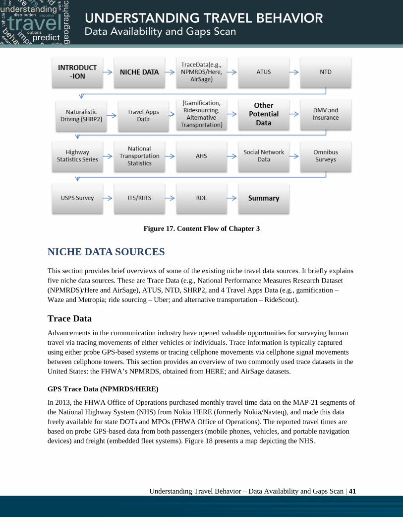
Understanding Travel Behavior – Data Availability and Gaps Scan | 41
Figure 17. Content Flow of Chapter 3
NICHE DATA SOURCES
This section provides brief overviews of some of the existing niche travel data sources. It briefly explains five niche data sources. These are Trace Data (e.g., National Performance Measures Research Dataset (NPMRDS)/Here and AirSage), ATUS, NTD, SHRP2, and 4 Travel Apps Data (e.g., gamification – Waze and Metropia; ride sourcing – Uber; and alternative transportation – RideScout).
Trace Data Advancements in the communication industry have opened valuable opportunities for surveying human travel via tracing movements of either vehicles or individuals. Trace information is typically captured using either probe GPS-based systems or tracing cellphone movements via cellphone signal movements between cellphone towers. This section provides an overview of two commonly used trace datasets in the United States: the FHWA’s NPMRDS, obtained from HERE; and AirSage datasets.
GPS Trace Data (NPMRDS/HERE)
In 2013, the FHWA Office of Operations purchased monthly travel time data on the MAP-21 segments of the National Highway System (NHS) from Nokia HERE (formerly Nokia/Navteq), and made this data freely available for state DOTs and MPOs (FHWA Office of Operations). The reported travel times are based on probe GPS-based data from both passengers (mobile phones, vehicles, and portable navigation devices) and freight (embedded fleet systems). Figure 18 presents a map depicting the NHS.

Understanding Travel Behavior – Data Availability and Gaps Scan | 42
Figure 18. NPMRDS National Highway System
Source: Map Generated by California State University, Fresno using GIS Files from NHS HERE captures probe travel time data in real time; then, the data is aggregated over both space and time. In regards to space, highways are divided into directional shorter spatial segments, called Traffic Message Channels (TMCs). On the other hand, with respect to time, recorded travel times are aggregated over 5-minute bins, called Epocs. Hence, there are 288 epocs in a day (12 epocs per hour and 24 hours in a day). The first epoc (epoc #0) spans from 12:00 to 12:05 am, and the last epoc (epoc #287) spans from 11:55 pm – 12:00 am. The HPMRDS is composed of three different file types (FHWA Office of Highway Policy Information, 2014):
a. Static TMC definition file: contains spatial information about every TMC segment. Table 12 presents a sample of a TMC definition file.
b. Travel time data files: contain travel time data on specific TMC segments at specific epocs, during a specific month. These files are updated monthly. Table 13 presents a sample of a data file. It can be seen that while both passenger and freight travel times are reported separately, the size of the sample is not reported. Also, the date of the observed data is not reported.
c. Static GIS shapefile: contains geo-referenced spatial information for every TMC segment and can be used for data visualization.

Understanding Travel Behavior – Data Availability and Gaps Scan | 43
Table 12. Sample of a TMC Definition File
tmc adm1 adm2 adm3 mile_ length
radioID local name latitude longitude direction
103P04423 US Pennsylvania Bucks 1.1703 US-202 40.294 -75.1392 Northbound
120P10923 US New York Kings 0.5436 Flatbush Ave Ext
40.6956 -73.9842 Northbound
120P04970 US New Jersey Hudson 0.8451 US-1-9 40.7318 -74.0528 Northbound
103P09904 US Pennsylvania Montgomery 0.3887 PA-663 N Charlotte St 40.2686 -75.6244 Northbound
120N10781 US New Jersey Monmouth 2.3824 RT-35 Broad St 40.3239 -74.0615 Southbound
120N14970 US New Jersey Essex 1.0138 CR-577-SPUR/ Prospect Ave
40.7744 -74.2609 Southbound
120P18351 US New York New York 0.3559 Grand St 40.7152 -73.9843 Westbound
120N06737 US New York New York 0.3724 Brooklyn Brg 40.7117 -74.0038 Southbound
120P17770 US New York Richmond 1.0778 Amboy Rd 40.5433 -74.1642 Northbound
120P06864 US New York New York 0.2954 RT-9A West Side Hwy 40.7607 -74.0021 Northbound
120N17123 US New York Queens 1.3052 Rockaway Blvd 40.6744 -73.8012 Eastbound
120N11051 US New York Westchester 1.7553 US-6 41.337 -73.7861 Eastbound
103N11674 US New Jersey Camden 0.5421 CR-636 Cuthbert Blvd 39.9259 -75.0551 Southbound
120N06411 US New York Nassau 0.6327 RT-25 40.7295 -73.6998 Westbound
120N18220 US New York Bronx 0.9427 Eastchester Rd 40.8445 -73.8462 Southbound
Source: (FHWA Office of Highway Policy Information, 2014)
Table 13. Sample of a Data File
TMC EPOC TravelTimeAll(s) TravelTimePassenger(s) TraqvelTimeFreight(s)
120N06411 0 458 458
120N06411 0 111 111
120N06411 0 138 138
120N06411 0 81 81
120N06411 0 104 104
120N06411 1 112 112
120N06411 1 305 305
120N06411 1 89 89
120N06411 2 89 89
120N06411 3 190 190
120N06411 3 92 92 Source: (FHWA Office of Highway Policy Information, 2014)

Understanding Travel Behavior – Data Availability and Gaps Scan | 44
The NPMRDS is used by the FHWA, state DOTs, and MPOs in a number of ways. The FHWA is using the dataset as a primary data source for two of its programs: the Freight Performance Measures (FPM) program and the Urban Congestion Report (UCR). State DOTs and MPOs are using the data in other ways, including as performance indicators and for travel demand modeling and validation. Recently, the Atlanta Regional Commission (ARC) has been utilizing the NPMRDS for updating the free flow travel speeds and the volume delay functions of their travel demand model’s highway network links. Their findings about speeds at capacity discrepancies for the weaving sections are particularly interesting and reflect the value of integrating the NPMRDS in travel demand modeling. Possible further uses of the dataset include estimation of dynamic travel times to be used in models of dynamic traffic assignment. It is worth noting that while the NPMRDS covers only the NHS. Many cities and MPOs have opted to purchase other HERE datasets that provide more comprehensive coverage of streets in their local vicinities. While GPS-based trace data has several strength in comparison to traditional travel survey methods – including higher accuracy, larger sample sizes, and cheaper costs – issues of individual privacy constitute a major limitation for data usage. Tracing movements of individuals can easily allow identification of their home and work addresses and other personal travel information, which represents a privacy violation. Accordingly, this type of GPS-trace data is aggregated over highway segments and reports only highway travel times, rather than providing individual travel traces. A recent FHWA TMIP Webinar hosted a presentation about using the NPMRDS for travel model development at Atlanta’s MPO (ARC). The presentation included several demonstrations of how the NPMRDS can be utilized to improve understanding and modeling of travel behavior at the local level. Examples of applying data to the regional travel behavior model included updating the volume delay functions and free flow speeds of the different highway classes, as well as at weaving sections (Rousseau). Figure 19 depicts the improvement in model predictions after use of the NPMRDS.

Understanding Travel Behavior – Data Availability and Gaps Scan | 45
Figure 19. A Comparison of Estimated and Observed Speeds on Different Highway Segments in Atlanta Before and After Using the NPMRDS
Source: (Rousseau) In general, one of the limitations of vehicle-based GPS trace data is its inability to track or explain individual travel movements. Smartphone-based GPS-trace data are characterized with high battery consumption, and accordingly require timing the trace log into longer time increments. This increases the possibility of missing intermediate stops and characterizes a limitation of the data. This limitation is less significant in cell-phone trace data, which is presented in the next section.
Cellphone Trace Data (AirSage)
While NPMRDS traces the movements of passengers and freight through GPS-enabled and embedded devices, AirSage collects traces of cellphone locations. As long as a cellphone is turned on, locations and movements of individual cellphones can be identified and traced based on communication with cellphone towers. AirSage reports that it collects cellphone trace data from two of the top cellphone carriers in the United States. This data represents more than 100 million devices and see more than 15 billion locations every day. Accordingly, in comparison to other travel datasets, cellphone trace data has the highest penetration rates and widespread coverage, and may be the most comprehensive representation of human travel. Similar to the GPS trace data, raw cellphone trace data can contain personally identifiable information (PII) and therefore cannot be commercially available. Accordingly, the raw data is first processed and aggregated to eliminate any PII. Cellphone trace data is always aggregated over geographic regions and/or over time. Then, the processed data is made commercially available for public use. Examples of AirSage travel data products include the following: Trip matrices: representing the number of and type of trips traveling between two geographic
locations. Figure 20 depicts a graphical visualization of AirSage Trace Data of 24-hour trips in the Lexington, KY metro area.

Understanding Travel Behavior – Data Availability and Gaps Scan | 46
Home-work reports: number of individuals living and working at specific geographic locations. Select zone analyses: information about the number and type of trips that go to or come from a
specific zone. Arrival and departure studies: temporal distributions of volumes and types of trips going to or
coming from a specific zone or traveling between specific geographic locations. Cellphone trace data has strong potentials for being among the most valuable travel behavior datasets. It has many advantages, including large sample size, cheap cost, temporal and geographic distribution of observations, continuous rate of update, and the possibility of real-time observation of travel behavior. On the other hand, some of the limitations of the dataset include PII limitations and challenges for imputation of travel mode and trip purpose. Many cities and MPOs are currently using AirSage for (origin-destination) OD demand estimation as well as validation of the travel behavior models outputs. Dynamic and temporal OD demand estimates could be a valuable potential benefit from using such dataset.
Figure 20. AirSage Graphical Visualization of Trace Data of 24-hour Trips in the Lexington, KY Metro Area
Source: (AirSage)
American Timeuse Travel Survey (ATUS) The ATUS is a continuous one-time individual phone interview survey that succeeds the 8-months household Current Population Survey (CPS). While the CPS collects information about the labor force,

Understanding Travel Behavior – Data Availability and Gaps Scan | 47
the ATUS collects information about how individuals spend their time on the “previous day,” including travel and where and with whom they spent their time. Official data collection for the ATUS started in 2003 and has been continuously ongoing since then (U.S. Bureau of Labor Statistics, 2015). Individuals for the ATUS are randomly picked from a subset of households that complete their eighth and final month of interviews for the CPS. The CPS interviews around 60,000 households every month (prior to 2001, it was 50,000 households) for a period of 8 months. Every month, around one eighth of the 60,000 households are newly selected to participate in the CPS and the same number of households retires (i.e., around 7,500 households per month). Two months after households retire from the CPS, they become eligible for selection into the ATUS. Since 2004, out of the households retiring from the CPS, approximately 2,190 individuals (only one individual per household), are interviewed in the ATUS every month (about 26,400 individuals every year). The monthly sample is divided into 4 panels, one for every week of the month. Within every panel, designated individuals are interviewed to report on the time spent during the “previous” day. These days are equally divided between weekdays and weekends (i.e., 50% of the days are selected to be weekdays and 50% as weekend days). The weekdays are equally split over the five days of the week. To elaborate, every weekday has a 10% share of the sample, and every weekend day has a 25% share. Designated individuals are interviewed using a computer assisted telephone interviewing (CATI) process. The interview process is composed of both structured and conversational questions. The interviewed individuals answer questions covering five major topics. Figure 21 depicts these five topics. Four of the topics have not changed since 2003. These topics are household roster, travel time diary, summary question, and questions related to the eighth CPS interview. The fifth topic, on the other hand, was changed in 2011. Between 2003 and 2010, the fifth topic covered questions pertaining to overnight trips away from home. It asked questions about the number, duration, and purpose of overnight trips that have happened in the previous month. However, starting in 2011, this topic was removed and replaced with questions pertaining to eldercare.

Understanding Travel Behavior – Data Availability and Gaps Scan | 48
Figure 21. The Five Main Topics of the ATUS
Source: Generated by California State University, Fresno
While most of the interview is composed of structured approach, the time diary questions are primarily conversational. The conversational approach was adopted to allow interviewers to use methods to guide interviewees and ensure more complete and consistent data collection. While the time use diary includes information about travel modes, travel times, and ride sharing that are explicitly reported by the interviewee, the trip purpose information is automatically coded according to preset rules as a function of the preceding and succeeding activities. The ATUS includes highly valuable information for understanding and modeling of travel behavior, yet it appears that it has yet to be sufficiently utilized for transportation research. For example, since it captures how individuals spend their time, it could be potentially useful for investigating the impacts of travel alternatives on demand (e.g., online shopping). The periodicity of the dataset represents one of its major strengths since it is collected monthly and reported annually. While the data is reported annually, it includes information about the exact date of reported travel. Another strength of the dataset includes its conversation-based approach for time use diary data collection, which could presumably reduce potential under-reporting of travel and minimizing data inconsistencies. Also, the dataset includes interviewees’ geographic information at the state level and includes additional variables that differentiate between metropolitan and non-metropolitan locations. It is an activity-based travel survey, which makes the dataset more readily suitable for activity-based travel demand models. On the other hand, potential challenges for using the dataset include its inability to capture and analyze travel behavior differences between geographical locations within states. In addition, only trip travel times are reported. Travel distances are not captured in the survey. Also, the survey captures travel of

Understanding Travel Behavior – Data Availability and Gaps Scan | 49
only a single household individual, instead of the entire household. Lastly, using the dataset for travel demand modeling may require the additional effort of reviewing and recoding of the automatically coded trip purposes. Figure 22 depicts an excerpt of the trip purpose coding algorithm in the ATUS. On the other hand, since one of the major drawbacks of passive data collection (e.g., GPS) is that purpose information is not captured, this ATUS data could be instrumental in helping derive this information.

Understanding Travel Behavior – Data Availability and Gaps Scan | 50
Figure 22. Coding of Trip Purpose in ATUS
Source: Exhibit 5.1 from 2015 American Time Use Survey User’s Guide

Understanding Travel Behavior – Data Availability and Gaps Scan | 51
National Transit Database (NTD) According to the website of the NTD, “Today the transit industry consists of over 140,000 vehicles, traveling over 48 billion passenger miles, and collecting over $8.5 billion in passenger fares. In the past 10 years the transit industry has grown by over 20 percent - faster than either highway or air travel. As the industry continues to grow, every indication is that the NTD will continue to expand both in scope and use in the years to come” (Federal Tansit Administration). The NTD is a federal reporting structure for urban and rural transit agencies receiving funds from the Federal Transit Administration (FTA). It was established by Congress in 1974 and is primarily used to allocate FTA funds to transit agencies. It also serves as the national repository for transit data and statistics in the United States. All urban and non-urban (rural), both public and private, transit agencies receiving FTA funds are required to submit data to the NTD. This data covers a wide range of information about the transit service and safety data. This includes comprehensive information on “transit organization characteristics, vehicle fleet characteristics, revenues and subsidies, operating and maintenance costs, vehicle fleet reliability and inventory, services consumed and supplied, and safety and security” (Gan, Ubaka, & Zhao, 2002). A few annual waiver exceptions exist for small transit agencies (that operate a fleet of less than 30 vehicles and have no fixed-guideway service) and for transit agencies suffering from natural disasters or strikes. While most of the data submissions are required annually, four key factors are submitted monthly. These four factors are:
1. Unlinked Passenger Trips, which are “the number of passengers who board public transportation vehicles. Passengers are counted each time they board vehicles no matter how many vehicles they use to travel from their origin to their destination.”
2. Vehicle Revenue Miles, which are “The miles that vehicles travel while in revenue service. Vehicle revenue miles (VRM) include revenue service. Actual vehicle revenue miles exclude deadhead, operator training, maintenance testing, and school bus and charter services”
3. Vehicle Revenue Hours, which are “the hours that vehicles travel while in revenue service. Vehicle revenue hours (VRH) include revenue service and layover/recovery time. Actual vehicle revenue hours exclude deadhead, operator training, maintenance testing, and school bus and charter services.”
4. Vehicles Operated in Maximum Service (Peak Vehicles), which are “the number of revenue vehicles operated to meet the annual maximum service requirement. This is the revenue vehicle count during the peak season of the year; on the week and day that maximum service is provided. Vehicles operated in maximum service (VOMS) excludes atypical days and one-time special events.”
In 2013, which is the latest dataset available on the NTD website, includes 857 listed agencies in 483 urbanized areas, where 849 agencies submitted reports, and 536 agencies submitted full systems reports. Figure 23 depicts the unlinked passenger trip volumes on transit systems in urbanized areas in the United States.
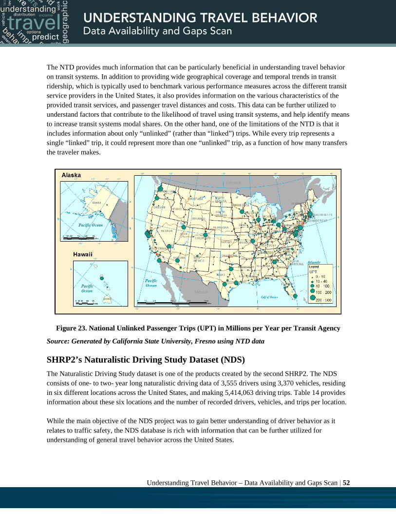
Understanding Travel Behavior – Data Availability and Gaps Scan | 52
The NTD provides much information that can be particularly beneficial in understanding travel behavior on transit systems. In addition to providing wide geographical coverage and temporal trends in transit ridership, which is typically used to benchmark various performance measures across the different transit service providers in the United States, it also provides information on the various characteristics of the provided transit services, and passenger travel distances and costs. This data can be further utilized to understand factors that contribute to the likelihood of travel using transit systems, and help identify means to increase transit systems modal shares. On the other hand, one of the limitations of the NTD is that it includes information about only “unlinked” (rather than “linked”) trips. While every trip represents a single “linked” trip, it could represent more than one “unlinked” trip, as a function of how many transfers the traveler makes.
Figure 23. National Unlinked Passenger Trips (UPT) in Millions per Year per Transit Agency
Source: Generated by California State University, Fresno using NTD data
SHRP2’s Naturalistic Driving Study Dataset (NDS) The Naturalistic Driving Study dataset is one of the products created by the second SHRP2. The NDS consists of one- to two- year long naturalistic driving data of 3,555 drivers using 3,370 vehicles, residing in six different locations across the United States, and making 5,414,063 driving trips. Table 14 provides information about these six locations and the number of recorded drivers, vehicles, and trips per location. While the main objective of the NDS project was to gain better understanding of driver behavior as it relates to traffic safety, the NDS database is rich with information that can be further utilized for understanding of general travel behavior across the United States.

Understanding Travel Behavior – Data Availability and Gaps Scan | 53
Table 14. Locations of SHRP2 NDS and Recorded Number of Participant Vehicles, Drivers, and Trips per Location
# LOCATION STATE NUMBER OF VEHICLES
NUMBER OF DRIVERS
NUMBER OF TRIPS
1 Bloomington Indiana 255 282 459,849
2 Buffalo New York 775 786 1,312,668
3 Central Pennsylvania Pennsylvania 272 287 346,293
4 Durham North Carolina 546 576 905,385
5 Seattle Washington 741 836 1,165,357
6 Tampa Bay Florida 781 788 1,224,511
Sum 3,370 3,555 5,414,063 Source: Generated by California State University, Fresno from SHRP2 Dataset Participant’s vehicles in the NDS were instrumented with three main data collection devices, and collected continuous information for a time period spanning one to two years. The three main data collection devices included:
a. Head unit placed beside the rear view mirror and collected continuous video feed of the driver, short 30-second audio feeds upon driver prompt, and ambient alcohol levels in the passenger compartment
b. Main unit placed in the vehicle trunk, which collected continuous GPS location data, as well as a vehicle network box placed under the front dashboard that collected information about vehicle speed, throttle position, turn signal indication, and brake application
c. Front radar system that collected information about the vehicle’s surroundings. In addition to the continuous data collection systems installed on the participant vehicles, participants completed a number of surveys that collected information about their medical conditions, vehicle characteristics, driving behavior, risk attitudes, demographic, socioeconomic, and personality characteristics, among others. In addition to safety and driving insights, the NDS dataset holds potentially valuable information for understanding travel behavior. Examples of information that can be identified from this study include driver departure time choices, seasonal variation in travel activity, daily travel activity patterns, route choice behavior, trip times and lengths, effect of weather on driving activity, effects of socioeconomic and demographic factors, and geographical differences in driving behavior across the United States. Figure 24 depicts variations in annual commute route choice behavior of four drivers (Tawfik, Rakha, & Du, 2012). In addition, the data can be utilized for estimation of static and dynamic OD tables. Also, Figure 25 presents traversal density of recorded Trips Data in Tampa, FL, which can be used to estimate travel paths, OD pairs, and associated route choice behaviors.

Understanding Travel Behavior – Data Availability and Gaps Scan | 54
Figure 24. Sample Images of Differences between Drivers Commute Route Choice Behavior:
Number of Commute Routes and Frequency of Route Choice Switching
Source: (Tawfik et al., 2012)

Understanding Travel Behavior – Data Availability and Gaps Scan | 55
On the other hand, a few limitations of this dataset include its limit to driving trips (i.e., it captures only car-based trips). Additionally, while the unavailability of a travel diary could limit the possibility of trip purpose imputation, use of the passenger compartment recordings can serve as a novel valuable resource. For example, a video recording showing a parent dropping off kids with school bags in the morning at a school location and picking them again in the afternoon significantly simplifies imputation of this trip purpose.
Figure 25. Traversal Density of Recorded Trips Data in Tampa, FL
Source: (InSight Data Access Website: SHRP 2 Naturalistic Driving Study)
Travel Apps Data Recent booms in smartphones and communication technologies have catalyzed the potential impacts of travel data apps on travel behavior. Since these apps are predominantly commercial, data is proprietary and not publicly available for research. Accordingly, understanding the impacts of these systems on travel behavior remains limited. Additionally, as discussed later in the omnibus surveys section (Section 3.7), millennials and young travelers use smartphones and apps at a much higher frequency than older travelers. Therefore, understanding the impacts of these apps on travel behavior may be beneficial in understanding and explaining recent trends in travel behavior in the United States.

Understanding Travel Behavior – Data Availability and Gaps Scan | 56
The following sections present information about four different travel data apps: Waze and Metropia are used as examples of gamification apps, Uber is used as an example of a ridesourcing app, and RideScout is used as an example of an alternative transportation apps. These sections discuss their potential influences on travel behavior.
Gamification
The Merriam-Webster dictionary defines gamification as “the process of adding games or gamelike elements to something (as a task) so as to encourage participation.” Several novel travel apps have integrated gamification elements. The increasing popularity and usage trends of these apps seem to suggest that gamification may represent an impactful factor in future travel behavior. The following subsections represent a quick overview of two travel apps with integrated gamification elements, Waze and Metropia. Waze Waze define themselves as “the world’s largest community-based traffic and navigation app” (Transportation Research Board, 2011). While Waze serves as a regular dynamic route guidance system (it provides drivers with turn-by-turn real-time navigation to their destinations), the app simultaneously collects passive travel information and uses this information to update its estimates for travel conditions and dependent navigation processes. Additionally, Waze uses gamification features to entice drivers to use the map more often, as well as to take a more active role and share voluntary reports on traffic incidents such as congestion, accidents, road hazards, and police presence. Furthermore, the app provides the users with the added advantage of sharing real-life information about their location and estimated time of arrival with friends. Figure 26 depicts a snapshot of the Waze app route guidance screen displaying navigation information, locations of surrounding Waze users, and Waze-user-reported traffic reports. For a novel user, however, not all functions are readily available. For example, a novel Waze user may not be allowed to share their location with their friends. To be allowed to use this feature, the user has to accumulate a certain number of Waze points. Points are earned as a function of usage of the Waze app. Figure 27a shows a list of tasks a Waze user can accomplish and the number of points associated with completing each of these tasks. Figure 27b depicts the five possible levels for Waze users. It should be noted that the higher three levels are not defined by points. Instead, they are defined by the percentile ranking of a user in comparison to the other users in the state. This means that a higher level user can be demoted to a lower level when s/he stops accumulating points, while other users in the state surpass the his/her points and cause his/her percentile ranking to drop. This aspect ensures the continual participation of users regardless of the number of points accumulated. In addition to the standard features (points and levels), Waze entices users to contribute to the creation of the Waze map and transportation system. Figure 27c depicts a few additional features that are restricted to users contributing to the correction and editing of the highway map.

Understanding Travel Behavior – Data Availability and Gaps Scan | 57
There appears to be evidence that dynamic electronic route guidance systems, particularly Google Maps and Waze, are significantly influencing travelers’ en-route route choice behavior. This effect is particularly noticeable during high levels of congestion, where these apps guide travelers to less congested routes. This results in reductions in congestion and associated travel times, and possibly emissions.
Figure 26 Snapshot of Waze Route Guidance Screen
Source: Acquired from (Stern, 2013)

Understanding Travel Behavior – Data Availability and Gaps Scan | 58
Figure 27. Snapshots of Waze Tasks and User Levels
Source: Generated by California State University, Fresno Metropia Instead of focusing on real-time route guidance, unlike Google Maps and Waze, Metropia, is an app that focuses on trip planning. Metropia claim that they use “next-generation traffic prediction ... [and] … do not only give [travelers] the best routes to take … [but also] the best times to travel”. They ask travelers to “reserve [their] routes in advance to avoid traffic”, and ask users to “think ahead to save time, earn rewards and reduce CO2 emissions.” Metropia’s main paradigm focuses on reducing traffic’s greenhouse gas emissions. Metropia’s service is currently available only in three cities in the United States (Tucson,
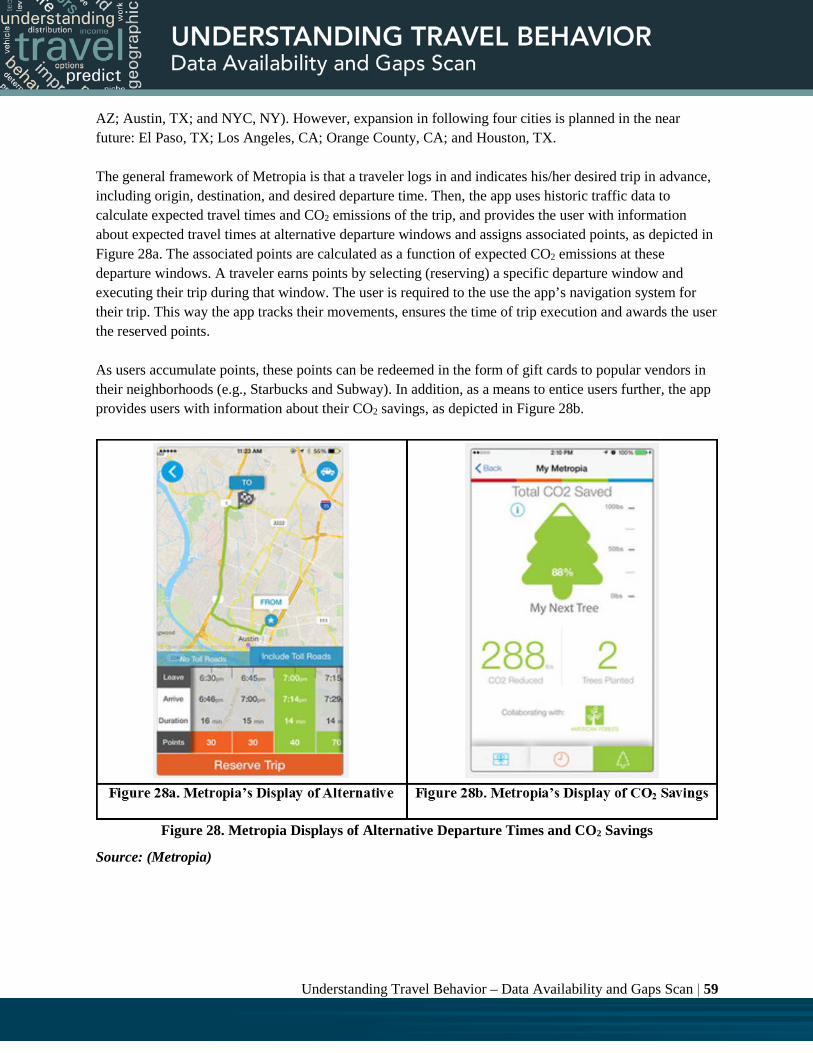
Understanding Travel Behavior – Data Availability and Gaps Scan | 59
AZ; Austin, TX; and NYC, NY). However, expansion in following four cities is planned in the near future: El Paso, TX; Los Angeles, CA; Orange County, CA; and Houston, TX. The general framework of Metropia is that a traveler logs in and indicates his/her desired trip in advance, including origin, destination, and desired departure time. Then, the app uses historic traffic data to calculate expected travel times and CO2 emissions of the trip, and provides the user with information about expected travel times at alternative departure windows and assigns associated points, as depicted in Figure 28a. The associated points are calculated as a function of expected CO2 emissions at these departure windows. A traveler earns points by selecting (reserving) a specific departure window and executing their trip during that window. The user is required to the use the app’s navigation system for their trip. This way the app tracks their movements, ensures the time of trip execution and awards the user the reserved points. As users accumulate points, these points can be redeemed in the form of gift cards to popular vendors in their neighborhoods (e.g., Starbucks and Subway). In addition, as a means to entice users further, the app provides users with information about their CO2 savings, as depicted in Figure 28b.
Figure 28. Metropia Displays of Alternative Departure Times and CO2 Savings
Source: (Metropia)

Understanding Travel Behavior – Data Availability and Gaps Scan | 60
Ride Sourcing: Uber
There is probably no doubt that ridesourcing services (such as Uber and Lyft) are booming worldwide, not only in the United States. Today, Uber alone provides service in 173 U.S. cities and 60 countries. Uber provides different services in different cities. Figure 29a depicts six different services in San Francisco and Figure 29b depicts only three services in Fresno. Following is a brief explanation of these services.
1. Pool Service: requests a ride pool service, i.e., a vehicle with space for 1 – 2 passengers 2. UberX Service: requests a regular 4 passenger vehicle 3. UberXL Service: requests a larger, 6 passenger, vehicle 4. UberBlack Service: requests a higher end vehicle; one that is typically used by businesses such as
a Lincoln, Cadillac or Mercedes 5. Taxi Service: requests a regular cab 6. Access Service: requests a vehicle suitable for individual with accessibility needs – there are two
different types access service, as depicted in Figure 29b, explained below a. ASSIST requests a vehicle with a trained driver that can provide a helping hand. It is also a
vehicle that can accommodate a folding wheelchair, walker or scooter (but does not have wheelchair accessibility and a ramp or hydraulic lift)
b. WAV requests a vehicle with wheelchair accessibility and a ramp or hydraulic lift. Recent publications have concluded that novel ride sourcing services, such as Uber and Lyft, are influencing travel behavior in a few ways: inducing new demand, and causing shifts in modal shares (Rayle, Shaheen, Chan, Dai, & Cervero, 2015). Additionally, Uber data could potentially be particularly beneficial for understanding travel demand for disabled travelers.

Understanding Travel Behavior – Data Availability and Gaps Scan | 61
Figure 29. Screenshots of Uber Services in San Francisco and Fresno Cities in CA
Source: Captured by California State University, Fresno

Understanding Travel Behavior – Data Availability and Gaps Scan | 62
Alternative Transportation: RideScout
In addition to the apps that focus on automobile travel, there is another large group of apps that focus on providing travelers with information about alternative transportation options (RideScout). Ridescout is one of these apps. While Figure 30a depicts the rideshare, taxi, driving, transit, and bike travel options in a specific geographic region, Figure 30b displays details about departure and arrival times, travel costs, and calories associated with different transportation alternatives for a specific trip. These apps have the potential of affecting modal shares of existing transportation systems. For example, by providing travelers with information about non-vehicle they may increase modal shares of ridesharing, transit, or active transportation modes.
Figure 30. Screenshots of Ridescout Services
Source: Captured by California State University, Fresno

Understanding Travel Behavior – Data Availability and Gaps Scan | 63
OTHER POTENITAL DATA SOURCES
Introduction This section provides information about other datasets that may be potentially relevant in understanding and explaining emerging travel behavior trends in the United States.
Department of Motor Vehicles (DMV) and Insurance Data Since every driver requires a license to operate a motor vehicle and every vehicle requires both vehicle registration and insurance to operate on public streets, the DMV and vehicle insurance datasets are probably the only datasets that cover the entire driver and vehicle populations in the United States. Unfortunately, though, these datasets are not publicly available and are characterized with further limitations. Individual state motor vehicle agencies own data about every driver and every vehicle in their respective state. However, every state DMV defines and collects its respective dataset independently. Both the design of the forms and the collected information are not consistent between states. Accordingly, the datasets are not consistent. Additionally, since the datasets include PII, the datasets are not publicly available, and acquiring any of these datasets would require processing the data and removing PII. Fortunately, the FHWA collects aggregate information about the number of licensed drivers and registered vehicles in every state, and publishes this information as part of their annual Highway Statistics Series – presented in the following section. Vehicle insurance agencies also collect information about every licensed vehicle in the United States, as well as socioeconomic information about the drivers using these vehicles. In addition, several insurance agencies have launched programs that collect information about the commute and annual distances travelled by these vehicles. A few insurance agencies also track vehicle driving behavior (e.g., speed, acceleration, and deceleration), and use this information to asses driving safety indicators and provide dependent insurance rates. Vehicle insurance datasets suffer from the same limitations associated with the DMV datasets: the collected information is not consistent and varies across insurance agencies, the datasets include PII, and are not publicly available. Table 15 summarizes the major data collected by DMV and insurance agencies.
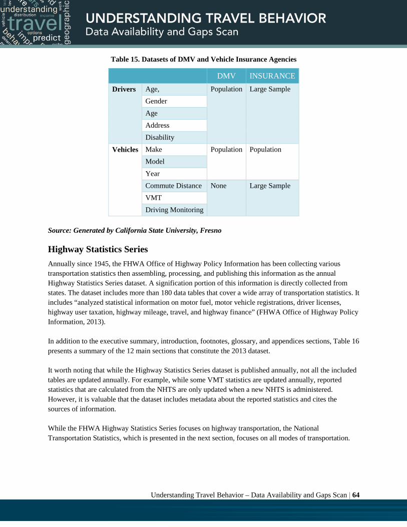
Understanding Travel Behavior – Data Availability and Gaps Scan | 64
Table 15. Datasets of DMV and Vehicle Insurance Agencies
DMV INSURANCE Drivers Age, Population Large Sample
Gender Age
Address Disability
Vehicles Make Population Population Model
Year Commute Distance None Large Sample VMT Driving Monitoring
Source: Generated by California State University, Fresno
Highway Statistics Series Annually since 1945, the FHWA Office of Highway Policy Information has been collecting various transportation statistics then assembling, processing, and publishing this information as the annual Highway Statistics Series dataset. A signification portion of this information is directly collected from states. The dataset includes more than 180 data tables that cover a wide array of transportation statistics. It includes “analyzed statistical information on motor fuel, motor vehicle registrations, driver licenses, highway user taxation, highway mileage, travel, and highway finance” (FHWA Office of Highway Policy Information, 2013). In addition to the executive summary, introduction, footnotes, glossary, and appendices sections, Table 16 presents a summary of the 12 main sections that constitute the 2013 dataset. It worth noting that while the Highway Statistics Series dataset is published annually, not all the included tables are updated annually. For example, while some VMT statistics are updated annually, reported statistics that are calculated from the NHTS are only updated when a new NHTS is administered. However, it is valuable that the dataset includes metadata about the reported statistics and cites the sources of information. While the FHWA Highway Statistics Series focuses on highway transportation, the National Transportation Statistics, which is presented in the next section, focuses on all modes of transportation.

Understanding Travel Behavior – Data Availability and Gaps Scan | 65
Table 16. Summary of Data Included in the 2013 Highway Statistics Series Data
# AREA EXAMPLES OF TYPES OF DATA REPORTED
1 Bridges Wearing surfaces, years built, structural information, and ownership
2 Highway Infrastructure National and state tables, ownership, and trends, lengths
3 Highway Travel VMT by functional system and federal aid
4 Travelers (or System Users) Licensed drivers by state, gender and age, and registered vehicles
5 Vehicles DMV registrations, and publicly owned vehicles, bus, and truck and tractor registrations
6 Motor Fuel Motor fuel usage, and tax rates on motor fuels, lubricating oils, and motor vehicles
7 Revenue National, state and local revenues from fuels, taxes, and mass transit
8 Debt Obligation for Highways Annual bond financing for highways and mass transit
9 Apportionments, Obligations, and Expenditures
Obligation, expenditure and disbursements by functional classes
10 Conditions and Safety Fatalities and highway conditions by functional class
11 Performance Indicators Trends of travel density, volumes and pavement conditions
12 International and Metric Data about other countries for comparison Source: Generated by California State University, Fresno from (FHWA Office of Highway Policy Information, 2013)
National Transportation Statistics The National Transportation Statistics is a dataset that is compiled and published quarterly by the USDOT’s Bureau of Transportation Statistics. It “presents statistics on the U.S. transportation system, including its physical components, safety record, economic performance, the human and natural environment, and national security” (FHWA Bureau of Transportation Statistics, 2015). The latest dataset includes more than 260 data tables. In addition, the dataset includes information about the source and estimated accuracy of the reported statistics. Similar to the case with the Highway Statistics Series, while the National Transportation Statistics dataset is updated quarterly, not all included tables are updated with the same frequency. In July 2015, less than 40 tables were updated. This is because the data sources of reported statistics are not updated with the same frequency; for example, the NHTS is updated only once every five to seven years, on average. The National Transportation Statistics dataset is divided into four main sections. Table 17 provides a summary of the data included in each of these sections.

Understanding Travel Behavior – Data Availability and Gaps Scan | 66
Table 17. Summary of Data Included in the July 2015 National Transportation Statistics
# AREA EXAMPLES OF TYPES OF DATA REPORTED
1 Transportation system
Physical extent, vehicle inventory, condition, travel and goods movements, and performance, such as delays of the transportation network
2 Safety record Accidents, crashes, fatalities, injuries and hazardous material incidents by air, highway, transit, railroad, water, and pipelines
3 Economic performance
Transportation’s contribution to the gross domestic product; transportation-related consumer and government expenditures; transportation revenues, employment, and productivity; and federal, state, and local government finance
4 Energy and the Environment
U.S. and transportation energy profiles; transportation energy consumption by mode; transportation energy intensity and fuel efficiency; air pollution; and water pollution, noise, and solid waste
Source: Generated by California State University, Fresno from (FHWA Bureau of Transportation Statistics, 2015)
AHS The American Housing Survey is “sponsored by the Department of Housing and Urban Development (HUD) and conducted by the U.S. Census Bureau” (U.S. Census Bureau and US Department of Housing and Urban Development). It has been conducted annually from 1973 to 1981, and biennially in odd years thereafter. While, before 1981, it was named as the Annual Housing Survey, since 1981, it has been named as the American Housing Survey (AHS). The AHS is divided into two main surveys, a national survey and a metropolitan survey. Sample selection represents the difference between the two surveys. While the national survey sample is randomly selected from the national population of housing units, the metropolitan survey sample is selected from housing units in only metropolitan areas. The AHS collects information from both occupied as well as vacant housing units. In 1997, the AHS transformed from being a paper-based questionnaire, into a computer assisted personal interviewing (CAPI) survey using laptop computers. In 1973, the AHS surveyed more than 60,000 housing units. The latest survey, conducted in 2013, surveyed 84,400 housing units. The AHS collects a variety information pertaining to housing, demographics, and socioeconomic characteristics. The survey is composed of a permanent core questionnaire, and rotating topical supplement surveys. The core questionnaire collects information about “size and composition of the nation’s housing inventory, vacancies, fuel usage, physical condition of housing units, characteristics of occupants, equipment breakdowns, home improvements, mortgages and other housing costs, persons eligible for and beneficiaries of assisted housing, home values, and characteristics of recent movers.” The topical supplement questionnaires covers topics such as “public transportation, emergency and disaster preparedness, community involvement, neighborhood characteristics, doubled-up households (movers entering and leaving unit), health and safety hazards, modifications made to assist occupants with

Understanding Travel Behavior – Data Availability and Gaps Scan | 67
disabilities, and energy efficiency” (U.S. Census Bureau and US Department of Housing and Urban Development). The AHS collects varying information relevant to travel behavior. However, this information is collected intermittently, because it is typically included in a few different topical supplement questionnaires. While the journey to work (JTW) and telecommuting questions were part of the core questionnaire, they were removed in 2011. In 2013, the latest AHS, two of the four supplement questionnaires included travel behavior relevant information. These are public transportation, and neighborhood characteristics and doubled-up households. The other two supplement questionnaires were disaster planning and community involvement. Figure 31 presents a Transportation Alternatives Infographic published by the U.S. Census Bureau and U.S. Department of Housing and Urban Development in 2013. It depicts transportation mode choices, costs, and accessibility statistics in several regions in the United States. The AHS is a panel survey. The same housing units are surveyed every time the survey is conducted. While this is a particularly unique and valuable feature about the AHS, it does not mean that it is a panel survey of households because households often move.

Understanding Travel Behavior – Data Availability and Gaps Scan | 68
Figure 31. AHS Transportation Alternatives Infographic Depicting Transportation Mode Choices, Costs, and Accessibility Statistics in Several Regions in the United States
Source: (U.S. Census Bureau and US Department of Housing and Urban Development)

Understanding Travel Behavior – Data Availability and Gaps Scan | 69
Social Network Data Today, the majority of the U.S. adult population owns and uses smartphones. A large number of smart applications (e.g., Foursquare, Twitter, Yelp, Flickr, Gowalla, and Brightkite, among many others) collect and log frequent GPS-based location information from the smartphone devices. In the literature, this is described as location-based social network (LBSN) data. After stripping any personal identifying information, this information is made publicly available. Table 18 presents a sample of a typical Gowalla log (Cho, Myers, & Leskovec, 2011), which shows the smartphone ID, date and time of the logged instance, location of the user (latitude and longitude coordinates), and ID of the venue associated with this instant (e.g., a specific restaurant). Every record in the data, called check-in, represents a specific instance where the date, time, and location of a specific user is known.
Table 18. Gowalla Location Based Social Network Data
Source: Generated by California State University, Fresno (from (Cho et al., 2011) Two main factors contribute to the differences between data logs from different smartphone apps: user volumes and check-in frequencies. While some applications are popular and are installed on and frequently used by a large number of users, others are not as popular and are used by less users and less frequently (user volume). On the other hand, while being used, some apps collect check-in information with a much higher frequency than others (frequencies). For example, users use FourSquare to identify interesting events and attractions within their vicinity. Hence, while on, FourSquare continuously collects and logs check-in information, in order to provide users with such information. On the other hand, users use Flickr to share geo-tagged photos (photos associated with specific geographic attractions). Hence, Flickr check-in frequency is limited to the frequency of geo-tagged photos shared by users. Compared to FourSquare, this typically happens in a much lower frequency. As a result, FourSquare’s LBSN data is much bigger and richer with information about human movement. Today, FourSquare’s data is one of the largest. LBSN data can be utilized to identify the exact location and track movements of individuals. Figure 32a depicts the check-in information of five smartphone devices in California’s San Francisco-Oakland Metropolitan Area, and Figure 32b depicts the check-in information of the same five devices across the

Understanding Travel Behavior – Data Availability and Gaps Scan | 70
continental United States. The two figures demonstrate the possibility of using LBSN data to track individual movements and identify travel patterns at local, regional, national, and international scales.
Figure 32a: Gowalla Location Based Social Network Data in the San Francisco-Oakland Metropolitan Area of Five Individuals

Understanding Travel Behavior – Data Availability and Gaps Scan | 71
Figure 32b. Gowalla Location Based Social Networking Data in the Conterminous U.S. of Five Individuals
Figure 32. Gowalla Location Based Social Networking Data of Five Individuals
Source: Maps Generated by California State University, Fresno (from (Cho et al., 2011) LBSN data presents a rich, novel, and unique resource for understanding and modeling of travel behavior. Research efforts exploring the potential uses and benefits of using this data are consistently rising. Examples of such efforts include (Jin et al., 2014) and (Yang, Jin, Cheng, Zhang, & Ran, 2015), who demonstrate the potential of using the data for estimating OD demand matrices. (Noulas, 2013) demonstrates the possibility of using the data to forecast an individual’s next destination. (Zheng, Xie, & Yang, 2012) demonstrate the potential of using LBSN data to infer popular driver route choices.
Omnibus Surveys “An omnibus survey is a method of quantitative marketing research where data on a wide variety of subjects is collected during the same interview. Also called piggyback survey. Multiple clients share the cost of conducting the research during an omnibus survey. Subscribers usually receive the portion of the information that is collected specifically for them. [It is a] survey which covers a number of topics, usually for different clients.” (Analytics). In other words, for a specific cost, any researcher or agency can add questions onto an existing survey. These types of surveys represent a potentially valuable method that could be relatively beneficial and inexpensive in collecting on-demand travel and travel-related data.

Understanding Travel Behavior – Data Availability and Gaps Scan | 72
Bureau of Transportation Statistics Omnibus Surveys
A “convenient way to get very quick input on transportation issues; to see who uses what, how they use it, and how users view it, and what they think about it; and to gauge public satisfaction with the transportation system and government programs” (USDOT Bureau of Transportation Statistics), the USDOT Bureau of Transportation Statistics (BTS) had been conducting two main types of omnibus surveys between 2000 and 2009:
a. A regular household survey of 1,000 households: monthly between August 2000 and December 2002, bimonthly until October 2003, and one in 2009. In general, the survey questions collected information about general travel experiences, satisfaction with the system, and some demographic information. The questions were divided into three main groups: 1. Core questions covering critical information needs for the USDOT. 2. Supplemental questions corresponding to one of the five USDOT’s strategic goals:
safety, mobility, economic growth, human and natural environment, and security. 3. Specific questions posed by the various USDOT modes; varying from month to month.
b. Targeted surveys that address special transportation issues. Examples of these survey topics included: Highway Use Survey (2000), Mariner Survey (2001 and 2002), National Survey of Pedestrian and Bicyclist Attitudes and Behaviors (2002), National Transportation Availability and Use Survey (2002), and Survey on FAA-Sponsored Safety Seminars (2003).
Topics and questions on these surveys varied according to the need of the requesting office or agency. In addition to BTS’s omnibus surveys, data about travel and travel-related information are typically collected in many omnibus surveys conducted by varying other agencies. Many of these surveys and collected data are publicly available and could serve as an additional valuable resource for understanding and modeling of travel behavior in the United States.
Pew Research Center Omnibus Surveys and Data Repository
The Pew Research Center (Pew Research Center) serves as a nonpartisan fact tank. It has been conducting public opinion polling, demographic research, content analysis, and other data-driven social science research since 2001. It also hosts a large number of datasets from a wide variety of sources, spanning over national, regional, state, local, and private surveys and associated data. While the Pew Research Center’s website classifies the hosted surveys and associated datasets into 224 topics, none of the topics are related to transportation or travel. Nonetheless, several of the datasets contain transportation and transportation-related questions. The website aggregates these 224 topics into 7 main areas. Particularly, two of these areas incorporate surveys that seem potentially relevant for understanding travel behavior and travel behavior trends. Following is a list of the seven areas and examples of travel-related surveys within the third and seventh areas.
1. U.S. Politics & Policy 2. Journalism & Media

Understanding Travel Behavior – Data Availability and Gaps Scan | 73
3. Internet, Science & Tech. Examples of relevant transportation-related surveys include: a. Mobile Health (2012 Health, 2010 Health Tracking, 2008 Health, among others). These
surveys could be potentially beneficial for understanding trends in remote health services which could explain changes to health related travel.
b. Cell phone ownership, usage and attitudes (2010 Cell Phone, 2009 Teens and Mobile Phones, 2006 Cellphone, among others). These surveys could be potentially beneficial for understanding trends in smartphone usage and impacts of travel apps on travel behavior.
4. Religion & Public Life 5. Hispanic Trends 6. Global Attitudes & Trends 7. Social & Demographic Trends. Examples of relevant transportation-related surveys include:
a. Education (2013 Higher Education, Gender and Work, 2011 Youth and Economy, 2011 Higher Ed/Housing, among others). These surveys could be potentially beneficial for understanding education and distant learning trends which could explain changes to education related travel.
b. Work (2006 Work, 2006 Optimism and Cars, 2009 Mobility/HH location choice, among others). These surveys could be potentially beneficial for understanding trends in work and telecommuting which could explain changes to work related travel.
The 2006 Optimism and Cars survey is perhaps the most transportation-relevant survey in the Pew Research Centers’ repository. It is composed of a national sample of more than 2000 adults who were interviewed in June and July of 2006. The participants were asked more than 50 questions covering several topics such as gender, education, work, and life achievement and satisfaction. However, a large set of questions primarily focused on car ownership and travel, driving habits and personal and public attitudes towards cars in general. Figure 33 depicts the results of this survey’s question of “why respondents considered driving a chore.”

Understanding Travel Behavior – Data Availability and Gaps Scan | 74
Figure 9. Driving Attitudes from Pew Research Center’s 2006 Work/Optimism/Cars Omnibus Survey.
Source: (Taylor, Funk, & Craighill, 2006)
University of Michigan’s ICPSR Omnibus Surveys
The University of Michigan’s Inter-university Consortium for Political and Social Research (ICPSR) was established, established in 1962, serves as a research data-sharing service for the social and behavioral sciences. It hosts more than 8,000 discrete studies/surveys and more than 65,000 datasets, covering various topics and from varying sources that include national, regional, state, local, and private surveys and associated datasets (ICPSR). Each dataset is accompanied with valuable resources that include metadata, codebooks, data-related biography, and other data tools. The website provides users with a variety of search tools. Users can search for datasets by topic, series, geography, investigator, thematic collection, or keywords. Table 19 presents sample search results by using five different travel-related keywords.

Understanding Travel Behavior – Data Availability and Gaps Scan | 75
Table 19. ICPSR Sample Search Results for Travel and Transportation Related Datasets
# KEYWORD NUMBER OF
RESULTS
SAMPLE OF RELEVANT DATASETS
1 Travel 978 Travel surveys, time use surveys, and others
2 Transportation 1741 Transportation surveys, public transportation and biotechnology, cost of providing transportation and care to elderly, and others
3 Driving 1102 Drinking and driving, and others
4 Telecommute 12 NHTS, National Study of Business Strategy and Workforce Development, and Work and Family Life Study, and others
5 Food Deserts 196 New York Times Nutrition Survey, U.S. Agriculture Data, and others
Source: Generated by California State University, Fresno from (ICPSR)
Other Omnibus Survey Sources
While Pew Research Center and ICPSR are probably the largest publicly available repositories, several other data repositories exist. Examples of these repositories include the following:
1. Gallup: Founded in 1935, Gallup is possibly one of the oldest and most famous surviving institutions conducting omnibus surveys. However, being a private institution, the datasets are not publicly available.
2. Roper Center for Public Opinion Research: It was founded in 1947, and today, holds over 22,000 datasets.
3. CISER Cornell Institute for Social and Economic Research: It is free for Cornell University affiliates, and holds about 27,000 online files.
USPS Mail Survey Exploring and understanding changes in mail service can be particularly beneficial for understanding recent changes and shifts in travel behavior trends. Activities such as online shopping and telecommuting, which may be possible to capture via changes in mail service activity, could have significant impacts on travel activity patterns and associated changes in VMT, emissions, energy demand, and congestion. As part of a multi-year research study, USPS has been conducting an annual Household Diary Study (HDS) since 1987 (Mazzone, 2013). Every year USPS surveys 5,200 households, with the following objectives:
1. Measuring mail activity (sent and received) 2. Tracking household mail trends and attitudes 3. Comparing different household types.

Understanding Travel Behavior – Data Availability and Gaps Scan | 76
The HDS is composed of two parts: 1. The Household Recruitment Interview is composed of about 100 questions collecting information
about demographic and socioeconomic information, and mail and internet usage information. 2. The 1-Week Mail Diary collects daily information about sent and received mail.
This dataset could be particularly beneficial in understanding mail trends and impacts of the communication advancements and online shopping or mailing habits, trends, and volumes on the associated mail trips conducted by both households and mail fleet. Table 20 presents a sample of relevant interesting mail statistics and information. It shows that while total mail volume in the United States has decreased by 2.4% between 2001 and 2012, the delivery points increased by 0.9%. The reason for this increase may be attributed to the growing population and resulting increase in number of housing units. While USPS Household Diary Study provides annual reports with updated tables, the actual data is not publicly available online.
Table 20. Mail Volume and Demographics Average Annual Growth 1981 – 2012
1981-1990 1991-2000 2001-2012
Total Mail Volume 4.6% 2.3% -2.4%
Delivery Points 1.7% 1.5% 0.9%
Adult Population 1.5% 1.3% 1.2%
Households 1.4% 0.9% 1.0% Source: (Mazzone, 2013), Table 2-1
ITS/RIITS The transportation sector has capitalized on the technological advancements in the computation and communications field, and applied many of these technologies to improve traffic operations in varying ways. Intelligent transportation systems (ITS) is a term refers to such applications. The Regional Integration of Intelligent Transportation Systems (RIITS) of the Los Angeles County Metropolitan Transportation Authority (Metro) represents a notable example of these technologies. RIITS collects real-time multi-modal information from seven different agencies:
1. Los Angeles County Metropolitan Transportation Authority (Metro) 2. California Department of Transportation (Caltrans) 3. City of Los Angeles Department of Transportation (LA DOT) 4. California Highway Patrol (CHP) 5. Long Beach Transit (LBT) 6. Foothill Transit (FHT).
The following four different types of information are collected and shared across the agencies (RIITS):

Understanding Travel Behavior – Data Availability and Gaps Scan | 77
1. Congestion data on highway travel speeds from loop detectors 2. Information projected on the highway changeable message signs (CMS) 3. Feeds from highway video cameras 4. Incidents and events information from CA Highway Patrol.
Figure 34 presents a screenshot showing the different data types collected between collaborating agencies. The system is also planned to integrate additional sources of information in the future. Examples of these data sources include social media data and transit data (e.g., locations of transit modes and ridership information). Impacts of such systems on future transportation planning are numerous. In the future, such systems can provide valuables data for understanding and measuring travel behavior. Examples of future application of these novel data sources include modal shares, OD estimation by time of day and by mode, and impacts of weather and congestion on travel activity and model choices.
Figure 34. Screenshot of Information Collected and Shared on RIITS
Source: Image Acquired from (Regional Integration of Intelligent Transportation Systems - RIITS)
The Research Data Exchange (RDE) The Research Data Exchange (RDE) is a transportation data sharing system that was specifically created to support the development, testing, and demonstration of developing transportation technologies, such as the ITS multi-modal Dynamic Mobility Applications (DMA) program, and other connected vehicle research activities (USDOT Federal Highway Administration). Examples of the data collected and hosted by RDE include: Archived and real-time data Data from multiple sources (e.g., vehicle probes, infrastructure, and weather)

Understanding Travel Behavior – Data Availability and Gaps Scan | 78
Data from multiple transportation modes (e.g., different motorized modes, as well active transportation users like pedestrians and bicyclists).
At the moment, the RDE hosts 13 datasets spanning from 2008 until the present time. These datasets include a wide variety of information. Examples of variables included in these datasets include the following: Mobility data (e.g., locations of vehicles and travelers, loop detector data, travel times, queues,
and others) Safety data (e.g., braking, lane changing, traffic incidents, and others) Communication (e.g., V2V and V2I messages) Environmental (e.g., weather and emissions).
While these datasets may not be relevant at this time, they could be particularly valuable for predicting future travel trends. For example, it could be beneficial to understand the propensity of the different population groups in mastering and adopting such technologies. Also, these datasets could be beneficial in forecasting other potential major changes in travel behavior. For instance, shared autonomous vehicles (SAVs) could potentially cause significant reductions in transit ridership, and as a result significantly impact local, regional, and national VMT trends.
SUMMARY
Given the recent advancements in travel survey methods and resultant travel datasets, which were enabled by the significant developments in the computational and communications technologies, this chapter provided a brief overview of many different niche and other potential travel behavior datasets. These datasets could potentially serve as novel tools to improve our understanding, modeling, and forecasting of the unprecedented travel trends recently observed in the United States. The chapter presented nine niche datasets: the HPMRS GPS-based dataset, AirSage cellphone trace dataset, the ATUS, the NTD, the NDS, and four smartphone travel apps (categorized as either gamification, ridesourcing, and alternative transportation). Additionally, the chapter presented 9 potential data sources: DMV and Insurance data, HSS, NTS, AHS, LBSN Data, omnibus surveys (FHWA, Pew Research Center, and ICPSR), the USPS HDS, the RIITS ITS data, and the RDE repository. A short description was provided for each of the data sources, as well as their potential major uses and limitations.
REFERENCES
AirSage. trip matrix by AirSage. Retrieved August 5, 2015, from http://airsage.com/Population-Analytics/Trip-Matrix/
Analytics, S. Retrieved August 5, 2015, from https://www.surveyanalytics.com/omnibus-survey-definition.html

Understanding Travel Behavior – Data Availability and Gaps Scan | 79
Cho, E., Myers, S. A., & Leskovec, J. (2011). Friendship and mobility: user movement in location-based social networks. Paper presented at the Proceedings of the 17th ACM SIGKDD international conference on Knowledge discovery and data mining, San Diego, California, U.S.
Federal Tansit Administration. National Transit Database. Retrieved Juy 10, 2015, from http://www.ntdprogram.gov/ntdprogram/ntd.htm
FHWA Bureau of Transportation Statistics. (2015). National Transportation Statistics. FHWA Office of Highway Policy Information. (2013). Highway Statistics Series. FHWA Office of Highway Policy Information. (2014). Highway Performance Monitoring
System: Field Manual. from https://www.fhwa.dot.gov/policyinformation/hpms/fieldmanual/HPMS_2014.pdf
FHWA Office of Operations. National Performance Management Research Data Set. Retrieved August 7, 2015, from http://www.ops.fhwa.dot.gov/freight/freight_analysis/perform_meas/vpds/npmrdsfaqs.htm
Gan, A., Ubaka, I., & Zhao, F. (2002). Integrated National Transit Database Analysis System. Transportation Research Record: Journal of the Transportation Research Board, 1799, 78-88. doi: doi:10.3141/1799-11
ICPSR. from https://www.icpsr.umich.edu/icpsrweb/landing.jsp InSight Data Access Website: SHRP 2 Naturalistic Driving Study. from
https://insight.shrp2nds.us/ Jin, P. J., Cebelak, M., Yang, F., Zhang, J., Walton, C. M., & Ran, B. (2014). Location-Based
Social Networking Data: Exploration into Use of Doubly Constrained Gravity Model for Origin–Destination Estimation. Transportation Research Record: Journal of the Transportation Research Board(2430), pp 72–82.
Mazzone, J. (2013). The Household Diary Study: Mail Use and Attitudes in FY 2012. Metropia. Retrieved August 5, 2015, from http://www.metropia.com/ Noulas, A. (2013). Human Urban Mobility in Location-based Social Networks: Analysis,
Models and Applications (Doctoral Dissertation). Pew Research Center. Retrieved July 23, 2015, from http://www.pewresearch.org/ Rayle, L., Shaheen, S. A., Chan, N. D., Dai, D., & Cervero, R. (2015). App-Based, On-Demand
Ride Services: Comparing Taxi and Ridesourcing Trips and User Characteristics in San Francisco. Paper presented at the Transportation Research Board Annual Meeting, Washington, DC.
Regional Integration of Intelligent Transportation Systems - RIITS. Retrieved August 11, 2015, from http://www.riits.net/
RideScout. Retrieved August 20, 2015, from http://www.ridescoutapp.com/ RIITS. RIITS Guidebook. Rousseau, G. Using HERE - NPMRDS Data for Model Development @ARC: Lessons Learned.
from https://connectdot.connectsolutions.com/p8ooks59xe2/ Stern, J. (2013). Google Buys Popular Social Mapping App Waze to Fight Traffic, ABC News.
Retrieved from http://abcnews.go.com/Technology/google-buys-popular-social-mapping-app-waze-fight/story?id=19373836
Understanding Travel Behavior – Data Availability and Gaps Scan | 80
Tawfik, A. M., Rakha, H. A., & Du, J. (2012). Modeling Driver Heterogeneity in Route Choice Behavior Based on a Real-Life Naturalistic Driving Experiment.
Taylor, P., Funk, C., & Craighill, P. (2006). Americans and Their Cars: Is the Romance on the Skids? : Pew Research Center.
U.S. Census Bureau and U.S. Department of Housing and Urban Development. American Housing Survey Retrieved August 8, 2015, from http://www.census.gov/programs-surveys/ahs.html
U.S. Bureau of Labor Statistics. (2015). 2015 American Time Use Survey User’s Guide: Understanding ATUS 2003 to 2014
USDOT Bureau of Transportation Statistics. Omnibus Surveys. Retrieved September 2, 1015, from http://www.rita.dot.gov/bts/sites/rita.dot.gov.bts/files/subject_areas/omnibus_surveys/index.html
USDOT Federal Highway Administration. Retrieved July 28, 2015, from https://www.its-rde.net/
Waze. Retrieved August 4, 2015, from https://www.waze.com/ Yang, F., Jin, P. J., Cheng, Y., Zhang, J., & Ran, B. (2015). Origin-Destination Estimation for
Non-Commuting Trips Using Location-Based Social Networking Data. International Journal of Sustainable Transportation, 9(8), 551-564. doi: 10.1080/15568318.2013.826312
Zheng, Y., Xie, X., & Yang, Q. (2012). Constructing popular routes from uncertain trajectories. Proc. ACM SIGKDD Int. Conf. Knowl. Discov. Data Min. Proceedings of the ACM SIGKDD International Conference on Knowledge Discovery and Data Mining, 195-203.

Understanding Travel Behavior – Data Availability and Gaps Scan | 81
CHAPTER 4.0. DATA CHARACTERIZATION FOR HIGH-PRIORITY INFORMATION NEEDS
INTRODUCTION
The companion report to this document, entitled Understanding Travel Behavior: Research Scan, referred to as Research Scan throughout this document, scanned travel behavior research and identified eight HPINs. Earlier chapters of this document presented overviews of many different data sources that are traditionally utilized for understanding travel behavior and travel behavior trends. Additionally, it presented overviews of many other niche and potentially useful datasets that may be beneficial in augmenting information of the traditional data sources and explaining recent unprecedented travel behavior trends. In total, 23 data sources were presented. This chapter intends to cross-examine these 23 datasets against the 8 HPINs identified in the Research Scan. The objective of the cross-examination revolves around identifying promising data sources – data sources that may be most promising in addressing data gaps of the HPINs. Once the promising data sources are identified, they will be further evaluated and ranked in the succeeding chapter, Chapter 5. Chapter 4 is divided into four sections. Section 1 is this Introduction. For the convenience of the reader, Section 2 presents a summary of the 8 HPINs identified in the Research Scan, as well as the 23 datasets presented in Chapter 2 and 3 of this report. Section 3 identifies the most promising data sources by cross-examining the 8 HPINs against all 23 datasets. Last, Section 4 presents a summary of the chapter. Figure 35 depicts the graphical flow of Chapter 4.

Understanding Travel Behavior – Data Availability and Gaps Scan | 82
Figure 35. Content Flow of Chapter 4
HIGH PRIORITY INFORMATION NEEDS AND DATA SOURCES
For the convenience of the reader, this section provides a summary of the 8 HPINs identified in the Research Scan and the 23 data sources presented in Chapters 2 and 3.
High Priority Information Needs The Research Scan document reviewed present day travel behavior and measurement in United States, and explored the changing impacts of socioeconomic and demographic factors, transformative technologies and systems, and emerging methodologies and data on present day travel and associated trends. The Research Scan concluded by identifying eight HPINs. Table 21 presents a summary of these eight HPINs.
Table 21. Identified High Priority Information Needs
# INFORMATION GAP / HPIN HPIN DATA GAP
1 Vehicle Miles Traveled (VMT): VMT is currently tracked through an estimation derived from HPMS reports and variations in counts from highway detectors. It misses activity on local roads and may have other measurement errors. It is measured frequently (monthly) through sensor counts, but its estimation procedure may be in accurate.
HPIN 1: VMT • Improve measurement • Better accuracy
2 Person Miles Traveled (PMT): PMT is currently measured mostly through surveys such as the NHTS and regional travel surveys. These surveys provide important insights into travel across modes. PMT measurements are snapshots of activity, and because of the large effort required to undertake such surveys, are infrequently done.
HPIN 2: PMT Frequency (PMT Freq) • More frequent intervals

Understanding Travel Behavior – Data Availability and Gaps Scan | 83
# INFORMATION GAP / HPIN HPIN DATA GAP
3 Mode Share (MS): Related to gaps in PMT, information on mode share is derived from regional travel surveys and the ACS journey to work data. The journey to work data provides the most frequent measurement change in mode share. Better understanding of overall changes in mode share is needed on more frequent time intervals and at better spatial resolution.
HPIN 3a: MS Frequency (MS Freq) • More frequent intervals HPIN 3b: MS Resolution (MS Res.) • Better spatial resolution
4 Telecommuting (Telecom): Telecommuting is a challenging mode to define and to measure. Yet, it is becoming an exceedingly important mode. Better measurement of the share of telecommuting (avoided commuting) is needed.
HPIN 4: Telecommuting (Telecom) • Better measurements
5 Trip Purpose (TP Char) Work v. Non-work: Similar to the gaps in PMT and mode share, trip purpose is an infrequently measured data point for travel. This data is currently supplied by surveys, and it is difficult to understand evolving distinctions between work and non-work travel, including distinctions in mode share, distance, time of day, discretionary nature, and other attributes on a timely basis. Better spatial and temporal information is needed.
HPIN 5: TP & Characteristics (TP Char) • Better understanding of travel
characteristics (e.g., mode share, distance)
• Better spatial resolution • More frequent intervals
6 Demographics as crossed with Travel Metrics (Tr. Demog.): The association of demographic distributions with data as related to other measurements of travel (e.g., mode split, VMT, PMT) is limited, and only supplied by NHTS and other regional travel surveys.
HPIN 6: Trip Demographics (Tr. Demog) • Association of demographic
distributions with travel data (e.g., mode split, VMT, PMT)
7 Attitudes & Public Perceptions (Tr. Demog): Attitudes towards mobility have shifted across generations, which impacts the choices made by travelers in different situations. There is limited information on how those attitudes change and limited abilities to forecast attitude changes.
HPIN 7: Public Attitudes (Tr. Demog) • Attitudes towards mobility
across generations • Effect of attitude changes
8 Vehicle Occupancy (Veh. Occ.): Vehicle occupancy is a difficult data point to obtain, yet would be critical for better HOV enforcement, and for better understanding the impacts of ridesharing services. Ways to identify real-time vehicle occupancy and measure historical vehicle occupancy would be very useful.
HPIN 8: Vehicle Occupancy (Veh. Occ.) • Identify real-time vehicle
occupancy • Measure historical vehicle
occupancy Source: Research Scan, Chapter 7
Data Sources As discussed in previous chapters, a diverse set of 23 transportation- and travel- related data sources were identified, reviewed, and briefly presented in Chapters 2 and 3 of this report. These data sources included

Understanding Travel Behavior – Data Availability and Gaps Scan | 84
traditional, niche, and other potentially useful datasets. Table 22 presents a summary of the 23 data sources presented in Chapters 2 and 3 of this report.
Table 22. Presented Data Sources. Source: Chapters 2 and 3 of this Report
# DATA BLANK # DATA
1 NHTS blank 13 RideScout 2 HPMS blank 14 DMV 3 ACS blank 15 Insurance
4 Local Surveys blank 16 HWY Stats 5 NPMRDS Blank 17 NTS 6 AirSage Blank 18 AHS 7 ATUS Blank 19 LBSN
8 NTD Blank 20 Omnibus 9 SHRP2 Blank 21 USPS 10 Waze Blank 22 ITS 11 Metropia Blank 23 RDE
12 Uber blank
PROMISING DATA SOURCES
While the objective of this work is to develop and apply a ranking scheme that would identify the most suitable data sources for addressing the 8 identified HPINs, the objective of this chapter is less elaborate. It involves reducing the 23 data sources into a smaller subset of the most promising ones. The next chapter, Chapter 5, develops and applies a ranking scheme to the most promising data sources that are identified in Chapter 4. In order to identify the promising data sources, a three-step qualitative assessment approach was employed to cross-examine all 23 data sources against the 8 identified HPINs. The first step collectively examined whether each of the data source includes information relevant to each of the HPINs. The second step employed a more detailed approach where data sources that were found to include sufficient information about an HPIN (from step one) were further characterized according to more specific criteria (such as data cost, reliability, and potential usefulness). The third and last step in this section integrated all results developed in the second step to identify and select the preliminary list of promising data sources. The selected data sources are further examined via a more rigorous approach and ranked in the next chapter.

Understanding Travel Behavior – Data Availability and Gaps Scan | 85
Step 1: Collective Characterization of the Data Sources Against the HPINs In this step, all data sources were characterized against all HPINs. For every data source–HPIN combination, data sources were characterized into the following four levels. Level 1, Existing Info: The data source includes readily available information about the HPIN
(e.g., the NHTS includes readily available information to calculate VMT and PMT). Level 2, Potential Info: The data source includes information that may be partially (hence,
potentially) relevant to the HPIN; especially if integrated with information from other data sources (e.g., the HPMS may provide partial information relevant to PMT; especially if integrated with information about utilization of transit and active transportation modes).
Level 3, Future Info: The data source may in the future include information relevant to the HPIN (e.g., as part of HOV/HOT lane enforcement, future vehicles may be providing information about vehicle occupancy).
Level 4, Insufficient Info: The data source does not include information sufficiently relevant to the HPIN (e.g., the HPMS does not include information sufficiently relevant to telecommuting).
Table 23 presents the results of this step. As can be seen in Table 23, for the second HPIN, 16 of the 23 data sources were found to include some level of information relevant to PMT estimation. These 16 data sources (as well as all other data sources relevant for the other HPINS) are further examined in step two.
Step 2: Further Characterization of the Data Sources Against the HPINs In this step, for each HPIN, data sources that were found to include existing, potential, or future info were further characterized according to eight specific factors. The data sources were qualitatively characterized into three levels according to each of the following eight factors.
1. Covers (HPIN) Need: The degree to which the data source includes information relevant to the HPIN (high, partial, low).
2. Data Availability: The degree to which the relevant information is readily and publicly available (high, partial, low).
3. Data Reliability: The level of data reliability (high, partial, low). 4. Potential Usefulness: The degree to which the data is expected to be useful in addressing the
HPIN (high, partial, low). 5. Data Cost: The relative cost of the data (high, moderate, low). The relative cost reflects a
combination of the cost to the FHWA (e.g., NHTS is highly expensive, ACS is free, and AirSage is for purchase), and cost of data collection (e.g., household surveys are expensive, and GPS-based data is much cheaper).
6. National Trends: Whether the data source can explain national trends (high, partial, low). 7. Demographic, Socioeconomic, and Geographic Trends (D, SE &G): Whether the data source
captures demographic, socioeconomic, and geographic factors (high, partial, low). 8. Niche Mode and Behavior: Whether the data source captures niche travel or mode choice
behavior (high, partial, low).

Understanding Travel Behavior – Data Availability and Gaps Scan | 86
Tables 24a through 24h present the characterization results of the data sources against each of the respective HPINs. To acquaint the reader with the reasons behind the assigned characterization for every data source-factor combination, Table 24a-ii provides expanded explanations for reasons associated with the values assigned in Table 24a-i. The rightmost two columns in Tables 24a thru 24h represent a score and a ranking column – for every data source. The score column is based on a simple summation for the characterization values received by the data source. Except for data cost, all high values were accounted a score of three points, Moderate/partial values as 1 point, and low as 0. For data cost, on the other hand, high values were accounted a score of 0 points, moderate/partial values as 1 and low as 3. Hence, higher score values represent data sources that are more suitable for addressing their respective HPIN. Since there are 8 factors, if a data source was to receive a favorable grade (3 points) in all factors, it would receive a maximum score of 24. The ranking column represents a descending order of the data source scores (i.e., a lower rank represents a more suitable data source).
Step 3: Identifying the Most Promising Data Sources In order to identify the most promising data sources, all rankings of all data sources in Tables 24a thru 24h were integrated into a single table, Table 25. The two rightmost columns in Table 25 are sum, which is a summation of all rankings received by a data source, and collective ranking. Data sources that do not include insufficient info relevant to a specific HPIN received the lowest possible ranking, 23. Since a lower ranking represents a more suitable data source, a lower sum represents a data source that is more suitable for addressing all HPINs simultaneously. Accordingly, the collective ranking column represents an ascending order of the data source summation of rankings (i.e., the lowest sum and a lowest ranking represent the most suitable data source). Figure 36 provides a graphical depiction of the collective sum of ranking scores of all data sources – presented in Table 25. The results in Figure 36 (and Table 25) indicate that the six most promising data sources include the ATUS, ACS, omnibus surveys, local surveys, NHTS, and AHS. In addition to AirSage, these six data sources were selected to be further analyzed in a more rigorous process in Chapter 5. AirSage was added to the selection due to having a top-three rank for addressing VMT frequency and for being a novel proprietary data source that is currently commercially available, and which collects and provides continuous information that is not captured by any of the other sources. It is intriguing that these seven data sources ended up spanning all three groups of data sources presented in Chapters 2 and 3, traditional, niche, and potentially beneficial. While ACS, NHTS, and local surveys belong to the traditionally used data sources (in Chapter 2), omnibus surveys and AirSage belong to the niche data sources (presented in Chapter 3), and ATUS and AHS were presented (also, in Chapter 3) as potentially useful. It is worth noting that while the adopted methodology in this chapter is not rigorous, it is believed to be sufficient for identifying the most promising data sources. Chapter 5 presents the development and

Understanding Travel Behavior – Data Availability and Gaps Scan | 87
adoption of a more rigorous approach, which is then utilized to rank the promising data sources identified here.
SUMMARY
This chapter intended to cross-examine and characterize all 23 traditional, niche, and potentially useful data sources presented in Chapters 2 and 3 against the HPINs identified in the Research Scan. For convenience of the reader, the chapter started by presenting lists of the HPINs identified in the Research Scan and the 23 data sources presented in Chapter 2 and 3. However, the core objective of this chapter was achieved via a simple three-step qualitative method, adopted to identify the most promising data sources. In the first step, information captured by each of data sources was collectively characterized against each of the HPINs. Data sources that did not include sufficient information for a specific HPIN were not included in the second step. The second step presented a more detailed approach where information of each of the data sources were characterized according to eight specific factors (covers HPIN need; data availability; data reliability; potential usefulness; data cost; national trends; geographic, socioeconomic and demographic factors; and niche mode choice and travel behavior). Results of this characterization allowed for general ranking of the data sources with respect to each HPIN. By combining all rankings developed in the second step, the third and last step established a general collective ranking for all data sources. By exploring the outcome of the general ranking established in the last step, seven data sources were identified to be most promising. These data sources include the top six ranking ones and AirSage. The seven identified data sources are ATUS, ACS, omnibus surveys, local surveys, NHTS, AHS, and AirSage. It is intriguing that these seven data sources belong to the three groups of data presented in Chapters 2 and 3: traditional, niche, and potentially useful data sources. These seven data sources are further examined and ranked in Chapter 5, which presents the development and implementation of a more rigorous rating and ranking scheme.

Table 23. Step 1 – Collective Classification of Data Sources against HPINs.
# INFORMATION
1
NH TS
2
HP MS
3 ACS
4 LO-CAL
5 NPMRDS
6
AIR
SAGE
7
AT US
8
NTD
9 SH RP2
10
WA ZE
11
METROP
12
UB ER
13
RIDESC OUT
14
DMV
15
INS UR.
16
HW
STAT
17
NTS
18
AHS
19
LB SN
20
OMNIB US
21
US PS
22
ITS
23
RDE
1 VMT 2 PMT 3 Mode Share 4 Telecommuting 5 Trip Purpose
(work/non-work)
6 Demographics against Tr Metrics
7 Attitudes &
Public Perceptions
8 Vehicle Occupancy
Key: Existing Info, Potential Info, Future Info, Blank Insufficient Info
Understanding Travel Behavior – Data Availability and Gaps Scan | 88

Understanding Travel Behavior – Data Availability and Gaps Scan | 89
Table 24a.i. Step 2 – Further Characterization of Data Sources against VMT
# Data
Source Covers Need?
Data Availab.
Data Reliab.
Potent. Usefuln
Data Cost
Natnl Trends
D, SE & G
Mode & Nich
Beh Score (Max 24) Rank
1 NHTS ∼ (snapshot)
H ∼ (some) 17 1 2 HPMS ∼ (some) ∼ (models) M ∼ (geogr) × 13 6 3 ACS ∼ (comute) ∼ (models) L × 17 1 4 Local ∼ (local) ∼ (some) ∼
(snapshot) M ∼
(model) ∼ (some) 12 7
5 NPMRDS ∼ (estimate) ∼ (models) ∼ (models) M ∼ (model)
× × 8 19 6 AirSage ∼ (estimate) ∼ (purchs) ∼ (models) M ∼ (fusion) × 11 12 7 ATUS ∼ (time) ∼ (model) L × 17 1 8 NTD ∼ (indicat) ∼ (aggreg) ∼ (fusion) M ∼
(model) × × 8 19 9 SHRP2 ∼ (local) ∼
(snapshot) H ∼
(model) × 12 7
10 Waze ∼ (estimate) × ∼ (model) ~M ∼ (model)
∼ (selfselc)
∼ (beh) 9 15 11 Metropia ∼ (est/local) × ∼ (fusion) ~M × ∼
(selfselc) ∼ (beh) 8 19
12 Uber ∼ (indicat) × ∼ (models) ∼ (fusion) ~M ∼ (model)
∼ (selfselc)
9 15 13 RideScout ∼ (indicat) × ∼ (indicat) ∼ (fusion) ~M ∼
(model) ∼ (selfselc) ∼ (some) 7 22
14 DMV ∼ (future) × ∼ (lapse) M ∼ (some) × 10 14 15 Insurance ∼ (selfselc) × ∼ (volunt) M × 12 7 16 HWS Srs ∼ (HPMS) ∼ (aggreg) ∼ (models) ×
(HPMS) L × × 9 15
17 NTS ∼ (HWS Srs) ∼ (aggreg) ∼ (models) ×
(HPMS) L × × 9 15
18 AHS ∼ (snapshot) ∼ (models) ∼ (fusion) M ∼ (model)
× 11 12 19 LBSN ∼ (estimate) ∼ (models) L ∼ (fusion) × 15 4 20 Omnibus ∼ (future) × M ∼ (some) 15 4 21 USPS ∼ (estimate) ∼ (aggreg) ∼ (self) ∼ (fusion) M ∼
(model) ∼ (model) × 7 22 22 ITS ∼ (future) ∼ (future) ∼ (fusion) M ∼ (some) ∼ (some) 12 7 23 RDE ∼ (future) ∼ (future) ∼ (fusion) M ∼ (some) ∼ (some) 12 7
Key: /H High, ∼/M Partial/Moderate, ×/L Low

Table 24a-ii. Step 2 – Expanded Explanations of Further Characterization of Data Sources against VMT
# Data Source
Covers Need?
Data Availab.
Data Reliab.
Potent. Usefuln
Data Cost
Natnl Trends
D, SE & G
Mode & Nich Beh
Score (Max 24)
Rank
1 NHTS ∼ (snapshot): the data
represents an infrequent snapshot in
time
H ∼ (some): the data includes some but not all of niche modes and behaviors
17 1
2 HPMS ∼ (some): data estimates of VMT (especially on
local streets) are not based on timely data
collection
∼ (models): VMT
estimates are based on complex models
M ∼ (geogr): data includes only
geographic factors
× 13 6
3 ACS ∼ (comute): data includes only
commuting VMT
∼ (models): data requires
models to estimate total VMT (from
commute VMT)
L × 17 1
4 Local ∼ (local): data primarily includes only local
VMT
∼ (some): data not readily
available from all local
jurisdictions
∼ (snapshot): datasets
represent snapshots in
time
M ∼ (model): model
required to estimate national trends
∼ (some): the data includes some but not all of niche modes and behaviors
12 7
5 NPMRDS ∼ (estimate): data includes speeds which
may be used to calculate estimates of volumes
∼ (models): models are required to
estimate VMT
∼ (models): models are required to
estimate VMT
M ∼ (model): model
required to estimate national trends
× × 8 19
Understanding Travel Behavior – Data Availability and Gaps Scan | 90

# Data Source
Covers Need?
Data Availab.
Data Reliab.
Potent. Usefuln
Data Cost
Natnl Trends
D, SE & G
Mode & Nich Beh
Score (Max 24)
Rank
6 AirSage ∼ (estimate): data may be used to calculate estimates of PMT,
which can then be used to estimate VMT
∼ (purchs): data is
proprietary and only provides
summary tables
∼ (models): models are required to
estimate VMT
M ∼ (fusion): data captures geographic
trends, but demographic and socioeconomic
information can be fused.
× 11 12
7 ATUS ∼ (time): data provides only stated travel times,
which can be used to estimate travel distances
∼ (models): models are required to
estimate VMT
L × 17 1
8 NTD ∼ (indicat): data may be used to indicate
increase/decrease in transit travel, which may
indicate increase/decrease in
VMT
∼ (aggreg): data includes
only aggregate
measures of transit use
∼ (fusion): data may be beneficial if fused with other data sources
M ∼ (model): model
required to estimate national trends
× × 8 19
9 SHRP2 ∼ (local): data limited to some local areas
∼ (snapsht): data represents
only a snapshot in
time
H ∼ (model): model
required to estimate national trends
× 12 7
10 Waze ∼ (estimate): data may be able to provide
insights about route choices and associated
increase/decrease in VMT
× ∼ (models): models are required to
estimate VMT
~M ∼ (model): model
required to estimate national trends
∼ (selfselc): data potentially suffers from self-selection
bias
∼ (beh): data may provide
insights about niche
behavior
9 15
Understanding Travel Behavior – Data Availability and Gaps Scan | 91

# Data Source
Covers Need?
Data Availab.
Data Reliab.
Potent. Usefuln
Data Cost
Natnl Trends
D, SE & G
Mode & Nich Beh
Score (Max 24)
Rank
11 Metropia ∼ (est/local): data limited to some local
areas but may be able to provide insights about
flexibility of route choice and associated
changes in VMT
× ∼ (fusion): data may be beneficial if fused with other data sources
~M × ∼ (selfselc): data potentially suffers from self-selection
bias
∼ (beh): data may provide
insights about niche
behavior
8 19
12 Uber ∼ (indicat): data may be used to indicate increase
in auto travel and associated increase in
VMT
× ∼ (models): models are required to
estimate VMT
∼ (fusion): data may be beneficial if fused with other data sources
~M ∼ (model): model
required to estimate national trends
∼ (selfselc): data potentially suffers from self-selection
bias
9 15
13 RideScout ∼ (indicat): data may be used to indicate
increase/decrease in alternative
transportation, which may indicate
increase/decrease in VMT
× ∼ (indicat): data provides
only a potential indication
∼ (fusion): data may be beneficial if fused with other data sources
~M ∼ (model): model
required to estimate national trends
∼ (selfselc): data potentially suffers from self-selection
bias
∼ (beh): data may provide
insights about some niche mode
and behavior
7 22
14 DMV ∼ (future): data may be able to cover need if collected in future
× ∼ (lapse): reported and calculated
VMT would reflect past
VMT
M ∼ (some): includes geographic, and
some demographic and SE factors
× 10 14
15 Insurance ∼ (selfselc): data potentially suffers from
self-selection bias
× ∼ (volunt): data mostly
based on stated
volunteer values
M × 12 7
Understanding Travel Behavior – Data Availability and Gaps Scan | 92
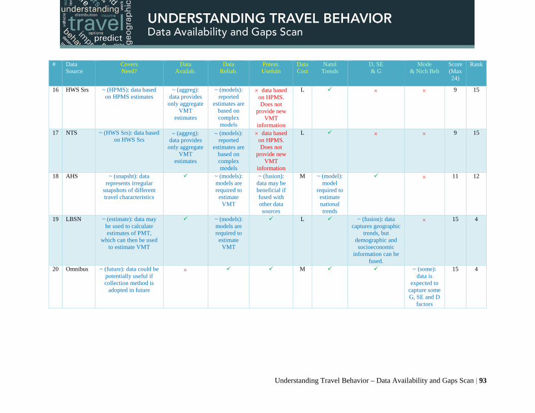
# Data Source
Covers Need?
Data Availab.
Data Reliab.
Potent. Usefuln
Data Cost
Natnl Trends
D, SE & G
Mode & Nich Beh
Score (Max 24)
Rank
16 HWS Srs ~ (HPMS): data based on HPMS estimates
~ (aggreg): data provides
only aggregate VMT
estimates
~ (models): reported
estimates are based on complex models
× data based on HPMS. Does not
provide new VMT
information
L × × 9 15
17 NTS ~ (HWS Srs): data based on HWS Srs
∼ (aggreg): data provides
only aggregate VMT
estimates
∼ (models): reported
estimates are based on complex models
× data based on HPMS. Does not
provide new VMT
information
L × × 9 15
18 AHS ~ (snapsht): data represents irregular
snapshots of different travel characteristics
~ (models): models are required to
estimate VMT
~ (fusion): data may be beneficial if fused with other data sources
M ~ (model): model
required to estimate national trends
× 11 12
19 LBSN ~ (estimate): data may be used to calculate estimates of PMT,
which can then be used to estimate VMT
~ (models): models are required to
estimate VMT
L ~ (fusion): data captures geographic
trends, but demographic and socioeconomic
information can be fused.
× 15 4
20 Omnibus ~ (future): data could be potentially useful if collection method is
adopted in future
× M ~ (some): data is
expected to capture some G, SE and D
factors
15 4
Understanding Travel Behavior – Data Availability and Gaps Scan | 93

# Data Source
Covers Need?
Data Availab.
Data Reliab.
Potent. Usefuln
Data Cost
Natnl Trends
D, SE & G
Mode & Nich Beh
Score (Max 24)
Rank
21 USPS ~ (estimate): data can be used to estimate
increase/decrease of mail trips and their
impact on human travel
~ (aggreg): data includes
only aggregate summaries
~ (self): data based on stated self reporting
~ (fusion): data may be beneficial if fused with other data sources
M ~ (model): model
required to estimate national trends
~ (model): data includes only
aggregate summaries.
Requires models to estimate D, SE & G
factors
× 7 22
22 ITS ~ (future): data could be potentially useful if collection method is
adopted in future
~ (future): data could be
available in future
~ (future): data could be
useful in future
M ~ (som)e: data is expected to capture
some G, SE & D factors
~ (some): data is
expected to capture some niche mode
and behavior
12 7
23 RDE ~ (future): data could be potentially useful if collection method is
adopted in future
~ (future): data could be
available in future
~ (future): data could be
useful in future
M ~ (some): data is expected to capture some G, SE and D
factors
~ (some): data is
expected to capture some niche mode
and behavior
12 7
Key: /H High, ∼/M Partial/Moderate, ×/L Low
Understanding Travel Behavior – Data Availability and Gaps Scan | 94

Understanding Travel Behavior – Data Availability and Gaps Scan | 95
Table 24b. Step 2 – Further Characterization of Data Sources against PMT Frequency
# Data Source
Covers Need?
Data Availab.
Data Reliab.
Potent. Usefuln
Data Cost
Natnl Trends
D, SE & G
Mode & Nich
Beh
Score (Max 24)
Rank
1 NHTS × 2 HPMS ~
(estimate) ~
(model) ~
(fusion) M × × 10 11
3 ACS ~ (comute)
~ (models)
M × 15 2 4 Local ~ (local) ~ (some) ~
(snapsht) M ~
(model) ~
(some) 12 6
5 NPMRDS ~ (indicat) ~ (models)
~ (fusion)
M ~ (model) × × 8 12
6 AirSage ~ (purchs)
M ~ (fusion) × 15 2
7 ATUS ~ (time) ~ (model)
L × 17 1 8 NTD ~ (transit) ~
(aggreg) ~
(fusion) M ~
(model) × × 8 12 9 SHRP2 × (lcl
snpsh) ~
(model) ~
(sample) H ~
(snapsht) ~ (some) × 7 14
10 Waze × 11 Metropia × 12 Uber ~ (fusion) × ~
(fusion) ~M ~
(model) ~
(selfselc) 11 9
13 RideScout ~ (fusion) × ~ (indicat)
~ (fusion)
~M ~ (model)
~ (selfselc)
~ (some)
7 14 14 DMV × 15 Insurance × 16 HWS Srs × 17 NTS × 18 AHS ~
(snapshts) ~
(models) ~
(fusion) M × 13 4
19 LBSN ~ (estimate)
~ (models)
~ (fusion)
L ~ (fusion) × 13 4
20 Omnibus ~ (future) × ~ (slf rprt)
~ (fusion)
M ~ (some)
11 9 21 USPS ~
(estimate) ~
(aggreg) ~ (self) ~
(fusion) M ~
(model) ~
(model) × 7 14 22 ITS ~ (future) ~
(future) ~
(future) M ~ (some) ~
(some) 12 6
23 RDE ~ (future) ~ (future)
~ (future)
M ~ (some) ~ (some)
12 6

Understanding Travel Behavior – Data Availability and Gaps Scan | 96
Key: /H High, ∼/M Partial/Moderate, ×/L Low
Table 24c. Step 2 – Further Characterization of Data Sources against MS Frequency
# Data Source
Covers Need?
Data Availab.
Data Reliab.
Potent. Usefuln
Data Cost
Natnl Trends
D, SE & G
Mode & Nich
Beh Score (Max 24)
Rank
1 NHTS × 2 HPMS ∼ (indicat) ∼ (model) ∼ (fusion) M × × 10 9 3 ACS ∼ (comute) ∼
(models) M × 15 2
4 Local ∼ (local) ∼ (some) ∼ (snapsht)
M ∼ (model)
∼ (some)
12 5 5 NPMRDS ∼ (indicat) ∼
(models) ∼ (fusion) M ∼ (model) × × 8 10
6 AirSage × 7 ATUS L × 21 1 8 NTD ∼ (transit) ∼
(aggreg) ∼ (fusion) M ∼ (model) × × 8 10
9 SHRP2 × 10 Waze × 11 Metropia × 12 Uber ∼ (fusion) × ∼ (fusion) ~M ∼
(model) ∼
(selfselc) 11 8
13 RideScout ∼ (fusion) × ∼ (indicat) ∼ (fusion) ~M ∼
(model) ∼
(selfselc) ∼
(some) 7 12
14 DMV × 15 Insurance × 16 HWS Srs × 17 NTS × 18 AHS ∼
(snapshts) ∼
(models) ∼ (fusion) M × 13 4 19 LBSN × 20 Omnibus ∼ (future) × M ∼
(some) 15 2
21 USPS ×
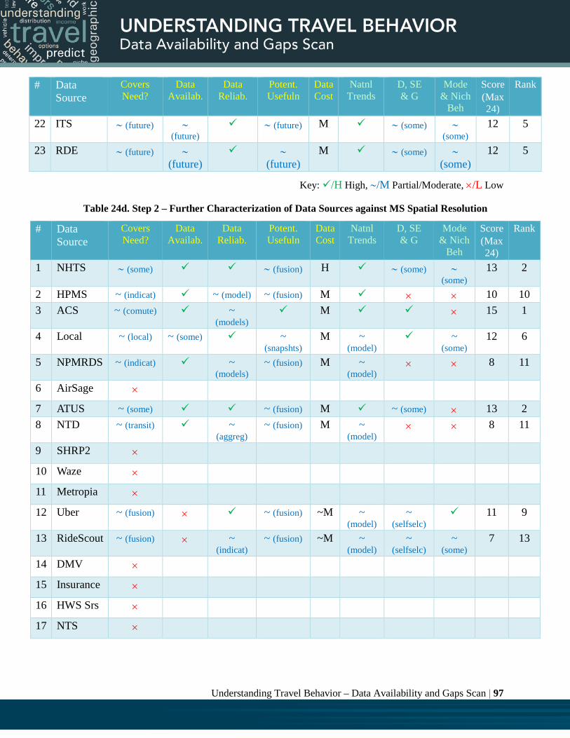
Understanding Travel Behavior – Data Availability and Gaps Scan | 97
# Data Source
Covers Need?
Data Availab.
Data Reliab.
Potent. Usefuln
Data Cost
Natnl Trends
D, SE & G
Mode & Nich
Beh Score (Max 24)
Rank
22 ITS ∼ (future) ∼ (future)
∼ (future) M ∼ (some) ∼ (some)
12 5 23 RDE ∼ (future) ∼
(future) ∼
(future) M ∼ (some) ∼
(some) 12 5
Key: /H High, ∼/M Partial/Moderate, ×/L Low
Table 24d. Step 2 – Further Characterization of Data Sources against MS Spatial Resolution
# Data Source
Covers Need?
Data Availab.
Data Reliab.
Potent. Usefuln
Data Cost
Natnl Trends
D, SE & G
Mode & Nich
Beh Score (Max 24)
Rank
1 NHTS ∼ (some) ∼ (fusion) H ∼ (some) ∼ (some)
13 2 2 HPMS ~ (indicat) ~ (model) ~ (fusion) M × × 10 10 3 ACS ~ (comute) ~
(models) M × 15 1
4 Local ~ (local) ~ (some) ~ (snapshts)
M ~ (model)
~ (some)
12 6 5 NPMRDS ~ (indicat) ~
(models) ~ (fusion) M ~
(model) × × 8 11 6 AirSage × 7 ATUS ~ (some) ~ (fusion) M ~ (some) × 13 2 8 NTD ~ (transit) ~
(aggreg) ~ (fusion) M ~
(model) × × 8 11 9 SHRP2 × 10 Waze × 11 Metropia × 12 Uber ~ (fusion) × ~ (fusion) ~M ~
(model) ~
(selfselc) 11 9
13 RideScout ~ (fusion) × ~ (indicat)
~ (fusion) ~M ~ (model)
~ (selfselc)
~ (some)
7 13 14 DMV × 15 Insurance × 16 HWS Srs × 17 NTS ×

Understanding Travel Behavior – Data Availability and Gaps Scan | 98
# Data Source
Covers Need?
Data Availab.
Data Reliab.
Potent. Usefuln
Data Cost
Natnl Trends
D, SE & G
Mode & Nich
Beh Score (Max 24)
Rank
18 AHS ~ (snapshts)
~ (models)
~ (fusion) M × 13 2 19 LBSN × 20 Omnibus ~ (future) × ~ (fusion) M ~
(some) 13 2
21 USPS × 22 ITS ~ (future) ~
(future) ~ (future) M ~ (some) ~
(some) 12 6
23 RDE ~ (future) ~ (future)
~ (future) M ~ (some) ~ (some)
12 6
Key: /H High, ∼/M Partial/Moderate, ×/L Low
Table 24e. Step 2 – Further Characterization of Data Sources against Telecommuting
# Data Source
Covers Need?
Data Availab.
Data Reliab.
Potent. Usefuln
Data Cost
Natnl Trends
D, SE & G
Mode &
Nich Beh
Score (Max 24)
Rank
1 NHTS H ~ (some)
19 4 2 HPMS × 3 ACS L × 21 1 4 Local ~ (some) ~
(snapshts) M ~
(model) ~
(some) 14 6
5 NPMRDS × 6 AirSage ~
(estimate) ~
(purchs) ~
(model) M ~
(model) ~
(fusion) × 9 8 7 ATUS L × 21 1 8 NTD × 9 SHRP2 ~
(estimate) ~
(snapsht) M ~
(model) × 13 7
10 Waze × 11 Metropia × 12 Uber × 13 RideScout ×

Understanding Travel Behavior – Data Availability and Gaps Scan | 99
# Data Source
Covers Need?
Data Availab.
Data Reliab.
Potent. Usefuln
Data Cost
Natnl Trends
D, SE & G
Mode &
Nich Beh
Score (Max 24)
Rank
14 DMV × 15 Insurance × 16 HWS Srs × 17 NTS × 18 AHS L × 21 1 19 LBSN × 20 Omnibus ~
(sample) L × 19 4
21 USPS × 22 ITS × 23 RDE ×
Key: /H High, ∼/M Partial/Moderate, ×/L Low

Understanding Travel Behavior – Data Availability and Gaps Scan | 100
Table 24f. Step 2 – Further Characterization of Data Sources against TP & Characteristics
# Data Source
Covers Need?
Data Availab.
Data Reliab.
Potent. Usefuln
Data Cost
Natnl Trends
D, SE & G
Mode &
Nich Beh
Score (Max 24)
Rank
1 NHTS H ~ (some)
19 1 2 HPMS × 3 ACS × 4 Local ~ (some) ~
(snapshts) M ~
(model) ~
(some) 14 3
5 NPMRDS × 6 AirSage ~ (some) ~
(purchs) ~
(model) M ~
(fusion) × 11 5 7 ATUS ~ (time) ~
(prcssing) L × 17 2
8 NTD × 9 SHRP2 ~
(prcssing) ~
(model) ~
(snapsht) M ~
(snapsht) ~
(some) × 9 7 10 Waze × 11 Metropia × 12 Uber × 13 RideScout × 14 DMV × 15 Insurance × 16 HWS Srs × 17 NTS × 18 AHS × 19 LBSN ~
(prcssing) ~
(model) ~ (fusion) L ~
(fusion) × 13 4 20 Omnibus ~ (some) ~ (some) ~ (fusion) M ~
(model) × 11 5
21 USPS × 22 ITS × 23 RDE ×
Key: /H High, ∼/M Partial/Moderate, ×/L Low

Understanding Travel Behavior – Data Availability and Gaps Scan | 101
Table 24g. Step 2 – Further Characterization of Data Sources against Trip Demographics
# Data Source
Covers Need?
Data Availab.
Data Reliab.
Potent. Usefuln
Data Cost
Natnl Trends
D, SE & G
Mode &
Nich Beh
Score (Max 24)
Rank
1 NHTS ~ (snapshot)
H ~ (some)
17 2 2 HPMS × 3 ACS ~
(comute) L ~ (model) × 17 2
4 Local ~ (local) ~ (some) ~ (snapshts)
M ~ (model) ~ (some)
12 4 5 NPMRDS × 6 AirSage ~
(estimate) ~
(purchs) ~
(models) ~ (fusion) M ~
(fusion) × 9 8 7 ATUS ~ (time) L ~
(some) 20 1
8 NTD × 9 SHRP2 ~
(prcssing) ~ (fusion) M ~
(snapshot) ~ (some
lcl) × 11 5 10 Waze ~ (some) × ~
(selfselc) ~ (fusion) M ~ (model) ~
(selfselc) ~
(beh) 7 12
11 Metropia ~ (some) × ~ (selfselc)
~ (fusion) M × ~ (selfselc)
~ (beh)
6 15 12 Uber ~ (some) × ~
(selfselc) ~ (fusion) M ~ (model) ~
(selfselc) 9 8
13 RideScout ~ (some) × ~ (selfselc)
~ (fusion) M ~ (model) ~ (selfselc)
~ (some)
7 12 14 DMV ~ (aggrgt) × ~
(future) ~ (fusion) M ~ (model) ~ (some) × 6 15
15 Insurance ~ (aggrgt) × ~ (future)
~ (fusion) M ~ (model) × 8 11 16 HWS Srs × 17 NTS × 18 AHS ~ (fusion) ~
(models) ~ (fusion) M ~ (some) × 11 5
19 LBSN ~ (fusion) ~ (models)
~ (fusion) M ~ (fusion) ~ (fusion) × 9 8
20 Omnibus ~ (future) × ~ (fusion) M ~ (some) × 10 7 21 USPS ~ (fusion ~
(aggrgt) ~
(models) ~ (fusion) M ~ (model) ~
(model) × 7 12 22 ITS × 23 RDE ×

Understanding Travel Behavior – Data Availability and Gaps Scan | 102
Table 24h. Step 2 – Further Characterization of Data Sources against Public Attitudes
# Data Source
Covers Need?
Data Availab.
Data Reliab.
Potent. Usefuln
Data Cost
Natnl Trends
D, SE & G
Mode &
Nich Beh
Score (Max 24)
Rank
1 NHTS ~ (some) ~ (infernce)
~ (fusion) L ~ (some)
16 2 2 HPMS × 3 ACS ~ (some) ~
(infernce) ~ (fusion) L × 15 4
4 Local ~ (some) ~ (some) ~ (infernce)
~ (snapshts)
L ~ (some)
14 7 5 NPMRDS × 6 AirSage × 7 ATUS ~ (some) ~
(infernce) ~ (fusion) L × 15 4
8 NTD ~ (indicat)
~ (aggrgt) ~ (fusion) L × × 12 9 9 SHRP2 × 10 Waze ~ (some) × ~ (fusion) M ~ (beh) 13 8 11 Metropia ~ (some) × ~ (fusion) M × ~ (lcl) ~ (beh) 8 14 12 Uber ~ (some) × ~ (fusion) M 15 4 13 RideScout ~ (some) × ~ (indicat) ~ (fusion) M ~
(indicat) 11 10
14 DMV ~ (future) × ~ (indicat) ~ (fusion) M ~
(indicat) ~
(some) × 6 16 15 Insurance ~ (some) × ~ (indicat) ~ (fusion) M ~
(indicat) × 8 14
16 HWS Srs × 17 NTS × 18 AHS ~ (some) L ~
(some) 20 1
19 LBSN ~ (indicat)
~ (infernce)
~ (fusion) M ~ (indicat)
~ (fusion) × 9 13
20 Omnibus ~ (some) ~ (some) M ~ (some)
16 2 21 USPS ~
(indicat) ~
(aggrgt) ~
(infernce) ~ (fusion) L ~
(indicat) ~
(fusion) ~ (beh) 10 11
22 ITS × 23 RDE ~
(future) ~
(future) ~
(infernce) ~ (future) M ~
(some) ~
(some) 10 11
Key: /H High, ∼/M Partial/Moderate, ×/L Low

Understanding Travel Behavior – Data Availability and Gaps Scan | 103
Table 24i. Step 2 – Further Characterization of Data Sources against Vehicle Occupancy
# Data Source
Covers Need?
Data Availab.
Data Reliab.
Potent. Usefuln
Data Cost
Natnl Trends
D, SE & G
Mode & Nich
Beh Score (Max 24)
Rank
1 NHTS L ~ (some) 22 1 2 HPMS × 3 ACS L × 21 2 4 Local ~ (some) ~
(snapshts) L ~
(model) ~ (some) 16 4
5 NPMRDS × 6 AirSage × 7 ATUS L × 21 2 8 NTD × 9 SHRP2 ~
(local) ~
(prcssing) ~
(snapshot) M ~
(model) × 11 8
10 Waze × 11 Metropia × 12 Uber ~
(some) × ~ (fusion) M ~
(model) ~
(selfselc) 11 8
13 RideScout × 14 DMV × 15 Insurance × 16 HWS Srs × 17 NTS × 18 AHS × 19 LBSN × 20 Omnibus ~
(future) × M ~
(possible) 15 5
21 USPS × 22 ITS ~
(future) ~ (future) ~ (future) M ~ (some) ~ (some) 12 6
23 RDE ~ (future)
~ (future) ~ (future) M ~ (some) ~ (some) 12 6
Key: /H High, ∼/M Partial/Moderate, ×/L Low

Understanding Travel Behavior – Data Availability and Gaps Scan | 104
Table 25. Step 3 – Identifying Promising Data Sources
# Data Source
VMT PMT Freq
MS Freq
MS Spatial Resoul
Telecommuti
ng TP and
Charact
Trip Demographi
cs
Public Attitud
es Vehicl
e Occup
Sum (Min
9) Collec
tive Rank
1 NHTS 1 23 23 2 4 1 1 2 2 59 5 2 HPMS 6 11 9 10 23 23 23 23 23 151 13 3 ACS 1 2 2 1 1 23 3 4 2 39 2 4 Local 7 6 5 6 6 3 4 7 4 48 4 5 NPMR
DS 19 12 10 11 23 23 23 23 23 167 16
6 AirSage 12 2 23 23 8 5 8 23 23 127 12 7 ATUS 1 1 1 2 1 2 1 4 1 14 1 8 NTD 19 12 10 11 23 23 23 9 23 153 15 9 SHRP2 7 14 23 23 7 7 5 23 8 117 9 10 Waze 15 23 23 23 23 23 12 8 23 173 18 11 Metropi
a 19 23 23 23 23 23 15 14 23 186 21
12 Uber 15 9 8 9 23 23 8 4 8 107 7 13 RideSco
ut 22 14 12 13 23 23 12 10 23 152 14
14 DMV 14 23 23 23 23 23 15 16 23 183 20 15 Insuranc
e 7 23 23 23 23 23 11 14 23 170 17
16 HWS Srs
15 23 23 23 23 23 23 23 23 199 23 17 NTS 15 23 23 23 23 23 23 23 23 199 23 18 AHS 12 4 4 2 1 23 5 1 23 75 6 19 LBSN 4 4 23 23 23 4 8 13 23 125 11 20 Omnibu
s 4 9 2 2 4 5 7 2 5 40 3
21 USPS 22 14 23 23 23 23 12 11 23 174 19 22 ITS 7 6 5 6 23 23 23 23 6 122 10 23 RDE 7 6 5 6 23 23 23 11 6 110 8

Understanding Travel Behavior – Data Availability and Gaps Scan | 105
Figure 36. Collective Sum of Data Source Rankings
The six most promising data

Understanding Travel Behavior – Data Availability and Gaps Scan | 106
CHAPTER 5.0. EVALUATION AND RANKING OF DATA SOURCES
INTRODUCTION
Chapter 4 of this report cross-examined the 23 data sources presented in Chapters 2 and 3 against the HPINs identified in the Research Scan. It adopted and presented a simple three-step method that concluded by identifying and selecting seven data sources that are believed to be promising for addressing the HPINs. These seven data sources are:
1. ATUS 2. ACS 3. Omnibus surveys 4. Local surveys 5. NHTS 6. AHS 7. AirSage.
This chapter intends to develop and implement a more rigorous rating scheme to rank these data sources with respect to their potential for addressing the HPINs. The chapter is divided into five sections and organized in the following sequence. Section 1 is this introduction. Section 2 discusses the rating scheme developed for this work and provides a detailed explanation of its different steps and components. Section 3 presents five different implementations of the developed rating scheme and associated ranking of the data sources. Section 4 presents a sensitivity analysis of the ranking of the data sources. The chapter concludes with Section 5, which presents a summary of the chapter. Figure 37 depicts the graphical flow of Chapter 5.

Understanding Travel Behavior – Data Availability and Gaps Scan | 107
Figure 37. Content Flow of Chapter 5
RATING SCHEME
For ranking of the seven most promising data sources, the multi-attribute decision making (MADM) model was adopted. The MADM is composed of the following four steps:
1. Evaluation Criteria: a. Definition: Defining the evaluation criteria. b. Measurement Scale: Determining the measurement scale of the of evaluation criteria (e.g.,
quantitative scales, such as years for periodicity of a data source; and qualitative scales, such as the Likert scale). This step includes identifying the minimum and maximum values of the scale (e.g., a 1 – 5 Likert scale).
c. Scale Direction: Determining positive and negative scales. In a positive scale, high values reflect favorable attributes (e.g., higher reliability is favorable to lower). On the other hand, in a negative scale lower values are preferred (e.g., cost).
2. Criteria Weights: identifying the weights of the evaluation criteria in a manner that reflects the
beliefs of the research team with respect to the priorities and values of the defined criteria. In order to minimize potential bias, the Pairwise Comparison method was adopted to identify the criteria weights. The following matrix explains the Pairwise Comparison method. Every cell in the matrix represents a pairwise comparison between the importance of its two respective criteria (row and column headings). Every value in the matrix Pij ranges between 0 and 1, and reflects the relative importance of criterion I (row) in comparison with criterion j (column). For example, the value of P1N equals 1, reflects that “Criterion1” is more important than “Criterion N”. Logically, this also means that “Criterion N” is less important than “Criterion1”; hence, PN1 equals 0. In essence, every Pji = 1 − Pij., and once values in the upper triangle are determined, all value in the lower
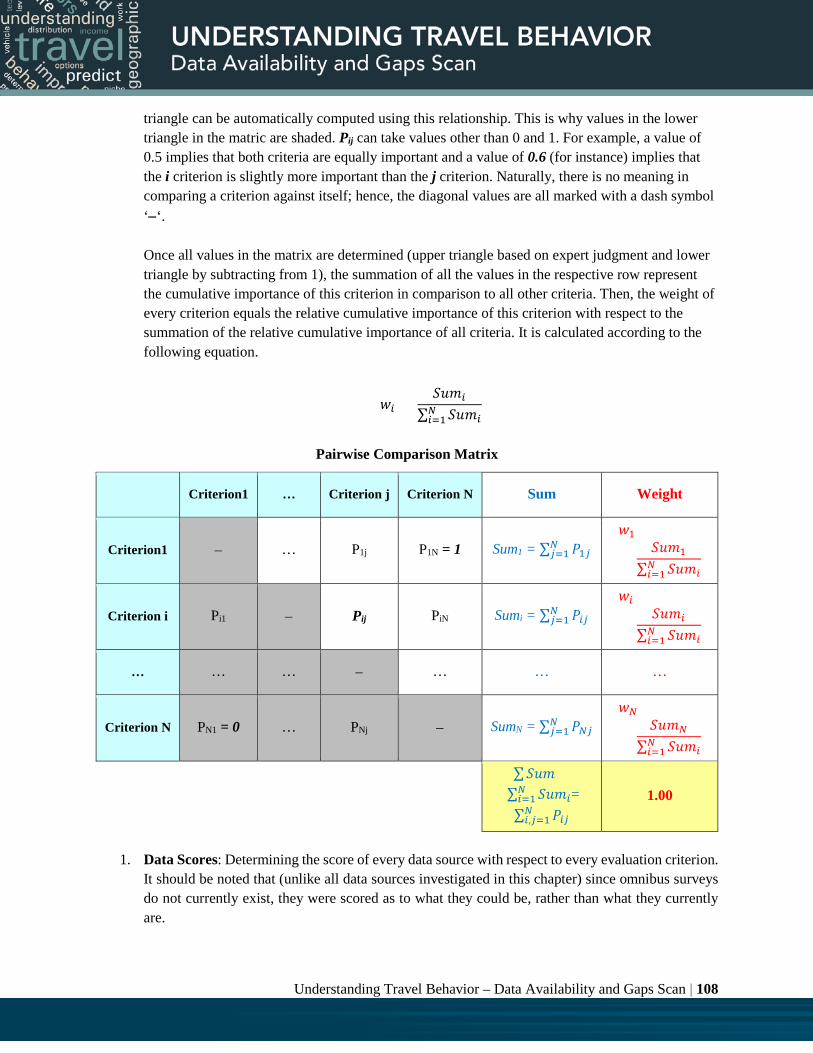
Understanding Travel Behavior – Data Availability and Gaps Scan | 108
triangle can be automatically computed using this relationship. This is why values in the lower triangle in the matric are shaded. Pij can take values other than 0 and 1. For example, a value of 0.5 implies that both criteria are equally important and a value of 0.6 (for instance) implies that the i criterion is slightly more important than the j criterion. Naturally, there is no meaning in comparing a criterion against itself; hence, the diagonal values are all marked with a dash symbol ‘−‘. Once all values in the matrix are determined (upper triangle based on expert judgment and lower triangle by subtracting from 1), the summation of all the values in the respective row represent the cumulative importance of this criterion in comparison to all other criteria. Then, the weight of every criterion equals the relative cumulative importance of this criterion with respect to the summation of the relative cumulative importance of all criteria. It is calculated according to the following equation.
𝑤𝑤𝑖𝑖 = 𝑆𝑆𝑆𝑆𝑚𝑚𝑖𝑖
∑ 𝑆𝑆𝑆𝑆𝑚𝑚𝑖𝑖𝑁𝑁𝑖𝑖=1
Pairwise Comparison Matrix
Criterion1 … Criterion j Criterion N Sum Weight
Criterion1 − … P1j P1N = 1 Sum1 = ∑ 𝑃𝑃1𝑗𝑗𝑁𝑁𝑗𝑗=1
𝑤𝑤1
= 𝑆𝑆𝑆𝑆𝑚𝑚1
∑ 𝑆𝑆𝑆𝑆𝑚𝑚𝑖𝑖𝑁𝑁𝑖𝑖=1
Criterion i Pi1 − Pij PiN Sumi = ∑ 𝑃𝑃𝑖𝑖𝑗𝑗𝑁𝑁𝑗𝑗=1
𝑤𝑤𝑖𝑖
= 𝑆𝑆𝑆𝑆𝑚𝑚𝑖𝑖
∑ 𝑆𝑆𝑆𝑆𝑚𝑚𝑖𝑖𝑁𝑁𝑖𝑖=1
… … … − … … …
Criterion N PN1 = 0 … PNj − SumN = ∑ 𝑃𝑃𝑁𝑁𝑗𝑗𝑁𝑁𝑗𝑗=1
𝑤𝑤𝑁𝑁
= 𝑆𝑆𝑆𝑆𝑚𝑚𝑁𝑁
∑ 𝑆𝑆𝑆𝑆𝑚𝑚𝑖𝑖𝑁𝑁𝑖𝑖=1
∑𝑆𝑆𝑆𝑆𝑚𝑚 =
∑ 𝑆𝑆𝑆𝑆𝑚𝑚𝑖𝑖𝑁𝑁𝑖𝑖=1 = ∑ 𝑃𝑃𝑖𝑖𝑗𝑗𝑁𝑁𝑖𝑖,𝑗𝑗=1
1.00
1. Data Scores: Determining the score of every data source with respect to every evaluation criterion.
It should be noted that (unlike all data sources investigated in this chapter) since omnibus surveys do not currently exist, they were scored as to what they could be, rather than what they currently are.

Understanding Travel Behavior – Data Availability and Gaps Scan | 109
2. Ranking of Data Sources:
a. Normalization of Data Scores: This step entails transformation of the scales of the different criteria and the scores of the different data sources into a homogeneous scale. To elaborate, this step is necessary to be able to add periodicity in years to accuracy in a 1 – 5 Likert scale. Normalized data scores were calculated according to the following equation. This ensures that every data score ranges between 100 for the most favorable score and 0 for the least favorable score, for every criterion.
𝑁𝑁𝑁𝑁𝑁𝑁𝑚𝑚𝑁𝑁𝑁𝑁𝑁𝑁𝑁𝑁𝑁𝑁𝑁𝑁 𝐷𝐷𝑁𝑁𝐷𝐷𝑁𝑁 𝑆𝑆𝑆𝑆𝑁𝑁𝑁𝑁𝑁𝑁 𝑓𝑓𝑁𝑁𝑁𝑁
𝐶𝐶𝑁𝑁𝑁𝑁𝐷𝐷𝑁𝑁𝑁𝑁𝑁𝑁𝑁𝑁𝐶𝐶 𝑁𝑁 (𝐶𝐶𝑁𝑁𝑠𝑠𝑖𝑖)=
⎩⎪⎨
⎪⎧
𝐷𝐷𝑁𝑁𝐷𝐷𝑁𝑁 𝑆𝑆𝑆𝑆𝑁𝑁𝑁𝑁𝑁𝑁 −𝑀𝑀𝑁𝑁𝐶𝐶 𝑆𝑆𝑆𝑆𝑁𝑁𝑁𝑁𝑁𝑁𝑀𝑀𝑁𝑁𝑀𝑀 𝑆𝑆𝑆𝑆𝑁𝑁𝑁𝑁𝑁𝑁 −𝑀𝑀𝑁𝑁𝐶𝐶 𝑆𝑆𝑆𝑆𝑁𝑁𝑁𝑁𝑁𝑁
× 100 𝑓𝑓𝑁𝑁𝑁𝑁 + 𝑣𝑣𝑁𝑁 𝑠𝑠𝑆𝑆𝑁𝑁𝑁𝑁𝑁𝑁𝑠𝑠
�1 −𝐷𝐷𝑁𝑁𝐷𝐷𝑁𝑁 𝑆𝑆𝑆𝑆𝑁𝑁𝑁𝑁𝑁𝑁 −𝑀𝑀𝑁𝑁𝐶𝐶 𝑆𝑆𝑆𝑆𝑁𝑁𝑁𝑁𝑁𝑁𝑀𝑀𝑁𝑁𝑀𝑀 𝑆𝑆𝑆𝑆𝑁𝑁𝑁𝑁𝑁𝑁 −𝑀𝑀𝑁𝑁𝐶𝐶 𝑆𝑆𝑆𝑆𝑁𝑁𝑁𝑁𝑁𝑁
�× 100 𝑓𝑓𝑁𝑁𝑁𝑁 − 𝑣𝑣𝑁𝑁 𝑠𝑠𝑆𝑆𝑁𝑁𝑁𝑁𝑁𝑁𝑠𝑠
b. Data Ranking Scores: This step involves the calculation of the data ranking score as a
weighted average of the criteria weights and the normalized data score for every criterion. Data ranking scores were calculated according to the following equation.
𝐷𝐷𝑁𝑁𝐷𝐷𝑁𝑁 𝑅𝑅𝑁𝑁𝐶𝐶𝑅𝑅𝑁𝑁𝐶𝐶𝑅𝑅 𝑆𝑆𝑆𝑆𝑁𝑁𝑁𝑁𝑁𝑁 = � (𝑤𝑤𝑖𝑖 ∙ 𝐶𝐶𝑁𝑁𝑠𝑠𝑖𝑖)𝐴𝐴𝐴𝐴𝐴𝐴
𝐶𝐶𝐶𝐶𝑖𝑖𝐶𝐶𝐶𝐶𝐶𝐶𝑖𝑖𝐶𝐶, 𝑖𝑖
c. Ranked Data Sources: In this last step, data sources are ranked in descending order of their
data ranking scores.
RANKING OF DATA SOURCES
In order to reach a more reliable understanding of the performance and value of the different data sources in addressing the identified HPINs, five different evaluations were implemented as presented below.
First Evaluation This section presents the MADM model adopted for ranking of the data sources according to the first evaluation scheme.
Evaluation Criteria
Table 26 presents a description of the eight evaluation criteria adopted in this evaluation. Also, it presents the adopted scale and associated scale directions.

Understanding Travel Behavior – Data Availability and Gaps Scan | 110
Table 26. Defined Evaluation Criteria for the 1st Evaluation
# CRITERIA DESCRIPTION SCALE DIRECTION
1 Cost Relative cost of data for FHWA Likert (1 – 5)
-ve
2 Reliability Reliability and accuracy of the data collection method
Likert (1 – 5)
+ve
3 Temporal Length How far back does the data go Years +ve
4 Periodicity How often is the data collected/updated? Years -ve
5 Usefulness Contribution to the overall understanding of emerging travel behavior trends
5a National Trends Ability to explain national trends Likert (1 – 5)
+ve
5b Demographic, Socioeconomic & Geographic (D, SE & G)
Ability to explain D, SE and G impacts Likert (1 – 5)
+ve
5c Niche Mod/Beh Ability to capture impacts of emerging modes and niche behavior
Likert (1 – 5)
+ve
6 Data Consistency Missing data, and changes to survey/data structure
Likert (1 – 5)
+ve
7 Integration Readiness of the data for integration with the other data sources
Likert (1 – 5)
+ve
8 Complexity Steepness of learning, difficulty of data reduction, and existence of developed data-dependent analysis tools
Likert (1 – 5)
-ve
Criteria Weights
To determine reliable values for the criteria weights, four team members (Ms. Heather Rose, FHWA project manager; Dr. Ismail Zohdy, Booz Allen Hamilton, Inc.; Dr. Susan Shaheen, University of California, Berkeley; and Dr. Aly Tawfik, California State University, Fresno) completed the pairwise comparison matrix independently. Table 27 presents the resultant pairwise comparison matrix, which is the sum of the four individual pairwise comparison matrices – performed independently by the four team members listed above. As can be seen in Table 27, most of the values in the matrix are predominantly between 0 – 1, or 3 – 4. This reflects consistent views about the relative importance of the different criteria since at least three of the four team members choose the same Pij value for the different pairwise comparisons. One notable exception to this observation is the 2.5 value between criterions 5b and 5c. This reflects that the team members were almost equally split (close to 2) about the relative importance of

Understanding Travel Behavior – Data Availability and Gaps Scan | 111
these two criteria. This result does not appear to be unusual (in fact potentially expected) since both criteria reflect the desired usefulness of the data source. The last two columns in Table 27 present the calculated sums and weights of every criterion, based on the equations provided earlier. The results indicate that the three criteria reflecting usefulness of the data source turned out to be the most important, with respective weights of 16% for National Trends, and 14% for each of demographic, socioeconomic, and geographic (D, SE & G); and niche mode and behavior criteria. On the other end, temporal length and consistency of the data sources were found to be the least important ones, with respective weights of 4% each.
Table 27. Identified Criteria Weight for the 1st Evaluation
#
CR
ITE
RIA
1) C
OST
2) R
EL
IAB
ILIT
Y
3) T
EM
P.L
NG
TH
4) P
ER
IOD
ICIT
Y
5A) N
AT
’L T
RN
DS
5B) D
,SE
,G
5C) N
ICH
E B
EH
6) D
AT
A C
ON
SIST
.
7) IN
TE
GR
AT
ION
8) C
OM
PLE
XIT
Y
SUM
WE
IGH
T
1 Cost − 0 4 1 1 0 1 4 4 4 19 11%
2 Reliability 4 − 4 3 3 0 1 3 4 4 26 14%
3 Temp. Length
0 0 − 1 1 1 1 1 1 1 7 4%
4 Periodicity 3 1 3 − 1 1 1 3 4 2.8 19.8 11%
5a Nation’l Trends
3 1 3 3 − 3.5 3.5 4 4 4 29 16%
5b D, SE & G 4 4 3 3 0.5 − 2.5 3 3 3 26 14%
5c Niche/Mode 3 3 3 3 0.5 1.5 − 4 4 4 26 14%
6 Data Consist.
0 1 3 1 0 1 0 − 1 0.5 7.5 4%
7 Integration 0 0 3 0 0 1 0 3 − 4 11 6%
8 Complexity 0 0 3 1.2 0 1 0 3.5 0 − 8.7 5%

Understanding Travel Behavior – Data Availability and Gaps Scan | 112
Data Scores
Table 28a presents the determined data scores for every data source under each of the defined criteria. In addition, Table 28b presents an expanded discussion of the reasons behind the determined scores. It is worth noting that no single value was readily available for determining the temporal length and periodicity of local surveys. Hence, the values in the table were based on analysis of Figure 38.
Table 28a. Determined Data Scores for the 1st Evaluation
# Criteria Scale Dir NHTS ACS Lcl Srv
Air-Sage
ATUS AHS Omni-bus*
1 Cost Likert (1 – 5)
-ve 5 1 1 3 1 1 2
2 Reliability Likert (1 – 5)
+ve 4 4 3 4 4 4 3
3 Temp. Length
Years +ve 46 15 30*** 6 12 42 0
4 Periodicity Years -ve 7 1 0.5*** 0.08** 1 2 0.08**
5a Nation’l Trends
Likert (1 – 5)
+ve 5 4 3 5 5 4 4
5b D, SE & G Likert (1 – 5)
+ve 5 4 5 3 5 4 4
5c Niche Mod/Beh
Likert (1 – 5)
+ve 4 2 3 1 3 2 5
6 Limitations Likert (1 – 5)
+ve 4 4 2 3 4 2 3
7 Integration Likert (1 – 5)
+ve 4 4 3 4 4 3 5
8 Complexity Likert (1 – 5)
-ve 2 1 5 1 3 2 1
Table Notes: * As mentioned earlier, since omnibus surveys do not currently exist, they were scored as to what they could be, rather
than what they currently are (as is the case with all other data sources in this chapter) ** Based on a value of 1 month, where 1 month was assumed to be the minimum value of interest (for explanations of
month-to-month variations in travel behavior) *** Based on the provided analysis of Figure 38.

Table 28b. Expanded Explanation of Determined Data Scores for the 1st Evaluation
# CRITERIA NHTS ACS LCL SRV AIRSAGE ATUS AHS OMNI-BUS
1 Cost Cost incurred by FHWA
Cost incurred by other agency
Cost incurred by other agencies
Depends on Requested Product
Cost incurred by other agency
Cost incurred by other agency
Depends on questions and sample
2 Reliability SP Survey, depends on respondent recollection
SP Survey, depends on respondent recollection
Depends on local survey design and data collection design and efforts
Depends on inference algorithms
SP Survey, depends on respondent recollection
SP Survey, depends on respondent recollection
SP Survey and depends on sample design (prob not as accurate as national surveys)
3 Temp. Length
Since 1969 Annually since 2001
MTSA: 84 datasets; 1960 to 2011
Since Jan 2009
Since 2003 Since 1973; annually
None yet
4 Periodicity ~ every 7 years Annually since 2001
Ch2 MTSA Figure 38
Monthly; set as a minimum
Annually Since 1981, biennially
Monthly; set as a minimum
5a Nation’l Trends
Limited to Commuting
Discrepancies btn surveys, urban vs rural
Limited to Survey Questions
Comprehensiveness
5b D, SE & G Limited to Commuting
Geog: Yes … SE&G: Fusion with Census
Limited to Survey Questions
D&SE: Yes, G: Comprehensiveness
5c Niche Mod/Beh
Gets updated but not immediately
Limited; Transp not primary focus
Discrepancies btn surveys
Mode not included
Limited; Transp not primary focus
Transpo questions get rotated, and transpo not main focus
Understanding Travel Behavior – Data Availability and Gaps Scan | 113

# CRITERIA NHTS ACS LCL SRV AIRSAGE ATUS AHS OMNI-BUS
6 Limitations Changes but with ample documentation
Changes but with ample documentation
Discrepancies btn surveys
Algorithms not transparent
Changes but with ample documentation
Transpo questions get rotated, and transpo not main focus
Different questionnaires
7 Integration Only for States, or MSA Designation
TAZs Summary Tbls
Discrepancies btn surveys
Summaries, not data
Only for States, or MSA Designation
Only for States, or MSA Designation
8 Complexity Much documentation and research usage
CTPP and Others, TAZs
Discrepancies btn surveys
Much documentation and research usage. Trip purpose classes
Much documentation and research usage
Understanding Travel Behavior – Data Availability and Gaps Scan | 114

Understanding Travel Behavior – Data Availability and Gaps Scan | 115
The Metropolitan Travel Survey Archive (MTSA) was used to estimate the temporal length and periodicity of the local surveys. Figure 38 presents a frequency distribution of the travel survey datasets on MTSA by year. By examining this distribution, it was assumed that local travel surveys have been consistently collected since 1986. Hence the temporal length of local surveys was determined to be 30 years. In addition, a value of 2 was determined for the periodicity of local travel surveys since 1986. This value may appear to be a little conservative. The reason for picking a possibly low conservative value is based on the following two reasons: 1) some of the travel surveys on the MTSA represent add-on surveys of the NHTS; and 2) quality and documentation of some of these surveys may be questionable – hence, making the data not particularly useful.
Figure 38. Frequency Distribution of Travel Survey Datasets of the Metropolitan Travel Survey Archive by Year
Ranking of Data Sources Using the equations provided earlier, Table 29 presents the normalized data scores, data ranking scores, and ranked data sources for the first evaluation. The results indicate that ATUS has the highest ranking, followed by omnibus surveys, then ACS and NHTS. On first sight, it may appear surprising that ranking of NHTS (which is the richest travel behavior dataset) turned out to be in the middle and not at the top of the rank. However, given that this work was originally motivated by an attempt to identify data gaps and address HPINs that are not presently possible to answer using traditionally used data sources, these findings appear to be quite possible. Paying an even closer look on Table 29 reveals that the NHTS has two major disadvantages in comparison to the other data sources. First, it is characterized with the highest

Understanding Travel Behavior – Data Availability and Gaps Scan | 116
absolute cost to the FHWA. Second, it has the lowest periodicity. These observations make the calculated results appear to be more reliable. Nonetheless, to reach a more reliable understanding of the performance and value of the different data sources in addressing the identified HPINs, four other evaluations were performed and are presented in the following sections.
Table 29. Normalized Data Scores, Data Ranking Scores, and Ranked Data Sources for the 1st Evaluation
# CRITERIA WEIGHT NHTS ACS LCL SRV
AIRSGE ATUS AHS OMNI-BUS
1 Cost 11% 0 100 100 50 100 100 75
2 Reliability 14% 75 75 50 75 75 75 50
3 Temp. Length 4% 100 33 65 13 26 91 0
4 Periodicity 11% 0 87 94 100 87 72 100
5a Nation’l Trends
16% 100 75 50 100 100 75 75
5b D, SE & G 14% 100 75 100 50 100 75 75
5c Niche Mod/Beh
14% 75 25 50 0 50 25 100
6 Limitations 4% 75 75 25 50 75 25 50
7 Integration 6% 75 75 50 75 75 50 100
8 Complexity 5% 75 100 0 100 50 75 100
Data Ranking Score 67.4 71.3 64.5 62.5 79.8 67.1 76.5
Ranked Data Sources 4 3 6 7 1 5 2
Second Evaluation This section presents the MADM model adopted for ranking of the data sources according to the second evaluation scheme.

Understanding Travel Behavior – Data Availability and Gaps Scan | 117
Evaluation Criteria
An additional criterion was added to the criteria adopted in the first evaluation, Criterion 5d: comprehensiveness. Table 30 presents a description of all the evaluation criteria adopted in this evaluation. The table also presents the adopted scale and associated scale directions.
Table 30. Defined Evaluation Criteria for the 2nd Evaluation
# Criteria Description Scale Direction
1 Cost Relative cost of data for FHWA Likert (1 – 5)
-ve
2 Reliability Reliability and accuracy of the data collection method
Likert (1 – 5)
+ve
3 Temporal Length
How far back does the data go Years +ve
4 Periodicity How often is the data collected/updated? Years -ve
5 Usefulness Contribution to the overall understanding of emerging travel behavior trends
5a National Trends
Ability to explain national trends Likert (1 – 5) +ve
5b D, SE & G Ability to explain D, SE and G impacts Likert (1 – 5) +ve
5c Niche Mod/Beh
Ability to capture impacts of emerging modes and niche behavior
Likert (1 – 5)
+ve
5d Comprehens-iveness
Comprehensiveness of travel information in the data source
Likert (1 – 5)
+ve
6 Data Consistency
Missing data, and changes to survey/data structure
Likert (1 – 5)
+ve
7 Integration Readiness of the data for integration with the other data sources
Likert (1 – 5) +ve
8 Complexity Steepness of learning, difficulty of data reduction, and existence of developed data-dependent analysis tools
Likert (1 – 5)
-ve

Understanding Travel Behavior – Data Availability and Gaps Scan | 118
Criteria Weights
Table 31 presents the criteria weights determined for the second evaluation. It can be seen that the addition of the new usefulness criterion, 5d, increased the total weight of criterion 5 from 44% to 52%, and that all of the usefulness criteria remained to be among the most important ones where they represent 4 of the 5 most important criteria.
Table 31. Identified Criteria Weight for the 2nd Evaluation
#
CR
ITER
IA
1) C
OST
2) R
EL
IAB
ILIT
Y
3) T
EM
P.L
NG
TH
4) P
ER
IOD
ICIT
Y
5A) N
AT
’L T
RN
DS
5B) D
,SE
,G
5C) N
ICH
E B
EH
5D) C
OM
PRH
NSV
E
6) D
AT
A C
ON
SIST
.
7) IN
TE
GR
AT
ION
8) C
OM
PLE
XIT
Y
SUM
WE
IGH
T
1 Cost − 0 4 1 1 0 1 1 4 4 4 20 9% 2 Reliability 4 − 4 3 3 0 1 2 3 4 4 28 13
% 3 Tmp. Length 0 0 − 1 1 1 1 1 1 1 1 8 4% 4 Periodicity 3 1 3 − 1 1 1 1 3 4 2.8 20.
8 9%
5a Nat’l Trends 3 1 3 3 − 3.5 3.5 2 4 4 4 31 14%
5b D, SE & G 4 4 3 3 0.5 − 2.5 2 3 3 3 28 13%
5c Niche 3 3 3 3 0.5 1.5 − 2 4 4 4 28 13%
5d Comprhens. 3 2 3 3 2 2 2 − 3 3.5 3.5 27 12%
6 Data Cnsist. 0 1 3 1 0 1 0 1 − 1 0.5 8.5 4% 7 Integration 0 0 3 0 0 1 0 0.5 3 − 4 11.
5 5%
8 Complexity 0 0 3 1.2 0 1 0 0.5 3.5 0 − 9.2 4%
Data Scores
Table 32 presents the normalized data scores, data ranking scores, and ranked data sources for the second evaluation. As expected, adding the comprehensiveness criterion resulted in an improved ranking for the NHTS (the NHTS is the most comprehensive travel behavior dataset). However, while the top four ranked datasets remained unchanged, the first pair (omnibus surveys and ATUS) exchanged positions and the second pair (NHTS and ACS) also exchanged positions.

Understanding Travel Behavior – Data Availability and Gaps Scan | 119
Table 32. Normalized Data Scores, Data Ranking Scores, and Ranked Data Sources for the 2nd Evaluation
# CRITERIA WEIGHT NHTS ACS LCL SRV
AIRSGE ATUS AHS OMNI-BUS
1 Cost 9% 0 100 100 50 100 100 75
2 Reliability 13% 75 75 50 75 75 75 50
3 Temp. Length 4% 100 33 65 13 26 91 0
4 Periodicity 9% 0 87 94 100 87 72 100
5a National Trends
14% 100 75 50 100 100 75 75
5b D, SE & G 13% 100 75 100 50 100 75 75
5c Niche Mod/Beh
13% 75 25 50 0 50 25 100
5d Comprehensive 12% 100 50 50 0 25 0 50
6 Data Consist. 4% 75 75 25 50 75 25 50
7 Integration 5% 75 75 50 75 75 50 100
8 Complexity 4% 75 100 0 100 50 75 100
Data Ranking Score 71.8 68.5 62.6 54.5 72.9 58.8 73.0
Ranked Data Sources 3 4 5 7 2 6 1
Third Evaluation This section presents the MADM model adopted for ranking the data sources according to the third evaluation scheme.

Understanding Travel Behavior – Data Availability and Gaps Scan | 120
Evaluation Criteria
In this evaluation, all four general usefulness criteria were removed and replaced with the eight specific HPINs identified in the Research Scan. Table 33 presents a description of all the evaluation criteria adopted in this evaluation, as well as the adopted scale and associated scale directions.
Table 33. Defined Evaluation Criteria for the 3rd Evaluation
# CRITERIA DESCRIPTION SCALE DIRECTION
1 Cost Relative cost of data for FHWA Likert (1 – 5)
-ve
2 Reliability Reliability and accuracy of the data collection method
Likert (1 – 5)
+ve
3 Temp. Length How far back does the data go Years +ve
4 Periodicity How often is the data collected/updated? Years -ve
5 5a) Nnt’l Trends; 5b) D, SE & G; 5c) Niche Mod/Beh; and 5d) Comprehensiveness
6 Data Consist. Missing data, and changes to survey/data structure
Likert (1 – 5)
+ve
7 Integration Readiness of the data for integration with the other data sources
Likert (1 – 5)
+ve
8 Complexity Steepness of learning, difficulty of data reduction, and existence of developed data-dependent analysis tools
Likert (1 – 5)
-ve
9a VMT Missing local streets, Possible measurement errors, Estimation procedure accuracy
Likert (1 – 5)
+ve
9b PMT Frequency Infrequent snapshots of activity Likert (1 – 5)
+ve
9c Mode Share Freq and Spati. Resol.
Better spatial resolution, More frequent intervals
Likert (1 – 5)
+ve
9d Telecommuting Better measurements Likert (1 – 5)
+ve
9e Trip Purpose (Work v. Non-work)
Better understanding of travel characteristics (mode share, distance, …), Better spatial resolution, More frequent intervals
Likert (1 – 5)
+ve
9f Demographics crossed with Travel
Association of demographic distributions with data as related to other, measurements of travel (mode split, VMT, PMT)
Likert (1 – 5)
+ve
9g Attitudes & Public Perceptions
Attitudes towards mobility across generations, Effect of attitude changes
Likert (1 – 5)
+ve
9h Vehicle Occupancy Identify real-time vehicle occupancy , Measure historical vehicle occupancy
Likert (1 – 5)
+ve

Understanding Travel Behavior – Data Availability and Gaps Scan | 121
Criteria Weights
The weights of the new eight criteria were calculated by dividing the former weight of the four usefulness criteria (52%, as discussed in Section 3.2.2) by eight. Hence, each of the eight new criteria was assigned a weight of 6.5%, as can be seen in Table 34.
Data Scores
Table 34 presents the normalized data scores, data ranking scores, and ranked data sources for the third evaluation. The results indicate that ranking of the data sources remained generally stable. While it is interesting that the ranking of the NHTS dropped to fifth, this result should not be surprising for the same reasons explained in section 3.1.4. Since this work was originally motivated by an attempt to identify data gaps and address HPINs that are not presently possible to answer using the traditionally used data sources, the inability of NHTS to address these data gaps and HPINs seems rather likely, and possibly expected.

Understanding Travel Behavior – Data Availability and Gaps Scan | 122
Table 34. Normalized Data Scores, Data Ranking Scores, and Ranked Data Sources for the 3rd Evaluation
# CRITERIA WEIGHT NHTS ACS LCL SRV
AIRSGE ATUS AHS OMNI-BUS
1 Cost 9% 0 100 100 50 100 100 75
2 Reliability 13% 75 75 50 75 75 75 50
3 Temp. Length 4% 100 33 65 13 26 91 0
4 Periodicity 9% 0 87 94 100 87 72 100
5 5a) Nnt’l Trends; 5b) D, SE & G; 5c) Niche Mod/Beh; and 5d) Comprehensiveness
6 Data Consist. 4% 75 75 25 50 75 25 50
7 Integration 5% 75 75 50 75 75 50 100
8 Complexity 4% 75 100 0 100 50 75 100
9a VMT 6.5% 100 75 50 50 50 0 75
9b PMT Frequency 6.5% 25 75 50 100 75 0 75
9c MS Freq. and Spatial Resol.
6.5% 50 75 75 0 75 25 75
9d Telecommuting 6.5% 75 75 50 25 75 25 75
9e Trip Purpose (Underst, Freq and Spatial Resol)
6.5% 50 0 50 25 75 0 50
9f Demographics crossed with Travel
6.5% 100 50 50 25 75 0 50
9g Attitudes & Public Perceptions
6.5% 50 0 25 0 25 25 100
9h Vehicle Occupancy (Real time and Historic)
6.5% 25 50 50 0 100 0 50
Data Ranking Score 53.9 64.9 56.2 48.6 72.3 40.4 69.6
Ranked Data Sources 5 3 4 6 1 7 2
Fourth Evaluation This evaluation is identical to the previous (third) evaluation with one exception. Instead of dividing the 52% of usefulness weights equally over the eight introduced specific HPINs criteria, a limited pairwise comparison was performed and the 52% were unequally distributed – over the eight introduced HPINs. The results of this evaluation was identical to the results of the third evaluation.
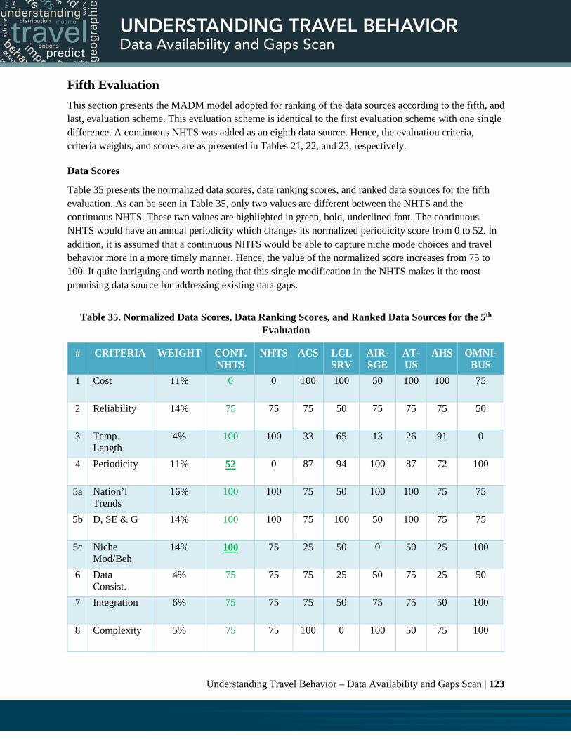
Understanding Travel Behavior – Data Availability and Gaps Scan | 123
Fifth Evaluation This section presents the MADM model adopted for ranking of the data sources according to the fifth, and last, evaluation scheme. This evaluation scheme is identical to the first evaluation scheme with one single difference. A continuous NHTS was added as an eighth data source. Hence, the evaluation criteria, criteria weights, and scores are as presented in Tables 21, 22, and 23, respectively.
Data Scores
Table 35 presents the normalized data scores, data ranking scores, and ranked data sources for the fifth evaluation. As can be seen in Table 35, only two values are different between the NHTS and the continuous NHTS. These two values are highlighted in green, bold, underlined font. The continuous NHTS would have an annual periodicity which changes its normalized periodicity score from 0 to 52. In addition, it is assumed that a continuous NHTS would be able to capture niche mode choices and travel behavior more in a more timely manner. Hence, the value of the normalized score increases from 75 to 100. It quite intriguing and worth noting that this single modification in the NHTS makes it the most promising data source for addressing existing data gaps.
Table 35. Normalized Data Scores, Data Ranking Scores, and Ranked Data Sources for the 5th Evaluation
# CRITERIA WEIGHT CONT. NHTS
NHTS ACS LCL SRV
AIR-SGE
AT-US
AHS OMNI-BUS
1 Cost 11% 0 0 100 100 50 100 100 75
2 Reliability 14% 75 75 75 50 75 75 75 50
3 Temp. Length
4% 100 100 33 65 13 26 91 0
4 Periodicity 11% 52 0 87 94 100 87 72 100
5a Nation’l Trends
16% 100 100 75 50 100 100 75 75
5b D, SE & G 14% 100 100 75 100 50 100 75 75
5c Niche Mod/Beh
14% 100 75 25 50 0 50 25 100
6 Data Consist.
4% 75 75 75 25 50 75 25 50
7 Integration 6% 75 75 75 50 75 75 50 100
8 Complexity 5% 75 75 100 0 100 50 75 100

Understanding Travel Behavior – Data Availability and Gaps Scan | 124
# CRITERIA WEIGHT CONT. NHTS
NHTS ACS LCL SRV
AIR-SGE
AT-US
AHS OMNI-BUS
Data Ranking Score 80.6 67.4 71.3 64.5 62.5 79.8 67.1 76.5
Ranked Data Sources 1 5 4 7 8 2 6 3
SENSITIVITY ANALYSIS
One additional analysis step was performed to investigate the reliability of the calculated results and identified data sources ranks. In this step, changes in ranked data sources were investigated as a result of a single-unit unilateral change in each of the assigned data scores. Figure 39 depicts the results of this analysis. Cell values in the figure are color coded. Green, red, and yellow colors indicate that the data source rank is sensitive to a unit change in this respective cell’s value. The green color indicates that it is sensitive to only a unit decrease in the cell’s value. Red indicates that it is sensitive to only a unit increase in the cell’s value. Yellow indicates that it is sensitive to a unit decrease or increase in the cell value. While a lighter color indicates that the data source ranking changes by a single rank, a darker color indicates that it changes by two ranks. Investigating the results of Figure 39 reveals the following three observations. Position of the top two ranked data sources does not appear to be sensitive to any single-unit
unilateral change in any of the assigned data scores. While several unit changes can result in these two data sources exchanging positions, no single-unit change makes either of them drop to third position.
ACS seems to have a stable third position. Only one value (decrease of the score that reflects its ability to forecast national trends) can result in its position descending to fourth rank.
Positions of the four remaining data sources seem to be more sensitive to assigned data scores, with many values resulting in ascent or descent of their identified ranking.
In general, according to the first evaluation scheme, the results indicate that the data sources may be classified into four groups, in terms of their potential for addressing the identified data gaps:
1. Two most promising data sources: ATUS and omnibus surveys 2. ACS 3. NHTS, AHS, and local surveys 4. AirSage.

Understanding Travel Behavior – Data Availability and Gaps Scan | 125
Figure 39. Sensitivity of Results of First Evaluation to a One-Unit Unilateral Change in Data Scores
SUMMARY
The previous chapter, Chapter 4, concluded by selecting seven most promising data sources to address the eight identified HPINs. This chapter, Chapter 5, developed and applied a rating scheme to rank these seven data sources in terms of their prospects for addressing this set of HPINs. The chapter started by developing an MADM rating scheme to rank the seven promising data sources. It introduced the different components of the adopted MADM. They include: a) defining the evaluation criteria, their measurement scales, and scale direction; b) determining the criteria weights using the Pairwise Comparison method; c) determining the data scores with respect to every evaluation criterion; and d) ranking of the data sources by normalizing the data scores, calculating the data ranking scores, and determining the ranked data sources. Then, the chapter applied the developed rating scheme to rank the data sources. Five different evaluation runs were developed and presented in the chapter. Differences between these evaluation runs are attributed to differences in the evaluation criteria and criteria weights. Results of the evaluation runs produced consistent results: ATUS and omnibus surveys seemed to consistently rank as the top two most

Understanding Travel Behavior – Data Availability and Gaps Scan | 126
promising data sources, followed by ACS. NHTS seemed to rank in the middle range, between third and fifth, followed by the local surveys. At the end, AirSage and AHS seem to rank in the sixth and seventh positions. While it could seem surprising that the NHTS consistently ranked in the middle (because NHTS is the most comprehensive travel behavior dataset), it should not be unexpected. Since this project was originally motivated by an attempt to identify data gaps and address HPINs that are not presently possible to answer using traditionally used data sources, the findings seem possible. The fifth and last evaluation run provided a particularly interesting finding. In addition to the seven promising data sources, it introduced and ranked and ranked an additional eighth data source: a continuous NHTS. Interestingly, results of this evaluation run indicated that a continuous NHTS ranked at the top; indicating it would be the most promising data source solution for addressing this set of HPINs. While the relatively consistent results of the five different evaluation runs provided proof about the reliability of the findings in regards to sensitivity to the chosen evaluation criteria and determined criteria weights, it did not examine their sensitivity to the assigned data scores. Therefore, the last part of this chapter examined the sensitivity of the results with respect to the assigned data scores. The last part of this chapter presented a sensitivity analysis, where the sensitivity of the resultant data rankings were examined against a single-unit unilateral change in the assigned data scores. Results of this sensitivity analysis seemed to confirm the earlier findings: ATUS and omnibus surveys seem to consistently rank as the top two most promising data sources, followed by ACS. NHTS seems to rank in the middle range, between third and fifth, followed by the local surveys. At the end, AirSage and AHS seem to rank in the sixth and seventh positions. Perhaps the most interesting finding in this chapter pertains to a continuous NHTS, which was identified as the most promising data source for addressing the identified set of data gaps. Yet, another similarly valuable finding include that neither of the top two ranking data sources (ATUS and omnibus surveys) is currently considered as a mainstream resource for understanding or modeling of travel behavior. Therefore, it appears that could be much to gain by imploring and capitalizing on these possibly underutilized data sources. It is also particularly interesting to observe that while none of the eight ranked data sources (including the continuous NHTS) achieved a total ranking score that was greater than 81%, many of the individual data scores achieved the top rank for specific evaluation criteria. This observation is potentially highly valuable because it indicates the possibility of achieving even higher scores by fusing data from a number of data sources. The next chapter, Chapter 6, introduces the data sources and attributes that are planned to be included in the metadata database of the different promising data sources investigated in this work.

Understanding Travel Behavior – Data Availability and Gaps Scan | 127
CHAPTER 6.0. DATABASE
INTRODUCTION
The last component of this project involves the creation of a database of data sources and associated metadata. The objective of this chapter involves introducing the reader to the datasets and associated attributes included in the produced database. In accordance with preference of the FHWA project manager, Ms. Heather Rose, it was decided to construct the database using Microsoft Excel. The following sections include an overview of the data sources and data source attributes included in the Excel database. Figure 40 depicts the graphical flow of Chapter 6.
Figure 40. Content Flow of Chapter 6
DATA SOURCES
Table 36 presents is a list of the data sources included in the Excel database. A few of the proprietary data sources reviewed in the preceding chapters were not included in the database. This is due to difficulties in obtaining complete metadata about these data sources from the data owners.

Understanding Travel Behavior – Data Availability and Gaps Scan | 128
Table 36. Data Sources Included in the Excel Database
ID DATA SOURCE
1 National Household Travel Survey (NHTS)
2 Highway Performance Monitoring System (HPMS)
3 American Community Survey (ACS)
4 Census Transportation Planning Package (CTPP)
5 American Time Use Survey (ATUS)
6 American Housing Survey (AHS)
7 National Transit Database (NTD)
8 National Performance Management Research Data Set (NPMRDS)
9 Here
10 Inrix
11 AirSage
12 NREL’s TSDC 1: CA 2012 Household Travel Survey
13 NREL’s TSDC 2: Atlanta Regional Commission 2011 Regional Travel Survey
14 NREL’s TSDC 3: Texas DOT 2002-2011 Regional Travel Surveys
15 NREL’s TSDC 4: Metropolitan Council of Minneapolis/St. Paul 2010 Travel Behavior Inventory
16 NREL’s TSDC 5: Chicago 2007 Regional Household Travel Inventory
17 NREL’s TSDC 6: Puget Sound Regional Council 2004–2006 Traffic Choices Study
18 NREL’s TSDC 7: Mid-America Regional Council — 2004 Regional Travel Study
19 NREL’s TSDC 8: Southern California Association of Governments — 2001–2002 Regional Travel Survey
20+ Most Recent and Complete Data Sets in the Metropolitan Travel Survey Archive (MTSA)
DATA SOURCE ATTRIBUTES
Table 37 presents is a list of the selected data source attributes included in the Excel database. In order to provide the database user with more information; most of the attributes included in the database are descriptive.

Understanding Travel Behavior – Data Availability and Gaps Scan | 129
Table 37. Data Source Attributes Included in the Excel Database
ID ATTRIBUTE NAME
EXPLANATION
1 ID Automatically generated ID number
2 Name e.g., National Household Travel Survey
3 Acronym e.g., NHTS
4 Short Description e.g., AirSage data collects cellphone traces and produces trip tables
5 Data Components e.g., 4 tables: HHs, persons, trips, vehicles
6 Data Type e.g., household travel survey, cellphone trace data, etc.
7 Data Collection Method
e.g., CATI, etc.
8 Data Structure e.g., cross-sectional, panel, random, etc.
9 Data Size (Records) Number of data records
10 Data Size (Digital Storage)
Megabytes of digital storage
11 Data Size (Variables)
Number of attributes
12 Data Content Types of attributes, e.g., socioeconomic, traffic, travel, GPS, etc.
13 Geographical Coverage
Geographic coverage of data; e.g., national, specific state, specific city, etc.
14 Geographical Unit Smallest geographic unit reported in data source: e.g., TAZ, Census Blocks, State, Urban/Rural, etc.
15 First Year of Data Collection
e.g., 1969, 2001, etc.
16 Most Recent Year of Data Collection
e.g., 2013, 2015, etc.
17 Data Periodicity Annual, monthly, daily, etc.
18 Consistency Changes in data structure, design and attributes
19 Ownership Who owns the data source, e.g., FHWA, U.S. Census Bureau, etc.
20 Relative Cost of Data Collection
e.g., High, Moderate, Low
21 Price of Data e.g., free, time-dependent, space-dependent, etc.
22 Contractor Agency/company that performed data collection
23 Data Website e.g., http://www.airsage.com
24 Relevant Attributes e.g., commute, telecommute, socioeconomic, demographic and geographic in ACS

Understanding Travel Behavior – Data Availability and Gaps Scan | 130
ID ATTRIBUTE NAME
EXPLANATION
25 Examples of Possible Uses
e.g., VMT, PMT, HPINs, Travel Demand, Traffic Operation, etc.
26 Relevance to Project Relevance to the 3 assessment criteria identified in the projects’ statement of work: 1) National Trends; 2) Geographic, Socioeconomic & Demographic Impacts; and 3) Impacts of Emerging Modes and Niche Behavior
27 Manuals Names (and web addresses) of existing data source manuals and other beneficial documents
28 Analysis Tools Existing analysis tools specifically developed for the data source
29 Comments Any notes
SUMMARY
The last component of this project involved the creation of a database of the data sources explored in this project, and associated metadata. This chapter provided an overview of all the data sources and attributes that are included in the created MS Excel database. The next chapter, Chapter 7, provides overall summary and conclusions of this report, and recommendations for future work.

Understanding Travel Behavior – Data Availability and Gaps Scan | 131
CHAPTER 7.0. SUMMARY, KEY FINDINGS, AND FUTURE WORK
INTRODUCTION
In the past few decades, and particularly in recent years, transportation science has increasingly shifted towards being data driven. The existence of high quality and continuously generated data sources has become a major factor for adequate understanding of travel behavior; forecasting of future travel demands; and management, design, and operation of our transportation infrastructure. As a result, over time, many different data sources have been developed and are being continually utilized to serve the varying needs of transportation research, policy, planning, design, and operation. However, as transportation science advances and simultaneously shifts towards becoming more data driven, the type and quality of needed data changes accordingly. In addition, concurrent advances in technology result in the creation of novel travel modes and travel behaviors. Furthermore, advances in survey and data sourcing technologies open the door for new data possibilities. The combination of the above factors leads to a need for continuous evaluations of the suitability of the existing travel behavior models and travel behavior datasets. Observations on unprecedented and unpredicted changes in travel behavior and travel behavior trends in recent years make this need even more critical. Accordingly, while the first part of this project provided a state-of-the-art travel behavior research scan, this part provides an inventory and assessment of current and potential data sources that can be used to identify and quantify emerging trends in travel behavior. This chapter is divided into 4 sections. Section 1 is this Introduction. Section 2 provides a summary of the report. Section 3 provides a synthesis of the key findings and Section 4 provides recommendations for future work. Figure 41 depicts the graphical flow of Chapter 7.

Understanding Travel Behavior – Data Availability and Gaps Scan | 132
Figure 41. Content Flow of Chapter 7
SUMMARY
This report started by identifying traditional, niche, and potentially useful data sources that can be used to identify and quantify emerging trends in travel behavior. Chapter 2 reviewed and provided brief overviews of the traditional data sources. Chapter 3 focused on niche and other potentially relevant data sources. Table 38 presents a list of the data sources reviewed in these two chapters.
Table 38. Traditional, Niche, and Other Potentially Relevant Data Sources Reviewed in Chapters 2 and 3
TRADITIONAL NICHE OTHER RELEVANT
NHTS HPMS (and TVT) ACS (and CTPP)
Local Surveys (NREL’s TSDC and MTSA)
NPMRDS/Here AirSage ATUS NTD
SHRP2’s NDS Travel Apps (Waze, Metropia,
Uber, and Ridescout)
DMV and Insurance HSS NTS AHS
LBSN Datasets Omnibus Surveys
USPS ITS/RIITS
RDE In order to identify the most promising data sources out of all data sources reviewed in Chapters 2 and 3, Chapter 4 examined the potential of the traditional, niche, and other relevant data sources for addressing the high-priority information needs (HPINs) identified in the first part of this project. Chapter 4 concluded by identifying seven promising data sources. These data sources are highlighted using green, italic font in Table 38. They are NHTS, ACS, local surveys, AirSage, ATUS, AHS, and omnibus surveys.

Understanding Travel Behavior – Data Availability and Gaps Scan | 133
Interestingly, these data sources spanned all three data categories: traditional, niche, and potentially relevant. To evaluate and rank the suitability of these data sources for addressing the eight HPINs identified in the first part of this project, Chapter 5 developed and applied a multi-attribute decision making (MADM) model. Five different evaluations were developed and applied to examine the robustness of the produced evaluation and ranking. The five evaluations were based on different combinations of evaluation criteria, criteria weights, and data sources. In addition, a sensitivity analysis was performed to examine the sensitivity of the ranking to the identified data scores in the MADM model. In general, the results of the MADM model seemed generally consistent, where a continuous NHTS received the highest score/ranking; followed by ATUS and omnibus surveys; then the existing NHTS, ACS, and local surveys. AirSage and AHS received the lowest score/ranking. The last part of this work involved the creation of a MS Excel database that includes the data sources and associated attributes. Chapter 6 presented a list of the included data sources and explanation of the different attributes included in the database.
KEY FINDINGS
The work presented in this report reveals a number of interesting insights and potentially beneficial findings. The most prominent key findings of this work include the following. None of the data sources is independently sufficient: None of the assessed data sources were
found to be completely and independently capable of addressing all of the eight HPINs – identified in the first part of this project. Scores of all data sources ranged between 60 to 80 out of 100. While this is a key finding, it should not be surprising. Rather, it should be expected. Since the motivation of this project was based on observations of unprecedented and unpredicted behavioral trends, particularly at the national level, it seems logical that the reason these trends were not predicted relates to existing data gaps. Accordingly, it seems logical that the existing data sources were found not to include all the needed information.
ATUS: While the American Time Use Survey has received some attention in transportation research, it has not been widely utilized. It was particularly surprising that the ATUS consistently ranked in the top two data sources in all performed evaluations. While the ATUS received high scores for being updated annually and capturing several variables of an individual’s travel behavior throughout a day, one of its major limitations is that it captures only self-reported travel times. It does not capture travel distances. Nonetheless, given the high ranking of the ATUS, it appears that much information can be captured by capitalizing on this under-utilized data source.
Continuous NHTS Solution: while the National Household Travel Survey is undoubtedly the richest and most comprehensive travel behavior data source in the United States, it may seem surprising that it did not rank at the top of the evaluated data sources. The NHTS ranked in the middle range. Closer examination of the NHTS scores revealed that the NHTS received low

Understanding Travel Behavior – Data Availability and Gaps Scan | 134
scores on two particular high-weight evaluation criteria: a) data periodicity (since NHTS is conducted every 7 years); and b) ability to capture impacts of emerging modes and niche behavior (due to being conducted every 7 years, hence, update of survey questions to capture emerging modes and niche behavior is infrequent). The two criterions contributed with respective weights of 11% and 14%, respectively. In light of this finding, the fifth evaluation was developed to examine the impact of conducting a continuous NHTS (instead of every 7 years), similar to ACS. The result of this evaluation revealed that a continuous NHTS was found to earn the highest score/ranking.
Omnibus Surveys: Similar to ATUS, omnibus surveys continuously placed in the top two ranks in all performed evaluations. Unlike all other evaluated data sources that currently exist (i.e., they can be acquired and analyzed), omnibus surveys were evaluated based on their potential. Currently there are not any travel-focused omnibus surveys (discounting the FHWA’s omnibus surveys program, which was discontinued years ago). Hence, it should not be surprising that omnibus surveys consistently ranked high. By definition, omnibus surveys are designed to capture specific trends at specific locations and times. Therefore, the advantages of omnibus surveys includes their flexibility and relatively low cost. Omnibus surveys can design and capture specific travel behavior trends with relatively low cost.
FUTURE WORK
Based on the above findings, details are listed below describing the most relevant future research opportunities. Data Fusion: While none of the assessed data sources was found to be completely and
independently capable of addressing all eight HPINs, different data sources exhibited different levels of strengths with different HPINs. Accordingly, it could be highly beneficial to build data fusion models that capitalize on the strengths of the different data sources to find better and more accurate answers to travel behavior questions. For example, the comprehensiveness of the NHTS could be integrated with the periodicity of the ACS or the ATUS to estimate continuous models of travel behavior trends.
Continuous NHTS: Since a continuous NHTS ranked highest in terms of its potential to address the eight HPINs, it would be beneficial to perform a more comprehensive research that identifies and quantifies potential costs, benefits, and limitations associated with a continuous NHTS.
ATUS: Since ATUS consistently ranked at the top of the evaluated data sources, it seems particularly promising to capitalize on the existence of this data source to address some of the existing data gaps. ATUS seems particularly promising because it is a national, annual, and freely available data source. In addition, it captures many aspects of an individual’s travel behavior during an entire day. Accordingly, it could be specifically beneficial to perform a research project to assess the quality of the ATUS’s travel behavior data as well as identify all potential travel-behavior-related uses of the dataset.

Understanding Travel Behavior – Data Availability and Gaps Scan | 135
Omnibus Surveys: Since omnibus surveys persistently ranked at the top of the evaluated data sources, it would be beneficial to conduct a comprehensive research project to identify particular travel behavior trends that would be most suitable to answer using this data source. Such research would include a cost-benefit analysis of the suitability of omnibus surveys to answer these specific travel behavior questions.
In conclusion, it is probably clear that travel behavior in the United States is experiencing major shifts. In addition, with the continual emergence of new technologies and the near expectations of self-driving vehicles and automated transportation systems, these shifts may continue to exist and possibly shift even further or again. Since understanding of travel behavior represents a critical foundation for efficient planning, design, operation, maintenance, and management of our transportation systems, this leaves transportation professionals with a challenging task. Transportation professionals have two major tools in their toolbox for understanding travel behavior. They are travel data and tools. Accordingly, this work demonstrated that niche and other potentially useful data sources could be valuable in addressing existing or potential information gaps. Additionally, the report developed and presented a tool that transportation professionals could utilize to assess and rank the usefulness of different data sources for addressing a specific data gap or set of data gaps. This should improve the quantity and quality of tools in the toolbox, and improve our understanding of travel behavior and all associated and dependent benefits.

Understanding Travel Behavior – Data Availability and Gaps Scan | 136
ACKNOWLEDGMENT
The authors acknowledge the funding support from the Transportation Futures Team, the Office of Transportation Policy Studies at the U.S. Federal Highway Administration (FHWA). In particular, the authors thank Heather Rose for her role in managing the project for the FHWA and the team reviewers for their constructive feedback. The authors also acknowledge the contribution of the team members in conducting this research effort: Elliot Martin, Susan Shaheen, Balaji Yelchuru, and Rachel Finson.

Produced by Booz Allen Hamilton For U.S. Department of Transportation Federal Highway Administration (FHWA)
Related Documents