Understanding the Lee-Carter Mortality Forecasting Method1 · Understanding the Lee-Carter Mortality Forecasting Method1 ... Lee and Carter developed their approach specifically

Understanding the Lee-Carter Mortality Forecasting Method1

Federico Girosi2 and Gary King3

September 14, 2007

1We appreciate the generosity and insight of Ron Lee and Nan Li for help in understanding theirapproach and the demographic literature in general. Many thanks also to John Wilmoth for veryhelpful comments.

2The RAND Corporation (1776 Main Street, P.O. Box 2138, Santa Monica, CA 90407-2138;[email protected]).

3David Florence Professor of Government, Harvard University (Center for Basic Re-search in the Social Sciences, 34 Kirkland Street, Harvard University, Cambridge MA 02138;http://GKing.Harvard.Edu, [email protected], (617) 495-2027).

Abstract

We demonstrate here several previously unrecognized or insufficiently appreciated proper-

ties of the Lee-Carter mortality forecasting approach, a method used widely in both the

academic literature and practical applications. We show that this model is a special case of

a considerably simpler, and less often biased, random walk with drift model, and prove that

the age profile forecast from both approaches will always become less smooth and unrealistic

after a point (when forecasting forward or backwards in time) and will eventually deviate

from any given baseline. We use these and other properties we demonstrate to suggest when

the model would be most applicable in practice.

The method proposed in Lee and Carter (1992) has become the “leading statistical model

of mortality [forecasting] in the demographic literature” (Deaton and Paxson, 2004). It was

used as a benchmark for recent Census Bureau population forecasts (Hollmann, Mulder

and Kallan, 2000), and two U.S. Social Security Technical Advisory Panels recommended

its use, or the use of a method consistent with it (Lee and Miller, 2001). In the last decade,

scholars have “rallied” (White, 2002) to this and closely related approaches, and policy

analysts forecasting all-cause and cause-specific mortality in countries around the world have

followed suit (Booth, Maindonald and Smith, 2002; Deaton and Paxson, 2004; Haberland

and Bergmann, 1995; Lee, Carter and Tuljapurkar, 1995; Lee and Rofman, 1994; Lee and

Skinner, 1999; Miller, 2001; NIPSSR, 2002; Perls et al., 2002; Preston, 1993; Tuljapurkar

and Boe, 1998; Tuljapurkar, Li and Boe, 2000; Wilmoth, 1996, 1998a,b).

Lee and Carter developed their approach specifically for U.S. mortality data, 1933-1987.

However, the method is now being applied to all-cause and cause-specific mortality data

from many countries and time periods, all well beyond the application for which it was

designed. It thus appears to be a good time to reassess the approach, as the issues these

new applications pose could not have been foreseen by the original authors. See Lee (2000a)

for an earlier effort along these lines.

In this paper, we demonstrate several previously unrecognized or insufficiently appre-

ciated properties of the Lee-Carter model, and use these properties to suggest where and

when the model would be most applicable. Section 1 describes the forecasting method in

some detail. Since the method can be seen as a special case of a principal components

method (Bozik and Bell, 1987; Bell and Monsell, 1991) with a single component , Section 2

summarizes a diverse array of 240 mortality data sets (24 causes of death from 10 countries

each) to give a sense of where the method has a chance of working well. Then, in Section 3

we show that the Lee-Carter model is equivalent to a special type of multivariate random

walk with drift (RWD) model, in which the covariance matrix depends on the drift vector.

The implication of this special structure is that while the RWD estimator is unbiased for

data generated by the Lee-Carter model and other types of data, the Lee-Carter model

is biased for data generated by the general RWD model with arbitrary covariance matrix.

The Lee-Carter estimator is more efficient when data are known to be drawn from the

Lee-Carter model. These observations suggest that, since the RWD does not make any

assumption about the structure of the covariance matrix, while the Lee-Carter approach

does, the Lee-Carter estimator will be preferable to the RWD only when we have high confi-

dence in its underlying assumptions. The similarity of the two models means that the much

1

simpler RWD model and estimator will prove especially useful in elucidating the properties

of the Lee-Carter approach.

Thus, in Section 4 we illustrate a property common to both the Lee-Carter and the

RWD forecasts that has not previously been highlighted in the literature. We show there

that the age profile of such forecasts will always become less smooth after a point (when

forecasting forward or backwards in time) and this nonsmoothness will continue forever,

and will eventually deviate from any given baseline. Finally, in Section 5, we comment

on the Lee and Carter’s second stage reestimation idea and Wilmoth’s (1993) alternative

estimation strategies, based on weighted least squares and maximum likelihood.

1 The Method

1.1 The Model

Let mat denote the log of the mortality rate in age group a (a = 1, . . . , A) and time t

(t = 1, . . . , T ) for one country. The first step of the Lee-Carter method consists of modeling

these mortality rates as

mat = αa + βaγt + εat (1)

where αa, βa and γt are parameters to be estimated and εat is a set of random distur-

bances. The parametrization in (1) is not unique, since it is invariant with respect to the

transformations:

βa à cβa γt à 1cγt ∀c ∈ R, c 6= 0

αa à αa − βac γt à γt + c ∀c ∈ R.

This is not a conceptual obstacle; it merely means that the likelihood associated with the

model above has an infinite number of equivalent maxima, each of which would produce

identical forecasts. In practice, we merely pick an arbitrary but consistent parameterization

sufficient for identification. This can be done by imposing two constraints. We follow Lee

and Carter in adopting the constraint∑

t γt = 0. Unlike Lee and Carter, however, we set∑

a β2a = 1 (they set

∑a βa = 1). This last choice is done only to simplify some calculations

later on, and has no bearing on empirical applications.

The constraint∑

t γt = 0 immediately implies that the parameter αa is simply the

empirical average over time of the age profile in age group a, αa = ma. We therefore

rewrite the model in terms of the mean centered log-mortality rate, mat = mat − ma.

2

Since practical uses of the Lee-Carter model implicitly assume that the disturbances εat

are normally distributed, we rewrite Equation 1 as a multiplicative fixed effects model for

the centered age profile:

mat ∼ N (µat, σ

2)

(2)

E(mat) ≡ µat = βaγt .

In this expression, we use only A+ T parameters (βaγt, for all a and t, represented on

the bottom and right margins of the matrix below) to approximate the A× T elements of

the matrix:

m =

5

10

15

20

25

30

35...

80

1990 1991 1992 1993 1994

m5,0 m5,1 m5,2 m5,3 m5,4

m10,0 m10,1 m10,2 m10,3 m10,4

m15,0 m15,1 m15,2 m15,3 m15,4

m20,0 m20,1 m20,2 m20,3 m20,4

m25,0 m25,1 m25,2 m25,3 m25,4

m30,0 m30,1 m30,2 m30,3 m30,4

m35,0 m35,1 m35,2 m35,3 m35,4

......

......

...

m80,0 m80,1 m80,2 m80,3 m80,4

β5

β10

β15

β20

β25

β30

β35

...

β80

γ0 γ1 γ2 γ3 γ4

m35,0 m35,1 m35,2 m35,3 m35,4

(3)

For example, Lee-Carter approximates m5,0 in the top left cell by the product of the pa-

rameters at the end of the first row and column β5γ0.

Seen in this framework, the Lee-Carter model can also be thought of as a special case

of log-linear models for contingency tables (Bishop, Fienberg, and Holland, 1975; King,

1989: Ch. 6), where cell values are approximated with estimates of parameters representing

the marginals. Indeed, this model is the most basic version of contingency table models,

where one assumes independence of rows (age groups) and columns (time periods), and the

expected cell value is merely the product of the two parameter values from the respective

marginals: E(mat) = βaγt. In a contingency table model, this assumption would be ap-

propriate if the variable represented as rows in the table were independent of the variable

represented as columns. The same assumption for the log-mortality rate is the absence of

age×time interactions — that βa is fixed over time for all a and γt is fixed over age groups

for all t.

Another way to phrase this independence assumption is that the coefficients β do not

vary over time. Lee and Miller (2001) point out that the evidence indicates that most data

3

do not fit this assumption. They recommend the simple solution proposed by Tuljapurkar,

Li and Boe (2000), which consists of using as the base forecasts, the year 1950. This is

equivalent to excluding the portion of the 20th century where most of the change took

place in infant and child mortality. Although this approach works in some countries, it

does not work well in others Booth, Maindonald and Smith (2002). In addition, a one-time

fix for β does not solve the problem that the smoothness of the age profiles declines over

time. Carter and Prskawetz (2000) discuss extensions to the Lee-Carter model to allow for

structural shifts and changes in βa over time.

1.2 Estimation

The parameters βa and γt in model 2 can be estimated via maximum likelihood. However,

the multiple maxima or constraints will make standard optimization programs work poorly.

Fortunately, as Lee and Carter point out, the optima can be found easily via the singular

value decomposition (SVD) of the matrix of centered age profiles, m = BLU ′, where the

estimate for β is the first column of B, and the estimate for γt is β′mt.1 If the SVD decom-

position of m is not available, one can compute as the normalized eigenvector of the matrix

C ≡ mm′ corresponding to the largest eigenvalue (we will use this alternative in Section 3,

to perform some analytical calculations). Whether one uses SVD or eignenvalues to find

the optimum, the theoretical justification of the procedure remains maximum likelihood.

In practice, Lee and Carter suggest, after β and γ have been estimated, that the pa-

rameter γt be re-estimated using a different criterion. This reestimation step, often called

“second stage estimation”, does not always have a unique solution for the criterion outlined

in Lee and Carter (1992). In addition, different criteria have been proposed more recently

(Lee and Miller, 2001; Wilmoth, 1993), and some researchers skip this re-estimation stage

altogether. Since it is not a defining feature of the method we skip this step and return to

this issue in Section 5.

1.3 Forecasting

To produce mortality forecasts, Lee and Carter assume that βa remains constant over

time and they use forecasts of γt from a standard univariate time series model. After

testing several ARIMA specifications, they find that a random walk with drift is the most

appropriate model for their data. They make clear that other ARIMA models might be1We assume that the singular values, the elements on the diagonal of L, are sorted in descending order

and that the columns of B have length one. If not, then the estimate for β is the column of B whichcorresponds to the largest singular value and β should be replaced by β/‖β‖.

4

preferable for different data sets, but in practice the random walk with drift model for γt

has been used almost exclusively. This model is as follows:

γt = γt−1 + θ + ξt

ξt ∼ N (0, σ2rw) (4)

where θ is known as the drift parameter and its maximum likelihood estimate is simply

θ = (γT − γ1)/(T − 1), which only depends on the first and last of the γ estimates.2. Then,

to forecast two periods ahead, we plug in the estimate of the drift parameter θ and also

substitute for the definition of γt−1 shifted back in time one period:

γt = γt−1 + θ + ξt

= (γt−2 + θ + ξt−1) + θ + ξt

= γt−2 + 2θ + (ξt−1 + ξt) (5)

To forecast γt at time T + (∆t) with data available up to period T , we follow the same

procedure iteratively (∆t) times and obtain

γT+(∆t) = γT + (∆t)θ +(∆t)∑

l=1

ξT+l−1

= γT + (∆t)θ +√

(∆t)ξt, (6)

where the second line is a simplification made possible by the fact that the random variables

ξt are assumed in this model to be independent with the same variance. The second line

indicates that the conditional standard errors for the forecast increase with the square root

of the distance to the forecast horizon (∆t). These are conditional standard errors and

would be larger if we included estimation uncertainty.

From this model, we can obtain forecast point estimates, which follow a straight line as

a function of (∆t), with slope θ:

E[γT+(∆t) | γ1, . . . , γT ] ≡ µT+(∆t) = γT + (∆t)θ (7)

The Lee-Carter model for the γ’s is thus very simple: Extrapolate from a straight line drawn

through the first γ1 and last γT points. All other γ’s are ignored.

We now plug these expressions into the empirical and vectorized version of Equation 2

to make a point estimate forecast for log-mortality:

µT+(∆t) = m+ βγT+(∆t)

= m+ β[γT + (∆t)θ]. (8)

2The MLE of the variance is σ2rw = 1

T−1

PT−1t=1 (γt+1 − γt − θ)2 with Var[θ] =

σ2rw

T−1

5

For example, the Lee-Carter model computes the forecast for year 2030, given data

observed from 1950 to 2000, as

µ2030 = m+ β × [γ2000 + 30θ] (9)

= m+ β ×[γ2000 + 30

(γ2000 − γ1950)50

].

2 Information Loss with One Principal Component

As is well known, the estimation stage of Lee-Carter is a special case of principal component

analysis, where the log-mortality data is summarized using only the first single principal

component, with other variation ignored for the purpose of making forecasts.3 The idea of

principal components is that a set of data mat (for all a and t) can be decomposed without

error as the sum of a set of basic shapes. The first shape, or principal component, is βaγt in

Equation 1. The full set includes as many as A components with the relationship holding

exactly and so is written without the need for an error term:

mat = αa + βa1γt1 + βa2γt2 + · · ·+ βaAγtA (10)

where the second subscript of each parameter refers to the principal component number

and the first component βa1γt1 equals βaγt from Equation 1. What was labeled as error

in Equation 1 is now decomposed into the remaining principal components: εat = βa2γt2 +

· · ·+ βaAγtA.

One way to understand the entire set of log-mortality data is as a sequence of time

points moving through A-dimensional space. The hypothesis inherent in the Lee-Carter

model is that the A-dimensional space can be reduced without much loss of information

to one-dimensional space, or in other words that the log-mortality age profiles move along

a straight line in RA. When this assumption is violated for a given dataset, so that one

principal component is insufficient to characterize a large enough proportion of the motion

of the age profiles, then the Lee-Carter model would not be expected to forecast as well.

Since comprehending A-dimensional space is difficult for A > 3, we examine a summary

of the data with the first three principal components and study how closely the first compo-

nent that Lee-Carter uses (i.e., a straight line) fits these three. We do this first graphically3Principal component analysis was first used in demography by Ledermann and Breas (1959), who used

factor analysis to analyze life table data from different countries and then Bozik and Bell (1987) and Siva-murthy (1987) for projecting age-specific fertility rates. The method of Bozik and Bell was then extendedby Bell and Monsell (1991) to forecast age-specific mortality rates, but it was not until Lee and Carter’s(1992) simpler formulation that these methods became widely used (see also Lee, 1993, 2000, 2000a; andLee and Tuljapurkar, 1994, 1998, 1998a). .

6

for a small number of data sets and then summarize each graph with the percentage of

variance explained by 1, 2, and 3 principal components, so that we can display the results

of these analyses for a much larger and more diverse group of data sets.4

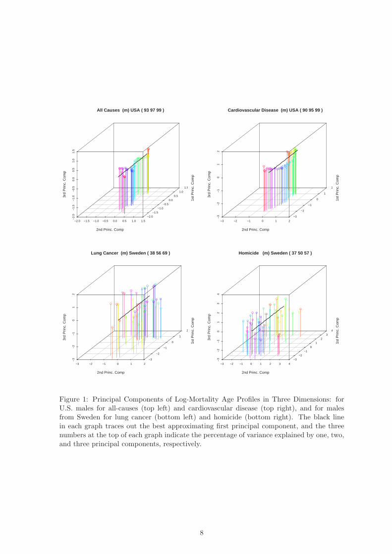
In each of the four graphs in Figure 1, we plot the first three principal components for

one specific population and cause of death for annual data from 1950 to 2000. The first,

second, and third principal components are plotted on the depth, horizontal, and vertical

axes of the graph. Each data point (summarized by the three principal components rather

than the raw data so that we can fit this in only three dimensions) appears as a circle. We

colored the time series of circles (and vertical lines we added for graphical clarity) in the

order of the rainbow (red, orange, yellow, green, blue, indigo, and violet). A solid black line

represents where all the circles should closely cluster around if the Lee-Carter assumption

of one principal component is adequate.

For example, all cause mortality (the top left graph), and to some degree cardiovascular

disease (the top right graph) show that most of the variation in the three dimensions lies

close to the direction of the first principal component (the depth dimension in the graph).

Cardiovascular disease shows some significant systematic nonlinear variation along the sec-

ond principal component (the horizontal dimension), and a smaller amount of variation

along the third (the vertical dimension). Note that the Lee-Carter assumption of a single

principal component does not require that the time series move in one direction along the

line, and indeed the time series of both top graphs jump back and forth along the line

to some degree (see especially the red circles appearing in both graphs near the front and

back).

The three numerical summaries (appearing in the title of each graph) indicates the

percentage of variance explained by the first, second, and third principal components, re-

spectively. Thus, for all-cause mortality (the top left graph), if we try to project the age

profiles on a one-dimensional subspace (which corresponds to the Lee-Carter model) we can

explain 93% of the variance in the data. Using a two-dimensional subspace we can explain

97% of the variance, while adding a third dimension takes us to 99%. Since the scale on the

three axes in each graph is the same, these numbers summarize the figures reasonably well.

4Denote by ε(k)t the error associated with a specification using k principal components: ε

(k)t ≡ mt −

(β1γ1t + β2γ2t + · · ·+ βkγkt). Averaging over time, a specification with k principal components leads to an

error ofPt ‖ε(k)t ‖2. In order to obtain a measure of relative error, which is easier to understand, we divide

this expression byPt ‖mt‖2, which makes it independent of the scale of mt. This ratio, which measures how

bad the k-component approximation is, is always between 0 and 1. Since it is customary to report goodness

rather than badness of fit, the standard measure is ∆Ek ≡ 1−P

t ‖ε(k)t ‖2P

t ‖mt‖2 , which is known as the percentage

of the variance which is “explained” (or linearly accounted for) by the first k principal components: It is 1when the specification with k components has no error, that is explains 100% of the variance.

7

All Causes (m) USA ( 93 97 99 )

−2.0 −1.5 −1.0 −0.5 0.0 0.5 1.0 1.5

−2.

0−

1.5

−1.

0−

0.5

0.0

0.5

1.0

1.5

−2.0−1.5

−1.0−0.5

0.0 0.5

1.0 1.5

2nd Princ. Comp

1st P

rinc.

Com

p

3rd

Prin

c. C

omp

Cardiovascular Disease (m) USA ( 90 95 99 )

−3 −2 −1 0 1 2−

3−

2−

1 0

1 2

−3

−2

−1

0

1

2

2nd Princ. Comp

1st P

rinc.

Com

p

3rd

Prin

c. C

omp

Lung Cancer (m) Sweden ( 38 56 69 )

−3 −2 −1 0 1 2

−3

−2

−1

0 1

2

−3

−2

−1

0

1

2

2nd Princ. Comp

1st P

rinc.

Com

p

3rd

Prin

c. C

omp

Homicide (m) Sweden ( 37 50 57 )

−3 −2 −1 0 1 2 3 4

−3

−2

−1

0 1

2 3

4

−3−2

−1 0

1 2

3 4

2nd Princ. Comp

1st P

rinc.

Com

p

3rd

Prin

c. C

omp

Figure 1: Principal Components of Log-Mortality Age Profiles in Three Dimensions: forU.S. males for all-causes (top left) and cardiovascular disease (top right), and for malesfrom Sweden for lung cancer (bottom left) and homicide (bottom right). The black linein each graph traces out the best approximating first principal component, and the threenumbers at the top of each graph indicate the percentage of variance explained by one, two,and three principal components, respectively.

8

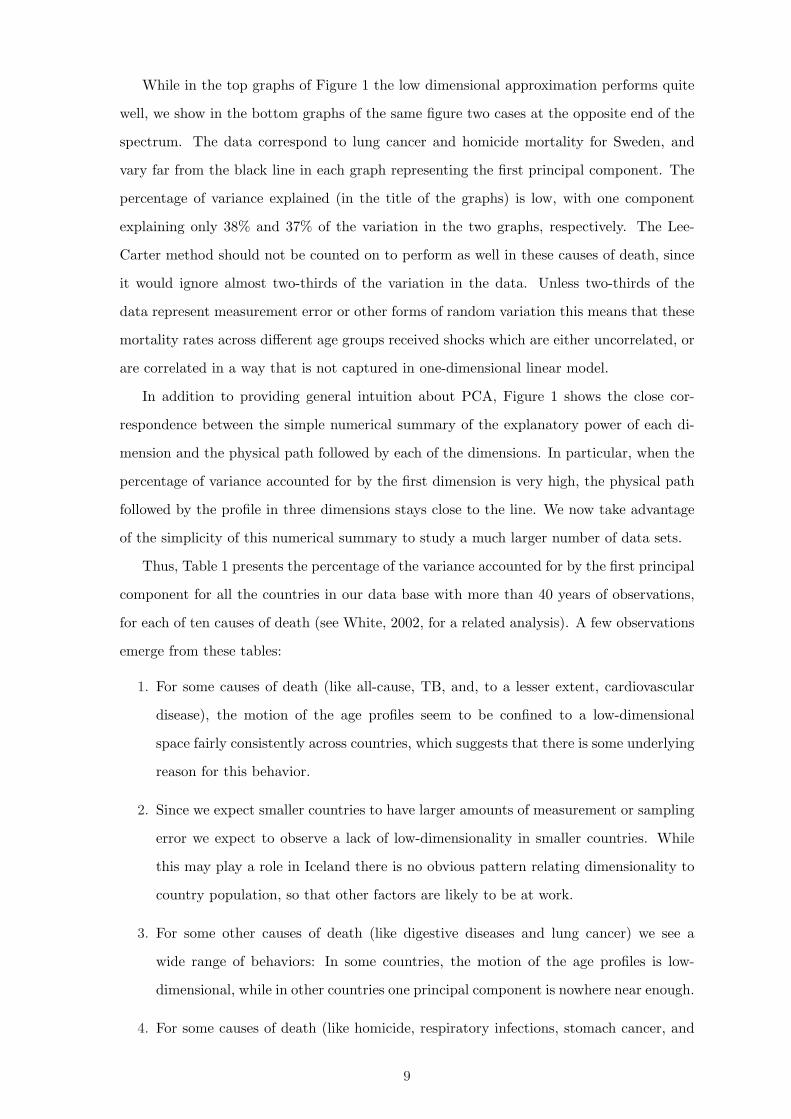
While in the top graphs of Figure 1 the low dimensional approximation performs quite

well, we show in the bottom graphs of the same figure two cases at the opposite end of the

spectrum. The data correspond to lung cancer and homicide mortality for Sweden, and

vary far from the black line in each graph representing the first principal component. The

percentage of variance explained (in the title of the graphs) is low, with one component

explaining only 38% and 37% of the variation in the two graphs, respectively. The Lee-

Carter method should not be counted on to perform as well in these causes of death, since

it would ignore almost two-thirds of the variation in the data. Unless two-thirds of the

data represent measurement error or other forms of random variation this means that these

mortality rates across different age groups received shocks which are either uncorrelated, or

are correlated in a way that is not captured in one-dimensional linear model.

In addition to providing general intuition about PCA, Figure 1 shows the close cor-

respondence between the simple numerical summary of the explanatory power of each di-

mension and the physical path followed by each of the dimensions. In particular, when the

percentage of variance accounted for by the first dimension is very high, the physical path

followed by the profile in three dimensions stays close to the line. We now take advantage

of the simplicity of this numerical summary to study a much larger number of data sets.

Thus, Table 1 presents the percentage of the variance accounted for by the first principal

component for all the countries in our data base with more than 40 years of observations,

for each of ten causes of death (see White, 2002, for a related analysis). A few observations

emerge from these tables:

1. For some causes of death (like all-cause, TB, and, to a lesser extent, cardiovascular

disease), the motion of the age profiles seem to be confined to a low-dimensional

space fairly consistently across countries, which suggests that there is some underlying

reason for this behavior.

2. Since we expect smaller countries to have larger amounts of measurement or sampling

error we expect to observe a lack of low-dimensionality in smaller countries. While

this may play a role in Iceland there is no obvious pattern relating dimensionality to

country population, so that other factors are likely to be at work.

3. For some other causes of death (like digestive diseases and lung cancer) we see a

wide range of behaviors: In some countries, the motion of the age profiles is low-

dimensional, while in other countries one principal component is nowhere near enough.

4. For some causes of death (like homicide, respiratory infections, stomach cancer, and

9

suicide) little evidence exists that the age profiles can be reduced to this lower dimen-

sional summary (indeed even three principal components, which we do not present

here) is insufficient in most situations.

5. For any given country, the percentage of the variance accounted for varies considerably

across causes of deaths.

All Cardio- Lung Homi- Respir- Stomach Other Sui- Diges-cause vascular cancer cide TB atory cancer cancer cide tive

Japan 98 87 96 74 97 69 66 62 65 97Chile 97 92 48 52 96 52 71 55 79 87Canada 95 77 84 38 89 50 64 80 85 79Australia 95 79 64 16 84 37 61 67 66 79U.K 94 72 77 60 91 80 70 87 87 83Mexico 93 81 77 64 97 82 32 71 63 97USA 93 90 81 70 94 78 63 95 91 85Austria 93 49 44 16 86 35 61 69 34 76Italy 92 74 88 43 93 61 46 70 60 90Finland 92 56 49 21 88 37 75 56 52 72Belgium 92 70 78 40 85 47 57 67 80 70Portugal 91 62 80 21 91 34 34 46 45 87Switzerland 91 36 45 22 83 24 64 53 33 75France 90 89 93 44 94 78 56 74 80 84Sweden 90 41 55 37 82 29 69 62 38 64Spain 89 91 93 66 94 74 54 74 73 94Netherlands 89 40 78 41 81 39 61 70 72 70Venezuela 86 64 46 50 93 37 52 43 23 93Hungary 85 64 86 30 79 39 52 62 73 79Norway 84 29 64 24 82 24 66 64 66 56Ireland 83 57 68 28 86 37 59 43 70 71New Zealand 82 57 40 19 79 40 40 34 59 61Denmark 70 39 58 31 67 36 56 51 48 55Iceland 57 53 42 40 54 20 55 18 18 32

Table 1: Percentage of Variance Explained in Male Mortality by the First Principal Com-ponent. Bold entries, indicating 90% or higher, highlight where Lee-Carter is more likelyto work well.

The main point of this table is the absence of any simple story that could explain the

patterns. As a result, one needs to be careful when analyzing the age profiles of different

countries, groups, and causes: Methods that rely on the assumption of low-dimensionality,

such as Lee-Carter, will usually be appropriate only for idiosyncratic choices of countries

and causes of death, and most importantly, there is no way to know ex ante which those

are. Across many countries, one principal component fits all-cause mortality well, even

outside the few developed countries for which the method was designed and where Lee and

Carter intended the method to be applied, although for other countries the fit is poor. One

principal component fits cause-specific data more rarely, which supports Lee and Carter’s

views that the method should not routinely be used in these applications.

10

3 The Lee-Carter Model and the Random Walk with Drift

Although the Lee-Carter model can be estimated with any time series process applied to

forecast γt, the random walk with drift specification in Equation 4 accounts for nearly all

real applications. This specification implies that the functional form of the forecast is no

different from the one obtained by a multivariate random walk with drift (RWD), although

with a different value for the drift parameter. In this section, we analyze the full two-stage

Lee-Carter model and estimator and discuss the following observations:

1. When considered together, the two stage Lee-Carter approach is shown to be equiv-

alent to a particular type of random walk with drift (RWD) model. The crucial

difference between the two is that in the Lee-Carter model the covariance matrix of

the error term is explicitly dependent on the parameter vector β, while in the RWD

the covariance matrix is not restricted.

2. If data are generated from the Lee-Carter model, then the Lee-Carter estimator and

the RWD estimator are both unbiased.

3. If the data are generated by the RWD model, then the two-stage Lee-Carter estimator

is biased, but the RWD estimator is unbiased.

These results thus pose the question of why or when one would prefer to use the Lee-

Carter estimator over the simpler RWD estimator. Empirically the Lee-Carter estimator

does not appear to perform better than the RWD (Bell, 1997) in short-term U.S. mortality

forecasts, but unfortunately for long-term forecast and more general cases no evidence

exists about which method performs better. We find that posing this question contributes

to understanding, since the RWD model is much easier to understand and apply.

It seems likely that the answer to this question depends on the framework in which the

Lee-Carter is applied. Researchers whose only interest is to produce a forecast may find

it more convenient to use the random walk with drift. However, researchers interested in

developing new models will find in the Lee-Carter method a solid starting point, and can

take advantage of the large body of knowledge already available on the performance of this

model.

After demonstrating these points in this section, we then use these results in the next

section to highlight some important properties of the Lee-Carter and RWD model that have

not been noted in the literature previously.

11

3.1 The Multivariate Random Walk with Drift Model

We begin with the pure mulitivariate random walk with drift (RWD) model on a multivariate

time series for the A× 1 vector mt (for t = 1, . . . , T ), which we write as

mt = mt−1 + ψ + ηt (11)

where ηt is normal random error with mean zero and A×A variance matrix Σ, and ψ is an

A× 1 vector of drift parameters.

The maximum likelihood estimate depends only on the first and last data points:

ψ =1

T − 1(mT −m1) (12)

with estimation uncertainty Var[ψ] = Σ/(T − 1). Proceeding similarly to Section 1.3 (see

Equation 6, Page 5), the stochastic forecast at time T +(∆t) with data observed up to time

T is

mT+(∆t) = mT + (∆t)ψ +√

(∆t)ηt

and its conditional point estimate is a linear function of time:

E[mT+(∆t) | m1, . . . ,mT ] = mT + (∆t)ψ. (13)

Thus, to forecast under the multivariate random walk with drift model, we merely draw a

straight line through the first and last data points and extrapolate.

3.2 Lee-Carter as a Random Walk with Drift

The Lee-Carter model was originally specified in two stages, described by the following

equations:

mt = m+ βγt + εt

γt = γt−1 + θ + ξt (14)

where the vector εt and the scalar ξt are independent normal random error terms with

variances σ2I and σ2rw, respectively. The two equations in 14 can be combined in one single

expression, so that the specification of the model then becomes:

mt = mt−1 + θβ + (βξt + εt − εt−1), (15)

where the parentheses denote the error term. We now equalize this expression with the

conditional point estimate from the pure random walk with drift model in Equation 11 by

12

noting that the drift parameter vector is θβ here and ψ in the more general random walk.

If we add to this the Lee-Carter normalization, we get θ = ‖ψ‖ and β = ψ‖ψ‖ , and thus

θβ = ψ. We can now rewrite Equation 15 as

mt = mt−1 + ψ +(

ψ

‖ψ‖ξt + εt − εt−1

). (16)

Thus, the only difference between the Lee-Carter model in Equation 16 and the RWD in

Equation 11 is the special restricted error term of Lee-Carter. In the standard RWD model

no structure is imposed on how shocks to mortality are correlated across age groups: The

covariance of the noise is an arbitrary matrix Σ, which is unrelated to the drift vector ψ

and not restricted. In the Lee-Carter model the error term (denoted by parentheses) is a

function of the drift vector ψ and therefore in the covariance matrix of the noise, which can

be written as follows:

ΣLC = σ2rw

ψψ′

‖ψ‖2+ 2σ2I (17)

This shows that in the Lee-Carter model shocks to mortality can be of only two kinds: The

term (εt−εt−1), with variance 2σ2I, describes shocks that are uncorrelated across age groups.

In contrast, the term ( ψ‖ψ‖ξt), with variance σ2

rwψψ′/‖ψ‖2, describes shocks that are perfectly

correlated across age groups. In addition, the relative size of the perfectly correlated Lee-

Carter shocks is restricted to be equal to the relative size of the rate of decline of mortality

over time (since β = ψ‖ψ‖). (For example, the ratio between the size of shock in age group 70

and in age group 60 is always equal to β70

β60.) Therefore, Lee-Carter assumes that age groups

whose mortality rates have been declining faster than others are assumed to receive larger

shocks. If the observed rate of change in mortality in a certain age group is indicative of its

“susceptibility to change,” we might expect that future mortality shocks to have the largest

affect on age groups that have already been declining the fastest. A problem is that it is not

immediately clear what these shocks represent. They must have zero mean, so they cannot

be epidemics or other negative health events (many of which also would target specific age

groups), but they could relate for example to weather patterns, changes in pollution levels,

or perhaps funding of health care facilities. The difficulty with the Lee-Carter specification,

that does not afflict the RWD model, is that shocks to mortality other than those that are

perfectly correlated or uncorrelated across age groups will be missed by the model.5

5Another way to look at Equation 16 is to think of it as a random walk mt = mt−1 + ψt + (εt − εt−1)with stochastic drift ψt = ψ

‖ψ‖ (‖ψ‖ + ξt) that has fixed direction ψ‖ψ‖ but whose length (‖ψ‖ + ξt) is

normally distributed around the mean. While this particular model is not well known, it is reminiscent ofthe commonly used “local linear trend” (LLT) model, in which the drift vector follows a random walk, ratherthan being stationary (Harvey, 1991). Again, the distinctive feature here is that shocks are constrained:the drift vector is only allowed to vary in length, and not in direction, fixing the relative sizes of the shocksacross age groups.

13

The observations above clarify the difference between the Lee-Carter model and the

RWD model. To summarize, the difference lies in the nature of the shocks to mortality,

which in the Lee-Carter model are restricted in a way which explicitly depends on the drift

vector. In other words, Lee-Carter can be thought of as a RWD model with an uninformative

prior on ψ but an extremely strong prior on the covariance matrix Σ.6 Priors of course can

be very useful, but if the wrong prior is selected results could be biased, and one may be

better off without prior. An example of this bias can be seen if we study the output of one

model when the data are generated from another, the issue to which we now turn.

3.2.1 Using the Random Walk with Drift Model on Data Generated by theLee-Carter Model

Let us assume now that mortality data are generated according to the Lee-Carter model.

What would happen if we attempt to forecast them using the random walk with drift

model? It is trivial to see that the RWD estimate for the drift parameter 12 is unbiased,

and therefore it will recover correctly the value of ψ (on average). Arguably this estimate

of ψ may be less efficient than the one obtained by the Lee-Carter model, since we expect

the generating model to be optimal in estimating its own parameters.

3.2.2 Using Lee-Carter Model on Data Generated by the Random Walk withDrift Model

We now show that if data are generated according to a RWD model with an arbitrary

covariance matrix, then the Lee-Carter model will be biased: on average it will not recover

the correct drift parameter. Exceptions will be when the noise in the RWD has spherical

symmetry, and/or shocks occur along the drift vector. The intuition behind this behavior

of the Lee-Carter model is very simple, and can be best understood with the use of figure

2, which refers to a hypothetical case in which there are only two age groups, and therefore

log-mortality in a given year is a point in a plane. In the left panel of the figure we show a

trajectory of log-mortality generated by a RWD with spherical disturbances (in red). The

starting point is at the top right, and mortality decreases over time following a drift vector

whose direction is shown by the dashed line (in black). The continous straight line (in

green) is the projection of log-mortality according to the Lee-Carter model. Therefore the

direction of this line coincides with the direction of the first principal component, which

is almost parallel to the direction of the drift vector. In this case the Lee-Carter model

is not biased. In the right panel we use non-spherical disturbances, and set the ratio

6To be specific, the prior implied by Lee-Carter is P(ψ,Σ) ∝ P(Σ | ψ)P(ψ) = δşΣ− σ2

rwψψ′‖ψ‖2 − 2σ2I

ť

where δ(·) is the point-mass measure.

14

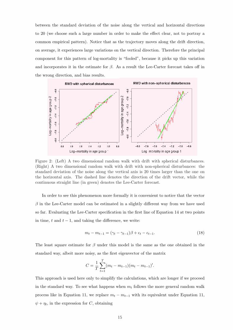
between the standard deviation of the noise along the vertical and horizontal directions

to 20 (we choose such a large number in order to make the effect clear, not to portray a

common empirical pattern). Notice that as the trajectory moves along the drift direction,

on average, it experiences large variations on the vertical direction. Therefore the principal

component for this pattern of log-mortality is “fooled”, because it picks up this variation

and incorporates it in the estimate for β. As a result the Lee-Carter forecast takes off in

the wrong direction, and bias results.

Figure 2: (Left) A two dimensional random walk with drift with spherical disturbances.(Right) A two dimensional random walk with drift with non-spherical disturbances: thestandard deviation of the noise along the vertical axis is 20 times larger than the one onthe horizontal axis. The dashed line denotes the direction of the drift vector, while thecontinuous straight line (in green) denotes the Lee-Carter forecast.

In order to see this phenomenon more formally it is convenient to notice that the vector

β in the Lee-Carter model can be estimated in a slightly different way from we have used

so far. Evaluating the Lee-Carter specification in the first line of Equation 14 at two points

in time, t and t− 1, and taking the difference, we write:

mt −mt−1 = (γt − γt−1)β + εt − εt−1. (18)

The least square estimate for β under this model is the same as the one obtained in the

standard way, albeit more noisy, as the first eigenvector of the matrix

C =1T

T∑

t=1

(mt −mt−1)(mt −mt−1)′.

This approach is used here only to simplify the calculations, which are longer if we proceed

in the standard way. To see what happens when mt follows the more general random walk

process like in Equation 11, we replace mt −mt−1 with its equivalent under Equation 11,

ψ + ηt, in the expression for C, obtaining

15

C =1T

T∑

t=1

(ψ + ηt)(ψ + ηt)′ = ψψ′ +1T

T∑

t=1

ηtη′t +

1T

T∑

t=1

(ψη′t + ηtψ′).

We rewrite this expression as:

C = ψψ′ + Σ + Z (19)

where Z is a random matrix with zero mean. The parameter vector β is now the first

principal component associated to the matrix C in Equation 19: in order for the Lee-Carter

method to be unbiased on average this vector should equal to ψ‖ψ‖ . This clearly cannot

happen in general, because the matrix Σ is arbitrary. The only exceptions occurr when Σ

is the identity matrix, or when the the first principal component of Σ happens, by chance,

to be ψ‖ψ‖ .

We now turn to the demographic implications of these implicit assumptions of the Lee-

Carter model.

4 Smoothness of Age Profiles Under Lee-Carter and RWD

The forecasts produced by Lee-Carter and RWD have identical functional forms: They are

a line in the multidimensional space of age profiles, and we refer to them as linear. Linear

forecasts are unlikely to generate unusual mortality patterns in the short run, although in

the long run some unlikely patterns will often develop. Some of these, such as inversions

in rank order of the age groups’ mortality rates, may or not may not occurr depending on

the data: even if they may look unlikely, they are not intrinisc features of these models.

However, there is one feature which is common to all forecasts of this type no matter what

patterns are present in the data: They will always produce a mortality age profile that

becomes less smooth, and more deviant from any given fixed baseline, over time, after a

point. A key point is that this phenomenon is data independent: If the data were generated

by a model in which the age profiles become smoother over time, these models will not be

able to capture this feature, and will always produce a forecast in which age profiles will

become less smooth overtime after a certain year.

The fact that age profiles may evolve in implausible ways under the Lee-Carter model

has been noted in the context of particular data sets (Alho, 1992). We extend this point

here and demonstrate that it does not depend on the particular time series extrapolation

process used or any idiosyncracies of the data set chosen. This point would also seem to

resolve a major point of contention in the published debates between Lee and Carter (1992)

16

and McNown (1992) about whether the Lee-Carter model sufficiently constrains the out-

of-sample age profile of mortality: Almost no matter what one’s prior is for a reasonable

age profile, Lee-Carter forecasts although they may be reasonable over the short run will

eventually violate it as time passes. Notice that we refer to the Lee-Carter model in the

following, but our arguments apply to the RWD model as well, since they originate from

the assumption of linearity, which is shared by the Lee-Carter and the RWD models.

4.1 Raw Patterns

We begin by examining raw patterns in the data that highlight the consequences of linearity

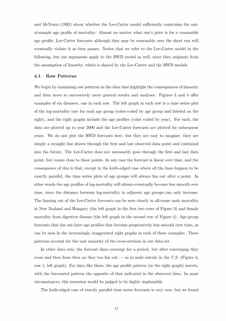
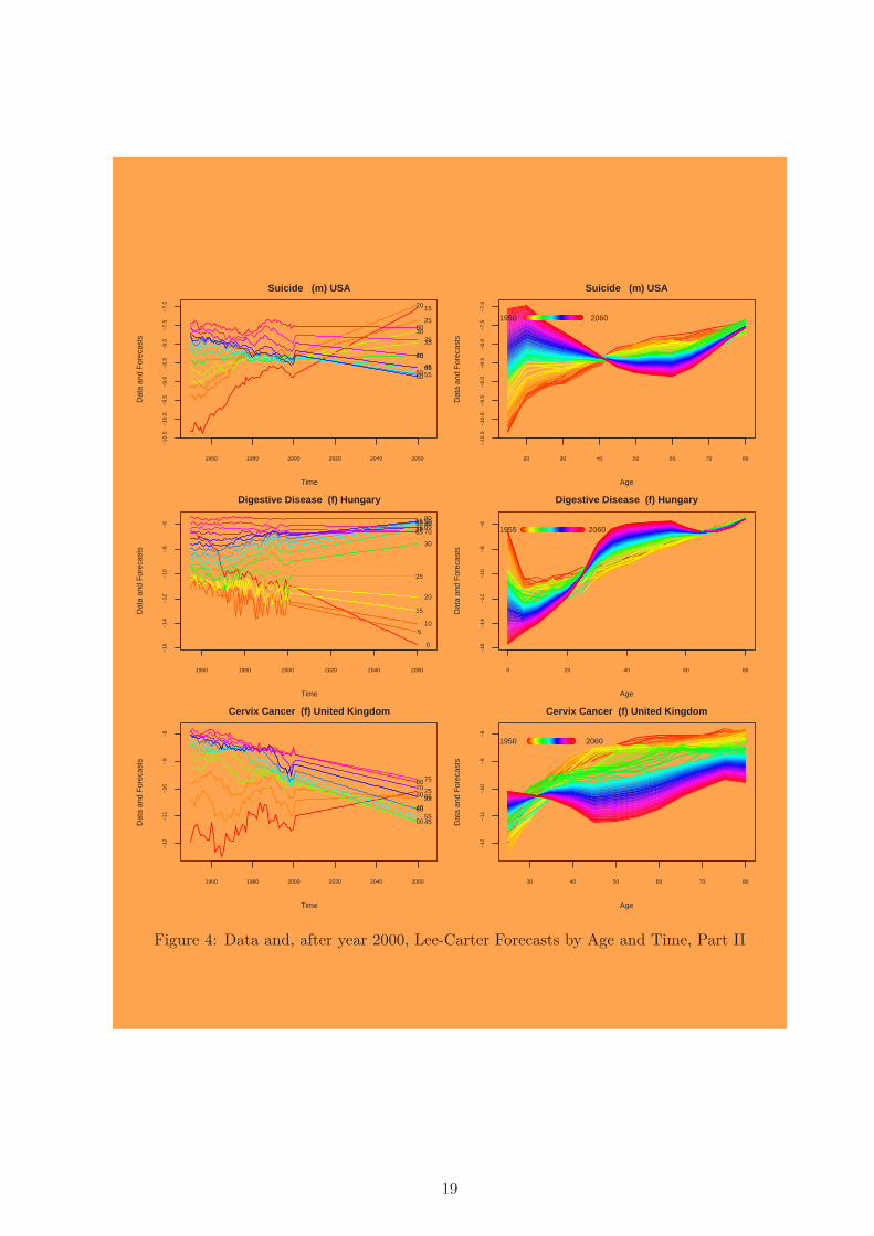
and then move to successively more general results and analyses. Figures 3 and 4 offer

examples of six datasets, one in each row. The left graph in each row is a time series plot

of the log-mortality rate for each age group (color-coded by age group and labeled on the

right), and the right graphs include the age profiles (color coded by year). For each, the

data are plotted up to year 2000 and the Lee-Carter forecasts are plotted for subsequent

years. We do not plot the RWD forecasts here, but they are easy to imagine: they are

simply a straight line drawn through the first and last observed data point and continued

into the future. The Lee-Carter does not necessarily goes through the first and last data

point, but comes close to these points. In any case the forecast is linear over time, and the

consequence of this is that, except in the knife-edged case where all the lines happen to be

exactly parallel, the time series plots of age groups will always fan out after a point. In

other words the age profiles of log-mortality will always eventually become less smooth over

time, since the distance between log-mortality in adjacent age groups can only increase.

The fanning out of the Lee-Carter forecasts can be seen clearly in all-cause male mortality

in New Zealand and Hungary (the left graph in the first two rows of Figure 3) and female

mortality from digestive disease (the left graph in the second row of Figure 4). Age group

forecasts that fan out have age profiles that become progressively less smooth over time, as

can be seen in the increasingly exaggerated right graphs in each of these examples. These

patterns account for the vast majority of the cross-sections in our data set.

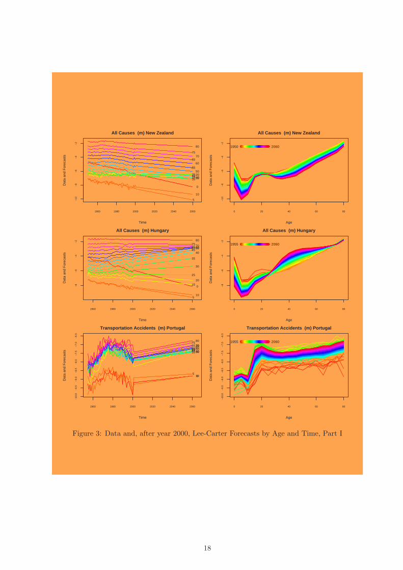
In other data sets, the forecast lines converge for a period, but after converging they

cross and then from then on they too fan out — as in male suicide in the U.S. (Figure 4,

row 1, left graph). For data like these, the age profile pattern (in the right graph) inverts,

with the forecasted pattern the opposite of that indicated in the observed data. In most

circumstances, this inversion would be judged to be highly implausible.

The knife-edged case of exactly parallel time series forecasts is very rare, but we found

17

1960 1980 2000 2020 2040 2060

−10

−8

−6

−4

−2

All Causes (m) New Zealand

Time

Dat

a an

d F

orec

asts

0

5

10

15202530354045

5055

6065

7075

80

0 20 40 60 80

−10

−8

−6

−4

−2

All Causes (m) New Zealand

Age

Dat

a an

d F

orec

asts

1950 2060

1960 1980 2000 2020 2040 2060

−8

−6

−4

−2

All Causes (m) Hungary

Time

Dat

a an

d F

orec

asts

0

510

1520

25

30

35

4045 5055 6065 7075

80

0 20 40 60 80

−8

−6

−4

−2

All Causes (m) Hungary

Age

Dat

a an

d F

orec

asts

1955 2060

1960 1980 2000 2020 2040 2060

−10

.0−

9.5

−9.

0−

8.5

−8.

0−

7.5

−7.

0−

6.5

Transportation Accidents (m) Portugal

Time

Dat

a an

d F

orec

asts

05

10

1520

253035 40455055 60

65 7075

80

0 20 40 60 80

−10

.0−

9.5

−9.

0−

8.5

−8.

0−

7.5

−7.

0−

6.5

Transportation Accidents (m) Portugal

Age

Dat

a an

d F

orec

asts

1955 2060

Figure 3: Data and, after year 2000, Lee-Carter Forecasts by Age and Time, Part I

18

1960 1980 2000 2020 2040 2060

−10

.5−

10.0

−9.

5−

9.0

−8.

5−

8.0

−7.

5−

7.0

Suicide (m) USA

Time

Dat

a an

d F

orec

asts

1520

25

30

35

40

45505560

65

70

75

80

20 30 40 50 60 70 80

−10

.5−

10.0

−9.

5−

9.0

−8.

5−

8.0

−7.

5−

7.0

Suicide (m) USA

Age

Dat

a an

d F

orec

asts

1950 2060

1960 1980 2000 2020 2040 2060

−16

−14

−12

−10

−8

−6

Digestive Disease (f) Hungary

Time

Dat

a an

d F

orec

asts

0

510

15

20

25

30

354045 505560

65 7075

80

0 20 40 60 80

−16

−14

−12

−10

−8

−6

Digestive Disease (f) Hungary

Age

Dat

a an

d F

orec

asts

1955 2060

1960 1980 2000 2020 2040 2060

−12

−11

−10

−9

−8

Cervix Cancer (f) United Kingdom

Time

Dat

a an

d F

orec

asts

253035

40

455055

60

6570

7580

30 40 50 60 70 80

−12

−11

−10

−9

−8

Cervix Cancer (f) United Kingdom

Age

Dat

a an

d F

orec

asts

1950 2060

Figure 4: Data and, after year 2000, Lee-Carter Forecasts by Age and Time, Part II

19

one that was close: male transportation accidents in Portugal (Figure 3, row 3, left graph).

The Lee-Carter forecast lines do not fan out (much) in this data set, and so the age profile

stays relatively constant. Coincidentally, however, this example also dramatically illustrates

the consequences of a forecasting method that ignores all but the first and last data points.

Except in the knife-edged case, the linearity of the forecasts frequently produce implau-

sible changes in the out of sample age profiles. We have already seen the dramatic example

of suicides in U.S. males. For another example, consider forecasts of all-cause male mortality

in New Zealand (Figure 3, first row). In these forecasts, the lines crossing in the left graph

produce implausible patterns in the age profiles, which can be seen in the right graph, with

20-year-olds dying at a higher rate than 40-year-olds. Mortality from cervix cancer in the

United Kingdom (Figure 4, last row) is another exmaple with implausible out-of-sample

age profiles. Cervix cancer is a disease known biologically to increase with age, with the

rate usually slowing after menopause. Although this familiar pattern can be seen in the

raw data in the right graph, the forecasts have lost any biological plausibility.

4.2 Formalizations

We now formalize and generalize the insights illustrated by the empirical analyses in Figures

3 and 4. To do this, we first note that in real data, including all-cause mortality for which the

model was originally designed, the Lee-Carter mortality index γt is typically a monotonic,

although not necessarily linear, function of time. The result we describe here indicates that

in this situation, Lee-Carter age profile forecasts always become less smooth. They may

become more smooth for a period, but they will always become less smooth eventually, and

at that point will continue to become less smooth for every subsequent year. This property,

which would seem to violate one of most well-known relationships in classical demography,

holds regardless of the patterns in the empirical data and for an extraordinarily large range

of different definitions of smoothness.

We now discuss this point in some detail, describing the problem in three distinct ways.

Ultimately, however, the culprit is the following elementary observation: When a one di-

mensional function, such as an age profile, is “stretched”, due to multiplication by a scale

factor, small differences between neighboring values become “amplified”. The one dimen-

sional function we have in mind, of course, is the age profile of the parameters βa, where

the scale factor that stretches the age profile at any point in time is γt.

We begin with the differences in expected log-mortality at any two points in time, t and

the “base period” t0:

20

µat − µat0 = (γt − γt0)βa (20)

To fix ideas, take all the βa positive and γt to be a decreasing function of time, so that

the (γt − γt0) < 0 and hence the expected log-mortality rate µat decreases over time. We

see from Equation 20 that, as time passes, expected log-mortality decreases, relative to the

base period, but at different rates in different age groups: Age groups with βa small will see

very little decrease and age groups with larger βa will see a larger decrease. This illustrates

the universal increasing nonsmoothness property of Lee-Carter forecasts.

An interesting point is that the forecast age profile will always becomes less smooth,

no matter whether we project forward or backward. Or put differently, if the Lee-Carter

forecasts fan out, and we reverse the time index on the data (so that 1950 is switched with

2000, 1951 is switched with 1999, etc.), the forecasts on the altered data set will still fan out.

This demonstrates that universal increasing nonsmoothness is a property of the model, not

of the data. Every difference in βa is thus amplified as we forecast farther into the future

(or past). Any values of βa that are not constant over a, in combination with the particular

parametric form of the Lee-Carter model, are the cause of the problem.7

To clarify and generalize these points, we now compute a direct measure of the smooth-

ness of the log-mortality age profiles generated by the Lee-Carter model, and observe how

it evolves over time. Thus, one simple measure of nonsmoothness is to take the average of

the squared differences between adjacent age groups:

Nonsmoothness(µt) ≡ 1A− 1

A∑

a=2

(µat − µa−1,t)2 (21)

where µt ∈ RA is the age profile of mortality at time t. (This measure is also closely related

to the even simpler variance of the age profiles at any point in time, which also increases in

Lee-Carter forecasts.) In Lee-Carter forecasts, this measure of nonsmoothness will always

increase after a point, and then will continue to increase forever thenceforth. (Proving

this point is slightly more convenient in a more general context, and so delay presenting

the proof for a moment.) The point past which Lee-Carter forecasts become increasingly

nonsmooth without limit will frequently occur before the end of the observed data (as in7We can also study this result by computing the mixed derivatives with respect to age and time: ∂

∂t∂µat∂a

=∂γt∂t

∂βa∂a

. The left side of this expression is the time variation of the slope of the age profile. If γt is monotonicwith time then its time derivative, on the right side, always has the same sign. Therefore the sign of theleft hand side is determined by the sign of the derivative of βa with respect to age. When the profile ofβa has a “bump,” its derivative changes sign, implying that there will be nearby age groups whose slopesmove in different directions over time, decreasing the smoothness of the age profile. This problem would beattenuated if the profile of βa were a monotonic function of age, but unfortunately this is rarely the case(we have not been able to find a single instance of this in any of the countries in our data base).

21

most of the examples in Figures 3 and 4, resulting in the time series plots of age group

forecasts fanning out) but will sometimes occur after the last observed point (in which case

the lines will converge until a point in time, and then diverge from then on, as in male

suicide in the U.S. in Figure 4, row 1). The point here is that the pattern seen in the figures

is perfectly general, when formalized by the expression in Equation 21.

4.3 Empirical Illustrations

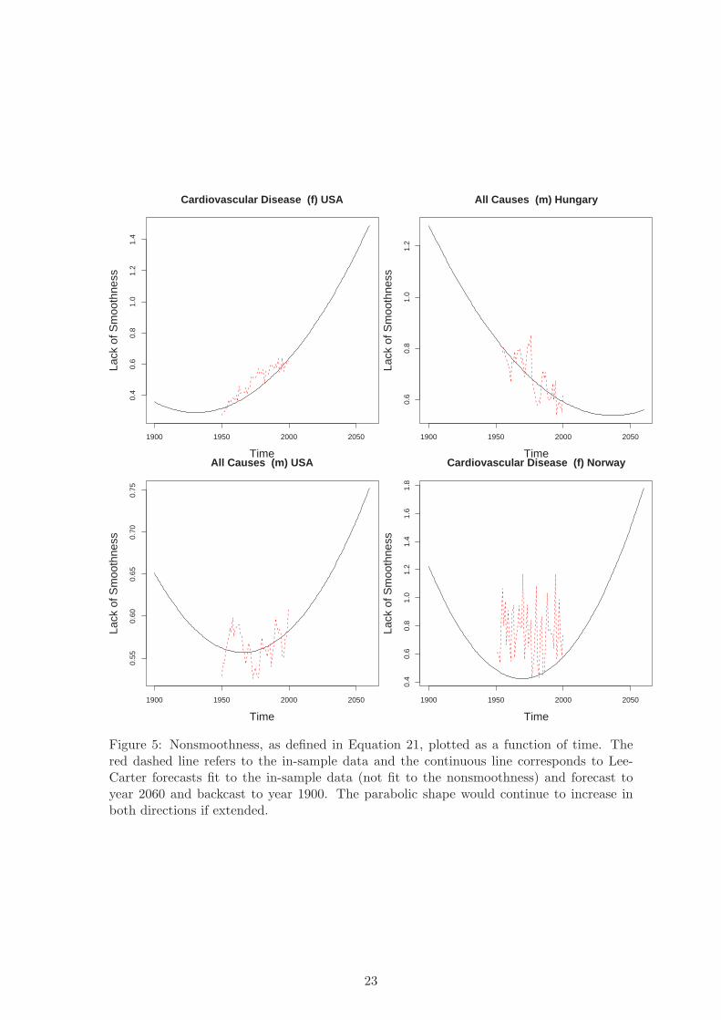
To illustrate this point, we offer Figure 5, which plots the nonsmoothness measure in Equa-

tion 21 applied to observed data (in red dashed lines) and Lee-Carter forecasts (in solid

black lines) up to 2060 and backwards (or “backcast”) to 1900, for four data sets observed

for 1950–2000. (The solid line is thus the smoothness of the Lee-Carter forecast age profile

rather than a forecast of the in-sample smoothness line.) For example, the top left graph

plots nonsmoothness for female cardiovascular disease in the U.S., which has been increas-

ing throughout the entire observed period. The nonsmoothness of the Lee-Carter forecasts

continues this trend into the future, which is obviously plausible. However, the backcasts

turn upward too, which cannot be seen as plausibly related to any empirical trend in the

data.

The top right graph, portraying nonsmoothness for all-cause male mortality in Hungary,

shows almost the opposite pattern. The backcasts seem to extend the trend in the data

upward, which may seem plausible, but the forecasts implausibly turn upward in about

2040, and if extended beyond where the graph ends in 2060 would increase for the rest of

time. Although short term forecasts may not be too severly affected by this property, the

method does not seem appropriate for most term forecasts unless one had some reason to

impose this property on the forecasts, since the patterns produced clearly have nothing to

do with empirical patterns generated by the data.

The two graphs at the bottom of Figure 5 offer examples with no clear in-sample trend in

nonsmoothness, but with nonsmoothness of forecasts and backcasts both increasing fast and

extending far above the range in the data. The bottom right graph, for female cardiovascular

disease in Norway, is especially dispositive, since in these data the first prinicple component

used by Lee-Carter explains only 29% of the variation (see Table 1, Page 10), and so we

might expect that forecasts from the model to “oversmooth.” Yet the nonsmoothness of

the Lee-Carter forecasts (and backcasts) are still rapidly increasing way above that in the

observed data. Taken together, the results from all four figures illustrate the main point:

Lee-Carter forecasts of mortality produce age profiles that are less and less smooth over

22

1900 1950 2000 2050

0.4

0.6

0.8

1.0

1.2

1.4

Cardiovascular Disease (f) USA

Time

Lack

of S

moo

thne

ss

1900 1950 2000 2050

0.6

0.8

1.0

1.2

All Causes (m) Hungary

Time

Lack

of S

moo

thne

ss

1900 1950 2000 2050

0.55

0.60

0.65

0.70

0.75

All Causes (m) USA

Time

Lack

of S

moo

thne

ss

1900 1950 2000 2050

0.4

0.6

0.8

1.0

1.2

1.4

1.6

1.8

Cardiovascular Disease (f) Norway

Time

Lack

of S

moo

thne

ss

Figure 5: Nonsmoothness, as defined in Equation 21, plotted as a function of time. Thered dashed line refers to the in-sample data and the continuous line corresponds to Lee-Carter forecasts fit to the in-sample data (not fit to the nonsmoothness) and forecast toyear 2060 and backcast to year 1900. The parabolic shape would continue to increase inboth directions if extended.

23

time, no matter what trends exist in the empirical data.

A different, more substantive way to make the same methodological point is to suppose

we were interested in forecasting the degree to which the forecast age profile flattens out

over time, an empirical pattern observed in some countries by Lee and Miller (2001). The

point of the study would be to quantify how much flattening there is in various countries,

causes, or groups. The implication of our results is that Lee-Carter would not be of much

use in a study like this because its forecasts will (except sometimes temporarily) never

indicate that the age profile is flattening. Under Lee-Carter, forecast age profile will always

be less and less flat after a point.

4.4 Generalizations

To generalize this result, suppose we (now) recognize that the flattness of the empirical or

forecast age profile (or equivalently the degree of fanning out of the time series age plots)

cannot be reasonably modeled by Lee-Carter in the long run, and we want to move on to

other issues. One way to do this is to use a measure of nonsmoothness that is indifferent to

levels and to slope shifts (or “rotations”) in the age profile. For example, as the standard all-

cause mortality “swoosh” shape rotates clockwise, the degree of flattness increases. Such as

measure is easy to construct by switching from the average first difference used in Equation

21 (a measure that is indifferent only to the level of log-mortality) to the average second

difference, that is differences between each pair of log-mortality differences of adjacent age

groups. This new measure indicates how close adjacent age groups are while ignoring the

absolute level of log-mortality for the entire age profile as well as any slope shifts in the

profile. Put differently, it measures how much log-mortality oscillates over the age groups

around its basic shape, ignoring any drop in average mortality or rotation in the age profile.

Our result indicates that Lee-Carter (or the more general random walk with drift) forecasts

guarantee that, after a point, this oscillation will increase, effectively indicating that even

this adjusted shape will fit less well over time.

To continue generalizing, suppose furthermore that one hypothesized that the shape of

the log-mortality age profile in some theoretical model or model life table is the place to

which log-mortality will eventually converge. To do this, we merely subtract the predicted

age profile from the observed age profile data, and then apply Equation 21, or a version

based on second differences. Our result is that Lee-Carter will still not be able to model the

convergence since it will always forecast that such predictions will become more and more

incorrect over time.

24

We now provide a simple proof of these claims. We begin with the same function in

Equation 21 applied to the mean adjusted age profiles, µat = γtβa (which define the vector

µt), where the adjustment accounts for the overall average shape or predicted pattern of the

log-mortality age profile. (Subtracting out some predicted age profile other than based on

the empirical mean would only slightly complicate this expression.) We express our result

in three ways:

Nonsmoothness(µt) = µ′tWµt (22)

= γ2t β

′Wβ (23)

∝ γ2t (24)

where, for first differences corresponding to Equation 21, W is a tridiagonal matrix with

ones on the diagonal and negative ones on the two adjacent bands. The result, in the

last line of this expression, combined with the empirical result that γt is monotonically

increasing, is enough to show that nonsmoothness will eventually increase as time passes.

To be specific, the lack of smoothness will increase as soon as γt is positive. If γt starts

out negative, the lack of smoothness will drop for a time, until γt is zero, and it will then

increase inexorably as all subsequent years go by. Nonsmoothness bottoms out at a point

that is a function of the predicted age profile. The increase in nonsmoothness after this

point will not stop, and no feature of the data or forecasting method for projecting the γt’s

can make it stop. The U-shaped solid line in Figure 5 is merely a plot Equation 23.

By generalizing the definition of W , so that it can be any semi-positive definite matrix,

Equation 22 can be used to examine the consequences of using any of a very broad class

of nonsmoothness definitions. (Many more sophisticated definitions of smoothness can be

derived, but most lead to quadratic forms like the one above, with different definitions for

W .) The key result of Equation 24 is that no matter what matrix is used for W , and thus no

matter what definition of smoothness one adopts, Lee-Carter forecasts still have the same

universal increasing nonsmoothness property. To be more precise, Equation 24 shows that

nonsmoothness, by any of these definitions, will always increase after a point.

These generalizations extend the substantive areas to which these results apply. They

imply that the same universal increasing nonsmoothness result applies if we consider nons-

moothness only after say age 20 and not before, or we penalize for deviations from smooth-

ness less for younger ages. The weights would merely change the definition of W . Suppose

furthermore that we recognize that the average squared differences in adjacent age groups in

Equation 21 reflects a random walk with drift over age groups and so might not be smooth

25

enough: If we adjust W so this is not an issue, nonsmoothness by this alternative will still

be universally increasing. Alternatively, if instead of using the first or second difference,

we adjust W so that it measures nonsmoothness by the n-th derivative, or the n-th deriva-

tive combined with the m-th derivative, or we adjusted for discreteness or edge effects, or

any of a variety of other patterns and issues, this definition would produce a measure of

nonsmoothness for Lee-Carter forecasts that would still increase after a point and continue

increasing for the rest of time. The cause of these issues is solely because of the assumption

of linearity and would occur regardless of patterns in the data.8

Therefore, forecasts from models such as Lee-Carter and RWD will be appropriate only

if we have external knowledge that the log-mortality age profile will eventually become less

smooth in this way. When mortality forecasts are used to allocate spending to reduce health

risks among chosen age groups, declining smoothness will unrealistically exaggerate alloca-

tion differentials. Insurance companies, which often impose a form of smoothness (or what

they call “graduation”) on the mortality age profiles to keep their insurance schedules look-

ing simple, would presumably find this aspect of the Lee-Carter model to be problematic.

Politically, forecasts that are insufficiently smooth could lead to unnecessarily adversarial

relationships among interest groups supporting research funding for the health problems of

different age groups.

5 Properties of Alternative Estimation Approaches

In this section, we discuss two alternative approaches to estimating the parameters of the

Lee-Carter model.

5.1 Second Stage Reestimation

In their original paper, Lee and Carter (1992) suggest an alternative method of estimating

the mortality index γt. We outline this method here and then point out several previously

unrecognized problems with this approach. Lee and Carter notice that once βa and γt have

been estimated, the observed total number of deaths dt ≡∑

a dat is not guaranteed to equal

to the total number of deaths dt predicted by the model:

dt =∑a

patema+βaγt .

8We can also put a lower bound on the degree of smoothness in Equation 23: Nonsmoothness(µt) =γ2t β′Wβ > λ1γ

2t , where λ1 is the first non-zero eigenvalue of W . This inequality is derived by taking

advantage of the normalization ‖β‖ = 1 and of the Raileigh variational characterization of the eigenvaluesof a matrix (Strang, 1988). This relationship is useful because it provides a lower bound for nonsmoothnessindependent of the profile of βa, which is another way of showing that this property is an intrinsic featureof the model and not of the data.

26

As a result, they propose computing a new estimate of γt, for each year t, by searching

for the value that makes the observed number of deaths equal to the predicted number of

deaths. Defining this new estimate of γt as γ∗t , Lee and Carter suggest setting:

dt =∑a

patema+βaγ∗t . (25)

This way of estimating γt has several advantages, which are described in detail in Lee and

Carter (1992). These can be useful in the life table representation of the data, and especially

for cases where only the total, rather than age-specific, death rates are known in certain

years.

A problem with the estimate of γt given by Equation 25 is that this equation has either

0, 1 or 2 solutions for γ∗t , depending on the values of β. When it has one solution, all is

fine, but with 0 or 2 solutions, the approach can be logically inconsistent and empirically

unhelpful.

A number of solutions different from 1 arise only when the estimated values βa do not all

have the same sign, which fortunately is easy to check. A nonuniform sign for the values of

βa implies that mortality is increasing in some age groups and decreasing in others. This is

rare when predicting all-cause mortality, which has been decreasing more or less worldwide,

with relatively few exceptions such as Hungary. Thus, when used for all-cause mortality

in the U.S., for which Lee-Carter was designed, this issue will only occasionally arise, and

in these situations this section only points out what will happen fairly rarely, although

enough to crash software not designed to detect the problem. In cause-specific mortality,

nonuniform signs in βa are much more common, and so reestimation would be ill-advised.

In order to see where this result comes from, we partition the coefficients βa in two

groups, those with positive sign, which we denote β+a = |β+

a | and those with negative sign,

which we denote β−a = −|β−a |. Then we rewrite Equation 25 as:

dt =∑a

patemaeβ

+a γ

∗t +

∑a

patemaeβ

−a γ

∗t .

When all the βa have the same sign then the right side of this equation is a sum of expo-

nentials in γ∗t , either all increasing or all decreasing, and therefore a monotonic function of

γ∗t , with range (0,+∞). This ensures that the equation has only one solution.

When the βa have different signs, the right side is the sum of exponentials, some increas-

ing and some decreasing. As is well known, such a function is U -shaped, with its minimum

a strictly positive number. Therefore, if dt is large enough, a horizontal line at height equal

to dt will intersect the U -shaped function in two places, and we have two solutions. If dt is

27

small enough, it will pass below the U -shaped function entirely, and the problem will have

no solution.

One alternative strategy is due to Lee and Miller (2001) who propose reestimating

γt so that the predicted and observed value of life expectancy at birth, rather than the

total number of deaths, match in each year. However, this result has the same property

as matching on the number of deaths.9 Of course, in addition, this approach cannot be

applied to cause-specific mortality. Fortunately, reestimation is not a crucial feature of the

Lee-Carter model.

5.2 Wilmoth’s Weighted Least Squares

Two other alternatives to the basic Lee-Carter estimation procedure are described in Wilmoth

(1993). This is a often-cited technical report, and since the methods proposed seem to be

quite popular we comment on them here.

Wilmoth’s insight was that the reason why the fitted number of deaths differs from the

observed number is that the estimates of γt are computed by minimizing the least square

error over log-mortality, rather than mortality. As a result, age groups with small numbers

of deaths receive the same weight as age groups with large numbers, even though they

contribute very little to the totals. Hence, rather than using the second stage estimation

of γt as described in Lee and Carter (1992), Wilmoth proposes two alternative estimation

strategies: a weighted least square (WLS) and a maximum likelihood (MLE) technique.

Both techniques have the significant advantage, over the original Lee-Carter formulation,

that they deal naturally with the case in which the observed number of deaths is zero, which

occurs when analyzing cause-specific data and/or when dealing with small countries. While

the MLE technique is statistically sound (if appropriate to the data at hand), we show that

the WLS procedure is not.

The WLS technique is based on the recognition that one could weight the first stage of

Lee-Carter in such a way that observed and predicted deaths are closer to each other. To

be specific, Wilmoth suggests finding the parameters αa, βa and γt of the Lee-Carter model

of Equation 1 as the solution of the weighted least squares (WLS) problem

minαa,βa,γt

∑at

dat(mat − αa − γtβa)2, (26)

where dat is the observed number of deaths in age group a at time t, and where γt and

βa satisfy the usual constraints of the Lee-Carter model. By weighting the error by the9Our thanks to Ron Lee and Nan Li for pointing this out to us.

28

observed number of deaths, the expression above gives more weight to those age groups and

years with large numbers of deaths, and the resulting estimates are more likely to fit the

total number of deaths in each year.

This procedure has two additional apparently appealing features. The first is that it

eliminates the problem that log-mortality is not defined when the number of deaths is zero.

Although when dat = 0 the expression mat = ln(dat/pat) is meaningless, these observations

are discarded in Equation 26, since they receive zero weight. A second appealing feature

of Equation 26 is that it is easy to write down the corresponding first order conditions

(Wilmoth, 1993: 3).

Unfortunately, the procedure is not statistically sound, and these advantages may be out-

weighed by the bias induced by the estimator. In particular, Wilmoth interprets Equation

26 as the log-likelihood of a model with normal, heteroskedastic disturbances, and variance

proportional to 1/dat. This claim is incorrect, since the variance of the disturbances cannot

be (inversely) proportional to the observed number of deaths. A valid weighted likelihood,

must use exogenous weights, but obviously the number of deaths is a random variable. As

such, estimates resulting from this minimization problem have no known statistical proper-

ties.

The other troubling feature of this approach is computational. Despite the apparent

simplicity of Equation 26, its minimization with numerical methods may suffer of a problem

of mulitple local minima. This is easily seen in the non-weighted case, where all the weights

are equal, which corresponds to the standard Lee-Carter model. In this case, one chooses

the value of β that maximizes the quadratic form β′Cβ in the unit sphere ‖β‖ = 1. Un-

fortunately, once the quadratic form β′Cβ (in A variables) is restricted to the unit sphere,

it acquires exactly 2A local extrema, and therefore any numerical maximization algorithm

which relies only on first order conditions may converge to a suboptimal solution. Fortu-

nately, using principal components or SVD to estimate β bypasses this problem. However,

when the weights are not all equal SVD cannot be used any longer. It is not obvious in this

case what happens to the number of local extrema, and we cannot prove easily that it is still

equal to 2A. However, since the function to be maximized in Equation 26 depends linearly

on the weights dat, it is a smooth deformation of the objective function whose weights are

constant. Consequently, we can still expect a certain number of local minima and max-

ima. It may turn out in practice that some minimization techniques lead to apparently

meaningful results. However, this adds another reason to prefer the MLE over the WLS

method. The MLE is based on the observation that the number of deaths is a counting

29

random variable which can be modeled by a Poisson process. Therefore, instead of the OLS

specification for log-mortality with homoskedastic errors used by Lee and Carter one could

use instead the following Poisson specification:

datpat

∼ Poisson(eµat) µat = αa + βaγt (27)

This approach leads to a standard maximum likelihood estimator, with its usual well-knwon

properties: its only difficulty is that many commonly used statistical packages for Poisson

regression will not be able to handle the bilinear form βaγt. However, in a recent paper

Brouhns et al. (2002) report the successful implementation of Wilmoth’s strategy 27 using

LEM, a freely available software package for the analysis of categorical data (Brouhns,

Denuit and Vermunt, 2002). Therefore if choosing between the WLS and MLE estimators,

MLE would be preferable, even if in the analysis of U.S. data little difference between the

two has been found.

6 Concluding Remarks

The insights in Lee and Carter (1992), and formalized in their model, clearly must be

included or at least addressed in any approach taken to forecasting mortality from U.S. or

other closely related data. The key recognition by Lee and Carter is that U.S. national

log-mortality data have with few exceptions followed a fairly linear path over recent history,

and different age groups are highly correlated over time. Over relatively short time periods

that may be adequate for some purposes, in some data the Lee-Carter forecasting model

continues these patterns. Over longer periods, the model is guaranteed to violate the

observed empirical patterns, and any fixed baseline prediction.

Whether any empirical pattern will continue into the future is of course a key question

that is the subject of almost every forecasting work. In this paper, we point out some ap-

parently unforseen or under-appreciated properties of the Lee-Carter model that guarantee

that forecasts (or backcasts) from it will not remain consistent with observed U.S. mortality

data and it will deviate in a way that will likely also be inconsistent with many demog-

raphers’ priors beliefs about the patterns of future mortality. Less surprisingly, we show

that the model is unlikely to be applicable to many cause- and country-specific mortality

data sets for which it was not designed. Those considering forecasting using the Lee-Carter

model should consider whether the patterns in their data match those that can be repre-

sented by this model, and they should assess whether the properties that all forecasts from

this model have are consistent with their prior beliefs.

30

References

Alho, J. M. 1992. “Comment on “Modeling and Forecasting U.S. Mortality” by R. Lee andL. Carter.” Journal of the American Statistical Association 87(419, September):673–674.

Bell, W.R. 1997. “Comparing and Assessing Time Series Methods for Forecasting Age-Specific Fertility and Mortality Rates.” Journal of Official Statistics 13(3):279–303.

Bell, W.R. and B.C. Monsell. 1991. “Using Principal Components in time Series modelingand Forecasting of Age-Specific Mortality Rates.” Proceedings of the American StatisticalAssociation, Social Statistics Section pp. 154–159.

Bishop, Y.M. M., S.E. Fienberg and P.W. Holland. 1975. Multivariate Analysis: Theoryand Practice. Cambridge, MA: MIT Press.

Booth, Heather, John Maindonald and Len Smith. 2002. “Applying Lee-Carter UnderConditions of Variable Mortality Decline.” Population Studies 56(3):325–336.

Bozik, J.E. and W.R. Bell. 1987. “Forecasting Age Specific Fertility Using Principal Com-ponents.” Proceedings of the Americal Statistical Association, Social Statistics Sectionpp. 396–401.

Brouhns, N., M. Denuit and J. Vermunt. 2002. “A Poisson Log-bilinear Regression Approachto the Construction of Projected Lifetables.” Insurance: Mathematics and Economics31:373–393.

Carter, Lawrence R. and Alexia Prskawetz. 2000. Examining Structural Shifts in Mortal-ity using the Lee-Carter Method. Technical report Bundesinstitut fur Bevolkerungswis-senschaften Germany: . Demographische Vorausschatzungen — Abhandlungen des Ar-beitkreises Bevolkerrungswissenschaftlicher Methoden der Statistischen Woche.

Deaton, Angus and Christina Paxson. 2004. Mortality, Income, and Income Inequality OverTime in the Britain and the United States. Technical Report 8534 National Bureau ofEconomic Research Cambridge, MA: . http://www.nber.org/papers/w8534.

Haberland, J. and K.E. Bergmann. 1995. “The Lee-Carter Model of the Prognosis ofMortality in Germany.” Gesundheitswesen 57(10, October):674–679. article in German.

Harvey, Andrew. 1991. Forecasting, Structural Time Series Models and the Kalman Filter.Cambridge University Press.

Hollmann, F.W., T.J. Mulder and J.E. Kallan. 2000. “Methodology and Assumptionsfor the Population Projections of the United States: 1999 to 2100.” Working Paper 38,Population Division, U.S. Bureau of Census.

King, Gary. 1989. Unifying Political Methodology: The Likelihood Theory of StatisticalInference. Michigan University Press.

Ledermann, S. and J. Breas. 1959. “Les Dimensions de la Mortalite.” Population 14:637–682. [in French].

Lee, Ronald D. 1993. “Modeling and Forecasting the Time Series of US Fertility: AgePatterns, Range, and Ultimate Level.” International Journal of Forecasting 9:187–202.

Lee, Ronald D. 2000a. “The Lee-Carter Method for Forecasting Mortality, with VariousExtensions and Applications.” North American Actuarial Journal 4(1):80–93.

Lee, Ronald D. 2000b. “Long-Term Projections and the US Social Security System.” Pop-ulation and Development Review 26(1, March):137–143.

31

Lee, Ronald D. and Jonathan Skinner. 1999. “Will Aging Baby Boomers Bust the FederalBudget.” Journal of Economic Perspectives 13(1, Winter):117–140.

Lee, Ronald D., Lawrence Carter and S. Tuljapurkar. 1995. “Disaggregation in PopulationForecasting: Do We Need It? And How to Do it Simply.” Mathematical PopulationStudies 5(3, July):217–234.

Lee, Ronald D. and Lawrence R. Carter. 1992. “Modeling and Forecasting U.S. Mortality.”Journal of the American Statistical Association 87(419, September).

Lee, Ronald D. and R. Rofman. 1994. “Modeling and Projecting Mortality in Chile.” NotasPoblacion 22(59, Jun):183–213.

Lee, Ronald D. and S. Tuljapurkar. 1994. “Stochastic Population Projections for the U.S.:Beyond High, Medium and Low.” Journal of the American Statistical Association 89(428,December):1175–1189.

Lee, Ronald D. and S. Tuljapurkar. 1998a. Stochastic Forecasts for Social Security. InFrontiers in the Economics of Aging, ed. David Wise. Chicago: University of ChicagoPress pp. 393–420.

Lee, Ronald D. and S. Tuljapurkar. 1998b. “Uncertain Demographic Futures and SocialSecurity Finances.” American Economic Review: Papers and Proceedings (May):237–241.

Lee, Ronald D. and Timothy Miller. 2001. “Evaluating the Performance of the Lee-CarterApproach to Modeling and Forecasting Mortality.” Demography 38(4, November):537–549.

McNown, Rober and Andrei Rogers. 1989. “Forecasting Mortality: A Parameterized TimeSeries Approach.” Demography 26(4):645–660.

McNown, Robert. 1992. “Comment.” Journal of the American Statistical Association87(419):671–672.

McNown, Robert and Andrei Rogers. 1992. “Forecasting Cause-Specific Mortality UsingTime Series Methods.” International Journal of Forecasting 8:413–432.

Miller, Tim. 2001. “Increasing Longevity and Medicare Expenditures.” Demography 38(2,May):215–226.

NIPSSR. 2002. Population Projections for Japan (January, 2002). National Institute ofPopulation and Social Security Research.

Perls, Thomas T., John Wilmoth, Robin Levenson, Maureen Drinkwater, Melissa Cohen,Hazel Bogan, Erin Joyce, Stephanie Brewster, Louis Kunkel and Annibale Puca. 2002.“Life-long Sustained Mortality Advantage of Siblings of Centenarians.” Proceedings of theNational Academy of Sciences 99(12, June 11):8442–8447.

Preston, Samuel H. 1993. Demographic Change in the United States, 1970–2050. In De-mography and Retirement: The Twenty-First Century, ed. A.M. Rappaport and SylvesterScheiber. New York: Praeger Publishers pp. 19–48.

Sivamurthy, M. 1987. Principal Components Representation of ASFR: Model of FertilityEstimation and Projection. In CDC Research Monograph. Cairo Demographic Center:pp. 655–693.

Strang, G. 1988. Linear Algebra and Its Applications. Saunders.

Tuljapurkar, S., N. Li and C. Boe. 2000. “A Universal Pattern of Mortality Decline in theG7 Countries.” Nature 405(June):789–792.

32

Tuljapurkar, Shripad and Carl Boe. 1998. “Mortality Change and Forecasting: How Muchand How Little Do We Know?” North American Actuarial Journal 2(4).

White, Kevin M. 2002. “Longevity Advances in High-IncomeCountries, 1955-96.” Popula-tion and Development Review 28(1, March):59–76.

Wilmoth, John. 1993. Computational Methods for Fitting and Extrapolating the Lee-CarterModel of Mortality Change. Technical report Department of Demography, University ofCalifornia, Berkeley.

Wilmoth, John. 1998a. “The Future of Human Longevity: A Demographer’s Perspective.”Science 280(5362, April 17):395–397.

Wilmoth, John. 1998b. “Is the Pace of Japanese Mortality Decline Converging TowardsInternational Trends?” Population and Development Review 24(3):593–600.

Wilmoth, John R. 1996. Mortality Projections for Japan: A Comparison of Four Methods.In Health and Mortality Among Elderly Populations, ed. G. Caselli and Alan Lopez.Oxford: Oxford University Press pp. 266–287.

33