Understanding The Functional Central Limit Theorems With Some Applications To Unit Root Testing With Structural Change

DEPARTAMENTODE ECONOMÍA

DEPARTAMENTO DE ECNOMÍAPONTIFICIA DEL PERÚUNIVERSIDAD CATÓLICA

DEPARTAMENTO DE ECONOMÍAPONTIFICIA DEL PERÚUNIVERSIDAD CATÓLICA







DEPARTAMENTO DE ECONOMÍA



DOCUMENTO DE TRABAJO N° 319

UNDERSTANDING THE FUNCTIONAL CENTRAL LIMITTHEOREMS WITH SOME APPLICATIONS TO UNIT ROOTTESTING WITH STRUCTURAL CHANGE

Juan Carlos Aquino y Gabriel Rodríguez

DOCUMENTO DE TRABAJO N° 319

UNDERSTANDING THE FUNCTIONAL CENTRAL LIMIT THEOREMS WITH SOME APPLICATIONS TO UNIT ROOT TESTING WITH STRUCTURAL CHANGE

Juan Carlos Aquino y Gabriel Rodríguez

Julio, 2011

DEPARTAMENTO DE ECONOMÍA

DOCUMENTO DE TRABAJO 319 http://www.pucp.edu.pe/departamento/economia/images/documentos/DDD319.pdf

http://www.pucp.edu.pe/departamento/economia/images/documentos/DDD319.pdf

© Departamento de Economía – Pontificia Universidad Católica del Perú, © Juan Carlos Aquino y Gabriel Rodríguez

Av. Universitaria 1801, Lima 32 – Perú. Teléfono: (51-1) 626-2000 anexos 4950 - 4951 Fax: (51-1) 626-2874 [email protected] www.pucp.edu.pe/departamento/economia/

Encargado de la Serie: Luis García Núñez Departamento de Economía – Pontificia Universidad Católica del Perú, [email protected]

Juan Carlos Aquino y Gabriel Rodríguez UNDERSTANDING THE FUNCIONAL CENTRAL LIMIT THEOREMS WITH SOME APPLICATIONS TO UNIT ROOT TESTING WITH STRUCTURAL CHANGE Lima, Departamento de Economía, 2011 (Documento de Trabajo 319) KEYWORDS: Hypothesis Testing / Unit Root / Structural Break / Functional Central Limit Theorem / Weak Convergence / Wiener Process / Ornstein-Uhlenbeck Procces PALABRAS CLAVES: Tests de Hipótesis / Cambio Estructural / Raíz Unitaria / Teorema del Límite Central Funcional / Proceso de Wiener / Proceso Ornstein-Ohlenbec

Las opiniones y recomendaciones vertidas en estos documentos son responsabilidad de sus autores y no representan necesariamente los puntos de vista del Departamento Economía.

Hecho el Depósito Legal en la Biblioteca Nacional del Perú Nº 2010-06580 ISSN 2079-8466 (Impresa) ISSN 2079-8474 (En línea) Impreso en Cartolan Editora y Comercializadora E.I.R.L. Pasaje Atlántida 113, Lima 1, Perú. Tiraje: 100 ejemplares

mailto:[email protected]

Understanding the Functional Central LimitTheorems with Some Applications to Unit Root

Testing with Structural ChangeJuan Carlos Aquino Gabriel Rodríguez

Banco Central de Reserva del Perú Ponti�cia Universidad Católica del Perú

Abstract

This paper analyzes and employs two versions of the Functional Central LimitTheorem within the framework of a unit root with a structural break. Initial at-tention is focused on the probabilistic structure of the time series to be considered.Later, attention is placed on the asymptotic theory for nonstationary time seriesproposed by Phillips (1987a), which is applied by Perron (1989) to study the ef-fects of an (assumed) exogenous structural break on the power of the augmentedDickey-Fuller test and by Zivot and Andrews (1992) to criticize the exogeneityassumption and propose a method for estimating an endogenous breakpoint. Asystematic method for dealing with e¢ ciency issues is introduced by Perron andRodríguez (2003), which extends the Generalized Least Squares detrending ap-proach due to Elliott, Rothenberg, and Stock (1996)

JEL Classi�cation: C12 C22Keywords: Hypothesis Testing, Unit Root, Structural Break, Functional CentralLimit Theorem, Weak Convergence, Wiener Process, Ornstein-Uhlenbeck Process.

Resumen

Este documento analiza y usa dos versiones del Teorema del Límite Central Fun-cional y su aplicación al contexto de raices unitarias con un quiebre estructural.La atención inicial se enfoca en la estructura probabilística de las series de tiempoa considerarse. Luego, la atención se situa en la teoría asintótica para series detiempo no estacionarias propuesta por Phillips (1987a), la cual es aplicada por Per-ron (1989) para estudiar los efectos de un quiebre estructural (asumido) exógenosobre la potencia de la prueba Dickey-Fuller aumentada y por Zivot y Andrews(1992) para criticar el supuesto de exogeneidad y proponer un método para estimarel punto de quiebre de manera endógena. Un método sistemático para abordaraspectos de e�ciencia es introducido por Perron y Rodríguez (2003), quienes extien-den el enfoque de extracción de tendencia por Mínimos Cuadrados Generalizadosatribuido a Elliott et al. (1996).

Clasi�cación JEL: C12 C22Palabras clave: Tests de Hipótesis, Cambio Estructural, Raíz Unitaria, Teoremadel Límite Central Funcional, Proceso de Wiener, Proceso Ornstein-Uhlenbeck.

Understanding the Functional Central LimitTheorems with Some Applications to Unit Root

Testing with Structural Change1

Juan Carlos Aquino Gabriel Rodríguez2

Banco Central de Reserva del Perú Ponti�cia Universidad Católica del Perú

1 Introduction

Four decades ago, the empirical study of key macroeconomic variables has beendone through the use of ARMA models proposed by Box and Jenkins (1970). Inthese type of models, �rst and second moments depend upon time separation butdo not depend on the time variable. Hence, these models are covariance station-ary3, whose behaviour reverts to a time invariant unconditional mean and whosemethodology is based on the steps of identi�cation, estimation and diagnostic4.However, assumptions underlying ARMA models are not adequate for mod-

elling macroeconomic series, which exhibit an upward trend along time. Hence,any model that aims to represent macroeconomic data must include such a trend.One of the most popular approachs for this task is the deterministic trend model:yt = � + �t + ut, t = 1; : : : ; T , � and � are constants, ut � N(0; �2u) and �

2u > 0.

Since a stationary process is obtained after substracting �t this process is calledtrend stationary. Notice also that each realization of ut only has a contemporane-ous e¤ect on yt.An alternative approach considers the data generating process as an autore-

gressive one containing a unit root: yt = � + �yt�1 + ut, t = 1; : : : ; T , � is aconstant, � = 1, y0 is an initial condition, ut � N(0; �2u) and �

2u > 0. In this case,

yt = y0+�t+Pt

i=1 ui or, equivalently, realization of any ui has a permanent e¤ecton the level of yt and the adequate procedure to obtain a stationary series is towork in �rst di¤erences �yt � yt � yt�1.From an economic viewpoint, all of these observations make it necessary to

identify the type of process representing macroeconomic data and to understandthe long run e¤ects of shocks. Also, based on a predictive perspective this dis-

1This paper is drawn from the Thesis of Master Degree in Applied Mathematics of Juan CarlosAquino at the Ponti�cia Universidad Católica of Peru. The authors are grateful to Loretta Gascoand Luis Valdivieso for their valuable comments and suggestions.

2 Address for Correspondence: Gabriel Rodríguez, Department of Economics, Ponti�cia Uni-versidad Católica of Peru, 1801 Av. Universitaria, Lima 32, Lima, Peru, Telephone: +511-626-2000 (4998), Fax: +511-626-2874, E-Mail Address: [email protected].

3Hereafter, any reference to a stationary process will be in this sense.4See Enders (2004) for an applied approach to this methodology.

1

mailto:[email protected]

tinction is nontrivial since in the deterministic case the forecasting error has aconstant variability whereas in the stochastic case this element has an increasingvariability5.Turning back to the empirical level, the previous framework allows to consider

a series fytgTt=0 that obeys a �rst order autoregressive process yt = �+�yt�1+ ut,t = 1; : : : ; T , where � and � are constants, y0 is an initial condition, ut � N(0; �2u)and �2u > 0. A �rst conclusion to be extracted is that the e¤ect of shocks on thedependent variable is linked to the value of �, an assertion that can be con�rmedafter manipulating the previous expression: yt = �ty0+�

Pti=1 �

t�i+Pt

i=1 �t�iui.

For � = 0, the process reduces to

yt = �yt�1 + ut (1)

and allows for testing

H0 : � = 1 against H1 : j�j < 1. (2)

The study of White (1958) is the �rst one to perform such a procedure: in orderto test H0 against H1 with a sample of size T and OLS estimator � for parameter�, under the null hypothesis, it is obtained that

Tp2(�� 1))

R 10W (r)dW (r)R 10W (r)2dr

=1

2

W (1)2 � 1R 10W (r)2dr

. (3)

In the previous expression (T=p2)(� � 1) denotes centered and standarized esti-

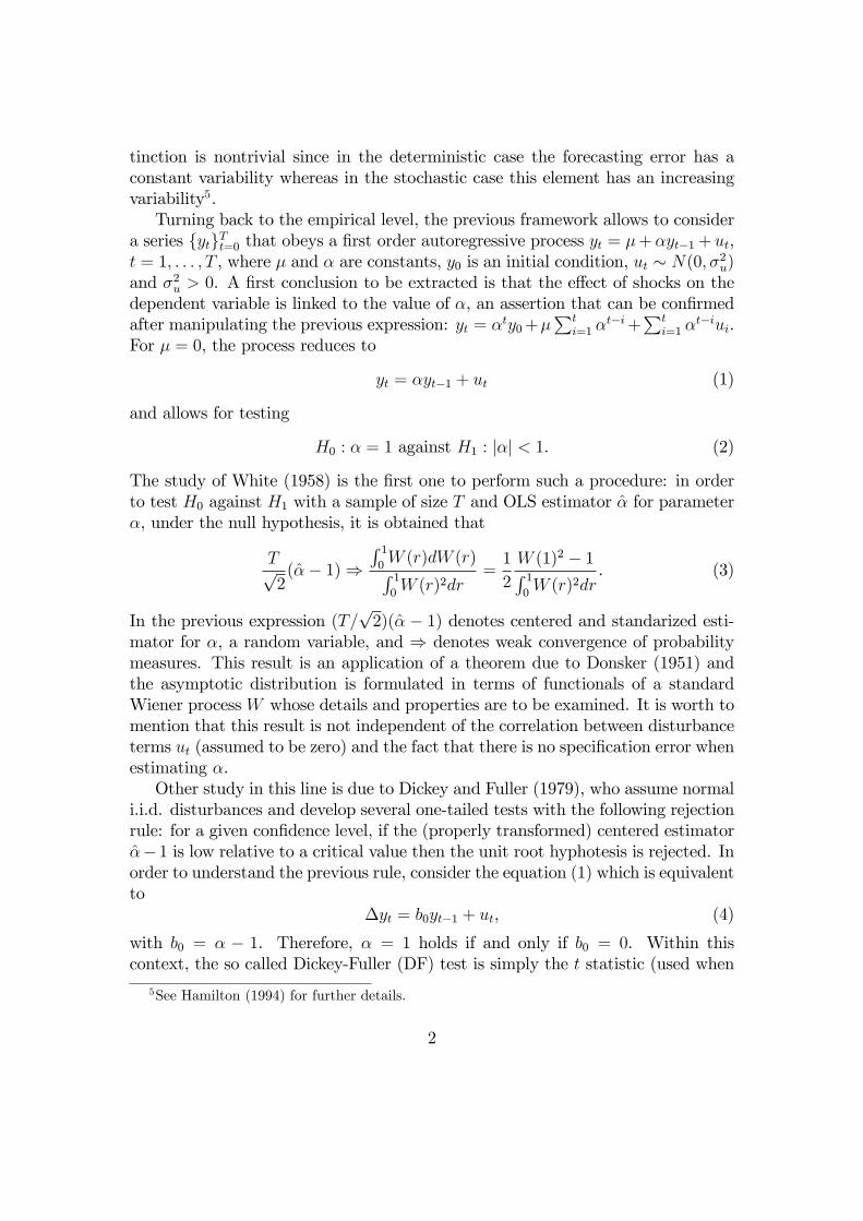
mator for �, a random variable, and ) denotes weak convergence of probabilitymeasures. This result is an application of a theorem due to Donsker (1951) andthe asymptotic distribution is formulated in terms of functionals of a standardWiener process W whose details and properties are to be examined. It is worth tomention that this result is not independent of the correlation between disturbanceterms ut (assumed to be zero) and the fact that there is no speci�cation error whenestimating �.Other study in this line is due to Dickey and Fuller (1979), who assume normal

i.i.d. disturbances and develop several one-tailed tests with the following rejectionrule: for a given con�dence level, if the (properly transformed) centered estimator�� 1 is low relative to a critical value then the unit root hyphotesis is rejected. Inorder to understand the previous rule, consider the equation (1) which is equivalentto

�yt = b0yt�1 + ut, (4)

with b0 = � � 1. Therefore, � = 1 holds if and only if b0 = 0. Within thiscontext, the so called Dickey-Fuller (DF) test is simply the t statistic (used when

5See Hamilton (1994) for further details.

2

Figure 1: Asymptotic distributions for several speci�cations.

testing for unit roots) for the signi�cance of yt�1 in (4). When lagged values of�yt are included in (4), the implied t statistic is known as the (lag) augmentedDickey-Fuller test or ADF test.Analysis is done considering three types of autoregressive models: without in-

tercept nor (deterministic) trend, with intercept but without trend and with bothintercept and trend. In this particular study, assumptions let asymptotic distribu-tions be represented through moment generating functions. By using Monte Carlosimulations, the power of these tests is compared with those of (autocorrelationbased) Q statistics proposed by Box and Pierce (1970). The main results are: �rst,Q statistics are sistematically less powerful; second, the performance of Dickey-Fuller tests is uniformly superior when there is no misspeci�caton error6; and third,there is evidence that Dickey-Fuller tests are biased towards not rejecting the nullhyphotesis for values of the autoregressive coe¢ cient � arbitrarily close to 1.A simple way to illustrate the role of speci�cation is provided by generating

samples from the data generating process yt = yt�1 + ut, ut � N (0; 1). The dis-tribution of T (�� 1) is plotted under three cases (see Figure 1): when there isno speci�cation error, when intercept is redundant and when both intercept andtrend are redundant. It can be appreciated that simulated distributions progres-sively move to the left and tabulated critical values tend to be higher (in absolutevalue) as far as redundant regressors are included. This makes the tests biasedtowards not rejecting the null hyphotesis and, in this sense, their power is reduced.

6Intuitively this ocurrs because, for example, it is exploited the knowledge that the interceptis zero.

3

This brief review shows that, up to the �rst half of the 1980 decade, unit rooteconometrics exhibited two well de�ned limitations: misspeci�cation and localstationary alternatives, and each of them implies an expected loss of power. Ad-ditionally, the recurrent use of normal i.i.d. disturbances considerably reduces theapplicability of these approaches by applied researchers. Two important advancesare produced during the second half of that decade. First, Phillips (1987a) pro-poses an asymptotic theory under very general conditions for integrated processes,which makes the posterior discussion be done under �rmly established founda-tions and, second, Perron (1989) identi�es the presence of a structural break as anelement that also reduces the power of the augmented Dickey-Fuller tests.The reader must also take into account that none of these two advances could

have been developed without the notion of weak convergence of probability mea-sures to be discussed. To motivate the need of this concept consider �rst theCentral Limit Theorem which, under conditions that vary along versions, allowsfor the distribution of the centered and standarized sample mean to converge tothose corresponding to a normal standard distribution. In an analogous fashion,this is a desirable property when dealing with dependent heterogeneously distrib-uted disturbances that do not satisfy the normal i.i.d. assumption in conventionalautoregressive models. Indeed, this idea is summarized by several versions of theFunctional Central Limit Theorem which, in a wider sense, states that the distrib-ution of standarized partial sums converges to those of a functional of a standardWiener process W . As described in Brzezniak and Zastawniak (1999), for a �xedvalue of r 2 [0; 1], the density fW (r) of the random variable W (r) is given by thefunction

fW (r)(x) =1p2�r

e�x2

r , x 2 R.

Therefore, in order to deal with advances in this literature two requisites areneeded. First, it is required to formally understand both the mathematical andprobabilistic structure of data generating processes in order to state the main(weak) convergence results. Second, and most important, it is required to recog-nize the importance of incorporating econometric problems faced by researchersinto the analysis, because their formalization leads to the development of neweconometric procedures and testing statistics. This task is frequently made withthe help of interesting alternative hypotheses.This paper reviews a selection of theoretical advances in the unit root literature,

starting from the second half of the 1980 decade and covering up to several contem-poraneous developments. The presentation emphasizes both the relevance of theFunctional Central Limit Theorem along the discussion as well as the econometricconsiderations behind novel approachs. Since time series literature can considerthe case of multiple structural breaks, attention is here focused only on a singularstructural break. An applied survey that considers multiple breaks can be found

4

in Glynn and Perera (2007).This paper is organized as follows. Section 2 describes the probabilistic struc-

ture of disturbance sequences involved, a building block for this literature. Section3 details a general version of the Functional Central Limit Thorem that covers awide class of disturbance processes. Section 4 presents the asymptotic theory forintegrated time series proposed by Phillips (1987a). Section 5 generalizes the for-mer framework in order to consider the so called near-integrated processes, as madeby Phillips (1987b). Section 6 studies linear processes and the class of modi�ed orM tests proposed by Stock (1999), which are meant to be employed in later de-velopments. Section 7 presents three econometric applications of the above theoryto the context of unit root testing when structural change is present. Section 7.1details the warning made by Perron (1989) about the e¤ects of structural breakson the power of Dickey-Fuller statistics and the methodology proposed for dealingwith an (assumed) exogenous break. Section 7.2 covers the critique made by Zivotand Andrews (1992) to this exogeneity assumption and the new test proposed,which involves estimating an endogenous structural break. Since none of the twoprevious studies deals with the power loss due to local-to-unity alternatives, Sec-tion 7.3 illustrates the results of Perron and Rodríguez (2003), who develop e¢ cient(power increasing) unit root tests under structural break and extend the resultsobtained by Elliott, Rothenberg, and Stock (1996) for linear processes. Section 8concludes with a retrospective view about the developments in statistical inferencewith integrated series and the role played by the theory of difussion processes.

2 Asymptotic Theory: The structure of weaklydependent heterogeneously distributed distur-bances

2.1 Some motivation

Most of the econometric theory to be covered is related with extensions of thefollowing autoregressive model: yt = �yt�1 + ut, t = 1; 2; : : :. The main objetivehere is to contrast the null hypothesis H0 : � = 1 when a sample of T observationsfytgTt=1 is available, and the previous section introduced this task in some detail.However, a major limitation is given by the assumption that the unobservable dis-turbance sequence futg1t=1 is composed by i.i.d. normal random variables. Thus,the empirical applicablity of several procedures is heavily restricted and it becomesdesirable to cover a case intended to be as general as possible. This case is formal-ized by considering a sequence of disturbance terms futg1t=1 that are dependentand heterogeneously distributed. A way to control the extent in which dependence

5

occurs, such that permits to derive convergence results, is to de�ne a measure ofdependence among random variables contained in a sequence. For this measure tobe well de�ned it needs to be refered to a speci�c probabilistic structure. Condi-tions that bound the extent of dependence are called mixing conditions. Resultsexposed here follow both White (1984) and Herrndorf (1984).

2.2 Mixing conditions

Consider a probabilistic space (;F ; P ), where is the sample space containingall of the possible results for an experiment, F is a set of events of (�-�eld)and P : F ! [0; 1] is a probability measure (P () = 1) over events contained inF . Next, consider a sequence of random variables futg1t=1 (that is, ut : ! Ris a Borel-measurable real function for all t) on (;F ; P ). Let m and n denotetwo positive integers and consider a track of disturbances fut : n � t � n +mg.Since it will be needed to assign probabilities to events involving random variablescontained in such a track, and since such events need to be included into a familywith a �-�eld structure, it becomes necessary to de�ne the �-�eld generated byrandom variables contained in the track as the smallest �-�eld that contains eventsfor which each ut, t = n; : : : ; n+m, is mesurable.

De�nition 1 Let B denote the Borel �-�eld on R. The Borel �-�eld generated bythe random variables included in the track fut : n � t � n+mg, Bn+mn = �(ut :n � t � n+m), is the smallest �-�eld that contains

1. all the sets of the form �n�1i=1 R�n+mi=n Bi �1i=n+m+1 R with Bi 2 B,

2. the complement Ac of each set A in Bn+mn , and

3. the unionS1i=1Ai of each sequence fAig contained in Bn+mn .

Intuitively, Bn+1n is the smallest collection of events that allows to assign proba-bilities to events, for example, of the form f! 2 : un (!) < a1 and un+1 (!) < a2g 2F , where a1; a2 2 R.The notion of mixing is needed to explicit the fact that, although two arbitrary

sets of random variables can exhibit dependence, this vanishes as time separationincreases7.In order to illustrate the former idea, consider the track composed by the

�rst n elements of futg1t=1 and denote it by futgnt=1. Within this track, two non-overlapping subtracks can be identi�ed: a �rst one starting at u1 and a second oneending at un. Let k � 1 denote the di¤erence between time indexes corresponding

7Notice that the idea of progressive lack of dependence includes that of ergodicity and as-ymptotic independence.

6

Figure 2: Dependence and mixing coe¢ cients.

to the last element of the �rst subtrack (denoted bym � 1) and the �rst element ofthe second subtrack (see Figure 2). Of course, the previous characterization doesnot completely determine both subtracks but allows for several cases. Indeed,the following de�nition of mixing coe¢ cients employs the previous observations inorder to quantify, given the �rst n elements of a sequence, the dependence betweenrandom variables separated by k periods at least.

De�nition 2 The mixing coe¢ cients of the sequence futg1t=1 are

�n (k) =

8><>:sup

A2�(ut:1�t�m)B2�(ut:m+k�t�n)

1�m�n�k

jP (A \B)� P (A)P (B)j for k � n� 1

0 for k � n

Intuitively, for n � 1 given, �n (k) measures how far dependence among eventscontained in the �-�elds H = �(ut : 1 � t � m) and G = �(ut : m + k � t � n)is situated from the independence case. k � 1 denotes time separation betweenthese two sets of random variables (see Figure 2). If H and G were independentthen for any h 2 H and g 2 G condition P (g \ h) = P (g)P (h) must hold or,equivalently �n (k) = 0.Since mixing coe¢ cients only take into account a �nite number of disturbances

(i.e. the �rst n random variables), this notion is extended to consider the highestdependence among random variables separated by at least k periods.

De�nition 3 The strong mixing coe¢ cient of the sequence futg1t=1 is�(k) = sup

n2N�n(k), for k 2 N.

Therefore, � (k) provides a measure of dependence. If �(k) = 0 for some k,events separated by k periods are independent. Also, if �(k) ! 0 as k ! 1,sequence futg1t=1 is said to be strong mixing, so that the notion of asymptoticindependence is considered too. For future reference, it is useful to emphasize fora strong mixing sequence the velocity at which �(k) tends to zero or, equivalently,the rate of decay of �(k). This will be denoted by �(k) = O(k��) for some � > 08.

8Let fatg and fbtg denote two sequences of positive real variables. Then at = O (bt) if thereexists M > 0 such that jat=btj �M for all t.

7

3 The Functional Central Limit Theorem

3.1 The Skorohod topology

The logics behind the Functional Central Limit Theorem relies on the convergenceof a sequence of standarized partial sums of disturbances ut. The limit for thisnew sequence isW a standard Wiener process. Correspondingly, elements of thesesequence of partial sums are contained on D = D[0; 1] the space of right-continousfunctions whose left limits exists everywhere on the unit interval, also refered ascàdlàg9 functions.Convergence above mentioned must be understood as weak convergence of a

sequence of random functions. As will be shown, in order to guarantee convergenceresults it is su¢ cient to endow D with a metric d such that (D; d) is a completeseparable space, so that the limit of any convergent sequence of elements containedin D is also contained in D. Concepts and results here discussed are stronglybased on Billingsley (1968), although this presentation follows Davidson (1994).The following de�nition characterizes the properties of the functions hereafter tobe considered.

De�nition 4 D[0; 1] is the space of functions x : [0; 1]! R satisfying the follow-ing conditions:

1. limt!r+ x(t) = x(r) for r 2 [0; 1),

2. limt!r� x(t) exists for r 2 (0; 1],

3. x(1) = limt!1� x(t).

Thus, only �rst class discontinuities are admited. A �rst metric to be consideredfor D is the uniform metric dU , de�ned as

dU(x; y) = supr jx(r)� y(r)j , x; y 2 D.

This metric states that two functions are arbitrairly close if the maximum di¤erencebetween ordinates corresponding to the same abcissa is small. Metric space (C; dU)is complete but, since C � D, completeness does not necessarily generalize to(D; dU). In fact, it is not di¢ cult to show that the limit of sequences of càdlàgfunctions in fact does not necessarily lie on D under dU . Thus, (D; dU) is not acomplete space and the strategy adopted by Billingsley (1968) consists in metrizingD as a separable complete space by introducing the Skorohod metric.

9In Frech: "continue à droite, limitée à gauche".

8

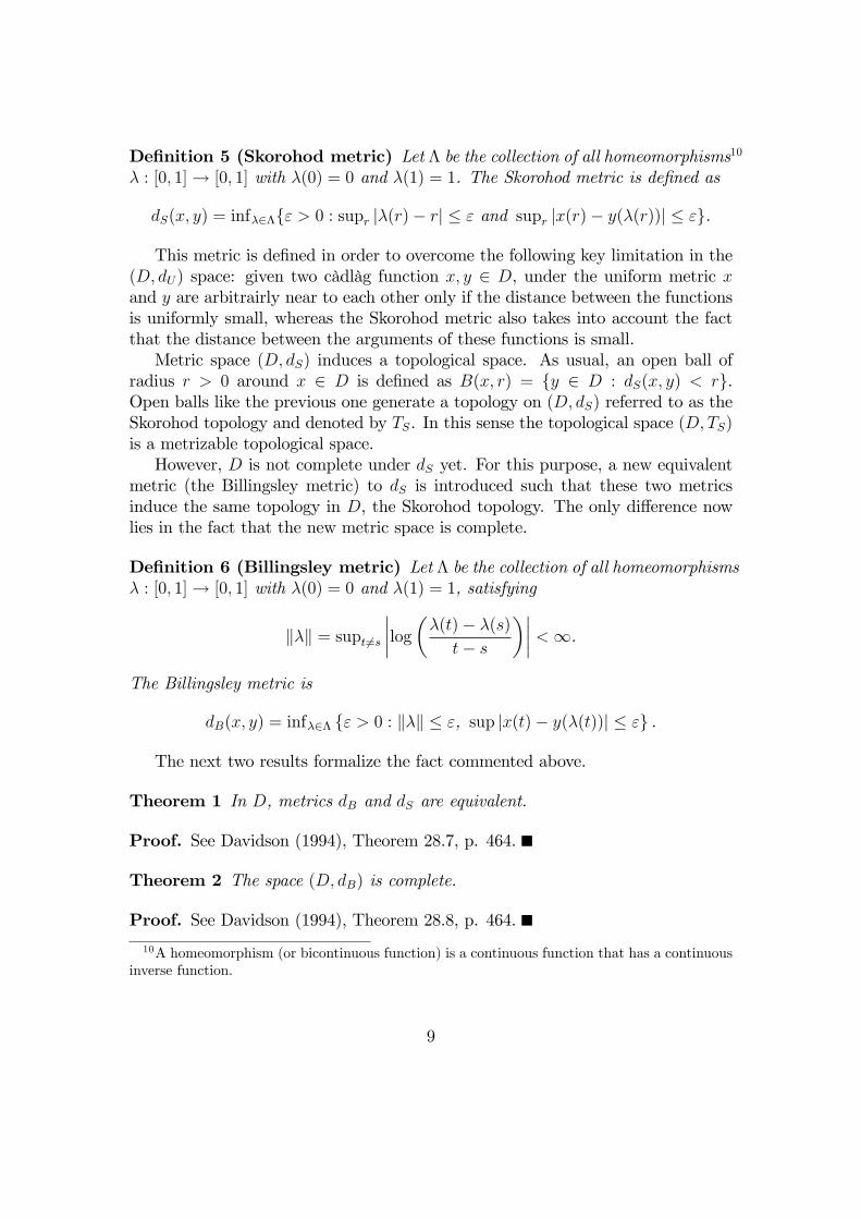
De�nition 5 (Skorohod metric) Let � be the collection of all homeomorphisms10

� : [0; 1]! [0; 1] with �(0) = 0 and �(1) = 1. The Skorohod metric is de�ned as

dS(x; y) = inf�2�f" > 0 : supr j�(r)� rj � " and supr jx(r)� y(�(r))j � "g.

This metric is de�ned in order to overcome the following key limitation in the(D; dU) space: given two càdlàg function x; y 2 D, under the uniform metric xand y are arbitrairly near to each other only if the distance between the functionsis uniformly small, whereas the Skorohod metric also takes into account the factthat the distance between the arguments of these functions is small.Metric space (D; dS) induces a topological space. As usual, an open ball of

radius r > 0 around x 2 D is de�ned as B(x; r) = fy 2 D : dS(x; y) < rg.Open balls like the previous one generate a topology on (D; dS) referred to as theSkorohod topology and denoted by TS. In this sense the topological space (D;TS)is a metrizable topological space.However, D is not complete under dS yet. For this purpose, a new equivalent

metric (the Billingsley metric) to dS is introduced such that these two metricsinduce the same topology in D, the Skorohod topology. The only di¤erence nowlies in the fact that the new metric space is complete.

De�nition 6 (Billingsley metric) Let � be the collection of all homeomorphisms� : [0; 1]! [0; 1] with �(0) = 0 and �(1) = 1, satisfying

k�k = supt6=s��log��(t)� �(s)

t� s

�� <1.The Billingsley metric is

dB(x; y) = inf�2� f" > 0 : k�k � ", sup jx(t)� y(�(t))j � "g .

The next two results formalize the fact commented above.

Theorem 1 In D, metrics dB and dS are equivalent.

Proof. See Davidson (1994), Theorem 28.7, p. 464.

Theorem 2 The space (D; dB) is complete.

Proof. See Davidson (1994), Theorem 28.8, p. 464.

10A homeomorphism (or bicontinuous function) is a continuous function that has a continuousinverse function.

9

3.2 The main theorem (Herrndorf, 1984)

The main result to be considered in this section is a generalization of the CentralLimit Theorem for the case of functional spaces such asD, known as the FunctionalCentral Limit Theorem. In order to understand the theorem, concepts previouslyde�ned are complemented with additional conditions for the disturbance sequencefutg1t=1 and, speci�cally, for the sequence of partial sums ST =

PTt=1 ut. First,

disturbances are required to have zero mean and �nite variance

E(ut) = 0, E(u2t ) <1 for t = 1; 2; : : : . (5)

Second, variance of partial sums must converge

limT!1E(T�1S2T ) = �2 > 0 for some � > 0. (6)

Consider now the space D endowed with the Skorohod topology with Borel�-�eld B and de�ne random functions WT : ! R by

WT (r) =1pT�

SbrT c, r 2 [0; 1], T = 1; 2; : : :

where b�c denotes the integer part of its argument. Each WT is a measurablemap from (;F) into (D;B). Sequence fWTg1T=1 is said to satisfy the invarianceprinciple if it is weakly convergent to a standard Wiener process W on D. For thedevelopment of this result, let kuk� be de�ned as

kuk� = (E juj�)1=� for � 2 [1;1)kuk� = ess sup juj for � =1.

As will be shown in the next section, the following version of the Functional CentralLimit Theorem is the starting point for all of the recent literature on unit roots.This result is due to Herrndorf (1984).

Theorem 3 (Herrndorf, 1984 Corollary 1 p. 142) Let � 2 (2;1] and =2=�. If futg1t=1 satis�es (5), (6) andP1

k=1 �(k)1� <1 and lim supt2N kutk� <1,

then WT ) W as T !1.

Proof. See Herrndorf (1984), Corollary 1, p. 148.

10

4 Asymptotics for integrated processes(Phillips, 1987a)

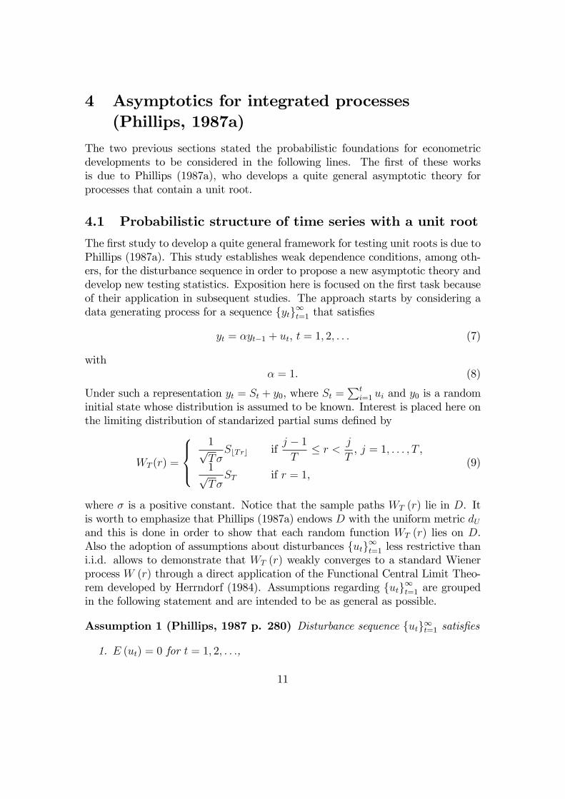
The two previous sections stated the probabilistic foundations for econometricdevelopments to be considered in the following lines. The �rst of these worksis due to Phillips (1987a), who develops a quite general asymptotic theory forprocesses that contain a unit root.

4.1 Probabilistic structure of time series with a unit root

The �rst study to develop a quite general framework for testing unit roots is due toPhillips (1987a). This study establishes weak dependence conditions, among oth-ers, for the disturbance sequence in order to propose a new asymptotic theory anddevelop new testing statistics. Exposition here is focused on the �rst task becauseof their application in subsequent studies. The approach starts by considering adata generating process for a sequence fytg1t=1 that satis�es

yt = �yt�1 + ut, t = 1; 2; : : : (7)

with� = 1. (8)

Under such a representation yt = St + y0, where St =Pt

i=1 ui and y0 is a randominitial state whose distribution is assumed to be known. Interest is placed here onthe limiting distribution of standarized partial sums de�ned by

WT (r) =

8><>:1pT�

SbTrc ifj � 1T

� r <j

T, j = 1; : : : ; T ,

1pT�

ST if r = 1,(9)

where � is a positive constant. Notice that the sample paths WT (r) lie in D. Itis worth to emphasize that Phillips (1987a) endows D with the uniform metric dUand this is done in order to show that each random function WT (r) lies on D.Also the adoption of assumptions about disturbances futg1t=1 less restrictive thani.i.d. allows to demonstrate that WT (r) weakly converges to a standard Wienerprocess W (r) through a direct application of the Functional Central Limit Theo-rem developed by Herrndorf (1984). Assumptions regarding futg1t=1 are groupedin the following statement and are intended to be as general as possible.

Assumption 1 (Phillips, 1987 p. 280) Disturbance sequence futg1t=1 satis�es

1. E (ut) = 0 for t = 1; 2; : : :,

11

2. suptE jutj� <1 for some � > 2,

3. �2 = limT!1 T�1E (S2T ) exists and �

2 > 0, with ST =PT

t=1 ut,

4. futg1t=1 is strong mixing, with strong mixing coe¢ cients �(k) that satisfyP1k=1 �(k)

1�2=� <1. (10)

As usual, condition 1 imposes a zero mean disturbance for every t. Condition2 bounds the probability of outliers: the higher � the lower the probability ofoutliers. As long as such � > 2 exists, all of the lower absolute moments of eachut (including the second one) are �nite. Condition 3 is conventional along centrallimit theory, concerning the convergence of the average variance of partial sumsST . Condition 4 bounds the temporal dependence among disturbances contained infutg1t=1, and elements covered in previous sections allows to assert that althoughdependence can exists between any pair of disturbances, this vanishes as timeseparation increases. Hence, two random disturbances su¢ ciently distant alongtime are almost independent. Finally, summability condition (10) is satis�ed aslong as the mixing decay rate is �(k) = O(k��) for some � > 0 such that ��(1�2=�) < 1 or, equivalently � > �=(� � 2).It is interesting to notice that as T increases the constant sections conform-

ing WT (r) 2 D reduce their size and discontinuities become less perceptible (seeFigure 3), re�ecting how this sequence of random functions in D converge to arandom function in C, the standard Wiener process. This property is exploitedby Phillips (1987a) through two lemmas. The �rst lemma is the Functional Cen-tral Limit Theorem shown in Theorem 3 and the second result is widely knownas the Continous Mapping Theorem and states conditions under which conver-gence to a Wiener process can be preserved along (almost everywhere) continoustransformations.

Lemma 4 (Phillips, 1987 p. 281) If futg1t=1 satis�es Assumption 1 then, asT !1, WT ) W a standard Wiener process on C.

Proof. See Herrndorf (1984), Corollary 1, p. 142.

Lemma 5 (Phillips, 1987 p. 281) If WT ) W (r) as T !1 and h is a con-tinous functional on D a.e. then h (WT )) h (W ) as T !1.

Proof. See Billingsley (1968), Corollary 1 p. 31.

12

Figure 3: Convergence of standarized sums.

4.2 Some asymptotic theory for econometricians

The importance of the two previous lemmas relies on the fact that they allowthe derivation of convergence rules often employed by theoretical econometricians.These rules are summarized in the next theorem.

Theorem 6 (Phillips, 1987 p. 282) If futg1t=1 satis�es Assumption 1 and if

supt jutj�+" <1 for some " > 0

(where � > 2 is the same as that in Assumption 1), then as T !1:

1. T�2PT

t=1 y2t�1 ) �2

R 10W (r)2 dr,

2. T�1PT

t=1 yt�1 (yt � yt�1)) (�2=2)(W (1)2 � �2u=�2),

3. T (�� 1)) 1

2(W (1)2 � �2u=�

2)=R 10W 2 (r) dr,

13

4. �p! 1,

5. t� ) (�=2�u)(W (1)2 � �2u=�2)=f

R 10W (r)2 drg1=2,

where �2u = limT!1 T�1PT

t=1E (u2t ), �

2 = limT!1E (T�1S2T ) and W is a

standard Wiener process on C.

Proof. See Phillips (1987a), Theorem 3.1 p. 296.In the previous theorem, results 1 and 2 constitute derivation rules for limit-

ing distributions. Result 3 is focused on the limiting distribution of the statisticT (�� 1), which corrects the results of White (1958)11, among others. Result 4states the consistency of the OLS estimator � in the presence of a unit root andunder the general case of dependent and heterogeneously distributed disturbances.Finally, result 5 shows the asymptotic distribution of the t statistic used when test-ing for unit roots. It is worth to mention that under (7) and (8) the t statisticdoes not follow a Student�s t distribution. Since W (1) follows a normal standarddistribution, W (1)2 follows a chi-squared distribution with one degree of freedom.However, the functional

R 10W (r)2 dr is a random variable with a rather complex

distribution, so that usual distributions (normal, chi-squared, t and F ) employedin the stationary case are not relevant for the subsequent analysis.In this way, results let Phillips (1987a) to propose (after developing consistent

estimators for parameters �2u and �2) two new test statistics for the unit roothypothesis often refered as the Z tests. Although it is important to rememberthat both (7) and (8) correspond only to the case of a unit without drift nordeterministic trend, the importance of this study relies on providing a generaltheory on test statistics for the unit root hypothesis. Distributions considerdhere di¤er from those involved in the stationary case (j�j < 1). Obviously, thismethodology is well suited for extensions that include both drift and deterministictrend, derived by Phillips and Perron (1988), and constitute the starting point forthe study of the unit root test under structural break in the following sections.

5 Asymptotics for Near-Integrated Processes(Phillips, 1987b)

For later discussion on the asymptotic power of unit root tests against alternativehypotheses that consider autoregressive coe¢ cients near to one, it will be useful toconsider generalizations of integrated processes often referred as near-integrated

11See equation (3).

14

processes and studied in detail by Phillips (1987b). For this case, time seriesfytg1t=1 is assumed to be generated according to the following model

yt = �yt�1 + ut, t = 1; 2; : : : (11)

� = ec=T , �1 < c <1. (12)

In the above model, initial condition y0 is allowed to be any random variable whosedistribution is �xed and independent of T . The constant c is interpreted as a non-centrality parameter that quanti�es deviations from the unit root null hypothesisthat holds when c = 0

H0 : � = 1. (13)

Under (13), fytg1t=0 is an integrated process of order 1 or I (1) process. Addition-ally, any c 6= 0 in (12) represents a local alternative to H0. For future reference,the next de�nition formally establishes this distinction.

De�nition 7 A time series fytg1t=1 that is generated by (11) and (12) with c 6= 0is called near-integrated. When c = 0, in (12), fytg1t=1 is also called integrated.

The main objetive of the present section is to present an asymptotic theoryfor this type of processes. Naturally, results and properties are indexed by theparameter c.

5.1 Probabilistic Structure of Time Series with a Near-to-Unit Root

For a wide applicability of this asymptotic theory, general assumptions concerningthe disturbance sequence futg1t=0 are necessary. For this reason, the following mix-ing conditions about the behaviour of disturbances futg1t=0 (hereby now familiar)are adopted and summarized in the next statement.

Assumption 2 (Phillips, 1987b p. 537) Disturbance sequence futg1t=1 satis-�es

1. E (ut) = 0 for t = 1; 2; : : :,

2. suptE jutj�+" <1 for some � > 2 and " > 0,


2 > 0, with ST =PT

t=1 ut,

4. futg1t=1 is strong mixing, with strong mixing coe¢ cients �(k) that satisfyP1k=1 �(k)

1�2=� <1. (14)

15

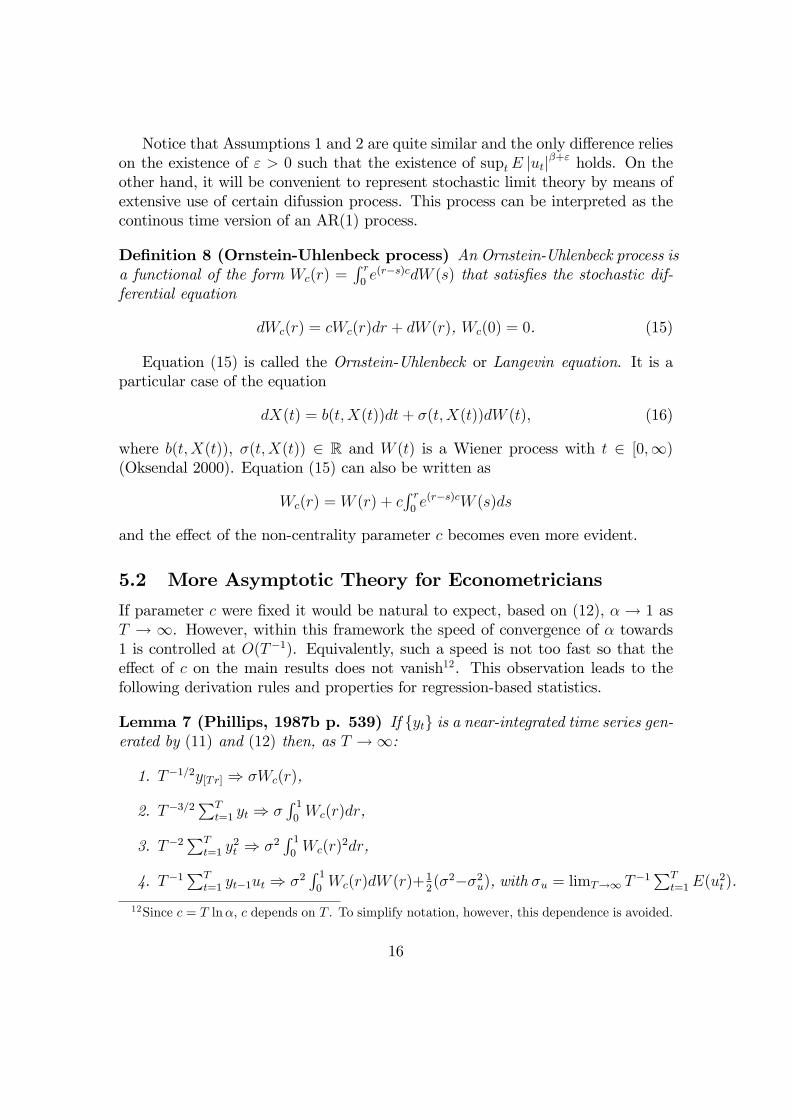
Notice that Assumptions 1 and 2 are quite similar and the only di¤erence relieson the existence of " > 0 such that the existence of suptE jutj

�+" holds. On theother hand, it will be convenient to represent stochastic limit theory by means ofextensive use of certain difussion process. This process can be interpreted as thecontinous time version of an AR(1) process.

De�nition 8 (Ornstein-Uhlenbeck process) An Ornstein-Uhlenbeck process isa functional of the form Wc(r) =

R r0e(r�s)cdW (s) that satis�es the stochastic dif-

ferential equation

dWc(r) = cWc(r)dr + dW (r), Wc(0) = 0. (15)

Equation (15) is called the Ornstein-Uhlenbeck or Langevin equation. It is aparticular case of the equation

dX(t) = b(t;X(t))dt+ �(t;X(t))dW (t), (16)

where b(t;X(t)), �(t;X(t)) 2 R and W (t) is a Wiener process with t 2 [0;1)(Oksendal 2000). Equation (15) can also be written as

Wc(r) =W (r) + cR r0e(r�s)cW (s)ds

and the e¤ect of the non-centrality parameter c becomes even more evident.

5.2 More Asymptotic Theory for Econometricians

If parameter c were �xed it would be natural to expect, based on (12), � ! 1 asT ! 1. However, within this framework the speed of convergence of � towards1 is controlled at O(T�1). Equivalently, such a speed is not too fast so that thee¤ect of c on the main results does not vanish12. This observation leads to thefollowing derivation rules and properties for regression-based statistics.

Lemma 7 (Phillips, 1987b p. 539) If fytg is a near-integrated time series gen-erated by (11) and (12) then, as T !1:

1. T�1=2y[Tr] ) �Wc(r),

2. T�3=2PT

t=1 yt ) �R 10Wc(r)dr,

3. T�2PT

t=1 y2t ) �2

R 10Wc(r)

2dr,

4. T�1PT

t=1 yt�1ut ) �2R 10Wc(r)dW (r)+

12(�2��2u), with �u = limT!1 T

�1PTt=1E(u

2t ).

12Since c = T ln�, c depends on T . To simplify notation, however, this dependence is avoided.

16

Proof. See Phillips (1987b), Lemma 1, p. 539.

Theorem 8 (Phillips, 1987b p. 540) If fytg is a near-integrated time seriesgenerated by (11) and (12) then, as T !1:

1. T (�� )) fR 10Wc(r)dW (r) +

12(1� �2u=�

2)g=R 10fWc(r)g2dr,

2. �p! 1, s2

p! �2u with s2 = T�1

PTt=1(yt � �yt�1)

2,

3. t� ) (�=�u)fR 10Wc(r)dW (r) +

12(1� �2u=�

2)g=[R 10fWc(r)g2dr]1=2.

Proof. See Phillips (1987b), Theorem 1, p. 540.Up to this point, the theory presented can be used in the analysis of the power of

unit root tests under local alternatives. For a non-centrality parameter c arbitrarilyclose to 0 it is easy to show that ec=T � 1 + c=T and this is the approach usuallyemployed in unit root testing. A brief illustration of this procedure can be found,for example, in Phillips (1988).

6 Linear Processes and Modi�ed Tests

6.1 Motivation

Although the reader must have noticed that the so called mixing conditions areintended to be a powerful tool that allows the derivation of weak convergenceresults for a wide class of processes, Phillips and Solo (1992) pointed out that,since much of the time series analysis is concerned with parametric models thatfall in the class of linear processes, mixing conditions exhibit a major drawback.The reason is quite simple since not all linear processes are strong mixing. Inspite of this, they propose a turnback to linear processes as the main focus fordeveloping time series asymptotics. Under the linear model class, Phillips andSolo (1992) make extensive use of the algebraic Beveridge-Nelson decomposition(see Appendix A) to demonstrate the Functional Central Limit Theorem once pro-vided with a disturbance sequence f"tg1t=0 that is a martingale di¤erence sequence(see Appendix B), strongly uniformly integrable (see Appendix C) with domi-nating random variables fZtg1t=0 such that E(Z

2+�t ) < 1 for some � > 0, further

T�1PT

t=1E("2t jFt�1)

a:s:! �2" > 0, where Ft is the �-�eld generated by f"t; "t�1; : : :g.Given the latter notation it is now possible to establish the following

Theorem 9 (Phillips and Solo, 1992) Suposse that futg1t=0 is the linear process

ut =P1

j=0 cj"t�j = C(L)"t, C(L) =P1

j=0 cjLj

17

with 0 < C(1) �P1

j=0 cj <1 andP1

j=0 c2j <1. If

P1j=1 jjcjj <1, then

1pT

PbrT ct=1 ut ) �"C(1)W (r).

Proof. See Phillips and Solo (1992) Theorem 3.4 p. 983.

Although the latter Functional Central Limit Theorem is less general thanversions previously presented, it will be frequently used in posterior work, speciallyalong the developments due to Stock (1999).

6.2 The M Class of Integration Tests (Stock, 1999)

Stock (1999) proposed a new class of statistics that directly test the implicationthat an integrated process has a growing variance having an order of probability13

of T�1=2 (Op(T�1=2)). Since the remaining of this paper deals with this class oftests under several frameworks, the general class is examined in some detail. First,suppose the following data ganerating process for fytg1t=1

yt = �t(�) +Pt

i=1 ui,

t = 1; : : : ; T . That is, under the null hypothesis the series fytg1t=1 can be written asthe sum of a purely deterministic component �t(�) (with �nite dimensional vector� estimated by �) and an integrated or I(1) component that is the partial sum ofweakly stationary or I(0) terms. Let the long run variance of ut be denoted by�2 = 2�su(0), where su(0) is the spectral density of ut at frequency zero and, forr 2 [0; 1], let

ST (r) =1pT

PbrT ci=1 ui, and

DT (r; �) = �brT c(�)

be càdlàg versions of the components of the discrete time process. As expected, thisis done in order to apply the Functional Central Limit Theorem above mentioned.Such functionals are assumed to satisfy the following

Assumption 3 (Stock, 1999 p. 137) The following conditions hold:

1. ST ) �W , where 0 < �2 <1, and13Let fytg denote a sequence of random variables and let fatg denote a sequence of positive

non-stochastic real numbers. Then yt = Op (at) if for each " > 0 there exists M > 0 such thatP (jytj =at > M) < ".

18

2.pTfDT (�; �) � DT (�; �)g ) �D, where D 2 D[0; 1] has a distribution that

does not depend on � or on the nuisance parameters describing the distribu-tion of futg.

In line with the proposal of Phillips and Solo (1992), Stock (1999) focuses onlinear processes

ut = C(L)"t,P1j=1 jjcjj < 1,C(1) 6= 0

where "t is a martingale di¤erence sequence (m.d.s.) with

E["tjFt�1] = 0, and (17)

suptE["2+�t jFt�1] < 1 for some � > 0. (18)

As usual, condition (17) imposes zero-mean disturbances whereas condition (18)bounds the probability of outliers in a similar fashion to condition 2 presented inAssumption 1. Also, although the deterministic component �t(�) is designed topotentially contain polynomial and further general trends, the following cases arehere considered for obvious reasons.

1. No deterministic trend: �t(�) = 0. In this case there is no need of detrending.For completeness, let the "detrended" series be y0t � yt.

2. Constant: �t(�) = �0. In this case �0 is estimated by �0 = �y = T�1PT

t=1 ytand the demeaned series is y�t � yt � �y.

3. Linear trend: �t(�) = �0 + �1(t=T ). If (�0; �1) is estimated by the OLSestimator (�0; �1) then the detrended series is y

�t � yt � �0 � �1(t=T ). Nor-

malization of the known part of the deterministic component is done for itscontinous time analogous to lie in the interval [0; 1].

The three former cases are enough for subsequent analysis. Since limiting rep-resentation in Assumption 3 depends on the nuisance parameter �2, it is assumedthat there exists a consistent estimator �2 for �2.

Assumption 4 (Stock, 1999 p. 137) Under the null hypothesis �2p! �2.

Elements for the development of the new class of tests are based on both theFunctional Central Limit Theorem and the Continous Mapping Theorem. For

19

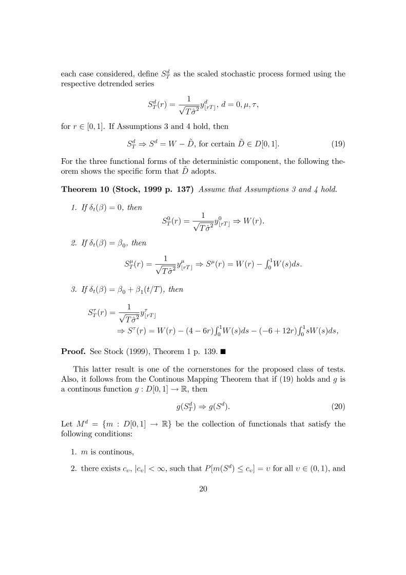
each case considered, de�ne SdT as the scaled stochastic process formed using therespective detrended series

SdT (r) =1pT �2

ydbrT c, d = 0; �; � ,

for r 2 [0; 1]. If Assumptions 3 and 4 hold, then

SdT ) Sd = W � ~D, for certain ~D 2 D[0; 1]. (19)

For the three functional forms of the deterministic component, the following the-orem shows the speci�c form that ~D adopts.

Theorem 10 (Stock, 1999 p. 137) Assume that Assumptions 3 and 4 hold.

1. If �t(�) = 0, then

S0T (r) =1pT �2

y0brT c ) W (r).

2. If �t(�) = �0, then

S�T (r) =1pT �2

y�brT c ) S�(r) =W (r)�R 10W (s)ds.

3. If �t(�) = �0 + �1(t=T ), then

S�T (r) =1pT �2

y�brT c

) S� (r) =W (r)� (4� 6r)R 10W (s)ds� (�6 + 12r)

R 10sW (s)ds,

Proof. See Stock (1999), Theorem 1 p. 139.

This latter result is one of the cornerstones for the proposed class of tests.Also, it follows from the Continous Mapping Theorem that if (19) holds and g isa continous function g : D[0; 1]! R, then

g(SdT )) g(Sd). (20)

Let Md = fm : D[0; 1] ! Rg be the collection of functionals that satisfy thefollowing conditions:

1. m is continous,

2. there exists c�, jc�j <1, such that P [m(Sd) � c�] = � for all � 2 (0; 1), and

20

3. m(0) < c� for all � 2 (0; 1).The classMd, refered only to continous functionals of SdT , groups test statistics

for the null hypothesis that yt is I(1) against the alternative that it is I(0). Since SdTrepresents any of the three detrended series mentioned, under the null hypothesism(SdT ) has an asymptotic distribution with critical values that depend on thefunctional m, whereas under a �xed alternative yt is I(0), which suggests theconstruction of one tailed tests of level � of the form:

reject H0 : yt � I(1) if m(SdT ) � c�.

This approach, as Stock (1999) asserts, suggests working backwards from the de-sired asymptotic representation to the actual test statistic. The fact that the formof the function m(�) does not depend on the type of detrending emphasizes thatthe steps of eliminating the deterministic components and testing for unit root aredistinct: detrending a series when it is not required does not a¤ect the size of thetests (although can a¤ect power) since ~D does not depend on �. In contrast, fail-ing to detrend a series that contains a trend typically leads to a loss of consistencyand an incorrect asymptotic size.In summary, always detrending a series before hypothesis testing does not af-

fect the size and this is a desirable property. Once size is guaranteed to be �xed,power increasing procedures can be perfomed. The next two subsections illus-trate the main idea behind: if certain test statistic VT has a limiting distributioncharacterized as the functional m of certain di¤usion process Sd, that is

VT ) m(Sd),

this asymptotic distribution can also be written as the limiting one of a respectivemodi�ed test statistic for detrended data m(SdT ):

m(SdT )) m(Sd),

such that VT and its modi�ed version m(SdT ) are asymptotically equivalent.

6.3 The Modi�ed Sargan-Bhargava Test

One of the test statistics to be covered along section 7.3 is due to Sargan andBhargava (1983) for the model

yt = �0 +Pt

s=1 �t�s"s, (21)

where "t � N(0; �2), t = 1; : : : ; T and (�; �0; �2) is a vector of unknown parame-

ters. The authors propose the following Durbin-Watson statistic for a regressionof yt against a constant

SB� =

PTt=2(�yt)

2PTt=1(y

�t )2,

21

where y�t � yt � �y. For the case where there exists a linear deterministic trendBhargava (1986) considers the extension

yt = �0 + �1t+Pt

s=1 �t�s"s, (22)

where "t � N(0; �2), t = 1; : : : ; T and (�; �0; �1; �2) is a vector of unknown para-

meters. A similar test is proposed

SB� =

PTt=2(�yt)

2PTt=1(y

�t )2,

where y�t � yt � ~�0 � ~�1(t=T ),

~�0 = �y � 12

T + 1

(T � 1)(yT � y1),

~�1 =T

T � 1(yT � y1).

For both tests, Stock (1999) derives the limiting distribution

T�1SBd )�2

var(�yt)

R 10Sd(r)2dr, for d = �; � . (23)

After noticing in (21) and (22) that �2 = var(�yt), (23) can be written as

T�1SBd )R 10Sd(r)2dr, for d = �; � .

Now, notice that the functional

mSB(f) =R 10f(r)2dr

is also involved in the limiting distribution of the following functional in D[0; 1]

1pT

PTt=1(y

dt )2.

This latter statistic will be refered as the modi�ed Sargan-Bhargava orMSB test.

6.4 A Modi�ed Z Test

For a model that contains a constant deterministic component, Phillips (1987a)and Phillips and Perron (1988) propose the test statistic

Z� = T (�� 1)� 12

�2 � �2u

T�2PT

t=1 y2t�1, (24)

22

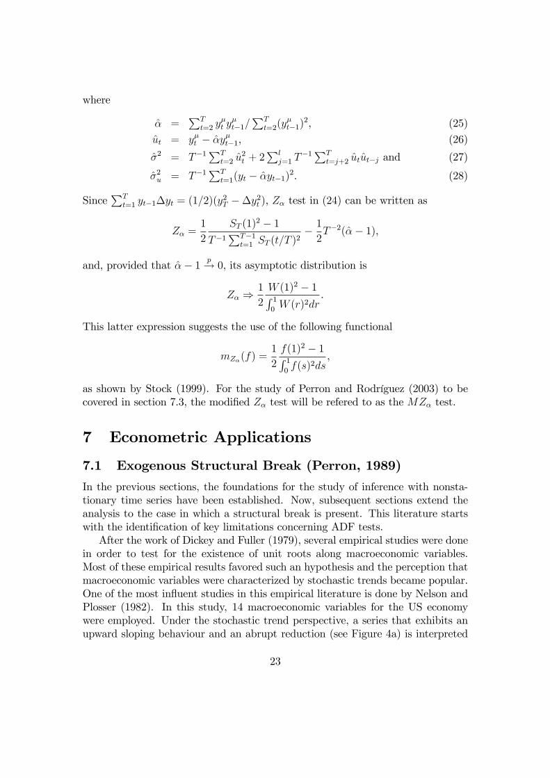
where

� =PT

t=2 y�t y

�t�1=

PTt=2(y

�t�1)

2, (25)

ut = y�t � �y�t�1, (26)

�2 = T�1PT

t=2 u2t + 2

Plj=1 T

�1PTt=j+2 utut�j and (27)

�2u = T�1PT

t=1(yt � �yt�1)2. (28)

SincePT

t=1 yt�1�yt = (1=2)(y2T ��y2t ), Z� test in (24) can be written as

Z� =1

2

ST (1)2 � 1

T�1PT�1

t=1 ST (t=T )2� 12T�2(�� 1),

and, provided that �� 1 p! 0, its asymptotic distribution is

Z� )1

2

W (1)2 � 1R 10W (r)2dr

.

This latter expression suggests the use of the following functional

mZ�(f) =1

2

f(1)2 � 1R 10f(s)2ds

,

as shown by Stock (1999). For the study of Perron and Rodríguez (2003) to becovered in section 7.3, the modi�ed Z� test will be refered to as the MZ� test.

7 Econometric Applications

7.1 Exogenous Structural Break (Perron, 1989)

In the previous sections, the foundations for the study of inference with nonsta-tionary time series have been established. Now, subsequent sections extend theanalysis to the case in which a structural break is present. This literature startswith the identi�cation of key limitations concerning ADF tests.After the work of Dickey and Fuller (1979), several empirical studies were done

in order to test for the existence of unit roots along macroeconomic variables.Most of these empirical results favored such an hypothesis and the perception thatmacroeconomic variables were characterized by stochastic trends became popular.One of the most in�uent studies in this empirical literature is done by Nelson andPlosser (1982). In this study, 14 macroeconomic variables for the US economywere employed. Under the stochastic trend perspective, a series that exhibits anupward sloping behaviour and an abrupt reduction (see Figure 4a) is interpreted

23

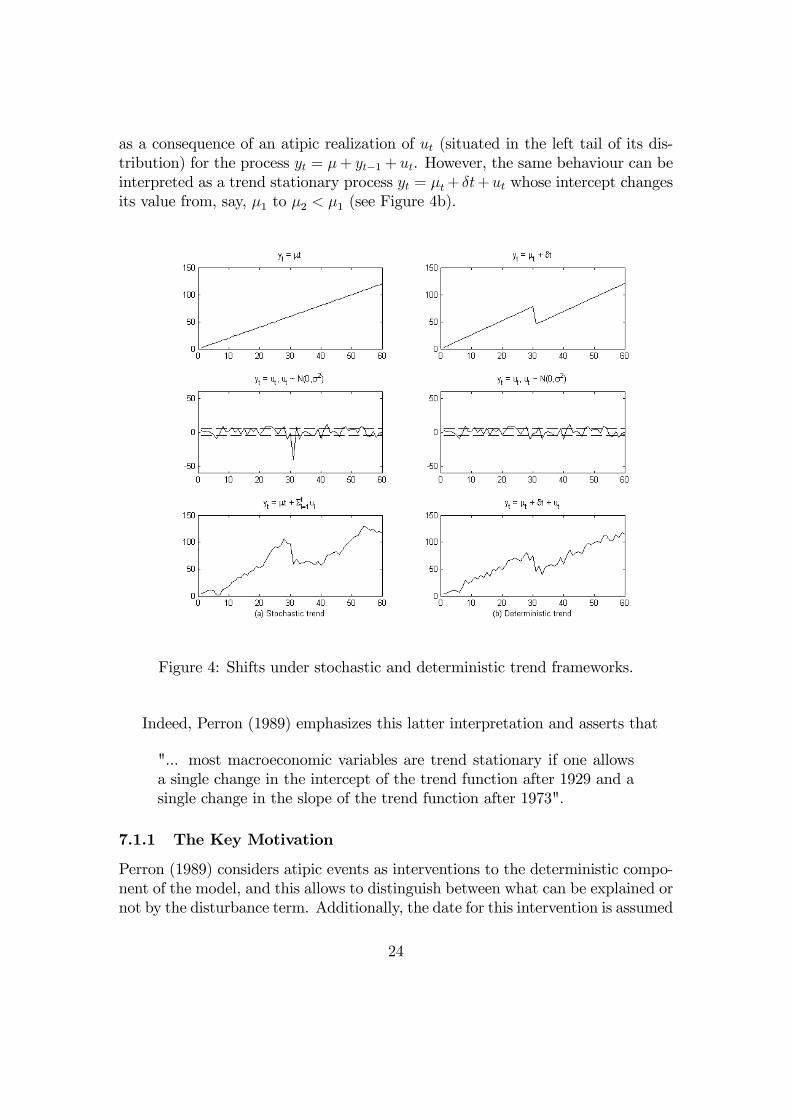
as a consequence of an atipic realization of ut (situated in the left tail of its dis-tribution) for the process yt = �+ yt�1 + ut. However, the same behaviour can beinterpreted as a trend stationary process yt = �t+ �t+ut whose intercept changesits value from, say, �1 to �2 < �1 (see Figure 4b).

Figure 4: Shifts under stochastic and deterministic trend frameworks.

Indeed, Perron (1989) emphasizes this latter interpretation and asserts that

"... most macroeconomic variables are trend stationary if one allowsa single change in the intercept of the trend function after 1929 and asingle change in the slope of the trend function after 1973".

7.1.1 The Key Motivation

Perron (1989) considers atipic events as interventions to the deterministic compo-nent of the model, and this allows to distinguish between what can be explained ornot by the disturbance term. Additionally, the date for this intervention is assumed

24

to be known by the researcher. Because there exist two competing interpretations(above mentioned) for time series with an abrupt shift, models considered by Per-ron (1989) are summarized in Table 1.In Table 1, �, �, �1, �2, �, �1 and �2 are parameters, A (L)ut = B (L) et and

et � i:i:d: (0; �2e). A (L) and B (L) are pth and qth order polinomials. That is,futg is an ARMA (p; q) process with p and q possibly unknown. This assumptionallows fytg to represent general processes. In this sense, di¤erent speci�cationsallow for di¤erent models:

1. Under the null hypothesis, model A contains a dummy variable that equals 1only inmediatly after TB (a one time change of the intercept), whereas underthe alternative hypothesis the series is trend stationary with a permanentshift in the intercept of the trend function after TB (see Figure 5).

2. For model B, under the null hypothesis a permanent change in the inter-cept is allowed after TB; whereas under the alternative hypothesis only apermanent shift is allowed in the slope of the deterministic component.

3. Finally, model C allows both the two shifting types simultaneously: a shiftin level accompanied by a shift in slope.

In this way, Perron (1989) introduces a third interpretation to the discussion(see Figure 5) in order to identify limitations present in already known testingstatistics.A �rst attempt to discriminate between the two approaches included in Figure

4 could be through the use of DF tests. However, by using numerical experiments,Perron (1989) examines the performance of these class of tests under the alterna-tive hypothesis. Speci�cally, Monte Carlo simulations reveal that when the datagenerating process is described as by model A under the alternative, DF tests tendto detect a spurious unit root that does not vanish, even asymptotically. There-fore, a power loss is expected. This property is also derived at the theoretical level(Perron 1989, Theorem 1) and for this result to be as general as possible, assump-tions identical to those adopted by Phillips (1987a) concerning the innovationssequence futg are adopted and summarized as follows.

Assumption 5 (Perron, 1989, p. 1371) Disturbance sequence futg1t=1 satis�es

1. E (ut) = 0 for all t;

2. suptE jutj�+" <1 for some � > 2 and " > 0;


2 > 0, where ST =PT

t=1 ut;

25

Figure 5: The �Crash�model.

26

Null hyphotesis Alternative hyphotesis

Model A Model Ayt = �+ yt�1 + �D (TB)t + ut yt = �1 + (�2 � �1)DUt + �t+ ut

Model B Model Byt = �1 + yt�1 + (�2 � �1)DUt + ut yt = �+ �1t+ (�2 � �1)DT

�t + ut

Model C Model Cyt = �1 + yt�1 + �D (TB)t yt = �1 + �1t+ (�2 � �1)DUt

+(�2 � �1)DUt + ut +(�2 � �1)DTt + ut

where whereD (TB)t = 1 if t = TB + 1, 0 otherwise DT �t = t� TB if t > TB, 0 otherwiseDUt = 1 if t > TB, 0 otherwise DTt = t if t > TB, 0 otherwise

Table 1: Null and alternative hypotheses considered by Perron (1989).

4. futg1t=1 is strong mixing with strong mixing coe¢ cients �(k) that satisfyP1k=1 �(k)

1�2� <1.

As expected, the Functional Central Limit Theorem due to Herrndorf (1984)can still be employed in this case. Speci�cally, Assumption 2 allows for the gen-eralization of the asymptotic theory included in Theorem 6 (Perron 1989, LemmaA.3), now under the presence of a breakfraction � 2 (0; 1). The next subsectionpresents the strategy adopted and the main results.

7.1.2 Structure of the Model and Main Findings

Because of the caveats when using DF tests, the strategy adopted by Perron (1989)consists on developing a unit root test under structural break. That is, the nullhypothesis speci�es the model as an autoregressive model that simultaneouslycontains both a unit root and a sudden shift (either on slope, intercept or both).The two statistics of interest are generalizations of the Z-tests proposed by

Phillips (1987a). The intuition behind is simple: since the researcher is assumedto know the breakfraction �, this e¤ect must be removed from data. Thus, letf~yitg denote detrended data under model i (i = A, B, C). Furthermore, let ~�i bethe least squares estimator of ~�i in the following regression

~yit = ~�i~yit�1 + ~et, (29)

27

where i = A, B, C; t = 1; 2; : : : ; T . If the null hypothesis were in fact true,the value of ~�i must be near to one or, equivalently, bias ~�i � 1 must be nearto zero. Formally, the next theorem presents the asymptotic distribution of bothstandarized bias T

�~�i � 1

�and t statistic t~�i along several speci�cations.

Theorem 11 (Perron, 1989, p. 1373) Let the process fytg be generated underthe null hypothesis of model i (i = A, B, C) with the innovation sequence futgsatisfying Assumption 5. Let ) denote weak convergence in distribution and � =TB=T for all T . Then, as T !1:

a) T�~�i � 1

�) Hi=Ki; b) t~�i ) (�=�u)Hi= (giKi)

1=2;

where

HA = gAD1 �D5 1 �D6 2; KA = gAD2 �D4 2 �D3 1;

HB = gBD1 +D5 3 +D8 4; KB = gBD2 +D7 4 +D3 3;

HC = gCD9 +D13 5 �D14 6; KC = gCD10 �D12 6 +D11 5;

with 1 = 6D4 + 12D3; 2 = 6D3 + (1� �)�1 ��1D4;

3 = (1 + 2�) (1� �)�1D7 � (1 + 3�)D3;

4 = (1 + 2�) (1� �)�1D3 � (1� �)�3D7;

5 = D12 �D11; 6 = 5 + (1� �)2D12=�3;

28

and

D1 = (1=2)�W (1)2 � �2u=�

2��W (1)

R 10W (r) dr;

D2 =R 10W (r)2 dr � [

R 10W (r) dr]2;

D3 =R 10rW (r) dr � (1=2)

R 10W (r) dr;

D4 =R �0W (r) dr � �

R 10W (r) dr;

D5 = W (1) =2�R 10W (r) dr; D6 = W (�)� �W (1);

D7 =R 1�rW (r) dr � �

R 1�W (r) dr �

�(1� �)2 =2

� R 10W (r) dr;

D8 =��1� �2

�=2�W (1)�

R 1�W (r) dr;

D9 =R 10W (r)2 dr � ��1[

R �0W (r) dr]2 � (1� �)�1 [

R 1�W (r) dr]2;

D10 =�W (1)2 � �2u=�

2�=2� ��1W (�)

R �0W (r) dr

� (W (1)�W (�)) (1� �)�1R 1�W (r) dr;

D11 =R 10rW (r) dr � (1=2) (1 + �)

R 10W (r) dr + (1=2)

R �0W (r) dr;

D12 =R �0rW (r) dr � (�=2)

R �0W (r) dr;

D13 = (1� �)W (1) =2 +W (�) =2�R 10W (r) dr;

D14 = �W (�) =2�R �0W (r) dr;

gA = 1� 3 (1� �)�; gB = 3�3; gC = 12 (1� �)2 ;

where �2 = limT!1E [T�1S2T ], ST =

PTt=1 ut, �

2u = limT!1E[T

�1PTt=1 u

2t ] and

W is a standard Wiener process on C.

Proof. See Perron (1989), Theorem 2 p. 1393.The reader must take into account that the previous limiting distributions

depend, besides �, on nuisance parameters �2 and �2u. The �nding of consistentestimators for the variance of innovations �2u and the long run variance of partialsums �2 constitues an empirical issue. In the case of weakly stationary innovations,�2 = 2�f (0) where f (0) is the spectral density of futg evaluated at the zero

29

Figure 6: Sample paths under di¤erent breakfractions.

frequency. Even more, Perron (1989) mentions that when the sequence futg isindependent and identically distributed, �2 = �2u and in that case the limitingdistributions are invariant with respect to nuisance parameters, except �.With this theoretical results and the tabulation of critical values through Monte

Carlo simulation, evidence is found against the unit root hypothesis for the seriesstudied by Nelson and Plosser (1982). Thus, the relevance of the results of Perron(1989) lies in the analysis of the performance of ADF tests when misspeci�cationis present. As will be shown below, misspeci�cation becomes crucial for the iden-ti�cation of desirable properties of new tests to be proposed. On the other hand,results generalize the tests due to Phillips (1987a) and the inference procedureassumes knowledge of both the existence of structural break and the breakfractionvalue. Subsequent studies progressively avoid this two assumptions and includedesireable properties.

7.2 Endogenous Structural Break (Zivot and Andrews, 1992)

7.2.1 A Simple Reason for Relaxing Exogeneity

Before the formal analysis corresponding to this section, it is important to illus-trate the main argument held by Zivot and Andrews (1992) against Perron (1989)through the following example. First, consider two sample paths as described inFigure 6. Under Perron�s perspective, applied researchers are going to choose abreakfraction near to 0.25 for the �rst sample path, whereas they are more likelyto choose a breakfraction near to 0.75 for the second one. Thus, breakfraction isnot longer exogenous since the previous selections are based on a priori inspectionof data, which incorporates an implicit selection rule behind. This fact is goingto be exploited formally and will lead to the use of the Functional Central LimitTheorem under somewhat di¤erent conditions.

30

Null hypothesis Alternative hyphotesis

Model A Model Ayt = �+ yt�1 + ut yt = �1 + (�2 � �1)DUt + �t+ ut

Model B Model Byt = �+ yt�1 + ut yt = �+ �1t+ (�2 � �1)DT

�t + ut

Model C Model Cyt = �+ yt�1 + ut yt = �1 + �1t+ (�2 � �1)DUt

+(�2 � �1)DTt + utwhereDUt = 1 if t > TB, 0 otherwise DT �t = t� TB if t > TB, 0 otherwiseDTt = t if t > TB, 0 otherwise

Table 2: Null and alternative hypotheses considered by Zivot and Andrews (1992).

7.2.2 The Approach

The �rst one of the two assumptions above mentioned is avoided by Zivot andAndrews (1992). They consider not an exogenous breakfraction but an endogenousone that has to be estimated. As they assert:

"If one takes the view that these events are endogenous, then the cor-rect unit root testing procedure would have to account for the fact thatthat the breakpoints in Perron�s regressions are data dependent. Thenull hypothesis of interest in these cases is a unit root process with driftthat excludes any structural change. The relevant alternative hypoth-esis is still a trend stationary process that allows for a one time breakin the trend function. Under the alternative, however, we assume thatwe do not know exactly when the breakpoint ocurrs".

As noticed, attention is turned back to competing approaches shown in Figure4 and formalized in Table 2. Additionally, while the tests developed by Perron(1989) are conditional on a given breakfraction � 2 (0; 1), Zivot and Andrews(1992) attemp to transform these tests into unconditional ones by designing anestimation method for �.It is important to mention that conventional wisdom in applied econometrics

considers the so called Zivot-Andrews tests as unit root tests under structuralbreak. By de�nition, this is not true since the null hypothesis considers only aunit root and no other deterministic component. On the other hand, in line with

31

the structural change literature under unknown changepoint Zivot and Andrews(1992) suggest to choose the breakfraction � that gives the least favorable resultfor the null hypothesis H0 : �

i = 1 (i = A, B, C) using the one sided t statistic

t�(�) when small values of the statistic lead to the rejection of the null. Let �i

inf

denote such a value for model i, then t�[�iinf ] � inf�2� t�i (�) where � is a speci�ed

closed subset of (0; 1). For models A, B and C, t statistics are obtained from thefollowing regression equations:

yt = �A + �ADUt(�) + �

At+ �Ayt�1 +

Pkj=1 c

Aj �yt�1 + et, (30)

yt = �B + �Bt+ BDT �t (�) + �Byt�1 +

Pkj=1 c

Bj �yt�1 + et, and (31)

yt = �C + �CDUt(�) + �

Ct+ CDT �t (�) + �Cyt�1 +

Pkj=1 c

Cj �yt�1 + et(32)

respectively, where parameter estimates are denoted with a hat and et is the resid-ual term. In (30)-(32) DUt(�) = 1 if t > T� and 0 otherwise and DT �t (�) = t�T�if t > T� and 0 otherwise. The number of extra lags k is here included to po-tentially take into account correlation between disturbances and � denotes theestimated value of �. In order to make the results as simple as possible, the au-thors consider �rst the case k = 0 (no correlation among disturbances). In contrastto the work of Perron (1989), when correlation between disturbances is present, itis restricted to be of the ARMA structure. It is worth to mention that this struc-ture is a particular case of mixing processes and this implies that the FunctionalCentral Limit Theorem still can be applied.For testing, intuition relies on the following reasoning: if H0 were in fact true

then the minimum t statistic should not signi�cantly di¤er from zero, whereas ifH1 were true then H0 should be rejected and an estimated value for � would beprovided for the alternative trend stationary speci�cation. When � is estimated,critical values in Perron (1989) cannot be employed for unit root testing. Consideran estimated � with minimum t statistic. Then, decission rule can be summarizedas

reject H0 if inf�2� t�i(�) < �iinf;�, i = A;B;C;

where �iinf;� denotes the asymptotic critical value of inf�2� t�i(�) for a size equalto �. By de�nition, critical values are as bigger (in absolute value) to those cal-culated on the basis of an arbitrary �. Thus, the tests built by Perron (1989) arebiased towards rejecting the null. In order to formally establish this distinction,distributions for the statistics inf�2� t�i (�) (i = A, B, C) are needed.

32

7.2.3 Asymptotic Distribution Theory

In order to obtain the limiting distribution for their proposed statistic, Zivot andAndrews (1992) make use of the framework suggested by Ouliaris, Park, andPhillips (1989), which allows for a compact form for their results. It is worthto mention that this framework is also used by Perron (1989) when the objetiveis to develop a generalization for his main theorem to the case of disturbancesthat exhibit autocorrelation. Attention is here focused on i.i.d. disturbances. Thefollowing two de�nitions are necessary for the undestanding of the main theorem.

De�nition 9 L2[0; 1] is the Hilbert space of square integrable functions on [0; 1]with inner product hf; gi �

R 10fg for f , g 2 L2[0; 1].

De�nition 10 W i(�; r) is the stochastic process on [0; 1] that is the projectionresidual in L2[0; 1] of a Wiener process projected onto the subspace generated bythe following:

1. for i = A: 1, r, du (�; r);

2. for i = B: 1, r, dt� (�; r); and

3. for i = C: 1, r, du (�; r), dt� (�; r)

where du (�; r) = 1 if r > �, 0 otherwise and dt� (�; r) = r � � if r > � and 0otherwise.

Asymptotic distribution is now given in the next theorem14.

Theorem 12 (Zivot and Andrews, 1992 Theorem 1 p. 256) Let fytg be gen-erated under the null hypothesis and let the disturbances futg be i.i.d., mean 0,variance �2 random variables with 0 < �2 < 1. Let t�i(�) denote the t statisticfor testing �i = 1 computed from either (30), (31), or (32) with k = 0 for Modelsi = A, B, and C, respectively. Let � be a closed subset of (0; 1). Then,

inf�2� t�i (�)) inf�2�[R 10W i (�; r)2 dr]�1=2[

R 10W i (�; r) dW (r)]

for i = A, B, and C, where ) denotes convergence in distribution.

Proof. See Zivot and Andrews (1992), Appendix A, p. 266.

It is worth to mention that when correlation of the ARMA type is allowed, theprevious result can be extended in order to obtain an autoregressive estimate thespectral density of et at the zero frequency. This empirical issue is addressed byauthors with the help of an assumption similar to assumption 2 of Phillips (1987a).That is, the probability of outliers is controlled and such an assumption will alsobe adopted in posterior work.14Although independent, the derivation here presented is done in a similar fashion to those

reported by Banerjee, Lumsdaine, and Stock (1992).

33

7.3 E¢ cient Unit Root Testing under Structural Break(Perron and Rodríguez, 2003)

7.3.1 Motivation

Based on elements contained in the previous sections, two features can be identi�edalong the unit root literature:

1. Deterministic trend and size. Most of the earlier unit root tests under lessrestrictive assumptions are extensions to augmented Dickey-Fuller tests andtherefore the asymptotic distributions depend on whether a deterministiccomponent has been added or not into the regression equation. Accordingto Stock (1999) this problem can be solved by �rst detrending the series andperforming (robust) modi�ed unit root tests such that size is not a¤ected.

2. Structural break and power. Perron (1989) illustrated how deterministictrends that contain a break can induce spurious unit roots in Dickey-Fullertests. Following Stock (1999), a trend with structural break can be incorpo-rated in the detrending process. Since it is guaranteed that size will not bea¤ected, it becomes desirable to increase the power of the tests against localalternatives. Such a procedure can be done following the near-integratedtime series approach proposed by Phillips (1987b) and developed by Elliott,Rothenberg, and Stock (1996) in the case of no structural break. Thus, anextension is called to.

Within this framework, Perron and Rodríguez (2003) extend the modi�ed orM tests, analyzed in detail by Ng and Perron (2001), to the case in which thereexists a structural break in the trend function.

7.3.2 Data Generating Process

Observed series fytgTt=0 is assumed to be generated according to

yt = 0zt + ut, and (33)

ut = �ut�1 + vt (34)

for t = 1; : : : ; T . Following the framework in Perron (1989), the test to be proposedconsiders a structural break under the null. Perron and Rodríguez (2003) considertwo models for structural change, summarized in Table 3. A model with structuralchange in the intercept is not considered since its limiting distribution is the sameas those corresponding to both intercept and slope. For disturbances the authors,following Phillips and Solo (1992), adopt the following

34

Structural change in slope Structural change in trend and slope

Model A Model B 0zt = �1t+ �2DT

�t 0zt = �1 + �2DUt + �1t+ �2DT

�t

where whereDT �t = t� TB if t > TB, 0 otherwise DUt = 1 if t > TB, 0 otherwise

Table 3: Deterministic components considered by Perron and Rodríguez (2003).

Assumption 6 (Perron and Rodríguez, 2003 p. 3) The following conditionshold:

1. u0 = 0, and

2. the noise function is vt =P1

i=0 i"t�i whereP1

i=0 ij ij < 1 and wheref"tg is a m.d.s. The process fvtg has a non-normalized spectral density atfrequency zero given by �2 = �2" (1)

2, where �2" = limT!1 T�1P1

t=1E("2t ).

Furthermore, T�1=2PbrT c

t=1 vt ) �W (r), where ) denotes weak convergencein distribution and W (r) is the standard Wiener process de�ned on C[0; 1]the space of continous functions on the interval [0; 1].

7.3.3 GLS Detrending and M Tests

First, de�ne transformed data by

~y��t = (y0; (1� ��L) yt), ~z��t = (z0; (1� ��L) zt), t = 0; : : : ; T ,

and let be the estimator that minimizes (35)

S�( ; ��; �) =PT

t=0(y��t � 0~z��t )

2. (35)

Data is transformed in order to make results dependent on parameter ��. Thegoal here is to derive an optimal unit root tests against a local alternative hypothe-sis. In this sense, later a computed value for �� will be necessary. Based on Phillips(1987b), both null and alternative hypotheses can be summarized by means of anear-integrated process. In (34), the autoregressive coe¢ cient can be written as

� = 1 +c

T.

Then, under the null c = 0 whereas under the alternative c < 0 and the powerfunction can thus be explicity obtained. The M tests, studied in section 6, are

35

de�ned by

MZGLS� (�) =1

2

T�1~y2T � �2

T�2PT

t=1 ~y2t�1, (36)

MSBGLS(�) = (T�2PT

t=1 ~y2t�1=�

2)1=2, (37)

MZGLSt (�) =1

2

T�1~y2T � �2

(�2T�2PT

t=1 ~y2t�1)

1=2, (38)

with local detrended data de�ned by ~yt = yt � 0zt where minimizes (35). The

term �2 is an autoregressive estimate of the spectral density at frequency zero ofvt, de�ned as

�2 =�2vk

[1� b(1)]2,

�2vk =

PTt=k+1 v

2tk

T � k,

b(1) =Pk

j=1 bj,

where bj and fvtkg are obtained from the auxiliar ADF regression

�~yt = b0~yt�1 +Pk

j=1 bj�~yt�j + vtk. (39)

7.3.4 Asymptotic Distributions

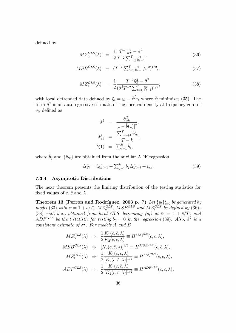
The next theorem presents the limiting distribution of the testing statistics for�xed values of c, �c and �.

Theorem 13 (Perron and Rodríguez, 2003 p. 7) Let fytgTt=0 be generated bymodel (33) with � = 1 + c=T , MZGLS� , MSBGLS and MZGLSt be de�ned by (36)-(38) with data obtained from local GLS detrending (~yt) at �� = 1 + �c=T , andADFGLS be the t statistic for testing b0 = 0 in the regression (39). Also, �

2 is aconsistent estimate of �2. For models A and B

MZGLS� (�) ) 1

2

K1(c; �c; �)

K2(c; �c; �)� HMZGLS� (c; �c; �),

MSBGLS(�) ) [K2(c; �c; �)]1=2 � HMSBGLS(c; �c; �),

MZGLSt (�) ) 1

2

K1(c; �c; �)

[K2(c; �c; �)]1=2� HMZGLSt (c; �c; �),

ADFGLS(�) ) 1

2

K1(c; �c; �)

[K2(c; �c; �)]1=2� HADFGLS(c; �c; �),

36

where

K1(c; �c; �) = V(1)c�c (1; �)

2 � 2V (2)c�c (1; �)� 1,

K2(c; �c; �) =R 10V(1)c�c (r; �)

2dr � 2R 1�V(2)c�c (r; �)dr,

and V (1)c�c (r; �) = Wc(r)� rb3, V

(2)c�c (r; �) = b4(r � �)[Wc(r)� rb3 � (1=2)(r � �)b4]

with Wc(r) the Ornstein-Uhlenbeck process that is the solution to the stochasticdi¤erential equation

dWc(r) = cWc(r)dr + dW (r) with Wc(r) = 0.

Also, b3 and b4 are de�ned by

b1 = (1� �c)Wc(1) + �c2R 10rWc(r)dr,

b2 = (1� �c+ ��c)Wc(1) + �c2R 1�Wc(r)(r � �)dr �Wc(�),

b3 = �1b1 + �2b2,

b4 = �2b1 + �3b2,

�1 = d=�,

�2 = �m=�,�3 = a=�,

d = 1� �� c+ 2c�� c�2 � c2�+ c2�2 + (c2=3)(1� �3),

m = 1� �� c+ c�+ (c2=2)�3 + (c2=3)(1� �3),

a = 1� c+ c2=3 and

� = ad�m2.

Proof. See Perron and Rodríguez (2003), Theorem 1, p. 22.

7.3.5 A Feasible Point Optimal Test with Known Breakdate

As Phillips (1988) pointed out, the discriminatory power of unit root tests is lowagainst local alternatives near but not equal to unity because under both hypothe-ses distributions are quite similar. The main idea behind e¢ ciency relies on theincrease of power or, equivalently, the probability of rejecting a false alternativehypothesis. As mentioned by Elliott, Rothenberg, and Stock (1996), if data distri-bution were known then the Neyman-Pearson Lemma would suggest the optimalpoint alternative against any other point alternative hypothesis and in such cir-cunstances a power envelope can be derived15.

15As Elliott, Rothenberg, and Stock (1996) mention, the Gaussian power envelope is an upperbound to the asymptotic power function for tests of the unit root hypothesis when the data are

37

However, although within this framework a uniformly most powerful (UMP)tests is not attainable, it is possible to de�ne an optimal test for � = 1 againstthe alternative � = ��. Even more, if vt were i.i.d. then such a test is given bythe likelihood ratio statistic which, under the normality assumption, equals thefollowing di¤erence

L (�) � S (��; �)� S (1; �) ,

where S (��; �) and S (1; �) are the sums of squares from GLS detrending bothunder � = �� and � = 1, respectively. Under the assumption of a known breakfrac-tion �, di¤erent values for �� lead to a family of point optimal tests and a gaussianenvelope for testing � = 1. Furthermore, in order to allow for correlation betweenerrors vt, Elliott, Rothenberg, and Stock (1996) propose a feasible optimal pointtest PGLST de�ned by

PGLST (c; �c; �) =S(��; �)� ��S(1; �)

�2, (40)

and its distribution is derived in the following

Theorem 14 (Perron and Rodríguez, 2003 p. 7) Let fytg be generated by(33) with � = 1 + c=T . Let PGLST be de�ned by (40) with data obtained fromlocal GLS detrending (~yt) at �� = 1 + �c=T: Also, let �

2 be a consistent estimate of�2. The limit distribution of the PGLST under Models A and B is given by

PGLST (c; �c; �))M(c; 0; �)�M(c; �c; �)

� 2�cR 10Wc(r)dW (r) + (�c

2 � 2�cc)R 10Wc(r)

2dr � �c � HPGLST (c; �c; �)

whereM(c; �c; �) = A(c; �c; �)0B(�c; �)�1A(c; �c; �) with A(c; �c; �) a 2�1 vector de�nedby"

W (1) + (c� �c)R 10Wc(r)dr � �c

R 10rdW (r)� (c� �c)�c

R 10rWc(r)dr

(1 + ��c)([W (1)�W (�)] + (c� �c)R 1�Wc(r)dr)� �c

R 1�rdW (r)� (c� �c)�c

R 1�rWc(r)dr

#and B (�c; �) is a symmetric matrix with entries�

�c2=3� �c+ 1 (1� �)(1� �c) + �c2(2 + �3 � 3)=6�c2(1� �3)=3� �c(1� �2)(1 + ��c) + (1� �)(1 + ��c)2

�.

generated byyt = dt + ut and ut = �ut�1 + �t

but under "ideal" conditions. Namely, the process f�tg has a moving average representationinvolving independent standard normal random variables, the initial condition u0 is 0 and thedeterministic component dt is known. Such unrealistic assumptions are made in order to employthe Neyman-Pearson theory.

38

Proof. See Perron and Rodríguez (2003), Theorem 2, p. 24.

The reader must remember that any test statistic is also a random variableand rejecting the unit root hypothesis is an event in which the test statistic liesbelow some critical value. Since distribution for the tests was derived both underthe null and the alternative hypothesis, the (asymptotic) power function can beexplicited by means of the probability of rejecting the null under the alternative.Such a function is given by

�(c; �) � P [HPGLST (c; c; �) < bPGLST (c; �)],

where the critical value bPGLST (c; �) is determined by the probability of Type I error

P [HPGLST (0; c; �) < bPGLST (c; �)] = �,

and � is the size of the test. Thus, di¤erent values of � generate di¤erent powerfunctions.

7.3.6 A Feasible Point Optimal Test with Unknown Breakdate and thePower Envelope

The previous subsections are referred to the case in which the breakfraction � isknown. In practice, however, this parameter is required to be estimated by appliedresearchers. For this reason the feasible version of the statistic in (40) is given by

PGLST;� (c; �c) =

�inf

�2[";1�"]S(��; �)� inf

�2[";1�"]��S(1; �)

��2. (41)

The principle behind (41) is the same as in (40). The main di¤erence relies onthe trimming parameter " introduced. This latter parameter is usually set to 0:15in order to bound critical values, a situation that arises in the context of tests forstructural change. Using Theorem 14, the following result is obtained

PGLST;� (c; �c)) sup�2[";1�"]

M(c; 0; �)� sup�2[";1�"]

M(c; �c; �)

� 2�cR 10Wc(r)dW (r) + (�c

2 � 2�cc)R 10Wc(r)

2dr � �c � HPGLST;� (c; �c) .

Accordingly, the asymptotic Gaussian power envelope is given by

��(c) � P [HPGLST;� (c; c) < bPGLST;� (c)],

where the critical value bPGLST;� (c) is such that P [HPGLST;� (0; c) < bP

GLST;� (c)] = �. It

must be pointed out that Elliott, Rothenberg, and Stock (1996) recommended a

39

value for �c such that ��(�c) = 0:5. Using Monte Carlo simulation, Perron andRodríguez (2003) found that �c = �22:5.It must be emphazised that, within this literature, the idea behind power in-

creasing unit root tests is related to the extent in which power functions are nearto the Gaussian power envelope (the benchmark case). When � is known, only oneset of simulations is performed in order to obtain the power function correspondingto that value. When � is unknown, on the contrary, several sets of simulations areperformed (one for each value of � in ["; 1� "]).

8 Conclusions

The present paper has analyzed the foundations and the applicability of the Func-tional Central Limit Theorem to the task of developing unit root tests. As shown,unit root tests can be described as functionals of stochastic processes such as thestandard Wiener process and the Ornstein-Uhlenbeck process.Therefore, a general framework involving mixing conditions (Phillips 1987a)

generalizes the results obtained under the assumption of normal i.i.d. disturbances(Dickey and Fuller 1979). Also, the analysis of modi�ed tests (Stock 1999) allowsto separate the size of unit root tests from the speci�c form of the deterministiccomponent, a problem not solved in earlier works. Tools developed also allowthe analitical tractability of several problem within this literature: the presenceof structural breaks and the low power against local alternatives. For the issueof structural breaks (Perron 1989), �rst detrending the series has shown to be arobust procedure, so that asymptotic size is not a¤ected (Stock 1999). For the issueof increasing power, asymptotic distribution can be derived by means of Ornstein-Uhlenbeck processes both under the null and local alternatives (Phillips 1987b)and a power function can be derived and maximized. When the two issues arecombined, the result is an e¢ cient test when a structural break is present underthe null (Perron and Rodríguez 2003).

40

References

Banerjee, A., R. L. Lumsdaine, and J. H. Stock (1992): �Recursive andSequential Tests of the Unit-Root and Trend-Break Hypotheses: Theory andInternational Evidence,�Journal of Business & Economic Statistics, 10(3), 271�87.

Bhargava, A. (1986): �On the Theory of Testing for Unit Roots in ObservedTime Series,�Review of Economic Studies, 53(3), 369�84.

Billingsley, P. (1968): Convergence of Probability Measures. John Wiley &Sons, Inc.

Box, G. E. P., and G. M. Jenkins (1970): Time Series Analysis: Forecastingand Control. John Wiley & Sons, Inc.

Box, G. E. P., and D. A. Pierce (1970): �Distribution of the Autocorrela-tions in Autoregressive Moving Average Time Series Models,� Journal of theAmerican Statistical Association, 65, 1509�26.

Brzezniak, Z., and T. Zastawniak (1999): Basic Stochastic Processes.Springer.

Davidson, J. (1994): Stochastic Limit Theory: An Introduction for Econometri-cians. Oxford University Press.

Dickey, D. A., and W. A. Fuller (1979): �Distribution of the Estimatorsfor Autorregresive Time Series with a Unit Root,� Journal of the AmericanStatistical Association, 74, 427�31.

Donsker, M. (1951): �An Invariance Principle for Certain Probability LimitTheorems,�Memoirs of the American Mathematical Society, 6, 1�12.

Elliott, G., T. J. Rothenberg, and J. H. Stock (1996): �E¢ cient Testsfor an Autoregressive Unit Root,�Econometrica, 64(4), 813�36.

Enders, W. (2004): Applied Econometric Time Series, Second Edition. JohnWiley & Sons, Inc.

Glynn, J., and N. Perera (2007): �Unit Root Tests and Structural Breaks: ASurvey with Applications,�Revista de Métodos Cuantitativos para la Economíay la Empresa, 3(1), 63�79.

Hamilton, J. D. (1994): Time Series Analysis. Princeton University Press.

41

Herrndorf, N. (1984): �A Functional Central Limit Theorem for Weakly De-pendent Sequences of Random Variables,� The Annals of Probability, 12(1),141�53.

Nelson, C. R., and C. I. Plosser (1982): �Trends and random walks in macro-econmic time series : Some evidence and implications,� Journal of MonetaryEconomics, 10(2), 139�62.

Ng, S., and P. Perron (2001): �LAG Length Selection and the Construction ofUnit Root Tests with Good Size and Power,�Econometrica, 69(6), 1519�54.

Oksendal, B. (2000): Stochastic Di¤erential Equations. Springer.

Ouliaris, S., J. Y. Park, and P. C. B. Phillips (1989): �Testing for a UnirRoot in the Presence of a Maintained Trend,� in Advances in EconometricsModelling, ed. by B. Raj. Kluwern Academic.

Perron, P. (1989): �The Great Crash, the Oil Price Shock, and the Unit RootHypothesis,�Econometrica, 57(6), 1361�1401.

Perron, P., and G. Rodríguez (2003): �GLS detrending, e¢ cient unit roottests and structural change,�Journal of Econometrics, 115(1), 1�27.

Phillips, P. C. B. (1987a): �Time Series Regression with a Unit Root,�Econo-metrica, 55(2), 277�301.

(1987b): �Towards a uni�ed asymptotic theory for autoregression,�Bio-metrika, 74(3), 535�47.

Phillips, P. C. B. (1988): �Regression Theory for Near-Integrated Time Series,�Econometrica, 56(5), 1021�43.

Phillips, P. C. B., and P. Perron (1988): �Testing for a Unit Root in TimeSeries Regression,�Biometrika, 75(2), 335�46.

Phillips, P. C. B., and V. Solo (1992): �Asymptotics for Linear Processes,�The Annals of Statistics, 20(2), 971�1001.

Sargan, J. D., and A. Bhargava (1983): �Testing Residuals from LeastSquares Regression for Being Generated by the Gaussian Random Walk,�Econometrica, 51(1), 153�74.

Stock, J. (1999): �A Class of Tests for Integration and Cointegration,�in Coin-tegration: Causality and Forecasting: A Festschrift in Honour of Clive W. J.Granger, ed. by R. F. Engle, and H. White, pp. 135�167. Oxford UniversityPress.

42

White, H. (1984): Asymptotic Theory for Econometricians. Academic Press.

White, J. S. (1958): �The Limiting Distribution of the Serial Correlation Co-e¢ cient in the Explosive Case,�The Annals of Mathematical Statistics, 29(4),1188�97.

Zivot, E., and D. W. K. Andrews (1992): �Further Evidence on the GreatCrash, the Oil-Price Shock, and the Unit-Root Hypothesis,�Journal of Business& Economic Statistics, 10(3), 251�70.

43

Appendix

A Beveridge-Nelson decomposition

Based on Phillips and Solo (1992), let the operator C(L) =P1

j=0 cjLj be a lag

polinomial. ThenC(L) = C(1)� (1� L) ~C(L)

where~C(L) =

P1j=0 ~cjL

j, ~cj =P1

k=j+1 ck.

If p � 1, thenP1j=1 j

pjcjjp <1 impliesP1

j=0 j~cjjp <1 and jC(1)j <1.

If p < 1, then P1j=1 jjcjjp <1 implies

P1j=0 j~cjjp <1.

B Martingale di¤erence sequence

Let fxtg and fytg denote two stochastic processes. Then fytg is a martingaledi¤erence sequence with respect to fxtg if its expectation, conditional to pastvalues of fxtg, is zero. Formally

E[ytjxt�1; xt�2; : : :] = 0, for all t.

When the expectation of fytg, conditional to its own past values, is zero then fytgis said to be a martingale di¤erence sequence (m.d.s.).

C Strongly uniform integrability

Let fZtg1t=1 be a sequence of random variables adapted to the �ltration fFtg1t=1.For Phillips and Solo (1992), fZtg is said to be strongly uniformly integrable (s.u.i.)if there exists a dominating random variable Z for which E(jZj) <1 and

P (jZtj � x) � cP (jZj � x)

for each x � 0, t � 1 and for some constant c.

44

ÚLTIMAS PUBLICACIONES DE LOS PROFESORES DEL DEPARTAMENTO DE ECONOMÍA

Libros José Rodríguez y Albert Berry (Eds.) 2010 Desafíos laborales en América Latina después de dos décadas de reformas

estructurales. Bolivia, Paraguay, Perú (1997-2008). Lima, Fondo Editorial, Pontificia Universidad Católica del Perú e Instituto de Estudios Peruanos.

José Rodríguez y Mario Tello (Eds.) 2010 Opciones de política económica en el Perú 2011-2015. Lima, Fondo Editorial,

Pontificia Universidad Católica del Perú. Felix Jiménez 2010 La economía peruana del último medio siglo. Lima, Fondo Editorial, Pontificia

Universidad Católica del Perú. Felix Jiménez (Ed.) 2010 Teoría económica y Desarrollo Social: Exclusión, Desigualdad y Democracia.

Homenaje a Adolfo Figueroa. Lima, Fondo Editorial, Pontificia Universidad Católica del Perú.

José Rodriguez y Silvana Vargas 2009 Trabajo infantil en el Perú. Magnitud y perfiles vulnerables. Informe Nacional 2007-

2008. Programa Internacional para la Erradicación del Trabajo Infantil (IPEC). Organización Internacional del Trabajo.

Óscar Dancourt y Félix Jiménez (Ed.) 2009 Crisis internacional. Impactos y respuestas de política económica en el Perú. Lima,

Fondo Editorial, Pontificia Universidad Católica del Perú. Alfredo Dammert y Raúl García 2009 Los Jones quieren casa nueva. Cómo entender la nueva crisis económica mundial.

Fondo Editorial, Pontificia Universidad Católica del Perú. Efraín Gonzales de Olarte y Javier Iguiñiz Echeverría (Eds.) 2009 Desarrollo económico y bienestar. Homenaje a Máximo Vega-Centeno. Lima, Fondo

Editorial, Pontificia Universidad Católica del Perú. Félix Jiménez 2008 Reglas y sostenibilidad de la política fiscal. Lecciones de la experiencia peruana.

Lima, Fondo Editorial, Pontificia Universidad Católica del Perú. Adolfo Figueroa 2008 Nuestro mundo social. Introducción a la ciencia económica. Lima, Fondo Editorial,

Pontificia Universidad Católica del Perú.

Serie: Documentos de Trabajo No. 318 “Brechas de ingresos laborales entre autoempleados y asalariados en el Perú”.

José S. Rodríguez, Julio 2011. No. 317 “Microcrédito y Crecimiento Regional en el Perú”. Giovanna Aguilar, Junio 2011. No. 316 “Estimation of a Time Varying Natural Interest Rate for Peru”. Alberto Humala y

Gabriel Rodríguez, Junio 2011. No. 315 “A factorial Decomposition of Inflation in Peru, An Alternative Measure of Core

Inflation”. Alberto Humala y Gabriel Rodríguez, Junio 2011. No. 314 “Does the Exchange Rate Pass-Through into Prices Change when Inflation

Targeting is Adopted? The Peruvian Case Study between 1994 and 2007”. Paul Castillo, Luis R. Maertens Odría y Gabriel Rodríguez, Mayo 2011.

No. 313 “Tesis de efectos del incremento de la remuneración mínima vital sobre el

empleo y los ingresos laborales”. Jesús Alejandro Palomino Samaniego, Marzo 2011.

No. 312 “Crisis financiera, sistema monetario y el desafío de los países emergentes”.

Jorge Rojas, Febrero, 2011. No. 311 “Ciencia, tecnología, cooperación tecnológica, TIC y rentabilidad de las

empresas manufactureras bajo un enfoque empresarial: El caso del Perú, 2004-2005”. Mario Tello, Febrero, 2011.

No. 310 “Indicadores del sector MYPE informal en el Perú: Valor agregado, potencial

exportador, capacidad de formalizarse y requerimientos de normas técnicas peruanas de sus productos”. Mario Tello, Febrero, 2011.

No. 309 “Determinantes socioeconómicos de las transiciones entre niveles educativos:

un enfoque sobre género y ruralidad en el Perú”. Denice Cavero, Verónica Montalva y José Rodríguez. Enero, 2011.

No. 308 “State Density and Capabilities Approach: Conceptual, Methodological and

Empirical Issues”. Efraín Gonzales de Olarte y Javier M. Iguiñiz Echeverría. Enero, 2011.

No. 307 “Crecimiento económico: enfoques y modelos. Capítulo 7 – Política económica,

crecimiento y desarrollo”. Félix Jiménez. Noviembre, 2010. No. 306 “Crecimiento económico: enfoques y modelos. Capítulo 6 – Teoría del

crecimiento dirigida por la demanda”. Félix Jiménez. Noviembre, 2010.

Departamento de Economía - Pontificia Universidad Católica del Perú Av. Universitaria 1801, Lima 32 – Perú.

Telf. 626-2000 anexos 4950 - 4951 http://www.pucp.edu.pe/economia

Understanding The Functional Central Limit Theorems With Some Applications To Unit Root Testing With Structural Change

Documents