Understanding Retail Trade Analysis by Al Myles, Economist and Extension Professor Department of Agriculture Economics Mississippi State University December.

Understanding Retail Trade Analysis

by

Al Myles, Economist and Extension Professor

Department of Agriculture Economics

Mississippi State University

December 11, 2008

Presented at Oktibbeha County Leadership Forum

Retail Trade Analysis-

Is a way to identify market trends within a local community, including the degree of surplus or leakage of dollars within specific retail sectors.

PURPOSE

•Gives an historical overview of a community’s or county’s retail trade sector

•Provides a basis for comparison with similar size communities and counties

•Is useful for identifying opportunities in the retail sector•Similar to annual health physical at the doctor’s office. Tells you what’s right and wrong.

Why Retail Trade?Retail trade is one of the most important indicators of economic activity in a community or county because local citizens spend a large part of their incomes on goods and services. The measures of retail trade and spending reflect consumers’ preference for the retail mix in the area and show how well the economy is doing overall. Since retail is one of the major economic forces in the country, local officials often want to know how they compare with their competitors. .

Purpose of Retail Promotions

Keeping Local Dollars at Home

Indicators of Retail ActivitySales Tax Collections Market Capture Gap Analysis (Potential sales-Actual Sales)

Pull factorsSales leakage

Introduction-Defining a town’s trade area is an important first step in developing a strong retail sector.

-This is the foundation of retail market analysis. It helps existing businesses to identify ways to expand their own market.

-Increasing retail sales is one way an area can:

capture dollars

increase income

improve employment multipliers of its local industries.

Defining the Trade Area

-Whatever the reasons for existing retail sales, city and county leaders can help local businesses to improve these trends.

-To determine the potential for increasing retail sales, one should establish the trade area.

A trade area is the geographic region from which a town draws the majority of its retail customers. This can be done in several ways:

1. Conducting a traffic flow study,

2. Using a retail gravity model,

3. Using a zip code method, and

4. Using commuting data to define the trade area boundaries.

Of these methods, COMMUTING and RETAIL GRAVITY approaches present the least amount of work to implement.

Traffic Flow….

Is the random canvassing of parking lots at major locations in town at different times on different days and over several weeks.

The locations might include

The downtown area,

Major shopping destinations such as shopping malls and centers, Wal-Mart Super Center, Home Depot, Krogers’, and

Other popular establishments in town.

One should combined the results of vehicle license plates from the different locations to obtain a composite count of vehicles from surrounding counties and compare them to regional commuting data.

Results from a traffic study will usually reveal

the major towns and counties that comprise the local trade area or market.

To determine the major communities in the local market one should:

1. Rank order the number of cars from various counties in the region, and

2. Select the top five or six localities based on the highest frequency and/or maximum percentage (10% or more) of license plates in the area.

Commuting…

Commuting time to work by local residents is another way of delineating a community’s retail trade area.

Converting commuting time to work into spatial distances or miles and plotting these data on a map, provide a visual picture of the geographic size of its trade area.

Figure 1. Trade Area: Major Commuting Counties

Figure 1. Trade Area: Immediate Commuting Counties

Reily’s Law…

Another easy way of defining the retail trade area is to use a gravity model. In retail trade analysis, the most popular method is “Reily’s Law of Retail Gravitation.”

Reily’s law is a rule-of-thumb used to ESTIMATE the distance customers will travel to PURCHASE goods and SERVICES after comparing price, quality, and style.

Reilly’s Law

The law assumes that people desire to shop in larger towns, but their desire declines the farther the distance and time they must travel to get there. Thus, LARGER TOWNS DRAW CUSTOMERS FROM FARTHER DISTANCES THAN SMALLER TOWNS.

The maximum distance a customer will travel to shop in a smaller town can be calculated using the following formula.

Population and Travel Distances in Community A’s Trade Area

County Total Population Distance (FROM Community A to County Seat)

Trade Area Distance

Community A 22,000

Community B 1,543 27 5.65

Community C 23,799 23 11.73

Community D 2,145 27 6.42

Community E 7,169 33 11.99

Community F 8,489 17 6.51

Average 10,/8/ 25.4 8.46

Figure 1. Picture of Community’s Trade Area

W E

Community B

Community E

N

S

Community F6.51 miles

Community ACommunity D Community C

5.65 miles

11.99 miles

6.42 miles

11.27 miles

Estimating Total Market Size

Once the physical boundaries of the trade area have been identified, one should estimate the total market size.

The total market consists of populations in the host community plus population from surrounding towns in the trade area.

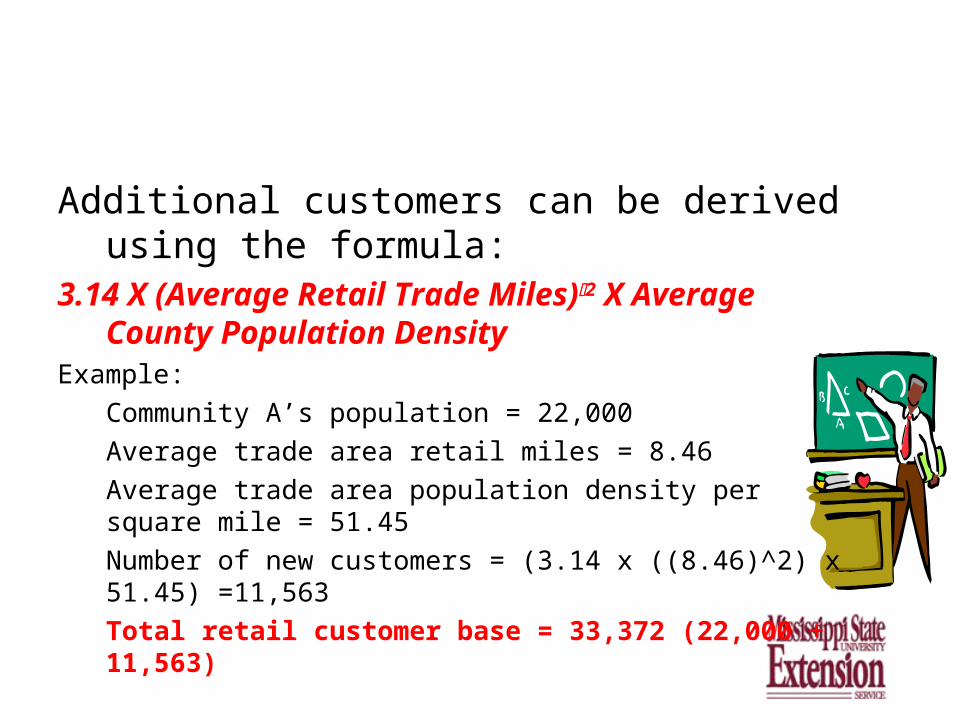
Additional customers can be derived using the formula:

3.14 X (Average Retail Trade Miles)2 X Average County Population Density

Example:

Community A’s population = 22,000

Average trade area retail miles = 8.46

Average trade area population density per square mile = 51.45

Number of new customers = (3.14 x ((8.46)^2) x 51.45) =11,563

Total retail customer base = 33,372 (22,000 + 11,563)

In using this approach, there are a few caveats:

1. Areas with large populations and densities per square mile can distort the actual situation in retail trade analysis.

2. Reily’s Law is less accurate when involving larger towns.

Trade Area Population Model

Answers the basic question:  What is the probability that a consumer located in communityi will shop in communityj, given the presence of competing

towns? The spatial interaction model takes into account such variables as distance, attractiveness and competition in different sites.

The probability (Pij)1 that a consumer located in communityi will choose to

shop in communityj is calculated as:

Where:

Aj is a measure of attractiveness of communityj, such as total retail sales, total personal income, or population of area.

Dij is the distance from i to j.

α2 is an attractiveness parameter from empirical observation.

Β3 is the distance decay parameter estimated from empirical observations. Simply, it is a parameter that reflects the propensity to travel by consumers.

n is the total number of communities including the host communityi .

The product derived from dividing  by  is known as the perceived utility of communityj by a consumer located in communityi.

Using Information About Market Size

After defining the trade area, one can ESTIMATE the local sales potential and COMPARE them to actual sales in the area. The following formula can be used to estimate potential retail sales.

POTENTIAL SALES

•Potential sales for a given sector in a given county can be estimated as

•Where

-PSij is potential sales for commercial sector j in county i

-Pi is population for county i

-SSPCj is state sales per capita for commercial sector j

-PCIi is per capita income for county i

-PCIs is per capita income for state s

PCIs

PCIiSSPCjPiPSij **

By comparing POTENTIAL with ACTUAL retail sales, one can determine whether the city has room for retail growth.

One should compare retail sales over SEVERAL YEARS to determine the LONG-TERM health of retail sectors in the city.

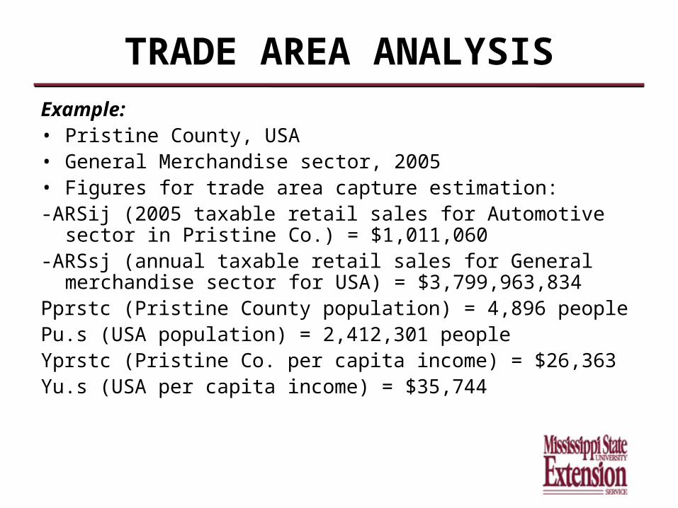
TRADE AREA ANALYSIS

Example:• Pristine County, USA• General Merchandise sector, 2005• Figures for trade area capture estimation:-ARSij (2005 taxable retail sales for Automotive sector in Pristine Co.)

= $1,011,060-ARSsj (annual taxable retail sales for General merchandise sector for

USA) = $3,799,963,834Pprstc (Pristine County population) = 4,896 peoplePu.s (USA population) = 2,412,301 peopleYprstc (Pristine Co. per capita income) = $26,363Yu.s (USA per capita income) = $35,744

TRADE AREA ANALYSIS Example:

Potential Sales

• The equation becomes:

• The potential sales are considerably greater than the actual sales of $1,011,060

281,688,5$

744,35$

363,26$*

301,421,2

834,963,799,3$*)896,4(

PS

PS

Potential Sales: Interpretation

•Can compare estimates of potential sales for commercial sector j in county i to realized sales of commercial sector j in county i

-Derive a value of captured or lost commercial sales for that sector and county

Determining Retail Power

Trade Area Capture (TAC)

Information about the trade area can help one to estimate the ability of community merchants to capture the retail business of people in the area.

Trade Area Capture (TAC)

is an estimate of the number of people who shop in the local area during a certain period.

Pull Factors…

Knowledge of the trade area is the first step in retail market analysis.

Knowing the trade area, one can determine the size and pulling power of local merchants in the market using a concept call pull factors.

Pull factors are ratios that estimate the proportion of local sales that occurs in a town.

The most common method of calculating pull factors is as follows:

Pull Factor (PF) = Trade Area Capture City Population

See slide 23

PF Value Interpretation

> 1 Retailers drawing customers from outside trade area

< 1 Retailers losing customers from outside trade area

= 1 Retailers maintaining customers in trade area

  1981 1982 1983 1984 1985 1986 1987 1988 1989 1990 1991 1992 1993 1994 1995 1996 1997 1998 1999 2000 2001 2002 2003 2004 2005 2006 2007

Clay 0.76 0.73 0.73 0.74 0.76 0.76 0.77 0.75 0.77 0.76 0.75 0.74 0.76 0.73 0.70 0.70 0.71 0.71 0.73 0.74 0.73 0.71 0.69 0.70 0.73 0.71 0.71

Lowndes 1.07 1.12 1.00 1.00 1.00 1.01 1.03 1.03 1.11 1.19 1.01 1.03 1.07 1.00 1.01 1.00 1.00 0.97 0.99 1.12 1.11 1.11 1.08 1.06 1.00 0.98 1.03

Oktibbeha 0.78 0.74 0.74 0.75 0.76 0.76 0.76 0.75 0.75 0.76 0.75 0.76 0.79 0.74 0.73 0.72 0.73 0.76 0.75 0.83 0.84 0.87 0.85 0.85 0.83 0.84 0.82

Mississippi 0.79 0.82 0.78 0.77 0.77 0.76 0.75 0.74 0.74 0.74 0.72 0.74 0.76 0.74 0.73 0.74 0.74 0.73 0.73 0.77 0.76 0.76 0.76 0.76 0.74 0.74 0.74

Pull factors for Selected Counties in Mississippi

PF>1.0 WhitePF>.8<=1 Light Blue

PF>.6<=.79 GreenPF>.4<=.59 Yellow

Figure 1. Weighted Average Pull Factors for Mississippi Counties, 2007

Mississippi Total .74

PF>1.0 White

PF>.8<=1 Light Blue

PF>.6<=.79 Green

PF>.4<=.59 Yellow

Some questions to think about when interpreting pull factors:

1. How has the pull factor changed over time? If it has increased, why do you think that is so? If it has declined, what are some possible causes?

2. How does the local pull factor compare to other counties? The state? Why do you think it is higher or lower?

3. What are some strategies your community can adopt to increase the amount of money drawn in from outside the county?

What Is Happening Locally?

Table 1. Oktibbeha County With and Without Federal Funds

Year With Without Median State Index Rank

1993 4.02 3.77 3.57 241994 3.95 3.69 3.56 271995 3.94 3.68 3.57 261996 3.88 3.63 3.57 281997 3.88 3.62 3.58 281998 3.90 3.65 3.56 281999 4.00 3.70 3.55 252000 4.06 3.74 3.56 262001 4.12 3.83 3.55 262002 4.18 3.87 3.55 242003 4.19 3.86 3.57 242004 4.16 3.86 3.52 23

Average 4.02 3.75

Economic Strength Index

Trade Area CaptureCurrent

Population2002Projected

Population 2019

TAC to Population

RatioCountyClay 21,751 21,979 22,840 98.96 Lowndes 98,344 61,586 65370 159.69 Oktibbeha 51,136 42,902 51200 119.19 Region Total 173,153 126,467 139,410 136.92

0

20,000

40,000

60,000

80,000

100,000

120,000

140,000

160,000

180,000

Market Population

Figure 1. Trade Capture

Series1 21,751 98,344 51,136 173,153

Clay Low ndes Oktibbeha Region Total

Figure 2. TAC and 2002 Population

0 50,000 100,000 150,000 200,000

Clay

Low ndes

Oktibbeha

Region Total

Series2 21,979 61,586 42,902 126,467

Series1 21,751 98,344 51,136 173,153

Clay Low ndes Oktibbeha Region Total

Figure 3. TAC, 2002 Population, and Projected 2019 Population

0

50,000

100,000

150,000

200,000

Series1 21,751 98,344 51,136 173,153

Series2 21,979 61,586 42,902 126,467

Series3 22,840 65370 51200 139,410

Clay Low ndes Oktibbeha Region Total

98.96

159.69

119.19

136.92

-

20.00

40.00

60.00

80.00

100.00

120.00

140.00

160.00

180.00

Clay Lowndes Oktibbeha Region Total

Per

cen

tFigure 4. Market Capture Above Population

Figure 5. County Retail Sales

$-

$100,000,000

$200,000,000

$300,000,000

$400,000,000

$500,000,000

$600,000,000

Series1 $363 $375 $398 $408 $435 $426 $447 $455 $529

98 99 00 01 02 03 04 05 06

Figure 6. Starkville Retail Sales

$-

$50,000,000

$100,000,000

$150,000,000

$200,000,000

$250,000,000

$300,000,000

$350,000,000

$400,000,000

Series1 $251, $272, $292, $300, $306, $302, $320, $328, $374,

98 99 00 01 02 03 04 05 06

Figure 7. Oktibbeha County Per Capita Sales Ratio

$-

$1,000

$2,000

$3,000

$4,000

$5,000

$6,000

$7,000

$8,000

$9,000

Series2 $5,967 $6,419 $6,799 $7,027 $7,203 $7,101 $7,447 $7,539 $8,499

98 99 00 01 02 03 04 05 06

Summary

This presentation shows how a few simple techniques can be used to determine the geographic size of a town’s trade area.

A trade area will often extend beyond its own geographic borders.

CONCLUSIONS•Trade area analysis shows how businesses can use existing data to learn more about their business power

•Trade area analysis provides information about:

-The number of customers in a county

-A sector’s pull factor in the region

-Potential sales in an area

•This information can all be used to create a plan or strategy for business owners

Shift-Share Results for Your Area

In economics, there is a technique called shift-share analysis.   Its purpose is to take the change in employment for an area and decompose it into the three sources that caused the change.  

National growthIndustrial growthCompetitive effect

The industries are ordered according to how many people they employed in the latest year selected ( 2007) .  

During the period 1990 to 2007, employment in Oktibbeha County grew by 2,869 jobs.   In terms of employment growth, the most important industry was Professional and Business Services (1,411 jobs).   It is followed by Education and Health Services( 1,376 jobs), and leisure and Hospitality ( 1,929 jobs).  

Table 1 presents the employment changes for the time period selected in Oktibbeha County, MS. During the period 1990 to 2007, employment in the county grew by 2,869 jobs.  

Table 1: Employment Changes in Your Area, 1990 to 2007.

SectorEmployment,

1990Employment,

2007Employment Change

Percent Growth,1990 - 2007

Education and Health Services

1,868 3,244 1,376 73.7

Trade, Transportation, and Utilities

2,025 2,299 274 13.5

Leisure and Hospitality 1,207 2,136 929 77.0

Professional and Business Services

396 1,807 1,411 356.3

Manufacturing 2,111 1,582 -529 -25.1

Public Administration 1,369 809 -560 -40.9

Financial Activities 554 437 -117 -21.1

Construction 330 410 80 24.2

Other Services 249 234 -15 -6.0

Information 119 162 43 36.1

Natural Resources and Mining

66 43 -23 -34.8

  10,294 13,163 2,869  

Table 1: Employment Changes in Oktibbeha County, 1990 to 2007.

Table 2: Shift-Share Analysis for Your Area, 1990-2007.

SectorNational Growth

Component, Percent

National GrowthComponent,

Jobs

Industrial MixComponent,

Percent

Industrial MixComponent,

Jobs

CompetitiveShare

Component,Percent

CompetitiveShare

Component,Jobs

Professional and Business Services

24.7 98 44.8 177 286.8 1,136

Education and Health Services

24.7 461 23.2 434 25.8 481

Leisure and Hospitality

24.7 298 17.9 216 34.4 415

Information 24.7 29 -15.2 -18 26.6 32

Natural Resources and Mining

24.7 16 -20.3 -13 -39.3 -26

Trade, Transportation, and Utilities

24.7 500 -8.7 -176 -2.5 -50

Manufacturing 24.7 521 -47.2 -997 -2.5 -53

Construction 24.7 81 19.3 64 -19.7 -65

Other Services 24.7 61 3.1 8 -33.8 -84

Financial Activities

24.7 137 -5.4 -30 -40.4 -224

Public Administration

24.7 338 -10.0 -136 -55.6 -762

    2,540   -471   800

Table 2: Shift-Share Analysis for Oktibbeha County, 1990-2007.

1. The National Growth Component

The first source of change is the growth or contraction in the United States economy.  This growth rate is listed in Table 2 as the national growth component.  

Overall, the national growth component was responsible for a total of 2,540 jobs in Oktibbeha County.

An understandable goal of some local leaders is to make their economy more 'recession proof'.   Economies with more employment in government, military and education will experience less fluctuation because those sectors are not directly related to the business cycle.

Also, economic sectors that are experiencing more growth will provide larger employment gains to a local economy.

2. The Industrial Mix Component

The industrial mix component measures how well an industry has grown, net the effects from the business cycle.

Table 2 lists these components for each sector.   If the county's employment were concentrated in these sectors with higher industrial mix components, then the area could expect more employment growth.   After adding up across all eleven sectors, it appears that the industrial mix component was responsible for decreasing Oktibbeha County’s employment by -471 jobs.  

Thus, the area has a concentration of employment in industries that are decreasing nation-wide, in terms of employment.   The majority of these jobs can be attributed to decreases (-997 jobs) in the Manufacturing sector.

3. The Competitive Share

The third and final component of shift-share analysis is called the competitive share.   It is the remaining employment change that is left over after accounting for the national and industrial mix components.  

If a sector's competitive share is positive, then the sector has a local advantage in promoting employment growth.

The top three sectors in competitive share were Professional and Business Services, Education and health Services, and leisure and Hospitality.   Across all sectors, the competitive share component equaled 800 jobs.   This indicates the county is competitive in securing additional employment.

A positive competitive share component indicates the county has a productive advantage.   This advantage could be due to local firms having superior technology, management, or market access, or the local labor force having higher productivity and/or lower wages.  

A negative competitive share component could be caused by local shortcomings in all these areas.

By examining the competitive share components for each industry, the development official can easily identify which local industries have a positive competitive share component.   This also indicates which industries have competitive advantages over other counties and regions.  

Local officials can then devise strategies to improve local conditions faced by particular industries selected for focus.   These strategies may include specialized training programs for workers and management, improved access to input and product markets through transportation and telecommunications, or arranged financial alternatives for new machinery and equipment.

Questions?

Question

s?

Questions?

THANK YOU!