Understanding Patterns In Nature - ScholarlyCommons

University of Pennsylvania University of Pennsylvania

ScholarlyCommons ScholarlyCommons

Publicly Accessible Penn Dissertations

2021

Understanding Patterns In Nature Understanding Patterns In Nature

Mingjun Zhang University of Pennsylvania

Follow this and additional works at: https://repository.upenn.edu/edissertations

Part of the Philosophy of Science Commons

Recommended Citation Recommended Citation Zhang, Mingjun, "Understanding Patterns In Nature" (2021). Publicly Accessible Penn Dissertations. 4059. https://repository.upenn.edu/edissertations/4059

This paper is posted at ScholarlyCommons. https://repository.upenn.edu/edissertations/4059 For more information, please contact [email protected].

Understanding Patterns In Nature Understanding Patterns In Nature

Abstract Abstract Nature is full of interesting patterns. One of the most important tasks across the natural sciences, especially the biological sciences, is to identify and explain real patterns in nature. This dissertation provides a philosophical investigation of the nature and roles of real patterns in biological inquiry and the various strategies that biologists employ to explain and understand real patterns in nature. In Chapter 1, I advocate for a pragmatic approach to the reality of patterns in data. I argue that patterns in data are expected to play different scientific roles in different research contexts and that a pattern in data is real if and only if it fulfills the scientific role it is expected to play in a specific research context. In Chapter 2, I give a critical evaluation of the use and limitations of null-model-based hypothesis testing as a research strategy to explain patterns in the biological sciences. I argue that null-model-based hypothesis testing fails to work as a proper analog to traditional statistical null-hypothesis testing as used in well-controlled experimental research, and that the random process hypothesis should not be privileged as a null hypothesis. Instead, the possible use of the null model resides in its role of providing a way to challenge scientists’ commonsense judgments about how a seemingly unusual pattern could have come to be. In Chapter 3, I clarify the definition of a baseline model and apply it to the niche-neutral debate about how to understand biodiversity patterns. I argue that from a process-based perspective, a neutral model in ecology should not be regarded as a baseline model relative to classical niche-based models. In Chapter 4, I investigate the testability and the scientific value of the notion of overall relative causal importance by carefully examining the controversy over empirical adaptationism in evolutionary biology. My analysis of the case of empirical adaptationism provides reasons for scientists to reconsider the value and necessity of engaging in scientific debates involving the notion of overall relative causal importance.

Degree Type Degree Type Dissertation

Degree Name Degree Name Doctor of Philosophy (PhD)

Graduate Group Graduate Group Philosophy

First Advisor First Advisor Michael Weisberg

Keywords Keywords baseline model, null model, real pattern, relative causal importance

Subject Categories Subject Categories Philosophy | Philosophy of Science

This dissertation is available at ScholarlyCommons: https://repository.upenn.edu/edissertations/4059

UNDERSTANDING PATTERNS IN NATURE

Mingjun Zhang

A DISSERTATION

in

Philosophy

Presented to the Faculties of the University of Pennsylvania

in

Partial Fulfillment of the Requirements for the

Degree of Doctor of Philosophy

2021

Supervisor of Dissertation

_________________

Michael Weisberg

Professor and Chair of Philosophy

Graduate Group Chairperson

_________________

Errol Lord

Associate Professor of Philosophy

Dissertation Committee

Erol Akçay, Associate Professor of Biology

Karen Detlefsen, Professor of Philosophy and Education

Quayshawn Spencer, Robert S. Blank Presidential Associate Professor of Philosophy

UNDERSTANDING PATTERNS IN NATURE

COPYRIGHT

2021

Mingjun Zhang

This work is licensed under the

Creative Commons Attribution-

NonCommercial-ShareAlike 4.0

License

To view a copy of this license, visit

https://creativecommons.org/licenses/by-nc-sa/4.0/us/

iii

Dedication

For my beloved family

(my mother Guo’ai Liu 刘国爱, my father Changli Zhang 张昌利,

my brother Yingjun Zhang 张颖君, and my nephew Yuwei Zhang 张育玮)

iv

ACKNOWLEDGMENT

I would like to express my deepest thanks to my supervisor, Michael Weisberg, not only for his guidance

and support throughout my dissertation writing and intellectual development, but also for his patience,

encouragement, and care during my life journey at Penn. His passion, openness, creativity, and diligence

have shaped my understanding of what it means to be a good philosopher, and his genuine care for my

development and well-being means the world to me.

I thank my committee members: Erol Akçay, Karen Detlefsen, and Quayshawn Spencer. Erol

welcomed me into his theoretical biology lab and never tires of answering my questions about ecology and

evolutionary biology. Karen made time to talk with me whenever I needed help and helped me clarify my

thoughts on many points and greatly improve the clarity of my dissertation. Quayshawn read and

commented in detail on every draft I have sent him; his challenging yet supportive criticisms helped to

considerably improve the strength of my arguments.

I thank the many faculty members who have mentored me during my time at Penn: Errol Lord and

Daniel Singer, who organized my cohort’s proseminar and helped me prepare for my philosophical study at

Penn; Lisa Miracchi, who offered extremely helpful suggestions on my teaching and on how to maintain

wellness at challenging times; Sukaina Hirji and Kok-Chor Tan, who read and commented on my job

application materials and helped me practice for my job interview during the process of job application.

I thank my friends and colleagues who helped me at various stages to explore the ideas in my

dissertation, including Zachary Agoff, Ben Baker, Clarissa Busch, Chetan Cetty, Shereen Chang, Mike

Gadomski, Javier Gomez-Lavin, Kate Nicole Hoffman, Karen Kovaka, Hanyu Ma, Dylan Manson, Paul

Musso, Raj Patel, Ian Peebles, Sara Purinton, Tyler Re, John Roman, Tiina Rosenqvist, Vanessa Schipani,

Maja Sidzinska, John A. Sime, Matthew Solomon, Daniel G. Swaim, Alexander Tolbert, Eugene Vaynberg,

Yosef Washington, Stephanie Wesson, and Younbin Yoon. I also thank all the members of MIRA Group

and Philosophy of Science Reading Group for invaluable conversations and feedback.

I thank my cohort – Eilidh Beaton, Grace Boey, Max Lewis, and Michael Vazquez – for their

company and friendship.

Finally, I would like to thank my parents for their unconditional love and sacrifice.

v

ABSTRACT

UNDERSTANDING PATTERNS IN NATURE

Mingjun Zhang

Michael Weisberg

Nature is full of interesting patterns. One of the most important tasks across the natural sciences, especially

the biological sciences, is to identify and explain real patterns in nature. This dissertation provides a

philosophical investigation of the nature and roles of real patterns in biological inquiry and the various

strategies that biologists employ to explain and understand real patterns in nature. In Chapter 1, I advocate

for a pragmatic approach to the reality of patterns in data. I argue that patterns in data are expected to play

different scientific roles in different research contexts and that a pattern in data is real if and only if it

fulfills the scientific role it is expected to play in a specific research context. In Chapter 2, I give a critical

evaluation of the use and limitations of null-model-based hypothesis testing as a research strategy to

explain patterns in the biological sciences. I argue that null-model-based hypothesis testing fails to work as

a proper analog to traditional statistical null-hypothesis testing as used in well-controlled experimental

research, and that the random process hypothesis should not be privileged as a null hypothesis. Instead, the

possible use of the null model resides in its role of providing a way to challenge scientists’ commonsense

judgments about how a seemingly unusual pattern could have come to be. In Chapter 3, I clarify the

definition of a baseline model and apply it to the niche-neutral debate about how to understand biodiversity

patterns. I argue that from a process-based perspective, a neutral model in ecology should not be regarded

as a baseline model relative to classical niche-based models. In Chapter 4, I investigate the testability and

the scientific value of the notion of overall relative causal importance by carefully examining the

controversy over empirical adaptationism in evolutionary biology. My analysis of the case of empirical

adaptationism provides reasons for scientists to reconsider the value and necessity of engaging in scientific

debates involving the notion of overall relative causal importance.

vi

TABLE OF CONTENTS

ACKNOWLEDGMENT ......................................................................................... IV

ABSTRACT ............................................................................................................. V

LIST OF TABLES .................................................................................................. IX

LIST OF ILLUSTRATIONS.................................................................................... X

INTRODUCTION .................................................................................................... 1

CHAPTER 1: WHAT IS A REAL PATTERN?

A PRAGMATIC APPROACH TO THE REALITY OF PATTERNS IN DATA ..... 6

1. Introduction ................................................................................................................................... 6

2. A pragmatic approach to the reality of patterns in data ................................................................. 7

3. Real patterns as efficient compressed representations of data ........................................................ 8

4. Real patterns in data as evidence for scientific phenomena........................................................... 11 4.1 Data, phenomena, and theories: Bogen and Woodward’s three-tiered framework............................. 11 4.2 Counterfactual dependence in data-to-phenomena reasoning ............................................................. 14 4.3 Locating the role of patterns in data-to-phenomena reasoning ........................................................... 15 4.4 Real vs. unreal patterns in the context of phenomenon detection ....................................................... 19

5. Patterns in data as targets of systematic explanation .................................................................... 21 5.1 Examples of important patterns in nature............................................................................................ 21 5.2 Desiderata for identifying real patterns in data ................................................................................... 26

6. McAllister’s stipulationist view of physically significant patterns in data ..................................... 32

7. Problems of the stipulationist view through the lens of the pragmatic approach ........................... 34

8. Conclusion ................................................................................................................................... 40

CHAPTER 2: THE USE AND LIMITATIONS OF NULL-MODEL-BASED

HYPOTHESIS TESTING ...................................................................................... 41

1. Introduction ................................................................................................................................. 41

2. Null-model-based hypothesis testing in species co-occurrence studies ........................................... 44 2.1 Constructing the null model ................................................................................................................ 45 2.2 Comparing simulated data with empirical data ................................................................................... 48 2.3 Technical controversies concerning the test ........................................................................................ 49

vii

3. A critical evaluation of null-model-based hypothesis testing ......................................................... 50 3.1 Connor and Simberloff’s interpretation .............................................................................................. 50 3.2 Evaluating the interpretation ............................................................................................................... 54 3.3 Applying the analysis results ............................................................................................................... 64

4. The possible use and limitations of null-model-based hypothesis testing ....................................... 67 4.1 Challenging “common sense” by providing how-possibly explanations ............................................ 68 4.2 The limitations of null-model-based hypothesis testing...................................................................... 70

5. Lessons from the debate ............................................................................................................... 72

6. Conclusion ................................................................................................................................... 74

CHAPTER 3: IN WHAT SENSE CAN NEUTRAL THEORY WORK AS A

BASELINE MODEL? ............................................................................................ 76

1. Introduction ................................................................................................................................. 76

2. Two approaches to explaining biodiversity patterns in ecological communities ............................ 77

3. The interpretation of neutral models as baseline models .............................................................. 79

4. Evaluating neutral models’ status as baseline models ................................................................... 81 4.1 What is a baseline model? ................................................................................................................... 82 4.2 The ideal gas model as a baseline model ............................................................................................ 83 4.3 In what sense can a neutral model work as a baseline model?............................................................ 85 4.4 The contrast between the ideal gas model and neutral models ........................................................... 89

5. Conclusion ................................................................................................................................... 91

CHAPTER 4: EMPIRICAL ADAPTATIONISM REVISITED ............................. 92

1. Introduction ................................................................................................................................. 92

2. The two themes of empirical adaptationism ................................................................................. 93

3. The first theme: the relationship between natural selection and constraints on evolution ............. 94

4. The second theme: the overall relative causal importance of natural selection in evolution ........ 102

5. Methodological difficulties in the long-run test of empirical adaptationism ................................ 109

6. Rethinking the value and necessity of testing empirical adaptationism ....................................... 114 6.1 Methodological heuristic value ......................................................................................................... 116 6.2 Explanatory value .............................................................................................................................. 118 6.3 Epistemic value ................................................................................................................................. 119 6.4 Spin-off value .................................................................................................................................... 120

7. Rethinking the value of scientific debates involving overall relative causal importance .............. 122

viii

8. Conclusion ................................................................................................................................. 124

BIBLIOGRAPHY ................................................................................................ 125

ix

LIST OF TABLES

Table 2-1: A 3-by-4 random matrix……………………………………………………...45

x

LIST OF ILLUSTRATIONS

Figure 1-1: The data-phenomena-theory framework advocated by Bogen and Woodward

……………………………………………………………………………………………13

Figure 1-2: The counterfactual dependence relationships between phenomenon-claims

and patterns in data………………………………………………………………………16

Figure 1-3: A four-level framework involving data, patterns, phenomena, and scientific

theories…………………………………………………………………………………...19

Figure 1-4: The distribution ranges of two species of fruit doves……………………….23

Figure 1-5: Preston’s (1948) reanalysis of the RSA of moths collected by C.B. Williams

……………………………………………………………………………………………25

Figure 1-6: Two patterns of relative species abundance…………………………………31

Figure 2-1: The relationship between the full null space and the sample null space…….47

Figure 2-2: Procedures of two types of hypothesis testing………………………………52

Figure 2-3: The relation between H0, H1, and H1*……………………………………….58

Figure 3-1: Genealogy of models used to describe the behavior of gases……………….85

Figure 3-2: Genealogy of ecological models used to investigate biodiversity patterns in

ecological communities (from a process-based perspective)…………………………….88

Figure 4-1: The two-stage process of the evolution of a trait, from Sober (1998)……..100

1

Introduction

Nature is complex, yet also full of interesting patterns. One of the most important tasks

across the natural sciences, especially the biological sciences, is to identify and explain

real patterns in nature. As Robert MacArthur (1972, p. 1), one of the most important

figures in modern ecology, once said, “To do science is to search for repeated patterns,

not simply to accumulate facts […]”. Despite this importance, the concept of pattern has

received relatively little philosophical attention. In an attempt to bridge this gap, this

dissertation provides a philosophical investigation of the nature and roles of real patterns

in biological inquiry and the various strategies that biologists employ to explain and

understand real patterns in nature.

This dissertation consists of four major chapters. The first chapter addresses the

question of what counts as a real pattern. The second and third chapters provide critical

examinations of two important research strategies that biologists use to explain patterns

in nature: null-model-based hypothesis testing and baseline modeling. The fourth chapter

examines the notion of the overall relative causal importance of pattern-generating

factors. Each chapter is an article that can be read independently, but all of them are still

thematically connected by their focus on the conceptual and methodological issues in the

study of biological patterns.

For many researchers, identifying real patterns from data is the starting point of

their work. However, theoretically speaking, one can identify infinitely many patterns

from one and the same data set. Are all these patterns real? If not, how should we

distinguish real patterns from unreal ones? In Chapter 1, I advocate for a pragmatic

2

approach to the reality of patterns in data. I argue that (a) patterns in data are expected to

play different scientific roles in different research contexts and (b) a pattern in data is real

if and only if it fulfills the scientific role that it is expected to play in a specific research

context. More specifically, I distinguish among three scientific roles that patterns in data

can play in scientific inquiry: (1) Patterns can serve as efficient compressed

representations of data in data description, storage, and transmission; (2) patterns in data

can serve as evidence for the existence of scientific phenomena; (3) patterns in data can

serve as targets of systematic explanation. For each of these roles, I elaborate the criteria

for evaluating the reality of patterns in data. Then I consider an alternative account of

patterns in data – McAllister’s stipulationist view – and discuss some of the problems of

this view through the lens of the pragmatic approach.

When faced with a pattern that requires an explanation, biologists usually appeal

to specific causal processes or mechanisms, but sometimes the pattern under investigation

may just be an arrangement that occurs by chance. Given this, some researchers argue

that in order to demonstrate that a particular process or mechanism is responsible for the

formation of a certain pattern, one needs to first build a null model based on a

randomization procedure and then try to reject the null hypothesis that the pattern under

investigation is the result of random processes. I call this research strategy null-model-

based hypothesis testing.

In Chapter 2, I give a critical evaluation of the use and limitations of null-model-

based hypothesis testing as a research strategy in the biological sciences. Using as an

example the controversy over the use of null hypotheses and null models in species co-

occurrence studies, I argue that null-model-based hypothesis testing fails to work as a

3

proper analog to traditional statistical null-hypothesis testing as used in well-controlled

experimental research, and that the random process hypothesis should not be privileged

as a null hypothesis. Instead, the possible use of the null model resides in its role of

providing a way to challenge scientists’ commonsense judgments about how a seemingly

unusual pattern could have come to be. Despite this possible use, null-model-based

hypothesis testing still carries certain limitations, and it should not be regarded as an

obligation for biologists who are interested in explaining patterns in nature to first

conduct such a test before pursuing their own hypotheses.

Community ecology is the study of patterns in the diversity, abundance, and

composition of species in ecological communities as well as the processes underlying

these patterns. One of the patterns that are of interest to community ecologists is the

pattern of relative species abundance, which describes the relative commonness or rarity

of different species on the same trophic level of an ecological community. The traditional

way to explain this pattern is to examine niche differences, i.e., the different ways that

different species use resources in a certain environment. Proponents of neutral models

have challenged this approach by arguing that species differences may not be essential

for explaining patterns of relative species abundance, and that those patterns can be

explained by building a neutral model which ignores the niche differences among species

and considers instead processes such as random reproduction, death, immigration, and

speciation. One way to justify the use of neutral models in ecology is to regard a neutral

model as a baseline model based on which more complicated models can be constructed.

In Chapter 3, I give a critical examination of the claim that neutral models of

biodiversity can be used as baseline models in community ecology. I define Model A as a

4

baseline model relative to Model B if and only if A contains necessary factors that must

also be considered in B in order to address certain type(s) of phenomena in a domain, and

B can be constructed by adding more complexity into A. Based on this characterization, I

argue that whether a model counts as a baseline model depends on what type of

phenomena it is intended to address and which models it is compared with. In the debate

between neutral theory and niche-based theory, a neutral model should not be regarded as

a baseline model relative to classical niche-based models from a process-based

perspective. As an implication, neutral models do not have methodological priority over

niche-based models.

Phenomena in biology are usually influenced by more than one causal factor. In

many cases, the question is not about which single factor provides the correct explanation

for a phenomenon, but about which causal factor plays a more important role in the

production of the phenomenon. Debates about relative causal importance can happen at

the level of individual cases, but more often they involve the overall relative causal

importance of different factors at a more general level, such as at the level of the totality

of phenomena in a domain. For example, in the long-standing nature-nurture debate,

scientists disagree on whether genetic or environmental factors are generally more

important in human development. While debates about overall relative causal importance

are common in scientific discourse, philosophical issues concerning this notion have

received relatively little attention.

In Chapter 4, I give a critical evaluation of the testability and the scientific value

of the notion of overall relative causal importance by carefully examining the controversy

over empirical adaptationism in evolutionary biology. Roughly speaking, empirical

5

adaptationism is the view that natural selection is, in most cases, the most (or the only)

important cause of evolution compared with other evolutionary factors. Philosophers and

biologists who have tried to formulate empirical adaptationism usually share (explicitly

or implicitly) two assumptions: (1) Empirical adaptationism, while its truth is currently

unknown or controversial, is an empirical claim about nature that is scientifically testable

in the long run; (2) empirical adaptationism is worth testing. In this chapter, I reexamine

these two assumptions and argue that both are mistaken given how empirical

adaptationism is currently formulated. A series of conceptual and methodological

difficulties makes testing empirical adaptationism in a biologically non-arbitrary way

virtually impossible. Moreover, those who argue in favor of testing empirical

adaptationism have yet to demonstrate the distinctive value as well as the necessity of

conducing such a test. My analysis of the case of empirical adaptationism also provides

reasons for scientists to reconsider the value and necessity of engaging in scientific

debates involving the notion of overall relative causal importance.

6

Chapter 1: What is a real pattern?

A pragmatic approach to the reality of patterns in data

1. Introduction

It is a common view that any data set can be thought of as containing two components: a

relatively simple pattern that shows certain features or order of data, and a certain level of

noise or deviation which indicates the discrepancy between the pattern and the data

(McAllister, 1997). An important part of scientific inquiry involves identifying real

patterns from data. However, theoretically speaking, one can identify infinitely many

patterns from one and the same data set. This fact raises a series of philosophical

questions concerning the nature of real patterns: Are all patterns exhibited by a data set

real? If not, how should we distinguish real patterns from unreal ones? In one data set, is

there only a single real pattern or multiple real ones? If there can be multiple real patterns

in one data set, are they equally real? Is it even reasonable to compare the realness of

patterns?

In this chapter, I attempt to address some of these issues by advocating a

pragmatic approach to the reality of patterns in data. I will argue that (1) patterns in data

are expected to play different scientific roles in different research contexts and (2) a

pattern in data is real if and only if it fulfills the scientific role that it is expected to play

in a specific research context. First, I give a general introduction of the pragmatic

approach and list three kinds of scientific roles that patterns in data can play in science.

Second, I will elaborate each of these roles of real patterns in more detail and show how

they feature in scientific inquiry. Then, I will come back to the issues raised by the

7

multiplicity of patterns in data and introduce McAllister’s response to this issue based on

a stipulationist view of patterns in data. Finally, I will show how McAllister’s

stipulationist view is problematic when we take into consideration the different roles of

patterns in science and how the problems faced by the stipulationist view might be

addressed under the pragmatic approach I suggest.

2. A pragmatic approach to the reality of patterns in data

One major problem with philosophical discussions of the reality of patterns in data is that

philosophers fail to distinguish among very different roles that patterns are expected to

play in science. Given different roles assigned to patterns, there can be different criteria

for what counts as a real pattern. I distinguish among three scientific roles that patterns in

data can play in scientific inquiry.1

(1) Patterns serve as efficient compressed representations of data in the

description, storage, and transmission of data.

(2) Patterns in data serve as evidence for the existence of scientific

phenomena in data-to-phenomena reasoning.

(3) Patterns in data serve as targets of systematic explanation.

In the following three sections, I will elaborate each of these roles of real patterns in more

detail. As we shall see, there is no single, over-arching account of real patterns. Different

research goals attribute different roles to patterns in data, which involve different criteria

with respect to the reality of patterns. This fact precludes a single account of real patterns.

1 I do not mean to suggest that this list is exhaustive. However, in reviewing the literature, these epistemic

roles of real patterns are particularly apparent.

8

3. Real patterns as efficient compressed representations of data

Suppose that you obtain a long string of numbers with some special importance, and you

have to report it to your colleague over the phone in very limited time. What would you

do? A sensible strategy would be to try to identify a pattern in those numbers – if possible

– and report the pattern, rather than each number, to your colleague. In this context, the

pattern works as an efficient description of data in the process of data transmission. In a

well-known discussion of real patterns, philosopher Daniel Dennett (1991) expresses a

similar idea: He thinks that “a series is not random – has a pattern – if and only if there is

some more efficient way of describing it” (p. 32).

Dennett’s account of real patterns is inspired by the mathematician and computer

scientist Gregory Chaitin’s discussion about the nature of randomness. Chaitin (1975)

proposes what he calls the “algorithmic definition” of randomness as follows:

A series of numbers is random if the smallest algorithm capable of specifying

it to a computer has about the same number of bits of information as the

series itself. (p. 48)

In other words, a series of numbers is random if a more efficient algorithm of specifying

the series does not exist. One important conclusion of Chaitin’s discussion of randomness

is that although randomness can be defined, the randomness of a specific series of digits

is unprovable. This is because in order to show that a series of digits is random, one must

prove that a more efficient algorithm of describing the series does not exist. But such a

proof, according to Gödel’s incompleteness theorem, cannot be obtained. This finding is

used by Chaitin to demonstrate the limitations of what can be done in mathematics.

Fortunately, although the randomness of a series of digits is unprovable, it is

possible to demonstrate that a particular series of digits is nonrandom – has a pattern – if

9

one can find a more efficient algorithm of describing the series. This fact allows Dennett

(1991) to develop an account of real patterns as follows:

A pattern exists in some data – is real – if there is a description of the data

that is more efficient than the bit map, whether or not anyone can concoct it.

(p. 34)

Here a “bit map” refers to a verbatim description of data, and any data description that is

more efficient than the bit map is a description of a real pattern in data. For example,

since “01010101010101010101” can be efficiently described as “01 repeated ten times,”

we can say that, according to Dennett’s account, there exists a real pattern in this string of

numbers.

Central to this understanding of real patterns is the notion of compressibility.

When a more efficient description of data exists, the data is said to be compressible, and

the pattern works as a compressed representation of that data. Given this, we can say that

Dennett provides a compression-based account of real patterns. Notice that, according to

this account, the transformation between data and real pattern should be two-way

symmetrical: If it is possible to identify a real pattern given a data set, then it should also

be possible to regenerate the data given the description of that pattern, and vice versa

(Millhouse, 2020, p. 5). For example, if we are told that the description “01 repeated ten

times, except that the sixth digit is 1” reveals a real pattern in a string of numbers, then

we are able to retrieve the original string “01010111010101010101.” The transformation

process from data to pattern (i.e., its compressed representation) can be called

compression, and the reverse process decompression.

Under the compression-based account, real patterns are expected to serve as

efficient compressed representations of data. Since the goal of identifying such real

10

patterns is to find more efficient ways of describing data so as to facilitate data storage or

transmission, a pattern is real if and only if it helps to achieve this goal.

What if there is more than one efficient way to describe a data set? If we adopt the

compression-based account of real patterns, then all of these efficient descriptions are

descriptions of real patterns. When there are multiple real patterns in the same data set,

one may wonder whether it is reasonable to compare their realness and claim one pattern

to be “more real” than another. The answer depends on how to define the degree of

realness of a pattern. If it is defined in terms of the extent to which a data set is

compressed, then claiming a pattern to be more real than another is simply a different

way to say that the former pattern provides a more efficient way to describe a data set,

and there is no deeper meaning to the notion of “more real” here.

There are two salient features of the compression-based account of real patterns.

One is that it is empirically indifferent: It does not consider the origin of data but depends

entirely on a formal criterion, namely, the compressibility of data (Chaitin, 1975, p. 47).

Since how the data were produced is not part of the criterion for deciding the reality of a

pattern, it does not matter whether the data under consideration were manually made up,

generated by a computer, or collected with complex scientific instruments in a well-

designed experiment.

Another feature of this account is that it regards the reality of a pattern as data-set-

specific. Whether a pattern is real or not depends solely on the features of the focal data

set. It does not matter whether the same pattern can also be identified in other data sets.

11

4. Real patterns in data as evidence for scientific phenomena

As argued in the last section, the compression-based account of real patterns is purely

formal and empirically indifferent. While this account of real patterns is important in

mathematical and computational sciences, it is less so in many other domains, especially

those dealing with data produced through carefully designed experiments or highly

structured observation schemes. Instead of serving as efficient compressed

representations of data, in these cases, patterns in data are primarily used as evidence for

the existence of scientific phenomena. My analysis of this role of patterns in data will

build on a critical reading of Bogen and Woodward’s three-tiered framework concerning

the relationship among data, phenomena, and theories in science.

4.1 Data, phenomena, and theories: Bogen and Woodward’s three-tiered framework

In a series of papers (Bogen and Woodward, 1988, 1992; Woodward, 1989, 2000, 2010,

2011), Bogen and Woodward introduced and defended a distinction between data and

phenomena in scientific inquiry.

According to Woodward (1989), data are “what registers on a measurement or

recording device in a form which is accessible to the human perceptual system, and to

public inspection” (p. 394). In his latest restatement and defense of the data/phenomena

distinction, Woodward (2011) similarly defines data as “public records produced by

measurement and experiment” (p. 166). By contrast, phenomena are “features of the

world that in principle could recur under different contexts or conditions” (Woodward,

2011, p. 166); they can be “detected through the use of data, but in most cases are not

observable in any interesting sense of that term” (Bogen and Woodward, 1988, p. 306).

12

Bogen and Woodward use a number of examples to illustrate this distinction

between data and phenomena. Consider the case of measuring the melting point of a

metal, such as lead. To determine the melting point of lead, one needs to use the same

measuring instrument (such as a certain kind of thermometer) to conduct a series of

measurements on the same sample. In this case, the thermometer readings constitute data,

while the melting point, which is a property of lead, is the phenomenon.

Also, consider the case of detecting weak neutral currents. Weak neutral currents

occur in subatomic interactions mediated by particles called Z bosons. While a weak

neutral current interaction is not directly observable by the human sensory system, it

produces electrically charged particles that can be detected by a bubble chamber. A

bubble chamber is a vessel filled with a superheated transparent liquid. When an

electrically charged particle passes through a bubble chamber, the superheated liquid

vaporizes and forms bubbles, thereby marking the track of the particle. In this case,

photographs of bubble chamber tracks are data, while weak neutral currents are the

phenomenon.

Based on the distinction between data and phenomena, Bogen and Woodward

advocate a three-tiered framework concerning the relationship among data, phenomena,

and theories (see Figure 1-1 for an illustration):

(1) Scientific theories are expected to provide systematic explanations for

phenomena; the existence of phenomena is used as evidence for scientific

theories.

(2) Phenomena under investigation, along with other causal factors involved

in the process of phenomenon detection, cause data. Data serve as evidence

for the existence of phenomena.

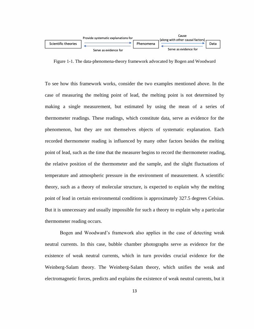
13

Figure 1-1. The data-phenomena-theory framework advocated by Bogen and Woodward

To see how this framework works, consider the two examples mentioned above. In the

case of measuring the melting point of lead, the melting point is not determined by

making a single measurement, but estimated by using the mean of a series of

thermometer readings. These readings, which constitute data, serve as evidence for the

phenomenon, but they are not themselves objects of systematic explanation. Each

recorded thermometer reading is influenced by many other factors besides the melting

point of lead, such as the time that the measurer begins to record the thermometer reading,

the relative position of the thermometer and the sample, and the slight fluctuations of

temperature and atmospheric pressure in the environment of measurement. A scientific

theory, such as a theory of molecular structure, is expected to explain why the melting

point of lead in certain environmental conditions is approximately 327.5 degrees Celsius.

But it is unnecessary and usually impossible for such a theory to explain why a particular

thermometer reading occurs.

Bogen and Woodward’s framework also applies in the case of detecting weak

neutral currents. In this case, bubble chamber photographs serve as evidence for the

existence of weak neutral currents, which in turn provides crucial evidence for the

Weinberg-Salam theory. The Weinberg-Salam theory, which unifies the weak and

electromagnetic forces, predicts and explains the existence of weak neutral currents, but it

14

cannot and is not expected to provide systematic explanations for the details of each

bubble chamber photograph.

4.2 Counterfactual dependence in data-to-phenomena reasoning

Let us focus on the evidential role of data in data-to-phenomena reasoning. Woodward

(2000) argues that in order for data to play their evidential role, a right sort of

counterfactual dependence relationship should hold between data and the phenomenon-

claim for which the data are to provide evidence. To illustrate the notion of

counterfactual dependence, consider a relatively simple case of phenomenon detection.

Suppose that P1 and P2 are two competing, mutually exclusive claims about a

phenomenon; D1 and D2 are two possible data outcomes produced in the process of trying

to detect the phenomenon of interest. In order for data to play their evidential role of

distinguishing between P1 and P2, in an ideal case the following counterfactual

dependence relationships are expected to obtain:

(a) D1 is produced when and only when P1 is true.

(b) D2 is produced when and only when P2 is true.

When (a) and (b) hold, we can make inferences as follows:

(c) If D1 is produced, conclude that P1 is true.

(d) If D2 is produced, conclude that P2 is true.

Notice that (a) is stronger than the requirement that P1 is sufficient for the production of

D1. This is because if P2 is also sufficient for the production of D1, then D1 is not able to

help discriminate between P1 and P2 and provide evidence for P1. The same point holds

for (b). It also needs to be recognized that what is described above is an ideal case. In

15

practice, there can be more than two competing, mutually exclusive claims about a

phenomenon of interest, and the satisfaction of the counterfactual dependence

relationships can come in degrees.

Several issues need to be clarified in order to make the counterfactual dependence

requirement work in practice. First, does D1 (or D2) refer to a particular data outcome or

a type of data outcome? The production of data is influenced by many other causal

factors besides the phenomenon of interest. Since it is unlikely to keep the states of all the

relevant causal factors exactly the same across different rounds of data collection, data

collected in different rounds are unlikely to be exactly the same even in well-designed

and controlled studies. Hence, D1 (or D2) should be understood as a type, rather than a

particular instance, of data outcome.

Second, if D1 (or D2) should be understood as a type of data outcome, how could

scientists tell whether a particular data outcome is an instance of D1 or D2? The answer to

this question is essential for evidential reasoning from data to phenomena: If the

counterfactual dependence relations between data and phenomenon-claims tell us that “if

D1 is produced, conclude that P1 is true; if D2 is produced, conclude that P2 is true,” then

at least in principle there should be some way to determine whether a particular data

outcome is an instance of D1 or D2. But how is this done? I will address this issue in the

following section.

4.3 Locating the role of patterns in data-to-phenomena reasoning

Since it is unlikely to obtain exactly the same data even in well-controlled experiments,

the indicator of the type of a data outcome should go beyond the features of specific data

16

points. I suggest that this indicator be a characteristic pattern in data. Patterns in this

context are understood as representations of data which show certain features or order of

data, and it is possible for multiple non-identical data sets to exhibit the same pattern.

Given this, we can modify the counterfactual dependence relationships involved in data-

to-phenomena reasoning as follows.

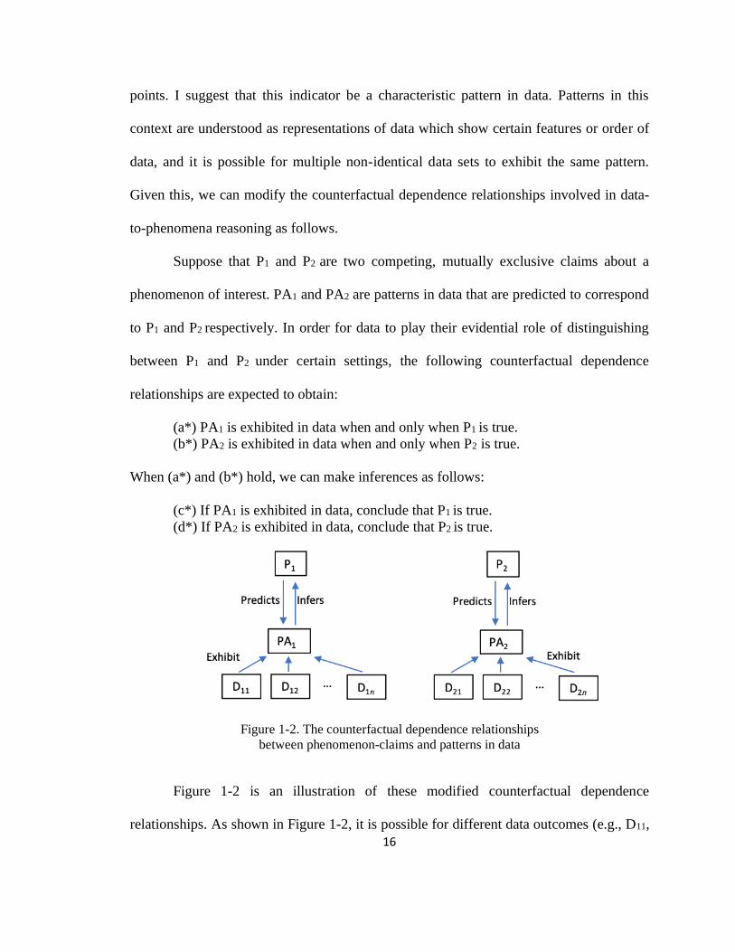
Suppose that P1 and P2 are two competing, mutually exclusive claims about a

phenomenon of interest. PA1 and PA2 are patterns in data that are predicted to correspond

to P1 and P2 respectively. In order for data to play their evidential role of distinguishing

between P1 and P2 under certain settings, the following counterfactual dependence

relationships are expected to obtain:

(a*) PA1 is exhibited in data when and only when P1 is true.

(b*) PA2 is exhibited in data when and only when P2 is true.

When (a*) and (b*) hold, we can make inferences as follows:

(c*) If PA1 is exhibited in data, conclude that P1 is true.

(d*) If PA2 is exhibited in data, conclude that P2 is true.

Figure 1-2. The counterfactual dependence relationships

between phenomenon-claims and patterns in data

Figure 1-2 is an illustration of these modified counterfactual dependence

relationships. As shown in Figure 1-2, it is possible for different data outcomes (e.g., D11,

17

D12, …) to exhibit the same pattern (e.g., PA1). When some data do exhibit a

characteristic pattern that is predicted to correspond to a phenomenon-claim, those data

can be used as evidence for that phenomenon-claim. In other words, patterns in data serve

as a steppingstone for data to play their evidential role in data-to-phenomena reasoning.

Taking patterns into consideration in data-to-phenomena reasoning helps

“dissolve” an issue mentioned above. Instead of asking whether a particular data set is an

instance of a type of data outcome, what matters is whether this data set exhibits the

characteristic pattern that is thought to correspond to the phenomenon of interest. This

renders unnecessary the extra step of determining the “type” of a particular data outcome

in data-to-phenomena reasoning.

To see how patterns actually feature in data-to-phenomena reasoning, consider the

case of measuring the melting point of lead again. Given previous studies on other

metals’ properties, it is reasonable to assume that lead has a fixed melting point under

certain environmental conditions. But under what conditions could the data support this

claim? To measure the melting point of lead, researchers make a series of measurements

of the temperature of a lead sample when it is melting; this process yields a series of

temperature readings. If lead does have a fixed melting point under certain environmental

conditions, and assuming that there is no systematic error in the measurement, then the

data points (i.e., the thermometer readings) would be expected to be more or less

normally distributed. When the temperature readings do exhibit a normal distribution

pattern, the required counterfactual dependence relationship between the pattern and the

phenomenon-claim is satisfied. In this case, temperature readings can work as evidence

for the phenomenon-claim that lead has a fixed melting point under certain environmental

18

conditions, and the mean of the distribution can be used as an estimation of the true

melting point of lead. However, if the temperature readings fail to exhibit a normal

distribution pattern, but exhibit, say, a multimodal distribution, then the data cannot serve

as evidence for the phenomenon-claim of interest, and the mean of the whole data

distribution also becomes physically meaningless.

Similar points also apply in the case of detecting weak neutral currents. In

experiments designed to detect such a phenomenon at CERN (European Organization for

Nuclear Research) between 1972-1973, researchers obtained about 290,000 bubble

chamber photographs as data, but only 100 or so of them were thought to provide

evidence for the existence of weak neutral currents. The key to identifying such

photographs is to look for characteristic patterns of particle tracks that are predicted to

appear if weak neutral currents really exist. Weak neutral currents can be produced in

many kinds of interactions. One example is the case where a neutrino strikes a nucleon,

which produces another neutrino and a shower of strongly interacting particles. While

neutrinos, which are electrically neutral, cannot leave tracks in a bubble chamber, the

strongly interacting particles produced in the above case, which are electrically charged,

can leave tracks, and these tracks show certain characteristic patterns. Hence, only when

bubble chamber photographs exhibit such characteristic patterns of particle tracks, can

they be thought to provide evidence for the occurrence of weak neutral currents.

My emphasis of the role of patterns in data-to-phenomenon reasoning is not

intended to be a denial of Bogen and Woodward’s data-phenomena distinction, but a

complement to their framework based on such a distinction. The aim here is to make

explicit the role of patterns in data-to-phenomena reasoning and incorporate it into Bogen

19

and Woodward’s framework. If my analysis is right, then the three-tiered framework

advocated by Bogen and Woodward should be complemented as a four-tiered one

involving the relationship among data, patterns in data, phenomena, and scientific

theories (see Figure 1-3).

Figure 1-3. A four-level framework involving data, patterns, phenomena, and scientific theories

4.4 Real vs. unreal patterns in the context of phenomenon detection

In phenomenon detection, data play their evidential role via exhibiting certain

characteristic patterns that correspond to the phenomena of interest. In this context, a

pattern is real if and only if it is exhibited by the data to an extent that satisfies the

criterion concerning allowable noise levels and it is indeed caused by the phenomenon of

interest.

Data may fail to play their evidential role in two ways. First, data may fail to

exhibit the characteristic pattern that is predicted to correspond to the phenomenon of

interest, given certain specified standards concerning allowable noise levels. Second, the

expected pattern is exhibited by the relevant data to a great enough extent, but it results

from factors other than the phenomenon of interest. It is in this case that the notion of

20

unreal (or bogus) pattern becomes relevant. A pattern is said to be unreal when it mimics

the characteristic pattern that is predicted to correspond to the phenomenon of interest,

but results from factors other than that phenomenon.

To illustrate this notion of unreal pattern, consider the experiment of detecting

weak neutral currents. Weak neutral currents can be produced when a neutrino strikes a

nucleon. During the experiment, however, the emitted neutrinos will also strike the

chamber and the surrounding apparatus, producing a large number of neutrons. When

these neutrons strike nucleons, they will produce a shower of hadrons, which leaves

movement patterns mimicking those of the strongly interacting particles produced in

weak neutral current interactions (Bogen & Woodward, 1988). In other words, it is

possible to observe the kind of characteristic patterns that are predicted to appear in the

presence of weak neutral currents, even when weak neutral currents do not actually occur.

In this case, such patterns might be called “unreal” in the sense that although they can be

identified on the bubble-chamber photographs, they fail to serve as evidence for the

existence of weak neutral currents.

21

5. Patterns in data as targets of systematic explanation

Nature is complex, yet also full of patterns requiring explanation. In many cases,

scientists search for patterns in data not because they need them as evidence for the

existence of phenomena to be detected, but simply because they want to find in a messy

and constantly changing world some order or feature that is worth explaining. In this

research context, identifying patterns from data becomes the starting point of these

scientists’ research, and the attempts to provide systematic explanation for the existence

of these patterns usually inspire and lead to significant theoretical development in science,

such as the development of unifying, explanatory theories. In this section, I will first

introduce some examples of patterns that have served as targets of systematic explanation

and featured in theoretical development in science. Then I will discuss a number of

desiderata for identifying real patterns in data (i.e., patterns that are qualified as targets of

systematic explanation).

5.1 Examples of important patterns in nature

As mentioned above, one of the most important tasks in scientific inquiry is to identify

real patterns from data, which can then serve as targets of systematic explanation.

Ecology is a particularly apt discipline to focus on for the explication of this role of

patterns in data because it heavily relies on bottom-up, data-driven inquiry and is fully of

interesting patterns in need of explanation. These patterns usually work as the first step of

many ecological studies. In his introduction to Geographical Ecology, ecologist Robert

MacArthur (1972, p. 1) wrote: “To do science is to search for repeated patterns, not

22

simply to accumulate facts, and to do the science of geographical ecology is to search for

patterns of plant and animal life that can be put on a map.” Ecologist John Lawton (1996,

p. 145) even claimed that “[w]ithout bold, regular patterns in nature, ecologists do not

have anything very interesting to explain”. In the following, I will introduce some

examples of ecologically significant patterns and explain why they have garnered the

attention of ecologists.

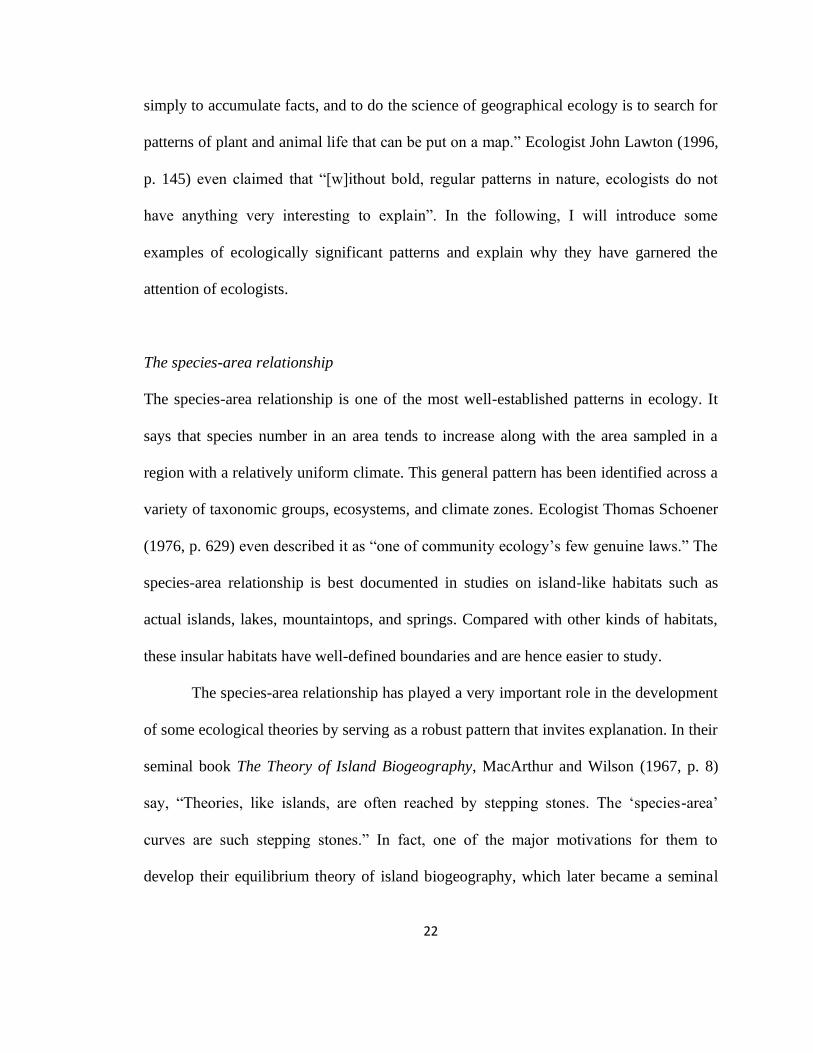
The species-area relationship

The species-area relationship is one of the most well-established patterns in ecology. It

says that species number in an area tends to increase along with the area sampled in a

region with a relatively uniform climate. This general pattern has been identified across a

variety of taxonomic groups, ecosystems, and climate zones. Ecologist Thomas Schoener

(1976, p. 629) even described it as “one of community ecology’s few genuine laws.” The

species-area relationship is best documented in studies on island-like habitats such as

actual islands, lakes, mountaintops, and springs. Compared with other kinds of habitats,

these insular habitats have well-defined boundaries and are hence easier to study.

The species-area relationship has played a very important role in the development

of some ecological theories by serving as a robust pattern that invites explanation. In their

seminal book The Theory of Island Biogeography, MacArthur and Wilson (1967, p. 8)

say, “Theories, like islands, are often reached by stepping stones. The ‘species-area’

curves are such stepping stones.” In fact, one of the major motivations for them to

develop their equilibrium theory of island biogeography, which later became a seminal

23

work in biogeography and ecology, is to explain the species-area relationship exhibited

on different-sized islands.

The checkerboard distribution pattern

Species occurrence sometimes demonstrates very intriguing patterns. The knob-billed

fruit dove (Ptilinopus insolitus) and the claret-breasted fruit dove (Ptilinopus viridis)

belong to the same genus Ptilinopus. They are ecologically similar in the sense that both

live in similar habitats (forest canopies) and eat similar food (fruit). Their distribution

ranges on New Guinea and nearby islands are shown in Figure 1-4 respectively.

(A) Ptilinopus insolitus (B) Ptilinopus viridis

Figure 1-4. The distribution ranges of two species of fruit doves

(the maps were downloaded from BirdLife Data Zone http://datazone.birdlife.org)

There are two salient features of their joint distribution pattern. First, the range of

Ptilinopus viridis encompasses that of Ptilinopus insolitus. Second, these two species do

not co-occur except on one island. This pattern, called checkerboard distribution because

24

the ranges of two species interlace like black and white squares on a checkerboard, has

garnered great attention from ecologists. Some ecologists, such as Diamond (1975),

believe that the existence of such checkerboard distribution patterns is mainly the result

of interspecific competition for limited resources. By contrast, Connor and Simberloff

(1979) contend that this pattern might just be a result of random assembling or can be

expected by chance alone, and they argue that a “null model” based on a randomization

procedure needs to be constructed to test this hypothesis. Although the debate was

initially about how to explain the formation of checkerboard distribution patterns, it has

kindled a more general discussion on the usefulness of null models in biology (Connor &

Simberloff, 1983, 1984; Gilpin & Diamond, 1982, 1984; Gotelli & Graves, 1996).

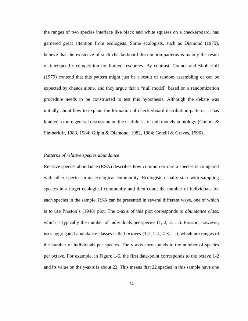
Patterns of relative species abundance

Relative species abundance (RSA) describes how common or rare a species is compared

with other species in an ecological community. Ecologists usually start with sampling

species in a target ecological community and then count the number of individuals for

each species in the sample. RSA can be presented in several different ways, one of which

is to use Preston’s (1948) plot. The x-axis of this plot corresponds to abundance class,

which is typically the number of individuals per species (1, 2, 3, …). Preston, however,

uses aggregated abundance classes called octaves (1-2, 2-4, 4-8, …), which are ranges of

the number of individuals per species. The y-axis corresponds to the number of species

per octave. For example, in Figure 1-5, the first data-point corresponds to the octave 1-2

and its value on the y-axis is about 22. This means that 22 species in this sample have one

25

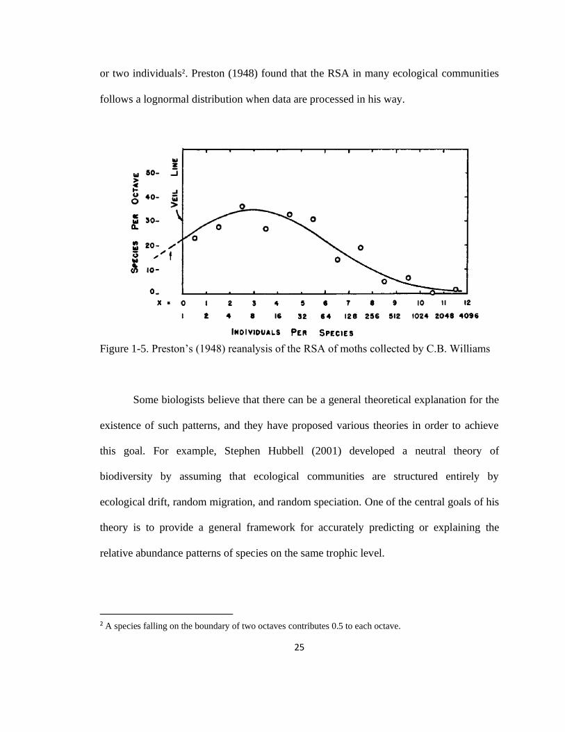
or two individuals2. Preston (1948) found that the RSA in many ecological communities

follows a lognormal distribution when data are processed in his way.

Figure 1-5. Preston’s (1948) reanalysis of the RSA of moths collected by C.B. Williams

Some biologists believe that there can be a general theoretical explanation for the

existence of such patterns, and they have proposed various theories in order to achieve

this goal. For example, Stephen Hubbell (2001) developed a neutral theory of

biodiversity by assuming that ecological communities are structured entirely by

ecological drift, random migration, and random speciation. One of the central goals of his

theory is to provide a general framework for accurately predicting or explaining the

relative abundance patterns of species on the same trophic level.

2 A species falling on the boundary of two octaves contributes 0.5 to each octave.

26

5.2 Desiderata for identifying real patterns in data

Patterns in data can be regarded as targets of systematic explanation (i.e., are real) when

they reveal some stable features of the target systems that scientists want to learn about.

In contrast, there are also patterns in data that are unreal in sense of being unqualified to

serve as candidates for systematic explanation. Although there are paradigm cases for

both real and unreal patterns, there are no criteria that can be used to draw hard and fast

distinction between these two groups of patterns. The lack of such criteria, however, does

not mean that there is no distinction at all. In the following, I will specify a number of

desiderata for identifying real patterns in data. These desiderata do not provide clear-cut

sufficient and necessary conditions for identifying real patterns in data, but they point out

important aspects that should be considered when evaluating the reality of a pattern.

Low noise level

The first desideratum is low noise level. “Noise” here refers to the discrepancy between a

given pattern and the data from which the pattern is identified. How the noise level

associated with a pattern in a data set is measured depends on the specific from of that

pattern. For example, in the case of a checkerboard distribution pattern of two species in

an archipelago, the noise level is measured by counting the islands where the two species

co-occur. In the case of patterns of relative species abundance, however, the noise level

can be measured by calculating the mean squared error of species abundance, which is

the average squared difference between the estimated species abundance according to the

proposed distribution pattern and the species abundance shown by the empirical data. No

27

matter how the noise level associated with a pattern is measured, other things being equal,

the lower the noise level is, the more real the pattern is to researchers.

Reproducibility

Low noise level cannot be the only desideratum of real patterns. A pattern according in

every detail with a data set is exhibited with zero noise, but it can hardly be a real pattern.

This is because such a pattern is overwhelmingly determined by the idiosyncratic features

of a particular data set; when it is applied to a new data set collected from a similar or

even the same system, the corresponding noise level will be extremely high. This fact

tells us that it is inappropriate to evaluate the reality of a pattern by merely considering its

corresponding noise level in one data set. Rather, a real patten is expected to be exhibited

with allowable noise level in different empirical data sets about the same system or

similar systems. Call this desideratum the reproducibility of patterns in data. According

to this desideratum, when a pattern is exhibited with zero (or extremely low) noise level

in only one or very few data sets but with extremely high noise level in most other data

sets collected from the same system or similar systems, it is unsuitable to be taken as a

real pattern for systematic explanation.

A real pattern is intended to reveal features or order of its target system in the real

world, not merely the formal properties of data. Low noise level and reproducibility are

two important features of real patterns, but these two features alone are not enough to

guarantee the realness of a pattern because they only concern the formal properties of

data sets. To evaluate the realness of a pattern, we should also consider the way the

28

relevant data are collected from the target system and the way they are classified and

processed in order to identify the pattern.

Representative sampling

To detect real patterns in a target system, the ideal is to make a complete census of every

relevant entity in that system and collect data from each of them. While sometimes this is

possible, in most cases it is impractical. In actual processes of pattern-seeking, scientists

usually have to rely on the data collected from a sample of the target system, and the goal

is to be able to understand the target system through the sample, or, in Preston’s (1948, p.

254) words, to “deduce the ‘universe’ from the sample.”

In order to achieve this goal, the sample must be representative of the target

system with respect to the features that researchers want to know about. Call this

desideratum representative sampling. Representative sampling should be understood as

an ideal, which is a goal governing the whole sampling process and whose realization can

come in degrees.

One way to improve the representativeness of a sample is to make sure that it is a

random collection. Preston (1948) stressed the importance of random sampling when he

discussed the study of relative species abundance of moths:

“[I]t is important to recognize that the randomness we seek is merely

randomness with respect to commonness or rarity. A light trap is satisfactory

in this respect and samples its own universe appropriately. It is definitely

selective in respect of phototropism, but it is random in respect of

commonness, i.e., it does not care which of two moths, equally phototropic, it

catches, though one may be a great rarity and the other of a very common

species.” (p. 254)

29

Preston thinks that although sampling moths with a light trap is selective with respect to

phototropism, it is random with respect to the commonness of different moths. This is not

necessarily true because moths of different species may have different levels of

phototropism, which will bias the relative abundance of different species of moths in the

sample. For example, if moths of a very rare species are more likely to be attracted by

light, this species of moths would be more common in the sample than in the actual

community. As I mentioned earlier, the representativeness of a sample can come in

degrees. The more biased the sample is, the less likely it is for researchers to identify real

patterns in the target system.

Good scientific classification

Good scientific classification is essential for identifying real patterns from empirical data

sets. In Section 5.1, I introduced three important patterns that ecologists take to be real

and worthy of systematic explanation, each of which involves the use of species as a kind

to classify the organisms in their respective target systems: The species-area relationship

concerns the number of species in a given area; the checkerboard distribution pattern

involves the geographic locations of species; the pattern of relative species abundance

concerns the number of individuals per species sampled in a given community. Without

the use of species as a proper scientific kind, it is even impossible for ecologists to

identify and formulate these patterns.

A real pattern that is qualified as a target of systematic explanation should be a

pattern based on good scientific classification and involving the use of proper scientific

kinds or real kinds. There are various philosophical accounts of what counts as a real kind,

30

and it goes beyond the scope of this chapter to come with a new one. But for a good

example of such a theory, consider briefly Quayshawn Spencer’s (2012, 2016) genuine

kind theory. According to Spencer (2012, p. 181), a genuine kind is “a valid kind in a

well-ordered scientific research program.” Here a well-ordered scientific research

program (SRP) refers to a SRP that is organized to achieve long-term scientific progress.

A valid kind in such a SRP is a kind that is both epistemically useful and epistemically

justified in that SRP (for more details of this theory, see Spencer (2012, 2016)).

Proper data processing

Patterns are not always immediately discernible in raw data. In many cases, researchers

need to process the raw data in a certain way in order to discern the pattern. But at the

same time, improper data processing may lead to the production of unreal patterns.

In Section 5.1, I introduced how to use Preston’s (1948) octaves to plot

distribution patterns of relative species abundance. When Preston’s octaves are not used,

the x-axis on a plot of relative species abundance corresponds to the number of

individuals per species (1, 2, 3, …), and the y-axis corresponds to the number of species

having a certain number of individuals. On such a plot, data points tend to be dense at the

end of rare species and sparse at the end of common species, which makes it difficult to

discern a pattern for the overall distribution of relative species abundance. To avoid this

problem, Preston uses aggregated abundance classes called octaves (1-2, 2-4, 4-8, …) on

the x-axis, which are ranges of the number of individuals per species. For example, the

first octave (1-2) includes species having 1 or 2 individuals in the sample, and the number

of species belonging to this octave should be summed up together as one data point. If a

31

species falls on the boundary of two octaves, it contributes 0.5 to each octave. For

example, if 5 species are found to have 2 individuals in the sample respectively, they

together should contribute 2.5 species to the 1-2 octave and 2.5 to the 2-4 octave.

Adopting this kind of logarithmic scale for the x-axis allows Preston to display data

points spanning over a wide range of values in a more compact way, which facilitates his

identification of the lognormal distribution pattern of relative species abundance in many

ecological communities (see Figure 1-6 (a) for an example of such a distribution pattern).

(a) Lognormal distribution of relative species abundance in a moth community according to

Preston’s method of octave construction, from Preston (1948)

(b) Bimodal distribution of relative species abundance in a dung beetle community according

to an erroneous method of octave construction, from Lobo and Favila (1999)

Figure 1-6. Distribution patterns of relative species abundance according to two different

methods of octaves construction.

32

Preston’s method of octave construction has been widely used by ecologists to

process data on relative species abundance, but sometimes it is used mistakenly, which

leads to the identification of unreal patterns in data. For example, according to Preston’s

method, species falling on the left boundary of the 1-2 octave (i.e., species having one

individual in the sample) should contribute only half of its number to this octave.

However, some ecologists forgot this rule and included all the species with one individual

to the 1-2 octave, leading to an increase of the number of species in the first octave.

Instead of identifying a lognormal distribution as shown in Figure 1-6 (a), they found a

bimodal distribution as shown in Figure 1-6 (b). This bimodal distribution should not be

regarded as a real pattern exhibited by the data on relative species abundance. Rather, it is

a statistical artifact resulting from researchers’ improper data processing.

6. McAllister’s stipulationist view of physically significant patterns in data

After introducing the pragmatic approach to the reality of patterns in data, I now turn to a

different account of patterns in data advocated by James McAllister (1997, 2010), which

I call the stipulationist view.

McAllister starts by asking a question as follows: Mathematically speaking, any

empirical data set can be said to exhibit infinitely many possible patterns with various

noise levels. If we accept the distinction between data and phenomena as advanced by

Bogen and Woodward, and if we believe that only some of the infinitely many possible

patterns exhibited by a data set correspond to phenomena in the world, then how could

we distinguish between patterns that correspond to phenomena and patterns that do not?

Since McAllister (2010) defines a pattern that corresponds to a structure in the world (i.e.,

33

a phenomenon) as being physically significant, the above question can also be phrased as

follows: How could we distinguish between physically significant and insignificant

patterns?

McAllister (2010) sets two restrictions on possible answers to this question. First,

the distinction between physically significant and insignificant patterns should not be

based on our knowledge, beliefs, expectations, or assumptions about what phenomena

there are in the world. The reason, according to McAllister, is that we are supposed to

infer the existence of phenomena in the world by identifying physically significant

patterns in data, not the other way around. Second, the distinction between physically

significant and insignificant patterns can only appeal to intrinsic facts about patterns

themselves. Contingent facts such as human preferences should not be used as the

criterion.

Under these two constraints, McAllister denies the possibility of specifying a

respect in which physically significant patterns differ from physically insignificant

patterns in empirical data sets. In particular, he rejects the view that physically significant

patterns should be patterns with low noise level.

To illustrate this point, he considers the research on the speed of rotation of the

Earth. The rotation rate of the Earth is not constant, which leads to variations in the

length-of-day (LOD). By analyzing the empirical data about the length-of-day,

geophysicists have identified multiple patterns. These include a linear increase in the

LOD of about 1 to 2 milliseconds per century; a pattern with an amplitude of a few

milliseconds and a period of around a decade; a fluctuation with an amplitude of around

0.2 milliseconds and a period of between 40 and 50 days; and several fluctuations with

34

amplitudes of around 0.1 milliseconds and periods of a few days. Among these patterns,

the last pattern – fluctuations with amplitudes of around 0.1 milliseconds and periods of a

few days – only accounts for about 1% of the overall variation of the LOD data.

According to McAllister’s interpretation, when geophysicists pick out such a pattern,

they regard 99% of the variation of the LOD data as noise. He uses this example to show

that patterns with high noise level can also be regarded as physically significant by

scientists. Hence, low noise level cannot be used as an overarching criterion for

distinguishing between physically significant and insignificant patterns (McAllister,

2010).

After failing to identify a respect in which physically significant patterns differ

from physically insignificant ones, McAllister suggests that we regard all patterns

exhibited by empirical data sets as physically significant. According to this view, some

patterns are picked out by researchers and regarded as corresponding to phenomena, not

because they have some inherent features that distinguish them from other patterns, but

because they happen to be the patterns that researchers intend to study or to explain. In

other words, according to McAllister, “which patterns count as those corresponding to

phenomena is entirely a matter of stipulation by investigators” (McAllister, 1997, p. 224),

and “any of the infinitely many patterns that data sets exhibit may be taken as the

explananda of scientific theories” (p. 227).

7. Problems of the stipulationist view through the lens of the pragmatic approach

One fundamental issue with McAllister’s stipulationist view is that he fails to distinguish

clearly between two different roles of patterns in data in scientific inquiry. Sometimes he

35

describes patterns in data as corresponding to and constituting evidence for phenomena in

the world, while sometimes he treats patterns in data as the explananda of scientific

theories. As I have argued in previous sections, serving as evidence for the existence of

scientific phenomena and as candidates for systematic explanation should be understood

as two different roles that patterns in data are expected to play in scientific inquiry.

Researchers are faced with different issues when utilizing patterns in these two different

ways.

Let’s first analyze the case where patterns in data are expected to provide

evidence for the existence of scientific phenomena. According to McAllister, the question

at issue is how to distinguish patterns that correspond to phenomena (i.e., physically

significant patterns) from patterns that do not. Call it the demarcation question of

physically significant patterns. Instead of focusing on a specific pattern in data and

determining whether it corresponds to the phenomenon of interest, the demarcation

question of physically significant patterns demands an overarching criterion that can be

used to evaluate the physical significance of all the possible patterns exhibited by a data

set. Framing the question at issue in this way, however, is misleading in the context of

phenomenon detection. When seeking evidence for the existence of a phenomenon,

researchers need not answer the demarcation question of physically significant patterns as

suggested by McAllister. Instead, they should consider the following three questions:

(i) Given the phenomenon under investigation and the detection method

employed, what kind of pattern is expected to be exhibited by the relevant

data if the phenomenon under investigation indeed exists?

(ii) To what extent is the expected pattern exhibited by the relevant data?

36

(iii) Do the relevant data exhibit the expected pattern to a great enough extent

so that they can serve as evidence for the existence of the phenomenon under

investigation?

Given these questions, we can see that although any empirical data set can be described

as infinitely many possible patterns with various noise levels, only the pattern that is

predicted to correspond to the phenomenon of interest is relevant in the context of

phenomenon detection. The determination of this pattern is not a matter of stipulation,

but based on researchers’ proposed hypothesis about the phenomenon of interest,

knowledge about the experimental setting designed to detect the phenomenon, and other

non-arbitrary background assumptions. As for the other possible patterns in the data set,

they may either correspond to phenomena that are not the focus of the current study or

have no clear physical meaning at all, and neither of these two types of patterns is

relevant for the research purpose. Hence, researchers do not need to come up with an

overarching criterion to demarcate patterns that correspond to phenomena and patterns

that do not. They only need to focus on the pattern that is predicted to correspond to the

phenomenon of interest.

To illustrate my point, consider first the example of determining the melting point

of lead. If lead really has a fixed melting point under certain environmental conditions,

then given certain assumptions (e.g., there is no systematic error introduced by the

equipment), the measurement results would be expected to follow a normal distribution.

The determination of this characteristic pattern does not depend on stipulations by

investigators, but on the proposed property of the phenomenon to be detected (the

fixedness of the melting point of lead) and a series of empirical assumptions about the

experimental conditions. Researchers need to evaluate the degree to which the

37

measurement results follow a normal distribution pattern through statistical analysis and

decide, based on the statistical analysis results, whether the data can support the claim

that lead has a fixed melting point under certain environmental conditions. It is irrelevant

for their purpose whether the other infinitely many patterns exhibited by the data set can

serve as evidence for other potentially existing phenomena.

The same point can also be illustrated with the example of detecting weak neutral

currents. Weak neutral currents occur in a variety of interactions involving the weak force.

For example, the Weinberg-Salam theory predicts that weak neutral currents will be

produced when a neutrino strikes a nucleon. Such an interaction will produce a set of

strongly interacting particles, leaving certain characteristic tracks (i.e., movement

patterns) while moving through a bubble chamber. In this case, seeking evidence for the

existence of weak neutral currents amounts to looking for bubble-chamber photographs

with particle movement patterns of a particular kind. The determination of this kind of

movement pattern does not rely on researchers’ stipulations, but on the proposed

properties of weak neutral currents, the researchers’ knowledge about the experimental

setting, as well as other experimental and theoretical assumptions. Bubble-chamber

photographs may also exhibit other kinds of movement patterns, which may even indicate

the occurrence of interactions other than weak neutral currents. But insofar as the goal of

researchers is to detect weak neutral currents, the physical significance of these

movement patterns is irrelevant in the current research context.

Now let us address some concerns that proponents of McAllister’s view might

raise. First, according to my account, researchers need to determine what kind of pattern

corresponds to the phenomenon of interest given a certain detection method. Doesn’t this

38

amount to answering McAllister’s demarcation question of physically significant patterns?

One way to determine whether two questions are essentially the same is to look at the

kind of answer that is expected for each question. To answer McAllister’s demarcation

question, the researcher needs to come up with a criterion that can be used to determine

whether each of the infinitely many possible patterns in a data set corresponds to a

phenomenon in the world, no matter what that phenomenon is. By contrast, to answer

“What kind of pattern is expected to be exhibited by data if the phenomenon of interest

exists?”, the researcher only needs to focus on a particular phenomenon and predict one

kind of characteristic pattern that corresponds to the focal phenomenon; the researcher’s

answer to the above question cannot help determine whether other patterns exhibited by

the same data set correspond to phenomena or not. Hence, the research question about

patterns in data asked in the context of phenomenon detection is different from

McAllister’s demarcation question.

Second, if the characteristic pattern that is predicted to correspond to a

phenomenon of interest is partly determined by the presupposed properties of that

phenomenon, how could such a pattern serve as evidence for the existence of the

phenomenon? Isn’t there a problem of circularity? This problem does not really exist,

because there is no a priori guarantee that the expected pattern will be exhibited by the

data set with a high enough degree. For example, in the case of determining the melting

point of lead, the thermometer readings may show a poor fit with the expected normal

distribution; in the case of detecting weak neutral currents, the bubble-chamber

photographs may not show the kind of movement patterns that are expected to appear as

a result of weak neutral currents. Since the evidential relationship between patterns in

39

data and phenomena is an empirical rather than a priori relationship, the worry of

circularity is unfounded.

I have responded to McAllister’s stipulationist view of physically significant

patterns in data by considering the case where patterns in data are expected to serve as

evidence for the existence of scientific phenomena. I now turn to the case where patterns

in data serve as targets for systematic explanation. In this context, McAllister’s

demarcation question becomes relevant, but it should be reformulated in a way to match

the role of patterns under consideration. Instead of asking “How to distinguish patterns

that correspond to phenomena from patterns that do not?”, the relevant question is:

How to distinguish patterns that can serve as targets for systematic

explanation from those that cannot?

As I emphasized in Section 5.2, although there is no hard and fast distinction between

these two classes of patterns, it does not mean that there is no distinction at all. In Section

5.2, I have specified a number of desiderata that can be used to evaluate whether a pattern

in data can serve as a target of systematic explanation. Hence, it is wrong to claim that

“any of the infinitely many patterns that data sets exhibit may be taken as the explananda

of scientific theories” (McAllister, 1997, p. 227).

In particular, I want to argue against McAllister’s denial of low noise level as a

feature of patterns that deserve systematic explanation. As is evident in his discussion

about patterns in the length-of-day data, when an empirical data set contains multiple

superimposed patterns, the noise of any single pattern, according to McAllister, amounts

to the sum of all the other patterns and a further residual noise term. This calculation of

the noise level of a pattern, however, ignores the fact that different patterns identified

40

from the same data set are on different scales and capture features regarding different

aspects of the data. Given this fact, the noise associated with one pattern may not count as

noise for another. For example, one pattern identified by geophysicists from the length-

of-day data says that the length-of-day increases by 1 to 2 milliseconds per century. Since

this pattern concerns the increase of the length-of-day on the time scale of a century,

variations of the length-of-day on other time scales should not count as noise for this

pattern. By the same token, fluctuation patterns identified on other time scales should not

be regarded as noise associated with this pattern, either. When calculated this way, the

noise level attributed to patterns identified by geophysicists from the length-of-day data

would drop dramatically. Although it is up to researchers to determine the highest

acceptable noise level, they tend to set the threshold value at a relatively low noise level.

In other words, low noise level is indeed a desideratum of real patterns.

8. Conclusion

In this chapter, I have endeavored to show that patterns in data can play three different

epistemic roles in scientific inquiry. Accordingly, the realness of a pattern identified from

data should be evaluated based on the extent to which it fulfills the epistemic role that it

is expected to play in a specific research context. There is no single, over-arching account

of real patterns. I have also argued against McAllister’s stipulationist view of patterns in

data and shown that whether a pattern corresponds to a phenomenon in the world, or

whether a pattern can be regarded as a target of systematic explanation, is not a matter of

stipulation by investigators.

41

Chapter 2: The use and limitations of null-model-based hypothesis

testing

1. Introduction

In a study of bird communities on New Guinea and nearby islands, especially the

Bismarck Archipelago, Diamond (1975) claimed to have found certain “assembly rules”

with respect to the distribution of bird species. One of them says that “[s]ome pairs of

species never coexist, either by themselves or as part of a larger combination” (Diamond,

1975, p. 344). For example, the Mackinlay’s cuckoo-dove (Macropygia mackinlayi) and

the bar-tailed cuckoo-dove (Macropygia nigrirostris), while ecologically similar and

overlapping in their geographical ranges, never co-occur on any island of the Bismarck

Archipelago.3 This pattern, called by Diamond a “checkerboard distribution” because the

geographical ranges of the two species interlace like black and white squares on a

checkerboard, seems to require an explanation.

Diamond (1975) proposed the hypothesis that the existence of such checkerboard

distribution patterns can be explained by, among other things, interspecific competition

for limited resources. Some other ecologists, however, thought that it is premature to

infer the existence of competitive exclusion among relevant species just by looking at

their distribution patterns. For example, Connor and Simberloff (1979) argued that in

order to demonstrate that competition is responsible for the formation of checkerboard

distribution patterns, one needs to first falsify a null hypothesis that those patterns are due

3 In species co-occurrence studies, when claiming that a species exists, occurs, or is present on an island,

ecologists typically mean that the species has established a breeding population on that island instead of

just having several vagile individuals.

42

to the random colonization of bird species. Their strategy is to build a null model in

which bird species are randomly assigned to different islands of an archipelago under

certain constraints and then calculate the values of certain statistics such as the number of

species pairs that never co-exist on any island. If the expected number of forbidden pairs

(or the value of other chosen statistics) is not statistically significantly different from

what is obtained based on the empirical data collected from the actual archipelago, then

there is no strong reason to appeal to interspecific competition as the explanation of

checkerboard distributions.

Connor and Simberloff’s challenge triggered sharp rebuttals from Diamond and

his colleagues (e.g., Diamond and Gilpin, 1982; Gilpin and Diamond, 1984), which in

turn incurred further rejoinders from Simberloff and his colleagues (e.g., Connor and

Simberloff, 1983, 1984). This disagreement has led to a schism between two camps that

persists even today (for a recent round of debate, see Connor et al., 2013, 2015; Diamond

et al., 2015).

This debate is worth attention because the strategy used by Simberloff and his

colleagues, which I will call null-model-based hypothesis testing, has been widely used in

the biological sciences, especially in ecological research such as studies of species co-

occurrences, species/genus (S/G) ratios, food webs, and character displacement. To be

clear, the use of the term “null model” is somewhat inconsistent in the biological

literature. For example, Hubbell (2001) and Rosindell et al. (2011) argue that the neutral

model of biodiversity provides a useful null model in community ecology, in which the

term “null model” just means a model providing a null hypothesis. While the practice of

using the neutral model as a null model has been criticized by Bausman (2018), the

43

neutral model that he considers is different from the null model that I will focus on here.4

The kind of null model that I will consider in this chapter is also called “random model”

or “stochastic model,” which is constructed based on a randomization procedure and used

to test the hypothesis that the existence of a pattern is the result of random processes or

can be expected by chance alone. This type of model is regarded by its proponents as

playing a role similar to the “control” as used in traditional statistical hypothesis testing

in experimental settings, and it is said to provide a null hypothesis against which other

hypotheses should be tested.

At the heart of the debate concerning null models is whether null hypotheses and

null models are useful at all in the biological sciences. Since an appropriate null model is

essential for the validity of null-model-based hypothesis testing, most discussions have

been focused on whether it is possible (and if so, how) to construct a model that is

genuinely null. Many constructive discussions have taken place, but many technical

details remain controversial. This chapter contributes to the literature from a somewhat

different perspective. Assuming that the technical controversies about the construction of

null models can be resolved, what would be the possible use of null-model-based

hypothesis testing, if it is useful at all, and how could that use be justified? What

limitations does this strategy have? These are the questions that I aim to answer in this

chapter.

My strategy is to use as an example the controversy over Connor and Simberloff’s

advocacy of null hypotheses and null models in species co-occurrence studies and draw

4 For a detailed discussion of the differences between neutral models and null models, see Gotelli and

McGill (2006).

44

some general lessons from it. I will argue that null-model-based hypothesis testing as a

research strategy can be useful – but in a limited sense. It is useful not because it works

as an analog or approximation to traditional statistical hypothesis testing in well-

controlled experimental settings, but because it provides a possible way to challenge

scientists’ commonsense judgments about how a seemingly unusual pattern could have

come to be. To better demonstrate this point, I will compare the null model used by

Connor and Simberloff with Schelling’s model of segregation. I will also analyze the

limitations on the use of null models and discuss some lessons drawn from the debate

concerning the use of null-model-based hypothesis testing in species co-occurrence

studies.

2. Null-model-based hypothesis testing in species co-occurrence studies

In order to answer the general question of the use and limitations of null-model-based

hypothesis testing, it is necessary to properly detail how it is actually used in scientific

research. In this section, I will use Connor and Simberloff’s (1979) null model of species

co-occurrences as a representative example to illustrate how null-model-based hypothesis

testing has been employed as a research strategy in the biological sciences.5

5 In species co-occurrence studies, the null models constructed by different ecologists may be more or less

different from each other. Even Connor and Simberloff themselves keep modifying their null models in

later publications. Nevertheless, the version I will introduce here, which appears in one of their earliest and

also most-cited publications on this subject, helps demonstrate the key features of null-model-based

hypothesis testing.

45

2.1 Constructing the null model

Table 2-1. A 3-by-4 random matrix

Island A Island B Island C Island D Row sum

Species a 1 0 1 0 2

Species b 1 0 0 1 2

Species c 0 1 0 1 2

Column sum 2 1 1 2

Connor and Simberloff (1979) want to use their null model to construct a simulated

archipelago in which bird species are randomly assigned to the islands. The null model

used in their species co-occurrence analyses is actually a set of random matrices. In the

rest of this section I will proceed by explaining what a random matrix is, how to construct

it, and in what sense it is “random.”

A random matrix used in species co-occurrence analyses is a rectangular array of

1’s and 0’s, in which each row corresponds to a species, and each column an island

within an archipelago (see Table 2-1). The number “1” means that a species is present on

an island, while “0” means that a species is absent. Hence, the process of randomly

assigning species to islands can be simulated by the process of randomly placing 1’s and

0’s in a matrix.

Since each element in the matrix has two choices (1 or 0), for a matrix with m

rows and n columns, there will be 2mn unique matrices if there is no constraint about how

to place 1’s and 0’s, which correspond to 2mn different ways of distributing m species on

46

n islands. But in the relevant literature, the placement of species on islands in a random

matrix is almost always subject to some constraints. Connor and Simberloff (1979, p.

1133) use the following three constraints:

(i) For each island, there is a fixed number of species, namely, that which

is observed.

(ii) For each species, there is a fixed number of occurrences, namely, that

which is observed.

(iii) Each species is placed only on islands with species numbers in the

range for islands which that species is, in fact, observed to inhabit. That is,

the “incidence” range convention is maintained.

The first constraint requires that each island hold a fixed number of species, which is

equal to the number of species actually observed on each island. For example, if a real

island holds two bird species, it should also hold two in the random matrix. Since a

column sum in a random matrix corresponds to the number of species present on an

island, constraint (i) is equivalent to keeping all the column sums fixed at certain

numbers according to the number of species actually observed on each island. Similarly,

constraint (ii) requires that each species occur on a fixed number of islands, which is

equivalent to keeping all the row sums fixed at certain numbers according to the number

of islands on which each species actually occurs. The third constraint is more

complicated. Some species may occur on islands with a wide range of species numbers,

while some others may be present only on species-poor (or, conversely, species-rich)

islands. Hence, constraint (iii) is a further restriction on the kind of islands to which each

species can be assigned. Note that although the matrices are called by Connor and

Simberloff as “random matrices,” the constraints used in these matrices are not

themselves random. Rather, they are decided according to the empirical data collected

from the actual archipelago. From a statistical point of view, these constraints amount to

47

very strong parametric restrictions. The matrices are called “random” because Connor

and Simberloff randomize the placement of bird species on islands in the simulation

given the preset constraints. Accordingly, a distribution pattern is said to be generated by

the species randomly colonizing an archipelago if their colonization of islands is not

subject to any other constraints besides the ones already mentioned above.

If all the non-equivalent random matrices satisfying the preset constraints are

collected together, they form the full null space. Given the number of species and islands

in an actual archipelago (e.g., there are at least 147 species of land birds and 50 islands in

the Bismarck Archipelago), the number of random matrices in this space can be very

large. When it is computationally intractable to get all the possible random matrices, one

can collect a sample of them. Random matrices in this sample constitute the sample null

space (see Figure 2-1).

Figure 2-1. The relationship between the full null space and the sample null space

Sample null space

Full null space

48

2.2 Comparing simulated data with empirical data

The test is conducted by comparing the empirical data collected from the actual

archipelago with the simulated data generated by the null model. In order to conduct this

test, one first needs to choose a statistic (i.e., a measure of some attribute of the sample)

so that it can be used to make the comparison. There is more than one kind of statistic

that can be used for the comparison, but what is most directly relevant to checkerboard

distributions is the number of pairs of species that never co-occur on any island within an

archipelago.

When understanding each random matrix in the sample null space as a simulated

archipelago, one can count how many pairs of non-coexisting bird species there are on

each of those archipelagos. Since these numbers may not be exactly the same, what one

actually obtains is a null distribution, which describes the probabilities of all the expected

values of the number of non-coexisting pairs based on the null model. Once this

distribution is obtained, one can calculate its mean and standard deviation, compare them

with the number of non-coexisting species pairs in the actual archipelago, and see

whether there is a statistically significant difference between them. If no such difference

is found, it means that the existence of checkerboard distributions is consistent with the

result of random colonization. If so, Connor and Simberloff (1979) argue, then there is no

strong reason to appeal to interspecific competition as the explanation of checkerboard

distributions. It is worth noting that depending on the target phenomena and statistics of

interest, researchers may choose measures other than the means and standard deviations

of null distributions to conduct the test.

49

2.3 Technical controversies concerning the test

Many discussions have taken place concerning Connor and Simberloff’s null model.

Diamond and Gilpin (1982), for example, provide seven criticisms of Connor and

Simberloff’s (1979) approach. Here I only recapitulate two issues that have drawn the

most attention. The first problem is called the dilution effect. According to Diamond and

Gilpin, interspecific competition most likely happens within guilds, i.e., groups of

ecologically similar species overlapping in resource utilization. Connor and Simberloff,

however, conduct their test in whole faunas. As a result, the effects of interspecific

competition within guilds are diluted by a mass of irrelevant data from ecologically

distinct species. But this should be understood as a criticism of the specific model

constructed by Connor and Simberloff (1979), rather than the use of null models as a

whole. In fact, Simberloff and his colleagues have accepted this criticism and revised

their models accordingly in later publications (Connor et al., 2013).

Another, perhaps more serious, problem is the incorporation of hidden effects of

competition into the null model. In Connor and Simberloff’s random matrices, the

placement of species on islands is subject to three constraints. Diamond and Gilpin argue

that since constraints (ii) and (iii) are themselves strongly influenced by competition, a

null model subject to these constraints would already contain some effects of competition

in its structure, making the model not as “null” as it needs to be. Since the construction of

a null model always involves some constraints, the problem always exists that some

effects of competition have already been included in the null model. If this is true, it

would be a criticism of the use of null models as a whole, at least in studies of species co-

occurrences. But whether this is a fatal issue is still controversial.

50

Technical issues like these, although important, are not the focus of this chapter.6

In what follows, I will put aside these technical issues for a moment and consider instead

some more general questions about the use and limitations of null-model-based

hypothesis testing as a research strategy in the biological sciences. The benefit of doing

so is that it can deepen our understanding of this research strategy in a more general way

without being trapped in still unsolved technical controversies.

3. A critical evaluation of null-model-based hypothesis testing

3.1 Connor and Simberloff’s interpretation

As mentioned before, advocates of null models think that null models provide a null

hypothesis against which other hypotheses should first be tested. Null-hypothesis testing

is not a native research method in ecology. Instead, it is borrowed from statistics.

The term “null hypothesis” was probably first introduced by R. A. Fisher. In his

seminal book The Design of Experiments, Fisher (1935) considered a case where a lady

claimed that by tasting a cup of tea mixed with milk she could tell whether the milk or the

tea was first added to the cup. He designed an experiment to test the hypothesis that the

lady did not have such discrimination ability, and labelled this hypothesis as the “null

hypothesis.” According to Fisher, a null hypothesis like this is characteristic of all

experimentation, but one may choose any hypothesis as the null hypothesis as long as it is

exact and free from vagueness and ambiguity. One important feature of the null

hypothesis is that it is “never proved or established, but is possibly disproved, in the

6 For reviews of the technical issues in the construction of null models, see Gotelli and Graves 1996;

Sanderson and Pimm 2015.

51

course of experimentation” (Fisher, 1935, p. 19). Whether the null hypothesis in an

experiment should be rejected can be decided by conducting a test of significance, which

was developed by Fisher in the 1920s (Fisher, 1925, 1926). The rationale behind this test

is to calculate the p-value, i.e., the probability of obtaining a result at least as extreme as

what is actually observed in the experiment given that the null hypothesis is true. If the p-

value is smaller than a certain threshold chosen by the researcher, such as 0.05, the result

of the test is said to be statistically significant and the null hypothesis is rejected.

Notice that in Fisher’s tests of significance, only a single hypothesis – the null

hypothesis – is considered. By contrast, in the Neyman–Pearson approach to statistical

hypothesis testing, it is required that the null hypothesis be tested against an alternative

hypothesis. While the debate between these two approaches is not the focus of this

chapter, it is worth mentioning that the current approach to statistical hypothesis testing,

which is widely used in statistical education and scientific research today, involves both

the null and alternative hypotheses.

Fisher (1925, 1926, 1935) also played an important role in advocating the use of

randomization in experimental design, which is used to avoid systematic biases and

proves to be essential for the validity of statistical hypothesis testing in experimental

research. Nowadays, randomized controlled trials 7 have become the gold standard in

experimental studies, especially those that aim to test the cause-and-effect relationship

between two variables. For example, in order to test whether an antihypertensive drug

7 Although the term “randomization test” is often used interchangeably with “permutation test,” actually

they are different. A randomization test is based on random assignment involved in experimental design;

the procedure of random assignment is conducted before empirical data are collected. By contrast, a

permutation test is a nonparametric method of statistical hypothesis testing based on data resampling.

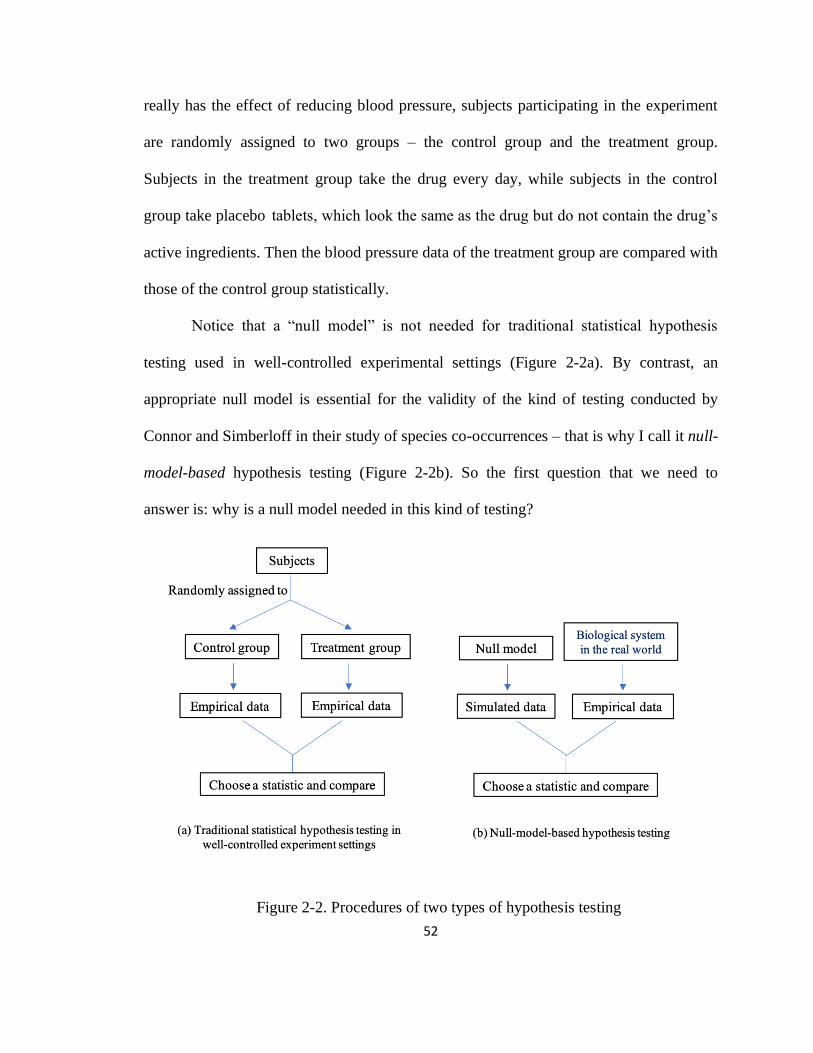
52

really has the effect of reducing blood pressure, subjects participating in the experiment

are randomly assigned to two groups – the control group and the treatment group.

Subjects in the treatment group take the drug every day, while subjects in the control

group take placebo tablets, which look the same as the drug but do not contain the drug’s

active ingredients. Then the blood pressure data of the treatment group are compared with

those of the control group statistically.

Notice that a “null model” is not needed for traditional statistical hypothesis

testing used in well-controlled experimental settings (Figure 2-2a). By contrast, an

appropriate null model is essential for the validity of the kind of testing conducted by

Connor and Simberloff in their study of species co-occurrences – that is why I call it null-

model-based hypothesis testing (Figure 2-2b). So the first question that we need to

answer is: why is a null model needed in this kind of testing?

Figure 2-2. Procedures of two types of hypothesis testing

53

The term “null model” does not belong to the terminology of traditional statistical

hypothesis testing. Instead, it was coined for the use of null hypothesis testing in non-

experimental research such as many studies in ecology and biogeography. In well-

controlled experimental studies, researchers collect data from both the control and

treatment groups, compare two data sets with respect to a statistic of interest, and see

whether there is a statistically significant difference between them. But in an ecological

case, the contrast between the control and treatment groups is usually lacking. For

example, in the debate about checkerboard distributions, what is of interest is whether

competition is responsible for the formation of those patterns. However, it is impossible

to find an actual archipelago as the “control” in which bird species are manipulated in a

way such that the level of interspecific competition is set as zero.

Given this, the role of the null model, as envisioned by Connor and Simberloff

(1983), is to construct an imaginary archipelago in which bird species are randomly

assigned to islands within the archipelago so that the effect of interspecific competition

can be excluded. By using the null model as an analog of the control in experimental

research, Connor and Simberloff (1983) aim to generate simulated data via the null

model so that they can be compared with the empirical data collected from the actual

archipelago. If this strategy works, then null-model-based hypothesis testing seems to be

justified as a legitimate extension of traditional statistical hypothesis testing.

But is this interpretation of null-model-based hypothesis testing really justified?

In the following sections, I will give a critical evaluation of this interpretation.

54

3.2 Evaluating the interpretation

3.2.1 The mismatch problem between the null and alternative hypotheses

Traditional statistical hypothesis testing used in well-controlled experimental research

involves a pair of hypotheses – a null hypothesis and an alternative hypothesis. These two

hypotheses must be mutually exclusive and collectively exhaustive of all the admissible

hypotheses given the question of interest (Sloep, 1986). For example, if researchers want

to test the effect of an antihypertensive drug, then the question of interest is whether there

is a cause-and-effect relationship between the use of this antihypertensive drug and the

reduction of blood pressure. Given this question of interest, the null hypothesis is that

such a cause-and-effect relationship holds, and the alternative hypothesis is that it doesn’t.

Although the reduction of blood pressure can also be caused by many other factors,

hypotheses involving those factors are not admissible hypotheses given the question of

interest, and hence do not undermine the “collectively exhaustive” criterion.

Now consider the null and alternative hypotheses involved in null-model-based

hypothesis testing. In their widely cited paper, Connor and Simberloff (1979, p. 1132)

argue that:

In order to demonstrate that competition is responsible for the joint

distributions of species, one would have to falsify a null hypothesis stating

that the distributions are generated by the species randomly and

individually colonizing an archipelago.

If we focus on the controversy over checkerboard distributions, it is reasonable to

formulate the null (H0) and alternative (H1) hypotheses used in Connor and Simberloff’s

test as follows:

55

H0: The checkerboard distributions of certain pairs of closely related bird

species on the islands of the Bismarck Archipelago are the result of

random colonization.

H1: The checkerboard distributions of certain pairs of closely related bird

species on the islands of the Bismarck Archipelago are caused by

interspecific competition.

Before analyzing the logical relationship between these two hypotheses, it is necessary to

clarify their meanings. In the interspecific competition hypothesis (H1), competition

refers to interspecific competition for limited resources, which does not include

interspecific differences in dispersal abilities. As to Connor and Simberloff’s null

hypothesis (H0), what exactly it means depends on one’s interpretation of the null model.

Gotelli and Graves (1996, pp. 3–4) provide an operational definition of a null model:

A null model is a pattern-generating model that is based on randomization

of ecological data or random sampling from a known or imagined

distribution. The null model is designed with respect to some ecological or

evolutionary process of interest. Certain elements of the data are held

constant, and others are allowed to vary stochastically to create new

assemblage patterns. The randomization is designed to produce a pattern

that would be expected in the absence of a particular ecological

mechanism.

This definition consists of both a description and an interpretation of a null model. The

description part indicates how a null model is actually constructed: It is constructed based

on the randomization of empirical data given certain constraints or random sampling

from a species pool.

The interpretation part is about what a null model is intended to represent.

According to the definition above, a null model in ecology is intended to simulate an

ecological system where a particular ecological mechanism is excluded. Under this

interpretation, Connor and Simberloff’s null model is intended to simulate an archipelago

56

where only interspecific competition is excluded, with their null hypothesis being simply

the denial of the interspecific competition hypothesis. But this interpretation faces a

serious problem. As Diamond and Gilpin (1982, p. 73) rightly point out, in order to use a

null model to test the effect of a particular factor, the null model must both exclude the

factor to be tested and include all the other important factors that could structure the

actual data. However, it is not clear how Connor and Simberloff’s null model can satisfy

this requirement. On the one hand, as mentioned earlier, Diamond and Gilpin (1982)

argue that the constraints in Connor and Simberloff’s null model contain hidden effects

of competition. On the other hand, even if this problem could be somehow managed,

there is no way to guarantee that all the other relevant factors are included in the null

model.

Another, perhaps better, interpretation of the null model is that it is intended to

provide an alternative explanation to the competing hypothesis by taking into account

chance processes. Under this interpretation, Connor and Simberloff’s null model is a

simulation of bird species’ random colonization of islands, and the constraints used in the

null model are structural assumptions about the ecological system under investigation.

Accordingly, their null hypothesis is an alternative explanation to, rather than a simple

denial of, the interspecific competition hypothesis.

Sloep (1986, p. 309) claims that the interspecific competition hypothesis (H1) and

Connor and Simberloff’s random colonization hypothesis (H0) cannot be an appropriate

pair of null and alternative hypotheses in the statistical sense because the first hypothesis

does not logically exclude the second. This is not true. H0 and H1 are indeed mutually

exclusive because they cannot both be true at the same time.

57

The real problem is that they are not collectively exhaustive. The question of

interest in this case is how the checkboard distribution patterns have come into being.

There are multiple possible answers to this question because whether two species will co-

occur on the same island can be influenced by many factors other than interspecific

competition, such as their dispersal abilities, habitat preferences, and responses to

predators, parasites, or pathogens. Since H0 and H1 together do not exhaust all the

admissible hypotheses given the question of interest, rejecting one of them does not

necessarily provide support for the other. More specifically, rejecting that the

checkerboard distribution patterns are the result of random colonization does not force us

to conclude that they are caused by interspecific competition. By the same token, even if

it can be shown that the patterns are not caused by interspecific competition, it does not

mean that they are the result of random colonization.

My analysis above has demonstrated an important disanalogy between traditional

statistical hypothesis testing and null-model-based hypothesis testing: the null and

alternative hypotheses in the former satisfy the condition of being collectively exhaustive

given the question of interest, while those in the latter do not. This difference is due to the

fact that traditional statistical hypothesis testing and null-model-based hypothesis testing

are faced with different tasks. Hypotheses involved in traditional statistical hypothesis

testing are usually statements about a relationship. Since a relationship either holds or not,

the “collectively exhaustive” criterion is readily satisfied. By contrast, hypotheses

involved in null-model-based hypothesis testing are usually explanations of a

phenomenon. Since a phenomenon usually has multiple possible explanations, the

“collectively exhaustive” criterion is typically unsatisfied.

58

It may be argued that the mismatch problem between the null and alternative

hypotheses is not a fatal issue for null-model-based hypothesis testing. For example, in

the case of checkerboard distributions, one can claim that when the random colonization

hypothesis (H0) is chosen as the null hypothesis, its appropriate alternative hypothesis is

not the interspecific competition hypothesis (H1), but the logical negation of H0, i.e., the

hypothesis that the checkerboard distributions are not the result of random colonization.

Let’s call this updated alternative hypothesis H1*. As shown in Figure 2-3, while H0 and

H1 do not satisfy the collectively exhaustive criterion, H0 and H1* do.

Figure 2-3. The relation between H0, H1, and H1*

Notice that the question of interest has been changed after the alternative

hypothesis is reframed this way. What is of interest is no longer how the patterns have

come into being, but whether those patterns are the result of random colonization. While

this kind of reframing seems to circumvent the mismatch problem, it does not guarantee

that null-model-based hypothesis testing is indeed an appropriate null hypothesis test in a

strict statistical sense. I will explain why in the following two sections.

H0 H1*

H1

59

3.2.2 The principle of equifinality and the lack of proper control of variables

In this section, I will examine Connor and Simberloff’s (1983, p. 464) claim that in null-

model-based hypothesis testing, a null hypothesis and a null model are contrived to

“usefully approximate the role of the ‘control’ in order to test a hypothesis involving non-

experimental evidence,” and see whether they are actually able to play the role as

envisioned.

In traditional statistical hypothesis testing, what counts as a proper control group

is not solely determined by the setting of the supposed control group per se, but also

influenced by how the treatment group is set up. Let’s again use the test of the effect of

antihypertensive drugs as an example. Suppose that the subjects participating in the

experiment are randomly assigned to two groups. Subjects in the supposed treatment

group take the antihypertensive drug and another kind of drug every day, while subjects

in the supposed control group take placebo tablets. It is clear that the supposed control

group does not count as a proper control because it does not guarantee that the only

independent variable in this test is whether the subjects take the antihypertensive drug or

not. Without proper control of variables, one is not justified to make any causal inference

about the effect of the antihypertensive drug. More specifically, one is not justified to

reject the alternative hypothesis that the antihypertensive drug has the effect of reducing

blood pressure even when there is no statistically significant difference between the

supposed control and treatment groups with respect to the subjects’ blood pressure. This

is because it is possible that the antihypertensive drug is indeed effective, but the other

drug has the effect of increasing blood pressure, thus counteracting its effect.

60

Now consider null-model-based hypothesis testing. In the last section, I have

argued that there exists a mismatch between the null and alternative hypotheses

commonly used in null-model-based hypothesis testing, namely, they do not satisfy the

“collectively exhaustive” criterion given that the question of interest is how to explain a

phenomenon. One possible way to circumvent this problem is to reframe the question of

interest as whether the pattern under investigation is the result of random processes. Since

the answer to this question is either yes or no, the null and alternative hypotheses after

this reframing will satisfy the “collectively exhaustive” criterion. Hence, if the empirical

data is consistent with the simulated data generated by the null model, one seems to be

able to retain the null hypothesis and reject the alternative hypothesis, just as what

researchers would do in traditional statistical hypothesis testing.

I will use the rest of this section to show that this is not the case. I argue that in

null-model-based hypothesis testing, because of the lack of proper control of variables,

one is not justified to reject the alternative hypothesis even when there is no statistically

significant difference between the simulated and empirical data with respect to the

statistics of interest. The case of checkerboard distribution patterns will still be used as an

example for demonstration.

In ecology, scientists make an important distinction between pattern and process

(Gotelli and Graves, 1996, p. 5). In the introduction to his book Geographical Ecology,

MacArthur (1972, p. 1) wrote: “To do science is to search for repeated patterns, not

simply to accumulate facts […].” This quote serves as a nice summary of a common

approach adopted by ecologists – they start by identifying patterns in nature and then try

to reveal the underlying processes that have produced these patterns. Since ecological

61

systems are thermodynamically open systems, the same final state may be reached from

different initial states and in different ways. This has been described as the principle of

equifinality (von Bertalanffy, 1968). Due to the equifinality of ecological systems, the

same pattern can be produced through different (or different combinations of) processes,

just as there are many roads to Rome.

In Connor and Simberloff’s null model of species occurrences, bird species are

randomly assigned to islands of the simulated archipelago. This procedure is intended to

exclude the effects of interspecific competition, but at the same time it also ignores many

other factors that may influence species’ co-occurrences such as the varied dispersal

abilities of different species. Hence, there is no proper control of variables in the

construction of the null model. Since closely related species tend to have similar dispersal

abilities, they are more likely to colonize the same islands than what they would do if

they were randomly distributed, which leads to an opposite effect of interspecific

competition (Colwell and Winkler, 1984; Harvey, 1987). Given the multiple producibility

of patterns, the joint effects of dispersal abilities and interspecific competition may

produce a similar number of pairs of non-coexisting species as would be expected by

random colonization. In other words, even if the simulated data generated by the null

model are not significantly different from the empirical data with respect to the number

of non-coexisting species pairs, one is not justified to reject the supposed alternative

hypothesis (H1*) that the pattern is not the result of random processes.

It may be argued that if a model based on a simpler hypothesis, such as the null

model based on the random colonization hypothesis in the case of checkerboard

distributions, is sufficient to produce a pattern statistically indistinguishable from the

62

empirical pattern, then this hypothesis should be favored because of its simplicity.

Although the principle of simplicity is often used to privilege simpler hypotheses over

more complex ones, its use is not without controversy. For example, Sober (1988, 1994)

has argued that there is no global justification for the principle of simplicity in general.

Instead, its legitimacy depends on researchers’ substantive background assumptions

about the way the world is in specific research contexts. Hence, what makes the principle

of simplicity reasonable in one research context may be different from that in another. If

proponents of different hypotheses have different background assumptions about the

phenomenon under investigation, appeals to simplicity alone may not be able to justify

privileging more parsimonious hypotheses. In the case of checkerboard distributions,

proponents of the interspecific competition hypothesis tend to think that in a real

biological context, it is very unlikely that the colonization of islands by birds is a purely

random process. By contrast, proponents of null-model-based hypothesis testing think

that it is problematic to exclude the random colonization hypothesis from the very

beginning without testing it, which is why they urge researchers to conduct null-model-

based hypothesis testing. However, if one chooses to privilege the random colonization

hypothesis by appealing to simplicity, she needs to explain why the simpler hypothesis is

more likely to be the true explanation of the phenomenon in this particular context.

As a brief summary, my analysis in this section reveals another important

disanalogy between traditional statistical hypothesis testing and null-model-based

hypothesis testing. For traditional statistical hypothesis testing used in well-controlled

experimental research, since the proper control of variables is in place, if there is no

statistically significant difference between the control and treatment groups with respect

63

to the statistics of interest, one is justified to maintain the null hypothesis and reject the

alternative hypothesis. In null-model-based hypothesis testing, however, because of the

equifinality of thermodynamically open systems and the lack of proper control of

variables, one is not justified to reject the alternative hypothesis even when the simulated

data match the empirical data.

3.2.3 The issue with the size of datasets

In null-model-based hypothesis testing, phrases such as “comparing simulated data with

empirical data” are rhetorically powerful and epistemically appealing because they leave

people with the impression that the comparison involved here is analogous to the

comparison between data from the control and treatment groups in an experimental

setting. However, while a comparison procedure does exist in null-model-based

hypothesis testing, the datasets that are compared may not be a good analog to those in

traditional statistical hypothesis testing.

To test a cause-and-effect relationship between two variables, the size of both the

control and treatment groups should be large enough in order to guarantee the statistical

power of the test. The specific minimum requirement is based on the evaluation of the

context of each specific test. In any case, if the sample size is too small, one is not

justified to make any causal inference based on the test. For example, if there are thirty

subjects in the control group and only one subject in the treatment group, one is not

justified to reject the alternative hypothesis even if there is no statistically significant

difference between the results of the two groups, because the statistical power of such a

test is so weak.

64

In null-model-based hypothesis testing, sample size is not inherently a problem

for the simulated dataset because one can conduct the randomization simulation multiple

times, and each round of simulation will contribute a data point for the statistic of interest.

In the case of species co-occurrence studies, for example, each random matrix works as a

simulated archipelago and contributes a data point about the number of non-coexisting

species pairs. The minimal size of the simulated dataset can be guaranteed by examining

multiple random matrices in the sample null space. But in the empirical dataset, there is

actually only one data point for comparison in each test, which is the number of pairs of

species that never co-exist in the actual archipelago. In other words, the comparison is

conducted between a null distribution, which describes the probabilities of all the

expected values of the number of non-coexisting pairs based on the simulated data

generated by the null model, and a single empirical data point. While one can still test

whether the value of the single empirical data point falls within the null distribution, it

does not count as a proper analog to the comparison involved in traditional statistical

hypothesis testing in experimental research.

3.3 Applying the analysis results

I have provided three reasons to show that null-model-based hypothesis testing is not an

appropriate approximation of traditional statistical hypothesis testing in experimental

research. Maybe this is an obvious point, but it does not always get enough attention in

the discussion of null-hypothesis testing in the biological sciences, even among

philosophers who aim to critically evaluate its use in specific cases. In this section, I will

65

apply the results of my critical analysis to a particular philosophical discussion of null

hypotheses and null models.

In a recent paper, Bausman and Halina (2018) evaluate the use of what they call

the “pseudo-null strategy” in explaining relative species abundance (hereafter RSA)

distributions, i.e., the relative commonness or rarity of different species on the same

trophic level of an ecological community. The traditional way to explain RSA patterns is

to appeal to niche differences. Every species has acquired a unique set of traits that allow

it to be adapted to a particular environment and occupy a unique niche. Different species

can coexist in the same environment because they have different niches and make use of

resources in different ways (Chase and Leibold, 2003). Hubbell (2001, 2006) has

challenged this explanation by proposing a neutral theory of biodiversity. He assumes

that all the individuals within a particular trophic level are ecologically similar regardless

of their species identity, i.e., they have the same chance of reproduction, death,

immigration, and speciation. Hubbell uses this neutral assumption as a null hypothesis

against which the niche-based hypothesis should be tested.

Bausman and Halina (2018) rightly point out that the neutral hypothesis is a

pseudo-null hypothesis because compared with the hypothesis based on niche differences,

it just appeals to a different set of processes, which include reproduction, death,

immigration, and speciation, to explain RSA distributions. What is more relevant to this

chapter is their suggestion about what counts as a genuine null hypothesis in this case:

Community ecologists have sampled communities from all over the world

and used the observed distributions to test whether ecological selection is

operating. The appropriate statistical null hypothesis for such tests is that

the observed species distributions will not differ significantly from what

we would expect if individuals of different species were distributed at

66

random in space and time […]. (Bausman and Halina, 2018, p. 11, my

italics)

Their suggestion is actually very similar to Connor and Simberloff’s (1979) strategy, i.e.,

building a model in which individuals of different species are randomly distributed and

then comparing the simulated data generated by this model with the empirical data

collected from actual ecological communities. And the random distribution hypothesis is

regarded as the null hypothesis. Not surprisingly, then, it suffers from the same problems

as Connor and Simberloff’s strategy. First, the authors’ claim about the appropriate null

hypothesis could be potentially misleading because they do not explicitly point out what

the alternative hypothesis is given the statistical null hypothesis they suggest. If the

alternative hypothesis is that the observed species distributions are the result of ecological

selection, then it suffers from the same problem as the case of species co-occurrence

studies, because the random distribution hypothesis that the authors suggest (the

supposed null hypothesis) and the ecological selection hypothesis (the supposed

alternative hypothesis) are not collectively exhaustive. This example reminds us again

that whether a hypothesis counts as an appropriate null hypothesis is not solely

determined by its own content, but is also influenced by the choice of its alternative

hypothesis. One cannot take for granted that a hypothesis is an appropriate statistical null

so long as it claims that a phenomenon is the result of some random processes or can be

expected by chance alone.

Bausman and Halina may reply to this critique by claiming that the corresponding

alternative hypothesis is not the ecological selection hypothesis, but the hypothesis that

RSA distributions are not the result of random distribution. But this change does not

67

solve the problem of lacking proper control of variables. RSA distributions can be

influenced by many processes, such as selection due to niche differences, ecological drift

(random birth and death), immigration, and speciation. It is possible that the same

distribution pattern of RSA can be produced through different combinations of those

processes. So even if the simulated data match the empirical data, one is not justified to

reject the alternative hypothesis and maintain the null.

The issue of dataset size also exists. In RSA studies, the unit of analysis is not the

value of the point estimation of a statistic, but a distribution pattern. Through the random

distribution model, one may be able to collect a set of distribution patterns by conducting

the random simulation multiple times. But in the actual ecological community, one can

only obtain a single distribution pattern of RSA for each trophic level. So what is

compared is a set of distribution patterns from the simulated data and a single distribution

pattern from the empirical data. This comparison fails to be a proper approximation to the

comparison conducted in traditional statistical hypothesis testing in experimental research.

4. The possible use and limitations of null-model-based hypothesis testing

In the last section, I argued that null-model-based hypothesis testing cannot be justified as

an appropriate analog to traditional statistical hypothesis testing in well-designed

experimental research. But this does not mean that null-model-based hypothesis testing

cannot be of any use at all. To better demonstrate the possible use of this strategy, I will

make a comparison between Connor and Simberloff’s (1979) null model of species co-

occurrences and Schelling’s (1978) model of segregation. I will argue that although these

two kinds of models are constructed in very different ways, both of them can work as a

68

way to challenge our commonsense judgments about what could have produced a

seemingly unusual pattern.

4.1 Challenging “common sense” by providing how-possibly explanations

In his book Micromotives and Macrobehavior, Schelling (1978) presents a very simple

model to study the segregation of people in neighborhoods. His model is based on a grid

representing a community. Suppose that residents in this community belong to two

different groups, and the distinction between the groups can be made based on any

reasonable criterion, such as people’s racial identity, language, religion, or occupation.

Each square in the grid can be either empty or occupied by a resident, and each resident

has a minimum requirement of their neighborhood, such as that at least one-third of

immediate neighbors be of the same group as the resident. The simulation starts from a

random distribution of two groups on the grid. Each individual takes turns to decide

whether they are content with their neighborhood. For those who are not, as a rule they

will move to the closest empty square that satisfies their requirement. It turns out that the

initial integrated distribution of two groups becomes strongly segregated when all the

residents are content with their neighborhood after a number of rounds. And the outcome

is robust when one alters the overall ratio of two groups, residents’ minimum requirement

of their neighborhood, the initial distribution, etc.

So what is the relevance of Schelling’s model of segregation to our evaluation of

the possible use of null models? After all, they are constructed in very different ways.

The answer is that both Connor and Simberloff’s null model of species co-occurrences

and Schelling’s model of segregation can be interpreted as a way to challenge the

69

commonly held explanation of a seemingly unusual pattern by providing an alternative

how-possibly explanation.

As I mentioned earlier, Schelling’s model can be used to study the segregation of

any two different groups in a community. Suppose that we specify the two groups in his

model as two racial groups (such as black and white people), then this model can be used

to study racial residential segregation in neighborhoods. More specifically, Schelling’s

model can be used to show that patterns of racial residential segregation can result from

individual choices based on small preferences for similarity that are not racist in the sense

of being entirely intolerant of racial diversity. This challenges the commonly held view

that racial residential segregation is due to the presence of extreme racist attitudes. By

using the word “challenge,” I do not mean that Schelling’s model refutes or falsifies the

categorical racism explanation; likewise, I do not claim that his model describes how

racial residential segregation actually forms. Nor does it follow that racist problems do

not exist or are not severe. Rather, it just provides another possible explanation. If both

explanations are compatible with the emergence of segregation patterns, then without

further evidence one cannot take for granted that the observation of racial residential

segregation implies categorical intolerance of racial diversity.

Similarly, in the case of species co-occurrence studies, if the simulated data

generated by Connor and Simberloff’s null model are consistent with the empirical data

collected from the actual archipelago with respect to the statistic of interest, then their

model shows that the existence of checkerboard distributions might just be the result of

random colonization. This alternative explanation challenges the prevailing view that

checkerboard distribution patterns result from interspecific competition. Again, it does

70

not follow that checkerboard distributions are indeed the result of random colonization,

or that relevant species do not compete in reality. Nevertheless, it shows that without

further evidence one cannot take for granted that exclusive competition among bird

species actually happens and causes checkerboard distributions.

A possible objection to my analysis is that since in this chapter I do not aim to

deal with the technical controversies over how to build an appropriate null model, if it

turns out that those issues cannot be solved, then the possible use that I propose for this

strategy would not be available. I agree. Whether the strategy of null-model-based

hypothesis testing can actually be useful does rely on whether an appropriate null model

can be constructed. This is why I employ the term “possible use” throughout this chapter.

Nevertheless, my analysis can still contribute to the discussion by showing the scope of

the use of this strategy, i.e., what it might be able to do and what it absolutely cannot do.

As I have shown, even if it is possible to construct a truly null model, null-model-based

hypothesis testing still fails to be an appropriate analog of traditional statistical

hypothesis testing, given the reasons provided in Section 3. Instead, its possible use

resides in its role of providing a way to challenge scientists’ commonsense judgments

about how a seemingly unusual pattern could have come to be.

4.2 The limitations of null-model-based hypothesis testing

Despite the possible use, null-model-based hypothesis testing still carries severe

limitations. In Section 3, I showed that null-model-based hypothesis testing cannot test

whether a particular process or mechanism such as interspecific competition is

responsible for the formation of certain patterns. Connor and Simberloff (1983, p. 464)

71

explicitly acknowledge this limitation by noting that “[w]ithout further evidence,

probably of an experimental nature, one can neither eliminate any particular causal

mechanism, nor conclude that a particular mechanism has operated.”

Another limitation of this strategy is that the null model lacks the potential for

dealing with other problems via further refinements and modifications. The null model is

constructed to test the hypothesis that the existence of a pattern is the result of random

processes or can be expected by chance alone. No matter whether this hypothesis can be

rejected, once the test is conducted, the null model’s mission is done. It may be argued

that the null model can be further revised or made more complex for other uses by

changing its constraints. This method is possible in principle, but difficult to use in

practice. The difficulty lies in how to construe the updated model when the constraints

are changed, and it is usually unclear what the updated model is supposed to represent. It

may also be argued that lacking the potential for dealing with other problems hardly

amounts to a fatal issue. Since the null model is a bespoke model that is designed to test a

particular hypothesis (i.e., the random process hypothesis), it does not matter so much if

it cannot be further developed to deal with other problems. I agree that this is not a fatal

problem for null-model-based hypothesis testing, but it is still a limitation; recognizing

this limitation can help us understand why many biologists are not so interested in null-

model-based hypothesis testing. Understood this way, my discussion of the null model’s

limitations is not so much a criticism as an observation.

72

5. Lessons from the debate

The controversy surrounding null-model-based hypothesis testing is commonly

interpreted as a debate about the usefulness of null hypotheses and null models in the

biological sciences, especially in ecology and biogeography. But it is also important to

take notice of the deeper origin of this debate. The motivation behind Connor and

Simberloff’s advocacy of null-model-based hypothesis testing is their general

dissatisfaction with the then prevailing “competitionist paradigm” in community ecology.

According to some ecologists, “competition has been invoked as an explanation for

patterns to such a degree that it is in danger of becoming a panchreston, a concept that

can explain everything” (Rathcke, 1984, p. 383). In this extreme case, one might invent a

competitionist explanation for almost any seemingly unusual pattern in ecological

communities without sufficient evidence. Connor and Simberloff (1979, 1983) have

repeatedly argued that the existence of checkerboard distributions per se is not evidence

for one species being actively resisted by another, and that more compelling evidence,

such as evidence based on detailed autecological study, field observation, or

experimentation, should be provided to support the interspecific competition hypothesis.

Against this background, null-model-based hypothesis testing is used by its

proponents as a way to challenge the “competitionists.” If one can show that the

empirical data is consistent with what would be expected by a null model, then merely

identifying certain distribution patterns is not enough to support the commonly proposed

competition hypothesis. Hence, ecologists like Connor and Simberloff are not really

against the role of competition as a possible mechanism for producing certain patterns.

What concerns them is the lack of compelling evidence for many competitionist

73

explanations of ecological patterns. As Simberloff emphasized, “I’ve never said that there

is no competition, that competition isn’t important in generating patterns in nature […].

All I’ve been addressing is the canons of evidence” (Simberloff as quoted in Lewin, 1983,

p. 639).

But this is not the only thing that they want to contend. Connor and Simberloff

(1979) were deeply inspired by Karl Popper’s falsificationism and thought that science

progresses by proposing testable hypotheses and then trying to falsify them. Hence,

besides requiring more compelling evidence, they also argued that proponents of the

competition hypothesis (or any non-random hypothesis) should first try to falsify or reject

a null hypothesis stating that the patterns under investigation are generated by random

processes. It is this requirement that stirred up the controversy because it is intended to

work as a normative claim about how research should be conducted, which puts extra

epistemic responsibility on the side of competitionists.

We should be careful about the relationship between Connor and Simberloff’s

concern about evidence and their normative claim about using null-model-based

hypothesis testing. First, while null-model-based hypothesis testing might be useful by

working as a way to challenge competitionist hypotheses of ecological patterns, its

usefulness is not a necessary condition in order to criticize the “competitionist paradigm”

with respect to the lack of compelling evidence. In other words, even if it turns out that

the technical problems of constructing an appropriate null model cannot be solved, and

null-model-based hypothesis testing is not useful at all, Connor and Simberloff’s call for

more compelling evidence will remain valid. Second, if Connor and Simberloff’s primary

concern is about the evidence for competitionist explanations, then null-model-based

74

hypothesis testing is neither a sufficient nor a necessary way for competitionists to deal

with this critique. It is not necessary because competitionists can reply to their critics by

collecting more compelling evidence through detailed autecological study, field

observation, or experimentation without having to conduct a null-hypothesis test. It is not

sufficient because even if competitionists successfully reject the null hypothesis, they

might still lack the kind of evidence for their competitionist hypothesis demanded by

their critics. Hence, competitionists do not have the responsibility to first conduct null-

model-based hypothesis testing before pursuing their own hypotheses.

In sum, by focusing their attention excessively on null hypotheses and null

models, both sides, including Connor and Simberloff themselves, deviate from the initial

problem of the lack of direct evidence. Although Connor and Simberloff are absolutely

right in claiming that more direct evidence is needed in order to support the interspecific

competition hypothesis, null-model-based hypothesis testing is not the way to obtain the

kind of evidence that they demand.

6. Conclusion

Null-model-based hypothesis testing has been used in many fields of biology, but its

usefulness remains a concern. Although proponents of this method usually think that it is

analogous to traditional statistical null-hypothesis testing in experimental research, I have

shown that this analogy is not justified. Also, the random process hypothesis should not

be privileged as a null hypothesis that biologists must try to reject before pursuing other

hypotheses. But this does not mean that null-model-based hypothesis testing is

necessarily useless. When trying to explain patterns in nature, biologists usually assume

75

that they are produced by specific causal factors, while ignoring the possibility that those

seemingly unusual patterns are the result of random processes. By explicitly testing the

random process hypothesis, null-model-based hypothesis testing might work as a way to

challenge scientists’ commonsense judgments about what count as unusual patterns and

how those patterns could have come to be. Despite this possible use, researchers should

also pay attention to the limitation of null-model-based hypothesis testing: the null model

cannot be used to test whether a particular process or mechanism is responsible for the

formation of certain patterns; it lacks the potential for dealing with other problems via

further development; it cannot provide direct evidence for any non-random hypothesis.

76

Chapter 3: In what sense can neutral theory work as a baseline model?

1. Introduction

One of the most debated theories in modern ecology is the neutral theory of biodiversity

(Hubbell, 2001). It claims that many biodiversity patterns in ecological communities can

be explained by assuming that individuals of different species at the same trophic level

are ecologically equivalent. Such a theory stands in stark contrast with the traditional

approach to understanding community assembly, which explicitly invokes niche

differences among species to explain biodiversity patterns in ecological communities

(MacArthur, 1957; Chase and Leibold, 2003).

Given its radical assumption, it is not surprising that neutral theory of biodiversity

has incurred strong criticisms since its proposal. As a response, supporters of neutral

theory have appealed to several different strategies to defend its use. One of these

strategies states that similar to the ideal gas model in physics, neutral models in ecology

can be regarded as baseline models, which serve as a simple starting point for further

research. When a neutral model fails, more complex non-neutral models can be

constructed by adding more complexity into the neutral model.

This chapter aims to give a critical examination of the claim that neutral models in

ecology can be regarded as baseline models. I will argue that whether a model counts as a

baseline model depends on what type of phenomena it is intended to address and which

models it is compared with. In the debate between neutral theory and niche-based theory,

a neutral model should not be regarded as a baseline model relative to classical niche-

77

based models from a process-based perspective. As an implication, neutral models do not

have methodological priority over niche-based models.

2. Two approaches to explaining biodiversity patterns in ecological communities

Community ecology is the study of patterns in the diversity, abundance, and composition

of species in ecological communities as well as the processes underlying those patterns.

One of the patterns of special interest to community ecologists is the distribution of

relative species abundance (hereafter RSA), which describes the relative commonness or

rarity of different species within the same ecological community.

The traditional way to explain RSA patterns is to appeal to niche differences.

Every species has acquired a unique set of traits that allow it to be adapted to a particular

environment and occupy a unique niche. Different species can coexist in the same

environment because they have different niches and make use of resources in more or

less different ways. Hence, RSA patterns can be explained by considering the partitioning

of niches among different species. There are a variety of niche-based models of RSA, of

which a classical one is MacArthur’s (1957) broken-stick model. According to this model,

the environment of an ecological community is compared to a stick with certain length.

Suppose that there are n species in this community. In order to measure the relative

abundance of these n species, n – 1 points are thrown onto the stick and break it into n

segments. The length of a segment is proportional to the abundance of the species

corresponding to that segment. Although the stick is used by MacArthur to refer to the

environment in general, it can be further specified in different cases. For example, it can

stand for an important resource competed for by different species. Also, the stick can be

78

broken in different ways. The method introduced above assumes that species in this

community occupy non-overlapping, continuous niches.

Neutral theory, however, takes a very different approach. Instead of considering

niche partitioning among different species, it adopts a stochastic dynamical approach to

explaining biodiversity patterns in ecological communities. There exist different versions

of neutral theory in the ecology literature. For the sake of discussion, here I only

introduce the most influential version of them, that is, Hubbell’s (2001) unified neutral

theory of biodiversity.

There are two important assumptions in Hubbell’s neutral theory. One is the

neutrality (or ecological equivalence) assumption: All the individuals within a particular

trophic level in an ecological community have the same probability of birth, death, and

dispersal on a per capita basis, regardless of their species identity. In other words, this

theory ignores the niche differences among different species in an ecological community.

This is also why it is called “neutral theory.” Notice that the neutrality assumption does

not imply that there are no interactions, such as competition, among individuals. Instead,

it allows interactions among individuals of different species as long as those interactions

are symmetrical. Since resources available in a given community are limited, there should

be competitions among individuals. But according to the neutrality assumption,

individuals of different species are equal competitors.

The other is the zero-sum assumption. According to this assumption, ecological

communities are always saturated, and community size – the total number of individuals

in an ecological community – is held constant. In such a community, no species can

increase in abundance without a matching decrease in the collective abundance of all the

79

other species. In other words, the dynamics of ecological communities are essentially a

zero-sum game.

When an individual in a local community dies, its empty space will be refilled by

another. This new individual can be reproduced by the same or a different species within

the local community; it can also migrate from the metacommunity. By including random

birth, death, migration, and speciation into a stochastic dynamical model, neutral theory

is intended to predict or explain various biodiversity patterns in ecological communities

at equilibrium, especially patterns of RSA.

3. The interpretation of neutral models as baseline models

Hubbell’s neutral theory of biodiversity has elicited strong criticism since its proposal,

which is no surprise given its radical and obviously false neutrality assumption. As

McGill, Maurer, and Weiser (2006, p. 1411) vividly summarize, “This contradicts 100

years of community ecology.” As a response, advocates of neutral theory have developed

several different strategies to justify its use in ecology. One strategy, which is the focus

of this chapter, is to argue that neutral models can work as “baseline models”:

“[N]eutral theory has a dual instrumentalist function: like any other theory,

it can be used to predict patterns, but unlike many other theories, it is well

positioned to act as a starting point, a baseline model to which one can

later add more ecological mechanisms. It is exactly when it makes

predictions that are not supported by empirical data that this second role is

played.” (Wennekes, Rosindell, and Etienne, 2012, p. 265)

Although there are quite a few cases where neutral models make very accurate

predictions of diversity patterns in ecological communities (Hubbell, 2001), failing cases

are also accumulating (Dornelas, Connolly, and Hughes, 2006; McGill, Maurer, and

80

Weiser, 2006). The second role described in the above quote, i.e., the role of acting as a

baseline model, provides a methodological justification for neutral theory, and a crucial

implication of this justification is that the usefulness of neutral theory would not be

undermined by its inability to match some empirical data. When a particular neutral

model fails to make accurate predictions, the ecologist can simply complicate the model

by including more factors, such as niche differences, to provide a better fit to empirical

data. This justification is intuitively appealing – there seems to be nothing wrong with

starting from a simple model and adding more complexity when needed. Hence, it won’t

hurt if the ecologist starts with a neutral model.

Advocates of neutral theory are not merely arguing that neutral models can be

used in ecology; in several other places, they also seem to think that neutral models have

methodological priority over niche-based models:

“[W]e argue that neutral theory should […] (be seen) as a baseline model

that contains necessary ingredients that more advanced models should

often also contain (…). We believe that starting from neutral theory is

much easier than starting from a model that assumes niche differentiation

from the outset. There might be other simple starting points as well.”

(Wennekes, Rosindell, and Etienne, 2012, p. 265)

As I mentioned earlier, there have been quite a few cases where neutral models make

very accurate predictions of ecological patterns. These successes make advocates of

neutral theory believe that niche differences, although having long attracted biologists’

attention, are not always necessary for predicting and explaining biodiversity patterns in

ecological communities. This judgment provides a ground for the belief that there exists a

methodological asymmetry between a neutral model and a niche-based model. Since a

neutral model is thought to contain essential factors that other models should also include,

81

when its predication fails to match the empirical data, one can learn something about

what missing biological factors are needed to improve it. But it is more difficult to draw

such conclusions from niche-based models, because failure could result from inclusion of

incorrect details.

Advocates of neutral theory also justify the role of neutral models as baseline

models by linking them with the ideal gas model in physics: “Ideal gases do not exist,

neither do neutral communities. Similar to the kinetic theory of ideal gases in physics,

neutral theory is a basic theory that provides the essential ingredients to further explore

theories that involve more complex assumptions” (Alonso, Etienne, and McKane, 2006,

451).

Although the argument that neutral models are baseline models does not have to

rely on the analogy between ecological neutral models and the ideal gas model, the

seeming similarity between these two kinds of models does help add extra rhetorical

power to the argument. The basic idea is that if the ideal gas model can be regarded as a

baseline model in physics, then, by the same token, a neutral model can also be regarded

as a baseline model in ecology. Since the usefulness of the ideal gas model has been

widely accepted in physics, there should be similar reasons to accept the usefulness of

neutral models in ecology.

4. Evaluating neutral models’ status as baseline models

In the last section, I introduced a strategy that has been employed to justify the use of

neutral theory in ecology: a neutral model can be thought of as a baseline model. In this

section, I will give a more formal characterization of baseline model. Given this

82

characterization, I will then examine whether and, if so, in what sense both the ideal gas

model and a neutral model can work as a baseline model.

4.1 What is a baseline model?

Although the term “baseline model” appears quite frequently in the scientific literature, it

does not catch much attention from philosophers of science (for an exception, see

Bausman, 2018). In general, it is a term that has been loosely used in the scientific

literature without being clearly defined. In order to better evaluate a model’s status as a

baseline model in science, I give a more formal characterization of baseline model as

follows:

Model A is a baseline model relative to Model B if and only if A contains

necessary factors that must also be considered in B in order to address certain

type(s) of phenomena in a domain, and B can be constructed by adding more

complexity into A.

According to this characterization, whether a model counts as a baseline model depends

on what type of phenomena it is intended to address and which models it is compared

with. It may be the case that a model works as a baseline model relative to one model, but

not relative to another.

Labeling a model as a baseline model has several important implications. First, it

assumes that the factors included in this model are causally relevant and non-negligible

for addressing certain type(s) of phenomena in a domain. Hence, accepting a model as a

baseline model means that the other models based on this model should also include the

factors represented in the baseline model. This is a non-trivial empirical assumption,

83

given that one of the most challenging tasks in scientific modelling is to figure out which

factors are causally relevant and which are not.

Second, labeling a model as a baseline model confers it a kind of methodological

priority over those models that it is compared with. Since a baseline model is used as a

starting point, if it can provide an accurate predication or an adequate explanation of the

phenomenon under investigation, then there is no need to construct more complicated

models. Besides, even when more complicated models do need to be constructed, the way

they are constructed will still be constrained by the structure of the baseline model.

4.2 The ideal gas model as a baseline model

As I mentioned in Section 3, advocates of neutral theory have tried to establish an

analogy between neutral models and the ideal gas model with respect to their status as

baseline models. In this part, I will first examine the ideal gas model’s status as a baseline

model. I will show that according to the characterization of baseline model given above,

the ideal gas model is indeed a baseline model relative to the other models in its relevant

domain.

I start by giving a brief introduction of the ideal gas model. As its name indicates,

an ideal gas is a kind of theoretical gas that does not exist in reality. There are several

distinctive features of an ideal gas compared with real gases. First, in an ideal gas the

volume of gas molecules is negligible compared with the space between them. Hence,

gas molecules move around as points that do not occupy space. Second, there are no

attractive or repulsive forces between gas molecules, which means that those molecules’

movements are independent of each other unless collisions occur. Third, all the collisions,

84

no matter happening between gas molecules or between gas molecules and the wall of the

container, are perfectly elastic. That is, there is no loss of kinetic energy of gas molecules

in the collisions.

The behavior of an ideal gas obeys the ideal gas law: PV = nRT, where P is the

gas pressure, V is the gas volume, n is the number of moles of gas molecules, R is a

constant, and T is the temperature in Kelvin. What is especially interesting about the ideal

gas model is that although an ideal gas does not exist in reality, the ideal gas model is

thought of as being extremely useful in studies of the behavior of real gases. Its

usefulness is mainly reflected in two aspects. On the one hand, some real gases do behave

like an ideal gas in certain conditions. Generally speaking, a real gas behaves more like

an ideal gas at higher temperature and lower pressure. On the other hand, even in cases

where the ideal gas model fails to adequately describe the behavior of a real gas, more

realistic models can be constructed by adding more complexity into the ideal gas model.

For example, in order to provide a better description of the behavior of real gases, van der

Waals (1873) constructed a more realistic model by taking into account molecular

volume and intermolecular forces. The mathematical formulation of this model, which is

known as the van der Waals equation, is as follows:

where a is a parameter associated with intermolecular attraction, and b is a parameter

associated with the volume of gas molecules. It is easy to notice the structural similarity

between the van der Waals equation and the ideal gas law, because the former is obtained

on the basis of the latter. More complicated models can be further constructed based on

85

the van der Waals equation. The genealogical relationship among these models is shown

in Figure 3-1.

Figure 3-1. Genealogy of models used to describe the behavior of gases

Factors included in the ideal gas model, such as the collisions between gas

molecules and the wall of the container, are essential factors that other gas models must

also include. At the same time, the ideal gas model is also the simplest model that can be

constructed in order to properly describe the behavior of real gases at least in some cases.

Any further simplification will lead to the “breakdown” of the model: it would not be

able to work in any case. Given this analysis, the ideal gas model is indeed a baseline

model among the family of models that are designed to describe the behavior of real

gases.

4.3 In what sense can a neutral model work as a baseline model?

In the last section, I showed that the ideal gas model is indeed a baseline model relative to

a family of models in its relevant domain. In this section, I will consider the question of

86

whether a neutral model can work as a baseline model as the ideal gas model does. I start

by introducing Mark Vellend’s general theory of community ecology and then use it as a

framework to examine neutral models’ status as baseline models.

Community ecology is considered by some ecologists as “a mess” (Lawton, 1999),

which consists of numerous theories and models but lacks an overarching conceptual

framework to organize them. Vellend proposes a general theory of community ecology

with the aim of achieving some kind of conceptual synthesis in this field from a process

perspective, which first appeared in a review paper (Vellend, 2010) and was later

developed into a whole book (Vellend, 2016). He argues that at the most general level,

there are only four classes of process that can influence the dynamics and structure of

ecological communities: selection, ecological drift, speciation, and dispersal. Selection

refers to the deterministic interactions among species and between species and their

environments that are related to the fitness differences among individuals of different

species; ecological drift refers to stochastic processes such as random birth and death

which lead to random changes in species’ relative abundances; speciation is the formation

of new species; dispersal is the movement of organisms across space. Vellend thinks that

these four processes are analogous to the “big four” in population genetics: selection,

genetic drift, mutation, and gene flow. Just as population genetics can be viewed as the

study of the genetic composition of biological populations and its changes over time

through the “big four” processes of evolution, community ecology can be seen as the

study of patterns in ecological communities through the four general ecological processes.

Influenced by the controversy surrounding the ecological equivalence assumption

in neutral theory, previous discussions have tended to characterize neutral models as

87

models excluding niche differences and focus on what is missing therein. Vellend’s

theory of community ecology provides a different perspective to look at neutral models.

Instead of focusing on what is missing in a neutral model, the process-based framework

encourages the ecologist to consider what processes are explicitly included in an

ecological model. Under this framework, both niche-based models and neutral models are

process-based models. The major difference between them is that they have focused on

different ecological processes: A niche-based model is a model based on the process of

selection, while a neutral model is a model that includes one or more processes of

ecological drift, dispersal, and speciation.

I have mentioned about both “neutral theory” and “neutral model” in this chapter.

Although there are different philosophical views of the relationship between theory and

model, for the sake of discussion I will follow Rosindell et al. (2012, p. 203) and

understand neutral theory as “an ensemble of different neutral models of community

assembly.” Given this, there is no such thing as the neutral model. Instead, what we have

is a family of neutral models that share the ecological equivalence assumption. Vellend

(2010, p. 183) surveys the literature and identifies four kinds of neutral models that

correspond to four different combinations of the major processes in community ecology:

Neutral model I: drift

Neutral model II: drift and speciation

Neutral model III: drift and dispersal

Neutral model IV: drift, speciation, and dispersal

According to my characterization of baseline model in Section 4.1, whether a model

counts as a baseline model depends on what types of phenomena it is intended to address

and which models it is compared with. In the case of neutral models, the kinds of

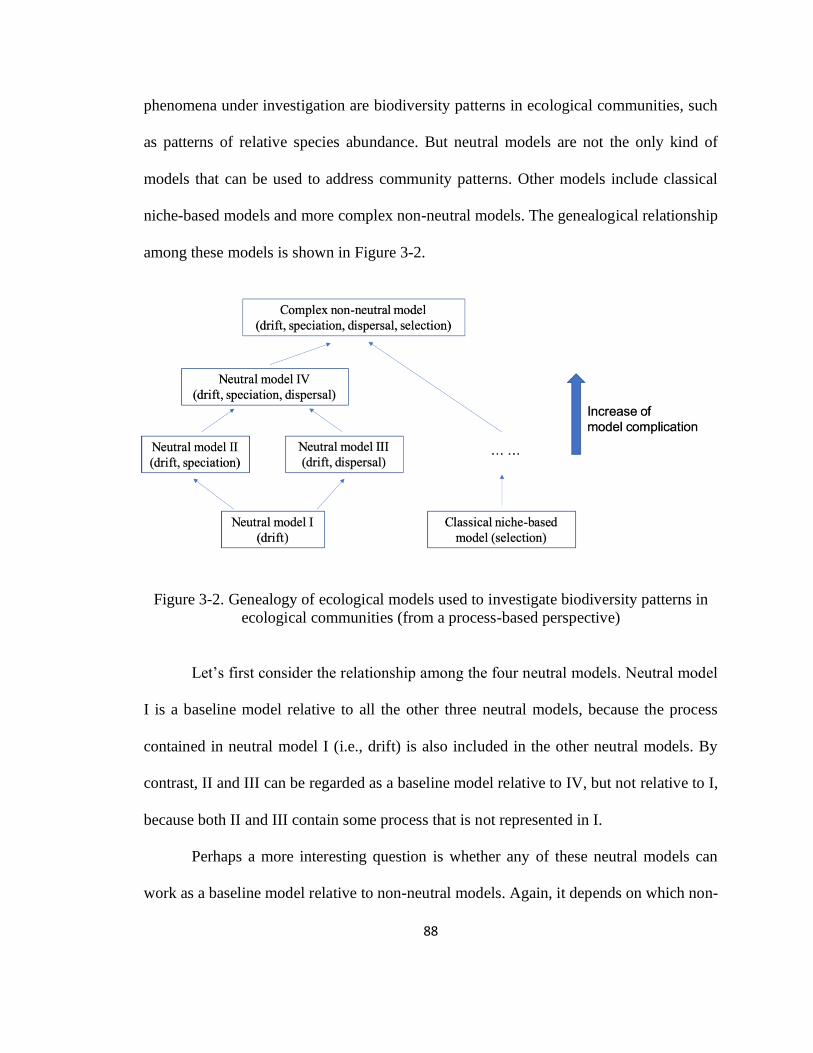
88

phenomena under investigation are biodiversity patterns in ecological communities, such

as patterns of relative species abundance. But neutral models are not the only kind of

models that can be used to address community patterns. Other models include classical

niche-based models and more complex non-neutral models. The genealogical relationship

among these models is shown in Figure 3-2.

Figure 3-2. Genealogy of ecological models used to investigate biodiversity patterns in

ecological communities (from a process-based perspective)

Let’s first consider the relationship among the four neutral models. Neutral model

I is a baseline model relative to all the other three neutral models, because the process

contained in neutral model I (i.e., drift) is also included in the other neutral models. By

contrast, II and III can be regarded as a baseline model relative to IV, but not relative to I,

because both II and III contain some process that is not represented in I.

Perhaps a more interesting question is whether any of these neutral models can

work as a baseline model relative to non-neutral models. Again, it depends on which non-

89

neutral models are under consideration. When compared with complex non-neutral

models that include all the four general ecological processes (see the model at the top of

Figure 3-2), all the four types of neutral models can be regarded as baseline models. This

is because the processes contained in neutral models are also included in those more

complex non-neutral models, which can be constructed by adding more processes into the

neutral models. However, when compared with classical niche-based models that only

include selection, none of the neutral models can be regarded as baseline models, because

the processes contained in neutral models are not contained in classical niche-based

models. In fact, there is no overlapping between neutral models and classical niche-based

models with respect to the ecological processes that they contain. An important

implication of this conclusion is that neutral models do not have methodological priority

over classical niche-based models. They work as different starting points with different

empirical assumptions about what factors are causally relevant for understanding the

dynamics and structure of ecological communities.

4.4 The contrast between the ideal gas model and neutral models

If we compare the genealogy of ecological models in Figure 3-2 with the genealogy of

gas models in Figure 3-1, we will find that they are different in one important aspect. In

the family of gas models, all the models can trace back to a single starting point, i.e., the

ideal gas model. In other words, the ideal gas model works as a baseline model for all the

other models in the family. By contrast, in the family of ecological models, there are

more than one single starting point. Hence, none of the models in the family, including

neutral models, can work as a baseline model for all the other models.

90

What makes this difference? I suggest that this is due to the different nature of the

phenomena to be addressed by these two families of models. The behavior of gas is

influenced by many factors, such as the collision between gas molecules and the wall of

the container, the volume of gas molecules, and intermolecular forces. Some of these

factors, such as the volume of gas molecules and intermolecular forces, are negligible in

modelling under certain circumstances, while some others, such as the collision between

gas molecules and the wall of the container, are always important and must be considered

in modeling under any circumstances. This is why it is possible to construct something

like the ideal gas model which can serve as a baseline model for all the other models in

its model family.

Biodiversity patterns in ecological communities are also the result of multiple

causal factors. As I noted earlier, if we follow Vellend’s process-based perspective, then

community patterns can be understood as the outcome of one or more processes of

selection, ecological drift, dispersal, and speciation. Vellend (2016, p. 175) has argued

that “all high-level processes can be important determinants of community structure and

dynamics,” depending on the specific systems under investigation. But here I want to

point out the other side of the coin: that is, none of these processes is always important in

structuring ecological communities. Since the relative causal importance of different

processes is very context-dependent, a process that plays an important role in one

situation may be negligible in another. Hence, when trying to construct a model to

explain or predict an ecological pattern, the ecologist does not have an overarching

judgment about which processes are essential components of an explanation. Instead,

which processes should be included in a model really depends on the type of

91

communities that one wants to investigate. This is also partly why modeling complex

ecological communities can be very challenging.

5. Conclusion

In this chapter, I have examined the claim that neutral models in ecology can be regarded

as baseline models. I have argued that whether a model counts as a baseline model

depends on what type of phenomena it is intended to address and which models it is

compared with. In a process-based perspective, neutral models are not baseline models

relative to classical niche-based models. Hence, they should not have methodological

priority over niche-based models. But this is not to deny the contribution and usefulness

of neutral models in community ecology. On the one hand, neutral theory challenges the

long-established view that niche differences are essential for explaining biodiversity

patterns. On the other hand, it draws biologists’ attention to processes such as ecological

drift and dispersal whose importance in structuring ecological communities has long been

underappreciated. Further research should focus on the conditions under which each of

the major ecological processes plays important roles in determining the dynamics and

structure of ecological communities.

92

Chapter 4: Empirical Adaptationism Revisited

1. Introduction

The debate about adaptationism has been one of the central topics within the philosophy

of biology and evolutionary biology communities (Gould & Lewontin, 1979; Mayr,

1983; Godfrey-Smith, 1999, 2001; Lewens, 2009; Orzack & Forber, 2010). Instead of

having a single, unified meaning, it refers to a family of views concerning the causal,

methodological, or explanatory importance of natural selection in the course of evolution

or in studies of evolutionary phenomena (Godfrey-Smith, 2001; Lewens, 2009; Orzack &

Forber, 2010). One variety of these adaptationist views tries to make an empirical claim

about the causal power of natural selection in evolution compared with non-selective

evolutionary factors. Since this view is intended to make an empirical claim about nature,

I will, for the sake of discussion, follow Godfrey-Smith (2001) and call it “empirical

adaptationism.”8

A number of philosophers and some biologists have tried to clarify the meaning

of empirical adaptationism and define it in ways that do not make it trivially true or

obviously false (e.g., Sober, 1987, 1998, 2000; Orzack & Sober, 1994; Godfrey-Smith,

2001; Lewens, 2009). Although these scholars may disagree on the details of how exactly

empirical adaptationism should be formulated, they usually share, explicitly or implicitly,

two assumptions about it: (1) Empirical adaptationism, while its truth is currently

8 There are different ways to name or describe this kind of adaptationist view in the literature. For example,

Sober (1998, p. 72) calls it “a non-trivial empirical thesis about the history of life”; Godfrey-Smith (2001)

uses the term “empirical adaptationism”; Lewens (2009) further distinguishes between three forms of

empirical adaptationism, and regards the view introduced here, which he calls “pan-selectionism,” as

merely one form of empirical adaptationism.

93

unknown or controversial, is an empirical claim about nature that is scientifically testable

in the long run; (2) empirical adaptationism is worth testing.

In this chapter, I will reexamine these two assumptions and argue that both are

mistaken given how empirical adaptationism is currently formulated. A series of

conceptual and methodological difficulties makes testing empirical adaptationism in a

biologically non-arbitrary way virtually impossible. Moreover, those who argue in favor

of testing empirical adaptationism have yet to demonstrate the distinctive value as well as

the necessity of conducing such a test. My analysis of the case of empirical adaptationism

also provides reasons for scientists to reconsider the value and necessity of engaging in

scientific debates involving the notion of overall relative causal importance.

2. The two themes of empirical adaptationism

I start by examining some influential formulations of empirical adaptationism in the

literature. The purpose of doing so is not to assess which is the best formulation or to

provide a new formulation based on existing ones. Rather, my aim is to figure out the

main themes of empirical adaptationism in its various forms, i.e., what empirical

adaptationism is about. Here are three influential formulations of empirical adaptationism

given by different philosophers of biology:

Natural selection has been the only important cause of most of the phenotypic traits

found in most species. (Sober, 1998, p. 72)

Natural selection is a powerful and ubiquitous force, and there are few constraints,

except general and obvious ones, on the biological variation that fuels it. To a large

degree, it is possible to predict and explain the outcome of evolutionary processes by

attending only to the role played by selection. No other evolutionary factor has this

degree of causal importance. (Godfrey-Smith, 2001, p. 336)

94

[N]atural selection is the most significant of the evolutionary forces that act on

populations. (Lewens, 2009, p. 162)

The above formulations of empirical adaptationism can be understood as different

clusters of claims regarding at least one of the following two themes:

(a) The relationship between natural selection and various constraints on

evolution

(b) The overall relative causal importance of natural selection in evolution

compared with other evolutionary factors

These two themes are not necessarily bundled together; a biologist who makes an

empirical claim about one theme may not necessarily take a position on the other. For

example, while all three formulations above involve the overall relative causal

importance of natural selection in evolution, only Godfrey-Smith’s (2001) formulation

contains an explicit claim regarding the relationship between natural selection and

constraints. Although neither of the two themes alone is sufficient to capture the whole

picture of empirical adaptationism, together they seem to provide a good coverage of the

relevant debates. In the following sections, I will introduce these two themes in more

detail and use them as a framework to examine the empirical testability of various claims

under the label of empirical adaptationism.

3. The first theme: the relationship between natural selection and constraints on

evolution

Although Darwin (1859, p. 6) explicitly acknowledged that natural selection is not the

“exclusive means of modification,” he is best known for his theory of evolution by

natural selection. Here is a simplest case of how natural selection can drive the evolution

of a trait in a given population: Heritable phenotypic variation arises among individuals

95

in a population. In a certain environment, different phenotypic variants may differ in their

fitness, i.e., individuals carrying different types of phenotypes tend to have different rates

of survival and reproduction. Over generations, natural selection will increase the

frequency of the phenotype with the highest fitness and eventually drive it to fixation in

the population.

This simple picture can be further complicated by taking into consideration

various constraints. First, there may be constraints on phenotypic variation, which set

limits on the raw material of natural selection. Among such constraints a much-discussed

type is developmental constraint, which is typically defined as “a bias on the production

of variant phenotypes or a limitation on phenotypic variability caused by the structure,

character, composition, or dynamics of the developmental system” (Maynard Smith et al.,

1985, p. 266). For example, a phenotypic variant may be developmentally prohibited

because the relevant mutation(s) lead to a lethal malformation in the process of

embryological development. As a result, phenotypes that would have been favored by

natural selection may not be able to appear in the population at all.

Other kinds of constraints do not limit the variety of phenotypes, but they may

“get in the way” of natural selection by preventing the fittest phenotype from going to

fixation in a population. These constraints may be properly called constraints on the

action of natural selection. One example is the case of heterozygote superiority. Suppose

that A and a are two alternative alleles at a locus in a diploid population, and the

heterozygote Aa has a higher fitness than the two homozygotes AA and aa. Despite being

favored by natural selection, the heterozygote Aa is not able to get fixed in the population

because it cannot breed true: When two heterozygotes mate, there is always a probability

96

that some of their offspring are homozygotes. This fact imposes a genetic constraint on

what natural selection can accomplish.

So what claims would an empirical adaptationist make regarding the relationship

between natural selection and various constraints on evolution? One claim that has often

been linked with empirical adaptationism is that natural selection is typically powerful

enough to overcome or conquer various constraints (Amundson, 1994, p. 572; Stephens,

2007, p. 117). The constraints here can refer to either constraints on phenotypic variation

or constraints on the action of natural selection, or both of them.

Let us first consider constraints on phenotypic variation. Amundson (1994, 572)

describes a position called “hard adaptationism” as follows:

All organic traits have adaptive values, and those adaptive values, via the

principle of natural selection, provide the proper historical explanation of the

existence of those traits. Any developmental constraints can be (and have

been) overcome by the forces of natural selection.

What does it mean that a developmental constraint has been overcome? Consider a case

where a phenotypic variant is developmentally prohibited. Sometimes new mutations

arise and lead to the change of the developmental system such that the previously

prohibited phenotypic variant is now allowed to be produced. In some sense, we can say

that the developmental constraint has been overcome. But this change has nothing to do

with the “power” of natural selection. Instead, it is due to the appearance of new

mutations that alter the features of the developmental system. It may be argued that in

order to really overcome a developmental constraint, the emerging new mutations must

persist and spread in the population, which would have to be due to the operation of

natural selection. Be that as it may, it is biologically inaccurate to claim that it is the

97

power of natural selection per se that overcomes the developmental constraint, and there

is no reason to privilege the role of natural selection over mutation in this process.

The same conclusion applies to other kinds of constraints. Consider the much-

discussed case of pleiotropy. Pleiotropy is the phenomenon that one gene has more than

one phenotypic effect. Suppose that two phenotypes always co-occur among the

individuals in a given population due to the effect of pleiotropy. If one phenotype has

positive effects on its carrier’s fitness while the other has negative effects, then the

phenotype that could have been favored by natural selection for its positive effects may

be eliminated from the population because of the stronger negative effects of the other

phenotype. In this case, the beneficial phenotype fails to be selected not because it is

prohibited to appear in the population, but because it is bundled together with another

deleterious phenotype. As a response, Dawkins (1982, 35) has argued that “if a mutation

has one beneficial effect and one harmful one, there is no reason why selection should not

favour modifier genes that detach the two phenotypic effects, or that reduce the harmful

effect while enhancing the beneficial one.” This quote has often been used as an

illustration of the view that natural selection is typically powerful enough to overcome

pleiotropic constraints (Sober 1987, 115; Stephens 2007, 119).

Sober (1987, 116) comments that the detachment of two phenotypic effects in the

case of pleiotropy is more indicative of the power of mutation rather than the power of

natural selection. Although I am sympathetic to Sober’s comment, I take it to be

problematic to interpret Dawkins as saying that the power of natural selection per se can

break the pleiotropic link between phenotypic effects. In fact, what Dawkins (1982, 35)

wants to argue is that pleiotropy is not a static and unchangeable property of certain

98

genes, and he believes that it is possible to break the link between pleiotropic phenotypes

when certain modifier genes emerge in a population and get selected. Hence, he would

presumably agree that the detachment of pleiotropic phenotypes, when happens, is not

merely due to the power of natural selection.

An alternative way to depict the relationship between natural selection and

constraints is to claim that there are few constraints on the raw material of natural

selection without explicitly attributing this rareness of constraints to the power of natural

selection. For example, Godfrey-Smith’s formulation of empirical adaptationism includes

the claim that “there are few constraints, except general and obvious ones, on the

biological variation that fuels it [natural selection]” (Godfrey-Smith, 2001, p. 336). An

empirical adaptationist holding this view may concede that natural selection per se cannot

overcome constraints, but nevertheless emphasizes the rareness of constraints on

phenotypic variation in the actual biological world.

However, this formulation of empirical adaptationism has its own problems. First,

Godfrey-Smith’s formulation excludes “general and obvious” constraints when

emphasizing the rareness of constraints on phenotypic variation. But it is unclear what

counts as a “general and obvious” constraint. In particular, whether a constraint is

obvious or not can be a matter of subjectivity. A constraint that is obvious to one

biologist may not be obvious to another with different expertise or background

knowledge. Second, there is much vagueness about the quantifier “few.” Claims with

quantifiers like “few” may be testable in some cases. For example, if there is no

constraint on phenotypic variation, then Godfrey-Smith’s formulation of empirical

adaptationism would be false. However, every biologist, including those holding various

99

forms of empirical adaptationism, agree that there are constraints on the range of

phenotypic variation. So the question becomes: How many constraints count as few?

Numerous specific examples can be found about such constraints, but it is unclear how

many would be enough to refute the empirical adaptationist claim. Of course, one can

stipulate that there are few constraints if and only if the number of constraints is smaller

than a certain threshold value. While this would make the empirical adaptationist claim

testable, it is testable only in a biologically arbitrary way.

The issues that I raise about the use of the quantifier “few” are not merely

semantic nitpicking; they are real issues that must be addressed for anyone who decides

to take the testability of empirical adaptationism seriously. Scientific debates concerning

very general claims about nature, such as empirical adaptationism, usually involve using

quantifiers, but the impact of such use on the testability of general claims has not

garnered much philosophical attention (but see Beatty (1997) for an exception). If

biologists cannot achieve some consensus on what counts as “few constraints” in a

biologically meaningful way, then it is very unlikely that debates about empirical

adaptationism can be resolved by merely accumulating more empirical studies.

One possible way to clarify the meaning of “few” is to compare the number of

prohibited phenotypic variants due to the existence of constraints and the number of

variants actually appearing in a population. This approach relies not on the specific

number of constraints, but on their causal effects on phenotypic variety. Fig. 4-1 is a

typical way to illustrate the influence of constraints on the range of discrete phenotypic

variants available for selection (Sober, 1998, p. 79). {P1, P2, …, Pn, …, Pn+m} refers to the

set of conceivable phenotypic variants in the absence of constraints; {P1, P2, …, Pn} is the

100

set of phenotypic variants that actually appear in the population; P1 is the variant that

becomes fixed in the population due to the action of natural selection. Given this setting,

m of the n+m phenotypic variants are prohibited from appearing due to the existence of

constraints. To clarify the meaning of “few,” it may be stipulated that there are few

constraints on the phenotypic variation of a trait if and only if the number of phenotypic

variants prohibited due to the existence of constraints (m) is smaller than the number of

variants actually appearing in the population (n).

Figure 4-1. The two-stage process of the evolution of a trait, from Sober (1998)

Although this definition seems to provide a more rigorous testing method, it still

falls prey to the problem of terminological ambiguity, which in this case involves the

concept of “conceivable variation.” Sober (1998, 79) argues that it is impossible to be

very precise about the value of m because the number of conceivable variants depends

more on biologists’ imaginations rather than on empirical facts. Hence, from a

biologically perspective, it does not make much sense to compare the values of m and n.

I agree with Sober’s conclusion, but for different reasons. First, the number of

conceivable variants may be empirically determinable if the concept of “conceivable

variation” is defined relative to a particular constraint. For example, conceivable

variation can refer to the phenotypic variants that would be possible to appear in a

101

population if a particular constraint were absent. According to this definition, it is

possible to estimate the number of conceivable variants by examining the actual variation

in the population and studying the causal effects of a particular constraint. The problem,

however, is that there is obviously more than one constraint for any group of evolving

organisms. In one sense, the history of organic evolution is a history of cumulating

constraints, which make the appearance of some traits less likely or even impossible and

others more probable. The further we trace back the evolutionary history of a group of

organisms, the more constraints we might be able to identify. When more and more

constraints are loosened or removed, the number of conceivable variants would become

larger and larger. Hence, the relative magnitudes of m and n depends on how far we

would like to trace back the evolutionary history of a population and hence how many

constraints are counterfactually removed.

In addition, the way Sober makes his argument reflects an inaccurate

understanding of the role of constraints that is common in the literature. According to the

illustration in Figure 4-1, {P1, P2, …, Pn, …, Pn+m} shrinks to {P1, P2, …, Pn} due to the

existence of various constraints. This typical way of depicting the effect of constraints

seems to suggest that they can only play a “negative” role in evolution by prohibiting the

production of certain conceivable phenotypic variants. However, if we switch our

perspective, we may find that the so-called constraints can also play a “positive” role in

evolution. Consider the case of developmental constraints. Developmental constraints are

defined as biases on the production of variant phenotypes or limitations on phenotypic

variability caused by the properties of the developmental system. But the properties that

prohibit the production of certain phenotypic variants may also be the properties that

102

support the normal development of other variants. To use an analogy, the prohibitive role

and the supportive role of certain properties of the developmental system are like the two

sides of a coin: From one side we see developmental constraints, while from the other

side we see support for new developmental opportunities. Here is an important

implication of this more nuanced understanding of the nature of constraints: Biologically

speaking, it is not very meaningful to ask the number of conceivable phenotypic variants

in the absence of all constraints, since a developmental system without any constraints

may not be able to produce any phenotypes at all.

In this section I examined two varieties of claims that empirical adaptationists

might make about the relationship between natural selection and constraints on evolution.

The first claim is that natural selection is typically powerful enough to overcome various

constraints. I have shown that this claim is biologically inaccurate. The second claim is

that there are few constraints on phenotypic variability. I have shown that the inherent

vagueness of this claim makes it unamenable to empirical testing.

4. The second theme: the overall relative causal importance of natural selection in

evolution

The second theme of empirical adaptationism concerns the overall relative causal

importance of natural selection in evolution. A typical adaptationist claim regarding this

theme is that natural selection is, in most cases, the most or the only important cause of

phenotypic evolution. In order to test the truth of this claim, biologists need to proceed in

two steps. First, they need to test whether natural selection is the most or the only

important cause of the evolution of various particular traits. Second, they need to

103

calculate how often it is the case that natural selection is the most or the only important

cause of the evolution of a trait.

Let’s start with the first step. To be clear, the claim that natural selection is the

most important cause of the evolution of a trait is different from the claim that natural

selection is the only important cause of the evolution of a trait. The former claim does not

deny the possibility of other evolutionary factors being causally important in the

evolution of a trait, but simply emphasizes the causal superiority of natural selection over

other evolutionary factors. The latter claim, however, regards the role of non-selective

evolutionary factors as negligible in the evolution of a trait. Hence, there are actually two

empirical adaptationist views regarding the second theme:

(I) Natural selection is in most cases the most important cause of phenotypic

evolution.

(II) Natural selection is in most cases the only important cause of phenotypic

evolution.

Notice that an empirical adaptationist who holds (I) may not accept the truth of (II).

Hence, it is important to keep these two claims distinct. In the following, I will examine

the testability of (I) and (II) respectively.

The testability of Claim (I)

Let us first consider claim (I): Natural selection is in most cases the most important cause

of phenotypic evolution. The idea that natural selection is in some sense more important

than other evolutionary factors has a long history in the development of evolutionary

thinking. At the very end of the Introduction in the first edition of On the Origin of

Species, Darwin claimed that “I am convinced that Natural Selection has been the main

104

but not exclusive means of modification” (Darwin, 1859, p. 6, my italics). In the fifth

edition, he revised the wording and stated that “I am convinced that Natural Selection has

been the most important but not the exclusive means of modification” (Darwin, 1869, p.

6, my italics). Darwin is not alone in this kind of thinking. For example, Jonathan Losos,

a leading evolutionary biologist today, thinks that “evolution is the historical occurrence

of change, and natural selection is one mechanism – in most cases the most important –

that can cause it” (Losos, 2014, p. 3, my italics).

In the following, however, I will argue that it is not always possible to compare

the relative causal importance of natural selection and other evolutionary factors. I will

consider several cases where the evolution of a trait is influenced by both natural

selection and a non-selective factor and show that in those cases it does not make sense to

privilege one evolutionary factor as causally more important than the other.

Case 1: Suppose that a beneficial phenotypic variant that would have been

favored by natural selection (labelled as T1) fails to appear in a population because of the

existence of a certain developmental constraint. As a result, natural selection favors an

alternative phenotypic variant available in the population (labelled as T2) and drives it to

fixation, although T2 would have a relatively lower fitness than T1 if T1 were allowed to

develop. However, if the developmental constraint did not exist, the result would be

entirely different. Natural selection would favor the initially prohibited variant T1 and

drive it to fixation. In this case, the developmental constraint and natural selection play

different kinds of causal roles in the evolution of the focal trait. The developmental

constraint determines which phenotypic variants are available in the population in the

first place, while natural selection determines which of the available phenotypic variants

105

finally gets fixed in the population. It does not make sense to claim that one of these two

evolutionary factors is a more important cause of evolution than the other.

Case 2: In his Shifting Balance Theory, Sewall Wright (1931, 1932) depicts a

scenario where a large population is divided into many partially isolated subpopulations

and its adaptive evolution is driven by the interaction between natural selection and

genetic drift. The whole process can be understood as consisting of three phases (Skipper,

2002): In the first phase, genetic drift causes gene frequencies to fluctuate in

subpopulations, allowing some of them to move across adaptive valleys and reach the

base of a higher adaptive peak; in the second phase, natural selection operates within

subpopulations, moving them to local adaptive peaks; in the third phase, organisms from

more fit subpopulations migrate to less fit ones, and natural selection between

subpopulations increases the average fitness of the whole large population.

It is clear that natural selection and genetic drift play different roles in the above

scenario: Genetic drift helps subpopulations shift across adaptive valleys toward new,

higher adaptive peaks; natural selection increases the average fitness of both each

subpopulation and the whole population. However, it is unclear how we can compare the

relative causal importance of natural selection and genetic drift. Without genetic drift,

subpopulations will be held at the nearest adaptive peaks by natural selection, having

little chance to move across the adaptive valleys toward a higher adaptive peak; without

natural selection, cumulative adaptive changes are unlikely to occur, no matter in

subpopulations or the whole population. In this situation, neither of these two

evolutionary factors can be said to be causally more important than the other – both

106

natural selection and genetic drift play an essential role in the evolutionary process

described above.

Case 3: Suppose that initially there exist three variants (V1, V2, V3) of a trait in a

population, and their fitness ranks as follows: Fitness (V1) > Fitness (V2) > Fitness (V3).

Among these three variants, V1 and V2 are new variants that have recently emerged in the

population, each having a very low frequency. Suppose that V1 is lost from the population

due to the effect of random genetic drift. Among the remaining two variants, V2 is

favored by natural selection and spreads to fixation in the population. In this case, genetic

drift eliminates the fittest variant from the population, while natural selection increases

the frequency of the second fittest variant. Both genetic drift and natural selection are

essential to explain why V2 can eventually get fixed in the population, and there is no

intelligible way to compare the relative causal importance between these two

evolutionary factors.

I have analyzed three problematic cases where we are not allowed to compare the

relative causal importance of natural selection and non-selective evolutionary factors in

an intelligible way, and they are not intended to be exhaustive of all the problematic cases.

The point is not that we cannot never make such comparison, but that it is not always

possible to do so. Since testing claim (I) requires comparing the relative causal

importance of natural selection and other evolutionary factors in individual cases, the

existence of various problematic cases would seriously undermine the testability of the

empirical adaptationist claim that “natural selection is in most cases the most important

cause of phenotypic evolution.”

107

Claim (II): Orzack and Sober’s formulation of empirical adaptationism

I now turn to claim (II): Natural selection is in most cases the only important cause of

phenotypic evolution. A formulation of empirical adaptationism like this has been

proposed by Orzack and Sober.

Orzack and Sober (1994b) distinguish three propositions about the role of natural

selection in the evolution of some individual trait T in a given population (p. 362):

(U) Natural selection played some role in the evolution of T.

(I) Natural selection was an important cause of the evolution of T.

(O) Natural selection is a sufficient explanation of the evolution of T, and T is

locally optimal.

Orzack and Sober think that proposition (O) best captures the adaptationist view on the

evolution of a trait. Notice that proposition (O) per se is not a formulation of empirical

adaptationism, because empirical adaptationism is not a claim about the role of natural

selection in the evolution of a particular trait, but a general claim about the overall

relative causal importance of natural selection in evolution. Given this, Orzack and Sober

(1994b, p. 364) formulate the thesis of empirical adaptationism9 as a generalized form of

proposition (O):

Natural selection is a sufficient explanation for most nonmolecular traits, and

these traits are locally optimal.

How could biologists tell whether natural selection is a sufficient explanation of the

evolution of a trait? Orzack and Sober suggest that this can be tested via an optimality

model. An optimality model is a kind of “censored” model in which non-selective

evolutionary processes such as genetic drift are ignored and only natural selection is

described. Under this setting, the most adaptive variant of a trait among a set of

9 Although Orzack and Sober (1994b) do not use the term “empirical adaptationism,” it is clear that the

kind of adaptationism discussed by them is intended to be an empirical claim about nature.

108

alternatives in a particular environment is expected to be selected and eventually driven

to fixation in the population. If the optimality model’s quantitative prediction about the

optimal value of an individual trait in a given population fits the empirical data

statistically, then natural selection would be a sufficient explanation of the evolution of

that trait. Under these circumstances, natural selection is also said to be the only

important cause of the evolution of the focal trait. Hence, in another place Sober (1998, p.

72) also formulates empirical adaptationism as follows:

Natural selection has been the only important cause of most of the phenotypic

traits found in most species.

For Orzack and Sober, claiming that natural selection is the only important cause of the

evolution of a trait does not mean that it is the only cause at work. In these cases, non-

selective evolutionary factors may still exist, but they play such a small role in the

evolution of a trait that they can be ignored without loss of accuracy when predicting or

explaining the evolutionary outcome of that trait. For example, since no biological

population in reality is infinitely big, genetic drift always plays some role in the evolution

of a population. But when the population is big enough, it is usually innocuous to ignore

the effect of genetic drift when studying the evolution of a trait in that population.

It is worth emphasizing again that Orzack and Sober’s formulation of empirical

adaptationism is different from the claim (I) that natural selection is in most cases the

most important cause of phenotypic evolution. One major benefit of formulating

empirical adaptationism in Orzack and Sober’s way is that it does not involve directly

comparing the relative causal importance of natural selection and non-selective

evolutionary factors, thus circumventing the comparison problem faced by the weaker

109

claim. This subtle but important difference has failed to be fully appreciated in the

literature. For example, Resnik (1997, p. 42) describes Sober’s definition of empirical

adaptationism as the claim that “natural selection is the most important cause of most

traits in most populations”; Lewens (2009, p. 163) summarizes Orzack and Sober’s

formulation of empirical adaptationism as the view that “selection is typically the most

important evolutionary force.” Both of them conflate Orzack and Sober’s formulation of

empirical adaptationism with claim (I).

Until now I have yet to analyze the testability of Orzack and Sober’s version of

empirical adaptationism. In the next section, I will discuss several methodological

difficulties that may well undermine the testability of empirical adaptationism as

envisaged by them.

5. Methodological difficulties in the long-run test of empirical adaptationism

Empirical adaptationism as formulated by Orzack and Sober is a general thesis about

nature – a claim about the overall relative causal importance of natural selection in

evolution. As an implication, the correctness of such a thesis cannot be assessed by

testing the local optimality of a single phenotypic trait. Orzack and Sober are fully aware

of the ensemble nature of such a test, and they suggest that empirical adaptationism is

testable by accumulating the results of investigations of many traits:

The test of adaptationism we advocate need not engender an interminable

debate. Forty or 50 appropriately structured studies might well provide a

reasonable assessment of adaptationism. For example, if 45 of the 50 tests

lead to the conclusion that the trait in question is locally optimal, in our

opinion one could conclude that adaptationism is correct. Attainment of

some agreed-on number of tests should be a goal of evolutionary

biologists. (In these days of the Human Genome Project, it may be

appropriate – and perhaps even more useful – to organize a far cheaper

Adaptationism Project in order to coordinate quantitative studies of

110

optimality models.) […] [A] test of adaptationism of the size mentioned

earlier might even be attainable in the next 10 yr or so. (Orzack & Sober,

1994b, pp. 377–378)

27 years have passed since Orzack and Sober made this proposal, but the kind of test

envisaged by them has yet to be conducted. It is an interesting question why biologists,

including Orzack himself, have not organized an Adaptationism Project to assess the

correctness of empirical adaptationism. But even if biologists decided to implement such

a project, they would have to first address a number of methodological difficulties to

guarantee the validity of the test.

In an ideal case, biologists would have a complete list of all the phenotypic traits

of all organisms in the history of life, and they are able to test in each case whether

natural selection is sufficient to explain the evolution of a trait. Clearly, this is not a

practical plan. A more feasible way to conduct the test is to choose a representative

sample of all the phenotypic traits.

Several methodological issues need to be addressed in order to obtain such a

representative sample. First, evolutionary biologists need to reach some kind of

consensus on the number of traits to be studied in the sample. Orzack and Sober (1994b,

p. 377) suggest that “[f]orty or 50 appropriately structured studies might well provide a

reasonable assessment of adaptationism.” But they provide no clue of how this number is

determined and justified from a statistical point of view. Even if the issue of sample size

can be resolved, another methodological difficulty remains, namely, how to select a

sample of traits such that the testing result is representative of the overall relative causal

importance of natural selection in the evolution of all the traits of all organisms appearing

in the history of life.

111

It may be argued that statisticians have developed various sampling techniques to

help ensure the representativeness of a sample. For example, if there are two colors of

glass beads – red and blue – in a box and a researcher wants to know the proportion of

the red ones, she can mix the beads sufficiently and select a sample of a certain size

randomly. This sampling technique is called simple random sampling, and the underlying

rationale is that in such a setting, every possible sample of the same size has the same

probability of being selected during the process of sampling.

However, sampling methods like this may not be easily applied to the case of

testing empirical adaptationism. One major goal of statistical research is to draw

conclusions about the properties of populations via studying samples. By “population,” or

more precisely, “statistical population,” I mean a group of individuals that a researcher

wants to draw conclusions about, which can be either concrete objects such as glass

beads, or abstract objects such as the possible moves of a chess player. From a statistical

point of view, having a well-defined statistical population is essential for getting a

representative sample of that population. A statistical population is well-defined if and

only if there is a clear standard about what should be included in the population and each

individual in the population is possible to be sampled during the time of investigation. In

the case of glass beads, the statistical population is the collection of all the glass beads in

the box, which is well-defined according to the preceding definition. Without the

existence of this well-defined statistical population, it does not even make sense to ask

whether a sample is representative, because the representativeness of a sample, by

definition, is always relative to the statistical population that it is intended to provide

information about.

112

Now consider the case of testing empirical adaptationism. What is the statistical

population that biologists want to know about? A quick answer would be “all the traits of

all organisms.” But this answer is too vague to be helpful. For example, should structures

like eyes or wings of different species be regarded as one trait? Or should each of them

count as a different trait? A clue of answers to these questions may be found in the subtle

changes in the way empirical adaptationism is formulated by Sober in different places:

(i) Natural selection is a sufficient explanation for most nonmolecular traits,

and these traits are locally optimal (Orzack and Sober, 1994b, p. 364, my

italics).

(ii) Natural selection has been the only important cause of most of the

phenotypic traits found in most species (Sober, 1998, p. 72, my italics).

(iii) Most phenotypic traits in most populations can be explained by a model

in which selection is described and nonselective processes are ignored (Sober,

2000, p. 124, my italics).

Formulation (i) talks of nonmolecular traits (i.e., phenotypic traits) 10 in general.

Formulation (ii) seems to suggest that analyses of phenotypic traits should be on the level

of species. If so, structures such as eyes or wings of different species should each count

as a different trait. Formulation (iii) goes one step further: Studies of the same trait in

different populations of a species may yield different results. For example, a trait that is

locally optimal in one population may not be so in another. Hence, it seems reasonable to

regard studies of the same trait in different populations as different individual cases while

sampling. Suppose that we adopt the granularity of analysis in formulation (iii), then the

statistical population being studied would be all the phenotypic traits in each population

of each species.

10 Sober’s discussion of empirical adaptationism focuses on nonmolecular traits.

113

However, such a statistical population is still poorly defined, which does not

allow biologists to obtain a representative sample of it. Although the concept of trait is

widely used in biology, it is notoriously difficult to define what a trait is. In a very

general sense, a trait is simply a character state of an organism. But exactly what feature

of an organism could be properly regarded as a trait depends on many factors, including

facts of developmental processes of organisms (Wagner, 2001), the researcher’s

background theories and beliefs (Resnik, 1997), as well as the specific content of the

research problem in question. Hence, different biologists would identify different

collections of traits even within one population of one species, and the situation will be

even worse when we consider all the populations of all species. But the problem goes

beyond this.

In the case of glass beads, each glass bead in the box has the same probability of

being selected in the process of sampling. In the case of testing empirical adaptationism,

however, many features of organisms have no chance to be sampled because they have

yet to be individuated by biologists as traits and hence cannot enter the sampling pool at

all. In other words, the statistical population that is intended to include all the phenotypic

traits in each population of each species is not well-defined, which makes it impossible to

collect a representative sample thereof.

It may be argued that instead of trying to obtain a representative sample of all the

possible phenotypic traits in each population of each species, biologists can just build a

list of all the traits that have already been individuated and studied. If most of the

already-studied traits are locally optimal, then the version of empirical adaptationism as

formulated by Orzack and Sober is true. This approach does not really solve the problem

114

of representativeness. The way we distribute our scientific resources can influence our

perception of the relative importance of natural selection in evolution (Beatty, 1987, pp.

53–54). The more scientific resources are distributed to studies on the apparent design of

organisms and their relations of adaptedness to their environments, the more likely it is to

find cases of local optimality. Similarly, the more funding is provided to studies on the

role of non-selective evolutionary factors (such as genetic drift) in evolution, the more

likely it is that counterexamples of optimality can be found. If the testing result of

empirical adaptationism is simply a statistical summary of the results of biologists’

previous studies, then this result would be more of a reflection of scientific resource

distribution and biologists’ research interest rather than what actually happens in nature.

This observation poses a serious problem for those in favor of testing empirical

adaptationism, for it contradicts with one of their core beliefs that empirical

adaptationism is an empirical thesis about nature.

In this section, I have discussed a series of methodological difficulties of

obtaining a representative sample in the test of empirical adaptationism. Although I use

Orzack and Sober’s proposal as a target of critique, my analysis reveals a general

challenge for any serious attempt to test empirical adaptationism as a general thesis about

nature. This challenge, in my view, makes testing empirical adaptationism in a

biologically non-arbitrary way virtually impossible.

6. Rethinking the value and necessity of testing empirical adaptationism

The previous sections have focused on the testability of empirical adaptationism. I now

turn to a different issue: Why should biologists care about the truth of this general thesis

115

at all? As mentioned earlier, a number of philosophers and some biologists have tried to

clarify the meaning of empirical adaptationism and provide their own formulations.

These scholars are not necessarily committed to the truth of empirical adaptationism.

Instead, they regard as an empirical matter whether empirical adaptationism is true and

leave the task of testing its truth to biologists. When doing so, they also assume that

empirical adaptationism is worth testing. However, in the existing literature, there has

been little explicit justification of why this should be the case.

In this section, I will consider four types of value that might be attached to the test

of empirical adaptationism. It turns out that some of these values simply do not exist; the

others either are trivial or can be achieved without having to test empirical adaptationism.

Hence, none of them can be used to justify the necessity of conducting such a test. To be

clear, the four types of value that I will consider below are not intended to be exhaustive

of all conceivable values. Hence, my analysis in this section does not allow me to

conclude that no other values of testing empirical adaptationism can be found in the

future. Nevertheless, my argument, if succeeds, will show that those in favor of testing

empirical adaptationism have yet to demonstrate the distinctive value as well as the

necessity of conducting such a test.11 Unless a proper justification can be provided, there

seems no reason to assume that empirical adaptationism is worth testing.

11 This argument should not overshadow the necessity of evaluating the testability of empirical

adaptationism. Even if one can find some value in testing empirical adaptationism, the previous sections

show that empirical adaptationism, as currently formulated, is not genuinely testable in practice.

116

6.1 Methodological heuristic value

As mentioned in the introduction, there are different kinds of adaptationism. Those in

favor of testing empirical adaptationism may seek to argue for the necessity of such a test

by appealing to the relationship between empirical adaptationism and another kind of

adaptationist position – methodological adaptationism. Godfrey-Smith (2001, p. 337)

defines methodological adaptationism as the following view: “The best way for scientists

to approach biological systems is to look for features of adaptation and good design.

Adaptation is a good ‘organizing concept’ for evolutionary research.” Lloyd (2015), a

representative critic of methodological adaptationism, formulates this research method in

terms of the research question asked by its practitioners: A methodological adaptationist

assumes, at the beginning of investigation, that a trait under consideration is an

adaptation and asks “What is the function of this trait?”; given such a research question,

they would try to look for adaptative explanations for the evolution of this trait.

Those in favor of testing empirical adaptationism may argue that many biologists

are motivated to adopt methodological adaptationism in their actual scientific research

because they believe the truth of empirical adaptationism: The belief in the power and

ubiquity of natural selection in evolution motivates these researchers to assume, at the

beginning of their investigation, that a trait is an adaptation until shown otherwise. For

these researchers, it truly matters whether empirical adaptationism is correct or not,

because methodological adaptationism – a widely-practiced methodology – is justified by

the truth of empirical adaptationism. Given the central role of empirical adaptationism in

motivating and justifying actual scientific practice, it is valuable and necessary to test this

thesis.

117

This argument does not work because it fails to distinguish the beliefs that

motivate someone to adopt a methodology and the genuine justification that is needed to

defend such a methodology. It is perfectly possible that a methodological adaptationist is

motivated to adopt this methodology because she believes that empirical adaptationism is

true and that the truth of empirical adaptationism justifies the legitimacy of

methodological adaptationism as a valid research strategy. However, the occurrence of

such a situation does not mean that the justification of methodological adaptationism

actually relies on the truth of empirical adaptationism. Godfrey-Smith (2001, p. 338) has

shown that empirical adaptationism and methodological adaptationism are logically

independent of each other. As a consequence, the truth or falsity of empirical

adaptationism does not really bear on the justifiability of methodological adaptationism –

even if empirical adaptationism turns out to be false, it does not exclude the possibility of

methodological adaptationism being a valid and productive research strategy. Notice that

I am not denying the fact that empirical adaptationist beliefs motivate some (or even

many) biologists to adopt methodological adaptationism. But this fact does not guarantee

the value and necessity of testing empirical adaptationism. To evaluate the validity of

methodological adaptationism, we need to examine its merits (or problems) from a

methodological perspective, rather than test the truth of empirical adaptationism.

This analysis is also supported by the actual critiques offered by opponents of

methodological adaptationism. For example, in her systematic critique of methodological

adaptationism, Lloyd (2015) objects to this research method by identifying various

dangers that result from the logic of its research question, such as the lack of a stopping

rule in pursuing adaptive explanations for the evolution of traits and the loss of ability to

118

evaluate and weigh evidence for alternative causal hypotheses. None of these critiques is

based on the falsity of empirical adaptationism. Lloyd also proposes an alternative

research strategy called the “evolutionary factors” framework, whose fundamental

research question is “What evolutionary factors account for the form and distribution of

this trait?”. When discussing the relationship between this alternative framework and

empirical adaptationism, she notes that “the evolutionary factors framework is

independent of any commitment regarding empirical (or ‘metaphysical’) adaptationism”

(p. 345). It goes beyond the scope of this chapter to evaluate whether the evolutionary

factors framework is indeed a better alternative to methodological adaptationism. What is

relevant here is that, for Lloyd, the reason why biologists should abandon methodological

adaptationism and adopt the evolutionary factors framework has nothing to do with the

truth or falsity of empirical adaptationism, but with the relative methodological

superiority of the evolutionary factors framework in biological research.

6.2 Explanatory value

It may be argued that empirical adaptationism is worth testing because its truth (or falsity)

has explanatory value. A piece of information has explanatory value in science if and

only if it contributes to explaining certain scientific phenomena. Now the question is: Can

we find any biological phenomenon whose explanation at least partly relies on the test

result of empirical adaptationism? To the best of my knowledge, no such examples have

ever been presented in the relevant literature. And in my view, the prospects for finding

such examples are dim: Even if empirical adaptationism is testable, its truth (or falsity) is

simply based on a statistical summary of the testing results of individual cases; it is

119

unclear how such a highly contingent and general fact can help to explain the occurrence

of any biological phenomenon.

One possible objection is that while the truth (or falsity) of empirical

adaptationism per se has no explanatory value, testing this general claim requires testing

specific hypotheses about the causal role of natural selection in the evolution of particular

traits. The results of such tests would contribute to explaining the form and distribution of

those particular traits. This argument is problematic because it seems to assume that

testing empirical adaptationism is a necessary condition for testing hypotheses about the

evolution of particular traits when this is actually not the case. Since the truth (or falsity)

of empirical adaptationism has no bearing on why a particular trait has evolved,

biologists do not need to test empirical adaptationism in order to pursue and test

hypotheses about the evolution of particular traits.

6.3 Epistemic value

Resnik (1997) argues that Sober and Orzack’s long-run test of empirical adaptationism is

valuable because it can “increase our knowledge about evolutionary trends” (Resnik,

1997, p. 46). If testing empirical adaptationism can increase our biological knowledge,

then it seems to have epistemic value.

There are two issues with this proposal. First, it is not clear what exactly those

“evolutionary trends” refer to. In my view, they refer to nothing but whatever is already

described in various formulations of empirical adaptationism, such as the overall relative

causal importance of natural selection in evolution. If this is the case, then it leads to the

second issue, that is, it remains unexplained why it is scientifically valuable to have

120

knowledge about these trends. Failing to answer this question is tantamount to saying that

it is scientifically valuable to test empirical adaptationism because it is scientifically

valuable to know the result of such a test, which merely begs the question.

It may be argued that testing empirical adaptationism is valuable for those who

want to conduct such a test because it satisfies their curiosity, and there is no need to ask

further what the value of such curiosity is. Notice that this justification focuses only on

the value of testing empirical adaptationism in terms of satisfying individual curiosity,

but it says nothing about the value of such a test to science in general and biology in

particular. An inquiry that arouses the curiosity of certain individuals may not be of

scientific value. For example, an individual might want to know the center of gravity of

all the humans on Earth, but knowledge of such a fact (if there is such a fact at all) does

not seem to have any scientific value. By the same token, testing empirical adaptationism

may be interesting to some researchers, but this does not automatically demonstrate why

it is scientifically valuable to know the result of such a test. If we view scientific research

as a social practice and scientific knowledge as social knowledge (Longino, 1990), then

individual scientists need to provide further justification about why certain questions of

interest to themselves are scientifically valuable and hence worth investigating and

discussing within the scientific community.

6.4 Spin-off value

Not all scientific controversies can be resolved in the end. In many cases, participants in a

scientific debate simply lose their interest and move to other topics (Kovaka, 2017).

Nevertheless, these debates usually promote many meaningful discussions along the way,

121

hence creating great spin-off value. In the case of empirical adaptationism, one may

concede that there is no conclusive answer with respect to its correctness, but still

contend that the debates surrounding empirical adaptationism have inspired many in-

depth discussions about a number of important topics in evolutionary biology. Given this,

it seems reasonable to say that testing empirical adaptationism has some spin-off value.

Historically speaking, there is some element of truth in the above claims. For

example, given Orzack and Sober’s formulation of empirical adaptationism, evaluating

the correctness of this thesis inevitably involves assessing the validity of the optimality

approach in evolutionary research. This awareness has motivated them to publish a series

of papers with the aim of clarifying how to properly construct and test an optimality

model (Orzack & Sober, 1994b, 1994a, 1996), which are in no doubt scientifically

valuable for evolutionary research. But facts like these do not justify the necessity of

continuing the debates over empirical adaptationism or trying to test its correctness.

Potochnik (2009) has convincingly shown that the fate of optimality modeling is not

necessarily linked to that of empirical adaptationism. No matter whether empirical

adaptationism is testable or not, and if it is testable, no matter whether it is true, the

centrality of various uses of optimality models ensures a continuing role for the

optimality approach in evolutionary research. Hence, stopping the debate about the truth

of empirical adaptationism will not hinder the study of optimality modeling. In fact,

much confusion can be avoided if studies like this can be detached from the debates over

empirical adaptationism.

122

7. Rethinking the value of scientific debates involving overall relative causal

importance

As mentioned before, a major theme of empirical adaptationism involves comparing the

overall relative causal importance of natural selection and other evolutionary factors. The

notion of overall relative causal importance is actually the combination of the notions of

relative causal importance and relative frequency. The notion of relative causal

importance is involved in the case where the production of a phenomenon is influenced

by more than one causal factor and different factors may make different amounts of

causal contributions to the focal phenomenon. A typical example is the case where a

particle is accelerated by two forces acting in the same direction. One of the two forces

can be regarded as a more important cause if it makes more causal contributions to the

acceleration of the particle. The notion of relative frequency is involved in the case where

there exist multiple, alternative accounts of a domain of phenomena but each of them can

only account for a proportion of the phenomena in that domain (Beatty, 1997; Kovaka,

2017). Proponents of different accounts may debate what proportion of cases each

account correctly describes, or which account covers a larger proportion of cases in a

domain. For example, speciation can occur via different mechanisms, and evolutionary

biologists and systematists have argued about the relative frequency of different modes of

speciation. The notion of overall relative causal importance is a combination of the above

two notions, because it concerns not only whether a factor plays a more important causal

role in the production of particular instances of a type of phenomena, but also how often

that is the case in the relevant domain.

123

Debates involving the notion of overall relative causal importance are actually

quite common in scientific research. For example, in the nature-nurture debate,

researchers argue about whether genes or environmental factors generally play a more

important role in human development; in the niche-neutral debate, ecologists disagree

about whether niche-based processes or neutral processes are generally more important in

structuring ecological communities (Chase, 2014); in the field of cultural evolution, there

is the debate about whether cultural transmission is generally more influenced by

preservative processes or transformative processes (Acerbi and Mesoudi, 2015). All these

debates concern the overall relative causal importance of different factors with respect to

the totality of phenomena in a domain, and participants in these debates usually take the

value and necessity of engaging in such debates for granted. However, my analysis of the

case of empirical adaptationism has shown that this kind of “taking-for-granted” can be

very problematic. On the one hand, in many cases it is just impossible to compare the

relative causal importance of different factors in an intelligible way. On the other hand,

even when this kind of comparison is possible, the sheer generality of debates involving

the notion of overall relative causal importance may leave us unclear about the value of

such debates, especially given the fact that the relative causal importance of different

factors in a domain can be very context-dependent and may change from case to case.

The applicability of these problems to debates involving the notion of overall relative

causal importance should be assessed case by case. However, the general lesson is that

scientists should change their default attitude towards such debates. Instead of assuming

that debates involving the overall relative causal importance of different factors are self-

evidently necessary and valuable, scientists should evaluate, case by case, the value and

124

necessity of engaging in such debates. When an alleged empirical debate involves claims

that are confusingly vague, or when it is not clear what the scientific value of such a

debate is, it is better to stop and think about whether it is worthwhile to step into this

debate and whether there is a more productive way to structure the discussion.

8. Conclusion

As its name indicates, empirical adaptationism is typically described as an empirical

claim about nature, a “genuine scientific hypothesis” that can be and should be tested in

the long run. In this chapter, I have challenged both the testability of empirical

adaptationism and the scientific value of testing such a general thesis. I have identified a

series of conceptual and methodological difficulties that may well undermine the

testability of empirical adaptationism. I have also shown that those who argue in favor of

testing empirical adaptationism have yet to demonstrate the distinctive value as well as

the necessity of conducing such a test.

The core of empirical adaptationism is to privilege the causal role of natural

selection in evolution. Since the course of evolution is usually influenced by multiple

evolutionary factors, it is not surprising that this privileging has led to great controversy.

The fact that the debate about empirical adaptationism is notoriously difficult to resolve

suggests that we may have asked the wrong question. Instead of asking “Which

evolutionary factor is generally more important?”, in future research it may be more

productive to ask “How do different evolutionary factors interact with each other to

influence the course of evolution?”.

125

BIBLIOGRAPHY

Acerbi, A., & Mesoudi, A. (2015). If we are all cultural Darwinians what’s the fuss

about? Clarifying recent disagreements in the field of cultural evolution. Biology

and Philosophy, 30(4), 481–503. https://doi.org/10.1007/s10539-015-9490-2

Alonso, D., Etienne, R. S., & McKane, A. J. (2006). The merits of neutral theory. Trends

in Ecology and Evolution, 21(8), 451–457.

https://doi.org/10.1016/j.tree.2006.03.019

Amundson, R. (1994). Two Concepts of Constraint: Adaptationism and the Challenge

from Developmental Biology. Philosophy of Science, 61(4), 556–578.

Bausman, W. C. (2018). Modeling: Neutral, Null, and Baseline. Philosophy of Science,

85(4), 594–616.

Bausman, W., & Halina, M. (2018). Not null enough: pseudo-null hypotheses in

community ecology and comparative psychology. Biology and Philosophy, 33(3–4),

1–20. https://doi.org/10.1007/s10539-018-9640-4

Beatty, J. (1987). Natural selection and the null hypothesis. In J. Dupre (Ed.), The Latest

on the Best: Essays on Evolution and Optimality (pp. 53–75). MIT Press.

Beatty, J. (1997). Why Do Biologists Argue like They Do? Philosophy of Science, 64.

Bogen, James, & Woodward, J. (1988). Saving the Phenomena. Philosophical Review,

97(3), 303–352.

126

Bogen, Jim, & Woodward, J. (1992). Observations, Theories and the Evolution of the

Human Spirit. Philosophy of Science, 59(4), 590–611.

Chaitin, G. J. (1975). Randomness and mathematical proof. Scientific American, 232(5),

47–53.

Chase, J. M. (2014). Spatial scale resolves the niche versus neutral theory debate. Journal

of Vegetation Science, 25(2), 319–322. https://doi.org/10.1111/jvs.12159

Chase, J. M., & Leibold, M. A. (2003). Ecological niches: linking classical and

contemporary approaches. University of Chicago Press.

Colwell, R. K., & Winkler, D. W. (1984). A Null Model for Null Models in

Biogeography. In D. R. Strong Jr, D. Simberloff, L. G. Abele, & A. B. Thistle

(Eds.), Ecological Communities: Conceptual Issues and the Evidence (pp. 344–359).

Princeton University Press.

Connor, E. F., Collins, M. D., & Simberloff, D. (2013). The checkered history of

checkerboard distributions. Ecology, 94(11), 2403–2414.

Connor, E. F., Collins, M. D., & Simberloff, D. (2015). The checkered history of

checkerboard distributions: reply. Ecology, 96(12), 3388–3389.

Connor, E. F., & Simberloff, D. (1979). The Assembly of Species Communities: Chance

or Competition ? Ecology, 60(6), 1132–1140.

Connor, E. F., & Simberloff, D. (1983). Interspecific Competition and Species Co-

Occurrence Patterns on Islands: Null Models and the Evaluation of Evidence. Oikos,

127

41(3), 455–465.

Connor, E. F., & Simberloff, D. (1984). Neutral models of species’ co-occurrence

patterns. In D. R. Strong Jr, D. Simberloff, L. G. Abele, & A. B. Thistle (Eds.),

Ecological Communities: Conceptual Issues and the Evidence (pp. 316–331).

Princeton University Press.

Darwin, C. (1859). On the Origin of Species (1st ed.). John Murray.

Darwin, C. (1869). On the Origin of Species (5th ed.). John Murray.

Dawkins, R. (1982). The Extended Phenotype. Oxford University Press.

Dennett, D. C. (1991). Real Patterns. The Journal of Philosophy, 88(1), 27–51.

Diamond, J. M. (1975). Assembly of Species Communities. In M. L. Cody & J. M.

Diamond (Eds.), Ecology and Evolution of Communities (pp. 342–444). Harvard

University Press.

Diamond, J. M., & Gilpin, M. E. (1982). Examination of the “Null” Model of Connor and

Simberloff for Species Co-occurrences on Islands. Oecologia, 52(1), 64–74.

Diamond, J., Pimm, S. L., & Sanderson, J. G. (2015). The checkered history of

checkerboard distributions: comment. Ecology, 96(12), 3386–3388.

https://doi.org/10.1890/14-1848.1

Dornelas, M., Connolly, S. R., & Hughes, T. P. (2006). Coral reef diversity refutes the

neutral theory of biodiversity. Nature, 440(7080), 80–82.

128

Fisher, R. A. (1925). Statistical Methods for Research Workers. Oliver and Boyd.

Fisher, R. A. (1926). The arrangement of field experiments. The Journal of the Ministry

of Agriculture, 33, 503–513.

Fisher, R. A. (1935). The Design of Experiments. Oliver and Boyd.

Gilpin, M. E., & Diamond, J. M. (1982). Factors contributing to non-randomness in

species co-occurrences on islands. Oecologia, 52(1), 75–84.

Gilpin, M. E., & Diamond, J. M. (1984). Are species co-occurrences on islands non-

random, and are null hypotheses useful in community ecology? In D. R. Strong Jr,

D. Simberloff, L. G. Abele, & A. B. Thistle (Eds.), Ecological Communities:

Conceptual Issues and the Evidence (pp. 297–315). Princeton University Press.

Godfrey-Smith, P. (1999). Adaptationism and the Power of Selection. Biology and

Philosophy, 14, 181–194. https://doi.org/10.1023/A:1006630232690

Godfrey-Smith, P. (2001). Three Kinds of Adaptationism. In S. H. Orzack & E. Sober

(Eds.), Adaptationism and Optimality (pp. 335–357). Cambridge University Press.

Gotelli, N. J., & McGill, B. J. (2006). Null versus neutral models: What’s the difference?

Ecography, 29(5), 793–800. https://doi.org/10.1111/j.2006.0906-7590.04714.x

Gotelli, Nicholas J., & Graves, G. R. (1996). Null Models in Ecology. Smithsonian

Institution Press.

Gould, S. J., & Lewontin, R. C. (1979). The Spandrels of San Marco and the Panglossian

Paradigm: A Critique of the Adaptationist Programme. Proceedings of the Royal

129

Society of London, 205(1161), 581–598.

Harvey, P. H. (1987). On the Use of Null Hypotheses in Biogeography. In M. H. Nitechi

& A. Hoffman (Eds.), Neutral Models in Biology (pp. 109–118). Oxford University

Press.

Hubbell, S. P. (2001). The Unified Neutral Theory of Biodiversity and Biogeography.

Princeton University Press.

Hubbell, S. P. (2006). Neutral Theory and the Evolution of Ecological Equivalence.

Ecology, 87(6), 1387–1398.

Kovaka, K. (2017). Understanding Innovation and Imitation in Evolution. University of

Pennsylvania.

Lawton, J. H. (1996). Patterns in Ecology. Oikos, 75(2), 145–147.

Lawton, J. H. (1999). Are There General Laws in Ecology？. Oikos, 84(2), 177–192.

Lewens, T. (2009). Seven types of adaptationism. Biology & Philosophy, 24(2), 161–182.

Lewin, R. (1983). Santa Rosalia Was a Goat. Science, 221(4611), 636–639.

Lloyd, E. A. (2015). Adaptationism and the Logic of Research Questions: How to Think

Clearly About Evolutionary Causes. Biological Theory, 10(4), 343–362.

https://doi.org/10.1007/s13752-015-0214-2

Lobo, J. M., & Favila, M. E. (1999). Different Ways of Constructing Octaves and Their

Consequences on the Prevalence of the Bimodal Species Abundance Distribution.

130

Oikos, 87(2), 321–326.

Longino, H. E. (1990). Science as social knowledge: Values and objectivity in scientific

inquiry. Princeton University Press.

Losos, J. B. (2014). What Is Evolution? In J. B. Losos, D. A. Baum, D. J. Futuyma, H. E.

Hoekstra, R. E. Lenski, A. J. Moore, C. L. Peichel, D. Schluter, & M. J. Whitlock

(Eds.), The Princeton Guide to Evolution. Princeton University Press.

MacArthur, R. (1972). Geographical Ecology: Patterns in the Distribution of Species.

Harper & Row, Publishers, Inc.

MacArthur, R. H. (1957). On the Relative Abundance of Bird Species. Proceedings of the

National Academy of Sciences, 43(3), 293–295.

http://www.pnas.org/content/43/3/293.short

MacArthur, R. H., & Wilson, E. O. (1967). The theory of island biogeography. Princeton

University Press.

Maynard Smith, J., Burian, R., Kauffman, S., Alberch, P., Campbell, J., Goodwin, B.,

Lande, R., Raup, D., & Wolpert, L. (1985). Developmental Constraints and

Evolution: A Perspective from the Mountain Lake Conference on Development and

Evolution. The Quarterly Review of Biology, 60(3), 265–287.

Mayr, E. (1983). How to Carry Out the Adaptationist Program? The American Naturalist,

121(3), 324–334.

McAllister, J. W. (1997). Phenomena and Patterns in Data Sets. Erkenntnis, 47(2), 217–

131

228.

McAllister, J. W. (2010). The Ontology of Patterns in Empirical Data. Philosophy of

Science, 77(5), 804–814. https://doi.org/10.1086/656555

McGill, B. J., Maurer, B. A., & Weiser, M. D. (2006). Empirical Evaluation of Neutral

Theory. Ecology, 87(6), 1411–1423.

Millhouse, T. (2020). Compressibility and the Reality of Patterns. Philosophy of Science.

https://doi.org/10.1086/710027

Orzack, S. H., & Forber, P. (2010). Adaptationism. In Stanford Encyclopedia of

Philosophy.

Orzack, S. H., & Sober, E. (1994a). How (not) to test an optimality model. Trends in

Ecology and Evolution, 9(7), 265–267. https://doi.org/10.1016/0169-

5347(94)90296-8

Orzack, S. H., & Sober, E. (1994b). Optimality Models and the Test of Adaptationism.

The American Naturalist, 143(3), 361–380.

Orzack, S. H., & Sober, E. (1996). How to Formulate and Test Adaptationism. The

American Naturalist, 148(1), 202–210.

Potochnik, A. (2009). Optimality modeling in a suboptimal world. Biology and

Philosophy, 24(2), 183–197. https://doi.org/10.1007/s10539-008-9143-9

Preston, F. W. (1948). The Commonness, and Rarity, of Species. Ecology, 29, 254–283.

132

Rathcke, B. J. (1984). Patterns of Flowering Phenologies: Testability and Causal

inference Using a Random Model. In D. R. Strong Jr, D. Simberloff, L. G. Abele, &

A. B. Thistle (Eds.), Ecological Communities: Conceptual Issues and the Evidence

(pp. 383–396). Princeton University Press.

Resnik, D. (1997). Adaptationism: Hypothesis or Heuristic. Biology & Philosophy, 12(1),

39–50.

Rosindell, J., Hubbell, S. P., & Etienne, R. S. (2011). The Unified Neutral Theory of

Biodiversity and Biogeography at Age Ten. Trends in Ecology and Evolution, 26(7),

340–348. https://doi.org/10.1016/j.tree.2011.03.024

Rosindell, J., Hubbell, S. P., He, F., Harmon, L. J., & Etienne, R. S. (2012). The case for

ecological neutral theory. Trends in Ecology and Evolution, 27(4), 203–208.

https://doi.org/10.1016/j.tree.2012.01.004

Sanderson, J. G., & Pimm, S. L. (2015). Patterns in Nature: The Analysis of Species Co-

occurences. The University of Chicago Press.

Schelling, T. C. (1978). Micromotives and Macrobehavior. W. W. Norton & Company.

Schoener, T. W. (1976). The species-area relation within archipelagos: models and

evidence from island land birds. In H. J. Frith & J. H. Calaby (Eds.), Proceedings of

the 16th International Ornithological Congress (pp. 629–642). Australian Academy

of Sciences.

Skipper, R. A. (2002). The persistence of the R.A. Fisher-Sewall Wright controversy.

133

Biology and Philosophy, 17(3), 341–367. https://doi.org/10.1023/A:1020178411042

Sloep, P. B. (1986). Null Hypotheses in Ecology : Towards the Dissolution of a

Controversy. Philosophy of Science, 1, 307–313.

Sober, E. (1987). What Is Adaptationism? In J. Dupre (Ed.), The Latest on the Best:

Essays on Evolution and Optimality (pp. 105–118). MIT Press.

Sober, E. (1988). Reconstructing the Past: Parsimony, Evolution, and Inference. The

MIT Press.

Sober, E. (1994). Let’s Razor Ockham’s Razor. In From a Biological Point of View (pp.

136–157). Cambridge University Press.

Sober, E. (1998). Six Sayings about Adaptationism. In D. L. Hull & M. Ruse (Eds.), The

Philosophy of Biology (pp. 72–86). Oxford University Press.

Sober, E. (2000). Adaptationism. In Philosophy of Biology (2nd ed., pp. 121–145).

Westview Press.

Spencer, Q. (2012). What “biological racial realism” should mean. Philosophical Studies,

159(2), 181–204. https://doi.org/10.1007/s11098-011-9697-2

Spencer, Q. (2016). Genuine kinds and scientific reality. In C. Kendig (Ed.), Natural

kinds and classification in scientific practice (pp. 157–172). Routledge.

Stephens, C. (2007). Natural Selection. In M. Matthen & C. Stephens (Eds.), Philosophy

of Biology (pp. 111–127). Elsevier.

134

Vellend, M. (2010). Conceptual synthesis in community ecology. The Quarterly Review

of Biology, 85(2), 183–206.

Vellend, M. (2016). The Theory of Ecological Communities. Princeton University Press.

Volkov, I., Banavar, J. R., Hubbell, S. P., & Maritan, A. (2003). Neutral Theory and

Relative Species Abundance in Ecology. Nature, 424(13), 1035–1037.

https://doi.org/10.1038/nature01883

von Bertalanffy, L. (1968). General System Theory: Foundations, Development,

Applications. George Braziller.

Wagner, G. P. (2001). The character concept in evolutionary biology. Academic Press.

Wennekes, P. L., Rosindell, J., & Etienne, R. S. (2012). The Neutral-Niche Debate: A

Philosophical Perspective. Acta Biotheoretica, 60(3), 257–271.

Woodward, J. F. (2011). Data and phenomena: a restatement and defense. Synthese,

182(1), 165–179. https://doi.org/10.1007/s11229-009-9618-5

Woodward, James. (1989). Data and Phenomena. Synthese, 79(3), 393–472.

Woodward, James. (2010). Data, Phenomena, Signal, and Noise. Philosophy of Science,

77(5), 792–803. https://doi.org/10.1086/656554

Woodward, Jim. (2000). Data, Phenomena, and Reliability. Philosophy of Science, 67,

S163–S179.

Wright, S. (1931). Evolution in Mendelian populations. Genetics, 16(2), 97–159.

135

Wright, S. (1932). The roles of mutation, inbreeding, crossbreeding and selection in

evolution. Proceedings of the Sixth International Congress of Genetics, 356–366.