Uncovering phase-coupled oscillatory networks in electrophysiological data

Uncovering Phase-Coupled Oscillatory Networksin Electrophysiological Data

Roemer van der Meij,1 Joshua Jacobs,2 and Eric Maris1*

1Radboud University Nijmegen, Donders Institute for Brain Cognition and Behaviour,Nijmegen, The Netherlands

2School of Biomedical Engineering, Science and Health Systems, Drexel University,Philadelphia, Pennsylvania 19104

r r

Abstract: Phase consistent neuronal oscillations are ubiquitous in electrophysiological recordings, andthey may reflect networks of phase-coupled neuronal populations oscillating at different frequencies.Because neuronal oscillations may reflect rhythmic modulations of neuronal excitability, phase-coupledoscillatory networks could be the functional building block for routing information through the brain.Current techniques are not suited for directly characterizing such networks. To be able to extractphase-coupled oscillatory networks we developed a new method, which characterizes networks byphase coupling between sites. Importantly, this method respects the fact that neuronal oscillationshave energy in a range of frequencies. As a consequence, we characterize these networks by between-site phase relations that vary as a function of frequency, such as those that result from between-sitetemporal delays. Using human electrocorticographic recordings we show that our method can uncoverphase-coupled oscillatory networks that show interesting patterns in their between-site phase relations,such as travelling waves. We validate our method by demonstrating it can accurately recover simu-lated networks from a realistic noisy environment. By extracting phase-coupled oscillatory networksand investigating patterns in their between-site phase relations we can further elucidate the role ofoscillations in neuronal communication. Hum Brain Mapp 00:000–000, 2015. VC 2015 Wiley Periodicals, Inc.

Key words: neuronal oscillation; brain rhythm; brain network; phase coupling; decomposition

r r

INTRODUCTION

Oscillations are a prominent feature of neuronal signals[Buzsaki and Draguhn, 2004]. When measured at multiplesites, these site-specific signals are very often phase consist-

ent. As these sites may measure multiple sources, they can

reflect phase-coupled oscillatory networks. Because oscilla-

tions may reflect rhythmic modulations of neuronal excit-

ability [Buzsaki et al., 2012; Fries, 2005], phase-coupled

oscillatory networks could be the functional building block

Additional Supporting Information may be found in the onlineversion of this article.

Conflict of interest: The authors declare that there is no conflict ofinterest.Contract grant sponsor: BrainGain Smart Mix Programme of theDutch Ministry of Economic Affairs and the Dutch Ministry ofEducation, Culture and Science (R.M. and E.M.), and; Contractgrant sponsor: Brain and Behavior Research Foundation (J.J.);Contract grant sponsor: European Union’s Seventh FrameworkProgramme (FP7/2007–2013) (R.M. and E.M.); Contract grantnumber: 600925

*Correspondence to: Eric Maris, Radboud University Nijmegen,Donders Institute for Brain Cognition and Behaviour, Montessori-laan 3, 6525 HR Nijmegen, The Netherlands.E-mail: [email protected]

Received for publication 20 September 2014; Revised 2 March2015; Accepted 17 March 2015.

DOI: 10.1002/hbm.22798Published online 00 Month 2015 in Wiley Online Library(wileyonlinelibrary.com).

r Human Brain Mapping 00:00–00 (2015) r

VC 2015 Wiley Periodicals, Inc.

for routing of information in the brain [for reviews see Palva

and Palva, 2012; Schnitzler and Gross, 2005; Siegel et al.,2012]. These networks will overlap at least partially inspace, frequency and time, forming a complex structure inwhich the routing of information depends on phase rela-tions at multiple frequencies [Akam and Kullmann, 2014;Canolty et al., 2010; Canolty and Knight, 2010; Miller et al.,2012; Schyns et al., 2011; van der Meij et al., 2012].

Networks of functionally connected brain regions havebeen studied for more than a decade using the hemody-namic response measured by functional magnetic resonanceimaging [fMRI; for a review see Deco and Corbetta, 2011].Networks of coupled sites have also been found using elec-trophysiological signals, on the basis of correlationsbetween envelopes of oscillatory amplitudes at different fre-quencies [Brookes et al., 2011; de Pasquale et al., 2010; Hippet al., 2012]. Crucially, between-site amplitude envelope cor-relations do not reflect between-site phase consistency, andtherefore, cannot be interpreted in terms of phase-coupledfluctuations of neuronal excitability.

Characterizing coupling between sites using fluctuationsin neuronal excitability with existing methods is a tremen-dous challenge if there are no strong hypotheses aboutwhich neuronal populations are likely to interact. This isbecause existing methodology is based on pair-wise meas-ures, such as coherence [Rosenberg et al., 1998], Granger-causality [Bernasconi and Konig, 1999], phase-lockingvalue [Lachaux et al., 1999], and others. Such measuresquantify the strength and/or direction of phase couplingat the level of site-pairs, and therefore, do not reveal thespatial distribution of phase-coupled networks, at least notwithout prior information about a seed region and the fre-quency band in which this phase-coupling occurs.

To investigate phase-coupled oscillatory networks it iscrucial to appreciate the fact that brain rhythms haveenergy in a range of frequencies. This has important impli-cations for the between-site phase relations. For instance,networks with consistent between-site time delays havebetween-site phase relations that are a linear function offrequency. We developed a new method that is capable ofextracting such networks from electrophysiological data.

In the following, we present, apply and validate a methodthat extracts phase-coupled oscillatory networks. Thismethod is grounded in a plausible model of a neurobiologi-cal rhythm: a spatially distributed oscillation with energy ina range of frequencies and involving between-site phaserelations that vary as a function of frequency. The method isuseful because electrophysiological data almost alwaysinvolve multiple networks, overlapping in both space andfrequency. Our method separates these networks and char-acterizes them in a neurobiologically informative way. Todemonstrate that our method works we apply it real data,and validate it using simulations. Using ECoG recordingswe show that it is capable of uncovering networks and char-acterizing them in an informative way. Using simulateddata we show that it is capable of uncovering ground truthnetworks in the context of neurobiologically realistic noise.

MATERIALS AND METHODS

Extracting Phase-Coupled Oscillatory Networks

Using SPACE

To extract phase-coupled oscillatory networks we devel-oped a new decomposition technique, denoted as Spatiallydistributed PhAse Coupling Extraction (for SPACE). It isinspired by complex-valued PARAFAC [Bro, 1998; Carroland Chang, 1970; Harshman, 1970; Sidiropoulos et al.,2000]. In this section, we provide a brief introduction intothe method. A full description of the method and theunderlying algorithm is provided in the Appendix.

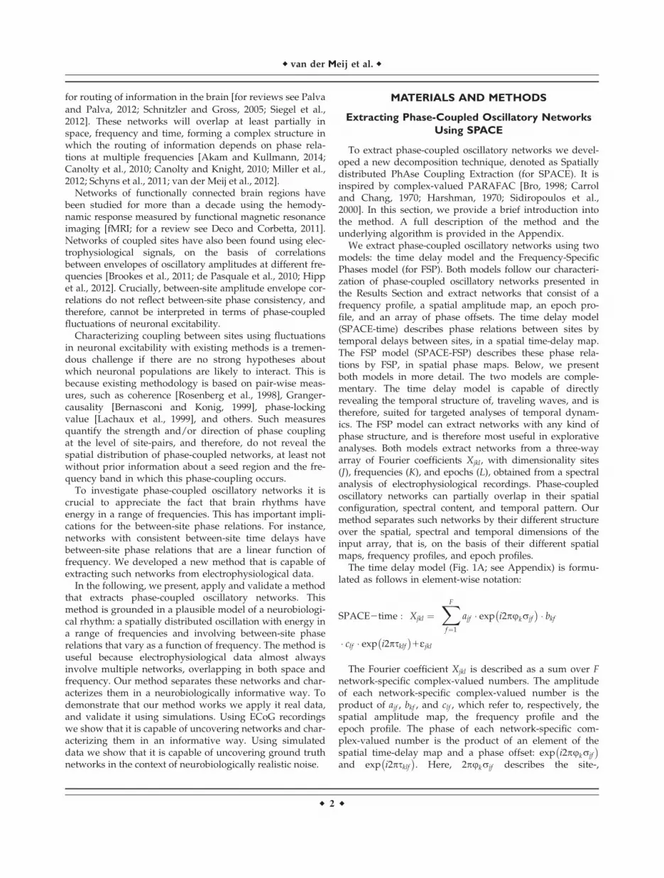
We extract phase-coupled oscillatory networks using twomodels: the time delay model and the Frequency-SpecificPhases model (for FSP). Both models follow our characteri-zation of phase-coupled oscillatory networks presented inthe Results Section and extract networks that consist of afrequency profile, a spatial amplitude map, an epoch pro-file, and an array of phase offsets. The time delay model(SPACE-time) describes phase relations between sites bytemporal delays between sites, in a spatial time-delay map.The FSP model (SPACE-FSP) describes these phase rela-tions by FSP, in spatial phase maps. Below, we presentboth models in more detail. The two models are comple-mentary. The time delay model is capable of directlyrevealing the temporal structure of, traveling waves, and istherefore, suited for targeted analyses of temporal dynam-ics. The FSP model can extract networks with any kind ofphase structure, and is therefore most useful in explorativeanalyses. Both models extract networks from a three-wayarray of Fourier coefficients Xjkl, with dimensionality sites(J), frequencies (K), and epochs (L), obtained from a spectralanalysis of electrophysiological recordings. Phase-coupledoscillatory networks can partially overlap in their spatialconfiguration, spectral content, and temporal pattern. Ourmethod separates such networks by their different structureover the spatial, spectral and temporal dimensions of theinput array, that is, on the basis of their different spatialmaps, frequency profiles, and epoch profiles.

The time delay model (Fig. 1A; see Appendix) is formu-lated as follows in element-wise notation:

SPACE2time : Xjkl ¼XF

f¼1

ajf � exp i2pukrjf

� �� bkf

� clf � exp i2psklf

� �1Ejkl

The Fourier coefficient Xjkl is described as a sum over Fnetwork-specific complex-valued numbers. The amplitudeof each network-specific complex-valued number is theproduct of ajf , bkf , and clf , which refer to, respectively, thespatial amplitude map, the frequency profile and theepoch profile. The phase of each network-specific com-plex-valued number is the product of an element of thespatial time-delay map and a phase offset: exp i2pukrjf

� �and exp i2psklf

� �. Here, 2pukrjf describes the site-,

r van der Meij et al. r

r 2 r

frequency-, and network-specific phases, in which uk denotesthe k-th frequency (in Hz) and rjf denotes the site- andfrequency-specific time delay. 2psklf describes the frequency-,epoch-, and network-specific phase offset. The time delaymodel is based on the assumption that between-site phasedifferences are the result of between-site time delays. Tomake this concrete, let r be the time delay between two sitesand let u be frequency. Then, the between-site phase differ-ence is u � r, which increases linearly with frequency. In theFSP model (Fig. 1B; see Appendix), the spatial phase mapsreplace the spatial time-delay maps. For this model, the phaseof each network-specific complex-valued number is the prod-uct of an element of the spatial phase maps and a phase off-set: exp i2pkjkf


� �. The FSP model is

formulated as follows in element-wise notation:

SPACE-FSP: Xjkl¼XF

f¼1

ajf �exp i2pkjkf

� ��bkf �clf �exp i2psklf

� �1Ejkl

Except for the site-, frequency- and network-specificphases kjkf , this model has the same parameters as thetime delay model. In contrast to the time delay model, noconstraints are imposed on the between-site phase differ-ences as a function of frequency. The parameters of bothmodels can be estimated using an alternating least squares(ALS) algorithm, which monotonically decreases a leastsquares (LS) loss function. For this algorithm, new optimi-zation techniques were developed which are fullydescribed in the Appendix.

To be estimable, all parameters of the two modelshave to be normalized (see Appendix). Because of thisnormalization, the individual amplitudes ajf , bkf , clf ,and the individual phases/time delays kjkf , rjf , arenot meaningful. Crucially, however, amplitude ratios,and time delay differences and phase differencesbetween sites, frequencies, and epochs, are notaffected by these normalizations, and reveal importantcharacteristics of the extracted phase-coupled oscilla-tory networks.

Figure 1.

SPACE: describing phase-coupled oscillatory networks by

FSP and time delays. We developed a new decomposition tech-

nique that extracts phase-coupled oscillatory networks, SPACE.

Networks are extracted using two models, the time delay model

and the FSP model. The time delay model (SPACE-time) describes

phase relations between sites by temporal delays between sites, in

a spatial time-delay map. The FSP model (SPACE-FSP) describes

these phase relations by FSP, in spatial phase maps. A: The time

delay model describes networks by a spatial amplitude map, a fre-

quency profile, a spatial time-delay maps, an epoch profile, and

phase offsets. The equation in A is the element-wise formulation

of the time delay model, and it shows how each Fourier coeffi-

cients Xjkl of site j, frequency k, and epoch l is described. The

example shows the same network as in Figure 3. The time-delay

maps describe all phase differences by site-specific time delays. In

the example, each site row has a time delay of 50 ms from top to

bottom. These 50 ms steps produce the same phases as shown in

B, and match the time delays in Figure 3A. B: The FSP model

describes networks by a spatial amplitude map, a frequency profile,

an epoch profile, phase offsets, and frequency-specific spatial phase

maps. The spatial phase maps describe all phase differences

between sites, matching those in Figure 3A. No constraint is

placed on phases over frequencies, in contrast to the time delay

model. For a detailed description see Materials and Methods and

Results Section: Characterizing Phase-Coupled Oscillatory Net-

works In Terms of Frequency Profiles, Spatial Maps, and Epoch

Profiles. [Color figure can be viewed in the online issue, which is

available at wileyonlinelibrary.com.]

r Uncovering Phase-Coupled Oscillatory Networks r

r 3 r

http://wileyonlinelibrary.com

In the three-way array of Fourier coefficients, everyepoch is described by a single Fourier coefficient per siteand frequency. However, it is often desired to control thefrequency resolution by means of multitaper estimation.When using multitaper estimation, every epoch has multi-ple tapers, and each of these tapers produces one Fouriercoefficient. These taper-specific Fourier coefficients areorganized in an additional dimension, turning the three-way array into a four-way array of Fourier coefficients.However, because frequencies and epochs can differ intheir number of tapers, this four-way array may be par-tially empty, and the three-way formulation of the modelscannot accommodate this aspect of the data array. Fortu-nately, we can make use of the cross-product formulationof our models to deal with this. This is the formulation ofthe models that is used in the remainder of the article, andit is fully described in the Appendix. Crucially, the cross-product formulation does not affect the spatial amplitudemaps, the frequency profiles, the epoch profiles, nor thespatial phase maps or spatial time-delay maps, asdescribed above and in the Results Section. The phase off-sets, however, are parameterized differently (see Appen-dix). An important difference with the models for thethree- and four-way arrays of Fourier coefficients is that inthe cross-product formulation of these models, between-network coherence is explicitly modeled. Although thiscan be of great benefit, it also has an undesirable conse-quence: if the between-network coherences are treated asestimable parameters, then a distributed phase-coupledoscillatory network can be described by an arbitrary num-ber of coherent subnetworks. To avoid this, we forcebetween-network coherence to be zero (see Appendix).

The number of networks F that are extracted needs tobe estimated. The number of networks that should beextracted cannot be determined analytically. To find theoptimal F, we can make use of an index of the reliabilitywith which the networks can be estimated from the data,as described by Maris et al. [2011].The number of net-works that are extracted can be increased incrementallyuntil this reliability index drops below a preset level. Aconservative approach is to split the data into two halves,extract networks from both halves, and stop increasing thenumber of networks when they start to differ betweenhalves. We use this approach for analyzing the ECoG data,and it is described in detail below. Other methods of esti-mating the optimal F are also possible [see Bro, 1998, forexamples from the perspective of PARAFAC/2].

Experimental Paradigm and Preprocessing of

ECoG Recordings

Three pharmacoresistant epilepsy patients (1 male, 2female) were implanted with subdural grid and strip elec-trodes prior to undergoing resective surgery. Informedconsent was obtained from the patients or their guardiansif they were underage. The research protocol was

approved by the appropriate institutional review boards atthe Children’s Hospital (Philadelphia, PA) and the Univer-sity Clinic (Freiburg, Germany). Some of the datasets havebeen analyzed before [see e.g., Jacobs and Kahana, 2009;Maris et al., 2011; Raghavachari et al., 2006; Rizzuto et al.,2003; van der Meij et al., 2012; van Vugt et al., 2010].Patients performed a Sternberg working memory task[Sternberg, 1966] while ECoG recordings were obtained.Patients were presented with a series of letters (with vari-able length from 1 to 6) on a computer screen, and theywere instructed to remember these. The trial started withthe presentation of a fixation cross, followed by a letter for700 ms and by 275–350 ms (uniformly distributed) of blankscreen. Every additional letter was presented for 700 msand followed by 275–350 ms of blank screen, except for thelast letter which was followed by a reten tion in terval of425–575 ms (uniformly distributed as well). After the reten-tion interval, a probe letter was presented. Patients wererequired to indicate by means of key press whether theprobe letter was part of the previously presented letterseries. We analyzed the period between the fixation crossand the onset of the probe letter, a period during which thepatients were actively engaged in the task. We did not dis-tinguish between the cognitive operations encoding andretrieval, which occur in this period. The main purpose ofthe current analyses was to demonstrate that plausiblephase-coupled oscillatory networks can be extracted.

ECoG recordings were sampled at 256 Hz and rerefer-enced to the common average. Artifact rejection was per-formed by visual inspection. All trials and/or electrodescontaminated by epileptiform activity were removed. Thedata was band-stop filtered with 1 Hz windows at 50 and60 Hz (depending on continent) and at other frequenciescontaining line noise. Recordings were additionally band-pass filtered between 0.01 and 100 Hz. All filters werefourth-order Butterworth. Subsequently, the mean and thelinear trend were removed from each trial. To suppressthe 1/fx pattern in the power spectrum, the data was pre-whitened by taking the first temporal derivative. Electrodelocations were determined by coregistering a postoperativecomputed tomography scan with a higher resolution pre-operative magnetic resonance image. Patients’ brains werenormalized to Talairach space [Talairach and Tornoux,1988]. All preprocessing and spectral analysis was per-formed using custom analyses scripts and the FieldTripopen-source MATLAB toolbox [Oostenveld et al., 2011].

Extracting Phase-Coupled Oscillatory Networks

from ECoG Recordings

Spectral analysis was performed for 2–30 Hz withequally spaced 0.5 Hz bins and a Welch multitaperingapproach [Welch, 1967] to control frequency resolution.First, each trial was cut into several 2 second segments,such that each next segment would have a temporal over-lap of 75% with the previous segment (incomplete


r 4 r

segments at the end of a trial were not used). Each of the2 second segments was multiplied with a Hanning win-dow, followed by a Discrete Fourier Transform (DFT).These multiple 2 second segments of each trial are the sep-arate Welch tapers. Each epoch used in the analyses corre-sponds to three consecutive trials and we combined theFourier coefficients obtained from these trials. Thisresulted in 30 epochs out of 92 trials for patient 1, 54epochs out of 163 trials for patient 2, and 89 epochs out of270 trials from patient 3. Combining tapers of multiple tri-als was necessary because our method requires that thesmallest number of tapers per epoch is larger than thenumber of networks extracted. Because we wanted to esti-mate the number of networks using a high frequency reso-lution, this sometimes lead to a larger number of networksthan tapers when defining each trial as an epoch.

The same preprocessing procedure was used for displayingsingle trials at the peak frequency of the example networks(see Results Section). The resulting time series were then con-volved with a complex-valued wavelet at the selected fre-quencies. This wavelet was constructed by an element-wisemultiplication of a three-cycle complex exponential and aHanning taper of equal length. The real part of the resultingcomplex-valued time series was then used for display.

Fourier coefficients resulting from spectral analysis werearranged to form a four-way array and decomposed usingthe cross-product formulation of both SPACE-time andSPACE-FSP (see Appendix). To avoid local minima, eachalgorithm was randomly initialized 20 times, and the solu-tion with the highest explained variance was selected(explained variance over initializations is shown in Sup-porting Information Fig. S1). To avoid degenerate decompo-sitions from unfortunate initializations, all decompositionswere run with an orthogonality constraint (Dk ¼ I; seeAppendix). The number of networks to extract (four, two,and four for patient 1, 2, and 3, respectively) was deter-mined on the basis of a split-half approach using the out-put of SPACE-time. In this procedure, the number ofnetworks was increased until the networks extracted fromthe odd numbered trials were no longer similar enough tothe networks extracted from the even numbered trials. Assuch, the number of networks that is extracted depends onthe networks that are consistently activated by the task.Similarity was evaluated on the basis of a number of split-half reliability coefficients. One coefficient was calculatedfor each of the parameter sets.

This split-half reliability coefficient was computed forthe spatial amplitude map and the frequency profiles asthe normalized network-specific inner-product. For thespatial time-delay maps, the split-half reliability coefficientwas constructed in two steps:

split2half coefficient:

PKk¼1

��<A1 �exp i2pukr1ð Þ; A2 �exp i2pukr

2ð Þ>A1 �A2

��B1k1B2

k

2

� �PK

k¼1B1

k1B2

k

2

h i(1)

First, per split-half s and frequency k, a complex-valuedspatial time-delay map exp i2pukr

sð Þ was computed andweighted with the split-half specific spatial amplitude mapAs. Then, the normalized inner-product h; i was takenbetween both halves. The final reliability coefficient for thespatial time-delay maps was then constructed by comput-ing the average over frequencies of the absolute value(denoted by jj) of this inner-product, weighted by theaverage of the frequency profiles Bs

k of both split-halves.For the spatial phase maps, the reliability coefficient wasconstructed by replacing ukr

s by ksk in the above equation.

When either this coefficient or that of the spatial ampli-tude map or the frequency profile fell below 0.7, the proce-dure was stopped, and the previous number of networkswas set as the final number of networks. As Dk ¼ I, it wasnot part of the split-half reliability coefficient.

We additionally computed a similarity coefficient thatwas used to compare networks extracted using the timedelay model to networks extracted using the FSP model.This coefficient was similar to the split-half coefficientdescribed above. For the spatial amplitude map, the fre-quency profiles, and the epoch profile the coefficient wascomputed as the normalized inner-product. For the spatialtime-delay map and the spatial phase maps the coefficientwas constructed as in Eq. (1), except that the spatial time-delay map of the second network exp i2pukr

2� �

wasreplaced by the spatial phase maps exp i2pk2

k

� �. The simi-

larity coefficient for the whole network was then obtainedas the average of the coefficients for spatial amplitudemap, the spatial phase map, the frequency profile, and theepoch profile.

Simulating Phase-Coupled Oscillatory Networks

To show that both our method is capable of extractingnetworks from noisy data we simulated three phase-coupled oscillatory networks travelling over a 5 3 5 sitesgrid. Each network had a spatial amplitude map that wasnonzero for a selected set of sites, with overlap betweenthe networks. There was one network in the theta range(4–8 Hz), one in the alpha range (8–12 Hz), and one in thebeta range (10–25 Hz). Every network was present in 15out of 25 epochs, with overlap between the epochs. Perepoch, we generated a signal that propagated over theinvolved sites with a fixed time delay, thus forming a trav-elling wave. The time delay step size (i.e., the time delaybetween two adjacent sites) was systematically varied overthe values 5, 25, 50, and 100 ms. We additionally variedthe signal-to-noise ratio (SNR) and the spatial noise corre-lation, as described below.

The signal was generated as follows. First, 1.5 (theta) or1 s (alpha and beta) of white noise was generated usingMATLAB’s pseudorandom number generator. Then, aftertaking the DFT, all Fourier coefficients not belonging tothe network’s frequency band were set to zero. Subse-quently, the signal was transformed back to the time


r 5 r

domain using the inverse DFT, and the resulting signalwas multiplied with a Hanning window of equal lengthand padded out to 3 s. This resulted in an oscillatory sig-nal within the specified frequency band. Then, again usinga DFT, the amplitudes of the Fourier coefficients werescaled such the amplitude spectrum was proportional to1/f, giving the power spectrum a 1/f2 shape [Miller et al.,2009]. The resulting signal was then transformed back tothe time domain using the inverse DFT. The site-specificsignals were obtained by shifting this time domain signalin accordance with the order of the site in travelling waveand the time delay step size. To every site, we added 3 sof noise. These noise signals were generated in the sameway as the source signals but without the removal of par-ticular frequencies, and independently for each site. Wevaried the amount of spatial noise correlation by generat-ing new site-specific noise signals as a weighted averageof the initial noise signals. These weights were propor-tional to a bivariate Gaussian of which the full-width halfmaximum [the width of the Gaussian at the point whereits magnitude is at the half of its maximum; full-widthhalf-maximum (FWHM)] was systematically varied overthe values 0, 10, 20, and 40 mm (simulated sites werespaced 10 mm apart). This results in a FWHM that encom-passed 0, 3, 5, and 9 sites, respectively. We also systemati-cally varied noise strength. This was achieved in a finalstep by setting the SNR of the time series at each site to be4, 0.16, 0.04, or 0.01.

Analyzing the Simulated Data

Except for artifact removal, the simulated data were pre-processed in the same way as the ECoG data. First, themean and the linear trend were removed from each epoch.Next, to suppress the 1/fx shape of the power spectrum,the data was prewhitened by taking the first temporalderivative.

Spectral analysis was performed for 2–30 Hz withequally spaced 1 Hz bins. First, each 3 second epoch wascut into several 1 second segments, such that each nextsegment would have a temporal overlap of 75% with theprevious segment. For 2–16 Hz, each of the 1 second seg-ments was multiplied with a Hanning window, followedby a DFT. For 17–30 Hz, each segment of each epoch wasmultiplied several times with different tapers prior to tak-ing the DFT. These tapers were the first 3 tapers of the Sle-pian sequence [Percival and Walden, 1993] of order 4,resulting in a frequency resolution of approximately 2 Hz.

The Fourier coefficients of all segments were then col-lected per epoch, and arranged in a four-way array. Thisarray consisted of 25 sites, 29 frequencies, 25 epochs, and57 tapers for every simulation run. Each four-way array ofFourier coefficients resulting from one simulation run wasdecomposed using the cross-product formulations of bothSPACE-time and SPACE-FSP. To avoid local minima, eachalgorithm was randomly initialized 10 times, of which the

solution with the highest explained variance was retained(explained variance over initializations is shown in Sup-porting Information Fig. S1). As for the analyses of theECoG data, all decompositions were run with an ortho-gonality constraint (Dk ¼ I; see above). All preprocessingand spectral analysis was performed using custom analy-ses scripts and the FieldTrip open-source MATLAB tool-box [Oostenveld et al., 2011].

Coefficients for Evaluating the Goodness-of-

Recovery of the Simulated Networks

We calculated a number of coefficients to assess thegoodness-of-recovery of the simulated networks. We usefour different coefficients: (1) one for the spatial amplitudemaps, frequency profiles and epoch profiles, (2) one forthe spatial phase maps, (3) one for the spatial time-delaymaps, and (4) one for the temporal order of the timedelays. The first coefficient is the Pearson correlation coef-ficient, which ranges from 21 to 1. The other three coeffi-cients were constructed for the purpose of this study, andwill be described in more detail in the following. Each ofthe four coefficients was computed per network and persimulation run and subsequently averaged.

The recovery coefficient for a network-specific spatialtime-delay map was calculated as follows:

recovery :

PKk¼1

�� hAsim�exp i2pukrð Þ; Asim�exp i2pukrsimð Þi

jAsimj2

�� Bsimk

� �PK

k¼1 Bsimk

First, the inner-product h; i is taken between the spatialtime-delay map of the extracted network and its simulatedcounterpart, weighted by the simulated spatial amplitudemap. The coefficient is then constructed as the sum overfrequencies of the absolute value of this inner-product,weighted by the simulated frequency profile. Here, Asim

denotes the simulated spatial amplitude map, ukr theloading vector containing the spatial time-delay map of anextracted network r multiplied by frequency uk in Hz, uk

rsim its simulated counterpart, and Bsimk the frequency-

specific loading of the simulated frequency profile of thesame network. This coefficient is sensitive to the similaritybetween the extracted spatial time-delay map and itssimulated counterpart, with a weighing that amplifies thecontribution of the sites and the frequencies that arestrongly involved in the simulated network. It is similar tothe coefficient described in the split-half procedure, exceptthat only the simulated spatial amplitude map and simu-lated frequency profile are used for weighting.

The recovery coefficient for the spatial phase maps isconstructed similarly as for the spatial time-delay maps,except ukr is replaced by kk, and ukr

sim by ksimk . Here, kk

denotes the frequency-specific spatial phase map, and ksimk

its simulated counterpart. This coefficient is sensitive tothe similarity between FSP generated by the extracted


r 6 r

phases and their simulated counterparts, again with aweighing that amplifies the contribution of the sites andthe frequencies that are strongly involved in the simulatednetwork.

The recovery coefficient for the temporal order of thespatial time-delay map is calculated as the proportion ofsite-pairs that are in agreement with respect to their esti-mated and simulated temporal order:

recovery :

PJsim21j1¼1

PJsim

j2¼j1xj1 2xj2

� �¼¼ xsim

j12xsim

j2

� �Jsim� Jsim21ð Þ

2

Here, xj denotes the position of the j-th site in theordered set of time delays from an extracted network, andxsim

j denotes its simulated counterpart. Only sites wereused that were part of the simulated network, as definedby the sites that have nonzero simulated values: Jsim refersto the total number of involved sites. The numerator ofthis coefficient is the sum of the site-pairs that have identi-cal ordinal distances between the estimated site-pairs(xj1 2xj2 ) and their simulated counterparts (xsim

j12xsim

j2).

This sum is then divided by the total number of possibleagreements, such that the coefficient expresses agreementas a proportion relative to perfect agreement.

RESULTS

Characterizing Phase-Coupled Oscillatory

Networks In Terms of Frequency Profiles,

Spatial Maps, and Epoch Profiles

Neuronal oscillations are ubiquitous in electrophysiolog-ical recordings, and their phase is very often consistent

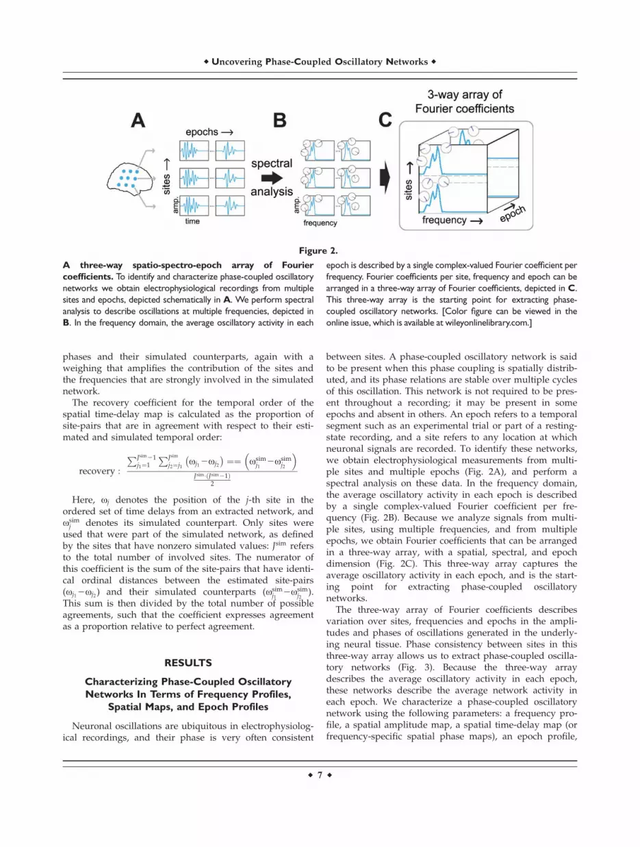
between sites. A phase-coupled oscillatory network is saidto be present when this phase coupling is spatially distrib-uted, and its phase relations are stable over multiple cyclesof this oscillation. This network is not required to be pres-ent throughout a recording; it may be present in someepochs and absent in others. An epoch refers to a temporalsegment such as an experimental trial or part of a resting-state recording, and a site refers to any location at whichneuronal signals are recorded. To identify these networks,we obtain electrophysiological measurements from multi-ple sites and multiple epochs (Fig. 2A), and perform aspectral analysis on these data. In the frequency domain,the average oscillatory activity in each epoch is describedby a single complex-valued Fourier coefficient per fre-quency (Fig. 2B). Because we analyze signals from multi-ple sites, using multiple frequencies, and from multipleepochs, we obtain Fourier coefficients that can be arrangedin a three-way array, with a spatial, spectral, and epochdimension (Fig. 2C). This three-way array captures theaverage oscillatory activity in each epoch, and is the start-ing point for extracting phase-coupled oscillatorynetworks.

The three-way array of Fourier coefficients describesvariation over sites, frequencies and epochs in the ampli-tudes and phases of oscillations generated in the underly-ing neural tissue. Phase consistency between sites in thisthree-way array allows us to extract phase-coupled oscilla-tory networks (Fig. 3). Because the three-way arraydescribes the average oscillatory activity in each epoch,these networks describe the average network activity ineach epoch. We characterize a phase-coupled oscillatorynetwork using the following parameters: a frequency pro-file, a spatial amplitude map, a spatial time-delay map (orfrequency-specific spatial phase maps), an epoch profile,

Figure 2.

A three-way spatio-spectro-epoch array of Fourier

coefficients. To identify and characterize phase-coupled oscillatory

networks we obtain electrophysiological recordings from multiple

sites and epochs, depicted schematically in A. We perform spectral

analysis to describe oscillations at multiple frequencies, depicted in

B. In the frequency domain, the average oscillatory activity in each

epoch is described by a single complex-valued Fourier coefficient per

frequency. Fourier coefficients per site, frequency and epoch can be

arranged in a three-way array of Fourier coefficients, depicted in C.

This three-way array is the starting point for extracting phase-

coupled oscillatory networks. [Color figure can be viewed in the

online issue, which is available at wileyonlinelibrary.com.]


r 7 r


and epoch-specific phase offsets per frequency (Fig. 3B–G).All these parameters will be described below in detail.Importantly, this characterization follows from theassumption that oscillatory networks can be conceived asspatially distributed neuronal sources measured at a

number of sites. The sources induce phase-consistent oscil-lations measurable at different sites, within the frequenciesthat characterize the network. The phases of thefrequency-specific Fourier coefficients can vary both oversites and epochs but, because we assume phase-

Figure 3.

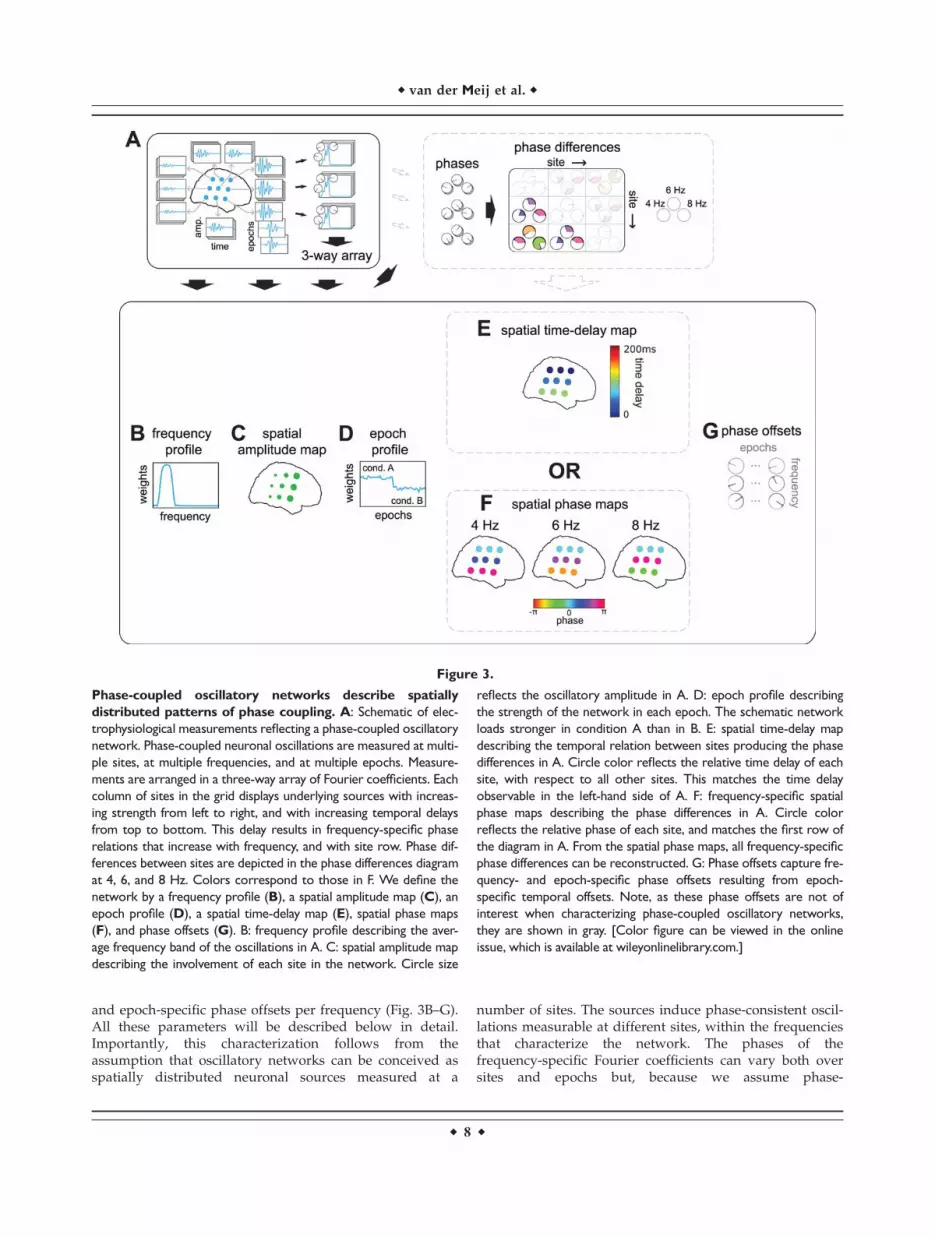
Phase-coupled oscillatory networks describe spatially

distributed patterns of phase coupling. A: Schematic of elec-

trophysiological measurements reflecting a phase-coupled oscillatory

network. Phase-coupled neuronal oscillations are measured at multi-

ple sites, at multiple frequencies, and at multiple epochs. Measure-

ments are arranged in a three-way array of Fourier coefficients. Each

column of sites in the grid displays underlying sources with increas-

ing strength from left to right, and with increasing temporal delays

from top to bottom. This delay results in frequency-specific phase

relations that increase with frequency, and with site row. Phase dif-

ferences between sites are depicted in the phase differences diagram

at 4, 6, and 8 Hz. Colors correspond to those in F. We define the

network by a frequency profile (B), a spatial amplitude map (C), an

epoch profile (D), a spatial time-delay map (E), spatial phase maps

(F), and phase offsets (G). B: frequency profile describing the aver-

age frequency band of the oscillations in A. C: spatial amplitude map

describing the involvement of each site in the network. Circle size

reflects the oscillatory amplitude in A. D: epoch profile describing

the strength of the network in each epoch. The schematic network

loads stronger in condition A than in B. E: spatial time-delay map

describing the temporal relation between sites producing the phase

differences in A. Circle color reflects the relative time delay of each

site, with respect to all other sites. This matches the time delay

observable in the left-hand side of A. F: frequency-specific spatial

phase maps describing the phase differences in A. Circle color

reflects the relative phase of each site, and matches the first row of

the diagram in A. From the spatial phase maps, all frequency-specific

phase differences can be reconstructed. G: Phase offsets capture fre-

quency- and epoch-specific phase offsets resulting from epoch-

specific temporal offsets. Note, as these phase offsets are not of

interest when characterizing phase-coupled oscillatory networks,

they are shown in gray. [Color figure can be viewed in the online

issue, which is available at wileyonlinelibrary.com.]


r 8 r


consistency, the between-site phase relations are identicalfor all epochs (Fig. 3A). Crucially, we characterize a net-work by multiple frequencies, which is in line with thegeneral observation that neuronal oscillations always haveenergy in a band of frequencies. These frequencies canform a narrow range, for example, 4–8 Hz (the thetaband), or a very broad range, for example, 30–60 Hz (thegamma band). Which frequencies are involved in a net-work is specified in the frequency profile.

A frequency profile (Fig. 3B) specifies the degree towhich different frequencies are involved in the network. Itis described by a vector of positive real numbers, whichare high for frequencies that are strongly involved, andclose to zero for those that are weakly involved. A spatialamplitude map (Fig. 3C) specifies the degree to which thedifferent sites reflect the network, and is also described bya vector of positive real numbers. An epoch profile (Fig.3D) specifies the degree to which the different epochsreflect the network, also described by a vector of positivereal numbers. The frequency profile, the spatial amplitudemap, and the epoch profile (Fig. 3B–D) together describethe degree to which the network is determined by each ofthe 3 dimensions of the three-way array of Fourier coeffi-cients. All phase characteristics of the network aredescribed by the spatial time-delay map (Fig. 3E; or spatialphase maps, Fig. 3F), and the phase offsets (Fig. 3G). Thelatter of these, the phase offsets (Fig. 3G), capture the tem-poral offset of the network within each epoch. These phaseoffsets are frequency-specific. The spatial time-delay map(Fig. 3E; or frequency-specific spatial phase maps, Fig. 3F)specifies the consistent between-site phase relations.Importantly, we present a model for coupled oscillatorynetworks in which any two interacting sites is character-ized by phase differences that may vary as a function offrequency (within the frequency band that characterizesthis network). The way these phase differences vary overfrequencies can provide important insights into how twosites interact. For instance, if there would be a consistenttime delay between two interacting sites, then this wouldresult in phase differences that increase linearly with fre-quency. These phase differences are jointly characterizedby the spatial time-delay map (Fig. 3E). A spatial time-delay map is the map from which the time delay betweenany pair of sites can be obtained by taking the differencebetween the corresponding coefficients in the map. Bymultiplying this time delay with the frequency of interest,we obtain the between-site phase difference for that fre-quency. The spatial phase maps (Fig. 3F) specify thebetween-site phase differences more directly, without theconstraint of a linear relation with frequency. These mapsare frequency-specific spatial maps from which the con-sistent between-site phase differences can be obtained bysimple subtraction between the sites. Because the spatialphase maps do not enforce a particular pattern on thebetween-site phase differences (e.g., a linear relation withfrequency), they are most useful in explorative studies.The spatial time-delay maps are more useful for a targeted

investigation of temporal dynamics. Importantly, althoughphase coupling at the level of site pairs can be recon-structed from both types of spatial maps, the maps them-selves describe phase coupling at the level of individualsites. This is useful, because it can directly reveal the spa-tial structure of the network.

Together, the frequency profile, the spatial amplitudemap, the epoch profile, the spatial time-delay maps or spa-tial phase maps, and the phase offsets, characterize aphase-coupled oscillatory network. That is, they describethat part of the three-way array of Fourier coefficients thatoriginates from a particular phase-coupled oscillatory net-work. To extract and characterize these networks, wedeveloped a new method, denoted as SPACE. This methodis briefly described in the Materials and Methods Section,and a full description of the method and the underlyingalgorithm is provided in the Appendix. The method isbased on two models: the time delay model (SPACE-time)that characterizes networks using spatial time-delay maps,and the FSP model (SPACE-FSP), that characterizes net-works using spatial phase maps. In the following, we firstdescribe example networks extracted from ECoG record-ings. Next, we provide evidence for the robustness of themethod, by recovering simulated networks from realisticnoisy data. In each section, both models are used and theirresults compared.

SPACE Extracts Phase-Coupled Oscillatory Net-

works from Human ECoG Recordings

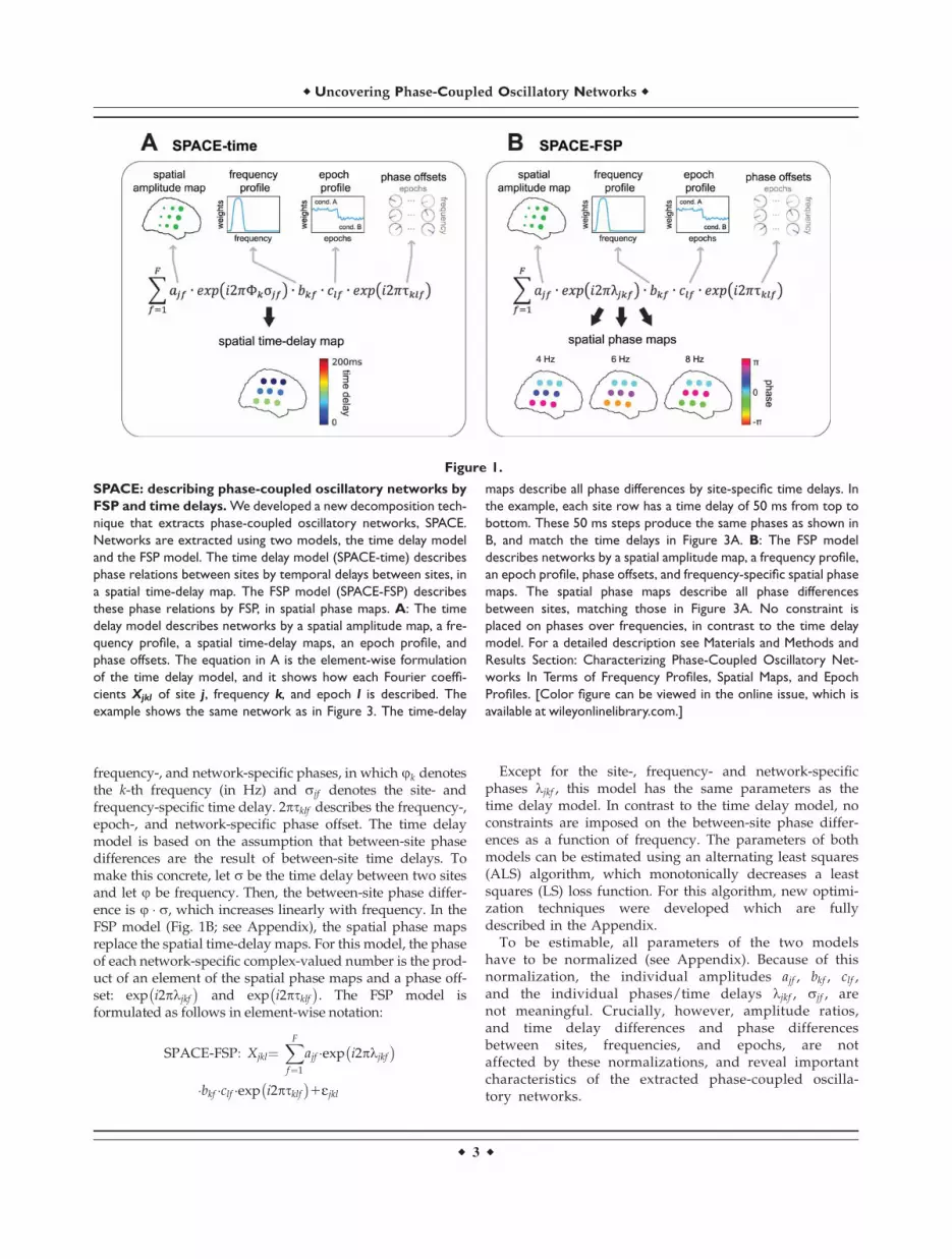
We now present three example networks extracted fromECoG recordings of three epilepsy patients while theywere performing a Sternberg working memory task (seeMaterials and Methods; Fig. 4). We analyzed the taskperiod during which the patients were engaged in thetask. We did not distinguish between the cognitive opera-tions encoding and retrieval occurring in this period, asthe main purpose of the current analyses was to demon-strate that plausible phase-coupled oscillatory networkscould be extracted.

Fourier coefficients of each of the three datasets wereobtained using a Welch tapering approach with multipleoverlapping 2 second windows per trial, yielding a four-way array of Fourier coefficients with a 0.5 Hz frequencyresolution and a taper dimension (in contrast to the three-way array introduced above, see Materials and Methods).Each of the three datasets was analyzed using bothSPACE-time and SPACE-FSP. Because the four-way arraysof Fourier coefficients were obtained using multitaper esti-mation, we used the cross-product formulation of bothmodels (see Materials and Methods and Appendix).Because we wanted to estimate the number of networksusing a high frequency resolution (0.5 Hz), each epochwas constructed by combining the tapers of three consecu-tive trials (see Materials and Methods). The number ofextracted networks was determined on the basis of their


r 9 r

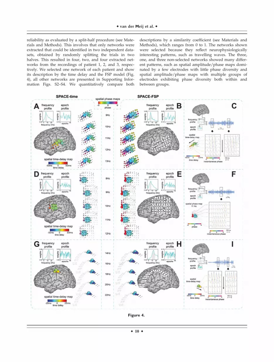
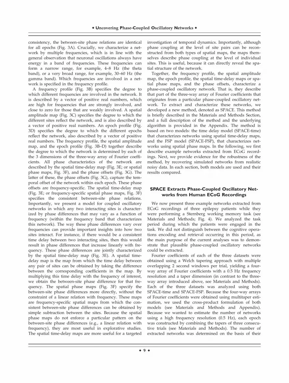
reliability as evaluated by a split-half procedure (see Mate-rials and Methods). This involves that only networks wereextracted that could be identified in two independent data-sets, obtained by randomly splitting the trials in twohalves. This resulted in four, two, and four extracted net-works from the recordings of patient 1, 2, and 3, respec-tively. We selected one network of each patient and showits description by the time delay and the FSP model (Fig.4), all other networks are presented in Supporting Infor-mation Figs. S2–S4. We quantitatively compare both

descriptions by a similarity coefficient (see Materials andMethods), which ranges from 0 to 1. The networks shownwere selected because they reflect neurophysiologicallyinteresting patterns, such as travelling waves. The three,one, and three non-selected networks showed many differ-ent patterns, such as spatial amplitude/phase maps domi-nated by a few electrodes with little phase diversity andspatial amplitude/phase maps with multiple groups ofelectrodes exhibiting phase diversity both within andbetween groups.

Figure 4.


r 10 r

From patient 1, we extracted a network that shows atravelling alpha wave over parieto-temporal electrodes(Fig. 4A–C). The network extracted using the time delaymodel (Fig. 4A) closely corresponds to the one extractedusing the FSP model (Fig. 4B): (1) the frequency profileand the epoch profile of the two networks are very similar(similarity coefficient 5 0.91) and (2) the progression ofphases over electrodes and over frequencies generatedfrom the time delay network follows the spatial phasemaps of the FSP network, with the time delay and the FSPnetwork both showing the alpha wave travelling in theposterior to anterior direction. The only clear difference isthat the spatial amplitude map of the FSP networkincludes more electrodes than the one of the time delaynetwork. We also show the travelling wave in the trialwith the highest amplitude at the peak frequency of thenetwork (�11 Hz). We do this for a selection of electrodesthat lie in the direction of the travelling wave (Fig. 4C).This example shows that, at the level of a single trial, thereis a close match between the time delays extracted usingthe time delay model (calculated over all trials) and thesesingle trial time delays. We additionally computed thespeed of the travelling wave using the network from thetime delay model. This was done by computing the distan-ces between all electrode-pairs (using Talairach coordi-nates), dividing these distances by the between-electrodetime delays, and subsequently averaging the resultingspeeds. (We calculated a weighted average with the

weights being the product of the spatial amplitude maploadings of all electrode-pairs.) This resulted in an averagespeed over electrode-pairs for this travelling alpha waveof 4.38 m/s. This is similar to speeds reported by Massi-mini et al. [2004] in extracranial human recordings, but ismuch faster than those reported by Rubino et al. [2006] inECoG recordings of monkey motor cortex. The direction ofthe wave is given by the temporal order of the timedelays, provided that none of the between-site time differ-ences exceeds 2 s (a critical time delay that depends onthe frequency resolution, which is 0.5 Hz for our analysis;see Appendix).

From patient 2, we extracted a dipolar alpha networkover fronto-parietal electrodes of which the spatial phasemaps are dominated by phase relations that are either 0or p (Fig. 4D–F). The network extracted using the timedelay model (Fig. 4D) closely corresponds to the oneextracted using the FSP model (Fig. 4E; similarity coef-ficient 5 0.96), except for the spatial time-delay maps. Thephase differences that are implied by the spatial time-delay maps are much smaller than the phase relationsthat were estimated under the FSP model. We also showphase relations in the trial with the highest amplitude atthe peak frequency of the network (�11 Hz) for a selec-tion of electrodes from the two clusters (Fig. 4F). The sin-gle trial phase differences between the two clusters ofelectrodes closely match the dipolar phase relations esti-mated under the FSP model.

Figure 4.

Example phase-coupled oscillatory networks from

human ECoG recordings. We show three-phase-coupled

oscillatory networks from ECoG recordings during a Sternberg

working memory task from three epilepsy patients (see Materials

and Methods). Networks are displayed on a Talairach template

brain. The first network shows a travelling alpha wave over

parieto-temporal electrodes (A,B,C). The second network

shows an alpha network with phase relations dominated by 0 or

p over fronto-parietal electrodes (D,E,F). The third network

shows a travelling beta wave over parieto-frontal electrodes

(G,H,I). Each dataset was analyzed using the cross-product for-

mulation of SPACE-time (A,D,G) and SPACE-FSP (B,E,F) and the

extracted networks were compared (see Materials and Meth-

ods). The Fourier coefficients were obtained from Welch-

tapered signals of 2 s, and therefore had a frequency resolution

of 0.5 Hz. We also show single trial observations of the networks

(C,F,I). Only those grids/strips with high amplitudes in the spatial

amplitude map are shown. A: Travelling alpha wave described by

the time delay model. Frequency and epoch profiles are shown in

the top left. The full grid is shown in the center on a Talairach

template. The spatial time-delay map is shown on the right side.

Electrode size reflects the spatial amplitude map. Electrode color

reflects the time delay relative to the strongest electrode. The

displayed frequencies are selected from the gray band in the

frequency profile. Spatial phase maps are shown on the left to

compare phases resulting from the time delay model to those of

the FSP model. These maps were generated by multiplying each

time delay by 2puk, where uk reflects the k-th frequency. B: Trav-

elling alpha wave corresponding to the one in A described by the

FSP model. Frequency and epoch profiles are shown on the top

left. The spatial phase maps are displayed in the center. Electrode

size reflects the spatial amplitude map. Electrode color reflects

the phase relative to the strongest electrode in A. C: Single trial

oscillations displaying the travelling alpha wave at the peak fre-

quency (�11 Hz) in the strongest trial. The top panel displays the

selected trial, frequency, and electrodes. The bottom panel

shows excerpts from this trial. Instantaneous amplitude is col-

ored by instantaneous phase. The gray solid line reflects the time

delay between electrodes. Oscillations matching the time delays

cross this gray line at their peaks. Black arrows denote the direc-

tion of the travelling wave. D,E: same as A,B but for a dipolar

alpha network with 0 or p phase relations. F: same as in C but for

the dipolar alpha network shown in D and E (�11 Hz), using the

estimates for the FSP model. The dashed gray line is now straight.

Oscillations matching the spatial phase maps cross this line at

their troughs for the top three electrodes and at their peaks for

the bottom three electrodes. G,H: same as A,B but now for a

travelling beta wave. I: same as C but now for the travelling beta

wave (�19 Hz) shown in G and H. [Color figure can be viewed in

the online issue, which is available at wileyonlinelibrary.com.]


r 11 r


From patient 3, we extracted a network that shows atravelling beta wave over fronto-parietal electrodes (Fig.4G–I). For all parameters, the network extracted using thetime delay model (Fig. 4G) closely corresponds to the oneextracted using the FSP model (Fig. 4H; similarity coef-ficient 5 0.99). Importantly, the progression of phases overelectrodes and over frequencies generated from the timedelay network follows the spatial phase maps of the FSPnetwork, with the time delay and the FSP network bothshowing the beta wave travelling in the anterior to poste-rior direction. We also show the phase relations in the trialwith the highest amplitude at the peak frequency (�19Hz) for a selection of electrodes that lie in the direction ofthe travelling wave (Fig. 4I). The average speed overelectrode-pairs of this travelling beta wave was 5.19 m/s.

SPACE Recovers Phase-Coupled Oscillatory Net-

works from Realistic Noisy Signals

We performed simulations to test the ability of ourmethod to recover phase-coupled networks from noisy sig-nals. To accurately recover simulated networks, ourmethod needs to fulfill two important requirements: (1) itssolutions need to be unique and (2) it needs to be robustagainst biologically realistic noise. Although we cannotprovide a theoretical proof of uniqueness, in the Appen-dix, we show the results of a simulation study thatstrongly suggest uniqueness. To investigate the secondrequirement, we conducted simulations using realisticnoisy signals. These signals were obtained by adding spa-tially correlated noise to time-domain signals that weregenerated under the time delay model. This spatially cor-related noise reflects scattered neuronal sources without aconsistent oscillatory phase coupling structure in some fre-quency range. These scattered sources distort the structurethat is induced by the simulated networks because theycannot be fitted parsimoniously by our models. By increas-ing noise strength and spatial correlation, we create anenvironment where it becomes increasingly difficult to dis-tinguish the networks of interest from the backgroundactivity. The importance of spatial correlation of the noisebecame very obvious when we performed pilot simulationstudies with uncorrelated noise. We observed that it wastrivially easy to accurately and uniquely recover networksin this situation. For instance, we simulated data in the fre-quency domain by directly generating the three-way (andfour-way) array of Fourier coefficients using the parame-ters of both models. Adding large amounts of uncorrelatedcomplex-valued noise had a very weak effect on the recov-ery of the networks. To test our method under more chal-lenging and more realistic conditions, we generated datain which we controlled both the amount and the spatialcorrelation of the noise.

We simulated phase-coupled oscillatory networks withvarying noise strength, spatial noise correlation, and timedelays across a 5 3 5 sites grid (Figs. 5–7; for a detailed

description see Materials and Methods). Using these simu-lations, we investigated (1) how network recovery variesas a function of noise strength and correlation and (2) howrecovery varies as a function of the time delays. To thisend we performed two sets of simulations: (1) fixedbetween-site time delays but varying noise strength andspatial noise correlation and (2) varying time delays, vary-ing noise strength but fixed spatial noise correlation. TheSNR was varied over 4 levels: 4, 0.16, 0.04, and 0.01. Spa-tial noise correlation was determined by the FWHM of abivariate Gaussian distribution at 0, 10, 20, or 40 mm.These distances are evaluated relative to the inter-site dis-tances of our 5 3 5 grid, which had a 10mm spacing.Finally, between-site time delays were varied over the fol-lowing 4 levels: 5, 25, 50, and 100 ms. In the following, wefirst briefly describe how we simulated phase-coupledoscillatory networks, and how we assessed the similaritybetween the extracted and simulated networks. Next, wepresent the results of the two parts of our simulationstudy.

We simulated three-phase coupled oscillatory networkstravelling on a 5 3 5 sites grid, which were partiallyrepeated over 25 epochs (Fig. 5). The three networks haddifferent but partially overlapping frequency profiles: onein the theta, one in the alpha, and one in the beta band(Fig. 5B). Each network was further characterized by aspatial amplitude map specifying which sites showed theoscillatory signal and a spatial time-delay map specifyingthe time and phase relations between these sites (Fig. 5A).Spatial amplitude maps were partially overlapping. Pernetwork and epoch, a 1–1.5 s source signal was randomlygenerated as band-pass filtered brown-noise (see Materialsand Methods), which was subsequently mapped to thesensor level (the 5 3 5 sites grid) according to the spatialamplitude and the spatial time-delay map for that net-work. Per network, the frequency profile to-be-recoveredwas set as the average amplitude spectrum (over allepochs; Fig. 5B). Epochs varied with respect to whether ornot a particular network was involved, and this was speci-fied by the network’s epoch profile (Fig. 5B). Each networkwas present in 15 out of 25 epochs. Noisy 3 second signalswere created by adding randomly generated brown noiseto the model signals that were generated as phase-coupledoscillatory networks (after zero padding the 1–1.5 s modelsignals to 3 s). In Figure 5C, we show a set of exampleepochs with varying noise strength. For each of the simu-lation parameter combinations (4 SNR levels, four noisecorrelation levels and four time delays), we generated 100data sets; each of these simulations will be denoted as arun. Per run, Fourier coefficients were obtained using aWelch tapering approach with multiple overlapping 1 sec-ond windows per epoch. This yielded a four-way array ofFourier coefficients with a taper dimension and a 1 Hz fre-quency resolution for frequencies below 17 Hz and, usingadditional tapering, 2 Hz for frequencies of 17 Hz andabove (see Materials and Methods). These four-way arrayswere subsequently analyzed using both SPACE-time and


r 12 r

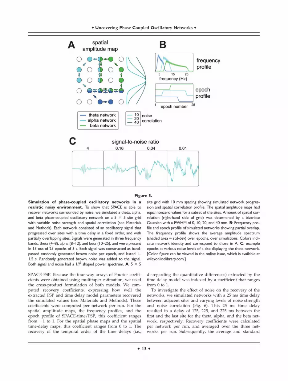
SPACE-FSP. Because the four-way arrays of Fourier coeffi-cients were obtained using multitaper estimation, we usedthe cross-product formulation of both models. We com-puted recovery coefficients, expressing how well theextracted FSP and time delay model parameters recoveredthe simulated values (see Materials and Methods). Thesecoefficients were computed per network per run. For thespatial amplitude maps, the frequency profiles, and theepoch profile of SPACE-time/FSP, this coefficient rangesfrom 21 to 1. For the spatial phase maps and the spatialtime-delay maps, this coefficient ranges from 0 to 1. Therecovery of the temporal order of the time delays (i.e.,

disregarding the quantitative differences) extracted by thetime delay model was indexed by a coefficient that rangesfrom 0 to 1.

To investigate the effect of noise on the recovery of thenetworks, we simulated networks with a 25 ms time delaybetween adjacent sites and varying levels of noise strengthand noise correlation (Fig. 6). This 25 ms time delayresulted in a delay of 125, 225, and 225 ms between thefirst and the last site for the theta, alpha, and the beta net-work, respectively. Recovery coefficients were calculatedper network per run, and averaged over the three net-works per run. Subsequently, the average and standard

Figure 5.

Simulation of phase-coupled oscillatory networks in a

realistic noisy environment. To show that SPACE is able to

recover networks surrounded by noise, we simulated a theta, alpha,

and beta phase-coupled oscillatory network on a 5 3 5 site grid

with variable noise strength and spatial correlation (see Materials

and Methods). Each network consisted of an oscillatory signal that

progressed over sites with a time delay in a fixed order, and with

partially overlapping sites. Signals were generated in three frequency

bands, theta (4–8), alpha (8–12), and beta (10–25), and were present

in 15 out of 25 epochs of 3 s. Each signal was constructed as band-

passed randomly generated brown noise per epoch, and lasted 1–

1.5 s. Randomly generated brown noise was added to the signal.

Both signal and noise had a 1/f2 shaped power spectrum. A: 5 3 5

site grid with 10 mm spacing showing simulated network progres-

sion and spatial correlation profile. The spatial amplitude maps had

equal nonzero values for a subset of the sites. Amount of spatial cor-

relation (right-hand side of grid) was determined by a bivariate

Gaussian with a FWHM of 0, 10, 20, and 40 mm. B: Frequency pro-

file and epoch profile of simulated networks showing partial overlap.

The frequency profile shows the average amplitude spectrum

(shaded area 5 std-dev) over epochs, over simulations. Colors indi-

cate network identity and correspond to those in A. C: example

epochs at various noise levels of a site displaying the theta network.

[Color figure can be viewed in the online issue, which is available at

wileyonlinelibrary.com.]


r 13 r


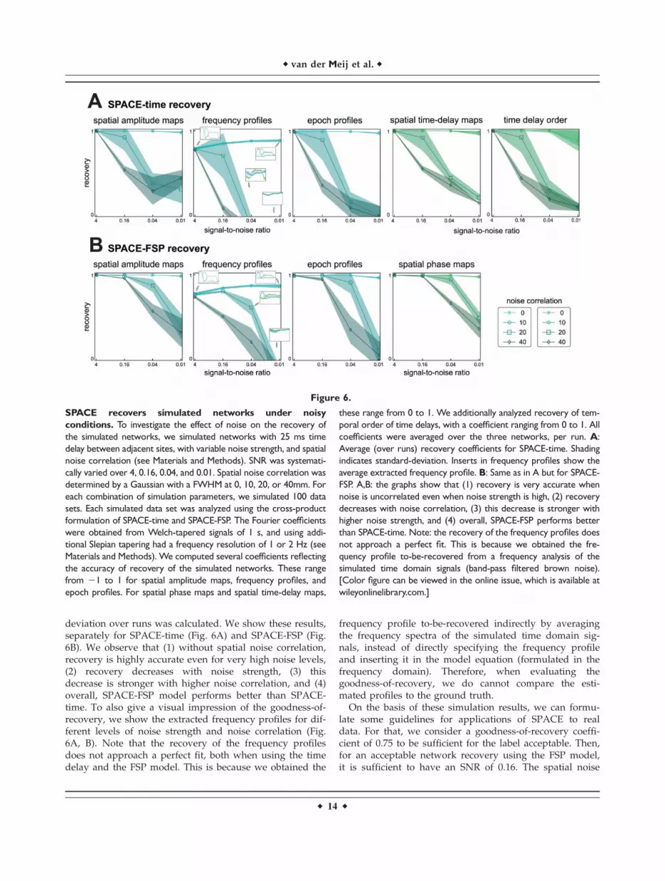
deviation over runs was calculated. We show these results,separately for SPACE-time (Fig. 6A) and SPACE-FSP (Fig.6B). We observe that (1) without spatial noise correlation,recovery is highly accurate even for very high noise levels,(2) recovery decreases with noise strength, (3) thisdecrease is stronger with higher noise correlation, and (4)overall, SPACE-FSP model performs better than SPACE-time. To also give a visual impression of the goodness-of-recovery, we show the extracted frequency profiles for dif-ferent levels of noise strength and noise correlation (Fig.6A, B). Note that the recovery of the frequency profilesdoes not approach a perfect fit, both when using the timedelay and the FSP model. This is because we obtained the

frequency profile to-be-recovered indirectly by averagingthe frequency spectra of the simulated time domain sig-nals, instead of directly specifying the frequency profileand inserting it in the model equation (formulated in thefrequency domain). Therefore, when evaluating thegoodness-of-recovery, we do cannot compare the esti-mated profiles to the ground truth.

On the basis of these simulation results, we can formu-late some guidelines for applications of SPACE to realdata. For that, we consider a goodness-of-recovery coeffi-cient of 0.75 to be sufficient for the label acceptable. Then,for an acceptable network recovery using the FSP model,it is sufficient to have an SNR of 0.16. The spatial noise

Figure 6.

SPACE recovers simulated networks under noisy

conditions. To investigate the effect of noise on the recovery of

the simulated networks, we simulated networks with 25 ms time

delay between adjacent sites, with variable noise strength, and spatial

noise correlation (see Materials and Methods). SNR was systemati-

cally varied over 4, 0.16, 0.04, and 0.01. Spatial noise correlation was

determined by a Gaussian with a FWHM at 0, 10, 20, or 40mm. For

each combination of simulation parameters, we simulated 100 data

sets. Each simulated data set was analyzed using the cross-product

formulation of SPACE-time and SPACE-FSP. The Fourier coefficients

were obtained from Welch-tapered signals of 1 s, and using addi-

tional Slepian tapering had a frequency resolution of 1 or 2 Hz (see

Materials and Methods). We computed several coefficients reflecting

the accuracy of recovery of the simulated networks. These range

from 21 to 1 for spatial amplitude maps, frequency profiles, and

epoch profiles. For spatial phase maps and spatial time-delay maps,

these range from 0 to 1. We additionally analyzed recovery of tem-

poral order of time delays, with a coefficient ranging from 0 to 1. All

coefficients were averaged over the three networks, per run. A:

Average (over runs) recovery coefficients for SPACE-time. Shading

indicates standard-deviation. Inserts in frequency profiles show the

average extracted frequency profile. B: Same as in A but for SPACE-

FSP. A,B: the graphs show that (1) recovery is very accurate when

noise is uncorrelated even when noise strength is high, (2) recovery

decreases with noise correlation, (3) this decrease is stronger with

higher noise strength, and (4) overall, SPACE-FSP performs better

than SPACE-time. Note: the recovery of the frequency profiles does

not approach a perfect fit. This is because we obtained the fre-

quency profile to-be-recovered from a frequency analysis of the

simulated time domain signals (band-pass filtered brown noise).

[Color figure can be viewed in the online issue, which is available at

wileyonlinelibrary.com.]


r 14 r


correlation can then correspond to a noise FWHM cover-ing 9 recording sites (i.e., 40 mm FWHM in the above). Ifthe SNR is only 0.04, an acceptable network recoveryrequires that the noise FWHM covers at most 5 recordingsites (a 20 mm FWHM in the above). For an acceptablenetwork recovery using the time delay model, the spatialnoise correlation has to be less: with an SNR of 0.16 or0.04, the noise FWHM must cover at most 5 or 3 recordingsites, respectively.

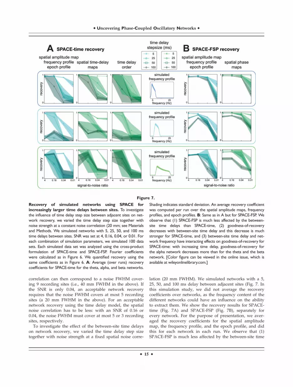
To investigate the effect of the between-site time delayson network recovery, we varied the time delay step sizetogether with noise strength at a fixed spatial noise corre-

lation (20 mm FWHM). We simulated networks with a 5,25, 50, and 100 ms delay between adjacent sites (Fig. 7. Inthis simulation study, we did not average the recoverycoefficients over networks, as the frequency content of thedifferent networks could have an influence on the abilityto extract them. We show the recovery results for SPACE-time (Fig. 7A) and SPACE-FSP (Fig. 7B), separately forevery network. For the purpose of presentation, we aver-aged the recovery coefficients for the spatial amplitudemap, the frequency profile, and the epoch profile, and didthis for each network in each run. We observe that (1)SPACE-FSP is much less affected by the between-site time

Figure 7.

Recovery of simulated networks using SPACE for

increasingly larger time delays between sites. To investigate

the influence of time delay step size between adjacent sites on net-

work recovery, we varied the time delay step size together with

noise strength at a constant noise correlation (20 mm; see Materials

and Methods. We simulated networks with 5, 25, 50, and 100 ms

time delays between sites. SNR was set at 4, 0.16, 0.04, or 0.01. For

each combination of simulation parameters, we simulated 100 data

sets. Each simulated data set was analyzed using the cross-product

formulation of SPACE-time and SPACE-FSP. Fourier coefficients

were calculated as in Figure 6. We quantified recovery using the

same coefficients as in Figure 6. A: Average (over runs) recovery

coefficients for SPACE-time for the theta, alpha, and beta networks.

Shading indicates standard deviation. An average recovery coefficient

was computed per run over the spatial amplitude maps, frequency

profiles, and epoch profiles. B: Same as in A but for SPACE-FSP. We

observe that (1) SPACE-FSP is much less affected by the between-

site time delays than SPACE-time, (2) goodness-of-recovery

decreases with between-site time delay and this decrease is much

stronger for SPACE-time, and (3) between-site time delay and net-

work frequency have interacting effects on goodness-of-recovery for

SPACE-time: with increasing time delay, goodness-of-recovery for

the alpha network decreases more than for the theta and the beta

network. [Color figure can be viewed in the online issue, which is

available at wileyonlinelibrary.com.]


r 15 r


delays than SPACE-time, (2) goodness-of-recoverydecreases with between-site time delay and this decreaseis much stronger when using the time delay model, and(3) between-site time delay and network frequency haveinteracting effects on goodness-of-recovery when using thetime delay model: with increasing time delays, goodness-of-recovery for the alpha network decreases more than forthe theta and the beta network. We therefore concludethat, when expected time delays are large, using the FSPmodel is preferred over the time delay model.

In sum, we have shown that SPACE can recover net-works from signals that contain spatially correlated noise.For the FSP model, an SNR of 0.16 suffices to produce anacceptable recovery even when the spatial noise correla-tion encompasses 9 recording sites. If the SNR is only 0.04,an acceptable network recovery requires that the spatialnoise correlation encompasses at most five recording sites.For an acceptable network recovery using the time delaymodel, the spatial noise correlation has to be substantiallyless. Additionally, when the expected time delays of aphase-coupled oscillatory network are large relative tocycle length of the network oscillation, then SPACE-FSPcan more accurately recover the between-site phase rela-tions generated from the time delays.

DISCUSSION

We developed a method capable of extracting phase-coupled oscillatory networks. Our contribution involvesfour-key elements. First, we provide a precise definition ofa phase-coupled oscillatory network in terms of six param-eters: a frequency profile, a spatial amplitude map, spatialphase maps or a spatial time-delay map, an epoch profile,and phase offsets (or an equivalent parameter in case ofthe cross-product formulation). Crucially, this definitionrespects the fact that brain rhythms involve a range of fre-quencies, and cannot be characterized by line spectra. Sec-ond, we developed a method that extracts these networksfrom electrophysiological data. Third, we demonstrate thatthis method is able to extract networks with a revealingphase structure from ECoG data. And fourth, using a sim-ulation study, we quantify the robustness of this methodagainst violations of the phase-coupling structure imposedby the model. This demonstrates the method’s usefulnessin practical applications.

Neuronal networks realize the many processes thatunderlie cognitive functions: selecting and routing infor-mation, keeping the information in working memory, stor-ing and retrieving information from a more permanentstore, and so forth. All these processes involve interactionsbetween anatomically distinct but connected brain regions.This is the prime motivation for the development of meth-ods that extract these networks from neurobiological data.

Compared to electrophysiology, the fMRI communityhas a long tradition in identifying functional networks.Networks of coactivated brain regions can be found using

the spontaneous covariation of the blood oxygenation leveldependent signal measured at rest, that is, in absence ofstimulation or a task [Biswal et al., 1997; Deco and Cor-betta, 2011; Fox et al., 2005; Honey et al., 2009; Raichleet al., 2001; Smith et al., 2009]. These networks are usuallyreferred to as resting state networks [RSNs; Beckmannet al., 2005]. An important observation constraining thepossible functional role of these fMRI-derived RSNs is thatthey also exist in the absence of consciousness duringanesthesia and sleep [Vincent et al., 2007].

Recently, RSNs have begun to be investigated using mag-netoencephalography (MEG) recordings [Brookes et al.,2011; de Pasquale et al., 2010]. This is important progress,because MEG directly measures electrophysiological brainactivity, bypassing the indirect hemodynamic response.Crucially, the RSNs that were identified did not depend onoscillatory phase coupling. As a part of the analyses, MEGrecordings were transformed into time series of band-limited power (BLP) in several frequency bands. These BLPtime series were then correlated using a seed-basedapproach [de Pasquale et al., 2010] or decomposed usingindependent component analysis [Brookes et al., 2011].With this approach, it was shown that RSNs could beextracted using BLP time series (especially in the beta band;15–25 Hz) that were highly similar to those found in fMRIsignals [Brookes et al., 2011; de Pasquale et al., 2010].

Another recent method to identify networks is based onphase-amplitude coupling [Maris et al., 2011; van der Meijet al., 2012]. Contrary to a correlation between BLP timeseries, phase-amplitude coupling does depend on oscilla-tory phase coupling: it indexes the preference for ampli-tude envelopes at a certain frequency (equivalent to a BLPtime series) to have high values at a certain phase of aslower phase-providing oscillation. Most reports focus onthe coupling between amplitude-providing and phase-providing oscillations obtained from the same site [Brunsand Eckhorn, 2004; Canolty et al., 2006; Chrobak and Buz-saki, 1998; Cohen et al., 2009; Mormann et al., 2005; Schacket al., 2002]. However, focusing on between-site phase-amplitude coupling inspired the development of methodswith which networks could be identified [Maris et al.,2011; van der Meij et al., 2012]. With these methods,revealing differences between amplitude-providing andphase-providing networks could be identified.

The method presented in this article allows for an iden-tification of networks using phase coupling between oscil-lations alone. Crucially, this method respects the fact thatbrain rhythms have energy in a range of frequencies, andtherefore allows between-site phase differences to varyover frequencies. As we have illustrated in the Results Sec-tion, this property allows us to distinguish different net-work configurations. One such example is a travellingwave (e.g., the networks in Fig. 4A, G, and the simulatednetworks in Figs. 527). This wave could be generated by adistributed oscillatory source in which the many subpopu-lations interact with a temporal delay. The signals gener-ated by such a distributed source can be described by our


r 16 r

time delay model. A second example, which can bedescribed by our FSP model, involves a source that issmall relative to its distance from the sensors, as is oftenthe case in macroscopic measurements like MEG and elec-troencephalography (EEG), but is also present in morelocal measurements such as ECoG (see Results Section).Such a distant source generates a dipolar potential distri-bution (two groups of sites whose potentials have oppositesigns) over sites that are at the same distance from thissource (e.g., the network in Fig. 4E, network 2 in Fig. S2B,and network 1 Fig. S3B). The phase differences betweenthese sites are either 0 (synchrony) or p (antiphase) and,importantly, do not vary as a function of frequency. Thisexample shows that the spatial phase maps can depend onthe recording technique. The dependence of the spatialdistribution of the measurements on the recording tech-nique has been put forward by other authors, startingfrom the spatial filtering characteristics of the measure-ment technique [Nunez et al., 2001]. A third example is anetwork driven by thalamocortical interactions [Suffczyn-ski et al., 2001], which has elements of the above twoexamples. A possible scenario involves multiple corticalpopulations that are driven by a common thalamic pace-maker. The timing of the input to these cortical popula-tions will differ as a function of the delay in the axonalconnection with this thalamic pacemaker. As a result, thephase relations between these cortical populations will belarger than the phase relations within them (which are 0in the idealized scenario of no within-population differen-ces in axonal delay). The essential difference with thisexample configuration and the previous dipolar configura-tion is that between-site phase differences are not only 0or p, but can take any value in between (as determined bythe difference in thalamocortical delay). Such a networkcan be described by both of our models.

Between-site phase relations in electrophysiologicalrecordings may be of crucial importance for the under-standing of neuronal communication. Electrophysiologicalrecordings of neural activity (local field potentials (LFPs),ECoG, EEG, MEG) reflect synchronized membrane poten-tial fluctuations. Importantly, membrane potential fluctua-tions reflect fluctuations in neuronal excitability. Thisimplies that oscillations may reflect rhythmic fluctuationsin neuronal excitability. It has therefore been proposedthat effective communication between two neuronal popu-lations depends on whether or not the spike input fromthe sending population arrives at an excitable phase of thereceiving population [Borgers and Kopell, 2008; Fries,2005; Tiesinga et al., 2008]. This idea can easily be general-ized to motifs that involve more than two neuronal popu-lations, of which some pairs can effectively communicateand others cannot, depending on their phase relations[Fries, 2005]. Thus, neuronal populations forming net-works by phase-coupled oscillations could be a key mech-anism for interareal communication and selective routingof information through the brain. In line with this hypoth-esis, it has been shown that local field potentials at one

site coordinate spikes in task-relevant neurons at a remotesite [Canolty et al., 2010, 2012b].

From a methodological point of view, it is important todistinguish our multivariate approach from the more com-mon bivariate approach, in which oscillatory phase cou-pling is evaluated by pair-wise measures such ascoherence [Mormann et al., 2000], imaginary coherence[Nolte et al., 2004], phase-locking value [Lachaux et al.,1999], pair-wise phase consistency [Vinck et al., 2010], thephase-slope index [Nolte et al., 2008], and Granger causal-ity [Bernasconi and Konig, 1999; Kaminski et al., 2001].Some methods can make use of a full multivariate descrip-tion of the data, but nevertheless only provide a quantifi-cation at the level of site-pairs, using the multivariatedescription to partial out for the contribution of other sites.This holds for phase coupling estimation [Canolty et al.,2012a], partial coherence [Rosenberg et al., 1998], Grangercausality [Bernasconi and Konig, 1999; Kaminski et al.,2001], Transfer Entropy [Schreiber, 2000], and Phase Trans-fer Entropy [Lobier et al., 2014]. This quantification at thelevel of site-pairs is unfortunate, as pair-wise measures donot directly reveal the spatial distribution of phase-coupled networks, unless there is prior information abouta seed region via which the other nodes of the networkcan be identified.

A method that shares several aspects with the methodpresented in this article is shifted CP [SCP; Morup, et al.,2008]. This method builds on earlier work in which PAR-AFAC [Carrol and Chang, 1970; Harshman, 1970] wasused to decompose spatio-spectro-temporal electrophysio-logical data [Miwakeichi et al., 2004; Morup et al., 2006].Importantly, in these earlier studies, PARAFAC was onlyapplied to the amplitudes of the Fourier coefficients; thephase information was ignored. The novel method, SCP,decomposes the complex-valued raw Fourier coefficientsover sites, frequencies and epochs into multiple compo-nents. Each SCP component is described by a real-valuedspatial map, a complex-valued frequency profile, and areal-valued epoch profile. Importantly, each component isadditionally described by a set of epoch-specific time-shifts, which allows the method to model between-epochdifferences in the temporal onset of a network. However,as between-site phase relations are not explicitly modeled,only networks with between-site phase differences of 0and 6p are extracted (by allowing for negative values inthe spatial maps). Though this makes SCP suitable forextracting dipolar potential distributions, other types ofphase-coupled oscillatory networks cannot be accuratelydescribed.

What holds for the comparison with shifted CP, alsoholds for the comparison with other decompositions, suchas independent component analysis (ICA) [Bell and Sej-nowski, 1995] and regular PARAFAC for complex-valueddata [Sidiropoulos et al., 2000]: our method improves onthese alternatives because it is grounded in a plausiblemodel of a neurobiological rhythm, a spatially distributedsignal with energy in a limited range of frequencies and


r 17 r

involving between-site phase relations that vary as a func-tion of frequency. For example, we could apply complex-valued PARAFAC to a three-way array of raw Fouriercoefficients obtained from electrophysiological data. Toour knowledge, this has not been reported yet, but there isnothing that prevents it. However, when applying thismodel, it imposes the restriction that the between-sitephase relations in a network are identical for all frequen-cies. In contrast, our method extracts phase-coupled oscil-latory networks that are characterized by a single spatialamplitude map and multiple frequency-specific spatialphase maps, as is required for modeling brain rhythmswhose between-site phase relations depend on frequency.

Our method estimates spatial maps and frequency pro-files without applying constraints on the shape of the spa-tial or spectral distribution. This is not necessarily optimal,and future improvement of our method could involvesuch constraints. Especially smoothness constraints couldturn out to be beneficial, and improve the interpretabilityof the extracted spatial structure and spectral content ofnetworks. Such constraints have been applied successfullybefore in source reconstruction methods, such as LORETA[Pascualmarqui et al., 1994].

It is useful to compare our approach to the more theory-driven approach of computational neuroscientists thatbuild networks of spiking model neurons, often with theobjective of explaining correlated neuronal activity [e.g.,Borgers and Kopell, 2003; Kopell et al., 2000; Whittingtonet al., 2000]. These networks of spiking model neuronsserve as the neurobiological motivation for network mod-els at a coarser level of description, typically involvingweakly coupled Kuramoto oscillators [Brown et al., 2004;Ermentrout and Kopell, 1990; Hoppensteadt and Izhike-vich, 1997; Kuramoto, 1984, 1997]. Networks of Kuramotooscillators are characterized by their phase interactionfunction (PIF), which specifies how the oscillators affecteach other’s phase velocity. These networks describedynamics in phase relations and therefore can be used tomodel non-stationary processes. SPACE can also beapplied to non-stationary processes, but can accommodatenon-stationarity only by adding networks, because everynetwork can only model a stationary pattern of phaserelations.

Ideally, we would be able to motivate our method byestablishing the relation between the parameters of theuncovered networks and a set of PIFs that may underliethese parameters. This would ground the output of ourmethod in the well-developed mathematical theory of Kur-amoto models. Unfortunately, it is unclear what the rela-tion is between, on the one hand, the phase configurationsinduced by a Kuramoto model (e.g., different types oftravelling waves), and on the other hand, Fourier coeffi-cients (the raw frequency domain observations whenactual data are collected). This state of affairs limits theapplication of Kuramoto models to a comparison betweenobserved and simulated/fitted phase configurations, as ispossible for instance using Bayesian model comparison

[see Penny et al., 2009, for an example of this approach].This differs from our approach in which we estimate thefull networks from the raw Fourier coefficients.

In conclusion, our work starts from a precise defini-tion of a phase-coupled oscillatory network that is inagreement with the fact that brain rhythms have energyin a range of frequencies. Crucially, this definition andthe associated method allow for between-site phase rela-tions that vary as a function of frequency. This allows usto distinguish different network configurations. Ourmethod identifies networks on the basis of between-sitephase coupling. This is an important contributionbecause (1) the existing bivariate methods can only indi-rectly reveal networks (using a seed region approach)and (2) the existing multivariate methods can only iden-tify networks using amplitude envelope correlations.When identifying networks of oscillatory brain activity,it is crucial to take into account between-site phase rela-tions. Because oscillations may reflect rhythmic fluctua-tions in neuronal excitability, phase-coupled oscillatorynetworks could be the functional building block forinter-areal communication and selective routing of infor-mation throughout the brain.

APPENDIX

SPACE: An Alternating Least Squares Algorithm

for Extracting Phase-Coupled Oscillatory

Networks

We developed a method for extracting phase-coupledoscillatory networks from a three- or a four-way array ofFourier coefficients. This algorithm is denoted as SPACE.It is inspired by complex-valued PARAFAC [Bro, 1998;Carrol and Chang, 1970; Harshman, 1970; Sidiropouloset al., 2000], an N-way decomposition technique. PAR-AFAC describes the structure in an N-way array by sets ofloading vectors (one vector per dimension), which arejointly denoted as components. These components areextracted without requiring statistical constraints likeorthogonality or independence, and are unique up to triv-ial indeterminacies. PARAFAC formed the base fromwhich our new method was build, and it inherits many ofits aspects.

SPACE uses two models to extract phase-coupled net-works, which are described below (see the Materialsand Methods and Results Sections for a concise graphicalintroduction to the method). Extracting phase-coupledoscillatory networks starts with electrophysiological meas-urements Vjl tð Þ (electrical potentials or magnetic fieldstrength) as a function of time t, at multiple sites j, and inmultiple epochs l. Then, by performing a spectral analysison Vjl tð Þ we can describe the average (over the epoch)oscillatory activity at site j and in epoch l by a complex-valued Fourier coefficient Xjkl, per frequency k. These Fou-rier coefficients can then be arranged in a three-way array,with dimensions sites (J), frequencies (K), and epochs (L).This three-way array of Fourier coefficients is the startingpoint for our method to extract phase-coupled oscillatorynetworks. These networks describe spatially distributed


r 18 r

patterns of phase-coupling, by a spatial amplitude map, afrequency profile, an epoch profile, a spatial phase mapper frequency, and a set of phase offsets.

SPACE uses two models to extract networks: SPACE-time and SPACE-FSP, which differ in how they describethe between-site phase relations per frequency. SPACE-time describes all phase differences (which vary as a func-tion of frequency) by site-specific time delays, forming aspatial time-delay map. SPACE-FSP describes thebetween-site phase differences by site- and FSP, forming aspatial phase map per frequency. Importantly, the phasedifferences at the level of the site-pairs are calculated fromthe spatial time-delay map and spatial phase maps (repre-sentations at the level of the sites, instead of site-pairs).The element-wise formulations of these two models are asfollows:

SPACE2time : Xjkl ¼XF

f¼1

ajf � exp i2pukrjf

� �� bkf � clf

� exp i2psklf

� �1Ejkl

SPACE2FSP : Xjkl ¼XF

f¼1

ajf � exp i2pkjkf

� �� bkf

� clf � exp i2psklf

� �1Ejkl

The Fourier coefficient Xjkl is described as a sum over Fnetwork-specific complex-valued numbers. For both mod-els, the amplitude of each network-specific complex-val-ued number is the product of ajf , bkf , and clf , which referto, respectively, the spatial amplitude map, the frequencyprofile and the epoch profile. For the time delay model thephase of each network-specific complex-valued number isthe product of an element of the spatial time-delay mapand a phase offset: exp i2pukrjf


� �. Here, 2

pukrjf describes the site-, frequency-, and network-specificphases, in which uk denotes the k-th frequency (in Hz)and rjf denotes the site- and frequency-specific time delay.2psklf describes the frequency-, epoch-, and network-specific phase offset. For the FSP model, the phase of eachnetwork-specific complex-valued number is the product ofan element of the spatial phase maps and a phase offset:exp i2pkjkf


� �. Compared to the time delay

model, ukrjf is replaced by kjkf . Using the above parame-terization of phase-coupled oscillatory networks our modelsparsely describes an array of 2JKL elements (with the 2reflecting the complex-valued nature of the input data) bysets of 2J1K1L1KL (SPACE-time) or J1JK1K1L1KL(SPACE-FSP) elements.

All parameters are estimated using an ALS algorithm.Within each ALS iteration, we alternate over the fiveparameter sets characterizing the networks, obtaining anew LS estimate of each, while keeping the other fourparameter sets fixed. After all parameters are updated, asingle iteration is completed. This process continues untila predetermined convergence criterion is reached.

We now describe the calculations within a single ALSiteration. Whereas the estimation of the spatial amplitudemaps, the frequency and the epoch profiles uses knownequations, the estimation of the time delays, FSP, and

phase offsets requires new algorithms, and these aredescribed in a separate paragraph below.

All parameters are initialized by random starting values.Importantly, like PARAFAC, the algorithm can convergeto a local minimum of the LSs loss function. These subop-timal decompositions can be avoided by starting the algo-rithm multiple times. When the algorithm repeatedlyconverges to the same optimal solution starting from mul-tiple random starting points, it can be assumed that theglobal minimum is reached. Besides local minima, as aconsequence of an unfortunate starting point, the algo-rithm may also get trapped in a degenerate solution, inwhich networks become highly correlated, and the modelestimates become arbitrarily large. This is a well-knownproblem in PARAFAC [see Bro, 1998, and the referencestherein] and can be dealt with using multiple randomstarts. Another strategy to avoid degeneracy is presentedbelow in the section describing the cross-product formula-tion of both models.

The algorithm(s) described below will be made availablein a public GitHub (www.github.com) repository termednwaydecomp. Additionally, it will be made availablethrough the FieldTrip open-source MATLAB toolbox [Oos-tenveld et al., 2011].

Obtaining the Least Squares Estimates of the

Spatial Amplitude Maps, the Frequency and the

Epoch Profiles

The LS estimation of the spatial amplitude maps (ajf ),frequency profiles (bkf ) and epoch profiles (clf ) resemblesan ALS step in PARAFAC, however with two importantdifferences. First, these maps and profiles are real-valuedparameters in a complex-valued LSs minimization prob-lem. As will be described in more detail in the next para-graph, this requires that the real and imaginary parts ofsome complex-valued matrices are concatenated, resultingin an expanded real-valued matrix. Second, we cannotmake use of the regular Khatri–Rao product formulation,which plays a central role in the ALS algorithm for PAR-AFAC. This is due to the fact that the phases resultingfrom the time delays, the spatial phase maps and theepoch-specific phase offsets are frequency-specific. As aconsequence, the LSs estimates of the spatial amplitudemaps (ajf ), frequency profiles (bkf ), and epoch profiles (clf )are obtained separately for every site, frequency, andepoch. We first describe the estimation of the spatialamplitude maps; the estimation of the frequency and theepoch profiles has exactly the same structure. The LSs esti-mate of the parameters of the j-th site are obtained asfollows:

Aj ¼ Xcatj � Zcat � ZcatT � Zcat

� �21(2)

Aj is a vector of size 13F, T denotes the regular trans-pose and 21 denotes the inverse. Here, Zcat and Xcat

j referto Real Zð Þ; Imag Zð Þ

and Real Xj

� �; Imag Xj

� � , which

are the row-wise and column-wise concatenation of thereal and imaginary parts of Z and Xj, respectively. Matrix


r 19 r

http://www.github.com

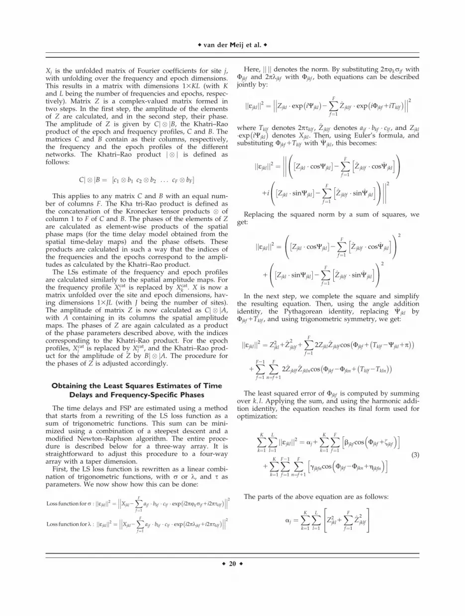
Xj is the unfolded matrix of Fourier coefficients for site j,with unfolding over the frequency and epoch dimensions.This results in a matrix with dimensions 13KL (with Kand L being the number of frequencies and epochs, respec-tively). Matrix Z is a complex-valued matrix formed intwo steps. In the first step, the amplitude of the elementsof Z are calculated, and in the second step, their phase.The amplitude of Z is given by Cj � jB, the Khatri–Raoproduct of the epoch and frequency profiles, C and B. Thematrices C and B contain as their columns, respectively,the frequency and the epoch profiles of the differentnetworks. The Khatri–Rao product j � j is defined asfollows:

Cj � jB ¼ c1 � b1 c2 � b2 . . . cF � bF½ �

This applies to any matrix C and B with an equal num-ber of columns F: The Kha tri-Rao product is defined asthe concatenation of the Kronecker tensor products � ofcolumn 1 to F of C and B. The phases of the elements of Zare calculated as element-wise products of the spatialphase maps (for the time delay model obtained from thespatial time-delay maps) and the phase offsets. Theseproducts are calculated in such a way that the indices ofthe frequencies and the epochs correspond to the ampli-tudes as calculated by the Khatri–Rao product.

The LSs estimate of the frequency and epoch profilesare calculated similarly to the spatial amplitude maps. Forthe frequency profile Xcat

j is replaced by Xcatk . X is now a

matrix unfolded over the site and epoch dimensions, hav-ing dimensions 13JL (with J being the number of sites).The amplitude of matrix Z is now calculated as Cj � jA,with A containing in its columns the spatial amplitudemaps. The phases of Z are again calculated as a productof the phase parameters described above, with the indicescorresponding to the Khatri-Rao product. For the epochprofiles, Xcat

j is replaced by Xcatl , and the Khatri–Rao prod-

uct for the amplitude of Z by Bj � jA. The procedure forthe phases of Z is adjusted accordingly.

Obtaining the Least Squares Estimates of Time

Delays and Frequency-Specific Phases

The time delays and FSP are estimated using a methodthat starts from a rewriting of the LS loss function as asum of trigonometric functions. This sum can be mini-mized using a combination of a steepest descent and amodified Newton–Raphson algorithm. The entire proce-dure is described below for a three-way array. It isstraightforward to adjust this procedure to a four-wayarray with a taper dimension.

First, the LS loss function is rewritten as a linear combi-nation of trigonometric functions, with r or k, and s asparameters. We now show how this can be done:

Loss function for r : jjEjkljj2 ¼��Xjkl2

XF

f¼1

ajf � bkf � clf � exp i2pukrjf 1i2psklf

� ��2

Loss function for k : jjEjkljj2 ¼��Xjkl2

XF

f¼1

ajf � bkf � clf � exp i2pkjkf 1i2psklf

� ��2

Here, jj jj denotes the norm. By substituting 2pukrjf withUjkf and 2pkjkf with Ujkf , both equations can be describedjointly by:

jjEjkljj2 ¼��Zjkl � exp iWjkl

� �2XF

f¼1

Zjklf � exp iUjkf 1iTklf

� ��2

where Tklf denotes 2psklf , Zjklf denotes ajf � bkf � clf , and Zjkl

�exp iWjkl

� �denotes Xjkl. Then, using Euler’s formula, and

substituting Ujkf 1Tklf with Wjkl, this becomes:

jjEjkljj2 ¼�� Zjkl � cosWjkl

2XF

f¼1

Zjklf � cosW jkl

h i0@

1A

1i Zjkl � sinWjkl

2XF

f¼1

Zjklf � sinW jkl

h i0@

1A��2

Replacing the squared norm by a sum of squares, weget:

jjEjkljj2 ¼ Zjkl � cosWjkl

2XF

f¼1

Zjklf � cosWjkl

h i0@

1A

2

1 Zjkl � sinWjkl

2XF

f¼1

Zjklf � sinWjkl

h i0@

1A

2

In the next step, we complete the square and simplifythe resulting equation. Then, using the angle additionidentity, the Pythagorean identity, replacing Wjkl byUjkf 1Tklf , and using trigonometric symmetry, we get:

jjEjkljj2 ¼ Z2jkl1Z

2

jklf 1XF

f¼1

2ZjklZjklf cos Ujkf 1 Tklf 2Wjkl1p� ��

1XF21

f¼1

XF

n¼f 11

2Zjklf Zjklncos Ujkf 2Ujkn1 Tklf 2Tkln

� ��

The least squared error of Ujkf is computed by summingover k; l. Applying the sum, and using the harmonic addi-tion identity, the equation reaches its final form used foroptimization:

XK

k¼1

XL

l¼1

jjEjkljj2 ¼ aj1XK

k¼1

XF

f¼1

bjkf cos Ujkf 1fjkf

� �h i

1XK

k¼1

XF21

f¼1

XF

n¼f 11

gjkfncos Ujkf 2Ujkn1hjkfn

� �h i (3)

The parts of the above equation are as follows:

aj ¼XK

k¼1

XL

l¼1

Z2jkl1

XF

f¼1

Z2

jklf

24

35


r 20 r

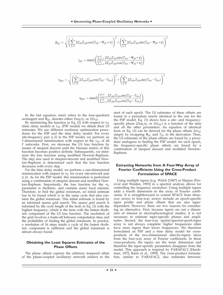
bjkf ¼

ffiffiffiffiffiffiffiffiffiffiffiffiffiffiffiffiffiffiffiffiffiffiffiffiffiffiffiffiffiffiffiffiffiffiffiffiffiffiffiffiffiffiffiffiffiffiffiffiffiffiffiffiffiffiffiffiffiffiffiffiffiffiffiffiffiffiffiffiffiffiffiffiffiffiffiffiffiffiffiffiffiffiffiffiffiffiffiffiffiffiffiffiffiffiffiffiffiffiffiffiffiffiffiffiffiffiffiffiffiffiffiffiffiffiffiffiffiffiffiffiffiffiffiffiffiffiffiffiffiffiffiffiffiffiffiffiffiffiffiffiffiffiffiffiffiffiffiXL

l¼1

2ZjklZjklf cos Tklf 2Wjkl1p� � !2

1XL

l¼1

2ZjklZjklf sin Tklf 2Wjkl1p� � !2

vuut

fjkf ¼ atan2

PLl¼1 2ZjklZjklf sin Tkln2Wjkl1p

� �PL

l¼1 2ZjklZjklf cos Tkln2Wjkl1p� �

!

gjkfn ¼

ffiffiffiffiffiffiffiffiffiffiffiffiffiffiffiffiffiffiffiffiffiffiffiffiffiffiffiffiffiffiffiffiffiffiffiffiffiffiffiffiffiffiffiffiffiffiffiffiffiffiffiffiffiffiffiffiffiffiffiffiffiffiffiffiffiffiffiffiffiffiffiffiffiffiffiffiffiffiffiffiffiffiffiffiffiffiffiffiffiffiffiffiffiffiffiffiffiffiffiffiffiffiffiffiffiffiffiffiffiffiffiffiffiffiffiffiffiffiffiffiffiffiffiffiffiffiffiffiffiffiffiffiffiffiffiffiffiXL

l¼1

2Zjklf Zjklncos Tklf 2Tkln

� � !2

1XL

l¼1

2Zjklf Zjklnsin Tkln2Tklnð Þ !2

vuut

hjkfn ¼ atan2

PLl¼1 2Zjklf Zjklnsin Tklf 2Tkln

� �PL

l¼1 2Zjklf Zjklncos Tklf 2Tkln

� � !

In the last equation, atan2 refers to the four-quadrantarctangent and Ujkf , denotes either 2pukrjf or 2pkjkf .

By minimizing the function in Eq. (3) with respect to rjf

(time delay model) or kjkf (FSP model) we obtain their LSestimates. We use different nonlinear optimization proce-dures for the FSP and the time delay model. For everysite-frequency pair (j; k) in the FSP model, we perform anF-dimensional minimization with respect to the kjkf of allF networks. First, we decrease the LS loss function bymeans of steepest descent until the Hessian matrix of thisfunction becomes positive definite. Subsequently, we mini-mize the loss function using modified Newton–Raphson.The step size used in steepest-descent and modified New-ton–Raphson is determined such that the loss functiondecreases with every step.

For the time delay model, we perform a one-dimensionalminimization with respect to rjf for every site-network pair(j; k). As for the FSP model, this minimization is performedusing a combination of steepest descent and modified New-ton–Raphson. Importantly, the loss function for the rjf

parameter is rhythmic, and contains many local minima.Therefore, to find the global minimum, an initial estimatehas to be found which is in the same cycle that also con-tains the global minimum. This initial estimate is found byan informed sparse grid search. The sparse grid search isinformed by the cycle length of the term in Eq. (3) with thehighest frequency, which is the term with the fastest rhyth-mic component of the LS loss function. The resolution ofthe grid involves a trade-off between computation time andthe probability of finding the global minimum. In practice,a resolution of 16 steps inside a cycle of the fastest rhyth-mic component is sufficient and the global minimum isalmost always found.

Obtaining the Least Squares Estimates of the

Phase Offsets

The phase offsets capture the arbitrary temporal offsetof the phase-coupled oscillatory network relative to the

start of each epoch. The LS estimates of these offsets arefound in a procedure nearly identical to the one for thethe FSP model. Eq. (3) shows how a site- and frequency-specific phase (2pukrjf or 2pkjkf ) is a function of the dataand all the other parameters. An equation of identicalform as Eq. (3) can be derived for the phase offsets 2psklf

simply by swapping Ujkf and Tklf in the derivation. Then,the LS estimates of the phase offsets are found by a proce-dure analogous to finding the FSP model: for each epoch,the frequency-specific phase offsets are found by acombination of steepest descent and modified Newton–Raphson.

Extracting Networks from A Four-Way Array of

Fourier Coefficients Using the Cross-Product

Formulation of SPACE

Using multiple tapers [e.g. Welch [1967] or Slepian [Per-cival and Walden, 1993] in a spectral analysis allows forcontrolling the frequency resolution. Using multiple tapersadds a fourth dimension to the array of Fourier coeffi-cients. It is straightforward to extend SPACE from three-way arrays to four-way arrays: include an epoch-specifictaper profile and phase offsets that are also taper-dependent. However, there are two reasons for consider-ing an alternative. First, because tapers are not a dimen-sion of interest in electrophysiological studies, it is notnecessary to estimate taper-specific phases and ampli-tudes. Second, the four-way spatial-spectral-epoch-taperarray is not always complete: higher frequencies oftenhave more tapers than lower frequencies. We thereforeformulated an FSP and a time delay model for cross-products of the two-dimensional sites-by-tapers slicesfrom the four-way array of Fourier coefficients. In thesecross-products, the tapers are the inner dimension andtherefore the taper-specific parameters disappear from themodel. This approach is inspired by PARAFAC2 [Harsh-man, 1972; Kiers et al., 1999]. The cross-product formula-tion, similar to PARAFAC2, also estimates between-


r 21 r

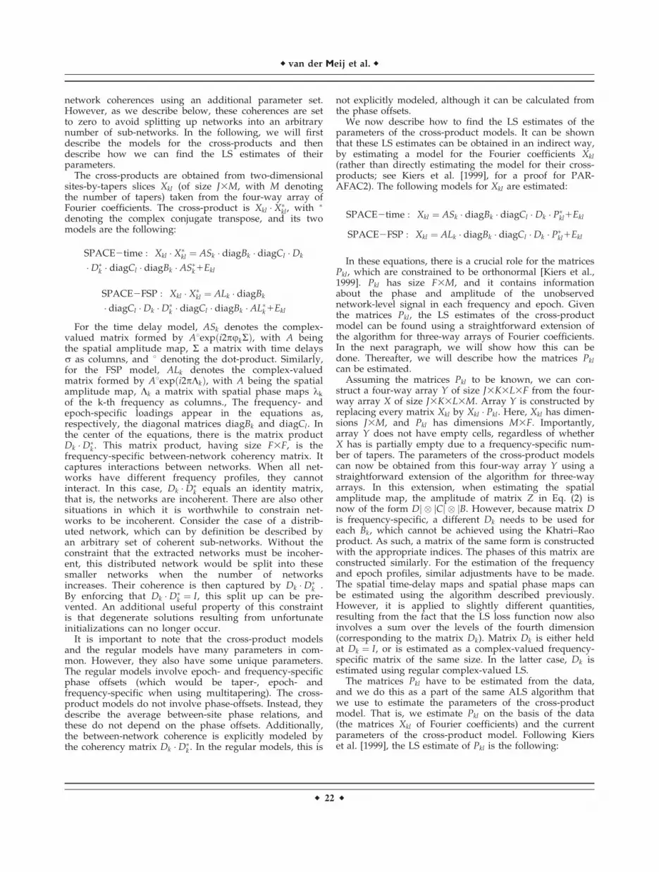
network coherences using an additional parameter set.However, as we describe below, these coherences are setto zero to avoid splitting up networks into an arbitrarynumber of sub-networks. In the following, we will firstdescribe the models for the cross-products and thendescribe how we can find the LS estimates of theirparameters.

The cross-products are obtained from two-dimensionalsites-by-tapers slices Xkl (of size J3M, with M denotingthe number of tapers) taken from the four-way array ofFourier coefficients. The cross-product is Xkl � X�kl, with �

denoting the complex conjugate transpose, and its twomodels are the following:

SPACE2time : Xkl � X�kl ¼ ASk � diagBk � diagCl �Dk

�D�k � diagCl � diagBk � AS�k1Ekl

SPACE2FSP : Xkl � X�kl ¼ ALk � diagBk

� diagCl �Dk �D�k � diagCl � diagBk � AL�k1Ekl

For the time delay model, ASk denotes the complex-valued matrix formed by A8exp i2pukRð Þ, with A beingthe spatial amplitude map, R a matrix with time delaysr as columns, and 8 denoting the dot-product. Similarly,for the FSP model, ALk denotes the complex-valuedmatrix formed by A8exp i2pKkð Þ, with A being the spatialamplitude map, Kk a matrix with spatial phase maps kk

of the k-th frequency as columns., The frequency- andepoch-specific loadings appear in the equations as,respectively, the diagonal matrices diagBk and diagCl. Inthe center of the equations, there is the matrix productDk �D�k . This matrix product, having size F3F, is thefrequency-specific between-network coherency matrix. Itcaptures interactions between networks. When all net-works have different frequency profiles, they cannotinteract. In this case, Dk �D�k equals an identity matrix,that is, the networks are incoherent. There are also othersituations in which it is worthwhile to constrain net-works to be incoherent. Consider the case of a distrib-uted network, which can by definition be described byan arbitrary set of coherent sub-networks. Without theconstraint that the extracted networks must be incoher-ent, this distributed network would be split into thesesmaller networks when the number of networksincreases. Their coherence is then captured by Dk �D�k .By enforcing that Dk �D�k ¼ I, this split up can be pre-vented. An additional useful property of this constraintis that degenerate solutions resulting from unfortunateinitializations can no longer occur.

It is important to note that the cross-product modelsand the regular models have many parameters in com-mon. However, they also have some unique parameters.The regular models involve epoch- and frequency-specificphase offsets (which would be taper-, epoch- andfrequency-specific when using multitapering). The cross-product models do not involve phase-offsets. Instead, theydescribe the average between-site phase relations, andthese do not depend on the phase offsets. Additionally,the between-network coherence is explicitly modeled bythe coherency matrix Dk �D�k . In the regular models, this is

not explicitly modeled, although it can be calculated fromthe phase offsets.

We now describe how to find the LS estimates of theparameters of the cross-product models. It can be shownthat these LS estimates can be obtained in an indirect way,by estimating a model for the Fourier coefficients Xkl

(rather than directly estimating the model for their cross-products; see Kiers et al. [1999], for a proof for PAR-AFAC2). The following models for Xkl are estimated:

SPACE2time : Xkl ¼ ASk � diagBk � diagCl �Dk � P�kl1Ekl

SPACE2FSP : Xkl ¼ ALk � diagBk � diagCl �Dk � P�kl1Ekl

In these equations, there is a crucial role for the matricesPkl, which are constrained to be orthonormal [Kiers et al.,1999]. Pkl has size F3M, and it contains informationabout the phase and amplitude of the unobservednetwork-level signal in each frequency and epoch. Giventhe matrices Pkl, the LS estimates of the cross-productmodel can be found using a straightforward extension ofthe algorithm for three-way arrays of Fourier coefficients.In the next paragraph, we will show how this can bedone. Thereafter, we will describe how the matrices Pkl

can be estimated.Assuming the matrices Pkl to be known, we can con-

struct a four-way array Y of size J3K3L3F from the four-way array X of size J3K3L3M. Array Y is constructed byreplacing every matrix Xkl by Xkl � Pkl. Here, Xkl has dimen-sions J3M, and Pkl has dimensions M3F. Importantly,array Y does not have empty cells, regardless of whetherX has is partially empty due to a frequency-specific num-ber of tapers. The parameters of the cross-product modelscan now be obtained from this four-way array Y using astraightforward extension of the algorithm for three-wayarrays. In this extension, when estimating the spatialamplitude map, the amplitude of matrix Z in Eq. (2) isnow of the form Dj � jCj � jB. However, because matrix Dis frequency-specific, a different Dk needs to be used foreach Bk, which cannot be achieved using the Khatri–Raoproduct. As such, a matrix of the same form is constructedwith the appropriate indices. The phases of this matrix areconstructed similarly. For the estimation of the frequencyand epoch profiles, similar adjustments have to be made.The spatial time-delay maps and spatial phase maps canbe estimated using the algorithm described previously.However, it is applied to slightly different quantities,resulting from the fact that the LS loss function now alsoinvolves a sum over the levels of the fourth dimension(corresponding to the matrix Dk). Matrix Dk is either heldat Dk ¼ I, or is estimated as a complex-valued frequency-specific matrix of the same size. In the latter case, Dk isestimated using regular complex-valued LS.

The matrices Pkl have to be estimated from the data,and we do this as a part of the same ALS algorithm thatwe use to estimate the parameters of the cross-productmodel. That is, we estimate Pkl on the basis of the data(the matrices Xkl of Fourier coefficients) and the currentparameters of the cross-product model. Following Kierset al. [1999], the LS estimate of Pkl is the following:


r 22 r

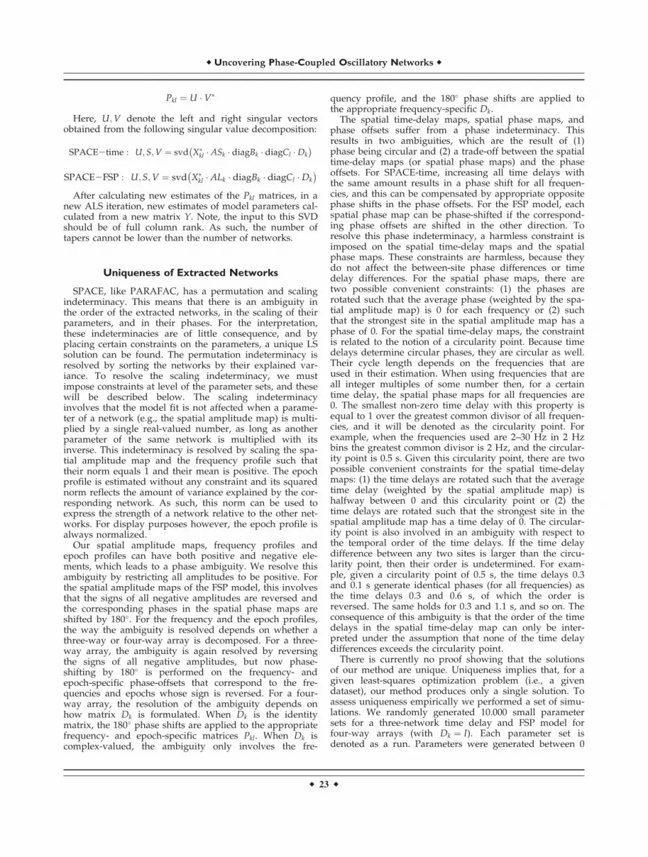
Pkl ¼ U � V�

Here, U;V denote the left and right singular vectorsobtained from the following singular value decomposition:

SPACE2time : U; S;V ¼ svd X�kl � ASk � diagBk � diagCl �Dk

� �SPACE2FSP : U;S;V ¼ svd X�kl � ALk � diagBk � diagCl �Dk

� �After calculating new estimates of the Pkl matrices, in a

new ALS iteration, new estimates of model parameters cal-culated from a new matrix Y. Note, the input to this SVDshould be of full column rank. As such, the number oftapers cannot be lower than the number of networks.

Uniqueness of Extracted Networks

SPACE, like PARAFAC, has a permutation and scalingindeterminacy. This means that there is an ambiguity inthe order of the extracted networks, in the scaling of theirparameters, and in their phases. For the interpretation,these indeterminacies are of little consequence, and byplacing certain constraints on the parameters, a unique LSsolution can be found. The permutation indeterminacy isresolved by sorting the networks by their explained var-iance. To resolve the scaling indeterminacy, we mustimpose constraints at level of the parameter sets, and thesewill be described below. The scaling indeterminacyinvolves that the model fit is not affected when a parame-ter of a network (e.g., the spatial amplitude map) is multi-plied by a single real-valued number, as long as anotherparameter of the same network is multiplied with itsinverse. This indeterminacy is resolved by scaling the spa-tial amplitude map and the frequency profile such thattheir norm equals 1 and their mean is positive. The epochprofile is estimated without any constraint and its squarednorm reflects the amount of variance explained by the cor-responding network. As such, this norm can be used toexpress the strength of a network relative to the other net-works. For display purposes however, the epoch profile isalways normalized.

Our spatial amplitude maps, frequency profiles andepoch profiles can have both positive and negative ele-ments, which leads to a phase ambiguity. We resolve thisambiguity by restricting all amplitudes to be positive. Forthe spatial amplitude maps of the FSP model, this involvesthat the signs of all negative amplitudes are reversed andthe corresponding phases in the spatial phase maps areshifted by 180�. For the frequency and the epoch profiles,the way the ambiguity is resolved depends on whether athree-way or four-way array is decomposed. For a three-way array, the ambiguity is again resolved by reversingthe signs of all negative amplitudes, but now phase-shifting by 180� is performed on the frequency- andepoch-specific phase-offsets that correspond to the fre-quencies and epochs whose sign is reversed. For a four-way array, the resolution of the ambiguity depends onhow matrix Dk is formulated. When Dk is the identitymatrix, the 180� phase shifts are applied to the appropriatefrequency- and epoch-specific matrices Pkl. When Dk iscomplex-valued, the ambiguity only involves the fre-

quency profile, and the 180� phase shifts are applied tothe appropriate frequency-specific Dk.

The spatial time-delay maps, spatial phase maps, andphase offsets suffer from a phase indeterminacy. Thisresults in two ambiguities, which are the result of (1)phase being circular and (2) a trade-off between the spatialtime-delay maps (or spatial phase maps) and the phaseoffsets. For SPACE-time, increasing all time delays withthe same amount results in a phase shift for all frequen-cies, and this can be compensated by appropriate oppositephase shifts in the phase offsets. For the FSP model, eachspatial phase map can be phase-shifted if the correspond-ing phase offsets are shifted in the other direction. Toresolve this phase indeterminacy, a harmless constraint isimposed on the spatial time-delay maps and the spatialphase maps. These constraints are harmless, because theydo not affect the between-site phase differences or timedelay differences. For the spatial phase maps, there aretwo possible convenient constraints: (1) the phases arerotated such that the average phase (weighted by the spa-tial amplitude map) is 0 for each frequency or (2) suchthat the strongest site in the spatial amplitude map has aphase of 0. For the spatial time-delay maps, the constraintis related to the notion of a circularity point. Because timedelays determine circular phases, they are circular as well.Their cycle length depends on the frequencies that areused in their estimation. When using frequencies that areall integer multiples of some number then, for a certaintime delay, the spatial phase maps for all frequencies are0. The smallest non-zero time delay with this property isequal to 1 over the greatest common divisor of all frequen-cies, and it will be denoted as the circularity point. Forexample, when the frequencies used are 2–30 Hz in 2 Hzbins the greatest common divisor is 2 Hz, and the circular-ity point is 0.5 s. Given this circularity point, there are twopossible convenient constraints for the spatial time-delaymaps: (1) the time delays are rotated such that the averagetime delay (weighted by the spatial amplitude map) ishalfway between 0 and this circularity point or (2) thetime delays are rotated such that the strongest site in thespatial amplitude map has a time delay of 0. The circular-ity point is also involved in an ambiguity with respect tothe temporal order of the time delays. If the time delaydifference between any two sites is larger than the circu-larity point, then their order is undetermined. For exam-ple, given a circularity point of 0.5 s, the time delays 0.3and 0.1 s generate identical phases (for all frequencies) asthe time delays 0.3 and 0.6 s, of which the order isreversed. The same holds for 0.3 and 1.1 s, and so on. Theconsequence of this ambiguity is that the order of the timedelays in the spatial time-delay map can only be inter-preted under the assumption that none of the time delaydifferences exceeds the circularity point.

There is currently no proof showing that the solutionsof our method are unique. Uniqueness implies that, for agiven least-squares optimization problem (i.e., a givendataset), our method produces only a single solution. Toassess uniqueness empirically we performed a set of simu-lations. We randomly generated 10.000 small parametersets for a three-network time delay and FSP model forfour-way arrays (with Dk ¼ I). Each parameter set isdenoted as a run. Parameters were generated between 0


r 23 r

and 1 except for the time delays, which were generatedbetween 0.125 and 0.375. This resulted in 10.000 four-wayarrays of Fourier coefficients for each model, consisting of6 sites, 5 frequencies, 4 epochs, and 3 tapers (frequenciesequally spaced between 2 and 10 Hz). We then decom-posed these four-way arrays using both models, randomlyinitiating each algorithm five times and then selecting thesolution with the highest explained variance. The averageexplained variance over 10.000 runs was >99.99%(SD 5 0.137%) for the time delay model and >99.99%(SD 5 0.037%) for the FSP model. This shows that ourmethod is able to find at least one solution of the least-squares optimization problem. We then computed theaverage absolute difference between the simulated andrecovered parameters, with averaging over sites, frequen-cies, epochs and networks. The average absolute deviationwas 1.86*1024 (SD 5 2.35*1023) for the time delay model,and 4.16*1024 (SD 5 1.83*1023) for the FSP model. Thissmall average absolute deviation shows that the solutionof our method is most likely unique. Additional evidencefor uniqueness is provided by the results of our recoverystudy (see Results and below).

ACKNOWLEDGMENT

The authors would like to thank H. Zhang for assistancein data collection.

REFERENCES

Akam T, Kullmann DM (2014): Oscillatory multiplexing of popu-lation codes for selective communication in the mammalianbrain. Nat Rev Neurosci 15:111–122.

Beckmann CF, DeLuca M, Devlin JT, Smith SM (2005): Investiga-tions into resting-state connectivity using independent compo-nent analysis. Philos Trans R Soc B-Biol Sci 360:1001–1013.

Bell AJ, Sejnowski TJ (1995): An information maximizationapproach to blind separation and blind deconvolution. NeuralComput 7:1129–1159.

Bernasconi C, Konig P (1999): On the directionality of corticalinteractions studied by structural analysis of electrophysiologi-cal recordings. Biol Cybern 81:199–210.

Biswal BB, VanKylen J, Hyde JS (1997): Simultaneous assessmentof flow and BOLD signals in resting-state functional connectiv-ity maps. NMR Biomed 10:165–170.

Borgers C, Kopell N (2003): Synchronization in networks of excita-tory and inhibitory neurons with sparse, random connectivity.Neural Comput 15:509–538.

Borgers C, Kopell NJ (2008): Gamma oscillations and stimulusselection. Neural Comput 20:383–414.

Bro R (1998): Multi-way Analysis in the Food Industry. Models,Algorithms, and Applications [A.K. Smilde]. Universiteit vanAmsterdam. Amsterdam (the Netherlands).

Brookes MJ, Woolrich M, Luckhoo H, Price D, Hale JR,Stephenson MC, Barnes GR, Smith SM, Morris PG (2011):Investigating the electrophysiological basis of resting state net-works using magnetoencephalography. Proc Natl Acad SciUSA 108:16783–16788.

Brown E, Moehlis J, Holmes P (2004): On the phase reduction andresponse dynamics of neural oscillator populations. NeuralComput 16:673–715.

Bruns A, Eckhorn R (2004): Task-related coupling from high- tolow-frequency signals among visual cortical areas in humansubdural recordings. Int J Psychophysiol 51:97–116.

Buzsaki G, Draguhn A (2004): Neuronal oscillations in corticalnetworks. Science 304:1926–1929.

Buzsaki G, Anastassiou CA, Koch C (2012): The origin of extracel-lular fields and currents—EEG, ECoG, LFP and spikes. NatRev Neurosci 13:407–420.

Canolty RT, Edwards E, Dalal SS, Soltani M, Nagarajan SS, KirschHE, Berger MS, Barbaro NM, Knight RT (2006): High gammapower is phase-locked to theta oscillations in human neocor-tex. Science 313:1626–1628.

Canolty RT, Knight RT (2010): The functional role of cross-frequency coupling. Trends Cogn Sci 14:506–515.

Canolty RT, Ganguly K, Kennerley SW, Cadieu CF, Koepsell K,Wallis JD, Carmena JM (2010): Oscillatory phase couplingcoordinates anatomically dispersed functional cell assemblies.Proc Natl Acad Sci USA 107:17356–17361.

Canolty RT, Cadieu CF, Koepsell K, Ganguly K, Knight RT,Carmena JM (2012a): Detecting event-related changes ofmultivariate phase coupling in dynamic brain networks.J Neurophysiol 107:2020–2031.

Canolty RT, Ganguly K, Carmena JM (2012b): Task-dependentchanges in cross-level coupling between single neurons andoscillatory activity in multiscale networks. PLoS Comput Biol 8:e1002809.

Carrol JD, Chang J (1970): Analysis of individual differences inmultidimensional scaling via an N-way generalization of“Eckart-Young” decomposition. Psychometrika 35:283.

Chrobak JJ, Buzsaki G (1998): Gamma oscillations in the entorhi-nal cortex of the freely behaving rat. J Neurosci 18:388–398.

Cohen MX, Axmacher N, Lenartz D, Elger CE, Sturm V,Schlaepfer TE (2009): Good vibrations: Cross-frequency Cou-pling in the Human Nucleus Accumbens during Reward Proc-essing. J Cogn Neurosci 21:875–889.

de Pasquale F, Della Penna S, Snyder AZ, Lewis C, Mantini D,Marzetti L, Belardinelli P, Ciancetta L, Pizzella V, Romani GL,Corbetta M (2010): Temporal dynamics of spontaneous MEGactivity in brain networks. Proc Natl Acad Sci USA 107:6040–6045.

Deco G, Corbetta M (2011): The dynamical balance of the brain atrest. Neuroscientist 17:107–123.

Ermentrout GB, Kopell N (1990): Oscillator death in systems ofcoupled neural oscillators. SIAM J Appl Math 50:125–146.

Fox MD, Snyder AZ, Vincent JL, Corbetta M, Van Essen DC,Raichle ME (2005): The human brain is intrinsically organizedinto dynamic, anticorrelated functional networks. Proc NatlAcad Sci USA 102:9673–9678.

Fries P (2005): A mechanism for cognitive dynamics: Neuronalcommunication through neuronal coherence. Trends Cogn Sci9:474–480.

Harshman R (1972): PARAFAC2—Extensions of a procedure forexplanatory factor-analysis and multidimensional scaling.J Acoust Soc Am 51:111.

Harshman RA (1970): Foundations of the PARAFAC procedure:Model and conditions for an ‘explanatory’ multi-mode factoranalysis. UCLA Working Papers in Phonetics 16:1–84. (Univer-sity Microfilms, Ann Arbor, No. 10,085).

Hipp JF, Hawellek DJ, Corbetta M, Siegel M, Engel AK (2012):Large-scale cortical correlation structure of spontaneous oscil-latory activity. Nat Neurosci 15:884–890.

Honey CJ, Sporns O, Cammoun L, Gigandet X, Thiran JP, MeuliR, Hagmann P (2009): Predicting human resting-state


r 24 r

functional connectivity from structural connectivity. Proc NatlAcad Sci USA 106:2035–2040.

Hoppensteadt FC, Izhikevich EM (1997): Weakly connected neuralnetworks. New York: Springer.

Jacobs J, Kahana MJ (2009): Neural representations of individualstimuli in humans revealed by gamma-band electrocortico-graphic activity. J Neurosci 29:10203–10214.

Kaminski M, Ding MZ, Truccolo WA, Bressler SL (2001): Evaluat-ing causal relations in neural systems: Granger causality,directed transfer function and statistical assessment of signifi-cance. Biol Cybern 85:145–157.

Kiers HAL, Ten Berge JMF, Bro R (1999): PARAFAC2—Part I. Adirect fitting algorithm for the PARAFAC2 model. J Chemometr13:275–294.

Kopell N, Ermentrout GB, Whittington MA, Traub RD (2000):Gamma rhythms and beta rhythms have different synchroniza-tion properties. Proc Natl Acad Sci USA 97:1867–1872.

Kuramoto Y (1984): Chemical oscillations, waves, and turbulence.New York: Springer-Verlag.

Kuramoto Y (1997): Phase- and center-manifold reductions forlarge populations of coupled oscillators with application tonon-locally coupled systems. Int J Bifurcat Chaos 7:789–805.

Lachaux JP, Rodriguez E, Martinerie J, Varela FJ (1999): Meas-uring phase synchrony in brain signals. Hum Brain Mapp 8:194–208.

Lobier M, Siebenhuhner F, Palva S, Palva JM (2014): Phase trans-fer entropy: A novel phase-based measure for directed connec-tivity in networks coupled by oscillatory interactions.Neuroimage 85:853–872.

Maris E, van Vugt M, Kahana M (2011): Spatially distributed pat-terns of oscillatory coupling between high-frequency ampli-tudes and low-frequency phases in human iEEG. Neuroimage54:836–850.

Massimini M, Huber R, Ferrarelli F, Hill S, Tononi G (2004): Thesleep slow oscillation as a traveling wave. J Neurosci 24:6862–6870.

Miller KJ, Sorensen LB, Ojemann JG, den Nijs M (2009): Power-law scaling in the brain surface electric potential. PLoS Com-put Biol 5:e1000609.

Miller KJ, Foster BL, Honey CJ (2012): Does rhythmic entrainmentrepresent a generalized mechanism for organizing computationin the brain? Front. Comput Neurosci 6:85.

Miwakeichi F, Martinez-Montes E, Valdes-Sosa PA, Nishiyama N,Mizuhara H, Yamaguchi Y (2004): Decomposing EEG data intospace-time-frequency components using Parallel Factor Analy-sis. Neuroimage 22:1035–1045.

Mormann F, Lehnertz K, David P, Elger CE (2000): Mean phasecoherence as a measure for phase synchronization and its appli-cation to the EEG of epilepsy patients. Physica D 144:358–369.

Mormann F, Fell J, Axmacher N, Weber B, Lehnertz K, Elger CE,Fernandez G (2005): Phase/amplitude reset and theta-gammainteraction in the human medial temporal lobe during a contin-uous word recognition memory task. Hippocampus 15:890–900.

Morup M, Hansen LK, Herrmann CS, Parnas J, Arnfred SM(2006): Parallel factor analysis as an exploratory tool for wave-let transformed event-related EEG. Neuroimage 29:938–947.

Morup M, Hansen LK, Arnfred SM, Lim LH, Madsen KH (2008):Shift-invariant multilinear decomposition of neuroimagingdata. Neuroimage 42:1439–1450.

Nolte G, Bai O, Wheaton L, Mari Z, Vorbach S, Hallett M (2004):Identifying true brain interaction from EEG data using theimaginary part of coherency. Clin Neurophysiol 115:2292–2307.

Nolte G, Ziehe A, Nikulin VV, Schlogl A, Kramer N, Brismar T,Muller, KR (2008): Robustly estimating the flow direction of infor-mation in complex physical systems. Phys Rev Lett 100:234101.

Nunez PL, Wingeier BM, Silberstein RB (2001): Spatial-temporalstructures of human alpha rhythms: Theory, microcurrentsources, multiscale measurements, and global binding of localnetworks. Hum Brain Mapp 13:125–164.

Oostenveld R, Fries P, Maris E, Schoffelen J-M (2011): FieldTrip: Opensource software for advanced analysis of MEG, EEG, and invasiveelectrophysiological data. Comput Intell Neurosci 2011:156869.

Palva S, Palva JM (2012): Discovering oscillatory interaction net-works with M/EEG: Challenges and breakthroughs. TrendsCogn Sci 16:219–230.

Pascualmarqui RD, Michel CM, Lehmann D (1994): Low-resolu-tion electromagnetic tomography—A new method for localiz-ing electrical-activity in the brain. Int J Psychophysiol 18:49–65.

Penny WD, Litvak V, Fuentemilla L, Duzel E, Friston KJ (2009):Dynamic causal models for phase coupling. J Neurosci Meth-ods 183:19–30.

Percival D, Walden A (1993): Spectral Analysis for Physical Appli-cations: Multitaper and Conventional Univariate Techniques.New York: Cambridge Univ. Press. 583 pp.

Raghavachari S, Lisman JE, Tully M, Madsen JR, Bromfield EB,Kahana MJ (2006): Theta oscillations in human cortex during aworking-memory task: Evidence for local generators.J Neurophysiol 95:1630–1638.

Raichle ME, MacLeod AM, Snyder AZ, Powers WJ, Gusnard DA,Shulman GL (2001): A default mode of brain function. ProcNatl Acad Sci USA 98:676–682.

Rizzuto DS, Madsen JR, Bromfield EB, Schulze-Bonhage A, SeeligD, Aschenbrenner-Scheibe R, Kahana MJ (2003): Reset ofhuman neocortical oscillations during a working memory task.Proc Natl Acad Sci USA 100:7931–7936.

Rosenberg JR, Halliday DM, Breeze P, Conway BA (1998): Identifi-cation of patterns of neuronal connectivity-partial spectra, par-tial coherence, and neuronal interactions. J Neurosci Methods83:57–72.

Rubino D, Robbins KA, Hatsopoulos NG (2006): Propagatingwaves mediate information transfer in the motor cortex. NatNeurosci 9:1549–1557.

Schack B, Vath N, Petsche H, Geissler HG, Moller E (2002): Phase-coupling of theta-gamma EEG rhythms during short-termmemory processing. Int J Psychophysiol 44:143–163.

Schnitzler A, Gross J (2005): Normal and pathological oscillatorycommunication in the brain. Nat Rev Neurosci 6:285–296.

Schreiber T (2000): Measuring information transfer. Phys Rev Lett85:461–464.

Schyns PG, Thut G, Gross J (2011): Cracking the code of oscilla-tory activity. PLoS Biol 9:8.

Sidiropoulos ND, Giannakis GB, Bro R (2000): Blind PARAFACreceivers for DS-CDMA systems. IEEE Trans Signal Proces 48:810–823.

Siegel M, Donner TH, Engel AK (2012): Spectral fingerprintsof large-scale neuronal interactions. Nat Rev Neurosci 13:121–134.

Smith SM, Fox PT, Miller KL, Glahn DC, Fox PM, Mackay CE,Filippini N, Watkins KE, Toro R, Laird AR, Beckmann CF(2009): Correspondence of the brain’s functional architectureduring activation and rest. Proc Natl Acad Sci USA 106:13040–13045.

Sternberg S (1966): High-speed scanning in human memory. Sci-ence 153:652–654.


r 25 r

Suffczynski P, Kalitzin S, Pfurtscheller G, da Silva FHL (2001):Computational model of thalamo-cortical networks: Dynamicalcontrol of alpha rhythms in relation to focal attention. Int JPsychophysiol 43:25–40.

Talairach J, Tornoux P (1988): Co-planar stereotaxic atlas of thehuman brain: 3-dimensional proportional system: An approachto cerebral imaging. Stuttgart: Georg Thieme. 122 p.

Tiesinga P, Fellous JM, Sejnowski TJ (2008): Regulation ofspike timing in visual cortical circuits. Nat Rev Neurosci 9:97–109.

van der Meij R, Kahana M, Maris E (2012): Phase-amplitude cou-pling in human electrocorticography is spatially distributedand phase diverse. J Neurosci 32:111–123.

van Vugt MK, Schulze-Bonhage A, Litt B, Brandt A, Kahana MJ(2010): Hippocampal gamma oscillations increase with mem-ory load. J Neurosci 30:2694–2699.

Vincent JL, Patel GH, Fox MD, Snyder AZ, Baker JT, Van EssenDC, Zempel JM, Snyder LH, Corbetta M, Raichle ME (2007):Intrinsic functional architecture in the anaesthetized monkeybrain. Nature 447:83–U4.

Vinck M, van Wingerden M, Womelsdorf T, Fries P, PennartzCMA (2010): The pairwise phase consistency: A bias-freemeasure of rhythmic neuronal synchronization. Neuroimage51:112–122.

Welch PD (1967): The use of fast Fourier transform for the estima-tion of power spectra: A method based on time averaging overshort, modified periodograms. IEEE Trans Audio Electroacoust15:70–73.

Whittington MA, Traub RD, Kopell N, Ermentrout B, Buhl EH(2000): Inhibition-based rhythms: Experimental and mathemati-cal observations on network dynamics. Int J Psychophysiol 38:315–336.


r 26 r

Uncovering phase-coupled oscillatory networks in electrophysiological data

Documents