Uncorrected Proof - imbriw.hcmr.grimbriw.hcmr.gr/.../2017/02/...Hydrology-Research_Uncorrected-proof.pdf · doi: 10.2166/nh.2016.352 Uncorrected Proof. Among the previously described

1 © IWA Publishing 2016 Hydrology Research | in press | 2016

Uncorrected Proof

Comparison of West Balkan adult trout habitat predictions

using a Pseudo-2D and a 2D hydrodynamic model

Christina Papadaki, Vasilis Bellos, Lazaros Ntoanidis and Elias Dimitriou

ABSTRACT

Hydraulic-habitat models combine the dynamic behavior of river discharge with geomorphological

and ecological responses. In this study, they are used for estimating environmental flow

requirements. We applied a Pseudo-two-dimensional (2D) model based on the (one-dimensional) 1D

HEC-RAS model and an in-house 2D (FLOW-R2D) hydrodynamic model to a section of river for several

flows in respect of summer conditions of the study reach, and compared the results derived from the

models in terms of water depths and velocities as well as habitat predictions in terms of weighted

usable area (WUA). In general, 2D models are more promising in habitat studies since they quantify

spatial variations and combinations of flow patterns important to stream flora and fauna in a higher

detail than the 1D models. Relationships between WUA and discharge for the two models were

examined, to compare the similarity as well as the magnitude of predictions over the modelled

discharge range. The models predicted differences in the location of maxima and changes in

variation of velocity and water depth. Finally, differences in spatial distribution (in terms of suitability

indices and WUA) between the Pseudo-2D and the fully 2D modelling results can be considerable on

a cell-by-cell basis.

doi: 10.2166/nh.2016.352

Christina PapadakiElias Dimitriou (corresponding author)Hellenic Centre for Marine Research, Institute of

Marine Biological Resources and Inland Waters,46.7 km of Athens-Sounio Ave.,Anavissos 19013,GreeceE-mail: [email protected]

Vasilis BellosSchool of Rural and Surveying Engineering,

National Technical University of Athens,Athens,Greece

Lazaros NtoanidiD. Argyropoulos & Associates,Tinou 2,Cholargos 15562,Greece

Key words | habitat modelling, hydraulic model, hydrodynamic model, trout

INTRODUCTION

Flow regime is a key component for the ecological integrity

of all biotic interactions among riverine ecosystems (Lai

et al. ). Changes in river flow quantity and timing are

more likely to cause perturbations to the instream biota

and consequences to biodiversity that are more destructive

than consequences caused by other choices (Richter &

Thomas ). Nevertheless, the growing demands for

water have increased the need to build dams, which in

many cases alter the seasonal and interannual streamflow

variability of rivers (Poff et al. ), while they also

reduce the available amount of water downstream (Li

et al. ; Mao et al. ). In order to mitigate the down-

stream impact of dams, several countries worldwide have

established environmental flow rules in order to quantify

the water required for ecosystem conservation and resource

protection (Tharme ).

Today, there are several environmental flow estimation

methods and they can be grouped into four categories:

hydrological rules, hydraulic rating methods, habitat simu-

lation methods and holistic methodologies (Dyson et al.

; Tharme ). The hydrological methods depend on

statistical analysis of hydrological data, while the hydraulic

methods rely on the estimation of a specific wetted per-

imeter or maximum depth, based on geomorphology and

hydrodynamic behaviour of a river reach. Physical habitat

methods quantify trade-offs between water use and environ-

mental benefits of flowing water for particular species or

groups of species (Dunbar et al. ). Finally, the incorpor-

ation of environmental, social and economic features, into a

modified or regulated flow regime which would maintain

the functional integrity of the riverine ecosystem, comprises

the holistic methodologies (Arthington et al. ).

2 C. Papadaki et al. | Comparison of West Balkan adult trout habitat predictions Hydrology Research | in press | 2016

Uncorrected Proof

Among the previously described categories, physical

habitat methods are commonly used to assess habitat quality

and quantity of riverine ecosystems. This approach inte-

grates a hydraulic model and a habitat suitability model,

usually developed at a microhabitat scale for specific

species. The basic idea of this approach is that the hydro-

physical stream conditions formulate the abiotic back-

ground within which riverine biota have to adapt. In this

concept habitat, suitability modelling provides information

about the spatial requirements of specific organisms, usually

by relating hydraulic parameters (e.g., depth, velocity) to a

habitat suitability index (HSI) (Olsen et al. ). The

weighted area by the composite HSI (a combined index

including all the examined hydraulic parameters) within

the entire domain of the hydrodynamic model corresponds

to the weighted usable area (WUA) (Bovee et al. ),

which is a well-known general indicator of habitat quality

and quantity.

Although in situ studies of habitat selection can be

made, to some extent, in a river reach, still it is impossible

to cover all likely spatial and temporal heterogeneities (Heg-

genes et al. ). To overcome these limitations, prediction

of ecological response to flow changes are made by hydrau-

lic modelling integrated with habitat suitability modelling.

The hydraulic characteristics of the river are simulated

by either one-dimensional (1D) (García et al. ) or two-

dimensional (2D) hydrodynamic models (Leclerc et al.

) (in Benjankar et al. ). Flow properties in 1D

models are estimated based on the physical characteristic

of the cross sections (e.g., mean depth, average velocity).

In some cases, it is possible to divide each cross section

into sub-areas simulating Pseudo-2D situations. Regarding

2D models, water depths and velocities are calculated

across a grid or mesh which defines the topographic

information.

The selection of a 1D or 2D hydrodynamic model

depends on the complexity of the river reach. 1D models

are usually applied for long river lengths and 2D models

are used over shorter representative river reaches (Katopo-

dis ). Previous studies have shown that 1D and 2D

models can provide comparable cross-sectional-averaged

flow properties in simple uniform channels; nevertheless,

different flow proprieties may be predicted in morphologi-

cally complex channels (Brown & Pasternack 2009). More

specifically, complex flow patterns cannot be easily rep-

resented from cross-sectional-averaged properties predicted

by 1D models (Mason et al. 2003), while 2D models predict

depth, magnitude and direction (X,Y) of mean vertical vel-

ocity at points providing better habitat metrics (Bovee ).

Even though there are several sources of uncertainty

incorporated into the modelling process including the

input data, the required parameters, the structure of the

models and the propagation of the uncertainty between

several sub-models (Deletic et al. ), it is noted that the

model structure is the most crucial to the model results

(Refsgaard et al. ). In this study, a comparative assess-

ment of the habitat quality spatial distribution, in terms of

WUA, as simulated by a Pseudo-2D and a 2D model, has

been attempted, focusing on the differences among model

structures.

We used a Mediterranean mountain reach, with limited

anthropogenic disturbance and we examined several dis-

charges in both Pseudo-2D and actual 2D models, with

respect to the summer conditions of the study area. To ana-

lyse the differences in spatial distribution we used the error

matrix which quantifies models’ differences (Benjankar

et al. ). This analysis was performed on a cell-by-cell

basis throughout the Pseudo-2D model inundated domain.

Habitat duration curves were constructed following the

procedures described within the Instream Flow Incremental

Methodology for environmental flow studies (Bovee et al.

) indicating the exceedance probability for the habitat

area in the corresponding models (Pseudo-2D and 2D),

with combined HSI higher than 0.5. The habitat duration

curves were estimated based on the hydrological simulated

summer flows (June to October) for the study reach,

according to previous work (Papadaki et al. ).

STUDY AREA

The study was carried out in the upper part of Acheloos

River located in the central western mountainous region of

Greece. The mean summer (June–October) discharge of

the upper Acheloos basin is 3.11 m3 s�1. A typical native

species of the basin is the Balkan trout (Salmo farioides)

(hereafter W.B. trout). However, this species is now

scarce, especially in the lower part of the Acheloos basin

3 C. Papadaki et al. | Comparison of West Balkan adult trout habitat predictions Hydrology Research | in press | 2016

Uncorrected Proof

as a result of severe overfishing, even involving illegal spear

fishing, electrofishing and habitat alteration.

Habitat mapping of a 1.5 km river stretch of the upper

course of the Acheloos River (at 670 m a.s.l., 39.479443W,

21.326510W, WGS 84) was carried out in order to select a

representative study site of 390 m (Figure 1). More specifi-

cally, several types of hydromorphological units (i.e.,

pools, runs, riffles), were identified, and their extent and

physical attributes measured. Measurements of water

depth and velocity at seven cross sections (Figure 1) perpen-

dicular to the flow provided data for the validation of both

models. Depth (m) was measured with a wading rod to the

nearest cm and the mean flow velocity of the water

column (hereafter velocity (ms�1)) was measured with a

propeller current meter (OTT®).

The assessment of the flow requirements for the adult

W.B. trout (>20 cm) was made by combining hydraulic

simulation and habitat suitability modelling.

Riverbed topography was surveyed encompassing the

main channel and banks with a GPS/GNSS Geomax

Zenith 20 using geodesic references (i.e., GGRS ‘87 Greek

Geodetic Reference System) to generate a digital elevation

model as the base for the models. The fish microhabitat-

use survey, as part of the habitat simulation method was

conducted during summer 2014 in the Voidomatis River; a

Figure 1 | Study reach in the upper part of the Acheloos River.

reference river with near-natural conditions within Greece’s

Northern Pindos National Park (Papadaki et al. ).

METHODS

Pseudo-2D hydraulic model

HEC-RAS (Version 4.1) was used to perform a Pseudo-2D

hydrodynamic simulation for 14 flow scenarios with respect

to monthly summer flows in the study reach. The model

solves the 1D Saint-Venant equations, for steady state and

gradually varied flow. In a HEC-RAS steady state simu-

lation, Water Surface Elevation (WSE) profiles were

computed from one cross section to the next using the stan-

dard step iterative procedure to solve the energy equation.

To account for the Pseudo-2D hydraulic simulation

every cross section was subdivided into 12 cells both in

the main channel and the overbank area. The number of

cells was primarily a function of the number of water vel-

ocity measurements and substrate variation along the cross

sections. For every cross section a single water stage was

simulated by the standard solving procedure, while vel-

ocities were calculated separately for each cell for the

simulated water stage (procedure described in details in

HEC-RAS v4.1, Hydraulic Reference Manual ).

Pre-process of the geometry of the reach was carried out

using Autodesk Civil 3D software. Simulations were per-

formed at 27 cross sections along the river reach. Friction

losses were calculated applying Manning’s roughness coeffi-

cient to every cross section. Furthermore, roughness

coefficient was horizontally varied to account for substrate

variation. Manning’s n initial values varied for the main

channel between 0.023 and 0.044 while for the overbank

areas between 0.055 and 0.08.

2D hydrodynamic model

The FLOW-R2D model is an in-house numerical model

(Tsakiris & Bellos ), which solves the fully dynamic

form of the 2D shallow water equations (2D-SWE) through

the finite difference method and the McCormack numerical

scheme (McCormack 1969), in a cell-centred, non-staggered

computational grid. The McCormack numerical scheme is

4 C. Papadaki et al. | Comparison of West Balkan adult trout habitat predictions Hydrology Research | in press | 2016

Uncorrected Proof

explicit and therefore is stable under the Courant–Frie-

drichs–Lewy (CFL) condition.

The non-rectangular computational domains were

approached with a pseudo-computational rectangular

domain which encloses the real one. For the solid bound-

aries, a modified reflection boundary was used (Bellos &

Tsakiris a).

The wet/dry bed modelling was achieved using a water

depth threshold (hdry) which distinguishes wet and dry

cells. As well, artificial viscosity was added in the context

of the 2D-SWE discretization, through a diffusion factor

(ω). For the friction modelling, the Manning empirical

model was used, while several applications of the model

for both experimental benchmark tests and real world appli-

cations are also available (Bellos & Tsakiris a, b,

2015c).

Numerical simulation and calibration phase

In previous work, Pseudo-2D model roughness calibration

was made in the upper section of the Acheloos River (Papa-

daki et al. ). Normal depth was used as downstream

boundary condition, whereas the flow was considered as

subcritical in the entire computational domain and therefore

no specific upstream boundary condition was set. The

energy slope required for the downstream boundary con-

dition was assumed to be equal with the surface slope.

Calibration of the model was conducted by adjusting Man-

ning’s coefficient (n) at seven critical cross sections for the

discharge of 4 m3 s�1, and by comparing graphically both

the simulated water stage and velocities with the observed

ones from field measurements. The adjusted Manning’s n

values through calibration were close enough to the starting,

bibliographical values (Cowan ; Chow ; Barnes

) with few exceptions (e.g., n¼ 0.012) which were

necessary in order to achieve velocity convergence with

the measurements in some cross sections. This low rough-

ness value was assigned in particular in two adjacent cross

sections and found to be necessary due to their main

channel complex geometry.

For the numerical simulation using the 2D model, a grid

of 46,957 square cells with 1 × 1 m size was generated, in

order to represent the computational domain. The lateral

boundaries of the river were considered solid, in order to

preserve the water mass balance. For the downstream

boundaries, the open boundary condition was used. The

wet/dry threshold was determined as hdry¼ 1 cm, and the

Courant number as CFL¼ 0.1, according to the authors’

experience in similar real-world case studies (Tsakiris &

Bellos ; Bellos & Tsakiris b, ). For the friction

modelling, Manning’s equation was used.

A slightly different procedure was used to calibrate the

required parameters of the 2D model, in relation to the

Pseudo-2D. However, conventional or evolution optimiz-

ation methods cannot be implemented for the calibration

phase, due to the computational burden of the 2D model.

The parameters which were calibrated were the diffusion

factor ω and the Manning’s coefficients n, for the friction

modelling. For the calibration phase, water depth and flow

velocity measurements were used, derived from 100 points

located across seven cross sections (Figure 1) of the study

reach.

The trial and error method was used in order to calibrate

the diffusion factor and the Manning’s coefficient in the four

friction zones of the computational domain (sand, gravel,

cobble and boulder zone). Specifically, 32 scenarios were

implemented, in which the diffusion factor ranged from

0.90 to 0.95, Manning’s coefficient at the sand zone

ranged from 0.03 to 0.04 sm�1/3, at the gravel zone ranged

from 0.04 to 0.06, at the cobble zone ranged from 0.05 to

0.07 sm�1/3 and at the boulder zone ranged from 0.06 to

0.09 sm�1/3. In a rough approximation, the diffusion factor

simulates the eddy viscosities of the flow in all the scales

(reach and sub-grid scale) (Tsakiris & Bellos ). Based

on this approximation, it is generally recommended from

the developers of the model, that in real-world conditions

the diffusion factor takes the value ω¼ 0.90 (Bellos &

Tsakiris ). However, when turbulence phenomena in

reach or sub-grid scale are expected to be relatively small,

this factor could be increased. The grid size of the present

case study, which is relatively small, combining with the

relatively low flow velocity values indicate that the interval

of the diffusion factor could range from 0.90 to 0.95, accord-

ing to the authors’ experience. For the intervals of Manning

coefficients, the ranges were also predefined according to

the authors’ experience (Bellos & Tsakiris b, ).

In the next step of the calibration phase, the sum of the

root mean square error (RMSE) was calculated, for both

Figure 2 | Habitat suitability curves for W.B. trout (size >20 cm).

5 C. Papadaki et al. | Comparison of West Balkan adult trout habitat predictions Hydrology Research | in press | 2016

Uncorrected Proof

water depths and flow velocities at the 100 points where

measurements exist, between the numerical results and the

observed data. The above values were normalized through

a utility function, in which the maximum sum of the

RMSE took the value 0 and the minimum took the value 1.

Finally, the normalized values of the water depths and the

flow velocities were summed in order to determine the per-

formance of the scenarios. The maximum score of the

summed normalized values defined the best scenario.

According to this procedure, the calibrated parameters

took the following values: diffusion factor ω¼ 0.95, Man-

ning’s coefficient for the sand zone n¼ 0.03 sm�1/3, for the

gravel zone n¼ 0.06 sm�1/3, for the cobble zone n¼0.07 sm�1/3 and for the boulder zone n¼ 0.06 sm�1/3. It is

noted that the corresponding summed normalized value

was also calculated for the results derived from the cali-

bration phase of the Pseudo-2D model and it was found

that the score obtained using the 2D model was better. For

the upstream boundaries, the steady flow condition was

used, determined by Manning’s equation. The required par-

ameters for these boundaries were the water elevation stage

and the effective slope of the upstream cross section. The

above parameters were optimized based on the flow inlet

at the computational field which was defined at 4 m3 s�1

(equal to the corresponding measured discharge), and the

minimum RMSE between the observed data and the numeri-

cal results across the cross section for both water depth and

flow velocity values. As previously mentioned, in the context

of the calibration phase, two values for the Manning’s coef-

ficient were considered for each friction zone. The upstream

cross section was exclusively located in the boulder zone

and therefore two values for the effective slope and the

water elevation stage were derived. Specifically, the effective

slope values were determined as 0.00541 and 0.01224 for

the Manning’s coefficient 0.06 and 0.09 sm�1/3, respectively,

(boulder zone), whereas the water elevation stage was

derived as 668.01 m a.s.l., in both of these cases.

Habitat model development

Physical habitat was quantified using depth and velocity uni-

variate HSI curves (Figure 2), developed according to Bovee

(), representing generalized suitability for the W.B. trout;

103 fish adult (size >20 cm). The HSI curves relate the

hydraulic variables (i.e., depth or velocity) with a suitability

index (SI), ranging from 0 (unsuitable for the aquatic species)

to 1 (excellent). The intermediate values represent the suitable

range based on a specified hydraulic variable (i.e., depth or

velocity) (Bovee et al. ). These two individuals’ suitability

indices were then combined to form a composite SI for every

cell of the hydraulic models, using the product mathematical

operation (Vadas & Orth ). At the cell scale, Cell Suit-

ability Index (CSI) indicates whether the physical parameters

(depth and velocity in this case) are within those required by

individual species and particular life stages (Bovee 1978).

WUA was calculated by multiplying the CSI for a given

cell by the area assigned to that specific cell, which in this

case is 1 m for both models. In order to study only the suit-

able conditions for the target species, WUA was estimated

considering the cells with CSI higher than 0.5 only (here-

after WUA0.5). The whole procedure was carried out in R

software (R Development Core Team R: A language

and environment for statistical computing).

Habitat suitability

A comparison between the spatially distributed CSI, calcu-

lated from the Pseudo-2D and the 2D model using the

error matrix method (Congalton & Green ) was made

as a standard technique for quantifying the accuracy

among maps, specifically designed for raster comparisons.

The error matrix compares maps by calculating overall accu-

racy (OA) and the agreement index between the maps using

the kappa statistic (K). A K value of 1 indicates perfect

agreement, whereas a K value of 0 indicates agreement

6 C. Papadaki et al. | Comparison of West Balkan adult trout habitat predictions Hydrology Research | in press | 2016

Uncorrected Proof

equivalent to chance. The OA is a ratio between the num-

bers of correctly predicted cells to total number of cells

considered in the analysis. CSIs were separated into classes

of 0¼ 0, 0–0.19¼ 1, 0.20–0.39¼ 2, 0.4–0.59¼ 3, 0.60–

0.79¼ 4 and 0.80–1.00¼ 5 in order to estimate the K

statistic using the error matrix.

RESULTS

Comparison of the model’s hydraulic output

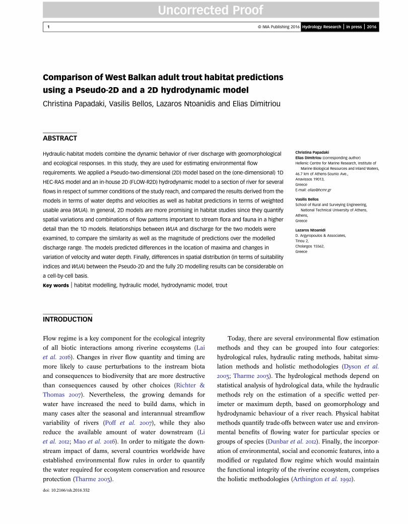
The models’ performance indices indicated a relatively

better performance of the FLOW-R2D model (RMSE: 0.11

and r: 0.49) in relation to HEC-RAS (RMSE: 0.12 and

r: 0.36) for the depth simulations (Tables 1 and 2, Figure 1).

The velocity model outputs were simulated with less accu-

racy by both models but HEC-RAS (RMSE: 33 and r: 0.39)

Table 2 | Pearson correlation coefficients for depth and velocity model outputs and observati

Observed depth

Observed depth 1

FLOW-R2D depth 0.491

HEC-RAS depth 0.364

Observed velocity

Observed velocity 1

FLOW-R2D velocity 0.372

HEC-RAS velocity 0.387

Table 1 | Statistical comparisons and RMSEs between observations and simulated values for

Depth (m)

Observations FLOW-R2D HE

Mean 0.26 0.22 0.

Min 0.00 0.00 0.

Max 1.12 1.07 1.

StD 0.21 0.18 0.

Median 0.25 0.19 0.

25th percentile 0.13 0.09 0.

75th percentile 0.35 0.32 0.

RMSE 0.11 0.

illustrated a slightly better performance than FLOW-R2D

(RMSE: 33 and r: 0.37).

The statistical comparisons between observations and

simulated values indicated that both models underestimate

the actual depth and velocity fluctuations while HEC-RAS

presents a quite higher standard deviation in relation to the

FLOW-R2D (Table 1, Figure 3). Moreover, both models

have a significant degree of agreement in the depth simulated

values (r: 0.95) while in the respective velocity values the

agreement is quite lower (r: 0.65) with HEC-RAS presenting

a very wide value distribution (Table 2, Figure 3).

The relationship between observed and simulated water

velocities and depths derived from the Pseudo-2D and the

2D models (FLOW-R2D) indicated that both models do

not capture satisfactorily the variance of the observations

since all linear R2 values are relatively low (Figure 3).

Nevertheless, the FLOW-R2D illustrates a slightly better

performance for depth with a R2 value of 0.24.

ons (all coefficients are statistically significant at the 0.01 level)

FLOW-R2D depth HEC-RAS depth

0.491 0.364

1 0.952

0.952 1

FLOW-R2D velocity HEC-RAS velocity

0.372 0.387

1 0.646

0.646 1

both models in flow depth and velocity

Velocity (ms�1)

C-RAS Observations FLOW-R2D HEC-RAS

21 0.54 0.41 0.15

00 0.00 0.00 0.00

09 1.58 1.08 1.42

19 0.39 0.23 0.42

19 0.58 0.34 0.39

07 0.19 0.26 0.02

30 0.81 0.55 0.76

12 0.33 0.33

Figure 3 | Correlation between Pseudo-2D (HEC-RAS) and 2D (FLOW-R2D) models’

predicted water depths (m) and velocities (m s�1).

7 C. Papadaki et al. | Comparison of West Balkan adult trout habitat predictions Hydrology Research | in press | 2016

Uncorrected Proof

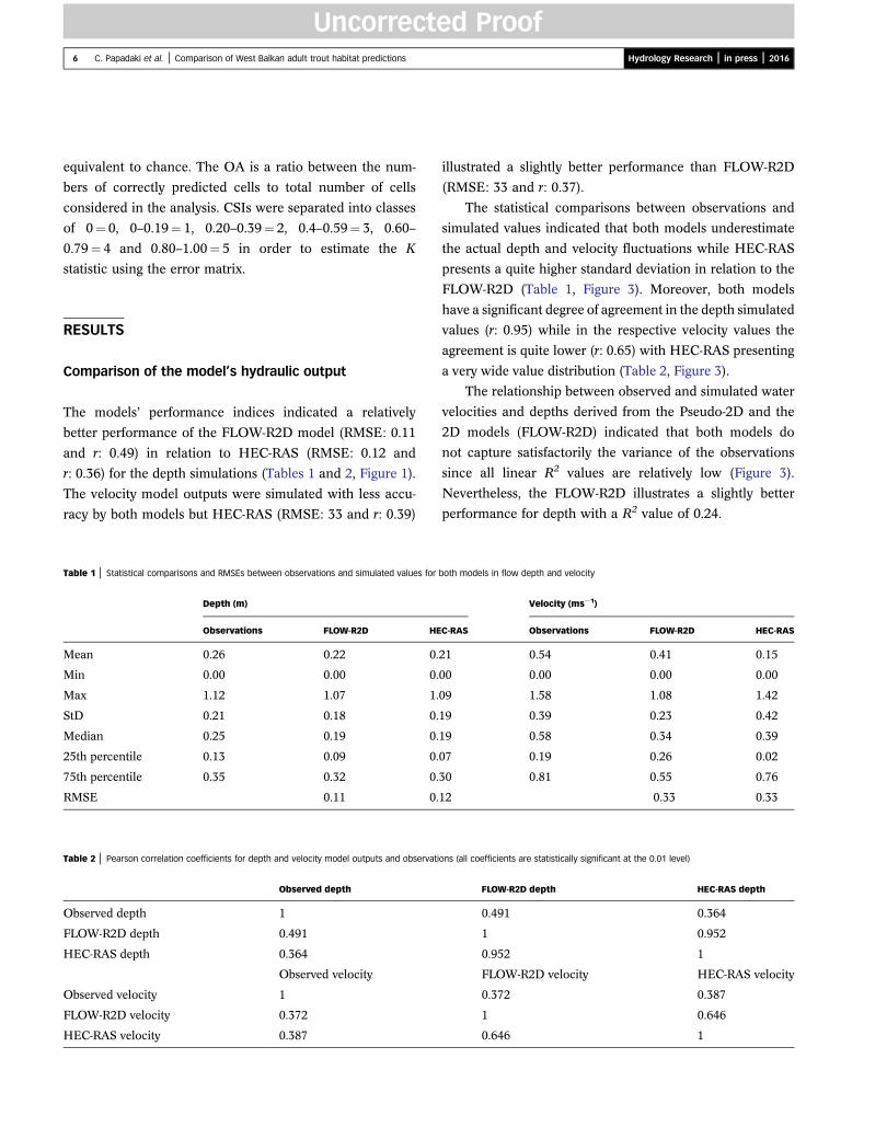
The comparison of the observed and estimated depths

and velocities in four characteristic cross sections for the

two models endorsed the aforementioned respective results.

In most cases the depth is relatively accurately estimated by

both models while the velocity illustrates significant discre-

pancies (Figure 4). In the particular four cross-sections,

HEC-RAS illustrated a slightly better performance regarding

velocity in comparison to the 2D model since its estimated

values follow more closely the observations’ fluctuations

(Figure 4).

Spatial distribution of the models’ outputs

From the spatial distribution of the model outputs, it was

observed that relatively small differences in the simulated

water depths derived from the Pseudo-2D and the 2D

model exist in all discharge scenarios (Figure 5). The most

distinctive differences between the two models were in the

average depth values (0.6–1 m) that were more spatially

extended in the FLOW-R2D outputs than in HEC-RAS.

Moreover, these differences became more pronounced as

the discharge increased from 2 to 6 m3 s�1 (Figure 5).

However, the estimated flow velocities between the two

models had greater differences (Figure 6). HEC-RAS indi-

cated significantly higher velocities in the discharge

scenarios of 2 and 4 m3 s�1 in relation to the FLOW-R2D

while in the discharge scenario of 6 m3 s�1 the differences

between the models were much lower (Figure 6). The

study reach has an inherent behaviour of a run-type river

with turbulence. This can be justified by the fact that flow

velocity varies rapidly in magnitude and direction, along

space and time, which underlines the capability of a

2D model to simulate complex flow distribution that a

Pseudo-2D model cannot.

After transforming the models’ estimated velocities and

depths for each discharge scenario into WUAs by using the

West Balkan adult trout CSI, a comparison diagram was cre-

ated (Figure 7). The results of the two models’ habitat

analysis show that the Pseudo-2D (HEC-RAS) model under-

estimates WUA0.5 for discharges over 3 m s�1 in comparison

with the 2D model, while the opposite occurs for lower

discharges (Figure 7). Moreover, following the peak WUA

values (Figure 7), the estimated best minimum ecological

flow differs significantly between the two models with

HEC-RAS indicating a value close to 2 m3 s�1 and FLOW-

R2D a value close to 6 m3 s�1. This is a very big difference

from a water management perspective and further in-depth

investigation should be performed in order to identify the

potential causes.

In Figure 8, habitat duration curves for summer conditions

(June–October) for the years 1986 to 2004 are presented for

both models. The discharge range was from 4 m3 s�1 to

45 m3 s�1. The results indicate that 30% of the time, habitat

area according to the 2Dmodel is equalled or exceeded in com-

parison with the Pseudo-2D model (HEC-RAS) results. In

contrast, 70% of the time the Pseudo-2D model (HEC-RAS)

indicated higher habitat area than the FLOW-R2D model.

Based on a graphical comparison (Figure 9) of the

spatially distributed CSI, the largest differences were near

Figure 4 | Comparison of measured and predicted water depths (m) and velocities (m s�1) at 4 m3 s�1 using the Pseudo-2D (HEC-RAS) and 2D (FLOW-R2D) hydrodynamic model.

8 C. Papadaki et al. | Comparison of West Balkan adult trout habitat predictions Hydrology Research | in press | 2016

Uncorrected Proof

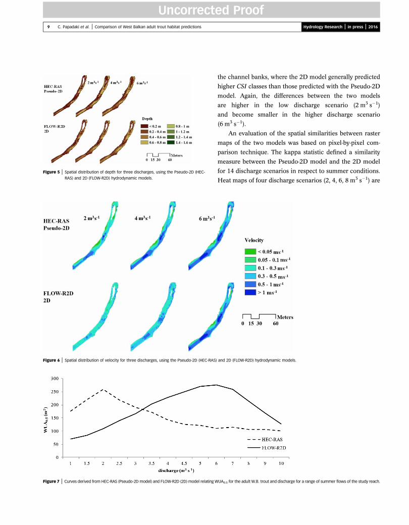
Figure 5 | Spatial distribution of depth for three discharges, using the Pseudo-2D (HEC-

RAS) and 2D (FLOW-R2D) hydrodynamic models.

Figure 6 | Spatial distribution of velocity for three discharges, using the Pseudo-2D (HEC-RAS

Figure 7 | Curves derived from HEC-RAS (Pseudo-2D model) and FLOW-R2D (2D) model relating W

9 C. Papadaki et al. | Comparison of West Balkan adult trout habitat predictions Hydrology Research | in press | 2016

Uncorrected Proof

the channel banks, where the 2D model generally predicted

higher CSI classes than those predicted with the Pseudo-2D

model. Again, the differences between the two models

are higher in the low discharge scenario (2 m3 s�1)

and become smaller in the higher discharge scenario

(6 m3 s�1).

An evaluation of the spatial similarities between raster

maps of the two models was based on pixel-by-pixel com-

parison technique. The kappa statistic defined a similarity

measure between the Pseudo-2D model and the 2D model

for 14 discharge scenarios in respect to summer conditions.

Heat maps of four discharge scenarios (2, 4, 6, 8 m3 s�1) are

) and 2D (FLOW-R2D) hydrodynamic models.

UA0.5 for the adult W.B. trout and discharge for a range of summer flows of the study reach.

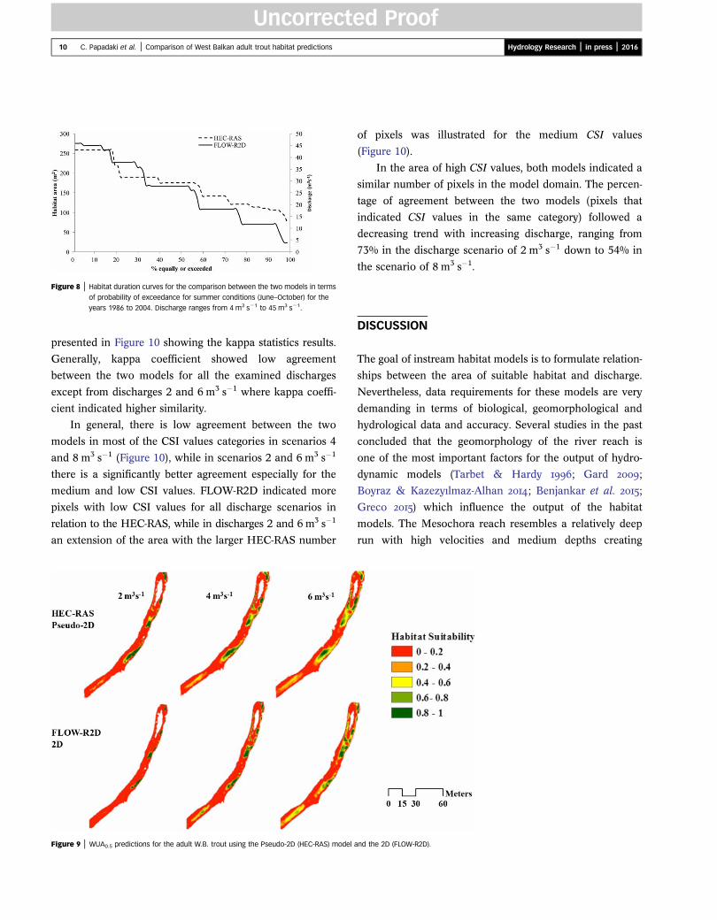
Figure 8 | Habitat duration curves for the comparison between the two models in terms

of probability of exceedance for summer conditions (June–October) for the

years 1986 to 2004. Discharge ranges from 4 m3 s�1 to 45 m3 s�1.

10 C. Papadaki et al. | Comparison of West Balkan adult trout habitat predictions Hydrology Research | in press | 2016

Uncorrected Proof

presented in Figure 10 showing the kappa statistics results.

Generally, kappa coefficient showed low agreement

between the two models for all the examined discharges

except from discharges 2 and 6 m3 s�1 where kappa coeffi-

cient indicated higher similarity.

In general, there is low agreement between the two

models in most of the CSI values categories in scenarios 4

and 8 m3 s�1 (Figure 10), while in scenarios 2 and 6 m3 s�1

there is a significantly better agreement especially for the

medium and low CSI values. FLOW-R2D indicated more

pixels with low CSI values for all discharge scenarios in

relation to the HEC-RAS, while in discharges 2 and 6 m3 s�1

an extension of the area with the larger HEC-RAS number

Figure 9 | WUA0.5 predictions for the adult W.B. trout using the Pseudo-2D (HEC-RAS) model a

of pixels was illustrated for the medium CSI values

(Figure 10).

In the area of high CSI values, both models indicated a

similar number of pixels in the model domain. The percen-

tage of agreement between the two models (pixels that

indicated CSI values in the same category) followed a

decreasing trend with increasing discharge, ranging from

73% in the discharge scenario of 2 m3 s�1 down to 54% in

the scenario of 8 m3 s�1.

DISCUSSION

The goal of instream habitat models is to formulate relation-

ships between the area of suitable habitat and discharge.

Nevertheless, data requirements for these models are very

demanding in terms of biological, geomorphological and

hydrological data and accuracy. Several studies in the past

concluded that the geomorphology of the river reach is

one of the most important factors for the output of hydro-

dynamic models (Tarbet & Hardy ; Gard ;

Boyraz & Kazezyılmaz-Alhan ; Benjankar et al. ;

Greco ) which influence the output of the habitat

models. The Mesochora reach resembles a relatively deep

run with high velocities and medium depths creating

nd the 2D (FLOW-R2D).

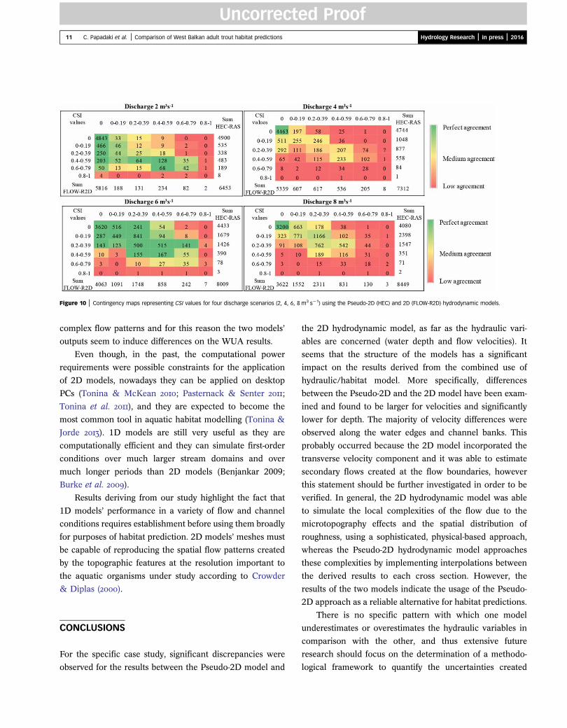
Figure 10 | Contingency maps representing CSI values for four discharge scenarios (2, 4, 6, 8 m3 s�1) using the Pseudo-2D (HEC) and 2D (FLOW-R2D) hydrodynamic models.

11 C. Papadaki et al. | Comparison of West Balkan adult trout habitat predictions Hydrology Research | in press | 2016

Uncorrected Proof

complex flow patterns and for this reason the two models’

outputs seem to induce differences on the WUA results.

Even though, in the past, the computational power

requirements were possible constraints for the application

of 2D models, nowadays they can be applied on desktop

PCs (Tonina & McKean ; Pasternack & Senter ;

Tonina et al. ), and they are expected to become the

most common tool in aquatic habitat modelling (Tonina &

Jorde ). 1D models are still very useful as they are

computationally efficient and they can simulate first-order

conditions over much larger stream domains and over

much longer periods than 2D models (Benjankar 2009;

Burke et al. ).

Results deriving from our study highlight the fact that

1D models’ performance in a variety of flow and channel

conditions requires establishment before using them broadly

for purposes of habitat prediction. 2D models’ meshes must

be capable of reproducing the spatial flow patterns created

by the topographic features at the resolution important to

the aquatic organisms under study according to Crowder

& Diplas ().

CONCLUSIONS

For the specific case study, significant discrepancies were

observed for the results between the Pseudo-2D model and

the 2D hydrodynamic model, as far as the hydraulic vari-

ables are concerned (water depth and flow velocities). It

seems that the structure of the models has a significant

impact on the results derived from the combined use of

hydraulic/habitat model. More specifically, differences

between the Pseudo-2D and the 2D model have been exam-

ined and found to be larger for velocities and significantly

lower for depth. The majority of velocity differences were

observed along the water edges and channel banks. This

probably occurred because the 2D model incorporated the

transverse velocity component and it was able to estimate

secondary flows created at the flow boundaries, however

this statement should be further investigated in order to be

verified. In general, the 2D hydrodynamic model was able

to simulate the local complexities of the flow due to the

microtopography effects and the spatial distribution of

roughness, using a sophisticated, physical-based approach,

whereas the Pseudo-2D hydrodynamic model approaches

these complexities by implementing interpolations between

the derived results to each cross section. However, the

results of the two models indicate the usage of the Pseudo-

2D approach as a reliable alternative for habitat predictions.

There is no specific pattern with which one model

underestimates or overestimates the hydraulic variables in

comparison with the other, and thus extensive future

research should focus on the determination of a methodo-

logical framework to quantify the uncertainties created

12 C. Papadaki et al. | Comparison of West Balkan adult trout habitat predictions Hydrology Research | in press | 2016

Uncorrected Proof

from models’ structure. It seems that as far as the water

depths is concerned, the differences between the Pseudo-

2D and 2D results were smaller (from ±0.30 m), with a

decreasing trend as the discharge increases. Regarding

flow velocities, the models’ outputs indicated higher differ-

ences (from ±0.60 m s�1), but no significant trend was

observed in relation to the discharge. It should be noted

that the local extreme differences which were observed

were excluded from the analysis since they were probably

caused by various inherent errors and biases, such as the

possible numerical oscillations in 2D modelling and the

interpolations implemented for the Pseudo-2D modelling.

Further research should be conducted to understand the

mechanisms associated with the biological responses from

the hydrodynamic behaviour of rivers. More parameters,

such as the substrate, the cover, the temperature and the

food availability should be incorporated in future similar

works in order to adapt a holistic approach in the ecological

flow estimations.

REFERENCES

Arthington, A. H., King, J. M., Okeeffe, J. H., Bunn, S. E., Day,J. A., Pusey, B. J., Bluhdorn, D. R. & Tharme, R. Development of an holistic approach for assessingenvironmental flow requirements of riverine ecosystems. In:Water Allocation for the Environment – Proceedings of anInternational Seminar and Workshop (J. J. Pigram & B. P.Hooper, eds). Armidale, Australia, pp. 69–76.

Barnes, H. H. Roughness characteristics of natural channels.U.S. Geological Survey, Water Supply Paper 1849 7 (3), 219.DOI: 10.1016/0022-1694(69)90113-9.

Bellos, V. & Tsakiris, G. a Comparing various methods ofbuilding representation for 2D flood modelling in built-upareas. Water Resources Management 29 (2), 379–397. DOI:10.1007/s11269-014-0702-3.

Bellos, V. & Tsakiris, G. b 2D Flood Modelling: the Case ofTous Dam Break. In: Proceedings of 36th World Congress ofIAHR Deltas of the Future and what Happens Upstream,28 June–3 July, The Hague, the Netherlands.

Bellos, V. & Tsakiris, G. A hybrid method for floodsimulation in small catchments combining hydrodynamicand hydrological techniques. Journal of Hydrology 540,331–339. DOI:10.1016/j.jhydrol.2016.06.040.

Benjankar, R., Tonina, D. & Mckean, J. One-dimensional andtwo-dimensional hydrodynamic modeling derived flowproperties: impacts on aquatic habitat quality predictions.

Earth Surface Processes and Landforms 40 (3), 340–356.DOI: 10.1002/esp.3637.

Bovee, K. D. Development and evaluation of habitatsuitability criteria for use in the instream flow incrementalmethodology. In: Instream Flow Information Paper #21FWS/ OBS-86/7 235, USDI Fish and Wildlife Service,Washington DC, USA.

Bovee, K. D. Perspectives on two-dimensional river habitatmodels: the PHABSIM experience. In: Ecohydraulics 2000Proceedings of Second International Symposium on HabitatHydraulics B (M. Leclerc, H. Capra, S. Valentin, A.Boudreault & Y. Côté, eds). INRS-Eau & FQSA, IAHR/AIRH, pp. B149–B162.

Bovee, K. D., Lamb, B. L., Bartholow, J. M., Stalnaker, C. B.,Taylor, J. & Henriksen, J. Stream habitat analysis usingthe instream flow incremental methodology. Information andTechnology Report 1998–0004 130. U.S. Geological Survey,Fort Collins, CO, USA.

Boyraz, U. & Kazezyılmaz-Alhan, C. M. An investigation onthe effect of geometric shape of streams on stream/groundwater interactions and ground water flow. HydrologyResearch 45 (4–5), 575–588. DOI: 10.2166/nh.2013.057.

Brown, R. A. & Gregory, B. P. Evaluation of energyexpenditure in adult spring Chinook salmon migratingupstream in the Columbia River basin: an assessment basedon sequential proximate analysis. River Research andApplications 25, 745–772. DOI: 10.1002/rra.

Burke, M. P., Jorde, K. & Buffington, J. M. Application of ahierarchical framework for assessing environmental impactsof dam operation: changes in streamflow, bed mobility andrecruitment of riparian trees in a western North Americanriver. Journal of Environmental Management 90, S224–S236.

Chow, V. T. Open Channel Hydraulics. McGraw-Hill,New York, USA.

Congalton, R. G. & Green, K. Assessing the Accuracy ofRemotely Sensed Data: Principles and Practices. CRC Press/Taylor & Francis Group, Boca Raton, FL, USA, p. 183.

Cowan, W. L. Estimating hydraulic roughness coefficients.Agricultural Engineering 37 (7), 473–475. DOI: 10.2514/2.6901.

Crowder, D. W. & Diplas, P. Using two-dimensionalhydrodynamic models at scale of ecological importance.Journal of Hydrology 230, 172–191.

Deletic, A., Dotto, C. B. S.,McCarthy, D. T., Kleidorfer,M., Freni, G.,Mannina, G., Uhl, M., Henrichs,M., Fletcher, T. D., Rauch,W.,Bertrand-Krajewski, J. L. & Tait, S. Assessing uncertaintiesin urban drainage models. Physics and Chemistry of the Earth42–44, 3–10. DOI: 10.1016/j.pce.2011.04.007.

Dunbar, M. J., Alfredsen, K. & Harby, A. Hydraulic-habitatmodelling for setting environmental river flow needs forsalmonids. Fisheries Management and Ecology 19 (6),500–517. DOI: 10.1111/j.1365-2400.2011.00825.x.

Dyson, M., Berkamp, G. & Scanlon, J. (eds.). Flow: TheEssentials of Environmental Flows. IUCN. Gland,Switzerland and Cambridge, UK. http://www.iucn.org/.

13 C. Papadaki et al. | Comparison of West Balkan adult trout habitat predictions Hydrology Research | in press | 2016

Uncorrected Proof

García, A., Jorde, K., Habit, E., Caamaño, D. & Parra, O. Downstream environmental effects of dam operations:changes in habitat quality for native fish species. RiverResearch and Applications 27, 312–327.

Gard, M. Comparison of spawning habitat predictions ofPHABSIM and River2D models. International Journal ofRiver Basin Management 7, 55–71. DOI: 10.1080/15715124.2009.9635370.

Greco, M. Effect of bed roughness on grain-size distribution inan open channel flow.Hydrology Research 46 (1), 1–10. DOI:10.2166/nh.2013.122.

Heggenes, J., Saltveit, J. & Lingaas, O. Predicting fish habitatuse to changes in water flow: modelling critical minimumflows for Atlantic salmon, Salmo salar, and brown trout, S.trutta. Regulated Rivers: Research and Management 12, 331–344. DOI: 10.1002/(SICI)1099-1646(199603)12:2/3< 331::AID-RRR399> 3.3.CO;2-5.

Hydrologic Engineering Center HEC-RAS River AnalysisSystem, Hydraulic Reference Manual. Hydraulic EngineeringCenter Report 69, US Army Corps of Engineers, Davis, CA,USA.

Katopodis, C. C. Ecohydraulic approaches in aquaticecosystems: integration of ecological and hydraulic aspects offish habitat connectivity and suitability. EcologicalEngineering 48, 1–7. DOI: 10.1016/j.ecoleng.2012.07.007.

Lai, G., Wang, P. & Li, L. Possible impacts of the Poyang lake(China)hydraulic project on lakehydrologyandhydrodynamics.Hydrology Research 1–19. doi:10.2166/nh.2016.174.

Leclerc, M., Boudreault, A., Bechara, J. A. & Corfa, G. Two-dimensional hydrodynamic modeling: a neglected tool in theinstream flow incremental methodology. Transactions of theAmerican Fisheries Society 124, 645–662.

Li, Q., Yu, M., Zhao, J., Cai, T., Lu, G., Xie, W. & Bai, X. Impact of the Three Gorges reservoir operation ondownstream ecological water requirements. HydrologyResearch 43 (1–2), 48–53. DOI: 10.2166/nh.2011.121.

Mao, J., Zhang, P., Dai, L., Dai, H. & Hu, T. Optimaloperation of a multi-reservoir system for environmental waterdemand of a river-connected lake. Hydrology Research 1–19.doi:10.2166/nh.2016.043.

Olsen, M., Boegh, E., Pedersen, S. & Pedersen, M. F. Impactof groundwater abstraction on physical habitat of browntrout (Salmo trutta) in a small Danish stream. HydrologyResearch 40 (4), 394–405. DOI: 10.2166/nh.2009.015.

Papadaki, C., Soulis, K., Muñoz-Mas, R., Martinez-Capel, F.,Zogaris, S., Ntoanidis, L. & Dimitriou, E. Potentialimpacts of climate change on flow regime and fish habitat inmountain rivers of the south-western Balkans. Science of theTotal Environment 540, 418–428. DOI: 10.1016/j.scitotenv.2015.06.134.

Pasternack, G. B. & Senter, A. 21st Century instream flowassessment framework for mountain streams. Public InterestEnergy Research (PIER), California Energy Commission.

Poff, N. L., Olden, J. D., Merritt, D. M. & Pepin, D. M. Homogenization of regional river dynamics by dams andglobal biodiversity implications. Proceedings of the NationalAcademy of Sciences of the United States of America 104(14), 5732–5737. DOI: 10.1073/pnas.0609812104.

R Core Team R: A Language and Environment for StatisticalComputing. Version 3.1.1. Vienna, Austria.

Refsgaard, J. C., van der Sluijs, J. P., Brown, J. & van der Keur, P. A framework for dealing with uncertainty due to modelstructure error. Advances in Water Resources 29 (11),1586–1597. DOI: 10.1016/j.advwatres.2005.11.013.

Richter, B. D. & Thomas, G. A. Restoring environmentalflows by modifying dam operations. Ecology and Society12 (1).

Tarbet, K. L. & Hardy, T. B. Evaluation of one-dimensionaland two-dimensional hydraulic modeling in a natural riverand implications. Part B. In: Ecohydraulics 2000.Proceedings of 2nd Symposium on Habitat Hydraulics(A. Leclerc, H. Capra, S. Valentin, A. Boudreault & Y. Côté,eds). Quebec, Canada, pp. 395–406.

Tharme, R. E. A global perspective on environmental flowassessment: emerging trends in the development andapplication of environmental flow methodologies for rivers.River Research and Applications 19 (5–6), 397–441. DOI: 10.1002/rra.736.

Tonina, D. & Jorde, K. Hydraulic modeling approaches forecohydraulic studies: 3D, 2D, 1D and non-numerical models.In: Ecohydraulics: An Integrated Approach (I. Maddock, P. J.Wood, A. Harby & P. Kemp, eds). Wiley-Blackwell, NewDelhi, India, pp. 31–66.

Tonina, D. & McKean, J. A. Climate change impact onsalmonid spawning in low-land streams in Central Idaho,USA. In: 9th International Conference on Hydroinformatics2010 (J. Tao, Q. Chen & S.-Y. Liong, eds). Chemical IndustryPress, Tianjin, China, pp. 389–397.

Tonina, D., McKean, J. A., Tang, C. & Goodwin, P. New toolsfor aquatic habitat modeling. In: 34th IAHR World Congress2011. IAHR, Brisbane, Australia, pp. 3137–3144.

Tsakiris, G. & Bellos, V. A numerical model for two-dimensional flood routing in complex terrains. WaterResources Management 28 (5), 1277–1291. DOI: 10.1007/s11269-014-0540-3.

Vadas, R. L. & Orth, D. J. Formulation of habitat suitabilitymodels for stream fish guilds: do the standard methodswork? Transactions of the American Fisheries Society 130(2), 217–235. DOI: 10.1577/1548-8659(2001)130< 0217:FOHSMF> 2.0.CO;2.

First received 24 May 2016; accepted in revised form 11 September 2016. Available online 5 December 2016