Unclassified DSTI/DOC(2004)9 - OECD

Unclassified DSTI/DOC(2004)9 Organisation de Coopération et de Développement Economiques Organisation for Economic Co-operation and Development 08-Oct-2004 ________________________________________________________________________________________________________ English text only DIRECTORATE FOR SCIENCE, TECHNOLOGY AND INDUSTRY

HANDBOOK ON HEDONIC INDEXES AND QUALITY ADJUSTMENTS IN PRICE INDEXES: SPECIAL APPLICATION TO INFORMATION TECHNOLOGY PRODUCTS STI WORKING PAPER 2004/9 Statistical Analysis of Science, Technology and Industry

Jack Triplett

JT00171062 Document complet disponible sur OLIS dans son format d'origine Complete document available on OLIS in its original format

DST

I/DO

C(2004)9

Unclassified

English text only

DSTI/DOC(2004)9

2

STI Working Paper Series

The Working Paper series of the OECD Directorate for Science, Technology and Industry is designed to make available to a wider readership selected studies prepared by staff in the Directorate or by outside consultants working on OECD projects. The papers included in the series cover a broad range of issues, of both a technical and policy-analytical nature, in the areas of work of the DSTI. The Working Papers are generally available only in their original language – English or French – with a summary in the other.

Comments on the papers are invited, and should be sent to the Directorate for Science, Technology and Industry, OECD, 2 rue André-Pascal, 75775 Paris Cedex 16, France.

The opinions expressed in these papers are the sole responsibility of the author(s) and do not necessarily reflect those of the OECD or of the governments of its member countries.

http://www.oecd.org/sti/working-papers

Copyright OECD, 2004 Applications for permission to reproduce or translate all or part of this material should be made to: OECD Publications, 2 rue André-Pascal, 75775 Paris, Cedex 16, France.

DSTI/DOC(2004)9

3

TABLE OF CONTENTS

BACKGROUND ............................................................................................................................................ 8

A. OECD initiative................................................................................................................................ 8 B. Related work by Eurostat ................................................................................................................. 8

CHAPTER I INTRODUCTION.................................................................................................................... 9

Relevance of quality adjustment for ICT products; potential impact of mismeasurement on international productivity comparisons; and purpose and outline of the volume............................................................. 9 Acknowledgements ................................................................................................................................... 11

CHAPTER II QUALITY ADJUSTMENTS IN CONVENTIONAL PRICE INDEX METHODOLOGIES12

A. Prologue: conventional price index methodology .......................................................................... 12 B. The inside-the-sample quality problem.......................................................................................... 15 C. Matched model methods: overlapping link .................................................................................... 18 D. Matched model methods: methods used in practice....................................................................... 20

1. Direct comparison method........................................................................................................ 21 2. The link-to-show-no-price-change method............................................................................... 23 3. The deletion, or imputed price change–implicit quality adjustment (IP-IQ), method .............. 24

a. The BLS “class mean” method ................................................................................................. 25 b. Evaluation of the deletion (IP-IQ) method ............................................................................... 26 c. Final comments on the deletion (IP-IQ) method ...................................................................... 29

4. Summary: four matched model methods .................................................................................. 29 5. Other methods........................................................................................................................... 30

a. Package size adjustments.......................................................................................................... 30 b. Options made standard.............................................................................................................. 31 c. Judgemental quality adjustments .............................................................................................. 32 d. Production cost quality adjustments ......................................................................................... 32

E. Conclusions to Chapter II............................................................................................................... 33

CHAPTER III HEDONIC PRICE INDEXES AND HEDONIC QUALITY ADJUSTMENTS ................ 41

A. Hedonic functions: a brief overview .............................................................................................. 42 B. Using the hedonic function to estimate a price for a computer ...................................................... 43

1. Estimating prices for computers that were available and for those that were not..................... 43 2. Estimating price premiums for improved computers................................................................ 45 3. Residuals................................................................................................................................... 46

C. Hedonic price indexes .................................................................................................................... 47 1. The time dummy variable method ............................................................................................ 48

a. The method explained............................................................................................................... 48 b. The index number formula for the dummy variable index ....................................................... 51 c. Comparing the dummy variable index and the matched model index: no item replacement ... 53 d. Comparing the dummy variable index and the matched model index: with item replacements54 e. Concluding remarks on the dummy variable method ............................................................... 55

2. The characteristics price index method..................................................................................... 56 a. The index .................................................................................................................................. 56 b. Applications .............................................................................................................................. 59 c. Comparing time dummy variable and characteristics price index methods.............................. 60 d. Concluding remarks on the characteristics price index method................................................ 64

3. The hedonic price imputation method ...................................................................................... 65

DSTI/DOC(2004)9

4

a. Motivation................................................................................................................................. 65 b. The imputation and the index ................................................................................................... 66 c. A double imputation proposal................................................................................................... 70

4. The hedonic quality adjustment method ................................................................................... 74 a. The method explained............................................................................................................... 75 b. Diagrammatic illustration ......................................................................................................... 76 c. Empirical comparisons with conventional methods ................................................................. 77 d. Criticism of the hedonic quality adjustment method and comparison with hedonic imputation method................................................................................................................................................ 78

D. The hedonic index when there are new characteristics .................................................................. 84 E. Research hedonic indexes............................................................................................................... 85 F. Conclusions: hedonic price indexes ............................................................................................... 86

APPENDIX A TO CHAPTER III HISTORICAL NOTE........................................................................... 87

APPENDIX B FOR CHAPTER III HEDONIC QUALITY ADJUSTMENTS AND THE OVERLAPPING LINK METHOD........................................................................................................................................... 90

CHAPTER IV WHEN DO HEDONIC AND MATCHED MODEL INDEXES GIVE DIFFERENT RESULTS? AND WHY? .......................................................................................................................... 105

A. Inside-the-sample forced replacements and outside-the-sample quality change.......................... 105 B. Fixed samples and price changes outside the sample................................................................... 107

1. Research studies...................................................................................................................... 107 2. Hedonic and FR&R indexes ................................................................................................... 110

C. Price changes outside FR&R samples.......................................................................................... 110 1. Case one.................................................................................................................................. 111 2. Case two.................................................................................................................................. 112 3. Case three................................................................................................................................ 112

D. Empirical studies .......................................................................................................................... 114 1. Early studies: research hedonic indexes and statistical agency matched model indexes........ 114 2. Same database studies: hedonic indexes and matched model indexes.................................... 115 3. Analysis .................................................................................................................................. 118

E. Market exits.................................................................................................................................. 120 F. Summary and conclusion ............................................................................................................. 120

1. Three price effects................................................................................................................... 121 2. Price measurement implications: FR&R and hedonic indexes ............................................... 122

a. Effectiveness........................................................................................................................... 122 b. Cost ......................................................................................................................................... 123

APPENDIX TO CHAPTER IV A MATCHED MODEL INDEX AND A NON-HEDONIC REGRESSION INDEX .............................................................................................................................. 125

CHAPTER V PRINCIPLES FOR ESTIMATING A HEDONIC FUNCTION: CHOOSING THE VARIABLES.............................................................................................................................................. 136

A. Introduction: best practice ............................................................................................................ 136 B. Interpreting hedonic functions: variables and coefficients........................................................... 137

1. Interpreting the variables in hedonic functions....................................................................... 137 2. Interpreting the coefficients in a hedonic function: economic interpretation ......................... 138 3. Interpretation of regression coefficients: statistical interpretation.......................................... 139

C. A case study: variables in computer hedonic functions ............................................................... 140 1. A bit of history: where did those computer characteristics come from?................................. 140 2. Variables in mainframe computer equipment studies: connection with PCs.......................... 141 3. Mainframe and PC computer components and characteristics ............................................... 142

DSTI/DOC(2004)9

5

4. Computer “boxes”, computer centres and personal computers .............................................. 144 D. Adequacy of the variable specifications in computer studies....................................................... 146

1. Comprehensiveness of performance variables for PCs: the Dell data .................................... 146 2. Benchmark measures of computer performance..................................................................... 147

a. What is a computer benchmark?............................................................................................. 148 b. Proxy variables and proper characteristics measures.............................................................. 149 c. Discussion............................................................................................................................... 149 d. Empirical implications............................................................................................................ 150

E. Specification problems in hedonic functions: omitted variables.................................................. 150 1. The uncorrelated case ............................................................................................................. 151

a. The hedonic coefficients (uncorrelated case).......................................................................... 151 b. The hedonic index (uncorrelated case) ................................................................................... 151

2. The correlated cases................................................................................................................ 153 a. The hedonic coefficients (correlated case).............................................................................. 153 b. The hedonic index (correlated case) ....................................................................................... 155

F. Interpreting the coefficients – again ............................................................................................. 158 G. Specification problems in hedonic functions: proxy variables..................................................... 159 H. Choosing characteristics: some objections and misconceptions .................................................. 161

1. Is the choice of characteristics subjective? ............................................................................. 161 2. The choice of characteristics should be based on economic theory........................................ 161 3. No-one can know the characteristics ...................................................................................... 162

CHAPTER VI ESTIMATING HEDONIC FUNCTIONS: OTHER RESEARCH ISSUES..................... 172

A. Introduction .................................................................................................................................. 172 B. Multicollinearity........................................................................................................................... 172

1. Sources of multicollinearity.................................................................................................... 173 a. Multicollinearity in the universe............................................................................................. 173 b. Multicollinearity in the sample ............................................................................................... 174 c. Conclusion: sources and consequences of multicollinearity................................................... 176

2. Detecting multicollinearity ..................................................................................................... 176 3. Multicollinearity and data errors............................................................................................. 177 4. Interpreting coefficients in the presence of multicollinearity ................................................. 178 5. Multicollinearity in hedonic functions: assessment ................................................................ 179

C. What functional forms should be considered? ............................................................................. 180 1. Functional forms in hedonic studies ....................................................................................... 180 2. Hedonic contours .................................................................................................................... 180 3. Choosing among functional forms.......................................................................................... 181 4. Theory and hedonic functional forms ..................................................................................... 182 5. Hedonic functional form and index formula........................................................................... 186 6. Functional form and heteroscedasticity .................................................................................. 186 7. Non-smooth hedonic functional forms ................................................................................... 187 8. Conclusion on hedonic functional forms ................................................................................ 188 9. A caveat: functional form for quality adjustment ................................................................... 188

D. To weight or not to weight?.......................................................................................................... 189 1. We want a weighted hedonic function because we want a weighted hedonic index number. 190 2. Do we want sales weighted hedonic coefficients?.................................................................. 190

a. Low sales weights: first illustration ........................................................................................ 191 b. Low sales weights: a second illustration................................................................................. 191 c. Discussion............................................................................................................................... 192 d. Hedonic estimates of implicit prices for characteristics ......................................................... 192

3. Econometric issues.................................................................................................................. 193

DSTI/DOC(2004)9

6

4. Conclusion on weighting hedonic functions: research procedures ......................................... 193 E. CPI vs PPI hedonic functions ....................................................................................................... 194

1. Do hedonic functions measure resource cost or user value?................................................... 194 2. Can hedonic functions from producers’ price data be used for the CPI?................................ 196

CHAPTER VII SOME OBJECTIONS TO HEDONIC INDEXES .......................................................... 208

A. The criticism that hedonic indexes fall too fast............................................................................ 209 1. General statements .................................................................................................................. 209 2. Computer price indexes fall too fast ....................................................................................... 209

a. The price indexes .................................................................................................................... 210 b. Plausibility .............................................................................................................................. 210

3. Summary................................................................................................................................. 214 B. Technical criticisms of hedonic indexes....................................................................................... 215

1. General criticisms ................................................................................................................... 215 a. Functional form....................................................................................................................... 215 b. Transparency and reducibility................................................................................................. 215

2. The CNSTAT panel report...................................................................................................... 217

THEORETICAL APPENDIX: THEORY OF HEDONIC FUNCTIONS AND HEDONIC INDEXES. 223

A. Hedonic functions......................................................................................................................... 223 1. The buyer, or user, side........................................................................................................... 226 2. Forming measures of “quality”............................................................................................... 228 3. The production side................................................................................................................. 229 4. Special cases ........................................................................................................................... 230

a. Identical buyers....................................................................................................................... 230 b. Identical Sellers....................................................................................................................... 231 c. Identical buyers and sellers..................................................................................................... 231 d. Conclusion: functional forms for hedonic functions............................................................... 231

B. Hedonic indexes ........................................................................................................................... 232 1. The exact characteristics-space index..................................................................................... 233

a. The characteristics-space exact index: overall........................................................................ 233 b. The exact characteristics price index: subindexes for computers and other products ............ 234

2. Information requirements........................................................................................................ 234 3. Bounds and approximation: empirical hedonic price indexes ................................................ 235 4. Conclusion: exact characteristics-space indexes..................................................................... 235

C. Recent developments.................................................................................................................... 236 1. The identification problem...................................................................................................... 236 2. The problem with estimating smooth hedonic contours ......................................................... 237

REFERENCES ........................................................................................................................................... 240

DSTI/DOC(2004)9

7

HANDBOOK ON HEDONIC INDEXES AND QUALITY ADJUSTMENTS IN PRICE INDEXES: SPECIAL APPLICATION TO INFORMATION TECHNOLOGY PRODUCTS

Jack E. Triplett Brookings Institution

Washington, DC

Abstract

This handbook reviews the methods employed in price indexes to adjust for quality change: “conventional” quality adjustment methods, which are explained in Chapter II, and hedonic price indexes (Chapter III). Hedonic indexes have a prominent place in price indexes for information and communication technology (ICT) products in several OECD countries, and are also used for measuring prices for some other goods and services, notably housing. The handbook’s objective is to contribute to a better understanding of the merits and shortcomings of conventional and hedonic methods, and to provide an analytic basis for choosing among them.

This handbook compares and contrasts the logic and statistical properties of hedonic methods and conventional methods and the results of employing them in different circumstances. In Chapter IV, it reviews empirical evidence on the difference that alternative methods make in practice, and offers an evaluation framework for determining which is better. In Chapters III, V, and VI, the handbook sets out principles for “best practice” hedonic indexes. These principles are drawn from experience with hedonic studies on a wide variety of products. Although most of the examples in the handbook are drawn from ICT products, the principles in it are very general and apply as well to price indexes for non-ICT products that experience rapid quality change, and also to price indexes for services, which are affected by quality changes fully as much as price indexes for goods, though sometimes that has not been recognised sufficiently.

Some objections that have been raised to hedonic indexes are presented and analysed in Chapter VII. An appendix discusses issues of price index theory that apply to quality change, and presents the economic theory of hedonic functions and hedonic price indexes.

The handbook brings together material that is now scattered in a wide number of places, but goes beyond the economic literature in significant respects. The handbook has been written because there is a widespread view that the principles for conducting hedonic investigations are not written down fully anywhere. Research practices have just coalesced from procedures used by the most rigorous researchers. They are not therefore readily assembled for statistical agency work which is the primary audience of the handbook, although researchers involved in empirical work in areas such as productivity, innovation and technological or structural change will also benefit from the discussion of methods, theory and its application to ICT.

DSTI/DOC(2004)9

8

BACKGROUND

A. OECD initiative

Over the past years, the Statistical Working Party of the OECD Industry Committee has dealt with several different aspects of productivity measurement and analysis. One of these issues was the impact of using different price indices for constructing volume output measurements of information and communication (ICT) industries. At the international level, there are different approaches in this field, often leading to widely diverging profiles of ICT price indices. As a consequence, international comparability of trends in volume output measures of certain industries but also volume measures of final demand components can be hampered. As there exists no concise source of information to assess and compare the different approaches and to bring together the advantages and inconveniences associated with each of them, the Working Party launched a project [DSTI/EAS/IND/SWP(98)4] for a handbook on ICT deflators.

The Working Party identified as main objectives of the handbook to:

• Provide an accessible guide to the different approaches towards constructing ICT deflators, to permit officials involved in producing and using such series making informed choices.

• Discuss, in particular, some of the arguments that have surrounded the construction and use of hedonic methods in deriving price indices and compare them with more traditional practices.

• Improve international harmonisation by increasing transparency about different countries practices in this field and by providing methodological guidance for new work.

To advance work in a relatively specialised area, the Secretariat set up a small steering group of experts. This steering group has so far met twice (19 November 1999 and 22 June 2000) to discuss consecutive drafts of chapters 1-4 of the handbook, prepared by Mr. Jack Triplett (Brookings Institution), consultant to the OECD. The present document presents the revised version, in which the chapters are reorganised and expanded, and a theoretical appendix has been added.

B. Related work by Eurostat

In 1999, Eurostat launched several Taskforces to investigate into price and volume measures of different parts of National Accounts. One of these taskforces reviewed price and volume measures for computers and software. This review of current practices revealed a large variety of quality adjustment procedures in European countries. Different practices were assessed and preferred methods identified, among them the hedonic approach. Subsequently, Eurostat established the European Hedonic Centre to explore the question of hedonic indexes for countries of the European Community.

OECD and Eurostat work are highly complementary: whereas the Eurostat Task Force undertook a broad review of the issue with a view to recommending certain methods and to advise against others, the OECD Handbook aims at significantly more detail in its theoretical and practical detail of the issue of quality adjustment and the construction of hedonic price indices. There has been close interaction between the OECD and the Eurostat so as to ensure complementarity and to avoid duplication. Additionally, Mr. Triplett, the author of this document, was involved in the European Hedonic Centre, which provided another link.

DSTI/DOC(2004)9

9

CHAPTER I

INTRODUCTION

Relevance of quality adjustment for ICT products; potential impact of mismeasurement on international productivity comparisons; and purpose and outline of the volume

Deflators for real output, real input, and real investment – for producing productivity measures or value added in national accounts – are derived primarily from price indexes estimated by statistical agencies. Whether the deflators are consumer (retail) price indexes (CPI or RPI) or producer (wholesale) price indexes (PPI or WPI), quality change has long been recognised as perhaps the most serious measurement problem in estimating price indexes (among the many possible references are: Hofsten, 1952; Stone, 1956; Price Statistics Review (Stigler) Committee, 1961; Nicholson, 1967; Griliches, 1971; Boskin Commission, 1996; Eurostat, 1999).

In national accounts, any error in the deflators creates an exactly equivalent error of opposite sign in the real output, real input, real investment and real consumption measures (which are hereafter referred to as “quantity indexes”1). For this reason, discussing the problems posed by quality change in price indexes is the same thing as discussing the problems of quality change in quantity indexes, and therefore in measures of productivity change as well.

There is tremendous interest in understanding the contribution of ICT products to economic growth and to measures of labour productivity (see, for example, Schreyer, 2001). These are products that show very rapid rates of quality change, and accordingly they throw the quality adjustment problem in price indexes into high relief.

Different quality adjustment methodologies are employed for ICT products across OECD countries, and they seemingly make large differences in the trends of price movements for these products. Wyckoff (1995) reported that changes in computer equipment deflators among OECD countries ranged from plus 80% to minus 72% for the decade of the 1980s; the largest decline occurred in the US hedonic price indexes for computer equipment.

A Eurostat Task Force (Eurostat, 1999), reviewing ICT indexes for the early 1990s, found a smaller dispersion among European countries’ ICT deflators. But still, price declines recorded by national computer deflators in Europe ranged from 10% to 47%, and again, the largest price decline was recorded by a hedonic price index (France). The Task Force calculated that price variation in this range could affect GDP growth rates by as much as 0.2%-0.3% per year, depending on the size of a country’s ICT sector. International comparisons of productivity growth would be affected by approximately the same magnitude.

If different quality adjustment procedures among OECD countries make the data noncomparable, then the measured growth of ICT investment and of ICT capital stocks will not be comparable across OECD 1. The 1993 System of National Accounts (Commission of the European Communities et al., 1993) uses the

term “volume indexes”. However, in both the index number literature and in normal English language usage in economics, quantity index is the preferred term, so this handbook follows general usage, rather than the specialized language that has developed in national accounts.

DSTI/DOC(2004)9

10

countries. Data noncomparability for ICT deflators, investment and capital stocks therefore creates serious limitations to making international comparisons of economic growth and understanding international differences in productivity trends and levels and sources of growth. And when ICT data are not internationally comparable, estimates of the impact of ICT on economic growth in different OECD countries will have limited, if any, meaningfulness.

As the Wyckoff (1995) and Eurostat (1999) studies suggest, hedonic price indexes show rapidly declining ICT prices in most countries in which they have been estimated. Conventional methodologies for adjusting for quality change generally yield smaller price declines for ICT products; in some countries conventional methodologies have even produced rising ICT price indexes in the past.

This handbook reviews the methods employed in price indexes to adjust for quality change. A natural division is between “conventional” methods typically employed by the statistical agencies of many OECD countries, which are discussed in Chapter II, and hedonic methods for adjusting for quality change (alternatively known as hedonic price indexes). The latter have a prominent place in price indexes for ICT products in several OECD countries. Hedonic methods for producing quality-adjusted price indexes are reviewed in Chapter III.

The handbook brings together material that is now scattered in a wide number of places, but goes beyond the economic literature in significant respects, particularly in the comparison of conventional and hedonic methods in Chapter IV. This handbook compares and contrasts the logic of hedonic methods and conventional methods and the results of employing them in different circumstances. Although most of the examples in the handbook are drawn from ICT products, the principles in it are very general and apply as well to price indexes for non-ICT products that experience rapid quality change, and also to price indexes for services, which are affected by quality changes fully as much as price indexes for goods, though sometimes that has not sufficiently been recognised.

The handbook sets out principles for “best practice” hedonic indexes (in Chapters III, V, and VI). These principles are drawn from experience with hedonic studies on a wide variety of products. The handbook has been written because there is a widespread view that the principles for conducting hedonic investigations are not written down fully anywhere, partly because they have just coalesced from procedures used by the most rigorous researchers. They are not therefore readily assembled for statistical agency work. Again, the best practice examples in this handbook are drawn primarily from research on ICT equipment, but they apply as well to hedonic investigations of all products, and not just ICT products. For example, there is a huge literature on hedonic functions and hedonic price indexes in housing markets, both rental units and the house prices themselves. Though the examples in the handbook were drawn from ICT products, not primarily from housing markets, the analysis and the principles apply to housing market hedonic functions.

Chapter VII considers some objections that have been raised to hedonic indexes. An appendix discusses some issues of price index theory and applications to hedonic price indexes; though much of what is written in the manual depends on the theory, this material is placed at the end as a reference document, in order to make the operational parts of the manual more accessible.

With respect to statistical agencies in OECD countries, the handbook is descriptive, not prescriptive, and in this sense its purpose differs from, for example, the System of National Accounts (Commission of the European Communities et al., 1993). For the professional audience, the handbook contributes to a better understanding of the merits and shortcomings of conventional quality adjustment methods and of hedonic price indexes. The best practice principles developed in Chapters V and VI supplement other sources, such as the chapter on hedonic indexes in the empirically-oriented econometrics textbook by Berndt (1991).

DSTI/DOC(2004)9

11

The handbook is complementary to two other works in preparation by international statistical organisations. An updated international manual on consumer price indexes, to replace the ILO manual (Turvey, 1989) will have a chapter on quality change in consumer price indexes. A parallel manual for producer price indexes will also discuss the problem of adjusting for quality change. This handbook goes somewhat beyond the other two in its discussion of methodologies, in its comparison of the merits and shortcomings of conventional and hedonic methods, and in its descriptive chapters V and VI, which provide guidelines for conducting hedonic studies.

Note by Jack Triplett

In a report on national accounts prepared for the OECD, Richard Stone (1956) included a section on the use of hedonic price indexes to improve the deflators for national accounts. Stone’s was the second contribution on hedonic price indexes in the economics literature, following by 17 years the initial contribution of Andrew Court (1939), and preceding by five years the influential study by Zvi Griliches (1961).

This handbook represents a return by the OECD to the work initiated by Stone 50 years ago. In the intervening years, a great amount of empirical work on hedonic price indexes has taken place, and they have been introduced into the national accounts of a number of countries, the first being a hedonic price index for new house construction, introduced into the United States national accounts in 1974. Yet, many outstanding issues in the construction and interpretation of hedonic price indexes remain, and their use remains somewhat controversial, 50 years after Stone suggested their value for national accounts. By bringing together in one place material that is now scattered through many publications and is accordingly inaccessible to statistical agency practitioners and researchers alike, this handbook is intended to enhance understanding of hedonic price indexes and hedonic methods for making quality adjustments.

The handbook is dedicated to the memory of Stone, who introduced the topic of hedonic indexes to national accounts, and of Griliches, whose work on hedonic indexes and on quality change greatly advanced knowledge on both topics, and who is largely responsible for the state of the art as it is known today.

Acknowledgements

This handbook has benefited from the input from many people, some within statistical agencies, some in the OECD, and some in academic and research institutions. I cannot thank them all, but extremely valuable contributions beyond the usual professional norm were provided by Ernst R. Berndt, Mick Silver, and my colleague, Charles Schultze. The exposition and content were also enriched by presentations, and especially discussions with participants, at the following: The Industry Committee meetings at the OECD, the Deutsche Bundesbank Symposium on Hedonic Methods in Price Statistics (Wiesbaden, June, 2001), the ZEW conference Price Indices and Quality Change (University of Mannheim, April 25-26, 2002), the Brookings Institution Workshop on Economic Measurement “Hedonic Indexes: Too Fast, Too Slow or Just Right?” February 1, 2002, and courses on price indexes and quality change at the University of Orebro, June 2003, and the University of Maryland’s Joint Program on Statistical Methodology, December, 2003.

DSTI/DOC(2004)9

12

CHAPTER II

QUALITY ADJUSTMENTS IN CONVENTIONAL PRICE INDEX METHODOLOGIES

A. Prologue: conventional price index methodology

Agencies that estimate price indexes employ, nearly universally, one fundamental methodological principle. The agency chooses a sample of sellers (retail outlets in the case of consumer price indexes, or CPIs, producers for producer price indexes, or PPIs) and of products. It collects a price in the initial period2 for each of the products selected. Then, at some second period it collects the price for exactly the same product, from the same seller, that was selected in the initial period. The price index is computed by matching the price for the second period with the initial price, observation by observation, or “model by model,” as it is often somewhat inaccurately called.

The full rationale for this “matched model” methodology is seldom explicitly stated, and its advantages sometimes are not fully appreciated. Matching, it is well known, is a device for holding constant the quality of the goods and services priced for the index. Indeed, one significant source of price index error occurs when the matching methodology breaks down for some reason – some undetected change in the product makes the match inexact or the product observed in the initial period disappears and cannot be matched in the second. These situations impart quality change errors into the ostensibly matched price comparisons. Analysis of quality change errors is one major topic of this handbook.

Another aspect of the matched model methodology is less commonly perceived: Matching also holds constant many other price determining factors that are usually not directly observable. For example, matching on sellers holds constant, approximately, retailer characteristics such as customer service, location, or in-store amenities for CPI price quotations. For the PPI, matching holds constant, again approximately, unobserved reliability of the product, the reputation of the manufacturer for after-market service, willingness to put defects right or to respond to implicit warranties, and so forth. Although controlling for quality change is one of its objectives, matching the price quotes model by model is not just a methodology for holding quality constant in the items selected for pricing. It is also a methodology for holding constant nonobservable aspects of the transactions that might otherwise bias the measure of price change.

The problem of quality change potentially arises in price indexes whenever transactions are not homogeneous. It thus affects all price indexes, not just price indexes for high tech products, or price indexes for goods and services that are thought, by some measure, to experience rapid quality change. Even if the commodity is homogeneous (which is itself so infrequent empirically that it is of little practical importance), transactions are not homogeneous. It is transactions that matter in a price index. The matched model method is a device that is intended to hold constant the characteristics of transactions.

2. Index number terminology is not standard. The point at which samples are initiated is seldom the index

base period, so this first period might be called the “initiations period”, however, in some price index programs, the first or the first several prices that are collected after sample initiation are not actually used in calculating the index. Accordingly, I write first (or initial) and second (or comparison) periods in the text, to avoid ambiguity.

DSTI/DOC(2004)9

13

Nonobservables in transactions may be incompletely controlled by the matching methodology. Oi (1992) suggests that changes in the quantity and types of retailing services may have been ignored in the matching process, producing bias in retail price indexes. Manufacturers may become less willing or more assiduous in responding to buyers’ claims under warranties or in responding to implicit warranties or in offering after-market service. When changes in retailing or after-market services are not fully taken into account, they create errors in matched model indexes.

Moreover, buyers switch from one seller to another in search of a more favourable price/services combination. For example, personal computers (PCs) are increasingly sold over the Internet, rather than in retail computer stores. Consumers on average evidently value the retailing services provided by “brick and mortar” stores by less than the price differential between them and on-line sellers. When buyers switch between distribution outlets, they may experience true price changes that are more favorable than the ones that the matched model, matched-outlet method measures. These issues are not confined to ICT equipment price indexes. The Boskin Commission (1996) maintained that what it called “outlet substitution bias” caused the US Consumer Price Index to overstate inflation. Saglio (1994) contains data on shifting sales across sellers of chocolate bars in the French CPI, and his study implies similar questions about outlet bias. Although buyers may value the services provided by traditional French retailers, they sometimes put a value on these services that are less than the price differential between high-service and low-service retail outlets. Switching away from traditional retailers toward hypermarkets and other newer distribution channels provides gains to buyers, gains that are inevitably missed by the matched-model, matched-outlet methodology.

Matching thus does not always hold everything constant that should be held constant. As well, the matched-model, matched-outlet method may not capture some price changes that are relevant to buyers. But clearly, matching is better than not matching. The changes in nonobservables for one seller that occur between one pricing period and the next (a month, or a quarter) must be far smaller than the much larger unobservable differences that exist across different sellers. Simple unit value indexes (ratios of average prices per unit across sellers) that do not control at all for unobservable variables will normally contain more errors than matched model indexes, not fewer.3

As the following chapters show, some methods that have been proposed for computing quality-adjusted price indexes imply modifying or replacing the matched model methodology. Price index agencies have been reluctant to adopt alternatives that require abandoning the matched model methodology. Sometimes this has been interpreted as a reluctance to embrace new methods for handling quality change in the items selected for the indexes. It may be that. But it may be more. One does not want to solve one set of problems at the cost of incurring others. The virtues as well as the shortcomings of the matched model method need to be evaluated in assessing proposals for improved methods for handling quality change in price indexes. Subsequent sections of Chapter II address some of these issues, and others are confronted in Chapter IV.

As the foregoing implies, dealing with quality change in price indexes is part of the problem of estimating price index basic components – indexes for cars and computers, for books and bananas, for dry 3. Some recent price index articles have suggested unit values as the first step in computing an “elementary

aggregate” or “basic component” (Diewert, 1995 and Balk, 1999). This is surprising, in view of the old wisdom that unit values always hide a quality change problem. For example, Allen (1975) remarked: “Unit values are tempting substitutes for prices; they are often easily obtained from the data and look like prices… However…they reflect both changes in quoted prices and shifts in the varieties bought and sold.” The “shift” that Allen referred to can cover services provided by retailers that are not measured explicitly by the price-collecting agency. Balk remarks that Diewert “typically thinks of a homogeneous commodity.” Homogeneous commodities are rare and homogeneous transactions are rarer. Unit values are always suspect and provide no solution to the problem of computing basic components.

DSTI/DOC(2004)9

14

cleaning and dental services – the fundamental, lowest-order indexes from which an aggregate CPI or PPI is constructed.4 The estimation of basic components has received much attention in recent years, and the topic remains in active ferment. Much of the literature on basic components concerns the form of the index – use of a geometric mean rather than an arithmetic mean and so forth – which has typically been approached as another form of the classic index number formula problem (see, for example, Diewert, 1995, and Balk, 1999). Another strand of thinking about basic components concerns changes in index number compilation methods and new collection strategies, such as using scanner data (see the contributions in Feenstra and Shapiro, eds., 2003).

One cannot consider quality change methods in isolation from index sampling and compilation methods, nor ignore formulas and estimation considerations for the basic components. As well, one cannot consider other aspects of index methodology independently of the questions posed by quality change. For example, price index compilers know that quality change is one of their most difficult problems; accordingly, when they use judgemental sampling (employed widely for selecting the product varieties for pricing), they often select varieties that are not likely to change in subsequent periods, in order to reduce the incidence of quality changes encountered. But this judgemental sampling strategy for minimizing the incidence of quality changes implies that the representativeness of the index sample is compromised, which introduces error of its own. Choosing a methodology for making quality adjustments in price indexes – that is, for situations when matching is not possible – requires paying attention as well to other aspects of price index methodology, such as sampling or lower-level index formulas and calculating methods, lest attention to one kind of price index error lead inadvertently to another. Although these are important matters that interact with the problem of dealing with quality change in price indexes, I must necessarily neglect sampling, estimators and so forth in this handbook, even if they have implications for what is included, and even if some of the issues discussed in the handbook have implications (which they do) for other aspects of price index number methodology. This handbook cannot cover all aspects of price index methodology.5

However, one of these interactions between quality change and index methodology cannot be ignored. In recent price index literature a distinction has arisen between quality change inside the sample and outside the sample. The first of these problems – the “inside the sample” problem – concerns the questions: What are the methods used for handling quality changes in the varieties selected for the index? What are their implications? Can better methods be devised? Pakes (2003) remarks that in the price index literature quality change is something that happens within the sample. The present chapter considers the inside the sample problem, especially the first two questions.

The “outside the sample” problem arises when quality change or price change occurs on some products that have not been selected for the index. Use of judgemental samples, or lags in introducing new product varieties into the price index when probability sampling is employed, may cause outside the sample errors because the sample is not representative of price changes, or has become unrepresentative. Another class of outside the sample quality changes are price changes that are implied by the very introduction of new and improved ICT equipment, no matter how rapidly new products are brought into

4. The lowest-level price indexes in a CPI or PPI are called “basic components” or “elementary price

indexes.” Turvey (2000) prefers the term “elementary aggregates,” which is also used widely. In OECD countries, they are mostly unweighted indexes, and a number of calculating formulas are in use.

5. Manuals for CPIs and PPIs are being prepared under the auspices of the Inter-secretariat Working Group on Price Statistics. The paper by Greenlees (2000), which was prepared as an input to the CPI manual, covers some of the same ground as this chapter, with special though not exclusive emphasis on US experience. For European countries, Hoven (1999) presents a discussion of quality change in the Dutch CPI, and Dalén (1998) presents similar information for Sweden. Armknecht and Maitland-Smith (1999) provide a review that cuts across experience in various countries.

DSTI/DOC(2004)9

15

the index, and no matter how large or how representative is the price index sample. Though these are also sampling problems, they are uniquely connected to quality change because they arise from the introduction of new and improved product varieties, and for this reason need to be addressed in this handbook as part of the problem of dealing with quality change in price indexes.

For ICT products, these outside the sample quality and price changes may be as important as inside the sample quality changes. Chapter IV considers the outside the sample quality change problem, after the intervening Chapter III, which has as its subject hedonic methods for estimating quality-adjusted price indexes.

B. The inside-the-sample quality problem

From the “matched model” terminology for describing the fundamental methodology for compiling price indexes, the term “matched model” has also come to refer to a quality adjustment method – or actually, a group of methods. In this usage, “matched model” means that price comparisons are used in the index only when the models can be matched. “Matched models only” is perhaps a better term to describe this methodology, and indeed the term “model” is not a very good one. In this handbook, I use the terms “model” and “variety” (or “product variety”) interchangeably.6

For many products, determining when a match exists is not an obvious matter. Model numbers, product names, and so forth can change when there is no change in the product itself. Conversely, the product can change with no change in product nomenclature to signal it.

Some countries rely only on the price collecting agent’s knowledge of the product variety priced in the initial period to confirm the match in the second. More typically, a statistical agency maintains a pricing specification for each product that lists the characteristics of the product that are deemed to be important. Hoven (1999, page 3) states, of the Netherlands CPI: “…specifications of the article to be priced…which are provided centrally, are as tight as possible”; in the Dutch case, the specification often includes the brand. Moulton, LaFleur and Moses (1999) reproduce the actual US CPI specification for television sets, which lists the characteristics that are controlled in matched model comparisons (this specification is reproduced as an example in Figure 2.1).

The pricing specification usually documents as well the size of the variation in product characteristics that is acceptable for a match, and therefore specifies whether matching is achieved. Small changes in quality, or those that are judged to have inconsequential effects on the price, may be ignored. For example, in the “flow chart” for the US BLS methodology (Figure 2.2) the following question is asked of a product replacement: Are “quality changes within the range of specification?” A “match” is thus not necessarily an exact match, but country statistical agencies typically limit the range in the specification that is acceptable for a match. In some countries, these decisions are left to the pricing agent, but in most they are controlled or reviewed centrally.

The “quality adjustment problem” that has to be solved is a consequence of situations where the old model and its replacement cannot be matched within the limits of the agency’s pricing specification.

What happens when a match is not achieved? Prices that are collected for models that are not matched are not used in the index, or they are not used directly, or they are “adjusted” before being used, or else a

6. Turvey (2000) suggests rejecting “variety” on the grounds that the French equivalent (varieté) has acquired

a special meaning in the French CPI. However, this should not preclude international usage of the English word in English language documents, otherwise through extensions we will have a very impoverished vocabulary.

DSTI/DOC(2004)9

16

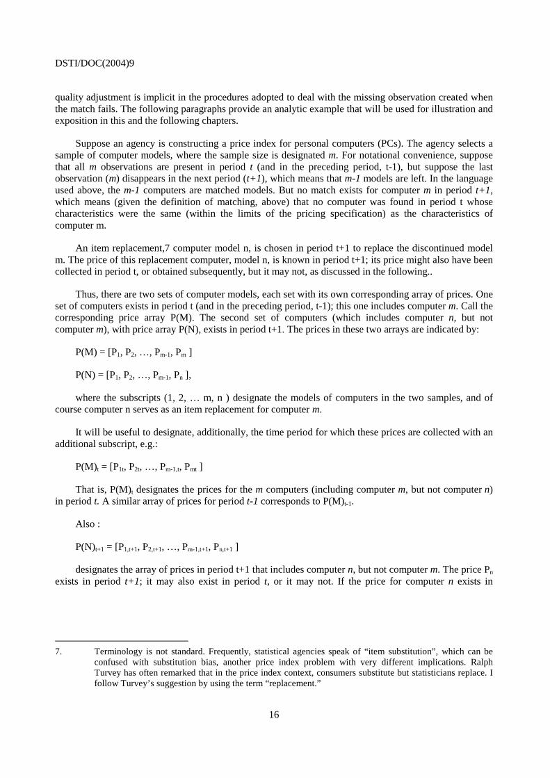
quality adjustment is implicit in the procedures adopted to deal with the missing observation created when the match fails. The following paragraphs provide an analytic example that will be used for illustration and exposition in this and the following chapters.

Suppose an agency is constructing a price index for personal computers (PCs). The agency selects a sample of computer models, where the sample size is designated m. For notational convenience, suppose that all m observations are present in period t (and in the preceding period, t-1), but suppose the last observation (m) disappears in the next period (t+1), which means that m-1 models are left. In the language used above, the m-1 computers are matched models. But no match exists for computer m in period t+1, which means (given the definition of matching, above) that no computer was found in period t whose characteristics were the same (within the limits of the pricing specification) as the characteristics of computer m.

An item replacement,7 computer model n, is chosen in period t+1 to replace the discontinued model m. The price of this replacement computer, model n, is known in period t+1; its price might also have been collected in period t, or obtained subsequently, but it may not, as discussed in the following..

Thus, there are two sets of computer models, each set with its own corresponding array of prices. One set of computers exists in period t (and in the preceding period, t-1); this one includes computer m. Call the corresponding price array P(M). The second set of computers (which includes computer n, but not computer m), with price array P(N), exists in period t+1. The prices in these two arrays are indicated by:

P(M) = [P1, P2, …, Pm-1, Pm ]

P(N) = [P1, P2, …, Pm-1, Pn ],

where the subscripts (1, 2, … m, n ) designate the models of computers in the two samples, and of course computer n serves as an item replacement for computer m.

It will be useful to designate, additionally, the time period for which these prices are collected with an additional subscript, e.g.:

P(M)t = [P1t, P2t, …, Pm-1,t, Pmt ]

That is, P(M)t designates the prices for the m computers (including computer m, but not computer n) in period t. A similar array of prices for period t-1 corresponds to P(M)t-1.

Also :

P(N)t+1 = [P1,t+1, P2,t+1, …, Pm-1,t+1, Pn,t+1 ]

designates the array of prices in period t+1 that includes computer n, but not computer m. The price Pn exists in period t+1; it may also exist in period t, or it may not. If the price for computer n exists in

7. Terminology is not standard. Frequently, statistical agencies speak of “item substitution”, which can be

confused with substitution bias, another price index problem with very different implications. Ralph Turvey has often remarked that in the price index context, consumers substitute but statisticians replace. I follow Turvey’s suggestion by using the term “replacement.”

DSTI/DOC(2004)9

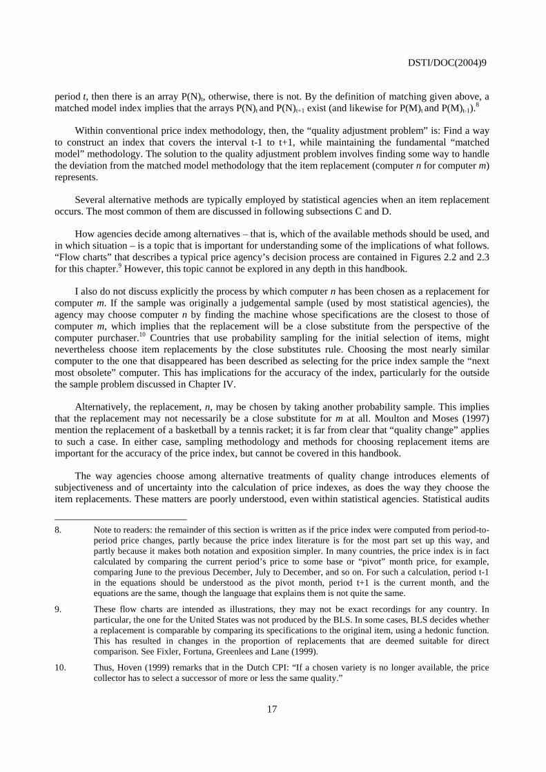
17

period t, then there is an array P(N)t, otherwise, there is not. By the definition of matching given above, a matched model index implies that the arrays P(N)t

and P(N)t+1 exist (and likewise for P(M)t and P(M)t-1).

8

Within conventional price index methodology, then, the “quality adjustment problem” is: Find a way to construct an index that covers the interval t-1 to t+1, while maintaining the fundamental “matched model” methodology. The solution to the quality adjustment problem involves finding some way to handle the deviation from the matched model methodology that the item replacement (computer n for computer m) represents.

Several alternative methods are typically employed by statistical agencies when an item replacement occurs. The most common of them are discussed in following subsections C and D.

How agencies decide among alternatives – that is, which of the available methods should be used, and in which situation – is a topic that is important for understanding some of the implications of what follows. “Flow charts” that describes a typical price agency’s decision process are contained in Figures 2.2 and 2.3 for this chapter.9 However, this topic cannot be explored in any depth in this handbook.

I also do not discuss explicitly the process by which computer n has been chosen as a replacement for computer m. If the sample was originally a judgemental sample (used by most statistical agencies), the agency may choose computer n by finding the machine whose specifications are the closest to those of computer m, which implies that the replacement will be a close substitute from the perspective of the computer purchaser.10 Countries that use probability sampling for the initial selection of items, might nevertheless choose item replacements by the close substitutes rule. Choosing the most nearly similar computer to the one that disappeared has been described as selecting for the price index sample the “next most obsolete” computer. This has implications for the accuracy of the index, particularly for the outside the sample problem discussed in Chapter IV.

Alternatively, the replacement, n, may be chosen by taking another probability sample. This implies that the replacement may not necessarily be a close substitute for m at all. Moulton and Moses (1997) mention the replacement of a basketball by a tennis racket; it is far from clear that “quality change” applies to such a case. In either case, sampling methodology and methods for choosing replacement items are important for the accuracy of the price index, but cannot be covered in this handbook.

The way agencies choose among alternative treatments of quality change introduces elements of subjectiveness and of uncertainty into the calculation of price indexes, as does the way they choose the item replacements. These matters are poorly understood, even within statistical agencies. Statistical audits

8. Note to readers: the remainder of this section is written as if the price index were computed from period-to-

period price changes, partly because the price index literature is for the most part set up this way, and partly because it makes both notation and exposition simpler. In many countries, the price index is in fact calculated by comparing the current period’s price to some base or “pivot” month price, for example, comparing June to the previous December, July to December, and so on. For such a calculation, period t-1 in the equations should be understood as the pivot month, period t+1 is the current month, and the equations are the same, though the language that explains them is not quite the same.

9. These flow charts are intended as illustrations, they may not be exact recordings for any country. In particular, the one for the United States was not produced by the BLS. In some cases, BLS decides whether a replacement is comparable by comparing its specifications to the original item, using a hedonic function. This has resulted in changes in the proportion of replacements that are deemed suitable for direct comparison. See Fixler, Fortuna, Greenlees and Lane (1999).

10. Thus, Hoven (1999) remarks that in the Dutch CPI: “If a chosen variety is no longer available, the price collector has to select a successor of more or less the same quality.”

DSTI/DOC(2004)9

18

can throw light on them, but have too infrequently been carried out. Work within Eurostat (Dalén, 2002; Ribe, 2002) is enlightening. It has often been asserted that hedonic methods contain subjective elements, which is true (Schultze and Mackie, eds., 2002); but this assertion is apparently coupled with the premise that “conventional” methods do not. This is a misconception.

C. Matched model methods: overlapping link

The “overlap” method dominates the discussion of quality change, especially in the older price index literature. The terminology for this case, as elsewhere in the quality change literature, is unfortunately not standard: The words “link” and “splice” and “overlap” are all employed, but the first two, especially, are applied to many different situations, so that their meaning has become obscure.11 To minimize ambiguity, I will use the term “overlapping link” method, which is described in the following.

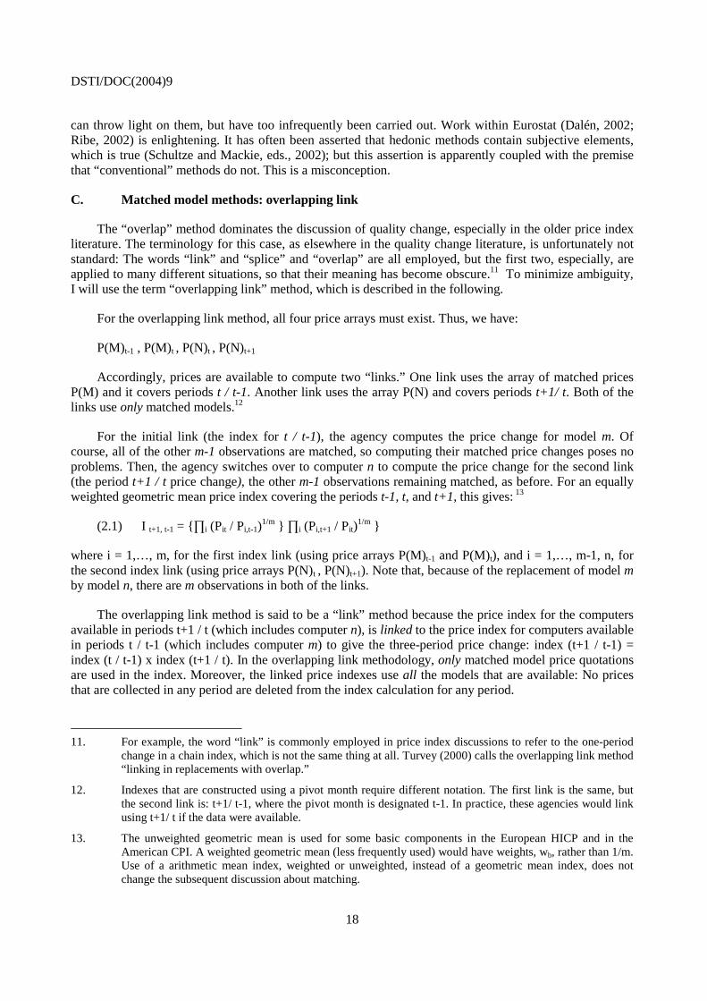
For the overlapping link method, all four price arrays must exist. Thus, we have:

P(M)t-1 , P(M)t , P(N)t , P(N)t+1

Accordingly, prices are available to compute two “links.” One link uses the array of matched prices P(M) and it covers periods t / t-1. Another link uses the array P(N) and covers periods t+1/ t. Both of the links use only matched models.12

For the initial link (the index for t / t-1), the agency computes the price change for model m. Of course, all of the other m-1 observations are matched, so computing their matched price changes poses no problems. Then, the agency switches over to computer n to compute the price change for the second link (the period t+1 / t price change), the other m-1 observations remaining matched, as before. For an equally weighted geometric mean price index covering the periods t-1, t, and t+1, this gives: 13

(2.1) I t+1, t-1 = {∏i (Pit / Pi,t-1)1/m } ∏i (Pi,t+1 / Pit)

1/m }

where i = 1,…, m, for the first index link (using price arrays P(M)t-1 and P(M)t), and i = 1,…, m-1, n, for the second index link (using price arrays P(N)t , P(N)t+1). Note that, because of the replacement of model m by model n, there are m observations in both of the links.

The overlapping link method is said to be a “link” method because the price index for the computers available in periods t+1 / t (which includes computer n), is linked to the price index for computers available in periods t / t-1 (which includes computer m) to give the three-period price change: index (t+1 / t-1) = index (t / t-1) x index (t+1 / t). In the overlapping link methodology, only matched model price quotations are used in the index. Moreover, the linked price indexes use all the models that are available: No prices that are collected in any period are deleted from the index calculation for any period.

11. For example, the word “link” is commonly employed in price index discussions to refer to the one-period

change in a chain index, which is not the same thing at all. Turvey (2000) calls the overlapping link method “linking in replacements with overlap.”

12. Indexes that are constructed using a pivot month require different notation. The first link is the same, but the second link is: t+1/ t-1, where the pivot month is designated t-1. In practice, these agencies would link using t+1/ t if the data were available.

13. The unweighted geometric mean is used for some basic components in the European HICP and in the American CPI. A weighted geometric mean (less frequently used) would have weights, wb, rather than 1/m. Use of a arithmetic mean index, weighted or unweighted, instead of a geometric mean index, does not change the subsequent discussion about matching.

DSTI/DOC(2004)9

19

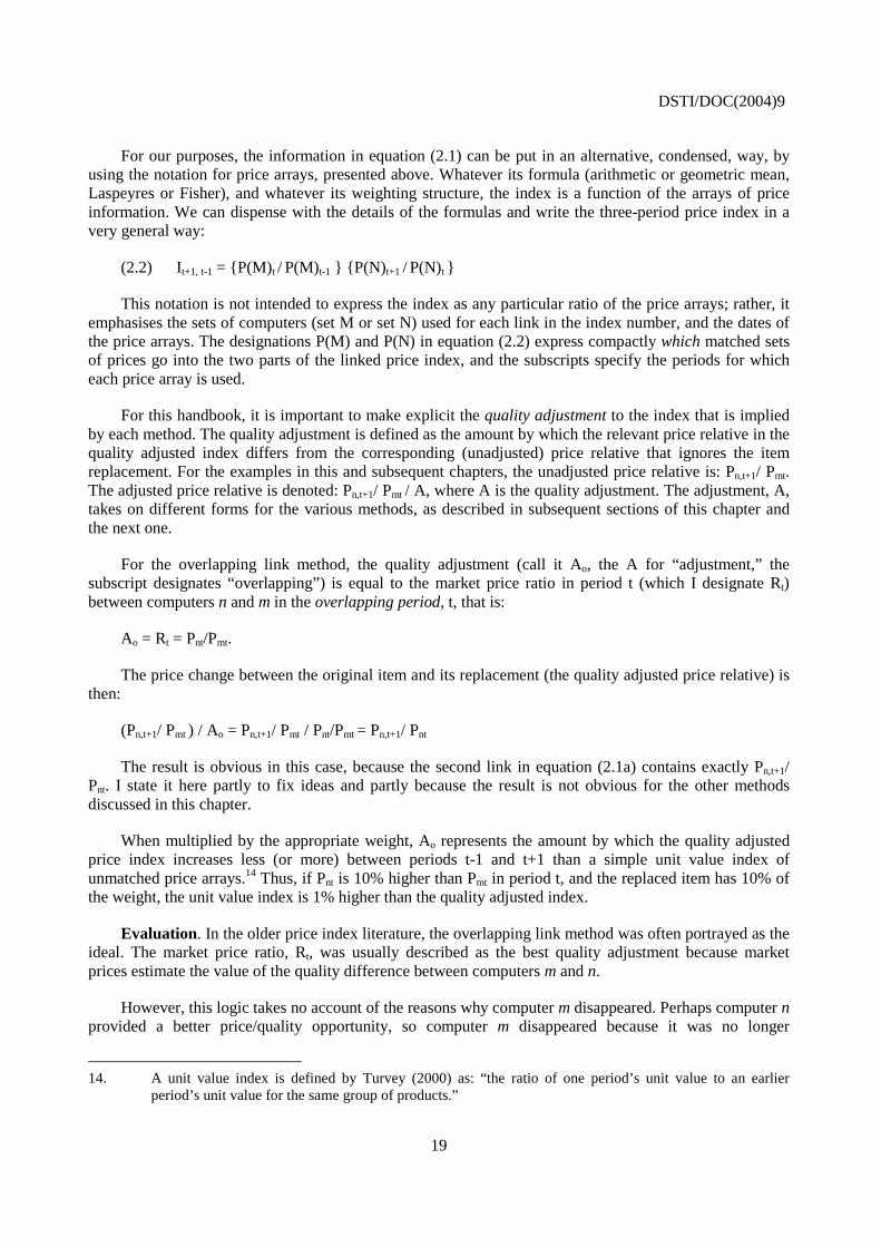
For our purposes, the information in equation (2.1) can be put in an alternative, condensed, way, by using the notation for price arrays, presented above. Whatever its formula (arithmetic or geometric mean, Laspeyres or Fisher), and whatever its weighting structure, the index is a function of the arrays of price information. We can dispense with the details of the formulas and write the three-period price index in a very general way:

(2.2) It+1, t-1 = {P(M)t / P(M)t-1 } {P(N)t+1 / P(N)t }

This notation is not intended to express the index as any particular ratio of the price arrays; rather, it emphasises the sets of computers (set M or set N) used for each link in the index number, and the dates of the price arrays. The designations P(M) and P(N) in equation (2.2) express compactly which matched sets of prices go into the two parts of the linked price index, and the subscripts specify the periods for which each price array is used.

For this handbook, it is important to make explicit the quality adjustment to the index that is implied by each method. The quality adjustment is defined as the amount by which the relevant price relative in the quality adjusted index differs from the corresponding (unadjusted) price relative that ignores the item replacement. For the examples in this and subsequent chapters, the unadjusted price relative is: Pn,t+1/ Pmt. The adjusted price relative is denoted: Pn,t+1/ Pmt / A, where A is the quality adjustment. The adjustment, A, takes on different forms for the various methods, as described in subsequent sections of this chapter and the next one.

For the overlapping link method, the quality adjustment (call it Ao, the A for “adjustment,” the subscript designates “overlapping”) is equal to the market price ratio in period t (which I designate Rt) between computers n and m in the overlapping period, t, that is:

Ao = Rt = Pnt/Pmt.

The price change between the original item and its replacement (the quality adjusted price relative) is then:

(Pn,t+1/ Pmt ) / Ao = Pn,t+1/ Pmt / Pnt/Pmt = Pn,t+1/ Pnt

The result is obvious in this case, because the second link in equation (2.1a) contains exactly Pn,t+1/ Pnt. I state it here partly to fix ideas and partly because the result is not obvious for the other methods discussed in this chapter.

When multiplied by the appropriate weight, Ao represents the amount by which the quality adjusted price index increases less (or more) between periods t-1 and t+1 than a simple unit value index of unmatched price arrays.14 Thus, if Pnt is 10% higher than Pmt in period t, and the replaced item has 10% of the weight, the unit value index is 1% higher than the quality adjusted index.

Evaluation. In the older price index literature, the overlapping link method was often portrayed as the ideal. The market price ratio, Rt, was usually described as the best quality adjustment because market prices estimate the value of the quality difference between computers m and n.

However, this logic takes no account of the reasons why computer m disappeared. Perhaps computer n provided a better price/quality opportunity, so computer m disappeared because it was no longer

14. A unit value index is defined by Turvey (2000) as: “the ratio of one period’s unit value to an earlier

period’s unit value for the same group of products.”

DSTI/DOC(2004)9

20

competitive in the price/quality dimension with the new computer, n. Then, since Pmt is in the denominator of the expression for Ao, and is too high (relative to the quality of computer m), Rt (=Ao ) < A*, where A* designates the correct quality adjustment. The quality adjusted index should fall, relative to the measure obtained from the overlapping link method, because the true quality adjustment is larger than what is implied by the overlapping link. The price index is upward biased in this case because the new variety offered a more favourable price/quality ratio (it had a lower “quality-adjusted” price) than the former one, and this price reduction is not reflected in the index.

Alternatively, perhaps computer m was on sale just before it disappeared from the particular seller from whom prices had been collected in the past; it was being used as a “loss leader” to increase store traffic. Using the price collected during the sale to calculate Rt may result in a quality adjustment that is too large. The price index is downward biased in this case because some of the “return to normal” price increase is inappropriately treated as the value of the quality change by the overlapping link method.

Another possibility: Perhaps computer m was serving a market niche. It was better than computer n for those buyers who bought it, but computer m’s manufacturer withdrew it or went out of business because its price did not cover its cost. For those buyers who actually bought computer m, A* < 1; accordingly, Rt (> 1) is not only too large an adjustment, it indeed goes in the wrong direction. The price index should rise for those users (that is, the method is downward biased) because the more favourable price/quality ratio offered by computer m is no longer available.15 Pakes (2003) suggests that producers with market power might discontinue the “good buys” because they are less profitable; if so, this causes the index to miss quality-corrected price increases paid by some buyers, which would not be detected by the overlapping link method.

Thus, the overlapping link method conceals some potentially serious problems for implementing the matched models only index, and contains potential biases. But even though it may be less ideal, conceptually, than has sometimes been thought, the real difficulty with the overlapping link method is that it can seldom be implemented. Normally, the pricing agency does not have prices for both computers m and n in the overlap period. The overlapping link method is seldom used because the data for implementing it do not exist. In the session on quality change at the 1999 Reykjavik meeting of the International Working Group on Price Indices (the Ottawa group), I asked the statistical agencies represented whether any of them were able routinely to implement the overlapping link method. None among those present indicated that the method was frequently employed in their countries. Assertions to the contrary that have sometimes been made reflect the confusion that has arisen from using the word “link” (without qualifying adjective) to cover a variety of methods.

Comment. The importance of the overlapping link method is not its empirical or pragmatic importance, because it is not in fact employed with any frequency. However, the method has more or less provided the framework for reasoning about the quality adjustment methods that have actually been utilised when overlapping prices are not available.

D. Matched model methods: methods used in practice

In actual application, the available price arrays are:

15. This is not likely to happen if computer m was better for everyone. Heterogeneity among buyers and

manufacturers is discussed at greater length in the subsequent chapter on hedonic price indexes. It is fundamental to the conceptual foundations of hedonic methods. Moreover, recognition that there are many buyers and sellers, and that the aggregate index number must be thought of as an average across many buyers who may differ in their preferences for computers (or any other product) is an emerging problem in the construction of price indexes that has not yet been resolved in a fully satisfactory manner.

DSTI/DOC(2004)9

21

P(M)t-1 , P(M)t , P(N)t+1

The array P(N)t , which contains the crucial price Pnt, does not exist, so no overlapping, matched price exists for the replacement computer, model n.

Several major alternatives have been used in practice. For the first link of equation (2.1), all methods compose the index out of matched price quotes from the arrays:

P(M)t-1, P(M)t

In this, they are identical with the overlapping link method. Indeed, most of the practical methods are predominantly matched models only methods.

For the second link in equation (2.1), most operational methods estimate the missing price, Pnt , or estimate the missing market price ratio, Rt (sometimes implicitly), or impute the quality-adjusted price relative (Pn,t+1/ Pmt ) / A. These estimates either require an explicit quality adjustment or imply an implicit quality adjustment.

The first two methods discussed below (“direct comparison” and “link-to-show-no-price-change”) can be thought of as methods in which the statistical agency makes assumptions about the unobserved market price ratio, Rt. In the third method (section D.3), an estimate of the price change for the replaced computer is made (that is, one estimates Pm,t+1/Pm,t), based on price change information for the m-1 models that can be matched from arrays P(M)t and P(N)t+1. Several other methods are grouped together in section D.4.

The discussion of each of these methods focuses on its shortcomings as an estimate of Rt, as defined in the previous section. However, one should keep in mind as well that Rt might have its own bias, for the reasons stated above. Chapters III and IV, which discuss hedonic quality adjustments, contain additional analysis of conditions under which Rt is or is not an appropriate way to think about the desired quality adjustment.

1. Direct comparison method16

One approach for estimating Rt is to assume there is no quality difference between computer m and its replacement, n. The price index is constructed by “direct comparison” of computers m and n.

With a judgemental sample, perhaps the price statistics agency has chosen the replacement computer, n, by actually searching out the computer with specifications closest to the one that disappeared (m). A probability sampling method for choosing the items might still be combined with a “most similar item” replacement rule (Lane, 2001, pages 10 and 14; Fixler, Fortuna, Greenlees, and Lane, 1999). Or even if this is not the case, the commodity analyst may judge that the replacement is essentially equivalent in quality to the old computer, so that direct comparison of the new and the old is the appropriate way of handling the quality change (see the flow charts at the end of this chapter).

In the direct comparison method, the quality adjustment (designate it A1) is unity, by assumption or analyst’s judgement. The estimate for the market price ratio Rt (est1 Rt) is also unity because the direct

16. This has long been the English language name. Turvey (2000) suggests another name for this method, but

also notes that it is called “comparaison directe” in French, which is an obvious cognate for the usual term in English. Bascher and Lacroix (1999) use the term “equivalent” in French, which they translate into English as “direct comparison.” This suggests retaining the usual English usage.

DSTI/DOC(2004)9

22

comparison method implies an imputation for the missing price for computer n in period t (call this est Pnt) that is equal to the actual, observed price for computer m in the same period (est Pnt = Pmt). Thus, we have:

A1 = 1, by assumption, so

Est Pnt = Pmt , and

Est1 Rt = est Pnt / Pmt = Pmt / Pmt = 1

The estimated price change (∆) for this replacement is based on the ratio of actual, observed prices for the new and old computers:

Est1 (1 + ∆t+1,t ) = Pn,t+1 / Pmt.

The index for periods t+1 / t is based on direct comparison of all the prices in the price arrays: P(M)t

and P(N)t+1 (because m and n are deemed a match).

If the inside-sample quality changes are improvements, then using the direct comparison method biases price indexes upward, regardless of the direction that prices are actually changing. If quality is deteriorating, then the direct comparison method biases price indexes downward.

A complete statement would pay attention to the pricing specification for the product. Statistical agencies of most countries use the direct comparison method only for those item replacements where quality differences are small, by some measure – for example, a manual for the operating system is no longer supplied, but in other respects the replacement computer is the same as the old one. Larger or more significant quality changes (increases in computer speed, memory, or included software) are usually handled by some other method (see the flow charts in Figures 2.2 and 2.3). This means that direct comparisons will only be permitted for relatively small quality changes. Then, conditional on quality changes being small, both negative and positive quality changes may be observed, even when the unconditional quality changes are on balance improvements.

In the critical writings about price indexes emanating from outside statistical agencies (particularly in the United States), authors have often presumed that direct comparison is the typical or dominant way that quality changes are handled by statistical agencies. Quality changes, it often is alleged, are usually either ignored when they are encountered, or not detected at all. On balance, the argument goes, quality change biases price indexes upward. This conclusion, however, applies only to circumstances where all, or nearly all, quality changes are handled by direct comparison.

In the most comprehensive analysis so far, Moulton and Moses (1997) indicate that 65% of item replacements in the US CPI in 1995 were treated as direct comparisons.17 For the “entertainment goods and services” component, Moulton and Moses (1997) report that 59% of the product replacements were treated as direct comparisons. Electronics products in the US CPI are mostly located in the “entertainment goods” component (though some were in housing before the most recent revision).

Moulton and Moses (1997 – see their Table 7) present data on these direct comparisons. Their data suggest the following conclusions: (1) direct comparisons are indeed made frequently when quality changes are encountered; (2) they are normally made for small quality differences; (3) the average price

17. See their Table 4: item replacements accounted for 3.90% of total price quotations for the year, and direct

comparisons (they use the term “comparable items”) were 2.54% of the price quotations; 2.54 / 3.90 = 65.1%.

DSTI/DOC(2004)9

23

increase for direct comparison cases was about the same as the quality-adjusted price increase for cases that received explicit quality adjustments (2.51% in the month in which replacement occurred and 2.66%, respectively). This behaviour of quality-adjusted indexes does not suggest serious upward bias from the direct comparisons that are actually made in the US CPI, probably because direct comparison is used only for small quality changes, and for these both positive and negative quality changes occur.

2. The link-to-show-no-price-change method18

As before, the arrays of available prices are:

P(M)t-1 , P(M)t , P(N)t+1

The link-to-show-no-price-change method applies the opposite assumption from the direct comparison method – all of the difference between the price of the replacement computer and the price of the old one is assumed to be quality change. That is, designating the quality adjustment as A2 and the estimate of the price ratio between m and n at time t as est2 Rt:

A2 = Pn,t+1/Pm.

est2 Rt = Pn,t+1/Pm

Because by assumption no true price change has taken place between periods t and t+1 and between computers m and n (∆t+1,t = zero), the estimated price relative that goes into the index is:

Est2 (1 + ∆t+1,t ) = 1.

Where the direct comparison method implies that the entire price change between the old computer model and its replacement is inflation, the link-to-show-no-price-change method implies no inflation at all. It biases the index downward when prices are rising, and biases them upward when (true, quality-adjusted) prices are falling. However, statistical agencies frequently note in their documentations cases where the price of the replacement item is lower, but its quality is judged higher. In those cases, the link-to-show-no-price-change method will not be employed, and the obvious bias avoided. Its frequent use in cases where the bias is not so obvious does not mean that there is no bias.

Note that the bias of the link-to-show-no-price-change method does not depend on whether quality is improving or deteriorating. It depends, instead, on whether prices are rising or falling. Oddly, the critical literature on price indexes has paid very little attention to the bias that results from the link-to-show-no-price-change method. Instead, it has focused almost exclusively on the bias from the direct comparison method. For example, Gordon (1990), in his book on US investment goods price indexes, does not discuss the use in the US PPI of the link-to-show-no-price-change method, and neglects the implication that it produces downward bias (in inflationary periods) in the price indexes that use it. The mostly downward biases that are created by the link-to-show-no-price-change method have been known at least since the discussion in Triplett (1971), and probably before.

18. The term adopted here is in use, though not universally. It is used by Hoven (1999) in referring to the

Dutch CPI, for example. It has the virtue of indicating the effect of the action. This method is sometimes just called the “link” method, without distinguishing it from either the overlapping link method (discussed in section II.C, above) or the deletion (IP-IQ) method (subsection II.D.3, below), which is called by the same name. Lowe (1999) refers to it as “splice” but splice has been used in numerous ways in the price index literature. Basher and Lacroix (1999) use “dissemblable” as the French term for the link-to-show-no-change method.

DSTI/DOC(2004)9

24

The link-to-show-no-price-change method has been used in many countries, including the Canadian CPI (see Lowe, 1999), and the producer price index (PPI) in the United States. Eurostat has banned this method for compiling harmonised indexes of consumer price indexes (HICP). However, Dalén (2002) and Ribe (2002) document its use in Austrian and Swedish national CPIs in the late 1990s, and Hoven (1999) records it as a method in use for the Dutch CPI.

3. The deletion, or imputed price change–implicit quality adjustment (IP-IQ), method

In this method, the prices for both computer m and computer n are dropped (that is, deleted) from the index for the link month, t. Then, the price index for computers is calculated from the other m-1 models in the sample, ignoring both computer m and its replacement, n. The name “deletion method” expresses what is actually done when quality change is encountered: It is the only conventional quality adjustment method in which both observed prices are discarded.

The effect of the deletion method is one of the most misunderstood aspects of price index numbers. Effectively, the price change for the item replacement in the sample is imputed from price changes of the other items whose quality did not change in the same component of the index (hence, imputed price, or IP). No explicit assumption about quality change is made. However, imputing price change in this fashion creates an implicit quality adjustment (IQ), as explained in the following. The alternative name used in this handbook (IP-IQ) emphasizes these two properties of the method. 19

Because the analysis of the deletion (IP-IQ) method is somewhat complicated, it may be helpful to state the conclusions at the outset. Suppose that quality is improving. Then, the deletion (IP-IQ) method misses some price change – up or down – because it inappropriately counts some price change as quality change. If prices are rising, the method implicitly overadjusts for quality change, and understates inflation. If prices are falling (usually the case with computers), the method symmetrically misses some of the price decline because it implicitly underadjusts for quality change. The direction of bias in the index is thus more a function of the direction of price change than of the direction of quality change, in the sense that quality improvements are consistent with upward or downward bias in the index. The reasoning is developed in the following paragraphs.

19. Again, there is no standard terminology. One would like terminology to convey accurately what is in fact

done, or else its implication. In previous writing (e.g., Triplett, 1990, 1997), I used the term “deletion” to express the mechanical fact that with this method prices of both the old and the replacement computer were dropped from the index. Although it does convey the difference between the deletion method and other methods discussed in this chapter (because only in the deletion method are both prices that are collected dropped in calculating the index), Turvey contends that the term deletion is not a good one. However, “deletion” has been used in Europe to describe the method. But following Turvey’s suggestion, I have therefore searched for another, and have arrived at IP-IQ as an alternative. Turvey (2000) refers to the IP-IQ method as “linking in replacements with imputed overlap” but what is imputed is really the price change, not an overlap. Turvey’s proposal fails the test of descriptiveness. More recently (indeed, after the first version of this handbook was circulated), Eurostat has coined the term “bridged overlap.” This term is also not descriptive. In the United States, the deletion method has been described by the same “linking” language used for the link-to-show-no-price-change method. Historically, the US CPI and PPI indexes used different methods and this was not well understood, partly because similar “linking” language was used to describe quite different methods. Bascher and Lacroix (1999) call this method “dissemblable corrigé” (which they translate into English as “adjusted dissimilar”) and “dissemblable national” (“national dissimilar”); these two are very close to their French term for the link-to-show-no-change method (dissemblable, which they render “dissimilar” in English). Hoven (1999) calls it the “imputation method”, which corresponds to one half of the IP-IQ terminology, and Silver and Heravi (2002) use both “imputation” and “implicit imputation” method.

DSTI/DOC(2004)9

25

For the deletion (IP-IQ) method, the imputed price relative (1 + ∆t+1,t) and the implicit quality adjustment (A3) for the item that was replaced are given by (for a geometric mean index):20

2.3a) est3 (1 + ∆t+1,t ) = ∏j (Pj,t+1/Pjt)wj , j ≠ m, n

2.3b) A3 = (Pn,t+1/Pmt ) / (∏j (Pj,t+1/Pjt)wj ), j ≠ m, n

If the micro index were Laspeyres, or arithmetic mean, then the imputed price relative in equation (2.3a) is ∑wj (Pj,t+1/Pjt), j ≠ m, n. The quality adjustment is, analogously, a difference, rather than a quotient, as in equation (2.3b). Whatever the micro index formula, the weights must be redistributed in some manner because one observation is deleted. For example, if the micro index were unweighted, the exponent in equation (2.3a) would be wj = (1/ (m-1)).

The implication of the imputed price change-implicit quality adjustment (IP-IQ) method is probably the most misunderstood aspect of price measurement. It may be useful to rewrite equations (2.3a) and (2.3b) in terms of the true, quality-adjusted price relative for computers m and n, which I write (1 + ∆t+1,t )*. Then:

(2.4) (1 + ∆t+1,t)* = (Pn,t+1/Pmt ) /A*,

where A* is the true quality adjustment. The true measure of price change for the item that changed or was replaced is the actual (unadjusted) price ratio for the new and old, adjusted by the true quality change ratio, A*.

Thus, the bias from application of the deletion (IP-IQ) method can be written in two ways. First, the bias is the extent that the implicit quality adjustment, A3, differs from the true quality change:

2.5a) Bias = A3 - A* (or alternatively, A3 / A*)

A second expression states the bias as the extent that the true price change differs from the price change imputed from unchanged items:

2.5b) Bias = (1 + ∆t+1,t)3 - (1 + ∆t+1,t)* (or alternatively, these expressions in ratio form)

Because of (2.3b) one can also write the estimated quality-corrected price relative as the product of the actual price relative, (Pn,t+1/Pmt ), and a quality adjustment. That is:

2.5c) (1 + ∆t+1,t)3 = A3 / (Pn,t+1/Pmt ) = (A3) (Pn,t+1/Pmt )-1

It is therefore possible to analyse the effects of the IP-IQ method empirically by calculating the price imputation that appears in ((1 + ∆t+1,t)3) and the implicit quality adjustment that is associated with use of the method (A3). This important implication is used in the empirical work discussed in the evaluation section that follows.

a. The BLS “class mean” method

Fairly recently, what the BLS calls a “class mean” method has been introduced. This idea was introduced into the price index literature in Armknecht and Weyback (1989), though it was already in use in the US CPI.

20. Equation (2.3b) is the same as equation (3) in Triplett (1990).

DSTI/DOC(2004)9

26

The class mean method is a modification of the basic deletion (IP-IQ) method. It qualifies the price quotations that go into the bracket on the right-hand side of equation (2.3a). Rather than using all the m-1 matched price quotes to estimate equation (2.3a), the class mean method restricts the observations, j, that are used in the imputation to cover only models that are thought to have the relevant price behavior for a forced substitution. For example, the observations, j, might be only those models that experienced quality change and which received some explicit quality adjustment. The class mean modification was developed in order to reduce the tendency of the deletion (IP-IQ) method to subsume some price change in the implicit quality adjustment, as explained in the previous section. Note that the class mean method was introduced because BLS agreed with the analysis of the deletion (IP-IQ) method that is presented here.

Because the class mean method is a variation on the deletion (IP-IQ) method, I do not discuss it further here, to conserve space. The basic method is still described by equations (2.3a) and (2.3b). For more information, see Armknecht (1996), Moulton and Moses (1997), and draft chapter No. 7 (Adjusting for Quality Change) of the CPI manual being developed by the Inter-secretariat Working Group on Price Statistics (IWGPS, 2003).

b. Evaluation of the deletion (IP-IQ) method

The deletion (IP-IQ) method over-adjusts for quality change when prices are rising, or – what is the same thing – it misses some price change because it inappropriately counts some price change as quality change. This subsection explains.

Consider, first, equation (2.5a). The sign of the bias imparted to the index by the IP-IQ method depends on whether the true quality change, A*, is greater than or less than the implicit quality change adjustment, A3, created by the method–that is, on whether A*>A3 or A*<A3.

It is widely believed that the quality change bias in a price index depends on whether quality is improving (A*>0) or deteriorating, (A*<0). For the IP-IQ method, it does not. The bias under the IP-IQ method occurs when the method over-adjusts or under-adjusts for quality change – that is, the bias depends on whether A*>A3 or A*<A3, and not whether A*>0 or A*<0.

One cannot know, a priori, the direction of the bias in the IP-IQ method. In particular, since the bias depends on A3/A* (or A3- A*), and not on A*, evidence, anecdotes, or introspection about the prevalence, direction, or magnitude of A* sheds no light, by itself, on the probable bias in the index from the IP-IQ methodology.21 Improved product quality can create a downward bias in the price index (when A3>A*>0); improved quality creates an upward bias when A*>A3>0. Deteriorating quality (A*<0) can even bias the index upward, when the implicit quality adjustment for deteriorating quality is too small. The sign of the bias is entirely an empirical matter that requires (1) measuring A3, the size of the implicit adjustment associated with the IP-IQ method, and (2) comparing it with some estimate of A*.

Until recently, no empirical estimate of the size of A3 has been available. Absent a value for A3, one cannot test it against other evidence on the trend of A*, or against one’s intuition. Perhaps for this reason, possible downward bias from the IP-IQ method was not considered by the Boskin Commission (1996), which considered mainly whether A*>0, not whether A*>A3.

One can also address the IP-IQ method’s potential bias by considering equation (2.5b): The bias depends on whether the estimated price change, (∆t+1,t)3, is greater or less than the true price change, (∆t+1,t)*. That is, the bias depends on whether

21. Note the prevalence of this type of reasoning in, e.g., Boskin Commission (1996), and elsewhere.

DSTI/DOC(2004)9

27

(1 + ∆t+1,t)* > ∏j (Pj,t+1/Pjt)wj , j ≠ m, n, or

(1 + ∆t+1,t)*< ∏j (Pj,t+1/Pjt)wj , j ≠ m, n

The bias depends on whether the true, quality-adjusted price change for the item that changed is greater than or less than the price changes in items (equation 2.3b) that were used to impute (1 + ∆t+1,t)3. The bias occurs when too much or too little price change is imputed from items that did not change in specification to the items that did change.

Under this way of looking at it, the bias depends on the price imputations. One might ask, then: “What do we expect of those imputations?” An instructive example is the annual model changeover of new cars.22

Suppose that each car model had a life of two years, and was relatively unchanged in the off year. This is not unrealistic. Equation (2.3a) shows that the price change of a new car model (one whose quality changed) would be imputed in the month that it changed from the prices of cars whose quality did not change.

Now suppose that it is more likely for car manufacturers to make changes in prices (either up or down) when a new model is announced, rather than in a month in which the model has not changed. Again, this supposition clearly is realistic, from everything known about automobile pricing. In this case, the IP-IQ method has a bias toward no price change: If prices really were rising, the price index would understate inflation, and if prices were falling (true of electronic products, though not typically of cars), the price index would miss price decline. In the extreme case where no price change occurred except when a new model was introduced, the price index would never change (because none of the Pj,t+1/Pjt terms in equation 2.3a ever changes).23

Thus, looking at the bias from the perspective of equation (2.5b), one would ask: Is there evidence that the quality-adjusted prices estimated with the IP-IQ method (i.e., (1 + ∆t+1,t)3) behave systematically differently from price changes that are not imputed in this way?

Moulton and Moses (1997) provide data from which estimates for all three terms of equation set (2.3a-2.3b) can be computed. Their data for the US CPI for 1995 on deletions (the IP-IQ method) appear in their Tables 7 and 9 (the columns headed “replacement items, link method”). These estimates were supplemented with special tabulations, and correction of a programming error, which were published in Triplett (1997, Table 7). The following uses information from the latter. Moulton and Moses (1997) compute averages as logarithmic and as arithmetic means, and because of some extreme outliers, these means differ greatly. Although the US CPI used arithmetic means at that time, the logarithmic mean calculations are probably more meaningful, as they reduce the impact of the outliers, and additionally, they conform to the calculating methods now used in most US CPI basic components. The following discussion presents the values of logarithmic means.

22. Vehicles receive cost-based quality adjustments in the US CPI and PPI but not in most other countries,

which is one reason for using this example.

23. This phenomenon entered the price index literature a long time ago. For example, Hofsten (1952, pp.52-53) wrote: “The price of a certain model of a certain make rarely undergoes any change. The price changes occur when new models are put into the market. If prices are collected often enough, one can almost always find a model which has maintained its price since the previous price collection. By continually changing models for price collection it is thus possible to construct an index which will always be unity. But this does not exclude the possibility that important price changes have taken place. Every new model may have been of a slightly higher quality than its predecessor but the price has increased a good deal.”

DSTI/DOC(2004)9

28

On average, item replacements in 1995 that were handled with the IP-IQ method experienced “raw” price changes of 4.44%, i.e., mean (Pn,t+1/Pmt) = 1.0444. That is, when a replacement item entered the CPI, its price was on average 4.44% higher than the item it replaced.24

The IP-IQ method created implicit quality adjustments (A3 in equation (2.3b)) amounting to 4.19 index points, on average. Accordingly, these item replacements contributed 0.25% (4.44 – 4.19) to the CPI in the month that they entered the index. The quality-adjusted price change that entered the index was thus over 4 points lower that the average price change that was actually observed for the replacement items. 25

Putting this another way that is heuristic, but not quite precise, the BLS implicit quality adjustment, A3, implies that quality improved in these CPI item replacements by 4.19% in 1995. In food and beverages, quality improved by 1.35%, in housing excluding rent by 9.24%, in apparel by 11.70%, in entertainment by 10.28% and in medical care items by 10.57% (Moulton and Moses, 1997, Table 9, logarithmic means, no truncation). These are not estimates of the extent of quality change in the US economy, for several reasons. First, they apply only to those CPI items where replacements took place (item replacements occur when an old item is driven out of the index for some reason, not necessarily when a new or improved item appears), and among item replacements only to those handled by IP-IQ. Second, the replacement might have been chosen to be the most similar item to the item that disappeared; quality improvements among all goods in the category could well have been larger. Moreover, some item replacements in the Moulton and Moses (1997) database are not quality changes, as one would normally think of them, because the BLS sampling procedures within heterogeneous CPI components permit replacement by quite dissimilar commodities. And finally, the BLS implementation of the IP-IQ method also uses its “class mean” modification (see the discussion of this in the previous subsection); hence, some BLS imputations are drawn from other items that experienced quality change, not from all items (these are reported in a separate “class mean” column in Moulton and Moses’ tables, but not in the above).

Yet, they are relevant numbers in the following sense: If 4.2 percentage points of quality improvement had not been taken out of the raw price changes observed for these CPI item replacements – had they been compared directly, using the direct comparison method – these 4.2 percentage points of quality change from replacement items would have increased the overall CPI in 1995. An alternative, and useful, way to put it is to say: When this 4.2% improvement in quality 26 was taken out of the CPI, it was put into the measures of real consumption growth in the national accounts.

As suggested in the discussion of equation (2.3a), above, one can also ask whether the quality-adjusted price changes for item replacements handled by the IP-IQ method seem reasonable. In Moulton and Moses’ data, the quality-adjusted price change for item replacements handled by the IP-IQ method was only 0.25% in 1995. This is substantially below the price change recorded for item replacements handled by any other method, and below the price change for unchanged CPI items. The numbers are consistent with downward bias from the IP-IQ method, which is expected from utilisation of this method when prices are rising.

24. This number appears in Triplett (1997), Table 7, column headed “deletion method, traditional.” As noted

earlier, the logarithmic means in this and the following paragraphs are special tabulations that do not appear in this form in the original Moulton and Moses article.

25. The US CPI at that time used an arithmetic mean formula in its micro indexes. The corresponding untrimmed arithmetic means are: raw price change, 30.73; quality change, 30.39; pure price change, 0.34. The first two figures are distorted by extreme values, but the result (that the IQ adjustment takes out most of the observed price change) carries though.

26. 5.45 %, using Moulton and Moses’ trimmed arithmetic mean estimate.

DSTI/DOC(2004)9

29

c. Final comments on the deletion (IP-IQ) method

That the deletion (IP-IQ) method can produce downward price index bias when quality is improving and prices are rising has been in the price index literature since at least Triplett (1971), and possibly before. Partly in response to the analysis in the literature, the potential downward bias of the IP-IQ method – the fact that it can miss part of the price increases that take place, incorrectly recording them implicitly as quality changes – has been of concern to BLS staff who work on the US CPI. Armknecht (1996) remarks:

“At one time in the CPI the rule of thumb for assessing the quality content when [replacements] occurred was ‘when in doubt, link it out’. This practice resulted in some true price changes being removed as quality change.”

Armknecht and his BLS colleagues developed the class mean modification to attenuate the bias from the unmodified IP-IQ method.

The errors produced by the IP-IQ method are symmetric, in the sense that when prices are falling the IP-IQ method tends also to miss price declines. This tendency is best seen by considering equations (2.4) and (2.3a): When new introductions are accompanied by price declines, then imputing price change from the products that do not change misses those price declines. Prices have generally been falling for electronic products, including IT products. When the IP-IQ method is used to construct price indexes for electronic products, the price indexes are biased upward because they do not adequately measure price declines that accompany new introductions.

Thus, even when quality is improving, the IP-IQ method can produce price index bias in either direction. Determining the sign of the quality error in the index is an empirical exercise requiring component-by-component studies – what Shapiro and Wilcox (1996) called the “house-to-house combat” of price index research. There are no short cuts, and little of value can be produced by introspective exercises about the extent that quality has or has not improved, despite the long history of mistaken attempts to do so.

Moulton and Moses’ (1997) data suggest that the deletion (IP-IQ) method tends on balance to overstate quality change and to understate price change: The quality error in the IP-IQ cases tends, on average, to bias the aggregate CPI downward – the opposite direction from economists’ usual expectations when quality improves. However, prices for electronic products have been falling. When prices are falling, the IP-IQ method misses price declines, so conventional methods will result in a price index for electronic products that falls too slowly. This conclusion is consistent with a wide range of research on price indexes for electronic products, some of which is reviewed in Chapter IV.

I have dwelt at considerable length on the deletion (IP-IQ) method because the implications of quality changes handled by this method are difficult to explain and understand, and have been widely misunderstood within the economics profession, even among some who have written on price index measurement bias. The Boskin Commission, for example, did not adequately consider the IP-IQ method in its report, nor did Gordon (1990). Additionally, and most crucially, statistical agency staffs in many countries still apparently do not understand the potential bias created by the IP-IQ method, nor that its bias can be substantial.

4. Summary: four matched model methods

Table 2.1 summarizes, for the four main matched model methods discussed so far, the three expressions that indicate the impact of each one on the price index. The three expressions are: the explicit or implicit quality adjustment (A), the price ratio (or estimated or assumed price ratio) between computers m and n at time t (Rt) and est (Rt), and the quality adjusted price change between period t and period t+1

DSTI/DOC(2004)9

30

that goes into the index, the price relative ((1 + ∆t+1,t)), or its estimate. The four methods are quite different algebraically. One could also expect that they will give different indexes in practice.

The four methods are used in different situations, not in similar situations. Accordingly, it is not very enlightening to work out from the algebraic expressions in Table 2.1 how much difference they would make if they were applied to the same situation, though it is possible to do so. That exercise is not performed here.

5. Other methods

Package size adjustments, options made standard, judgemental quality adjustment, and production cost adjustments are used by statistical agencies.

a. Package size adjustments

Agencies frequently encounter changes in package sizes, particularly in food: a 1.1 kg box might be replaced by a 1.2 kg box. They typically convert the price per box into a price per kilogram, Pmt / sm, where sm is the size of the package in kilograms and grams or pounds and ounces. When the original product and its replacement are expressed in prices per kilogram, the price relative becomes:

(1 + ∆t+1,t)4 = (Pn,t+l / sn)/ ( Pmt / sm)

The implied quality adjustment for this example is:

A4 = sn / sm = 1.2/1.1.

Sometimes, the package size adjustment is applied to other commodities by analogy: Hoven (1999) gives as examples automobile tires and razor blades that have longer lifetimes (so the cost per mile, or cost per shave, becomes the basis for (1 + ∆t+1,t)4). One might consider converting the prices of computers into a price per megahertz measure and calculating the computer price index using (1 + ∆t+1,t)4 for the replacement computer.

For (1 + ∆t+1,t)4 to give unbiased quality adjustments, changing package sizes must lead to proportionate changes in price, that is, for the same data:

(Pn,t / sn) = ( Pmt / sm) = constant, for all m and n.

Empirical evidence indicates that larger package sizes frequently sell for less per ounce or gram. Sometimes package sizes are the vehicle for seller experimentation with consumer demand, so the relation between price and package size is occasionally U-shaped. The relation between size and price may vary, product by product, conforming to no general function. These cases suggest that prices generally do not vary proportionately with package sizes, as A4 requires.

Considering that the relation between size and price is seldom linear, it is a bit surprising that statistical agencies use predominantly the simple linear form of package size adjustment given by A4. When the price per gram falls as package size increases, package size adjustments by A4 bias the price index downward, because they over-adjust for the value of the larger package. Hedonic functions can be used to estimate a more appropriate package size adjustment (see Chapter V).

DSTI/DOC(2004)9

31

b. Options made standard

Sometimes the specification of the priced item changes by incorporating into the specification some feature that was formerly available only as an option at extra cost. An example might be an automobile model that is unchanged between periods t and t+1, except that air conditioning was made part of the standard equipment in period t+1, where it had been sold only as an extra cost option in period t. Another example is a PC price that includes a 3-year warranty that was formerly offered as an extra-cost option.

The option cost adjustment is actually a variant of the overlapping link method. The automobile with air conditioning was indeed available in period t, as was the computer with the three year warranty. Both prices were in a sense known, even if not collected directly.

The agency estimates a previous period market price for the new computer out of the prices for options. Thus, est Pnt = Pmt + vmt, where vmt is the (old) option price of the option made standard. This implies: A5 = Pn,t+1 / est Pnt . The index is computed essentially by equation (1).

Hoven (1999) presents option price quality adjustments for cars in the Dutch CPI. He follows the price history of one make and model of car in the Dutch CPI sample: Over ten years, its actual price rose over 80%, but option quality adjustments removed all by 10% of the increase from the index. Ball et al. (2002) describes the use of option prices for computers in the UK retail and wholesale price indexes, and presents some of the problems experienced with this method as a device for constructing computer prices.

If options prices were not collected originally, sometimes the only information is the list price of the option in the former period, and not its transaction price, so that is a source of difficulty. The list price might over-adjust for what the median buyer really pays for the option after negotiating a discount.

More serious difficulties with the options made standard method are sometimes overlooked. In the first place, economic theory tells us that car buyers who did not buy air conditioning when it was an option must have valued it at less than the option price. For those buyers, the inclusion of air conditioning is a forced change, and the option price is an over-adjustment, so the index is biased downward, for those buyers - but not for the buyers who selected the air conditioning option in period t (some of whom would have valued it at more than the option price). One can make a similar argument against a hedonic quality adjustment in the same circumstances.

Another similar problem arises on the cost side. When an option is made standard, typically the cost of providing that specification falls, because it is cheaper to build all the machines with the same specifications. For example, Levy et al. (1999) discuss an automobile theft system that was in fact installed on all vehicles at the factory, but disabled for those buyers who did not pay the option price – for production economies, it was cheaper to do it that way than to build some cars with and some without the theft system feature.27 Thus, the option price in the period in which the feature was an option overstates the implicit cost change when it became standard. Using the period t option price as a quality adjustment when the feature became standard in period t+1 over-adjusts for quality change.

For all three reasons given, option cost imparts a downward bias to the index, because the option price overstates the value of quality change when the feature is made standard. In tacit recognition of this problem, statistical agencies have frequently adjusted the option price in some way so that its full value is not the index quality adjustment (this has been done in the United Kingdom, for example – see Ball et al., 2002). One strategy is to weight the option price by its sales penetration: If two-thirds of the buyers bought

27. When the buyer did not pay the option price, a disabling wire was installed, so in a sense it cost more to

provide the vehicle without the theft system than with it.

DSTI/DOC(2004)9

32

the option, for example, the option price would be weighted by two-thirds, the other third receiving zero value. Because even buyers who did not pay the option price may nevertheless value it at more than zero, this weighting sets too low a value on the option.28 BLS has sometimes weighted option price and production cost (which is typically lower than the option cost) with market share data.

c. Judgemental quality adjustments

In some countries, quality adjustment is done judgementally, either locally by price collecting agents or centrally by commodity specialists. Lowe (1999) records that in the Canadian CPI, clothing quality adjustments were done by judgements by the pricing agents, and similar judgements by pricing agents are made in other countries. Dalén (2002) shows an example for PCs in the Austrian CPI: Judgements about improved quality of new PCs are based on examining the speed, memory size, monitor size, and so forth of the new machines. On the basis of these characteristics, quantitative judgements determine the size of the quality adjustment in the index (i.e., amounts ranging from 0, ¼, ½, and so forth are judged the proportionate amount of quality improvement).29

The usual justification for this practice is the absence of information for implementing alternatives. Hoven (1999, section 3.2.4) remarks: “It should come as no surprise that index number compilers wish to avoid subjective quality adjustment as much as possible and that users of the index demand that it be objective. In reality, however, this [judgemental] approach is not an exception to the rule.”

It is sometimes contended that the pricing agents, who have the opportunity to actually examine the product and to question store personnel, potentially have access to non-quantifiable information about the products that is not available elsewhere and that might be useful even when commodity analysts implement formal quality adjustment methods. In opposition, Lowe (1999) states: “The weakness of this method lies in that it relies on the skill and experience of the individual collector, on the fact that it is inconsistently applied, and that the collector’s evaluation appears to be coloured by the price difference between the old and new items.” Whatever the merit of the judgemental quality adjustment method for, say, clothing, it is doubtful that it has much merit for the “high tech” electronic goods that are the main subjects for this handbook.

d. Production cost quality adjustments

In this method, the agency seeks information from manufacturers on the cost of quality improvements made to their products. For computers, they might ask: What would it have cost to build the previous period’s computer with an extra 100 MHz in its specification?

In the United States and Canada, cost-based quality adjustments for automobiles have been routine for many years. Triplett (1990) presents a time series of quality adjustments made to US cars since 1967, and Schultz (2001) contains similar data for Canada. A number of countries have implemented some form of cost-based quality adjustments, usually on an “as available information” basis, for selected cases.

In my view, production cost adjustments usually overstate the value of quality changes. What is wanted, in principle, is the cost of making the change in the production conditions of period t: Scale of production, labour and input costs, and production technology should all be held constant. It is difficult to obtain such data from manufacturers, unless their own management information systems are set up this

28. The weighting system also ignores consumers who valued the option at more than the option price, but a

well-established convention excludes “consumer surplus” from price indexes. Hausman (1997, 2003) argues that price indexes should include consumer surplus from new and improved products.

29. One could say that the Austrians were running an informal hedonic function in their heads.

DSTI/DOC(2004)9

33

way, which sometimes is the case, but not universally. Since the question is a hypothetical one, it is often difficult even to convey what is wanted. Too frequently, what is provided instead is the actual change in cost from period t to period t+1 – the cost of going from one specification to the other, which includes, for example, re-design and set-up costs for the improved specification, as well as wage increases and so forth. A more extended discussion is in Triplett (1971) and Triplett (1990). Schultz (2001), who provides a recent analysis for Canadian autos, also suggests that the production cost method may have over-adjusted the Canadian automobile index for quality change.

Production cost adjustments are not very likely on electronic products. They were attempted by BLS in their first measures of computer prices in the PPI. My understanding is the manufacturers told BLS that the computer with new features usually cost less than the one it replaced (because of technological change), so they had no basis for valuing computer performance improvements by the production cost method.

E. Conclusions to Chapter II

In this chapter, I have considered “conventional” quality adjustment methods. Every method has problems.

Although the unsatisfactory nature of available quality adjustment methods is widely understood within statistical agencies, and is recorded in the price index literature at large, not all the assessments in this chapter are commonly held, even within agencies. For example, it seems not widely understood that the IP-IQ method contains potential downward bias in inflationary situations (and upward bias when prices are falling), nor are the downward biases from package size adjustments and production cost-based quality adjustments very widely cited within statistical agency documentations or elsewhere. Moreover, the potential downward biases are commonly ignored in the economics and statistics literature on price index measurement problems.

Looking across different conventional quality adjustment methods, some generate upward biases to the price indexes and others generate downward bias, and the direction of the bias depends on specific circumstances. That conclusion will probably not surprise statistical agency staffs, but it will come as a surprise to some outside analysts, because the view is so widespread that quality change imparts upward bias to price indexes, no matter what the method or the circumstances. However, the direction of quality change bias is an empirical issue that demands empirical analysis and evidence, and cannot be resolved by a priori analysis that focuses on whether quality improvements have taken place.

It is nevertheless the case that as evidence accumulates, cases of upward bias due to quality change are predominant in high tech and electronic products – conventional matched model price indexes fall too slowly. Why do studies so frequently show upward quality bias?

First, note the conclusion that determining the bias is an empirical, not an analytic issue. Even if both positive and negative biases were contained in price indexes, there is no reason why the upward biases might not dominate, empirically. For electronic and high-tech products, upward bias seems to be the case, and it is necessary to examine price index methodologies more closely to determine why this is so. One likely cause is the continued use of the link-to-show-no-change method in some programs and the more widespread employment of the deletion (IP-IQ) method, both of which inappropriately link some amount of price change out of the price index.

Additionally, this chapter considers only inside-the-sample quality change issues. Outside-the-sample quality change problems are considered in Chapter IV. It is also likely that outside-the-sample quality

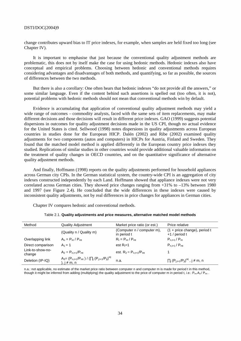
DSTI/DOC(2004)9

34

change contributes upward bias to IT price indexes, for example, when samples are held fixed too long (see Chapter IV).

It is important to emphasise that just because the conventional quality adjustment methods are problematic, this does not by itself make the case for using hedonic methods. Hedonic indexes also have conceptual and empirical problems. Choosing between hedonic and conventional methods requires considering advantages and disadvantages of both methods, and quantifying, so far as possible, the sources of differences between the two methods.

But there is also a corollary: One often hears that hedonic indexes “do not provide all the answers,” or some similar language. Even if the content behind such assertions is spelled out (too often, it is not), potential problems with hedonic methods should not mean that conventional methods win by default.

Evidence is accumulating that application of conventional quality adjustment methods may yield a wide range of outcomes – commodity analysts, faced with the same sets of item replacements, may make different decisions and those decisions will result in different price indexes. GAO (1999) suggests potential dispersions in outcomes for quality adjustment decisions made in the US CPI, though no actual evidence for the United States is cited. Sellwood (1998) notes dispersions in quality adjustments across European countries in studies done for the European HICP. Dalén (2002) and Ribe (2002) examined quality adjustments for two components (autos and computers) in HICPs for Austria, Finland and Sweden. They found that the matched model method is applied differently in the European country price indexes they studied. Replications of similar studies in other countries would provide additional valuable information on the treatment of quality changes in OECD countries, and on the quantitative significance of alternative quality adjustment methods.

And finally, Hoffmann (1998) reports on the quality adjustments performed for household appliances across German city CPIs. In the German statistical system, the country-wide CPI is an aggregation of city indexes constructed independently by each Land. Hoffmann showed that appliance indexes were not very correlated across German cities. They showed price changes ranging from +31% to –13% between 1980 and 1997 (see Figure 2.4). He concluded that the wide differences in these indexes were caused by inconsistent quality adjustments, not by real differences in price changes for appliances in German cities.

Chapter IV compares hedonic and conventional methods.

Table 2.1. Quality adjustments and price measures, alternative matched model methods

Method Quality Adjustment Market price ratio (or est.) Price relative

(Quality n / Quality m) (Computer n / computer m), in period t

(1 + price change), period t +1 / period t

Overlapping link Ao = Pnt / Pmt Rt = Pnt / Pmt Pn,t+1 / Pnt

Direct comparison A1 = 1 est Rt=1 Pn,t+1 / Pmt Link-to-show-no-change A2 = Pn,t+1/Pmt est. R2 = Pn,t+1/Pmt 1

Deletion (IP-IQ) A3= (Pn,t+1/Pmt ) / (∏j (Pj,t+1/Pjt)wj

), j ≠ m, n n.a. ∏j (Pj,t+1/Pjt)wj , j ≠ m, n

n.a.: not applicable, no estimate of the market price ratio between computer n and computer m is made for period t in this method, though it might be inferred from adding (multiplying) the quality adjustment to the price of computer m in period t, i.e.: Pmt A3 / Pmt .

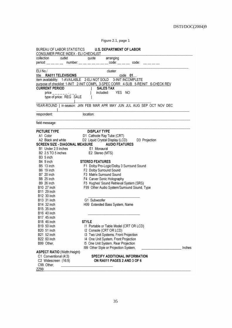
DSTI/DOC(2004)9

35

Figure 2.1, page 1

DSTI/DOC(2004)9

36

Figure 2.1, page 2

DSTI/DOC(2004)9

37

Figure 2.1, page 3

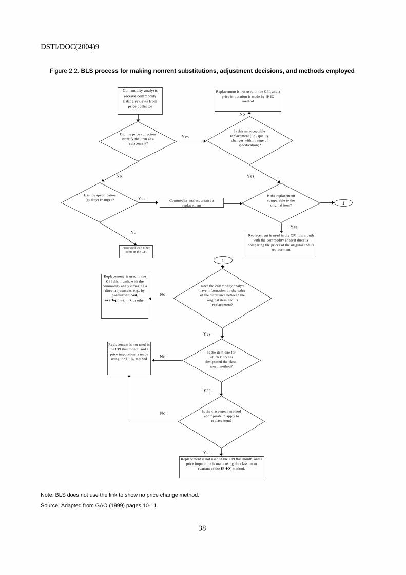
DSTI/DOC(2004)9

38

Figure 2.2. BLS process for making nonrent substitutions, adjustment decisions, and methods employed

No

Yes

No Yes

Yes

YesNo

No

Yes

No

Yes

No

Yes

Commodity analysts receive commodity listing reviews from

price collector

Did the price collectors identify the item as a

replacement?

Is this an acceptable replacement (I.e., quality changes within range of

specification)?

Is the replacement comparable to the

original item?

Replacement is used in the CPI this month with the commodity analyst directly

comparing the prices of the original and its replacement

Replacement is not used in the CPI, and a price imputation is made by IP-IQ

method

Has the specification (quality) changed? Commodity analyst creates a

replacement

Processed with other items in the CPI

1

1

Does the commodity analyst have information on the value of the difference between the

original item and its replacement?

Replacement is used in the CPI this month, with the

commodity analyst making a direct adjustment, e.g., by

production cost, overlapping link or other

Is the item one for which BLS has

designated the class-mean method?

Replacement is not used in the CPI this month, and a price imputation is made using the IP-IQ method

Is the class-mean method appropriate to apply to

replacement?

Replacement is not used in the CPI this month, and a price imputation is made using the class mean

(variant of the IP-IQ) method.

Note: BLS does not use the link to show no price change method.

Source: Adapted from GAO (1999) pages 10-11.

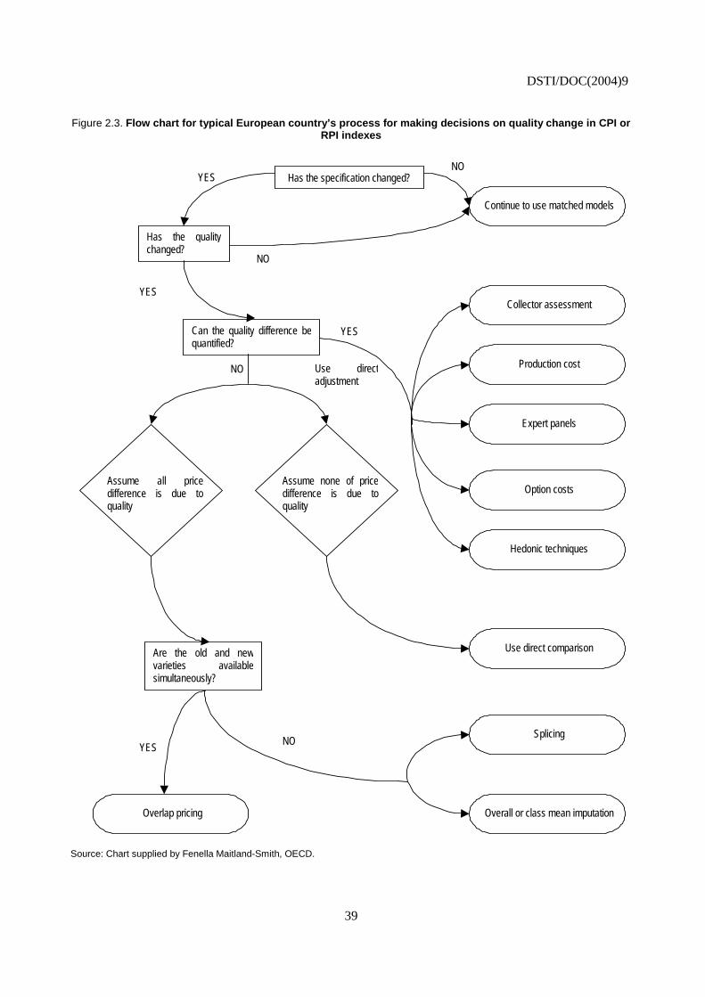
DSTI/DOC(2004)9

39

Figure 2.3. Flow chart for typical European country’s process for making decisions on quality change in CPI or RPI indexes

Has the specification changed?

Continue to use matched models

Has the qualitychanged?

YESNO

NO

Can the quality difference bequantified?

YES

Production cost

Option costs

Hedonic techniques

Collector assessment

Expert panels

YES

Use directadjustment

Assume all pricedifference is due toquality

Assume none of pricedifference is due toquality

NO

Use direct comparison

Overall or class mean imputation

Splicing

Are the old and newvarieties availablesimultaneously?

Overlap pricing

YESNO

Source: Chart supplied by Fenella Maitland-Smith, OECD.

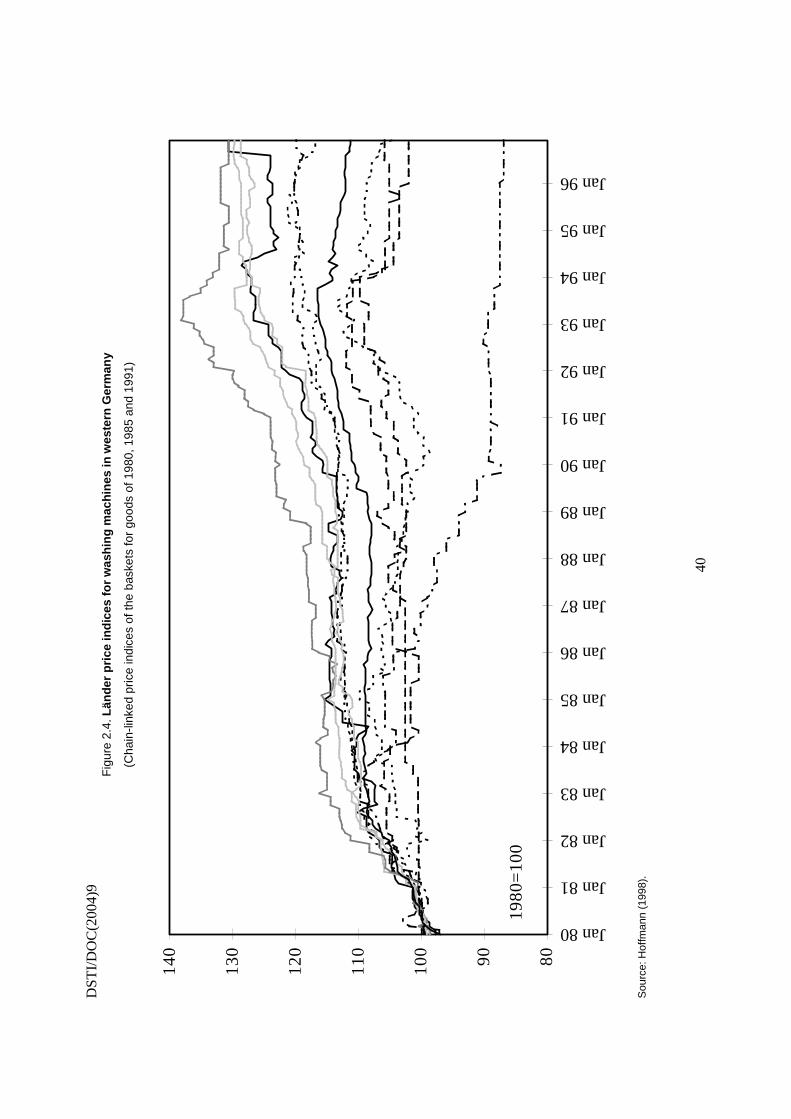
DST

I/D

OC

(200

4)9

40

Fig

ure

2.4.

Län

der

pri

ce in

dic

es f

or

was

hin

g m

ach

ines

in w

este

rn G

erm

any

(Cha

in-li

nked

pric

e in

dice

s of

the

bask

ets

for

good

s of

198

0, 1

985

and

1991

)

8090100

110

120

130

140

Jan 80

Jan 81

Jan 82

Jan 83

Jan 84

Jan 85

Jan 86

Jan 87

Jan 88

Jan 89

Jan 90

Jan 91

Jan 92

Jan 93

Jan 94

Jan 95

Jan 96

1980

=10

0

Sou

rce:

Hof

fman

n (1

998)

.

DSTI/DOC(2004)9

41

CHAPTER III

HEDONIC PRICE INDEXES AND HEDONIC QUALITY ADJUSTMENTS

Conventional, matched model quality adjustment methods are described in Chapter II. Hedonic methods offer an alternative methodology for producing quality-adjusted price indexes.

The first hedonic price index was estimated by Andrew Court (1939).30 Their modern standing stems from the work of Zvi Griliches (1961), who like Court estimated hedonic price indexes for automobiles. Hedonic indexes have been implemented in the statistical systems of a number of OECD countries, mainly for “high-tech” electronic goods and housing.

A hedonic price index is any price index that makes use of a hedonic function. A hedonic function is a relation between the prices of different varieties of a product, such as the various models of personal computers, and the quantities of characteristics in them. Section A of this chapter contains an overview of hedonic functions and characteristics, and they are discussed more fully in Chapter V and the Theoretical Appendix.

As the definition of a hedonic price index implies, hedonic indexes may be computed in a number of ways. Alternative implementations are described in section C of this chapter. Research studies have typically estimated hedonic indexes from a regression by means of the “dummy variable” method (described in section III.C.1), but it is a serious misconception to take the dummy variable method as an essential or necessary part of a hedonic price index. The original Griliches (1961) paper contained several hedonic indexes, not just indexes produced by the dummy variable method. Moreover, hedonic computer equipment indexes that are estimated by OECD country statistical agencies typically do not use the dummy variable method. The definition of a hedonic index in the preceding paragraph makes explicit that a hedonic index is not necessarily a regression price index – and, conversely, a regression price index is not necessarily a hedonic index, if it does not make use of a hedonic function.

Whatever the implementation, estimating a hedonic function is the first step in computing a hedonic price index. Putting the exposition of hedonic indexes (this chapter and the following one) before discussing procedures for estimating hedonic functions violates the order in which a research project will be carried out. It is valuable, however, to consider the use of hedonic functions to compute hedonic price indexes before exploring the technical problems that arise in doing research on hedonic functions. Additionally, the order of the chapters facilitates the comparison of hedonic methods and conventional matched model methods, a topic on which there has been much confusion.

30. In recent years, historians of economic thought have discovered earlier researchers who developed

something that resembles a hedonic function (though of course they did not use that term). See the historical note at the end of this chapter.

DSTI/DOC(2004)9

42

A. Hedonic functions: a brief overview

The first government hedonic price index for computers was based on research by Dulberger (1989). Cartwright (1986) provides the details of implementation by the Bureau of Economic Analysis in the US national accounts.31 Most subsequent work on computers, including research on personal computers (PCs), follows an approach that is basically an extension of Dulberger’s work, so hedonic functions that resemble hers describe most existing hedonic research on computer equipment (see Chapter V). For these reasons, Dulberger’s computer hedonic function provides the illustration for this chapter.

Dulberger’s (1989) computer hedonic function (her equation 2′) is:

(3.1) LnPit = a0 + 0.783 ln(speed)i + 0.219 ln(memory)i + “technology” variables + εit

Equation (3.1) says that the logarithm of the price for any computer model, i, at time t depends on the logarithm of its speed and the logarithm of the amount of “main” memory included in the machine, measured in megabytes. In Dulberger’s study, speed was measured in MIPS, millions of instructions per second, a speed measure that has been widely used in the computer industry. Her equation also included a set of technology variables, which need not concern us at this point, nor do we need to discuss at this point the intercept term, a0.

32 Finally, εit, the regression residual, indicates whether the price of the particular computer, model i, is close to the regression line at time t.

In common with many other computer hedonic functions, Dulberger’s is in “double log” form – logarithms of all the continuous variables are used in the equation. Other functional forms have been used in hedonic research, including research on computers. These other forms are discussed in Chapter VI, but most of what follows in this chapter applies to hedonic indexes that are based on any of the most frequently-encountered functional forms. Equation (3.1) was estimated by ordinary least squares (OLS) regression, using a database of mainframe computer characteristics and prices that covered IBM mainframe computers and computers from certain other manufacturers that were constructed on similar computer architectural principles (to assure compatibility in the speed measure).

In the economics literature on hedonic functions, variables such as speed and memory size are called characteristics. The theory of hedonic indexes is built on the proposition that the characteristics are the variables that the buyers of the product want, and that the characteristics of the product also are costly to produce (see the Theoretical Appendix). That is, computer buyers want more speed, other things equal, and faster computers are more costly to produce, with a given production technology. An implication of the theory is that variables that do not have both “user value” and “resource cost” interpretations do not belong in hedonic functions. This is considered further in Chapter V.

The regression coefficients (0.783 and 0.219 in equation 3.1) are the major interest for this chapter. The regression coefficients value the characteristics. They are often called implicit prices or characteristics prices, because they indicate the prices charged and paid for an increment of one unit of (respectively) speed and memory. Implicit prices are much like other prices, they are influenced by demand and by

31. However, the first hedonic index used in the US national accounts was a hedonic price index for new

houses, introduced in 1974, extending back to 1968 (Survey of Current Business, August, 1974, pp.18-27). Lowe (1999) indicates that the first Canadian government hedonic index was also for new houses, beginning in 1974. A similar French index is described in Laferrère (2003). For earlier computer hedonic indexes, see the historical note to this chapter (Appendix A).

32. The technology variables were dummy variables indicating the technology embodied in the semiconductor chip used in the computer. This is considered in chapter V.

DSTI/DOC(2004)9

43

supply – which means, for example, that they do not measure uniquely user value.33 To avoid confusion, one should note that in a double log hedonic function such as equation (3.1), the regression coefficient is not technically itself the price of the characteristic, but rather the logarithm of the characteristic’s price.

Arriving at a satisfactory hedonic function is the major part of the work in constructing hedonic price indexes. For the exposition of this chapter, I assume that a satisfactory hedonic function has already been estimated, following the principles developed in chapters V and VI.

B. Using the hedonic function to estimate a price for a computer

For the hedonic price indexes discussed in section III.C, it is essential to explain how one can use a hedonic function to estimate, under certain conditions, the price of a computer (or any other product). For example, a new 50 MIPS computer replaces the 45 MIPS computer that was previously in the price index sample. In the language of Chapter II, this is an item replacement. One wants either (a) to estimate the price of one or both of the two computers for the period in which it was not available (to permit comparing prices of computers having the same specification), or (b) to estimate the value of the 5 MIPS increase in computer speed in one or both of two periods (to serve as a quality adjustment).

To illustrate this diagrammatically, suppose a hypothetical computer hedonic function that has only one characteristic, speed. This would resemble equation (3.1) with only speed in the regression, so it contains only the logarithm of a computer’s speed and the logarithm of its price. The graph of this one-variable computer hedonic function (for some period, t) is shown in Figure 3.1. The estimation discussed in the following paragraphs is similar if there are more variables in the computer hedonic function, but it cannot conveniently be illustrated graphically.

1. Estimating prices for computers that were available and for those that were not

Suppose some computer (call it model r) was sold in period t, but that model r was not in the price index sample of computers. This computer was available on the market, so its price could have been collected, had it been in the sample. Its speed was Sr.

Under the condition that computer r was available, one can use the hedonic function to estimate a price for computer r in period t. This estimated (or predicted) price for computer r is shown on Figure 3.1 – if computer r operates at speed Sr, its price is estimated as Pr, the value predicted from the hedonic function for period t. Pr is the best estimate of the price for computer r, in the sense that it is the mean price for a computer that was sold in period t and that has speed Sr.

In this example, we do not know the actual price for computer r. It was not observed, or was not collected for the sample. The actual price for computer r might have been greater or lesser than the estimated price. If the actual price for computer r was lower than the mean price for a computer with speed Sr, then it is a “bargain.” Bargain computers lie below the hedonic function – they have negative residuals from the hedonic function, shown on the graph in Figure 3.1 as a solid “dot.” Conversely, computer r might have been “overpriced” relative to its speed. In this case, its price will lie above the hedonic function, so it will have a positive regression residual, as shown in Figure 3.1 by an open “dot.”

Now consider estimating the price of a new computer – computer model n – that was not available at all in period t. This seemingly is a similar problem. On Figure 3.1, computer n has a speed rating of Sn. If the introduction of computer n does not change the existing price regime for computers, then the best estimate of the price for computer n is also shown in Figure 3.1: From the speed of computer n, Sn, its

33. See the Theoretical Appendix.

DSTI/DOC(2004)9

44

predicted price is given by the hedonic regression line as Pn, by a procedure parallel to the one for estimating the price for computer r.

However, estimating a price for computer n from the hedonic regression for period t involves a subtly different economic and statistical problem from estimating the price for computer r. Computer r existed in period t, computer n did not exist. For this reason, the estimates Pr and Pn depend on different assumptions.

Computer r existed in period t, so its influence was already incorporated into the computer market pricing structure, and therefore into the period t hedonic function. No special assumption is required to estimate the price of computer r, even if computer r was not included in the data from which the hedonic function was estimated.34 The question is simply: What is our best estimate of the price that computer r did actually bring at time t? Of course, this estimated price is estimated with error, as with all estimates.

But a seemingly similar question concerning the price of computer n is not identical. For computer n, the question is not: What did it sell for? Instead the question is: What would computer n have sold for if it were on the market in period t? If it were on the market in period t, it might have altered the demands for all computers, so that the hedonic function itself would have been different from the one that actually existed in period t.

The estimate Pn (which is based on the hedonic function for period t) is valid only if we can assume that the introduction of computer n in period t would not have changed the hedonic computer regression line in period t. This might be the case, for example, if computer n was introduced at a price that was exactly on the regression line, and not above or below it. This is quite an old point, but it has often been overlooked.35 Its importance has been emphasised recently by Pakes (2003): Producers of differentiated products try to find unfilled niches in the product spectrum of varieties, and filling them changes the demands for existing varieties, resulting in changes in the characteristics prices.

Estimating the price of a new computer is most hazardous for computers that are outside the characteristics range that existed in period t. PCs of 1 000 megahertz (MHz) speed became available in early 2000, and subsequently substantially higher speeds were offered.36 Price index compilers may need to consider the question: What would a 1 000 megahertz or faster PC have sold for in some earlier period, when machines so fast were not available? There may be no sensible answer to that question.

Presumably, building the 1 000 megahertz machine was not possible with the technology of the earlier period. The first IBM PC, introduced in 1981, ran at 4.77 MHz, and the first 400 megahertz PC was introduced in 1998. It was certainly not feasible to produce a 1 000 MHz PC in 1981, and it is reasonable to presume that 400 MHz represented the upper limit to PC speed with the technology of 1998. As shown in Figure 3.2, the hedonic function for 1998 (designated h(1998)) has a vertical section at the technological upper limit of computer speed, 400 MHz. By 2000, technological change has shifted the hedonic function downward (computers of all speeds became cheaper) and also extended the hedonic function’s domain into

34. This statement is not intended to imply that there are no econometric problems that might arise when

computer r is missing from the sample on which the hedonic function was computed.

35. For example, Committee on National Statistics panel’s (Shultze and Mackie, eds, 2002, page 124) review of hedonic indexes says: “The basic idea behind hedonic techniques is that one can use a hedonic equation to calculate the expected price of a particular variety – which may not in fact be offered for sale in the period being considered….” That requires special assumptions, as noted above, which the committee also noted at another point.

36. MHz, sometimes referred to as “clock speed”, is another measure of computer speed that is widely used, especially for PCs. Alternative speed measures are reviewed in Chapter V.

DSTI/DOC(2004)9

45

regions of the commodity space that were not technologically feasible earlier – the vertical portion of the hedonic function now occurs at 1 000 MHz.

One cannot use the hedonic function for 1998 to predict what the 1 000 MHz machine would have sold for in 1998, for the correct answer to that question might be infinity, at least from the production side.37 On the other hand, one can almost always answer the question: what would the typical computer sold in period t cost in period t+1? The hedonic function for 2000 (Figure 3.2) can be used to estimate the price for a 400 MHz machine in 2000. Only if the two periods are far apart will the initial period’s computer be obsolete. The 400 MHz computer was still available in 2000, but the 4.77 MHz PC was not.

Making quality adjustments in price indexes sometimes requires estimating a price in period t for a new computer that first became available in period t+1. One cannot ignore the fact that the new computer was not actually available in period t, and the possible reasons why it was not available. The special assumptions necessary to validate “backcasting” a price for a machine that was not in fact produced should be kept in mind.

2. Estimating price premiums for improved computers

For price indexes, another employment of the hedonic function will prove useful. Suppose computer m was in the sample in the previous period, but it was replaced in the sample by a new and faster computer, computer n. Rather than estimating the price for computer n in period t, we can ask instead: What premium should computer n sell for, compared with computer m? The expected premium provides a quality adjustment when computer n is an item replacement for computer m in a price index sample.

Using the hedonic function to estimate a price premium for the improved computer is really just a transformation of the hedonic function estimate considered in the previous section. Suppose computer m, with 400 MHz, was in the sample (so its price was known), but it was replaced by computer n, with 500 MHz. Suppose additionally for simplicity that the 400 MHz machine was priced to lie on the regression line. This is indicated by the open “dot” in Figure 3.3. The value of the extra 100 MHz in computer n is given by the difference ((est Pn ) – (Pm)), the logarithms of which can be read from the slope of the regression line in Figure 3.3. Estimating the increment to the price of the extra 100 MHz implies exactly the same estimator as estimating the price of the 500 MHz computer: The points marked “est lnPn” in Figures 3.1 and 3.3 are the same estimate, just arrived at in a different way.

Empirical estimates show that the premium for an additional 100 MHz of computer speed declines over time. For this reason, there are two possible valuations for speed in a price index that covers periods t and t+1 – the initial period’s value in period t and the comparison period’s value in period t+1. One must decide which period’s valuation is appropriate. Because the same choice is necessary for some other quality adjustment methods (production cost adjustments, for example), this is not a unique problem for hedonic indexes.

Using the hedonic function to estimate the price increment of an additional 100 MHz does not evade the backcasting problem discussed in the previous subsection. If the replacement computer is really new and was not on the market in period t, then its introduction might have changed the price increment associated with an additional 100 MHz. Moreover, if the extra 100 MHz was beyond the technological

37. It is common to think about goods that were not available in an earlier period using the demand side:

“What would a buyer be willing to pay for a 1 000 megahertz PC in 1998?” The suggestion is due to Hicks (1940). See Hausman (1997) for an empirical estimate. The willingness-to-pay estimate is clearly lower than infinity. However, the theory underlying hedonic functions requires that production be possible (see the Theoretical Appendix).

DSTI/DOC(2004)9

46

frontier of period t (as it is for the 1998 function in Figure 3.2), then the hedonic function is undefined for this increment, and so is the estimated price premium for the faster computer. Notice that even if the premium is undefined in period t, it may be estimated without difficulty for period t+1 (refer to Figure 3.2). On the other hand, if computer n was in fact available in period t – that is, it was missing from the price index sample but not from the market – no special assumption is required to estimate the price increment associated with its increment to speed. This is parallel with the discussion in the previous section. Because statistical agencies frequently choose item replacements that are similar to the computer in the old sample, the replacement is often within the range of characteristics available in the previous period.

3. Residuals

Hedonic functions have residuals, the εit term in equation (3.1), and the solid and open “dots” in Figure 3.1. For what follows in this chapter, we need to consider why these residuals exist, and what economic and statistical interpretations to give them.

Of course, “noise” always exists in actual data. Statistical noise is one interpretation for the regression residuals. That is another way of saying that the residuals may not mean anything economically, they are just random observational errors of some sort that are hopefully (but not probably) uncorrelated with anything of interest.

But the residuals may also have an economic interpretation. If the prices are transactions prices, negative residuals (the points marked with solid “dots” on Figure 3.1) are “bargains,” as already noted: These computers cost less than one would expect from the quantities of characteristics they contain. Conversely, positive residuals (the points marked o on Figure 3.1) cost “too much” for what they provide in characteristics. Actual prices include manufacturer’s pricing errors, so the residuals have an economic interpretation, not just a statistical one.

Griliches (1961) long ago noted that if the hedonic function is correctly specified, then the residuals should predict changes in market shares. Bargains should experience increasing market shares. Cowling and Cubbin (1971) explored this suggestion on the market for automobiles in the United Kingdom. Knight (1966) used residuals from an early hedonic function for computers to predict whether a particular computer would find a market, considering its performance relative to its price.38 Waugh (1928) analysed residuals from his hedonic functions for vegetables.

“Bargains” and “good buys” may exist alongside overpriced computers because people are not perfectly efficient shoppers. Some people know what to buy, others make mistakes. Alternatively, some people find it congenial to shop for the best price and best value, others do not want to invest their time, and buy without searching out the best price. For these reasons, the overpriced computers do not immediately disappear from the market. Retailing and marketing studies persistently show that the “law of one price” does not hold across retail outlets and especially across urban areas and among cities (one recent example of a large literature is O’Connell and Wei, 2002).

It has often been said that the hedonic function requires perfect markets, or that hedonic price indexes require market equilibrium. Such statements are partly germane and partly (depending on what is meant) misunderstandings. Consumer ignorance, in the sense described above, exists, and markets are not “perfect;” this just implies that hedonic functions have residuals. Regression residuals present no particular difficulties for the estimation and use of hedonic functions. Under and over-pricing errors are random for

38. Knight did not call his function a hedonic function, but it was one. His consulting use of his hedonic

function to predict market success of new computers worked quite well (personal conversation with Kenneth Knight). Knight’s work was converted into a price index for computers in Triplett (1989).

DSTI/DOC(2004)9

47

interpreting the hedonic function (though certainly not for analysing buyer behaviour toward market price differentials). It has also often been said that publications such as Consumer Reports in the United States and Which? in the United Kingdom show there is no correspondence between price and “quality;” that is also a misconception. What these magazines show, in effect, is that hedonic functions have residuals, and they try to point buyers toward negative residuals and away from positive ones.

On the other hand, hedonic residuals could have a less benign interpretation. Suppose an important characteristic that consumers value is left out of the hedonic equation. For example, perhaps the computers marked “o” in Figure 3.1 include packages of software that buyers value and that are not offered on the other computers. If we added data on the missing software characteristics to the hedonic regression we might find that prices of these computers (including software characteristics) would be at the regression line, or even below it. Thus, when bundled software or other characteristics are omitted from the hedonic function, the residuals may reflect specification error in the hedonic function, rather than overpricing.

The residuals may also record other measurement errors that are distributed irregularly across the observations. If list prices are used as the left-hand side variable in the regression, the residuals may measure the error between list and transactions prices, where markups or markdowns differ among the various computers. If the prices are “unit values” – averages aggregated across sellers, as is typical in scanner data – residuals may reflect differences in retail amenities or services that affect the price but are in effect missing variables for a (retail price) hedonic function. Or perhaps we did not record the prices exactly right, or speed or some other variable is measured with error, and the errors are not uniform across the observations.39 As another alternative, if we inadvertently mis-specify the functional form for the hedonic function (for example, estimate a linear hedonic function, when the true hedonic function is logarithmic), the measured residuals from the fitted hedonic function will not be the true residuals. In these cases, regression residuals may not measure bargains or overpriced machines; instead, they indicate errors in the hedonic function specification.

Missing or omitted or mismeasured variables and other specification errors can cause serious problems for hedonic functions and hedonic price indexes. I discuss in Chapter V how to search for and minimise problems that arise from omitted characteristics in hedonic functions, and consider hedonic functional forms and other estimation issues in Chapter VI. For the rest of this chapter, it is appropriate to put these interpretative, procedural and econometric problems aside, for consideration later. We assume, for the exposition of this chapter, that the hedonic function is correctly estimated and its variables are correctly measured.

C. Hedonic price indexes

With these preliminaries, we are now ready to discuss hedonic price indexes. As defined at the beginning of this chapter, a hedonic price index is a price index that uses a hedonic function in some way. Four major methods for calculating hedonic price indexes have been developed and used to estimate computer and ICT price indexes.

Each of these four hedonic price index methods uses a different kind of information from the hedonic function. The first two described below (the time dummy variable method and the characteristics price index method) have sometimes been referred to as “direct” methods, because all their price information comes from the hedonic function; no prices come from an alternative source. Direct methods require that a hedonic function be estimated for each period for which a price index is needed.

39. An extensive econometric literature considers the consequences of mismeasured variables for biases in the

estimated regression coefficients. See any standard econometrics textbook, such as Gujarati (1995), and Berndt (1991), pp. 128-129, for application to hedonic indexes.

DSTI/DOC(2004)9

48

The second two hedonic price index methods (the hedonic price imputation method and the hedonic quality adjustment method) have been described as “indirect” or “composite” methods. They are often called “imputation” methods, because the hedonic function is used only to impute prices or to adjust for quality changes in the sample of computers in cases where matched comparisons break down. The rest of the index is computed according to conventional matched model methods, using the prices that are collected in the statistical agency’s usual sample.

Indirect methods imply merging two sources of price information – the full cross-sections of computer prices and characteristics, to estimate a hedonic function, and the price index samples that statistical agencies normally collect. Indirect methods also imply that the hedonic function can be estimated from a data source that is different from the one used for calculating the price index, which in turn implies that the hedonic function can be estimated less frequently than the price index publication schedule. For example, if the price index is monthly, use of an indirect method permits estimating the hedonic function quarterly or semi-annually or even annually, according to whatever frequency is required to keep it up to date; the indirect method does not require estimating hedonic functions monthly in order to produce an index that is computed monthly, as the direct methods demand.

This “direct” and “indirect” language is not particularly felicitous. “Indirect” has sometimes been taken as suggesting that the index is somehow not a “real” hedonic index or that it is in some manner inferior to a “full” (“direct”) hedonic index. That is wholly a misconception, as the following sections show. Perhaps the misconception is not entirely attributable to language, but the “direct-indirect” language seems to have fostered it. Nevertheless, I follow what has become common, if somewhat recent, usage because it has attained such currency.

For expositional simplicity, I assume that only speed and memory size matter to computer buyers and sellers, and not some other characteristics of computers that have been left out of the analysis and not considered. That is, there are no omitted variables. I also assume that we have measured speed, memory, and price correctly, and that we have already estimated a hedonic function that is satisfactory, according to the principles discussed in chapters V and VI. Variables are correctly measured and the hedonic functional form has been determined, empirically. Under these conditions, regression residuals measure over or underpricing of particular computers, relative to their included content of characteristics. Except where noted, I utilize the double log form of equation (3.1) in the exposition, not because a double-log form is necessarily best, but because it has been used so frequently in empirical studies on computers. The calculations are very similar, and in some cases identical, for other functional forms.

1. The time dummy variable method

Most research hedonic price indexes have used the time dummy variable method. For example, the hedonic price index for PCs in Berndt, Griliches and Rappaport (1995) is a dummy variable index. The dummy variable method has also sometimes been called the direct method, in the sense that the index number is estimated directly from the regression, without another intervening calculation. Because there can be more than one “direct” method, I retain the historical “time dummy variable method” terminology.

a. The method explained

To illustrate, suppose one wants a computer price index for three periods. For each computer model, i, one must gather data on the characteristics of the machine, which are – using equation (3.1) for illustration – its speed (measured in MIPS or megahertz, MHz) and its memory size (measured in megabytes). The characteristics of each model of computer do not change between the periods: indeed, a computer model is defined by its characteristics, so if one of the characteristics changes, this is a new model for our purposes,

DSTI/DOC(2004)9

49

regardless of the manufacturer’s designation.40 The price of a computer model may of course change between periods, so we must have a price for each machine for each of the three periods.

To discuss the time dummy variable method, I need to change the time notation. Let the three periods for which the price index is calculated be designated τ, τ+1, and τ+2. Then, in the hedonic regression (equation 3.2, below), t = τ designates the first period, t = τ+1 the second, and t = τ+2 the third.

In one form of the dummy variable method, all three periods’ data are combined into regression equation (3.2):

(3.2) lnPit = ao + a1ln(speed)i + a2ln(memory)i + b1(Dτ+1) + b2(Dτ+2) + ε it

where t = τ, τ+1, and τ+2, respectively, for the three periods. Where equation (3.1) implied a hedonic function using data for only one period, equation (3.2) implies a single hedonic function that covers three periods’ data, τ, τ+1, and τ+2. This approach is sometimes called a “pooled” regression, or a “multi-period pooled” regression, because data for several periods are “pooled.”

On the left-hand side, the equation has the logarithm of the price of computer i in year t (which is τ, τ+1, or τ+2). A computer that is in the sample for all three years appears in the regression for all three years, with its appropriate price for each year. But some computers appear only in certain periods: If computer m replaces computer n (recall the example in Chapter II), each of these computers is in the regression only for the periods in which each is sold – τ and τ+1, for the old computer m, and τ+2, only, for the new computer n. Using notation adapted from that of Chapter II, equation (3.2) contains three arrays of computer prices: P(M)τ,

P(M)τ+1, and P(N)τ+2.

The right-hand side has the same variables as in equation (3.1) – the intercept term, a0 and for each computer, i, its speed and its memory. Speed and memory have regression coefficients a1 and a2, as in equation (3.1), except in this case the coefficients are constrained to be the same over all periods covered by the regression. They are in effect an average of the coefficients for each of the three periods. Constraining the coefficients is controversial; further discussion appears in section III.C.2.b, which also contains an empirical evaluation.

As with equation (3.1), the term εit in equation (3.2) records whether the price of computer i in year t is above or below the regression line. Note that in principle computer i could lie above the regression line in one of the three years, and below it in another, and will if its seller lowered its price more or less than the price changes for rival computers.

In addition to the variables in equation (3.1), equation (3.2) contains variables that record the year in which each price is collected: The first “dummy variable,” Dτ+1, takes on the value of 1 for each computer, i, when its price pertains to period τ+1 (and zero otherwise). The second dummy variable, Dτ+2, takes on the value 1 when computer i’s price pertains to period τ +2, and zero otherwise. The regression contains no dummy variable for period τ because τ is the base from which price change is computed.

The regression coefficient of the dummy variable, b1 (strictly speaking, the antilogarithm of it41) shows the percentage change in computer prices between period τ and period τ+1, holding constant the 40. In practice manufacturers sometimes change their model codes when a characteristic of the product

changes. However, sometimes a change might be introduced without a change in the model code and sometimes the model code may change without any change in the product’s characteristics. Some research on computers has proceeded as if the manufacturer’s model code makes getting data on the characteristics unnecessary; this is incorrect.

DSTI/DOC(2004)9

50

characteristics of the computer. It represents the price change (sometimes called the “pure” price change) between period τ and period τ+1 that is not associated with changes in computers’ speed and memory.

Similarly, the regression coefficient b2 shows the constant-quality computer price change between period τ and period τ+2. One could also code the data so the dummy variable coefficient b2 gives the change between τ+1 and τ+2, instead of between τ and τ+2: In this case, the dummy variables are coded Dτ+1 = 1 for both periods τ+1 and τ+2 (that is, for all periods other than τ), and Dτ+2 = 1 for only period τ+2 (as before). The estimates are equivalent in either case. Because the latter – that is, where b2 provides an estimate of the one-period change between periods τ+1 and τ+2—has a simpler interpretation, I discuss this case in the following.

The dummy variable price index is illustrated in Figure 3.4. Like the preceding figures, Figure 3.4 depicts a single variable hedonic function (so it has only a “speed” coefficient, a1), with two time dummy variables, Dτ+1 and Dτ+2.

As Figure 3.4 suggests, with this technique there are really three regression lines, not one. They all have the same slope, a1 (because the regression coefficients are constrained by the methodology to be the same in all three periods). Coefficients on the dummy variables act as alternative regression intercept terms: The time dummy variables allow the regression for each period to lie above or below the others.

If the coefficient on the dummy variable Dτ+1 is negative – that is, b1 < 0—then b1 measures the rate at which the hedonic line or surface falls, and therefore the rate of decline in computer prices, computer characteristics (and also valuations of the characteristics) held constant. This is shown in Fig. 3.4 as the distance between the solid line (t = τ ) and the dashed one (t = τ+1). The coefficient b2 has a similar interpretation, with respect to τ+2 – in Figure 3.4, it is the distance between the dashed and dotted lines.

When the estimated b1 and b2 coefficients are positive, computer prices are rising. When prices are rising, the dashed and dotted lines will lie above the solid one. The rest of the discussion applies to both rising and falling price situations.

This technique can be extended to more than three periods by “pooling” more periods of data and adding additional dummy variables as necessary. However, multi-period pooled regressions are not the best way to construct a time series of hedonic indexes.

A preferable alternative is the “adjacent period” approach. Using the same data as for equation 3.2, first combine data for periods τ and τ+1, and drop the variable Dτ+2. This adjacent-period regression provides an alternative estimate of the coefficient b1.

42 Second, combine data for periods τ+1 and τ+2 (discarding the data for period τ), and drop the variable Dτ+1. This equation provides an alternative estimate

41. It is well established in statistics that the antilog of the OLS regression estimate of b1 is not an unbiased

estimate of b1, which means that price indexes estimated by the dummy variable method are biased. A standard bias correction (Goldberger, 1968; also Kennedy, 1981, and Teekens and Koerts, 1972) is to add one-half the coefficient’s squared standard error to the estimated coefficient. For hedonic indexes, this correction is usually quite small. I corrected nearly all of the computer equipment price indexes reviewed in Triplett (1989). The bias correction made little difference to reported annual rates of price change – because most hedonic functions for computers have very tight “fits”, the dummy variable coefficient has a small standard error, and (typically) a rather large coefficient (prices are falling rapidly). This finding does not seem to have informed the recent hedonic price index literature.

42. Or rather, of the population parameter that b1 estimates. The statistical estimate of b1 from equation (3.1) is not the same as the statistical estimate of b1 from the alternative regression. The same statements apply to b2. I retain the same notation for simplicity.

DSTI/DOC(2004)9

51

of b2. The three period price index for τ+2 / τ is obtained by multiplying together (antilogs of) the two adjacent year estimates b1 and b2. The adjacent-period alternative is still a pooled regression, but its pooling is the minimal amount necessary to implement the dummy variable method.

Any pooled regression holds fixed the hedonic coefficients, and holding the coefficients fixed has been criticised. However, the adjacent-period dummy variable approach holds the a1 and a2 coefficients constant for only two periods, where the multi-period pooled regression holds them constant for a larger number of periods, as indicated in equation (3.2). The adjacent-period estimator is a more benign constraint on the hedonic coefficients because coefficients usually change less between two adjacent periods than over more extended intervals (see section III.C.2.b). The adjacent-period form of the dummy variable method is preferred for most cases, and indeed should be thought of as “best practice” among dummy variable indexes. For this reason, in the following subsections, I use examples that are adjacent-period dummy variable indexes: As appropriate, some examples refer to an adjacent-period regression covering periods τ and τ+1, others to an adjacent-period regression covering periods τ+1 and τ+2.

b. The index number formula for the dummy variable index

The coefficient of the Dτ+1 dummy variable in equation (3.2) is an estimate of the logarithm of the price index between period τ and period τ+1. Griliches (1971) remarked that the dummy variable method gave a price index that “is not well articulated with the rest of the index number literature.” Traditionally, price indexes are computed by “formulas” – Laspeyres, Paasche, Fisher, and so forth. What price index formula corresponds to the time dummy variable estimate? We need the answer to compare analytically the dummy variable price index with a conventional price index.

Triplett and McDonald (1977, section IV) noted that the index number formula implied by the dummy variable method can be derived from the expression for the regression coefficient for the time variable, denoted as b1 in the following,. The index formula depends on the functional form for the hedonic function.

For a hedonic function with a logarithmic dependent (price) variable, rearranging the expression for the ordinary least squares (OLS) estimate of b1 (for the dummy variable Dτ+1 in equation (3.2)) yields the price index:

(3.3a) index {(τ+1) / τ} = exp(b1)

= [ Π (Pi,τ+1)1/n / Π (Piτ)

1/m ] ÷ [hedonic quality adjustment]

In words, the dummy variable index equals the ratio of unweighted geometric means of computer prices in periods τ and τ+1, divided by a hedonic quality adjustment. In the usual case, hedonic regressions are run on unbalanced samples, so the number of observations may differ in the two periods, as indicated by the subscripts m and n.

The hedonic quality adjustment in equation (3.3a) also depends on the form of the hedonic function. For a logarithmic hedonic function, the hedonic quality adjustment is given by:

(3.3b) hedonic quality adjustment = exp [Σ aj ((Σ Xijτ+1 /n) – (ΣXijτ / m))]

In equation (3.3b), I designate characteristics by the subscript “j” because in most cases there will be more characteristics in the hedonic function than the two in equation (3.1).

Equation (3.3b) is itself an index number – it is a quantity index that measures the change in characteristics of computers sold in periods τ and τ+1. It is not a standard index number formula, partly

DSTI/DOC(2004)9

52

because of the unbalanced samples in it. More exactly, the term in square brackets is the mean change in computer characteristics, e.g., speed and memory, between periods τ and τ+1; the changes in computer characteristics are valued by their implicit prices, which are the aj coefficients from the hedonic function (equation 3.2). The hedonic quality adjustment is the exponential of the square-bracketed term.

If the hedonic function in equation (3.2) were estimated with a sales-weighted regression, equation (3.3a) would be a ratio of weighted geometric means, rather than the equally-weighted geometric mean written there. The quality adjustment in equation (3.3b) would also involve means of characteristics that are weighted by sales, rather than the equally-weighted means in equation (3.3b). Similar statements apply to the following examples, but need not be repeated for every case.

For a linear hedonic function, the formula for the dummy variable index becomes an unweighted arithmetic mean, and the quality adjustment term is a linear quantity index of characteristics:

(3.3c) index {(τ+1) / τ} = (b1)

= [∑ (Pi,τ+1)/n / ∑ (Piτ)/m ] – [hedonic quality adjustment]

(3.3d) hedonic quality adjustment = [Σ aj ((Σ Xijτ+1 / n) – (ΣXijτ / m))].

Other hedonic functional forms imply dummy variable indexes that have index formulas that depend similarly on the expressions for the coefficients of the dummy variables, when the regressions are estimated by OLS.

Triplett and McDonald (1977) computed a price index for refrigerators by the dummy variable method, and then compared it with the conventional (Laspeyres) index number formula used in the US PPI index for refrigerators. Using equation (3.3a) they decomposed the difference into an index number formula effect (geometric, compared with the arithmetic mean formula used in the PPI) and a quality adjustment effect (hedonic, compared with matched model method used in the PPI; the quality adjustment effect was estimated as a residual). The index number formula effect accounted for about 10% of the difference between the dummy variable hedonic index and the PPI.

It is a bit surprising that little subsequent hedonic research has considered index number formula effects. It is well known that geometric and arithmetic mean formulas for price index components give different measures. Sometimes these formula effects are quite large – see, for example, the calculations for the Canadian CPI in Schultz (1994). For this reason, a great amount of attention has been given in recent years to the formula to be used for price index basic components. Diewert (1995) reviews index number theory for basic components; Balk (1999) and Dalén (1999) add more recent developments. This work on index number formulas for price index basic components seems not to have touched research on hedonic indexes, so that the typical hedonic study has remained poorly “articulated” into the price index literature, as Griliches put it. More seriously, few studies have determined what part of the difference between research indexes for PCs and a statistical agency’s PC index lies in the use of geometric compared with arithmetic mean index number formulas.43

43. As an example, the US PPI for computers is a quality adjusted (by hedonic methods) arithmetic mean.

Some part of the difference between the BLS index and the dummy variable index in Berndt, Griliches and Rappaport (1995) is caused by the difference between arithmetic and geometric means.

DSTI/DOC(2004)9

53

c. Comparing the dummy variable index and the matched model index: no item replacement

An enduring research issue concerns whether hedonic indexes and matched model indexes give similar or different results. To address this issue, whether empirically or analytically, one needs expressions for the alternative estimators that correspond to matched model and hedonic indexes.44

To facilitate comparison, consider exactly the same data that were discussed in Chapter II. That is: (a) there are three periods for which we want a price index; (b) a matched set of m computer models exists in period τ and period τ+1, and (c) computer n replaces computer m in period τ+2, with the remaining m-1 models unchanged. In the notation employed in this chapter (see the discussion of equation (3.2), above), we have three arrays of computer prices: P(M)τ,

P(M)τ+1, and P(N)τ+2, where the notation P(N)τ+2 indicates that computer n has replaced computer m in the sample in period τ+2. As in Chapter II, this implies that i = 1, …, n, but the number of observations in each two-period regression is 2m (because one observation is missing for each of the years).45 We calculate equations (3.3a and 3.3b).

Suppose the statistical agency uses a geometric mean formula for its matched model index. The hedonic index in equation (3.2) implies a price index that is also a geometric mean, as shown in equation (3.3.a). Thus, no formula effects are present in the comparison of matched model and hedonic indexes.

No item replacement occurs between periods τ and τ+1. The computer models in the price arrays P(M)τ and P(M)τ+1 are only matched models. In equation (3.3b), each Xijτ equals the corresponding Xijτ+1, and the number of items is also the same (m = n), so the terms inside the square bracket sum to zero. Thus, the hedonic quality adjustment in equation (3.3b) is unity, because there is no quality change in any of computers in the sample.46

Accordingly, the price index number formula implied by a dummy variable (logarithmic) regression run on matched models is a ratio of equally-weighted geometric means. This is the same unweighted geometric mean formula that has come to be preferred by many statistical agencies for detailed components of consumer price indexes.47

One would seldom want to compute a price index from the regression dummy variable when all of the computer models in both periods are matched models. Equation (3.3a) shows why: The dummy variable index yields exactly the matched model index, because (a) matching already holds the quality of computers constant, and (b) the index number formula that is implied by the regression coefficient on the time dummy variable is the same geometric mean that is commonly used by statistical agencies.

For completeness, it should be noted that statistical agencies also use formulas other than the geometric mean index to estimate basic component indexes – a ratio of arithmetic means, an unweighted arithmetic mean of price relatives, and in some cases weighted forms of these estimators. Obviously, the index exp(b1) in equation (3.3a) will differ from these other basic component index formulas. For example, the estimate from equation (3.3c) would be consistent with an arithmetic mean index formula.

44. An empirical review of matched model and hedonic indexes is contained in Chapter IV.

45. The dummy variable method does not require particular assumptions about data availability. I use the data from Chapter II in order to make a clear contrast between different methods applied to the same data. A broader consideration of the elements held constant here is contained in Chapter IV.

46. Note that e (0) = 1.

47. See, for example, Eurostat (1999); United States Bureau of Labor Statistics (1998).

DSTI/DOC(2004)9

54

d. Comparing the dummy variable index and the matched model index: with item replacements

In our example, periods τ+1 and τ+2 involve an item replacement in the index – computer n replaces computer m in the sample. For this τ+2 / τ+1 index, the formula of the dummy variable hedonic index is parallel to the one before, so for an adjacent-period regression involving data for periods τ+1, and τ+2:

(3.4) price index (τ+2) / τ +1 = exp(b2)

= [ ∏ (Pi,τ+2)1/m / ∏ (Piτ+1)

1/m ] ÷ [hedonic quality adjustment]

As before, the hedonic quality adjustment is given by (3.3b), only noting that the subscripts in these expressions involve τ+1 and τ+2. Note that, because of the replacement, there are m computers in each of the two periods; this is a property of the example, which builds on the item replacement problem from Chapter II, in order to provide an explicit comparison of matched model and hedonic methods. Balanced samples are not necessary for hedonic indexes, and might not be typical of practical applications – for example, there might be entering computers in the hedonic index without any corresponding exits, or the number of entering and exiting computers might differ.

When an item replacement takes place, the ratio of geometric means in equation (3.4) is not matched. The geometric mean in the numerator applies to a different set of observations from the geometric mean in the denominator (the former includes computer m, the latter computer n). The dummy variable hedonic index in this case is not equal to the matched model index, even when the matched model index is an unweighted geometric mean index. The matched model index is computed on only the m-1 models that can be matched. In contrast, the hedonic index is computed over all the m models that are in the sample in each of the periods, because the hedonic index provides a quality adjustment, or imputation, for any price change associated with the replacement of computer m by computer n.

The item replacement implies the hedonic quality adjustment in equation (3.3b). The adjustment depends on the change in computer characteristics between models m and n and on the implicit prices of these characteristics, that is to say, on the coefficients of the hedonic function.

However, as explained in Chapter II, conventional index procedures for handling item replacements also imply a quality adjustment for an item replacement. Suppose the deletion (IP-IQ) method is used in the conventional index number methodology (refer to Chapter II). The implicit quality adjustment from the deletion (IP-IQ) method (A3 from equation 2.3b from Chapter II) is reproduced below with the time subscripts changed to fit notation for this section. This implicit quality adjustment can be compared with the explicit hedonic quality adjustment (Ah) given by equation (3.3b).

(2.3b) A3= (Pn,τ+2/Pmτ+1 ) / (∏i (Pi,τ+2/Pi,τ+1)wi ), i ≠ m, n

(3.3b) Ah = exp [Σ aj ((Σ Xijτ+2 /n) – (ΣXijτ+1 / m))]

It is evident that the two quality adjustments differ algebraically, but in a way that is not easy to summarize compactly. It is also evident that all the terms in the two questions can be quantified, with information from price index files and from an estimated hedonic function. It is possible, therefore, to calculate the sizes of the quality adjustments that are made with the two methods.

Suppose some other quality adjustment method is used in the conventional index, for example, manufacturer’s production cost. Triplett (1990) and Schultz (2001) present information on manufacturers’ cost quality adjustments for automobiles in the US and Canadian CPIs. Such quality adjustment data from

DSTI/DOC(2004)9

55

agency price index files could be compared quantitatively with the dummy variable hedonic quality adjustment from equation (3.3b).

Despite the quantifiable nature of these comparisons of quality adjustment methods, few empirical comparisons have been performed. Dalén (2002) and Ribe (2002) present implicit quality indexes for certain products and countries in Europe, but at this point no hedonic adjustments exist with which to compare them. Moulton and Moses (1997) present implied quality adjustments from a variety of BLS procedures for handling quality change. Schultze (2002) tabulates comparisons of hedonic and conventional quality adjustments for a number of products in the US CPI, based on data from BLS (but the BLS hedonic indexes are not dummy variable indexes). Triplett and McDonald’s similar calculations have already been discussed.

Although it is probably not feasible for outside researchers to produce much information on the adjustments made inside a statistical agency’s price index sample, too few have considered the matter, despite the good example set by Griliches’ (1961) thoughtful examination of the US automobile indexes. As a result of this research gap, it is often not entirely clear, quantitatively, why research dummy variable hedonic price indexes differ from those of statistical agencies.

e. Concluding remarks on the dummy variable method48

For this chapter, I have used an example in which dummy variable regressions are run on a dataset consisting of the same computer models that were collected for the matched model price index discussed in Chapter II. The example was chosen to isolate the differences between hedonic quality adjustments and conventional quality adjustments, holding constant other aspects of index number construction, as well as any differences in samples and data. The equations in this section indicate the effect of alternative quality adjustments on a price index for computers, or for other products, and can be used to quantify comparisons of conventional and hedonic quality adjustments.

By using this example, I do not necessarily mean to imply that one would want to run a hedonic regression on the small number of computers in a typical price index sample. Indeed, including a large number of computer models in the regression is important for econometric reasons, essentially to get more precise coefficient estimates. Moulton, LaFleur, and Moses (1999) estimate a hedonic function for television sets, using the TV prices in the US CPI sample, roughly 300 price quotations per month. For most electronic and computer products, the number of prices collected monthly is no doubt much smaller.

In practice dummy variable hedonic indexes often differ from conventional statistical agency indexes because the hedonic indexes are based on a more comprehensive sample. Dummy variable indexes from the research literature have often been based on all the computers that exist in periods τ, τ+1, and τ+2; statistical agency indexes use a sample of these computers, perhaps a sample that remains fixed for all three periods, except for forced replacements. It is well established that fixed samples often give an erroneous estimate of price change when used for technological products where the models or varieties change rapidly (see the discussion in Chapter IV). Thus, dummy variable indexes (or any hedonic index that is based on a more comprehensive sample) may correct for some outside-the-sample changes that are missed in the matched model, fixed-sample methodology. Outside-the-sample issues are discussed in Chapter IV.

48. See also the comparison of dummy variable and characteristics price indexes at the end of section III.C.2.

DSTI/DOC(2004)9

56

2. The characteristics price index method

A second “direct” hedonic method uses the implicit characteristics prices (the regression coefficients from the hedonic function) in a conventional weighted index number formula. Griliches (1971) called this method a “price-of-characteristics index,” and Triplett (1989 and earlier) and Dulberger (1989) speak of a “characteristics price index” or a “price index for characteristics.” More recently, other names have been introduced. Schultze and Mackie (2002), apparently under the impression that the method is new, call it the “direct characteristics method.” Moulton, LaFleur, and Moses (1999) call it “an alternative direct measure of the price change.” Okamoto and Sato (2001) call it “the single period method.” This recent proliferation of names has caused a certain amount of confusion and has obscured the commonality in several empirical studies reviewed in section C.2.b, below. In this handbook, I use the simpler and more descriptive – and earlier – name “characteristics price index.”

The motivation for the characteristics price index method comes from the interpretation of hedonic function coefficients, such as those in equations (3.1-3.3). The coefficients estimate implicit prices for characteristics – the price for a one unit increment to the quantities of speed, memory, and other characteristics embodied in the computer (see the discussion in section III.A and in Chapter V). When estimating hedonic price indexes, researchers have mostly ignored these implicit characteristics prices, or else treated them as merely a step toward calculating something else. For example, in the dummy variable method, only the coefficient on the time dummy is used, though the researcher usually inspects the other coefficients to reassure that the hedonic function is reasonable. Pakes (2003) goes so far as recommending that researchers ignore the coefficients of the characteristics.

If characteristics prices are indeed prices, it is not a great step to construct an explicit price index from them. This price index for characteristics prices looks like any price index, except that the quantity weights are quantities of characteristics, rather than quantities of goods. A price index for computer characteristics is a natural consequence of the idea that consumers, when they buy a computer, purchase so many units of speed, memory and so forth. Computer buyers want the speed and memory contained in a computer box, and not the box itself. The quantities of speed and memory are also what producers of computers produce. This interpretation of the characteristics price index method only requires that the quantities of characteristics are the variables that buyers want and use and that sellers produce and market, and, additionally, that the hedonic function estimates the prices of these variables.49

a. The index

The price index for characteristics is easier to illustrate if we assume that the hedonic function is linear. The Bureau of Labor Statistics uses a linear hedonic function for quality adjustments in its price indexes, partly for ease in interpreting coefficients that are expressed in monetary terms. However, there is nothing in the notion of a price index for characteristics that requires a linear hedonic function. Dulberger (1989) calculated a characteristics price index from a double log hedonic function. Moulton, LaFleur, and Moses (1999) and Okamoto and Sato (2001) calculated it from a semilog hedonic function.

We need hedonic functions for two periods, which following the conventions for this chapter will be designated as τ+1 and τ+2:

(3.5) Pi,τ+1 = co,τ+1 + c1,τ+1 (speed)i + c2,τ+1 (memory)i + ε i,τ+1

Pi,τ+2 = co,τ+2 + c1,τ+2 (speed)i + c2,τ+2 (memory)i + ε i,τ+2

49. It does not require, for example, that characteristics prices equal the marginal costs of producers.

DSTI/DOC(2004)9

57

In equations (3.5) I have designated the regression coefficients as “c” to avoid confusion with coefficients from nonlinear hedonic regressions discussed earlier: The coefficient c1 gives the price of speed in direct monetary terms (dollars or euros), and similarly for c2, the price of memory. For example, a hedonic function estimated on the BLS data indicates that the price of an incremental 1 MB of memory cost USD 1.699 in October, 2000 (see the regressions reported in Chapter V).

Using equations (3.5) but ignoring the intercept term, a Laspeyres price index for characteristics can be written as:

(3.6) Index = Σj cj,τ+2 qj,τ+1 / Σ cj,τ+1 qj,τ+1

As before, I designate the characteristics with the subscript “j” so the characteristics prices in period τ+1 are designated cj,τ+1.

To construct any price index, we need weights, which are designated qj in equation (3.6). Weights for a characteristics price index are quantities of characteristics. Suppose that this price index applies to the average computer purchased by the CPI population.50 Then, the numerator of equation (3.6) is constructed from the mean initial-period (τ+1) computer characteristics (qj,τ+1) valued by the second period’s hedonic function, that is, by the characteristics prices, cj,τ+2. The denominator is the initial period mean computer characteristics, valued by the initial period’s hedonic function, which is just the mean computer price in the initial period.

More generally, the initial period quantities of characteristics can be thought of as the total quantity of characteristics purchased by the index population. In the CPI one might think of the weights as the quantities of computer characteristics purchased by consumers in the initial period: For speed, the quantity qj is the number of computers of each type times the speed of each type. Suppose for illustration that there are two computer types, with 400 MHz and 500 MHz, respectively. Suppose further that consumers bought 300 of the first type and 200 of the second. Then, consumers bought 220 000 MHz of speed (300 x 400 + 200 x 500).

Alternatively, one might use as weights the characteristics quantities in the typical or average computer consumers purchase. Taking the data in the above example, the mean quantity of speed bought by consumers is 440 MHz. Similar statements apply to the characteristic memory – for example, the weight is the total number of megabytes of memory the index population purchased in the initial period. This formulation of the price index for characteristics is more nearly attuned to the usual formulation of price indexes, and would result if we used “plutocratic” CPI population weights to determine the total quantities of characteristics in equation (3.6).

In a PPI context, equation (3.6) could be thought of as the total number of megabytes of memory produced by the industry and the total number of units of speed produced, in the initial period.51 The numerator of the index values the initial period’s output of characteristics with characteristics prices of the second period: It is the industry’s hypothetical revenue if it sold the initial period’s production of

50. This “average” machine might not exist; it is merely the average quantity of characteristics purchased. One

might instead use the “median” computer purchased for calculating the index. In the example, this is the 400 MHz computer.

51. An anecdote from the mainframe computer days: IBM engineers reportedly spoke of monthly computer production in terms of “number of MIPS shipped.” MIPS was the speed measure used by Dulberger (1989). This engineering jargon meshes with the quantity units in the characteristics price index formulation.

DSTI/DOC(2004)9

58

characteristics at the characteristics prices that prevailed in the second period. The denominator is the actual industry revenue in the initial period.

The characteristics price index falls as the prices of computer characteristics fall. As an example, Dulberger (1989, Table 2.5) reports that the price of one MIP fell from USD 1.8 million to USD 220 thousand between 1972 and 1984 (an annual rate of decline of 16%), while the price of a megabyte of memory fell from USD 497 thousand to USD 25 thousand over the same interval (–22% per year). Her characteristics price index fell at the rate of 17% per year.

Some convention must be adopted for handling the intercept term, c0. It can be interpreted as the price of a computer box with no performance at all. One can treat it simply as another characteristic, or as the group of characteristics that are not included in the regression (software, for example), which always has one unit per box in the index, and put its price in the index (equation 3.6).

As for any other price index, there are two periods and two possible sets of weights for a characteristics price index. Equation (3.6) corresponds to a Laspeyres characteristics price index because its weights were drawn from the initial period. One could also value the typical second-period computer with the hedonic function of the initial-period, or the second period’s production of characteristics (in the PPI case) with the hedonic function of the initial period. That corresponds to a Paasche price index for characteristics, because it has characteristics quantity weights from the second period, that is, the weights are qj,τ+2.

A Fisher characteristics price index has the same relation to Laspeyres and Paasche characteristics price indexes as it does to the corresponding “goods-space” indexes. The Fisher index is the geometric mean of the Laspeyres and Paasche price indexes for characteristics. Still presuming a linear hedonic function (equation 3.5), the Fisher price index for characteristics is:

(3.6a) Index = {[Σ c j,τ+2 q j,τ+1 / Σ c j,τ+1 q j,τ+1 ] [Σ c j,τ+2 q j,τ+2 / Σ c j,τ+1 q j,τ+2 ]}1/2

In equation (3.6a), the first term is the Laspeyres characteristics price index from equation (3.6), and the second term is the Paasche characteristics price index.

In general, however, the hedonic function is not linear. Using the same notation for characteristics j, and designating the hedonic function for period τ+2 as hτ+2 (and for period τ+1 as hτ+1), in the general case the Fisher price index for characteristics can be written:

(3.6b) Index = {[ hτ+2 (qτ+1 ) / hτ+1(qτ+1)] [hτ+2 (qτ+2) / hτ+1 (qτ+2)]}1/2

In equation (3.6b), qτ+1 and qτ+2 designate two vectors of characteristics that are evaluated with the hedonic functions indicated.

In words, a Fisher price index for characteristics values two computer characteristics bundles, for example, the mean computer characteristics bought in periods τ+1 and τ+2, having characteristics qτ+1 and qτ+2, respectively. Those two characteristics bundles (weights) define Laspeyres (weights qτ+1) and Paasche (weights qτ+2) index numbers. In turn, the two characteristics bundles are valued by the hedonic function of period τ+1 and by the hedonic function of period τ+2. In the first term on the right hand side of equation (3.6b) – the Laspeyres half – the initial period’s characteristics quantities (qτ+1) are valued by the hedonic function in the initial period (hτ+1) in the denominator, and the hedonic function for the comparison period (hτ+2), in the numerator. The Paasche half, the second term in equation (3.6b), uses the characteristics of the comparison period, τ+2, valuing them again by hτ+2 in the numerator and hτ+1 in the denominator. The

DSTI/DOC(2004)9

59

hedonic function gives the characteristics prices for both indexes; the prices will generally differ between the two periods, as in any price index.

A complication arises when the hedonic price surface is nonlinear, because a characteristic does not have a single market price. Different buyers pay different prices for characteristics, depending on their preferences for characteristics and where they are “located” on the hedonic function (see the Theoretical Appendix). In equation (3.6b), the hedonic function hτ+2 is used to evaluate computers with characteristics qτ+1 (for the numerator of the Laspeyres index component) and for the characteristics qτ+2 (for the Paasche index component). The corresponding characteristics prices will not be the same in these two calculations, because the two machines being evaluated lie on different portions of the hedonic function, and the characteristics prices depend on the point on the (nonlinear) hedonic function that is being evaluated. The same point applies when the same two machines are evaluated with hedonic function hτ+1 (both denominators). Because of this complication, when the nonlinear hedonic function is used to computer the characteristics price index, weights and prices vary in price and quantity indexes for characteristics in ways that they do not in normal price indexes for goods.52 This is not a difficult computational problem. I have added this explanatory paragraph to avoid confusion.

b. Applications

The price index for characteristics has many applications, calculating it for the typical or average computer in the CPI was just an example. One could calculate separate characteristics price indexes for each model, or for each buyer. In a study of television sets, Moulton, LaFleur, and Moses (1999) estimate price indexes for characteristics for every set in the CPI sample, and calculate Laspeyres and Fisher price indexes for characteristics. That is, in equation (3.6b), they use (for the Laspeyres) each qij,τ+1 corresponding to each item i in the CPI sample for period τ+1, and each qij,τ+2 (for the Paasche) in the CPI sample for period τ+2. The Fisher index is calculated in the usual way.

Using the characteristics price index method, it is particularly easy to compute price indexes for individual households, or for household groups. To do this, one sets the characteristics of the computer purchased by household k (qkj,τ+1 and qkj,τ+2), or by household group g, into expressions (3.6), (3.6a), or (3.6b). One might calculate, for example, a computer index for computers bought by the middle deciles of the income distribution, or for any other specified household group. Because they buy different computers, different consumers or consumer groups experience different price changes; the price index for characteristics approach permits calculating different computer price indexes for individuals or for household groups.

As another example, Moch and Triplett (2004) estimate a Fisher-type characteristics price index to obtain a place-to-place (purchasing power parity, or PPP) price index to determine if computer prices differ in France and Germany. This PPP uses characteristics quantities corresponding to mean computer purchases in each of the two countries as weights to calculate the PPP, and uses as well characteristics prices for each country that were computed from hedonic functions for France and Germany.

One can also calculate characteristics quantity indexes. A Laspeyres characteristics quantity index is:

52. This matter does not come up in “good space” indexes, which are the normal kind. For example, the

Laspeyres price index for goods corresponds to a price surface for goods that is often called the “budget constraint.” It is linear by the assumptions of the consumer demand model. Thus, using the standard model implies the assumption that the consumer always pays the same price, no matter what quantity the consumer purchases. This is not the case for implicit characteristics prices, because the corresponding price surface (for characteristics prices) can be nonlinear. See the Theoretical Appendix.

DSTI/DOC(2004)9

60

(3.7) Q-index = Σ qj,τ+2 cj,τ+1 / Σ qj,τ+1 cj,τ+1

For example, Griliches (1961) computed the change in the characteristics of a group of automobiles (those that were then included in the US CPI), valued by the base-period hedonic function’s estimated prices for characteristics. Griliches called this a “quality index” for automobiles, but it was also a quantity index of characteristics, for it measured the changes in characteristics quantities, valued by characteristics prices. Griliches then divided the change in average list price for these CPI cars by the quantity index in equation (3.7) to get a quality-adjusted price index. This is much like national accounts practice, where the change in expenditures on automobiles is divided by a quantity index to produce an implicit price index for automobiles.

As with the characteristics price index, the characteristics quantity index can be computed with Laspeyres or Paasche or Fisher (and other) formulas. When the hedonic function is nonlinear, as it generally is, the Fisher characteristics quantity index is:

(3.7a) Q-index = {[ hτ+1 (qj,τ+2 ) / hτ+1 (qj,τ+1)] [hτ+2 (qj,τ+2) / hτ+2 (qj,τ+1)]}1/2

In equation (3.7a) all the symbols correspond to those of the characteristics price index in equation (3.6b). Thus, the Laspeyres component of the quantity index (the first term in the brackets on the right hand side of equation (3.7a)) has period τ+1 characteristics price weights (from the period τ+1 hedonic function), the Paasche component has period τ+2 characteristics price weights (from the period τ+2 hedonic function).

As noted in section III.C.1, the hedonic quality adjustment in the dummy variable method is also a characteristics quantity index, but it is not the same index. Compare equation (3.7a) with the quantity index in equation (3.3b).

c. Comparing time dummy variable and characteristics price index methods

The characteristics price index method has several advantages over the dummy variable method.

1. Index number formula. The index number formula for the characteristics price index is an entirely separate matter from the form of the hedonic function. As explained in the Theoretical Appendix, the form of the hedonic function depends only the empirical relation between the prices of varieties of the good and their characteristics. However, in the time dummy variable method, the form of the hedonic function also dictates the index number formula (see section III.C.1); this may not provide the desired price index number formula, because the index number formula depends on the usual theoretical conditions from index number theory, not on the statistical relation established empirically by the hedonic function.

The characteristics price index method permits the two functional forms (hedonic function and index number) to be determined independently. For example, one can compute characteristics price indexes using a superlative index number formula (Diewert, 1976) without imposing a specific superlative aggregator function on the hedonic surface. In recent literature, Silver and Heravi (2001b) emphasise particularly the possibility of estimating superlative indexes of characteristics prices.

The price index for characteristics permits breaking the connection between hedonic functional form and index number functional form. This is a theoretical as well as a practical advantage.

A similar point can be made about weights. A weighted index number is always preferred to an unweighted one, if weights are available. One might also prefer a hedonic function that is estimated from a weighted regression, but that is not always the case (there are econometric arguments for either option

DSTI/DOC(2004)9

61

– see Chapter VI). With the time dummy variable method, one cannot have the one without the other. However, a weighted characteristics price index can readily be constructed using coefficients from an unweighted hedonic function, if desired.

2. Constraining the regression coefficients. The dummy variable method requires that hedonic coefficients be constrained to be unchanged over all the time periods included in the regression. This has always been criticized, because it amounts to maintaining the hypothesis of constant (characteristics) prices – a kind of parallel to the “fixed weight” assumption that produces bias in Laspeyres price indexes for goods. The usual “Chow test” (see Berndt, 1991, for the use of Chow tests for hedonic functions) can be applied to determine if hedonic coefficients differ statistically across the periods of a study. Among the studies of high tech goods that have reported the results of such empirical tests, most record rejection of the hypothesis that the coefficients are unchanged, even between adjacent periods.

The characteristics price index method is not subject to this criticism. Because the method uses one hedonic function for each of the periods included in the price index, not a single hedonic function for both periods, all the characteristics prices can change over the periods of the price index calculation.

Constraining the characteristics prices is a difficulty with the dummy variable method, but possibly too much has been made of this matter recently. For example, Schultze and Mackie (2002) urge the US BLS (and by extension, other statistical agencies) to avoid putting resources into the dummy variable method, but to conduct research on the characteristics price index method (which, as noted earlier, the panel thought was new). Is there a conceptual or empirical basis for this recommendation? The following section explores the issues.

3. Evaluation: constraining regression coefficients in the dummy variable method. Empirical evidence indicates that hedonic function coefficients frequently differ in adjacent periods, τ+1 and τ+2, even when the periods are close together. The coefficients are even more likely to differ when periods are far apart, which will be the case when multi-period pooled hedonic regressions are fitted, so constraining them to equality over multiple periods is even more likely to be rejected empirically on normal statistical tests. As noted in the previous section, this is the basis for the recent criticism of the dummy variable method.

However, what matters is the price index, not the coefficients themselves. So, the essential question is: Does constraining the coefficients make any substantial difference to the dummy variable price index? Surprisingly, none of the recent criticisms of the dummy variable method – including Schultze and Mackie (2002) – cites any quantitative support whatever. I review the empirical evidence in the next subsection.

4. Empirical studies. If constraining the hedonic coefficients matters empirically, a dummy variable index will differ from a characteristics price index, which does not constrain the coefficients. A few studies have compared dummy variable and characteristics hedonic price indexes computed from the same data. They are summarized in Table 3.1.

In most cases, I evaluate adjacent-period dummy variable estimates, not multi-period pooled regressions. The objection to constraining the coefficients is, after all, valid. Best practice implementations of the dummy variable method should constrain the coefficients as little as possible. Adjacent-period dummy variable indexes provide the minimum constraint on characteristics prices that is compatible with the dummy variable method. Multi-period hedonic regressions should normally be shunned, unless it can be shown empirically that coefficients have not changed over the periods for which they are held constant in the hedonic regression.

DSTI/DOC(2004)9

62

Dulberger (1989) estimated several hedonic indexes for mainframe computers, as noted already. Her dummy variable index and her characteristics price index differed about two percentage points per year, which is not negligible (Table 3.1). However, Dulberger’s characteristics price index differs computationally from the methods outlined in the section on that topic (section III.C.2), and it is unclear how much this may matter. She also reported that she could not reject the hypothesis of constant coefficients, so holding them constant in a dummy variable index is not so problematic as it would be when the coefficients change.

Okamoto and Sato (2001) computed dummy variable and characteristics price indexes (they called them “two period” and “one period” estimates) for Japanese PCs, television sets, and digital cameras. In all three cases the two indexes coincided very closely (Table 3.1): in TVs, the two indexes agree to the tenth (10.4% per year decline in four years), and the same exact correspondence emerged for digital cameras, over a shorter period (21.9% decline). In PCs, the difference between the two hedonic indexes was quantitatively greater, but not relatively so (0.6 percentage points on a 47% per year decline). Chow tests on equality of adjacent month coefficients were not published in the paper; however, coefficient equality was rejected for PCs, was not rejected in the case of colour TV sets, and was ambiguous for digital cameras.53

Berndt and Rappaport (2002), in research still in progress, compute dummy variable and characteristics price indexes for laptop and desktop PCs. They report rejection of the hypothesis that coefficients were equal across periods. Their index comparisons yield results that are consistent with the other studies: The differences between dummy variable and characteristics price indexes are small. Moreover, they do not always go in the same direction. For example, the laptop indexes differ by one percentage point over the 1996-2001 interval (on a 40% annual rate of decline), and by about the same amount for 1991-96, but in the opposite direction. For desktops, the differences are slightly larger both absolutely and relatively (1.4 and 1.6 percentage points).

Finally, Silver and Heravi (2002, 2003) computed dummy variable indexes and characteristics price indexes for UK appliances over the 12 months of 1998. In both cases, equality of the adjacent-month coefficients was rejected. For washing machines, the two index number calculations differed by only 0.2 percentage points.54 For TVs, the difference is slightly larger, 0.4 percentage points, but the TV comparison was done on a dummy variable index for a pooled twelve-month regression, so the difference would undoubtedly be smaller for an adjacent-month regression.55 In neither case is the difference between the two hedonic indexes large.

53. Private communication with Masato Okamoto, January 26, 2003.

54. The published version of their research compared a dummy variable index from a twelve-month pooled regression with a characteristics price index computed from regression coefficients from monthly regressions, and then chained. This comparison gave a difference of 1.6 percentage points, but the twelve-month pooled regression constrains the coefficients more than is necessary to estimate a dummy variable index. Saeed Heravi has kindly recomputed the dummy variable price index for this study so that it is based on adjacent-month regressions, with the results chained to give a twelve-month index (private communication, January 25, 2003). This calculation is the one displayed in Table 3.1. The same communication conveyed results of Chow tests on adjacent-month coefficient equality. Notice that twelve-month pooled and adjacent-period regressions yield dummy variable indexes that are farther apart than are adjacent-month and characteristics price indexes. Constraining hedonic coefficients matters. However, the relevant comparison is between methods that do not constrain the coefficients at all and a form of the dummy variable method that puts minimal constraint on the coefficients that is compatible with the dummy variable method.

55. See the previous footnote.

DSTI/DOC(2004)9

63

The studies in Table 3.1 amount to eight author/product pairs, three of them for personal computers. Taken together, they suggest negligible empirical difference between the dummy variable method, which constrains hedonic coefficients to equality across periods, and the characteristics price index method, which does not constrain the coefficients. The only caveat is that the result applies only to best practice dummy variable estimates, not to multi-period pooling, which constrains the coefficients more than is necessary.

Eight studies are hardly the last word on this subject. This suggests a second question: Should we expect constraining the coefficients to make a difference in the price index? How likely are additional studies to find index number differences from constraining hedonic coefficients that are larger than those that have been found so far?

5. Analysis. The estimator for the time dummy variable suggests that constraining the regression coefficients usually will not have a large effect on the index, at least in adjacent-period regressions.

Recall from section III.C.1.a that the dummy variable index can be written as the ratio of two geometric means (in the logarithmic regression case) multiplied by a hedonic quality adjustment. For the logarithmic case, the hedonic quality adjustment is a quantity index of characteristics, having the following form (this is taken from equation (3.3.b), above):

Hedonic quality adjustment = exp [Σ aj ((Σ Xijτ+2 /n) – (ΣXijτ+1 / m))]

As noted earlier, this quality adjustment index is normally computed from an unbalanced panel (m is not necessarily equal to n). But the unbalanced panel poses no problem because the ratio of geometric means that is being adjusted is also computed on an unbalanced panel.

The constrained hedonic coefficients are, of course, the aj terms, which the adjacent period dummy variable method requires to be the same in both periods. The true coefficient vectors (the implicit prices) vary by period, that is, they are ajτ+1 and ajτ+2. Empirically, the adjacent period regression that combines data for periods τ+1 and τ+2 often yields coefficients that are approximately the average of coefficients obtained from a separate regression for τ+1 and another for τ+2. Thus,

aj ≈ (ajτ+1 + ajτ+2) / 2

This is not a necessary condition, from the econometrics of the regressions, but it is one of the earliest and most widely documented empirical regularities in hedonic functions. For example, this condition was found in Griliches’ (1961) pioneering study of automobiles (see the extract in Table 3.2): Every coefficient in the pooled, adjacent-period regression lies midway between coefficients of the corresponding single-year regressions.

Substituting the approximation back into equation (3.3b) yields:

Modified hedonic quality adjustment ≈ exp [Σ ((ajτ+1 + ajτ+2) / 2) ((Σ Xijτ+2 /n) – (ΣXijτ+1 / m))]

The formula for the modified quality adjustment corresponds to no standard index number formula, but its weights resemble those in a Tornqvist index (though the second term is a difference, rather than the Tornqvist index ratio). Is it likely to differ from the (unmodified) quality adjustment term implied by the usual dummy variable formulation, in which the coefficients are constrained? The algebra suggests: not much.

DSTI/DOC(2004)9

64

A number of writers have denounced the dummy variable method. Most of them seemingly have not thought through fully the index number implications of holding constant the characteristics prices. Although I slightly prefer other hedonic methods over the dummy variable method (for other reasons), the “fixed coefficients” matter has not nearly so much empirical importance as some critics have presumed.

Holding coefficients fixed in a multi-period pooled regression will no doubt create more serious problems, but multi-period pooled regressions can easily be avoided in favour of a sequence of adjacent-period regressions. In the rare case where small samples force multi-period regressions, the researcher should bear in mind the potential problems created by constraining the coefficients to equality over too lengthy a period, but no practical advice can be provided in such situations, solutions must depend on the researchers’ good judgements.

d. Concluding remarks on the characteristics price index method

This method is not a new idea. The US new house price index, the first hedonic price index in any country’s statistics (it dates from 1968), is a form of the characteristics price index. In the hedonic computer price literature, Dulberger (1989) introduced the price index for characteristics. It was also discussed in the review of computer price research in Triplett (1989), and actually dates back to Griliches (1961), and in quantity index form to Court (1939). Some regrettable confusion has arisen because some recent researchers have not recognized the lengthy intellectual antecedents of the characteristics price index approach.

The characteristics price index method has a number of useful attributes. First, the characteristics price index provides an alternative way to think about hedonic price indexes and quality change, and a more explicit or obvious way to link hedonic indexes into the conventional price index literature. A theoretical characteristics price index was the subject of Triplett’s (1983) translation of price index theory from “goods space” to “characteristics space,” in order to analyse quality change. Fixler and Zieschang (1992) have fruitfully extended the same idea, as have some other following writers. The theory of hedonic price indexes (see the Theoretical Appendix) is really a theory of the characteristics price index, so estimating a hedonic price index for characteristics meshes more obviously with the theory than is the case for some other estimation methods, where the connection is less immediately apparent.56 When the characteristics price index is computed using a superlative index number formula, it has the natural interpretation (in the consumer price case) of an approximation to a COLI “subindex” on computer characteristics.57

The characteristics price index concept also suggests alternative hedonic calculations that can be quite useful and enlightening in certain contexts. Because hedonic prices differ across household units (see the Theoretical Appendix), so also will the quality adjustment. This is not a new point, but it is usefully emphasized in the Committee on National Statistics report (Schultze and Mackie, 2002). The weights that individual households give to characteristics will also differ. For example, households who need graphics capabilities value graphics and video cards more than households who use their computers only to calculate, or for word processing. The characteristics price index offers a way to take into account these differences in households’ tastes, incomes, the characteristics prices they face in consequence, and the weights that should apply to the characteristics in calculating the index.

56. I suspect that some of the “hedonic indexes have no theory” criticism that is still heard, long after

considerable theory has been developed, might have less currency if the price index for characteristics were better known.

57. A COLI subindex is defined in Pollak (1975).

DSTI/DOC(2004)9

65

One theoretical problem becomes more apparent with a characteristics price index. The price index for characteristics implies that only the characteristics matter to buyers. This is a very special assumption. Two 400 MHz computers will not do what one 800 MHz computer will do, so how the characteristics are packaged into the computer box matters to consumers. See the discussion of this point in the Theoretical Appendix, especially the contribution of Pollak (1983). One gets around this problem to an extent by including the price of the box (the intercept term) in the price index, but it is an end run, not a confrontation or a solution.

Both time dummy and characteristics price index methods use information from the hedonic function to compute price indexes, without recourse to the prices for the individual goods themselves. They both require that the hedonic function be estimated for each period. The price index for May, for example, requires a hedonic function for May, as well as one for the previous or initial period. This requirement poses severe problems in practice.

Both methods also imply that the price index is computed on a large dataset, because estimating a hedonic function requires an extensive cross-section of prices and characteristics. Thus, if not a universe of computers, these two methods require at least a larger sample than is usual for statistical agency methodology, and (as noted previously) this larger sample must be available monthly, for a monthly index.58

The timeliness and database requirements of the dummy variable and characteristics price index methods have greatly inhibited their adoption in official statistics. These problems have led to the development of alternative methods for implementing hedonic indexes (considered in subsections 3 and 4) that have less restrictive practical implications.

3. The hedonic price imputation method

In this subsection and in the next, I consider two hedonic methods that have been called “indirect” or “composite” methods because they superimpose a hedonic imputation or hedonic quality adjustment onto the traditional matched model index. This language is a sense a misnomer: section C.1.b shows that a matched model index and a dummy variable hedonic index are algebraically the same when there is no quality change and index number formulas (and databases) coincide. When there is quality change, the dummy variable hedonic index is equivalent to a matched model index with a hedonic quality adjustment. From this, using an explicit hedonic imputation (this section) or an explicit hedonic adjustment (the next section) in a matched model index produces a hedonic index that is no less “direct” and no more “indirect” that any other method, because the observations that are matched are handled equivalently in both “direct” and “indirect” methods.

a. Motivation

To motivate the hedonic price imputation method, note that three arrays of computer prices, P(M)τ, P(M)τ+1, P(N)τ+2 , were used in the regression of equation (3.2). The models in the first two arrays – P(M) in both period τ and period τ+1 – are all matched, so their characteristics are already held constant by the fundamental index number matching methodology described in Chapter II.

58. The hedonic functions for TV sets estimated by Moulton, LaFleur and Moses (1999) used the dataset

actually collected for the US CPI. It contained around 300 observations monthly. The sample for many high tech products is likely to be smaller, even in the United States. Additionally, as the authors and Schultze (2002) point out, the CPI replacement rules restrict the hedonic sample, so that new items, or items with characteristics differing from the items that exit the sample, are less likely to be included.

DSTI/DOC(2004)9

66

Somewhat the same point can be made about the second interval (periods τ+1 and τ+2). Although an item replacement occurred, only two differences exist between arrays P(M)τ+1 and P(N)τ+2: one computer (computer m) disappeared and one new one (computer n) appeared. All of the other m-1 models were unchanged.

Statistical agencies may be reluctant to change calculation methods for the m-1 computers where the traditional approach appears adequate. Pakes (2003) emphasizes the variance of the index: matched observations contain sampling variance,59 but hedonic imputations contain both sampling variance and estimation variance. Another reason is the omitted variables that are associated with the retailer, and not necessarily with the product. Matching holds those mostly unobservable variables constant, so the agencies are properly reluctant to surrender control over them in order to improve their methods for handling a relatively small number of sample exits and entries.

For both operational and statistical reasons, it is thus natural to use traditional matched model price comparisons for the m-1 unchanged computers, and to direct attention to devising an imputation for the missing computer prices. The hedonic imputation method permits exactly that. Where matched model comparisons are possible, they are used. Where they are not possible, a hedonic imputation is made for the item replacement. Hedonic imputation methods make maximum use of observed data, and minimum use of imputation, thereby minimizing estimation variance. The hedonic imputation method was employed in the hedonic computer indexes introduced into the US national accounts in 1985 (Cartwright, 1986).

b. The imputation and the index

Section III.B.1 already discussed using the hedonic function to estimate one, or both, of the “missing” prices, which are Pm,τ+2 and Pn,τ+1. One imputation involves computer n, an entering machine that first appeared in the sample in period τ+2. Because statistical agencies will nearly always link over in some fashion to follow computer n in future periods, it is natural to impute the price of computer n in the period (τ+1) before it was introduced, and compare the imputed price of computer n in period τ+1with its actual price in period τ+2.

We begin from a regression similar to equation (3.2), but specified for only one period:

(3.8) lnPit = ao + a1ln(speed)i + a2ln(memory)i + ε it

The imputation for computer n (which first appeared in period τ+2) requires that equation (3.8) be run on data for the previous period, period τ+1. Thus, in equation (3.8), t = τ+1. From an operational point of view, this imputation is convenient because the hedonic function for period τ+1 can be prepared in advance and the agency can have it ready to impute the price when needed.

The imputed price for computer n is calculated from equation (3.8) as:

(3.9) est Pn,τ+1 = exp {a0τ+1 + a1τ+1 (speed)n + a2τ+1(memory)n )}

where the “est” designates an estimated or imputed price, and the subscripts τ+1 indicate coefficients from the hedonic function for period τ+1. The values of speed and memory in equation (3.9) correspond to the characteristics of computer n, as the subscripts indicate. Thus, we estimate the price of new computer n in the period prior to its introduction by valuing its characteristics – its speed and memory – at the implicit prices for speed and memory that are estimated from the regression that applies to period τ+1. Because

59. If a probability sample; a variance is not defined for non-probability samples.

DSTI/DOC(2004)9

67

equation (3.9) is logarithmic, the regression prediction is biased as an estimate of the predicted price; the usual adjustment involves adding one-half of the regression variance estimate as a bias correction.60

The imputed price for the new computer (model n), from equation (3.9), can be used to estimate a matched model price relative (1 + ∆) for computer n, or:

(3.10a) est (1 + ∆)n,τ+2, τ+1 = Pn,τ+2/ est Pn,τ+1

The notation for the price relative term (1 + ∆) follows the convention adopted in Chapter II. The numerator is the actual observed price for the new computer, the denominator is its imputed price in the previous period.

Alternatively, one could impute the price in period τ+2 of the machine that disappeared or exited (computer m). The price imputation for exiting computer m in period τ+2 is determined analogously by substituting data for the appropriate time period (τ+2) in equation (3.8) and data for the exiting computer (model m) in equation (3.9). Then, the estimated price relative for computer m is:

(3.10b) est (1 + ∆)m,τ+2, τ+1 = (est Pm,τ+2 ) / Pm,τ+1

The denominator in equation (3.10b) is the actual price observed for the old computer in period τ+1, and the numerator is its estimated price when computer m is no longer observed. For exits, one must have the hedonic regression for period τ+2, which poses operational problems because the price index for period τ+2 cannot be published until the hedonic regression for period τ+2 has been estimated and analysed. On the other hand, there is asymmetry in imputing for entries and not for exits (or the other way around).

To compute the price index, either the estimated price or the estimated price relative, est (1 + ∆), can be used in an ordinary unweighted geometric or arithmetic mean formula, as in equation (2.1), along with the matched prices for the other m-1 computers in the sample. Taking as an example the geometric mean formula for basic components and using the imputation for the new computer from equation (3.10a) gives as the hedonic imputation price index:

(3.11) Iτ+2, τ+1 = { ∏i (Pi,τ+2 / Pi,τ+1)1/m } = ∏i (P1,τ+2/P1,τ+1, P2, τ+2/P2,τ+1, … Pm-1,τ+2/Pm-1,τ+1, Pn,τ+2/ est

Pn,τ+1 ) 1/m

As written, equation (3.11) imputes for the new computer, model n. If one were to impute for the exiting computer, model m, as in equation (3.10b), then the last term in equation (3.11) would be equation (3.10b), rather than equation (3.10a). If one were to impute a price relative for both entering and exiting computers, then both equations (3.10 and 3.10b) appear in equation (3.11), but one must then split the weight between them to avoid over-weighting the computer observation that changed.

60. The imputed price Pit incorporates the bias to the estimate of a0 that was discussed in the preceding section,

plus what Teekens and Koerts (1972) refer to as a “transformation bias.” Wooldridge (1999, page 202) explains the bias to the predicted price and the reasons for adjusting the estimate (by half the squared standard error of the regression) for the bias; he illustrates predicting the price of a house from a logarithmic hedonic house price function. Note that there is a close relation between the adjustment for prediction bias and the adjustment for regression coefficient bias – the former uses half the squared standard error of the regression (standard error of estimate), the latter uses half the squared standard error of the estimated regression coefficient.

DSTI/DOC(2004)9

68

Compare equation (3.11) with the matched model indexes in Chapter II, for example, equation (2.1). Compare also the imputed price relatives in equations (3.10a and 3.10b) with the actual or imputed price relatives for the conventional quality adjustments shown in Table 2.1.

I use the device of the “residual diagram” (Figure 3.5) to illustrate and explain hedonic price imputations. Suppose, solely to simplify the diagram, that the hedonic function is the same in both periods (the examples suggest instead that it must have declined).

Consider first that we impute a price for exiting computer m and that computer m’s last pre-exit price was above the hedonic line, as shown by the open “dot” in Figure 3.5 – that is, computer m was over-priced, relative to its speed. Any imputed price, of course, lies on the hedonic line (see section III.B, above), so computer m’s imputed price in period τ+2 lies on the hedonic surface, as shown in Figure 3.5. Thus, in this case the hedonic price imputation method results in a price decrease (refer to the estimated price relative in equation (3.10b)). This imputation seems intuitively reasonable: The exit of an overpriced machine lowers the average (quality-adjusted) price of computers.

Had computer m been a “bargain” (price lying below the regression line in Figure 3.5), hedonic imputation would have resulted in a rising price index, because the imputed price in period τ+2 (on the regression line) would have been higher than computer m’s actual price in period τ+1 (below the line). The exit of a bargain priced computer raises the average (quality-adjusted) price of computers, just as the exit of an overpriced machine lowers the average price level.61

In practice, the hedonic regression line will not remain unchanged. Thus, the hedonic imputation will reflect two forces – whether the hedonic surface is lower (or higher) in τ+2 than in τ+1, and whether the exiting computer was over- or under-priced (or neither) in the period before it existed.62

Now apply the same exercise to the imputation of computer n, which is shown as introduced in period τ+2 at a price that lies below the regression line in Figure 3.5. However, the new computer’s imputed price in period τ+1 is on the regression line (Figure 3.5). Hedonic price imputation in this case results in a falling price estimate. This imputation makes intuitive sense because the introduction of a new model at a better quality-adjusted price should be recorded as a price decrease. Had the new computer been introduced at a price above the regression line, the hedonic imputation would have recorded an increase. The residual analysis for the new computer, model n, is parallel to the case for the exiting computer, model m.

The Boskin Commission (1996) emphasized the entry of cheaper (relative to their quality) varieties. In the computer context, this has often happened. Quality-adjusted price decline associated with the introduction of new computers was implied by Fisher, McGowan, and Greenwood’s (1983) discussion of equilibrium and computer hedonic functions; it motivated the empirical methods employed by Dulberger (1989).

However, newly introduced products might have introductory prices that are more expensive relative to their quality if “newness” itself is desired by some buyers, or if manufacturers take the opportunity presented by new model introductions to incorporate price increases at the same time. Silver and Heravi (2002) provide examples of new introductions that raise the quality-adjusted price. Whether new

61. Recall the interpretation of the imputation, from section III.B: the regression line gives the mean price of a

computer with speed Sm.

62. Note that if imputations were made for all the computers sold in period τ+2, this would just recover the hedonic regression line in period τ+2, because regression residuals (over and under-pricing) sum to 0 for all the observations.

DSTI/DOC(2004)9

69

introductions are associated with rising or falling prices is thus an empirical question, which is discussed further in Chapter IV.

Conversely, Pakes (2002) suggests that products that exit from the price index sample have price changes that fall, relative to products that survive.63 This might be so, but it is an empirical proposition. Evidence is reviewed in Chapter IV.

In general, it is a very good idea to estimate both missing prices when possible. Price change can occur from the entry into the commodity spectrum of new models that are cheaper, relative to their quality, than the models that existed before, or from the entry of new models that are more expensive, relative to their quality. It can also occur because some relatively good buys disappear, or because “market shakeout” leads to the exit of models that offer poor price/performance values. Imputing prices for new introductions as well as for disappearances provides estimates of both kinds of price changes.64

When indexes are estimated with the hedonic price imputation method, researchers and statistical agencies should beware of imputing from an outdated hedonic function. Because of resource constraints, it is tempting to estimate a hedonic function for one period, say τ, and use it to impute for later periods, say τ+1 or τ+2. Computer prices fall very rapidly. The estimated price based on equation (3.9) will usually be lower in period τ+1 than in period τ, and lower yet in period τ+2; using coefficients for period τ in equation (3.9) – rather than the coefficients for period τ+1 – results in an estimated denominator in equation (3.10a) that is too high, and this causes the index to fall too fast (because the price in the numerator is so much lower than the overstated denominator).

Dulberger (1989) introduced imputation hedonic indexes into the hedonic literature on computer prices, using the estimations in equations (3.10a) and (3.10b). Indeed, all the IBM-BEA hedonic computer equipment price indexes (Cartwright, 1986) were estimated by the hedonic price imputation method. BEA called its imputation indexes “composite” indexes, to emphasize that the hedonic estimate was only used for calculating some price relatives, the others being calculated by matching models. Pakes (2003) uses the term “hybrid” index for any form of the hedonic imputation index of equation (3.11), a term that has also been applied by others.

Silver and Heravi (2002) refer to hedonic price imputation indexes (and also to the hedonic quality adjustment method discussed in the following section) by the colourful, if slightly pejorative, term “patching,” because they view them as repairing the normal statistical agency fixed sample for “holes” – when items in the sample disappear. However, hedonic imputation methods remain relevant even if the price index is computed on the full universe of computers. If the agency collected the universe of computer prices, it might still prefer to calculate the m-1 price relatives directly, for the statistical reasons noted above, and to make hedonic imputations or hedonic quality adjustments (or “patches”) only for exits and new introductions in the universe. Changes in the range of computers available are great, even between periods that are not far apart, so quality change remains a serious problem no matter how large is the sample.

Note, particularly, that hedonic imputation can be useful for outside-the-sample quality change. A statistical agency may know that its fixed sample misses some price change, for the reasons discussed in 63. “Goods which disappear…tend to be goods which were obsoleted by new products, i.e., goods which have

characteristics whose market values have fallen. The matched model index is constructed by averaging the price changes of the goods that do not disappear, so it selects disproportionately from the right tail of the distribution of price changes.” (Pakes, 2003, page 1)

64. On the other hand, new introductions often occur outside the sample, so the adjustments outlined in this section, though appropriate, may not be adequate. See Chapter IV.

DSTI/DOC(2004)9

70

Chapter IV. It may react by jettisoning the fixed sample, and aggressively augmenting the sample to bring in the new varieties promptly, or as soon after their introduction as possible. However, augmenting the sample will not be fully effective if the new computers are simply linked into the index without taking account of any price/quality advantages they may have over existing machines. Bringing in the new computers by using hedonic imputations for their previous prices permits a fuller measure of the price impacts of entering computers. Accordingly, handling quality change by hedonic price imputation “patching” remains a viable option even if a universe of prices is available, though patching is by no means the only option.

c. A double imputation proposal

In the hedonic price imputation method, all observed prices are used. The price for an entering computer is observed in the period when it enters, τ+2; its observed price is not replaced with an imputation. Similarly, the observed price of an exiting computer in the period before it exits, period τ+1, is not imputed. As explained in the preceding section, an imputation appears in the index only when a price is unavailable.

Some researchers have proposed discarding the observed prices for entering (or exiting) computers and imputing both prices. That is, for entering computers one carries out the double imputation:

(1 + ∆)n,τ+2, τ+1 = est Pn,τ+2/ est Pn,τ+1

Pakes (2003) proposes the same thing for sample exits (forced replacements): His “complete hybrid” index calls for discarding the observed period τ+1 price for exits (computer m) and for imputing the price relative for periods τ+1 and τ+2 from the hedonic function, giving:65

(1 + ∆)m,τ+2, τ+1 = est Pm,τ+2/ est Pm,τ+1

Alternative notations for the preceding two expressions are, respectively: hτ+2(n) / hτ+1(n) and hτ+2(m) / hτ+1(m), where hτ+2(n) indicates that the characteristics of computer n are valued with the hedonic function of period τ+2.

Why would one want to discard a “hard” price that has been collected for a price index and replace it with an imputation? Silver and Heravi (2001a, page 7) present one argument for this, Pakes (2003) another. The residual diagram device can be used to explain and evaluate (Figure 3.5).66

Consider an entering computer (computer n) that corresponds to the solid point in Figure 3.5: the price of computer n lies below the hedonic regression line, when it is introduced. With single imputation, the index falls, as explained previously, because the actual price for period τ+2 lies below the regression line, while the imputed price for period τ+1 lies on the line – see est Pn,τ+1 in Figure 3.5. The index will record 65. Pakes (2003, page 19): The complete hybrid “is constructed by averaging the observed price relatives for

the goods [present in the initial period’s sample] which are found in the comparison period with the hedonic estimate of the price relatives for goods which are not.” He also suggests what he refers to as a “Paasche-like hedonic index” that would replace all of the observed prices in the initial period with hedonic imputations, which would be compared with observed prices in the comparison period, thus, for all observations: Pi,τ+2 / est Pi,τ+1. This index would obviously include the new computer, n, but not the exiting computer, m.

66. As before, I suppose for simplicity in drawing the diagram that the same hedonic function existed in two periods. This is inconsistent with the parts of the example that imply that the hedonic function should fall, or rise, but this is initially neglected for clarity. The matter is considered in later in this section.

DSTI/DOC(2004)9

71

an additional price change if the prices of continuing computers fall in reaction and push the whole hedonic function down further, as explained in the previous section.

With double imputation, prices in both periods are estimated from the regression line. Thus when the hedonic function does not change: est Pn,τ+2 = est Pn,τ+1 and (1 + ∆)n,τ+2, τ+1 = 1. Refer to Figure 3.5. The double imputation procedure, in effect, holds the regression residual constant in the imputations that are used in estimating the index. With double imputation, the price index cannot change from the effects of a new product that is priced above or below the regression line, nor from an exit of an overpriced or bargain product variety.

Of course, even if no other price changes, the hedonic function will not remain unchanged. The entry of computer n will push the regression line down, by an amount that depends on the size of the regression residual in Figure 3.5 and computer n’s market share. Suppose the new regression line is the dotted line in Figure 3.6 (where for simplicity, I assume that the regression slope remains unchanged). Double imputation means that prices for computer n are estimated from the regression line in both periods; this in turn means that we record the amount b as an imputed price for computer n, and not the amount ∆n, the amount we would record with the normal single imputation discussed above.

As the price decline of computer n, do we want to record the amount ∆n in Figure (3.6)? Or b? That is the same thing as asking whether we want to hold the residual constant in estimating the price relatives in equations (3.10a) and (3.10b).

In one sense, the answer is straightforward from the example. The quantity b is the average price change in the sample. In the example, the average price change is composed of “none” for the m-1 matched machines and ∆n for the machine that changed. Putting in “none” for the m-1 matched machines and “b” for the machine that changed clearly understates the price decline for the new machine (by the difference d = ∆n – b), and it also understates the average price change (by wnd, where wn is the weight for the machine that changed).

The same error occurs, incidentally, if one were to impute the price change of computer n from the time dummy coefficient in an adjacent period regression covering periods τ+1 and τ+2, which has also been proposed.67 As explained in section III.C.1, b equals the coefficient on a time dummy variable, so double imputation approximates using the time dummy coefficient as the imputation for the price change implied by the introduction of computer n. Either way, the price change of the changed or new machine is greatly under-estimated, and the price index is biased toward the change in the matched model index. Double imputation forces the imputation hedonic index to agree with the matched model index because the price change that is imputed to the new model is forced to be similar to the price changes for continuing models. Double imputation yields a “hedonic” price index that approximates the IP-IQ (deletion) method of Chapter II, because in both cases the price change for the model that changed is estimated by the price changes for the models that are matched.

An indication of the magnitudes comes from the computer price indexes of Van Mulligen (2003), which are discussed in Chapter IV. Van Mulligen estimated both single imputation and double imputation indexes for PCs, notebooks, and servers (in addition to dummy variable and matched model indexes – see the summary in Table 4.7 and the footnote to the table). In every case, the double imputation index lies midway between the single imputation index and the matched model index. For example, for PCs matched model and single imputation hedonic indexes yielded price changes of, respectively, –21.9%, and –26.2% average annual rates of change. The double imputation hedonic index recorded –24.3% per year over the same period, with the same data.

67. Using the dummy variable coefficient for imputation has been explored by Van Mulligen (2003).

DSTI/DOC(2004)9

72

1. Silver and Heravi’s proposal. Another part of the answer depends on one’s view about what the residual is measuring. The exposition of this chapter has been built on the specification that hedonic residuals are measures of under or over-pricing. This interpretation of the residuals depends on having a well-specified hedonic function (see section III.B.3). In these circumstances, there is no good reason to assume, contrary to observation, that computer n was not introduced at a “bargain” price below the regression line. Its actual price at introduction is Pn,τ+2; it is not est Pn,τ+2.

Perhaps, however, the hedonic function is not well specified. Suppose the hedonic function has missing characteristics, such as the omission of a variable to measure the amount of software that is bundled into the transaction. A negative residual for the new computer might just reflect its containing less software (or a positive residual more software) than the average for other machines in the sample. Holding the residual constant might be interpreted as controlling for the amount of bundled software in the new machine – holding constant, that is, the unobserved omitted variables.

This is one justification for Silver and Heravi’s double imputation proposal (which they call “predicted versus predicted”): In their example, the residual, ∆n is associated with a “missing” brand dummy. If a brand dummy for the seller of computer n were included in a hedonic function, it might be associated with a premium or discount in both periods, but the brand effect would be missed if brand is not included as an explanatory variable. In this circumstance, using the price predicted from the regression for only one period introduces an imputation error, because the brand effect is not held constant between the two periods. 68

However, the mis-specified hedonic function argument is not a rationale for general application of double imputation. The treatment Silver and Heravi propose relies on specific information on the nature of omitted variables that is not incorporated into the hedonic function, especially, information that these unobserved variables have remained constant. Generally, we do not know that. Generally, therefore, use of double imputation introduces error.

Alternatively, perhaps the hedonic residual associated with an exiting computer represents unobserved store amenities; in this case, a replacement computer in the same outlet might be associated with the same unobserved store amenities. Holding the regression residuals constant might be interpreted as a mechanism for controlling for unobservable retailing variables, in the same way that the matched model index relies on matching by outlet for controlling unobserved characteristics of the transaction (see Chapter II). Again, however, this is not a rationale for general application of double imputation. It is a rationale that depends on specific additional information on the outlet, information that was not, for some reason, introduced into the hedonic function – so if the replacement computer was in the same outlet we can assume that the unobserved outlet characteristics are constant, and can assume, additionally, that the entire regression residual reflects outlet variables.

Imputing the price of computer n (or m) from the regression line for the period when computer n (or m) is not observed rests on the statistical principle that the predicted value from the regression line is the best estimate for a computer that has the characteristics of computer n (or m), in the period in which this computer is not observed. 69 However, the regression line does not provide the best estimate of the price when the price of computer n (or m) is actually observed. The observed price is always more accurate than the imputed price.

In general, the double imputation procedure introduces additional estimation variance into the index, and very possibly introduces bias. For these reasons it should be avoided, unless the investigator has reason 68. This paragraph draws on conversations with Mick Silver.

69. See the discussion of prediction in section III.B and in Gujarati (1995), pages 137-139.

DSTI/DOC(2004)9

73

to believe that omitted variables, or store amenities, or some related reasons, account for the residual, and that the omitted variables have not changed. This is a demanding condition that is not, for the most part, met in the data sets normally used for estimating hedonic price indexes.

However, it might be justified for specific applications of hedonic imputations within an agency’s price index. For example, the pricing agent may have information about specific changes within the retail outlet, or the agency’s commodity analyst may know that the brand of the entering computer is associated with a smaller amount of unmeasured software than is present for other computers, and may know that this accounts for the negative residuals shown in Figures 3.5 and 3.6. One always wants to take into account all the information available on quality change, and to resist mechanical application of any statistical procedure. This same principle means that general application of double imputation should be avoided, it should be utilized only when specific information that is not incorporated into the hedonic function applies to a specific case.

Double imputation assures that entries and exits from the sample carry with them no price changes. We know that they often do.

2. Pakes’ proposal. Pakes (2003) has independently made a similar double imputation proposal, though he proposes to impute for sample exits, only. His reasoning begins from a different point.

Considering the buyer of discontinued computer m, Pakes seeks the amount that would compensate that buyer for the disappearance of the computer bought in the initial period. He reasons that a bound on the compensation amount is the change in the hedonic function between periods τ+1 and τ+2, evaluated at the bundle of characteristics embodied in the exiting computer, model m.70 That gives est Pm,τ+2/ est Pm,τ+1, as noted above. If the hedonic function is unchanged, no compensation is necessary and the price relative is unity (see Figure 3.5); if the hedonic function changes, this compensation is the amount b in Figure (3.6).

Pakes does not discuss the residuals. Based on seminar presentations of his paper, the text of the revised paper, and his earlier drafts, I think Pakes would emphasize two hypotheses about the residuals. First, they may measure omitted characteristics. This point has already been addressed. It is valid but should be confronted by improving the hedonic specification where possible, and does not make a case for routine application of double imputation.

Second, Pakes points to differences in preferences among buyers: Some individuals value a particular bundle of characteristics more than others. Under or overpricing, relative to the average valuations incorporated into the hedonic function, reflects pricing strategies of oligopoly sellers who exploit market niches that arise because of these differences in buyers’ preferences. This is the right way to look at the theory (see the Theoretical Appendix), and Pakes is right to stress markups.

Taking these two points together, what appears to be an overpriced computer (a positive hedonic residual), is not necessarily judged overpriced by the buyers who choose it. Even if there are no unobserved characteristics that induce buyers to choose computer m, their valuation of its characteristics may influence them to choose it because their tastes differ from buyers who choose a similar, but not identical specification.

But this does not yield a clear prescription for how to handle the price change that occurs when computer m exits. If computer m was a bargain in period τ+1, compensation by the shift in the hedonic function will be insufficient.

70. He goes on to note the standard cost-of-living index result that this compensation is too large if consumer

substitution is feasible, but I ignore the COL index question for present purposes.

DSTI/DOC(2004)9

74

Suppose computer m’s price lay above the hedonic regression line in period τ+1, because it served a market niche that valued its characteristics bundle more highly than did other buyers. Imputing computer m’s price from the new hedonic function for period τ+2 obviously ignores whatever it was that made computer m unique for its period τ+1 buyers. If computer m’s uniqueness lay in its constellation of observed characteristics, and if it was truly not available in period τ+2, then an imputation from the regression line does not compensate. If computer m contained unobserved characteristics that accounted for its hedonic residual, then we cannot be sure that imputation from comparable a point on the period τ+2 hedonic function implies the same unobserved characteristics.

3. Summary: Double imputation. This matter is not settled, and depends, as noted in the introductory paragraph in this section, on one’s interpretation of hedonic residuals. If the hedonic function is correctly specified, then it seems incontrovertible that double imputation creates error. If the hedonic function is not correctly specified – if the residuals measure the effects of omitted variables (Silver and Heravi) or differential markups because sellers of unique varieties have different amounts of market power (Pakes) – then one could justify double imputation in circumstances where the researcher knows something about the omitted variables for individual cases that are to be imputed. It seems harder to justify routine application of double imputation. The remedy for incorrectly specified hedonic functions is improving the specification, and it is not clear that routine application of double imputation can correct for specification errors.

It is worth noting that Griliches (1961) pointed to the interpretation of hedonic residuals, so this question, also, is not a new one in the hedonic literature. He suggested research on residuals that, though not proposed in the context of the present discussion, would be useful in evaluating the double imputation proposals. Griliches suggested that if residuals were evidence of under or overpricing, then they should predict changes in market shares. If they do, then this is evidence that the hedonic function is correctly specified, that the residuals are measures of under and over pricing, and double imputation is therefore inappropriate. On the other hand, if residuals reflect omitted characteristics, as the proposals for double imputation suggest, then they should not be associated with changes in market shares. Research on hedonic residuals and changes in market shares would clarify the issues. If the residuals are associated with differential markups, then the methods pioneered by Berry, Levinsohn and Pakes (1995) may be used to analyse the economic interpretation of hedonic residuals, and accordingly their appropriate treatment in price indexes. This is a complicated research effort that has hardly begun.

4. The hedonic quality adjustment method

An alternative imputation method takes the form of estimating a quality hedonic adjustment, rather than imputing the missing price. The hedonic quality adjustment method has properties that distinguish it from other hedonic methods.

Dummy variable and characteristics price index methods imply, as noted in previous sections, that the database for the hedonic function and the database for the price index must be the same, and that the hedonic function must be estimated with the same timeliness as the index. As it has actually been implemented in work on computers, the hedonic price imputation method also uses the same database, because otherwise the imputations in equations (3.10a and 3.10b) might differ in some manner from the actual observed prices in the index – in the discounts, for example. Dulberger (1989) constructed an imputation index from the same data she used to estimate the hedonic function.

The hedonic quality adjustment method makes it possible to estimate the hedonic function from a database that is different from the database for the index itself. In this, it is unique among hedonic methods. The hedonic function database may be larger and it might be drawn from a completely different source. It may also refer to a different period from the month or quarter for which the index is published. These are

DSTI/DOC(2004)9

75

practical advantages in statistical agency environments, and are the reasons why the hedonic quality adjustment method is the most widely used hedonic method within statistical agencies – as examples, the US CPI (Fixler, Fortuna, Greenlees and Lane, 1999), PPI (Holdway, 2001), the French National Accounts Computer Deflator (Lequillier, 2001), the Canadian PC Price Index (Barzyk and MacDonald, 2001), and the British PC Index (Ball et al., 2002).

a. The method explained

The estimator for the hedonic quality adjustment method has already been presented in the section “estimating price premiums for improved computers” (section III.B.2). As an example, suppose that computer n was 10% faster than the computer it replaced (computer m) and that it had 15% more memory. The hedonic coefficients (see equation (3.8) or (3.1)) can be used to estimate a hedonic quality adjustment, (A(h)), which is:

(3.12) A(h) = exp {(a1[(speed)n / (speed)m) + (a2(memory)n / (memory)m)}

Taking for illustration the regression coefficients of equation (3.1), the additional speed adds approximately 9% to the price of a computer (antilog .783 x 1.10) and the additional memory adds about 3% (antilog .219 x 1.15). Computer n is thus worth approximately 12% (1.09 x 1.03) more than computer m. Suppose that computer m cost EUR 4 000; the quality adjustment in monetary terms is then EUR 490 (4 000 x 0.12227). This implies that the estimated price for computer n in the period before it was introduced (period τ+1) is EUR 4 490. Thus, we have:

(3.13) est Pn,τ+1 = Pm, τ+1 (A(h)), and

est (1 + ∆)n,τ+2, τ+1 = Pn,τ+1 / est Pn,τ+1

For nonlinear hedonic functional forms, including the double log form, the value of the hedonic quality adjustment depends on which point on the hedonic function is chosen for evaluation.

Equation (3.12) provides a hedonic quality adjustment – A(h) – that makes one of the computers equivalent to the other. It does not really matter which one, but it is customary in many statistical agencies to reduce the price of the new computer to make it comparable to the old one rather than the other way around. This requires that equation (3.12) be computed from coefficients from a regression using period τ+1 data, the period before computer n was introduced. For example, Bascher and LaCroix (1999, their section 1.1.1) write the hedonic quality adjustment method as applied in France as (translating into the notation used in this section):

(3.12a) est Pn,τ+1 = Pm,τ+1 + {exp [a1Sn + a2Mn] – exp [a1Sm + a2Mm] }

Thus, they estimate a previous period price (they say base period) for the new computer by quality adjusting the price of the old computer for the difference between the characteristics of the new and old computers.

Applying the hedonic quality adjustment to the price of the new machine, the adjusted price becomes the estimated price for computer n in period τ+1(in the example, EUR 4 490). It is used as the estimated price in the denominator in the price relative of equation (3.13), that is, est (1 + ∆)n = Pn,t+2/ est Pn,t+1. Compare equation (3.13) with the corresponding equation (3.10e) of the preceding section.

The price index is then calculated conventionally, by using the quality-adjusted price relative (3.13) in the matched model formula of equation (2.1). That is:

DSTI/DOC(2004)9

76

(3.14) Iτ+2, τ+1 = { ∏i (Pi,τ+2 / Pi,τ+1)1/m } = ∏i (P1,τ+2/P1,τ+1, P2, τ+2/P2,τ+1, … Pm-1,τ+2/Pm-1,τ+1, Pn,τ+2/ est

Pn,τ+1 ) 1/m

Equation (3.14) is identical to equation (3.11) from the previous section. They differ only in the way the denominator of the final term is estimated, that is whether est Pn,τ+1 is imputed directly from the hedonic function for period τ+1 (equation 3.11) or is imputed by applying a hedonic quality adjustment derived from the hedonic function for period τ+1 to the price of the exiting machine, computer m (equation 3.14).

The hedonic quality adjustment method and the hedonic imputation method are equivalent when they are applied to the same data. Though I return to this in a later section, the point needs emphasis here because it has often been overlooked in recent criticism of the hedonic quality adjustment method, for example, Schultze and Mackie (2002) and Pakes (2003).

One might apply the hedonic quality adjustment to the price of the exiting computer, computer model m, by adjusting its price for its lower level of characteristics to make it comparable to the price of computer n in period τ+2. Hoven (1999, section 3.2) suggests that adjusting the old price is the standard Dutch practice. This is exactly parallel to the calculations described in equations (3.12-3.14), except that the adjusted price est Pm,τ+2 becomes the numerator in the price relative of equation (3.13), the actual price Pm,τ+1 being the denominator. The price index is calculated as before, by using the estimated price relative for computer m in equation (3.14).

To quality adjust the exiting computer, one needs coefficients from a regression for period τ+2 in equation (3.12). This often poses operational difficulties because the regression may not be available in time to calculate the quality adjustment that pertains to period τ+2. In contrast, estimating the previous period’s quality-adjusted price for the entering computer (that is, the denominator of equation 3.13) implies having the period τ+1 regression available before period τ+2, which is inherently feasible. Thus, quality adjusting the price of the new computer not only fits in with normal agency practice it also has operational advantages in providing time for preparing the hedonic function.

b. Diagrammatic illustration

The hedonic quality adjustment is shown diagramatically in Figure 3.7, where, as before, a one-variable hedonic function is shown, in order to draw a two-dimensional diagram.

As an initial example, suppose that computer m was overpriced relative to its speed, as shown by the open “dot” in the figure. Suppose, additionally for simplicity, that computer n was introduced at the price indicated by the solid “dot” in Figure 3.7 (its price lies on the hedonic line).

The value of the speed difference between computers m and n, as determined by the hedonic function for period τ+1, is designated as A(h) in the figure. Then, the quality-adjusted difference between the prices for computer m and computer n consists of an adjustment component (the term A(h)), plus the price decrease shown as the difference between the adjusted price for computer n and the actual price for computer m, marked “B” in the figure. The total price change between computer m and computer n (which is ln pn – ln pm) can thus be decomposed into (–B + A(h)). Of this, +A(h) is the quality adjustment for the improvement in computer n’s speed, and –B is the price change that goes into the index.

If computer m’s price had been below the hedonic line, the B term would have been a price increase (because a bargain exited from the market). This situation is depicted in Figure 3.8. In this case, the difference between Pn and Pm equals +A(h) +B. The quality adjustment term A(h) is removed from the total change between the prices of computers m and n, leaving B as the price change (an increase in this case).

DSTI/DOC(2004)9

77

In these two examples, computer n’s introductory price lies on the hedonic line. Suppose, however, that computer n had a lower introductory price (below the regression line, for example). Then, as shown in Figure 3.9, the total price decline becomes –A–B–C, where C is the amount that computer n lies below the regression line, and A and B are defined as before. In this case, there are three parts to the price decline: The exit of an over-priced machine (B), the entry of a bargain-priced machine (C) and the value of the improvement between the two machines’ specifications (A). Obviously, there are corresponding cases where computer n is introduced at a higher price than the regression line, computer m exited as a bargain, and so forth, which are not illustrated but follow the same principles.

Comment. The US Bureau of Labor Statistics hedonic indexes for computers (Holdway, 2001) use the hedonic quality adjustment method. They combine a linear form of equations (3.8) and (3.12) to obtain the quality adjustment and estimated price relative of equation (3.13). In the case of the Producer Price Index, the index number formula is the average of price relatives (AR), rather than the geometric mean formula of equation (3.14), but otherwise the procedures in this section apply to the BLS computer indexes, for the most part. In the BLS implementation, hedonic functions are re-estimated roughly three times a year because the coefficients change rapidly. The US CPI also uses the hedonic quality adjustment method for most of its hedonic indexes (see Fixler, Fortuna, Greenlees and Lane, 1999, and the summary in Schultze, 2002). Similar employments of the method are the PC price indexes computed by Statistics Canada (Barzyk and MacDonald, 2001), INSEE (Bascher and LaCroix, 1999) and ONS (Ball et al., 2002).

Ideally, equations (3.8) and (3.12) should pertain to period τ+1 or to period τ+2. It is common practice to estimate the hedonic regression for some previous period (perhaps τ or τ-1) and use it for making quality adjustments for several periods before re-estimating the equation. When this is done, the potential for error from using an outdated regression may be considerable. An extra 100MHz of speed, for example, cost far more in 1998 than it does presently, so making a quality adjustment from an old regression over-adjusts for the current value of the quality change, and biases the index downward. The same point was made above in the discussion of the imputation index. The Schultze and Mackie (2002) report criticized the BLS CPI hedonic indexes for appliances because BLS had insufficient plans for updating the coefficients.

The hedonic quality adjustment method requires that coefficients be estimated precisely. The method is subject to bias from omitted variable problems, and to mis-specification of the hedonic function. In these cases, the coefficients used in equation (3.12) may be biased and will give incorrect quality adjustments. Omitted variable and mis-specification problems, however, affect all hedonic methods, and not uniquely the hedonic quality adjustment method (as has sometimes erroneously been suggested). These matters are discussed in Chapter V.

c. Empirical comparisons with conventional methods

The hedonic quality adjustment method permits ready comparison with other quality adjustments that might be employed in the index, which is a major advantage for analytical purposes, and yields quantitative assessments. For example, Schultze (2002) tabulates and discusses BLS data that compare hedonic and conventional quality adjustments in a number of CPI index components, and Moulton, Lefleur and Moses (1999) performed a comprehensive comparison for TV sets. In the US CPI, quality changes are mostly handled by direct comparison or by the deletion (IP-IQ) method.71 The BLS studies summarized by Schultze replaced direct comparisons or IP-IQ treatments with hedonic quality adjustments, and he compared the resulting indexes. In some cases, the hedonic-adjusted index shows less price increase, in some more, but in most the differences were not great. Moulton, Lefleur and Moses (1999) reported that their simulated CPI TV index that used hedonic quality adjustments for sample replacements declined by

71. Actually by the “class mean” variant of the deletion (IP-IQ) method. See Chapter II.

DSTI/DOC(2004)9

78

13.5%, over the 1993-1997 interval, which was very close to their “simulated” CPI comparison index (which declined 13.2%).

The Triplett and McDonald (1977) study has already been mentioned: They applied a hedonic quality adjustment corresponding to equation (3.12) to each quality change that occurred in the US PPI refrigerator index, holding everything else in the price index compilation the same, and compared the result with the quality adjustments that had actually been made in the published index. In the US PPI, quality changes are handled either by direct comparison (when the difference in quality between new and old machines was judged small) or by link-to-show-no-change.

Silver and Heravi (2003) carried out a similar study, only using scanner data. They calculated a benchmark index from the scanner data that replicated normal agency practice for replacements; this matched model index fell by 9.1% over the period they studied. They compared this matched model index with several different hedonic indexes computed from the same data, including a version of the hedonic imputation method, and one using the hedonic quality adjustment method. The hedonic indexes mostly fell somewhat less than the matched model index – 8.6% for the imputation index, 8.8% for the hedonic quality adjusted index, but all the hedonic indexes were relatively close together.72 Silver and Heravi (2003) are the only authors, to my knowledge, who have compared hedonic imputation and hedonic quality adjustment methods on the same data – indeed, they compare all four forms of hedonic methods with alternative forms of matched model indexes, all using the same database. None of their hedonic indexes are very far apart (see Table 3.3), and all fall somewhat more slowly than a matched model index computed from the same data.

d. Criticism of the hedonic quality adjustment method and comparison with hedonic imputation method

Schultze and Mackie (2002) have criticized the hedonic quality adjustment method, as has Pakes (2003). The issues need sorting.

1. Database. There is first the difficult question of databases. Database issues have not always been fully considered by critics.

The hedonic quality adjustment method is designed to be used in situations where the database for the index is inadequate for estimating the hedonic function, which therefore must be estimated from a different database. First, normal price index samples are frequently too small to estimate accurate hedonic functions (though there are exceptions). Second, in the normal statistical agency environment, there is not sufficient time to estimate a hedonic function and have one of the “direct” hedonic price indexes ready in time for an ongoing monthly price index program.

The hedonic quality adjustment method was designed to surmount these two difficulties. As implemented by the BLS, for example, one estimates the hedonic function beforehand so coefficients are available for making a quality adjustment when a forced replacement takes place. The hedonic function is estimated from a different database from the one that is used to calculate the index. Indeed, the hedonic quality adjustment method was designed to permit maximum flexibility in choice of databases.

72. I used their “geometric mean” versions of each, as tabulated in their Table 9.7. It is interesting that both

Silver and Heravi (2003) and Moulton, Lefleur and Moses(1999) report that the price index for characteristics gave larger differences from the matched model index than the index that applied hedonic quality adjustments to forced replacements. This suggests that hedonic adjustments for forced replacements inside the sample are outweighed in significance by outside-the-sample price changes that are missed by the matched model method. See the discussion in Chapter IV.

DSTI/DOC(2004)9

79

If an agency were to implement any of the other hedonic methods (including the hedonic imputation method), the database for the hedonic function and for the index must match. This usually implies changing price collection and computational methods. Changing traditional methods should not be an issue that is out of bounds. One might believe that traditional collection methods are flawed, and that alternative price collections (such as scanner data) might be better. One advantage of scanner data, which might weigh more heavily in some judgements, is that scanner data permit more alternatives for implementing hedonic indexes. But it is a separate issue (see the following section).

Critics of the hedonic quality adjustment method, particularly in the United States, have mostly ignored the database matter, and proceeded instead with econometric and statistical estimation contentions, which are discussed in the next subsection. The statistical properties of alternative implementations of hedonic indexes are important, but they cannot be considered independently of the choice and availability of databases. If the database for estimating the hedonic function must be different from the one used for the index, the hedonic imputation method is not a feasible substitute in practice for the hedonic quality adjustment method.

Thus, it seems useful to proceed in the following way: First, distinguish circumstances where the hedonic imputation method and the hedonic quality adjustment method can be implemented on the same database. An example is when the CPI sample contains a sufficient number of observations to estimate a hedonic function, as in Moulton, Moses and Lefleur’s (1999) TV indexes from the US CPI database, or Van Mulligen’s (2003) price indexes estimated from the database for the Dutch CPI. This same database case is considered in subsection 2, to follow. I conclude that when the hedonic quality adjustment and hedonic imputation methods are estimated from the same database there is no conceptual or statistical reason for preferring one over the other, contrary to much that has been written recently.

Then I consider alternatives where statistical agencies estimate the hedonic function from sellers’ website data or market information datasets on computers, and use the results in an index that uses prices that are directly collected for that purpose. This case matches the US PPI, Statistics Canada, and the UK price indexes for personal computers. It raises a different set of statistical issues that have not figured very prominently in recent discussions and criticisms of hedonic indexes. These issues are reviewed in subsection 3.

2. Multicollinearity and the precision of the adjustment. All hedonic price indexes are subject to problems arising from multicollinearity, which arises when independent variables in regressions (characteristics in hedonic functions) are highly correlated. Multicollinearity in hedonic functions is defined and discussed in Chapter VI. An extreme case is where multicollinearity, usually in conjunction with measurement errors of some sort, results in negative values for one or more coefficients that ought, on a priori grounds, to have positive coefficients. This problem is well known in the hedonic literature, it is not a new point, either for hedonic price indexes generally or for the hedonic quality adjustment method in particular.

Pakes (2003) criticizes the hedonic quality adjustment method, as implemented in the BLS PPI and CPI computer price indexes on mulicollinearity grounds:

“…characteristics are typically highly correlated … and this produces negatively correlated regression coefficients. Consequently the weighted sums of coefficients used to predict comparison period prices will be estimated more precisely than the individual coefficients used for the BLS’s [hedonic quality adjustment method].” (Pakes, 2003, page 32)

The criticisms in Schultze and Mackie (2002) are also tied to multicollinearity – see their Chapter 4. Both Pakes and the Committee on National Statistics group prefer the hedonic imputation method. Some of

DSTI/DOC(2004)9

80

the criticisms in both sources pertain to idiosyncratic implementations by the BLS. My main focus in the following is on the method, not particular applications of it.

The econometric point is illustrated with equation (3.9), reproduced below:

est Pn,τ+1 = exp {a0τ+1 + a1τ+1 (speed)n + a2τ+1(memory)n )}

Even if the hedonic coefficients a1 and a2 are not estimated very precisely, the imputed price, est P, may be estimated with low variance, if the overall fit of the regression is good. On the other hand, using the OLS estimate of either a1 or a2 by itself as an adjustment may not produce a very accurate estimate.

However, the hedonic quality adjustment method, correctly applied, uses all the coefficients, not just one coefficient, or a subset of them. Because of this, the hedonic quality adjustment method and the hedonic imputation method yield the same result, when applied to the same data. This seems not adequately appreciated by the critics.

Using the definition of the hedonic quality adjustment, A(h) from equation (3.12), one can obtain an estimated price for the replacement variety, computer n, in the period before it was introduced by adjusting the price of the exiting computer (computer m) for the value of the difference in the two machines’ characteristics:

est Pn,τ+1 = Pm,τ+1 { A(h) }

= Pm,τ+1 {exp ((a1[(speed)n / (speed)m) + (a2(memory)n / (memory)m))

= exp {a0τ+1 + a1τ+1 (speed)n + a2τ+1(memory)n )}

= equation (3.9)

when Pm,τ+1 lies on the regression line (which results in the simplification in the third line). Thus, when the hedonic imputation and hedonic quality adjustment methods employ the same data, the imputations derived from each are computationally and statistically equivalent.

Because the hedonic quality adjustment method uses all the coefficients, it is equivalently a price imputation for the adjusted product variety, as explained earlier. Equation (3.12) is an adjustment that makes the price of computer m equivalent to that of computer n in period τ+1. It is an adjustment for all of the characteristics, not just one or a subset of them.

The point may be clarified with the example similar to the one originally used to illustrate equation (3.12), above. Suppose that the new computer was 10% faster than the computer it replaced, but that its memory size was the same. Following the illustrative calculations for equation (3.12), the new computer’s additional speed adds 9% to its price (antilog .219 x 1.15, as before). But memory change is zero for the purpose of calculating the hedonic quality adjustment in equation (3.12), so there is no additional adjustment for memory size.

It might appear that the hedonic quality adjustment in this case uses only the coefficient for the speed variable, so it is subject to the multicollinearity objection. However, the coefficient for memory is still used in the hedonic quality adjustment, it is just that the memory change is zero, so the coefficient contributes nothing to the adjustment. Applying the hedonic quality adjustment through equation (3.12) yields the same imputed price as imputing the value of the new machine directly through equation (3.9).

DSTI/DOC(2004)9

81

The general “multicollinearity” criticism of the hedonic quality adjustment method seems to have taken a problem that affects all hedonic methods (including the hedonic imputation method) and directed it at the hedonic quality adjustment method. Correctly applied, the hedonic quality adjustment method is no more subject to the multicollinearity objection than are other hedonic methods.

Comment: BLS implementation. Nevertheless, BLS procedures for hedonic computer price indexes do not escape the multicollinearity criticism, because BLS uses a subset of the hedonic coefficients, not all of them. The BLS hedonic function contains a speed coefficient, but BLS does not use the speed coefficient from its hedonic function to adjust computer prices for speed changes. Instead, it uses information on the cost of the computer microprocessor chip as an adjustment (Holdway, 2001). To the extent that multicollinearity between the ignored speed variable affects some other coefficient that is used in the BLS hedonic quality adjustment process, error might result.

In general, one should not implement the hedonic quality adjustment method by employing single coefficients, or subsets of coefficients when multicollinearity among variables is strong. In these cases, it may be possible to adjust for the joint effect of the collinear variables. For example, if it is known (from the regression diagnostics, for example) that the size of the hard drive and the size of the main memory are highly correlated in the sample, then one should always use the combined coefficients from the two variables as a quality adjustment for the combined effect of the correlated variables. Normally, when confronted with a “wrong” sign on a coefficient, the investigator will not make an adjustment that obviously goes in the wrong direction; the combined values of the coefficients of the collinear variables may provide an acceptable quality adjustment.

A final observation is relevant. It is striking that critics of BLS procedures provide no quantitative evidence. The multicollinearity criticism of the hedonic quality adjustment method depends for its force on the presumption that hedonic functions have high multicollinearity. In Chapter IV, I show that multicollinearity is rather low in the BLS hedonic functions for computers. Secondly, the important question is: How much difference does a departure from best practice make to the index? Does the BLS’ particular implementation of the hedonic quality adjustment method yield a different price index from the index that the hedonic imputation method yields? The matter cries out for an empirical assessment, which is wholly absent from recent criticisms, including the Committee on National Statistics Panel’s review (Schultze and Mackie, 2002).

3. Combining different databases: conditions and assumptions. The hedonic quality adjustment method normally is implemented by estimating the adjustment from one database and applying it to another. For example, in the US BLS hedonic computer indexes, the database for estimating the hedonic function is compiled from publicly-available data on computer sellers’ Internet sites. The adjustments are then applied to adjust actual prices collected for the PPI, the CPI and international price indexes for changes in characteristics encountered in computers in the BLS samples. UK personal computer price indexes are estimated similarly, as is the Statistics Canada index.

Even though combining databases it the method’s strength, it is necessary to consider the conditions under which it is legitimate to estimate a hedonic quality adjustment from one database and transfer it to an index that is computed from another database. The issues are most transparently posed if we assume a linear hedonic function, under which indeed the problems are greatest.

Suppose the linear hedonic function is estimated from manufacturers’ list prices or on prices collected from manufacturers’ Internet sites, both of which are common data sources for cross-section computer prices used in hedonic functions. Using such data in a linear hedonic function yields the price of speed in dollars or euros, so an incremental MHz might be estimated (from the hedonic function) to cost, say, USD 1.19 (which was the actual BLS estimate in October, 2000). This implicit price does not reflect any

DSTI/DOC(2004)9

82

discounts that are offered – it is the list price of MHz, not the transaction price of MHz, or it may be the transaction price for direct Internet sales or the price to resellers, but it is not necessarily the price for sales through other distribution channels. Even if the price quoted on sellers’ websites is a transactions price for single unit Internet sales, the PPI may incorporate discounts for 10, 25 or 100 computers sold at the same time. The implicit price of MHz to volume buyers will be lower than to single computer buyers, so the estimate from the hedonic function will be too large to apply to these volume sales.

The class of problems discussed here also reverberates to another question: Can one make quality adjustments to both the PPI and the CPI with estimates from the same hedonic function?73 The appropriate considerations are similar to those discussed immediately above. If manufacturers’ selling prices, the database for estimating the hedonic function, are prices charged to resellers, the USD 1.19 per MHz price is a wholesale price, not a retail price. Using USD 1.19 as a quality adjustment for an additional MHz in the CPI understates the retail price of MHz. A similar point applies to hedonic functions estimated from retail prices collected by market information firms: They typically report the average selling price of a computer, aggregated across sellers. This average may differ from the retail price collected for a particular outlet in the CPI (it might be higher or lower). The estimated price per MHz might therefore be too high or too low as a quality adjustment for a replacement computer in the CPI.

These are certainly important and difficult points. By reciting them, I do not mean to imply they have not been considered by statistical agencies that have implemented the hedonic quality adjustment method. For example, in the BLS implementation, the quality adjustments are themselves adjusted to value them at retail and wholesale prices, for the CPI and PPI, respectively (see Holdway, 2001). This revaluation of hedonic quality adjustments is parallel to revaluation of other quality adjustments. Manufacturers’ production cost, for example, is collected by BLS at the manufacturers’ level and marked up to retail by BLS.

Revaluation problems are less severe with other hedonic functional forms, under reasonable assumptions. For the double-log form (equation 3.8), the regression coefficient on MHz estimates the elasticity. For the semi-log form, the coefficient estimates its percentage contributions to the price of the computer. Suppose the retail markup on computers does not depend on the proportion of MHz and MB in individual computers contained in equation (3.12), or suppose that discounting does not depend on this proportion. Then, the percentage change in MHz and MB estimated from equation (3.8) can be applied to either the CPI or the PPI. Refer to the numerical illustration in section C.3.a, above: if a 10% increment to speed adds 9% to the price of the computer, it adds 9% to the wholesale price and 9% to the retail price. Similarly, 10% additional memory adds 3% to both wholesale and retail prices.

To put this another way, consider estimating two versions of equation (3.8), one with the left-hand side variable the retail price, the other using the wholesale price. Under the assumption that retail markups and discounting do not depend on the proportions of the characteristics, the two regressions would be the same except for the intercept term, a0. The difference in intercept terms between the two regressions measures the discounts or markups. However, the intercept term does not appear in the hedonic quality adjustment in equation (3.12). Thus, the quality adjustment would be the same (in percentage terms or elasticity terms) whether the regression was run on wholesale or retail prices, or on list or transactions

73. A more tangled issue is discussed in Chapter VI and the Theoretical Appendix: Does the “resource cost”

quality adjustment criterion generally accepted for the PPI require a different quality adjustment from the “user value” criterion generally accepted for the CPI? For reasons discussed in the appendix, I believe that generally the same hedonic information can serve for each, subject only to the level of the adjustment (the problem discussed in the present section). The conceptual issues are, however, complicated. I have discussed this class of questions in Triplett (1983 and 1987).

DSTI/DOC(2004)9

83

prices.74 This is one of the advantages of non-linear functional forms. Additional discussion occurs in Chapter VI.

On the other hand, the crucial assumption might be wrong: Larger computers might be discounted more heavily than smaller ones. If differential discounting twists the price structure in this manner, it would bias the estimate of the hedonic price of MHz (and of MB). If low margin computer sellers concentrate, say, on high-end machines, this will also twist the price structure and potentially bias an adjustment applied to computers sold by sellers of smaller machines who charge closer to list prices.

The only thing that can be said about this class of potential problems is that researchers need to be aware of them and to check the accuracy of their estimates against any other information they may have available. Other methods are not immune to similar difficulties – differential discounting will affect any hedonic index.

4. Residuals. For the hedonic imputation method, the interpretation of residuals is an issue, which was reviewed in an earlier section (III.C.3.c). For the hedonic imputation method, the residual issue involves est Pn,τ+2/ est Pn,τ+1 (or the comparable estimation for computer m). That is, the interpretation of residuals came up because hedonic imputation requires comparing the same characteristics bundle on two hedonic functions.

We need to consider whether there is a parallel issue for the hedonic quality adjustment method, though I do not know that anyone has actually raised this issue. For the hedonic quality adjustment method, we compare estimates for two different characteristics bundles on the same hedonic function, that is: est Pn,τ+1 / est Pm,τ+1 (or the equivalent for the hedonic function for period τ+2). The hedonic quality adjustment method is neutral with respect to the residuals.

5. Evaluation of database and computation choices. Although the choice of price index computation and collection methods is generally beyond the scope of this handbook, something must be said.

Many statistical agencies presently have no price indexes for computer equipment, or judge their present indexes to be inadequate. Many are also exploring alternative data sources to the usual direct collection of prices, scanner data, for example (see the volume on this subject by Feenstra and Shapiro, 2003). Others are exploring proprietary datasets, such as from the International Data Corporation (IDC); examples are the Australian Bureau of Statistics (ABS), the French statistical agency (INSEE), Statistics Netherlands, and Eurostat (Konijn, Moch, and Dalén, 2003).

For some agencies, there is a trade-off between proprietary datasets, where the agency has less control over collection and data quality issues, and more expensive direct collection. If in their judgements, their database needs are met by proprietary datasets, the choice among hedonic methods is accordingly larger, because the index dataset and the hedonic function dataset can be the same. For example, ABS has contemplated using proprietary data, and computing a time dummy variable hedonic index from the proprietary data.

On the other hand, if an agency feels that its price collection methods for computer or ICT equipment are optimal for its needs, but that quality adjustment is the issue, then they typically wish to find a hedonic method that suits their price collection strategy. Obviously, this is again a cost-benefit calculation, which weighs the data quality assurance that traditional collection methods are thought to provide against the relative costs and accuracy of alternative collections. These questions cannot be confronted in this

74. The dollar or euro value would of course be different, because the percentage adjustment would be applied

to a different level of prices. See the numerical example in section III.C.3.

DSTI/DOC(2004)9

84

handbook. Statistical agencies have made varying judgements, based on their own experiences, resources, and their assessments of the relative strengths and costs of the alternatives.

On the relative strengths of the alternatives, compilers of proprietary datasets do not always have price index purposes in mind, so comparability of observations over even adjacent periods does not always receive high priority (Evans, 2002, discusses this problem and explains how the French resolved it). Also, matching observations by model numbers or nomenclatures (sometimes the only information available in proprietary datasets) invites undetected quality change in the matches as sellers upgrade ICT equipment without necessarily changing model numbers. This, of course, can also be a problem for conventional price collection, though normally the statistical agency will also collect information on the characteristics, which reduces the incidence of undetected quality changes.

D. The hedonic index when there are new characteristics

The four versions of the hedonic index that are reviewed in this chapter all make allowances or adjustments for quality changes that can be represented as increases or decreases in the quantities of the characteristics that were available in both periods. For example, if a CD/RW drive was included in the price of some computers in the period τ+1, as well as in some computers in period τ+2, then one can estimate an implicit price for inclusion of a CD/RW drive in both periods; the implicit price can be used for the hedonic quality adjustment method if the replacement and the machine that exited the sample differed in having or not having a CD/RW drive. Alternatively, one could estimate a dummy variable index in this case, since the CD/RW drive was present in both periods.

Sometimes, however, a new characteristic arrives in the second period. At some point in the past, no computer had a CD/RW drive. If the CD/RW drive was present in period τ+2 but was not present in period τ+1, no period τ+1 implicit price is available to carry out the hedonic quality adjustment method or the hedonic imputation method. The hedonic quality adjustment method requires valuing the characteristics in which computers n and m differ, and so it requires the implicit price of the CD/RW drive in period τ+1. Similarly, the hedonic imputation method for the new computer, model n, requires estimating its price in period τ+1, but that is not possible, unless one ignores the value of the of the CD/RW. Ignoring it effectively ignores the quality change that took place.

The dummy variable method will also be ineffective. If one adds a dummy variable for the CD/RW drive to data for the second period, this dummy variable will be exactly collinear with the time dummy. The method cannot work.

There are a few ways around the problem. One can still estimate the price of the old computer in period τ+2, so long as some computers are still sold that do not have CD/RW drives. Thus, a hedonic imputation for the exiting machine is still practical, even if hedonic imputation for the price of the new machine is not. If one thinks of the Laspeyres index as measuring the prices of the machines in the period τ+1 sample, then in this restricted sense the hedonic imputation method can be applied.75 One can also use the hedonic quality adjustment method by taking the adjustment from the hedonic function for period τ+2 (that is, adjust Pm to make it comparable to Pn in the hedonic function of period τ+2). As well, the Laspeyres version of the characteristics price method works The weight of CD/RW in period τ+1 is zero, so the missing period τ+1 characteristics price for the CD/RW drive is not a difficulty (though it is not clear that the Laspeyres version is satisfactory). Neither the Paasche version nor the Fisher version can be computed.

75. Though it is common to think about the price index sample in a Laspeyres index (fixed basket) context, it

is probably a misleading way to think about it. See Dalén (1999).

DSTI/DOC(2004)9

85

Generally, the arrival of a new characteristic cannot be evaluated satisfactorily with hedonic methods. A truly new characteristic is like a truly new good: its value can readily be estimated after it is introduced, but its value in the period before it is introduced is problematic. Hausman (2003) correctly notes this problem with hedonic indexes and connects it to the estimation of a “virtual price” for new product varieties (see his well known estimate for new breakfast cereals, Hausman, 1997). The appropriate valuation in a COL index is the minimum price in the previous period that would have resulted in consumers demanding none of the product, or in our example, the price which would have induced computer buyers to forego entirely a CD/RW drive.

Even if one can compute one of these Laspeyres-type indexes described above, the problem remains unresolved: computer quality changed in the example by inclusion of a new characteristic. One needs to value that characteristic in order to estimate a price index on all the computers. Ignoring the new variety with its improved specification will, like ignoring any new introduction, produce bias in the index, for the reasons discussed previously in this chapter, and in Chapter IV.

E. Research hedonic indexes

The language and examples in this chapter have been oriented to the statistical agency problem of forced replacements in fixed samples. However, the content of the chapter applies as well to research hedonic indexes, or to cases where a statistical agency might decide to estimate hedonic indexes from some extended database such as scanner or market information databases. A few matters from the research context justify some additional remarks.

As noted earlier, most research hedonic indexes use the dummy variable method, and most of them have been conducted on large databases that include, so far as possible, all the varieties of a product that exist in all the periods of the study. Few statistical agencies have considered this method, but the reasons have much to do with the database used for the price index, the need to produce an index in a timely manner, and so forth, as discussed earlier in this chapter. These constraints do not similarly constrain researchers.

From the research standpoint, the dummy variable method is the simplest (which is the major reason it has been employed so frequently in research). The hedonic imputation method and hedonic quality adjustment methods are the most resource intensive.

The hedonic quality adjustment method will probably not appeal to researchers. First, its advantages stem from the freedom it gives statistical agencies to estimate the quality adjustment from a different database from the one used for the index, and to estimate the hedonic function (from which the adjustment is taken) prior to the publication of the index. Neither is any particular advantage to the researcher, except for cases where the researcher desires to replicate price index practices for some reason.

Relevant research choices, then, appear to be the dummy variable method, the characteristics price index method and the hedonic imputation method.

The dummy variable method has been criticized, seemingly forever, for its holding characteristics prices fixed over the estimation period, and (far less prominently) for its implied index number formula, which might not be the appropriate one from index number theory. Table 3.1 suggests that the empirical importance of these points has been exaggerated, at least if best practice is pursued. However, certainly with respect to the first criticism, researchers ought to abandon the multi-period pooled form of the dummy variable method, in favour of a series of adjacent-period estimates. The logic is simple: Constraining the coefficients is clearly undesirable, and usual statistical tests indicate that coefficients in fact change, so best practice calls for the minimum constraint on the coefficients that is consistent with the method. Minimum

DSTI/DOC(2004)9

86

constraint is the adjacent-period regression, which ideally should be estimated for relatively short intervals, monthly or quarterly, if data permit, and not (say) annually or longer intervals.

The price index for characteristics is straightforward and relatively easy to do. Even though its neglect in the research literature has left some methodological matters relatively unexplored, it should be estimated more frequently in research studies. For one thing, it permits evaluating the weighting and index number formula objections to the dummy variable method. Even if future studies produce similar findings to those displayed in Figure 3.1 (that is, the dummy variable index and the price index for characteristics agree closely), that is a research finding of importance. The price index for characteristics fits more closely the theory of hedonic indexes and ought to receive more attention in empirical studies than it has in the past.

Finally, research studies ought to consider the hedonic imputation method. With modern computers, this is not a taxing computation. Imputing all entering and exiting machines is valuable in itself, for it assures that the price index implications of all changes in the sample are built into the index. But as well, displaying these imputations separately, as done in a few hedonic studies, is essential information to determine why hedonic indexes differ from matched model indexes. The reasoning and existing empirical examples are presented more fully in Chapter IV.

F. Conclusions: hedonic price indexes

Hedonic price indexes have sometimes been called “regression price indexes.” Although it is true that regressions are used to estimate the hedonic function, hedonic indexes are not necessarily regression indexes. A hedonic index may be constructed in at least four ways: The dummy variable method, the characteristics price index method, the imputation method, and the hedonic quality adjustment method. In practice, statistical agencies that have implemented hedonic indexes have mostly used the latter, partly because of the necessity for producing a timely index. The hedonic quality adjustment method can be estimated using a hedonic function from a prior period, where the dummy variable method (and other methods) requires the current period’s hedonic function as well. But there is no reason why the dummy variable method should not be employed when it is feasible. Its major liability is the difficulty in introducing weights into the dummy variable index. As discussed in Chapter IV, there is virtue in methods that make use of all the data that can be collected, and the dummy variable method, as well as the characteristics price index method, does that.

DSTI/DOC(2004)9

87

APPENDIX A TO CHAPTER III

HISTORICAL NOTE

Although Andrew Court (1939) published the first article on hedonic price indexes, researchers before Court discovered relations that resemble hedonic functions to some extent. Examples are Waugh (1928), who estimated price-characteristics functions on vegetables, and Haas, who even earlier estimated land price-location functions, as discussed in Colwell and Dilmore (1999). Taylor (1916), discussed as another precursor by Ethridge (2002), investigated quality dispersion in the cotton market and associated price differentials, but he did not relate price differentials to the characteristics of cotton in a statistical analysis.76

Many relations in economics resemble a hedonic function. A hedonic function is simply a regression on value and explanatory variables that is based on the notion that the transaction that one can observe is a bundle of lower order transactions that determine the value of the bundle – the “hedonic hypothesis.” For example, “human capital” wage regressions from the labour economics literature are also hedonic functions – earnings on the left hand side of the equation are regressed against variables such as years of schooling and years of experience, where the characteristics schooling and experience stand for the intrinsic productiveness of the worker. The estimated regression coefficients are interpreted, or used to obtain, the implicit return to investment in education, or the price the employer pays for education in the workforce, which is exactly parallel to using the regression coefficients of a hedonic function on computers to estimate the implicit price of computer characteristics. Indeed, such wage regressions are sometimes referred to as “hedonic wage regressions.” The idea of human capital has been traced back to Adam Smith.

Thus, even outside agricultural economics ideas similar to the hedonic hypothesis have been around for a long time. Court (1939) was undoubtedly not the first to discover a relation between value and explanatory variables that one could call “hedonic,” and of course he never claimed that. Finding “precursors” to Court in this sense is somewhat beside the point. If one wants to determine who was the first to actually estimate what we would now call a hedonic function, it was undoubtedly an agricultural economist (I say that because in so many empirical research topics in economics, agricultural economists were estimating things, when most other economists were still indulging in speculation – “armchair” reasoning, as it used to be called).

Court does seem to be the first to came up with the idea of applying a value function (which he named “hedonic”) to the problems of quality change in price indexes. It is, however, interesting that Court himself gave credit to Sidney W. Wilcox, then chief statistician of BLS, for suggesting the statistical analysis so the proper place to look for a precursor to Court might be in BLS published or unpublished materials somewhere. Court credited Andrew Sachs for suggesting the name hedonic, which was chosen on the presumption hedonic indexes measured “the potential contribution … to the welfare and happiness of its 76. Though Taylor was interested in quality price differentials in the cotton market (as was Waugh for the

asparagus market), Taylor did not quite grasp the hedonic function idea. Both Taylor and Waugh were trying to provide analysis that would help either the farmers or improve the efficiency of agricultural markets. The two examples show that agricultural economists were working on problems of heterogeneous products when most non-agricultural economists were quite content with the assumption that products were homogeneous.

DSTI/DOC(2004)9

88

purchaser and the community” (Court, 1939, page 107). Of course, we now know that this “user value” interpretation of hedonic indexes is not necessarily the appropriate one (a question reviewed in the Theoretical Appendix).

A second Court – Louis Court (1941) – was the first to explore the idea of constructing a model of economic behaviour toward the characteristics. Louis Court was thus a precursor (as was Gorman, 1980, but written much earlier) of Lancaster (1971) and Ironmonger (1973), who explored consumer demand toward the characteristics of complex goods.

The dummy variable method for estimating hedonic price indexes first appeared in Court (1939). Stone (1956) and Griliches (1961) estimated dummy variable indexes in several specifications, and the dummy variable method was the major method employed for hedonic price indexes in most of the research of the 1960s and 1970s.

Griliches (1961 and 1971) was the first to produce hedonic indexes by methods other than the dummy variable one, and to discuss the advantages of alternative estimation methods for hedonic indexes. He estimated a quality adjusted automobile index that used a method that was closely related to the hedonic imputation indexes described above. In a second example, Griliches calculated the (geometric) mean unadjusted price change for a group of cars and divided it by a “quality index.” Griliches’ quality index valued the changes in average specifications for the automobiles in his sample, using the coefficients from a hedonic function. Court (1939) suggested an identical procedure, but did not estimate it. See also Griliches (1971), where he discusses a number of difficulties with the dummy variable approach and remarks that using the hedonic function only for estimating the implicit prices of characteristics is the approach “most directly in the usual price index spirit.” As noted in the main body of the text, Griliches is also the first to describe the characteristics price index, which he called the “price-of-characteristics” index.77

The first government application of the characteristics price method was the New House Price Index, which has been constructed by the US Census Bureau since 1968. This index was introduced in the US national accounts beginning in 1974, and extended back to 1968. Thus, the hedonic index for new house construction is not only the first hedonic index in any country’s economic statistics, it is also the first hedonic index used in any country’s national accounts. This index is still published, and can be retrieved at the US Census Bureau website (US Census Bureau, undated).

Considering the controversy that has sometimes surrounded the extension of hedonic indexes to other products, it is odd that the new house hedonic index has been free from controversy (see the review of construction price indexes in Pieper (1990), for example). Even Denison (1989), who denounced the BEA hedonic price indexes for computer equipment, accepted the hedonic price index for new houses without criticism.

The method of applying hedonic quality adjustments to replacement items in a price index was first introduced in Triplett and McDonald (1977). They replaced the actual quality adjustments that had been made in the US Producer Price Index (then called the Wholesale Price Index) for refrigerators with hedonic quality adjustments applied to the same PPI refrigerator sample, and compared the resulting indexes. Most of these PPI refrigerator quality adjustments at that time were link-to-show-no-price-change methods (see Chapter II).

77. The bizarre title of the paper by Koskimäki and Vartia (2001) shows how much the flavor of Griliches’

work has sometimes been misinterpreted. Indeed, in Griliches (1971) he expressed reservations about the dummy variable method.

DSTI/DOC(2004)9

89

As noted in Chapter V, the earliest computer hedonic functions and price indexes were estimated by computer scientists, and by economists such as Chow (1967) and Knight (1966), mostly with the dummy variable method. The first government price index for computers (Cole et al., 1986; Cartwright, 1986) used the hedonic price imputation method to estimate prices for computers that were present in one period but not in the other. This IBM-BEA index was constructed by the Paasche price index number formula because it corresponded to the deflation system then in use in the US national accounts; weights were based on sales data for individual models of (mainframe) computers, and of peripheral equipment. In the research that led up to the final index, several other hedonic indexes were calculated for research and comparison purposes, including a price index for characteristics and a time dummy variable index. All of them coincided closely. These are discussed in Dulberger (1989). In Europe, the first government hedonic price indexes for computers built on the work of Dalén (1999) for Sweden and Moreau (1996) and Bourot (1997) for France.

Although there was, dating from Griliches (1961), a great amount of interest in defining the hedonic index from a theoretical perspective, little of that proceeded as if the index number could be defined in characteristics space. For example, in Adelman and Griliches (1961), which the authors themselves note was assembled from independent manuscripts, the index number theory is not a theory of a characteristics space index, but a very general theory of a goods space index to which the characteristics have been somewhat uncomfortably grafted on. Triplett (1971b) was the first to redefine a price index formula into characteristics space. He pointed out that you could think about a Laspeyres index, such as the CPI, as if the index weights were the quantities of characteristics of the product that were consumed in the base period, and not just the quantities of the products themselves. “Quality adjustment” (an adjustment for changes in characteristics included in the product) could then be given the interpretation that it was merely a device for holding constant the index (characteristics) weights. Turvey (1999) apparently discovered this idea independently. This characteristics-space index number framework is an implication of Lancaster’s (1971) demand for characteristics model, where the characteristics are the quantities demanded and consumers respond to changes in the characteristics prices.

A more general price index formulation of characteristics price indexes is Triplett (1983, 1987), who distinguished exact (in the sense of Diewert, 1976) characteristics space input or cost-of-living indexes and exact output price indexes for characteristics. These two correspond to CPI and PPI concepts, respectively. It has long been well known that CPI (cost-of-living) and output price indexes (PPI) have different theoretical properties (Fisher and Shell, 1972; Archibald, 1977); Fisher and Shell show that this difference carries over to the treatment of quality change. Triplett’s results are consistent with that tradition. Feenstra (1995) expanded on the idea of exact COLI indexes for characteristics, and suggested (stringent) conditions where they might be produced empirically by hedonic indexes. Fixler and Zieschang (1992) explore a similar exact characteristics price index idea. Pakes (2003) discusses bounds that might be placed on the true characteristics price index by using the hedonic function (he actually talks about bounds on the compensating variation – the amount that would have to be given to an individual to leave the individual on the same indifference curve – but the concepts are derived from the same principle). However, Pollak (1983) had already showed that all characteristics space COLI formulations (including all of the above) are special cases that depend on particular specifications of how characteristics enter the utility function (for COLI indexes). He also showed that there are many special cases. This means that deriving bounds on the COLI indexes, or on the compensating variation, is not so simple as it is in the normal Laspeyres, good-space world in which the usual COLI theory is developed.

DSTI/DOC(2004)9

90

APPENDIX B FOR CHAPTER III

HEDONIC QUALITY ADJUSTMENTS AND THE OVERLAPPING LINK METHOD

As explained in Chapter II, The overlapping link method takes the actual difference in prices between two computers in some overlapping period as the “ideal” quality adjustment. As also noted in Chapter II, the overlapping link method is seldom employed in practice, but it provides the conceptual framework for the actual adjustments made conventionally. The hedonic function can be used to examine the conditions under which the overlapping link method gives the appropriate measure, so this Appendix evaluates the conceptual framework for conventional quality adjustment.

For this appendix, I use figures that have already been used in this chapter, to avoid replication of additional figures; however, the analysis of this appendix refers to situations where prices of entering and exiting computers are both observed at the same time, where the earlier use of these figures applied to cases where these prices were only observed for different periods. For this appendix, the reader must ignore the time subscripts in these figures. Otherwise, they suit the analysis.

1. The Overlapping Link Method if Both Prices Are on the Hedonic Function. In Figure 3.3, computers m and n (discontinued and replacement computers) both lie exactly on the hedonic function (recall that for the overlapping link method, prices for both computers are observed in the overlap period, which is period t+1). Thus, the higher market price for computer n in period t+1 equals exactly the value of its higher level of characteristics, no more and no less.

Under this scenario, the treatment of these two computers under a hedonic price index and under the overlapping link method is exactly the same. From Chapter III, section C.3, the hedonic quality adjustment, shown as A(h) on Figure 3.3, equals the ratio of the prices of computers m and n in period t, or Rt. This Rt is also the adjustment, Ao, implied by the overlapping link method discussed in Chapter II.

It is sometimes said that hedonic indexes and the overlapping link method require the same assumption, namely that the two prices indicate relative valuations of the quality of the two computers. Figure 4.1 shows that this assertion is true only if both the old computer and its replacement lie exactly on the hedonic line.

Note that for this example no price change takes place either when a model exits or when a new one enters. However, it will not in general be true that both the discontinued computer and its sample replacement both lie exactly on the hedonic surface. Accordingly, it will not in general be true that the introduction of new computer models and the exits of old ones have no implications for price change. Moreover, it will not in general be true that a hedonic quality adjustment equals the adjustment implied by the overlapping link method. I turn to other cases in the following.

2. The Overlapping Link Method if Prices Are Not Exactly on the Hedonic Function. Suppose that computer m is supplanted in the market by computer n because computer m was overpriced, relative to its characteristics content. Economists usually believe that the overpriced machines will be displaced because buyers will shift to better values, that is, toward more favorable price/quality ratios.

DSTI/DOC(2004)9

91

Assume for the moment and for simplicity that the new computer, n, is introduced at a price that lies exactly on the hedonic surface. This case is depicted in Figure 3.8. Computer n’s price is just equal to the value of its characteristics, so the introduction of computer n does not change the hedonic function (which is why the assumption was said to simplify the discussion). The old one, computer m, was overpriced, relative to its characteristics content, so that it lies above the hedonic function.

Using the hedonic function to estimate the value of the difference between m and n yields the same hedonic quality adjustment A(h), as before. However, using Rt (the ratio of the two computers’ actual prices) as a quality change estimate is much too small. Computer n supplants computer m because for very little increase in price, computer buyers can get a substantial increment in speed. In this case, if A(h) is used as a quality adjustment, the quality adjusted price falls (by the amount B). The overlapping link method would suggest that prices have remained constant, which is clearly incorrect.

Now assume, instead, that the price of computer m, the old computer, lies below the hedonic line. For example, it might have been on sale when prices were collected in period t. This would introduce the opposite error. This error is shown in Figure 3.9.78

However, price statistics agencies have become reluctant to permit a price observation to either enter or leave the sample when the price collected is a special sales price, to prevent cases where the return to normal of a sales price is advertently linked out of the index. I think they are right to do this. This suggests an asymmetry in prevailing statistical agency practice: Price changes for computers that are underpriced because they are on sale are censored when they leave the sample. There is no equivalent censoring of overpriced models.

Pakes (2003) has suggested another mechanism that motivates exits: Producers will withdraw machines whose prices are below the hedonic surface (bargains), because they are less profitable. This can only happen when producers have market power (otherwise new entrants will provide the bargains), but Pakes also points out that market power is typical of producers in markets that are characterised by rapid technological progress. In Pakes’ case, Figure 3.9 also applies, and market exits produce a downward bias in conventional indexes – the exit of a bargain raises the price, but this will not be detected by the overlapping link method, nor by normal matched model methods.

When the new computer is priced so it is exactly on the hedonic line, the direction of the bias from the overlapping link method (or from the IP-IQ method) depends on whether there is a systematic tendency for the new computer to displace old ones that were overpriced or ones that were underpriced. The seller of overpriced computer, m, for example, ought to attempt to meet the (quality adjusted) price of the new computer, n. There is evidence in the computer market that this does not happen, that more typically, the overpriced computers just lose their market shares and disappear, without ever meeting the price/quality terms that are offered by newer machines. On the other hand, Silver and Heravi (2002) suggest that exits have higher quality-adjusted prices than continuing models in the market they explored; this finding supports Pakes (2003) expectation that producer’s search for more profitable models explains market exits. There is need for more research on the impact of new machines and new technologies on existing markets.

78. A reader of the draft version of this handbook has suggested that in a probabilistic sense, the errors

suggested by Figures 3.8 and 3.9 should cancel out, so there may be no overall index error. Although this might be true, the diagrams are intended to show the errors incumbent with each case; one suspects that the distribution of the cases themselves are not random, particularly for ICT products. If sellers systematically introduce new products at price/quality ratios that are more favourable than those of continuing products, the introduction of new products implies price reduction. The contrary is true if sellers take the introduction of new products as an opportunity to increase prices, or if price increases are timed to coincide with new model introductions.

DSTI/DOC(2004)9

92

Finally, the new computer might be priced above or below the (old) hedonic line. Pricing below the line is the case that empirically emerges in many price index studies of high-tech equipment. This casecorresponds to Figure 3.5. For almost any price of the old computer, the ratio of actual prices (the overlap) is an inaccurate measure of the quality difference between the two computers.

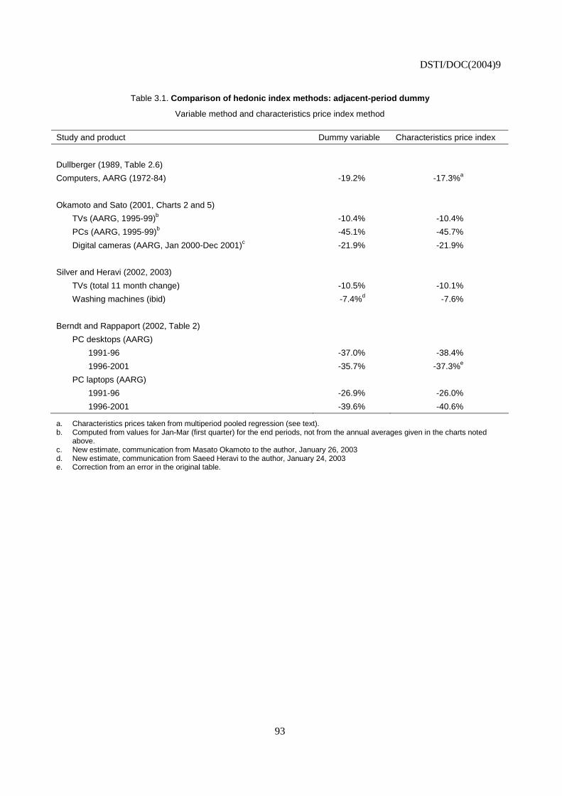
DSTI/DOC(2004)9

93

Table 3.1. Comparison of hedonic index methods: adjacent-period dummy

Variable method and characteristics price index method

Study and product Dummy variable Characteristics price index

Dullberger (1989, Table 2.6)

Computers, AARG (1972-84) -19.2% -17.3%a

Okamoto and Sato (2001, Charts 2 and 5)

TVs (AARG, 1995-99)b -10.4% -10.4%

PCs (AARG, 1995-99)b -45.1% -45.7%

Digital cameras (AARG, Jan 2000-Dec 2001)c -21.9% -21.9%

Silver and Heravi (2002, 2003)

TVs (total 11 month change) -10.5% -10.1%

Washing machines (ibid) -7.4%d -7.6%

Berndt and Rappaport (2002, Table 2)

PC desktops (AARG)

1991-96 -37.0% -38.4%

1996-2001 -35.7% -37.3%e

PC laptops (AARG)

1991-96 -26.9% -26.0%

1996-2001 -39.6% -40.6%

a. Characteristics prices taken from multiperiod pooled regression (see text). b. Computed from values for Jan-Mar (first quarter) for the end periods, not from the annual averages given in the charts noted

above. c. New estimate, communication from Masato Okamoto to the author, January 26, 2003 d. New estimate, communication from Saeed Heravi to the author, January 24, 2003 e. Correction from an error in the original table.

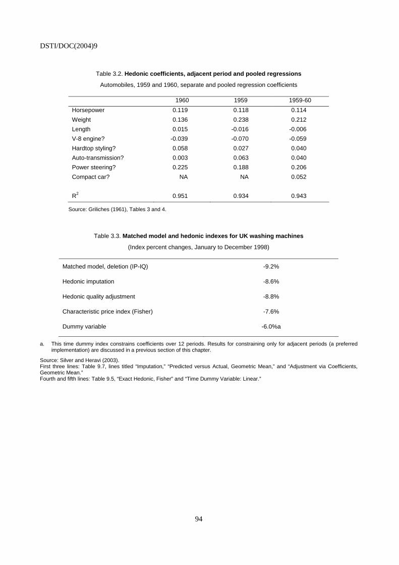
DSTI/DOC(2004)9

94

Table 3.2. Hedonic coefficients, adjacent period and pooled regressions

Automobiles, 1959 and 1960, separate and pooled regression coefficients

1960 1959 1959-60

Horsepower 0.119 0.118 0.114

Weight 0.136 0.238 0.212

Length 0.015 -0.016 -0.006

V-8 engine? -0.039 -0.070 -0.059

Hardtop styling? 0.058 0.027 0.040

Auto-transmission? 0.003 0.063 0.040

Power steering? 0.225 0.188 0.206

Compact car? NA NA 0.052

R2 0.951 0.934 0.943

Source: Griliches (1961), Tables 3 and 4.

Table 3.3. Matched model and hedonic indexes for UK washing machines

(Index percent changes, January to December 1998)

Matched model, deletion (IP-IQ) -9.2%

Hedonic imputation -8.6%

Hedonic quality adjustment -8.8%

Characteristic price index (Fisher) -7.6%

Dummy variable -6.0%a

a. This time dummy index constrains coefficients over 12 periods. Results for constraining only for adjacent periods (a preferred implementation) are discussed in a previous section of this chapter.

Source: Silver and Heravi (2003). First three lines: Table 9.7, lines titled “Imputation,” “Predicted versus Actual, Geometric Mean,” and “Adjustment via Coefficients, Geometric Mean.” Fourth and fifth lines: Table 9.5, “Exact Hedonic, Fisher” and “Time Dummy Variable: Linear.”

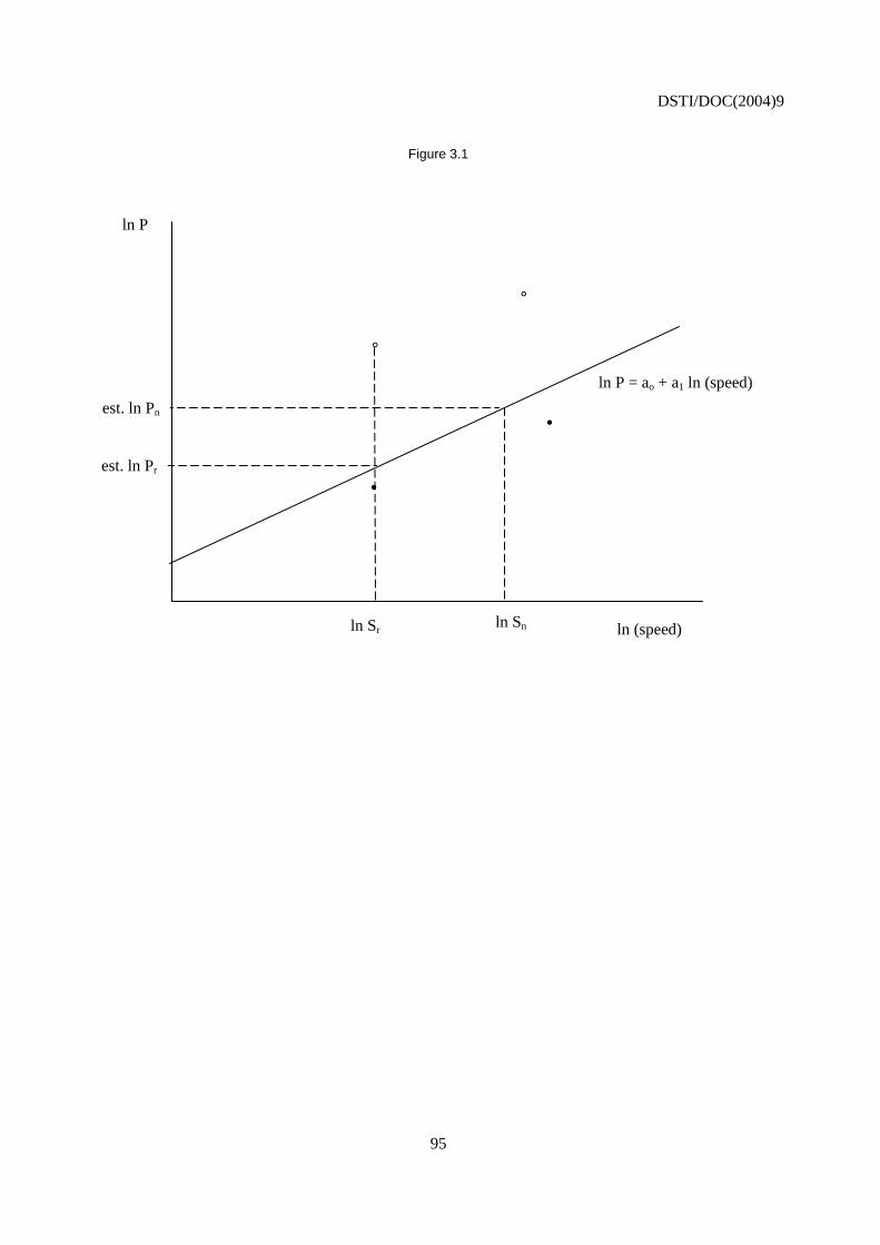
DSTI/DOC(2004)9

95

Figure 3.1

ln Sr ln Sn

•

°

est. ln Pr

est. ln Pn

ln P

°

•

ln P = ao + a1 ln (speed)

ln (speed)

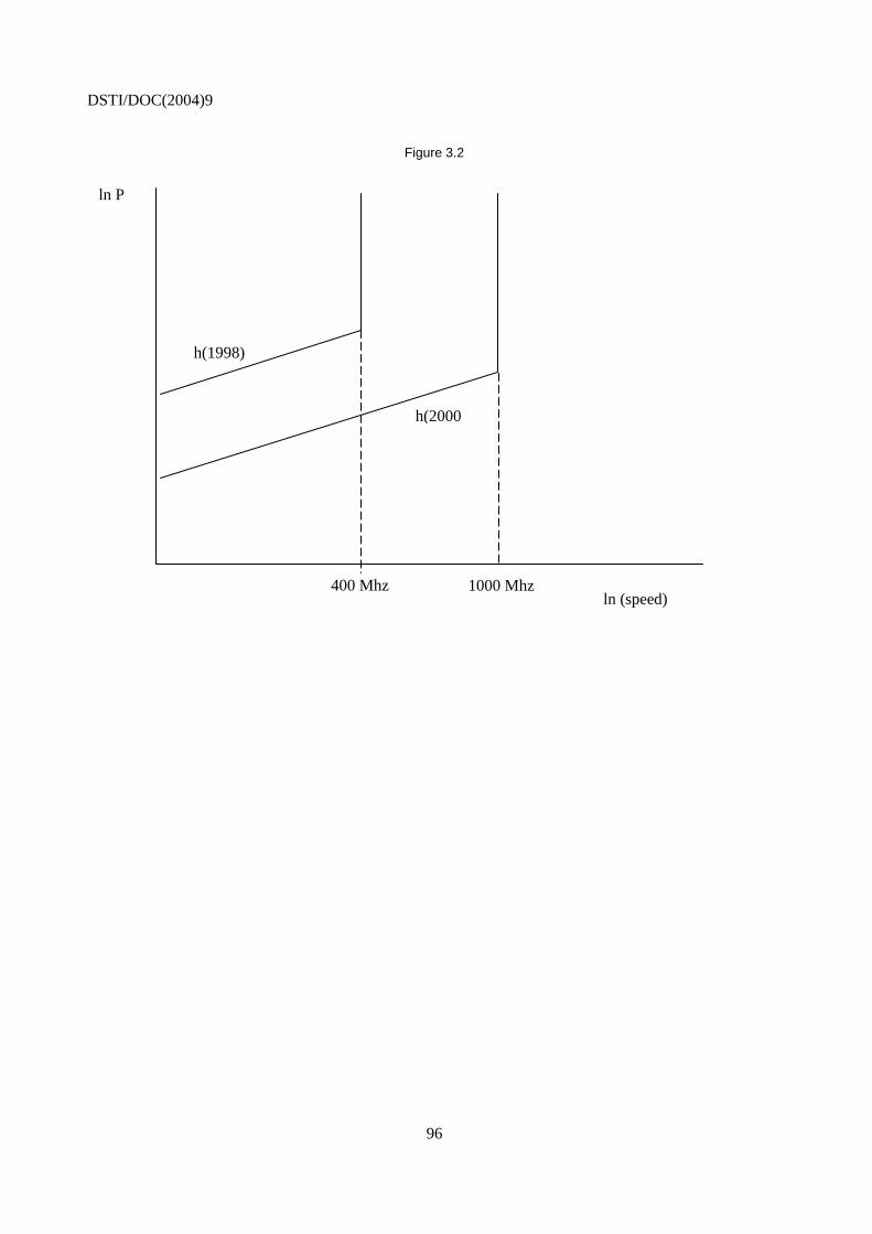
DSTI/DOC(2004)9

96

Figure 3.2

400 Mhz

h(2000

1000 Mhz

h(1998)

ln P

ln (speed)

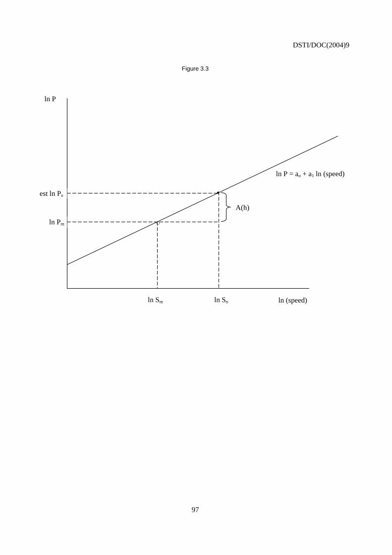
DSTI/DOC(2004)9

97

Figure 3.3

•

○

ln (speed)

A(h)

ln Pm

est ln Pn

ln P

ln Sm ln Sn


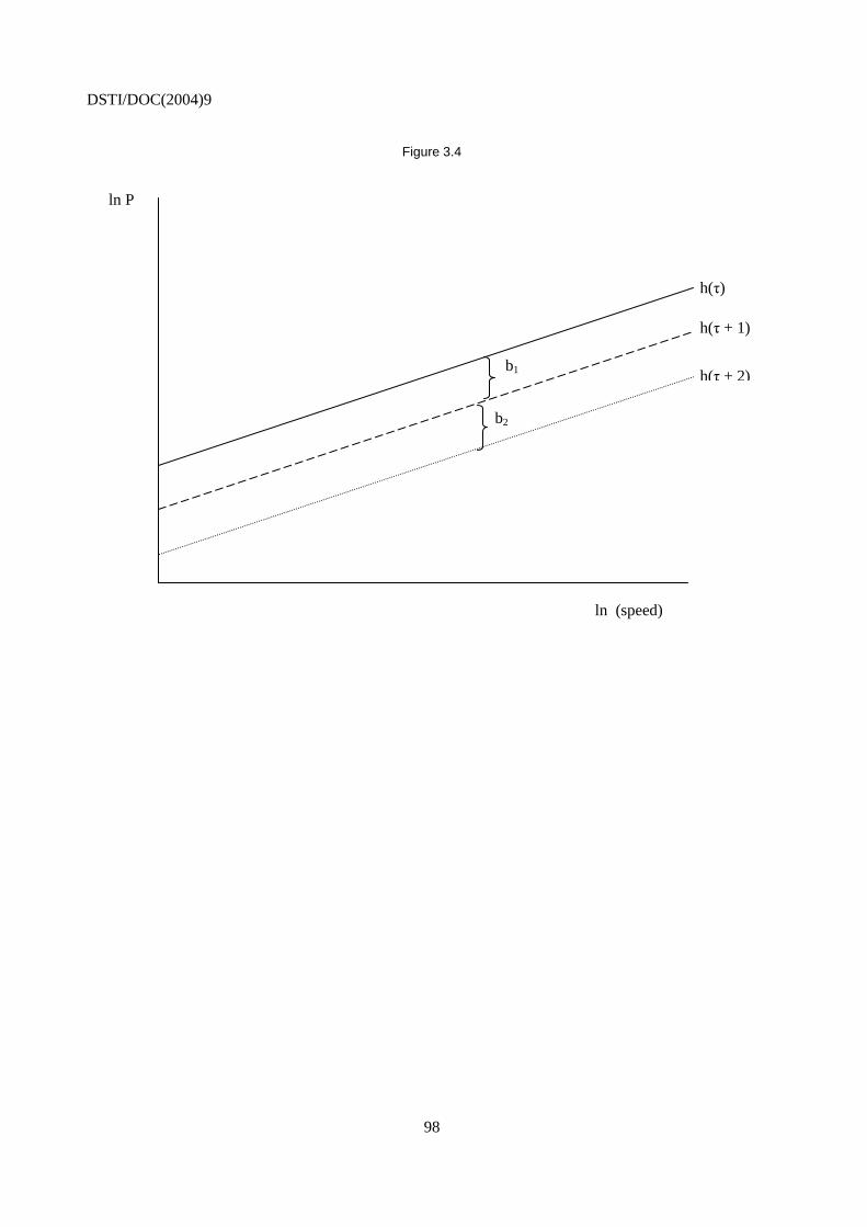
DSTI/DOC(2004)9

98

Figure 3.4

ln (speed)

ln P

b1

b2

h(τ)

h(τ + 1)

h(τ + 2)

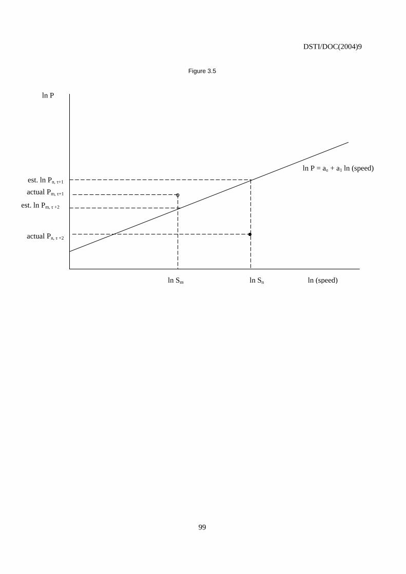
DSTI/DOC(2004)9

99

Figure 3.5

ln Sm ln Sn

est. ln Pm, τ +2

est. ln Pn, τ+1

ln P


actual Pm, τ+1

actual Pn, τ +2

°

●

ln (speed)

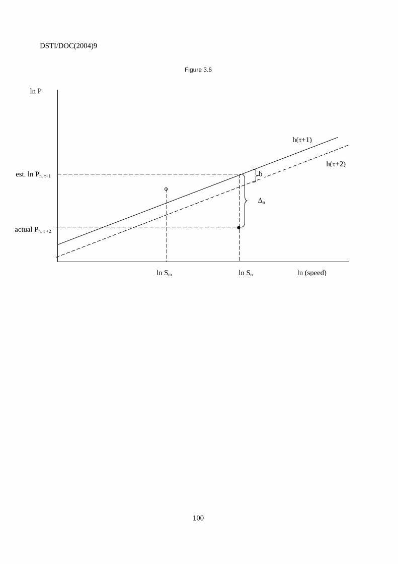
DSTI/DOC(2004)9

100

Figure 3.6

°

ln Sm ln Sn

est. ln Pn, τ+1

ln P

h(τ+1)

actual Pn, τ +2 ●

ln (speed)

h(τ+2)

∆n

b

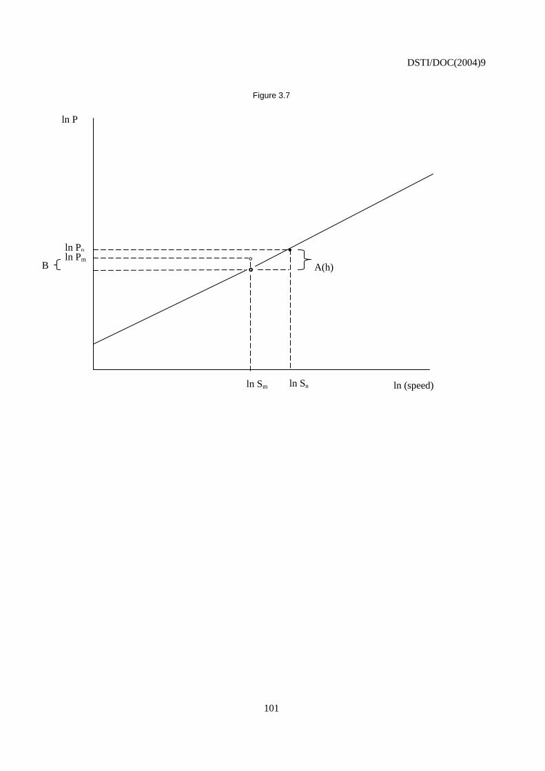
DSTI/DOC(2004)9

101

Figure 3.7

•

ln (speed) ln Sm

ln Pm

ln Sn

ln Pn

ln P

° A(h) B

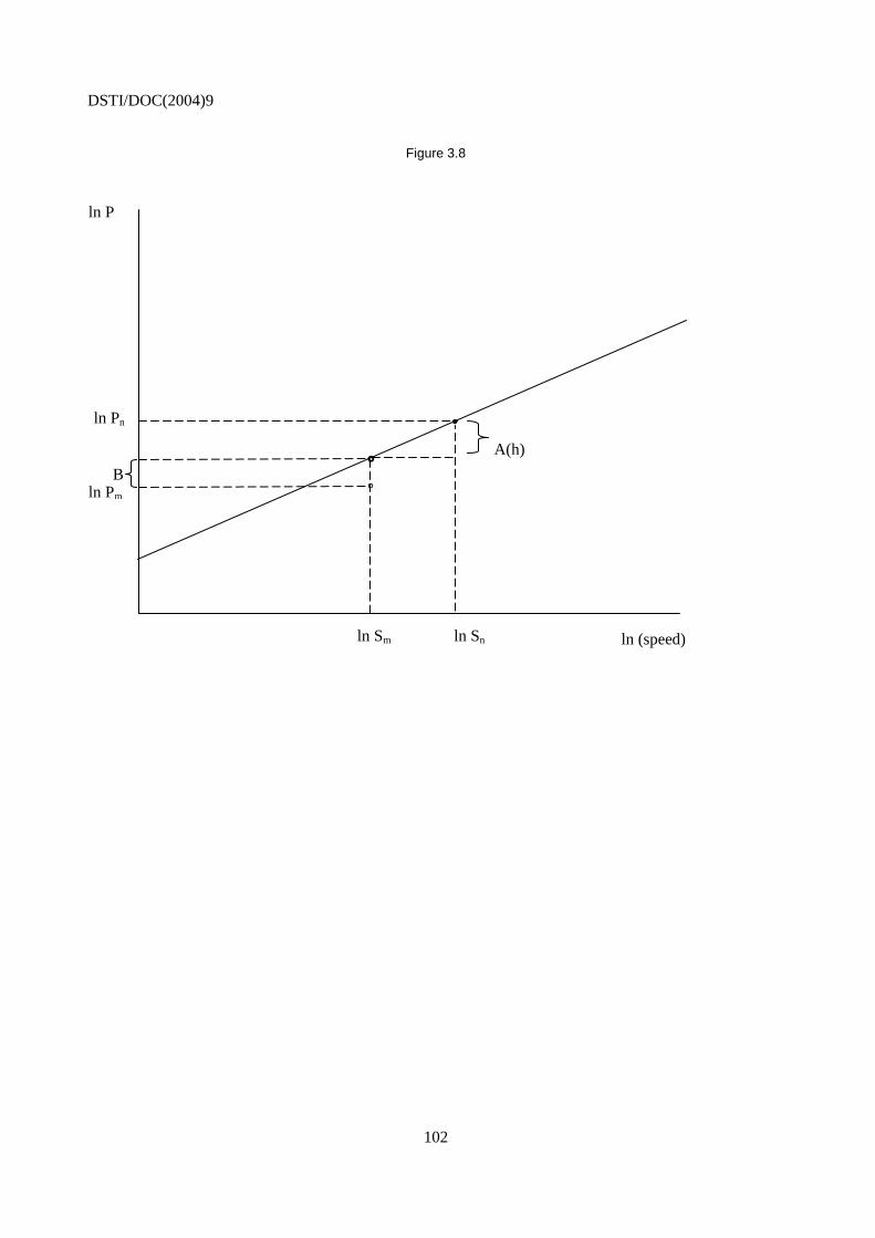
DSTI/DOC(2004)9

102

Figure 3.8

°

•

A(h)

ln (speed) ln Sm ln Sn

ln Pn

ln P

B ln Pm

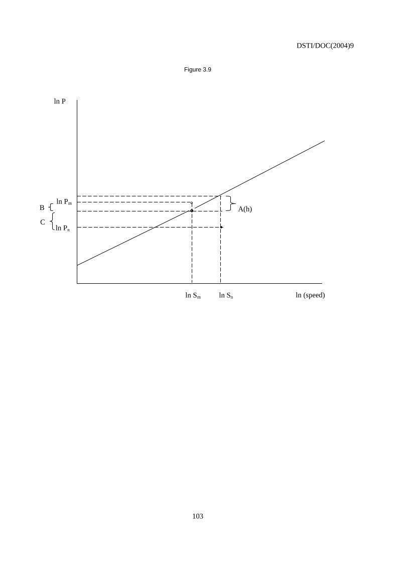
DSTI/DOC(2004)9

103

Figure 3.9

•

ln (speed) ln Sm

°

ln Pm

ln P

A(h) B

C ln Pn

ln Sn

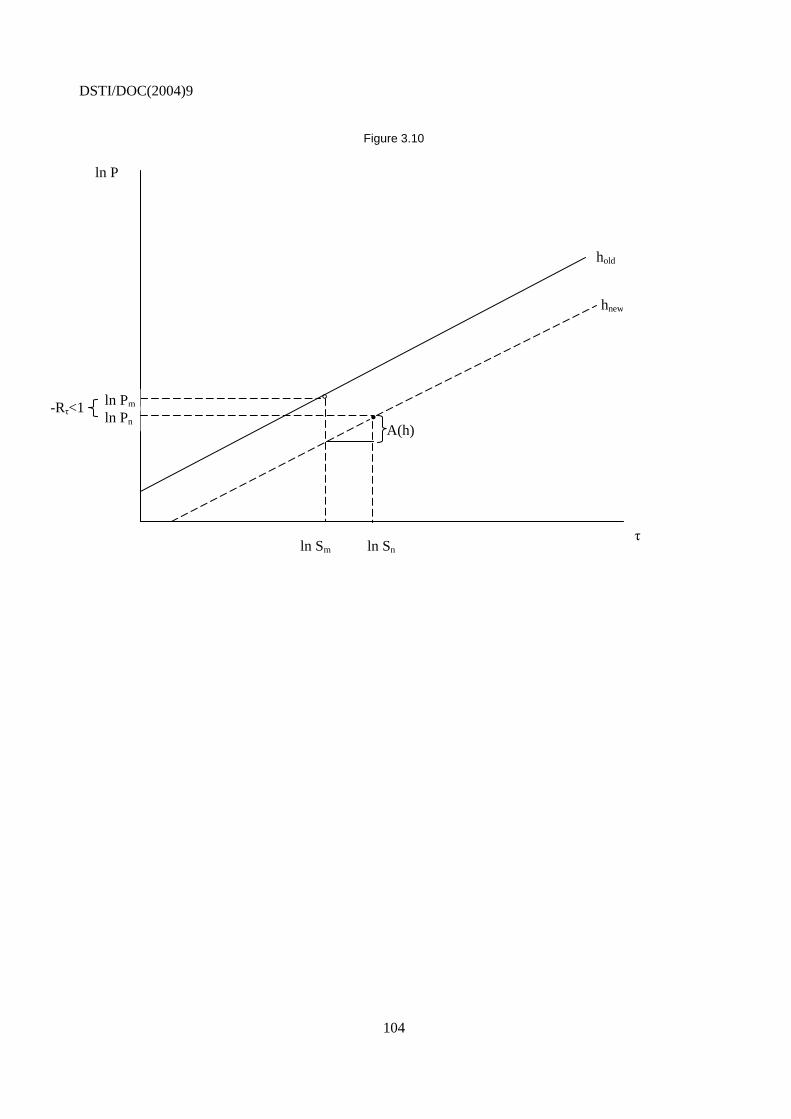
DSTI/DOC(2004)9

104

Figure 3.10

° •

A(h)

τ ln Sm ln Sn

ln Pm

ln Pn

ln P

-Rτ<1

hold

hnew

DSTI/DOC(2004)9

105

CHAPTER IV

WHEN DO HEDONIC AND MATCHED MODEL INDEXES GIVE DIFFERENT RESULTS?

AND WHY?

Many economists believe that hedonic indexes generally rise more slowly, or fall more rapidly, than matched model indexes. One also frequently hears the opposite, particularly from within statistical agencies: Hedonic indexes should give the same result as matched model indexes.

The question “do they differ?” is too simple. Empirical studies show that matched model and hedonic indexes seldom coincide, they usually differ. I review the empirical work in section D of this chapter. More crucial are the “when?” and the “why?” parts of the questions in the chapter title. One needs to understand the circumstances under which matched model indexes and hedonic indexes will give the same result and the circumstances under which they will differ.

A portion of this topic – but only a portion – was addressed in chapters II and III. The content of chapters II and III was kept narrowly focussed on the forced replacement problem inside price index samples: Some items that were in the index sample disappear and their disappearance forces selection of a replacement. Forced replacements require the statistical agency to make suitable quality adjustments for the quality changes between replacement items and the old items they replace in the sample. Hedonic quality adjustments for forced replacements may yield different indexes from those produced with conventional quality adjustments, but this will depend (among other things) on which conventional quality adjustment method is used for the forced replacement. See the conclusions of chapters II and III.

This forced replacement focus was preserved partly for expositional reasons, in order to highlight differences in the way conventional and hedonic indexes handle quality change. The framework used in chapters II and III explicitly and purposefully set the rest of the index number context the same: the index databases (whether small or large sample or universe), sampling procedures, calculation methods, and collection strategies were held fixed. By abstracting from other issues that may also arise in constructing accurate price indexes for high tech products, the “other things equal” exposition in chapters II and III directed attention to one set of issues on which there has been much confusion – the difference between hedonic and conventional indexes, particularly conventional and hedonic quality adjustments – without introducing elements that, though important, complicate the discussion.

However, a complete treatment goes beyond forced replacements in fixed samples (no matter how large). This chapter compares hedonic and matched model indexes in a broader context, in which the effects of entries and exits in product markets – not just exits and replacements in the sample – are considered.

A. Inside-the-sample forced replacements and outside-the-sample quality change

The forced replacement problem addressed in chapters II and III is perfectly general, it does not apply solely to price indexes that are based on small samples. It is indeed true that most statistical agency samples of high tech products normally include only a small part of the universe of those products. However, even if the price index were based on the initial period’s universe of transactions for some

DSTI/DOC(2004)9

106

product, the forced-replacement quality adjustment problem arises as items in the initial period’s universe exit and are replaced by new product varieties in subsequent periods.

Numerous studies of personal computers have documented an extraordinary rate of model turnover: Pakes (2003) records annual sample attrition of 80% in IDC data for US PCs, and Van Mulligen (2002) reports that in a near universe of Dutch computer models sample attrition rates average nearly 20% per month. Koskimäki and Vartia (2001) and Lim and McKenzie (2002) present comparable sample attrition rates from two widely separated markets (Finland and Australia). Rapid model turnover is not confined to computers. Silver and Heravi (2002) examined the scanner data transactions universe for UK appliances; they show that exits reduce the original coverage by 20% in 12 months. 79 Moreover, when entrants were also ignored, the fixed sample’s coverage declined to only 50% of expenditures by the end of the year.

Because exits and entries are the essence of the forced replacement problem, the analysis of chapters II and III still applies to large samples. A number of computer price indexes have now been produced which use matched model methods on a large sample or near universe (see the review in section D of this chapter). Regardless of the size of the sample, one can still ask: Would the index have been different had hedonic quality adjustments been employed for forced replacements instead of matched model methods?

However, the impacts of quality change on price indexes go beyond adjusting the fixed sample for forced replacements. Forced replacements are caused by exits of old product varieties from the sample. Equally important are the price impacts of entering new product varieties, new varieties that may not be in the sample at all. What matters is not only how the agency (or the researcher) adjusts for inside-the-sample quality changes, but also whether the fixed-sample design systematically misses price change from rapid turnover of product varieties in high tech products. Size of the sample may be an issue. Of more importance are frequency of sample updating, weighting of the sample, principles for selecting the item samples, item replacement rules when an item exits from the sample, and – especially – the impact of new product entries on the pricing structure. I refer to this complex of measurement problems as “outside-the-sample” quality change problems, because they cannot be ameliorated in any way by improving the adjustment methods for quality changes encountered inside the sample, nor can they be understood in the context of the inside-the-sample (forced replacements) analysis.

In turn, one can think of the outside-the-sample problem as having two parts: first, do the relatively small fixed samples normally drawn for price indexes remain representative for multiple periods? The very rapid rates of sample deterioration already cited suggest they are not representative for high tech products.

Second, do large samples, or even universe samples that are replenished frequently, account for all price change when used in a matched model price index calculation? This second question is considerably more complicated. A matched model index that is based on a broad sample, or a universe, and that is updated frequently is sometimes called the “frequently resample and reweight” method (hereafter, FR&R).80 Can an agency get equivalent results from an FR&R reform of the traditional matched model index methodology, without adopting hedonic methods? If it can, are there advantages in cost and data requirements of expanded, FR&R matched model indexes over hedonic indexes for high tech products? Conversely, if hedonic and FR&R matched model indexes differ, why do they and under what circumstances?

79. To avoid misinterpretation, one should note that a 20% (or 80%) attrition rate does not mean that the

statistical sample at the end of the period will be 20% (or 80%) smaller than in the initiation period, because agencies will normally replace exits.

80. I have taken this term from European usage, there seems no equivalent in English language usage elsewhere. I am told that Eurostat has introduced a new term recently,

DSTI/DOC(2004)9

107

The answers to all these questions depend on the operation of markets – the way price changes come about, the way new products are introduced and priced, and the marketing strategies pursued by producers of high tech (and much low tech) equipment. The following sections develop these ideas.

B. Fixed samples and price changes outside the sample

Statistical agencies typically draw product samples at some period and hold them fixed, or attempt to hold them fixed, over some interval. If probability samples, fixed samples may be drawn conceptually from what Dalén (2001) has called the “fixed universe” or they may have been drawn with the intention of representing Dalén’s “dynamic universe” but without the statistical methodology to do it adequately. Even if originally representative, the longer the interval over which the sample remains fixed, the more likely that it will become unrepresentative of the universe of transactions.

In some countries’ price indexes, product or item samples of high-tech products are judgemental. Items may be selected with an eye to reducing the incidence of future forced replacements – the rule is to find products that are likely to remain for sale, and less likely to disappear. When quality change takes the form of new product varieties, samples of varieties that do not change may be very unrepresentative right from the start. Trying to minimise the incidence of forced replacements generates another “quality problem” that is equally, and perhaps more, serious.

Though we speak of the “fixed sample,” the sample never really remains fixed; replacement items are brought in as old varieties exit, and the index is linked over in some manner, or adjusted, as explained in Chapter II. The sample is “fixed” in the sense that a new sample is not drawn for some interval (which varies across countries and sometimes across products), and in the sense that entering computers have no probability of entering the sample, except as replacements for computers that exit the sample. The sample is not fixed in the sense that the products in it never change; but changes are forced, they are not changes by design.

Accordingly, replacement rules matter. Whether the sample was originally drawn on probability or judgemental principles, when forced replacements occur the agency may select a replacement item that is as close as possible to the one that exited the sample. The logic of this “nearest product variety” rule is to minimize the quality changes for which adjustments are required. This replacement rule has been called (by Walter Lane, of the US BLS) “find the next most obsolete product.” “Nearest product variety” replacement rules assure that the sample will increasingly be unrepresentative of high-tech product varieties that are for sale. Again, attempting to minimise one kind of quality error risks introducing another.

Whether fixed samples are drawn on a probability or judgemental basis, the price behaviour of the fixed sample will not adequately represent the price behaviour of the total market in the face of rapid technological change and the introduction of new product varieties. Replacing products that exit from the sample is not the same thing as bringing new products into the sample on a timely basis. Though much thinking about these topics has proceeded recently in conjunction with the HICP program in Europe, it is important not to overlook antecedents, for the lessons that can be learned from them are not the less valuable for being old lessons.

1. Research studies

One of the first studies on the fixed sample quality change problem was Berndt, Griliches, and Rosett (1993). Working on a product completely unrelated to IT, they found that prices for newer pharmaceuticals fell, relative to older ones. Indeed, this study produced the arresting finding that drug manufacturers

DSTI/DOC(2004)9

108

typically raised the prices of older branded prescription pharmaceuticals when new generic competition followed expiration of a patent.

At that time, the US BLS selected pharmaceuticals for the PPI on a probability basis, but once they were selected, they stayed in the sample for five years, until another probability sample was drawn.81 Using an exhaustive database of pharmaceutical prices obtained from manufacturers, Berndt, Griliches, and Rosett were able to mimic the US PPI for pharmaceuticals. They then constructed a price index that brought new pharmaceuticals into the index as soon as they were introduced. Because prices of newer pharmaceuticals declined relative to older ones, the price index that mimicked the PPI sample rose considerably more than the universe of drug prices. Berndt, Griliches, and Rosett (1993) showed that holding the sample fixed in the face of technological innovation and new products resulted in a substantially upward-biased price index. Theirs was a very influential study, for it caused changes in PPI sampling procedures for pharmaceuticals.

A second pair of studies concerned semiconductors. Dulberger (1993) and Flamm (1993) documented the effect of delay in bringing new semiconductor chip products into the price index. In the PPI for semiconductors at that time, the BLS chose a probability sample of chips and held the sample fixed for approximately five years, except for forced replacements. The prices of newer types of semiconductors were declining more rapidly than older ones, similar to the case of pharmaceutical prices. Both Dulberger and Flamm presented semiconductor price indexes that differed substantially from the published US PPI indexes for semiconductors. Table 4.1 summarises Dulberger’s findings. When new semiconductor chips were brought rapidly into the price index, standard index number formulas exhibited price declines of 20%-35% per year (see the first four entries in Table 4.1). In contrast, when Dulberger mimicked the PPI procedures on the same data, so that new chips entered the index with a delay, the price index fell only about 8.5%, which was closer to the PPI’s 4.5% decline (last two lines of Table 4.1).

None of these studies had anything to do with hedonic indexes – they were all computed with matched model methods. Essentially, they were all FR&R indexes, though sometimes equally weighted. They provided great insight into the question of constructing price indexes for products that were experiencing rapid technological change: They found that rapid quality change made fixed samples obsolete because prices of new product varieties, after their introduction, declined more rapidly than did prices of older products. The problems they uncovered did not originate in the treatment of inside the sample, forced replacements.

Silver and Heravi present similar results in a series of papers, though they use hedonic indexes to quantify their conclusions. As Silver and Heravi (2002) put it, two conditions must be met for price index bias from fixed samples: First, the samples must lose representativeness. Second, the price changes of the varieties that remain in the fixed sample must be systematically different from those that do not (the new and the exiting products). They show that the fixed sample for appliances in the UK deteriorates very rapidly; thus, the first condition is met. The second condition is also met, because price changes of entrants and exits from the sample are different from the price changes for products that continue. Substantial bias arose from holding appliance samples fixed for even a few months.

Moulton, Lafleur, and Moses (1999) compared matched model and hedonic indexes using the database collected for the CPI. They estimated two hedonic indexes for colour TVs: (a) a characteristics price index for TVs, using hedonic functions estimated from the CPI database, and (b) an index in which

81. Forced replacements are not frequent in drug price index samples.

DSTI/DOC(2004)9

109

hedonic quality adjustments (using the same hedonic function) were made for forced replacements in the actual US CPI TV index.82

The index with hedonic quality adjustments for forced replacements differed only insignificantly from the published CPI TV index (Table 4.2). This implies that hedonic quality adjustments for forced replacements – about 15% of the price quotes – equalled in magnitude the actual CPI quality adjustments, which were mostly by the “class mean” variant of the IP-IQ method (explained in Chapter II).

The characteristics price index, however, differed substantially from the actual CPI, even though both were based on the same CPI database (Table 4.2). The US CPI sample is periodically replenished; in new samples, new TV models are selected with a probability proportionate to their sales. Moulton, Lafleur, and Moses reasoned that (in the language used in this handbook) the characteristics price index allowed for the price impacts of new introductions into the CPI sample, where CPI quality adjustments (hedonic or not) were made only for forced replacements for sample exits. When allowance was made for the entry of new product varieties, and not solely for forced replacements, the price index showed a steeper rate of decline.83

As these studies suggest, new varieties may exhibit price changes after their introduction that differ from the price changes of older varieties. In the usual economists’ notion of the pricing cycle, prices of newer varieties fall more than the prices of continuing products, and for this reason the newer ones earn larger market shares.

New products might also be initially introduced at low (quality adjusted) prices, to induce consumers to try them. In this case, their subsequent prices rise, relative to those of continuing products, especially if they are successful introductions. Though this also implies an error from use of the fixed sample of established varieties, the direction of price index error in this case is not always obvious.84

Most price indexes are constructed around some notion of a representative sample of sales in the initiation period. A sample of initiation period sales may be adequate when little change occurs in the range of products that are for sale, when yesterday’s products are pretty much the same as today’s. Or the fixed sample may work fairly well when the prices of any new products that are introduced move more or less consistently with those of established products. In semiconductors, pharmaceuticals, and computers in the United States, and in appliances in the United Kingdom (and possibly in the United States), a price index that records only price movements in established products misses much of the price change that occurs. These studies all show that price movements from new introductions, after they are introduced, can be different from price movements measured by the continuing varieties (and item replacements) that are contained in a fixed sample.

82. See Chapter III for definitions of the characteristics price index and of hedonic quality adjustment.

83. In the Moulton, Lafleur, and Moses (1999) study, it is not clear whether prices of new entrants into the CPI sample – which are not, after all, necessarily new entrants into the market – were declining relative to established TV models after the new models entered the sample, or had prices that were lower (quality adjusted) at entry. For the latter problem, see the next section of this chapter. Most other studies have shown that matched model indexes overstate the rate of decline for TVs; see section D of this chapter.

84. Pakes (2003) contains an example where the price of the new product rises after introduction, yet, because the new products are better on a quality-adjusted basis than those that they displace, the price index should fall as their market share rises. Though economists have speculated about which behavior of new product prices – falling or rising prices after introduction – is the dominant one, few empirical studies exist to confirm which speculation is born out in actual markets.

DSTI/DOC(2004)9

110

2. Hedonic and FR&R indexes

The new introductions bias discussed in the previous section can be ameliorated by FR&R methods, in which new products are brought promptly into the sample. Hedonic indexes are not strictly necessary. It is true, nonetheless, that hedonic index samples often approach universes of product varieties, and their samples are normally replenished for each period covered in the investigation. Accordingly, hedonic indexes share sample size, sample replenishment, and near universe coverage with FR&R index methods; perhaps these are the features of hedonic indexes that ameliorate the fixed sample problem. One might expect, at any rate, that when new models have price changes after introduction that differ from price changes for continuing models, FR&R and hedonic indexes will coincide because both incorporate these new models promptly.

FR&R methods, however, cannot confront another potential problem posed by new product introductions. If price change takes place at the introduction of new product varieties, or if price change is associated with product exits, price changes can be missed even with rapid replenishment of samples. This class of problems is addressed in the following section.

C. Price changes outside FR&R samples

New varieties may experience different price movements after their introductions from those of older varieties, as explained in the previous section. However, there is a second price effect from new varieties. Price changes may accompany the introduction of new products, or the exit of old ones. A “residual diagram” similar to the ones used in Chapter III, illustrates (Figure 4.1).

Suppose a new computer (model n) is introduced that is faster than the one it replaces (model m), but is cheaper, because it embodies a new technology. Statistical agencies frequently observe that replacements appear that are higher in quality but lower in price than the products they replace, which is the situation depicted in Figure 4.1. Because the old hedonic function (hold) reflects the old technology, computer n’s introductory price is also lower than the old hedonic function.

Disregarding for the moment what happens to the prices of continuing computers (the matched models), the replacement of computer m by computer n amounts to a price reduction – the spectrum of (quality-adjusted) prices is lower than it was before computer n’s introduction (refer to the discussion of this point in Chapter III, section C.3). The hedonic function “residual” in Figure 4.1 shows the price difference between the actual price of the new computer (model n) and an old one with the same specification – the value “est ln Pn” in Figure 4.1 is the estimated price of a computer with computer n’s specification, estimated from the old hedonic function. The hedonic function residual therefore indicates the downward pressure on the prices of competitive computers implied by the introduction of the new computer.

The residual also measures – in this particular case – the price decline of the new computer (model n), compared with the one that it replaced (model m). The actual price difference between these two computers is labelled V in Figure 4.1, but V under-estimates the true price decline because computer n is faster than computer m. The quality-adjusted price difference is the actual price difference (V) plus (in this case) the value of the quality difference, which is labelled A(h) in Figure 4.1. The sum of these two terms equals the residual, so the residual measures the quality adjusted price difference that should go into the price index.

In this chapter, we do not need the more complicated notation that was introduced in Chapter III. I thus revert to the simpler notation of Chapter II, and designate the “old” or previous period’s hedonic function as period t, the “new” or current period’s hedonic function as period t+1.

DSTI/DOC(2004)9

111

1. Case one

Suppose initially that no other price changed in response to the new computer. Any hedonic method would give a declining price index. Matched model indexes generally will not, whether fixed or FR&R samples.

Consider first the hedonic dummy variable method. Even if prices of other computers do not change in response, computer n’s introductory price (below the old hedonic surface) will pull the hedonic function downward, by an amount that depends on the size of the residual in Figure 4.1 and computer n’s market share. The new hedonic function might, for example, look like the hedonic function h (t+1) shown in Figure 4.2. The coefficient of the dummy variable in an adjacent-period regression measures the price change (see Chapter III); in Figure 4.2, the dummy variable index is shown as the downward shift of the hedonic function, from h (t) to h (t+1), marked ∆h, in Figure 4.2.85

Now consider the hedonic imputation method. The hedonic index also would fall. The imputed price decline for the entering computer is measured by the residual in Figure 4.1, as noted above. This decline is shown as ∆Pn in Figure 4.2 (∆Pn is the same as the residual in Figure 4.1). The index declines by ∆Pn, weighted by computer n’s index weight.

One could also impute a price change for the exiting computer (which would be good practice). This yields a price decline equal to the amount ∆Pm, which is also shown in Figure 4.2. It might not seem intuitively obvious that the imputed price for the exiting computer falls, when no continuing computer experiences price change. In this example, computer m’s price in period t lay on the old hedonic line, h(t). The decline occurs because the hedonic function for the new period (t+1) is used to impute the price of exits (see Chapter III). The hedonic function h(t+1) is below h(t), so the imputed price of exiting computer m in period t+1 is below its actual price in period t, yielding ∆Pm as the price decline for computer m. 86

What about the FR&R method? Will it record a price decline? Generally it will not, though the complete answer depends on which method of quality adjustment is used in the FR&R index.

Most FR&R indexes will probably shift over to the new computer when it is encountered and drop the old one, linking together the index from the old sample to the index that uses the replenished one. This implies the deletion (IP-IQ) quality adjustment method (Chapter II), in which the price change for the exiting/entering computer is implicitly imputed from actual price changes of continuing ones.

In our example, none of the continuing computers changes in price. Hence, imputed price change for exiting or entering computers is zero. The FR&R method clearly misses price change, and it differs from the hedonic index. The result for the FR&R sample is the same as from the fixed sample index, which was discussed in chapters II and III. The FR&R sample does not surmount the problems of the fixed sample when prices of continuing computers do not respond to new entrants.

85. Entry of the new computer might also change the slope of the hedonic function, but this is neglected for

simplicity in the diagram (see the parallel point in Chapter III, section B). One needs to worry about the weight of computer n in the regression (in the usual equally weighted regression, computer n might have a weight that is too high or too low), but that matter is discussed in Chapter VI.

86. A different period t price for computer m would obviously change this example. Consider the implication if Pmt were below the (new) regression line; in this case the exit of computer m implies a price increase.

DSTI/DOC(2004)9

112

Some alternative quality adjustment method might be combined with the FR&R method. For example, the price index agency might use option prices to adjust for the quality difference between computer n and computer m, or it might apply a production cost adjustment, or even use a hedonic quality adjustment. In these cases, some or all the price decline might be recorded in the FR&R index. But the claimed advantages of the FR&R method evaporate, because FR&R has been proposed as a way to estimate accurate price indexes for high tech products without going to the expense of hedonic methods.

2. Case two

The first case (no price response of continuing computers to the entering computer) is a limiting or extreme one. Consider the case at the other extreme: suppose prices of the continuing computers fall fully and instantaneously to respond to the new computer. This yields a new hedonic function, such as h(t+1) in Figure 4.3, in which computer n is on the hedonic surface (for simplicity, I continue to suppose that the price of computer m lay on the old hedonic surface).

In the case of instantaneous price response, the FR&R index will pick up all the price decline accompanying the introduction of computer n, because the market effect of the new computer is reflected in the price changes of continuing computers that are inside the FR&R sample. On the other hand, the fixed sample index will also suffice, because with instantaneous market adjustment, the index will record the full price decline even if computer n is not included in the sample. In case two, then, the FR&R index equals the hedonic index, but the FR&R index is not necessary, the fixed sample will also pick up all the price change.

3. Case three

The most realistic case lies between the two extremes: the introduction of the new technology brings about some price response, but the market does not fully adjust instantaneously. Some of the price decline accompanying the new computer’s introduction will be picked up by the matched model FR&R index, but not all of it. The reasoning is the same as for case one: If the FR&R index is implemented with the deletion (IP-IQ) quality adjustment method, as would normally be the case, the imputed price change for the exiting/entering computer will be the price change for the continuing computers; by specification in the example, prices of continuing computers do not decline as much as the price of the entering computer. The FR&R index misses some price change measured by the hedonic index, but not necessarily all of it. The hedonic index measures all of the price decline, whether estimated by the dummy variable method, the hedonic imputation method, or another hedonic method.

Ultimately, as more new computers similar to computer n are introduced, the new technology will shift the hedonic function down to a new level, but this may take some time. When that happens, all computers made with the old technology may disappear, because it is not possible to produce computers on the new price/quality frontier with the old technology. For example, 386 chip technology for PCs replaced 286, Pentium replaced 386 and 486, and was in turn replaced by Pentium II, III and IV.

One might contend therefore that the FR&R index eventually follows the hedonic index, so the error in case three would be small, or that it would just amount to a lag. This is an empirical proposition that might be true, but it is hazardous to count on it. Suppose all of the matched models initially remain in the sample (that is, computer m does not exit, so it does not trigger a forced replacement). Computer n enters at a lower price/quality level and is followed by its technology mates. No prices of m-type computers fall. The pricing agency updates its sample frequently (a FR&R index), so it gradually replaces m-type computers with n-type computers. Then at some point all the m-type computers, having gradually been

DSTI/DOC(2004)9

113

replaced in the sample, exit from the market. No price decline will be recorded in any matched models comparison. Yet, the quality-adjusted prices are lower in the end period than at the beginning.87

Summary. Whether a FR&R matched model index incorporates all the price change recorded in a hedonic index depends on several factors:

(a) The speed with which the FR&R matched model index incorporates new varieties. An annual resampled and reweighted index might be considerably less effective than a monthly one, because too much model turnover takes place before the annual sample is replenished. The hedonic index is better because it contains an explicit price change measure for exits and entries, which may be large over a year’s time. Conversely, the higher the frequency of the FR&R, the more its measurement should approach that of the hedonic index.

(b) The amount of price change that occurs at the point of introduction of new varieties, rather than after their introduction. If new varieties are introduced with (quality-adjusted) prices that are lower – or higher – than the ones they replace, these price effects will be missed by the FR&R index. If the price/quality ratios of entering computers are similar to old ones, little price change is implied by entries, and little is lost by omitting them from the FR&R index. Similar statements apply to price changes implied by exits.

(c) The effect of factor (b) is combined with a third factor – how rapidly do prices of continuing varieties respond to the new introductions? If markets respond instantaneously to the competition of new and improved varieties, then the FR&R price index, which necessarily imputes the price changes of entering and exiting varieties from the price changes of continuing ones, nevertheless will pick up the price impact of the entering varieties. If market responses are slow, the FR&R index will miss price change associated with entries and exits, or will incorporate them with a lag.

(d) The weight of the entering and exiting varieties. If the weight of entering and exiting varieties is small, one expects that their market impact will also be small, whether or not the entering varieties have lower – or higher – quality-adjusted prices than the varieties they replace (factor b), and whether the market adjusts instantaneously or does not (factor c). One would expect, though, that the weight of entering varieties will be greater when they offer price reductions and when the market response is slow.

These four factors imply the need for empirical work to quantify them in different markets and for different ICT products, for the purpose of guiding practical strategies for constructing accurate ICT price indexes. Available information is reviewed in section D.

Before turning to the existing empirical studies, it is worth noting that the assertion that hedonic indexes and conventional indexes should give the same answer is quite old. Jaszi (1964) gave an example of coffee-chicory mixes in different proportions, and asserted that the price should reflect the costs of the different mixes, which would also be recovered in a production cost quality adjustment method (see Chapter II), or in the ratios of their prices in the overlapping link method.88

87. This speculation appears broadly consistent with the findings of Moulton, Lefleur, and Moses (1999). It is

explicit in Dulberger (1989). See also von Hofsten (1952) for a parallel discussion involving new car models. The point is quite old, and the potential problem is quite well known and discussed in the price index literature, yet it is still neglected.

88. The example is interestingly dated. Chicory root was once used to “cut” coffee in some places in the United States to make a less expensive beverage.

DSTI/DOC(2004)9

114

Jaszi’s example, as does other similar reasoning on the issue, implicitly assumes market equilibrium prices for both periods in a price index comparison. If newer computers had higher quality relative to their price, this logic goes, that should push down the prices of existing models – in factor (c), above, response is instantaneous. Both the hedonic index and the matched model index should reflect the effects of quality improvements, whether the quality change occurred on the models in the sample or outside it. A properly constructed matched model index, on this line of reasoning, should equal a hedonic index.

The interesting cases are those where market equilibrium might not prevail. Moreover, what might seem reasonable for coffee-chicory mixes (which anyone can mix) might not seem so reasonable for differentiated high-tech products. With differentiated products, sellers look for market niches that are not served by the existing variety spectrum. If they locate such a niche, innovation in creating a new variety implies a return, and so implies at least short-run market power, which can hardly be conceived for a new coffee-chicory mix. Reasoning that markets should respond quickly to innovation in new product varieties is not confirmation that markets do in fact respond quickly.

D. Empirical studies

Many comparisons between hedonic indexes and matched model indexes have been carried out, on many products.

1. Early studies: research hedonic indexes and statistical agency matched model indexes

The early studies that compared hedonic indexes with statistical agencies’ matched model indexes are reviewed in Triplett (1975). Gordon (1990) contains similar comparisons for many investment goods.

In many of these studies, researchers found that hedonic indexes rose less rapidly, or fell, compared with published government matched model indexes, and this result has found its way into the folklore of economics, despite the fact that contrary examples are numerous. These contrary findings – when hedonic indexes rose more rapidly than the price indexes with which they were compared – should have received more attention. The analysis in Chapter II shows that the direction of bias from the application of conventional methods is sometimes more nearly a function of the direction (rising or falling) of true price change than the direction (improving or deteriorating) of quality change. Thus, if hedonic indexes are more accurate than conventional ones, they might show less price increase or more price increase, depending on the direction of quality change bias from conventional methods; they might also agree, if conventional quality adjustments happened to give the same result as hedonic methods.

In any case, these early studies were not true evaluations of alternative quality adjustment methodologies. Most researchers computed hedonic indexes from databases consisting of a series of large, extensive annual samples or near universes of models, in which the prices were usually list prices, not transactions prices. They compared them with statistical agency matched model price indexes for the same or a similar product. The statistical agency indexes were derived from small samples, and their prices were transactions prices, as nearly as the agencies could obtain them.

Thus, these early hedonic-matched model comparisons confounded differences in databases, fixed sample-universe sample differences, and so forth, with differences in quality adjustment methods. To an undetermined extent, reported differences between research hedonic indexes and published government agency matched model indexes reflected something more than the difference between matched model and hedonic methodologies. Missing from the early studies were hedonic index-matched model index comparisons that covered the same database.

DSTI/DOC(2004)9

115

2. Same database studies: hedonic indexes and matched model indexes

We need studies that estimate, solely, differences associated with matched model and hedonic methodologies. I am accordingly very selective in the studies included in this review. I include only studies that (1) estimate matched model and hedonic indexes using the same database, and (2) conform to best practice for both methodologies. That means FR&R indexes for the matched model method and one of the best practice examples of hedonic indexes. Even so, no doubt some studies that could have been included in this review were not, but any exclusions were not purposeful.

Dulberger (1989) was the first computer study that compared hedonic and matched model indexes computed from the same database. Dulberger’s data consisted of a universe of IBM and “plug compatible” mainframe computers, a selection that was done to assure comparability in the speed measure in her hedonic function. The data were, then, not a full universe of computers, but also not a sample in the usual sense, and consisted of many more computers than would be included in normal statistical agency samples. In addition to hedonic price indexes constructed by several different methods, already discussed in Chapter III, Dulberger also computed a matched model index from the same data. The results are summarised in Table 4.3.

Over the entire interval of her study, Dulberger’s hedonic indexes declined at similar rates, 17%-19% per year for the three hedonic indexes. But her matched model index declined only half as much – 8.5 percent per year. These calculations involved the whole dataset, not a relatively small statistical sample. All indexes were based on annual data.

Lim and McKenzie (2002) used IDC data that covered desktop and laptop computers sold in Australia. Lim and McKenzie’s IDC database was a large sample, though coverage of the Australian market was by no means complete, and it contained “high frequency” data, in their case bi-monthly observations. However, market share weights were only available at the firm, not the model, level. Separate indexes for desktops and notebook computers were estimated; in Table 4.4, these are weighted together (desktop and notebook price movements were not greatly different in Australia over this period).

Lim and McKenzie computed four indexes: (a) small sample and large sample matched model indexes, both of which used ordinary linking methods (IP-IQ, see Chapter II) for changing sample composition, and (b) two forms of hedonic index (dummy variable using the large sample, hedonic imputation using the small sample). The four indexes resulted in two different hedonic and matched model index comparisons, a large sample comparison and a small sample comparison. In both comparisons, sample size and composition were held constant. This permitted a more complete and thorough analysis of the issues than in some other studies.

The large-sample matched model index declined rapidly – more than 30% in less than two years. The small-sample matched model index was designed to mimic the sample that a statistical agency might adopt, except that the models were chosen so that an overlap always existed for entries and exits from the sample (in practice, this would not be likely). This “overlap sample” index declined about the same rate as the full sample, matched model index, actually a bit more (see Table 4.4). This somewhat surprising result may be an artefact of choosing, retroactively, an overlap sample.

Lim and McKenzie then computed two hedonic indexes. One applied hedonic quality adjustments for sample forced replacements to the small sample matched model index. This is methodologically similar to the method used by the US BLS (see Chapter III). The second hedonic index used the classic dummy variable method (Chapter III), applied to the large sample. As Table 4.4 shows, these two hedonic indexes

DSTI/DOC(2004)9

116

are not identical.89 However, both hedonic indexes declined substantially faster (10 to 20 percentage points faster, depending on the comparison) than either the large sample or the small sample matched model indexes.

It is intriguing that Lim and McKenzie’s two large-sample indexes differed the most – the matched model, all models index fell by 32%, the hedonic pooled dummy variable index by 52%, a difference of 20 index points. Moreover, the FR&R index declined more slowly than the fixed-sample, hedonically adjusted index (32%, compared with 45%). In Australian data, a large-sample, FR&R matched model index does not give the same answer as a hedonic index calculated on the same data, nor is the large sample index demonstrably better than the small sample index with hedonic quality adjustments.

Okamoto and Sato (2001) compared FR&R matched model indexes with hedonic indexes covering several products, all computed from monthly scanner data for Japan. The authors computed alternative hedonic indexes (dummy variable method and characteristics price index methods) as well as alternative matched model indexes (different formulas). Table 4.5 shows an extract of results for PCs, for colour TVs, and for digital cameras. All the indexes show rapid rates of decline. PC indexes decline at the fastest rate (over 40% per year) The price indexes for colour TVs show similar price declines as those estimated for other countries.

Two result from this study stand out. First, among hedonic indexes, on the one hand, and matched model indexes, on the other, alternative implementation methods are not important, quantitatively. Dummy variable and characteristics price methods give exactly or nearly the same hedonic indexes in each product – over 45% per year in the case of PCs, approximately 22% per year for digital cameras, 10.4% per year for TVs. Similarly, matched model indexes are not sensitive to alternative index number formulas, when the formulas are restricted to those with good index number properties. 90

Second, hedonic indexes differ from FR&R matched model indexes. One might judge the difference to be small in the case of PCs, where the hedonic index declines at 45% annually and the matched model index at 42%. At around three percentage points, this difference is still several times larger than the difference between alternative implementations of each method, so the difference is in some not quite precise sense statistically significant (see the summary section, below). The difference between hedonic indexes and matched model FR&R indexes is larger for TVs, where hedonic indexes fall substantially more slowly (10.5% annually) than matched model FR&R indexes (nearly 19% annually); it is nearly as large (nearly six percentage points, over a shorter interval) for digital cameras. Okamoto and Sato present a chart for digital camera indexes (reproduced as Figure 4.4) showing that these correspondences do not just apply to the end periods: for every month, alternative hedonic indexes agree and alternative matched model indexes agree, but hedonic indexes differ from matched model indexes.

Evans (2002) constructed hedonic indexes with the hedonic imputation method and matched model indexes, using IDC data for France. Subjects were three ICT products (desktop PCs, laptops, and servers). Indexes were produced at quarterly frequency, where the hedonic function was re-estimated quarterly, and then aggregated into a price index for computers. Table 4.6 presents aggregated indexes. As Evans notes: “Over the six quarter period, the hedonic computer producer price index fell 42.1%, compared to a decline of 13.7% recorded for a matched model index derived from the same database.”

89. This comparison has already been discussed in Chapter III.

90. The authors also present chained Laspeyres versions of the matched model index and the characteristics price index; the Laspeyres versions predictably drop less than either the geometric mean or the superlative index number formulas.

DSTI/DOC(2004)9

117

Van Mulligen (2002) computed FR&R matched model and hedonic indexes for desktops (PCs), laptops and servers, using a near universe of “market intelligence” data (from the GfKcompany) for the Netherlands. Average annual rates of change for these indexes are presented in Table 4.7.

For each of the three products in Van Mulligen’s study, the FR&R matched model index declined by 21%-22% per year over the three-year period. Hedonic indexes for all three products recorded more price decline than the corresponding matched model index, but the matched model-hedonic difference varied with hedonic computation method and with the product: The smallest (about three percentage points per year) applied to the comparison using the hedonic imputation indexes for notebooks and servers, the largest (nearly 11 percentage points per year) emerged for the dummy variable index for PCs.

Even though a difference of three percentage points per year might seem small, it still suggests that the matched model index understates price decline by roughly 14%-15% (three percentage points over 22% decline). The largest difference, 10.7 percentage points for PCs (21.9% per year for the matched model, compared with 32.6% per year for the dummy variable index) indicates an understatement of nearly half, measured using the matched model index as the base. As with Okamoto and Sato’s results, what may appear small differences (by some metric) still suggest that methodology creates significant differences.

Note that in every case, Van Mulligen’s dummy variable indexes recorded the greatest decline. At this writing, it is not entirely clear why his hedonic imputation indexes decline so much less than his dummy variable indexes.91

Silver and Heravi (2001b, 2003) compared matched model and hedonic indexes for UK television sets and washing machines. Although the latter do not qualify as ICT products, they complement the relatively small number of available ICT studies, so are included in the present discussion. Table 4.8 presents the results.

Like Okamoto and Sato, Silver and Heravi computed hedonic indexes according to several methods and matched model indexes by several formulas. They find that matched model indexes uniformly fall more rapidly than hedonic indexes, which implies that new appliance models enter at prices that are above the quality-adjusted average for continuing models (contrary to all the results for computers). This finding is also repeated in the TV study by Okamoto and Sato (2001). A particularly valuable comparison involves the two Fisher-formula indexes. The Fisher matched model index weights by sales of models; the Fisher characteristics price index weights by quantities of characteristics. Thus, the weighting patterns are not the same. Nevertheless, both are superlative indexes, so comparisons involving them are cleansed of poor index number properties, and might therefore be said to be the best examples of their respective types. In each case, the matched model index records more than two percentage points more price decline than the hedonic index.

Summary. These are a small number of studies. The differences between hedonic indexes and matched model indexes are also small in some cases, though not small in others. Nevertheless, the estimates that exist provide little support for the idea that matched model and hedonic indexes generally give the same result when FR&R methods are used.

We can sharpen the conclusions drawn in this section by utilising the old statistical distinction of variability within groups, compared with variability between groups. An extensive price index literature on differences in formula exists, and it is well known that different index number formulas can produce

91. See the discussion in Chapter III, and also Moulton, Lafleur and Moses’s (1999) somewhat similar

findings.

DSTI/DOC(2004)9

118

different results. This is within-group variability: Differences in matched model index number outcomes across index number formulas record variability within the matched model method (one group).

It is also established that hedonic indexes may differ according to the method of application, though as discussed in Chapter III, the divergence among alternative hedonic indexes is not so great as has often been supposed. Differences in index number outcomes among alternative hedonic methods constitute within-group variability for the second group (hedonic methods).

Consider the size of the variability within index type (that is, within the group of hedonic indexes and within the group of matched model indexes). One can ask whether systematic differences between the two groups is larger than the differences within the groups. In the absence of a good measure of central tendency for this problem, I use the range.

Silver and Heravi, and also Okamoto and Sato, estimate different matched model indexes and different hedonic indexes on the same data. In Table 4.9, I show the ranges of matched model indexes and of hedonic indexes calculated by these two sets of authors. In every case but one, the within-group range is greatly exceeded by the between-group range.

For example, for PCs Okamoto and Sato (2001) find that the range of matched model indexes amounts to 0.5 index points, and the range of hedonic indexes is 0.6 index points; these represent about ¼ to 1/5 of the between-group range (variously, 2.4 to 3.0 percentage points). Thus, in a not quite statistical sense, we can say that hedonic indexes and matched model indexes for PCs differ statistically. Differences are larger for the other two products.

Similarly, Silver and Heravi (2002) find ranges within matched model and hedonic indexes of 1.0 and 0.8, respectively, for TV indexes. The range of the between-group difference for this product (2.2 to 2.5 percentage points) is more than twice as large. The main exception in Table 4.8 is the case of washing machines in Silver and Heravi, but this is ambiguous. Even though the between-group range is little larger than the within-group range for this product, every matched model index declines more than any hedonic index, so there is not much question that the two alternative methodologies give different answers.

Actually, there is no overlap in the ranges of hedonic and matched model indexes for any product studied by either pair of authors. All hedonic indexes lie outside the range of all the matched model indexes.

I have restricted the within-group and between-group comparisons to indexes with “good” properties — a rough and ready Baysian restriction. Okamoto and Sato, for example, also calculate a Laspeyres index, which predictably diverges from their two superlative indexes. Had I included that, the range for matched model indexes would have enlarged considerably. However, if a Laspeyres index differs from a superlative index, we know from index number theory that the superlative is better. There is little sense in including index numbers that are not best practice in the comparison in Table 4.9. Similarly, I do not report in Table 4.9 results from studies where the matched model index reported is not FR&R. The same point applies to hedonic indexes that are not best practice. The appropriate test for whether hedonic methodology and matched model methodology matters rests on comparing best practice versions of each type.

3. Analysis

As the preceding discussion and Tables 4.1 to 4.7 show, in most empirical comparisons matched model and hedonic indexes produce different indexes, even when the matched model indexes are constructed on FR&R methods. In some studies, the differences are small. One can analyse these studies in terms of the four factors discussed at the end of section C, namely:

DSTI/DOC(2004)9

119

• Frequency of resampling and reweighting.

• The amount of price change that occurs at new product introduction.

• The speed with which prices of older products adjust.

• The weight of entering and exiting products.

We expect that the difference between matched model and hedonic indexes will be smaller the greater are the first and third factors (e.g., if older products adjust rapidly to prices of new entrants, the difference between matched model FR&R indexes and hedonic indexes should be small). The difference will be greater when the second and fourth factors are larger (e.g., the larger the price change at introduction, the greater will be the difference between FR&R indexes, which miss such price changes, and hedonic indexes).

Information on these four factors is summarised in Table 4.10. A few points stand out.

Dulberger had weights, but hers was not a high frequency sample (it was annual, so R&R, but not “F”). Her matched model indexes might therefore not conform to the results of a full FR&R index. On the other hand, all the other studies produced full FR&R matched model indexes. Most of them reported that hedonic indexes differed from matched model indexes on the same data. Frequent resampling and reweighting does not, by itself, assure that matched model indexes will coincide with hedonic indexes.

Only two studies produced information on the second factor (price change at product introduction). Dulberger (1989) contended that new computer models were introduced at lower quality-adjusted prices than were offered by older computers. She produced estimates in support of her position: entering computers implied substantial price reductions. Matched model indexes miss these introductory price changes, because they only track price changes after a new model’s introduction. Silver and Heravi (2002) find that both entrants and exits produce price changes that differ from those of continuing products, so the matched model index misses both kinds of price change, in their case. No other study has produced direct estimates of this effect.

The importance of evaluating price behaviour of entering and exiting computers cannot be stressed too strongly. Most matched model indexes — and nearly all FR&R matched model indexes — are constructed so that price changes for entering and exiting computers are implicitly imputed from the continuing models (the IP-IQ-deletion method, discussed in Chapter III). They build in, that is, the assumption that entrants have no independent impact on price changes at the point of their introductions, nor do exits imply any price changes by the fact of their exiting. Some researchers have speculated that entry and exit effects are not important, and perhaps they are not in some cases. But the only researchers who have explicitly evaluated the matter empirically (Dulberger and Silver and Heravi) have concluded that entries and exits do matter. Future comparisons of matched model and hedonic indexes would benefit from following the good examples of these studies.

Speeds of adjustment are the third factor. They are difficult to estimate. Dulberger and Silver and Heravi reasoned somewhat indirectly: Prices of continuing models did not adjust quickly (Dulberger) or did not decline as fast as those of new entrants (Silver and Heravi). No other study considered this matter.

With respect to the final factor, Aizcorbe, Corrado and Doms (2000) emphasise that their frequently-reweighted system means that entries and exits from their sample get low weights. Price changes that are associated with entries and exits, they contend, will therefore have a small impact on their indexes, even when the FR&R procedures miss these price changes. At some degree of frequency, their contention must

DSTI/DOC(2004)9

120

be correct. On the other hand, Van Mulligen (also FR&R) found that entries and exits corresponded to around 20% of the expenditure weight, monthly. Silver and Heravi also emphasize that weights of entrants and exits are not low. Too little information has been presented on this matter; it is certainly an important factor that influences whether matched model and hedonic indexes differ.

E. Market exits

Market exits deserve more attention in empirical studies. A product that exits from the market might imply price change, either for all buyers or for buyers occupying some market niche. Pakes (2003) emphasises market exits.

Suppose the old computer, m, disappears from the matched model sample and that its price was higher than what would have been predicted from its characteristics (that is, it lies above the hedonic surface, as shown in Figure 3.5, in Chapter III). Its exit implies a price reduction in the sense that the range of (quality adjusted) prices is lower than it was previously. Pakes (2003) speculates that product varieties disappear because they decline in price more than surviving varieties (and hence are withdrawn). One might contend that the exits of overpriced computers cannot have a major impact because buyers could always have selected a model that was not overpriced, so their disappearance should be of concern to no buyer.

On the other hand, suppose the exiting computer was a “bargain,” its price lay below the hedonic line, as in Figure 3.9 (in Chapter III). Then its exit from the sample implies a price increase, in the sense that the range of (quality adjusted) prices is higher than it was previously.

One normally expects the overpriced computer models disappear from the market, not the bargains. Many product exits no doubt occur because they do not offer good value.

However, the whole analysis of quality change requires that the buyers have different preferences. If not, as Rosen (1974) showed, little variety will exist, because everyone who wants a EUR 2 000 computer will buy exactly the same configuration. Producers will make a single computer model at each price. In fact, all consumers do not buy the same product variety; instead, they occupy distinct market niches.92 If a product niche disappears, those consumers will be affected, even if other consumers are made better off by the products that replace them.

Are exits predominantly of over-priced products, or do some of them represent disappearances of market niches? The latter implies a price increase for consumers who bought niche products that are no longer available. There is little research on this matter. The effect of product exits has been too little studied in the price index literature, and the topic has generally been treated far too cavalierly.

In any case, however, the matched model index has no way to take account of these market exits. In most matched model applications, the price behaviour of exits is imputed from price changes for continuing models.

F. Summary and conclusion

When does the matched model methodology give the same result as hedonic methodology? The answer depends largely on the nature of competition in the market for computers and high tech products, and secondarily on the form of the matched model method that is used.

92. Berry, Levinsohn, and Pakes (1995) analyse this market niche problem in a market for differentiated

products.

DSTI/DOC(2004)9

121

1. Three price effects

The discussion in this chapter suggests that three price index effects arise from the introduction of new product varieties outside the price index sample. These effects apply to universe samples with FR&R, they are not restricted to small, fixed samples.

First, the introduction of new varieties at a more favourable price/quality ratio than established varieties will put pressure on the prices of the older varieties in the price index sample. If prices of older computers adjust rapidly to the competitive threat of the new computers, then the matched model methodology may adequately record the price change, especially when the deletion (IP-IQ) form of quality adjustment is used.93 Matched model indexes — even fixed sample matched model indexes — and hedonic indexes should not differ greatly. This case is the one that motivates most contentions that matched model and hedonic indexes ought to record the same measure of price change.

The second price effect arises out of the stereotypical “product pricing cycle.” Prices of new product varieties are introduced at relatively high prices, but the prices of these new varieties subsequently fall, relative to the existing ones. Their market shares, initially quite small because of their initially high prices, expand rapidly as their prices fall, and the shares of the old varieties fall as they are displaced by newer, cheaper (on a quality-adjusted basis) varieties.

For this problem – price change for new introductions that differs from the price change for older computer models – it is important to distinguish between two kinds of samples. This product pricing cycle problem creates error in fixed sample indexes. It can be handled effectively by changing the sample frequently, and chaining the indexes (FR&R). Griliches (1990, page 191) remarked that a chained index with a frequently updated sample might approximate a hedonic index; but in practice, “the detailed data were not being collected and new products and new varieties of older products were not showing up in the indexes until it was much too late. The hedonic approach was one way of implementing what they should have ben doing in the first place.”

The rapidly replenished (FR&R) samples will typically show more price decline than the fixed sample in the case of high technology goods. Because hedonic indexes are typically run on extensive cross sections of computers and are updated in each period, they also bring new introductions into the price index quickly.94 If samples are large and very frequently replenished, product cycle pricing effects should be measured consistently with FR&R matched model methodology and with hedonic methodology, provided the “frequently” in FR&R is “frequent enough.”

The third price effect is price change that occurs, not after the introduction of new product varieties, but contemporaneously with new introductions, and that is not matched by price changes in continuing models. This price effect occurs when the price/quality ratio of new machines differs from old machines and the prices of old machines do not adjust instantaneously. When these entry and exit effects are large, FR&R matched model indexes will differ from hedonic indexes, unless some non-traditional method of quality adjustment is incorporated into the FR&R methodology. On the other hand, when entry and exit price effects are relatively small, either because the price changes themselves are small, or the weight of the entry/exits is small, then keeping the sample up to date is effective in dealing with the new product variety problems. Matched model indexes in these cases may give price indexes that are close to hedonic indexes.

93. The link-to-show-no-change method (still used in some price index programs – see Chapter II) will miss

these changes entirely.

94. If they are run on annual data, say, then they may not bring the new introductions in quickly, but they make a quality adjustment for them, which accomplishes much the same thing.

DSTI/DOC(2004)9

122

Some economists and statisticians have supposed that the third effect cannot be large, that it cannot dominate other price changes that can be measured with FR&R sampling methods. The empirical work cited in this chapter indicates that such faith in traditional methods is misplaced, at least for high tech products with a great amount of product turnover.

2. Price measurement implications: FR&R and hedonic indexes

The empirical review in section D indicates that hedonic indexes differ from FR&R matched model indexes in every study of computers where both types of indexes have been estimated. In some cases the differences may be small, or they may be small enough that statistical agencies feel they can be ignored. If difference are small, they might ask, why go to the expense of estimating hedonic indexes? Matched model indexes will do – or considering both costs and benefits, hedonic indexes, they may say, may not be cost effective.

Cost effectiveness is the right question to ask. One can ask the cost-effective question of FR&R methods, not just of hedonic methods. FR&R sampling is expensive. There is a general perception that fixed sample methods with conventional quality adjustments are cheapest, but least effective. A less generally held perception has hedonic indexes as the most effective approach, but they are judged the most costly, with FR&R somewhere in between. However, this simple ranking is oversimplified, both on the cost side and on the effectiveness side.

a. Effectiveness

Existing research suggests that for technologically dynamic products FR&R methods record some price change that fixed sample methods miss, and that hedonic indexes record price change that FR&R methods miss. Owing to the small number of studies that have been carried out on the same database, one cannot be that precise about the magnitudes of the differences: sometimes they will be small, but not always. Small or not, where comparisons have been made on the same data, differences are statistically significant, judged by the within group, between group analysis in section D.

One should also underscore that hedonic indexes are not always lower than matched model indexes, despite the widespread perception that they will be. TV price indexes are a good example.

The effectiveness of FR&R over fixed sample methodology, and of hedonic over FR&R methodology, depends on the industrial organisation of particular markets and on the way that new products are introduced and priced. These considerations imply that the margins of effectiveness among the three approaches will vary market by market, that is, product by product and country by country. For computers, it seems clear that hedonic indexes are most effective. However, the results for computers and for some appliances that are summarised here may not apply to price indexes for other products, where market conditions differ. This represents a strong caveat to the findings of existing research.

This “it depends” conclusion is in a real sense discouraging, because it implies a continuing research program to find out how much gain in effectiveness more advanced price index methods will yield in particular markets. The most that can be said is: Reliance on simple market equilibrium notions to justify fixed sample methods with conventional quantity adjustments is holding on to a treacherous and unreliable standard.

Before turning to cost considerations, it is worth noting that hedonic indexes can be used to evaluate the potential error when agencies are not able to execute FR&R sampling strategies, because hedonic indexes facilitate constructing a price index when the observations in the beginning and ending periods are quite different. To avoid the expense of FR&R methods, price index agencies often try to measure technologically dynamic industries with a sample of old products, or make do with fixed samples where

DSTI/DOC(2004)9

123

continuing products, hopefully, represent the price changes of all products that are not in the sample. If universes of prices and characteristics are available from some source, perhaps on an annual basis, the results of a hedonic index can be compared with the results from a normal statistical agency fixed sample. Evaluation studies using hedonic indexes can be valuable in tracking situations where the effectiveness of alternative methods is in doubt.

b. Cost

On the cost side, it is usually presumed that FR&R methods and hedonic methods are more expensive than fixed samples, mostly because FR&R and hedonic indexes require much more data. It is less clear that either is more expensive than a smaller fixed sample that adequately allows for quality change and is set up to reach out for new products and bring them rapidly into the index: For example, Lane (2001) discusses “directed” and “targeted” rotations of CPI samples to assure that new goods are rotated more rapidly into the index sample.

It is also less clear that hedonic methods are more expensive than FR&R methods, when both are done with comparable data quality concerns. It is sometimes contended that FR&R methods are cheaper than hedonic methods because FR&R indexes require only a large-scale sample of prices, and do not require data on characteristics. There is something to this. However, to do matched model indexes right one needs to control the matches for characteristics of the products, as discussed in Chapter II. For high-tech products, the characteristics incorporated into an statistical agency’s pricing specification are often the same or nearly the same as the characteristics that go into a hedonic function. Thus, FR&R methods need data on characteristics, even for a matched model calculation, and the characteristics will be the same as those needed to estimate hedonic indexes.

It is sometimes contended that manufacturers’ model numbers are sufficient for matching in a FR&R sample, that characteristics are not needed. Model numbers are certainly useful, but statistical agency commodity analysts generally are not satisfied with model numbers for assuring a match in conventional price index collections. There is little reason to suppose that model numbers are any more adequate when much larger samples are collected for FR&R indexes. One needs the characteristics to be sure that matching by model numbers creates real matches. From this, FR&R indexes need nearly the same body of characteristics data that are necessary for estimating a hedonic index.

It is often said: if one has the data for an FR&R index, why do the hedonic index? It might be better to turn this question around. If one has good data for an FR&R matched model index, including the characteristics necessary to assure an accurate match, one normally has the data for computing a hedonic index. So why not do the hedonic index? Research results indicate that the hedonic index is more effective.

Sometimes in-between cases are posited: the FR&R sample may have data on some characteristics, which can accordingly be used for matching, but perhaps too many variables are missing to estimate a reliable hedonic function. But this contention is also flawed: If variables are missing for the hedonic function, they are also missing for the matched model index. Undetected changes in these missing variables will bias the matched model index, just as they bias the hedonic index.

The FR&R matched model index that uses some of the characteristics might be cheaper than the full hedonic index that uses all of the relevant ones. But these are not like comparisons. The FR&R matched model index that makes matches on an inadequate set of variables is not as good as a hedonic index constructed on all of the characteristics. The “FR&R is cheaper” view does not, in this case, apply to equally effective methods.

DSTI/DOC(2004)9

124

In all these comparisons, one must ask: What is the cost of producing alternative quality adjustments? There is a great shortage of cost estimates that reflect actual conditions inside agencies and that are therefore relevant to the choices that must be made.

In work leading up to the adoption of hedonic indexes for computers in the United Kingdom (Ball et al., 2002), the Office for National Statistics (ONS) compared costs for estimating a hedonic index for computer equipment with the costs of its previous method (matched model indexes, with quality adjustments by the option price method). Obtaining option prices for sample changes caused by forced replacements is not without cost. Making hedonic quality adjustments for changes in the sample is actually cheaper than the option cost method, case by case; but this cost saving was offset by the need to do the research and estimate the hedonic function. In all, whether the hedonic index was more expensive depended on how frequently the hedonic function needed to be re-estimated. But whatever the cost comparison, ONS concluded that hedonic quality adjustments were better than option price quality adjustments, in part because hedonic adjustments were less likely to require arbitrary judgements, and so were more objective than option price adjustments.

Decisions on cost and effectiveness must be made by individual countries’ statistical agencies. Situations differ sufficiently across countries that different judgements may well emerge.

DSTI/DOC(2004)9

125

APPENDIX TO CHAPTER IV

A MATCHED MODEL INDEX AND A NON-HEDONIC REGRESSION INDEX

A widely-noticed, unpublished paper by Aizcorbe, Corrado, and Doms (2000, hereafter, ACD) has been interpreted as saying that a matched model index that is computed from a frequently-replenished, frequently re-weighted sample would coincide with a hedonic index. A second paper on the same lines is Turvey (2000).

ACD computed a matched model index from cells that were defined by manufacturers’ model nomenclatures. They replenished their sample frequently, it was a very large sample, and they had weights for each of the cells. Their matched model index declined at a rate that is not far from the rates recorded in the US PPI personal computer index, which incorporates hedonic quality adjustments. Not unreasonably, ACD conclude that a matched model index constructed on the FR&R principle will probably decline more rapidly than one where the sample is not so large, where it is not replenished frequently, and where no weights are applied to the individual cells. This conclusion is consistent with previous work on high technology products, particularly the pioneering work by Dulberger (1993) and Berndt, Griliches and Rosset (1993).

ACD further state that the difference between their matched model index and a hedonic index will be smaller the smaller is the weight of entries and exits, which is correct (the weight of entries and exits is one of the four conditions discussed at the end of section IV.C). They contend that their frequent replenishment and re-weighting must surely work better than the typical statistical agency fixed sample, and again this contention is certainly correct and, as noted above, consistent with earlier work that has perhaps not been given sufficient attention. The fairly close correspondence between their index and the PPI computer index is suggestive: Carefully constructed matched model indexes, computed on a large frequently replenished database which contains current information on weights will show rapid declines in computer prices, and might well approximate hedonic indexes if conditions are right.

Their work is saluatory in another dimension: some economists and statisticians still distrust hedonic indexes because the indexes fall so fast and they, like Denison (1989), see the hedonic index as a “black box”. For those persons, the size of the price declines in ACD’s matched model indexes should be reassuring.

It might also be true that such a matched model index will decline as fast as a hedonic index estimated from the same data. ACD have also been interpreted as showing that, and hence have been interpreted as providing a counter-example to the studies that are reviewed in the text of Chapter IV (all of which find that matched model and hedonic indexes computed on the same data give different results). However, ACD do not actually do what the other studies do, for they estimate no hedonic function. The regression index that they compare with their matched model index differs from a normal hedonic index in ways that assure that it will be close to a matched model index, and, actually, it will have the same deficiencies as a matched model index.

For both their indexes, ACD divide up the computer commodity spectrum into cells, which are defined by manufacturer’s model numbers. They count on the model number to assure that within a cell no quality variation is permitted. They collect the price and sales quantity for each cell, but they have no

DSTI/DOC(2004)9

126

information on the characteristics of the computer in each cell. Their matched model index uses the price and quantity associated with each cell in a traditional index number formula (they compute several).

ACD contend (communications with the authors) that their regression index methodology is like a hedonic function with “fixed effects” for each computer model. They assign a unique dummy variable to each computer that is available in both of two periods (this is the fixed effect). The fixed effects control for computer quality in a way that is similar to the use of explicit controls for characteristics in the usual hedonic function. The regression covering two periods (t and t+1) contains the prices of the computers, in the usual way, and the fixed effects variables plus the normal time dummy variable. Adapting the equation for the dummy variable method (equation 3.1 from Chapter III), this gives (for an adjacent period regression):

lnPit = do + ∑difi + b1(Dt+1) + ε it ,

where fi designates the fixed effect variable for computer i and di is its coefficient. The index is estimated from the coefficient b1, as explained in Chapter III.

The fixed effects idea has potential in estimating hedonic functions. As noted in Chapter V, researchers who estimate the usual hedonic functions impose smooth contours on the function. But computer models are unique. They are only available for some combinations of characteristics, not for every combination. The usual smooth hedonic functions that are estimated with OLS regressions imply that the product space is filled densely without any gaps, but there are gaps. Thus, it seems reasonable to suspect that the true hedonic function has “kinks and bumps” in it, rather than the smooth functions that everyone estimates. Estimating a function that has fixed effects for each computer model permits the function to take on shapes that are not smooth. In that sense, the function estimated by ACD is a substitute for the usual hedonic function, and one that might be justified empirically, if the objective were only to determine the shape of the hedonic function.

For estimating hedonic price indexes, though, the fixed effects model has exactly the same deficiency as the conventional matched model quality adjustment methods discussed in Chapter II. Suppose new computer models were introduced in period t + 1, models that were not available in period t. Those new computers cannot be assigned a fixed effect in period t + 1, because the fixed effects would be exactly collinear with the time dummy variable for period t + 1. For this reason, the new computers must either be left out of the regression, or they are treated with one of the three matched model quality methods discussed in Chapter II – though ACD do not discuss this point, leaving them out of the regression implies something equivalent to the deletion (IP-IQ) method described in Chapter II.

We know there is potential for price change when a new product enters the sample or when an old one exits. As explained in Chapters III and IV, the hedonic index measures these price changes, because it estimates a quality-corrected price change for the entries and the exits. The matched model index does not, whether or not it is frequently resampled and re-weighted. Fixed-effects regression indexes also contain no estimates for entering and exiting computers, they can only measure price change on the continuing part of the sample, as is also true of most conventional matched model indexes. The empirical magnitudes of entry and exit price effects are presented and discussed in Chapter IV.

Comparing a fixed effects regression index with a matched model index on the same data does not compare alternative quality adjustment procedures (as do the studies presented in Chapter IV), for the quality adjustment procedures are the same. Instead, it compares alternative index number formulas. The formula for the fixed effects regression time dummy coefficient (d1 in the above equation) is generally a geometric mean formula (see Chapter III, section D); the matched model index uses a normal index number formula (like the Tornqvist index or the Fisher index). Finding that the fixed effects regression

DSTI/DOC(2004)9

127

index approximates the normal matched model calculation is just showing that these index numbers are close together.

If it were useful to do so, one could also refer to the typical statistical agency matched model procedure as a fixed effects model. The agencies define the cell so that only “small” quality deviations are permitted from one pricing period to the next (Chapter II). This avoids having too many empty cells in the second period, which will be the case if the product (as is the case for computers) is changing rapidly. As discussed in Chapter II, quality change problems arise (a) when unrecorded changes arise within those cells, and (b) when new cells appear and old ones disappear and these appearances and disappearances result in unmeasured price changes. Bias infects the index when the procedures used to account for quality changes are inadequate, and when price changes are missed.

With respect to the first effect (a), ADC’s cells are defined on manufacturer’s nomenclature. Nomenclature frequently hides changes in specifications, so what are in effect inadvertent direct comparisons of unlike computers occur. This is why agencies normally collect the characteristics, rather than relying on nomenclature (as discussed in Chapter II). With respect to the second factor (b), price changes from exits and entries are also missed in the fixed effects index, a point made above.

In summary, the ACD study is valuable is showing that frequent resampling and reweighting produces an index that declines in magnitude similar to a hedonic index, such as the PPI index for PCs (the interpretation of one of the authors, with which I do not disagree). What is still not resolved, however, is how much a FR&F index with conventional procedures differs from an index with hedonic quality adjustments carried out on the same data used by ACD. On the datasets of other authors who have examined this issue (the studies are reviewed in the body of Chapter IV), these indexes differ, they do not coincide.

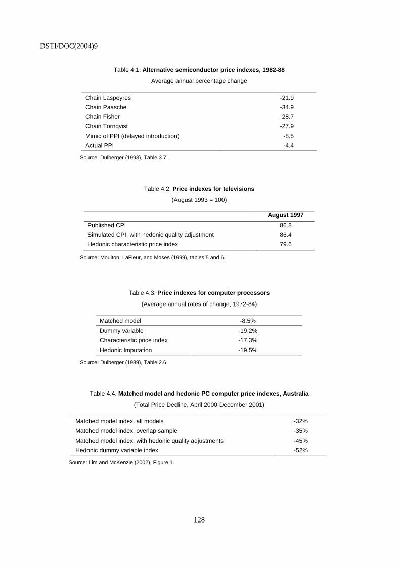
DSTI/DOC(2004)9

128

Table 4.1. Alternative semiconductor price indexes, 1982-88

Average annual percentage change

Chain Laspeyres -21.9

Chain Paasche -34.9

Chain Fisher -28.7

Chain Tornqvist -27.9

Mimic of PPI (delayed introduction) -8.5

Actual PPI -4.4

Source: Dulberger (1993), Table 3.7.

Table 4.2. Price indexes for televisions

(August 1993 = 100)

August 1997

Published CPI 86.8

Simulated CPI, with hedonic quality adjustment 86.4

Hedonic characteristic price index 79.6

Source: Moulton, LaFleur, and Moses (1999), tables 5 and 6.

Table 4.3. Price indexes for computer processors

(Average annual rates of change, 1972-84)

Matched model -8.5%

Dummy variable -19.2%

Characteristic price index -17.3%

Hedonic Imputation -19.5%

Source: Dulberger (1989), Table 2.6.

Table 4.4. Matched model and hedonic PC computer price indexes, Australia

(Total Price Decline, April 2000-December 2001)

Matched model index, all models -32%

Matched model index, overlap sample -35%

Matched model index, with hedonic quality adjustments -45%

Hedonic dummy variable index -52%

Source: Lim and McKenzie (2002), Figure 1.

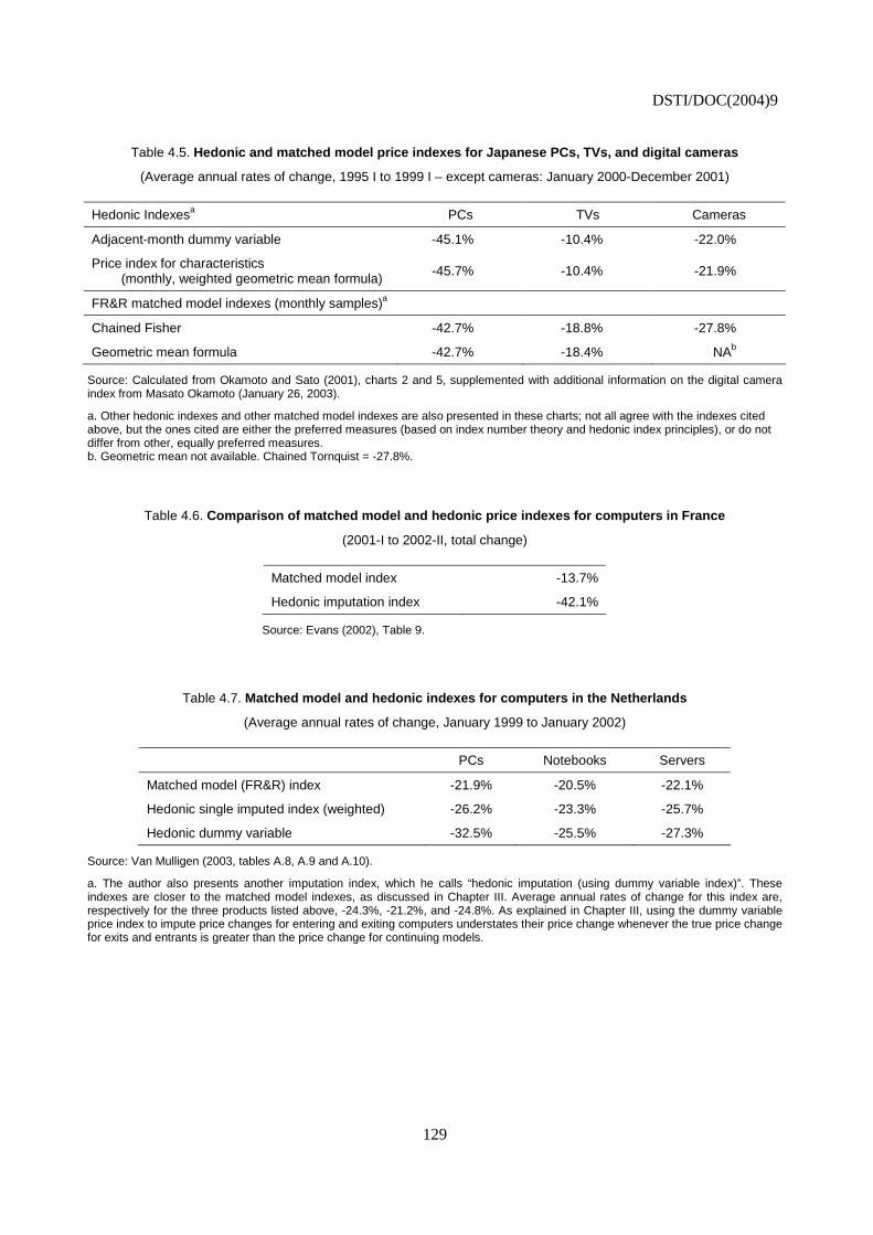
DSTI/DOC(2004)9

129

Table 4.5. Hedonic and matched model price indexes for Japanese PCs, TVs, and digital cameras

(Average annual rates of change, 1995 I to 1999 I – except cameras: January 2000-December 2001)

Hedonic Indexesa PCs TVs Cameras

Adjacent-month dummy variable -45.1% -10.4% -22.0%

Price index for characteristics (monthly, weighted geometric mean formula)

-45.7% -10.4% -21.9%

FR&R matched model indexes (monthly samples)a

Chained Fisher -42.7% -18.8% -27.8%

Geometric mean formula -42.7% -18.4% NAb

Source: Calculated from Okamoto and Sato (2001), charts 2 and 5, supplemented with additional information on the digital camera index from Masato Okamoto (January 26, 2003).

a. Other hedonic indexes and other matched model indexes are also presented in these charts; not all agree with the indexes cited above, but the ones cited are either the preferred measures (based on index number theory and hedonic index principles), or do not differ from other, equally preferred measures. b. Geometric mean not available. Chained Tornquist = -27.8%.

Table 4.6. Comparison of matched model and hedonic price indexes for computers in France

(2001-I to 2002-II, total change)

Matched model index -13.7%

Hedonic imputation index -42.1%

Source: Evans (2002), Table 9.

Table 4.7. Matched model and hedonic indexes for computers in the Netherlands

(Average annual rates of change, January 1999 to January 2002)

PCs Notebooks Servers

Matched model (FR&R) index -21.9% -20.5% -22.1%

Hedonic single imputed index (weighted) -26.2% -23.3% -25.7%

Hedonic dummy variable -32.5% -25.5% -27.3%

Source: Van Mulligen (2003, tables A.8, A.9 and A.10).

a. The author also presents another imputation index, which he calls “hedonic imputation (using dummy variable index)”. These indexes are closer to the matched model indexes, as discussed in Chapter III. Average annual rates of change for this index are, respectively for the three products listed above, -24.3%, -21.2%, and -24.8%. As explained in Chapter III, using the dummy variable price index to impute price changes for entering and exiting computers understates their price change whenever the true price change for exits and entrants is greater than the price change for continuing models.

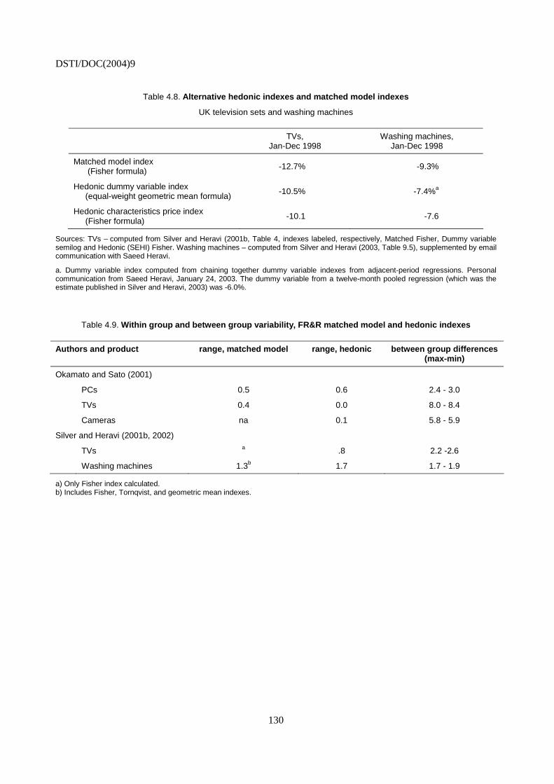
DSTI/DOC(2004)9

130

Table 4.8. Alternative hedonic indexes and matched model indexes

UK television sets and washing machines

TVs, Jan-Dec 1998

Washing machines, Jan-Dec 1998

Matched model index (Fisher formula) -12.7% -9.3%

Hedonic dummy variable index (equal-weight geometric mean formula) -10.5% -7.4%a

Hedonic characteristics price index (Fisher formula)

-10.1 -7.6

Sources: TVs – computed from Silver and Heravi (2001b, Table 4, indexes labeled, respectively, Matched Fisher, Dummy variable semilog and Hedonic (SEHI) Fisher. Washing machines – computed from Silver and Heravi (2003, Table 9.5), supplemented by email communication with Saeed Heravi.

a. Dummy variable index computed from chaining together dummy variable indexes from adjacent-period regressions. Personal communication from Saeed Heravi, January 24, 2003. The dummy variable from a twelve-month pooled regression (which was the estimate published in Silver and Heravi, 2003) was -6.0%.

Table 4.9. Within group and between group variability, FR&R matched model and hedonic indexes

Authors and product range, matched model range, hedonic between group differences (max-min)

Okamato and Sato (2001)

PCs 0.5 0.6 2.4 - 3.0

TVs 0.4 0.0 8.0 - 8.4

Cameras na 0.1 5.8 - 5.9

Silver and Heravi (2001b, 2002)

TVs a .8 2.2 -2.6

Washing machines 1.3b 1.7 1.7 - 1.9

a) Only Fisher index calculated. b) Includes Fisher, Tornqvist, and geometric mean indexes.

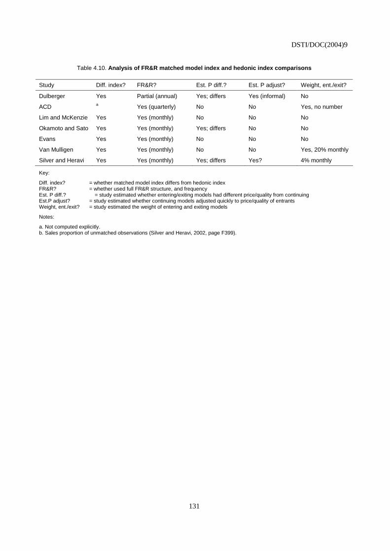
DSTI/DOC(2004)9

131

Table 4.10. Analysis of FR&R matched model index and hedonic index comparisons

Study Diff. index? FR&R? Est. P diff.? Est. P adjust? Weight, ent./exit?

Dulberger Yes Partial (annual) Yes; differs Yes (informal) No

ACD a Yes (quarterly) No No Yes, no number

Lim and McKenzie Yes Yes (monthly) No No No

Okamoto and Sato Yes Yes (monthly) Yes; differs No No

Evans Yes Yes (monthly) No No No

Van Mulligen Yes Yes (monthly) No No Yes, 20% monthly

Silver and Heravi Yes Yes (monthly) Yes; differs Yes? 4% monthly

Key:

Diff. index? = whether matched model index differs from hedonic index FR&R? = whether used full FR&R structure, and frequency Est. P diff.? = study estimated whether entering/exiting models had different price/quality from continuing Est.P adjust? = study estimated whether continuing models adjusted quickly to price/quality of entrants Weight, ent./exit? = study estimated the weight of entering and exiting models

Notes:

a. Not computed explicitly. b. Sales proportion of unmatched observations (Silver and Heravi, 2002, page F399).

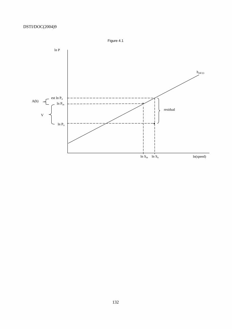
DSTI/DOC(2004)9

132

Figure 4.1

A(h)

V

residual °

•

ln(speed) ln Sm

ln Pm

ln Pn

ln P

hold (t)

est ln Pn

ln Sn

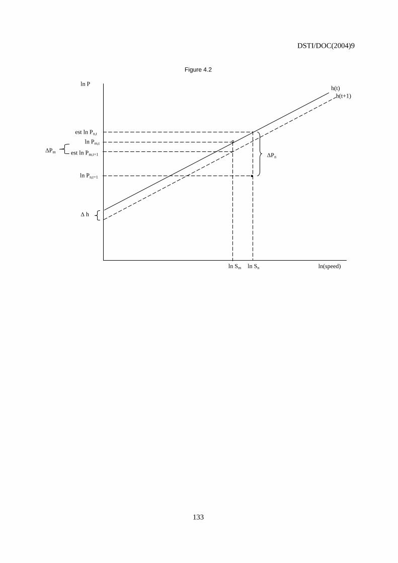
DSTI/DOC(2004)9

133

Figure 4.2

°

•

ln(speed) ln Sm

ln Pm,t

ln Pn,t+1

ln P

∆Pm

h(t)

est ln Pn,t

∆Pn

h(t+1)

est ln Pm,t+1

ln Sn

∆ h

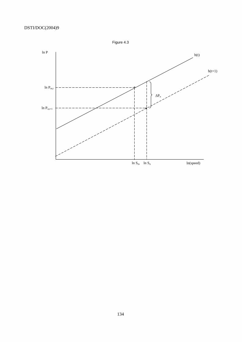
DSTI/DOC(2004)9

134

Figure 4.3

°

•

ln(speed) ln Sm

ln Pm,t

ln Pn,t+1

ln P h(t)

∆Pn

h(t+1)

ln Sn

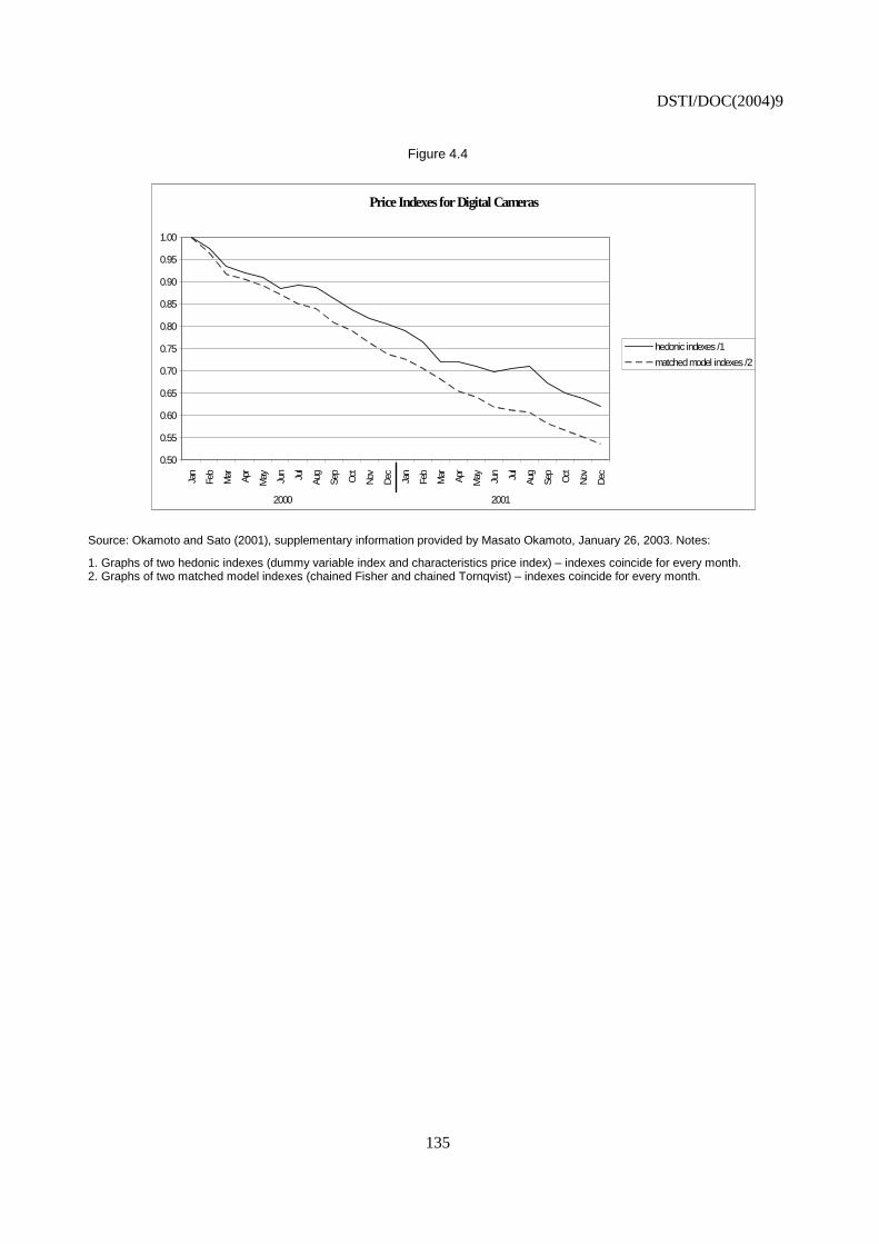
DSTI/DOC(2004)9

135

Figure 4.4

Price Indexes for Digital Cameras

0.50

0.55

0.60

0.65

0.70

0.75

0.80

0.85

0.90

0.95

1.00

Jan

Feb

Mar Apr

May Jun Jul

Aug

Sep

Oct

Nov

Dec Jan

Feb

Mar Apr

May Jun Jul

Aug

Sep

Oct

Nov

Dec

hedonic indexes /1

matched model indexes /2

2000 2001

Source: Okamoto and Sato (2001), supplementary information provided by Masato Okamoto, January 26, 2003. Notes:

1. Graphs of two hedonic indexes (dummy variable index and characteristics price index) – indexes coincide for every month. 2. Graphs of two matched model indexes (chained Fisher and chained Tornqvist) – indexes coincide for every month.

DSTI/DOC(2004)9

136

CHAPTER V

PRINCIPLES FOR ESTIMATING A HEDONIC FUNCTION: CHOOSING THE VARIABLES

A. Introduction: best practice

A hedonic price index study has two parts. First, the investigator must estimate a hedonic function. In the second part, the investigator decides how to use the hedonic function to calculate a price index.

Principles for the second part – using a hedonic function to compute a hedonic price index – were presented in Chapter III. There, four alternative methods for constructing hedonic price indexes were developed. In this handbook, it seemed useful to consider first the use of the hedonic function to estimate a price index, in order to clarify the relationship of the hedonic price index to conventional price index and quality adjustment techniques. A statistical agency must decide that it wants to estimate or explore hedonic price indexes before it needs to confront questions about estimating hedonic functions. Researchers and users of hedonic indexes need also to understand the relation between hedonic and conventional indexes.

In this chapter, and the following one, I consider principles for conducting the first part of the investigation, namely, estimating the hedonic function. These “best practice” principles should be understood as general guidance for designing and carrying out hedonic studies, not as a set of rigid rules. Improved methods can always be developed, this handbook is not intended to freeze methodology at its present state. In keeping with the “high tech products” orientation of this handbook, most of the examples pertain to research on computer equipment. However, the principles in this chapter and the next one are very general, and apply as well to hedonic studies on other products, and even to hedonic studies on services.

“Best practice” means current state-of-the-art. Anything can be improved, so best practice does not mean the best that ever could be.

Statistical agencies sometimes ask: why should we care about “best practice”? In their contention, best practice may be relevant for research questions, but statistical agencies are interested in producing price indexes, not primarily in research for its own sake.

The answer to that question is not a simple one. What really matters is: how much difference does a deviation from best practice make to the price index?

Statistical agencies have often pointed to examples of anomalous behaviour in hedonic indexes – instability in estimated regression coefficients, for example, and price indexes that do not seem to be robust with respect to decisions made by the investigator. The report of the US Committee on National Statistics panel on the CPI (Schultze and Mackie, eds., 2002, Chapter 4) reiterates these concerns. Some of those anomalous results – I suspect most of them —reflect deviations from best practice. If deviations from best practice are tolerated, and the index is sensitive to deviations from best practice, the resulting hedonic price indexes or hedonic quality adjustments may be inaccurate.

DSTI/DOC(2004)9

137

The reason for carrying out hedonic research on some product is to produce better price indexes. On this line of reasoning, statistical agencies should desire best practice because they want accurate price indexes. The research methods discussed in this chapter are relevant to producing accurate price indexes with hedonic methods.

On the other hand, eliminating a deviation from best practice might be expensive. The deviation might also not make all that much difference in computing a quality-adjusted price index. It is always appropriate to apply a cost-benefit analysis to research methodology, and to tolerate deviations from best practice that do not matter very much. To make such decisions, we have to know whether deviations from best practice matter, which deviations matter, and how much they matter. We need to know the answer to the question: How much difference does it make? That implies that someone, somewhere, has performed the relevant research.

Best practice can help guide data collection strategies. Even for statistical agencies, data availability is one of the major limitations in achieving best practice hedonic indexes. Getting the right data on prices and on all of the characteristics is a demanding task, and sometimes an expensive one. In academic studies, it is common to respond to problems raised with empirical work by saying “we have no data”. Statistical agencies may face exactly the same data-acquisition barriers, but statistical agencies have reasons to fill data gaps that academics might simply excuse or overlook.

Codification of best practice helps to determine when an expensive data collection program might pay dividends. If one knows that a particular piece of missing data has been shown to be crucial in best practice studies, the implications for a statistical agency or a researcher are clear. If one does not know whether the missing data really make a difference, initiating a collection program to fill in the dataset may be less justifiable.

Estimating any hedonic function has two crucial parts. The first and most vital one is selection of the variables that will serve as characteristics and obtaining complete and accurate data on the characteristics and on the prices. Additionally, there is the matter of functional form for hedonic functions, and some econometric and other research considerations. The first topic is considered in subsequent sections of this chapter, after review of some interpretive questions that, though quite well resolved in the hedonic literature, nevertheless do seem still to cause difficulty. The second group of topics are the subjects of Chapter VI.

B. Interpreting hedonic functions: variables and coefficients

As already discussed in Chapter III, a hedonic function is a statistical relation between the prices of different varieties of a product, such as personal computers (PCs), and the product’s characteristics. For example, an estimated hedonic function for PCs might be:

(5.1) Pit = c0 + c1 (MHz)it + c2 (MB)it + c3 (HD)it + uit

In this example, the price of the PC depends on its speed, measured in MHz, its memory size in megabytes (MB), and the size of its hard drive (HD), also measured in megabytes (MB); uit designates the regression error term, or regression residual. I emphasize in the remainder of this chapter that an adequate hedonic function specification for a PC requires more variables than these three, but they serve here simply as an opening example.

1. Interpreting the variables in hedonic functions

The economic theory underlying hedonic functions rests on the hedonic hypothesis: heterogeneous goods are aggregations of characteristics. In turn, characteristics (for computers, speed, memory size, HD

DSTI/DOC(2004)9

138

size, and other capacities) are variables that are at the same time outputs for producers and consumption commodities for consumers.

Under the hedonic hypothesis, one does not buy a computer as a “box”; one buys the bundle of characteristics that the producer packages into the box. The characteristics are the variables that generate utility to the user, so the purchase of a computer is the choice of a bundle of characteristics from among the various alternative bundles offered by various sellers. The economics of consumer choice among the characteristics that are potentially in the bundle are explored in Lancaster (1971), Ironmonger (1972), Rosen (1974) and Berry, Levinsohn, and Pakes (1995). The Theoretical Appendix summarizes implications of this work for hedonic functions.

Similarly, the hedonic hypothesis implies that the cost of making a computer depends on the bundle of characteristics that are packaged into the computer box. Thus, larger quantities of characteristics packaged into the computer “box” imply rising production cost for the box (as well as increased value for the consumer who buys it). The output of computer manufacturers is the quantity of computer characteristics produced, not just the number of computers. An anecdote from the days of the mainframe computer is illustrative: engineers spoke of computer production as “shipping MIPS”. MIPS (millions of instructions per second) is a measure of computer speed that has been used for both mainframe and personal computers. The engineers meant that the volume of output was not described by the number of computers that went out the factory door, but by the total quantity of MIPS per month (in effect, the number of computers times their average MIPS).

The design of a computer is the producer’s choice to build a certain bundle of characteristics, from among the potential characteristics bundles that are technologically feasible. Rosen (1974) developed the output theory for producers in a competitive industry. Triplett (1987) pointed out that this competitive, large numbers, case was unrealistic for technological products, and Berry, Levinsohn, and Pakes (1995) developed an extension of the Rosen model for cases where a small number of rivalrous producers look for product innovations that fill gaps in the existing range of product varieties – see the Theoretical Appendix.

From the hedonic hypothesis, it follows that the search for the appropriate set of variables in a hedonic function is in effect a search for the essence of the product itself. Selecting the right variables for a hedonic function requires, in principle, engineering information, information about what producers are indeed producing – the technology that specifies the bundling of characteristics – and also marketing information, information on what the users desire when they buy the product. The first principle for conducting a hedonic study is: know your product.

2. Interpreting the coefficients in a hedonic function: economic interpretation

For many purposes, including estimating hedonic price indexes, researchers need the estimated regression coefficients, c1, c2, and c3 from equation (5.1). If the equation is estimated with the standard ordinary least squares (OLS) method, statistical theory indicates that under specified assumptions (see any econometrics textbook), a regression coefficient shows the effect on the dependent variable of a change in the independent variable, holding all other variables constant.

Equation (5.1) specifies a linear (non-logarithmic) hedonic function. In the linear case, the coefficient c1 shows the increment to the price of a computer arising from a one unit increase in MHz (other variables in the regression constant), the coefficient c2 shows the price increment from a one unit increment in memory size, and so forth. From this, we say that the coefficient c1 measures the “implicit price” of a unit of speed, c2 is the implicit price of memory, and so forth. For example, in the hedonic function of the US Bureau of Labor Statistics (BLS) for October, 2000, one additional MHz of speed cost USD 1.195, one additional MB of memory cost USD 1.688, and one additional GB of hard drive cost USD 4.177.

DSTI/DOC(2004)9

139

Suppose the hedonic function is logarithmic, instead of linear, as in equation (5.1):

(5.2) ln Pit = a0 + a1 ln (MHz)it + a2 ln (MB)it + a3 ln (HD)it + eit

For the “double log” case of equation (5.2), the coefficients are elasticities – they show the proportionate increase in price associated with a given proportionate increase in units of speed and so forth (see the section on functional forms in Chapter VI). For example, in Ellen Dulberger’s mainframe hedonic function (equation 3.1 in Chapter III), the coefficient on speed was 0.783 and on memory 0.219 (HD was not in her regression); these coefficients mean that a 10% increase in speed increased the price by 7.83% and a 10% increase in memory increased the price by 2.19%. The regression coefficient itself is not the implicit price, but the implicit price can be derived from it by computing the dollar value of an increase in speed or memory evaluated at mean. For example, if the mean memory were 100 MB, and the mean price were USD 1000, then the price of a 10% increment to memory around the mean is: USD 1078.30 / 1.10 = USD 9.80.

The hedonic function contains, therefore, both prices and quantities. These characteristics prices and quantities are (almost) like other, conventional, prices and quantities for goods – for ships and sealing wax and cabbage, as the poem has it. We can think of the hedonic function as “disaggregating” the complex good itself into a bundle of constituent prices and quantities (the characteristics), where the characteristics are the true economic variables for both buyers and sellers, according to the hedonic hypothesis. This interpretation is only appropriate for empirical hedonic functions if we have enumerated the characteristics and measured them accurately. Interpreting the hedonic function as containing characteristics prices and quantities has already been used in section III.C, where the price index for characteristics was developed.

The regression coefficients measure implicit prices for characteristics (or the logarithms of them). This implies that the implicit prices ought to have some relation to what buyers are paying for units of the characteristic and the costs of adding more characteristics to the bundle. In particular, if a characteristic is desired by the users and is costly to produce, one does not expect a negative sign in the hedonic function. It is customary to inspect estimated hedonic functions for the plausibility of the estimated coefficients, and for the researcher to comment on the coefficients’ plausibility in assessing the estimated hedonic function. Indeed, such discussions have come to be part of a best-practice investigation and part of the researcher’s assuring that the “know your product” rule has been followed.

Whether hedonic coefficients should be subjected to a priori assessments of reasonableness has recently been challenged by Pakes (2003). This matter is deferred until section F of this chapter, after a review of estimated coefficients in different hedonic function specifications.

3. Interpretation of regression coefficients: statistical interpretation

Though it is a relatively familiar econometrics topic, the statistical interpretation of hedonic regression coefficients deserves consideration here, because evidently some aspects of interpreting regression coefficients for hedonic studies have become somewhat confused.

Consider the hedonic function for computers in equation (5.1), where the price of the computer depends on its speed, measured in MHz, memory size in megabytes (MB), and the size of its hard drive (HD, also measured in megabytes). To simplify, we suppose that equation (5.1) is the complete hedonic function, it has only these three variables (later sections of this chapter show that more than three are required for an adequately specified computer hedonic function). To focus on the central issues, suppose as well that all three of the variables are correctly measured, as is the price.

As noted already, the statistical theory for ordinary least squares (OLS) regressions indicates that under specified assumptions (see any econometrics textbook), a regression coefficient shows the effect on

DSTI/DOC(2004)9

140

the dependent variable of a one unit change in the independent variable, holding all other variables constant. The “other things equal” interpretation of the regression coefficient is important, and sometimes not sufficiently stressed. A number of statistical and technical conditions disturb or invalidate the other things equal interpretation of hedonic regression coefficients and thus their interpretation as implicit prices of characteristics. Most important are the regression specification problems caused by omitted variables and proxy variables, which are discussed later in this chapter, and others that are covered in Chapter VI.

C. A case study: variables in computer hedonic functions

Getting the characteristics right is not just the first step in estimating a hedonic function, it is the most important step. Unless the characteristics are right, no other step is worth doing.

Selecting the characteristics for a hedonic study requires knowledge of the technology, which is a type of knowledge that economists often do not have. They must therefore acquire a certain amount of technical knowledge in order to carry out a hedonic study. One does not need to know the engineering principles behind the technology (how the engineer gets what is wanted in a product), but it is necessary to understand what an engineer is trying to put into a product.

I use computers as a case study to illustrate choosing characteristics for a hedonic function, partly because so much hedonic research has been carried out on IT products, and partly because the choice of variables in computer equipment studies has been informed by interactions of economists with computer scientists. Indeed, the characteristics that appear in computer equipment hedonic functions originate in work by computer scientists, who were interested in measuring progress in computer performance. The principles illustrated by this case study apply to all hedonic studies, whether they are done for computer equipment, other IT equipment, or cars, appliances or other products – or even services.

1. A bit of history: where did those computer characteristics come from?

It is intriguing that what an economist calls a computer hedonic function first appeared, in an essentially equivalent form, in the computer science literature. The earliest research on computer performance measurement grew out of, or was influenced by, research issues in for computer systems. Some performance measures were devised as a practical aid to equipment selection. Alternatively, computer technologists wanted to estimate the rate of technical change in computers. It makes no sense to do that without considering both performance and price. So where the economist naturally thinks of the price of computers, adjusted for performance, the computer technologist thinks of performance per dollar spent on computers. For example, Knight (1966, 1973, 1985), who is actually an economist but was writing for computer publications, was interested in estimating in the rate of technical progress for computers, and not a computer price index. He estimated an equation that was similar to equation (5.2). Sharpe (1969) cites several unpublished computer studies that were quasi-hedonic (that is, they were similar to hedonic studies, though the authors did not recognize it – neither did Knight, at least not explicitly).

Economists were interested in a somewhat different, but closely related problem: measuring performance-corrected price indexes for computers. Among economists, the early hedonic researchers on computers more or less followed the lead of technologists in choosing their performance measures. The study by Chow (1967) might have been the first one that was explicitly a hedonic price index for computers. Early computer studies are reviewed in Triplett (1989).

Performance characteristics of computer processors: Speed and memory size. From the earliest studies, the performance specification of computer processors consisted primarily of the speed with which

DSTI/DOC(2004)9

141

the computer carries out instructions and its memory size (main memory storage capacity).95 These early studies pertained to mainframe computers, as the personal computer (PC) had not yet been developed.

It has always been difficult to obtain a measure of speed that is both sufficient and at the same time comparable across processors. A computer executes a variety of instructions. The execution rate of each instruction is properly a computer characteristic. Computer “speed” is accordingly a vector, not a scalar; one needs to evaluate the separate elements of the vector, and then to find some way for combining them, if it is appropriate to do so.

Applications require instructions in different proportions or amounts. For example, graphics and “office productivity” programs make use of computer capabilities in different proportions. Moreover, even if they employ the same applications, different users employ them in different frequencies – I use both graphics and office productivity program applications, but my usage differs greatly from the usage of a graphics designer. Accordingly, numerous measures of “speed” exist, in principle, because speed is a vector and there are many ways of valuing and combining the elements in the speed vector.

Nevertheless, some scalar summary of the speed vector is needed. Several approaches have been employed by economists (and technologists) in hedonic studies. The ones still commonly in use are discussed in the following sections. In considering these, it is well to bear in mind the twin aggregations of the speed vector – the first one aggregates over instructions (to obtain applications speeds), the second one aggregates application speeds over users who use applications in different proportions.

2. Variables in mainframe computer equipment studies: connection with PCs

A joint project between the IBM Corporation and the US Bureau of Economic Analysis (BEA) resulted in the first introduction of hedonic computer equipment prices into the national accounts of any country (Cartwright, 1986).

The IBM-BEA price indexes covered four products: mainframe computers, disk drives, printers, and displays (terminals) – see Cole et al. (1986). As noted in the previous section, the IBM hedonic studies were not by any means the first hedonic studies of computer equipment.

For this handbook, the IBM group of studies are instructive for two reasons. First, the hedonic functions estimated by the IBM economists (Cole et al., 1986) were best practice at the time. These hedonic functions were subject to a great amount of scrutiny, both within the economics research community and within the computer industries, precisely because they were a pioneering effort in constructing price indexes for high tech equipment. Had they been deficient with respect to choice of variables, criticism would have surfaced long ago.96

Secondly, and more importantly, the variables used in the IBM hedonic functions have provided the basis for most subsequent investigations of computer equipment, including price indexes for personal computers (which were not included in the IBM-BEA hedonic indexes). The IBM hedonic functions for computer equipment continue, therefore, to provide guidance for empirical investigations of computer equipment today.

95. Phister (1979), Sharpe (1969), and Flamm (1987) contain good statements of the rationale for the

specification, and Fisher, McGowan, and Greenwood (1983, at pp. 140-141) emphasize its limitations.

96. Some discussion of the speed variable (MIPS) that took place at the time is summarized in my review of computer research (Triplett, 1989). See also the parallel discussion of PC speed variables, below.

DSTI/DOC(2004)9

142

3. Mainframe and PC computer components and characteristics

Table 5.1A summarises the variables used in a number of recent studies on personal computers, and compares them with the variables employed in the IBM study (the left-hand column of Table 5.1A). These studies are not a complete review of research. They have been drawn from studies conducted in a number of different countries to show the degree of international comparability in hedonic research on personal computers.

Most of these studies have succeeded, to a perhaps surprising extent, in combining into one hedonic function many of the variables in three of the IBM studies (Cole et al., 1986): processors, disk drives and displays. None of the existing PC studies tries to combine printers (subject of a separate IBM study) in the PC hedonic function, because the acquisition of a printer still typically remains a separate transaction, even though the printer, too, is sometimes bundled with the rest of the PC. Barzyk (1999) does not include monitors and keyboards, presumably because they were not bundled into the Canadian data set used for his research. Dalén (1994) also excludes the monitor and keyboard from his hedonic regression. With these exceptions, all the PC studies can be viewed as combing into a single hedonic function three of the separate pieces of equipment studied in the IBM work.

The PC has a central processing unit, like the mainframe computer. Now, the computational capacity is typically mounted on a single computer chip, but this production detail (though tremendously important for the engineering history of the computer) does not matter for modelling hedonic functions because it need not concern the PC user.

All PC studies measure processor performance with speed and memory size, as did Dulberger (1989). However, the speed measures differ. In PC studies, CPU speed is commonly measured in megahertz (or MHz), which was called “clock speed” in the mainframe days. Dulberger used MIPS, known as a “weighted instruction mix,” which was designed to be measure of work done. The speed measure is discussed additionally below.

Memory size is measured in megabytes (MB), the same unit used in mainframe days.97 As was true of mainframe computers, a typical PC’s memory is expandable, so alternative memory sizes are offered on any particular machine. For example, in the fall of 2000, a Dell 4100 series computer running at 900 MHz offered memory sizes ranging from 64 MB to 560 MB. The buyer can add to the machine’s memory in the original purchase transaction, paying an option price; at more trouble and expense the buyer can also retrofit more memory to an existing machine.

As with the mainframe, a PC’s memory performance is not only a function of the size of the memory, but also depends on the speed with which information can be withdrawn from the memory. This specification was called in the mainframe days “memory cycle time.” Continuing with the Dell 4100 example, its memory speed was recorded as 133 MHz. Some hedonic functions in the mainframe days measured processor speed with memory time, but few entered both CPU speed and memory cycle time for reasons of multicollinearity. They seem far less collinear now. No PC hedonic functions has used memory speed as a computer performance characteristic.

Dulberger introduced the idea of specifying the semiconductor type used in the processor (technology dummies). A majority of the PC studies follow this innovation (BLS, Chwelos, Bourot, and in modified form, Moch and Finland CPI).

97. A byte is a unit of storage.

DSTI/DOC(2004)9

143

A PC also comes with an internal hard drive (HD). The PC HD corresponds exactly to the old mainframe disk drive, which was used for the same purpose, auxiliary storage. The modern HD also stores the programs that are used to run the computer. A typical PC is offered with alternative HDs, having different specifications, although the seller usually offers a standard specification. The PC user must decide how much optional HD capacity and speed to include in his purchase, a decision made by the computer centre manager in the mainframe days.

As with the IBM disk drive hedonic function from mainframe days, a modern disk drive has its capacity as one specification. Capacity ratings now typically now go into the GB, or gigabyte range: a Dell series 4100 computer offered up to 80 gigabytes of capacity in the fall of 2000 (Table 5.2), and far larger drives became available later. The difference between megabytes (MB) and gigabytes (GB) is merely a scaling, adopted for convenience because hard disk capacity has grown so large.

The PC’s HD also has as a characteristic the speed with which information can be retrieved. These speeds are actually vectors, not scalars, which raises the question of how they should be combined to measure performance. In Cole et al. (1986) three indicators of HD disk speed were summed. For the Dell 4100 series PC, several different hard drives are offered, with vectors of speeds given in Table 5.2. Note that these speeds are not simply proportional to the size of the HD, and indeed the fastest HD (taking all the speeds together) is neither the smallest nor the largest one. Of the PC studies, only Dalén uses a hard drive speed variable, although the type dummy variables used by Barzyk (1999) and Bourot (1997) control to an extent for HD speed.

A modern PC is typically supplied with a monitor and a keyboard, although they are often priced separately. The two functions were combined in “general purpose displays” in the IBM study.

For monitors (displays) all the studies– PC and mainframe – employ measures of the quantity of information that can be shown on the screen and the resolution of the picture. Resolution is still an important characteristic for monitors, as it was in the IBM-BEA displays index. None of the PC studies follows the IBM lead in representing the number of characters that can be displayed on the screen, probably because in the case of the PC that is determined by the nature of the software. Because some software producers have taken increasing amounts of the screen for control “bars” and so forth that are not readily hidden by the user, screen size may be an imperfect measure, but it clearly influences the price of the monitor. Other monitor characteristics include flat screen, and the thickness of the monitor, which reflects users’ desires that the machine occupy a smaller amount of desk space; those characteristics are omitted from existing studies.

Keyboards having ergonomic features are available now: carpal and radial tunnel problems were nearly unknown in the early 1980s. Yet, even in the mainframe days, ergonomics were a factor: “Displays also differ in various ergonomic attributes, such as the feel and shape of the keys or tilt positions of the monitor; these are difficult to quantify and are assumed to be uncorrelated with the measured characteristics” (Cole et al., 1986, page 42).

In addition to the basic hardware items – processor, hard drive, and monitor/keyboard – a modern PC comes bundled with a number of other hardware features. Many of these are a consequence of the fact that the computer’s function is increasingly not “computations,” but the manipulation of digitised data, including sound and pictures. Sound cards, video cards, network cards, and so forth may be regarded as other pieces of hardware that are attached to the basic PC components, as are input/output devices such as CD-ROM, or CD/RW drives.

Most of the PC studies have included dummy variables for the presence or absence of at least some of these auxiliary functions, or alternatively, for more advanced versions of the functions in cases where (like

DSTI/DOC(2004)9

144

the CD-ROM) some version of the feature has become nearly universal. Table 5.1B displays these other hardware features.98 Little consensus has emerged among researchers about which of these auxiliary hardware features should be added to the PC hedonic function. Additional research will be required to determine the reasons for the differences between the variables included in, for example, the BLS study and the others tabulated in Table 5.1B: do they differ because markets differ in the United States and other countries, or because of data availability differences, or because of different decisions made by the researchers? The Eurostat study (Konijn, Moch and Dalén, 2003) points to data gaps. And even more importantly: how much difference in the computer price indexes computed by BLS and others results from differences in the variables in the hedonic function?

A PC may be sold with a printer included as part of the package, the printer may be purchased separately, or in some cases the printer is included “free.” In the IBM study, printer characteristics were “speed, resolution, and the number of fonts available online” (Cole et al., l986, page 42). Even in 1986, laser printers and inkjet printers were available. Color printing is a much larger factor in the printer market now than it was 15 years ago, and a number of other characteristics of printers are important. I know of no recent study for printers. In addition to printers, other auxiliary hardware (scanners, digital cameras and so forth) are significant portions of computer-related equipment, but few studies exist, except for cameras (Chapter IV).

4. Computer “boxes”, computer centres and personal computers

The four IBM-BEA hedonic indexes were price indexes for computer equipment “boxes”. They controlled for quality change that arose as manufacturers increasingly put more performance into each of the separate pieces of computer equipment (the boxes).

In the mainframe days of the computer, disk drives, processors, and so forth were normally produced and sold separately. The buyer assembled a computer centre, the centre was not sold as a unit by the manufacturer. The main objective of the IBM research was to develop price indexes for deflating the output of computer equipment production. For this reason, the study paid no direct attention to how the boxes – or properly, the characteristics of the separate boxes – were combined into an operating computer centre, because an operating computer centre was not produced and sold as a unit.

Even in the mainframe era there was great interest in principles for determining an optimal combination of characteristics, combined across all the separate pieces of equipment. In purchasing equipment, computer centre managers decided how to combine the separate boxes, or rather the characteristics of the separate boxes, with computer software and with computer centre staff in order to perform “computations”.99 Research on measuring the computer did not follow this course (see the discussion of this point in Triplett, 1989).

The personal computer (PC) is, in effect, a pre-assembled computer centre. The PC contains separate components that link nearly one-to-one to the individual “boxes” that were the subjects of Cole et al. (1986). For example, the PC’s central processing unit (CPU), its hard drive and a display (keyboard/monitor) correspond to separate mainframe era components. Most of this equipment can be purchased separately, indeed, PC components are typically initially built by different manufacturers. PC components are not technologically linked together into a PC in the sense that performance of the components cannot be investigated separately. However, from the final purchaser’s perspective, the PC

98. The entry for the INSEE price index is based on Bourot (1997), but the INSEE index is re-estimated

frequently and variables are updated.

99. Many computer operations are not in fact technically computations, but the word is a natural one that can cover all computer operations, whether truly computations or not.

DSTI/DOC(2004)9

145

transaction typically combines several of them (for example, a monitor and a keyboard are almost always included in the price). The transaction, more than the engineering, determines the unit that economists must analyze.

Thus, in modelling PC performance for hedonic functions, one must ask a question that was never confronted in the IBM-BEA studies: Are we interested in the performance of the PC (that is, in the computer system)? Or of its components? Of course, we are interested, ultimately, in both, for several reasons. But it will be important to keep the distinction between system performance and component performance in mind.

A typical PC transaction bundles together several hardware components, each of which is a bundle of characteristics. The PC transaction therefore contains a considerably larger bundle of characteristics than did the separate pieces of computer hardware in mainframe computer days. In the IBM studies (Cole et al., 1986), separate hedonic functions were estimated for each of four components of computer equipment. Each of the IBM hedonic functions contained two to five characteristics. In the old days, the task of specifying hedonic functions was easier, because it involved a larger number of hedonic functions, with fewer characteristics in each one. When several hardware items are bundled into a single PC transaction, the hedonic function must incorporate in some way all of the characteristics of the separate computer components that are bundled together.

For a modern PC, the sheer number of characteristics makes modelling the PC hedonic function more complicated in a number of ways. For example, the PC hedonic function used by the BLS for its PPI, CPI and international price indexes routinely has 25 or more variables.

The large number of PC characteristics has a number of econometric consequences. It tends to exacerbate the multicollinearity problem, and it complicates the problem of determining the functional form. I review these problems in Chapter VI.

More important, however, is a third consequence of the more complicated bundling of a PC: the typical modern PC transaction includes a great quantity of software, and it includes as well as some hardware components, such as speakers and sound cards, that were not significant pieces of equipment in the old computer centre. Many studies of PCs have ignored at least a part of the increased bundling of software and additional hardware components. In choosing variables to include in PC hedonic functions, researchers have (whether consciously or not) followed the lead of the IBM studies to the point of excluding from PC hedonic functions a portion of the increased bundling that is new in the PC transaction. For example, only the BLS and Bourot studies include variables for sound reproduction (a set of speaker dummies in the BLS case, a sound card dummy in the Bourot study). Perhaps sound equipment was not bundled into the machines used for the other studies or perhaps it was missing from the data. If sound equipment was indeed bundled into the transaction in the data used in the other studies, then the omission of variables for sound equipment represents an omitted variable problem in their hedonic functions.

In sum, researchers within statistical agencies and in academic institutions have described the hardware portions of a modern PC with characteristics that are very similar to those used in the 1986 IBM hedonic studies on computer equipment. Data on almost the same list of variables are regularly published in PC manufacturer’s brochures, and on web sites and other printed and electronic data sources. What has changed technologically in the past two decades is not so much the basics of the machine, and the characteristics it supplies its users, but rather the miniaturisation of the functions that make computers now readily fit into a smaller space, as the terms “desktop” and “laptop” abundantly suggest. The data used by researchers reflect that in their specification of variables that have been used in PC hedonic functions. The transaction, however, has changed more fundamentally, in that a greater number of characteristics are now

DSTI/DOC(2004)9

146

bundled together. The question remains: do the IBM specifications for the mainframe computer and its ancillary equipment provide an adequate specification of the performance of the PC?

D. Adequacy of the variable specifications in computer studies

Three reasons exist for concern about the adequacy of existing hedonic functions for PCs.

• First, even compared with the IBM studies of separate computer equipment boxes, the PC studies omit some performance variables that were included in mainframe era research (e.g., hard drive speed). Moreover, the variables that are advertised by computer sellers are more extensive than the list of variables in any of the studies arrayed in Tables 5.1A and B, which suggests the possibility of missing variable bias to PC hedonic functions.

• Second, the PC processor speed measure (almost exclusively clock speed, measured in megahertz, MHz) is a step backward from Dulberger’s weighted instruction mix measure (MIPS), because MIPS was based, in principle, on the speed of performing jobs. This is potentially a serious measurement error if the relation between clock speed and performance has changed. Recent evidence suggests that it has.

• Third, PC hedonic studies measure the performance of system components – or in some cases, simply the presence or absence of components, such as the video card. They do not measure the performance of the system. They follow, that is, the IBM approach of measuring the characteristics of the components, only they combine them into one regression, rather than the several separate regressions used in the IBM research. The PC transaction that researchers have been modelling is the sale of a computer system, not the separate sale of computer components, such as processors, hard drives, and video cards, yet, their hedonic functions are patterned after research done on separate pieces of equipment. This third difficulty entwines with the second, in the sense that system performance measures can both avoid reliance on clock speed and can also integrate performance of the components to get a measure of performance of the system.

These three points are discussed in the following subsections.

1. Comprehensiveness of performance variables for PCs: the Dell data

A page from a recent Dell catalogue (Table 5.3) illustrates how Dell markets computers to buyers. Most hedonic functions for personal computers do not contain nearly so many variables. The page suggests the complexity of the bundle of PC computer characteristics and suggests as well that the representation of the computer in most existing PC hedonic functions may not be adequate.

Dell advertises megahertz (now renamed gigahertz or GHz). But it also advertises the speed of the bus and the size of the cache.100 Memory size is there, but the specification page also talks about the speed of the memory, 266 MHz or 333 MHz SDRAM or RDRAM, which is a faster form of memory. The size of the hard drive is there, but so also is its speed. Specifications for the monitor and the DVD drive, not just their presence or absence are included. Different cards are distinguished, the graphics card and the sound card, for example, and the table makes clear that it is not just their presence or absence that describes the computer, but the differing performance of these cards. How is that performance to be measured? Economists have left that out. Similarly, audio and speaker performance must now be modelled in the PC bundle of characteristics, a topic on which there is a minimal amount of hedonic research but nothing that has been applied to the computer bundle.

100. Some PC hedonic functions include information on the cache – see Table 5.1A.

DSTI/DOC(2004)9

147

Then, there is the software included in the Dell choices. This is a huge problem. A tiny amount of economic research exists on the performance of software, even though software in the national accounts is a larger component in the United States than purchases of hardware (in the aggregate economy, though not necessarily for PCs).101 Software actually included in a Dell machine is more extensive than what is mentioned in the catalogue. Little or none of this software is modelled in PC hedonic functions.

There is also, of course, the warranty and the Internet access. Once, Dell offered one-year “free” Internet access from MSN.com. More recently, it offered only six months “free,” but it gave a choice between AOL, MSN, or EarthLink. Is that an improvement or not?

Judged by the Dell catalogue, existing research by economists on PCs is not very adequate in the way they model computer performance. The relevant question is: how much difference does it make? Does the “clock speed” measure of processor speed adequately measure improvements in processor performance? Do the omitted characteristics (such as hard drive speed, performance of cards, and quantity of software included in the sale) bias hedonic price indexes?102

Even aside from the adequacy of the variables in hedonic functions for PCs, there is another point: do these variables measure the performance of the PC? Or do they measure the performance of inputs to PC performance? Aspects of those questions are considered in the next subsection.

2. Benchmark measures of computer performance

“The only sure way of getting an accurate reading on how much work a machine does is to pick a specific job, run it on a lot of machines, and see how much time it takes. The relative productivity of the machines, unfortunately, varies considerably by job. Furthermore…the mix of jobs being run on machines…is constantly changing.” Flamm (1987)

“…On the basis of clock [speed], the [IBM] PS/2 model 30 has the same speed as one model of the PC/AT; all the [benchmarks] show its speed to be slower. The speed of the PS/2 model 50 is twice that of the PC/XT based on the clock rate measure; all the alternatives [benchmarks] show it to be four to five times as fast.” Cole (1993, page 96)

“Numerous demonstrations have been performed by Apple to show that the slower [by clock speed] PowerPC chips it uses can actually perform better than Pentium 4 chips at certain tasks.” Butler Group (2001.)

“While [AMD] Athlons don’t churn as many computing cycles per second (measured by megahertz) as [Intel] Pentium 4 chips, they perform more work per cycle.” Kanellos (2002)

“Modern desktop systems are used to run a broad range of software applications… For this reason, a wide range of benchmarks should be used to evaluate processor and system performance.” Intel Corporation (2001)

101. For software price/performance research by economists, see Harhoff and Moch (1997), Gandal (1994),

Prud’homme and Yu (2002), Levine (2002), and Abel, Berndt and White (2003). Discussions of software measurement in the US national accounts are contained in Parker and Grimm (2000) and Moylan (2001).

102. Some economists will no doubt observe that the omitted characteristics may be correlated with the included ones. Omitted characteristics and the possible biases they can create for hedonic functions and hedonic indexes are discussed in section E.

DSTI/DOC(2004)9

148

“[Computer A] easily outscored [computer B]… on performance tests….. That’s especially impressive [because Computer A] has a 1.6 GHz Pentium M and 512 MB of memory; [computer B] had a 3.06 GHz P4 and 1 GB of memory.” Morris (2003).

As these quotations show, most computer authorities think that clock speed (megahertz, MHz, or gigahertz, GHz) is an inadequate measure of computer performance. Benchmark measures of performance, which measure the speeds of a set of actual computer jobs, are greatly preferred. Yet clock speed is the overwhelming choice as a performance measure among hedonic studies of PCs. What does the use of the inferior clock speed imply for the accuracy of PC hedonic price indexes? For economic measurement, what we care about is: how much difference does the specification of speed make to the hedonic price index?

It is useful to state at the outset that the only empirical comparison of clock speed and benchmark measures in hedonic indexes is Chwelos (2003). As discussed below, he finds the indexes differ trivially, both speed measures yield price declines of 40% per year. It is far from clear that this study is the last word on the subject. But, given Chwelos’ results, some readers may find that this section amounts to “more than I want to know about computer performance”. They might skip over to section E.

However, this section presents material that illustrates principles for carrying out hedonic function research for other complex products (cars, for example, or communications equipment), so it is an appropriate part of the handbook, whether or not decisions on computer speed measures turn out to matter greatly for computer hedonic indexes. Understanding the product also entails understanding when a hedonic function is adequate for economic measurement purposes and when it is not. This is not necessarily exactly the same as adequacy of the hedonic function as a description of computer methodology in an engineering sense. Yet one must begin from an engineering understanding because one cannot tell, before the investigation is completed, whether a simpler or more complete specification of a product’s characteristics is necessary for a particular hedonic price index. Determining the proper specification of the hedonic function is part of the empirical investigation.

a. What is a computer benchmark?

SYSmark 2002, a widely used computer benchmark, provides an example. The SYSmark benchmark has two major parts, “Office Productivity” and “Internet Content Creation.” Each part has several major components, which in the following are called “applications;” each application, in turn, is made up of detailed tasks, which are timed. For each of these detailed tasks, the benchmark obtains a response time.

“Response time…is defined as the time it takes the computer to complete a task…. For example, the response time for a Replace All command in [Microsoft] Word 2000 is the time between clicking the Replace All button in the Edit/Replace window and the time that Word 2000 brings up the completion window.” Bapco (2002)

Search-and-replace is one task of about 35 tasks in the benchmark for Microsoft Word. In turn, Microsoft Word is one (with 17% of the weight) of nine applications programs included in SYSmark office productivity workloads. The other applications programs (for example, Microsoft Access, MacAfee Virus Scan) also have, similarly, lists of tasks that are timed. The aggregate times of all these tasks are combined into a score for office productivity applications. SYSmark 2002 also contains benchmark tasks for “Internet content creation.” These tasks primarily test the speed of the computer in graphics applications. In a final step, office productivity and Internet content creation scores are combined (with a geometric mean) into an overall benchmark for each machine. Some benchmark methods produce separate scores for office productivity and graphics applications, without combining them as done in SYSmark 2002.

DSTI/DOC(2004)9

149

Basing a benchmark on a large number of tasks avoids, essentially, small sample bias. A computer that is faster in one instruction is not necessarily faster in another one. On the other hand, that large numbers of tasks are included in the benchmark does not necessarily mean that the benchmark is appropriate for an individual user’s set of tasks.

b. Proxy variables and proper characteristics measures

Ohta and Griliches (1976) introduced the distinction between what they called “technical characteristics” or engineering characteristics and “performance characteristics.” In their language, processor MHz and hard drive speed and size are “technical characteristics”. The benchmark measure of computer performance is a “performance characteristic”, in their language. Chwelos (2003) contains a good discussion of the relation between technical variables such as MHz and benchmark performance measures.

The same distinction has also been discussed in the hedonic literature under the name “proxy variables”: The Ohta-Griliches technical characteristics have some relation to (are proxies for) the performance that buyers want from a PC, but they do not measure the performance that buyers really want. Variables in hedonic functions should represent what buyers buy (and sellers sell), not proxy measures that have some relation or other to the true characteristics that are important for buyers and sellers behaviors. For example, weight as a variable in automobile hedonic functions almost always results in a high R2 value, but it is an unreliable proxy for the true characteristics (size, space, luxury appointments and equipment) that buyers really seek (Triplett, 1969).

Benchmark measures have the advantage that they measure machine performance, rather than measuring some proxy for machine performance. Among the few researchers who have so far tried to incorporate benchmark data into PC hedonic functions are Chwelos (2003), Barzyk (1999) and Van Mulligen (2002).

c. Discussion

From browsing e-sites, one would think that quite a number of benchmarks exist for PCs. The impression is illusory: it is a bit like the days when Sears sold Whirlpool appliances under its own name – a good many Internet sites repackage benchmark tests from two companies: Veritests’ Winstone and Bapco’s SYSmark 2002. Both these perform separate benchmarks for performance on office productivity applications and graphics applications, as described already.

These benchmarks appear better suited to economists’ needs for performance measures than is MHz, or clock speed. The benchmark is still subject to the problems listed above: two or three applications benchmarks may not be representative of the range of applications that are important to users, and how one aggregates across users (the weights applied to the individual tasks within applications) are still not fully resolved, nor are the weights assigned to applications across users: SYSmark effectively assumes that applications have equal weight, Winstone remains partially agnostic on the matter, leaving the final aggregation to the user of the benchmark.

Data on benchmarks may not always be available to economists. Even if they are, they are not necessarily consistent over time, because the benchmark is periodically revised and updated. For example, SYSmark 2002 is different from SYSmark 2001. “The workload of SYSmark 2002 is more balanced than its predecessor...” (Bapco, 2002, page 21). Times series comparability of the benchmark, vital for

DSTI/DOC(2004)9

150

producing hedonic price indexes, is not vital for making choices among computers that are available in today’s computer market.103

Serverworld (Butler group, 2001) commented that “attempts to market processors using something other than their clock speed have found limited success…. Consumers are used to dealing with the seemingly easy to compare clock speed, even though this may not be the greatest performance indicator it has been the only one available.” Economists, too, have had to measure performance with the only data available, which has been MHz.

One also needs to distinguish a benchmark for the speed of the microprocessor chip, which is the focus of a considerable amount of recent interest in benchmark measures, from a benchmark for the system as a whole. A number of available benchmarks appear designed to measure chip performance, not system performance.104

d. Empirical implications

As noted at the beginning of this section, most computer authorities believe that benchmarks provide a more accurate appraisal of computer speed than do proxy measures like MHz. In the end, the key question is: How much does an inferior or proxy measure of speed matter for the hedonic price index for computers?

Chwelos (2003) compared usual proxy measures of speed (MHz and so forth) with benchmark tests from PC magazine. He found that the relation between MHz and performance differs across microprocessor generations.105 This bears out the assertions of computer authorities.

However, the price indexes he estimated differed trivially: an index using benchmarks declined 39.6% per year, one using technical specifications declined 39.3% annually, where the indexes used otherwise comparable computational forms (see his Table XII). One reason for this result is that Chwelos’ technical specification was unusually rich: It included measures for cache memory, and dummy variables for chip generation, and so forth, in addition to clock speed.106 The same result might not apply to the simpler hedonic models employed in most of the other studies tabulated in Table 5.1.

Yet the results are provocative. Simple measures of processor speed may not be that inadequate, empirically, though they are clearly inadequate on technical grounds.

E. Specification problems in hedonic functions: omitted variables

The review of computer hedonic functions in Table 5.1 indicates that missing variables are endemic in existing research, in the sense that many studies omit variables that have been found significant in other

103. Chwelos (2003) used overlaps to estimate comparable points to create time series of benchmarks.

104. For example, AMD released a report by PricewaterhouseCooper listing a variety of benchmark tests on AMD products (http://www.amd.com/us-en/Processors/ProductInformation/0,,30_118_756_3734^3746,00.html)

105. “…a MHz of clock speed from a 286 processor produces less performance that a MHz from a 386, a 386 less than a 486, and so on.” Chwelos (2003, page 14). Cole (1993) presents some comparable examples for PCs of the early 1990s, and makes a similar point: It has long been recognized that MHz is an inadequate measure of PC speed.

106. Chwelos contains probably the best discussion in the economics literature of the architecture of the PC, and the implications of the architecture for measuring price/performance.

DSTI/DOC(2004)9

151

work. Even for studies that include a lengthy set of variables, other relevant ones may have been omitted, as suggested by the discussion in the previous section.

The effects of omitted variables on the regression coefficients are reviewed in good econometrics textbooks. However, the effects of omitted variables on hedonic price indexes are particularly difficult to analyse. To compute hedonic price indexes, we apply econometric estimates from a cross-section (the hedonic function) to adjust a time series (the price changes). Textbook analyses usually analyse either cross-section or time series regressions, but they seldom do the econometrics of omitted variables in the combined cross section-time series form that matters for hedonic price indexes. Wooldridge (1999, Chapter 13) contains a good introduction to cross-section, time-series econometrics that is relevant to hedonic price indexes.107

There are two cases: the omitted variables may be correlated with the included ones, or they may not. Moreover, it is essential to distinguish the effects of missing variables on the hedonic coefficients from their effects on the hedonic index. We are ultimately interested in the index, but the best known econometric results concern the coefficients.

For illustration, suppose that the HD variable is missing from the hedonic function in equation (5.1). Perhaps we knew that HD capacity was an important determinant of the price of computers, but that data were not available on this computer characteristic for all the computers in the sample, so the HD variable was not included in the regression. We thus estimate equation (5.3), which is equation (5.1) less its HD variable:

(5.3) Pit = b0 + b1 (MHz)it + b2 (MB)it + vit

1. The uncorrelated case

Suppose that HD capacity is not correlated with the other two characteristics, MHz and memory size.

a. The hedonic coefficients (uncorrelated case)

In this uncorrelated case, estimates of the “price” of speed and of memory (b1 and b2) will be unbiased, statistically (see Gujarati, 1995, pages 456-458, and Wooldridge, 1999, pages 87-92). These two coefficients will still have their “other things equal” interpretation, and they will attain the same estimated values as the corresponding coefficients in equation (5.1) – that is, b1 = c1 and b2 = c2. We can accordingly use the regression coefficients b1 and b2 in a hedonic quality adjustment for an increase in the speed and memory of the computer that is priced for the index (refer to the hedonic quality adjustment method, section III.C.3).

b. The hedonic index (uncorrelated case)

Even though the hedonic coefficients are unbiased in the uncorrelated case, the hedonic price index itself is generally biased, because the quality adjustment is incomplete. This is true no matter which form of hedonic index is computed.

107. See, for example, his example 13.1, which involves interpretation of a time dummy variable in a problem

where data for two different periods are pooled. This example, though it does not pertain to hedonic functions, is similar to estimating a dummy variable hedonic index, which is discussed in Chapter III of this handbook.

DSTI/DOC(2004)9

152

Consider the dummy variable method. Gujarati (1995) points out that omitting a variable such as the HD variable from equation (5.1) will produce a bias in the intercept term, even when the other coefficients are unbiased (it will be biased by the value (c3 (∆HD)). Thus, c0 ≠ b0, even if c1 = b1 and c2 = b2. In the dummy variable method, the coefficient on the dummy variable is an alternative intercept term. Thus, the dummy variable index may be biased even if the coefficients on the characteristics are unbiased.

For additional insight, consider the price index formula for a dummy variable hedonic index (from Chapter III, equations 3.3c and 3.3d). This formula contains a quality adjustment term, which takes the form of a quantity index of characteristics. If the HD variable is omitted from the regression, as in equation (5.3), it is also omitted from the quality adjustment term in equation (3.3d). Thus, the quality adjustment in the dummy variable method is incomplete when the HD variable is omitted from the regression. Indeed, it is again biased by (c3 (∆HD)) – see equation (3.3d).

As a second example, under the hedonic quality adjustment method (Chapter III.C.3), the proper hedonic quality adjustment (from equation 6.1) is:

(5.4) hedonic adjustment = c1 (∆MHz) + c2 (∆MB) + c3 (∆HD)

where the notation “∆MHz” should be understood as the difference in speed between the computer in the original sample and its replacement, and similarly for the other two terms. If the HD variable is omitted, we base the quality adjustment only on the speed and memory coefficients—that is, without (c3 (∆HD)). In effect, we make an allowance for part of quality change (∆MHz and ∆MB), but not all of it, because no quality adjustment is made for increases (or decreases) in HD capacity. A partial correction is better than none, but the index is still subject to quality change error because the quality adjustment is incomplete by its omission of the value (c3 (∆HD)).

The price of characteristics and hedonic imputation methods suffer from parallel problems.

I have sometimes heard the statement that “the econometrics” shows that there is no bias from missing variables in the uncorrelated case. If one is only concerned with the hedonic function estimates of the coefficients of the included variables, the statement is correct – but it is also irrelevant. Our concern is the price index, not just the hedonic coefficients. Uncorrelated missing variables clearly bias the price index.

In the uncorrelated case, the only time the price index will be unbiased is when ∆HD = 0 – that is, when there is no change in the omitted variable between the two periods for any computer in the sample. Consider first the dummy variable method. Though the intercept term is biased, as noted above, the coefficient on the time dummy variable is not. Essentially, there is no correlation between ∆HD and the time dummy variable (because HDt = HDt+1).

Moreover, when ∆HD = 0, then the hedonic quality adjustment in equation (5.4) is the same whether it is estimated from equation (5.3) or from equation (5.1). That may seem uninteresting, in the general case, because when data on the variable are missing, we do not usually know whether or not ∆HD = 0. But with the hedonic quality adjustment method, we might be able to tell from information on the original and replacement computer whether ∆HD = 0, for that pair of computers, even if HD information is missing on other computers in the regression. One advantage of the hedonic quality adjustment method is that it facilitates use of additional information that might be available on the two machines involved in the quality adjustment.

If, as we are supposing, the missing variable is uncorrelated with the variables included in the hedonic function, it may also be possible to supplement hedonic quality adjustments with quality adjustments obtained from other sources. For example, suppose a computer in the sample was replaced by one that was

DSTI/DOC(2004)9

153

faster and had more HD capacity. Suppose the manufacturer offered different HD capacities as options, with option prices attached (as in the data in Table 5.3). This option price data could be obtained for the subject computer (even though data are HD capacity were not available for all the computers in the observations used for the hedonic regression). The hedonic quality adjustment for MHz could be combined with the option price for the change in HD capacity to make the quality adjustment in the index. Similarly, the hedonic dummy variable index could be combined with an option price adjustment for changes in the missing variable in this uncorrelated case.108

In the uncorrelated case, there is no “double-counting” from combining quality adjustments in this manner. Adding option price adjustments is only legitimate, however, for the uncorrelated case, it is not legitimate for the correlated cases, to be discussed next. And generally, one does not know whether missing variables are or are not correlated with included variables, precisely because data on the missing variables are missing.

In summary, for the uncorrelated case, the hedonic coefficients of the included variables are unbiased. However, the hedonic index is generally biased, except in the special circumstance where none of the excluded variables changes between the periods covered by the price index. The fact that hedonic coefficients are unbiased in the uncorrelated case opens the possibility for using other information, extraneous to the hedonic function, to improve the hedonic estimates, where other information can be obtained.

2. The correlated cases

In the more usual state of affairs the omitted HD variable is correlated with MHz and/or with MB.

a. The hedonic coefficients (correlated case)

In this correlated case, if HD is omitted from the estimated equation, as in equation (5.3), then the coefficient on the speed variable, b1, will pick up part of the effect on the price of the computer of the omitted HD variable. The coefficient of the included variable (that is, b1) is thus a biased measure of the implicit price of MHz, because the coefficient includes, in effect, the price of MHz plus (when the correlation is positive) a portion of the price of HD. A similar statement applies to the coefficient b2. See any econometrics textbook – for example, the sections already cited in Gujarati, 1995, and Wooldridge, 1999.109

Suppose for simplicity that MHz and MB are uncorrelated, but that HD is omitted, as in equation (5.3) and is correlated with MHz. Consider a regression such as:

(5.5) HD = d0 + d1 MHz + w

We can think of this in the following way: suppose that d1 equals (say) 0.5. Then, equation (5.5) says that for every additional of increment of MHz you buy, you also buy ½ GB hard drive. The estimated price of MHz in the regression where HD is omitted (c1, in equation 5.3) equals the true estimate of the price of 108. Gordon (1990) apparently first introduced into the hedonic literature the idea of combining hedonic and

other quality adjustments. However, Gordon applied them in the correlated case, where they are problematic.

109. Wooldridge (1999, page 90, Table 3.2) contains a four-way classification, showing the direction of the bias with respect to the sign of the correlation between included and excluded variables and the sign of the (omitted) coefficient of the excluded variable. In the examples in this section, I presume a positive regression coefficient for the omitted variable.

DSTI/DOC(2004)9

154

speed (b1, in equation 5.1) plus the indirect effect of the HD on the price of computers, through equation (5.5). The reason is that buying an extra unit of MHz implies buying more HD as well, so the implicit price of MHz should be interpreted as including both increments to the characteristics bundle. A similar statement applies to the coefficient of the MB variable, b2, in equation (5.3). In the correlated case, then, c1 ≠ b1 and c2 ≠ b2. Note that both coefficients are biased, even if only one of them is correlated with the omitted variable.

When there are multiple variables in the regression, the strength of the relation depends on the partial correlations between the omitted variable and the included ones, not on the simple correlation coefficients among them, as in equation (5.5). But as an approximation, I will use the simple R from equation (5.5) in the following. Simple R values appear in regression printouts and convey valuable information, whereas estimating the correct partial correlations involves more work. More importantly, in the following exercise, I have the data, which I use in a “thought experiment.” In usual applications, one does not have the data on missing variables. It is easier to think about simple correlations between omitted variables and included ones, they have straightforward intuitive interpretations. The partial correlations are not nearly so intuitive, and require access to the missing variables plus formal statistical analysis which is not possible in most cases. On the other hand, analysts who know their products frequently have access to extraneous information about the excluded variables, and can apply their intuitions even if they lack the information to carry out a formal statistical analysis.

Empirical illustration. To illustrate the effects of omitted variables on the coefficients of included variables, we deleted variables from the BLS PC hedonic function to approximate the hedonic function specification used by Berndt and Rappaport (2001).110 The first column of Table 5.4 presents the full PC hedonic function used by BLS in October, 2000 (the BLS approach to hedonic indexes is described in Holdway, 2001). It contains four continuous variables and 20 dummy variables. The second column presents the hedonic function specification used by Berndt and Rappaport (2001), but estimated using the BLS data and the BLS linear functional form. The hedonic function in the second column has variables that are a subset of the hedonic function in the first column, but the data for the estimates in both columns are the same.

This exercise does not assess the hedonic function of Berndt and Rappaport (2001), for their full specification includes a different functional form (semi-log) from the linear one used by BLS, and of course their data are different from the BLS data. It assesses, rather, what the BLS hedonic function, given the BLS linear specification and the BLS data, would have lost in accuracy, had the BLS employed in its hedonic function only the variables of Berndt and Rappaport.

As the columns of Table 5.4 indicate, the reduced set of variables results in substantial changes in coefficients of the included variables. We can use simple correlations among the full set of variables (Table 5.5) as approximations, and two examples to indicate the analysis that can be performed and to illustrate the points made above about the effects of correlations among the included and excluded variables.

First, consider the coefficient for the CDR/W variable, which is considerably larger in the reduced specification (USD 395) than in the full specification (USD 213). The table of simple correlation

110. We supplemented the information on variables in Berndt and Rappaport (2001) with the additional

unpublished information in Berndt and Rappaport (2002), and included the Celeron variable from the latter. Also, Berndt and Rappaport include company dummies that are not necessarily the same as the BLS set of company dummy variables (we do not have the names of these companies, they are confidential); we retained the BLS company dummies for purposes of this comparison. David Gunter executed the regressions.

DSTI/DOC(2004)9

155

coefficients for the BLS data for the same month (Table 5.4), suggests the omitted variables that contribute the most to the change in the CDR/W coefficient. The CDR/W variable is most strongly correlated with video capacity (R = .25), with “premium” video (R = .28), with 19-inch premium monitor (R = .37) and with premium speakers (R = .48). Thus, the USD 182 increase in the estimated price for a CDR/W unit in the reduced specification (that is, USD 395 – USD 213) has in it some part of the USD 472 estimated value for the latter three variables (with the rest of their value distributed among other included variables). Additionally, the CDR/W variable picks up value from other excluded variables in the full specification.

Second, consider the DVD player variable, which is included in the full specification, but is a missing variable in the reduced specification. Referring again to Table 5.4, the largest correlations in the table suggest the following impacts of omitting the DVD variable: Omission should raise the coefficient for MHz (R = .30), and for “company B” (R = .36), while lowering the coefficient for Celeron (R = -.28). All the coefficients in the second column of Table 5.3 differ from those in the first column in the expected direction. For example, the estimated Celeron discount changes from USD 74 in the full specification to USD 195 in the reduced specification. This change in the Celeron coefficient is caused by all the omitted variables, of course, not by the DVD variable alone. Also, omission of the DVD variable will also affect other coefficients, but by smaller amounts. As in the first example, a full accounting must consider all the variables and interactions, and involves the partial correlations not just the simple R values. The examples here are only illustrative.

Generally, as these examples suggest, when there are multiple omitted variables there are multiple effects. Each omitted variable impacts several included variables, and each included variable receives impacts from several omitted variables. The size of each impact depends on the partial correlation between the variables in question.

Sometimes investigators assess the validity of their estimated hedonic functions by the regression R2 – if the R2 is high, their contention is, omitted variables cannot be a very great problem. For any use of the hedonic function where the coefficient values matter, relying on the R2 alone is problematic. The difference in R2 is not large between the full and reduced specification in Table 5.3. Yet the impact of omitted variables on the regression coefficients is substantial. Moreover, the values of the coefficients in the full specification appear more reasonable than those from the reduced specification.111

Rather than relying solely on the R2 to judge the adequacy of a hedonic function, an investigator must fall back on the first principle for conducting a hedonic investigation: Know your product.

b. The hedonic index (correlated case)

In a previous section, we concluded that the hedonic index is generally biased even in the uncorrelated case in which the hedonic coefficients are unbiased. In the correlated case, the hedonic coefficients are biased so it is tempting to conclude that the hedonic index must also be biased.

However, the situation is more complicated. We have to ask whether the correlations among included and omitted characteristics in the cross section imply the same correlations in the time series. If cross section correlations and time series correlations are the same, the hedonic index may be unbiased (if we do it right), even though the hedonic coefficients are biased.

111. Note also that the standard error of the regression (often called root mean square error of the regression)

doubles in the reduced specification, suggesting that imputations from the reduced specification lose accuracy. I return to this point.

DSTI/DOC(2004)9

156

1. Perfect correlation. Suppose that HD is perfectly correlated with MHz – a faster computer always has increased hard drive capacity, in the same proportion. Then we must drop HD from the equation (even if we have data on it) and b1 (equation 5.3) will measure the combined effect of MHz and HD (more or less). In effect, b1 should be interpreted as the price of speed combined with the price of HD, as indicated earlier.112

Now consider using b1 as a quality adjustment in the price index when a faster computer enters the sample (i.e., the hedonic quality adjustment method). If the perfectly correlated or strongly correlated relation holds for the new computer, MHz and HD of the new computer will have changed in proportion, compared with the one that was replaced. In this circumstance, adjusting the computer’s price by the coefficient b1 will produce an unbiased price index, because it adjusts for the combined effects of both MHz and of HD, even though b1 is biased as an estimate of the contribution of speed to the price of computers.

Similarly, the dummy variable price index is unbiased if MHz and HD remain perfectly correlated. Recall from Chapter III that the dummy variable index has the interpretation that it measures the residual price change after allowing for changes in the quantities of characteristics. If MHz and HD are perfectly correlated and always change in proportion, then the hedonic function has allowed for them both through the coefficient b1; then, the dummy variable coefficient correctly measures the price change. A parallel statement applies to the characteristics price index.

2. Imperfectly correlated. It is likely, however, that the omitted variable, HD, does not always move with the included variable, that MHz and HD are correlated, but not perfectly correlated. For example, in Table 5.4, the correlation between MHz and HD is approximately 0.5. This is the case that causes the problems.

Generally in the imperfectly correlated case, the quality adjustment will be biased and so will the price index that is produced with the hedonic quality adjustment method. This is true even if there is no change in the omitted variable (∆HD = 0), because the quality adjustment will implicitly impute a value for HD whether HD changed or not.

For the dummy variable method, the case is more complicated. The issue here is whether the time series correlations of the changes in omitted and included variables match their cross-section correlations. Since the dummy variable measures the residual change in price that is not associated with changes in the characteristics, it is always possible that changes in (unobserved) characteristics quantities between two periods move just so to offset the error in estimating the implicit prices of included variables. Thus, we need some empirical studies, because – as with other econometric points in hedonic studies – it is always the effect on the price index that matters, not just the effect on the hedonic coefficients.

3. Effects of omitted variables on the hedonic index. Few studies of omitted variables have been carried out, partly because this class of issues has not received the attention it deserves, but more because investigators usually use all the variables they have. They do not have the luxury of gathering data on their omitted variables to test the empirical importance of omitted variables in their price indexes. The BLS has generously made available a very rich dataset that has been used to estimate hedonic functions for its computer price indexes.113 I use the BLS data to estimate how the hedonic price index differs when a reduced hedonic function is employed.

112. That is, a1, from equation (6.2), plus c1, from the regression of HD on MHz (equation 6.4).

113. These are not the data used for the PPI or the CPI, which are confidential. Rather, these are publicly available data that have been collected from computer sellers’ websites and used to estimate hedonic

DSTI/DOC(2004)9

157

The simplest estimation, computationally, is to use the adjacent-period dummy variable method. Because the BLS does not use the dummy variable method, the list of variables varies to an extent from quarter to quarter. I chose adjacent periods where the variables do not differ greatly (May and October, 2000), and omitted variables from the BLS specification that do not appear in both periods. Table 5.6 presents the adjacent-period regression and the dummy variable estimate: The DV coefficient shows that prices declined by USD 259 over that period (the BLS hedonic function is linear, so it expresses price decreases directly, rather than in relative or in index form). This amounts to 14.9% of the mean price in the May, 2000 sample, so the price decline is 14.9%.

Now suppose that the BLS had used the Berndt and Rappaport specification.114 Using the BLS data and the BLS linear functional form, an adjacent period regression using the reduced specification is displayed in the right-hand column of Table 5.6. This gives a larger price decline, USD 277, or 15.9%. This difference of USD 18, however, is not statistically significant, as the standard error (from the full specification) is about USD 12.

To check whether this comparison of regression specifications was sensitive to functional form, we recomputed the May to October changes using the Berndt-Rappaport semilog functional form in both cases. Using the full specification, exponentiating the time dummy coefficient and applying the logarithmic bias correction, gives a price decline of 13.9%. The reduced specification yields –14.1% for the estimated price change. Even though the reduced specification gave a somewhat larger estimate of the price decline, the difference is not statistically significant.115

We next checked that comparison of regression specifications was not sensitive to the type of the hedonic index. The only possible comparison was the characteristics price index (see Chapter III). We computed characteristics price indexes using coefficients from May and October full and reduced specification regressions, and mean values of the characteristics, in a Fisher index formula. The Fisher indexes for full and reduced specifications were, respectively, -14.1% and -14.6% (see Table 5.6).

These three alternative index number comparisons all show that the reduced specification gave the most rapidly falling price index – ranging from 0.2 to 1.0 index points over the five-month period. These are not large differences. Nevertheless, they do suggest that reduced specifications yield bias in hedonic indexes, and the empirical bias is downward. This is the expected direction of bias. The reduced specification contains speed and memory capacity (RAM and HD) variables, which have been improving substantially faster than the improvements in the omitted variables. Even fairly small biases of the order shown in Table 5.6 could cumulate over longer time periods to a substantial difference in price trend estimates.

Comment. It is a bit surprising that both dummy variable and characteristics price indexes were not very sensitive to omitted variables. I suspect that this finding will not hold up in all other studies. It is important to carry them out, because too little is known about the subject. It is obvious that hedonic

functions. As noted in Chapter III, the BLS hedonic indexes are produced by the hedonic quality adjustment method, where the hedonic adjustments are estimated from a different database than the ones that support the PPI and CPI indexes. I thank the BLS for making these data available and Mike Holdway for his time in explaining the data and answering questions, and for his valuable advice and suggestions.

114. To facilitate comparison, it was necessary to make slight adjustments. For example, we used the Celeron dummy variable from the BLS regression for both specifications.

115. The full specification gave a coefficient on the time dummy variable of –0.148, the reduced specification - 0.152%, which is not a significant difference, in view of the standard error (from the full specification) of 0.007. Testing the significance of coefficients does not require the bias correction discussed in an earlier section.

DSTI/DOC(2004)9

158

specifications are very different in different studies, as Table 5.1 shows. It would be surprising that these comparability differences in international statistical agency and research procedures had no implications for the price indexes.

All of the countries that now calculate computer price indexes with hedonic methods use the hedonic quality adjustment approach outlined in Chapter III. Different variables in different countries’ hedonic functions imply that a different set of coefficients are available for making quality adjustments. For example, the US hedonic function has as many as 25 or more variables, the German one has very few, and other countries’ hedonic functions contain are in between, with respect to numbers of variables. This also implies that different quality adjustments are made in the indexes in different countries. How much difference does that make to the index? Are these indexes internationally comparable? Clearly, quality adjustments are being made for different variables. These questions need to be explored more fully in research on PCs and other high tech equipment.

When there are missing variables, it will be very hard to know whether the correlated or uncorrelated case prevails, and often hard to know whether significant variables are missing at all. If the missing variable is uncorrelated with the included ones, then its exclusion from the regression will lower the regression R2, which is one possible clue. The R2 for hedonic regressions not uncommonly exceeds 0.9 which is quite high for normal economic empirical work), but there is no real standard for what should be considered “low.” When the hedonic regressions are carried out on retail selling prices (such as scanner data), which almost always have more “noise” in them than manufacturers’ prices, value of R2 may be lower than otherwise. In any case, it is hard to tell from the fit of the regression whether significant variables are excluded.

When the omitted variable is correlated with the included one, then the included one “stands for” the omitted one, and normal regression diagnostics may give few clues that an important variable has been omitted. As noted earlier, values of R2 are typically quite high for hedonic functions, so the practice of examining the R2 and concluding that “all’s well” is not a good one, for the R2 may give insufficient clues about omitted variables. Knowledge of the product, and not merely examining the regression R2, provides a basis for determining whether some important variable is omitted from the regression.

In conclusion, even if omitted variables are uncorrelated with an included variable, failing to consider them will bias the price index, unless the omitted variable improves at the same rate as the included variable with which it is correlated. My own conclusion, from considerations that are developed elsewhere in the hedonic literature, is that omitted variable bias in hedonic price indexes and in measures of computer performance can be serious, and that omitted variables predominantly result in missing some of the improvement in computer performance, or what is the same thing, missing some of the decline in computer prices. For a similar conclusion on different grounds, see Nordhaus (2001). On the other hand, see the discussion of the work of Chwelos (2003) in section D of this chapter.

I have spent considerable space on the topic of omitted variables, for two reasons. First, the topic is important for estimating hedonic indexes. Second, the framework for analysis of omitted variables – asking whether cross-section relations are appropriate for adjusting a time series – is useful as well for analysing other econometric issues. Two of these issues are considered in sections G and H.

F. Interpreting the coefficients – again

Hedonic coefficients measure the implicit prices of characteristics (section B). Implicit prices are not exactly like other prices, but they have similar economic properties. In particular, buyers and sellers react to implicit prices and adjust their supplies of characteristics and their demands for them in response to the prices (as discussed at various places in this Handbook, and in the Theoretical Appendix). These

DSTI/DOC(2004)9

159

considerations imply that hedonic prices ought also to look like other prices: a high coefficient on some characteristic that common sense and engineering knowledge tells us is cheap is a signal that something is wrong. When they occur, unreasonable coefficients have always been cited, by researchers and by their reviewers, as an indication of some estimation or data problem with hedonic functions. An unreasonable coefficient is a signal to go back and re-examine the choice of variables (and perhaps other aspects of the investigation).

Pakes (2003, 2004) has challenged this venerable practice. He emphasises that differentiated products are often sold in markets that have few sellers and that pricing strategies by sellers who have market power may create implicit prices that do not conform to a priori expectations. Rosen (1974) shows that distributions of buyers (and sellers) around the hedonic surface determines the shape of the hedonic function, and hence the values of implicit characteristics prices. Pakes contends that these buyers’ distributions will also affect sellers’ markups and that under imperfect competition temporary markups or premia may exist for some models. Additionally, these same considerations may cause hedonic implicit prices to change rapidly within markets and to differ across markets.

Let us distinguish between the true implicit characteristics prices and the estimated ones. It is quite reasonable that producers will mark up new characteristics, or characteristics that are in high demand, more than old ones, or mark up product varieties that contain the new characteristics more than older varieties that contain less of them. That may mean that the true characteristics prices do not equal ratios of marginal costs, as would be the case under a competitive market structure, which is the point Pakes makes. In assessing hedonic function coefficients for reasonableness, one should not go too far in demanding that the regression coefficients measure relative production costs, for example.

However, Pakes goes on to say that the same principle means that negative estimated coefficients are theoretically acceptable. It is hard, however, to see why even the most aggressive oligopolist would find that the profit maximising price for a characteristic could be negative. It is equally hard to see what buyer behaviour makes sense in response to negative prices. One might give away “free” razors to encourage the sale of blades (an old example of market power on the part of a seller), or sell printers at very low prices in order to earn high profits on the sale of ink. But paying the customers to take the razors (which is the negative price) in order to sell more blades, or paying the customer to take the printer, is not seller behaviour that is often seen, for good reason. There is little reason to expect that negative prices for characteristics would be in the interest of sellers, either.

There is nothing inconsistent in saying that seller behaviour needs to be considered in reviewing hedonic coefficients and in saying at the same time that negative estimated coefficients (for characteristics that are both desired and costly to produce) are suspect. Whatever seller behaviour does to the values of the true coefficients, one can be sure that a negative estimated coefficient indicates data problems or multicollinearity problems or some other specification problem of the estimated hedonic function. Thus, the practice of reviewing the estimated hedonic coefficients for reasonableness ought not to be abandoned.

Additional remarks on this question are contained in the functional form section of Chapter VI.

G. Specification problems in hedonic functions: proxy variables

A proxy variable is a special kind of omitted variable. When an omitted variable is correlated with the included variables, as discussed in the previous section, then one or more of the included variables is serving as a proxy for the omitted variable. This interpretation holds even if the included variable is properly interpreted in its own right as a characteristic of computers.

DSTI/DOC(2004)9

160

A more pernicious variation on this proxy variable problem arises when the included variable is not one that is wanted for its own sake, it is not properly a characteristic of the product; instead, the included variable is correlated with some other variable that is the proper measure of a characteristic, but which is excluded from the regression. We then say that the included variable is a proxy variable.

An example of a proxy variable is the use of weight in automobile hedonic functions. Weight is not desired for its own sake, but merely stands as a proxy for a host of different automotive characteristics that are desired, each of which weighs something. An example from the computer literature is the use long ago of the size of the machine, or the floor space that it occupies, as a variable in hedonic regressions (this was discussed in Triplett, 1989). Yet another example, discussed earlier in this chapter, is using clock speed (MHz) as a proxy for a computer’s speed at performing jobs. The hedonic literature is in fact filled with proxy specifications of characteristics.

Proxy variables often result in outstanding-looking regression diagnostics. For example, Triplett (1969) showed that a fairly simple hedonic step function on weight could explain 90% of the variation in US car prices. Heavier cars contain more automotive characteristics – not only interior passenger size and trunk space, but also drivability and comfort features (power steering and brakes, air conditioning, better seating upholstery, and so forth), because improving all of these characteristics tends to increase the weight of the car, for a given production technology. However, car owners would prefer a lighter car that gives the same performance and luxury characteristics, if they could get it (lighter cars give better fuel economy), and car manufacturers typically substitute lighter materials and components over time to reduce the weight penalty attached to improvements in automobile performance characteristics.

Proxy variables may appear to work well in the cross-section hedonic function estimates. For example, they commonly result in high values of R2. The reason they work is that they represent or are a consequence of the technology at a given time. For example, the physical size of the mainframe computer was correlated with its computing capacity, given the stage of technology of the day. PCs with larger cases still tend to contain more computing power – portables are smaller and less powerful than desktops, and desktops with “tower” cases tend to be more powerful than PCs that have cases that actually mount on the desk. However, miniaturisation has over time changed the technology of computers; miniaturisation has in fact been the source of improved computer performance. Using the size of the machine as a proxy for computer performance yields the incorrect conclusion that computer performance has declined over time (because the size variable has decreased), when in fact performance has greatly increased. It is common knowledge that a PC that today fits on a desk provides more performance than a computer of 50 years ago that occupied an entire room. Moreover, smaller size and lighter weight in a computer is desired for its own sake, as the growth of notebook and super-portable computers attests. Over time, the decline in the size of computers is a positive attribute of quality change. Size appears negatively related to quality in the cross-section, but the cross-section relation is inappropriate for adjusting the time series, because the technology – fixed in the cross section – changes over time.

The issue, as it was in the previous section, is whether a cross-section relation holds for the time series. Using computer size as a measure of computer quality “works” in cross-section regressions because in the cross-section at a point in time, the miniaturisation technology is approximately constant, so size is positively correlated with computer performance. But using size as a measure of computer quality in a time-series (that is, for adjusting price changes for quality changes) fails spectacularly because miniaturisation technology is evolving continuously, so change in size is inversely correlated with computer performance in the time series.

This example may seem obvious in the case of computers. Or it may seem obvious now (it did not seem obvious when the floor space variable was employed originally). But many proxy relations are not so obvious.

DSTI/DOC(2004)9

161

In any case, regression diagnostics will not detect when a variable in a hedonic function is a proxy variable. Sometimes, it has been contended that shifting proxy variable relationships should be evident in the patterns of changes in hedonic coefficients over time. That is, if lighter cars contain more of the true characteristics that buyers desire than did the equivalent cars of the past, then the hedonic coefficient on weight should increase over time. The difficulty is that too many things change, and many sources may affect values of hedonic coefficients. One cannot use the regression coefficients to test many hypotheses at once.

In the end, the investigator can only detect proxy variables through knowledge of the product. It is vital to address proxy variable problems, because they can create very large errors in hedonic quality adjustments and in hedonic price indexes.

H. Choosing characteristics: some objections and misconceptions

The first principle of knowing the product – determining the set of characteristics that truly are the outputs that producers produce and the commodities that consumers buy – has often been violated in hedonic studies, or honoured in the breech. Indeed, the economic literature on hedonic studies has so many lapses from best practice in this respect that one often hears statements such as: “The choice of characteristics in hedonic studies is ‘subjective’”.

1. Is the choice of characteristics subjective?

It is often hard to know exactly what this “subjective” charge really means. If subjective means that the list of variables in a hedonic function is arbitrary, or that the variables are chosen without analytic rationales for their inclusion, then in a good hedonic study the choice of variables is not subjective. Principles for selecting variables in a hedonic study are illustrated in this chapter: variables in a computer hedonic function are the characteristics that measure the performance of computers. Comparable specifications must be developed on similar principles for hedonic functions for other products.

To be sure, the investigator in a hedonic study must make some decisions in conducting research, must use judgement and perform statistical and econometric analyses, just as in any empirical investigation. If this is what is meant by “subjective,” then any empirical investigation in economics is subjective, and the “subjective” epithet has little meaning. Judgements and choices must obviously also be made as well for traditional methods of dealing with quality change (as discussed in chapters II and IV). So in this sense as well, use of “subjective” to refer to hedonic studies – inappropriately implying that traditional methods are “objective” – seems more a debating tactic than expressing a concern of real substance.

2. The choice of characteristics should be based on economic theory

A second assertion – at the other end of the pole, but somewhat complementary, nonetheless – is sometimes made, especially by economists. For a valid hedonic function, they ask, shouldn’t economic theory specify the variables in the function? Otherwise, the contention goes, the choice of variables is subjective.

It is a bit hard to know what to make of this assertion. The variables in hedonic functions are the characteristics that buyers want when they buy a computer. Speed, MB of memory, and so forth, are for the computer buyer like the “goods” on which conventional economic theory is based. Economic theory doesn’t specify that sugar and heating oil are “goods” for consumers, it only works out the implications. Similarly, economic theory does not specify the characteristics in computer hedonic functions, we must know something about consumption to determine them. That is, we need to know what consumers want when they buy a computer, and to know which variables properly describe what they want.

DSTI/DOC(2004)9

162

An economic theory of demand for characteristics exists, in the work of Lancaster (1971), who erected a theory of consumer demand for goods that was founded on the demand for characteristics of the goods.116 For example, in Lancaster’s framework, buyers will demand more computer speed when the price of speed falls, so Lancaster’s is a theory of how the quality of goods changes, not just a theory of how the quantity changes, as in usual consumer demand theory. Implementing a “Lancastrian” model of consumption requires finding the appropriate characteristics that can be used to analyse consumer behaviour toward complex goods. Though this is not the place to pursue this topic at any great length, I believe that economists eventually concluded that Lancaster’s framework for analysing characteristics left major operational difficulties unresolved. Whether that is true or not, interest in Lancaster’s “new consumer demand theory” died out rather quickly when few empirical applications seemed forthcoming. In my own view (expressed in Triplett, 1973), had this theoretical work been melded with the only available empirical work on characteristics (empirical hedonic functions), more progress would have been made more quickly. Recently, interest in this topic has revived (see the Theoretical Appendix).

In the end, economic theory does not specify the characteristics. Choosing the characteristics requries marketing or engineering or other information about the product and what buyers want to do with it. Economic theory works out the implications.

3. No-one can know the characteristics

A different, though again somewhat related, view is no one can know the characteristics. It is simply too hard, in this view, to understand what buyers want when they buy a computer and too hard to understand what producers are producing, so there is no way to determine what are the characteristics.

Pakes (2003) has the appropriate response. Statistical agencies have been determining characteristics of products when they develop pricing specifications. Yet no one has raised this as a problem for conventional quality adjustments. Indeed, Triplett (1971) proposed using hedonic functions to test the validity of pricing specifications used by the US Bureau of Labor Statistics, and Fixler et al. (1999) reported results of such experiments within the BLS. Since determining the set of characteristics that should be held constant in pricing is an ongoing activity of statistical agencies, it is worthwhile using statistical analysis to improve the list of variables in the pricing specifications; statistical analysis of the relation between prices and characteristics is, of course, exactly a hedonic function. But the charge that no one can know the characteristics ignores the fact that it is routine for statistical agencies to develop lists of characteristics and to use them to control or adjust for quality change.

It may be difficult to determine the full set of characteristics for a complicated product. Saying it is difficult is not at all the same thing as saying that it is impossible.

116. See also Ironmonger (1972) for a similar set of ideas, as well as Gorman (1980, but written decades

earlier).

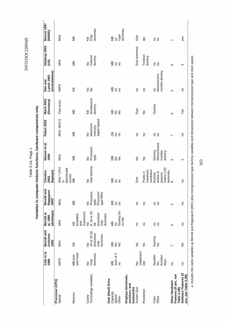
D

STI/

DO

C(2

004)

9

16

3

Tab

le 5

.1A

, Pag

e 1

Var

iab

les

in c

om

pu

ter

hed

on

ic f

un

ctio

ns,

har

dw

are

com

po

nen

ts o

nly

C

ole

et

al.

1986

B

ern

dt

and

G

rilic

hes

19

93

Ber

nd

t et

al

. 199

5 (d

eskt

op

s)

Ber

nd

t an

d

Rap

pap

ort

20

02a

Ch

wel

os

2003

(l

apto

ps)

Nel

son

et

al.

1994

P

akes

200

3 M

och

200

1 (G

erm

any)

R

ao a

nd

L

ynch

199

3 (w

ork

stat

ion

s)

Ho

ldw

ay 2

001

(US

) B

ou

rot

1997

(I

NS

EE

)

Pro

cess

or

(CP

U)

S

peed

M

IPS

M

Hz

MH

z M

Hz

MH

z *

CP

U

or

benc

hmar

k sc

ores

MH

z M

Hz,

MH

z^2

Tes

t sco

re

MIP

S

MH

z M

Hz

Mem

ory

MB

(min

an

d m

ax)

KB

K

B

(inst

alle

d an

d m

axim

um)

MB

M

B

MB

M

B

MB

K

B

MB

M

B

Cac

he

No

No

No

No

No

No

No

KB

N

o N

o K

B

Tec

hnol

ogy

varia

bles

C

hip

dum

mie

s 16

or

32 b

it pr

oces

sor

chip

du

mm

ies

8, 1

6 or

32

bit

proc

esso

r ch

ip

dum

mie

s

Pro

cess

or

type

; P

roce

ssor

ty

pe*M

Hz

Inte

l dum

my

Pro

cess

or

type

M

axim

um

mem

ory;

A

pple

*spe

ed

Arc

hite

ctur

e du

mm

y N

o C

eler

on

dum

my

Chi

p du

mm

ies

Dis

k (H

ard

) D

rive

Cap

acity

M

B

MB

M

B

MB

M

B

MB

G

B

MB

M

B

MB

M

B

Spe

ed

Sum

of 3

N

o no

no

no

N

o no

N

o no

no

no

O

ther

no

N

o D

umm

y fo

r no

HD

no

no

N

o no

N

o no

no

T

ype

dum

mie

s D

isp

lays

(te

rmin

als,

m

on

ito

rs, a

nd

ke

ybo

ard

s)

Scr

een

Siz

e N

o.

char

acte

rs

No

no

no

Siz

e N

o no

S

ize

no

Siz

e du

mm

ies

Siz

e

Res

olut

ion

Dpi

N

o no

no

P

ixel

s in

m

axim

um

reso

lutio

n

No

no

No

no

Trin

itron

du

mm

y dp

i

Col

or

Num

ber

Dum

my

no

no

Dum

my

Dum

my

no

Dum

my

no

no

no

Oth

er

No.

fu

nctio

n ke

ys

No

no

no

Act

ive

or

pass

ive

mat

rix L

CD

du

mm

ies

Mon

ochr

ome

mon

itor

dum

my

no

M

onoc

hrom

e m

onito

r du

mm

y no

no

Oth

er H

ard

war

e F

eatu

res

(If

yes,

see

T

able

5.2

B)

no

7 6

2 8

5 7

6 3

9 7

So

ftw

are

Fea

ture

s (I

f ye

s, s

ee T

able

5.2

B)

no

No

no

no

no

2 no

Y

es

no

3 ye

s

a. In

clud

es th

e sa

me

varia

bles

as

Ber

ndt a

nd R

appo

port

(20

01)

plus

mic

ropr

oces

sor

type

dum

my

varia

bles

and

inte

ract

ions

bet

wee

n m

icro

proc

esso

r ty

pe a

nd c

lock

spe

ed.

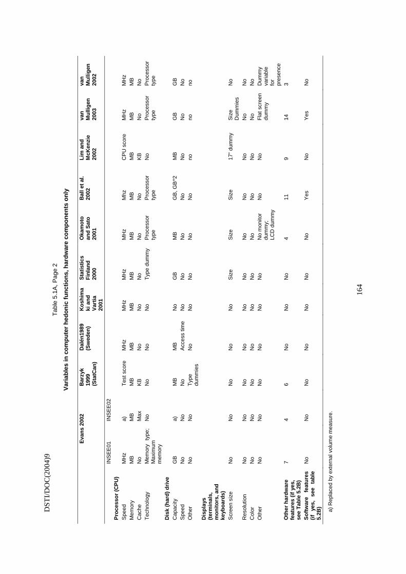
DST

I/D

OC

(200

4)9

16

4

Tab

le 5

.1A

, Pag

e 2

Var

iab

les

in c

om

pu

ter

hed

on

ic f

un

ctio

ns,

har

dw

are

com

po

nen

ts o

nly

E

van

s 20

02

Bar

zyk

1999

(S

tatC

an)

Dal

én19

89

(Sw

eden

) K

osh

ima

ki a

nd

V

arti

a 20

01

Sta

tist

ics

Fin

lan

d

2000

Oka

mo

to

and

Sat

o

2001

Bal

l et

al.

2002

L

im a

nd

M

cKen

zie

2002

van

M

ulli

gen

20

03

van

M

ulli

gen

20

02

IN

SE

E01

IN

SE

E02

Pro

cess

or

(CP

U)

S

peed

M

Hz

a)

Tes

t sco

re

MH

z M

Hz

MH

z M

Hz

Mhz

C

PU

sco

re

MH

z M

Hz

Mem

ory

MB

M

B

MB

M

B

MB

M

B

MB

M

B

MB

M

B

MB

C

ache

N

o M

ax

KB

N

o N

o N

o N

o N

o K

B

No

No

Tec

hnol

ogy

Mem

ory

type

; M

axim

um

mem

ory

No

No

No

No

Typ

e du

mm

y P

roce

ssor

ty

pe

Pro

cess

or

type

N

o P

roce

ssor

ty

pe

Pro

cess

or

type

Dis

k (h

ard

) d

rive

Cap

acity

G

B

a)

MB

M

B

No

GB

M

B

GB

, GB

^2

MB

G

B

GB

S

peed

N

o N

o N

o A

cces

s tim

e N

o N

o N

o N

o N

o N

o N

o O

ther

N

o N

o T

ype

dum

mie

s N

o N

o N

o N

o N

o no

no

no

Dis

pla

ys

(ter

min

als,

m

on

ito

rs, a

nd

ke

ybo

ard

s)

Scr

een

size

N

o N

o N

o N

o N

o S

ize

Siz

e S

ize

17”

dum

my

Siz

e D

umm

ies

No

Res

olut

ion

No

No

No

No

No

No

No

No

No

No

No

Col

or

No

No

No

No

No

No

No

No

No

No

No

Oth

er

No

No

No

No

No

No

No

mon

itor

dum

my;

LC

D d

umm

y

No

No

Fla

t sc

reen

du

mm

y D

umm

y va

riabl

e fo

r pr

esen

ce

Oth

er h

ard

war

e fe

atu

res

(if

yes,

se

e T

able

5.2

B)

7 4

6 N

o N

o N

o 4

11

9 14

3

So

ftw

are

feat

ure

s (i

f ye

s,

see

tab

le

5.2B

)

No

No

No

No

No

No

No

Yes

N

o Y

es

No

a) R

epla

ced

by e

xter

nal v

olum

e m

easu

re.

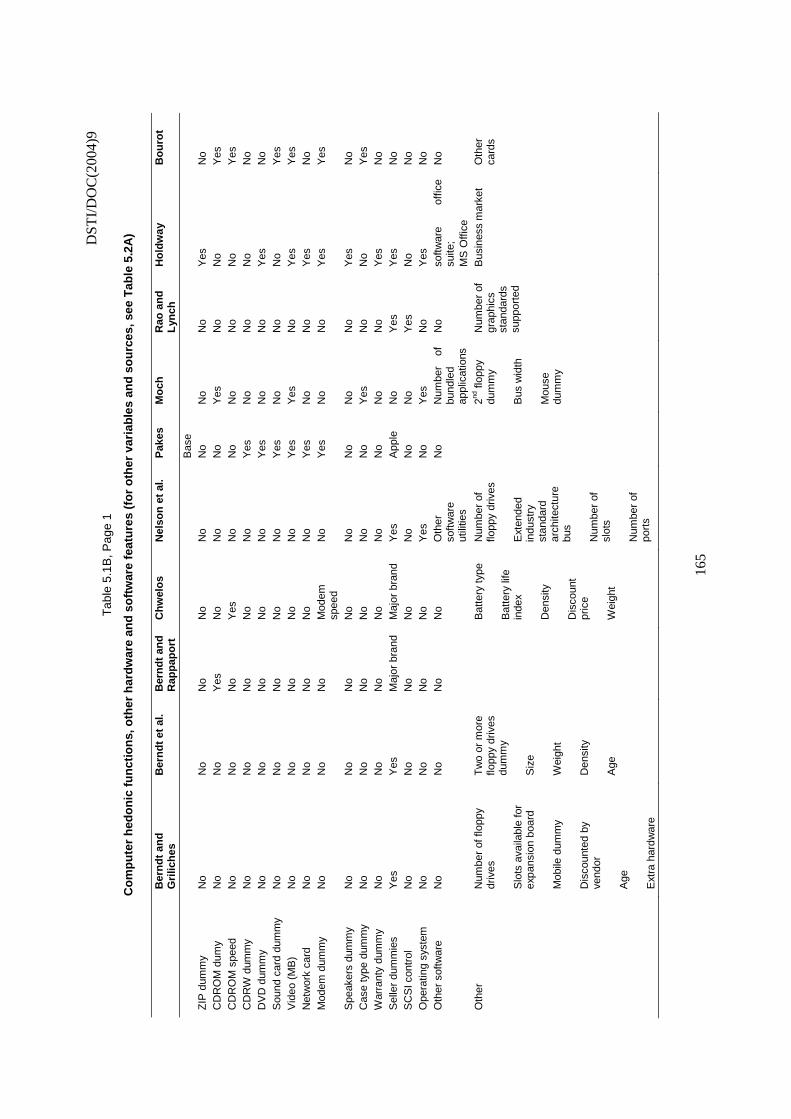
D

STI/

DO

C(2

004)

9

16

5

Tab

le 5

.1B

, Pag

e 1

Co

mp

ute

r h

edo

nic

fu

nct

ion

s, o

ther

har

dw

are

and

so

ftw

are

feat

ure

s (f

or

oth

er v

aria

ble

s an

d s

ou

rces

, see

Tab

le 5

.2A

)

B

ern

dt

and

G

rilic

hes

B

ern

dt

et a

l.

Ber

nd

t an

d

Rap

pap

ort

C

hw

elo

s N

elso

n e

t al

. P

akes

M

och

R

ao a

nd

L

ynch

H

old

way

B

ou

rot

Bas

e

Z

IP d

umm

y N

o N

o N

o N

o N

o N

o N

o N

o Y

es

No

CD

RO

M d

umy

No

No

Yes

N

o N

o N

o Y

es

No

No

Yes

C

DR

OM

spe

ed

No

No

No

Yes

N

o N

o N

o N

o N

o Y

es

CD

RW

dum

my

No

No

No

No

No

Yes

N

o N

o N

o N

o D

VD

dum

my

No

No

No

No

No

Yes

N

o N

o Y

es

No

Sou

nd c

ard

dum

my

No

No

No

No

No

Yes

N

o N

o N

o Y

es

Vid

eo (

MB

) N

o N

o N

o N

o N

o Y

es

Yes

N

o Y

es

Yes

N

etw

ork

card

N

o N

o N

o N

o N

o Y

es

No

No

Yes

N

o M

odem

dum

my

No

No

No

Mod

em

spee

d N

o Y

es

No

No

Yes

Y

es

Spe

aker

s du

mm

y N

o N

o N

o N

o N

o N

o N

o N

o Y

es

No

Cas

e ty

pe d

umm

y N

o N

o N

o N

o N

o N

o Y

es

No

No

Yes

W

arra

nty

dum

my

No

No

No

No

No

No

No

No

Yes

N

o S

elle

r du

mm

ies

Yes

Y

es

Maj

or b

rand

M

ajor

bra

nd

Yes

A

pple

N

o Y

es

Yes

N

o S

CS

I con

trol

N

o N

o N

o N

o N

o N

o N

o Y

es

No

No

Ope

ratin

g sy

stem

N

o N

o N

o N

o Y

es

No

Yes

N

o Y

es

No

Oth

er s

oftw

are

No

No

No

No

Oth

er

softw

are

utili

ties

No

Num

ber

of

bund

led

appl

icat

ions

No

softw

are

offic

e su

ite;

MS

Offi

ce

No

Oth

er

Num

ber

of fl

oppy

dr

ives

S

lots

ava

ilabl

e fo

r ex

pans

ion

boar

d M

obile

dum

my

Dis

coun

ted

by

vend

or

Age

E

xtra

har

dwar

e

Tw

o or

mor

e flo

ppy

driv

es

dum

my

Siz

e W

eigh

t D

ensi

ty

Age

B

atte

ry ty

pe

Bat

tery

life

in

dex

Den

sity

D

isco

unt

pric

e W

eigh

t

Num

ber

of

flopp

y dr

ives

E

xten

ded

indu

stry

st

anda

rd

arch

itect

ure

bus

Num

ber

of

slot

s N

umbe

r of

po

rts

2nd

flop

py

dum

my

Bus

wid

th

Mou

se

dum

my

Num

ber

of

grap

hics

st

anda

rds

supp

orte

d

Bus

ines

s m

arke

t O

ther

ca

rds

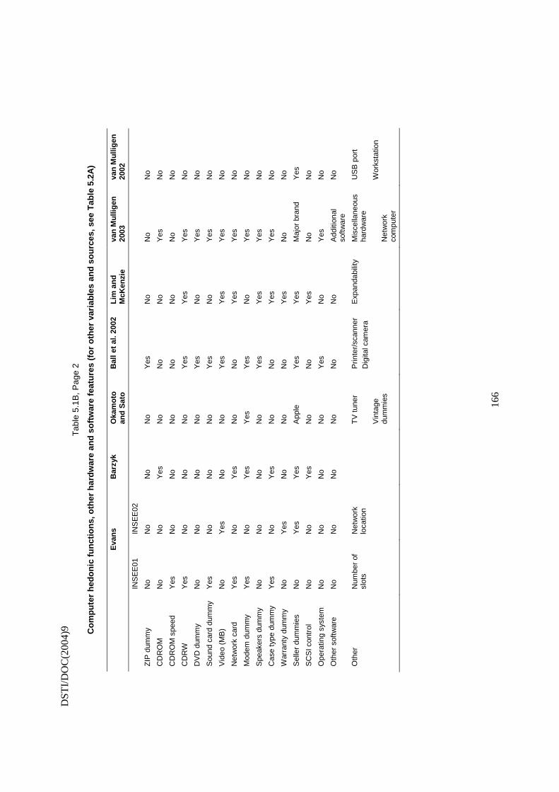
DST

I/D

OC

(200

4)9

16

6

Tab

le 5

.1B

, Pag

e 2

Co

mp

ute

r h

edo

nic

fu

nct

ion

s, o

ther

har

dw

are

and

so

ftw

are

feat

ure

s (f

or

oth

er v

aria

ble

s an

d s

ou

rces

, see

Tab

le 5

.2A

)

E

van

s B

arzy

k O

kam

oto

an

d S

ato

B

all e

t al

. 200

2 L

im a

nd

M

cKen

zie

va

n M

ulli

gen

20

03

van

Mu

llig

en

2002

IN

SE

E01

IN

SE

E02

ZIP

dum

my

No

No

No

No

Yes

N

o N

o N

o

CD

RO

M

No

No

Yes

N

o N

o N

o Y

es

No

CD

RO

M s

peed

Y

es

No

No

No

No

No

No

No

CD

RW

Y

es

No

No

No

Yes

Y

es

Yes

N

o

DV

D d

umm

y N

o N

o N

o N

o Y

es

No

Yes

N

o

Sou

nd c

ard

dum

my

Yes

N

o N

o N

o Y

es

No

Yes

N

o

Vid

eo (

MB

) N

o Y

es

No

No

Yes

Y

es

Yes

N

o

Net

wor

k ca

rd

Yes

N

o Y

es

No

No

Yes

Y

es

No

Mod

em d

umm

y Y

es

No

Yes

Y

es

Yes

N

o Y

es

No

Spe

aker

s du

mm

y N

o N

o N

o N

o Y

es

Yes

Y

es

No

Cas

e ty

pe d

umm

y Y

es

No

Yes

N

o N

o Y

es

Yes

N

o

War

rant

y du

mm

y N

o Y

es

No

No

No

Yes

N

o N

o

Sel

ler

dum

mie

s N

o Y

es

Yes

A

pple

Y

es

Yes

M

ajor

bra

nd

Yes

SC

SI c

ontr

ol

No

No

Yes

N

o N

o Y

es

No

No

Ope

ratin

g sy

stem

N

o N

o N

o N

o Y

es

No

Yes

N

o

Oth

er s

oftw

are

No

No

No

No

No

No

Add

ition

al

softw

are

No

Oth

er

Num

ber

of

slot

s N

etw

ork

loca

tion

T

V tu

ner

Vin

tage

du

mm

ies

Prin

ter/

scan

ner

Dig

ital c

amer

a E

xpan

dabi

lity

Mis

cella

neou

s ha

rdw

are

Net

wor

k co

mpu

ter

US

B p

ort

Wor

ksta

tion

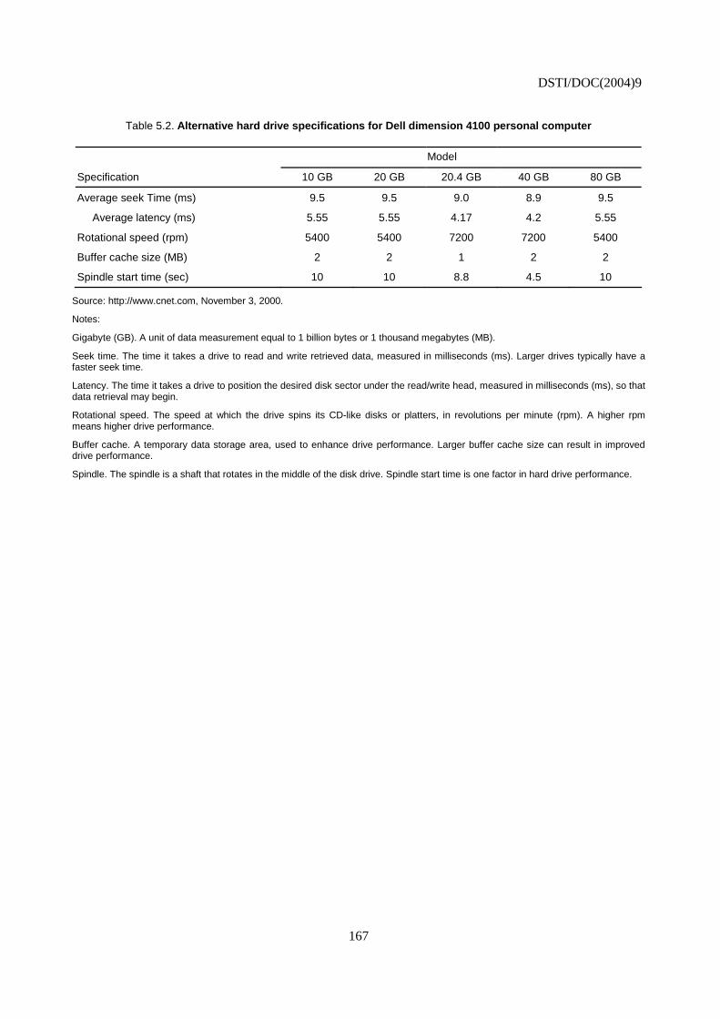
DSTI/DOC(2004)9

167

Table 5.2. Alternative hard drive specifications for Dell dimension 4100 personal computer

Model

Specification 10 GB 20 GB 20.4 GB 40 GB 80 GB

Average seek Time (ms) 9.5 9.5 9.0 8.9 9.5

Average latency (ms) 5.55 5.55 4.17 4.2 5.55

Rotational speed (rpm) 5400 5400 7200 7200 5400

Buffer cache size (MB) 2 2 1 2 2

Spindle start time (sec) 10 10 8.8 4.5 10

Source: http://www.cnet.com, November 3, 2000.

Notes:

Gigabyte (GB). A unit of data measurement equal to 1 billion bytes or 1 thousand megabytes (MB).

Seek time. The time it takes a drive to read and write retrieved data, measured in milliseconds (ms). Larger drives typically have a faster seek time.

Latency. The time it takes a drive to position the desired disk sector under the read/write head, measured in milliseconds (ms), so that data retrieval may begin.

Rotational speed. The speed at which the drive spins its CD-like disks or platters, in revolutions per minute (rpm). A higher rpm means higher drive performance.

Buffer cache. A temporary data storage area, used to enhance drive performance. Larger buffer cache size can result in improved drive performance.

Spindle. The spindle is a shaft that rotates in the middle of the disk drive. Spindle start time is one factor in hard drive performance.

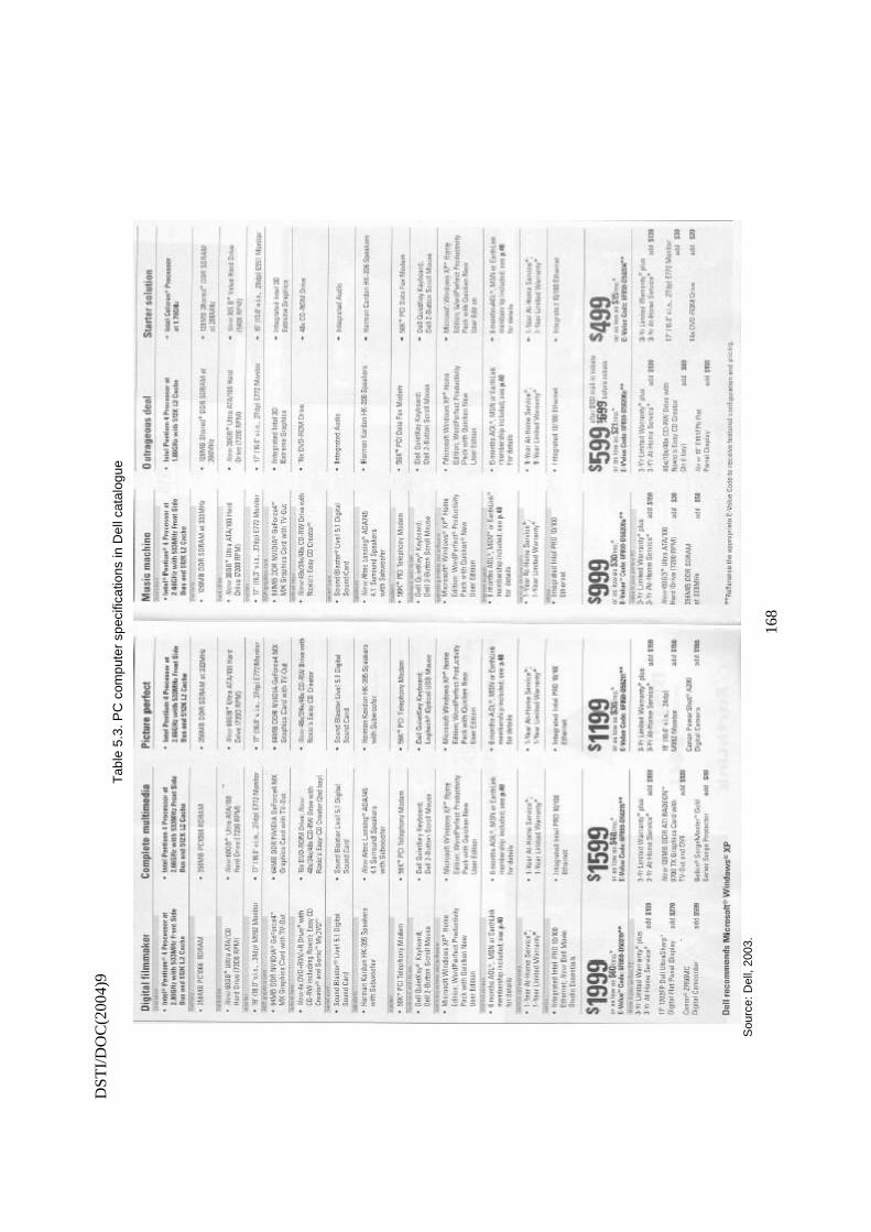
DST

I/D

OC

(200

4)9

16

8

Tab

le 5

.3. P

C c

ompu

ter

spec

ifica

tions

in D

ell c

atal

ogue

Sou

rce:

Del

l, 20

03.

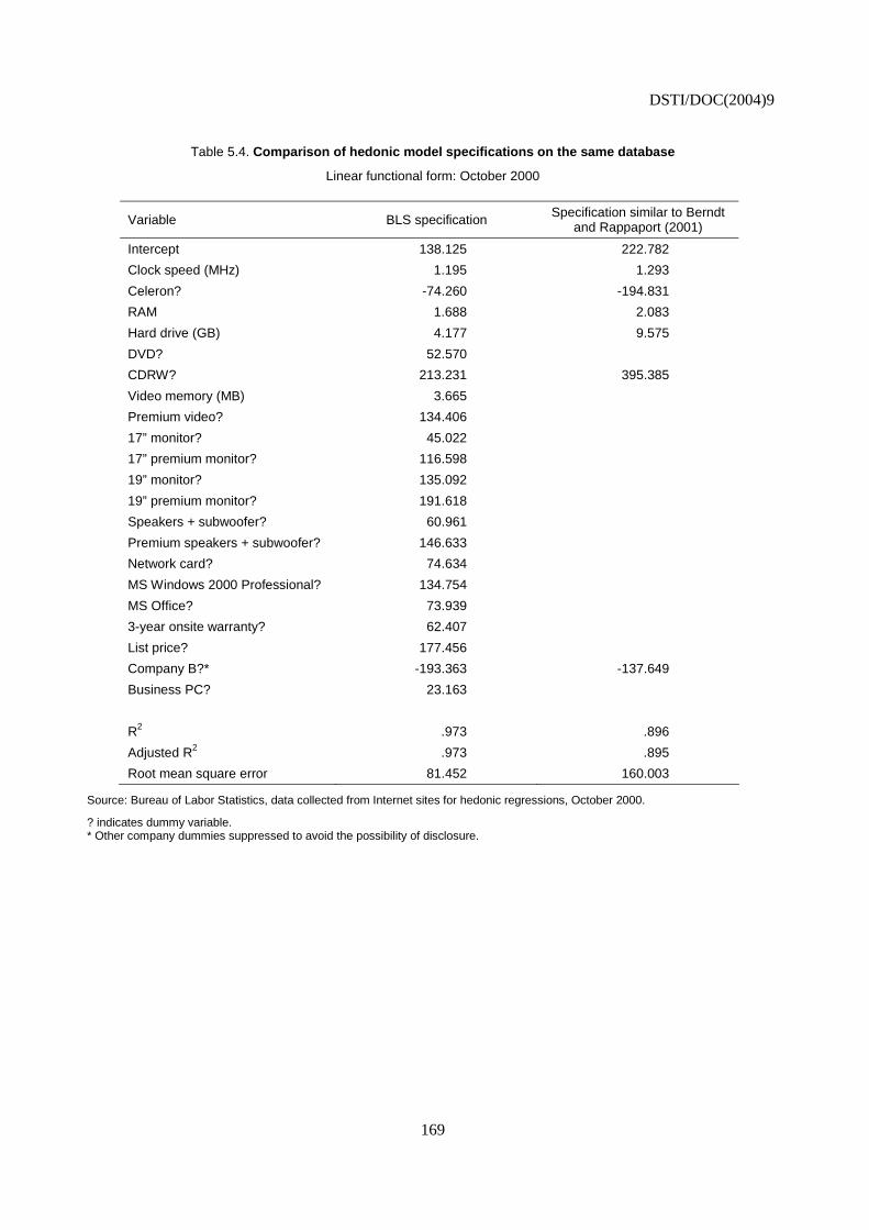
DSTI/DOC(2004)9

169

Table 5.4. Comparison of hedonic model specifications on the same database

Linear functional form: October 2000

Variable BLS specification Specification similar to Berndt and Rappaport (2001)

Intercept 138.125 222.782

Clock speed (MHz) 1.195 1.293

Celeron? -74.260 -194.831

RAM 1.688 2.083

Hard drive (GB) 4.177 9.575

DVD? 52.570

CDRW? 213.231 395.385

Video memory (MB) 3.665

Premium video? 134.406

17” monitor? 45.022

17” premium monitor? 116.598

19” monitor? 135.092

19” premium monitor? 191.618

Speakers + subwoofer? 60.961

Premium speakers + subwoofer? 146.633

Network card? 74.634

MS Windows 2000 Professional? 134.754

MS Office? 73.939

3-year onsite warranty? 62.407

List price? 177.456

Company B?* -193.363 -137.649

Business PC? 23.163

R2 .973 .896

Adjusted R2 .973 .895

Root mean square error 81.452 160.003

Source: Bureau of Labor Statistics, data collected from Internet sites for hedonic regressions, October 2000. ? indicates dummy variable. * Other company dummies suppressed to avoid the possibility of disclosure.

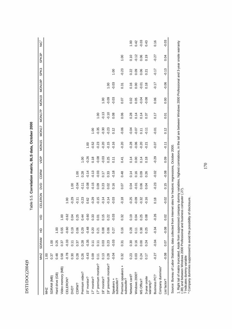
DST

I/D

OC

(200

4)9

17

0

Tab

le 5

.5. C

orr

elat

ion

mat

rix,

BL

S d

ata,

Oct

ob

er 2

000

M

HZ

S

DR

AM

H

D

VID

C

ELE

RO

N

DV

D

CD

RW

V

IDP

M

ON

15

MO

N17

M

ON

17P

M

ON

19

MO

N19

P

SP

K3

SP

K3P

N

IC1

MH

Z

1.00

SD

RA

M (

MB

) 0.

37

1.00

Har

d dr

ive

(GB

) 0.

48

0.25

1.

00

Vid

eo m

emor

y (M

B)

0.58

0.

37

0.55

1.

00

CE

LER

ON

? -0

.78

-0.3

3 -0

.60

-0.6

2 1.

00

DV

D?

0.30

0.

11

0.19

0.

04

-0.2

9 1.

00

CD

RW

? 0.

28

0.37

0.

06

0.25

-0

.11

-0.0

4 1.

00

Pre

miu

m v

ideo

? 0.

26

0.28

0.

29

0.44

-0

.23

-0.1

1 0.

28

1.00

15”

mon

itor?

-0

.43

-0.3

5 -0

.48

-0.6

0 0.

62

-0.0

8 -0

.14

-0.2

6 1.

00

17”

mon

itor?

0.

09

0.11

0.

20

0.33

-0

.29

-0.1

5 -0

.13

0.18

-0

.52

1.00

17”

prem

ium

mon

itor?

0.

11

0.11

0.

21

0.01

-0

.15

0.09

-0

.03

-0.0

8 -0

.23

-0.3

5 1.

00

19”

mon

itor?

0.

13

0.03

0.

08

0.15

-0

.14

0.23

0.

17

-0.0

3 -0

.20

-0.3

0 -0

.13

1.00

19”

prem

ium

mon

itor?

0.

28

0.23

0.

06

0.22

-0

.14

0.02

0.

33

0.25

-0

.15

-0.2

3 -0

.10

-0.0

9 1.

00

Spe

aker

s +

su

bwoo

fer?

-0

.04

-0.0

3 0.

27

-0.0

3 -0

.03

0.16

-0

.18

0.11

-0

.16

0.12

0.

08

-0.0

3 -0

.03

1.00

Pre

miu

m s

peak

ers

+

subw

oofe

r?

0.32

0.

31

0.16

0.

32

-0.1

8 0.

07

0.48

0.

41

-0.2

0 -0

.06

0.06

0.

07

0.31

-0

.23

1.00

Net

wor

k ca

rd?

0.23

0.

30

0.28

0.

19

-0.2

5 0.

04

0.14

0.

14

-0.2

8 -0

.04

0.28

0.

02

0.16

0.

22

0.10

1.

00

Win

dow

s 20

00?

0.03

0.

16

0.11

0.

04

-0.0

9 -0

.01

0.16

0.

00

-0.0

6 -0

.07

0.14

0.

05

0.00

0.

09

-0.1

2 0.

42

MS

Offi

ce?

0.24

0.

00

0.38

0.

25

-0.3

2 0.

06

0.09

0.

14

-0.2

0 0.

11

0.14

-0

.04

-0.0

1 0.

06

0.06

-0

.03

3-ye

ar o

nsite

w

arra

nty?

0.

17

0.24

0.

25

0.08

-0

.16

0.04

0.

26

0.18

-0

.21

-0.1

1 0.

37

-0.0

8 0.

18

0.21

0.

19

0.43

Bus

ines

s P

C?

-0.2

7 -0

.04

-0.3

4 -0

.26

0.18

-0

.23

-0.0

2 -0

.29

-0.0

7 -0

.01

0.17

0.

06

-0.1

7 -0

.17

-0.2

7 0.

16

Com

pany

dum

mie

s*

List

fact

or?

-0.0

8 0.

07

-0.0

8 0.

02

-0.0

2 0.

15

-0.0

8 0.

09

-0.1

1 0.

12

0.01

0.

00

-0.0

6 -0

.13

0.04

-0

.03

Sou

rce:

Bur

eau

of L

abor

Sta

tistic

s, d

ata

colle

cted

from

Inte

rnet

site

s fo

r he

doni

c re

gres

sion

s, O

ctob

er 2

000.

1. R

ight

tail

of m

atrix

trun

cate

d. A

side

from

sup

pres

sed

com

pany

dum

my

varia

bles

, hig

hest

cor

rela

tions

, in

the

tail

are

betw

een

Win

dow

s 20

00 P

rofe

ssio

nal a

nd 3

-yea

r on

site

war

rant

y (.

38)

and

betw

een

Win

dow

s 20

00 P

rofe

ssio

nal a

nd b

usin

ess

com

pute

r (.

27).

?

Indi

cate

s du

mm

y va

riabl

e

* C

ompa

ny d

umm

ies

supp

ress

ed to

avo

id th

e po

ssib

ility

of d

iscl

osur

e.

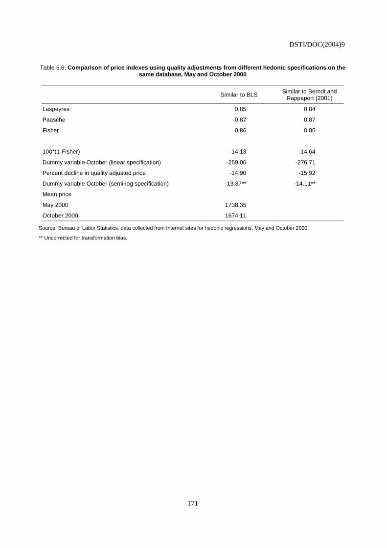
DSTI/DOC(2004)9

171

Table 5.6. Comparison of price indexes using quality adjustments from different hedonic specifications on the same database, May and October 2000

Similar to BLS Similar to Berndt and Rappaport (2001)

Laspeyres 0.85 0.84

Paasche 0.87 0.87

Fisher 0.86 0.85

100*(1-Fisher) -14.13 -14.64

Dummy variable October (linear specification) -259.06 -276.71

Percent decline in quality adjusted price -14.90 -15.92

Dummy variable October (semi-log specification) -13.87** -14.11**

Mean price

May 2000 1738.35

October 2000 1674.11

Source: Bureau of Labor Statistics, data collected from Internet sites for hedonic regressions, May and October 2000.

** Uncorrected for transformation bias.

DSTI/DOC(2004)9

172

CHAPTER VI

ESTIMATING HEDONIC FUNCTIONS: OTHER RESEARCH ISSUES

A. Introduction

From the statistical or econometric point of view, there is nothing very complicated about estimating hedonic functions. The economics that lie behind hedonic functions are not necessarily simple, but the economics of hedonic functions do not imply complex econometric methods.

Most hedonic functions have been estimated by ordinary least squares (OLS) regression, which is the most straightforward statistical technique employed by economists. Indeed, in Berndt’s (1991) empirically-oriented econometrics text, hedonic functions and hedonic indexes serve as the research topic to teach OLS – the book shows how to estimate hedonic functions with OLS and gives examples and exercises, using actual datasets for computer equipment.117 OLS methods are widely taught in undergraduate economics courses, and widely mastered. Statistical agency personnel with good undergraduate training in economics or statistics should have no difficulty estimating a hedonic function.

Because methods for estimating OLS regressions are thoroughly treated in econometrics textbooks, there is no need to discuss them here – examples of excellent textbooks which serve as references in this chapter include Gujarati (1995), Wooldridge (1999) and Berndt (1991), though these are by no means the only excellent texts. For the same reason, attaining best practice with respect to statistical estimation of hedonic functions does not need elaboration in this handbook.

That the econometrics of hedonic regressions themselves are relatively easy does not mean, however, that designing and carrying out a hedonic study is always a simple task. Rather, running the regression on the computer is not the major difficulty. This chapter considers the major statistical and econometric issues that arise in estimating hedonic functions (other than selection of variables, which was covered in Chapter V).

For the purposes of this chapter, I take the computer hedonic function from earlier chapters as the basis for the discussion:

(6.1) Pit = a0 + a1 (MHz)it + a2 (MB)it + a3 (HD)it + eit

B. Multicollinearity

“Although the problem of multicollinearity cannot be clearly defined, one thing is clear: everything else being equal, for estimating [regression coefficient] bj it is better to have less correlation between xj and the other independent variables” (Wooldridge, 1999, page 96)

117. Berndt (1991) used for student exercises one dataset from research on the BEA computer equipment

hedonic indexes described in Cole et al. (1986) and Cartwright (1986) and another from the Chow (1967) study of mainframe computers.

DSTI/DOC(2004)9

173

In the classic statistical regression model, each of the right hand variables in equation (6.1) is correlated with the price. Multicollinearity arises when there are statistical dependencies among the explanatory variables in a regression. For example, the HD capacity of a computer might be correlated with its speed, as it is in the BLS data, where the correlation of MHz and HD in October, 2000 was approximately 0.5 (actually, 0.48 – see Table 6.1).

Multicollinearity is reviewed in an extensive literature in econometrics, and in other parts of statistics as well.118 Multicollinearity is not a problem that is unique to hedonic functions, but it is considered extensively in the hedonic literature, and it is widely viewed as a major problem for hedonic functions. For example, Schultze and Mackie (2002, Chapter 4) point to multicollinearity in their review of hedonic price indexes.

However, the problems posed for hedonic functions by multicollinearity are not always well addressed by standard econometrics textbooks, which tend to emphasise instability of regression coefficients and the sizes of standard errors.119 Occasionally, hedonic regression standard errors may “blow up,” though this has not been observed very often in empirical studies. In most well-constructed hedonic functions – with or without high mulicollinearity – coefficients of the major characteristics are usually statistically significant; that is, standard errors are not so large as to create a major difficulty. More frequently, coefficients are unstable from one cross section to another; but even here, coefficient instability in hedonic functions is often caused empirically by data errors combined with multicollinearity, not just multicollinearity by itself. Multicollinearity exacerbates difficulties caused by other problems, including missing variables and proxy variables, which were discussed in Chapter V.

1. Sources of multicollinearity

It is useful to distinguish between multicollinearity in the population or universe and multicollinearity in the sample.

a. Multicollinearity in the universe

From the point of view of computer production technology, it might be possible to increase the MHz of a computer without necessarily increasing its memory capacity or its HD capacity. If this is the case, there is nothing in the technology of computer production that necessarily implies multicollinearity, and there is no necessary multicollinearity in the universe of computer models.

Absence of technologically-based multicollinearity might not always be true for other products. For automobiles, researchers commonly report that fuel economy enters hedonic function regressions with a negative sign, though size and performance variables have the expected positive signs. A negative sign suggests that fuel economy is a negative quality characteristic of an automobile, something that consumers do not want, which seems improbable. Clearly, fuel economy is desirable from the buyer’s point of view, and engineering steps to improve it (better fuel injection systems, for example) are costly, so one expects a positive sign for greater fuel economy. This negative sign on fuel economy really means that larger cars use more gasoline, so there is a negative correlation between size and performance characteristics and fuel economy. Buyers would like more fuel economy, everything else equal, but engineering relations limit the

118. An excellent introduction to multicollinearity is Chapter 10 of Gujarati (1995), who draws extensively on

the insightful contributions of Goldberger (1991). See also Wooldridge (1999).

119. Goldberger (1991) pokes fun at standard textbook treatments of multicollinearity. He compares them to a fictitious textbook that discusses, without insight, small sample size under the heading of “micronumerosity.” Insofar as the discussion of multicollinearity in this section differs from its treatment in standard textbooks, it is closer to the discussion in Goldberger.

DSTI/DOC(2004)9

174

degree that larger cars can be made without incurring a fuel economy penalty. Its negative sign in the hedonic function for cars reflects technological or engineering relations that create multicollinearity among automotive characteristics and fuel economy.

In the auto case, we are trying to model the hedonic function for the good, when the transportation services provided by the good require a cooperating good (fuel) that is not specified in the model. The cost of operating larger, more luxurious cars arises partly because of their higher initial purchase prices, but partly because of their fuel requirements. In a hedonic function for automobile transportation services, the fuel cost as well as the capital cost would appear on the left-hand side (in the form of operating cost per mile), and the performance variables on the right.

As another example, Chwelos, Berndt and Cockburn (2003) report that increased weight enters a hedonic function for portable computing devices with a positive sign, even though it is clear that lighter devices are greatly desired by computer buyers (so the sign should be negative). The reason is similar to the automobile case – more powerful computers impose size and weight penalties in the production technology of a specified period, and the penalties (with their positive signs) are incorporated into the cross section hedonic regressions. At a given stage of computer technology, one cannot get more performance without incurring a weight and size penalty, and correlations between the various performance variables and weight and size causes the regression coefficients to take on “wrong” signs. Over time, however, portable computer technology improves by achieving more computational capacity per unit of size or of weight (early portable computers have sometimes been called “luggable,” reflecting their awkward size and excessive weight). One wants to take this weight saving into account as an improvement in product quality. Valuing computer weight by the (positive) cross-section hedonic coefficients means that weight saving is treated as diminishing product quality, when we know the opposite is true. Engineering relations among the characteristics at a moment of time make it difficult to use cross-section regressions to account for weight saving innovations over time, and indeed the cross-section estimates (with their inappropriate positive signs) adjust the time series in the wrong direction.

Thus, one requirement for absence of multicollinearity is absence of technical or engineering relations among the characteristics that restrict possibilities for increasing or decreasing one characteristic without concomitant increases of decreases in the other characteristics. Put another way, the first requirement is absence of technical conditions that create statistical dependencies among the characteristics, across the universe of computer models.120

b. Multicollinearity in the sample

Absence of multicollinearity also requires absence of intercorrelations among the variables within the sample. Multicollinearity in hedonic functions is best thought of as a property of the sample, and not as a property of the underlying hedonic model.121

As an illustration, multicollinearity in the BLS PPI sample of computer models is not constant across different months’ samples. In December, 2001, the simple R values among the variables are all lower than they were in October, 2000 (compare tables 6.1 and 6.2). For example, the correlation between MHz and

120. Economic relations among regression variables can also create multicollinearity. Gujarati (1995, page 323)

gives as an example a regression of electricity use on income and house size, where income and house size are usually correlated for obvious economic reasons. On this general topic, see also the discussion of proxy variables in Chapter V, since the use of proxy variables depends on relations among explanatory variables, either those inside the regression or outside it (excluded variables).

121. Gujarati (1995), following Goldberger, stresses relations between the sample, and the sample size, and multicollinearity in the general regression model.

DSTI/DOC(2004)9

175

hard drive capacity (0.48 in October, 2000) is only 0.22 in December, 2001; and although a number of correlations above 0.6 appear in the October 2000 data (most of them involving the Celeron dummy), none are as high as 0.4 in the later month.122

In work on computer hedonic functions, some studies use samples of models. For example, the BLS PPI sample takes specifications and prices data from producers’ websites. Others use samples of transactions, for example, scanner data. Generally, more multicollinearity arises in samples of transactions than in samples of computer models because buyers tend to cluster in the middle of the distribution of computer models.

Companies offer many choices to buyers. Technically, from the engineering point of view, it is possible to vary computer characteristics proportions, e.g., to build a very fast computer that has little memory and storage capacity. However, when computer buyers spend more on computers, they typically increase their spending on all computer characteristics – when they buy a faster computer, they also buy more MB and HD capacity. Computer characteristics have the properties of “normal goods”, in that expenditure elasticities for characteristics are positive, and they may be roughly proportional.123

Figure 6.1: the figure shows a series of “hedonic contours” (hedonic contours are explained in section C, below), here assumed linear for simplicity in drawing the figure. Each contour shows combinations of speed and memory that can be purchased at a specified price: any contour, such as P1, shows speed and memory sizes of all the models of computers than are offered at price P1, and similarly for P2, P3, and so forth. When a consumer pays more for a computer (P3 > P2 > P1), the consumer generally buys more of all the characteristics, so the scatter plot of transactions is more densely packed around the diagonal (dashed) line than at other points in the characteristics space. Put another way, the distribution of computer buyers is more dense across the characteristics than the is distribution of computer models.

When computer characteristics have similar expenditure elasticities from the buyers’ side, computer sales will tend to cluster in the centre of the characteristics space. Models in the centre of the space (models with proportional amounts of all characteristics) will be more popular models and will thus be repeated in the sample of transactions. This is shown in Figure 6.1.

Expenditure patterns thus set up multicollinearity in the transactions sample, because consumers tend to have similar tastes and buy more memory (and other computer characteristics) when they buy more speed. For this reason, multicollinearity results in the sample, even when no engineering or technical reason for multicollinearity exists among the characteristics of the models. More multicollinearity will generally be present in samples of transactions than will be present in samples of models.

Table 6.3 shows the simple R measures in the sample of personal computers in the US Consumer Price Index. The CPI sample is a probability sample that is drawn from consumer transactions. Predictably, there is more multicollinearity in the CPI sample of computer transactions (Table 6.3) than in the PPI samples of computer models (tables 6.1 and 6.2).124 For example, the correlation of MHz and HD (which was 0.48 and 0.22 in the PPI samples in tables 6.1 and 6.2) is 0.663 in the CPI sample, and the correlation 122. Though this example, and subsequent ones, uses the simple R, a more appropriate statistic is the partial

regression coefficient of two variables. Obtaining this statistic is often more work. The simple R values among variables are printed out in normal regression packages and convey most of the information needed.

123. This relation between increased purchases of individual characteristics and expenditure on a computer is analogous to what is usually called an Engel curve, which in normal demand analysis relates increasing expenditures on individual goods to increasing total expenditure. See the Theoretical Appendix.

124. The increased multicollinearity in the sample of transactions has implications for the controversy on whether to weight hedonic regressions by sales, which is discussed in section D of this chapter.

DSTI/DOC(2004)9

176

between internal memory (RAM) and disk memory (HD), which was only 0.25 and 0.03 in the PPI data, rises to 0.69 in the CPI.

c. Conclusion: sources and consequences of multicollinearity

Authors of empirical hedonic studies have so often reported finding multicollinearity that others have come to regard it a the state of the characteristics world and of hedonic functions. Sometimes it is. Sometimes, there are technical reasons why multicollinearity is high in a hedonic function regime.

But multicollinearity has also become an excuse for poor research strategies and for failing to ask penetrating questions about the data. Researchers need always to consider the nature of their samples, and the nature of the data that they get from others’ samples. One might be able to choose sampling strategies with less, rather than more, multicollinearity. Because multicollinearity is often a property of the sample, it may sometimes be ameliorated by increasing the sample, or by searching out samples with more variation in the observations. We need to analyse the data, not throw up our hands in surrender to the monster of multicollinearity.

Multicollinearity has also become a “red flag” against hedonic functions and hedonic indexes. There is little empirical evidence that multicollinearity is a greater problem in hedonic research than for other economic research. More importantly, in hedonic functions where – as in the BLS work summarised in Tables 6.1 and 6.2 – samples are large and data are carefully cleaned there is little evidence of the unstable coefficients and large standard errors that are the classic signs of multicollinearity. It is correct to say that multicollinearity is a problem. But it is not necessarily an unmanageable problem for hedonic indexes, despite assertions to the contrary.

2. Detecting multicollinearity

In a very real sense, multicollinearity is the normal state of the world. It will seldom be the case that the explanatory variables in a hedonic regression will all be correlated with the price, yet not correlated with each other. Indeed, the low values of the simple Rs in Table 6.2, where a number of them are below 0.1, will surprise most researchers with experience with regression models containing so many variables, for in empirical work outside hedonic functions it is rare to find regressions containing many variables with so little multicollinearity.

There are degrees of multicollinearity, it is not a property that is either present or not present. An investigator must determine whether mulitcollinearity is sufficiently great that it poses a problem for an investigation, and unfortunately, there are no real tests for the severity of multicollinearity. One test is to examine the matrix of simple R or R2 values among independent variables in the regression by inspecting tables such as tables 6.1, 6.2, and 6.3. If the simple Rs are high, then there is multicollinearity.125 Gujarati (1995, pages 335-339) lists other diagnostics for multicollinearity, including the condition index (see Gujarati’s discussion on page 338), and the variance inflation factor. However, these more sophisticated measures, though useful, still require judgement. They indicate whether or not multicollinearity is “high,” they do not provide a statistical test of its acceptability. Inspection of the simple R values remains instructive, and because it is transparent, it is sometimes preferred to more sophisticated, but less easy to interpret, measures like the condition index.

Knowing that multicollinearity is “high” is not the same as knowing whether it is a debilitating problem for an investigation. There are no hard and fast rules. The problem requires, instead, careful thought, sometimes subtle analysis, and most importantly, knowing one’s product. The investigator must

125. But see footnote 6, above.

DSTI/DOC(2004)9

177

also think carefully about the implications of intercorrelations among the explanatory variables for the interpretation of the coefficients that will be used for making the hedonic quality adjustment.

A standard way around the multicollinearity problem is to reduce the number of variables in the regression. Combining two or more correlated variables gives a coefficient that measures the combined effect of the combined variables on the price. One might, for example, combine variables for the size of the monitor so that larger monitors are all coded “greater than 17 inch” screen size. Whether consciously or not, some of the hedonic studies on PCs have done exactly this (see the review of hedonic function variables in Chapter V). Although reducing the number of variables might sometimes be unavoidable if multicollinearity is severe enough, researchers should beware that the reduction introduces other problems. For example, a single coefficient for “larger” monitors measures the price for the average larger monitor and will introduce error if the distribution of those larger monitors changes toward, say, the very largest of them. See also the discussion of omitted variables and proxy variables in Chapter V.

3. Multicollinearity and data errors

Researchers have become inured, to an extent, to evidence of multicollinearity, largely because (a) textbooks give instability as a consequence of multicollinearity and (b) instability of coefficients has often been noted in hedonic functions. Griliches (1961) in his original article on hedonic functions for automobiles pointed out that annual regressions on US cars exhibited instability in regression coefficients. Other researchers have reported the same thing, not only for automobiles but also in investigations covering other products.

However, the veil of multicollinearity has sometimes hidden the effects of poor data quality in hedonic research. Research folklore has it that multicollinearity will show itself in the form of unstable regression coefficients, and anomalous results. Researchers who find unstable coefficients accordingly seize on multicollinearity as the reason, and although this is sometimes appropriate, fail to ask questions about their data.

Frequently, it is not multicollinearity that causes the problems, but rather multicollinearity combined with what Longley (1984) called “perturbations in the data.” When the data for a hedonic study contain errors, seemingly small errors (especially in data points at the extremes of the distribution) become magnified through the effects of multicollinearity into larger than anticipated impacts on regression coefficients. I know of no econometrics textbook that proves that this must be the case, though Gujarati (1995) suggests that multicollinearity makes coefficients sensitive to data changes.

Wide experience with hedonic functions, however, shows that it is true empirically that the estimated coefficients are sensitive to errors in data. Regrettably, this is the kind of result that does not get reported in journals. It is therefore only spread among professionals by oral exchange, it is not written down in convenient form. For this reason, the result is not be known by some researchers.

Hedonic functions are very demanding of data quality. This is probably not widely appreciated. In the early days of hedonic research, it was difficult to find any suitable data at all, especially cross-sections of transactions prices. Researchers usually made do with whatever “found data” (the term is Griliches’) they located in trade journals and so forth.

That these data might contain errors was understood, particularly the fact that the prices were frequently list prices, rather than true transactions prices. It is, however, also true that published data on prices and characteristics in trade publications and so forth are often marred by recording and typographical errors. Many of them are no doubt small, which is why they are not caught in review. But seemingly small data errors may have consequences that are not small.

DSTI/DOC(2004)9

178

Examples show the point. In my own hedonic research on automobiles (Triplett, 1969), discrepancies among published sources were used as indicators to suggest where data cleaning was needed. Data cleaning produced noticeable effects on the regression coefficients – the coefficients on the cleaned data were more stable and more reasonable than the coefficients from the uncleaned data, and were somewhat more stable than in other automobile hedonic functions. I did not publish the regressions that were run before data cleaning took place (journals are no more interested in bad data than are researchers).

IBM research on computer equipment (Cole et al., 1986) relied on published data, partly because of the desire to make a publicly available data set available through BEA; but the data were cleaned by consulting internal IBM and industry sources, and some of the changes were substantial. More recently, BLS has announced that it has abandoned use of published trade source information on PCs and other computer equipment because too many errors were found in published data. Similar results arise in other studies: researchers who have used scanner and market intelligence data for PCs report informally the need to clean the data and to work with data suppliers to correct errors.

Pakes (2003) used proprietary data that have also been used by other researchers, including Barzyk and MacDonald (2001). Pakes reports substantial instability in the regression coefficients (for example, his coefficient on speed goes from -4.72 in 1997 to +16.79 in 1998), and he reports regression R2 values that, at 0.3 to 0.5, are at the bottom end for published computer hedonic functions (Barzyk and MacDonald got around 0.8, which is typical for computer hedonic studies). Barzyk, in personal conversations with other researchers and with myself, has reported on Statistics Canada’s extensive consultation program with the vendor that provides data for their hedonic studies. Comparison of his results and those of Pakes are consistent with data quality problems, though other reasons are of course possible (Canadian and US hedonic functions might indeed differ in the ways the studies suggest). Research for Eurostat’s European Hedonic Centre (Konijn, Moch and Dalén, 2003) indicates that data quality differs across countries, even from the same vendor.

Data always have errors. That the data are not without fault does not mean they are without usefulness. Data errors in the source materials do mean that conducting a hedonic research project requires the researcher to spend a great amount of time compiling, checking, and correcting information on prices and characteristics, regardless of the data source. An often overlooked source of error in regression coefficients stems from errors in the prices and characteristics data themselves.

Rather than blaming multicollinearity when they encounter coefficient instability, researchers ought to consider the medicine of thorough data cleaning. It will often greatly reduce the problem.

4. Interpreting coefficients in the presence of multicollinearity

As noted in Chapter V, one wants to interpret the coefficients of a hedonic function as measures of the implicit prices of characteristics (in non-linear cases, they are logarithms of the implicit prices or functions of them). On this economic view, when the buyer pays EUR 3 000 for computer model Y, the buyer is really buying the bundle of characteristics that model Y contains – the quantities of speed, memory, and so forth that are embodied in the computer. The hedonic function recovers the implicit prices for the various characteristics from the total value of the bundle (which is EUR 3 000). The coefficient, such as a1 in equation (6.1), measures the effect on the price of the product for a one-unit increment of the characteristic MHz (in the linear case).

Multicollinearity does not interfere with this “characteristics price” interpretation, in the sense that in repeated samples, the value of the estimated coefficient will converge on the true characteristics price. This is the econometric property known as “consistency”. However, because of “perturbations in the data,”

DSTI/DOC(2004)9

179

when multicollinearity is present the value of the estimated coefficient in the sample at hand might differ appreciably from the true characteristics price.

Multicollinearity is an especially vexing problem if one uses the regression coefficients from a hedonic function to make a quality adjustment in the price index (refer to the hedonic quality adjustment method described in Chapter III). In this case, the validity of the hedonic regression coefficients must be the researcher’s major concern, rather than the overall “fit” of the regression, which usually gets the most attention.

If multicollinearity compromises the interpretation of each regression coefficient considered by itself, one might limit the problems by always following the rule of adjusting for the combined group of correlated variables. An imputation for the combined changes in all the variables in equation (6.1), or in all the collinear variables, is less problematic than an imputation for a single variable.

On the other hand, as noted in Chapter III, in the hedonic quality adjustment method, properly implemented, the hedonic quality adjustment is based on an estimate of the price of the computer that is missing from the sample, so it uses all of the coefficients of the regression. Multicollinearity may affect the estimate of a single coefficient, but its impact on the group of regression coefficients is less severe, because the combined coefficients for the group of variables will be estimated more precisely than any single one. This implies adjusting for all variables in the hedonic function, not just for some of them. If this rule is followed, the multicollinearity objection to the hedonic quality adjustment method has much less force than it seems to have (see also Chapter III and Chapter VI).

5. Multicollinearity in hedonic functions: assessment

Multicollinearity is a problem for hedonic functions, as it is for other economic research. Some discussions of hedonic indexes are written as if actual multicollinearity is very high, so high that it limits, allegedly, the usefulness of hedonic indexes. One response is that it may not be so high as sometimes thought – see Tables 6.1 and 6.2. As well, the usual evidence for multicollinearity problems (unstable coefficients and large standard errors) is far less evident in hedonic functions where the investigator carefully cleaned the data, so probably too much has been made of the “pure” effect of multicollinearity on hedonic functions.

But additionally, some of this criticism also lacks perspective, in that some economists seem to have different standards for hedonic indexes than for other research: Multicollinearity is held up as a serious problem for hedonic indexes, when it might be just accepted for, say, estimating foreign trade elasticities. The Committee on National Statistics report (Schultze and Mackie, 2002) has a bit of this flavor, their contention apparently being that economic statistics should be held to a higher standard than used for other economic research.126

Balance requires examining the actual amount of multicollinearity in hedonic functions (rather than presuming that it is unacceptably high), assessing its effects on hedonic indexes (not so great as sometimes speculated), considering hedonic research in the same context as other economic research that may have similar problems, and finally asking whether the multicollinearity “evidence” is not instead evidence of inadequately cleaned data.

126. Hulten (2002) referred to the committee’s position as reflecting an adage that “old statistical methodology

is good statistical methodology” (because it is supposedly familiar). See Chapter VII.

DSTI/DOC(2004)9

180

C. What functional forms should be considered?

1. Functional forms in hedonic studies

In the long history of research on hedonic functions, a relatively few functional forms have been used. The three most common forms appear at the top of Table 6.4, which also displays other functional forms.

The hedonic functions in Table 6.4 differ mainly in whether the variable itself or its logarithm appears in the equation. The linear functional form uses no logarithms at all. Both price and the explanatory (right hand side) variables appear in their own, or native, values.

The overwhelming favourite for research on computers is the “double-log” function (sometimes called “log-log”) in which all of the continuous variables appear as natural logarithms. In the semi-log function, as its name implies, only the left-hand side variable (the price) appears as a logarithm. The right-hand side (explanatory) variables appear in their own values. For noncomputer products, the semilog form is the most widely used one, and it has also been used in IT equipment studies. These three – double-log, semi-log and linear – are the dominant functional forms in hedonic research on all products, and not just on computer equipment.127

All of the variables on the right hand side of the equation need not have the same form. For example, the speed of the CPU may be related to the logarithm of the price of the PC, but the number of fonts on the printer might be related arithmetically. Barzyk (1999) and the computer price index used at INSEE employed a mixed functional form in which some of the variables appear linearly and some logarithmically, depending on statistical analysis for each variable. Note that when dummy variables appear in the regression, designating the presence or absence of a characteristic (such as a sound card, for example), these dummy variables are not entered logarithmically. Strictly speaking, then, dummy variables in a double-log regression have the semi-log form, so all double log functions with dummy variables are really “mixed” forms.

Barzyk (1999) also experimented with a non-linear functional form, following a suggestion in Triplett (1989), who referred to this alternative as “t-identification.” The t-identification idea expands the choices, so providing more flexibility in choosing functional forms (see the additional discussion below). Flexibility is needed because the three popular hedonic functional forms are quite restrictive in the curvatures they permit.

2. Hedonic contours

Figure 6.2 illustrates curvature properties of hedonic function forms. The dimensions in this figure may be a little unfamiliar – though they are important ones – so it requires explanation.

Suppose we ask: how does the hedonic function change if we vary the characteristics while holding the price constant? This is a meaningful question, because a computer buyer may have a fixed computer budget, and may wish to know what alternatives are available that are within the budget. Figure 6.2 presents this information – that is, all the combinations of MHz and MB that are available for some price, Pa (for simplicity in constructing the diagram, we consider only two characteristics at a time, MHz and

127. The term “log linear” also appears in research. It is best avoided because it can mean either the double log

function (which is linear in the logarithms) or the form of semi-log function that is logarithmic on the left hand side and linear on the right hand side, sometimes called “log-lin.” In the econometrics literature, another “semi-logarithmic” function has the right-hand side variables in logs, and the left-hand side not. It is sometimes called “lin-log.” This form has not been used in hedonic studies.

DSTI/DOC(2004)9

181

MB). Such a locus is called a “hedonic contour,” and Figure 6.2 shows hedonic contours for various hedonic functional forms. Putting it another way, a hedonic contour shows all the models of computers that are available at price Pa, together with the characteristics each model contains.

Consider the linear hedonic function (from Table 6.4). The hedonic contour for a linear function is a straight line, with its slope given by the ratio of hedonic coefficients for MHz and MB, that is –a2/a1.

128 The linear hedonic function’s hedonic contour is shown in Figure 6.2. There are many hedonic contours, of course, one for each price; the contour for a higher price, Pb (not shown), lies above the contour for Pa – see the example in Figure 6.1. For the linear hedonic function, hedonic contours are all straight lines and they are parallel.

Now consider the semi-log function. Because the semi-log is linear on the right-hand side, its hedonic contour is the same as the linear hedonic function (perform the same partial differentiation shown in footnote 12). The semi-log hedonic contour is shown on Figure 6.2.

Next, the double-log hedonic function has a non-linear hedonic contour that curves away from the axes (is convex to the origin). See Figure 6.2.

As Figure 6.2 shows, the three popular hedonic functional forms do not permit hedonic contours that curve toward the axes (are concave to the origin). Such curvatures are very reasonable, so excluding them from consideration is a serious omission if the purpose is (as it should be) to determine the empirical form of the hedonic function. Barzyk (1999) estimated the function shown in Table 6.4, where each variable has a normal coefficient and is also raised to a power. Its hedonic contour is labelled “t-identification” in Figure 6.2 (the name and the rationale are presented in Triplett, 1989), It performed marginally better in his statistical tests than the usual hedonic functional forms. Unfortunately, these “t-identification” hedonic functions require nonlinear estimation, which is no doubt one reason why they have so little been used.

Although it has not been employed in computer studies, or in hedonic functions generally, the trans-log functional form has some advantages (the translog function is presented in Table 6.4). The second order and cross-product terms in the translog permit a wider choice of curvatures, compared with other functional forms.129 The translog might curve away from the axes or toward the axes. It therefore avoids the problem that is present in the three most popular functions, which constrain the hedonic contours so they cannot curve toward the axes.

One drawback to these more complex functional forms is that computing the implicit characteristics prices is more complicated. Additionally, the implicit prices vary over the range of the hedonic function. But this is exactly what the theory of hedonic functions suggests, so if the true functional form is a complex one, this is what we want to estimate.

3. Choosing among functional forms

In some hedonic studies, a functional form has been chosen, on some a priori or arbitrary grounds. It is better to choose among alternative functional forms on the basis of statistical tests.

128. To see this, differentiate the hedonic function according to: ∂MHz / ∂MB, P=constant (= Pa). For a hedonic

function containing variables X1, X2, …, Xk, the hedonic contour for any hedonic function can be found by partially differentiating the function in the Xi, / Xj dimension, holding the dependent variable (price or log price) constant.

129. The translog function was introduced by Christensen, Jorgenson, and Lau (1973).

DSTI/DOC(2004)9

182

The theory of hedonic functions shows that the form of the hedonic function is entirely an empirical matter (see the next subsection). Accordingly, one should choose the functional form that best fits the data, empirically. As examples, Cole et al. (1986) found that the double-log function performed best for all four pieces of computer equipment they studied (which did not include PCs) and Finland CPI (Statistics Finland, 2000) reported the same result for PCs.

Sometimes researchers have used measures of “goodness of fit”, including examination of values of R2, the standard error of the regression, and so forth, for choosing among functional forms. However, the normal econometric test for choosing functional forms has come to be the “Box-Cox” test (after Box and Cox, 1964). The test involves adding nonlinear parameters on both sides of the hedonic function equation, so that, depending on these estimated parameters, the function collapses to either logarithmic or linear (on either side). The Box-Cox function thus “nests” the three popular functional forms for hedonic studies, and depending on its estimated nonlinear parameters, it yields linear, semi-log or double log functions (or, actually, none of them, if all are rejected statistically). The test is discussed in econometric textbooks and it is an option in standard statistical packages.

The Box-Cox test quite commonly results in rejection of all the functional forms offered up to it. As an illustration, I applied Box-Cox procedures for choosing among hedonic functional form to the BLS personal computer data for April, 2000 (these data were described in Chapter IV). The resulting parameter estimates (not shown here) indicted there was not much to choose among linear, semilog and double log forms, and all were rejected statistically. The linear form appears slightly better than the two logarithmic forms, in the sense that it is less strongly rejected by the tests.

The result is mildly surprising. In other studies, most hedonic functions for computers are not linear. On the other hand, most of them have far fewer variables than the BLS specification. Perhaps the nonlinearity that has emerged in other studies is statistical compensation, of a sort, for their incomplete specification of variables. Little is known about interactions between variable specifications and functional form specifications in hedonic studies. This is a topic that deserves more consideration.

Partly because the Box-Cox procedures are so often inconclusive, other methods have been developed and are also discussed in econometrics textbooks. The reader is referred to Gujarati (1995) or a similar source.

4. Theory and hedonic functional forms

It has been remarked that too much attention has been paid to functional form in the economic literature on hedonic studies. I agree in one sense, in that much of what has been written is neither useful nor correct, and in a more fundamental second sense, in that hedonic prices indexes may not be particularly sensitive to hedonic functional form.

A number of “theoretical” contributions have appeared that purport to show that one of the other of the standard functional forms for hedonic research are or are not permissible, theoretically. Some of these contributions were written before Rosen’s (1974) classic article on the theory of hedonic functions, so can now be disregarded. Some more recent ones have either ignored or misunderstood Rosen.

Rosen (1974) showed conclusively why in the general case theory cannot specify the appropriate functional form for hedonic functions, and in consequence why the hedonic functional form is purely an empirical issue, to be determined from analysis of the data. This matter is discussed at greater length in the Theoretical Appendix to this handbook, but it may be helpful to consider here just what economic structure is being estimated by a hedonic function, and why researchers can and should ignore “theoretical” contributions that purport to rule out one functional form or another.

DSTI/DOC(2004)9

183

Figure 6.3 is adapted from the book on consumer demand for characteristics by Lancaster (1971). Suppose there are two computers, A and B, both of which sell for USD 2 000. Computer A is a little faster than computer B but it has a smaller memory size. For example, a Dell Dimension 4100 computer with 1 800 MHz and 256 MB of memory cost USD 2,000 in March 2003; the same 4100 model computer with 1600 MHz and 512 MB cost the same.

Those two computers clearly indicate two of the choices available to buyers for USD 2000. Lancaster assumed that the buyer could always obtain a computational package that lay somewhere in between computer A and computer B by buying some of each and combining them, which he illustrated with a straight line connecting A and B on the diagram. This might not be realistic for home buyers of computers, since they often purchase only one, but it is realistic for business buyers who have different computers assigned to different jobs.

Perhaps there are other computers also available for USD 2000, such as C, which is similarly connected with a line to B, on the same reasoning as with A and B. The line connecting A, B, and C outlines a price frontier or surface; its “piece-wise linear” shape is a consequence of the fact that only a limited number of computers selling for USD 2000 exist. Except for its piece-wise linear form, the line A-B-C is exactly the hedonic contour that appears elsewhere in this handbook (but up to this point drawn as smooth curves) – compare Figure 6.3 with the dotted hedonic contour in Figure 6.2.

Points such as A, B, and C on Figure 6.3 show the possibilities open to the buyer for the fixed price of USD 2000. The points delimit the buyer’s choices, they describe an opportunity locus. One can say that they show something analogous to a consumer’s budget constraint in characteristics space – given a decision to spend USD 2 000 on a computer, the line shows all possible combinations of characteristics where expenditures total USD 2 000.

Depending on preferences for speed or memory, a buyer will choose a point from the opportunity locus, A, B or C or a combination. We rule out the combination for the moment, in the interest of simplicity, and suppose each buyer purchases only one computer.

One buyer’s choice is shown in Figure 6.3 with the standard economic apparatus of an indifference curve, only here the indifference curve is defined on the characteristics speed and memory. Individual I will choose computer A. Individual II, whose tastes for speed and memory differ (likely this individual uses the computer in a different way), will choose computer B, some other individual will choose C, and so forth. Different buyers with different preferences will buy different computers, even if they all spend USD 2 000 on a computer.

More expensive computers may be faster and have more memory than A, B, and C, but also cost more. There are other piece-wise linear price surfaces that lie above the one for A, B, and C (not shown in the diagram), and some below. There are many such contours, indeed one contour corresponding to each price for PCs, as in the smooth, linear hedonic contours shown in Figure 6.1. These contours are price surfaces. The set of all possible price surfaces of this kind is identical, conceptually, to the hedonic function.

Computer buyers differ in their preferences for characteristics. They spend different amounts on a computer (some buyers locate at higher price contours than the one shown in Figure 6.3, some at lower ones). They also differ in their allocations among characteristics, even when they spend the same amount. This is shown in Figure 6.3.

The assumption that individuals differ, that they have different preferences over the characteristics bundle, is a very important assumption for the analysis of quality change and for understanding hedonic

DSTI/DOC(2004)9

184

functions. Indeed, it is an essential assumption. Suppose everyone were like individual I: then, computers B and C would not exist, because everyone who spent USD 2 000 on a computer would buy computer A. It is easy to verify that different computers do exist, even at the same price (and different cars with different characteristics exist, even at the same price of, say USD 25 000). This empirical observation – that variety exists – implies that there must be differences in tastes across buyers, which is in accord with common observation. If tastes did not differ among buyers, everyone who was spending USD 2 000 on a computer would buy the same computer, and the hedonic contour shown in Figure 6.3 would collapse into a single point (this insight is from Rosen (1974)).

The hedonic function is a way to estimate price contours such as A, B, C. Using one of the regression functional forms in Table 6.4 implies that these hedonic contours are smooth, rather than the “piece-wise linear,” as depicted in Figure 6.3. For any of the functional forms in Table 6.4, one in effect assumes that there are a very large number of computers that sell for USD 2 000, which might not be true at all. For example, the linear functional form yields a straight line, which by the properties of OLS estimation, will pass near the points A,B,C, but may not go through any of them. But it is easier to estimate a smooth contour than a piece-wise linear one, which is the sole justification for doing it.

Despite a lot of misunderstanding, the hedonic function is not a way to estimate the indifference curves. The line A-B-C is not the indifference curve of either individual I or individual II (and estimating it with a smooth hedonic function would not make it an indifference curve).

It is sometimes not easy to think about a computer characteristic, such as “speed,” in terms of prices and quantities. The quantity of speed in a computer times its price, the quantity of memory times its price, and the quantity of hard drive capacity times its price, all aggregated together, yields total expenditures on computer characteristics when a computer is purchased. It cannot be otherwise. If we value the quantity of each characteristic by its price and then aggregate across all of the characteristics (the aggregation is a simple sum if the hedonic function is linear, but is more complicated if a hedonic function is not linear), then the aggregate equals the price of the computer – that is, the aggregation yields what the bundle of computer characteristics costs when bought as a bundle.

One might interpret the hedonic function, therefore, as a function that describes how consumer expenditure on computer characteristics changes (provided the consumer buys one computer at a time) when the consumer’s choice of computers changes. However, interpreting this characteristics-price function has, surprisingly, always been subject to a great amount of confusion.

The confusion goes like this: the variables in the hedonic function (the characteristics) are the variables in the consumers’ utility function. This part is correct. Accordingly, the incorrect reasoning goes, the hedonic function must be some sort of consumers’ utility function, defined on the characteristics. This is not correct, generally.130

An (inappropriate) example. Most attempts to use theory to specify hedonic functional form have started from the confusion noted above: They take the hedonic function as some sort of utility function. They then use consumer theory to describe what the hedonic function should look like. No reasonable indifference curve could look like the contour A, B, C, in Figure 6.1, even if it were smoothed, because it bows toward the axes, rather than away from them. Thus, these economists conclude that such a contour is not theoretically valid.

Even though the contour A,B, C does not resemble an indifference curve, this is completely irrelevant. The contour A, B, C describes neither of the indifference curves I or II, nor does it describe the

130. The Theoretical Appendix discusses the unusual and atypical special case where it might be correct.

DSTI/DOC(2004)9

185

indifference curve of the representative consumer (presumably, the average of the indifference curves I and II). This line of reasoning is an unproductive dead end, though this has not discouraged some economists from pursuing it, one or two, astonishingly enough, relatively recently.

The contour A, B, D in Figure 6.3 has a bowed-in shape, or at least it would if it were smooth. We got that shape from the prices of computers A, B, and C, and their embodied characteristics, that is, we got it empirically. The price contour is what it is. Nothing in the theory says that the shape it takes on empirically is invalid. In a more complicated way, this is what Rosen showed in 1974.

Another (inappropriate) example. Arguea and Hsiao (1993) use the representative consumer assumption and the idea of “arbitrage” to contend that hedonic functions should be linear, in competitive situations. The arbitrage concept was mentioned by Rosen (1974), who noted that whenever arbitrage was possible, the hedonic function would be linear. Arguea and Hsiao thus show what was already shown by Rosen, but contend that in a “competitive” world, arbitrage would exist, which leads to their conclusion that empirical hedonic functions should be estimated with a linear functional form.131 Is their theoretical contention valid?

Arguea and Hsiao (1993) use an automotive example, involving two-litre and four-litre engines. To continue with autos, suppose we consider horsepower and passenger space as characteristics of automobiles. Imagine that the axes of Figure 6.3 are labelled “horsepower” and “space.” If the hedonic function for automobiles is non-linear (either bowed in or bowed out), the implicit prices charged for horsepower differ across the hedonic surface. This means that the implicit price (actually, the relative implicit price) charged for horsepower in a two passenger sports car may differ from the implicit price for horsepower charged in a nine passenger van.

“Arbitrage” in this context essentially means that when manufacturers do not offer horsepower at the same prices in sports cars and in vans, the buyers of vans and sports cars can swap engines and force the same price for horsepower on all the cars in the market. As noted, Rosen already considered the arbitrage possibility, so what Arguea and Hsiao (1993) develop is not really new. Is it empirically valid?

In the analysis of hedonic functions, bundling matters. A transaction involving an IT good, or any other differentiated good or service, is the purchase and the sale of a set of characteristics that are bundled together. Some bundles might be assembled solely for the convenience of buyers, or for some promotional considerations – offering “free” Internet service with the purchase of a computer, for example, or travel toothbrushes with toothpaste. Technologically, such bundles could be separated; the Internet service could be sold separately, or the toothbrush.

More frequently, the bundle is assembled for technological reasons: Even though in principle cars could be sold separately from automobile engines (which provide the characteristic power, or performance), and computer CPUs sold separately from memory, neither machine would work without the unassembled characteristic. Buyers would find it more expensive if they had to buy and assemble their cars with the power source bought separately, or assemble memory into computers (with a modern PC, adding memory is not particularly complicated, but swapping engines on new cars is prohibitively expensive, and might not even be legal – regulations in the United States nearly prohibit engine swapping among different kinds of cars, for example). In most cases, technology drives the assembly of characteristics into the transaction bundle. And in these dominant cases, the bundling is an essential part of the product or transaction. It is not legitimate to reason about hedonic functions as if bundling were only incidental.

131. Note that other theorists contend that the linear form is invalid (see the previous example).

DSTI/DOC(2004)9

186

If bundling of characteristics is done for technological reasons, it may not be feasible to unbundle the characteristics, or it will be excessively costly. Arbitrage will be either impossible or too expensive. For complex products, arbitrage is unlikely to influence the shape of hedonic functions. If arbitrage is simple (perhaps selling travel toothbrushes in a package combined with toothpaste) arbitrage may be possible, but the cases to which this applies may not be particularly interesting for hedonic functions.

Moreover, pricing of products, even in a competitive world, is sometimes idiosyncratic. For example, consumers could readily arbitrage (as the word is used here) across different sizes of boxes of corn flakes—simply buy a large size and divide it among two families. That possibility does not prevent non-linear pricing for package sizes for a wide range of food and household cleaning commodities.

Is arbitrage relevant to empirical estimates of hedonic functions? The reader may judge whether costless arbitrage fits very many examples of heterogeneous products where hedonic functions are estimated. In most of these cases, arbitrage will be costly to buyers. It may perhaps even technically be impossible or prohibited.

There is little reason for predicting that the hedonic function should be linear because of arbitrage.

Conclusion on theory and functional form. These two examples, drawn from recent hedonic literature, present two propositions: The first holds that linear hedonic functions (among others) are theoretically invalid, the second that functions other than linear ones are theoretically invalid. Neither conclusion is valid, nor are other examples that have been produced. Any empirical form that fits the data is consistent with the theory.

5. Hedonic functional form and index formula

Mostly within statistical agencies, it has been proposed that the form of the hedonic function should match the formula for the price index in which the hedonic price index will be used.

As explained in Chapter III, a dummy variable hedonic index estimated from a linear hedonic function is consistent with a Laspeyres formula or an arithmetic mean price index. If the price index is an unweighted geometric mean (used in the CPIs of a number of OECD countries), the price index is consistent with a dummy variable index from a double-log hedonic function.132 Some of the functional forms in Table 6.4 correspond to no price index formula in actual use.

Using logic from the price index formula, however, ignores what we want to measure with the hedonic function. For example, imposing a linear hedonic function on the data in figure 6.3 implies a straight line somewhere in the vicinity of A, B, C, one which might miss all three points, or perhaps might connect A and C, leaving B as an outlier. Imposing a linear hedonic function to preserve consistency with a Laspeyres price index would create bias in the estimated hedonic function coefficients, and might create an error in the hedonic price index or the hedonic quality adjustment.

6. Functional form and heteroscedasticity

Heteroscedasticity means that the residuals from the true economic relation do not have constant variance, which violates one of the basic assumptions for OLS methods. See any econometrics text (for example, Gujarati, 1995, Chapter 11 or Wooldridge, 1999, Chapter 8). Estimating a logarithmic function

132. Another linkage is between a translog hedonic function – which has infrequently been used in the hedonic

literature, and not for computers – and a Tornqvist price index. Few country statistical agencies compute Tornqvist price indexes.

DSTI/DOC(2004)9

187

has sometimes been proposed as an approach for dealing with heteroscedasticity. For example, it seems plausible that the variance in prices of expensive car models is greater than in low priced cars; if so, a hedonic function might exhibit heteroscedasticity if estimated as a linear function, but might not if a logarithmic function (double log or semi-log) is used.

However, choosing a logarithmic hedonic function in order to reduce heteroscedasticity is not a good idea, for two reasons.

First, it is important to note that heteroscedasticity does not bias the coefficients of a regression, it biases the standard errors. Methods for dealing with heteroscedasticity in regression analysis exist (that is, to adjust the standard errors – see the two textbooks cited above). Accordingly, avoiding heteroscedasticity need not be a factor in choosing hedonic functional forms.

Second, a hedonic function estimates the relation between the prices of product varieties and the characteristics embedded in them, and gives us estimated implicit prices for the characteristics. Those implicit prices are our major interest. Choosing an empirically inappropriate functional form (for example, using a logarithmic hedonic function when the true function is not logarithmic) biases our estimates of the hedonic coefficients, and thus possibly biases as well the hedonic price index. The point is the same as the one presented in the previous section – one needs to estimate the empirical relation, not to impose some a priori relation on the data.

Choosing a hedonic functional form to eliminate heteroscedasticity is equivalent to accepting biased coefficients in an attempt to obtain unbiased standard errors. The right way to deal with this problem is to correct the standard errors with standard econometric methods, not by distorting the empirical relation that we are trying to estimate.133

7. Non-smooth hedonic functional forms

Nearly everyone estimates a smooth hedonic function. Smooth functions imply that the product space is dense, that is, there is a computer that corresponds to every possible combination of characteristics. There are no gaps in the range of available products. This is a property of the Rosen (1974) model, in fact one of its simplifying assumptions. For high tech products, it is not very persuasive on the supply side, as I noted in my summary of the theory (Triplett, 1987)

Ariel Pakes (2003, 2004), building on Berry, Levinsohn and Pakes (1995), has recently emphasised this problem. For highly differentiated products (automobiles, for example), there are frequently relatively few sellers, and competition among them often takes the form of product innovation. Sellers reap great rewards for finding a product niche that is not filled but for which there is potential demand. Finding and filling such a niche may be highly profitable, and implies that there is market power to be gained from product innovation, at least temporarily. The Rosen model assumes a group of competitive suppliers, which leads to his supply-side “envelope” (see the Theoretical Appendix). When competition does not exist, markups may not equal the competitive state assumed in the Rosen model. Recognising markups and the gains from innovation requires the (considerably) more complex models in Berry, Levinsohn, and Pakes (1995, and subsequent work).

Translating this more complex, but more realistic, specification of the hedonic model into estimated hedonic functions is not easy. One way to think about it is to use the “Lancaster diagram” in Figure 6.3.

133. Gujarati (1995, page 355), quotes Mankiw: “Heteroscedasticity has never been a reason to throw out an

otherwise good model.” To which Gujarati adds: “But it should not be ignored either.” Both quotations are consistent with the discussion in this section.

DSTI/DOC(2004)9

188

There, the product space is not filled. The hedonic contour, in consequence, is piece-wise linear, as pointed out in the last section. Regression models for such shapes are called “spline regressions,” and are discussed in advanced econometrics texts.

Pakes (2003, 2004) contends that seller markup behaviour could lead to more extreme hedonic functions, perhaps like Figure 6.3B. There, varieties A, B, and C are the same as in Figure 6.3. However, a new variety, D, is introduced that contains characteristics in a new combination. Though A and B would appear to dominate D, if a large number of buyers like this new combination, the seller may mark up variety D to take advantage of market power that stems from the innovation of a new variety. In that case, D will be priced at P1, the same as A and B. The hedonic contour may look a bit odd, and the hedonic prices may appear rather different form what one expects, either from the smooth hedonic contour cases in Figures 6.1 and 6.2, or from the Lancaster case of Figure 6.3.

Whether the true hedonic function looks like Figure 6.3B has not been determined. In Chapter V, I suggested that signs such as negative hedonic coefficients in the estimated hedonic function were more likely to indicate data and estimation problems than evidence of producer markup behaviour, but again, this has not been determined by rigorous empirical work, so it is an open question.

Another way to think about the problem is to say that gaps in product spectra and differential markups by firms with some market power create “kinks and bumps” in the hedonic surface. Fitting any smooth function, even a spline regression, will miss the true contours. On this point, bear in mind the remark earlier that Box-Cox tests on (smooth) hedonic functional forms often reject them all – perhaps the true function has kinks and bumps.

Aizcorbe, Corrado and Doms (2000) estimate a hedonic function with fixed effects. Their regression was described in the Appendix to Chapter IV. Basically, the fixed effects model makes no presumption at all about the functional form, certainly not that it is smooth. It can take on any shape because each computer model is identified with its own fixed effect, or dummy variable, and can accommodate kinks and bumps. On the other hand, the fixed effects also absorb hedonic function residuals; the fixed effects for individual models include over- or under-pricing of individual computer models. 134

Especially for exploratory work to determine an appropriate form for the hedonic function, the fixed effects method has real usefulness. Fixed effect regression models are covered in standard econometrics texts, so they need not be described in detail here.

8. Conclusion on hedonic functional forms

The hedonic function represents a method for determining what market prices and embodied characteristics say about the implicit prices for characteristics. Imposing some rule for what the hedonic function “should” look like destroys part of the information that market prices convey. The functional form for hedonic functions should depend on the data, and not on some a priori reasoning. The basic reference on this remains Rosen (1974). Although more recent work on the economics of characteristics models, cited above, suggests more complex hedonic functions, the implications of these developments have not been worked out at present.

9. A caveat: functional form for quality adjustment

There is one qualification to the conclusion expressed in the preceding section. For price index purposes, it is not so much that we want to know the shape of the hedonic surface. We often want to

134. The method has some difficulties if used to estimate a hedonic price index, as noted in Chapter IV.

DSTI/DOC(2004)9

189

estimate the implicit prices for characteristics, so that coefficients from the hedonic function can be used to make quality adjustments in the price index, along the lines indicated in Chapter III.

Barzyk (1999) imposes a test that the predicted values for quality changes should be reasonable. In his example, one of the functional forms (the t-identification case) gave an unreasonable estimate of the value of quality change for a specified but reasonable example. Accordingly, he rejected the t-identification form for use for quality adjustments within a price index, in favour of the “mixed” form displayed in Table 6.4.

It is not entirely clear why Barzyk’s example worked the way it did. There is as yet only a very small exploration of t-identification hedonic functional forms, and perhaps the implementation he chose produced results that were not very robust.

But Barzyk’s point is nevertheless a sound one. One purpose for estimating a hedonic function is to determine the implicit prices for the characteristics. One needs to examine those implicit prices for plausibility, consistency with other information, and so forth, and not just mechanically accept the rule of “highest R2.”

D. To weight or not to weight?135

Should the hedonic regression for computers also incorporate in some way the sales of the different models, perhaps in the form of a regression in which the models are weighted by market shares? This is an old issue that dates back at least to Griliches (1961), but it has defied resolution, partly because the questions to be answered have not been set out very well.

One can approach the matter from the conceptual point of view (what do we want to measure?). The econometric side provides another approach (what are the statistical properties of our estimates?). Both are relevant. Additionally, one must distinguish separately the question of weights in hedonic indexes and weights in hedonic functions, for different considerations apply (a point that has been overlooked in some writings on the topic of weighted hedonic regressions).

First, let us acknowledge that weighting can make a great deal of difference. Coefficients in a PC hedonic function that is estimated by unweighted (that is, equally weighted) OLS may differ substantially from coefficients estimated on the same data, but using a weighted OLS estimate, where the observations for the models are weighted by sales.

Differences in the empirical results cause us to ask another question: what is the source of the difference between weighted and unweighted hedonic functions? The answer to that question will also help resolve whether we want to use weighted or unweighted hedonic functions.

I proceed by first reviewing a very simple argument in favor of weights in hedonic indexes. I then turn to the more complex questions concerning weights in hedonic functions, which are really the relevant questions.

135. The material in this section has benefited greatly from a series of ONS meetings in 2003 on the weighted

hedonic function issue (involving Adrian Ball, David Fenwick and others at ONS, and Mick Silver), and to the conversations, documents and memos flowing out of those meetings. The conclusions and analysis in this section, however, are my own.

DSTI/DOC(2004)9

190

1. We want a weighted hedonic function because we want a weighted hedonic index number

Most early hedonic indexes were produced with the dummy variable method. The only way to get a weighted index number out of a dummy variable estimate is to weight the regression. As Griliches remarked (speaking of the dummy variable estimate): “…we should use a weighted regression approach, since we are interested in an estimate of a weighted average of the pure-price change, rather than just an unweighted average over all possible models, no matter how peculiar or rare”. (Griliches 1988, page 109)

In a price index, we want weights, whenever it is possible to introduce them. The price index should be an index of the average transaction price change, not the average model price change.

However, the dummy variable method is only one method for estimating hedonic price indexes, and it is the only one where weights for the index and weights for the hedonic function imply the same questions. Chapter 3 describes three other methods for estimating hedonic price indexes – the characteristics price index method, the hedonic imputation method and the hedonic quality adjustment method – in all of which a weighted index number can be produced using an unweighted hedonic function.

Most statistical agencies employ the hedonic quality adjustment method in some form (for example, BLS and ONS). In the hedonic quality adjustment method, the weights in the price index for computers are derived from the rest of the index construction, not from the hedonic function. The hedonic function is used only to estimate the quality adjustment or to obtain an imputation for the price for new or replacement computers. Accordingly, the representativeness of the computer price index depends on the sampling method for the index, not on the sample that is used to estimate the hedonic function, or on its weighting scheme.

There are two different issues: do we want a weighted index number? The answer to that is almost always yes, but obtaining a weighted index does not necessarily require a weighted hedonic function. Do we want a weighted hedonic function? The answer to the second question needs to be developed on its own grounds and not just answered as a corollary to the answer to the first question. Weighting the hedonic index and weighting the hedonic function imply different considerations.

2. Do we want sales weighted hedonic coefficients?

In a hedonic function for computers, the left-hand side variable is the price for each computer model, and the right-hand side variables are the quantities of characteristics contained in each model. An equally-weighted hedonic regression produces coefficients that correspond to the models, that is, each computer model has equal weight. A sales-weighted hedonic regression assures equal weight for each computer transaction. A useful way to think about the weighting question is to ask: do we want a hedonic function estimated on a sample of computer models? Or a hedonic function estimated on a sample of computer transactions?136

This way of thinking about the weighting issue suggests that the answer to the weighting question depends on: what do we want to measure? The answer to our question will depend partly on the reason why computers that have low sales do not sell more. These issues are reviewed in the present section. However, hedonic prices are estimated prices, not observed ones, so we must also think about properties of

136. Erickson (2003) asks a slightly different question: If one wants a hedonic function on transactions, will the

estimated coefficients be unbiased if the transactions are grouped into unit values (which is typical for scanner data)? He shows that the latter estimate is biased, relative to the former. But he does not consider the issue of models vs. transactions hedonic functions.

DSTI/DOC(2004)9

191

the estimator, which is where the econometric issues enter in. Estimating questions are discussed in subsection 3.

a. Low sales weights: first illustration

To simplify, suppose that the hedonic function is linear, as in equation 6.1. Then, a portion of the hedonic surface corresponding to equation 6.1 is shown in Figure 6.4. The figure shows two hedonic contours, corresponding to two levels of computer prices, P1 and P2. The contour P1 shows all the combinations of characteristics (all the models) that can be purchased for price P1 and similarly for P2.

137

Suppose in this first illustration that only three computer models are available at price P1 and three more at the higher price P2.

138 Assume for the illustration that all computers are located exactly on the regression line, there are no residuals in this example, unlike the discussion in previous chapters (I introduce residuals in the next illustration).

In Figure 6.4, computer A is purchased by individual 1, computer B by eight individuals (individuals 2 through 9) and computer C by individual 10. The same distribution of sales occurs for higher priced computers that sell at price P2. In both cases, buyers cluster in the middle of the hedonic surface, similarly to Figure 6.1. This is not an atypical example. For most complex products, buyers tend to cluster in the middle, there is a distribution of preferences across characteristics, and most people have similar tastes. A smaller number of people have preferences at the extremes. Sports cars for example (which are located at the extreme with respect to the ratio of space/performance) have smaller sales than sedans.

In this illustration, putting more weight on the computers that are in the middle of the hedonic surface (where the buyers cluster) effectively reduces the variance in the observations that go into the regression. One winds up with, effectively, computers B and E, because computers A, C, D and F receive a very low weight (in our example, 20% of the market, though they are two-thirds of the models). For the example in Figure 6.2, one expects that the weighted regression for computers would be less stable than the unweighted regression. In econometric terms, this means that the unweighted regression is in fact more efficient. The weighted regression is likely to exhibit more multicollinearity, for the reasons discussed in section B of this chapter.

In this first illustration, then, models of computers that have low sales are very valuable in estimating the shape of the hedonic function. We do not want to reduce their weights.

b. Low sales weights: a second illustration

On the other hand, perhaps computer models have low sales for a different reason, given in the next illustration.

In Figure 6.5, computers B and E are the same market leaders as in Figure 6.4. However, computer G is offered at the same price as computer B, though it has inferior performance (fewer characteristics) than computer B. Similarly, computer H is offered at the same price as computer E, though it is inferior in characteristics. Note the slightly altered convention in this diagram: a point marked with an asterisk, such

137. From the hedonic function in equation 6.1, the contour P1 is derived from taking the partial derivative,

∂X1/∂X2, P=constant (=P1), where X1 and X2 and the characteristics. The equation for the contour P2 is derived similarly.

138. This implies, strictly, that hedonic contours are not smooth, a point that is neglected for this discussion. The conclusions apply if there are a large number of models that have unequal sales shares.

DSTI/DOC(2004)9

192

as G and H, has the same price as the contour that lies above it, but its characteristics are lower than the equivalent point on the hedonic surface (so G is not sold at a price lower than P1).

139

Computers G and H have a small share of the market because they are overpriced. Relative to computers that are priced on the hedonic function, their prices are too high, compared with what other producers are charging for computer characteristics, or alternatively, their characteristics quantities are too low, considering their prices. This overpricing is why computers G and H have a small share of the market (and one expects that their shares would decline). This is obviously what Griliches had in mind:

“A characteristic and its price are important only to the extent that they capture some relevant fraction of the market … but at any point of time some manufacturers may offer models with characteristics in undesirable combinations and at ‘unrealistic’ (from the consumer’s point of view) relative prices. Such models will not sell very well and hence should not be allowed to influence our analyses greatly.” (Griliches, 1988, page 107)

One does not want computers G and H to have much weight in estimating the computer hedonic function because computers G and H are not on the hedonic function, they are systematically off it. If computer models received equal weight, computers G and H will bias the true hedonic function. On the other hand, referring back to Figure 6.4, assigning market-share weights to computers A and C (and also D and F) creates error in the hedonic function for a different reason.

c. Discussion

On this way of looking at it, one must know why computers that have small market shares have small shares. If their shares are small because they are supplying a market niche, we do not want to diminish their contributions to the estimate of the hedonic function. On the other hand, if computers (like G and H) have small shares because they are market failures, it is appropriate to keep their weights low, and estimating the hedonic function with market share weights does this. The difficulty is: it is hard to know in advance which of the two cases prevails in a particular dataset.

d. Hedonic estimates of implicit prices for characteristics

As emphasized at numerous places in this handbook, the coefficients of hedonic functions are estimates of implicit prices for characteristics.140 Regardless of the considerations in the preceding subsections, do we not want those implicit prices to be average prices of transactions? For example, if we want to use the hedonic coefficients to make hedonic quality adjustments for computers that exit the CPI sample, should those imputations not be weighted so that they reflect the average prices paid by the CPI population for computer speed and memory, instead of the average prices charged per computer model for those characteristics?

The issue is subtle and different people have come out in different ways. One way to approach it is to recall that the hedonic function is, in economic theory, like a consumer’s budget constraint. It is a constraint, or the boundary of a choice set, or the characteristics/price frontier (all these are equivalent terms), with respect to the quantities of characteristics that the consumer purchases and the prices of characteristics that the consumer pays (this is explained more fully in the Theoretical Appendix).

139. Computers G and H are overpriced, relative to their speeds. The relation between the prices of computers G

and B and computers H and E in Figure 6.5 expresses the same relation that is diagramed differently in Figures 3.5-3.7 in Chapter III.

140. In non-linear hedonic functions, the coefficients are functions of the implicit prices, from which one can compute the implicit prices in pounds, euros, or kroner.

DSTI/DOC(2004)9

193

In estimating a hedonic function, we are not estimating the demands for computer characteristics. If we were trying to estimate the demand for computer characteristics, then we might put a heavier weight on computers B and E (Figure 6.4), because we might want to weight by transactions. The hedonic function, however, is not the same thing as the demand for characteristics. Instead, we are estimating the boundary of the choice set that the consumer faces, not the choices the consumer makes.

The consumer chooses among models, not among transactions. Why should the boundary of any individual’s choice set be weighted by what all his neighbours are buying? If all my neighbours buy Mercedes, does that make BMW less relevant for me?

It is not at all obvious that the answer to the relevant question yields a weighted hedonic function. Indeed, in plausible economic specifications, it does not (though allowance for the point raised by Griliches must be made). Analysis of residuals from the hedonic function, and of their variances, is appropriately the way to proceed.

3. Econometric issues

In econometric texts “weighted regression” usually means a regression estimator that is weighted by variances. We have been reviewing proposals to weight by the observations.

Suppose we have scanner data on computer prices. These will be average prices (unit values) across groups of sellers. It seems reasonable that if a computer model is reported by (say) 100 retailers, then the variance of the prices for that model will be larger than if it is reported by only one or two retailers. If we simply treat the means of grouped data equivalently, we have lost more variance from the models with larger sales than with smaller ones (see Erickson, 2003, for the same point). Older econometrics books suggested weighting the regression and estimating by generalized least squares. For example, Johnston (1972, pages 228-230) discusses using what he calls a “weighting matrix” in which the weights are the numbers of observations in each group. This question is obviously related to the discussion of heteroscedasticity in the section on functional form, as we are concerned with variances and their effects on the econometric properties of the estimator for the hedonic function. Erickson (2003) proposes correcting the estimates when grouping reduces the variance, rather than weighting the regression by sales.

On the other hand, suppose our hedonic function uses, not grouped scanner data, but data from manufacturer’s websites, such as used by BLS. Variance of the grouped data is not the issue. Essentially, one price exists for each model, no matter how many are sold.141 In this case, mechanically citing the econometric principle that comes from grouped data is not the appropriate principle.

Dickens (1990) argues against weighting by observations, even when grouped. As we do not want to get too deeply into econometric methods in this handbook, the best thing to carry out of this is that the econometrics of weighting by observations is not uniformly in favour. As usual with hedonic function problems, the questions usually need analysis in terms of what we are estimating with the econometrics as well as with the econometrics method itself.

4. Conclusion on weighting hedonic functions: research procedures

Dickens (1990) contends that when weighted and unweighted regression estimates differ, it is a sign of specification error – in our context, an example would be a hedonic function in which crucial

141. This is not strictly correct, because sellers may have different price schedules somewhere with discounts

for volume sales. But for each schedule, we are not far wrong in saying that variance in the prices is absent from our estimation problem.

DSTI/DOC(2004)9

194

characteristics variables are missing. Missing information on software characteristics and some characteristics of hardware are common in hedonic investigations, so hedonic function sensitivity to weighting in the presence of missing variables is consistent with Dickens’ contention. On Dickens’ analysis, in a properly specified hedonic function weighted and unweighted regressions should not differ. As with so many issues in the hedonic literature, then, the weighted regression question may in fact be simply a symptom of an improperly specified hedonic function, rather than the econometric or substantive issue that it sometimes appears to be.

It seems useful to pursue a multi-step research strategy. First, when market share weights are available, one can estimate weighted and unweighted hedonic functions. If the two differ, then one should ask whether this is evidence of misspecification in the hedonic function, following Dickens’ rule. Perhaps there are important missing variables. Rather than choosing either weighted or unweighted regressions, perhaps both should be discarded in favor of determining a more adequate hedonic function.

After checking the hedonic function specification, one should then examine the prices and characteristics of the computers that have low market shares. In many cases, it might be easy to determine when computers with low market shares are dominated (in characteristics space) by computers with higher market shares – to identify, that is, computers like G and H that sit in the shadows of superior price/performance computers. Similarly, examination of computer characteristics combined with computer market information can identify computers that have low sales because they are filling market niches. This can be a lot of work, but it is simplified by simply plotting hedonic function residuals against market shares.

The question “to weight or not to weight?” needs to be resolved by analysis of the hedonic function, not by purely abstract arguments or a priori decisions.

A complication in all of this arises when computers supplying market niches have different hedonic functions from the mainstream computers. Sports cars and family sedans are both cars, but perhaps the hedonic function for sports cars differs from the hedonic function for sedans. It is even more difficult to determine whether low sales indicate market failure or market niches when the hedonic function is nonlinear. Again, analysis of outliers against market shares can tell us a great deal about the circumstances.

E. CPI vs PPI hedonic functions

Several issues arise under this rubric. Are there conceptual reasons that hedonic quality adjustments are more appropriate for CPI or for PPI indexes? Should CPI hedonic indexes be based on a different hedonic function than for PPI? Because the latter question has both a conceptual and a pragmatic element, I consider the former question first.

1. Do hedonic functions measure resource cost or user value?

This is an old chestnut. The issue was settled long ago, but it has recently reared its head again.

The word “hedonic” was originally chosen by Court (1939) because he thought that hedonic indexes did measure value to the user. For some time, this was the accepted interpretation of hedonic indexes, especially with respect to their use in the CPI and for investment measures. For example, when computers are used as investment, one wants the valuation of computers to depend on computers’ contributions to production. That is known in the literature as a “user value” measure of quality change. User value is also the appropriate way to value quality change in consumer price indexes, where quality change in a CPI should be evaluated by what consumers are willing to pay for quality improvements.

DSTI/DOC(2004)9

195

The identification of hedonic indexes with user value became controversial when economists began to focus on economic measurements where user value was not the appropriate way to value quality change. Measures of output in national accounts (and producer price indexes as output deflators) are the major cases where resource cost, not user value, is the theoretically appropriate way to value quality change. Theoretical references for this conclusion are Fisher and Shell (1972) and Triplett (1983). The intuitive rationale (for what sometimes strikes economists as a counter-intuitive result) is that improved quality of computers or automobiles for a given technology requires use of more resources; to take a computer example, output prices for two grades of computers will differ, in a competitive industry, by the ratio of their marginal costs. When the price index for computers is adjusted by the marginal costs of producing the improved computer, the result is to put into the output measure for the computer industry output improvements that are also in the ratio of the marginal costs of production.

The issue of user value and resource cost was played out in a major debate on productivity measurement between Jorgenson and Griliches (1972) and Denison (1969). Triplett (1983) discusses the issues in this debate at some length, and suggested a resolution, which is to adjust output measures with a resource cost criterion and input measures with a user value criterion.

With the path-breaking contribution of Rosen (1974), it became for the first time clear that hedonic functions were not uniquely identified with the demand side of the market, so that hedonic indexes were not uniquely described as user value measures. As noted numerous times in this handbook, Rosen’s fundamental contribution was to show that hedonic functions are envelopes. That means that they do not trace out demand functions for characteristics (utility functions for computer buyers), nor do they map supply functions for characteristics (production functions for computer suppliers). As well, they are not “reduced form” relations involving supply and demand functions, as the term reduced form is generally used in economics. The economic interpretation of hedonic functions is really more complicated than the user value-resource cost debate, but one way to think about it is to say that for small, incremental changes, one can give hedonic quality adjustments interpretations as approximations to both user value and resource cost.

One intuitive and valuable way to think about the matter is to focus on the hedonic coefficients, which are estimates of the prices of characteristics. As with any prices, characteristics prices do not depend solely on supply or demand, but on the influences of both. Alfred Marshall’s famous “scissors” example showed this in the 19th century for the prices of goods;142 in some ways the debate in the late 20th century on the interpretation of hedonic (or characteristics) prices duplicated the 19th century debate on goods prices. The resolution was the same. Characteristics prices (the price of a unit of computer speed or memory) depend on both producers’ costs and users’ valuations. Hedonic prices are as appropriate for CPI purposes (where user valuations are wanted) as for the PPI (where the resource cost of quality improvements provides the criterion for quality change). Hedonic indexes are not uniquely user value measures, they are appropriate both for computer output and producer price indexes as well as for investment or consumer price indexes.

Under competitive conditions, hedonic indexes approximate production costs as well. This conclusion has been qualified more recently (see the Theoretical Appendix), when we recognize that deviations from competitive conditions in oligopolistic markets (like computers and automobiles) means that hedonic prices do not measure marginal cost of production, on the supply side, even in the envelope interpretation.

142. To the question of whether demand or supply determined prices, Marshall observed that this question was

like asking which blade of the scissors did the cutting.

DSTI/DOC(2004)9

196

2. Can hedonic functions from producers’ price data be used for the CPI?143

A hedonic function might be based on producers prices or on consumer (retail) prices, which can be thought of as two markets. The characteristics of computers will be the same in both markets, but the level of prices will be higher in retail markets. The question is: under what conditions can we use the cross-section prices collected in one market to make quality adjustments for an index that pertains to the other market? For example, BLS collects prices from computer sellers’ websites, at least some of which are prices for computers that are entering reseller markets; a hedonic function estimated on those prices is used to adjust computer prices in the CPI, according to the hedonic quality adjustment method (Chapter III), after BLS marks up the quality adjustments from the producer to the retail price level.

Higher retail than producer prices reflect amounts and characteristics of retailing services, which one might want to allow for explicitly in estimating hedonic functions. For example, changing amounts of services provided to computer buyers or to buyers of other retail goods imply changes in the retail price, and it might well be that more expensive product varieties typically carry with them larger quantities of retail services.

Thus, we can think of several hedonic functions that correspond to different markets (basing each of them on the example in equation 6.1):

(6.2a) Pit(p) = a0 + a1 (MHz)it + a2 (MB)it + a3 (HD)it + eit

(6.2b) Pit(r) = b0 + b1 (MHz)it + b2 (MB)it + b3 (HD)it + b4 (retail service) + uit

Equation (6.2a) is the producer price equation, using the producer price of each computer, or Pit(p); equation (6.2b) is the retail price equation, which has an extra term or set of terms in it to account for the influence of retailing services on the retail price (Pit(r)). The difference between the two constant terms, a0 and b0, then has the interpretation of a pure retail markup that is above the value of retail services estimated by b4. If all retail services have been accounted for, then it should be true that a0 = b0.

Typically, however, we do not have data on the quantity of retail services. Then we might estimate:

(6.2c) Pit(r) = b* + b1 (MHz)it + b2 (MB)it + b3 (HD)it + vit

where we impound the retail services into the constant term, b* (so b* is a function of b0 and b4(retail service), from equation 6.2b). The hedonic function in equation (6.2c) implies that the level of retailing services might depend on the level of price, but that the level does not depend on the relative amounts of computer characteristics, MHz, MB, and HD. Buying a larger hard drive than is typical for the speed of one’s computer does not mean that more retail services are necessarily provided, though buying a machine that has greater amounts of all characteristics might.

The producer price of the characteristic will still differ from its retail price, that is b1 is not equal to a1, and similarly for the other coefficients. With a linear hedonic function, some “blow up” factor must be applied to get from the producer level to the retail level.

Suppose, however, that the true hedonic function is logarithmic. Logarithmic functional forms have emerged from most hedonic studies. For illustration, suppose that the variables on the left-hand side of equations (6.2b) and (6.2c) are ln Pit(p) and ln Pit(r), respectively, which means that the hedonic function is

143. Some of the material in this section has already been covered in Chapter III, but it is included here for

continuity.

DSTI/DOC(2004)9

197

semilog. Retail services have been impounded into the constant term in equation (6.2c). This implies that the quantity of retailing services does not depend on the relative proportions of characteristics. Moreover, in the semilog form, hedonic coefficients measure the percentage contribution to the price of a one unit increment of the characteristic – a1 is an estimate of the percentage increase in the retail price of a one unit increase in MHz, b1 is its estimated percentage contribution to the producer price.

For a logarithmic functional form, then, a not improbable hypothesis is that a characteristic makes the same proportional contribution to the price at the producer and the retail level. Thus, a hypothesis is: a1 = b1, a2 = b2, and similarly for the other coefficients.

If this hypothesis is true, it justifies taking coefficients from a producer price hedonic function to adjust the CPI, or to take a retail price hedonic function to adjust the PPI. The hypothesis is a reasonable one. Moreover, even if it does not hold exactly, it may be approximately correct, so the error from using it should be small. But it has not been tested empirically, and should be. This is a research project that requires collecting the same data at two market levels (which is why the research has not been done).

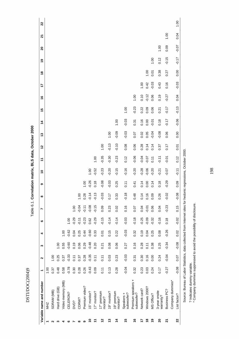
DST

I/D

OC

(200

4)9

19

8

Tab

le 6

.1. C

orr

elat

ion

mat

rix,

BL

S d

ata,

Oct

ob

er 2

000

Var

iab

le n

ame

and

nu

mb

er

1 2

3 4

6 7

8 9

10

11

12

13

14

15

16

17

18

19

20

21

22

1 M

HZ

1.

00

2 S

DR

AM

(M

B)

0.37

1.

00

3 H

ard

driv

e (G

B)

0.48

0.

25

1.00

4 V

ideo

mem

ory

(MB

) 0.

58

0.37

0.

55

1.00

6 C

ELE

RO

N?

-0.7

8 -0

.33

-0.6

0 -0

.62

1.00

7 D

VD

? 0.

30

0.11

0.

19

0.04

-0

.29

1.00

8 C

DR

W?

0.28

0.

37

0.06

0.

25

-0.1

1 -0

.04

1.00

9 P

rem

ium

vid

eo?

0.26

0.

28

0.29

0.

44

-0.2

3 -0

.11

0.28

1.

00

10

15”

mon

itor?

-0

.43

-0.3

5 -0

.48

-0.6

0 0.

62

-0.0

8 -0

.14

-0.2

6 1.

00

11

17”

mon

itor?

0.

09

0.11

0.

20

0.33

-0

.29

-0.1

5 -0

.13

0.18

-0

.52

1.00

12

17”

prem

ium

m

onito

r?

0.11

0.

11

0.21

0.

01

-0.1

5 0.

09

-0.0

3 -0

.08

-0.2

3 -0

.35

1.00

13

19”

mon

itor?

0.

13

0.03

0.

08

0.15

-0

.14

0.23

0.

17

-0.0

3 -0

.20

-0.3

0 -0

.13

1.00

14

19”

prem

ium

m

onito

r?

0.28

0.

23

0.06

0.

22

-0.1

4 0.

02

0.33

0.

25

-0.1

5 -0

.23

-0.1

0 -0

.09

1.00

15

Spe

aker

s +

su

bwoo

fer?

-0

.04

-0.0

3 0.

27

-0.0

3 -0

.03

0.16

-0

.18

0.11

-0

.16

0.12

0.

08

-0.0

3 -0

.03

1.00

16

Pre

miu

m s

peak

ers

+

subw

oofe

r?

0.32

0.

31

0.16

0.

32

-0.1

8 0.

07

0.48

0.

41

-0.2

0 -0

.06

0.06

0.

07

0.31

-0

.23

1.00

17

Net

wor

k ca

rd?

0.23

0.

30

0.28

0.

19

-0.2

5 0.

04

0.14

0.

14

-0.2

8 -0

.04

0.28

0.

02

0.16

0.

22

0.10

1.

00

18

Win

dow

s 20

00?

0.03

0.

16

0.11

0.

04

-0.0

9 -0

.01

0.16

0.

00

-0.0

6 -0

.07

0.14

0.

05

0.00

0.

09

-0.1

2 0.

42

1.00

19

MS

Offi

ce?

0.24

0.

00

0.38

0.

25

-0.3

2 0.

06

0.09

0.

14

-0.2

0 0.

11

0.14

-0

.04

-0.0

1 0.

06

0.06

-0

.03

0.01

1.

00

20

3-ye

ar o

nsite

w

arra

nty?

0.

17

0.24

0.

25

0.08

-0

.16

0.04

0.

26

0.18

-0

.21

-0.1

1 0.

37

-0.0

8 0.

18

0.21

0.

19

0.43

0.

38

0.12

1.

00

21

Bus

ines

s P

C?

-0.2

7 -0

.04

-0.3

4 -0

.26

0.18

-0

.23

-0.0

2 -0

.29

-0.0

7 -0

.01

0.17

0.

06

-0.1

7 -0

.17

-0.2

7 0.

16

0.27

-0

.15

0.09

1.

00

C

ompa

ny d

umm

ies*

22

List

fact

or?

-0.0

8 0.

07

-0.0

8 0.

02

-0.0

2 0.

15

-0.0

8 0.

09

-0.1

1 0.

12

0.01

0.

00

-0.0

6 -0

.13

0.04

-0

.03

0.00

-0

.17

-0.0

7 0.

04

1.00

Sou

rce:

Bur

eau

of L

abor

Sta

tistic

s, d

ata

colle

cted

from

Inte

rnet

site

s fo

r he

doni

c re

gres

sion

s, O

ctob

er 2

000.

? In

dica

tes

dum

my

varia

ble.

*

Com

pany

dum

mie

s su

ppre

ssed

to a

void

the

poss

ibili

ty o

f dis

clos

ure.

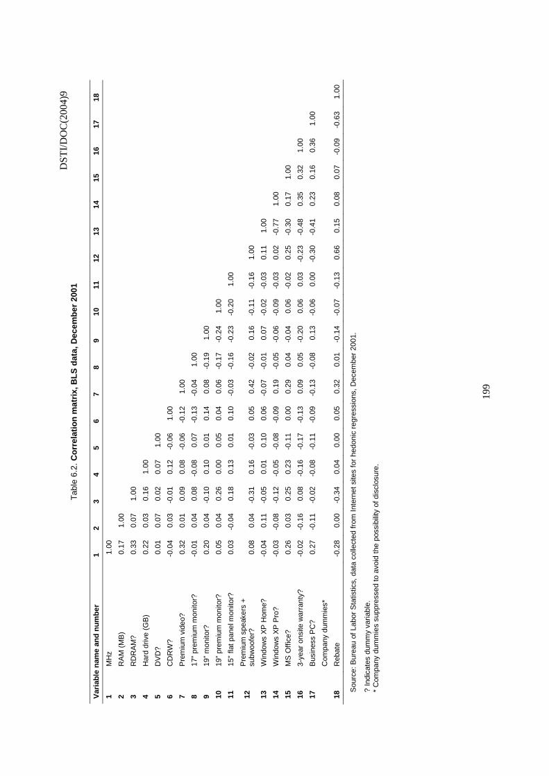
D

STI/

DO

C(2

004)

9

19

9

Tab

le 6

.2. C

orr

elat

ion

mat

rix,

BL

S d

ata,

Dec

emb

er 2

001

Var

iab

le n

ame

and

nu

mb

er

1 2

3 4

5 6

7 8

9 10

11

12

13

14

15

16

17

18

1 M

Hz

1.00

2 R

AM

(M

B)

0.17

1.

00

3 R

DR

AM

? 0.

33

0.07

1.

00

4 H

ard

driv

e (G

B)

0.22

0.

03

0.16

1.

00

5 D

VD

? 0.

01

0.07

0.

02

0.07

1.

00

6 C

DR

W?

-0.0

4 0.

03

-0.0

1 0.

12

-0.0

6 1.

00

7 P

rem

ium

vid

eo?

0.32

0.

01

0.09

0.

08

-0.0

6 -0

.12

1.00

8 17

” pr

emiu

m m

onito

r?

-0.0

1 0.

04

0.08

-0

.08

0.07

-0

.13

-0.0

4 1.

00

9 19

” m

onito

r?

0.20

0.

04

-0.1

0 0.

10

0.01

0.

14

0.08

-0

.19

1.00

10

19”

prem

ium

mon

itor?

0.

05

0.04

0.

26

0.00

0.

05

0.04

0.

06

-0.1

7 -0

.24

1.00

11

15"

flat p

anel

mon

itor?

0.

03

-0.0

4 0.

18

0.13

0.

01

0.10

-0

.03

-0.1

6 -0

.23

-0.2

0 1.

00

12

Pre

miu

m s

peak

ers

+

subw

oofe

r?

0.08

0.

04

-0.3

1 0.

16

-0.0

3 0.

05

0.42

-0

.02

0.16

-0

.11

-0.1

6 1.

00

13

Win

dow

s X

P H

ome?

-0

.04

0.11

-0

.05

0.01

0.

10

0.06

-0

.07

-0.0

1 0.

07

-0.0

2 -0

.03

0.11

1.

00

14

Win

dow

s X

P P

ro?

-0.0

3 -0

.08

-0.1

2 -0

.05

-0.0

8 -0

.09

0.19

-0

.05

-0.0

6 -0

.09

-0.0

3 0.

02

-0.7

7 1.

00

15

MS

Offi

ce?

0.26

0.

03

0.25

0.

23

-0.1

1 0.

00

0.29

0.

04

-0.0

4 0.

06

-0.0

2 0.

25

-0.3

0 0.

17

1.00

16

3-ye

ar o

nsite

war

rant

y?

-0.0

2 -0

.16

0.08

-0

.16

-0.1

7 -0

.13

0.09

0.

05

-0.2

0 0.

06

0.03

-0

.23

-0.4

8 0.

35

0.32

1.

00

17

Bus

ines

s P

C?

0.27

-0

.11

-0.0

2 -0

.08

-0.1

1 -0

.09

-0.1

3 -0

.08

0.13

-0

.06

0.00

-0

.30

-0.4

1 0.

23

0.16

0.

36

1.00

C

ompa

ny d

umm

ies*

18

Reb

ate

-0.2

8 0.

00

-0.3

4 0.

04

0.00

0.

05

0.32

0.

01

-0.1

4 -0

.07

-0.1

3 0.

66

0.15

0.

08

0.07

-0

.09

-0.6

3 1.

00

Sou

rce:

Bur

eau

of L

abor

Sta

tistic

s, d

ata

colle

cted

from

Inte

rnet

site

s fo

r he

doni

c re

gres

sion

s, D

ecem

ber

2001

.

? In

dica

tes

dum

my

varia

ble.

*

Com

pany

dum

mie

s su

ppre

ssed

to a

void

the

poss

ibili

ty o

f dis

clos

ure.

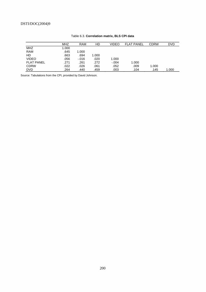
DSTI/DOC(2004)9

200

Table 6.3. Correlation matrix, BLS CPI data

MHZ RAM HD VIDEO FLAT PANEL CDRW DVD MHZ 1.000 RAM .645 1.000 HD .663 .694 1.000 VIDEO .056 -.016 .020 1.000 FLAT PANEL .271 .261 .272 -.004 1.000 CDRW .022 .026 .061 .052 .009 1.000 DVD .264 .440 .459 .003 .104 .145 1.000

Source: Tabulations from the CPI, provided by David Johnson.

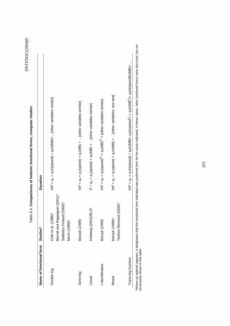
D

STI/

DO

C(2

004)

9

20

1

Tab

le 6

.4. C

om

par

iso

ns

of

hed

on

ic f

un

ctio

nal

fo

rms,

co

mp

ute

r st

ud

ies

Nam

e o

f fu

nct

ion

al f

orm

S

tud

ies*

E

qu

atio

n

Dou

ble-

log

Col

e et

al.

(198

6)*

lnP

= a

o +

a1l

n(sp

eed)

+ a

2ln(

MB

)+…

[oth

er v

aria

bles

sim

ilar]

B

ernd

t and

Rap

papo

rt (

2001

)*

S

tatis

tics

Fin

land

(20

00)*

M

och

(199

9)*

Sem

i-log

B

arzy

k (1

999)

ln

P =

ao

+ a

1(sp

eed)

+ a

2(M

B)

+ …

[oth

er v

aria

bles

sim

ilar]

Line

ar

Hol

dway

(20

01)/

BLS

* P

= a

o +

a1(

spee

d) +

a2(

MB

) +

…[o

ther

var

iabl

es s

imila

r]

t-id

entif

icat

ion

Bar

zyk

(199

9)

lnP

= a

o +

a1(

spee

d)b1

+ a

2(M

B)b2

+ [o

ther

var

iabl

es s

imila

r]

Mix

ed

Bar

zyk

(199

9)*

lnP

= a

o +

a1(

spee

d) +

a2l

n(M

B)

+ …

[oth

er v

aria

bles

: see

text

]

T

iedr

ez-R

emon

d (2

000)

*

Tra

ns-lo

g fu

nctio

n

lnP

= a

o +

a1l

n(sp

eed)

+ a

2ln(

MB

)+ a

3ln(

spee

d2 ) +

a4l

n(M

B2 )+

a5l

n(sp

eed)

ln(M

B)+

…

*Whe

re a

n as

teris

k ap

pear

s, it

des

igna

tes

that

the

func

tiona

l for

m in

dica

ted

was

pre

ferr

ed fo

rm fo

r th

e st

udy

indi

cate

d; in

thes

e ca

ses,

oth

er fu

nctio

nal f

orm

s w

ere

also

trie

d, b

ut n

ot

nece

ssar

ily s

how

n in

this

tabl

e.

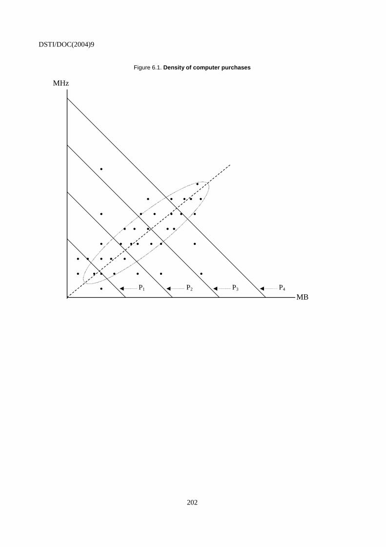
DSTI/DOC(2004)9

202

Figure 6.1. Density of computer purchases

MHz

. . . . . . . . . . . . . . . . . . . . . . . . . . . . . . . . . . . . . . P1 P2 P3 P4 MB

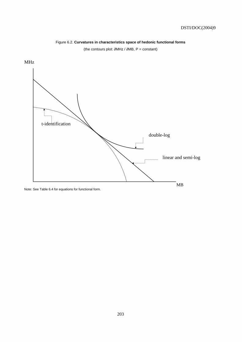
DSTI/DOC(2004)9

203

Figure 6.2. Curvatures in characteristics space of hedonic functional forms

(the contours plot: ∂MHz / ∂MB, P = constant)

MHz t-identification double-log linear and semi-log

MB

Note: See Table 6.4 for equations for functional form.

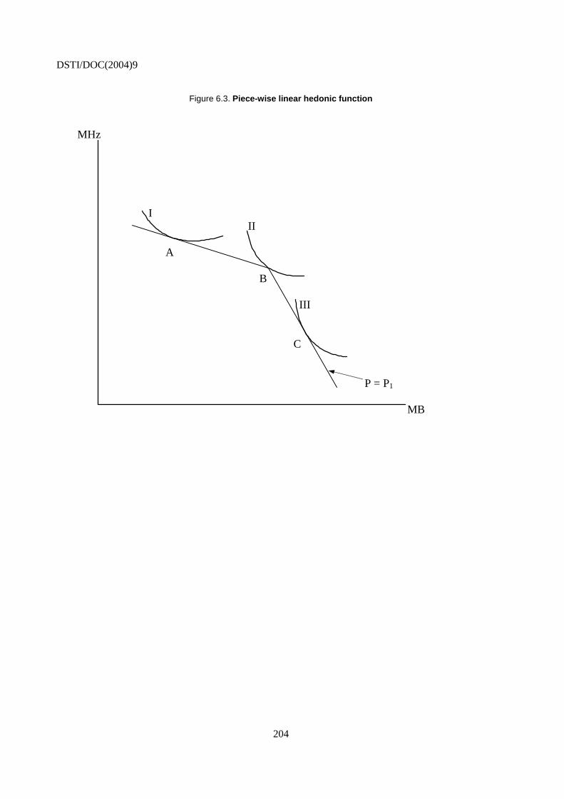
DSTI/DOC(2004)9

204

Figure 6.3. Piece-wise linear hedonic function

MHz I II A B III C P = P1 MB

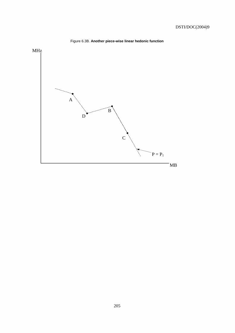
DSTI/DOC(2004)9

205

Figure 6.3B. Another piece-wise linear hedonic function

MHz A B D C P = P1 MB

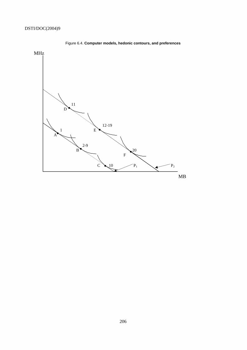
DSTI/DOC(2004)9

206

Figure 6.4. Computer models, hedonic contours, and preferences

MHz 11 D 12-19 1 E A 2-9 B 20 F C 10 P1 P2 MB

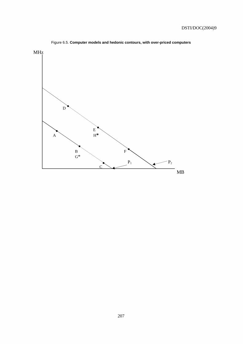
DSTI/DOC(2004)9

207

Figure 6.5. Computer models and hedonic contours, with over-priced computers

MHz D E A H* B F G* P1 P2 C MB

DSTI/DOC(2004)9

208

CHAPTER VII

SOME OBJECTIONS TO HEDONIC INDEXES

Objections to hedonic indexes began with the publication of Griliches’ (1961) first article, and they have not abated. Over this 40-plus year period, the major criticism has taken two forms.

One persistent criticism concerns the results: Hedonic indexes are thought to “fall too fast,” by some criterion. Denison (1987) was one of the first to voice this criticism. A reader of the draft of this Handbook forwarded a comment from a 2002 Eurostat seminar, which went, roughly: “I would not have paid EUR 15 000 for today’s PC ten years ago so I cannot accept that the price has fallen by 90%.” Variations on this “falls too fast” theme have appeared in many places.

A second and nearly as persistent criticism concerns the technical properties of hedonic indexes, presumably independently of their results. Ho, Rao, and Tang (2003, footnote 16, page 11) remark: “It [the hedonic technique] has been criticised for lack of theoretical foundation, especially for its functional forms, lack of transparency, and its subjectiveness in selecting the quantities of characteristics.” A Committee on National Statistics panel (Schultze and Mackie, eds., 2002, Chapter 4) expressed criticisms of hedonic indexes, and urged the US Bureau of Labor Statistics to slow its implementation of hedonic indexes in the US CPI.

This chapter reviews criticisms under the two headings suggested by the preceding paragraphs. Some criticisms of hedonic indexes have been considered in previous chapters of this Handbook. Nevertheless, it seems useful to draw responses to criticisms together in one place, for easier reference, even though some duplication results. Other criticisms that have not yet been addressed are also considered here. The chapter may be incomplete, in ignoring some criticism; if so, it is because I have not been made aware of it, or through omission.

In one of the commonest criticism of hedonic indexes, a speaker says that he has “reservations” about hedonic indexes – or that others have expressed “reservations.” When pressed to be more specific, the speaker responds that he has reservations, but not (in effect) objections, that he cannot give specifics, he has rather “unease” (a frequently used word) about the method, or that it is others who express “unease” without providing specifics. This form of criticism has often been passed from one person to another, with the result that the origin of the criticism, or what the originator of the criticism had in mind, is impossible to determine. I have encountered this kind of criticism of hedonic indexes many times, and it is a frustration: One cannot respond to a criticism that has no specific content that can be analysed empirically or logically or methodologically. It seems to me that those who make such nebulous criticisms ought to put them into an explicit form that permits analytic discussion, or ought to be challenged to do so. Criticisms are useful in that they may sharpen our thinking, or responses to their salient points may increase understanding, but criticism that takes the form of nonexplicit “reservations” or statements of “unease” contribute neither.

Hulten (2002) noted that, among statisticians and among users, there is a tendency to view old methodology as good methodology because it is known; knowledge of the implications of new methodology is not so extensive, so it is mistrusted (perhaps properly). One suspects that this conservative

DSTI/DOC(2004)9

209

tendency with respect to methodology explains some of the mistrust of hedonic indexes that is so evidently widespread.

One the other hand, however, it is doubtful that users really understand the matched model methodology, its implications, and its potential biases, and it is likely that the agencies themselves have not always fully understood the potential biases (these matters are reviewed in Chapter II). Accordingly, even if conservatism with respect to changes in statistical methods has a certain validity, it is doubtful that the “known” properties of the old matched model methods for treating quality change are correctly valued (because the old methods are in fact not well understood). There are abundant grounds for supposing that the old linking methodologies, correctly understood, should also cause “unease” (see Chapter II). It is the fact of quality change that creates the problem, not new methods for dealing with it.

A. The criticism that hedonic indexes fall too fast

Several strands to the “falls too fast” contention exist. Some of these criticisms are general statements, or are meant to be, and some are specific to ICT investment and computer equipment price indexes.

1. General statements

A long-standing presumption has hedonic indexes always falling faster, or rising more slowly, than price indexes constructed with conventional matched model methods. If this presumption were correct empirically, someone who leans toward conservatism with respect to statistical methods might infer that hedonic indexes were suspect, that they “fall too fast,” where someone who was critical of the matched model method might take the same putitave fact as an indictment of the conventional method. Indeed, a good amount of the past debate about hedonic indexes can be understood in precisely this way – different judgements about the likely relative errors of alternative statistical methods, positions that have been argued under the presumption that hedonic indexes generally decline more, or rise less, than matched model indexes that are constructed from the same database.

The empirical evidence indicates the presumption is wrong, as a general proposition. Hedonic indexes do not always decline more rapidly than matched model indexes. For example, the survey in Chapter IV of this Handbook shows that hedonic indexes fall faster for computers, but not for TVs – refer to tables 4.5 and 4.8. This same conclusion is borne out in other work. Schultze (2002), using information from BLS, shows that after hedonic quality adjustments were added to a number of US CPI series, changed methods did not necessarily result in faster-falling price indexes.

The general criticism, at least in this form, seems poorly informed or based on judgements that are out of date. No general or regular pattern across products emerges from comparisons of matched model and hedonic indexes that have been computed from the same database. For this reason, the view that hedonic indexes generally “fall too fast” cannot be based on empirical evidence of the actual differences, in practice, between the two methods, when applied across the range of products for which hedonic indexes have been estimated.

2. Computer price indexes fall too fast

It may not be a general pattern that applies to all products, but it is certainly true empirically that hedonic indexes for computer equipment fall more rapidly than matched model indexes. The survey in Chapter IV presents some empirical evidence. In that chapter I concluded that even where matched model and hedonic indexes were fairly close together, the two different statistical methods produced statistically significant differences.

DSTI/DOC(2004)9

210

It is also true that hedonic computer equipment price indexes fall very rapidly. Moreover, computer price indexes are the subjects where one most often hears the “falls too fast” objection.

a. The price indexes

Matched model indexes for computers also fall rapidly if done with matched model, FR&R (frequently resample and reweight) methods, just not as fast as hedonic indexes that are estimated from the same database. For example, all four matched model and hedonic computer price indexes estimated by Okamoto and Sato (see Table 4.5) decline more than 40% per year. The rapid decline in computer prices is not solely an artefact of hedonic methods. At the same time, where we can determine the causes of differences between hedonic and matched model indexes (see the review in Chapter IV), the analysis makes us confident that where they differ, the hedonic is better. Hedonic indexes pick up price changes that matched model indexes miss, particularly price changes that accompany entries and exits of computers (and other products) when those entry and exit price effects are not instantaneously reflected into price changes for continuing computer models (see the summary in Chapter IV).

If the “falls too fast” contention is made with full knowledge of the research results, therefore, it must rest on some other evidence or on subtle arguments about plausibility. In evaluating these, it is worth bearing in mind that computer prices have been declining at prodigious rates (15% to 30% per year, or more) for more than 50 years, though generally computer peripheral equipment and communications equipment prices have fallen somewhat less rapidly (see the review of semiconductor and communications equipment price trends in Chapter 10 of Triplett and Bosworth, 2004). Those huge price declines for computer equipment reflect a technological marvel that has no precedent, at least over such an extensive time span. The fact of the technological change is not in serious dispute, but it is clearly worth asking whether that technological change has been measured accurately. Set against the “falls too fast” presumption is Nordhaus (2001), who contended that computing power price decline has been understated in hedonic indexes (his historical series on computing technology extends over 100 years, as he considers pre-computer technology as well).

b. Plausibility

Some criticisms rest on plausibility, which is always an appealing test for an economic measurement. A reader of the draft of this Handbook reported the following conversation:

“Your index says that the price of a PC is 30% of its price three years ago, while the nominal price has not changed, it is EUR 1 000. I, as a consumer, cannot find a PC worth EUR 300, even if I accept that it has the same functions as three years ago. In other words, I am obliged to buy a computer of EUR 1 000, while I don’t want to use the new functionalities which go with it and of which the statisticians tell me that they have lowered the price by 70%.”

A similar statement opened this chapter: “I would not have paid EUR 15 000 for today’s PC ten years ago so I cannot accept that the price has fallen by 90%.” This last statement has an element of veracity. Extend it further: we now have a 50-year history of performance-corrected computer prices. From this, we can calculate that a computer with the performance of today’s USD 2 000 PC cost (10 000 x USD 2 000) in 1953. There were virtually no sales of computers to individuals in 1953, so far as I know. None of us who own computers today would have bought one for USD 20 million (in 1953 prices). What is going on here? Is this an argument against the validity or plausibility of the computer price index?

The following sections assess the points made in the above quotations concerning the plausibility of hedonic PC and computer equipment price indexes.

DSTI/DOC(2004)9

211

1. You can’t buy a cheap computer. As a point of fact, you can. The cheapest Dell desktop computer in spring 2004 (at USD 339, including applications software, but not a monitor) is close to the EUR 300 example. But to an extent, the point is still valid. Generally, computer makers have used declining production costs (which originate largely in declining semiconductor production costs) as an opportunity to offer more performance per dollar or per euro, and not as an opportunity to cut the price even more by holding the performance constant.

Presumably, computer makers understand their markets. For cars, as well, the current models of the very cheapest cars still offer much more performance, comfort and features than the low-cost models of 20 years or so ago. The number of buyers for minimal transportation autos is low enough that scale economies prevent continued production of the basic transportation models of the past. The same thing is true of computers: If there were sufficient buyers for 100 MHz computers, one would expect they would still be sold. At about the time that 1 000 MHz PCs first arrived (at roughly USD 2 000), I noticed a batch of new 100 MHz computers offered on the Internet, for a little over USD 50 each. Critics who say they want them either do not know where to find 100 MHz computers, or (more probably) there are fewer buyers with preferences for 100 MHz computers than the critics think. Or to put it another way, in today’s technology the price premium for adding another 100 MHz to the performance of the 100 MHz machine is small enough that no buyer would sensibly stop at 100MHz or 200 MHz, even though they were quite pleased with that level of performance in the past.

For buyers who really want a 100 MHz computer, it disappearance represents a forced upgrade, which the index should record as a price increase. As explained in Chapter IV, the price effects of exits from the index sample (forced or not) are in fact better estimated with hedonic methods than with conventional matched model price comparisons, because the hedonic method estimates the quality-corrected price change that the exit implies, where the conventional method invokes the assumption that there is none. Neither method, however, records the value of forced upgrading. Evidence suggests that this source of bias is small, in any case, because the number of buyers who are really forced to upgrade is small.

An adage for technological products is that one can put in value (to the user) faster than cost. When that is the case, the economics of supply and demand result in the disappearance of low-end technology, which does seem to describe the computer market. Indeed, you can’t buy yesterday’s computer conveniently if you want one, because too few buyers seem to want it to make it economical to produce. That you cannot buy yesterday’s computer does not mean that the price index for computers is wrong – if anything, the disappearance of yesterday’s computer confirms that prices have dropped greatly.

2.Performance increases are more than most users need. This is a variant on the “price falls too fast” argument. The computer price index is performance corrected, but the performance improvements, according to this criticism, are redundant to the needs of users. Alan Blinder, when he was vice chairman of the US Federal Reserve Board, once wrote to me that he was using perhaps 20% of the capability of his computer, since he only used it for simple word processing; despite this, the FRB staff replaced it with a new one, he said, which he used at perhaps 15% of its capability. The new machine’s increased performance gave him little increased usefulness, so for his purposes the quality adjustments applied to hedonic computer price indexes overstate the value of the quality change and overstate the decline in computer prices. Many others have followed Blinder’s criticism.

A variant appeals to the voracious hardware demands of modern software. Robert Gordon, in his criticism of computer performance measures, has often repeated a witticism from the computer industry: “What Intel giveth, Microsoft taketh away.” Because hardware capacity (increased speed and memory) is becoming cheaper and cheaper, it makes economic sense for software designers to expropriate part of increasing hardware capabilities for their software. For example, software designers know that because machine memory is increasingly cheap computers will have large memory sizes, so there is little need to

DSTI/DOC(2004)9

212

economize on memory demands of the software at the expense of other functionalities. In this sense, some computer users may not realize what increased computer performance is doing for them: Graphics capability, for example, is very demanding of hardware capacity. Graphics operate even the screen icons that make mouse control of computer functions feasible, and graphics capability is essential for Internet uses. But the package (hardware and software, taken together) may not improve in performance as fast as the measured performance of the hardware, viewed by itself, because some of the increased hardware capacity is employed to accommodate the software’s requirements.

A further variant depends on efficiency of the computer network. Computers interact, and the efficiency of a computer system requires compatibility among all the nodes. System efficiency, therefore, may demand more capability at individual nodes than is required for a particular user at that node, which is probably one reason that the FRB staff insisted that Blinder have a more powerful machine than his word processing strictly required.

Ultimately, though, one needs to ask why users buy ever more powerful computers, if they really do not use their capabilities. Though games and graphics uses drive much of the demand for performance that is built into the really high end PC, faster computers with larger memories and more features occupy the bulk of the market. It might be, as critics contend, that users do not really need the performance of the computers they are buying. But so what? They still buy them. Is there any precedent in economic statistics for subtracting from an industry’s output the performance it produces that is not used by buyers of the industry’s product?144 I observe that an astonishing number of Ferraris and other high-performance cars are parked on London streets and used to motor into the city, where they must use only one or two of their six gears, and a tiny fraction of their performance. Do we deduct from auto manufacturers’ output the portion of Ferrari performance that is not used by Ferrari owners? If computer buyers purchase increased PC performance, that is what they choose to buy, and it is output of computer manufacturers, just as surely as the output of Ferraris used to go grocery shopping is part of the output of the auto industry.

It is possible to buy cheaper, lower performance computers than the typical PC computer sold today. Buyers don’t. Thus, they don’t behave the way this critique presumes.

3. Performance measures used in hedonic functions are incomplete or inadequate measures of computer performance. Though most critics do not make this argument, they could and it might be used to buttress their other contentions.

The adequacy of performance measures used in empirical work on PCs was considered at length in Chapter V. As explained there, existing measures are problematic, to an extent. But the direction of bias to hedonic price indexes from inadequate performance measures it is not entirely clear. For example, MHz as a measure of computer speed is clearly inferior to a direct measure of work done, for the reasons discussed in Chapter V; but the only comparison of alternatives to date (Chwelos, 2003) finds little bias.

McCarthy (1997) contended that hardware performance measures (such as MHz) that are used in most PC hedonic functions also serve as proxies for the improvement in the software that increasingly has been bundled into computers. McCarthy posited that the software portions of the package were declining in price more slowly than the hardware components.145 Under those circumstances, MHz, memory size and

144. If the increased performance is not treated as quality change, it will not show up in industry output

measures that are formed, as is usually the case, by deflation by an output price index.

145. On prices for PC component software, see Prud’homme and Yu (2002), Abel, Berndt, and White (2003), and White, Abel, Berndt, and Monroe (2004). The latter reports price declines for PC operating system and productivity suite software of around 13%-18% per year, where PC hardware prices have been falling at 20%-30% per year, or even more, which is consistent with McCarthy’s speculation.

DSTI/DOC(2004)9

213

similar measures of hardware capability overstate the performance change of the hardware/software package, which causes the price index for the PC bundle to decline too rapidly. McCarthy’s contention is correct so far as it goes (see the section on proxy variable bias in Chapter VI). But existing measures of computer performance also make no allowance for the inclusion of new software packages. When word processing software and photo editing software were first added “free” to the price of the PC, no adjustment was made for their inclusion in most empirical studies, which biases the PC index in the other direction.

Bias from inappropriate or inadequate performance measures poses a potential problem for existing empirical work on computer prices. But the magnitude of the bias is unknown. Surely a one or two variable PC hedonic function is subject to substantial bias from omitted variables. But it is not so clear that the bias is large in hedonic indexes that are based on more adequate hedonic functions, and the direction of bias, if any, has not been determined.

The same objections, incidentally, could be raised against conventional matched model indexes, because they normally control for quality change in computers using the same variables that are used in the hedonic function. If the variables are inadequate for hedonic indexes, they are inadequate to exactly the same extent when used as the pricing specification for matched model comparisons (see Chapter II).

4. We are forced to buy the improved technology because of monopolistic behaviour on the part of computer and software producers. On the industrial organization aspects of the computer industries, there is little market power for PCs. It is easy to assemble PCs from purchased components and therefore relatively easy to enter the PC market. Market power is more of a factor in the production of microprocessor chips and of PC software.

Aizcorbe, Oliner, and Sichel (2003) make a nice estimate of the influence of the market power markup on semiconductor price changes. They estimate that markup changes account for only a small proportion of the price decline. Most of the decline in semiconductor prices reflects technological change, not changes in the markups in response to oligopolistic rivalry.

In software, on the other hand, this is a big problem, as antitrust cases on both sides of the Atlantic against the leading software supplier bear out. The essence of the antitrust cases involved alleged behaviour that forced packages on unwilling buyers, who were ultimately the consumers. However, as the antitrust cases abundantly show, one can find economists on either side. Whether there has been welfare loss from slowing innovation is in dispute. There is little evidence of a price effect, but some for forced quantity and, one suspects, effects from spurious “upgrading.” The evidence at this point is mixed, and insufficient to make an assessment for the bias, if any, in PC price measures that include software in the bundle.

5. “Whatever: I wouldn’t have paid the price suggested by extrapolating the hedonic index into the past.” This objection, though no doubt coupled with some of the points above, is logically separate from them. It is a more subtle point that requires a complex response.

As the textbooks show, the market demand for any product is made up of the aggregation of individual demands. In the case of new products such as computers, sales are small at a relatively high price (such as existed in the past). A famous “forecast” in the early 1950s predicted that world-wide demand for computers would amount to only a small number of machines, and this might have been correct at computer prices of the time. For most buyers, and certainly for individuals, computer prices were too high to consider buying one. For those individuals, demands were zero.

DSTI/DOC(2004)9

214

Hicks (1940) showed a way to analyse the demand for new products. The “reservation price” is the highest price an individual would pay for the new product, or the minimum price that would keep the individual out of the market. The price index for the new good that did not exist in the previous period could be found by comparing the current price (that was paid) to the reservation price (the price that resulted in zero demand) in the previous period. Hausman (1997) famously used Hicks’ approach to estimate price indexes for new products.

Somewhat overlooked at times is the applicability of Hicks’ approach to the demands for individuals. Consider individual A (the speaker in the sentence quoted at the beginning of this section). He indicated that his demand for a computer (with specifications equal to the current one) was zero when the price of that PC was EUR 15 000, so his reservation price is lower than EUR 15 000. Though he has not given his reservation price, suppose it is EUR 2 000. He certainly would buy one when the price fell to EUR 1 000.

Then we can apply Hicks’ rule to construct a price index for individual A: the decline in PC prices from EUR 15 000 to EUR 2 000 is irrelevant for individual A, because he was not in the market for a computer at any price above EUR 2 000. But the decline from the point where a PC cost EUR 2 000 to its EUR 1 000 cost is relevant.

Individuals differ in taste, so each has a different reservation price. Early computer buyers have higher reservation prices, so they own computers when the rest of us are still computerless. Increasing market demand for computers occurs as computer prices fall to or below the reservation prices of more and more potential buyers. As the price of computers falls, more and more individuals and firms buy computers. The market demand for computers, of course, is the aggregation of the individual demands of those potential buyers who have different reservation prices.

Similarly, aggregate price indexes are aggregations, in principle, of individual price indexes (see the discussion in Pollak, 1989, for the consumer price index, or cost-of-living index, but the point applies to other price indexes as well). That the aggregate price index for PCs, over the whole history of PCs, does not follow individual A’s own price index for PCs is an expected result because individual A’s own price index for computers is undefined above his reservation price. For individual B, who was willing to pay EUR 15 000 for a PC with today’s specification, the aggregate price index from the EUR 15 000 cost point to the present is relevant, but not perhaps the index for earlier years that extrapolates the price back to EUR 20 million. On the other hand, the firm that was willing to pay EUR 20 million for an early computer has a massive gain from being able to buy one (or many) for EUR 15 000 or EUR 1 000.

The aggregate price index will not represent the price experience for buyers who were not in the market for PCs. This does not, however, invalidate the aggregate hedonic price index as a measure of what actually happened to computer prices. The aggregate price index measures the price declines that potential buyers face, not necessarily what each of them would have been willing to pay at points where they were not computer buyers. As prices fall, as measured by the hedonic index, more and more buyers for computers exist, so for more and more of them the aggregate price index also matches their personal price index. This, as noted at the outset, is a subtle point in interpreting aggregate price indexes.146

3. Summary

The “falls too fast” arguments are not compelling. The size of computer price declines provokes, understandably, astonishment, and strains (it seems) credulity. Yet, the anecdotes that have been spun as

146. The price index literature also contains references to consumer surplus, the gains to buyers who would

have been willing to pay more than the current price to obtain a computer but who do not have to. I ignore that for present purposes, but the above discussion is obviously closely related.

DSTI/DOC(2004)9

215

criticism do not stand up very well to analysis. Computer prices have been falling at 20%-30% per year for a very long time, and the great improvement in computer performance is not in doubt among computer professionals. It is implausible that very much of the 10- or 20- or 50-year improvement in computer capabilities and the consequent decline in the price of computer performance is disguised by forced changes or lack of free choice among computer buyers and so forth.

Technical improvements to hedonic indexes can be made – improvements in the variables in hedonic functions, for example – and will no doubt lead to revisions of hedonic indexes. But there is little reason to suppose that that such revisions will eliminate or reduce appreciably the remarkable story of the computer’s 50-year price decline.

B. Technical criticisms of hedonic indexes

1. General criticisms

Ho, Rao and Tang (2003) repeat what they have heard said about hedonic indexes, and they accurately summarise a persistent form of technical criticism. Their list includes theoretical appropriateness of the functional forms, transparency and reproducibility, and the origin and choice of the characteristics variables.

a. Functional form

First, there is the criticism of an alleged lack of theoretical foundation with respect to choice of hedonic functional form. As Chapter VI and also the Theoretical Appendix explains, this longstanding criticism is misconceived. Rosen (1974) showed conclusively why in theory the choice of functional form is entirely an empirical matter, it is not determined on theoretical grounds. Significant contributions since Rosen (including Pakes, 2003, and the work with collaborators he cites there) has not changed this conclusion. Even though one still sometimes sees erroneous statements that one or the other of the functional forms commonly used in hedonic research is theoretically unacceptable, the authors of such statements apparently do not understand the appropriate theory.147 In Triplett (2004), I considered the curious fact that this functional form criticism has arisen for product hedonic functions (such as for computers) but it has not arisen in the parallel literature in labour economics on human capital or wage hedonic functions.

b. Transparency and reducibility

It has often been said that hedonic indexes lack transparency and reducibility. This contention, expressed by statistical agencies in the past, has been revived by the recent Committee on National Statistics report (Schultze and Mackie, eds., 2002): are the quality adjustments that hedonic indexes provide objective and reproducible? Some observers imply that investigator effects create too much dispersion in hedonic indexes to rely on them in official statistics, and that there is too much subjectiveness in choosing the characteristics.

The transparency criticism of hedonic methods implies the converse – that matched model methods for handling quality change are transparent and reproducible. This is a dreadful misunderstanding. The

147. Or they ignore the salient parts of it, in favor of special cases that do not provide guidance for empirical

research. An example is Diewert (2003).

DSTI/DOC(2004)9

216

opposite is more nearly the case – it is hedonic methods that are more transparent and more capable of reproduction, certainly outside statistical agencies, which is where it matters.148

Traditional methods are not transparent. If an agency decides to use the IP-IQ method (see Chapter II) when a quality change arises in a price index sample, then the price index operation itself is more transparent – to it – than the dummy variable form of the hedonic method (e.g., equation 4.1). The same thing is true of the direct comparison method. But when does an agency decide to use implicit quality adjustment (IP-IQ)? When does it use direct comparison or, in cases where it is still done, link-to-show-no-price-change? Those decisions, which are not transparent to outsiders, contribute to opaqueness in the conventional method.

Neither are the quality adjustment procedures themselves transparent. The various forms of “linking” that are traditionally done when quality changes are encountered may not be liked, but agencies understand what they do, and how what they do relates to the rest of the index calculations. Judgmental quality adjustments may be arbitrary, but they are transparent, at least to the agencies that do them. Observers outside statistical agencies, however, cannot see what is done within them. The total calculation of the index using conventional methods is decidedly not transparent to outsiders.

Moreover, the implications of the use of some of these methods have not always been understood even by the agencies themselves. Their properties are not transparent (see the discussion in Chapter II), whether or not the procedures themselves are transparent.149

The conventional method is also not as reproducible as sometimes assumed. Reproducibility of a statistical method requires that capable people, confronted with similar problems, resolve them in ways that produce quantitatively similar results. As noted earlier, Hoffmann (1998) describes a virtual experiment in the German CPI price index for washing machines. In Germany, separate consumer price indexes are computed for each German Land and quality adjustments are performed independently in each of these Lander indexes. Because quality change arises from particular events in the samples, there is no assurance that each Land’s price index compiler faced exactly the same quality adjustment problem. Nevertheless, over a fifteen-year period, those independently adjusted washing machine price indexes gave a very large range of estimates of price change – from more than 10% decline in the index that fell the most to just over a 30% increase in the highest (see Figure 2.4 in Chapter II). Chapter II discusses similar “virtual experiments” on computer price indexes across OECD and European countries that have yielded similar variances among matched model methods implemented in different statistical systems – see Wyckoff (1995) and Eurostat Task Force (1999), and also the Dalén (2002) and Ribe (2002) studies. Additional studies within Eurostat for the HICP are exemplary.

Accordingly, the transparency and reproducibility argument does not provide strong support for the traditional method. Mechanical or computational transparency might be greater in conventional methods; but overall transparency is not greater, because the statistical procedures that come into play before quality adjustments are carried out are not themselves transparent. The effects of these decisions have mostly not been quantified and are not factored into calculation of index number variances, even in countries where

148. I mean no criticism of Ho, Rao, and Tang (2003) here, they are correctly reporting what has often been

said.

149. Two changes in agency practice illustrate what I have in mind. Armknecht (1996) remarked that the former rule followed when quality changes were encountered in the US CPI was: “When in doubt, link it out [with the IP-IQ method]”. This implies, correctly, that the implications of the IP-IQ method had formerly not fully been understood within BLS. A second: Eurostat banned use of the link-to-show-no-price-change method in the HICP indexes, because of its severe bias. That the method was widely used in Europe and is still used elsewhere suggests that its properties are not fully understood.

DSTI/DOC(2004)9

217

price index sampling variances are routinely published. Agencies think, or behave, as if their methods were reproducible; but actually, all they know is one set of decisions were made with one result, not that the same result would be reached if the decision process were in fact replicated.

Griliches (1990, pages 190-91) said it well: “The fact that [hedonic research] is difficult to do, and that an actual empirical implementation calls for much judgement on the part of the analyst and hence exposes him to the charge of subjectivity, is still the most telling objection today. The fact that the standard procedures also involve much judgement…is usually well hidden behind the official facade of the statistical establishment.”

One might, indeed, prefer a method whose statistical properties can be examined (the hedonic price index) over one whose statistical properties are less easy to describe. Especially when an agency does not use probability sampling in selecting items and outlets, the statistical properties and the overall transparency of conventional methods are not their strong points.

2. The CNSTAT panel report

The report of the US Committee on National Statistics (CNSTAT) Panel on Conceptual, Measurement, and Other Statistical Issues in Developing Cost-of-Living Indexes (Schultze and Mackie, eds., 2002, hereafter “Panel”) contains a chapter on quality change and hedonic indexes (its Chapter 4). The report has been read in a number of ways. Its interpretation was clarified by a series of presentations at the Brookings Institution in February, 2002150, at the Bureau of Labor Statistics in June 2002, at the National Bureau of Economic Research in July, 2002, at the American Economic Association’s annual meetings in January, 2003, and in a subsequent article by its chairman (Schultze, 2003).

On the one hand, the report contains positive statements about hedonic methods (all pages from Schultze and Mackie, eds., 2002):

• “Hedonics currently offers the most promising technique for explicitly adjusting observed prices to account for changing product quality.” (page 122)

• “In a well-specified equation, coefficients on the explanatory variables [of the hedonic function] reveal the marginal relationship between the product characteristics and price at various values of [the characteristics]…. Then, as long as the set of observable characteristics includes all characteristics that matter to consumers and the equation is properly specified, these results can be used to correct for product quality change.” (pages 123-124)

• “The successful use of hedonic methods rests on a modeler’s ability to identify and measure quality-determining characteristics and specify an equation that effectively links them to the prices of different models or varieties.” (page 124)

Accordingly, one interpretation of the Committee’s chapter is that it was intended as a compendium of good practices. Though the language of the report sometimes suggests that members of the Committee thought their points were new, most of the prescriptions in this part of the Committee’s report are well established in the hedonic literature. Indeed, they are consistent with the analysis of the Chapters II-VI of this Handbook, and the Committee cites the “Advance” version of the Handbook. Looked at in that way, the Committee’s section on hedonic indexes would probably be endorsed by most hedonic researchers. On

150. The presentations were made at a Brookings Institution Workshop on Economic Measurement and can be

accessed online at: http://www.brookings.edu/es/research/projects/productivity/20020201.htm

DSTI/DOC(2004)9

218

the other hand, the chapter also contains language that is inconsistent with this interpretation, and apparently very few readers of the chapter have so interpreted it.

Another way of interpreting the Committee’s report is that it was critical of the BLS implementation of hedonic indexes, rather than of the method itself. For example, the Committee expresses disapproval of hedonic functions whose variables are disproportionately or largely brand dummy variables (true of some BLS hedonic functions),151 it criticizes the BLS for instituting hedonic quality adjustments (the hedonic quality adjustment method is described in Chapter III, above) without plans for updating the hedonic functions,152 and it expresses concern that too little research had been done on the stability of coefficients in the hedonic functions estimated by the BLS. Those seem valid reservations against the BLS’ particular implementations, but do not necessarily imply a defect in the hedonic technique – quite the contrary, the Panel’s points suggest BLS deviations from best practice (see for example the discussion about keeping the coefficients up to date in Chapters III and IV of this Handbook). Against that interpretation of the report, however, is the language “the panel is not convinced that anyone could have done this work better than the BLS” (page 134), an odd assessment since other countries’ statistical agencies have implemented hedonic indexes with explicit plans for, e.g., updating coefficients regularly, and researchers regularly update coefficients for hedonic studies.

A third interpretation of the Committee’s views is possible. When the CNSTAT Committee’s staff director, Christopher Mackie, presented the hedonic portions of the report at the Brookings Workshop on Economic Measurement in February, 2002153, he seemed to interpret the Panel’s conclusions as a set of empirical impossibility theorems. Mackie’s interpretation is consistent with some of the language in the report: “The long list of unresolved issues discussed in this chapter explains why even some proponents of hedonics advocate a less aggressive expansion of its use in the CPI than BLS appears to be taking” (p.144)].154 Many readers of the report have so interpreted it. At subsequent meetings, particularly at the NBER 2002 Summer Institute, the principal author of the Committee’s Chapter 4 (Richard Schmalensee) indicated that Mackie’s interpretation was not the appropriate one to give to the Committee’s report, and Schultze (2003) makes the same point. Some notably infelicitous language (for example, the “long list of unresolved issues” boils down to a small number of mostly standard matters) and some carelessness with the hedonic literature155 makes this understandably a bit hard for readers to comprehend from the report alone.

Assessment. A review of the Panel’s Chapter 4 suggests the following main critical points about hedonic indexes.

151. “If one assumes that brand, in itself, does not lead to higher valuations by consumers, one must believe that

it is an acceptable proxy for unmeasured quality characteristics. Incidence of repairs might be one such example…. Moreover, brands are repositioned in terms of relative quality from time to time, and reputations sometimes change in response to advertising campaigns, so that brand dummy coefficients may be inherently unstable.” (Schultze and Mackie, eds., 2002, page 133)

152. Some BLS hedonic functions (TVs, clothing, and computers) are regularly updated, but others apparently are not. The Panel’s criticism has seemingly been accepted by BLS, at least for some of its hedonic functions.

153. See his outline notes on the Brookings website at: http://brook.edu/dybdocroot/es/research/projects/productivity/workshops/20020201_schultze.pdf

154. No citations support this statement, and I can identify no “proponent” whose views can be so summarised.

155. Van Mulligen (2003, page 154) remarks: “The work by [the Panel] ignores a lot of recent research on hedonic indices…”; he goes on to cite as a source corroborating this view a paper by one of the Panel members.

DSTI/DOC(2004)9

219

• “In practice, the critical question is whether one can reliably estimate functions that capture the relationship between market price and characteristics that confront individual consumers.” (page 124)156

• The Panel refers to “difficult econometric problems that plague all hedonic analysis – e.g., identifying appropriate functional forms and relevant product characteristics…” (page 126)

• “Theory provides little guidance to help determine the appropriate functional form for hedonic equations.” (page 142)157

• “For many classes of goods – and perhaps especially services – it can be extremely difficult to identify which characteristics are actually associated with price.” (page 142)

• The Panel refers to “the general problem of price data that reflect nonobservable seller attributes…”158 and “the data requirements and the operational difficulty of producing [some types of hedonic indexes] on a high-frequency, up-to-date schedule.” (page 128)

• “It is hard to know when a hedonic function is good enough for CPI work.” (page 143)

• “…Hedonic surfaces may change rapidly. The ability of BLS or any other agency to capture those changes in real time is, at best, doubtful. It is unclear whether usable estimates of hedonic surfaces can be routinely and rapidly computed for a wide variety of goods.” (page 143)

Most of these points are relevant ones. They just say that doing hedonic research is not simple or mechanical or routine, as is of course true with any other economic research. There is nothing very surprising or controversial in them, though the last one (which is an empirical judgement) might be answered by an empirical review that the Panel did not undertake. And the list is neither very long (despite the report’s referring to a “long list” in more than one place), nor a particularly negative one, nor one that is particularly damaging to the concept of hedonic indexes. The Panel’s views, as summarised in the above quotations would probably be shared by researchers who have actually worked on hedonic indexes.

The Panel’s chairman, Charles Schultze, addressed perceptions of the Panel’s report in a paper written subsequently:

In recent months, a number of panel members have heard comments to the effect that the panel’s report takes a negative view about the potential of hedonic techniques – apparently because the report discusses some of the difficulties with hedonic techniques. Yet our report explicitly

156. The Panel goes on to emphasize, appropriately, that consumer tastes differ, so that the quality adjustment

that might be appropriate to one individual’s cost-of-living index may not be appropriate to another’s. See the discussion in section A.2.b.5 of the present chapter about differences in individuals’ price indexes for computers, which is a parallel point.

157. Curiously, the Panel does not acknowledge here that it is the index that matters, as Pakes (2003) points out, not just the hedonic function. Research suggests that the hedonic index is not very sensitive empirically to the functional form chosen (see Chapter VI). It is also odd that the Panel omits the simple point that standard econometric methods for choosing among functional forms exist and are widely used (Chapter VI); since the theory indicates that choice of hedonic functional form is entirely an empirical matter, as the Panel’s report itself notes, the Panel could profitably just have ended its discussion of functional forms with that observation, rather than bringing up the outmoded “no theory” contention. One suspects that the Panel’s report was somewhat inconsistently reflecting views of its various members.

158. For example, scanner data aggregated across stores.

DSTI/DOC(2004)9

220

concluded: “Hedonics currently offers the most promising technique for explicitly adjusting observed prices to account for changing product quality.”

The issue is not whether hedonics is potentially of great usefulness. It is. Rather…[the BLS] could, as the as the panel suggests, channel its efforts principally into analyses, tests, and experiments aimed at exploring and resolving some of the methodological issues discussed in the panel’s report. The results might well justify the modification of BLS item replacement procedures and an expanded application of hedonics…. (Schultze, 2003, page 17, emphasis supplied)

The passage emphasised is easy to overlook. The Panel was impressed by the fact that the small number of BLS studies showed that using the hedonic quality adjustment method (explained in Chapter III, above) on forced replacements in the CPI sample made little change to the index (Schultze, 2002). This finding implies that the implicit quality adjustments that BLS had been making for forced replacements were surprisingly adequate, which in itself is an interesting empirical finding, that runs counter to the usual professional presumption that hedonic indexes will differ from conventional ones.159 But of course it applies only to the components that the BLS has studied and only to the treatment of forced substitutions in the CPI.

The Panel was also convinced (from BLS materials) that the item replacement rule used in the US CPI assured that the quality changes observed for forced replacements were small, which is one reason why hedonic and conventional quality adjustments yielded similar indexes.160 Quality changes in the universe, however, were not necessarily small. Changing the BLS item replacement rule (for example, assuring that the replacement product was representative of the market, rather than similar to the item that disappeared) would likely introduce larger quality changes into the index, and for larger quality changes, it might not be true that conventional and hedonic quality adjustments were similar. The Panel, however, felt reluctant to recommend changes to the BLS item replacement policy because of its reservations about the stage of development of hedonic methods, at least in the BLS implementation of them. If hedonic indexes were more thoroughly developed, this might permit changing the product replacement rule. It might also justify some adjustment when the whole sample is rotated, what the Europeans call “many to many” replacements (Chapter III):

“…the application of hedonic adjustments in a different way and on a larger scale might produce more significant downward adjustments. The panel believes that… further research, testing, and evaluation of hedonic methodology and specific applications should precede expansion of its use, such as to sample rotation – something that the panel is not in principle opposed to – where the impact on index growth would likely be more significant (Schultze and Mackie, eds., 2002, page 140).

159. In a purely research mode, this finding might have suggested more hedonic studies to see if BLS

conventional quality adjustments were equally adequate across a larger range of products. The Panel did recommend “audits” of CPI components, which goes in the same direction.

160. The item replacement rule the Panel cites is: find the replacement product with the closest characteristics to the one that disappeared. However, this is not always the replacement rule, sometimes BLS resamples (makes a new probability selection) from the items currently for sale in the outlet. In this case, the characteristics of the replacement might not be similar to the item that disappeared. Moulton and Moses (1997) give as an example the replacement of a basketball with a tennis racket in the sporting goods index. It is doubtful that hedonic adjustments would be appropriate to such replacements, but it is also not clear that the example is typical of situations where resampling is employed when products exit the sample.

DSTI/DOC(2004)9

221

Rather than putting additional resources into estimating more hedonic functions and using them to quality adjust forced replacements in CPI samples, in the Panel’s view the same resources could yield more improvement in the CPI if spent in different ways. Though this was apparently the underlying motivation for the Panel’s recommendations that the BLS pursue “a more cautious integration of hedonically adjusted price change estimates into the CPI” (Schultze and Mackie, eds., 2002, page 141), it is also fair to say that the eight recommendations in its Chapter 4 do not explicitly make this point.161

If the foregoing interpretation of the Panel’s thinking is correct, what is surprising is the Panel’s characterisation of it. At one place, it says: “this recommendation [that the BLS slow its implementation of hedonic indexes] is based on theoretical grounds, not on empirical ones” (page 141). More telling, perhaps: “Our conservative view on integrating hedonic techniques [into the CPI] has more to do with concern for the perceived credibility of the current models” (page 141). Hulten’s (2002) observation is relevant here: He said the Panel behaved as if old methods were good methods.

As with most economic measurement issues, analysis of the choice between hedonic and conventional methods requires balance. Refraining from adopting hedonic methods means relying on conventional methods.

Difficulties or problems in hedonic methods often have counterpart or parallel or corollary difficulties in conventional methods. For example, the Panel’s report says that determining the relevant characteristics for hedonic analysis is difficult, which is clearly true; unless the characteristics are well chosen the hedonic index may be defective, as pointed out in Chapter V. But the conventional method also requires determining the characteristics because the characteristics must be built into the pricing specification. The specification determines when a match is successfully made and when some quality adjustment method must be brought into play because a match is not successful (see the discussion in Chapter II). Pakes (2003) points out perceptively that BLS (and other statistical agencies around the world) have been determining characteristics for years, because they are built into pricing specifications. Yet, BLS choice of characteristics has not generally been controversial and the Panel does not point to the difficulty of choosing the characteristics as a flaw in conventional methods. One can agree with the Panel’s reservation that knowing the characteristics is a limitation on the validity of hedonic research without agreeing at all that this is an argument against hedonic methods and in favour of conventional methods.

Pakes (2004) goes further. He contends that most of the existing criticisms of hedonic indexes are either solved, in the sense that we know what to do to produce hedonic indexes that are not subject to the criticism, or they apply equally to hedonic indexes and to conventional matched model ones. Moreover, in a number of the latter cases, the defect in the hedonic index is less severe than the corresponding defect in the matched model index. For example, the hedonic index may not estimate adequately the loss to a computer buyer when the 100 MHz computer the buyer prefers disappears (see the discussion in section A.2 of this chapter), but neither does the matched model index.

Too often, the general discussion of hedonic and conventional methods has not considered adequately or put sufficient weight on cases where adopting hedonic methods can bring about corollary improvements in the index. Two examples illustrate.

161. Three of the eight recommendations focus on the difference between what the Panel called the “direct” and

“indirect” methods. These recommendations concern essentially empirical matters, but they were unfortunately not backed by an empirical review. For example, the Panel instructed BLS not to put resources into the dummy variable method, but to explore the price index for characteristics method. Though I share some of the Panel’s reservations about the dummy variable method, as pointed out in Chapter III of this handbook, the review in Chapter III of hedonic indexes computed by different methods indicates that the method may not make as much difference empirically as the Panel apparently thought.

DSTI/DOC(2004)9

222

The Panel notes approvingly that hedonic functions can be used to perform statistical testing on the validity of BLS pricing specifications (first suggested in Triplett, 1971, and employed, rather sparingly to date, in BLS studies). The Panel also points out that the present BLS product replacement rules (which are effectively to find the next most similar product to the one that disappeared) create considerable potential for “outside the sample” quality change error (see in this Handbook Chapter II and the discussion of outside the sample error in Chapter IV). It judges that outside the sample error may be as significant for accuracy of the indexes as the usual concern for accuracy in pricing what is inside the sample, a judgement that is consistent with price index research. Yet, changing the item replacement rules and BLS sampling rules would require more reliance on hedonic methods to handle replacements that differ appreciably from the items in the sample previously.

Ball and Fenwick (2004) propose a novel use of hedonic methods to facilitate probability sampling. They use a computer hedonic function estimated in the Office for National Statistics in the United Kingdom to isolate the price-determining characteristics. Then, using scanner data, they array sales of computers by cross-classified characteristics. This gives a matrix from which they select with normal probability methods a particular specification for each pricing agent. The result is a probability sample that is much cheaper to implement than the probability sampling methods used by the BLS.

I would reverse the Panel’s recommendation to pursue “a more cautious integration of” hedonic methods. The potential error from outside the sample error, and from an inadequate replacement rule when old products exit the sample, is a defect in the CPI, and a reason for the BLS to accelerate its implementation of hedonic methods in order to facilitate ancillary changes elsewhere. Even if one agrees with the Panel’s reservations about the quality of some of the hedonic functions estimated in the past by BLS, surely it is much easier to correct these deficiencies than the Panel’s report suggests. Had the ONS followed the CNSTAT Panel’s recommendations to slow implementation of hedonic indexes, their innovative improvement to UK data would have been foreclosed because they would not have had a hedonic function available.

The Panel’s report does not make a case that hedonic methods have insurmountable flaws, and Schultze (2003) indicates that it did not intend to do so. It does make the supportable case that implementing hedonic indexes well is difficult, though not that it is impossible. It does validly criticise aspects of the BLS implementation, but (though the writing is insufficiently clear on the point) its criticisms are fundamentally of a particular, flawed, implementation of the technique, rather than of the technique itself. Finally, the report gave insufficient weight to whether some of the problems it raises with hedonic indexes have parallel problems in matched model methods for handling quality change, and it also does not consider sufficiently or emphasise that abstaining from the use of hedonic methods in price indexes results, by default, in use of conventional methods, which have their own well-known deficiencies.

DSTI/DOC(2004)9

223

THEORETICAL APPENDIX:

THEORY OF HEDONIC FUNCTIONS AND HEDONIC INDEXES

This appendix is based on Triplett (1987), updated to include more recent developments. As it applies to hedonic price indexes, the basic content of the theory has not appreciably been altered in the past 15 years, which justifies presenting, initially, the stage of understanding as of the earlier period.

Additionally, most recent developments concern the economic analysis of characteristics and how buyers’ and sellers’ behaviours toward characteristics can be used to understand markets for differentiated products. Modern developments have incorporated more realism (for example, recognition that differentiated product markets often are composed of a small number of sellers, who look for niches that can be exploited for extra profit). Realism brings consequently more complication. Though these newer developments are important for hedonic functions, they have not yet been absorbed into knowledge of hedonic indexes, which remain rooted in the theory that is described in sections A and B of this appendix.

Most importantly, the misunderstandings of the theory of hedonic functions and hedonic indexes that are still frequently encountered in the price index literature are misunderstandings of the theory as it stood in the mid-1980s, not misunderstandings of recent developments. This justifies even more an initial straightforward presentation of the earlier material.

As befits a theoretical summary, mathematics are employed. Experience has shown that without it, those who are most conversant with economic theory will find the exposition wanting. However, the mathematics in this appendix are almost exclusively expositional. I have tried to put the content of the theory into words, so that the words of the appendix can be read without the mathematics for those who are inclined to do so.

A. Hedonic functions

A hedonic function is a relation between prices of varieties or models of heterogeneous goods – or services – and the quantities of characteristics contained in them:

(A.1) P = h (c)

where P is an n-element vector of prices of varieties, and (c) is a k x n matrix of characteristics. Thus, there are n varieties of the product and k characteristics. The text provides concrete examples of equation (A.1), for example equation (6.1) in chapter VI where the computer specifications MHz, MB and HD correspond to the characteristics, (c), in equation (A.1). Though all of the following applies to hedonic functions for services, to avoid excess wordage the exposition proceeds as if heterogeneous goods make up the subject.

The theory providing the economic interpretation of hedonic functions rests on the hedonic hypothesis – heterogeneous goods are aggregations of characteristics, and economic behaviour relates to the characteristics, and not simply or only to the goods. The hedonic hypothesis implies that a transaction is a tied sale of a bundle of characteristics, so the price of a variety of a good is interpreted as itself an aggregation of lower-order prices and quantities, that is, the prices and quantities of characteristics. This point deserves some elaboration.

DSTI/DOC(2004)9

224

Under the hedonic hypothesis, the price of a good such as a computer equals total expenditure on computer characteristics when a computer is purchased. Total expenditure on characteristics equals the summation of characteristics prices times characteristics quantities, if the hedonic function is linear, and a more complicated expression otherwise. Similarly, when a cart of groceries is purchased at the checkout line of a grocery store the aggregation of prices paid for groceries times the quantities purchased yields total expenditure on groceries. This grocery cart example (it comes from Triplett, 1976) is instructive.

Suppose grocery stores offered consumers choices among preloaded carts of groceries containing different quantities of groceries in each cart. The price for each cart is posted, but not the prices of the individual items loaded into the cart. One could estimate a hedonic function for grocery carts: The price attached to the cart of groceries is the dependent variable in equation (A.1), and the quantities of groceries in each cart make up the right-hand side variables (c) – loaves of bread, boxes of breakfast cereal, heads of cabbage, and so forth. The estimated implicit prices for groceries from the hedonic function can then be interpreted as the prices of these groceries as they would have been if they had been posted on the grocer’s shelves.

Prices for the computer characteristics that are bundled into a computer are analogous to prices of groceries bundled into a grocery cart, except that (a) computer bundling is technologically driven, grocery cart bundling is not and (b) in consequence, the computer hedonic function might not be linear. This latter is an important point.

The theory of hedonic functions and hedonic price indexes is a theory of the prices and quantities of characteristics, not a theory of the prices and quantities of goods. Under the hedonic hypothesis, the prices of goods have an interpretation that differs from the usual one: we interpret the price of the good as an aggregation that equals total expenditure on characteristics, and is formed from the prices and quantities of the characteristics that are included in the aggregation.

The hedonic hypothesis implies that characteristics of heterogeneous products are the true variables in utility functions. Hence, the consumer’s utility function can be written:

(A.2) Q = Q(c, M)

where Q is utility, M is a vector of other, homogeneous consumption goods, and for expositional simplicity we specify only one heterogeneous good in the system, with characteristics (c). Analysis of consumer behaviour toward characteristics of goods is frequently linked to the literature on household production (such as Lancaster, 1971), but the two subjects are conceptually distinct, and the latter is ignored here, in the interest of brevity.

It is well known that the theory of the firm’s purchase of inputs is analogous to the consumer’s purchase of consumption goods. Therefore, we can also interpret equation (A.2) as a production function for output, Q, which has some heterogeneous input with characteristics (c), and other, homogeneous inputs, M. For analysing their contributions to production, the characteristics of computers as investment or capital goods (designated as the vector c, in equation A.2) are the inputs to the production process. For a heterogeneous labour type, productive characteristics are typically assumed to have been acquired through investment in human capital, so that equation (A.1) is a hedonic wage equation, with wage rates on the left hand side, and the human capital characteristics from equation (A.1) appear in equation (A.2). There are many heterogeneous inputs. Their characteristics might interact. For example, economists have speculated that improved performance of ICT products is complementary with skilled labour, which would be an example of complementarity among computer and worker characteristics.

DSTI/DOC(2004)9

225

The hedonic hypothesis implies that production of a heterogeneous good is the joint production of a bundle of characteristics:

(A.3) t (c,K,L,M) = 0

The transformation function of equation (A.3) states that the output of computers, for example, is measured by the quantities of computer characteristics produced, c; the characteristics are produced with the standard inputs of capital, labour, and materials (K, L, and M, respectively). The inputs might also be heterogeneous and properly represented in the production function by their characteristics. Cases where both inputs and outputs are heterogeneous are interesting, but cannot be explored here.

It is important to note that characteristics may be attached to goods through externalities (air quality as a housing characteristic) or by an act of nature (risk as an attribute of jobs), as well as by explicit production decisions of producers. Many hedonic studies concern exactly the effects of these non-produced characteristics on the prices of goods and services and on the behaviours of buyers and sellers of them, particularly in labour and housing markets. For example, an extensive body of research exists on housing hedonic functions in which the hedonic function is used to estimate the impact of neighborhood amenities, school quality, and so forth on house prices.

Equations (A.2 and A.3) exhibit the extreme form of the hedonic hypothesis: only the characteristics of heterogeneous goods enter behavioural relations. For example, if MB is a characteristic of computers in equation (A.2), then only the total amount of memory matters to the consumer, not whether it is bundled into one, two or more computers. This is not a very reasonable specification. Plausible cases exist where both quantities of goods and of their characteristics matter, particularly where there are complementarities in (2) between characteristics and other inputs or outputs (two small cars are not necessarily equivalent to a large one with the same total quantities of characteristics because consumption also requires input of driving time). Alternatively, when conventional scale economies are present in (3), the cost of producing a given quantity of characteristics is not independent of whether they are embodied in a large number of small computers or a smaller number of larger ones. For present purposes, such considerations are ignored because they complicate the exposition, and because they are more relevant to investigating the demand and supply of characteristics than for explaining hedonic functions.

To avoid complications of these kinds, it is usual to specify in the consumption model that only one unit of a heterogeneous good is purchased. That is neither innocuous nor realistic, but it is necessary to impose some simplifying structure on the demands for characteristics in order not to become inundated in too much detail. Conventional demand theory for goods often imposes parallel or comparable simplifying assumptions, so this practice is not unique to analyses of characteristics.

It is well-established – but still not sufficiently understood — that the functional form of h )(⋅ cannot

be derived from the form of Q )(⋅ or of t )(⋅ .162 That is, the functional form of the hedonic function cannot be determined from the form of the consumer’s utility function, nor does it depend on the form of the supplier’s demand or production function. Neither does h )(⋅ represent a “reduced form” of supply and

demand functions derived from Q )(⋅ and t )(⋅ , as the term “reduced form” is conventionally used. Establishing these results requires consideration of buyer and seller behaviours toward characteristics, which are addressed in the following two sections.

162. Here, and in the following, expressions such as h )(⋅ are intended to focus attention on the mathematical or

functional form of the expression, not on its mathematical arguments, which in the case of h )(⋅ are the

characteristics, c.

DSTI/DOC(2004)9

226

1. The buyer, or user, side

It is convenient to represent the buyer's choice of characteristics in what is known as a “two-stage budgeting process.” Suppose that the utility function in equation (A.2) can be written

(A.4) Q = Q(q (c), M)

where q )(⋅ is an aggregator over the characteristics (c). This aggregator function is sometimes called a “sub-utility function,” or a “branch utility function.”

Suppose the heterogeneous good is a computer. The motivation for equation (A.4) is the hypothesis that the consumer in the first stage decides how much of the budget will be allocated to computers and how much to other goods (M). Then, once the consumer decides how much to spend on a computer, the consumer chooses the characteristics of the computer in the second stage.

At the second stage, the consumer decides how much MHz, MB, and HD to buy considering only the prices of those characteristics, and the choice does not depend on consumption of any of the goods in M. For a business buyer, equation (A.4) says that a firm first decides on the budget for computers or for the computer centre; once this is decided, then the computer manager decides which computers to buy – how to allocate the computer budget among the characteristics.

Formally: equations (A.4 and A.5) specify that, conditional on M and a utility level Q*, the allocation of characteristics (choice of computer variety or model) can be determined by minimizing the cost of attaining the sub-aggregate q (c). Thus, if q* is a value of q )(⋅ such that Q* = Q (q*, M), the optimal choice of (c) is the solution to:

(A.5) c

min h(c), s.t. q(c) = q*

The expression h(c), of course, is the hedonic function. Equation (A.5) shows that the hedonic function performs the role in this consumer choice problem that is analogous to the consumer budget constraint in normal “goods space” consumer choice models: the hedonic function provides the constraint under which optimisation takes place.

Marginal conditions for an optimum are, where the subscripts show partial derivatives of q(c) and h(c) with respect to ci or cj:

(A.6) qi / qj = hi / hj

The ratio of marginal “sub-utilities” of ci and cj must equal the ratio of acquisition costs for incremental units of ci and cj. One obtains the acquisition costs from the coefficients of the hedonic function. Note that the ratio hi / hj is the slope of h )(⋅ in the ci / cj plane, variety price held constant.

We can illustrate the solution to the variety choice problem represented in equations (A.4-A.6) with a conventional-looking indifference curve diagram, except that instead of two goods on the axes (the conventional textbook case) we put two characteristics. Suppose for illustration a non-linear, two characteristic, continuous hedonic function such that, for any fixed price P*, the graph of

(A.7) P* = h (c1, c2)

DSTI/DOC(2004)9

227

has the form of the contours P1 and P2 in Figure 1. The locus P1 connects all varieties selling for the price P1 – point A designates a variety described by the price-characteristics vector [P1, c1A, c2A], point B by [P1, c1B, c2B], and so forth. The slope of P1 at any point gives relative marginal acquisition costs for characteristics c1 and c2, that is, h2/h1 in the notation in equation (A.6). The marginal utilities of characteristics (q2 and q1, in equation A.6) represent, as in any other indifference curve diagram, the slope of the indifference curve, which is defined here on characteristics 1 and 2. We might call this a partial or conditional indifference curve for user J, to reflect the fact that it comes from the “branch” of the utility function that is specified on computer characteristics, that is, q(c). The solution to the choice of variety problem is shown in Figure 1 by the tangency of a partial or conditional indifference curve q1J* for user J and P1, which is the hedonic contour. The hedonic contour, of course, is derived from the hedonic function.

What is known in consumer demand analysis as a “quantal choice” problem is contained in this optimization, whenever the range of computers does not occupy every part of the characteristics space: The buyer selects the variety whose embodied characteristics are closest to the optimal ones. When the spectrum of varieties is continuous in c1, c2 (every point on P1 is filled with a computer model), the quantal choice is trivial so long as only one unit of the good is bought. Lancaster (1971), following Gorman (1980, but written in 1956), models the non-continuous case by specifying the P1, P2,... contours as piece-wise linear, and permitting the buyer to obtain an optimal set of characteristics by combining two varieties. This is discussed additionally in section D.

The remainder of the user optimization (variety choice) problem proceeds as in other two-stage allocations. The consumer must decide how much to spend on a computer, that is, how much of the consumer’s budget should be allocated to expenditure on computer characteristics and how much on other commodities. Total expenditure on characteristics (the level of “quality” when only one unit is bought) is determined by:

(A.8) max Q (q(c), M)

subject to: q(c) ⋅ v(c) + PM M = y

where y equals total expenditure on all commodities, and v (c), the price of the composite commodity q – or alternatively, the “price of quality” – is the slope of the hedonic surface above an expansion path such as AA' in Figure 1. This slope shows how the price of computers (in this example) rises as more of all computer characteristics are purchased (more is spent on computers), considering only the computer models that are optimal for individual J at each level of computer expenditures (such as A’, for computer price P2). With respect to any good i in M, the solution entails:

(A.9) Qq / Qi = v (c) / pi

The set of such conditions determines the price of the model chosen (equals total expenditure on characteristics).

The characteristics-space consumer choice problem of equations (A.8) and (A.9) has many similarities to normal “goods space” consumer choice problems. The hedonic contours P1, P2,... provide analogs to conventional budget constraints and serve to constrain the consumer's optimization problem in characteristics space. The hedonic contours are the constraints themselves, they are not the cost functions of conventional duality theory. That is, hedonic contours are not obtained by substituting hedonic prices into the utility or “indirect” utility function, in the manner that demand functions are typically derived in the theory of consumer demand.

DSTI/DOC(2004)9

228

It is observed that varieties having differing characteristics are available at the same price and are chosen by different buyers. In Figure 1, model B is chosen by buyer K, though both J and K choose computers that cost the same (P1). As this suggests, divergence of tastes and technologies is an essential part of the theory for hedonic functions. “Representative consumer” (firm) models do not describe market outcomes.163

The hedonic contours that make up the constraints may be non-linear; if so, characteristics prices are not fixed across buyers, but are uniquely determined for each buyer by the buyer's location on the hedonic surface (compare the slope of P1 at A and B). This is an important point: Because the hedonic contours are generally nonlinear, if model A disappears buyer J cannot be compensated by giving him model B, or any other combination of characteristics, even if the other machines sell for the same price as the model that disappeared.

If there are a large number of buyers, Rosen (1974) shows that each frontier P1, P2,…, will trace out an envelope of tangencies with relations such as qJ*, qK*,…. As with any envelope, the form of h )(⋅ is

independent of the form of the buyers’s utility function, Q )(⋅ , as is evident from Figure A.1. Instead, the

form of h )(⋅ is determined on the demand side by the distribution of buyers across characteristics space. This is an important result for the interpretation of hedonic functions

2. Forming measures of “quality”

This section is not essential to other parts of this appendix, or of the handbook, and might be skipped. It is included because measures of “quality” are often referred to in economics, so it is useful to develop how these fit into characteristics space models. A more extensive treatment of some of this material is Pollak (1989), who points out that there are many characteristics models, which have different implications, only a few of which are addressed here.

It is well known that equation (A.4) implies weak separability of Q(.) on (c), which permits consistent aggregation over the characteristics in (c) – see Blackorby and Russell (1978). It is natural to take such an aggregate as a measure of “quality”.

One can thus use weak separability on characteristics to rationalize the common practice of writing scalar “quality” in the utility or production function, as for example Houthakker’s (1952) model of quantity and quality consumed – a model that has many empirical progeny, and much appeal for its simplicity. Weak separability on characteristics also provides the analytic bridge between characteristics-space models and Fisher and Shell’s (1972) notion of “repackaging,” in which quality change enters the utility function by scalar multiplication of the good whose quality changed. Because hedonic functions have mostly been used for purposes (like constructing a “quality-adjusted” price index for automobiles: Griliches, 1971) for

163. An objection to this statement has been raised, along the following lines: In normal goods-space analysis of

consumer demand, different consumers choose different baskets of goods and services. This dispersion is usually ignored. Why not similarly ignore it in the analysis of hedonic functions? Part of the reason is that in the hedonic case, we are trying to analyze the heterogeneity of the good; in conventional consumer analysis, heterogeneity of the market baskets that consumers choose is ignored because the focus of the analysis is different. A second part of the reason is that hedonic functions are in general nonlinear (see the subsequent discussion); the analogous “budget constraint” of normal consumer demand theory is always linear, by specification or assumption. For that reason, one does not have to estimate the goods-space budget constraint econometrically, as must be done for the characteristics-space constraint, and so consumer heterogeneity can be ignored in the goods-space problem, but it is an inherent part of the characteristics-space problem.

DSTI/DOC(2004)9

229

which separability was assumed (usually implicitly), separability assumptions on characteristics are thus a common thread through most analysis of “quality,” whether explicitly hedonic or otherwise.

Obviously, when Q is not separable on (c), no consistent scalar measure of “quality” can be formed. It is not hard to think of cases where characteristics separability is not realistic (are refrigerator characteristics separable from what is stored in them, or transportation equipment characteristics separable from energy consumption?). One should note that characteristics-space approaches could be adapted to certain non-separable cases (computing the cost per mile of constant-quality transportation services), where scalar approaches may be more problematic. Moreover, since weights for the aggregator are the marginal subutilities q1 and q2, the quality measure will depend on relative characteristics prices – properly, on the position of the P-contours in Figure 1 – whenever substitution among characteristics quantities is possible; a scalar quality measure is therefore not in general unique, even when consistent. These points suggest that a major advantage of hedonic, or characteristics-space, methods is their potential for dealing with non-separable cases and with changing relative characteristics costs regimes, though there is little demonstration of this potential in existing empirical work.

3. The production side

A comparable theory shows how a price-taking producer selects the optimal variety or varieties to sell, given equations (A.1) and (A.3). For a particular level of input usage or production cost, a two-characteristic form of t )(⋅ yields transformation surfaces, for producers (or production processes) G and H, like t1G and t1H in Figure A.1. These correspond to equation (A.3), for a fixed level of K, L, and M. The transformation function t1G describes producer G’s technology for marginal cost level equal to P1, and t1H is the comparable production technology possessed by producer H.

Revenue from increments of characteristics added to the design can be computed from partial derivatives of the hedonic function. Optimal product design (choice of characteristics quantities to produce) is determined by:

(A.10) t1 / t2 = h1 / h2

where, as before, the subscripts indicate partial derivatives of the transformation function and of the hedonic function. Equation (A.10) shows that producer G chooses the design for his computer model by finding the combination of characteristics where relative marginal costs of characteristics equal incremental revenue from them. This point is shown in Figure A.1 by the tangency of G’s transformation function and the hedonic contour P1, and yields computer A, which has characteristics c1A and c2A. This choice of characteristics problem is comparable to the usual production analysis problem where competitive producers who have two products decide the amounts of them by equating the ratios of their marginal revenues to the ratios of their marginal costs.

In the hedonic case, the quantity produced of the optimal design is determined in the usual way by setting the marginal cost of quantities of the optimal design (equation omitted here for brevity) equal to the variety price (given by the hedonic function, h )(⋅ ).164

As in the consumer case, if there is heterogeneity in producers’ transformation functions (as shown in Figure A.1), producers will locate at different points on the hedonic contours. That is, they will produce different models, even if they decide to sell a computer at price P1. In this, the theory seems realistic, in

164. This last result is comparable to a “scale effect” in conventional analysis, but in conventional analysis of a

competitive firm, it is usual to assume constant scale economies. The analogies here are still parallel, but the matter is a bit more complex than it is useful to develop here.

DSTI/DOC(2004)9

230

that one observes different models offered by different producers, and in some markets at least, the different producers’ models are associated with distinctly different characteristics.

For greater production cost, equal to P2, a different set of transformation functions will appear and be tangent to this higher level of hedonic contour. Producers G and H might also produce these more expensive computers, or they might be made by different producers, this does not matter for the theory.

If there are a large number of sellers, Rosen (1974) shows that, except for special cases, each hedonic frontier P1, P2,… will trace out an envelope of tangencies with relations such as t1G and t1H. The form of h )(⋅ is therefore influenced on the supply side by the distribution of sellers across characteristics space and

by their output scales. The form of h )(⋅ cannot in general be derived from the form of t )(⋅ , which Figure A.1 clearly suggests. This envelope result is parallel with the envelope on the buyer side, as presented in the previous section.

The production-side theory is problematic, compared with the user case, because in the absence of scale economies in the production of varieties, producers would build “custom products”, offering all product designs on the hedonic surface where variety price exceeds cost, rather than specializing in the most profitable variety. In a sense, the market for PCs resembles this (a buyer can often tailor the machine to unique specifications by altering the characteristics from a menu offered by the seller). But for most heterogeneous products, the competitive, large numbers case is not an appealing one, unless product design is to an extent fixed by sellers' endowments at least in the short run (the normal assumption for labour markets, and for land).

4. Special cases

a. Identical buyers

If q )(⋅ is identical for all users, then only a single set of indifference curves appears in Figure A.1. Suppose it is q1J, q2J, …, so everyone is like J. Then, each hedonic frontier P1, P2,… traces out the associated qJ contour. To see this, suppose that computer B appeared, priced at P1. No one would buy it, for everyone regards computer A as superior to computer B at price P1. Indeed, at price P1, the only computers that could find a market are those whose characteristics lie exactly on the indifference curve q1J. In this special case where every buyer is alike, each hedonic contour in Figure A.1 must be identical to the corresponding indifference curve in the figure.

In this special case, the form of h )(⋅ is determined by the form of q )(⋅ , up to a monotonic transformation. Hedonic contours in this special case should conform to the principles of classical utility theory – which means that each hedonic frontier, P, bows inward, toward the origin, rather than as drawn in Figure A.1. Semilog and linear hedonic functions are accordingly inconsistent with the special case of identical buyers’ preferences, because hedonic contours for both these functions are straight lines (see Chapter VI).

Is the special case empirically plausible? Suppose c1 and c2 were computer speed and memory. In Chapter VI, I noted that different combinations of speed and memory were in fact available at the same computer price. It is certainly possible that each buyer would be indifferent between the speed and memory combinations in different computers available at price P1, that they just do not care which one they buy – that is, after all, what an indifference curve represents. Though indifference might prevail over some range of characteristics, it seems highly unlikely that buyers are indifferent among combinations of characteristics across the whole spectrum of varieties that may be offered for a fixed price. Car buyers who spend, say, EUR 30 000 on a station wagon might find two models at that price where they find it difficult

DSTI/DOC(2004)9

231

to choose between them; but do buyers behave as if they were indifferent between a EUR 30 000 sports car and a EUR 30 000 station wagon? This seems highly unlikely.

The special case where all buyers have identical utility functions for characteristics does not seem to correspond to many markets for heterogeneous goods. Indeed, it seems quite the opposite: the reason sellers differentiate their products is that they know that buyers have different preferences and they try to tailor their products to the buyers’ preferences.

b. Identical Sellers

If t )(⋅ is identical for all sellers, and there is a competitive market, then only a single set of

t )(⋅ contours appears in Figure A.1. In this case, each hedonic frontier P1, P2,… traces out the associated

t )(⋅ contour.

To see this, suppose all sellers were like G. Then, they could each make computer A for price P1, but none of them could make computer B for that price. If all sellers were alike, then computer B could not exist at the price P1. Indeed, the only computers any seller could make for price P1 are those that lie on the transformation curve t1G, in Figure A.1. They could also, of course, make more expensive computers having larger quantities of characteristics, like A’ in Figure A.1 (from some transformation function, t2G, not shown in Figure A.1), but again, all of the producers would make only computers that lie on this same transformation curve.

In the case of identical seller technologies, then, the form of h )(⋅ is determined by the form of t )(⋅ . In this case, the usual reasons for assuming convexity of production sets apply. The P-frontiers should bow outward from the origin, in the manner of a normal production transformation curve, and as noted already, each hedonic contour, P1, P2, P3,… will coincide with the associated t )(⋅ contour in Figure A.1, rather than being tangent to them as drawn there.

c. Identical buyers and sellers

If there is no diversity on either side of the market, only one design will be available at each model price. This follows from combining the two special cases discussed previously. The hedonic frontiers degenerate into a series of points, one for each model price. In this case, the only part of the hedonic function that remains is the expansion line A-A′ in Figure A.1.

Of the possible special cases, uniformity of t )(⋅ across sellers (except for labour services) is the most

likely, especially in the long run when access to technology is freely available. Uniformity of q )(⋅ is improbable, and appears inconsistent with available evidence.

d. Conclusion: functional forms for hedonic functions

Neither classical utility nor production theory can specify the functional form of h )(⋅ . The P-frontiers can bow in, bow out, or take the form of straight lines (or even irregular shapes). In particular, and contrary to assertions that have appeared in the literature, nothing in the theory rules out the semi-logarithmic form (which has often emerged as best in goodness-of-fit tests in product market hedonic studies), nor does theory exclude the linear functional form that BLS determined was empirically best in their work on PC hedonic price indexes. Though non-linear in P and (c), the semi-log is nevertheless linear in the [ci, cj] plane and thus even has some ‘nice’ properties (because all buyers and sellers face the same characteristics prices, for equal expenditure on, or revenue from, characteristics).

DSTI/DOC(2004)9

232

The early theoretical approaches to hedonic functional form included Muellbauer (1974), which was written before Rosen’s (1974) contribution appeared. After Rosen, it became evident that Muellbauer was discussing a special case, one where all buyers have identical preferences (because Muellbauer did not explicitly model diversity of tastes). He showed that, for this special case, semilog (and linear) hedonic functions were not theoretically appropriate, which is fully consistent with Rosen – but only, of course, for the special case, not for the general one.

More recently, Diewert (2003) has presented a theoretical piece on hedonic functions. Diewert’s analysis also corresponds to Rosen’s special case where all buyers have identical preferences, as acknowledged by Diewert (conversation with the author). He, like Muellbauer before him, finds that some hedonic functions are inconsistent with the special case he analyzes, a result that was anticipated in Rosen’s analysis of the special case that Diewert considers. However, from Rosen (1974), we know that findings from the special case of identical buyers’ preferences do not apply to the general case where buyers have differences in tastes: In the general case, the form of the hedonic function is entirely an empirical matter that is determined by the distributions of buyers around the hedonic surface, and not by the form of their utility functions.

In my judgement, the special case where all buyers are identical does not provide an empirically appropriate starting point for the analysis of hedonic functions. The results in Diewert (2003) are correct, so far as they go (they were mostly contained in Muellbauer many years previously). But with the contribution of Rosen (1974), the hedonic literature has long since gone beyond special cases.

B. Hedonic indexes

A hedonic price index is any index that makes use of information from the hedonic function (this is the definition that is given in Chapter III). As noted there, adding time dummy variables to a multi-period regression on (1) is a favourite empirical procedure, but is by no means the only way to compute a hedonic price index. For example, the characteristics price index (see the definition in Chapter III) is another form of hedonic price index.

The price index literature distinguishes the theoretical price index, sometimes called the exact price index, from other indexes that are approximations or bounds. For example, a cost-of-living (COL) index shows the minimum change in cost between two periods that leaves utility unchanged. The Laspeyres price index, the formula that is usually computed in a consumer price index (CPI), is an approximation and upper bound to a cost-of-living (COL) index.165 On wants, then, as a theory of hedonic indexes a theory of an exact index in characteristics space.

The following is couched in terms of a COL index because a frequent application of hedonic price indexes concerns the CPI, and it is an application (but not the only one) that is germane to this Handbook. Application to other contexts (quality-adjusted output measures in national accounts, for example) can be made by suitable extensions (Triplett, 1983; Fisher and Shell, 1972).

It turns out that the usual hedonic index, somewhat like the Laspeyres index, does not provide an estimate of the exact index, that is, it does not provide an estimate of the COL index defined in characteristics space, though it does provide an approximation There is a parallel between hedonic characteristics-space indexes and Laspeyres goods-space indexes. One can think of the Laspeyres goods-space index as computed from consumer budget constraints; the goods-space COL index requires,

165. As Pollak (1989) emphasizes, the Laspeyres index the least upper bound. Other index calculations exist

that can also given interpretations as upper bounds on the COL index, but they are not minimum upper bounds.

DSTI/DOC(2004)9

233

additionally, information about the utility function or preference ordering. Similarly, one can think of the hedonic index as based on consumer’s budget constraints in characteristics space, which are formed from hedonic functions, along the lines as suggested in section A; the characteristics-space COL index requires, in addition, information about the consumer’s preferences across characteristics.

Almost any empirical application of hedonic functions (e.g., use of hedonic wage regressions to estimate race or sex discrimination in labour markets) can be interpreted as an index number. Accordingly, the theory of characteristics-space indexes has wide applicability.

1. The exact characteristics-space index

A cost-of-living (COL) index shows the minimum change in cost between two periods that leaves utility unchanged. When applied to goods, the theory is well known. The standard reference is Pollak (1989, Chapter 1), though other summaries have also been written, such as Diewert and Nakamura (1993, chapter 7). See also the somewhat critical discussion of the theory as it applies to consumer price indexes in Schultze and Mackie, eds, (2002) and also for its pragmatic use in constructing the CPI, Triplett (2001).

Translating the COL index into characteristics space, in order to accommodate quality change, has been a less well-trod topic. Pollak (1983) provides a formal discussion. The following is one way to proceed; by Pollak’s analysis, it is a special case, because it uses the assumption that only the characteristics matter (described in section A, above, as the extreme form of the hedonic hypothesis). But Pollak also shows that all approaches suffer from being special cases.

a. The characteristics-space exact index: overall

Using equations (A.1) and (A.2), the minimum cost of attaining utility level Q* in any period is:

(A.11) C* = C(PM, h )(⋅ , Q*) = Mc,

min [PMM + h(c): Q(c, M) = Q*]

In equation (A.11), the cost of attaining a specified level of utility (or standard of living, which is the same thing) depends on goods prices (for the homogeneous goods, M), hedonic prices for the characteristics of the heterogeneous good, and of course the level of utility. The consumer minimizes the cost of attaining a specified level of utility (Q*) by choosing quantities of goods, M, and characteristics, c, that do so, given goods prices for the homogeneous goods and the hedonic function for the heterogeneous good (the hedonic function, of course, gives the prices for characteristics of the heterogeneous good).

The form of the cost functional, C )(⋅ , depends on the form of Q )(⋅ and the budget constraint; this is standard consumer theory. But in the present case, the budget constraint of consumer theory is not standard, because the hedonic function makes up that portion of the budget constraint that pertains to the acquisition of characteristics. Since the hedonic function is in general nonlinear, this means that the budget constraint in equation (A.11) is also nonlinear, as suggested by the right-hand side, even though the portion that refers to the homogeneous goods, M, is linear in the familiar way. I write the budget constraint as additive in goods prices and the hedonic function mainly for convenience.

The cost-of-living index between periods r and s is then:

(A.12) sr

COL,

= C(PMr , h )(⋅ r , Q*) / C(PMs, h )(⋅ s , Q*)

Equation (A.12) is similar to the usual COL index, except for its inclusion of the hedonic function in the ratio of costs, the result of the specification in equation (A.11).

DSTI/DOC(2004)9

234

b. The exact characteristics price index: subindexes for computers and other products

Generally, the full index is intractable, because it is too complicated, especially if there are many heterogeneous goods. Moreover, we are usually interested in a theory for, e.g., hedonic indexes for cars and computers, and less interested in the full specification of a COL index that contains (perhaps large numbers of) characteristics. For this reason, we need to consider a less comprehensive measure that is more nearly congruent with the problem at hand.

Pollak (1975) considers theory for what he called “sub-indexes” of the COL index.166 A price index for computers (or automobiles) is a subindex, as is a price index for computer or automobile characteristics.

The utility function in equation (A.4) has the property known as “separability.” Decisions about the allocation of characteristics in this separable utility function do not depend on other goods, M. (Pollak, 1975) shows that an exact “subindex” can be computed that involves only the goods that are inside the separable “branch”. I translate this result to apply to the characteristics of the heterogeneous good.

Define the cost functional d by:

(A.13) d = d(h )(⋅ , q*) = c

min [h(c):q(c)=q*)

Then the exact characteristics price index is:

(A.14) Ir,s = [d (h )(⋅ r , q*] / [d(h )(⋅ s , q*]

where the subscripts designate characteristics costs in period r and s, respectively, or alternatively, the hedonic functions of these two periods. Expression (A.14) is the ratio of the costs, under two characteristics price regimes, of a constant-utility collection of characteristics.

Note that equation (A.14) does not hold characteristics constant – it is not the price of the same, or “matched” variety in two periods. Rather, equation (A.14) permits substitution among characteristics as relative characteristics costs change, in a manner analogous to the normal COL index defined on goods. Equation (A.14) would be implemented by finding a computer variety (bundle of computer characteristics) in period s that was equivalent in utility to the one chosen in period r, but which minimized consumption costs in the relative (characteristics) price regime of period s.

2. Information requirements

The normal ‘goods’ COL index requires knowledge of the utility function. The form of the characteristics price index (A.14) depends on the form of the utility function (or the “branch” utility function, q )(⋅ ) and the form of the hedonic function, h )(⋅ . Both are unobservable or must be estimated. The reason equation (A.14) requires more information than the analogous “goods-space” COL index is that in general the hedonic function is non-linear and therefore its form enters into d )(⋅ . In contrast, “goods” COL indexes assume a bounding hyperplane, whose linearity implies a mirror-image duality between the utility function and the consumption cost function. Use in characteristics space of the demand-systems approaches that have been used to estimate goods-space COL indexes (Braithwait, 1980) is complicated by the non-linearity of the hedonic function and by the necessity to estimate both the demand equations and the budget constraint. 166. See also Blackorby and Russell (1978).

DSTI/DOC(2004)9

235

Note that, contrary to assertions that have sometimes appeared in the literature, imposing functional forms with properties of classical utility theory on the hedonic function does nothing to identify the index in equation (A.14). This will work only for the special case of uniform preferences across all buyers, where the hedonic function sketches out the characteristics-space preference map. In the general case, the hedonic function cannot be identified with the utility function, for the reasons explained in a previous section.

3. Bounds and approximation: empirical hedonic price indexes

It is evident that equation (A.14) is not an index number that can be computed from the hedonic function alone, so it is not an empirical hedonic price index. It is important to specify the relation of empirical hedonic indexes to equation (A.14).

In the usual goods case, the budget constraint is assumed a hyperplane. Accordingly, bounds on goods-space COL indexes are fixed-weight (Laspeyres or Paasche) indexes – the denominator of the Laspeyres index, for example, is the equation for the reference period budget constraint, and the numerator is the equation for another budget constraint that has comparison-period prices. Fixed-weight indexes are convenient approximations to COL indexes, since they require only knowledge of one actual budget constraint and two price regimes, and one knows that the fixed-weight index differs from the true index only by the expenditure saving from substitution.

For characteristics-space price indexes, it is natural to follow an analogous procedure and construct approximations to equation (A.14) from the characteristics-space budget constraint, when it is known. The characteristics-space budget constraint is precisely the hedonic function. Accordingly, hedonic price indexes – those computed from hedonic functions – can be interpreted as approximations to the true characteristics-space indexes (equation A.14) in the similar sense that fixed weight Laspeyres and Paasche price indexes approximate goods COL indexes: The approximations are, in each case, based solely on the budget surface, where the true indexes, in each case, require also knowledge of the utility function.

Hedonic indexes differ from goods-space approximating indexes in two major respects. In the characteristics-space case, the form of the budget surface must be estimated empirically. When the hedonic function is linear or is semi-log, the P-contours of Figure A.1 are linear—each budget constraint is a hyperplane. Otherwise, the constraints are non-linear. Secondly, and as a corollary, the form of the approximating hedonic index depends on the form of the hedonic function. A third, subsidiary, point is that with some hedonic index procedures, the hedonic index records the shift in the whole hedonic surface, rather than a shift in a single selected budget hyperplane, as goods-space fixed-weight indexes are usually calculated.

Hedonic indexes may also be bounds on the true index, though this interpretation requires careful empirical specification of the hedonic function, and it is not clear whether they are the best bounds. The theory of bounds for characteristics-space indexes is not well worked out (see Pollak, 1983). Pakes (2003) discusses some hedonic bounds.

4. Conclusion: exact characteristics-space indexes

The foregoing discussion approaches the characteristics-space index number problem in a manner that is equivalent or analogous to the way the exact COL index is specified in goods space, and in a manner that is in the spirit of Pollak (1983), though not in its details. But in a sense, it may be too complicated, with too restrictive implications. A close empirical approximation to the exact characteristics price index can be developed in a more straightforward fashion, following the exposition of Chapter III.

First, recall that Diewert (1976) showed that, in goods space, a close approximation to the COL index is provided by a superlative index, among which is the Fisher Ideal index number formula. This formula

DSTI/DOC(2004)9

236

uses, as is well known, only prices and quantities of goods. It requires no explicit estimation of demand or utility functions, as in other empirical estimates of COL indexes,167 because Diewert shows that the utility function that corresponds to the superlative index number provides a second-order approximation to the unknown true utility function. Some strong reservations about this theoretical result have recently been expressed (see Schultze and Mackie, eds, 2002), but the paper remains a landmark of the price index literature, especially for its demonstration that the theoretical objective can be implemented empirically in a simple manner with a minimum of assumptions.

Second, one form of the empirical “price index for characteristics” that was developed in Chapter III (section III.C.2) combines a Fisher Ideal index number formula with prices and quantities of characteristics. The prices of characteristics are obtained from the hedonic function, and quantities of characteristics from data on consumer expenditures or on purchases of computers. As in any other superlative index number, the approach does not require explicit estimation of utility or demand functions (in this case, for characteristics).

The conclusion one draws: Like the goods-space COL index, the exact characteristics price index requires too much information about preferences to implement it empirically in any straightforward fashion. Additionally, when preferences differ, there are many COL indexes, and many exact characteristics price indexes, one for each consuming unit. But a close approximation in both goods-space and characteristics-space cases can be obtained through estimation of superlative indexes. Though subject to the aggregation problems, as is any price index calculation, the good news is that it is also possible and quite feasible to estimate superlative price indexes for characteristics for individual buyers or groups of buyers, so the aggregation issues can be confronted directly, not just (as is the case generally with calculations of the CPI) buried in the structure of the index some place.

C. Recent developments

Important recent literature on hedonic functions concerns two topics. First, considerable effort has been put into trying to determine if some econometric methods can be found to extract from the hedonic function information about the buyers’ utility functions. From Figure A.1 and section A, above, the hedonic function and the buyer’s utility function are not the same, in the general case. For price indexes, if an econometric method could be found to “identify” (in the econometric sense) the utility function with the hedonic function, the hedonic index could then be interpreted as the exact COL index for characteristics. Most of the focus has been on uses for hedonic functions other than hedonic price indexes, largely estimating measures of “willingness to pay” in labour and housing markets.

Second, attention has been paid to relaxing some restrictive properties of the Rosen (1974) framework. As explained in section A, that framework relies on the twin assumptions of large numbers of competitive sellers and a product space that is densely filled, with no gaps in it. These assumptions yield the smooth hedonic contours that are drawn in Figure A.1. However, as Pakes (2003) notes, the Rosen framework leaves no room for product innovation to fill gaps (there are none). Moreover, the assumption of large numbers of competitive sellers means that not even short-run market power can be reaped from product innovation, so there is no incentive in this model for it to occur. These aspects of the Rosen model can be regarded as simplifying assumptions, but it is valuable to try more realistic ones.

1. The identification problem

The problem can be explained using Figure A.1, and taking housing as the application. Suppose that two characteristics of housing are space (square feet or number of rooms) and some environmental quality

167. For example, Braithwait (1980), Manser and McDonald (1988), Blow and Crawford (2001).

DSTI/DOC(2004)9

237

variable, such as noise or air pollution, or school quality. Hedonic studies on housing show that such variables affect house prices, so we can take the diagram as depicting housing market outcomes.

One reason for estimating hedonic house price functions is to generate demand or “willingness to pay” estimates, particularly of the value of air quality or neighbourhood amenities. One would like, then, to use the hedonic price of the amenity, which can be estimated with little difficulty, to measure how much a consumer would be willing to pay for having more of it (less in the case of an undesired variable, or “disamenity”).

However, as Figure A.1 shows, buyers J and K, though located on the same hedonic price surface (which means they pay the same amount for housing) may face different prices for characteristics. The slopes of the P-function at A and B are different; the choices of space and amenities by J and K are influenced by the hedonic prices, but their choices also reflect their different preferences. Someone who does not mind noise will give up less space to abate noise than someone who has a strong dislike for it. Referring to Figure A.1, take quietness (absence of noise) as characteristic c1: individual J, who hates noise, could hardly be given enough housing space to induce him/her to move to individual K’s neighborhood (follow individual J’s indifference curve out to the quantity of c2 corresponding to point B). Conversely, individual K, who does not mind noise, would not be willing to surrender enough space for quiet to permit a move to individual J’s neighborhood. What we want as measures of willingness to pay are the slopes of the indifference curves around point A and point B; those slopes, which are obviously different, still do not look at all like the slope of the hedonic function over the interval between A and B.

Of course, if all buyers have identical tastes, then the hedonic contour collapses to the common indifference curve, as explained in section A. In that case, the hedonic function yields willingness to pay estimates directly. The question is whether econometrics can be devised to distinguish the separate influences on the allocations of characteristics of characteristics prices and of differences in preferences, as they are diagrammed in Figure A.1.

This turns out to be a very hard problem. The details are beyond the scope of this appendix. Major contributions are Bartik (1987) and Epple (1987), who reached negative conclusions. Recently, Ekeland, Heckman and Nesheim (2002, 2004) have turned to the problem.

As noted, this work has not been motivated by hedonic price indexes or directed toward them. If the hedonic function could be identified econometrically on the demand side, then hedonic price indexes could be given an exact COL index interpretation. As noted earlier, empirically the exact index can be approximated by a price index for characteristics that is calculated by a superlative index number formula, so for price index purposes perhaps little would be gained empirically if the identification problem were solved. Feenstra (1995) considered assumptions that would permit exact hedonic indexes in the sense of COL indexes or subindexes. Diewert (2003) assumes the problem away by assuming that all buyers have the same preferences; but as noted above identification in the general case in which buyers differ in preferences is a hard problem that cannot legitimately be ignored.

2. The problem with estimating smooth hedonic contours

Figure A.1 shows smooth curves. Smoothness is largely the consequence of the assumption that the product space is entirely filled, so that one can find a limitless number of computers with differing characteristics arrayed around contour P1 and similarly for P2. If hedonic contours are smooth, then the major empirical task is to determine curvature from among the options shown in Figure 6.2.

Moreover, the production side of Figure A.1 (the transformation curves for producers G and H) implies that producers are selling characteristics at their marginal cost of production. This property, also,

DSTI/DOC(2004)9

238

seems very unlikely, because typically differentiated products are sold by a small number of sellers, who exercise at least a degree of market power. For example, the marginal cost of producing microprocessor semiconductors (the engine of modern computers) is very low, compared with the cost of development and of capital needed to start up a production line, so partly for this reason only a small number of producers exists. Markups over marginal cost are consequently substantial. Similar statements can be made about other types of ICT equipment, automobiles and other products.

Berry, Levinsohn and Pakes (1995, and other places) have pioneered in developing characteristics models that can be used in industries having a small number of producers with market power in their pricing, where product gaps exist, and where economic gains accrue to product innovation to fill the gaps. Discussion of this work is beyond the limits of this appendix, and the reader is advised that it is not easy going (increased realism proves to have substantial costs to the model). Yet, this work is the future of hedonic theory, not more proliferation of “representative consumer” models.

Where gaps in the product space occur, the smooth-form econometric estimates discussed in Chapter VI might need to be replaced by other types of estimates, as suggested there (see Figure 6.3, and the related discussion). Pakes (2003; 2004) has suggested other implications for construction of hedonic price indexes, some of which are controversial. This work is new enough that it cannot be absorbed into a survey of this kind, but readers may keep it in mind for subsequent research.

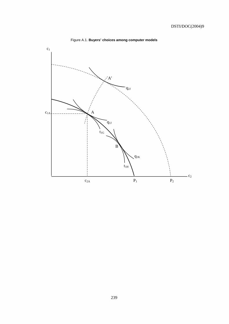
DSTI/DOC(2004)9

239

Figure A.1. Buyers’ choices among computer models

c1 A′ q2J

c1A A q1J t1G B q1K t1H c2

c2A P1 P2

DSTI/DOC(2004)9

240

REFERENCES

Abel, Jaison R., Ernst R. Berndt and Alan G. White (2003), “Price Indexes for Microsoft’s Personal Computer Software Products”, NBER working paper no. 9966, September, Cambridge, MA: National Bureau of Economic Research.

Adelman, Irma and Zvi Griliches (1961), “On an Index of Quality Change”, Journal of the American Statistical Association, 56(295) (September), pp. 535-48.

Aizcorbe, Ana, Carol Corrado and Mark Doms (2000), “Constructing Price and Quantity Indexes for High Technology Goods”, Industrial Output Section, Division of Research and Statistics, Board of Governors of the Federal Reserve System, July, Washington, D.C.

Aizcorbe, Ana, Stephen Oliner and Daniel Sichel (2003), “Semiconductor Price Puzzles”, presented at National Bureau of Economic Research Conference on Research in Income and Wealth, Cambridge, MA, July 28-29.

Allen, Roy George Douglas (1975), Index Numbers in Theory and Practice, London: MacMillan.

Archibald, Robert B. (1977), “On the Theory of Industrial Price Measurement: Output Price Indexes”, Annals of Economic and Social Measurement, 6(1) (Winter), pp. 57-72.

Arguea, Nestor M. and Cheng Hsiao (1993), “Econometric Issues of Estimating Hedonic Price Functions: With an Application to the US Market for Automobiles”, Journal of Econometrics, 56(1-2) (March), pp. 243-67.

Armknecht, Paul A. (1996), “Improving the Efficiency of the US CPI”, International Monetary Fund Working Paper 96/103, Washington, D.C.: International Monetary Fund.

Armknecht, Paul A. and Fenella Maitland-Smith (1999), “Price Imputation and Other Techniques for Dealing with Missing Observations, Seasonality and Quality Changes in Prices Indices”, International Monetary Fund Working Paper 99/78, Washington, D.C.: International Monetary Fund.

Armknecht, Paul and Donald Weyback (1989), “Adjustments for Quality Change in the US Consumer Price Index”, Journal of Official Statistics, 5(2), pp. 107-23.

Balk, Bert M. (1999), “On the Use of Unit Value Indices as Consumer Price Subindices”, in: Walter Lane, ed., Proceedings of the Fourth Meeting of the International Working Group on Price Indices, Washington, D.C.: US Department of Labor, pp. 112-20.

Ball, Adrian and David Fenwick (2004), “Static Samples in a Dynamic Universe: The Potential Use of Scanner Data and Hedonic Regressions”, presented at SSHRC International Conference on Index Number Theory and the Measurement of Prices and Productivity, Vancouver, June 30-July 3.

DSTI/DOC(2004)9

241

Ball, Adrian, Sukwinder Mehmi, Prabhat Vaze, Anthony Szary, Nicola Chissell, and Jeremy Heaven (2002), “Implementing Hedonic Methods for PCs: The UK Experience”, presented at the Office of National Statistics 2002 New Economy Workshop, available at http://www.statistics.gov.uk/events/new_economy_measurement/downloads/NEMW(04)_AB_Hedonics.pdf

Bapco (2002), “An Overview of SYSmark 2002 Business Applications Performance Corporation”, available at http://www.bapco.com/techdocs/SYSmark2002Methodology.pdf, accessed February 19, 2003.

Bartik, Timothy J. (1987), “The Estimation of Demand Parameters in Hedonic Price Models”, Journal of Political Economy, 95(1) (February), pp. 81-8.

Barzyk, Fred (1999), “Updating the Hedonic Equations for the Price of Computers”, working paper of Statistics Canada, Prices Division, November.

Barzyk, Fred and Matthew MacDonald (2001), “The Treatment of Quality Change for Computer Price Indexes – A Review of Current and Proposed Practices”, unpublished working paper of Statistics Canada, Prices Division, October.

Bascher, Jérôme and Thierry Lacroix (1999), “Dish-washers and PCs in the French CPI: Hedonic Modeling, from Design to Practice”, presented at the Fifth Meeting of the International Working Group on Price Indices, Reykjavik, Iceland, August 25-27.

Berndt, Ernst R. (1991), The Practice of Econometrics: Classic and Contemporary, Reading, MA: Addison-Wesley Pub. Co.

Berndt, Ernst R. and Zvi Griliches (1993), “Price Indexes for Microcomputers: An Exploratory Study”, in: Murray F. Foss, Marilyn Manser and Allan H. Young (eds.), Price Measurements and Their Uses, National Bureau of Economic Research Studies in Income and Wealth, Vol. 57. Chicago, IL: University of Chicago Press, pp. 63-93.

Berndt, Ernst R. and Neal J. Rappaport (2001), “Price and Quality of Desktop and Mobile Personal Computers: A Quarter-Century Historical Overview”, American Economic Review, 91(2) (May), pp. 268-73.

Berndt, Ernst R. and Neal J. Rappaport (2002), “Hedonics for Personal Computers: A Reexamination of Selected Econometric Issues”, draft manuscript, July 18 (earlier version of Berndt and Rappaport, 2003).

Berndt, Ernst R. and Neal J. Rappaport (2003), “Hedonics for Personal Computers: A Reexamination of Selected Econometric Issues”, presented at “R&D, Education and Productivity”, an international conference in memory of Zvi Griliches (1930-1999), August 25-27, Paris, France.

Berndt, Ernst R., Zvi Griliches and Joshua G. Rosett (1993), “Auditing the Producer Price Index: Micro Evidence from Prescription Pharmaceutical Preparations”, Journal of Business and Economic Statistics, 11(3) (July), pp. 251-64.

Berndt, Ernst R., Zvi Griliches and Neal Rappaport (1995), “Econometric Estimates of Prices in Indexes for Personal Computers in the 1990s”, Journal of Econometrics, 68(1), pp. 243-68.

DSTI/DOC(2004)9

242

Berry, Steven, James Levinsohn and Ariel Pakes (1995), “Automobile Prices in Market Equilibrium”, Econometrica, 63(4) (July), pp. 841-90.

Blackorby, Charles and Robert R. Russell (1978), “Indices and Subindices of the Cost-of-Living and the Standard of Living”, International Economic Review, 19(1) (February), pp. 229-40.

Blow, Laura and Ian Crawford (2001), “The Cost of Living with the RPI: Substitution Bias in the UK Retail Prices Index”, Economic Journal, 111(472) (June), pp. F357-82.

Boskin Commission (1996), See Boskin et al., 1996.

Boskin, Michael J., Ellen R. Dulberger, Robert J. Gordon, Zvi Griliches and Dale Jorgenson (1996), “Toward a More Accurate Measure of the Cost of Living”, final report to the Senate Finance Committee, Advisory Commission to Study the Consumer Price Index, December 4, available at http://www.ssa.gov/history/reports/boskinrpt.html

Bourot, Laurent (1997), “Indice de prix des micro-ordinateurs et des imprimantes: Bilan d’une rénovation”, working paper of the Institut National de la Statistique et des Études Économiques (INSEE), Paris, France, March 12.

Box, G. E. P. and D. R. Cox (1964), “An Analysis of Transformations”, Journal of the Royal Statistical Society. Series B (Methodological), 26(2), pp. 211-52.

Braithwait, Steven D. (1980), “The Substitution Bias of the Laspeyres Price Index: An Analysis Using Estimated Cost-of-Living Indexes”, American Economic Review, 70(1) (March), pp. 64-77.

Butler Group (2001), “Is Clock Speed the Best Gauge for Processor Performance?”, Server World Magazine, September, available at http://www.serverworldmagazine.com/opinionw/ 2001/09/06 clockspeed.shtml, accessed February 7, 2003.

Cartwright, David W. (1986), “Improved Deflation of Purchases of Computers”, Survey of Current Business, 66(3) (March), pp. 7-9.

Chwelos, Paul (2003), “Approaches to Performance Measurement in Hedonic Analysis: Price Indexes for Laptop Computers in the 1990s”, Economics of Innovation and New Technology, 12(3) (June), pp. 199-224.

Chwelos, Paul, Ernst Berndt, and Iain Cockburn (2003), “Valuing Mobile Computing: A Preliminary Price Index for PDAs”, presented at 3rd ZEW Conference on the Economics of Information and Communication Technologies, Mannheim, Germany, July 4-5.

Chow, Gregory C. (1967), “Technological Change and the Demand for Computers”, American Economic Review, 57(5) (December), pp. 1117-30.

Christensen, Laurits R., Dale W. Jorgenson, and Lawrence J. Lau (1973), “Transcendental Logarithmic Production Frontiers”, The Review of Economics and Statistics, 55(1) (February), pp. 28-45.

Cole, Rosanne (1993), “High-Tech Products: Computers: Comment”, in: Murray F. Foss, Marilyn E. Manser, and Allan H. Young (eds.), Price Measurements and Their Uses, National Bureau of Economic Research Studies in Income and Wealth, Vol. 57, Chicago and London: University of Chicago Press, pp. 93-9.

DSTI/DOC(2004)9

243

Cole, Rosanne, Y.C. Chen, Joan A. Barquin-Stolleman, Ellen Dulberger, Nurhan Helvacian, and James H. Hodge (1986), “Quality-Adjusted Price Indexes for Computer Processors and Selected Peripheral Equipment”, Survey of Current Business, 66(1) (January), pp. 41-50.

Colwell, Peter and Gene Dilmore (1999), “Who Was First? An Examination of an Early Hedonic Study”, Land Economics, 75(4), pp. 620-26.

Commission of the European Communities, International Monetary Fund, Organisation for Economic Co-operation and Development, United Nations, and World Bank (1993), System of National Accounts 1993, Office for Official Publications of the European Communities Catalogue number CA-81-93-002-EN-C, International Monetary Fund Publication Stock No. SNA-EA, Organisation for Economic Co-operation and Development OECD Code 30 94 01 1, United Nations publication Sales No. E.94.XVII.4, World Bank Stock Number 31512.

Court, Andrew T. (1939), “Hedonic Price Indexes with Automotive Examples”, in: The Dynamics of Automobile Demand, New York, NY: General Motors Corporation, pp. 99-117.

Court, Louis M. (1941), “Entrepreneurial and Consumer Demand Theories for Commodity Spectra (Part I)”, Econometrica, 9(2) (April), pp. 135-162, concluded: “Entrepreneurial and Consumer Demand Theories for Commodity Spectra (Concluded)”, Econometrica 9(3/4), (July-October), pp. 241-97.

Cowling, Keith and John Cubbin (1971), “Price, Quality and Advertising Competition: An Econometric Investigation of the United Kingdom Car Market”, Economica N.S., 38(152) (November), pp. 378-94.

CPI Commission (1996), See Boskin et al., 1996.

Dalén, Jörgen (1989), “Using Hedonic Regression for Computer Equipment in the Producer Price Index”, R&D Report 1989:25, Statistics Sweden.

Dalén, Jörgen (1994), “Sensitivity Analyses for Harmonising European Consumer Price Indices”, presented at the First Meeting of the International Working Group on Price Indices, Ottawa, Canada, October 31-November 2.

Dalén, Jörgen (1998), “Studies on the Comparability of Consumer Price Indices”, International Statistical Review, 66(1) (April), pp. 83-113.

Dalén, Jörgen (1999), “On the Statistical Objective of a Laspeyres’ Price Index”, in: Walter Lane, ed., Proceedings of the Fourth Meeting of the International Working Group on Price Indices, Washington, D.C.: US Bureau of Labor Statistics, pp. 121-41.

Dalén, Jörgen (2001), “Statistical Targets for Price Indexes in Dynamic Universes”, presented at the Sixth Meeting of the International Working Group on Price Indices, Canberra, Australia, April 2-6.

Dalén, Jörgen (2002), “Personal Computers in Different HICPs”, presented at Brookings Institution Workshop on Productivity in the Services Sector “Hedonic Price Indexes: Too Fast? Too Slow? Or Just Right?”, Washington, D.C., February 1, available at: http://brook.edu/dybdocroot/es/research/projects/productivity/workshops/20020201_dalen.pdf

DSTI/DOC(2004)9

244

Denison, Edward F. (1969), “Some Major Issues in Productivity Analysis: An Examination of Estimates by Jorgenson and Griliches”, Survey of Current Business, 49(5) Part II, pp. 1-27, reprinted in Survey of Current Business, 52(5) (May, 1972) Part II, pp. 37-63.

Denison, Edward F. (1989), Estimates of Productivity Change by Industry: An Evaluation and an Alternative, Washington, D.C.: Brookings Institution Press.

Dickens, William T. (1990), “Error Components in Grouped Data: Is it Ever Worth Weighting?” Review of Economics and Statistics, LXXII(2) (May), pp. 328-33.

Diewert, W. Erwin (1976), “Exact and Superlative Index Numbers”, Journal of Econometrics, 4(2) (May), pp. 115-45.

Diewert, W. Erwin (1995), “Axiomatic and Economic Approaches to Elementary Price Indexes”, NBER working paper no. 5104, May, Cambridge, MA: National Bureau of Economic Research.

Diewert, W. Erwin (2003), “Hedonic Regressions: A Consumer Theory Approach”, in: Robert C. Feenstra and Matthew D. Shapiro (eds.), Scanner Data and Price Indexes, National Bureau of Economic Research Studies in Income and Wealth, Vol. 64. Chicago, IL: University of Chicago Press, pp. 317-48.

Dulberger, Ellen R. (1989), “The Application of a Hedonic Model to a Quality-Adjusted Price Index for Computer Processors”, in: Dale W. Jorgenson and Ralph Landau (eds.), Technology and Capital Formation, Cambridge, MA: Massachusetts Institute of Technology Press, pp. 37-75.

Dulberger, Ellen (1993), “Sources of Price Decline in Computer Processors: Selected Electronic Components”, in: Murray F. Foss, Marilyn E. Manser, and Allen H. Young (eds.), Price Measurements and Their Uses, National Bureau of Economic Research Studies in Income and Wealth, Vol. 57, pp. 103-24, Chicago and London: The University of Chicago Press.

Ekeland, Ivar, James J. Heckman and Lars Nesheim (2002), “Identifying Hedonic Models”, American Economic Review, 92(2) (May), pp. 304-09.

Ekeland, Ivar, James J. Heckman, and Lars Nesheim (2004), “Identification and Estimation of Hedonic Models”, Journal of Political Economy, Part 2 Supplement, 112(1) (February), pp. S60-109.

Epple, Dennis (1987), “Hedonic Prices and Implicit Markets: Estimating Demand and Supply Functions for Differentiated Products”, Journal of Political Economy, 95(1) (February), pp. 59-80.

Erickson, Timothy (2003), “A Note on Hedonic Regression with Scanner Data”, unpublished paper, US Bureau of Labor Statistics, September 17.

Ethridge, Don E. (2002), “Daily Hedonic Price Analysis: An Application to Regional Cotton Price Reporting”, presented at Center for European Economic Research (ZEW) conference “Price Indices and the Measurement of Quality Changes”, April 25-26, Mannheim, Germany.

Eurostat (1999), Compendium of HICP Reference Documents: Harmonisation of Price Indices, Eurostat, September.

Eurostat Task Force (1999), “Volume Measures for Computers and Software”, report of the Eurostat Task Force on Volume Measures for Computers and Software, June.

DSTI/DOC(2004)9

245

Evans, Richard (2002), “INSEE’s Adoption of Market Intelligence Data for Its Hedonic Computer Manufacturing Price Index”, presented at the Symposium on Hedonics at Statistics Netherlands, October 25.

Feenstra, Robert C. (1995), “Exact Hedonic Price Indexes”, Review of Economics and Statistics, 77(4) (November), pp. 634-53.

Feenstra, Robert C. and Matthew D. Shapiro (eds.) (2003), Scanner Data and Price Indexes, National Bureau of Economic Research Studies in Income and Wealth, Vol. 64., Chicago and London: The University of Chicago Press.

Feenstra, Robert C. and Matthew D. Shapiro (2003), “High-Frequency Substitution and the Measurement of Price Indexes”, in: Robert C. Feenstra and Matthew D. Shapiro (eds.), Scanner Data and Price Indexes, National Bureau of Economic Research Studies in Income and Wealth, Vol. 64., Chicago and London: The University of Chicago Press, pp. 123-46.

Fisher, Franklin M. and Karl Shell (1972), The Economic Theory of Price Indices: Two Essays on the Effects of Taste, Quality, and Technological Change, New York, NY: Academic Press.

Fisher, Franklin M., John J. McGowan, and Joen E. Greenwood (1983), Economic Analysis and US v. IBM, Cambridge, MA: MIT Press.

Fixler, Dennis J. and Kimberly D. Zieschang (1992), “Incorporating Ancillary Measures of Process and Product Characteristics into a Superlative Productivity Index”, Journal of Productivity Analysis, 2(2), pp. 245-67.

Fixler, Dennis, Charles Fortuna, John Greenlees and Walter Lane (1999), “The Use of Hedonic Regressions to Handle Quality Change: The Experience in the US CPI”, presented at the Fifth Meeting of the International Working Group on Price Indices, Reykjavik, Iceland, August 25-27.

Flamm, Kenneth (1987), Targeting the Computer: Government Support and International Competition, Washington, D.C.: The Brookings Institution.

Flamm, Kenneth (1993), “Measurement of DRAM Prices: Technology and Market Structure”, in: Murray F. Foss, Marilyn E. Manser and Allan H. Young (eds.), Price Measurements and Their Uses, National Bureau of Economic Research Studies in Income and Wealth, Vol. 57. Chicago and London: The University of Chicago Press, pp. 157-206.

Gandal, Neil (1994), “Hedonic Price Indexes for Spreadsheets and an Empirical Test for Network Externalities”, RAND Journal of Economics, 25(1) (Spring), pp. 160-70.

GAO (US General Accounting Office) (1999), Consumer Price Index: Impact of Commodity Analysts’ Decisionmaking Needs to Be Assessed, report GGD-99-84, Washington, D.C.: US Government Printing Office.

Goldberger, Arthur S. (1968), “The Interpretation and Estimation of Cobb-Douglas Functions”, Econometrica, 36(3/4) (July - October), pp. 464-72.

Goldberger, Arthur S. (1991), A Course in Econometrics, Cambridge, MA: Harvard University Press.

Gordon, Robert J. (1990), The Measurement of Durable Goods Prices, National Bureau of Economic Research Monograph series, Chicago and London: University of Chicago Press, p. 723.

DSTI/DOC(2004)9

246

Gorman, W.M. (1980), “A Possible Procedure for Analysing Quality Differentials in the Egg Market”, The Review of Economic Studies, 47(5) (October), pp. 843-56.

Greenlees, John S. (2000), “Consumer Price Indexes: Methods for Quality and Variety Change”, Statistical Journal, 17(1), pp. 59-74.

Griliches, Zvi (1961), “Hedonic Price Indexes for Automobiles: An Econometric Analysis of Quality Change”, in: Price Statistics Review Committee, National Bureau of Economic Research, The Price Statistics of the Federal Government: Review, Appraisal, and Recommendations, General Series No. 73. New York, NY: National Bureau of Economic Research, pp. 173-96, reprinted in Zvi Griliches, Technology, Education, and Productivity, Oxford: Basil Blackwell, 1988, pp. 76-104.

Griliches, Zvi (ed.) (1971), Price Indexes and Quality Change: Studies in New Methods of Measurement, Cambridge, MA: Harvard University Press.

Griliches, Zvi (1988), “Hedonic Price Indexes Revisited”, in: Zvi Griliches, Technology, Education, and Productivity, Oxford: Basil Blackwell, pp. 105-19, originally published as “Introduction: Hedonic Price Indexes Revisited”, in: Zvi Griliches (ed.), Price Indexes and Quality Change: Studies in New Methods of Measurement, Cambridge, MA: Harvard University Press, pp. 3-15.

Griliches, Zvi (1990), “Hedonic Price Indexes and the Measurement of Capital and Productivity: Some Historical References”, in: Ernst R. Berndt and Jack E. Triplett (eds.), Fifty Years of Economic Measurement: The Jubilee of the Conference on Research in Income and Wealth, National Bureau of Economic Research Studies in Income and Wealth, Vol. 54. Chicago: University of Chicago Press, pp. 185-202.

Gujarati, Damodar N. (1995), Basic Econometrics, New York, NY: McGraw-Hill.

Harhoff, Dietmar and Dietmar Moch (1997), “Price Indexes for PC Database Software and the Value of Code Compatibility”, Research Policy, 24(4-5) (December), pp. 509-20.

Hausman, Jerry A. (1997), “Valuation of New Goods Under Perfect and Imperfect Competition”, in: Timothy F. Bresnahan and Robert J. Gordon (eds.), The Economics of New Goods, National Bureau of Economic Research Studies in Income and Wealth, Vol. 58, pp. 209-37, Chicago and London: The University of Chicago Press.

Hausman, Jerry A. (2003), “Sources of Bias and Solutions to Bias in the Consumer Price Index”, Journal of Economic Perspectives, 17(1) (Winter), pp. 23-44.

Hicks, John R. (1940), “The Valuation of the Social Income”, Economica N.S., 7(26) (May), pp. 105-124.

Ho, Mun S., Someshwar Rao, and Jianmin Tang (2003), “Sources of Output Growth in Canadian and US Industries in the Information Age”, presented at the 37th Annual Meetings of the Canadian Economics Association, Ottawa, May 29-June 1.

Hoffmann, Johannes (1998), “Problems of Inflation Measurement in Germany”, discussion paper 1/98, Economic Research Group of the Deutsche Bundesbank, Frankfurt, Germany: Deutsche Bundesbank.

Holdway, Michael (2001), “Quality-Adjusting Computer Prices in the Producer Price Index: An Overview”, Bureau of Labor Statistics, October, Washington, D.C.: United States Bureau of Labor Statistics, available on-line at: http://stats.bls.gov/ppi/ppicomqa.htm

DSTI/DOC(2004)9

247

Houthakker, H.S. (1952), “Compensated Changes in Quantities and Qualities Consumed”, Review of Economic Studies, 19(3) (1952-1953), pp. 155-64.

Hoven, Leendert (1999), “Some Observations on Quality Adjustment in the Netherlands”, presented at the Fifth Meeting of the International Working Group on Price Indices, Reykjavik, Iceland, August 25-27.

Hulten, Charles R. (2002), “Price Hedonics: A Critical Review”, Federal Reserve Bank of New York Economic Policy Review, 9(3) (September), pp. 5-15.

Intel Corporation (2001), “Mobile Intel Pentium III Processor Featuring Intel SpeedStep Technology: Performance Brief”, May, available at: http://developer.intel.ru/download/design/mobile/perfbref/p3_pb.pdf

Inter-secretariat Working Group on Price Statistics (2003), Revision of the ILO Manual on CPI, unpublished, available online at: http://www.ilo.org/public/english/bureau/stat/guides/cpi/index.htm

Ironmonger, D.S. (1972), “New Commodities and Consumer Behavior”, University of Cambridge, Department of Applies Economics Monographs 20, Cambridge, United Kingdom: Cambridge University Press.

Jaszi, George (1964), “Comment” (on “Notes on the Measurement of Price and Quality Changes” by Zvi Griliches), in: Conference on Models of Income Determination, Models of Income Determination, National Bureau of Economic Research Studies in Income and Wealth, Vol. 28. Princeton, NJ: Princeton University Press, pp. 404-09.

Johnston, J. (1972), Econometric Methods, 2nd Edition. New York, NY: McGraw-Hill Book Company.

Jorgenson, Dale W. and Zvi Griliches (1972), “Issues in Growth Accounting: A Reply to Edward F. Denison”, Survey of Current Business, 52(5) (May) Part II, pp. 65-94.

Kanellos, Michael (2002), “AMD, Intel Trot Out New Chips”, News.com, June 10, available at: http://news.com.com/2100-1001-934359.html

Kennedy, Peter E. (1981), “Estimation with Correctly Interpreted Dummy Variables in Semilogarithmic Equations”, The American Economic Review, 71(4) (September), p. 801.

Knight, Kenneth E. (1966), “Changes in Computer Performance: A Historical View”, Datamation, 12(9) (September), pp. 40-54.

Knight, Kenneth E. (1973), “Application of Technological Forecasting to the Computer Industry”, in: James R. Bright and Milton E.F. Schoeman (eds.), A Guide to Practical Technological Forecasting, Englewood Cliffs, NJ: Prentice-Hall, pp. 377-403.

Knight, Kenneth E. (1985), “A Functional and Structural Measurement of Technology”, Technological Forecasting and Social Change, 27(2-3) (May), pp. 107-27.

Konijn, Paul, Dietmar Moch and Jörgen Dalén (2003), “Comparison of Hedonic Functions for PCs across EU Countries”, Eurostat discussion paper, presented at 54th ISI Session, Berlin, August 13-20.

DSTI/DOC(2004)9

248

Koskimäki, Timo and Yrjö Vartia (2001), “Beyond Matched Pairs and Griliches-type Hedonic Methods for Controlling Quality Changes in CPI Sub-indices”, presented at the Sixth Meeting of the International Working Group on Price Indices, Canberra, Australia, April 2-6.

Laferrère, Anne (2003), “Hedonic Housing Price Indices: The French Experience”, prepared for the IMF and BIS conference on Real Estate Indicators and Financial Stability, October 27-28, 2003, Washington, D.C.

Lancaster, Kelvin (1971), Consumer Demand: A New Approach, New York, NY: Columbia University Press.

Lane, Walter (2001), “Addressing the New Goods Problem in the Consumer Price Index”, presented at the Sixth Meeting of the International Working Group on Price Indices, Canberra, Australia, April 2-6.

Lequiller, François (2001), “The New Economy and the Measurement of GDP Growth”, Série des documents du travail de la Direction des Etudes et Synthèses Economiques G2001/01, INSEE, February.

Levine, Jordan (2002), “US Producer Price Index for Pre-Packaged Software”, presented at the 17th Voorburg Group Meeting, Nantes, France, September.

Levy, Frank, Anne Beamish, Richard J. Murnane and David Autor (1999), “Computerization and Skills: Examples from a Car Dealership”, presented at the Brookings Institution Program on Output and Productivity Measurement in the Service Sector, “Workshop on Measuring the Output of Business Services”, May 14.

Lim, Poh Ping and Richard McKenzie (2002), “Hedonic Price Analysis for Personal Computers in Australia: An Alternative Approach to Quality Adjustments in the Australian Price Indexes”, presented at Center for European Economic Research (ZEW) conference, Mannheim, Germany, April.

Longley, James W. (1984), Least Squares Computations Using Orthogonalization Methods, New York, NY: Marcel Dekker.

Lowe, Robin (1999), “The Use of the Regression Approach to Quality Change for Durables in Canada”, presented at the Fifth Meeting of the International Working Group on Price Indices, Reykjavik, Iceland, August 25-27.

Manser, Marilyn E. and Richard J. McDonald (1988), “An Analysis of Substitution Bias in Measuring Inflation, 1959-85”, Econometrica, 56(4) (July), pp. 909-30.

McCarthy, Paul. (1997), “Computer Prices: How Good is the Quality Adjustment?”, presented at Capital Stock Conference, Canberra, Australia, March 10-14; Canberra Group on Capital Stock Statistics, available at http://www.oecd.org/dataoecd/9/0/2666828.pdf

Moch, Dietmar (2001), “Price Indices for Information and Communication Technology Industries: An Application to the German PC Market”, Center for European Economic Research (ZEW) Discussion Paper No. 01-20, Mannheim, Germany.

Moch, Dietmar and Jack E. Triplett (2004), “PPPs for PCs: Hedonic Comparison of Computer Prices in France and Germany”, unpublished paper, Center for European Economic Research, University of Mannheim and Brookings Institution.

DSTI/DOC(2004)9

249

Moreau, Antoine (1996), “Methodology of the Price Index for Microcomputers and Printers in France”, in: Industry Productivity: International Comparison and Measurement Issues, OECD proceedings, Paris, France: Organization for Economic Co-operation and Development, pp. 99-118.

Morris, John (2003), “The Real Truth about Centrino”, CNET Reviews, March 20, available at http://att.com.com/4520-3000_7-5023907-1.html

Moulton, Brent R. and Karin E. Moses. (1997), “Addressing the Quality Change Issue in the Consumer Price Index”, Brookings Papers on Economic Activity, 1997(1), pp. 305-49.

Moulton, Brent R., Timothy J. LaFleur, and Karin E. Moses (1999), “Research on Improved Quality Adjustment in the CPI: The Case of Televisions”, in: Walter Lane, ed., Proceedings of the Fourth Meeting of the International Working Group on Price Indices, Washington, D.C.: US Bureau of Labor Statistics, pp. 77-99.

Moylan, Carol (2001), “Estimation of Software in the US National Income and Product Accounts: New Developments”, OECD Paper STD/NA(2001)25, Organisation for Economic Co-operation and Development, Statistics Directorate, National Accounts, September, available at http://www.brookings.edu/dybdocroot/es/research/projects/productivity/workshops/20011012_moylan.pdf

Muellbauer, John (1974), “Household Production Theory, Quality, and the ‘Hedonic Technique’”, American Economic Review, 64(6) (December), pp. 977-94.

Nelson, Randy A., Tim L. Tanguay and Christopher D. Patterson (1994), “A Quality-Adjusted Price Index for Personal Computers”, Journal of Business and Economics Statistics, 12(1) (January), pp. 23-31.

Nicholson, J. L. (1967), “The Measurement of Quality Changes”, The Economic Journal, 77(307), (September), pp. 512-30.

Nordhaus, William D. (2001), “The Progress of Computing”, Cowles Foundation discussion paper No. 1324, September, Yale University, presented at Brookings Institution workshop “Hedonic Price Indexes: Too Fast, Too Slow, or Just Right?”, available at http://brook.edu/dybdocroot/es/research/projects/productivity/workshops/20020201_nordhaus.pdf

O’Connell, Paul G.J. and Shang-Jin Wei (2002), “The Bigger They Are, the Harder They Fall: Retail Price Differences across US Cities”, Journal of International Economics, 56(1), pp. 21-53.

Ohta, Makoto and Zvi Griliches (1976), “Automobile Prices Revisited: Extensions of the Hedonic Hypothesis”, in: Nestor E. Terleckyj (ed.), Household Production and Consumption, National Bureau of Economic Research Studies in Income and Wealth, Vol. 40, New York, NY: Columbia University Press, pp. 325-90.

Oi, Walter Y. (1992), “Productivity in the Distributive Trades: The Shopper and the Economies of Massed Reserves”, in: Zvi Griliches (ed.), Output Measurement in the Service Sector, National Bureau of Economic Research Studies in Income and Wealth, Vol. 56, Chicago and London: University of Chicago Press, pp. 161-91.

Okamoto, Masato and Tomohiko Sato (2001), “Comparison of Hedonic Method and Matched Models Method Using Scanner Data: The Case of PCs, TVs and Digital Cameras”, presented at the Sixth Meeting of the International Working Group on Price Indices, Canberra, Australia, April 2-6.

DSTI/DOC(2004)9

250

Pakes, Ariel (2003), “A Reconsideration of Hedonic Price Indexes with an Application to PCs”, American Economic Review, 93(5) (December), pp. 1578-96.

Pakes, Ariel (2004), “Hedonics and the Consumer Price Index”, earlier version presented at “R&D, Education and Productivity”, an international conference in memory of Zvi Griliches (1930-1999), August 25-27, 2003, Paris, France.

Parker, Robert P. and Bruce Grimm (2000), “Recognition of Business and Government Expenditures for Software as Investment: Methodology and Quantitative Impacts, 1959-98”, presented to BEA’s Advisory Committee, May 5, available at http://www.bea.gov/bea/about/software.pdf

Phister, Montgomery (1979), Data Processing Technology and Economics, second edition, Bedford, MA: Santa Monica Pub. Co.

Pieper, Paul. (1990), “The Measurement of Structures Prices: Prospect and Retrospect”, in: Ernst R. Berndt and Jack E. Triplett (eds.), Fifty Years of Economic Measurement: The Jubilee of the Conference on Research in Income and Wealth, National Bureau of Economic Research Studies in Income and Wealth, Vol. 54., Chicago and London: University of Chicago Press, pp. 239-68.

Pollak, Robert A. (1975), “Subindexes of the Cost of living”, International Economic Review, 16(1) (February), pp. 135-50, reprinted in: Robert A. Pollak, The Theory of the Cost-of-Living Index, Chapter 2, pp. 53-70, 1989, Oxford, United Kingdom: Oxford University Press.

Pollak, Robert A. (1983), “The Treatment of ‘Quality’ in the Cost of Living Index”, Journal of Public Economics, 20(1) (February), pp. 25-53, reprinted in Robert A. Pollak, The Theory of the Cost of Living Index, Chapter 8, pp. 153-80, 1989, Oxford, United Kingdom: Oxford University Press.

Pollak, Robert A. (1989), The Theory of the Cost of Living Index, Oxford, United Kingdom: Oxford University Press.

Price Statistics Review Committee, National Bureau of Economic Research (1961), The Price Statistics of the Federal Government: Review, Appraisal, and Recommendations, A Report to the Office of Statistical Standards, Bureau of the Budget, General Series No. 73, New York, NY: National Bureau of Economic Research.

Prud’homme, Mark and Kam Yu (2002), “A Price Index for Computer Software Using Scanner Data”, presented at Brookings Institution workshop “Two Topics in Services: CPI Housing and Computer Software”, Washington, D.C., May 23, available at http://www.brookings.edu/es/research/projects/productivity/workshops/20030523_kam.pdf

Rao, H. Raghaw and Brian D. Lynch (1993), “Hedonic Price Analysis of Workstation Attributes”, Communications of the Association for Computing Machinery (ACM), 36(12) (December), pp. 95-102.

Ribe, Martin (2002), “Quality Adjustment (QA) for New Cars in Austria and Sweden”, presented at Brookings Institution workshop “Hedonic Price Indexes: Too Fast? Too Slow? Or Just Right?”, Washington, D.C., February 1, available at http://www.brook.edu/es/research/ projects/productivity/workshops/20020201.htm

Rosen, Sherwin (1974), “Hedonic Prices and Implicit Markets: Product Differentiation in Pure Competition”, Journal of Political Economy, 82(1) (January-February), pp. 34-55.

DSTI/DOC(2004)9

251

Saglio, A. (1994), “Comparative Changes in Average Price and a Price Index: Two Case Studies”, presented at the First Meeting of the International Working Group on Price Indices, Ottawa, Canada, October 31-November 2.

Schreyer, Paul (2001), Measuring Productivity: Measurement of Aggregate and Industry-Level Productivity Growth: OEDC Manual, Paris, France: OEDC Publications.

Schultz, Bohdan J. (1994), “Choice of Price Index Formulae at the Micro-Aggregation Level: The Canadian Empirical Evidence”, presented at the First Meeting of the International Working Group on Price Indices, Ottawa, Canada, October 31-November 2.

Schultz, Bohdan J. (2001), “User-cost Approach to the Estimation of Price Change for Private Transportation: Experimental Study in the Spirit of the Cost-of-Living Index”, presented at the Sixth Meeting of the International Working Group on Price Indices, Canberra, Australia, April 2-6.

Schultze, Charles L. (2002), “Notes for Presentation” (with Christopher Mackie) at Brookings Institution workshop “Hedonic Price Indexes: Too Fast? Too Slow? Or Just Right?”, Washington, D.C., February 1, 2002.

Schultze, Charles L. (2003), “The Consumer Price Index: Conceptual Issues and Practical Suggestions”, Journal of Economic Perspectives, 17(1) (Winter), pp. 3-22.

Schultze, Charles and Christopher Mackie (eds.) (2002), At What Price? Conceptualizing and Measuring Cost-of-Living and Price Indexes, Panel on Conceptual, Measurement, and Other Statistical Issues in Developing Cost-of-Living Indexes, Committee on National Statistics, National Research Council, Washington, D.C.: National Academy Press.

Sellwood, Don J. (1998), “In Search of New Approaches to the Problem of Quality Adjustment in CPI”, in: B. Balk (ed.), Proceedings of the Third Meeting of the International Working Group on Price Indices, Voorburg: Statistics Netherlands.

Shapiro, Matthew D. and David W. Wilcox (1996), “Mismeasurement in the Consumer Price Index: An Evaluation”, in: Ben S. Bernanke and Julio Rotemberg (eds.), NBER Macroeconomics Annual, Cambridge, MA: MIT Press, pp. 93-142.

Sharpe, William F. (1969), The Economics of the Computer, New York and London: Columbia University Press.

Silver, Mick and Saeed Heravi (2001a), “Quality Adjustment, Sample Rotation and CPI Practice: An Experiment”, presented at the Sixth Meeting of the International Working Group on Price Indices, Canberra, Australia, April 2-6.

Silver, Mick and Saeed Heravi (2001b), “Scanner Data and the Measurement of Inflation”, Economic Journal, 111(472), June, pp. 383-404.

Silver, Mick and Saeed Heravi (2002), “Why the CPI Matched Models Method May Fail Us: Results From an Hedonic and Matched Experiment Using Scanner Data”, presented at Brookings Institution workshop “Hedonic Price Indexes: Too Fast, Too Slow, or Just Right?”, February, available at http://brook.edu/es/research/projects/productivity/workshops/20020201_silver.pdf

Silver, Mick and Saeed Heravi (2003), “The Measurement of Quality-Adjusted Price Changes”, in: Robert C. Feenstra and Matthew D. Shapiro (eds.), Scanner Data and Price Indexes, National Bureau of

DSTI/DOC(2004)9

252

Economic Research Studies in Income and Wealth, Vol. 64, Chicago and London: The University of Chicago Press, pp. 277-316.

Statistics Finland (2000), “Measuring the Price Development of Personal Computers in the Consumer Price Index”, paper for the Meeting of the International Hedonic Price Indexes Project, Paris, France, September 27.

Stigler Committee Report (1961), see Price Statistics Review Committee.

Stone, Richard (1956), Quantity and Price Indexes in National Accounts, Paris, France: Organization for European Economic Cooperation.

Taylor, Fred (1916), “Relation Between Primary Market Prices and Qualities of Cotton”, US Department of Agriculture Bulletin No. 457, November 24.

Teekens, R. and J. Koerts (1972), “Some Implications of the Log Transformation of Multiplicative Models”, Econometrica, 40(5) (September), pp. 793-819.

Tiendrez-Remond, Isabelle (2000), personal communication via email, September 19.

Triplett, Jack E. (1969), “Automobiles and Hedonic Quality Measurement”, Journal of Political Economy, 77(3) (May-June), pp. 408-17.

Triplett, Jack E. (1971), “Quality Bias in Price Indexes and New Methods of Quality Measurement”, in: Zvi Griliches (ed.), Price Indexes and Quality Change: Studies in New Methods of Measurement, Cambridge, MA: Harvard University Press, pp. 190-94.

Triplett, Jack E. (1971b), “The Theory of Hedonic Quality Measurement and Its Use in Price Indexes”, US Bureau of Labor Statistics Staff Paper 6, Washington, D.C.: US Government Printing Office.

Triplett, Jack E. (1973), “Review of ‘Consumer Demand: A New Approach by Kelvin Lancaster”, Journal of Economic Literature, 11(1) (March), pp. 77-81.

Triplett, Jack E. (1975), “The Measurement of Inflation: A Survey of Research on the Accuracy of Price Indexes”, in: Paul H. Earl (ed.), Analysis of Inflation, Lexington, MA: Lexington Books, pp. 19-82.

Triplett, Jack E. (1976), “Consumer Demand and Characteristics of Consumption Goods”, in: Nestor E. Terleckyj (ed.), Household Production and Consumption, National Bureau of Economic Research Studies in Income and Wealth, Vol. 40, New York and London: Columbia University Press, pp. 305-23.

Triplett, Jack E. (1983), “Concepts of Quality in Input and Output Price Measures: A Resolution of the User Value-Resource Cost Debate”, in: Murray F. Foss (ed.), The US National Income and Product Accounts: Selected Topics, National Bureau of Economic Research Studies in Income and Wealth, Vol. 47, Chicago and London: University of Chicago Press, pp. 296-311.

Triplett, Jack E. (1987), “Hedonic Functions and Hedonic Indexes”, in: John Eatwell, Murray Milgate, and Peter Newman (eds.), The New Palgrave: A Dictionary of Economics, Vol. 2. New York, NY: Stockton Press, pp. 630-34.

DSTI/DOC(2004)9

253

Triplett, Jack E. (1989), “Price and Technological Change in a Capital Good: A Survey of Research on Computers”, in: Dale W. Jorgenson and Ralph Landau (eds.), Technology and Capital Formation, Cambridge, MA: MIT Press, pp. 127-213.

Triplett, Jack E. (1990), “Hedonic Methods in Statistical Agency Environments: An Intellectual Biopsy”, in: Ernst R. Berndt and Jack E. Triplett (eds.), Fifty Years of Economic Measurement: The Jubilee of the Conference on Research in Income and Wealth, National Bureau of Economic Research Studies in Income and Wealth, Vol. 54, Chicago, IL: University of Chicago Press, pp. 207-33.

Triplett, Jack E. (1997), “Measuring Consumption: The Post-1973 Slowdown and the Research Issues”, Federal Reserve Bank of St. Louis Review, 79(3) (May-June), pp. 9-42.

Triplett, Jack E. (2001), “Should the Cost-of-Living Index Provide the Conceptual Framework for a Consumer Price Index?”, The Economic Journal, 111(472) (June), pp. F312-334.

Triplett, Jack E. (2004), “Zvi Griliches’ Contributions to Economic Measurement”, revised version presented at National Bureau of Economic Research Conference on Research in Income and Wealth in Memory of Zvi Griliches, Bethesda, Maryland, September 21-22, 2003.

Triplett, Jack E. and Barry P. Bosworth (2004), Services Productivity in the United States: New Sources of Economic Growth, Washington, D.C.: Brookings Institution Press.

Triplett, Jack E. and Richard J. McDonald (1977), “Assessing the Quality Error in Output Measures: The Case of Refrigerators”, Review of Income and Wealth, 23(2) (June), pp. 137-56.

Turvey, Ralph (1989), Consumer Price Indices: An ILO Manual, Geneva: International Labour Office.

Turvey, Ralph (1999), “True Cost of Living Indexes”, presented at the Fifth Meeting of the International Working Group on Price Indices, Reykjavik, Iceland, August 25-27.

Turvey, Ralph (2000), “CPI Terminology”, accessed May 15, 2000 from http://www.turvey.demon.co.uk/. Partially published in Ralph Turvey, “CPI Terminology”, presented at Conference of European Statisticians, Statistical Commission and Economic Commission for Europe, Joint ECE/ILO Meeting on Consumer Price Indices, Geneva, November 3-5, 1999, available at http://www.unece.org/stats/documents/ces/ac.49/1999/4.rev.1.e.pdf

US Census Bureau (undated), “Description of Price Index for Sales Price of New One-Family Houses Sold”, available at http://www.census.gov/const/C25/newresindextext.html

US Department of Labor, Bureau of Labor Statistics (1998), “The Use of the Geometric Mean in the Elementary Indexes of the Consumer Price Index”, unpublished draft report.

van Mulligen, Peter Hein (2002), “Alternative Price Indices for Computers in the Netherlands Using Scanner Data.”, presented at the 27th General Conference of the International Association for Research in Income and Wealth, Djurhamn, Sweden, August.

van Mulligen, Peter Hein (2003), Quality Aspects in Price Indices and International Comparisons: Application of the Hedonic Method, Voorburg: Statistics Netherlands.

von Hofsten, Erland (1952), Price Indexes and Quality Changes, London: George Allen & Unwin Ltd.

DSTI/DOC(2004)9

254

Waugh, Frederick Vail (1928), “Quality Factors Influencing Vegetable Prices”, Journal of Farm Economics, 10 (April), pp. 185-96.

White, Alan G., Jaison R. Abel, Ernst R. Berndt and Cory W. Monroe (2004), “Hedonic Price Indexes for Personal Computer Operating Systems and Productivity Suites”, NBER working paper no. 10427, April, Cambridge, MA: National Bureau of Economic Research.

Wooldridge, Jeffrey M. (1999), Introductory Econometrics: A Modern Approach, South-Western College Publishing.

Wyckoff, Andrew W. (1995), “The Impact of Computer Prices on International Comparisons of Labour Productivity”, Economics of Innovation and New Technology, 3(3-4), pp. 277-93.