Uncertainty quantification and reduction using Jacobian and ...

Uncertainty quantification andreduction using Jacobian andHessian informationJosefina Sánchez1 and Kevin Otto 2

1 Department of Mechanical Engineering Aalto University, Espoo, Finland2 Department of Mechanical Engineering The University of Melbourne, Melbourne, Australia

AbstractRobust design methods have expanded from experimental techniques to include samplingmethods, sensitivity analysis and probabilistic optimisation. Such methods typically requiremany evaluations. We study design and noise variable cross-term second derivatives of aresponse to quickly identify design variables that reduce response variability. We firstcompute the response uncertainty and variance decomposition to determine contributingnoise variables of an initial design. Then we compute the Hessian second-derivative matrixcross-terms between the variance-contributing noise variables and proposed design changevariables. Design variable with large Hessian terms are those that can reduce responsevariability. We relate the Hessian coefficients to reduction in Sobol indices and responsevariance change. Next, the first derivative Jacobian terms indicate which design variable canshift the mean to maintain a desired nominal target value. Thereby, design changes can beproposed to reduce variability while maintaining a targeted nominal value. This workflowfinds changes that improve robustness with a minimal four runs per design change.We alsoexplore further computation reductions achieved through compounding variables. Anexample is shown on a Stirling engine where the top four variance-contributing tolerancesand design changes identified through 16 Hessian terms generated a design with 20% lessvariance.

Key words: robust design, simulation based design, uncertainty analysis, uncertaintymodelling

1. Introduction

1.1. Background

Parametric robust design has been well researched and developed into what hasbecome the standard experimental robust design method (RDM), making use ofdesign-of-experiments to reduce the performance variability of a design due tomultiple causes (Taguchi 1986; Phadke 1989; Taguchi & Taguchi 2000; Thornton2003; Arvidsson & Gremyr 2008; Wu & Hamada 2011; Montgomery 2017). RDMismore than a statistical experiment, it involves amultiple step workflow includingidentifying possible sources of variability, quantifying their relative contributionwith noise experiments, generating ideas for design changes that may promotevariation reduction and then quantifying the ability of design changes to reducethis variability through a further set of experiments. Modern computer-based

Received 03 May 2021Revised 07 September 2021Accepted 08 September 2021

Corresponding authorKevin [email protected]

©TheAuthor(s), 2021. Published byCambridge University Press. This isan Open Access article, distributedunder the terms of the CreativeCommons Attribution licence (http://creativecommons.org/licenses/by/4.0), which permits unrestrictedre-use, distribution andreproduction, provided the originalarticle is properly cited.

Des. Sci., vol. 7, e20journals.cambridge.org/dsjDOI: 10.1017/dsj.2021.20

1/27

available at https://www.cambridge.org/core/terms. https://doi.org/10.1017/dsj.2021.20Downloaded from https://www.cambridge.org/core. IP address: 65.21.229.84, on 27 Jan 2022 at 05:27:19, subject to the Cambridge Core terms of use,

methodological updates include use of uncertainty quantification (UQ), surrogatemodelling, global sensitivity analysis (GSA) and optimisation (Chen et al. 1996;Du & Chen 2001; Jin, Chen, & Simpson 2001; Du, Sudjianto, & Chen 2004; Fang,Li, & Sudjianto 2005; Allen et al. 2006; Chen, Jin, & Sudjianto 2006; Jiang et al.2013; Jiang, Chen, & German 2016; Hu & Du 2019; Otto & Sanchez 2019; Otto,Wang, & Uyan 2019; Nellippallil et al. 2020; Sanchez, Björkman, & Otto 2020;Yin & Du 2021).

The problem considered here is to reduce the variability in a system responsey= f d,nð Þ, where d are design variables to be chosen and n are manufacturingnoise variables described with known parameters. The noise variable uncer-tainties give rise to a distribution of uncertainty on the response. We considerthe UQ of forward uncertainty propagation of aleatoric parameter uncertainty,specifically that from manufacturing parameters. Therefore, here UQ is simpli-fied to computing the uncertainty induced on the response due to themanufacturing input variability. Next with the variance of this response uncer-tainty, GSA is simplified to considering the decomposition of the responsevariance into portions from contributing noise variables, to identify which noisevariables contribute most. The problem addressed is to reduce the variance of theresponse uncertainty through changes to the design variable values, for example,the RDM problem.

Unfortunately, executing RDM remains a complex task for many industries,which has impeded adoption of RDM (Arena et al. 2006; Arvidsson et al. 2003).This is particularly evident when used in conjunction with simulation tools,which have prohibitively long manual setup times and long execution times.While automation can help reduce the burden (Otto & Sanchez 2019; Otto,Wang, &Uyan 2019), means are needed tomore quickly identify potential designchanges that can reduce variability arising from different contributing noisevariables. Given that at least 30 runs are generally needed to create a reasonablehistogram of a distribution, repeating this for different design configurationalternatives is prohibitive. Computer-based design of experiments with surrogatemodels or otherwise can improve upon this in a more structured exploration ofthe design space, but often require dozens of runs for a few design variables eachwith several runs over the noise variables.

We explore here using rapidly computed Hessian second derivative terms torank potential design changes. We also combine this with computed Jacobian firstderivative terms to enable reshifting the mean to remain on target while reducingvariation.We find that when using this approach, one can estimate in four runs thevariation reduction impact that a design change can have due to a causal noisevariable.

Next, we review related works. Then, we outline a workflow and derive thecalculations to (i) quantify uncertainty rank contributing noise variables usingSobol indices, (ii) rank design changes using a Hessian derived calculation,(iii) construct variance and mean prediction equations using as few experimentalruns as possible, (iv) compute a constrained optimal set of design changes thatminimise variance subject to a nominal target constraint and (v) verify theuncertainty variation reduction at the new design configuration. We demonstratethe work using an open source data project, a Stirling engine design (Otto &Sanchez 2019).

2/27

https://www.cambridge.org/core/terms. https://doi.org/10.1017/dsj.2021.20Downloaded from https://www.cambridge.org/core. IP address: 65.21.229.84, on 27 Jan 2022 at 05:27:19, subject to the Cambridge Core terms of use, available at

1.2. Related work

Robust design was introduced by Taguchi as an experimental method to study theeffect of different input noise variables on performance variability, and how thesecan be reduced through design variable selections (Taguchi 1986; Taguchi &Taguchi 2000). Arvidsson & Gremyr (2008) provide a review of experimentalRDM research. Thornton (2003) notes that executing RDM early in design isneeded to reduce the risk of noncompliance as a design goes in production. Wu &Hamada (2011) highlight noise and design variable interactions and design ofexperimental arrays meant to highlight such terms. Montgomery (2017) furtherderives the response variance as a Hessian terms as is used here but in experimentaldesign.

On the other hand, in recent years, the need for RDM has increased, sincesystems are now increasingly design-optimised for higher performance, higherefficiency and lower cost; see for example Arena et al. (2006) for a discussion ontrends in defense system programmes. Optimising a system can unfortunately andunknowingly result in tighter design margins to achieve the higher performance,leading to costly production problems (Tan, Otto, & Wood 2017). Systemsdesigned with tighter margins are inherently more prone to variability problems(Thornton 2003). In summary, using modern design optimisation methods hasincreased the need for clarifying and understanding how much performancevariability there will be in a design, to compare the variability distribution againstthe targeted design margin and thereby quantify the future manufacturing qualityrisks.

Göhler, Eiffler, & Howard (2016) provide a review of robust design formula-tions in the literature. Another body of work explores the use of computer-basedexperiments over traditional design-of-experiments, leveraging the various formsof higher discrepancy experimental sampling enabled with computationalmethods. UQ and GSA have grown rapidly as an interdisciplinary field (Iooss &Lemaître 2015). UQ provides the means to quantify the expected variability in anew design before observing it in production. GSA provides the means to decom-pose the variation, to identify which tolerances and noises variables are the majorcontributors (Saltelli et al. 2008). Main effect and total effect Sobol sensitivityindices quantify the percent contribution of noise variables to the variance of thecomputed performance response uncertainty. Sobol indices typically require largesamples and so surrogate models are used (Jin, Chen, & Simpson 2001). Panda &Hicken (2018) studied expressing response variance as an expansion usingHessianterms, similar to a surrogatemodel of variance.We here look for design variables toreduce this variance (Sanchez Mosqueda & Otto 2021) considering here com-pounded variables reduction.

Using this UQ/GSA approach, a design concept’s variabilities can be assessedagainst design margins for risk of not meeting requirements. There are manyexamples in the literature of implementing Latin Hypercube and quasi MonteCarlo methods for higher discrepancy resolution of robustness optimisationagainst design problems (Iooss & Lemaître 2015). These generally apply optimi-sation search of an objective function computed based on uncertainty. Reliabilitybased optimisation methods can also be used to solve for the most probable pointsolution to the robust design problem (Jiang et al. 2013; Hu & Du 2019; Yin &Du 2021). Surrogate models of the mean and variance can be fit as functions of

3/27

https://www.cambridge.org/core/terms. https://doi.org/10.1017/dsj.2021.20Downloaded from https://www.cambridge.org/core. IP address: 65.21.229.84, on 27 Jan 2022 at 05:27:19, subject to the Cambridge Core terms of use, available at

design variables (Chen et al. 1996; Fang, Li, & Sudjianto 2005; Allen et al. 2006;Chen, Jin, & Sudjianto 2006). This requires samples of noise variable combinationsat the design variable combinations and can quickly lead to sampling plans withhundreds to thousands of runs.

For responses computed through computationally expensive simulations,quasi Monte Carlo sequence sampling is effective, such as Sobol or Haltonsequences (Jin, Chen, & Simpson 2001; Saltelli et al. 2008; Iooss & Lemaître2015). Unlike Latin Hypercube sampling, any initial sample can be sequentiallyincremented with follow-on samples of the sequence. This enables one to start witha small sample and determine howwell a surrogatemodel can fit, and increase untila sufficient fit is achieved, thereby needing a minimal number of runs needed tocompute the uncertainty and the variance-decomposition GSA.

Nevertheless, these uncertainty propagation methods generally remain ‘black-box’ simulators in nature, as they require large numbers of evaluations forquantifying uncertainty of the response. Combined with uncertainty optimisation,it becomes computationally expensive for even moderate dimensional problems.Rather than design of experiments or optimisation formulations, we explore hereinterrogating the simulation model using (finite difference) derivatives forimproved understanding of the causes of the uncertainty. We particularly consideridentifying both the causes of variation (noise variables) that contribute toresponse variation as well as those whose variation effect can be mitigated bychanging particular design variables.

2. Robustness optimisation estimationIt becomes important for computationally expensive simulations to constructsampling strategies that can capture the influence of design changes on responsevariability efficiently. We consider first identifying the most contributing noisevariables (from the initial UQ/GSA). To study how their impact can change withpotential design changes, we compute Hessian second derivatives to prioritisedesign variables for optimisation. Then, we consider the impact of the designchanges on the average response, to enable constraints on any mean shift. First, wedefine terminology on the basis of UQ and GSA and explain the overall Hessian-based robust-design workflow.

2.1. Workflow

We first present a five-step workflow to practically execute an uncertainty reduc-tion. Typically, one would consider performing an analysis on minimising vari-ability only after first quantifying the uncertainty (UQ) as a histogram of adistribution on the response of interest. Often, one would also decompose thisuncertainty into a rank-ordered Pareto chart of noise variables contributors asa GSA.

First, we quantify response uncertainty and identify input noise variables withlarge contribution. Then a Hessian cross-term matrix is calculated to quicklyscreen design variables for their variation reduction capability against thesecontributing sources of variation. Each proposed design variable needs only fourruns to determine if it can reduce the variation contribution of a noise variable, andthe impact on the mean shift. Having identified design variables to change and by

4/27

https://www.cambridge.org/core/terms. https://doi.org/10.1017/dsj.2021.20Downloaded from https://www.cambridge.org/core. IP address: 65.21.229.84, on 27 Jan 2022 at 05:27:19, subject to the Cambridge Core terms of use, available at

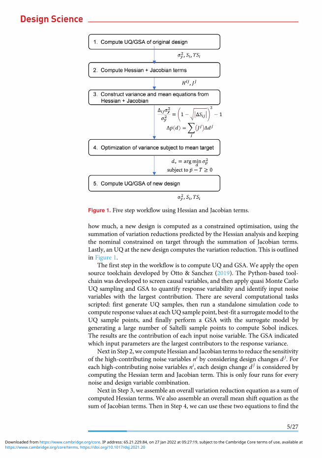
how much, a new design is computed as a constrained optimisation, using thesummation of variation reductions predicted by the Hessian analysis and keepingthe nominal constrained on target through the summation of Jacobian terms.Lastly, an UQ at the new design computes the variation reduction. This is outlinedin Figure 1.

The first step in the workflow is to compute UQ and GSA. We apply the opensource toolchain developed by Otto & Sanchez (2019). The Python-based tool-chain was developed to screen causal variables, and then apply quasi Monte CarloUQ sampling and GSA to quantify response variability and identify input noisevariables with the largest contribution. There are several computational tasksscripted: first generate UQ samples, then run a standalone simulation code tocompute response values at eachUQ sample point, best-fit a surrogatemodel to theUQ sample points, and finally perform a GSA with the surrogate model bygenerating a large number of Saltelli sample points to compute Sobol indices.The results are the contribution of each input noise variable. The GSA indicatedwhich input parameters are the largest contributors to the response variance.

Next in Step 2, we computeHessian and Jacobian terms to reduce the sensitivityof the high-contributing noise variables ni by considering design changes d j. Foreach high-contributing noise variables ni, each design change d j is considered bycomputing the Hessian term and Jacobian term. This is only four runs for everynoise and design variable combination.

Next in Step 3, we assemble an overall variation reduction equation as a sum ofcomputed Hessian terms. We also assemble an overall mean shift equation as thesum of Jacobian terms. Then in Step 4, we can use these two equations to find the

Figure 1. Five step workflow using Hessian and Jacobian terms.

5/27

https://www.cambridge.org/core/terms. https://doi.org/10.1017/dsj.2021.20Downloaded from https://www.cambridge.org/core. IP address: 65.21.229.84, on 27 Jan 2022 at 05:27:19, subject to the Cambridge Core terms of use, available at

changes to the design variables that minimise the variation subject to the meanfixed to a target. Lastly in Step 5, we recompute the UQ/GSA at the new values ofthe design variables. This confirms the variation reduction and the targeting of themean response.We next derive theseHessian and Jacobian terms and optimisationequations.

2.2. UQ and GSA

We consider here when anUQhas been computed for the initial design. That is, fora selection of noise variables, a sample was generated and at each sample point theresponse evaluated, resulting in a histogram of response values. A distributionfunction with statistics against distribution parameters is fit, for example, a normaldistribution function withmean and variance statistics. Nomatter the distribution,we consider the variance statistic σ2y as a statistic of interest on the response y.

We also then consider the GSA of the total response variance σ2y . FollowingSaltelli et al. (2008), we decompose the total response variance into variancecontributors of the noise variables ni. The main effect Vi of a noise variable ni isthe response variance fraction due to the noise variable alone, also expressed as apercentage as the Sobol Sensitivity Index Si. Higher order effects such as a two-wayinteraction, Vi1i2 is the response variance fraction due to both inputs varying.That is,

σ2y =Xi

ViþXi1<i2

Vi1i2 þ⋯þX

i1<i2<⋯<N

Vi1⋯N , (1)

and Vi is the main effect response variance contribution of ni and the others arehigher order effects. From Equation (1), we can compute Si to indicate the maineffect contribution of ni. Another useful metric is the Sobol Total Sensitivity IndexTSi which computes the effect of all interactions for a noise variable ni as apercentage contributions of the total response variation σ2y . That is,

Si =Vi

σ2y, (2)

TSi = SiþðS1iþS2iþ…ÞþðS12iþS13iþ…Þþ⋯þX

i1<::i::<N

Si1::i::N : (3)

This UQ/GSA analysis forms the first step of a proposed robust design variationreduction workflow. With this, the initial design concept variability is quantified(σ2y) and the noise variables which contribute most are identified (those with largeSi). We now seek to find design variables that can reduce the impact of noisevariables with large impact.

2.3. Hessian cross terms

To study the impact of changes to different design variables, we consider theHessian matrix cross terms of the variance-contributing noise variables andthe design variables of any proposed design changes. Hessian terms will showthe influence that design variable changes have over the uncertainty contribution

6/27

https://www.cambridge.org/core/terms. https://doi.org/10.1017/dsj.2021.20Downloaded from https://www.cambridge.org/core. IP address: 65.21.229.84, on 27 Jan 2022 at 05:27:19, subject to the Cambridge Core terms of use, available at

of noise variables. To see this, consider a Taylor Series expansion of the response atthe current nominal,

y= f d,nð Þ= y0þ∂f∂n

n�n0ð Þ: (4)

Typically, we compute this only for the large noise variables contributors ni. Nowconsider a design variable d j for any proposed design change. We could make thechange and recompute the UQ or similar. However, if d j changes the UQ, it mustbe because d j changed the impact of the contributing ni. That is, the sensitivityterm ∂f

∂n changed. Therefore, a nonzero Hessian term indicates a d j can change thenoise variable’s variability influence on the response at a nominal design d0,n0ð Þ:

Find d j such that∂

∂d j

∂

∂nif d,nð Þ d0,n0 6¼ 0:j (5)

Hence, to quickly compute how effective any design variable is at reducingresponse variability, one can compute the Hessian cross terms of design and noisevariables denoted by

Hij =∂

∂d j

∂f∂ni

=∂2f

∂d j∂ni

, (6)

and search which design variables d j cause a significant change to the sensitivityterm ∂f

∂ni .Consider for the moment noise variables with symmetric uncertainty such as a

normal distribution and design variables which can be optimised through eitherincreasing or decreasing changes. Then one can use a central finite-differenceapproximation with perturbations hi on a noise variable ni and h j on a designvariable d j. We define the differences of a design or noise variable from nominaldo,nð Þ as

d j� = d j0�h j d j� = d j

0þh j,

ni� = ni�hi niþ = niþhi:(7)

The Hessian cross terms can be numerically computed as the central differencecross term change in response value:

Hij =f d jþ,niþ� �� f d jþ,ni�

� �� �� f d j�,niþ� �� f d j�,ni�

� �� �4hih j

: (8)

From the engineering perspective of variation reduction from design changes, it iseasier to interpret Hij with the sign of Hij only indicating the directionality of thedesign change and not the noise variable change.We therefore apply absolute valueto the noise factor differences since it is inconsequential if f is increasing ordecreasing with changes to ni, and it is very consequential to the differences withchanges to d j. That is,

Hij =f d jþ,niþ� �� f d jþ,ni�

� ��� ��� f d j�,niþ� �� f d j�,ni�

� ��� ��4hih j

: (9)

The absolute values thereby provide the computedHij effective sign in engineeringterms, a negative Hij indicates variance reduction with increases in d j and a

7/27

https://www.cambridge.org/core/terms. https://doi.org/10.1017/dsj.2021.20Downloaded from https://www.cambridge.org/core. IP address: 65.21.229.84, on 27 Jan 2022 at 05:27:19, subject to the Cambridge Core terms of use, available at

positive Hij indicates variance reduction with decreases in d j. Each Hij cantherefore be interpreted in engineering terms as the amount of variation changepossible by making the design variable shift from d� to dþ, for the performancevariation due to the noise variable variation range of n� to nþ.

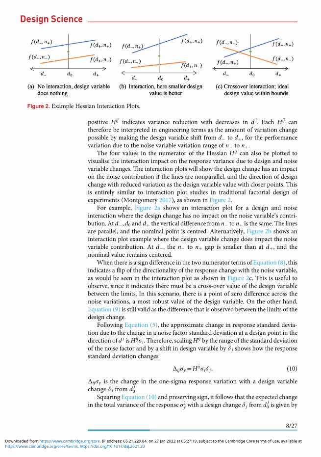
The four values in the numerator of the Hessian Hij can also be plotted tovisualise the interaction impact on the response variance due to design and noisevariable changes. The interaction plots will show the design change has an impacton the noise contribution if the lines are nonparallel, and the direction of designchange with reduced variation as the design variable value with closer points. Thisis entirely similar to interaction plot studies in traditional factorial design ofexperiments (Montgomery 2017), as shown in Figure 2.

For example, Figure 2a shows an interaction plot for a design and noiseinteraction where the design change has no impact on the noise variable’s contri-bution. At d�, d0 and dþ the vertical difference from n� to nþ is the same. The linesare parallel, and the nominal point is centred. Alternatively, Figure 2b shows aninteraction plot example where the design variable change does impact the noisevariable contribution. At d�, the n� to nþ gap is smaller than at dþ, and thenominal value remains centered.

When there is a sign difference in the two numerator terms of Equation (8), thisindicates a flip of the directionality of the response change with the noise variable,as would be seen in the interaction plot as shown in Figure 2c. This is useful toobserve, since it indicates there must be a cross-over value of the design variablebetween the limits. In this scenario, there is a point of zero difference across thenoise variations, a most robust value of the design variable. On the other hand,Equation (9) is still valid as the difference that is observed between the limits of thedesign change.

Following Equation (5), the approximate change in response standard devia-tion due to the change in a noise factor standard deviation at a design point in thedirection of d j isHijσi. Therefore, scalingHij by the range of the standard deviationof the noise factor and by a shift in design variable by δ j shows how the responsestandard deviation changes

Δijσy =Hijσiδ j: (10)

Δijσy is the change in the one-sigma response variation with a design variablechange δ j from d j

0.Squaring Equation (10) and preserving sign, it follows that the expected change

in the total variance of the response σ2y with a design change δ j from d j0 is given by

Figure 2. Example Hessian Interaction Plots.

8/27

https://www.cambridge.org/core/terms. https://doi.org/10.1017/dsj.2021.20Downloaded from https://www.cambridge.org/core. IP address: 65.21.229.84, on 27 Jan 2022 at 05:27:19, subject to the Cambridge Core terms of use, available at

Δijσy� �2 = σ2i H

ijδ j

�� �� Hijδ j� �

: (11)

Equation (11) includes the absolute value form to preserve directionality of thedesign change. A negative Δijσy

� �2indicates making a positive δ j change to

nominal design variable d j0 towards dþ will reduce noise variable ni contribution

to response variance, whereas a positive Δijσy� �2

indicates making a negative δ j

change towards d� will reduce noise variable ni contribution to response variance.By definition of Si as the normalised variance, dividing Δijσy

� �2by the UQ total

variance σ2y results in the expected change in a noise variable’s Sobol index Si by adesign variable d j changes. This provides a more informative percentage change.Therefore, the expected change in a noise variable’s Sobol index ΔSij by making adesign change from nominal is computed as

ΔSij =σ2iσ2y

Hijδ j

�� �� Hijδ j� �

: (12)

A large value of ΔSij indicates changing towards d jþ increases Si by ΔSij(a possibly negative amount) and that changing to d j� decreases Si by ΔSij (againa possibly negative amount). Thus, whatever the sign of ΔSij is, you would changed j in the opposite direction to achieve a reduction in Si.

The impact of any oneΔSij change to a Sobol index does not simply scale σ2y, forexample, a 10% change in Si does not mean a 10% change in σ2y . This is becauseΔS= σnew�σoldð Þ2=σ2old, so rather the change in σ2y from a variation reducingdesign change δ j can be computed as

σ2new�σ2oldσ2old

=Δijσ2yσ2y

= 1�ffiffiffiffiffiffiffiffiffiffiffiΔSij�� ��q� �2

�1: (13)

Further, the overall change in the Sobol indices to multiple design variableschanged in the direction of reducing variance is the sum over the design changes,

ΔSi =1σ2y

Xj

Hijσiδ j

!2

: (14)

Similarly for a set of noise variables, the overall change in the sum of a set ofSobol indices from M noise variables is a sum. However, each noise term iscomputed with the noise variable value set at a number of standard deviationsfrom nominal, and so to maintain that over multiple noise variables the sum needsto be reduced by the square root of the number of noise factors summed. That is,

ΔS j =1

Mσ2y

Xi

Hijσiδ j

!2

: (15)

Then the new response variance due to multiple design variables changed in thedirection of reducing variance is computed as before using Equation (13).

2.4. Central, forward and backward differencing

The central differencing derivation of Equation (9) is not adequate in all cases. Forexample, not all noise and design variables can be changed in both positive and

9/27

https://www.cambridge.org/core/terms. https://doi.org/10.1017/dsj.2021.20Downloaded from https://www.cambridge.org/core. IP address: 65.21.229.84, on 27 Jan 2022 at 05:27:19, subject to the Cambridge Core terms of use, available at

negative directions. For example, geometric tolerance variations such as flatness,roundness, concentricity and so on, have only positive variations from a desirednominal of zero. Further, some noise variations are nonmonotonic and causeincreasing performance drift with either a positive or negative input variation. Forexample, mis-alignments can cause worse performance with any deviation fromnominal, positive or negative. These noise variables should therefore not be studiedwith central differencing. Similarly, certain design variables may only have feasibleincreases or only feasible decreases. With these variables, forward or backwarddifferencing is needed, with associated changes to Equation (9).

Consider noise variables which can only be positive, the only allowed values arein the domain nio,n

iþ

� . Then Equation (9) becomes

Hij =f d jþ,niþ� �� f d jþ,ni0

� ��� ��� f d j�,niþ� �� f d j�,ni0

� ��� ��2hih j

, (16)

which is a combination of central differencing on d j and forward differencing onni. Similarly, Equation (9) would switch for design variables which can only bepositive and noise variables which can be negative or positive,

Hij =f d jþ,niþ� �� f d jþ,ni�

� ��� ��� f d j0,niþ� �� f d j0,ni�

� ��� ��2hih j

: (17)

And similarly for a selection of design and noise variables neither of which can benegative becomes

Hij =f d jþ,niþ� �� f d jþ,ni0

� ��� ��� f d j0,niþ� �� f d j0,ni0

� ��� ��hih j

: (18)

For the variable types that cannot use the central differencing Hessianapproach, the Hessian-indicated variation reduction using central differencingwould not materialise when the design variable is changed and a new UQ isexecuted at the new design. Further, the central differencing Hessian term alonewill not identify when this is the case.

Instead, additional checks are needed to highlight when the central differencingform Equation (9) needs expansion with additional runs using Equations (1–1). Toidentify such cases where central differencing fails, the Hessian numerator termsmust be compared with the nominal value result y0 = f d0,n0ð Þ. If the y0 value is notbounded by the Hessian terms, there is a nonmonotonic quadratic nature to theresponse f . This is well known in traditional factorial experimentation(Montgomery 2017) and applies equally here. So instead of just four Hessianpoints to evaluate f , one should also include the nominal value point and ensure thenominal falls within the bounds of the Hessian points. This is shown as interactionplots in Figure 3.

When the nominal value falls outside of the Hessian term response values, thecentral differencing domain must be split into two regimes, the upper and lowerrange on either d j, ni or both. Typically, an engineer expects quadratic behaviour ofcertain variables andwhether the cause is from the d j, ni or both can be self-stated apriori. Whichever it is, the four central differenced Hessian points must beaugmented with two more axial points on that variable. Then backward differenc-ing is used between the negative points and nominal points, and forward

10/27

https://www.cambridge.org/core/terms. https://doi.org/10.1017/dsj.2021.20Downloaded from https://www.cambridge.org/core. IP address: 65.21.229.84, on 27 Jan 2022 at 05:27:19, subject to the Cambridge Core terms of use, available at

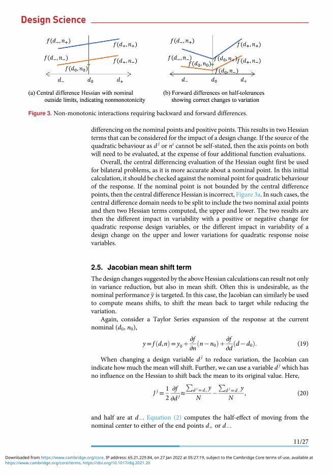
differencing on the nominal points and positive points. This results in two Hessianterms that can be considered for the impact of a design change. If the source of thequadratic behaviour as d j or ni cannot be self-stated, then the axis points on bothwill need to be evaluated, at the expense of four additional function evaluations.

Overall, the central differencing evaluation of the Hessian ought first be usedfor bilateral problems, as it is more accurate about a nominal point. In this initialcalculation, it should be checked against the nominal point for quadratic behaviourof the response. If the nominal point is not bounded by the central differencepoints, then the central difference Hessian is incorrect, Figure 3a. In such cases, thecentral difference domain needs to be split to include the two nominal axial pointsand then two Hessian terms computed, the upper and lower. The two results arethen the different impact in variability with a positive or negative change forquadratic response design variables, or the different impact in variability of adesign change on the upper and lower variations for quadratic response noisevariables.

2.5. Jacobian mean shift term

The design changes suggested by the aboveHessian calculations can result not onlyin variance reduction, but also in mean shift. Often this is undesirable, as thenominal performance y is targeted. In this case, the Jacobian can similarly be usedto compute means shifts, to shift the mean back to target while reducing thevariation.

Again, consider a Taylor Series expansion of the response at the currentnominal (d0, n0),

y= f d,nð Þ= y0þ∂f∂n

n�n0ð Þþ ∂f∂d

d�d0ð Þ: (19)

When changing a design variable d j to reduce variation, the Jacobian canindicate howmuch the mean will shift. Further, we can use a variable d j which hasno influence on the Hessian to shift back the mean to its original value. Here,

J j =12∂f

∂d j≈P

d j = dþy

N�P

d j = d�y

N, (20)

and half are at d�. Equation (2) computes the half-effect of moving from thenominal center to either of the end points dþ or d�.

Figure 3. Non-monotonic interactions requiring backward and forward differences.

11/27

https://www.cambridge.org/core/terms. https://doi.org/10.1017/dsj.2021.20Downloaded from https://www.cambridge.org/core. IP address: 65.21.229.84, on 27 Jan 2022 at 05:27:19, subject to the Cambridge Core terms of use, available at

The overall change in responsemean is then approximately a linear summationof the design variable changes,

Δp dð Þ=Xj

J j� �

Δd j, (21)

where again Δd j is the amount of change to d j in a new design configurationconsidered.

In combination with the variation reduction as computed by Equation (13) andthe mean shift as computed by Equation (21), one can select design variablechanges to reduce the variation while constraining the mean to a target. Designvariables that reduce variation can be determined and set using Equation (13). Theassociated mean shift from those changes can be computed using Equation (21),and different design variables changed to shift the mean back to the desired target.In this way, variation can be minimised subject to a constrained mean. Further-more, the reasons for the variation reduction are made explicit. The identifieddesign variables that can reduce the impact of identified noise variables will beclear, rather than a black box experimental optimisation approach.

3. Stirling engine design exampleIn previous work, (Otto & Sanchez 2019; Otto, Wang, & Uyan 2019) workflowswere developed applying UQ and GSA methods to identify root causes ofmanufacturing quality problems and in Sanchez, Björkman, & Otto (2020), aworkflow was developed using design of experiments to achieve robustnessimprovement, and in Sanchez Mosqueda & Otto (2021), we introduced usingHessian terms. Here, we build on these previous works to now consider the greaterinsight and fewer runs offered by the Hessian approach and in conjunction withcompounded variables.

3.1. Stirling engine case study

In these previous works, we introduced the example of aminiature Stirling enginecase study. At Aalto University students fabricated, assembled and tested Stirlingengines as part of the senior level machine design course. Students measured thespeed at which the crank shaft rotates when there is no torque load applied, theno-load speed. The no-load speed tests demonstrated 25% variation in speedacross the fabricated engines, due to variations in fabrication. This outcomeexposed the high sensitivity of the Stirling engine to manufacturing and assemblyvariations. Here, we follow the approach of Figure 1 to explore if the variability ofthe design could be reduced through parametric design changes. We also com-pare the insights and speed of the approach with traditional robustness optimi-sation.

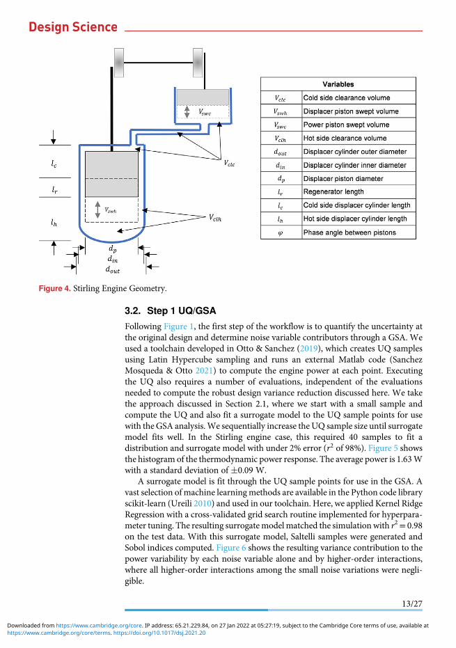
The geometric input variables of the Stirling engine are shown in Figure 4.There is a hot side cylinder heated externally with a transfer piston that exchangesair from the hot side to the cold side. There is a cold-side power cylinder and pistonthat extracts mechanical power from the air as it expands and contracts due to thetransfer pistonmovement. The pistons are connected by a shaft with an offset angleof 90°.

12/27

https://www.cambridge.org/core/terms. https://doi.org/10.1017/dsj.2021.20Downloaded from https://www.cambridge.org/core. IP address: 65.21.229.84, on 27 Jan 2022 at 05:27:19, subject to the Cambridge Core terms of use, available at

3.2. Step 1 UQ/GSA

Following Figure 1, the first step of the workflow is to quantify the uncertainty atthe original design and determine noise variable contributors through a GSA. Weused a toolchain developed in Otto & Sanchez (2019), which creates UQ samplesusing Latin Hypercube sampling and runs an external Matlab code (SanchezMosqueda & Otto 2021) to compute the engine power at each point. Executingthe UQ also requires a number of evaluations, independent of the evaluationsneeded to compute the robust design variance reduction discussed here. We takethe approach discussed in Section 2.1, where we start with a small sample andcompute the UQ and also fit a surrogate model to the UQ sample points for usewith the GSA analysis.We sequentially increase the UQ sample size until surrogatemodel fits well. In the Stirling engine case, this required 40 samples to fit adistribution and surrogate model with under 2% error (r2 of 98%). Figure 5 showsthe histogram of the thermodynamic power response. The average power is 1.63Wwith a standard deviation of �0.09 W.

A surrogate model is fit through the UQ sample points for use in the GSA. Avast selection of machine learningmethods are available in the Python code libraryscikit-learn (Ureili 2010) and used in our toolchain. Here, we applied Kernel RidgeRegression with a cross-validated grid search routine implemented for hyperpara-meter tuning. The resulting surrogatemodelmatched the simulation with r2= 0.98on the test data. With this surrogate model, Saltelli samples were generated andSobol indices computed. Figure 6 shows the resulting variance contribution to thepower variability by each noise variable alone and by higher-order interactions,where all higher-order interactions among the small noise variations were negli-gible.

Figure 4. Stirling Engine Geometry.

13/27

https://www.cambridge.org/core/terms. https://doi.org/10.1017/dsj.2021.20Downloaded from https://www.cambridge.org/core. IP address: 65.21.229.84, on 27 Jan 2022 at 05:27:19, subject to the Cambridge Core terms of use, available at

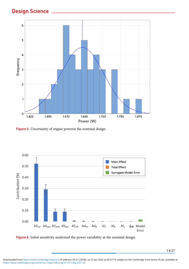
Figure 5. Uncertainty of engine powerat the nominal design.

Figure 6. Sobol sensitivity analysisof the power variability at the nominal design.

14/27

https://www.cambridge.org/core/terms. https://doi.org/10.1017/dsj.2021.20Downloaded from https://www.cambridge.org/core. IP address: 65.21.229.84, on 27 Jan 2022 at 05:27:19, subject to the Cambridge Core terms of use, available at

The GSA indicates variation of the cold-side clearance volume, outer transfercylinder diameter, swept volume of the expansion piston and swept volume of thecompression piston as the largest contributors to power variability.

3.3. Unconstrained minimisation

The second step in the workflow is to construct Hessian cross terms to quicklycompute the effect of any design change on reducing contributions to responsevariability. First, design variables are proposed. We make use of input volumetricvariables compounded from dimensional geometry of the engine. Clearance andswept volumes from compression and expansion sides V clc,V swc,V clh andV swhð Þwere selected as design variables d j. From the GSA the largest contributors toengine power variability were ΔV clc,ΔV swc,ΔV swh andΔdoutð Þ and so used asnoise variables ni. Then �4σ ranges were defined for the noise variables and areasonable �20% range of optimisation for the design variables.

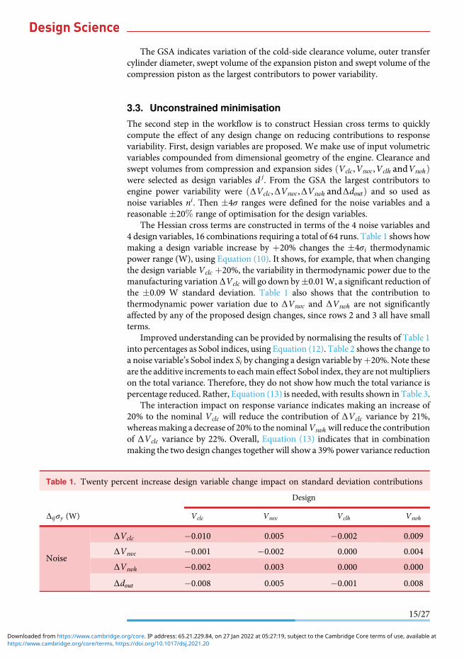
The Hessian cross terms are constructed in terms of the 4 noise variables and4 design variables, 16 combinations requiring a total of 64 runs. Table 1 shows howmaking a design variable increase by þ20% changes the �4σi thermodynamicpower range (W), using Equation (10). It shows, for example, that when changingthe design variable V clc þ20%, the variability in thermodynamic power due to themanufacturing variationΔV clc will go down by�0.01W, a significant reduction ofthe �0.09 W standard deviation. Table 1 also shows that the contribution tothermodynamic power variation due to ΔV swc and ΔV swh are not significantlyaffected by any of the proposed design changes, since rows 2 and 3 all have smallterms.

Improved understanding can be provided by normalising the results of Table 1into percentages as Sobol indices, using Equation (12). Table 2 shows the change toa noise variable’s Sobol index Si by changing a design variable byþ20%. Note theseare the additive increments to eachmain effect Sobol index, they are notmultiplierson the total variance. Therefore, they do not show how much the total variance ispercentage reduced. Rather, Equation (13) is needed, with results shown in Table 3.

The interaction impact on response variance indicates making an increase of20% to the nominal V clc will reduce the contribution of ΔVclc variance by 21%,whereasmaking a decrease of 20% to the nominalV swh will reduce the contributionof ΔVclc variance by 22%. Overall, Equation (13) indicates that in combinationmaking the two design changes together will show a 39% power variance reduction

Table 1. Twenty percent increase design variable change impact on standard deviation contributions

Δijσy (W)

Design

Vclc V swc V clh V swh

Noise

ΔV clc �0.010 0.005 �0.002 0.009

ΔV swc �0.001 �0.002 0.000 0.004

ΔV swh �0.002 0.003 0.000 0.000

Δdout �0.008 0.005 �0.001 0.008

15/27

https://www.cambridge.org/core/terms. https://doi.org/10.1017/dsj.2021.20Downloaded from https://www.cambridge.org/core. IP address: 65.21.229.84, on 27 Jan 2022 at 05:27:19, subject to the Cambridge Core terms of use, available at

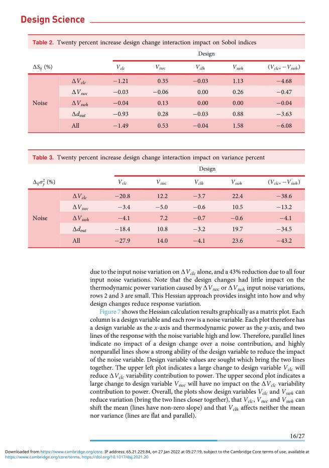
due to the input noise variation onΔV clc alone, and a 43% reduction due to all fourinput noise variations. Note that the design changes had little impact on thethermodynamic power variation caused byΔV swc orΔV swh input noise variations,rows 2 and 3 are small. This Hessian approach provides insight into how and whydesign changes reduce response variation.

Figure 7 shows theHessian calculation results graphically as amatrix plot. Eachcolumn is a design variable and each row is a noise variable. Each plot therefore hasa design variable as the x-axis and thermodynamic power as the y-axis, and twolines of the response with the noise variable high and low. Therefore, parallel linesindicate no impact of a design change over a noise contribution, and highlynonparallel lines show a strong ability of the design variable to reduce the impactof the noise variable. Design variable values are sought which bring the two linestogether. The upper left plot indicates a large change to design variable V clc willreduce ΔV clc variability contribution to power. The upper second plot indicates alarge change to design variable V swc will have no impact on the ΔV clc variabilitycontribution to power. Overall, the plots show design variables Vclc and V swh canreduce variation (bring the two lines closer together), that Vclc, V swc and V swh canshift the mean (lines have non-zero slope) and that V clh affects neither the meannor variance (lines are flat and parallel).

Table 2. Twenty percent increase design change interaction impact on Sobol indices

ΔSij (%)

Design

Vclc V swc Vclh V swh (V clc, �V swh)

Noise

ΔV clc �1.21 0.35 �0.03 1.13 �4.68

ΔV swc �0.03 �0.06 0.00 0.26 �0.47

ΔV swh �0.04 0.13 0.00 0.00 �0.04

Δdout �0.93 0.28 �0.03 0.88 �3.63

All �1.49 0.53 �0.04 1.58 �6.08

Table 3. Twenty percent increase design change interaction impact on variance percent

Δijσ2y (%)

Design

Vclc V swc Vclh V swh (V clc, �V swh)

Noise

ΔV clc �20.8 12.2 �3.7 22.4 �38.6

ΔV swc �3.4 �5.0 �0.6 10.5 �13.2

ΔV swh �4.1 7.2 �0.7 �0.6 �4.1

Δdout �18.4 10.8 �3.2 19.7 �34.5

All �27.9 14.0 �4.1 23.6 �43.2

16/27

https://www.cambridge.org/core/terms. https://doi.org/10.1017/dsj.2021.20Downloaded from https://www.cambridge.org/core. IP address: 65.21.229.84, on 27 Jan 2022 at 05:27:19, subject to the Cambridge Core terms of use, available at

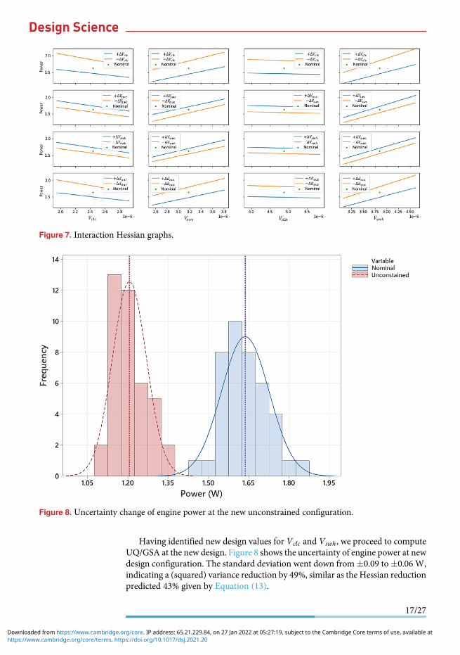
Having identified new design values for V clc and V swh, we proceed to computeUQ/GSA at the new design. Figure 8 shows the uncertainty of engine power at newdesign configuration. The standard deviation went down from�0.09 to�0.06 W,indicating a (squared) variance reduction by 49%, similar as the Hessian reductionpredicted 43% given by Equation (13).

Figure 7. Interaction Hessian graphs.

Figure 8. Uncertainty change of engine power at the new unconstrained configuration.

17/27

https://www.cambridge.org/core/terms. https://doi.org/10.1017/dsj.2021.20Downloaded from https://www.cambridge.org/core. IP address: 65.21.229.84, on 27 Jan 2022 at 05:27:19, subject to the Cambridge Core terms of use, available at

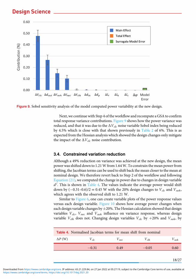
Next, we continue with Step 4 of the workflow and recompute aGSA to confirmtotal response variance contributions. Figure 9 shows how the power variance wasreduced, and that it was due to the ΔV clc noise variable Sobol index being reducedby 4.5% which is close with that shown previously in Table 2 of 6%. This is asexpected from theHessian analysis which showed the design changes onlymitigatethe impact of the ΔV clc noise contribution.

3.4. Constrained variation reduction

Although a 49% reduction on variance was achieved at the new design, the meanpowerwas shifted down to 1.21W from1.64W.To constrain themean power fromshifting, the Jacobian terms can be used to shift back themean closer to themean atnominal design. We therefore revert back to Step 2 of the workflow and followingEquation (21), we computed the change in power due to changes in design variabled j. This is shown in Table 4. The values indicate the average power would shiftdown by (�0.31–0.6)/2 = 0.45 W with the 20% design changes to V clc and V swh,which agrees with the observed shift to 1.21 W.

Similar to Figure 6, one can create variable plots of the power response valuesversus each design variable. Figure 10 shows how average power changes wheneach design variable changes by�20%. TheHessian calculation showed that designvariables Vclc, V swc and V swh influence on variance response, whereas designvariable V clh does not. Changing design variables V clc by þ20% and V swh, by

Figure 9. Sobol sensitivity analysis of the model computed power variability at the new design.

Table 4. Normalised Jacobian terms for mean shift from nominal

ΔP (W) Vclc V swc Vclh V swh

�0.31 0.49 �0.05 0.60

18/27

https://www.cambridge.org/core/terms. https://doi.org/10.1017/dsj.2021.20Downloaded from https://www.cambridge.org/core. IP address: 65.21.229.84, on 27 Jan 2022 at 05:27:19, subject to the Cambridge Core terms of use, available at

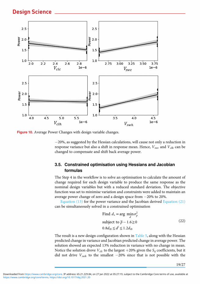
�20%, as suggested by the Hessian calculations, will cause not only a reduction inresponse variance but also a shift in response mean. Hence, V swc and Vclh can bechanged to compensate and shift back average power.

3.5. Constrained optimisation using Hessians and Jacobianformulas

The Step 4 in the workflow is to solve an optimisation to calculate the amount ofchange required for each design variable to produce the same response as thenominal design variables but with a reduced standard deviation. The objectivefunction was set to minimise variation and constraints were added to maintain anaverage power change of zero and a design space from �20% to 20%.

Equation (13) for the power variance and the Jacobian derived Equation (21)can be simultaneously solved in a constrained optimisation

Find d∗ = arg mind

σ2p

subject to p�1:6≥0

0:8di0 ≤ di ≤ 1:2di0

(22)

The result is a new design configuration shown in Table 5, along with the Hessianpredicted change in variance and Jacobian predicted change in average power. Thesolution showed an expected 13% reduction in variance with no change in mean.Notice the solution drove Vclc to the largest þ20% given the Sij coefficients, but itdid not drive V swh to the smallest �20% since that is not possible with the

Figure 10. Average Power Changes with design variable changes.

19/27

https://www.cambridge.org/core/terms. https://doi.org/10.1017/dsj.2021.20Downloaded from https://www.cambridge.org/core. IP address: 65.21.229.84, on 27 Jan 2022 at 05:27:19, subject to the Cambridge Core terms of use, available at

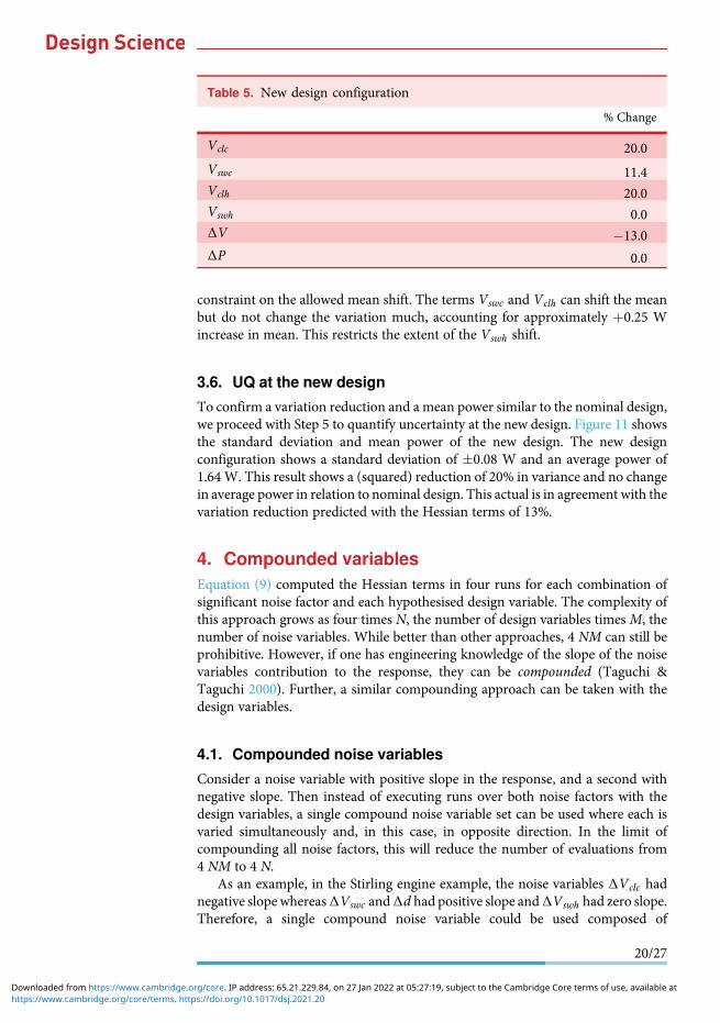
constraint on the allowed mean shift. The terms V swc and V clh can shift the meanbut do not change the variation much, accounting for approximately þ0.25 Wincrease in mean. This restricts the extent of the V swh shift.

3.6. UQ at the new design

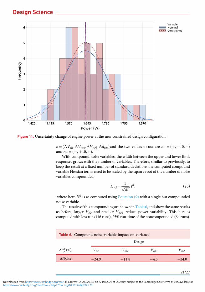
To confirm a variation reduction and a mean power similar to the nominal design,we proceed with Step 5 to quantify uncertainty at the new design. Figure 11 showsthe standard deviation and mean power of the new design. The new designconfiguration shows a standard deviation of �0.08 W and an average power of1.64W. This result shows a (squared) reduction of 20% in variance and no changein average power in relation to nominal design. This actual is in agreement with thevariation reduction predicted with the Hessian terms of 13%.

4. Compounded variablesEquation (9) computed the Hessian terms in four runs for each combination ofsignificant noise factor and each hypothesised design variable. The complexity ofthis approach grows as four times N, the number of design variables timesM, thenumber of noise variables. While better than other approaches, 4 NM can still beprohibitive. However, if one has engineering knowledge of the slope of the noisevariables contribution to the response, they can be compounded (Taguchi &Taguchi 2000). Further, a similar compounding approach can be taken with thedesign variables.

4.1. Compounded noise variables

Consider a noise variable with positive slope in the response, and a second withnegative slope. Then instead of executing runs over both noise factors with thedesign variables, a single compound noise variable set can be used where each isvaried simultaneously and, in this case, in opposite direction. In the limit ofcompounding all noise factors, this will reduce the number of evaluations from4 NM to 4 N.

As an example, in the Stirling engine example, the noise variables ΔV clc hadnegative slope whereasΔV swc andΔd had positive slope andΔV swh had zero slope.Therefore, a single compound noise variable could be used composed of

Table 5. New design configuration

% Change

V clc 20.0

V swc 11.4V clh 20.0V swh 0.0ΔV �13.0

ΔP 0.0

20/27

https://www.cambridge.org/core/terms. https://doi.org/10.1017/dsj.2021.20Downloaded from https://www.cambridge.org/core. IP address: 65.21.229.84, on 27 Jan 2022 at 05:27:19, subject to the Cambridge Core terms of use, available at

n= ΔVclc,ΔV swc,ΔV swh,Δdoutð Þand the two values to use are n� = þ, � ,0,�ð Þand nþ = �, þ ,0,þð Þ.

With compound noise variables, the width between the upper and lower limitresponses grows with the number of variables. Therefore, similar to previously, tokeep the result at a fixed number of standard deviations the computed compoundvariable Hessian terms need to be scaled by the square root of the number of noisevariables compounded,

Hn,j =1ffiffiffiffiffiM

p Hij, (23)

where here Hij is as computed using Equation (9) with a single but compoundednoise variable.

The results of this compounding are shown inTable 6, and show the same resultsas before, larger Vclc and smaller V swh reduce power variability. This here iscomputed with less runs (16 runs), 25% run-time of the noncompounded (64 runs).

Figure 11. Uncertainty change of engine power at the new constrained design configuration.

Table 6. Compound noise variable impact on variance

Δσ2y (%)

Design

Vclc V swc Vclh V swh

ΔNoise �24.9 �11.8 �4.5 �24.0

21/27

https://www.cambridge.org/core/terms. https://doi.org/10.1017/dsj.2021.20Downloaded from https://www.cambridge.org/core. IP address: 65.21.229.84, on 27 Jan 2022 at 05:27:19, subject to the Cambridge Core terms of use, available at

In the workflow of Figure 1, compounding noise variables is an easy simplifi-cation to make, since in the first step a UQ is performed and the results can beplotted against each noise variable and the nominal slope direction determined.

On the other hand, while reducing calculations, the noise factor compoundingalso reduces information provided. It is not clearly highlightedwhich Sobol index isbeing reduced, and therefore which noise factor contribution in the compoundedvariable is being reduced.While it is highlighted the response variance is reduced, itis not highlighted that the reductions are contributions from noise factors ΔV clcand Δdout being reduced. It is not highlighted that the contributions from noisefactors ΔV swc or ΔV swh are negligibly changed. Overall, compounding is moreefficient, but at the expense of less engineering insight on how the design changesare impacting which noise factor contributions.

4.2. Compounded design variables

Similar to noise variables, design variables can also be compounded. Unlike withnoise variables, though, doing so requires a priori engineering knowledge of howthe response changes with design variable changes. As with noise factors, if twodesign variables have the same slope, they can be varied the same, and if they haveopposite slopes they can be varied in opposition.

For example, with the Stirling engine we may have knowledge that decreases inthe cold side volume V clc reduces power, and increasing the swept volume V swhincreases power. These could be varied as a single design variable d= V clc,V swhð Þ.Then the compounded values would be d� = þ,�ð Þ and dþ = �:þð Þ. The resultsof this are shown in Table 7, larger V clc and smaller V swh reduce power variability,and impact the ΔV clc and Δdout noise contributions most. This is similar to ascomputed before but with less runs, (16 runs), 25% run-time of the noncom-pounded (64 runs).

In the workflow of Figure 1, there are no steps to provide any indication on howto compound design variables. Without a-priori knowledge, one factor at a timeruns could be done (axial points), but at added expense of more evaluations.

Finally, notice that if it were possible to be equipped with a priori knowledge ofboth design and noise variable directionality then all variables could be com-pounded, on both the design and noise variables. This reduces the entire 4 NM setof runs down to a mere four runs. The sign of the one term of Equation (9) wouldindicate which direction to change the compound design variable to reducevariability from the compounded noise variables.

Table 7. Compound design variable impact on variance

Δσ2y (%) Design

ΔV clc �28.5

ΔV swc �6.7ΔV swh �1.8

Δdout �18.3

22/27

https://www.cambridge.org/core/terms. https://doi.org/10.1017/dsj.2021.20Downloaded from https://www.cambridge.org/core. IP address: 65.21.229.84, on 27 Jan 2022 at 05:27:19, subject to the Cambridge Core terms of use, available at

For example, with the Stirling engine, compounding the noise variables into asingle compound noise variable and compounding the two V clc and V swh designvariables into a single compound design variable, the results of this are shown inTable 8, and compute most compactly the same as before. Making a 20% change tothe two design variables (Vclc larger and V swh smaller) reduces the variation fromthe four noise factors by 46%. This is similar to as computed earlier but with muchless evaluations (4 runs), 6% run time compared to the non-compounded(64 runs).

While one cannot compute constrained variation reduction of Equation (22),this compounded variable Hessian approach is nonetheless substantially moreefficient in comparison to many alternative optimisation formulations with exten-sive computational requirements. It does, however, require engineering knowledgeof how the noise and design variables change the response. In comparison to therich literature on probabilistic optimisation methods and robust design of exper-iments, it demonstrates a substantial limit case of computational simplificationsthat are possible in solving unconstrained variability minimisation. All otherknown probabilistic optimisation methods apply more than four evaluations.

5. Discussion: comparison with uncertaintyoptimisation

The approach successfully computed a new design with less variability, andsuccessfully found a new design with less variability constrained to target thenominal average power. Further, the approachmade use of only 64 runs to quantifythe individual impact potential of 4 design variable changes on the contributions of4 significantly contributing noise variables. Insight was provided that only two ofthe four most contributing noise variables can be impacted by the proposed designchanges.

The results can be compared against a more comprehensive exploration of thedesign and noise space using robust optimisation. In earlier work (Sanchez,Björkman, & Otto 2020) an RDM UQ minimisation approach was undertakenusing traditional surrogate-model probabilistic optimisation (Chen et al. 1996;Fang, Li, & Sudjianto 2005; Allen et al. 2006; Chen, Jin, & Sudjianto 2006; Jiang,Chen, & German 2016). One hundred sample points were used over the designspace and 40 sample points used in a UQ to cover the noise space. This resulted in4000 runs total. At each design space point, a 40-point UQ was executed and themean and variance of the power computed. The two statistics were computed ateach sample point in the design space, and surrogatemodels were fit. Then a Paretooptimisation was solved to show the best combinations of surrogate modelestimated mean and variance of power over the �20% domain of the design

Table 8. Compound design variable impact on compound noise variance

Δσ2y (%) Design

Noise �45.9

23/27

https://www.cambridge.org/core/terms. https://doi.org/10.1017/dsj.2021.20Downloaded from https://www.cambridge.org/core. IP address: 65.21.229.84, on 27 Jan 2022 at 05:27:19, subject to the Cambridge Core terms of use, available at

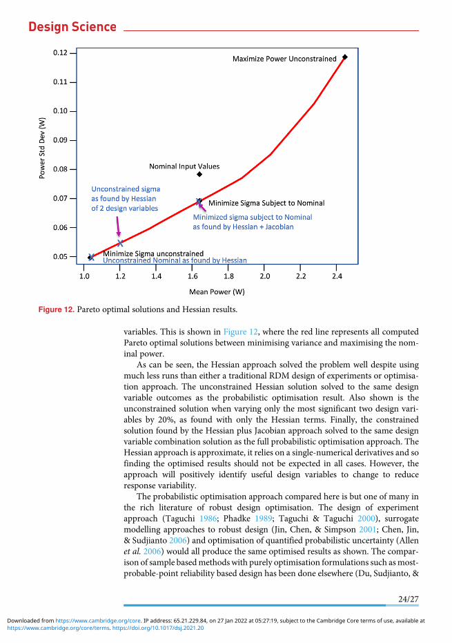
variables. This is shown in Figure 12, where the red line represents all computedPareto optimal solutions between minimising variance and maximising the nom-inal power.

As can be seen, the Hessian approach solved the problem well despite usingmuch less runs than either a traditional RDM design of experiments or optimisa-tion approach. The unconstrained Hessian solution solved to the same designvariable outcomes as the probabilistic optimisation result. Also shown is theunconstrained solution when varying only the most significant two design vari-ables by 20%, as found with only the Hessian terms. Finally, the constrainedsolution found by the Hessian plus Jacobian approach solved to the same designvariable combination solution as the full probabilistic optimisation approach. TheHessian approach is approximate, it relies on a single-numerical derivatives and sofinding the optimised results should not be expected in all cases. However, theapproach will positively identify useful design variables to change to reduceresponse variability.

The probabilistic optimisation approach compared here is but one of many inthe rich literature of robust design optimisation. The design of experimentapproach (Taguchi 1986; Phadke 1989; Taguchi & Taguchi 2000), surrogatemodelling approaches to robust design (Jin, Chen, & Simpson 2001; Chen, Jin,& Sudjianto 2006) and optimisation of quantified probabilistic uncertainty (Allenet al. 2006) would all produce the same optimised results as shown. The compar-ison of sample basedmethods with purely optimisation formulations such asmost-probable-point reliability based design has been done elsewhere (Du, Sudjianto, &

Figure 12. Pareto optimal solutions and Hessian results.

24/27

https://www.cambridge.org/core/terms. https://doi.org/10.1017/dsj.2021.20Downloaded from https://www.cambridge.org/core. IP address: 65.21.229.84, on 27 Jan 2022 at 05:27:19, subject to the Cambridge Core terms of use, available at

Chen 2004). Optimising quantified uncertainty has least approximations at theexpense of computational burden; surrogatemodelling introduces approximationsbut provides significant reductions in calculations. Design of experiments sim-plifies the calculations even further to regression models, with further approxima-tion.We here simplify even further to consideration ofmerely theHessian terms, atsignificant reduced calculations but also increased approximation.

As such, the Hessian approach here cannot determine an optimal solutionwhen the search function has multiple optima; the previously mentioned methodsought be considered. However, when a design engineer must compute theUQ/GSA for verification purposes, this approach also allows a rapid manner toidentify design variables to consider and their direction of change to reduceresponse variance.

Overall, we find the Hessian approach to variation reduction explorationintuitive and insightful. It allows one to quickly screen design variables for theirability to reduce response variance and with a clear indicator of how the designvariable is doing this variance reduction, in terms of interaction contributions ofsignificant noise variables.

6. ConclusionThe traditional and well-researched RDM has a wealth of research and techniquesto compute design changes that reduce performance variability. Such optimisationof uncertainty can sometimes become computationally difficult, whether throughdirect optimisation of quantified uncertainty as an objective function or throughTaguchi type robust design of experiments.

Here, we made use of the more easily computed Hessian matrix cross termsbetween the variance-contributing noise variables and the variables of anyproposed design changes. Design variable changes with large Hessian termsagainst noise variables are design changes that can reduce variability. Further,the Jacobian terms of these design changes can indicate which design variablescan shift the mean response, to maintain a desired performance target. Using acombination of the more easily computed Hessian and Jacobian terms, designchanges can be proposed to reduce variability while maintaining a targetednominal.

We relate here the Hessian predicted reductions to the associated reductions inSobol indices that indicate the percentage contribution of noise variables. We alsorelate these to the percentage reduction expected in the response variance. Thisallows for rapid interpretation of the impact of different design variable changes ina modern UQ/GSA optimisation workflow.

Themost basic industrial RDMworkflow is to estimate the variance of a designconcept, propose design changes and then estimate the reduced variance aftermaking the design changes. We applied this workflow to computational practicethrough UQ and GSA as a first and last step. An example was shown on a Stirlingengine design where the impact of the top three variance-contributing toleranceswere studied for variation reduction. The approach quickly identified two signif-icant design variables, and found a new design with 20% less variance and nochange in nominal average power. Overall, we find this Hessian-based RDMapproach useful for classes of problems with high-computational burdens.

25/27

https://www.cambridge.org/core/terms. https://doi.org/10.1017/dsj.2021.20Downloaded from https://www.cambridge.org/core. IP address: 65.21.229.84, on 27 Jan 2022 at 05:27:19, subject to the Cambridge Core terms of use, available at

AcknowledgementsThis work was made possible with support from the Academy of Finland, ProjectNumber 310252.

ReferencesAllen, J. K., Seepersad, C., Choi, H., &Mistree, F. 2006 Robust design for multiscale and

multidisciplinary applications. ASME Journal of Mechanical Design 128 (4), 832–843.doi:10.1115/1.2202880.

Arena, M., Leonard, R., Murray, S., & Younossi, O. 2006 Historical Cost Growth ofCompleted Weapon System Programs. Rand Corporation.

Arvidsson, M. and Gremyr, I. 2008 Principles of robust design methodology. Quality andReliability Engineering International 24 (1), 23–35; doi:10.1002/qre.864.

Arvidsson, M., Gremyr, I., & Johansson, P. 2003 Use and knowledge of robust designmethodology: A survey of Swedish industry. Journal of Engineering Design 14 (2),129–143; doi:10.1080/0954482031000138192.

Chen,W.,Allen, J.,Tsui, K., &Mistree, F. 1996 A procedure for robust design:Minimizingvariations caused by noise factors and control factors. Journal of Mechanical Design,Transactions of the ASME 118 (4), 478–485; doi:10.1115/1.2826915.

Chen, W., Jin, R., & Sudjianto, A. 2006 Analytical global sensitivity analysis and uncer-tainty propagation for robust design. Journal of Quality Technology 38 (4), 333–348; doi:10.1080 / 00224065.2006.11918622.

Du, X. & Chen, W. 2001 A most probable point-based method for efficient uncertaintyanalysis. Journal of Design and Manufacturing Automation 4 (1), 47–66; doi:10.1080/15320370108500218.

Du, X., Sudjianto, A., & Chen, W. 2004 An integrated framework for optimization underuncertainty using inverse reliability strategy. Journal of Mechanical Design 126 (4),562–570; doi:10.1115/1.1759358.

Fang, K., Li, R., & Sudjianto A. 2005 Design and Modelling for Computer Experiments.Chapman and Hall/CRC.

Göhler, S., Eiffler, T., &Howard, T. 2016 Robustness metrics: Consolidating the multipleapproaches to quantify robustness. Journal of Mechanical Design 138, 11407.

Hu, Z. & Du, X. 2019 Efficient reliability-based design with second order approximations.Engineering Optimization 51 (1), 101–119; doi:10.1080/0305215X.2018.1440292.

Iooss, B. & Lemaître P. 2015 A review on global sensitivity analysis methods. OperationsResearch/Computer Science Interfaces Series 59 (30), 101–122; doi:1007/978-1-4899-7547-8_5.

Jiang, Z., Chen, W., Fu, Y., & Yang, R. 2013 Reliability-based design optimization withmodel bias and data uncertainty. SAE International Journal of Materials andManufacturing 6, 3; doi:10.4271/2013-01-1384.

Jiang, Z., Chen, W., & German B. 2016 Multidisciplinary statistical sensitivity analysisconsidering both aleatory and epistemic uncertainties.AIAA Journal 54 (4), 1326–1338;doi:10.2514 / 1.J054464.

Jin, R., Chen, W., & Simpson, T. 2001 Comparative studies of metamodelling techniquesunder multiple modelling criteria. Structural and Multidisciplinary Optimization 23,1–13; doi:10.1007/s00158-001-0160-4.

Montgomery, D. 2017 Design and Analysis of Experiments. John Wiley & Sons.

26/27

https://www.cambridge.org/core/terms. https://doi.org/10.1017/dsj.2021.20Downloaded from https://www.cambridge.org/core. IP address: 65.21.229.84, on 27 Jan 2022 at 05:27:19, subject to the Cambridge Core terms of use, available at

Nellippallil, A. B.,Mohan, P., Allen, J. K., &Mistree, F. 2020 An inverse, decision-baseddesign method for robust concept exploration. Journal of Mechanical Design 142 (8);pp.1–15. doi:10.1115/1.4045877.

Otto, K. & Sanchez, J. 2019 Model based root cause analysis of manufacturing qualityproblems using uncertainty quantification and sensitivity analysis. In ASME Interna-tional Design Engineering Technical Conferences; doi:10.1115/DETC2019-97766.

Otto, K. , Wang, J., & Uyan, T. 2019 Using open source code libraries for robust designanalysis. In Proceedings of the International Conference on Engineering Design ICED,pp.1733–1741. doi:10.1017 / dsi.2019.179.

Panda, K. & Hicken, J. 2018 Hessian-based dimension reduction for optimization underuncertainty. In Multidisciplinary Analysis and Optimization Conference AIAA. doi:10.2514/6.2018-3102.

Phadke, M. 1989 Quality Engineering Using Robust Design. Pearson.

Saltelli, A., Marco R., Terry A., Francesca C., Jessica C., Debora G., Michaela S., andStefano T. 2008 Global Sensitivity Analysis. The Primer. John Wiley & Sons.

Sanchez, J., Björkman, Z., & Otto, K. 2020 Robustness improvement using open sourcecode libraries. Proceedings of the Design Society Design Conference. 1, 365–374; doi:10.1017/dsd.2020.82.

Sanchez Mosqueda, J. & Otto, K. 2021 Uncertainty quantification and reduction usingsensitivity analysis and hessian derivatives. In ASME International Design EngineeringTechnical Conferences, DETC2021-71037.

Taguchi, G. 1986 Introduction to Quality Engineering: Designing Quality into Products andProcesses. Asian Productivity Organization.

Taguchi, G. & Taguchi S. 2000 Robust Engineering. McGraw Hill.

Tan, J., Otto, K., &Wood, K. 2017 Relative impact of early versus late design decisions insystems development. Design Science 3; pp.1–27. doi:10.1017/dsj.2017.13.

Thornton, A. 2003Variation RiskManagement: Focusing Quality Improvements in ProductDevelopment and Production. John Wiley & Sons.

Ureili, I. 2010 Stirling cycle machine analysis. www.ohio.edu/mechanical/stirling/.

Wu, J.&Hamada, M. 2011 Experiments: Planning, Analysis, and Optimization. JohnWiley& Sons.

Yin, J. & Du, X. 2021 A safety factor method for reliability-based component design.Journal of Mechanical Design 143 (9); 1–34 doi:10.1115/1.4049881.

27/27

https://www.cambridge.org/core/terms. https://doi.org/10.1017/dsj.2021.20Downloaded from https://www.cambridge.org/core. IP address: 65.21.229.84, on 27 Jan 2022 at 05:27:19, subject to the Cambridge Core terms of use, available at