UNCERTAINTY PROPAGATION IN HYPERSONIC FLIGHT DYNAMICS AND COMPARISON OF DIFFERENT METHODS A Thesis by AVINASH PRABHAKAR Submitted to the Office of Graduate Studies of Texas A&M University in partial fulfillment of the requirements for the degree of MASTER OF SCIENCE December 2008 Major Subject: Aerospace Engineering brought to you by CORE View metadata, citation and similar papers at core.ac.uk provided by Texas A&M University

Welcome message from author
This document is posted to help you gain knowledge. Please leave a comment to let me know what you think about it! Share it to your friends and learn new things together.
Transcript
UNCERTAINTY PROPAGATION IN HYPERSONIC FLIGHT DYNAMICS
AND COMPARISON OF DIFFERENT METHODS
A Thesis
by
AVINASH PRABHAKAR
Submitted to the Office of Graduate Studies ofTexas A&M University
in partial fulfillment of the requirements for the degree of
MASTER OF SCIENCE
December 2008
Major Subject: Aerospace Engineering
brought to you by COREView metadata, citation and similar papers at core.ac.uk
provided by Texas A&M University
UNCERTAINTY PROPAGATION IN HYPERSONIC FLIGHT DYNAMICS
AND COMPARISON OF DIFFERENT METHODS
A Thesis
by
AVINASH PRABHAKAR
Submitted to the Office of Graduate Studies ofTexas A&M University
in partial fulfillment of the requirements for the degree of
MASTER OF SCIENCE
Approved by:
Chair of Committee, Raktim BhattacharyaCommittee Members, Suman Chakravorty
Bani Mallick
Head of Department, Helen Reed
December 2008
Major Subject: Aerospace Engineering
iii
ABSTRACT
Uncertainty Propagation in Hypersonic Flight Dynamics
and Comparison of Different Methods. (December 2008)
Avinash Prabhakar,
B.Eng., Indian Institute of Technology, Roorkee
Chair of Advisory Committee: Dr. Raktim Bhattacharya
In this work we present a novel computational framework for analyzing evolution
of uncertainty in state trajectories of a hypersonic air vehicle due to uncertainty in
initial conditions and other system parameters. The framework is built on the so
called generalized Polynomial Chaos expansions. In this framework, stochastic dy-
namical systems are transformed into equivalent deterministic dynamical systems in
higher dimensional space. In the research presented here we study evolution of uncer-
tainty due to initial condition, ballistic coefficient, lift over drag ratio and atmospheric
density.
We compute the statistics using the continuous linearization (CL) approach. This
approach computes the jacobian of the perturbational variables about the nominal
trajectory. The covariance is then propagated using the riccati equation and the
statistics is compared with the Polynomial Chaos method. The latter gives better
accuracy as compared to the CL method.
The simulation is carried out assuming uniform distribution on the parameters (ini-
tial condition, density, ballistic coefficient and lift over drag ratio). The method is

iv
then extended for Gaussian distribution on the parameters and the statistics, mean
and variance of the states are matched with the standard Monte Carlo methods. The
problem studied here is related to the Mars entry descent landing problem.

v
To my parents and teachers for their guidance and encouragement

vi
ACKNOWLEDGMENTS
I would like to express my sincere thanks to Dr. Raktim Bhattacharya, Chair of my
Advisory Committee, for introducing me to the amazing field of uncertainty analysis
and estimation theory and lending his invaluable suggestions and guidance through-
out my research. It was a learning experience for me especially in the context of
getting practical and applicable results with the application of theories. I also thank
him for providing an open and cordial atmosphere during our interactions and dis-
cussions. Further, I am also thankful to the members of my advisory committee, Dr.
Suman Chakravorty and Dr. Bani Mallick for providing helpful suggestions and for
reviewing my thesis.
The opportunity to work with the CISAR team has been a learning and enriching
experience. In particular, I would like to thank Prasenjeet Sengupta, Baljeet Singh
and James Fisher for their guidance and helpful discussions on various topics.
Finally, it is a pleasure to acknowledge my parents and friends for their encour-
aging support and patience throughout my study without which it would have been
impossible for me to have completed the work.
vii
TABLE OF CONTENTS
CHAPTER Page
I INTRODUCTION . . . . . . . . . . . . . . . . . . . . . . . . . . 1
A. Problem Statement . . . . . . . . . . . . . . . . . . . . . . 1
B. Approach . . . . . . . . . . . . . . . . . . . . . . . . . . . 3
II POLYNOMIAL CHAOS . . . . . . . . . . . . . . . . . . . . . . 5
A. Generalized Polynomial Chaos . . . . . . . . . . . . . . . . 5
B. Approximate Solution of Stochastic Differential Equations 6
C. Stochastic Dynamics and Polynomial Chaos . . . . . . . . 7
D. Limitations of Polynomial Chaos . . . . . . . . . . . . . . 11
III VINH’S EQUATION WITH PROBABILISTIC UNCERTAINTY
ON SYSTEM PARAMETERS . . . . . . . . . . . . . . . . . . . 13
A. Obtaining Statistics from Polynomial Chaos . . . . . . . . 18
1. Uncertainty Propagation Using the Standard Ap-
proach of Monte Carlo Simulations . . . . . . . . . . . 19
B. Simulation Results for the Moments Propagation Using
Polynomial Chaos Theory . . . . . . . . . . . . . . . . . . 21
IV CONTINUOUS LINEARIZATION APPROACH AND DOWN-
RANGE ANALYSIS . . . . . . . . . . . . . . . . . . . . . . . . 28
A. Simulation Results . . . . . . . . . . . . . . . . . . . . . . 31
B. State Acquisition . . . . . . . . . . . . . . . . . . . . . . . 31
V SUMMARY AND CONCLUSIONS . . . . . . . . . . . . . . . . 39
A. Summary . . . . . . . . . . . . . . . . . . . . . . . . . . . 39
B. Future Work . . . . . . . . . . . . . . . . . . . . . . . . . . 40
REFERENCES . . . . . . . . . . . . . . . . . . . . . . . . . . . . . . . . . . . 43
APPENDIX A . . . . . . . . . . . . . . . . . . . . . . . . . . . . . . . . . . . 45
APPENDIX B . . . . . . . . . . . . . . . . . . . . . . . . . . . . . . . . . . . 46
APPENDIX C . . . . . . . . . . . . . . . . . . . . . . . . . . . . . . . . . . . 53

viii
CHAPTER Page
APPENDIX D . . . . . . . . . . . . . . . . . . . . . . . . . . . . . . . . . . . 58
VITA . . . . . . . . . . . . . . . . . . . . . . . . . . . . . . . . . . . . . . . . 61
ix
LIST OF TABLES
TABLE Page
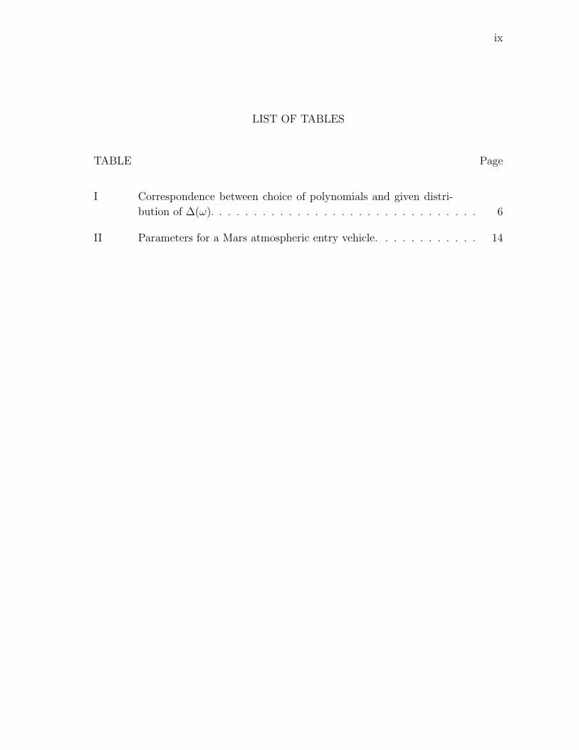
I Correspondence between choice of polynomials and given distri-
bution of ∆(ω). . . . . . . . . . . . . . . . . . . . . . . . . . . . . . . 6
II Parameters for a Mars atmospheric entry vehicle. . . . . . . . . . . . 14
x
LIST OF FIGURES
FIGURE Page
1 Uncertainty in initial condition. . . . . . . . . . . . . . . . . . . . . . 2
2 Uncertainty in landing site. . . . . . . . . . . . . . . . . . . . . . . . 3
3 Uncertainty in parameters for a dynamic model. . . . . . . . . . . . . 3
4 Evolution of Monte Carlo(blue) and Polynomial Chaos(green and
red) trajectories with time. With higher order of expansions Poly-
nomial Chaos trajectory approaches the Monte Carlo trajectory. . . . 12
5 Planar 3 dimensional Vinh’s equation is used for modeling the
dynamics. Here the states are height(h), velocity(v), flight path
angle (γ). The states(h, v) are non dimensionalized using the
radius of the planet(R0), and the escape velocity(vc) . . . . . . . . . 13
6 Evolution of uncertainty using 5% uniform uncertainty on initial
conditions of state h0. The solid black trajectory is the mean
trajectory. . . . . . . . . . . . . . . . . . . . . . . . . . . . . . . . . . 21
7 Evolution of uncertainty using 5% uniform uncertainty on initial
conditions of state v0. Evolution of uncertainty is more predomi-
nant in this case. The solid black trajectory is the mean trajectory. . 22
8 Evolution of uncertainty using 5% uniform uncertainty on initial
conditions of state γ0. The solid black trajectory is the mean
trajectory. . . . . . . . . . . . . . . . . . . . . . . . . . . . . . . . . . 23
9 Evolution of uncertainty using 5% uniform uncertainty on density
(ρ0). . . . . . . . . . . . . . . . . . . . . . . . . . . . . . . . . . . . . 23
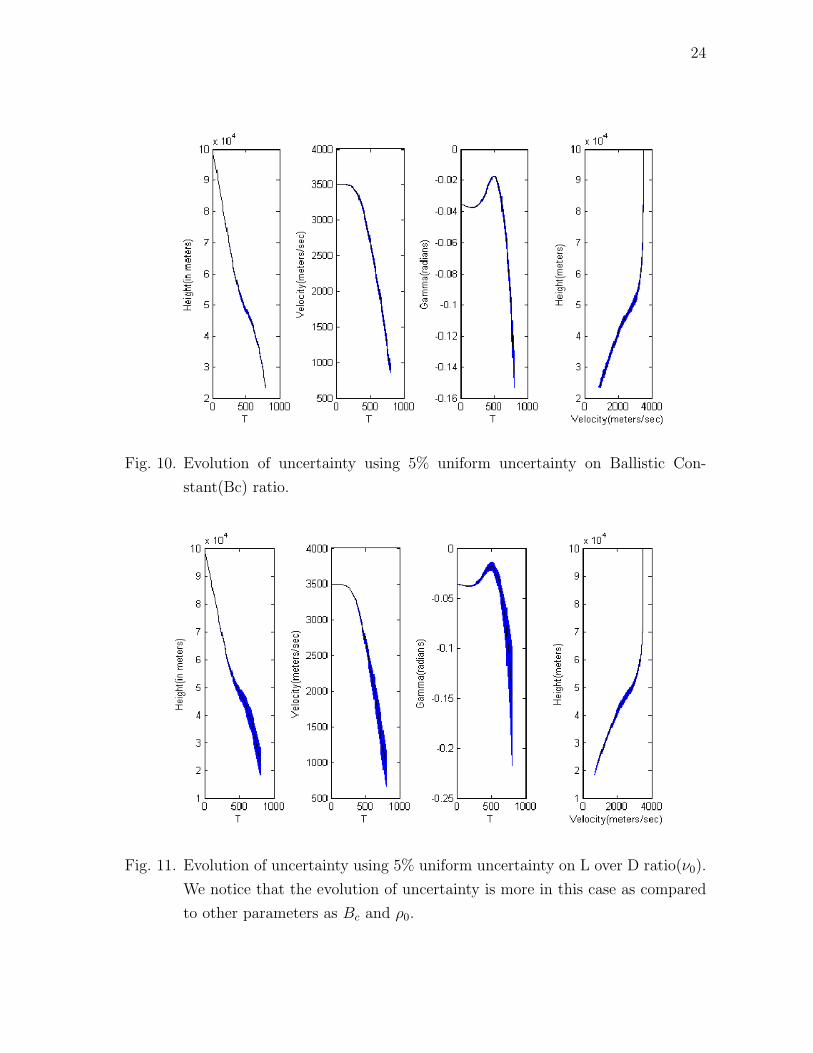
10 Evolution of uncertainty using 5% uniform uncertainty on Ballistic
Constant(Bc) ratio. . . . . . . . . . . . . . . . . . . . . . . . . . . . . 24
11 Evolution of uncertainty using 5% uniform uncertainty on L over
D ratio(ν0). We notice that the evolution of uncertainty is more
in this case as compared to other parameters as Bc and ρ0. . . . . . . 24
xi
FIGURE Page
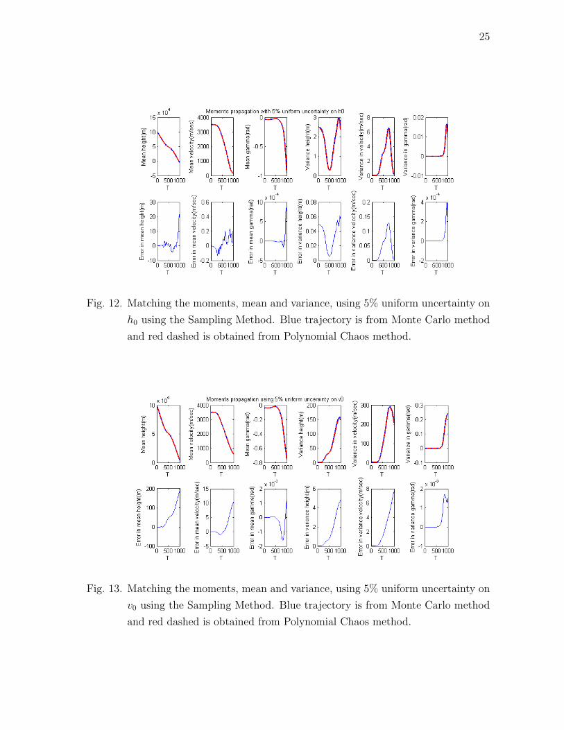
12 Matching the moments, mean and variance, using 5% uniform
uncertainty on h0 using the Sampling Method. Blue trajectory
is from Monte Carlo method and red dashed is obtained from
Polynomial Chaos method. . . . . . . . . . . . . . . . . . . . . . . . 25
13 Matching the moments, mean and variance, using 5% uniform
uncertainty on v0 using the Sampling Method. Blue trajectory
is from Monte Carlo method and red dashed is obtained from
Polynomial Chaos method. . . . . . . . . . . . . . . . . . . . . . . . 25
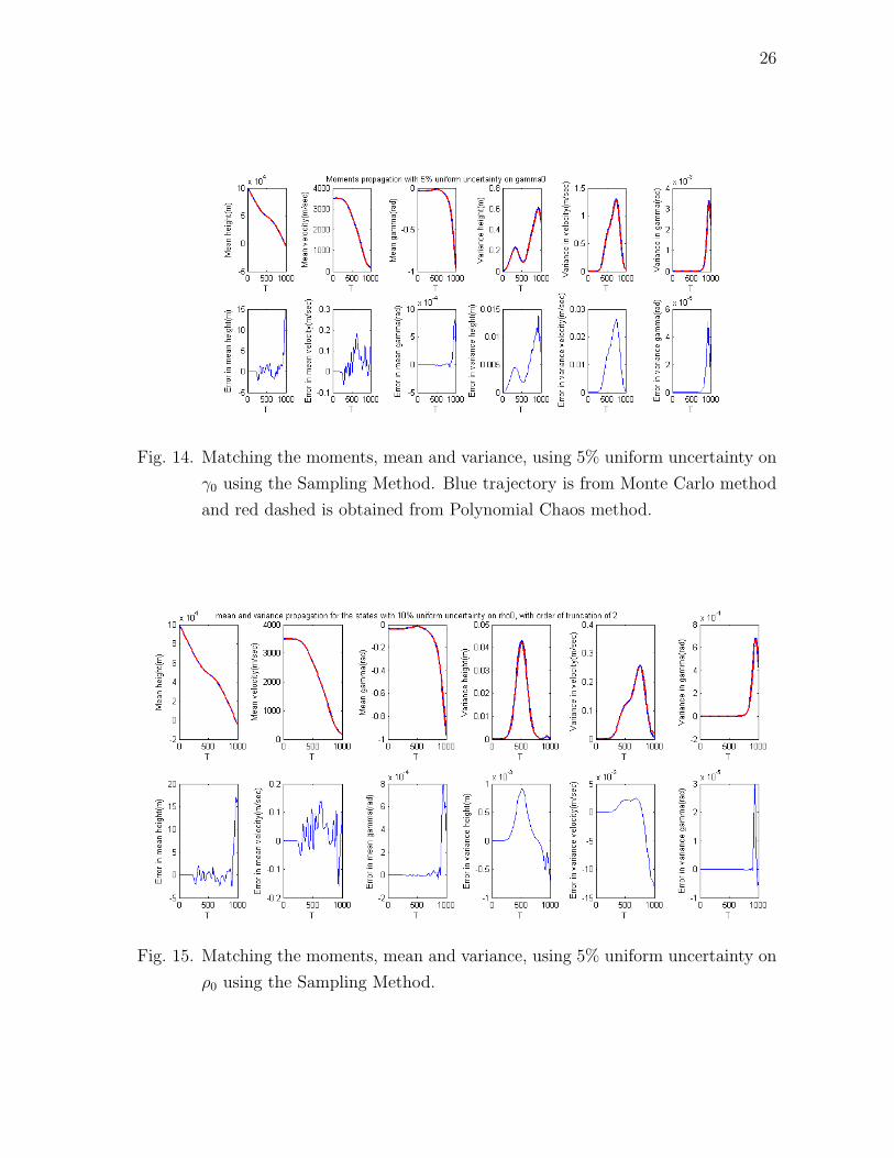
14 Matching the moments, mean and variance, using 5% uniform
uncertainty on γ0 using the Sampling Method. Blue trajectory
is from Monte Carlo method and red dashed is obtained from
Polynomial Chaos method. . . . . . . . . . . . . . . . . . . . . . . . 26
15 Matching the moments, mean and variance, using 5% uniform
uncertainty on ρ0 using the Sampling Method. . . . . . . . . . . . . . 26
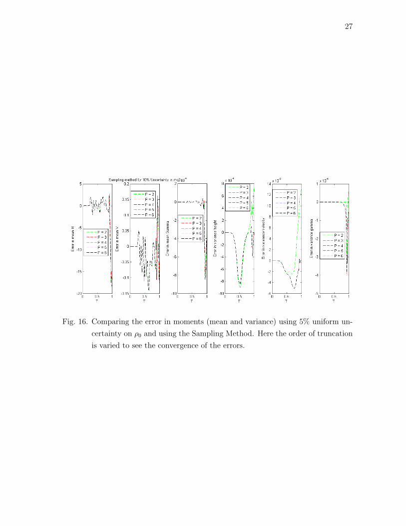
16 Comparing the error in moments (mean and variance) using 5%
uniform uncertainty on ρ0 and using the Sampling Method. Here
the order of truncation is varied to see the convergence of the errors. 27
17 Matching the moments, mean and variance, using 5% Gaussian
uncertainty on IC for the three approaches (MC, PC, CL). . . . . . . 34
18 Matching the moments, mean and variance, using 5% Gaussian
uncertainty on IC and ρ0 for the three approaches (MC, PC, CL). . . 35
19 Matching the moments, mean and variance, using 5% Gaussian
uncertainty on IC and L over D(ν) ratio for the three approaches
(MC, PC, CL). . . . . . . . . . . . . . . . . . . . . . . . . . . . . . . 37
20 Matching the moments, mean and variance, using 5% Gaussian
uncertainty on IC and Bc ratio for the three approaches (MC, PC, CL). 38
21 Evolution of the dynamics using statistical linearization method.
The simulation is run with starting statistics of mean 0.5 and
variance of 1. . . . . . . . . . . . . . . . . . . . . . . . . . . . . . . 51
xii
FIGURE Page
22 Evolution of the PDF using the Fokker Plank Equation. The
simulation is run with starting statistics of mean 0.5 and standard
deviation of 0.01. . . . . . . . . . . . . . . . . . . . . . . . . . . . . 52
23 Numerical values of the coefficients of Hermite Chaos expansion
used for capturing exponential distribution. . . . . . . . . . . . . . . 56
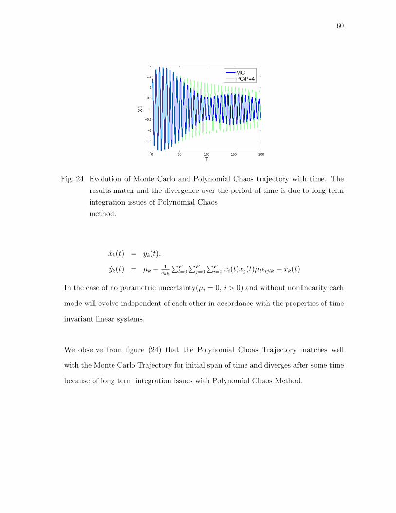
24 Evolution of Monte Carlo and Polynomial Chaos trajectory with
time. The results match and the divergence over the period of
time is due to long term integration issues of Polynomial Chaos
method. . . . . . . . . . . . . . . . . . . . . . . . . . . . . . . . . . . 60
1
CHAPTER I
INTRODUCTION
A. Problem Statement
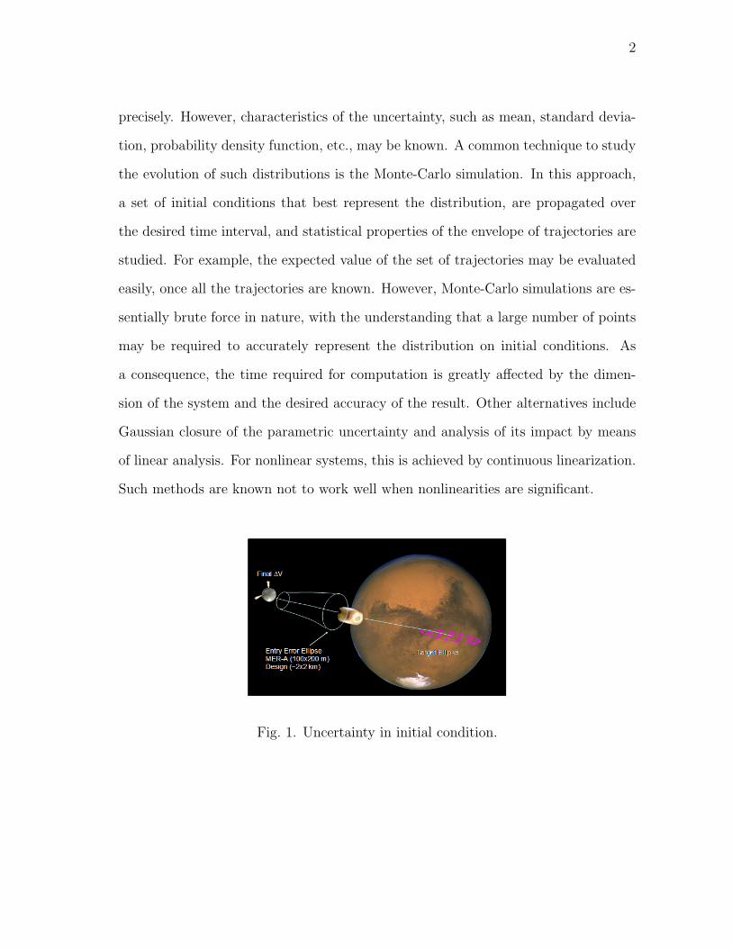
NASA has clearly identified the need for fundamental research on entry, descent, and
landing of large robotic and manned spacecraft (> 30 MT) on the surface of Mars
with high accuracy. The expected mass of the next Mars Science Laboratory mis-
sion is approximately 2, 800 kg at entry. The mission includes plans for a precision
guided entry and a tether-based payload deployment system, which is expected to
provide a landing accuracy of 20 − 40 km, from the target. Another major concern
with high-mass entry is the mismatch between the entry conditions and the decelera-
tion capabilities provided by supersonic parachute technologies. In such applications,
there is uncertainty present in initial condition and other system parameters. Hence,
for successful mission, it is critical to study the impact of such uncertainties on state
trajectories and determine uncertainty in the landing site and the entry condition for
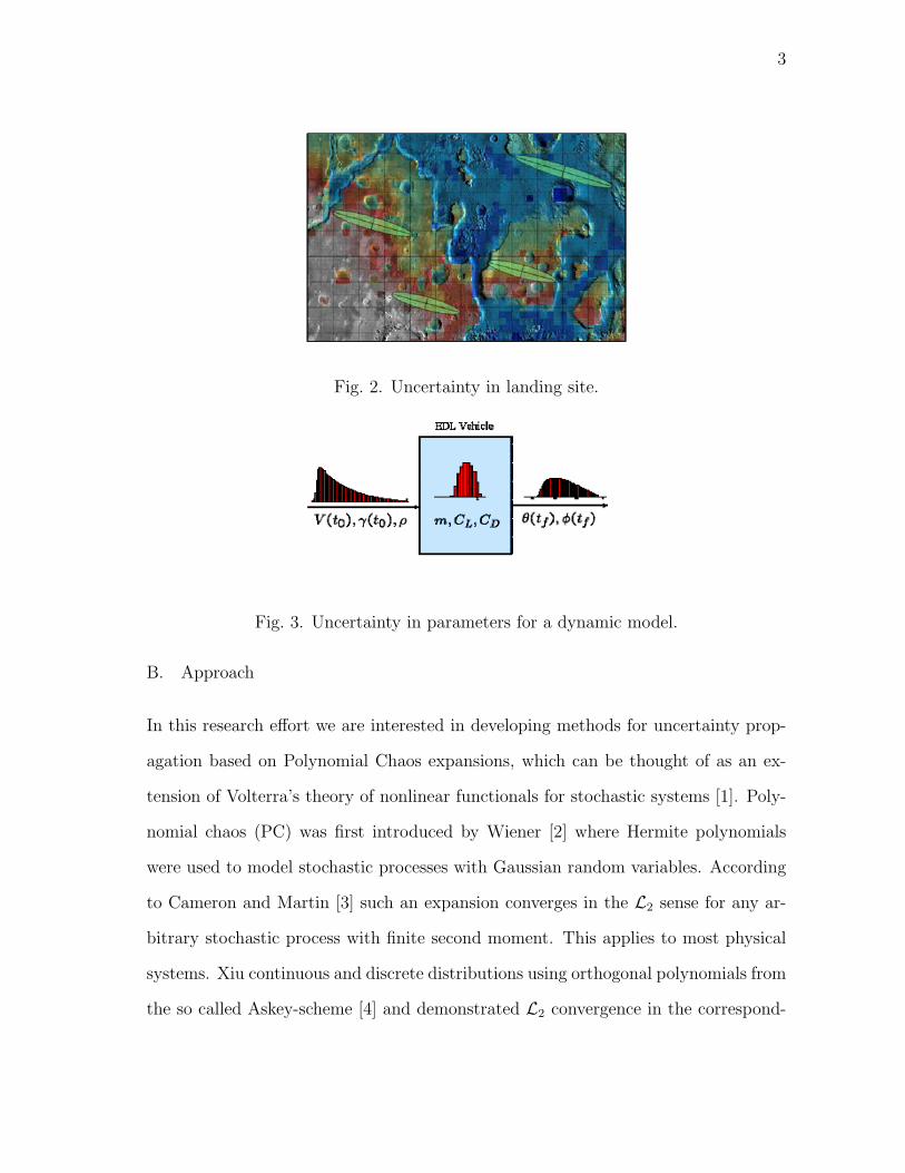
super sonic parachute deployment. Figures 1 and 2 shows how the uncertainty on
initial condition effects the uncertainty on landing site. Figure 3 summarizes the re-
search problem addressed in this work. The figure clearly shows that the uncertainty
on parameters like initial conditions and mass induces uncertainty on the final state
of the dynamics.
The problem of studying the evolution of uncertainty in dynamical systems has been
of interest consistently in the scientific community. In many cases, the uncertainty in
initial condition and other system parameters for a dynamical system are not known
The journal model is IEEE Transactions on Automatic Control.
2
precisely. However, characteristics of the uncertainty, such as mean, standard devia-
tion, probability density function, etc., may be known. A common technique to study
the evolution of such distributions is the Monte-Carlo simulation. In this approach,
a set of initial conditions that best represent the distribution, are propagated over
the desired time interval, and statistical properties of the envelope of trajectories are
studied. For example, the expected value of the set of trajectories may be evaluated
easily, once all the trajectories are known. However, Monte-Carlo simulations are es-
sentially brute force in nature, with the understanding that a large number of points
may be required to accurately represent the distribution on initial conditions. As
a consequence, the time required for computation is greatly affected by the dimen-
sion of the system and the desired accuracy of the result. Other alternatives include
Gaussian closure of the parametric uncertainty and analysis of its impact by means
of linear analysis. For nonlinear systems, this is achieved by continuous linearization.
Such methods are known not to work well when nonlinearities are significant.
Fig. 1. Uncertainty in initial condition.
3
Fig. 2. Uncertainty in landing site.
Fig. 3. Uncertainty in parameters for a dynamic model.
B. Approach
In this research effort we are interested in developing methods for uncertainty prop-
agation based on Polynomial Chaos expansions, which can be thought of as an ex-
tension of Volterra’s theory of nonlinear functionals for stochastic systems [1]. Poly-
nomial chaos (PC) was first introduced by Wiener [2] where Hermite polynomials
were used to model stochastic processes with Gaussian random variables. According
to Cameron and Martin [3] such an expansion converges in the L2 sense for any ar-
bitrary stochastic process with finite second moment. This applies to most physical
systems. Xiu continuous and discrete distributions using orthogonal polynomials from
the so called Askey-scheme [4] and demonstrated L2 convergence in the correspond-
4
ing Hilbert functional space. This is popularly known as the generalized Polynomial
Chaos (gPC) framework. The gPC framework has been applied to various applica-
tions including stochastic fluid dynamics [6], stochastic finite elements [7], and solid
mechanics. Application of gPC to problems related to control and estimation of dy-
namical systems, has been surprisingly limited.
The work is organized as follows. We first present preliminaries on the theory of
Polynomial Chaos and demonstrate transformation of stochastic dynamics, with para-
metric uncertainty, into deterministic dynamics in higher dimensional state space.
We then present the stochastic Vinh’s equation [9] for longitudinal motion where we
assume uncertainty in ballistic coefficient, lift over drag ratio, density parameters
and initial conditions. The stochastic hypersonic dynamics is then transformed into
deterministic dynamics in higher dimensional state space using Polynomial Chaos
expansions. This is followed by numerical results that characterize uncertainty prop-
agation in state trajectories induced by uncertainty in system parameters. The results
obtained from Polynomial Chaos framework are compared with Monte-Carlo simula-
tions, which are shown to agree well.
5
CHAPTER II
POLYNOMIAL CHAOS
A. Generalized Polynomial Chaos
Let (Ω,F , P ) be a probability space, where Ω is the sample space, F is the σ-algebra of
the subsets of Ω, and P is the probability measure. Let ∆(ω) = (∆1(ω), · · · ,∆d(ω)) :
(Ω,F) → (<d,Bd) be an <d-valued continuous random variable, where d ∈ ℵ, and
Bd is the σ-algebra of Borel subsets of <d. A general second order process X(ω) ∈
L2(Ω,F , P ) can be expressed by Polynomial Chaos as
X(ω) =∞∑i=0
xiφi(∆(ω)), (2.1)
where ω is the random event and φi(∆(ω)) denotes the gPC basis of degree p in terms
of the random variables ∆(ω). The functions φi are a family of orthogonal basis in
L2(Ω,F , P ) satisfying the relation
E[φiφj] = E[φ2i ]δij, (2.2)
where δij is the Kronecker delta and E[·] denotes the expectation with respect to the
probability measure dP (ω) = f(∆(ω))dω and probability density function f(∆(ω)).
Henceforth, we will use ∆ to represent ∆(ω).
For random variables ∆ with certain distributions, the family of orthogonal basis
functions φi can be chosen in such a way that its weight function has the same
form as the probability density function f(∆). These orthogonal polynomials are
members of the Askey-scheme of polynomials [4], which form a complete basis in the
Hilbert space determined by their corresponding support. Table I summarizes the
6
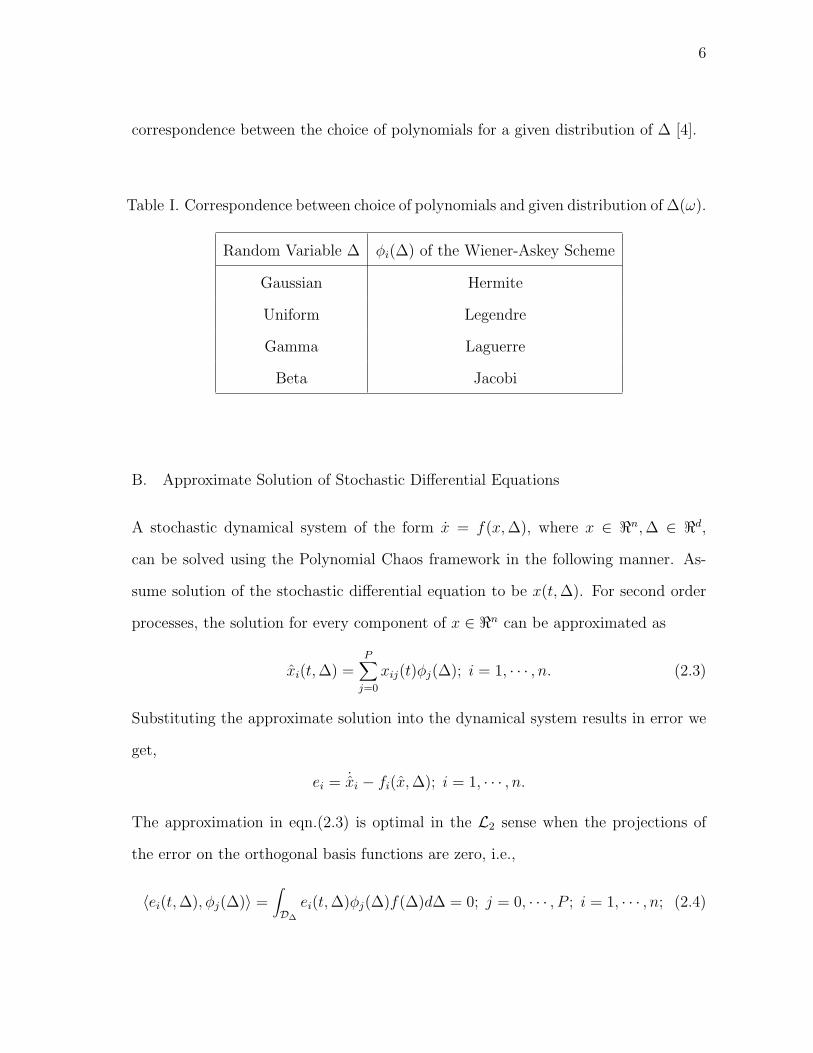
correspondence between the choice of polynomials for a given distribution of ∆ [4].
Table I. Correspondence between choice of polynomials and given distribution of ∆(ω).
Random Variable ∆ φi(∆) of the Wiener-Askey Scheme
Gaussian Hermite
Uniform Legendre
Gamma Laguerre
Beta Jacobi
B. Approximate Solution of Stochastic Differential Equations
A stochastic dynamical system of the form x = f(x,∆), where x ∈ <n,∆ ∈ <d,
can be solved using the Polynomial Chaos framework in the following manner. As-
sume solution of the stochastic differential equation to be x(t,∆). For second order
processes, the solution for every component of x ∈ <n can be approximated as
xi(t,∆) =P∑j=0
xij(t)φj(∆); i = 1, · · · , n. (2.3)
Substituting the approximate solution into the dynamical system results in error we
get,
ei = ˙xi − fi(x,∆); i = 1, · · · , n.
The approximation in eqn.(2.3) is optimal in the L2 sense when the projections of
the error on the orthogonal basis functions are zero, i.e.,
〈ei(t,∆), φj(∆)〉 =∫D∆
ei(t,∆)φj(∆)f(∆)d∆ = 0; j = 0, · · · , P ; i = 1, · · · , n; (2.4)
7
where D∆ is the domain of ∆. Equation, eqn.(2.4) results in n(P + 1) deterministic
ordinary differential equations, which can be solved numerically to obtain the ap-
proximated stochastic response. Therefore, the stochastic dynamics in <n has been
transformed into deterministic dynamics in <n(P+1). The series is truncated after
P + 1 terms, which is determined by the dimension d of ∆ and the order r of the
orthogonal polynomials φj, satisfying P + 1 = (d+r)!d!r!
.
C. Stochastic Dynamics and Polynomial Chaos
We first consider stochastic linear systems of the form
x(t,∆) = A(∆)x(t,∆) +B(∆)u(t), (2.5)
where x ∈ <n, u ∈ <m. The system has probabilistic uncertainty in the system param-
eters, characterized by A(∆), B(∆), which are matrix functions of random variable
∆ ≡ ∆(ω) ∈ <d with certain stationary distributions. Due to the stochastic nature
of (A,B), the system trajectory will also be stochastic. The control u(t) is considered
to be deterministic in this paper. We do not consider stochastic forcing in this paper,
but this framework can be easily extended to include stochastic forcing and will be
addressed in future publications.
Let us represent components of x(t,∆), A(∆) and B(∆) as,
x(t,∆) = [x1(t,∆) · · · xn(t,∆)]T , (2.6)
A(∆) =
A11(∆) · · · A1n(∆)
......
An1(∆) · · · Ann(∆)
, (2.7)
8
B(∆) =
B11(∆) · · · B1m(∆)
......
Bn1(∆) · · · Bnm(∆)
. (2.8)
By applying the Wiener-Askey gPC expansion to xi(t,∆), Aij(∆) and Bij(∆), we get
xi(t,∆) =p∑
k=0
xi,k(t)φk(∆) = xi(t)TΦ(∆), (2.9)
Aij(∆) =p∑
k=0
aij,kφk(∆) = aTijΦ(∆), (2.10)
Bij(∆) =p∑
k=0
bij,kφk(∆) = bTijΦ(∆), (2.11)
where xi(t), aij,bij,Φ(∆) ∈ <p are defined by
xi(t) = [xi,0(t) · · · xi,p(t)]T , (2.12)
aij = [aij,0(t) · · · aij,p(t)]T , (2.13)
bij = [bij,0(t) · · · bij,p(t)]T , (2.14)
Φ(∆) = [φ0(∆) · · · φp(∆)]T . (2.15)
(2.16)
The number of terms p+ 1 is determined by the dimension d of ∆ and the order r of
the orthogonal polynomials φk, satisfying p + 1 = (d+r)!d!r!
. The coefficients aij,k and
bij,k are obtained via Galerkin projection onto φkpk=0 given by
aij,k =〈Aij(∆), φk(∆)〉〈φk(∆)2〉
, (2.17)
bij,k =〈Bij(∆), φk(∆)〉〈φk(∆)2〉
. (2.18)
The n(p+1) time varying coefficients, xi,k(t); i = 1, · · · , n; k = 0, · · · , p, are obtained
by substituting the approximated solution in the governing equation (eqn.(2.5)) and
9
conducting Galerkin projection onto φkpk=0, to yield n(p + 1) deterministic linear
differential equations, given by
X = AX + Bu, (2.19)
with X ∈ <n(p+1); M,A ∈ <n(p+1)×n(p+1); B ∈ <n(p+1)×m and
X = [xT1 xT2 · · · xTn ]T , (2.20)
A = M−1
A11 · · · A1n
......
An1 · · · Ann
Aij = 〈ΦΦT ⊗ ΦT 〉(Ip+1 ⊗ aij), (2.21)
M = In ⊗
〈φ0, φ0〉 0 · · · 0
0 〈φ1, φ1〉 · · · 0
......
...
0 0 · · · 〈φp, φp〉
,
B =
b11 · · · b1m
......
bn1 · · · bnm
,
where In ∈ <n×n, Ip+1 ∈ <(p+1)×(p+1) are identity matrices, ⊗ is the Kronecker
product, and the inner product in eqn.(2.21) is performed element wise. Therefore,
transformation of a stochastic linear system with x ∈ <n, u ∈ <m, with pth order
gPC expansion, results in a deterministic linear system with increased dimensional-
ity equal to n(p+ 1).
10
Here we consider certain types of nonlinearities that may be present in the system
model. The nonlinearities considered here are rational polynomials, transcendental
functions and exponentials. We outline the process for representing these nonlineari-
ties in terms of Polynomial Chaos expansions.
If x, y are random variables with gPC expansions similar to eqn.(2.9) then the gPC
expansion of the expression xy can be written as
xy =p∑i=0
p∑j=0
xiyjφiφj.
The gPC expansion of x2 can be derived by setting y = x in the above expansion to
obtain
x2 =p∑i=0
p∑j=0
xixjφiφj.
Similarly x3 can be expanded as
x3 =p∑i=0
p∑j=0
p∑k=0
xixjxkφiφjφk.
This approach can be used to derive the gPC expansions of any multi-variate whole
rational monomial in general.
The gPC expansion of fractional rational monomials of random variables is illustrated
using the the expression z = xy. If x, y are random variables then z is also a random
variable with gPC expansions similar to eqn.(2.9). The expansions of x, y are known.
The gPC expansions of z can be determined using the following steps. Rewrite
z =x
yas yz = x,
11
Expanding yz and x in terms of their gPC expansions gives
p∑i=0
p∑j=0
ziyjφiφj =p∑
k=0
xkφk.
To determine the unknown zi we project both sides of the equation on the subspace
basis to obtain a system of p+ 1 linear equations
1
〈φk, φk〉
p∑i=0
p∑j=0
ziyj〈φiφjφk〉 = xk, k = 0, . . . , p;
to solve for the p unknowns zi. This can be generalized to obtain the gPC expansion
of any fractional rational monomial.
When nonlinearities involve non polynomial functions, such as transcendental func-
tions and exponentials, difficulties occur during computation of the projection on the
gPC subspace. The corresponding integrals may not have closed form solutions. In
such cases, the integrals either have to be numerically evaluated or these nonlinear-
ities are first approximated as polynomials using Taylor series expansions and then
the projections are computed using methods described above. While Taylor series
approximation is straightforward and generally computationally cost effective, it can
become severely inaccurate when higher order gPC expansions are required to repre-
sent the physical variability. A more robust algorithm is presented by Debusschere
et al. [10] for any non polynomial function u(x) for which dudx
can be expressed as a
rational function of x, u(x).
D. Limitations of Polynomial Chaos
The gPC framework is well suited for evaluating short term statistics of dynamical
systems. However, their performance degrades upon long term integration. Consider
12
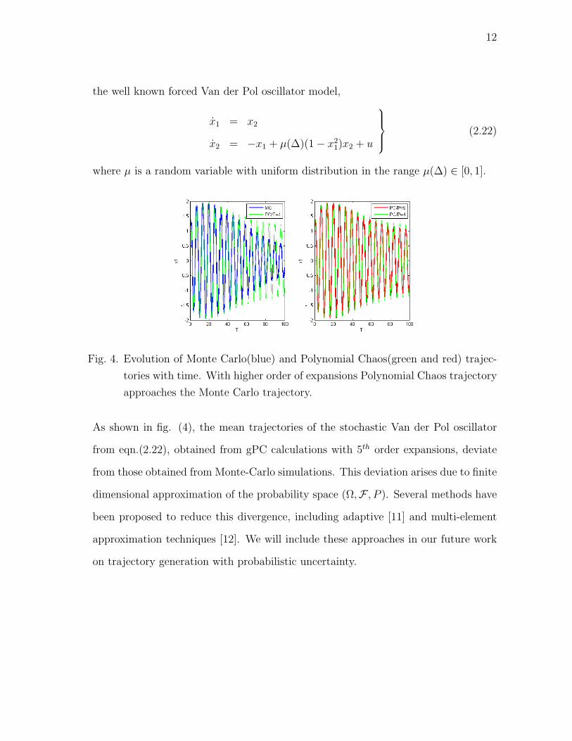
the well known forced Van der Pol oscillator model,
x1 = x2
x2 = −x1 + µ(∆)(1− x21)x2 + u
(2.22)
where µ is a random variable with uniform distribution in the range µ(∆) ∈ [0, 1].
Fig. 4. Evolution of Monte Carlo(blue) and Polynomial Chaos(green and red) trajec-
tories with time. With higher order of expansions Polynomial Chaos trajectory
approaches the Monte Carlo trajectory.
As shown in fig. (4), the mean trajectories of the stochastic Van der Pol oscillator
from eqn.(2.22), obtained from gPC calculations with 5th order expansions, deviate
from those obtained from Monte-Carlo simulations. This deviation arises due to finite
dimensional approximation of the probability space (Ω,F , P ). Several methods have
been proposed to reduce this divergence, including adaptive [11] and multi-element
approximation techniques [12]. We will include these approaches in our future work
on trajectory generation with probabilistic uncertainty.
13
CHAPTER III
VINH’S EQUATION WITH PROBABILISTIC UNCERTAINTY ON SYSTEM
PARAMETERS
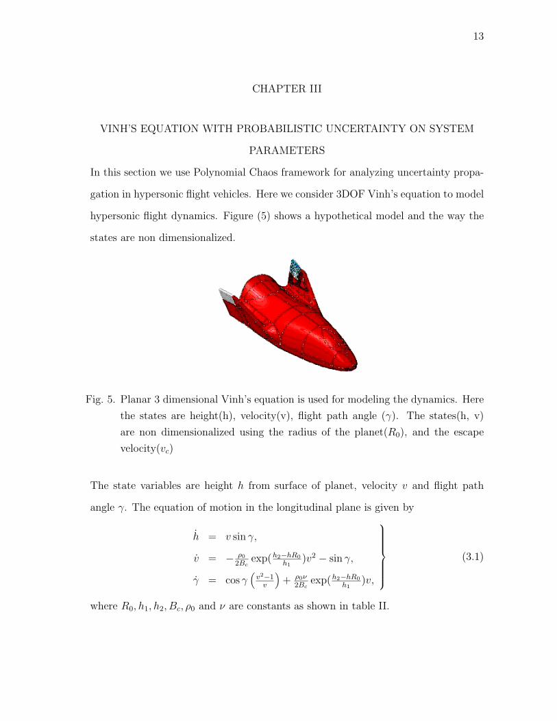
In this section we use Polynomial Chaos framework for analyzing uncertainty propa-
gation in hypersonic flight vehicles. Here we consider 3DOF Vinh’s equation to model
hypersonic flight dynamics. Figure (5) shows a hypothetical model and the way the
states are non dimensionalized.
Fig. 5. Planar 3 dimensional Vinh’s equation is used for modeling the dynamics. Here
the states are height(h), velocity(v), flight path angle (γ). The states(h, v)
are non dimensionalized using the radius of the planet(R0), and the escape
velocity(vc)
The state variables are height h from surface of planet, velocity v and flight path
angle γ. The equation of motion in the longitudinal plane is given by
h = v sin γ,
v = − ρ0
2Bcexp(h2−hR0
h1)v2 − sin γ,
γ = cos γ(v2−1v
)+ ρ0ν
2Bcexp(h2−hR0
h1)v,
(3.1)
where R0, h1, h2, Bc, ρ0 and ν are constants as shown in table II.
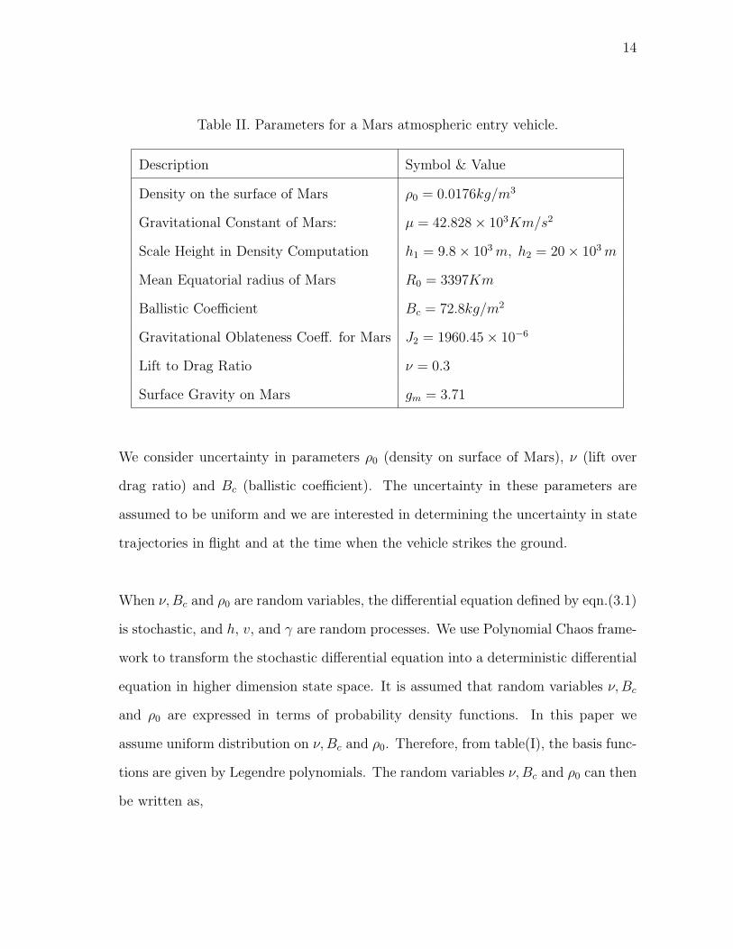
14
Table II. Parameters for a Mars atmospheric entry vehicle.
Description Symbol & Value
Density on the surface of Mars ρ0 = 0.0176kg/m3
Gravitational Constant of Mars: µ = 42.828× 10³Km/s2
Scale Height in Density Computation h1 = 9.8× 10³m, h2 = 20× 103m
Mean Equatorial radius of Mars R0 = 3397Km
Ballistic Coefficient Bc = 72.8kg/m2
Gravitational Oblateness Coeff. for Mars J2 = 1960.45× 10−6
Lift to Drag Ratio ν = 0.3
Surface Gravity on Mars gm = 3.71
We consider uncertainty in parameters ρ0 (density on surface of Mars), ν (lift over
drag ratio) and Bc (ballistic coefficient). The uncertainty in these parameters are
assumed to be uniform and we are interested in determining the uncertainty in state
trajectories in flight and at the time when the vehicle strikes the ground.
When ν,Bc and ρ0 are random variables, the differential equation defined by eqn.(3.1)
is stochastic, and h, v, and γ are random processes. We use Polynomial Chaos frame-
work to transform the stochastic differential equation into a deterministic differential
equation in higher dimension state space. It is assumed that random variables ν,Bc
and ρ0 are expressed in terms of probability density functions. In this paper we
assume uniform distribution on ν,Bc and ρ0. Therefore, from table(I), the basis func-
tions are given by Legendre polynomials. The random variables ν,Bc and ρ0 can then
be written as,
15
ν(∆) = ν + δν∆,
Bc(∆) = Bc + δBc∆,
ρ0(∆) = ρ0 + δρ0∆,
where ∆ ∈ [−1, 1] and δν, δBc, and δρ0 are the perturbations about nominal values ν,
Bc and ρ0 respectively. In this research we have assumed the parameters to have uni-
form distributions about their nominal values. The random processes h(t,∆), v(t,∆)
and γ(t,∆) are expanded as
h(t,∆) =∑P
0 hi(t)φi(∆),
v(t,∆) =∑P
0 vi(t)φi(∆),
γ(t,∆) =∑P
0 γi(t)φi(∆).
Note that for the parameters with uniform uncertainty, only two basis functions are
required to completely capture their respective probability density functions. No
benefit is obtained by including more terms. However for the states, the expansion
includes higher order basis functions. From the gPC theory, we are guaranteed expo-
nential convergence as higher order basis functions are included[4].
Substituting these in eqn.(3.1) results in the following
∑P0 hiφi =
∑P0 viφi sin(
∑P0 γiφi),
∑P0 viφi = − ρ0(∆)
2Bc(∆)
exph2h1
expR0
∑P
0hiφi
h1
∑P0
∑P0 φiφjvivj − sin(
∑P0 γiφi),
∑P0 γiφi = cos(
∑P0 γiφi) (
∑P0 viφi − 1∑P
0viφi
) + ρ0(∆)ν(∆)2Bc(∆)
(exp
h2h1
expR0
∑P
0hiφi
h1
)∑P
0 viφi.
The above equations are further simplified by the following substitutions
16
∑P0 wiφi = 1∑P
0viφi
,
∑P0 xiφi =
exph2h1
expR0
∑P
0hiφi
h1
,
∑P0 yiφi = ρ0(∆)
2Bc(∆),
∑P0 ziφi = ρ0(∆)ν(∆)
2Bc(∆),
where coefficients wi, xi, yi, zi ∈ < are yet to be determined. The Vinh’s equation can
now be written as
∑P0 hiφi =
∑P0 viφi sin
(∑P0 γiφi
),
∑P0 viφi = −∑P
i,j,k,l=0 φiφjφkφlxiyjvkvl − sin(∑P
i=0 γiφi),
∑P0 γiφi = cos
(∑Pi=0 γiφi
) (∑Pi=0 viφi −
∑Pi=0wiφi
)+∑Pi,j,k=0 φiφjφkxizjvk.
Taking Galerkin projection on basis functions φi(∆), we get the following determin-
istic differential equations,
hm = 1〈φ2m〉∑P
0 vi⟨φiφm sin
(∑P0 γiφi
)⟩,
vm = − 1〈φ2m〉∑Pi,j,k,l=0 〈φiφjφkφlφm〉xiyjvkvl − 1
〈φ2m〉
⟨φm sin
(∑Pi=0 γiφi
)⟩,
γm = 1〈φ2m〉∑Pi=0 vi
⟨φiφm cos
(∑Pi=0 γiφi
)⟩− 1〈φ2m〉∑Pi=0wi
⟨φiφm cos
(∑Pi=0 γiφi
)⟩+ 1〈φ2m〉∑Pi,j,k=0 〈φiφjφkφm〉xizjvk,
(3.2)
where m = 0, · · · , P . Equation (3.2) is the equivalent deterministic dynamics of the
stochastic dynamics given by eqn.(3.1), approximated by gPC expansions. Solution
17
of this differential equation, in higher dimensional state space, can then be used to
characterize h(t,∆), v(t,∆) and γ(t,∆).
The terms wi, xi, yi and zi in eqn.(3.2) are computed as follows. Define
α =P∑0
γiφi, β =R0∑P
0 hiφih1
.
Multiplying,
P∑0
xiφi =exp h2
h1
expR0
∑P
0hiφi
h1
,
by exp(β) on both the sides we get
exph2
h1
=P∑0
xiφi exp β.
Taking projection on the basis functions yields,
〈exph2
h1
φk〉 = 〈P∑0
φiφk exp β〉xi.
This produces a set of (P + 1) linear equations in xi. Similarly, wi are computed by
multiplying
1∑P0 viφi
=P∑0
wiφi,
by∑P
0 viφi on both the sides, which reduces to
1 =P∑0
P∑0
φiφjviwj.
18
Now taking projection on the basis functions we get,
〈φk〉 =P∑0
P∑0
〈φiφjφk〉viwj,
which also is a system of linear equations in wi. The coefficients yi and zi can also be
determined in the similar manner.
The terms sin(α) and exp(β) are computed by approximating them by a Taylor series
expansion of the perturbation about the mean [10]. For example, computing the
exponential of a random variable ξ, the perturbation around the mean is given as
d = ξ − ξ0, where ξ0 is the mean. Therefore,
exp(ξ) = exp(ξ0)(1 +Ntay∑n=1
dn
n!).
Here d is the stochastic part of ξ and Ntay is the number of terms in the Taylor series
expansion. The sine of the random process is computed similar to the exponential,
in the following manner,
sin(ξ) = sin(ξ0 + d) = sin(ξ0) cos(d) + cos(ξ0) sin(d).
While Taylor series approximation is straightforward and generally computationally
cost effective, it can become severely inaccurate when higher order gPC expansions
are required to represent the physical variability.
A. Obtaining Statistics from Polynomial Chaos
Mean and variance of the state trajectories can be easily computed from the coeffi-
cients of the gPC expansions. The mean trajectories can be derived as,
19
E[h(t,∆)] = E[p∑i=0
hiφi] =p∑i=0
hiE[φi] =p∑i=0
hi
∫D∆
φifd∆,
and similarly,
E[v(t,∆)] =∑pi=0 vi
∫D∆
φifd∆,
E[γ(t,∆)] =∑pi=0 γi
∫D∆
φifd∆,
where hi, vi, γi are the coefficients of the gPC expansions of h(t,∆), v(t,∆), γ(t,∆)
respectively, and f is the probability density function of the parameters.
The variance of a trajectory h(t,∆) is given by
σ2[h(t,∆)] = E[(h(t,∆)2]− E[h(t,∆)]2,
=∑Pi,j=0 hihj
∫D∆
φjφjfd∆− E[h(t,∆)]2
=∑Pi=0 h
2i
∫D∆
φ2i fd∆− E[h(t,∆)]2, because of orthogonality of φi, φj.
In this manner, the covariance matrix for the system can also be determined.
1. Uncertainty Propagation Using the Standard Approach of Monte Carlo
Simulations
In the subsequent analysis, we have assumed 5% parametric variation in ρ0, ν and
Bc, about the nominal values listed in table(II). The distribution is assumed to be
uniform about the nominal values. We have obtained statistics of the states trajecto-
ries from Monte-Carlo simulations and have compared them with those obtained from
Polynomial Chaos theory, to verify the validity of the Polynomial Chaos approach for
analyzing uncertainty in hypersonic flight dynamics.
20
In the thesis work, we analyze the effect of uncertainty in initial condition and pa-
rameters on the downrange error and compare the results obtained from Monte-Carlo
simulations and Polynomial Chaos theory. Numerical analysis is also performed to
determine the sensitivity of the number of basis functions, Taylor series approxima-
tion and Debusschere’s method, on the statistics of the state trajectories. In the
simulation results shown, the dynamics has been non dimensionalized using the ra-
dius of planet and escape velocity.
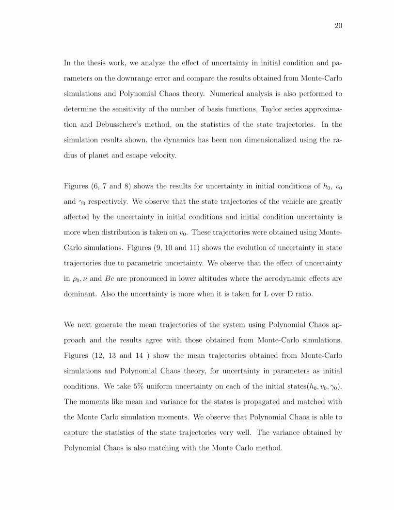
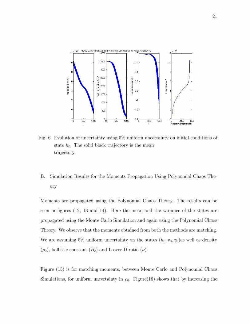
Figures (6, 7 and 8) shows the results for uncertainty in initial conditions of h0, v0
and γ0 respectively. We observe that the state trajectories of the vehicle are greatly
affected by the uncertainty in initial conditions and initial condition uncertainty is
more when distribution is taken on v0. These trajectories were obtained using Monte-
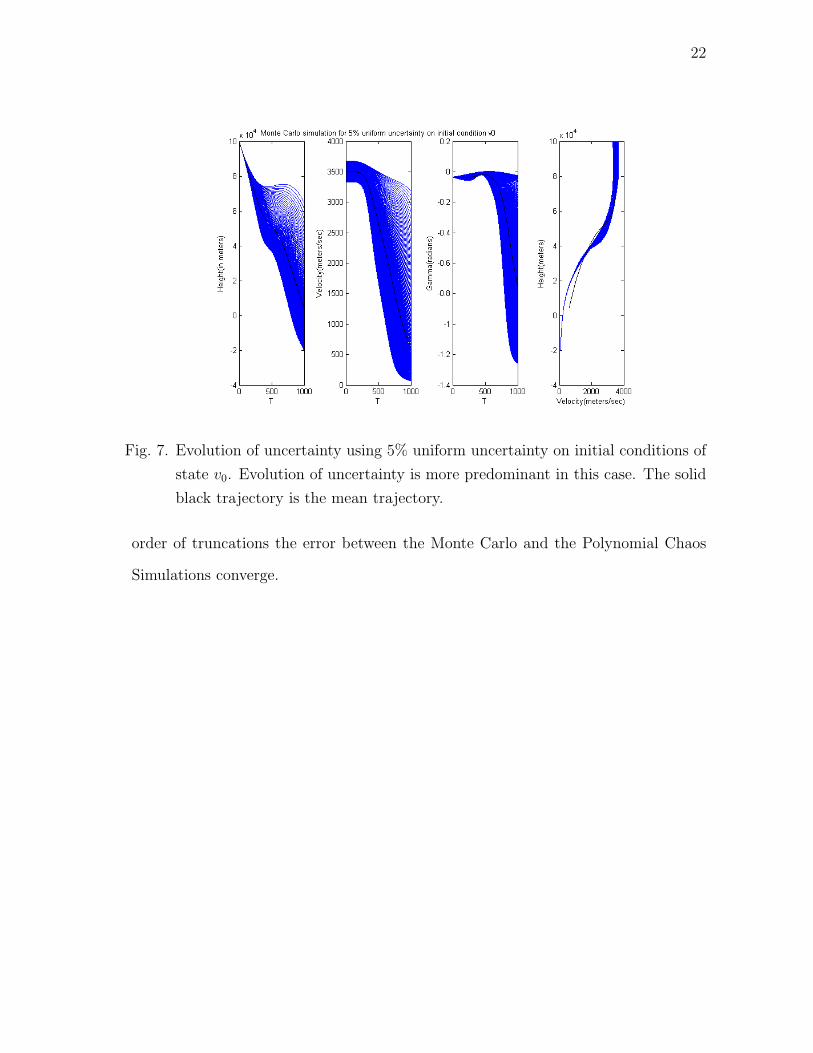
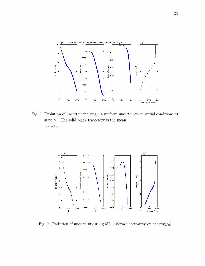
Carlo simulations. Figures (9, 10 and 11) shows the evolution of uncertainty in state
trajectories due to parametric uncertainty. We observe that the effect of uncertainty
in ρ0, ν and Bc are pronounced in lower altitudes where the aerodynamic effects are
dominant. Also the uncertainty is more when it is taken for L over D ratio.
We next generate the mean trajectories of the system using Polynomial Chaos ap-
proach and the results agree with those obtained from Monte-Carlo simulations.
Figures (12, 13 and 14 ) show the mean trajectories obtained from Monte-Carlo
simulations and Polynomial Chaos theory, for uncertainty in parameters as initial
conditions. We take 5% uniform uncertainty on each of the initial states(h0, v0, γ0).
The moments like mean and variance for the states is propagated and matched with
the Monte Carlo simulation moments. We observe that Polynomial Chaos is able to
capture the statistics of the state trajectories very well. The variance obtained by
Polynomial Chaos is also matching with the Monte Carlo method.
21
Fig. 6. Evolution of uncertainty using 5% uniform uncertainty on initial conditions of
state h0. The solid black trajectory is the mean
trajectory.
B. Simulation Results for the Moments Propagation Using Polynomial Chaos The-
ory
Moments are propagated using the Polynomial Chaos Theory. The results can be
seen in figures (12, 13 and 14). Here the mean and the variance of the states are
propagated using the Monte Carlo Simulation and again using the Polynomial Chaos
Theory. We observe that the moments obtained from both the methods are matching.
We are assuming 5% uniform uncertainty on the states (h0, v0, γ0)as well as density
(ρ0), ballistic constant (Bc) and L over D ratio (ν).
Figure (15) is for matching moments, between Monte Carlo and Polynomial Chaos
Simulations, for uniform uncertainty in ρ0. Figure(16) shows that by increasing the
22
Fig. 7. Evolution of uncertainty using 5% uniform uncertainty on initial conditions of
state v0. Evolution of uncertainty is more predominant in this case. The solid
black trajectory is the mean trajectory.
order of truncations the error between the Monte Carlo and the Polynomial Chaos
Simulations converge.
23
Fig. 8. Evolution of uncertainty using 5% uniform uncertainty on initial conditions of
state γ0. The solid black trajectory is the mean
trajectory.
Fig. 9. Evolution of uncertainty using 5% uniform uncertainty on density(ρ0).
24
Fig. 10. Evolution of uncertainty using 5% uniform uncertainty on Ballistic Con-
stant(Bc) ratio.
Fig. 11. Evolution of uncertainty using 5% uniform uncertainty on L over D ratio(ν0).
We notice that the evolution of uncertainty is more in this case as compared
to other parameters as Bc and ρ0.
25
Fig. 12. Matching the moments, mean and variance, using 5% uniform uncertainty on
h0 using the Sampling Method. Blue trajectory is from Monte Carlo method
and red dashed is obtained from Polynomial Chaos method.
Fig. 13. Matching the moments, mean and variance, using 5% uniform uncertainty on
v0 using the Sampling Method. Blue trajectory is from Monte Carlo method
and red dashed is obtained from Polynomial Chaos method.
26
Fig. 14. Matching the moments, mean and variance, using 5% uniform uncertainty on
γ0 using the Sampling Method. Blue trajectory is from Monte Carlo method
and red dashed is obtained from Polynomial Chaos method.
Fig. 15. Matching the moments, mean and variance, using 5% uniform uncertainty on
ρ0 using the Sampling Method.
27
Fig. 16. Comparing the error in moments (mean and variance) using 5% uniform un-
certainty on ρ0 and using the Sampling Method. Here the order of truncation
is varied to see the convergence of the errors.
28
CHAPTER IV
CONTINUOUS LINEARIZATION APPROACH AND DOWNRANGE ANALYSIS
A variety of error sources contribute to the discrepancy between the position of the
intended target and the position of the reentry vehicle. Though the sources have
identifiable physical origin, it is not possible to assign the numerical value of precision
to these uncertainties. However, it is feasible to establish a mean value of a given error
source and a distribution of likely value that would closely resemble the uncertainty
present on the parameters. To illustrate, the atmospheric property such as density
or the parameters like ballistic constant or L by D ratio can be thought of having
Gaussian distribution with a mean value and suitably chosen standard deviation about
the mean. Let the nominal state or the state vector associated with the nominal
trajectory be designated by X0 and the actual state vector be X. The error in the
state vector can now be defined as
e = X−X0
A precise statistical description of the error state is given by the state covariance
matrix P, defined as the expectation of all possible pairs of error vector components.
P = E[eeT ] = E[(X−X0)(X−X0)T ]
This gives us a powerful tool for assessing the size of the error vector and the degree
of coupling among the components of the error vector. Hence, In assessing errors
induced by uncertainty, a useful procedure is to define one trajectory - a nominal
trajectory - assumed error free. The impact point of this trajectory is simply the in-
tended impact point or the reference point. The remaining trajectories then become
the perturbations, by some error source, about this nominal trajectory. We can then
29
separate the state vector X into two parts. The nominal part X0 and a perturbed
part, X, as
X = X0 + X
The nonlinear vector function can be linearized and written as follows:
F ≈ F0 +dF
dX(X−X0)
Where a subscript 0 indicates the nominal trajectory. We insert the above equation
to get
dX0
dt+dX
dt≈ F(X)|X=X0 +
dF
dX(X−X0) = F(X0) +
dF
dX|X0X
But from the state equation we know:
dX0
dt= F(X0)
Consequently,
dX
dt=dF
dX|X0X = AX
The above equation is the linear differential equation that describes perturbation
about the nominal trajectory. The matrix A is the jacobian of the perturbational
variables whose elements are given as follows
A = [aij] = [∂fi∂Xj
]X=X0
We note that the elements of matrix A is evaluated using the current states of the
nominal trajectory. Even though the elements of A are time varying, reflecting the
time varying states of the nominal trajectory, the elements of A are treated as time
constant for integration of the perturbational variable X. A convenient way of rep-
resenting the relationship between the perturbational state vector X at time ti and
30
time ti+1 is by the use of the transition matrix, φ. Hence
Xi+1 = φ(ti+1, ti)Xi
If φ is assigned some fixed value by the nominal states, then according to the above
equation, φ may be accepted as a matrix that transitions the perturbation or the
error state vector X over the time interval ti to ti+1. The transition matrix φ can
formally be identified with the matrix exponent and more usefully with the matrix
series.
φ(ti+1, ti) = eA(ti+1−ti) = eA∆t
Which can conveniently be expanded as
φ = I + A∆t+1
2!A2∆t2 +
1
3!A3∆t3 + .......+
1
n!An∆tn
Further we note that the error ellipsoid is the quadratic form of the covariance matrix.
We define the error covariance matrix at time ti, Pi as
Pi = E[XiXiT
]
Where Xi is the perturbational or error state vector at time ti. It can now be inferred
for time ti+1 that
Pi+1 = E[Xi+1XT
i+1]
Hence insertion of equation gives:
Pi+1 = φiPiφTi
31
The preceding equation provides the discrete propagation of the covariance matrix.
Using the expansion of the state transition matrix we get
Pi+1 ≈ [(I + A∆t)Pi(I + A∆t)T ]
Which upon simplification gives
Pi+1 − Pi∆t
= APi + PiAT
We use the above approach for computing the covariance matrix. The nominal tra-
jectory is computed assuming that the parameters are known with certainty and the
jacobian of the perturbational variables are computed about the nominal trajectory.
This approach is used for populating the covariance matrix along the nominal trajec-
tory.
A. Simulation Results
Here the simulation is run with Gaussian distribution on the parameters and the three
methods, Monte Carlo, Polynomial Chaos and Continuous Linearization approach is
compared.
B. State Acquisition
It is common to use the estimation or optimization algorithms for the system whose
states are given by the equation of the form:
x = f(t,x,p)
Where,
p = [p1, p2, p3......, pq]T
32
is a set of model constants which appear in the system’s differential equations. In
our application initial conditions are poorly known as well as one or more elements of
the model parameters vector p. Hence it becomes necessary to estimate both x(t0)
and p based upon the measurements of of x(t) or a function thereof. Conventional
estimation require the partial derivative matrices:
Φ(t, t0) =∂x(t)
∂x(t0)
and,
Ψ(t, t0) =∂x(t)
∂p
These derivative matrices can be computed as
x(t) = x(t0) +∫ t
t0f(τ,x,p)dτ
This when applied to the derivative matrices give:
Φ(t, t0) = I +∫ t
t0
∂f(τ,x,p)
∂x(τ)
∂x(τ)
∂x(t0)dτ
and
Ψ(t, t0) =∫ t
t0(∂f(τ,x,p)
∂p+∂f(τ,x,p)
∂x(τ)
∂x(τ)
∂x(t0))dτ
Taking the time derivative of the above equations we see that the desired derivative
matrices satisfy the first order linear differential equations:
Φ(t, t0) = F (t)Φ(t, t0)
Where Φ(t0, t0) = I, and
Ψ(t, t0) = F (t)Ψ(t, t0) +∂f(t,x,p)
∂p
33
with Ψ(t0, t0) = 0 and
F (t) =∂f(t,x,p)
∂x(t)
The above derivations can be viewed in a more systematic way by augmenting the
system differential equation as:
x = f(t,x,p)
p = 0
The above equations can be rewritten as
z = g(t, z)
Where, z ≡ [xTpT ]T and g(t, z) ≡ [fT0T ]T . We now form this augmented matrix:
Γ(t, t0) ≡ ∂z(t)
∂z(t0)=
Φ(t, t0) Ψ(t, t0)
0 I
(4.1)
(4.2)
The augmented state transition matrix satisfies:
Γ(t, t0) =∂g(t, z)
∂z(t)Γ(t, t0)
and
Γ(t, t0) = I
Where,
∂g(t, z)
∂z(t)=
F (t) ∂(t,x,p)
∂p
0 0
(4.3)
(4.4)
34
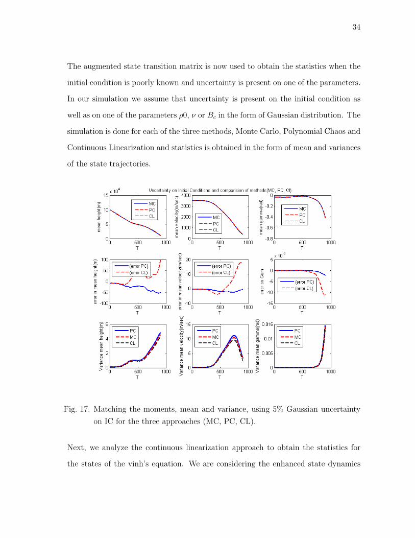
The augmented state transition matrix is now used to obtain the statistics when the
initial condition is poorly known and uncertainty is present on one of the parameters.
In our simulation we assume that uncertainty is present on the initial condition as
well as on one of the parameters ρ0, ν or Bc in the form of Gaussian distribution. The
simulation is done for each of the three methods, Monte Carlo, Polynomial Chaos and
Continuous Linearization and statistics is obtained in the form of mean and variances
of the state trajectories.
Fig. 17. Matching the moments, mean and variance, using 5% Gaussian uncertainty
on IC for the three approaches (MC, PC, CL).
Next, we analyze the continuous linearization approach to obtain the statistics for
the states of the vinh’s equation. We are considering the enhanced state dynamics
35
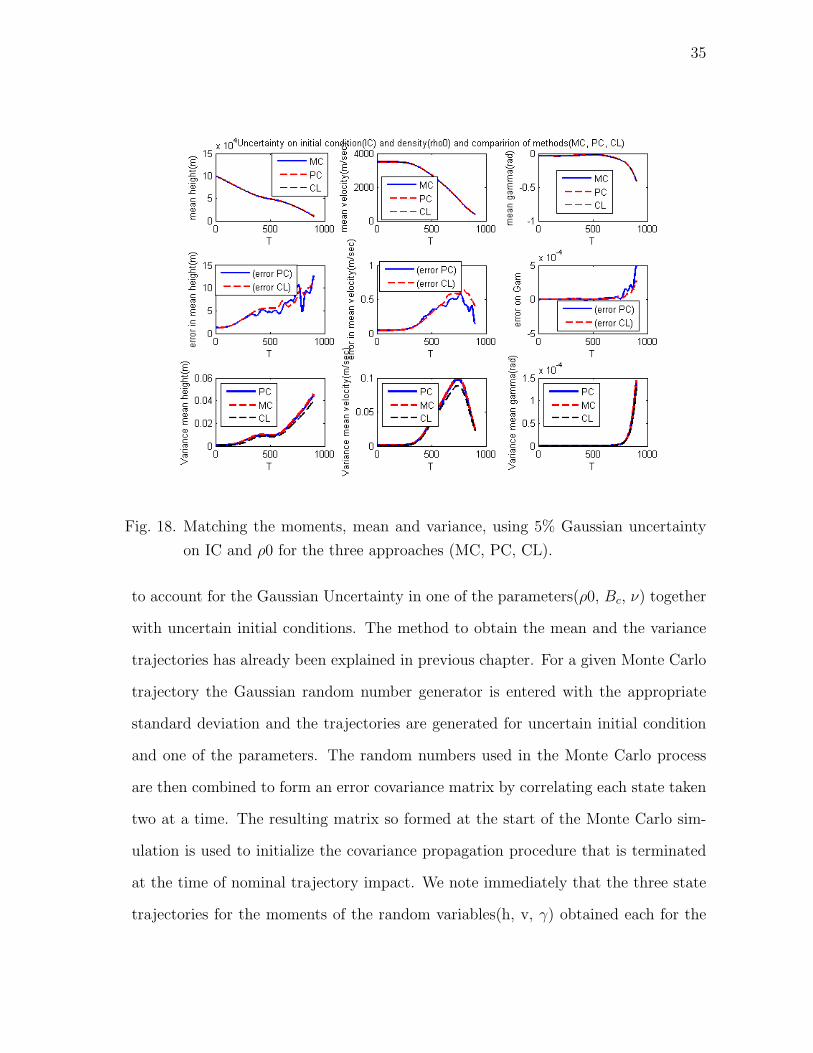
Fig. 18. Matching the moments, mean and variance, using 5% Gaussian uncertainty
on IC and ρ0 for the three approaches (MC, PC, CL).
to account for the Gaussian Uncertainty in one of the parameters(ρ0, Bc, ν) together
with uncertain initial conditions. The method to obtain the mean and the variance
trajectories has already been explained in previous chapter. For a given Monte Carlo
trajectory the Gaussian random number generator is entered with the appropriate
standard deviation and the trajectories are generated for uncertain initial condition
and one of the parameters. The random numbers used in the Monte Carlo process
are then combined to form an error covariance matrix by correlating each state taken
two at a time. The resulting matrix so formed at the start of the Monte Carlo sim-
ulation is used to initialize the covariance propagation procedure that is terminated
at the time of nominal trajectory impact. We note immediately that the three state
trajectories for the moments of the random variables(h, v, γ) obtained each for the
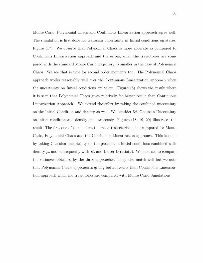
36
Monte Carlo, Polynomial Chaos and Continuous Linearization approach agree well.
The simulation is first done for Gaussian uncertainty in Initial conditions on states,
Figure (17). We observe that Polynomial Chaos is more accurate as compared to
Continuous Linearization approach and the errors, when the trajectories are com-
pared with the standard Monte Carlo trajectory, is smaller in the case of Polynomial
Chaos. We see that is true for second order moments too. The Polynomial Chaos
approach works reasonably well over the Continuous Linearization approach when
the uncertainty on Initial conditions are taken. Figure(18) shows the result where
it is seen that Polynomial Chaos gives relatively far better result than Continuous
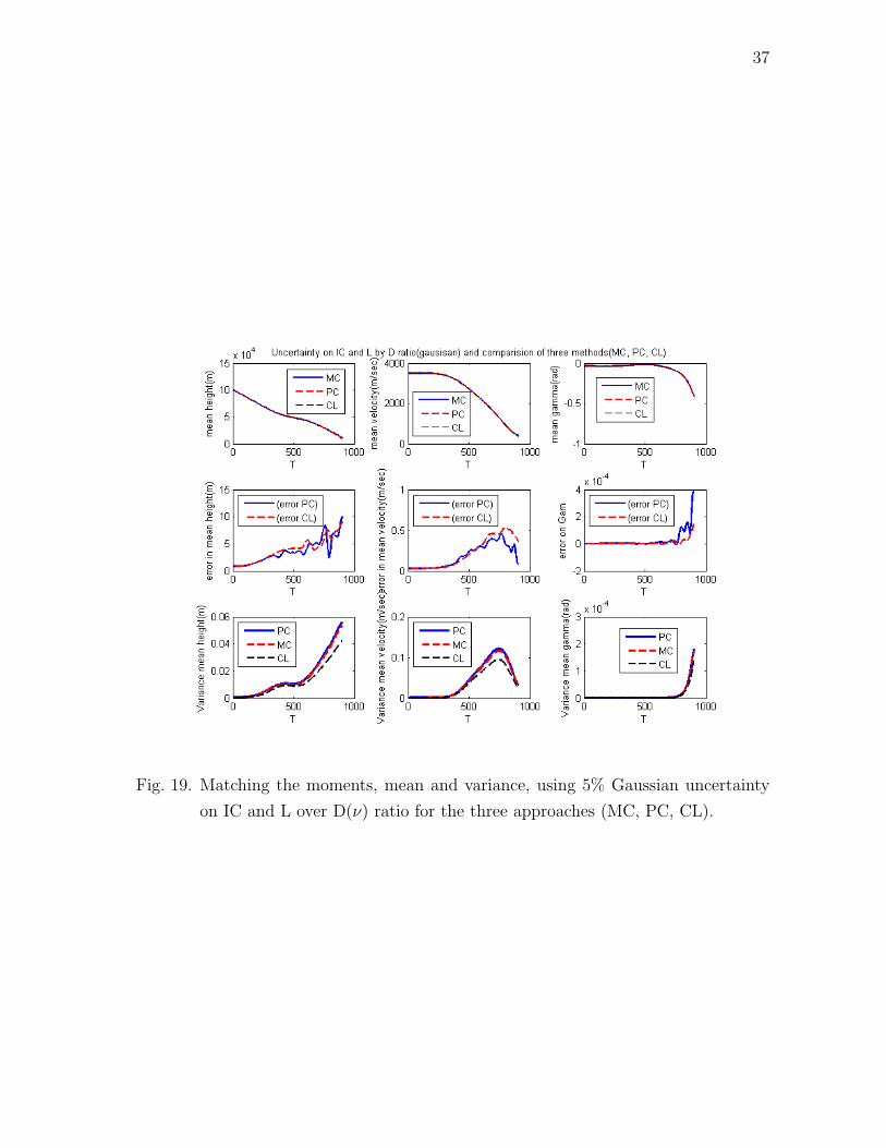
Linearization Approach . We extend the effort by taking the combined uncertainty
on the Initial Condition and density as well. We consider 5% Gaussian Uncertainty
on initial condition and density simultaneously. Figures (18, 19, 20) illustrates the
result. The first one of them shows the mean trajectories being compared for Monte
Carlo, Polynomial Chaos and the Continuous Linearization approach. This is done
by taking Gaussian uncertainty on the parameters initial conditions combined with
density ρ0 and subsequently with Bc and L over D ratio(ν). We next set to compare
the variances obtained by the three approaches. They also match well but we note
that Polynomial Chaos approach is giving better results than Continuous Lineariza-
tion approach when the trajectories are compared with Monte Carlo Simulations.
37
Fig. 19. Matching the moments, mean and variance, using 5% Gaussian uncertainty
on IC and L over D(ν) ratio for the three approaches (MC, PC, CL).
38
Fig. 20. Matching the moments, mean and variance, using 5% Gaussian uncertainty
on IC and Bc ratio for the three approaches (MC, PC, CL).
39
CHAPTER V
SUMMARY AND CONCLUSIONS
A. Summary
In this thesis, we have presented a framework for analyzing evolution of uncertainty
in hypersonic flight. This framework is based on the generalized Polynomial Chaos
framework, which has been successfully applied to areas such as stochastic computa-
tional fluid dynamics and solid mechanics. We have demonstrated that this frame-
work captures the trajectory statistics quite accurately and is computationally less
demanding than methods based on Monte-Carlo simulations. Monte-Carlo methods
were used in this paper solely to verify the results obtained from the generalized Poly-
nomial Chaos approach.
However, the generalized Polynomial Chaos based approach has limitations related
to errors due to long term integration. This makes it suitable for estimation of short
term statistics. Further, we have used this method to capture the dynamics with
fewer dimensions. Further, in terms of computation, Polynomial Chaos requires some
effort in computing the tensors 〈φiφj · · ·φl〉, which has to be done once. This can be
computed in the preprocessing stage and stored for later use. It is the computation
of these tensors that makes higher order Taylor series approximation computation-
ally prohibitive. In general Polynomial Chaos based approach is computationally far
superior to Monte-Carlo methods.
40
B. Future Work
Polynomial Chaos has long term integration issues. It cannot capture the statistics of
the dynamics over a long period of time. This was demonstrated for the well known
Van der Pol dynamics where the trajectory obtained by the Polynomial Chaos devi-
ated from the Monte Carlo trajectories. This will become more apparent when the
stochastic solutions are periodic with frequencies varying in random fashion. We can
choose the polynomial order adaptively but it will increase the computational burden.
Methods exist that reduce the error growth over time and they incorporate adaptive
multi-element schemes [11, 12]. The multi-element approach approximates Ω using
local approximations, instead of global approximations. It is well known in approx-
imation theory that locally supported basis functions provide superior results than
globally supported functions. The idea works on the framework of Multi-Element
generalized Polynomial Chaos where the random space is decomposed into smaller
elements and the gPC scheme is implemented for each of the elements. This will
allow us to work with low polynomial order as even the lower order approximation
will capture the short term statistics. This multi element gPC method is analogous
to h-p type convergence in Finite Element Theory. Here h will be the size of the
random element and p will be the order of the Polynomial Chaos.
We have used this method when the forcing is not there. For most of the practi-
cal cases we have forcing of stochastic nature. Polynomial Chaos scheme can be used
in this case if the forcing is represented using Karhunen-Loeve expansions. This is the
representation of the stochastic process as an infinite linear combination of orthog-
onal basis functions. The choice of basis functions is not restricted. The particular
interest is to restrict the basis functions to those which will make Xi uncorrelated
41
random variables. Mathematically this will require:
E[XiXj] = E[Xi]E[Xj]
∀i, j 6= i
gPC works for standard distributions like uniform, Gaussian. Since most of the
practical simulations involve non standard type distributions, this method should be
extended to capture the dynamics with non standard distributions. This is done by
choosing the set of orthogonal polynomials using Gram-Schmidt orthogonalization.
Mathematically, the orthogonal polynomials can be represented as:
φj(ξ) = ej(ξ)−j−1∑k=0
cjkφk(ξ)
with φ0 = 1 and
cjk =〈ej(ξ), φk(ξ)〉〈φk(ξ), φk(ξ)〉
Here the polynomials ej(ξ) are polynomials of exact degree j. Further, to obtain
exponential convergence the weighting function has to be equal to the probability
distribution function(PDF) of the random variable. This will extend the use of gPC
method to other non standard type of distributions as well with exponential conver-
gence realized.
Although we have shown that the gPC scheme works well over the standard Monte
Carlo method for three dimensional stochastic planar dynamics, it needs to be checked
as how will this behave with cases having multi dimensional random spaces. It is ap-
parent that the evaluation of statistics of the dynamics will become more involved.
This approach might have problems when applied to partial differential equations

42
with random fields.
43
REFERENCES
[1] V. Volterra., Lecons sur les Equations Integrales et Integrodifferentielles. Paris:
Gauthier Villars, 1913.
[2] N. Weiner., “The homogeneous chaos,”AJM, vol. 60, no. 4, pp. 897-936, 1938.
[3] R. H. Cameron and W. T. Martin., “The orthogonal developmment of non-linear
functionals in series of Fourier-Hermite Functionals,” Ann Math, vol. 48, no. 2,
pp. 385-392, 1947.
[4] D. Xiu and G. Em Karniadakis., “The Weiner Askey Polynomial Chaos for
stochastic differential equations ,” SIAM J. Sci. Comput., vol. 24, no. 2, pp.
619-644, 2002.
[5] R. Askey and J. Wilson., “Some basic hypergeometric polynomials that general-
ize Jacobi Polynomials,” Memoirs Amer. Math. Soc., vol. 66, no. 7, pp. 319-360,
1985.
[6] T. Y. Hou, W. Luo, B. Rozovskii, and Hao-Min Zhou. “Weiner Chaos Expansions
and numerical solutions of randomly forced equations of fluid mechanics.,” J.
Comput. Phys., vol. 187, no. 1, pp. 137-167, 2003.
[7] R. G. Ghanem and Pol D. Spanos, Stochastic Finite Elements: A Spectral Ap-
proach. New York: Springer-Verlag, 1991.
[8] R. Ghanem and J. Red-Horse., “Propagation of probabilistic uncertainty in com-
plex physical systems using a stochastic finite element approach,” Phys. D., vol.
133, nos. 1-4, pp. 137-144, 1999.
44
[9] N. Vinh. Hypersonic and Planetary Entry Flight Mechanics., Ann Arbor, MI:
University of Michigan Press, June 1980.
[10] B. J. Debusschere, H. N.Najm, P. P. Pebay, Omar M. Knio, R. G. Ghanem
and O. P. Le Maitre. “Numerical challenges in the use of Polynomial Chaos
representations for stochastic processes,” SIAM J. Sci. Comput., vol. 26 no. 2,
pp. 698-719, 2005.
[11] R. Li and R. Ghanem.“Adaptive Polynomial Chaos expansions applied to statis-
tics of extremes in non linear random vibration.,” Probabilist Eng Mech, vo. 13,
pp 125-136, April 1998.
[12] X. Wan and G. Em Karniadakis., “An adaptive multi-element generalized Poly-
nomial Chaos method for stochastic differential equations.,” J. Comput. Phy.,
vol. 209, no. 2, pp. 617-642, 2005.
[13] S. I. Resnick, A Probability Path., Boston, MA: Birkhauser, 1998.
[14] M. Jardak, C.-H. Su, G.E. Karniadakis. “Spectral polynomial choas solutions of
the stochastic advection equation.,” J. Sci Comput., vol. 17, pp. 319- 338, 2002.
[15] G. Lin, C.-H. Su, G.E. Karniadakis, “Stochastic solvers for the euler equations,”
43rd AIAA Aerospace Sciences Meeting and exhibit Reno, Nevada, 2005.
[16] L. Mathelin, M.Y. Hussaini, T. Z. Zang., “Stochastic approches to uncertainty
quantification in CFD simulations,” Numerical Algorithms, vol. 38, pp. 209 -
236, 2005.
45
APPENDIX A
NOMENCLATURE
Ω Sample space
F σ-algebra defined over subsets of Ω
P Probability measure
ω ∈ Ω An event in the sample space
∆ ≡ ∆(ω) Random variables representing system parameters
f(∆) Joint probability density function of system parameters
h Non dimensional altitude, scaled by R0
V Non dimensional velocity, scaled by vc
γ Flight path angle
L/D Lift over drag ratio
Bc Ballistic coefficient of vehicle
ρ0 Density on surface of planet
t Non dimensional time, scaled by R0/vc
g GM/R20
R0 Radius of planet
vc Escape velocity =√gR0
M Mass of planet
G Universal gravitation constant
46
APPENDIX B
DIFFERENT METHODS FOR UNCERTAINTY PROPAGATION
Monte Carlo methods belong to a class of computational algorithms which uses re-
peated random sampling for the computation. This becomes computationally cost
prohibitive as the number of sample points increase as the mathematical or physical
simulation needs to be run for each of the sample points. This technique is often
used when deterministic algorithm is not present to compute the exact result. This
method is particularly helpful in analyzing a system with large number of coupled
degrees of freedom such as fluids, disordered materials or strongly coupled solids. It
is used for modeling phenomena with significant uncertainty in inputs or parameter
constants. The general pattern for using this approach is to select a domain with
random possible inputs. This domain is used for generating random inputs and per-
forming a deterministic computation on them. The results of individual computation
is collected to get the final result. As an illustrative example, this method can be
used for the evaluation of definite integrals with complicated boundary conditions
which cannot be defined analytically or as in our case it is used for computing the
statistics like mean and variance of the states defined by the dynamical differential
equation where it is realized for each of the sample points in the domain selected for
the parameters like initial condition and constants.
Consider the differential equation:
dX = f(x)dt+ dW
Replacing the non linear system by the equivalent linear system:
˙Xeq = (A(t)Xeq + b(t))dt+ dW
47
Now, Stochastic Linearization implies:
f(Xt) = f(Xt−1) + f ′(xt−1)dt
and define the error term as:
e = X −Xeq
Therefore the problem statement reduces to :
min(E[∫ T
0eT edt])A(t),b(t)
Now since
e = (f(x)− AXeq − b) ≈ (f(x)− AXeq − b)
The cost function is defined as:
J =∫ T
0E[(f(x)− AXeq − b)T (f(x)− AXeq − b)]dt
Therefore,
δJ =∫ T
0([∂E(eT e)
∂A]δA+ [
∂E(eT e)
∂b]δb)dt = 0
Minimization require:
[∂E(eT e)
∂A] = 0
[∂E(eT e)
∂b] = 0
⇒ 2E[f(x)− Ax− b] = 0
⇒ ˙X = E[f(x)] = Ax+ b
Similarly from the first inequality:
A = E[f(x)xT ]− xE[fT (x)]P−1
48
Now since,
P = (AP + PAT +Q)
⇒ P = E[f(x)(x− x)T ] + E[(x− x)fT (x)] +Q(t)
Hence we get the final set of differential equations for the propagation of the mean
and variance:
˙X = E[f(x)]
P = E[f(x)(x− x)T ] + E[(x− x)fT (x)] +Q(t)
The Fokker-Plank equation gives the time evolution of the probability density function
and is commonly used for computing the probability densities of stochastic differential
equations. This is also commonly known as Kolmogorov forward equation. The
Fokker-Plank equation was first used to give the statistical description of Brownian
motion of a particle in a fluid.
In one spatial direction x, the Fokker-Plank equation for a process with drift D1(x, t)
and diffusion D2(x, t) is :
∂
∂tf(x, t) = − ∂
∂x[D1(x, t)f(x, t)] +
∂2
∂x2[D2(x, t)f(x, t)]
More generally, the time dependent probability distribution function may depend on
a set of N variables xi. The general form of the Fokker-Plank equation can then be
written as:
∂
∂tf(x, t) = −
N∑i=1
∂
∂xi[D1
i (x1, x2, ..xN t)f ] +N∑i=1
N∑j=1
∂2
∂xi∂xj[D2
ij(x1, x2, .....xN , t)f(x, t)]
Here D1 and D2 are drift and the diffusion tensors respectively. The diffusion term
results from the presence of the stochastic forces. Probability density of stochastic
differential equations are computed using Fokker-Plank equations. We take the Ito
49
stochastic differential equation:
dXt = µ(Xt, t)dt+ σ(Xt, t)dWt
This can be understood as the stock price model used by Black and Scholes where
µ(Xt, t) represents the instantaneous rate of return on a riskless asset, σ(Xt, t) is the
volatility of the stock, and dWt represents the infinitesimal change in a Brownian
motion over the next instant of time. Where Xt ∈ RN is the state and Wt ∈ RM is
a standard M-dimensional Wiener process. If we assume the initial distribution to
be X0 ∼ f(x, 0) then the probability density f(x, t) of the state Xt is given by the
Fokker-Plank equation with drift and diffusion terms as :
D1i (x, t) = µi(x, t)
D2ij(x, t) =
1
2
∑k
σik(x, t)σTkj(x, t)
Being a partial differential equation(PDE), the Fokker-Plank equation(FPK) can be
solved analytically only in special cases. Different numerical techniques are used for
computing the PDE’s generated by the FPK. This however is computationally faster
than the monte carlo technique where the simulation is run for greater number of
sample points.
Let us consider the scalar differential equation excited by white noise(W) of unit in-
tensity. We can write the differential equation as :
x = −x+ εx3 +W
Here W is the white noise of unit intensity and ε is a parameter. For our computa-
tional purposes we are taking the value of epsilon as ε = −0.1. The value of epsilon
is so chosen such that the probability distribution function shows a stable behavior.
50
We will use the different methods for the propagation of uncertainty and compare the
statistics obtained by each of them.
The given differential equation is:
x = −x+ εx3 + w
Where w is white noise of unit intensity It is intuitive to write the differential equation
as:
∆x = (−x+ εx3)∆T + ∆w
Now here δT is fixed. We start with a small value of ∆T (= 0.1) and run the monte
carlo simulation and match the mean and variance with the Gaussian closure method.
We are running the simulation for this small period of time though the process can be
run for higher time spans by breaking that span into small (smaller!) increments and
capturing the statistics accurately and then propagating the states. The end result of
the integration for each step would become the initial condition for the next propaga-
tion. Matlab goes dismally slow and hence puts the restriction on running these for
smaller steps and capturing the accurate dynamics for even higher samples. Though,
it is being illustrated here that the dynamics is being captured adequately with even
small number of samples.(n = 100 for noise and IC, assumed to be Gaussian).
x = −x+ εx3 +W
Clearly,
f(x) = −x+ εx3
51
Upon substitution we get the differential equation for the mean and variance:
˙X = ε(X)3 + X(3εP − 1)
P = 2(−P + ε(6µ2P + 3P 2 − 3µP )) +Q
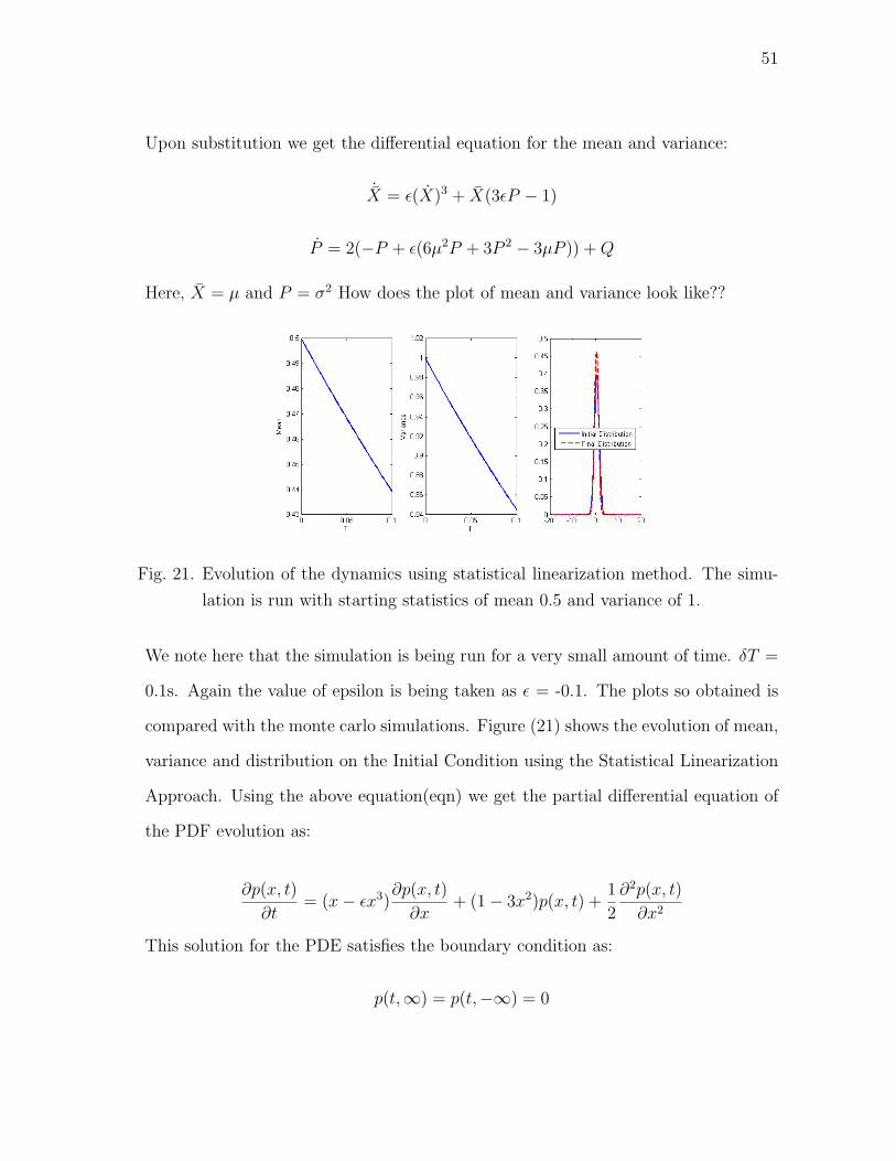
Here, X = µ and P = σ2 How does the plot of mean and variance look like??
Fig. 21. Evolution of the dynamics using statistical linearization method. The simu-
lation is run with starting statistics of mean 0.5 and variance of 1.
We note here that the simulation is being run for a very small amount of time. δT =
0.1s. Again the value of epsilon is being taken as ε = -0.1. The plots so obtained is
compared with the monte carlo simulations. Figure (21) shows the evolution of mean,
variance and distribution on the Initial Condition using the Statistical Linearization
Approach. Using the above equation(eqn) we get the partial differential equation of
the PDF evolution as:
∂p(x, t)
∂t= (x− εx3)
∂p(x, t)
∂x+ (1− 3x2)p(x, t) +
1
2
∂2p(x, t)
∂x2
This solution for the PDE satisfies the boundary condition as:
p(t,∞) = p(t,−∞) = 0
52
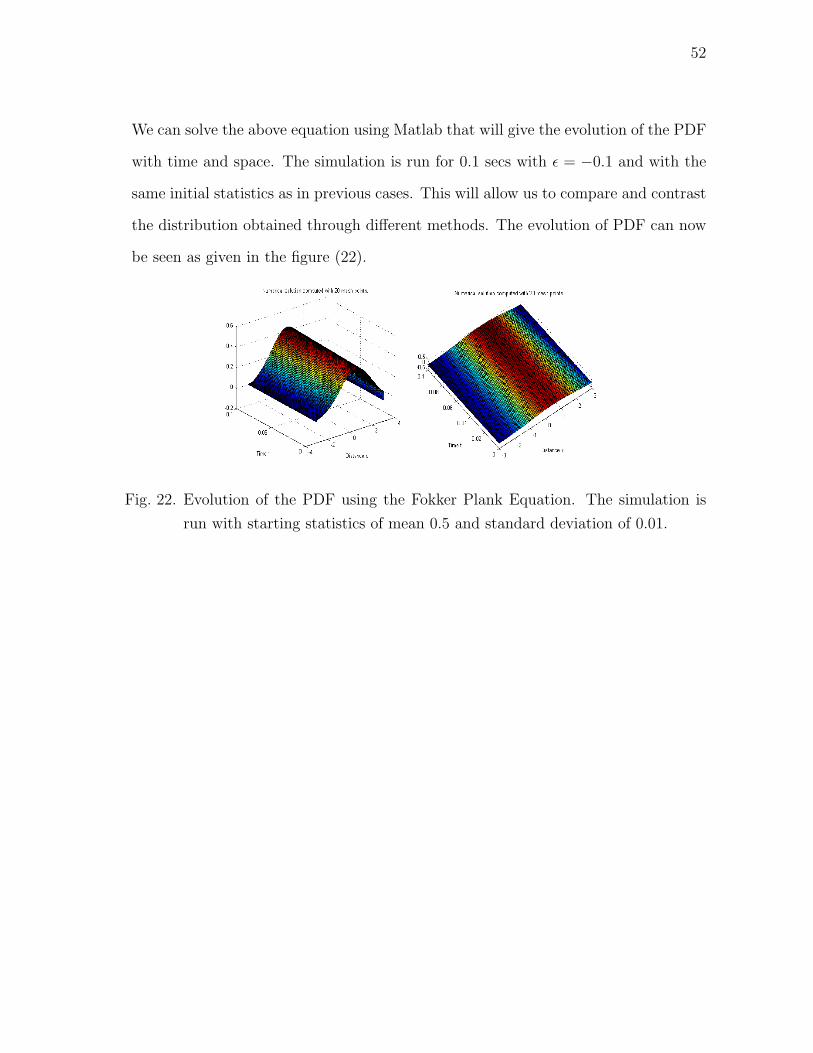
We can solve the above equation using Matlab that will give the evolution of the PDF
with time and space. The simulation is run for 0.1 secs with ε = −0.1 and with the
same initial statistics as in previous cases. This will allow us to compare and contrast
the distribution obtained through different methods. The evolution of PDF can now
be seen as given in the figure (22).
Fig. 22. Evolution of the PDF using the Fokker Plank Equation. The simulation is
run with starting statistics of mean 0.5 and standard deviation of 0.01.
53
APPENDIX C
REPRESENTATION OF ARBITRARY RANDOM INPUTS
We know that with appropriately chosen Weiner Askey Polynomial Chaos expansion
based on the type of standard arbitrary random inputs, optimal convergence rate of
the chaos expansion is realized. However, for most of the cases the distribution of
the random input is not of the standard type as given in the table or even if they
do belong to certain standard types, the correspondence is not explicitly known. For
these cases we need to project the input process onto the weiner askey Polynomial
Chaos basis directly in order to solve the differential equation.
For example, let us consider the ordinary differential equation :
dy(t)
dt= −ky, y(0) = y
Now let us assume that the distribution of the decay parameter k is known in the
form of the probability function f(k). The representation of k by the weiner-askey
Polynomial Chaos expansion takes the form
k =P∑i=0
kiφi
where,
ki =〈kφi〉φ2i
Where we know from the previous work that the operation 〈., .〉 denotes the inner
product in the Hilbert space spanned by the Weiner-Askey chaos basis φi, ie.,
ki =1
〈kφ2i 〉
∫kφi(ξ)g(ξ)dξ
54
Where g(x) and g(xi) are the probability function of the random variable ξ in the
Weiner-Askey Polynomial Chaos for continuous cases. Here we are taking the as-
sumption that that the random variable ξ is fully dependent on the target random
variable k. We understand that the support of k and ξ are different. This is the other
way of saying that k and ξ can belong to two different probability spaces (Ω,Λ, P ),
with different event spaces Ω, σ − algebra Λ and probability measure P.
For us to be able to conduct the above projection we need to transform the fully
correlated random variables k and ξ to the same probability space. The standard
method is to transform them to the uniformly distributed probability space u ∈ U(0,
1). This is the key to random number generation, where the uniformly distributed
numbers are generated as the seeds and then the inverse transformation is performed
according to the desired distribution function. Let us assume that the random variable
u is uniformly distributed in (0, 1) and the PDF’s for k and ξ are f(k) and g(ξ)
respectively. A transformation of the variable in probability space shows that
du = f(k)dk = dF (k), du = g(ξ) = dG(ξ)
Where F and G are the distribution functions of k and ξ, respectively, ie,
F (k) =∫ k
−∞f(t)dt,G(ξ) =
∫ ξ
−∞g(t)dt.
If it is desired to convert the random variables to k and ξ to be transformed to the
same uniformly distributed random variable u, we obtain
u = F (k) = G(ξ)
After inverting the above equation we get
k = F−1(u) ≡ h(u), ξ = G−1(u) ≡ l(u)
55
By doing so we convert the two random variables k and ξ to the same probability
space defined by u ∈, the projection (6.2) can be performed as,
ki =1
〈φ2i 〉
∫kφi(ξ)g(ξ)dξ =
1
〈φ2i 〉
∫ 1
0h(u)φi(l(u))du
It is difficult to evaluate the above integral analytically. However it is possible to
evaluate the above integral using the Gauss quadrature in the closed domain [0, 1]
with reasonable accuracy. The analytical form for some of the standard distributions
are known. The above process requires that the distribution functions are known
and the inverse functions F−1 and G−1 exist and be known as well. In practice this
is not always satisfied and we know only the probability function f(k) for a specific
problem. The probability function g(ξ) is known from the choice of Weiner-Askey
Polynomial Chaos but the inversion is not known always. In this case we can per-
form the projection(6.2) directly by monte carlo integration, where a large ensemble
of random numbers k and ξ are generated. Further the requirement that k and ξ
be transformed to same probability space U ∈ (0, 1) requires that k and ξ has to
be generated from the same seed of uniformly generated random number U ∈ (0,
1). In this section we present numerical examples of representing an arbitrarily given
random distribution. Here, we will try to capture non Gaussian random variables us-
ing Hermite Chaos. Although, the solution by Hermite chaos converges but optimal
exponential convergence is not realized. It is assumed that the decay parameter k in
the ordinary differential equation is a random variable with exponential distribution
with pdf of the form
f(k) = e−k, k > 0
56
The inverse of its distribution function is known as
h(u) ≡ F−1(u) = −ln(1− u), u ∈ U(0, 1)
We now take the Hermite-chaos as the Polynomial Chaos expansion of k instead of
the optimal Laguerre-chaos. The standard random variable ξ is a standard Gaussian
random variable with PDF g(ξ) = 1√2πe−
ξ2
2 . The inverse of the Gaussian distribution
G(ξ) is known as
l(u) ≡ G−1(u) = −sign(u− 1
2)(t− c0 + c1t+ c2t
2
1 + d1t+ d2t2 + d3t3)
Where,
t =√−ln[min(u, 1− u)]2
and c0 = 2.515517, c1 = 0.802853, c2 = 0.010328 d0 = 1.432788, d1 = 0.189269, d2 =
0.001308 The above analytical form is taken from Hastings.
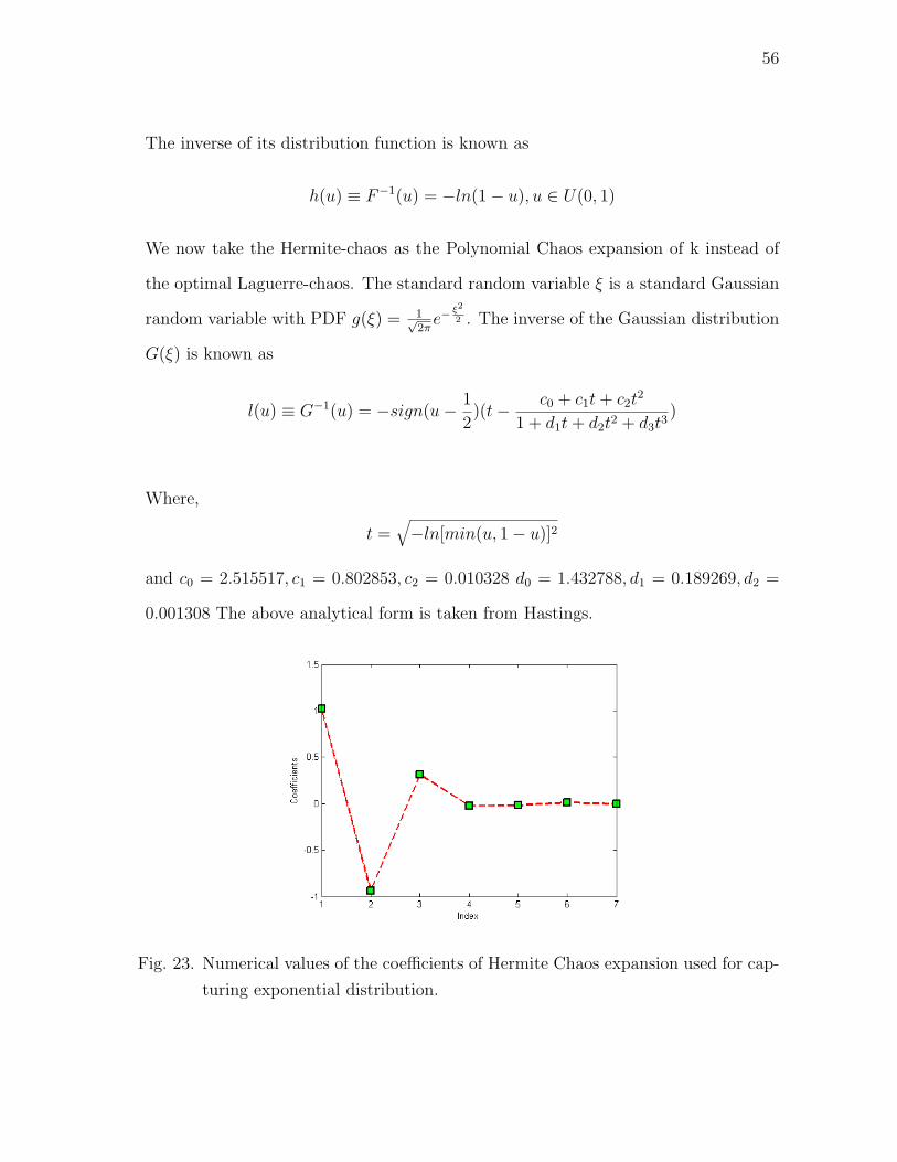
Fig. 23. Numerical values of the coefficients of Hermite Chaos expansion used for cap-
turing exponential distribution.

57
The figure (23) shows the results when the exponential distribution is captured by the
Hermite Chaos. We see that the major contribution of the Hermite chaos expansion
is coming from the first three terms.
58
APPENDIX D
POLYNOMIAL CHAOS EXPANSION METHOD FOR SOLVING
UNCERTAINTY IN VAN DER POL EQUATIONS
The Cameron-Martin theorem states that any second-order(i.e, finite variance), one
dimensional process G can be written as the weighted sum of the Hermite polynomials
in the Gaussian random variable ξ(taken to have zero mean and unity variance), and
that series converges in the L2 sense. Using the symbolic notation of Abramowitz
and Stegun,
G =∞∑i=0
giHei(ξ)
Clearly, the distribution G is constructed from modes which are Hermite Polynomi-
als: He0 = 1, He1(ξ) = ξ,He2(ξ) = ξ2 − 1,..... Further, inner product of Hermite
polynomials are orthogonal with respect to the Gaussian PDF of the random variable
ξ. i.e., ∫ ∞−∞
e−ξ2
2 Hei(ξ)Hej(ξ)dξ = eijδij
Where δij are Kronecker delta function. We note that the orthogonality holds when
the weight functions are replaced by equivalent PDF of the random variable. Higher
tensors can similarly be defined as,
∫ ∞−∞
e−ξ2
2 Hei(ξ)Hej(ξ)Hek(ξ)dξ = eijkδijk
We will cite a specific example to illustrate the use of Polynomial Chaos expansion
to handle parametric uncertainty. Let us consider the case of van der pol equation,
d2y
dt2+ µ(y2 − 1)
dy
dt+ y = 0
59
Here x is the position coordinate which is a function of time t, and µ is a random
variable with uniform distribution. The above equation now becomes stochastic in
nature. We will illustrate in this example the way Polynomial Chaos method con-
verts the stochastic differential equation into deterministic linear equations in higher
dimensions. Let us write the differential equation in the state space form as,
dx
dt= y
dy
dt= µ(1− x2)− x
In this problem, the random variable µ is expressed as a finite summation of modes,
up to the order P, along with the states. Hence the mathematical form is given as,
µ =P∑i=0
µiLei(ξ)
y(t) =P∑i=0
yi(t)Lei(ξ)
x(t) =P∑i=0
xi(t)Lei(ξ)
Where Le0 = 1, Le1 = ξ, Le2 = 12(3ξ2−1), Le3 = 1
2(5ξ3−3ξ) are Legendre polynomials
and possess the inner product property as Hermite polynomials. Substituting into
the dynamic equation we obtain,
P∑i=0
xi(t)Lei(ξ) =P∑i=0
yi(t)Lei(ξ)
P∑i=0
yi(t)Lei(ξ) =P∑i=0
µiLei(ξ)(1−P∑i=0
P∑i=0
xi(t)xj(t)LeiLej)−P∑i=0
xi(t)Lei
Next, using the inner product property of these series of orthogonal polynomials,
we multiply by the kth mode and take the Galerkin projection to obtain a set of
deterministic linear equations in higher dimensions:
60
0 50 100 150 200−2
−1.5
−1
−0.5
0
0.5
1
1.5
2
T
X1
MCPC/P=4
Fig. 24. Evolution of Monte Carlo and Polynomial Chaos trajectory with time. The
results match and the divergence over the period of time is due to long term
integration issues of Polynomial Chaos
method.
xk(t) = yk(t),
yk(t) = µk − 1ekk
∑Pl=0
∑Pj=0
∑Pi=0 xi(t)xj(t)µleijlk − xk(t)
In the case of no parametric uncertainty(µi = 0, i > 0) and without nonlinearity each
mode will evolve independent of each other in accordance with the properties of time
invariant linear systems.
We observe from figure (24) that the Polynomial Choas Trajectory matches well
with the Monte Carlo Trajectory for initial span of time and diverges after some time
because of long term integration issues with Polynomial Chaos Method.
61
VITA
Avinash Prabhakar was born in India. He received his baccalaureate degree in
aerospace engineering from the Indian Institute of Technology, Roorkee, India in
2002. In August 2002, he joined Tata Steel as a Graduate Engineer Trainee before
coming to Texas A&M University on August 2006 for his graduate studies. All grad-
uate level work was performed under the supervision of Dr. Raktim Bhattacharya.
His master’s thesis focussed on the uncertainty propagation in the hypersonic flight
dynamics using Polynomial Chaos Theory.
He can be reached by contacting Dr. Raktim Bhattacharya, Department of Aerospace
Engineering, Texas A&M Univerity, College Station, TX 77843-3141.
The typist for this thesis was Avinash Prabhakar.
Related Documents