Uncertainty Determinants of Corporate Liquidity Christopher F. Baum * Department of Economics Boston College Mustafa Caglayan Department of Economics University of Leicester Andreas Stephan DIW – Berlin Europa–Universit¨ at Viadrina Oleksandr Talavera DIW – Berlin Europa–Universit¨ at Viadrina 31st January 2005 * The standard disclaimer applies. We gratefully acknowledge comments and helpful suggestions by Christopher F. Baum and Yuriy Gorodnichenko. Corresponding author: Oleksandr Talavera, tel. (+49) (0)30 89789 207, fax. (+49) (0)30 89789 200, e-mail: [email protected], mailing address: K¨ onigin-Luise-Str. 5, 14195 Berlin, Germany. 1

Welcome message from author
This document is posted to help you gain knowledge. Please leave a comment to let me know what you think about it! Share it to your friends and learn new things together.
Transcript

Uncertainty Determinants of Corporate Liquidity
Christopher F. Baum∗
Department of Economics
Boston College
Mustafa CaglayanDepartment of Economics
University of Leicester
Andreas StephanDIW – Berlin
Europa–Universitat Viadrina
Oleksandr TalaveraDIW – Berlin
Europa–Universitat Viadrina
31st January 2005
∗The standard disclaimer applies. We gratefully acknowledge comments and helpful suggestionsby Christopher F. Baum and Yuriy Gorodnichenko. Corresponding author: Oleksandr Talavera,tel. (+49) (0)30 89789 207, fax. (+49) (0)30 89789 200, e-mail: [email protected], mailing address:Konigin-Luise-Str. 5, 14195 Berlin, Germany.
1
Uncertainty Determinants of Corporate Liquidity
Abstract
This paper investigates the link between the optimal level of non–financialfirms’ liquid assets and uncertainty. We develop a partial equilibrium model ofprecautionary demand for cash that shows that firms are likely to change theirliquidity ratio in response to changes in uncertainty. We test this propositionusing a panel of non–financial US firms drawn from COMPUSTAT quarterlydatabase covering the period 1991-2001. The results show that firms increasetheir liquidity ratios when macroeconomic uncertainty increases. We demon-strate that our results are robust with respect to the inclusion of detrendedindex of leading indicators and interest rates.
Keywords: cash, uncertainty, non–financial firms, dynamic panel data.
JEL classification C23, D8, D92, G32.
2
1 Introduction
“As a result of the foregoing, Honda’s consolidated cash and cash equivalents amounted
to ¥547.4 billion as of March 31, 2003, a net decrease of ¥62.0 billion from a year
ago. ... Honda’s general policy is to provide amounts necessary for future capital
expenditures from funds generated from operations. With the current levels of cash
and cash equivalents and other liquid assets, as well as credit lines with banks, Honda
believes that it maintains a sufficient level of liquidity.”1
“Standard & Poor’s said those reserves have declined severely over the last year
and blamed the drain, in part, on Schrempp’s massive spending spree, which included
taking a 34 percent stake in debt-ridden Japanese automaker Mitsubishi Motors.
According to an article in Newsweek magazine, DaimlerChrysler’s cash reserves – a
cushion against any economic turndown – will dwindle to $ 2 billion by the end of
the year, down 78 percent from two years ago. That compares with cash reserves of
more than $13 billion at rivals General Motors and Ford, the magazine said.”2
Why is it considered so good when a company is able to maintain considerable
amounts of cash like in Honda’s case? Why is it so bad when cash reserves go
down as in DaimlerChrysler’s case? What determines the optimal level of liquidity?
In the seminal paper of Modigliani and Miller (1958) cash is considered as a zero
net present value investment. There are no benefits from holding cash in a world
without information asymmetries, transaction costs, or taxes, and with perfect capital
markets.
However, the real world is imperfect and firms can avoid some costs by holding
liquid assets. Keynes (1936) suggests two main reasons of maintaining a positive level
of liquid assets. First, firms hold liquid assets to reduce transaction costs. Second,
cash stock provide a buffer to meet unexpected contingencies. Managers can increase
1Citation. http://world.honda.com/investors/annualreport/2003/17.html2Citation. http://www.detnews.com/2000/autos/0012/04/-157334.htm
3
firm value by managing their cash balances. This cash buffer allows the company to
maintain the ability to invest when the company does not have sufficient current cash
flows to meet investment demands.
There is great variation in liquidity ratios among different types of firms which
is systematically related to firm size, industry, and leverage ratios. Econometric
analysis in the recent literature suggests that liquid assets are positively correlated
with proxies for agency problems. Therefore, firms cannot borrow easily and maintain
higher levels of cash to finance investment opportunities. For instance, BMW Group
invested 2,807 million Euro in 1999 and these investment were financed in full out of
the Group’s cash flow.3 The link between cash flow and investment has been often
investigated in the literature (Fazzari, Hubbard and Petersen (1988), Schnure (1998),
Cummins, Hasset and Oliner (1995), Charlton, Lancaster and Stevens (2002)). Kim
and Sherman (1998) argue that firms increase investment in liquid assets in response
to increase in the cost of external financing, the variance of future cash flows, and
the return on future investment opportunities. Moreover, they document that larger
firms tend to have lower ratios of cash to assets.4 Additionally, Harford (1999) argues
that corporations with excessive cash holdings are less likely to be takeover targets.
In an important recent paper, Almeida, Campello and Weisbach (2004) develop
a liquidity demand model where firms have access to investment opportunities but
cannot finance them. In a world without financial constraints cash holdings are
irrelevant and firms undertake all positive NPV projects regardless of cash position.
However, when firms have financial constraints they have an optimal level of liquid
assets, determined through equating marginal costs of cash holdings to marginal
benefits of cash holdings.5
3Citation. BMW Annual Report 1999. http://www.autointell-news.com/european companies/BMW/business-figures/bmw-annual-1999.htm
4See also Opler, Pinkowitz, Stulz and Williamson (1999), Mills, Morling and Tease (1994).5See also Bruinshoofd (2003).
4

The idea of a precautionary demand for cash is further explored by Myers and
Majluf (1984). They argue that firms facing information asymmetry–induced finan-
cial constraints are likely to accumulate cash holdings. In the recent paper Baum,
Caglayan, Ozkan and Talavera (2002) develop a static model of cash management
with a signal extraction mechanism. It shows a positive relationship between cash
holdings, the interest rate on loans, and levels of uncertainty. Moreover, they find
that firms behave similarly in response to increases in macroeconomic uncertainty.6
The purpose of this paper is to provide a theoretical and empirical investigation
of the firm’s decision to hold liquid assets. Furthermore, we attempt to bridge the
gap in existing research by matching firm–specific data with information on their
macroeconomic environment. This matching allows us to investigate whether both
macroeconomic and idiosyncratic uncertainties have effects on cash holdings.
We present a model that formalizes the precautionary demand for cash.7 The firm
maximizes its assets by investing funds and holding cash to offset an adverse cash flow
shock distributed according to triangular distribution with fixed bounds. The optimal
level of cash holdings is derived as a function of expected return on investment, the
expected interest rate on loans, the bounds of cash flow distribution, the probability of
getting a loan, and initial wealth. After parametrization we anticipate that managers
change levels of liquidity in response to changes in uncertainty.
For testing this prediction we utilize a panel of non–financial firms obtained from
the quarterly COMPUSTAT database over the 1991–2001 period. After screening
procedures our data include more than 30,000 manufacturing firm–year observations,
with 700 firms per quarter. We also consider a sample split, defining categories of
durable–goods makers vs. non–durable goods makers. We apply one- and two–step
6In a recent paper Bo (1999) suggests that presence of uncertainty factors changes the structuralparameters of the Q-model of investment.
7The model ignores the transaction motive for holding cash, and the optimal amount of liquidassets is zero in the absence of costly external financing.
5

system GMM estimators (Arellano and Bond, 1991).
Our main findings can be summarized as follows. We find evidence of a positive
association between the optimal level of liquidity and macroeconomic uncertainty,
proxied by the conditional variance of industrial production. US companies also
increase their liquidity ratios when idiosyncratic uncertainty increases. The results
differ for durable and non–durable goods–makers. While macroeconomic uncertainty
does matter for the former group, we do not observe statistically significant effects
for the latter group. The durable goods–makers also have a higher sensitivity to
idiosyncratic uncertainty. The results are shown to be robust to the inclusion of of
such macroeconomic variables as index of leading indicators and interest rates.
The remainder of the paper is organized as follows. Section 3.2 discusses the the-
oretical model of firms’ precautionary demand for liquid assets. Section 3.3 describes
our data and empirical results. Finally, Section 3.4 concludes.
2 Theoretical Model
2.1 Model Setup
We develop a simple cash buffer–stock model, where a firm manager maximizes assets
of the firm in the next period. This framework allows the manager to vary optimal
level of liquid assets in response to idiosyncratic and/or macroeconomic uncertainty.
The model has two periods, t and t + 1. At time t the firm has wealth Wt−1
that comes either from stock issue if the firm has been just established or from the
previous period’s activity. At time t the initial wealth Wt−1 has to be distributed
between investment (It) and cash holding (Ct).8 For simplicity, the firm does not
finance any other activities. Investment is expected to earn E[R]t+1, the gross return
8The term Cash holdings may include not only cash itself but also low–yield liquid assets, e.g.Treasury Bills.
6

in the time t + 1.9 Liquid asset holdings, Ct, are required to guard against negative
shock.
Between periods t and t + 1 the firm faces a cash–flow shock ψt, distributed
according to a symmetric triangular distribution with mean zero and defined on the
range ψt ∈ [−Ht, Ht].10 In our framework Ht serves as a measure of uncertainty faced
by firm. There are three possible cases.
First, there is a positive cash–flow shock that occurs with probability p1 and has
conditional expectation ψt,1:
p1 = Pr(ψt > 0) =1
2
ψt,1 = E(ψt|ψt > 0) = Ht
(1−
√2
2
)
The firm’s wealth in this case is
Wt+1,1 = ItE[R]t+1 + Ct + ψt,1 = ItE[R]t+1 + Ct +Ht
(1−
√2
2
)(1)
Second, there is a negative cash–flow shock, but the firm has enough liquid assets to
cover it. This shock occurs with probability p2 and has conditional expectation ψt,2:
p2 = Pr(0 > ψt > −Ct) =1
2
Ct(2Ht − Ct)
H2t
ψt,2 = E(ψt|0 > ψt > −Ct) = −Ct
(1−
√2
2
)
In this notation the assets of the firm in the case when 0 > ψt > −Ct are equal to
Wt+1,2 = ItE[R]t+1 + Ct + ψt,2 = ItE[R]t+1 + Ct
√2
2(2)
9For simplicity we assume that distribution of return is independent from all other variables’distributions.
10The triangular distribution is chosen as an approximation to the normal distribution, whichwould require evaluation of nonlinear function.
7

Finally, there is the situation when the firm does not have enough liquid assets to cover
negative cash–flow shock. This event occurs with probability p3 and has conditional
expectation ψt,3:
p3 = Pr(−Ct > ψt) =H2
t − 2HtCt + C2t
2H2t
ψt,3 = E(ψt| − Ct > ψt) = −Ht +
√2
2(Ht − Ct)
In this case the firm must seek external finance and borrow −(ψt + Ct) at the rate
Xt. However, there is probability st that the firm gets the funds, otherwise it declares
bankruptcy and its wealth at time two is equal to zero.11 For simplicity we assume
that the probability of getting external funds is independent of the distribution of
cash–flow shocks. The assets of the firm in the last case are equal to
Wt+1,3 = st (ItE[R]t+1 + Ct + ψt,3 −Xt(ψt,3 + Ct)) + (1− st)0 = (3)
= st
[ItE[R]t+1 − (1 +Xt)(Ht − Ct)
(1−
√2
2
)]
We denote It = Wt−1−Ct. Given all three possible cases, the objective is to maximize
the expected wealth (asset value) of the firm in period t+ 1. The firm’s problem can
be written as
maxCt
(E(Wt+1)) = maxCt
(p1Wt+1,1 + p2Wt+1,2 + p3Wt+1,3
)= (4)
= maxCt
(1
2
((Wt−1 − Ct)E[R]t+1 + Ct +Ht
(1−
√2
2
))
+1
2
Ct(2Ht − Ct)
H2t
((Wt−1 − Ct)E[R]t+1 + Ct
√2
2
)
+(Ht − Ct)
2st
2H2t
((Wt−1 − Ct)E[R]t+1 − (1 +Xt)(Ht − Ct)
(1−
√2
2
)))11For instance, firm has fire accident at production line. Then it does not have funds to replace
equipment and all investment vanishes.
8

which is our objective function and Ct, optimal level of cash holdings, is the only
choice variable.
The first order condition imply that the optimal cash has to be12
Ct =1
3
(2.83− 1.75st)Ht + 1.75stXtHt − 2E[R]t+1(1− st)(2Ht +Wt−1) +√D
1.41− 0.59st − 2(1− st)E[R]t+1 + 0.58stXt
(5)
The solution is not linear and we linearize it around equilibrium levels.
Ct = α1ˆWt−1 + α2Rt+1 + α3Ht + α4Xt + α5st (6)
where coefficients α1 − α5 depend on model parameters. The expected signs of
the coefficients are discussed in the following subsection.
2.2 Model solution discussion
The analytical solution for the optimal cash holdings is a non–linear function of the
initial wealth, Wt−1; the expected gross return on investment, E[R]t+1; the gross
interest rate for borrowing, Xt; the bounds of the triangular distribution of cash
shocks, Ht and probability of getting a credit when negative shock is higher than
available cash holdings, st. The implicit solution is a complicated function of the
model parameters. We cannot obtain comparative static results but we may employ
graphical analysis to determine the signs of α, the parameters in equation 6.
Figure 1 presents the relationship among optimal cash holding and interest rate
for external borrowing and bounds of cash shock distribution. If we take Wt−1 = 30,
E[R]t+1 = 1.2 then the level of cash increases if Ht increases from 5 to 25. Moreover,
the company holds more cash (17 out of 30 for Ht = 25 and st = 0; 13 out of 30 for
12 D is a function f(E[R]t+1, Xt, st,Ht,Wt−1)
D = (16.49− 6st + 6stXt)H2t − (43.11− 33.17st + 7.03stXt)E[R]t+1H
2t + 4(1− st)2E[R]2t+1W
2t−1
+(4s2t − 32st + 28)E[R]2t+1H
2t − 8(1− st)2E[R]2t+1Wt−1Ht + 5.66(1− st)E[R]t+1Wt−1Ht
9

Ht = 25 and st = 0.5) when the probability of accessing external credit decreases.
Cash holdings are marginally sensitive to changes in the interest rate for external
borrowing, Xt. The firm’s reaction to changes in interest rate for external borrowing
is minimal. However, it responds to changes in probability of getting a loan.
When we fix E[R]t+1 = 1.2 and Wt−1 = 30, the optimal level of cash decreases
as the expected return on investment E[R]t+1 increases (see Figure 2). The expected
return on investment is the opportunity cost of holding liquid assets. The sensitivity of
cash is higher when st = 0.5, and is lower when st = 0.0. When expected earnings are
low (E[R]t+1=1.1), cash holdings decrease when the bounds of cash shock distribution
increase. However, when expected return on investment is much higher (E[R]t+1=1.7)
the optimal cash holdings first increase in response to increase of bounds of cash shock
distribution, and then decrease. Thus, when a firm expects high return, it has a non–
linear response to uncertainty.
Figure 3 represents the relationship among cash holdings, Ct, bounds of cash shock
distribution, Ht and the probability of receiving credit when the firm does not have
enough liquid assets to cover negative cash shock, st. When Wt−1 = 30, Xt = 1.3
or Xt = 1.6 and Rt+1 = 1.2 cash holdings decrease in response to an increase in the
probability of getting a loan. The relationship between cash holdings and bounds of
cash shock distribution can be either positive or negative depending on levels of other
variables.
Finally, Figure 4 describes the relationship among share of initial wealth used
as cash holdings, initial wealth and bounds of cash holding distribution. Fixing
E[R]t+1 = 1.2, Xt = 1.3 and st = 0.0 or st = 0.5 we observe a decrease in liquidity
ratio when initial wealth increases. Moreover, there is a negative relationship between
cash share and bounds of cash distribution.
Our theoretical model predicts positive sign for α1 and negative signs for α2 and
α5. The signs of α3 and α4 depend on the levels of the firm’s variables.
10

2.3 Parametrization
In order to test our theoretical model we have to make some parametrization assump-
tions. We assume that the firm maximizes its profit equal to
Π(Kt, Lt) = P (Yt)Yt − wtLt − ft
where P (Yt) is an inverted demand curve, ft represents fixed costs, Lt is labor and wt
is wages. The firm produces output, Y given by the production function F (Kt, Lt).
Expected return on investment, E[R]t+1 is equal to expected marginal profit of
capital, which is contribution of one extra unit of capital to profit.
E[R]t+1 = E
[∂Π
∂K
]=E[P ]t+1
µ
∂Y
∂K
where µ = 1/(1 + 1/η) and η is price elasticity of demand, η = ∂Y∂P
Pt+1
Yt+1.
Assuming Cobb–Douglas production function, Yt+1 = At+1Kαkt+1L
αlt+1 we rewrite
marginal product of capital, ∂Y∂K
as
E[R]t+1 =E[P ]t+1
µ
αkYt+1
K=αk
µ
E[S]t+1
Kt+1
=αk
µ
(St+1
Kt+1
)+ κ+ ω + ν (7)
where E[S] denotes expected sales, equal to sales in period t + 1. Furthermore, we
assume rational expectations that allow us to replace expectations with future values
plus a firm–specific expectation error term, νt, orthogonal to information set available
at the time when optimal cash holdings are chosen. Moreover, we allow for different
profitabilities of capital among firms and industries, adding an industry specific term,
κ, and a firm specific term, ω.
In linearized form we have
E [R]t+1 = θ(St+1
Kt+1
)+ κ+ ω + νt (8)
We also assume that firm existed in the period t− 1 and survived in case of negative
cash flow shock. Its initial wealth, Wt−1 is equal to Wt−1 = Ct−1+RtIt−1+ψt−1+Bt−1,
11

where It−1 is investment in the period t − 1, Ct−1 is cash in the previous period, Rt
is return on investment in period t, ψt−1 is level of the cash flow shock just before
the period t and Bt−1 is the amount of borrowed funds if the firm went to external
market. The linearized initial wealth is equal to
Wt−1 = ζ1Ct−1 + ζ2It−1 + ζ3ψt−1 + ζ4Bt−1 (9)
Higher debt increases financial constraints and it does not allow the firm to increase
the level of liquidity. 13.
Interest rate on borrowing in the case when the firm does not have enough cash
to cover negative cash flow shock is parametrized:
Xt = Interestt (10)
where Xt is the interest rate for external borrowing.14
We employ macroeconomic uncertainty and idiosyncratic uncertainty as determi-
nants of bounds of cash flow shock distribution. Ht = β21τ
2t + β2
2ε2t + β1β2cov(τt, εt).
Keeping the covariance term constant we get linearized version
Ht = β21 τ
2t + β2
2 ε2t (11)
where τ 2t denotes macroeconomic uncertainty proxy while ε2t is idiosyncratic uncer-
tainty measure.
Finally, probability of getting a loan, st is parametrized as
st = γ1Leadingt + γ2E[R]t+1 (12)
where Leadingt is index of leading indicators that denotes overall economic health,
E[R]t+1 is expected return on investment. Better economic environment and/or
higher expected return on investment increase probability of getting credit.
13 See also Baskin (1987), Opler et al. (1999), Ozkan and Ozkan (2004)14We assume that loan interest rate is a function of risk-free interest rate, Xt = η ∗ Interestt.
12

Substituting parametrized expressions into Equation 6 yields
C = α1ζ1Ct−1 + α1ζ2It−1 + ζ3ψt−1 + (α2 + α5γ2)θ
(S
K
)t+1
+ α3β21 τ
2t
+ α3β22 ε
2t + α4
Interestt + α5γ1Leadingt + α5ζ4Bt−1 + (α2 + α5γ2)(κ+ ω + ν)
After normalization of cash holdings, debt and investment by total assets we get our
econometric model specification for firm i at time t:
Cit
TAit
= φ1Cit−1
TAit−1
+ φ2Iit−1
TAit−1
+ φ3Sit+1
TAit+1
+ φ4Bit−1
TAit−1
(13)
+φ5Leadingt + φ6
Interestt + φ7ψt−1 + φ8ε2it + φ9τ 2t−1 + κ′t + ω′
t + ν ′it
where φ1 − φ9 are functions of model parameters, ε2it and τ 2it−1 stand for idiosyncratic
and macroeconomic uncertainty respectively.
Since COMPUSTAT gives end–of–period values for firms, we include lagged prox-
ies for macroeconomic variables in the regressions instead of contemporaneous proxies.
Thus, we can say that recently–experienced volatility will affect firms’ behavior. The
first hypothesis of our paper can be stated as:
H0 : φ8 = 0 (14)
H1 : φ8 6= 0
That is, idiosyncratic uncertainty affects the optimal level of cash holdings. The
second hypothesis is described as:
H0 : φ9 = 0 (15)
H1 : φ9 6= 0
That implies that managers of a firm find it optimal to change thier level of liquid
assets in response to uncertainty in macroeconomic environment.
13

2.4 Macroeconomic uncertainty identification
The macroeconomic uncertainty identification approach resembles the one used by
Baum et al. (2002). Firms determine the optimal liquid assets holdings in anticipa-
tion of future profitability and cash–holding shocks. The difficulty of evaluating the
optimal amount of liquidity increases with the level of macroeconomic uncertainty.
The literature suggests candidates for macroeconomic uncertainty proxies such
as moving standard deviation (see Ghosal and Loungani (2000)), standard deviation
across 12 forecasting terms of the output growth and inflation rate in the next 12
month (see Driver and Moreton (1991)). However, as in Driver, Temple and Urga
(2002) and Byrne and Davis (2002) we use a GARCH model for measuring macro-
economic uncertainty. We argue that this approach suits better in our case because
disagreement among forecasters may not a valid uncertainty measure and it may
contain measurement errors. Finally, conditional variance is a better candidate for
uncertainty comparing to unconditional variance, because it is obtained using the
previous period’s information set.
As a macroeconomic uncertainty measure, the conditional variance of the de-
trended log industrial production is used to capture the uncertainty emerging from
the economy.15
We draw our series for measuring macroeconomic uncertainty from from industrial
production (International Financial Statistics series 64IZF ). We build a generalized
ARCH (GARCH(2,2)) model for the series, where the mean equation is an autoregres-
sion.16 Details of the estimated model are described in Table 1. We have significant
ARCH and GARCH coefficients for both time series. The conditional variances de-
rived from these GARCH models are averaged to the quarterly frequency and then
15We regress log(IPt) on trend and constant. The generated residuals from this equation are usedas detrended log of industrial production.
16We try also ARCH(GARCH(2,1)) model to check whether results are sensitive to the ARCHspecification model. We obtain quantitatively similar results.
14
used in the analysis.
2.5 Idiosyncratic uncertainty proxy
There are different measures of firm–specific risk employed in the literature. Sterken,
Lensink and Bo (2001) use three measures: stock price volatility, estimated as differ-
ence between the highest and the lowest stock price normalized by the lowest price;
volatility of sales measured by a seven–year window coefficient of variation of sales;
and volatility of number of employees estimated similar to volatility of sales.
A slightly different approach is used in Bo (1999). First, he sets up the forecasting
AR(1) equation for the underlying uncertainty variable. Second, the unpredictable
part of the fluctuations, the estimated residuals, are obtained. Third, the estimated
three–year moving average standard deviation is obtained. As underlying variables
the author uses sales and interest rates.
In addition to sales uncertainty, Kalckreuth (2000) also uses cost uncertainty. He
runs a regression with operating costs as dependent variable and sales as independent.
The three month aggregated orthogonal residuals are further used as uncertainty
measures.
In contrast to the mentioned firm uncertainty measures, we employ the standard
deviation of close price for the stock of firm during last nine months.17 This measure
is calculated using COMPUSTAT items data12, 1st month of quarter close price;
data13, 2nd month of quarter close price; data14, 3rd month of quarter close price;
and their first and second lags. We suggest that volatility of stock prices reflect not
only sales or costs uncertainty, but also captures other idiosyncratic risks.
17To check the robustness of our results to the change of window of variation we also try standarddeviation of close price for the stock during last 6 months and we receive quantitatively similarresults.
15

3 Empirical Implementation
3.1 Dataset
For empirical investigation of cash holdings determinants we work with the COM-
PUSTAT Quarterly database of U.S. firms. The initial database includes 173,505
firm–quarter characteristics over 1991-2001. We restrict our analysis to manufactur-
ing companies for which COMPUSTAT provides information. The firms are classi-
fied by two–digit Standard Industrial Classification (SIC). The main advantage of the
dataset is that it contains detailed balance sheet information. However, one potential
shortcoming of the data is the significant over–representation of large companies.
In order to construct firm–specific variables we utilize COMPUSTAT data items
Cash and Short–term Investment (data1 item) and Total Assets (data6 item), Long-
term debt (data9 item) and Capital Expenditures (data90 item), Sales (data2 item)
for Leverage (Cash/TA), Investment–to–Asset ratio (I/TA) and Sales–to–Asset ratio
(S/TA). Moreover, cash–flow shock is calculated as percentage change of Cash and
Short–term Investment variable.18
We also apply a few sample selection criteria to the original sample. The following
sets of the firms are set as missing in our sample: (a) negative values for cash–to–
assets, leverage, sales–to–assets and investment–to–assets ratios; (b) the values of
ratio variables lower than 1st percentile or higher than 99th percentile. We decided to
use the screened data to reduce the potential impact of outliers upon the parameter
estimates. After the screening and including only manufacturing sector firms we
obtain on average 700 firms’ quarterly characteristics.19
Table 2 presents descriptive statistics Cash/TA, B/TA, S/TA, I/TA and ψ
variables for the pooled time–series cross-sectional data. There are possible a 32,252
18Cash shock = (Casht − Casht−1)/Casht−1.19We also use winsorized measures of balance sheet measures and receive similar quantitative
results.
16
firm–quarter observations for each variable. However, because of missing observations
all panel data variables have less than 32,252 firm–quarter observations. The smallest
number of observation is for the ψ variable with 27,375 observations. The median and
mean for C/TA are 3% and 7% respectively. Thus, cash holdings are an important
component of total assets.
We subdivide the data of manufacturing–sector firms (two–digit SIC 20–39) into
producers of durable goods and producers of non–durable goods on the basis of SIC
firms’ codes. A firm is considered DURABLE if its primary SIC is 24, 25, 32–39.20
SIC classifications for NON–DURABLE industries are 20–23 or 26–31.21
As a macroeconomic environment variable, we also use the detrended index of lead-
ing indicators (Leadingt) and interest rate, (Interest). The former is computed from
DRI–McGraw Hill Basic Economics series DLEAD. In order to detrend we regress
the index on trend and constant and generated residuals consider as a detrended in-
dex. The latter is three–month Treasury Bill rate obtained from the same database
(FY GM3 item).
3.2 Empirical results
This subsection contains the findings of our investigation of the determinants of cash
holdings. Estimates of the optimal corporate structures usually suffer from endogene-
ity problems, and the use of instrumental variables may be considered as a possible
solution. We estimate our econometric models using system dynamic panel data es-
timator. It combines differenced equations with level equations to make a system
GMM (see Blundell and Bond (1998)). Lagged levels are used as instruments for dif-
ferenced equations and lagged differences are used as instruments for level equations.
20These industries include lumber and wood products, furniture, stone, clay, and glass products,primary and fabricated metal products, industrial machinery, electronic equipment, transportationequipment, instruments, and miscellaneous manufacturing industries.
21These industries include food, tobacco, textiles, apparel, paper products, printing and publish-ing, chemicals, petroleum and coal products, rubber and plastics, and leather products makers.
17

The models are estimated using an orthogonal transformation for cleaning the firm
specific effect.22
The reliability of the our econometric methodology depends on validity of in-
struments. We check it with Sargan’s test of overidentifying restrictions, which is
asymptotically distributed as χ2. The consistency of estimates also depends on the
serial correlation in the error terms. We present tests for first-order and second-order
serial correlation. Moreover, two–step results are estimated using (Windmeijer, 2000)
finite sample correction.
The results of estimating Equation (14) are given in Tables 3–4 for all manu-
facturing firms, durable–goods makers and non–durable goods makers respectively.
Column (1) of Table 3 represents the Arellano–Bond one–step system GMM estimator
with weighted conditional variance of industrial production and weighted conditional
variance of money growth as proxies for macroeconomic uncertainty. Column (2)
contains the results from two–step system GMM estimator. In columns (3) and (4)
we also include detrended index of leading indicators (Leadingt−1) and interest rate
(Interestt−1) in order to control for the macroeconomic environment.
Our main findings include a positive and significant relationship between cash–to-
assets ratios of US non–financial firms and uncertainty measures. The coefficients for
the macroeconomic uncertainty variables varies from 0.0203 to 0.0269 and are sta-
tistically different from zero. Idiosyncratic uncertainty also matters with coefficients
varying between 0.0155–0.0177.
The results also suggest significant positive persistence in the liquidity ratio (0.8998
– 0.9021). The coefficients for cash–flow shock is negative that means that the firm
22The orthogonal transformation uses
x∗it =(
xit −xi(t+1) + ... + xiT
T − t
)(T − t
T − t + 1
)1/2
where the transformed variable does not depend on its lagged values.
18
is likely to increase cash holdings if it faced a negative cash shock in the previous
period. The effect of interest rate is positive suggesting that firms increase liquidity
if they face increase in interest rate for external borrowing. However, this effect is
small as has been also predicted by our theoretical model. The coefficient is equal to
0.0005.
Negative and significant effect of the next period’s expected sales–to-assets ratio
also responds to our expectations. It is used as a proxy for expected return on
investment. When expected opportunity cost of holding cash increases, firms are
likely to decrease liquidity ratio. Lagged value of leverage ratio has a negative effect
on liquidity ratio. Firms facing higher debt burden are not able to maintain big cash
stock.
We receive an interesting contrast in results for durable good makers and non–
durable goods makers reported in Table 4. Durable goods makers exhibit negative
significant effects for macroeconomic uncertainty. However, macroeconomic uncer-
tainty does not really affect behavior of non–durable goods makers. Since durable
goods makers’ products generally involve greater time lags in production and larger
inventories of work–in–progress, they are also more sensitive to macroeconomic un-
certainty than are nondurable–goods producers. Idiosyncratic uncertainty similarly
affects both groups of firms.
In summary, we find strong support for our hypotheses (Equations 14 and 15).
Firms increase liquidity ratio in uncertain times. The results are qualitatively different
for durable and non–durable good makers. When macroeconomic environment is
more less predictable, companies become more cautious and increase liquidity ratio.
Note that these results confirm the results regarding the impact of uncertainty on
investment reported in Bloom, Bond and Reenen (2001).
19
4 Conclusions
This paper investigates the link between the level of liquidity of manufacturing firms
and uncertainty measures using Quarterly COMPUSTAT data. Based on the the-
oretical predictions developed using a simple static wealth maximization problem,
we anticipate that firms will increase the level of cash holdings when uncertainty in-
creases. This result confirms the existence of a precautionary motive for maintaining
cash level. In order to test empirically our model we employ dynamic panel data
methodology. The results suggest negative and significant effects of uncertainty on
cash holdings for US non–financial firms during 1991–2001.
There are significant differences in results for durable good makers and non–
durable goods manufacturers. The former group exhibits larger sensitivity to macro-
economic uncertainty from monetary policy makers side, while the latter firms react
to changes in industrial production volatility. Our results are shown to be robust to
inclusion of such macroeconomic variables as the index of leading indicators and the
interest rate.
This outcome can be used for monetary policy decisions. Policy shocks that ignore
effects of uncertainty on liquidity maybe based on biased measure of demand for liquid
assets. Any balance sheet shocks affect the amplitude of investment cycle in a simple
neoclassical world (Bernanke and Gertler, 1989). Furthermore, monetary policy can
affect the demand for cash through credit channel. In the time of tight monetary
policy when interest rate is high firms find harder to get access to external financing
(see Yalcin, Bougheas and Mizen (2003)).
20
References
Almeida, H., Campello, M. and Weisbach, M. (2004), ‘The cash flow sensitivity of
cash’, Journal of Finance 59(4), 1777–1804.
Arellano, M. and Bond, S. (1991), ‘Some tests of specification for panel data: Monte
carlo evidence and an application to employment equations’, Review of Economic
Studies 58(2), 277–97.
Baskin, J. B. (1987), ‘Corporate liquidity in games of monopoly power’, The Review
of Economics and Statistics 69(2), 312–19.
Baum, C. F., Caglayan, M., Ozkan, N. and Talavera, O. (2002), The impact of
macroeconomic uncertainty on cash holdings for non-financial firms, Working
Papers 552, Boston College Department of Economics.
Bernanke, B. and Gertler, M. (1989), ‘Agency costs, net worth, and business fluctu-
ations’, American Economic Review 79(1), 14–31.
Bloom, N., Bond, S. and Reenen, J. V. (2001), The dynamics of investment under
uncertainty, Working Papers WP01/5, Institute for Fiscal Studies.
Blundell, R. and Bond, S. (1998), ‘Initial conditions and moment restrictions in dy-
namic panel data models’, Journal of Econometrics 87(1), 115–143.
Bo, H. (1999), The Q theory of investment: Does uncertainty matter?, Working
Papers 07, University of Groningen.
Bruinshoofd, W. (2003), Corporate investment and financing constraints: Connec-
tions with cash management, WO Research Memoranda (discontinued) 734,
Netherlands Central Bank, Research Department.
21

Byrne, J. P. and Davis, E. P. (2002), Investment and uncertainty in the G7, Discussion
papers, National Institute of Economic Research, London.
Charlton, W. T., Lancaster, C. and Stevens, J. L. (2002), ‘Industry and liquidity
effects in corporate investment and cash relationships’, The Journal of Applied
Business Research 18(1), 131–142.
Cummins, J. G., Hasset, K. A. and Oliner, S. D. (1995), Investment behavior, observ-
able expectations, and internal funds, Working Papers 97-30, C.V. Starr Center
for Applied Economics, New York University.
Driver, C. and Moreton, D. (1991), ‘The influence of uncertainty on aggregate spend-
ing’, Economic Journal 101, 1452–1459.
Driver, C., Temple, P. and Urga, G. (2002), Profitability, capacity, and uncertainty: A
robust model of UK manufacturing investment, Royal Economic Society Annual
Conference 2002 66, Royal Economic Society.
Fazzari, S., Hubbard, R. G. and Petersen, B. C. (1988), ‘Financing constraints and
corporate investment’, Brookings Papers on Economic Activity 78(2), 141–195.
Ghosal, V. and Loungani, P. (2000), ‘The differential impact of uncertainty on in-
vestment in small and large business’, The Review of Economics and Statistics
82, 338–349.
Harford, J. (1999), ‘Corporate cash reserves and acquisitions’, Journal of Finance
54, 1967–1997.
Kalckreuth, U. (2000), Exploring the role of uncertainty for corporate investment
decisions in Germany, Discussion Papers 5/00, Deutsche Bundesbank - Economic
Research Centre.
22

Keynes, J. M. (1936), The general theory of employment, interest and money, London,
Harcourt Brace.
Kim, Chang-Soo, D. C. M. and Sherman, A. E. (1998), ‘The determinants of corporate
liquidity: Theory and evidence’, Journal of Financial and Quantitative Analysis
33, 335–359.
Mills, K., Morling, S. and Tease, W. (1994), The influence of financial factors on
corporate investment, RBA Research Discussion Papers rdp9402, Reserve Bank
of Australia.
Modigliani, F. and Miller, M. (1958), ‘The cost of capital, corporate finance, and the
theory of investment’, American Economic Review 48(3), 261–297.
Myers, S. C. and Majluf, N. S. (1984), ‘Corporate financing and investment decisions
when firms have informationthat investors do not have’, Journal of Financial
Economics 13, 187–221.
Opler, T., Pinkowitz, L., Stulz, R. and Williamson, R. (1999), ‘The determinants and
implications of cash holdings’, Journal of Financial Economics 52, 3–46.
Ozkan, A. and Ozkan, N. (2004), ‘Corporate cash holdings: An empirical investigation
of UK companies’, Journal of Banking and Finance in press.
Schnure, C. (1998), Who holds cash? and why?, Finance and Economics Discussion
Series No. 1998-13, Board of Governors of the Federal Reserve System.
Sterken, E., Lensink, R. and Bo, H. (2001), Investment, cash flow, and uncertainty:
Evidence for the Netherlands, Working Papers 14, University of Groningen.
Windmeijer, F. (2000), A finite sample correction for the variance of linear two-step
GMM estimators, Working Papers WP00/19, Institute for Fiscal Studies.
23

Yalcin, C., Bougheas, S. and Mizen, P. (2003), Corporate credit and monetary policy:
The impact of firm–specific characterestics on financial structure, Discussion
Papers 2003/1, European University Institute.
24
Appendix A: Construction of macroeconomic and firm specific mea-
sures
The following variables are used in the quarterly empirical study.
From the COMPUSTAT database:
DATA1: Cash and Short–Term Investments
DATA2: Sales
DATA6: Total Assets
DATA9: Long-Term Debt
DATA12: 1st month of quarter close price
DATA13: 2nd month of quarter close price
DATA14: 3rd month of quarter close price
DATA90: Capital Expenditures
From International Financial Statistics:
64IZF: Industrial Production monthly
From the DRI–McGraw Hill Basic Economics database:
DLEAD: index of leading indicators
FYGM3: 3-month U.S. treasury bills interest rate
25

Table 1: GARCH (2,1) and GARCH (2,2) proxies for macroeconomic uncertainty.
GARCH(2,1) GARCH(2,2)
log(IP )t−1 0.9812∗∗∗ 0.9810∗∗∗
[0.0099] [0.0102]
Constant 0.0006 0.0006[0.0006] [0.0001]
AR(1) 0.8076∗∗∗ 0.8057∗∗∗
[0.0680] [0.0701]
MA(1) -0.5904∗∗∗ -0.5874∗∗∗
[0.0968] [0.0977]
ARCH(1) 0.2915∗∗∗ 0.2868∗∗∗
[0.0542] [0.0549]
ARCH(2) -0.2039∗∗∗ -0.2192∗∗∗
[0.0497] [0.0361]
GARCH(1) 0.8888∗∗∗ 0.9717∗∗∗
[0.0305] [0.1395]
GARCH(2) -0.0582[0.1166]
Constant 0.0000∗∗ -0.0000[0.0000] [0.0000]
Observations 535 535
Note: Models fit to detrended log(Industrial production) and to money growth. * significant at 10%;** significant at 5%; *** significant at 1%.
26
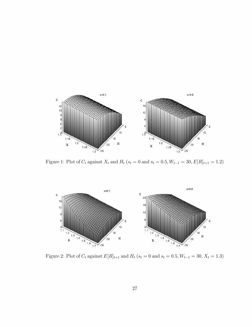
Figure 1: Plot of Ct againstXt andHt (st = 0 and st = 0.5,Wt−1 = 30, E[R]t+1 = 1.2)
Figure 2: Plot of Ct against E[R]t+1 andHt (st = 0 and st = 0.5,Wt−1 = 30, Xt = 1.3)
27
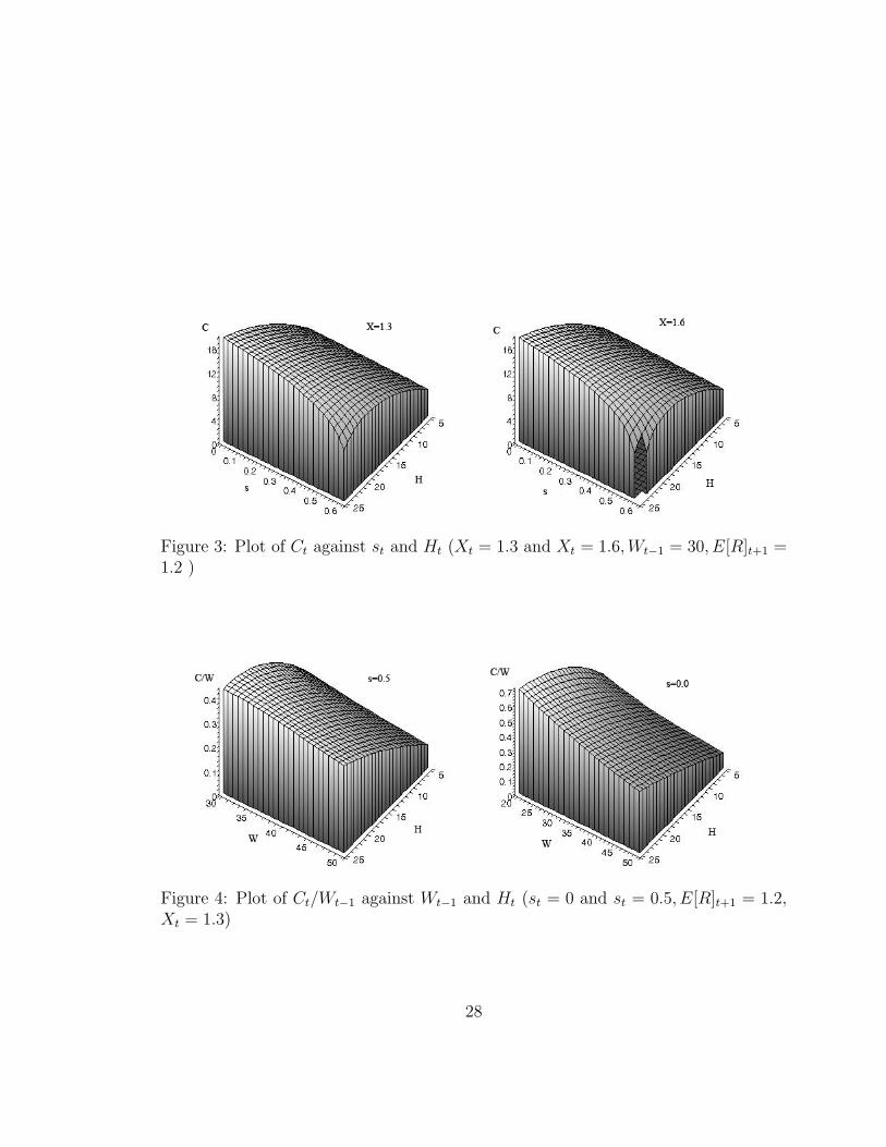
Figure 3: Plot of Ct against st and Ht (Xt = 1.3 and Xt = 1.6,Wt−1 = 30, E[R]t+1 =1.2 )
Figure 4: Plot of Ct/Wt−1 against Wt−1 and Ht (st = 0 and st = 0.5, E[R]t+1 = 1.2,Xt = 1.3)
28
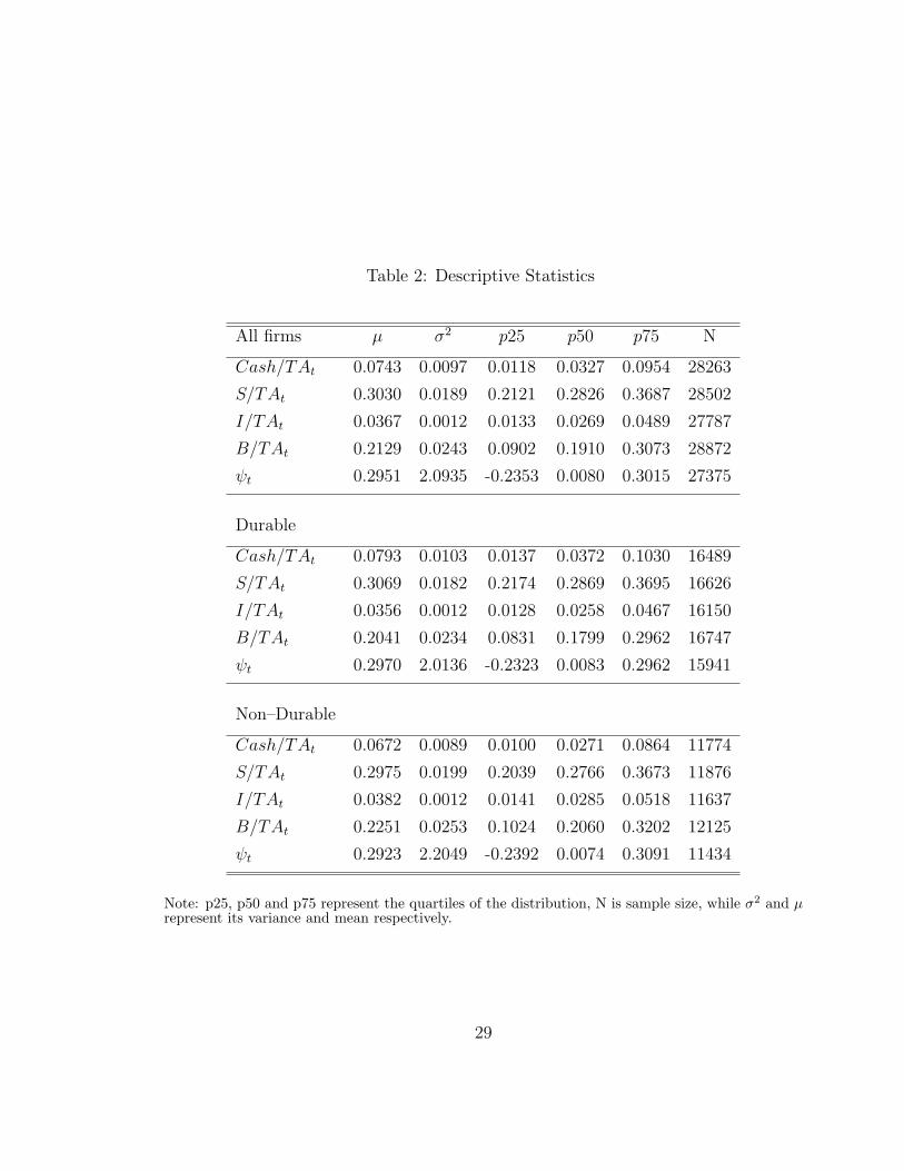
Table 2: Descriptive Statistics
All firms µ σ2 p25 p50 p75 N
Cash/TAt 0.0743 0.0097 0.0118 0.0327 0.0954 28263
S/TAt 0.3030 0.0189 0.2121 0.2826 0.3687 28502
I/TAt 0.0367 0.0012 0.0133 0.0269 0.0489 27787
B/TAt 0.2129 0.0243 0.0902 0.1910 0.3073 28872
ψt 0.2951 2.0935 -0.2353 0.0080 0.3015 27375
Durable
Cash/TAt 0.0793 0.0103 0.0137 0.0372 0.1030 16489
S/TAt 0.3069 0.0182 0.2174 0.2869 0.3695 16626
I/TAt 0.0356 0.0012 0.0128 0.0258 0.0467 16150
B/TAt 0.2041 0.0234 0.0831 0.1799 0.2962 16747
ψt 0.2970 2.0136 -0.2323 0.0083 0.2962 15941
Non–Durable
Cash/TAt 0.0672 0.0089 0.0100 0.0271 0.0864 11774
S/TAt 0.2975 0.0199 0.2039 0.2766 0.3673 11876
I/TAt 0.0382 0.0012 0.0141 0.0285 0.0518 11637
B/TAt 0.2251 0.0253 0.1024 0.2060 0.3202 12125
ψt 0.2923 2.2049 -0.2392 0.0074 0.3091 11434
Note: p25, p50 and p75 represent the quartiles of the distribution, N is sample size, while σ2 and µrepresent its variance and mean respectively.
29
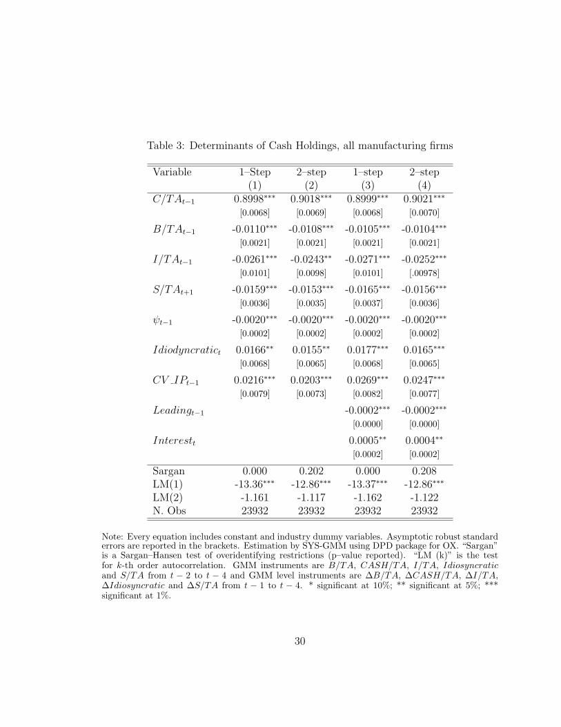
Table 3: Determinants of Cash Holdings, all manufacturing firms
Variable 1–Step 2–step 1–step 2–step(1) (2) (3) (4)
C/TAt−1 0.8998∗∗∗ 0.9018∗∗∗ 0.8999∗∗∗ 0.9021∗∗∗
[0.0068] [0.0069] [0.0068] [0.0070]
B/TAt−1 -0.0110∗∗∗ -0.0108∗∗∗ -0.0105∗∗∗ -0.0104∗∗∗
[0.0021] [0.0021] [0.0021] [0.0021]
I/TAt−1 -0.0261∗∗∗ -0.0243∗∗ -0.0271∗∗∗ -0.0252∗∗∗
[0.0101] [0.0098] [0.0101] [.00978]
S/TAt+1 -0.0159∗∗∗ -0.0153∗∗∗ -0.0165∗∗∗ -0.0156∗∗∗
[0.0036] [0.0035] [0.0037] [0.0036]
ψt−1 -0.0020∗∗∗ -0.0020∗∗∗ -0.0020∗∗∗ -0.0020∗∗∗
[0.0002] [0.0002] [0.0002] [0.0002]
Idiodyncratict 0.0166∗∗ 0.0155∗∗ 0.0177∗∗∗ 0.0165∗∗∗
[0.0068] [0.0065] [0.0068] [0.0065]
CV IPt−1 0.0216∗∗∗ 0.0203∗∗∗ 0.0269∗∗∗ 0.0247∗∗∗
[0.0079] [0.0073] [0.0082] [0.0077]
Leadingt−1 -0.0002∗∗∗ -0.0002∗∗∗
[0.0000] [0.0000]
Interestt 0.0005∗∗ 0.0004∗∗
[0.0002] [0.0002]
Sargan 0.000 0.202 0.000 0.208LM(1) -13.36∗∗∗ -12.86∗∗∗ -13.37∗∗∗ -12.86∗∗∗
LM(2) -1.161 -1.117 -1.162 -1.122N. Obs 23932 23932 23932 23932
Note: Every equation includes constant and industry dummy variables. Asymptotic robust standarderrors are reported in the brackets. Estimation by SYS-GMM using DPD package for OX. “Sargan”is a Sargan–Hansen test of overidentifying restrictions (p–value reported). “LM (k)” is the testfor k-th order autocorrelation. GMM instruments are B/TA, CASH/TA, I/TA, Idiosyncraticand S/TA from t − 2 to t − 4 and GMM level instruments are ∆B/TA, ∆CASH/TA, ∆I/TA,∆Idiosyncratic and ∆S/TA from t − 1 to t − 4. * significant at 10%; ** significant at 5%; ***significant at 1%.
30
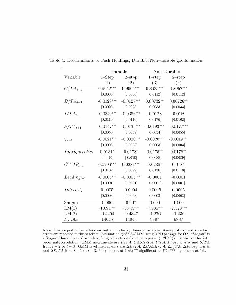
Table 4: Determinants of Cash Holdings, Durable/Non–durable goods makers
Durable Non–DurableVariable 1–Step 2–step 1–step 2–step
(1) (2) (3) (4)C/TAt−1 0.9042∗∗∗ 0.9064∗∗∗ 0.8935∗∗∗ 0.8962∗∗∗
[0.0086] [0.0086] [0.0112] [0.0112]
B/TAt−1 -0.0129∗∗∗ -0.0127∗∗∗ 0.00732∗∗ 0.00726∗∗
[0.0028] [0.0028] [0.0033] [0.0033]
I/TAt−1 -0.0349∗∗∗ -0.0356∗∗∗ -0.0178 -0.0169[0.0119] [0.0116] [0.0176] [0.0162]
S/TAt+1 -0.0147∗∗∗ -0.0135∗∗∗ -0.0193∗∗∗ -0.0177∗∗∗
[0.0050] [0.0049] [0.0054] [0.0055]
ψt−1 -0.0021∗∗∗ -0.0020∗∗∗ -0.0020∗∗∗ -0.0019∗∗∗
[0.0003] [0.0003] [0.0003] [0.0003]
Idiodyncratict 0.0181∗ 0.0178∗ 0.0175∗∗ 0.0176∗∗
[ 0.010] [ 0.010] [0.0088] [0.0089]
CV IPt−1 0.0296∗∗∗ 0.0281∗∗∗ 0.0236∗ 0.0184[0.0102] [0.0099] [0.0136] [0.0119]
Leadingt−1 -0.0003∗∗∗ -0.0003∗∗∗ -0.0001 -0.0001[0.0001] [0.0001] [0.0001] [0.0001]
Interestt 0.0005 0.0004 0.0005 0.0005[0.0003] [0.0003] [0.0003] [0.0003]
Sargan 0.000 0.997 0.000 1.000LM(1) -10.94∗∗∗ -10.45∗∗∗ -7.836∗∗∗ -7.573∗∗∗
LM(2) -0.4404 -0.4347 -1.276 -1.230N. Obs 14045 14045 9887 9887
Note: Every equation includes constant and industry dummy variables. Asymptotic robust standarderrors are reported in the brackets. Estimation by SYS-GMM using DPD package for OX. “Sargan” isa Sargan–Hansen test of overidentifying restrictions (p–value reported). “LM (k)” is the test for k-thorder autocorrelation. GMM instruments are B/TA, CASH/TA, I/TA, Idiosyncratic and S/TAfrom t − 2 to t − 3. GMM level instruments are ∆B/TA, ∆CASH/TA, ∆I/TA, ∆Idiosyncraticand ∆S/TA from t− 1 to t− 3. * significant at 10%; ** significant at 5%; *** significant at 1%.
31
Related Documents

![Uncertainty Footprint: Visualization of Nonuniform ... · PDF fileUncertainty Footprint: Visualization of Nonuniform Behavior of ... [ALM 14]. No matter how their parameters were adjusted,](https://static.cupdf.com/doc/110x72/5aad13467f8b9a8d678daa79/uncertainty-footprint-visualization-of-nonuniform-footprint-visualization.jpg)


