Uncertainty and Probabilistic Reasoning

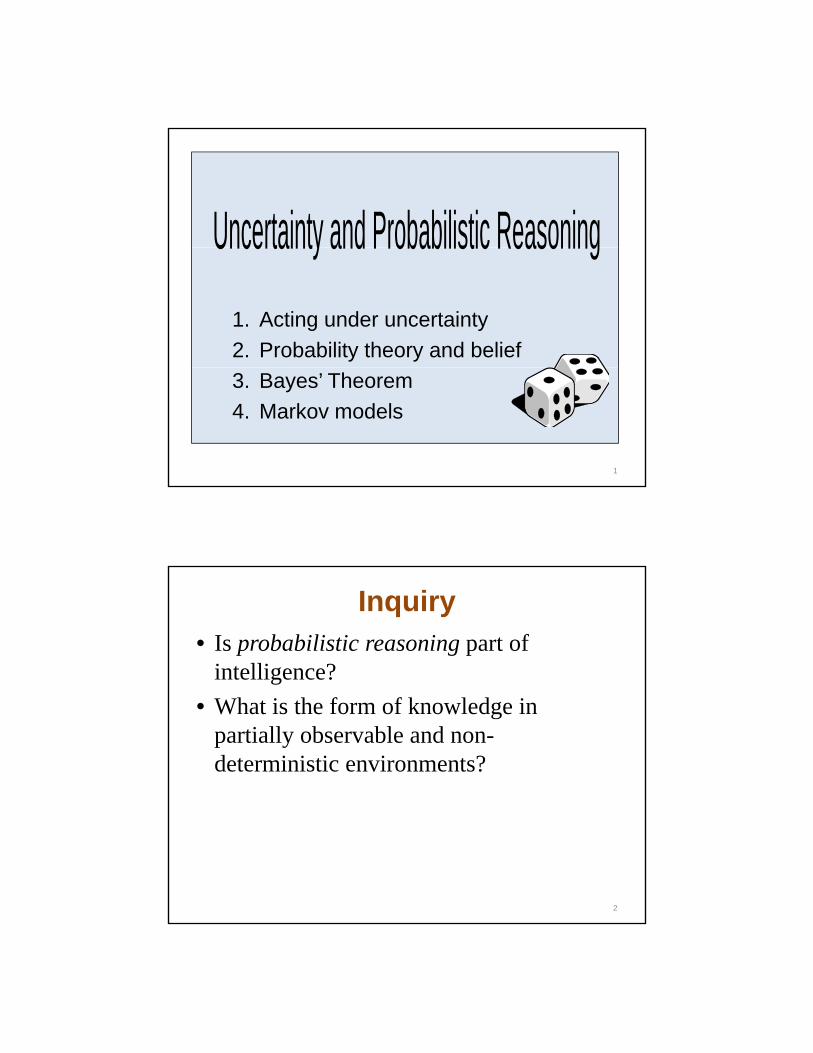
1. Acting under uncertainty2. Probability theory and belief3. Bayes’ Theorem 4. Markov models

1

Inquiry• Is probabilistic reasoning part of

intelligence?• What is the form of knowledge in

partially observable and non-deterministic environments?

2

Uncertainty and Probabilistic Reasoning

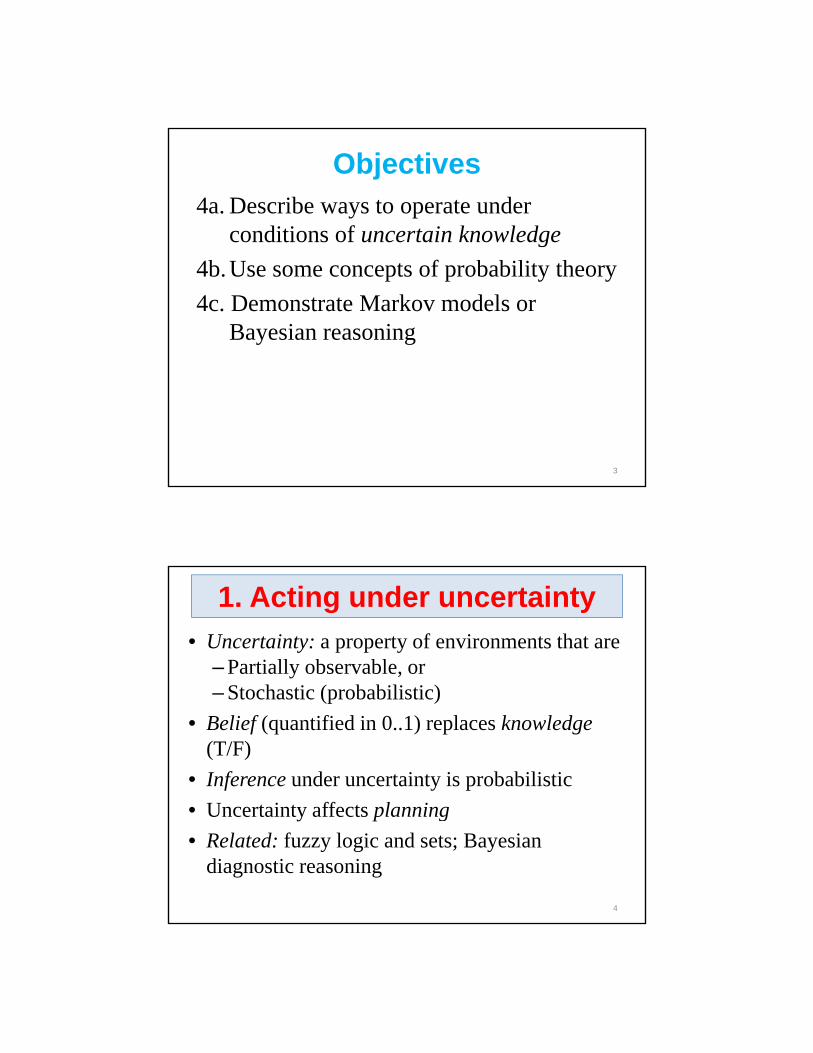
Objectives4a. Describe ways to operate under

conditions of uncertain knowledge4b.Use some concepts of probability theory4c. Demonstrate Markov models or

Bayesian reasoning

3

1. Acting under uncertainty• Uncertainty: a property of environments that are

– Partially observable, orS h i ( b bili i )– Stochastic (probabilistic)

• Belief (quantified in 0..1) replaces knowledge(T/F)

• Inference under uncertainty is probabilisticU t i t ff t l i• Uncertainty affects planning

• Related: fuzzy logic and sets; Bayesian diagnostic reasoning

4

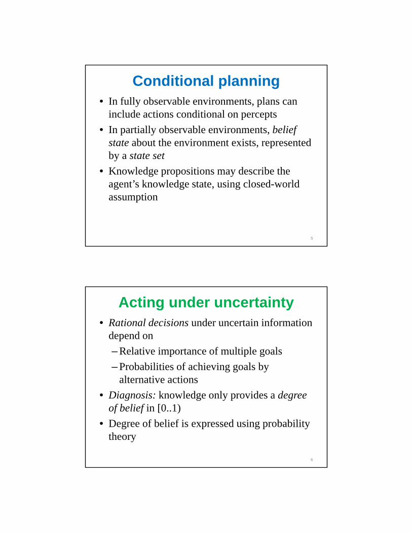
Conditional planning• In fully observable environments, plans can

include actions conditional on percepts• In partially observable environments, belief

state about the environment exists, represented by a state set

• Knowledge propositions may describe the agent’s knowledge state using closed-worldagent s knowledge state, using closed world assumption

5

Acting under uncertainty• Rational decisions under uncertain information

depend on– Relative importance of multiple goals– Probabilities of achieving goals by

alternative actions• Diagnosis: knowledge only provides a degree

of belief in [0 1)

6

of belief in [0..1)• Degree of belief is expressed using probability

theory

Planning under uncertainty• In partially observable and non-deterministic

environments, an agent may interact with its environment obtaining percepts to verify orenvironment, obtaining percepts to verify or correct planned actions

• For bounded uncertainty, sensorless planning may be used to coerce the environment, or contingency planning may be usedg y p g y

• For unbounded uncertainty, agent may use execution monitoring and replanning, or continuous planning

7

Execution monitoring• Action monitoring verifies that the environment

is ready for the next action to work• Plan monitoring verifies that the remaining part• Plan monitoring verifies that the remaining part

of plan should work• Replanning entails responding to the unexpected

by creating a new plan• Continuous planning agents include planning in p g g p g

their activities, continuously monitoring their environments; similar to partial-order planning

8

Application of stochastic methodsSome applications:• Diagnostic reasoning, because cause-effect

l ti hi i t l b irelationship is not always obvious• Natural language processing, because

semantics are fuzzy or ambiguous• Planning, because of uncertainty of future

events and cause-effect relationships

9

events and cause effect relationships• Learning, because conclusions to draw from

experience are ambiguous and probabilistic

• Monotone functions have nondecreasing values as arguments rise; graph never slopes downward

Nonmonotonic reasoning

• Mathematical logic is monotonic, in that adding facts makes the set of true assertions larger

• Beliefs, in contrast, change over time• Nonmonotonic reasoning allows for subtracting

b li f d (d f ibilit )beliefs and consequences (defeasibility)

10

Truth maintenance• When inference is uncertain and contrary

evidence arises, belief revision must occur• Justification based truth maintenance

annotates each sentence in KB with justification, enabling efficient retraction

• Truth-maintenance systems can generate explanations for sentences in KBexplanations for sentences in KB

• TM is NP-hard

11

• In probabilistic reasoning, belief is quantified• Random process: one whose outcome is from a set

f ibiliti th t t i l di t bl

2. Probability theory and belief

of possibilities that are uncertainly predictable• Examples: tossing a coin, playing lottery, or rolling

dice are random processes • Sample space: the set of possible outcomes in a

random process

12

p• Event: a subset of a sample space• Atomic events: mutually exclusive and exhaustive

Uniform probability space• A probability space S is a set of possible

outcomes of an experiment• Example: S for a die throw is• Example: S for a die throw is

{1, 2, 3, 4, 5, 6}• Let | S | = n for probability space S• Uniform probability function P : S → R is

defined P(x) = (1/n) for any x in S( ) ( ) y• Example: Using fair die, P(3) = 1/6, because

there are 6 possible events, all equally likely

13

• Discrete probability assumes finite sample spaceP b bili f i f h

Discrete probability

• Probability of an event x: ratio of the number of outcomes in the event to the size of the sample space; 0 ≤ P(x) ≤ 1

• For event E in sample space S, P(E) = | | |S||E| ÷ |S|

14

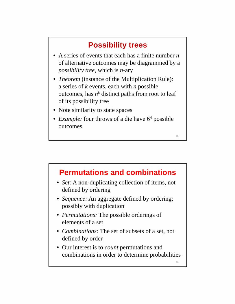
Possibility trees• A series of events that each has a finite number n

of alternative outcomes may be diagrammed by a possibility tree which is n-arypossibility tree, which is n ary

• Theorem (instance of the Multiplication Rule): a series of k events, each with n possible outcomes, has nk distinct paths from root to leaf of its possibility tree

15

• Note similarity to state spaces• Example: four throws of a die have 64 possible

outcomes

Permutations and combinations• Set: A non-duplicating collection of items, not

defined by ordering• S An aggregate defined b ordering;• Sequence: An aggregate defined by ordering;

possibly with duplication• Permutations: The possible orderings of

elements of a set• Combinations: The set of subsets of a set not

16

Combinations: The set of subsets of a set, not defined by order

• Our interest is to count permutations and combinations in order to determine probabilities

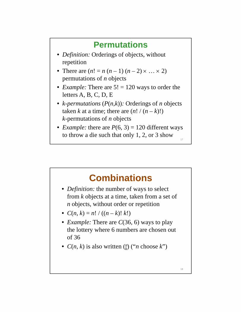
Permutations• Definition: Orderings of objects, without

repetition• There are (n! = n (n – 1) (n – 2) × … × 2) ( ( ) ( ) )

permutations of n objects• Example: There are 5! = 120 ways to order the

letters A, B, C, D, E• k-permutations (P(n,k)): Orderings of n objects

k k i h ( ! / ( k)!)taken k at a time; there are (n! / (n – k)!) k-permutations of n objects

• Example: there are P(6, 3) = 120 different ways to throw a die such that only 1, 2, or 3 show

17

Combinations• Definition: the number of ways to select

from k objects at a time, taken from a set of bj t ith t d titin objects, without order or repetition

• C(n, k) = n! / ((n – k)! k!)• Example: There are C(36, 6) ways to play

the lottery where 6 numbers are chosen out of 36of 36

• C(n, k) is also written (nk) (“n choose k”)

18

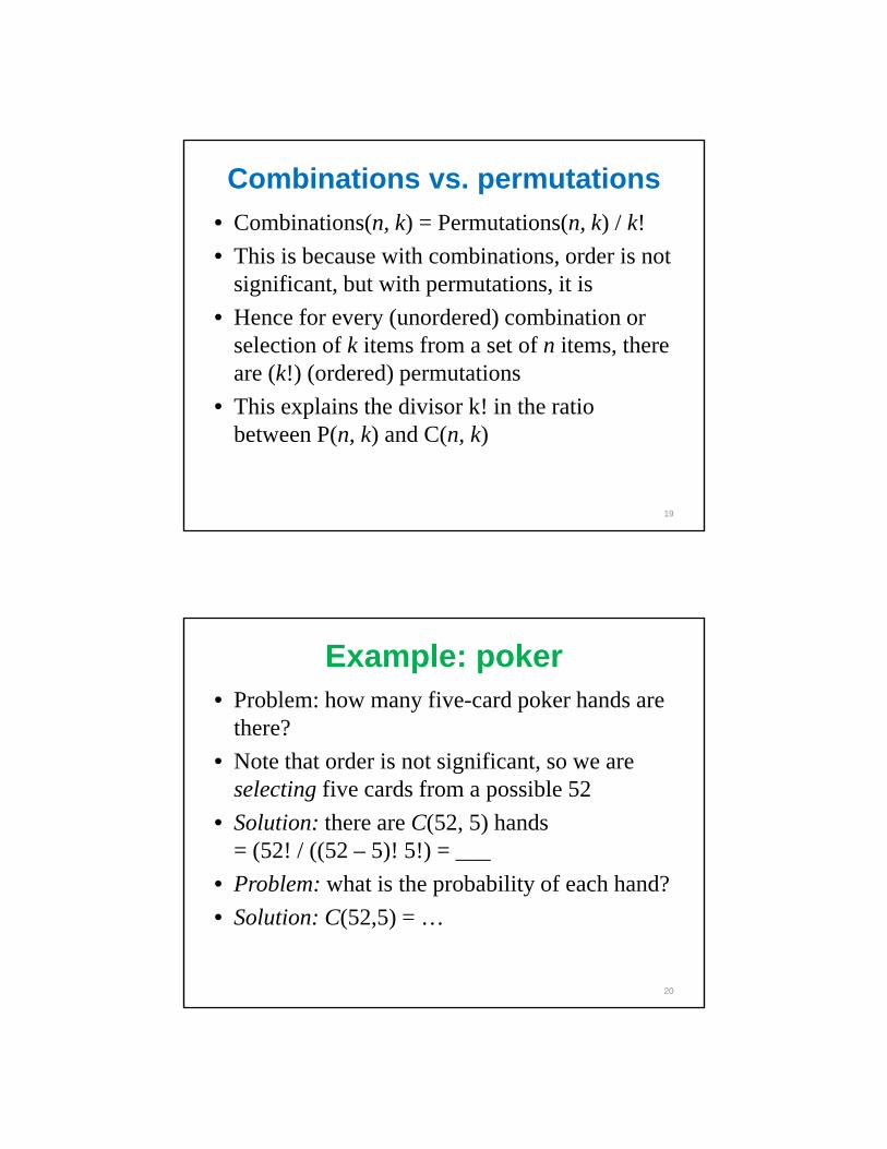
Combinations vs. permutations• Combinations(n, k) = Permutations(n, k) / k!• This is because with combinations, order is not

significant, but with permutations, it is• Hence for every (unordered) combination or

selection of k items from a set of n items, there are (k!) (ordered) permutationsThi l i th di i k! i th ti• This explains the divisor k! in the ratio between P(n, k) and C(n, k)

19

Example: poker• Problem: how many five-card poker hands are

there?• Note that order is not significant, so we are

selecting five cards from a possible 52• Solution: there are C(52, 5) hands

= (52! / ((52 – 5)! 5!) = ___P bl h t i th b bilit f h h d?• Problem: what is the probability of each hand?

• Solution: C(52,5) = …

20

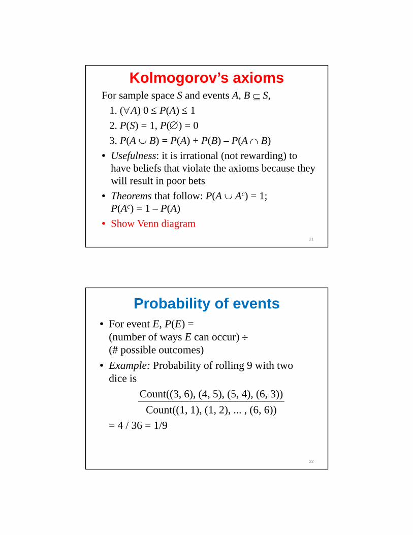
Kolmogorov’s axiomsFor sample space S and events A, B ⊆ S,

1. (∀A) 0 ≤ P(A) ≤ 12 P(S) = 1 P(∅) = 02. P(S) = 1, P(∅) = 03. P(A ∪ B) = P(A) + P(B) – P(A ∩ B)

• Usefulness: it is irrational (not rewarding) to have beliefs that violate the axioms because they will result in poor bets

21

• Theorems that follow: P(A ∪ Ac) = 1; P(Ac) = 1 – P(A)

• Show Venn diagram

Probability of events• For event E, P(E) =

(number of ways E can occur) ÷(# ibl t )(# possible outcomes)

• Example: Probability of rolling 9 with two dice is

Count((3, 6), (4, 5), (5, 4), (6, 3))___________________________Count((1 1) (1 2) (6 6))

22

Count((1, 1), (1, 2), ... , (6, 6))= 4 / 36 = 1/9

Expected values• For n different possible outcomes of a random

process, where ak is the value of the kth

outcome the expected value of the process isoutcome, the expected value of the process isΣk=1..n ak pk

• Examples:- In coin toss, expected value is (0.5)- In die throw, expected outcome is

(1 + 2 + 3 + 4 + 5 + 6) / 6 = 3.5- Expected time for linear search is (n / 2)

23

Independent events• Intuition: Independent events can have no

effect on each other or overlap with each other• Formally: Events A and B are independent iff• Formally: Events A and B are independent iff

P(A ∩ B) = P(A) P(B)• Single coin tosses and die rolls are independent • Example: For draw of cards, P(♥) is

independent of P(J or Q or K)• For non-independent events, notion of

conditional probability is used, i.e., probability of E1 given E2

24

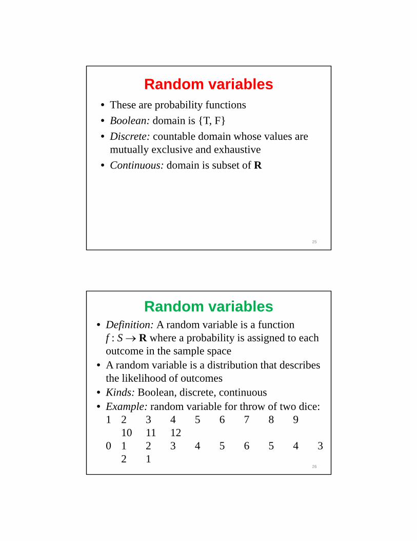
Random variables• These are probability functions• Boolean: domain is {T, F}• Discrete: countable domain whose values are

mutually exclusive and exhaustive• Continuous: domain is subset of R

25

Random variables• Definition: A random variable is a function

f : S → R where a probability is assigned to each outcome in the sample spaceoutcome in the sample space

• A random variable is a distribution that describes the likelihood of outcomes

• Kinds: Boolean, discrete, continuous• Example: random variable for throw of two dice:

26

1 2 3 4 5 6 7 8 910 11 12

0 1 2 3 4 5 6 5 4 32 1

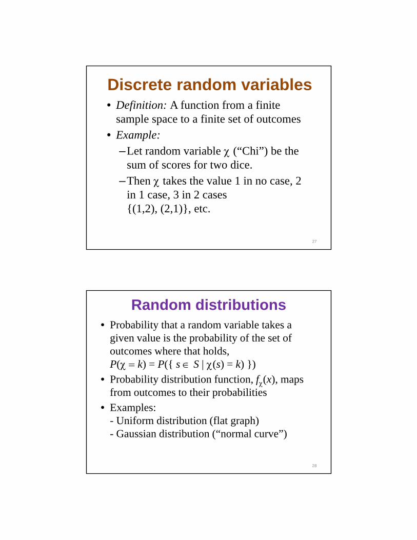
Discrete random variables• Definition: A function from a finite

sample space to a finite set of outcomes• Example:

–Let random variable χ (“Chi”) be the sum of scores for two dice.

–Then χ takes the value 1 in no case, 2 in 1 case, 3 in 2 cases {(1,2), (2,1)}, etc.

27

Random distributions• Probability that a random variable takes a

given value is the probability of the set of outcomes where that holdsoutcomes where that holds, P(χ = k) = P({ s ∈ S | χ(s) = k) })

• Probability distribution function, fχ(x), maps from outcomes to their probabilities

• Examples:p- Uniform distribution (flat graph)- Gaussian distribution (“normal curve”)

28

Probability in predicate logic• A probabilistic knowledge base should give

probabilities of all models in predicate logic• For sentence φ, where µ gives probability of a

model, P(φ) = ΣM s.t. φ holds µ(M)• Causal dependencies can be denoted by parent

relationships, similar to semantic networksI f if t k t ti• Inference may occur if network representation is finite and has fixed structure

29

Prior probability• Prior (unconditional) probability P(α): degree

of belief in the absence of other information• Probability distribution: sequence of• Probability distribution: sequence of

probabilities of possible event outcomes• Joint probability distribution: grid of

probabilities of all combinations chosen from sets of random variables, e.g., weather, traffic

30

• Probability density function: probability distribution of a continuous variable

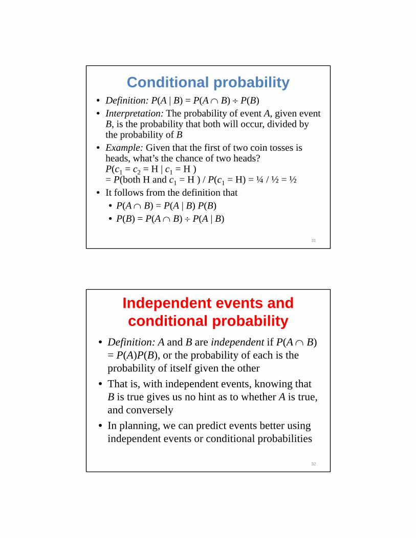
Conditional probability• Definition: P(A | B) = P(A ∩ B) ÷ P(B)• Interpretation: The probability of event A, given event

B, is the probability that both will occur, divided byB, is the probability that both will occur, divided by the probability of B

• Example: Given that the first of two coin tosses is heads, what’s the chance of two heads?P(c1 = c2 = H | c1 = H ) = P(both H and c1 = H ) / P(c1 = H) = ¼ / ½ = ½

• It follows from the definition that • P(A ∩ B) = P(A | B) P(B)• P(B) = P(A ∩ B) ÷ P(A | B)

31

Independent events and conditional probability

• Definition: A and B are independent if P(A ∩ B) = P(A)P(B), or the probability of each is the probability of itself given the other

• That is, with independent events, knowing that B is true gives us no hint as to whether A is true, and converselyand conversely

• In planning, we can predict events better using independent events or conditional probabilities

32

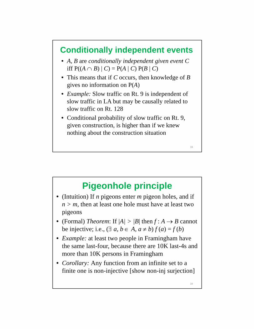
Conditionally independent events• A, B are conditionally independent given event C

iff P((A ∩ B) | C) = P(A | C) P(B | C)• This means that if C occurs then knowledge of B• This means that if C occurs, then knowledge of B

gives no information on P(A)• Example: Slow traffic on Rt. 9 is independent of

slow traffic in LA but may be causally related to slow traffic on Rt. 128

• Conditional probability of slow traffic on Rt. 9, given construction, is higher than if we knew nothing about the construction situation

33

Pigeonhole principle• (Intuition) If n pigeons enter m pigeon holes, and if

n > m, then at least one hole must have at least two pigeonsp geo s

• (Formal) Theorem: If |A| > |B| then f : A → B cannot be injective; i.e., (∃ a, b ∈ A, a ≠ b) f (a) = f (b)

• Example: at least two people in Framingham have the same last-four, because there are 10K last-4s and

h 10 i i h

34

more than 10K persons in Framingham• Corollary: Any function from an infinite set to a

finite one is non-injective [show non-inj surjection]

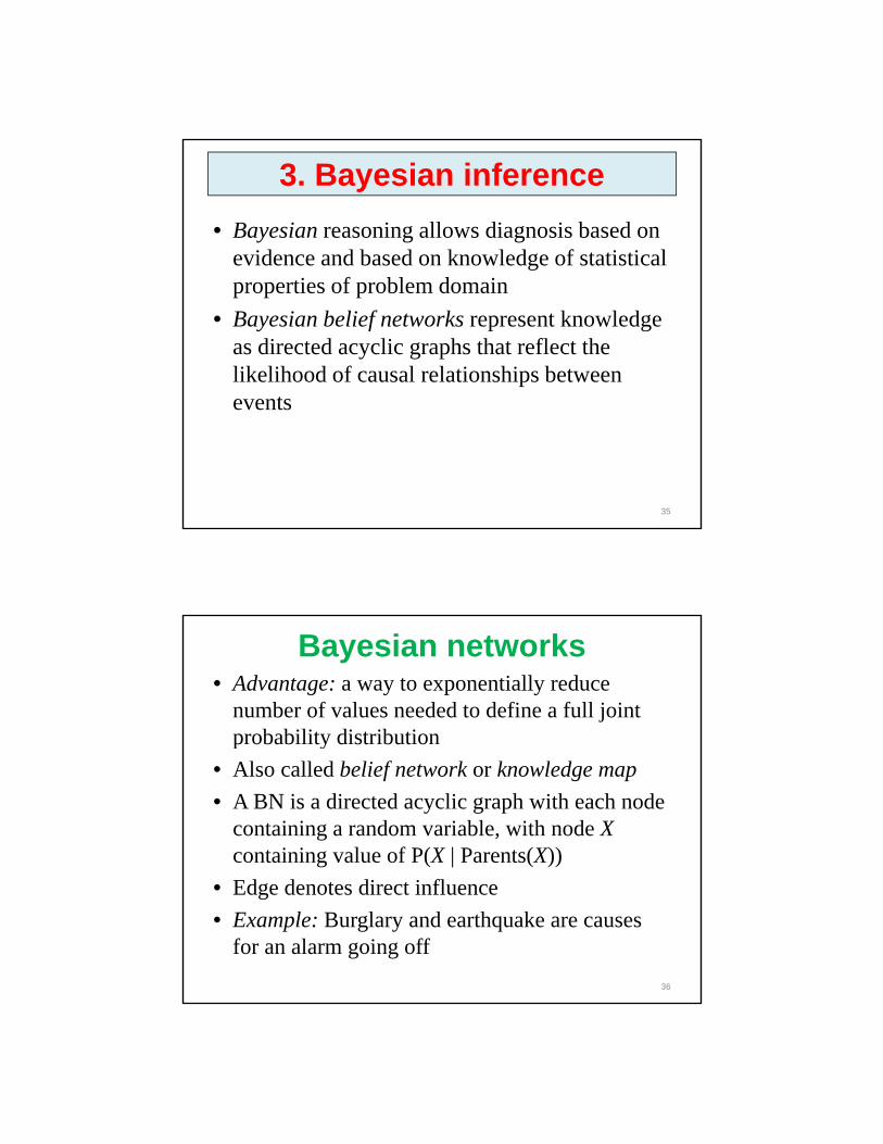
3. Bayesian inference• Bayesian reasoning allows diagnosis based on

evidence and based on knowledge of statistical gproperties of problem domain

• Bayesian belief networks represent knowledge as directed acyclic graphs that reflect the likelihood of causal relationships between e entsevents

35

Bayesian networks• Advantage: a way to exponentially reduce

number of values needed to define a full joint probability distributionp obab ty d st but o

• Also called belief network or knowledge map• A BN is a directed acyclic graph with each node

containing a random variable, with node Xcontaining value of P(X | Parents(X))

• Edge denotes direct influence• Example: Burglary and earthquake are causes

for an alarm going off36

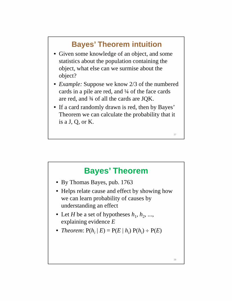
Bayes’ Theorem intuition• Given some knowledge of an object, and some

statistics about the population containing the object, what else can we surmise about the j ,object?

• Example: Suppose we know 2/3 of the numbered cards in a pile are red, and ¼ of the face cards are red, and ¾ of all the cards are JQK. f d d l d i d h b ’• If a card randomly drawn is red, then by Bayes’

Theorem we can calculate the probability that it is a J, Q, or K.

37

Bayes’ Theorem• By Thomas Bayes, pub. 1763• Helps relate cause and effect by showing how

we can learn probability of causes by understanding an effect

• Let H be a set of hypotheses h1, h2, ..., explaining evidence E

• Theorem: P(h | E) = P(E | h ) P(h ) ÷ P(E)

38

• Theorem: P(hi | E) = P(E | hi) P(hi) ÷ P(E)

Bayesian representation• Full joint distribution entry:

P(x1, ... xn) = Πi≤ n P(xi | xi-1, ... , x1)• Bayesian network is far more compact than

full joint distribution, n2k vs. 2n values, where k is maximum number of local influences

• [Clarify this]

39

Bayesian belief networks• BBNs are a selective use of Bayes’ theorem,

which requires a number of parameters exponential in the number of observationsexponential in the number of observations

• It is reasonable that some observations don’t interact, such as construction and accident in traffic-jam example

• Hence nodes in belief network depend only on th i t d

40

their parent nodes• Because causality has direction, BBNs have

directed acyclic graph (dag) form

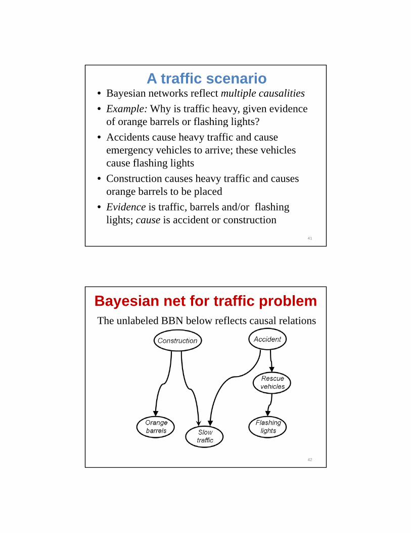
A traffic scenario• Bayesian networks reflect multiple causalities• Example: Why is traffic heavy, given evidence

of orange barrels or flashing lights? g g g• Accidents cause heavy traffic and cause

emergency vehicles to arrive; these vehicles cause flashing lights

• Construction causes heavy traffic and causes orange barrels to be placed

• Evidence is traffic, barrels and/or flashing lights; cause is accident or construction

41

Bayesian net for traffic problemThe unlabeled BBN below reflects causal relations

42

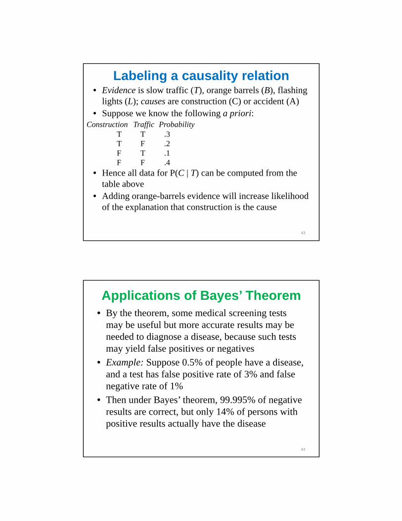
Labeling a causality relation• Evidence is slow traffic (T), orange barrels (B), flashing

lights (L); causes are construction (C) or accident (A)• Suppose we know the following a priori:

C t ti T ffi P b bilitConstruction Traffic ProbabilityT T .3T F .2F T .1F F .4

• Hence all data for P(C | T) can be computed from the t bl b

43

table above• Adding orange-barrels evidence will increase likelihood

of the explanation that construction is the cause

Applications of Bayes’ Theorem• By the theorem, some medical screening tests

may be useful but more accurate results may be needed to diagnose a disease, because such testsneeded to diagnose a disease, because such tests may yield false positives or negatives

• Example: Suppose 0.5% of people have a disease, and a test has false positive rate of 3% and false negative rate of 1%Th d B ’ th 99 995% f ti

44

• Then under Bayes’ theorem, 99.995% of negative results are correct, but only 14% of persons with positive results actually have the disease

• A Markov state machine or chain is a system with a finite number of observable states, and with probabilistic transitions between states

4. Markov models

w t p obab st c t a s t o s betwee states• Example: weather at any location• Markov assumption: current state depends only

on finite history of previous states• Nth-order Markov process: state depends only on

45

nth-previous state• To improve approximations, increase number of

state variables or order of Markov process

Markov decision processes• Defined by initial state s0, transition model

T(s, a, s′), and reward function R(s)• A solution specifies a policy π(s): what agentA solution specifies a policy π(s): what agent

should do given any state of environment • Policies have expected utilities: utility of possible

environment histories generated by it• Optimal (maximal-utility) policy is called π*

l i h i l

46

• Proper policy: one certain to reach a terminal state• Future rewards may be discounted in deciding

expected utility

Markov chains• Probability of being in a given state at a given

time is dependent on state at previous times• First-order Markov chain is one where

probability of present state depends only on previous state

• Example: weather at any location

47

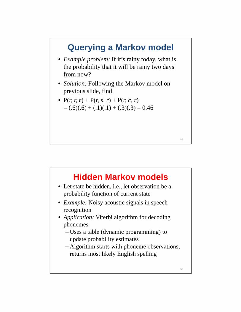
Example: Weather• Let states be {sunny, cloudy, rainy}• Let transitions be as follows:

sunnycloudy rainysunnycloudy rainysunny .4 .5 .1cloudy .2 .5 .3rainy .1 .3 .6

• First-order Markov model:

48

Querying a Markov model• Example problem: If it’s rainy today, what is

the probability that it will be rainy two days f ?from now?

• Solution: Following the Markov model on previous slide, find

• P(r, r, r) + P(r, s, r) + P(r, c, r) = ( 6)( 6) + ( 1)( 1) + ( 3)( 3) = 0 46 (.6)(.6) + (.1)(.1) + (.3)(.3) 0.46

49

Hidden Markov models• Let state be hidden, i.e., let observation be a

probability function of current state• Example: Noisy acoustic signals in speech• Example: Noisy acoustic signals in speech

recognition• Application: Viterbi algorithm for decoding

phonemes– Uses a table (dynamic programming) to

update probability estimatesupdate probability estimates– Algorithm starts with phoneme observations,

returns most likely English spelling

50

Application: Speech recognition• Bayesian probabilistic inference is used• Where words is a sequence of words, signal is

sound we want to maximize P(words | signal)sound, we want to maximize P(words | signal) = αP(signal | words) P(words)

• Acoustic model: P(signal | words)• Language model: P(words)• HMM for toe-mah-toe | toe-may-toe:

51

• HMM for toe-mah-toe | toe-may-toe:[pic 9]

action monitoringatomic eventBayes' theoremBayesian inference

plan monitoringprior probabilityprobability density

function

Conceptseventexpected outcome hidden Markov modelindependent eventsBayesian inference

Bayesian networkbelief networkbelief statechain rulecircumscriptionclosed world

i

probability theoryrandom variablerational agentrational decisionresolution proofsample spacet th i t

independent eventsKolmogorov axiomsMarkov assumptionMarkov chainsMarkov processminimal modelmodal logic

d lassumptioncombinationconditional

probability

52

truth maintenanceunconditional probability

modelnonmonotonic

reasoningpermutation

ReferencesSusanna Epp. Discrete Mathematics with

Appplications. Brooks/Cole, 2011.George Luger. Artificial Intelligence. Addison

Wesley, 2005.Stuart Russell and Peter Norvig. Artificial

Intelligence: A Modern Approach, 2nd ed. Prentice Hall 2003Prentice Hall, 2003.

53