Unbalanced Growth Slowdown - UNC Charlotte Pages

Unbalanced Growth Slowdown∗

Georg Duernecker (University of Mannheim and IZA)

Berthold Herrendorf (Arizona State University)

Akos Valentinyi (University of Manchester, MTA KRTK, CEPR)

November 2, 2016

Abstract

Unbalanced growth slowdown is the reduction in aggregate productivity growth that resultsfrom the reallocation of economic activity to industries with low productivity growth. Weshow that unbalanced growth slowdown has considerably reduced past U.S. productivitygrowth and we assess by how much it will reduce future U.S. productivity growth. Toachieve this, we build a novel model that generates the unbalanced growth slowdown ofthe postwar period. The model makes the surprising prediction that future reductions inaggregate productivity growth do not exceed past ones. The key reason is that the stagnantindustries do not take over the economy.

Keywords: Productivity Slowdown; Structural Transformation; Unbalanced Growth.JEL classification: O41; O47; O51.

∗For comments and suggestions, we thank Bart Hobijn, B. Ravikumar, Michael Sposi, and the audiences ofpresentations at Arizona State University, the European Monetary Forum 2016 (held at the Bank of England),the Federal Reserve Bank of St. Louis, the RIDGE Workshop on Growth and Development, Erasmus UniversityRotterdam, Southern Methodist University, and the University of Manchester. All errors are our own.

Figure 1: Growth Slowdown in Major English–speaking Countries

0.000

0.005

0.010

0.015

0.020

0.025

0.030

0.035

1970 1975 1980 1985 1990 1995 2000 2005 2010 2015Source: Total Economy Database 2016

average of the previous 20 yearsGrowth of real U.S. GDP per hour

0.000

0.005

0.010

0.015

0.020

0.025

0.030

0.035

1970 1975 1980 1985 1990 1995 2000 2005 2010 2015

Australia Canada United Kingdom United States

Source: Total Economy Database 2016

average of the previous 20 yearsGrowth of real GDP per hour

1 Introduction

There is ample evidence that long–term economic growth has slowed in the U.S. The left panelof Figure 1 shows this by plotting the average growth rates of U.S. labor productivity duringthe previous 20 years where labor productivity is measured as real aggregate value added perhour. We can see that labor productivity growth declined by almost a percentage point froman average of about 2.5% during 1950–1970 to a little higher than 1.5% during 1990–2010.1

Although we focus on the U.S. in this paper, growth slowdown has happened in other richcountries too. The right panel of Figure 1 shows similar downward trends for the three English–speaking countries Australia, Canada, and the U.K. We choose them as comparisons becausethey are rich countries that after World War II did not experience exceptionally large growthrates as the result of growth miracles (like Japan and South Korea) or of massive reconstructionefforts (like France and Germany).

One of the hotly debated questions of the moment is whether growth slowdown is a tem-porary or a permanent phenomenon. Fernald and Jones (2014) pointed out that engines ofeconomic growth like education or research and development require the input of time whichcannot be increased ad infinitum. This suggests that there is a natural limit to growth and thatthe slowdown might well be permanent. Gordon (2016) reached the same conclusion, arguingthat we picked the “low–hanging fruit” (e.g., railroads, cars, and airplanes) during the “specialcentury 1870–1970” and that more recent innovations pale in comparison.

In this paper, we investigate to which extent growth slowdown results from the interactionbetween unbalanced growth and structural transformation, which we refer to as unbalanced

growth slowdown. To explain how unbalanced growth slowdown arises, it is helpful to go backto the observation of Baumol (1967) that modern economic growth has been unbalanced inthat labor productivity growth differed widely across industries. Baumol drew particular atten-

1Antolin-Diaz et al. (2016) (and several of the reference therein) offer statistical analyses of growth slowdown,confirming the same conclusion that we draw from eyeballing the graph.

1

tion to the fact that many industries in the service sector experienced low labor productivitygrowth or even outright stagnation.2 More recently, Ngai and Pissarides (2007) observed thatas economies develop resources are systematically reallocated towards the service industries.Taken to the extreme, their analysis implies that in the limit the service sector with the slowestproductivity growth takes over the whole economy.3 Together, unbalanced growth and struc-tural transformation therefore lead to unbalanced growth slowdown.

We begin our analysis by showing that unbalanced growth slowdown was quantitativelyimportant in the private U.S. economy after the second world war. We leave out the govern-ment sector because labor productivity of the government sector is not well measured. Weuse the broad disaggregation into goods (tangible value added) and services (intangible valueadded) that is common in the literature on structural transformation. Since the service sectorcomprises most of the U.S. economy and its industries have rather different labor productivitygrowth, we disaggregate it further. We follow the classification of WORLD KLEMS whichdistinguishes between market services like financial services and non–market services like res-idential real estate. Market services tend to have faster productivity growth than non–marketservices, which essentially stagnated during the last thirty years. To measure the importanceof unbalanced growth slowdown in the postwar U.S. private economy, we calculate how largeaggregate productivity growth would have been during 1947–2010 for the counterfactual casewithout structural transformation. Using WORLD KLEMS data and the productivity account-ing method of Nordhaus (2002), we find that the annual average growth rates of productivityper efficiency hour would have been between 0.2 and 0.3 percentage points higher than they ac-tually were, depending on the counterfactual that we focus on. These numbers are in the sameball park as those of Nordhaus (2008) and they amount to 20–30% of the one percentage pointreduction in average labor productivity growth that is suggested by the left panel of Figure 1.This finding suggests that a sizeable part of the observed growth slowdown can be attributed tounbalanced growth slowdown.

Although unbalanced growth slowdown is empirically important, the literature on structuraltransformation has all but ignored it. The likely reason for this is that analytically characterizingthe equilibrium path of multi–sector models is usually possible only if a generalized balancedgrowth path exists along which aggregate variables are either constant or grow at constant rates.If aggregate labor productivity grows at a constant rate along the generalized balanced growthpath, then unbalanced growth slowdown does not appear to be an issue. Our first contributionis to clarify that this is a misconception. We develop a canonical model of structural transfor-mation and show that it exhibits unbalanced growth slowdown in terms of welfare, in that thegrowth rate of welfare is declining of time. We then show that whether or not this is pickedup by aggregate labor productivity growth depends critically on how one measures real quan-

2See Oulton (2001), Nordhaus (2008) and Baumol (2013) for more restatements of this observation.3Herrendorf et al. (2014) review the literature on structural transformation.

2

tities. Specifically, the model has a generalized balanced growth path along which aggregatelabor productivity grows at a constant rate if one measures real quantities in “the usual modelway”. This involves expressing the variables of a given period in units of a numeraire fromthe same period. In other words, the model way uses a different numeraire and different rela-tive prices in each period. In contrast, “the NIPA way” of calculating real quantities uses fixedprices from a base period that do not change between two periods. We will show that this dif-ference is critical: although our model displays balanced growth if real quantities are calculatedin the model way, it displays unbalanced growth slowdown if real quantities are calculated inthe NIPA way.4 Having clarified this, we restrict our model to generate the unbalanced growthslowdown of labor productivity in the postwar U.S. and use the restricted model to assess byhow much unbalanced growth and structural transformation will slow down labor productivitygrowth in the next half century. To put the bottom line upfront, this will yield the surprisingconclusion that although unbalanced growth slowdown has been quite a drag on postwar U.S.growth, it will not become more of a challenge to the future growth performance. The reasonfor this conclusion is that, in contrast to the implication that is usually derived in the literature,it will turn out that the slowest growing sector won’t take over our entire model economy in thelimit. This will restrain the future effect of unbalanced growth slowdown.

To guide which features to put into our canonical model of structural transformation, wedocument key stylized facts about unbalanced growth and structural transformation betweengoods and services and between market and non–market services. The usual patterns hold be-tween goods and total services: the shares of goods in total expenditure and total hours workeddecline; the labor productivity of goods grows more strongly than that of total services; theprice of goods relative to total services reflects this and declines. We then establish the fol-lowing novel patterns about the two subsectors of the service sector: the shares of non–marketservices in the hours and expenditures of total services increase until about 1980 after whichthey remain roughly constant; labor productivity of market services grows over the whole pe-riod by less than that of goods and by more than that of non–market services; labor productivityin non–market services grows somewhat until around 1980 and stagnates afterwards; the priceof non–market relative to market services reflects this: it initially increases until around 1980and then it increases strongly. Together, these stylized facts imply that when the labor produc-tivity of non–market services starts to stagnate around 1980 the shares of non–market servicesstop increasing. This is the crucial observation for what is to come, because it suggests that theslow–growing non–market services are not taking over the entire service sector.

Our canonical model has three sectors, which produce goods, market services, and non–

4When we refer to the NIPA way of calculating real quantities, we mean calculating real quantities via chainindexes, which conforms to the best practice used by the BEA. A chain index is the geometric average of theLaspeyres index and the Paasche index, which are both fixed–price indexes that use either the fixed prices of theinitial period or the subsequent period. We emphasize that although it might sound similar, using chain indexes iscompletely different from using relative prices that change from period to period.

3

market services. There is exogenous, sector–specific technological progress. Preferences aredescribed by the non–homothetic CES utility function that has recently been proposed byComin et al. (2015) in the context of structural transformation and that implies that incomeeffects do not disappear in the limit when consumption grows without bound. This feature isconsistent with the existing evidence [Boppart (2016) and Comin et al. (2015)], and it is po-tentially crucial in the present context because we are after the limit behavior of the economy.The novelty of our model compared to the literature on structural transformation is that we al-low the elasticity of substitution between goods and total services to differ from the elasticitybetween market and non–market services. To achieve this, we nest two non–homothetic CESutility functions: an outer layer aggregates goods and total services; an inner layer aggregatesmarket and non–market services into total services. This allows the model to do two things:keep the well established feature of preferences that goods and total services are complements,see for example Herrendorf et al. (2013); match the fact that the share of non–market servicesdid not increase when their relative price increased strongly after 1980, for which market andnon–market services must be substitutes, instead of complements.

Assuming that the recent sectoral labor productivity growth continues into the future, ourmodel implies that unbalanced growth slowdown will be at most as large in the future as inthe past. The reason for this surprising finding is that in our model the stagnating non–marketservices do not take over the entire the entire economy. This comes about because the sub-stitutability between market and non–market services puts a limit on how much future growthslowdown may occur in our model. If the relative price of non–market services increases with-out bound because non–market services stagnate, then households substitute market servicesfor non–market services. This does not happen in existing models of structural transformationwhich impose a common elasticity of substitution among goods and all services and find thatthen goods and services are complements.

Our work is related to several papers arguing that the service sector has become so largeand heterogenous that it is useful to disaggregate it into subsectors; see for example Baumolet al. (1985), Jorgenson and Timmer (2011), and Duarte and Restuccia (2016). Our workis also related to several papers that measured cross–country gaps in sectoral TFP or laborproductivity; see for example Duarte and Restuccia (2010), Herrendorf and Valentinyi (2012)and Duarte and Restuccia (2016). Instead of focusing on cross–sections of countries, we focuson the evolution of U.S. labor productivity over time. The most closely related paper to ours isDuarte and Restuccia (2016), which features in both sets of papers. Duarte and Restuccia usethe 2005 cross section of the International Comparisons Program of the Penn World Table toestimate sectoral productivity gaps between rich and poor countries. They distinguish betweentraditional and modern services, which roughly corresponds to our distinction between non–market and market services. They find that the largest cross–country productivity gaps are in

4

goods and modern services and the smallest cross–country gaps are in traditional services. Thiscross sectional evidence nicely complements our time series evidence from the U.S. that laborproductivity in non–market services grows less than in the other two sectors. If we took arich and a poor country with that feature and looked at the productivity differences in a givensector, then our findings would imply that over time larger productivity differences betweenthese countries emerge in goods and market services than in non–market services.

The remainder of the paper is organized as follows. In the next Section, we present evidencethat structural transformation has led to growth slowdown in the postwar U.S. In Section 3, wedevelop our model. In the next section, we characterize under what conditions our model leadsto unbalanced growth slowdown. In section 5, we calibrate our model and use it to predict howmuch future growth slowdown results from structural transformation. Section 6 concludes andan Appendix contains the detailed description of our data work, the proofs of our results, andadditional evidence.

2 Unbalanced Growth Slowdown in the Postwar U.S. Data

We use WORLD KLEMS as our data source, because it offers information about both raw hoursand adjusted hours that take into account differences in human capital (“efficiency hours”).5

Since we will study counterfactuals that reallocate workers with potentially different levelsof human capital across sectors, having information about efficiency hours will allow us toperform important robustness checks. We focus on the private U.S. economy. This implies thatwe leave out the two industries of the government sector, namely compulsory social securityas well as public administration and defense, whose value added is hard to measure. We splitthe private economy into the standard broad sectors goods and services. The goods sectorcomprises agriculture, construction, manufacturing, mining, and utilities and the service sectorcomprises the remaining industries.

Baumol et al. (1985) observed that the service sector “contains some of the economys mostprogressive activities as well as its most stagnant”. To capture the heterogeneity in the pro-ductivity of the service industries, we follow the sector classification of WORLD KLEMS anddisaggregate aggregate services into market and non–market services. As the names suggest,market services are traded in reasonably undistorted markets whereas non–market services areeither not traded in markets at all or are trade in markets that are subject to heavy governmentintervention. Market services comprise the following industries: business services except forreal estate activities; distribution; finance; personal services; and post and telecommunication.Non–market services comprise the following industries: education; health and social work; andreal estate activities. The cleanest example of non–market services is real estate activities, be-

5See Jorgenson et al. (2013) for a description of the data set.

5

cause much of its value added comes from the imputed rents for owner–occupied housing thatare not traded in markets by definition.

Like all disaggregation schemes, the disaggregation of services into market and non–marketservices involves arbitrary judgement. We therefore chose to adopt a widely used disaggrega-tion scheme that underlies WORLD KLEMS, instead of coming up with our own scheme. Thedisaggregation into market and non–market services is natural to use in our context, because itgroups the services for which we do and do not have reasonably reliable market prices into twodifferent groups. This implies that most services for which unmeasured quality improvementsare likely to be a severe problem are in non–market services.

Instead of disaggregating aggregate services into market and non–market services, Duarteand Restuccia (2016) disaggregated them into traditional and modern services to study the dif-ferences in sectoral productivities in a cross section of countries. The defining criterion theyused was how the relative price of a service category changed with the level of GDP per capitaacross countries. It it increases (decreases) then they called the service category traditional(modern). Their distinction between traditional and modern services corresponds broadly toWORLD KLEMS’ distinction between non–market and market services. The exception is per-sonal services which are included in Duarte and Restuccia’s traditional services and in WORLDKLEMS’ market services. We established that our conclusions would not change in quantita-tively important ways if we disaggregated the service sector into traditional and non–traditionalservices.

2.1 Structural transformation in the data

Figure 2 shows the behavior of our sectors in the postwar U.S. economy.6 The left panel plotsthe standard distinction between goods and services while the right panel plots the new dis-tinction between market and non–market services. The figures in the upper panel plot ratios ofsectoral efficiency hours and sectoral nominal expenditures. The upper–left figure shows thatusual pattern that the ratios of goods relative to aggregate services increased. The upper–rightfigure shows that the novel pattern that the ratios of non–market to market services increaseduntil about 1980 after which they remained roughly constant. The figures in the lower panelplot relative labor productivities and relative prices. The lower–left figure shows the usual pat-tern that the labor productivity of goods relative to services and the price of services relative togoods increased for most of the postwar period. The lower–right panel shows the novel patternthat both the labor productivity of market relative to non–market services and the price of non–market relative to market services increased somewhat until about 1980 and increased stronglyafterwards.

6All figures in the text use raw hours worked. The patterns are qualitatively similar for raw hours and efficiencyhours. The corresponding figures for efficiency hours can be found in Appendix D.

6

Figure 2: Postwar U.S. Structural Transformation – Hours Worked

0.0

1.0

2.0

3.0

4.0

1950 1960 1970 1980 1990 2000 2010

Value added of services to goods Hours of services to goods

Source: WORLDKLEMS

private economyRelative nominal value added and hours

0.0

0.2

0.4

0.6

0.8

1950 1960 1970 1980 1990 2000 2010

Value added of non-market to market services Hours of non-market to market services

Source: WORLDKLEMS

private economyRelative nominal value added and hours within services

0.0

0.5

1.0

1.5

2.0

1950 1960 1970 1980 1990 2000 2010

Real value added per hour of goods to services Price of services to goods

Source: WORLDKLEMS

relative prices 1947=1, private economyRelative productivities and prices

0.0

0.5

1.0

1.5

2.0

2.5

3.0

1950 1960 1970 1980 1990 2000 2010

Real value added per hour of market to non-market services Price of non-market to market services

Source: WORLDKLEMS

relative prices 1947=1, private economyRelative productivities and prices within services

The slow productivity growth of many service industries may in part come from the fact thatquality improvements in services are not properly measured. Triplett and Bosworth (2003), forexample, wrote that “perhaps the services industries were never sick, it was just, as Griliches(1994) has suggested, that the measuring thermometer was wrong”. Mis–measured quality maytranslate into mis–measured aggregate productivity slowdown, although Byrne et al. (2016) andSyverson (2016) argued that this is not likely to be the case for the recent productivity slowdownsince the early 2000s. We will nonetheless take the numbers from WOLD KLEMS at facevalue in this paper and pretend that there are no mismeasured quality issues. Our estimatesof unbalanced growth slowdown therefore provide an upper bound for the actual unbalancedgrowth slowdown; if there are unmeasured quality improvements in services, then the futuregrowth slowdown will be smaller than our estimate. This way of proceeding is informative inour context because our key finding will be that unbalanced growth slowdown will be limitedin the future.

7

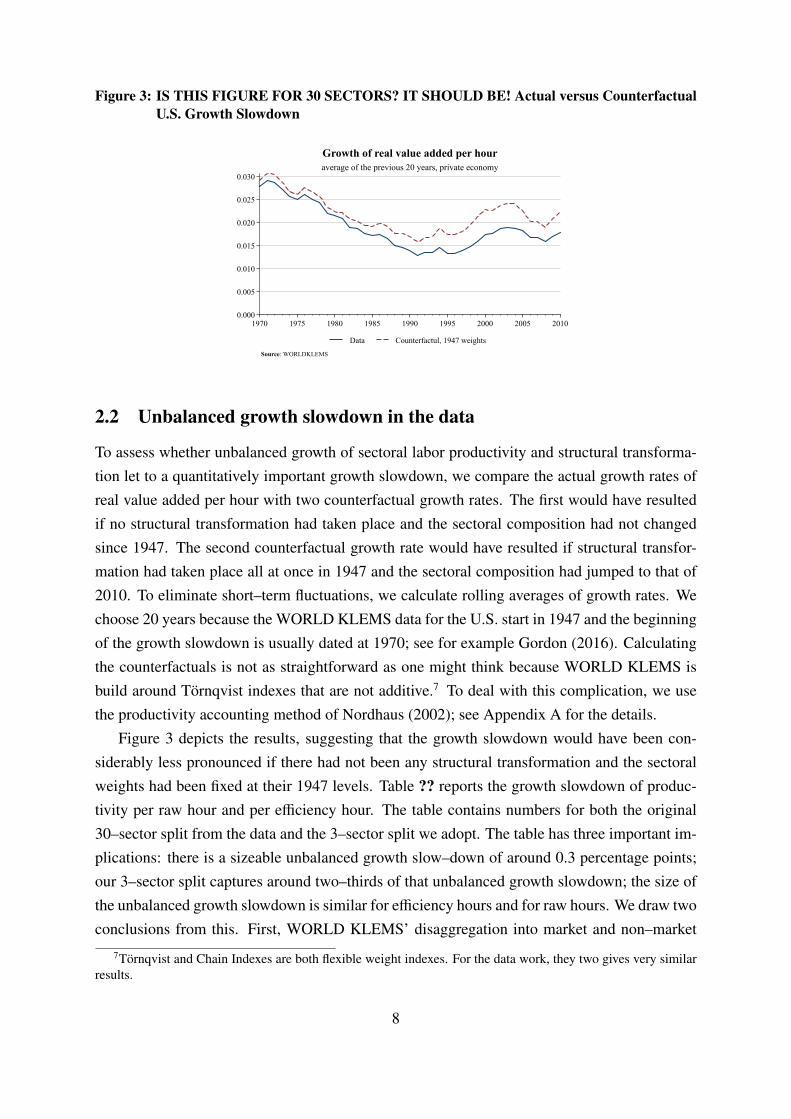
Figure 3: IS THIS FIGURE FOR 30 SECTORS? IT SHOULD BE! Actual versus CounterfactualU.S. Growth Slowdown

0.000

0.005

0.010

0.015

0.020

0.025

0.030

1970 1975 1980 1985 1990 1995 2000 2005 2010

Data Counterfactul, 1947 weights

Source: WORLDKLEMS

average of the previous 20 years, private economyGrowth of real value added per hour

2.2 Unbalanced growth slowdown in the data

To assess whether unbalanced growth of sectoral labor productivity and structural transforma-tion let to a quantitatively important growth slowdown, we compare the actual growth rates ofreal value added per hour with two counterfactual growth rates. The first would have resultedif no structural transformation had taken place and the sectoral composition had not changedsince 1947. The second counterfactual growth rate would have resulted if structural transfor-mation had taken place all at once in 1947 and the sectoral composition had jumped to that of2010. To eliminate short–term fluctuations, we calculate rolling averages of growth rates. Wechoose 20 years because the WORLD KLEMS data for the U.S. start in 1947 and the beginningof the growth slowdown is usually dated at 1970; see for example Gordon (2016). Calculatingthe counterfactuals is not as straightforward as one might think because WORLD KLEMS isbuild around Tornqvist indexes that are not additive.7 To deal with this complication, we usethe productivity accounting method of Nordhaus (2002); see Appendix A for the details.

Figure 3 depicts the results, suggesting that the growth slowdown would have been con-siderably less pronounced if there had not been any structural transformation and the sectoralweights had been fixed at their 1947 levels. Table ?? reports the growth slowdown of produc-tivity per raw hour and per efficiency hour. The table contains numbers for both the original30–sector split from the data and the 3–sector split we adopt. The table has three important im-plications: there is a sizeable unbalanced growth slow–down of around 0.3 percentage points;our 3–sector split captures around two–thirds of that unbalanced growth slowdown; the size ofthe unbalanced growth slowdown is similar for efficiency hours and for raw hours. We draw twoconclusions from this. First, WORLD KLEMS’ disaggregation into market and non–market

7Tornqvist and Chain Indexes are both flexible weight indexes. For the data work, they two gives very similarresults.

8

Table 1: Actual vs. Counterfactual Productivity Growth

sector composition growth of value added per hour (in %)

actual 2.07counterfactual 13 fast growing / traditional / market / skilled /

sectors slow growing non–traditional non–market unskilledfixed at 1947 2.27 2.31 2.31 2.31 2.32fixed at 2010 1.70 1.73 1.74 1.75 1.75

Table 2: Actual vs. Counterfactual Productivity Growth

sector composition growth of value added per hour (in %)

actual 2.1counterfactual 13 fast growing / traditional / market / skilled /

sectors slow growing non–traditional non–market unskilledfixed at 1947 2.3 2.3 2.3 2.3 2.3fixed at 2010 1.7 1.7 1.7 1.8 1.8

services captures most of unbalanced growth slowdown, although it is very simple and remainsanalytically tractable. Second, it is acceptable in the current context to focus on productivityper raw hour, instead of on productivity per efficiency house. Focusing on productivity per rawhour has the advantages of being simpler and of making our results more easily comparablewith those of other studies.

Given that we used the productivity accounting method of Nordhaus, it is natural to compareour results with his which were based on the comparison between the two counterfactuals withfixed initial and fixed final sector weights. Nordhaus (2008) found that the difference betweenthem amounts to 0.6 percentage points. The second column of Table 3 shows that for 30 sectorsand productivity per raw hour, we find 0.7 percentage points. Possible reasons for the discrep-ancy is that Nordhaus (2008) investigated the shorter period 1948–2001 and used data from theBEA. Moreover, he reported the productivity effect from reallocating labor among industrieswith different growth rates of sectoral productivity, whereas we report the combined produc-tivity effects from reallocating labor among industries with different growth rates and levels

of sectoral productivity. These two different effects are sometimes referred to as the “BaumolEffect” and the “Denison Effect”; see Nordhaus (2008) for a more detailed discussion of them.

ROBUSTNESSAfter having established that structural transformation led to an economically significant

unbalanced growth slowdown, we now build a model to capture this. Afterwards, we willcalibrate the model and use it to assess by how much unbalanced sectoral productivity growth

9

Table 3: Value Added per Hour vs. Efficiency Hour for 13 Sectors

sector composition growth of value added (in %)per hour per efficiency hour

actual 2.07 1.67counterfactual fixed at 1947 2.27 1.89counterfactual fixed at 2010 1.70 1.22

Table 4: Value Added per Hour vs. Efficiency Hour for 13 Sectors

sector composition growth of value added (in %)per hour per efficiency hour

actual 2.1 1.7counterfactual fixed at 1947 2.3 1.9counterfactual fixed at 2010 1.7 1.2

and structural transformation will reduce future productivity growth.

3 Model

3.1 Environment

There are three sectors. In each sector, value added is produced from labor:

Yit = AitHit (1)

i = g,m, n is the sector index which stands for goods, market services, and non–market services.Yi, Ai, and Hi denote value added, total factor productivity, and labor of sector i. The linearfunctional form implies that labor productivity equals TFP, that is, Yit/Hit = Ait. We use itbecause it is simple and captures the essence of the role that technological progress plays forstructural transformation; see Herrendorf et al. (2015) for further discussion.

There is a measure one of identical households. Each household is endowed with one unitof labor that is inelastically supplied and can be used in all sectors. As a result, GDP and GDPper capita, GDP per worker, and GDP per hour (“labor productivity”) are all equal in our model.

Utility is described by two nested, non–homothetic CES utility functions. The utility from

10

the consumption of goods and (aggregate) services, Cgt and Cst, is given by:

Ct =

α 1σcg C

εg−1σc

t Cσc−1σc

gt + α1σcs C

εs−1σc

t Cσc−1σc

st

σcσc−1

(2a)

Services are given by a non–homothetic CES aggregator of market and non–market services,Cmt and Cnt:

Cst =

α 1σsm C

εm−1σs

t Cσs−1σs

mt + α1σsn C

εn−1σs

t Cσs−1σs

nt

σsσs−1

(2b)

αg, αs, αm, αn ≥ 0 are weights; σc, σs ≥ 0 are elasticities of substitution; εg, εs, εm, εn > 0capture income effects. We follow Comin et al. (2015) and assume that in each aggregator onegood is a luxury good whereas the other one is a necessity: min{εg, εs} < 1 < max{εg, εs} andmin{εm, εn} < 1 < max{εm, εn}.

The non–homothetic CES utility function (2) goes back to the work of Hanoch (1975) andhas recently been used in the context of structural transformation by Comin et al. (2015) and bySposi (2016). For εi = 1 it reduces to the standard CES utility that implies homothetic demandfunctions for each consumption good. For εi , 1, the level of consumption affects the relativeweight that is attached to the consumption goods. Although in this case there is no closed–form solution for utility as a function of the consumption goods, it turns out that the impliednon–homothetic demand functions remain tractable. Moreover, the income effects that areimplied by the non–homothetic demand functions do not disappear in the limit as consumptiongrows without bound, which is consistent with the available evidence [see Boppart (2016) andComin et al. (2015)]. Having long–run income effects is potentially important in our contextbecause growth slowdown in the far future depends on the limit behavior of the economy. Astandard Stone–Geary utility specification would not capture long–run income effects because,as consumption grows without bound, it converges to a homothetic utility function.8

The non–homothetic CES aggregators make economic sense only if they are monotonicallyincreasing in each of the arguments. To ensure that this is the case, we restrict the parametersas follows:

Assumption 1

• min{εg, εs} ≤ 1 ≤ max{εg, εs} and σc < min{εg, εs} or max{εg, εs} < σc.

8We should mention that a disadvantage of the functional form (2) is that it is not aggregable in the Gormansense; if there is a distribution of households with different consumption expenditure instead of a continuum ofmeasure one of identical households, then it is not obvious how to derive the aggregate demand for the differentconsumption goods from the decisions of a representative household. While that is not a crucial limitation for ourapplication with a representative household, it is likely to be an issue in environments with a non–degenerate crosssection of households.

11

• min{εm, εn} ≤ 1 ≤ max{εm, εn} and σs < min{εm, εn} or max{εm, εn} < σs.

Appendix B proves that these restrictions have the desired effect:

Lemma 1 Assumption 1 is necessary and sufficient for

∂Ct(Cgt,Cst)∂Cit

> 0 ∀i ∈ {g, s} ∀Cgt,Cst ≥ 0

∂Cst(Cmt,Cnt)∂C jt

> 0 ∀ j ∈ {m, n} ∀Cmt,Cnt ≥ 0

We complete the description of the environment with the resource constraints:

Cit ≤ Yit, i = g,m, n (3a)

Ht = Hgt + Hst = Hgt + Hmt + Hnt ≤ 1 (3b)

3.2 Equilibrium

We focus on competitive equilibrium. In the competitive equilibrium of many multi–sectormodels, the nominal labor productivities per hour are equalized across sectors. To capture thefact that this is not borne out by our data, we introduce a sector–specific tax, τit, that firms haveto pay per unit of wage payments. The proceeds of the tax are lump–sum rebated through atransfer Tt =

∑i=g,m,n τitwtHit to households. The problem of firm i = g,m, n then becomes:

maxHit

PitAitHit − (1 + τit)wtHit

The first–order condition implies that

P jt

Pgt=

(1 + τ jt)Agt

(1 + τgt)A jt, j = m, n (4)

Using this and the production function, (1), we obtain that the relative sectoral labor productiv-ities equal the relative taxes:

P jtC jt/H jt

PgtCgt/Hgt=

1 + τ jt

1 + τgt, j = m, n (5)

In other words, the taxes drive a wedge between the expenditure ratio and the hours ratio. Asa result, our model captures that the nominal sectoral labor productivities are different. This isimportant in our context, because the effects of structural transformation on aggregate produc-tivity depend on the differences in both the growth rates and the levels of sectoral productivity(“Baumol Effect” and “Denisson Effect”).

12

It is also crucial to capture that labor productivity growth is strongest in the goods sector andweakest in the non–market service sector. To ensure tractability, we assume for the analyticalpart that sectoral taxes and sectoral labor productivity growth are constant.

Assumption 2 Taxes are constant and technological progress is constant and uneven across

sectors: A jt = γ j where j ∈ {g,m, n} and

A jt ≡A jt

A jt−1

denote growth factors and γ j are constants with 1 < γn < γm < γg.

Note that equation (4) and the assumption that taxes are constant imply that

(P jt

Pit

)∧

=γi

γ j, i, j ∈ {g,m, n} (6)

To solve the household problem, we split it in two layers. The “inner layer” is to allocatea given quantity of service consumption between the consumption of market and non–marketservices:

minCmt ,Cnt

PmtCmt + PntCnt s.t.

α 1σsm C

εm−1σs

t Cσs−1σs

mt + α1σsn C

εn−1σs

t Cσs−1σs

nt

σsσs−1

≥ Cst

Appendix B shows that the first–order conditions imply that

PntCnt

PmtCmt=αn

αm

(Pnt

Pmt

)1−σs

Cεn−εmt (7a)

Pst =(αmCεm−1

t P1−σsmt + αnC

εn−1t P1−σs

nt

) 11−σs . (7b)

where Pst is price index of aggregate services. The “outer layer” is to allocate a given quantityof total consumption between the consumption of goods and services:9

minCgt ,Cst

PgtCgt + PstCst s.t.

α 1σcg C

εg−1σc

t Cσc−1σc

gt + α1σcs C

εs−1σc

t Cσc−1σc

st

σcσc−1

≥ Ct

9The given quantity of total consumption is determined by the endowment of labor and the technology: Ct =

Agt/Pt. This is shown in the proof of Lemma 2 in Appendix B. A particular household takes Agt/Pt as givenbecause Agt is exogenous and Pt is the aggregate price index that is independent of its actions.

13

Appendix B shows that the first–order conditions imply

PstCst

PgtCgt=αs

αg

(Pst

Pgt

)1−σc

Cεs−εgt (8a)

Pt =(αgC

εg−1t P1−σc

gt + αsCεs−1t P1−σc

st

) 11−σc (8b)

PtCt =(αgC

εg−σct P1−σc

gt + αsCεs−σct P1−σc

st

) 11−σc (8c)

where Pt is the aggregate price index and PtCt ≡∑

i=g,m,n PitCit.

4 Unbalanced Growth Slowdown in the Model

We are now ready to study how unbalanced growth slowdown arises in our model. We will pro-ceed in two steps. We will first identify parameter restrictions under which our model gives riseto the stylized facts of structural transformation and then study unbalanced growth slowdownin two special cases in which we can obtain analytical solutions.

4.1 Structural transformation

We begin with the structural transformation between goods and services. Dividing (8a) forperiods t + 1 and t by each other, we obtain:

(PstCst

PgtCgt

)∧

=

(Pst

Pgt

)∧1−σc

Ctεs−εg (9)

The first term on the right–hand side is the relative price effect and the second term is the incomeeffect. We make the standard assumption that goods and aggregate services are complements,goods are necessities, and services are luxuries:10

Assumption 3 0 < σc < 1 and εg < 1 < εs.

Expression (9) shows that our model then generates the observed structural transformation fromgoods to services if Pst/Pgt and Ct both grow. We will impose additional restrictions below thatmake sure that this is the case.

We continue with the structural transformation between market and non–market services.Combining Equations (5), (6) and (7a), we obtain:

(PntCnt

PmtCmt

)=

(γm

γn

)1−σs

Ctεn−εm (10)

10See Kongsamut et al. (2001), Ngai and Pissarides (2007), and Herrendorf et al. (2013) for justifications ofthese assumptions.

14

Figure 4: Relative Prices and Expenditures in Services

0.00

0.25

0.50

0.75

1.00

1.25

1950 1960 1970 1980 1990 2000 2010

Price of non-market to market services Value added of non-market to market services

Source: WORLDKLEMS

Private service sector

We assume that market and non–market services are substitutes, market services are a necessity,and non–market services are a luxury:

Assumption 4 1 < σs and εm < 1 < εn.

Assumption 4 implies that the relative price effect, which is the first term on the right–hand sideof Equation (10), decreases the expenditure ratio of non–market to market services becauseproductivity growth is slower in non–market services. The income effect, which is the secondterm on the right–hand side, increases the expenditure ratio of non–market to market servicesif Ct increases. Combining these effects, our model can replicate the patterns of structuraltransformation within the service sector as summarized by Figure 4. Until around 1980 the priceof non–market relative to market services increased along with the corresponding expenditureratio. Our model replicates this pattern if the the income effect dominates the relative priceeffect before 1980. For this to happen, non–market services must be luxuries. After 1980, theincrease in the price of non–market relative to market services accelerated while the expenditureratio remained roughly constant. Our model replicate this pattern if the income effect offsetsthe relative price effect after 1980. For this to happen, the two service subcategories mustbe substitutes and the acceleration in the relative price increase after 1980 must sufficientlystrengthen the price effect.

Alternative parameter constellations would not be able to generate the observed patterns.To see this, note first that the income effects do not change in 1980 but work in the samedirections during the whole period. So the change in the relative expenditure share pattern mustbe coming from the acceleration in the relative prices. If the services were complements, thenthe expenditure of non–market relative to market services would have increased by more after1980 than before 1980, which is counterfactual. Given that the two services must be substitutes,

15

non–market services must be a luxury and market services must be a necessity. If the oppositewas true and market services were luxuries and non–market services were necessities, then theexpenditure of market relative to non–market services would have increased during the wholeperiod, which again is counterfactual.

We are left with the task of ensuring that Ct and Pst/Pgt both grow, which we have as-sumed but not proved so far. We need to impose further restrictions on the parameters to showthis. First, the elasticity of consumption expenditures with respect to real consumption is non–negative. Appendix B shows that a sufficient condition is:

Assumption 5

εg − σc

1 − σc<εn − 11 − σs

+εs − σc

1 − σc(11)

We can now ensure that the growth of aggregate consumption is positive and finite:

Lemma 2 If Assumptions 1–5 hold, then the growth of aggregate consumption is bounded from

below and above: 1 <¯C ≤ Ct ≤ C where

¯C ≡ γ

(1−σc)(1−σs)(εm−1)(1−σc)+(εs−σc)(1−σs)n (12a)

C ≡ γ1−σcεg−σcg (12b)

Lastly, we need to ensure that the price of aggregate services relative to goods increases.We need two additional assumptions:

Assumption 6 The growth factors of sector labor productivity satisfy:

γm < γ1+

(1−σc)(εm−εn)(εm−1)(1−σc)+(εs−σc)(1−σs)

n (13a)

γn < γ1− (1−σc)(εn−1)

(εg−σc)(σs−1)g (13b)

Note that a sufficient condition for (13b) to be satisfied is that

εn − 1σs − 1

<εg − σc

1 − σc(14)

Lemma 3 Suppose that Assumptions 1–6 hold. Then the price of services relative to goods

increases over time, Pst > 1.

We conclude this subsection by summarising the patterns of structural transformation in ourmodel. We start with goods and services:

16

Proposition 1 If Assumptions 1–6 hold, then along the equilibrium path the expenditure and

employment shares of the goods sector are monotonically decreasing and converge to zero as

time goes to infinity.

In other words, our model generates the standard pattern of the structural transformation be-tween goods and services that is familiar from many two–sector models of structural trans-formation: the goods sector shrinks and eventually the service sector takes over the modeleconomy.

Regarding the structural transformation within the service sector, Lemma 2 and Equation(10) immediately imply:

Proposition 2 If Assumptions 1–6 hold, then along the equilibrium path

γm

γn<

¯Cεn−εmσs−1 =⇒

(PntCnt

PmtCmt

)∧

> 1 (15a)

γm

γn> C

εn−εmσs−1 =⇒

(PntCnt

PmtCmt

)∧

< 1 (15b)

In other words, if the productivity growth in the two service sectors is “sufficiently close”, thenthe income effect will dominate and non–market services take over in the limit. In contrast,if productivity in the two service sectors is “sufficiently different”, then the price effect willdominate and market services will take over in the limit. The fact that both cases are possiblein the limit suggest that there is a third knife–edge case in which the two forces exactly offseteach other and the share of market services remains constant. Which of the three cases prevailsin the long run for plausible parameter values is a quantitative question which we will answerbelow by simulating a calibrated version of our model.

4.2 Growth slowdown

After having established that our model can qualitatively generate the patterns of structuraltransformation that we observe in the data, we now turn to the question whether it generatesgrowth slowdown along the equilibrium path. We start by exploring what we can say aboutbalanced growth of welfare in our model. Given that we have a continuum of measure one ofidentical households, the natural welfare measure is Ct. Appendix B shows that:

Proposition 3 If Assumptions 1–6 hold, then the growth factor of welfare, Ct, decreases along

the equilibrium path.

In other words, our model generates an unbalanced growth slowdown in terms of welfare. Thisshould not come as a surprise given that the interaction of preferences and uneven technologicalprogress reallocates labor from the faster growing goods sector to the slower growing service

17

sectors. In practice, researchers use GDP per capita as a proxy for welfare because GDP percapita is so widely available over time and across countries. Note that the way in which wehave set up our model implies that GDP per capita equals labor productivity, so we will use thetwo concepts interchangeably in what follows.

We now answer the obvious question whether standard measures of GDP per capita capturethe unbalanced growth slowdown in welfare. The answer is more nuanced than one mightinitially think. We will show that it depends critically on which measure of GDP per capita isused and on what the relative sizes of the taxes are. We will derive analytical results in twospecial cases, which serve as useful benchmarks to sharpen our intuition: the growth factors areconstant but uneven across sectors and taxes are zero (“uneven technological progress and zerotaxes”);11 the growth factors are the same in all sectors and taxes are constant but uneven acrosssectors (“even technological progress and unequal taxes”). We will deal with the general case(“uneven technological progress and non–zero taxes”) in the subsequent quantitative section.

4.2.1 Uneven technological progress and zero taxes

If taxes are zero, it turns out that whether or not our model leads to unbalanced growth slow-down in terms of GDP per capita depends on the way in which GDP capita is calculated. Thereare two possibilities. The literature on multi–sector models chooses the units of a current–period numeraire j ∈ {g,m, n}:

Yn jt ≡

∑i=g,m,n

PitP jt

Cit∑i=g,m,n

Pit−1P jt−1

Cit−1

This means that the numeraire differs between two adjacent periods: in period t it is C jt whereasin t−1 it is C jt−1. In contrast, NIPA statisticians calculate GDP per capita by using chain indexes,that is, the geometrically weighted average of the Laspeyres and the Paasche quantity indexes.

Ycht =

√ ∑i=g,m,n Pit−1Cit∑

i=g,m,n Pit−1Cit−1·

∑i=g,m,n PitCit∑

i=g,m,n PitCit−1

Note that it does not matter whether one calculates GDP from a chained quantity index like theone above or from nominal GDP and a chained price index. This is shown in the next lemma,which is proven again in Appendix B.

Lemma 4 Chained quantity and price indexes satisfy:

Ycht × Pch

t = PtYt

11Note that technically it is enough if taxes are the same in all sectors. But there is no important difference inour context between all taxes being equal to zero and all taxes being the same.

18

We start with characterizing the growth of GDP per capita when we use a current–periodnumeraire. Appendix B shows that:

Proposition 4 Suppose that τit = τt for i = g,m, n and that we use a current–period numeraire

j = g,m, n to calculate real GDP. If Assumptions 1–2 hold, then the growth factor of real GDP

per capita is constant: Yn jt = γ j.

The fact that the growth of real GDP per capita in units of a current–period numeraire is constantgreatly simplifies the characterization of the equilibrium path, because it can be calculatedas a balanced growth path. This is particularly helpful in model versions with capital. Thedisadvantage is that the growth factor of real GDP per capita depends on the choice of thenumeraire, which is sometimes called the Gerschenkron Effect. In addition, constant growth ofreal GDP per capita is in sharp contrast to the unbalanced growth slowdown of welfare.

Chain indexes avoid the Gerschenkron Effect and have the additional advantage that thegrowth rate of real GDP per capita is independent of the base year. In addition, it turns out thatthey can capture the unbalanced growth slowdown in terms of welfare:12

Proposition 5 Suppose that τit = τt for i = g,m, n and that we use the chain index to calculate

real GDP. then the equilibrium growth of real GDP per capita

• changes with the sectoral composition of the economy (“unbalanced growth”);

• slows over time if Hnt ≥ 0.

Proposition 4 provides a sufficient condition under which our model generates growth slow-down in terms of GDP per capita: the forces of structural transformation have to play out insuch a way that labor is reallocated to the non–market service sector, Hn ≥ 0. To develop intu-ition for this condition we proceed in two steps. First, fix the allocation of aggregate servicesbetween market and non–market services. The reallocation from goods to aggregate servicethen slows down aggregate productivity growth, because productivity growth is larger in thegoods sector than in the service subsector. This is an example of what Nordhaus (2002,2008)called the “Baumol Effect”. Consider now the additional reallocation within aggregate services.Since market services have higher productivity growth than non–market services, reallocationtowards market services increases the productivity growth of aggregate services. For growthslowdown to happen, this effect must not be too strong. A sufficient condition for this is thatthis reallocation is absent, which is the case if the hours share of non–market services does notdecline.

In sum, whether or not our model exhibits unbalanced growth slowdown in terms of GDPper capita depends critically on which of the two methods we use to calculate GDP. This is not

12The proof again is in Appendix B.

19

at all appreciated in the literature on multi–sector models, which tends to connect growth ratesfrom the model economy which are calculated with current–period numeraires to growth ratesfrom the data which are calculated with chain indexes. Since the growth properties of GDP aredramatically different under the two methods, proceeding in this way can be very misleading.13

4.2.2 Even technological progress and unequal taxes

We now turn to the second case in which we can derive analytical results: the growth factorsare the same in all sectors but the sectoral taxes differ. This case captures the feature of realitythat the levels of sectoral labor productivity differ. Using equation (4), it is then straightforwardto show that

Proposition 6 If Assumptions 1–6 hold and that γ ≡ γi, i = g,m, n. The growth factor of real

GDP per capita is not constant in general:

Yn jt = Ych

t = γ

∑i=g,m,n(1 + τi)Hit∑

i=g,m,n(1 + τi)Hit−1(16)

The proposition shows that even if labor productivity growth is the same in all sectors, thegrowth factor of real GDP per capita will in general not be equal to that rate. This comes aboutbecause the tax differences introduce a wedge between the nominal labor productivities of thedifferent sectors; compare (5). Structural transformation then leads to an acceleration (slowdown) of the growth of GDP per capita if labor is reallocated towards the sectors with higher(lower) levels of labor productivity. Figure 5 shows that in the data

PntCnt

Hnt≥

PgtCgt

Hgt

PmtCmt

Hmt≤

PgtCgt

Hgt

Normalizing τg = 0, this implies that τn > 0 and τm < 0 and that the reallocation to non–marketservices increase GDP growth whereas the reallocation to market services decreases the growthof real GDP per capita. Nordhaus (2002,2008) called this the “Denison Effect”.

13Critical readers might have noticed that in our empirical analysis we use aggregate growth rates from theWORLD KLEMS dataset, which are based on the Tornqvist index, whereas in our theoretical analysis we considerthe aggregate growth rates calculated by the chain–weighted index (a Fischer index). Although both indexesare conceptually different, they are equal to a second–order approximation. In applied work, they are thereforetypically used interchangeably.

20

Figure 5: Relative Nominal Productivities

0.00

0.25

0.50

0.75

1.00

1.25

1.50

1950 1960 1970 1980 1990 2000 2010

Market services to goods Non-market services to goods

Source: WORLDKLEMS

private economyRatios of sectoral nominal value added per hour

5 Calibration and Predictions

In this section, we calibrate our model to match key features of the postwar U.S. economy,such as the sectoral growth rates and the reallocation across sectors. We then use the calibratedmodel to study how big unbalanced growth slowdown will be in the future. Our model impliesthat it will not be larger than in the past.

5.1 Calibration

We start with the calibration of the taxes and sectoral TFPs. Normalizing the taxes in the goodssector to zero, τg = 0, and defining nominal value added as VA jt ≡ P jtC jt = P jtA jtH jt, (4)–(5)give

1 + τ jt =VA jt/H jt

VAgt/Hgt, j = m, n

Measuring {(VA jt/H jt)/(VAgt/Hgt)} for j = m, n and t = 1947, ..., 2010 from the data, thisrelationship gives us the values for {τ jt}. Next, we set Pg1947 = Pm1947 = Pn1947 = Ag1947 = 1and back out the implied A j1947. We then take {Pit} for i = g,m, n and t = 1947, ..., 2010from the data and calibrate {A jt} so as to match the observed changes in real labor productivity,{[VA jt/(P jtH jt)]/[VAgt/(PgtHgt)]}, in the data. Figure 6 shows the calibrated taxes and TFPs.

We jointly calibrate the remaining ten parameters (αg, αs, αm, αn, σs, σc, εg, εs, εm, εn). Thefirst targets are the nominal value added of non–market services relative to goods and relativeto market services: {

PntCnt

P jtC jt

}t=1947,...,2010

, j = g,m (17)

21

Figure 6: Taxes and Sector TFPs

(a)

1940 1950 1960 1970 1980 1990 2000 2010−0.3

−0.2

−0.1

0

0.1

0.2 Distortions

τm

τn

(b)

1940 1950 1960 1970 1980 1990 2000 20100.5

1

1.5

2

2.5

3

3.5

4 Sector TFP

Ag

Am

An

These targets allow us to identify all parameters except for the εi. To be precise, we can identifyεg−εs and εm−εn, but not all four εi. Different from ?, we need these parameter values becausewe are solving for the equilibrium path of the whole model, instead of for the implied demandsystem that takes prices and income as given.

To obtain additional targets, we use the fact that the values of εi affect how changes in Ct

translate into changes in (Pst,Cst, Pt,Ct). We stress that, in general, it is not appropriate tocompare the model–implied (Pst,Cst, Pt,Ct) directly with the corresponding statistics from thedata, because the model aggregates use non–homothetic CES aggregators whereas WORLDKLEMS aggregates use Thornquivst indexes. Although locally the two are equal to a second–order approximation, over time they may grow far apart. Hence, the model statistics and the datastatistics with the same names are really different objects, and it does not make conceptual senseto require them to be close. To find a calibration strategy that makes conceptual sense, we applythe model’s non–homothetic CES aggregator to raw quantities from the model and from the dataand compare the resulting aggregates. In particular, we first calculate the {Pst, Cst, Pt, Ct} thatare implied by the data values of {Cgt(D),Cmt(D),Cnt(D) (where D indicates data) and the non–homothetic CES aggregators from the model given the model parameters; we then minimize thedifference between the {Pst, Cst, Pt, Ct} and the {Pst,Cst, Pt,Ct} that are generated by the modelquantities {Cgt,Cmt,Cnt}.

To implement this, let us start with the definitions of the non–homothetic CES aggregators:

Ct −(α

1σcg C

σc−1σc

gt Cεg−1σc

t + α1σcs C

σc−1σc

st Cεs−1σc

t

) σcσc−1

= 0

Cst −(α

1σsm C

σs−1σs

mt Cεm−1σs

t + α1σsn C

σs−1σs

nt Cεn−1σs

t

) σsσs−1

= 0(18)

The first step is to substitute in the consumption quantities from the data so as to obtain the con-

22

sumption aggregates that are implied by the data given the functional forms and the parametersof the model:

Cst −[α

1σsm

(Pm(D)Cm(D)

Pm(D)

)σs−1σs C

εm−1σs

t + α1σsn

(Pn(D)Cn(D)

Pn(D)

)σs−1σs C

εn−1σs

t

] σsσs−1

= 0

Ct −[α

1σcg

(Pg(D)Cg(D)Pg(D)

)σc−1σc C

εg−1σc

t + α1σcs C

σc−1σc

st Cεs−1σc

t

] σcσc−1

= 0

The next step is to solve this system of equations for Cst and Ct. Then, we use definition of theprice indexes to solve for the price indexes that that are implied by the data given the functionalforms and the parameters of the model:

Pst −[αnPnt(D)1−σsCt

εn−1 + αmPmt(D)1−σsCtεm−1

] 11−σs

= 0

Pt −[αgPgt(D)1−σcCt

εg−1 + αsP1−σcst Ct

εs−1] 1

1−σc= 0

(19)

We can now run an OLS regression of Ps, Cs, or P on C and a constant. The slope coefficientcontains the information on εi that we are interested in, and so we can use it as a target in thecalibration. This way of calibrating is called indirect inference: we use an auxiliary model (theequation that we estimate with OLS) and require the calibrated model to match an auxiliaryparameter (here the slope of the estimated equation). Endogeneity is not a problem because weestimate the same equation on actual data and on simulated model data, so possible endogeneityappears in both equations in the same fashion. We tried different combinations of targets andOLS coefficients and many of them worked, i.e., we got a fixed point and all parameters wereseparately identified. The calibrated parameter values were similar across the different casesthat work. Our preferred strategy is target the expenditure shares from (17), Cst/Ct, Pst/Pt, andthe OLS coefficient in the linear regression of Pst on a constant and on Ct.

The calibration results are in Table 5. We find the expected parameter constellation forgoods and services: they are complements (σc < 1); goods are necessities (εg < 1); servicesare luxuries (εs > 1). We find the expected parameter constellation for market and non–marketservices: they are substitutes (σs < 1); market services are necessities (εm < 1); non–marketservices are luxuries (εn > 1). The parameter values satisfy Assumption 1, except for the factthat σs < εn. This does not create a problem though because Assumption 1 was necessaryand sufficient for the utility aggregator Cst to increase in its arguments for all possible values

of C jt ≥ 0 ( j = m, n). Although that is not the case for our calibrated parameters, we haveverified that the utility aggregator Cst increases in its arguments for all equilibrium values ofC jt ( j = m, n) that the model economy actually assumes.14

Figures 7, 8, and 9 show that the calibrated model matches well the targeted moments andseveral non–targeted moments. The calibrated model also matches that the effect of unbalanced

14This amounts to verifying that the denominator of (27b) is negative along the actual equilibrium path.

23

Table 5: Calibrated Parameters

αg αs αm αn σs σc εg εs εm εn

0.54 0.46 0.66 0.34 1.28 0.17 0.57 1.45 0.42 1.39

growth slowdown among our three sectors is 0.2 percentage points per year as it is in the data.

Figure 7: Prices – Model and Data

(a)

1940 1950 1960 1970 1980 1990 2000 20100.5

1

1.5

2

2.5

3

3.5 Relative prices

Pn/P

g Data

Pn/P

m Data

Pn/P

g Model

Pn/P

m Model

(b)

1940 1950 1960 1970 1980 1990 2000 20100

2

4

6

8

10

12

14

16

18 Service Price Index Ps

Ps(t)/P

s(1947) Data

Ps(t)/P

s(1947) Model

(c)

1940 1950 1960 1970 1980 1990 2000 20100

2

4

6

8

10

12

14 Aggregate Price Index P

P(t)/P(1947) Data

P(t)/P(1947) Model

(d)

1940 1950 1960 1970 1980 1990 2000 20100.9

1

1.1

1.2

1.3

1.4 Ps / P (Target)

Ps(t)/P(t) Data

Ps(t)/P(t) Model

5.2 Model simulation

To produce the out–of–sample implications of our model, we simulate it forward, starting in2010. We assume that between 2010–2010+T , the variables {Agt, Amt, Ant, Pgt) grow at thesame constant rates on average as they did “in the past”. The key issue to settle is what wemean by “in the past”. The evidence presented in Section 2 suggests that there was a structural

24

Figure 8: Productivity, Employment and Value Added – Model and Data

(a)

1940 1950 1960 1970 1980 1990 2000 20100

0.5

1

1.5

2

2.5

3 Aggregate Labor Productivity

Data

Model

(b)

1940 1950 1960 1970 1980 1990 2000 20100

0.5

1

1.5

2

2.5

3

3.5

4 Labor Productivity: Goods

(c)

1940 1950 1960 1970 1980 1990 2000 20100

0.5

1

1.5

2

2.5

3

3.5

4 Labor Productivity: Market services

(d)

1940 1950 1960 1970 1980 1990 2000 20100

0.5

1

1.5

2

2.5

3

3.5

4 Labor Productivity: Non−Market services

(e)

1940 1950 1960 1970 1980 1990 2000 20100.1

0.2

0.3

0.4

0.5

0.6 Employment Shares

(f)

1940 1950 1960 1970 1980 1990 2000 20100.2

0.4

0.6

0.8

1

1.2

1.4

1.6 Relative value added

VAn/VA

g Data

VAn/VA

m Data

VAn/VA

g Model

VAn/VA

m Model

break in the productivity patterns changed at some time around 1980. We therefore do not gofurther back then 1980. We calculate average growth rates for {Agt, Amt, Ant, Pgt) during threeperiods: 1980–2010, 1990–2010, and 1980–2005. The first period uses information from the

25

Figure 9: Consumption – Model and Data

(a)

1940 1950 1960 1970 1980 1990 2000 20100.8

1

1.2

1.4

1.6

1.8

2

2.2

2.4

2.6 Service Consumption Cs

Cs(t)/C

s(1947) Data

Cs(t)/C

s(1947) Model

(b)

1940 1950 1960 1970 1980 1990 2000 20101

1.1

1.2

1.3

1.4

1.5

1.6

1.7

1.8

1.9 Aggregate Consumption C

C(t)/C(1947) Data

C(t)/C(1947) Model

(c)

1940 1950 1960 1970 1980 1990 2000 20100.44

0.46

0.48

0.5

0.52

0.54

0.56

0.58

0.6

0.62 Cs(t) / C(t) (Target)

Cs(t)/C(t) Data

Cs(t)/C(t) Model

entire period. The second period starts somewhat later in 1990 in case the structural break hap-pened after 1980. The third period stops in 2005 to avoid having data from the Great Recession,which is an unusual episode. Table 6 shows the data inputs and the results. The top rows showthe average annual growth rate of {Agt, Amt, Ant, Pgt) and the average tax rates for different cal-ibration periods. The bottom rows show the implied average annual growth rates of aggregatelabor productivity. The model implies that the future unbalanced growth slowdown in produc-tivity growth is most 0.22 percentage points, which is close to the number we calculated for thepostwar period.

It is important to realize that the model is essential for making these predictions. If insteadwe had just run a simple regression on past data and extrapolated the result into the future, wewould have gotten different results. For example, during the period from 1990–2010 the linearfit of aggregate labor productivity gives a slope coefficient of -0.021. This implies that a simpleextrapolation by 20 years would predict a slowdown from 1.30% to 1.30 − 0.022 · 20 = 0.86%

26

Table 6: Future Unbalanced Growth Slowdown

calibration period data averages over calibration period∆Ag/Ag ∆Am/Am ∆An/An ∆Pg/Pg τm τn

1980–2010 1.98 1.71 -0.33 2.32 -0.11 0.091990–2010 1.94 1.88 -0.21 1.78 -0.08 0.111980–2005 2.11 1.90 -0.32 2.28 -0.l1 0.10

aggregate productivity growth (in %)1990–2010 2010–2030 2030–2050 2050–2150

1980–2010 1.21 1.10 1.05 1.001990–2010 1.30 1.22 1.17 1.111980–2005 1.34 1.22 1.17 1.12

which is quite far from the 1.22% that the model predicts. This means that the non–lineardynamics that results from the model is not well captured by a simple regression. Hence, themodel is needed for making out–of-sample forecasts.

We end this section with providing some intuition for why our model predicts that there willbe at most as much future productivity slowdown than there was past productivity slowdown.A first reason is that while the value added and the hours shares of services were of similarsize as those of goods in 1947, in 2010 they were almost four times those of goods. Hence,between 1947 and 2010 there was a lot of reallocation from goods with the fastest productivitygrowth to services with slower productivity growth, which led to productivity slowdown. Giventhat the goods sector is rather small in 2010, that source of unbalanced growth slow down isbound to be of much less importance in the future. Instead, the center stage is now taken bychanges in the composition of the service sector, which lead to the reallocation between marketservices, which have fast productivity growth, and non–market services, which are stagnating.Since the data suggest that market and non–market services are substitutes, the model predictsthat non–market services are not taking over the economy in the limit, which bounds the extentof future productivity slowdown.

Our conclusion differs sharply from that of standard models of structural transformation.These models feature just one elasticity of substitution among the value added of all sectors,which is typically set such that the different sectoral value added are complements. They implythat the sector with the slowest productivity growth takes over in the limit, which are non–market services in our three–sector split. Since non–market services have had no productivitygrowth in the recent past (and even shrank somewhat), doing our extrapolation exercise with astandard model of structural transformation would predict that in the limit productivity growthfalls all the way to zero and then even shrinks somewhat.

27

6 Conclusion

We have have demonstrated that structural transformation considerably slowed down produc-tivity growth in the post World War II period. We have build a model that accounts for this.Our model implies that future structural transformation will not be more of a drag on produc-tivity growth than it has been in the past. To reach this conclusion it has been crucial thatwe have disaggregated services into the subcategories market and non–market services. Thedata suggest that they had very different productivity performances: market services have hadsteady productivity growth in the post–war U.S. whereas non–market service have had stag-nating productivity growth since the 1980s. The data also suggest that the two subcategoriesof services are substitutes. This implies that the stagnating non–market services will not takeover the economy in the limit, which is in sharp contrast to what existing models of structuraltransformation imply.

In this paper, we have taken the sectoral growth rates as given and we have explored whichconsequences changes in the sectoral composition have for unbalanced growth slowdown. Afirst interesting question for future work is why different sectors show different productivitygrowth. A second interesting question for future work is to study whether the slow growingsectors will continue to grow slowly even when they comprise sizeable shares of the economy.We plan to tackle these questions next.

References

Antolin-Diaz, Juan, Thomas Drechsel, and Ivan Petrella, “Tracking the Slowdown in Long–Run GDP Growth,” Review of Economics and Statistics, 2016, forthcoming, 2167–2196.

Baumol, William J., “Macroeconomics of Unbalanced Growth: The Anatomy of the UrbanCrisis,” American Economic Review, 1967, 57, 415–426.

, The Cost Disease: Why Computers Get Cheaper and Health Care Doesn’t, New Haven,Connecticut: Yale University Press, 2013.

, Sue Anne Batey Blackman, and Edward N. Wolff, “Unbalanced Growth Revisited:Asymptotic Stagnacy and New Evidence,” American Economic Review, 1985, 75, 806–817.

Boppart, Timo, “Structural Change and the Kaldor Facts in a Growth Model with RelativePrice Effects and Non–Gorman Preferences,” Econometrica, 2016, pp. 2167–2196.

Byrne, David M., John G. Fernald, and Marshall B. Reinsdorf, “Does the United StatesHave a Productivity Slowdown or a Measurement Problem,” Brookings Papers on Economic

Activity, 2016, p. Forthcoming.

28

Comin, Diego, Martı Mestieri, and Danial Lashkari, “Structural Transformations withLong–run Income and Price Effects,” Manuscript, Northwestern University 2015.

Duarte, Margarida and Diego Restuccia, “The Role of the Structural Transformation in Ag-gregate Productivity,” Quarterly Journal of Economics, 2010, 125, 129–173.

and , “Relative Prices and Sectoral Productivity,” Manuscript, University of Toronto2016.

Fernald, John G. and Charles I. Jones, “The Future of US Growth,” American Economic

Review: Papers and Proceedings, 2014, 104, 44–49.

Gordon, Robert, The Rise and Fall of American Growth: The US Standard of Living since the

Civil War, Princeton, New Jersey: Princeton University Press, 2016.

Griliches, Zvi, “Productivity, R&D, and the Data Constraint,” American Economic Review,1994, 84, 1–23.

Hanoch, Giora, “Production and Demand Models with Direct or Indirect Implicit Additivity,”Econometrica, 1975, 43, 395–419.

Herrendorf, Berthold and Akos Valentinyi, “Which Sectors Make Poor Countries so Unpro-ductive?,” Journal of the European Economic Association, 2012, 10, 323–341.

, Christopher Herrington, and Akos Valentinyi, “Sectoral Technology and StructuralTransformation,” American Economic Journal – Macroeconomics, 2015, 7, 1–31.

, Richard Rogerson, and Akos Valentinyi, “Two Perspectives on Preferences and Struc-tural Transformation,” American Economic Review, 2013, 103, 2752–2789.

, , and , “Growth and Structural Transformation,” in Philippe Aghion andSteven N. Durlauf, eds., Handbook of Economic Growth, Vol. 2, Elsevier, 2014, pp. 855–941.

Jorgenson, Dale W. and Marcel P. Timmer, “Structural Change in Advanced Nations: A NewSet of Stylised Facts,” Scandinavian Journal of Economics, 2011, 113, 1–29.

, Mun S. H, , and Jon D. Samuels, “A Prototype Industry-Level Production Account forthe United States, 1947–2010,” Mimeo, National Bureau of Economic Research, Cambridge,MA 2013.

Kongsamut, Piyabha, Sergio Rebelo, and Danyang Xie, “Beyond Balanced Growth,” Review

of Economic Studies, 2001, 68, 869–882.

29

Ngai, L. Rachel and Chrisopher A. Pissarides, “Structural Change in a Multisector Model ofGrowth,” American Economic Review, 2007, 97, 429–443.

Nordhaus, William D., “Productivity Growth and the New Economy,” Brookings Papers of

Economic Activity, 2002, 2, 211–265.

, “Baumol’s Disease: A Macroeconomic Perspective,” The B.E. Journal of Macroeco-

nomics (Contributions), 2008, 8.

Oulton, Nicholas, “Must the Growth Rate Decline? Baumol’s Unbalanced Growth Revisited,”Oxford Economic Papers, 2001, 53, 605–627.

Sposi, Michael, “Evolving Comparative Advantage, Sectoral Linkages, and StructuralChange,” Manuscript, Federal Reserve Bank of Dallas, Dallas 2016.

Syverson, Chad, “Challenges to Mismeasurement Explanations for the U.S. ProductivitySlowdown,” Working Paper 21974, NBER 2016.

Triplett, Jack E. and Barry P. Bosworth, “Productivity Measurement Issues in Services In-dustries: “Baumols Disease” Has Been Cured,” FRBNY Economic Policy Review, September2003, pp. 23–33.

Appendix A: Data Work

A Calculations behind Table ??

A.1 Preliminary remarks

Conceptually, the first two columns of the table are the actual and the counterfactual accumu-lated growth factors where the counterfactual accumulated growth factor are calculated withthe counterfactual sector labor shares from 1947:[

Y2010

H2010

]/ [Y1947

H1947

]and

∑i=g,m,n

Hi,1947

H1947

Yi,2010

Hi,2010

/ [Y1947

H1947

]

As in the body of the paper, Y and H denote real value added and hours worked. The thirdand the fourth column are the average annual growth rates that are calculated with sector labor

30

shares from 2010 and 1947: ∑

i=g,m,n

Hi,2010

H2010

Yi,2010

Hi,2010

/ ∑

i=g,m,n

Hi,2010

H2010

Yi,1947

Hi,1947

1/63

=

[

Y2010

H2010

] / ∑i=g,m,n

Hi,2010

H2010

Yi,1947

Hi,1947

1/63

and

∑

i=g,m,n

Hi,1947

H1947

Yi,2010

Hi,2010

/ ∑

i=g,m,n

Hi,1947

H1947

Yi,1947

Hi,1947

1/63

=

∑

i=g,m,n

Hi,1947

H1947

Yi,2010

Hi,2010

/ [Y1947

H1947

]1/63

In practise, these statistics are unfortunately not as straightforward to calculate as the aboveformulas suggest. The complications arise from the fact that WORLD KLEMS calculates quan-tity and price indices according to a Tornqvist aggregation procedure, which implies that thequantity indices are not additive. Below we describe how average annual growth rates andaccumulated growth factors can be calculated without imposing additivity.

A.2 Aggregate growth rates as sector aggregates

The growth rate of a variable in period t is defined by the log difference between periods t andt − 1. The aggregate growth rates of real value added, Yt, and efficiency hours, Ht, are definedas the weighted averages of the corresponding sectoral growth rates:

∆ ln(Yt) ≡∑

i=g,m,n

S (Yit)∆ ln(Yit) (20a)

∆ ln(Ht) ≡∑

i=g,m,n

S (Hit)∆ ln(Hit), (20b)

where S (Yit) and S (Hit) denote the averages over periods t and t − 1 of the nominal shares ofsector i’s value added and compensation of labor in the corresponding totals. We use averageshere because the shares are used as weights of growth rates from on period to the next.

A.3 Aggregate productivity measures as sector aggregates

We first calculate the growth rate of aggregate value added per hour:

∆ ln(LP(Ht)

)≡ ∆ ln(Yt) − ∆ ln(Ht)

=∑

i=g,m,n

S (Yit) [∆ ln(Yit) − ∆ ln(Hit)] +∑

i=g,m,n

S (Yit)∆ ln(Hit) − ∆ ln(Ht).

31

Since,

∆ ln(Ht) = ln(

Ht

Ht−1

)= ln

(∑i=g,m,n(Hit − Hit−1 + Hit−1)

Ht−1

)= ln

1 +∑

i=g,m,n

Hit−1

Ht−1

Hit − Hit−1

Hit−1

≈ ∑i=g,m,n

Hit−1

Ht−1∆ ln(Hit).

the growth rate of aggregate value added per hour is approximately equal to

∆ ln(LP(Ht)

)=

∑i=g,m,n

S (Yit)∆ ln(LP(Hit)

)+

∑i=g,m,n

[S (Yit) −

Hit−1

Ht−1

]∆ ln(Hit) (21)

We now turn to the calculation of the growth rates of aggregate value added per efficiencyhour. Applying the definitions (20), we obtain:

∆ ln(LP(Ht)

)≡ ∆ ln(Yt) − ∆ ln(Ht) =

∑i=g,m,n

S (Yit)∆ ln(Yit) −∑

i=g,m,n

S (Hit)∆ ln(Hit)

=∑

i=g,m,n

S (Yit)∆ ln(LP(Hit)

)+

∑i=g,m,n

[S (Yit) − S (Hit)

]∆ ln(Hit). (22)

Thus, the growth rate of aggregate value added per efficiency hour is the sum of the weighted av-erage of the growth rates of sector value added per efficiency hour and a correction term, whichcaptures the role of the difference between the sectoral–value–added shares and the sectoral–labor–compensation shares, [S (Yit) − S (Hit)].

A.4 Counterfactual experiments

To assess the effect of structural transformation on aggregate productivity growth, we definecounterfactual labor productivity measures with fixed period–T sector weights using expres-sions (21) and (22):

∆ ln(LP(Ht,T )

)≈

∑i=g,m,n

S (YiT )∆ ln(LP(Hit)

)+

∑i=g,m,n

[S (YiT ) −

HiT−1

HT−1

]∆ ln(Hit), (23a)

∆ ln(LP(Ht,T )

)=

∑i=g,m,n

S (YiT )∆ ln(LP(Hit)

)+

∑i=g,m,n

[S (YT ) − S (HT )

]∆ ln(Hit). (23b)

The first two columns of Tables ?? compare the actual with the counterfactual accumulatedgrowth factors of GDP between 1948 and 2010 where the counterfactual accumulated growth

32

factor is calculated with the counterfactual sectoral weights from 1947/48:15

exp

2010∑t=1948

∆ ln(LP(Ht)

) vs exp

2010∑t=1948

∆ ln(LP(Ht, 1948)

) (24a)

exp

2010∑t=1948

∆ ln(LP(Ht)

) vs exp

2010∑t=1948

∆ ln(LP(Ht, 1948)

) . (24b)

The last two columns of Tables ?? compare the average growth rates calculated with thesector weights from 2010 and 1948:16

163

2010∑t=1948

∆ ln(LP(Ht, 2010)

)vs

163

2010∑t=1948

∆ ln(LP(Ht, 1948)

)(25a)

163

2010∑t=1948

∆ ln(LP(Ht, 2010)

)vs

163

2010∑t=1948

∆ ln(LP(Ht, 1948)

)(25b)

Appendix B: Derivations and Proofs

Proof of Lemma 1

Rewrite (2a) as

1 = α1σcg C

εg−σc

σct C

σc−1σc

gt + α1σcs C

εs−σcσc

t Cσc−1σc

st

Differentiating with respect to Cgt gives:

0 = α1σcgεg − σc

σcCεg−2σc

σct

∂Ct

∂CgtCσc−1σc

gt + α1σcg C

εg−σc

σct

σc − 1σc

C−1σcgt + α

1σcsεs − σc

σcCεs−2σcσc

t∂Ct

∂CgtCσc−1σc

st

Solving for the partial derivative gives:

∂Ct

∂Cgt=

(1 − σc)α1σcg C

εg

σct C

−1σcgt

(εg − σc)α1σcg C

εg−1σc

t

(Cgt

Ct

)σc−1σc

+ (εs − σc)α1σcs C

εs−1σc

t

(Cst

Ct

)σc−1σc

(26)

15Recall that to calculate the sectoral weights we take averages over 1948 and 1947.16Recall that to calculate the sectoral weights we take averages over 2009–2010 and 1947–1948.

33

Similar derivations yield:

∂Ct

∂Cit=

(1 − σc)α1σci C

εiσct C

−1σcit


εg−1σc

t

(Cgt

Ct

)σc−1σc

+ (εs − σc)α1σcs C

εs−1σc

t

(Cst

Ct

)σc−1σc

, i = g, s (27a)

∂Cst

∂C jt=

(1 − σs)α1σsj C

ε j

σsst C

−1σsjt

(εm − σs)α1σsm C

εm−1σs

st

(Cmt

Cst

)σs−1σs

+ (εn − σs)α1σsn C

εn−1σs

st

(Cnt

Cst

)σs−1σs

, j = m, n (27b)

Clearly, Assumption 1 is sufficient for these partial derivatives to be positive. To see thatit is also necessary, let’s pick one of them, ∂Ct/∂Cgt and note that the proof for the others isanalogous. The right–hand side of equation (26) then has to be positive for all non–negative(Cgt,Cst). For σc > 1 and Cst = 0 or for σc < 1 and Cst → ∞, this amounts to:

∂Ct

∂Cgt=

(1 − σc)α1σcg C

εg

σct C

−1σcgt


εg−1σc

t

(Cgt

Ct

)σc−1σc

> 0

For σc > 1 this is the case if and only if σc > εg and for σc < 1 this is the case if and onlyif σc < εg. Using the same arguments for ∂Ct/∂Cst shows that to have both partial derivativespositive requires either σc < min{εg, εs} or max{εg, εs} < σc. This is Assumption 1 for i = g, s.QED

Derivation of equilibrium conditions

The first–order condition to the inner and outer parts of the household’s problem are:

P jt = µtα1σsj C

−1σs

jt Cε j−1σs

t C1σsst , j = m, n (28a)

Pit = λtα1σci C

−1σc

it Cεi−1σc

t C1σct , i = g, s (28b)

To derive (7b), multiply both sides of (28a) with C jt and adding up the resulting equations,we get

PmtCmt + PntCnt = µt

α 1σsm C

εm−1σs

t Cσs−1σs

mt + α1σsn C

εn−1σs

t Cσs−1σs

nt

C1σsst = µtC

σs−1σs

st C1σsst = µtCst (29)

34

which implies that

Pst =PmtCmt + PntCnt

Cst= µt (30)

Rewriting (28a) again

P1−σsjt = P1−σs

st α

1−σsσs

j Cσs−1σs

jt C(1−σs)

ε j−1σs

t C1−σsσs

st

which implies

α jCε j−1st P1−σs

jt = P1−σsst α

1σsj C

σs−1σs

jt Cε j−1σs

t C1−σsσs

st

Adding this up over j = m, n yields

αmCεm−1t P1−σs

mt + αnCεn−1t P1−σs

nt = P1−σsst

α 1σsm C

εm−1σs

t Cσs−1σs

mt + α1σsn C

εn−1σs

t Cσs−1σs

nt

C1−σsσs

st

= P1−σsst C

σs−1σs

st C1−σsσs

st = P1−σsst

implying that the price index is given as

Pst =(αmCεm−1

t P1−σsmt + αnC

εn−1t P1−σs

nt

) 11−σs

which is (7b). Similar steps give (8b) and (8c).To derive expressions for the expenditure shares, we rewrite the relative expenditure share

(8a) as

PitCit = αiCεi−σct P1−σc

it

PgtCgt

αgCεg−σct P1−σc

gt

i = {g, s}

Summing over i = {g, s} yields

PgtCgt + PstCst =(αgC

εg−σct P1−σc


st

) PgtCgt


gt

Hence, the expenditure shares of i = g, s can be expressed as

χit ≡PitCit

PtCt=

αiCεi−σct P1−σc

it



st

=αiC

εi−1t P1−σc

it

αgCεg−1t P1−σc

gt + αsCεs−1t P1−σc

st

(31a)

35

where PtCt = PgtCgt + PstCst. A similar derivation for j = m, n yields

χ jt ≡P jtC jt

PstCst=

α jCε j−σst P1−σs

jt

αmCεm−σst P1−σs

mt + αnCεn−σst P1−σs

nt

=α jC

ε j−1t P1−σs

jt



nt

(31b)

Combining (8c) and (31a), we obtain

χit = αiCεi−σct

(Pit

PtCt

)1−σc

i = {g, s}

which is (32a). Similarly, we obtain (32b)

χ jt = α jCε j−σst

(P jt

PstCst

)1−σs

j = {m, n}

where PstCst = PmtCmt + PmtCmt.For what follows, it is also sometimes useful to have expressions for the expenditure shares.

Appendix B shows that

χit = αiCεi−σct

(Pit

PtCt

)1−σc

, i = {g, s} (32a)

χ jt = α jCε j−σst

(P jt

PstCst

)1−σs

, j = {m, n} (32b)

where PstCst = PmtCmt + PmtCmt. QED

Interpretation of Assumption 5

First we express consumption expenditures as function of prices and Ct. Combining (8c) and(7b), and using the fact that Pgt = 1, we get

Et ≡ PtCt =

αgCεg−σct + αsC

εs−σct

(αmCεm−1

t P1−σsmt + αnC

εn−1t P1−σs

nt

) 1−σc1−σs

1

1−σc

(33)

Next we take the derivative of Et with respect to Ct using (33)

∂Et

∂Ct=

11 − σc

Et



st

[αgC

εg−σct

εg − σc

Ct+ αsC

εs−σct P1−σc

stεs − σc

Ct

+1 − σc

1 − σs

αsCεs−σct P1−σc

st



nt

(αmCεm−1

t P1−σsmt

εm − 1Ct

αnCεn−1t P1−σs

ntεn − 1

Ct

)

36

Using the expression for expenditure shares in (31a), we can simplify this as

∂Et

∂Ct=

Et

1 − σc

[χgtεg − σc

Ct+ χst

εs − σc

Ct+

1 − σc

1 − σsχst

(χmt

εm − 1Ct

+ χntεn − 1

Ct

)]It follows that the elasticity in question is

Ct

Et

∂Et

∂Ct=εg − σc

1 − σcχgt +

εs − σc

1 − σcχst +

εm − 11 − σs

χstχmt +εn − 11 − σs

χstχnt (34)

We can restate this condition as

Ct

Et

∂Et

∂Ct=εg − σc

1 − σcχgt +

(εs − σc

1 − σc+εn − 11 − σs

+εm − εn

1 − σsχmt

)χst

Since (εm − εn)/(1 − σs) > 0, we have

Ct

Et

∂Et

∂Ct≥εg − σc

1 − σcχgt +

(εs − σc

1 − σc+εn − 11 − σs

)χst

Next we use that χgt = 1 − χst.

Ct

Et

∂Et

∂Ct≥εg − σc

1 − σc+

(εs − σc

1 − σc+εn − 11 − σs

−εg − σc

1 − σc

)χst ≥

εg − σc

1 − σc

which says that the elasticity of consumption expenditures with respect to real consumption isnon–negative.

Proof of Lemma 2

First rewrite (8c) as

(PtCt)1−σc = αgCεg−σct P1−σc


st (35)

Taking into account that the taxes are rebated we have

PtCt = AgtHgt + PmtAmtHmt + PntAntHnt = Agt

which implies thatPCt+1 = Agt+1 = γg

37

Using this and recalling (31a), we can rewrite the growth rate of consumption expenditure as

γ1−σcg = PCt+1

= χgtP1−σcgt+1 Cεg−σc

t+1 + χstP1−σcst+1 Cεs−σc

t+1

= χgtCεg−σc

t+1 + χstP1−σcst+1 Cεs−σc

t+1 (36)

Using equations (7b) and (31b) and the equilibrium relation for relative prices, P jt = Agt/A jt,we obtain

P1−σsst+1 = χmtP

1−σsmt+1Cεm−1

t+1 + χntP1−σsnt+1 Cεn−1

t+1

= χmt

(γg

γm

)1−σs

Cεm−1t+1 + χnt

(γg

γn

)1−σs

Cεn−1t+1 (37)

Combining (36) and (37), and rearranging, we get

1 = χgt

Cεg−σc

1−σct+1

γg

1−σc

+ χst

χmt

Cεs−σc1−σc

+εm−11−σs

t+1

γm

1−σs

+ χnt

Cεs−σc1−σc

+εn−11−σs

t+1

γn

1−σs

1−σc1−σs

(38)

We first derive a lower bound on Ct+1. Note that the following inequalities hold

εg − σc

1 − σc<εs − σc

1 − σc+εn − 11 − σs

<εs − σc

1 − σc+εm − 11 − σs

(39)

The first inequality is our Assumption 5, and the second inequality follows from Assumption 4,σs > 1, εm < 1 < εn. Using these inequalities and Assumption 2 that γg > γn, γm, equation (38)implies the inequality

1 > χgt

Cεg−σc

1−σct+1

γg

1−σc

+ χst

χmt

Cεg−σc

1−σct+1

γg

1−σs

+ χnt

Cεg−σc

1−σct+1

γg

1−σs

1−σc1−σs

which implies the claimed upper bound:

γ

1−σcεg−σcg ≥ Ct+1

To derive the lower bound, we use again the inequalities (39) and γn < γg, γm. Equation

38

(38) then implies the following inequality:

1 < χgt

Cεs−σc1−σc

+εm−11−σs

t+1

γn

1−σc

+ χst

χmt

Cεs−σc1−σc

+εm−11−σs

t+1

γn

1−σs

+ χnt

Cεs−σc1−σc

+εm−11−σs

t+1

γn

1−σs

1−σc1−σs

which implies the lower bound:

γ

(1−σc)(1−σs)(εm−1)(1−σc)+(εs−σc)(1−σs)n ≤ Ct+1

QED

Proof of Lemma 3

Using equations (7b) and (31b) and the equilibrium relation for relative prices, P jt = Agt/A jt,we obtain

Pst+1 =[χmtP

1−σsmt+1Cεm−1

t+1 + χntP1−σsnt+1 Cεn−1

t+1

] 11−σs

=

χmt

γg

γmCεm−11−σst+1

1−σs

+ χnt

γg

γnC

εn−11−σst+1

1−σs

11−σs

(40)

The term in the square bracket in the (40) is of the form χmtx1−σs1t + (1−χmt)x1−σs

2t . Since 1 < σs,we know that x1−σs is a convex function. Hence,

χmtx1−σs1t + (1 − χmt)x1−σs

2t ≤ [χmtx1t + (1 − χmt)x2t]1−σs

Since the exponent on the square brackets is negative, 1 − σs < 0, this implies that

Pst+1 ≥ χmtγg

γmCεm−11−σst+1 + χnt

γg

γnC

εn−11−σst+1 =

(χmt

γn

γmCεm−εn1−σs

t+1 + χnt

)γg

γnC

εn−11−σst+1

The term in the round brackets is increasing in Ct+1 because εm − εn < 0 and 1 − σs < 0.Hence the inequality is satisfied at the lower bound for Ct+1 given by (12a). Taking account theparameter restriction from (13a), we conclude that the lower bound on the coefficient of χmt islarger then 1. Hence the inequality can be restated as

Pst+1 >γg

γnC

εn−11−σst+1

39

The right–hand side is larger than one if and only if

(γg

γn

)σs−1εn−1

> Ct+1

A sufficient condition for this is that

(γg

γn

)σs−1εn−1

> C

Using Lemma 2, this is equivalent to:

(γg

γn

)σs−1εn−1

> γ

1−σcεg−σcg

Rearranging gives inequality (13b). QED

Proof of Proposition 1

Using equation (32a), the growth rate of the expenditure share of goods follows as

χgt+1

χgt=

(Pgt+1

Pgt

PtCt

Pt+1Ct+1

)1−σc

Cεg−σc

t+1 (41)

Using that Pgt = 1 and that PtCt is growing at rate γg, the previous equation can be rewritten as

χgt+1

χgt=

1

γ1−σcg

Cεg−σc

t+1 . (42)

Using the upper bound from Lemma 2, we have

χgt+1

χgt<

1

γ1−σcg

(γ

1−σcεg−σcg

)εg−σc

= 1. (43)

It follows now that χgt+1 < χgt for all t.To see why it is not possible that limt→∞ χgt = χg > 0, consider equation (42). It implies

that χgt converges to a positive limit if Cεg−σc

t+1 converges to γ1−σcg . We know from the previous

argument that χgt is decreasing over time and that

Cεg−σc

t+1 < γ1−σcg .

If Ct+1 decreases when χgt decreases, then we are done because it implies that Cεg−σc

t+1 shrinks

40

further away from γ1−σcg as time evolves.

To show that Ct+1 decreases when χgt decreases, recall the equilibrium condition (38)

1 = χgt

Cεg−σc

1−σct+1

γg

1−σc

+ χst

χmt

Cεs−σc1−σc

+εm−11−σs

t+1

γm

1−σs

+ χnt

Cεs−σc1−σc

+εn−11−σs

t+1

γn

1−σs

1−σc1−σs

If

Cεg−σc

1−σct+1

γg

1−σc

<

χmt

Cεs−σc1−σc

+εm−11−σs

t+1

γm

1−σs

+ χnt

Cεs−σc1−σc

+εn−11−σs

t+1

γn

1−σs

1−σc1−σs

(44)

for all χmt, χnt = 1 − χmt, then decreasing χgt – and thereby increasing χst = 1 − χgt – increasesthe right–hand side. To restore the equality with 1, the right–hand side must decrease. Sincethe assumptions imply that

0 <εg − σc


1 − σc+εn − 11 − σs

<εs − σc

1 − σc+εm − 11 − σs

. (45)

implies that both terms on the right–hand side increase in Ct+1, the right–hand side decreases ifCt+1 decreases.

To complete the proof, we have to show that Assumptions 1–5 implies (44). To see this,rearrange (44) as

Cεg−σc

1−σct+1

γg

1−σs

> χmt

Cεs−σc1−σc

+εm−11−σs

t+1

γm

1−σs

+ χnt

Cεs−σc1−σc

+εn−11−σs

t+1

γn

1−σs

where we used that σc < 1 and σs > 1. To derive a sufficient condition for this inequality tohold, increase the right–hand side by replacing γn with γm and εm with εn (recall 1 − σs < 0):

Cεg−σc

1−σct+1

γg

1−σs

> χmt

Cεs−σc1−σc

+εn−11−σs

t+1

γm

1−σs

+ χnt

Cεs−σc1−σc

+εn−11−σs

t+1

γm

1−σs

=

Cεs−σc1−σc

+εn−11−σs

t+1

γm

1−σs

Since γg > γm andεg − σc


1 − σc+εn − 11 − σs

,

this inequality holds. Since this sufficient condition does not feature χgt, χst, inequality (44)

41

holds for all expenditure shares. QED


The claim is implied by the proof of Proposition 1. QED

Proof of Lemma 4

It is straightforward to show that:

Y lat =

PtYt

Ppat

Y pat =

PtYt

Plat

Hence,

Ycht =

√Y la

t × Y pat =

√PtYt

Ppat

×PtYt

Plat

=PtYt

Pcht

QED


We want to show that the growth factor in units of the current–period numeraire C jt is given byYn j

t = γ j. Using (3b) and (4), we have

Yn jt =

∑i=g,m,n AitHit

Pit

P jt∑i=g,m,n Ait−1Hit−1

Pit−1

P jt−1

=A jt

A jt−1

∑i=g,m,n

Ait

A jt

Pit

P jtHit

∑i=g,m,n

Ait−1

A jt−1

Pit−1

P jt−1Hit−1

=A jt

A jt−1

∑i=g,m,n Hit∑

i=g,m,n Hit−1

= γ j

where we used that∑

i=g,m,n Hit =∑

i=g,m,n Hit−1 = 1. QED

42


That the growth factor with a current–period numeraire is constant follows from Lemma 1.To show that ∆Ych

t < 0, we will show that ∆Y lat < 0 and ∆Y pa

t < 0. We start with theLaspeyres Quantity Index with period t–1 as the base year for the prices:

Y lat =

Pgt−1Cgt + Pmt−1Cmt + Pnt−1Cnt

Pgt−1Cgt−1 + Pmt−1Cmt−1 + Pnt−1Cnt−1

=Pgt−1Cgt−1

Pt−1Ct−1

Cgt

Cgt−1+

Pmt−1Cmt−1

Pt−1Ct−1

Cmt

Cmt−1+

Pnt−1Cnt−1

Pt−1Ct−1

Cnt

Cnt−1

=Hgt−1

Ht−1

AgtHgt

Agt−1Hgt−1+

Hmt−1

Ht−1

AmtHmt

Amt−1Hmt−1+

Hnt−1

Ht−1

AntHnt

Ant−1Hnt−1

= γgHgt + γmHmt + γnHnt

= γg(1 − Hst) + γm(Hst − 1) + γnHnt

= γg − (γg − γm)Hst − (γm − γn)Hnt

where we used (5) and that Ht−1 = 1, Hgt = 1 − Hst, and Hmt = Hst − Hnt.∆Y la

t < 0 iff

(γg − γm)∆Hst − (γm − γn)∆Hnt < 0

Since γg > γm > γn and we know that ∆Hst < 0, a sufficient condition is that ∆Hst ≤ 0.We continue with the Paasche Quantity Index with period t as the base year for prices:

1

Y pat

=PgtCgt−1 + PmtCmt−1 + PntCnt−1

PgtCgt + PmtCmt + PntCnt

=PgtCgt

PtCt

Cgt−1

Cgt+

PmtCmt

PtCt

Cmt−1

Cmt+

PntCnt

PtCt

Cnt−1

Cnt

=Hgt

Ht

Agt−1Hgt−1

AgtHgt+

Hmt

Ht

Amt−1Hmt−1

AmtHmt+

Hnt

Ht

Ant−1Hnt−1

AntHnt

=1γg

Hgt−1 +1γm

Hmt−1 +1γn

Hnt−1

=1γg

+

(1γm−

1γg

)Hst−1 −

(1γn−

1γm

)Hnt−1

where we used (5) and that Ht = 1, Hgt−1 = 1 − Hst−1, and Hmt−1 = Hst−1 − Hnt−1.∆Y pa

t < 0 iff (γg − γn

γgγn

)∆Hst−1 +

(γm − γn

γmγn

)∆Hnt−1 > 0

Since γg > γm > γn and we know that ∆Hst < 0, a sufficient condition again is that ∆Hst−1 ≤ 0.

43

QED

Appendix C: Details of the Calibration

Equilibrium conditions

C −[α

1σcg C

σc−1σc

g Cεg−1σc + α

1σcs C

σc−1σc

s Cεs−1σc

] σcσc−1

= 0

Cs −[α

1σsm C

σs−1σs

m Cεm−1σs + α

1σsn C

σs−1σs

n Cεn−1σs

] σsσs−1

= 0

1 − Ln − Lg − Lm = 0Cg − AgLg = 0Cm − AmLm = 0Cn − AnLn = 0Pg − w/Ag = 0Pm − (1 + τm)w/Am = 0Pn − (1 + τn)w/An = 0

Ps −[αnP1−σs

n Cεn−1 + αmP1−σsm Cεm−1

] 11−σs

= 0(Pg

Ps

)−

(αg

αs

) 1σc(Cg

Cs

)− 1σc C

εg−εsσc = 0(

PmPn

)−

(αmαn

) 1σs(

CmCn

)− 1σs C

εm−εnσs = 0

(46)

We solve this system of 12 equations in the following 12 unknowns:

Cg,Cm,Cn,C,Cs Ln, Lg, Lm w Pm, Pn, Ps

Notice that in the calibration, Pg is set equal to the price of goods that we observe in thedata.

C.1 Construction of quality–adjusted labor hours

The levels of efficiency hours for 1995 are expressed in terms of quality adjusted hours. Thenusing the levels we use the changes in the index for efficiency hours from the WORLD KLEMSdata set to calculate the levels for each year.

The quality–adjusted hours for the year 1995 were constructed as follows. The USA datain the WORLD KLEMS data set comes with a so called labor input file, which provides foreach year and each industry labor compensation per hour worked in current $, total numberof persons engaged and the average number of hours worked per week for 96 different typesof labour. These types are defined by sex (2 types), class of worker (2 types, employed, self-employed), age (8 types), educational level (6 types), 2 × 2 × 8 × 6 = 96.

44

We proceed in four steps. Step 1: we calculate the economy wide average of the laborcompensation per hour worked for the lowest educational group (completed 8th grade or less).Step 2: we express the labor compensation per hour worked for each type of labor relative tothe average labor compensation of the lowest educational group. Step 3: we calculate qualityadjusted hours for each type of labor as total hours worked per week of that type of labor scaledby the relative labor compensation we calculated in step 2. Step 4: we add up the qualityadjusted hours across labor types for each level of aggregation to obtain the efficiency hourlevels.

45

D Facts for Other Classifications

Figure 10: Postwar U.S. Structural Transformation – Efficiency Hours Worked

0.0

1.0

2.0

3.0

4.0

1950 1960 1970 1980 1990 2000 2010

Value added of services to goods Efficiency hours of services to goods

Source: WORLDKLEMS

private economyRelative nominal value added and efficiency hours

0.0

0.2

0.4

0.6

0.8

1950 1960 1970 1980 1990 2000 2010

Value added of non-market to market services Efficiency hours of non-market to market services

Source: WORLDKLEMS

private economyRelative nominal value added and efficiency hours within services

0.0

0.5

1.0

1.5

2.0

1950 1960 1970 1980 1990 2000 2010

Real value added per efficiency hour of goods to services Price of services to goods

Source: WORLDKLEMS

relative prices 1947=1, private economyRelative productivities and prices

0.0

0.5

1.0

1.5

2.0

2.5

3.0

1950 1960 1970 1980 1990 2000 2010

Real value added per efficiency hour of market to non-market services Price of non-market to market services

Source: WORLDKLEMS

relative prices 1947=1, private economyRelative productivities and prices within services

0.00

0.25

0.50

0.75

1.00

1.25

1.50

1950 1960 1970 1980 1990 2000 2010

Market services to goods Non-market services to goods

Source: WORLDKLEMS

private economyRatios of sectoral nominal value added per efficiency hour

46

Unbalanced Growth Slowdown - UNC Charlotte Pages

Documents