A0 A145 712 MAIHEMATICAL MODELS Or ItE CIRCADIAN SLEEP-WAKE CYCLE i/ ll HARVARD MEDICAL SCHOOL BOSTON MA DEPT OF PHYSIOLOGY AND BIOPllVSICS U C MOORE-ED 01 MAY 84 AFOSR TR 84 0781 AF 0R 81 0131 F/G /16 N1 ummmmm .11m Iiil'111111

Welcome message from author
This document is posted to help you gain knowledge. Please leave a comment to let me know what you think about it! Share it to your friends and learn new things together.
Transcript

A0 A145 712 MAIHEMATICAL MODELS Or ItE CIRCADIAN SLEEP-WAKE CYCLE i/ll HARVARD MEDICAL SCHOOL BOSTON MA DEPT OF PHYSIOLOGYAND BIOPllVSICS U C MOORE-ED 01 MAY 84AFOSR TR 84 0781 AF 0R 81 0131 F/G /16 N1
ummmmm .11mIiil'111111

q-
cw
III | .1211-4lull- 2:
oC
I7
r1'

AD-A 145 712
Tis document has been approveddlitz,.bUtiori izL-Urixrted
84 09 18 043

mathematical Models Vof the Circadian
steep -Wake Cycle
fMartir, C. Moore Ede
(:Lt' A C zeilsCr
* "T ' X
WWI ~ ~ C i zlor_ - ald the CitrOl Ot the SleCP-
wate cycle is a rapidly evolving area at the
zati-:0 of tMe enormo,,uS mrTI~afCe Of neural
cifs.iir :acerr),e: s'!n such areas as lnia
'1', 'AC . .19 pati:flC.' n e;,tt ('- g_ ~ i3V~l
_rrf,."' ,Q iJ arl l,;r'sm ,,r:cti.l ri trav.9' (i.e.. ij-l
* d '.kic~c'sof the C,;tad!aT Sipep-Wake Cycle
ma~n ,is vailabie a variety of ma,,deiing tools tar
reso' wcht,- and v '-qutrr cancerned with
he _-, n at Ih nc~ cq~ 4.1
jd. j0 ,ipj,. L,;, v '10 T'12"
v),.-;ce to deycrioe ' :- 83h
1140 Avenue of tihe Amricas
Nc-.i Y ork. New Ycild 100316

REPORT DOCUMEN4TATION PAGE BEOR IUCOM tNF001.A(~ U 41 -- L VT ACCESSiON NO0 3. 01CIP1IS C!NT'S
4. T&YI.a (isd S-6-Iti.) jSj. f p
MATHEMATICAL MODELS OF THE CIRCADIAN SLEEP-WAK ina /1/81 - 11/30/82poor~i'4CYCLE 1578 11/30/82_______________________
1. AUtrNOXg) 1. CZ%7AC7 OX ;tA?? '43E~AtJ
Martin C. IModre-Ede, N.D., Ph.D. AFOSR 81-0133
Department of Physiology and Biophysics ARA!2 (.NI '3~
Harvard Medi cal School I 2125 Shattuck Street, Boston MV.02115______________
it. coOLIA6eOFFPICE IAMC AM0 LOONSS I, i. ASP0,11 OATC
AIR '70RCE OFFICE OF SCIENTIFIC RESEARCH /AtI May 1. 1984BoilingL Afejorce Base, Washington DC 20332 IS. N,;a&AfO'PAGe
IL411 .I01414G AGILPCY 31AI 0 AOCACSS(Ai ilt.,.. tom. ControllinA Olfl.e) 1. iCCUMITI CI-AI$ (of ill. -"pit)
IS.. CECLAS 0'ICATIC~iQ@M SCM-*
Approved f or public releasegd1strI but &or uzzljg~ft4*d
27 IS';I3;T.3% STAramenyr .t ino sa.I:.I ,ntZ. in atijS j2. it L. -r~
Cfrcadfan Rhythms Jet-LagPhase-Resetting of Circadian Pacemakers Sleep-Wake CyclesM~athematical ModelingA
@'. *~nCT ie. -oe ol...d*l U W54 eE.nf . Ir ,O.
Ths contraC t funded a Satellite Symposium on the Mathematical Modeling of FCircadian Systems which was held on June 21, 1981 in ionjunction with the Annual .1Meeting of the Association for the Psychophysiological Study of Sleep (APSS)from June 17-21, 1981, at Dunfey's Hyannis Hotel on Cape Cod. Massachusetts.4wTh modellingte cpoibrughsyte toetenrea the gvrios rooreddlwth Satellingte ymposium brougte toeer te lhadin thvesios oncreddlwere critically reviewed and their strengths and weaknesses in predictin9 (Ctd
* ~ 1173 ''~ '~ "~UNCLASSFE

•NLASIrIw, 2AID
CLASIF]CAT'i OF f'TIS PAG.E (W-iE!N DATA ENTERED),,/ periodic bio ogical phenomena were ful ly -un-erstod..Wte 'papers oe-c
participant and an edited transcription of the discussion were published as abook entitled "Mathematical Models of the Circadian Sleep-Wake Cycle" by RavenPress in 1984. The published volume serves as an important source for all thosewho are concerned about the temporal organization of human and animal behaviorand physiology.
U
• . | " .... NOLIASSIFIF.D

I0
Mathematical Modelsof the
Circadian Sleep-Wake Cycle
Editors
Martin C. Moore-Ede, M.D., Ph.D.Department of Physiology and Biophysics
Harvard Medical SchoolBoston, Massachusetts
Charles A. Czeisler, Ph.D., M.D. DTICJ Neuroendocrinology Laboratory ELECTI
Division of EndocrinologyDepartment of Medicine SEP2 018Harvard Medical School D
Brigham and Women's HospitalBoston. Massachusetts
and C"XDivision of Health Policy Research and Education
Harvard UniversityBoston, Massachusetts
4cCessirofl ForD)T1,1 TAB
07 Avntnoed 0
Raven Press • New Yorkc Av' jbilitY CodOS
Rven ress N ew York ." Avail and/orDlst Specil
doameut has beenap vd(im pubc zelease and so* itsdistrution is unlimied. 1
I II, . .. ,3.

Raven Preas, 1140 Avenue of the Americas, New York. New York 10036
© 1984 by Raven Press Books, Ltd. All rights reserved. This book isprotected by copyright. No part of it may be reproduced, stored in a retrievalsystem, or transmitted, in any form or by any means, electronic, mechanical,photocopying, recording, or otherwise, without the prior written permission ofthe publisher.
Made in the United States of America
Library of Congress Cataloging In Publlcation DataMain entry under title:
Mathematical models of the circadian sleep-wake cycle.
Includes bibliographical references and index,1. Sleep. 2. Wakefulness. 3. Circadian rhythms-
Mathematical models. 1. Moore-Ede, Martin C.II. Czeisler, Charles A. lII. Title: Sleep-wake cycle.QP425.M35 1984 612'.022 83-19054ISBN 0-89004-843-6
The material contained in this volume was submitted as previouslyunpublished material, except in the instances in which credit has been given tothe source from which some of the illustrative material was derived.
Great care has been taken to maintain the accuracy of the informationcontained in the volune. However, Raven Press cannot be held responsible forerrors or forjpu consequences arising from the use of the informationcontained her i.~, ,
lesymposium and volume preparation were in pan suppomied byNIH Grant RR-01329 and AFOSR Grant 81-0133.
to

PreF Ifa ce
It may seem presumptuous to attempt to model so fundamental a humanbehavior as sleep. The time when one falls asleep appears to be so complexlydependent on subjective decisions (how absorbing a book one is reading), onprior behavior (how hard one worked that day), and on one's constitutionalpredilection as a "morning" or "evening" person that the very idea ofmathematical description may seem preposterous to all but the most foolhardy.
Yet, what leads us to resort to mathematical modeling are the datathemselves: the striking regularity of the circadian rhythms in sleep andwakefulness, body temperature, hormone levels, and many other functionsespecially in environments where human subjects have no knowledge of the timeof day. Even more intriguing are the characteristic but complex patterns in thetiming of sleep episodes that can develop in environments devoid of 24-hr timecues. Different physiological variables may display different, "free-running,"non-24-hr periods that interact within the same individual, providing glimpses ofinternal counterpoint within the human body.
In 1972, a cluster of neurons in the hypothalamus, the suprachiasmatic nuclei(SCN), was identified as a key pacemaker of the mammalian circadian timingsystem. When the SCN are destroyed, circadian rhythms in a variety ofphysiological and behavioral functions are lost. This finding has stimulated aI rapid increase in research activity on the anatomy and physiology of thecircadian timing system. It has become apparent that it is a multioscillatorsystem, with oscillators in different tissues coupled by neural and endocrinepathways.
The identification of endogenous oscillating systems within the body has ledto a search for useful analogies to aid in the conceptualization of possiblemechanisms that could account for the biological phenomena being observed.Hence, circadian physiologists have become increasingly interested in oscillatortheory-a subject that has long been the province of the mathematician andengineer. Just as the engineer has a need to understand oscillations in complexsystems, so too does the biologist; yet, there is very little in the biologicalliterature to aid in this effort.
Attempts to model circadian systems have been made since 1960. However,only a few individuals had made serious theoretical efforts until 1973, whenPavlidis wrote Biological Oscillators: Their Mathematical Analysis. Sincethat time, there has been an intensification of interest in oscillator models thatcan describe circadian phenomena. Recently, books by Winfree, Enright, andWever and articles by each of the other contributors to this volume havepresented coupled-oscillator models of the circadian timing system.
V

vi PREFACE
These works have represented major syntheses of oscillator theory andphysiological evidence, with attempts to develop mathematical models of thecircadian timing system that will help define experimental questions andconceptualize the potential mechanisms that may account for the behaviorsbeing observed. It is now possible to model many aspects of periodic human andanimal behavior. Indeed, any model of a physiological system thai does not takeinto account the system's periodic nature may have major limitations.
The author of each of the mathematical models of the circadian timing systemthat has been proposed has typically presented a prima facie case with littleconsideration of other modeling attempts. When each model has been presentedat a scientific conference, it usually has been presented to an audience that hasnot included other investigators who have modeled circadian systems. Althougheach model has attracted much interest from biologists who are concerned withthe strengths and the failures of prediction of the models, usually there never hasbeen more than one proponent of a circadian mathematical model at any givenmeeting. Thus, it has been impossible to get a productive interaction andmeaningful debate at such meetings, particularly because the mathematicalsubtleties are not readily appreciated in a brief presentation.
Hence, the modeling of circadian systems has been an isolated activity, withnone of the normal interaction that should occur between those who havethought most about a scientific problem. The reason for this is that theproponents of the models belong to different scientific disciplines and normallynever meet at national or international meetings. The Satellite Symposium atthe Association for the Psychophysiological Study of Sleep, which forms thebasis for this volume, brought together the various investigators who havedeveloped models of the circadian system and allowed them to interact in aproductive environment where there were also many circadian biologists whocould help focus the discussion as to whether or not the various modelsaccurately depicted the research data gathered in actual experiments.
This volume provides a review of the state of the art of circadian modeling.Discussions at the end of every chapter also provide critical insights into thestrengths and weaknesses of each approach. The reverberations of the debatewill be heard for many years, and this book should provide a stimulating startingpoint for all those who wonder what determines when we sleep and when wewake.
Martin C. Moore-EdeCharles A. CzeislerBoston, Massachusetts
p ' . ...
l i |

Contents
1 Mutual Excitation of Damped Oscillators and Self-Sustainmentof Circadian Rhythms
J. T Enright
17 Toward a Mathematical Model of Circadian RhythmicityRfutger A. Wever
81 Are Separate Temperature and Activity Oscillators Necessary toExplain the Phenomena of Human Circadian Rhythms?
Charmane Eastman
105 Modeling Principles for Human Circadian RhythmsRichard E. Kronauer
129 Circadian Gating of Human Sleep-Wake CyclesSerge Daan and Domien Beersma
159 Looking at Human Circadian Phenomena from a Framework ofSimple Stochastic Models
Gerhard Dirlich
187 Exploratory Data Analysis: Published Records of UncuedHuman Sleep-Wake Cycles
Arthur T Winfree
201 Sleep Duration for Human Subjects During InternalDesynchronization
J. T. Enright
207 General Discussion
211 Subject Index
vii
. ,0

Contributors
Domien BeersmaDepartment of Biological Psychiatry, Costersingel 59, 9713 EZ Groningen,
The Netherlands
Serge DaanZoologisch Laboratory der RUksuniversiteit te Groningen, Kerklaan 30, 9751 NN
Haren (Gr.), The Netherlands
Gerhard 1DirfichMax-Planck-Institutfuer Psychiatrie, Kraepelinstrasse 2-10, 8000 Munich 40,
Federal Republic of Germany
Charinane EastmanUniversity of Chicago Sleep Laboratory, 5741 South Drexel Chicago, Illinois 60637
J. T. EnrightScripps Institution of Oceanography, University of California, Sari Diego, La Jolla
California 92093
Richard E. KronauerDivision of Applied Sciences, Harvard University, Pierce 324, Cambridge,
Massachusetts 02138
Rotger A. WeverMax-Planck-Institutfuer Psychiatrie Klinik, Arbeitsgruppe Chronobiologie,
Aubenstelle Andechs D 8138, Erling-Andechs, Federal Republic of Germany
Arthur T. WinfreeDepartment ofBiological Sciences, Purdue University, West Lafayette, Indiana 47906
Iii

Mathematical Models of the Circadian Sleep-Wake Cy'cle. edited by M. C. Moore-Ede andC. A. Czeisler. Raven Press, New York © 1984.
Mutual Excitation of Damped Oscillators and
Self-Sustainment of Circadian Rhythms
J. T. Enright
Scripps Institution of Oceanography, University of California,La Jolla, California 92093
When an animal is placed under constant environmental conditions that areappropriate for the expression of endogenous circadian rhythmicity, the rhythmwill usually persist indefinitely without any appreciable damping. This propertyof circadian systems, known as self-sustainment, is so general that when acircadian rhythm is seen to damp out under a given set of circumstances, one isapt to suspect that the wrong experimental conditions have been chosen, i.e.,too cold, too much light, inappropriate monitoring equipment, and so on. Ittherefore seems entirely appropriate that the various sorts of single-oscillatormodels that have been proposed for circadian systems have embodied thecapacity for self-sustainment as an essential characteristic. From a mathe-matical point of view, this represents a strong assumption; it focuses ourattention on a relatively restricted set of oscillatory systems to the neglect of themuch broader class of mechanisms and processes that can give rise only todamped oscillations.
As the modeling of circadian systems has become more sophisticated, manyresearchers have been led by their experimental data to propose two-oscillatormodels. In this case as well, it seems perfectly natural to assume that at leastone of those oscillators is capable of persistent, self-sustained rhythmicity(2,10,11). Building on that tradition, it has also become customary, whenproposing formulations for larger ensembles of mutually coupled oscillators, toassume that each element in the array has the capacity for self-sustainment(4,5,8,14,15). The question this article addresses is whether or not thatassumption remains necessary in a multioscillator model. Suppose, instead, thateach oscillator of a mutually coupled group, if it could be observe4 in isolation,would show only strongly damped rhythmicity: Given an impulse that sets it inmotion, its rhythm will completely decay within a few cycles. Suppose, further,however, that when an oscillator is in resonance with the mutually synchronizedactivity of other elements in the ensemble, it receives a "push" that enhances itsamplitude. Can the ensemble then show self-sustained rhythmicity? Thisquestion has both relevance and importance for circadian systems, but I will not
1
P , , . .

2 MUTUAL EXCITATION OF DAMPED OSCILLA TORS
initially invoke any evidence whatever on that point, postponing such matters tothe Discussion.
METHODS: COUPLED STOCHASTIC SYSTEMS
In order to address the question of interest, I begin with a class of coupled-oscillator models that has proved useful in other contexts and proposeadditional assumptions in order to speculate, "What if things were built one wayrather than another?" The initial objective of these models, which I have calledcoupled stochastic systems, was to determine whether or not mutual couplingamong oscillators can provide a plausible explanation for the precision oftenobserved in circadian systems. Because the models and simulations have beendescribed in detail in a recent monograph (4), only a sketchy and qualitativeexplanation is necessary here.
Consider first a group of mutually triggered relaxation oscillators, forexample, an array of elements, each consisting of a capacitor, a voltage source,and a neon glow tube, with these units so interconnected that as soon as any oneelement discharges, the whole ensemble is triggered and reset to phase zero. Ifstochastic variability is small, the whole array will flash along at the frequency(and the level of regularity) dictated by the fastest element present. If stochasticvariation is large, the role of leadership will be exchanged on a cycle-to-cyclebasis among the faster elements, and such a system can behave somewhat moreregularly than any single element; however, as shown elsewhere (5), this is not aparticularly efficient way to gain temporal reliability from sloppy components,unless one is willing to provide an inordinate number of elements.
Because precision of system output was of central interest, I have elaboratedon this scheme. Consider now an array of relaxation-oscillator-type elements inwhich group triggering arises not because of the first element to discharge butbecause of the nth element, where n is some appreciable fraction of the entireensemble. It is easy to envision interconnections by which first-elementtriggering could be achieved, but how might nth-element triggering beaccomplished? An engineer might well propose a scheme involving counting,but for a physiologist a more plausible alternative is to assume that theindividual elements do not complete their discharges instantaneously, butinstead continue to discharge over some appreciable fraction of each cycle.Then the sum of the outputs, from all active elements, can serve as the stimulusthat, when of sufficient magnitude, triggers the other nondischarging ele-ments.
This is, in very schematic outline, the kind of model, the sort of mutualcoupling in which I have been interested. One of the important merits of suchmodels is that they represent an efficient way of improving precision of thesystem, even when based on very sloppy oscillators (5). In order to gain somequalitative insight into how such a system functions, let us briefly look into thequestion of which oscillators in the ensemble will be entrained, given that they

MUTUAL EXCITATION OF DAMPED OSCILLATORS 3
have a broad range of intrinsic periods. It turns out that only the lower-frequency elements oscillate with a single, common average period; only theslower units are fully entrained by mutual interactions. Let us suppose that thereare N elements in the array; define threshold for the triggering interaction as n9,a number that is ad appreciable fraction of N; and set all elements into motion atthe start of their charging phase. The higher-frequency elements will eventuallystart to discharge spontaneously, but from n, up to no there is no interaction;only those from no to N will be accelerated in that cycle. In their next cycle, thehigh-frequency elements will discharge even earlier, relative to the main group,and the long-term result is that the high-frequency elements "scan" repetitivelythrough the oscillations of the mutually entrained ensemble rhythm.
Two other aspects of my simulations also deserve clarification: (a) A largemeasure of stochastic variability has been incorporated into the cycle-to-cyclebehavior of each element Any single element has an intrinsic period, '., thatdefines its cycle length averaged over many cycles, but even in isolation fromthe ensemble, a very sloppy performance is assumed. Randomly timed eventscan greatly alter the realized cycle length of an element (b) Instead of assumingthat triggering of all nondischarging elements is an immediate consequence ofdischarge by a suprathreshold number of elements, I have treated the interactionin a probabilistic manner, which takes into account also the phase of theresponding element, i.e., the time since its last discharge (Fig. 1). Extensive
/a(:.. LO,
~ ~IF ENSEMBLE IS """"
.5 SUPRA - THRESHOLD/,F'NS M
['FEEDBACK SUB - THRESHOLD
0 e
TIME SINCE END OF LAST OISCHARGE, HOURSFIG. 1. Probabilistic treatment of ensemble interactions. Age-specific failure rate (aterm from renewal theory) is the probability per unit time that an element will begin todischarge, given that it has not yet begun; it is here plotted as a funtion of the timesince the end of its last preceding discharge. Either of the two functions illustratedwill lead to a Gaussian distribution of intervals, with mean interval determined byposition along the abscissa. Greater stochastic variation In performance would beassociated with curves with lesser slopes. Feedback sensitivity corresponds to theparameter. in the simulations leading to Fig. 2.
. . ... .. .. . .. .. . . .. . ..... .... . ... " . .. . , . < ,

4 MUTUAL EXCITATION OF DAMPED OSCILLATORS
background from neurophysiology, involving concepts like absolute refractorytime and relative refractory time, underlies this choice of formulation (4), but forpresent purposes, we need only recognize that this is the calculational schemeinvoked by the models.
Although a verbal description of such a coupled svstem embodies simple-sounding ideas, translation of these ideas into a quantitative model for computersimulation requires a surprisingly long list of parameters-seven in all. Even tospecify the simple concept of "an ensemble of sloppy circadian oscillators"requires four parameters: (a) the number of elements in the ensemble, (b) theiroverall mean period length (i.e., a scaling factor), (c) a coefficient of intrinsicvariability to quantify differences among elements in their average periods, and(d) a coefficient of stochastic variability to quantify the intraelement, cycle-to-cycle unreliability. Three more parameters are required for the sort ofnth-element coupling envisioned here: a charge-dscharge factor that deter-mines the fraction of its total cycle length that an element will be discharging; athreshold value, the equivalent of ng described earlier, at which interactionarises; and the magnitude of this interaction, designated "feedback sensitivity"in Fig. 1. (In most of my simulations, I have, for the sake of realismincorporated an additional parameter, so that the elements will differ from eachother not only in mean period but also in the fraction of the cycle devoted todischarge; however, that parameter is largely a luxury. I have been unable todiscern significant ways in which it qualitatively alters system performance andhave done many simulations without it.)
These seven parameters represent the skeleton for a coupled stochastic/ system. With the supplementary assumption that light alters threshold (no), themodels prove to be extremely versatile as descriptors for many sorts ofcircadian rhythm data involving responses of higher vertebrates to lightregimes, as summarized elsewhere (4). This is the kind of model I have used toexamine the question as to whether or not the constituent elements of amutually coupled ensemble must be assumed to be self-sustained oscillators. Torephrase the question initially posed, "Can self-sustained rhythms in systemperformance arise even if each of the constituent elements, is, by itself, onlycapable of damped oscillations?"
RESULTS
Simulations have demonstrated that the answer to the foregoing question is"yes."~ The initial incorporation of damped-oscillator behavior into the modelsinvolved a very modest change in formulation. The generalized models assumethat each element, when discharging, contributes a value of 1.0 to a sum, andthat interaction arises when this sum is greater than threshold. Assume now,instead, that each element, if examined in isolation, will have an output duringits discharge phase (recognized as its potential contribution to the sum) of 1.0 inthe initial cycle in which it receives a triggering impulse, a value of k in the next

MUTUAL EXCITATION OF DAMPED OSCILLATORS 5
cycle (where k < 1), a value of kc2 in the next, and so on- a process equivalentto an exponential decay of amplitude. Further, assume that if an element hasbeen triggered by ensemble activity (i.e., has had its phase reset) during the timewhen most resetting occurs (within, say, the first hour after the system reachesthreshold), then that element receives a stimulus that forces its amplitude backto the initial level, so that its discharge can again contribute 1 .0 to the sun. Theconsequence of this treatment is that when any element is brought to dischargein phase synchrony with most other elements in the group, and is therefore infull resonance with the ensemble, it is not only reset in phase but also reset inamplitude, to a maximum value of 1.0.
Incorporation of this rule into simulations with coupled stochastic systemsresults in ensemble rhythms that show some initial damping; however, if k (thecycle-to-cycle damping factor) is not too large, the ensemble soon reaches asteady state in which its rhythm persists indefinitely with constant amplitude.Examples of the resulting trends in "amplitude" of the system oscillation areshown in Fig. 2. From these simulation data, it appears that cycle-to-cycledamping of 50% is just barely tolerable for self-sustainment of the systemrhythm, but this critical value depends on several other parameters of the model.Somewhat greater damping (smaller values of k) would be acceptable if any offour parameters were to be decreased in value: stochastic, intraelementvariability in period, intrinsic, mnterelement variability in average period;threshold for onset of feedback-, or duration of the phase at which amplituderesetting occurs. The important point of Fig. 2 is only that the intrinsic dampingof the constituent oscillators can be surprisingly large, provided that resonancewith the ensemble provides a strong impulse and thereby restores large/ amplitude to the elements.
There are many obvious ways in which the simulations of Fig. 2 areunrealistic in the extreme. For example, a damped oscillator that is almost inresonance with the system should perhaps receive a large measure of amplitudeexcitement; I have given it none unless it is in nearly perfect resonance. Also, adamped oscillator that is in full antiphase with the ensemble should perhaps bedamped to an unusual extent in that cycle; I have not incorporated that featureinto the simulations. It is my opinion that these particular refinements would notalter the qualitative conclusions, but this interpretation rests on intuition ratherthan empirical demonstration.
'One other matter of realism has, however, been of concern (arising fromdiscussions with Dr. A. Winfree). For the simulations of Fig. 2, the phase-shifting effect of the ensemble on each element (" feedback sensitivity" in Fig. I1)was kept constant, regardless of that element's concurrent amplitude. This hasthe implausible consequence that even if an element were, through successivecycles, to reach a point of vanishingly low amplitude, it would be no moresusceptible to phase resetting than when at full amplitude. I have thereforeexamined the consequences of several alternative formulations that seemsomewhat more realistic in this regard and incorporated the idea that sensitivity
-w.
L,

6 MUTUAL EXCITATION OF DAMPED OSCILLATORS
t00 1.0.7
so k 0.6
A• (.Ito 5 1015 92
a 1100.k Q6
80
0 Ba 10 I0 20
I0-4
dOL4
9 10 I 2150SUCCESSIVE CYCLE NUMBER
FIG. 2. Cycle-specific amplitude of ensemble oscillation (range between maximumand. subsequent minimum of summed system discharge) from simulations of acoupled stochastic system in which discharge output of an element was assumed todamp in successive cycles unless discharge began in complete resonance with theensemble rhythm. Parameter values, as defined elsewhere (4), were assigned asfollows: ATU= V hr, N= 100; X=17 hr, a= P= 1 hr, 8=0.5; y= 1/24; a=8 hr,9 = 0.2N; values for k (the per cycle damping factor for output of each element) asindicated. Amplitude was reset to 1.0 If the element began to discharge during thefirst hour after the system reached threshold. In parts B and C, the pairs of solid andbroken lines with the same k values refer to separate simulations with identicalparameters, with differences in outcome resulting from stochastic factors.
of an element to phase resetting by the ensemble is inversely related to thatelement's concurrent amplitude. The left side of Fig. 3 illustrates theformulations investigated, and the right side shows the consequences of theseformulations on trends in amplitude of the system oscillations. The data of Fig.

MUTUAL EXCITATION OF DAMPED OSCILLATORS 7
#6
100
so CAS Z0~
I10-
IS" °°l
=. 'STANDARD"
Z CASE!
: IIo o ) o o o
SOO¢£SIVECSE I
"AM~PLITUDE0 OF PACER, UCSW CCEAAW
PROPORTION OF MNAXIMUMW VALUE
FIG6 3. Left: Three alternative formulations of an inverse relationship betweenfeedback sensitivity, as defined in Fig. 1, and amplitude of an element measured asits contribution to the sum of system discharge. Right: Cycle-specific amplitude ofensemble oscillation resulting from these formulation,,, All parameters except~feedback sensitivity (e) were assigned the same values as for the simulations of Fig.2, with k = 0.5. Two Independent simulations of case III are shown by solid andbroken lines.
U
3 were obtained with the damping factor k set at 0.5, and the resulting rhythmswere even more robust than under the initial assumptions, in the sense that therewas less damping of the system oscillation (cf. Fig. 2, for k = 0.5).
DISCUSSION
Theory
My primary purpose in the project described here has been to focus attentionon an assumption that underlies most current thinking about multioseillatormodels for circadian systems and to demonstrate by means of some examplesthat this assumption may be unnecessary. Demonstration by counterexample is,of course, an approach with many pitfalls. It is conceivable that the undampedrhythms of Figs. 2 and 3 depend critically on some unrealistic aspect of the wayin which I have formulated the simulations, or on some peculiar property of
m

8 MUTUAL EXCITATION OF DAMPED OSCILLATORS
coupled stochastic systems-but I think not. Basically, the results do not nowseem to be at all counterintuitive, and they have, in fact, been qualitativelyanticipated by Pavlidis (9, p. 326). Suppose that the individual oscillators of anensemble, when left to themselves, had rhythms that were subject to very weakdamping tendencies (say, with k =0.98), and suppose further that whencoupled together, this damping process could be overcome by some verygeneralized sort of intense resonance effect In this situation, regardless of thedetails by which the coupling mechanism produces mutual entrainment of theensemble, it should not be surprising to find that the system could showundamped rhythmicity, provided that the restoring force at resonance issufficiently large. Here I have represented that restoring force as immediatesaturation, given complete phase synchrony; the only somewhat unexpectedaspect of the results is that the potential damping of the individual elements canbe quite large and still permit undamped rhythmicity of the ensemble.
Applications
Why should the issue of damped versus undamped oscillators be of interest tothose studying circadian rhythms? As emphasized elsewhere (3), one of theproperties of circadian rhythms that is most puzzling for an evolutionist is theirself-sustainment. Dozens of ways can be easily imagined in which a daily timingability might be useful to an organism, and there are, in addition, a variety ofsituations imaginable in which a rhythmic timing ability that persists for three orfour cycles might be of ecological value. But the evolutionist has no answerwhen asked about the adaptiveness of a rhythm that persists indefinitely underconstant conditions. As I admitted more than 10 years ago," .... to propose inconcrete terms some plausible selective advantage which could account for thispersistence is an unmet challenge" (3, p. 236).
The reality of the phenomenon is unquestionable, but the full ecological needsfor endogenous timing of behavior and physiology appear, in principle, to bepotentially soluble by a damped circadian rhythm, which could be regularlyentrained, and even reinitiated, by the daily environmental cycle. Because anecological need for self-sustainment is so difficult to imagine, one would seemforced to the interpretation that this property is only an accidental by-product ofthe way in which the rhythms are generated. Apparently, one must assume thatthose physiological mechanisms that can result in a circadian rhythm thatfunctions reliably for three or four cycles will automatically lead to self-sustained rhythms (at least under some sorts of constant conditions), but "thismakes severe demands on our credulity" (3, p. 236). A great many differentbiophysical and biochemical feedback systems can be proposed that would haveoscillatory output; of these, only a very restricted subset would result in self-sustained rhythms. Consider, for example, a generalized second-order feedbackloop shown schematically in Fig. 4, for which many physiological counterparts
____ ___
• . , : 1' :

MUTUAL EXCITATION OF DAMPED OSCILLATORS 9
INPUT
RESPONSEOF F, OR F,
ALONE
OVERDAMPED
OUTPUT
UNOEROAWED
( < I)
FIG. 4. Schematic diagram of a second-order linear system that can producedamped oscillatory output. Two low-pass filters, F1 and F2, are connected in series,Sinusoidal oscillations result from step or pulse input, provided that the dampingcoefficient () is less than 1.0, meaning that A 1A2 < (al - a2)2 /4, where a, and a2 arethe rate constants of the two filters and A1 and A2 are proportional to their gains.Magnitude of output to the brief pulse is plotted with fourfold vertical exaggerationin the "F1 or F2" case and the overdamped case.
can easily be imagined, e.&, sequential, self-inhibiting chemical reactions.Neither of the low-pass filters alone will lead to oscillations, but if the two areconnected in series in such a loop, the system will produce damped sinusoidaloscillations with constant period following pulsed input, over a broad range ofparameter values for the filters. Even the sequence of the two filters (ie.,whether the slower or the faster is first in series) is irrelevant. Note that this typeof generalized system seems to be automatically excluded from consideration asa basis for circadian rhythms because its oscillations are not self-sustained. Thiskind of system could, however, provide the building blocks, the damped-oscillator type of elements, that might participate in a coupling schemeresembling the one considered here (as I have demonstrated by furthersimulations). The fixation on the undamped rhythm of the whole animal hasautomatically, and mistakenly, led to the acceptance of the idea that the
p -

10 MUTUAL EXCITATION OF DAMPED OSCILLATORS
constituent oscillators of a circadian ensemble must also have the intrinsiccapacity for self-sustainment.
Most researchers in the field of circadian rhythms are now willing to entertainthe idea that in higher animals the pacemaker may well consist of a system ofmutually entrained oscillators. Stripped to its essentials, mutual entrainmentimplies a sort of interaction that produces appropriate phase shifts of theindividual component rhythms, so that they are kept in synchrony. All previousconsiderations of mutually entrained oscillators as models for circadian systemshave emphasized this phase shifting, with little attention, if any, to thepossibility of effects on amplitude. The result of that approach is that thepuzzling phenomenon of self-sustanment remains unexplained, it is a propertythat then must be taken as an assumed property of the constituent oscillators.However, if one entertains the hypothesis that the phase shifting of mutualentrainment may also have systematic effects on amplitude of constituentoscillators, so that those in resonance with the ensemble are subject toamplitude enhancement, then one can potentially account for self-sustainmentof the whole-animal rhythm as an emergent property associated with coupling ofan array of oscillators that by themselves need not be self-sustaining.
It is worth emphasis that the required hypothesis is a very modestassumption. One can, of course, imagine schemes in which phase shifting willhave no effect on the amplitude of an oscillation (4), but generalized sorts ofoscillatory dynamics, such as those associated with the scheme shown in Fig. 4,will ordinarily have exactly the property hypothesized here: Any input that canshift the phase of an ongoing rhythm automatically also has the capacity to alteroscillatory amplitude.I The outcome of these considerations is the following set of propositions:
1. There are clear ecological advantages associated with circadian rhythmsthat will persist reliably for several cycles.
2. For a multiceilular organism to achieve this goal, a plausible mechanismwould be environmental synchronization of an ensemble of mutually entrainedoscillators.
3. Mutual entrainment can be reasonably assumed to involve amplitudeenhancement for those oscillators that are most closely in resonance with theensemble.
4. If this amplitude enhancement is sufficiently strong, the result should beself-sustainment of the ensemble rhythm (ije., at the whole-animal level), even ifthe constituent oscillators do not have this property.
Another way of summarizing these propositions is to say that once circadianrhythms are viewed as the output of a coupled multiosciflator system theobservation that the rhythms are self-sustained need not be regarded asparticularly surprising; but the experimentalist has every right to ask how suchspeculation can be useful. What is the empirical evidence in favor of or againstthis interpretation, and what experimental tests can be proposed to distinguish
among alternatives? One important piece of evidence that deserves attention here
MUTUAL EXCITATION OF DAMPED OSCILLATORS If
is the demonstration that isolated single cells of the alga Acetabularia arecapable of many cycles of apparently undamped circadian rhythmicity underconstant conditions (6). Hence, multicellular interactions are not essential toself-sustained circadian rhythms. (One cannot be fully certain, on the availableevidence, that the rhythms of Acetabularia are truly self-sustained, as are thoseof higher vertebrates, but they are at least not strongly datnped.) Acetabulariais, of course, an extremely large cell-large enough that one could speculateabout an ensemble of mutually entrained, intracellular oscillatory systems andstill remain within the context of the viewpoint considered here. But it remainsimportant to recognize that circadian rhythms, which are apparently undamped,can be observed even at the level of the single celL One cannot, therefore,legitimately ignore the possibility that the self-sustainment observed in thecircadian rhythms of higher animals is simply an evolutionary inheritance fromunicellular ancestors that had already developed that capacity.
There are a good many cases in the literature in which clear damping of anovert circadian rhythm has been empirically observed, cases that might be takenas evidence in favor of the conceptual scheme described here, but unfortunatelythese examples are usually open to alternative interpretations. If one assumesthat an animal's pacemaker is a multioscillator ensemble, then damping of anovert rhythm could represent decreases in amplitude of a non-self-sustainedcircadian oscillator or group of oscillators, the sort of phenomenon postulatedhere. It could, however, also represent the gradual loss of synchrony within anarray of self-sustained oscillators because of the absence of adequate entrainingstimuli, either those stimuli leading to mutual entrainment of the ensemble orthose associated with external synchronization. This problem proves to be verygeneral; in most cases, it will be very difficult to distinguish between these twoalternatives. However, the problem is not completely hopeless.
One of the experimental techniques for producing complete damping of acircadian rhythm is to expose a diurnal bird to constant bright light. The usualresult of this treatment is that overt rhythmicity vanishes over a few days, duringwhich the amplitude of the circadian cycle rapidly diminir.:,': This phenomenonseems to be readily interpretable (4) as indicating los:s of phase synchronyamong constituent elements of a multioscillator ensemble in which the elementsare normally mutually entrained. A subsidiary experiment, however, indicatescertain difficulties with this interpretation: The subsequent transfer of such anarrhythmic bird into constant dim light or darkness usually results in immediaterecovery of rhythmicity, with phasing roughly determined by the time of thebright-to-dim transition; moreover, the recovered rhythm usually begins with itsfull, steady-state amplitude (1, and J. T. Enright, unpublished data).
If one assumes that the constituent oscillators of the hypothesized ensemblecontinue their undamped, self-sustained rhythms under bright light, eventuallyachieving a random distribution of phases relative to each other but havingotherwise unchanged properties, then it is surprising to find that the restoredsystem rhythmicity immediately recovers to its full amplitude. Instead, onewould expect a gradual buildup of the whole-animal rhythm as the constituent
9 ' ... ,. '

12 MUTUAL EXCITATION OF DAMPED OSCILLATORS
oscillators are gradually drawn back into full synchrony with others in thegroup. A possible remedy for this difficulty is to postulate that the constituentoscillators of the hypothesized ensemble are capable only of damped rhythms,once mutual entrainment is lost, and that therefore all are completely resettableto a common phase at the onset of system rhythmicity. It should be noted,however, that this sort of interpretation does not necessarily demand amplitudedamping. It invokes, instead, a progressive increase, during constant light, inresponsiveness to resetting stimuli, an increase in feedback sensitivity (Fig. 1),such as was proposed as a likely concomitant of damped-oscillator behavior.However, such change in sensitivity could, of course, also arise in self-sustainedoscillators during constant light. Damped oscillators could account for theexperimental results, but undamped oscillators would also be adequate, grantedan ad hoc supplementary assumption.
Another potentially relevant line of evidence is contained in the dataillustrated in Fig. 5, from recent elegant experiments with isolated chick pinealorgans ( 13). In the presence of an entraining light cycle, the rhythmic outputcontinues without significant damping for at least four cycles, demonstrating theadequacy of the culture conditions. Under constant dark, however, the rhythmshows rapid decrease in amplitude: "it was ... heavily damped compared to therhythm present under light/dark conditions" (13). This result is initially adisappointing one for the hypothesis (7) that the pineal organ may be the"master oscillator" of the bird circadian system because a capacity for self-sustained rhythmicity is one of the key properties by which a master oscillatorwould presumably be identified However, the recognition that an ensemble ofdamped oscillators could, through their coupling, produce a self-sustainedrhythm suggests that the search for a master oscillator, a dominant, discretelylocalizable driver for the whole-animal circadian system, may be a search for a
600- A 600- B400- 400-
200- 200- FIG. 5. Melatonin output from sin-S0 0 gle, in vitro cultured chick pineal
24 72 120 24 72 120 organs under light/dark conditions(A and B) and under constant dark-
0O 200- ness following light cycles (C and 0).Note strong damping of the rhythms
-J50-s C 15- in darkness. The culture flow ratew was twice as high for experiments ofto00 to00 C and Das for those of Aand B,
50]1 which accounts for differences insoso- amplitude in the light/dark re-
sponse. (From Takahashi et al., ref.0 0 13, with permission.)
12 48 96 12 48 96
TIME: HOURS

MUTUAL EXCITATION OF DAMPED OSCILLATORS 13
phantom. Perhaps the interactive pacemaker system consists only of dampedensembles, with behavior in isolation that resembles that of the pineal organ.Hence, the bird pineal organ may turn out to be a more important component ofthe circadian system than the initial consideration of the results shown in Fig. Swould lead one to suspect.
It should be noted that the results of Fig. 5 are open to at least one otheralternative interpretation. The data in Fig. SC are typical of what wouldordinarily be expected of a damped oscillator, with progressive decline inamplitude over successive cycles; however, the data of Fig. SD are somewhatdifferent. No clear sign of further decrease in peak height was evident after thesecond peak in melatonin. Hence, it is not well established that the steady-statebehavior of the organ in constant darkness should be considered a dampedrhythm. Figure SD is compatible with the idea that the amplitude of the firstfree-running peak is enhanced by the last-seen light treatment and that therhythm thereafter shows no damping greater than that under light/darkconditions (K. Hoffmuann, personal communication).
Even if one is willing to set aside such reservations and accept that theisolated pineal organ behaves as a true damped oscillator, the question remainsas to whether this result indicates that cellular rhythms that are self-sustainedand undamped rapidly get out of synchrony with each other in the absence ofentrainment by light, as suggested by Takahashi et al. (13), or whether itindicates instead the damping of the rhythms of individual cells of the tissue. Adefinitive answer to this question will depend on measurements of rhythmicity
~ in single, isolated pineal cells, a demand that goes far beyond present-dayexperimental techniques. Nevertheless, the implications of the desynchroni-zation interpretation can be examined. If we assume that the rhythm of thewhole organ, during entrainment and the first free-run peak, accurately reflectsthe fully synchronized rhythms of the single cells, an extremely broad range offree-running periods among the individual cellular oscillators would be requiredin order to produce damping that is as intense as that observed underconstant conditions. Rough calculations based on Fig. SC suggest that therequired distribution of free-running periods would have a standard deviation onthe order of 6 hr, that is, the "circadian" periods of the cells would range fromabout 12 to 36 hr. [Because the width of the first, presumably synchronized,melatonin peak is about 12 hr, assume that the single cell's melatonin output hasa Gaussian distribution in time, with standard deviation on the order of about 3hr. Assuming additivity of variances, the second peak would have a variance of(9 +0 4) hr 2, the third a variance of (9 + 4q2 ) hr 2, the fourth a variance of(9 + 90' 2) hr 2, where or, is the standard deviation of free-running period. Notingthat the peak height of a Gaussian distribution is inversely proportional to itsstandard deviation, we ind that if o,, is taken to be 6 hr, the heights of thesecond, third, and fourth peaks should be about 45%, 24%, and 15%,respectively, of the height of the first peak. Such values are in reasonableagreement with the data of Fig. 5C.] There are, of course, no empirical data to

14 MUTUAL EXCITATION OF DAMPED OSCILLATORS
indicate whether such a broad distribution of period values is either plausible orvery unlikely, but it is my intuition that natural selection would have led tocircadian oscillators appreciably less variable in period. Hence, an interpreta-tion based on damped circadian oscillators is more appealing with such data asin Fig. 5 than is the idea of loss of phase synchrony among undampedoscillators.
Neither of the two examples considered here can be taken as strong evidencethat the circadian systems of higher animals include strongly damped oscillatorsas components of a mutually coupled system, and other more persuasiveevidence is not presently available. Nevertheless, I am optimistic that suchevidence may well be found. Recent research has demonstrated that restrictedfeeding regimes, although usually unable to entrain in an animal's entire intactcircadian system, are nevertheless often able to induce persistent activitypatterns that are most easily interpreted in terms of entrainment of a subset ofoscillatory components within the circadian system. The results of suchexperiments are particularly clear-cut when undertaken with animals in whichthe suprachiasmatic nucleus-a presumed site for the light-sensitive circadianpacemaker-has been ablated (12). However, such rhythmic patterns ofactivity, induced by food regimes, do not persist as self-sustained oscillationswhen food is thereafter offered ad libitum; instead, they show acute dampingwithin a few cycles. Whether or not this damping should be interpreted as truedamping of circadian oscillators or as some other phenomenon, such as loss ofmutual synchrony among self-sustained oscillators, remains to be established,but this experimental system appears to be ideal for further study of thisquestion. Perhaps the concept of damped oscillators will prove to be superfluousfor the interpretation of circadian systems; nevertheless, it is a possibility that atleast deserves more thorough exploration than has been attempted to date.
ACKNOWLEDGMENTS
Drs. John Thorson, A. T. Winfree, and G. D. Lange have contributedimportantly to the ideas developed here. Drs. J. Aschoff and IC Hofftnannoffered valuable comments on an early version of the manuscript. This researchwas supported, in part, by Grant PCM-7719949 from the National ScienceFoundation.
REFERENCES
I. Binkley, S. (1977): Constant light: Effects on the circadian locomotor rhythms in the housesparrow. Physiol. Zool., 50:170-18 1.
2. Daan, S., and Berde, C. (1978): Two coupled oscillators: Simulations of the circadianpacemaker in mammalian activity rhythms. J. Theor. BioL, 70:297-313.
3. Enright, J. T. (1970): Ecological aspects of endogenous rhythmicity. Ann= Rev. EcoL Syst,1:221-238.
_____________1_____

MUTUAL EXCITATION OF DAMPED OSCILLATORS 15
4. Enright, J. T. (1980): The Timing of Sleep and Wakefulness On the Substructure andDynamics of the Circadian Pacemakers Underlying the Wake-Sleep Cycle Studies in BrainFunction, Vol. 3. Springer-Verlag, Berlin.
5. Enright, J. T. ( 1980): Temporal precision in circadian systems: A reliable neuronal clock fromunreliable components? Science, 209:1542-1545.
6. Karakashian, M. W., and Schweiger, H. G. (1976): Circadian properties of the rhythmicsystem in individual nucleated and enucleated cells of Acetabularia mediterranea. Exp. CellRes., 97:366-377.
7. Menaker, M., and Zimmerman, N. ( 1976): Role of the pineal in the circadian systems of birds.Am. ZooL, 16:45-55.
8. Pavlidis, T. (1969): Populations of interacting oscillators and circadian rhythms. J. Theor.Biol., 22: 418-436.
9. Pavlidis, T. ( 1971): Populations of biochemical oscillators as circadian clocks. J. Theor. BioL,33:319-338.
10. Pittendrigh, C. S. (1981): Circadian organization and the photoperiodic phenomena. In:Biological Clocks in Seasonal Reproductive Systems, edited by B. K. Follett, pp. 1-35. JohnWright, Bristol.
11. Pittendrigh, C. S., Bruce, V. G., and Kaus, P. (1958): On the significance of transients in dailyrhythms. Proc. NatL Acad Sci. USA, 44:965-973.
12. Stephan, F. (1981): Limits of entrainment to periodic feeding in rats with suprachiasmaticlesions. J. Comp. PhysioL A, 143:401-420.
13. Takahashi, J. S., Hanem, H., and Menaker, M. (1980): Circadian rhythms of melatonin releasefrom individual superfused chicken pineal glands in vitro. Proc. Natl. Acad Set USA,77:2319-2322.
14. Winfree, A. T. (1967): Biological rhythms and the behavior of populations of coupledoscillators. J Theor. BioL, 16:15-42.
15. Winfree, A. T. (1980): The Geometry of Biological Time. Springer-Verlag, Berlin.
DISCUSSION
Dr. Czeisler Do you view the different neurons to which you referred as residingtogether in one location in the central nervous system, thus forming a precise pacemakerthat then drives the rest of the circadian rhythms of the organism? Or do you view theseseparate elements as being located in different parts of the whole organism, which in itsentirety produces one observable rhythmicity?
Dr. Enright- For the general purposes of the model it does not matter. My owninterpretation of the data from birds suggests that the pineal organ may be a part of thepacemaker, probably a component of the discriminator which I have proposed here. Butthe whole pacemaker is not located in the pineal organ. I think there is strong reason tosuspect the suprachiasmatic nucleus as being the site of many such oscillators which mayrepresent the entire ensemble of the pacemakers that I have talked about here. It wouldnot disturb me at all to entertain the idea that many of these oscillators are located in thesuprachiasmatic nucleus. There may be other ensembles elsewhere. So I am simply notgoing to pin myself down. Sorry.
Dr. Edmunds: We were treated at a recent Gordon conference to some data showingthat cockroaches entrained to particular non-24-hr periods were apparently able to free-run but retain the non-24-hr period for several weeks. Do your simulations show this?
Dr. Enright. The simulations show aftereffects comparable in direction, but not inmagnitude to the phenomenon you are describing. This corresponds to the mammaliandata on aftereffects. If you entrain a hamster to a 22-hr fight/dark cycle, you will notsubsequently see a free run that has a 22-hr period. You will see one that has perhaps a23-hr free run, rather than the normal 24 hr. Similarly, the aftereffects that I have beenable to simulate usually do not display the full "memory" of the period to which theanimal has previously been subjected.
m4
, p

16 MUTUAL EXCITATION OF DAMPED OSCILLATORS
Dr. Dirlich: In your book you emphasize one crucial property of your model, that is,that the cycles are so slow they are circadian in nature, while the firing of neurons mostlyis at a much higher frequency. What can you do to explain this problem?
Dr. Enright- It is indeed one of the most outrageous assumptions of the model that asingle neuron can show a circadian periodicity. It is an outrageous assumption becausethere are no data that I know of from isolated neurons to support this interpretation.There are excellent data from unicellular organisms, algae in particular, that show that asingle cell is a sufficient physiological entity for circadian rhythmicity to develop. But interms of circadian rhythms in single cells, there are no data that are available. Theoriginal claims by Strumwasser that he had found such circadian rhythms in the'singlecells of Aplysia have, I think, largely been retracted. There is evidence for aftereffects ofthe prior light/dark cycle which persist for the first subsequent postoperative peak, butthereafter a persistent rhythm in a single cell has not been demonstrated.
Dr. Weitzman: Is your model really getting at the mechanism of the oscillator ratherthan being a model of complex multioscillator function?
Dr. Enright:. That is right. It is a one-oscillator model.Dr. Weitzman: It does not assume there is only one oscillator. You are looking at an
oscillator and trying tc understand how it works rather than showing that all behavior isbased on one oscillator.
Dr. Enright. Yes. But this interpretation is justified by the animal and bird data. Fornearly all experimental results, a single oscillator is sufficient to account for the data.
Dr. Weitzman: In blinded birds with feathers intact on top of the head, there was avery significant difference in the activity/rest ratio when the birds were free-running ascompared to when they were entrained by a light/dark cycle. Not only did theentrainment process change, but also there was a very significant difference in theactivity/rest ratio from one to the other. Now, how would a single-oscillator modelexplain such changes?
Dr. Enright. Without trying to go into detail, that is one of the questions that rvelooked into in great detail in my simulations. I have not been concerned simply with theperiod, but with the distribution of activity time and rest time. I have not attempted tosimulate this particular result in the blinded sparrow, but I do not think I would have anydifficulty.
Dr. Kronauer: Woody Hastings has spent a lifetime studying Gonyaulax, a singlecell with circadian rhythmicity, which at constant temperature has an accuracy in itsfree-running period of a few percent. So it seems to me that within a single cell you canhave a very accurate pacemaker.
Dr. Enright. Hastings has, in fact, in his very beautiful work, studied entirepopulations of cells in a test tube, in which there remains the residual concern that theremay be some interaction within the ensemble-I know that he has tried to rule that out-and so I am more impressed with the data from Acetabularia, where one knows one has asingle cell. One finds a rhythm which persists and which shows a cycle-to-cyclevariability with a standard deviation of about 2 hr.
Dr. Kronauer Beatrice Sweeney has actually isolated single Gonyaulax cells.Dr. Enright: Sweeney did a couple of experiments which were published in the Cold
Spring Harbor Symposium (Cold Spring Harbor Symp. Quant. Biol, 25:145, 1960).Let me simply say that I have recognized for a while that circadian rhythms can existwithin a single cell. We see it unequivocally in Acetabularia. We see it on a veryprobable basis when one looks at assembled populations of unicellular organisms likeGonyaulax and Euglena.
i4",...q -. €, ,~~~~~eeee. ,,

Mathematical Models of the Circadian Sleep-Wake Cycle, edited by M. C. Moore-Ede andC. A. Czcisler. Raven Press, New York 0 1984.
Toward a Mathematical Model ofCircadian Rhythmicity
Rutger A. Wever
Chronobiology Laboratory Max Planck Institute for Psychiatry,D-8138 Andecks, West Germany
The efficiency of a model describing biological phenomena, such as circadianrhythmicity, can be measured by the ratio between the basic preconditions putinto the modeling process and the predictions deduced from different modelapplications and confirmed by the results of biological experiments. No singlemodel can describe all the different aspects of a biological phenomenonequally well; rather, there will be several models complementing one another,each of which will describe specific aspects of the system. In order to criticallyexamine any model, the basic preconditions used for constructing the modelshould be listed, and the predictions tested through biological experimentation.If possible, these predictions should be formulated quantitatively.
Models have been developed that simulate the dynamics of biologicalsystems; these are usually "hardware" models that consist of mechanical,/ hydraulic, or electrical devices. Their mechanisms have, in principle, no directrelation to biological mechanisms. Such models are rarely flexible enough tosimulate all biological conditions, and applications of such models run the riskof inappropriately representing biological mechanisms. Other models are basedon features of the biological systems under consideration, e.g., on neuronalinterconnections, properties of membranes, or structural transformations. Thesesimplifications of the structural processes of the biological phenomena underconsideration can lead to a more thorough understanding of them. However,there is a danger in such models that correlation between model predictions andexperimental data may suggest a similar correlation between the structuralmechanisms of the model and the biological system; knowledge of the mecha-nisms underlying circadian rhythmicity is as yet insufficient to apply thesehardware models effectively.
Thorough understanding of the dynamics of biological processes is aprecondition for subsequent analysis of their underlying mechanisms. It istherefore advantageous to use "software," or mathematical, models thatdescribe these dynamics without assuming their anatomical basis. Of relevancehere are kinetic models that render the dynamics of the system;, special waveshapes are then the result of computations describing the behavior of the system
17

18 MATHEMATICAL MODEL OF CIRCADIAN RHYTHMS
under varying external conditions. The mathematical expression of such adynamic type of model is a differential equation, and the expressions ofpeculiarities in biological results are nonlinearities.
A mathematical model describing circadian rhythmicity will be presentedbased on a simple differential equation. The method of deducing the model isthat of trial and error. Alternative models and modifications are formulated andtested, based on relevant biological experiments, in successive iterative steps(31). After establishing the relevant model equations, solutions of this modelwill be presented, as computed under varying external conditions, constitutingpredictions for the behavior of the biological system under various environ-mental conditions. Different types of equations have the capacity to describecorrelations between separated rhythm parameters and experimental conditionswhen the coefficients are selected properly. More powerful is the prediction ofsummarizing multifold correlations and, in particular, of interdependencesbetween different rhythm parameters in both the steady state and duringtransient states. Therefore, of special relevance is the determination of manydifferent rhythm parameters in both the mathematical analysis and thebiological experiment
DEDUCTION OF THE MODEL EQUATION
/ The Initial Equation: Stochastic versus Oscillatory Approach
In establishing a model of circadian rhythmicity, the first step is to decidewhether this model should be based on stochastic or oscillatory processes;however, the two methods lead to remarkably coinciding results. The modelingprocess cannot culminate in a deterministic model, because all endpoints ofrhythms to be determined in biological measurements show random fluctua-tions; most rhythm parameters, the interdependences of which are of specialconcern, do not yield absolute values, but rather variabilities of rhythmendpoints.
In the analysis of long-term variations in autonomous rhythms, a negativeserial correlation between the duration of successive cycles within a circadiantime series is a consistent result (15,45,49). Such a correlation is achievedbetween a relatively stable "pacemaker" that might be of stochastic oroscillatory origin and an "overt rhythm" that is controlled by the pacemaker viarelatively labile coupling processes. As an alternative, a serial correlation isobtained by a special type of oscillator that generates those correlations underthe influence of random noise. Discrimination between these concepts ispossible by analyzing the increase of the "relative stability," or the ratiobetween long-term variability (calculated as twice the standard deviation of

MATHEMATICAL MODEL OF CIRCADIAN RHYTHMS 19
successive reference phases around the computed linear regression-thereciprocal value of "stability") and short-term variability (calculated as thestandard deviation of the durations of successive cycles-the reciprocal value of"4precision") with increasing length of the time series under consideration.Results from long-term human experiments and various animal experiments arecompatible only with the oscillatory concept (56). Simultaneously, theseanalyses indicate that overt rhythms reflect, to a great extent, properties andvariabilities of pacemakers and that the interconnecting coupling processes arerather negligible in their effects on these rhythms.
Using the oscillator instead of the stochastic process as the basis for furthermodeling evaluations, a differential equation is formulated, beginning with thesimple oscillation equation of the second order
y+2p +W(1)
In this equation, y represents the oscillating variable, which is a function of timet; and y~ are the first and second time derivatives of y. The variable z
represents the "external force" controlling the oscillation, i.e., the independentvariable; it may be constant or likewise may depend on time t. fi and W are freeparameters. With a constant value of z, equation 1 has the solution
y = Z/W + A e-1 sin(Vfw_ .: t+ ) (1la)
This solution shows that, in the long run, y approximates z/w2 as eitheroscillatory (if 0 < P < 1) or aperiodically adapting (if fi> 1). In case ofoscillatory adaptation, the coefficient of ' in equation 1, iLe., the "damping,"determines the rate of fading away of the oscillation per unit time, and thecoefficient of y in equation 1, L~e., the "restoring force," determines-with greatvalues of P together with the coefficient of $'-the frequency of the dampingoscillation; the parameters A (initial amplitude) and 0' (phase) depend on theinitial conditions. In the case of Pi = 0, iLe., when the term with j is missed inequation 1, the oscillation remains running infinitely, with the frequency w anda constant amplitude that is determined exclusively by the initial conditions. Inthe case of a negative value of P, equation 1 describes an oscillation withinfinitely increasing amplitude. In the case of a negative value of w2, thesystem is not pushed back to its neutral position after every elevation but ispushed even father away, becoming unstable.
If z in equation I is not temporally constant but is a periodic function of time,y does not approximate a constant value, but a periodic function: z operates as aforcing oscillation that synchronizes the forced y oscillation. The frequency ofthe forced oscillation equals that of the forcing oscillation, independent of , itssteady-state amplitude and the phase-angle difference between the z and yoscillations are essentially determined by the ratio between the frequency of thez oscillation and the intrinsic frequency of the y oscillation.

20 MATHEMATICAL MODEL OF CIRCADIAN RHYTHMS
Nonlinear Damping
Circadian rhythms are considered to be endogenously generated, Le., basedon self-sustaining oscillations (1,13). The only alternative to this concept hasbeen discussed by Brown (8,9). He assumed all rhythms to be products ofenvironmental influence. Under "constant conditions" with "free-running'rhythms (having periods independent of environmental time cues), he postu-lated influence by "subtle stimuli" operating via frequency transformation.However, it has been shown that synchronization of a rhythm by environmentalstimuli, including "subtle stimuli" (49), is effective because of phase control,not frequency control. Because phase control is not compatible with frequencytransformation (46), this sole alternative to the concept of self-sustainment hasbeen ruled out.
The next alternative concerns the initial behavior of self-sustaining oscilla-tors. Such oscillators either can be self-excitatory, i.e., capable of starting tooscillate from rest spontaneously, or can depend on external stimuli to initiatethe mechanism. In other words, the self-sustainment mechanism either ispermanently in operation or is in operation only after the system is elevatedabove a certain threshold by an external stimulus. It is only recently thatcircadian rhythms have been shown to be self-excitatory (51); therefore, themodeling process must start with an oscillator that is both self-sustaining andself-excitatory.
A damping term fulfilling these conditions had been specified by Van der Pol(17-19). At this level, other types of damping terms are appropriate as well(e.g., according to the Raleigh differential equation); it is only because of thefollowing supplementations that the Van der Pol type of damping is sufficientexclusively (22). The Van der Pol equation (with the coefficient of frequency! taken for unity) reads
y + e(y 2 -I)); +y=o (2)
Solutions of this equation describe self-sustaining and self-excitatory oscilla-tors. When the amplitude (and hence y2) is small or even zero, the damping isnegative, and the amplitude of the oscillation increases; when the amplitude islarge, the damping is positive, and the amplitude decreases. After everyperturbation, therefore, an intermediate steady-state amplitude adjusts, wherethe damping is, on the average, zero (21). The character of the resultingoscillation is determined by the "coefficient of damping increment" e. The caseof e >> 1 ("relaxation oscillation") is characterized by a large energydissipation into the environment (by "friction") during parts of the cycle (whenthe elevation from the zero position is large) and, correspondingly, by a largeenergy restitution (by the "feedback mechanism") during other parts of thecycle (when the elevation from zero is small). On the other hand, the case ofe << I ("pendulum oscillation") is characterized by a small energy exchangewith the environment. To illustrate the dependence of the oscillation parameters
- .p l '.1

MATHEMATICAL MODEL OF CIRCADIAN RHYTHMS 21
-2
2
0.1 0 . .
LEM .t -21v / V V V V T[0.2 0 ^ n n n n~
_ -21vvvvvVVVV
f0.j 1 4 V A A P V A A V) A P11 ,
-21v V V/ V V V V V V V
~5 2_.2) L"; J L-- L./ Lj
920 ... FI ! II I I I I I I I I -r
0 10 20 66 40 50 60 10# , (. y1_l) .y • 0
FIG. 1. Solutions of equation 2 with nine different e values. Initial conditions:y(O) = 0.2; y(0) = 0. (From Wever, ref. 22, with permission.)
on e, Fig. I presents solutions of equation 2 with nine different values of e. Thefrequency and waveform of the generated oscillation, as well as the duration oftransient processes, depend on e (22).
When the external force in equation 2 is not zero but is periodically varying,the generated self-sustaining oscillation becomes separately excited, or forced.The frequency of this generated oscillation equals that of the varyingenvironmental stimuli only when the frequency of the forcing oscillation iswithin a limited range of entrainment. Outside this range the oscillation shows(on the average) its natural frequency (or free-running period). The limitation inthe capability to become synchronized is a general property of all self-sustainingoscillations.
To be more general, the "external force" is assumed not to be zero as inequation 2 butz (cf. equation 1). Again, z may be a finction of time, e.g., it mayvary periodically. The extended Van der Pol equation is then
p + e(y 2 - I) +y = z (3)
If z is temporally constant, equation 3 describes self-sustaining oscillations
--74

22 MATHEMATICAL MODEL OF CIRCADIAN RHYTHMS
within a limited range of external forces, or mean values, respectively:-1 <z <+1 (21). Inside this "oscillatory range," all parameters of theoscillation depend on z as well as on e. To illustrate this dependence, Fig. 2presents solutions of equation 3 computed with the medium value e= 1 andwith nine different z values. As can be seen in this figure, the oscillation loses itssymmetry when its mean value deviates from zero; apart from the waveform, thefrequency, amplitude, and duration of transient processes depend on z.
With z values outside the oscillatory range, the system remains at rest. Whenelevated by any disturbance, the oscillation damps out. The return to theoriginal steady state is oscillatory only inside the larger "range of periodicadaptation," I z I < (1 + 2/e)". With external forces outside the latter range, thesystem approximates z by a periodic adaptation (22).
In the case of periodically changing z, equation 3 describes an oscillation thatis not only self-sustaining but also externally excited; within a limited range offrequencies, it becomes synchronized to the z oscillator. Outside this "range ofentrainment," the y oscillator runs on its natural frequency but is rhythmicallymodified by "relative coordination" with z. The periodic external force affectsthe oscillation by putting energy into the system; to equalize the energy balance,the amplitude of the forced oscillation enlarges, as does the energy output.
Z=2
0.95 "0~ / . . .09
20.4 oV \ NVC V
-2
-09 0
I O,2-I) jy Z 2
FIG. 2. Solutions of equation 3 with e = 1 and nine different z values. Initial range ofoscillation = 10% of the steady-state range. (From Wever, ref. 27, with permission.)
• . ; .',,,,... ' U

MATHEMATICAL MODEL OF CIRCADIAN RHYTHMS 23
Consequently, under the influence of a forcing oscillation, the energy exchangebetween the oscillating system and environment increases, and every oscillationtends toward a relaxation oscillation, in spite of unchanged e and meanz values.Figure 3 illustrates the superelevation of the amplitude under the influence ofexternal excitation; it shows various solutions of equation 3 computed with andwithout the influence of a rectangular Zeitgeber. As can be seen, the amount of"resonance superelevation" is greater as e is smaller and as z deviates fromzero.
Solutions of the Van der Pol equation may, in some respects, be appropriateto simulate biological rhythmicity;, they are, in other instances, not very wellsuited to certain biological variables. This is partly due to the fact that theresulting oscillations run either symmetrically around zero (original equation 2,Fig. 1) or at least with changing signs (extended equation 3, Fig. 2). Obviously,when representing biological variables like temperature, concentrations ofhormones, or rates in cellular growth, negative values of the variables aremeaningless. The absolute value of a variable may be insignificant in a linearoscillation; however, it is of great importance in a nonlinear self-sustainingoscillation where all parameters have been shown to depend considerably on themean value. Therefore, the model equation must be modified in a manner thatexcludes alternations in signs:
yp + E(y2 + y-2 - a)j + y = z (4)
According to this equation, the damping of the resulting oscillation will increase
/ YO TuO.g
without 0 With without with nwtgelr2
-410
-'*
0 10 20J 0 N W00 g 0 'V 0 0 'x3Numbrs: rltto of arWituA wlh and wul zeIgmr
FIG. 3. Steady-state solutions of equation 3 with three different e values and twodifferent z values; each diagram shows at left the oscillation with constant z value("autonomous") and at right the oscillation under the influence of a rectangularZeitgeber with Az = *0.5 and a period each coinciding with the correspondingautonomous period ("heteronomous"). Dotted lines, mean values. (From Wever, ref.27, with permission.)
.°.
-- p.\(
pim

24 MATHEMATICAL MODEL OF CIRCADIAN RHYTHMS
infinitely when y approximates zero, wherein the system would becomeimmovable. The system, therefore, can never transgress zero. In equation 4, aspecifies (together with E and z) the steady-state amplitude of the oscillation, orits "'oscillatory strength"; a < 2 is a precondition for self-sustainment. If a = 3is set, the minimum value of the net damping is -1, as in the original Van derPol equation (equation 2); using this value, the oscillatory range is0.618 < z < 1.618. To illustrate the effect of the modified damping on therhythm behavior, Fig. 4 presents solutions of equation 4 in the steady state, withthree different e values and five different z values. Solutions of equation 4 withnegative signs are possible as well; then the oscillating variable can neverbecome positive. Consequently, there is another oscillatory range: -1.618 <z < -0.618.
In a last step, the value of e in the nonlinear damping term must be specifiednumerically, according to biological results. Many independent evaluationsmeet in the statement that circadian rhythms are positioned close to the middlewithin the continuum of pendulum-relaxation oscillation; an appropriateaverage approximation to biological results seems to be e = 0.5. With this value(and, furthermore, a = 3), the range of periodic adaptation is 0.382 <z < 2.618. In special cases, deviating e values may better fit biological facts; inthese cases, of course, e may be subject to variations.
/, - _ ._.... _ _= -Z . ..... .. .. .. . ....
4"t~~ C-------- ------
t
1 6,2#Y2.-3)J, #y. -
FIG. 4. Steady-state solutions of equation 4 with a = 3, three different e values, andseven different z values. Dotted lines, mean values. (From Wever, ref. 22, withpermission.)
I
• , > ''.._.,._...,.- -- *----=

MATHEMATICAL MODEL OF CIRCADIAN RHYTHMS 25
Nonlinear Restoring Force
In all oscillation equations discussed thus far, the restoring force is linear, thatis, the force driving the system back to its neutral position is proportional to theactual elevation from that position. A consequence in the linear equation 1 wasthe mutual independence of the different rhythm parameters, mainly frequencyand mean value. In self-sustaining oscillations (equations 2-4), at least withsmall e values, the frequency is independent of the mean value and therefore ofthe external force. With large - values, in fact, the frequency varies with themean value; however, the correlation has an inconsistent sign, even whendamping is asymmetrical (cf. equation 4). Conversely, one of the firstgeneralizations derived from biological testing of circadian rhythms in variousorganisms was that changes in frequency and mean value are consistentlypositively correlated; this statement constituted the "circadian rule" (1,20). Torealize the circadian rule mathematically, a nonlinear restoring force has to beintroduced (according to the Duffing differential equation). The least arbitraryway is to replace the frequency coefficient in equation I for a power seriesof Y:
Wj2 l+ gly+ g 2 y 2 +g 3 yl+ .. .
In a system oscillating around zero, there is a fundamental difference in themeanings of terms with even and odd powers in this series; the resultingrestoring force is either symmetric or asymmetric. However, if the oscillation isrestricted to values with unchangeable sign, this difference disappears. In thiscase, therefore, the power series can be broken off after the first term without aI relevant loss in specificity. Then the resulting equation reads
y + ~yl y- - a + I +gy~y= z(5)
Averaging the results of free-running circadian rhythms in various animalspecies and in humans, a value of g = 0.6 seems to be appropriate to describethe experimentally observed correlation between changes in frequency andmean value. Again, this value is a rough average from various experiments, andin special cases other g values may be more suitable to special biological data.With a nonlinear restoring force, as in equation 5, the external force z is nolonger identical with the mean value; with g = 0.6, the oscillatory range is0.847 < z < 3.189, and the range of periodic adaptation is 0.470 <z <6.730.
An alternative to this model may be an oscillation that violates the circadianrule. In such a model, the term describing the restoring force, (I + gy) inequation 5, must be exchanged for (1 - gy). Such a model, however will notlead to stable oscillations, because the coefficient of frequency will beimaginary, yielding an infinitely increasing or decreasing function (24).Therefore, an oscillation violating the circadian rule cannot be used in this way.

26 MATHEMATICAL MODEL OF CIRCADIAN RHYTHMS
Rather, a precondition for such an application would be a coefficient offrequency that, in fact, decreases with increasing y but can never becomenegative. A term fulfilling this condition, for instance, would be w2 = e-y.
The external excitement by a forcing oscillation is no longer only non-parametric; in addition, it gains a parametric component. It is clear that stablesynchronization is possible only if both components of the phase-controlmechanism lead to the same phase relationship; this condition is guaranteedonly when the circadian rule is fulfilled (20). Even if it seems to be possible toviolate the circadian rule in autonomous oscillations, as just discussed, everyviolation of the rule leads to instabilities in heteronomous rhythms (24). Thecontribution of a parametric component in separate excitation has, in addition,another consequence. Normally, i.e., in oscillations around zero, parametricexcitation leads to periodic solutions with half the period of the forcingoscillations (according to the Mathieu differential equation). However, if theoscillating variable does not change its sign, parametric excitation leads to 1:1synchronization, like nonparametric excitation. If components of both excita-tion modes operate in a combined action, the restriction of the oscillatingvariable as introduced in equation 4 is a precondition for stable synchroni-zation.
The most general expression for the restoring force is the power seriesmentioned. In fact, if all coefficients g, to g. always equal zero, the result is astable oscillation with linear restoring force. However, if these coefficientsfluctuate randomly in the course of superimposed noise, it may happen that thenet value of the nonlinearity becomes negative, and therefore the oscillationbecomes unstable (vide sup ra). In order to prevent the system from such/ instabilities, it is advantageous to set the coefficients mentioned slightly positivein the sense of equationS5; in this case, the oscillation then remains stable evenwith fluctuating values of the coefficients under consideration.
Another source of stabilization is the continuing mutual interdependencebetween rhythm parameters effected by the nonlinear restoring force. It effects anegative serial correlation between the durations of successive cycles thatstabilizes the frequency of the generated rhythm when exposed to random noise(vide infra). Consequently, a nonlinear restoring force, as introduced inequation 5, protects the generated rhythm from disturbing influences of randomfluctuations in various respects.
Structure of the External Fore
The model equations 3-S are controlled by an external force. In themodifications of equations 4 and 5, this force must deviate from zero; if theexternal force varies periodically, constituting a forcing oscillation, its meanvalue has to deviate from zero. Biological rhythms are, on the average, more orless in phase with the controlling environmental cycles; with a varying ratio
between forced and forcing rhythms, the external phase relationship changes its

MATHEMATICAL MODEL OF CIRCADIAN RHYTHMS 27
sign. Depending on the definition of the external stimuli, biological rhythms canalso simply run counterphase to the environmental cycles; in this case, also, theexternal phase relationship changes with varying ratios of the frequencies. Such aphase relationship could be quantified when the external force is not constitutedby the environmental stimuli themselves but by their first time derivatives.Then, however, the system would be immovable, because the time derivative is,on the average, zero. Consequently, a combination of z and its time derivativesmust be applied.
To achieve mathematical stability, the appropriate combination is that of zwith its first and second time derivatives (25). If, to simplify matters, allrelevant coefficients are taken for the unit, the resulting model equation reads
y+ E(y 2 + y--a)y + ( I+gy)y =2+ i+ z (6)
The Resulting Model Equation
The previous sections started with the simple oscillation equation of thesecond order, and subsequently the two relevant terms were modified bynonlinearities, (a coefficient of the term with yj can always be abolished bydivision). The two nonlinearities were compelled by very general summaries ofbiological experimental results; alternatives to the basic equation, as well as tothe modifications, were tested at every step, but all had to be expressly rejected.Finally, the controlling external force was specified with the same method.Through previous deductions, the iterative process of discriminating betweenalternatives resulted in the model equation 6. For the three free parametersincluded in this equation, r, a, and g, numerical values were proposed. Settingthese values, the equation constituting the model for circadian rhythmicityreads
Y +0.5(y + -- 3)j'+ (I+O.6y)y + i+ z (7)
In this model equation, the independent variable z represents the external forcecontrolling the system, and the dependent variable y represents the biologicalvariable under consideration. Because equation 7 does not contain any otherfree coefficient, there is an unambiguous dependence in the behavior of y on z,whether it is constant or varying.
It is evident that solutions of this simple equation 7 can describe only generalproperties of circadian rhythmicity. Peculiarities of single species, or even ofindividual organisms, cannot be reproduced by this simple model. Severalmodifications are necessary when describing properties of a specific rhythm, thefirst of which involves varying several coefficients. Second, additional termsmust be introduced, and the coefficients must be adapted to specific experi-mental findings. Examples of possible extensions of the models discussed thusfar will be given in the following sections.

28 MATHEMATICAL MODEL OF CIRCADIAN RHYTHMS
Systems of Coupled OscillatorsA simplified system of two coupled oscillators can be explained by the
following equation:
IF +y+e(y 2 -1)+y=z (8)
It depicts an oscillator of the second order capable of self-sustainment and asimple oscillator of the first order that is capable only of damped oscillations. Insuch a case, it is preferable to speak not of a multioscillator system but of oneoscillator generating an oscillation of a more complicated wave shape. Figure 5presents several solutions of equatior- 8, computed with various E and z values.As can be seen, the generated oscillation has, in the case of e << 1, an enlargedamplitude, but it keeps its monomodal shape; the case of e = 1 results in abimodal oscillation wherein the relation between the two peaks depends on z;in the case of e >> 1, the result is a multimodal oscillation in which the basicoscillation seems to be superimposed by a damped oscillation of a much higherfrequency. A great variety of different wave shapes can be generated when, inaddition, the term of third order in equation 8 is varied by correspondingcoefficients; more details are given elsewhere (22).
It has been mentioned in the context of equation 7 that the external force z
A -41 = A --
VVVVI: v v
iAAAA.A AAAA le
-VVVV\ V V.,
. ....... .............. . ,' ,
P. flyk.z
FIG. 5. Steady-state solutions of equation 8 with three different t values and fivedifferent z values, Doffed lines are mean value& (From Wever, ref. 22, withpermission.)
lt
pt

MATHEMATICAL MODEL OF CIRCADIAN RHYTHMS 29
represents all those external stimuli that control the generated oscillation.However, it is not cogent that these be solely environmental stimuli; rather, it ispossible that they may originate from the output of another oscillator within thesame organism (21). This means that the oscillating variable y, generated by oneoscillator, is simultaneously a part of the external force controlling anotheroscillator, x, which, in return, participates in the control of the first oscillator.Starting with equation 6, but with an additional coefficient of frequencyaccording to equation 1, the two-oscillator system is formulated:
y~r1y 2 +f-a 1 + +W2(l + gly)y.p el(y2 +y-' -a); + Io ( + l)
= W[c 1(x + + x) + 2 + j + z]+ s 2 (x 2 + X- 2 ). +o(l +Wg2 x)x
((9)=t2[e2(Y + ; + Y) + 2 + ' +Z] (9)
The only additional coefficients that must be introduced are the couplingcoefficients c. Mathematically, this system of two coupled equations of secondorder each is equivalent to one equation of fourth order. It is arbitrary,therefore, whether solutions of this system are considered as two interactingsimple oscillators or one oscillator that is more complex. In the generalformulation of equation 9, the environmental input z is fed into the systemtwice, into the y and the x oscillators; however, the separate control is apparentonly because the equivalent fourth-order equation includes only one environ-mental input (in a more complicated term).
* Extension of the Model to Other Frequencies
Complementing the term withy in equation 7 by a frequehcy coefficient (cf.equation 1) may enlarge the range of applicability of the model equation. Withw = 1, solutions of the model equation have been normalized to result in aperiod corresponding to about 1 day (vide infra). With deviating w values, theymay be applied as models of biological rhythms with other frequencies. Themanner in which the meanings of the other terms in equation 7 change withvariable w must be considered.
The external force z keeps its meaning only when multiplied by the samecoefficient as the term with y; in particular, the z values defining the oscillatoryrange keep their numerical values only in this case. The coefficient e determinesthe position of the resulting oscillation within the relaxation-oscillation-pendulum-oscillation continuum only with w = 1; with deviating w values, thisposition is determined by e/t0. This will mean that, with increasing w, thefrequency of the resulting oscillation increases, and, simultaneously, the type ofoscillation changes in direction toward a pendulum oscillation. However,evaluations of biological rhythms show that high-frequency rhythms tend moreto the relaxation type and low-frequency rhythms more to the pendulum type ofoscillation (25). With necessary modification, the equation then becomes
"*" . , .. 1
- II - I

30 MATHEMATICAL MODEL OF CIRCADIAN RHYTHMS
Y + 0.5WI.2 5 (y 2 + y-2 - 3) + &)2 (l + O.6y)y = w2(f + j + Z) (10)
This model equation will be applied to describe biological rhythms with highfrequencies, particularly the rhythm of the central nervous system (24).
Summary of Preconditions of the Model
The model equation describing circadian rhythmicity is based on a fewpreconditions:
1. Circadian rhythmicity is based on a feedback mechanism that leads,within a certain range of external conditions, to self-sustaining and self-excitatory oscillations; under all conditions, the oscillating variable does notchange its sign.
2. In autonomous rhythms, changes in frequency and mean level areconsistently correlated; in heteronomous rhythms, parametric and nonpara-metric components contribute simultaneously in separate excitations. As aconsequence of the intrinsic correlation, the generated oscillation is insensitiveto fluctuations in its decisive coefficients.
3. When circadian rhythms are synchronized by external periodicities, thephase-angle difference between biological and environmental rhythms is, wherethe periods of both rhythms coincide, zero, or the rhythms run counter-phased.
These preconditions are sufficient to establish the model equation applicable tosingle circadian rhythms. If the model should be extended to a system of
mutually coupled rhythms, another precondition must be added:4. If one oscillation influences another, it does so equivalent to the external
influence on this oscillator.
If the model should be extended to biological rhythms of very deviatingfrequencies, e.g., to rhythmic activities of the central nervous system, yetanother precondition must be added:
5. If the frequency of the generated rhythm changes considerably because ofthe introduction of a coefficient of frequency deviating considerably from unity,the position of the resulting oscillation within the continuum of relaxation-pendulum oscillation will change in direction to the relaxation type withincreasing frequency.
SOLUTIONS OF THE MODEL EQUATION:PREDICTIONS FOR CIRCADIAN RHYTHMS
In this section, computed solutions of the model equations will be discussed.Because circadian rhythmicity is the main topic, solutions of equation 7 will

MATHEMATICAL MODEL OF CIRCADIAN RHYTHMS 3)
be considered first. This equation includes the external force z as the onlyfree parameter, therefore, the solutions to be considered differ only in theenvironmental conditions controlling the rhythm. If the model is applied toanimal rhythms, where light is the most effective environmental stimulus, z canbe taken as an analogue to the intensity of illumination. In the versionapplicable to light-active organisms, z must then be accepted as positivelycorrelated to light intensity (e.g., proportional to the logarithm of lightintensity); for nocturnal species, z is negatively correlated to light intensity. Ifthe model is applied to human rhythms, where light is marginally effective, zmay be correlated to the amount of social stimuli or to behavioral functions. Inany event, every external stimulus affecting circadian rhythmicity is reflected inz.
To enlarge the range of applicability, in what follows we shall consider notonly the behavior of the resulting oscillation itself. In this case, y will represent asteadily varying variable, such as body temperature, locomotor activity, orexcretion of any substance in the urine. In addition, a square wave will beconsidered that is derived from the course of the oscillation by introducing athreshold, separating sections where the oscillation runs above threshold("activity") from sections where it runs below threshold ("rest"); in this case,the derived variable alternating between two discrete states may represent theactivity-rest rhythm (20). Moreover, in this case the area between thresholdand oscillation during "activity time" may represent the amount of theperformed activity. If applied to animal rhythms, where the temporal ratiobetween activity and rest (ct/p ratio) is mostly in the range of unity, it seems to/ be appropriate to set the threshold at y = 1. If applied to human rhythms, wherethe alp ratio is commonly in the range of two, the threshold has to be set lower,at about y = 0.5. Finally, solutions of equation 7 have periods in the range offour units of time. Because this period should correspond to the circadianperiod, all solutions of equation 7 are normalized so that the unit of timecorresponds to 6 hr, of four units of time correspond to 24 hr.
Autonomous Rhythms
Rhythms under Constant Conditions
When the external conditions are considered to be constant, only z itself has afinite value, whereas i and -* are constantly zero. Under this condition, equation7 describes a remaining oscillation only as long as z is within the limitedoscillatory range, 0.847 < z < 3.189. Figure 6 presents solutions of equation 7with seven different constant z values, all within the oscillatory range; fromevery solution, three steady-state cycles are drawn. With increasing z value,the period shortens, the amplitude transgresses a maximum, and the waveshape changes from skewed to the right ("form factor" < 1) to skewed to the left(form factor > 1). The separation of activity and rest by a threshold constitutes

32 MATHEMATICAL MODEL OF CIRCADIAN RHYTHMS
3.t15o
2.6 0 ,FIG. 6. Steady-state solutions of themodel equation 7 with seven different z2 ^ Of A, values; from every solution, three suc-
cessive cycles are drawn. A thresholdat y = 1 separates the course of the
'b00 oscillation in sections above the thres-1,6 0 hold ("activity" a; hatched areas) and0 below the threshold ("rest" p; open
1. __areas). (Adapted from Wever, ref. 29.)
02
0,9 1____________01
7ime (hours)
additional rhythm parameters. Only in the two most extreme diagrams, such aseparation is not possible, though the rhythmicity persists. In the lowermostdiagram the persisting rhythm remains below threshold, describing "continuousrest," and in the uppermost diagram the similarly persisting rhythm remainsabove threshold, describing "continuous activity." In the remaining diagrams,the activity time a lengthens with increasing z, despite the shortening period.The amount of the performed activity increases over the full range withincreasing z (25). Figure 6 does not show that the duration of transient statesalso depends on z, being shortest in about the middle of the oscillatory range.
Outside the oscillatory range, the system remains at rest. Only when pushedby any stimulus does the system move, but it returns to its constant steady state.Inside the range of periodic adaptation, i.e., with 0.470 < z < 0.847 and3.189 <z < 6.730, the feedback mechanism is sufficient to compensate forfriction to such a degree that the system returns to its steady-state valueof oscillation. In other words, inside these two ranges adjacent to the oscillatoryrange, the system is capable of damped oscillations. Only outside these ranges,i.e., with 0 < z < 0.470 and z > 6.730, is the net damping so large that thesystem adapts to its steady state aperiodically.
Rhythms Under the Influence of Random Noise
The assumption of the deterministic model, as applied in the precedingsection, was not realistic; it was presented only to make obvious the
,----Air-- If

MATHEMATICAL MODEL OF CIRCADIAN RHYTHMS 33
interdependences between different rhythm parameters. In nature, the observedrhythms are always disarranged by superimposed random fluctuations. There-fore, of special interest is the computation of solutions of the model equationunder the influence of random noise. All following presentations are based onrandom fluctuations of the external force. Preliminary computations show thatthe results are similar when other coefficients of equation 7 fluctuaterandomly.
Figure 7 shows two solutions of equation 7, computed with different meanvalues of the external force z but with equal random fluctuations of z. From bothsolutions, we present not only the generated rhythms themselves but also thesquare-wave rhythms derived by using the threshold that separates activity aand rest p; for once, the threshold is taken at y = 0.5 to describe rhythms withan ct/p ratio generally larger than unity, as is the case in human rhythms. As canbe seen in this figure, not only the means of the period and amplitude aredifferent in the two rhythms (Fig. 6) but also the variabilities of these twoparameters. Generally, the rhythm with the longer period and the smalleramplitude is much more sensitive to standard random disturbances, or it isless precise (38).
Successive cycles within the time series, when fluctuating because of randomnoise, are not independent of each other. Rather, there are serial correlationsbetween corresponding phases in successive cycles. At first, the durations ofsuccessive cycles are negatively serially correlated; this holds true with themaximum and minimum values for reference, as well as with "activity onset"and "activity end" for reference, i.e., with the passings of the threshold. Thisinternal stabilization causes an accumulation of the cycle-to-cycle variationsthat is much smaller than it would be with randomly distributed deviations of the
y 2 7:Z*28.05 13.82 h
z=.1,AAAA A A0
,~ ~ A ,795 2.04 h
I 2 ' 3 ' 4 ' 6 ' 7 ' 8'' 9 ' 10 It 12Time (days)
FIG. 7. Two solutions of the model equation 7 with different mean z values andsuperimposed random fluctuations of z with equal variabilities; from every solution,10 successive cycles are drawn. In addition to the courses of the rhythms, thederived square waves (with the threshold at y = 0.5) are drawn. (From Wever, ref. 38,with permission.)
fY

34 MATHEMATICAL MODEL OF CIRCADIAN RHYTHMS
same magnitude; in other words, it causes a ratio between stability and precisionthat increases much less with increasing duration of the time series than with arandom series (56). In addition, there is another negative serial correlationbetween activity time and rest time. This correlation can be observed betweenan activity time and the following rest time, but also with a slightly smallerprobability between a rest time and the subsequent activity time. Consequently,the stabilization mechanism just mentioned operates on the full cycle, and itdoes not stabilize the separated sections within a cycle (36).
In particular, the serial correlation between successive cycles deservesattention, because such an internal stabilization mechanism is commonlyattributed exclusively to a coupled system consisting of "pacemaker" and"overt rhythm" (vide supra). In equation 7, however, it is an inherent propertyof the isolated system, due to the nonlinear restoring force. This becomesobvious in Fig. 8, where two different solutions of the model equation arepresented, with a linear restoring force (left) and a nonlinear restoring force(right). In all respects except the coefficient of nonlinearity in the restoringforce, the two solutions are equivalent; in particular, they are computed withequivalent superimposed random noises. They are only normalized to equal
Time (hoursJ
0 6 12 18 24 6 12 18 24 0 6 12 18 24 6 12 18 24
2/3 , • ,
4/5 * "--'----- =_6/7 ' . * ...--. =* '
-. 0 /11 =.- - . ., " : •213A6- ==A-
12/13 ='-=- • * =
14/15 p .- " -
16/17-- • - * "9a9 .- . ; . --. p * p__ _:18119 ~ ~ 'p
20121 -A.- * i
22/23 _ p p * -
24125 i * - *
26/27 * * _ *
28/29 "-- - P p *-"--
linear non - linearrestoring force
FIG. 6. Two solutions of the model equation 7 under the influence of the samerandom noise (random fluctuations of z), however with linear restoring force (g = 0)(left) and normalized to the same period as the solution with the nonlinear restoringforce (right). The rhythms are presented in the manner of biological data (doubleplots); "activity" is represented by bars, and from the course of the rhythm only thetemporal positions of maximum (open triangles) and minimum values (filled triangles)are given. Successive cycles are drawn one beneath the other.
"" " ~~ ~, l

MA THEMA TICAL MODEL OF CJRCADIAN RHYTHMS 35
periods (without the normalization, the period with the linear restoring forcewould be slightly longer than that with the nonlinear). The solutions arepresented in the same manner in which human rhythms are frequentlypresented: The rhythm's courses are separated into "activity" and "rest" by afixed threshold, and the maxima and minima of the rhythms are indicated. Ascan be seen, the two solutions behave differently with regard to long-termfluctuations: The model with the nonlinear restoring force is, in the long run,much more stable than the model with the linear restoring force, despite theslightly larger cycle-to-cycle variations. This stability is due to the negativeserial correlation between the durations of successive cycles (r, = -0.409) inthe model with nonlinear restoring force; the correlation is zero in the othermodel.
The stabilization mechanism mentioned is based on the intrinsic couplingbetween changes in the actual values of frequency and amplitude. The couplingthat is due to the nonlinear restoring force compensates for the effects ofperturbations on the phase of the rhythm. Therefore, the stabilization mecha-nism can be effective only in the range around e = 1 (i.e., the middle betweenpendulum and relaxation oscillations), where both frequency and amplitude aresubjected to changes following any perturbation (42). Neither in pendulumoscillations (e << 1), where the amplitude is changed by a perturbation but notthe frequency, nor in relaxation oscillations (v >> 1), where the frequency ischanged but not the amplitude, can the intrinsic coupling be effective.Therefore, the demand for long-term stability of the generated oscillationrestricts the coefficient of damping increment to values close to e = 1. It isremarkable that just these values are also demanded by the results of biologicalexperiments.
The solutions of the model equations shown in Fig. 8 are accidental realiza-tions out of a great variety of possibilities. However, all the differentrealizations show the same essential results: Solutions with a nonlinearrestoring force consistently show a negative serial correlation, whereassolutions with a linear restoring force show a serial correlation close to zero.The accidental differences in the patterns of the generated rhythms reveal apitfall in the analysis of circadian time series. Comparing the first 10 cycles andthe second 10 cycles (as frequently performed in biological analyses) in thesolution with a linear restoring force (Fig. 8, left), the mean cycle durationsdiffer, and the short-term, or cycle-to-cycle, variations re,;ul in standarddeviations to guarantee statistically significant differences in periods. Of course,such a statement is completely meaningless, because two accidental samplesfrom the same basic entity are considered; it is based on an inadequate appli-cation of statistics neglecting fundamental preconditions. Because of mutualinterdependence, successive cycles within a time series cannot be usedfor statistical purposes, although such a consideration may be of a highdescriptive value; a "period" is defined only by considering a total time seriesconsisting of many successive periodically repeated intervals, not by con-sidering single intervals. Of course, a correct period analysis of any type does
td'R'I

36 MA THEMA TICAL MODEL OF CIR CADIAN RHYTHMS
not allow differentiation between the periods of the first and second 10 days ofthis example.
In the contrast to the serial correlation among successive cycles, that betweenadjacent sections within a cycle is independent of the structure of the restoringforce. With linear as well as nonlinear restoring force, an activity time and thefollowing rest time are negatively correlated, as are (but to a lesser degree) a resttime and the following activity time. The level of these negative serialcorrelations depends on the slope of the rhythm at the point where it crosses thethreshold. In the relevant range, this slope is flatter during the descending part inthe rhythmic course of the variable, where the threshold crossing marks "end ofactivity" or "onset of rest," than during the ascending part. Consequently, thevariability of "end of activity" is larger than that of "onset of activity," and theserial correlation between an activity time and the following rest time is morenegative than that between a rest time and the following activity time.
Interdependence of Rhythm Parameters
In preceding sections, the dependences of several rhythm parameters on theexternal force have been discussed. In fact, the same 'correlation betweenisolated rhythm parameters and certain external conditions can be realized withvarious types of model equations if the free coefficients are selected in a properway. Therefore, agreement between model predictions and experimental datayields very little information about the structure of the system as long as it isrestricted to a few points. Of relevance is simultaneous experimental confir-mation of many diverse predictive modes. Therefore, each model must/ determine as many different rhythm parameters as possible and also the mutualinterdependence between all these parameters.
Figure 9 summarizes, necessarily incompletely, the dependences of variousrhythm parameters on z as calculated from equation 7; several of theseparameters have already been mentioned with the discrete solutions of thisequation as presented in Figs. 6-8. It is characteristic that many of theseparameters are positively correlated to z within the largest part of the oscillatoryrange; simultaneously, this means that within this range the parametersmentioned are positively correlated with each other. It is only close to the limitsof this range that opposite correlations occur. In the following, the parameterspresented will be discussed separately.
The range of oscillation, or the rhythm's amplitude, deviates from zero onlyinside the oscillatory range; its maximum is not in the middle of this range, butclose to its upper end, at z = 2.5 8. The sensitiveness of the amplitude against astandard noise is not least when the amplitude is largest, but at a lower z value.Even if the power of the superimposed noise is not constant but is a fixedpercentage of the amplitude, the variability is least at about the middle of theoscillatory range, and it increases toward the ends. The course of the meanvalue had been presupposed in the modeling process; it is always positively

MA4THEMATICAL MODEL OF CIRCADIAN RHYTHMS 37
correlated to z and therefore cannot be rated as a prediction. The positivecorrelation of the rhythm's frequency to the mean value is the substance of the"circadian rule" (vide supra); it is worth noting that the course of frequencypasses a weakly marked minimum close to the lower end of the oscillatoryrange. The sensitivity of this frequency to the standard noise is least at about thez value where the amplitude is largest, i.e., at a distinctly higher z value than thesensitivity of the amplitude. If the power of noise is a fixed percentage of therespective rhythm amplitude, its influence on the variability of the frequency isnearly independent of z, again in contrast to that of the amplitude. Thedifference in the sensitivities of amplitude and frequency against standard noiseis especially obvious in the diagram showing the "precisions" (ratios betweenmeans and standard deviations) of these parameters depending on z.
Apart from the common rhythm parameters, several more parameters can beconsidered and are therefore included in Fig. 9. The next parameters are the"form factor" (ratio between descending and ascending parts of the cycle) andthe "ratio of deviations" (between the variations of end and onset of activity);these two parameters are closely related. With small z values, the shape of therhythm is skewed to the right; under the influence of random noise, the onset ofactivity varies more than does the end of activity. With higher z values, theshape of the rhythm is skewed to the left, and the end of activity is more affectedby superimposed random noise than is the onset of activity. Close to the limitsof the oscillatory range, both parameters tend toward unity (like otherparameters defined as ratios, both of these parameters are drawn on logarithmicscales)./ The introduction of a threshold separating activity time and rest time creates
( additional rhythm parameters. The ratio between activity time and rest time(alp ratio) increases, with common threshold at y =1, continuously withincreasing z; it approaches zero close to the lower limit and approaches aninfinite value close to the upper limit of the oscillatory range (Fig. 6). Withalternative thresholds, however, the course of the alp ratio deviates. With alower threshold (i.e., with generally high alp ratios) it becomes negativelycorrelated to z when z is small: with a higher threshold (i.e., with generally lowalp ratios) it becomes negatively correlated to z when z is large. The amount ofactivity increases steadily with increasing z; because this statement is valid withall thresholds, the amount of activity is presented only with the mediumthreshold at y =1.
Particularly interesting is the course of the "internal phase-angle difference"between the oscillation itself and its square-wave derivative. It is evident thatthe "true" phase-angle difference can only be zero, independent of z, becausethe two rhythms represent different manifestations of the same oscillation.Nevertheless, the diagram shows that the formally computed phase-angledifference between these two manifestations is not constantly zero (positivephase-angle differences mean that the acrophase of the complete rhythm leadsthat of its square-wave derivative). With the "standard threshold" (y =1), the

38 MATHEMATICAL MODEL OF CIRCADIAN RHYTHMSr!
08Fed-bock
0i
200 Internal phase relationship
Amount of activity 2
O FIG. 9. Solutions of the model equa-to0 tion 7: several rhythm parameters de-30 . pending on the external force z. From1.0 .... . ...- - range of oscillation and frequency,03 ._....., means and formally computed stan-o0 W, 7,o 20, dard deviations of successive cycles
are presented, calculated under theRatio of deviations .---- influence of "standard random noise."
---- 1.0 The other rhythm parameters are ex-Form-factor a plained in the text.
0640- frequenC
Preision of20 .. ngo
." oscillation 's
1.0Frequency 0
Ran. of
fA on value\
0 2 3 zExternal force
phase-angle difference is always positive, but it varies with z. With the higherand lower thresholds, in fact, the phase-angle differences show even changingsigns depending on z, although the courses of the correlations are different in thetwo cases. Inconsistencies in formal computations are clearly understood to bedue to the combined changes in wave shape and in the a/p ratio. Thisinconsistency should be a warning about extrapolating from such a formalcomputation (which, in principle, is based on sine waves) to "true" phase-angledifferences without reference to a special model (43).
Finally, the uppermost diagram of Fig. 9 illustrates the "energy exchange"per cycle between an oscillating system and the environment, expressed in thecoefficient el; it is calculated according to previous models (25). This diagramdemonstrates that the model oscillation as derived from equation 7 tends moreto the relaxation type near the middle of the oscillatory range and more to the
.m~p
p '.>

MATHEMATICAL MODEL OF CIRCADIAN RHYTHMS 39
pendulum type toward the limits of this range; this result is in agreement withFig. 2. It is remarkable that this analytical estimation of the feedback coefficientfrom equation 7 coincides with an empirical estimation based on the behavior ofthe oscillation under the influence of random noise: It has been shown that thecoefficient of damping increment equals the ratio between the coefficients ofvariability (reciprocal value of precision) in period and amplitude (42). In apendulum oscillation (el <<1), the amplitude is relatively more altered than isthe frequency by superimposed distortions, and in a relaxation oscillation(e' > 1), the frequency is relatively more altered than the amplitude.
Rhythms under Special Conditions
In addition to the conditions discussed thus far, there are other states in whichrhythms run autonomously, but in which the external conditions are neitherconstant nor randomly fluctuating (vide supra) but instead are regularlychanging.
In experiments excluding the natural day-night cycle, it may be the case thatthe external conditions are not really constant but are self-controlled by theactivity-rest cycle of the experimental organism. An example is a self-controlled light-dark cycle in which it is light during the activity time and darkduring the rest time. Of course, other external stimuli (e.g., ambient tempera-ture) can be self-controlled as well. Beyond this, the hypothesis has been offeredthat the self-control mechanism can also be behavioral. This is, for instance, thecase if an organism in constant illumination has open eyes during activity timeand closed eyes during rest time and if the eyes have been shown to be the/ pathway in the entrainment of the circadian system by the light (3 5,44).
A self-controlled cycle of environmental stimuli necessarily lags behind thecontrolling biological rhythm; i.e., light can be switched on only after the onsetof activity, not before. Because of the strong correlation between period andphase relationship (vide iira), this lag slows down the period of the controllingrhythm, until a shifted equilibrium between period and phase relationship hasbeen adjusted. Consequently, according to equation 7, self-control alwayslengthens the autonomous period of a free-running rhythm.
The period-lengthening effect of this self-control is stronger where theamplitude of environmental stimuli is larger (e.g., the larger the difference in theintensities of illumination in a light-dark alternation). Because lower values of zare frequently limited in their potential to vary (e.g., total darkness), the meanvalue of z usually increases with the amplitude. Under "constant conditions,"the period will shorten with increasing z (cf. Fig. 6). There are, therefore, twoopposite effects: the continuous-action approach, in which the correlationbetween z and the period is negative; the self-control effect, in which thecorrelation is positive. These effects may neutralize each other, more or less.The self-control effect concerns only the period, without affecting the otherrhythm parameters like mean value. Therefore, changes in these parametershold their original correlations to changes in the external force also in the

40 MATHEMATICAL MODEL OF CIRCADIAN RHYTHMS
presence of self-control. Although fulfillment of the circadian ruile is aprecondition for the general stability of the oscillating system (vide supra), thisinconsistency may explain why this rule seems to be violated in someorganisms. However, this inconsistency is valid only with diurnal behavior, withnocturnal behavior, the continuous-action approach is reversed, but the self-control effect is not, so that both effects operate in the same direction. If the self-control effect should be evaluated separately, without being obscured by theeffects of possible changes in the mean of z, solutions of an equation with alinear restoring force (cf. equation 3 or 4) should be computed.
Another state in which rhythms run autonomously under regularly changingconditions is realized in an experimental environment in which the lightintensity (or the ambient temperature) is slowly but consistently changing (5 1).Whereas under constant conditions the time derivatives of z in equation 7 areconstantly zero, under steadily changing conditions 1 is no longer constant buthas a value deviating from zero. In a self-sustaining oscillation, the limits of itsoscillatory range are defined by the sum of z and its time derivatives.Consequently, the limits of the oscillatory range under steadily increasing z(i.e., with a positive value of i) are reached with a lower absolute z value thanunder constant conditions (where i = 0); they are reached with a higherabsolute z value with steadily decreasing z values. Therefore, because of theeffects of the time derivatives of the external force, the influence of steadychanges in the external force on the system will be opposite to that assumedwhen hysteresis is presupposed (51).
/ Heteronomous Rhythms
The number of possible predictions increases considerably when equation 7is computed with a periodically changing external force. Already, in auton-omous rhythms, in which the external force has only one degree of freedom inwhich it can vary, numerous different predictions have been derived from thesolutions of the model equation. In heteronomous rhythms, the external forcehas several more degrees of freedom in which it can vary. Therefore, the varietyof possible predictions to be made is difficult to survey. Within the scope of thisbrief summary, only some samples of predictions can be presented.
Influence of Djfferent Zeirgeber Parameters
In this section, variations in the temporal course of a periodically changingexternal force will be considered, i.e., the dependence of the forced rhythm onthe shape of the forcing oscillation, or Zeitgeber. In accordance with mostexperimental studies of circadian rhythmicity, a trapezoidal shape of theZeitgeber is presupposed, i.e., the external force alternates, with interposed"twilight" transitions, between two fixed states. With such a Zeitgeber, fivedifferent parameters can be varied: (a) the difference (or the ratio) between the

MATHEMATICAL MODEL OF CIRCADIAN RHYTHMS 41
values of the external force during the two states; (b) the period of thealternation between the two states; (c) the mean level of the external force; (d)the temporal ratio ("LD ratio") between the two states; (e) the duration of thetwilight transitions between the two states. Effects of variations in the respectiveparameters of the Zeitgeber will be considered in this sequence. To keep thenumber of solutions to be presented within reason, each of the other Zeitgeberparameters is kept constant at a medium value (or at two values, in case of therange of the Zeitgeber): Unless explicitly stated otherwise, the range of theZeitgeber is set at Az = ±0.1 and ±0.5, the period is T = 24 hr, the mean levelis T = 2.1 [when z = 2.1 is set continuously, the autonomous rhythm has aperiod of 24.9 hr (cf. Fig. 6)], the LD ratio is 1:1, and the twilight duration is5% of the period (1 hr 12 min in the 24-hr day). The conclusions to be drawnfrom the different solutions are restricted, in this section, primarily to the phaserelationship between the forced rhythm and its forcing Zeitgeber (25).
Figure 10 illustrates the influence of the range of the Zeitgeber, it indicatesthe influence of the Zeitgeber's strength. In this and the following figures, thestrip below the rhythm indicates the course of the Zeitgeber. White meanshigher z values ("light"), and black means lower z values ("dark"); thetransitions between white and black indicate the twilights. Figure 10 demon-strates that, apart from drastic changes in the wave shape, the phase of therhythm advances relative to that of the Zeitgeber with increasing Zeitgeberstrength. In order to keep the energy input affected by the Zeitgeber comparableto that affected by the feedback mechanism (vide supra), the two strongest ofthe five different Zeitgeber strengths presented will not be used in thefollowing.
Figure 11 illustrates the influence of the Zeitgeber period. With the weakZeitgeber (left), synchronization takes place only for periods between about 22and 28 hr (25 ± 3 hr); secondary ranges of entrainment of about half this width
FIG. 10. Solutions of the model equation7 under the Influence of a Zeitgeber, withfive different ranges of the forcing (trap-ezoidal) oscillation. (From Wever, ref. 25,
10 with permission.)
. .2.1. Az
* .- ip /

42 MATHEMATICAL MODEL OF CIRCADIAN RHYTHMS
Period of Zeltgeber thours)
z= 21.1 zZ2 1.205
FIG. 11. Solutions of the model equation 7 under the influence of a Zeitgeber, with
13 different periods and two different ranges of the forcing (trapezoidal) oscillation.The ranges of periods where the rhythms are synchronized ("ranges of entrainment")are indicated by vertical lines. (From Wever, ref. 25, with permission.)
are positioned around 12.5 hr (synchronization to half the Zeitgeber period) andaround 50 hr (synchronization to twice the Zeitgeber period). With all otherZeitgeber periods, the rhythm free-runs but is affected by the Zeitgeber("relative coordination") (vide iqtfra). With the strong Zeitgeber (right), theranges of entrainment are about three times broader. The range of periods seems
i nlI m- - u - - -i-

MATHEMATICAL MODEL OF CIRCADIAN RHYTHMS 43
to be unlimited to short periods, at first glance; however, closer inspectionshows that the rhythm is only apparently synchronized to the shortest periods(vide infra). Within the ranges of the entrainment (in Fig. 11 indicated byvertical lines), the phase of the rhythm advances relative to that of the Zeitgeberwith lengthening period, and the amplitude is largest in the middle of theseranges.
Most evident in Fig. 11 are the limitations of the ranges of entrainment.However, it must be considered that the statement of an unambiguous size ofthis range is a simplification. In nonlinear oscillations, one must differentiatebetween a larger "range of holding" and a smaller "range of catching" a rhythm(21). When the period of a Zeitgeber that previously synchronized a rhythm isslowly changed, the limits of entrainment are expanded, depending on thechanging speed. When, on the other hand, a previously free-running rhythm isexposed to a Zeitgeber, or the period of a Zeitgeber that previously did notsynchronize the rhythm is changed in the direction of the intrinsic period, theZeitgeber is capable of starting synchronization of the rhythm only withinconsiderably narrower limits. This behavior may resemble "learning," althoughit is but a mathematical consequence of nonlinearity (27).
Figure 12 illustrates the influence of the level of the Zeitgeber. It shows thatthe phase of the rhythm advances relative to that of the Zeitgeber when the levelincreases. This change in the external phase relationship is more obviouslymarked with the weaker Zeitgeber than with the stronger Zeitgeber, with thestronger Zeitgeber, changes in its intensity are primarily expressed in variations
/Mean level
2.1 4 yj y- ,- - I-Z
F.1. 6ouin ftemdleuto nerteifuneo eteewt7;:, - :1 - a T.
FIG. 12. Solutions of the model equation 7 under the influence of a Zeltgeber, withfive different mean levels of the forcing (trapezoidal) oscillation. (From Wever, ref. 25,with permission.)
... _ if/
m.
"p' -- . 1

44 MATHEMATICAL MODEL OF CIRCADIAN RHYTHMS
of the wave shape. With the lowest Zeitgeber level, a special phenomenon isindicated: When a variable with an already low level is influenced by a strongsignal, lowering it even more, it can be "frozen" for a while. It does not return tothe original wave shape with the next upward push, but only with the second;consequently, activity occurs only during every second light time.
Figure 13 illustrates the influence of the LD ratio. With the weak Zeitgeber,the phase of the rhythm relative to that of the Zeitgeber is most nearlycoinciding when the Zeitgeber is symmetric (LD = 12:12), and it delays withboth increasing and decreasing LD ratios. This change in the external phaserelationship is mainly due to a change in the strength of the Zeitgeber with theLD ratio (the Zeitgeber is strongest when symmetric). With a strong Zeitgeber,there is a consistent advancing of the rhythm's phase relative to that of theZeitgeber when the LD ratio increases. This change in the external phaserelationship is due to the preponderance of changes in the mean level of theZeitgeber with changing LD ratio over changes in the Zeitgeber strength (themean level is 1 = 2.1 only with a symmetric Zeitgeber; it varies between Y= 2.48 with LD = 21:3 hr and 1 =-1.72 with LD---3:21 hr when the
Zeitgeber is strong, but only between Y = 2.18 and 2.02 when the Zeitgeber is
L 0- ratio(hours),/ 2,:3 !7
19:6 --
I5:9 - -
12:12 ---
9:15S
6: ?a -
3:21
Za 2.120. 1 z,2. 01 O.5
FIG. 13. Solutions of the model equation 7 under the influence of a Zeltgeber, withseven different LD ratios (temporal ratios between sections with higher and lower zvalues) and two different ranges of the forcing (trapezoidal) oscillation. (From Weverref. 25, with permission.)
- ,

MATHEMATICAL MODEL OF CIRCADIAN RHYTHMS 45
weak). Again, with a strong Zeitgeber, variations in wave shape with changingLD ratios are considerable.
Finally, Fig. 14 illustrates the influence of twilight duration on the rhythm,computed with three different LD ratios but only with the stronger Zeitgeber(Az = ±0.5). Independent of the LD ratio, the phase of the rhythm advancesrelative to that of the Zeitgeber with increasing twilight duration. In addition,the twilight duration has a remarkable influence on the dependence of theexternal phase relationship on the LD ratio. With the shortest twilight, thephase relationship is nearly independent of the LD ratio; conversely, there isstrong dependence with the longest twilight-the larger the LD ratio, the earlierthe rhythm's phase. Therefore, in addition to this advancing effect, it issuggested that a lengthening of the twilight duration operates like a strength-ening of the Zeitgeber (25).
The influences of the various Zeitgeber parameters on the phase relationshipbetween rhythm and Zeitgeber can be summarized by a few generalizations: (a)A stronger Zeitgeber yields a closer phase relationship; conversely, with aweaker Zeitgeber the absolute value of the phase-angle difference betweenrhythm and Zeitgeber is larger, independent of its direction. (b) A shorterintrinsic period of the rhythm relative to the Zeitgeber will phase-advance itsperiod relative to that of the Zeitgeber, the rhythm's intrinsic period isdetermined by the level of the external force (vide supra). (c) With lengtheningof the twilight duration, the relative weights of z and its time derivatives (videsupra) are shifted so that a phase advance results.
When speaking of light and dark, usually we are referring to "light-active"behavior (vide supra): The external force is positively correlated to the intensityof illumination. When "dark-active" behavior is to be considered, several of theanalogues to biological behavior are reversed. This especially concerns the
Ourotion oftwli ght
A-- - -N-7
L: D18:6h L:ODa12:12h L:D&6:Mh
FIG. 14. Solutions of the model equation 7 under the influence of a Zeitgeber, withthree different "durations of twilight" (sections of transitions between constantlyhigher and lower z values) and three different LO ratios of the forcing (trapezoidal)oscillation. (From Wever, ref. 25, with permission.)
M,

46 MATHEMATICAL MODEL OF CIRCADIAN RHYTHMS
influence of the LD ratio: In nocturnal organisms, the phase of the rhythmshould be earlier the smaller this ratio (provided the twilights are sufficientlylong). This reversion, however, does not concern the influence of the twilightduration. In the course of nature's seasons, there are variations in not onlythe LD ratio but also the twilight duration; the course of the external phaserelationship (depending on the season), as computed for nocturnal behavior, istherefore not simply a reflection of that for diurnal behavior. On the basis ofdata for LD ratio and twilight duration from 45 degrees of latitude, computa-tions for diurnal behavior result in a marked early phase in midsummer and aconsistently late phase for nearly half a year during winter. Computations fornocturnal behavior result in two moderate but nearly equal phase advances inmidsummer and midwinter and, correspondingly, late phases in spring and fall(30).
The Masking Effect
Under the influence of a forcing oscillation, or a Zeitgeber, with varyingparameters, the rhythm changes its wave shape. This is especially obvious inFigs. 10- 14 with a stronger Zeitgeber. These changes in wave shape are due inpart to a phenomenon that is caused by the cooperation of time derivatives ofthe external force (vide supra). If solutions of equation 7 are considered wherethe rhythm and Zeitgeber are considerably out of phase, it suggests that therhythm would be composed of two components: an endogenous component of ashape not unlike the sinusoidal shape and an exogenous component that runsdirectly parallel to the Zeitgeber. Of course, the solution of equation 7 describesa homogeneous rhythm, and the two components are inherently inseparable.However, with a very rough approximation, the solution of equation 7 can beseparated into two components by splitting the equation:
yj + 0.5(y I+y- 3). 1 + (1 + 0.6y)y, i + (7a)
Y2 + 0.6y 2 = z - Y (7b)
In these equations, F is the mean level of the external force. In this system, Yj asthe solution of equation 7a will describe the endogenous component, and Y2 inthe solution of equation 7b will describe the exogenous component: y = yi + Y2then describes the combined rhythm.
A "masking effect" has frequently been observed in circadian experiments(1,49). This term describes a course of the observed variable (e.g., locomotoractivity) that reflects directly changes in the Zeitgeber (e.g., light intensity). Forinstance, in a diurnal organism, introducing light during the organism's naturalnighttime can evoke a burst in locomotor activity at a phase where the organismshould be at rest; similarly, enforcing darkness during its "day" can blocklocomotor activity. This masking effect is especially obvious when the
: ~:n

MATHEMATICAL MODEL OF CIRCADIAN RHYTHMS 47
locomotor-activity rhythm and the light-dark cycle have different periods; itthen tends to superimpose itself over the organism's "true" clock rhythm.
It is a reasonable assumption to set the apparent superimposition ofendogenous and exogenous rhythm components described by equation 7 asanalogous to the apparent combination of the "true" rhythm with a maskingeffect. In fact, the similarities are striking. If the biological rhythm is consideredas being composed of two components (with and without using the clock),instead of being a uniform system, the mathematical equivalent will be thesystem of equations 7a and 7b. The solutions of equation 7 and the sums of thesolutions of equations 7a and 7b are similar, but they differ in several details.For instance, the feedback is controlled by y in equation 7 but by y, in equation7a, i.e., only by one of the two components constituting y. Moreover, thecontribution of the second time derivative of the external force is missed inequation 7a and, hence, the influence of the twilight duration on the rhythm(Fig. 14) is different in the two alternatives. More important, according toequation 7 the degree of the masking effect depends on the movability of thesystem, which is a function of its elevation. The movability is highest withmedium elevations, where the "friction" is smallest (vide supra); consequently,the masking effect is largest with medium elevations, i.e., around the turningpoints of the oscillation. The movability (and hence the masking effect) issmallest around the maximum and minimum values of the oscillation. On theother hand, according to the combined system described by equations 7a and7b, the amount of the masking effect is independent of the phase of the rhythm/ where it occurs.
( The masking effect, according to experimental evidence, seems to be phase-dependent, with maximum values around the turning points and minimumvalues around the extremes of the oscillation (6). This means that the maskingeffect actually seems to be an inherent property of the "clock system," thereforeusing the same physiological pathways as the rhythm itself. The alternativeexplanation-a separate pathway of the masking effect bypassing the clock, asexpressed in equations 7a and 7b-must be rejected. The masking effect cantherefore be stated as the direct and obvious reflection of a Zeitgeber. Certainlythe masking effect is by no means restricted to self-sustaining oscillations; it isalso present outside the oscillatory range where the system is not self-sustainingbut is capable of exerting forced oscillations.
Borderline Cases of Entrainment
Self-sustaining oscillations can be synchronized by external periodicities onlywithin limited ranges of entrainment. Inside these ranges they are synchronizedto a forcing oscillation; outside these ranges they maintain their own endog-enous period, in spite of the presence of the forcing oscillation. Consequently,the transition from inside to outside the oscillatory range results in a

48 MATHEMATICAL MODEL OF CIRCADIAN RHYTHMS
considerable change in the measurable period of the rhythm. The change inperiod, however, should not be considered an abrupt alteration between twoconstant period values; rather, close to the limits of the range of entrainment,special phenomena occur that manifest themselves in the regular modulations inphase and amplitude of the rhythm. Because these phenomena are generalproperties of all self-sustaining rhythms, they can be verified with the originalVan der Pol equation; to simplify matters, therefore, the following demon-strations are calculated as solutions of equation 2.
Outside the range of entrainment, the energy exchange between Zeitgeberand oscillating system (vide supra) is not sufficient to synchronize theirperiodicities. This interaction leads to relative coordination (12) that is morepronounced as the period approaches the limit of the range of entrainment.Relative coordination means that, in fact, all phase-angle differences betweenrhythm and Zeitgeber occur successively but are not equally distributed. Whenthe period is closest to that of the Zeitgeber, the amplitude of the rhythm ismaximal; it is minimal at the opposite phase, when the period deviates mostfrom the Zeitgeber period. Figure 15 presents two examples of relativecoordination. The left diagram shows the solution of equation 2 with e = 0.2,with a Zeitgeber period slightly shorter than the lower limit of the range ofentrainment; the right diagram shows a rhythm with E = 5 under the influence ofa Zeitgeber whose period is slightly longer than the upper entrainment limit.Figure 15 shows that the phenomenon of relative coordination is independent ofthe type of the self-sustaining rhythm (39).
Inside the range of entrainment, but close to its limits, a regular modulation ofperiod and amplitude can occur. Figure 16 shows two examples of "relativeentrainment" (39). Here, the phase-angle difference between rhythm andZeitgeber fluctuates, but covering only a part of the full cycle; in the leftdiagram, no less than 1800 are covered, and in the right diagram 650. Again, theZeitgeber period is, in the left diagram, close to the lower limit and, in the rightdiagram, close to the upper limit of the range of entrainment. In both examplesthe rhythm seems to free-run for several cycles, but with continuous reduction inits amplitude; then it returns to its original phase within one or two cycles,while the amplitude increases again. In the left diagram, the amplitude isreduced to such a degree that it is difficult to differentiate whether the phasejumps forward or backward, or to distinguish between relative entrainment andrelative coordination; in the example shown at the right, however, there is nodoubt about its classification. Finally, there are borderline cases betweenrelative and absolute entrainment. The right diagram of Fig. 17 shows, forcomparison, the normal type of absolute entrainment; after a phase shift of theZeitgeber, the phase of the rhythm adjusts to its original phase aperiodically, orasymptotically. In the left diagram the rhythm adjusts, after the same phaseshift, periodically fluctuating to its steady-state phase, i.e., the phase adapts inthe course of a damped oscillation. There are important differences betweenthese two examples; at the right, the period of the Zeitgeber is close to the
a

- I U I -
MATHEMATICAL MODEL OF CIRCADIAN RHYTHMS 49
Zent-gthber -----
1 0.2f- 23 y- 34 45 56 67 78 8"
9 90 10
11 itJ!12 12
13 13414 ?4
s .. 156 t1617 178 18.
19 1920 20
FIG. 15. Two solutions of equation 2 under the influence of a rectangular forcingZeitgeber, with periods just outside of the range of entrainment. Left: E = 0.2; periodof the Zeitgeber shorter than the lower entrainment limit. RIght: e = 5; period of theZeitgeber longer than the upper entrainment limit. The dotted line combinescorresponding phases of successive cycles. (From Waver, ref. 39, with permission.Copyright: Academic Press Inc., London, Ltd.)
middle of the range of entrainment, whereas at the left, it is close to the upperlimit of this range. It is another consequence of this difference in the Zeitgeberperiod that the final phase relationship between generated rhythm and Zeitgeberdiffers, in the two diagrams, about 900.
The borderline cases of entrainment, as shown in Figs. 15-17, can beobserved in all self-sustaining oscillations; for instance, they are present insolutions of equation 7 as well as those of the simple equation 2. Therefore, themere existence of the phenomena just described tells little about the underlyingequation except that it describes self-sustaining oscillations. There is only aweak dependence on the coefficient e: The larger e, the smaller is the range ofZeitgeber periods where these phenomena occur. Moreover, the same phenom-ena occur when a limit of the range of entrainment is transgressed not becauseof a change in the Zeitgeber period (or, with fixed Zeitgeber period, because of achange in the intrinsic period of the oscillation) but because of a change in the
IA 1

50 MATHEMATICAL MODEL OF CIRCADIAN RHYTHMS
3" 12 2
13 .5. 8.
6
9' 9
12 12-
14. 115 15,1W 1617- 17
19. - 19 .20- 20,
FIG. 16. Two solutions of equation 2 under the influence of a rectangular forcingZeitgeber, with periods just inside of the range of entrainment; e = 0.2. Left: Periodvery close to the lower entrainment limit. Right: Period close to the upper entrain-ment limit. The doffed lines combine corresponding phases of successive cycles.(From Wever, ref. 39, with permission. Copyright: Academic Press Inc., London,Ltd.)
amplitude of the Zeitgeber, or its "strength"; also in this case, the limits of therange of entrainment shift relative to the period of the oscillation. Further detailsof the borderline cases mentioned are given elsewhere (39).
Influence of Self-Sustainment
Phenomena near the limits of the range of entrainment have been consideredwhere self-sustainment of the rhythms has been a precondition; only self-sustaining rhythms have finite limits of entrainment. On the other hand,rules derived from the numerous solutions with varying Zeitgeber parametersare valid, as well with rhythms that are not self-sustaining but are capable ofdamped oscillations. In fact, many properties as observed under the influence ofa Zeitgeber are very similar to self-sustaining and non-self-sustaining rhythms;this is true, for instance, for the three rules determining the rhythm's phase (vide
n m m ann l mll :- ., = , '...e,",{

MATHEMATICAL MODEL OF CIRCADIAN RHYTHMS 51
.2 23 34 4
6 67 7
9 9'
10 1011 . if .12 12.13 1314 14
76 -16.17 17 •18 16.
19 19.20 20'
FIG. 17. Two solutions of equation 2 under the influence of a rectangular forcingZeitgeber, with periods inside of the range of entrainment; e = 0.2. Left: Period closeto the upper entrainment limit. Right: Period in the middle of the range ofentrainment. In both diagrams, the Zeitgeber had been phase-shifted for 90o at day 0.The dotted lines combine corresponding phases of successive cycles. (From Wever,ref. 39, with permission. Copyright: Academic Press Inc., London, Ltd.)
supra). The precondition for fulfilling the mentioned rules is that the system bewithin the range of periodic adaptation. Outside this range, a system can reactonly passively to changes in external forces; consequently, in heteronomousrhythms the larger range of periodic adaptation is more important than thesmaller oscillatory range. In autonomous rhythms, however, the latter range ismore important, because it is only within this oscillatory range that the systemmaintains a self-sustaining oscillation, whereas it comes to rest outside thisrange.
Figure 18 shows the behavior of a rhythm (as the solution of equation 7)under the influence of a wide range of external forces. On the left, the behaviorunder the influence of a Zeitgeber is shown. As can be seen, there are steadytransitions in phase relationship, amplitude, and wave shape as long as thesystem is inside the range of periodic adaptation; only after leaving this range(uppermost diagram) does the behavior alter considerably. At the right side of
? 1 *

52 MATHEMATICAL MODEL OF CIRCADIAN RHYTHMS
Heteronomous (Transients) Autonomousrhythms rhythms
2
~~0/o _.l_ __
2o '.
' d //inV/i'l III. V l l" "i Cv
o
0 21. 18 72 96 720 1/. 16 192 216 ,%0
Time (hours)
~FIG. 18. Solutions of the model equation 7 with six different external forces z(increasing from bottom to top), at left under the influence of a 24-hr Zeitgeber(Az--+±0.5) and at right under constant external forces, with transient states inbetween. At the right border, the revelant ranges of z values are indicated. (FromWever, ref. 50, with permission.)
Fig. 18, the behavior of the same rhythm under constant conditions is shown.Evidently, the range of periodic adaptation is without relevance (at least, afterthe transients), and only the oscillatory range is important In between bothheteronomous and autonomous rhythm states, transient states are demon-strated; they last longest as the rhythm approaches the limits of the oscillatoryrange. Of course, Fig. 18 covers only a part of the possible external forces z.With further decreasing external forces, the other limit of the oscillatory range(and then that of the range of periodic adaptation) is transgressed until,eventually, with very low z values, a range of aperiodic reactions to externalstimuli is again reached.
It is sometimes overlooked that most circadian experiments are performedwithin a range of experimental conditions that is relatively small in comparisonwith the range of external conditions present in the natural environment This ispartly due to the fact that in larger ranges of constant experimental conditions
0- 1
Zp
C 2
0/

MATHEMATICAL MODEL OF CIRCADIAN RHYTHMS 53
(e.g., when the intensity of illumination is too high or the ambient temperature istoo low), most organisms become arrhythmic-conditions that are frequentlystated to be "insufficient" for circadian experiments. However, it has beenshown that even under the latter conditions, circadian rhythms are present whenthe conditions vary periodically, in which case all properties of the synchro-nized rhythms correspond to properties observable under conditions where therhythms free-run (50). As shown in Fig. 18, these conditions must correspondto external forces inside the range of periodic adaptation but outside theoscillatory range.
Considering only the behavior of the system inside the smaller oscillatoryrange, the circadian system has been described as an "oscillator." Considera-tion of the whole range of conditions where circadian phenomena can beobserved, which includes the larger range of periodic adaptation, leads rather tothe description of it as a "resonance amplifier" (50). In fact, this amplifier be-comes "overmodulated" in a certain range of conditions (the oscillatory range)where it initiates a self-sustaining oscillation; however, it holds its amplificationcapacity within a much larger range. The mathematical basis of this system isthe active reduction of the "net damping" by a feedback mechanism, expressedin the negative value of a in equation 6, or the term "-3" in equation 7. Withincertain ranges of external forces this mechanism overcompensates the positivedamping due to "friction," with the result of self-sustainment. In larger ranges,however, the feedback mechanism reduces the net damping to the extent thatthe system remains capable of oscillating under the influence of periodicallyvarying external conditions, in spite of relatively high "friction." Without thefeedback mechanism in operation (i.e., with a = 0), the system would reactperiodically only in a relatively small range (and even then only with e valuessmaller than unity).
Zeitgeber Phase Shifts
In the previously presented solutions of equation 7 describing heteronomousrhythms, the Zeitgeber was always temporally constant, and the rhythm wasalways shown in the steady state; only in the borderline cases of entrainmentwas there no steady state, but rather regular fluctuations. However, it is ofspecial interest to see in what way a steady state is reached-specifically, tolook for the transients. A particularly appropriate and reliable way to do so is tolook for the behavior of the rhythm following a phase shift of the Zeitgeber (28),which may also be of practical interest (53). In the following, therefore, solu-tions of equation 7 are presented based on a phase shift of the Zeitgeber; in allcomputations, the mean level of the Zeitgeber is = 2.1, and unless otherwisestated, its range is Az = ±0.2.
At first, solutions with phase shifts of the synchronizing Zeitgeber for 6 hr arecomputed. Figure 19 shows some different possibilities. Columns A and C show6-hr delays, and columns B and D show 6-hr advances; in columns A and B
lot,,

54 MATHEMATICAL MODEL OF CIRCADIAN RHYTHMS
To A a C 0
,, IlA. //,
as
FIG. 19. Solutions of the model equation 7 under the Influence of a 24-hr Zeitgeber,the phase of which Is shifted for 6 hr at the third day. In particular, equation 7 ismodified by a "frequency coefficient," resulting in five different intrinsic periods r.The phase of the Zeitgeber is shifted by lengthening a single "light time" for 6 hr(column A) or shortening it for 6 hr (column 9), or by lengthening a single "dark time"
~for 6 hr (column C) or shortening it for 6 hr (column D). Successive "activity episodes!'
are Indicated by bars, drawn one beneath the other. Marks at the bars: maximumvalues of the oscillation. (From Wever, ref. 28, with permission. Copyright: AcademicPress Inc., London, Ltd.)
once a "light time" had been altered, and in columns C and D once a "darktime." Deviating from the previous computations, a coefficient of frequency isadded in equation 7 and set so that the autonomous rhythms have periods ofexactly 22, 23, 24, 25, and 26 hr, it is therefore possible to study the influenceof the intrinsic period r on the reentrainment behavior (the Zeitlgeber alwayshas a period of 24.0 hr). In Figl. 19, the bars indicate activity time (oscillatingvariable above the threshold at y - 1), and the marks at the bars indicate themaxima of the rhythms. At first glance, reentranment is not symmetricfollowing delays and advances. With the 24-hr rhythm, the duration ofreentrainment is clearly shorter after 6-hr advances than after 6-hr delays, inspite of a coincidence in the periods of rhythm and Zeitgeber, only with the 25-hr rhythm are the durations equivalent. The delaying phase shifts are alwaysanswered by regular reentrainment: The duration of reentrainment decreasessteadily with increasing intrinsic period of the rhythm. In contrast, reentrain-
-~ /
.... .. . .
/.:1/ '
Nl l l l immli in: , - , . .+ T -

MATHEMATICAL MODEL OF CIRCADIAN RHYTHMS 55
ment after advancing phase shifts is not so regular: The duration of reentrain-ment is shortest with medium intrinsic periods, and it increases with changes inthe period of the rhythm; with the slowest rhythm, advancing shifts areanswered by an overshooting reentrainment. When the intrinsic period is stillslower (r = 27 hr), the 6-hr advancing Zeitgeber shifts are accompanied by 18-hr delays of the rhythm; delaying Zeitgeber shifts does not result in comparablebehavior change. Finally, reentrainment is expedited in all cases when theZeitgeber shift is released by a single alteration of a dark time instead of a lighttime.
To describe the irregular reentrainment behavior after advancing Zeitgebershifts, Fig. 20 presents longitudinally the courses of the rhythms from column Bin Fig. 19. Here, particularly with the 26-hr rhythm, the amplitude is drasticallyreduced for some cycles following the Zeitgeber shift. It has been shown that atemporary reduction of the amplitude below its steady-state value speeds up therhythm during the transient state (22). This indicates that the duration ofreentrainment is shortened after advancing shifts and lengthened after delayingphase shifts when the amplitude of the rhythm is reduced during reentrainment(53). In general, a closer inspection of the reentrainment with regard to waveshape shows that during reentrainment the rhythms are significantly altered.The result is, in general, faster reentrainment of "end of activity" than of"activity onset" and faster reentrainment of the minima than of the maxima.
FIG. 20. Solutions of the model equation 7 under the influence of a 24-hr Zeltgeber,the phase of which is advanced for B hr at the second day by shortening a singlelight time" for 6 hr (cf. column B in FIg. 19). In particular, equation 7 is modified by a4frequency coefficient," resulting In five different Intrinsic periods r. The courses ofthe oscillations are presented for six successive cycles. (From Wever, ref. 28, withpermission. Copyright: Academic Press lncu, London, Ltd.)
.- . I ,--- , ,
22-
23a

56 MATHEMATICAL MODEL OF CIRCADIAN RHYTHMS
Zeitgeber shifts of other varying degrees have also been examined. Withadvancing Zeitgeber shifts, the probability of reentrainment via the longerpathway is greater the larger the Zeitgeber shift. Consequently, 12-hr phaseshifts of the Zeitgeber are always responded to by delays of the 24-hr rhythm,whether the Zeitgeber shift occurs by doubling a light time or a dark time (Fig.21). The same Zeitgeber shifts are always responded to by phase advances ofthe 22-hr rhythm; with the 23-hr rhythm, the amplitude is reduced after the 12-hr Zeitgeber shift to such an amount that the interpretation is ambiguous.
All computations discussed thus far have been computed with the sameZeitgeber of medium strength; there remains the influence of the strength of theZeitgeber. Figure 21 shows two solutions with a 24-hr rhythm and a 12-hrphase shift of the Zeitgeber (by a doubling of light time) with a commonZeitgeber and a Zeitgeber 2.5 times stronger. As can be seen, reentrainment isobviously faster with the stronger Zeitgeber than with the weaker Zeitgeber.Also, in the diagram with the stronger Zeitgeber the influence of the "maskingeffect" (vide supra) is particularly obvious. Shortly before the 12-hr-delayed"lights off'" the system becomes active by passing the threshold; the im-mediately following "lights off" forces down the variable by masking (and henceblocking the activity) to such an extent that it transgresses the threshold againonly about 6 hr later. Similar results concerning the influence of the strength ofthe Zeitgeber can be observed experimentally with all other Zeitgeber shifts.More details of these computations are given elsewhere (28).
Influence of Random Fluctuations
The deterministic model is not realistic for heteronomous rhythms, just aslittle as for autonomous rhythms; circadian rhythms are, in addition, influencedby random noise when under the influence of a synchronizing Zeitgeber.However, with heteronomous rhythms, the number of meaningful predictions is
FIG. 21. Solutions of the model equation 7 under the influence of a 24-hr Zeitgeber,the phase of which is delayed for 12 hr at the second day by doubling a single "lighttime." in particular, equation 7 Is modified by a "frequency coefficient," so that theintrinsic period is 24 hr. In the two solutions presented, the strengths or the ranges ofthe Zeitgeber are different. The courses of the oscillations are presented for sixsuccessive cycles. (From Wever, ref. 28, with permission. Copyright: Academic PressInc., London, Ltd.)
- -- -.- -- - m m . m / mmmmm m | m ' : wl ' [

MATHEMATICAL MODEL OF CIRCADIAN RHYTHMS 57
already great when refraining from the additional influence of such stimuli. Inthe interest of brevity, only some of the possible indications will be given; theyconcern effects where the influence of superimposed random noise deviatesfrom that with autonomous rhythms (vide supra) and where it qualitativelychanges the properties of heteronomous rhythms, as discussed in the previoussections.
In heteronomous rhythms, long-term stability is controlled by the Zeitgeber(which has, at least in laboratory experiments, no variability in itself). Thoserhythms show, therefore, a negative serial correlation. It is for this reason thatserial correlations tell little, if anything, about the mechanisms of generating therhythms as they do in autonomous rhythms (vide supra).
A rhythm that is synchronized to a Zeitgeber with a period close to anentrainment limit and is superimposed, in addition, by random fluctuations maytransgress this limit spontaneously because of an accidental elevation ofexcessive amount. The result is a rhythm that is no longer synchronized to theZeitgeber. In this case (leaving the range of entrainment), the entrainment limitis defined by the larger "range of holding" (vide supra). However, forspontaneous resynchronization (reentering the range of entrainment), thesmaller "range of catching" will be applicable; here the entrainment limit forspontaneous resynchronization is shifted closer to the intrinsic period of therhythm. Therefore, spontaneous resynchronization would need another acci-dental elevation of a larger amount and would therefore be more improbablethan spontaneous desynchronization. In summary, it is probable that apreviously synchronized rhythm spontaneously loses its synchrony to the/Zeitgeber rather than becoming spontaneously resynchronized by the sameZeitgeber.
The range of periods where spontaneously external desynchronization canoccur as a consequence of random fluctuations is similar to that range where theborderline cases of entrainment occur (vide supra). This means that the latterrange can be overcome when random fluctuations are especially large; in thisrange, the borderline cases cannot occur, and they are therefore restricted torhythms with relatively small variability. Because the range where theborderline cases can occur becomes smaller with increasing values of e (videsupra) the probability for the occurrence of the borderline cases decreases withincreasing e values of the constituting equation.
Phase Response Curves
Solutions of equation 7 have been computed describing undisturbed auton-omous and heteronomous rhythms. Of interest also is the behavior of anautonomously running rhythm after exposure to single perturbations. Everytemporary change in the external force, or every "stimulus" that synchronizesthe rhythm when given periodically, is capable of phase-shifting the rhythm. It isthe expression of the phase-control mechanism on which the synchronization is
- UJP

58 MATHEMATICAL MODEL OF CIRCADIAN RHYTHMS
y
12
ISBN,
012 3 4
FIG. 22. Solutions of the model equation 7 under the influence of solitary "lightpulses" (increase of z for Az= 2, lasting for 2 hr). In the upper diagram, theundisturbed oscillation with z = 1.1 is presented for comparison. In the lowerdiagrams, the courses of the oscillation are presented with the single "light pulse" at14 different phases of the oscillation. The dotted lines combine "activity onset" in thedifferent oscillations that are differently phase-shifted by the single perturbations("phase response curves"). (From Wever, ref. 25, with permission.)
based that a phase shift released by the stimulus depends in amount (and mostlyalso in direction) on the phase of the rhythm hit by the stimulus (20). Incircadian experiments, phase response curves have indicated that the releasedphase shifts are a function of the phase of the releasing stimulus. In thefollowing, corresponding computations based on equation 7 are presented.
Figure 22 demonstrates the generation of a phase response curve. The sameautonomous rhythm (z = 1.1) is pushed by a solitary increase of z (Az = 2)lasting 2 hr, repeated successively 14 times at different phases. As can be seen,the single perturbation causes, at several phases, a delay of the rhythm and, atother phases, an advance; simultaneously, the amplitude of the rhythm is partlyincreased and partly decreased because of the stimulus. If the stimulus hits therhythm shortly before activity onset, the first cycle following the stimulus isadvanced, but after the transients fade, the rhythm is delayed relative to thecontrol (uppermost diagram). As a rule, when the stimulus effects an increase inamplitude, the transients cause an additional delay, and when the stimulus
p 4

MATHEMATICAL MODEL OF CIRCADIAN RHYTHMS 59
effects a decrease in amplitude, the transients cause an additional advance ofthe rhythm; only when the amplitude is not affected at all will there be anabsence of transients in the resulting phase shift. As a result, the direction andamount of the phase shifts of the rhythm depend on the phase of the rhythm hitby the stimulus; different phase response curves result when the phase shifts aremeasured either immediately after the stimulus or in the steady state severalcycles later.
The phase response curve, in total, depends primarily on the initial state ofthe rhythm. Figure 23 shows phase response curves (dotted lines, measuredimmediately following the stimulus; solid lines, measured in the steady state),measured with the same stimulus, in rhythms with three different constant levelsof z (the left diagram originates from Fig. 22). The rhythm with the mediumlevel, which has the largest amplitude and is least sensitive against perturbations(Fig. 9), shows the phase response curve with the smallest amplitude and themost sinusoidal shape. Moreover, the phase response curve is dependent on theparameters of the stimulus. Figure 24 shows phase response curves measured inthe same rhythm (with z = 2. 1) but with stimuli of varying duration (above) andintensity (below). In summary, the stronger the stimulus (in the duration and/orintensity), the larger is the amplitude of the generated phase response curve, andthe more its shape deviates from the sinusoidal and tends to be sawtooth; withvery strong stimuli, the range of the curve covers a full cycle, and at a certainphase it is ambiguous whether there is a phase delay or a phase advance.
From a phase response curve, some general statements can be made aboutthe ability of the rhythm to become synchronized by corresponding periodic
4/ stimuli. For example, the amplitude of the phase response curve is positively
hours
0 ? 24 .3 0 12 X4 0 12 X hoursZ -1. .1 z a3..
FIG. 23. Solutions of the model equation 7. Phase response curves (upper diagrams)computed according to Fig. 22, from oscillations with three different initial conditions(I values; lower diagrams, for comparison) but with Identical stimuli. Solid lines,phase response curves measured many cycles after the perturbations (in the steadystate). Dotted lines, phase response curves measured within the first cycle after theperturbations. (From Wever, ref. 25, with permission.)

60 MATHEMATICAL MODEL OF CIRCADIAN RHYTHMS
-120.minutes:
720-6.0
120074 20
I FIG. 24. Solutions of the model equa-* I tion 7. Phase response curves, com-
60- puted according to Fig. 22, from iden-0C Itical oscillations (z = 2.1) (lowerdiagram, for comparison) but with dif-
t 12.0 en ferent stimuli. Top: "Light pulses" ofsity different durations (always Az=2).(Az): Middle: Two "light pulses" of different
- #. *20.0 intensity and one "dark pulse" (dura-0* 2. 0 tion always 2 hr). (From Wever, ref. 25,
-6.0 with permission.)
Y21
-6 0 6 12 16 24 30Time (hours)
correlated to tJe width of the range of entrainment (26). Or, the slope of theresponse curve at a certain phase indicates the mode of synchronization at thisphase: with a slope less than 1, aperiodic adaptation to a steady state in thephase relationship is described; with a slope between I and 2, alternating butfading phase-angle differences are described; with a slope greater than 2, asteady state in the phase relationship cannot be realized (22).
These general statements are based on the fact that phase response curvesand synchronization are both expressions of the phase-control ability ofexternal forces. Special statements have also been made concerning phaseresponse curves. The assumption is that from the phase response curve of anorganism (as measured in the manner demonstrated in Fig. 22), one cancompute phase-angle differences of circadian rhythms of the same organism to astimulus given periodically. This assumption is based on two preconditions: (a)the phase response curve that is valid under the influence of a Zeitgeber isidentical with that measured under constant conditions (as in Fig. 22), or can bederived by rules to be stated from the measured curve. (b) Preconditionsconcerning phase relationship with a special organism fit better when computedfrom a phase response curve of the same organism (or at least the same species)than when computed from any other phase response curve. The secondprecondition has been demonstrated only in special cases among very different
.".
m* i r i Hm m immmmm m . .- ---,mm m

MATHEMATICAL MODEL OF CIRCADIAN RHYTHMS 61
species. The first precondition can be shown to be doubtful on the basis ofcomputations just discussed.
Phase response curves can be measured directly, not only under constantconditions but also under varying conditions (2). When doing so under theinfluence of a Zeitgeber, the most efficient method is to use a Zeitgeber outsidethe range of entrainment, hence producing relative coordination (vide supra).Figure 25 presents a population of computed phase response curves that are allbased on the same rhythm (upper panel) and that are all computed with thesame periodic alternation of the external force, but with slightly varyingZeitgeber periods. The solid lines represent computations with Zeitgeberperiods outside the range of entrainment where relative coordination occurs; thedotted line comes from a Zeitgeber period inside the range of entrainment(computed during reentrainment after Zeitgeber shifts). It is obvious that all
2
6.0
46.5.4'
f 5.2
5.0
4.6
'.4
4.2
4.0
-. o in 3i203024
FIG. 25. Solutions of equation 2. Phase response curves from Identical oscillations(upper diagram), computed under the Influence of Zeitgebers with Identical strengthsbut different periods laccording to Aschoff (2), type IV]. Solid lines, Computed withZeitgeber periods outside the range of entrainment (i.e., In the state of "relativecoordInation"). Dotted line, Computed with a Zeitgeber period In the middle of therange of entrainment after phase shifts of the Zeltgeber. (From Wever, ref. 39, withpermission. Copyright: Academic Press Inc., London, Ltd.)
$lot,

62 MATHEMATICAL MODEL OF CIRCADIAN RHYTHMS
phase response curves differ considerably in amplitude, wave shape, and meanvalue; the differences between the individual curves are greater than differencesin phase response curves when based on different rhythms (39). The width ofthe range of entrainment cannot be derived, as there is only one range ofentrainment but many different ranges of phase response curves. The reason forthe great differences within the population of phase response curves, measuredwith the same original rhythm and released by the same external stimulus, is thedifferential change in the rhythm's amplitude under the influence of thesestimuli. All parameters of a phase response curve depend strongly on theamplitude of the original rhythm. And during the course of relative coordina-tion, the amplitude of the original rhythm varies considerably (cf. Fig. 15) andvery differently with different Zeitgeber periods.
SOLUTIONS OF EXTENDED MODEL EQUATIONS
Systems of Coupled Oscillators
A system consisting of two or more mutually coupled oscillators has a greatdegree of freedom and hence is capable of describing much more specific detailsof circadian rhythmicity than a single oscillator. Every additional degree offreedom reveals a great variety of possibilities in describing additionalproperties, Only to avoid ambiguities have the possibilities of a one-oscillatormodel been stressed in the preceding sections; this does not mean thatmultioscillator models should be neglected. Sufficient experimental evidencedemands recognition of the multioscillator system (47).
Undoubtedly, every detail that can be described by one oscillator can bedescribed as well by a two-oscillator or even a multioscillator system. Therelevant question becomes how complicated details can also be described by asimple one-oscillator model having only one degree of freedom. Starting withthe more complicated model raises the possibility of overlooking essentialfeatures of the simple model that, while being essential parts of the complicatedmodel, cannot be studied reliably when only the complicated model isconsidered. It is therefore only after all possibilities of the one-oscillator modelhave been exhausted that, in a subsequent step, two or even more mutuallycoupled oscillators should be studied.
Out of the variety of solutions, which is much greater in the complex modelthan in the simple model, only some few examples, according to extensions ofthe simple model equation of the second order, will be presented. Much morethan in previous discussions, the solutions cannot be complete; they can onlysuggest the directions in which the referred model extensions will lead. With this,of course, the rule is violated that the number of predictions deduced from the

MATHEMATICAL MODEL OF CIRCADIAN RHYTHMS 63
solutions must be greater for several orders of magnitude than the number ofpreconditions put into the modeling process.
Third-Order Systems
In circadian rhythms of many organisms, a bimodal or even a multimodalwave shape is observed, rather than a monomodal one (4). Such shapes cannot,in principle, be described by an equation of the second order. Preceding theapplication of a multioscillator system, which is defined by the cooperation of atleast two self-sustaining oscillators, the possibilities of the more simpleextension to the third order should be evaluated. In Fig. 5, the most simple caseof a self-sustaining oscillation of the third order (extended Van der Polequation) has been shown. It shows the characteristics of the third-ordersupplementation; these characteristics maintain when the more appropriateequation 6 is supplemented by a corresponding term. It is characteristic thatwith a large enough e value, the monomodal shape of the rhythm is exchangedfor a multimodal shape. In general, the primary rhythm is superimposed by asecondary rhythm that has a higher frequency, where it is not capable ofpersisting self-sustainingly but damps out; the secondary rhythm startsoscillating only after it is pushed by the primary rhythm, and that is stronger thesteeper the slope of the primary rhythm. In particular, this means in the case ofe = 1 (an appropriate approximation to biological results), that the shape isbimodal; with increasing external force (with shortening period), it alters from/an "alternans" (secondary maximum preceding the primary) to a "bigeminus"(secondary maximum lagging behind the primary) (3).
Revised solutions to equation 8 are presented in Fig. 26 (slightly modified bya nonlinear restoring force) in the form of a multiple "actogram," as results fromanimal experiments are mostly presented; it shows the transient behavior of anactivity-rest rhythm during a decrease of the external force (analogue to adecrease in light intensity). At day 10, the "activity episode" splits into twocomponents. The stronger primary component holds its general pattern duringthe whole course; even before the split, the activity episode shows a bimodalpattern, with the higher peak at its beginning. The secondary componentbecomes smaller and smaller until it eventually disappears; it moves steadilyaway from its original primary component and gradually approaches theprimary component of the following cycle. Consequently, the intervals betweensuccessive secondary components are, from its occurrence until its dis-appearance, consistently longer than the intervals between successive primarycomponents because of the transiential change in the wave shape. With slightmodifications of the coefficients, particularly an enlargement of e, the originallyuniform activity episode splits into three or more components (Fig. 5, withe = 10); the general course of the then multiply split rhythm is similar to thatshown in Fig. 26.
X

64 MATHEMATICAL MODEL OF CIRCADJAN RHYTHMS
S 771 of day thours)0 12 a~1 ~ 1 a x 2 aA
15-49 --
20-23-- -
25--8-
45-8
0.-.53 . ...
-6365-6
FIG. 26. Solutions of equation 8 (with e 1, and modified by slightly nonlinearrestoring force) with a slight decrease in the external force. From the oscillation, onlythe "activity episodes" (above a threshold at y = 0) are drawn in the manner ofbiological data (quadruple plot).
Figure 26 resembles a phenomenon frequently observed in animal ex-periments, i.e., the "splitting" phenomenon. Either spontaneously or afterchanges in light intensity, a freerunning activity-rest rhythm splits into two (ormore, in rarer cases) activity components, with a simultaneous change in theoverall period (10,11,13,14,16). After the splitting of the activity episode, thedifferent components shift apart from each other, but never more than 1800. Inthe final steady state, therefore, the different components are synchronized writha constant mutual phase relationship. Consequently, these components showdifferent intervals between successive cycles during the transient state (as theydo in Fig. 26); if the precision of the rhythm is sufficiently high, the difference inintervals may be statistically significant. Correct period analyses do not result inseparable periods; it would therefore be misleading to speak of different periodsto be measured from the different components. The pitfall in the apparentestimation of a period is not readily obvious as it is in the comparablemathematical computation (Fig. 26). Its estimation would be based on
dq'.
.. .. . -.
nm nIImll i••In n i p ' ,--

MATHEMATICAL MODEL OF CIRCADIAN RHYTHMS 65
misapplication of statistics and on an inadequate definition of a period, similarto the error in period estimation mentioned in the context of Fig. 8. Extensivedemonstration of both these cases should prevent incorrect conclusions beingdrawn from faulty analyses.
The diversity of possible solutions for model equations of the third orderincreases considerably with additional variations of the coefficient; then, theratios in both period and amplitude of the primary and secondary components ofthe bimodal or multimodal rhythm vary (22). With further variations in othercoefficients of equation 8, numerous phenomena can be described that arefrequently coordinated to multioscillator systems. However, a third-orderequation cannot generate a rhythm with two (or more) separate periods withinthe circadian range. Third-order systems should be classified, therefore, as one-oscillator systems.
Fourth -Order Systems
There have been experiments with humans clearly demonstrating thepersistence of two or more steady-state oscillators with different periods, henceshifting apart from each other for multiples of 360' (47). To describe theseresults, both the simple equation 7 and the third-order equation 8 areinsufficient; here, two (or more) separately self-sustaining oscillators have to beaccepted that are mutually coupled; therefore, the system of equation 9 must beapplied.
In order to reasonably restrict the number of free parameters in equation 9,ratios between the various coefficients will be determined from results of human/ experiments. With an iterative process, then, the application of these ratios willbe tested with regard to their agreement with results of diverse experiments.Again, it is remarkable that consideration of but a few different complementaryexperimental results leads to the determination of such ratios. In this way, theestablishment of an appropriate system of equations yields a reduction in thedegrees of freedom.
In the case of spontaneous internal desynchronization, the periods of differentovert rhythms shift in opposite directions, with a ratio of change always close to1: 12. Of course, the precondition for the occurrence of internal desynchroni-zation is different intrinsic periods (or coefficients of frequency w~) of the tworhythms. The differential change in periods, however, can be described inalternative ways, with additional consequences. First, assuming correspondingdifferent coupling coefficients c, the intrinsic amplitudes (or the coefficients a)will then be equal in both rhythms. Alternatively, equal coupling coefficientswill lead to differing intrinsic amplitudes. With regard to the periods, bothalternatives are compatible with biological results as well. Therefore, additionaltypes of experiments must be considered in examining additional aspects ofrhythms.
With a synchronizing external Zeitgeber, the external force either can affect
lot le

66 MATHEMATICAL MODEL OF CIRCADIAN RHYTHMS
only one of the underlying oscillators (i.e., the "sleep-wake oscillator") or canaffect both simultaneously. In the first case, the Zeitgeber will affect anotheroscillator (i.e., the "temperature oscillator") only indirectly, via the firstoscillator. This assumption will necessarily lead to a correlation between thecombined periods of the two rhythms and their mutual phase relationship, whichis independent of the presence of a synchronizing Zeitgeber. In fact, humancircadian rhythms consistently show a change in internal phase relationshipwhen the period of a synchronizing Zeilgeber changes; on the other hand, aconstant internal phase relationship i, ahown when the period changes underconstant conditions (43). Therefore, these results do not agree with thenecessary consequences of the first assumption. However, they are inagreement with the second assumption when the intrinsic amplitudes of the tworhythms are assumed to be different. Consequently, one can now discriminatebetween these alternatives concerning the opposite changes in period duringspontaneous internal desynchronization.
Simultaneous consideration of both types of experiments leads to anunambiguous conclusion: In the two subequations of the system (equation 9),the right sides are equivalent; the environmental stimuli z, as well as thecoupling coefficients c, are identical (or nearly identical). Apart from thefrequency coefficients, the amplitude coefficients a must be larger in the"temperature oscillator" than in the "activity oscillator." Moreover, thecoefficient of damping increment e is set slightly larger in the "activityoscillator" (e % 2) than the common value of e = 0.5. The consequence of thisselection of coefficient ratios is that they may be tested independently, underconditions where subjects are exposed to competing external stimuli of differentmodes, operating with different temporal schedules (49).
Figure 27 shows a solution of equation 9 where the two oscillations arepresented separately. Because both oscillations are self-sustaining, the mutualinteraction leads to mutual synchronization only within limited ranges ofperiods, similar to the effect of a Zeitgeber. In this special case, the twocoefficients of frequency deviate from each other to such a degree that they areclose to the mutual entrainment limit. In the upper diagram, both oscillationsare synchronized. After 14 days, a small decrease in their amplitudes (a) leadsto drastic alterations in periods, which no longer coincide (lower diagram). Thisdecrease in amplitude and therefore in the mutual interaction is sufficient todeviate from the mutual range of entrainment. If the system were to be affectedby random noise, there would be a great probability that the system woulddeviate from the mutual entrainment limit and become internally desynchro-nized. This behavior would be analogous to that of a single rhythm under theinfluence of a Zeitgeber with a period close to the entrainment limit (videsupra). Again, it would be unlikely that the internally desynchronized systemwould resynchronize spontaneously, as a consequence of another excessiverandom fluctuation, because of the difference in the ranges of holding andcatching a rhythm (vide supra).
t

MATHEMATICAL MODEL OF CIRCADIAN RHYTHMS 67
Type of oscillator Internal synchronizationTemperature'
Internal desynchronization
IP
15 16 17 ' 0 19 20 21 '22 '23 '24 25 '26 27 28Time (days)
FIG. 27. Solutions of equation 9 computed with el < e2, 81 > a2, W1 > W'2, andC1 = c2 . The courses of the two suboscillations are drawn separately; the course ofthe type II oscillation is divided by a threshold in "activity" (hatched areas) and "rest."Top: both oscillations run in synchrony. Bottom: both a values are slightly decreased,and the oscillations do not run in synchrony.
In several respects, the separate rhythms in Fig. 27 behave as if under theinfluence of a Zeitgeber. In fact, there is no external Zeitgeber; however, eachrhythm affects the other as an "internal Zeitgeber." Inside the mutual range ofentrainment, the internal phase relationship between the two rhythms dependson the ratio between the intrinsic periods of the two rhythms (vide supra).Outside the mutual range of entrainment, the rhythms show the phenomenon of"internal relative coordination" (32) (vide supra), as expressed in thescalloping patterns of their phases; this is especially obvious in Fig. 28, wherethe same data are presented in a manner commonly used in human circadianrhythms. In special cases, even "internal relative entrainment" can be observed;this state presupposes sufficient differences in the amplitudes of the differentrhythms. Moreover, as synchronization by an external Zeitgeber via phase-control is another expression for the existence of a "phase response curve"against the external stimulus under consideration (vide supra), mutualsynchronization among different rhythms presupposes the existence of "mutualphase response curves." This means, the internal phase relationship betweentwo rhythms (e.g., rhythms of deep body temperature and sleep-wake)determines the probability for the occurrence of special phases (e.g., minimumin temperature or sleep onset) and determines the duration of actual cycles andsections within a cycle. For instance, the interval between two successiveminimum values in temperature (and the range of the temperature cycle)
_ _ _I ,

68 MATHEMATICAL MODEL OF CIRCADIAN RHYTHMS
Time (hours)0 12 22 V2aa 4 12 24 12 24 12 24
2
4
6~ = 25.5 h
12
,2
2621
24
FIG. 28. Same solutions of equation 9 as in Fig. 27, but drawn in the manner ofhuman data. The "activity rhythm" is represented by bars (solid, activity; open, rest),and the "rectal temperature rhythm" is represented by triangles indicating thetemporal positions of the extremum values (upright triangles, maxima; invertedtriangles, minima; open triangles, temporally correct redrawings of correspondingsolid triangles).
depends on the actual position of the temperature cycle within the sleep-wakecycle; the duration of a sleep or wake episode depends systematically, i.e., in apredictable manner, on the actual position of sleep or wake onset relative to theminimum in deep body temperature. The corresponding correlations asmeasured in human circadian rhythms (60) are, therefore, consequences of theexistence of mutual phase response curves and, hence, are necessary conse-quences of the ability of the rhythms to synchronize mutually.
In addition to the "oscillatory interaction" between the two rhythms, eachrhythm affects the other directly via the "internal masking effect" (55) (videsupra). For instance, body temperature is generally higher during wakefulnessthan during sleep, independent of the mutual phases; this is particularly obviouswhen comparing corresponding extremumn values of temperature during bothstates (Fig. 27). Also the internal masking effect contributes to the phenomenonof scalloping in the pattern of the phases.
Figures 27 and 28 demonstrate that this interaction leads to mutualsynchronization only when the oscillators that are involved in the coupledsystem remain close in period (within a mutual range of entrainment). Because

MATHEMATICAL MODEL OF CIRCADIAN RHYTHMS 69
these oscillators are nonlinear, there are also secondary ranges of entrainment(vide supra). Outside the primary and secondary ranges of entrainment, themutual interaction does not lead to mutual synchronization. When thehypothesis is introduced that the separable oscillators originate from twodifferent populations with different "oscillatory strengths" and, correspond-ingly, different standard deviations in their coefficients of frequency (47), themutual interaction according to equation 9 leads to a concentration of theperiods. Figure 29 demonstrates this effect. The dotted lines represent thehypothetical normal distributions in the periods of the oscillators of types I and11 (nomenclature according to ref. 47) when the mutual interaction has ceased(i.e., with cl = c2= 0). After initiating the mutual coupling, the strongeroscillators of type I ("temperature oscillators") do not considerably alter thedistribution of their periods. Conversely, the weaker oscillators of type 11("activity oscillators") alter the distribution of their periods considerably, asshown by the solid lines in Fig. 29. The arrows indicate the synchronizinginfluence of type I oscillators on type 11 oscillators within limited primary andsecondary ranges of entrainment. In the distribution, the corresponding rangesof periods become empty, -whereas other parts of the previous normaldistribution are left. The result is a multimodal distribution of periods of type 11
Pi
2 II 03 4 5;/oidhusFIG. 29. Effect of the mutual interact~iobtentesbyteso qain9o
the ditiuino eid.Dte iehpthtcldsrbtosi eid ftp(narrow disribution) ad type 11 (iistiuinsiltoswtotmta
FIG.u29.(symectrofathecmutualginteractionhbete n the ubsystes ofe eton nr
action. (From Wever, ref. 47, with permission.)

70 MATHEMATICAL MODEL OF CIRCADIAN RHYTHMS
oscillators. It is obvious that the multimodality of the resulting distribution ispossible only because of their self-sustainment capacity, not only of the strongertype I oscillators but also of the weaker type II oscillators (47).
The self-sustainment capacity of the two oscillatory components is achievedin a manner similar to that for simple oscillators (vide supra), only within alimited oscillatory range. This range, however, is no longer defined by only thatpart of the external force that comes from the environment (z) but, in addition,by the influence of the other oscillator. In special solutions, only one oscillatoris self-sustaining; it will drive the other rhythm, producing a mutual maskingeffect independent of its self-sustainment capacity.
As solutions of equation 9 are applicable to human circadian rhythms, theymust be computed with the constant external force and with periodicallyalternating z. The total system of the two coupled oscillators (or oscillatorycomponents) is then under the influence of an external Zeitgeber. Synchroni-zations of the two oscillators do not necessarily occur simultaneously;depending on the frequency of coefficients and the period of the Zeitgeber, onlyone of the two subsystems can be synchronized, while the other free-runs("partial synchronization") (49). This state is mainly based on the differentialwidths of the ranges of entrainment of the two subsystems due to the differentialoscillatory strengths.
Finally, the frequency coefficients in the two components of equation 9 mustnot be of the same order of magnitude. It is also possible to describe the mutualinteraction of components with considerably differing periods. Here, theinteraction between circadian and ultradian rhythms in humans (e.g., the 90-min sleep rhythm) is considered. The higher-frequency rhythm is thennecessarily modulated in frequency and amplitude by the slower rhythm.Moreover, there exist solutions where the higher-frequency rhythm oscillatesonly at certain phases of the slower rhythm, e.g., during rest time, or duringphases with lower (or higher) temperatures; it damps out at other parts of thecycle.
In summary, the number of possibilities with the multioscillator system(equation 9) is a high multiple of that with the one-oscillator system (equation7). Additional solutions of the larger system that were necessary in order toreach a similar degree of completeness as in case of the single system would befar beyond the scope of this chapter. Moreover, they would not be meaningful,because they would lead to a host of predictions even for relatively simpleproblems, whereas the one-oscillator model (equation 7) offers one testableprediction for every problem.
Last, but not least, a very different aspect of the multioscillator system shouldbe mentioned. A system of two mutually coupled oscillators according toequation 9 had been shown earlier to be of great interest in solving problems ofhomeostasis (23,29). The same terms that assist in stabilizing the period of thegenerated rhythms (vide supra) likewise guarantee stabilization of the meanvalue; in particular, this is the nonlinearity in the restoring force. Considering
"- - E
p .

MATHEMATICAL MODEL OF CIRCADIAN RHYTHMS 71
this equivalence, two main (and apparently contradictory) principles in thedynamics of biological systems, rhythmicity and homeostasis, appear to meltinto one another. They seem to be rather two complementary aspects of onegeneral biological principle.
High-Frequency Rhythms
The purpose of this chapter is to establish a mathematical model for circadianrhythmicity; the deduced model equations, in fact, have the capacity to describethe dynamics of this rhythmicity. However, of additional interest is to examinethe same model in its efficiency to describe different biological rhythmicities aswell. In this regard, the applicability of the model will be extended, and itssoundness can be confirmed as well. In order to examine this possibility, anextension of the original model equation had been offered that includes acoefficient of frequency (vide supra). In the following, solutions of equation 10with high frequencies are presented that may describe phenomena of the centralnervous system (24).
At first, solutions of equation 10 will be presented with 0) = 108. Solutionsinside and outside of the oscillatory range are of equal interest; the limits of thisrange are identical with those of equation 7, i.e., the lower limit is at z = 0.847.Because of the high value of the effective coefficient of damping increment(e = 100), the lower limit of the range of periodic adaptation is nearly identical(z = 0.846). Figure 30 shows solutions inside the oscillatory range with fourdifferent z values; it shows a series of spikes, the shape of which is independentof z, and the frequency or rate of which varies considerably with slightly varyingz. Figure 31 shows solutions outside the oscillatory range (and the range ofperiodic adaptation) with z = 0.65, under the influence of different stimuli(short increases of z; the length of the arrow indicates the strength of thestimulus). The upper row shows the effects of a single stimulus: If a stimulus is
,2 .... FIG. 30. Solutions of equation 10with to= 1 0 and four different z
1,0 values inside of the oscillatoryrange. (From Wever, ref. 24, with
05 Ij , permission.)
A I . ..... ... ... . ...,
o.o 0 o 0,06 46 0Time (See)
V"

72 MA THEMA TICA L MODEJL OF CIR CA DIANA RH YTHMS
0 J 2i L4 me1FIG. ~ ~ ~ 31 Souin feuto 0wt)=18adazvleoideteocl
FIrg. 31nolughtnass of equaction 0Wtha is 108 annddavlen otid the sil-s
inceasdesz)Upe row , inwsfences of te stegofoitad stimuli the lenth ofrtheorrowpndicates the increasein effct Mide right influncetrcominerastiuiofydiffeen Trent lower row, inwseflece of periodically repeated stimuli: ofdifen t
/' stimuli are too frequent to affect one reaction per stimulus, there is frequencydemultiplication. In summary, equation 10, with to 108, seems to be anappropriate model for describing the activity of nerve cells, either spontaneous(Fig. 30) or reactive (Fig. 3 1).
Reactive and spontaneous actions can merge into each other when theexternal force z is still closer to the limit of the range of entrainment. Figure 32shows solutions of equation 10 with z = 0. 848 (this time, (o is slightly smaller).The different lines show the effects of different stimuli (arrows) where the firststimulus remains the same. The comparison of lines (a) and (b) once moredemonstrates the existence of a refractory phase. In line (c), a weaker stimulusat the same position as the second stimulus in (b) does not produce a reaction;however, it does release a reaction when occurring still later, as demonstrated inline (d). When no second stimulus follows at all (e), eventually a reactionoccurs spontaneously (idle action). In lines (a) and (c), the dotted lines indicatethe occurrence of the next reaction that was not released, in these cases, by astimulus. They demonstrate that the second stimulus, though not releasing adirect reaction, was not completely ineffective; it releases a spontaneousreaction that is earlier than it would be without the stimulus [compare line (e)].In summary, the readiness for the release of a reaction by a stimulus increases

MA THEMA TICA L MODEL OF CIR CA DIA N RHYTHMS 73
2-r
0
21b FIG. 32. Solutions of equation 10 with
a ~ 16, zvalue just inside of theI oscillatory range (z = 0.848), and the
additional influence of combined stim-2 Nuli. After an initial stimulus (equal
1 L.....strength in every row), a second stimu-o ______________ lus of varying strength and with varying
I interval is given. The dotted lines indi-2 cate the "spontaneous" occurrence of
the next "reaction" after a "subliminald I stimulus." (From Wever, ref. 24, with
0 permission.)
2-
0f 0.15 1.0 115rim. (mmi
with increasing interval following the preceding reaction, or the threshold for therelease of the reaction lowers, eventually down to zero. These solutions may be/ adequate models for the release of instinctive actions (24).
CONCLUSIONS
In summarizing the results of the preceding sections, a simple oscillationequation that is based on very few preconditions is capable of predictingnumerous features of circadian rhythmicity under a great variety of externalconditions. The model equation has been deduced using alternative hypothesestested in biological experiments. It is therefore meaningfuil to ask only to whatdegree it is sufficient, rather than if it is right or wrong. The equation in its simpleform contains only one free parameter when all other coefficient values are fixedaccording to results of relevant experiments.
A sound agreement between model predictions and experimentally derivedproperties of circadian rhythms indicates that simple laws of oscillation theorygovern the apparently very complex rhythmicity in the behavior of livingorganisms, including humans. It is tempting to conclude from this result that thebasic structural mechanisms of generating and controlling circadian rhythms arealso simple; and the evaluated dynamics of biological systems should assist indiscovering these mechanisms. Therefore, it should not be hopeless to transpose
- 'If

74 MA THEMA TICAL MODEL OF CIR CADIAN RHY'THMS
the mathematical parameters to structural properties. An example of such acorrelation may be the coordination of the "oscillatory strength," or therhythm's amplitude, to the number of cells cooperating in the establishment of a"4pacemaker" in the circadian system (49). Following Wiener (57), the largerthe number of mutually synchronizing "oscillatory cells," the more precise isthe resulting "oscillatory center"; this principle has been introduced in circadianresearch by Barlow (7). In the human multioscillator system this principlemeans that the differential oscillatory strengths of different types of oscillatorsare due to the differential numbers of oscillatory cells cooperating in theconstitution of an oscillatory center (49).
The primary basis for the modeling considerations as discussed in thischapter is the one-oscillator system. It is only such a simple system, with notmore than one degree of freedom, that leads to unambiguous, testablepredictions. Evidently, results from human experiments necessitate the conceptof two-oscillator or even multioscillator models. The increasing degree offreedom in such extended systems can only lead to ambiguous predictions; withsmall variations in free parameters, a great variety of rhythm patterns can beverified. Within a multioscillator system, the properties of the single oscillatorsdetermine the behavior of the combined system. Therefore, thorough knowledgeof all properties of the constituent single oscillators is a necessary preconditionfor the understanding of a multioscillator system. In addition, the interactionsbetween the single oscillators determine the behavior of the combined system.This is why the degrees of freedom increase considerably when the increase inthe number of participating oscillators is slight.
If predictions should be made concerning a two-oscillator system, the degreesof freedom must be considerably reduced. In the single-model equation, thecoefficients of the various terms were set according to results of many diversebiological experiments, so that only the external force was a free parameter.Correspondingly, it has been shown in human experiments that in this way thedetermination of ratios between corresponding coefficients in the two equationsis possible. Here, the coefficients in an equation that corresponds to "type Ioscillator" rhythms can be set according to the coefficients in the single-modelequation. Continuing in this manner, the use of results from more sophisticatedexperiments will eventually lead to unambiguous predictions from the two-oscillator model. Because in humans behavioral aspects control to a significantdegree circadian rhythmicity (3 7,48), their consideration is of special relevancewhen the multioscillatory character of the circadian system is examined (54).
The model equation with all its extensions, as discussed in this chapter, wasestablished in a series of papers about 20 years ago; simultaneously, themathematical bases have been developed (20-29). The system of two coupledoscillators had been introduced originally to describe complicated (multimodal)wave shapes (21) and special problems of homeostasis (23,29). The modelsolutions presented here originate in large part from that time; the originalsolutions concerned the behavior of rhythms in the steady state. Several aspectsof the model solutions were discovered only several years later (38-47),
~v* --- 12

MATHEMATICAL MODEL OF CIRCADIAN RHYTHMS 75
including the application of the two-oscillator model to internally desynchro-nized rhythms; and interesting new properties of generated model rhythmscontinue to be developed (52-56). Hence, the process of evaluating solutionsunder continuously varying conditions is still in progress. It facilitates theselection of preferences for time-consuming experimental resenrch, and itassists in formulating new hypotheses about the substantial basis of circadianrhythmicity.
It is remarkable that until the present time there has been no need to modifythe original model equation, in spite of the fact that new experimentalapproaches have continually been applied to test the model predictions.Nevertheless, the model equation must be subject to further specifications. Forexample, when squares of the variable y are given, the only meaning is that theterm under discussion has to increase more than proportional to y; differingpowers, or even other functions like an exponential (with, of course, corre-spondingly differing numerical coefficients), may fit the experimental results aswell. More important, the appropriateness of the mathematical model presentedin this chapter must not preclude its being subjected to rigorous criticism. It isthe aim of this chapter to demonstrate that this kind of successive trial-and-errormodification will lead to a successful model equation; the same method whenstarting from a fundamentally differing base may lead to a very different butlikewise sufficient model. The modeling process, in general, however, can neverbe assumed to be completed, because it is dynamic in itself.
/REFERENCES
1. Aschoff, J. (1960): Exogenous and endogenous components in circadian rhythms. Cold SpringHarbor Symp. Quant. Biol., 25:11-27.
2. Aschoff, J. (1965): Response curves in circadian rhythmicity. In: Circadian Clocks, edited byJ. Aschoff, pp. 95-111. North Holland, Amsterdam.
3. Aschoff, J. (1966): Circadian activity pattern with two peaks. Ecology, 47:657-662.4. Aschoff, J., and Honma, K. (1959): Art- und Individualmuster der Tagesperiodik. Z. Vegi.
Physiol., 42:383-392.5. Aschoff, J., Gerecke, U., Kureck, A., Pohl, H., Rieger, P., von Saint Paul, U., and Wever, R.
(1971): Interdependent parameters of circadian rhythms in birds and man. In: Biochrono-metry, edited by M. Menaker, pp. 3-27. National Academy of Sciences, Washington, D.C.
6. Aschoff, J., and von Saint Paul, U. (1976): Brain temperature in the unanaesthetized chicken:Its circadian rhythm of responsiveness to light. Brain Res., 101:1-9.
7. Barlow, J. S. (1960): Discussion remark. Cold Spring Harbor Symp. QuanL BioL, 25:54-55.
8. Brown, F. A., Jr. (1965): A unified theory for biological rhythms. In: Circadian Clocks, editedby J. Aschoff, pp. 231-261. North Holland, Amsterdam.
9. Brown, F. A., Jr. (1972): The 'clock' timing biological rhythms. An. Sc4, 60:756-766.10. Hoffmann, K. (1970): Circadiane Periodik bei Tupajas (Tupaia glis) in konstanten Bedin-
gungen. ZooL Anz. [Suppl.], 33:171-177.11. Hoffmann, K. (1971): Splitting of the circadian rhythm as a function of light intensity. In:
Biochronometry, edited by M. Menaker, pp. 134-146. National Academy of Sciences,Washington, D.C.
12. von Hoist, E. (1939): Die relative Koordination als Phaenomen und als Methode zentral-nervoeser Funktionsanalyse. Ergeb. Physiol., 42:228-306.
.S....

76 MATHEMATICAL MODEL OF CIRCADIAN RHYTHMS
13. Pittendnigh, C. S. ( 1960): Circadian rhythms and the circadian organization of living systems.Cold Spring Harbor Symp. Quant. Biol., 25:159-184.
14. Pittendrigh, C. S. (1967): Circadian rhythms, space research and manned space flight LifeSci. Space Res., 5:122-134.
15. Pittendrigh, C. S., and Daan, S. (1976): A functional analysis of circadian pacemakers innocturnal rodents. 1. The stability and lability of spontaneous frequency. J. Comp. PhysioL. A,106:223-252.
16. Pittendrigh, C. S., and Daan, S. (1976): A functional analysis of circadian pacemakers innocturnal rodents. V. Pacemaker structure: A clock for all seasons. J. Comp. Physiol.A, 106:333-355.
17. Van der Pol, B. (1926): Ueber "Relaxationsschwingungen." Jb. Drahtd. Telegr. Telep/L,28: 178-184.
18. Van der Pol, B. (1927): Ueber "elaxationsschwingungen" 11. Jb. Drahtl. Telegr. Teleph.,29:114-118.
19. Van der Pol, B. (1934): The nonlinear theory of electric oscillations. Proc. J.RE., 22:1054-1086.
20. Wever, R. (1960): Possibilities of phase-control, demonstrated by an electronic model. ColdSpring Harbor Symp. Quant. Biol., 25:197-201.
21. Wever, R. (1962): Zum Mechanisnius der biologischen 24..Stunden-Periodik. Kybernetik,1:139-154.
22. Wever, R. (1963): Zumn Mechanismus der biologischen 24-Stunden-Periodik. II. Mitteilung.Der Einfluss des Gleichwertes auf die Eigenschaften selbsterregter Schwingungen. Kybernetik,1:213-231.
23. Wever, R. (1963): Zum Problem der Regelung in der Biologie. Pfluegers Arch., 278:89-90.24. Wever, R. (1964): Emn mathemnatisches Modell fuer biologische Schwingungen. Z. Tierpsych.,
21:359-372.25. Wever, R. (1964): Zum Mechanismus der biologischen 24-Stunden-Periodik. III. Mitteilung.
Anwendung der Modell-Gleichung. Kybernetik, 2:127-144.26. Wever, K. (1965): A mathematical model of circadian rhythms. In: Circadian Clocks, edited
by J. Aschoff, pp. 47-63. North Holland, Amsterdam27. Wever, R. ( 1965): Pendulum versus relaxation oscillation. In: Circadian Clocks, edited by J.
Aschoff, pp. 74-84. North Holland, Amsterdam.28. Wever, R. (1966): The duration of re-entrainment of circadian rhythms after phase shifts of the/ zeitgeber. A theoretical investigation. J. Thieor. Biol, 13:187-201.29. Wever, R. (1966): Ein mathemnatisches Modell flier die circadiane Periodik. Z Angew. Math.
Mech., 46:148-157.30. Wever, R. (1967): Zumn Einfluss der Daemmerung auf die circadiane Periodik. Z. Vergl.
Physiol., 55:255-277.31. Wever, R. (1967): Modelle circadianer Rhythmen. Nachr. Akad. Wiss. Goettingen, 10: 129-
131.32. Wever, R. (1968): Einfluss schwacher elektro-magnetischer Felder auf die circadiane Periodik
des Menschen. Naturwissenschaften, 55:29-32.33. Wever, R. (1968): Mathematical models of circadian rhythms and their applicability to men.
In: Cycles biologiques etpsychiatrie, edited by J1. de Ajuriaguerra, pp. 6 1-72. Masson & Cie,Paris.
34. Wever, R. (1968): Gesetzmaessigkeiten der circadianen Periodik des Menschen, geprueft ander Wirkung eines schwachen elektrischen Wechsclfeldes. Pfluegers Arch., 302:97-122.
35. Wever, R. (1969): Autonome circadiane Periodik des Menschen unter demn Einflussverschiedener Beleuchtungs-Bedingungen. Pfluegers Arch., 306:71-91.
36. Wever, R. (1969): Untersuchungen zur circadianen Periodik des Menschen mit besondererBeruecksichtigung des Einflusses schwacher elektrischer Wechselfelder. Bundesminist. wisa.Forschg., Forschungsber. W 69-31.
37. Wever, P. (1970): Zur Zeitgeber-Staerke eines Licht-Dunkel-Wechsels flier die circadianePeriodik des Mcnschen. Pfluegers Arch., 321:133-142.
38. Wever, R. (1971): Influence of electric fields on some parameters of circadian rhythms in man.In: Biochronometry, edited by M. Menaker, pp. 117-132. National Academy of Sciences,
Washington, D.C.
_ _____I,

MATHEMATICAL MODEL OF CIRCADIAN RHYTHMS 77
39. Wever, R. (1972): Virtual synchronization towards the limits of the range of entriinment. J.Theor. Biol., 36:119-132.
40. Wever, R. (1972): Mutual relations between different physiological functions in circadianrhythms in man. J. Interdiscipl. Cycle Res., 3:253-265.
41. Wever, R. (1972): Ein mathematisches Modell fuer die biologische Tagesperiodik. In: Akustikund Schwingungslehre, pp. 512-515. VDE-Verlag, Berlin.
42. Wever, R. (1973): Reactions of model-oscillations to external stimuli depending on type ofoscillation. In: Biogenesis-Evolution-Homeostatis, edited by A. Locker, pp. 81-83. Springer-Verlag, Berlin.
43. Wever, R. (1973): Internal phase-angle differences in human circadian rhythms: Causes forchanges and problems of determinations. Intern. J. Chronobiol., 1:371-390.
44. Wever, R. (1973): Der Einfluss des Lichtes auf die circadiane Periodik des Menschen. I.Einfluss auf die autonome Periode. Z. Physik Med., 3:121-134.
45. Wever, R. (1974): Die biologische Zeituhr. Koelner Techn. Mitteil., 89/6:1-4.46. Wever, R. (1974): Different aspects of the studies of human circadian rhythms under the
influence of weak electric fields. In: Chronobiology, edited by L. E. Scheving, F. Halberg, andJ. E. Pauly, pp. 694-699. Igaku Shoin, Tokyo.
47. Wever, R. (1975): The circadian multi-oscillator system of man. Int. J. Chronobiol., 3:19-55.
48. Wever, R. (1978): Grundlagen der Tagesperiodik beim Menschen. In: Rhythmusprobleme inder P ychiatrie, edited by H. Heimann and B. Pflug, pp. 1-23. Gustav Fischer Verlag,Stuttgart.
49. Wever, R. A. (1979): The Circadian System of Man. Springer-Verlag, Berlin.50. Wever, R. A. (1980): Circadian rhythms of finches under bright light: Is self-sustainment a
precondition for circadian rhythmicity? J. Comp. Physiol., A139:49-58.51. Wever, R. A. ( 1980): Circadian rhythms of finches under steadily changing light intensity: Are
self-sustaining circadian rhythms self-excitatory? J. Comp. Physiol., A140:113-119.52. Wever, R (1980): Die Tagesperiodik des Menschen-Grundlagen und Probleme. Betrieb-
saerztliches, 80/1:1-33.53. Wever, R. A. (1980): Phase shifts of human circadian rhythms due to shifts of artificial
zeitgebers. Chronobiologia, 7:303-327.54. Wever, R. A. (1982): Behavioral aspects of circadian rhythmicity. In: Rhythmic Aspects of
Behavior, edited by F. M. Brown and R. C. Graeber, pp. 105-171. L. Erlbaum Associates,Hillsdale, N.J.
55. Wever, R. A. (1983): Organization of the human circadian systems: Internal interactions. In:Circadian Rhythms in Psychiatry, edited by T. A. Wehr and F. K. Goodwin, Boxwood Press,Neuroscience Series, Los Angeles.
56. Weyer, R. A. (1983): The problem of long-term stability in circadian rhythms (inpreparation).
57. Wiener, N. (1958): Nonlinear Problems in Random Theory. Wiley, New York.58. Zulley, J. (1976): Shlaf und Temperatur unter freilaufenden Bedingungen. Ber. 30. Kongr.
Dtsch. Ges. lsychoi., pp. 398-399.
59. Zulley, J. (1979): Der Einfluss von Zeitgebern auf den Schlof des Menschen. Fischer-Verlag,Frankfurt am Main.
60. Zulley, J., Wever, K., and Aschoff, J. (1981): The dependence of onset and duration of sleepon the circadian rhythm of rectal temperature. Pftuegers Arch., 391:314-318.
DISCUSSION
Dr. Kronauer: I would like to make one comment and ask a question. The comment isin defense of the mathematician. The phenomenon that you describe as relativeentrainment was actually described in Stokler's very excellent book on nonlinearoscillators in 1949, and, for all I know, it may have been described earlier. There is onequestion I would like to ask you that has always puzzled me, because you use as theexcitation on the right-hand side of your equation a combination of z, its first derivative,
... .. . .. . . . . .. i

78 MATHEMATICAL MODEL OF CIRCADIAN RHYTHMS
and its second derivative. If you put a square wave in, of course, that gives you a deltafunction and a second-order delta function at every place the square wave comes. Andso, first of all, do you really think that there is a mechanism that converts steps of lightinto impulses, and, second, how do you handle it mathematically in your differentialequation routine?
Dr. Wever: The answer is simple. I cannot deal with step f'unctions. But in nature wenever have steps, so we have only more or less slow increases, and then I can calculatethe duration of a twilight; and in fact from biological experiments we have clearindications that the twilight transition has a remarkably large influence on many differentparameters of the entrained rhythm. You are right that I cannot compute a rectangularcycle, but I don't see any reason for trying to do it.
Dr. Edmunds: It may be heresy, but I do not think unicells ever sleep or wake oreither do all one or all the other. In your models dealing with the activity-rest ratio,would you eliminate the threshold in order to model unicells?.
Dr. Wever: The threshold had been introduced secondarily to describe additionalfeatures like sleep-wake alternation; it is not a constituent of the original model. I havethe feeling that introduction of a threshold separating these two states is a very late stepin evolution. I do not need the threshold for 90% of what I am saying, but for the last10% dealing with the sleep-wake cycle, I need such a threshold.
Dr. Moore-Ede: I would like to have you clarify why you see it as so unacceptable tohave a function which goes alternately negative and positive as an oscillation. You madethe point that you do not see negative values in body temperature. I agree with you, buton the other hand, in neural systems we clearly see changes in membrane potential whichcan be either positive or negative during the course of an action potential. So I see nofundamental reason why you cannot have a fuinction that moves either side of a zeroline.
Dr. Wever: We have secured entrainment because of the second nonlinearity. As aresult, we have simultaneously parametric as well as nonparametric entrainment. Whenyou look solely for the loss of parametric entrainment, you can see that you have a'I bistable phase when the rhythm is alternating between positive and negative values, but
$ you have an unambiguous phase relation when you have a consistent sign. That is one ofthe reasons. All these modifications assist in stabilizing the generated rhythm in spite ofthe superimposed value fluctuations.
Dr. Weitzman: Along those lines, just for clarification, you know that somephysiological functions do reach zero values for periods of time. For example, cortisol istotally not secreted for many hours and therefore remains at zero, even though it nevergoes negative, obviously. How do you deal with that?
Dr. Wever~ I cannot give you an answer. Please consider that my equations are morethan 20 years old. At that time we knew nothing about cortisol, so we were surprised thatmost of the data fit. Maybe it would be a good idea to modify the equations, but I don'tthink that is a very important point in the general picture. This equation should shownothing but the very general behavior-nothing more, not specifically cortisol oranything else.
Dr. Moore-Ede: You made the comment that you do not like coupled oscillators, if Iunderstand what you said. Could you explain that?
Dr. Wever: What I do not like is to apply coupled oscillators before the potentialitiesof single oscillators have been exhausted. That is, because they have such a tremendousnumber of free parameters. What I would like is a model with only one free parameter.Then we get an unambiguous answer. A system of two coupled oscillators has six freeparameters. The combination of these six parameters gives us such a tremendous number

MATHEMATICAL MODEL OF CIRCADIAN RHYTHMS 79
of answers, so when we get a fit between a model simulation and a biological result, it ishard to decide whether or not it is only due to a good choice of the parameters with a verypoor equation.
Dr. Moore-Ede: You are saying that you view the human system as a multioscillatorsystem, but at the same time, you are not modeling a multioscillator system?
Dr. Wever: Of course, results of human experiments force the assumption of amultioscillator system, and my multioscillator model fits the data very well. However,the consideration of only coupling properties says nearly nothing about the structure ofeach single oscillator. It says, in this respect, much more when parameters of a one-oscillator model are estimated, as the basis also of combinations of oscillators.
Dr. Edmunds: You do not like multioscillator systems because they are hard tomodel, but in reality the experimental data clearly show coupling interactions. Therefore,it is a problem in trying to model these things. Just because you cannot model them doesnot mean that they are not good.
Dr. Wever: Multioscillator systems are not hard to model, but agreement betweenmodel simulations and biological results is hard to interpret in multioscillator systems.Rather, multioscillator systems are easy to model, because agreement with everyexperimental result can be achieved with various combinations of the many parameters.My only point is that we need a great amount of biological data to differentiate betweenall these possibilities; and in several respects, we have not yet enough of them.
/
v | '
9,. ,;-

Mathematical Models of the Circadian Sleep-Wake Cycle, edited by M. C. Moore-Ede andC. A. Czeisler. Raven Press, New York © 1994.
Are Separate Temperature and Activity OscillatorsNecessary to Explain the Phenomena of Human
Circadian Rhythms?
Charmane Eastman
University of Chicago Sleep Laboratory, Chicago, Illinois 60637
TWO TYPES OF MULTIPLE-OSCILLATOR THEORIES
It is generally accepted that circadian systems are composed of multipleoscillators. This chapter describes a single-oscillator model of human circadianrhythms. This does not necessarily represent a contradiction. The potential forconfusion stems from the fact that there are two different types of multiple-oscillator theories based on different types of experimental evidence.
In the first type of theory, multiple oscillators interact to control a singlerhythmic variable, usually locomotor activity (17,18,23,24,28,35-38,42,50,51). Evidence for this type of organization is provided by various sets ofdata, including the "splitting" of locomotor-activity rhythms in various animalspecies (37), the breakdown of circadian rhythms after lesions of thesuprachiasmatic nuclei (SCN) (38,42), coexisting free-running and food-entrained activity rhythms in rodents (12), and the demonstration of circadianrhythms in isolated mammalian organs and tissues (13,26,39,43).
In the second type of multiple-oscillator theory, separate oscillators areresponsible for the control of different physiological and behavioral circadianrhythms. The strongest evidence for this type of multiple-oscillator organizationhas been "spontaneous internal desynchronization" in the human, which hasbeen attributed to the uncoupling of separate temperature and activityoscillators (9,10,30,34,48,49) (see R. E. Kronauer, this volume).
The single-oscillator model presented here is an alternative to the second typeof multiple-oscillator theory, in that all the various circadian rhythms arecontrolled by the same circadian oscillator. This model does not dispute themultiple-oscillator organization proposed by the first type of multiple-oscilatortheory; in fact, the single oscillator may itself be composed of multipleoscillators (23,24). However, the model demonstrates that spontaneous internaldesynchronization, as well as other human circadian phenomena, can beexplained with the single oscillator remaining intact, i.e., without a desynchro-nization or breakdown of the circadian system into its component parts.
8 1 R V O U S P A G
SAN m
t

82 ARE SEPARATE OSCILLATORS NECESSARY?
SPONTANEOUS INTERNAL DESYNCHRONIZATION
Humans in temporal isolation, like other animals, usually show synchronized,free-running circadian rhythms in all the various physiological and behavioralmeasures (9,10,34,49). An example is shown in Fig. 1, section A. For the first14 days, the circadian rhythms of temperature and activity were internallysynchronized; they free-ran with the same period (25.7 hr) and maintainedfairly fixed internal phase relationships. Then, at about day 15, spontaneously,for no apparent reason, the rhythmic patterns changed dramatically. Theperiodograms in section B show that two periods were present in each rhythm,one at 33.4 hr that was dominant in the activity rhythm and one at 25.1 hr thatwas dominant in the temperature rhythm. The daily chart (Fig. 1, top) showsactivity plotted to emphasize the 33.4-hr period and temperature plotted on theI -ft (solid triangles) to emphasize the 25.1-hr period. Over the course of days,Lme activity and temperature rhythms assumed radically different internal phaserelationships.
For many years, patterns like these have been known as spontaneous internaldesynchronization, from the extensive work of Aschoff's group (9,10,48,49).Other investigators have found similar aberrations in the activity rhythm (othervariables were not always measured), but they have not always labeled thesepatterns as spontaneous internal desynchronization (15,16,27,32,44,45).Aschoff's group has found that only about one-third of subjects becomeinternally desynchronized. These investigators isolated subjects in constantconditions for about a month (9,10,48,49). Czeisler claims that when subjectsare isolated for longer periods of time, at least 2 months, they all eventuallydesynchronize (16,30,45).
A summary of all the major periods revealed by periodograms from over 100subjects isolated from time cues by Aschofls group is shown in Fig. 2. Duringsynchronized free runs (Fig. 2, top) the average period was about 25 hr. Foreach subject, both temperature and activity free-ran with the same period.During "true" spontaneous internal desynchronization (Fig. 2, bottom) theperiodograms usually revealed two periods in each rhythm (Fig. 1). One wasabout 25 hr, falling into distribution C. This period was usually dominant in thetemperature rhythm. The other was either very long, between about 30 and 40hr, falling into distribution D, or very short, between about 15 and 20 hr, fallinginto distribution B. This period was usually dominant in the activity rhythm.Twenty-four percent of the subjects showed "true" internal desynchronizationin which the two periods were not multiples of each other. Another 8% showed"6apparent desynchronization," in which a bicircadian period (about 50 hr) or asemicircadian period (about 12.5 hr) appeared with the circadian period (ofabout 25 hr) (10,49).
The type of internal desynchronization described here has been seen only inhumans. Moore-Ede's group has reported spontaneous internal desynchroni-zation in squirrel monkeys maintained in constant light. However, in their
"'. A '

ARE SEPARATE OSCILLATORS NECESSARY?" 83
rim* (hours)0 12 24 12 24 12? 24 12 24 12 24 12 24 12 24
246
8 r.' OA7 hr
~2
24
16
20
Act iv,1 h
IS IO hr JOS /S 4S h 04
FIG.1. op: Activity rhtm(Ai as ctivity;oebasrstantmpaue
seIon . (om Actver refth 48,oith brisciiton) asrs)adteprtr
studies, desynchronization occurred between the renal rhythms, on the onehand, a-d the temperature and feeding rhythms, on the other. Although theactivity rhythm was not measured, it would very likely follow the temperature
and feeding rhythms. Thus, there was no evidence for a desynchronization

84 ARE SEPARATE OSCILLATORS NECESSARY?
SYNCHRONIZATION
A
24e A 29U,
UL-
rSPONTANEOUSCINTERNAL
DESYNCHRONIZAT ION
DB
30 35 40PERIOD (HOURS)
FIG. 2. Diagrammatic representation of all the major periodogram peaks producedby the human subjects who showed internally synchronized free-running rhythmsand true spontaneous internal desynchronization when isolated in the undergroundbunkers by Aschoff's group. Apparent desynchronization is not included. Althoughthese distributions resemble the histograms of Wever (ref. 49, Fig. 37; ref. 48, Figs. 4,5), they are not the same. Wever separates the periods according to whether theyare dominant in temperature or activity, i.e., on the basis of the tallest periodogrampeak for each rhythm. In this figure the periods are separated according to the typeof pattern, synchronization or desynchronization.
between the temperature and activity rhythms in the monkey. Furthermore, noneof the rhythms showed the extremely long or short periods, of more than 30 orless than 20 hr, seen in the human (34,40,41).
THE TRADITIONAL MODEL OF SPONTANEOUSINTERNAL DESYNCHRONIZATION
Wever (48,49) has developed a comprehensive multiple-oscillator theory ofhuman circadian rhythms based on the phenomenon of spontaneous internaldesynchronization. Recently, a similar model has been elaborated by Kronauer(this volume, and 30). In these models, which will be referred to as"traditional," temperature and activity are controlled primarily by separateoscillators, although each oscillator exerts some croitrol over all the rhythms. In
p ,' •

ARE SEPARATE OSCILLATORS NECESSARY? 8
Wever'smodel these oscillators are termed group I and group 11; in Kronauer'smodel they are termed x and y; for simplicity, we shall refer to them as thetemperature and activity oscillators. According to the traditional models, thetemperature and activity oscillators are coupled and free-run together during thesynchronized free runs. Eventually these oscillators uncouple and free-runmore or less independently, revealing their own natural frequencies. Thisuncoupling is the cause of internal desynchronization. When the two oscillatorsare mutually synchronized, they assume a compromise period between theperiods they would assume when free-running independently. This compromiseperiod is closer to the period of the temperature oscillator than to the period ofthe activity oscillator, because the temperature oscillator is stronger. (Forexample, in Fig. 1, the compromise period of 25.7 hr is closer to 25.1 than to33.4 hr.)
In Wever's theory, there is a broad, normal distribution of activity oscillatorsranging from less than 15 hr to more than 40 hr, depending on the individualsubject, whereas the temperature oscillators of all the subjects have a periodclose to 25 hr, ranging from about 24 to 26 hr. Those subjects who have activityoscillators in the circadian range, between about 20 and 30 hr, neverdesynchronize. Their activity oscillators always remain coupled to theirtemperature oscillators. Only those subjects who have activity oscillators on thefringes of the distribution, less than about 20 hr and greater than about 30 hr,show internal desynchronization. For these subjects the disparity between theperiod of their activity oscillator and the period of their temperature oscillator isso great that the oscillators eventually uncouple during constant conditions. This/ theory explains the multimodal distribution of periods seen during spontaneous
* internal desynchronization (Fig. 2) and accounts for the finding that themajority of subjects never desynchronize. In Kronauer's theory, the activityoscillators start out with a period in the circadian range, but this graduallylengthens over days in isolation, reaching values of 30 hr or more. All subjectswill eventually desynchronize when the disparity between the periods of theactivity and temperature oscillators becomes too great.
Wever's theory has served over the years to help organize and analyze thecomplex data on human circadian rhythms, and Kronaue's model follows inthis tradition. A major drawback of these models is that it is necessary topostulate that humans have activity oscillators with unusually long or shortperiods outside of the usual circadian range. These extreme periods are not seenin other animals, not even in the squirrel monkeys who are described asinternally desynchronized (41). Even in "splitting," where two distinct periodstemporarily appear in the activity rhythm, both periods are in the circadianrange (37). Some authors have been skeptical that human circadian rhythmscan be controlled by oscillators with such periods, and they have suggested thatthese periods might represent some type of artifact (2,7,31,32,40). Neverthe-less, most of us have accepted the idea that in this respect the circadian systemof humans differs from that of the other animals.

86 ARE SEPARATE OSCILLATORS NECESSARY?
THE PHASE-SHIFT MODEL OF SPONTANEOUSINTERNAL DESYNCHRONIZATION
The phase-shift model is a single-oscillator model that is an alternative to thetraditional model of spontaneous internal desynchronization. It represents theconvergence of various observations about human circadian rhythms andvarious computer models of circadian oscillators. Some of these observationswill be summarized briefly before the phase-shift model is described.
In most cases of spontaneous internal desynchronization the activity rhythmshows a scalloped pattern (Fig. 1, section B) that has been described asconsisting of "phase jumps" (49) or "clusters" (15). Czeisler pointed out thatthe free-running period of each cluster is the same as the period displayed duringthe synchronized free run preceding the desynchronization (15). This raises thepossibility that the activity rhythm continues to free-run during internaldesynchronization with the same period as during synchronization, but with theaddition of occasional phase shifts. Figure 3 shows a computer model used tohelp interpret the data on rats exposed to non-24-hr light-dark (LD) cycles (20-22). This model shows the pattern produced by a sine wave (representing acircadian oscillator) that free-ran until it reached a certain phase relationship tothe LD cycle, at which point it was abruptly shifted; then it free-ran again untilthe same phase relationship was reached. Then it was shifted again, etc. For thisparticular model, the free-running period of the oscillator was 24 hr, but thisperiod did riot appear in the periodogram (Fig. 3, bottom). Instead, there was aperiod at 22 hr, corresponding to the period of the LD cycle, and a period at25.2 hr, which can be considered a mathematical artifact in the sense that itdoes not correspond to an oscillator in the model. This model shows that when
4/, time-series analyses are used on nonstationary data, the periods indicated donot necessarily reveal the periods of the underlying oscillators. If internaldesynchronization consists of an alternation between free running (with acircadian period) and phase shifting, then the unusually long or short (i.e.,noncircadian) periods in the periodograms will be considered mathematicalartifacts. For example, the long period of 33.4 hr in Fig. 1 will be an artifactanalogous to the period of 25.2 hr in Fig. 3.
During synchronized free runs, sleep begins near the minimum of the dailytemperature cycle (47,49) (Fig. 1, section A, or Fig. 7, top). This is the phase atwhich subjective alertness and performance efficiency are the lowest, the phaseat which sleep-deprived subjects feel the most sleepy (1,14,25,29). Duringinternal desynchronization, sleep usually begins near the temperature minimumas well. However, there are also many sleep episodes that begin at unusualphases of the temperature cycle (15,16,52,53). Sleep does not always occurnear the temperature minimum, even though subjective alertness has alsoreached its minimum (e.g., ref. 15, Fig. 62).
During internal desynchronization, the length of a sleep episode depends onits phase relative to the temperature rhythm. Most wake times occur on the
lt. , .- , . ,

ARE SEPARATE OSCILLATORS NECESSARY? 87
L D L D L D L D
8
16~
24 FIG. 3. Top: Computer model of a= sine wave that free-ran until it
2 ---.--- ,-- _ reached a certain phase relation-52_ ship to the 22-hr LD cycle. It was_4,0 __________,_______ 'then abruptly shifted and then free-40 i: ii;_ .... ; =.. ran again until the same phase
relationship was reached, etc. In the48- quadruple-plotted graph, each "0"
2represents an hour above the mean0 1 2,2 11 22 11 22 11 22 of each circadian day. Bottom:
Periodogram (19) of the model dataHOURS shown above. The dashed horizon-
025.2 tal line represents the 95% con-I 2fidence limit. (From Eastman, ref.
22, with permission.)
5 22
020 22 24 i6 2
PERIOD (HOURS)
Irising phase of the temperature cycle. Therefore, the longest sleep episodes arepossible when sleep begins well before the rising phase. Accordingly, sleepepisodes that begin near the temperature maximum are the longest (up to about18 hr), sleep episodes that begin on the rising phase of the temperature cycle arethe shortest, and sleep episodes that begin near the temperature minimum are ofnormal length (15,16,52,53). Czeisler's graphics (15) revealed that internaldesynchronization consists of a repetitive pattern of long sleep episodesalternating with clusters of normal-length episodes.
In addition to these recent findings that show how sleep and waking dependon the temperature rhythm, it is well known that sleep and waking affect bodytemperature through "masking" effects (4,10). Sleep lowers body temperature,and being awake and active raises body temperature. The magnitude of thesemasking effects depends on the circadian phase (33). Aschoff (6) emphasizedthis bidirectional mode of interaction between the sleep-wake rhythm and thebody-temperature rhythm.
These and other observations led to the phase-shift model of internaldesynchronization, as illustrated in Fig. 4. A single circadian oscillator controlsboth the temperature rhythm and the activity (sleep-wake) rhythm. For
9-.°
• ' p '

MAIHEMATICAL MODELS o ItE CIRCADIAN SLEEP VAK CYCLE OFP/0JUI HARVARD MEDICAL SCHOOL BOSTON MA DEPT OF PHISIOLO(.
AND BIOPHYSICS M C MOORk EDE 01 MAY 84
1 AFOR TR.R4 0781 AFOSR Al 0131 T 6 / 16
liii lllliIImmmhmn mmii mm
Iirm

2--
1- 1.8
WI 12.2
1 14

| I
/
88 ARE SEPARATE OSCILLATORS NECESSARY?
ADVANCETEMPERATURE
OSCILLATOR I II i I I I
WAKE . .. .SLEEP
FIG. 4. Method for producing computer phase-shift models of spontaneous internaldesynchronization. A single oscillator (thick sine wave) controls the temperaturerhythm (dotted line) as well as the activity or sleep-wake rhythm (square wave).Masking is added to the temperature rhythm; temperature is raised during wakingand lowered during sleep. Sleep usually begins on the minimum of the oscillation (inthis case, sleep episodes 1, 2, 4, and 5), but sleep is occasionally misplaced (sleepepisode 3). The misplaced sleep episode may have an unusual length, and it causesa small feedback shift (advance) in the circadian oscillator. (From Eastman, ref. 21,with permission.)
simplicity, the circadian oscillator is represented by a sine wave. Temperaturefollows the oscillator, but in addition masking is simulated; temperature israised by a constant amount during waking and lowered by a constant amountduring sleep. Sleep usually begins on the minimum of the temperature cycle.The signal to go to sleep, or the desire to go to sleep, might be a direct result ofthe falling body temperature. Alternatively, the signal could be transmitted fromthe circadian oscillator along other pathways, in which case the temperaturecycle would merely serve as a convenient marker for the rhythm of sleepiness.Occasionally, sleep does not occur when temperature reaches its minimum. Thesubject may override the signal from the circadian oscillator for many reasons:he may want to finish an interesting book, or in his distorted sense of time it isnot nighttime and he has been told to avoid naps, or he drank too much coffee, etc.The subject finally goes to sleep, perhaps because of the perception that enoughtime has passed and/or because of an accumulation of sleep "need." As aresult, the onset of the subsequent sleep episode is misplaced, occurring laterthan the temperature minimum. This misplaced sleep episode will usually lastuntil the next upward swing in body temperature and alertness (15,16,53) or,less frequently, may end early, perhaps because of hunger, some otherdiscomfort, or sleep satiation.
In the phase-shift model, the misplaced sleep episode causes a small advanceshift in the circadian oscillator (Fig. 4). In other words, the model proposesfeedback from the activity (sleep-wake) rhythm to the circadian oscillator.Thus, there are actually two types of shifts in the phase-shift model, a shift in theactivity rhythm because of the misplaced sleep episode and the subsequent shift
B
" 4
p.. . .:(

ARE SEPARATE OSCILLATORS NECESSARY? 89
Time (hours)0 12 24 12 24 12 24 12 24 12 24 12 24 12 24
2
4
8 I =257hr I10 A
1l44)16-:E I& B ' =33.4 hr
20 , I2224 T=25.1 hr262830
i.°I 33.425.1
ACTIVITY .51
.5i .TEMPERATURE ... .
25 30 35
PERIOD (HOURS)
FIG. 5. Phase-shift model of the case of spontaneous internal desynchronizationshown in Fig. I made by the method shown in Fig. 4. See text for parameters. Top:Symbols as in Fig. 1. Bottom: Periodograms (19) of the model data from section B.
in the circadian oscillator. The feedback from the activity rhythm to thecircadian oscillator could be caused by sleep per se or, as suggested by A. Lewy(personal communication), could result from the light the subject is exposed toon awakening.
Variations of the simple method shown in Fig. 4 were used to mimic specificcases of spontaneous internal desynchronization. Figure 5 shows the phase-shiftmodel designed to match the case of internal desynchronization shown in Fig. 1.For this model, the single circadian oscillator free-ran with a period of 25.7 hrthroughout sections A and B. In section A, sleep episodes of 8 hr started on theminima of the oscillation. In section B, sleep onset skipped every fourthminimum, and then sleep began on the subsequent maximum. The mis-
• ., a.:
I I I~llilli Vl • .. . ."E - II~M

90 ARE SEPARATE OSCILLATORS NECESSARY?
placed sleep episodes were 14 hr long and advanced the circadian oscillator2.34 hr. The sixth parameter specified the masking factor. Clearly, this modelbears a close resemblance to the empirical data. The periodograms of the modelare also a good match. The periodogram peaks reveal the same periods withsimilar relative heights, i.e., the 33.4-hr peak is taller for activity, and the 25.1-hr peak is taller for temperature.
Figure 6 shows the phase-shift model designed to match another case ofspontaneous internal desynchronization. With this method of graphing, it iseasy to see the pattern of long and normal-length sleep episodes during internaldesynchronization that started at day 36. Eight long sleep episodes occurred outof phase with the clusters of normal-length sleep episodes. For this model,normal-length sleep episodes began on the minima of the circadian oscillationfor about the first month. On day 36 the minimum was skipped; sleep finallybegan much later, and its duration was very long, causing the circadianoscillator to be shifted (advanced). Then skips and subsequent long sleepsrecurred at more or less random intervals matched to the behavior of thesubject. Notice how each cluster of normal-length sleep episodes is slightlyadvanced compared with the preceding cluster because of the advanced shifts ofthe circadian oscillator. The periodogram from the section of internal desyn-chronization (Fig. 6, bottom) has two main peaks. In the traditional model, thepeak at 24.6 hr would be interpreted as the period of the temperature oscillator,and the peak at 29.2 hr would be interpreted as the period of the activityoscillator. In terms of the phase-shift model, all of the periodogram peaks areconsidered artifacts, because none corresponds to the period of the circadianoscillator, i.e., the period of the sine wave that was fed into the model, at 25.3hr.
In conclusion, the phase-shift model demonstrates that spontaneous internaldesynchronization can be produced while the circadian system is controlled bya single oscillator. It is not necessary to hypothesize separate temperature andactivity oscillators. It is not necessary to hypothesize that activity is controlledby oscillators with periods outside of the usual circadian range. Finally, it is notnecessary to hypothesize that spontaneous internal desynchronization is causedby an uncoupling or desynchronization between component oscillators.
THE PHASE-SHIFT MODEL: FURTHER DESCRIPTIONSAND SPECULATIONS
In the phase-shift model, spontaneous internal desynchronization is viewedas a sequence of normally placed and misplaced sleep episodes. Normallyplaced sleep episodes begin near the minima of the circadian temperaturerhythm, and misplaced sleep episodes begin at other phases. The exactsequence of the normal and misplaced sleep episodes and the phase of themisplaced sleep episodes depend on the individual subject. The phase-shift
44- 4
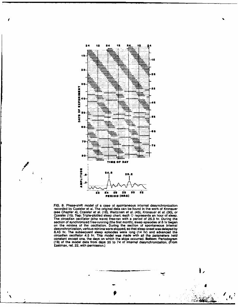
_ I
14 12 24 12 4 1 4
-:::w oo: ----------:: .. ..oo .. .. .
:::: ;:::: - 1::.o ..
---- -- - ---::: .::: ;;; ; -:: --- 0 ....
20 ------ O 000000-0--0-----
20 - ~ 0 0000 ------ 00- o. -- --- 00
........... 0.- - - -------
000000 ---- -------- 0- o
00000 ........... ,00 -- -: 0 - 000 , ----o --:0- - ...- -,- -o 0- -00000IN . 00000 ------- o ----- --- 0 -000---3
00000 00000000 .. ....
-, o oo _ .--- -- --- -- ---- -- -:--- . . ._o. . ... ........... .. . .- Go - . .... ... .
00 -oo 0000-- ------............. 4o
o ~ ~ G w-om ---------------_- ....... --... . ---- -- -- G - o. o , - ---. -.. . .... --o-...
Go --- ------ -G G
.... .. --- -- -- -. . ----- ..... -----. ' ... -- ' ......
--- 000 00 0 ------- -- 0 000 0
---000 0 0000o
------------ -F--- --as---h-ft ---- of - "'o
recoded yCei re l.Tho ri data -- - - f d in te w k o
------t 00000 Go,, W -----(-- K on
Cze r --------------- Top TripGo-plotted -le - r ------- L ----- G- = - o f
TI ---------e G D A o f --- h D
s- of ---- -----on --- minim a of the G1 ------
EastmanDo ref -2 wihpriso.
'3-
U.,/
- - 0 ----- _
- "w "' - -------- ---- --S ---0 - 33- E IO - ------- -1 G ------
FIG.~~~~~~~~~~~~~ -.-ae----mdlofacseo- potnou-nera-esnhonztorecorded~~~~~~~~~~~~--- by--i-ret-.Th-rgia-at-anb-oudi-tewrk--roae(see ~ ~ ~ ------ Chate 4),------ ..lse eta.(6,.et.neta.(5, .r.ure a.(0,ozeisler (15. Top: -Tripl-lte sleep------ chart-- eah0 -ereetsa- hu-o-lepThe circadian ~ ------- oscllto ------ wave) fe - - iha- eido-2 . r D rn hsection~~~8 of sycroie free--runn (tefis-onhsle-pioe-o- rea
on the minima of th oscillation. Durin th sci- ofsotnosItradesynchronlzation, *"w variou miim-wr-siped-o-ha-sep-nst-a-dlaedb
24.629.2
IL,

92 ARE SEPARATE OSCILLATORS NECESSARY?
models produced thus far are crude representations of a few individual patternsof spontaneous internal desynchronization. If this line of modeling were to bepursued, several refinements could be made. For example, the model might beimproved by changing the constant masking factor of sleeping and waking ontemperature to one that varies with the phase of the circadian cycle (33). Foreach specific model developed thus far, all the misplaced sleep episodes havestarted at exactly the same phase. More realistically, the phase of the misplacedsleep episodes for any individual subject probably varies somewhat. Phase-shiftmodels can be made to mimic more complex patterns of internal desynchroni-zation in which clear phase jumps or clusters are not seen. For example, thephase-shift model for one subject (not shown) consisted of two misplaced sleepepisodes in a row, which appeared fairly regularly within a string of normallyplaced sleep episodes. Some subjects sleep, or at least take a nap, on almostevery minimum, but in addition have some misplaced sleep episodes. Phase-shift models of these subjects would produce the extremely short periodsbetween about 15 and 20 hr (Fig. 2).
The phase-shift model of internal desynchronization proposes a feedbackshift from the activity rhythm to the circadian oscillator. This feedback shift wasincluded not because of any direct evidence or preconceived notion thatfeedback should occur but merely because the shift was necessary to make thecomputer simulations match the empirical data. In the model, only themisplaced sleep episodes produce feedback, not the normally placed episodesthat start near the minimum of the temperature cycle. If feedback from theactivity rhythm to the circadian oscillator really exists, then it should occur inother situations, besides internal desynchronization, in which sleep does not
1 occur near the minimum. Therefore, during entrainment to the 24-hr day,feedback should occur, because sleep begins about 900 before the temperatureminimum (Fig. 7, middle) (47,49). It appears that the circadian oscillator isshifted during entrainment to the 24-hr day. There must be an advance shift ofabout 1 hr per day, because the average free-running period is about 25 hr. Thisadvance could be due to feedback from the activity rhythm. Perhaps thisplacement of sleep several hours before the minimum helps advance theoscillator by the amount necessary for entrainment. In other words, one of thefunctions of sleep may be to help entrain the circadian oscillator. Alternatively,the perception of light on awakening may be the important factor in entrain-ment. During prolonged sleep deprivation there is a slight delay of circadianrhythms such as the temperature rhythm (5,6,49). These delays may result fromthe lack of normal sleep episodes, or normally timed awakenings, which couldadvance the circadian oscillator.
The phase-shift model for each subject was made by choosing severalparameters based on a careful scrutiny of the subject's data and a trial-and-errorprocess to better approximate the individual's pattern of deaynchronization.Two of these parameters were the phase of the misplaced sleep episodes and theamount the circadian oscillator was shifted. A graph relating these two
4
IpI I~n .. H•n"";

ARE SEPARATE OSCILLATORS NECESSARY? 93
FREERUN
S
24 HRDAY
26 2/3 HR
FIG. 7. Diagram of phase relationships during synchronized free runs (top), entrain-ment to a 24-hr day (middle), and entrainment to a 26%h-hr day (bottom). The sinewave represents the temperature rhythm (T). The square wave represents the rhythmof sleeping (S) and waking (W). The shaded area represents the dark portion of theLD cycle. The dotted line emphasizes the phase at which the sleep episodes begin.The free-run diagram (top) is made from the average of many subjects, as shown byWever (ref. 49, Fig. 17). The 24- and 26%-hr diagrams are redrawn from the data of asingle subject isolated in an underground bunker. He was exposed to an overheadLD cycle with twilights and periodic gongs and could use reading lamps during thedark phase [subject 72a in Aschoff et al. (8); also known as subject S.R. in Wever (ref.49, Fig. 69)]. This subject's data can also be seen in the work of Aschoff and Wever(ref. 10, Fig. 78) and Kronauer (ref. 30, Fig. 108). Other subjects show similarchanges in internal phase relationships (8).
parameters from a few specific phase-shift models and the case of normalentrainment to the 24-hr day showed that the amount of shift appeared to berelated to the phase of the misplaced sleep episode. In principle, it should bepossible to generate a full phase response curve (PRC) using a large sample ofphase-shift models of desynchronized subjects. In other words, the shifts of the
. p. I

94 ARE SEPARATE OSCILLATORS NECESSARY?
circadian oscillator might be shown to vary in magnitude and direction(advances or delays) depending on the phase of the sleep episodes, or of theawakening light.
The phase-shift model was the first to demonstrate that there are alternativesto the traditional model of spontaneous internal desynchronization. Thestrategy has been to show that the most typical, most publicized, individualcases of spontaneous internal desynchronization can be mimicked with a single-oscillator model. In the phase-shift model there are several determinants of theovert circadian rhythms, including the circadian oscillator, masking, "volun-tary" behavior (behavior that cannot be predicted in these experiments), and aprocess of sleep need and recovery. However, the sleep-need-and-recoveryfactor was invoked in only the most rudimentary fashion. Daan and Beersma(this volume) have developed a more sophisticated single-oscillator model thatincludes a precise description of a sleep-need-and-recovery function based onBorbely's model (11). In contrast to the activity oscillator of the traditionalmodel, this cycle of sleep need and recovery is a relaxation process. It is notcontrolled by a true self-sustained, fixed-period oscillator. In the moreconventional style of modeling, a set of general solutions was produced byvarying one parameter at a time. Their model can account fairly well for a widerange of human circadian phenomena. Feedback from the activity rhythm to thecircadian oscillator was not included.
Earlier versions of the phase-shift model (20-22) proposed that a secondshift-inducing oscillator, either internal or external to the subject, might beinvoked to explain cases of internal desynchronization in which the misplaced
* sleep episodes occurred regularly (Fig. 1). There was no reason to postulate asecond oscillator in cases with irregular patterns (Fig. 6). Daan and Beersma(this volume) have shown that regularly misplaced sleep episodes can arisefrom a single oscillator plus a cycle of sleep need and recovery. Theirdemonstration shows that there is little need for a shift-inducing oscillator.
In the phase-shift model, spontaneous internal desynchronization occurswhen the subject ignores the signal from the circadian oscillator and does not goto sleep near the minimum. We might ask why some individuals becomedesynchronized while others do not, or, if all subjects eventually desynchronize,why some subjects become desynchronized before others. One possibility mightbe that some subjects become highly motivated to stay awake, for example, tocontinue work on some important project, and thus tend to ignore the internalsignals to go to sleep. Another possibility is that some individuals have weakercircadian oscillators that produce oscillations of smaller amplitude, so that theytend to misjudge the right time for sleep. Daan and Beersma (this volume)include amplitude changes as an important part of their model. By graduallydecreasing the amplitude of the circadian oscillation, they show how synchro-nized free running can abruptly change to internal desynchronization and that atthe extreme a very small amplitude can produce a bicircadian pattern. This typeof progressive change from synchronization to desynchronization to a bicir-
V
-- N t Sa l .lllmllll Il ll4

ARE SEPARATE OSCILLATORS NECESSARY? 95
cadian pattern was first described by Czeisler (15). In the phase-shift model thischange occurs when the minimum is skipped more and more frequently. InKronauer's model (this volume; and 30) this change is accounted for by agradual lengthening in the period of the activity oscillator. In Daan andBeersma's model, a gradual decrease in amplitude can account for the changingpattern of desynchronization. Daan and Beersma have also pointed out that theamplitude of circadian rhythms free-running in constant conditions is typicallylower than during entrainment. This can explain why desynchronization occursmore frequently in constant conditions than in normal life.
The phase-shift model of spontaneous internal desynchronization does notrefute the traditional model; it is merely offered as an alternative. Hopefully,some tests or experimental manipulations will be designed to distinguishbetween the two models. Meanwhile, there is one component of the phase-shiftmodel that can be tested, the feedback shift from the activity rhythm to thecircadian oscillator. Temporally isolated subjects showing synchronized free-running rhythms could be instructed to sleep at various phases of theirtemperature cycle, and the resulting course of the free run could be determined.In other words, misplaced sleep episodes could be experimentally produced todetermine if they shift the circadian oscillator. This would be the equivalent ofgenerating a PRC. The phase-shift model is a crude first step in the developmentof alternative models of internal desynchronization. Even if many of itspropositions become obsolete, at least it has served to remind us that thetraditional model is still open to question, and it has prompted the developmentof other single-oscillator models (S. Daan and D. Beersma, this volume).
CHANGES IN INTERNAL PHASE RELATIONSHIPSBETWEEN FREE RUNNING AND ENTRAINMENT
Although spontaneous internal desynchronization has been considered thebest evidence for the theory of separate temperature and activity oscillators,other observations of human circadian rhythms have often been cited as furthersupport for the traditional theory. These observations include the internal phaserelationships between the temperature and activity rhythms-how these changebetween synchronized free runs, entrainment to the 24-hr day, and entrainmentto Zeitgebers of other periods (8-10,47,49). Figure 7 schematically shows thephase relationships between the temperature and activity rhythms during threeconditions. As discussed earlier, during synchronized free runs (top diagram),sleep begins around the minimum of the temperature cycle, whereas duringentrainment to the 24-hr day (middle diagram), sleep begins about 900 beforethe minimum. The traditional model can easily account for this change in theinternal phase relationships. According to the model, the temperature andactivity oscillators are mutually synchronized during the free-running condition,but they assume different phase relationships to the Zeitgeber during entrain-ment because they have different characteristics (10,49).
4,
p K

96 ARE SEPARATE OSCILLATORS NECESSARY?
The bottom diagram shows that both the temperature and activity rhythmsshow an advanced phase to the LD cycle when entrained to the 26 i-hr day, ascompared with entrainment to the 24-hr day. The maximum of the temperaturerhythm advances from around "lights off" in the 24-hr day to many hours before"lights off" in the 26i-hr day. The activity rhythm also advances. This subject,who is a "night owl" in the 24-hr day, waking up around "noon," becomes an"early bird" in the 26W-hr day, waking at the crack of "dawn." These advancesare predicted by oscillator theory, which states that as the period of theZeitgeber increases, the phase of circadian rhythms advances (3,46). Notice,however, that the temperature rhythm advances more than the activity rhythm.This difference in the amount of advance results in different internal phaserelationships between temperature and activity in the 26%-hr day as comparedwith the 24-hr day. Sleep begins near the minimum of the temperature cycle inthe 265-hr day, whereas it begins about 90 before the minimum in the 24-hrday. Once again, this change in the internal phase relationships can beexplained by the traditional model in which the temperature oscillator advancesmore than the activity oscillator as the Zeitgeber is lengthened, because thetemperature oscillator is stronger (49).
Let us explore one of the ways in which these changes in internal phaserelationships might be explained with a single circadian oscillator. Thesynchronized free-running condition (Fig. 7, top) is easily accounted for by asingle oscillator that drives the temperature rhythm and triggers sleep near itsminimum. Given this mechanism, how can we explain the fact that sleep beginsabout 900 before the temperature minimum during entrainment to the 24-hr day(Fig. 7, middle)? We can assume that the phase of the circadian oscillator andthe rhythms it drives, such as the temperature rhythm, is set by virtue of its
/ entrainment to the 24-hr Zeitgeber. If sleep were to begin at the temperatureminimum, when the subject feels the most sleepy, then sleep would begin toolate; it would begin during the light phase and would occur entirely within thelight phase. This subject is a "night owl"; the phase of his temperature rhythm isdelayed. For other subjects, the temperature minimum occurs somewhat earlier,near the end of the dark period, but sleep triggered at the minimum will stilloccur too late. These late sleep times will not be adaptive ecologically orsocially, in most circumstances.
We can account for the earlier onset of sleep in the 24-hr day by consideringother factors. The subject may go to bed before the minimum because he knowsit has been dark for a long while and believes it is the proper time for sleep. Thiscould be called masking by the LD cycle, or behavior prompted by theknowledge of time. In addition, he has been awake all day, has built up somesleep need, and may feel tired. Finally, his temperature has started to drop; sohe is beginning to feel sleepy. All these factors, circadian rhythm, masking, andsleep need, may contribute to his desire and ability to go to sleep before theminimum. In the 26%-hr day, the circadian oscillator and therefore thetemperature rhythm assume a new entrained phase relationship to the
4,
-, .''!
IP , : v." / ,

ARE SEPARATE OSCILLATORS NECESSARY? 97
Zeitgeber. The temperature minimum occurs shortly after "lights out." At thispoint the subject is the most sleepy, and he knows it is nighttime. All factorsconverge to make it a perfect time for bed. In conclusion, only one oscillator isnecessary to explain these various phase relationships if we assume that otherfactors in addition to the circadian oscillator can influence the scheduling ofsleep and wake in the human.
FORCED INTERNAL DESYNCHRONIZATION
Although internal desynchronization may never occur spontaneously in somesubjects, at least during the time in isolation, it can be reliably forced byZeitgebers with periods near the limits of entrainment. Figure 8 shows a subjectwho was entrained to the 24-hr Zeitgeber, but became desynchronized (asdefined by the presence of more than one period in the activity periodogram)when a 28-hr Zeitgeber was applied. According to the traditional theory, 28 hrwas outside the range of entrainment for the temperature oscillator, so that itfree-ran with a period of 24.8 hr. On the other hand, the activity oscillator had alarger range of entrainment, so that it remained entrained, or relativelyentrained, to the 28-hr Zeitgeber (9,10,48,49).
Once again, let us explore one of the ways these results can be explained witha single circadian oscillator. This oscillator could drive the temperature rhythmand free-run in the 28-hr day because 28 hr is beyond the limit of entrainment.The activity rhythm, on the other hand, could have been partially controlled bythe circadian oscillator and partially influenced directly by the LD cycle. Thedaily chart (Fig. 8) shows that the onsets of activity followed the free-runningtemperature rhythm. On each day, activity started a little before the temperaturemaximum. On the other hand, the onsets of rest did not follow the free-runningrhythm, but tended to occur near the beginning of the dark phase. This isperfectly understandable, because this subject did not have access to readinglamps and had little choice but to go to bed when the overhead lights were off. Inthis view, then, the activity rhythm consists of two components (both of whichappear in the activity periodogram), a free-running component produced by thecircadian oscillator and a masking component due to the LD cycle. Accordingto this single-oscillator theory, the range of entrainment of the activity rhythmwas not larger than the range of entrainment of the temperature rhythm; it onlyappeared to be larger because of masking by the 28-hr LD cycle. In conclusion,only one oscillator is necessary to explain forced internal desynchronization ifwe assume that other factors in addition to the circadian oscillator can influencethe activity rhythm of humans.
CONCLUSIONS
The traditional model of human circadian rhythms, developed over the yearsprimarily by Wever (48,49), can explain many phenomena, including spon-
9if
"p ,• , -,

98 ARE SEPARATE OSCILLATORS NECESSARY?
rime (hours)0 14 28 14 28 14 28 14 28 14 28
24
x r-24.0hr6 r =24;.O0hr
141610
20 r 24. 8 hr .. xx..hr22
24 LA",'- -
28 ..' •m '
JOa." • a.
32
24.0 hr 2 04.0 h,I A
so Activity
so Rectal
0.
Period (hours)
FIG. 8. Top: Daily chart of a subject isolated in an underground bunker and exposedto Zeitgebers consisting of an overhead LD cycle with twilights and periodic gongs.Solid bars, activity. Open bars, rest. Triangles, maxima and minima of the dailytemperature cycle. Shaded areas, dark phase. For the first 8 days the subject wasentrained to a 24-hr Zeitgeber. Then internal desynchronization was forced by a 28-hr Zeitgeber. Notice that this graph is plotted on a 28-hr time axis. Bottom:Periodograms during entrainment to the 24-hr day (A) and during forced internaldesynchronization (8). (From Wever, ref. 49, with permission.)
Af
, -

ARE SEPARATE OSCILLATORS NECESSARY? 99
taneous internal desynchronization, changes in internal phase relationships, andforced internal desynchronization. This theory relies on the concept of anactivity oscillator that can have an extremely long or short free-running periodand is weaker (and therefore has a larger range of entrainment) than thetemperature oscillator. However, we have also seen that the same humancircadian phenomena can also be explained by a single circadian oscillator.Rather than invoking a separate activity oscillator to explain the divergentpattern of activity, the single-oscillator model employs "voluntary" behavior,masking, and sleep need, in addition to the basic circadian oscillation.
In the excitement of unraveling the components of multiple-oscillator systemsin recent years, we may have overestimated the need for multiple oscillators toexplain much of the data. Any apparent dissociations or desynchronizationsbetween rhythms are often ascribed to the uncoupling of component oscillators.We might learn more about circadian rhythms by considering how thesepatterns could be produced while the oscillators of the circadian system functionsynchronously as a single unit.
ACKNOWLEDGMENTS
This work was supported by N.I.M.H. Grant MH-4151 from the NationalInstitutes of Health to Dr. Allan Rechtschaffen and by N.I.M.H. training GrantMH-14651 to the University of Chicago, Department of Psychiatry.
REFERENCES
1. Akerstedt, T., Froberg, J. E., Friberg, Y., and Wetterberg, L. (1979): Melatonin excretion,body temperature and subjective arousal during 64 hours of sleep deprivation. Psycho-neuroendocrinology, 4:219-225.
2. Aschoff. J. (1965): Circadian rhythms in man. Science, 148:1427-1432.3. Aschoff, J. (1965): The phase-angle difference in circadian periodicity. In: Circadian Clocks,
edited by J. Aschoff, pp. 262-276. Elsevier/North Holland, Amsterdam.4. Aschoff, J. (1970): Circadian rhythm of activity and of body temperature. In: Physiological
and Behavioral Temperature Regulation, edited by J. D. Hardy, A. P. Gagge, and J. A. J.Stolwijk, pp. 905-919. Charles C Thomas, Springfield, II.
5. Aschoff, J. (1978): Features of circadian rhythms relevant for the design of shift schedules.Ergonomics, 21:739-754.
6. Aschoff, J. (1981): Circadian rhythms interference with and dependence on work-restschedules. In: The 24 Hour Workday. A Symposium on Variations in Work-Sleep Schedules,edited by L. C. Johnson, D. 1. Tepas, W. P. Colquhoun, and M. J. Colligan, pp. 13-50.National Institute for Occupational Safety and Health, Washington, D.C.
7. Aschof1, J., Gerecke, U., and Wever, R. (1967): Desynchronization of human circadianrhythms. Jpn. J. Physiol., 17:450-457.
8. AschoT, J., Poppel, E., and Wever, R. (1969): Circadian rhythms in men as influenced byartificial light-dark cycles of various periods. Pfluegers Arch., 306:58-70.
9. Aschoff, J., and Wever, R. (1976): Human circadian rhythms: A multioscillatory system. Fed.Prvc., 35:2326-2332.
10. Aschofl, J., and Wever, R. (1981): The circadian system of man. In: Handbook of BehavioralNeurobiology, Vol. 4: Biological Rhythms, edited by J. Aschoff, pp. 311-331. Plenum Press,New York.
... .... .t
' - ,I . .
..... " " " w~ l ,

100 ARE SEPARATE OSCILLATORS NECESSARY?
11. Borbely, A. A. (1980): Sleep: Circadian rhythm versus recovery process. In: FunctionalStates of the Brain: Their Determinants, edited by M. Koukkou, D. Lehmann, and J. Angst.pp. 151-161. Elsevier/North Holland, Amsterdam.
12. Doulos, Z., and Terman, M. (1980): Food availability and daily biological rhythms. Neurosci.Biobehav. Rev., 4:119-131.
13. Bunning, E. (1973): The Physiological Clock. English Universities Press, London.14. Colquhoun, W. P. (1971): Circadian variations in mental efficiency. In: Biological Rhythms
and Human Performance, edited by W. P. Colquhoun, pp. 39-108. Academic Press, NewYork.
15. Czeisler, C. A. (1978): Human circadian physiology: Internal organization of temperature,sleep-wake and neuroendocrine rhythms monitored in an environment free of time cues. Ph.D.dissertation, Stanford University.
16. Czeisler, C. A., Weitzman, E. D., Moore-Ede, M. C., Zimmerman, J. C., and Knauer, R. S.(1980): Human sleep: Its duration and organization depend on its circadian phase. Science,210:1264-1267.
17. Daan, S., and Berde, C. (1978): Two coupled oscillators: Simulations of the circadianpacemaker in mammalian activity rhythms. J. Theoret. Biol., 70:297-313.
18. Davis, F. C., and Menaker, M. (1980): Hamsters through time's window: Temporal structureof hamster locomotor rhythmicity. Am. J. Physiol., 239:R1 49-RI 55.
19. Dorrscheidt, G. J., and Beck, L. (1975): Advanced methods for evaluating characteristicparameters (ra,p) of circadian rhythms. J. Math. Biol., 2:107-121.
20. Eastman, C. 1. (1980): Circadian rhythms of temperature, waking, and activity in the rat:Dissociations, desynchronizations, and disintegrations. Ph.D. dissertation, University ofChicago.
21. Eastman, C. 1. (1981): Circadian rhythms of rats at the limits of entrainment and a phase-shiftmodel of "spontaneous internal desynchronization" in humans. In: Sleep 1980, 5th EuropeanCongress on Sleep Research, edited by W. P. Koella, pp. 59-64. S. Karger, Basel.
22. Eastman, C. I. (1982): The phase-shift model of spontaneous internal desynchronization inhumans. In: Vertebrate Circadian Systems: Structure and Physiology, edited by J. Aschoff, S.Daan, and G. Groos, pp. 262-267. Springer-Verlag, New York.
23. Enright, J. T. ( 1980): Temporal precision in circadian systems: A reliable neuronal clock fromunreliable components? Science, 209:1542-1544.
24. Enright, J. T. (1980): The Timing of Sleep and Wakefulness. Springer-Verlag, New York./ 25. Gillberg, M., and Akerstedt, T. (1981): Possible measures of "sleepiness" for the evaluation ofdisturbed and displaced sleep. In: Night and Shift Work: Biological and Social Aspects,edited by A. Reinberg, pp. 155-160. Pergamon Press, London.
26. Hardeland, R., Hohmann, D., and Rensing, L. (1973): The rhythmic organization of rodentliver: A review. . Interdiscip. Cycle Res., 4:89-118.
27. Jouvet, M., Mouret, J., Chouvet, G., and Siffre, M. (1974): Toward a 48 hour day:Experimental bicircadian rhythm in man. In: The Neuroscience Third Study Program, editedby F. 0. Schmitt and F. G. Worden, pp. 491-497. M.I.T. Press, Cambridge.
28. Kawato, M., and Suziki, R. ( 1980): Two coupled neural oscillators as a model of the circadianpacemaker. J. Theor. Biol., 86:547-575.
29. Kleitman, N. (1963): Sleep and Wakefulness. University of Chicago Press, Chicago.30. Kronauer, R. E., Czeisler, C. A., Pilato, S. F., Moore-Ede, M. C., and Weitzman, E. D.
(1982): Mathematical model of the human circadian system with two interacting oscillators.Am. J. Physiol., 242:R3-R17.
31. Mills, J. N. (1973): Transmission processes between clock and manifestations. In: BiologicalAspects of Circadian Rhythms, edited by J. N. Mills, pp. 27-83. Plenum Press, New York.
32. Mills, J. N., Minors, D. S., and Waterhouse, J. M. (1974): The circadian rhythms of humansubjects without timepieces or indication of the alteration of day and night. J. Physiol.,240:567-594.
33. Mills, J. N., Minors, D. S., and Waterhouse, J. M. (1978): The effect of sleep upon humancircadian rhythms. Chronobiologia, 5:14-27.
34. Moore-Ede, M. C., and Sulzman, F. M. (1981): Internal temporal order. In: Handbook ofBehavioral Neurobiology, Vol. 4, Biological Rhythms, edited by J. Aschoff, pp. 215-241.Plenum Press, New York.
w-

ARE SEPARATE OSCILLATORS NECESSARY? 101
35. Pavlidis. T. (1969): Populations of interacting oscillations and circadian rhythms. J. Theor.Biol., 22:418-436.
36. Pavlidis, T. (1973): Biological Oscillators: Their Mathematical Analysis. Academic Press,New York.
37. Pittendrigh, C. S., and Daan, S. (1976): A functional analysis of circadian pacemakers innocturnal rodents. V. Pacemaker structure: A clock for all seasons. J. Comp. Physiol.,106:333-355.
38. Rusak, B. (1979): Neural mechanisms for entrainment and generation of mammalian circadianrhythms. Fed. Proc., 38:2589-2595.
39. Shiotsuka, R., Jovonovich, J., and Jovonovich, J. A. ( 1974): In vitro data on drug sensitivity:Circadian and ultradian corticosterone rhythms in adrenal organ cultures. In: Chrono-biological Aspects of Endocrinology. edited by J. Aschoff, F. Ceresa, and F. Halberg, pp.255-267. Schaffauer-Verlag, New York.
40. Sulzman, F. M., Fuller, C. A., and Moore-Ede, M. C. (1977): Spontaneous internaldesynchronization of circadian rhythms in the squirrel monkey. Comp. Biochem. Physiol.,58A:63-67.
41. Sulzman, F. M., Fuller, C. A., and Moore-Ede, M. C. (1979): Tonic effects of light on thecircadian system of the squirrel monkey. J. Comp. Physiol., 129:43-50.
42. Takahashi, J. S., and Menaker, M. (1979): Physiology of avian circadian pacemakers. Fed.Proc., 38:2583-2588.
43. Tharp, G. D., and Folk, G. E., Jr. (1964): Rhythmic changes in rate of the mammalian heartand heart cells during prolonged isolation. Comp. Biochem. Physiol., 14:255-273.
44. Webb, W. B., and Agnew, H. W. (1974): Sleep and waking in a time free environment.Aerospace Med., 45:617-622.
45. Weitzman, E. D., Czeisler, C. A., and Moore-Ede, M. C. (1979): Sleep-wake, neuro-endocrine and body temperature circadian rhythms under entrained and non-entrained (free-running) conditions in man. In: Biological Rhythms and Their Central Mechanism, edited byM. Suda, 0. Hayaishi, and H. Nakagawa, pp. 199-227. Elsevier/North Holland, Amsterdam.
46. Wever, R. (1965): A mathematical model for circadian rhythms. In: Circadian Clockv, editedby J. Aschoff, pp. 47-63. Elsevier/North Holland, Amsterdam.
47. Wever, R. (1972): Mutual relations between different physiological functions in circadianrhythms in man. J. Interdiscip. Cycle Res., 3:253-265.
48. Wever, R. (1975): The circadian multi-oscillator system of man. Int. J. Chronobiol., 3:19-/55.
49. Wever, R. (1979): The Circadian System of Man. Springer-Verlag, New York.50. Winfree, A. T. (1967): Biological rhythms and the behavior of populations of coupled
oscillators. J. Theor. Biol., 16:15-42.51. Winfree, A. T. (1980): The Geometry of Biological Time. Springer-Verlag, New York.52. Zulley, J., and Wever, R. A. (1982): Interaction between the sleep-wake cycle and the rhythms
of rectal temperature. In: Vertebrate Circadian Systems: Structure and Physiology, edited byJ. Aschoff, S. Daan, and G. Groos, pp. 253-261. Springer-Verlag, New York.
53. Zulley, J., Wever, R., and Aschoff, J. (1981): The dependence of onset and duration of sleepon the circadian rhythm of rectal temperature. Pfluegers Arch., 391:314-3 18.
DISCUSSION
Dr. Czeisler: Most of your phase-shift data seem to be based on free-running patternsof human subjects in which there is a reversion after each phase jump to the period seenduring the internally synchronized free run. Have you modeled subjects who consistentlyhave a 30- or 40-hr free-running period?
Dr. Eastman: The more often the subject skips the minimum, the longer the periodsbecome, and you can get all the way up to bicircadian days if you skip every other
..... ! t :
102 ARE SEPARATE OSCILLA TORS NECESSARY?
minimum. There are two patterns of bicircadian days. In one, the subject sleeps on aminimum, skips a minimum, sleeps on a minimum, etc., and you can explain that easilywith this model. Another pattern is when the subject skips a minimum and then goes tosleep a little past the time where the temperature starts to drop, has a very long sleep, andthen skips the next temperature minimum since it has not been that long since he hasbeen up.
Dr. Czeisler: When you model these shifts, do you have to take the original data,program each shift into a computer, and then say, "Now, there is another shift"? If so, itwould then become a question of whether you have a model or whether you are justtelling the computer to reproduce the actual data.
Dr. Eastman: Well, the model predicts that the subject will usually go to sleep on theminimum, and it will soon, I hope, predict how much feedback there is. Of course, if thesubject skips the minimum because of some reason that only he knows (for example, if heis reading a book), we could never predict that. So, of course, I have to copy that from thereal data.
Dr. Czeisler: Dr. Wever said in his talk that he does not like two oscillators becausesix parameters must be defined, but at least those are defined at the beginning, before theprogram is run.
Dr. Eastman: My parameters are all set for the whole model. There is only oneparameter that changes, and that is the day on which there is a shift.
Dr. Czeisler But that is the key thing, the thing that needs to be explained.Dr. Eastman: What if that happens because of the subject's behavior?, You cannot
hope to predict that. That is the cognitive factor that people want to explain.Mr. Pilato: To what extent is the pattern of skipping sleep periods systematic, and
what kind of mechanism would you use to explain it? Does the subject have to countevery 4 days? Is it a sleep-debt system, and is that an oscillator?
Dr. Eastman: Well, I think whatever you have, you have to introduce noise in termsof the subject's behavior. Serge Daan has what I consider to be a beautiful,sophisticated version of my model. [See S. Daan and D. Beersma, this volume. D.Wiza:Itiktepitta btesm oti h ocp fa
unknowable, not unknown, but unknowable, factor. That is, from a scientific point ofview, not acceptable. You rule out the search for causality by saying that the subject justdecided to do some particular action and that is his "behavior."
Dr. Eastman: In my view you have got two things going. You have got an oscillatorwhich induces a tendency to go to sleep at the minimum, but which the subject canignore to a certain extent.
Dr. Czeisler: In our studies we are in frequent contact with the subject and have askedourselves why they stay up late on some nights. The first few times subjects stayed uppast their temperature troughs and remained awake for an extended length of time, wesearched for things that might be keeping the subject awake. Was he trying to finish acrossword puzzle, or was he trying to read a book, as you suggest? The remarkable thingis that in the vast majority of cases they were not working on anything in particular. Theywere not in the middle of a project that was keeping them awake, as we might havethought. We have the subjects on a video monitor, and we can sit there quietly and watchthem. They may prepare lunch or do something else. It is very hard to imagine whilewatching them that something is directly keeping them up.
Dr. Eastman: But is it not true that when they skip sleep they still feel tired when thatminimum comes along?
Dr. Czeisler. Yes, according to their subjective assessments of alertness.
1 r&A4

ARE SEPARATE OSCILLATORS NECESSARY? 103
Dr. Borbely: Dr. Czeisler, do you discourage the subjects from napping?Dr. Czeisler: Yes. As you know, the instructions to the subject were that they could
go to sleep at any time that they desired, but we asked the subjects not to nap. When theychose to go to sleep, we ask that it be for the night.
Dr. Kronauer: I would like to make a mathematical comment. Dr. Eastman, first Iwould like to compliment you on the two-oscillator model that you have introduced usingtwo periodicities. It is an ingenious way to take two periods that are both close tocircadian and end up with one that is quite far removed. But because the one-oscillatormodel involves a skip every 3 or 4 days, you must recognize that what comes out of thatat peak periods in ratios are the ratios of low integers, like 4 to 3. In other words,basically what you are generating is one oscillation with something on top of it which is atype of super subharmonic, and I think that the data simply do not support the fact thatthese desynchronized periods are the ratios of low integers.
Dr. Wever: In one experiment there was a subject in our bunker who was free-runningduring the first 2 weeks and then became synchronized to a 24-hr Zeitgeber. He was thefirst case we ever had of unintended social cues. The Zeitgeber was the female technicianwho was taking out the urine samples and who did not follow our instructions to go to thelocked outer chamber once a day at very irregular intervals, if possible when the subjectwas sleeping. Later on, I found that the technician had fallen a little bit in love with thesubject before the experiment She left some letters in the locked chamber at a regulartime. [Laughter So the subject went into his outer chamber every 10 min until he foundthat his urines were removed, and there on some days was a letter. He was not aware, ofcourse, that his rhythm changed. That was the first case we really had of socialsynchronization.
p
.2 ..

Mathematical Models of the Circadian Sleep-Wake Cycle, edited by MI. C. Moore-Ede andC. A. Czeisler. Raven Press. New York 0 1984.
Modeling Principles for Human Circadian Rhythms
Richard E. Kronauer
Division of Applied Sciences, Harvard University,Cambridge, Massachusetts 02138
The objective of this chapter is to present a review of features of humancircadian rhythms that must affect any attempt to model the human circadiansystem. It is unfortunate but true that direct physiological knowledge of thissystem is so rudimentary as to afford almost no basis for model construction.This means that models are merely mathematical constructs that serve toorganize our view of system performance. One model has an advantage overanother only if it matches more data features or is more economical in form.
ESSENTIAL MODEL COMPLEXITY
Perhaps the most important single experimental observation is that the sleep-wake cycle and the body-temperature rhythm of the free-running human canexhibit two different circadian periods at the same time (1). Furthermore, these/ periods do not appear to be related by any ratio of low integers, so that oneoscillation cannot be supposed to derive from the other by any relatively simplefrequency multiplication/demultiplication scheme. Within the family of modelsdescribed by ordinary differential equations it is possible to generate twoincommensurate oscillk ';ng frequencies with a third-order system (2), but onlywhen special care is exercised. The ordinary third-order system generatesfrequencies that are rationally related. The mathematical distinction betweenthese two situations is that in the former the limit set is a toroidal surface,whereas in the latter the limit set is a line that spirals about the torus andultimately closes in a finite number of cycles. If one wishes to avoidmathematical oddities and still retain the differential equation form, it makessense to advance to the fourth-order system. This also permits a kind of paritybetween the two rhythms in that each can be viewed as originating principally inits own second-order system, while mathematically identifiable mechanismsgenerate interactions between these two subsystems. Thus, whereas a generalfourth-order system is intrinsically more complex than a third-order system, thereduced fourth-order system represented by two coupled second-order systemscan actually be the more economical form. Furthermore, the idea that the fullsystem is a conjunction of two oscillatory subsystems is given physiological
105 P~~
W.-nI

106 MODELING PRINCIPLES
support by studies in which lesions destroying the suprachiasmatic nuclei(SCN) in squirrel monkeys disrupt the rest-activity cycle but leave a persistingbody-temperature rhythm (3). Other experiments in rats have shown that knifecuts in the hypothalamus that isolate the SCN neurally do not abolish circadianrhythmicity within the SCN (4). Thus, the SCN appear to act as a discretepacemaker, but other oscillating centers also exist in the organism. When thesleep-wake cycle and body-temperature rhythm show different circadianperiods, the two subsystems are understood to have lost internal synchrony.
FUNDAMENTAL VARIABLES AND THEIRPHYSIOLOGICAL REPRESENTATIONS
Following the nomenclature introduced earlier (5), we shall refer to xandy asthe fundamental variables of the oscillatory subsystems. In so doing it is notnecessary that the system be describable by differential equations, althoughsome of the evidence to be cited later strongly suggests that such a description isrealistic. When the x and y rhythms display different periods, it is possibkc toidentify these periods in a variety of physiological variables in human subjects.It would be ideal if two readily measurable quantities could be found that woulddirectly represent one or the other of the primary rhythmic variables x and y.Two quantities usually suggested for these roles are core body temperature, T~,and sleep-wake itself (which we shall call the variable SW; SW 1corresponds to sleep, SW = 0 corresponds to wake). From the data it is evidentthat T, and SW each contain a mixture of the two rhythms, but T, is dominatedby the period close to 24 hr (which we call x), whereas SW is dominated by the/ other period (typically 30 hr or more, which we call y).
At this point it is necessary to address a very important functional distinction:intrinsic summation versus output summation. It is the same distinction that isdrawn between feedback and feedforward in control theory. Suppose, forexample, that the x subsystem affects a particular physiological variable such asplasma cortisol. If cortisol then affects the y subsystem, a mechanism isestablished for x to exert a drive onto y, or to couple x and y. Either the cortisolor some other variables can similarly couple y into x. Given the numerousvariables that display strong circadian variation, it would be most surprising ifsignificant coupling of both kinds did not exist in the human circadian timingsystem. Consequently, even within the subsystems there would always be amixture of the two rhythms. Neither x nor y will display a pure periodicity. Themere fact that a physiological variable exhibits both rhythms is no grounds forrejecting that variable as being a possible "perfect" representation of either x ory. On the other hand, a quite different situation can be envisaged. Suppose thatthe coupling (internal feedback) is weak, so that x and y are almost purerhythmic variables (only slightly contaminated). It is possible that somevariable other than x or y can receive strong drives from both subsystems andyet have little effect back on the subsystems. This third variable is in a

MODELING PRINCIPLES 107
feedforward position with respect to x and y. It can also be said to combine orsum the outputs of the subsystems.
Using the foregoing definitions, when the system is internally desyn-chronized, the dominant period in T, is that of x, whereas the dominant period inSW is that of y. The question remains how well T, represents x and SWrepresents y. The previous discussion shows the question to be essentiallyunanswerable unless interventions can be made that either isolate the sub-systems or drastically alter the coupling between them.
The only way this unanswerable question can be approached at present isthrough arguments of plausibility and consistency, based on additional data.Individual subjects are often observed to progress from internal synchrony todesynchrony during prolonged temporal isolation. During synchrony thecomposite rhythm has a period lying between the periods that T, and SW showduring desynchrony, and this period is heavily biased in favor of T,. (6). Theimplication is that the drive of x onto y is much stronger than the drive of y ontox [a ratio of about 4, according to a model of coupled Van der Pol oscillators(5)]. A measure of the overall strength of the interoscillator coupling is affordedby the differences of x and y periods when desynchrony first appears (typicallyan 18% to 30% difference).
Putting these observations together, we are led to expect that the intrinsic yvariable will necessarily contain a significant component with the period of x,while x itself will remain relatively pure. It is therefore highly improbable thatany observed rhythmic variable will have only the y periodicity (unless, by
perverse chance, output summation puts just the correct amount of negativeta x~cnan infcn opnn wt h eididctsotuinto some variable so as to cancel the component of x already within y). Thus,SW becomes a plausible candidate fory itself (insofar as timing is concerned),and some simulations support this hypothesis (5). On the other hand, the factsummation and suggests that T, is not a straightforward indicator of x. Anotherway in which this output summation is characterized is to say that there is acomponent of core temperature that is "evoked" by activity or suppressed by
sep(7). This concept is quite widely accepted, but it is important to note thathidnwithin it is the assumption that the drive from y onto the x subsystem is
not important in this context.
THE CHARACTER OF SYNCHRONY LOSS
A very important feature of human free-run data is that synchrony anddesynchrony are not the only states observed. A condition commonly exists inwhich the SW rhythm has, on average, the same period as the T, rhythm, butSW has large excursions of phase with respect to T, Although some of thesephase variations are undoubtedly random, there are also significant regularcomponents that modulate the phase with periods in the range of 4 to 7 days.This phenomenon is called phase trapping (5). Three examples are shown in

108 MODELING PRINCIPLES
Fig. I. The middle of each sleep episode is marked, and a slightly smoothed lineis drawn through or near these points to emphasize the fundamental regularities.Observe how in each case most of the variations of phase can be accommodatedby this regular modulation. Note that the modulation periods are comparable tothe beat periods between x and y that are observed early in desynchrony (seeFigs 2 and 4A). Phase trapping is often encountered as an intermediate stagebetween synchrony and desynchrony; this suggests that phase trapping anddesynchrony are related and that desynchrony may be the further developmentof a process begun with the initiation of phase trapping. Phase trapping actuallyrepresents the failure of the free-running system to enforce synchrony between xand y, and in this sense phase trapping bears a closer relation to desynchronythan to synchrony.
There is a simple explanation of phase trapping within the context ofquasilinear oscillators that, although specialized, is worth summarizing here,because it may possibly have more universal implications. The explanationbegins with the idea that there is a progressive reduction of the tendency of xand y to synchronize, either because of a reduction in coupling strength orbecause of an increase in the disparity of the oscillatory periods intrinsic to the xand y subsystems. (I shall offer evidence to suggest that it is more likely theincrease in disparity of period that reduces the tendency to synchronize.) Atsome point, synchrony is lost, and the y subsystem begins to develop a smallcomponent at or near it intrinsic period, in addition to the large componentalready imposed on it by x. Further reduction of the tendency to synchronizecauses progressive growth of the intrinsic component, with concomitant growthin the amplitude of phase-trapped modulations. All the while the average periodis that of x, because the imposed x component is still the larger. The transitionto desynchrony occurs when the intrinsic component becomes larger than theimposed component, whereupon the average period of y becomes that of theintrinsic component.
This explanation is extremely economical in terms of modeling. Furthermore,phase trapping appears to be very difficult to explain in any other way. In anyevent, phase trapping is a phenomenon that any credible model must be able toaccommodate. A consequence of this interpretation of the relationship betweenphase trapping and desynchrony is that the transition from the former to thelatter is the result of a minor change in the relative strengths of imposed andintrinsic components. The overt effect of the transition is a dramatic lengtheningof the average period of SW (typically to 30 hr from a previous value of 25 hr),and usually with an exceptionally long subjective day-night cycle at the verybeginning (often 40 hr). It is also possible to imagine that in some subjects thecircadian system might remain poised at or very close to the transition thresholdand under small extraneous influences might cross and recross the transitionboundary. An example of this kind of system behavior is shown in Fig. 2. Thissubject lived in isolation from temporal cues for 170 days at the Laboratory ofHuman Chronophysiology, Montefiore Hospital, New York City. The subject
--. -f-. m ==.= m,=ww w mmmm mm~mmmmmn mm m

ID 0~ 8. 0
0
-00~0 '9 - 0o
0Emm
ID a
0 u
s al
0 cli (D Co
at
_ 0CL
0 o o o 0 ,2 o:o
cl ccai

110 MODELING PRINCIPLES
TIME OF DAY
2 4 12 24 12 24 12 24 12 24
10-
20,
30'
40
60-
70-
so
IL 9
x
U.
FIG. 2. Activity-rest cycle pattern plot: The sleep record of a subject allowed to runfree for 170 days. These data were taken at the Laboratory of Human Chrono-physiology, Montefilore Hospital, New York City, by C. A. Czeisler, J. M. Zimmen,and E. D. Weltzman. Internal desynchronlzation occurs first at day 82, but the subjectreturns from time to time to the phase-trapped state. After day 145, the subjectremains permanently in the state of internal desynchronlzatlon. The average lengthof the activity cycle increases progressively (but not monotonicaly) throughout the6-month study. (From Kronauer et aL, ref. 10, with permission.)
140 ISO,
160170

MODELING PRINCIPLES 111
first became desynchronized on clock day 82 and remained so for 10 days.From day 92 to day 101 there were two phase-trapped modulation cycles,whereupon desynchrony resumed. Phase trapping reappeared between day 119and day 146, with the exception of one cycle of desynchrony centered at day130. After day 146 the subject remained desynchronized for the remainder ofthe experiment.
MODE OF ACTION OF A LIGHT/DARK ZEITGEBER
Further information about the circadian system has been provided byexperiments in which external Zeitgebers have been manipulated. At theMontefiore Hospital facility, an imposed 24-hr light/dark cycle has been foundto be an effective entrainer of SW in humans. In certain experiments of Aschoffand Wever (6), light/dark cycles alone were not effective in entraining SW at avariety of periods. The difference may well be due to the strictness of the light/dark cycle at Montefiore; no auxiliary light could be switched on by the subjectduring the dark (an available option in the relevant Aschoff and Wever cases).At other times, a stronger Zeitgeber protocol was also employed by Aschoff andWever, this included the ringing of bells at intervals of one-eighth of theimposed period and a somewhat stricter observance of "dark." This strongerZeitgeber entrained subject activity from periods as short as 18 hr to periods aslong as 30 hr.
An important question is the mode of action of the light/dark stimulus(designated z) on the circadian system. In particular, does z act directly on oneor both of the x and y subsystems? Because of the physiological evidence ofdirect input to the SCN from the retina via the retinohypothalamic tract inmammals (8), it is highly likely that z acts on the y subsystem. Because y acts onx, the pathway z - y - x provides a two-stage connection from z to x. That is,the intrinsic coupling between y and x transmits the effect of z to x as well as toy. The same can be said of any possible direct action of z on the x subsystem;the action will be felt on y as well.
One of the amply documented (6,7) effects seen on release of a subject from a24-hr entraining Zeitgeber is an adjustment of the relative phase of T and SW:T advances with respect to SW. The extent to which x advances with respect toy cannot be estimated with high accuracy because of the evoked effect of SW onT, but it is probably about 5 hr, typically. The substantial size of this shift (750of phase) is very revealing. The phase relationship observed in free runrepresents the situation where x is effectively controllingy (because the drive ofx onto y is so much stronger than that ofy onto x). Under Zeitgeber action, if zwere to enter the x - y feedback loop predominantly by drive onto x, the phaserelation between x and y would have to be essentially the same as in free run.The large phase shift actually observed shows that z enters the looppredominantly by drive onto y (and perhaps exclusively so).
IP , WI

112 MODELING PRINCIPLES
Substantiation of this view of the way in which z acts on the x - y system isafforded by phase-shift experiments. When subjects are transported acrossseveral time zones, the adjustment of the SW rhythm is effected rapidly (withina day or two). The adjustment of T proceeds much more slowly, seldomattaining a shift rate of I hr per clock day (9). If z were to act directly on x to asignificant degree, the adjustment of T would occur at a rate comparable toSW. In fact, the slow adjustment of T reflects not only the absence ofsignificant z - x drive but also the relative weakness of the y - x drive.
If one makes the conjecture that the "absence of significant z - x drive" isactually the total absence of drive from z to x (when z is a light/dark stimulus),then x is remarkably isolated from z. How then is one to explain the observationthat, under appropriate conditions, such a Zeitgeber can entrain x withoutentraining y [as in Fig. 81 of Wever (6), reproduced here as Fig. 31. Thisapparent paradox has a rational explanation and is also susceptible to modeling,as I shall show later. It is first necessary to point out that such a subject, in theabsence of z, is in desynchrony and that the free-running periods of x and y arevery disparate. Furthermore, the intrinsic period of x is within 1% or 2% of theperiod of the imposed z. Thus, in order for z to entrain x but not y, it is onlynecessary for the component that z induces in y to be insufficient to bridge thelarge disparity in z and y periods yet sufficient to bridge the tiny disparity in zand x periods (despite the large attenuation that component suffers through the
Time (hours)0 12 24 12 24 12 24 12 24 12 24 12 24 12 24
46 "t-25.0 hr : 1
1012
7O
200
FIG. 3. A record of rest (open bars), activity (filled bars), body-temperature maxima(upward-pointing triangles), and temperature minima (downward-pointing triangles)for a subject under a light/dark Zeitgeber influence. (Vertical hatched bars, Zeitgeberdark.) (From Wever, ref. 6, with permission.)
A ..
S 4l l.Il 1 1 li~

MODEL ING PRINCIPLES 113
weak y - x drive). In fact, there must always be a small band of disparitiesbetween the z and x periods for which such an entrainment will be found,regardless of whether or not y is entrained.
The converse situation to the one just described, where z entrains y but not x,hardly needs comment. All that is required is for the z and x periods to besufficiently disparate that the combined effects of z and y (now both having theperiod of z) felt through the y - x coupling be insufficient to enforce synchronyof x. What is perhaps less obvious is that in either situation, where only one ofthe two subsystems is entrained to z, the entrainment of that subsystem isimperfect. Because the nonentrained subsystem possesses an average perioddifferent from that of z, and because the two subsystems are mutually coupled, itis inescapable that the entrained subsystem will contain a component havingthat different period. The component will be small, but nevertheless it willmodulate the entrained variable so as to give the appearance of phase trappingwith respect to z, rather than perfect synchrony with z.
Finally, two other situations can arise under the action of z. In one of thesesituations, x and), can proceed with the same average period, but it is a periodthat is different from that of z. (This is the case of a subject whose free-runningstate is either synchrony or phase trapping and for which the Zeitgeber either isvery weak or has a large period disparity with the x -~ y composite.) In the othersituation, x, y, and z all exhibit different periods. In either of these two situationsthere will be phase modulations of both x and y.
/ AN EXEMPLARY MODEL
My colleagues and I have presented elsewhere (5, 10) a mathematical modelthat incorporates all of the performance features described. A brief summarywill be given here, but for full details the earlier presentations should beconsulted. Each of the x and y subsystems is represented by a Van der Poloscillator, and the mutual coupling is represented by a single linear term in eachoscillator. The Zeitgeber, z, is presumed to act on y alone. In nondimensionalform, the model differential equations are
k29 + kA,(- I + X2).j + w,2x + ~ -
(k 7r/1~2)
k'y + kL(- I + y') + &'y + F.,ki = ,.
As written, the intrinsic oscillator frequencies W,~ and w , assume values of unityif the corresponding periods are 24 hr. Periods longer than 24 hr are representedby w,~ or wy less than unity. The reasons for the particular form chosen for themutual coupling will not be reviewed here, except to note that this form gives acompromise period for the two oscillators, when they synchronize, that liesbetween the intrinsic periods of the separate oscillators.

114 MODELING PRINCIPLES
Parameter values that give good agreement with observed system perfor-mance are
f,> = -0. 16, Fyx = -0.04, fLtx = O. 1, jt y = O. 1,
tx = 0.985, 0.95 > w., > 0.5
Because both y, and p.. are much less than unity, the individual oscillators areof the quasilinear type (their limit cycles are almost circular, and theirwaveforms are almost pure sinusoids). For each, the transient adjustment inamplitude after an impulsive disturbance is relatively slow (approximately 10radians or 2 cycles as the adjustment time constant). The ratio of the mutualcoupling coefficients is 4, giving x a large dominance over y. Consequently, it isthe absolute size of F,y that establishes the range of frequency disparity,to. - wo, for which synchrony can be found. Approximately, whena - .I >I F, I, phase trapping or desynchrony will be encountered. The
intrinsic period assigned to the x oscillator is slightly over 24 hr (24,36); phasetrapping is found when the period of the y oscillator (r,,) exceeds 27.7 hr, anddesynchrony occurs when r,. is more than 29.3 hr.
As discussed elsewhere (5), studies of subjects in extended free run haveshown that once desynchronization occurs, there is often a progressivelengthening of the period of SW. Figure 2 is a case in point: Between day 80 andday 140 the desynchronized sections show r. in the range 30 to 35 hr, whereasafter day 140 the r, lie in the range 32 to 49 hr. The lengthening of -r.t iscertainly not monotonic, but the overall trend is unmistakable. I postulate that asubject who displays internal synchrony when released into free run and thensubsequently displays phase trapping and desynchrony does so because w, isprogressively decreasing during these events. Other subjects who go directlyinto phase trapping or desynchrony on release presumably do so because Wy isalready sufficiently small when free run is begun. I have found that free-runrecords generally can be well simulated by our model while holding allparameters other than w,. fixed throughout. I am consequently led to postulatethat, for unexplained reasons, w, is a very labile parameter, whereas all theother system parameters are very stable over the time course of an experiment.Figure 4 shows a comparison, taken from an earlier study (5), between anextended free-run experiment and a model simulation in which W, was made todecline steadily while all other parameters remained fixed. There is reasonablequalitative agreement. In Fig. 4B (and in Figs. 7, 8, and 9), the sleep episodes(solid bars) correspond to the central two-thirds of the times when y is belowzero, and the stippling corresponds to the times when x is below zero. Becauseof the evoked effects of SW on T (as yet inadequately understood), theepisodes where T is below its mean should occupy some intermediate positionwithin the stippled band and the sleep bars, presumably favoring the stippledportion.
Computer simulations reported earlier (5) show that there are relatively
A'p.. . .. .. 
.0 00 C) L 0
EMA
co E: E~
4- 'U 0
0 Cw0Al M
*15
1 a0 g0.0
N 0 0 0 0 0 0 0
CIDer C-i qt 0go 6E too,
oo- a. ms)
2~ WE0
.0
'ED S5 3 2
.2 ,0 .- N
- --6'5
=- a
-O -0
I.--
.. 0..
0c 0
IN3V4W3dX3 .40 SkVa 0
0.8 C
.q.. a

116 MODELING PRINCIPLES
stringent limitations on model parameters for phase trapping to exist. Inaddition to the frequency disparity, w, - wt,, having to be sufficiently large (butnot too large, or desynchrony will occur), there are two other importantconditions. First, ply must be quite small (less than 0.2 approximately), and,second, the drive from x - y must be considerably larger than the drive fromy - x. Both of these conditions obtain in the normal human circadian system,and it is especially interesting to note that the meeting of these conditions can bededuced from evidence that has nothing to do with the existence of phasetrapping itself. The fact that p, is approximately 0. 1 can be estimated from thetime course of the internal phase adjustment that is seen on release from z. Themuch larger x -, y drive than y -- x drive is evidenced by the strong bias of thesynchronized compromise period in favor of the intrinsic x period.
THE MODEL WITH PERIODIC ZEITGEBER EXCITATION
The inclusion of Zeitgeber drive presents the modeler with two fundamentalquestions: Is the waveform of z important? What amplitude of drive should bechosen to simulate the relatively weak or relatively strong light/dark stimulidescribed earlier? If z is periodic in the circadian range, and if the parameters ofthe model are in the normal range (close to those listed earlier), the waveform ofz appears to be irrelevant for phenomena that involve two or more circadiancycles. Different waveforms are approximately equal in their effects, providedthe fundamental Fourier component (i.e., the circadian component) is the samein the two waveforms. The reason is that the y subsystem is a quasilinearoscillator and acts like a resonant filter. Only the z component in that resonantrange has any significant influence on y. Consequently, it is possible to use thesimple functional form
z Fzy cos(kwt + Oz)
in entrainment studies. For acute phenomena, such as determining the length ofrebound sleep after a specific sleep-deprivation episode, a more detaileddescription of z may be required.
How large the influence coefficient, Fy, should be to represent weak orstrong Zeitgebers can be estimated by choosing values that produce in thesimulation entrainment limits that match observed limits. The strong Zeitgeberof Aschoff and Wever (6), for which entrainment of SW in the period range 20to 30 hr has been demonstrated, requires Fy to be approximately 2. At the otherend of the range, a Zeitgeber that fails to entrain SW to an imposed 24-hr periodwhen the intrinsic wy is 0.85 (a period of 28.5 hr) corresponds to F, of about0.7. The entrainment of y also depends on the value assigned to to, and theforegoing estimates are based on w, = 0.985.
I have undertaken a study of entrainment limits for a fixed Fy in which eachof w,,, toy, and o, take on a wide range of values relevant to experimental

MODELING PRINCIPLES 117
conditions. All the other system parameters are held fixed at the valuesdescribed earlier. Ostensibly, such a study involves three system parametersand is consequently very laborious. However, mathematical arguments (whichwill not be expounded here) show that the performance of the system (includingentrainment limits) can be characterized with reasonable accuracy in terms offrequency differences alone. For these I have chosen ao, - W, and W, - W,.Furthermore, the mathematics show that changing the signs of both frequencydifferences (but preserving their magnitudes) leads to the same systemperformance (except for an inversion of the phase relationships with z).Consequently, the study for either one of the frequency differences can berestricted to only its positive or negative values. I have therefore chosen W,. -to have only negative values (the conventional situation), and wx - w isassigned both positive and negative values.
The results of the study for a weak Zeitgeber (F,: = 0.7) are shown in Fig. 5.The contours in this entrainment diagram represent the values of frequencydifferences at which changes occur in the character of the system response tothe imposed Zeitgeber. The areas of the diagram demarcated by the contourscorrespond to specific types of system responses and are designated by lettersymbols. The meanings of these symbols are as follows:
WY- WZ
S
-08 -06 -04 02 -0 02 04 06
PPy'
-2pP
2
N S 4
FIG. 5. The entrainment diagram for a system of two interacting Van der Poloscillators with a sinusoidal Zeitgeber acting on y alone. The lettered symbols areexplained in the text. Zeitgeber strength is 0.7.
, • "
, -. ' I"-' : q
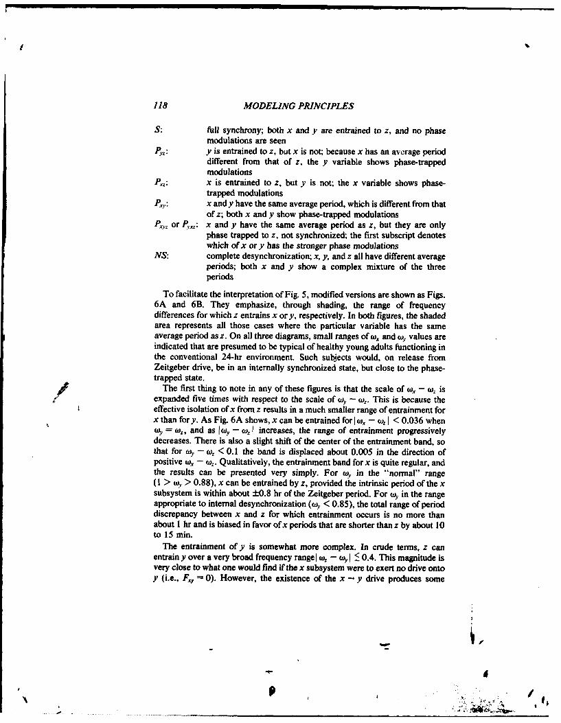
118 MODELING PRINCIPLES
S: full synchrony; both x and y are entrained to z, and no phasemodulations are seen
Py,: y is entrained to z, but x is not; because x has an average perioddifferent from that of z, the y variable shows phase-trappedmodulations
P"z: x is entrained to z, but y is not; the x variable shows phase-trapped modulations
P,': x and y have the same average period, which is different from thatof z; both x and y show phase-trapped modulations
P,, or .x: x and y have the same average period as z, but they are onlyphase trapped to z, not synchronized; the first subscript denoteswhich of x or y has the stronger phase modulations
NS: complete desynchronization; x, y, and z all have different averageperiods; both x and y show a complex mixture of the threeperiods
To facilitate the interpretation of Fig. 5, modified versions are shown as Figs.6A and 6B. They emphasize, through shading, the range of frequencydifferences for which z entrains x or y, respectively. In both figures, the shadedarea represents all those cases where the particular variable has the sameaverage period as z. On all three diagrams, small ranges of ox and wy values areindicated that are presumed to be typical of healthy young adults functioning inthe conventional 24-hr environment. Such subjects would, on release fromZeitgeber drive, be in an internally synchronized state, but close to the phase-trapped state.
The first thing to note in any of these figures is that the scale of w, - w, isexpanded five times with respect to the scale of woy - co. This is because theeffective isolation of x from z results in a much smaller range of entrainment forx than for y. As Fig. 6A shows, x can be entrained for I W, - Io, < 0.036 wheny = w, and as I wy - w I increases, the range of entrainment progressively
decreases. There is also a slight shift of the center of the entrainment band, sothat for toy - to, < 0. 1 the band is displaced about 0.005 in the direction ofpositive (p, - w,. Qualitatively, the entrainment band for x is quite regular, andthe results can be presented very simply. For wy in the "normal" range(1 w,, > 0.88), x can be entrained by z, provided the intrinsic period of the xsubsystem is within about ±0.8 hr of the Zeitgeber period. For w,, in the rangeappropriate to internal desynchronization (, < 0.85), the total range of perioddiscrepancy between x and z for which entrainment occurs is no more thanabout 1 hr and is biased in favor of x periods that are shorter than z by about 10to 15 min.
The entrainment of y is somewhat more complex. In crude terms, z canentrain y over a very broad frequency range I w, - (0),I 1 0.4. This magnitude isvery close to what one would find if the x subsystem were to exert no drive ontoy (i.e., Fy 0). However, the existence of the x -. y drive produces some
-p 4

'tV
do
E
C4 4Z
LO
I E
w1 eCL k
--- _ ~ c
mE
CLC

~1
120 MODELING PRINCIPLES
marked differences from such a simple picture. In the region where x isentrained by z and w, - wo < 0 there is a marked reduction in the ability of z toentrain y (this is represented by the tongue-shaped region labeled p). Thisreduction is due to opposition between the x - y drive and the direct z - ydrive. The other marked effect of the x - y drive is the creation of the P,,regions. In these regions, y prefers to be entrained to x (i.e., phase trapped to x)rather than entrained to z. Interestingly, these regions do not correspond to thecondition w. = w, as might have been supposed, but are displaced from thislocus in the direction of larger I w. - w, I. In fact, the existence of these P,.,.regions must be counted one of the least easily explained phenomena of this not-too-complicated system. What is particularly surprising is that at any fixedw, -(wz < 0.042, as w.- wz is progressively decreased below zero, the ysubsystem prefers first to be linked with z, then to be linked with x, and thenagain linked with z before, finally, desynchrony occurs. Because the progressivedetuning between y and z (i.e., increase in I wy. - w, I) is accompanied by anequal progressive detuning between y and x (increase in I o, - ), it is not atall obvious why the y entrainment preference should alternate in this way.
Probably the most remarkable result displayed in this entrainment diagram isthe existence of the extensive P,, regime, where the failure of y to be entrainedoccurs for values of wy - w that are well within entrainment limits if the x - ydrive is absent. The x subsystem is actively suppressing y entrainment, while atthe same time x itself is entrained. What is also very interesting is that thisremarkable situation occurs for values of the frequency differences that are notfar from "typical" values. Suppose the "typical" subject were to be releasedinto free run and his wy were then to decrease secularly, so as to bring aboutinternal desynchrony. Such a subject would then have exactly the proper w, andw,. values to exhibit P. when a relatively weak 24-hr light/dark cycle is
reinstated.Between the P, regime and the S regime the entrainment diagram shows a
narrow band of Py,,. There is an analogy between this and the free-run situationwhere the phenomenon of phase trapping is interposed between synchrony anddesynchrony. Here, as y is breaking away from the xz alliance, there is a band inwhich y is phase-trapped to xz before the complete break occurs.
It is instructive to see the actual forms that the computer simulations take forvarious cases of partial entrainment. Figures 7A and 7B show examples of P,and Py), respectively. In both of these simulations the period of the Zeitgeberwas maintained at 24 hr (w.. = 1), and the appropriate frequency differences,wx - wz and wy - w, were achieved by adjusting w and wy. Consequently, w,,is below what I would consider the normal physiological range (which is a verysmall range). The simulations could alternatively be taken to represent a normalsubject exposed to a Zeitgeber of period less than 24 hr (approximately 23 hr),for which the plotting has been made with respect to the 23-hr reference. TheZeitgeber is a cosine function of amplitude 0.7, with its positive maximumoccurring in the center of each time band. Thus, it is convenient to think of the
t .q-.

MODELING PRINCIPLES 121
Time of Day (hrs)
24 24 24Day 0 AI?20.'i
30 -FIG. 7. A: A simulation demonstrating Pyz.-For this example, wz = 1.0, wx = 0.98, and
40 w = 0.77. The Zeitgeber is sinusoidal, withstrength 0.7, and acts on y only. The center ofeach band corresponds to the time when z
50 has a positive maximum. Plotting conventionas in Fig. 4B. B: A simulation demonstrating
60- Pvx For this example, *' = 1.0, ct = 0.94,and (a. = 0.85. Except for o and 0y, every-thing is as in A. Plotting convention as in Fig.
DayB 4B.
fo
30X
center of each band as representing "dawn," or the principal awakeningstimulus.
Consider PiT first (Fig. 7A). Here x displays its intrinsic period (which islonger than the period of z), although there are significant modulations of itsphase drift. The regions ofx below the mean tend to drift more slowly at thephase position in which they occur shortly after "dawn." Sleep generally occursin approximately the normal relation to the "dawn" stimulus. It can, however,be drawn off to later daily times by the influence of x, when x reaches a phaserelative to sleep that is close to that normally observed in synchrony. It isespecially interesting to note that when the Zeitgeber and x work in concert ony (as for days 0 to 15, fot example), the sleep episodes occur with a smoothregularity. However, when their effects oppose (as for days 16 to 38), theZeitgeber is able to enforce only a phase-trapping constraint on y. This phase-trapping cycle has a period of 4.5 days.
In the example of Py, (Fig. 7B) there are some evident effects of z on x, butmuch less than those seen in Py,, because y is itself no longer following z.
v |I
P . "p. ? ..... Y I1

122 MODELING PRINCIPLES
Although y is following x (on average), the effect of z on y is very strong, andthere is the suggestion that y is periodically almost "captured" by z. Thisoccurs, understandably, when x has drifted to the phase position with respect toz that it assumes for normal entrainment to a 24-hr Zeitgeber. It is at this phasethat x and z act on y in a cooperative way.
Figure 8 shows an example of a system with no mutual entrainmentwhatsoever (NS). For this simulation it is convenient to think of the Zeitgeberas having the normal 24-hr period and the intrinsic period of x as being withinthe normal range (24.5 hr). However, the intrinsic period of y is much longerthan normal (40 hr). This period is one that is seen in some internallydesynchronized free-running subjects, usually after the desynchrony haspersisted for a long time. Thus, the simulation can be thought of as what mightbe found if such a free-running subject were to be expos;d to a relatively weak24-hr Zeitgeber. As in Figs. 7A and 7B, it is clear that when the drift of x bringsits phase, relative to z, to the value it has under ordinary entrained conditions,the action of x together with z makes y appear to be phase-trapped to z (with amodulation cycle of about 3 days). However, as x drifts away from this special
Time of Day (hrs)
24 24 24
Day.
30
40 FIG. 8. A simulation demonstrating NS.For this example, wz = 1.0, w, = 0.98, and5y = 0.63. All other properties and con-ventions as in Fig. 7.
60
70
80
90
100

MODELING PRINCIPLES 123
phase, y breaks loose and exhibits its own intrinsic period. Thus, the NS state ofFig. 8 is readily seen to be similar to Py. of Fig. 7A, except that the ability of zand x to influence y is weaker for Fig. 8 by virtue of the greater disparity of the yand z periods.
To demonstrate the rather unusual system behavior of Pxz, a simulation ischosen (Fig. 9) in which the z period is 24 hr and the intrinsic x period is 24.24hr (a normal value), but the intrinsic period of y is allowed slowly to lengthen,increasing from 28.24 hr to 30 hr over 100 days. At the outset, both x and y areentrained to z in a very conventional set of relative phases. As the y periodlengthens, the phases of both y and x are delayed progressively with respect to"dawn," until at day 23 the model subject does not awaken until about 6 hr after"dawn." But with further increase in the y period, the phase of y advances,while the phase of x is delayed further. Then, because the effect of x on y nowtends to oppose the effect of z on y, y begins to break loose from the combinedinfluences. First, y falls into phase trapping with respect to the xy group (Py,,,and as the phase-trapping amplitude grows, it ultimately develops into a loss ofentrainment for y, (P,,,) This sequence bears a very close resemblance to thesequence of synchrony, phase trapping, and desynchrony seen in free-runningsubjects as the period of y is lengthened (Fig. 4B). Indeed, the loss ofentrainment takes place at ty, = 29.3 hr, which is closely comparable to thevalue at which desynchrony is often seen in free run. There is, however, a veryimportant difference from the free-run situation because of the phase of x. Mid-low x occurs after sleep in the P,,,. regime, whereas it occurs Weore sleep in thefree-run phase trapping. The reason for this reversal, according to the model, isthat it is z that exercises the dominant influence over y in both PX and P.,
whereas in free run there is no z, and y is necessarily under the influence of
Figure 9 illustrates that in P,, the sleep episodes cluster about the middle ofeach 24-hr interval, which is the time of Zeitgeber "dawn" (peak z drive). Thelongest sleep episodes are centered about 12 hr after this. Also, there is a bandof 6-hr width that begins about 14 hr after "dawn" and ends about 4 hr before"dawn," during which no awakening takes place. It is this suppression ofawakening that gives rise to the long sleep episodes. It is very interesting tomake a comparison of this phenomenon with the human example of P", given byWever (ref. 6, Fig. 81, and shown earlier here as Fig. 3). These data suggestthat the subject was never entrained to the Zeitgeber and became internallydesynchronized at day 11, at which point body temperature became entrainedto z. These data also show that there is a time band lying between the hours1900 and 2400 during which no awakening is observed. If "dawn" is taken to bethe time when the lights of the Zeitgeber are turned on, this corresponds to hour0400 in the experiment. The no-awakening band is then seen to extendfrom 15 hr after "dawn" to 4 hr before "dawn," in very good agreement with themodel. The temperature data reported in Fig. 3 give only the times at whichmaxima and minima were observed, and it is very unreliable to ascertain cycle
01

124 MODELING PRINCIPLES
Time of Day (hrs)
24 24 24Day.
10
20
30
FIG. 9. A simulation demonstrating the40 transition sequence: S, P, Pz. For this
example, wz = 1.0, wx = 9 9 , and wz de-creases uniformly from 0.85 to 0.80. All
50 other properties and conventions as inFig. 7.
60
70
8o
90-
100-/phase from such scanty evidence. Bearing in mind this caveat, low temperatureoccurs close to "dawn," whereas the model places mid-low x some 6 hr later.Partial explanation of the discrepancy may lie in the sleep-evoked component ofT. This component has a minimum of evoked T at the time of sleep onset.Because the clustering of sleep episodes occurs centered at "dawn," the sleep-evoked T minimum will generally occur some 4 hr or so ahead of "dawn," andconsequently the minimum of T, accounting for the effects of both x and sleep,will be well in advance of mid-low x.
Two other sets of human data taken from the work of Wever (ref. 6, Fig. 71,69) are shown as Figs. IOA and 10B. In Fig. IOA, when the Zeitgeber period ismade short (22.67 hr), the subject's activity cycle follows the imposed light/dark cycle, but T is no longer entrained and instead follows a 24.8-hr period.This is P,.. In Fig. 10B, for the same 22.67-hr Zeitgeber, the subject's activityand T follow a 25.2-hr average cycle length. This is Py,,. Because we have noindependent calibration of what strength the Zeitgeber of these experimentsshould represent in terms of the model system, comparison between theseresults and model results can be only semiquantitative. However, note thatr,-22.67 corresponds to w, = 1.059, and for either data set, t, 24.8
.' /

MODELING PRINCIPLES 125
A Time (hours) B rime (hours)
012 241224122A122X 01224 1224A 2
4 22
.=- 00 hr T 25.33 hr6
81 810
12 12 Tz24.00 hr14 14 t16 116 C 1 -18 i6 *8 1I T=22.67 hr
18 20
20 T=26.67hr 20 r=2 hr
. '=24.8 hr
22 22
~24 24266E 26
2830 FIG. 10. A: A subject under the32 influence of light/dark Zeitgeber.
Conventions as for Fig. 3. From34 day 16 onward, body temperature36 failed to entrain to the Zeitgeber,
38 although the activity rhythm re-mained entrained (Pyz). (From
40 Wever, ref. 6, with permission.) B:42 A subject under the influence of a
44 T=22.67hr r=25.2 hr light/dark Zeitgeber. Conventionsas for Fig. 3. From day 38 onward,
46 body temperature and activity
48 failed to entrain to the Zeitgeber,although they retained a mutual
50 entrainment (PYx). (From Wever,52 / ref. 6, with permission.)
(to -- 0.97) is a reasonable estimate. This gives w,, - w, = -0.09, which lies abit off the left limit of the entrainment diagram, Fig. 5. It is clear that either Pyor P,, can be found at this value of w, - o for values of wy within the normalrange. A value of Fy = 0.7 was used in the simulations from which Fig. 5 wasdeduced. In very crude terms, increasing Fy by some small multiple of 0.7 willexpand the scale of the response diagram by that same multiple. Therefore, F,.can be at least doubled without losing the two alternative responses, Py, or P.,at that value of w - wo. In short, the fact that two different subjects displayedthe two different responses is attributable to different intrinsic Wy. But either ofthose wy values is within what may be regarded as the normal range.Furthermore, this explanation is not dependent on choosing a particular F, inthe model but is valid over a considerable range of Zeitgeber strengths.
9-= imi l

126 MODELING PRINCIPLES
SUMMARY AND PROJECTIONS
From a large body of human free-run data it is possible to extract generalfeatures that any successful model of the human circadian system mustreproduce. Once the existence of two rhythmic subsystems is acknowledged,probably the most significant feature of the data in terms of modelingimplications is the phenomenon of phase trapping, which actually represents alimited loss of synchrony between the subsystems.
A very simple model consisting of two quasilinear oscillators, interactingmutually through linear coupling, is able to mimic the requisite general featuresprovided that one parameter (the intrinsic period of the y oscillator) is assigneda secular variation. The physiological basis of the drifting y period is unknown.If this simple model system is subjected to a periodic excitation via the ysubsystem, a varied collection of full and partial entrainment responses iselicited; these depend on the differences between the intrinsic periods of thesubsystems and the period of z. These model responses have their counterpartsin various human responses seen in experiments with light/dark Zeitgebers,thereby lending an encouraging qualitative (and semniquantitative) support to thebasic model concept.
Further progress in modeling appears to require two major experimentalthrusts. The first is an effort to quantify Zeitgeber strength through a carefulseries of experiments designed to determine entrainment limits. If the model isassumed to be fundamentally correct as it now stands, simulations show thatinternal adjustments of the system take place very slowly, and therefore theyimply that experimental determination of entrainment limits is liable to serious/ error unless special precautions are taken. It therefore seems reasonable to usemodel simulations to guide the design of these difficult experiments.
The second experimental development should be an effort to obtain a betterrepresentation of x than T, alone affords. One approach is to assume that T,represents a simple sum of the x and y influences. If, further, the y influence ispresumed to be timed by the partitioning of the activity cycle into sleep andwake, but otherwise independent of the magnitude of y, the influence can bedetermined by correlation methods, using the timing of sleep to provide markersof cycle phase. Then the y-evoked contribution to T, can be subtracted. Theremainder is expected to be a better representation of x than T,~ itself, andcomparison with model simulations can be used to test this hypothesis.
REFERENCES
1. Aschoff, J., and Wever, R. (1976): Human circadian rhythms: A multioscillatory system. FedLProc., 35:2326-2332.
2. D'Heedene, R. N. (1959): On limit sets of n-th order ordinary differential equations. Ph.D.thesis, Division of Engineering and Applied Physics, Harvard University.

I1'
126 MODELING PRINCIPLES
SUMMARY AND PROJECTIONS
From a large body of human free-run data it is possible to extract generalfeatures that any successful model of the human circadian system mustreproduce. Once the existence of two rhythmic subsystems is acknowledged,probably the most significant feature of the data in terms of modelingimplications is the phenomenon of phase trapping, which actually represents alimited loss of synchrony between the subsystems.
A very simple model consisting of two quasilinear oscillators, interactingmutually through linear coupling, is able to mimic the requisite general featuresprovided that one parameter (the intrinsic period of the y oscillator) is assigneda secular variation. The physiological basis of the drifting y period is unknown.If this simple model system is subjected to a periodic excitation via the ysubsystem, a varied collection of full and partial entrainment responses iselicited; these depend on the differences between the intrinsic periods of thesubsystems and the period of z. These model responses have their counterpartsin various human responses seen in experiments with light/dark Zeitgebers,thereby lending an encouraging qualitative (and semiquantitative) support to thebasic model concept.
Further progress in modeling appears to require two major experimentalthrusts. The first is an effort to quantify Zeitgeber strength through a carefulseries of experiments designed to determine entrainment limits. If the model isassumed to be fundamentally correct as it now stands, simulations show thatinternal adjustments of the system take place very slowly, and therefore theyimply that experimental determination of entrainment limits is liable to serious
/error unless special precautions are taken. It therefore seems reasonable to usemodel simulations to guide the design of these difficult experiments.
The second experimental development should be an effort to obtain a betterrepresentation of x than T alone affords. One approach is to assume that T,represents a simple sum of the x and y influences. If, further, the y influence ispresumed to be timed by the partitioning of the activity cycle into sleep andwake, but otherwise independent of the magnitude of y, the influence can bedetermined by correlation methods, using the timing of sleep to provide markersof cycle phase. Then the y-evoked contribution to T can be subtracted. Theremainder is expected to be a better representation of x than T itself, andcomparison with model simulations can be used to test this hypothesis.
REFERENCES
1. Aschoff, J., and Wever, R. (1976): Human circadian rhythms: A multioscillatory system. Fed.Proc., 35:2326-2332.
2. D'Heedene, R. N. (1959): On limit sets of n-th order ordinary differential equations. Ph.D.thesis, Division of Engineering and Applied Physics, Harvard University.
. .. . - .I m, .mm~mmmm m mm mlmlm " ° " ; lr (i " '" :' l)'"4

MODELING PRINCIPLES 127
3. Fuller, C. A., Lydic, R., Sulzman, F. M., Albers, H. E., Tepper, B., and Moore-Ede, M. C.(1981): Circadian rhythm of body temperature persists after suprachiasmatic lesions in thesquirrel monkey. Am. J. Physiol., 241:R385-R391.
4. Iouye, S. T., and Kawamura, H. (1979): Persistence of circadian rhythmicity in mammalianhypothalamic island containing the suprachiasmatic nucleus. Proc. Natl Acad. Sci. USA,76:5961-5966.
5. Kronauer, R. E., Czeisler, C. A., Pilato, S. F., Moore-Ede, M. C., and Weitzman, E. D.(1982): Mathematical model of the human circadian system with two interacting oscillators.Am. J. Physiol., 242:R3-RI7.
6. Wever, R. A. (1979): The Circadian System of Man. Springer-Verlag, New York.7. Czeisler, C. A. (1978): Human circadian physiology: Internal organization of temperature,
sleep-wake and neuroendocrine rhythms monitored in an environment free of time-cues. Ph.D.thesis, Department of Neuro- and Biobehavioral Sciences, Stanford University.
8. Moore, R. Y., and Leen, N. J. (1972): A retinohypothalamic projection in the rat. J. Comp.Neurol., 146:1-14.
9. Klein, K. E., Wegemann, H. M., and Hunt, B. 1. (1972): Desynchronization of bodytemperature and performance circadian rhythms as a result of outgoing and homegoingtransmeridian flights. Aerospace Med., 43:119-132.
10. Kronauer, R. E., Czeisler, C. A., Pilato, S. F., Moore-Ede, M. C., and Weitzman, E. D.(1983): Mathematical representation of the human circadian system: Two interactingoscillators which affect sleep. In: Sleep Disorders: Basic and Clinical Research, edited byM. H. Chase and E. D. Weitzman, pp. 173-194. Spectrum, New York.
DISCUSSION
Dr. Pastel: In all of these circadian studies the subjects are told not to sleep unlessthey are going to sleep for a long period of time-in other words, they are asked not tonap. However, many people have a tendency to nap in the afternoon. Would your modelaccount for that?
Dr. Kronauer. No. We have not got such a mechanism in our model. But I think there- is a little misconception. The subject can go to sleep whenever he wishes. However, there
is a certain ritual involved. He has to give notice, be fitted with the electrodes, andchange into his pajamas. As a result, there is less tendency to go to sleep for casualreasons.
Dr. Wever. Our model has only one input, simultaneously for phasic and tonic effects,and it can model very nicely all effects. So, why complicate the system? There is anotherway my model is different. My impedance ratio is 1, but there is a difference in theamplitudes.
Dr. Kronaue. There are two different ways of scaling. I happen, arbitrarily, to havechosen the scales where the oscillations both have an amplitude of 2, i.e., the nominalamplitude of my oscillators is 2. Consequently, I put the difference in the impedanceratio. Alternatively, I could have put it in as a change in amplitude and it would havebeen the same thing.
Dr. Wever No. It is not the same. It is the same in all the experiments you haveshown. But there are many additional experiments which you cannot explain with animpedance ratio of 12 or 14 or 4, but they must have the same amplitude.
Dr. Kronauer. Excuse me, but with the Van der Pol oscillator they are identical.
Dr. Wever Yes, with the Van der Pol, but that is one reason why I think the Van derPol oscillator is not a good model. May I ask another question? You showed very nicelythat it is much better to have the Zeitgeber influence only the y oscillator. Why have younot tried to influence both? Then you get a much better coincidence.
P4
I" ' " " ,. , '...

128 MODELING PRINCIPLES
Dr. Kronauer Let me respond. Don't misunderstand me. I'm not trying to say that itis not possible, through one agency or another, to have an influence on the x oscillatordirectly-chemicals could perhaps do it.
Dr. Wever But even the subjects show that.Dr. Kronauer The results that I've seen of your work are in fact the only extensive
results of Zeitgeber effects that I know of, and they appear to me to be totally consistentwith a drive solely on y. That is a simple statement, and I think we have much more workto do with various timekeepers before we can answer the question fully.
Dr. Wever: As you know, we have thought for a long time in the same way as you. Butother people have suggested that different Zeitgebers influence the two oscillatorsdifferently. I have the feeling that the simplest way that is consistent with all the differentZeitgeber modes of action, whether they be social cues or light/dark cycles, is that theZeitgebers influence both oscillators, and to the same degree. That gets the bestcoincidence with all experiments of very different types.
Dr. Kronauer If we could accept other features-for example, that the way the Vander Pol oscillators couple represents the real internal structure of the system-then wewould be in the position to design specific experiments as to whether Zeitgeber A orZeitgeber B affects x or affects y. That is what I would hope would be one of the resultsof utilizing a model of this kind.
Dr. Wever Have you superimposed random noise in your modeling?
Dr. Kronauer: No, but the system is robust. That is to say, both of these oscillatorsare very stable and will come back to their mean values. So the addition of noise will notproduce any untoward, remarkable changes.
Dr. Lerman: Can noise send the oscillators outside their own boundaries?
Dr. Kronauer Oh yes. These are all predictions from a deterministic model. And, infact, I might comment that it is extremely difficult to identify those boundaries. As Dr.Gander will be glad to tell you, if you are trying to drift across one of those boundaries,/ one must change the parameters extremely slowly. And it turns out that if that is the waythe human system works, to find a desynchronization boundary you have to runexperiments that change the Zeitgeber less than a minute a day, or else you will not getthe correct boundary.
Dr. Enright: If I understood correctly, the feedback of the temperature oscillator onthe sleep oscillator is through the rate of change of temperature, rather than thetemperature itself. To me, biologically it seems more plausible that absolute bodytemperature would affect the time to go to sleep, much more than the rate of changes.
Dr. Kronauer I agree. There is a degree of arbitrariness in the way you construct thecoupling. But you have to be careful. If you do not assign the correct signs of thosecouplings, you will find that the system will not come to a compromise. So, in fact,there's a certain sign ratio that must be observed. Second, it would work perfectly well ifI had x in the one and y in the other. The only thing is, the absolute phases would then beshifted about 90 ° . This particular choice of variables gave what were the correctphases.
9 4
p I',
" 'I'

Mathematical Models of the Circadian Sleep-Wake C 'wce. edited by M. C. Moore-Ede andC. A. Ceisler. Raven Press, New York (© 1984.
Circadian Gating of Human Sleep-Wake Cycles
*Serge Daan and **Domnien Beersma
*Zoological Laboratory and **Department of Biological Psychiatry,University of Groningen, The Netherlands
CIRCADIAN MODELING: AIMS AND STRATEGY
The temporal organization of behavior in animals, including humans,presents one of the major challenges today for both physiological and functionalanalysis. Circadian processes play a key role by their function in integratingbehavioral organization into the predictable time patterns of the environment ona rotating planet. Two aspects of circadian rhythmicity make its analysisexceedingly complicated: first, the fact that such rhythms behave as self-sustained, nonlinear oscillations (40); second, the recognition that they may bethe combined output of several structures (probably a multitude of structures)with such oscillatory capacity, in continuous interaction with each other andwith environmental periodicities. This complexity has called for extensivemathematical modeling of the circadian system (19,22,32,38,39,51,53,55) tohelp in understanding the relationships among empirical results and occasion-ally to suggest new experimental designs. Of the many models developed, fewhave been refuted by subsequent experimental analysis. Most models stillsurvive in peaceful coexistence, albeit with fluctuating popularity. Indeed, themainstream of current physiological research in circadian rhythms is hardlyinfluenced by mathematical simulations. In our view, this is because of asuperabundance of parameters in many of the models and because of theabsence of specific hypotheses regarding the physiological equivalents of thoseparameters [with the notable exception of Enright's model (22)). The physiol-ogist hoping to gain further insight into a system is left without guidance fromthe mathematicians as to how to test their models. There is a continuing dangerof overcomplication and overabstraction in mathematical modeling. A usefulmodel should be minimally complex to account for an existing set of data andmaximally specific about what its parameters mean in physiological terms. Itshould not aim at completeness. The essence of a model's usefulness is in beinga simplification of nature, rather than in approaching the complexity of natureitself.
The aim of this chapter is to propose a simple hypothesis of the generation ofhuman sleep-wake rhythms and to follow its complex consequences with the
129
Xf

130 GA TING OF SLEEP- WAKE C YCLES
help of mathematical simulations. There are several precursors of this model,and their essential characteristics can be summarized as follows:
Enright (22) designed an elegant model of a circadian pacemaker, composedof a multitude of neuronal elements, each capable of rather imprecise circadianfiring oscillations, and together formiing an ensemble with very precise self-sustained circadian properties, matching in great detail what is known ofvertebrate activity rhythms. Enright's assumption is that the activity of such apacemaker will directly elicit activity of the organism, whereas rest of thepacemaker will lead to rest of its bearer.
Wever (53), in addition to extensively reviewing the main body of dataobtained in 20 years of isolation experiments, proposed a general mechanismfor the generation of human circadian rhythms. In this concept, there are at leasttwo self-sustained oscillators involved, one stronger than the other, andmutually interacting in such a way that they are normally running in synchrony.The strong oscillator controls rhythms in body temperature; the weak oscillatorcontrols rhythms in sleep and wakefulness. The latter oscillator, althoughnormally synchronized to the frequency of the stronger one, may in free-runningconditions occasionally dissociate from the latter and exhibit its own fre-quency.
Kronauer et al. (32) presented simulations based on a mathematicalformulation of this model using two coupled Van der Pol oscillators. Using sixvariable parameters, these authors were able to select values such that areasonable approximation of observed sleep-wake rhythms was obtained.
Eastman (21; and this volume) stated that the assumption of a secondoscillator is not required to explain these observed patterns. In her view,occasional spontaneous extensions of the activity time, toggther with a strongfeedback effect of sleep and wakefulness on the single basic oscillator, may besufficient assumptions to account for the data. If such extensions occurregularly, however, such as in "circabidian" rhythms, Eastman's model alsorequires a second oscillator (the "phase-shifting oscillator").
Of these models, Enright's is the only one that makes specific assumptionsabout the (neuronal) structure generating sleep and wakefulness. The othermodels are abstract, and their specific parameters, insofar as definied, have noobvious physiological counterparts. Enright's model, designed as a generalhypothesis of circadian sleep-wake pacemakers, is also the only one at variancewith the human data, unless an additional oscillator, controlling bodytemperature and interacting with the sleep-wake pacemaker, is invoked. Noneof the models considers the body of knowledge on sleep per se, its temporalstructure, and experimental manipulation of sleep. The simple fact that sleep inhumans is not fixed exclusively by deterministic oscillatory structures, but mayto a large extent be modified consciously, is also rarely considered (however,see C. Eastman, this volume).
Dissatisfied with this situation, we have attempted to formulate a minimallycomplex hypothesis incorporating known homeostatic properties of sleep with a

GA TING OF SLEEP- WAKE CYCLES 131
circadian regulatory mechanism. The model formulated and used for simula-tions to study its behavior invokes a single circadian oscillator or pacemaker, assuggested by Eastman (21; and this volume). In addition, it includes ahomeostatic regulatory process of sleep and wakefulness with empiricallyestimated parameters along the lines proposed by Borbdly (9). This model,essentially using two free parameters, is able to match most of the availabledata. We see no evidence in the literature at variance with the model, but wehope it will help to generate such evidence in the future.
SLEEP: HOMEOSTATIC VERSUS CIRCADIAN PROCESS
Before elaborating on the construction of our model, a digression on thegeneral nature of rhythms in sleep and wakefulness is appropriate. In order totruly understand such rhythms, we need to examine the contribution of sleepand wakefulness to evolutionary fitness, the final common path in biologicalanalysis. However, sleep, more than any other element in animal behavior, haseluded functional understanding. As recently as 1979, in the introduction to asymposium on the functions of sleep, Rechtschaffen stated that "we do notknow why so much of our own lives, the lives of all the mammals and, verylikely submammalian species as well, should be captured by sleep" (44). Yetspeculations and hypotheses have been manifold. In a useful review, Webb (48)arranged the existing theories into five categories, admittedly with somemeasure of overlap. Without attempting to rehearse them in great detail, wesummarize them as follows:
Restorative theories. Most staunchly defended by Hartmann (28), suchtheories presume that sleep restores physiological properties of some body/ tissues (often restricted to the central nervous system or parts of it) and thatsuch restoration is needed for their proper functioning during the active phase.Specific hypotheses are rarely articulated.
Protective theories. Along similar lines, Pavlov [cited in Webb (48)] arguedthat sleep suppresses cortical activity and thereby prevents the exhaustion ofcortical neurons.
Instinctive theories. In this view, taken, for instance, by Moruzzi [cited inWebb (48)], sleep is seen as a consummatory behavior associated with aninnate organized pattern.
Energy-conservation theories. Sleep researchers such as Berger (7) havestressed the possible energy savings that warm-blooded animals achieve duringsleep by turning their thermostats down and remaining inactive.
Immobilization theories. Recent id;eas expressed by Webb (47) and Meddis(3 3,34) presume that sleep enhances survival by rendering animals immobileand nonresponsive, thereby increasing their safety, during ecologically adverseparts of the day-night cycle.
These approaches are obviously not mutually exclusive; in fact, the instincttheories represent a way of describing sleep behavior rather than defining

132 GA TING OF SLEEP- WAKE CYCLES
benefits to the organism arising from it. The extreme positions stress thepossible benefits with respect to either the internal milieu or the externalperiodic environment The more classic views (i.e., restorative theories,protective theories) of sleep as a process of recovery from the fatigue created byprior activity are associated with the long-term maintenance of some homeostat-ic balance within the organism. We shall call these the homeostatic theories. Inthe energy-conservation and risk-reduction theories, the timing of sleep withrespect to the day-night cycle is crucially important, and hence emphasis isplaced on the circadian aspect of fuinction.
Sleep-deprivation experiments have played a significant role in the contro-versy between the homeostatic and circadian approaches. The increasedtendency to sleep and the "rebound" observed in EEG analysis after a night ofsleep deprivation present a problem for the circadian theories, because thebehavior should be optimized with respect to time of day regardless of theanimal's prior history. On the other hand, sleep deprivation is never completelycompensated for by subsequent sleep, as would be predicted by the homeostatictheories. The general negative correlation between activity time and subsequentsleep duration (53) would similarly not be expected on the basis of ahomeostatic recovery process. However, none of these arguments completelyexcludes either type of function. That sleep duration is not positively associatedwith prior wake time, natural or forced, is easily accommodated if therestorative processes are nonlinear. The rebound after sleep deprivation maylikewise be explained as resulting from the motivational mechanism controllingsleep without contradicting its circadian function, as Meddis (33) haspersuasively argued./ The proponents of the homeostatic and circadian theories of sleep fuinctioncertainly agree in one respect: The pressure to sleep builds up during activityand during enforced sleep deprivation. The difference is that this is seen eitheras crucial for sleep function or merely as part of the sleep-generating mechanism(Fig. 1). Although the circadian control of sleep and wakefulness is beyonddoubt, recent evidence suggests that a homeostatic rebound after sleepdeprivation is still seen in rats with lesions of the suprachiasmatic nuclei thathave destroyed any circadian rhythmicity, including that of sleep and wakeful-ness ( 12,35).
The contributions of sleep to survival may eventually be evaluated bymanipulating sleep behavior in animals in their natural environment andstudying the consequences for the number of offspring propagated. But until thisformidable task is undertaken, we do well to accept the available evidence forboth the circadian control and the restorative aspects of sleep. In an integratedview, we can acknowledge that the periodic reduction of energy expenditureassociated with lowered metabolic rate and inactivity at times of day whenactivity would be inefficient may benefit the animal. In some cases, immobilitymay further reduce predatory risks, although one would not expect reducedsensory perception at times when the dangers of predation are maximal. The

GA TING OF SLEEP- WAKE CYCLES 133
6 10.3 12Recovery sleep hs =
S se
Wake-.p -. othreshold
8 t 24 32 40 48 so W4 72 6O
Hours of sleep deproatior
FIG. 1. Meddis's explanation of incomplete compensation of sleep deprivation. Theincrease in sleep time may not be proportional to sleep deprivation if the rise in sleeppressure (during waking) is linear and the decrease (during sleep) is exponential.(From Meddis, ref. 34, with permission.)
reduction of energetic expenditure during sleep may have enabled animals toincrease their bodily activity and central nervous system activity in the activepart of the circadian cycle above the maximum level that could be sustained ona permanent basis had sleep not occurred. In this sense, sleep may now serve torestore a homeostatic balance, although the nature of the physiologicaldeterioration in the absence of sleep remains virtually unknown. Even if theoriginal contributions of sleep have been to ecological efficiency, this itself maypossibly have permitted overstraining the organism's tissues during activity to alevel where subsequent sleep is normally indispensable.
Thus, although there is reason to take an integrative view on the function ofsleep, careful studies by Borbely (8-10) have recently been leading to asynthesis of homeostatic and circadian aspects in the mechanism generatingsleep and wakefulness. The model proposed by Borbly on the basis of hissleep-deprivation experiments is essentially one of a circadian oscillatorinteracting with a self-regulated homeostatic process (Fig. 2). Borbely proposedthat there is a sleep-regulating variable that increases in strength duringwakefulness and decreases exponentially during sleep. Onset and cessation ofsleep are largely determined by a threshold that oscillates in circadian fashion(Fig. 2). Borbely did not specify the variable, but suggested that a humoral CSFfactor (11,23,36,37) with a concentration dependent on prior waking time isassociated with it. It is further reminiscent of the "sleep pressure" in Meddis'smodel (Fig. 1), although there the threshold for sleep onset was not identified.
Our model for the human system relies heavily both on Borbely's data and on
.4 . .. ..
'-A m mm mlmlmm s-

134 GATING OF SLEEP- WAKE CYCLES
SLEEP BASELINELSLEEP
SLEEP DEPRIVATION
•CONFLICT-
FIG. 2. Borbely's model of sleep regulation based on the combination of a circadianoscillator and a self-regulated process. A single threshold varies with circadianfrequency. A rise of the sleep-regulating variable above this threshold triggers sleep,a (exponential) drop below the threshold terminates sleep. (From Borbely, ref. 9, withpermission.)
his general integrative views of sleep and wakefulness. For present purposes, itmakes no difference if the breakdown of the "sleep-regulating variable" itselfconfers the ultimate survival value of sleep behavior or, alternatively, if it is partof the mechanism ultimately leading to energy savings and reduction of naturalrisks. Whatever the ultimate value, it can be conferred to the organism only ifthe entire process is optimally timed in the external day-night cycle. There isprecedence for the daily timing of spontaneous processes in the pupal eclosionof Drosophila. In an elegant series of experiments, Pittendrigh and Skopik (42)have shown that among the various developmental processes during larval andpupal life, there is one that is "gated" by a circadian oscillator, running insynchrony with the light-dark cycle and guaranteeing that adult P;es emergeduring a 6-hr "gate" opened around sunrise. Similarly, recordings 'hamsteractivity presented by Davis and Menaker (20) strongly suggest that a gate isopened once during every circadian cycle for the expression of higher-frequencyperiodicities in locomotor activity. Our model assumes that sleep andwakefulness are essentially homeostatically self-regulated processes varyingbetween upper and lower thresholds, but that a circadian oscillation in thesethresholds gates sleep such that it normally coincides with the night We shallmake no assumptions about the circadian pacemaker that regulates this gating,how it is composed of different elements, or how it is synchronized by light anddarkness. It may be essentially a multiunit oscillator of the type proposed byEnright (22). Our only concern here will be with its output on the thresholds for
" 4
p m - #|

GATING OF SLEEP- WAKE CYCLES 135
the sleep-regulating variable, how it coordinates the homeostatic process ofsleep, and how it may under some circumstances lose control.
A HUMAN CIRCADIAN GATING MODEL
Our first assumption is that sleep is regulated by a variable S (Borbely'ssleep-regulating variable) that builds up during activity and breaks down duringsleep. Following Borbdly (9), we have further assumed that the breakdown of Sis reflected in characteristics of the sleep EEG. The kinetics of the buildup andbreakdown processes can then be derived from the data of Borbdly et al. (10) onthe temporal course of the integrated EEG power density during sleep inhumans, as affected by sleep deprivation (Fig. 3).
The decrease in power density in the 0.7- to 25-Hz domain during sleep,primarily due to a decrease in slow-wave sleep (0.7-2.5 Hz), is essentiallyexponential. Thus, we have simulated the S breakdown process by theexponential equation
Si = (d)'-e (1)
where Si is the value of S at i time units after the onset of sleep, and S is thevalue of S at sleep onset (which equals end of activity). We use the half hour asthe time unit for the process and derive for the breakdown rate d a value of0.888 from the slope of Borbely's oblique line (-0.0515 log units/half hour) in
~RECOVERY
01 gU"S 4SLEEP.,4--WAKE----4--- SLEEP DEPRIVATION.-Yp4SLEEPP
2.2-8
1.84 G 4-,.____ IT% t
1.4- 0 00 6 12 0 2 14 4 k 3 42 48 ,4 (o
time in hours
FIG. 3. Left: Data of Borbely et al. (10) on EEG power density during sleep inhumans. Lower line: baseline night. Upper line, recovery night after sleep depriva-tion. Right: Derivation of the exponential rise of S during wakefulness, on the basis ofthe data in the left panel.
Ip ( : - . • .-,L '" -,'' / ,
. _ A,. ' |

136 GA TING OF SLEEP- WA KE C YCLES
the logarithmic plot of Fig. 3, left panel. During sleep, S asymptoticallyapproaches zero.
In a similar way, the results of sleep deprivation suggest that the buildup of Sduring activity can be approximated by an exponential process of the form
S=A - (r)'(A -So) (2)
where Si is the value of S at i time units (half hours) after sleep termination.During activity, S approaches an upper asymptote A. If a normal sleep durationof 7 hr is assumed, the buildup rate r can be estimated from the breakdown rateduring sleep and the increase duning sleep deprivation, as follows.
S34 is the value of S at 34 half hours after sleep termination, that is, at sleeponset. During activity, 7 hr of breakdown are compensated for, and
S 34 = I l/(0.888)141 - So = 5.26 So = A - r14 (A - SO) (3)
During 24 hr of sleep deprivation after t =34, thus at t =82, S is furtherincreased by 0. 14 log units Ilas in Borbely et al. ( 10), Fig. 10 1, such that
S 8 2 = 1.38 -5.26 S =7.26 S =A- r2 -(A- So) (4)
Subtraction of So from both equations 3 and 4 yields
I - r14 = 4.26 -S/(A - SO)1 - r52 = 6.26 -S0 /(A - SO)
r34 l= 0.681 -(r8 - 1) (5)
Numerical approximation of equation 5 gives a value of r of 0.973. This value is/ independent of both So and A. For convenience, we have chosen a value of 1.0* for the upper asymptote A, and So then equals 0. 124.
Next we assume that the buildup of S is terminated by sleep onset when anupper threshold Th is reached and that the breakdown of S during sleep isterminated when S reaches a lower threshold T1. Thresholds Th and T, are, onaverage, symmetrically distributed around the level L. The emerging self-regulating process, in the absence of circadian modulation, is illustrated in Fig.4. It is obvious that the periodicity of buildup (duration a) and breakdown(duration p) emerging depends on the threshold levels. In analogy with normalthermostats, we have a "somnostat" with a frequency depending on the settingsof the upper and lower thresholds. This periodic process acts as a relaxationoscillator and is distinct from true self-sustained oscillators by having a positiverather than a negative correlation between a and p. For instance, incidentalrandom elevation of TA will lead to a longer a followed by a longer p.
In order to let our somnostat run in synchrony with the day-night cycle, weassume that there are circadian variations in the threshold levels T and T1. Wehave not systematically explored the alternative possibility, i.e., that theparameters of the homeostatic process, r and d, are subject to circadian

GA TING OF SLEEP- WAKE CYCLES 137
A=0, =0.3, 13=0 TI= 1.
S.5-
A=0,a=07, p=O Ts 40.5
S
a5-
0 24 48 72 96 120 144 168 192 216 240 hrs
FIG. 4. Deterministic simulations of the self-regulated sleep-wake process, showinga high frequency when the distance between thresholds is small and a low frequencywhen the distance is large.
/modulation. However, the latter seems to us the less plausible of the twoalternatives, for the following reason: to cause normal daily timing of sleep, inthis alternative, the buildup of S should be faster in the evening than in themorning, whereas breakdown should be slower in the evening than in themorning. This deduction is incompatible with the general proposition that thesleep EEG will reflect some aspect of the breakdown process. In our model, wehave assumed that the two thresholds, T and T, are controlled simultaneouslyby a single circadian oscillator. It is not unthinkable that the two are controlledseparately by different oscillators or by the same oscillator generating differentamplitudes. However, such complications are presently uncalled for.
For further simplicity, we have assumed that the thresholds vary in sinusoidalfashion, as a generalized oscillatory pattern. A nonlinear oscillatory movementwould, of course, be more realistic for biological systems, but it would not affectthe qualitative predictions obtained. We do not specify how this oscillation inthe sleep threshold is generated, but suggest that a circadian pacemaker such asthe suprachiasmatic nucleus (45) is involved that may express itself simul-taneously in other physiological variables, such as body temperature. Theintroduction of parallel sine waves in the thresholds forces us to specify threeother parameters: period, amplitude, and phase. Of these, phase specification is
.... ..... . .. i
-, ,

138 GA TING OF SLEEP- WAKE CYCLES
irrelevant, because we shall be discussing the steady-state behavior of thesystem rather than initial conditions.
For the period (r) of the oscillation in free run, we have generally chosen 25hr, this value being the grand average of human free-running circadian periods(53). We shall initially be concerned with free-running behavior, and later weshall simulate entrained conditions simply by setting r at 24 hr.
We did not include in the model any feedback effect from sleep on r. Such aneffect is an essential feature in both Wever's model (53) and Eastman's model(this volume). The empirical evidence of the effect is not very strong. Sleep-deprivation experiments in rats, lasting either 24 hr (9) or shorter times(D. Beersma, unpublished data), revealed no effects on circadian period. Also,rat brain neurotransmitter receptor rhythms were unaffected by sleep depriva-tion (56). Circadian redistribution of activity and rest in response to restrictedfeeding schedules likewise leaves the circadian pacemaker essentially un-influenced (13,25,30). On the other hand, there is some evidence for aninfluence of the sleep-wake cycle on the circadian oscillator in human subjectsstudied in isolation. When spontaneous internal desynchronization occurs, withrepeated delay phase shifts of the sleep-wake cycle, the body-temperaturerhythm often exhibits a shorter period ( 17). The average difference in r beforeand during internal desynchronization is small (0.70 ± 0.38 hr) but signifi-cantly different from zero (p < 0.001) (53, p. 52). It is likely that in humans,studied in light, sleep behavior affects the light cycle perceived, even if it is notactively selected. Changing phase relationships between the light and thecircadian oscillator in internal desynchronization may possibly affect theoscillator's period. In the DD studies (i.e., constant darkness) in rats, no such/ influences can be expected. Incorporating a feedback effect due to light wouldprobably lead to a minor refinement of our model, but this is presently notessential.
Another element to be introduced in our system is stochastic variation. Againwe have chosen to introduce such variation in the thresholds rather than in thevariable S itself. This has intuitive appeal. It is common knowledge that theresponse to sleepiness may 6e consciously or subconsciously suppressed, e.g.,by people enjoying lively social interaction late at night. On the other hand,sleep may be stimulated by circumstances such as sitting in a warm dark lecturehall while listening to a dull scientific presentation. It would be contrary to ourgeneral proposition to assume that the lively activity would suppress the sleep-regulating variable, S, rather than enhance it, or that reduced activity in thelatter case would increase S. Therefore, in introducing noise into the system, wehave assumed that it affects the behavioral response to fatigue rather thanfatigue itself.
A final comment on the design of our model concerns the phenomenology ofsleep. We have implicitly disregarded the various sleep stages. The data ofBorbdly et al. (10) we used concern the EEG power density during consecutivesleep cycles. The temporal distribution of this density during sleep is
N4

GA TING OF SLEEP- WAKE CYCLES 139
homogeneous. Although there is an increasing body of knowledge regardingphysiological changes [e.g., in thermoregulation (29)1 associated with sleepstages, there is no evidence suggesting to us whether or not breakdown of S isrestricted to specific stages. For simplicity, we have assumed that breakdown iscontinuous regardless of sleep stage. The parameter describing the rate ofbreakdown (d) was in any case derived from complete sleep periods,independent of when precisely this breakdown occurred.
DETERMINISTIC SIMULATIONS: EXPLORATION OFTHE PARAMETER SPACE
The model described here was formulated as a FORTRAN algorithm, andsimulations were obtained using a PDP- 11I computer. The behavior of themodel is fully determined by seven variable input parameters:
r = rate of buildup of S during wakefulnessd = rate of breakdown of S during sleepA = distance between upper threshold (Th) and lower threshold (TI)L = mean level of thresholdsr = period of oscillation in the thresholds
A = amplitude of oscillation in the thresholdsp = standard deviation of a Gaussian N(0,p) distribution from which a
random variable x is drawn once per time unit and is added to boththresholds. In addition, half the deviation from the sine function in the/ preceding time unit is added to allow for some continuity in the thresholdnoise.
Of these parameters, r and d were held constant at 0.888 and 0.97 3,respectively, on the basis of Borbely's data (Fig. 3); r was likewise fixed, at 25hr. Parameter L. was initially set at 0.5, such that the thresholds weresymmetrically distributed with respect to the asymptotes of the S process (seeFigs. 3-7). L primarily affects the ci/p ratio of the sleep-wake periodicity, andthus, for the stochastic simulations (see Figs. 8-16), a value of L = 0.42 wasselected to obtain more realistic sleep times of about 8 hr (see Fig. 16). We aretherefore left with three free parameters: A, A, andp. We shall first consider thecase in which p = 0 and discuss the effects of variations in A and A in thedeterministic version of the model.
With A = 0, i.e., in the absence of circadian threshold oscillations, anincrease in A causes a regular lengthening of the sleep-wake periodicity (Fig.4). For other values of A, the lengthening of the sleep-wake periodicity atincreasing values of A is, of course, observed only when the thresholdoscillations do not synchronize the sleep-wake rhythm. This tendency towardlonger periods can be observed even in conditions of synchronization, becausethe sleep episodes occur in a later phase of the threshold oscillations. For a

140 GA TING OF SLEEP- WAKE CYCLES
a)b) ,c dA0.0 A b07 A-0.14 A=021
0 100 200 0 100 200 0 100 200 0 100 200 hrs
0 24 0 24 0 24 0 24 hrs
FIG. 5. Deterministic simulations showing the effects of different amplitudes ofthreshold oscillations (A) on the ensuing sleep-wake rhythm. Upper graphs show thetemporal course of S (heavy line) and Th, T, (thin lines). Lower diagrams plot the samedata in actogram format. Thin lines pass through consecutive zero phases (inflectionpoints of the upward slope) of the threshold oscillation.
fixed value of A (set at 0.7 in the example of Fig. 5) and increasing values of A,there is an increasing tendency for the sleep-wake periodicity to lock onto thecircadian oscillation, either b: -quency demultiplication (Fig. 5b,c) or in 1:1synchrony (Fig. 5d). Figure Jo shows a case described as circabidianperiodicity in the literature (31,53). The average period V, of the sleep-wakecycle was 50 hr in Fig. 5b, as compared with 25 hr in Fig. 5d and 36.7 hr (2:3synchronization) in Fig. 5c.
A more complete exploration of the effects of variations in A and A on theaverage period is summarized in Fig. 6. When A is close to zero, a wide range ofperiods (r, = 5.0-82.9 hr) is obtained by varying A between 0.05 and 0.95.When A is large, only a few periods of the sleep-wake rhythm can be observed,centered around 12.5, 16.7, 25, 36.7, and 50 hr.
Whereas circadian rhythms typically continue and reveal their own naturalperiods when released from entrainment into constant conditions, theiramplitudes (when measured) usually are lower in free run than in entrainment.This effect is well documented in numerous plant circadian rhythms (14), and italso seems widespread in rhythms of animal behavior and physiology, e.g., inchicken brain temperatures (5), chaffinch oxygen consumption (43), and bodytemperatures in rats (21,46) and squirrel monkeys (24). In humans, also, thereis evidence that the amplitudes of various physiological oscillations decrease in
|,
' ~~~~p ... r /f

GATING OF SLEEP-WAKE CYCLES 141
4-3:2
-4:3
4)
020--3:4
Z
12
-1:2
0
0.0 0fl5 0:10 0.;5 0.0 .kamplitude af threshold oscillation, A
FG. 6. Average period r, of the sleep-wake rhythms as a function of A, for 19 valuesof A. Ratios to the right show some preferred patterns of synchrony and frequencymultiplication of the system. When A is large, only a few preferred frequencies occur;when A is small, rs can have almost any value.
association with the change from entrained to free-running conditions, e.g., inbody temperature and plasma cortisol (49,53). There is thus ample basis forproposing that the circadian oscillation in the S thresholds may decrease afterentry to free run. There are various instances in Fig. 6 where, with constant A, areduction in A leads to rather sudden changes in the resulting period, ,.However, each point in Fig. 6 is obtained from a simulation with A and A keptconstant over 50 threshold periods. The results of this static approach do notnecessarily predict what happens with a changing value of A. In simulations
- - L' , ' .. 4 " ,
' ,. .. .

142 GATING OF SLEEP- WAKE CYCLES
S03A =05 A =.6 0.
0 24 0 24 0 24 0 24 hrs
FIG. 7. Deterministic simulation with A decreasing linearly from 0.25 to 0 in thecourse of 50 cycles for various values of A. Note the abrupt occurrence of internaldesynchronization in examples a, c, and d.
where A is gradually reduced by 0.005 S units per cycle, as in Fig. 7, weobserve an initial periodicity of 25 hr, which changes gradually until a suddentransition to 2:3 or 1:2 synchrony occurs. We therefore propose that it is thereduction in threshold amplitude in isolated conditions that has led in someindividuals to "internal desynchronization" of sleep and wakefulness from otherphysiological rhythms. This explains why such desynchronization occurs morefrequently in free run than in normal life. A gradual reduction would alsoexplain why desynchronization is typically preceded by a number of days ofinternally synchronized free run.
STOCHASTIC SIMULATIONS:PRECISION AND INTERNAL SYNCHRONY
The model in the deterministic formulation does not account for theirregularity of the patterns of internal desynchronization observed in the studiesof Wever (53) and Czeisler (16). The regularity of the circabidian case, withphase jumps of the sleep-wake rhythm occurring every other circadian cycle, isexceptional. More commonly, such phase jumps are observed in variableintervals of 2 to 10 cycles [e.g., Wever (53), Figs. 30, 32, and 361. Suchunpredictability is an essential aspect of the behavior of the system, and itobviously calls for some sort of stochastic variation. Furthermore, someinteresting analyses of variability in human sleep-wake rhythms have beenreported (2). It is appropriate to ask if observed patterns of variability may be aconsequence of circadian gating of a homeostatic process as we propose.
a4
p y . /'l
mwm mI m-I

GA TING OF SLEEP- WAKE CYCLES 143
For purposes of simulation, we introduced a fixed noise parameter (p = 0.05)in the system. Together with the coarse time scale we used (using time units ofhalf hours), this led to reasonable variance in the cycle length (standarddeviations of r, usually between 1 and 3 hr in conditions of synchrony). Thesame variation affected upper and lower thresholds. This is probably somewhatunrealistic. It is likely that conditions affecting the thresholds are much moreconstant during sleep than during activity. It was, however, not quite clear tous which noise values had to be selected for the upper and lower thresholds, andin this chapter we restrict ourselves to equal noise. We have further chosenA = 0.12, L = 0.42, and A = 0.5 as standard parameter values in entrainedconditions, in order to obtain an optimal fit to the available human data (Fig.16).
The introduction of noise into the threshold not only leads to variations inonset and end of activity during synchronized free run but also leads to a certainamount of unpredictability in the occurrence of phase jumps, as a samplesimulation in Fig. 8 shows. Such phase jumps can occur with any averagefrequency, depending on the values of A and A. Some preferred frequencies are0 ("internal synchrony") and once per two cycles ("circabidian pattern"). In aninfinitely long simulation, any average frequency of the ensuing sleep-wakerhythm may be iealized.
More informative of the nature of the underlying process are the distributionsof sleep duration and the phases of sleep onset relative to the circadian system.Such data from experiments with human subjects in isolation have beenthoroughly analyzed by Zulley (57), as summarized in Fig. 9. When subjectsshowing internal desynchronization are considered, there is a clear bimodality/ in the time of spontaneous sleep onset relative to the minimum of the circadiancycle of body temperature. A peak in sleep-onset times is observed 2 to 3 hr
A=Oj]8, a a(652, P=Om5
_ _FIG. 8. Stochastic simulation, plotted indouble actogram format. Note the irreg-ular occurrence of phase jumps.
0 24 48 hrs
k,-A. . , ,

144 GA TING OF SLEEP- WAKE CYCLES
Minimum of
2r foOIfO su cts
2% stein. 'mmis-
-3 5 -1 -9 6 -3 0 6
1-
0 J 0.6 -is -it J~ 4 j J :i i 6 Oirim* from minimum of redtal temperature Frequency
FIG. 9. Distributions of sleep onsets and sleep durations in 10 human subjectsshowing interval desynchronization. Data from J. Zulley. (From Czeisler et al., ref.17a, with permission.)
before the rectal-temperature minimum. The subsequent duration of sleep istypically in the range of 6 to 9 hr and corresponds to the normal internallysynchronized situation (58). A second concentration of sleep onsets occurs atapproximately 7 hr before the minimum of rectal temperature and is followed byconsiderably longer sleep (8-12 hr). Infrequent sleep onsets occurring between9 and 12 hr before the rectal-temperature minimum are followed by either short(ca. 6 hr) or very long (12-16 hr) sleep lengths.
This pattern, confirmed by Czeisler et al. (17), is also observed in a series ofsimulations such as the one presented in Fig. 8. In all of these, A was set at0.08, i.e., slightly below the value of 0.12 chosen for normal entrainedconditions, to allow for a one-third decrease in amplitude due to free run; A wasvaried above the standard value of 0.5 to represent a sample of parametervalues with increased tendency toward internal desynchronization. Theresulting distributions of sleep-onset times with respect to the thresholdoscillation minimum and the corresponding sleep durations (Fig. 10) showreasonable agreement with the experimental data. There are, however,
p I 4nBilI I i

GA TING OF SLEEP- WAKE CYCLES 145
7 simulationsA.08, t=055/O8, p05 221 sIeep times
15-
10
18-
".' -- FIG. 10. Distribution of sleep15 .. onsets and sleep durations in
L .-. . simulations with various A valuesI - leading to internal desynchroni-12" zation.
I .:• .....8 '.4=,:. "
3-
25 .20 5 10 5 025sleep onset in hours before threshold
oscillation minimum(
quantitative differences. The distributions are slightly shifted to the right, suchthat the main sleep-onset peak occurs shortly after, instead of before, theoscillation minimum. However, there is no reason to assume that thetemperature curve will precisely match the threshold curve, especially becausebody temperature itself is directly influenced by sleep and activity Ie.g., Aschoffand Wever (6), Fig. 41. The early sleep-onset peak is narrower than in theexperimental data (Fig. 9), and thereby the gap between the peaks is wider. Thismay be related to ambiguities in determining the temperature minimum and, inaddition, may be the result of our use of a sine wave instead of a more realisticwaveform of the thresholds, i.e., one with a flatter drop phase, where sleep onsetoccurs. Sleep lengths are somewhat long for the early sleep onsets. Thissuggests that a distorted waveform with a steeper rise of the threshold, whichwould shorten the sleep, would produce a better fit to the data. Later we shallindicate ways of experimentally approaching the precise shape of the thresholdwaveform.
Also in the state of internal synchrony the introduction of noise in the system
4
p -=k,, . ,--- ,,m,,a mmmmm mmmmmm ~ mi /

146 GATING OF SLEEP- WAKE CYCLES
has some interesting consequences for the patterns of variability and precisionof the system. We have not yet fully explored all of these, but we wish to outlinehow the system may give rise to the negative serial correlations (r,) that havebeen considered indicative of the oscillatory origin of the sleep-wake rhythm(53, p. 71).
In human subjects, the lengths of consecutive sleep-wake cycles are ingeneral negatively correlated with each other (53), as also in other circadianrhythms (41). A series of simulations with standard parameter values, but with rvarying beaween 23 and 27 hr, gave about the same average values of r, whenbased on activity onset (-0.31) and activity end (-0.41). These valuescompare well with Wever's empirical value of -0.40, valid for both (Fig.11).
The match of the correlations between a and p with empirical data is muchless good. Only in a qualitative sense does our model, at least with the standardparameter values, match the empirical facts that a is negatively correlated withthe following p and that a is not significantly correlated with the preceding p.But in the human data, the correlation is much stronger (-0.52 as comparedwith -0.25). Again, this may indicate where our model is incorrect and in needof improvement.
The correlations between a and p depend on (a) the slope of the thresholdwhere it is intersected by the S process and (b) the amount of noise in thethreshold. The first effect may be illustrated by the way in which the twocorrelation coefficients depend on the average phase of sleep onset (Fig. 12).These simulations used slightly different parameter values, and variations insleep-onset phase were created by letting A vary over a large range. Theytherefore do not match any human data, but merely serve to illustrate theargument that with a later phase of sleep onset, a is more negatively correlatedwith the following plr(a,p)] and less negatively or more positively with thepreceding plr(p,a)l. Thus, the generally late phase of sleep onset before thethreshold oscillation minimum leads to a more negative value of r(a,p). Thesteeper the slope at sleep onset, the more precise is sleep-onset time, and the
COEFFICIENTS OF CORRELATION9 simulations human subectsA. 0.12 a,05 (WEV1ER ,t900)
pOZ L23,27
r(e;FOLLOWaNG c) -0.12 0.16 -0.02t 031r (cx FOLLOWING e) -025 ± 013 -0.52 t 023
,T serial r(To) -031 +010 0.40017serial r (M) -0.41 ±0.14 O
FIG. 11. Comparison of coefficients of correlation between a and p and betweenconsecutive rs measurements, obtained in human experiments and by simulation.
9- a
sp
.,,,.. ,

GATING OF SLEEP- WAKE CYCLES 147
less negative r(a,p) will become. In contrast, the steeper the slope at the end ofsleep, the more precise is the time of sleep end, and the more negative r(a,p)becomes. A distortion of the threshold waveform with a steeper rise and lesssteep drop would cause r(a,p) to be more negative and bring r(p,a) closer tozero, thus leading to a better match with Wever's empirical data.
The second factor involved is the amount of noise in the two thresholds. Inour model we used the same noise level in both thresholds, being aware that thisis unrealistic. The standard deviations of r, when based on activity onset oractivity end are generally equal (Fig. 13) for standard parameters (with Avarying between 0. 12 and 0.06 to allow for some reduction of amplitude in freerun). For comparison, data presented by Aschoff et al. (2) are included in Fig.13, showing variation in activity end (sleep onset) increased about 1.5 timesrelative to variation in activity onset. This suggests that a better fit would beobtained by introducing more noise in the upper threshold than in the lowerthreshold in our model. Such differential variation would at the same time leadto more negative r(p, a). It is noteworthy that the relative amounts of variation
A=.15, A =02/75, 0=D0,5,T=23/271.0-
0 1 AND FOLLOWING 0(
* CX AND FOLLOWING e
Q50 0
0 00 o 00
01 0 FIG. 12. Coefficients of correla-::~ 0 0 function of the average phase of;0O 0 ao 0 sleep onset in a series of simu-logo lations in which A and r areS Sb varied.
00 0
0
0 0-0.5• Go 0
S00 S0 0
-too,g 2o iT
•-ik
_ 1o' ' o ' 'le o' 'phase ot slee onset
t

1 48 GA TING OF SLEEP- WAKE CYCLES
A=06,012. L=05, p=0W520-
means of 2x10human subjects(ASCHOFF t al. 1971)
- FIG. 13. Ratio of standard deviationsof %~ based on activity end and activity1.0- onset, obtained during internal syn-
Smeans of 9x13 chrony in human experiments and bysimulations simulation.
GO23 24 25 26 27
circadian period, 'r in hours
in cycle lengths based on onset and end of activity change with r in the samemanner as observed in human data (Fig. 13). In our simulations this is due tochanges in the phase of the sleep-wake process with changes in r. Aschoff et al.(2) attributed the effect to a change in form factor of the oscillation in theirmodel.
Clearly, the analysis of variation in the system may suggest some improve-ments in the model, but we postpone a more exhaustive analysis until moreempirical data have been incorporated in it
MANIPULATION OF THE SLEEP-WAKE SYSTEM
So far we have discussed only the spontaneous behavior of the sleep-wakesystem in conditions of isolation from exogenous time cues. There was areasonable correspondence between the behavior of our model and the mainphenomena of human sleep and wakefulness. However, the model should be putto the test by means of experimental manipulation of the system, rather than bymerely phenomenological similarities between simulation and observation.
Essentially, such experiments would involve manipulations of the thresholdsrather than of the S renewal process itself. We presume that the upper thresholdcan be strongly affected by prevailing conditions and by conscious decisions. Itmay be raised during forced nocturnal shiftwork, during sleep-deprivationexperiments, during lively social interaction at a late-night party. Warmth,darkness, silence, a comfortable bed or chair, and absence of intellectual orphysical activity all represent conditions characterizing low upper and lowerthresholds. The lower threshold may be raised and early awakening induced bynoise (alarm clock), cold, bright light, etc.

GA TING OF SLEEP- WAKE CYCLES 149
A=025, AAL5. 0=O0M. Th=24
S
0 2 4 71 b 96 12014416M 212 M 24hrS
FIG. 14. Example of the effect of sleep deprivation for 16.5 hr on the temporalcourse of S. The lower threshold, running parallel at a distance of 0.5 below theupper threshold, is omitted for clarity.
Only sleep deprivation has so far been systematically explored. We shallcompare its effect with temporally raising the upper threshold in our model. Anexample of a simulation, with 16.5 hr of sleep deprivation (SD) on night 5, isshown in Fig. 14. The S value continues to rise until the deprivation is stopped,and a slightly lengthened recovery sleep follows. However, the sleep lengthfollowing sleep deprivation is not always lengthened in such simulations. Thelower panel of Fig. 15 plots recovery sleep as a function of prior SD. Initially,recovery sleep gradually shortens with increasing SD, jumping to a maximumafter 16 hr of SD, and then gradually returning to only slightly elevated recoverysleep times after 24 hr of SD.
Careful data on the duration of voluntary sleep following different lengths ofSD have recently been collected by Akerstedt and Gillberg (1,26). The originaldata were kindly sent to us by Dr. Akerstedt, and we plotted the individualvalues in the upper panel of Fig. 15. The same general shape of the sleep lengthsas a function of prior SD is observed. At least in three of the six subjects a steeprise was seen, either between 12 and 16 or between 16 and 20 hr of SD.
We would not anticipate a better match with our simulations, because theassumption of a sine wave as the threshold waveformn is unrealistic. In fact, thedata of Akerstedt and Gillberg (1) may be used to obtain a crude estimate of thewaveform of the lower threshold. This is attempted in Fig. 16. Normal bedtimefor the Stockholm subjects was hour 23:00 and normal sleep length 8 hr. Thisfully defines the values of S at any time of day in our model. Assuming that Scontinues to rise exponentially during sleep deprivation, the values labeled 3, 7,11, etc., in Fig. 16 are obtained at the respective clock times. Because averagevoluntary sleep lengths following SD were measured, the values of S after anexponential drop during recovery sleep can be derived. A line fitted by eyethrough these points yields the average lower-threshold curve during bed rest.This was extended left and right with a periodicity of 24 hr and reproduced

150 GA TING OF SLEEP- WAKE CYCLES
4f FIG. 15. Effect of different dura-~ ~1 _______________tions of sleep deprivation on the
0~ 1 subsequent duration of voluntarySsim~tans A.12,N0,p00 sleep. Upper panel: Experimen-
4 rf tal data (courtesy of Dr.~ '~ Akerstedt). Lower panel: Simula-
tion results.112-
8-I
4
0 0 4 2bl 4hou~rs of sleep depritonl
/ _ _ _ _ _ _ _ _ _ _ _ __.0_
08 92
asme o7 da1 n u
FIG. 163eosrcino h oe hehlduigtedt nsepdpiainoAkraed an08le-() eie prmtrvle niaedt h ih eeue
in O at so h siLi uains5letI-soito wt ie w v heh l
cuv.
0.3-
p -,.

GATING OF SLEEP- WAKE CYCLES 151
upward to pass through the point at hour 23:00 to obtain a first estimate of theupper-threshold curve under the assumption that the two run parallel.
The lower-threshold curve, as thus constructed from the Stockholm data, ismarkedly skewed, with a steep rise followed by a less steep fall. On severaloccasions before, we had other reasons to assume a steeper rise [on the basis ofZulley's data (57) on spontaneous sleep lengths in isolation, Wever's (53)measurements of r(a,p) and r(p,a), and calculations of cycle-to-cyclevariance by Aschoff et al. (2)]. There is thus good reason to reject the sine-wavemodel. In a subsequent publication (D. Beersma and S. Daan, in preparation)we shall analyze the model using the threshold curve empirically derived as inFig. 16.
Processes other than SD by which the system can be manipulated includephase shifting of the circadian oscillator, such as in transmeridian flights. Thetransients observed in such experiments (3) seem to last longer than can beaccounted for by the gradual regaining of synchrony of the sleep-wake rhythmin response to an instantaneously reset oscillator. As long as no straightforwardassumptions can be made regarding the kinetics of oscillator resetting, we do notfind it useful to study this kind of manipulation in model simulations at thistime.
PREDICTIONS AND PERSPECTIVE
Because the model discussed generates precise predictions of the temporal/course of sleep and wakefulness, it is possible to test various elements in it inquantitative detail.
The first type of prediction concerns Borbely's basic hypothesis that the EEGpower density reflects the level of the sleep-regulating variable. If this iscorrect, it should be possible to estimate precisely the kinetics of the S buildupprocess. This can be done by recording initial EEG power densities of subjectswho are allowed to fall asleep in strictly controlled conditions at different timesof day and after different durations of sleep deprivation. Also, it should bepossible to predict the initial EEG power density after any exotic forced-sleepschedule (e.g., 7:00 wake up; 23:00 sleep onset; 1:00 wake up; 12:00 sleeponset). One example of such predictions is implied in Fig. 16. Subjects inAkerstedt and Gillberg's (1) study when sleep-deprived for 16 hr (until 15:00),slept until 22:30. These subjects should also show a higher EEG power densitythan normal on the second recovery night when starting sleep the next day at19:30. In contrast, after 24 hr of sleep deprivation the EEG is back to normalon the second recovery night (10).
The second type of prediction concerns the lower or wake-up threshold. It iscrucial to the predictive value of the model that this is independent of the actualvalue of S. It was shown by Akerstedt and Gillberg (1, Fig. 2) that SD lastinguntil 3, 7, 11, and 15:00 led to high terminal SWS percentages, whereas low
#I
--. m,.,., .o,,m m mmm ,m, ~ mmmmmmmm m m m m

152 GA TING OF SLEEP- WAKE CYCLES
terminal SWS percentages were seen after normal sleep and SD lasting until 19and 23:00. Because EEG power density is determined mainly by slow-wavesleep, this suggests that terminal S values do indeed vary in circadian manner assuggested by Fig. 16. It should be possible to collect more empirical points forthe lower-threshold curve by applying other, more complex sleep-wakeschedules.
A much more difficult task is to determine the upper threshold. This curve ispresumably subject to much larger variations due to external conditions and toconscious decisions of subjects. Only carefully controlled conditions, such aswith continuous bed rest, can allow quantification of at least the falling part ofthe curve. Figure 16 suggests that studying spontaneous sleep behavior in thesecond night following SD experiments may be useful in this context. The curvemay, to some extent, be related to subjective sleepiness ratings, becausesleepiness' at bedtime in the study of Akerstedt and Gillberg (1, Fig. 3) waslowest at bedtimes 23, 11, and 15, where also in our computations (Fig. 16) Sshould be considerably less above threshold than at 3, 7, 19, and 23.
Flexibility of the thresholds in response to conditions may also be involved inadjustments of sleep-wake periodicity to conscious or subconscious habits, toshiftwork, and to Wever's forced-sleep schedules (53, Figs. 86-94) by applyingstro.ng light-dark Zeitgebers. The consequences of such exogenous schedulesfor the sleep-wake process can of course be easily simulated with the modelpresented, but we postpone this until a more realistic formulation (not using sinewaves) is available. Such a formulation may have to include bimodality of thethreshold curve to account for a midday drop in sleep latency and afternoonnapping behavior (15)./ Finally, our model may find application in understanding anomalies of thecircadian system such as occur in some depressive conditions. The usualreduction in slow-wave sleep in such patients (27) is suggestive of a number ofpossible anomalies in the system: An advanced phase of threshold oscillation[corresponding to a hypothesis of Wehr et al. (50)], lowered thresholds, or areduced rate of S buildup would all lead to shorter and shallower sleep. Preciseconsequences of such deviations remain to be explored.
Finally, we wish to comment on some general implications of gating systemsas proposed here for human sleep and wakefulness.
The model presented is certainly not correct in great quantitative detail. Itshows, however, that the main characteristics of human sleep-wake rhythmscan be produced without the help of a second oscillator or pacemaker. Even thenegative correlation between a and p, seen by Wever (5 3, p. 7 1) as evidence ofthe oscillatory origin of the sleep-wake rhythm, is likewise produced by ourrelaxation system. We have expounded the view that sleep may have evolved asa means of allowing organisms to exploit their nervous tissues during part of theday-night cycle more intensively than would be possible on a permanent basis.Sleep would then provide the necessary recovery (whatever its nature) duringthe other, adverse part of the cycle. Such a process might, of course, be

GATING OF SLEEP- WAKE CYCLES 153
controlled by a separate central pacemaker, as suggested by Aschoff and Wever(6), or directly by the central pacemaker (22). The presence of a single circadianpacemaker that normally gates the sleep-wake process such that sleep occurs atthe adaptively correct time of day is the more parsimonious hypothesis, and italso has intuitive appeal. Such a system would allow for the flexibility neededby animals in nature. Sometimes food may be more abundant in that part of theday-night cycle in which sleep normally occurs. A host of experiments showthat activity rhythms are rapidly adjusted to such unusual circumstances (18),while the central timer probably keeps running under LD control. Such force ofexternal conditions and daily habits may affect the threshold system such thatsleep occasionally shifts to unusual parts of the cycle (the night in rats fed onlyin daytime; the day in workers on a night shift). For optimal and flexible timing,a precise central oscillator is required, exerting gentle control over the processesit gates.
ACKNOWLEDGMENTS
The idea of our approach originated at the Ringberg Conference on Structureand Physiology of Vertebrate Circadian Systems in response to stimulatingpapers by Drs. Eastman, Borbely, and Zulley. Later, suggestions arose fromdiscussions with Drs. Aschoff, Groos, v. d. Hoofdakker, and Wirz-Justice. Drs.Akerstedt, Aschoff, and Borbely were so kind as to put their experimental dataat our disposal. We are further grateful to Dick Visser for drawing the figuresand to Mrs. H. Lochorn-Hulsebos for typing the manuscript.
REFERENCES
,. Akerstedt, T., and Gillberg, M. ( 1981 ): The circadian variation of experimentally displacedsleep. Sleep, 4:159-169.
2. Aschoff, J., Gerecke, U., Kureck, A., Pohl, H., Rieger, P., von Saint Paul, U., and Wever, R.(1971): Interdependent parameters of circadian activity rhythms in birds and man. In:Biochronometry, edited by M. Menaker, pp. 3-27. National Academy of Sciences,Washington, D. C.
3. Aschoff, J., Hoffmann, K., Pohl, H., and Wever, R. (1975): Re-entrainment of circadianrhythms after phase-shifts of the Zietgeber. Chronobiologia, 2:23-78.
4. Aschoff, J., von Goetz, C. H., and Honma, K. (1983): Restricted feeding in rats: effects ofvarying feeding cycles. Z. Tierpsychol. (in press).
5. Aschofl, J., and von Saint Paul, U. (1973): Brain temperature as related to gross motoractivity in the unanaesthetized chicken. Physiol. Behav., 10:529-533.
6. Aschoff, J., and Wever, R. (1981): The circadian system of man. In: Handbook ofBehavioral Neurobiology, Vol. 4, Biological Rhythms, edited by 1. Aschoff, pp. 311-322.Plenum, New York.
7. Berger, R. J. (1975): Bioenergetic functions of sleep and activity rhythms and their possiblerelevance to aging. Fed. Proc., 34:97-102.
8. Borb6ly, A. A. (1980): Sleep: Circadian rhythm versus recovery process. In: FunctionalStates of the Brain: Their Determinants, edited by M. Koukkow, D. Lermann, and J. Angst,pp. 151-161. Elsevier, Amsterdam.
9. Borbtly, A. A. (1982): Sleep regulation: Circadian rhythm and homeostasis. In: Sleep:Clinical and Experimental Aspects, edited by D. Ganten and D. Pfaff, pp. 83-103. Springer,Berlin, Heidelberg, New York.
I'I
., .. • ',

154 GATING OF SLEEP- WAKE CYCLES
10. Borbdly, A., Baumann, F., Brandeis, D., Strauch, I., and Lehrmann, D. (1981): Sleepdeprivation: Effect on sleep stages and EEG power density in man. Electroencephalogr. Clin.Neurophysiol., 51:483-493.
11. Borbly, A., and Tobler, 1. (1980): The search for an endogenous 'sleep substance.' TrendsPharmacol. Sci., 2:356-358.
12. Borbely, A. A., Tobler, 1., and Groos, G. (1982): Sleep homeostasis and the circadian sleep-wake rhythm. In: New Perspectives in Sleep Research, edited by M. H. Chase, Spectrum,Jamaica, New York.
13. Boulos, Z., Rosenwasser, A. M., and Terman, M. (1980): Feeding schedules and thecircadian organization of behavior in the rat. Behav. Brain Res., 1:39-65.
14. Blnning, E. (1977): Die physiologische Uhr, 3rd ed. Springer, Berlin.15. Carskadon, M. A. (1983): Daytime sleep tendency. Implications for napping. In: Sleep
Research, Vol. 10, edited by M. H. Chase, D. F. Kripke, and P. L Walter. Brain InformationService/Brain Research Institute, Los Angeles (in press).
16. Czeisler, C. (1978): Human circadian physiology: Internal organization of temperature,sleep-wake and neuroendocrine rhythms monitored in an environment free of time cues. Ph.D.dissertation, Stanford University.
17. Czeisler, C., Weitzman, E. D., Moore-Ede, M. C., Zimmerman, J. C., and Kronauer, R. S.(1980): Human sleep: Its duration and organization depend on its circadian phase. Science,210:1264-1267.
17a. Czeisler, C. A., Zimmerman, J. C., Ronda, J. M., Moore-Ede, M. C., and Weitzman, E. D.(1980): Timing of REM sleep is coupled to the circadian rhythm of body temperature in man.Sleep, 2:329-346.
18. Daan, S. (1981): Adaptive daily strategies in behavior. In: Handbook of BehavioralNeurobiology, Vol. 4." Biological Rhythms, edited by J. Aschoff, pp. 275-298. Plenum, NewYork.
19. Daan, S., and Berde, C. (1978): Two coupled oscillators: Simulations of the circadianpacemaker in mammalian activity rhythms. J. Theor. BioL, 70:297-313.
20. Davis, F. C., and Menaker, M. (1980): Hamsters through time's window: Temporal structureof hamster locomotor activity. Am. J. Physiol., 239:RI49-RI55.
21. Eastman, C. 1. (1980): Circadian rhythms of temperature, waking, and activity in the rat.Ph.D. thesis, University of Chicago.
22. Enright, J. T. (1980): The Timing of Sleep and Wakefulness. Springer-Verlag, Berlin.23. Fencl, V., Koski, G., and Pappenheimer, J. R. (1971): Factors in cerebrospinal fluid from
goats that affect sleep and activity in rats. J. Physiol. (Lond.), 216:565-589.24. Fuller, C. A., Sulzman, F. M., and Moore-Ede, M. C. (1978): Thermoregulation is impaired
in an environment without circadian time cues. Science, 199:794-796.25. Gibbs, F. B. ( 1979): Fixed interval feeding does not entrain the circadian pacemaker in blind
rats. Am. J. Physiol., 236:R249-R253.26. Gillberg, M. and Akerstedt, T. (1983): Body temperature and sleep at different times of day.
Sleep (in press).27. Gillin, J. C., Duncan, W. C., Murphy, D. L, Post, R. M., Wehr, T. A., Goodwin, F. K.,
Whyatt, R. J., and Bunny, W. E. (1981): Age-related changes in sleep in depressed andnormal subjects. Psychiatry Res., 4:73-78.
28. Hartmann, E. L (1973): The Functions of Sleep. Yale University Press, New Haven.29. Heller, H. C., and Glotzbach, S. F. (1977): Thermoregulation during sleep and hibernation.
Int Rec. Physiol. Environmental Physiol., 15:147-187.30. Honma, K., von Goetz, C. H., and Aschoff, J. (1983): Effects of restricted daily feeding
on free running circadian rhythms in rats. Physiol. Behav. (in press).31. Jouvet, M., Mouret, J., Chouvet, G., and Siffre, M. (1974): Toward a 48-hour day:
Experimental bicircadian rhythm in man. In: The Neurosciences: Third Study Program,edited by F. A. Schmitt and G. Worden, pp. 491-497. M.I.T. Press, Cambridge, Mass.
32. Kronauer, R. E., Czeisler, C. A., Pilato, S. F., Moore-Ede, M. C., and Weitzman, E. D.(1982): Mathematical model of the human circadian system with two interacting oscillators.Am. J. Physiol., 242:R3-RI7.
33. Meddis, R. (1975): On the function of sleep. Anim. Behav., 23:676-691.34. Meddis. R. (1977): The Sleep Instinct. Routledge & Kegan Paul, London.
9 J '

GA TING OF SLEEP- WAKE CYCLES I55
35. Mistlberger, R., Waldenar, W., and Rechtschaffen, A. (1981): Effect of suprachiasmaticnuclei lesions on rebounds from sleep deprivation. In: Sleep Research, Vol. 10, edited by M.H. Chase, D. F. Kripke, and P. L. Walter. Brain Information Service/Brain ResearchInstitute, Los Angeles (in press),
36. Nagasaki, H., Kitahama, K., Valatx, J. L., and Jouvet, M. (1980): Sleep-promoting effect ofthe sleep-promoting substance (SPS) and delta-sleep inducing peptide (DSIP) in the mouse.Brain Res., 1972:276-280.
37. Pappenheimer. J. R.. Koski. G., Fencl, V., Karnovsky, M. L., and Krueger, J. (1975):Extraction of sleep-promoting factor S from cerebrospinal fluid and from brains of sleep-deprived animals. J. Neurophysiol., 38:1299-1311.
38. Pavlidis, T. (1967): A model for circadian clocks. Bull. Math. Biophys., 29:7 81-79 1.39. Pavlidis, T. (1973). Biological Oscillators: Their Mathematical Analysis. Academic Press,
New York.40. Pittendrigh, C. S. ( 1960): Circadian rhythms and the circadian organization of living systems.
Cold Spring Harbor Symp. Quant. Biol., 25:159-182.41. Pittendrigh, C. S., and Daan, S. (1976): A functional analysis of circadian pacemakers in
nocturnal rodents. 1. Stability and lability of spontaneous frequency. J. Comp. Physiol.,106:233-252.
42. Pittendrigh, C. S., and Skopik, S. D. (1970): Circadian systems. V. The driving oscillationand the temporal sequence of development. Pec. Nail. Acad. Sci. USA, 65:500-507.
43. Pohl, H. (1970): Zur Wirkung des Lichtes auf die circadiane Periodik des Stoffwechsels undder Aktivitit beimn Buchfinken. Z. Vergi. Physiol., 66:141-163.
44. Rechtschaffen, A. D. (1979): The function of sleep: Methodological issues. In: The Functionsof Sleep, edited by R. Drucker-Colin, M. Shkurovich, and M. B. Stemian, pp. 1-18.Academic Press, New York.
45. Rusak, B., and Zucker, 1. (1979): Neural regulation of circadian rhythms. Physiol Rev.,59:449-526.
46. Spencer, F., Shirer, H. W., and Yachim, J. M. (1976): Core temperature in the female rat:Effect of pinealectomny or altered lighting. Am. J. Physiol., 231:355-360.
47. Webb, W. B. (197 1): Sleep behavior as a biorhythm. In: Biological Rhythms and HumanPerformance, edited by P. Colquhoun, pp. 149-177. Academic Press, London.
48. Webb, W. B. (1979): Theories of sleep functions and some clinical implications. In: The/ Function of Sleep, edited by I, Drucker-Colin, M. Shkurovich, and M. B. Sterman, pp. 19-35. Academic Press, New York.
49. Weitzman, E. D., Czeisler, C. A., and Moore-Ede, M, C. (1 979): Sleep-wake, neuro-endocrine and body temperature circadian rhythms under entrained and non-entrained(freerunning) conditions in man. In: Biological Rhythms and Their Central Mechanism,edited by M. Suda, 0. Hayaishi and H. Nakagawa, pp. 199-227. Elsevier/North Holland,Amsterdam.
50. Wehr, T. A., Wirz-Justice, A., Goodwin, F. K., Duncan, W., and Gillin, J. C. (1979): Phaseadvance of the circadian sleep-wake cycle as an antidepressant. Science, 206:710-713.
51. Wever, R. (1965): A mathematical model for circadian rhythms. In: Circadian Clocks,edited by J. Aschoff, pp. 47-63. North Holland, Amsterdam.
52. Wever, R. (1967): Ueber die Beeinfluissung der circadiane Periodik des Menschen durchschwache elektrornagnetischen Felder. Z Vergi. Physiol., 56:111-128.
53. Wever, R. ( 1979): The Circadian System of Mon. Springer-Verlag, Berlin.54. Winfree, A. T. (1970): An integrated view of resetting of a circadian clock. J. Theor. Biol.,
28:327-374.55. Winfree, A. T. (1980): The Geometry of Biological Time. Springer-Verlag, Berlin.56. Wirz-Justice, A., Tobler, I., Borbtly. A., Kafka, M. S., Naber, D., Marangos, P., and Wehr,
T. A. (1981): Sleep deprivation: Effects on circadian rhythms of rat brain neurotransmitterreceptors. Psychiatry Res., 5:67-76.
57. Zulley, J. (1979): Der Einfluss von Zeitgebern auf den Schiaf des Menschen. Rita G.Fischer Verlag, Frankfurt.
58. Zulley, J., Wever, R., and Aschoff, J.(1981I): The dependence of onset and duration of sleepon the circadian rhythm of rectal temperature. Pf&ger Arch., 391:314-318.

156 GATING OF SLEEP- WAKE CYCLES
DISCUSSION
Dr. Moore-Ede: Let me start off by clarifying one point. This is essentially a two-oscillator model. One of them really is a relaxation oscillator with a buildup of a factorwhich then dissipates at a threshold. And the other is a nonrelaxation oscillator. Thus,would it be fair to characterize your system as a two-oscillator rather than a one-oscillator model?
Dr. Daan: The sleep-wake process I assume would be periodic, even if you had nocircadian inputs. However, I do not want to be drawn into a discussion as to whether thisthing is an oscillator or not. It does not have the usual characteristics of what might beconsidered an oscillator. However, it is certainly periodic.
Dr. Winfree: I would like to just say that this is the first I have heard of this work, andI think it is a terrific example of modeling. I have a question. One of the things that hasbeen troubling me is coming to terms with how sleep onset might be timed. I havedetected an irregularity, therefore, in the data sets that I have not yet really come to grpswith. For example, I have thought of the phase of sleep onset as a fuinction of the phasingof the previous sleep onset or the previous wake onset or both. What we must have is abelievable determination of sleep onset.
Dr. Daan: Sleep onset in my model is greatly influenced by external conditions andby conscious decisions. And so the system muffles every variation that might be prior tothe timing of sleep. But occasionally you get effects where the organism is isolated fromtime cues, and sleep onset phase will more strongly depend on wake onset because of thereduced threshold amplitude. However, I have not yet quantified how the solutionsdepend on prior conditions.
Dr. Kripke: One of the delights of the dual-oscillator model is that it explains thephase trapping that has been observed. Does your model display that?
Dr. Dean: I undertook one simulation. You saw a double plot in my presentation. Ithad occasional phase jumps.
Dr. Kripke: I saw phase jumps, but I did not see phase trapping. You can distinguishbetween the two, because phase trapping has an oscillation in phase without 3600 jumps
Dr. Dean: Our model does not do that.Dr. Weitzman: Your mathematical modeling of Dr. Borbely's concept provides a
very powerful way to explain the relationship between a sleep-oscillator model and asleep-deprivation model (or a relaxation oscillator), whatever the term you like to use.And if one uses Stage 3-4 as indicating the S (sleep) factor, and it is probably a verygood approximation of that, one certainly finds that the longer one stays awake, therewill be more Stage 4. After the long wake periods, there is more Stage 3-4 the first 2 hrthan after the shorter wake periods, even though they do occur at different phases of thetemperature cycle. However, there are a number of well-known phenomena that mustalso be explained. One is that long-term sleep deprivation leads to the intrusion of sleepprocesses, validated by EEG measurement, while the subject remains awake. That is,there are microsleeps, and there are changes in EEG waves. Second, if you sleep -deprivesomeone for a week, they are not going to sleep for 4 days straight. In the longest sleep-deprivation study ever scientifically studied, a subject stayed awake for 11I days straightand then slept for about 12 to 14 hr and felt perfectly fine thereafter. The explanationthat I have is that his brain was sleeping, while he remained awake during those 11I days.Third, we know from many studies that the waking phenomenon will appear during sleep.For example, the presence of alpha waves will often occur in pathological andeven natural conditions. We have seen that some of our subjects during free runningshow microsleeps. So that is another phenomenon in which the process of waking
9- A

GA TING OF SLEEP- WAKE CYCLES 157
occurred during the sleeping process. Lastly, your model does not take into account otherkinds of rhythmic processes besides the sleeping-waking issue, namely, the timing ofREM, the timing of temperature phase, the timing of hormonal (e.g., cortisol) phase. Itseems to me that your one-oscillator model with an additional relaxation process is finefor sleep-wake phenomena, but then we have to move to some other control system,perhaps another oscillator system, for the other kinds of biological and physiologicalrhythms.
Dr. Daan: The thing that is characteristic of the model is a limit on the recoveryprocess. However long you would keep your subject awake, you would never need morethan 12 to 14 hr to recover. I cannot explain the other phenomena.
Dr. Borbely: Just to repeat these points about non-REM sleep, the idea is that REMreflects a circadian aspect of sleep, essentially governed by a sine wave. In addition,there is a slight sleep-dependent aspect of REM stages. These in conjunction explainmost of REM sleep and explain the reciprocal interaction with non-REM sleep andREM sleep interacting negatively and inhibiting each other's peaks.
Dr. Weitz man: Well, I just have to say that Stage 3-4 sleep occurs during the first 2hr after the subject goes to sleep, whether he be free running or entrained. The timing ofREM sleep, however, shifts. It does not occur at the same time in free-running andentrained subjects. If REM sleep is timed, as you say, with respect to the sleepingprocess, and if your indicator of the sleeping process is Stage 3-4, it should occur in thesame phase relationship whether you are entrained or free running.
Dr. Daan: No. The amplitude of the system is much lower during free running; soautomatically it changes the phase relationship, and the process hits the thresholdsomewhere else. The phase differences between the two stages are thus easilyexplained.
Dr. McCarley: One of the most compelling pieces of evidence for a relativelyindependent ultradiar REM oscillator is the clinical phenomenon of narcolepsy, whichrepresents a periodic breakthrough of REM sleep phenomena dissociated from slow-wave sleep phenomena with the same ultradian rhythm throughout the day, as itnormally occurs only at night. I think that you have an excellent model because you aretying it to physiology. But I do not think it is necessary to have slow-wave sleep andREM sleep mutually inhibitory. They could instead be competing for expression. Theneuronal or hormonal generators do not necessarily have to mutually inhibit oneanother.
Dr. Gander~ In your simulations of free-running conditions, when you were gettingvery long sleeps and thus very long periods, did you see a progressive decline in theamplitude of the threshold?
Dr. Daan: Yes. However, it was very gradual.Dr. Gander: I would like to make two points. You referred to our data on the monkey
temperature rhythm, where there was a decline in amplitude between entrainment andfree run. That could be explained by the masking effects of light; for example, inexperiments with LD 2:2 cycles you can actually demonstrate that there is an increase intemperature during "lights on." Furthermore, the difference in amplitude between theentrained and free-running temperature rhythms can be explained purely in terms of themasking effects of light on the rhythm. The second thing is that the temperature rhythmmight not be a good example to cite in your modeling, because it does not decline inamplitude in at least 140 days of free run in humans.
Dr. Daan: You maybe have a very good explanation for the free-running state, but Ihave referred only to the empirical evidence, that the amplitudes of circadian rhythmstend to be smaller in free run than in entrainment, whatever the cause of that may be.

158 GATING OF SLEEP- WAKE CYCLES
Dr. Gander~ I am just suggesting that that might not be an ideal example, because webelieve we can explain the amplitude differences in another way.
Dr. Daan: The amplitude difference is not all that important. I have shown onesimulation where you have a constant amplitude and you still get the initial free run.

Mathemotical Models of the Cireadian Sleep-Wake Cycle, edited by ME. C. Moore-Ede andC. A. Czeisler. Raven Press, New York 0 1984.
Looking at Human Circadian Phenomenafrom a Framework of Simple Stochastic Models
Gerhard Dirlich
Max Planck Institute for Psychiatry, 8000 Munich, West Germany
PRELIMINARY REMARKS
Self-Sustaining Circadian Rhythm: A Universal Phenomenon?
Research in circadian systems was initiated by the discovery of self-sustaining, approximately periodic rest-activity cycles under constant environ-mental conditions. Rest-activity cycles have been observed in some animalspecies under certain experimental conditions, and these are some of thetemporally most precise biological rhythms known thus far (4, p. 16).
Such highly regular rest-activity patterns inspired the creation of the termcircadian clock, moreover, they became the inductive basis of severalmathematical models of circadian systems (4,10,13,14). These models are allaimed at explaining recurrent phenomena of high cycle -to-cycle precision; morerandomly organized rhythms, which also exist, have to be treated byI incorporation of sources of perturbation into the models. This is due to theintrinsic philosophy of these models, according to which circadian rhythms arebasically periodic phenomena that under the influence of perturbing factors mayappear more or less veiled or distorted (14, p. 99) (see R. A. Wever, thisvolume).
This implicit assumption may lead a layperson in this field of research to theconjecture that circadian fluctuations of life functions in general are distinct andtemporally precise phenomena. No expert in the field, however, would deny thefact that this is not true. There are three important factors for the observation ofcircadian rhythms in constant environments, namely, the chosen species, thegiven experimental conditions, and the observed life function.
Persistent circadian rhythms can be observed only for certain configurationsof these factors; ie., for a given species, certain species-specific environmentalconditions and an appropriate choice of the observed life function are required(5, p. 14).
For example, it has been shown experimentally that rest-activity behavior isnot always organized in the form of circadian cycles (8). Moreover, it has beenexplored systematically how self-sustainment of precise circadian rhythms
159

160 STOCHASTIC MODELS
depends on certain environmental variables. For instance, rest-activity cyclespersist only when the light intensity lies between critical lower and upperthresholds. With values of the intensity outside this interval, the animalsdevelop more or less irregular rest-activity patterns.
The existence of regular 24-hr fluctuations has been demonstrated in manybiological and behavioral variables (13, p. 3). However, despite the vastliterature on experiments under constant conditions, our knowledge aboutcircadian rhythms under these circumstances is still limited with respect to theentire spectrum of candidate variables: the majority of investigations in animalshave been concerned with the rest-activity behavior, a much smaller amount ofdata on body temperature is available, and there are relatively few data onendocrine variables. In humans, the observational data comprise the rest-activity cycle, the body temperature, some parameters of the blood -circulatingsystem, some ingredients of blood plasma and urine, and finally somepsychometric variables.
Thus, circadian rhythms as distinct and temporally precise phenomena arenot universal, but rather an indication of some special mode of operation of thebiological timing mechanisms in cases of favorable configurations of species,environment, and observed variable. For certain other configurations of thesefactors it has been demonstrated that the circadian rhythms degenerate inconstant environments.
This delimits the validity of oscillator models of circadian systems. They aresuitable only for approximately periodic phenomena; they do not allow for thedescription of aperiodically recurring events.
In this situation it appears attractive to consider the possibility of developinga more general biological theory of the temporal organization of life functions,Is whose range of validity includes the case of ongoing distinct and precisecircadian rhythms as a special case. Some elements of a theory of this kindwould certainly have to be borrowed from mathematics, just like the concept ofoscillators, which was borrowed from physics. This chapter is concerned with aclass of mathematical models that might be useful for such an approach. They arebased on the concept of stochastic processes. This type of model is suitable forthe description of irregular, random phenomena, as well as for almost perfectlyperiodic rhythms. Thus, in contrast to oscillator models of the circadian clock,periodicity is here not an assumption but a property resulting from a specialchoice of model parameters or the special structure of the model.
Overview
This chapter consists of three parts. In the first, the basic philosophy ofstochastic models is outlined, and a simple type of stochastic model-therenewal model -and its performance are described in detail. The second partdeals with an application of this model to human rest-activity data. Empiricaldata are analyzed with respect to the question of how precise the human

STOCHASTIC MODELS 161
circadian clock is in the state of internal synchronization. The last part reportsan application of the renewal model in the framework of a complex system ofseveral simultaneously operating processes, describes some features of itsperformance, and discusses its relevance as a model of a candidate mechanismfor the generation of circadian rhythms.
STOCHASTIC MODELS
Although an introduction of a mathematically correct notion of stochasticmodels (6) is beyond the scope of this chapter, an outline of the basicphilosophy and possible applications may help to explain the followingparagraphs. Let us first consider a simple physical system whose dynamics canbe described by a stochastic model.
A Storing System
The system is a container with an input and an output channel. It operates inthe following way: Initially the container is empty, and the output channel isclosed. Then, through the input channel, the container is filled. When it is full,the input is shut off, and the output channel is opened. The container's content isreleased. As soon as the container is empty, the cycle begins anew (Fig. 1).Each cycle consists of an alternation of the two states of operation. Let theamounts of input and output per time unit be randomly varying quantities. Then,obviously the time intervals required for filling and emptying the container (ie.,
FIG. 1. Storing system with two states of operation (a, filling; r, emptying). Top: Timecourse of the instantaneous content. Bottom: Sequence of the holding times of thealternating states.

162 STOCHASTIC MODELS
the holding times of the two states of operation), as well as the cycle duration,are stochastic quantities.
Assume that we have been watching this system for some time through aseries of several cycles. Although we know part of its history exactly, inprinciple we are unable to predict the future holding times with certainty. This isbecause of the stochastic nature of input and output. The important feature ofthis system is the existence of many possible continuations of the process ateach time. This is the common property of processes for which stochasticmodels are suitable.
The explicit formulation of a stochastic model requires additional specificknowledge to be expressed in the form of model assumptions. In the following, amodel for the system described here is constructed, starting from a set ofintuitively appealing assumptions.
Systems with Two States
Before going into details, let us reconsider the general case of cyclic processeswith two alternating states. Formally similar to the system discussed here, therest-activity cycle can be regarded as a cyclic process with two states, onerepresenting activity and the other representing rest. Besides the correspon-dence of their state spaces, the previously described storing system and the rest-activity cycle can be related in a more substantial respect. The stored contentmay correspond to the hypothetical sleep factor that is assumed to accumulateduring activity and to decline during sleep (1) (see S. Daan and D. Beersma,this volume). This correspondence, however, is not further discussed here,because this chapter is mainly concerned with model-related considerations ofcyclic processes.
A cyclic process with two states may be characterized by the state diagramshown in Fig. 2. Within each time unit, exactly one state transition occurs.During uninterrupted sequences of transitions of type 1 or 4, the system stays instate a or r, respectively, for certain holding times, labeled h(a,) and h(r1) in thefollowing. A realization of the process can be described by a vector of holdingtimes:
(h(a1 ),h(r1 ),h(a2),h(r2),. . . h ,)h~,)
21 aE r3 4
FIG. 2. State diagram of a process with two states labeled a and r. Transitions arelabeled 1 through 4.
Ai "

STOCHASTIC MODELS 163
The Alternating Renewal Model
Now, let us introduce a simple probability model for this process. Itsprobability assumptions are the following:
1. (H. 1 , H,1, .... ,H,,> is a series of random variables, and<h(aj),h(rj), . .. h(r,)> is a sample.
2. All H, (i = ,n ) have the same probability distribution function Fa (i.e.,they are identically distributed), and analogously the H, (i= ln) areidentically distributed with F,.
3. All pairs (Hx,,H,.), with x and y elements of Jai, i= 1,n}Uri, i = l,n}and x * y, are stochastically independent. These assumptions define thestochastic model of an alternating renewal process (6, p. 278).
Originally, the stochastic renewal model was suggested for applications tophysical systems with components that expired after a variable time ofoperation and had to be replaced by new ones. The renewal paradigm has beenused in models of circadian clocks (4), in which cyclic behavior of neurons isdepicted by alternating renewal processes. Another biological application wassuggested by Lehmann (7). He has used alternating renewal models to describeirregular rest-activity patterns.
These hints may suffice to demonstrate the range of possible applications ofthe stochastic renewal model. Although the performance of the model is wellknown, it appears useful to describe here some basic features. Its performance isdetermined by the assumptions stated earlier and by the probability distri-
/
FIG. 3. Chronobiological standard plotof a series of 100 cycles of an alter-nating renewal process. State a, bars;Ple -16.2 hr; 0 --3 .0 hr; N1 =8.0 hr;Orr= 1.0 hr.
1200 WO0 2=~ MW0 1200time Ihr)
9hr4
....-- eI

164 STOCHASTIC MODELS
butions Fa and F. In the following, it is assumed that Fa and F, are parametricprobability distributions: i.e., Gaussian distributions that are determined by theparameters p and a and p4 and or,., respectively.' Although the performance ofthe model is, in principle, qualitatively the same for any choice of parametervalues, it looks very different when depicted in the form of the well-knownchronobiological standard plot (Fig. 3).
In the alternating renewal model, simple laws hold for the expectation and thestandard deviation of sums of holding times, especially for the sum of anactivity-phase holding time h(ai) and the following rest-phase holding time h(ri),which constitute the cycle duration 'i:
!L =Ilua +Lr' , a,= Va +
In the case presented here, the expectation of the cycle duration is Y, = 24.2 hr,and the standard deviation of the cycle duration is 0r = 3.16 hr. The quantity v,defined as q,/p,, is a parameter that characterizes the relative cycle-to-cycleimprecision of the process. In this case, v, = 0.130.
From Fig. 3 it is obvious that it is not possible in this case to make predictionsabout the future of the process even after a long time of observation: Betweencycles 5 and 17 the transition times drift to the left- then until cycle 30 theyoscillate around a fixed time; then a phase jump of about 6 hr occurs duringcycle 31; after cycle 64, the transition times drift to the right. Note that all theseevents occur at random; the system has been stationary during the entireinterval of 100 cycles.
Figure 4 shows a realization of the alternating renewal model with reducedvalues of the standard deviation of the holding times. Here, r, = 0.71 hr, and
v, = 0.029. Now the pattern looks much more regular. However, also in thiscase, an estimation of the period from sequences of 20 to 30 cycles would yieldmisleading results. Take, for instance, cycles 20 to 42 and 73 to 100. We wouldestimate ? values of 24.42 hr and 23.86 hr. It should be emphasized here that animportant feature of the performance of the alternating renewal model is theslow fluctuations and drifts of the transition times along the time axis that makeit impossible to predict the phase of these events with respect to the geophysicaltime for cycles that are more than a few days ahead.
When the cycle-to-cycle precision is further increased, the performance of thealternating renewal model resembles more and more a periodic process. This isshown in Fig. 5. The imprecision here is v, = 0.006.
These examples reveal some aspects of the performance of the alternating
1It is mathematically not correct to use Gaussian distributions for holding times, because theprobability of negative holding times is theoretically not zero. However, for appropriate choices of Iand o, this probability can be neglected in practice. Therefore, Gaussian distributions are used inthe following.
q . iI4
'\ , i . r. .p

STOCHASTIC MODELS 165
20LLq
4.0
FIG. 4. Series of 100 cycles of analternating renewal process; A = 16.2
60-- hr; oa = 0.5 hr; pr = 8.0; or = 0.5 hr.
80-
t°o1200 10 24.00 o0otime [hr)
renewal model. Their purpose is to give an impression of how the temporal state
pattern represented in the form of a chronobiological standard plot is affected bythe variance of the holding times of the two states. Obviously, it is possible togenerate approximately periodic patterns, as well as highly irregular patterns,
1
20
40 ,
S FIG. 5. Series of 100 cycles of an
alternating renewal process; IL, = 16.260 hr; aa =0.1 hr;py= 8.0 hr;- =0.1 hr.
80
100 1 200 is00 24.00 000 1200time thrl

166 STOCHASTIC MODELS
by choosing appropriate values of the variances of the holding times. Formathematical investigation, the model can also be used as a statistical basis foran analysis of observational data by testing its assumptions and estimating itsparameters. Such an investigation may be regarded as part of a search forappropriate models that can account for irregular rest-activity data as well asfor rest-activity cycles with higher cycle-to-cycle precision.
IMPRECISION OF THE HUMAN CIRCADIAN CLOCK INTHE STATE OF INTERNAL SYNCHRONIZATION
This section reports an empirical investigation of the cycle-to-cycle precisionof human rest-activity data observed during temporal isolation of the subject. Itis based on a mathematical model of a clock and an overt rhythm that is coupledto it.
How Precise Is the Circadian Clock in Humans inthe State of Internal Synchronization?
A visual comparison of standard plots of human rest-activity data fromexperiments in temporal isolation (2,13,15) (see R. E. Kronauer, this volume)with plots from animal experiments under constant conditions (11) shows thatthe cycle-to-cycle precision of the human rest-activity cycle in most cases issignificantly lower. In fact, almost randomly organized rest-activity patternshave been observed in humans (3). Let us consider this in connection with twowell-known statements about circadian clocks and the human rest-activitycycle: First, it is commonly assumed that the precision of circadian clocksincreases with increasing complexity of the organism. Second, the human rest-activity cycle is regarded as a relatively unreliable indicator of the clock cycle.Thus, the question arises whether or not the obviously greater imprecision of thehuman rest-activity cycle can be fully attributed to a weak interconnectionbetween a precise underlying clock and the overt process. If this is not the case,the circadian clock must be assumed to generate a cycle with variable period.Supposedly, this may be because of the given experimental conditions: Even intime-cue-free environments, some known and perhaps also some still unknownfactors may affect the circadian clock, causing instantaneous phase shifts thatvary its cycle duration. In light of this, another question arises: Is it possible atall to create environmental conditions that favor the sustainment of precisecircadian rhythms in humans? If such conditions cannot be established, thevalidity of models implying a precise clock will be severely restricted. Theseconsiderations triggered the investigation reported here; its objective wasto estimate the imprecision of the human circadian clock in the state of internalsynchronization.
Ai_______ p__I
IPap

STOCHASTIC MODELS 167
TABLE 1. Empirical data
Source (Ref.) Identification of data seta
Czeisler (2) FRO1, FR02, FR05, FRO6, FR07, FRO9, FR 1318 9 13 13 14 14 28
Kronauer (this volume) 0232
Lund (9) 154, 158, 160, 164, 167, 16914 13 12 13 12 12
Wever (13) HS61, HS62, AG, DB21, MS23, AS, DP, HZ27 22 31 24 23 27 28 17
Zulley (15) CMoZ,CMmZ, MCmZ, MCoZ,AFmZ,WLmZ, WLoZ, MKmZ22 29 29 19 19 13 13 11
aldentification labels are those used in the sources. The number of cycles includedin the analysis described here are indicated below the labels.
Empirical Data
The data analyzed in this investigation come from different sources (Table 1).During the time intervals analyzed here, all subjects were in the state of internalsynchronization. Figure 6 shows the distribution of the standard deviations ofcycle durations s, in these subjects .2 The standard deviations lie in the rangefrom 0.4 hr to 3.4 hr. The imprecision v, varies in the range from 0.017 to0.141. These values cannot directly be interpreted as estimates of the precisionof the clock cycle, because the overt rest-activity cycle is only a fuzzy indicatorof the assumed underlying clock cycle. However, estimates of the clock cycleprecision can be obtained by analyzing the data on the basis of a model of aclock and an overt cyclic process coupled to it.
Model of a Clock and an Overt Rhythm Coupled to It
Pittendrigh and Daan (12) outlined such a model. It is schematicallyrepresented in Fig. 7. They described a method to split the variance of the rest-activity cycle duration s2 into two components, one of which gives an estimateof the variability of the oscillator-cycle duration s2 and one of which gives anestimate of the coupling strength between the oscillator and the overt rhythm s!.In this approach, the serial correlation rs between the durations t; and ti+1 ofsuccessive cycles is of central importance.
2Cycles were defined from the beginning of an activity phase to the beginning of the next activity
phase.3The variance of the clock-cycle duration is estimated by 2 - (I + 2r,)s, and the strength of the
coupling by s 2= -rss 2 (12).

168 STOCHASTIC MODELS
Cz e *
Kr
Lu .e c
W e e • o .
Zu @0 0 * **@ 0
st
0 0.5 1.0 1.5 2.0 2.5 30 [hrl
FIG. 6. Frequency distribution of the standard deviation of the duration of the rest-activity cycle st. The labels at the y axis identify the different sources of the data (seeTable 1). Circles indicate experiments with Zeitgeber.
" TJ " clock
.. €met-tctivit
FIG. 7. Schema of a model of a clock and an overt rhythm (rest-activity cycle)coupled to it; ri is duration of the clock cycle; ti is duration of the rest-activity cycle.Shaded areas are time intervals during which state transitions of the rest-activitycycle must occur; wi is the difference of transition times in clock cycle and overtcycle.
Besides this method, there are other computational procedures that allow forseparation of the previously mentioned sources of variability. Estimates of s.can be derived from s2, and s3, the respective variances of the series of sums oftwo and three adjacent cycle durations4 :
2 = 2 -S2Sr =S 2 ~
2 =(W, - s)/2
4Besides a - ' + 20.2, also oJ = 2a2 + 2o.2 holds. Thus. a2 = aj, - o"2.
,,i4
' p , , .

STOCHASTIC MODELS 169
In the investigation reported here, the formula of Pittendrigh and Daan as wellas these formulas were used to estimate the respective parameters of the model.In addition to the variance of the cycle duration s,, also s,, rs, and s,,. wereestimated. Besides an analysis of the observational data listed in Table 1, thestatistical properties of these parameters were investigated by Monte Carlostudies.
Results
Serial Correlation Coefficient
The first result concerns the serial correlation coefficient r that has beeninterpreted as a discriminator between cycles of oscillatory and stochastic origin( 13, p. 32). Approximations of the probability distribution of r in dependenceof the model parameters q, and q,, were computed by Monte Carlo techniques.
For different choices of the model parameters a, and a,., realizationscovering 14, 21, and 28 days were computed. From these data, the distributionsof s, r, s, and s.. were estimated. Figure 8 shows the regions containing 95% ofthe r, values in the case of realizations over 14 days. For the four choices of a,and q, represented here, 5 the tolerance intervals overlap each other to a largeextent. Therefore, it is not possible to infer the imprecision of the underlyingclock solely from the serial correlation coefficient. Pittendrigh and Daan's
51n the cases or, = 0 and a. = 0, distributions with very small variances (02 = 0.0001) wereused.
0 0
1 0
0 1
1 1
rs-0.75 -0.'5 -0.25 0 0.'25
FIG. 8. Ninety-five percent tolerance intervals of the serial correlation coefficient r.(left). From top to bottom: Intervals for four choices of the model parameters (right)computed by Monte Carlo techniques. Tolerance intervals are represented by bars,mean values by dots.
p ,.

170 STOCHASTIC MODELS
model shows that a joint analysis of the variance of the overt cycle s,2 and thecorrelation r, is necessary.
The values of r, computed from the observational data are represented inFig. 9. The median of their distribution is -0.13. This value lies outside thetolerance interval only for the case a, = 0.0 hr and ocr,= 1.0 hr. These resultsare a by-product of the investigation. We shall now return to the main line of ourconsiderations, which are aimed at achieving an estimation of the imprecision ofthe human circadian clock.
Imprecision of the Clock Cycle
Estimates of the imprecision of the clock cycle from single series of rest-activity cycles are unreliable, because s, s,, and S,' also have overlappingdistributions, similar to the situation just demonstrated concerning r, Therefore,the results presented in the following are interpreted only from a group-statistical point of view.
In Fig. 10, the values of sr are displayed, together with the upper limit of the95% tolerance interval of s, for the case in which the model parameters area,= 0.2 hr and a-, = 1.0 hr. For I1I of 30 subjects (37%), the hypothesis that
the clock cycle has a high precision (s, < 0.2 hr), i.e., v, < 0.009, must berejected. On the other hand, all of these data are compatible with the hypothesisof an imprecise clock cycle (s, > 1.0 hr), i.e., v, > 0.04.
Strength of the Coupling
/ Finally, the results concerning the strength of the coupling between the clockand the overt cycle are briefly reported. The strength of the coupling between
Cz m
Kr
We . . . ..
-015 -0625 02 05
FIG. 9. Frequency distribution of the aerial correlation coefficient rs (see Fig. 6).

170 STOCHASTIC MODELS
model shows that a joint analysis of the variance of the overt cycle s and thecorrelation r, is necessary.
The values of rs computed from the observational data are represented inFig. 9. The median of their distribution is -0.13. This value lies outside thetolerance interval only for the case o = 0.0 hr and or,. = 1.0 hr. These resultsare a by-product of the investigation. We shall now return to the main line of ourconsiderations, which are aimed at achieving an estimation of the imprecision ofthe human circadian clock.
Imprecision of the Clock Cycle
Estimates of the imprecision of the clock cycle from single series of rest-activity cycles are unreliable, because s,, s,, and s,, also have overlappingdistributions, similar to the situation just demonstrated concerning r,. Therefore,the results presented in the following are interpreted only from a group-statistical point of view.
In Fig. 10, the values of s, are displayed, together with the upper limit of the95% tolerance interval of s, for the case in which the model parameters area, = 0.2 hr and or, = 1.0 hr. For 11 of 30 subjects (37%), the hypothesis thatthe clock cycle has a high precision (s, < 0.2 hr), ie., v, < 0.009, must berejected. On the other hand, all of these data are compatible with the hypothesisof an imprecise clock cycle (s, > 1.0 hr), i.e., v > 0.04.
Strength of the Coupling
/Finally, the results concerning the strength of the coupling between the clockand the overt cycle are briefly reported. The strength of the coupling between
Cz
Kr
LU
We . . . . .
Zu ® 8 ® * 4
-05 -0.25 0125 05
FIG. 9. Frequency distribution of the serial correlation coefficient rs (see Fig. 6).
, ..- ~m ~mmmumm Lw. ! I I I

I I
STOCHASTIC MODELS 171
Cz S . __
Kr III
Lu . 5 0
Zu 5 *b 1 0 25 3
FIG. 10. Frequency distribution of the standard deviation of the duration of the clockcycle s. (see Fig. 6). Shaded area: this interval under the hypothesis a. < 0.2 hr andaw = 1.0 hr has a probability of less than 5%.
the clock and the overt rhythm determines the variance s.. In Fig. 11, thedistribution of the estimated s. values is shown. The median of the distributionis 0.6 hr. This is 38% of the median of s, which is 1.6 hr. These figures show thecontribution of the stochastic coupling between the clock and the overt cycle tothe variance of the duration of the overt cycle.
Discussion
The results reported here show an average imprecision of 7% for the humanrest-activity cycle. The most precise circadian rhythms in animals observedthus far have an imprecision of about 0.2%. These figures emphasize thedifference in the cycle-to-cycle precision of circadian rhythms in temporallyisolated humans and in animals under certain constant conditions. Theestimated imprecision of the cycle of the human circadian clock is significantlysmaller, it has a magnitude of 4% (median of the a, distribution: 1.0 hr). Evenfor this value of s,, however, the 95% confidence interval for the duration of theclock cycle covers about 4 hr. In other words, the data analyzed here indicate aconsiderable cycle-to-cycle variability of the human circadian clock even in thestate of internal synchronization.
However, the model applied here does not provide a fully satisfactory a
explanation of this result, in that not only random variability of the duration ofthe clock cycle contributes to s, but also systematic variations of the period ofthe clock. Examples of types of such systematic variations are the following:trends of phase shifts of the rest-activity cycle that are reversed after severaldays ("weekend shift"); variations of the period in cases of relative coordina-tion.
The model used here does not allow for a separation of factors that causenonrandom (ie., systematic) variations of the cycle duration from random
--------------. -
9 4
p .. q

|
172 STOCHASTIC MODELS
Cz . *e
Kr
Lu . ..
Zu * s 0 *o •
_____ ____SW
-1o -65 0 1.0 1.5 rt~l
FIG. 11. Frequency distribution of the standard deviation sw characterizing thestrength of the coupling (see Fig. 6).
effects. The observations analyzed in this investigation, however, were allobtained from subjects in a steady state of internal synchronization.6 Thus, thepreviously mentioned major sources of systematic variability were not inoperation, and we must acknowledge that the period of the human circadianclock varies randomly in the state of internal synchronization. This may be anintrinsic property of the clock, or it may be the result of randomly induced phaseshifts in the clock cycle.
The first hypothesis according to which the variability of the period is aproperty of the clock is compatible with the concept that the entire set oftemporally coordinated cyclic life functions performs cycles whose periods varyrandomly due to random fluctuations in the cycle durations of the functionsparticipating in this system. The second hypothesis implies the existence of aclock-like organ that is (in contrast to a physical clock) not completely shieldedfrom external influences and is reset by certain factors on a random schedule(C. Eastman, this volume). In the last part of this chapter, the first of thesehypotheses is illustrated by the conception of a mathematical model, whoseperformance is then analyzed.
A NETWORK OF RANDOM PROCESSES
In the following, a system consisting of several simultaneously operatingrandom processes, a network of random processes (NORP), is described. Theseprocesses are interconnected by a network of directed relations. It is shown that
6This state is essentially different from the transient states of beginning desynchronization thathave been analyzed empirically (2,13) as well as through the study of mathematical models (R. A.Wever, this volume, and R. E. Kronauer, this volume).
I' pp

STOCHASTIC MODELS 173
the system is capable of sustaining relatively precise cycles, with all partici-pating processes staying mutually synchronized. Several aspects of theperformance of the system are demonstrated, and implications of the model areoutlined.
Biological Frame of Reference
Some theories of the circadian clock assume that the observable physiologicaland behavioral variables represent processes external to but functionallyconnected with the clock (vide supra). According to these theories, the clockcontrols the overt circadian rhythms (13, p. 236). From an alternative point ofview, the entire variety of cyclic physiological and behavioral functions of theorganism may be regarded as constituents of the circadian clock. According tothis concept, the circadian clock is a certain mode of operation of the set ofcircadian and more rapidly cycling life functions. An important component of amodel based on this philosophy is the assumption of mechanisms that enablemutual control of the timing of the participating processes. Would a systemequipped with such mechanisms be able to exhibit self-sustaining cycles, withthe participating processes staying internally synchronized in constant condi-tions? What are the minimal requirements concerning the structural details ofthe control mechanisms and the structure of the network of interconnections toenable the system to generate self-sustaining cycles? This section deals withquestions of this kind.
Some features of the model envisioned here formally resemble Enright'scoupled stochastic system (4). There are, however, also important differences.Enright's model maps onto a different part of the biological reality, i.e., onto thestructure and performance of neuronal networks, whereas the model conceivedhere is aimed at depicting another layer of organismic functions, which incomparison with processes in single cells and delimited neuronal networks arerather global variables characterizing the state of the organism. Examplesinclude body temperature, the sensation of hunger, and the excretion rate ofadrenalin. Some of these processes are consciously perceivable, and others arenot. This layer of life functions with its intrinsic structure of interconnections isregarded here as a system that may essentially contribute to the self-sustainment of circadian rhythms in temporal isolation. Especially, somephenomena observed in temporal isolation of humans, such as the state ofinternal desynchronization, may be the result of processes in this layer of bodyfunctions.
Our present knowledge about the functional dependencies between differentphysiological systems and about the interaction between physiological andcognitive processes in humans is, of course, insufficient for the conception of astructural model for this complex system. Nevertheless, even a speculativemodel whose purpose may be an exploration of the structure and performance
.... tV

174 STOCHASTIC MODELS
of a certain type of complex system may contribute to the generation of newideas and to the development of new theories of circadian rhythms.
The following consideration played important roles in the conception of themodel: In an organism that has lived for a long time in an environment with aperiodically recurring 24-hr schedule of events and tasks, many body functionshave become temporally coordinated with each other in the form of a timetablethat may be stored in memory. When the organism is exposed to time-cue-freeconditions, two antagonistic forces start to operate. On one hand, eachphysiological process and each behavioral cycle has a tendency to develop itsown free -running schedule. On the other hand, the organism as a whole mayhave a preference for maintaining the normal learned pattern of temporalcoordination of its subsystems to which it is accustomed.
The Orchestra Metaphor
The main features of the system suggested here can be vividly described bycomparison of a biological system with an orchestra. The system corresponds tothe entire orchestra; each participating process corresponds to one of themusicians. Each musician has on his music stand a sheet containing his part ofthe piece of music to be played. The notes constitute a memory from which hecan read what he is supposed to play. The conductor has a score on his musicstand containing the parts of all musicians. He takes care of the timing of theorchestra. Let us assume that at some time the conductor leaves and theorchestra continues playing without a pacemaker, and each musician goes onplaying his part without paying attention to the playing of his colleagues. Sooneror later the musicians will run out of synchrony and will become mutuallydesynchronized with each other, because each musician's part consists of aseries of tones whose holding times are subject to small random variations. Theperformance of each musician in this state can appropriately be described by arenewal model with several states, each corresponding to a note.
Let us slightly change the scene (Fig. 12). Each musician receives a sheetthai shows not only his own part but also the part of at least one other musicianin the orchestra. Now, even if the conductor leaves, each musician can listen tothe play of those colleagues whose parts he can compare with his own part as areference for his timing. He will notice if he is relatively behind or ahead of theschedule and will correct his play, if necessary. Several relations of this kindconstitute a network interconnecting the musicians. This metaphor demon-strates the essential features of the mathematical model suggested here.
A Realization of NORP
The model was realized in the form of a computer program. This kind ofrealization has several obvious advantages over the classic form of representingmathematical models by closed formulas (R. A. Wever, this volume and R. E.

STOCHASTIC MODELS 175
p3 bc
p2 eabb p5 oab
pi bbbc 2' - pl bcc
3 4.
FIG. 12. A NORP with five processes. Each process has a memory (box) containinginformation on the temporal coordination between its scheduled sequence of states(row 1) and the scheduled sequences of states of one or several other processes(consecutive rows). Each state transition is represented by a state vector (column) inthe memory. Arrows indicate directed relations between the processes.
Kronauer, this volume). First, a computer realization makes the structure of themodel transparent, so that missing elements and inconsistencies of the structurecan be detected. Second, a computer model is easy to modify. This allows forcomparisons of different versions of the model. Third, the performance of themodel can be explored by Monte Carlo techniques.
Structure
The computer realization of the model described in the following is a verysimple and special version of NORP. An understanding of its performance,however, requires some details about its structure that will be outlined next.
Cyclic Random Processes
The implemented NORP is constituted by 10 cyclic random processesP1,... ,P10 . Each process cycles through 10 states x =a,b,... i,k. Theholding times in all states of all processes are identically distributed accordingto a Gaussian distribution with parameters p, and o.. When the processes runindependent of each other, they are renewal processes, in essence. Thus, theyhave the following property: The expectation of the cycle duration is p4 10p,,,and the standard deviation of the cycle duration becomes , -(10)"x =
-- -- - -- "nmm ~ i l •

176 STOCHASTIC MODELS
3.1 6q .7 The instantaneous state of the system at time t is described by thestate vector
<x (t),x2(t) ... X10(t)P
with xk(t) symbolizing the state of process Pk at time t (Fig. 13, bottom). Ifq, > 0, the probability for a given state vector to recur periodically is verysmall. The system described thus far is analogous to an orchestra without aconductor and with each musician having only his own part on his musicstand.
71n the general case of n processes with states x i ... xk for process Pk, the holding time instate x1 of Pk is given by a Gaussian random variable with Milk and alk. If the holding times areindependent of each other, the distribution of the cycle duration rk or process Pk has the followingparameters:
/rk 1=1 Ark 012k
pubbbc e e e a a a a b b b c c d d d e e e a a a abP a b c d d d dd e a a a a b b b b cd d d dde a ca
a b b b c c c c c d e e e eo a b b b c c c c c d e e e e a a
pbe a a a a b c c d d d d e eo a a b b c d d dp2 a a b b b b b c, c, d d d e e e a a b b b b c c. d d d d d d d ep3 a b b b c c c c c c d e e e e e e e a b b b b b c c d d d c c
FIG. 13. Pattern of temporal coordination between three processes. Top: State ofinternal synchronization. Bottom: State of asynchrony. Each process cycles throughfive states (a-e). During Internal synchronization, a cycle Is terminated after 15transitions (15 state vectors). Functions of the state vectors may be defined. Thecurves represent the course of a function of the state vector with clear periodicity inthe state of internal synchronizaton and random fluctuations in the case ofasynchrony.
a,
ptqnI IlJll l J l l Ill

STOCHASTIC MODELS 177
Directed Relations: The Elements of the Network
The modification of the orchestra described earlier is now performedaccordingly with our model. Components are incorporated into the system thatenable it to maintain a predetermined pattern of temporal coordination betweenthe different processes. The basic idea is that this control mechanism is solelybased on directed relations between pairs of processes; ize., it is of the form
Pk- Pk,. In other words, a central component that is connected to all P valuesis not assumed. This feature constitutes an important structural difference incomparison with the coupled stochastic system (4). The control mechanismsuggested here is decentralized.
How does Pk - Pk, work? If a distinct pattern of temporal coordinationbetween the two processes recurs repeatedly (Fig. 13, top), a simultaneousobservation of the processes (Pk,Pk') can be represented in the matrixsymbolizing all possible states of (Pk ,Pk,). Let k =I and k' = 2. Imagine thatP, and P2 operate simultaneously (Fig. 14). At some time, P1 will change itsstate; some time later, either P2 or once again P, will change its state. Let usassume that , is presently in state a, and P2 is in state d. The next transitionmay be made by P1, which goes into state b. Then it assumes the states c and d,while P2 is still in state d. Now, P2 makes a transition to state e; then P, goes to
Pilo b c d d e a f g g g g h h h h ik k kPd d d d 9 e f f f g h i k a b b b c d
abC
d
P0-
h
FIG. 14. Joint state space of two processes. A predetermined cyclic pattern oftemporal coordination Is Indicated (arrows). The shaded fields represent states Inwhich control mechanisms are activated.

178 STOCHASTIC MODELS
e, and so on. Such a series of state transitions describes the pattern of temporalrelationship between processes I and 2. Let us assume that after some moretransitions the system returns to the initial state (a, d).
In case process I s related to process 2, process I has a memory containing amatrix with a cyclic path of state transitions representing the schedule of thetemporal coordination between the two processes. Because both P, and P2 arerandom processes, in the sense that the actual holding times in each of theirstates are random quantities, it may happen that the system leaves the path thatis intended by the schedule. Consider, for instance, the following situation:When the system is in state (d, d), it may occur that the next transition is madeby P1. In this case, the system will deviate from the path and enter state (e, d).Now, a mechanism is activated that slightly increases the probability that thesystem may return to the memorized path. In the present case, an appropriateaction will be to slow down P, by increasing the expectation of the holding timeof its present state. This gives P2 a greater chance to make a transition to state ewhile P, is still in state e. Thus, it is not unlikely that the system may reach thememorized path in state (e, e) again. This mechanism is activated whenever P,notices that the system is in one of the shaded fields adjacent to the path.
These details may suffice to show how directed relations between twoprocesses are realized that enable the "looking" process to augment the chanceto correct small deviations from its predetermined schedule of temporalcoordination. Two important features of the model must be emphasized here: Itdoes not contain a central unit to which all participating processes areconnected, and there are no devices in the model that measure time, but onlymechanisms that attract a process to the path in case of a deviation.
I Types of Networks
In a system with 10 processes, a variable number of relations of the kinddescribed here may exist: On one end of the spectrum there is the case of mutualindependence (ie., there are no relations at all); on the other end, when t..-process is related to each of the remaining 9 processes, there are 90relations.
Different types of organization of the network of relations are conceivable(Fig. 15). Relation R I represents the case in which each process is related toeach remaining process. In case R2, one process is the pacemaker to which allthe other processes are related, and R3 represents a hierarchical network of theexisting relations. In R4 the relations form a cycle connecting all processes, andR5 represents a system with two independent networks. Relation RO representsthe case in which there are nn relations between the processes.
The features of the NORP version reported thus far may suffice to explain theconcept of the mathematical model suggested here. Moreover, they provide aframe of reference for some aspects of the performance of the model that will bediscussed next. It should be noted that the model has great flexibility.

STOCHASTIC MODELS 179
R1 R2
FIG. 15. Types of networks. Circles,processes; arrows, directed relations.
R3 R4
p 0 00 0
R5 R0
Modifications in its structure or constituent elements will result in differences inits performance. The performance features reported here reflect the essentialproperties of its structure, as well as some of its minor details.
Performance
Obviously, the processes of the NORP do not stay internally synchronizedunder all conditions (Fig. 13, bottom), whereas it is highly likely that undercertain conditions internal synchrony is sustained, i.e., when each process isrelated to every other process (R 1) and the variance of the holding time is small.Let us assume that we observe the system for a time interval that is long enoughto contain a series of 100 cycles. Because the initial state of the NORP liesalways in the predetermined pattern of temporal coordination, a loss of internalsynchrony will become apparent only after some time. Thus, we may ask howthe length of the series of cycles during which asynchrony does not occurdepends on the structure of the network and on the variance of the holdingtimes.
Sustainment of Internal Synchronization
In the case represented in Fig. 16, the NORP structure is R1, and cr- 1.6.The system of 10 processes stays internally syzhronized during the entire
p I4

180 STOCHASTIC MODELS
20
1.0*
FIG. 16. Chronobiological standard
plot of 100 cycles of a NORP equipped60 with network R 1.
1200 1800 24.00 0600 1200time Ihr]
series of 100 cycles. Figure 17 shows how the length of the series ofsynchronized cycles depends on the NORP structure and the standard deviation
/of the holding time. With networks R 1, R2, and R3 (Fig. 15), the system staysinternally synchronized for 100 cycles and more, even if the standard deviationof the holding time assumes large values. In case of a cyclic network (R4), thereis a certain probability that from time to time the system temporarily loses itscoordination. But this is only a transient phenomenon, and the system resyn-chronizes again after another cycle. A completely different performance isfound when there are no interconnections between the processes (RO). In thiscase, the system gradually runs out of synchrony right from the beginning.However, the desynchronization becomes apparent during a series of 100cycles only when the standard deviation of the holding time is at least 0.8 hr.
Let us assume that we are investigating NORP like a behavioral scientist whoinvestigates circadian rhythms under constant conditions. We decide to observethe system for a series of 50 cycles. In case the processes are unrelated (RO),the asynchrony will become apparent only if o,, > 1.4, i.e., if the participatingprocesses are quite imprecise, with vr > 0.04. For smaller o,. values, however,we might wrongly conclude that the processes are mutually coordinated. Thisconsideration shows that long series of cycles may be observed before a latentasynchrony becomes apparent.
,p. ,

STOCHASTIC MODELS 181
100, RIR2.R3
1O.
~50a40,
io
0.2 1.0 2.0 3 ax
FIG. 17. Persistence of internal synchronization in a NORP: x axis, standarddeviation of the holding times ax; y axis, length of series of cycles before asynchronybecomes apparent; RO,.... R4, types of networks.
Cycle Duration
The results reported thus far have demonstrated a dependence of theperformance on the type of the network. Now another aspect of the performancewith the networks RI and R2 (Fig. 15) will be demonstrated (Fig. 18). Let usconsider a system containing only one renewal process. Here, the expectation ofthe cycle duration Air = 100. The standard deviation or depends on the standarddeviation of the holding time a,, as shown in Fig. 17. We can now compare theperformance of the NORP containing 10 processes with this case. The standarddeviations s, estimated for a NORP with a structure R 1 or R2 are drasticallysmaller than of for a single renewal process. Thus, the interactions of the 10processes participating in the system cause a strong reduction in the variabilityof the cycle duration. Moreover, the results show that quite differently struc-tured sets of interconnections can reduce s,, i.e., increase the cycle-to cycleprecision of the entire system.
There is, however, another aspect of the results shown in Fig. 17. Whereasfor R2the mean value ofris close to 100 for all values ofao, there is a trend of?for R 1. This effect is caused in the following way: Assume that a certain processhas just changed its state and is now looking at the processes to which it isrelated. There are three possible cases: (a) The looking process realizes that it ison schedule. In this case no action is initiated. (b) It notices that it is ahead ofschedule. In this case, it will slow down a little by augmenting the expectation ofthe holding time of the just-assumed state. (c) It notices that it is behind schedule.
.4
p

182 STOCHASTIC MODELS
105 A R
103
102 FIG. 18. Mean period r and standarddeviation of the period sr of a NORP
101 in internal synchronization: x axis,standard deviation of the holding
100 R2 times; y axis, mean period. Lighter99 shading, region y:ly > l., + or'U
y < A, - a, for a single renewal pro-cess; darker shading, y:lr'+sr>
97 ;y > r - sJ1 for NORPs with networksR1 and R2, respectively.
95
1,0 Z.0 3.0 al
Of course, it will speed up now. But at the same time there is another effectDuring this delay, some other processes may have looked at the process andconcluded that they were relatively ahead of their schedules. Consequently, theyhave slowed down. Thus, there are several slowing-down actions and just onespeeding-up action. The two antagonistic types of actions are not balanced, andthe probability for an increase of the overall mean cycle duration is greater thanthe probability for a reduction in this case. This shows that a NORP withnetwork RI will increase its mean period with increasing probability of controlactions, i.e., increasing variance a2 of the holding time.
Imprecision of the Cycle
The chronobiological standard representation of a series of simulated cyclesof the NORP system (Fig. 16) has a superficial similarity to human rest-activity data. The last aspect of the performance of the model to be discussedhere concerns the cycle-to-cycle precision of the simulated data in comparisonwith the precision of the human circadian clock.
An analysis of simulated data obtained with the networks R I and R2 by theprocedure described earlier yielded the following results: The serial correlationcoefficient between consecutive cycle durations is almost always negative.Therefore, the variance of the cycle duration s2 can be split into a component s.and a component S2. The latter is an estimate of the impr.cision of the clock-cycle duration. The obtained values of v. range from about 0.005 to 0.020 forRl.
These findings lead to the following conclusions: First, series of cycles of
,p

AA 14, 12 MAIHEMA ICAL MODE S Of 1E CIRCADIAN SL[EP WAKE CY 3/3(U HARVARD MEDICA SCOO BOA 0t4 MA DEPTO P 1 ( /AND ROP AYSCS M C MU B ED 01 MAY 94
A', f ) F R IA4 0RI AOiRRI 013 66 f I
II M~lE

1.0
uuuu. IUg.
... .---.- =., .,m mm m l fl m m uml

STOCHASTIC MODELS 183
NORP cannot be described by a renewal model because of the negativecorrelation of consecutive cycle durations. Second, the cycle-40-cycle precisionof the system investigated here is greater than the cycle-to-cycle precision of thehuman circadian clock estimated from rest-activity data. This may be regardedas a hint that the hypothesis stated earlier, according to which the imprecision ofthe clock cycle is a result of variability of the periods of the processesconstituting the clock, is insufficient to explain the degree of imprecision seen inthe human clock cycle in the state of internal synchronization. Thus, influencesfrom shift-inducing factors on the clock must be assumed in order to explain theobserved magnitude of imprecision in human observational data.
Although the structure of systems like NORP may be purely speculative withrespect to biological reality, the aspects of model performance reported here areintended to emphasize that studies of such systems may help to clarify ideas andsupport the conception of hypotheses that can lead to new perspectives oncircadian phenomena.
CONCLUSIONS
Two properties of the model need to be considered again: NORP does notpossess a central unit to which all its elements are connected. The structure ofthe interconnections is a network solely based on relations between singleprocesses. Thus, NORP does not contain a clock, but as a whole it behaves likeaclock. Another main feature of the model is the assumption of memoriesassigned to each participating process. Here, only the case of predeterminedmemory contents has been considered, ie., the possibility of studying learningprocesses has not been used thus far.
The concept of memory incorporated into the model has still anotherimplication: A process that is just looking at another process has to collect andinterpret information about its own state and the state of the process it is lookingat. This information then is compared with the respective piece of information inits memory. As a result of the comparison, some control mechanism isactivated, if necessary. This mechanism may, in principle, work on aIsubconscious level, or, in humans, it may be a conscious cognitive process. Inthe latter case, some specifically human abilities may influence the mode ofoperation of the mechanism. Two factors may be particularly important: Theyare goal-oriented activations of control mechanisms (C. Eastman, this volume)and misinterpretations of information about the present state of certain bodyfunctions. These kinds of factors have not yet been explored systematically byincorporating them into models of the circadian system, either in the empiricaldomain or in the theoretical domain.
Different kinds of biological systems that possess the ability to generatecircadian rhythms are known. The existence of cyclic biochemical processeswith circadian period in single cells has been demonstrated, and these ame self-sustaining under constant conditions. Also, the ability to generate persisting

184 STOCHASTIC MODELS
circadian rhythms has been proved for delimited structures of the centralnervous system in higher vertebrates. Besides these two layers in the hierarchyof life functions, other systems of functions may contribute to sustainment ofcircadian rhythms under constant conditions. In complex organisms, especiallyin humans, these different systems supporting the persistence of circadianrhythms operate simultaneously in a hierarchical structure. Cyclic processes insingle cells constitute the elementary pacers in a neuronal network. The networkas a whole then exhibits circadian rhythms. These signals control variousphysiological functions such as the production rate of hormones and the bodytemperature. The behavior of animals or humans is influenced by thesephysiological processes, and vice versa.
The processes in single cells, as well as on the level of neuronal networks, arebeing explored experimentally and have been described formally by appropriatemathematical models. The possible contribution of the layer of physiologicaland behavioral variables to the sustainment of circadian rhythms is still not wellunderstood. The purpose of the model suggested here is to provide a means forexploration of the performance of a complex system of simultaneouslyoperating interconnected processes that shares some basic structural featureswith the layer of physiological and behavioral variables. Cognitive processes,especially storage and retrieval of information in memory, constitute essentialcomponents of the model.
A main result obtained from the Monte Carlo studies is the fact that alreadythe availability of limited information about the familiar pattern of temporalcoordination of life functions from a memory constitutes a factor that supportsthe sustainment of mutually synchronized ciruadian rhythms under constantconditions. This fact appears to be especially relevant for an understanding ofthe phenomena occurring in isolation experiments with humans.
REFERENCES
1. Borbdly, A. A. (1982): A two-process model of sleep regulation. Hum. Neurobiol., 1:195-204.
2. Czeisler, C. A. (1978): Human circadian physiology: Internal organization of temperature,sleep-wake and neuroendocrine rhythms monitored in an environment free of time cues.Dissertation, Stanford University.
3. Dirlich, G., Kammerloher, A., Schulz, H., Lund, R., Doerr, P., and von Zerssen, D. (1981):Temporal coordination of rest-activity cycle, body temperature, urinary free cortisol and moodin a patient with 48-hour-unipolar depressive cycles in clinical and time-cue-ftee environments.Biol. Psychiatry, 16:163-179.
4. Enright, J. T. (1980): The 1Tming of Sleep and Wakeuiness. Springe-Verlag, New York.5. Enright, J. T. (1981): Methodology. In: Handbook ofBehavioral Neurobiology, Vol. 4,edited
by J. Aschoff, pp. 11-39. Plenum, New York.6. Feller, W. (1958): An Introduction to Probability Theory and Its Applications. Wiley, New
York.7. Lehmann, U. (1976): Stochastic principles in the temporal control of activity behavior. Int. J.
Chronobiol., 4:223-266.
-,

STOCHASTIC MODELS 185
8. Lehmann, U., Neumann, D., and Kaiser, H. (1974): Gezeitenrhythmische und spontaneAktivitaetsmuster von Winkerkrabben. 1. Ein neuer Ansatz zur quantitativen Analyse vonLokomotionsrhythmen. J. Comp. Physiol., 91:187-221.
9. Lund, R. (1974): Circadiane Periodik physiologischer und psychologischer Variablen beisieben blinden Versuchspersonen mit und ohne Zeitgeber. Doctoral dissertation, Milnchen.
10. Pavlidis, T. (1973): Biological Oscillators: Their Mathematical Analysis. Academic, NewYork.
11. Pittendrigh, C. S. (1965): On the mechanism of the entrainment of a circadian rhythm by lightcycles. In: Circadian Clocks, edited by J. Aschoff, pp. 277-297. North Holland, Amsterdam.
12. Pittendrigh, C. S., and Daan, S. (1976): A functional analysis of circadian pacemakers innocturnal rodents, I. J. Comp. Physiol., 106:223-252.
13. Wever, R. A. (1979): The Circadian System of Man. Springer-Verlag, New York.14. Winfree, A. T. (1980): The Geometry of Biological Time. Springer-Verlag, New York.15. Zutley, J. (1979): Der Einfluss von Zeitgebern auf den Schiof des Menschen. R. G. Fischer
Verlag, Frankfurt.
DISCUSSION
Dr. Kronauer: In the analysis of the synchronized human data, did you assume thatthey were random according to the renewal process when you analyzed them? Or did youconduct some test of this?
Dr. Dirlich: I did not assume that they were random. The procedure that I used doesnot discriminate between systematic and random variations of tau. It just is a procedurethat separates the variance component caused by the coupling and the variancecomponent caused by the sloppiness of the clock cycle. But I cannot say if the estimatedvariance of the clock cycle is due to systematic or random variations.
Dr. Enright: You emphasized in your chapter the importance of models that offerpredictions. What kinds of predictions did you arrive at from your model?
Dr. Dirlich: None, at the moment. It is pure speculation.Dr. Edmunds: I guess there is no point in asking why you think the clocks in
unicellular organisms are so precise. The latest Gonyaulax work shows a standarddeviation in precision of 17 min per day. Would you care to speculate on the differencebetween sloppy human clocks and the precise unicellular clocks?
Dr. Dirlich: I cannot say much about it. I think there may be a circadian clock inhumans of the kind that Dr. Enright has described. If this is the case, it is part of a higherkind of control mechanism. This control mechanism can then modify the speed of theclock at random.
Mr. Milato: You mentioned that with the hierarchical model, you have got a ratherconstant tau which was independent of the standard deviations, whereas with thecollective model, tau increased with standard deviation. In Dr. Kronauer's two-oscillatormodel, one has to change tau over time in order to get a progressive change in states,leading to desynchronization. The underlying tau gradually increases, beginning atrelease from Zeitgeber. At that time, I suspect there may be either a gradual change fromhierarchical to collective organization or an increase in standard deviation over time.
a
<4V

Mathematical Models of the Circadian Sleep-Wake Cycle, edited by M. C. Moore-Ede andC. A. Czeisler. Raven Press, New York 0 1984.
Exploratory Data Analysis: Published Records of
Uncued Human Sleep-Wake Cycles
Arthur T. Winfree
Department of Biological Sciences, Purdue University,West Lafayette, Indiana 47907 and
Institute for Natural Philosophy,West Lafayette, Indiana 47906
Everything should be made as simple as possible... but not simpler.Albert Einstein
I am exploring that limit, in the case of modeling human circadian rhythms, by
taking the risk that I may err on the side of oversimplification. I shall attempt toredescribe some recordings of human sleep and waking made in severallaboratories in the past decade. My objective is to avoid models as far aspossible, then to compare only the sketchiest versions of them against publisheddata in order to find out what further elaborations the data seem to require. Afirst look at the data suggests that under some conditions there may be aninteresting discontinuity in the dependence of wake-up time on prior sleep-onsettime. This feature may find simple interpretation in terms of circadian variationin a threshold process that initiates wake-up. It may therefore help to clarify theconnection between the continuous variables of oscillator models and thediscrete events of sleep onset and wake-up. Also, I have observed none of theregularities in the timing of sleep onset that would be expected according to thedozen or so models currently under consideration.
Curious and elusive regularities lurk in records of sleep and wake transitiontimes. Among the most intriguing are the following:
1. Aschoff and Wever (9, and citations therein) have observed that sleep andwake timing need not stay synchronous with the steadier beating of ourcircadian clock, as reflected in the ups and downs of core temperature.
2. The more recent discoveries by Czeisler (1,2) have shown that there is anatural periodic time base to which to refer human sleep-wake transitions, thatthe time of awakening depends mainly on the time of prior falling asleep whenboth times are referred to that natural period, and that something about humansleep-wake behavior is slowly changing week after week and month after monthduring temporal isolation.
187 PA 3

188 WAKE-UP TIMING DURING FREE RUN
3. Kronauer (6,7) has demonstrated that a two-oscillator analogy descendedfrom that of Wever, with several critical mutations, does reproduce many of thecurious regularities of human sleep-wake timing.
Because I am not in a position to do my own experiments in this area, I havechosen to begin with the published data. In particular, it struck me that onefeature of the data-a feature that I have often seen in my own experiments andin those of others on invertebrates--has not been emphasized in manuscriptsavailable to me at this writing. Because it may have an important bearing oncontemporary interpretations, I would like to draw attention to it here.
WHAT COMES DOWN NEED NOT HAVE FIRST GONE UP
This feature emerges most starkly in plots of sleep duration against the time ofsleep onset, modulo Czeisler's discovered time base. What Czeisler found isthat there is a period in the range of 24 to 25 hr, quite sharply defined in somedata sets, wherein the sleep onset phase predicts sleep duration with minimalvariance. In at least one other data set that I have examined (8, Fig. 8), thesame holds true, except that the underlying period must be assumed to increasevery slowly during the months of observation. That period turns out to be thedominant component of core-temperature fluctuations, too; so a plot of sleepduration against the phase of sleep onset in the temperature rhythm also tends to'I look quite orderly. So does a plot of duration against sleep onset time measuredin hours past the most recent temperature minimum or since the middle of thesub-average-temperature interval, etc. Figure 1 shows a series of plots derivedfrom the data of Jouvet et al. (4) in the manner of Czeisler et al. (2): each sleepduration is plotted against its time of onset modulo and assumed period, andthen the period chosen is varied by 2 min from one plot to the next until a periodis found (a fixed period in this case) that brings out a functional dependence. Inthis case, the data look most orderly at T- 24 hr, 20 min.
The most conspicuous feature of this plot is its lack of continuity;, it seems tobreak near a critical phase at which sleep may continue either for anuncommonly short time or for an uncommonly long time, but seldom inbetween, as observed in less exaggerated form by Czeisler et al. (1,2) in PRO Iand other subjects. Should one draw through these data an idealized smoothcurve? To me, these data and those of Zulley (13), plotted by reference to thedaily temperature minimum, suggest an alternative piecewise-continuousredescription in the fashion of Fig. 2.
It is not necessary in theory that the curve through such data should rise andfall continuously, as, for example, in the work of Kronauer et al. (6, Fig. 10). Adiscontinuity (even an overlapping discontinuity, as fantasized in Fig. 2) can bea sensible alternative interpretation of the observed sleep and wake times, as Ishall show below.
The simplest model provides an acceptable interpre-ation of disconthanuty in
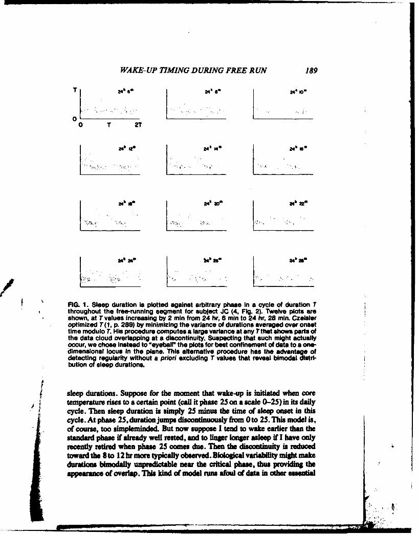
WAKE-UP TIMING DURING FREE RUN 189
T 24 60 24 h as 24 blo
00 T 2T
2han24 a 24 0 a
224 200a$223
FIG. 1. Sleep duration Is plotted against arbitrary phase in a cycle of duration Tthroughout the free-running segment for subject JC (4, Fig. 2). Twelve plots areshown, at T values increasing by 2 min from 24 hr, 6 min to 24 hr, 28 min. Czelsleroptimized T(1, p. 289) by minimizing the variance of durations averaged over onsettime modulo T. His procedure computes a large variance at any Tthat shows parts ofthe data cloud overlapping at a discontinuity. Suspecting that such might actuallyoccur, we chose instead to "eyebair the plots for best confinement of data to a one-dimensional locus in the plane. This alternative procedure has the advantage ofdetecting regularity without a priori excluding T values that reveal bimodal distri-bution of sleep durations.
6
sleep durations. Suppose for the moment that wake-up is initiated when coretemperature rises to a certain point (call it phase 25 on a scale 0-25) in its dailycycle. Then sleep duration is simply 25 minus the time of sleep onset in thiscycle. At phase 25, duration jumps discontinuously from 0 to 25. This model is,of course, too simpleminded. But now suppose I tend to wake earlier than thestandard phase if already well rested, and to le long asleep if I have onlyrecently retired when phase 25 comes due. Then the discontmuity is reducedtoward the 8to 12 hr more typically observed. Biological variability might makedurations bimodally ule near the critical phase, thus providing theappearance of overlap. This kind of model runs afoul of data in other essential

190 WAKE- UP TIMING DURING FREE RUN
T A
SLOPE =-I
-W
010 T 2T
HOUR OF SLEEP ONSET (MOD T)
FIG. 2A. One panel of Fig. I is overlaid with a suggested curve threading the data.The curve is discontinuous and lacks upslope in the manner described earlier (10).
/T SLw"OPE -I
CL
4 44
0-0 0 25
HOUR OF SLEEP ONSETAFTER MINIMUM TEMPERATURE
FIG. 28. The data of Zulley (13) are similarly overlaid These points were locatedhorizontally by absolute hours after the most recent temperature minimum, notby simply postulating a rhythmical Influence and then seeking Its period as InFig. I. Thaw two methods amount to nearly the same thing If the postulatedInfluence Is conspicuous In temperature fluctuations, However, Zu~leys data areprobably somewhat displaced by the temperature-reducing effect of sleep. Theture minimum. Very few wake-ups occur In this region.

WAKE-UP TIMING DURING FREE RUN 191
regards, but it suffices here to make the point that there is nothing intrinsicallyunreasonable about discontinuity in the dependence of sleep duration on sleeponset phase.
Czeisler (1) also noted the sudden change in sleep durations and compared itto the "breakpoint" in the transients of phase resetting. Kawato et al. (5)presented an interpretation according to which an underlying mechanism phase-shifts abruptly to change the sleep duration. My own preference is for aninterpretation, sketched below, more in line with the models of Wever (9; andthis volume) and Kronauer et al. (6; and this volume). But the point I wish tomake here is that there is no theoretical reason prejudicial to interpretation ofthe data by a piecewise-discontinuous curve or (what is the same) recognition ofa range of circadian clock phases during which wake-up seldom or never occurs.This gap is conspicuous in the raster-plotted raw data (when the raster period isaccurately matched to the individual's circadian clock) as a vertical band devoidof spontaneous awakenings (11,12).
I have been cautioned (K Kronauer, personal communication) thatalthough discontinuities may present no obstacle to model makers, they maystill be artifacts of data processing:
1. There are some dots that might indicate a very steep upslope rather thanstrict nonexistence of any curve rising through intermediate sleep durations.
2. In sleep-wake recordings unaccompanied by temperature data, and to a ,lesser extent even with such data, there is some slight latitude of choice aboutthe base period. It commonly happens in long records that the longest sleepsoccur preferentially near the end of the record. By choosing a slightly longerbase period, one can plot these sleeps at earlier phases, overlapping short sleepsinitiated at the same phase earlier in the record. This effect spuriously steepensthe upslope or introduces frank overlap of longest and shortest sleeps.
3. A different problem afflicts analysis of data in which base period seemsunsteady. In such cases one can only plot sleep onsets relative to the recenttemperature excursions. Wake-up causes a temperature rise; so the temperatureminimum cannot easily follow wake-up. Thus emerges an apparent butartifactual gap in wake-up phases, and the corresponding discontinuity in sleepdurations. This effect would tend to condense sleep onsets around one quartercycle before apparent temperature minimum while rarefying wake-ups in thatrange, with the opposite effect near the opposite phase in both cases. This isexactly what Zulley's data show (Fig. 2B). This "masking" of the core-temperature rhythm by the direct effect of activity can be compensatednumerically, but I have not yet am sleep-wake timing replotted on this basis.In principle, this is a continuous distortion; so it cannot make a continuouscurve look disconinuous, or vice versa. But, in fact, one deals with data points,and only imagine curves. I am not sure how one's imagining might be affectedafter making this correction.
4. It would appear from the work of Czelsler st al. (2) and Kronauer et al. (6)

192 WAKE-UP TIMING DURING FREE RUN
that bimodality and discontinuity are not universal: A smooth, almostsinusoidal, curve derived from the two-oscillator model fits quite nicely to thedata of PRO 1 (6, Fig. 10). The models computed by Wever and by Kronauer(at least with parameters as then adjusted) do not exhibit discontinuity. Asillustrated by Fig. 10 of Kronauer et al. (6), every realizable sleep duration canbe elicited at either of two phases of sleep onset, one where the curve isdescending and one in the midst of its opposite ascent.
Those are some of the caveats. Only laboratory observation will clarify thematter, so it may be years before it is known how common this feature is thatcan now be perceived only ambiguously, But suppose for the moment that thisdiscontinuous interpretation may be as appropriate as the original smoothinterpretation and enquire what it may signify. The question is of interest initself, concerning, as it does, a distinct qualitative feature of the psycho-physiological mechanisms of sleep. It also has interest in connection withmodels. According to one mathematical metaphor, any mechanism involvingaccumulation or depletion of some quantity toward a threshold that is subject toa periodic influence can exhibit such bimodality, overlap, and discontinuity. Ishall present a simple caricature to illustrate how this comes about and tounderscore some of the diagnostic idiosyncrasies of this class of mechanism.1
I believe attention to this feature might prove useful to discriminate betweenadmissible and inadmissible ways of relating the smoothly varying quantities ofIf an underlying oscillator to the discrete transitions between sleep and waking. Inunderscoring the deficiencies of Wever's early choice of a threshold inter-pretation, Kronauer et al. (6) pointed to the need for such discriminatingobservations 2
A GATING MODEL
Kronauer et al. (6) and Aschoff and Wever (9, and citations therein) arguedthat human sleep-wake data are best construed as revealing two separatecircadian clocks: one of relatively constant 24- to 25-hr period and another oflonger and more labile period. [Note, however, the dissenting opinions ofDirlich (this volume) and Eastman (this volume).] They further inferred thatboth oscillators involve two or more smoothly varying quantities in their basicmechanisms and that both oscillators have limit cycles to which they recover ata leisurely pace during transient changes of amplitude. This understanding of
Daan and Beetama (thiu volume) have described a well-developed model ofjust this sort. It goesfurther to also interpret wake durations in the same terms, despite the lack of conmspon 8ftreularip t in the published observations (vide iqfa).
21 am indebted to R. Kronauer for his subsequent observation that with appropriate adjstment ofits threshold mechanism, his model can also represent the discontinuity, as shown in Komauer at aL(7, Fi. 10). Figure 3 frm the same work reinterprets the PROI data as in my Fil. 2 and thea4usted model
I

WAKE- UP TIMING DURING FREE RUN 193
human clockworks needs to be set in context by understanding also why nearbyalternative interpretations do not work. As a step toward verifying both thesufficiency and the necessity of the existing two-oscillator model, I wouldtherefore like to gather observations appropriate for testing it against the manyalternatives it seems to be provoking.
I now present one more such alternative: a simple interpretation of thedependence of waking time on prior sleep onset, both being measured byreference to a smoothly varying rhythmic influence. This influence may beconstrued as coming from the autonomous circadian clock that also influencescore temperature or, when external scheduling is dominant, as coming fromsome outside Zeitgeber. Suppose that the first oscillator, the one with steadierperiod, which is more conspicuous in core temperature, makes its appearance inthe sleep-wake system simply as a smooth rhythmical modulation of somethreshold at which wake-up is initiated (Fig. 3). (There is no cause to assumethat its maximum and minimum correspond to those of core temperature.) Thisinterpretation is lifted directly from my interpretation of the pupal eclosionrhythm in the fruitfly (10, pp. 403-406). The model has been studied in somedetail mathematically, but, skipping all that, the bottom line is that models ofthis class exhibit a characteristic idiosyncrasy that seems to appear also in thedependence of sleep duration on sleep onset time (Fig. 1).
Figure 3 illustrates the timing of wake-up given one particular choice of sleeponset time, where the rising quantity (call it "restedness") starts its rise from
RESTEDNESS T
[ THRESHOLD
40.
SLEEP WAKE- UP
ONSETI I.
DURATION OF SLEEP
FIG. 3. "Restedneas," defined proportional to cumulative sleep, dses toward athreshold at which wake-up is Irrevocably Initiated. This threshold is postulated tovary with subjective circadlan time at a period T to be discovered in the data.

194 WAKE- UP TIMING DURING FREE RUN
baseline. (It would, of course, be equivalent to fantasize a declining "tired-ness.") Were there no modulation of the threshold level, sleep duration wouldbe the same no matter when sleep begins; in fact, there would be no grounds fordistinguishing one "when" from another, so far as the threshold is concerned.With nonzero threshold modulation, the duration of sleep depends on the timingof sleep onset. In fact, with arbitrarily strong modulation, the dependence isexactly as in the "simplest" model described earlier~ Wake-up can occur only ata standard phase in this rhythm. So one needs to consider modulation at somemoderate amplitude between the extremes.
In Fig. 3, sleep duration would decrease if the phase of sleep onset weremoved to the right. Moved farther right to a critical phase, the rising quantitywould altogether miss the trough of the threshold rhythm, and hit threshold onlymuch later (Fig. 4). (The same might be accomplished by sleep deprivation,causing restedness to start from a lower origin or, equivalently but more con-veniently for graphic anticipation of the results, elevating the threshold curve.)At this critical phase, the shortest sleep abruptly changes to the longest. There isno ascending branch of the curve. In fact, if very short sleep sometimes fails toterminate at threshold, i.e., if sleep sometimes lingers until the threshold isuncrossed again a short time later (Fig. 5), then shortest and longest may be twoalternative choices for the duration of sleeps initiated near that critical phase.The top and bottom parts of the curve would then overlap in the way suggestedby the data of Fig. 1. Wake-up is gated by the rise and fall of the threshold. Itcan occur spontaneously only in a certain range of phases (where the thresholdis not rising too fast). Forced waking at other times might be uncomfortable andunproductive.
At sufficiently high amplitudes of threshold modulation, wake-up neveroccurs in a certain range of phases in the temperature cycle, regardless of onsetphase. But at sufficiently low amplitude of modulation, wake-up can occur atany phase, depending on onset phase. In other words, if the thresholdmodulation is weak (if the 25-hr circadian rhythm and/or exogenous Zeitgeberhas less impact on the sleep-wake mechanism), then no discontinuity occurs.This is because the weakly modulated threshold never rises faster thanrestedness (Fig. 6). In such a case, duration varies smoothly with onset phase,as represented by Kronauer et al. (6, Fig. 10). In this situation the duration ofsleep averages much longer, too, corresponding more nearly to the time it takesfor restedness to reach average threshold level, never being interrupted by aplunging descent of threshold. Could this have anything to do with Wever'sobservation (9) that when a subject's temperature amplitude decreases, hissleeps average longer?
This caricature of the rhythmically modulated timing of a discrete event canbe put together in a single three-dimensional diagram (10), as in Fig. 7. Thisparticular diagram is computed from a mathematically tidy representative casein which restedness increases steadily (by definition) while the threshold for
wake-up fluctuates sinusoidally (or in any other fashion). Note that the

WAKE-UP TIMING DURING FREE RUN 195
T
z0
I-....... V .'.
4 T ONSET
z A
SOONSET
FIG. 4. Top: Figure 3 is tilled in with threshold interceptions from all sleep onsetphases spanning 1.5 cycles of T. Bottom: The dependence of duration on choice ofonset is replotted in upright coordinates.
FIG. 5. As in Fig. 3, but differentlyscaled to suggest how a bimodaldistribution of sleep durations mightarise by transgressing the thresholdonly briefly near a critical phase.
,q"VAii

196 WAKE-UP TIMING DURING FREE RUN
FIG. 6. As in Fig. 3, but differentlyscaled to suggest how weak modu-lation of threshold may result in asmooth up-and-down dependenceof duration on onset phase withouta break, as in PRO1 (1,2,6).
o IDURATION
b -
d - ONSETPHASE
AMPLITUDEOF MODULATION
FIG. 7. Threshold-modulation models produce different curves of sleep durationversus sleep onset according to the amplitude of modulation (by an endogenousclock or by an external scheduler). At amplitude 0, duration Is always the same (a). Atlow amplitudes (b) it varies somewhat according to onset time modulo T. At middlingamplitudes (c) It gets a steep narrow upslope region of high variance, but durationsare still unimodally distributed. At high amplitudes (d) the upslope has vanished,leaving a frank discontinuity, even with overlapping edges. Durations are bimodallydistributed near this phase. The whole picture is called a "Whitney cusp." It Is typicalof a great variety of control systems.

WA KE- UP TIMING D URING FREE RUN 197
threshold could equivalently be regarded as constant while restedness risessometimes faster and sometimes falls back a little; the consequences for timingwould be identical. In fact, any model exhibits this qualitative behavior if itcombines a smoothly rhythmical wiggle with a quantity slowly approaching athreshold to switch sleep on or off. In particular, the oscillator models of Wever(9) and Kronauer (6) should show such duration-versus-onset curves whenparameters are so adjusted that the wiggle's amplitude exceeds the cusp point inFig. 7. Unfortunately, this statement seems to apply equally to sleep duration(wake onset) and wake duration (sleep onset) in those models.
Such notions can be put to trial by sleep-deprivation experiments and/or bychanging the vigor or period of rhythmic driving (the threshold modulation). Theresults expected (discontinuities appearing or disappearing, moving righut or left)would be hard to mistake in the laboratory.
Before going on, note that if a process similar to that here conceived to governsleep duration were at work also in the determination of wake duration, then mysimplified caricature would constitute a second oscillator functionally equiva-lent to the y (activity) oscillator of Kronauer et al. (6). [This is the model ofDaan and Beersma (this volume).] It differs from his only in that my amplitudeis inflexibly determined and my equilibrium state either does not exist or is aviolent repeller. This is getting to be fairly exotic speculation, but the businesscan, in principle, be resolved by a singularity experiment (10). This is not yettechnically feasible in humans, so there is not much point in belaboring it. Butwhen and if one does find out how to perturb human clocks to their phaselessstates, then Kronauer's model can be expected to show that recovery will berather slow; if so, then simpler models of the sort here explored will be starklyinadequate.
For the present, I have not been able to make sense of wake-duration data(i.e., the times of sleep onset), so I postulate no second oscillator. This chapteris confined to an interpretation of sleep duration alone, or, in other words, ofwake-up timing.
WHAT DETERMINES SLEEP ONSET?
Sleep durations taken from any stage in the secular progression of sleep-wakebehavior under temporal isolation all seem to fall on the same curve, as thoughthe shape of Fig. 7 and the modulation amplitude both remain unchanged.While the patterning of sleep-wake alternations is metamorphosing, the timingof sleep is not. The change, then, may lie exclusively in the mechanismdetermining sleep onset, or the duration of waking. I need now to direct myexploratory data analysis to the other half of the sleep-wake cycle by asking"What determines when one goes to sleep?" Is the same periodic time base a
* conspicuous organizer of that dependence Does the time of sleep onset depend

198 WA KE- UP TIMING DURING FREE RUN
mainly on the previous time of waking or mainly on the previous times of wakingand sleep onset (perhaps through their difference, the previous sleep duration),or additionally on more remote prior events?
Perhaps it would not be surprising to find disappointingly little determinismhere, as we all have the subjective impression that we can voluntarily defer sleepto a much greater extent than we can adjust the moment of waking, giventhe time of sleep onset. Attempts in this direction may be premature. Cer-tainly they are hobbled still by a shortage of long unperturbed free runs in thepublished record, and by the intriguing fact that during such runs, some essentialparameter is apparently drifting and, as it slowly drifts, distorting the functionaldependences I seek to observe. But it would be so valuable to know how onesleep episode (or several) predetermines the onset of the next (if it does) that Ihave undertaken to spend some time looking. I am inclined to take a lesson fromthe recent mathematical literature of iterated mappings: that lovely regularitiesmay lurk in ostensibly random data, awaiting discovery by someone inpossession of a long enough and steady enough time series who makes afelicitous choice of what to plot against what
It seems that this can be done in a model-free and theory-independent way. IfI had two records of alternating sleep and wakefulness, identically timedthrough a dozen episodes, then I might reasonably expect the next sleep onsetsto be identically timed. Just as a matter of phenomenological description, thehour of sleep onset should be somehow implicit in the timing of earlier events.
'-VT Tis is known to be so in the case of wake onset; in fact, only one previous eventsuffices for excellent prediction. But in the case of sleep onset, I have not foundany clear regularity either in terms of the phases of the previous three transitionsor mn terms of the durations of prior waking and sleep.
In contrast, every model I have examined (by making artificial data sets tosubmit to the same data-analysis programs) does show clear regularities ofdiverse sorts, but none of these appear in the data. The regularities in the modelsare, of course, quite similar for the two halves of the sleep-wake cycle. This isbecause existing models treat the two stages evenhandedly, as two sides of acoin, e.g., above and below a threshold. So my impression is that timing of sleepand of wake is not so symmetrically handled in real people; for example,whatever is changing during months of isolation appears to affect the timing ofsleep onset far more than it affects the timing of wake onset.
ACKNOWLEDGMENTS
All the participants in the symposium that was the basis of this book havebeen more then generous in bringing me up to date since I first undertook tolearn about circadian clocks. Specifically, S. Sam at the USAF School ofAerospace Medicine drew my attention to the practical importance of jet lag.From J. Enright I learned of Wever's book The Circadian System of Man, andF. Sulzman directed me to Czeisler's thesis on human circadian physiology. ML

WAKE-UP TIMING DURING FREE RUN 199
Moore-Ede introduced me to the coupled-oscillator model of Kronauer.Funding for many travels during sabbatical leave from Purdue University camethrough the Institute for Natural Philosophy and USAF School of AerospaceMedicine.
REFERENCES
1. Czeisler, C. A. (1978): Human circadian physiology: Internal organization of temperature,sleep-wake, and neuroendocrine rhythms monitored in an environment free of time cues.Dissertation, Stanford University Medical School.
2. Czeisler, C. A., Weitzman, E. D., Moore-Ede., M. C., Zimmerman, J. C., and Knauer, R. S.(1980): Human sleep: Its duration and organization depend on its circadian phase. Science,210:1264-1267.
3. Enright, J. T. (1980): The Timing of Sleep and Wakefulness. Springer-Verlag, Berlin.4. Jouvet, M., Mouret, J., Chouvet, G., and Siffre, M. (1974): Toward a 48-hour day:
Experimental bicircadian rhythm in man. In: The Neurosciences: Third Study Program,edited by F. Schmidt and F. Worden, pp. 491-497. M.I.T. Press, Cambridge, Mass.
5. Kawato, M., Fujita, K., Suzuki, R., and Winfree, A. T. (1982): A three-oscillator model ofthe human circadian pacemaker controlling body temperature and the sleep-wake cycle. J.Theor. BioL, 98:369-392.
6. Kronauer, R. E., Czeisler, C. A., Pilato, S., Moore-Ede, M. C., and Weitzman, E. D. (1982):Mathematical model of the human circadian system with two interacting oscillators. Am. J.Physiol., 242:R3-R1 7.
7. Kronauer, R. E., Czeisler, C. A., Pilato, S. F., Moore-Ede, M. C., and Weitzmian, E. D.(1982): Mathematical model of the human circadian system with two interacting oscillators.Am. J. Physiol., 242:R3-RI7.
8. Mills, J. N., Minors, D. S., and Waterhouse, J. M. (1974): The circadian rhythms of humansubjects without timepieces or indication of the alternation of day and night. J. Physiol(Lond), 240:567-594.
9. Wever, R. (1979): The Circadian System of Man. Springer-Verlag, Berlin.10. Winfree, A. T. (1980): The Geometry of Biological Time. Springer-Verlag, Berlin.11. Winfree, A. T. (1982): Human body clocks and the timing of sleep. Nature, 297:23-27.12. Winfree, A. T. (1982): The timing of sleep and wakefulness in men and women. Am. J.
Physiol., 243:RI93-R204.13. Zulley, J. (1980): Discussion. Sleep, 2:344-346.
DISCUSSION
Dr. Wever When we look for precision in various phase points, sleep onset is by farthe least precise reference phase that exists in the sleep-wake cycle; it has 50% largervariability than all other phase point reference points, including, for instance, themidpoint of sleep.
Dr. Czeisler Are your data that you have presented all from internally synchronizedsubjects?
Dr. Wever Yes, only internally synchronized people.Dr. Weitzman: If you look at what sleep stage ends the sleep episode during free run,
as compared to entrained subjects, it is very clear that there is a much increasedprobability (i.e., about 80%) that the subject will wake up out of REM sleep. However,in the entrained condition, the probability is down to 20 to 30%. That is in spite of thefact that REM sleep during free running is shifting earlier, so there should even be a
-- t
-- --- =~i~ii I Im m'm

200 WAKE-UP TIMING DURING FREE RUN
lower probability of waking out of that stage. Now, that means that there is somepowerful set of presumably ultradian REM/non-REM cycles which is somehowstructuring that endpoint. This suggests there is some kind of interrelationship betweenthe ultradian REM/non-REM cycle and the circadian sleep-wake cycle which is verypredictable.
Dr. Winfree- That sounds like a factor for determining the endpoint of the REM/non-REM cycle, but I do not believe it to be related to the timing of circadian cycles.
Dr. Rosenthal: I am fascinated by your model.
Dr. Wigfree- Don't call it a model! [LaughterJ
Dr. Rosenthal: I am very interested in how it is similar to Dr. Borb6ly's model in thatit presupposes an interaction between a single circadian oscillating system and some"buildup" or "hourglass" system. I am particularly interested in the way in which it mayexplain abnormal sleep phenomena such as we see in depression. One could postulate areduced pressure to sleep, which could explain the reduced delta sleep seen indepression. Your suggestion of a reduced threshold for wakefulness would explain a lotof things.
Dr. Winfree. Well, that is precisely the point.Dr. Rosenthal: Depressives do have a different sleep duration. They have early
morning waking, which could be predicted by your model, but it would be predicted thatthey would have early morning waking that would cause sleep deprivation. There would,therefore, be REM pressure which might explain why there is the observed increase inREM in the early part of the night when the depressive subsequently goes to sleep. Therestriction of REM would increase REM density in the early part of the night. All of
these phenomena could be explained in terms of the picture you have drawn.
ff
, €'

Mathematical Models of the Circadian Sleep-Wake Cycle, edited by M. C. Moore-Ede andC. A. Czeisler. Raven Press, New York Q 1984.
Sleep Duration for Human Subjects DuringInternal Desynebronization
I. T. Enright
Scripps Institution of Oceanography, University of California,La Jolla, California 92093
Zulley [in Czeisler et al. (2)] and Czeisler et al. (1), in their analyses of datafrom circadian studies of isolated human subjects, have noted that when asubject shows dissociation of the wake-sleep rhythm from the core-temperaturerhythm, there is a systematic relationship between the phase of the temperaturecycle at which the subject falls asleep and the duration of the ensuing sleep. Onthe basis of these data, as well as of his own analyses of similar data, Winfree(this volume) has suggested that this quantitative relationship may well involvea discontinuity: If sleep onset occurs at a certain critical phase of the underlyingendogenous; pacemaker rhythm (as indexed by the temperature cycle), the resultcan be either a very short sleep or a very long one, with intermediate valuesbeing unlikely. A slightly earlier sleep onset leads consistently only to very shortsleep, and a slightly later sleep onset only to very long sleep. Both Winfree (thisvolume) and Daan and Beersma (this volume) have proposed models, ofdiffering complexity, in which such a discontinuity is predicted to occur becauseof interactions between a cumulative renewal process and a rhythmicallyfluctuating threshold. In this chapter I shall outline a possible alternativeexplanation for that phenomenon.
AN INTERESTING RESEMBLANCE
I have been struck by the similarity between these empirical results and theoutcome of certain computer simulations based on models I have called"coupled stochastic systems" (3). Those models were initially formulated as ameans of accounting for wake-sleep data from nocturnal rodents and fromdiurnal birds. The parameter values for the specific model of interest here wereassigned to provide an adequate fit to phase-shift data for 6-hr light stimu-lation of the house sparrow (3, Figs. 11.5 and 11.6). The simulations, inwhich there are resemblances with the human data, represent predictions for thebird's rhythm when single light stimuli of varying duration are administeredduring free run, with onset of the light always corresponding to onset of activity(wake-up time) (3, Fig. 13.8). Because of the formulation of this specific model
201

202 SLEEP DURA TION
(corresponding to the behavior of birds), onset of sleep would be expected tooccur at the end of the light treatment for all stimuli longer than about 4 hr.When those predictions are replotted in a coordinate system similar to that usedby Winfree and others for the human data, the hypothesized behavior of the birdshows a phase-dependent pattern of sleep duration similar to that of the humansubjects (Fig. 1). [Note particularly the sudden transition from very short tovery long sleeps; compare with human data of Winfree (this volume).]Numerous other simulations with this particular model have convinced me thatqualitative aspects of this result are due almost exclusively to the time at whichthe light stimulus ends (3, Fig. 13.6).
DISCUSSION
It may well be that this qualitative resemblance between (hypothetical) birddata and the real human data is only fortuitous; certainly the subsequentbehavior of the wake-sleep pacemaker of my models, following such treatment,seems to differ appreciably from that of the body-temperature cycle of humansubjects. Nevertheless, it seems worthwhile to pursue briefly the speculationthat the resemblance could reflect qualitatively similar processes in the wake-sleep pacemakers of bird and human.
In a bird, the light receptors of importance for circadian rhythmicity are notretinal, but directly in the brain (5); whether the bird is awake or asleep, its
0
hi 12I10 0 3PHS-FSLE NE
(EDO(LGTS0AUU)
HOR ATRWAEU
FI.1 rdctosfrtebeairefasprofloin ih tmlita0rdc
shoul . nored~cin thnoe bhor f valusparw fo l owing lighmtrsl tat produced
with human data in mind.

SLEEP DURATION 203
pacemaker is continually subject to prevailing light intensity (unless, assometimes happens in dim light, the sleeping bird tucks it head beneath itswing). The pacemaker of a human subject, however, like that of other mammalsinvestigated, can presumably be affected only by retinally perceived light, withthe result that when awake, with open eyes, the human administers to hispacemaker system a light stimulus. Onset of sleep and/or turning off of the roomlights are the usual ways in which that stimulus is terminated each day. Hence,the photic regime of a bird, subjected to externally imposed light stimuli,beginning at wake-up time and varying in duration, can be thought of ascomparable with the light-mediated consequences of human wakefulness, withvarying times of sleep onset. If the human subject were, for any reason, to delayhis sleep onset from its usual circadian timing, he would presumably beadministering unusual light stimuli to his pacemaker. Should the phase-shiftingeffects of light stimuli on the human wake-sleep pacemaker qualitativelyresemble those in the sparrow, then one might well expect the sort ofrelationship between phase of sleep onset and duration of sleep seen in thehuman subjects, arising as a consequence of repeated self-administered lightstimuli.
The assumption involved here, that the wake-sleep pacemakers of humanand sparrow respond to the phase-shifting effects of light in qualitatively similarways, represents an extremely speculative leap beyond the limits of experi-mental data. Light has been shown to be the dominant Zeitgeber for the
circadian rhythms of all nonhuman species; and because bird and human areboth day-active creatures, one might well expect evolution to have producedcertain similarities in their responsiveness to light, at least very cruderesemblances, so as to permit entrainment of their pacemakers with compar-able, ecologically appropriate phase control. There is, however, no necessity forthe resemblances to go as far as assumed here; in fact I know of no unequivocaldemonstration to date that light can directly produce phase shifts of any sort inthe human pacemaker. On the contrary, Wever's attempts (6) to synchronizehuman subjects with lighting regimes suggest that the human pacemaker may beappreciably less sensitive to light than that of birds (see also ref 4).Nevertheless, while admitting the validity of such reservations, I find thishypothesis attractive because it does not involve the interpretation (R. A.Wever, this volume, t. E. Kronauer this volume) that the human wake-sleep
* pacemaker is unique in having or developing an intrinsic period that is manyhours longer than the values seen in circadian rhythms of all nonhumanvertebrates.
Phase shifting by light stimuli would, of course, offer only partial explanationfor why human subjects occasionally show the phenomenon of internaldesynchronization, with attendant wake-sleep cycles that are so far beyond theusual circadian range. One must also explain why humans during this sort ofexperiment would fail to "istea to" their circadian pacemakers, at the interUallyprposed time of sleep onset, md postpone that onset for so many hours, dwuif
m, mmnm mu--lm m ",', . ..

204 SLEEP D URA TION
which light effects of the sort here postulated might arise. Perhaps the answerlies in the cognitive interaction of a human subject with the protocol typical ofsuch studies in temporal isolation. In the Erling experiments (6), the subjectsare instructed to follow their normal, regular daily routine, with three primarymeals per day, but to avoid afternoon naps if at all possible. One of theexperimental subjects who experienced internal desynchronization (6, Fig. 57,right) has retrospectively reported the following sort of subjective experience:"I'm tired now, but this is probably not my bedtime; I have only eaten breakfastand lunch, so I presume that this sleepiness represents an urge to nap, perhapsbecause I'm cooped up here with too little chance to exercise. I won't go to bednow, but try some gymnastics instead, to wake me up." As another example ofsuch cognitive interactions, discussion speakers at this symposium have calledattention to the fact that in other laboratories, the decision to retire "for thenight" during temporal-isolation studies is a much more momentous one thansimply climbing into bed;, the subject must be fully instrumented (EEG, etc.) bylaboratory personnel before sleep ii permitted. Could this aspect of the protocollead some subjects, some of the time, to postpone the decision to go to bed, toprocrastinate, waiting to see if the inner alarm clock is really giving anirrevocable bedtime signal? We are all familiar with the experience thatcognitive issues of far less direct consequence, such as good company orIinteresting reading material, can lead us to postpone our sleep time-thoughseldom to the extreme sometimes observed in temporal-isolation experiments.
Perhaps, as Winfree (this volume) has suggested, cognitive processes of thesesorts could be responsible also for the discouraging outcome of his search forany consistent correlation between the timing of sleep onset and the priorfeatures of a given subject's wake-sleep behavior. (Note that the simulationresults shown in Fig. I depend primarily on the time at which the light stimulusends, i.e., time of sleep onset, with only minor influence of light onset, Le.,preceding wake-up time.) Although there is no direct evidence yet available toindicate whether or not cognitive factors can influence the outcome of humantemporal-isolation experiments, that absence could c-"-ceivably reflect only thefaiure systematically to collect, analyze, and interwet adequate data on thesubjective aspects of the isolation experience.
Whether or not the preceding interpretation contains an element of the truth,the predictability of sleep duration on the basis of phasing of sleep onset is anexciting empirical result, a central feature of these remarkable experiments thatdemonstrates the conspicuous involvement of a circadian pacemaker even inthese very noncircadian data. The speculations in this chapter about those dataare offered in the spirit that alternative hypotheses are essential to the progressof experimental science. The hypotheses suggested here are sufficientlydifferent from the others currently under consideration that a variety of criticalexperiments to distinguish between alternatives could be designed. One of themost obviou of these would be to attempt to induce internal dIaYncro ationby sleep deprivation of a diurnal animal (a monkey, for example) during free-

SLEEP D URA TION 205
running conditions, first in a well-lit environment and then in total darkness. Ifself-induced phase shifting of the wake-sleep pacemaker by lighting isresponsible for human internal desynchronization, the sleep-deprived monkeyshould show phase shifting of its wake-sleep rhythm in a well-lit environment,resulting in internal desynchronization, but should not be so affected indarkness. I deeply regret that I am not now in a position to undertake such anexperiment myself.
SUMMARY
The complex dependence of sleep duration on circadian phase of sleep onsetthat is seen in human experiments bears a clear resemblance to simulationresults that predict the duration of sleep of a sparrow following abnormally longlight stimuli. This resemblance suggests the hypothesis that the human resultsmay be due to (a) cognitive interactions of the human subject with theexperimental protocol such that he sometimes forces himself to remain awakefar after the time suggested by his circadian pacemaker and (b) phase shifting ofthat pacemaker by self-administered light stimuli during such intervals ofprolonged wakefulness. This hypothesis implies that the free-running period ofthe underlying wake-sleep pacemaker could be near 24 hr, even when theaverage period of the observed rhythm is much longer.
I
ACKNOWLEDGMENTS
This work resulted in part from informal conversations, particularly thosewith Drs. S. Daan, G. Dirlich, C. Eastman, and A. Winfree, that took placeduring the course of the symposium reported in this volume. Dr. Winfree hasalso offered valuable comments on the manuscript. This work was supported inpart by Grant PCM-7719949 from the National Science Foundation.
REFERENCES
1. Czeisler, C. A., Weitzman, E. D., Moore-Ede, M. C., Zimmerman, J. C., and Knauer, R. S.(1980): Human sleep: Its duration and orpnization depend upon its circadian phase. Science,210:1264-267.
2. Czeisler, C. A., Zimmerman, J. C., Roa, J. M., Moore-Ede, M. C., and Weitzman, E. D.(1980): Timing of REM sleep is coupled to the circadian rhythm of body temperature in man.Slee, 2:329-346.
3. ElgiUK J. T. (1980): The 71ming of Sleep and Wake&bmes. Spingar-Veda& Berlin.4. Lwy, A. J., Wehr, T. A., Goodwin, F. K., Newsome, D. A., and Markey, S. P. (1980Y Light
uppreues melatonin secretion in humams. Science, 210,1267-1269.S. Meaker, M. (968): Extraretinal li perception in the qprow. Proac NaL Acai Sc. USA,
59.414-421.6. Wever, R. (1979): The Ci-adian System of Ma. Spd-Vrlag& Berlin.
.. .........

Mathematical Models of the Circadian Sleep-Wake Cycle, edited by M. C. Moore-Ede andC. A. Czeisler. Raven Press, New York © 1984.
General Discussion
Dr. Kronauer Both Dr. Czeisler's data and Dr. Jouvet's data show that there is apreponderance of the short sleep periods and not very many of the long sleep periods ininternally desynchronized subjects. But I look at the data that Dr. Winfree put togetherfrom Dr. Zulley's experiments and I find that in this distribution there are a lot of longsleeps and not very many short sleeps. It is a puzzle; I do not understand what mightmake that kind of difference.
Dr. Wever There is a difference in the way the data are presented that maybe you donot realize. What Dr. Czeisler did was to relate sleep duration to the educed waveform ofthe temperature rhythm rather than to the waveform of the rhythm on the given day.
Dr. Kronaue. But that does not explain why there should be more long and fewershort sleep episodes, as opposed to what Dr. Czeisler reported.
Dr. Wever. I would say our study used much more data. (Laughter] The difference inthe results depends on whether the educed minimum or actual minimum is used. Theactual minimum is shifted away from the mean of the educed rhythm systematically.
Dr. Czeisler Well, this analysis was done because we were relating the timing ofsleep-wake processes to the circadian phase at which they were occurring and not theabsolute temperature per se. There is an evoked response when you go to sleep with alowering of temperature immediately thereafter. In contrast, when Dr. Wever sub-jectively determines the minimum in each cycle, that process requires a subjectiveIdecision to be made as to the time of the minimum in each curve. We wanted to use anobjective method which related sleep to the phase of the cycle. So we determined theaverage period length by either spectral analysis or various other techniques that we havedeveloped and then educed an average waveform around that period. In those cases, weeliminate the evoked component of the cycle and are able to look at the relationship ofthese processes to the phase of the circadian oscillator controlling the temperaturecycle.Dr. Schulz: Maybe one of the differences between Dr. Jouvet's data and Dr. Zulley's
data was that Dr. Jouvet's single experiment was done in a cave where the temperaturewas rather low. In the German bunker experiments of Dr. Zulley and Dr. Wever,however, the ambient temperature was self-selected.
Dr. Cze ler. Even in the isolation facility in New York, where the ambienttemperature is self-selected (along with the Ul-dark cycle), there is a preponderance ofself-selected sleep onsets near the trough of body-temperature cycle. I think that it alsomay have to do with the particular subjects that Dr. Zuey selected, because the greaterthe length of the average period of the cycle (in other words, the fewer clusters that returnto the near 25-hr period), the fewer cycles will have short sleeps. You can take sectionsof Dr. Jouvet's data, for ezamle. which have a preo nderance of the short sleep
-; episodes and odr sections which have a preponderaa of the longer sleep episodes.But, in general, if you averae many subjets together, since most of them start off at thebeginf of dsy rauhatlon with a period lnoth of around 30 hr, there is aprpomdae of dusters of shotslesp episodes,Dr. Wehm f you us Ot edmued wavetom to rehl the sleep duration to the phase,
sad f there Is a certn varliatio fm cycl to cycLk you will have a rather imprec sd 1 f the acual phase at which each of those temperature cycles rlat to te
207
F W OM
ii -. 4~

208 SLEEP DURATION
sleep episode. On the other hand, Professor Wever's method, if it in fact accuratelyidentified the specific phase of temperature oscillator, would correct for that problem.But is the actual temperature rhythm really so tightly related to the actual phase of thedriving oscillator? So I do not see either method as being superior.
Dr. Czeisler Well, I do. (Laughter] And the reason is twofold: First of all, if you lookat the actual data from one of our long free-running experiments with up to 6 months ofdata, you can see that the temperature cycle does not have the kind of phase shifts whichDr. Wever presupposes. The troughs of the temperature cycle are remarkably consistentand are without shifts. In fact, it is the absence of shifts during free run that reallysurprises us, given the nature of the sleep-wake cycle. Second, even if there were suchshifts, I do not see the method that Dr. Wever uses as any improvement ovef detectingthe phase. In fact, his method is much more subject to the evoked responses of going tosleep and of activity which are superimposed on the endogenous circadian system.
Dr. Enright: Like Serge Daan, I consider myself an evolutionary biologist, but I thinkone of the most important and unanswered questions here is why we frequently seeinternal desynchronization in humans and do not see it in any other organism, even theprimates that have been looked at. The one obvious correlation I see is that in humansthere is the potential influence of cognitive factors. If you have got a good book, you arelikely to stay up later, but if you are bored, you are likely to go to bed earlier. Now wehear from Art Winfree that the time of sleep onset, the characteristic that I would expectto be most readily influenced by such cognitive factors, is apparently unpredictable withrespect to other aspects of the rhythm. Can anybody offer speculation about why we donot see internal desynchronization in other animals?
Dr. Moore-Ede: The contrasts between the human and the animal studies are fraughtwith more problems than just differences in cognitive activity. First, Dr. Weitzman andDr. Czeisler have pointed out that there is little obvious evidence that subjects arestaying awake in order to finish some task whenever they are displaying a very longperiod of wakefulness and, therefore, extending their time of sleep onset. Second, theexperiments that have been done in monkeys have shown spontaneous internaldesynchronization by all criteria between other variables such as the urinary rhythmsand the behavioral rhythms, but not so far like the human subjects, between body-temperature rhythms and activity rhythms. Now the work of Dr. Gander in my labreported at this meeting shows that the activity rhythm shows a rather greater variabilitythan the temperature rhythm and may, in fact, show quite large dissociations in phasebetween these two rhythms in free-running monkeys. We have seen the data of Dr. Wirz-Justice, which suggest such phenomena may exist in rodents treated with anti-depressants. So, given the correct conditions, we very well may be able to show internaldesynchronization in other species. It is quite possible that playing around with variousagents, either that change the period or by using self-selected light-dark cycles, we maybe able to induce internal desynchronization.
Dr. Czeisler. I think that it is interesting to note that it is the people who have not doneJ) actual experiments with human subjects who are most concerned about the volitional
aspect and that those of us who have actually done those experiments and have seen thatvolitional factors do not play a part in internal desynchronization are least concerned.
Dr. Enright: In animal experiments you do not see the noncircadian periods you seeso often in humans.
Dr. Kripke. In the human data the idea of a single 24-hr sleep-wake cycle isreasonable because many people will stay awake for 16 hr and go to sleep for 8 hr.Animals do not do that. A rat, for example, wakes up every hour, at the least, for a periodof time. So the human is relatively unique compared to all our animal models, whichhave polycyclic sleep.

SLEEP DURATION 209
Mr. Plato: I've heard a quite narrow conception of what cognitive activity is here,and that is reading a book late at night.[Laughterj I would like to refer to an anecdotethat was reported by a newspaper reporter, who took part in one of the experiments in theMontefiore lab, which I thought was very interesting. She said that after a while hernormal sequence of daily activity started to break down, and her normal timingmechanisms within the day were harder to determine because she could not tell the timeby the fact that she had just finished one typical daily activity followed by another. So Iwould like to propose that humans, under normal circumstances, utilize not only lightand dark to time themselves, but also their sequence of activities as well as external cuessuch as the position of the sun or the use of a wristwatch. In the absence of such cues,humans are at a loss because they depend on those kinds of nonnatural environmentalcues.
Dr. Czeisler I would also like to point out that it is not just the last part of the daywhich is extended. It is not just that they stay up late performing some activity, but theentire day changes its character under these conditions. The time between waking up andhaving breakfast might be 6 or 8 hr, the time between breakfast and lunch might be 8 to10 hr. So dinner usually comes just before the subjects go to sleep, even when they are ona 40- or 50-hr day. In the outside world we might have gone through breakfast, lunch,and dinner before the subject even has breakfast, despite the fact that he got up at thesame time. So it is not just an isolated part of the day that has lengthened under thiscircumstance, but the subject's entire perception of the length of his day.
Dr. Edmunds: I would like to challenge the conclusion that internal desynchroni-zation has not been observed in any organisms besides humans. A couple of years ago Ipublished data suggesting that the rhythms of photosynthetic capacity can showdissociated circadian rhythms in free-running Euglena over an interval of 2 or 3 days,with virtually any phase relation observable, suggesting that the detection of internaldesynchronization may depend on what you look at.
Dr. Weitzman: I would like to expand on what Dr. Czeisler said. If you ask a subjectwho has been up for 30 some hours if anything is different (being careful not to imply tohim that something might be different), almost invariably you get a statement, "Well,maybe the day seemed a little longer but basically it was unchanged." On a 50-hr day,you often will find that they feel like they are ready to go to sleep but they have not haddinner yet. And so they are conflicted-"Should I have dinner, should I go to sleep?" Infact, sleep generally takes precedence, and they say, "I just cannot stay awakeanymore," and they will go without dinner. Thus, the whole structure of the day, thewhole internal organization, changes, but the subject is totally unaware of the time thathas elapsed in these very long days.
Dr. Wever We find there is a very strong correlation between internal desynchroniza-tion and the age of the subject. We can divide our subjects into two groups: a youngergroup from 17 to 35 or 40, only a few of whom show internal desynchronization. In theelder subjects, up to age 73, 80% show internal desynchronization.
Dr. Weitzman: We have not seen such a high incidence of internal desynchronizationin older subjects. We have studied a series of older subjects up to the age of 84, and therehave been some who have desynchronized, but most of them have not. We do not have avery large series, but it suggests to us that it is more the length of time in isolation ratherthan the age of the subject that is important
Dr. W lfiw. Dr. Weitzman, on these 50-hr days, do your subjects eat 6,000 caloriesper cycle?
Dr. Weitzman: No. They do not.
Dr. W*7fr. If they eat three meals a day, do they get skinny after a while?

210 SLEEP DURATION
Dr. Weitzman: Yes, they do. In fact, some subjects increase the amount per meal;they will say they feel hungry. But another subject might say, "I do not know what youare doing here, but you are not giving me enough food to eat. You weigh me every day,and I am hungry all the time and I am losing weight every day." He was only eating threemeals and a snack on each 50-hr day. So we told him, "If you want more food or moremeals, just ask for it; you have that choice. You can do anything you want." That's ourparadigm: We give them any amount of food at any time; it is a wonderful hotel! But hedid not choose to do that. He continued to eat essentially three or four meals a day andjust increased the size of the meal somewhat, and thus continued to lose weight duringthat time. It is a good weight-losing technique, a little expensive, but.... [Laughter]
Dr. Lewy: Why does internal desynchronization occur either exclusively or at leastmore often in humans as compared to other species? Second, why does internaldesynchronization occur when it does occur in the free-running studies? I think one factorthat we should consider is the light-dark cycle and the sensitivity of humans to light.Humans require much brighter light for the same suppression of melatonin than otherspecies. Another finding that we have not published yet is that there seems to be quite alarge variability in light sensitivity in individuals, and there may be a seasonal rhythm inlight sensitivity in man. During the summer our subjects are relatively insensitive to light,as compared to when they are studied in the winter. So I would suggest to those of youwho have data that you look at what time of the year the experiments wereconducted.
Dr. Borboly: Two basically different models of the sleep-wake process have beenproposed. One of them postulates a single oscillator (Dr. Daan's and Dr. Eastman'smodel), and the other has two oscillators (Dr. Kronauer's model). It is crucial that wethink of experiments which could determine which model is more valid. As Dr. SergeDaan has proposed, sleep deprivation is a method which has not yet been sufficientlyexploited. It seems to me that along these lines a critical experiment could bedesigned.

212 SUBJECT INDEX
Coupled stochastic systems, as model of circa- for y, 118-122dian system precision, 2-14 simulation demonstrating, 121
allowance for stochastic variability in, 2-3 External forceapplications of, 8-14 mathematical stability of equation for, 27explanation of function of, 2-4 structure of, 26-27merits of, 2 External phase relationships, changes in, 27parameters for computer simulation of, 4
Cycle-to-cycle precision, of alternating renewalmodel, 163-166 Feedback, from activity rhythm to circadian
Cycle duration of a NORP in internal synchro- oscillator in phase-shift modelnization, 181,182 in desynchronization, 88-89,92
Cyclic random processes, to implement in entrainment, 92NORP, 175-176 testing of, 95
Feedback sensitivity, of ensemble oscillations,3,5
Damped-oscillator behavior relationship to amplitude of an element, 7of ensemble rhythms, 5-6 Forced internal desynchronization, by Zeit-incorporation of, into models of circadian geber, 97,98
system precision, 4 Form factorDamped oscillators, mutual excitation of, and relationship to ratio of deviations, 37
self-sustainment of circadian rhythms, as rhythm parameter, 371-16 Free run, wake-up timing during, 187-200
Deterministic simulationsexploration of the parameter space for,
139-142 Gatingof human circadian gating model, 139-142 in animals, 134amplitudes of threshold oscillations on in human sleep-wake pattern, 134-135
sleep-wake rhythm, 140 Gating model, of human circadian cycles,Discontinuity, in dependence of sleep duration 135-158,192-197
and onset, 188-191possible explanation for, 191-192C Heteronomous rhythms, 40-57
and entrainment, 47-50Energy exchange, between oscillating system influence of different Zeitgeber parameters
and environment, 38-39 on, 40-46illustration of, 38 influence of self-sustainment on, 50-53
Ensemble interactions, probabilistic treatment effect of masking on, 46-47of, 3-4 influence of random fluctuations on, 56-57
Ensemble oscillation, cycle-specific amplitude and Zeitgeber phase shifts, 53-56of High-frequency rhythms, equation for, 30
resulting from formulations of an inverse re- as appropriate model for describing activitylationship between feedback sensitivity of nerve cells, 72and amplitude of an element, 6-7 solutions with values inside and outside of
from simulation of a stochastic system, 5-6 the oscillatory range, and with one orEntrainment more stimuli, 71-73
borderline cases of, 47-50 Human circadian clockeffect of Zeitgeber periods on, 49-50, biological frame of reference for, 173-174
51-52 Enright's model of, 173examples of, 49,50,51 model of, and an overt rhythm coupled to it,
influence of self-sustainment on, 50-53 167-169ofx to z but not y (P.), 123-124 "omputational pmcedures in, 168-169
sleep episode in, 123-124 frequency distribution of the standard de-transition sequence in, 124 viation of the duration of, 171
of y to z but not x (P,), 118--122 imprecision of, 170,171simulation demonstrating, 121 results of, 169-172under light/dark Zeitgeber, 124-125 schema of, 168
Entrainment limits serial correlation coefficient for, 169-170for fixed F,, 116-117 strength of coupling in, 170-171,172for various Zeitgebers, 117-125 precision in humans in Internal synchronza-
diagrams of, 117-119 tion of, 166-167,170,171

Subject Index
Absolute entrainment Circadian rhythmdescription of, 48-49 damping ofexample of, 51 empirical observation of, I I
Acetabularia, ability for undamped circadian technique for complete, 1Irhythmicity, 10-11 recovery of, 11-12
Activity-rest cycle pattern, of subject allowed Circadian rhythmicityto run free for 170 days, 108-111 analysis of, 129
plot of, 110 Eastman's model of, 130-131Activity rhythm equation constituting model for, 27
effect on phase-shift of spontaneous internal and changing w value, 29-30desynchronization, 88-90 considered as composed of two compo-
free-run of, 86 nents, 46-47of a human isolated from all time cues, effect of internal stimuli on, 29
82,83 summary of preconditions for, 30Alternating renewal model extended model equations for, solutions of,
applications of 62-73general, 163-164 Kronauer's model of, 130to human rest-activity data, 166-172 self-sustainment of, propositions for, 10to system of several simultaneously oper- solution of model equation for, 30-62
ating systems, 166-184 under constant conditions, 31-32with change in cycle-to-cycle precision, under influence of random noise, 32-36
164-166 effect of interdependence of rhythm pa-pattern of, 165 rameters on, 36-39
description of, 162-166 Wever's model of, 130probability asumptions of, 163 Circadian rhythms
and rest-phase holding time, 164 mathematical model of, 17-79Alternating renewal process, chronobiological deduction of, 18-30
standard plots of, 163,165 stochastic versus oscillatory approach inAmplitude, variations in, effect on average pe- development of, 18-19
riod of sleep-wake rhythm with constant observation in nature of, 159and changing A, 140-142 self-sustainment of, 159-160
universality of, 160under special conditions, 39-40
Bicircadian pattern, change to, 94-95 Circadian ruleBiological frame of reference, in theory of cir- definition of, 25
cadian clock, 173-174 and nonlinear restoring force, 25and the orchestra metaphor, 174 violation of, 25-26
Biological rhythms, equation for, 30 effc of, 26Circadian systems
of Mge animals, conditions that affect,Central nervous system, equation for rhythm 10-14
of,30 two-ocilltor modeling of, 1-2Circabidin pattern, explanation of, 142,143 and self-sutainnient, 1-2Circadian clock, use of term, 159 Coefficient-of-damping increment (a)Circedi experiments, conditions for, S2-53 dependence of oscllation parmmeem on,Circadian gating, of human sleep-wake cycles, 20-21
129-158 description of, 20Circadian modeling, aims and stmaley of, Cognitive processes, influence on human tem-
129-131 pord isolaton expeimeat, 204-205Circadli pacemaker, Eariht's model of, 130 Coupled oscillators, System of, e SysemsCirce" periods, of cells, 13-14 of coupled oscillators
211
, ,-" .'.A.

SUBJECT INDEX 213
compared with animals, 166 Ught/dark ratio, variation in, effect on circa-empirical data in the study of, 167 dian model equation, under influence of avariables affecting, 166 Zeitgeber alone or with different twilight
Human circadian gating model durations, 44-45applications of, 152 Lightidark Zeitgeberdesign of, 135-139 effect on x-y feedback system, 1]2-113deterministic simulations of, input parame- as entraimer of SW in humans, 111-113
ters in, 139-142 mode of action of, 111-113implications of, 152-153 Lght receptors, for circadian rhythmicity,predictions and perspective for, 151-153 202-203stochastic simulations in, precision and in- Linear restoring force, effect on solution of
ternal synchrony of, 142-148 circadian rhythmicity equation under in-Human circadian rhythms fluence of random noise, 34-36
comprehensive multiple-oscillator theorymodels of, 84-85
by Kronanuer, 84-85 Masking effectmajor drawbacks of, 5 in circadian experiments, 46-47by Wever, 8m l5,97-99 phase dependency of, 47
a mathematical model of, 113-116 Mathematical modelmodeling of of biological phenomenacomplexity of, 105-106 development of, 17-18fundamental variables and their physio- efficacy of, 17
logical representation in, 106-107 of circadian rhythms, 17-79with periodic Zeitgeber excitation, Melatonin output, from single, in vitro cul-
116-125principles for, 105-128 tured chick pineal organs under lightdark
need for separate temperature and activity conditions, 12-13
oscillators to explain, 81-103 Misplaced sleep episodes, demonstrations of,
simple model of, 114,126 need for shift-inducing oscillator in, 94siople Carlo tehnqus useof,11217Human circadian timing system, variables in, Monte Carlo techniques, use of, 169,175
106 Multioscillator system equation, applications ofHuman sleep-wake cycles different aspects of, 70-71
circadian gating of, 129-158 to human rhythms, 70
correlation of, 146-148 possibilities for, 70factors in, 147-148 Multiple oscillator theories, to explain humanin. 17-148circadian rhythms
Human temporal isolation experiments, influ- drawbacks of, 85ence of cognitive factors on, 204-205 types of, 81584-83
by Wever and Kronauer, 84-85Mutual entrainment
Incomplete compensation of sleep deprivation, adecirainm t
Meddis's explanation of, 133 and circadian rhythmicity, 10
Internal desynchronization definition of, 10
distribution of sleep onset and sleep durationin, 143-144
with various A values, 144-145 Networks, types ofsleep duration in humans during, 201-209 chronobiological standar plot for cycles of,
Internal phase relationships, changes in 180between synchronized free runs and entrain- in NORP, 178-179
met, 93,95-97 Network of random processes (NORP)with changes in Zeitgeber, 95-96 clock in, 183oscillators for, 97 computer realization of, 174-183
Internal relative coordination, presence of, cycle duration in, 181-18267-68 cyclic random processes of, 175-176
illustration of, 66 diagram of, 175intenal synchronizatim, sustainment of, in elements of network of, 177-178
NORP, 179-180,181 imprecision of the cycle in, 182-183iMAtMMeS state of the system at timet, 176
Uight-dork cycle (LD cycle), 24-hr, effect on sustainment of internal syncwnizatIon in,activity rhythm of rats, 86,87 179-160
..Pl
, ,i i

212 SUBJECT INDEX
Coupled stochastic systems, as model of circa- for y, 118-122dian system precision, 2-14 simulation demonstrating, 121
allowance for stochastic variability in, 2-3 External forceapplications of, 8-14 mathematical stability of equation for, 27explanation of function of, 2-4 structure of, 26-27merits of, 2 External phase relationships, changes in, 27parameters for computer simulation of, 4
Cycle-to-cycle precision, of alternating renewalmodel, 163-166 Feedback, from activity rhythm to circadian
Cycle duration of a NORP in internal synchro- oscillator in phase-shift modelnization, 181,182 in desynchronization, 88-89,92
Cyclic random processes, to implement in entrainment, 92NORP, 175-176 testing of, 95
Feedback sensitivity, of ensemble oscillations,3,5
Damped-oscillator behavior relationship to amplitude of an element, 7of ensemble rhythms, 5-6 Forced internal desynebronization, by Zeit-incorporation of, into models of circadian geber, 97,98
system precision, 4 Form factorDamped oscillators, mutual excitation of, and relationship to ratio of deviations, 37
self-sustainment of circadian rhythms, as rhythi parameter, 371-16 Free run, wake-up timing during, 187-200
Deterministic simulationsexploration of the parameter space for,
139-142 Gatingof human circadian gating model, 139-142 in animals, 134amplitudes of threshold oscillations on in human sleep-wake pattern, 134-135
sleep-wake rhythm, 140 Gating model, of human circadian cycles,Discontinuity, in dependence of sleep duration 135-158,192-197
and onset, 188-191possible explanation for, 191-192
and entranment, 47-50Energy exchange, between oscillating system influence of different Zeitgeber parameters
and environment, 38-39 on, 40-46illustration of, 38 influence of self-susamnent on, 50-3
Ensemble interactions, probabilistic treatment effect of masking on, 46-47of, 3.-4 influence of random fluctuaions on, 56-57
Ensemble oscillation, cycle-specific amplitude and Zeitgeber phase shifts, 53-56of High-frequency rhythms, eqution for, 30
resulting from formulations of an inverse re- as appropriate model for describing activitylationship between feedback sensitivity of nerve cels, 72
and ampihide of an element, 6-7 solutions with values inside and outside offrom simulation of a stochastic system, 5-6 the oscilltory rng, and with one or
Entrainment more stimuli, 71-73borderline cams of, 47-50 Human circadian clock
effect of Zeitgeber periods on, 49-50, biological frame of reference for, 173-17451-52 Enright's model of, 173
examples of, 49,.50,51 model of, and an overt rhythm coupled to it,influence of self-sustainment on, 50-53 167-169ofx to z but not y (P.), 123-124 -mputaional procedures in, 168-169
sleep episode in, 123-124 frequency distribution of the standard de-transition sequence in, 124 vistion of the duration of, 171
of y to : but not x (P,), 118-122 impecision of, 170,171simulation demonstrating, 121 results of, 169-172under ligItdark Zeleeber, 124-125 schema of, 168
EtaimeM t limits serial correlation coefficient for, 169-170for flxed F,,, 116-117 stength of coupling in, 170-171,172for "rims Zdtpeb , 117-125 pcislon in humms in interMal sync ada-
diagrams of, 117-119 tin of, 166-167,170,171

214 SUBJECT INDEX
Network of random processes Phase shifting, by light stimuli, role in internalcomputer realization of (contd.) desynchronization, 203-204
temporal coordination between processes Phase trappingof, 176 description of, 107-108
types of networks of, 178-179 limitations on model parameters for, 116cycles of in sleep episodes for free-running subjects,
imprecision of, 182 107-109use of renewal model to describe, illustration of, 109
182-183 Pineal organ, role in bird circadian system,description of, 172-184 12-13memory in, 183a
Noise, effects of, on synchronized free runsand phase jumps, 143-146,147-148,156 Radmfuttinnleceohero-
Nonlinear damping, of oscillators, 20-24 Rno uaainifuneo eeaoNonlinear restoring force mou rhythmns, 56-57
effect on solution of circadian rhtmct Random noise, effect on solution of circadiaequaionunde inluece o radomrhythmnicity model equation, 32-36
neto une4i- uec3o6ano illustration of, 33eqaino, 25~ effect of linear restoring force on, 34-36
staiuation f, 2 feto nonlinear restoring force on, 34--36
NS (no mutual entrainment) Ratio of deviationspresence of, 122-123 relationship to form factor, 37simulation demonstration, 122 as rhythm parameter, 37
Reactive and spontaneous actions, merging of,72-73
Orchestra metaphor, for NORP. 174,175 Rentrainment, following variations in Zeit-IOscillation equation, for modeling of circadian geber phase, and modification by fre-
rhythms, 19 quency coefficient, 54,55,56Oscillatory range, effects of transitions from Relative coordination, and self-suistaining
inside to outside of, 47-48 rhtm 48-49Oscillatory strength, and self-sustainment, 24 Relative entrainment
description of, 48Period ~example of, 50Rerio sleepes dicusin-f,15
Phase-angle difference, of rhythms, 37-38 RE lestcisccleuation of 5Phase-dependent sleep pattern, of bird, simi- Rs-ciiycce uaino
larity with human, 202 freuncy distribution of the standard devia-PHase jump, and phase trapping, in gaiing of tions in, 168,171
sleep-wake cycles, 156 imprecision of, 170,171Phase response curve, 57-62 strength of coupling with overt rhythm in,
and computation of phase-angle differences, 170-171,172 eqaio or 6
generation of. 58-59 Restedness, definition of, 193from oscillations with three different ini- Rhythm parameters
tial conditions and with stimuli of vary. corelation of, 36-37ing uraton, 9-60dependencies of, 36,38
inu atidonf 5-6 inedpndnc of, 36-39of, 61 Rhythms, in sleep and wakefulness, theories
under influence of Zegeber, 61-62 of, 131-132and rhythm synchronization, 59-60
Phase-shift modelas alternative to spontaneous internal desyn- Second order linear syslem, producing dusied
chronization model, 92-94 aecillatoy otput, 8-10of sponaneou internal desynchronization achemutic representton of, 9
description of, 86-90 Se~ffcontial, ~fec on flee-ramming thydihm,eftof temperature on, 86-88,39 3%-Q0
prodection by comnpuser of, 96 Self-regulased sleep-wake Icus deaumlals-shifts in, 384 dc sImulations, of, 136,137end sleep-wakec rhythm Med Ik, 88-90 seff-stalnlag Oscllatiosvariou applications of, 89.91 equatIn far, 0-24
.

SUBJECT INDEX 215
and oscillatory strength, 24 Sleep-wake thresholdof the third order factors affecting, 14&-149,194-197
description of, 63 flexibility of, 152illustration of, 28 Slaep-wake transition times, regularities in,
Self-sustainmet 187-188capacity for, of two oscillatory components, Sleepiness at bedtime, studies of, 152
70 Sonanosta, synebmaization of, 136-137of circadian systems, definition of, I Splitting; phenomenon, description of, 64influence on entrainment of, 50-53 Spontaneous internal desynchronizationmechanism in oscillators of, 20 in animals, 82--84
Serial correlation coefficient (r,) in fouth order systems, 65-66frequency distribution of, 170 in humnprobability distribution of, computation of, in temporal isolation, 824
169-170 variation in, 94-95sleep pattern of, 86
EEG) power density in humans during, the phase-shift model of, 86-90,90-95135-136 and feedback, 888,92,95
homeostatic versus circadian processes in, fuather descriptions and speculations for,131-135 90-95
phenomenologly of, 138-139 ipoentof, 92and survival, 132-133 sleep episodes in, 8691
Sleep deprivation (SD)), effects of diffrent factors affecting, 86-8lengths of placement of, 90-91
on course of sleep, 149 traditional model of, 84-5on duration of voluntary sleep following, diagrmmatic representation of, 84
149-15 1 Stochastic approach, to mathematical model ofon SWS percentges, 151-152 circadian thythms, versus oscillatory ap-
Sleep-deprivation experiments, for determining proach, 18-19robe of bomeosttc and circadia pro. Stochastic models, of human circadian phe-cesses in sleep, 132-133.134,138 nomena, 1 95
Sleep duration description of, 161-166
mans 20-0 ploedin double actogram former, 143
194,195 142-148prediction of, 188 Stochastic variability, allowance for, indevel-time of onset and -eo planting of, aping model of circadian system preci-
188,189 sion, 2-3discontinuity in, 188-192 Stochastic variation, as variable in human ci,-
variability of, threshold-modulation models cadian gating model, 132to produoe. 194-197 Storing system
Sleep-need-an-tecovery, descriptibn of flinc- states of operation of, 161-162in of, 94 dlan of, 161
sleep onset with tw does, 162factors that determine, 197-198 diara of, 162
*~ ~ U emutiid prodacing response of apurow Supraechiasmtlc nuclei (SCN), destruction of,to, 201-202 effects on rectivity cycle, 105-106
tSleep-reglating variable (3) Sfrcrolee iea-and EDO pmwe density, 151 chneto insernal synchronIzatdon to bkci-
* In bun ,circa dimgaig model, 133 cadl= patter-, 94-95* equation for, 135-136 hu -l d o..p, donfng 92,93
in mdl of sleep regulation, 134 and sleep, 86.93,95,114-115Sleep regulation, BOWSbe mode of, Synchrony loss
133-134,135,13l7 character of, 107-1112119e-Wa (SM zhyda effec of ligludek cycle on, I1I1
Photo vaiaton An, 107 nd SW period, 114and syockn" loss, 114 System of coupled osilltors, 28-29,62-71
SheP-w syste.m, W o ofdtl.c, 148-151 eqtlona for, 28-29feasi,148 revised eclatioms for, 63,64,67-ES

216 SUBJECT INDEX
Systems of coupled oscillators modification to exclude altenation in sips,equations for (comid.) 23-24
for self-sustainment. 28 results of, 24solutions for, 28 solution with varying z and e values for,solutions that apply to human rhythms, 70 24
fourth-ordler, 65-71 solutions for, 20-21third-order, 63-65 appropriateness for simulation of biologicuses of, 62-63 rhythmnicity, 23
Temperature (Ts)entrainment of, 124,126effect ofSW on, 114 W n a,~ef~f 9-9as variable for modeling of human circadian W~e up. tiincur re e-nm, ac o, 194-210
rhythm, 106-107,111-1 12Waeutiigdrngfern,172Temperature rhythm, effect on phase-shift of Waking time, and sleep onset, 193-19%
spontaneous internal desynchronization, foamr affecting, 1948&-88.89,90
Temporal coordination, of NO"P computerprocesses, 176,177
directed relations in, 177-178Temporal isolation, and spontaneous internal efltale.of
desyncbronization, 82-44deitonf,0
Threshold-modulation models, productio of and measurement of phase-response curves,different sleep duration curves. 194-197 61-62
Threshol separting activity, as rhythm pa- didw no syero e tocetono,5rameter, 37 vre mtr ih 04
Twilight dwadton, influence on circadian soltn o druadia model equatmorhythm with different light/dark ratis and with, 41-46with Zeitgeber, 45 aunanwy of inflhences of, 45-46
Two-oscillator system equation, 29,66-70 Zekprhe exittion, periodicIeffects of mutual interaction between ut- equation for, 116
systemof on distribution opeiod, mo 6-12f5,126ka ryhmwih69--7011- .2
solution with oscillators presented separately Z*APw level, influenc of, on solution topresented in the ijnne of hua daa circadian model equation, 43-44
67-66 Zkitpbe period, and circadian rhythm phseraw"e of entrainment for, 69959
Zeltgebe period, influence of variation inon solutions to circadian modal equation,
Undamped rhythinicity, presence of, 8 42-43on synchroniation, 43
Va der Pol equadon 20-24 Zeilgeber phase shft, effects of variation is.
solutio with varying z arnd a values for, on reentralrment of, 54-56
22-23 Zeltgebe stength qutiyn.I .- 2
Related Documents


