INFORMATION TO USERS This manuscript has been reproduced from the microfilm master. UMI films the text directly from the original or copy submitted. Thus, some thesis and dissertation copies are in typewriter face, while others may be from any type of computer printer. The quality of this reproduction is dependent upon the quality of the copy submitted. Broken or indistinct print, colored or poor quality illustrations and photographs, print bleedthrough, substandard margins, and improper alignment can adversely affect reproduction. In the unlikely event that the author did not send UMI a complete manuscript and there are missing pages, these will be noted. Also, if unauthorized copyright material had to be removed, a note will indicate the deletion. Oversize materials (e.g., maps, drawings, charts) are reproduced by sectioning the original, beginning at the upper left-hand comer and continuing from left to right in equal sections with small overlaps. Each original is also photographed in one exposure and is included in reduced form at the back of the book. Photographs included in the original manuscript have been reproduced xerographically in this copy. Higher quality 6" x 9" black and white photographic prints are available for any photographs or illustrations appearing in this copy for an additional charge. Contact UMI directly to order. UMI University Microfilms tnternauonar A Bell & Howell Information Company 300 North Zeeb Road. Ann Arbor. MI 48106-1346 USA 313/761·4700 800:521-0600

Welcome message from author
This document is posted to help you gain knowledge. Please leave a comment to let me know what you think about it! Share it to your friends and learn new things together.
Transcript

INFORMATION TO USERS
This manuscript has been reproduced from the microfilm master. UMI
films the text directly from the original or copy submitted. Thus, some
thesis and dissertation copies are in typewriter face, while others may
be from any type of computer printer.
The quality of this reproduction is dependent upon the quality of the
copy submitted. Broken or indistinct print, colored or poor quality
illustrations and photographs, print bleedthrough, substandard margins,
and improper alignment can adversely affect reproduction.
In the unlikely event that the author did not send UMI a complete
manuscript and there are missing pages, these will be noted. Also, ifunauthorized copyright material had to be removed, a note will indicate
the deletion.
Oversize materials (e.g., maps, drawings, charts) are reproduced by
sectioning the original, beginning at the upper left-hand comer and
continuing from left to right in equal sections with small overlaps. Eachoriginal is also photographed in one exposure and is included in
reduced form at the back of the book.
Photographs included in the original manuscript have been reproduced
xerographically in this copy. Higher quality 6" x 9" black and white
photographic prints are available for any photographs or illustrations
appearing in this copy for an additional charge. Contact UMI directly
to order.
UMIUniversity Microfilms tnternauonar
A Bell & Howell Information Company300 North Zeeb Road. Ann Arbor. MI 48106-1346 USA
313/761·4700 800:521-0600


EFFECTS OF LIGHT AND TEMPERATURE ON INFLORESCENCE DEVELOPMENT
OF HELICONIA STRICTA 'DWARF JAMAICAN'
A DISSERTATION SUBMITTED TO THE GRADUATE DIVISION OF THEUNIVERSITY OF HAWAI" IN PARTIAL FULFILLMENT OF THE
REQUIREMENTS FOR THE DEGREE OF
DOCTOR OF PHILOSOPHY
IN
HORTICULTURE
MAY 1995
By
Setapong Lekawatana
Dissertation Committee:
Richard A. Criley, ChairmanKent D. KobayashiDouglas C. FriendChung-Shih TangWilliam S. Sakai

OMI Number: 9532599
OMI Microform 9532599COpyright 1995, by OMI Company. All rights reserved.
This aicroform edition is protected against unauthorizedcopying under Title 17, United States Code.
UMI300 North Zeeb RoadAnn Arbor, MI 48103
--- -- --- --- ---

ACKNOWLEDGMENTS
My thanks are due to Ms. K. Pith and Dr. D. A. Grantz for their generous
support on ELISA chemical, equipment and procedures, and to Dr. J. S. Hu for the
Microplate Reader.
iii
ABSTRACT
Plants of He/iconia stricte 'Dwarf Jamaican' were grown under different light
conditions: continuous long days (LO: 14 hr. daylength), continuous short days (SO: 9 hr.
daylength) and those grown under LO until the plant reached a 3 or 4 expanded leaf stage
then treated with 4 weeks of SD then returned to LO. Leaf length was measured on
alternate days for each treatment. A Richards model was chosen to represent the leaf
growth. There were no differences in leaf growth curves of different treatments within the
same leaf position, but curves were different by leaf position. Common leaf growth curves
for 3'd and s" leaf were proposed.
After the 4 weeks of SD treatment, plants were grown in growth chambers under 4
different temperature conditions (1 8, 21, 24 and 28°C) with 14 hr days (LO). As night
temperature increased from 18 to 28°C percent flowering decreased from 55% to 31 % and
percent flower bud abortion increased from 0% to 19.2%. Inflorescence abortion was
observed 6 weeks after the start of SD when flower primordia were evident.
Plants grown under full sun, 40% sun, and 20% sun in ambient outdoor conditions
after the start of SO, did not significantly differ in percent flowering or aborted apices.
Foliar ABA content of H. stricta was quantified by an indirect enzyme-linked
immunosorbent assay (ELISA) specific for free (+ )-abscisic acid (ABA). Effects of
environmental factors on foliar ABA level were investigated. Foliar ABA level increased as
temperature decreased. As light intensity was decreased from full sun to 20% sun foliar
ABA increased. Foliar ABA does not seem to be involved in inflorescence abortion as
abortion was less under conditions leading to high ABA levels. However, ABA was not
analyzed in the pseudostem tissue where the reproductive development was occurring.
iv
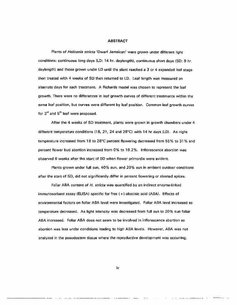
TABLE OF CONTENTS
ACKNOWLEDGEMENTS iii
ABSTRACT iv
LIST OF TABLES ix
LIST OF FIGURES x
LIST OF APPENDIX A: TABLES xiii
LIST OF APPENDIX B: FIGURES xxiii
LIST OF APPENDIX A: PROGRAMS xxiv
CHAPTER 1 INTRODUCTION 1
CHAPTER 2 LITERATURE REViEW 3
HELICONIA 3
ECOLOGy 3
TAXONOMY 3
MORPHOLOGy 4
RESEARCH 4
MODELS FOR GROWTH AND DEVELOPMENT 6
LEAF GROWTH 6
CHOICE OF GROWTH MODEL ~ 9
STARTING VALUES FOR FITTING RICHARDS MODEL. 10
BIOLOGICALLY RELEVANT PARAMETERS 11
COMPARING PARAMETERS ESTIMATES 12
ENVIRONMENTAL STRESS 13
WATER STRESS 13
CHILLING STRESS 14
HEAT STRESS 15
LIGHT STRESS 15
ABSCISIC ACiD 15
PHySiOLOGy 16
BIOCHEMiSTRy 17
v
---- --_._.... _... '---'--'---

CHAPTER 3 LEAF GROWTH MODEL OF HELICON/A 5TR/CTA 26
ABSTRACT 26
INTRODUCTION 26
MATERIALS AND METHODS 27
PLANT MATERIAL AND CULTURAL PRACTiCE 27
TREATMENT SETUP 27
DATA COLLECTION 28
STATISTICAL ANALySiS 29
RESULTS 32
PSEUDOSTEM STATUS 32
NUMBER OF LEAVES SUBTENDING THE INFLORESCENCE 32
FLOWERING 36
PLANT GROWTH 36
GROWTH MODEL 39
DiSCUSSiON 53
FLOWER INDUCTION PERIOD 53
FLOWERING 54
PLANT GROWTH 56
RICHARDS MODEL 56
HELICON/A 5TR/CTA 'DWARF JAMAICAN' FLOWERING PROGRAM 57
CHAPTER 4 EFFECT OF TEMPERATURE ON INFLORESCENCE DEVELOPMENT ANDABSCISIC ACID LEVELS IN H. STRICTA 58
ABSTRACT 58
INTRODUCTION 58
MATERIALS AND METHODS FOR INDIRECT ELISA PROCEDURE 60
PLANT MATERIALS 60
ABA EXTRACTION 61
ELISA MATERIALS 62
ELISA PROCEDURE 63
ELISA DATA PROCESSING 66
DETERMINING CONJUGATE CONCENTRATION 66
DETERMINING REPRODUCIBILITY OF THE ELISA OUTPUT 67
SPECIFICITY TEST 67
vi

PERCENT RECOVERY 67
MATERIALS AND METHODS FOR THE EXPERIMENT 68
PLANT MATERIALS 68
TREATMENT SETUP 69
DATA COLLECTION 69
SHOOT STATUS DETERMINATION 70
STATISTICAL ANALySiS 70
RESULTS FOR THE ELISA PROCEDURE 70
ASSAY SENSITIVITY AND PRECISION 70
SPECIFICITY 71
QUANTIFICATION OF ABA IN HELICONIA LEAF TISSUE 76
RESULTS FOR THE EXPERIMENT 76
ABA LEVELS BEFORE AND DURING SO 76
EFFECTS OF TEMPERATURE TREATMENTS COMBINEDOVER 4 TO 11WEEKS AFTER SO 76
EFFECT OF TEMPERATURE TREATMENTS AT DIFFERENTTIMES
OF DEVELOPMENT 81
TEMPERATURE AND FOLIAR ABA CONTENT MODEL. 84
SHOOT STATUS AT THE END OF THE EXPERIMENT 88
CHARACTERISTICS OF FLOWER BUD DEVELOPMENT 88
DiSCUSSiON 99
CONCLUSiON 101
CHAPTER 5 EFFECT OF LIGHT INTENSITY ON INFLORESCENCE ABORTION ANDABSCISIC ACID LEVELS IN H. STRICTA 102
ABSTRACT 102
INTRODUCTION 102
MATERIALS AND METHODS ; 103
PLANT MATERIAL AND CULTURAL PRACTICE 103
TREATMENTS SETUP 104
DATA COLLECTION 105
EXTRACTION AND DETERMINATION OF ABA LEVEL 106
STATISTICAL ANALySiS 106
vii
-_..._--- ---- ....__ . .- .- -- .__._-----•. _----------_.. -_. - --

RESULTS 106
ABA LEVELS DURING SO 106
EFFECT OF SHADINGS FOLLOWING SO 106
SHOOT STATUS AT THE END OF THE EXPERIMENT 111
FLOWERING PARAMETERS 111
DiSCUSSiON 114
CHAPTER 6 CONCLUSiON 11 7
PLANT GROWTH 117
LEAF LENGTH 11 7
FLOWER INITIATION 118
FLOWER DEVELOPMENT 118
TEMPERATURE 118
LIGHT 118
INFLORESCENCE ABORTION 119
TEMPERATURE 119
LIGHT 119
FOLIAR ABA LEVELS 119
PROGRAM FOR THE PRODUCTION OF FLOWERING H. STRICTA 120
APPENDIX A: TABLES 122
APPENDIX B: FIGURES 181
APPENDIX C: PROGRAMS 187
REFERENCES : 203
viii
LIST OF TABLES
1. Flowering status of H. stricta pseudostems under different daylengthtreatments 33
2. Production and lengths of H. stricta inflorescences under different daylength .treatments 34
3. Time from potting and from start of SO to inflorescence emergence andanthesis 37
4. Parameter estimates of growth models, additive and multiplicative errors 40
5. Student's t-values, as the ratios of the parameter estimates to their standarderrors 41
6. Lack of fit analysis for different models fitted to plants in trt. 1 and trt. 2 41
7. Parameter estimates of Richards function on leaf length and time after leafemergence of different daylength treatments from the 2nd leaf to thes" leaf 44
8. Parameter estimates of Richards function on leaf length and time after leafemergence of different daylength treatments of each pseudostem status fromthe 4 th leaf to the 6th leaf 48
9. Parameter estimates for Richards model on relative leaf length and relativetime of different leaf position from the 3'd leaf to the 5th leaf 49
10. Parameter estimates of Richards function on leaf length and time after leafemergence of different leaf position from the 3'd leaf to the 5th leaf 49
11 . Inflorescence and pseudostem length under different light intensitytreatments 112
ix

LIST OF FIGURES
1. ABA structures 18
2. Synthesis of ABA-serum albumin conjugates, ABA-c-1-HSA andABA-c-4'-BSA 22
3. Indirect ELISA. Antibody binds to antigen (ABA-BSA) in the solid phase andis subsequently detected by the color which develops when an enzyme-labeled antibody binds to the complex 23
4. The percentage of all harvested Heliconia striate showing vegetative, abortedor flowering status in different treatments 35
5. Influence of daylength treatment and leaf position on leaf length of H. stricta........ 38
6. Influence of daylength treatment and leaf position on time from potting toleaf emergence of H. stricte 38
7. Influence of daylength treatment and leaf position on time frame betweensuccessive leaves, starting with the time for the appearance of leaf 3 afterthe emergence of leaf 2 42
8. Influence of daylength treatment and leaf position on rate of leaf unfoldingfrom leaf emergence to fully expanded in cm/day of H. stricta 42
9. Raw data plot of length of individual leaves in sample plants H. stricta grownunder different treatment 45
10. Richards curves fitted to the length of individual leaves in H. stricta grownunder different treatment 46
11 . Richards curves fitted to the length of individual leaves in H. stricta grownunder different treatment 50
12. Richards curve fitted to relative leaf length and relative time of different leafposition from the 3rd leaf to the 5th leaf 51
13. Program for H. srticta 'Dwarf Jamaican' from potting until anthesis underconditions similar to the experiment 52
14. Flow chart of ELISA procedures 64
15. The effect of varying the coating concentration of the ELISA standard curvefor free +ABA. Microtitration plates coated with ABA-4'-TH-BSA conjugateat: a) 5 ,ug/ml; b) 10 ,ug/ml; c) 20,ug/mJ. After development the absorbanceat 405 nm was read after 60 min, 80 min, and 108 min 72
x
16. Standard curve for ELISA of free ABA displaying: a) average percent bindingand ABA concentration and b) LOGIT and ABA concentration both wereconstructed from n = 8 consecutive assays to show day-to-dayreproducibility..•................•..............•...•........•..................•............................ 73
17. Parallelism of Heliconia stricta leaf extract dilution curves and ABA standardcurves as determined by ELISA••.••........•.••.••..............•...........•........................ 74
18. Parallelism of Heliconia stricta shoot apex extract dilution curves and ABAstandard curves as determined by ELISA. . 75
19. Leaf ABA levels of Heliconia stricta at different stages of growth and differenttemperature conditions 77
20. Concentration of ABA in leaf tissue from Heliconia stricta pseudostemspooled across all temperatures during 4 to 11 weeks after start of SO 79
21. Effect of average daily temperatures on leaf ABA levels averaged over allgrowth stages for 4 to 11 weeks after start of SO 79
22. Effect of temperatures during a period 4 to 11 weeks after the start of SO onpercentage of pseudostems: showing vegetative, elongated, flowering oraborted pseudostem 80
23. Leaf ABA levels of Heliconia stricta pseudostems with different number ofexpanded leaves 80
24. Leaf ABA levels and percentage of pseudostems (bars) showing vegetative,elongated, flowering or aborted. at different time period in weeks after startof short day (8 hr.) with different numbers of expanded leaves at start ofshort day , , , 82
25. Leaf ABA levels and percentage of pseudostems showing vegetative,elongated, flowering or aborted. at different time period in weeks after startof short day (8 hr.) with different numbers of expanded leaves at the timesamples were taken , 83
.26. Leaf ABA levels and percentage of pseudostems showing vegetative,elongated, flowering or aborted at different time period in weeks after start ofshort day (8 hr.) in each temperature treatment 85
27. Concentration of ABA in leaf tissue from Heliconia stricta pseudostems atdifferent average daily temperatures during 4 to 11 weeks after start of SO 86
28. The comparison of leaf ABA level responses of Heliconia stricta under18-21 °C and 24-28°C 87
xi
29. Apical longitudinal section of H. stricta 'Dwarf Jamaican' treated with aninitial floral induction stimulus of 4 weeks of SO at different stages ofdevelopment 89
30. Apical longitudinal section of H. stricta 'Dwarf Jamaican' treated with fourtemperatures under 14 hr daylength after an initial floral induction stimulus of4 weeks of SO at different stages of development 91
31. Apical longitudinal section of H. striate 'Dwarf Jamaican' treated with fourtemperatures under 14 hr daylength after an initial floral induction stimulus of4 weeks of SO at different stages of development 93
32. Apical longitudinal section of H. stricta 'Dwarf Jamaican' treated with fourtemperatures under 14 hr daylength after an initial floral induction stimulus of4 weeks of SO at different stages of development 95
33. Apical longitudinal section of H. stricta 'Dwarf Jamaican' treated with fourtemperatures under 14 hr daylength after an initial floral induction stimulus of4 weeks of SO showing various stages of flower bud abortion 97
34. Effect of shading on leaf ABA levels 108
35. Effect of shading on percentage of pseudostems showing vegetative,flowering or aborted apices 8-11 weeks after the start of SO 108
36. Concentration of ABA in leaf tissue from vegetative, flowering, or abortedH. stricta pseudostems apices based on average of stems sampled over 4 to11 weeks after start of SO 109
37. Leaf ABA levels of most recently matured leaf of H. stricta pseudostem withdifferent number of expanded leaves based on average of stems sampledover 4 to 11 weeks after start of SO 109
38. Percentage of pseudosterns showing vegetative, elongated, flowering, oraborted apices and leaf ABA level at the time samples were taken after thestart of SO 110
39. Effect of shading on percentage of pseudostems showing vegetative,flowering, or aborted apices at time of experiment termination 110
40. Effect of leaf number at the start of SO on number of leaves subtendinginflorescence 113
xii
-------- --- ._--_._-_._--
LIST OF APPENDIX A: TABLES
1. ANOVA Effect of daylength treatments on number of leaves subtendinginflorescence of H. stricta 122
2. ANOVA Effect of daylength treatments on length of the last leaf subtendinginflorescence of H. stricta 122
3. ANOVA Effect of daylength treatments on number cincinnal bracts ofH. stricta 122
4. ANOVA Effect of daylength treatments on length of peduncle of H. stricta......... 122
5. ANOVA Effect of daylength treatments on length of inflorescence ofH. stricta 123
6. ANOVA Effect of daylength treatments on length of inflorescence andpeduncle combined of H. stricta 123
7. ANOVA Effect of daylength treatments on number of days to from potting tolast leaf emergence of H. stricta 123
8. ANOVA Effect of daylength treatments on number of days from time of lastleaf emergence to inflorescence emergence of H. stricta 123
9. ANOVA Effect of daylength treatments on number of days to from time ofinflorescence emergence to anthesis of H. stricta 124
10. ANOVA Effect of daylength treatments on number of days to anthesis frompotting of H. stricta 124
11. ANOVA Effect of daylength treatments on number of days to inflorescenceemergence from started of SO treatments of H. stricta 124
12. ANOVA Effect of daylength treatments on number of days to anthesis from-started of SO treatments of H. stricta 124
13. ANOCOVA Effect of daylength treatments and leaf position on leaf length ofH. stricta 125
14. ANOCOVA Effect of daylength treatments and leaf position on days frompotting to leaf emergence of H. stricta 125
15. ANOCOVA Effect of daylength treatments and leaf position on days toproduce each leaf from time of previous leaf emergence of H. stricta 125
16. ANOCOVA Effect of daylength treatments and leaf position on leaf unfoldingrate (em/day) of H. stricta 126
xiii
- ----- ------ - - -------- -

17. Nonlinear regression for least-squares estimates of parameters of Richardsfunction for length of 2nd leaf of Heliconia stricta in conLD as a dependentvariable and time after leaf emergence as an independent variable 126
18. Nonlinear regression for least-squares estimates of parameters of Richardsfunction for length of 2nd leaf of Heliconia stricta in 3L-SD as a dependentvariable and time after leaf emergence as an independent variable 127
19. Nonlinear regression for least-squares estimates of parameters of Richardsfunction for length of 2nd leaf of Heliconia stricta in 4L-SD as a dependentvariable and time after leaf emergence as an independent variable 127
20. Nonlinear regression for least-squares estimates of parameters of Richardsfunction for length of 2nd leaf of Heliconia stricta in conSD as a dependentvariable and time after leaf emergence as an independent variable 128
21. Nonlinear regression for least-squares estimates of parameters of Richardsfunction for length of 3rd leaf of Heliconia stricta in conLD as a dependentvariable and time after leaf emergence as an independent variable 128
22. Nonlinear regression for least-squares estimates of parameters of Richardsfunction for length of 3rd leaf of Heliconia stricta in 3L-SD as a dependentvariable and time after leaf emergence as an independent variable 129
23. Nonlinear regression for least-squares estimates of parameters of Richardsfunction for length of 3rd leaf of Heliconia stricta in 4L-SO as a dependentvariable and time after leaf emergence as an independent variable 129
24. Nonlinear regression for least-squares estimates of parameters of Richardsfunction for length of 3rd leaf of Heliconia stricta in conSO as a dependentvariable and time after leaf emergence as an independent variable 130
25. Nonlinear regression for least-squares estimates of parameters of Richardsfunction for length of 4th leaf of Heliconia stricta in conLO as a dependentvariable and time after leaf emergence as an independent variable 130
26. Nonlinear regression for least-squares estimates of parameters of Richardsfunction for length of 4th leaf of Heliconia stricta in 3L-SO as a dependentvariable and time after leaf emergence as an independent variable 131
27. Nonlinear regression for least-squares estimates of parameters of Richardsfunction for length of 4th leaf of Heliconia stricta in 4L-SO as a dependentvariable and time after leaf emergence as an independent variable 131
28. Nonlinear regression for least-squares estimates of parameters of Richardsfunction for length of 4th leaf of Heliconia stricta in conSO as a dependentvariable and time after leaf emergence as an independent variable 132
xiv

29. Nonlinear regression for least-squares estimates of parameters of Richardsfunction for length of 5th leaf of Heliconia stricta in conLD as a dependentvariable and time after leaf emergence as an independent variable 132
30. Nonlinear regression for least-squares estimates of parameters of Richardsfunction for length of 5th leaf of Heliconia stricta in 3L-SD as a dependentvariable and time after leaf emergence as an independent variable 133
31 . Nonlinear regression for least-squares estimates of parameters of Richardsfunction for length of 5th leaf of Heliconia stricta in 4L-SD as a dependentvariable and time after leaf emergence as an independent variable 133
32. Nonlinear regression for least-squares estimates of parameters of Richardsfunction for length of 5th leaf of Heliconia stricta in conSD as a dependentvariable and time after leaf emergence as an independent variable 134
33. Nonlinear regression for least-squares estimates of parameters of Richardsfunction for length of 6th leaf of Heliconia stricta in conLD as a dependentvariable and time after leaf emergence as an independent variable 134
34. Nonlinear regression for least-squares estimates of parameters of Richardsfunction for length of 6th leaf of Heliconia stricta in 3L-SD as a dependentvariable and time after leaf emergence as an independent variable 135
35. Nonlinear regression for least-squares estimates of parameters of Richardsfunction for length of 6th leaf of Heliconia stricta in 4L-SD as a dependentvariable and time after leaf emergence as an independent variable 135
36. Nonlinear regression for least-squares estimates of parameters of Richardsfunction for length of 6th leaf of Heliconia stricta in conSD as a dependentvariable and time after leaf emergence as an independent variable 136
37. RSS from fitting the 2nd leaf data of Heliconia on each treatment withcommon c, ~, 1, and 0 136
38. RSS from fitting the 3rd leaf data of Heliconia on each treatment withcommon «. ~, 1, and 0 136
39. RSS from fitting the 4th leaf data of Heliconia on each treatment withcommon u, ~, 1, and 0 137
40. RSS from fitting the 5th leaf data of Heliconia on each treatment withcommon a, ~, 1, and 0 137
41 . RSS from fitting the 6th leaf data of Heliconia on each treatment withcommon c, ~, 1, and 0.•.. .. .. .. . .. . .. . . . .. . ... .. . . .. ... .. .. ... .. .. .. .. .. . .. .. .. .. . . . .. .. . . . . ... . .. .. . . . 137
42. Comparison of fits for Heliconia 2nd leaf data to test invariance of a, ~, 1 and/) for conLD and 3L-SD 138
xv

43. Comparison of fits for Heliconia 2nd leaf data to test invariance of Ct., ~, Y and5 for conLO and 4L-SO 138
44. Comparison of fits for Heliconia 2nd leaf data to test invariance of c, ~, Y and5 for conLO and conSO 139
45. Comparison of fits for Heliconia 2nd leaf data to test invariance of Ct., ~, Y and5 for 3L-SO and 4L-SO 139
46. Comparison of fits for Heliconia 2nd leaf data to test invariance of c, ~, Y and5 for 3L-SO and canSO 140
47. Comparison of fits for Heliconia 2nd leaf data to test invariance of c. ~, Y and5 for 4L-SO and conSO 140
48. Comparison of fits for Heliconia 3th leaf data to test invariance of Ct., ~, Y and5 for conLO and 3L-SO 141
49. Comparison of fits for Heliconia 3th leaf data to test invariance of c, ~, Y and5 for conLO and 4L-SO 141
50. Comparison of fits for Heliconia 3th leaf data to test invariance of Ct., ~, Y and5 for conLO and conSO 142
51 . Comparison of fits for Heliconia 3th leaf data to test invariance of e, ~, Y and5 for 3L-SO and 4L-SO 142
52. Comparison of fits for Heliconia 3th leaf data to test invariance of c, ~, Yand5 for 3L-SO and conSO 143
53. Comparison of fits for Heliconia 3th leaf data to test invariance of c, ~, Y and5 for 4L-SO and conSO 143
54. Comparison of fits for Heliconia 4th leaf data to test invariance of Ct., ~, Yand5 for conLO and 3L-SO 144
55. Comparison of fits for Heliconia 4th leaf data to test invariance of Ct., ~, Yand5 for conLO and 4L-SO 144
56. Comparison of fits for Heliconia 4th leaf data to test invariance of a, ~, Y and5 for conLO and conSO 145
57. Comparison of fits for Heliconia 4th leaf data to test invariance of Ct., ~, Yand5 for 3L-SO and 4L-SO 145
58. Comparison of fits for Heliconia 4th leaf data to test invariance of c, ~, Y and5 for 3L-SO and canSO 146
xvi
--.-- ---- ----- ---

59. Comparison of fits for Heliconia 4th leaf data to test invariance of a, 13, yandofor 4L-SO and conSO 146
60. Comparison of fits for Heliconia 5th leaf data to test invariance of a, 13, y andofor conLO and 3L-SO 147
61. Comparison of fits for Heliconia 5th leaf data to test invariance of a, 13, y andofor conLO and 4L-SO 147
62. Comparison of fits for Heliconia 5th leaf data to test invariance of a, 13, y andofor conLO and conSO 148
63. Comparison of fits for Heliconia 5th leaf data to test invariance of a, 13, y andofor 3L-SO and 4L-SO 148
64. Comparison of fits for Heliconia 5th leaf data to test invariance of a, 13, y andofor 3L-SO and conSO 149
65. Comparison of fits for Heliconia 5th leaf data to test invariance of a, 13, y andofor 4L-SO and conSO 149
66. Comparison of fits for Heliconia 6th leaf data to test invariance of a, 13, y andofor conLO and 3L-SO 150
67. Comparison of fits for Heliconia 6th leaf data to test invariance of a, 13, y andofor conLO and 4L-SO 150
68. Comparison of fits for Heliconia 6th leaf data to test invariance of a, 13, y andofor conLD and conSO 151
69. Comparison of fits for Heliconia 6th leaf data to test invariance of a, 13, y andofor 3L-SO and 4L-SO 151
70. -Comparison of fits for Heliconia 6th leaf data to test invariance of a, 13, y andofor 3L-SO and conSO 152
71. Comparison of fits for Heliconia 6th leaf data to test invariance of a, 13, y andofor 4L-SO and conSO 152
72. Nonlinear regression for least-squares estimates of parameters of Richardsfunction for length of 4th leaf of non flowered Heliconia stricta in conLO as adependent variable and time after leaf emergence as an independent variable ...... 153
73. Nonlinear regression for least-squares estimates of parameters of Richardsfunction for length of 4th leaf of flowered Heliconia stricta in 3L-SO as adependent variable and time after leaf emergence as an independent variable ...... 153
xvii
--_. -- ---- ------------

74. Nonlinear regression for least-squares estimates of parameters of Richardsfunction for length of 4th leaf of flowered Heliconia stricta in 4L-SD as adependent variable and time after leaf emergence as an independent variable 154
75. Nonlinear regression for least-squares estimates of parameters of Richardsfunction for length of 4th leaf of flowered Heliconia stricta in conSD as adependent variable and time after leaf emergence as an independent variable ...... 154
76. Nonlinear regression for least-squares estimates of parameters of Richardsfunction for length of 5th leaf of non flowered Heliconia stricta in conLD as adependent variable and time after leaf emergence as an independent variable ...... 155
77. Nonlinear regression for least-squares estimates of parameters of Richardsfunction for length of 5th leaf of flowered Heliconia stricta in 3L-SD as adependent variable and time after leaf emergence as an independent variable ...... 155
78. Nonlinear regression for least-squares estimates of parameters of Richardsfunction for length of 5th leaf of flowered Heliconia stricta in 4L-SD as adependent variable and time after leaf emergence as an independent variable ...... 156
79. Nonlinear regression for least-squares estimates of parameters of Richardsfunction for length of 5th leaf of flowered Heliconia stricta in conSD as adependent variable and time after leaf emergence as an independent variable ...... 156
80. Nonlinear regression for least-squares estimates of parameters of Richardsfunction for length of 6th leaf of non flowered Heliconia stricta in conLD as adependent variable and time after leaf emergence as an independent variable...... 157
81. Nonlinear regression for least-squares estimates of parameters of Richardsfunction for length of 6th leaf of flowered Heliconia stricta in 3L-SD as adependent variable and time after leaf emergence as an independent variable ...... 157
82. Nonlinear regression for least-squares estimates of parameters of Richardsfunction for length of 6th leaf of flowered Heliconia stricta in 4L-SD as adependent variable and time after leaf emergence as an independent variable ...... 158
83. Nonlinear regression for least-squares estimates of parameters of Richardsfunction for length of 6th leaf of flowered Heliconia stricta in conSD as adependent variable and time after leaf emergence as an independent variable ...... 158
84. RSS from fitting the 4th leaf data of Heliconia on each treatment andpseudostem status with common a, ~, y and 8 159
85. RSS from fitting the 5th leaf data of Heliconia on each treatment andpseudostem status with common a, ~, y and 8 159
86. RSS from fitting the 6th leaf data of Heliconia on each treatment andpseudostem status with common a, ~, y and 8 159
xviii
----- -_. -_. ----- -- ------~.-
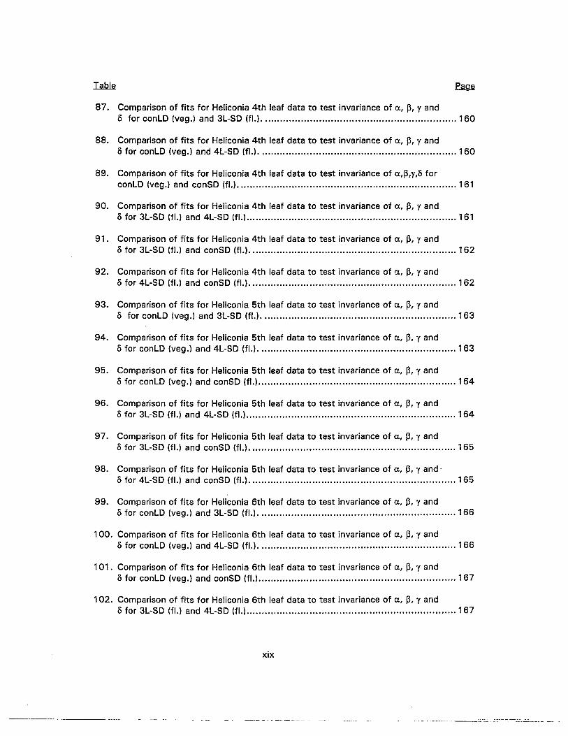
87. Comparison of fits for Heliconia 4th leaf data to test invariance of a, ~, y ando for conLD (veg.) and 3L-SD (fl.) 160
88. Comparison of fits for Heliconia 4th leaf data to test invariance of a, ~, y ando for conLD (vag.) and 4L-SD (fl.) 160
89. Comparison of fits for Heliconia 4th leaf data to test invariance of a,13,y,o forconLD (veg.) and conSD (fl.) ....•....•.....•..•....................•....•............................ 161
90. Comparison of fits for Heliconia 4th leaf data to test invariance of a, ~, y ando for 3L-SD (fl.) and 4L-SD (fl.) 161
91. Comparison of fits for Heliconia 4th leaf data to test invariance of a, ~, y ando for 3L-SD (fl.) and conSD (fl.) .....•................•..............•...•........•........•......... 162
92. Comparison of fits for Heliconia 4th leaf data to test invariance of a, ~, y ando for 4L-SD (fl.) and conSD (fl.) 162
93. Comparison of fits for Heliconia 5th leaf data to test invariance of a, 13, y ando for conLD (veg.) and 3L-SD (fl.) 163
94. Comparison of fits for Heliconia 5th leaf data to test invariance of a, 13, y ando for conLD (veg.) and 4L-SD (fl.) 163
95. Comparison of fits for Heliconia 5th leaf data to test invariance of a, 13, yando for conLD (veg.) and conSO (fl.) 164
96. Comparison of fits for Heliconia 5th leaf data to test invariance of a, 13, y andofor 3L-SD (fl.) and 4L-SD (fl.) 164
97. Comparison of fits for Heliconia 5th leaf data to test invariance of a, 13, y ando for 3L-SD (fl.) and conSD (fl.) 165
98. Comparison of fits for Heliconia 5th leaf data to test invariance of a, 13, y and,o for 4L-SD (fl.) and conSD (fl.) 165
99. Comparison of fits for Heliconia 6th leaf data to test invariance of a, 13, y ando for conLD (veg.) and 3L-SO (fl.) 166
100. Comparison of fits for Heliconia 6th leaf data to test invariance of a, 13, y ando for conLD (veg.) and 4L-SO (fl.) 166
101. Comparison of fits for Heliconia 6th leaf data to test invariance of a, 13, y ando for conLD (veg.) and conSO (fl.) 167
102. Comparison of fits for Heliconia 6th leaf data to test invariance of a, 13, y ando for 3L-SD (fl.) and 4L-SD (fl.) 167
xix
... _--_.---- .._----_ ..------- -- -+------ - -
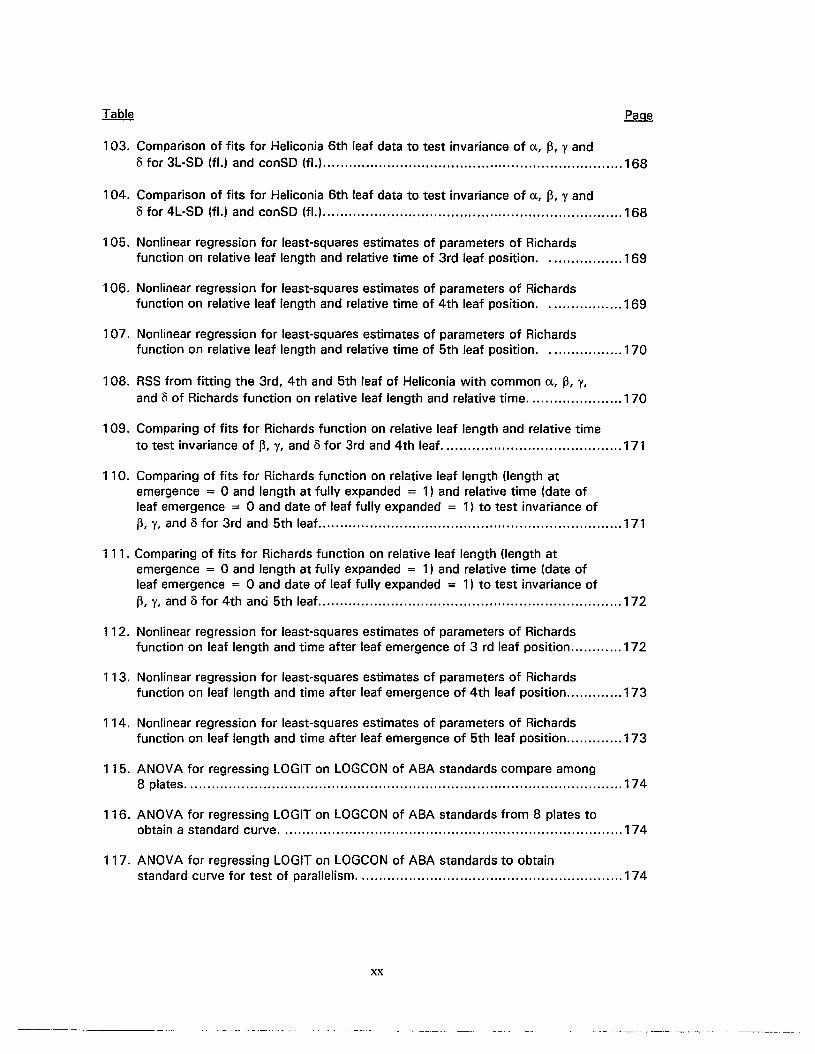
103. Comparison of fits for Heliconia 6th leaf data to test invariance of (J." p, ¥ andofor 3L-SO (fl.) and conSO (fl.) 168
104. Comparison of fits for Heliconia 6th leaf data to test invariance of (J." p, ¥ andofor 4L-SO (fl.) and conSO (fl.) 168
105. Nonlinear regression for least-squares estimates of parameters of Richardsfunction on relative leaf length and relative time of 3rd leaf position. . 169
106. Nonlinear regression for least-squares estimates of parameters of Richardsfunction on relative leaf length and relative time of 4th leaf position. . 169
107. Nonlinear regression for least-squares estimates of parameters of Richardsfunction on relative leaf length and relative time of 5th leaf position. . 170
108. RSS from fitting the 3rd, 4th and 5th leaf of Heliconia with common (J." p, t.and 0 of Richards function on relative leaf length and relative time 170
109. Comparing of fits for Richards function on relative leaf length and relative timeto test invariance of p, ¥, and 0 for 3rd and 4th leaf 171
110. Comparing of fits for Richards function on relative leaf length (length atemergence = 0 and length at fully expanded = 1) and relative time (date ofleaf emergence = 0 and date of leaf fully expanded = 1) to test invariance ofp, t, and 0 for 3rd and 5th leaf 171
111 . Comparing of fits for Richards function on relative leaf length (length atemergence = 0 and length at fully expanded = 1) and relative time (date ofleaf emergence = 0 and date of leaf fully expanded = 1) to test invariance ofp, ¥, and 0 for 4th anc.i 5th leaf 172
112. Nonlinear regression for least-squares estimates of parameters of Richardsfunction on leaf length and time after leaf emergence of 3 rd leaf position 172
113. Nonlinear regression for least-squares estimates of parameters of Richardsfunction on leaf length and time after leaf emergence of 4th leaf position 173
114. Nonlinear regression for least-squares estimates of parameters of Richardsfunction on leaf length and time after leaf emergence of 5th leaf position 173
115. ANOVA for regressing LOGIT on LOGCON of ABA standards compare among8 plates 174
116. ANOVA for regressing LOGIT on LOGCON of ABA standards from 8 plates toobtain a standard curve 174
117. ANOVA for regressing LOGIT on LOGCON of ABA standards to obtainstandard curve for test of parallelism 174
xx
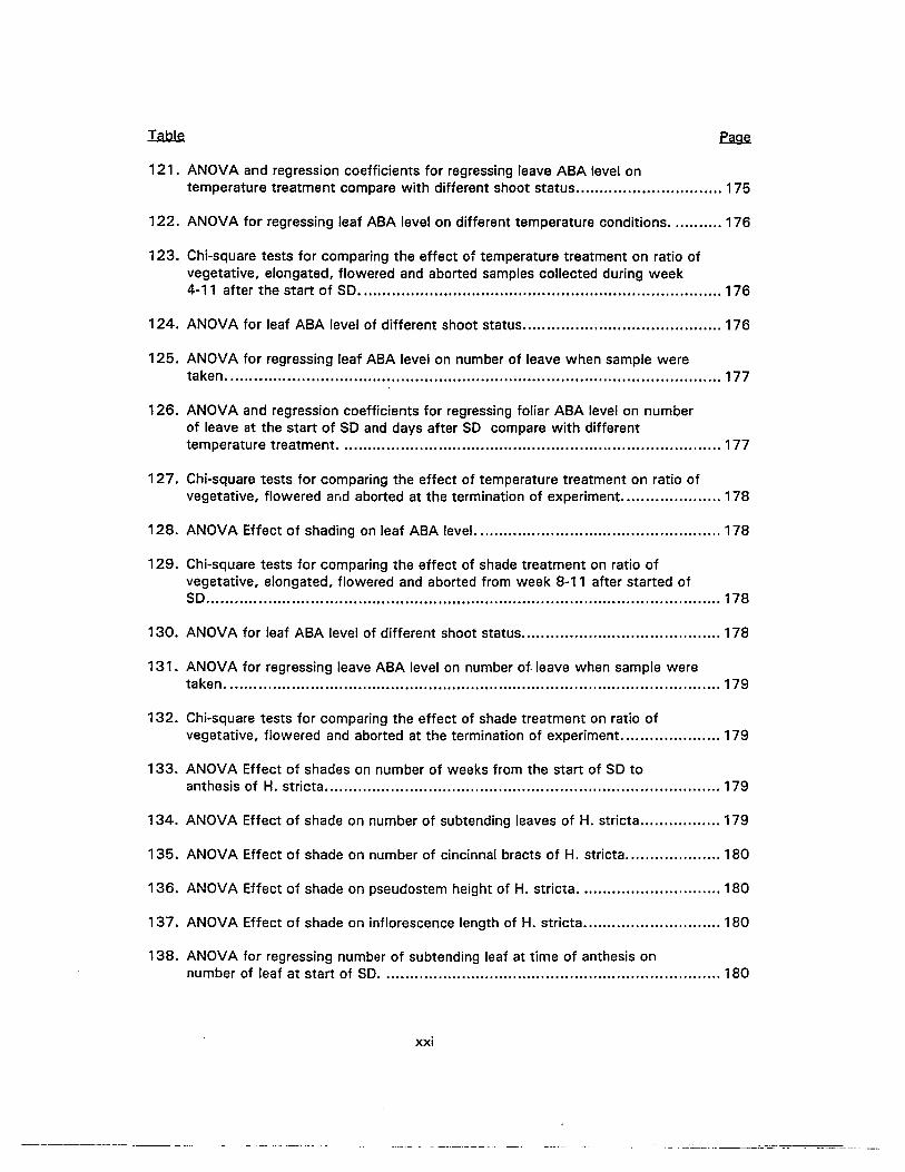
121. ANOVA and regression coefficients for regressing leave ABA level ontemperature treatment compare with different shoot status 175
122. ANOVA for regressing leaf ABA level on different temperature conditions 176
123. Chi-square tests for comparing the effect of temperature treatment on ratio ofvegetative, elongated, flowered and aborted samples collected during week4-11 after the start of SO 176
124. ANOVA for leaf ABA level of different shoot status 176
125. ANOVA for regressing leaf ABA level on number of leave when sample weretaken 177
126. ANOVA and regression coefficients for regressing foliar ABA level on numberof leave at the start of SO and days after SO compare with differenttemperature treatment 177
127. Chi-square tests for comparing the effect of temperature treatment on ratio ofvegetative, flowered and aborted at the termination of experiment 178
128. ANOVA Effect of shading on leaf ABA level 178
129. Chi-square tests for comparing the effect of shade treatment on ratio ofvegetative, elongated, flowered and aborted from week 8-11 after started ofSO 178
130. ANOVA for leaf ABA level of different shoot status 178
131. ANOVA for regressing leave ABA level on number of. leave when sample weretaken 179
132. Chi-square tests for comparing the effect of shade treatment on ratio ofvegetative, flowered and aborted at the termination of experiment 179
133. ANOVA Effect of shades on number of weeks from the start of SO toanthesis of H. stricta 179
134. ANOVA Effect of shade on number of subtending leaves of H. stricta 179
135. ANOVA Effect of shade on number of cincinnal bracts of H. stricta 180
136. ANOVA Effect of shade on pseudostem height of H. stricta 180
137. ANOVA Effect of shade on inflorescence length of H. stricta 180
138. ANOVA for regressing number of subtending leaf at time of anthesis onnumber of leaf at start of SO 180
xxi

136. ANOVA Effect of shade on pseudostem height of H. stncta 180
137. ANOVA Effect of shade on inflorescence length of H. stricta 180
138. ANOVA for regressing number of subtending leaf at time of anthesis onnumber of leaf at start of SO 180
139. ANOVA for regressing time from SO to anthesis on number of leaf at start ofSO 180
xxii

LIST OF APPENDIX B: FIGURES
1. Daily maximum, minimum and average temperatures in °C at the inside ofMagoon greenhouse facility of the University of Hawaii during 1988-1989 181
2. Daily maximum photosynthetically active radiation (PAR) in pmol/sec./sq.m.at the inside of Magoon greenhouse facility of the University of Hawaii during1988-1989 182
3. Hourly average photosynthetically active radiation (PAR) in pmollsec./sq.m. infull sun, 40% sun and 20% sun at the Magoon greenhouse facility of theUniversity of Hawaii 1991 183
4. Daily maximum, minimum and average temperature in °C in full sun, 40%sun and 20% sun at the Magoon greenhouse facility of the University ofHawaii 1991 184
5. Daily maximum photosynthetically active radiation (PAR) in pmol/sec./sq.m. infull sun, 40% sun and 20% sun at the Magoon greenhouse facility of theUniversity of Hawaii 1991 185
6. Daily average total photosynthetically active radiation (PAR) inpmol/sec./sq.m. in full sun, 40% sun and 20% sun at the Magoongreenhouse facility of the University of Hawaii 1991 186
xxiii
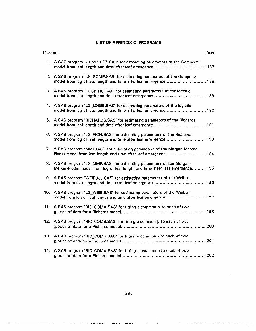
LIST OF APPENDIX C: PROGRAMS
Program
1. A SAS program 'GOMPERTZ.SAS' for estimating parameters of the Gompertzmodel from leaf length and time after leaf emergence 187
2. A SAS program 'LG_GOMP.SAS' for estimating parameters of the Gompertzmodel from log of leaf length and time after leaf emergence 188
3. A SAS program 'LOGISTIC.SAS' for estimating parameters of the logisticmodel from leaf length and time after leaf emergence 189
4. A SAS program 'LG_LOGIS.SAS' for estimating parameters of the logisticmodel from log of leaf length and time after leaf emergence 190
5. A SAS program 'RICHARDS.SAS' for estimating parameters of the Richa~ds
model from leaf length and time after leaf emergence 191
6. A SAS program 'LG_RICH.SAS' for estimating parameters of the Richardsmodel from log of leaf length and time after leaf emergence 193
7. A SAS program 'MMF.SAS' for estimating parameters of the Morgan-Mercer-Flodin model from leaf length and time after leaf emergence 194
8. A SAS program 'LG_MMF.SAS' for estimating parameters of the Morgan-Mercer-Flodin model from log of leaf length and time after leaf emergence 195
9. A SAS program 'WEIBULLSAS' for estimating parameters of the Weibullmodel from leaf length and time after leaf emergence 196
10. A SAS program 'LG_WEIB.SAS· for estimating parameters of the Weibullmodel from log of leaf length and time after leaf emergence 197
11. A SAS program 'RIC_COMA,SAS' for fitting a common a to each of twogroups of data for a Richards model : 198
12. A SAS program 'RIC_COMB.SAS' for fitting a common f3 to each of twogroups of data for a Richards model.. 200
13. A SAS program 'RIC_COMK.SAS' for fitting a common y to each of twogroups of data for a Richards model. 201
14. A SAS program 'RIC_COMV.SAS' for fitting a common 0 to each of twogroups of data for a Richards model. 202
xxiv
CHAPTER 1
INTRODUCTION
Heliconia is a rather new cut-flower crop that has been introduced to tropic regions
around the world during the past 10 years. However, there have been only a few
horticultural studies of these plants. Research on Heliconia stricta 'Dwarf Jamaican' has
been conducted at the University of Hawaii for almost 10 years partly because of its
compactness and manageability. Moreover, it can be grown for pot plant as well as cut
flower use. H. stricta 'Dwarf Jamaican' showed a seasonal flowering pattern with
production higher in winter than in summer and was found to require a minimum of 4
weeks of short day (SO) for flower initiation (Criley and Kawabata, 1986). Only plants that
had 3 or more leaves were susceptible to the initial stimulus. Plants with 4 initial leaves
reached anthesis approximately 13 weeks after start of SO (Criley and Kawabata, 1986).
Further experiments showed that decreasing night temperature during 4 weeks of SO from
25°C to 15°C increased the flowering percentage of pseudostems from 15.5% to 57.6%
(Lekawatana, 1986). It was observed that pseudostems that did not flower were either in
a vegetative phase or their inflorescences had been aborted.
Aborted pseudostems cause losses in flower production since each pseudostem is
capable of producing only one inflorescence. This is not a problem in species that flower
year-round such as H. psittacorum which has a high flowering percentage and multiplies
very quickly. However, with species that flower seasonally and usually produce better
quality inflorescences, such as H. stricta 'Dwarf Jamaican', H. angusta 'Holiday', and H.
wagneriana, this problem of flower bud abortion is quite severe for cut flower production.
If the percentage of flower bud abortion for these species can be reduced, there is a good

chance of retaining their existence as a cut flower crop because the market for cut flowers
requires a stable supply (Criley and Lekawatana, 1994).
The research reported in this dissertation was undertaken to develop a better
understanding of the environmental factors influencing flowering in H. stricta I Dwarf
Jamaican'; to continue studies on the physiological basis for flower initiation, development
and abortion; and to determine if a relationship existed between abscisic acid (ABA)
production in mature leaves and flower bud abortion.
The ultimate goal of this work is control of flower production to ensure a steady
supply of cut heliconia flowers for the flower market of the world. H. stricta has served as
the model plant for these studies, but it is hoped that the information gained in its study
can be generaiized to other important cut flower heliconia species.
2

CHAPTER 2
LITERATURE REVIEW
HELICONIA
Heliconias have been popular conservatory plants, and interior plantscapers have
begun to use them in containers and interior plantings. Recently, the cut flower market for
Heliconias has expanded with much interest expressed by commercial growers in tropical
area seeking crops for export. The intense interest in new potted flowering plants has also
led to the development of heliconia as potted plants (Criley, 1991).
ECOLOGY
Most Heliconia species are found in the New World tropic from the Tropic of Cancer
in Mexico and the Caribbean islands to the Tropic of Capricorn in South America. Only six
species are found in the Pacific island tropics. Heliconia attain their most vigorous growth
in the humid lowland tropics at elevations below 500 meters. Many species are found in
middle elevation rain and cloud-forest habitats. Few species are found above 2,000 meters
(Kress, 1984; Criley and Broschat, 1992).
TAXONOMY
Heliconia is a monotypic genus that is estimated to consist of 200-250 species
(Berry and Kress, 1991). The taxa within the order Zingiberales have been debated for a
long time, but the heliconias long were placed with the Musa complex (Criley and Broschat,
1992). Nakai (1941) suggested that the Heliconiaceae was distinct from the Musaceae,
and recent studies and publications also accepted this classification (Tomlinson, 1962;
Dahlgren and Clifford, 1982; Kress, 1984; Dahlgren et et., 1985).
3

MORPHOLOGY
Heliconias are rhizomatous, perennial herbs with an erect, aerial, and stem-like tube
called a pseudostem composed of overlapping leaf sheaths. The rhizome branches
sympodially from buds at the base of the pseudostem. Leaves are alternately arranged and
distichous (Berry and Kress, 1991; Criley and Broschat, 1992). A pseudostem is often
composed of a specific and limited number of 5-9 leaves which may be influenced by
cultural and environmental conditions (Criley and Broschat, 1992). Leaf blades are usually
green; with some species they are tinted maroon or red underneath especially along the
margin and midrib (Berry and Kress, 1991). The leaf apex is acute to acuminate with the
base of the lamina unequal and usually obtuse to truncate (CrUey and Broschat, 1992). The
colorful inflorescence structure is the main attraction of Heliconia for ornamental and cut
flower purposes. The inflorescence has either an erect or pendent orientation and is made
up of peduncle, modified leaflike structures called inflorescence bracts (cincinnal bracts),
the rachis, and a coil of flowers within each bract. The inflorescence bracts are usually red,
yellow, or both, but are sometimes green or pink in some species. Each inflorescence bract
contains a varying number of flowers, up to 50 depending on the species. The perianth is
made up of three outer sepals and three inner petals united at the base and to each other in
various ways. The flowers are bisexual, epigynous and strongly zygomorphic. There are
five functional stamens and one staminode which is subulate or, to some degree, petaloid.
The overy is inferior and 3-locular. Fruits of the New World species are blue in color while
those of Pacific tropical species are red when mature.
RESEARCH
It was not until recently that Heliconia was grown commercially for cut flowers.
Therefore, the basic knowledge of these plants is limited. However, there were some
4

studies with H. psittacorum, H. stricta, H. chartacea and H. wagneriana done in Hawaii and
in Florida.
Increased nitrogen fertilizer rate to H. psittacorum yielded more inflorescences
especially for plants grown in full sun compared to those under 60% shade (Broschat and
Donselman, 1982, 1983).
H. psittacorum, H. X nickeriensis, H. episcopalis, H. hirsuta, H. X'Golden Torch', H.
chartacea and some cultivars of H. stricta and H. bihai flower year-round and are considered
to be day-neutral. H. stricta 'Dwarf Jamaican', H. wagneriana, and H. aurantiaca have
been shown to initiate flowers under short days (Criley and Kawabata, 1986; Criley and
Broschat, 1992) with 4 weeks of short days required at 15°C for flower initiation in H.
stricta 'Dwarf Jamaican'. A minimum of 3 leaves must be present for this species to
respond to photoperiodic stimuli (Criley and Kawabata, 1986). Research on H. angusta
'Holiday' showed that flower initiation was induced by long days (minimum of 13 hr. for 7
weeks) (Lekawatana, 1986; Sakai et al., 1990; Kwon, 1992). A daylength requirement
was proposed in the flower development of H. chartacea since large number of flowers
were aborted from shoots that emerged from April to June (Criley and Lekawatana, 1994).
Temperature is a limiting factor in the production of H. psittacorum in Florida.
Growth and flower production declined as minimum temperature decreased from 21 to 1DOC
and ceased altogether at 1DOC (Broschat and Donselrnan, 1983).
Postharvest life for some H. psittacorum cultivars is about 14-17 days, while
flowers of other species often last less than one week (Criley and Broschat, 1992). H.
psittacorum showed no improvement in vase life with different floral preservatives.
However, the use of antitranspirants increased the vase life of H. psittacorum (Broschat,
1987).
Application of 2-(3,4-dichlorophenoxy)triamine (DCPTA) to H. stricta 'Dwarf
Jamaican' increased number of inflorescences under full sun compared to 5D% shade while
5
application of DCPTA to H. caribaea caused no increase in inflorescence production
(Broschat and Svenson, 1994).
Growth retardants were used to control plant height in potted heliconias.
Ancymidol was suggested for height control on H. stricta 'Dwarf Jamaican' (Lekawatana
and Criley, 1989). Paclobutrazol, ancymidol, and uniconazole effectively decreased plant
height of H. psittacorum making it suitable for potted plant use (Tjia and Jierwiriyapant,
1988; Broschat and Donselman,1988).
MODELS FOR GROWTH AND DEVELOPMENT
LEAF GROWTH
The simplest measure of size of an unfolding leaf often is its length. The
exponential relationships of leaf length, volume, area, weight, etc. with time continue until
after emergence from the enclosing sheaths and then decline, giving the S-shaped curves
characteristic of post-primordial growth (Dale and Milthrope, 1983).
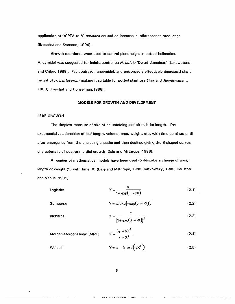
A number of mathematical models have been used to describe a change of area,
length or weight (Y) with time (X) (Dale and Milthrope, 1983; Ratkowsky, 1983; Causton
and Venus, 1981):
Logistic:
Gompertz:
Richards:
Morgan-Mercer-Flodin (MMF)
Weibull:
a.Y = ---:-----:-
1+ exp(~ -vx)
Y.= a..exp[-exp(p -yX))
a.Y - ------:"7"
- [1+exp(p -yx)f
py +a.Xo
Y= 0Y +X
Y = a. - 13 .exp(-yX13
)
6
(2.1 )
(2.2)
(2.3)
(2.4)
(2.5)
These growth rate curves start at some fixed point and increase monotonically to
reach an inflection point; after this the growth rate decreases to approach asymptotically
some final value (a). ~,y, and 0 are parameters (Ratkowsky, 1983; Causton and Venus,
1981 ).
Logistic Model
The logistic model has been used extensively in the field of animal ecology for
modeling the numbers of individuals within a population. In plant growth studies, the fact
that the model is S-shaped has rendered it very popular. The model has been applied to
many primary data such as single leaf growth, stem length, sugar content, flower number,
etc. in many species such as cucumber cotton, asparagus, wheat, grape, etc. (Hunt, 1982).
The logistic model, 2.1, is the best known sigmoid model with asymptotes at Y = 0
and Y = a. Of the other two model parameters, y is a 'rate' parameter - a high value
indicating a rapid rise of Y between the two asymptotes, and vice versa - and I3/y (~ divided
by y) defines the value of X at the point of inflection (Causton and Venus, 1981).
Gompertz Model
The Gompertz model, 2.2, devised by Benjamin Gompertz in 1825, from work with
animals and population studies, has three parameters arranged as a double exponent. The
majority of applications of the Gompertz model in plant growth analysis has been connected
with the modeling of the growth of individual organs, especially leaves (Hunt, 1-982).
The parameters have the same general meaning as in the logistic model. The
asymptotes are again at Y = 0 and Y = a, but the value of Y at the point of inflection is
ale instead of a/2 (Causton and Venus, 1981). Amer and William (1957) considered that
the asymmetry of the Gompertz model was more appropriate to leaf growth data than the
symmetry of the logistic model.
7

Richards Model
The Richards model, 2.3, (Richards, 1959) was first derived from one developed by
Von Bertalanffy which was based on theoretical considerations of animal growth. This
model is largely applied to single leaf growth (Causton and Venus, 1981). In contrast to
both the logistic and Gompertz models that have fixed inflection points relative to the two
asymptotes, the inflection point of a Richards model varies in location on the curve. This
variability allows much flexibility in describing growth patterns. The Richards function often
gives good representation of plant growth (Causton and Venus, 1981).
The Richards model has four parameters. The fourth parameter, 0, controls whether
or not the model has an inflection, and if so where it occurs. With 0 = -1 no inflection is
possible, while increasing the value of 0 moves the point of inflection progressively higher
up the curve (Hunt, 1982).
Weibull Model
The Weibull model, 2.5, has been put forward by Yang et et, (1978) as a flexible
sigmoid empirical model for data in forestry, a. being the asymptote, and y and 0 being scale
and shape parameters, respectively.
Morgan-Mercer-Flodin Model
The Morgan-Mercer-Flodin model (MMF), 2.6, is derived from two well-known
models in use in catalytic kinetic studies. When 13 = 0, MMF model reduces to the Hill
model and when 13 = 0 and 0 = 1, it reduces to Michaelis-Menten rectangular hyperbola
(Ratkowsky, 1983). The parameter p in this model allows the model to have a nonzero
intercept on the Y-axis.
8
---------- -----------

(2.7)
CHOICE OF GROWTH MODEL
If there are scientific reasons for preferring one model over the others, strong
weight should be given to the researcher's reasons because the primary aim of data analysis
is to explain or account for the behavior of the data, not simply to get the best fit. If the
researcher cannot provide convincing reasons for choosing one model over others, then
statistics can be used to evaluate various models. The smallest residual mean square and
the most random-looking residuals should be chosen (Bates and Watts, 1988).
Stability of Parameter Estimates to Varying Assumptions About the Error Term
The first series of estimations were carried out assuming an additive error term,
which means that models (2.1H2.5) were of the form
YtM = f (Xt,S) + etA (2.6)
where S designates the vector of the parameters a, B, and y (and 0 where appropriate) to be
estimated, and etA is assumed to be iidN (independent identically distributed normal) with
mean zero and unknown variance 0A2. The second series of estimations are carried out
assuming a multiplicative error term, which means that models (2.1 )-(2.5) are
logarithmically transformed and are of the form
log YtM = log f (XI'S) + elM
where etM is assumed to be iidN with mean zero and unknown variance OM2.
T-Test
Another useful criterion for examining the acceptability of a model is Student's t.
The t value is the ratio of the parameter estimate to its standard error. The t values may be
tested by reference to a Student's t-distribution with N - P degrees of freedom. A high t
value tends to indicate that the estimate is well determined in the model; a low t value
tends to indicate that the estimate is poorly determined (Ratkowsky, 1983).
9

Lack of Fit
When the data set includes replications, it is also possible to perform tests for lack
of fit of the expected model. The data takes the form (V~r,Xqr) where r represents the
repetitions, r = 1, ... , nq, at distinct locations q = 1, ... , s. Thus I:nQ = N. These analyses
are based on an analysis of variance in which the residual sum of squares (RSS) with (N-P)
degrees of freedom ( P = number of parameters) is decomposed into the replication sum of
squares s,
(2.8)
swith M degree of freedom ( Vqr = I:Yqr/rq) and M = 2: (rq - 1) and the lack of fit sum of
r=1
squares SI = RSS - Sr with N-P-M degrees of freedom. The ratio of the lack of fit mean
square to the replication mean square (2.9) is compared with appropriate value in the F
table (Borowiak, 1989; Bates and Watts, 1988).
(SI/N-P-M)!(Sr/M) with F(N-P-M,M;a) (2.9)
If no lack of fit is found (low F-value), then the lack of fit analysis of variance has
served its purpose, and the estimate of 02 should be based on the residual mean square.
Considering the above criteria, Richards model is chosen as the most appropriate
model for this studies.
STARTING VALUES FOR FITTING RICHARDS MODEL
The physical interpretability of many of the parameters means that crude initial
estimates can often be obtained from a scatterplot of the growth data in the form of Y
versus X. A visual estimate of the asymptote a, denoted ao, may be obtained as the
maximum value approached by the response at high values of X. To obtain an estimate 00
of 0, an estimate of point of inflection (XF, YF) was used. Differentiating (2.3) twice with
10
-_ _ _.- -----_.
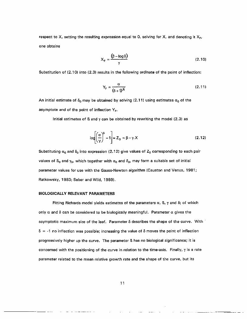
respect to X, setting the resulting expression equal to 0, solving for X, and denoting it XF,
one obtains
(2.10)
Substitution of (2.10) into (2.3) results in the following ordinate of the point of inflection:
aY, ---.,...,..
F - (0+ 1)X
An initial estimate of 00 may be obtained by solving (2.11) using estimates ao of the
asymptote and of the point of inflection YF'
Initial estimates of 13 and Y can be obtained by rewriting the model (2.3) as
(2.11)
(2.12)
Substituting ao and 00 into expression (2.12) give values of Zo corresponding to each pair
values of 130 and Yo, which together with ao and 00' may form a suitable set of initial
parameter values for use with the Gauss-Newton algorithm (Causton and Venus, 1981;
Ratkowsky, 1983; Seber and Wild, 1989).
BIOLOGICALLY RELEVANT PARAMETERS
Fitting Richards model yields estimates of the parameters a, 13, y and 8; of which
only a and 0 can be considered to be biologically meaningful. Parameter a gives the
asymptotic maximum size of the leaf. Parameter 0 describes the shape of the curve. With -
o = -1 no inflection was possible; increasing the value of 0 moves the point of inflection
progressively higher up the curve. The parameter 13 has no biological significance; it is
concerned with the positioning of the curve in relation to the time-axis. Finally, y is a rate
parameter related to the mean relative growth rate and the shape of the curve, but its
11
interpretation depends upon the value of 0 (Causton and Venus, 1981; Hunt, 1982;
Karlsson and Heins, 1994).
COMPARING PARAMETERS ESTIMATES
Curves for different sets of data can be compared or tested for invariance of some
or all of the parameters (the null hypothesis is that the parameter(s) tested are not different
among sets of data or treatments). Examination of the difference between the residual
sums of squares (RSS) for the model making the least restrictive assumption about the
parameters and that for other models with more restrictive assumptions about the
parameters could be used to make a decision about parameter invariance. The following
steps were adapted from Ratkowsky (1983) for comparing lX, y, and 0 in different data sets
(treatments) .
A) Fit c, f?" y, and 0 to data sets in each data set (all data sets). Each of the data
sets may be fitted individually. Their RSS are added together to produce a
pooled RSSs. This provides the most general, or least restricted, model for
carrying out subsequent tests.
B) . Fit c, f?" y, and 0 to data sets in each of two sets of data to be compared
(obtained from A.)
C) Fit a common c, f?" y, and 0 to each of the two sets of data to be compared.
D) Fit a common lX to each of the two individual sets of data to be compared, but
fit individual f?" y, and o.
E) Fit a common f?, to each of the two individual sets of data to be compared, but
fit individual c, y, and o.
F) Fit a common y to each of the two individual sets of data to be compared, but
fit individual c, f?" and o.
12

G) Fit a common 0 to each of the two individual sets of data to be compared, but
fit individual a, l!., and y.
With the hypothesis of an invariant a, l!., y and 0 (no difference of the 4 parameters
across treatments), testing for invariance was done by taking differences between the RSSs
obtained from step C and B finding the residual means square (RMS) and dividing by the
RMS obtained from step A yielding an F-value whose significance is read from the F table
using the degrees of freedom from step A as denominator.
Testing for individual invariants (a, l!., y or 0) and ignoring the others was performed
by using the differences D-B, E-B, F-B, and G-B finding the RMS and dividing by the RMS
obtained from step A resulting in the F-value.
ENVIRONMENTAL STRESS
WATER STRESS
Water stress affects many aspects of plant physiology, in particular the ABA
content and the growth rate. Water deficit may influence growth via effects on several
parameters such as the hydraulic conductivity of tissues, the osmotic properties of the cell,
and the rheological properties of the cell wall (Ribaut and Pilet, 1991). In water stressed
leaves, the level of ABA is often related to water potential, but turgor seems to be the
essential parameter influencing ABA accumulation under a water stress condition.
In water stressed sunflower, the rise in ABA concentration in xylem under stress
was a sequential response; the initial increase being derived from the roots, and the
subsequent increase being at least partially derived from the stressed leaves. This second
source of ABA is transported downwards in the phloem to the roots then transferred to the
transpiration stream in the xylem (Creelman, 1989).
The primary site of action of ABA is on the outer surface of the plasmalemma of
guard cells, it is the apoplastic ABA that is physiologically relevant (Creelman, 1989). There
13
are two possible ways to increase ABA concentrations in the apoplast in this region. These
are: (a) an enhanced transport to the leaves of root-sourced ABA in transpiration stream,
and (b) a rapid release of ABA from mesophyll compartments to the apoplast. The later
response can be promoted by a small change in leaf water status (Hartung and Davies,
1991 ).
The transport of ABA in the apoplast of the leaf, from xylem to epidermis, is
influenced among other things, by pH and the rate of ABA biosynthesis, metabolism and
conjugation. Therefore, it does not necessarily follow that the ABA concentration to which
guard cells respond is the same as that measured in the xylem sap (Neales and McLeod,
1991). By using enzyme-amplified immunoassay (ELISA), the ABA content of guard cells
was found to be only 0.15% of the leaf ABA of Vicia faba L. (Harris et al., 1988).
CHILLING STRESS
A chilling temperature can be defined as any temperature that is cool enough to
produce injury but not cool enough to freeze the plant. For vast majority of plants, a
chilling stress refers to any temperature below 10-15°C, and down to O°C. Rice and sugar
cane may suffer chilling injury at 15°C. At chilling temperatures, respiration rate may
exceed the rate of photosynthesis, and this may lead to starvation eventually (Levitt, 1980
a).
A number of researchers have demonstrated increased ABA content following
chilling exposure (Pan, 1990). Cooling roots of bean seedlings to 10°C resulted in an
increase in the content of free ABA in the primary leaves and a reduction in their otherwise
rapid growth (Smith and Dale, 1988). Exposure of chilling-sensitive cucumber seedlings to
chilling temperatures caused a significant rise in the level of ABA. However, it was
concluded that the increase of ABA was due to a temperature-induced water deficit and not
to the low temperature per se (Capell and Dorffling, 1989).
14
.._-_ ...-=---==

HEAT STRESS
Temperature below the optimum temperature decreases growth rate of plants due
to the depressing effect of temperature on the rate of chemical reaction. However,
temperature above the optimum temperature also decrease growth rate which can not be
explained by the direct effect of temperature on chemical reaction. The longer plants are
exposed to the high temperatures, the longer it takes them to recommence growth. The
temperature at which the rate of respiration equal the rate of photosynthesis is called the
temperature compensation point. Respiration rate was higher than photosynthetic rate at
high temperature. If plant temperature rises above the compensation point, the plant
reserves will begin to be depleted and ultimately lead to starvation and death (Levitt,
1980a).
LIGHT STRESS
A level of illumination below the light compensation point can lead to a slow,
indirect injury, due to starvation (decrease in carbohydrates). To avoid light deficit, plants
can increase the total interception of light by increasing leaf area. Shade leaves are thin
and have a low dry matter content, providing a maximum photosynthetic surface per unit
dry matter. Resistance to light deficit is associated with a decrease in resistance to the
temperature and water stress (Levitt, 1980b). However, plants grown under higher light
intensity usually have smaller and thicker leaves than those under low light intensity
(Whatley and Whatley, 1980).
ABSCISIC ACID
Most higher plant tissues are capable of synthesizing ABA which have been
demonstrated in fruit tissues, seeds (embryo, cotyledon, endosperm), roots, stem and
leaves. Within the cells of these tissues it appears likely that most of the ABA is
synthesized in the plastids (Goodwin and Mercer, 1983).
15

ABA and its metabolites are very mobile. ABA can be transported over long
distances in plants via phloem and xylem (Walton, 1980). However, in various species the
most actively growing organs act as sinks for ABA. Young tissues have the highest levels
of endogenous ABA. Older tissues such as cotyledons and primary leaves are weaker sinks
but are strong exporters (Habick and Reid, 1988). Ross and McWha (1990) reported over
90% of ABA in the Pisum sativum plant was located in the young seed.
PHYSIOLOGY
Since its isolation in 1965, ABA has figured prominently in discussions on the
regulation of plant development. Among other processes, there is evidence for an
involvement of ABA in the induction and processes of dormancy (including abscission and
senescence) and in many plant developmental responses to water deficit (Trewavas and
Jones, 1991).
Flower Induction
Abscisic acid applications promote flowering in short day plants (Milborrow, 1984).
ABA does not appear as a major determinant in the floral transition, except in some species.
S-( + )-abscisic acid applied to short day Phabitis nil completely inhibited floral bud initiation
(Karnuro et et., 1990). High concentrations of ABA inhibited or delayed flowering in a
number of species, but this effect was probably a result of an inhibitory effect on growth
(Milborrow, 1984).
Increases in endogenous ABA were reported to promote flower initiation in short
day plants and inhibit it in long day plants. However recent studies do not support earlier
findings since it appears that there is no consistent relationship between photoperiod and
ABA content in plant tissues (Bernier, 1988; Bernier et et., 1981).
16

Flower Development
The ability of ABA to induce, promote or to accelerate flower abscission has been
demonstrated in many species such as Begonia, Gossypium, Unum, Rosa, etc. (Addlcott,
1983). Application of synthetic ABA to buds of tulip and differentiating flower buds of
Phaseo/us vulgaris resulted in bud blasting in tulip and abscission of many of the buds at
later stages of development in Phaseo/us (Bentley et al., 1975; Kinet et al., 1985).
Correlations of high levels of endogenous ABA with the abscission process were
reported on cotton flowers and young fruits (Davis and Addicot, 1972; Guinn et al. 1990),
bean flower buds (Bentley et al., 1975) and Lupin flowers (Porter, 1977).
BIOCHEMISTRY
Naturally occurring abscisic acid (ABA; Figure 1) is exclusively the + (S)-enantiomer.
The 2-cis double bond of ABA can be isomerized by light to give the biologically inactive 2
trans isomer (Neill and Horgan, 1987), which has been regarded as an artifact formed from
ABA during extraction and isolation. However, trans-ABA is present in plant extracts
obtained even under dim light (Hirai, 1986).
If plant extracts are hydrolyzed by alkali, the free ABA content of the extracts is
increased. The source of this ABA is ABA-conjugates. At least two conjugates have been
identified in plant tissues. The most prevalent compound is the glucose ester of ABA
(ABAGE: (+ )-abscisyl-B-D-glucopyranoside); however, a second conjugate, 1'-O-glucoside
(ABAGS: 1'-O-abscisic acid-B-D-glucopyranoside), has also recently been characterized.
There is no evidence that these conjugates act as a source of free ABA, since wilted plants
accumulate ABA in the absence of a change in levels of ABA conjugates (Neill et al., 1983;
Roberts and Hooley, 1988).
17
. _... _- ._._- -_._--

eOOH
cis-(+)-ABA trans-(+)-ABA
iJ:,,~IQH Ia eOOH
cis-(-)-ABA
Figure 1. ABA structures
18
-- --- ---------------

Extraction
Although ABA is chemically stable under a wide range of conditions (liquid N2 to 70
°C, pH 2.0-11.0), extracts should receive the minimum exposure to light to prevent
isomerization of ABA to its 2·trans isomer (Hirai, 1986; Parrry and Horgan, 1991b). ABA
levels also rapidly change in response to drought. If fresh material is not extracted
immediately, it is usually frozen in liquid N2 and stored at -20°C (Neill and Horgan, 1987).
Strong acid or basic conditions and heating should be avoided during extraction and
isolation (Hirai, 1986).
Distilled water, 80% methanol, and 80% acetone have been used as solvents for
extraction (Piaggesi et al., 1991; Vernieri, 1989b; Daie and Wyse, 1982; Norman et al.,
1988; Neill and Horgan, 1987). The addition of antioxidants such as BHT (2,6-di-tert-butyl
4-methyl-phenoll at concentrations up to 100 mg/l has been recommended (Neill and
Horgan, 1987).
Quantitation
Quantitative measurement of the endogenous levels of ABA is quite difficult
because of its instability and low concentration in plants (ng/g fresh weight range). For the
determination of ABA, several methods including bioassays and chromatographic
procedures have been used. Detection limits range from that of UV spectroscopy at 1-3 pg,
and optical rotary dispersion at 0.5 pg/ml, to high pressure liquid chromatography (HPLC) at
1-2 ng, gas chromatography (GC) with flame ionization detection (FID) at 10-100 ng, and
GC/mass spectrometry and electron capture detection (ECD) at 10 pg • 50 ng (Weiler,
1979; Hirai, 1986). All of these analytical techniques require prior preparation of highly
purified extracts which are achieved by one or more differential solvent extractions followed
by at least one chromatographic step and often a derivative synthesis. The same degree of
19
purification is also required for all known ABA-bioassays. The sensitivity of the best
bioassays was about 100-200 ng/ml (Weiler, 1979).
Recently, immunoassay for ABA has been confirmed as the most sensitive and
selective detection method for ABA with detection limits as low as 2 x 10-16 mole (Harris
and Outlaw, 1990). In theory, the assay should offer maximal specificity with minimal
interference from extraneous compounds (Roberts and Hooley, 1988). Preparation of
antigen and antiserum is a time-consuming process, but the advantage of the immunoassay
method is that a number of crude samples without preliminary purification can be tested
semiautomatically in a short time with high accuracy (Hirai, 1986).
Immunoassay
Historically, radioimmunoassays (RIA) comprised the first generation of
immunoassays that were sensitive enough to cope with PGR at physiological levels. These
assays made use of polyclonal antisera raised in rabbits. Tritium or iodine-125-labeled PGR
or their derivatives were employed (Weiler et al., 1986a). Immunoassay is based on the
competition of a known amount of labeled antigen and an unknown amount of sample
antigen for a limited number of high-affinity antibody binding sites. Monoclonal antibodies
(MAbs) useful for immunoassay have to exhibit both high affinity and specificity. This
combination has rarely been achieved for low molecular weight antigens such as ABA and
other PGRs. Therefore, synthesis of a PGR-protein conjugate is necessary for an immune
response, and this introduces changes in the structure of the PGR with which the animal
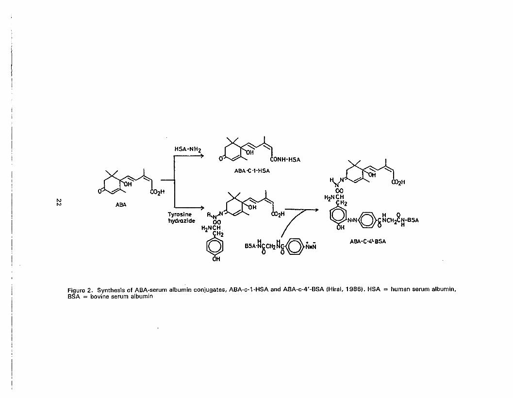
immune system is confronted (Weiler, 1984).
By coupling the carrier to the PGR molecules at different sites, it is possible to
generate antibodies exhibiting different selectivity (Roberts and Hooley, 1988). Bovine
serum albumin (BSA), human serum albumin (HSA), and hemocyanin have been used for
carrier proteins to be conjugated with a Hapten ABA. There are two ways of conjugation,
20
as shown in Figure 2. Antigen conjugated to C-4' of ABA through a hydrazone linkage is
used for free ABA determination; antigen conjugated to C-1 of ABA through an amide bond
is used for total ABA determination (Hirai, 1986). Antigen conjugated to C-1 of ABA
through the carboxyl group did not discriminate between free ABA or C-1 conjugated ABA
(Perata et al., 1990).
Enzyme-linked immunosorbent assay (ELISA). The antibody is bound to a solid
phase such as the well of a microtitre plate, and 'free' and enzyme-linked antigen molecules
compete for the immobilized binding sites. At equilibrium, the 'free' phase is decanted and
the quantity of 'bound' enzyme determined after the addition of the enzyme's substrate.
Most commonly, the antigen is linked to alkaline phosphatase or horseradish peroxidase,
since these enzymes exhibit high activity against substrates which produce products which
are colored or fluorescent and are therefore readily quantifiable (Roberts and Hooley, 1988).
Indirect ELISA. This method employs the conjugation of the antigen to a protein
which is immobilized to the walls of a support such as the well of a microtitre plate. 'Free'
antigen and antibody are added to the reaction vessel, and the antibody molecules bind to
either the immobilized or the 'free' antigen (Figure 3). The soluble antibody-antigen
conjugate is decanted away. An enzyme-linked second antibody, which specifically
recognizes the antiserum in which the primary antibody was raised, is introduced into the
reaction vessel. The secondary antibody binds to the immobilized conjugate. After the
liquid phase has been removed, the substrate of the enzyme linked to the secondary
antibody is added and the amount of product quantified (Roberts and Hooley, 1988).
Indirect ELISA was reported 5 to 10 times more sensitive than the direct procedure and was
about 50 times more sensitive than GC-MS (Belefant and Fong, 1989).
Control of Assay Performance. A high degree of binding specificity does not
guarantee a valid assay because of interference. Therefore, assay precision, reproducibility
and accuracy need to be checked. The checks required reflect the sources of potential
21
f\JN
~OVH !02H
ABA
HSA-NH2
Tyrosinehydrazide
~O~H- -!ONH-HSA
ABA -c ·l-HSA
~ffw-N~H -~2T
~Q BSA-~&CH2~&-<O>N.N
~~.N~ 'bH
CO
~Q"'~d>6~CH,g~-BSA
ABA-C-4~BSA
Figure 2. Synthesis of ABA-serum albumin conjugates, ABA-c-1-HSA and ABA-c-4'-BSA (Hirai, 1986). HSA = human serum albumin,BSA = bovine serum albumin

..... COLOR
substrate
ABA-8SA IgEAntiJ9E
microtitreplate Antibody
Figure 3. Indirect ELISA. Antibody binds to antigen (ABA-BSA) in the solid phase and issubsequently detected by the color which develops when an enzyme-labeled antibodybinds to the complex. (lgE = antibody or immunoglobulin; Enzyme Anti-lgE =enzyme-labelled anti-immunoglobulin)
23
.. - _._---_._._-----~--:-:..-.;.-------=-==------ - -
interference peculiar to immunoassays. The most relevant potential sources of interference
in immunoassays are the following (Pengelly, 1986; Weiler, 1986; Weiler et el., 1986b):
1. Compound antigenically (structurally) similar to the plant hormone under study.
2. The presence of excessive amounts of compounds which exhibit only weak
cross-reactions.
3. The presence of antibody denaturing or desorbing agents, For example, high
levels of phenolic compounds may partially denature antibodies; the presence of surfactants
may likewise denature soluble antibodies or may desorb them from solid supports.
4. The presence of factors which prevent the binding of hormone to its binding site
(e.g., by complexation).
5. The presence of contaminants which impair the quantitation step.
No single test for assay validity is absolutely safe. It is recommended to use the
maximum number of the following controls when dealing with a new source of plant
material (Weiler, 1986).
1. Losses of hormone during extract work-up will affect accuracy. Work-up losses
are detected by use of radioactive hormone internal standards or by using hormone-spiked
split extracts processed in parallel. This also compensates for any isomerization of cis,
trans-ABA to trans, trans-ABA which might have occurred during extraction and assay
(Weiler, 1986; Weiler, 1980).
2. Parallelism test of a plant extract dilution curve with the standard curve is a test
for specificity. This can be done by performing a dilution series of the extracts and to show
additivity, or parallelism to the standard curve. The plot will yield a line parallel to the
standard curve if there is no interference (Daie and Wyse, 1982; Pengelly, 1986, Wang et
el., 1986).
3. Dilution analysis with internal standardization: increasing amounts of extracts are
added to standards. Absence of interference is indicated if the data points (plot hormone
24
------- --_.------
found vs hormone added) fall on a straight line parallel to each other and to the standard
line. Information of quantitative recovery will also be obtained and values should be close
to 100% recovery of the added hormone. Highly cross-reactive material may be overlooked
this way (Mertens etal., 1985; Vernieri et et., 1989a; Weiler, 1986).
4. Successive approximation: This approach makes use of a series of different
purification steps. This process is continued until an estimate is obtained that does not
change on purification. An internal standard is used so sample losses encountered during
purification can be assessed (Crozier et et., 1986; Weiler, 1986).
Factors included in group 2 are best for checking a dilution analysis at various levels
of added standard hormone. Deviation from uniformity (slope = 1) indicates interference.
Cross reactants as defined under 1 will show up in this test if their dose response curves do
not run parallel to the hormone standard curve. Cross reactants with tracer displacement
curves parallel to the standard curve cannot by detected by this method. Cross reactants
are best detected in immunohistograms of separated extracts (Weiler et al., 1986b).
25
...'" .-_.._---
CHAPTER 3
LEAF GROWTH MODEL AND FLOWERING PROGRAM OF HELICONIA STRICTA
ABSTRACT
Heliconia stricta cv. Dwarf Jamaican plants were grown under: continuous long
days (14 hr. daylength), continuous short days (9 hr. daylength), or grown under long days
(Lo) until the plants reached the 3 to 4 expanded leaf stage, then 4 weeks of short days
(SO) and returned to long days. Plants grown under continuous SO and Lo +SO until the 3
leaf stage had the highest flowering percentage (45 and 46%), while only 17% of plants
grown under Lo + SO until the 4-leaf stage flowered, and no flowers were produced in
plants grown under continuous Lo. Plants grown under Lo until the 3 or 4-leaf stage
flowered 13 weeks after the start of SO. The plants and inflorescences were more vigorous
than those under continuous SO. Leaf length was measured on alternate days for each
treatment and fitted to the Richards model. There were no differences in leaf growth
curves of different treatments within the same leaf position (3rd, 4th and 5th
) . By fitting
relative leaf elongation and relative time to full leaf expansion to the Richards model, leaf
growth curves of different leaf positions were shown to be significantly different. Common
leaf growth curves for leaf positions 3-5 and a program for H. stricta 'Dwarf Jamaican'
culture were proposed.
INTRODUCTION
Crllev and Kawabata (1986) found that established Heliconia stricta cv. Dwarf
Jamaican plants with 3 or more expanded leaves could be induced to flower in 13 weeks by
growing them under a minimum of 4 weeks of short days. Continuous long days (t.D) had a
strong effect in prolonging the vegetative phase or inducing flower bud abortion in the first
generation of shoots produced after potting, while continuous short days (SO) enhanced
26

flowering of pseudostems (Lekawatana, 1986). The effect of LD decreased with
successive generations of daughter pseudostems as some plants did flower in continuous
LD. The lengths of both inflorescence and pseudostem were longer in continuous LD than
in SO.
The purpose of this experiment was to determine growth of plants raised under
different daylength condition at different stages of development with the goal to develop a
cultural program of He/iconia stricta 'Dwarf Jamaican' from potting to flowering.
MATERIALS AND METHODS
PLANT MATERIAL AND CULTURAL PRACTICES
Eighty-four rhizome pieces of He/iconia stricta cv. Dwarf Jamaican were propagated
on June 20, 1988. Rhizome pieces including pseudostems were separated from the mother
plants, and the roots removed. The pseudostem was cut to 5-cm lengths from the leaf
sheath base, treated in a 55°e water bath for 5 minutes, dipped in fungicide solution
(Dithane M45) and drained. The rhizomes were then held in plastic bags for 3 weeks at
200e to stimulate root and shoot growth. They were planted in a 1: 1 ratio (v/v) perlite and
vermiculite medium and held under mist for 1 week. Rooted rhizome pieces were potted
singly into a mixture of peat and perlite 1:1 ratio (v/v) in 15-cm pots on July 18, 1988 in a
greenhouse at the Magoon greenhouse facility of the University of Hawaii. The potting
medium was amended with dolomite, Micromax and treble superphosphate at the rates of
6.0, 1.0 and 0.6 kg per cubic meter, respectively. Plants were drip irrigated twice daily
with nutrient solution, 200N-OP-200K (ppm).
TREATMENT SETUP
After potting, plants were divided into 4 groups (21 pots each) for 4 treatments:
Tr. 1: Plants grown under continuous long days (LD).
27
Tr.2: Plants grown under LO until the 3-leaf stage (Aug. 22, 1988). This stage is
when the third leaf has expanded and the fourth leaf has started to emerge.
Then, the plants were moved into short days (SO) for 4 weeks and returned
to LO.
Tr. 3: Plants were grown under LO until the 4-leaf stage (Sept. 2, 1988). This
stage is when the fourth leaf has expanded and the fifth leaf has started to
emerge. Then the plants were moved into short days (SO) for 4 weeks and
returned to LO.
Tr. 4: Plants grown under continuous SO
Labels for these treatments have been abbreviated to:
Tr. 1: conLO; Tr. 2: L0 3L +SO; Tr. 3: L0 4L + SO; Tr.4: conSO;
SO was provided by placing plants under an automatic black cloth shading system
from 5:00 p.rn. to 8:00 (9-hr. photoperiod). Plants under LO were also under the shading
system. However, they were given LO by supplementing daylength with incandescent
illumination from 5:00 p.m, to 10:00 p.m, with 60-W lamps placed 1.3 m above the pots to
give 14 hr. daylength (LO). One month after potting, plants that were not uniform were
removed, leaving 15 pots in conLO, 13 pots in L0 3L +SO, 17 pots in L0 4L +SO, and 11 pots
in conSO.
DATA COLLECTION
Lengths of each leaf from soil line to top of the plants were measured every other
day from time of emergence until those leaves stopped growing. A total of 9,228 leaf
length data points were recorded, averaging 20 data points per leaf. Time of inflorescence
emergence and anthesis, peduncle and inflorescence lengths, and number of cincinnal
bracts were recorded. Plants were discarded after anthesis. The experiment was
28

terminated on December 10, 1988. For pseudostems that did not show an inflorescence, a
determination of status (vegetative or aborted) was then made by dissecting the stems.
Photosynthetically active radiation (PAR) in the 400 to 700 nm waveband was
measured by a L1-COR quantum sensor model L1-190SZ. The light sensor and an air
temperature sensor were connected to a Datapod model DP211 (Omnidata Int., Inc., Utah).
Data were averaged over 5 minutes intervals and recorded every 60 minutes. The unit of
PAR is micromoles per second per square meter (average daily maximum PAR was 449.3
pmole.s·'.m·2 with a range of 40-680 pmol.s·'.m·2) . The average minimum and maximum
temperatures throughout the experiment were 22.8°C (range: 19-25°C) and 34.7°C (range:
27-41.5°C), respectively. A summary of the weather data is presented in Appendix 8:
Figures 1-2.
STATISTICAL ANALYSIS
Chi-Square
Chi-Square tests for independence were used in analyzing quantitative data such as
number of pseudostems in each status (flowered, vegetative or aborted). The null
hypothesis was that the differences among the ratios were not significant. The null
hypothesis was rejected when the significance probability was 0.05 or less. If the null
hypothesis was rejected, a chi-square test for a fixed ratio hypothesis was performed for
the ratio of pseudostem numbers in each status. The test was done on different pairs of
pseudostem numbers within each status. The null hypothesis was that the ratio of
pseudostems in each status between two daylength treatments was not significantly
different. This test enabled the comparison of numbers of pseudostem among different
daylength treatments within a status.
29
Covariance Analysis and Comparison of Regression lines
In this experiment, daylengths were the primary treatments, but since leaves
emerged sequentially during treatment over different periods of time, this was also
considered a source of variation. The analysis of covariance was applied to this experiment
by including leaf position on the pseudostem in the model as a covariate. When the
covariate is measured after the treatments have been applied, it is important to determine if
the behavior of the covariate is substantially influenced by the treatments applied. If the
treatments significantly affect the covariate, the use of the covariance analysis takes on a
different role. Instead of being used to reduce experimental error, it is now used to assist in
the interpretation and characterization of the treatment effects upon the character of
interest in much the same way that regression and correlation analyses are used (Gomez
and Gomez, 1976). Testing for heterogeneity of slopes is an extension of covariance
analysis (Freund et al., 1986). In this regression model the continuous measured variable
was number of leaves. A qualitative variable, daylength treatment, enabled the data to be
stratified into groups, with different regression coefficients for linear and quadratic effects
assigned to each treatment. This regression model tested whether the regression
coefficients were constant over groups (daylength treatments). A model sequence
approach was used for each response variable, the most general model including terms for
common intercept, linear, and quadratic differences among daylength treatments (Allen and
Cady, 1982). Testing progressed until reduced models were found that described the data
adequately. The overall goodness of fit of reduced models is described in figures
represented by the model I. Single degree of freedom contrast coefficients were used to
compare intercepts and regression coefficients among each daylength treatment. If two or
more treatments were not significantly different as to intercept, slope, or curvature, they
were presented as a single regression equation.
30

Growth Model Fitting
Least-square estimates of model parameters were calculated by the Gauss-Newton
method in nonlinear regression (NUN) procedure of statistical analysis system (Freund and
Little, 1986; SAS Institute lnc., 1987; Appendix C: Programs 1-10). Model selection was
done using sample leaf length data from the 4th leaf of plants which flowered in L03L +SO.
The selection was based on scientific reasons, stability of parameter estimates to varying
assumptions about the error term, lack of fit test, and Student's t-test as described in
chapter 2.
After a model was selected, leaf length data for each leaf position (2nd to 6th) of the
plants in each treatment were fitted to it to study the growth curves. Estimated parameters
of models among treatments within the same leaf position were compared using the method
described in chapter 2 (Appendix C: Programs 11-14).
Growth curves among leaf positions were compared by transforming leaf expansion
time and leaf length to relative scales from 0 to 1. This method facilitated the comparisons
of different leaf lengths among leaf positions and the different time frames from emergence
(T =0) to fully expanded (T =1). Leaf length at emergence time was assigned 0 and fully
expanded, 1. Estimated parameters of leaf growth models among different leaf positions
were then compared.
Richards Model Parameters
By fitting ~ichards equation (3.1) the change of leaf length (Y) with time (X) can be
described. The model yields estimates of the parameters a, 13, y and 5.
Richards model:a
Y=-----~
[1 + expU3 - yX)t(3.1)
Parameter a gives the asymptotic maximum size of the leaf. Parameter 5 describes the
shape of the curve. With /) = -1 no inflection was possible; increasing the value of 5 moves
31
the point of inflection progressively higher up the curve. The constant ~ has no biological
significance; it is concerned with the positioning of the curve in relation to the time-axis.
Finally, y is a rate constant related to the mean relative growth rate (RGR) (3.2) and the
shape of the curve but its interpretation depends upon the value of 0 (Causton and Venus,
1981; Hunt, 1982; Karlsson and Heins, 1994).
Mean relative growth rate (RGR): = Y
0+1(3.2)
Generally RGR is the rate of growth per unit weight of plant (Charles-Edwards et al., 1986).
In this experiment it will be referred to as rate of leaf growth per unit leaf length.
RESULTS
PSEUDOSTEM STATUS
The pseudostems grown under conLO did not flower. Those grown under L0 3L+ SO
and conSO had higher flowering percentage than those grown under L04L+ SO (Table 1 and
Figure 4). However, pseudostems grown in conLO had a higher percentage of vegetative
pseudostems than those in conSO. There was very low percentage of vegetative
pseudostems in plants grown under L0 3L +SO and L0 4L+ SO. Percentage of flower bud
abortion was highest in plants grown in L04L+SO while there was no flower bud abortion in
plants grown under conSO (Table 1).
NUMBER OF LEAVES SUBTENDING THE INFLORESCENCE
Pseudostems grown under L0 4L +SO had significantly more subtending leaves (7
Ivs.) than those grown under L0 3L+ SO and conSO (6 Ivs; Table 2, Appendix A:Table 1).
However, those grown under conLO produced up to 8 leaves (Table 2).
32
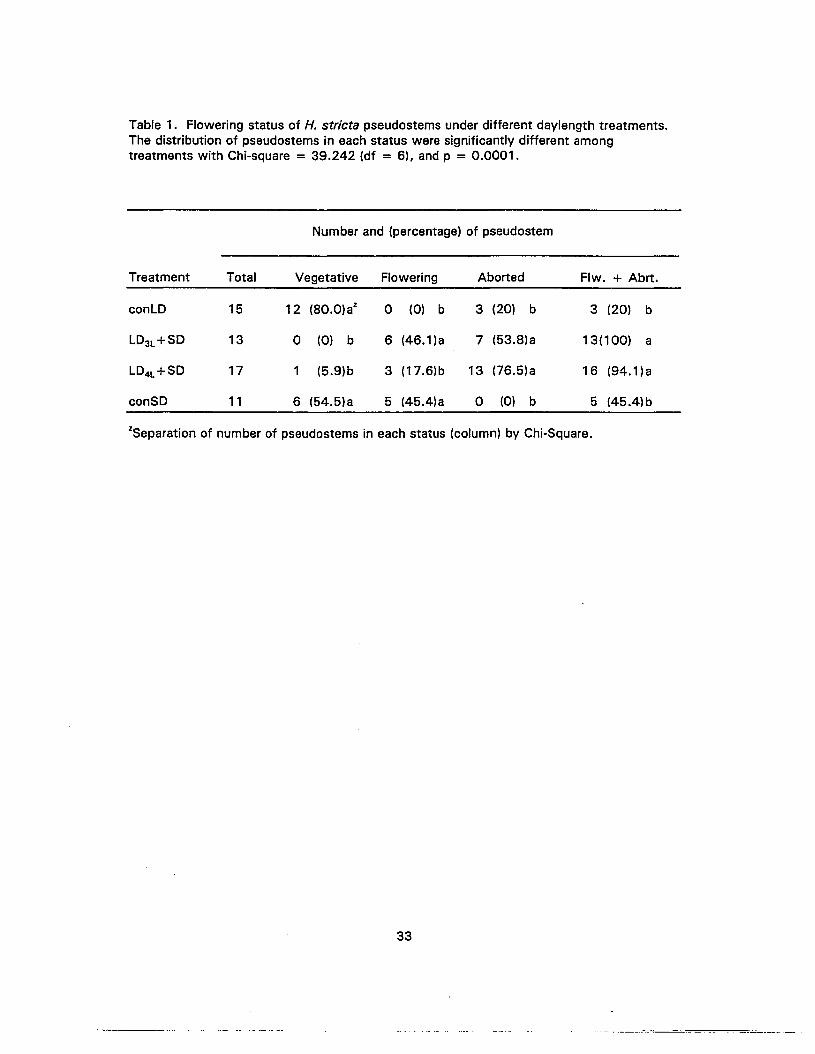
Table 1. Flowering status of H. stricta pseudostems under different daylength treatments.The distribution of pseudostems in each status were significantly different amongtreatments with Chi-square = 39.242 (df = 6), and p = 0.0001.
Number and (percentage) of pseudostem
Treatment Total Vegetative Flowering Aborted Flw. + Abrt,
conLO 15 12 (80.0)az 0 (0) b 3 (20) b 3 (20) b
L03L +SO 13 0 (0) b 6 (46.1)a 7 (53.8)a 13(100) a
LD4L +SO 17 1 (5.9)b 3 (17.6)b 13 (76.5)a 16 (94.1)a
conSO 11 6 (54.5)a 5 (45.4)a 0 (0) b 5 (45.4)b
zSeparation of number of pseudostems in each status (column) by Chi-Square.
33
.=~~~-=-----
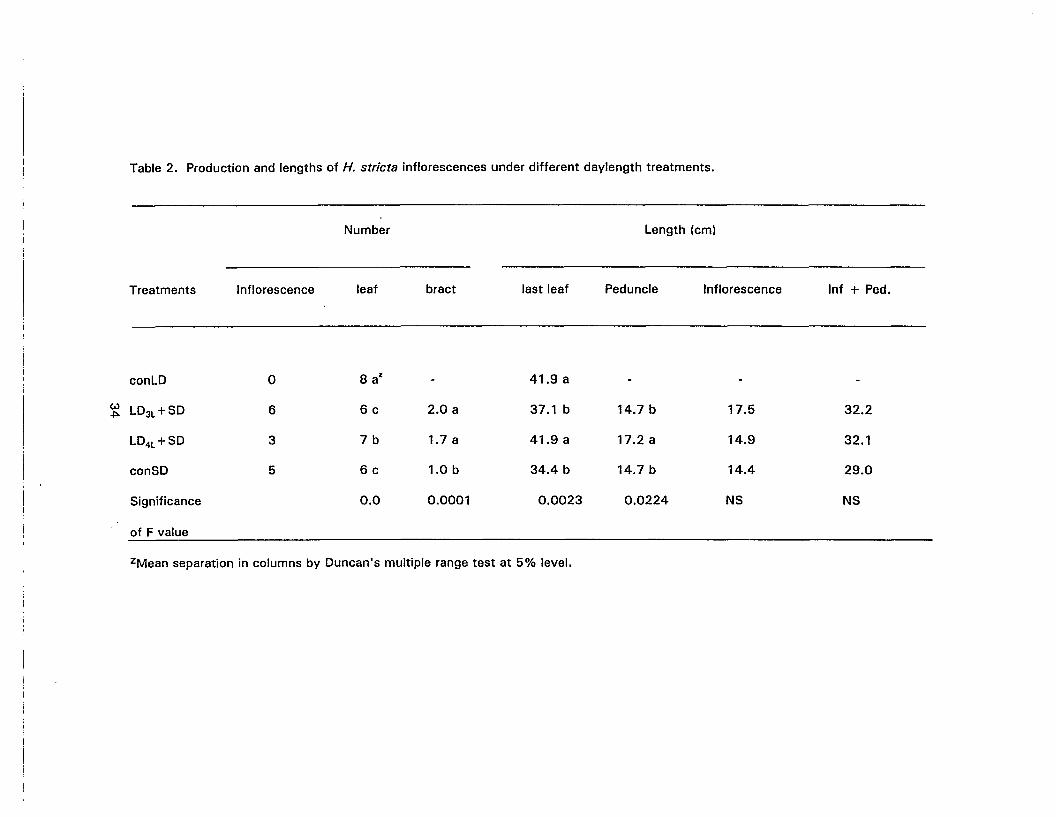
Table 2. Production and lengths of H. stricta inflorescences under different daylength treatments.
Number Length (em)
Treatments Inflorescence leaf bract last leaf Peduncle Inflorescence Inf + Ped.
conLD 0 8 aZ - 41.9 a
~ LD3L +SD 6 6c 2.0 a 37.1 b 14.7 b 17.5 32.2
LD4L +SD 3 7b 1.7 a 41.9 a 17.2 a 14.9 32.1
conSD 5 6c 1.0 b 34.4 b 14.7 b 14.4 29.0
Significance 0.0 0.0001 0.0023 0.0224 NS NS
of F value
zMean separation in columns by Duncan's multiple range test at 5% level.
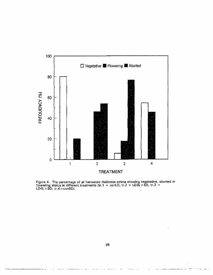
100 r---------------------..,
o Vegetative • Flowering • Aborted
80
~->UZw::::>dwa::LL.
60
40
20
o2
TREATMENT
3 4
Figure 4. The percentage of all harvested Heliconia stricta showing vegetative, aborted orflowering status in different treatments Itr.1 = conLD, tr.2 = LD3L+SD, tr.3 =LD4L+SD, tr.4=conSD).
35

FLOWERING
Inflorescence Characteristics
Cincinnal bract count for flowered plants grown under canSO was significantly less
(1 br.) than for those grown under L0 3L+SO and L04L+SD (approx. 2 br.; Table 2). There
was no significant difference among treatments on the overall length of the inflorescence
(inflorescence and peduncle combined) (Table 2, Appendix A:Tables 3-4). However the
length of the subtending leaves and the peduncle length of plants grown under L0 4L+ SO
was significantly longer than those grown under L03L+ SO or those under canSO (Table 2,
Appendix A:Tables 2-6).
Time to Flower
Plants grown under canSO required less time from potting to anthesis (15 wks)
compared to those grown under L03L+ SO and L04L+ SO (18 and 19 wks.; Table 3).
PLANT GROWTH
Leaf length of plants grown under canSO was significantly shorter than those grown
under conLO, L03L+ SO and L04L+ SO. Leaf position had significant linear components with
leaf length at the 5% level and the length increased with successive leaf position (Figure 5,
Appendix A:Table 13).
Time from potting to leaf emergence of plants grown under canSO was significantly
less than those grown under conLO, L03L+SO and L04L+SO. Leaf position had a highly
significant quadratic effect on the time from potting until any given leaf emergence at the
1% level (Figure 6, Appendix A:Table 14).
The time increment between successive leaves of plants grown under canSO was
significantly less than those grown under conLO, L03L+ SO and L04L+ SO. Leaf position
had significant quadratic components with days to produce each leaf at the 1% level
36
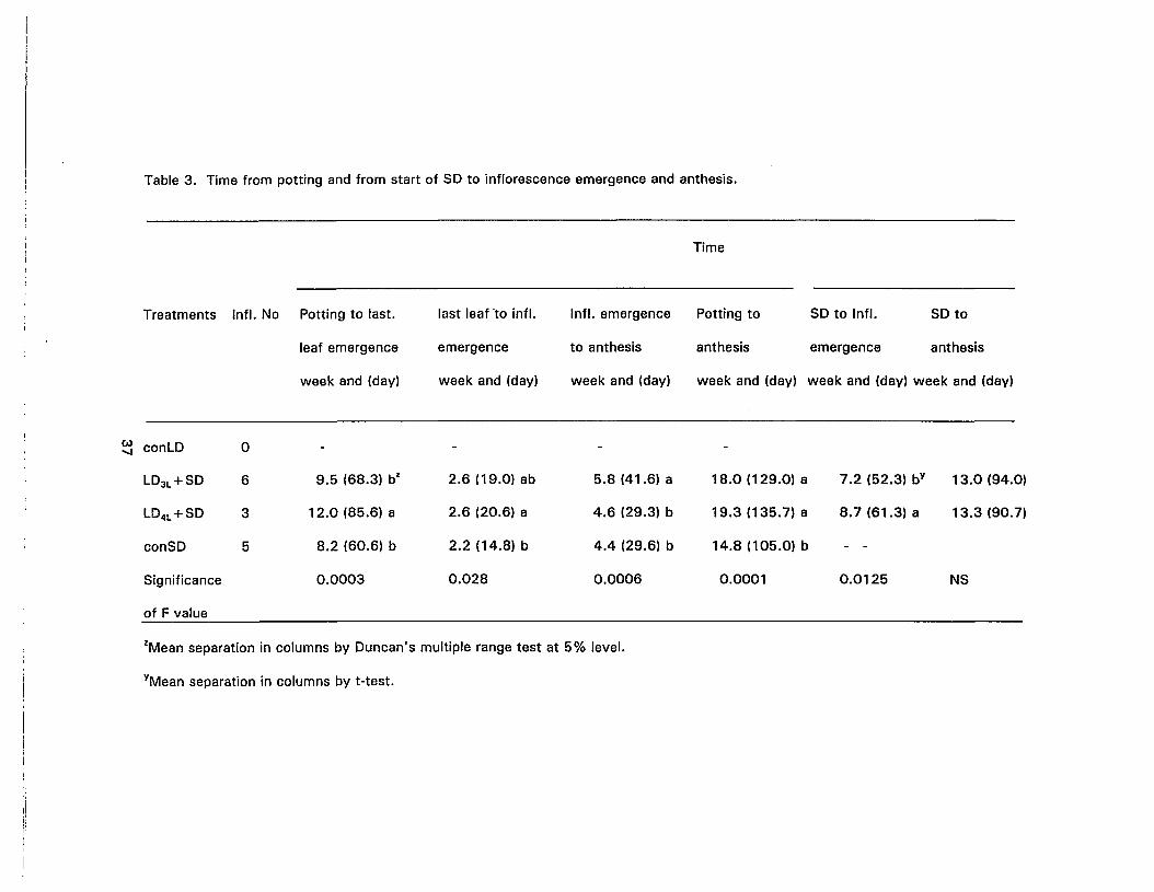
Table 3. Time from potting and from start of SD to inflorescence emergence and anthesis.
Time
Treatments Infl. No Potting to last. last leaf 'to infl. Infl. emergence Potting to SD to Infl. SD to
leaf emergence emergence to anthesis anthesis emergence anthesis
week and (day) week and (day) week and (day) week and (day) week and (day) week and (day)
~ conLD 0
LD3L +SD 6 9.5 (68.3) bZ 2.6 (19.0) ab 5.8 (41.6) a 18.0 (129.0) a
LD4L +SD 3 12.0 (85.6) a 2.6 (20.6) a 4.6 (29.3) b 19.3 (135.7) a
conSD 5 8.2 (60.6) b 2.2 (14.8) b 4.4 (29.6) b 14.8 (105.0) b
Significance 0.0003 0.028 0.0006 0.0001
of F value
7.2 (52.3) bY 13.0 (94.0)
8.7 (61.3) a 13.3 (90.7)
0.0125 NS
ZMean separation in columns by Duncan's multiple range test at 5% level.
YMean separation in columns by t-test.

TRT. 1-3: Y =14.144 + 3.718 X
6345LEAF POSITION
.....-
2
TRT.4: Y=12.055 + 3.718 X ••••••
r"2 =0.85 ••••••••••••••••••••.'••
~.
••••••••••
40
- 35E0-IJ- 30C)ZW--I 25u,<t:w--I 20
15
Figure 5. Influence of daylength treatment and leaf position on leaf length of H. stricta(tr.1 = conLD, tr.2 = LD3L+SD, tr.3 = LD4L+SD, tr.4=conSD).
70 .....-----------------...,
TRT.1-3: Y =-9.235 + 8.209X + 0.695X1\2
,.TRT. 4: Y =-5.458 + 6.220X + 0.695 XI\2 "
•r"2 =0.94 •••••••
•••,..'.'••••.'".••,".'••10
20
50
30
40
60C)Z
~oa.:2o~u,en~o
6345LEAF POSITION
2O....--.....--.....----I----~--~-_....Figure 6. Influence of day length treatment and leaf position on time from potting to leafemergence of H. stricta ttr.t = conLD, tr.2 = LD3L+SD, tr.3 = LD4L+SD,tr.4 = conSD).
38

(Figure 7, Appendix A:Table 15). The time required to produce each leaf increased
minimally from leaf 3 to leaf 4. However, substantially more time was needed to produce
leaves 5 and 6.
Significantly longer time was needed for plants grown under L0 4L +SO (12 wks.) to
produce the last subtending leaf (7th If) than for those grown under L0 3L + SO and conSO
(6th If) 9.5 and 8.2 wks., respectively (Table 3, Appendix A:Tables 7-12).
Rate of leaf unfolding
Plants grown under conLO, L03L + SO and L0 4L+SO had a significantly higher rate
of leaf unfolding (calculated from the length differences from leaf emergence to fully
expanded divided by the period of time) than those under conSO. Leaf position accounts
for significant differences in the rate of leaf unfolding as leaf number increases in a way
that has a quadratic asymptote at the 1% level (Figure 8, Appendix A:Table 16).
GROWTH MODEL
Model Selection
Table 4 shows the least square (LS) estimates of the parameters of Gompertz,
Logistic, Richards, Morgan-Mercer-Flodin (MMF), and Weibull models for a data sets of
the 4th If of flowered plants grown under L03L + SO, for both additive and multiplicative error
assumptions. For the 3-parameter models, the logistic model had a lower residual variance
(0-2
) than the.Gompertz model. However, the Richards model had the lowest residual
variance. With regard to the stability of the LS estimates, all of the estimates were
relatively stable (little variation) for all parameters except that for parameter y of the MMF
model.
T-values for the parameter estimates for each of the five models are presented in
Table 5. The t value is the ratio of the parameter estimate to its standard error. A high
39 .
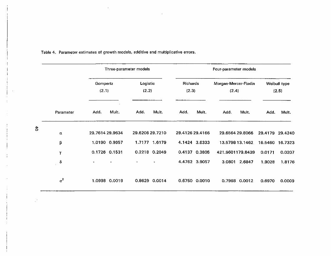
Table 4. Parameter estimates of growth models, additive and multiplicative errors.
Three-parameter models Four-parameter models
Gompertz
(2.1 )
Logistic
(2.2)
Richards
(2.3)
Morgan-Mercer-Flodin
(2.4)
Weibull type
(2.5)
Parameter Add. Mult. Add. Mult. Add. Mult. Add. Mult. Add. Mult.
.J=lo0
CL 29.761429.9634 29.620629.7210 29.4126 29.4166 29.656429.8066 29.4179 29.4240
P 1.0190 0.9657 1.7177 1.6179 4.1424 3.6333 13.579813.1462 16.5460 16.7323
y 0.1726 0.1531 0.2218 0.2049 0.4137 0.3805 421.9601179.8439 0.0171 0.0207
IS - - - - 4.4762 3.9057 3.0801 2.6847 1.9028 1.8176
0-2 1.0998 0.0019 0.8629 0.0014 0.6750 0.0010 0.7968 0.0012 0.6970 0.0009

Table 5. Student's t-values, as the ratios of the parameter estimates to their standarderrors.
Gompertz Logistic Richards MMF Weibull
Parameter (2.1) (2.2) (2.3) (2.4) (2.5)
a 234.09 297.97 325.17 245.34 322.22
~ 38.90 28.98 5.55 42.46 42.98
Y 29.06 32.64 8.08 2.41 3.77
S 5.31 16.07 16.68a • maximum leaf length, y related to mean RGR,S describes the shape of curve, 13 -highly correlated with y and S
Table 6. Lack of fit analysis for different models fitted to plants in trt. 1 and trt. 2.
RSS
F
P
Gompertz
(2.1)
152.87
3.58
< 0.01
Logistic
(2.2)
119.95
1.73
< 0.05
41
Richards
(2.3)
93.16
0.22
NS
MMF
(2.4)
105.97
1.08
NS
Weibull
(2.5)
92.71
0.28
NS
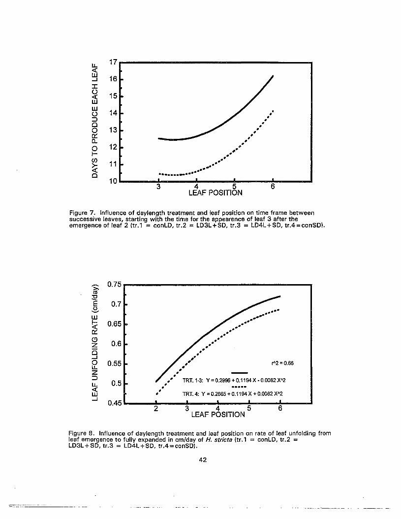
u. 17-cw 16...J
J:o 15«ww
14 •o •:::> ••0 ••0 13 ••~ ••a.. •
12 •0 ~,..- •••(/)
11 ".~
,,"..""""""0 ...........
104 5 63
LEAF POSITION
Figure 7. Influence of daylength treatment and leaf position on time frame betweensuccessive leaves, starting with the time for the appearence of leaf 3 after theemergence of leaf 2 (tr.1 = conLD, tr.2 = LD3L+SD, tr.3 = LD4L+SD, tr.4=conSDI.
6
..........
,,",,",,",,",,",,",,"
",,",,"
","~ ~=Q~,
""•,," TRT.1-3: Y=0.2996+ 0.1194X- 0.OO82X"2". .....
II· TRT.4: Y=O.2665+0.1194X+O.OO82Xh2
2
....... 0.75>-ell
32E 0.70'-"
w!< 0.65~
<9 0.6z0...J0 0.55u.z::Ju. 0.5-cw...J 0,45
Figure 8. Influence of daylength treatment and leaf position on rate of leaf unfolding fromleaf emergence to fully expanded in em/day of H. stricta (tr.t = conLD, tr.2 =LD3L+SD, tr.3 = LD4L+SD, tr.4=conSDI.
42
--------- --._---
t value tends to indicate that the estimate is well determined in the model, a low t value
tends to indicate that the estimate is poorly determined (Ratkowsky, 1983). These values
were relatively high for the estimates of the 3-parameter models. For the Richards model,
the t-values associated with the estimates of lX and y were higher than those of MMF and
Weibull models. However, the t-values associated with the estimates of ~ and 0 were
relatively lower than those of MMF and Weibull models.
No lack of fit for leaf length data was found in the 4-parameter models (Richards,
MMF and Weibull). However, there was significant lack of fit in the 3-parameter models
(Gompertz and logistic) (Table 6).
Largely because of its application to single leaf growth (Causton and Venus, 1981)
and the results of the above selection criteria, the Richards model was selected for fitting
the leaf length data.
Comparing Parameters within Each Leaf Position
Leaf length data of plants under different treatments and leaf position (Figure 9)
were fitted to the Richards model (Appendix A:Tables 17-36). Parameters B, y, and 0 were
all highly correlated (greater than 0.95). The correlation of lX with other parameters was
smaller and negative. Because of the high correlation among ~, y and 0, together with lack
of biological meaning of the first two, only the lX and 8 would be discussed.
The maximum leaf length (lX) of plants grown under conLD, LD3L +SO, L0 4L + SO leaf
2 to leaf 4 was longer than those grown under conSO (Table 7). Leaf 5 and leaf 6 of plants
grown under L0 3L+SO were shorter than those grown under conLO and LD4L + SO but were
longer than those under conSO. There was no significant difference for parameter f3 and 0
among treatments within each leaf position (Appendix A:Tables 37-71). This is summarized
in Figure 10 as there was no significant different in the shape of the growth curves among
treatments within each leaf position, although maximum leaf length was different.
43

Table 7. Parameter estimates of Richards function on leaf length and time after leafemergence of different daylength treatments from the 2nd leaf to the 6th leaf.
Parameter
Leaf position Treatment a. @ y 0
2nd conLO 21.60 aZ 3.647 a 0.363 a 3.604 a
L03L +SO 22.33 a 5.286 a 0.451 ab 4.980 a
L04L +SO 22.45 a 3.438 a 0.337 a 3.616 a
conSO 19.89 b 0.612 a 0.259 b 1.026 a
3r d conLO 25.12 a 4.740 a 0.414 a 4.708 a
L03L +SO 24.83 a 5.242 a 0.457 a 5.181 a
L0 4L +SO 25.56 a 2.931 a 0.309 a 3.035 a
conSO 23.21 b 2.554 a 0.328 a 2.766 a
4 t h conLO 28.64 a 2.238 a 0.297 a 2.369 a
L0 3L +SO 28.92 a 2.928 a 0.308 a 2.998 a
L0 4L +SO 29.76 a 3.176 a 0.336 a 3.271 a
conSO 27.29 b 3.487 a 0.400 a 3.840 a
5 t h conLO 33.86 a 1.917 a 0.234 a 1.887 a
L0 3L +SO 32.67 b 3.261 a 0.279 a 3.232 a
L0 4L +SO 34.20 a 2.950 a 0.269 a 2.856 a
conSO 31.16 c 3.062 a 0.340 a 3.268 a
6 t h conLO 37.45 a 1.745 a 0.206 b 1.932 a
L0 3L +SO 35.81 b 3.610 a 0.309 a 4.075 a
L0 4L +SO 37.16 a 3.046 a 0.261 ab 3.307 a
conSO 34.14 c 2.150 a 0.216ab 2.413 a
ZParameter estimates separation in columns of each leaf position by F-test at 5% level.a = maximum leaf length, y related to mean RGR, Ii describes the shape of curve, J3 highly correlated with y and Ii
44
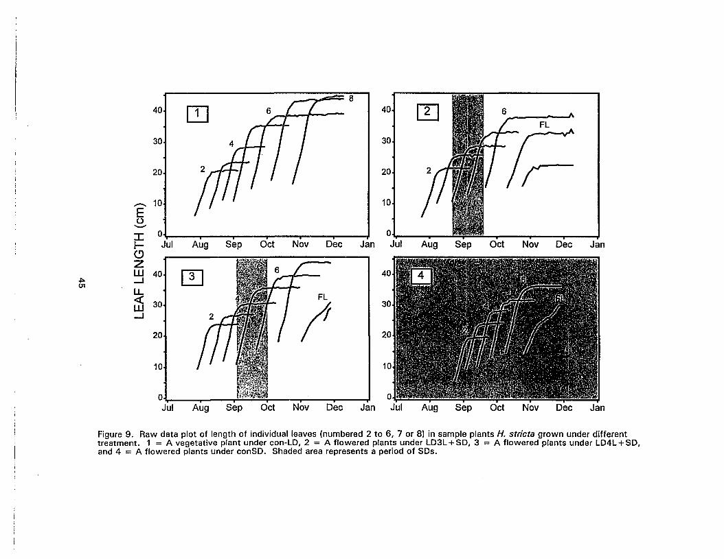
Jan
Jan
Dec
Dec
FL
Nov
Nov
Oct
Oct
Sep
Aug
Aug
~
30
10
30
40
10
20
20
40
_,¢C'F' ~ 8
FL
;1
Nov
Nov Dec
Oct
Oct
Sep
Sep
Aug
Aug
Q]
[U
OJ, , ,H~~:~:;;;~' , , " 0Jul
20
10
40
30
20
J:I<.9ZW 40....Ju,« 30W....J
-... 10Eo-
~01
Figure 9. Raw data plot of length of individual leaves (numbered 2 to 6, 7 or 8) in sample plants H. stricta grown under differenttreatment. 1 = A vegetative plant under con-LD, 2 = A flowered plants under LD3L+SD, 3 = A flowered plants under LD4L+SD,and 4 = A flowered plants under conSD. Shaded area represents a period of SDs.

Dec
Dec
Nov
Nov
Oct
OctSepAug
~
20
30
30
40
10
40
10
20
6
Oct
Oct
Sep
Sep
Aug
Aug
Q]
~
oJ ~~~:w'lf~.'lo".lil I 0i , , , , ,
Jul
20
20
40
10
30
-10Eo
'--"
IloZill-I 40U.«ill 30-I
~0)
Figure 10. Richards curves fitted to the length of individual leaves (numbered 2 to 6) in H. stricta grown under different treatment.1 = Plants under con-LO, 2 = Plants under L03L+SO, 3 = Plants under L04L+SO, and 4 = Plants under conSO. Shaded arearepresents a period of SOs.

Results of fitting leaf length to Richards model of vegetative pseudostems from
conLO and flowered pseudostems from L0 3L+50, L0 4L +SO and conSO are shown in Table
8 (Appendix A:Table 72-83). Flowering pseudostems grown under L04L + SO had
significantly longer maximum leaf length (al than the flowering pseudostems grown under
L0 3L + SO, the vegetative pseudostems grown under conLO or the flowering pseudostems
grown under conSO respectively within each leaf position (If.4 to If. 6). There was no
significant difference for parameter 0 among different treatments (Appendix A:Tables 84
104). However there was a trend in leaf 6 that parameter 0 of plants in conSO was less
than plants in other treatments resulting in a flatter curve as shown in Figure 11 .
Comparing Parameters of Different Leaf Positions
Since there were no significant differences in estimated parameters for growth
models among treatments for leaf position 3, 4 and 5, the possibility of fitting a common
leaf growth curve for each leaf position was investigated. This was done by transforming
leaf length and time to fully expanded to relative length and time. Results of fitting relative
length and time are shown in Table 9 (Appendix A:Tables 105-107). Parameter estimates
for leaf growth curves for each position (3-5) were significantly different (Appendix
A:Tables 108-112). Mean RGR of the s" leaf, calculated from yand 0, was greater (6.7)
than those in 4th and 3rd leaf (5.1) resulting in a steeper slope for the s" leaf than the 4th and
3rd leaf (Figure 12).
Common Growth Curve for ;tri to ffh Leaf
Since leaf growth curves of positions 3-5 were significantly different, but were
common among treatments (tr.1-tr.3) within each position, common growth curves were
fitted leaf for positions 3-5 across tr. 1 to tr. 3 as follows (Figure 13, Table 10, Appendix
A:Tables 112-114):
47

Table 8. Parameter estimates of Richards function on leaf length and time after leafemergence of different daylength treatments of each pseudostem status (Flowered:LD3L +SD, LD4L+SD and conSD, Vegetative conLD) from the 4th leaf to the 6th leaf.
ParameterLeafposition Treatment Status a. p y 0
4th conLD Veg. 28.00 CZ 3.052 a 0.369 a 3.273 a
LD3L +SD Flw. 29.31 b 4.315 a 0.399 a 4.405 a
LD4L +SD Flw. 30.21 a 3.900 a 0.398 a 4.175 a
conSD Flw. 28.59 c 4.863 a 0.493 a 5.130 a
5th conLD Veg. 33.45 b 2.214 a 0.252 b 2.153 a
LD3L +SD Flw. 33.05 b 4.061 a 0.332 ab 4.188 a
LD4L +SD Flw. 35.00 a 4.033 a 0.345 ab 3.717 a
conSD Flw. 32.41 c 5.190 a 0.489 a 5.785 a
6th conLD Veg.. 37.18 b 1.344 ab 0.194 b 1.596 a
LD3L +SD Flw. 37.23 b 3.648 a 0.313 a 4.229 a
LD4L +SD Flw. 38.91 a 3.910 a 0.309 a 4.276 a
conSD Flw. 34.90 c 0.395 b 0.137 b 0.981 a
ZParameter estimates separation in columns of each leaf position by F-test at 5% level.a = maximum leaf length. y related to mean RGR, Ii describes the shape of curve, p highly correlated with y and Ii
48
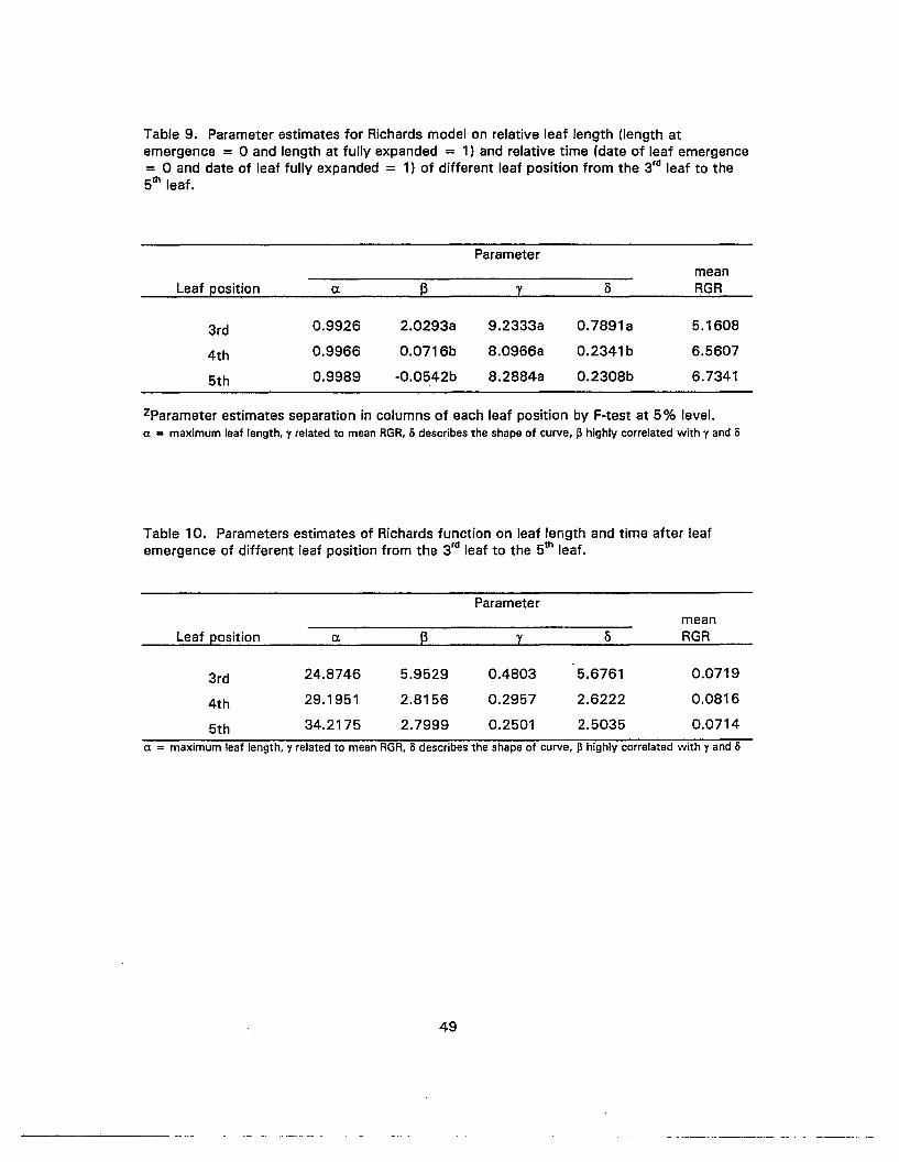
Table 9. Parameter estimates for Richards model on relative leaf length (length atemergence = 0 and length at fully expanded = 1) and relative time (date of leaf emergence= 0 and date of leaf fully expanded = 1) of different leaf position from the 3rd leaf to the5th leaf.
Parametermean
Leaf position a @ y 0 RGR
3rd 0.9926 2.0293a 9.2333a 0.7891 a 5.1608
4th 0.9966 0.0716b 8.0966a 0.2341b 6.5607
5th 0.9989 -0.0542b 8.2884a 0.2308b 6.7341
ZParameter estimates separation in columns of each leaf position by F-test at 5% level.et = maximum leaf length, y related to mean RGR.Ii describes the shape of curve, ~ highly correlated with y and Ii
Table 10. Parameters estimates of Richards function on leaf length and time after leafemergence of different leaf position from the 3rd leaf to the s" leaf.
Parametermean
Leaf position a @ y 0 RGR
3rd 24.8746 5.9529 0.4803 5.6761 0.0719
4th 29.1951 2.8156 0.2957 2.6222 0.0816
5th 34.2175 2.7999 0.2501 2.5035 0.0714
et = maximum leaf length, y related to mean RGR, Ii describes the shape of curve, ~ highly correlated with y and Ii
49

Jan
JanDec
Dec
FL
..........,-,"I,
Nov
Nov
.- .,-,-..-
:'fi
Oct
Sep Oct
2
Aug
Aug
[2J
10
30
30
20
10
20
40
40
Jan
FL
".,,,,",::'
i
Nov Dec
:,:
f:i,:
86 , .....•, .....-'- II ', '
I :
! !, ', ', ', .. '. 'I I, ', ., .,
Oct
OctSep
2 r:,#••/ ••.. ,
I :! iI :I I. ,
:
2 .'u:, ,, ,, ,. ,
I :I II '
! !
Aug
Aug Sep
Q]
[!]
o{ , "i'l';'4;;r.,,;.~,/,;: i , } 0
Jul
0" ,, , , , , , ,Jul
30
30
10
20
20
40
40
IloZw.....Ju,
~.....J
-E 10o-
eno
Figure 11. Richards curves fitted to the length of individual leaves (numbered 2 to 6) in H. stricta grown under different treatment.1 = Vegetative plants under con-LO, 2 = Flowered plants under L03+S0, 3 = Flowered plants under L04L+SO, and 4 =Flowered plants under conSO. Shaded area represents a period of SOs. Oot lines represents length of leaf 2, 3, 7 and 8 or first andsecond cincinal bract. This lines were not fitted to Richards curve.

1 .. ......~.''t=••
-'......c <....
0.8 ~.,.
-t-J0') / ...C / /(1) I ...·
...J 1/~ 0.6ro I ::(1) I ::
...J I ::(1) 0.4 Ii> I::.- 1/ 3rd 4th 5th-t-Jro ~.,:(1) 0.20:: ~: ...... ---.'I"
10.80.60.40.2OL-------'"----.:...-~-'--~-.:.....-.:..-..---:-----I
oRelative Time after Leaf Emergence
Figure 12. Richards curve fitted to relative leaf length (length at emergence = 0 andlength at fully expanded = 1) and relative time (date of leaf emergence = 0 and date ofleaf fully expanded = 1) of different leaf position from the 3rd leaf to the 5th leaf.
51
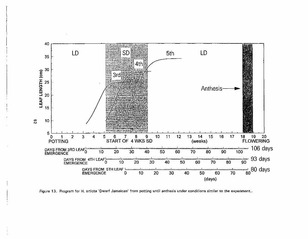
'" ~Anthesis -
LD5th
5 I !, ! I ! ,,-,-.
o 1 2 3 4 5 6 7 8 9 10 11 12 13 14 15 16 17 18 19 20POnlNG START OF 4 WKS SD (weeks) FLOWERING
DAYS FROM 3RD LEAF~"""" ~'~"'"'' ~~, .. I I" ~'~'"''''~'~""'" ~'~""" I ~~I" 1'1' ~~""'" ~~"'''' I ~~"" I' '~~'':'''' II 106 daysEMERGENCE
DAYS FROM 4TH LEAF' . , , , .. , . ,\ .. " . , I , ,!, • , ' • , , " I " . , , , • , I I, , , I , , , I ,!, I , • , , I , I! , , , , , • I I ,I" , , • , , I ,! , ! , , • , I' ,',' I 93 daysEMERGENCE 0 10 20 30 40 50 60 70 80 90
DAYS FROM 5TH LEAF I.""" I""" 1'1 I"'! I'" I" I,! ."., I' 1,1 I I'I!' , ••• ""',' II" """""." •• , 80 daysEMERGENCE 0 10 20 30 40 50 60 70 80
(days)
40I
35 . LD
-30Eo-::r:t- 25 I-
e>zw..J 20u.<W..J 15 .-
Ut 10N
Figure 13. Program for H. srticta 'Dwarf Jamaican' from potting until anthesis under conditions similar to the experiment..
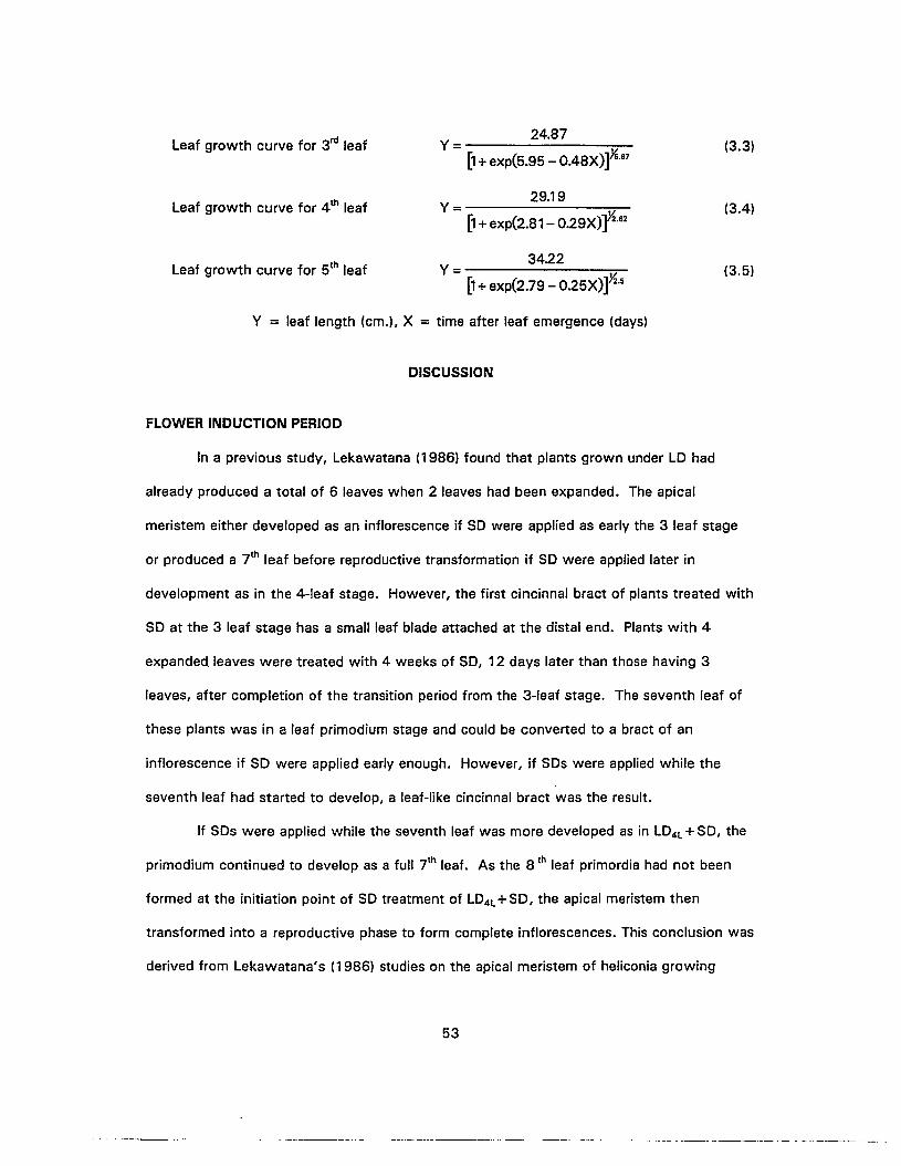
Leaf growth curve for 3rd leaf
Leaf growth curve for 4t h leaf
Leaf growth curve for 5th leaf
24.87Y =-------~-
[1 + exp(5.95 - O.48X)]Ys·B7
29.19Y =----------,~
[1 + exp(2.81- O.29X)]Yz·B2
3422Y =---------:-:,..-
[1 + exp(2.79 - O.25X)]Y2.s
(3.3)
(3.4)
(3.5)
Y = leaf length (cm.), X = time after leaf emergence (days)
DISCUSSION
FLOWER INDUCTION PERIOD
In a previous study, Lekawatana (1986) found that plants grown under LO had
already produced a total of 6 leaves when 2 leaves had been expanded. The apical
meristem either developed as an inflorescence if SO were applied as early the 3 leaf stage
or produced a 7 th leaf before reproductive transformation if SO were applied later in
development as in the 4-leaf stage. However, the first cincinnal bract of plants treated with
SO at the 3 leaf stage has a small leaf blade attached at the distal end. Plants with 4
expanded. leaves were treated with 4 weeks of SO, 12 days later than those having 3
leaves, after completion of the transition period from the 3-leaf stage. The seventh leaf of
these plants was in a leaf primodium stage and could be converted to a bract of an
inflorescence if SO were applied early enough. However, if SOs were applied while the
seventh leaf had started to develop, a leaf-like cincinnal bract was the result.
If SOs were applied while the seventh leaf was more developed as in L0 4L +SO, the
primodium continued to develop as a full 7th leaf. As the 8 th leaf primordia had not been
formed at the initiation point of SO treatment of L0 4L+SO, the apical meristem then
transformed into a reproductive phase to form complete inflorescences. This conclusion was
derived from Lekawatana's (1986) studies on the apical meristem of heliconia growing
53

under LO at different stages of development and from the plot in Figure 7 of time required
to produce each leaf. It would take more than 10 days from 7 th leaf emergence to 8 th leaf
emergence assuming that the leaf primordia emergence correlated with the leaf emergence.
Plants grown under continuous SO produced 6 leaves before flowering and
produced only one cincinnal bract per inflorescence. Plants grown under LO continued to
produce up to 9 leaves and no flowers at the time of harvest. These results implied that
plants were susceptible to floral stimulus before reaching the 3-leaf stage since plants
grown under SO flowered earlier than those treated with SO at the 3-leaf stage. This also
showed that a period of apical competence for floral initiation ranges from before the 3-leaf
stage to sometime after the 4-leaf stage. This was in agreement with previous suggestion
that pseudostems with 2 to 3 expanded leaves up to 5 leaves were capable of
differentiating into inflorescences if exposed to SO (Lekawatana, 1986; Criley and
Kawabata, 1986).
FLOWERING
This experiment confirmed that the first generation of Heliconia stricta pseudostems
grown under LO condition until 3 or 4 fully expanded leaves were evident and then given a
floral stimulus (4 weeks of SO) could be induced to flower in 13 weeks after the start of
SO.
Flowering percentage of pseudostems grown under con SO (46.1 %) was similar to
those reported by Lekawatana (1986; 42.5%) under similar condition. Heliconia grown
from a single rhizome piece have little food reserve to begin with. Young emerging new
shoots of the second generation pseudostem might be a stronger sink than the developing
inflorescence of the first generation pseudostem. Therefore, plants grown from a single
rhizome piece had lower flowering percentage of pseudostems than those of well
established plants.
54
----------- ---- ------- ----

Plants grown under conSO initiated flowers as soon as their apical meristems were
competent for initiation, while those under LD3L + SO and L04L + SO were still vegetative.
However, inflorescence development of plants grown under SO was inferior than those
grown under L0 3L+ SO and L0 4L +SO.
Plants treated with SO at 3 leaf stage had higher percentage of flowering than those
treated at 4 leaf stage. Oue to the small sample size, this results was inconclusive despite
the significant differences.
The plants and inflorescences of plants grown under L0 3L + SO and L04L + SO
produced more bracts (2) than those grown under continuous SO (1). However, the
number of cincinnal bracts (1 or 2 in this experiment) was fewer than those of well
established plants (2 or 3: Lekawatana, 1986; Criley and Kawabata, 1986). This might be
explained as follows:
a) Plants under conSO had smaller and shorter leaves than those under L0 3L + SO
and L0 4L +SO. Therefore, plants under conSO had less leaf area and,
presumably, less assimilates.
b) Under limited assimilates, the young flower bud constitutes a weaker sink
compared with the vegetative apices, developing leaves and it competes poorly
with them for the available assimilates (Halevy, 1984). After heliconia plants
were given flower initial stimulus, 3 or 4 cincinnal bracts may be produced within
the inflorescence, but not all cincinnal bracts will be fully developed due to
limited assimilates.
c) Plants materials in this experiment were first generation of pseudostems planted
from single rhizome pieces while those in previous experiments (Lekawatana,
1986; Criley and Kawabata, 1986) were from plants that were well established
in pots. Therefore, well established plants might have more food reserves in the
55
rhizomes to support inflorescence development than those recently planted as a
single rhizome piece.
PLANT GROWTH
Plants grown under conSO produced significantly shorter and smaller leaves
compared to those grown under conLO, L0 3L +SO, and L04L +SO. This is in agreement with
other results which showed that plants grown under LO are usually taller with longer
internodes and larger leaves, which are often lighter green in color than those grown under
SO (Whatley and Whatley, 1980; Vince-Prue and Tucker, 1983).
Number of leaves produced after SO for plants grown under L0 3L +SO, and
L0 4L +SO is constant at 3 leaves. This reflects the number of leaves that are already
produced by the plants but have not fully expanded yet. The conSO pseudostems must
have had 6 leaves/leaf primodia when flower initiation occured.
Plant grown under conLO remained vegetative and could produced up to 8 to 9
leaves. However, leaf emergence interval was longer as more leaf were produced (Figure
9).
RICHARDS MODEL
The Richards model for leaf length estimated the parameter a well. There were no
differences for growth parameters across treatments within each leaf position of 3rd, 4th and
5th except for the asymptote (a: maximum leaf length). However, these 3 leaf positions
have different growth curves as the s" leaf has a steeper curve than do leaves 4 and 3
(Figure 12). It means that the s" leaf has the fastest development rate (em/day) as shown
by the leaf unfolding rate that had quadratic response to leaf position and mean relative
growth rate.
56
- -- -- --_.- ._-------
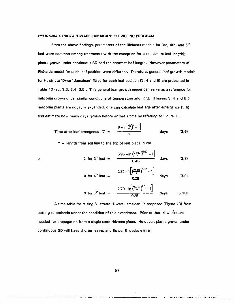
HELICONIA STRICTA 'DWARF JAMAICAN' FLOWERING PROGRAM
From the above findings, parameters of the Richards models for 3rd, 4th, and s"
leaf were common among treatments with the exception for a. (maximum leaf length);
plants grown under continuous SD had the shortest leaf length. However parameters of
Richards model for each leaf position were different. Therefore, general leaf growth models
for H. stricta 'Dwarf Jamaican' fitted for each leaf position (3, 4 and 5) are presented in
Table 10 (eq. 3.3, 3.4, 3.5). This general leaf growth model can serve as a reference for
heliconia grown under similar conditions of temperature and light. If leaves 3, 4 and 5 of
heliconia plants are not fully expanded, one can calculate leaf age after emergence (3.6)
and estimate how many days remain before anthesis time by referring to Figure 13.
Time after leaf emergence (X) =y
days (3.6)
Y = length from soil line to the top of leaf blade in cm.
or X for 3rd leaf =
X for 4th leaf =
X for 5th leaf =
5.95 -It(¥LtG7-1J
0.48
2.81- 11(¥ y"G2-1J
0.29
2.79 -11(¥'l5 -1J
0.25
days
days
days
(3.8)
(3.9)
(3.10)
A time table for raising H. stricta 'Dwarf Jamaican' is proposed (Figure 13) from
potting to anthesis under the condition of this experiment. Prior to that, 4 weeks are
needed for propagation from a single stem rhizome piece. However, plants grown under
continuous SO will have shorter leaves and flower 5 weeks earlier.
57
--- -._.- -------
CHAPTER 4
EFFECT OF TEMPERATURE ON INFLORESCENCE DEVELOPMENT
AND ABSCISIC ACID LEVELS IN H. STRICTA
ABSTRACT
Plants of Heliconia stricta Huber 'Dwarf Jamaican' were treated with four
temperatures (18°C, 21°C, 24°C and 28°C) under an 14 hr. daylength after an initial floral
induction stimulus of 4 weeks of SD at 21°C. Free (+ )-abscisic acid (ABA) content of
mature leaves was measured by indirect enzyme-linked immunosorbent assay (ELISA).
Increased night temperature decreased percent flowering (from 55% to 31 %) and increased
the percent aborted pseudostems from 0% to 19.2%. However, temperature during this
period had no influence on percent reproductive pseudostems (flowering +aborted). Lower
temperatures during inflorescence development increased levels of ABA in H. stricta 'Dwarf
Jamaican' leaves from 264.6 ± 18.8 ng/g dry wt. at 28°C to 441.0 ± 42.3 ng/g dry wt. at
18°C. A lower level of ABA was found in leaves of aborted pseudostems (285.5 ± 55.7
ng/g dry wt.) compared to that found in leaves of inflorescence developing pseudostems
(386.9 ± 37.3 ng/g dry wt.). The smallest developing inflorescence that was found to be
aborted was 2 cm long and was found 6 weeks after start of SO.
INTRODUCTION
Flower bud abortion in Heliconia has been found in many species such as H.
angusta, H. chartacea and H. stricta (Lekawatana, 1986; Criley and Lekawatana, 1994;
Kwon, 1992). Lekawatana (1986) reported that pseudostems grown under different night
temperatures (18-28°C) at the time of flower initiation (4 weeks of short days) showed no
difference in percent flower bud abortion. If one could induce these plants to flower year
58

round, reducing the percent of flower bud abortion would be beneficial to the cut flower
industry.
Roles of ABA in promoting or inhibiting flower abortion have not been fully
understood. Trewavas and Jones (1991) stated that exogenous application of ABA
increased flower abscission which was similar to the effect of water stress. Furthermore,
ABA was found to inhibit flower initiation in several short day plants and long-day plants
grown under inductive conditions (Bernier, 1988). Increased ABA levels paralleled the
increase of ethylene which was responsible to the onset of irreversible wilting in carnation
petals (Hanley and Bramlage, 1989).
Several environmental factors affect the endogenous level of abscisic acid (ABA) in
plant tissues. Most prominent is the effect of drought stress, but other kinds of stress such
as aeration stress and temperature extremes have been reported to change the level of ABA
(Addicott, 1983). Exposure to low temperature causes a rise in the level of ABA of some
plants (Capell and D6rffJing, 1989).
The common methods of quantification of ABA are by high-pressure liquid
chromatography with UV detection (HPLC-UV), gas chromatography with flame ionization
detection (GC-FID) or gas chromatography with electron capture detection (GC-ECD), all of
which require rigorous cleanup procedures to reduce contaminants. Immunoassay provides
a technique to use a selective antibody (Ab) to identify and quantify the low physiological
concentrations of ABA in unpurified plant extracts (Weiler, 1979).
Mertens et al. (1983) developed a specific monoclonal antibody (MAb) directed at
free ABA. This MAb is now available commercially (Idetek, 1985). Norman et al. (1988)
developed an indirect ELISA procedure which requires less commercial MAb than the direct
procedure the company suggested. This provided a rapid, sensitive, and efficient technique
for ABA quantification.
59

high temperature was also reported to promote flower abortion (Kinet et aI., 1985).
This experiment was carried out to investigate the effect of temperature during flower bud
development on percent abortion and ABA content in Heliconia stricta 'Dwarf Jamaican'.
An indirect ELISA procedure for free ABA was adapted for analyzing ABA content in
Heliconia leaves and apices. This procedure was adapted from those used by USDA
(Hawaii) researchers for analyzing ABA content in sugarcane leaves, which in turn, were
based on Norman et al. (1988) and Walker-Simmons (1987). Assay sensitivity, precision
and specificity were verified.
MATERIALS AND METHODS FOR INDIRECT ELISA PROCEDURE
PLANT MATERIAL
Heliconia stricta 'Dwarf Jamaican' plants were grown in 15-cm pots in a greenhouse
at the Magoon greenhouse facility of the University of Hawaii. The average minimum and
maximum temperatures during the growing period (December 1989-January 1990) were
20.4°C (range: 15.5-22.5°C) and 32.8°C (range: 22.5-36°C), respectively
Apex tissues (1 em. in length) used in this experiment was selected from plants
with 3-4 leaves. Twenty pieces of apex tissue were harvested and immediately frozen in
liquid N2 , then powdered and lyophilized. Three apical tissues per sampling time were
analyzed through ELISA, and the resulting ABA concentrations were calculated.
Leaves used in this experiment were selected from the top mature leaves of plants
with 3-4 expanded leaves. Ten leaves were harvested. Leaf blades were stripped from
their midribs. Each sample was placed in a plastic tube and immediately stored in liquid
nitrogen (-70°C). Leaves were then powdered by grinding in a precooled mortar and pestle
with liquid nitrogen then lyophilized. The lyophilized samples were then stored in plastic
60
tubes at -20°C. Three leaf tissues per sampling time were analyzed through ELISA, and the
ABA concentrations were calculated.
ABA EXTRACTION
Leaf Samples
Heliconia leaf samples (0.5 g dry wt.) were ground in 10 ml of 80% acetone with a
Tissumizer (Tekmarl. The extract was suction-filtered through Whatman No.1 filter paper.
The residue was extracted twice more with 10 ml of 80% acetone. The volume of the
combined supernatant was brought up to 25 ml with 80% acetone.
Then 0.5 ml of the supernatant was placed in 3 ml glass tube and dried in a Speed
Vac Concentrator (Savant). The dry extract was resuspended to 0.01 g dry weight
tissue/ml with TBST (Tris-buffered saline with Tween 20). Norman et. al (1998) reported
that the use of 0.2-/lm Lid/x filter improved ELISA values compared to no filter or other filter
procedures (silica Sep Paks, centrifugation and other filters). Therefore, aliquots of the
extract were passed through a 0.2-pm Lid/x nylon 66 syringe filter (Genex Corp.) twice.
This extract solution was then ready to be tested by ELISA.
Apex Tissue
Since the apex tissue samples were much smaller than the leaf samples, only 0.1 g.
dry wt. was used. Heliconia apex tissue samples (0.1 g dry wt.) were ground in 2 ml of
80% acetone with a glass tube and a pestle. The extract was centrifuged to separate the
supernatant. The residue was extracted twice more with 2 ml of 80% acetone. The
volume of the combined supernatant was brought up to 5 ml with 80% acetone.
Subsequent procedures were identical to the method described for leaf samples.
61
ELISA MATERIALS
Buffer
TBST (Tris-buffered saline with Tween 20): 6 9 of Tris [tris(hydroxymethyl)
aminomethaneJ, 0.2 9 of MgCI2' 8.8 9 of NaCl, 0.5 ml of Tween 20, and 0.1 9 of sodium
azide, pH 7.5.
Bicarb: 50 mM NaHC03 with sodium azide, 0.1 gIL, pH 9.6.
Standards
A stock solution 0.01 9 (+ leis-trans ABA (Sigma Chemical Co.) was prepared in
100 ml of MeOH. This was further diluted with TBST to 10, 20, 40, 80, 160, 300 and
5000 pg/1 00 pL.
ABA-4'-TH-BSA conjugate
(± I-ABA-4'-tyrosyl-hydrazone and p-aminohippuric acid substituted BSA were
prepared and coupled to form an ABA-4'-TH-BSA conjugate according to Weiler (1980;
conjugate solution was obtained from K. Pitz, USDA). The solution contained about 1.4 mg
of conjugate/ml and was stored in 0.5 ml aliquots at -20°C. A 0.5 ml aliquot was diluted
to 20 pg/ml with bicarb buffer for coating microtitration plates.
Monoclonal Antibody
Two mg of MAb to free eis-,trans-( +)-ABA (Idetek, Inc.) were dissolved in 2.0 ml of
TBST. This stock solution was diluted to 0.8 pg/ml with TBST just before use.
MAb stored at -20°C for several years showed no obvious deterioration. However,
storage at 4°C for only a few days resulted in some reduction of activity, and freezing and
thawing caused measurable loss in activity. Dilute Ab preparations lose significant amounts
62
------- -- ---- -- -- --- - - ------ --_~---- - - -~~=------ -- -

of activity by adsorption onto plastic surfaces; thus, polypropylene tubes are preferred to
polystyrene (Zola, 1987).
Antimouse Alkaline Phosphatase Conjugate
Just prior to use, 0.85 g of PEG 8000 was added to 21 ml of TBST buffer and then
27 pi of rabbit antimouse alkaline phosphatase (RaMAP) conjugate (Sigma Chemical Co.)
was added. The enzyme activity doubles between 25°C and 37 °C (Kemeny, 1991).
Substrate
Five tablets of p-nitrophenyl phosphate (p-NPP; 5 mg/tablet plus filler) were
dissolved in 25 ml of bicarb buffer previously warmed to 37°C. Hydrolysis of the p-NPP
occurs at temperatures above 30 °C (Kemeny, 1991).
Microtitration Plates
Immulon 2 flat bottom, polypropylene 96-well microtitration plates (Dynatech
Laboratories, Inc.) were utilized. The outer wells of the plate were not used.
ELISA PROCEDURE (FIGURE 14)
Coating of Wells with ABA-4'TH-BSA Conjugate
A 200 pI aliquot of the conjugate was added to each well of the microtitration
plates. Plates were covered with parafilrn, wrapped in foil, and incubated at 4°C overnight.
The binding of proteins to plastic depends on time and temperature. For
convenience coating is usually done at 4°C overnight. The optimum pH for binding
immunoglobulin is pH 9.6 (Kemeny and Chantler, 1988).
63
--- ------------------_._-- --- ---
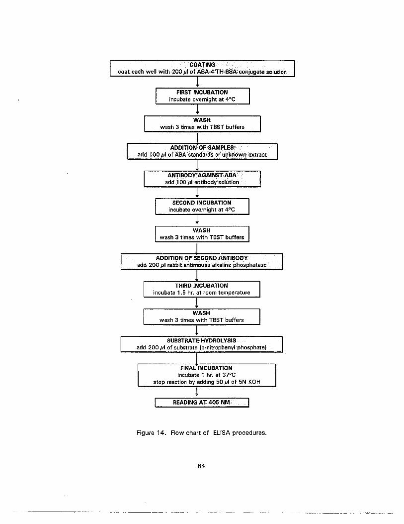
COATING'·coat.each well with·200j,t1 ofABA';;4~TH~BSNconjugate solution
FIRST INCUBATIONincubate overnight at 4°C
WASHwash 3 times with TSST buffers
ADDITION;OFSAMPLES,add 100 pi of ·ASAstaridatcfs;or onknown•extract
ANTIBODY'AGAINST;ABA·····.··add}OOpl· antibody solution
SECOND INCUBATIONincubate overnight at 4°C
WASHwash 3 times with TSST buffers
ADDITION OFSECOND,ANTIBODYadd 200 pi rabbitantimousealkalille"phosphatase •.
THIRD INCUBATIONincubate 1.5 hr. at room temperature
WASHwash 3 times with TSST buffers
I!
SUBSTRATE HYDROLYSISadd 200 pi of substrate (p-nltrcphenviphcsphate)
IFINAL INCUBATION
incubate 1 hr. at 37°Cstop reaction by adding 50 pi of 5N KOH
READING AT.405 NM ...
Figure 14. Flow chart of ELISA procedures.
64
I
---_._- .._-- -----
Addition ofABA Samples
Plate wells coated with conjugate were washed three times with TBST buffer. The
final washing solution was left in the plates for 10 min. and then discarded. Each well was
filled with 100 pi of one of the eight ABA standards, TBST buffer or leaf tissue extract
(representing 1 mg of leaf dry weight). All standards, apex and leaf tissue extracts were
replicated three times (3 wells). Leaf tissue extract was diluted to 1 (undiluted) and 1/2
dilution. One column contained excess ABA (5,000 pg) for nonspecific binding (NSB).
Absorbance reading from this column was used as a correction number. Another column
contained TBST buffer only for a maximum absorbance reading (Bo)' When absorbance
readings from this column (Bo) reached 1 the final incubation was stopped.
Addition of MAb
One hundred pi of diluted MAb were added to each sample or standard. Plates were
covered with parafilm, wrapped in foil, and incubated at 4°C overnight.
Since binding of ABA to MAb is pH dependent, and binding decreases at pH 6.0 or
below but is not affected in the range of pH 6.0-9.0 (Oaie arid Wyse, 1982), a pH of 7.5
was used in the assays.
Addition of the Second Antibody
Wells were washed three times with TBST. Two hundred pi of Rabbit antimouse
alkaline phosphatase conjugate containing PEG were added to each well. Plates were
incubated for 1.5 h at room temperature in the dark.
Measurement of Alkaline Phosphatase
Wells were washed three times with TBST. Two hundred pi of substrate (p
nitrophenyl phosphate) solution were added to each well. Plates were incubated for around
65
--- --- ------ -------

1 h until the absorbance of control sample containing no ABA (Bo) measured at 405 nm was
approximately 1.0. The incubation was stopped by adding 50,£11 of 5 N KOH, after which
the sample absorbance was measured at 405 nm with Microplate Reader Model 450 (Blo-
Rad Lab.). Since the method used was indirect ELISA, the absorbance reading of the
samples is inversely proportional to the amount of ABA in the original sample.
ELISA DATA PROCESSING
Absorbance readings (optical density: 0.0.) for the ABA standards were converted
to percent binding (BI Bo%, 4.1) and then logit transformed (4.2).
B/Bo% = (Standard or Sample 0.0. - NSB 0.0. x 100) I (Bo 0.0. - NSB 0.0.)
(B/Bo% )Logit.B IB o = Ln ----=---
100 - B I Bo%
NSB = Non Specific Binding
Bo = Maximum absorbance reading
B = Absorbance reading for ABA standard series
(4.1)
(4.2)
Standard curves were linearized by plotting logit-Iog transformed data against the Ln
of ABA added (Vernieri et aI., 1989a; Parata et al., 1990). All sample absorbance readings
were converted to BIBo % , and logit transformed; ABA concentration was extrapolated
from the linear regression line of the ABA standard curve (Hanley and Bramlage, 1989).
There were 3 replicates of each sample.
DETERMINING CONJUGATE CONCENTRATION
Three concentrations of ABA-4'-TH-BSA conjugate (5, 10 and 20 Ilglml) were used
to determine the optimal concentration range to be used in the routine ELISA. The
concentrations of MAb and second Ab were held constant at 0.8 pglml MAb and 1.29 pl/ml
second Ab. The goal was to obtain an optical reading of 1.0 of Bo (blanks containing only
TBST) within 1 hour of the final incubation. Two microtitration plates were used for each
66
concentration and followed the above ELISA procedure. Only the ABA standards and TBST
blank were used with 6 wells of each per plate.
DETERMINING REPRODUCIBILITY OF THE ELISA OUTPUT
Eight microtitration plates were processed through the ELISA procedure using 20 pg
Iml ABA-4'-TH-BSA conjugate (coating), 0.8 MAb pg/ml Mab, 6 levels of ABA standard.
and 1.29 pl/ml second Ab. The absorbance readings among plates were analyzed to
determine whether the readings were significantly different among plates.
SPECIFICITY TEST
A test for specificity in immunoassays is to test for parallelism of a plant extract
dilution curve with the standard curve (Daie and Wyse, 1982). Any interfering substances in
the leaf extract should change the slope of the curve (Pengelly, 1986). Therefore heliconia
leaf extract, diluted to 5 levels of concentration (1, 1/2, 1/4, 1/8, and 1/16), was added to
a microtitration plate as unknowns in triplicate, and ABA was determined through ELISA.
The linear regression line of the logit B/Bo on log of leaf extract dilution was analyzed.
Parallelism was then evaluated by comparing the slope of the leaf extract dilution to the
standard slope of the regression equations.
PERCENT RECOVERY
One hundred nglg dry wt, of cis-,trans-( +)-ABA (Sigma Chemical Co.) were added
as an internal standard to each of 5 dry leaf samples (0.5 9 dry wt). These samples,
together with those without added ABA, were analyzed through routine ELISA. The percent
recovery was calculated (4.3) to confirm the specificity and accuracy of the assay (Daie and
Wyse, 1982).
SA-SO% recovery = --- x 100
A
67
----------- --- ._------------------------_._----
(4.3)

A = Amount of ABA added to sample
SA = ABA cone. from sample with added ABA
SO = ABA cone. from sample without ABA added
MATERIALS AND METHODS FOR THE EXPERIMENT
PLANT MATERIALS
Three hundred rhizome pieces of He/iconia stricta 'Dwarf Jamaican' were
propagated on September 20, 1989. Rhizome pieces including pseudostems were
separated and the roots removed. Pseudostems were cut to 5 em in length from the leaf
sheath base, treated in a 55°C water bath for 5 minutes, dipped in fungicide (Dithane M
45) and drained. The rhizomes were then held in plastic bags for 3 weeks at 20°C to
stimulate root and shoot growth. They were then rooted in metal trays containing perlite
and vermiculite 1:1 ratio (v/v) in a growth chamber at the Pope laboratory of the University
of Hawaii. The environmental conditions were: photoperiod: 14 hours (long day: LD) using
a combination of fluorescent and incandescent lamps, 214 J,lmol.m·2.s·'; temperature 25/20°
C Day/Night (D/N). On November 2, 1989 rooted rhizome pieces were potted into 15-cm
pots with 3 plants/pot for a total of 100 pots. The potting medium was a mixture of peat
and perlite 1:1 ratio (v/v) amended with dolomite, Micromax and treble superphosphate at
the rates of 6.0, 1.0 and 0.6 kg per cubic meter, respectively. Plants were continued in
growth chambers under the same condition and were hand-watered daily with nutrient
solution 200N-200P-200K (ppm) throughout the experiment. When approximately 50% of
plants had reached the 3 to 4 expanded leaf stage (January 16, 1990), they were subjected
to short day (8 hour daylength, SO) at 25/20 °C D/N temperature for 4 weeks to provide
the flower initiation stimulus to these plants (Criley and Kawabata, 1986). Throughout the
experiment plants were provided with adequate water, therefore the effect of water stress
was minimized.
68
---~-- _..._- -- --.._--

TREATMENT SETUP
After 4 weeks in SO (February 18, 1990) heliconia plants were placed in 4 growth
chambers with different day and night temperatures (O/N) as follows:
Trt. 1. 20/15 °C
Trt. 2. 23/18 °C
Trt. 3. 26/21 °C
Trt. 4. 30/25 °C
(14 x OT)+ (1 0 x NT)Average daily temperature = -------
24(4.4)
OT = day temperature, NT = night temperature
Only the average daily temperature (calculated by eq. 5.1), 18°C, 21 °C, 24°C and 28°C,
will be used throughout this chapter to represent treatments 1, 2, 3, and 4, respectively.
The photoperiod was 14 hours (long day: LO) using combination of fluorescent and
incandescent lamps, 214 umol.rn" .S-1. Treatments were terminated on May 31, 1990 at
19 weeks after the start of SO.
DATA COLLECTION
At the beginning of SO the expanded leaf number of all pseudostems (250
pseudostems) was determined. Ouring the SO induction period (January 16 - February 17,
1990) 6 plants (2 pots) were removed each week for sample collection. From February 18
to April 6, 1990, 6 plants (two pots) were removed from each chamber every 7 days for
sample collection (except weeks 5 and 9 after the start of SO).
Leaf blades of the topmost mature leaves of each shoot were selected for ABA
analysis (180 samples). Tissue around the apical meristematic region (-1.5 cm long) of
each shoot was fixed with FAA for shoot status determination (255 samples). The number
of expanded leaves when collected was recorded for each sample.
69
-------_._---

At the end of the experiment (May 31, 1990) the growing status of the remaining
plants (total of 43 pseudostems with approximately 9 plants or 3 pots per treatment) was
determined (vegetative, elongated, flowering or aborted).
SHOOT STATUS DETERMINATION
Two hundred and fifty-five samples of shoot apical meristems were collected to
determine their developmental status through microscopy of thin longitudinal sections.
Tissues to be examined were fixed in FAA solution (formalin-aceto-alcohol) and dehydrated
in a graded series of ethyl alcohol-tertiary butyl alcohol (TSA) solutions (Johansen 1940).
Infiltration with Parowax and embedding in Paraplast followed a standard paraffin
embedding technique (Johansen 1940). Longitudinal sections were made on a rotary
microtome at 20 micrometer thickness. Tissues were then stained with 0.05% toluidine
blue 0 (Sakai, 1973). The status of each meristem was determined (vegetative, elongate,
flower, or aborted) (Lekawatana, 1986).
STATISTICAL ANALYSIS
The statistical analysis was by SAS general linear model (PROe GLM) analysis of
variance with mean separation by t-test or contrast (SAS Institute, 1987). Quantitative
data such as meristem and shoot status were analyzed by Chi-Square test for independence
with the null hypothesis that the differences among the ratios in each temperature
treatment were not significant.
RESULTS FOR THE ELISA PROCEDURE
ASSAY SENSITIVITY AND PRECISION
Standard curves for ELISA were obtained by plotting absorbance at 405 nm versus
the log of ABA concentration in the assay. The lower detection limit was 10 pg/1 00 pi and
the assay concentrations ranged from 10-300 pg/1 00 pI. To improve the sensitivity of
70
- - ---- --------
standard curves, coating concentration, MAb dilution, second Ab dilution and the duration
of the incubations could be adjusted. With MAb and second Ab at constant levels (0.8 pgl
ml MAb and 1.29 pllml second Ab), an increase in coating concentration (ABA-4'-TH-BSA
conjugate; 5, 10, and 20pg/ml) decreased time for Bo (blanks) absorbance reading to reach
1.0. Curves of similar shape were obtained either at 10 pglml with a 108 min. incubation,
or 20 pg/ml with a 60 min. incubation (Figure 151. The latter were used as a standard
concentration for ABA-4'-TH-BSA conjugate.
Figure 16 demonstrated the high day-to-day reproducibility of the assay using
identical dilutions of antibody, conjugate, and ABA solutions (8 consecutive assays
(Appendix A:Table 115). There was no significant difference among assay means and
slopes at the 5% level. The coefficient of variation was -13.5 % and n =8 (Appendix
A:Table 116).
SPECIFICITY
Leaf Samples
When Heliconia leaf extract was used in a serial dilution (1, 1/2, 1/4, 1/8, and
1/16), the curve (Figure 17, Appendix A:Table 118) was parallel to the standard curve
(Figure 20, Appendix A:Table 117) with both slopes = -2.57 (Figure 20). This confirmed
the absence of interference.
When known amounts of ABA (100 nglg dry wt.) were added to leaf extracts as
internal standards, the recovery was 92.1 ± 2.3 %. This confirmed the specificity and
accuracy of the assay (Daie and Wyse, 1982).
Shoot apex samples
When Heliconia apex extract was used in a serial dilution (1, 1/2, 1/4 and 1/8), the
curve (Figure 18, Appendix A:Table 119) was not parallel to the standard curve (Figure 21,
71
------- _.- . __..._-- .-.._---
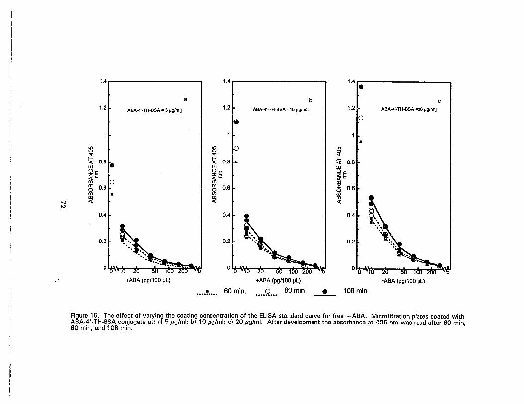
+ABA (pg/100 IJL)
o~"'/n x·x itX:; Ax "Ax '5:\~
0.2
108 min•"0 5
+ABA (pg/100 IJL)
•..•Q... 80 min
0.2
••••~.... 60 min.
'" , -.:.~~_ Io~'::;n >iX I:x"Y.A
0.2
1.4. • 1.4 • 1.4 •a 12~ b c
ABA-4'-TH-BSA = 5 fig/mil ABA-4'-TH-BSA =10 fig/mil 1.2 ABA-4'-TH-BSA =20 fig/mil
0
1•
I{) I{) I{)0 0 0'<t '<t '<t
~ 0.8 • ~ ~ 0.8w w wU E U E U E~c
0~c ~cCO
0:: 0.6 0:: 0:: 0.60 0 0en • en enCO CO CO
'" « « «I\)
0.4 0.4~ • I 0.4
Figure 15. The effect of varying the coating concentration of the ELISA standard curve for free +ABA. Microtitration plates coated withABA-4'-TH-BSA conjugate at: a) 5 pg/ml; b) 10 pg/ml; c) 20 pg/ml. After development the absorbance at 405 nm was read after 60 min,80 min, and 108 min.
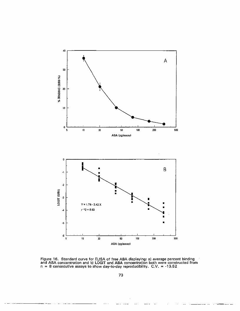
4Or------------------------,
50020010050
ABA lpg/assay)
20100'-"--'""--'---'-'-------''--_-'---'-'---'--'-.........-'--'- -'-_--'-_""-...
5
30
~0
~Cl 20Zisziii~
10
Y=1.78- 2.42 X
r A2=0.93
0
-I
-2
0cee-3t::
Cl0...
-4
-5
-l;5 10
•
20 50
ABA lpg/assay)
100 200
B
•
••
500
Figure 16. Standard curve for ELISA of free ABA displaying: a) average percent bindingand ABA concentration and b) LOGIT and ABA concentration both were constructed fromn = 8 consecutive assays to show day-to-day reproducibility. C.V. = -13.52
73
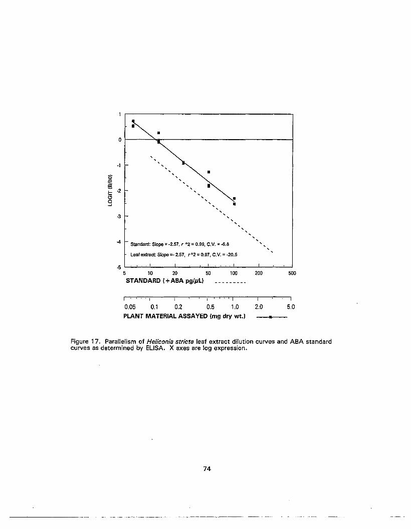
Standard: Slope =-2.57. r A2=0.99, C.V. =-6.8
Leaf extract: Slope =- 2.57, r A2 =0.97, C.V. =-20.5
, , , , , , , , , , , , , , , , , , , , ,-4
0
, ,-1 , ,
0, ,
CD,
e , , ,~ -2 ,a0..J
-3
-5 .... I
5 10 20 50
STANDARD (+ABA pglpL)
. I
100 200 500
Ii. " I iii [ I
0.05 0.1 0.2 0.5 1.0 2.0 5.0PLANT MATERIAL ASSAYED (mg dry wt.) --1.1--
Figure 17. Parallelism of Heliconia stricta leaf extract dilution curves and ABA standardcurves as determined by ELISA. X axes are log expression.
74

4.-------------------------,
•2 f- •
•
-2 f-
-4 f-
Standard: slope =-2.57. r A2 =0.99, C.V.=-6.8
Shoot apex extract: slope =2.83, r A2 =0.61, C.V. =-349.8
. I
100
I
200 500
Iii "'I i i •• I
0.05 0.1 0.2 0.5 1.0 2.0 5.0PLANT MATERIAL ASSAYED (mg dry wt.) -...,_..._-
Figure 18. Parallelism of HelicoiJia stricta shoot apex extract dilution curves and ABAstandard curves as determined by ELISA. X axes are log expression.
75
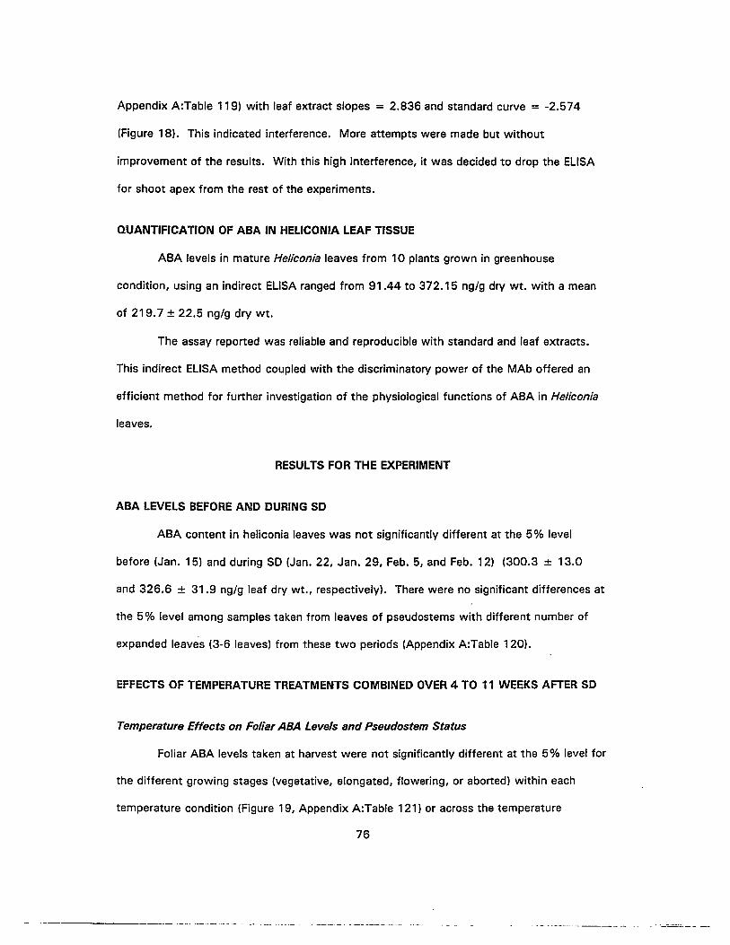
Appendix A:Table 119) with leaf extract slopes = 2.836 and standard curve = -2.574
(Figure 18). This indicated interference. More attempts were made but without
improvement of the results. With this high interference, it was decided to drop the ELISA
for shoot apex from the rest of the experiments.
QUANTIFICATION OF ABA IN HELICONIA LEAF TISSUE
ABA levels in mature Heliconia leaves from 10 plants grown in greenhouse
condition, using an indirect ELISA ranged from 91.44 to 372.15 ng/g dry wt. with a mean
of 219.7 ± 22.5 nglg dry wt,
The assay reported was reliable and reproducible with standard and leaf extracts.
This indirect ELISA method coupled with the discriminatory power of the MAb offered an
efficient method for further investigation of the physiological functions of ABA in Heliconia
leaves.
RESULTS FOR THE EXPERIMENT
ABA LEVELS BEFORE AND DURING SO
ABA content in heliconia leaves was not significantly different at the 5% level
before (Jan. 15) and during SD (Jan. 22, Jan. 29, Feb. 5, and Feb. 12) (300.3 ± 13.0
and 326.6 ± 31.9 ng/g leaf dry wt., respectively). There were no significant differences at
the 5 % level among samples taken from leaves of pseudostems with different number of
expanded leaves (3-6 leaves) from these two periods (Appendix A:Table 120).
EFFECTS OF TEMPERATURE TREATMENTS COMBINED OVER 4 TO 11 WEEKS AFTER SO
Temperature Effects on Foliar ABA Levels and Pseudostem Status
Foliar ABA levels taken at harvest were not significantly different at the 5% level for
the different growing stages (vegetative, elongated, flowering, or aborted) within each
temperature condition (Figure 19, Appendix A:Table 121) or across the temperature
76
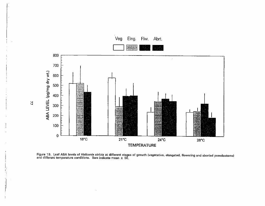
Veg Elng. Flw. Abrt.
o --
28°C
800
700 .-
~ 600~
"0tn 500'-E-tnS- 400'-
...J~ W~ > 300w
...J
«200m«100
018°C 21°C 24°C
TEMPERATURE
Figure 19. Leaf ABA levels of Heliconia stricta at different stages of growth (vegetative, elongated, flowering and aborted pseudostemsland different temperature conditions. Bars indicate mean ± SE.
j
:1I,iI

condition (Appendix A:Table 122). Across all temperature conditions, foliage of flowering
pseudostems had the highest ABA level at 386.9 ± 37.3 ng/g dry wt. while foliage of
aborted pseudostems contained the lowest ABA level at 285.5 ± 55.7 ng/g dry wt (Figure
20). Foliage of vegetative and elongated pseudostems was intermediate at 349.5 ± 47.7
and 334.6 ± 52.2 ng/g dry wt. of ABA, respectively.
The foliar ABA content of heliconia grown under different temperature conditions
(across all growth stages) had a significant linear effect at 5% level (Appendix A:Table
121). An increase in average daily temperature led to a decrease in foliar ABA content (18
DC: 441.0 ± 42.3, 21°C: 339.5 ± 29.8, 24°C: 331.5 ± 20.8, and 28°C: 264 ± 18.8 ng/g
dry wt.; Figure 21; Appendix A:Table 123).
Temperature Effects on Pseudostem Status
For a period of 4 to 11 weeks after the start of SO, temperature treatments had a
significant effect on the proportion of flowering, elongated, vegetative and aborted
pseudostems (Figure 22, Appendix A:Table 124). At the lower temperatures, the
percentage of flowering pseudostems increased from 31 % at 28°C to 55% at 18°C. The
percent aborted pseudostems Increased from none at 18°C to 19.2% at 28°C. However,
there was no significant difference at the 5% level in the proportion of reproductive shoot
stages (flowering plus aborted apices) among different temperature treatments (Appendix
A:Table 124) with an average of 50.2 % reproductive stage.
Foliar ABA Levels and Expanded Leaf Number at Harvest
Foliar ABA content from the topmost mature leaf, exhibited a quadratic relationship
with the position of leaves on the pseudostems when samples were taken (averaged over
all 4 temperature conditions and developmental stages; Figure 23, Appendix A:Table 125).
ABA level decreased from 438.1 ± 45.6 ng/g dry wt. at the 4-leaf stage to 287.8 ± 19.3
78
_...__ . _...._.__ . ._--

Abrt.Flw.Elng.Veg.o
500
400 T~~-c
300Cl
~.9--JW> 200w-J
-cIII-c
100
PSEUDOSTEM STATUS
Figure 20. Concentration of ABA in leaf tissue from Heliconia stricta pseudostems pooledacross all temperatures during 4 to 11 weeks after start of SO (Veg. = vegetative, Elng.= elongated, Flw. = flowering, Abrt. = aborted). Bars indicate mean ± SE.
3027
Y=841.63 - 20.96 X. '''2 =0.14
24
TEMPERATURE (OC)
500
450
i~4oo'0Cl.§Cl~ 350..JW>W..J 300«m«
250
20015 18 21
Figure 21. Effect of average daily temperatures on leaf ABA levels averaged over allgrowth stages for 4 to 11 weeks after start of SO. Bars indicate mean ± SE.
79
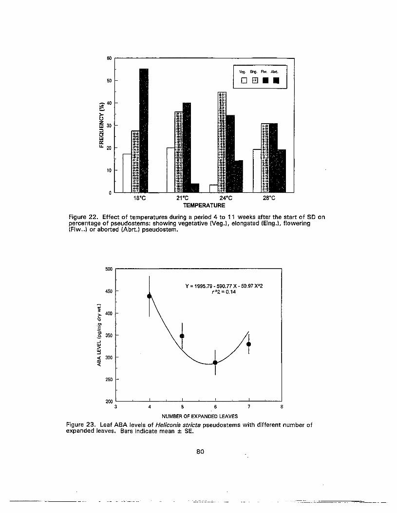
60
50
..... 40~>-0ffi 30:::law0::11. 20
10
01SoC
Veg. Bog. Aw. AM.
2S"C
Figure 22. Effect of temperatures during a period 4 to 11 weeks after the start of SD onpercentage of pseudostems: showing vegetative (Veg.), elongated (Elng.), flowering(Flw ..) or aborted (Abrt.) pseudostem.
Y = 1995.79 - 590.77 X - 50.97 X/l2(/12=0.14
500
450
~400
~"0Cl
~Cl
350Eo....IW>W....I
oct: 300OJoct:
250
2003 4 5 6 7 8
NUMBER OFEXPANDED LEAVES
Figure 23. Leaf ABA levels of Heliconia stricta pseudostems with different number ofexpanded leaves. Bars indicate mean ± SE.
80

ng/g dry wt. at the 6-leaf stage then increased to 329 ± 22.1 ng/g dry wt. at the 7-Ieaf
stage.
EFFECT OF TEMPERATURE TREATMENTS AT DIFFERENT TIMES OF DEVELOPMENT
Pseudostems with 2 to 5 leaves at the Start of SD
During the 11 weeks after the start of SO, pseudostems with 4 and 5 leaves at the
start of SO showed signs of apical meristem elongation in the second week of SO while
those with fewer than 4 expanded leaves did not elongate until 4 weeks after the start of
SO (Figure 24). Flower primordia were found at 3 weeks after the start of SO in plants with
5 expanded leaves at start of SO, at 4 weeks after SO in plants with 3 and 4 expanded
leaves and not until after 4 weeks after the start of SO for plants with 2 leaves. Evidence
of flower bud abortion was found 6 weeks after the start of SO in shoots with 2, 3, and 4
leaves at start of SO but not until 10 weeks after the start of SO in shoots with 5 expanded
leaves at start of SO (Figure 24).
Foliar ABA content of plants with different numbers of leaves at the start of SO
fluctuated over time (averaged over all 4 temperature conditions and developmental stages).
However, the patterns of peaks and valleys for pseudostems with 3-4 expanded leaves at
start of SO were quite similar with a dip at 3 weeks after start of SO and a peak at 4
weeks.
Pseudostem with 3 To 6 Leaves at Time of Sampling
During the 11 weeks after the start of SO, pseudostems with 5 and 6 expanded
leaves at sampling showed apical meristem elongation in the second week of SO while
those with fewer than 5 expanded leaves did not elongate until 4 weeks after the start of
SO (Figure 25). However, flower primodia were found in pseudostems with 6 expanded
leaves at 3 weeks after the start of SO while those with 3-5 expanded leaves showed
flower primordia at 4 weeks after the start of SO. The first sign of flower bud abortion was
81
------------ -- ---- - - ------------------
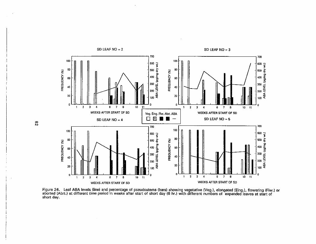
10 116 7 82 3 4
SD LEAF NO = 3
700 700100 -
-. 600 ~ 600 ~~
-. 500 ~~
80- • 500 ~Cl Cl
-. 400 E ~ 60- - 400 Ia, z.& w
-. 300 ...J :> 300 ...J
-. 200 ~0
~w 40 -II:
200 ~u.<l: -cCD 20 - CD
100 -c - 100 <l:
0 0 010 11
SD LEAF NO = 2
SD LEAF NO = 4
WEEKS AFTER STARTOF SO
o
600~
500~"t:ICl
400 i300 ::;
~200 ~
<l:
100 ~
700
10 11678234o
Veg. Elng. Flw. Abrt. ABA
D£m •• --
I -
-
I .
I -
;'. VI - r- -I-- -
I -
IT l IT-
I
10 11678234
100
i! 80
>u 60zw:>0w 40II:u.
20
0
OJI\.)
WEEKS AFTER STARTOF SO WEEKS AFTER STARTOF SO
Figure 24. Leaf ABA levels (line) and percentage of pseudostems (bars) showing vegetative (Veg.), elongated (Elng.), flowering (Flw.) oraborted (Abrt.) at different time period in weeks after start of short day (8 hr.) with different numbers of expanded leaves at start ofshort day.

LEAF NO = 4
700 700100 -
600 ..., - 600 ...,~ ~
500 ~~
80 -500~Cl Cl
400 ~>-
- 400 ~u 60 -z.e w .e300 u:J ::>
300 u:Ja40> w
200 ~200 ~a:u.
~ -clD 20 - lD
100 ~ - 100 ~
0 0 02 3 4 6 7 8 10 1110678234
I -
- -
-
~v:~-
-1/r-,
r--.I -
,~
20
LEAF NO = 3
o
100
~ 80
>-~ 60wa~ 40u.
00co
WEEKS AFTER START OF SO
LEAF NO =: 5
Veg. Elng. Flw. Abrt. ABA
OIJ[) ••
WEEKS AFTER START OF SO
LEAF NO = 6
700 700
100600 ..., 600-
~ ~500 ~
~80- 500~
"0Ol Cl
400 ~ ?i 60 - - 400 ~z.e w .e300 ...J ::> - 300 u:Jw a
40 -200 ~
w200 ~a:u.
~ ~lD 20 lD
100 ~ 100 ~
0 0 02 3 4 6 7 8 10 1110 11678234
-
~//r--. -
; -
I-
IT Ir20
o
100
~ 80
>-~ 60w::>a~ 40u.
WEEKS AFTER START OF SO WEEKS AFTER START OF SO
Figure 25. Leaf ABA levels (line) and percentage of pseudostems (bars) showing vegetative (Veg.), elongated (Elng.), flowering (Flw.) oraborted (Abrt.) at different time period in weeks after start of short day (8 hr.) with different numbers of expanded leaves at the timesamples were taken.

found at 6 weeks after start of SO in shoots with 3, 4 and 5 expanded leaves but not until
8 weeks after the start of SO for shoot with 6 expanded leaves.
The foliar ABA content of plants with different expanded leaf numbers fluctuated
over time (average over all 4 temperature conditions and developmental stages). However,
the patterns of peaks and valleys for pseudostems with 4-6 expanded leaves at harvest
were quite similar with a peak at 4 weeks and a dip at 6 weeks after the start of SO.
Pseudostem Status and Temperature Treatments
At 4 weeks after the start of SO, pseudostems in all treatments showed signs of
flower primodia formation (Figure 26). Flower bud abortion occurred 6 weeks after the
start of SO for pseudostems growing at 24°C and 28°C while those at 21°C showed signs
of flower bud abortion at 7 weeks.
Foliar ABA levels of pseudostems grown under 18°C and 21°C fluctuated highly
with a dip at 7 and 6 weeks after the start of SO respectively. Foliar ABA of pseudostems
grown at 24°C and 28°C was more constant and peaked at 8 weeks similar to those
grown under 18°C and 21°C (Figure 26).
TEMPERATURE AND FOLIAR ABA CONTENT MODEL
Considered across all leaf counts and weeks after the start of SO, the mean foliar
ABA content of plants grown at 18°C and 21°C was significantly higher than for plants
grown at 24°C and 28°C DIN at 5% level (Figure 27, Appendix A:Table 126). Statistical
differences between treatments were found for the interactions with the straight-line effect
of leaf number at the start of SO and the quadratic effects of time after SO. Foliar ABA
content increased linearly with increasing leaf number at the start of SO (Appendix A:Table
126.). Foliar ABA content of plants grown under 18°C and 21°C exhibited a quadratic
relationship with time after the start of SO with bottom of the curve around 7-8 weeks
(Figure 28l. Foliar ABA levels of plants grown under 24°C and 28°C exhibited a different
84
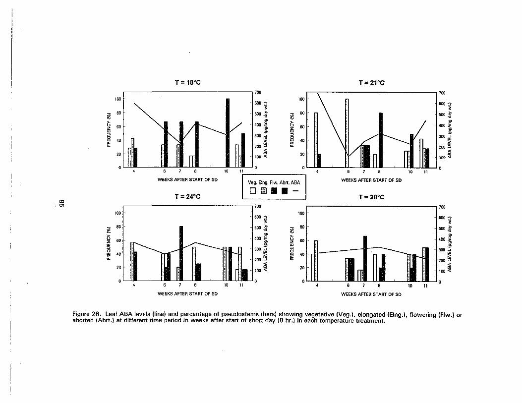
iI
T =18°C T =21°C
WEEKSAFTER START OF SO
T= 24°C
-. 600 -~
.• 500 ~'tICl
"400 ~
300 ~w200 ~
~100 «
11108
I II. , ,,;;. II-i-. '076
T= 28°C
WEEKSAFTERSTART OF SO
I • 1100700
100 .--. 600 ..,
~-. 500 .a
~80 .-
Cl
400 ~ iJ 60 .-z~ w
-. 300 irl =>CJ
.• 200 ~w 40a:u.
-cm 20 .--. 100 «
0 010 11 4
IVeg. Elng. Flw. Abrt. ABA
DmTI ••
876
100 ••
~80 .-
>-u 60zw=>CJw 40a:u.
20 .-
04
o
700
600 ~
500 ~'tICl
400 ~
300 ~w200 ~
~100 «
1110876
WEEKSAFTER START OF SO
4
20
40
o
60
80
100
0), '01
100 ~ 1700
600 ~
~80 500 .a
~Cl>-
400 ~ iJo 60z zw ~ w=> 300 ..J =>CJ
200 ~CJw 40 - wa: a:u. u.
«20 m
100 «
0 04 6 7 8 10 11
WEEKSAFTERSTARTOF SO
Figure 26. Leaf ABA levels (line) and percentage of pseudostems (bars) showing vegetative (Veg.), elongated (Elng.), flowering (Flw.) oraborted (Abrt.l at different time period in weeks after start of short day (8 hr.) in each temperature treatment.

1210864
1S"C 21'C 24"C 2S"C+·0· ....- '*
f········........•.. -. .*----;..'"=:::..~;..~ '
800
700
600
~~ 500"CCl
.€Cl
400.5-...JW>w 300...J
<I:CD<I:
200
100
a2
WEEKS AFTER START OFSO
Figure 27. Concentration of ABA in leaf tissue from Heliconia striate pseudostems atdifferent average daily temperatures (18°C, 21°C, 24°C, and 28°C) during 4 to 11weeks after start of SO. Bars indicate mean ± SE.
86

a) 18 & 21·C
700
?2:-"C 467Cl.§ClS:...JW
Gi 233...J 5.0eX:CD-c
4.0
SOLFNO
3.0
WEEKS AFTER START OF SO
700 b) 24 &28· C
?e-
"C 467Cl.§ClS:...JW
Gi 233...J 5.0-cCD-c
4.0
SOLFNO·
WEEKS AFTER START OF SO
Figure 28. The comparison of leaf ABA level responses of Heliconia stricta under18-21 °C (a) and 24-28°C (b). Statistical differences between treatments were foundfor the interactions with the straight-line effects of leaf number at start of SD (SDLFNO)and the quadratic effects of time after start of SO (Appendix Table 123).
87
quadratic relationship with time after start of SO curve with the top of the curve around 6-7
weeks after the start of SO (Figure 28).
SHOOT STATUS AT THE END OF THE EXPERIMENT
At the termination of the experiment (20 weeks after start of SO), plants grown at
18°C yielded the highest percent flowering (61 %) while those grown at 21, 24 and 28°C
flowered at the rate of 50%, 33%, and 27% respectively. The higher the temperature the
more flower buds were aborted, ranging from 7% at 18°C to 27% at in 28°C (Appendix
A:Table 127).
Average time to flower from the start of SO for all pseudostems grown at 18°C and
21°C was 18 weeks which was one week later than those grown at 24°C and 28°C. This
was in good agreement with Lekawatana (1986).
CHARACTERISTICS OF FLOWER BUD DEVELOPMENT
Figures 29-31 showed apical longitudinal sections of H. stricta 'Dwarf Jamaican'
grown at 18, 21, 24 and 28°C under 14 hr daylength after an initial floral induction stimulus
of 4 weeks of SO at advance stage of development. Before SO, the apical meristem
remained vegetative (Figure 29A). Two to 3 weeks after the start of SO, pseudostem
elongation was observed (Figure 29B,C). Four weeks after the start of SO, the first and the
second cincinnal bracts were distinguishable (Figure 30A). At 6 weeks after the start of
SO, flower primordia were conspicuous (Figure 30B). At .11 weeks after the start of SO,
flower primordia in the first cincinnal bract were almost 1 ern in length (Figure 31C).
There were however, some pseudostems that did not develop into stages described
above, but remained in vegetative (Figure 32A,C), early flower development stage (Figure
32B) or aborted (Figure 31A,B,C).
88

en(0
Figure 29. Apical longitudinal section of H. stricta 'Dwarf Jamaican' treated with an initial floral induction stimulus of 4 weeks of SO
at different stages of development. Bar equal 500 urn.
A. Vegetative pseudostem with 4 visible, expanded leaves and 6 total leaves produced before the start of so.
B. Pseudostem elongation commenced with 5 visible, expanded leaves and 6 total leaves produced 1 weeks after the start of
so. (4 leaves at the start of SO)
C. Pseudostem elongation commenced with 5 visible, expanded leaves and 6 total leaves produced 2 weeks after the start of
so. (4 leaves at the start of SO)
(L = leaf number, B = cincinnal bract, P= unidentified primodium, FP = flower bud primodium, PO = peduncle)


co....
Figure 30. Apical longitudinal section of H. stricta 'Owarf Jamaican' treated with four temperatures (18,21,24 and 28°C) under 14
hr daylenqth after an initial floral induction stimulus of 4 weeks of SO at different stages of development. Bar equal 500 11m.
A. Pseudostem with 5 visible, expanded leaves and 6 total leaves produced 3 weeks after the start of SO (4 leaves at the start
of SO). The first and second cincinnal bracts were evident.
B. Pseudostem with 5 visible, expanded leaves and 6 total leaves produced 4 weeks after the start of SO (4 leaves at the start
of SO). The first flower primordium was evident.
C. Pseudostem with 5 visible, expanded leaves and 6 total leaves produced 6 weeks after the start of SO (4 leaves at the start
of SO; 25°C LO). The second flower primordium was evident.
(L = leaf number, B = cincinnal bract, P= unidentified primodium, FP = flower bud primodium, PO = peduncle)
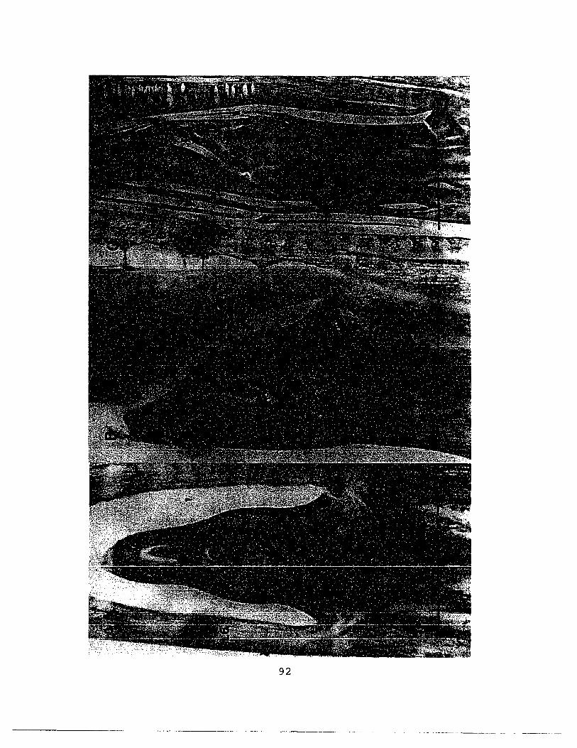
92
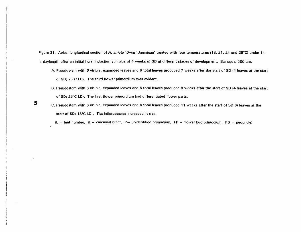
(0w
Figure 31. Apical longitudinal section of H. stricte ' Dwarf Jamaican' treated with four temperatures (18, 21, 24 and 28De ) under 14
hr daylength after an initial floral induction stimulus of 4 weeks of SO at different stages of development. Bar equal 500 urn.
A. Pseudostem with 6 visible, expanded leaves and 6 total leaves produced 7 weeks after the start of SO (4 leaves at the start
of SO; 25 De LOI. The third flower primordium was evident.
B. Pseudostem with 6 visible, expanded leaves and 6 total leaves produced a weeks after the start of SO (4 leaves at the start
of SO; 25 D e LO). The first flower primordium had differentiated flower parts.
e. Pseudostem with 6 visible, expanded leaves and 6 total leaves produced 11 weeks after the start of SO (4 leaves at the
start of SO; laDe LO). The inflorescence increased in size.
(L = leaf number, B = cincinnal bract, P= unidentified primodium, FP = flower bud primodium, PO = peduncle)

94

(0U1
Figure 32. Apical longitudinal section of H. stricta 'Dwarf Jamaican' treated with four temperatures (18, 21, 24 and 28°C) under 14
hr daylength after an initial floral induction stimulus of 4 weeks of SD at different stages of development. Bar equal 500 urn.
A. Vegetative pseudostem with 6 visible, expanded leaves and 8 total leaves produced 11 weeks after the start of SD. (4
leaves at the start of SD; 18°C LD
B. Pseudostem with 6 visible, expanded leaves and 6 total leaves produced 8 weeks after the start of. SD (4 leaves at the start
of SD; 25°C LD). The inflorescence was in an early stage of development.
C. Vegetative pseudostem with 6 visible, expanded leaves and 6 total leaves produced 10 weeks after the start of SD (4 leaves
at the start of SD; 18°C LD).
(L = leaf number, B = cincinnal bract, P= unidentified primodium, FP = flower bud primodium, PD = peduncle)
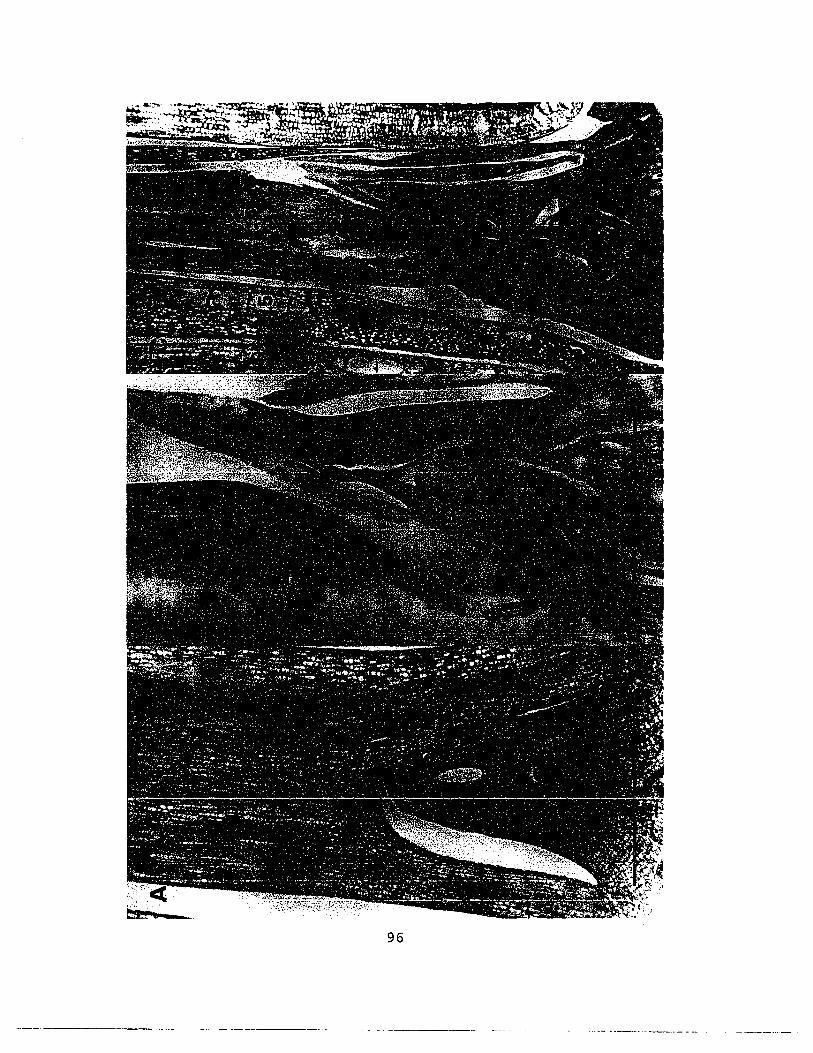
96

Figure 33. Apical longitudinal section of H. stricta 'Dwarf Jamaican' treated with four temperatures (18, 21, 24 and 28°C) under 14
hr daylength after an initial floral induction stimulus of 4 weeks of SD showing various stages of flower bud abortion. Necrotic cells
were not stained (purplish blue) with toluidine blue were brown in color. Bar equal 500 urn.
A. Pseudostem with 6 visible, expanded leaves and 6 total leaves produced 10 weeks after the start of SO (3 leaves at the
start of SO; 2PC LO). Failure to stain (brown color) in elongating peduncle reflected early stage of inflorescence abortion.
Note the inflorescence was stained normally.
CDo"J B. Pseudostem with 6 visible, expanded leaves and 6 total leaves produced 10 weeks after the start of SD (4 leaves at the
start of SO; 21°C LD). In elongating inflorescence, some part of rachis failed to stain. Note the flower primordia were
stained normally.
C. Pseudostem with 6 visible, expanded leaves and 6 total leaves produced 11 weeks after the start of SO (4 leaves at the
start of SO; 25°C LO). In elongating inflorescence, some part of rachis failed to stain. Note the flower primordia were
stained normally.
(L = leaf number, 8 = cincinnal bract, P= unidentified primodium, FP = flower bud primodium, PO = peduncle)

98

In aborted inflorescences, necrotic cells were not stained (purplish blue) with
toluidine blue 0 but were brown in color. The location of necrotic tissue was from the tip
of the inflorescence to the top part of peduncle (Figure 33). The smallest developing
inflorescence that was found to be aborted was 2 em long (from the tip of the inflorescence
to the base of peduncle) and was found as early as 6 weeks after start of SO in plants
growing at 28°C.
DISCUSSION
After the initial SO stimulus, pseudostems grown under high temperature developed
a high percent of flower bud abortion. This is in agreement with studies in other plants
such as snap bean, tulip, tomato, Iris, citrus etc (Konsens et al., 1991; Kinet et al., 1985).
Kinet et al. (1985) generalized that the higher the temperature, the higher the percent
abortion.
In a study by Lekawatana (1986), Heliconia stricta 'Owarf Jamaican' were given an
initial stimulus of 4 weeks of SO at 15, 20 and 25°C night temperature and later were
grown until flowering in ambient temperatures with a mean night temperature of 20.2°C.
There was no significant difference in percent of aborted shoots among temperature
treatments. Plants grown at 20°C night temperature during SO, similar to this experiment,
yielded similar percent flowering plus flower bud abortion pseudostems (52%).
Furthermore, percent reproductive pseudostems (flowering + aborted) among temperature
treatments of this experiment were not significantly different (mean of 50%). This
demonstrates a consistent response of the species to temperature during SO. These two
experiments indicate the following:
1) As night temperature decreased, from 25°C to 15°C, during the initial stimulus
period (4 weeks of SO) the percent of reproductive pseudostem increased from 31 % to
99

78% (Setapong, 1986). Night temperature during initiation does not have an influence on
percent flower bud abortion.
2) As night temperature increased from 15°C to 25°C after the initial stimulus (4
weeks of SO) the percent that finally flowered decreased from 61 % to 27% and the
percent aborted pseudostems increased from 8% to 27%. However, night temperature
during the development period did not influence the total percent reproductive pseudostem
initiated.
Flower bud abortion was not found in plants grown at 18°C and was found 7
weeks after the start of SO for plants grown at 21°C. In plants grown at 24°C and 28°C,
flower bud abortion found from 6 weeks after the start of SO.
When the average air temperature was increased, foliar ABA content decreased
linearly. Similar findings were found in bean and cucumber seedlings (Smith and Dale,
1988; Capell and 06rffling, 1989). The rise in ABA content in leaf is most likely to be due
to local synthesis in the leaf itself, although the stimulus behind this, which presumably
must emanate from the roots, remains unknown (Smith and Dale, 1988).
The quadratic surfaces for foliar ABA content regressed on initial leaf number and
weeks after the start of SO together with the ABA content regressed on number of
expanded leaves indicated that, with progress of time and the increase in leaf number, the
foliar ABA content of the top mature leaf tended to decrease at first and increase later on.
The results are similar to Ross and McWha (1990) found that the ABA content of Pisum
sativum leaflets toward the base of the plant was greater than at a higher position in the
plant. However, the high levels of ABA could also be correlated with senescence. Ross
and McWha (1990) reported that a high percentage of total ABA in pea was present in its
reproductive tissues.
Due to the limitation of our knowledge on the influence of ABA on flower bud
abortion and its mechanism, it can only be stated that high temperature during
100

inflorescences development decreased level of ABA in H. stricta 'Dwarf Jamaican' leaves
and that a lower level of ABA was found in the foliage of aborted pseudostems compared
to that found in developing inflorescences.
CONCLUSION
1. Temperatures of 18-21 °C improved reproductive success both in terms of
greater percent bud set and lower rate of abortion compared to plants grown at 24-28°C.
2. Flower bud abortion in H. stricta 'Dwarf Jamaican' was observed 6 weeks after
the start of SO when the developing inflorescence was approximately 2 cm and flower
primordia were conspicuous. The appearance of flowers coincides with the onset of
abortion of the inflorescences and a lower ABA level in the foliage.
3. The hypothesized role for ABA as a stimulus to flower bud abortion appears to
be unsupported as flower bud set was greater under conditions leading to high ABA levels
in the foliage. However, ABA level in the foliage may have no relationship to ABA level at
the meristem.
101

CHAPTER 5
EFFECT OF LIGHT INTENSITY ON INFLORESCENCE ABORTION AND ABSCISIC ACID
LEVELS IN H. STRICTA
ABSTRACT
Plants of Heliconia stricte Huber 'Dwarf Jamaican' were grown under three light
intensity treatments of full sun, 40% sun, and 20% sun in ambient outdoor conditions after
an initial floral induction stimulus of 4 weeks of SD at 26/21°C. Free (+ )-abscisic acid
(ABA) content of mature leaves was measured by indirect enzyme-linked immunosorbent
assay (ELISA). Changes in light intensity did not significantly affect percent flowering or
percent aborted pseudostems. Decreased light intensity during inflorescence development
increased the levels of ABA in H. stricta leaves from 88.8 ± 11.5 pg/mg dry wt, in full sun
to 276.4 ± 39.1 and 219.5 ± 22.4 pg/mg dry wt. in 40% and 20% sun respectively.
Different pseudostem statuses (vegetative, aborted or flowering) showed no significant
difference relative to leaf ABA level.
INTRODUCTION
Flower bud abortion in Heliconia has been found in many species such as H.
angusta, H. chartacea and H. stricta (Criley and Lekawatana, 1994; Lekawatana, 1986).
Reports on some Heliconia species (H. psittacorum and H. angusta) stated that increased
light intensity increased flower production (Broschat and Donselrnan, 1982, 1983; Kwon,
1992).
In most species increased photosynthesis in leaves is the major system that
promotes flower development. The young developing flower bud is a major sink for
assimilates under favorable growing conditions, when the metabolites essential for its
growth are in ample supply (Halevy, 1987). Under stress conditions with an inadequate
102

supply of assimilates, the young flower bud constitutes a weaker sink compared with the
vegetative apices, developing leaves, fruits or storage organs, and it competes poorly with
them for the available assimilates (Halevy, 1984). This was found to be the case for
conditions of light, temperature and water stress. In the developing bud, these
environmental stresses promoted abortion, blasting or abscission of the flower buds, while
other organs were only slightly affected (Kinet and Sachs, 1984; Halevy, 1987).
Several environmental factors increase the endogenous level of abscisic acid (ABA)
in plant tissues. Most prominent is the effect of drought stress, but other kinds of stress
such as aeration stress and temperature extremes have been reported to increase the level
of ABA (Addicott, 1983). At the time the study initiated, no reference on the effect of light
intensity on ABA levels in plants was found.
This experiment was carried out to investigate the effect of light intensity during
flower bud development on percent flower bud abortion and ABA content in foliage of
He/iconia stricta 'Dwarf Jamaican'
MATERIALS AND METHODS
PLANT MATERIAL AND CULTURAL PRACTICE
Two hundred rhizome pieces of He/iconia stricta cv. Dwarf Jamaican were
propagated on March 25, 1991. Rhizome pieces including pseudostems were separated,
and the roots removed. The pseudostem was cut to 5 cm in length from the leaf sheath
base, treated in a 55°C water bath for 5 minutes, dipped in fungicide (Dithane M451 and
drained. The rhizomes were then held in plastic bags for 3 weeks at 20°C to stimulate root
and shoot growth. They were planted in perlite and vermiculite 1:1 ratio (v/v) and held
under mist for 1 week. Three rooted rhizome pieces were potted per 15-cm pot on April
18, 1991, and placed in a greenhouse at the Magoon greenhouse facility of the University
of Hawaii. The potting medium was a mixture of peat and perlite 1:1 ratio (v/v) amended
103

with dolomite, Micromax and treble superphosphate at the rates of 6.0, 1.0 and 0.6 kg per
cubic meter, respectively. Plants were drip irrigated twice daily with nutrient solution, 200
N-OP-200K (ppm). On June 17, 1991, when forty-six percent of pseudostems were in the
3-leaf stage and 54% were in the 4-leaf stage, plants were given a flower initiation stimulus
by subjecting them to short day conditions in growth chambers for 4 weeks from June 17,
1991 to July 15, 1991. The growth chamber conditions were: photoperiod 8 hour
daylength using a combination of fluorescent and incandescent lamps with
photosynthetically active radiation (PAR) measured 214 J.1molls·'/m·2 and temperature
25/20°C day/night (D/N). The average minimum and maximum temperatures in the
greenhouse prior to growth chambers were 21.6°C (range: 19.0-23.5°C) and 31.8°C (range:
25.5-36.0°C), respectively. Average daily maximum PAR was 609.28 pmole.s·'.m·2 with a
range of 240-1,000 pmol.s·'.m·2
•
TREATMENT SETUP
After SO treatment (July 15, 1991) 50 pots of H. stricta plants were placed in 3 different
shading treatments at the magoon area as follows:
Trt.1 .- Full sun (average 1,476.2 J.1mol.sec·'.m·2 at 1:00 pm)
Trt.2 - 40% sun (average 591.9 umol.sec" .m·2 at 1:00 pm)
Trt.3 - 20% sun (average 262.6 umol.secl.rn? at 1:00 pm)
Two shading conditions were made by covering a bench with structures made by wooden
frames sized 185 X 150 X 180 cm. These structures were covered with saran cloth with
different percent shading (20% and 40% of sunlight). Fourteen pots each were placed
under the two structures and another 15 pots were placed on a bench in full sun (100%
sun). Plants were hand-watered daily with a nutrient solution 200N-200P-200K (ppm).
Throughout the experiment plants were provided with adequate water, therefore the effect
of water stress was minimized.
104
~~=~~=.- ,~_. ---,,-------- - .
DATA COLLECTION
At the start of SD the expanded leaf number was recorded for all 192 pseudostems.
On June 25 (1 pot); July 2 (1 pot) and July 15 (3 pots), pseudostems were collected.
After 4 weeks SD, 2 pots of each shade treatment were collected on August 8; August 17;
August 25; and September 2. These represent 8, 9, 10, and 11 weeks after the start of
SO. Then pseudostems were dissected to determine their status (vegetative, flowering,
aborted). Twenty-five leaf blades of the topmost mature leaves were collected from each
treatment at each harvest for foliar ABA analysis.
At the end of the experiment (October 25, 1991) the status (vegetative, elongate,
flowering or aborted) of 16 pots of Heliconia stricta were determined. Length of
pseudostems were measured from base to the tip of the last leaves. Length of
inflorescences were measured from base to the tip of inflorescences and number of
cincinnal bracts were counted.
Photosynthetically active radiation (PAR: urnol.s" .m·2) in the 400 to 700 nm
waveband was measured by a Licor quantum sensor model L1-200S. Three light sensors
and 3 air temperature sensors placed approximately 50 cm above bench in the middle of
each treatment were connected to a Oatalogger model L1-1000. Data were averaged over 5
minutes intervals and the way of the 12 intervals were recorded every 60 minutes.
Average PAR readings, throughout the experiment period, at 1:00 pm for the different
shading treatments from full sun, 40% sun and 20% sun were 1,476.2, 591.9 and 262.6
urnot.secl.rn" which equaled 100%,40.1 % and 17.8% of the solar intergral respectively.
Average air temperatures measured at 1:00 PM in the full sun, 40% sun and 20% sun
treatments were 30.4 ± 0.2,28.7 ± 0.2, and 27.8 ± 0.1°e respectively. Average
temperatures measured at 5:00 am in the full sun, 40% sun and 20% sun treatments were
22.4 ± 0.2, 22.3 ± 0.1, and 22.4 ± 0.1°e. Summaries of the weather data are
presented in Appendix: B Figures 3-6.
105

EXTRACTION AND DETERMINATION OF ABA LEVEL
Leaf blades were stripped from their midribs. Each sample was placed in a plastic
tube and immediately stored in liquid nitrogen (-70 "C), Leaves were then powdered by
grinding in a precooled mortar and pestle with liquid nitrogen then lyophilized (freeze dried).
The lyophilized samples were then stored in plastic tubes at -20 ec. The samples were
extracted and their ABA content determined using an indirect enzyme-linked immunosorbent
assay (ELISA) as described in Chapter 4. With this method the percent recovery was more
than 90%. The standard used was (+) cis-trans-ABA (Sigma Chemical Co.) and the
Monoclonal Antibody (MAb) was MAb to free cis-,trans-( + )-ABA (Idetek, lnc.), Samples
were tested in triplicate (3 wells for each sample).
STATISTICAL ANALYSIS
The statistical analysis was by SAS general linear model (PROC GLM) analysis of
variance with mean separations by the t-test and contrast (SAS Institute, 1987).
Quantitative data such as shoot status were analyzed by Chi-Square test for independence,
based on the null hypothesis that the differences among the ratios were not significant.
RESULTS
ABA LEVELS DURING SD
ABA content of the combined 3rd and 4th leaf blades of heliconia during SD (4
weeks) was 296.9 ± 37.4 pg/mg leaf dry wt. (n= 12).
EFFECT OF SHADINGS FOLLOWING SO
Shading Effects on ABA levels
Foliar ABA content of Heliconia grown under 20% and 40% sun (219.5 ± 22.4
and 276.4 ± 39.1 .pg/mg dry wt.) were significantly higher than for those grown under
106
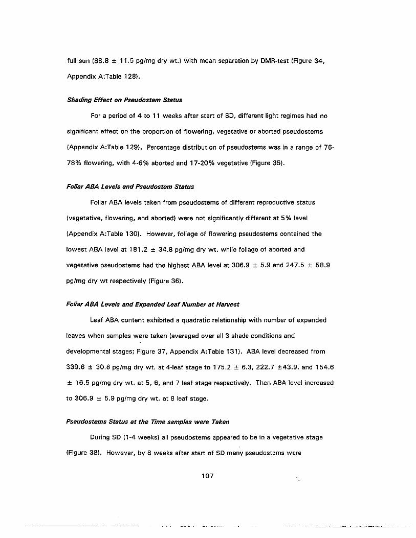
full sun (88.8 ± 11.5 pg/mg dry wt.) with mean separation by OMR-test (Figure 34,
Appendix A:Table 128).
Shading Effect on Pseudostem Status
For a period of 4 to 11 weeks after start of SO, different light regimes had no
significant effect on the proportion of flowering, vegetative or aborted pseudostems
(Appendix A:Table 129). Percentage distribution of pseudostems was in a range of 76
78% flowering, with 4·6% aborted and 17-20% vegetative (Figure 35).
Foliar ABA Levels and Pseudostem Status
Foliar ABA levels taken from pseudostems of different reproductive status
(vegetative, flowering, and aborted) were not significantly different at 5% level
(Appendix A:Table 130). However, foliage of flowering pseudostems contained the
lowest ABA level at 181.2 ± 34.8 pg/mg dry wt. while foliage of aborted and
vegetative pseudostems had the highest ABA level at 306.9 ± 5.9 and 247.5 ± 58.9
pg/mg dry wt respectively (Figure 36).
Foliar ABA Levels and Expanded Leaf Number at Harvest
Leaf ABA content exhibited a quadratic relationship with number of expanded
leaves when samples were taken (averaged over all 3 shade conditions and
developmental stages; Figure 37, Appendix A:Table 131). ABA level decreased from
339.6 ± 30.8 pg/mg dry wt, at 4-leaf stage to 175.2 ± 6.3, 222.7 ±43.9, and 154.6
± 16.5 pg/mg dry wt. at 5, 6, and 7 leaf stage respectively. Then ABA level increased
to 306.9 ± 5.9 pg/mg dry wt, at 8 leaf stage.
Pseudostems Status at the Time samples were Taken
During SO (1-4 weeks) all pseudostems appeared to be in a vegetative stage
(Figure 38). However, by 8 weeks after start of SO many pseudostems were
107

350
300
j 250
~'t:l
ell 200ECi~..Jw 150>w..J
<l:CD
100-c
50
020 40 100
%SUN
Figure 34. Effect of shading (20, 40 and 100% sun) on leaf ABA levels. Bars indicatemean ± SE.
100
100
o Veg. 0 Flw.•Abrt.
80
~ 60>uzw::Jaw 40a:u..
20
40
%SUN
Figure 35. Effect of shading (20, 40 and 100% sun) on percentage of pseudostemsshowing vegetative (Veg.), flowering (Flw.) or aborted (Abrt.) apices 8-11 weeks(accumulative over 4 weeks period) after start of SD:
108

350
300
~250
~"CCl 200.€ClEo..Jw 150>w..J
~CD
100~
50
0Vag. Flw. Abrt.
PSEUDOSTEM STATUS
Figure 36. Concentration of ABA in leaf tissue from vegetative (Veg.), flowering (Flw.),or aborted (Abrt.) Heliconia stricta pseudostems apices based on average of stemssampled over 4 to 11 weeks after start of SO. Bars indicate mean ± SE.
Y=1256.59- 330.63X- 25.38X"2r"2 = 0.21
•
400
350
~ 300~
"CCl
.€Cl
250Eo..JW>W..J
~ 200III~
150
1003 4 5 6
+7 8 9
NUMBER OF EXPANDED LEAVES
Figure 37. Leaf ABA levels of most recently matured leaf of H. stricte pseudostem withdifferent number of expanded leaves based on average of stems sampled over 4 to 11weeks after start of SO. Bars indicate mean ± SE.
109

120 350
Vag. Flw. Abrt. ABA
100 D~.-300
250 ::80
;:~
~ 'C
>- 200 Clu .€z 60 Clw .9-:>
..J0
I 150 ~wa: wu, g ..J
40 <l:11 100 ~~i.!
20 ~ 50~'f
0 02 3 4 5 6 7 8 9 10 11
WEEKS AFTER START OF SO
Figure 38. Percentage of pseudostems showing vegetative (Veg.), elongated (Elng.),flowering (Flw ..) or aborted (Abrt.) apices and leaf ABA level (line) at the time sampleswere taken after the start of SD. No samples for weeks 6 and 7.
100oVag. G Flw.•Abrt.
~1Jzw:>owa:u.
80
60
40
20
20 40
%SUN
100
Figure 39. Effect of shading on percentage of pseudostems (bars) showing vegetative(Veg.), flowering (Flw..) or aborted (Abrt.) apices at time of experiment termination (18weeks after the start of SO).
110
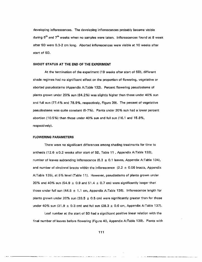
developing inflorescences. The developing inflorescences probably became visible
during 6th and 7th weeks when no samples were taken. Inflorescences found at 8 week
after SO were 0.3-2 cm long. Aborted inflorescences were visible at 10 weeks after
start of SO.
SHOOT STATUS AT THE END OF THE EXPERIMENT
At the termination of the experiment (19 weeks after start of SO), different
shade regimes had no significant effect on the proportion of flowering, vegetative or
aborted pseudostems (Appendix A:Table 132). Percent flowering pseudostems of
plants grown under 20% sun (84.2%) was slightly higher than those under 40% sun
and full sun (77.4% and 78.9%, respectively, Figure 39). The percent of vegetative
pseudostems was quite constant (5-7%). Plants under 20% sun had a lower percent
abortion (10.5%) than those under 40% sun and full sun (16.1 and 15.8%,
respectively) .
FLOWERING PARAMETERS
There were no significant differences among shading treatments for time to
anthesis (12.6 ±0.2 weeks after start of SO, Table 11 , Appendix A:Table 133),
number of leaves subtending inflorescence (6.3 ± 0.1 leaves, Appendix A:Table 134),
and number of cincinnal bracts within the inflorescence (2.2 ± 0.06 bracts, Appendix
A:Table 135), at 5% level (Table 11). However, pseudostems of plants grown under
20% and 40% sun (54.9 ± 0.9 and 51.4 ± 0.7 em) were significantly longer than
those under full sun (44.5 ± 1.1 ern, Appendix A:Table 136). Inflorescence length for
plants grown under 20% sun (33.5 ± 0.5 ern) were significantly greater than for those
under 40% sun (31.9 ± 0.3 ern) and full sun (28.3 ± 0.6 ern, Appendix A:Table 137).
Leaf number at the start of SO had a significant positive linear relation with the
final number of leaves before flowering (Figure 40, Appendix A:Table 138). Plants with
111
------- --_. ------- - -_..- - - ----_ ...- .
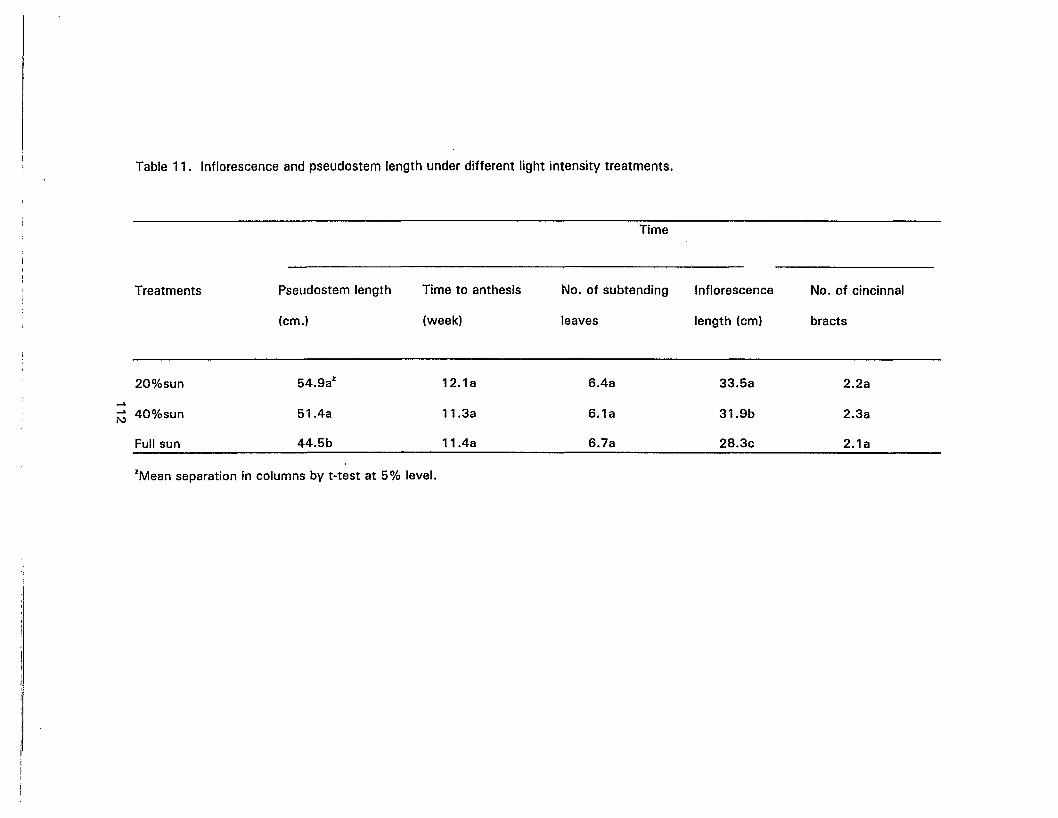
Table 11. Inflorescence and pseudostem length under different light intensity treatments.
Time
Treatments Pseudostem length
(em.)
Time to anthesis
(week)
No. of subtending
leaves
Inflorescence
length (em)
No. of cincinnal
bracts
20%sun 54.9az 12.1a 6.4a 33.5a 2.2a
-'
N 40%sun 51.4a 11.3a 6.1a 31.9b 2.3a
Full sun 44.5b 11.4a 6.7a 28.3c 2.1a
zMean separation in columns by t-test at 5% level.

8wu •zwuenwa:0 7...JU.Z
oz15zwI- 6CD~enenw~W...JU. 5 •0a: Y = 3.67 + 0.75 Xw
(1\2 = 0.68CD~~z
41 2 3" 4 5 6
LEAF NUMBER AT START OF SD
Figure 40. Effect of leaf number at the start of SD on number of leaves subtendinginflorescence.
113

2 leaves at the start of SD added 3 leaves before flowering, while 5 leaf plants added
an average of 2.6 leaves before flowering.
Leaf number at the start of SD had no significant linear relationship with number
of weeks from start of SD to anthesis (Appendix A:Table 139).
DISCUSSION
This experiment produced no differences in proportion flowering and aborted
pseudostems among different light intensity treatments. Many species of Heliconia
were found to be light intensity limited (H. psittacorum and H. angusta) as an increase
in light intensity increased flower production (Broschat and Donselman, 1982, 1983;
Kwon, 1992). Broschat and Svenson (1994) reported that H. stricta 'Dwarf Jamaican'
in full sun produced more flowers than those grown under 50% shade for a period of
one year. However their finding was not conclusive since only 25% of the
pseudostems in full sun flowered. This was probably due to the lack of a suitable short
day induction period. The finding in this experiment suggests that H. stricta 'Dwarf
Jamaican' can be grown under diverse light conditions without altering final percent
flowering after receiving an initial 4 weeks of SD stimulus to induce flower inltiatlon,
The time from start of SD to anthesis was 12.6 weeks which was similar to the 13
weeks reported by Criley and Kawabata (1986) and in chapter 4 of this dissertation.
The time to anthesis was not different among different light intensity treatments.
However, increased light intensity significantly decreased plant height and inflorescence
length. Lekawatana (1986) reported a flowering peak at 19 weeks after the start of
SD. This may be due to plant materials having only 1-3 leaves at the time of SD, which
postponed the susceptibility period.
ABA levels measured in leaves of aborted, vegetative or flowering pseudostems
were not significantly different, similar to results of the temperature study in Chapter 4.
114

Foliage of plants grown under 20% and 40% sun contained higher leaf ABA than those
grown under full sun. In temperature treatment 4 of Chapter 4, the environment
(30/25°C DIN, PAR = 214 /lmol.s·1.m·2) was similar to that of the 20% sun treatment
of this chapter. Leaf ABA levels of the two similar treatments in different experiments
were 264 ± 18.8 and 219.5 ± 22.4 pglmg dry wt. for the high temperature of chapter
4 and low light of this experiment.
Foliar ABA content regressed on number of expanded leaves showed a quardratic
relationship with the increase in leaf number. The foliar ABA content of the top mature leaf
decreased with an increase in leaf number of the pseudostems. This result is similar to that
in Chapter 4 and to Ross and McWha (1990) who fond that the ABA content of Pisum
sativum leaflets toward the base of the plant was greater than at higher position in the
plant. Foliar ABA content in this study was from the top most mature leaf of different
stages of growth while those from Ross and McWha (1990) were from leaves locating on
position of a plant. Therefore, interpretation has to be done carefully.
Fewer leaves were produced before flowering with plants that had more leaves
at the start of SO. Plants with 2 to 3 leaves at the start of SO produced additional 3
leaves afterward while those with more than 3 leaves produced additional 2 leaves. A
similar number of leaves subtended the inflorescences (6-7 leaves) no matter what the
initial leaf count- was. Bernier (1994) stated that most photoperiodic species, when
shifted from noninductive to inductive conditions, went on initiating extra leaves before
producing reproductive structures. However, H. stricta was reported to have already
produced a total of 6 leaves at the time the second leaf expanded (Lekawatana, 1986).
Heliconia plants grown in full sun were shorter than those under shade.
Cosgrove (1986) suspected that hormone metabolism was involved in the
photoinhibition of pea stems by light. It was suggested that light might modify growth
115

in three potential ways: a reduction in GA synthesis, an increase in GA destruction, or a
reduction in the plant's responsiveness to GA (Lockhart, 1959).
The anticipated differences in foliar ABA levels with stress of reduced light
intensity did not parallel flower bud abortion under these conditions. Thus, it is not
possible to conclude that a role for foliar-produced ABA exists in the abortion of the
flower bud. However, since ABA was not analyzed in the pseudostem tissues where
reproductive development was occurring, the question is far from settled.
The timing of the flower bud abortion appears to begin 10 weeks after the start
of SD. The determination of shoot status was done by manual dissection. Therefore,
the early stage of flower bud abortion might not be detected when compared with
those in chapter 4 of this dissertation.
116

CHAPTER 6
CONCLUSION
With the attempt to control flower production of heliconia to ensure a steady supply
of cut heliconia in the world market, we are just beginning to understand this plant through
H. stricta 'Dwarf Jamaican' and other species. From these experiments and others we may
conclude that:
PLANT GROWTH
LEAF LENGTH
Leaf growth parameters of H. stricta 'Dwarf Jamaican' were determined. Richard's
growth curve were chosen to represent the leaf growth. The time required to produce each
leaf increased minimally from leaf 3 to leaf 4. However, substantially more time was
needed to produce leaves 5 and 6.
Environmental Effects
Light intensity affected H. stricta 'Dwarf Jamaican' growth. Plants grown under full
sun were shorter than those under shade with smaller leaves and shorter petiole. It was
suggested that light might modify growth in three potential ways: a reduction in GA
synthesis, an increase in GA destruction, or a reduction in the plant's responsiveness to GA
(Lockhart, 1959).
The number of leaves produced after SD for plants grown under LD3L+ SO, and
LD4L + SD was constant at 3 leaves. This reflected the number of leaves that already
produced by the plants but not fully expanded yet.
The time increment between successive leaves of plants grown under conSD was
significantly shorter than for those grown under conLD, LD3L+ SD and LD4L+SD. Leaf
117
position had significant quadratic components with days to produce each leaf at the 1%
level.
FLOWER INITIATION
The condition of flower initiation has been reported prior to these experiments. A
minimum of 4 weeks of SO was required for flower initiation (Criley and Kawabata, 1986).
Ouring SO induction, decreased night temperature increased percent reproductive
pseudostems (Lekawatana, 1986).
Flower initiation did not occur in plants grown under conLD and the plants remained
vegetative and produced up to 8 to 9 leaves.
FLOWER DEVELOPMENT
H. stricta 'Dwarf Jamaican' responds well to a floral initial stimulus (4 weeks of SO)
when plants have 3 or more leaves.
TEMPERATURE
As night temperature increased from 18°C to 28°C after the initial stimulus (4
weeks of SO) the percent of pseudostems that finally flowered decreased from 55% to
31%.
Average time to flower from the start of SO for all pseudostems grown at 18°C and
21°C was 18 weeks, which was one week later than those grown at 24°C and 28°C (under
reduced energy of growth chamber condition).
LIGHT
After receiving an initial 4 weeks of SO stimulus to induce flower initiation, H.
stricta 'Owarf Jamaican' can be grown under diverse natural light conditions without
altering final percent flowering. The percent flowering pseudostems for plants grown under
118

20% sun (84.2%) was slightly higher than for those under 40% sun and full sun (77.4%
and 78.9%, respectively).
There was no different of time from start of SD to anthesis among shading
treatments (12.6 weeks).
INFLORESCENCE ABORTION
The smallest developing inflorescence that was found to be aborted was 2 cm long
and was at the stage when the second flower primordium was evident.
TEMPERATURE
The higher the temperature the more flower buds were aborted, ranging from 0% at
18°e to 19.2% at in 28°e in growth chamber condition.
Flower bud abortion was not found in plants grown at 18°e and was found 7
weeks after the start of SD for plants grown at 21 °e. In plants grown at 24°e and 28°e,
flower bud abortion found from 6 weeks after the start of SD.
LIGHT
There was no significant difference in inflorescence abortion for various shading
treatments (natural light). Plants under 20% sun had a lower percent abortion (10.5%)
than those under 40% sun and full sun (16.1 and 15.8%)
Flower bud abortion was detected by the to" week after the start of SD.
FOLIAR ABA LEVELS
Foliar ABA content of H. stricta 'Dwarf Jamaican' was successfully quantified by
indirect ELISA. However, apex tissue ABA content was not reliably determined by this
method due to interference such as impurity.
Foliar ABA level increased as temperature decreased. Foliar ABA level decreased as
light intensity increased. ABA does not seem to induce flower bud abortion as flower bud
119
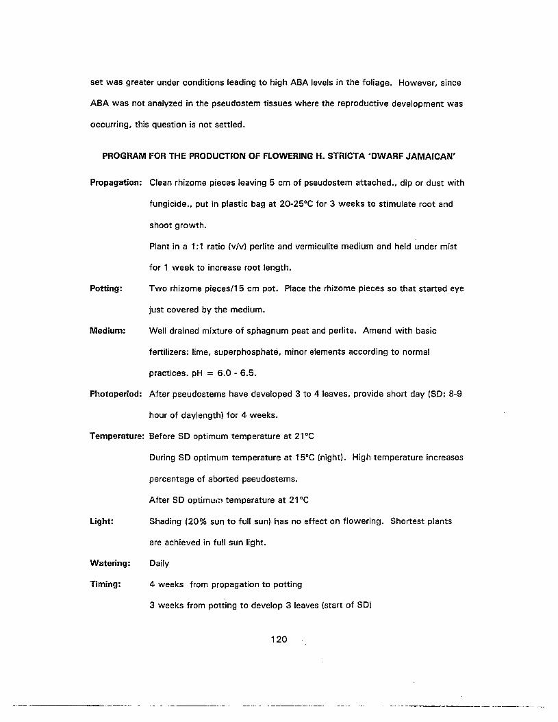
Potting:
Medium:
Light:
set was greater under conditions leading to high ABA levels in the foliage. However, since
ABA was not analyzed in the pseudostem tissues where the reproductive development was
occurring, this question is not settled.
PROGRAM FOR THE PRODUCTION OF FLOWERING H. STRICTA 'DWARF JAMAICAN'
Propagation: Clean rhizome pieces leaving 5 cm of pseudostem attached., dip or dust with
fungicide., put in plastic bag at 20-25°C for 3 weeks to stimulate root and
shoot growth.
Plant in a 1:1 ratio (v/v) perlite and vermiculite medium and held under mist
for 1 week to increase root length.
Two rhizome pieces/15 cm pot. Place the rhizome pieces so that started eye
just covered by the medium.
Well drained mixture of sphagnum peat and perlite. Amend with basic
fertilizers: lime, superphosphate, minor elements according to normal
practices. pH = 6.0 - 6.5.
Photoperiod: After pseudostems have developed 3 to 4 leaves, provide short day (SO: 8-9
hour of daylength) for 4 weeks.
Temperature: Before SO optimum temperature at 21°C
During SO optimum temperature at 15°C (night). High temperature increases
percentage of aborted pseudostems.
After SO optimum temperature at 21°C
Shading (20% sun to full sun) has no effect on flowering. Shortest plants
are achieved in full sun light.
Watering:
Timing:
Daily
4 weeks from propagation to potting
3 weeks from potting to develop 3 leaves (start of SO)
120
---_ .._--------
(5 weeks from potting to develop 4 leaves)
4 weeks of SO
13 weeks from start of SO to anthesis.
Note: - Prior to SO lower the temperature will slow down vegetative growth.
- During the flower development period (after the SO), lowering the temperature to
18°C will increase percentage flowering of pseudostems. However, longer time will
be required for time to anthesis compared to those grown at 25°C.
121
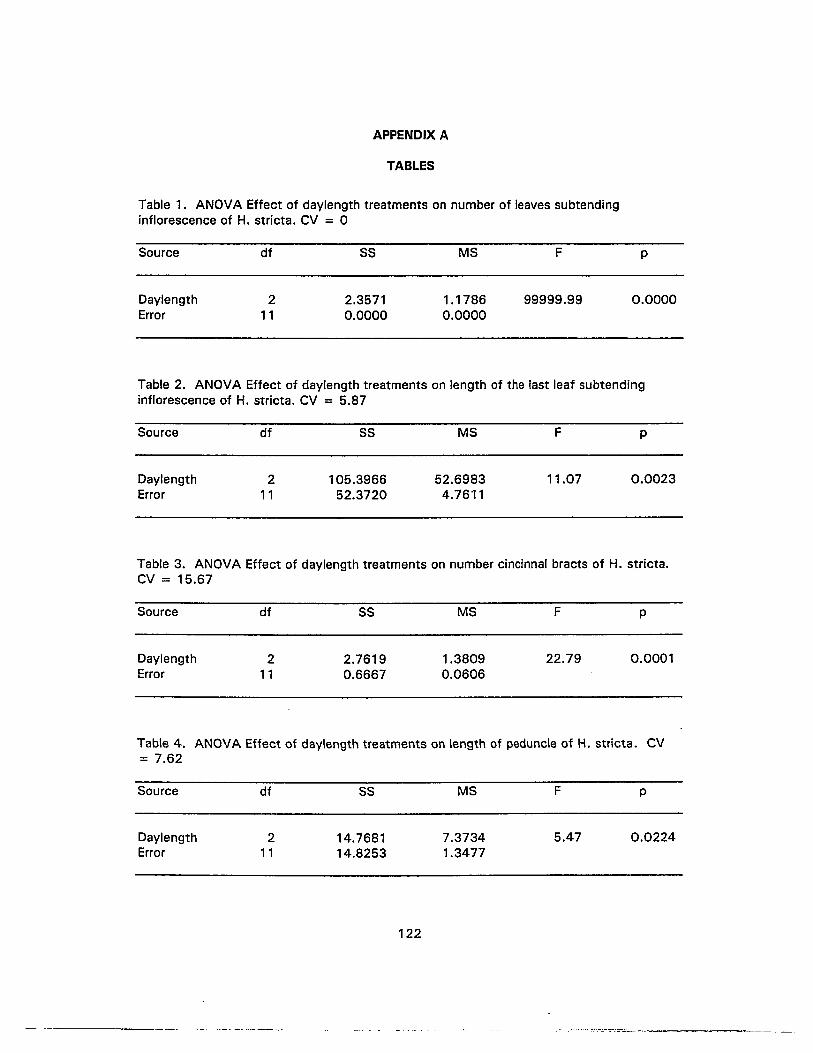
APPENDIX A
TABLES
Table 1. ANOVA Effect of daylength treatments on number of leaves subtendinginflorescence of H. stricta. CV = 0
Source
DaylengthError
df
211
SS
2.35710.0000
MS
1.17860.0000
F
99999.99
p
0.0000
Table 2. ANOVA Effect of daylength treatments on length of the last leaf subtendinginflorescence of H. stricta. CV = 5.87
Source
DaylengthError
df
211
SS
105.396652.3720
MS
52.69834.7611
F
11.07
p
0.0023
Table 3. ANOVA Effect of daylength treatments on number cincinnal bracts of H. stricta.CV = 15.67
Source
DaylengthError
df
211
SS
2.76190.6667
MS
1.38090.0606
F
22.79
p
0.0001
Table 4. ANOVA Effect of daylength treatments on length of peduncle of H. stricta. CV= 7.62
Source
DaylengthError
df
211
SS
14.768114.8253
122
MS
7.37341.3477
F
5.47
p
0.0224
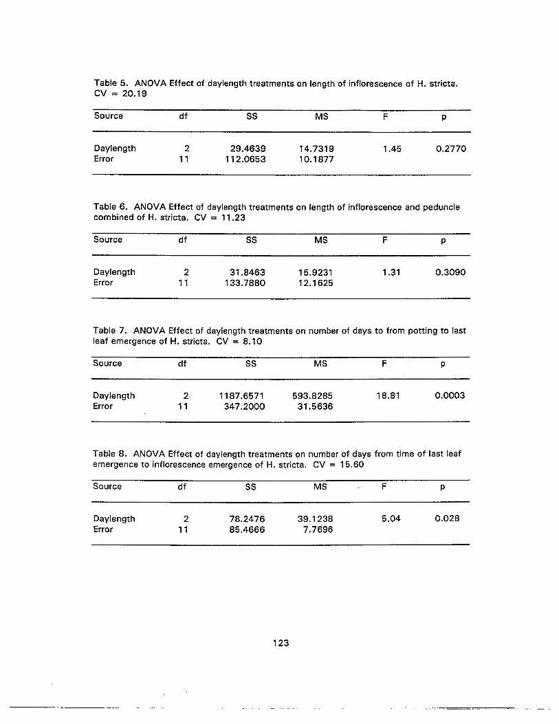
Table 5. ANOVA Effect of daylength treatments on length of inflorescence of H. strlcta.CV = 20.19
Source
DaylengthError
df
211
SS
29.4639112.0653
MS
14.731910.1877
F
1.45
p
0.2770
Table 6. ANOVA Effect of daylength treatments on length of inflorescence and pedunclecombined of H. stricta. CV = 11.23
Source
DaylengthError
df
211
SS
31.8463133.7880
MS
15.923112.1625
F
1.31
p
0.3090
Table 7. ANOVA Effect of daylength treatments on number of days to from potting to lastleaf emergence of H. stricta. CV = 8.10
Source
DaylengthError
df
211
SS
1187.6571347.2000
MS
593.828531.5636
F
18.81
p
0.0003
Table 8. ANOVA Effect of daylength treatments on number of days from time of last leafemergence to inflorescence emergence of H. stricta. CV = 15.60
Source
DaylengthError
df
211
SS
78.247685.4666
123
MS
39.12387.7696
F
5.04
p
0.028

Table 9. ANOVA Effect of daylength treatments on number of days to from time ofinflorescence emergence to anthesis of H. stricta. CV = 11.56
Source
OaylengthError
df
211
S5
507.6571177.2000
MS
253.828516.1090
F
15.76
p
0.0006
Table 10. ANOVA Effect of daylength treatments on number of days to anthesis frompotting of H. stricta. CV = 4.65
Source
OaylengthError
df
211
SS
2299.0476354.6666
MS
1149.523832.2424
F
35.65
p
0.0001
Table 11. ANOVA Effect of daylength treatments on number of days to inflorescenceemergence from started of SO treatments of H. stricta. CV = 6.89
Source
OaylengthError
df
17
162102
SS MS
162.000014.5714
F
11.12
p
0.0125
Table 12. ANOVA Effect of daylength treatments on number of days to anthesis fromstarted of SO treatments of H. stricta. CV = 4.71
Source
OaylengthError
df
17
SS
22.2222218.6666
124
MS
22.222231.2380
F
0.71
p
0.4269
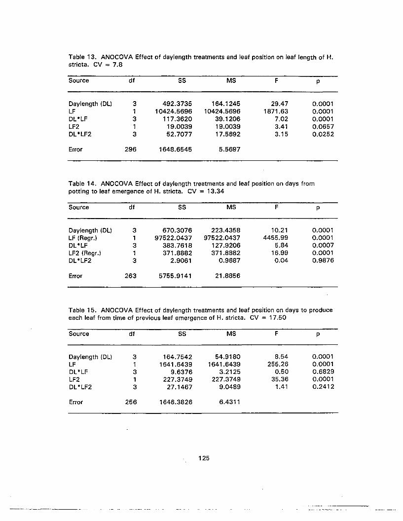
Table 13. ANOCOVA Effect of daylength treatments and leaf position on leaf length of H.stricta. CV = 7.8
Source df SS MS F p
Oaylength (Oll 3 492.3735 164.1245 29.47 0.0001IF 1 10424.5696 10424.5696 1871.63 0.0001Ol*lF 3 117.3620 39.1206 7.02 0.0001lF2 1 19.0039 19.0039 3.41 0.0657Ol*lF2 3 52.7077 17.5692 3.15 0.0252
Error 296 1648.6545 5.5697
Table 14. ANOCOVA Effect of daylength treatments and leaf position on days frompotting to leaf emergence of H. stricta. CV = 13.34
Source df SS MS F p
Oaylength (Oll 3 670.3076 223.4358 10.21 0.0001IF (Reqr.) 1 97522.0437 97522.0437 4455.99 0.0001Ol*lF 3 383.7618 127.9206 5.84 0.0007lF2 (Regr.l 1 371.8882 371.8882 16.99 0.0001Ol*LF2 3 2.9061 0.9687 0.04 0.9876
Error 263 5755.9141 21.8856
Table 15. ANOCOVA Effect of daylength treatments and leaf position on days to produceeach leaf from time of previous leaf emergence of H. stricta. CV = 17.50
Source df SS MS F p
Oaylength (Oll 3 164.7542 54.9180 8.54 0.0001LF 1 1641.6439 1641.6439 255.26 0.0001Ol*LF 3 9.6376 3.2125 0.50 0.6829lF2 1 227.3749 227.3749 35.36 0.0001Ol*lF2 3 27.1467 9.0489 1.41 0.2412
Error 256 1646.3826 6.4311
125

Table 16. ANOCOVA Effect of daylength treatments and leaf position on leaf unfoldingrate (em/day) of H. stricta. CV = 13.34
Source df SS MS F P
Oaylength .ou 3 0.05213 0.0173 5.55 0.0011IF 1 1.5171 1.5171 484.16 0.0001Ol*lF 3 0.0237 0.0079 2.52 0.0583lF2 1 0.0493 0.0493 15.75 0.0001Ol*lF2 3 0.0089 0.0029 0.95 0.4177
Error 256 0.08021 0.0031
Table 17. Nonlinear regression for least-squares estimates of parameters of Richardsfunction for length of 2nd leaf of He/iconia striate in conlO as a dependent variable andtime after leaf emergence as an independent variable.
Source
RegressionResidualTotal
OF
4300304
Sum of Squares
112352.67391305.7160
113658.3900
126
Mean Square
28088.16844.3523
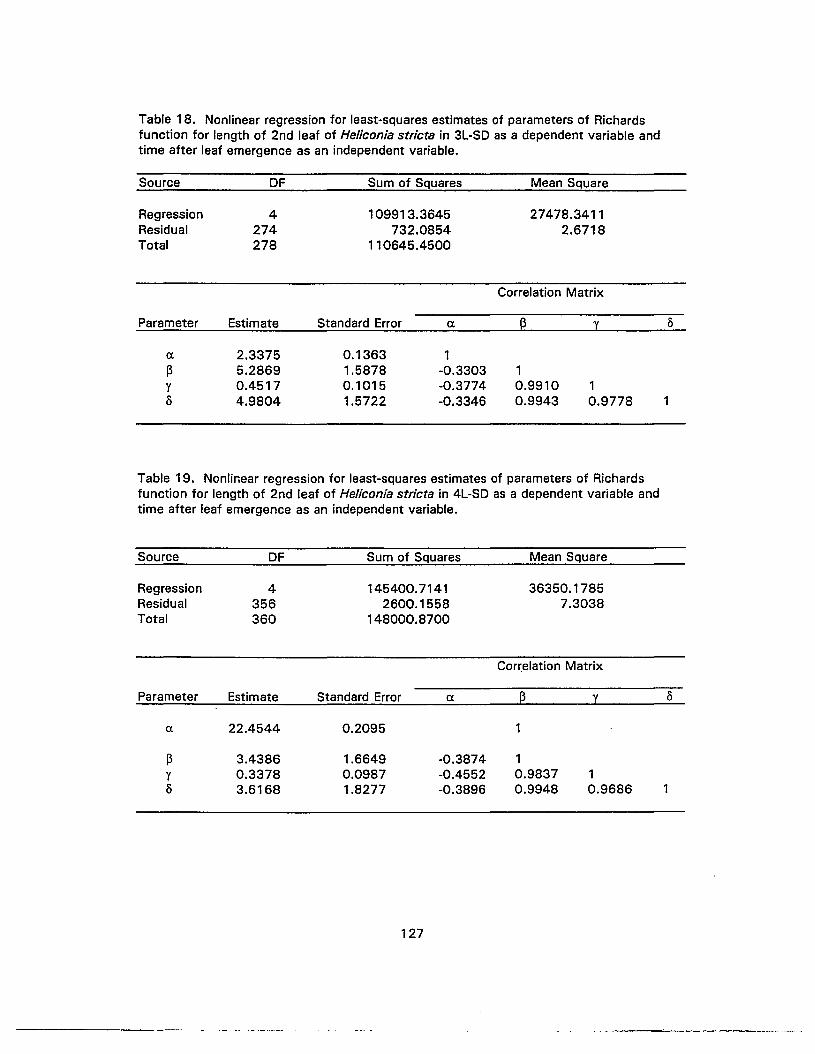
Table 18. Nonlinear regression for least-squares estimates of parameters of Richardsfunction for length of 2nd leaf of Heliconia stricta in 3L-SO as a dependent variable andtime after leaf emergence as an independent variable.
Source OF Sum of Squares Mean Square
Regression 4 109913.3645 27478.3411Residual 274 732.0854 2.6718Total 278 110645.4500
Correlation Matrix
Parameter Estimate Standard Error a @ y
a 2.3375 0.1363 1~ 5.2869 1.5878 -0.3303 1y 0.4517 0.1015 -0.3774 0.9910 10 4.9804 1.5722 -0.3346 0.9943 0.9778
Table 19. Nonlinear regression for least-squares estimates of parameters of Richardsfunction for length of 2nd leaf of Heliconia stricta in 4L-SO as a dependent variable andtime after leaf emergence as an independent variable.
Source OF Sum of Squares Mean Square
Regression 4 145400.7141 36350.1785Residual 356 2600.1558 7.3038Total 360 148000.8700
Correlation Matrix
Parameter Estimate Standard Error a @ y
a 22.4544 0.2095 1
~ 3.4386 1.6649 -0.3874 1y 0.3378 0.0987 -0.4552 0.9837 10 3.6168 1.8277 -0.3896 0.9948 0.9686 1
127
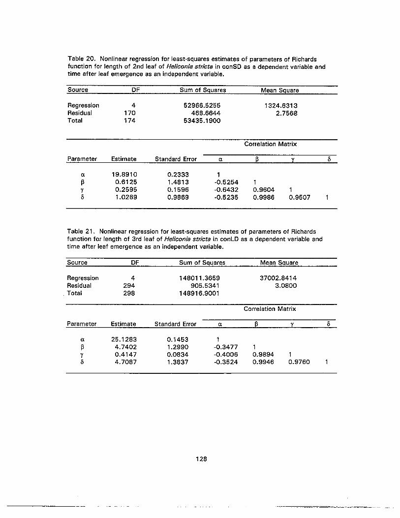
Table 20. Nonlinear regression for least-squares estimates of parameters of Richardsfunction for length of 2nd leaf of Heliconia stricta in conSD as a dependent variable andtime after leaf emergence as an independent variable.
Source DF Sum of Squares Mean Square
Regression 4 52966.5255 1324.6313Residual 170 468.6644 2.7568Total 174 53435.1900
Correlation Matrix
Parameter Estimate Standard Error a ~ y
a 19.8910 0.2333 1~ 0.6125 1.4813 -0.5254 1y 0.2595 0.1596 -0.6432 0.9604 10 1.0269 0.9869 -0.5235 0.9986 0.9507
Table 21. Nonlinear regression for least-squares estimates of parameters of Richardsfunction for length of 3rd leaf of Heliconia stricta in conLD as a dependent variable andtime after leaf emergence as an independent variable.
Source DF Sum of Squares Mean Square
Regression 4 148011.3659 37002.8414Residual 294 905.5341 3.0800
. Total 298 148916.9001
Correlation Matrix
Parameter Estimate Standard Error a p y
a 25.1283 0.1453 1~ 4.7402 1.2990 -0.3477 1y 0.4147 0.0834 -0.4006 0.9894 10 4.7087 1.3837 -0.3524 0.9946 0.9760
128
.~~=~===.=-~-~.-~.=----- - -

Table 22. Nonlinear regression for least-squares estimates of parameters of Richardsfunction for length of 3rd leaf of Heliconia stricta in 3L-SO as a dependent variable andtime after leaf emergence as an independent variable.
Source OF Sum of Squares Mean Square
Regression 4 139739.0939 34934.7734Residual 277 742.6060 2.6809Total 281 140481 .7000
Correlation Matrix
Parameter Estimate Standard Error IX @ Y
IX 24.8301 0.1333 1~ 5.2422 1.4402 -0.3215 1y 0.4577 0.0962 -0.3684 0.9908 10 5.1814 1.5290 -0.3263 0.9945 0.9779
Table 23. Nonlinear regression for least-squares estimates of parameters of Richardsfunction for length of 3rd leaf of Heliconia stricta in 4L-SO as a dependent variable andtime after leaf emergence as an independent variable.
Source OF Sum of Squares Mean Square
Regression 4 190285.7668 47571.4417Residual 360 2483.6031 6.8989Total 364 192769.3700
Correlation Matrix
Parameter Estimate Standard Error IX @ YIX 25.5650 0.2055 113 2.9313 1.2846 -0.3986 1y 0.3093 0.0719 -0.4739 0.9804 10 3.0351 1.3491 -0.3993 0.9951 0.9646
129

Table 24. Nonlinear regression for least-squares estimates of parameters of Richardsfunction for length of 3rd leaf of Heliconia stricta in conSD as a dependent variable andtime after leaf emergence as an independent variable.
Source DF Sum of Squares Mean Square
Regression 4 74161.4291 18540.3572Residual 175 844.4708 4.8255Total 179 75005.9000
Correlation Matrix
Parameter Estimate Standard Error (l p y
(l 23.2115 0.2768 1P 2.5544 1.5606 -0.4645 1'Y 0.3281 0.0962 -0.5510 0.9782 10 2.7660 1.6459 -0.4658 0.9959 0.9643 1
Table 25. Nonlinear regression for least-squares estimates of parameters of Richardsfunction for length of 4th leaf of Heliconia stricta in conLD as a dependent variable andtime after leaf emergence as an independent variable.
Source DF Sum of Squares Mean Square
Regression 4 233300.0379 58325.0094Residual 339 1677.5720 4.9485Total 343 234977.6100
Correlation Matrix
Parameter Estimate Standard Error (l @ y
(l 28.6421 0.1682 1P 2.2387 0.9759 -0.3680 1'Y 0.2972 0.0532 -0.4475 0.9748 10 2.3699 0.9631 -0.3677 0.99575 0.9587
130
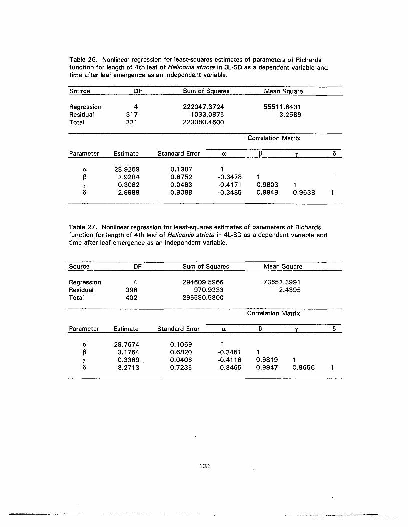
Table 26. Nonlinear regression for least-squares estimates of parameters of Richardsfunction for length of 4th leaf of Heliconia stricta in 3L-SO as a dependent variable andtime after leaf emergence as an independent variable.
Source OF Sum of Squares Mean Square
Regression 4 222047.3724 55511.8431Residual 317 1033.0875 3.2589Total 321 223080.4600
Correlation Matrix
Parameter Estimate Standard Error ex p y
ex 28.9269 0.1387 113 2.9284 0.8752 -0.3478 1y 0.3082 0.0483 -0.4171 0.9803 10 2.9989 0.9088 -0.3485 0.9949 0.9638
Table 27. Nonlinear regression for least-squares estimates of parameters of Richardsfunction for length of 4th leaf of Heliconia stricta in 4L-SO as a dependent variable andtime after leaf emergence as an independent variable.
Source OF Sum of Squares Mean Square
Regression 4 294609.5966 73652.3991Residual 398 970.9333 2.4395Total 402 295580.5300
Correlation Matrix
Parameter Estimate Standard Error ex p y
ex 29.7674 0.1069 113 3.1764 0.6820 -0.3451 1y 0.3369 0.0406 -0.4116 0.9819 10 3.2713 0.7235 -0.3465 0.9947 0.9656 1
131
-- --~-~.-- .._._-".- ..._-~-.-

Table 28. Nonlinear regression for least-squares estimates of parameters of Richardsfunction for length of 4th leaf of Heliconia stricta in conSD as a dependent variable andtime after leaf emergence as an independent variable.
Source OF Sum of Squares Mean Square
Regression 4 100801.7829 25200.4457Residual 166 701.9370 4.2285Total 170 101503.7200
Correlation Matrix
Parameter Estimate Standard Error a p y
a. 27.2928 0.2296 1P 3.4877 1.5436 -0.3559 1Y 0.4008 0.1088 -0.4234 0.98415 18 3.8407 1.7657 -0.3609 0.9952 0.9703 1
Table 29. Nonlinear regression for least-squares estimates of parameters of Richardsfunction for length of 5th leaf of Heliconia stricta in conLO as a dependent variable andtime after leaf emergence as an independent variable.
Source OF Sum of Squares Mean Square
Regression 4 342441.7918 85610.4479Residual 363 1606.1481 4.4246Total 367 344047.9400
Correlation Matrix
Parameter Estimate Standard Error a p y
a. 33.8665 0.1566 1P 1.9173 0.6977 -0.3629 1Y 0.2344 0.2917 -0.4496 0.9713 18 1.8876 0.6065 -0.3605 0.9959 0.9540
132
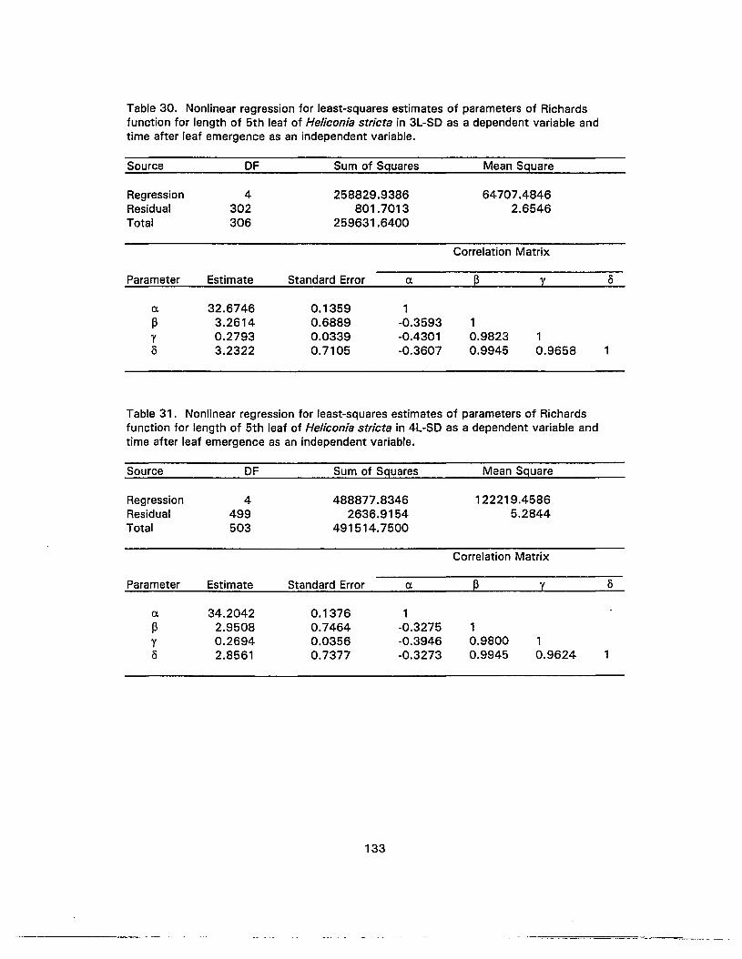
Table 30. Nonlinear regression for least-squares estimates of parameters of Richardsfunction for length of 5th leaf of Heliconia stricta in 3L-SO as a dependent variable andtime after leaf emergence as an independent variable.
Source OF Sum of Squares Mean Square
Regression 4 258829.9386 64707.4846Residual 302 801.7013 2.6546Total 306 259631 .6400
Correlation Matrix
Parameter Estimate Standard Error a p y
a 32.6746 0.1359 1P 3.2614 0.6889 -0.3593 1y 0.2793 0.0339 -0.4301 0.9823 10 3.2322 0.7105 -0.3607 0.9945 0.9658 1
Table 31. Nonlinear regression for least-squares estimates of parameters of Richardsfunction for length of 5th leaf of Heliconia stricta in 4L-SO as a dependent variable andtime after leaf emergence as an independent variable.
Source OF Sum of Squares Mean Square
Regression 4 488877.8346 122219.4586Residual 499 2636.9154 5.2844Total 503 491514.7500
Correlation Matrix
Parameter Estimate Standard Error a ~ y 0
a 34.2042 0.1376 1P 2.9508 0.7464 -0.3275 1y 0.2694 0.0356 -0.3946 0.9800 10 2.8561 0.7377 -0.3273 0.9945 0.9624 1
133

Table 32. Nonlinear regression for least-squares estimates of parameters of Richardsfunction for length of 5th leaf of Heliconia stricta in conSO as a dependent variable andtime after leaf emergence as an independent variable.
Source OF Sum of Squares Mean Square
Regression 4 2101233.9444 50308.4861Residual 242 1032.2455 4.2654Total 246 202266.1900
Correlation Matrix
Parameter Estimate Standard Error a p y 8
a 31.1602 0.1759 113 3.0621 1.1208 -0.3297 1Y 0.3403 0.0679 -0.3978 0.9800 18 3.2689 1.2192 -0.3313 0.9948 0.9638 1
Table 33. Nonlinear regression for least-squares estimates of parameters of Richardsfunction for length of 6th leaf of Heliconia stricta in conLD as a dependent variable andtime after leaf emergence as an independent variable.
Source OF Sum of Squares Mean Square
Regression 4 485850.7930 121462.6982Residual 404 1728.3869 4.2781Total 408 487579.1800
Correlation Matrix
Parameter Estimate Standard Error a 13 y
a 37.4570 0.1367 113 1.7456 0.6589 -0.3294 1Y 0.2060 0.0240 -0.4139 0.9686 18 1.9321 0.6118 -0.3281 0.9965 0.9526
134

Table 34. Nonlinear regression for least-squares estimates of parameters of Richardsfunction for length of 6th leaf of Heliconia stricta in 3L-SO as a dependent variable andtime after leaf emergence as an independent variable.
Source OF Sum of Squares Mean Square
Regression 4 360423.1029 90105.7757Residual 326 1581.0470 4.8498Total 330 362004.1500
Correlation Matrix
Parameter Estimate Standard Error CI ~ Y
CI 35.8116 0.1585 1~ 3.6104 1.0505 -0.3073 1y .3091 0.0554 -0.3671 0.9839 18 .0751 1.2435 -0.3102 0.9947 0.9687
Table 35. Nonlinear regression for least-squares estimates of parameters of Richardsfunction for length of 6th leaf of Heliconia stricta in 4L-SO as a dependent variable andtime after leaf emergence as an independent variable.
Source OF Sum of Squares Mean Square
Regression 4 668137.2106 167034.3026Residual 559 2018.7993 3.6114Total 563 670156.0100
Correlation Matrix
Parameter Estimate Standard Error CI p Y
Cl. 37.1652 0.1026 1~ 3.0467 0.6160 -0.2994 1y 0.2613 0.2858 -0.3617 0.9806 18 3.3074 0.6827 -0.3008 0.9949 0.9642
135
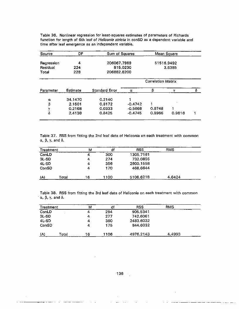
Table 36. Nonlinear regression for least-squares estimates of parameters of Richardsfunction for length of 6th leaf of Heliconia stricte in canSO as a dependent variable andtime after leaf emergence as an independent variable.
Source OF Sum of Squares Mean Square
Regression 4 206067.7969 51516.9492Residual 224 815.0230 3.6385Total 228 206882.8200
Correlation Matrix
Parameter Estimate Standard Error (X ~ y
(X 34.1470 0.2140 1~ 2.1501 0.8172 -0.4742 1Y 0.2168 0.0333 -0.5668 0.9748 10 2.4138 0.8425 -0.4745 0.9966 0.9616 1
Table 37. RSS from fitting the 2nd leaf data of Heliconia on each treatment with commonu, 13, t. and o.
Treatment M df RSSConLO 4 300 1305.71613L-SO 4 274 732.08554L-SO 4 356 2600.1558CanSO 4 170 468.6644
(A) Total 16 1100 5106.6218
RMS
4.6424
Table 38. RSS from fitting the 3rd leaf data of Heliconia on each treatment with common- (X, 13, y, and o.
Treatment M df RSSConLO 4 294 905.53413L-SO 4 277 742.60614L-SO 4 360 2483.6032CanSO 4 175 844.6032
(A) Total 16 1106 4976.2143
RMS
4.4993
136
- ------- -- ---
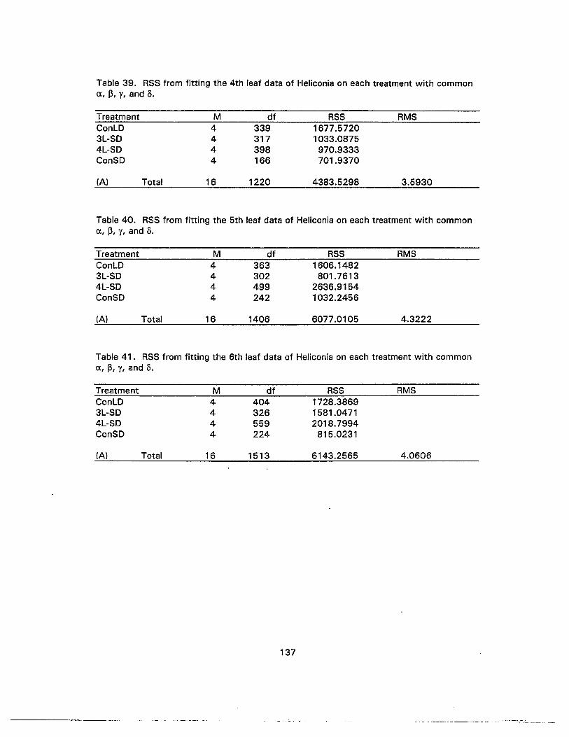
Table 39. RSS from fitting the 4th leaf data of Heliconia on each treatment with common0., ~, y, and o.
Treatment M df RSSConLO 4 339 1677.57203L-SO 4 317 1033.08754L-SO 4 398 970.9333CanSO 4 166 701.9370
(AI Total 16 1220 4383.5298
RMS
3.5930
Table 40. RSS from fitting the 5th leaf data of Heliconia on each treatment with common0., ~, y, and o.
Treatment M df RSSConLO 4 363 1606.14823L-SO 4 302 801.76134L-SO 4 499 2636.9154CanSO 4 242 1032.2456
(AI Total 16 1406 6077.0105
RMS
4.3222
Table 41. RSS from fitting the 6th leaf data of Heliconia on each treatment with common0., ~, y, and o.
Treatment M df RSSConLO 4 404 1728.38693L-SO 4 326 1581.04714L-SO 4 559 2018.7994CanSO 4 224 815.0231
(AI Total 16 1513 6143.2565
RMS
4.0606
137
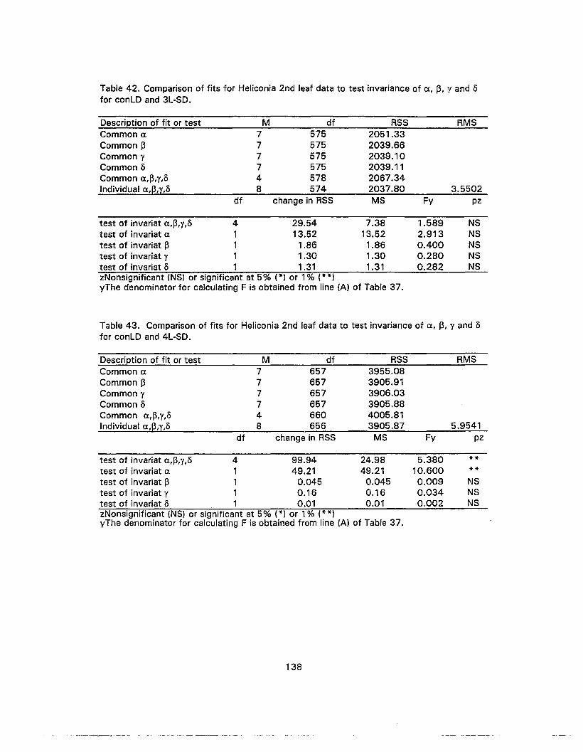
Table 42. Comparison of fits for Heliconia 2nd leaf data to test invariance of 0., [3, Y and 0for conLD and 3L-SD.
Description of fit or test M df RSS RMSCommon 0. 7 575 2051.33Common [3 7 575 2039.66Common y 7 575 2039.10Common 0 7 575 2039.11Common a,[3,y,o 4 578 2067.34Individual a,p,y,o 8 574 2037.80 3.5502
df change in RSS MS Fy pz
test of invariat a,p,y,o 4 29.54 7.38 1.589 NStest of invariat a 1 13.52 13.52 2.913 NStest of invariat p 1 1.86 1.86 0.400 NStest of invariat y 1 1.30 1.30 0.280 NStest of invariat 0 1 1.31 1.31 0.282 NSzNonsignificant (NS) or significant at 5% (*) or 1% (* *)yThe denominator for calculating F is obtained from line (A) of Table 37.
Table 43. Comparison of fits for Heliconia 2nd leaf data to test invariance of 0., [3, Y and 0for conLD and 4L-SD.
Description of fit or test M df RSS RMSCommon 0. 7 657 3955.08Common [3 7 657 3905.91Common y 7 657 3906.03Common 0 7 657 3905.88Common a,p,y,o 4 660 4005.81Individual a,@,y,o 8 656 3905.87 5.9541
df change in RSS MS Fy pz
test of invariat a,p,y,o 4 99.94 24.98 5.380 **
test of invariat a 1 49.21 49.21 10.600 **
test of invariat p 1 0.045 0.045 0.009 NStest of invariat y 1 0.16 0.16 0.034 NStest of invariat 0 1 0.01 0.01 0.002 NSzNonsignificant (NS) or significant at 5% (*) or 1% (* *)yThe denominator for calculating F is obtained from line (A) of Table 37.
138

Table 44. Comparison of fits for Heliconia 2nd leaf data to test invariance of lX, ~, Y and afor conLD and conSD.
Description of fit or test M df RSS RMSCommon lX 7 471 1864.40Common ~ 7 471 1781.32Common y 7 471 1801.96Common a 7 471 1780.35Common lX,~,y,a 4 474 1971.52IndividuallX,~,y,a 8 470 1774.38 3.7753
df change in RSS MS Fy pz
test of invariat lX,~,y,a 4 197.14 49.28 10.615 **
test of invariat lX 1 90.02 90.02 19.390 **
test of invariat ~ 1 6.95 6.95 1.497 NStest of invariat y 1 27.58 27.58 5.940 *
test of invariat a 1 5.97 5.97 1.286 NSzNonsignificant (NS) or significant at 5% (*) or 1% (* *)yThe denominator for calculating F is obtained from line (A) of Table 37.
Table 45. Comparison of fits for Heliconia 2nd leaf data to test invariance of c, ~, Yand afor 3L-SD and 4L-SD.
Description of fit or test M df RSS RMSCommon lX 7 631 3333.26Common ~ 7 631 3334.96Common y 7 631 3334.81Common a 7 631 3334.57Common lX,~,y,a 4 634 3378.36Individual lX,p,y,a 8 630 3332.24 5.289
df change in RSS MS Fy pz
test of invariat lX,~,y,a 4 46.14 11.53 2.483 *
test of invariat lX 1 1.02 1.02 0.219 NStest of invariat ~ 1 2.72 2.72 0.586 NStest of invariat y 1 2.57 2.57 0.554 NStest of invariat 15 1 1.33 1.33 0.286 NSzNonsignificant (NS) or significant at 5% (*) or 1% (* *)yThe denominator for calculating F is obtained from line (A) of Table 37.
139
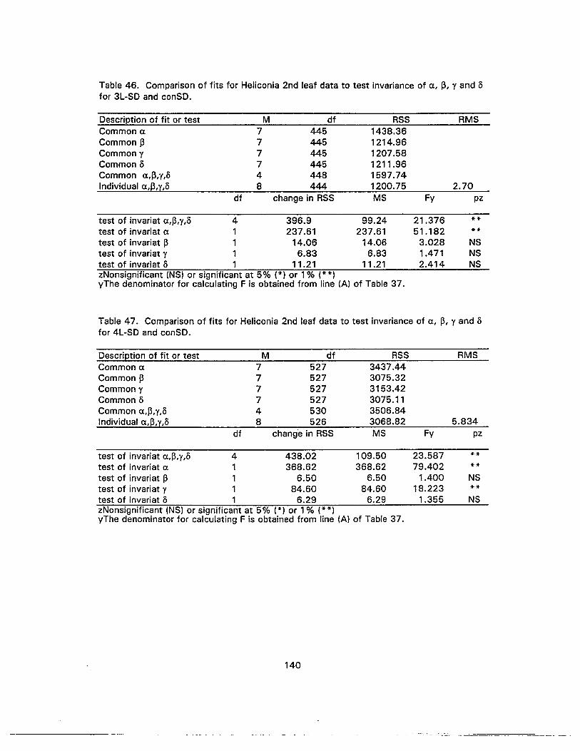
Table 46. Comparison of fits for Heliconia 2nd leaf data to test invariance of a, ~, y and 0for 3L-SD and canSO.
Description of fit or test M df RSS RMSCommon a 7 445 1438.36Common ~ 7 445 1214.96Common y 7 445 1207.58Common 0 7 445 1211.96Common a,~,y,o 4 448 1597.74Individual a,p,y,o 8 444 1200.75 2.70
df change in RSS MS Fy pz
test of invariat a,~,y,o 4 396.9 99.24 21.376 **
test of invariat a 1 237.61 237.61 51.182 **
test of invariat ~ 1 14.06 14.06 3.028 NStest of invariat y 1 6.83 6.83 1.471 NStest of invariat 0 1 11.21 11.21 2.414 NSzNonsignificant (NS) or significant at 5% (*) or 1% (**)yThe denominator for calculating F is obtained from line (A) of Table 37.
Table 47. Comparison of fits for Heliconia 2nd leaf data to test invariance of a, ~, y and 0for 4L-SD and canSO.
Description of fit or test M df RSS RMSCommon a 7 527 3437.44Common ~ 7 527 3075.32Common y 7 527 3153.42Common 0 7 527 3075.11Common a,~,y,o 4 530 3506.84Individual a,p,y,o 8 526 3068.82 5.834
df change in RSS MS Fy pz
test of invariat a,~,y,o 4 438.02 109.50 23.587 **
test of invariat a 1 368.62 368.62 79.402 **
test of invariat ~ 1 6.50 6.50 1.400 NStest of invariat y 1 84.60 84.60 18.223 **
test of invariat 0 1 6.29 6.29 1.355 NSzNonsignificant (NS) or significant at 5% (*) or 1% (U)yThe denominator for calculating F is obtained from line (A) of Table 37.
140

Table 48. Comparison of fits for Heliconia 3th leaf data to test invariance of a, 13, y and 0for conLD and 3L-SD.
Description of fit or test M df RSS RMSCommon a 7 572 1654.47Common 13 7 572 1648.31Common y 7 572 1648.43Common 0 7 572 1655.14Common a,l3,y,o 4 575 1655.54Individual a,l3,y,o 8 571 1648.14 2.89
df change in RSS MS Fy pz
test of invariat a,l3,y,o 4 7.40 1.85 0.411 NStest of invariat a 1 6.33 6.33 1.407 NStest of invariat 13 1 0.17 0.17 0.038 NStest of invariat y 1 0.29 0.29 0.064 NStest of invariat 0 1 7.40 7.40 1.645 NSzNonsignificant (NS) or significant at 5% (*) or 1% (**)yThe denominator for calculating F is obtained from line (A) of Table 38.
Table 49. Comparison of fits for Heliconia 3th leaf data to test invariance of a, 13, y and 0for conLD and 4L-SD.
Description of fit or test M df RSS RMSCommon a 7 655 3402.83Common 13 7 655 3393.02Common y 7 655 3392.60Common 0 7 655 3408.68Common a,l3,y,o 4 658 3435.11Individual a,@,y,o 8 654 3389.14 5.·18
df change in RSS MS Fy pz
test of invariat a,l3,y,o 4 45.96 11.49 2.553 *
test of invariat a 1 13.69 13.69 3.042 NStest of invariat 13 1 3.88 3.88 0.862 NStest of invariat y 1 3.46 3.46 0.769 NStest of invariat 0 1 19.54 19.54 4.342 *
·zNonsignificant (NS) or significant at 5% (*) or 1% (**)yThe denominator for calculating F is obtained from line (A) Table 38
141
..-------- ---===:-::-::----
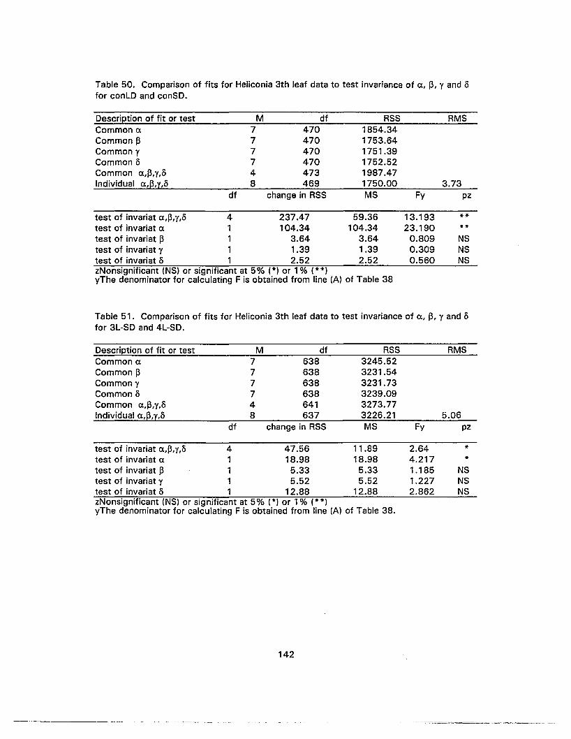
Table 50. Comparison of fits for Heliconia 3th leaf data to test invariance of a, 13, Y and 0for conLD and canSO.
Description of fit or test M df RSS RMSCommon a 7 470 1854.34Common 13 7 470 1753.64Common Y 7 470 1751.39Common 0 7 470 1752.52Common a,l3,y,o 4 473 1987.47Individual a,l3,y,o 8 469 1750.00 3.73
df change in RSS MS Fy pz
test of invariat a,l3,y,o 4 237.47 59.36 13.193 **
test of invariat a 1 104.34 104.34 23.190 **
test of invariat 13 1 3.64 3.64 0.809 NStest of invariat y 1 1.39 1.39 0.309 NStest of invariat 0 1 2.52 2.52 0.560 NSzNonsignificant (NS) or significant at 5% (*) or 1% (**)yThe denominator for calculating F is obtained from line (A) of Table 38
Table 51. Comparison of fits for Heliconia 3th leaf data to test invariance of a, 13, Y and 0for 3L-SD and 4L-SD.
Description of fit or test M df RSS RMSCommon a 7 638 3245.52Common 13 7 638 3231.54Common y 7 638 3231.73Common 0 7 638 3239.09Common a,l3,y,o 4 641 3273.77Individual a,@,y,o 8 637 3226.21 5.06
df change in RSS MS Fy pz
test of invariat a,l3,y,o 4 47.56 11.89 2.64 *
test of invariat a 1 18.98 18.98 4.217 *
test of invariat 13 1 5.33 5.33 1.185 NStest of invariat Y 1 5.52 5.52 1.227 NStest of invariat 0 1 12.88 12.88 2.862 NSzNonsignificant (NS) or significant at 5% (*) or 1% (* *)yThe denominator for calculating F is obtained from line (A) of Table 38.
142

Table 52. Comparison of fits for Heliconia 3th leaf data to test invariance of a, ~, y and 0for 3L-SD and conSD.
Description of fit or test M df RSS RMSCommon ex 7 453 1676.80Common ~ 7 453 1591.85Common y 7 453 1589.62Common 0 7 453 1590.45Common ex,~,y,o 4 456 1770.78Individual ex,~,y,o 8 452 1587.08 3.51
df change in RSS MS Fy pz
test of invariat ex,~,y,8 4 183.70 45.92 10.206 **
test of invariat ex 1 89.72 89.72 19.940 **
test of invariat ~ 1 4.77 4.77 1.060 NStest of invariat y 1 2.52 2.52 0.560 NStest of invariat 0 1 3.37 3.37 0.749 NSzNonsignificant (NS) or significant at 5% (*) or 1% (* *)yThe denominator for calculating F is obtained from line (A) Table 38.
Table 53. Comparison of fits for Heliconia 3th leaf data to test invariance of a, ~, y and 0for 4L-SD and conSD.
Description of fit or test M df RSS RMSCommon ex 7 536 3489.03Common ~ 7 536 3328.22Common y 7 536 3328.17Common 0 7 536 3328.15Common ex,~,y,o 4 539 3679.16Individual ex,~,y,o 8 535 3328.07
df change in RSS MS Fy pz
test of invariat ex,~,y,o 4 351.09 87.77 19.507 **
test of invariat ex 1 160.96 160.96 35.774 **
test of invariat ~ 1 0.15 0.15 0.033 NStest of invariat y 1 0.10 0.10 0.022 NStest of invariat 0 1 0.08 0.08 0.018 NSzNonsignificant (NS) or significant at 5% (*) or 1% (* *)yThe denominator for calculating F is obtained from line (A) of Table 38.
143
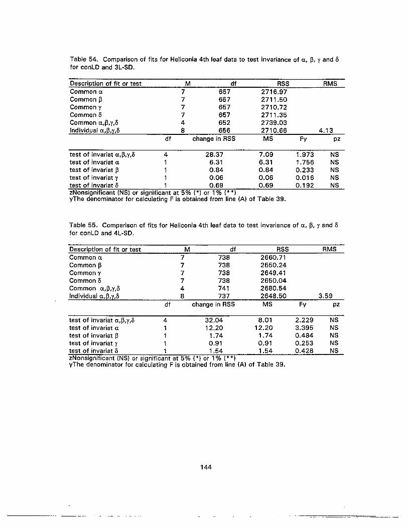
Table 54. Comparison of fits for Heliconia 4th leaf data to test invariance of a, p, y and 8for conLD and 3L-SD.
Description of fit or test M df RSS RMSCommon a 7 657 2716.97Common p 7 657 2711.50Common y 7 657 2710.72Common 8 7 657 2711.35Common a,p,y,8 4 652 2739.03Individual a,@,y,8 8 656 2710.66 4.13
df change in RSS MS Fy pz
test of invariat a,p,y,o 4 28.37 7.09 1.973 NStest of invariat a 1 6.31 6.31 1.756 NStest of invariat p 1 0.84 0.84 0.233 NStest of invariat y 1 0.06 0.06 0.016 NStest of invariat 8 1 0.69 0.69 0.192 NSzNonsignificant (NS) or significant at 5% (*) or 1% (* *)yThe denominator for calculating F is obtained from line (A) of Table 39.
Table 55. Comparison of fits for Heliconia 4th leaf data to test invariance of a, p, y and 8for conLD and 4L-SD.
Description of fit or test M df RSS RMSCommon a 7 738 2660.71Common p 7 738 2650.24Common y 7 738 2649.41Common 8 7 738 2650.04Common a,p,y,8 4 741 2680.54Individual a,@,y,8 8 737 2648.50 3.59
df change in RSS MS Fy pz
test of invariat a,p,y,8 4 32.04 8.01 2.229 NStest of invariat a 1 12.20 12.20 3.395 NStest of invariat p 1 1.74 1.74 0.484 NStest of invariat y 1 0.91 0.91 0.253 NStest of invariat 8 1 1.54 1.54 0.428 NSzNonsignificant (NS) or significant at 5% (*) or 1% (**)yThe denominator for calculating F is obtained from line (A) of Table 39.
144
-- -__ - __ ===-0-=-....,..-,=

Table 56. Comparison of fits for Heliconia 4th leaf data to test invariance of a, ~, ¥ and 0for conLD and conSD.
Description of fit or test M df RSS RMSCommon a 7 506 2464.89Common ~ 7 506 2381.49Common ¥ 7 506 2382.89Common 0 7 506 2381.91Common a,~,¥,o 4 509 2484.69Individual a,~,y,o 8 505 2379.51 4.71
df change in RSS MS Fy pz
test of invariat a,13,¥,o 4 105.18 26.295 7.318 **
test of invariat a 1 85.38 85.38 23.763 **
test of invariat ~ 1 1.98 1.98 0.551 NStest of lnvarlat ¥ 1 3.38 3.38 0.940 NStest of invariat 0 1 2.4 2.4 0.668 NSzNonsignificant (NS) or significant at 5% (*) or 1% (**)yThe denominator for calculating F is obtained from line (A) of Table 39.
Table 57. Comparison of fits for Heliconia 4th leaf data to test invariance of a, 13, ¥ and 0for 3L-SD and 4L-SD.
Description of fit or test M df RSS RMSCommon a 7 716 2014.74Common ~ 7 716 2004.14Common ¥ 7 716 2004.47Common 0 7 716 2004.14Common a,~,¥,o 4 719 2030.82Individual a,@,y,o 8 715 2004.02 2.80
. df change in RSS MS Fy pz
test of invariat a,13,¥,o 4 26.80 6.70 1.865 NStest of invariat a 1 10.72 10.72 2.983 NStest of invariat 13 1 0.11 0.11 0.030 NStest of invariat ¥ 1 0.45 0.45 0.125 NStest of invariat 0 1 0.12 0.12 0.033 NSzNonsignificant (NS) or significant at 5% (*) or 1% (* *)yThe denominator for calculating F is obtained from line (A) Table 39.
145

Table 58. Comparison of fits for Heliconia 4th leaf data to test invariance of a, 13, Y and 8for 3L-SD and conSD.
Description of fit or test M df RSS RMSCommon a 7 484 1852.60Common 13 7 484 1735.39Common Y 7 484 1737.58Common 8 7 484 1735.73Common a,13,y,o 4 487 1894.33Individual a,13,y,o 8 483 1735.02 3.5922
df change in RSS MS Fy pz
test of invariat a,13,y,o 4 159.31 39.83 11.085 **
test of invariat a 1 117.58 117.58 32.725 **
test of invariat 13 1 0.37 0.37 0.103 NStest of invariat Y 1 "2.56 2.56 0.712 NStest of invariat 8 1 0.71 0.71 0.197 NSzNonsignificant (NS) or significant at 5% (*) or 1% (**)yThe denominator for calculating F is obtained from line (A) Table 39.
Table 59. Comparison of fits for Heliconia 4th leaf data to test invariance of a, 13, Y and 0for 4L-SD and conSD.
Description of fit or test M df RSSCommon a 7 565 2101.34Common 13 7 565 1672.99Common Y 7 565 1674.09Common 0 7 565 1673.20Common a,13,y,o 4 568 2087.00Individual a,@,y,o 8 564 1672.87
df change in RSS MS Fy
RMS
2.96pz
test of invariat a,13,y,8 4 414.13test of invariat a 1 428.47test of invariat 13 1 0.12test of invariat Y 1 1.22test of invariat 8 1 0.33
100.53428.47
0.121.220.33
27.979119.25
0.0330.3390.091
****
NSNSNS
zNonsignificant (NS) or significant at 5% (*) or 1% (**)yThe denominator for calculating F is obtained from line (A) of Table 39.
146

Table 60. Comparison of fits for Heliconia 5th leaf data to test invariance of a, p, y and 0for conLD and 3L-SD.
Description of fit or test M df RSS RMSCommon a 7 666 2510.85Common p 7 666 2413.47Common y 7 666 2410.67Common 0 7 666 2414.05Common a,p,y,o 4 669 2635.95Individual a,p,y,o 8 665 2407.85 3.62
df change in RSS MS Fy pz
test of invariat a,p,y,o 4 228.10 57.03 13.194 **
test of invariat a 1 103.00 103.00 23.830 **
test of invariat p 1 5.62 5.62 1.300 NStest of invariat y 1 2.82 2.82 0.652 NStest of invariat 0 1 6.2 6.2 1.434 NSzNonsignificant (NSI or significant at 5% (*1 or 1% (**1yThe denominator for calculating F is obtained from line (A) of Table 40.
Table 61. Comparison of fits for Heliconia 5th leaf data to test invariance of a, p, y and 0for conLD and 4L-SD.
Description of fit or test M df RSS RMSCommon a 7 863 4254.17Common p 7 863 4246.97Common y 7 863 4245.14Common 0 7 863 4247.07Common a,p,y,o 4 866 4270.08Individual a,p,y,o 8 862 4243.06 4.92
df change in RSS MS Fy pz
test of invariat a,p,y,o 4 27.02 6.76 1.564 NStest of invariat a 1 11.11 11.11 2.570 NStest of. invariat p 1 3.92 3.92 0.906 NStest of invariat y 1 2.08 2.08 0.481 NStest of invariat 0 1 4.01 4.01 0.927 NSzNonsignificant (NSI or significant at 5% (*1 or 1% (UIyThe denominator for· calculating F is obtained from line (A) of Table 40.
147
._---.__._--_.- _..-..__._--_.
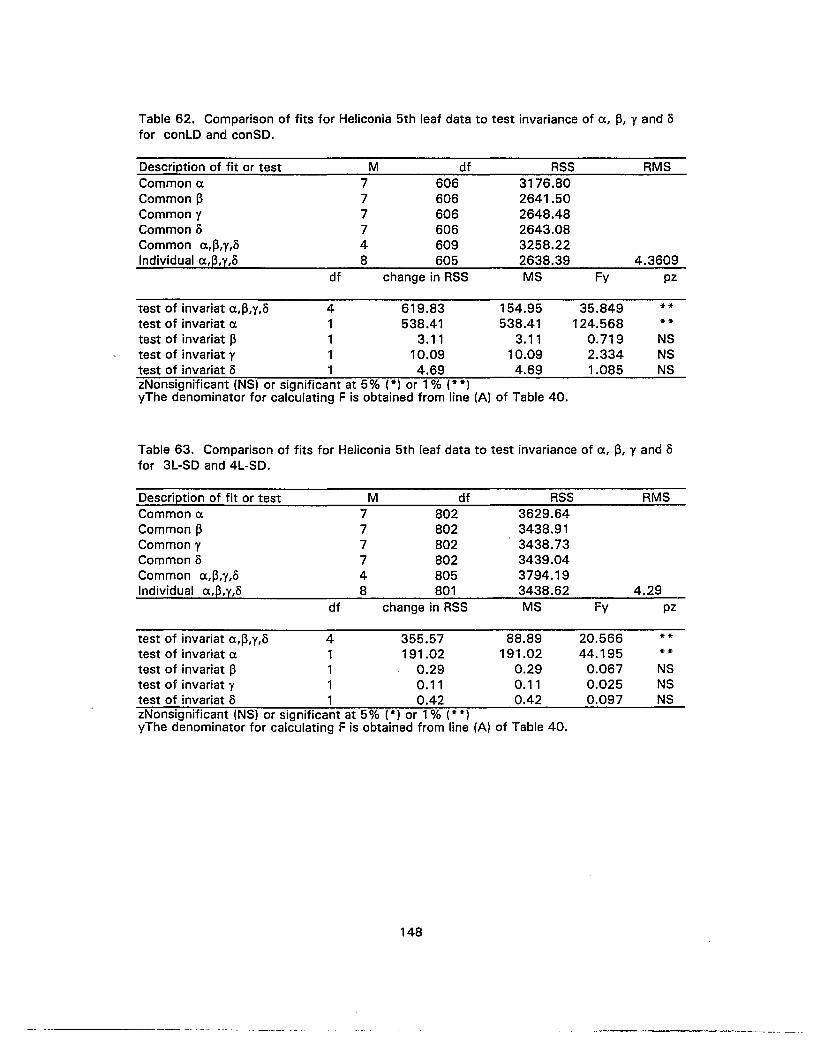
Table 62. Comparison of fits for Heliconia 5th leaf data to test invariance of a, ~, y and /)for conLO and canSO.
Description of fit or test M df RSSCommon a 7 606 3176.80Common ~ 7 606 2641.50Common y 7 606 2648.48Common /) 7 606 2643.08Common a,~,y,/) 4 609 3258.22Individual a,@,y,/) 8 605 2638.39
df change in RSS MS Fy
RMS
4.3609pz
test of invariat a,~,y,/) 4 619.83test of invariat a 1 538.41test of invariat ~ 1 3.11test of invariat y 1 10.09test of invariat /) 1 4.69
154.95538.41
3.1110.094.69
35.849124.568
0.7192.3341.085
****NSNSNS
zNonsignificant (NS) or significant at 5% (*) or 1% (**)yThe denominator for calculating F is obtained from line (A) of Table 40.
Table 63. Comparison of fits for Heliconia 5th leaf data to test invariance of a, ~, y and /)for 3L-SO and 4L-SO.
Description of fit or test M df RSS RMSCommon a 7 802 3629.64Common ~ 7 802 3438.91Common y 7 802 3438.73Common /) 7 802 3439.04Common a,~,y,/) 4 805 3794.19Individual a,@,y,/) 8 801 3438.62 4.29
df change in RSS MS Fy pz
test of invariat a,~,y,/) 4 355.57 88.89 20.566 **
test of invariat a 1 191.02 191.02 44.195 **
test of invariat ~ 1 0.29 0.29 0.067 NStest of invariat y 1 0.11 0.11 0.025 NStest of invariat /) 1 0.42 0.42 0.097 NSzNonsignificant (NS) or significant at 5% (*) or 1 % (**)yThe denominator for calculating F is obtained from line (A) of Table 40.
148
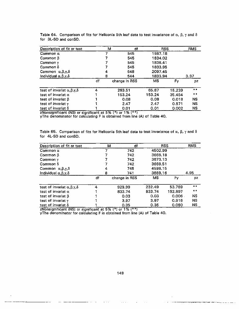
Table 64. Comparison of fits for Heliconia 5th leaf data to test invariance of ex, ~, y and 0for 3L-SD and conSD.
Description of fit or test M df RSS RMSCommon ex 7 545 1987.18Common ~ 7 545 1834.02Common y 7 545 1836.41Common 0 7 545 1833.95Common ex,~,y,o 4 548 2097.45Individual ex,~,y,o 8 544 1833.94 3.37
df change in RSS MS Fy pz
test of invariat ex,~,y,o 4 263.51 65.87 15.239 **
test of invariat ex 1 153.24 153.24 35.454 **
test of invariat ~ 1 0.08 0.08 0.018 NStest of invariat y 1 2.47 2.47 0.571 NStest of invariat 0 1 0.01 0.01 0.002 NSzNonsignificant (NS) or significant at 5% (*) or 1% (**)yThe denominator for calculating F is obtained from line (A) of Table 40.
Table 65. Comparison of fits for Heliconia 5th leaf data to test invariance of ex, ~, y and 0for 4L-SD and conSD.
Description of fit or test M df RSSCommon ex 7 742 4502.99Common ~ 7 742 3669.18Common y 7 742 3673.13Common S 7 742 3669.51Common ex,~,y,o 4 745 4599.15Individual ex,~,y,o 8 741 3669.16
df change in RSS MS Fy
RMS
4.95pz
test of invariat ex,~,y,o 4 929.99test of invariat ex 1 833.74test of invariat ~ 1 0.03test of invariat y 1 3.97test of invariat 0 1 0.35
232.49833.74
0.033.970.35
53.789192.897
0.006.0.9180.080
****
NSNSNS
zNonsignificant (NS) or significant at 5% (*) or 1% (**)yThe denominator for calculating F is obtained from line (A) of Table 40.
149

Table 66. Comparison of fits for Heliconia 6th leaf data to test invariance of a, ~, y and 0for conLD and 3L-SD.
Description of fit or test M df RSS RMSCommon a 7 731 3574.99Common ~ 7 731 3320.77Common y 7 731 3325.69Common 0 7 731 3322.49Common a,13,y,o 4 734 3597.56Individual a,@,y,o 8 730 3309.43 4.53
df change in RSS MS Fy pz
test of invariat a,~,y,o 4 288.13 72.03 17.740 **
test of invariat a 1 265.56 265.56 65.404 **
test of invariat 13 1 11.34 11.34 2.793 NStest of invariat y 1 16.26 16.26 4.004 *
test of invariat 0 1 13.06 13.06 3.216 NSzNonsignificant (NS) or significant at 5% (*) or 1% (**)yThe denominator for calculating F is obtained from line (A) of Table 41.
Table 67. Comparison of fits for Heliconia 6th leaf data to test invariance of a, 13, y and 0for conLD and 4L-SD.
Description of fit or test M df RSS RMSCommon a 7 964 3758.42Common 13 7 964 3754.84Common y 7 964 3754.77Common 0 7 964 3755.35Common a,13,y,o 4 967 3762.40Individual a,@,y,o 8 963 3747.18 3.89
df change in RSS MS Fy pz
test of invariat a,~,y,o 4 15.22 3.80 0.935 NStest of invariat a 1 11.24 11.24 2.768 NStest of invariat 13 1 7.66 7.66 1.886 NStest of invariat y 1 7.59 7.59 1.869 NStest of invariat 0 1 8.17 8.17 2.012 NSzNonsignificant (NS) or significant at 5% (*) or 1% (* *)yThe denominator for calculating F is obtained from line (A) of Table 41.
150

Table 68. Comparison of fits for Heliconia 6th leaf data to test invariance of ex, p, y and 0for conLD and conSO.
Description of fit or test M df RSSCommon ex 7 629 3257.75Common p 7 629 2543.95Common y 7 629 2543.65Common 0 7 629 2544.21Common ex,p,y,o 4 632 3702.45Individual ex,@,y,o 8 628 2543.41
df change in RSS MS Fy
RMS
4.05pz
test of invariat ex,p,y,o 4 1159.04test of invariat ex 1 714.34test of invariat p 1 0.54test of invariat y 1 0.24test of invariat 0 1 0.80
289.76714.34
0.540.240.80
71.364175.933
0.1330.0590.197
****
NSNSNS
zNonsignificant (NS) or significant at 5% (*) or 1% (**)yThe denominator for calculating F is obtained from line (A) of Table 41.
Table 69. Comparison of fits for Heliconia 6th leaf data to test invariance of ex, p, y and /)for 3L-SD and 4L-SD.
Description of fit or test M df RSS RMSCommon ex 7 886 3810.61Common p 7 886 3600.81Commony 7 886 3602.63Common 0 7 886 3601.22Common ex,p,y,o 4 889 3840.46Individual ex,@,y,o 8 885 3599.85 4.07
df change in RSS MS Fy pz
test of invariat ex,p,y,o 4 240.61 60.15 14.814 **
test of invariat ex 1 210.76 210.76 51.907 **
test of invariat p 1 0.96 0.96 0.236 NStest of invariat y 1 2.78 2.78 0.685 NStest of invariat 0 1 1.37 1.37 0.337 NSzNonsignificant (NS) or significant at 5% (*) or 1% (* *)yThe denominator for calculating F is obtained from line (A) Table 41.
151
- ------ ---
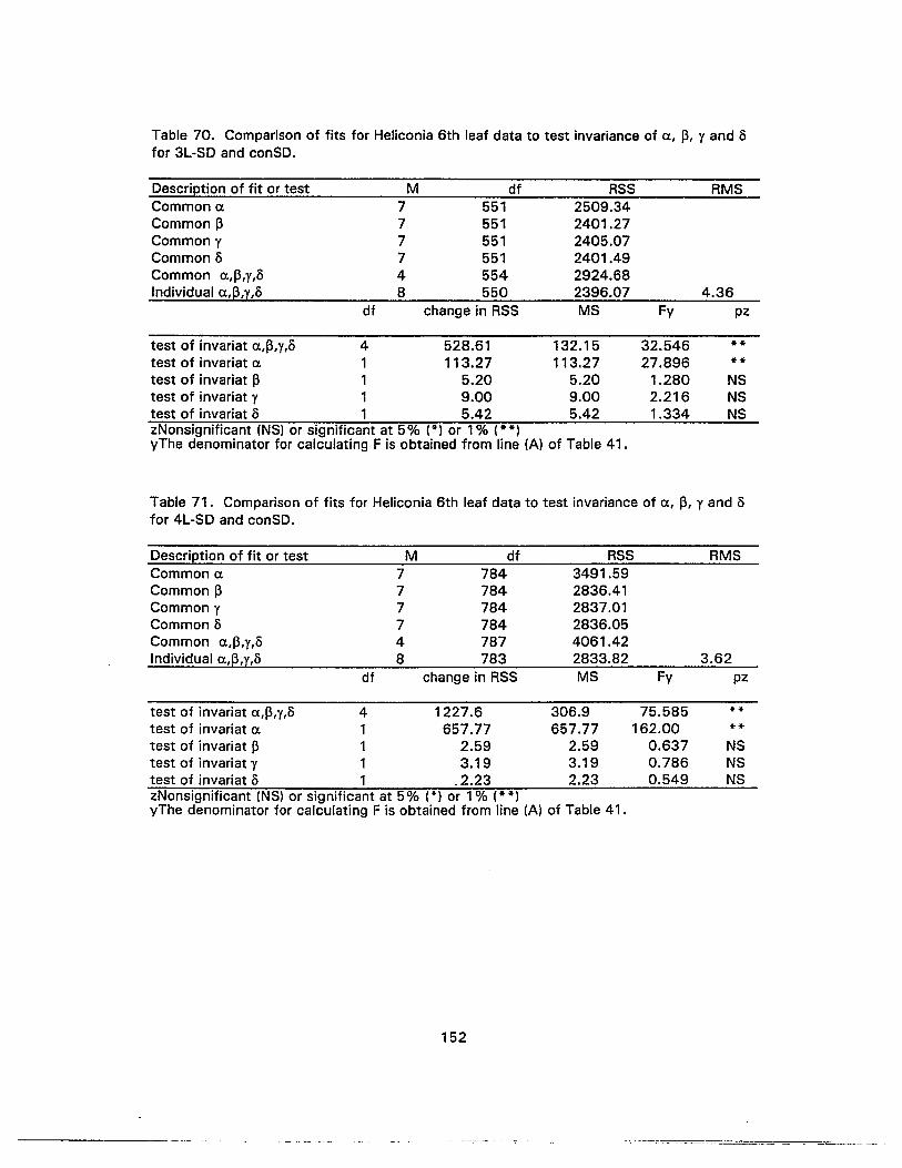
Table 70. Comparison of fits for Heliconia 6th leaf data to test invariance of a., 13, y and 8for 3L-SD and canSO.
Description of fit or test M df RSS RMSCommon a. 7 551 2509.34Common 13 7 551 2401.27Common y 7 551 2405.07Common 8 7 551 2401.49Common a.,I3,y,8 4 554 2924.68Individual a.,I3,y,8 8 550 2396.07 4.36
df change in RSS MS Fy pz
test of invariat a.,I3,y,8 4 528.61 132.15 32.546 **
test of invariat a. 1 113.27 113.27 27.896 **
test of invariat 13 1 5.20 5.20 1.280 NStest of invariat y 1 9.00 9.00 2.216 NStest of invariat 8 1 5.42 5.42 1.334 NSzNonsignificant (NS) or significant at 5% (*) or 1% (**)yThe denominator for calculating F is obtained from line (A) of Table 41.
Table 71. Comparison of fits for Heliconia 6th leaf data to test invariance of a., 13, y and 8for 4L-SD and canSO.
Description of fit or test M df RSSCommon a. 7 784 3491.59Common 13 7 784 2836.41Common y 7 784 2837.01Common 8 7 784 2836.05Common a.,I3,y,8 4 787 4061.42Individual a.,@,y,8 8 783 2833.82
df change in RSS MS Fy
RMS
3.62pz
test of invariat a.,I3,y,8 4 1227.6test of invariat a. 1 657.77test of invariat 13 1 2.59test of invariat y 1 3.19test of invariat 8 1 _2.23
306.9657.77
2.593.192.23
75.585162.00
0.6370.7860.549
****
NSNSNS
zNonsignificant (NS) or significant at 5% (*) or 1% (* *)yThe denominator for calculating F is obtained from line (A) of Table 41.
152

Table 72. Nonlinear regression for least-squares estimates of parameters of Richardsfunction for length of 4th leaf of non flowered Heliconia stricta in conLO as a dependentvariable and time after leaf emergence as an independent variable.
Source OF Sum of Squares Mean Square
Regression 4 175948.0437 43987.0109Residual 263 1122.1862 4.2668Total 267 177070.2300
Correlation Matrix
Parameter Estimate Standard Error Ct ~ Y
a. 28.0046 0.1691 1~ 3.0521 1.2056 -0.3309 1Y 0.3691 0.0797 -0.3965 0.9810 10 3.2739 1.3146 -0.3329 0.9949 0.9652 1
Table 73. Nonlinear regression for least-squares estimates of parameters of Richardsfunction for length of 4th leaf of flowered Heliconia stricta in 3L-SO as a dependentvariable and time after leaf emergence as an independent variable.
Source OF Sum of Squares Mean Square
Regression 4 103927.7656 25981.9414Residual 142 195.5043 1.3767Total 146 104123.2700
Correlation Matrix
Parameter Estimate Standard Error Ct ~ Y
Ct 29.3179 0.1294 1~ 4.3158 1.0689 -0.3155 1Y 0.3992 0.0685 -0.3679 0.9877 10 4.4059 1.1657 -0.3189 0.9943 0.9729
153
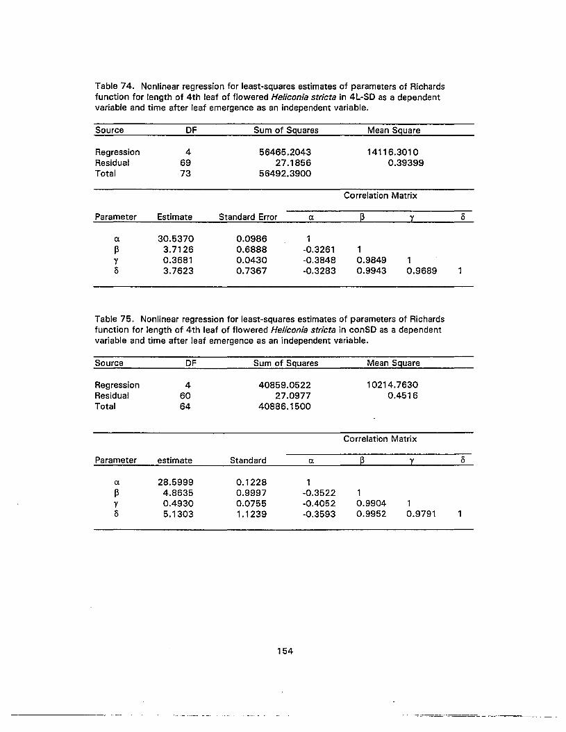
Table 74. Nonlinear regression for least-squares estimates of parameters of Richardsfunction for length of 4th leaf of flowered Heliconia stricta in 4L-SO as a dependentvariable and time after leaf emergence as an independent variable.
Source OF Sum of Squares Mean Square
Regression 4 56465.2043 14116.3010Residual 69 27.1856 0.39399Total 73 56492.3900
Correlation Matrix
Parameter Estimate Standard Error a 13 y
a 30.5370 0.0986 113 3.7126 0.6888 -0.3261 1y 0.3681 0.0430 -0.3848 0.9849 18 3.7623 0.7367 -0.3283 0.9943 0.9689 1
Table 75. Nonlinear regression for least-squares estimates of parameters of Richardsfunction for length of 4th leaf of flowered Heliconia stricta in conSO as a dependentvariable and time after leaf emergence as an independent variable.
Source OF Sum of Squares Mean Square
Regression 4 40859.0522 10214.7630Residual 60 27.0977 0.4516Total 64 40886.1500
Correlation Matrix
Parameter estimate Standard a @ y
a 28.5999 0.1228 1/3 4.8635 0.9997 -0.3522 1y 0.4930 0.0755 -0.4052 0.9904 18 5.1303 1.1239 -0.3593 0.9952 0.9791 1
154
.~==-- .-~---- - -
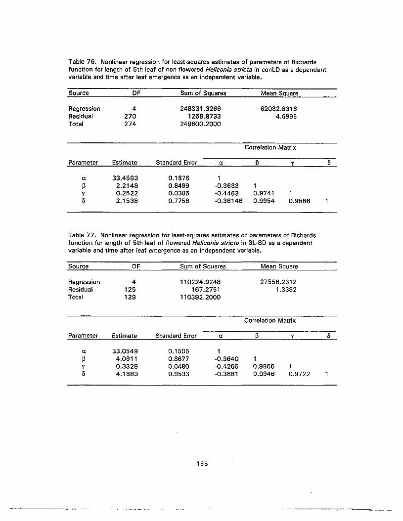
Table 76. Nonlinear regression for least-squares estimates of parameters of Richardsfunction for length of 5th leaf of non flowered Heliconia stricta in conLO as a dependentvariable and time after leaf emergence as an independent variable.
Source OF Sum of Squares Mean Square
Regression 4 248331.3266 62082.8316Residual 270 1268.8733 4.6995Total 274 249600.2000
Correlation Matrix
Parameter Estimate Standard Error ex p y
ex 33.4593 0.1876 113 2.2148 0.8499 -0.3633 1Y 0.2522 0.0386 -0.4463 0.9741 18 2.1538 0.7756 -0.36146 0.9954 0.9566 1
Table 77. Nonlinear regression for least-squares estimates of parameters of Richardsfunction for length of 5th leaf of flowered Heliconia stricta in 3L-SD as a dependentvariable and time after leaf emergence as an independent variable.
Source OF Sum of Squares Mean Square
Regression 4 110224.9248 27556.2312Residual 125 167.2751 1.3382Total 129 110392.2000
Correlation Matrix
Parameter Estimate Standard Error ex 13 y
ex 33.0549 0.1506 113 4.0611 0.8677 -0.3640 1Y 0.3328 0.0480 -0.4265 0.9866 18 4.1883 0.9533 -0.3681 0.9946 0.9722 1
155
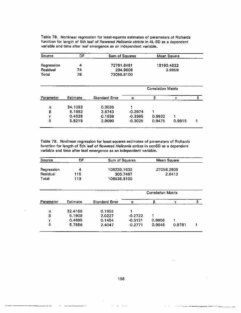
Table 78. Nonlinear regression for least-squares estimates of parameters of Richardsfunction for length of 5th leaf of flowered Heliconia stricta in 4L-SO as a dependentvariable and time after leaf emergence as an independent variable.
Source OF Sum of Squares Mean Square
Regression 4 72761.8491 18190.4622Residual 74 294.9608 3.9859Total 78 73056.8100
Correlation Matrix
Parameter Estimate Standard Error ex ~ y
ex 34.1093 0.3036 1~ 6.1882 2.8743 -0.2974 1Y 0.4328 0.1638 -0.3365 0.9932 1cS 5.8219 2.9090 -0.3025 0.9475 0.9815 1
Table 79. Nonlinear regression for least-squares estimates of parameters of Richardsfunction for length of 5th leaf of flowered Heliconia striate in canSO as a dependentvariable and time after leaf emergence as an independent variable.
Source OF Sum of Squares Mean Square
Regression 4 108233.1632 27058.2908Residual 115 303.7467 2.6412Total 119 108536.9100
Correlation Matrix
Parameter Estimate Standard Error ex p y
ex 32.4166 0.1855 1~ 5.1909 2.0227 -0.2722 1y 0.4895 0.1454 -0.3131 0.9908 1cS 5.7856 2.4047 -0.2771 0.9946 0.9781 1
156

Table 80. Nonlinear regression for least-squares estimates of parameters of Richardsfunction for length of 6th leaf of non flowered Heliconia stricta in conLO as a dependentvariable and time after leaf emergence as an independent variable.
Source OF Sum of Squares Mean Square
Regression 4 370433.0114 92608.2527Residual 311 1498.9988 4.8199Total 315 371932.0100
Correlation Matrix
Parameter Estimate Standard Error ex. p y
ex 37.1862 0.1658 1/3 1.3446 0.8158 -0.3330 1Y 0.1949 0.0270 -0.4243 0.9638 1s 1.5961 0.6997 -0.3315 0.9972 0.9492 1
Table 81. Nonlinear regression for least-squares estimates of parameters of Richardsfunction for length of 6th leaf of flowered Heliconia stricta in 3L-SO as a dependentvariable and time after leaf emergence as an independent variable.
Source OF Sum of Squares Mean Square
Regression 4 201468.9703 50367.2425Residual 165 594.4596 3.6027Total 169 202063.4300
Correlation Matrix
Parameter Estimate Standard Error ex. p y
ex 37.2388 0.1887 1P 3.6481 1.2584 -0.3024 1Y 0.3136 0.0671 -0.3625 0.9834 1s 4.2297 1.5310 -0.3054 0.9948 0.9682 1
157
------ -- ------------- ~==---==-------~.-~---------- -

Table 82. Nonlinear regression for least-squares estimates of parameters of Richardsfunction for length of 6th leaf of flowered Heliconia stricte in 4L-SO as a dependentvariable and time after leaf emergence as an independent variable.
Source OF Sum of Squares Mean Square
Regression 4 104106.9137 26026.7284Residual 80 105.2262 1.3153Total 84 104212.1400
Correlation Matrix
Parameter Estimate Standard Error a @ y
a 38.8178 0.1699 1~ 3.9319 0.9603 -0.3290 1Y 0.2947 0.0473 -0.3864 0.9857 10 4.0918 1.0615 -0.3317 0.9944 0.9701
Table 83. Nonlinear regression for least-squares estimates of parameters of Richardsfunction for length of 6th leaf of flowered Heliconia stricta in conSO as a dependentvariable and time after leaf emergence as an independent variable.
Source OF Sum of Squares Mean Square
Regression 4 91495.2114 22873.8028Residual 97 278.6285 2.8724Total 101 91773.8400
Correlation Matrix
Parameter Estimate Standard Error a @ y
a 34.9091 0.4028 1~ 0.3952 1.3605 -0.6307 1Y 0.1375 0.0279 -0.7477 0.9647 10 0.9819 0.9144 -0.6298 0.9992 0.9586
158

Table 84. RSS from fitting the 4th leaf data of Heliconia on each treatment andpseudostem status with common a, 13, yand o.
Treatment Status M df RSS RMSConLO Veg. 4 263 1122.18633L-SO FI. 4 142 195.50434L-SO FI. 4 69 27.1856ConSO FI. 4 60 27.0977
(AI Total 16 534 1371.9739 2.5692
Table 85. RSS from fitting the 5th leaf data of Heliconia on each treatment andpseudostem status with common a, 13, yand o.
Treatment Status M df RSS RMSConLO Veg. 4 270 1268.8733L-SO FI. 4 125 167.2754L-SO FI. 4 74 294.960ConSO FI. 4 115 303.747
(AI Total 16 584 2034.8562 3.4843
Table 86. RSS from fitting the 6th leaf data of Heliconia on each treatment andpseudostem status with common a, 13, yand o.
Treatment Status M df RSS RMSConLO Veg. 4 311 1498.99893L-SO FI. 4 165 594.45964L-SO FI. 4 80 105.2262ConSO FI. 4 97 278.6285
(AI Total 16 653 2477.3132 3.7937
159

Table 87. Comparison of fits for Heliconia 4th leaf data to test invariance of a, ~, y and 0for conLD (veg.) and 3L-SD (fl.).
Description of fit or test M df RSSCommon a 7 406 1406.7652Common ~ 7 406 1318.9962Common y 7 406 1317.8588Common 0 7 406 1318.5706Common a,~,y,o 4 409 1434.5086Individual a,@,y,o 8 405 1317.6906
df change in RSS MS Fy
RMS
3.2535pz
test of invariat a,~,y,o 4 116.8180test of invariat a 1 89.0746test of invariat ~ 1 1.3056test of invariat y 1 0.1682test of invariat 0 1 0.8800
29.204589.0746
1.30560.16820.8800
11.367134.67020.50820.06540.3425
****NSNSNS
zNonsignificant (NS) or significant at 5% (*) or 1% (H)yThe denominator for calculating F is obtained from line (A) of .Table 84
Table 88. Comparison of fits for Heliconia 4th leaf data to test invariance of a, ~, y and 0for conLD (veg.) and 4L-SD (fl.).
Description of fit or test M df RSSCommon a 7 333 1359.7421Common ~ 7 333 1149.6355Common y 7 333 1149.3720Common 0 7 333 1149.4904Common a,~,y,o 4 336 1399.4104Individual a,@,y,o 8 332 1149.3719
df change in RSS MS Fy
RMS
3.4619pz
test of invariat a,~,y,o 4 250.0384test of invariat a 1 210.3702test of invariat ~ 1 0.2636test of invariat y 1 0.0001test of invariat 0 1 0.1245
62.5096210.3702
0.26360.00010.1245
24.330481.88160.10260.00000.0484
****
NSNSNS
zNonsignificant (NS) or significant at 5% (*) or 1% (H)The denominator for calculating F is obtained from line (A) of Table 84 .
. 160

Table 89. Comparison of fits for Heliconia 4th leaf data to test invariance of CL,~,y,o forconLD (veg.) and conSD (fl.).
Description of fit or test M df RSS RMSCommon CL 7 324 1158.1751Common ~ 7 324 1150.6757Common y 7 324 1150.5320Common 0 7 324 1150.4699Common CL,~,y,o 4 327 1166.0118Individual CL,~,y,o 8 323 1149.2840 3.5581
df change in RSS MS Fy pz
test of invariat CL,~,y,o 4 16.7278 4.1819 1.6277 NStest of invariat CL 1 8.8911 8.8911 3.4606 NStest of invariat ~ 1 1.3917 1.3917 0.5417 NStest of invariat y 1 1.2480 1.2480 0.4857 NStest of invariat 0 1 1.1859 1.1859 0.4616 NSzNonsignificant (NS) or significant at 5% (*) or 1% (* *)yThe denominator for calculating F is obtained from line (A) of Table 84.
Table 90. Comparison of fits for Heliconia 4th leaf data to test invariance of CL, ~, Y and 0for 3L-SD (fl.) and 4L-SD (fl.).
Description of fit or test M df RSS RMSCommon CL 7 212 263.3556Common ~ 7 212 222.8474Common y 7 212 222.7941Common 0 7 212 222.8441Common CL,~,y,O 4 215 285.4730Individual CL,~,y,O 8 211 222.6899 1.0554
df change in RSS MS Fy pz
test of invariat CL,~,y,O 4 62.7831 15.6958 6.1092 **
test of invariat CL ·1 40.6657 40.6657 15.8281 **
test of invariat ~ 1 0.1575 0.1575 0.0613 NStest of invariat y 1 0.1042 0.1042 0.0406 NStest of invariat 0 1 0.1542 0.1542 0.0600 NSzNonsignificant (NS) or significant at 5% (*) or 1% (**)yThe denominator for calculating F is obtained from line (A) Table 84.
161
.... _... ------- ------
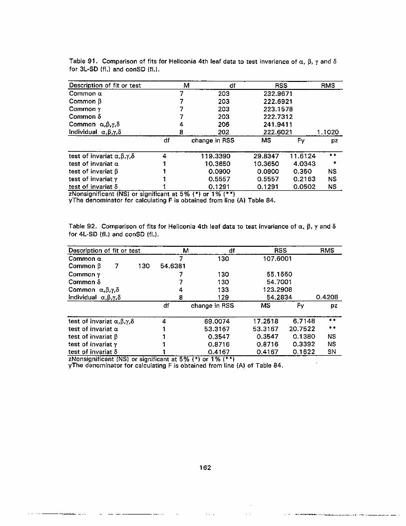
Table 91. Comparison of fits for Heliconia 4th leaf data to test invariance of a, p, y and <5for 3L-SD (fl.) and canSO (fl.).
Description of fit or test M df RSSCommon a 7 203 232.9671Common p 7 203 222.6921Common y 7 203 223.1578Common <5 7 203 222.7312Common a,p,y,<5 4 206 241.9411Individual a,~,y,<5 8 202 222.6021
df change in RSS MS Fy
RMS
1.1020pz
test of invariat a,~,y,<5 4 119.3390test of invariat a 1 10.3650test of invariat p 1 0.0900test of invariat y 1 0.5557test of invariat <5 1 0.1291
29.834710.36500.09000.55570.1291
11.61244.03430.3500.21630.0502
***
NSNSNS
zNonsignificant (NS) or significant at 5% (*) or 1% (U)yThe denominator for calculating F is obtained from line (A) Table 84.
Table 92. Comparison of fits for Heliconia 4th leaf data to test invariance of a, p, y and <5for 4L-SD (fl.) and canSO (fl.),
Description of fit or test M df RSS RMSCommon a 7 130 107.6001Common p 7 130 54.6381Common y 7 130 55.1550Common <5 7 130 54.7001Common a,p,y,<5 4 133 123.2908Individual a,p,y,<5 8 129 54.2834 0.4208
df change in RSS MS Fy pz
test of invariat a,p,y,<5 4 69.0074 17.2518 6.7148 **test of invariat a 1 53.3167 53.3167 20.7522 **test of invariat p 1 0.3547 0.3547 0.1380 NStest of invariat y 1 0.8716 0.8716 0.3392 NStest of invariat <5 . 1 0.4167 0.4167 0.1622 SNzNonsignificant (NS) or significant at 5% (*) or 1% (**)yThe denominator for calculating F is obtained from line (A) of Table 84.
162

Table 93. Comparison of fits for Heliconia 5th leaf data to test invariance of c. ~, Y and cSfor conLD (veg.) and 3L-SD (fl.).
Description of fit or test M df RSS RMSCommon lX 7 396 1442.4675Common ~ 7 396 1441.2927Common y 7 396 1439.7295Common s 7 396 1442.1992Common lX,~,y,cS 4 399 1452.6991Individual lX,~,y,cS 8 395 1436.1485 3.636
df change in RSS MS Fy pz
test of invariat lX,~,y,cS 4 16.5506 4.1376 1.1875 NStest of invariat a 1 6.3265 6.3265 1.18157 NStest of invariat ~ 1 5.1442 5.1442 1.4764 NStest of invariat y 1 3.5810 3.5810 1.0277 NStest of invariat cS 1 6.0437 6.0437 1.7345 NSzNonsignificant (NS) or significant at 5% (*) or 1% (* *)yThe denominator for calculating F is obtained from line (A) of Table 85.
Table 94. Comparison of fits for Heliconia 5th leaf data to test invariance of c, ~, Y and cSfor conLD (veg.) and 4L-SD (fl.).
Description of fit or test M df RSS RMSCommon lX 7 345 1577.3317Common ~ 7 345 1576.4195Common y 7 345 1572.3465Common cS 7 345 1574.8569Common lX,~,y,cS 4 348 1618.4625Individual lX,P,y,cS 8 344 1563.8342 4.5460
df change in RSS MS Fy pz
test of invariat lX,~,y,cS 4 54.6283 13.6570 3.9196 **
test of invariat lX 1 13.4975 13.4975 3.8738 *
test of invariat ~ 1 12.5853 12.5853 3.6120 NStest of invariat y 1 8.5123 8.5123 2.4430 NStest of invariat cS 1 11.0227 _ 11.0227 3.1635 NSzNonsignificant (NS) or significant at 5% (*) or 1% (* *)yThe denominator for calculating F is obtained from line (A) Table 85.
163

Table 95. Comparison of fits for Heliconia 5th leaf data to test invariance of a, p, y and 0for conLD (veg.) and canSO (fl.).
Description of fit or test M df RSSCommon a 7 386 1623.1695Common p 7 386 1580.2460Common y 7 386 1586.8344Common 0 7 386 1582.3859Common a,p,y,o 4 389 1695.0953Individual a,p,y,o 8 385 1572.6201
df change in RSS MS Fy
RMS
4.0847pz
test of invariat a,p,y,o 4 122.4752test of invariat a 1 50.5494test of invariat p 1 7.6259test of invariat y 1 14.2143test of invariat 0 1 9.7658
30.618850.5494
7.625914.2143
9.7658
8.787614.50772.18864.07952.8028
****NS
*NS
zNonsignificant (NS) or significant at 5% (*) or 1% (H)yThe denominator for calculating F is obtained from line (A) of Table 85
Table 96. Comparison of fits for Heliconia 5th leaf data to test invariance of a, p, y and 0for 3L-SD (fl.) and 4L-SD (fl.).
Description of fit or test M df RSS RMSCommon a 7 199 489.2784Common p 7 199 464.2808Common y 7 199 463.6188Common 0 7 199 463.3224Common a,p,y,o 4 202 513.9936Individual a,p,y,o 8 198 462.2359 2.3345
df change in RSS MS Fy pz
test of invariat a,p,y,o 4 51.7577 12.9394 3.7136 **test of invariat a 1 27.0425 27.0425 7.7612 **test of invariat p 1 2.0449 2.0449 0.5869 NStest of invariat y 1 1.3829 1.3829 0.3969 NStest of invariat 0 1 1.0865 1.0865 0.3118 NSzNonsignificant (NS) or significant at 5% (*) or 1% (H)yThe denominator for calculating F is obtained from line (A) Table 85.
164
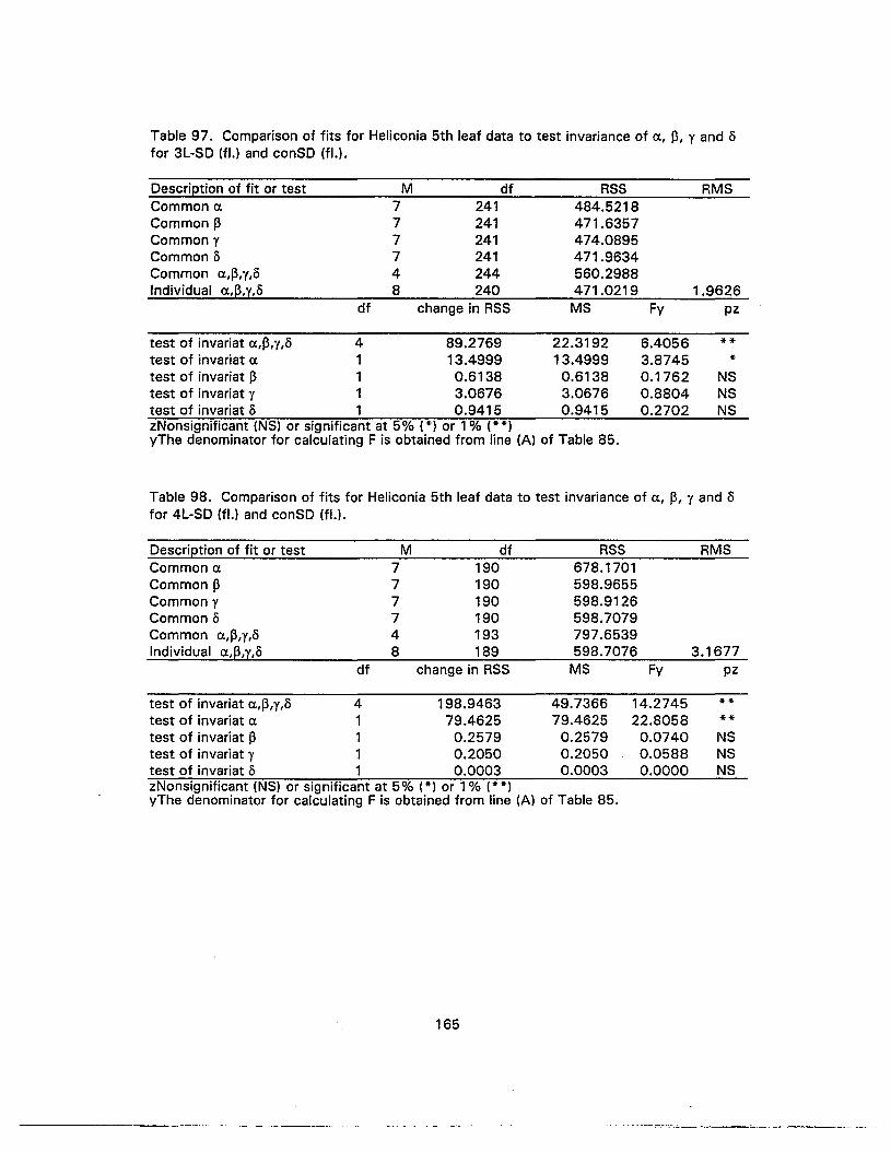
Table 97. Comparison of fits for Heliconia 5th leaf data to test invariance of a, p, y and I)
for 3L-SD (fl.) and conSD (fl.).
Description of fit or test M df RSS RMSCommon a 7 241 484.5218Common ~ 7 241 471.6357Common y 7 241 474.0895Common I) 7 241 471.9634Common a,~,y,1) 4 244 560.2988Individual a,~,y,1) 8 240 471.0219 1.9626
df change in RSS MS Fy pz
test of invariat a,~,y,1) 4 89.2769 22.3192 6.4056 **
test of invariat a 1 13.4999 13.4999 3.8745 *
test of invariat ~ 1 0.6138 0.6138 0.1762 NStest of invariat y 1 3.0676 3.0676 0.8804 NStest of invariat I) 1 0.9415 0.9415 0.2702 NSzNonsignificant (NS) or significant at 5% (*) or 1% (**)yThe denominator for calculating F is obtained from line (A) of Table 85.
Table 98. Comparison of fits for Heliconia 5th leaf data to test invariance of a, ~, y and I)
for 4L-SD (fl.) and conSD (fl.).
Description of fit or test M df RSSCommon a 7 190 678.1701Common ~ 7 190 598.9655Common y 7 190 598.9126Common I) 7 190 598.7079Common a,~,y,1) 4 193 797.6539Individual a,@,y,1) 8 189 598.7076
df change in RSS MS Fy
RMS
3.1677pz
test of invariat a,~,y,1) 4 198.9463test of invariat a 1 79.4625test of invariat ~ 1 0.2579test of invariat y 1 0.2050test of invariat I) 1 0.0003
49.736679.4625
0.25790.20500.0003
14.274522.8058
0.07400.05880.0000
****
NSNSNS
zNonsignificant (NS) or significant at 5% (*) or 1% (**)yThe denominator for calculating F is obtained from line (A) of Table 85.
165

Table 99. Comparison of fits for Heliconia 6th leaf data to test invariance of a, p, y and 0for conLD (veg.) and 3L-SD (fl.).
Description of fit or test M df RSS RMSCommon a 7 477 2093.6301Common p 7 477 2104.2471Common y 7 477 2107.6382Common 0 7 477 2105.8241Common a,p,y,o 4 480 2105.0575Individual a,@,y,o 8 476 2093.4584 4.3980
df change in RSS MS Fy pz
test of invariat a,p,y,o 4 71.5991 17.8997 4.7182 **
test of invariat a 1 0.1717 0.1717 0.0452 NStest of invariat p 1 10.7887 10.7887 2.8438 NStest of invariat y 1 14.1798 14.1798 3.7377 NStest of invariat 0 1 12.3657 12.3657 3.2595 NSzNonsignificant (NS) or significant at 5% (*) or 1% (**)yThe denominator for calculating F is obtained from line (A) of Table 86.
Table 100. Comparison of fits for Heliconia 6th leaf data to test invariance of a, 13, y and 0for conLD (veg.) and 4L-SD (fl.).
Description of fit or test M df RSSCommon a 7 392 1701.8034Common 13 7 392 1613.2738Common y 7 392 1611.2547Common 0 7 392 1612.4604Common a,!3,y,o 4 395 1761.4216Individual a,@,y,o 8 391 1604.2251
df change in RSS MS Fy
RMS
4.1029pz
test of invariat a,!3,y,o 4 157.1965test of invariat a 1 97.5783test of invariat 13 . 1 9.0487test of invariat y 1 7.0296test of invariat 0 1 8.2353
39.299197.5783
9.04877.02968.2353
10.359025.7211
2.38521.85292.1707
****
NSNSNS
zNonsignificant (NS) or significant at 5% (*) or 1% (**)yThe denominator for calculating F is obtained from line (A) of Table 86.
166

Table 101. Comparison of fits for Heliconia 6th leaf data to test invariance of a, ~, y and 0for conLD (veg.) and canSO (fl.).
Description of fit or test M df RSSCommon a 7 409 2169.9944Common ~ 7 409 1778.9187Common y 7 409 1783.5728Common 0 7 409 1778.5075Common a,~,y,o 4 412 2322.8729Individual a,~,y,o 8 408 1777.6274
df change in RSS MS Fy
RMS
4.3569pz
test of invariat a,~,y,o 4 545.2455test of invariat a 1 392.3670test of invariat ~ 1 1.2913test of invariat y 1 5.9454test of invariat 0 1 0.8801
136.3114392.3670
1.29135.94540.8801
35.9309103.4259
0.34041.56720.2320
****NSNSNS
zNonsignificant (NS) or significant at 5% (*) or 1% (**)yThe denominator for calculating F is obtained from line (A) of Table 86.
Table 102. Comparison of fits for Heliconia 6th leaf data to test invariance of a, ~, y and 0for 3L-SD (fl.) and 4L-SD (fl.).
Description of fit or test M df RSSCommon a 7 246 778.7539Common ~ 7 246 699.7499Common y 7 246 699.7898Common 0 7 246 699.6971Common a,~,y,o 4 249 804.4889Individual a,@,y,o 8 245 699.6858
df change in RSS MS Fy
RMS
2.8559pz
test of invariat a,~,y,o 4 104.8031test of invariat a 1 79.0681test of invariat ~ 1 0.0641 "test of invariat y 1 0.1040test of invariat 0 1 0.0113
26.200779.0681
0.06410.10400.0113
6.906420.84190.01690.02740.0029
****NSNSNS
zNonsignificant (NS) or significant at 5% (*) or 1% (**)yThe denominator for calculating F is obtained from line (A) Table 86."
167
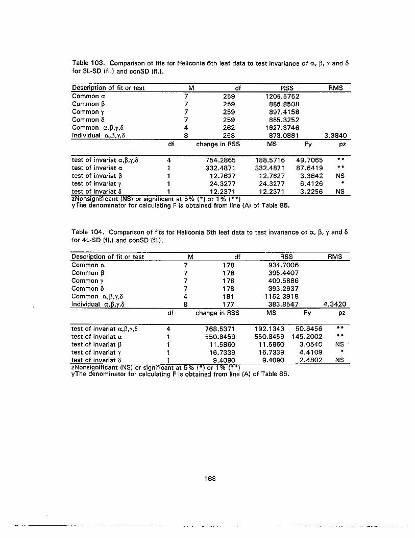
Table 103. Comparison of fits for Heliconia 6th leaf data to test invariance of a, ~, y and 0for 3L-SD (fl.) and canSO (fl.).
Description of fit or test M df RSSCommon a 7 259 1205.5752Common ~ 7 259 885.8508Common y 7 259 897.4158Common 0 7 259 885.3252Common a,~,y,o 4 262 1627.3746Individual a,p,y,o 8 258 873.0881
df change in RSS MS Fy
RMS
3.3840pz
test of invariat a,~,y,o 4 754.2865test of invariat a 1 332.4871test of invariat ~ 1 12.7627test of invariat y 1 24.3277test of invariat 0 1 12.2371
188.5716332.4871
12.762724.327712.2371
49.706587.6419
3.36426.41263.2256
**
**NS
*NS
zNonsignificant (NS) or significant at 5% (*) or 1% (**)yThe denominator for calculating F is obtained from line (A) of Table 86.
Table 104. Comparison of fits for Heliconia 6th leaf data to test invariance of a, ~, y and 0for 4L-SD (fl.) and canSO (fl.).
Description of fit or test M df RSSCommon a 7 178 934.7006Common ~ 7 178 395.4407Common y 7 178 400.5886Common 0 7 178 393.2637Common a,~,y,o 4 181 1152.3918Individual a,p,y,o 8 177 383.8547
df change in RSS MS Fy
RMS
4.3420pz
test of invariat a,~,y,o 4 768.5371test of invariat a 1 550.8459test of invariat ~ 1 11.5860test of invariat y 1 16.7339test of invariat 0 1 9.4090
192.1343550.8459
11.586016.7339
9.4090
50.6456145.2002
3.05404.41092.4802
****
NS*
NSzNonsignificant (NS) or significant at 5% (*) or 1% (**)yThe denominator for calculating F is obtained from line (A) of Table 86.
168
--------- ----- ---

Table 105. Nonlinear regression for least-squares estimates of parameters of Richardsfunction on relative leaf length (length at emergence = 0 and length at fully expanded =1) and relative time (date of leaf emergence = 0 and date of leaf fully expanded = 1) of 3rd leaf position.
Source DF Sum of Squares Mean Square
Regression 4 589.0705 147.2676Residual 917 3.8509 0.0042Total 921 592.9214
Correlation Matrix
Parameter Estimate Standard Error a @ y
a 0.9927 0.0040 1/3 2.0293 0.3397· -0.5143 1Y 9.2333 0.4675 -0.6152 0.9666 10 0.7891 0.1324 -0.4872 0.9925 0.9342
Table 106. Nonlinear regression for least-squares estimates of parameters of Richardsfunction on relative leaf length (length at emergence = 0 and length at fully expanded =1) and relative time (date of leaf emergence = 0 and date of leaf fully expanded = 1) of 4th leaf position.
Source DF Sum of Squares Mean Square
Regression 4 644.7933 161.1983Residual 963 4.7378 0.0049Total 967 649.5312
Correlation Matrix
Parameter Estimate Standard Error a @ y 0
a 0.9966 0.0042 1/3 0.0716 0.5999 -0.5004 1t 8.0966 0.3979 -0.6413 0.9356 10 0.2341 0.1103 -0.4853 0.9984 0.9176
169

Table 107. Nonlinear regression for least-squares estimates of parameters of Richardsfunction on relative leaf length (length at emergence = 0 and length at fully expanded =1) and relative time (date of leaf emergence = 0 and date of leaf fully expanded = 1) of 5th leaf position.
Source OF Sum of Squares Mean Square
Regression 4 612.4569 153.1142Residual 905 7.5202 0.0083Total 909 619.9772
Correlation Matrix
Parameter Estimate Standard Error (X ~ y
a. 0.9989 0.0057 113 -0.0542 0.8291 -0.4918 1y 8.2884 0.5487 -0.6346 0.9352 18 0.2308 0.1526 -0.4786 0.9987 0.9188 1
Table 108. RSS from fitting the 3rd, 4th and 5th leaf of Heliconia with common c, ~, y,and 8 of Richards function on relative leaf length (length at emergence = 0 and length atfully expanded = 1) and relative time (date of leaf emergence = 0 and date of leaf fullyexpanded = 1).
Treatment
3rd leaf4th leaf5th leaf(A) Total
M
444
16
df
917963905
2785
170
RSS
3.85094.73797.5202
16.1090
RMS
0.0058
~~=~==.---.,.._.._ ...._--- _ ..
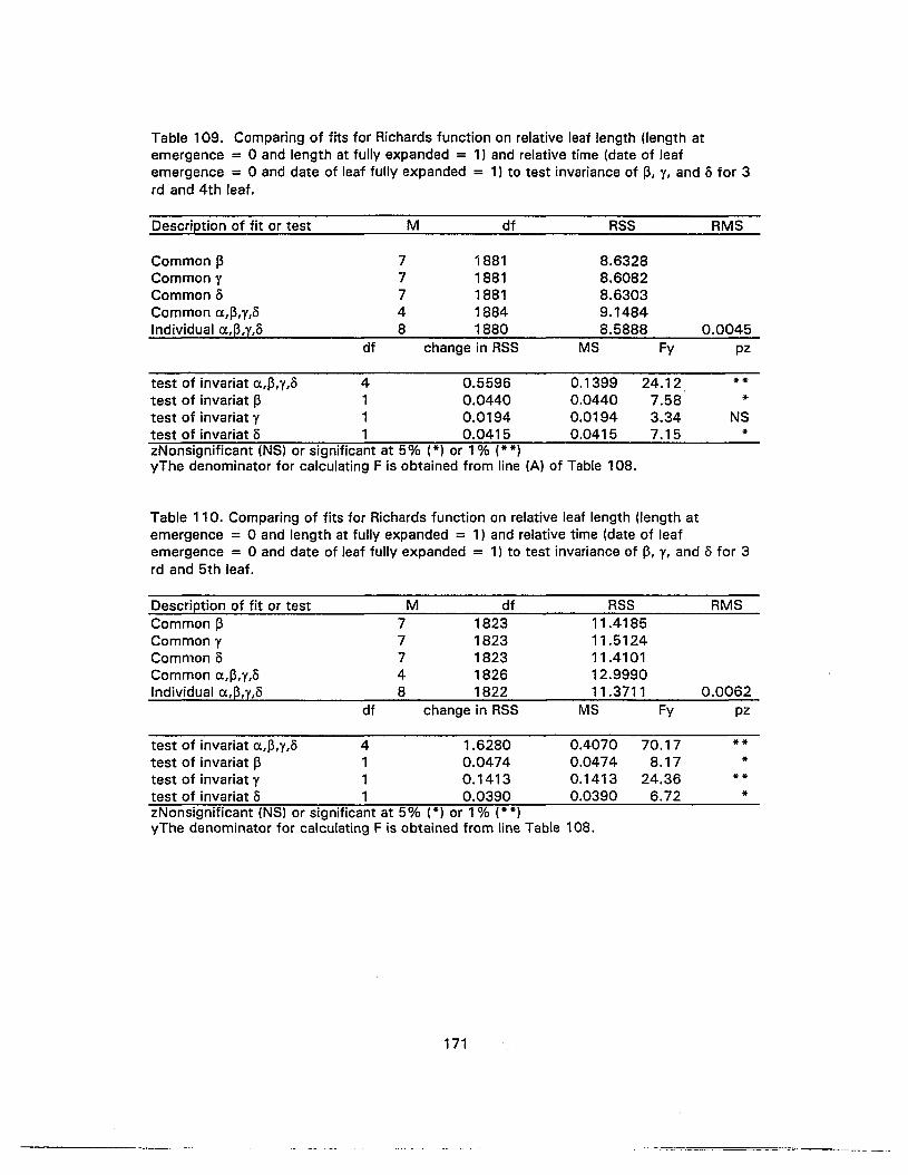
Table 109. Comparing of fits for Richards function on relative leaf length (length atemergence = 0 and length at fully expanded = 1) and relative time (date of leafemergence = 0 and date of leaf fully expanded = 1) to test invariance of ~, y, and 0 for 3rd and 4th leaf.
Description of fit or test M df RSS
Common ~ 7 1881 8.6328Common y 7 1881 8.6082Common 0 7 1881 8.6303Common cx,~,y,o 4 1884 9.1484Individual cx,~,y,o 8 1880 8.5888
df change in RSS MS Fy
RMS
0.0045pz
test of invariat cx,~,y,o 4 0.5596test of invariat ~ 1 0.0440test of invariat y 1 0.0194test of invariat 0 1 0.0415
0.13990.04400.01940.0415
24.127.583.347.15
***
NS*
zNonsignificant (NS) or significant at 5% (*) or 1% (**)yThe denominator for calculating F is obtained from line (A) of Table 108.
Table 110. Comparing of fits for Richards function on relative leaf length (length atemergence = 0 and length at fully expanded = 1) and relative time (date of leafemergence = 0 and date of leaf fully expanded = 1) to test invariance of ~, y, and 0 for 3rd and 5th leaf.
Description of fit or test M df RSSCommon ~ 7 1823 11.4185Common y 7 1823 11.5124Common 0 7 1823 11.4101Common cx,~,y,o 4 1826 12.9990Individual cx,~,y,o 8 1822 11.3711
df change in RSS MS Fy
RMS
0.0062pz
test of invariat cx,~,y,o 4 1.6280test of invariat ~ 1 0.0474test of invariat y 1 0.1413test of invariat 0 1 0.0390
0.40700.04740.14130.0390
70.178.17
24.366.72
***
***
zNonsignificant (NS) or significant at 5% (*) or 1% (**)yThe denominator for calculating F is obtained from line Table 108.
171
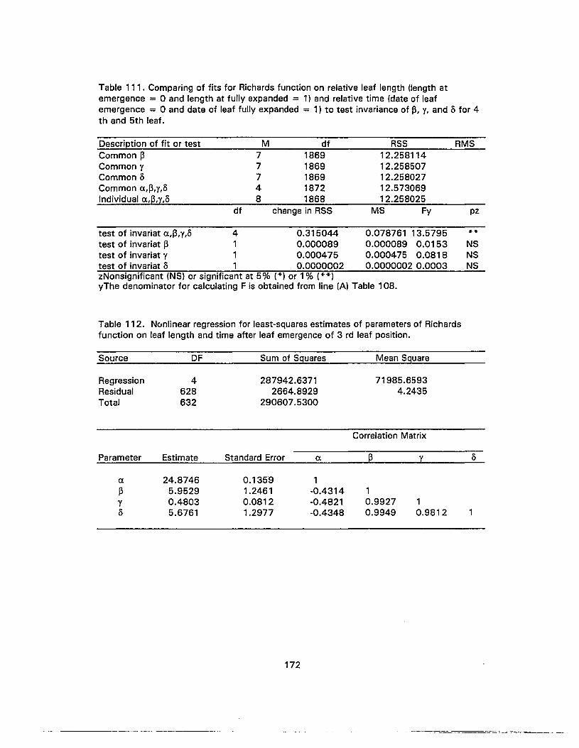
Table 111. Comparing of fits for Richards function on relative feaf length (length atemergence = 0 and length at fully expanded = 1) and relative time (date of leafemergence = 0 and date of leaf fully expanded = 1) to test invariance of ~, y, and 0 for 4th and 5th leaf.
Description of fit or testCommon ~
Common yCommon 0Common ex.,~,y,o
Individual ex.,~,y,o
M df7 18697 18697 18694 18728 1868
df change in RSS
RSS12.25811412.25850712.25802712.57306912.258025
MS Fy
RMS
pz
test of invariat ex.,~,y,o 4 0.315044test of invariat ~ 1 0.000089test of invariat y 1 0.000475test of invariat 0 1 0.0000002
0.078761 13.57950.000089 0.01530.000475 0.08180.0000002 0.0003
**
NSNSNS
zNonsignificant (NS) or significant at 5% (*) or 1% (**)yThe denominator for calculating F is obtained from line (A) Table 108.
Table 112. Nonlinear regression for feast-squares estimates of parameters of Richardsfunction on leaf length and time after leaf emergence of 3 rd leaf position.
Source DF Sum of Squares Mean Square
Regression 4 287942.6371 71985.6593Residual 628 2664.8929 4.2435Total 632 290607.5300
Correlation Matrix
Parameter Estimate Standard Error ex. ~ y
ex. 24.8746 0.1359 1~ 5.9529 1.2461 -0.4314 1Y 0.4803 0.0812 -0.4821 0.9927 10 5.6761 1.2977 -0.4348 0.9949 0.9812
172
~==.- ._.~----
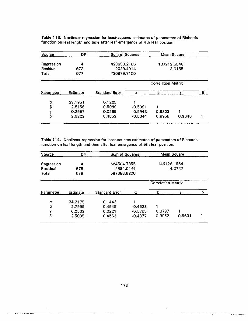
Table 113. Nonlinear regression for least-squares estimates of parameters of Richardsfunction on leaf length and time after leaf emergence of 4th leaf position.
Source OF Sum of Squares Mean Square
Regression 4 428850.2186 107212.5546Residual 673 2029.4914 3.0155Total 677 430879.7100
Correlation Matrix
Parameter Estimate Standard Error IX @ Y
IX 29.1951 0.1225 1f3 2.8156 0.5089 -0.5091 1y 0.2957 0.0269 -0.5943 0.9803 10 2.6222 0.4859 -0.5044 0.9955 0.9646 1
Table 114. Nonlinear regression for least-squares estimates of parameters of Richardsfunction on leaf length and time after leaf emergence of 5th leaf position.
Source OF Sum of Squares Mean Square
Regression 4 584504.7855 146126.1964Residual 675 2884.0444- 4.2727Total 679 587388.8300
Correlation Matrix
Parameter Estimate Standard Error IX @ Y
IX 34.2175 0.1442 1f3 2.7999 0.4946 -0.4928 1y 0.2502 0.0221 -0.5795 0.9797 10 2.5035 - 0.4562 -0.4877 0.9952 0.9631 1
173
-------- --------

Table 115. ANOVA for regressing LOGIT on LOGCON of ABA standards compare among 8plates. (PLATE).
Dependent Variable:SourcePLATELOGCONLOGCON*PLATEError
LOGITDF717134
r2 = 0.9701Sum of Squares0.1228228.46210.59077.3763
C.V. = -9.50F Value Pr > F0.32 0.94454149.30 0.00011.53 0.1613
Table 116. ANOVA for regressing LOGIT on LOGCON of ABA standards from 8 plates toobtain a standard curve.
Dependent Variable:SourceLOGCONError
Regression equations
LOGITDF
1148
r2 = 0.9332Sum of Squares220.053116.4988
C.V. = -13.52F Value Pr > F1973.94 0.0001
LOGIT = 1.7802 - 2.4227 LOGCON
Table 117. ANOVA for regressing LOGIT on LOGCON of ABA standards to obtain standardcurve for test of parallelism.
Dependent Variable:SourceLOGCONError
Regression equations
LOGITDF112
r2 = 0.9882Sum of Squares24.41400.2923
C.V. = -6.7821F Value Pr > F1002.05 0.0001
LOGIT = 1.9225 - 2.5739 LOGCON
Table 118. ANOVA for regressing LOGIT on LOGWT with different dilution of leaf wt. toobtain curve for test of parallelism.
Dependent Variable:SourceLOGWTError
Regression equations
LOGITDF113
r2 = 0.9775Sum of Squares18.01710.4137
C.V. = -20.52F Value Pr > F566.10 0.0001
LOGIT = -2.4192 - 2.5744 LOGCON
174
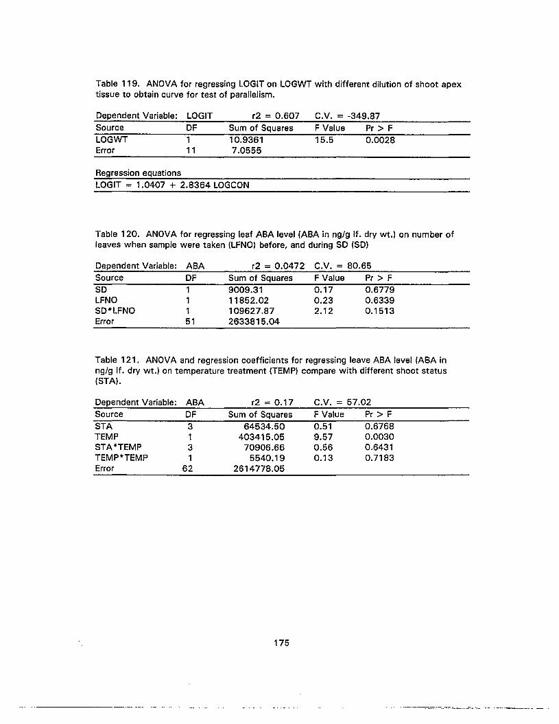
Table 119. ANOVA for regressing LOGIT on LOGWT with different dilution of shoot apextissue to obtain curve for test of parallelism.
Dependent Variable:SourceLOGWTError
Regression equations
LOGITDF111
r2 = 0.607Sum of Squares10.93617.0555
G.V. = -349.87F Value Pr > F15.5 0.0028
LOGIT = 1.0407 + 2.8364 LOGGON
Table 120. ANOVA for regressing leaf ABA level (ABA in ng/g If. dry wt.) on number ofleaves when sample weore taken (LFNO) before, and during SD (SD)
Dependent Variable:SourceSDLFNOSD*LFNOError
ABADF11151
r2 = 0.0472Sum of Squares9009.3111852.02109627.872633815.04
G.V. = 80.65F Value Pr > F0.17 0.67790.23 0.63392.12 0.1513
Table 121. ANOVA and regression coefficients for regressing leave ABA level (ABA inng/g If. dry wt.) on temperature treatment (TEMP) compare with different shoot status(STA).
Dependent Variable:SourceSTATEMPSTA*TEMPTEMP*TEMPError
ABADF3131
62
r2 = 0.17Sum of Squares
64534.50403415.05
70906.665540.19
2614778.05
175
G.V. = 57.02F Value Pr > F0.51 0.67689.57 0.00300.56 0.64310.13 0.7183
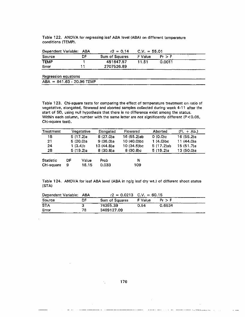
Table 122. ANOVA for regressing leaf ABA level (ABAl on different temperatureconditions (TEMPl.
Dependent Variable:SourceTEMPError
Regression equations
ABAOF
111
r2 = 0.14Sum of Squares
451647.572707526.89
C.V. = 55.01F Value Pr > F11.51 0.0011
ABA = 841 .63 - 20.96 TEMP
Table 123. Chi-square tests for comparing the effect of temperature treatment on ratio ofvegetative, elongated, flowered and aborted samples collected during week 4-11 after thestart of SO, using null hypothesis that there is no difference exist among the status.Within each column, number with the same letter are not significantly different (P<0.05,Chi-square test).
Treatment Vegetative Elongated Flowered Aborted (Ff. + Ab.)18 5 (17.2Ia 8 (27.0la 16 (55.2lab o to.oie 16 (55.2la21 5 (20.0la 9 (36.0la 10 (40.0lbc 1 (4.0lbc 11 (44.0Ia24 1 (3.4lb 13 (44.8la 10 (34.5lbc 5 (17.2lab 15 (51.7la28 5 (19.2Ia 8 (30.8la 8 (30.8Ic 5 (19.2Ia 13 (50.0la
Statistic OF Value Prob NChi-square 9 18.15 0.033 109
Table 124. ANOVA for leaf ABA level (ABA in nglg leaf dry wt.l of different shoot status(STAl
Dependent Variable:SourceSTAError
ABAOF378
r2 = 0.0213Sum of Squares
74355.393489127.09
176
C.V. = 60.15F Value Pr > F0.54 0.6534
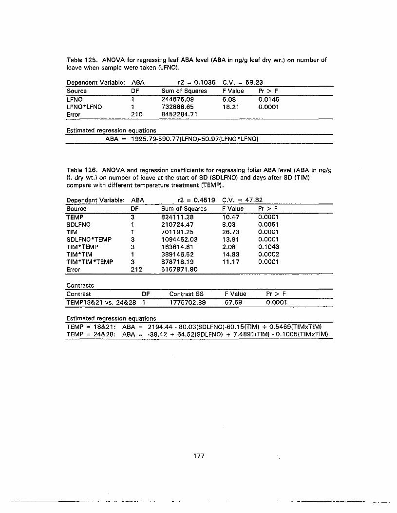
Table 125. ANOVA for regressing leaf ABA level (ABA in ng/g leaf dry wt.) on number ofleave when sample were taken (LFNO).
Dependent Variable:SourceLFNOLFNO*LFNOError
ABADF11210
r2 = 0.1036Sum of Squares244675.09732888.658452284.71
C.V. = 59.23F Value Pr > F6.08 0.014518.21 0.0001
Estimated regression equationsABA = 1995.79-590.77(LFNO)-50.97(LFNO*LFNO)
Table 126. ANOVA and regression coefficients for regressing foliar ABA level (ABA in ng/gIf. dry wt.) on number of leave at the start of SD (SDLFNO) and days after SD (TIM)compare with different temperature treatment (TEMP).
Dependent Variable:SourceTEMPSDLFNOTIMSDLFNO*TEMPTIM*TEMPTIM*TIMTIM *TIM *TEMPError
Contrasts
ABADF3113313212
r2 = 0.4519Sum of Squares824111.28210724.47701191.251094452.03163614.81389146.52878718.195167871.90
C.V. = 47.82F Value Pr > F10.47 0.00018.03 0.005126.73 0.000113.91 0.00012.08 0.104314.83 0.000211.17 0.0001
Contrast DFTEMP18&21 vs. 24&28 1
Estimated regression equations
Contrast SS1775702.89
F Value67.69
Pr > F0.0001
TEMP = 18&21: ABA = 2194.44 - 80.03(SDLFNO)-60.15(TIM) + 0.5469(TIMxTIM)TEMP = 24&28: ABA = -38.42 + 64.52(SDLFNO) + 7.4891(TIM) - 0.1005(TIMxTIM)
177

Table 127. Chi-square tests for comparing the effect of temperature treatment on ratio ofvegetative, flowered and aborted at the termination of experiment (20 weeks after thestart of SD). Using null hypothesis that no difference exist among the status. Within eachcolumn, numbers with the same letter are not significantly different (P>0.05, Chi-squaretest).
Treatment Vegetative Flowered Aborted Flowered + Aborted18 4 (30.7)a 8 (61.5)a 1 (7.7)a 9 (69.2)a21 4 (40.0)a 5 (50.0)ab 1 (10.0)a 6 (60.0)a24 4 (44.4)a 3 (33.3)ab 2 (22.2)a 5 (55.5)a28 5 (45.4)a 3 (27.3)bc 3 (27.3)a 6 (54.6)a
Statistic DF Value Prob NChi-square 6 4.163 0.655 43
Table 128. ANOVA Effect of shading on leaf ABA level (ABA in ng/g If. dry wt},
Dependent Variable:SourceSTAError
ABADF240
C.V. = 55.8Sum of Squares251543.2487525409.8331
F Value9.58
Pr > F0.0004
Table 129. Chi-square tests for comparing the effect of shade treatment on ratio ofvegetative, elongated, flowered and aborted from week 8-11 after started of SD. Usingnull hypothesis that no difference exist among the status. Within each column, numberswith the same letter are not significantly different (P>0.05, Chi-square test).
Treatment Vegetative Flowered Aborted Flowered + Aborted
20%sun 3 (16.7)a 14 (77.8)a 1 (5.6)a 15 (83.3)a40%sun 3 (17.6)a 13 (76.5)a 1 (5.9)a 14 (82.3)a100%sun 5 (20.0)a 19 (76.0)a 1 (4.0)a 2080.0)a
Statistic DF Value Prob NChi-square 4 0.162 0.997 60
Table 130. ANOVA for leaf ABA level (ABA in ng/g If. dry wt.) of different shoot status(STA)
Dependent Variable:SourceSTAError
ABADF232
r2 = 0.0649Sum of Squares59864.56862175.37
178
C.V. = 78.52F Value Pr > F1.11 0.3416

Table 131. ANOVA for regressing leave ABA level (ABA in ng/g If. dry wt.) on number ofleave when sample were taken (LFNO).
Dependent Variable:SourceLFNOLFNO*LFNOError
ABADF1152
r2 = 0.2072Sum of Squares148949.1166546.46824597.54
C.V. = 55.85F Value Pr > F9.39 0.00344.20 0.0456
Estimated regression equationsABA = 1256.5899-330.6298(LFNO) + 25.3855(LFNO*LFNO)
Table 132. Chi-square tests for comparing the effect of shade treatment on ratio ofvegetative, flowered and aborted at the termination of experiment (18 weeks after startedof SD). Using null hypothesis that no difference exist among the status. Within eachcolumn, numbers with the same letter are not significantly different (P>0.05, Chi-squaretest).
Treatment Vegetative Flowered Aborted Flowered + Aborted20% 1 (5.3)a 16 (84.2)a 2 (10.5)a 18 (94.7)a40% 2 (6.5)a 24 (77.4)a 5 (16.1)a 29 (93.5)a100% 1 (5.3)a 15 (78.9)a 3 (15.8)a 18 (94.7)a
Statistic DF Value Prob NChi-square 4 4.163 0.397 69
Table 133. ANOVA Effect of shades (Trt.) on number of weeks from the start of SD toanthesis (WKFL) of H. stricta
Dependent Variable:SourceTrt.Error
WKFLDF239
C.V. = 12.30Sum of Squares F Value4.7654 1.1779.3535
Pr> F0.3207
Table 134. ANOVA Effect of shade (Trt.) on number of subtending leaves (SUBLF) of H.stricta
Dependent Variable:SourceTrt.Error
SUBLFDF252
C.V. = 15.59Sum of Squares F Value3.3800 1.7450.3654
179
Pr> F0.1847

Table 135. ANOVA Effect of shade (Trt.l on number of cincinnal bracts (BRNO) of H.stricta
Dependent Variable:SourceTrt.Error
BRNODF246
C.V. = 20.94Sum of Squares F Value0.1591 0.379.8000
Pr > F0.6903
Table 136. ANOVA Effect of shade (Trt.) on pseudostem height (HT) of H. strictaDependent Variable: HT C.V. = 7.29Source DF Sum of Squares F ValueTrt. 2 797.4421 28.98Error 52 715.3517
Pr > F
0.0001
Table 137. ANOVA Effect of shade (Trt.) on inflorescence length (FLLGTHl of H. stricta
Dependent Variable: HTSource DFTrt. 2Error 47
C.V. = 5.38Sum of Squares F Value178.6619 30.80136.3380
Pr> F0.0001
Table 138. ANOVA for regressing number of subtending leaf at time of anthesis (SLFNO)on number of leaf at start of SD (LFNO).
Dependent Variable:SourceLFNOError
SLFNODF143
r2 = 0.68Sum of Squares21.150410.0495
C.V. = 7.46F Value Pr > F90.50 0.0001
Estimated regression equationsSLFNO = 3.67 +O.7535(LFNO)
Table 139. ANOVA for regressing time from SD to anthesis (WKSDFL) on number of leafat start of SD (LFNO).
Dependent Variable:SourceLFNOError
SLFNODF140
r2 = 0.03Sum of Squares2.631381.4877
180
C.V. = 12.31F Value Pr > F1.29 0.2625

APPENDIX BFIGURES
50 oJ •
Figure 1. Daily maximum, minimum and average temperatures in °C at the inside of Magoon greenhouse facility of the University ofHawaii during 1988-1989.
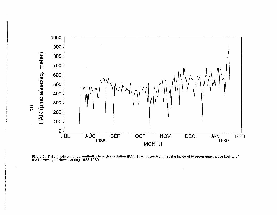
JAN FEB1989
DECOCT NOV
MONTH
AUG SEP1988
1000 I I
900
800
7'00
600
500
400
300
200
100
0, IJUL I ] I I I I I
-.L-a>......a>E.coooa>~a>oE::J.
"'-"
c::<o,
-'OJN
I
II',II!III
Figure 2. Daily maximum photosynthetically active radiation (PAR) in pmol/sec./sq.m. at the inside of Magoon greenhouse facility ofthe University of Hawaii during 1988-1989.

1,600 r'--------------------------.
1,400 .-
,......... 1,200 .-E0"en 1 000 .-0'Q)en
:::::: 800oE::::L
......... 600·c::«n, 400.-.....
coto)
200 .-
o L ! di",.... ,- ! ! ! ! ! ! ! ! ! r-···i?·~ I
6:00 7:00 8:00 9:00 10:00 11:00 12:00 1:00 2:00 3:00 4:00 5:00 6:00 7:00 8:00AM PM
TIME OF DAYFULL SUN 40 % SUN 20 % SUN
Figure 3. Hourly average photosynthetically active radiation (PAR) in pmollsec./sq.m. in fullsun, 40% sun and 20% sun at the Magoongreenhouse facility of the University of Hawaii 1991.

AVG35
30 ~ , 1-. jf 'Y ,,', ' 'V, 'Y '} v I/C-······,·," ,...._ _": _, \ ~ \ I , Ii \ - ... , •••••.•;, !.I I ..... .... \ ... ! ": i\ ...... .....' "',
E ~,V '~"""""""'.:.\ t~,"<.;·~·i t···..',,/ \ ..\ .,.. rv···.. .......... '...:.. '.\ l V·······................· \w0::::JI- 25~Wa.
~ lV+:y? v,'~ V~ V\jV <:~ .I- '<.J I '". :
co . ~~\..j:I.20
MIN " ~full sun 40% sun 20% sun
15 t I I I I I I I I I I I I I I I I I I I I I I I I I I I I I I I I I I I I I I I I I I I ~ :1~ ; 1'1 I·;·;·;··,~···IAug. 1 Aug. 15 Sept. 1 Sept. 15 Oct. 1 Oct. 15 Oct. 25
MONTH (1991)
Figure 4. Daily maximum, minimum and average temperature in °C in ful Isun, 40% sun and 20% sun at the Magoon greenhousefacility of the University of Hawaii 1991.
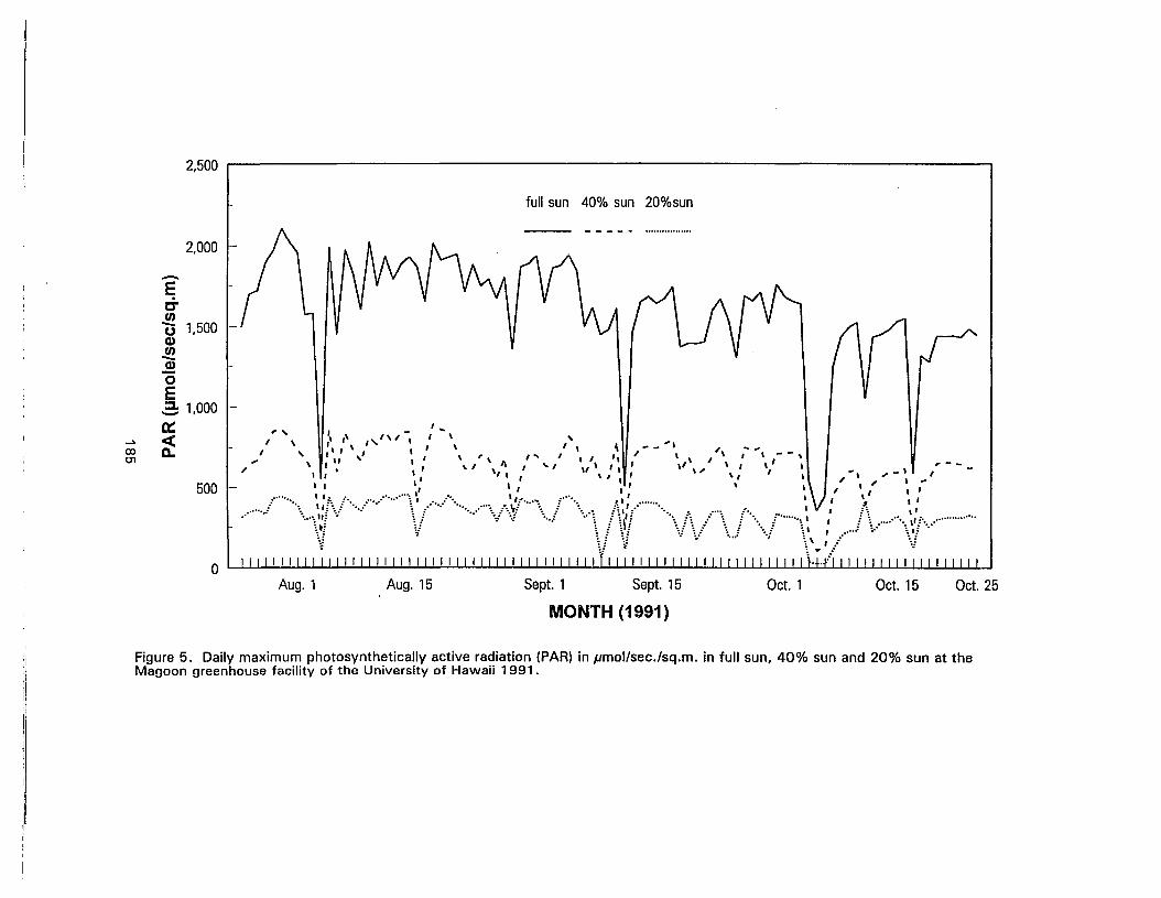
2,500
full sun 40% sun 20%sun
Oct. 25
,.--
Oct. 15Oct. 1Sept. 15Sept. 1Aug. 15Aug. 1
,
o
t ~ "~ __ "I '1 t~'-, __ ,' '" - , , , , " "" .'. -, -,,. " i""" '" r » , • " '. , v " , ' , 'v' \" 1 ,.-" .. ' , " "'. " " '" '. , , ,
r "", , , "'.. : " • , '. • ~ • :
500 1- F··\.:'~~····/·······t···J···········\f':j·\./····-VW· · - · ···VV\t··· r··~,.>.J: \1 - .
2,000
1,000 .-
1,500 .-
-Er:T.!!0Q)
.!!
.!!!0E:::1.-0::.... <C
ex>U1
a.
MONTH (1991)
Figure 5. Daily maximum photosynthetically active radiation (PAR) in pmollsec./sq.m. in full sun, 40% sun and 20% sun at theMagoon greenhouse facility of the University of Hawaii 1991.
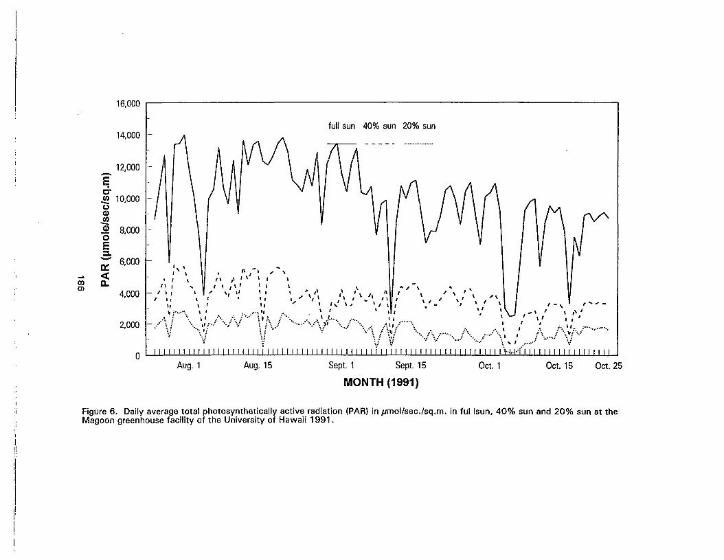
Oct. 25
, ..... ,-
Oct. 15Oct. 1Sept. 15Sept. 1
• : \ • \ 1\ •• II .- , ' ..\ I"
., '.I - \ I 'I ,,' \ I \\. _, .v I"\ I
Aug. 15Aug. 1
full sun 40% sun 20% sun
l\ -. " \ II .. " \' \ .. ~.. "'" , '" . . -.»:" ",' , , , • "" .... .. .. \J ,"" , ,
.." , , ", , , ' .. , . .. , , • '.". r···..····...' " . . '.. ...." , ", ,, '... '" , !. !"" .,::·~··-····:':;_/···!\~······v\.!·····_ ....··~<?····/··\·vVr·\··..j\F·-../·....J/··~ , : ..•. f "'., V
16,000
14,000 .-
12,000-E;g 10000 .-- 'uQ)en- 8,000 .-Q)
(5E:::L- 6,0000:::
..... octen D-en
4,000
2,000
0
MONTH (1991)
Figure 6. Daily average total photosynthetically active radiation (PAR) in pmol/sec./sq.m. in fullsun, 40% sun and 20% sun at theMagoon greenhouse facility of the University of Hawaii 1991.

APPENDIX C
PROGRAMS
Program 1. A SAS program 'GOMPERTZ.SAS· for estimating parameters of the Gompertzmodel from leaf length (LENGTH) and time after leaf emergence [T). (A = ex, B = f3, ANDK = y)
* --------------------------------- .._--------------------------* ;
PROGRAM 'GOMPERTZ.SAS·
INPUT FILE: LEAFLGDIRECTORY USED: SAVE
VARIABLE----------LENGTHT
TYPE----------NUMERICNUMERIC
DESCRIPTION====================LENGTH OF LEAF MEASURED IN CM.TIME AFTER LEAF EMERGENCE
PARAMETER: STARTING VALUES OF A, B, AND K WERE PLACED IN PARAMETERSSTATEMENT (PARMS)
*------------------------------------------------------------- * ;
PROC NUN DATA=SAVE.LEAFLG METHOD = GAUSS;PARMS A = 29.0
B = 9.3K = 0.3;
U = -(K*T);Q = EXP(U);Z = EXP(-B*Q);MODEL LENGTH = A *Z;DER.A=Z;DER.B=-A*Z*Q;DER.K= A *B*Z*Q*T;TITLE 'GOMPERTZ MODEL';
RUN;
187
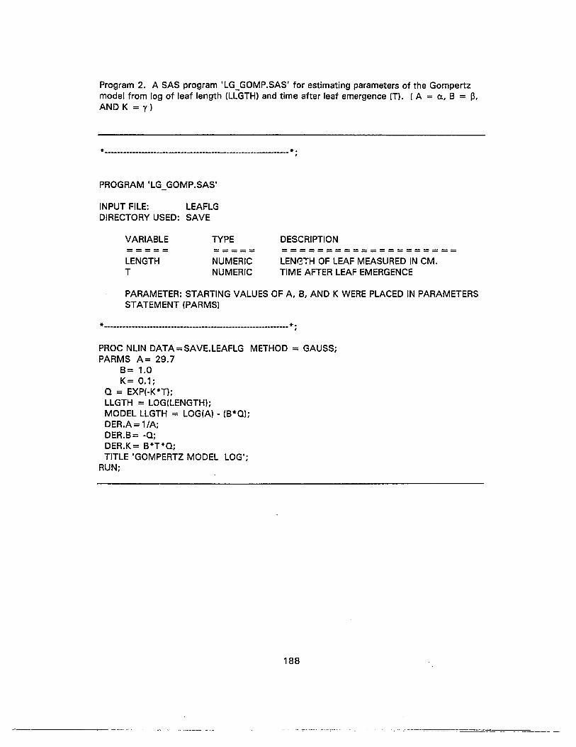
Program 2. A SAS program 'LG_GOMP.SAS' for estimating parameters of the Gompertzmodel from log of leaf length (LLGTH) and time after leaf emergence (T). (A = c, B = p,AND K = y)
*------------------------------------------------------------- * .,
PROGRAM 'LG GOMP.SAS'
INPUT FILE: LEAFLGDIRECTORY USED: SAVE
VARIABLE=====LENGTHT
TYPE=====NUMERICNUMERIC
DESCRIPTION----------------------------------------LENG"'fH OF LEAF MEASURED IN CM.TIME AFTER LEAF EMERGENCE
PARAMETER: STARTING VALUES OF A, B, AND K WERE PLACED IN PARAMETERSSTATEMENT (PARMS)
*--------------------------..--------_.._----------_..__....-------* ;
PROC NUN DATA=SAVE.LEAFLG METHOD = GAUSS;PARMS A= 29.7
B= 1.0K= 0.1;
Q = EXP(-K*T);LLGTH = LOG(LENGTH);MODEL LLGTH = LOG(A) - (B*Q);DER.A=1/A;DER.B= -Q;DER.K= B*T*Q;TITLE 'GOMPERTZ MODEL LOG';
RUN;
188

Program 3. A SAS program 'LOGISTIC.SAS' for estimating parameters of the logisticmodel from leaf length (LENGTH) and time after leaf emergence (T). (A = a, B = 13, ANDK = y)
*-------------------------_..._--------------------------------- * ;
PROGRAM 'LOGISTIC.SAS'
INPUT FILE: LEAFLGDIRECTORY USED: SAVE
VARIABLE=====LENGTHT
TYPE=====NUMERICNUMERIC
DESCRIPTION====================LENGTH OF LEAF MEASURED IN CM.TIME AFTER LEAF EMERGENCE
PARAMETER: STARTING VALUES OF A, B, AND K WERE PLACED IN PARAMETERSSTATEMENT (PARMS)
*------------------...--------------------------------...---------* ;
PROC NUN DATA=SAVE.LEAFLG METHOD = GAUSS;PARMS A=29.3
B=30K=O.2;
Q = -(K*T);U = EXP{Q);Z = 1 +(B*U);ZSQ = Z**{-2);MODEL LENGTH = A/Z;DER.A= 1/Z;DER.B=-A*U*ZSQ;DER.K= A*B*U*T*ZSQ;TITLE 'LOGISTIC MODEL';
RUN;
189
------ --- ---- ------- ------------------ -- -- -- - -- -------.---

Program 4. A SAS program 'LG_LOGIS.SAS' for estimating parameters of the logisticmodel from log of leaf length (LLGTH) and time after leaf emergence (T). (A = a, B = ~,
AND K = y)
*---------------------.----------------._--------------------- *.,
PROGRAM 'LG LOGIS.SAS'
INPUT FILE: LEAFLGDIRECTORY USED: SAVE
VARIABLE=====LENGTHT
TYPE- ---------NUMERICNUMERIC
DESCRIPTION====================LENGTH OF LEAF MEASURED IN CM.TIME AFTER LEAF EMERGENCE
PARAMETER: STARTING VALUES OF A, B, AND K WERE PLACED IN PARAMETERSSTATEMENT (PARMS)
*-----------------------..------------------------------------- *;
PROC NUN DATA =SAVE.LEAFLG METHOD = GAUSS;PARMS A= 29.6
B= 1.7K= 0.2;
o = EXP(-K*T);Z = 1 + (B*O);M = LOG(Z);LLGTH = LOG(LENGTH);
. MODEL LLGTH = LOG(A) - M;DER.A=1/A;DER.B= -O/Z;DER.K= (T*B*O)/Z;TITLE 'LOGISTIC MODEL LOG';
RUN;
190
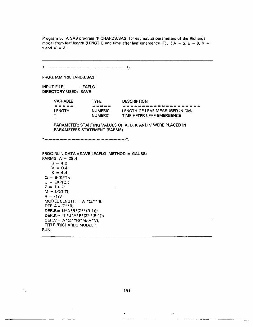
Program 5. A SAS program 'RICHARDS.SAS' for estimating parameters of the Richardsmodel from leaf length (LENGTH) and time after leaf emergence (T). (A = a, B = ~, K =y and V = 5)
*-------------------------------------------------------------*.,
PROGRAM 'RICHARDS.SAS'
INPUT FILE: LEAFLGDIRECTORY USED: SAVE
VARIABLE----------LENGTHT
TYPE=====NUMERICNUMERIC
DESCRIPTION====================LENGTH OF LEAF MEASURED IN CM.TIME AFTER LEAF EMERGENCE
PARAMETER: STARTING VALUES OF A, B, K AND V WERE PLACED INPARAMETERS STATEMENT (PARMS)
*-------------------------------------------------------------* .,
PROC NUN DATA=SAVE.LEAFLG METHOD = GAUSS;PARMS A = 29.4
B = 4.2V = 0.4K = 4.4
Q = B-(K*T);U = EXP(Q);Z = 1 +U;M = LOG(Z);R = -1N;MODEL LENGTH = A *(Z**R);DER.A= Z**R;DER.B= U*A*R*(Z**(R-1));DER.K= -T*U*A*R*(Z**(R-1));DER.V = A *(Z* *R) *M/(V*V);TITLE 'RICHARDS MODEL';
RUN;
191
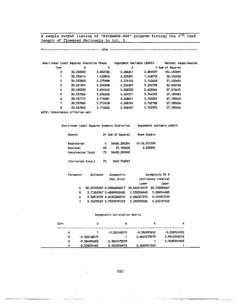
A sample output listing of "RICHARDS.SAS" program fitting the 4t h leaflength of flowered Heliconia in trt. 3.
*---------------... -.-.. ---------.-.- LF=4 ------.---.--.---- ••••• - •• -.------------------ •••• -----
Non-Linear Least Squares Iterative PhaseIter A B
o 32.000000 3.8027261 30.592414 1.4328162 30.553803 2.2759983 30.531991 3.2949984 30.539230 3.6045405 30.537866 3.6962086 30.537171 3.7106817 30.537065 3.7124288 30.537053 3.712626
NOTE: Convergence criterion met.
Dependent Variable LENGTH Method: Gauss-NewtonK V Sum of Squares
0.286241 3.890597 154.4508970.235301 1.448773 58.1349620.274124 2.142648 51.4206940.334997 3.202758 32.9067280.360332 3.633066 27.2764550.367071 3.744593 27.1859630.368041 3.760359 27.1856090.368154 3.762188 27.1856060.368167 3.762395 27.185606
Non-Linear Least Squares Summary Statistics
Source DF Sum of Squares
Regression 4 56465.204394Residual 69 27.185606Uncorrected Total 73 56492.390000
(Corrected Total) 72 2467.748767
Dependent Variable LENGTH
Mean Square
14116.3010990.393994
30.53705287 0.098668069173.712625670.688899224800.36816729 0.043028625143.76239467 0.73676191013
Parameter
A
B
K
V
Estimate AsymptoticStd. Error
Asymptotic 95 ~ .Confidence IntervalLower Upper
30.340215079 30.7338906672.338306648 5.0869446850.282327370 0.4540072202.292592026 5.232197323
ASymptotic Correlation Matrix
Corr
A
B
K
V
A
1
-0.326168579-0.384890652-0.328324902
B
-0.3261685791
0.98491735790.9943596912
192
K
-0.3848906520.9849173579
1
0.9689301965
v
-0.3283249020.99435969120.9689301965
1
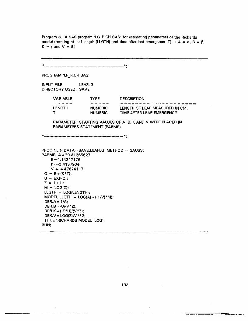
Program 6. A SAS program 'LG_RICH.SAS' for estimating parameters of the Richardsmodel from log of leaf length (LLGTH) and time after leaf emergence (T). (A = c, B = 13,K = y and V = 0)
*----------------------------------------_..-------------.._---- * ;
PROGRAM 'LF RICH.SAS'
INPUT FILE: LEAFLGDIRECTORY USED: SAVE
VARIABLE----------LENGTHT
TYPE=====NUMERICNUMERIC
DESCRIPTION====================LENGTH OF LEAF MEASURED IN CM.TIME AFTER LEAF EMERGENCE
PARAMETER: STARTING VALUES OF A, B, K AND V WERE PLACED INPARAMETERS STATEMENT (PARMS)
*------------------------------------------------------------- * ;
PROC NUN DATA=SAVE.LEAFLG METHOD = GAUSS;PARMS A=29.41265627
B=4.14247176K=-0.4137904V = 4.47624117;
Q = B+(K*T);U = EXP(Q);Z = 1 +U;M = LOG(Z);LLGTH = LOG(LENGTH);MODEL LLGTH = LOG(A) - «1N)*M);DER.A= 1/A;.DER.B=-U/(V*Z);DER.K= (-T*U)/(V*Z);DER.V= LOG(Z)N**2;TITLE 'RICHARDS MODEL LOG';
RUN;
193
...__._-====-:--:-c:---,=

Program 7. A SAS program 'MMF.SAS' for estimating parameters of the Morgan-MercerFlodin model from leaf length (LENGTH) and time after leaf emergence (T). ( A = a, B = ~,
K = y and V = 0)
*------....----..--------------------------------------.........---..--* ;
PROGRAM 'MMF.SAS'
INPUT FILE: LEAFLGDIRECTORY USED: SAVE
VARIABLE- ---------LENGTHT
TYPE=====NUMERICNUMERIC
DESCRIPTION====================LENGTH OF LEAF MEASURED IN CM.TIME AFTER LEAF EMERGENCE
PARAMETER: STARTING VALUES OF A, B, K AND V WERE PLACED INPARAMETERS STATEMENT (PARMS)
*-----------.._----------------------------...------------------- * .,
PROC NUN DATA=SAVE.LEAFLG METHOD = GAUSS;PARMS A = 29
B = 10K = 400V = 7;
Q = T**V;LT = LOG (T);MODEL LENGTH = ((B*K)+(A*Q))/(K+Q);DER.A = Q/(K+Q);DER.B = K/(K+Q);DER.K = Q*(B-A)/((K+Q)**2);DER.V = K*LT*Q*(A-B)/((K+Q)**2);OUTPUT OUT = SAVE.MMFT2F P=P R=R;TITLE 'MMF MODEL';RUN;
194
.~====-~~~~.-~-----.

Program 8. A SAS program 'LG_MMF.SAS' for estimating parameters of the MorganMercer-Flodin model from log of leaf length (LLGTH) and time after leaf emergence (T). ( A= <x, B = 13, K = y and V = 8 )
* ------------------..-----..---------------------------------.._- * ;
PROGRAM 'LG MMF.SAS'
INPUT FILE: LEAFLGDIRECTORY USED: SAVE
VARIABLE=====LENGTHT
TYPE----------NUMERICNUMERIC
DESCRIPTION====================LENGTH OF LEAF MEASURED IN CM.TIME AFTER LEAF EMERGENCE
PARAMETER: STARTING VALUES OF A, B, K AND V WERE PLACED INPARAMETERS STATEMENT (PARMS)
* --------------......_-------------------------------------------- * .,
PROC NUN DATA=SAVE.LEAFLG METHOD = GAUSS;PARMS A = 29.6
B = 13.5K = 421.9V = 3.0;
Q = T**V;LT = LOG (T);LLGTH = LOG(LENGTH);MODEL LLGTH = LOG«B*K)+(A*Q)) - LOG(K+Q);DER.A = Q/«B*K) + (A *Q));DER.B = K/«B*K) + (A *Q));DER.K = (B/«B*K) + (A *Q)))-(1/(K +Q));DER.V = «A*Q*LT)/«B*K) + (A *Q)))-«Q*LT)/(K +Q));OUTPUT OUT = SAVE.MMFT2FLG P=P R=R;TITLE 'MMF MODEL LOG';RUN;
195
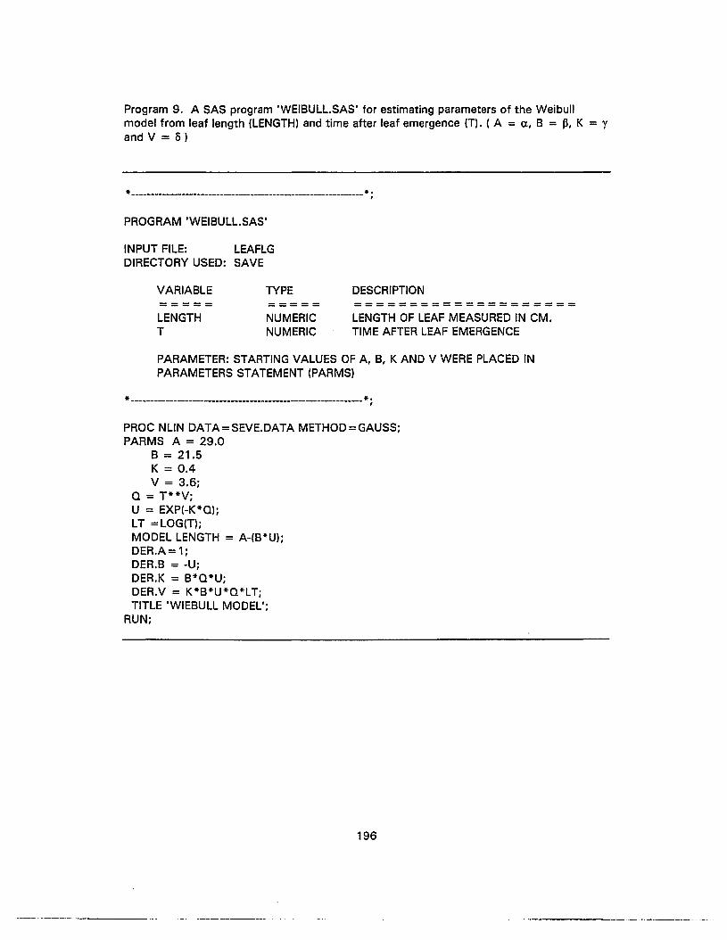
Program 9. A SAS program 'WEIBULL.SAS' for estimating parameters of the Weibullmodel from leaf length (LENGTH) and time after leaf emergence (T). ( A = a, B = p, K = Yand V = /»)
*--------------.----------------..----------------------------- *;
PROGRAM 'WEIBULL.SAS'
INPUT FILE: LEAFLGDIRECTORY USED: SAVE
VARIABLE----------LENGTHT
TYPE=====NUMERICNUMERIC
DESCRIPTION====================LENGTH OF LEAF MEASURED IN CM.TIME AFTER LEAF EMERGENCE
PARAMETER: STARTING VALUES OF A, B, K AND V WERE PLACED INPARAMETERS STATEMENT (PARMS)
*--------------------------------------------------------._--- * .,
PROC NUN DATA = SEVE.DATA METHOD=GAUSS;PARMS A = 29.0
B = 21.5K = 0.4V = 3.6;
Q = T**V;U = EXP(-K*Q);LT =LOG(T);MODEL LENGTH = A-(B*U);DER.A=1;DER.B = -U;DER.K = B*Q*U;DER.V = K*B*U*Q*LT;TITLE 'WIEBULL MODEL';
RUN;
196

Program 10. A SAS program 'LG_WEIB.SAS' for estimating parameters of the Weibullmodel from log of leaf length (LLGTH) and time after leaf emergence (T). ( A = a, B = ~,
K = y and V = IS)
*--------..-------------------------------------...--------------*;
PROGRAM 'LG WEIB.SAS·
INPUT FILE: LEAFLGDIRECTORY USED: SAVE
VARIABLE--- -------LENGTHT
TYPE----------NUMERICNUMERIC
DESCRIPTION====================LENGTH OF LEAF MEASURED IN CM.TIME AFTER LEAF EMERGENCE
PARAMETER: STARTING VALUES OF A, B, K AND V WERE PLACED INPARAMETERS STATEMENT (PARMS)
*------------------------------------------------------------- *;
PROC NUN DATA=SAVE.LEAFLG METHOD=GAUSS;PARMS A = 29.4
B = 16.5K = 0.01V = 1.9;
Q = T**V;U = EXP(-K*Q);LT =LOG(T);LLGTH = LOG(LENGTH);MODEL LLGTH = LOG(A-(B*U));DER.A= 1/(A-(B*U));DER.B = -U/(A-(B*U));DER.K = B*Q*U/(A-(B*U));DER.V = B*K*U*Q*LT/(A-(B*U));TITLE 'WIEBULL MODEL LOG';
RUN;
197

Program 11. A SAS program 'RIC_COMA.SAS' for fitting a common a to each of twogroups of data for a Richards model.
PROGRAM 'RIC_COMA.SAS'
INPUT FILE: LF4T1T3DIRECTORY USED: SAVE
VARIABLE----------LENGTHTTRTA
TYPE=====NUMERICNUMERICDISCRETE
DESCRIPTION====================LENGTH OF LEAF MEASURED IN CM.TIME AFTER LEAF EMERGENCETREATMENTS - 1: LD
2: LD+3IfSD+LD3: LD+4IfSD+LD4: SD
B3 = 3.17K3 = 0.34V3 = 3.27;
T1 = 1; T2 = 0; END;T1 = 0; T2 = 1; END;
PARAMETERS: - (A, B, K. AND V) COMMON PARAMETERS FinED TO 2GROUP OF DATA SET.
- (A1-A4, B1-B4, K1-K4, V1-V4) PARAMETERS FITTED TOINDIVIDUAL GROUP OF DATA SET (TREATMENT 1 TO 4).
*-------------------------..-----------------------------------*;
PROC NUN DATA=SAVE.LF4T1T3;PARMS A = 28.4
B1 = 2.24K1 = 0.29V1 = 2.37
IF TRTA = 1 THEN DO;IF TRTA = 3 THEN DO;B = (B1 *T1) + (B3*T2);K = (K1*T1)+(K3*T2);V = (V1*T1)+(V3*T2);o = B-(K*T);_U = EXP(O);Z = 1 +U;M = LOG(Z);R = -1N;MODEL LENGTH = A *(Z**R);DER.A=Z**R;DER.B1 = T1 *U*A*R*(Z**(R-1));DER.B3= T2*U*A*R*(Z**(R-1 I);DER.K1 = -T*T1 *U*A*R*(Z**(R-1));DER.K3= -T*T2*U*A*R*(Z**(R-1));DER.V1 = T1 *A *(Z**R)*M/(V*V);DER.V3= T2*A *(Z**R)*M/(V*V);
RUN;
198
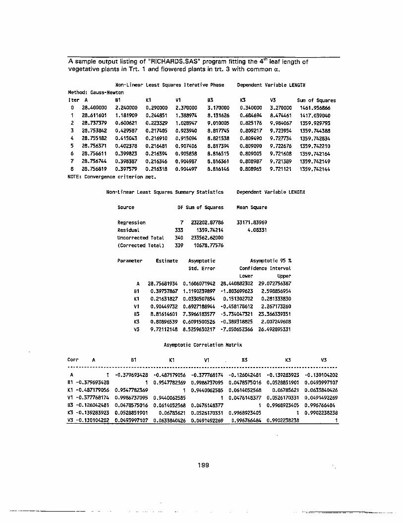
A sample output listing of "RICHARDS.SAS" program fitting the 4 th leaf length ofvegetative plants in Trt, 1 and flowered plants in trt. 3 with common a.
Non-Linear Least Squares Iterative Phase Dependent Variable LENGTHMethod: Gauss-NewtonIter A B1 1(1 V1 B3 K3 V3 Sun of Squares0 28.400000 2.240000 0.290000 2.370000 3.170000 0.340000 3.270000 1461.9568661 28.611601 1.181909 0.244851 1.388974 8.131626 0.684694 8.474461 1417.0390402 28.737379 0.600621 0.223329 1.028947 9.010005 0.825176 9.984067 1359.9297933 28.753842 0.429587 0.217405 0.923940 8.817745 0.809217 9.723954 1359.7443884 28.755182 0.415043 0.216910 0.915094 8.821538 0.809490 9.72m4 1359.7428345 28.756371 0.402378 0.216481 0.907406 8.817394 0.809090 9.722676 1359.7422106 28.756611 0.399823 0.216394 0.905858 8.816515 0.809005 9.721608 1359.7421647 28.756744 0.398387 0.216346 0.904987 8.816361 0.808987 9.721389 1359.7421498 28.756819 0.397579 0.216318 0.904497 8.816146 0.808965 9.721121 1359.742144
NOTE: Convergence criterion met.
Non-Linear Least Squares Summary Statistics Dependent Variable LENGTH
Source DF Sun of Squares Mean Square
Regression 7 232202.87786 33171.83969Residual 333 1359.74214 4.08331Uncorrected Total 3/.0 233562.62000(Corrected Total) 339 10678.77576
Parameter Estimate Asynptotic Asymptotic 95 xStd. Error Confidence Interval
Lower UpperA 28.75681934 0.1606071942 28.440882302 29.072756387
B1 0.39757867 1.1190239897 -1.803699623 2.5988569541(1 0.21631827 0.0330507854 0.151302702 0.281333830V1 0.90449732 0.6927188944 -0.458178612 2.267173260B3 8.81614601 7.3966183577 -5.734047321 23.366339351K3 0.80896539 0.6091500526 -0.389318825 2.007249608V3 9.72112148 8.5259630217 -7.050652366 26.492895331
Asymptotic Correlation Matrix
Corr A B1 1(1 V1 B3 K3 V3
A 1 -0.379693428 -0.487179056 -0.3m68174 -0.126042481 -0.139283923 -0.130104202B1 -0.379693428 1 0.9547782369 0.9986737095 0.0478575016 0.0528851901 0.04939971071(1 -0.487179056 0.9547782369 1 0.9440062585 0.0614052568 0.06785621 0.0633840426V1 -0.3m68174 0.9986737095 0.9440062585 1 0.0476148377 0.0526170331 0.0491492269B3 -0.126042481 0.0478575016 0.0614052568 0.0476148377 1 0.9968923405 0.996766484K3 -0.139283923 0.0528851901 0.06785621 0.0526170331 0.9968923405 , 0.9902238238V3 -0.130104202 0.0493997107 0.0633840426 0.0491492269 0.996766484 0.9902238238 1
199
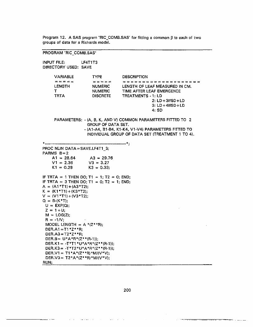
Program 12. A SAS program 'RIC_COMB.SAS' for fitting a common p to each of twogroups of data for a Richards model.
PROGRAM 'RIC COMB.SAS·
INPUT FILE: LF4T1 T3DIRECTORY USED: SAVE
VARIABLE=====LENGTHTTRTA
TYPE=====NUMERICNUMERICDISCRETE
DESCRIPTION====================LENGTH OF LEAF MEASURED IN CM.TIME AFTER LEAF EMERGENCETREATMENTS - 1: LD
2: LD+3IfSD+LD3: LD+4IfSD+LD4:SD
A3 = 29.76V3 = 3.27K3 = 0.33;
PARAMETERS: - lA, B, K, AND V) COMMON PARAMETERS FITTED TO 2GROUP OF DATA SET.
- IA1-A4, B1-B4, K1-K4, V1-V4) PARAMETERS FinED TOINDIVIDUAL GROUP OF DATA SET (TREATMENT 1 TO 4).
* ------------------------------------------------------------- * ;PROC NUN DATA=SAVE.LF4T1_3;PARMS B=2
A1 = 28.64V1 = 2.36K1 = 0.29
IF TRTA = 1 THEN DO; T1 = 1; T2 = 0; END;IF TRTA = 3 THEN DO; T1 = 0; T2 = 1; END;A = IA1*T1)+(A3*T2);K = (K1 *T1) + (K3*T2);V = (V1*T1)+IV3*T2);Q = B-(K*T);
U = EXPIQ);Z = 1 +U;M = LOGIZ);R = -1N;MODEL LENGTH = A *(Z**R);DER.A1 =T1 *Z**R;DER.A3=T2*Z**R;DER.B= U*A*R*(Z**IR-1));DER.K1 = -T*T1 *U*A*R*(Z**(R-1));DER.K3 = -T*T2*U*A *R*(Z* *(R-1I);DER.V1 = T1 *A*IZ**R)*M/(V*V);DER.V3= T2*A*(Z**R)*M/(V*V);
RUN;
200

Program 13. A SAS program 'RIC_COMK.SAS' for fitting a common y to each of twogroups of data for a Richards model.
PROGRAM 'RIC COMK.SAS'
INPUT FILE: LF4T1T3DIRECTORY USED: SAVE
VARIA8LE=====LENGTHTTRTA
TYPE----------NUMERICNUMERICDISCRETE
DESCRIPTION====================LENGTH OF LEAF MEASURED IN CM.TIME AFTER LEAF EMERGENCETREATMENTS -1: LD
2: LD + 31fSD + LD3: LD +4IfSD+LD4:SD
A3 = 29.7683 = 3.17V3 = 3.27;
PARAMETERS: - (A, 8, K, AND V) COMMON PARAMETERS FITTED TO 2GROUP OF DATA SET.
- (A1-A4, 81-84, K1-K4, V1-V4) PARAMETERS FITTED TOINDIVIDUAL GROUP OF DATA SET (TREATMENT 1 TO 4).
* ------------------------------------------------------------- * .,
PROC NUN DATA=SAVE.LF4T1_3;PARMS K = 0.473
A1 = 28.6481 = 2.24V1 = 2.37
IF TRTA = 1 THEN DO; T1 = 1; T2 = 0; END;IF TRTA = 3 THEN DO; T1 = 0; T2 = 1; END;B = (Bl*T1)+(83*T2);A = (A1*T1) + (A3*T2);V = (V1 *T1) + (V3*T2);Q = 8-(K*T);
U = EXP(Q);Z = 1 +U;M = LOG(Z);R = -1N;MODEL LENGTH = A *(Z**R);DER.A1 = T1 *Z* *R;DER.A3= T2*Z**R;DER.81 = T1 *U*A*R*(Z**(R-1));DER.83= T2*U*A*R*(Z**(R-1));DER.K= -T*U*A*R*(Z**(R-1));DER.V1 = T1 *A*(Z**R)*M/(V*V);DER.V3= T2*A*(Z**R)*M/(V*V);
RUN;
201
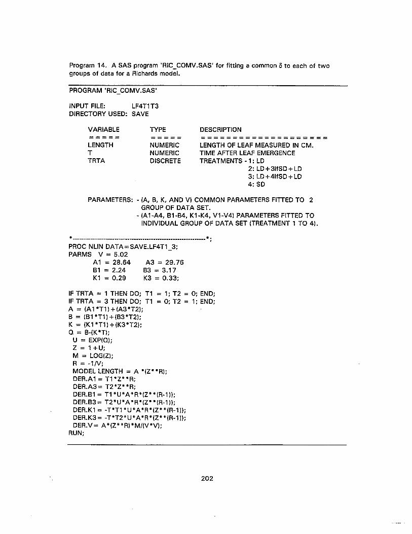
Program 14. A SAS program 'RIC_COMV.SAS' for fitting a common 0 to each of twogroups of data for a Richards model.
PROGRAM 'RIC COMV.SAS'
INPUT FILE: LF4T1T3DIRECTORY USED: SAVE
VARIA8LE----------LENGTHTTRTA
TYPE=====NUMERICNUMERICDISCRETE
DESCRIPTION====================LENGTH OF LEAF MEASURED IN CM.TIME AFTER LEAF EMERGENCETREATMENTS -1: LD
2: LD+ 31fSD + LD3: LD+4IfSD+LD4:SD
A3 = 29.7683 = 3.17K3 = 0.33;
PARAMETERS: - (A, 8, K, AND V) COMMON PARAMETERS FITTED TO 2GROUP OF DATA SET.
- (A1-A4, 81-84, K1-K4, V1-V4) PARAMETERS FITTED TOINDIVIDUAL GROUP OF DATA SET (TREATMENT 1 TO 4).
*------------------------------------------------------------- * ;PROC NUN DATA=SAVE.LF4T1_3;PARMS V = 5.02
A1 = 28.6481 = 2.24K1 = 0.29
IF TRTA = 1 THEN DO; T1 = 1; T2 = 0; END;IF TRTA = 3 THEN DO; T1 = 0; T2 = 1; END;A = (A1*T1) + (A3*T2);8 = (81 *T1) + (83*T2);K = (K1*T1 ) + (K3*T2);Q = 8-(K*T);
U = EXP(Q);Z = 1 +U;M = LOG(Z);R = -IN;MODEL LENGTH = A *(Z**R);DER.A1 = T1 *Z**R;DER.A3= T2*Z**R;DER.81 = T1 *U*A*R*(Z**(R-1));DER.83 = T2*U*A *R*(Z* *(R-1 ));DER.K1 = -T*T1 *U*A*R*(Z**(R-1»;DER.K3 = -T*T2*U*A *R*(Z**(R-1»;DER.V = A *(Z* *R) *M/(V*V);
RUN;
202
REFERENCES
Addicott, F. T. 1983. Abscisic Acid. Praeger. N.Y.
Addicott, F. T., and H. R. Carns. 1983. History and introduction, p. 1-22. In: F. T. Addicott(ed.). Abscisic acid. Praeger Pub., N.Y..
Allen, D. M. and F. B. Cady. 1982. Analyzing experimental data by regression. LifetimeLearning Publication. C.A. p. 232-259.
Amer, F. A. and W. T. William. 1957. Leaf growth in Pe/argonium zona/e. Annals ofBotany. 21 :339-342.
Bates, D. M. and D. G. Watts. 1988. Nonlinear regression analysis and its applications.John Wiley and Sons, Inc. N.Y. p. 66-133.
Belefant H., and F. Fong. 1989. Abscisic acid ELISA: organic acid interference. PlantPhysiol. 91 :1467-1470.
Bentley, B., C. B. Morgan, D. G. Morgan and F. A. Saad. 1975. Plant growth substancesand effect of photoperiod on flower bud development in Phaseo/us vulgaris. Nature256:121-122.
Bernier, G. 1988. The control of floral evocation and morphogenesis. Ann. Rev. PlantPhysio!. Plant Mol. Bioi. 39:175-219.
Bernier, G. 1994. Editor's note: vegetative plants may differ in their 'vegetativeness'. PHL.18:58-61.
Bernier, G., J. M. Kinet, and R. M. Sachs. 1981. The Physiology of Flowering: Volume IITransition to Reproductive Growth. CRe Press, Inc. Florida. p.135-160. .
Berry, F. and W. J. Kress. 1991. Heliconia: An identification guide. Smithsonian lnst,Press, Wash. p. 11-29.
Boonekamp, P. M., H. Pomp, E. Davelaar, and C. R. Vonk. 1990. Selection of Imonoclonalantibodies to the plant growth regulators indole-3-acetic acid and abscisic acid afterimmunization with conjugates coupled through the carboxylic group, p. 37-46. In:A. Schots (ed.). Monoclonal antibodies in agriculture. Pudoc, Wageningen.
Borowiak, D. S. 1989. Model discrimination for nonlinear regression models. MarcelDekker, Inc. N.Y. p. 15-136.
Broschat, T. K. 1987. Tropical cut flower research at the University of Florida's Ft.Lauderdale researcbh and education center. Bul. Heliconia Soc. Int. 4:6
Broschat, T. K. and H. Donselman. 1982. Heliconia: a promising new cut flower crop.Hcrtsclence. 18:2.
Broschat, T. K. and H. Donselman. 1983. Production and postharvest culture of Heliconiapsittacorum flowers in south Florida. Proc. Fla. State Hort. Soc. 96:272-273.
203
Broschat, T. K. and H. Donselman. 1988. University of Florida Research update #1. Bul.Heliconia Soc. Int. 3:4. (Abstr.),
Broschat, T. K. and S. E., Svenson. 1994. DCPTA enhances growth and flowering ofHeliconias. HortScience 29:891-892.
Capell, B., and K. Dorffling. 1989. Low temperature-induced changes of abscisic acidcontents in barley and cucumber leaves in relation to their water status. J. PlantPhysiol. 135:571-575.
Causton, D. R. and J. C. Venus. 1981. The biometry of plant growth. Edward Arnold Ltd.London. p. 86-172.
Charles-Edwards, D. A., D. Ooley, G. M. Rimmington. 1986. Modeling Plant Growth andDevelopment. Academic Press. N.Y. p, 21-33.
Cosgrove, D. J. 1986. Photomodulation of growth, p. 341-389. In: R. E. Kendrick and G.H. M. Kronenberg (eds.). Photomorphogenesis in Plants. Martinus NijhoffPublishers. Boston.
Cowan, A. K. and P. D. Rose. 1991. Abscisic acid metabolism in salt-stressed cells ofDunaliella salina. Plant Physiol. 97:798-803.
Creelman, R. A. 1989. Abscisic acid physiology and biosynthesis in higher plants. Physiol.Plant. 75:131-136.
Criley, R. A. 1991. Appendix III: Commercial Production of Heliconias. p 321-330. In: F.Berry and W. J. Kress (eds.). Heliconia: An identification guide. Smithsonian Inst.Press, Wash.
Criley, R. A. and O. Kawabata. 1986. Evidence of a short-day flowering response inHeliconia stricta 'Dwarf Jamaican'. HortScience 21 :506-507.
Criley, R. A. and S. Lekawatana. 1994. Year round production with high yields may be apossibility for Heliconia chartacea. XXIV 1h Internatioanl Horticultural CongressAbstract No. 0-71-2.
Criley, R. A. and T. K. Broschat. 1992. Heliconia: Botany and Horticulture of a New FloralCrop. Horticultural Reviews. 14: 1-55.
Crozier, A., G. Sandberg, A. M. Monteiro, and B. Sundberg. 1986. The use ofimmunological techniques in plant hormone analysis, p. 13-21. In: M. Bopp (ed.).Plant growth substances. 1985. Springer-Verlag, Berlin.
Dahlgren, R. M. T., and H. T. Clifford. 1982. The monocotyledons. A comparative study.Academic Press. N. Y.
Dahlgren, R. M. T., H. T. Clifford, and P. F. Yeo. 1985. The families of themonocotyledons: structure, evaluation, and taxonomy. Springer-Verlag, N.Y.
Daie, J. and R. Wyse. 1982. Adaptation of the enzyme-linked immunosorbent assay(ELISA) to the quantitative analysis of abscisic acid. Anal. Biochem. 119:365-371.
204

Dale, J. E. and F. L. Milthorpe. 1983. General features of the production and growth ofleaves, p, 151-178. In: J. E. Dale and F. L. Milthorpe (eds.). The Growth andFunctioning of Leaves. Cambridge Univ. Press. London.
Davis, L. A. and F. T. Addicott. 1972. Abscisic acid: correlations with abscission and withdevelopment in the cotton fruit. Plant Physiol. 49:644-648.
Freund, R. J. and R. C. Littell. 1986. SAS system for Regression. SAS Institute Inc. NC. p.133-140.
Freund, R. J., R. C. Littell, and P. C. Spector. 1986. SAS system for linear models. SASInstitute Inc. NC. p, 141-157.
Gomez, K. A. and A. A. Gomez. 1976. Statistical procedures for agricultural research withemphasis on rice. The Inter. Rice Resh. Ins. Los Banos.
Goodwin, T. W. and E. I. Mercer. 1983. Introduction to Plant Biochemistry. PergamonPress. N.Y. p. 606·614.
Guinn, G., J. R. Dunlap, and D. L. Brummett. 1990. Influence of water deficits on theabscisic acid and indole-3-acetic acid contents of cotton flower buds and flowers.Plant Physiol. 93:1117-1120.
Halevy, A. H. 1984. Light and autonomous induction, p. 63-73. In: D. Vince-Prue, B.Thomas and K. E. Cockshull (eds.). Light and the Flowering Process. AcademicPress. London.
Halevy, A. H. 1987. Assimilate allocation and flower development, p. 363-378. In: J. G.Atherton (ed.). Manipulating of Flowering. Butterworths. London.
Harrris, M. J. and W. H. Outlaw. 1990. Histochemical technique: a low-volumee, enzymeamplified immunoassay with sum-fmol sensitivity. Application to measurement ofabscisic acid in stomatal guard cells. Physiol. Plant. 78:495-500.
Harris, M. J., W. H. Outlaw, Jr., R. Mertens, and E. W. Weiler. 1988. Water-stress-inducedchanges in the abscisic acid content of guard cells and other cells of Vicia faba L.leaves as determined by enzyme-amplified immunoassay. Proc. Natl. Acad. Sci.85:2584-2588.
Hartung, W. and W. J. Davies. 1991. Drought-induced changes in physiology and ABA, p.63-79. In: E. J. Davies and H. G. Jones (eds.). Abscisic Acid: physiology andbiochemistry. BIOS Scientific Publishers Limited., Oxford.
Hirai, N. 1986. Abscisic acid, p. 201-248. In: N. Takahashi (ed.). Chemistry of planthormones. CRC Press Inc., Florida.
Hubick, K. T., and D. M. Reid. 1988. Effect of drought, on transport and metabolism ofabscisic acid in aeroponically grown Helienthus annuus. Physiologia Plantarum.74:317-325.
Hunt, R. 1982. Plant growth curves. University Park Press. Baltimore. p. 121-146.
205

Idetek Inc. 1985. Phytodetek™-ABA. Product Bulletin #06-007-A 9/85. (1057 SneathLane, San Bruno, CAl
Johansen, D. 1940. Plant Microtechnique. McGraw Hill. N.Y.
Kamuro, Y., K. Yotsumoto, S.-K. Lee, and S Marumo. 1990. Marked inhibition of floral budinitiation by optically active abscisic acid in Pharbitis nil. Agric. Bioi. Chem.54:3363-3365.
Karlsson, M. G. and R. D. Heins. 1994. A model of Chrysanthemum Stem Elongation. J.Amer.Soc. Hort. Sci. 119:403-407.
Kemeny, D. M. 1991. A Practical Guide to ELISA. Pergamon Press Inc. N.Y. p. 45-55.
Kemeny, D. M. and S. Chantler. 1988. An Introduction to ELISA, p.1-29. In: D. M. Kemenyand S. J. Challacombe (eds.). ELISA and Other Solid Phase Immunoassays. JohnWiley & Sons Ltd.
Kinet, J. M. and R. M. Sachs. 1984. Light and flower development, p. 211-225. In: D.Vince-Prue, B. Thomas and K.E. Cockshull (eds.). Light and the Flowering Process.Academic Press., London..
Kinet, J. M., R. M. Sachs, and G. Bernier. 1985. The Physiology of Flowering: Volume IIIthe Development of Flowers. CRC Press, Inc. Florida. p.89-106.
Konsens, I, M., Ofir and J. Kigel. 1991. The effect of temperature on the production andabscission of flowers and pods in snap bean (Phaseolus vulgaris L,). Annal ofBotany 67:391-399.
Kwon, E. 1992. Flowering of He/iconia angusta. Ph.D. Dissertation, University of Hawaii,Honolulu, HI.
Lekawatana, S. 1986. Growth and flowering of Heliconia stricta Huber. and H. angustaVeil. Master of Science Thesis, University of Hawaii, Honolulu, HI.
Levitt, J. 1980a. Responses of Plants to Environmental Stresses: Volume I chilling,Freezing, and High Temperature Stresses. Academic Press, New York. p.23-55.
Levitt, J. 1980b. Responses of Plants to Environmental Stresses: Volume II Water,Radiation, Salt, and Other Stresses. Academic Press, New York. p.283-293.
Lockhart, J. 1959. Studies on the mechanism of stem growth inhibition by visibleradiation. Plant Physiol. 34:457-460.
Mertens, R., B. Deus-Neumann, and E. W. Weiler. 1983. Monoclonal antibodies for thedetection and quantitation of the endogenous plant growth regulator, abscisic acid.FEBS Letters 160:269-272.
Mertens, R., J. Eberle, A. Arnscheidt, A. Ledebur, and E. W. Weiler. 1985. Monoclonalantibodies to plant growth regulators. II. Indole-3-acetic acid. Planta 166:389-393
206

Milborrow, B. V. 1984. Inhibitors, p. 76-110. In: M. B. Wilkins (ed.). Advanced PlantPhysiology. The Pitman Press, Bath.
Nakai, T. 1941. Notulae ad Plantas Asiae Orientalis (XVI). Japan. J. Bot. 17:189-203.
Neales, T. F., and A. L. McLeod. 1991. Do leaves contribute to the abscisic acid present inthe xylem sap of 'droughted' sunflower plants? Plant, Cell and Environment.14:979-986.
Neill, S. J., and A. Horgan. 1987. Abscisic acid and related compounds, p, 111-167. In: L.Rivier and A. Crozier (eds.). Principles and practice of plant hormone analysisvolume 1. Academic Press Inc., London.
Neill, S. J., R. Horgan, and J. K. Heald. 1983. Determination of levels of abscisic acidglucose ester in plants. Planta 157:371-375.
Norman M. S., S. M. Poling and v. P. Maier. 1988. As indirect enzyme-linkedimmunosorbent assay for (+ )-absciscic acid in Citrus, Ricinus, and Xanthiumleaves. J. Agric. Food Chern. 36:225-231.
Pan, A.-C. 1990. The role of abscisic acid in chilling resistance, p, 391-399. In: R. P. Pharisand S. B. Rood (eds.). Plant growth substances 1988. Springer-Verlag, Berlin.
Parry, A. D., and R. Horgan. 1991 a. Carotenoid metabolism and the biosynthesis ofabscisic acid. Phytochem. 30:815·821.
Parry, A. D., and R. Horgan. 1991 b. Physio-chemical methods in ABA research, p. 5-22.In: E. J. Davies and H. G. Jones (eds.). Abscisic Acid: physiology and biochemistry.BIOS Scientific Publishers Limited., Oxford.
Pengelly, W. L. 1986. Validation of immunoassays, p. 35-43. In: M. Bopp (ed.). Plantgrowth substances. 1985. Springer-Verlag, Berlin.
Perata, P., P. Vernieri, D. Armellini, M. Bugnoli, R. Presentini, P. Picciarelli, A. Alpi, and F.Tognoni. 1990. A monoclonal antibody for the detection of conjugated forms ofabscisic acid in plant tissues. J. Plant Growth Regul. 9: 1-6.
Piaggesi, A., P. Perata, C. Vitagliano, and A. Alpi. 1991. Level of abscisic acid ininteguments, nucellus, endosperm, and embryo of peach seeds (Prunus persica L.cv Springcrest) during development. Plant Physio!. 97: 793-797.
Porter, N. G. 1977. The role of abscisic acid in flower abscission of Lupinus Luteus.Physio!. Plant. 40:50-54.
Ratkowsky, D. A. 1983. Nonlinear regression modeling. Marcel Dekker, Inc. N.Y. p. 155182.
Ribaut, J. M. and P. E. Pilet. 1991. Effects of water stress on growth, osmotic potentialand abscisic acid content of maize roots. Physio!. Plant. 81 :156-162.
Richards, F. J. 1959. A flexible growth function for empirical use. J. Expt. Bot. 10:290300.
207

Roberts, J. A. and R. Hooley. 1988. Plant growth regulators. Blackies and son Ltd.,London. p, 34-48.
Robins, R. J. 1986. The measurement of low-molecular-weight, non-immunogeniccompounds by immunoassay, p 86-141. In: H. F. Linskens and J. F. Jackson (eds.).Immunology in plant sciences. Springer-Verlag, Berlin.
Ross, G. S., and J. A. McWha. 1990. The distribution of abscisic acid in Pisum sativumPlants during seed development. J. Plant Physiol. 136:137-142.
Sakai, W. S. 1973. Simple method for differential staining of paraffin embedded plantmaterial using toluidine blue O. Stain Tech. 48:247-249.
Sakai, W. S., A. Manarangi, R. Short, G. Nieson, and M. D. Crowell. 1990. Evidence oflong-day flower initiation in Heliconia angusta cv. Holiday: relationship betweentime of shoot emergence and flowering. Bul. Heliconia. Soc. IntI. 4: 1-3.
SAS Institute Inc. 1987. SAS/STAT guide for personal computers, Version 6 edition. SASInstitute Inc. N.C. p. 675-712.
Seber G. A. F. and C. J. Wild. 1989. Nonlinear Regression. John Wiley and Sons, Inc. N.Y.p.325-365.
Smith P. G., and J. E. Dale. 1988. The effects of root cooling and excision treatments onthe growth of primary leaves of Phaseolus vulgaris L. New Phytol. 110:293-300.
Tjia, B. and U. Jierwiriyapant. 1988. Growth regulator studies in 'Golden Torch' (Heliconiapsittacorum X spathocircinata). Bul. Heliconia Soc. Int. 3(3):1, 6.
Tomlinson, P. B. 1969. Classification of the Zingiberales (Scitaminae) with specialreference anatomical evidence. p. 295-302. In: C. R. Metcalfe (ed.) Anatomy of theMonocotyledons. Vol. 3. Clarendon Press. Oxford.
Trewavas, A. J. and H. G. Jones. 1991. An assessment of the role of ABA in plantdevelopment. p. 169-188. In: W. J. Davie and H. G. Jones (eds.). Abscisic Acid:physiology and biochemistry. Bios Scientific Publishers, Ltd. UK.
Vernieri, P., P. Perata, D. Armellini, M. Gugnoli, R. Presentini, R. Lorenzi, N. Ceccarelli, A.Alpi, and F. Tognoni. 1989a. Solid phase radioimmunoassay for the quantitation ofavscisic acid in plant crude extracts using a new monoclonal antibody. J. PlantPhysiol. 134:441-446.
Vernieri, P., P. Perata, R. Lorenzi, and N. Ceccarelli. 1989b. Abscisic acid levels duringearly seed development in Sechium edule Sw. Plant Physio!. 91:1351-1355.
Vince-Prue, D and D. J. Tucker. 1983. Photomorphogenesis in leaves, p. 233-269. In: J. E.Dale and F. L. Milthorpe (eds.l. The Growth and Functioning of Leaves. CambridgeUniv. Press. London.
.Walker-Simmons, M. 1987. ABA levels and sensitivity in developing wheat embryos ofsprouting resistant and susceptible cultivars. Plant Physiol. 84:61-66.
208

Walton, D. C. 1980. Biochemistry and physiology of abscisic acid. Ann. Rev. Plant.Physio!. 31 :453-489.
Wang, T. L., P. Griggs, and S. Cook. 1986. Immunoassays for plant growth regulators - ahelp or a hindrance, p 26-34. In: M. Bopp (ed.). Plant growth substances. 1985.Springe~Verlag,Berl~.
Weiler, E. W. 1979. Radioimmunoassay for the determination of free and conjugatedabscisic acid. Planta 144:255-263.
Weiler, E. W. 1980. Radioimmunoassays for the differential and direct analysis of free andconjugated abscisic acid in plant extracts. Planta. 148:262-272.
Weiler, E. W. 1984. Immunoassay of plant growth regulators. Ann. Rev. Plant Physio!.35:85-95.
Weiler, E. W. 1986. Plant hormone immunoassays based on monoclonal and polyclonalantibodies, p 1-17. In: H. F. Linskens and J. F. Jackson (eds.), Immunology in plantsciences. Springer-Verlag, Berlin.
Weiler, E. W., J. Eberle, R. Mertens. 1986a. Immunoassays for the quantitation of plantgrowth regulators using monoclonal antibodies, p. 22-25. In: M. Bopp (ed.). Plantgrowth substances. 1985. Springer-Verlag, Berlin.
Weiler, E. W., J. Eberle, R. Mertens, R. Atzorn, M. Feyerabend, P. S. Jourdan, A.Arnscheidt, and U. Wieczorek. 1986b. Antisera-and monoclonal antibody-basedimmunoassay of plant hormones, p 27-58. In: T. L. Wang (ed.). Immunology inplant science. Cambridge Univ. Press, N.V..
Whatley, J. M. and F. R. Whatley. 1980. Light and Plant Life. Edward Arnold Ltd., London.p.49-51
Vang, R. C., A. Kozak, and J. H. G. Smith. 1978. The potential of Weibull-type functionas flexible growth curves. Canadian Journal of Forest Research. 8:424-431.
Zola, H. 1987. Monoclonal antibodies: manual of techniques. CRC Press, Inc., Florida. p.·63-87,147-181.
209
Related Documents