UCGE Report Number 20270 Department of Geomatics Engineering Tightly Coupled MEMS INS/GPS Integration with INS Aided Receiver Tracking Loops (URL: http://www.geomatics.ucalgary.ca/research/publications/GradTheses.html) by Yong Yang May 2008

Welcome message from author
This document is posted to help you gain knowledge. Please leave a comment to let me know what you think about it! Share it to your friends and learn new things together.
Transcript

UCGE Report Number 20270
Department of Geomatics Engineering
Tightly Coupled MEMS INS/GPS Integration with
INS Aided Receiver Tracking Loops
(URL: http://www.geomatics.ucalgary.ca/research/publications/GradTheses.html)
by
Yong Yang
May 2008

THE UNIVERSITY OF CALGARY
Tightly Coupled MEMS INS/GPS Integration with INS Aided Receiver Tracking Loops
by
Yong Yang
A DISSERTATION
SUBMITTED TO THE FACULTY OF GRADUATE STUDIES
IN PARTIAL FULFILLMENT OF THE REQUIREMENTS
FOR THE DEGREE OF DOCTOR OF PHILOSOPHY
DEPARTMENT OF GEOMATICS ENGINEERING
CALGARY, ALBERTA
May, 2008
© Yong Yang 2008

iii
Abstract
Global Positioning System (GPS) receiver positioning capabilities are being challenged
by increasing requirements on positioning and navigation under environments with GPS
attenuated signal. This dissertation focuses on the performance enhancement of MEMS
INS/GPS integrated navigation systems in signal-attenuated environments. MEMS
INS/GPS tightly coupled integration with INS Doppler aided carrier tracking loops is
studied in this dissertation.
Based on an analysis of the conventional carrier tracking loop, carrier tracking capability
is enhanced by using INS Doppler aiding. INS aided tracking is implemented by adding
INS Doppler estimates to the receiver NCO. To theoretically analyze the performance of
aided tracking loop, an INS signal simulator is developed. With helps from the simulator,
the analysis concludes that INS aiding can effectively improve a standard GPS receiver
tracking performance in weak signals and high dynamics environments.
An EKF based MEMS INS/GPS tight integration scheme is used to control aiding errors
from a MEMS based INS to the tracking loop. The tightly coupled INS/GPS can work
well under the environment of fewer than four satellites. By using non-holonomic
constraints for land vehicle applications, the position accuracy can be improved by
around 60%. Furthermore, a novel pseudo-signal generation method is proposed to fulfill
one gyro and 2 accelerometers (1G2A) suboptimal INS configuration. The proposed
suboptimal INS/GPS tight integration can maintain the system positioning error within

iv
7m, 27m, 38m, or 40m during 30s GPS signal outages, with 3, 2, 1 or 0 satellite(s) in-
view, respectively.
With the error control by an EKF with INS/GPS tight scheme, MEMS INS Doppler
aiding can achieve an additional HzdB −3 margin for the receiver signal tracking,
allowing signals with power as weak as HzdB −24 . Furthermore, compared with the
conventional tight integration, the position accuracy of the tight INS/GPS integration
with aided tracking loops is improved under attenuated signal environments.

v
Acknowledgements
First of all, I would like to express my appreciation to my supervisor, Dr. Naser El-
Sheimy. His valuable supervision and continuous encouragement and support make it
possible to accomplish this work.
I am grateful to the members of my examining committee for their efforts in reading
through this thesis. I would like to extend my appreciation to members of MMSS group,
namely Xiaoji Niu, Sameh Nassar, Chris Goodall, Zainab Syed, Bruce Wright, Priyanka
Aggarwal, Dongqing Gu, Mahmoud El-Gizawy, Taher Abbas, for their help in various
ways, during my studies. This research was supported in part by the research grants from
Natural Science and Engineering Research Council of Canada (NSERC) and Geomatics
for Informed Decisions (GEOIDE) Network Centers of Excellence (NCE) to Dr. Naser
El-Sheimy.

vi
Table of Contents
Abstract .............................................................................................................................. iii
Acknowledgements............................................................................................................. v
Table of Contents ............................................................................................................... vi
List of Tables....................................................................................................................... x
List of Figures .................................................................................................................... xi
List of Abbreviations and Symbols................................................................................... xv
Chapter 1 Introduction ........................................................................................................ 1
1.1 Backgrounds ............................................................................................................. 1
1.2 Objectives and Contributions.................................................................................... 9
1.3 Dissertation Outline ................................................................................................ 12
Chapter 2 INS Signal Software Simulator ........................................................................ 15
2.1 Reference Frames.................................................................................................... 15
2.2 Theoretical Principle of the Simulator .................................................................... 19
2.3 Inertial Sensor Error Models in the Simulator ........................................................ 26

vii
2.4 Simulator Performance Tests and Analyses ............................................................ 30
2.5 Summary................................................................................................................. 46
Chapter 3 MEMS Based INS/GPS Tightly Coupled Integration...................................... 47
3.1 Overview of INS/GPS Integration .......................................................................... 48
3.2 MEMS Inertial Sensors........................................................................................... 54
3.3 Discrete-Time EKF................................................................................................. 57
3.4 EKF Design for Tight Integration ........................................................................... 62
3.4.1 INS Dynamic Error Models ............................................................................. 62
3.4.2 INS Doppler Measurement and Pseudorange Measurement ........................... 66
3.4.3 State Vector and Observables for EKF ............................................................ 69
3.5 Performance Tests and Analysis ............................................................................. 75
3.6 Using Non-holonomic Constraint ........................................................................... 80
3.7 Sub-optimal Tightly Coupled.................................................................................. 85
3.8 Summary................................................................................................................. 92
Chapter 4 GPS Receiver Tracking Loop and Its Parameters ............................................ 94
4.1 GPS Receiver Signal Processing ............................................................................ 94

viii
4.1.1 GPS L1 Signals ................................................................................................ 94
4.1.2 GPS Receiver Technology ............................................................................... 96
4.1.3 Front-End ......................................................................................................... 98
4.1.4 IF Signal Processing ........................................................................................ 99
4.1.5 Navigation Solution ....................................................................................... 106
4.1.6 Receiver Oscillator......................................................................................... 107
4.2 Tracking Loops ..................................................................................................... 109
4.2.1 Accumulation and Dump ............................................................................... 109
4.2.2 Discriminator ..................................................................................................111
4.2.3 Loop Filter ......................................................................................................116
4.3 PLL Performance and Its Parameters.....................................................................118
4.4 Summary............................................................................................................... 131
Chapter 5 INS Doppler Aided Receiver Tracking Loop................................................. 132
5.1 INS Aided Tracking Loop..................................................................................... 132
5.1.1 Implementation of IPLL ................................................................................ 132
5.1.2 Effect of INS Doppler Accuracy.................................................................... 136

ix
5.2 EKF based MEMS INS Aided Tracking Loop ..................................................... 140
5.2.1 EKF based IPLL ............................................................................................ 140
5.2.2 Performance Tests and Analyses.................................................................... 142
5.3 Summary............................................................................................................... 156
Chapter 6 Conclusions and Recommendations............................................................... 157
6.1 Summary............................................................................................................... 157
6.2 Conclusions........................................................................................................... 158
6.3 Recommendation for Future Work ....................................................................... 160
REFERENCES ............................................................................................................... 162
Dynamics Matrix for INS/GPS Tight Couple EKF ........................................................ 174
INS Direct Aiding – Second Simulation Example.......................................................... 178
Performance Test of EKF based IPLL – Second Data Period ........................................ 180

x
List of Tables
Table 2.1: Mathematical models for various random processes ....................................... 27
Table 2.2: Error models and parameters in INS simulator................................................ 29
Table 2.3: Parameters for sensor errors used in MEMS INS simulation .......................... 42
Table 3.1: Comparison of characteristics of INS and GPS............................................... 49
Table 3.2: Individual errors during 10 GPS signal outage periods ................................... 79
Table 3.3: Errors comparison of different numbers of satellites being tracked ................ 80
Table 3.4: Navigation errors and their improvement by using non-holonomic ................ 85
Table 3.5: Errors comparison in 1G2A INS configuration with using non-holonomic .... 92
Table 4.1: DLL Discriminator..........................................................................................114
Table 4.2: PLL Discriminator ..........................................................................................116
Table 4.3: Characteristics of loop filters ..........................................................................117
Table 4.4: Tracking errors of different parameters ......................................................... 131
Table 5.1: Tracking error with different grade INS aiding ............................................. 140

xi
List of Figures
Figure 2.1: The Earth frame and the navigation frame..................................................... 17
Figure 2.2: Principle of the Simulator .............................................................................. 24
Figure 2.3: Heading error behaviours by using simulated data from the simulator ......... 31
Figure 2.4: Simulated trajectories ..................................................................................... 32
Figure 2.5: Attitude changes ............................................................................................. 33
Figure 2.6: Velocities on ENU l-frame ............................................................................. 33
Figure 2.7: Signals from simulator with error-free........................................................... 34
Figure 2.8: INS signals with ARW ( hrdeg/3 ) and VRW ( hrsm //66.0 )................. 36
Figure 2.9: INS signals with SF errors ............................................................................. 37
Figure 2.10: INS signal difference due to SF errors ......................................................... 38
Figure 2.11: INS signals with vibration............................................................................ 39
Figure 2.12: INS signals with vibration – 1s zoomed-in .................................................. 40
Figure 2.13: INS signals with combined errors ................................................................ 41
Figure 2.14: Field test trajectory....................................................................................... 43
Figure 2.15: Comparison of INS signals between simulation and field test..................... 43

xii
Figure 2.16: Simulated trajectory with outage periods..................................................... 45
Figure 3.1: INS/GPS loosely coupled integration ............................................................ 50
Figure 3.2: INS/GPS tightly coupled integration.............................................................. 51
Figure 3.3: INS/GPS deeply coupled integration ............................................................. 53
Figure 3.4: EKF algorithm flow chart .............................................................................. 58
Figure 3.5: Field test setup................................................................................................ 75
Figure 3.6: Vehicle’s trajectory and motions .................................................................... 76
Figure 3.7: PVA errors for 2 satellites case....................................................................... 78
Figure 3.8: Clock errors for 2 satellites case .................................................................... 79
Figure 3.9: PVA errors for 2 satellites case by using non-holonomic constraint.............. 83
Figure 3.10: 1G2A sub-optimal INS configuration .......................................................... 86
Figure 3.11: Flow chart of 1G2A INS/GPS using INS pseudo-signals ............................ 89
Figure 3.12: PVA errors for 2 satellites case (1G2A, non-holonomic)............................. 91
Figure 4.1: Generic diagram of a software based GPS receiver ....................................... 98
Figure 4.2: Downconvert RF to IF and IF to baseband .................................................... 99
Figure 4.3: Block diagram of tracking Loops................................................................. 103

xiii
Figure 4.4: Code mismatch vs. early, prompt, and late correlations................................113
Figure 4.5: DLL discriminator comparisons....................................................................114
Figure 4.6: PLL discriminator comparisons ....................................................................116
Figure 4.7: Block diagrams of 2nd order loop filter ........................................................118
Figure 4.8: Simplified PLL..............................................................................................119
Figure 4.9: Linearized discrete model for a PLL............................................................ 120
Figure 4.10: Simulated trajectories and zoom-in 20s of interest ................................... 124
Figure 4.11: Simulated velocities of 20s......................................................................... 124
Figure 4.12: Calculated reference Doppler shift............................................................. 125
Figure 4.13: An example of 2nd order PLL behaviour of the simulation case ................ 126
Figure 4.14: In-phase and quadrature-phase components .............................................. 127
Figure 4.15: 0/ NC estimation ....................................................................................... 128
Figure 4.16: PLL lock detector behaviour with strong signal (40dB-Hz) ...................... 130
Figure 5.1: Phase errors due to signal strength and clock drift vs. bandwidth ............... 134
Figure 5.2: Restructured NCO in IPLL .......................................................................... 134
Figure 5.3: Phase errors vs. 0/ NC and nB with error-free aiding information.............. 135

xiv
Figure 5.4: IPLL behaviour of the simulation case......................................................... 136
Figure 5.5: Aiding Doppler and errors with different grade INSs .................................. 139
Figure 5.6: Proposed system configuration of INS/GPS integration with IPLL ............ 141
Figure 5.7: Module comparison of the conventional and INS-aided receivers .............. 142
Figure 5.8: ADI MEMS IMU and NordNav Front-end .................................................. 143
Figure 5.9: Satellites tracked in the field test.................................................................. 146
Figure 5.10: The signal strength during the test y-axis should C/N ............................... 146
Figure 5.11: 20s trajectories and signal strength of interest ........................................... 147
Figure 5.12: Lock detector output of conventional PLL with HzdBNC −= 26/ 0 ....... 148
Figure 5.13: Aiding Doppler to IPLL ............................................................................. 149
Figure 5.14: Outputs of IPLL discriminator and loop filter............................................ 150
Figure 5.15: Lock detector output and 0/ NC estimation from IPLL............................ 151
Figure 5.16: Output of IPLL lock detector vs. different signal strength......................... 152
Figure5.17: Output of IPLL lock detector vs. different bandwidth ................................ 153
Figure 5.18: Comparison of navigation errors by using PLL and IPLL......................... 154

xv
List of Abbreviations and Symbols
List of Abbreviations
AGPS Assisted Global Positioning System
AOA Angle of Arrival
ASIC Application-Specific Integrated Circuit
ARW Angular Rate Random Walk
BOC Binary Offset Carrier
C/A GPS Coarse/Acquisition code
COH Coherent
DCM Direction Cosine Matrix
DLL Delay Lock Loop
DOD Department of Defense
DR Dead Reckoning
DSP Digital Signal Processor
ECEF Earth-Centred-Earth-Fixed
EKF Extended Kalman Filter
ENU East-North-Up
EU European Union
FCC Federal Communications Commission
FE Front End
xvi
FFT Fast Fourier Transform
FLL Frequency Lock Loop
GM Gauss-Markov
GNSS Global Navigation Satellite System
GPS Global Positioning System
NCO Numerically Controlled Oscillator
HSGPS High Sensitivity GPS
IF Intermediate Frequency
IMU Inertial Measurement Unit
INS Inertial Navigation System
IPLL INS Doppler Aided Phase Lock Loop
KF Kalman Filter
LLF Local Level Frame
LNA Low Noise Amplifier
LO Local Oscillator
LOS Line Of Sight
MEMS Micro-Electro-Mechanical System
OCXO Oven Controlled Crystal Oscillator
OSC OSCillator
PDF Probability Density Function

xvii
PIT Pre-detection Integration Time
PLL Phase Lock Loop
PRN Pseudorandom Noise
P(Y) GPS Precise (encrypted) code
PSD Power Spectrum Density
PVA Position, Velocity and Attitude
RF Radio Frequency
SNR Signal to Noise Ratio
SF Scale Factor
SPS Standard Positioning Service
TCXO Temperature Controlled Crystal Oscillator
TDOA Time Difference of Arrival
3D Three-Dimension
TOA Time of Arrival
VRW Velocity Random Walk
WGS World Geodetic System

xviii
List of Symbols
•& Time derivative
• Estimated or computed values
• Mean
δ Error of
( )⋅δ Dirac delta function
1−• Inverse of matrix
T• Transpose of matrix
× Cross product
( )⋅E Expectation of
( )⋅R Cross-correlation function
( )∑ ⋅ Summation
A Heading angle
A GPS L1 signal amplitude
LB Loop bandwidth (Single-sided)
nB Equivalent noise bandwidth of the loop
b Bias vector
β Correlation time in the 1st order GM
C Speed of light
0/ NC Carrier to noise density ratio

xix
)(tC C/A PRN code
)(tD GPS navigation message
)(zD Loop filter’s transfer function in z-domain
utδ Receiver clock bias
rutδ Receiver clock drift
T∆ Temperature change
ε Attitude error vector
e Unit vector along LOS
e First eccentricity of the ellipsoid
f Frequency
doppd ff , Doppler frequency
f Specific force vector
F Dynamics matrix
φ Phase
ϕ Geodetic latitude
Φ Transition matrix
gg, Gravity
H Design matrix
( )fH Loop transfer function
( )fH n Loop noise transfer function

xx
h Geodetic altitude
I Identity matrix
I In-phase components
K Kalman gain matrix
λ Geodetic longitude
1Lλ Wave length of L1 carrier
EM Number of samples per COH accumulation
n Measurement noise vector
0N Noise power density
ω Angular velocity vector
0ω Tracking loop’s nature frequency
Ω Skew-matrix corresponding to an angular velocity vector
dω Angular Doppler frequency
eω The Earth rotation rate
p Pitch angle
P Covariance matrix of state vector
Q Quadrature-phase component
Q Covariance matrix of system noise vector
r Position vector
r Roll angle

xxi
NR Prime vertical radius of curvature
MR Meridian radius of curvature
R&& Maximum LOS acceleration
R Covariance matrix of measurement error vector
y
xR Rotation matrix from x-frame to y-frame
ρ Pseudorange
)(ts Waveform of L1 C/A signal from one satellite
S Signal power within the bandwidth of nB
eθ Tracking loop’s dynamics stress error
Aθ Allan deviation oscillator phase noise
σ Standard deviation
COHT COH accumulation interval
τ Code delay
U Output vector of inertial sensor triad
V Position vector
w System noise vector
x State vector
Zz, Measurement vector
1
Chapter 1 Introduction
Many technologies exist in positioning and navigation systems, out of which two are used
most commonly (Titterton and Weston, 2004). The first is Inertial Navigation Systems
(INS), which are self-contained Dead Reckoning (DR) navigation systems provide
dynamic information through direct measurements from an Inertial Measurement Unit
(IMU) (Savage, 2000). The GPS that relies on the radio-frequency (RF) signals for
positioning has been established as a dominant technology to provide location and
navigation capabilities with a high reliability and accuracy (Kaplan, 1996). The INS/GPS
integrated system takes advantage of the complementary attributes of both systems to
yield a system that outperforms either single system operating alone.
1.1 Backgrounds
The last decade has witness an increasing demand for small-sized and low-cost INS for
use in many applications such as aviation, personal navigation, car navigation, and
consumer products (Shin, 2005). An INS has the advantage of being independent of
external electromagnetic signals, and it can operate in any environment. This allows an
INS to provide a continuous navigation position, velocity and attitude (PVA) solution.
The performance of an INS is characterized by a time-dependent drift in the accuracy of
PVA. The INS suffers from time-dependent error growth which causes a drift in the
solution, thus compromising the long term accuracy of the system. The rate at which
navigation errors grow over time is governed predominantly by the accuracy of the initial
alignment, errors in inertial sensors and the dynamics of the trajectory followed (Titterton
and Weston, 2004). Although improved accuracy can be achieved through the use of high

2
quality INS, the high cost and government regulations prevent the wider application of
high quality INS in commercial navigation systems.
Recently the progress in micro-electro-mechanical systems (MEMS) technology enables
a complete inertial unit to be built on a chip, composed of multiple integrated MEMS
accelerometers and gyroscopes (El-Sheimy and Niu, 2007). The characteristics of
MEMS, immediate start-up time, low power consumption, light weight and low cost,
meet the specifications and requirements needed for commercial applications, such as car
navigation. However, due to relative lack of maturity of this technology, the performance
of these sensors is limited (Shin, 2005). The performance of current MEMS IMU based
INS does not meet the accuracy requirement of many navigation applications (Poh et al.,
2002; Ford et al., 2004). It therefore becomes necessary to provide a MEMS based INS
with regular updates in order to bound its errors to an acceptable level.
Over the years, the consumer market is being fueled by inexpensive, single-chip GPS
receivers, which are being increasingly used in an array of consumer products: cellular
phones, personal digital assistants, and security devices for personal possessions ranging
from cars to computers (Misra and Enge, 2001). The primary advantage of using GPS
includes its availability of absolute navigation information, and the long term accuracy in
the solution. Although the current standard GPS technologies have met most positioning
requirements for line-of-sight (LOS) navigation, they display limits to fulfill the
requirements of continuity and reliability in many situations (Godha, 2006).
The combination of GPS and INS not only offers the accuracy and continuity in the

3
solution, but also enhances the reliability of the system (Rogers, 2000). GPS, when
combined with INS, can restrict INS error growth over time, and allows for online
estimation of the sensor errors, while the INS can enhance the reliability and integrity of
the system (Brenner, 1995). It can bridge the position and velocity estimates when there
is no GPS signal reception or can assist GPS receiver operation when GPS signal is
degraded. Ultimately, the navigation solution derived from an INS/GPS system is better
than either standalone solution. As MEMS INS/GPS systems constitute an increasingly
attractive low cost option, it is of significant importance to research their performance.
Typically, three strategies are used for GPS and INS integration, namely loose
integration, tight integration, and ultra-tight (or deep) integration. Studies involving low
performance MEMS INS which have been conducted over the last few years have mainly
concentrated on the loosely coupled integration approach (Shin, 2005; Godha, 2006).
Under the conventional definition of tightly coupled, there is no local GPS filter. The
only one estimator is to fuse the pseudorange and pseudorange rate measurement from
both INS and GPS. Tight integration provides a more accurate solution than loose
integration (Petovello, 2003a; Hide, 2003; Brown et al, 2004; Syed et al, 2007). It
continues to generate integrated navigation solution even if fewer than four satellites are
being tracked. For both loosely and or tightly coupled under the conventional definition,
GPS is just used to control the INS error drift. GPS measurement still depends on the
GPS signal and the GPS receiver operation. Therefore, these two classes of integrated
systems are considered as GPS aided INS.

4
However, in order to meet the rapidly increasing requirements for GPS applications, the
new definition of tight INS/GPS integration appears. In some researchers’ description of
tight integration, the INS information is fed into the GPS receiver to improve the
sensitivity and robustness of GPS signal tracking so as to augment the availability and
continuity of GPS (Gebre-Egziabher et al., 2007; Chiou et al, 2004; Gebre-Egziabher,
2003). Such a tight integration scheme can be considered as INS aided GPS.
Various emerging applications require users’ location information in challenging
environments where typical GPS receivers suffer degraded performance or complete
signal outages. The Enhanced 911 (E911) Mandate by Federal Communications
Commission (FCC) is one of the most important new applications. It requires the wireless
carrier to provide automatic location identification of the emergency caller, based on
which the public-safety answering point then dispatches the rescue team (FCC, 2003).
Solely cellular-based positioning technology has difficulties providing the level of
accuracy required in a cost effective manner. In order to meet the requirements for weak
signal positioning in E911, high sensitivity GPS (HSGPS), assisted GPS (AGPS), and
cellular network-based solutions which use cellular phone signals, have been developed
in recent years (Carver, 2005; Klukas et al., 2004). HSGPS receivers are a class of
receivers that display significantly higher acquisition/tracking sensitivity in comparison
to standard receivers. Typical HSGPS receivers are designed for weak signal
acquisition/tracking using coherent and non-coherent integration, over periods longer
than 20 ms in the latter case (Watson, 2005). Due to the squaring processing loss, non-
coherent integration for weak signal acquisition/tracking is not as effective as coherent

5
integration (Lachapelle, 2005). As a result, assisted-GPS has been developed to enable
the use of long coherent integration by providing the navigation message, timing
information, almanac, and approximate position through alternate communications
channels. This assistance allows coherent integration intervals longer than 20 ms
(Karunanayake et al., 2004). Cellular network based solutions including time of arrival
(TOA), time difference of arrival (TDOA) and angle of arrival (AOA) methods are
similar to GPS in terms of positioning methodology (Klukas and Fattouche, 1998). The
positioning solutions of cellular network-based method are not accurate in both urban
canyons and indoor environments due to non-line-of-sight errors (Ma, 2003).
Beyond E911, rising consumers’ demands require the enhancement of stand-alone GPS to
continuously offer positioning information in environments where the signal is greatly
attenuated or severely corrupted by strong interference (Lachapelle 2005; Pany and
Eissfeller, 2006; Julien, 2005). The challenge is to acquire and track the attenuated
signals under foliage areas, in urban canyons areas, and indoors. The environments in
urban canyons are characterized by signal masking, multipath, and echo-only signals due
to the presence of skyscrapers and other high-rise buildings (Lachapelle, 2005; Gao,
2007). In these environments, signal attenuation and strong specular reflections constitute
various sources of signal degradation. Environmental variables such as height of
buildings, reflective characteristics of buildings’ walls, orientation of city streets, and
construction material used for skyscrapers can attenuate GPS signals by 10-30dB (Gao,
2007). For auto navigation in downtowns, multipath and echo-only signals are the
sources of interference. They change quickly and behave randomly due to the movement

6
of vehicles (MacGougan, 2003).
Attenuation and interference degrade the ability of GPS to acquire and track signals
effectively. To extend and improve the availability, reliability and accuracy of GPS,
innovative receiver algorithms for signal acquisition and tracking are required.
Generally speaking, for positioning purposes, a GPS receiver needs to fulfill several tasks
to derive the raw measurements from the GPS RF signals transmitted by the satellites. A
GPS receiver must create the pseudorandom noise (PRN) code and carrier frequency plus
Doppler frequency using a delay lock loop (DLL) and a phase lock loop (PLL) to track
the incoming signals by synchronizing its local carrier and code with the incoming
signals (Kaplan, 1996; Lian, 2004). The pseudorange measurement and the carrier phase
measurement are from the DLL and the PLL, respectively. Compared with the DLL, the
carrier tracking loop is more vulnerable to loss of lock and it is the weaker part in the
operation of a GPS receiver because (1) the same LOS motion leads to a larger carrier
Doppler variation as opposed to the code timing, and (2) the DLL is usually aided by
LOS motion estimate from the carrier tracking loop (Raquet, 2006).
The PLL tracking performance and measurement accuracy are affected by a number of
factors, such as signal-to-noise power ratio, Doppler frequency shift, the GPS receiver’s
jitter caused by vibration, and the Allan deviation (Kaplan, 1996). Among these factors,
the thermal noise and Doppler shift are the most predominant and have a large influence
on the design of the PLL. It is difficult for a pure (without INS aiding) PLL to

7
continuously maintain signal tracking under weak signals and high dynamic situations.
GPS receiver enhancement with external aiding information, namely using Doppler, has
been proposed recently to meet positioning and navigation requirements in degraded GPS
signal environments (Titterton and Weston, 2004; Gebre-Egziabher et al. 2005). By
aiding signal tracking loops in receivers with external INS information, receivers can
track incoming weak signals of low power that can’t be tracked by standard technologies.
In an INS-assisted GPS receiver, external INS information is used to provide receiver
dynamics information so as to allow the GPS receiver to track a weaker than normal
incoming signal (Petovello et al, 2007; Yang and El-Sheimy, 2006; Pany et al., 2005;
Gebre-Egziabher et al., 2005; Babu and Wang, 2005; Soloviev et al., 2004; Beser et al.,
2002). Furthermore, even when there are no external aiding sensors available, a similar
method derived from external sensor-aided GPS receiver can be used to improve receiver
tracking sensitivity. This class of technology regularly is referred to as optimal estimator
based GPS receiver (Gustafson et al., 2000; Psiaki and Jung, 2002). In this class of
receivers, optimal estimators are used to fuse all channel measurements and then estimate
code phase, carrier phase, Doppler shift, rate of change of Doppler shift, data bit sign, etc.
The estimator, typical being a Kalman filter, adopts a soft-mode to deal with the bit sign
uncertainty and adjusts the bandwidth to minimize the mean square carrier tracking error
(Yu, 2006).
The basic concept of the Doppler aiding is to use external Doppler information to adjust
the numerically controlled oscillator (NCO) frequency and therefore reduce, or cancel the
effect of dynamic stress (Petovello et al, 2003b; Gebre-Egziabher et al, 2003). In an INS

8
aided tracking loop, the NCO is driven not only by the output from loop filter but also by
the aiding Doppler information derived from the INS navigation data. The INS derived
Doppler removes the LOS dynamics from a receiver’s tracking loop so as to keep the
GPS signals in lock. An INS-assisted GPS receiver offers the greatest potential for
meeting GPS navigation and positioning requirements under attenuated signals. It will
provide INS/GPS integrated system with better tracking capability, higher positioning
accuracy, and greater availability.
However, due to the inertial sensor errors, the external INS derived Doppler estimates are
not always accurate. The disadvantage of INS derived Doppler aided tracking is that the
quality of the INS aiding Doppler heavily affects the receiver’s tracking capability (Yang
and El-Sheimy, 2006; Babu and Wang, 2005). For closed carrier loop operation, the
bandwidth of the loop is usually so narrow that the aiding must be very precise with little
or no latency.
The topic of INS aided tracking loops is relatively new, especially for low cost MEMS
INS aiding. In an unaided GPS receiver, frequency lock loop (FLL) assisted PLL and the
Kalman filter based PLL (Psiaki et al., 2002) are mainly used to improve the tracking
loop performance. However, under high dynamic situations, the two techniques can not
work well due to the measurement accuracy deterioration or the filter divergence (Lian,
2004). Kreye et al. (2000) claimed that an INS with gyro drift of less than hr/10 is
necessary to keep the phase tracking in lock. However, the cost of such INS limits the use
of this technique. Soloviev et al. (2004) uses a low cost and small size INS, with gyro in-

9
run bias of hr/3600 and accelerometer in-run bias of mg2 , to aid tracking the loops with
successful continuous tracking of HzdB −15 GPS signal. Alban et al. (2003) uses an
automotive INS and blended GPS/INS solution to aid the tracking loop. In his research,
Alban uses the velocity estimate from a loosely couple integration scheme as the aiding
source. Because the tracking loop can not discriminate the Doppler shift and the clock
frequency drift, the receiver clock frequency has to be calculated by the estimated GPS
velocity. A blended GPS/INS for aiding both Doppler and clock error estimates can be
found in Chiou’s (2005) work in which a tactical-grad INS was recommended to fulfill
the external inertial aiding. Gebre-Egziabher et al. (2005) presents a methodology for
analyzing the effect of Doppler aiding in terms of phase jitter on the output of the carrier
tracking loop.
For aiding with low-cost, low-accuracy MEMS INS, as used in this dissertation, the
tightly coupled INS/GPS integration scheme is used to provide the system navigation
solutions as well as the controlled MEMS INS Doppler estimates.
1.2 Objectives and Contributions
This dissertation focuses on the enhancement of the INS/GPS navigation system in
attenuated GPS signal environments. The aim of this dissertation is to develop, test and
analyze the tight INS/GPS integration with INS aided GPS receiver tracking loops. This
major objective includes the following research goals:
1. To develop and verify an INS signal software simulator. The simulator
provides an easy and flexible tool for the research of various INS/GPS integration
strategies and algorithms. The concept of INS simulator is also used for the sub-

10
optimal INS/GPS tightly coupled integration. The simulator is helpful for the
investigation of methodologies of INS aided receiver tracking loops.
2. To develop and test an extended Kalman filter (EKF) based INS/GPS tight
integration software. The tightly coupled INS/GPS uses the pseudorange and
Doppler measurements from both GPS and INS. It can continue to provide useful
navigation information in situations where fewer than four satellites are visible.
The tightly coupled integration filter is also used for the error controls of INS
aiding Doppler and the receiver clock drift, both of which are fed into the receiver
tracking loops. To minimize the size of the INS so as to be further integrated with
GPS on a single chip, a sub-optimal INS configuration with one gyroscope and
two accelerometers is developed based on the concept of INS signal simulator, i.e.
an inverse process of INS mechanization.
3. To investigate the GPS receiver tracking loop and its parameters. Following a
review of the process of GPS receiver signal processing, this research examines
the PLL behavior in the presence of the main error sources including thermal
noise and dynamics stress. The narrower bandwidth is helpful to the reduction of
the tracking errors.
4. To implement the algorithm of INS Doppler aided GPS receiver tracking
loop. INS aided tracking is implemented by adding both INS Doppler and the
receiver clock drift estimate to the NCO. The reconstructed NCO is driven by
both the output of the loop filter and the aiding information. The INS Doppler
aided PLL (IPLL) only needs to track the residual dynamics after aiding. Owing
to the removal of the loop’s dynamic stress, the weaker signal can be tracked. The

11
performance of IPLL not only is associated with its parameters but also heavily
depends on the quality of the aiding Doppler from INS. Therefore, for MEMS
INS, an EKF based navigation solution is used for INS Doppler error control.
The organization of the dissertation is determined by the nature of these four research
goals, and the tasks required to meet these goals, as described in Section 1.3.
The major contributions of this dissertation are given as follows:
• Development of an INS signal software simulator. Compared with using
hardware, the simulator is an effective and flexible tool for inertial system related
research, such as INS/GPS integration and evaluation of inertial sensors;
• Development of a 23-state EKF based MEMS grade INS/GPS tightly couple
integration software, which combines the pseudorange and Doppler
measurements from both INS and GPS. Description of the details of INS error
model, GPS error model of the INS Doppler calculation and the EKF design;
• Proposing a novel pseudo-signal generation method of the sub-optimal INS
configuration for INS/GPS tight integration. The method derives from the inverse
process of INS mechanization;
• A detailed analysis of critical parameters involved in GPS receiver tracking loop
design for weak signal tracking; Characterization of the benefits and limitations of
INS aided receiver tracking loop by using INSs of different qualities under weak
signal and high dynamics environments;
12
• Development and implementation of INS aided receiver carrier tracking
algorithm, which minimizes the phase tracking errors under weak signal and/or
high dynamics environments.
1.3 Dissertation Outline
This dissertation consists of six chapters.
Chapter 1 presents a short overview of INS, GPS, and the need for their integration. It
then addresses the challenges for continuous signal tracking by GPS receivers. To meet
these challenges, the dissertation aims to develop, test and analyze the INS/GPS tightly
coupled integration with INS aided receiver tracking loops. Next, this chapter presents
the methodology and limitations of this topic. Finally, the current research related to INS-
aided GPS receivers is discussed and this is followed by the research objectives and
research contributions of this dissertation.
Chapter 2 develops and validates a software-based INS signal simulator. The generation
of simulated signal of inertial sensors is an inverse process of INS mechanization. The
benchmarks of an inertial system, i.e. references frames, are defined firstly. Then, an
inverse INS mechanization based on the reference frames is proposed. The INS simulator
is a methodical combination of the inverse INS mechanization and various inertial sensor
errors applied in the simulator. The concepts of the INS simulator are used in the pseudo-
signal generation of the sub-optimal INS configuration for INS/GPS tight integration,
presented in Chapter 3. The outputs of INS simulator are also used in Chapter 5 to
13
analyze the performances of unaided PLL and aided PLL by different quality INSs under
weak signal environment, respectively.
Chapter 3 starts with an investigation of different integration schemes and an introduction
to MEMS-based INS. An INS/GPS tight integration algorithm based on an EKF of 23
states is built, along with the details of the error models of INS and GPS, the
mathematical expression of INS pseudorange and Doppler measurements, and the error
states and observables for the EKF. Specially, to minimize the size of the INS so as to be
integrated with GPS on a signal chip, the integration method of a sub-optimal INS
configuration with one heading gyro and two horizontal accelerometers is proposed and
tested. The tightly coupled algorithm and the sub-optimal INS configuration are
employed in Chapter 5 to implement the INS aided GPS receiver carrier tracking loop.
Chapter 4 investigates the operation of GPS tracking loop and the effects of its
parameters on the tracking performance. The beginning of this Chapter describes the GPS
receiver signal processing technology with ambition, which involves GPS signals,
receiver front-end (FE), acquisition, tracking, measurement derivation, and navigation
solution. Throughout the introduction, the received signal flow with mathematical
expression from RF to baseband is presented. Then, the Chapter focuses on the operation
of GPS receiver tracking loops including accumulator, discriminator, and loop filter.
Finally the tracking capabilities of a second order PLL are analyzed.

14
Chapter 5 discusses the method of INS Doppler aiding PLL. The aiding Doppler error
effects and the performance of the aiding by using different quality INSs under weak
signal environment are analyzed. An EKF-based INS Doppler aided tracking loop is
implemented. The aiding performances are presented and analyzed on both GPS receiver
tracking loop level and INS/GPS integrated system navigation solution level.
Chapter 6 summarizes the main conclusions of this dissertation and presents the
recommendations for future work.

15
Chapter 2 INS Signal Software Simulator
This chapter develops and validates a software-based INS signal simulator. The
generation of simulated signals of inertial sensors is an inverse process of INS navigation
mechanization. Compared with using hardware, using an INS simulator saves time for
research work and is flexible when developing new integration algorithms as it does not
impose experimental limitations. The correctness and effectiveness of the simulator has
been verified not only in theory, but also in practice by comparing the results from the
INS simulator to those from a real hardware INS using field test data. Section 2.1 defines
the reference frames used in this dissertation. Section 2.2, begins with reviewing the
principle of the simulator, and then presents the generation of the error free output of the
inertial sensors based on inverse INS mechanization equations. Section 2.3 describes the
mathematical models of the inertial sensor errors applied in the simulator. In section 2.4
several examples are given to demonstrate the correctness and effectiveness of the
simulator. Concepts and results of the INS simulator generated in this chapter will be
used in the sequent chapters.
2.1 Reference Frames
Reference frames are benchmarks in INS related technology. The frames defined in this
section will also be used in other parts of this dissertation. Each frame is an orthogonal,
right-handed Cartesian coordinate frame or axis set. There are four reference frames
(Titterton and Weston, 2004; Shin, 2005) frequently used in this dissertation.
The inertial frame (i-frame) is an ideal frame of reference in which the inertial sensors
comply with Sir Isaac Newton’s 1st and 2nd laws of motion. However, since it is hard to

16
construct a strict i-frame, a quasi-inertial frame is typically used in practice. This frame
has its origin at the center of the Earth and axes which are non-rotating with respect to
distant galaxies. Its z-axis is parallel to the spin axis of the Earth; its x-axis points
towards to the mean vernal equinox, and its y-axis completes a right-handed orthogonal
frame. The vernal equinox is the ascending node between the celestial equator and the
ecliptic.
The Earth centered Earth fixed frame (ECEF, abbreviated as e-frame) has its origin at the
center of the Earth and axes that are fixed with respect to the Earth with the x-axis
pointing toward the mean meridian of Greenwich in the equatorial plane and y-axis
perpendicular to the x-axis in the equatorial plane. Its z-axis is parallel to the mean spin
axis of the Earth. This dissertation takes the frame defined by World Geodetic System in
1984 (WGS-84) standard as the e-frame. The rotation rate vector of the e-frame with
respect to the i-frame projected to the e-frame is given as
[ ]T
e
e
ie ω00=ω (2.1)
where eω is the magnitude of the rotation rate of the Earth. For WGS-84 Earth ellipsoid
model, eω is equal to hrdeg/04108.15 (Schwarz and Wei, 2000). The position vector in
the e-frame by Cartesian coordinates ),,( zyx can be expressed in terms of the geodetic
longitude ( λ ), latitude (ϕ ) and altitude ( h ) as follows
+−
+
+
=
ϕ
λϕ
λϕ
sin])1([
sincos)(
coscos)(
2heR
hR
hR
z
y
x
N
N
N
(2.2)
where

17
e is the first eccentricity of the ellipsoid, and
NR is the radius of curvature in the prime vertical.
The navigation frame (n-frame) is a local geodetic frame, or local level frame (LLF)
which has its origin at the location of the INS. The INS mechanization is implemented
on the n-frame. In this dissertation the axes of n-frame align with the directions of the
WGS-84 Earth ellipsoid east, north and up, respectively. The east-north-up LLF is
typically abbreviated as ENU l-frame. Figure 2.1 shows the relations between the n-frame
and the e-frame.
Figure 2.1: The Earth frame and the navigation frame
The transformation from the ENU l-frame to the e-frame can be expressed by a rotation
matrix e
lR as follows
−
−−
=
ϕϕ
λϕλϕλ
λϕλϕλ
sincos0
sincossinsincos
coscoscossinsine
lR (2.3)

18
Therefore, the Earth rotation rate projected in l-frame can be written as
[ ]T
ee
e
ie
l
e
l
ie ϕωϕω sincos0== ωRω (2.4)
where Te
l
l
e )(RR = .
The rotation rate of the l-frame with respect to the e-frame is called the transport rate,
which can be expressed in terms of the rate of changes of latitude and longitude as
(Titterton and Weston, 2004; El-Sheimy, 2006),
[ ]Tl
el ϕλϕλϕ sincos &&&−=ω (2.5)
The body frame (b-frame) has its origin at the center of the accelerometer triad, which is
made coincident with the axes of the vehicle in which the INS is mounted. The x-y-z axes
are aligned with the pitch, roll and heading axes of the vehicle, i.e. right-forward-vertical
in this dissertation, respectively.
The transformation from the b-frame to the l-frame can be described by a rotation
matrix l
bR . This rotation matrix can be obtained through an Euler rotation sequence
(Savage, 2000), which is associated with the vehicle’s attitude (pitch, roll and heading).
In this dissertation, the heading angle, pitch angle and roll angle are defined as positive if
they are eastward, rightward and upward, respectively. Therefore, the transformation can
be carried out as three successive rotations as follows:
Rotate through heading angle (A) about the z axis of the b-frame

19
−=
100
0cossin
0sincos
)(3 AA
AA
AR (2.6)
Rotate through roll angle (r) about the new y axis of the b-frame
−
=
rr
rr
r
cos0sin
010
sin0cos
)(2R (2.7)
Rotate through pitch angle (p) about the new x axis of the b-frame
−=
pp
ppp
cossin0
sincos0
001
)(1R (2.8)
)()()( 123 prAl
b RRRR =
−
−−+−
−+
=
rpprp
rpArApArpArA
rpArApArpArA
coscossinsincos
cossincossinsincoscossinsincoscossin
cossinsinsincoscossinsinsinsincoscos
(2.9)
l
bR is typically named the direction cosine matrix (DCM) or strap-down matrix in the
strap-down inertial navigation system. The DCM plays an important role in the
implementation of either INS mechanization or the inverse process of mechanization,
which is used in the simulator.
2.2 Theoretical Principle of the Simulator
Given the ability to measure the acceleration by accelerometers, it would be possible to
calculate the change in velocity and position by performing successive mathematical
integrations with respect to time. Meanwhile, in order to navigate with respect to the
inertial reference frame, it is necessary to keep track of the direction in which the

20
accelerometers are pointing. Rotational motion of the body with respect to the inertial
reference frame is sensed using gyroscopes which determine the orientation of the
accelerometers at all times (Titterton and Weston, 2004). Hence, by combining these two
sets of measurements, it is possible to define the translational and rotational motions of
the vehicle within an inertial reference frame. The above position, velocity and attitude
calculation are possible using a specific navigation integration algorithm, called
mechanization equations, by using only the signals from the inertial gyroscopes and
accelerometers. The INS mechanization equations in the ENU l-frame are given directly
as follows (El-Sheimy, 2006).
Position mechanization
ll
h
VDr 1−=
=&
&
&
& λ
ϕ
(2.10)
Velocity mechanization
lll
el
l
ie
b
ib
l
b
l gVΩΩfRV ++−= )2(& (2.11)
Attitude mechanization
)( b
el
b
ie
b
ib
l
b
l
b ΩΩΩRR −−=& (2.12)
In above equations,
+
+
=
100
00)/(1
0]cos)/[(101
hR
hR
M
N
-
ϕ
D (2.13)
where,
MR is the meridian radius of the curvature;

21
lV is the vehicle’s velocity vector in the l-frame. According to the
definition of the l-frame, this velocity can be expressed by three
components along the east direction EV , north direction N
V , and
up direction UV , as [ ]TUNElVVV=V ;
b
ibf represents the specific force vector along the three axes of the body
frame, which is measured by the accelerometer triad. The notation
of b
ibf means the specific force on the b-frame with respect to the i-
frame as observed in the b-frame;
lg is the Earth’s local gravity vector, which is written as
[ ]Tlg−= 00g , where g is obtained from the well-known
normal gravity model (Schwarz and Wei, 2000),
2
6
2
54
4
3
2
21 )sin()sinsin1( hahaaaaag +++++= ϕϕϕ and 1a
to 6a are constant values, referred to El-Sheimy (2006) for details;
Ω denotes a skew-symmetric matrix corresponding to an angular
velocity vector ω ;
−
−
−
=
0
0
0
xy
xz
yz
ωω
ωω
ωω
Ω if [ ]Tzyx ωωω=ω .
l
ieω is the Earth rotation rate projected on the l-frame, which is given in
equation (2.4);
l
elω is the transport rate, which refers to the change of orientation of the
l-frame with respect to the Earth. Its expression is shown in

22
Equation (2.5), which can be further written as a function of
velocity on the l-frame, position and the Earth’s reference ellipsoid
as
T
N
E
N
E
M
Nl
elhR
V
hR
V
hR
V
+++−=
ϕtanω (2.14);
b
ibω represents the angular rate vector along the three axes of the body
frame, which is measured by the gyroscope triad;
b
ieω is equal to l
ie
b
lωR , where Tl
b
b
l )(RR = ;
b
elω is equal to l
el
b
lωR .
Generally speaking, the principle of an INS simulator is an inverse process of INS
mechanization. Inertial sensor outputs can be derived from the vehicle’s PVA information
which is obtained from real test data or through a user’s design. Although the
implementation of the simulator herein is based on a strapdown inertial system with the
configuration of three gyros and three accelerometers, the proposed simulation method is
instructive for pseudo-signal generation of a suboptimal INS configuration in very low-
cost INS based integrated navigation systems, as will be presented in Chapter 3.
The implementation process of the simulator is to apply Newton’s 1st and 2nd laws of
motion in the i-frame in order to generate the INS inertial sensor measurements in the b-
frame by means of an inverse INS mechanization and by combining external parameters,
such as the Earth rotation rate, normal gravity and the vehicle’s initial PVA information.

23
The main function of the INS simulator is to generate the raw measurements of any grade
of INS such as navigation grade, tactical grade, and consumer grade systems according to
a user-given application (such as airborne, land, drilling, pipeline geo-pig applications,
etc.). It can simulate a variety of sensor errors such as the bias instability, random walk,
scale factor errors, sensor errors due to thermal drift, g-sensitivity, non-orthogonalities,
misalignment, and their combinations (Yang and El-Sheimy, 2007).
Both user designed vehicle trajectories and injected external trajectories are acceptable in
the simulator. The simulator can generate raw measurements based on user defined
vehicle dynamics, such as straight lines, accelerations, turns, U-turns, surface
disturbances, constant velocities, static periods as well as varying attitudes, and their
combinations. It accepts external vehicle dynamics input from a real world test to
generate INS data as well. The simulator can also simulate different motion dynamics of
the vehicle in the e-frame.
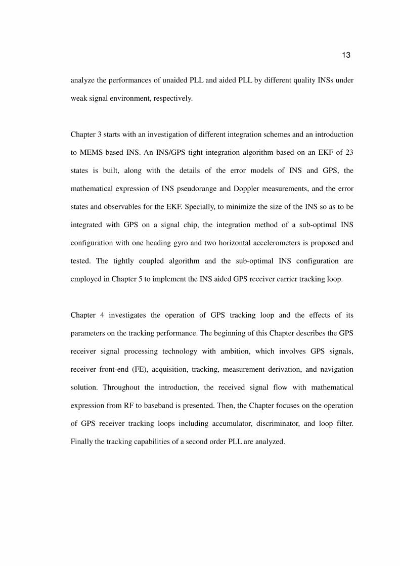
The conceptual principle of the simulator is shown in Figure 2.2. Differentiation of the
position and velocity information derives the acceleration when gravity is added.
However, such acceleration is only a transitory quantity on the navigation frame with
respect to the inertial frame. Frame rotation information is necessary to transform the
acceleration to the body frame, in which the accelerometers measure the vehicle’s
translational motions with respect to the inertial frame. Frame rotation can be computed
from the attitude when the Earth rotation is combined. Frame rotation information
indirectly provides the vehicle’s rotational motions on the body frame with respect to the
24
inertial frame, which are measured by gyroscopes. Translational and rotational motions
plus various sensor errors form the inertial sensor outputs form the inertial sensor outputs.
Figure 2.2: Principle of the Simulator
Applying the INS velocity l-frame mechanization equation (2.11) and considering an
inverse process in simulation reveal the following,
b
ib
lll
el
l
ie
lb
l
b
ib fgVωωVRf δ+−×++= ])2([ & (2.15)
In the implementation of the simulator through equation (2.15), if the PVA is from the
injected information, lV is one of the directly injected inputs or can be acquired through
a single differentiation of position (as depicted in equation (2.16)),
ervaltime
PositionPosition currentnextl
int
−=V (2.16)

25
Alternatively, if the inputs to the simulator are the user designed trajectory and motions,
lV can be calculated by
=
==
pV
ApV
ApV
Vl
b
bl
b
l
sin
coscos
sincos
0
0
RVRV (2.17)
where V is the user designed vehicle’s forward speed during one motion, which is
determined by the initial forward speed 0V , the acceleration V& and time interval t during
this motion period. 0V , V& and t are all user designed parameters.
tVVV ⋅+= &0 (2.18)
In equation (2.15), lV& is the vehicle’s acceleration on the l-frame, which is the first
difference of the velocity in the l-frame. It can be calculated through a double
differentiation of position or single differentiation of velocity
ervaltime
VelocityVelocity currentnextl
int
−=V& (2.19)
or alternatively, through the following equation
+
−−
+−
=
=
pppV
ApVAApVpApV
ApVAApVpApV
pV
ApV
ApV
dt
dl
cossin
sincoscossincoscos
coscossinsinsincos
sin
coscos
sincos
&&
&&&
&&&
&V (2.20)
where p& and A& are pitch angle change rate and heading angle change rate, respectively,
both of which are user-designed parameters. In equation (2.15), b
ibfδ represents the
accelerometer errors. The errors depend on the error model assumptions, which will be
discussed in the next section.

26
Applying the INS attitude l-frame mechanization equation (2.12) and considering an
inverse process in simulation, the output of the gyroscope triad from the simulator b
ibω
can be written as
b
ib
b
lb
l
el
l
ie
b
l
b
ib ( ωωωωRω δ+++= ) (2.21)
where,
b
ibωδ represents the gyroscope errors, and
b
lbω is the mathematical gimbals’ rate for a strap-down inertial system, which
has components related to the vehicle’s attitude and attitude change rate (Titterton and
Weston, 2004).
+
+
=
A
pr
p
rrTTTb
lb
&
&
& 0
0
)()(
0
0)(
0
0
122 RRRω
i.e.
=
A
r
p
rpr
p
rprb
lb
&
&
&
coscos0sin
sin10
sincos0cos
ω (2.22)
Equations (2.15) and (2.21) show that the inertial sensor outputs consist of two parts:
error-free values and sensor errors than are then added to the error free values.
2.3 Inertial Sensor Error Models in the Simulator
The INS simulator can simulate inertial sensor errors both on an individual basis and as a
combination to analyze multiple error effects. Inertial sensor errors are generally divided
into two parts: deterministic and stochastic (El-Sheimy, 2006). For a high-grade INS, the

27
manufacturer typically calibrates the INS extensively and stores the compensation
parameters inside the INS processor and therefore only small random errors remain. For a
low performance INS, like the MEMS based INS, there are many additional error
sources. This section uses a MEMS grade INS as an example to describe many of the
sensor errors modeled in the simulator. For a MEMS inertial sensor, the deterministic part
of the errors includes bias offset, scale factor (SF) error, gyro g-sensitivity, non-
orthogonality, and SF non-linearity which can be roughly estimated by lab calibrations or
manufacturer specifications (Titterton and Weston, 2004; El-Sheimy, 2006; Yang et al,
2007). These errors should be compensated before the INS data are used in the
mechanization algorithms. The stochastic part of MEMS inertial sensor errors includes
angular random walk (ARW), velocity random walk (VRW), SF changes due to
temperature and short term instabilities of the sensors errors. The random constant, the
random walk and the first-order Gauss-Markov models are typically used in modeling the
inertial sensor errors (Shin, 2005). These random models (Gelb, 1974; Brown and
Hwang, 1997) are described in Table 2.1.
Table 2.1: Mathematical models for various random processes
Random process )(tx
Continues-time equation
Discrete-time equation
Parameters
Random constant 0)( =tx& kk xx =+1 none
Random walk )()( twtx =& kkk wxx +=+1 kw driving white
noise
1st order Gauss-Markov
)()(1
)( twtxtx +−=β
& kx
t
k wxex
k
+=+∆
+β
1
1
kw driving white
noise
β correlation time
1+∆ kt time interval

28
For a general case, the output of a gyro gU and accelerometer aU can be modeled as
follows, respectively,
ωNωSωSSIU ggNLgLCgLg T ++∆⋅++= 2)( ggGgCgMg nfNbbb +++++ (2.23)
2)( fSfSSIU aNLaLCaLa T +∆⋅++= aaCaMaa nbbbfN +++++ (2.24)
where,
g (the subscript) represents the gyro related parameters;
a (the subscript) represents accelerometer related parameters;
f is the error-free accelerometer outputs which is calculated based on the
equation (2.15). f is denoted as b
ibf in that equation;
ω is the error-free gyro outputs which is calculated based on the equation
(2.21). ω is denoted as b
ibω in that equation;
LS represents the SF linear error vector along three axes caused by imperfect
manufacturing;
LCS represents the SF linear error vector along three axes caused by the
environment temperature change during INS operation;
NLS represents the SF non-linear error vector along three axes caused by the
environment temperature change during INS operation;
T∆ is the temperature change of the environment during INS operation;
N is a matrix with random Gaussian distributed components representing the
nonorthogonality of the sensor triad;

29
gN is the gyro g-sensitivity matrix with random Gauss distributed
components;
b is the inertial sensor’s turn-on bias;
Mb is the bias in-run instability;
Cb is the bias due to thermal drift;
n is the white noise which drives the ARW or VRW.
According to equations (2.23) and (2.24), the IMUS can simulate a variety of inertial
sensor errors. Table 2.2 summarizes the error models implemented in the IMUS.
Table 2.2: Error models and parameters in INS simulator
Error Model Parameters and Unit
gb random constant hrdeg/−−
standard deviation )1( σ− hrdeg/−− gMb 1st Gauss-Markov
correlation time hr−−
ARW spectral density hrdeg/−− gn white noise
bandwidth Hz−−
ab random constant gµ−−
σ−1 gµ−− aMb 1st Gauss-Markov
correlation time hr−−
VRW spectral density hrsm //−− an white noise
bandwidth Hz−−
σ−6 C0−−
T∆ 1st Gauss-Markov correlation time hr−−
gLS Constant ppm−−
gLCS Constant Cppm 0/−−
best fit straight line ppm−− gNLS Constant
measurement full scale sdeg/−−
gCb Constant Cs 0/deg/−−

30
Table 2.2: Error models and parameters in INS simulator (cont.)
Error Model Parameters and Unit
gN random constant σ−1 of matrix rad−−
gGN random constant σ−1 of matrix ghr /deg/−−
aLS Constant ppm−−
aLCS Constant Cppm 0/−−
best fit straight line ppm−− aNLS Constant
measurement full scale g−−
aCb Constant Cg 0/µ−−
aN random constant σ−1 of matrix rad−−
2.4 Simulator Performance Tests and Analyses
The correctness and efficiency of the simulator were verified at four levels. First, the
basic principles of the simulator were verified by comparing against standard INS
mechanization. Second, the individual inertial sensor errors and their combinations were
verified. Third, the simulated signals were compared with real hardware INS signals
collected in a field test.
Furthermore, in most civil applications, an INS is often integrated with GPS to provide
both long and short-term navigation accuracy. Integrated INS/GPS systems provide an
enhanced navigation solution that has superior performance in comparison to either
standalone system. To work for the inertial based integrated navigation system, the
optional GPS signals (position/velocity information with lever arm), odometer signals,
and magnetic heading signals are also simulated. Beyond the raw signal level
verifications in both theory and practice, the correctness of the INS simulator is also
validated at the INS/GPS integration level. In the fourth level test, both simulated signals
and the real hardware signals were processed through AINS® tool box (Shin and El-

31
Sheimy, 2002) to check the simulator performance. This software package processes the
aided inertial navigation system using INS/GPS data in a loosely coupled architecture.
I. Principle level verification
To verify the correctness of the simulator, an INS data set for a static case was simulated
and sent into INS mechanization. Since the simulation is an inverse process of
mechanization, the navigation error propagation should be the same as the INS behaviour
when the simulated data are sent to INS mechanization. The most typical behaviour of an
INS is that the distribution of the navigation errors should include the Schuler period
(84.4 min), Foucault period (34hr) and Earth’s rotation rate (24hr) (Titterton and Weston,
2004). Figure 2.3 is an example of the heading error of navigation over 45 hours with a
gyro bias of hr/01.0 0 under a static environment using simulated data.
0 5 10 15 20 25 30 35 40 45-0.05
0
0.05
0.1
0.15
0.2
0.25
navigation time (hr)
Headin
g e
rror (d
eg)
Schuler period 84.4 min
Earth period 24 hr
Foucault period 34 hr
Figure 2.3: Heading error behaviours by using simulated data from the simulator

32
There are three periods clearly shown in the Figure 2.3. They have the correct periods as
expected. These three periods are very basic characteristics for any inertial system, which
indicates the correct operation of the basic principles of the simulator.
II. Individual errors and their combinations
To complete the verification of the individual errors and their combinations from the
simulator, a set of vehicle trajectories and motions was designed. The designed data set
involved over 4400 seconds and included most of the vehicle’s dynamics, such as
accelerations, decelerations, static periods, turns, U-turns, tilts, and so on, as show in
Figures 2.4 to 2.6.
-4000 -2000 0 2000 4000 6000 8000 10000-4000
-2000
0
2000
4000
6000
8000
10000
12000
14000
East (m)
North (m
)
Figure 2.4: Simulated trajectories

33
0 1000 2000 3000 4000-10
0
10
Time (sec)
Pitch a
nd R
oll
(deg)
Pitch
Roll
0 1000 2000 3000 40000
100
200
300
Time (sec)
Headin
g (
deg)
Figure 2.5: Attitude changes
0 1000 2000 3000 4000-30
-20
-10
0
10
20
30
Time (sec)
Velo
city (
m/s
)
east-vel
north-vel
up-vel
Figure 2.6: Velocities on ENU l-frame

34
Figure 2.7 shows of the error-free outputs of the inertial sensors (gyro and accelerometer)
based on the above vehicle motions.
0 1000 2000 3000 4000-1
-0.5
0
0.5
1
1.5
2
x-g
yro
(d
eg
/s)
0 1000 2000 3000 4000-0.5
0
0.5
y-g
yro
(d
eg
/s)
0 1000 2000 3000 4000-10
-5
0
5
10
z-g
yro
(d
eg
/s)
Time (sec)
0 1000 2000 3000 4000-5
0
5
x-a
cce
l (m
/s2)
0 1000 2000 3000 4000-5
0
5
y-a
cce
l (m
/s2)
0 1000 2000 3000 40009
9.5
10
10.5
11
z-a
cce
l (m
/s2)
Time (sec)
Figure 2.7: Signals from simulator with error-free
By analyzing the motions, it is obvious that the inertial sensors correctly sense the
rectilinear and angular movement of the vehicle. For example, the x-axis gyro should
sense the pitch angle rotation. The designed pitch angle changes around 750s and 1250s
as shown in Figure 2.5.

35
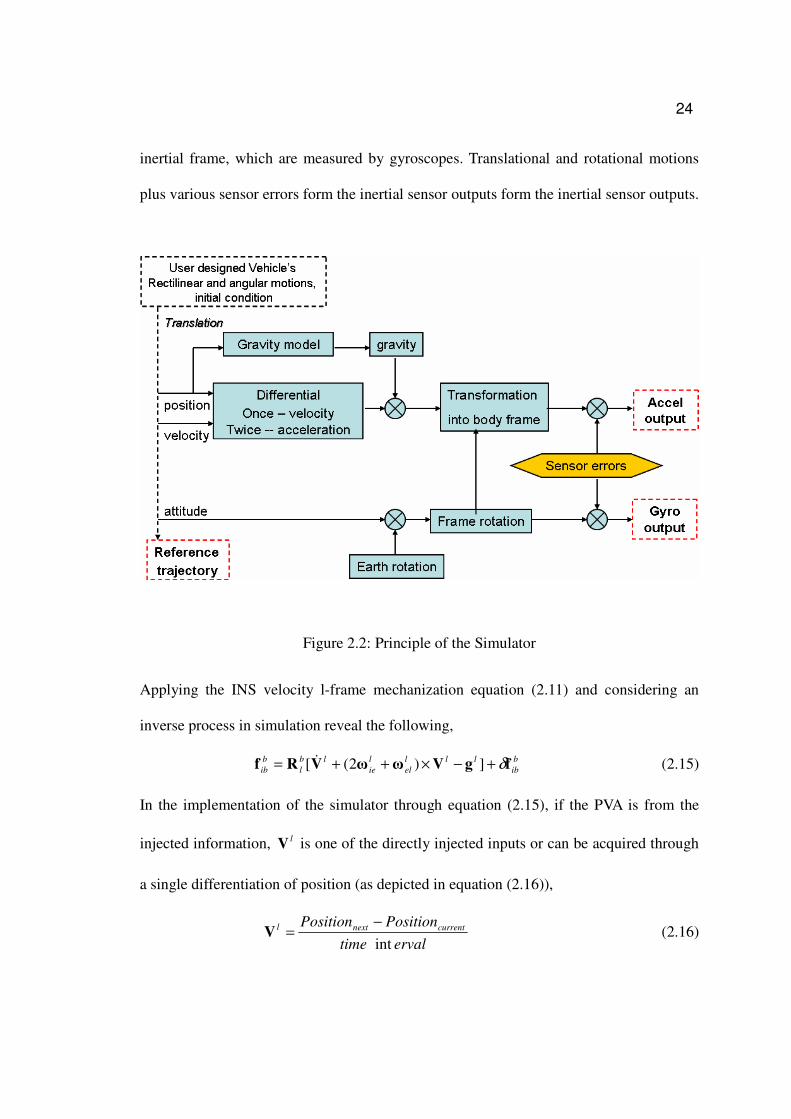
To show individual errors and their combinations from the simulator, some INS errors
were added to the error-free output through an ASCII file with a defined format to the
simulator. These errors were obtained from the manufacturer specifications and lab
calibrations of a hardware INS. Figure 2.8 to Figure 2.12 show examples of the simulated
MEMS grade INS signals with individual error sources, ARW/VRW, SF error, and
vibration, respectively. Figure 2.8 shows the simulated gyro triad signal and
accelerometer triad signal along three axes with a hrdeg/3 ARW and a hrsm //66.0
VRW, both based on the designed vehicle motions.

36
0 1000 2000 3000 4000-1
-0.5
0
0.5
1
1.5
2
2.5
x-g
yro
(d
eg
/s)
error-free + ARW
0 1000 2000 3000 4000-1
-0.5
0
0.5
1
y-g
yro
(d
eg
/s)
0 1000 2000 3000 4000-10
-5
0
5
10
z-g
yro
(d
eg
/s)
Time (sec)
0 1000 2000 3000 4000-5
0
5
x-a
cce
l (m
/s2)
error-free + VRW
0 1000 2000 3000 4000-5
0
5
y-a
cce
l (m
/s2)
0 1000 2000 3000 40009
9.5
10
10.5
11
z-a
cce
l (m
/s2)
Time (sec)
Figure 2.8: INS signals with ARW ( hrdeg/3 ) and VRW ( hrsm //66.0 )
Figure 2.9 shows the gyro triad signal with a SF non-linear error of about ppm1000 of
the full scale sdeg/150 and the accelerometer triad signal with a SF non-linear error of
ppm2000 of the full scale g5 .

37
0 1000 2000 3000 4000-1
0
1
2
x-g
yro
(d
eg
/s)
error-free + SF error
0 1000 2000 3000 4000-1
-0.5
0
0.5
1
y-g
yro
(d
eg
/s)
0 1000 2000 3000 4000-10
-5
0
5
10
z-g
yro
(d
eg
/s)
Time (sec)
0 1000 2000 3000 4000-5
0
5
x-a
cce
l (m
/s2)
error-free + SF error
0 1000 2000 3000 4000-5
0
5
y-a
cce
l (m
/s2)
0 1000 2000 3000 40009
9.5
10
10.5
11
z-a
cce
l (m
/s2)
Time (sec)
Figure 2.9: INS signals with SF errors
Figure 2.10 compares the difference between the error-free output and the actual output
with SF errors. It is also clear that the quantity of this individual error source matches
well to what it should be.
38
0 1000 2000 3000 4000
0
2
4
6
8
10x 10
-5
x-g
yro
(d
eg
/s)
error due to SF
0 1000 2000 3000 4000
0
2
4
6
8
10x 10
-7
y-g
yro
(d
eg
/s)
0 1000 2000 3000 4000
0
0.5
1
1.5
2
2.5x 10
-3
z-g
yro
(d
eg
/s)
Time (sec)
0 1000 2000 3000 4000
0
0.5
1
1.5
2
2.5
3x 10
-3
x-a
cce
l (m
/s2)
error due to SF
0 1000 2000 3000 4000
0
1
2
3
4x 10
-3
y-a
cce
l (m
/s2)
0 1000 2000 3000 40000
0.005
0.01
0.015
0.02
z-a
cce
l (m
/s2)
Time (sec)
Figure 2.10: INS signal difference due to SF errors
Figure 2.11 shows the IMU signals with a vibration on the pitch angle channel during its
operation. The parameters for the vibration are amplitude sdeg/1.0 and frequency 10Hz.
A zoomed-in Figure 2.12 shows 1s zoomed-in signals. The figure indicates that the
quantity of the vibration matches well to the defined parameters.

39
0 1000 2000 3000 4000-1
0
1
2
x-g
yro
(d
eg
/s)
error free + vibration
0 1000 2000 3000 4000-1
-0.5
0
0.5
1
y-g
yro
(d
eg
/s)
0 1000 2000 3000 4000-10
-5
0
5
10
z-g
yro
(d
eg
/s)
Time (sec)
0 1000 2000 3000 4000-5
0
5
x-a
cce
l (m
/s2)
error free + vibration
0 1000 2000 3000 4000-5
0
5
y-a
cce
l (m
/s2)
0 1000 2000 3000 40009
9.5
10
10.5
11
z-a
cce
l (m
/s2)
Time (sec)
Figure 2.11: INS signals with vibration

40
2500 2500.2 2500.4 2500.6 2500.8 2501-1
-0.5
0
0.5
1x-g
yro
(d
eg
/s)
error due to vibration (1s zoom-in)
2500 2500.2 2500.4 2500.6 2500.8 2501-1
-0.5
0
0.5
1x 10
-3
y-g
yro
(d
eg
/s)
2500 2500.2 2500.4 2500.6 2500.8 2501-0.01
-0.005
0
0.005
0.01
z-g
yro
(d
eg
/s)
Time (sec)
2500 2500.2 2500.4 2500.6 2500.8 2501-0.05
0
0.05
x-a
cce
l (m
/s2)
error due to vibration (1s zoom-in)
2500 2500.2 2500.4 2500.6 2500.8 2501-0.2
-0.1
0
0.1
0.2
y-a
cce
l (m
/s2)
2500 2500.2 2500.4 2500.6 2500.8 2501-1
0
1x 10
-4
z-a
cce
l (m
/s2)
Time (sec)
Figure 2.12: INS signals with vibration – 1s zoomed-in
Figure 2.13 shows the simulated MEMS grade INS signals with all error sources and
compares this case with the error-free output. The parameters used in this simulated data
set are listed in Table 2.3. This output and the outputs from the other axes of the simulator
are used in the level IV (INS/GPS loose integration level) test.

41
0 1000 2000 3000 4000-1
-0.5
0
0.5
1
1.5
2
2.5x-g
yro
(d
eg
/s)
error free + combined errors
0 1000 2000 3000 4000-1
-0.5
0
0.5
1
y-g
yro
(d
eg
/s)
0 1000 2000 3000 4000-10
-5
0
5
10
z-g
yro
(d
eg
/s)
Time (sec)
0 1000 2000 3000 4000-5
0
5
x-a
cce
l (m
/s2)
error free + combined errors
0 1000 2000 3000 4000-5
0
5
y-a
cce
l (m
/s2)
0 1000 2000 3000 40009
9.5
10
10.5
11
z-a
cce
l (m
/s2)
Time (sec)
Figure 2.13: INS signals with combined errors

42
Table 2.3: Parameters for sensor errors used in MEMS INS simulation
Error Value Error Value
gMb hrdeg/200 aMb gµ800
gn hrdeg/3 an hrsm //66.0
gNLS ppm1000 of sdeg/150 aNLS ppm2000 of g5
gCb Cs 0/deg/02.0 aCb Cg 0/600µ
gN rad04.0 aN rad04.0
gGN ghr /deg/180
T∆ C010
III. Comparison to a real INS signal at the raw signal level
Verification of the simulator at this raw signal level is performed based on an ADI
MEMS grade INS and its parameters. The hardware ADI INS is a very low-cost (<$100)
MEMS INS, developed by the mobile-multi-sensor-system (MMSS) research group at
the University of Calgary (Niu and El-Sheimy, 2005). The ADI INS integrates surface
micromachining MEMS gyroscopes (ADXRS150) and accelerometers (ADXL105)
developed by Analog Devices Inc. To compare simulated signals with those of the ADI
INS, a field test was conducted around Springbank, Alberta in December 2005. Figure
2.14 shows the test trajectory of the car. The trajectory was recorded by a tactical grade
LN200 INS and differential GPS, which is accurate enough as the reference (true values)
for the MEMS INS. The simulated INS signal of the x-axis gyroscope is compared with
that of the field test data, as shown in Figure 2.15.

43
-4000 -2000 0 2000 4000-1000
0
1000
2000
3000
4000
East (m)
North (m
)
Field test trajectory
Figure 2.14: Field test trajectory
0 200 400 600 800 1000 1200-10
-5
0
5
10
GPS time - 520000 (sec)
x-g
yro
(d
eg
/s) ADI IMU real data
0 200 400 600 800 1000 1200-10
-5
0
5
10
GPS time - 520000 (sec)
x-g
yro
(d
eg
/s) ADI IMU simulated data
0 200 400 600 800 1000 1200-1.5
-1
-0.5
0
0.5
1
GPS time - 520000 (sec)
x-g
yro
sig
nal diffe
rence (deg/s
) Signal difference between real and simulation
Figure 2.15: Comparison of INS signals between simulation and field test

44
From the Figure 2.15, it is obvious that the simulated INS signals have a good agreement
with the real test signals. The mean error of the x-gyro differences is sdeg/01.0 and the
standard deviation is sdeg/12.0 , which is highly related to time synchronization of the
recorded vehicle’s PVA information and the accuracy of the error model.
IV. Comparison with real INS signals of an INS/GPS integrated system
At this level of verification, the simulated signals and the real hardware signals are
compared using a loosely coupled INS/GPS navigation algorithm. Both simulation data
and real hardware data are processed through the AINS® software. To be compatible with
a loosely coupled INS/GPS integrated system, the GPS signals (i.e. Position and Velocity
information) were also simulated in the simulator by defining the GPS data rate and the
horizontal and vertical position/velocity standard deviations (10m/7m in this case). The
field test data set was taken from the ADI hardware INS with standalone GPS solutions
from a NovAtel OEM4 receiver. Both the simulated data and the field test data sets were
processed in AINS® and their average position drifts during GPS blockages were
compared. Figure 2.16 gives the simulated trajectory with the GPS outage periods. These
outages cover a variety of dynamics including constant velocities, accelerations,
decelerations, and turns. Figure 2.17 shows the position, velocity and attitude errors for
defined outages based on simulated data from the simulator.

45
-5000 0 5000 10000-2000
0
2000
4000
6000
8000
10000
12000
14000
East (m)
North (m
)
True
IMU/GPS
GPS gaps
Figure 2.16: Simulated trajectory with outage periods
0 500 1000 1500 2000 2500 3000 3500 4000 4500-400
-200
0
200
Positio
n e
rror
(m)
North
East
Height
STD
GPS gaps
0 500 1000 1500 2000 2500 3000 3500 4000 4500-10
0
10
Velo
city e
rror
(m/s
)
North
East
Height
STD
0 500 1000 1500 2000 2500 3000 3500 4000 4500-40
-20
0
20
Attitude e
rror
(deg)
GPS time - 0 (sec)
Roll
Pitch
Azimuth
STDR
STDP
STDA
Figure 2.17: PVA error results with simulated ADI INS
The average position drift for the simulation data, which contain 12 outage periods each
lasting 60 seconds, was approximately 115 meters. The largest drift was 219 meters and
the smallest was 35 meters. This corresponds well to the hardware ADI INS field test
results (Nasser et al, 2006) which typically averaged out to around 120 meters.

46
2.5 Summary
This Chapter describes a software method based INS signal simulator in details. The
implementation of INS simulator is a methodical combination of an inverse process of
INS mechanization and inertial sensor error models. The function of the INS simulator
presented in this Chapter can generate the raw measurements of any INS such as
navigation grade, tactical grade, and consumer grade systems according to a user-given
application (such as airborne, land, drilling, pipeline geo-pig applications, etc.). It can
simulate a variety of sensor errors such as the bias instability, random walk, scale factor
errors, sensor errors due to thermal drift, g-sensitivity, nonorthogonalities, misalignment,
and their combinations.
The simulator was verified through four distinct tests, involving basic principles,
individual error sources, raw signals, and INS/GPS integration outputs. Performance test
results show that the simulator can provide similar INS signals to that of a hardware INS.
The INS simulator is an effective, economical and flexible tool for INS related research.
It can be used efficiently when choosing or designing the required hardware
characteristics for a given application. It is also a fast and effective method for evaluating
new sensors using datasheet characteristics provided by manufacturers or lab tests and for
conducting error budgets for INS based integrated navigation system.

47
Chapter 3 MEMS Based INS/GPS Tightly Coupled Integration
The INS/GPS integrated system takes advantage of the complementary attributes of two
systems to yield a system that provides greater precision than either of the component
systems operating alone. Tightly coupled INS/GPS can continue to provide useful
navigation information in situations where fewer than four GPS satellites are visible.
Section 3.1 presents an overview of INS/GPS integration schemes including loose, tight
(with INS aiding receiver tracking loop) and deep integration. Section 3.2 briefly
introduces MEMS inertial sensors and MEMS based INSs. Section 3.3 gives mathematic
expression of the extended Kalman filter, which is widely used in INS/GPS integration
systems. Several implementation details are also described. Section 3.4 builds a 23-state
EKF for INS/GPS tightly coupled integration and tests the developed software. First, the
INS dynamic models are derived and the errors of the inertial sensors are modeled.
Second, the INS pseudorange and Doppler measurements are given mathematically.
Third, the tightly coupled system state vector including 23 error states and the
observables are set up. Section 3.5 presents test results and analyses of MEMS based
INS/GPS tight integration. To improve the navigation accuracy for a land vehicle
application, a non-holonomic constraint principle and its test results are discussed in
Section 3.6. Furthermore, to reduce the cost as well as the size of the physical unit of the
INS/GPS integration, the integration of a GPS and a sub-optimal INS configuration with
one heading gyro and two horizontal accelerometers is discussed in Section 3.7. The idea
of the pseudo-signal generation in this configuration comes from INS signal software
simulator described in the Chapter 2. This integration configuration will be used in the
Chapter 5.

48
3.1 Overview of INS/GPS Integration
An INS is self-contained system that can provide a PVA solution continuously. An INS is
a combination of the IMU, navigation algorithm, and the computer which hosts the
algorithm. The sensors used in an INS are a triad of gyros and accelerometers. The INS
algorithm is actually an integrating process that first detects acceleration then integrates it
to derive velocity and displacement (Titterton and Weston, 2004). The progress in MEMS
technology enables complete inertial units on a chip, composed of multiple integrated
MEMS accelerometers and gyroscopes. In addition to their compact and portable size, the
price of MEMS-based INS is far less than high quality INS.
An alternative navigation approach is to use GPS. A GPS receiver provides
measurements of position and velocity, and/or more specifically pseudorange, carrier
phase, and Doppler. The accuracy of these measurements is time-independent, i.e. with
bounded errors, which is totally different from INS estimates. However, the GPS
measurement accuracy is limited as a result of low signal strength, the length of the PRN
code and errors in the tracking loop (Titterton and Weston, 2004). Other GPS errors arise
as a result of multi-path, variations in the satellite geometry and receiver clock instability.
Furthermore, with the increasing application demands, the conventional GPS positioning
is challenged at the environments such as under foliage areas, urban canyons and indoors.
The main characteristics of an INS and GPS in terms of their respective advantages and
disadvantages are compared in Table 3.1, which indicates that they are complementary.

49
Table 3.1: Comparison of characteristics of INS and GPS
System INS GPS
Advantages --Immune to RF
--High data rate
--PVA information
--High accuracy in short-term
--Works well under all
environments
--Errors time-independent
(bounded)
--no pre-information needed
--time standard (GPST)
disadvantages --Errors time-dependent
--Need initial alignment
--no time standard
--Sensitive to RF interference
--Low data rate
--No attitude information
Integrated INS/GPS system provides an enhanced navigation system that has superior
performance in comparison with either a stand-alone system as it can overcome each of
their limitations. The integrated system presents the features of both long-term and short-
term accuracy, improved availability and greater integrity (Gao, 2007). Typically, there
are three strategies for the integration of GPS and INS, which are normally classified as
loose coupled, tight coupled and deep coupled.
The loosely coupled integration is the simplest method of coupling. Its architecture is
shown in Figure 3.1 (El-Sheimy, 2006). In this scheme, the INS and GPS receiver
generate navigation solutions independently. The information from them is blended using
an estimator to form a third navigation solution. Normally, an EKF is used to accomplish
the blending even though currently some interest in using other non-linear estimators
such as the unscented Kalman filter or particle filters has arisen (Shin, 2005).
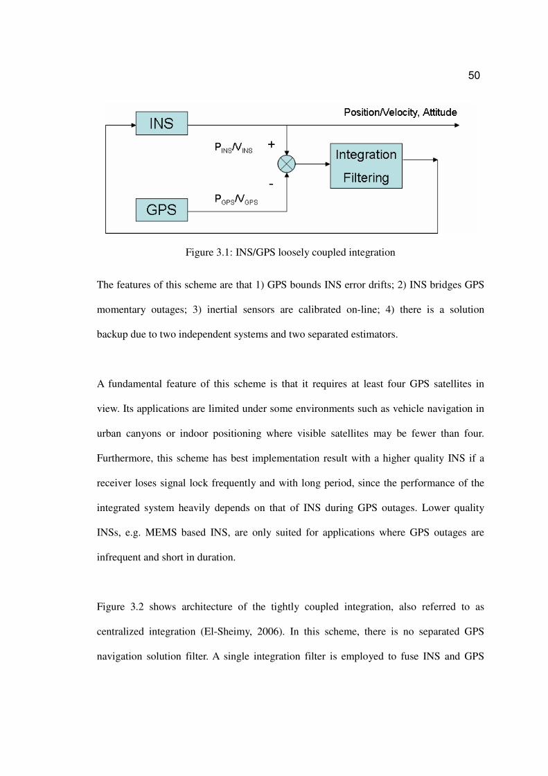
50
Figure 3.1: INS/GPS loosely coupled integration
The features of this scheme are that 1) GPS bounds INS error drifts; 2) INS bridges GPS
momentary outages; 3) inertial sensors are calibrated on-line; 4) there is a solution
backup due to two independent systems and two separated estimators.
A fundamental feature of this scheme is that it requires at least four GPS satellites in
view. Its applications are limited under some environments such as vehicle navigation in
urban canyons or indoor positioning where visible satellites may be fewer than four.
Furthermore, this scheme has best implementation result with a higher quality INS if a
receiver loses signal lock frequently and with long period, since the performance of the
integrated system heavily depends on that of INS during GPS outages. Lower quality
INSs, e.g. MEMS based INS, are only suited for applications where GPS outages are
infrequent and short in duration.
Figure 3.2 shows architecture of the tightly coupled integration, also referred to as
centralized integration (El-Sheimy, 2006). In this scheme, there is no separated GPS
navigation solution filter. A single integration filter is employed to fuse INS and GPS

51
measurements (Petovello, 2003a). The raw pseudorange and Doppler measurements from
GPS tracking loop output and those from INS prediction are combined to form the input
of the centralized integration filter. The filter directly accepts their differences to obtain
the INS error estimates (Knight, 1999).
Figure 3.2: INS/GPS tightly coupled integration
This scheme provides a more accurate solution than loose integration because the basic
GPS observables (pseudorange and Doppler) used in the blending process are not as
correlated as the position and velocity solutions used in loose couple (Alban et al., 2003).
It can continue to generate integrated navigation solution even when fewer than four
satellites are being tracked. Therefore, this integration strategy is a preferred approach in
urban canyons. In addition, tightly coupled leads to superior GPS fault detection and
exclusion (Petovello, 2003a). Applications where output of carrier phase measurements is
required especially benefit from tight integration because integer ambiguities can be
recovered and verified quickly (Alban et al., 2003), which is beyond the studies of this
dissertation. In general, this integration strategy is typically a preferred approach given its

52
better performance in terms of both accuracy and system robustness, especially in urban
canyon environments.
A further definition of tightly coupled appears in recent years. In the further definition,
information from the integration filter is fed back to the receiver to enhance its
performance (Gebre-Egziabher et al., 2007). Specifically, the INS derived
velocity/Doppler information is used to aid the code and carrier tracking loop in the
receiver, known as INS aiding to GPS signal tracking. This allows the receiver to remain
in lock with reducing measurement noise in high-dynamic maneuvers and some extent of
weak signal conditions (Petovello et al, 2007). Chapter 4 and 5 will discuss the principle,
methods and implementations of such an aiding in details.
The deep integration, also known as ultra-tightly, combines GPS signal tracking and
INS/GPS integration into a single Kalman filter, as illustrated in Figure 3.3 (Gebre-
Egziabher et al., 2007). In this scheme, by tracking the GPS signals together, instead of
using independent tracking loops, the tracking of each signal is aided by the others and by
inertial data.

53
Figure 3.3: INS/GPS deeply coupled integration
In deep integration scheme, a single vector delay lock loop (VDLL) is used to fulfill the
signal tracking function, which is completed by a batch of independent code and carrier
tracking loops in a conventional receiver (Pany and Eissfeller, 2006; Petovello et al,
2006). The receiver is no longer an independent navigator since its operation is also
partly dependent of INS information. The deep integration represents an optimal fusion of
the information from an INS and a GPS receiver (Gebre-Egziabher, et al., 2007; Kim et
al., 2003). However, the potential benefits described here may be achieved at the
expense of greatly increased complexity, increased computational load and tight time
synchronization requirements (Gebre-Egziabher, et al., 2007; Titterton and Weston,
2004).

54
3.2 MEMS Inertial Sensors
MEMS technology is one of the most exciting developments in inertial sensor in last
twenty years. The need to maintain reasonable cost levels when integrating an INS with
GPS for consumer applications is driving the technology development for MEMS inertial
sensors (Barbour and Schmidt, 2001). MEMS sensor technology makes direct use of the
chemical etching and batch processing techniques used by the electronics integrated
circuit industry. The properties of the resulting MEMS based inertial sensors are small
size, low weight, rugged construction, low power consumption, low cost as a result of
high volume manufacturing, low maintenance, and compatible with operation in hostile
environments (Titterton and Weston, 2004). So far, MEMS inertial sensors are the lowest
cost inertial sensors available for use in commercial applications, such as land navigation
(Hide, 2003). These sensors, based on their performance levels and intended applications,
are often categorized under automotive grade sensors (El-Sheimy and Niu, 2007; Godha,
2006). MEMS research on inertial sensors has focused primarily on accelerometers and
gyroscopes (Park, 2004).
Initial MEMS sensor developments focused on the generation of miniature
accelerometers, the system and performance requirements of which were driven by the
demands of the automobile industry. An accelerometer is used to measure the specific
force being applied to an input axis. MEMS accelerometers may be divided into two
distinct classes (Titterton and Weston, 2004): 1) the displacement of a proof mass
supported by a hinge or flexure in the presence of an applied acceleration; 2) the change
in frequency of a vibrating element caused by the change in tension in the element when

55
the element is subjected to acceleration. There are four types of MEMS accelerometers
named as pendulous mass, resonant (vibrating beam), tunneling, and electro-statically
levitated MEMS accelerometers, referred to Titterton and Weston (2004) for details.
MEMS gyroscopes are non-rotating devices and use the Coriolis acceleration effect on a
vibrating proof mass to detect inertial angular rotation. These gyros consist of a sensing
element vibrating with constant amplitude controlled by a vibrating motor that maintains
the oscillation at constant amplitude. When this system is rotated around any axis other
than the axis of its internal in-plane vibration, the Coriolis force causes the element to
oscillate out of the plane (Faulkner et al., 2002). This oscillation is picked-up by the
sensing capacitors and is used to provide a measure of angular rate. There are many
practical sensor configurations based upon this principle. They generally fall into one of
the following three categories: simple oscillators, balanced oscillators (e.g. tuning fork
MEMS gyroscope), shell resonators (e.g. resonant ring MEMS gyroscope).
As mentioned in Chapter 2, the inertial sensor errors can be divided into two parts,
deterministic errors and stochastic errors. For a high-grade INS, only small random errors
remain. By contrast, both deterministic part and stochastic part errors are remained in a
MEMS inertial sensors based INS. The kinds of error sources are described and
summarized in Equations (2.23) and (2.24). In order to integrate MEMS inertial sensors
with GPS and to provide a continuous and reliable navigation solution, the calibration
process is necessary. The calibration process is to understand the characteristics of
different error sources and the variability of these errors. Calibration is defined as the

56
process of comparing instrument outputs with known reference information and
determining coefficients that force the output to agree with the reference information over
a range of output values (Chartield, 1997). To accurately determine parameters related to
deterministic errors, special calibration devices such as turn tables or special techniques
are needed, such as LLF calibration, Six-position static acceleration test and angle rate
tests, referred to El-Sheimy (2006) for details. The Allan variance method is a popular
one to be used in determining the parameters related to random errors (Hou, 2003). Shin
(2001) developed a multi-position method to determine the non-orthogonality for a
sensor triad, in addition to the bias and the SF. Combining the above methods, excluding
LLF calibration, we can determine both deterministic part and stochastic part errors of the
gyro triad and the accelerometer triad in an IMU. The errors include bias offset, SF error,
gyro g-sensitivity, non-orthogonality, SF non-linearity, ARW, VRW, SF changes due to
temperature and short term instabilities. One calibration example for MEMS based INS
made of ADI inertial sensors was given in Table 2.3, Chapter 2.
The process of computing the initial parameter of the DCM l
bR is called the INS
alignment procedure. For navigation-grade and high-end tactical grade INSs, the
analytical coarse alignment method followed by fine alignment can be applied to estimate
the initial attitude parameters (Farrell and Barth, 2001). However, for MEMS based INSs,
these methods often fail owing to large sensor errors. The heading alignment cannot be
accomplished (Noureldin et al, 2003; Godha, 2006). Another practical problem in using
conventional static alignment methods is that the system is slated to be used in a
consumer vehicle; hence, the user cannot be expected to wait until the sensor alignment is
57
finished (Shin and El-Sheimy, 2004).
3.3 Discrete-Time EKF
Kalman filter is one the most popular techniques to integrate the INS and GPS. This
optimal estimation technique was developed in 1960s and has been developed
accompanying with the development of the modern control theory. Detailed
documentations about the Kalman filter can be found in Gelb (1974), Brown and Hwang
(1997), and Grewal and Andrews (2001). For a linear system with zero mean, Gaussian
noise, the KF is an optimal tool to do the estimation since its covariance of state error is
minimum. If the system is nonlinear or if the noise is not Gaussian, the KF is no longer
an optimal choice. In this case, we can extend the use KF in such a nonlinear system
through a linearization. If the linearization is around the predicted state vector, the
corresponding KF is so-called extended Kalman filter. The EKF applies the Taylor series
expansion for the nonlinear system and observation equations, and takes the first order
terms to apply the well-developed linear Kalman filter theory, where the probability
density function (PDF) is approximated by a Gaussian model (Gordon et al., 1993,
Maybeck, 1994).
Inertial navigation system typically is a nonlinear dynamic system; however, its error
propagation is typically done in a linear manner. The error state of the Kalman filter can
be considered as the EKF, especially for the INS error control feedback loop (Shin,
2005). That is because the EKF can be used to estimate a state vector consisting of PVA
and INS error states with the error states being reset to zero (ie expansion around the

58
predicted state vector value) at each new update. The EKF has long been used in such a
nonlinear system (Grewal and Andrews, 1993; Rogers, 2000; Schwarz and Wei, 2000).
This section will develop the EKF algorithm for INS/GPS integration to get more
accurate INS velocity measurement on the LLF. The EKF algorithm is a sequential
recursive algorithm for an optimal least-mean variance estimation of the error states
(Gelb, 1974). Figure 3.4 shows the flow chart of the EKF algorithm (El-Sheimy, 2006).
Figure 3.4: EKF algorithm flow chart
Given that a linear continuous-time (CT) system is described by the followed 1st order
error state equation (Scherzinger, 2004)
)())(( t(t(t)tt wGxF)x += δδ& (3.1)
where,
)(tF is the system dynamics matrix;
)(txδ is the error state vector;

59
)(tG is a noise disturbance mapping matrix;
)(tw is a noise vector, assumed as zero-mean and Gaussian distribution. Its
covariance matrix is given by [ ] )()()()( ⋅= δtttE T Qww , where )(tQ is the
spectral density matrix of )(tw and the operator )(tδ denotes the Dirac
delta function whose expression is
≠
==
00
01)(
t
ttδ .
Because inertial systems are usually implemented with high-rate sampled data, the CT
system dynamic equations are to be transformed to their corresponding discrete-time
(DT) form:
ττττδδ dtttttk
k
t
tkkkkk )()(),()(),()(
11 wGΦxΦx ∫
−
+= − (3.2)
or in abbreviated notation as
1111, −−−− += kkkkkk wGxΦx δδ (3.3)
where
kxδ is the system error state vector at kt epoch;
1−kw is the driven response at kt due to the presence of the input white
noise during the time interval ),( 1 kk tt − (Brown and Hwang, 1997).
Its covariance matrix is given as
≠
==
jk
jkE
kT
jk0
Qww ][ .
1−kG is the noise coefficient matrix;
1, −kkΦ is the transition matrix. If the time interval ),( 1 kkk ttt −=∆ is small
enough or )(tF is approximately constant over this interval, the
relation between the transition matrix and the system dynamic

60
matrix can be written as, with an assumption of equal interval
1−∆=∆ kk tt ,
L+∆+∆+≈= −−−∆
−− 2
11
2
1
)(
1, )(!2
1)(1
kkkk
tt
kk tttte kk FFIΦF (3.4)
Considering the system’s measurement is described by the following discrete-time
equation
kkkk nxHZ += δδ (3.5)
where
kZδ is the measurement error vector. It is a linear combination of the
error state vector kxδ and the measurement noise disturbance kn ;
kH is the design matrix, which is defined as
1,ˆ
][
−=∂
∂=
kkxx
kx
xhH , where ][xh is the non-linear vector
measurement function of the error states;
kn is the DT measurement noise. Its covariance matrix is given
as
≠
==
jk
jkE
kT
jk0
Rnn ][ .
In Equations (3.3) and (3.5), the system noise and the measurement noise are assumed to
be uncorrelated, i.e. 0nw =][ T
ikE for all ki, . The covariance matrix of the error state
vector is defined as k
T
kkkkE Pxxx-x =− ])ˆ)(ˆ[( δδδδ .
The following equations are the discrete-time EKF algorithm mathematical

61
implementation. The implementation of the EKF can be divided into two stages:
measurement update and prediction. In the prediction stage, also called “time-update”,
the estimate and its error covariance are as
11,1,ˆˆ
−−− = kkkkk xΦx δδ (3.6)
T
kkk
T
kkkkkkk 1111,11,1, −−−−−−− += GQGΦPΦP (3.7)
In the measurement update, the Kalman gain matrix kK , is computed first, then the state
and the covariance are updated using the predicted estimate 1ˆ
−kxδ and its
covariance 1, −kkP , as follows
1
1,1, ][ −−− += k
T
kkkk
T
kkkk RHPHHPK (3.8)
]ˆ[ˆˆ1,1, −− −+= kkkkkkkk xHZKxx δδδδ (3.9)
T
kkk
T
kkkkkkk KRKHKIPHKIP +−−= − ][][ 1, (3.10)
Typically, the frequency of the prediction loop and the update loop that are described by
Equations (3.6) to (3.10) is different (Grewal and Andrews, 1993; El-Sheimy, 2006).
In the implementation of EKF, kQ normally is not calculated separately. T
kkk 111 −−− GQG
is often calculated together as one item from the CT system (t)(t)(t) TGQG directly
(Kalman, 1963)
L+∆
++∆= −−
!2]))()(()([)(
2
11
kT
kkkk
tttttt QFFQQ (3.11)
or written as following if the calculation time interval kt∆ is small enough
2])([ ,1,1
kT
kkkkk
t(t)t
∆+= ++ ΦQΦQQ (3.12)

62
In above two equations, we define kQ and (t)Q as
T
kkkk GQGQ = and (t)t(t)t T)GQG)Q (( = (3.13)
3.4 EKF Design for Tight Integration
3.4.1 INS Dynamic Error Models
To formulate an EKF to fuse INS and GPS, it is necessary to develop a linear dynamic
model of the errors that are to be estimated. Linearization of the INS non-linear dynamic
system is the most common approach to derive a set of linear differential equations that
define the INS error states.
Applying Taylor series expansion to the position mechanization equation, i.e. Equation
(2.10), linearization and neglecting higher order terms, i.e. using a 1st order
approximation, we have:
The position error differential equation as:
rDDVDr δδδ r
ll 11 −− −=& (3.14)
where, 1−D is shown in Equation (2.13), and
+−
=
000
00
cos0cos)(
ϕ
ϕλϕλ
&
&& hRN
rD
[ ]Thδδλδϕδ =r is the position errors expressed by geodetic coordinates.
The velocity error differential equation as:
lll
el
l
ie
ll
el
l
ie
b
ib
l
b
b
ib
l
b
l gVΩΩVΩΩfRfRV δδδδδδδ ++−+−+= )2()2(&

63
lb
ib
l
b
l
ib
ll
el
l
ie
l
el
l
ie
l gfRεfVωωωωV δδδδδ ++×−×+−+×= )2()2( (3.15)
In the above equation,
[ ]T
UNE
lvvv δδδδ =V is the velocity errors along ENU;
× denotes the cross-product operation for two vectors;
l
ieωδ is the error of Earth rotation rate projected on l-frame, which is
equal to [ ]δϕϕωδϕϕωδ ⋅⋅−= cossin0 ee
l
ieω ;
l
ieωδ is the error of the transport rate, which is equal to (neglecting
higher order terms)
+++
−=
hR
v
hR
v
hR
v
N
E
N
E
M
Nl
ie
ϕδδδδ
tanω ;
lgδ is the gravity error. It is always assumed as 0 for a vehicle near the
Earth surface;
ε is the attitude error vector. The pitch error pδ , the roll error rδ and
the heading error Aδ are expressed as a vector [ ]TArp δδδ=ε .
The corresponding skew-symmetric matrix of ε can be written as
T
pr
pA
rA
−
−
−
=
0
0
0
δδ
δδ
δδ
E ;
l
ibf is the specific force projected on l-frame, which is equal to b
ib
l
bfR ;
b
ibfδ is the error of specific force measure by the accelerometer triad. A
stochastic model is necessary to describe it mathematically.

64
To derive the attitude error differential equation, we firstly have the error of DCM l
bR is
given as l
b
l
b ERR =δ and the computed l
bR is given as:
l
b
l
b
l
b
l
b REIRRR )(ˆ −=−= δ (3.16)
Differentiating Equation (3.16)
l
b
l
b
l
b
l
b RERERR &&&&−−=ˆ
b
lb
l
b
l
b
b
lb
l
b ΩERREΩR −−= & (3.17)
On the other hand, based on the attitude mechanization Equation (2.12), we have
)()(ˆ b
lb
b
lb
l
b
l
b ΩΩREIR δ+−=&
b
lb
l
b
b
lb
l
b
b
lb
l
b
b
lb
l
b ΩRΩERΩRΩR δδδ −−+= (3.18)
Comparing Equation (3.17) and (3.18), and neglecting 2nd order term, we have
b
l
b
lb
l
b RΩRE δ−=& , i.e. b
lb
l
b ωRε δ−=& (3.19)
In addition,
)( l
el
l
ie
b
l
b
ib
b
lb ωωRωω +−=
)()( l
el
l
ie
b
l
l
el
l
ie
b
l
b
ib
b
lb ωωRωωERωω δδδδ +−+−= (3.20)
Substituting (3.20) into (3.19), we have the attitude error differential equation as:
b
ib
l
b
l
el
l
ie
l
el
l
ie ωRεωωωωε δδδ −×+−+= )()(& (3.21)
where b
ibωδ is the error of angular rate measured by the gyro triad. A stochastic model is
necessary to describe it mathematically.

65
In theory, the inertial sensor errors b
ibfδ and b
ibωδ should be modeled as Equation (2.23)
and (2.24). However, after compensation for the deterministic part errors and
consideration of the computation burden, the inertial sensor can be modeled with
sufficient accuracy using random processes such as random constant (random bias),
random walk, or a Gauss-Markov (GM) process. Details of these stochastic models could
be found in Gelb (1974). Therefore, in practice, for MEMS grade sensors, only the bias
in-run instability, SF in-run instability and driving white noise (VRW, ARW) are
considered here, all of which are modeled as 1st order Gauss-Markov process. These
parameters will be changed accompanying with the KF tuning.
Therefore, we model the inertial sensor errors as
+
+
=
=
az
ay
ax
z
y
x
b
z
b
y
b
x
z
y
x
b
z
b
y
b
x
b
ib
n
n
n
asf
asf
asf
f
f
f
ab
ab
ab
f
f
f
00
00
00
δ
δ
δ
δf (3.22)
+
+
=
=
gz
gy
gx
z
y
x
b
z
b
y
b
x
z
y
x
b
z
b
y
b
x
b
ib
n
n
n
gsf
gsf
gsf
gb
gb
gb
ω
ω
ω
δω
δω
δω
δ
00
00
00
ω (3.23)
where,
zyxab ,, represent the accelerometer bias along body frame axes;
zyxasf ,, represent the SF error to the accelerometer along body frame axes;
zyxgb ,, represent the gyro bias along body frame axes;
zyxgsf ,, represent the SF error to the gyro along body frame axes;
azayaxn ,, represent the driving white noise that drives a VRW, which
presents as an additional velocity error to Equation (3.15);

66
gzgygxn ,, represent the driving white noise that drives a ARW, which
presents as an additional attitude error to Equation (3.21). The
approximate parameters for both azayaxn ,, and gzgygxn ,, can be
determined by Allan variance method. These parameters as well as
the followed correlation time of the white noise will be changed
accompanying with the KF tuning.
All the bias and SF error are modeled as 1st GM process, as illustrated as:
)()(1
)( twtxtx +−=β
& (3.24)
where,
)(tw is driving white noise that drives the GM process. Allan variance
method can determine the variance σ of the GM process. Based
on σ , the variance of the driving white noise wσ is determined by
β
σσ
22=w , and
β is the correlation time of GM. It can be roughly estimated from the
auto-correlation function of GM process )(tR . t=β , if
23678.0)( σ≈tR (Gelb, 1974; El-Sheimy, 2006).
3.4.2 INS Doppler Measurement and Pseudorange Measurement
As mentioned in section 3.1, tightly coupled INS/GPS integration involves the use of
more raw measurement data, namely GPS and INS pseudorange and Doppler. This

67
section shows how to map the INS position/velocity information on l-frame to
pseudorange/Doppler domain. The Doppler shift reflects the relative movement along
the line-of-sight between the satellite and the receiver antenna; i.e. the LOS movement
between satellite and INS (if the level arm is compensated). The INS derived Doppler to
the k-th satellite can be expressed simply as the velocity of the INS relative to this
satellite
1
,
,
L
kSVINST
kkINSdoppfλ
VVe
−⋅= (3.25)
where
1Lλ is the 1L carrier wavelength, mL 19.01 ≈λ ;
T
kzkykxk eee ][=e is the unit vector along the line-of-sight from the INS to the
k-th satellite. kzkykx eee ,, are the projected components of e along
x-axis, y-axis and z-axis in ECEF, respectively;
[ ]TzINSyINSxINSINS vvv ,,,=V is the INS velocity in ECEF. It has a relation
with the vehicle’s true velocity ),,( zyx vvv , illustrated as
+
+
+
=
zz
yy
xx
zIMU
yIMU
xIMU
vv
vv
vv
v
v
v
δ
δ
δ
,
,
,
(3.26)
where ),,( ztx vvv δδδ is the INS estimated position error expressed
in ECEF. Since the INS velocity mechanization is established on
the ENU l-frame, INSV is calculated by
le
lINS VRV = (3.27)

68
where e
lR is the rotation matrix between the l-frame and the e-
frame, expressed by Equation (2.3).
[ ]TzkSVykSVxkSVkSV vvv ,,,, =V is the k-th satellite’s velocity in ECEF. The
kSV ,V can be acquired based on the satellite’s position.
In Equation (3.25), the LOS vector e between the k-th satellite and the vehicle
(receiver/INS) is calculated as followed
−
−
−
=
∂
∂∂
∂∂
∂
=
=
k
ks
k
ks
k
ks
k
k
k
kz
ky
kx
k
r
zz
r
yy
r
xx
z
r
y
rx
r
e
e
e
,
,
,
e (3.28)
where,
),,( zyx represents the vehicle’s true position in ECEF, and
),,( ,,, ksksks zyx represents the k-th satellite position in ECEF. It can be computed
from the ephemeris data step by step. ICD-GPS-200C (2000) and
Kaplan (1996) give all the details.
kr is the true distance between the k-th satellite and the receiver. It is
written as
2
,
2
,
2
, )()()( ksksksk zzyyxxr −+−+−= (3.29)
Therefore, we have the INS Doppler measurement about the k-th satellite as
[ ])()()(1
,,,,,,,
1
zkSVzINSkzykSVyINSkyxkSVxINSkx
L
kINSdopp vvevvevvef −⋅+−⋅+−⋅=λ
(3.30)
and the INS pseudorange measurement as

69
2
,
2
,
2
,, )()()( ksIksIksIkINS zzyyxx −+−+−=ρ (3.31)
where
),,( III zyx is the INS estimated position in ECEF. It has a relation with the
vehicle’s true position ),,( zyx , illustrated as
+
+
+
=
zz
yy
xx
z
y
x
I
I
I
δ
δ
δ
where ),,( zyx δδδ is the INS estimated position error expressed in
ECEF.
3.4.3 State Vector and Observables for EKF
In tightly-coupled INS/GPS system, the error states of the EKF include two parts. The
first part is the INS error state. Its system dynamic equation is given as
IIIII wGxFx += δδ& (3.32)
If the inertial sensor errors are augmented in the error state vector, Ixδ can be expressed
as
=
×
×
×
×
×
×
×
×
31
31
31
31
31
31
31
121,
asf
gsf
ab
gb
ε
V
r
x
l
l
I
δ
δ
δ (3.33)
Section 3.4.1 gives the detailed description of the elements in Ixδ . The corresponding

70
elements in the dynamic matrix IF are listed in the Appendix A. In Equation (3.32),
[ ]T
I ww 211 L=w , of which the elements all comply with the assumptions of zero-
mean, Gauss distribution white noise and uncorrelated with each other. Thus, the
corresponding IG is a unit matrix with a rank of 21.
The second part of the error states in the tight integration EKF is the GPS error state.
Typically, two error states are used to model GPS receiver at the pseudorange and
Doppler level (Parkinson and Spiller, 1996; Godha, 2006). They are the receiver clock
bias utδ and the clock drift rutδ , both of which are modeled as a random walk process
(Parkinson and Spiller, 1996). The clock error states are defined in the units of range and
range rates, by multiplying by the speed of light C , for compatibility with position and
velocity states. Their differential equations can be written as followed,
uruu CwtCtC += δδ& (3.34)
ruru CwtC =&δ (3.35)
The system dynamic equation of GPS errors is given as
GGGGG wGxFx += δδ& (3.36)
In the above equation,
=
ru
u
Gt
t
δ
δδx (3.37)
=
00
10GF (3.38)
=
10
01GG (3.39)

71
=
ru
u
Gw
w
0
0w
=
ru
u
Gw
ww (3.40)
uw and ruw are assumed as the white noise.
Combining equations (3.32) and (3.36), we have the followed the system dynamic
equation for INS/GPS
+
=
G
I
G
I
G
I
G
I
G
I
w
w
G
G
x
x
F
F
x
x
0
0
0
0
δ
δ
δ
δ
&
&
i.e. GwxFx += δδ (3.41)
The pseudorange and Doppler differences between GPS measurements and INS
measurements are used as the observation vector Zδ in the tight integration EKF.
Assume there is number of m satellites in-view, the observables can be written as
−
−
−
−
=
=
=
mGPSdoppmINSdopp
GPSdoppINSdopp
mGPSmINS
GPSINS
fm
f
m
f
ff
ff
Z
Z
Z
Z
,,
1,1,
,,
1,1,
,
,1
,
,1
M
M
M
M
ρρ
ρρ
δ
δ
δ
δ
δ
δδ
ρ
ρ
ρ
Z
ZZ (3.42)
where kINS ,ρ and kINSdoppf , are the INS estimated pseudorange and Doppler that are
determined based on the Equation (3.31) and (3.30); kGPS ,ρ and kGPSdoppf , are the thk −
GPS satellite’s pseudorange and Doppler measurements.
The GPS pseudorange measurement to the thk − satellite can be written as (after
compensations of the tropospheric delay and the ionospheric delay, GPS satellite orbit
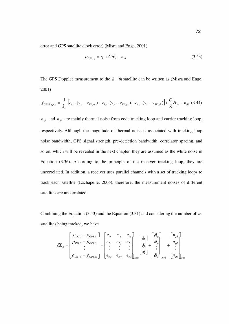
72
error and GPS satellite clock error) (Misra and Enge, 2001)
kukkGPS ntCr ρδρ ++=, (3.43)
The GPS Doppler measurement to the thk − satellite can be written as (Misra and Enge,
2001)
[ ] dkruzkSVzkzykSVykyxkSVxkx
L
kGPSdopp ntC
vvevvevvef ++−⋅+−⋅+−⋅= δλλ
)()()(1
,,,,
1
(3.44)
knρ and dkn are mainly thermal noise from code tracking loop and carrier tracking loop,
respectively. Although the magnitude of thermal noise is associated with tracking loop
noise bandwidth, GPS signal strength, pre-detection bandwidth, correlator spacing, and
so on, which will be revealed in the next chapter, they are assumed as the white noise in
Equation (3.36). According to the principle of the receiver tracking loop, they are
uncorrelated. In addition, a receiver uses parallel channels with a set of tracking loops to
track each satellite (Lachapelle, 2005), therefore, the measurement noises of different
satellites are uncorrelated.
Combining the Equation (3.43) and the Equation (3.31) and considering the number of m
satellites being tracked, we have
1
2
1
13
222
111
,,
2,2,
1,1,
×××
+
+
=
−
−
−
=
mmmu
u
u
mmzmymx
zyx
zyx
mGPSmINS
GPSINS
GPSINS
n
n
n
t
t
t
z
y
x
eee
eee
eee
ρ
ρ
ρ
ρ
δ
δ
δ
δ
δ
δ
ρρ
ρρ
ρρ
δMMMMMM
Z
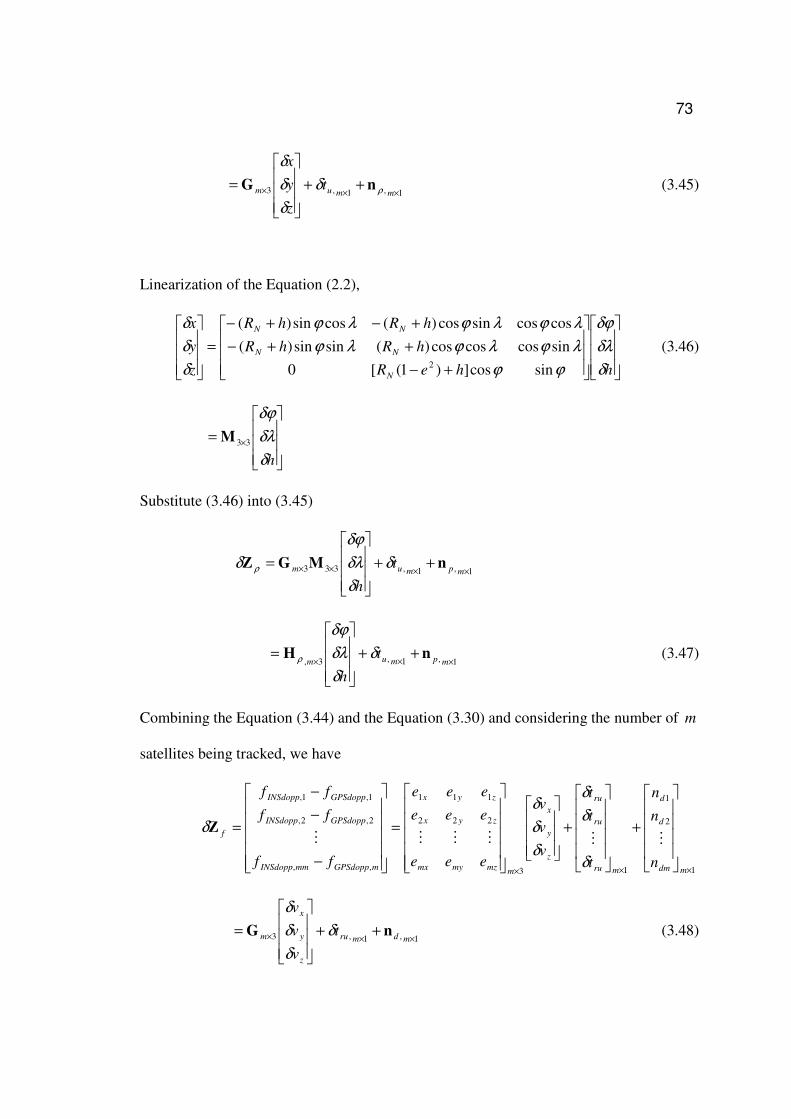
73
1,1,3 ××× ++
=mmum t
z
y
x
ρδ
δ
δ
δ
nG (3.45)
Linearization of the Equation (2.2),
+−
++−
+−+−
=
hheR
hRhR
hRhR
z
y
x
N
NN
NN
δ
δλ
δϕ
ϕϕ
λϕλϕλϕ
λϕλϕλϕ
δ
δ
δ
sincos])1([0
sincoscoscos)(sinsin)(
coscossincos)(cossin)(
2
(3.46)
= ×
hδ
δλ
δϕ
33M
Substitute (3.46) into (3.45)
1,1,333 ×××× ++
=mpmum t
h
nMGZ δ
δ
δλ
δϕ
δ ρ
1,1,3, ×××++
=mpmum
t
h
nH δ
δ
δλ
δϕ
ρ (3.47)
Combining the Equation (3.44) and the Equation (3.30) and considering the number of m
satellites being tracked, we have
1
2
1
13
222
111
,,
2,2,
1,1,
×××
+
+
=
−
−
−
=
mdm
d
d
mru
ru
ru
z
y
x
mmzmymx
zyx
zyx
mGPSdoppmmINSdopp
GPSdoppINSdopp
GPSdoppINSdopp
f
n
n
n
t
t
t
v
v
v
eee
eee
eee
ff
ff
ff
MMMMMM
δ
δ
δ
δ
δ
δ
δZ
1,1,3 ××× ++
=mdmru
z
y
x
m t
v
v
v
nG δ
δ
δ
δ
(3.48)

74
According to the definition of the rotation matrix e
lR , illustrated in the Equation (2.3), we
have
=
U
N
E
e
l
z
y
x
v
v
v
v
v
v
δ
δ
δ
δ
δ
δ
R (3.49)
Substitute (3.49) into (3.48)
1,1,3 ××× ++
=mdmru
U
N
E
e
lmf t
v
v
v
nRGZ δ
δ
δ
δ
δ
1,1,3, ×××++
=mdmru
U
N
E
mf t
v
v
v
nH δ
δ
δ
δ
(3.50)
Consequently, the system’s measurement equation is written as
nxHZ += δδ (3.51)
where
=
fZ
ZZ
δ
δδ
ρ is the observable vector, and
n is the measurement noise vector, which is expressed as
[ ]TT
d
Tnnn ρ= , and
H is the design matrix, which is expressed as
T
mcmmfm
mmcmm
=
××××
××××
1163,3
11183,
,
,
H0H0
0H0HH
ρ (3.52)
where [ ]T
mc ×=
1111 LH .

75
3.5 Performance Tests and Analysis
A field test was conducted around Springbank, Alberta in December 2005. The data from
an ADI MEMS INS and a NovAtel’s OEM4 receiver single point positioning were
collected. The OEM4 GPS antenna was mounted on the roof of a van. At the same time, a
tactical grade INS, LN200, was mounted inside the van to provide the reference
trajectory. The trajectory was acquired from the smoothed estimate of the LN200 and
differential GPS data processed by Applanix Corporation POSPac™ software. The
system setup is shown in Figure 3.5.
Figure 3.5: Field test setup
The ADI MEMS INS was powered by 9V batteries while the power of LN200 was
supplied from an external 24V battery cell. The OEM4 receiver was powered by the 12V
outlet in the van. In addition, a NordNav receiver antenna that was connected to the
NordNav front-end was also mounted on the roof of the van to record datasets used in the
Chapter 5.
OEM4 antenna NordNav antenna ADI MEMS INS
LN200 INS
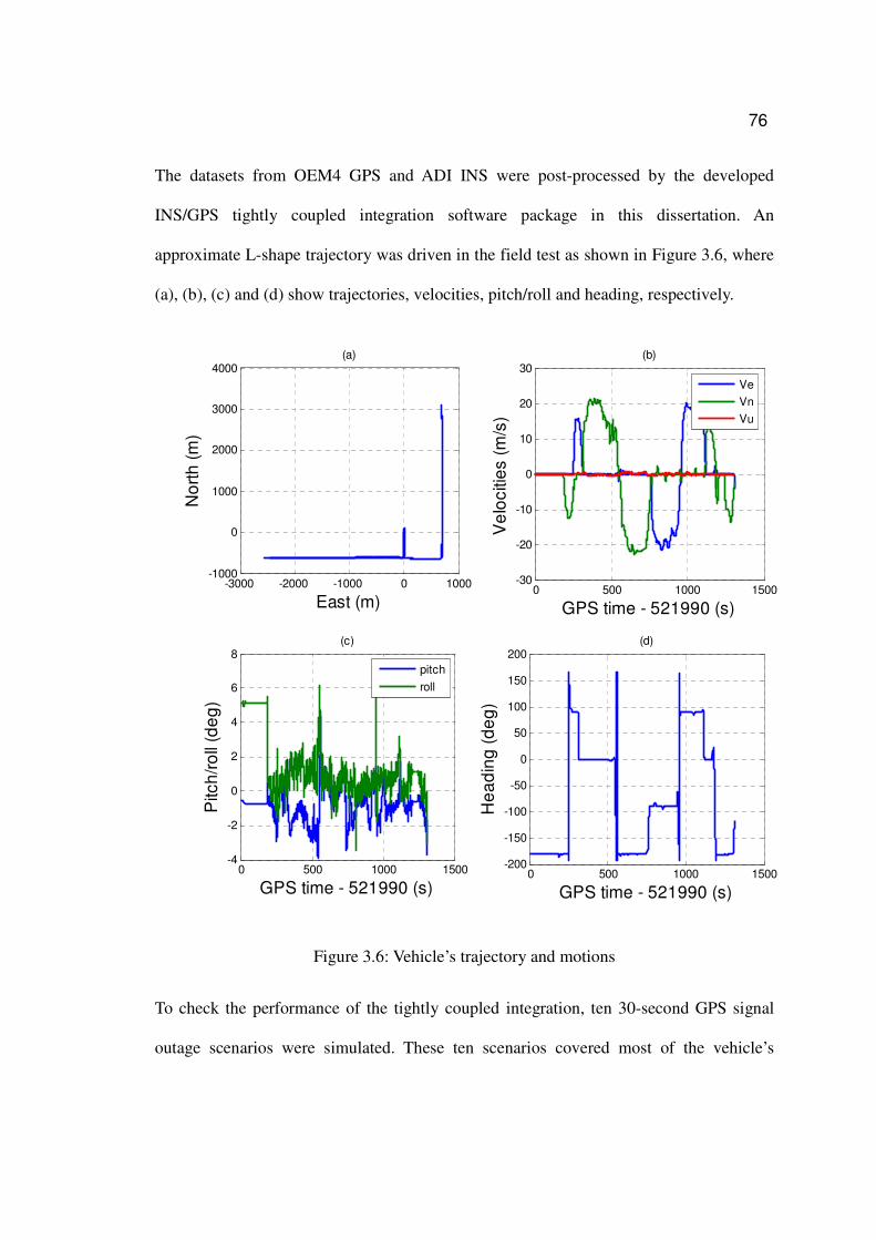
76
The datasets from OEM4 GPS and ADI INS were post-processed by the developed
INS/GPS tightly coupled integration software package in this dissertation. An
approximate L-shape trajectory was driven in the field test as shown in Figure 3.6, where
(a), (b), (c) and (d) show trajectories, velocities, pitch/roll and heading, respectively.
-3000 -2000 -1000 0 1000-1000
0
1000
2000
3000
4000
East (m)
No
rth
(m
)
(a)
0 500 1000 1500-30
-20
-10
0
10
20
30
GPS time - 521990 (s)
Ve
lociti
es (
m/s
)
(b)
Ve
Vn
Vu
0 500 1000 1500-4
-2
0
2
4
6
8
GPS time - 521990 (s)
Pitc
h/r
oll
(de
g)
(c)
pitch
roll
0 500 1000 1500-200
-150
-100
-50
0
50
100
150
200
GPS time - 521990 (s)
He
ad
ing
(d
eg
)
(d)
Figure 3.6: Vehicle’s trajectory and motions
To check the performance of the tightly coupled integration, ten 30-second GPS signal
outage scenarios were simulated. These ten scenarios covered most of the vehicle’s

77
dynamics, such as static periods, accelerations, decelerations, turns, U-turns, tilts, and so
on. During each outage period, it is assumed that fewer than four GPS satellites are being
tracked to simulate the urban canyon environments. The satellite geometry is selected
randomly, which means that the PRN of satellites being tracked is not fixed and the signs
of the azimuth of satellites might be same (satellites on one side of the vehicle) or
different (satellites on both sides of the vehicle). Figure 3.7 and Figure 3.8 show the
navigation errors and the receiver clock errors about an example with two satellites being
tracked. Table 3.2 lists the results of the 3D position error rδ , velocity error Vδ , and
heading error Aδ during the simulated ten GPS signal outage periods. Table 3.3 compares
mean values of the navigation errors for different situations where only 3 satellites, 2
satellites, 1 satellite, or 0 satellite is being tracked, respectively.

78
0 200 400 600 800 1000 1200 1400-100
-50
0
50
100
Time - 521990 (s)
Po
siti
on
err
or (m
) Position Error when 2 satellites
East
North
Up
0 200 400 600 800 1000 1200 1400-10
-5
0
5
Time - 521990 (s)
Ve
locity
err
or
(m/s
) Velocity Error when 2 satellites
East
North
Up
0 200 400 600 800 1000 1200 1400-20
0
20
40
60
Time - 521990 (s)
Attitu
de
err
or (d
eg)
Attitude Error when 2 satellites
Pitch
Roll
Heading
Figure 3.7: PVA errors for 2 satellites case

79
0 200 400 600 800 1000 1200 1400-10
-5
0
5
10
Time - 521990 (sec)
Clo
ck b
ias (
m)
Receiver Clock bias when 2 satellites
0 200 400 600 800 1000 1200 14000
5
10
Time - 521990 (sec)
Clo
ck d
rift (
Hz)
Receiver Clock drift when 2 satellites
Figure 3.8: Clock errors for 2 satellites case
Table 3.2: Individual errors during 10 GPS signal outage periods
No. of outage periods (2 satellites only) errors
1 2 3 4 5 6 7 8 9 10 Mean / σ1
)(mrδ 88.4 19.1 5.0 71.8 10.1 36.5 27.4 39.6 3.7 12.9 31.4 (mean)
)/( smVδ 8.8 1.5 0.4 4.4 0.3 3.2 2.6 2.6 0.1 0.4 2.4 (mean)
(deg)Aδ 19.4 45.5 8.6 6.1 1.0 4.7 0.7 4.4 1.4 6.9 9.4 (mean)

80
Table 3.3: Errors comparison of different numbers of satellites being tracked
numbers of
Satellites
)(mrδ
(mean)
)/( smVδ
(mean)
(deg)Aδ
(mean)
3 < 7.0 < 0.2 8.4
2 31.4 2.4 9.4
1 40.1 3.2 9.9
0 40.3 3.1 10.1
The results from the above figures and tables reveal that 1) the tightly coupled INS/GPS
can work well under the environment with fewer than four satellites, which is superior to
the loose couple; 2) the navigation errors increase dramatically during static periods
because of the bad observability in EKF; 3) fewer satellites being tracked result in worse
navigation performance due to the worse satellites geometry; 4) The navigation errors
with 1 satellite in-view are almost the same as that of the case of no satellite available. Its
estimation errors are also associated with both the vehicle’s dynamics and the satellite
geometry. There is a large standard deviation in the clock drift estimation in the case of
only one satellite being tracked. The clock drift estimate is to be used for the INS aided
GPS tracking loop discussed the Chapter 5 of this dissertation.
3.6 Using Non-holonomic Constraint
For land vehicle navigation, non-holonomic constraint is a popular method to improve
the navigation accuracy. Non-holonomic constraint refers to the fact that unless the

81
vehicle jumps off the ground (along z-axis) or slides on the ground (along x-axis), the
velocity of the vehicle in the plane perpendicular to the forward direction (along y-axis)
is almost zero (Sukkarieh, 2000; Shin, 2001). Therefore, two non-holonomic constraints
can be considered as additional measurement updates in addition to the GPS pseudorange
and Doppler measurements to the EKF.
Thus, the above concept can be described mathematically by
vbz
b
z
vbx
b
x
nV
nV
+≈
+≈
0
0 (3.53)
where vbxn and vbzn is the measurement noise value denoting any possible discrepancies
in the above stated assumptions for a particular direction (x or z). The magnitude of the
noise is chosen to reflect the extent of the expected constraint violations (Sukkarieh 2000;
Godha, 2006).
The estimation of the velocity in the b-frame b
ibV can be acquired by
)(ˆˆˆ l
ib
l
ib
b
l
l
ib
b
l
bb
ib
b
ib vVRVRvVV δδ +==+= (3.54)
where
[ ]Tb
z
b
y
b
x
b
ib VVV=V is the land vehicle’s true velocity in the b-frame;
[ ]Tb
z
b
y
b
x
bvvv δδδδ =v is the velocity error vector in the b-frame;
b
lR is the computed DCM, which is expressed by the Equation (3.16);
l
ibV is the vehicle’s velocity in the b-frame with respect to the i-frame
projected in the l-frame, and l
ibvδ is its corresponding error vector.

82
l
ibV can be mathematically expressed as
)( l
lb
ll
ie
b
l
b
ib VVVRV ++=
where l
ieV represents the Earth’s computed rectilinear motions with respect to the i-frame.
According to the frame definitions in the Chapter 2, l
ieV should be equal to a zero vector
if the Earth’s auto-rotation is the only motion considered with respect to the i-frame. l
lbV
represents the rectilinear motions between the b-frame and the l-frame. Similarly, l
lbV
should be equal to a zero vector due to the same origin according to the frame definitions.
Thus, we have lb
l
b
ib VRV = and ll
ib Vv δδ = .
So, the Equation (3.53) can be re-written as
))(( llb
l
bb
ib VVEIRvV δδ ++=+ (3.55)
Collecting terms to the first order, we have
εVRVRv )( ×−= lb
l
lb
l
b δδ (3.56)
Using non-holonomic constraint, we have the followed measurements
=
b
z
b
x
non-holv
v
δ
δδZ (3.57)
Therefore, the corresponding design matrix non-holH can be written as
[ ]14232232132 ,, ××−×−×= 0HH0H nonnonnon-hol (3.58)
where
=
)3,3()2,3()1,3(
)3,1()2,1()1,1(1 b
l
b
l
b
l
b
l
b
l
b
l
non-RRR
RRRH ,

83
−+−−
−+−−=
)2,3()1,3()3,3()1,3()3,3()2,3(
)2,1()1,1()3,1()2,1()3,1()2,1(2 b
l
Eb
l
Nb
l
Eb
l
Ub
l
Nb
l
U
b
l
Eb
l
Nb
l
Eb
l
Ub
l
Nb
l
U
non-RVRVRVRVRVRV
RVRVRVRVRVRVH
where,
),( jib
lR represents an element of b
lR located on the thi − row and the
thj − column.
Repeat the tests given in the above section. Figure (3.9) shows the navigation errors for
the case of two satellites being tracked and using non-holonomic constraint.
0 200 400 600 800 1000 1200-100
0
100
Time - 521990 (s)
Po
siti
on
err
or
(m) Position Error when 2 satellites
East
North
Up
0 200 400 600 800 1000 1200-10
-5
0
5
Time - 521990 (s)Ve
locity
err
or (m
/s)
Velocity Error when 2 satellites
East
North
Up
0 200 400 600 800 1000 1200-20
0
20
40
60
Time - 521990 (s)
Attitu
de
err
or
(de
g) Attitude Error when 2 satellites
Pitch
Roll
Heading
Figure 3.9: PVA errors for 2 satellites case by using non-holonomic constraint
Table 3.4 gives the results and improvements of navigation errors for 3 or 2 or 1 or 0

84
satellite(s) cases. The results clearly show that the non-holonomic constraint significantly
improves the navigation performance for periods of signal outage. It is an attractive
technique for land vehicle’s navigation. Normally, such a velocity constraint provides
more contributions to fewer satellites case. However, compared Figure 3.9 and 3.7, we
should note that the non-holonomic constraint has less improvements during static
periods because of the actual zero velocities along the b-frame. Furthermore, the
percentage of the improvement to the heading error decreases with the reduction of the
number of satellites. That is because that the worse satellite geometry results in the worse
velocity measurement update. From the view of the Kalman filter, the system relies more
on the prediction rather than the update under the worse geometry. In INS/GPS tight
couple integration, the prediction process of EKF is heavily dependent of INS behaviors,
where the heading error is weakly coupled with east velocity error due to Schuler effect
(El-Sheimy, 2006). Therefore, the non-holonomic constraint contributes less to the
heading error improvement in fewer satellites case.
In addition, from the principle of the non-holonomic, the use of this constraint provides
limited improvements in the forward direction. To prevent error growth in the forward
direction an odometer can be used alongside velocity constraints (e.g. Nassar et al.,
2006). Currently, the use of an odometer in a land vehicle is somehow compromised by
its cost and complexity.

85
Table 3.4: Navigation errors and their improvement by using non-holonomic
numbers of
Satellites
)(mrδ
(mean)
)/( smVδ
(mean)
(deg)Aδ
(mean)
errors < 7.0 < 0.1 3.5 3
improvement --- 50% 58%
errors 13.8 1.1 4.6 2
improvement 56% 54% 51%
errors 15.5 1.3 8.3 1
improvement 62% 59% 16%
errors 15.2 1.4 8.3 0
improvement 62% 55% 18%
3.7 Sub-optimal Tightly Coupled
In the current low-end navigation product markets, it is a trend to integrate a GPS
receiver and a low cost MEMS INS into one single application-specific integrated circuit
(ASIC) chip. With the development of the MEMS inertial sensor technology, the cost is
not a bottleneck, but the size of inertial sensor triads discourages such integration since
the pitch gyroscope and the roll gyroscope occupy a relatively large space in an INS. To
minimize the size of the INS, we are considering using a sub-optimal INS configuration
with one heading gyroscope and two level accelerometers (1G2A) to achieve INS/GPS
tightly coupled integration. 1G2A configuration is shown in Figure 3.10.
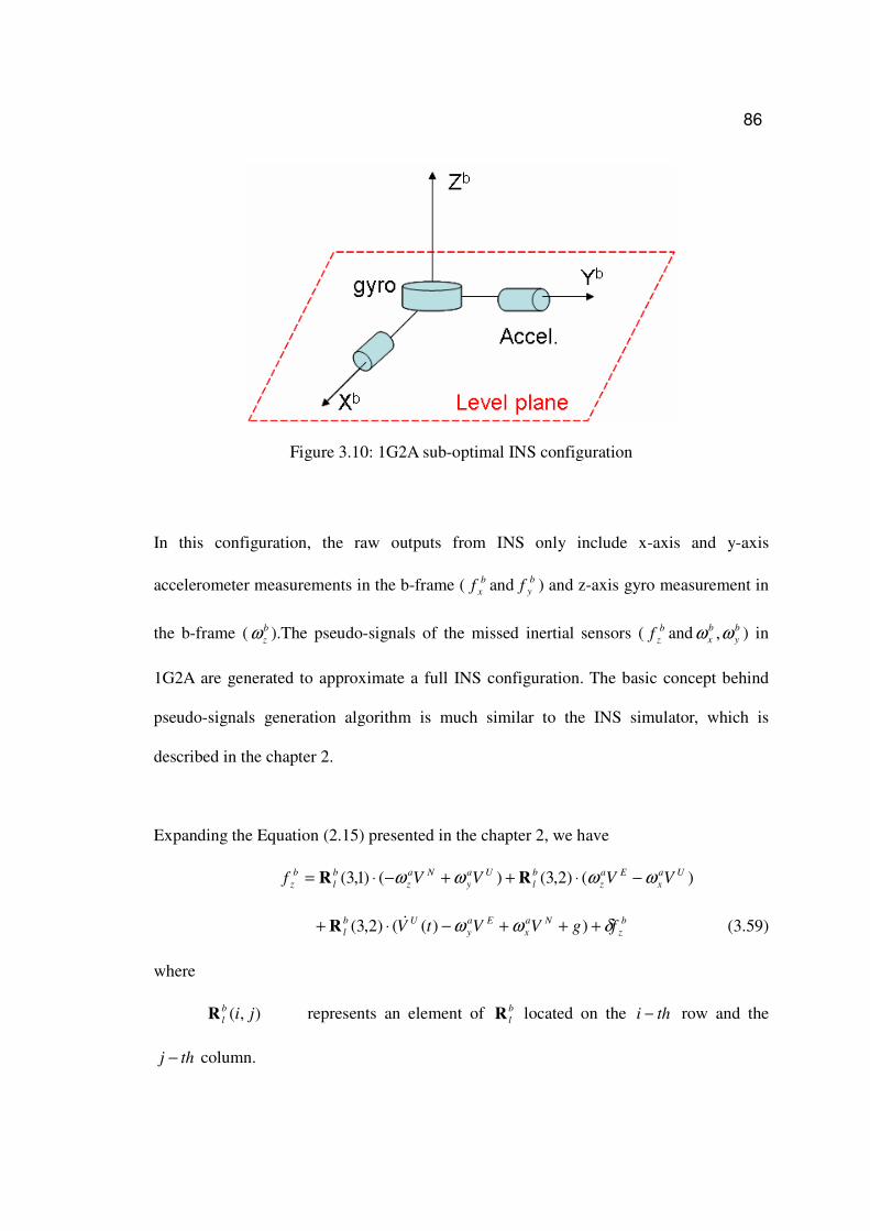
86
Figure 3.10: 1G2A sub-optimal INS configuration
In this configuration, the raw outputs from INS only include x-axis and y-axis
accelerometer measurements in the b-frame ( b
xf and b
yf ) and z-axis gyro measurement in
the b-frame ( b
zω ).The pseudo-signals of the missed inertial sensors ( b
zf and b
y
b
x ωω , ) in
1G2A are generated to approximate a full INS configuration. The basic concept behind
pseudo-signals generation algorithm is much similar to the INS simulator, which is
described in the chapter 2.
Expanding the Equation (2.15) presented in the chapter 2, we have
)()2,3()()1,3( Ua
x
Ea
z
b
l
Ua
y
Na
z
b
l
b
z VVVVf ωωωω −⋅++−⋅= RR
b
z
Na
x
Ea
y
Ub
l fgVVtV δωω +++−⋅+ ))(()2,3( &R (3.59)
where
),( jib
lR represents an element of b
lR located on the thi − row and the
thj − column.

87
g is the normal gravity;
l
el
l
ie
a
z
a
y
a
x
ωω +=
2
ω
ω
ω
;
)(tV U& is the upward acceleration in the l-frame. Considering a limited
dynamics in the land vehicle )( g< , it can be calculated by
dt
dttVdttVtV
UUU )2()(
)(−−−
≈& ;
b
zfδ represents the modeled error of z-axis accelerometer pseudo-
measurements, which is different from b
ibfδ presented in the
Equation (2.15). This error comes from the approximation process
in the pseudo-signal generation. A 1st order GM is used to model it.
Expanding the Equation (2.21), we have
b
x
b
xlb
g
z
b
l
g
y
b
l
g
x
b
l
b
x δωωωωωω ++⋅+⋅+⋅= ,)3,1()2,1()1,1( RRR (3.60)
b
y
b
ylb
g
z
b
l
g
y
b
l
g
x
b
l
b
y δωωωωωω ++⋅+⋅+⋅= ,)3,2()2,2()1,2( RRR (3.61)
where
)( l
el
l
ie
g
z
g
y
g
x
ωω +=
ω
ω
ω
, and
b
y
b
x δωδω , represent the modeled errors of x-axis and y-axis gyros’ pseudo-
measurements. 1st order GMs are used to model them.

88
=
A
r
p
rpr
p
rprb
lb
&
&
&
coscos0sin
sin10
sincos0cos
ω , which is already described in the Equation
(2.22), where
dt
dttrdttrtr
)2()()(
−−−≈& and
dt
dttpdttptp
)2()()(
−−−≈& .
To further explain the general algorithm of the pseudo-signal generation for 1G2A,
Figure (3.11) presents the flow chart of 1G2A used in INS/GPS. It takes 100Hz INS and
1Hz GPS as an example. According to the flow chart, the algorithm implementation of
1G2A INS/GPS has the followed nine steps: 1) use the initial PVA information and zero
attitude rate and zero vertical velocity rate to generate the first set of pseudo-signals
based on the Equation (3.59) – (3.61); 2) combine the generated pseudo-signals and the
measured real INS signals to form a full INS measurement; 3) perform INS
mechanization to derive INS PVA; 4) predict state errors through EKF prediction and
then correct INS PVA errors; 5) calculate attitude rate and vertical velocity rate by time
differential based on the current PVA and the previous PVA; 6) generate the next epoch
pseudo-signals based on the Equation (3.59) – (3.61); 7) repeat step 2 to step 6 till GPS
measurement is ready; 8) EKF update using GPS information and correct INS PVA
errors; 9) repeat step 7 and step 8.

89
Figure 3.11: Flow chart of 1G2A INS/GPS using INS pseudo-signals
90
It should be noted that a very basic assumption of the above signal generation is that there
are no dramatic change in pitch angle and roll angle during one GPS update cycle, so
pitch rate and roll rate are small. In addition, the large noise covariance matrix for the
pseudo-signals is recommended in the algorithm implementation because of the time
differential approximation and the correlated signals.
Figure 3.12 shows the navigation errors of 1G2A sub-optimal INS configuration for the
case of two satellites being tracked with non-holonomic constraint. Comparing Figure
(3.12) with Figure (3.9), we should note that 1G2A has larger navigation errors during
static periods than full-INS configuration. That is because 1) the attitude is hard to be
observed directly through position and velocity measurements. The EKF converges
slowly during the static periods due to the weak observability so that no sufficient
correction information can be provided to the attitude drift; 2) in addition, the non-
holonomic constraint takes effect on the level directions, but it does nothing along the
vehicle’s vertical axis. The errors of pitch and roll are smaller because there are coupled
with the level (east and north) velocities (El-Sheimy, 2006), even though the couplings
are weak. But the heading error is large; 3) furthermore, two satellites give a poor
geometry. The EKF relies more on the prediction rather than the update under such a
situation. The prediction only process for the MEMS grade INS results in large errors.
However, combining the Equation (3.60), (3.61) and Equation (2.22) and checking with
the vehicle’s trajectory/motions shown in Figure (3.6), we can note that the small errors
in pseudo signal generation will result in large inertial sensor errors. For example, o1 of
heading error with 100Hz INS rate at o5 roll angle in the pseudo-signal generation

91
process is roughly equivalent to a o1.7 / s bias to the pseudo x-gyro. This bias contributes
to the heading errors through l
bR . That is why a very large heading error is presented in
the figure. In addition, similar to the heading error analysis during static periods, from the
Equation (3.59), the z-axis accelerometer output is mainly determined by the coupling of
the normal gravity and l
bR . For example, o1 of pitch error at o0 heading angle is roughly
equivalent to a gµ17000 bias to the pseudo z-axis, which is huge enough to form a peak
at the 600-th second in the figure.
0 200 400 600 800 1000 1200 1400-200
-100
0
100
Time - 521990 (s)
Po
sitio
n e
rro
r (m
) Position Error when 2 satellites
East
North
Up
0 200 400 600 800 1000 1200 1400-10
-5
0
5
Time - 521990 (s)
Ve
locity e
rro
r (m
/s)
Velocity Error when 2 satellites
East
North
Up
0 200 400 600 800 1000 1200 1400-100
0
100
200
Time - 521990 (s)
Attitu
de
err
or
(de
g) Attitude Error when 2 satellites
Pitch
Roll
Heading
Figure 3.12: PVA errors for 2 satellites case (1G2A, non-holonomic)

92
Table 3.5: Errors comparison in 1G2A INS configuration with using non-holonomic
numbers of
Satellites
)(mrδ
(mean)
)/( smVδ
(mean)
(deg)Aδ
(mean)
3 <7 <0.2 22.4
2 26.1 1.9 23.1
1 37.3 2.3 42.5
0 39.6 2.3 43.4
3.8 Summary
First, this chapter clearly defines the INS/GPS integration schemes, i.e. loose couple,
tight couple and deep couple. Second, the chapter introduces the MEMS inertial sensor
based INS and the estimation mathematical tool (discrete EKF) for the integration
system. With derivations of INS errors and GPS errors, this chapter develops an EKF
based MEMS INS/GPS tightly coupled integration algorithm. The state vector has 23
states related to INS and GPS system errors. The pseudorange and Doppler
measurements from both INS and GPS are used as the observables for the EKF.
Specifically, to improve the navigation accuracy for land vehicle application, one
constraint was derived, namely the non-holonomic constraints. Furthermore, a pseudo-
signal generation method is proposed in the last section of this chapter.
The results and analyses based on the field test data set reveal that 1) the tightly coupled
INS/GPS can work well under the environment with fewer than four GPS satellites; 2)

93
fewer satellites being tracked result in worse navigation performance due to the worse
satellites geometry; 3) the receiver’s clock errors’ estimation are associated with both the
vehicle’s dynamics and the satellite geometry; 4) by using non-holonomic constraint for
land vehicle application, the position accuracy can be improved by around 60%; 5)
suboptimal INS/GPS tight integration with 1G2A INS configuration can maintain the
system positioning error smaller than 7m, 27m, 38m, or 40m during 30s GPS signal
outage environment, with 3, 2, 1 or 0 satellite(s) in-view, respectively.

94
Chapter 4 GPS Receiver Tracking Loop and Its Parameters
In a GPS receiver the signal is processed to obtain the required information, which in turn
is used to calculate the user position. Therefore, at least two areas of discipline, receiver
technology and navigation scheme, are employed in GPS receivers. This chapter
investigates the signal processing of a software method based GPS L1 C/A receiver. It
focuses on the receiver carrier tracking loop. Section 4.1 gives an overview of the GPS
receiver signal processing. The received signals from RF to baseband are mathematically
described. Section 4.2 investigates the operations of receiver signal tracking loops
including accumulation and dump, discriminators and loop filters. In Section 4.3 the
tracking capabilities of a 2nd order PLL are analyzed in details through simulated
experiments.
4.1 GPS Receiver Signal Processing
4.1.1 GPS L1 Signals
This research is only about the current L1 C/A code in GPS system. Mathematically, L1
C/A code GPS signals arriving at antenna may be represented by (Raquet, 2006;
Lachapelle, 2005):
)()()(1
tntstrm
k
k +=∑=
(4.1)
where
mk L,2,1= represents the number of satellites in view;
n(t) is the receiver noise;
)(ts k is the L1 C/A signal from k-th satellite. It can be expressed as:

95
])cos[()()()( 00 φωω ++= ttDtCAts d (4.2)
where
A is signal amplitude;
( )tC is C/A PRN code modulation (±1);
( )tD is 50 bps navigation data modulation (±1);
0ω is equal to 02 fπ ; carrier frequency =0f 1575.42 MHz for L1;
dω is the angular Doppler frequency due the LOS motions, clock drift and
propagation delay;
0φ is the nominal (but ambiguous) carrier phase.
In order not to interfere with the existing terrestrial wireless communication and
broadcast services, the currently received GPS signal power is set very low. The received
GPS signals by an antenna combines signals from all satellites in view with noise, and the
minimum specified received signal only carries 1610− watts, i.e. -160 dBW, for the
satellites located near the zenith or horizon (Lachapelle, 2005). In addition to this
characteristically low signal power, the high chipping rate PRN code spreads the signal
power over a wide bandwidth, thus resulting in a signal’s power spectral density (PSD)
below the usual ambient noise PSD level. The ambient noise can be approximately 60
(zenith) to 400 ( o5 elevation) times stronger than the C/A L1 signal from one satellite
(Misra and Enge, 2001). Since the PSD of GPS C/A signals is overwhelmed by that of
the noise, the GPS signal cannot be detected directly in L1 band, e.g. using classical tools

96
such as an oscilloscope. The receiver antenna captures this tiny signal and converts it into
the voltages and currents that the front-end can process.
Receiver performance is more dependent on a signal-to-noise ratio (SNR) than the
absolute signal power (Raquet, 2006). SNR is a ratio of signal power to noise power as
shown in Equation (4.3) (Tsui, 2000). The noise power depends on the processing
bandwidth of the GPS receiver.
BN
SSNR
20
= (4.3)
where,
B is the single bandwidth of the filter in the receiver to remove the out of
band noise (Raquet, 2006);
S is the signal power within the bandwidth of nB ;
0N is noise power density.
In practice, the ratio of total carrier power to the noise density 0/ NC in dB-Hz is the
most generic representation of signal power as it is independent of the implementation of
the receiver front-end bandwidth. The relationship of SNR and 0/ NC can be
represented as (Lian, 2004):
)()(/)( 0 HzBHzdBNCdBSNR −−= (4.4)
4.1.2 GPS Receiver Technology
The standard GPS receiver components can be broadly classified into one of the three
97
categories (Ledvina, 2004; Lachapelle, 2005) 1) the radio-frequency (RF) front-end
section; 2) the core intermediate frequency (IF) signal processing section; 3) the
navigation signal processing section. The IF signal processing is the heart of a GPS
receiver that performs most demanding tasks, a combination of hardware and software.
Navigation processing generates position, velocity and time from pseudorange, phase
and/or Doppler measurements. It has additional application specific software.
The generic architecture of a GPS receiver is illustrated Figure 4.1. The signals
transmitted from the GPS satellites are gathered by an omni-directional antenna.most
antenna are actually more hemi-spherial Through the receiver’s FE unit the RF is
amplified to proper amplitude and the frequency is down converted, filtered, and
digitized to a desired IF signal. Typical GPS receivers have 8 to 12 channels. Each
channel uses the same sampled IF data from the RF section. However, each channel locks
onto a different satellite. The receiver has high-level executive software that controls
which channels track which satellites (via unique C/A PRN code), when to declare if lock
has been lost, and when to reacquire. It tracks a particular PRN code and can change
tracked PRN while running. Each SV is tracked in one channel, even if more than one
signal (C/A code, L1 P-code, L2 P-code) is tracked.

98
Figure 4.1: Generic diagram of a software based GPS receiver (After Tsui, 2000)
4.1.3 Front-End
An antenna receives the RF GPS signal and filters out the interferences such as signals
outside the desired band and reflected signals of left hand circular polarization (Ray
2005). Then the signal is strengthened by a low noise amplifier (LNA) housed in the
antenna, and is fed into the FE. The FE down-converts the signal from L band to IF and
amplifies the signal to a workable level for digitization.
The FE of the receiver conditions the received signal described by equations (4.1) and
(4.2). The FE must down convert the frequency by a factor of 100 to 1000 to a lower one,
IF, which is more manageable by the rest of the receiver. Down conversion from RF to IF
is mathematically based on the trigonometric identity. It is accomplished by mixing the
incoming signal and noise with a local oscillator (LO) signal with the angular frequency
of 1ω . This process is illustrated in the first part of Figure 4.2 (Charkhandeh, 2007). The
IF signals can be expressed as (Raquet, 2006):
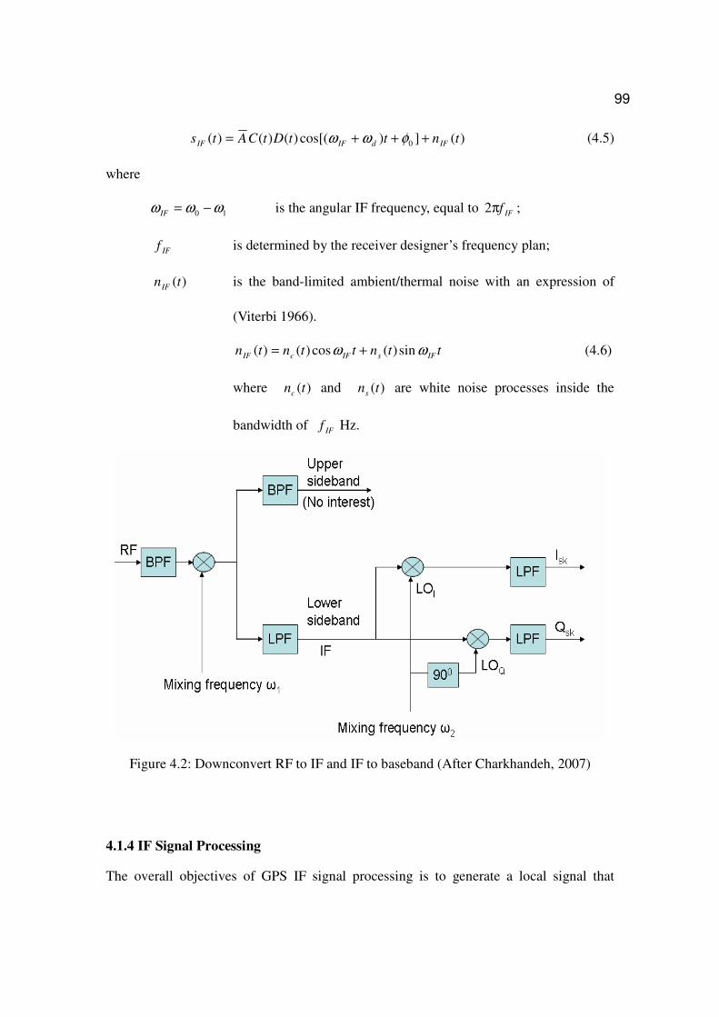
99
)(])cos[()()()( 0 tnttDtCAts IFdIFIF +++= φωω (4.5)
where
10 ωωω −=IF is the angular IF frequency, equal to IFfπ2 ;
IFf is determined by the receiver designer’s frequency plan;
)(tnIF is the band-limited ambient/thermal noise with an expression of
(Viterbi 1966).
ttnttntn IFsIFcIF ωω sin)(cos)()( += (4.6)
where )(tnc and )(tns are white noise processes inside the
bandwidth of IFf Hz.
Figure 4.2: Downconvert RF to IF and IF to baseband (After Charkhandeh, 2007)
4.1.4 IF Signal Processing
The overall objectives of GPS IF signal processing is to generate a local signal that

100
exactly matches the incoming signal. If this could be done perfectly, then measurements
could be found using the local signal only (since it is known). The received signal
described by equation (4.5) is then split into two branches. One branch is multiplied by
the in-phase mixing carrier, and the other one is multiplied by a quadrature-phase mixing
carrier (shifted by 90°, as compared to the in-phase carrier replica), as shown in the
second part of Figure 4.2. This processing wipes off the signal carrier and downconverts
the signal to baseband. The in-phase and quadrature-phase mixing signals are ILO and
QLO , respectively, as:
)cos(2 2tLOI ω= )sin(2)2/cos(2 22 ttLOQ ωπω −=+=
Therefore, the sampled in-phase signal and quadrature signal can be written as (Raquet,
2006):
Iskkkksk nDCA
I += )cos(2
φ (4.7)
Qskkkksk nDCA
Q += )sin(2
φ (4.8)
with the phase of
0)( φωωφ ++= kdBk t (4.9)
where
Bω is the baseband angular frequency of the signal, and 2ωωω −= IFB
4.1.4.1 Acquisition
The baseband samples are correlated with the local carrier replica (Doppler removal) and
the local code replica (correlation), and passed through the accumulation and dump filter
to achieve the coherent units, which are fed into the receiver’s acquisition and tracking

101
process. Acquisition is the first step in processing the sampled GPS baseband data. This
process separates the signals from satellites in view and allocates each satellite’s signal in
one of receiver’s parallel channels since those coherent units include the information for
all the visible satellites. The three key parameters to be determined during acquisition are
the C/A codes (for the satellites in view), their respective C/A code phases and carrier
frequencies (with individual Doppler shifts) (Lachapelle, 2005). Once the presence of
signals is detected, the resulting information is used by a bank of signal tracking
components to track the signal.
To acquire a signal, the receiver generates a replica of the known C/A code, and attempts
to align it with the incoming code by sliding the replica in time and computing the
correlation. From the auto-correlation property of the signal, the correlation function
exhibits a sharp peak when the code replica is aligned with the code received from the
satellite (Dong, 2003; Gregory and Garrison, 2004). The maximum uncertainty in
matching the replica with the incoming code is limited to only 1023 code chips. The
acquisition fundamentals described in many literatures, e.g. Kaplan (1996), Lin (2000),
Psiaki (2004), and the reader can refer to these references for details.
4.1.4.2 Tracking
After signal down conversion and acquisition, the sampled GPS baseband signal is sent
into the signal tracking loops for carrier phase and code delay coherent tracking to
recover the incoming signal accurately (Kaplan, 1996). Typically, the frequency and
range of incoming signals are constantly changing. Satellites dynamics cause Doppler

102
changes up to sHz /9.0 and code phase offset changes up to schips /3 (Tsui, 2000). The
LOS receiver dynamics between the satellite and receiver antennas cause additional
Doppler changes. High accelerations cause faster change in Doppler. In addition, the LO
used in the RF front end will have an associated frequency drift. Therefore, the tracking
process not only refines the rough estimates from the acquisition, but follows the carrier
Doppler and the code offset for each visible satellite due to the LOS motion between the
satellite and the receiver and the receiver’s clock drift. Unfortunately, a pure PLL can not
distinguish the LOS motion and the clock drift.
To track an incoming GPS signal, the replica of the local carrier frequency and code
offset needs to be matched with that. There are two or three tracking loops in each
channel: the DLL that tracks the spreading code delay; the PLL that synchronizes the
carrier phase, and/or the frequency-locked loop that tracks the signal Doppler. These
loops are normally coupled together, as shown in Figure 4.3.

103
Figure 4.3: Block diagram of tracking Loops (After Raquet, 2006)
As shown in the Figure 4.3, the inputs at Doppler removal unit are the baseband samples
skI and skQ described in Equations (4.7) and (4.8). Doppler removal is actually a process
of carrier removal since it removes the entire Doppler plus carrier at baseband frequency.
The output signals of Doppler removal can be written as,
kIrefkKkk nDCA
I 11 )ˆcos(2
+−= φφ (4.10)
kQrefkKkk nDCA
Q 11 )ˆsin(2
+−= φφ (4.11)
Based on the Figure 4.3 and Equation (4.9), we know that the output frequency after
Doppler removal is the difference between the true Doppler (Df ) and the receiver’s best

104
estimated Doppler ( Df ). If Df is accurate enough, we have kref φ≈φ (ignoring nominal
phase error temporary). Therefore,
kIKkk nDCA
I 11
2+= (4.12)
kQk nQ 11 0 += (4.13)
It indicates that the navigation data are only presented on the in-phase signal when the
signal is well tracked. In a traditional receiver, Df is acquired by the PLL or FLL.
However, as we shall soon discover, it is always difficult to obtain an accurate Df in the
weak signal environment. Df with large errors will result in a degraded tracking
performance, even loss-of-lock of GPS signals. Therefore, an external Df with high
accuracy from INS is considered aiding PLL during weak GPS signal period to maintain
the small difference between the local generate phase refφ and the incoming signal
phase kφ . That is the theoretical motive of this research work.
After Doppler removal, kI1 and
kQ1 are still overwhelmed by the noise and modulated by
C/A code. The power of the signals is distributed over a rather wide bandwidth of 1.023
MHz. They can provide us none of the useful information. Correlators in Figure 4.3
simply multiply kI1 and
kQ1 by receiver generated codes to produce kmI 2 and
kmQ2 (Ma,
2004)
kIrefkKmkrkkm nDCCA
I 2,2 )ˆcos(2
+−= φφ (4.14)

105
kQrefkKmkrkkm nDCCA
Q 2,2 )ˆsin(2
+−= φφ (4.15)
where
mkrC , are the local generated codes; m can be e (early), p (prompt) and l (late).
The cross-correlation function of codes is
>
≤−≈=
1,0
1,1)(][ ,
km
kmkm
kmmkrk RCCτ
τττE (4.16)
The precise pseudorange and carrier phase measurements can be derived from the
tracking loops. At the same time, good tracking ensures correct demodulation of
ephemeris which inherits the satellites’ position and velocity information. Once a receiver
keeps tracking the carrier phase and code offset of the incoming signal, it starts to detect
the bit boundary in a process named bit synchronization and to estimate 0C N . The
estimation of 0C N is necessary because the
0C N is associated with the quality of
tracking. The estimated 0C N decreases rapidly once the receiver loses lock.
Measurement errors, satellite motion and receiver motion all contribute to making the
tracking process more difficult (Lachapelle, 2005). The tracking section of a receiver tries
to minimize the tracking errors over time by monitoring them and adjusting how the
internal signal is generated.
4.1.4.3 Measurement Derivation
The carrier Doppler and phase measurements can be acquired from PLL directly. The
pseudorange measurement has to be derived after the navigation data decoding. The
pseudorange measurement derivation is to find the transmission time at the time of

106
measurement.
Assuming that the tracking loops are locked (i.e. in steady state), the navigation data will
be present in the in-phase arm of the Costas PLL (Kaplan, 1996). Demodulated
navigation data recovered from the in-phase arm of the carrier tracking loop PLL
combined with the code tracking loop measurements provide the necessary components
to compute a navigation solution. However, bit and frame synchronization operations are
required before any useful navigation information can be extracted from the raw
navigation data. There are several methods that are used for data bit synchronization. One
of the most common approaches is the histogram method (Lachapelle, 2005). The
decoded data bits must be searched for a possible preamble and if successful, a parity
check is performed, and data words are decoded and used in the calculation of a
navigation solution. The parity check is to confirm that the demodulation process is free
from errors. Once the resulting data passes through the check successfully, it is compiled
into a set of meaningful parameters necessary for positioning computation.
4.1.5 Navigation Solution
In a GPS receiver, a navigation algorithm combines GPS raw measurements from the
signal processing with the GPS satellite orbit data to estimate position related parameters.
Fundamentally, a navigation solution is an estimate of the user’s position and any other
required parameters. Normally at least 4 satellites are necessary for three-dimension (3D)
positioning. An estimator is used to estimate the required parameters. The typical
estimated states of a GPS receiver are three position components, the receiver clock bias
and the clock drift. The velocity is often added in dynamic applications.

107
In a tight INS/GPS integration system, as the INS provides most navigation information,
only the receiver clock bias and the clock drift are needed for the estimator.
4.1.6 Receiver Oscillator
The oscillator (OSC) is a core component to drive the receiver to operate properly. OSCs
can be classified into quartz crystal and atomic standard. Allan (1987) and Gierkink
(1999) have described the OSCs’ behaviour in detail. Compared with crystal OSCs, the
atomic OSCs demonstrate an improvement in accuracy by about 2 to 3 orders and in
aging by about 1 to 2 orders (Vig, 1992).
OSC provides a basic reference frequency, on which a frequency synthesizer generates all
the local frequencies for both the RF FE and the signal processor. The frequency
synthesizer is a PLL that forces the feedback frequency to lock on the reference
frequency. The output frequency relates with the feedback frequency by a frequency
divider; therefore by adjusting the parameters of the divider, one can generate the
required output frequency. In conclusion, a high quality OSC can shorten the time to
acquisition, improve the tracking capability and ambiguity resolution, and increase the
reliability and redundancy (Gebre-Egziabher et al, 2005; Yu, 2006). However the
significant cost and power consumption restricts the use of high quality OSC in
commercial applications (Parkinson and Spiller, 1996).
The receiver OSC timing jitter, is of particular importance for satellite navigation systems

108
for evaluating and assessing the accuracy, availability, and capability the system can
achieve (Chaffee, 1987; Zucca and Tavella, 2005). OSC timing error originates from the
oscillator’s deviation from clock’s nominal frequency. To mitigate the crystal OSC
oscillating deviation originating from the fluctuation of temperature, one can either
compensate for the temperature variation or mount the OSC in a temperature-stable
environment; the former technique is the basis for the temperature controlled crystal OSC
(TCXO) and the latter method is used in an oven controlled crystal OSC (OCXO).
Oscillators used in GPS receivers must be reasonably accurate and inexpensive. To this
end, GPS receivers usually employ TCXO. The OSC’s frequency fluctuation is classified
into systematic (deterministic) and random variations. Systematic variation of the OSC’s
periodicity is associated with the fluctuations external to the OSC circuit and can be
minimized by applying appropriate circuit techniques (Chaffee, 1987; Yu 2006).
The random variations result from the noise, produced in active and passive components
of the OSC circuit that modulates the frequency of oscillation. The random fluctuations
of the receiver’s clock are accommodated in the received IF signal. The Allan variance is
commonly used to evaluate the random part of the frequency stability of an OSC. The
oscillator’s instability can be suitably modeled by the random processes satisfying
stochastic differential equation (Davis et al., 2005; Zucca and Tavella, 2005); this model
is of particular importance to evaluate the impact of clock noise on the receiver’s tracking
performance, to predict and characterize clock behavior, and to replicate clock data using
filtering techniques (e.g. the KF). Yu (2006) uses an KF based method characterizing the
OSC behaviors. According to the results in Yu (2006), the stability of an OSC can be

109
evaluated over short-, medium-, and long-term intervals. Although oscillator
performances for long-term intervals are significantly different for different oscillators,
the stability performance of TCXO is the same or better than that of atomic standards for
short-term intervals. The carrier tracking update rate for a GPS receiver is always less
than 20 ms; as a result, the tracking jitter by phase noise is associated with the short-term
stability of the operating oscillator. The root of Allan variance of a TCXO over 0.1s is
typically 1010− (Raquet, 2006).
4.2 Tracking Loops
4.2.1 Accumulation and Dump
After the correlator, the correlated in-phase signal kmI 2 and quadrature-phase signal kmQ2
are still buried in noise. They should pass through the accumulation and dump filter to
achieve the coherent units. Accumulation and Dump, shown in Figure 4.3, effectively
filters out additional noise as a lowpass filter actually to increase the ratio between the
signal strength and noise. It is also named pre-detection integration. Pre-detection
integration, discriminator and loop filter typically characterize the receiver tracking loops
(Kaplan, 1996). In pre-detection integration, a total of ME samples are accumulated over
TCOH seconds. This integration is normally the first point in the receiver where the signal
is finally higher than the noise.
The pair of I and Q takes the analytical form of (Raquet, 2006; Yu, 2006)
kvIkCOHkkmkv
COHk
COHk
Ekv nTfDRTf
TfM
AI ,,,, )cos()(
)sin(
2+∆+⋅
⋅
⋅= φπδτ
πδ
πδ (4.17)

110
kvQkCOHkkmkv
COHk
COHk
Ekv nTfDRTf
TfM
AQ ,,,, )sin()(
)sin(
2+∆+⋅
⋅
⋅= φπδτ
πδ
πδ (4.18)
where
v could be early (e), prompt (p), and late (l) version of the locally-generated
PRN samples;
COHT represents the COH accumulation interval;
EM is number of samples per COH accumulation segment, equal to sCOH TT / ,
where )/(1 ratesamplingTs = is the sampling period;
kmD , is the data bit, 1± , over the k-th correlation interval. bj Ttm /= indicates the
index of the data bit, where bT is the data bit period of 20 ms and jt is the
start sample time for the k-th COH accumulation. x is the maximum
integer number no greater than x and COHj Ttk /= is the index of the COH
accumulation interval;
kfδ denotes the frequency error between the incoming samples and the local
carrier replica over the kth correlation interval, and assuming constant
frequency error over integration interval;
)(⋅vR is the filtered normalized autocorrelation for the v correlator, depicted by the
Equation (4.16);
kτ is the timing error over the correlation interval;
kφ∆ is the initial phase misalignment at start of integration, which is equation to
refk φφ ˆ− and assumed as a constant over one integration interval;

111
kvIn ,, represents the additive noise at in-phase arm for the v correlator, obeying the
2,0
2
sEMN
σ distribution, where [ ],*•N represents Gaussian distribution
with expectation of • and variance of *. 2
sσ is the variance of the noise
released from the analog to digital converter, i.e. ss TN /0
2 =σ , 0N is the
received noise density;
kvQn ,, is additive noise at quadrature-phase arm for the v correlator, which shares
the same distribution as kvIn ,, , but is independent of kvIn ,, ;
)( kvR τ and COHk
COHk
Tf
Tf
⋅
⋅
πδ
πδ )sin( each have a maximum amplitude of 1 when kτ and kfδ
take on the value of zero. This pair of equations is frequently used in the followed
sections. The performance analysis of PLL is based on these two equations.
4.2.2 Discriminator
Whatever carrier tracking or code tracking method is used, the loop is required to
correctly measure the misalignment of code/carrier phase. The discriminator, shown in
Figure 4.3 is a key component in measuring the misalignments for both code and carrier
tracking loops. COH units are used by the discriminator to measure the local estimation
mismatches.
There are two types of DLL discriminators, i.e. coherent and non-coherent (Raquet,
2006). Due to the requirement of phase lock, the coherent discriminator is only used in
some simple receivers to reduce the number of correlators. Non-coherent discriminators

112
are typically used in commercial receivers since they do not require phase lock. That
means the signal power can be in-phase or quadrature portion of the signal. For this
reason, only non-coherent discriminators are discussed and implemented in this
dissertation. The code mismatch between the incoming and the local generated is
calculated based on DLL discriminator algorithm. The early and late COH I and Q
components are variables in calculations. Under perfect code alignment, the early
correlation IE/QE is an image of the late one IL/QL with respect to the prompt correlation
IP/QP. Early and late samples herein are both 0.5 chip off from the prompt. The difference
between the early and late correlation reflects both magnitude and “direction” of the code
phase mismatch, which is illustrated by Figure 4.4 according to equation (4.16). In this
case, we assume the code phase mismatch is 0.3 chip and that the correlator spacing is
0.5 chip. Obviously, the early and late correlations are not balanced once the code
asynchronism occurs. A negative difference controls the coder to lag the phase (Yu,
2006). The early minus late correlation analytically forms the function of the
discriminator.

113
-2 -1.5 -1 -0.5 0 0.5 1 1.5 20
0.1
0.2
0.3
0.4
0.5
0.6
0.7
0.8
0.9
1
Code mismatch (chips)
No
rma
lize
d c
orr
ela
tor
ou
tpu
tNormalized
Early
Prompt
Late
0.3 chips code
mismatch
Figure 4.4: Code mismatch vs. early, prompt, and late correlations
Table 4.1 gives four well-known DLL discriminator recommended by Kaplan (1996) and
Raquet (2006). δτ is the input code error of discriminator in this table. Figure 4.5
presents the comparison of four types of discriminators. The normalized E-L envelope
discriminator described below is selected as the default one since it is good within +/- 1.5
chips errors for a early-late Correlator spacing of 1 chip, and its linear operation region is
wider than other types of discriminators.

114
Table 4.1: DLL Discriminator
Discriminator Algorithm Output code error
( 5.0≤δτ )
Dot product power
PLEPLE QQQIII )()( −+− )1(2 δτδτ −
Early minus late power
[ ])()(2
1 2222
LLEE QIQI +−+ δτ
Early minus late envelope
[ ]2222
2
1LLEE QIQI +−+
δτ
Normalized early minus late envelope
2222
2222
2
1
LLEE
LLEE
QIQI
QIQI
+++
+−+
δτ
-1.5 -1 -0.5 0 0.5 1 1.5-0.75
-0.5
-0.25
0
0.25
0.5
0.75
Code mismatch (chips)
DL
L d
iscrim
ina
tor
ou
tpu
t (c
hip
s)
Dot
Power
Envelop
Normalized power
Figure 4.5: DLL discriminator comparisons

115
The carrier loop discriminator defines the type of tracking loop as a PLL, a Costas PLL or
a FLL. PLL and Costas loops generate the phase error while FLL produces the frequency
error. The FLL is easier to acquire lock, but the tracking result of the FLL is much noisier
than that of the PLL (Yu, 2006). PLL and Costas PLL loops are more accurate, with the
cost of being more sensitivity to dynamics. The Costas PLL loop is insensitive to 50-Hz
data modulation in GPS signal therefore it is commonly used in GPS receivers. Costas
PLL loops can be used to detect the bits in satellite data message stream. The in-phase
prompt samples COH PI can be accumulated for the duration of one data bit (20 ms) and
the sign of the result is the data bit. The o180 phase ambiguity in Costas PLL can be
corrected during the frame synchronization process (Tsui, 2000; Charkhandeh, 2007).
The following PLLs are all referring to the Costas PLL. To produce the phase
misalignment, the prompt correlations for current and previous epochs are used in
following Costas PLL discriminators (Kaplan, 1996) that are listed in Table 4.2. δφ is the
input phase error of discriminator in this table. Figure 4.6 presents the comparison of four
types of PLL discriminators. Results reveal that all outputs repeat at o180 degree interval
so as to insensitive to o180 phase reversals from navigation data. Most discriminators are
approximately linear within o30± . The arctangent discriminator described below is
selected as the default one since it its linear operation region is wider than other types of
discriminators and it is optimal at high and low SNR (Raquet, 2006).

116
Table 4.2: PLL Discriminator
Discriminator Algorithm Output phase error
PP QIsign ⋅)( )sin(δφ
PP QI ⋅ 2/)2sin( δφ⋅
PP IQ / δφ
)/tan( PP IQa δφ
-180 -135 -90 -45 0 45 90 135 180-180
-135
-90
-45
0
45
90
135
180
Phase input error (deg)
PL
L d
iscrim
ina
tor
ou
tpu
t (d
eg
)
sign(I)*Q
I*Q
Q/I
atan(Q/I)
Figure 4.6: PLL discriminator comparisons
4.2.3 Loop Filter
To improve the accuracy of the error estimates, the raw measurements output by the
discriminator are fed into a low pass filter. This low pass filter is dedicated to reduce
noise, generate an accurate estimate of the desired signal. A very brief description of the
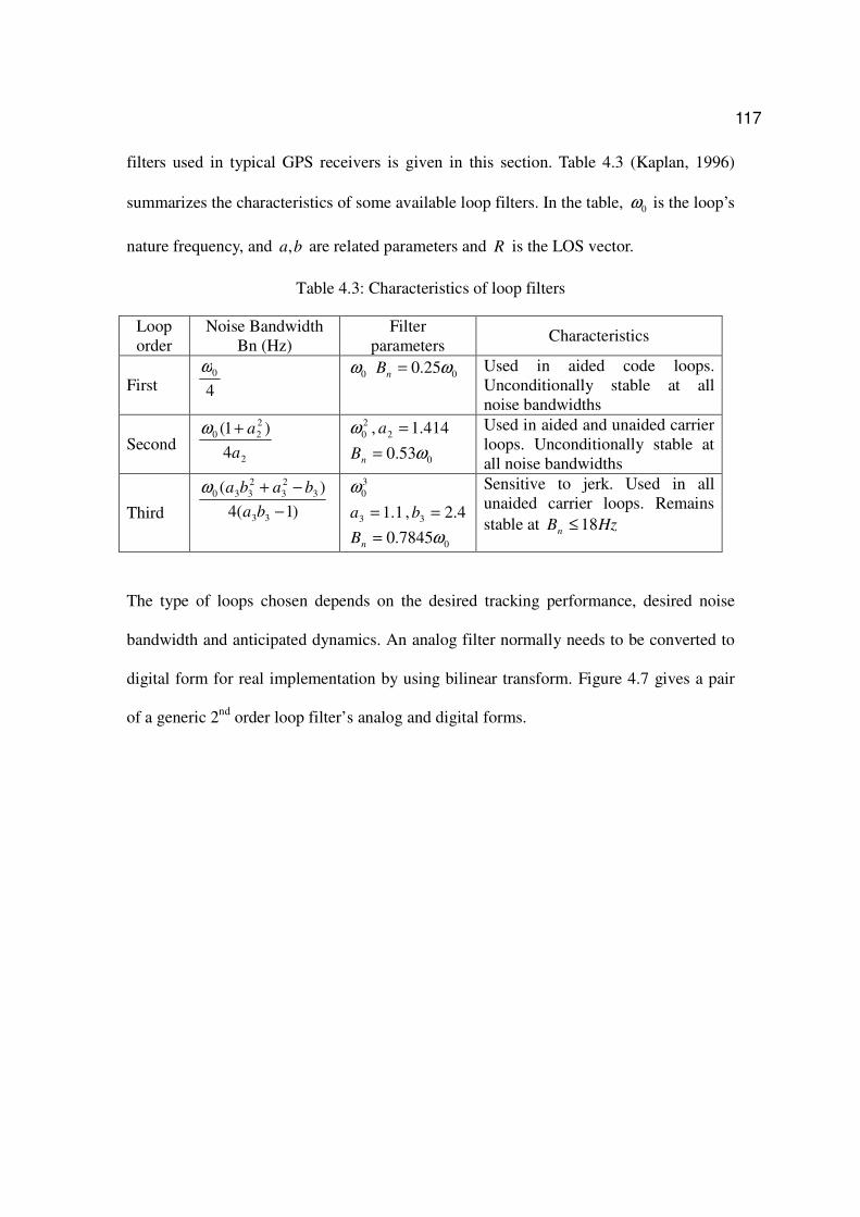
117
filters used in typical GPS receivers is given in this section. Table 4.3 (Kaplan, 1996)
summarizes the characteristics of some available loop filters. In the table, 0ω is the loop’s
nature frequency, and ba, are related parameters and R is the LOS vector.
Table 4.3: Characteristics of loop filters
Loop order
Noise Bandwidth Bn (Hz)
Filter parameters
Characteristics
First 40ω
0ω 025.0 ω=nB Used in aided code loops. Unconditionally stable at all noise bandwidths
Second 2
2
20
4
)1(
a
a+ω
2
0ω , 414.12 =a
053.0 ω=nB
Used in aided and unaided carrier loops. Unconditionally stable at all noise bandwidths
Third )1(4
)(
33
3
2
3
2
330
−
−+
ba
babaω
3
0ω
1.13 =a , 4.23 =b
07845.0 ω=nB
Sensitive to jerk. Used in all unaided carrier loops. Remains
stable at HzBn 18≤
The type of loops chosen depends on the desired tracking performance, desired noise
bandwidth and anticipated dynamics. An analog filter normally needs to be converted to
digital form for real implementation by using bilinear transform. Figure 4.7 gives a pair
of a generic 2nd order loop filter’s analog and digital forms.

118
Figure 4.7: Block diagrams of 2nd order loop filter (After Kaplan, 1996)
According to the above figure, the z-domain transfer function of the loop filter can be
expressed as
1
)2/()2/()( 02
2
0020
−
−++=
z
aTzaTzD COHCOH ωωωω
(4.19)
where, 0ω and 2a are determined by the loop filter parameters and COHT is the pre-
detection integration time (PIT).
4.3 PLL Performance and Its Parameters
Compared with the DLL, the carrier tracking loop is the weaker link in the operation of
GPS signal tracking and more vulnerable to loss of lock. That is because the carrier
wavelength is much shorter than the chip length. Furthermore, the carrier loop needs to
track all dynamics while the code loop needs only to track the dynamic difference
between carrier loop and code loop when carrier aiding is applied to code loop (Lian,

119
2004). We are focusing on the PLL in this section. A typical simplified PLL is illustrated
in Figure 4.8.
Figure 4.8: Simplified PLL
Simply speaking, the functionality of the pre-detection integration process is to increase
the incoming signal strength, which is executed in an “integrate and dump” operation.
The discriminator outputs phase errors between the true carrier and the replicated in-
phase carrier. As mentioned before, the arctangent discriminator is used herein. The loop
filter is to reduce phase error noise with the desired dynamics in order to produce an
accurate estimate of the incoming signal at its output. According to the Figure 4.8, the
Figure 4.9 presents a linearized loop model implementation.

120
Figure 4.9: Linearized discrete model for a PLL (After Yu, 2006)
where,
kφ is the carrier phase of the received sample;
refφ is the local estimate of kφ ;
OSC
kδφ models the phase noise induced by the instability of OSC;
z
z
2
1+ represents the “pre-detection” unit (Humphreys et al., 2005);
1−z
TCOH represents the NCO unit since NCO acts as an integrator;
kn is noise associated with the normalized additive noise at COH I and Q,
illustrated in equations (4.17) and (4.18). The variance of kn depends on
the type of discriminator. Nonlinear operation of the discriminator
amplifies the noise power, and thus excites a larger carrier tracking
error;
kE φδφ denotes the response of the discriminator;

121
δφ is the raw measured, which is much noisier because of a wider noise
bandwidth of COHT/1 ; subsequently this error signal is de-noised by the
loop filter ( )D z from which the output is used to drive the NCO.
The loop transfer function can be derived as
)()1
)(2
1(1
)()1
)(2
1(
)(
zDz
T
z
z
zDz
T
z
Z
zHCOH
COH
−
++
−
+
= (4.20)
The loop noise transfer function is
)()1
)(2
1(1
)()1
()(
zDz
T
z
z
zDz
T
zHCOH
COH
n
−
++
−= (4.21)
Using fjz π21+= , we can acquire the analog counterparts, )( fH and )( fH n , for
transfer functions by equations (4.20) and (4.21). This linear transform is valid if only
12 <<⋅Tfπ can be satisfied (Yu, 2006). The loop bandwidth LB and loop noise
bandwidth nB take the forms of
dffHBL
2
0)(∫
∞
= (4.22)
dffHB nn
2
0)(∫
∞
= (4.23)
The function of PLL is to maintain the phase error between the replica carrier and the
input GPS carrier signals at zero. The accuracy of the frequency and phase
synchronization in PLL are affected by a number of factors, such as signal-to-noise power
ratio, Doppler frequency shift, and the receiver clock quality. The PLL tracking error can
be divided into two parts: the thermal noise and the dynamic stress error (Raquet, 2006).
122
The standard deviation of the total phase error is described as follows in a basic rule-of-
thumb (Kaplan, 1996)
3
22 e
AtPLL
θθσσ ++= (4.24)
In the above equation, 2
tσ is the thermal noise with an equation of
)/2
11(
/2
360
00 ncTnc
B
COH
n
t⋅
+=π
σ (deg) (4.25)
where 0/ nc is the carrier to noise power expressed as a ratio or expressed by 10
0
10CN
in
dB-Hz. The 0/2
1
ncTCOH ⋅ results from the product of noise at I and Q arms, termed
squaring loss.
In equation (4.24), eθ is the steady state dynamics stress error. For a 2nd order loop, it
equals to
2
2809.0
n
eB
R&&⋅=θ (4.26)
where R&& represents the maximum LOS acceleration in 2deg/ s .
In equation (4.24), the Allan deviation oscillator phase noise Aθ for a 2nd loop can be
expressed as (Raquet, 2006; Gao, 2007),
n
LA
AB
f⋅⋅=
)(
5.2
360 τσθ (4.27)

123
Lf is L1 frequency. )(τσ Ais the root of Allan variance for the short-term gate time τ ,
which is equal to nB/1 .
A simulation case is presented to check the performance of a 2nd order PLL in order to
reveal the relations and the trade-off among PLL parameters. In this case, the motions of
a land vehicle are generated by the INS signal simulator, which is given in details in the
Chapter 2. Figure 4.10 shows the simulated trajectories of 4400 seconds, which are
almost same as the example used in Chapter 2. The only difference is that the GPS start
time tag is from GPS week 1352 and GPS seconds 516866 instead of from GPS seconds
0. The zoomed-in 20-second trajectory of interest is shown there as well. The
correspondingly vehicle’s velocities along ENU and heading change in the 20-second
period are presented in Figure 4.11 (a) and (b), respectively. The vehicle is turning with a
maximum forward acceleration of 2/3 sm during this period.

124
Figure 4.10: Simulated trajectories and zoom-in 20s of interest
0 5 10 15 20-20
-15
-10
-5
0
5
10
15
20
GPS time - 518000 (s)
Ve
loc
itie
s a
lon
g E
NU
(m
/s)
East
North
up
0 5 10 15 20
0
50
100
150
200
250
300
350
GPS time - 518000 (s)
He
ad
ing
ch
an
ge
(d
eg
)
Figure 4.11-a: Simulated velocities of 20s Figure 4.11-b Simulated heading of 20s
The GPS satellite’s position and velocity information of GPS satellite PRN13 is
calculated based on the real ephemeris corresponding to the simulated GPS time and an
assumption of 70 ms signal propagation time. The dynamic information combining both
-4000 -2000 0 2000 4000 6000 8000 10000-4000
-2000
0
2000
4000
6000
8000
10000
12000
14000
East (m)
No
rth
(m
)
Simulated trajectory
Zoom-in -3300 -3250 -3200 -3150
1050
1100
1150
1200
1250
1300

125
satellite and land vehicle provides the error-free reference Doppler frequency shift in the
simulation case, as shown in the Figure 4.12.
0 5 10 15 20-740
-720
-700
-680
-660
-640
Re
fere
nce
Do
pp
ler
sh
ift (
Hz)
GPS time - 518000 (s)
Figure 4.12: Calculated reference Doppler shift
As mentioned before, the inputs of the PLL are the COH I and Q samples, as
mathematically described in Equations (4.17) and (4.18). The PLL implementation
complies with the process depicted in Figure 4.9 with the arctangent discriminator
presented in Table 4.2 and Figure 4.6.
Figure 4.13 gives an example of the loop’s behaviour of the tracked Doppler frequency,
the estimated frequency error and the phase tracked error. A 40 dB-Hz incoming
signal’s 0/ NC , 1ms PIT and 15 Hz noise bandwidth are used in this example.

126
0 0.2 0.4 0.6 0.8 1 1.2 1.4 1.6 1.8 2
x 104
-750
-700
-650
-600
Tra
cke
d D
op
ple
r fr
eq
ue
ncy (
Hz)
0 0.2 0.4 0.6 0.8 1 1.2 1.4 1.6 1.8 2
x 104
-10
0
10
Do
pp
ler
err
or
(Hz)
0 0.2 0.4 0.6 0.8 1 1.2 1.4 1.6 1.8 2
x 104
-20
0
20
Ph
ase
err
or
(de
g)
I / Q samples number
Figure 4.13: An example of 2nd order PLL behaviour of the simulation case
( HzdBNC −= 40/ 0 HzBn 15= msPIT 1= )
From Figure 4.13, it is obvious that the PLL can lock the incoming signal carrier and the
frequency change well since the phase tracking error )1( σ is far beyond the threshold of
loss-lock, rule-of-thumb o15 (Kaplan, 1996; Raquet, 2006). In addition, as motioned
before, the signal power should be concentred on the in-phase component if the incoming
signal is correctly tracked. Figure 4.14 gives an example of 1000 COH pI and pQ of the
PRN 13 after 1ms accumulation from the above case. It clearly shows that the Q
component is noise-like signal and the I component contains almost all the signal power.

127
1.9 1.92 1.94 1.96 1.98 2
x 104
-800
-600
-400
-200
0
200
400
600
800
I / Q samples number
Ip (
time
s 1
00
)(a)
1.9 1.92 1.94 1.96 1.98 2
x 104
-400
-300
-200
-100
0
100
200
300
400
I / Q samples numberQ
p (
time
s 1
00
)
(b)
Figure 4.14: In-phase and quadrature-phase components
It should be also noted that the lock status is required to indicate the tracking status of
PLL. In theory, we should use the 0/ NC to determine if the receiver remains lock status.
The estimation of 0/ NC is necessary because it decreases rapidly once the receiver loses
lock. The 0/ NC can be estimated by comparison of the signal power in two different
bandwidths. We can typically select the wideband kWBP as PIT/1 and the narrow band
kNBP as ms20/1 . The estimation of 0/ NC is given as (Pakinson and Spiller, 1996),
⋅−
−=
PITP
PNC
)20(
1lg10/ 0
µ
µ (4.28)
where,
k
k
WBP
NBPP =µ ;
2
1
,
2
1
,
+
= ∑∑
==
m
i
iP
m
i
iPk QINBP ;

128
( )∑=
+=m
i
iPiPk QIWBP1
2
.
2
, ;
m is typical satisfied with msPITm 20=× .
Furthermore, the 0/ NC estimation can be improved by averaging several estimations
with number of K, because the standard deviation of 0/ NC estimation is reduced by a
factor of K . A total of 50 estimations is used here to get the final 0/ NC estimation.
Therefore, the output rate of 0/ NC is 1Hz since the average time is sPITmK 1=×× .
For the above example, the 0/ NC estimation is shown in Figure 4.15.
0 5 10 15 2037
38
39
40
41
GPS time - 518000 (s)
CN
estim
atio
n (
dB
-Hz)
Figure 4.15: 0/ NC estimation
The estimation of 0/ NC according to equation (4.28) is time consuming. Furthermore,
the bit-sync is pre-requirement for that. Therefore, typically, a PLL lock detector is used

129
to check the lock status instead of such estimation. The value of lock detector directly
reflects the quality of 0/ NC (Ma et al, 2004). Parkinson and Spiller (1996) give the
calculation details of the lock detector kCL φ2_ , as briefly summarized below.
)2cos(2_ k
k
k
kNBP
NBDCL δφφ ≈= (4.29)
where,
2
1
,
2
1
,
−
= ∑∑
==
m
i
iP
m
i
iPk QINBD
Obviously, the PLL lock detector is a function of the phase tracking error. It will
approach 1 when the phase tracking error is small enough. The threshold of kCL φ2_ is
selected by the receiver designer. Since the percentage of the incoming signal powers on
PI can be roughly expressed as kppp QII δφ2222 cos)/( ≈+ , a threshold of 0.7 is selected in
this study to assure at least 85% of the signal power still on the in-phase component. The
tracking will be assumed failure if the value of lock detector is smaller than this
threshold. For the above example, Figure 4.16 shows the output of lock detector. Both
Figure 4.16 (calculated) and Figure 4.13 (observed) conclude that the incoming signal
carrier and the frequency change described by Figure 4.10 to Figure 4.11 with signal
strength of HzdB −40 are well tracked by the designed 2nd order PLL.

130
0 0.5 1 1.5 2
x 104
0
0.2
0.4
0.6
0.8
1
I / Q samples number
Ou
tpu
t o
f lo
ck d
ete
cto
r
Figure 4.16: PLL lock detector behaviour with strong signal (40dB-Hz)
Table 4.4 compares tracking errors with different loop parameters. The results clearly
show that the tracking error is larger when the tracked signal is weaker. For example,
when 0/ NC decreased from 40 HzdB − to 30 HzdB − with the same bandwidth 15 Hz ,
the phase error increased from 1.24 degree to 14.05 degree. The narrower bandwidth is
helpful to the reduction of the tracking errors, e.g. nB decreased from 15 Hz to 12 Hz ,
accordingly, phase error decreased from 14.05 degree to 11.49 degree; however, the
bandwidth cannot be narrowed without limits as the PLL has to track the vehicle
dynamics as well. Unreasonable value for the noise bandwidth results in the loss-of-lock.

131
Table 4.4: Tracking errors of different parameters
(GPS week = 1352, GPS time = 518000~518020, PRN 13)
Tracking error )1( σ− nB
)(Hz
0/ NC
HzdB −
PIT ms
Doppler )(Hz Phase (deg)
Lock status
15 40 1 1.48 1.24 Yes
15 30 1 4.47 14.05 Yes
12 30 1 2.99 11.49 Yes
6 30 1 -- -- No
4.4 Summary
This Chapter 4 investigates the operation of GPS receiver. The tracking loop and its
tracking performance associated with its parameters are explained in details. The first
section in this chapter describes the GPS receiver signal processing technology, which
involves GPS signals, receiver FE, acquisition, tracking, measurement derivation, and
navigation solution. Based on the receiver signal flow, tracking loops including
accumulator, discriminator, and loop filter are studied.
The simulation tests from a 2nd order PLL with dynamic environment verify that 1) the
signal power is concentred on the I (in-phase) component when the incoming signal is
correctly tracked; 2) the tracking error is larger when the tracked signal is weaker; 3) the
narrower bandwidth is helpful to the reduction of the tracking errors; 4) under a high
dynamic environment, the extended integration time leads to an unacceptable phase error.

132
Chapter 5 INS Doppler Aided Receiver Tracking Loop
To accommodate dynamic stress, the most effective way is to broaden the PLL
bandwidth. This gives rise to a dilemma in GPS receiver design. The common method for
designing a PLL tracking loop is to choose a loop bandwidth which is primarily
determined by the loop filter while considering the worst case of 0/ NC and the highest
Doppler frequency caused by the dynamics (Lian, 2004). Usually these designs are robust
but not optimal. Fortunately, INS Doppler aiding contributes to the PLL to track much
weaker GPS signals continuously by removing most of the dynamic stress, which allows
the reduction of the noise bandwidth. Section 5.1 discusses the method and the
implementation of INS Doppler aiding to the conventional PLL. The effect of Doppler
accuracy on INS aided PLL is analyzed as well. Section 5.2 implements and tests an EKF
based INS Doppler aided tracking loop as well as the corresponding INS/GPS
integration.
5.1 INS Aided Tracking Loop
5.1.1 Implementation of IPLL
In urban canyon environments, a tightly coupled INS/GPS yields integrated navigation
solution continuously even if the situations of fewer than four satellites frequently occur.
But the navigation performance is dependent on the satellite geometry, i.e. the number of
satellites in-lock and the distribution of the satellites in the sky. GPS signals are not as
easy to be locked as in open-sky since the signal strength is attenuated by blockages,
reflections, cross-correlation, multipath, etc. INS aiding is helpful to remain the PLL in-
lock under weak signal environments by removing the loop’s dynamic stress.

133
From the Figure 4.9, we learn that the carrier frequency deviation (PLLf ) from the
baseband frequency is primarily comprised of three components: the Doppler frequency
( doopf ) due to the relative motion between the receiver and the satellite; frequency errors
due to the OSC ( oscf ); and errors due to thermal noise ( noisef ), which can be expressed as
noiseoscdoppPLL ffff ++= (5.1)
The main idea of INS aiding is to add the external Doppler frequency estimate ( INSdoppf )
from INS to the output of the loop filter in order to narrow the loop’s noise bandwidth.
As described before, the PLL can not distinguish the dynamics between the actual LOS
motions and OSC instability. Whereas, the INS with Doppler measurements only detects
the LOS relative motions between the INS and the satellite. Therefore, the dynamics due
to the receiver clock drift should be considered in an IPLL. Based on the Equations (4.25)
and (4.27), Figure 5.1 compares the phase errors introduced by thermal noise and by the
receiver clock (e.g. TCXO), both as a function of loop bandwidth. The results indicate
that in the low noise bandwidth range, especially for weaker signals, the clock dynamics
dominate the tracking errors.

134
2 4 6 8 10 12 14 16 18 200
5
10
15
20
25
Bn (Hz)
Ph
ase
err
or
(de
g 1
-sig
ma
)
thermal noise (CN0 25dB-Hz)
thermal noise (CN0 30dB-Hz)
thermal noise (CN0 35dB-Hz)
thermal noise (CN0 40dB-Hz)
clock
Figure 5.1: Phase errors due to signal strength and clock drift vs. bandwidth
Thus, a complete INS aiding is implemented by adding both INSdoppf and the OSC
estimate ( oscf ) to the output of the loop filter. The NCO, therefore, can be restructured as
shown in Figure 5.2.
Figure 5.2: Restructured NCO in IPLL

135
If the receiver dynamics are removed by using external estimates of INS Doppler with
very high precision, the error of PLL is mainly determined by thermal noise which is a
function of nB , COHT and 0/ NC . Based on the rule-of-thumb Equation (4.25), Figure 5.3
gives the phase error variations with the different 0/ NC and nB (with 1ms PIT).
Furthermore, the simulation experiment presented in Section 4.3 is repeated here except
that the bandwidth of IPLL is narrowed to Hz3 in order to track the incoming signal as
weak as HzdB −30 . Figure 5.4 shows the IPLL behaviour of the tracked Doppler
frequency, the estimated frequency error and the phase tracked error. The tracked Doppler
error )1( σ is 0.87Hz and the phase error )1( σ is 3.1 degrees. Both Figures 5.3 and 5.4
clearly show the advantages of external INS aiding, of which the narrower noise
bandwidth help PLL to track the weaker signal.
15 20 25 30 35 400
5
10
15
20
25
CN0 (dB-Hz)
Ph
ase
err
or
(de
g 1
-sig
ma
)
(a)
Bn = 1Hz
Bn = 5Hz
Bn = 10Hz
Bn = 15Hz
Bn = 20Hz
5 10 15 200
5
10
15
20
25
Bn (Hz)
Ph
ase
err
or
(de
g 1
-sig
ma
)
(b)
CN0 = 20 dB-Hz
CN0 = 25 dB-Hz
CN0 = 30 dB-Hz
CN0 = 35 dB-Hz
CN0 = 40 dB-Hz
threshold threshold
Figure 5.3: Phase errors vs. 0/ NC andnB with error-free aiding information

136
0 0.2 0.4 0.6 0.8 1 1.2 1.4 1.6 1.8 2
x 104
-750
-700
-650
-600
Tra
cked D
opple
r
frequency (H
z)
0 0.2 0.4 0.6 0.8 1 1.2 1.4 1.6 1.8 2
x 104
-4
-2
0
2
4
Dopple
r error (H
z)
0 0.2 0.4 0.6 0.8 1 1.2 1.4 1.6 1.8 2
x 104
-20
-10
0
10
20
Phase e
rror (d
eg)
I / Q samples number
Figure 5.4: IPLL behaviour of the simulation case
( HzdBNC −= 30/ 0 HzBn 3= msPIT 1= )
5.1.2 Effect of INS Doppler Accuracy
Although, owing to the removal of the loop’s dynamic stress, the weaker signal can be
tracked by virtue of INS Doppler aiding, the use of perfect aiding information in the
above cases is only an ideal case. In practice, the external INS Doppler estimate and
clock drift estimate are not always accurate. External aiding may introduce a different
form of dynamics stress in the form of errors from the Doppler and clock drift estimates

137
(Yang and El-Sheimy, 2006; Chiou, 2005). Therefore, the IPLL must be designed to track
phase dynamics due to the INS Doppler estimate errors ( INSdoppfδ ) and the receiver clock
drift error ( oscfδ ). The receiver clock drift is modeled as a process of random walk in this
research. As a result, the value of the loop filter’s output for IPLL can be written as
INSdoppnoisePLL fff ˆδ+= (5.2)
Assuming that the dynamics of the INS Doppler estimate errors are slower than the
vehicle’s dynamics, from the above equation, the use of INS Doppler aiding allows for
noise bandwidth reduction in IPLL when compare to a traditional PLL.
After removal of the dynamics, with a random constant assumption of the aiding
frequency error, the rule-of-thumb equation of phase error (4.25) can be re-written as the
following
)/2
11(
/2
360ˆ36000 ncTnc
BTf
COH
n
COHINSdoppPLL⋅
++⋅⋅=π
δσ (deg) (5.3)
As illustrated in the Equation (3.25) in the Chapter 3, the INS Doppler frequency of the
carrier signal can be expressed as the velocity of the INS relative to the satellite,
projected onto the LOS vector. Computing the value of the INS Doppler error requires
performing a covariance analysis. Based on that equation, we have the σ1 standard
deviation in the INS Doppler estimate with respect to the thk − satellite as following,
2
2
,
,2
2
,2,22
,,1
ˆˆˆ
kSVINSkkINSdopp
kSV
kINSdopp
INS
kINSdopp
k
kINSdopp
fL
fffVVe
2
VVeσσσσλ
∂
∂+
∂
∂+
∂
∂= (5.4)
Compared the LOS vector change rate of the thk − satellite with the INS rate, it is

138
reasonable to assume 0e =k
σ . In addition, the satellite velocity errors determined by the
broadcast ephemeris errors are always supposed to be much smaller than the velocity
errors from INS, especially for MEMS grade INS. Thus, the Equation (5.4) can be
expanded and re-written as
( )2
2
1
,
L
k
T
INSINS
T
k
f
EkINSdopp λ
δδσ
eVVe=
[ ]
=
kz
ky
kx
l
e
v
v
v
e
lkzkykx
Le
e
e
eee
U
N
E
RR2
2
2
2
00
00
001
1
δ
δ
δ
σ
σ
σ
λ (5.5)
where
( )⋅E represents the expectation operation;
222 ,,UNE vvv δδδ σσσ are the variances of the ENU velocity errors, respectively.
To establish the relations between INS Doppler aiding error and the INS ENU velocity
errors, an upper bound on the magnitude of the aiding error is considered here. Assume
that 2222222 ,,maxUNEUNE vvvvvv δδδδδδ σσσσσσσ ==== and the INS velocity vector along
ECEF ( INSV ) is aligned with the LOS vector. With these bound assumptions, from the
Equation (5.5), we have
λσσ /)max( 22
,=
kINSdoppf (5.6)
The above equation indicates that the maximum Doppler aiding error is determined by
the INS ENU velocity error. Thus, combining the Equation (5.2), the objective of
narrowing the loop bandwidth in IPLL is actually an effort to control the INS ENU
velocity error drift.

139
Without error control, i.e. by INS direct aiding, the IPLL performance heavily depends on
the quality of the INS since there is no bound of INS velocity error drift. Repeat the
simulation experiment presented in Section 4.3 again. In order to track the incoming
signal as weak as HzdB −30 , INS direct aiding is used to narrow bandwidth to Hz3 .
Figure 5.5 (a) and (b) compares the aiding Doppler shifts and their errors for different
grade INSs, respectively. Given that all the INSs operate 20s only without alignment
errors and the only inertial sensor error source of each INS is the heading gyro bias, e.g.
in run bias of 1deg/hr, 10deg/hr, 50deg/hr and 200deg/hr (MEMS grade). Table 5.1 lists
the tracking errors for different grade INSs aiding.
0 5 10 15 20-740
-720
-700
-680
-660
-640
Aid
ing
Do
pp
ler
fro
m IN
S (
Hz)
GPS time - 518000 (sec)
(a)
0 5 10 15 20-15
-10
-5
0
5
Aid
ing
IN
S D
op
ple
r e
rro
r (H
z)
GPS time - 518000 (sec)
(b)
True doppler
1deg INS aiding
10deg INS aiding
50deg INS aiding
MEMS INS aiding
1deg INS aiding
10deg INS aiding
50deg INS aiding
MEMS IMU aiding
Figure 5.5: Aiding Doppler and errors with different grade INSs
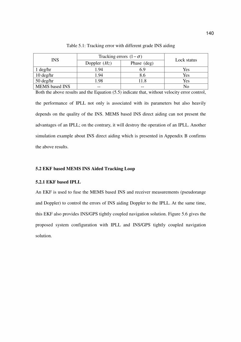
140
Table 5.1: Tracking error with different grade INS aiding
Tracking errors )1( σ− INS
Doppler )(Hz Phase (deg) Lock status
1 deg/hr 1.94 6.9 Yes
10 deg/hr 1.94 8.6 Yes
50 deg/hr 1.98 11.8 Yes
MEMS based INS -- -- No
Both the above results and the Equation (5.5) indicate that, without velocity error control,
the performance of IPLL not only is associated with its parameters but also heavily
depends on the quality of the INS. MEMS based INS direct aiding can not present the
advantages of an IPLL; on the contrary, it will destroy the operation of an IPLL. Another
simulation example about INS direct aiding which is presented in Appendix B confirms
the above results.
5.2 EKF based MEMS INS Aided Tracking Loop
5.2.1 EKF based IPLL
An EKF is used to fuse the MEMS based INS and receiver measurements (pseudorange
and Doppler) to control the errors of INS aiding Doppler to the IPLL. At the same time,
this EKF also provides INS/GPS tightly coupled navigation solution. Figure 5.6 gives the
proposed system configuration with IPLL and INS/GPS tightly coupled navigation
solution.

141
Figure 5.6: Proposed system configuration of INS/GPS integration with IPLL
In the above figure, the NCO details of the IPLL are depicted in the Figure 5.2. The
aiding information is calculated from the INS/GPS tight integration filter. The code loop
(not shown in this figure) aided by the IPLL carrier, as normal receiver does, provides the
receiver pseudorange measurements. In this configuration, the IPLL starts in normal PLL
mode until the ephemeredes are decoded and a first position/velocity/clock drift estimate
is available. It should be noted that the first clock drift estimate is assumed as a “constant
bias” during IPLL operation in this research. Therefore, the clock drift information to
IPLL is a combination of the above bias and an estimated value from EKF, in which the
clock drift is considered as a random walk. In most cases, the value of first clock drift is
not zero, so the clock drift aiding information oscf is mainly determined by its first
estimate, which comes from PLL. There are 23 error states in the EKF. The state vectors
and observables for EKF are thoroughly described in the Section 3.4.3. The INS Doppler
calculation is described in the Section 3.4.2.

142
According to the proposed INS aiding scheme, some modules in a conventional receiver
need to be changed, as illustrated in the Figure 5.7. The required changes in the INS-
aided receiver can be fulfilled through the software method in a software receiver.
Figure 5.7: Module comparison of the conventional and INS-aided receivers
5.2.2 Performance Tests and Analyses
To test the IPLL and the INS aided receiver performance, a field test was conducted
around Springbank, Alberta in December 2005, which has been described in Chapter 3.
The system setup was shown in Figure 3.4. The data from an ADI MEMS INS and
NordNav software GPS receiver were collected. The LN200 INS data and differential
GPS data are processed to generate the reference trajectory. The ADI MEMS INS and the
front-end of the NordNav receiver are shown in the Figure 5.8. The front-end was driven
by a laptop’s USB. The front-end of the receiver down-converts the 1L GPS signal to an

143
IF of MHz1304.4 . The sampling rate is MHz3676.16 .
Figure 5.8: ADI MEMS IMU and NordNav Front-end
The datasets from the software GPS and ADI INS were post-processed. Due to the lack of
full access to this receiver, the post-processing procedure consisted of the following five
steps:
1) Record receiver pseudorange and Doppler measurements then synchronize them with
INS data manually. Since the pseudorange measurements are associated with bit/frame
sync process and INS aiding mainly executes on the carrier tracking, we assume only
GPS Doppler measurements are changed by INS aiding.
2) The NordNav software provides two types of accumulator (after pre-integration)
messages. One is the standard early-prompt-late correlator (correlator spacing 1 chip)
message and the other is the multiple-correlator message, which is mainly used for anti-
multipath. To simplify the data processing, we only set parameters for the standard
correlator before running the receiver. The corresponding accumulator messages are
recorded. Then, synchronize the recorded accumulator data with the INS data manually
by virtue of a message header contained in each GPS message. This header includes a

144
receiver run time and a GPS time. The GPS time will indicate zero unless the receiver
tracks four or more satellites and computes a position. Combining the GPS time, the
receiver run time and measurements, it is easy to manually synchronize INS data and
accumulator data and select the accumulator data (I and Q samples after pre-integration)
during tracking process.
3) Tune the level of signal strength ( 0/ NC ) by injecting various power levels of white
Gaussian noise into the collected I and Q samples (Chiou, 2005), which generates the
new I and Q samples ( dd QI / ) under the degraded signal environments. The relations
between the injected white noise and 0/ NC can be expressed by the Equation (5.7).
)110(2
0/1.0
0
2
, −= ∆ NC
s
E
addw NT
Mσ (5.7)
where
2
,addwσ is the noise variance of the injected white noise;
EM is number of samples per COH accumulation segment, equal to
sCOH TT / , where sT is the sampling period, )103676.16/(1 6×=sT
for NordNav front-end;
0N is the received noise density and the typical value of 0N is
HzdBW /205− (Lachapelle, 2005);
0/ NC∆ is the signal strength difference between the collected signal and
the desired signal for degraded signal simulation.
4) dI and
dQ samples pass through the developed IPLL module (or conventional PLL)
and the developed INS/GPS tight integration navigation module to verify the

145
performance of tracking loop and navigation solution. Meanwhile,
5) Due to the limited access to the FE LO, dI and dQ samples are reconstructed by
multiplying a coefficient of normalized sinc function in each IPLL step to simulate the
NCO adjustments approximately. The sinc function is illustrated in the Equation (5.8).
COHropen
COHropen
coefTff
TffA
)(
])(sin[
deg
deg
−
−=
π
π (5.8)
where
coefA is the coefficient multiplied to dI and
dQ samples;
openf is the tracked frequency under the strong signal environment,
which is acquired in this section by using the collected I and Q
samples from the NordNav accumulator directly since the signal
environment is always open sky during the Springbank field test;
rfdeg is the tracked frequency from the IPLL (or conventional PLL )
under the simulated degraded signal environment.
An approximate L-shape trajectory was driven in the field test, same as shown in the
Figure 3.6. Figure 5.9 shows the satellites tracked by the NordNav receiver in the field
tests between GPS time 521990s to 523300s in 1352-th GPS week. According to the
receiver default setting, the cutoff elevation for the satellites is 05 . Figure 5.10 gives the
corresponding signal strength during the test. Since it is always open sky during the test,
four or more than four satellites are well tracked. We will use the Equation (5.7) to
simulate the signal degrade environments based on the field test data.

146
0 200 400 600 800 1000 12001
3
5
7
9
11
13
15
17
19
21
23
25
27
29
31
GPS time - 521990 (s)
Tra
cked P
RN
channel 1
channel 2
channel 3
channel 4
channel 5
channel 6
channel 7
channel 8
Figure 5.9: Satellites tracked in the field test
0 200 400 600 800 1000 1200
5
10
15
20
25
30
35
40
45
50
GPS time - 521990 (s)
Tra
cke
d P
RN
PRN 2
PRN 5
PRN 5
PRN 10
PRN 13
PRN 30
Figure 5.10: The signal strength during the test y-axis should C/N

147
Similar to the previous method, 20 seconds trajectory and motions of interest are selected
to analyze the IPLL thoroughly. Figure 5.11 (a) and (b) show the 20s zoom-in trajectories
and 0/ NC of interest (522730s to 522750s), when the vehicle was steering toward north
with a maximum acceleration of 2/8.2 sm . Most of 0/ NC for each satellite are
above HzdB −30 . To simplify the problem, we can simulate a signal outage case for PRN
2 by using the Equation (5.7).
703 703.5 704150
200
250
300
350
400
450
500
550
600
650
East (m)
North (m
)
(a)
740 750 760
5
10
15
20
25
30
35
40
45
50
GPS time - 521990 (s)
Carr
ier to
nois
e ratio
(dB
-hz)
(b)
PRN 2
PRN 5
PRN 5
PRN 10
PRN 13
PRN 30
Figure 5.11: 20s trajectories and signal strength of interest
Given that 0/ NC of PRN 2 is degraded to HzdB −26 . Figure 5.12 gives the lock
detector output of a conventional receiver PLL. It is obvious that the PLL loses the lock
of the carrier frequency, which results in fewer than four satellites being tracked during
this period of interest.

148
740 745 750 755 7600
0.1
0.2
0.3
0.4
0.5
0.6
0.7
0.8
0.9
1
GPS time - 521990 (s)
Ou
tpu
t o
f lo
ck d
ete
cto
rthreshold
Figure 5.12: Lock detector output of conventional PLL with HzdBNC −= 26/ 0
Under the same signal conditions, IPLL instead of conventional PLL is used to track the
PRN 2. The external Doppler and the estimate of the receive clock drift are fed into PLL
NCO. The aiding information is from ADI MEMS INS/NordNav GPS tightly integrated
system. As noted before, 1G2A suboptimal INS configuration is used for aiding. Figure
5.13 shows the aiding Doppler at 100Hz including both the INS Doppler estimate and the
clock drift estimate for the IPLL in the Channel 2 of the receiver, where the PRN 2 was
being tracked.

149
740 745 750 755 760-3405
-3400
-3395
-3390
-3385
-3380
GPS time - 521990 (s)
Aid
ing D
opple
r (H
z)
Figure 5.13: Aiding Doppler to IPLL
By using the above adding Doppler information, Figure 5.14 (a) and (b) show the outputs
of the IPLL discriminator and the loop filter, respectively, which are the indicators of the
IPLL tracking quality. The output of the IPLL discriminator (ATAN discriminator) is
actually the phase difference between the incoming signal and the generated local signal.
From the figure, the phase difference (not phase error) is around 48 degrees ( σ1 ). These
differences result from both the vehicle’s dynamic motions and the phase tracking errors.
As mentioned before, the Costas ATAN discriminator remains linear at a range of
o o90 ~ 90− . Thus, the Figure 5.14 (a) indicates the IPLL discriminator remains in a good
status to produce the difference between the incoming and replicated phases.

150
740 745 750 755 760-0.5
-0.4
-0.3
-0.2
-0.1
0
0.1
0.2
0.3
0.4
0.5
GPS time - 521990 (s)
Ou
tpu
t o
f IP
LL
ata
n d
iscrim
ina
tor
(Hz)
(a)
740 745 750 755 760-15
-10
-5
0
5
10
15
GPS time - 521990 (s)
Ou
tpu
t o
f IP
LL
loo
p filt
er
(Hz)
(b)
Figure 5.14: Outputs of IPLL discriminator and loop filter
In addition, by INS Doppler aiding, the LOS dynamics is removed from the tracking
loop. According to the Equation (5.2), the output of IPLL only includes the frequency of
aiding Doppler error and the errors due to thermal noise, all of which are relatively small
values. The theoretical Equation (5.2) is qualitatively verified in the Figure 5.14 (b).
Figure 5.15 (a) gives the lock detector output of IPLL. Compared with the Figure (5.12),
it is obvious that the carrier frequency of PRN 2 is locked by using MEMS INS Doppler
aiding, which is superior to the conventional PLL. Figure 5.15 (b) shows the receiver’s
corresponding estimation of 0/ NC based on the Equation (4.28). There is no rapid
change of 0/ NC , which indicates the channel with IPLL is well tracking the satellite.
Both (a) and (b) of the Figure 5.15 indicate the IPLL can track weak signal as low as

151
HzdB −26 .
740 745 750 755 7600
0.1
0.2
0.3
0.4
0.5
0.6
0.7
0.8
0.9
1
GPS time - 521990 (s)
Outp
ut of lo
ck d
ete
cto
r(a)
740 745 750 755 76021
22
23
24
25
26
27
GPS time - 521990 (s)
C/N
0 e
stim
atio
n
(b)
Figure 5.15: Lock detector output and 0/ NC estimation from IPLL
To search for the margin of the signal strength that could be tracked by IPLL for the same
case, Figure 5.16 compares the lock detector outputs with different signal strength (but
with the same loop bandwidth Hz14 same as before). It clearly shows the IPLL can track
the weak signals of approximate HzdB −24 . In a receiver with conventional PLLs, loss
of lock typically occurs at a signal power equal to approximately HzdB −27 (Gebre-
Egziabher et al., 2005; Ma et al, 2004). Figure 5.16 indicates that, with Doppler aiding,
an additional HzdB −3 margin can be achieved, allowing signals with power as low
as HzdB −24 . Another test of 20s based on the real dataset presented in Appendix C
confirms the above results.

152
740 745 750 755 7600
0.1
0.2
0.3
0.4
0.5
0.6
0.7
0.8
0.9
1
GPS time - 521990 (s)
Ou
tpu
t o
f lo
ck d
ete
cto
r
29dB-Hz
28dB-Hz
27dB-Hz
26dB-Hz
25dB-Hz
24dB-Hz
23dB-Hz
threshold
Figure 5.16: Output of IPLL lock detector vs. different signal strength
It should be noted that the further margin can not be obtained simply by reducing the loop
noise bandwidth. As described previously, the normalized noise variance is inversely
proportional to 0/ NC . According to Equation (5.3), it is no doubt that reducing the loop
noise bandwidth can mitigate the effect of this error; nevertheless, doing such increases
the tracking errors. The rule-of-thumb equation is based on two important assumptions:
small phase tracking errors and steady state. But in the real case, especially for dynamic
environment with low 0/ NC condition, the above two assumptions can not always be
satisfied. Figure 5.17 compares the lock detector outputs with different loop noise
bandwidths (but with the same signal strength HzdB −26 ), which indicates that too
narrow bandwidth results in unstable loop locks even loss-of-lock. That is because the
IPLL has to track the residual dynamics caused by thermal noise, Doppler aiding and
clock aiding; and the thermal noise error starts to dominate the total phase error at lower

153
0/ NC range (Chiou, 2005). A reasonable bandwidth should be selected to guarantee that
the discriminator operates within a linear region (Yu, 2006). A KF based carrier tracker
instead of conventional tracking loops can be used because the bandwidth chosen by this
estimator is optimal in the sense of minimum mean square error (Psiaki and Jung, 2002).
However, that topic is beyond the scope of this dissertation and will not be discussed
further.
740 745 750 755 7600
0.1
0.2
0.3
0.4
0.5
0.6
0.7
0.8
0.9
1
GPS time - 521990 (s)
Ou
tpu
t o
f lo
ck d
ete
cto
r
Bn=14Hz
Bn=12Hz
Bn=10Hz
Bn=8Hz
Bn=6Hz
threshold
Figure5.17: Output of IPLL lock detector vs. different bandwidth
After INS aiding, the Doppler output from IPLL and pseudorange measurements from
DLL (assumed no changes), together with MEMS INS measurements, are used as
observables to the MEMS INS/GPS tight integration EKF, Figure 5.18 compares the
navigation errors between tight integration with PLL and that with IPLL. We assume that
there is no GPS pseudorange and Doppler measurements available in the GPS channel
where the tracking loop loses satellite lock. The comparison takes place under weak

154
signal environment, e.g. HzdBNC −= 26/ 0 , of which two satellites suffer (PRN 2 and
PRN 30) loss in the conventional PLL while IPLL locks them. Again, the 1G2A
suboptimal ADI MEMS INS configuration is used in the tightly coupled navigation.
740 745 750 755 760-10
-5
0
5
10
Time - 521990 (s)
Po
siti
on
err
or
(m)
(a)
East
North
Up
740 745 750 755 760-10
-5
0
5
10
Time - 521990 (s)P
ositi
on
err
or
(m)
(b)
East
North
Up
740 745 750 755 760-0.5
0
0.5
1
1.5
Time - 521990 (s)
Ve
locity
err
or
(m/s
)
(a)
East
North
Up
740 745 750 755 760-0.5
0
0.5
1
1.5
Time - 521990 (s)
Ve
locity
err
or
(m/s
)
(b)
East
North
Up
740 745 750 755 760-2
0
2
4
Time - 521990 (s)
Attitu
de
err
or
(de
g)
(a)
Pitch
Roll
Heading
740 745 750 755 760-2
0
2
4
Time - 521990 (s)
Attitu
de
err
or
(de
g)
(b)
Pitch
Roll
Heading
Figure 5.18: Comparison of navigation errors by using PLL and IPLL
During this 20s of interest, the vehicle traveled m178 , known from reference trajectory

155
provided by LN200 and DGPS. In Figure 5.18, (a) shows the errors of integrated
navigation solution using PLL in the receiver. By contrast, (b) shows those using IPLL. In
(a), two satellites lose lock since the conventional PLL can not track weak signals as low
as HzdBNC −= 26/ 0 . Only the other two satellites (PRN 10 and PRN 5) provide raw
GPS measurements, which results in the degraded satellite geometry. As analyzed before,
the navigation performance is for sure degraded because of the geometry degradation.
The errors, especially for the velocity errors, are also from the INS pseudo-signal in
1G2A configuration due to the vehicle’s dynamics. However, the 3D position error is less
than m11 ( %6< of the travel distances), which is acceptable for MEMS INS based land
vehicle navigation system thanks to the advantages of INS/GPS tightly coupled
integration scheme.
Compared with (a), Figure 5.18 (b) clearly shows that the tightly coupled navigation
performance is improved by using IPLL. Another test result presented in Appendix C
shows a similar improvement. Totally four satellites are being tracked under weak signal
environments because of the use of IPLL, which improves the satellite geometry. In
addition, during this 20s, the tight couple EKF has a good observability due to the
relatively high dynamics, which mitigates errors caused by INS pseudo-signal in some
extent. The position error is reduced to %2< of the travel distances )4( m , which is %67
improvement compared with the previous one.

156
5.3 Summary
This chapter implements the INS Doppler aided GPS receiver tracking loop. INS aided
tracking is implemented by adding both INS Doppler and the receiver clock drift estimate
to the NCO. The IPLL can track weaker GPS signals continuously compared with the
convention PLL as it only needs to track the residual dynamics after aiding. The relations
between INS Doppler aiding error and the INS ENU velocity errors are established as
well as the effect of Doppler accuracy on IPLL is analyzed. In addition, this chapter
proposes a system configuration of INS/GPS integration with IPLL and future modules
for an INS aided receiver.
Simulation tests show that MEMS based INS direct aiding can not present the advantages
of an IPLL; on the contrary, it will destroy the operation of an IPLL. Therefore, an EKF
with INS/GPS tight scheme is used to control the INS aiding error as well as provide
navigation solution. Results based on the field test datasets indicate that, with MEMS
INS Doppler aiding, an additional HzdB −3 margin can be achieved, allowing signals
with power as low as HzdB −24 to be successfully tracked. Compared with the results of
conventional PLL in a tight INS/GPS integration, the position accuracy of IPLL is
significantly improved.

157
Chapter 6 Conclusions and Recommendations
This chapter contains a summary of the research work presented in this dissertation, the
conclusions drawn from the theoretical developments and test results, and
recommendations for future research and developments in this field.
6.1 Summary
The main objective of this research was to develop a tightly coupled MEMS INS/GPS
integration with INS aided GPS receiver tracking loops. To accomplish the dissertation
objective and test the proposed methods, four sub-topics were investigated and presented
in four Chapters. They are INS signal simulator, MEMS INS/GPS tight integration, GPS
receiver tracking loops, and INS aided carrier tracking loop.
The INS signal simulator is a methodical combination of the inverse INS mechanization
and various inertial sensor errors. The concepts of the INS simulator were used in the
pseudo-signal generation of the sub-optimal INS configuration for INS/GPS tight
integration. The simulator was also used in the performance analyses of unaided PLL and
aided PLL by different quality INSs under weak signal environment. This was followed
by investigations of INS/GPS integration schemes and the error models of INS and GPS,
an INS/GPS tight integration algorithm based on an EKF of 23 states which was
developed for this task. The pseudorange and Doppler measurements from both INS and
GPS were used as the observables for the EKF. Specially, MEMS INS/GPS tightly
coupled integration with a sub-optimal INS configuration of one gyro and two
accelerometers were proposed. The tightly coupled algorithm and the sub-optimal INS

158
configuration were used to implement the INS aided GPS receiver carrier tracking loop.
The GPS receiver tracking loop and its parameters were investigated. After a review of
the process of GPS receiver signal processing, the PLL behaviors in the presence of the
main error sources including thermal noise and dynamics stress were examined based on
the simulations. INS Doppler aiding contributes to the PLL to track much weaker GPS
signals continuously by removing most of the dynamic stress, which allows the reduction
of the noise bandwidth. The method of INS Doppler aiding to the conventional PLL was
discussed. An EKF-based MEMS INS Doppler aided tracking loop is implemented. The
aiding performances were presented and analyzed on both GPS receiver tracking loop
level and INS/GPS integrated system navigation solution level.
Two software packages, i.e. INS simulator (named INSS) and INS/GPS tight integration
(named TIG), were developed. They are not only used for this dissertation, but used for
other related works as both of them are integral and independent software written in C
language. IPLL algorithm was implemented in MATLAB for the dissertation research
purpose.
6.2 Conclusions
Analyses of the results lead to the following conclusions in terms of the objectives set out
in Chapter 1.
INS Signal Simulator
1. The INSS is an effective, economical and flexible tool for research related to

159
inertial navigation system. The simulator provides much similar INS signals to
that of a hardware INS. It can speed up the algorithm development on INS/GPS
integration;
Tightly Coupled INS/GPS
2. The tightly coupled INS/GPS can work well under the environment with fewer
than four satellites. The position errors are less than 7m, 31m, 40m or 41m during
30s GPS signal outage environment, i.e. 3, 2, 1, or 0 satellite(s) in-view,
respectively; Furthermore, by using non-holonomic constraint for land vehicle
application, the position accuracy can be improved by around 60%.
3. The performance of tightly coupled system is associated with both the vehicle
dynamics and satellites geometry. Fewer satellites being tracked result in worse
navigation performance due to the worse satellites geometry;
4. Suboptimal INS/GPS tight integration with 1G2A INS configuration can maintain
the system positioning error at an acceptable level, i.e. smaller than 7m, 27m,
38m, or 40m during 30s GPS signal outage environment, with 3, 2, 1 or 0
satellite(s) in-view, respectively.
GPS Receiver Tracking Loops
5. The tracking error is larger when the tracked signal is weaker. The narrower
bandwidth is helpful to the reduction of the tracking errors. The signal power is
concentred on the in-phase component when the incoming signal is correctly
tracked.

160
INS Aided Carrier Tracking
6. INS aiding can effectively improve a standard GPS receiver tracking performance
in weak signals and high dynamics environments. With the error controlled by an
EKF in INS/GPS tightly coupled scheme, MEMS INS Doppler aiding, can
achieve an additional HzdB −3 margin for the receiver signal tracking, allowing
signals with power as low as HzdB −24 to be tracked.
7. Compared with the conventional tight integration, the position accuracy of the
tight INS/GPS integration with IPLL is improved under attenuated signal
environments.
6.3 Recommendation for Future Work
Due to the experiment limitations, current IPLL tests presented in Chapter 5 comply with
an open loop manner with several assumptions. The complete operation from signal
acquisition to tracking, maintaining tracking, loss of tracking, and re-acquisition is a
closed loop manner (Dong, 2003). To achieve a close loop test, it is necessary to
complete the other GPS receiver processing functions involving acquisition/re-
acquisition, bit/frame sync, and measurements derivation. A software receiver would
speed up the research work. In addition, a software receiver makes it possible to
implement the proposed receiver modules in the Chapter 5. Furthermore, it is
recommended to test the algorithms with more data sets, particularly in real urban areas
environment instead of simulated urban environment, to represent broader ranges of
vehicle dynamics and satellite geometries.

161
In the current aiding scheme, the aiding rate of INS information is expected be as high as
possible since this information derives the NCO directly and is considered as a constant
frequency during the IPLL accumulation and dump. However, aiding at a high rate, e.g.
100 Hz, brings hard tasks for the NCO hardware implementation. In addition, the
problem of time synchronization increases the complexity of the IPLL. Further work is
recommended to test if low aiding rate, e.g. 1 Hz, can achieve similar benefits.
Although the Chapter 5 concludes that the narrower loop noise bandwidth using INS
Doppler aiding enhances the receiver carrier tracking capability, it has not solved the
problem of “how many hertz the IPLL bandwidth should be”. Constant bandwidths are
used for all the tests. The Equation (5.5) sets up a relation between INS Doppler aiding
errors and the ENU velocity error variances. The ENU velocity error variances are part of
diagonal components in the covariance matrix of EKF. It is recommended to establish the
relations between the bandwidth and the covariance matrix of EKF so as to adjust the
optimal bandwidth adaptively.

162
REFERENCES
Akos, D.M., Normark, P. (2001). Global Positioning System Software Receiver (gpSrx)
Implementation in Low Cost/Power Programmable Processors. ION GPS 2001, Salt Lake
City, UT, US, pp. 2851-2858.
Alban, S., Akos, D. M., Rock, S. M (2003). Performance Analysis and Architectures for
INS-Aided GPS Tracking Loops. ION NTM 2003, Anaheim, CA, US, pp. 611-622.
Allan, D.W. (1987), Time and Frequency (Time-Domain) Characterization, Estimation,
and Prediction of Precision Clocks and Oscillators, in IEEE Transactions on Ultrasonics,
Ferroelectrics, and Frequency Control, Vol. UFFC-34, No. 6, pp.647-654
Babu, R., and Wang, J. (2005). Analysis of INS-derived Doppler effects on carrier
tracking loop. The Journal of Navigation, Vol. 58(3), pp. 1-15.
Barbour, N. and G. Schmidt (2001). Inertial Sensor Technology Trends. IEEE Sensors
Journal, vol. 1, no. 4, pp. 332-339.
Beser J., S. Alexander, R. Crane, S. Rounds and J. Wyman (2002) .Trunavtm: A Low-
Cost Guidance/Navigation Unit Integrating A SAASM-Based GPS And MEMS IMU In A
Deeply Coupled Mechanization. ION GNSS 2002, Portland, OR, US, pp. 545-555.
Betz, J.W. (2002). Binary Offset Carrier Modulations for Radionavigation. The Journal of
Navigation, Vol. 48(4), pp. 227-246.
Bian, S., Jin, J., and Fang, Z. (2005). The Beidou Satellite Positioning System and Its
Positioning Accuracy. Journal of The Institute of Technology, 52(3), pp. 123-129.
Brenner, M. (1995). Integrated GPS/Inertial Fault Detection Availability. Proceedings of
ION GPS 1995, Palm Springs CA, US, pp. 1949-1958.

163
Brown, A., and Y. Lu. (2004). Performance Test Results of an Integrated GPS/MEMS
Inertial Navigation Package. ION GPS 2004, Long Beach CA, U. S, pp. 825-832.
Brown, R. G. and P.Y.C. Hwang (1997). Introduction to Random Signals and Applied
Kalman Filtering. John Wiley & Sons.
Carver, C. (2005). Myths and Realities of Anywhere GPS High Sensitivity versus
Assisted Techniques. GPS World, Sep 1, 2005. http://www.gpsworld.com/gpsworld.
Chaffee, J. W.,(1987). Relating the Allan Variance to the Diffusion Coefficients of a
Linear Stochastic Differential Equation Model for Precision Oscillators. IEEE
Transactions On Ultrasonics, Ferroelectrics, and Frequency control, Vol. UFFC-34, No.
6, pp. 655-658
Charkhandeh, S. (2007). X86-Based Real Time L1 GPS Software Receiver. MSc Thesis,
Department of Geomatics Engineering, University of Calgary, Canada, UCGE Report
No. 20253.
Chartield, A.B (1997). Fundamentals of High Accuracy Inertial Navigation. AIAA,
Reston, VA, USA.
Chiou T. Y., S. Alban, S. Atwater, J., etl (2004). Performance Analysis and Experimental
Validation of a Doppler-Aided GPS/INS Receiver for JPALS Applications. ION GNSS
2004, Long Beach, CA, US, pp. 1609-1618.
Chiou, T-Y (2005). GPS receiver performance using inertial-aided carrier tracking loop.
ION GNSS 2005, Long Beach, CA, US, pp. 2895-2910.
Davis, J. A., C. A. Creenhall, and P. W. Stacey, (2005), A Kalman filter clock algorithm
for use in the presence of flicker frequency modulation noise, Metrologia 42, Institute of

164
Physics Publishing, pp. 1-10.
Dong, L. (2003). IF GPS Signal Simulator Development and Verification. MSc Thesis,
Department of Geomatics Engineering, University of Calgary, Canada, UCGE Report
No. 20184.
El-Sheimy, N. (2006). Inertial Techniques and INS/GPS Integration. ENGO 623 Lecture
notes, winter, Department of Geomatics Engineering, the University of Calgary, Canada.
El-Sheimy, N. and Niu, X. (2007). The Promise of MEMS to the Navigation Community.
Inside GNSS, Invited Paper, , www.insidegnss.com, March/April, pp 26-56.
European Commission (2007). http://ec.europa.eu/dgs/energy_transport/galileo.
Farrell, J. A. and M. Barth (2001). The Global Positioning System & Inertial Navigation.
McGraw Hills.
Faulkner, N. M., Cooper, S. J. and Jeary, P. A. (2002). Integrated MEMS/GPS Navigation
Systems. Position Location and Navigation Symposium, April, Palm Springs CA, IEEE,
pp. 306-313.
FCC (2003). Enhanced 911 (FCC-911) Mandate.
http://ww.fcc.gov/Bureaus/Engineering_Technology/Public_Notics.
Ford, T., Hamilton, J. and Bobye,M. (2004). GPS/MEMS Inertial Integration
Methodology and Results. ION GNSS 2004, pp1587-1597.
Gao, G. (2007). INS-Assisted High Sensitivity GPS Receivers for Degraded Signal
Navigation. PhD Thesis, Department of Geomatics Engineering, University of Calgary,
Canada, UCGE Report No. 20252.

165
Gebre-Egziabher, Razavi, D., Enge, A. P. etl. (2003). Doppler Aided Tracking Loops for
SRGPS Integrity Monitoring. ION GPS 2003, pp. 2562-2571.
Gebre-Egziabher, Razavi, D., Enge, A. P. etl. (2005). Sensitivity and performance
analysis of Doppler-aided GPS carrier-tracking loops. Journal of the Institute of
Navigation, Vol. 52 (2), 2005, pp. 49-60.
Gebre-Egziabher, D., Petovello, M. and Lachapelle, G. (2007). What is the difference
between ‘loose’, ‘tight’, ‘ultra-tight’ and ‘deep’ integration strategies for INS and GNSS?
Inside GNSS, www.insidegnss.com, February, 2007, pp 28-33.
Gelb, A. (1974). Applied Optimal Estimation. The Massachusetts Institute of Technology
Press, US.
Gierkink, S. L. J. (1999), Control Linearity and Jitter of Relaxation Oscillators,
Eindhoven, The Netherlands.
Godha, S. (2006). Performance Evaluation of Low Cost MEMS-Based IMU Integrated
With GPS for Land Vehicle Navigation Application. MSc Thesis, Department of
Geomatics Engineering, University of Calgary, Canada, UCGE Report No. 20239.
Gold K. and Brown, A. (2004) Architecture and Performance Testing of a Software GPS
Receiver for Space-based Applications. Proceeeding s of IEEE AC, 2004, pp.1-12.
Gordon, N. J., Salmond, D. J., and Smith, A. F. M. (1993). Novel approach to
nonlinear/non-Gaussian Bayesian state estimation. IEE Proceedings Part F:
Communications, Radar, and Signal Processing, 140(2):107–113.
Gregory, W.H. and Garrison, J.L. (2004). Architecture of a Reconfigurable Software
Receiver. ION GNSS 2004, Long Beach, CA, US, pp 947-955.
166
Grewal, M.S. and Andrews, A.P. (1993). Kalman Filtering Theory and Practice. Prentice-
Hall, Inc.
Grewal, M. and Andrews, A. P. (2001). Kalman Filtering: Theory and Practice Using
Matlab. John Wiley and Sons Inc.
Gustafson D., Dowdle, J., and Flueckiger, K. (2000). A High Anti-Jam GPS based
Navigator. ION NTM 2003, Anaheim CA, US, pp. 495-503.
Hide, C. D. (2003) Integration of GPS and Low Cost INS Measurements. PhD Thesis,
Institute of Engineering, Surveying and Space Geodesy, University of Nottingham, UK.
Hein, G.W., Godet,J., Issler, J.-L. et al (2001). The GALILEO Frequency Structure and
Signal Design. ION GPS 2001, Salt Lake City, UT, US, pp. 1273-1282.
Hou, H. (2003). Inertial sensor errors modeling using Allan Variance. ION GPS/GNSS
2003, September, Portland, OR, US, pp. 2860-2867.
Humphreys, E. D., Psiaki, M. L., and Kinter,P. K. (2005). GPS Carrier Tracking Loop
Performance in the Presence of Ionospheric Scintillation. ION GNSS 2005, Long beach
CA, pp. 156-166.
ICD-GPS-200C (2000), GPS Interface Control Document, NAVSTAR GPS Space
Segment / Navigation User Interfaces, IRN-200C-004. http://www.navcen.uscg.gov/gps.
Julien, O. (2005) Design of Galieo L1F Receiver Tracking Loops. Ph.D. Thesis,
Department of Geomatics Engineering, University of Calgary, Canada., UCGE Reports
No. 20227.
Kalman, R.E. (1963). New Methods and results in linear filtering and prediction theory.
Proceeding of the First Symposium on Engineering Application of Random Function

167
Theory and Probability. John Wiley.
Kaplan, E.D. (1996). Understanding GPS Principles and Applications. Artech House
Publishers, Boston, MA.
Karunanayake, D., M.E. Cannon, G. Lachapelle, G. Cox (2004). Evaluation of AGPS in
Weak Signal Environments Using a Hardware Simulator. ION GNSS 2004, Long Beach
CA, US, pp. 2416-2426.
Kim, H., Bu, S. and Lee, G. (2003). An Ultra-tightly coupled GPS/INS Integration using
Federated Kalman filter. ION GNSS 2004, Portland, OR, US, pp. 2878-2885.
Klukas, R., O. Julien, L. Dong, M.E. Cannon, and G. Lachapelle (2004). Effects of
Building Materials on UHF Ranging Signals. GPS Solutions, Vol. 8, No. 1, pp1-8.
Klukas, R. and Fattouche, M. (1998). Line of Sight Angle of Arrival Estimation in the
Outdoor Multipath Environment. IEEE Trans. Vehicular Tech., vol. 47, no.1, pp. 342-
351.
Knight, D. T. (1999). Rapid Development of Tightly Coupled GPS/INS Systems. in
Aerospace and Electronic Systems Magazine, vol. 12, no. 2, IEEE, pp. 14-18.
Kovach, K, and K. Van Dyke (1997). GPS in Ten Years. Proceedings of the US Institute
of Navigation GPS Conference, Sept. 16-19, Kansas City, MS, USA, pp. 1251-1259.
Kreye, C., Eissfeller, B., Winkel, J. (2000). Improvements of GNSS Receiver
Performance Using Deeply Coupled INS Measurements. ION GPS 2000, Salt Lake City,
UT, US, pp. 844-854.
Krumvieda, K. (2001). A Complete IF Software GPS Receiver: A Tutorial about the
Details. ION GPS 2001, Salt Lake City, UT, US, pp. 789-811.

168
Kovach, K, and K. Van Dyke (1997). GPS in Ten Years. ION GPS 1997, Kansas City,
MS, US, pp. 1251-1259.
Lachapelle G., H. Kuusniemi and D. T. H. Dao (2003). HSGPS Signal Analysis and
Performance under Various Indoor Conditions. ION GNSS 2003, Portland, OR, US, pp.
1171-1184.
Lachapelle,G. (2005). Advanced GPS Theory and Applications. ENGO 625 Lecture
notes, Fall, Dept. of Geomatics Engineering, the University of Calgary, Canada.
Ledvina, B. M., Psiaki, M. L. Sheinfeld, D. J. et al. (2004). A Real-Time GPS Civilian
L1/L2 Software Receiver. ION GNSS 2004, Long Beach, CA, US, pp. 986-1005.
Lian, P. (2004). Improving Tracking Performance of PLL in High Dynamic Applications.
MSc Thesis, Department of Geomatics Engineering, University of Calgary, Canada,
UCGE Reports No. 20208.
Lim, D.W., Cho D.J., Lee, S.J. (2005). An Efficient Signal Processing Scheme and
Correlator Structure for Software GPS Receiver. ION NTM 2005, San Diego, CA, US,
pp. 1026-1032.
Lin, D. M., Tsui, J.B.Y. et al. (2000). Comparison of Acquisition Methods for Software
GPS Receiver. ION GPS 2000, Salt Lake City, UT, US, pp. 2385-2390.
Ma, C. (2003). Techniques to Improve Ground-Based Wireless Location Performance
Using a Cellular Telephone Network. PhD thesis, Department of Geomatics Engineering,
University of Calgary, Canada, UCGE Reports No. 20177.
Ma, C., Lachapelle, G., and Cannon, M.E. (2004). Implementation of a Software GPS
Receiver. ION GNSS 2004, Long Beach, CA, US, pp. 956-970.

169
MacGougan G. D. (2003). High Sensitivity GPS Performance Analysis in Degraded
Signal Environments. Master thesis, Department of Geomatics Engineering, University of
Calgary, Canada, UCGE Reports No. 20176.
Maybeck, P.S. (1994). Sochastic Models, Estimation, and Control. Navtech Book &
Software Store.
Misra, P. and Enge, P. (2001). Global Positioning System Signals, measurements and
performance. Ganga-Jamina Press.
Nassar, S. Syed, Z., and Niu, X. etc. (2006). Improving MEMS IMU/GPS Systems for
Accurate Land-Based Navigation Applications. ION NTM 2006, Monterey, CA, US, pp.
523-529.
Niu, X. and El-Sheimy, N. (2005). Development of a Low-cost MEMS IMU/GPS
Navigation System for Land Vehicles Using Auxiliary Velocity Updates in the Body
Frame. ION GNSS 2005, Long Beach, CA, US, pp. 2003-2012.
Noureldin, A., Shin, E., El-Sheimy, N. (2004). Improving the Performance of Alignment
Processes of Inertial Measurement Units Utilizing Adaptive Pre-Filtering Methodology.
Zeitschrift für Geodäsie, Geoinformation und Landmanagement, Germany, V 6, pp. 407
– 413.
O’Keefe, K. (2001). Availability and Reliability Advantages of GPS/Galileo Integration.
ION GPS 2001, Salt Lake City, UT, US, pp. 2096-2104.
Oleynik, E.G., Mitrikas, V.V., Revnivykh, S.G. (2006). High-accurate GLONASS Orbit
and Clock Determination for the Assessment of System Performance. ION GNSS 2006,
Ford Worth, Tx, US, pp. 2065-2079.
Pany, T., Kaniuth, R. and Eissfeller, B. (2005). Deep integration of Navigation Solution

170
and Signal Processing. ION GNSS 2005, Long Beach, CA, US, pp. 1095-1102.
Pany, T. and Eissfeller, B. (2006). Use of Vector Delay Lock Loop Receiver for GNSS
Signal Power Analysis in Bad Signal Conditions. IEEE PLANS 2006, San Diego, CA,
US, pp. 893-902
Park, M. (2004). Error Analysis and Stochastic Modeling of MEMS based Inertial
Sensors for Land Vehicle Navigation Applications. MSc Thesis, Department of
Geomatics Engineering, University of Calgary, Canada, UCGE Report No. 20194.
Parkinson, B.W. and Spiller, J.J., eds. (1996). Global Positioning System: Theory and
Applications, Vol. I. American Institute of Aeronautics and Astronautics.
Petovello, M.G. (2003a). Real-Time Integration of a Tactical-Grade IMU and GPS for
High-Accuracy Positioning and Navigation. Ph.D. Thesis, Department of Geomatics
Engineering, University of Calgary, Canada, UCGE Report No. 20173.
Petovello, M.G., Cannon, M.E. and Lachapelle, G. (2003b). Benefits of Using a Tactical
Grade INS for High Accuracy Positioning, Navigation. Journal of Institute of Navigation,
51 (1), pp. 1-12.
Petovello, M.G. and Lachapelle, G. (2006). Comparison of Vector-Based Software
Receiver Implementations with Application to Ultra-Tight GPS/INS Integration. ION
GNSS 2006, Fort Worth, TX, US, pp. 1790-1799.
Petovello, M.G., Sun, D., Lachapelle,G., Cannon, M.E. (2007). Performance Analysis of
an Ultra-Tightly Integrated GPS and Reduced IMU System. ION GNSS 2007, Fort
Worth, TX, US.
Poh, E., Koh, A. and Yu, X. (2002). Integration of Dead Reckoning Sensors with MEMS
IMU. Proceeding of ION GPS 2002, pp.1148-1152.

171
Progri, I.F., Bromberg, M.C., Michalson,W.R., Wang, J. (2007). A Theoretical Survey of
the Spreading Modulation of the New GPS Signals (L1C, L2C, and L5). ION NTM 2007,
San Diego, CA, US, pp. 561-569.
Psiaki, M. L. and Jung, H. (2002). Extended Kalman Filter Methods for Tracking Weak
GPS Signals. in the Proceedings of ION GPS/GNSS, Portland, OR, US, pp. 2539-2553.
Psiaki., M.L. (2004). FFT-Based Acquisition of GPS L2 Civilian CM and CL Signals.
ION GNSS 2004, Long Beach, CA, US, pp. 457-473.
Raquet, J. (2006). Advanced GNSS Receiver Technology. ENGO 699.45 Lecture Notes,
June, Department of Geomatics Engineering, the University of Calgary, Canada.
Ray, J. K. (2005) Advanced GPS Receiver Technology: Lecture Notes ENGO 699.73.
Department of Geomatics Engineering, University of Calgary, Canada.
Rogers, R. M. (2000). Applied Mathematics in Integrated Navigation Systems. American
Institute of Aeronautics and Astonautics, Inc.
Savage, P.M.(2000). Strapdown Analytics: Part I, Strapdown Associates, Inc., Maple
Plain, Minnesota.
Scherzinger, B.M. (2004). Estimation with application to Navigation: Lecture Notes
ENGO 699.11. Dept. of Geomatics Eng., The University of Calgary, Calgary, Canada.
Schwarz, K.-P. and Wei, M. (2000). INS/GPS Integration for Geodetic
Applications:Lecture Notes ENGO 623. Department of Geomatics Eng., The University
of Calgary, Calgary, Canada.
Shin, E. (2001). Accuracy Improvement of Low cost INS/GPS for Land Application.,

172
Msc Thesis, Department of Geomatics Engineering, University of Calgary, Canada,
UCGE Report No. 20156.
Shin, E.H. and El-Sheimy, N. (2002). Accuracy Improvement of Low Cost INS/GPS for
Land Applications. ION NTM 2002, San Diego, CA, US, pp. 146-157
Shin, E., and N. El-Sheimy (2004). An Unscented Kalman Filter for In-Motion
Alignment of Low Cost IMUs. in Proceedings of Position Location and Navigation
Symposium IEEE, 26-29 April, pp. 273-279.
Shin, E. (2005). Estimation Techniques for Low-Cost Inertial Navigation. PhD Thesis,
Department of Geomatics Engineering, University of Calgary, Canada, UCGE Report
No. 20219.
Soloviev A., Graas, F. V. and Gunawardena, S. (2004). Implementation of Deeply
Integrated GPS/Low-Cost IMU for Acquisition and Tracking of Low CNR GPS Signals.
ION NTM 2004, San Diego, CA, US, pp. 923-935.
Sukkarieh, S. (2000). Low Cost, High Integrity, Aided Inertial Navigation Systems for
Autonomous Land Vehicles. PhD Thesis, Department of Mechanical and
MechatronicEngineering, University of Sydney, Australia.
Titterton, D.H. and Weston, J.L.(2004). Strapdown Inertial Navigation Technology (2nd
Edition). The Institution of Electrical Engineers.
Tsui, J.B. (2000). Fundamentals of Global Positioning System Receivers: A Software
Approach. John Wiley & Sons, Inc.
Veitsel, A., Lebedinsky, A., Beloglazov, V., Fomin,I. (2007). Investigation and
Experimental Receiving of Galileo Signal. ION NTM 2007, San Diego, CA, US, pp. 974-
978.

173
Vig, J. R. (1992). Introduction to Quartz Frequency Standards, http://www.ieee-
uffc.org/freqcontrol/quartz/vig/.
Viterbi, A. J. (1966). Principle of Coherent Communication, McGraw-Hall NY.
Watson R., (2005) High-Sensitivity GPS L1 Signal Analysis for Indoor Channel
Modelling. MSc thesis, Department of Geomatics Engineering, The University of
Calgary, Canada, UGRE Report 20215.
Yang, Y., El-Sheimy, N. (2006). Improving GPS Receiver Tracking Performance of PLL
by MEMS IMU aiding. ION GNSS 2006, Forth Worth, TX, US, pp. 2192-2201.
Yang, Y., El-Sheimy, N., Goodall, C., Niu, X. (2007). IMU Signal Software Simulator.
ION NTM 2007, San Diego, CA, US, pp. 532-538.
Yu, W. (2006). Selected GPS Receiver Enhancements for Weak Signal Acquisition and
Tracking. Msc Thesis, Department of Geomatics Engineering, University of Calgary,
Canada, UCGE Report No. 20249.
Syed, Z., Yang, Y., El-Sheimy, N., Goodall, C. (2007). Vehicle Navigation Using
Constraints in Tightly Coupled INS/GPS Integration. IGNSS Symposium 2007, Sydney,
Australia, 2007 (to be published).
Zucca, C., and P. Tavella, (2005). The Clock Model and Its Relationship with Allan and
Related Variances, in IEEE Transactions on Ultrasonics, Ferroelectrics, and Frequency
Control, Vol. 52, No. 2, pp. 289-296.

174
Appendix A
Dynamics Matrix for INS/GPS Tight Couple EKF
The INS/GPS error states can be described by
GwxFx += δδ& (A-1)
First of all, we express the position in terms of Cartesian coordinate on ENU ),,( UNE rrr
instead of geodetic coordinate ),,( hλϕ . The position errors along east, north and up
),,( UNE rrr δδδ can be written as
+
+
=
h
hR
hR
r
r
r
M
N
U
N
E
δ
δϕ
ϕδλ
δ
δ
δ
)(
cos)(
(A-2)
If the error states are selected as
[ Arpvvvrrr UNEUNE δδδδδδδδδδ =x
]Tzyxzyxzyxzyx ttasfasfasfgsfgsfgsfabababgbgbgb &δδ
We have non-zero elements in the F matrix as following:
hR
V
N
E
+=
ϕtan)2,1(F ;
hR
V
N
E
+
−=)3,1(F ; 1)4,1( =F
hR
V
N
E
+
−=
ϕtan)1,2(F ;
hR
V
M
N
+
−=)3,2(F ; 1)5,2( =F
hR
V
N
E
+=)1,3(F ;
hR
V
M
N
+=)2,3(F ; 1)6,3( =F

175
hR
g
N +=)1,4(F ;
hR
V
N
E
e+
+=ϕ
ϕωtan
sin2)5,4(F ; hR
V
N
E
e+
−−= ϕω cos2)6,4(F ;
Uf−=)8,4(F ; Nf=)9,4(F ; )1,1()13,4( l
bRF = ; )2,1()14,4( l
bRF = ; )3,1()15,4( l
bRF = ;
x
l
b f)1,1()19,4( RF = ; y
l
b f)2,1()20,4( RF = ; z
l
b f)3,1()21,4( RF =
hR
g
M +=)2,5(F ;
hR
V
N
E
e+
−−=ϕ
ϕωtan
sin2)4,5(F ; hR
V
M
N
+−=)6,5(F ;
Uf=)7,5(F ; Ef−=)9,5(F ; )1,2()13,5( l
bRF = ; )2,2()14,5( l
bRF = ; )3,3()15,5( l
bRF = ;
x
l
b f)1,2()19,5( RF = ; y
l
b f)2,2()20,5( RF = ; z
l
b f)3,2()21,5( RF =
hR
g
N +=
2)3,6(F ;
hR
V
N
E
e+
+= ϕω cos2)4,6(F ; hR
V
M
N
+=)5,6(F ;
Nf−=)7,6(F ; Ef=)8,6(F ; )1,3()13,6( l
bRF = ; )2,3()14,6( l
bRF = ; )3,3()15,6( l
bRF = ;
x
l
b f)1,3()19,6( RF = ; y
l
b f)2,3()20,6( RF = ; z
l
b f)3,3()21,6( RF =
hR
V
N
E
e+
+=ϕ
ϕωtan
sin)8,7(F ; hR
V
N
E
e+
−−= ϕω cos)9,7(F ;
)1,1()10,7( l
bRF −= ; )2,1()11,7( l
bRF −= ; )3,1()12,7( l
bRF −= ;
x
l
b ω)1,1()16,7( RF −= ; y
l
b ω)2,1()17,7( RF −= ; z
l
b ω)3,1()18,7( RF −=

176
hR
V
N
E
e+
−−=ϕ
ϕωtan
sin)7,8(F ; hR
V
M
N
+−=)9,8(F ;
)1,2()10,8( l
bRF −= ; )2,2()11,8( l
bRF −= ; )3,2()12,8( l
bRF −= ;
x
l
b ω)1,2()16,8( RF −= ; y
l
b ω)2,2()17,8( RF −= ; z
l
b ω)3,3()18,8( RF −=
hR
V
N
E
e+
+= ϕω cos)7,9(F ; hR
V
M
N
+=)8,9(F ;
)1,3()10,9( l
bRF −= ; )2,3()11,9( l
bRF −= ; )3,3()12,9( l
bRF −= ;
x
l
b ω)1,3()16,9( RF −= ; y
l
b ω)2,3()17,9( RF −= ; z
l
b ω)3,3()18,9( RF −=
gbxβ/1)10,10( −=F ; gbyβ/1)11,11( −=F ; gbzβ/1)12,12( −=F ;
abxβ/1)13,13( −=F ; abyβ/1)14,14( −=F ; abzβ/1)15,15( −=F ;
gsfxβ/1)16,16( −=F ; gsfyβ/1)17,17( −=F ; gsfzβ/1)18,18( −=F ;
asfxβ/1)19,19( −=F ; asfyβ/1)20,20( −=F ;
asfzβ/1)21,21( −=F ;
1)23,22( =F .
where
ϕ is the latitude;
eω is Earth rotation rate;

177
mR is the meridian radius;
nR is the prime vertical radius;
g is the normal gravity;
TUNE VVV ][ is the velocity vector along ENU;
T
zyx fff ][ is the accelerometer measurements on the body frame;
TUNE fff ][ is the specific force on the LLF;
T
zyx ][ ωωω is the gyro measurements on the body frame;
l
bR is the rotation matrix from body frame to the LLF;
β is the correlation time in 1st order Gauss Markov model.

178
Appendix B
INS Direct Aiding – Second Simulation Example
Figure B.1: Simulated trajectories and zoom-in 20s of interest
0 5 10 15 20-20
-15
-10
-5
0
5
10
15
20
GPS time - 519935 (s)
Velo
citi
es a
long E
NU
(m
/s)
East
North
up
0 5 10 15 200
50
100
150
200
250
300
350
GPS time - 519935 (s)
Headin
g c
hange (deg)
Figure B.2: Simulated velocities and heading of 20s
-4000 -2000 0 2000 4000 6000 8000 10000-4000
-2000
0
2000
4000
6000
8000
10000
12000
14000
East (m)
No
rth
(m
)
Simulated trajectory
6160 6180 6200 6220 6240 6260 6280 630010220
10240
10260
10280
10300
10320
Zoom-in

179
0 5 10 15 203555
3565
3575
3585
3595
3605
Aid
ing
Do
pp
ler
fro
m IN
S (
Hz)
GPS time - 519935 (sec)
True doppler
1deg INS aiding
10deg INS aiding
50deg INS aiding
MEMS INS aiding
0 5 10 15 20-7
-5
-3
-1
1
3
Aid
ing
IN
S D
op
ple
r e
rro
r (H
z)
GPS time - 519935 (sec)
1deg INS aiding
10deg INS aiding
50deg INS aiding
MEMS INS aiding
Figure B.3: Aiding Doppler and errors with different grade INSs
Table B.1: Tracking error with different grade INS aiding (PRN 5)
Tracking errors )1( σ− INS
Doppler )(Hz Phase (deg) Lock status
1 deg/hr 1.94 8.1 Yes
10 deg/hr 1.95 8.6 Yes
50 deg/hr - - No
MEMS based INS -- -- No

180
Appendix C
Performance Test of EKF based IPLL – Second Data Period
Similar to the previous method, 20 seconds trajectory and motions of interest are selected
to analyze the IPLL thoroughly. Figure C.1 (a) and (b) show the 20s zoom-in trajectories
and 0/ NC of interest (523000s to 523020s). The maximum acceleration is 2/6.1 sm
during this period.
Given that 0/ NC of PRN 5 is degraded to HzdB −26 . Figure C.2 gives the lock detector
output of a conventional receiver PLL. It is obvious that the PLL loses the lock of the
carrier frequency.
Figure C.3 shows the aiding Doppler at 100Hz from the 1G2A ADI MEMS INS/GPS
integration including both the INS Doppler estimate and the clock drift estimate for the
IPLL in the Channel 4 of the receiver, where the PRN 5 was being tracked.
By using the above adding Doppler information, Figure C.4 (a) and (b) show the outputs
of the IPLL discriminator and the loop filter, respectively. Figure 5.15 (a) and (b) show
the IPLL lock detector output and the corresponding estimation of 0/ NC .
Figure C.6 compares the lock detector outputs with different signal strength (but with the
same loop bandwidth Hz9 ). It indicates that, with Doppler aiding clock, an additional
HzdB −3 margin can be achieved, allowing signals with power as low as HzdB −24 .
Figure C.7 compares the positioning errors between tight integration with PLL and that
with IPLL. The comparison takes place under weak signal environment,
e.g. HzdBNC −= 26/ 0 , of which two satellites suffer (PRN 5 and PRN 30) loss in the
conventional PLL while IPLL locks them.

181
During this 20s of interest, the vehicle traveled m220 . The position error is reduced from
%4< of the travel distances ( m8 ) to %2< of the travel distances ( m4 ), which is %50
improvement.
-2600 -2500 -2400 -2300-621.6
-621.4
-621.2
-621
-620.8
-620.6
-620.4
-620.2
-620
-619.8
-619.6
East (m)
Nort
h (
m)
(a)
1010 1015 1020 1025 1030
5
10
15
20
25
30
35
40
45
50
GPS time - 521990 (s)
Carr
ier to
nois
e ra
tio (d
B-h
z)
(b)
PRN 2
PRN 5
PRN 10
PRN 13
PRN 30
Figure C.1: 20s trajectories and signal strength of interest
1010 1015 1020 1025 10300
0.1
0.2
0.3
0.4
0.5
0.6
0.7
0.8
0.9
1
GPS time - 521990 (s)
Outp
ut of lo
ck d
ete
cto
r
Figure C.2: Lock detector output of conventional PLL with HzdBNC −= 26/ 0
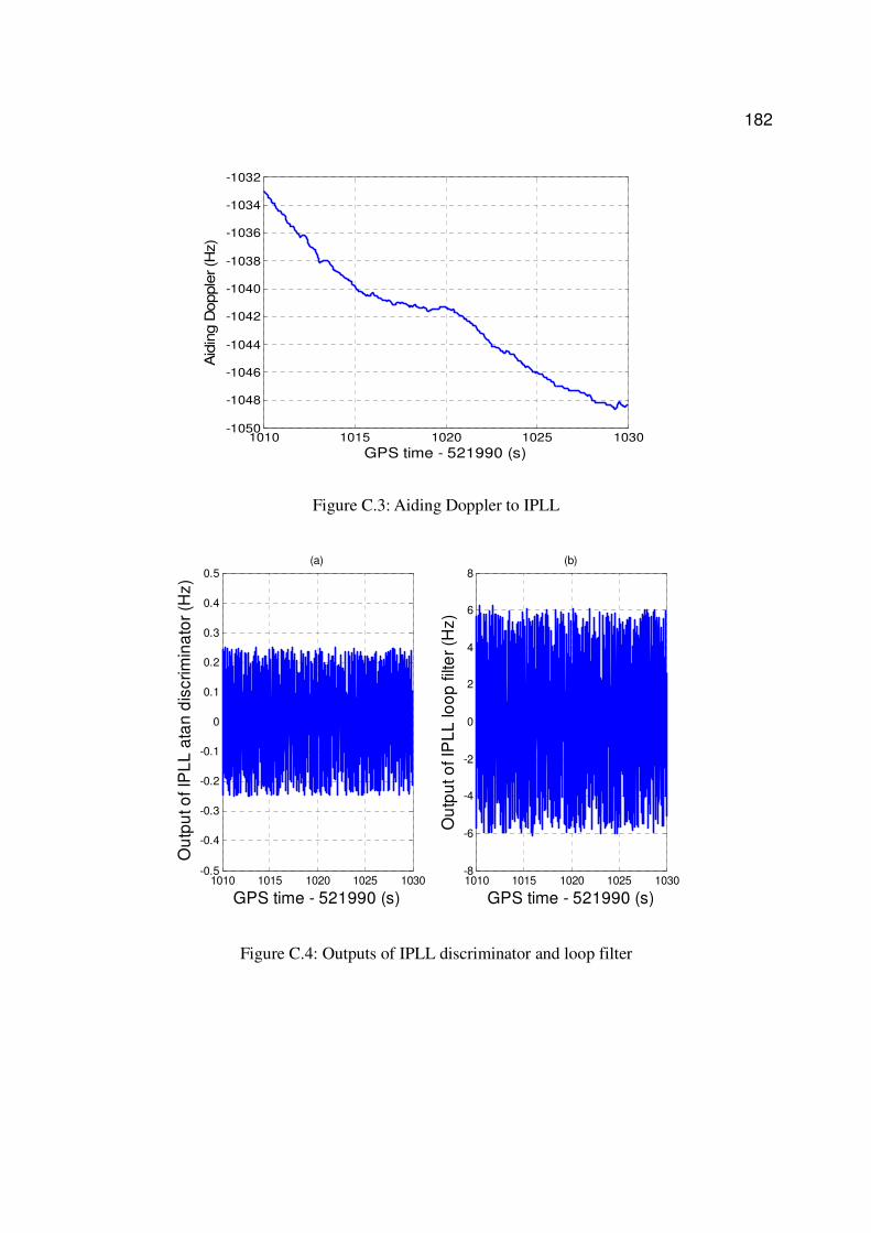
182
1010 1015 1020 1025 1030-1050
-1048
-1046
-1044
-1042
-1040
-1038
-1036
-1034
-1032
GPS time - 521990 (s)
Aid
ing D
opple
r (H
z)
Figure C.3: Aiding Doppler to IPLL
1010 1015 1020 1025 1030-0.5
-0.4
-0.3
-0.2
-0.1
0
0.1
0.2
0.3
0.4
0.5
GPS time - 521990 (s)
Ou
tpu
t o
f IP
LL
ata
n d
iscrim
ina
tor
(Hz)
(a)
1010 1015 1020 1025 1030-8
-6
-4
-2
0
2
4
6
8
GPS time - 521990 (s)
Ou
tpu
t o
f IP
LL
loo
p filt
er
(Hz)
(b)
Figure C.4: Outputs of IPLL discriminator and loop filter

183
1010 1015 1020 1025 10300
0.1
0.2
0.3
0.4
0.5
0.6
0.7
0.8
0.9
1
GPS time - 521990 (s)
Ou
tpu
t o
f lo
ck d
ete
cto
r
(a)
1010 1015 1020 1025 103021
22
23
24
25
26
27
GPS time - 521990 (s)
C/N
0 e
stim
atio
n
(b)
Figure C.5: Lock detector output and 0/ NC estimation from IPLL
1010 1015 1020 1025 10300
0.1
0.2
0.3
0.4
0.5
0.6
0.7
0.8
0.9
1
GPS time - 521990 (s)
Outp
ut of lo
ck d
ete
cto
r
29dB-Hz
28dB-Hz
27dB-Hz
26dB-Hz
25dB-Hz
24dB-Hz
23dB-Hz
Figure C.6: Output of IPLL lock detector vs. different signal strength

184
1010 1015 1020 1025 1030-10
-5
0
5
10
15
Time - 521990 (s)
Po
siti
on
err
or
(m)
(a)
East
North
Up
1010 1015 1020 1025 1030-10
-5
0
5
10
15
Time - 521990 (s)
Po
siti
on
err
or
(m)
(a)
East
North
Up
1010 1015 1020 1025 1030
-0.4
-0.2
0
0.2
0.4
0.6
Time - 521990 (s)
Ve
loc
ity e
rro
r (m
/s)
(a)
East
North
Up
1010 1015 1020 1025 1030
-0.4
-0.2
0
0.2
0.4
0.6
Time - 521990 (s)
Ve
loc
ity e
rro
r (m
/s)
(a)
East
North
Up
1010 1015 1020 1025 1030-2
-1
0
1
2
Time - 521990 (s)
Att
itud
e e
rro
r (d
eg
)
(a)
Pitch
Roll
Heading
1010 1015 1020 1025 1030-2
-1
0
1
2
Time - 521990 (s)
Att
itud
e e
rro
r (d
eg
)
(a)
Pitch
Roll
Heading
Figure C.7: Comparison of navigation errors by using PLL and IPLL
Related Documents