UC Santa Barbara UC Santa Barbara Electronic Theses and Dissertations Title Quantifying Speech Rhythms: Perception and Production Data in the Case of Spanish, Portuguese, and English Permalink https://escholarship.org/uc/item/1xs4b8gc Author Harris, Michael Joseph Publication Date 2015 Peer reviewed|Thesis/dissertation eScholarship.org Powered by the California Digital Library University of California

Welcome message from author
This document is posted to help you gain knowledge. Please leave a comment to let me know what you think about it! Share it to your friends and learn new things together.
Transcript
UC Santa BarbaraUC Santa Barbara Electronic Theses and Dissertations
TitleQuantifying Speech Rhythms: Perception and Production Data in the Case of Spanish, Portuguese, and English
Permalinkhttps://escholarship.org/uc/item/1xs4b8gc
AuthorHarris, Michael Joseph
Publication Date2015 Peer reviewed|Thesis/dissertation
eScholarship.org Powered by the California Digital LibraryUniversity of California

UNIVERSITY OF CALIFORNIA
Santa Barbara
Quantifying Speech Rhythms: Perception and Production Data in the Case of Spanish,
Portuguese, and English
A dissertation submitted in partial satisfaction of the
requirements for the degree Doctor of Philosophy
in Hispanic Languages and Literatures
by
Michael Joseph Harris
Committee in charge:
Professor Viola Miglio, Co-chair
Professor Stefan Gries, Co-chair
Professor Matthew Gordon
March 2015

The dissertation of Michael Joseph Harris is approved.
___________________________________________
Matthew Gordon
____________________________________________
Stefan Gries, Committee Co-chair
____________________________________________
Viola Miglio, Committee Co-chair
March 2015

iii
Quantifying Speech Rhythms: Perception and Production Data in the Case of Spanish,
Portuguese, and English
Copyright © 2015
by
Michael Joseph Harris

iv
ACKNOWLEDGEMENTS
I must begin this manuscript by thanking those people that have helped me along the way.
My life is rich in wonderful people who have supported me; if it takes a village to raise a child, it
took a city for this child to get a PhD. First and foremost, to my committee for their patience and
guidance along the way, a sincere thank you. I was fortunate to have a perfectly balanced
committee, providing encouragement when I was down, direction when I was lost, and a little truth
even when it hurt. For this reason I can truly be proud of what I have achieved herein, and I hope
you are too. To Viola, thank you for encouraging me to start and finish this whole journey, for
treating me as a scholar before I was one and thus convincing me that I could become scholarly.
Thank you for treating me as a colleague, for treating me with such respect, and allowing me the
freedom I needed to complete this work. I hope you go on to guide many other students; we
certainly need it. To Stefan, thank you for being a mentor who I could always trust to give me the
truth, nothing more or less, but also to deliver it with a startling sense of reality and practicality and
a dry, sardonic wit that I truly appreciated. To Matt, thank you for the endless enthusiasm and
energy. Your knowledge was apparently limitless and much needed, but to have it delivered with a
smile and word of encouragement made my work so much more pleasant.
I must also mention the kindness and support of the Department of Spanish and Portuguese.
Both the faculty and staff have stood behind me for the many years I spent haunting the halls of the
fifth floor of Phelps. Thank you for the kindness, the support, the advice, and a few blind eyes to
the beer cans in the recycle bin; sometimes late nights are indeed late nights. Also to my office
mates through the years, thank you for letting me listen to music when I needed it most. Sometimes
only music can keep one from losing his mind, and grad school can push one to these extremes. I
would also like to thank the Linguistics Department for adopting me. So many professors and
students gave their time that I often felt like one of their own. I would also like to express my
gratitude to UCSB at large; the students, staff, and faculty have been endlessly helpful and kind.
My family has been absolutely essential to every aspect of my life; without them I would
be nowhere and I certainly would not be here, teetering on the brink of graduation. Thank you for
the hot meals when I was hungry, the washing machine when my clothes were filthy, the money
when I was broke, and the laughter when I was sad. Most of all, thank you for the love. Thank you
Mom, thank you Dad, and thank you Sister Katie (and thank you for your work in Bolivia, of
which I am very proud).
My friends are also an integral part of my life. I was blessed with a wonderful family, and I
am also blessed with truly special friends that make me feel like family. I do not know what I have
done to be so lucky. My friends are a constant source of distraction and inspiration. I love them
dearly and am a little ashamed to know them. I can only hope that they feel the same about me.
There are too many to mention, but a few that come to mind that should not go without mention are
the Moreno family for housing me, to Jonas for going mad with me and thus providing the
sympathy I most needed, the Boysden Ascuenas for sharing their lives and dog (one and the same)
with me, my Crippled Pink family for the love and nurture and creativity, to the Bearded Ladies for
the adventures, to my partners in crime and my shoulders to cry on, to my fellow students in the
department for suffering along side me and the help when I was frayed to the point of breaking.
Thank you all.
Finally, to those obscure and non-human sources of inspiration: whiskey and caffeine
(whiskey to lubricate the creative wheels to turn and caffeine to sustain the cogs in motion), to my
dog Vera for the moral support and general adorableness, and to music and the Pacific Ocean.
This dissertation has been achieved with a minimum of tears and a maximum of smiles. It was not
easy, but all the wonderful people and so many more that I have not mentioned have made this
whole experience, in the end, actually kind of fun. My sincere gratitude to you all.

v
VITA OF MICHAEL JOSEPH HARRIS
March 2015
EDUCATION
2010- 2015: University of California, Santa Barbara
Postgraduate Studies in pursuit of a Ph.D. in Spanish
Emphasis: Iberian Linguistics, Department of Spanish and Portuguese
2008- 2010: University of California, Santa Barbara
Masters of Arts in Spanish
Emphasis: Iberian Linguistics, Department of Spanish and Portuguese
2002- 2005: California Polytechnic University, San Luis Obispo, California
Bachelors of Science, Business Administration
International Business Management Concentration
Minor in Spanish
Magna Cum Laude
PUBLICATIONS
Harris, Michael J., Viola G. Miglio and Stefan Th. Gries. (Accepted for publication).
Mexican and Chicano Spanish intonation: differences related to information
structure. Proceedings of the 6th Pronunciation in Second Language Learning and
Teaching Conference, Iowa State University online publication.
Harris, Michael J., Stefan Th. Gries, & Viola G. Miglio. 2014. Prosody and its application
to forensic linguistics. LESLI- Linguistic Evidence in Security, Law, and
Intelligence 2(2). 11-29.
Harris, Michael J. 2013. The origin of the Portuguese Inflected Infinitive: A corpus-based
perspective. In: Jessi Aaron, Jennifer Cabrelli Amaro, Gillian Lord, & Ana de Prada
Pérez (eds.), Selected Proceedings of the 15th Hispanic Linguistics Symposium.
Somerville, MA. Cascadilla Press. 303-311.
Miglio, Viola, Stefan Th. Gries, Michael J. Harris, Raquel Santana Paixão, & Eva Wheeler.
2013. Spanish lo(s)-le(s) clitic alternations in psych verbs: a multifactorial corpus-
based analysis. In: Jessi Aaron, Jennifer Cabrelli Amaro, Gillian Lord, & Ana de
Prada Pérez (eds.), Selected Proceedings of the 15th Hispanic Linguistics
Symposium. Somerville, MA. Cascadilla Press. 268-278.
Harris, Michael J. & Stefan Th. Gries. 2011. Measures of speech rhythms and the role of
corpus-based word frequency: a multifactorial comparison of Spanish(-English)
speakers. International Journal of English Studies 11(2). 1-22.
vi
GRANTS, FELLOWSHIPS, & HONORS
Humanities Research Assistantship, University of California, Santa Barbara, 2013- 2014
Dean’s Advancement Fellowship, University of California, Santa Barbara, Spring 2013
Outstanding PhD Student Award by the Dept. of Spanish & Portuguese, 2011- 2012, 2013-
2014
Timothy McGovern Memorial Award for Outstanding Ph.D. Student by the Dept. of
Spanish and Portuguese 2011-2012
Wofsy Travel Grant for Conference Presentation, Dept. of Spanish and Portuguese, UCSB
2011, UCSB 2010.
Outstanding MA Student Award by the Dept. of Spanish & Portuguese 2009- 2010
Outstanding Portuguese Language Student Award by the Dept. of Spanish and Portuguese
2008-2009
UC Mexus Award- Research grant from University of California Institute for Mexico and
the United States; awarded to complete research in Mexico. 2009
California Polytechnic University, San Luis Obispo, California:
-Dean’s Honor List: Fall 2002 through Spring 2004.
-President’s Honor List: 2002, 2003.
-Inducted to Beta Gamma Sigma Honor Society in recognition of high scholastic
achievement in 2003.
ACADEMIC WORK EXPERIENCE
Instructor of Record: Introduction to Hispanic Linguistics, an upper division course,
Department of Spanish and Portuguese, UCSB, 2013.
Instructor: Introduction to Romance Linguistics, an upper division course, Department of
Spanish and Portuguese and Department of Linguistics, UCSB, 2012.
Teaching Associate: Sole instructor of beginning and intermediate Spanish courses,
Department of Spanish and Portuguese, UCSB, 2008- 2013.
Teaching Associate: Sole instructor of beginning Portuguese, Department of Spanish and
Portuguese, UCSB, 2009- 2013.
vii
Substitute Instructor: Substitute as instructor of graduate level linguistics/statistics
courses and upper division Spanish courses at UCSB, 2011- Present.
Phonetics Research Assistant: Assist Professor Viola Miglio in phonetics laboratory
research, including subject recording and spectrogram analysis- Department of
Spanish and Portuguese, UCSB, 2009- Present.
R Programming Language Study Group Leader: Assist other graduate students in the
use of R programming language for statistical analysis of linguistic data, UCSB,
2009- 2011.
FIELDS OF STUDY
Major Field: Quantiative and experimental approaches to prosody and
phonetics/phonology
Studies in corpus linguistics, language variation, and sociolinguistics with R programming
language for statistics and Praat software for phonetics analysis

viii
ABSTRACT
Quantifying speech rhythms: Perception and production data in the case of Spanish,
Portuguese, and English,
by
Michael Joseph Harris
This dissertation addresses the methodology used in classifying speech rhythms in order to
resolve a long-standing linguistic conundrum about whether languages differ rhythmically.
There is a widespread perception, both among linguists and the general population, that
some languages are stress-timed and others are syllable timed. Stress-timed languages are
described as having less-regular rhythms, as syllable durations vary according to the
placement of stress in the phrase. Meanwhile, syllable-timed languages are described as
displaying less variation in rhythm, which syllable durations being more regular. This
dissertation quantitatively evaluates these described rhythmic differences in Spanish,
Portuguese, and English. The first chapter introduces speech rhythms and reviews past
literature on their perception and production. The second chapter evaluates a widely used
metric of speech rhythms, the PVI, and determines that it is not effective in distinguishing
between two dialects of Spanish. The third chapter compares the speech rhythms of
Mexican and Chicano Spanish. This chapter concludes that Chicano Spanish is more
restricted in its vowel duration variability, while Mexican Spanish employs both highly
variable durations (i.e. stress-timed) and highly uniform durations (i.e. syllable-timed). The

ix
fourth chapter describes a perception study used to compare the speech rhythms of Spanish,
English, and Portuguese, and shows that these languages’ rhythms do not always group
according to language. In the fifth chapter, I describe a study of the production of the same
utterances initially used in the perception experiment; this allows an analysis of what
prompts the perceptual differences in speech rhythm described in Chapter Four. The sixth
and final chapter discusses the implications and applications of these findings and gives
direction for further investigation. Although both production and perception studies of
speech rhythms have been performed in the past, my dissertation expands these
methodologies by combining production and perception data is a single analysis. I use
perception data to relatively classify the rhythms of utterances through low-pass speech
filtering, then analyze the production of these data computationally to provide a more
complete perspective of what prompts differences in speech-rhythms and how Spanish,
Portuguese, and English data relate rhythmically. Thus, my dissertation is thorough, while
still addressing traditional rhythm metrics and employing current computational
methodology. It seeks to challenge linguists' methodologies in quantitatively addressing
speech rhythms, and to further clarify the position of Spanish, Portuguese, and English on
the speech rhythm continuum.

x
TABLE OF CONTENTS
Ch 1. An Introduction to Speech Rhythms............................................................................1
1.1. Speech Rhythm Distinction................................................................................1
1.2. The Importance of Speech Rhythm Research.....................................................3
1.3. Production Speech Rhythm Studies....................................................................9
1.4. Speech Rhythm Discrimination Studies............................................................18
1.5. Conclusion.........................................................................................................25
Ch 2. A Comparative Evaluation of the PVI in Speech Rhythm Discrimination................ 27
2.1. Introduction.......................................................................................................28
2.2. Data....................................................................................................................29
2.3. Speakertype Mean PVI......................................................................................33
2.4. Speaker Mean PVI.............................................................................................37
2.5. Utterance Mean PVI..........................................................................................39
2.6. Cumulative PVI.................................................................................................43
2.7. Methodological Implications............................................................................46
2.8. Interim Summary ...............................................................................................49
Ch 3. A Comparison of Measures of Speech Rhythm in Mexican and Chicano Spanish....51
3.1. Introduction.......................................................................................................52
3.2. Data....................................................................................................................52
3.3. Multifactorial Analysis......................................................................................54
3.4. Discussion: Multifactorial Analysis..................................................................59
3.5. Implications.......................................................................................................66
Ch 4. Perception of English, Portuguese, and Spanish Speech Rhythms............................70
4.1. Introduction.......................................................................................................70
4.2. Perception Experiment: Conceptual Design......................................................72
4.3. Perception Experiment: Pilot Studies 1 and 2...................................................76
4.4. Perception Experiment......................................................................................84
Ch 5. Production Data of English, Portuguese, and Spanish...............................................94
5.1. Data and Variables.............................................................................................94
5.2. Statistical Evaluation and Results...................................................................108
5.3. Post Hoc Analysis............................................................................................128
5.4. Discussion........................................................................................................145
Ch 6. Implications, Directions for Further Study, and Concluding Remarks....................150
6.1. Dissertation Summary.....................................................................................151
6.2. Linguistic Implications....................................................................................155
6.3. Methodological Implications...........................................................................160
6.4. Practical Applications......................................................................................164
6.5. The Future of Speech Rhythm Research.........................................................167
6.6. Concluding Remarks.......................................................................................169

xi
References.......................................................................................................................171
Appendix 1. Calculation of Traditional Speech Rhythm Metrics...................................178
Appendix 2. Perception Experiment Data.......................................................................182

xii
LIST OF FIGURES AND TABLES
Ch1. An Introduction to Speech Rhythms.............................................................................1
Table 1.1. The Speech Rhythm Continuum.............................................................10
Figure 1.1. Equation for PVI....................................................................................10
Figure 1.2. Waveforms and Spectrograms: English and Spanish.............................11
Figure 1.3. Equation for rPVI...................................................................................12
Figure 1.4. Waveforms and Spectrograms: English and Spanish.............................17
Ch 2. A Comparative Evaluation of the PVI in Speech Rhythm Discrimination................27
Figure 2.1. Calculation for Mean PVI......................................................................34
Figure 2.2. Calculation for Mean PVI......................................................................34
Figure 2.3. Mean PVI by SPEAKERTYPE..............................................................36
Figure 2.4. Predicted SPEAKERTYPE by Mean PVI.............................................38
Figure 2.5. Utterance Mean PVI by SPEAKERTYPE.............................................40
Figure 2.6. Predicted SPEAKERTYPE by Utterance Mean PVI.............................42
Figure 2.7. Observed PVI Scores by SPEAKERTYPE............................................44
Figure 2.8. Predicted SPEAKERTYPE by Mean PVI.............................................45
Ch 3. A Comparison of Measures of Speech Rhythm in Mexican and Chicano Spanish....51
Table 3.1. Significant Predictors in Logistic Regression Model..............................56
Figure 3.1. Main Effects SD and VARCOEFFLOG.................................................57
Figure 3.2. Interaction LEMMAFRE:SDLOG.........................................................58
Figure 3.3. Interaction LEMMAFRE:PVI................................................................59
Figure 3.4. Waveforms and Spectrograms: Low Frequency Word...........................63
Figure 3.5. Waveforms and Spectrograms: High Frequency Word..........................65
Ch 4. Perception of English, Portuguese, and Spanish Speech Rhythms............................70
Table 4.1. Expected Position of Languages on Speech Rhythm Continuum...........74
Figure 4.1. Waveforms and Spectrograms: Low-Pass Filtered Utterance................77
Table 4.2. Utterances in Perception Experiment: Pilot 1 and Pilot 2.......................81
Table 4.3. Utterances in Perception Experiment......................................................84
Table 4.4. Demographics for Participants in Perception Experiment.......................85
Figure 4.2. Dendogram: Randomized Orders...........................................................88
Figure 4.3. Dendogram: Participants .......................................................................89
Figure 4.4. Dendogram: Languages.........................................................................91
Ch 5. Production Data of English, Portuguese, and Spanish...............................................94
Figure 5.1. Waveforms and Spectrograms: Division of Prosodic Units.................101
Figure 5.2. (Non)-Normal Distribution of Intensity...............................................104
Figure 5.3. (Non)-Normal Distribution of Pitch.....................................................105
Figure 5.4. Variable Importance Plot......................................................................112
Table 5.1. Categories of Variable............................................................................117
Figure 5.5. Conditional Inference Tree...................................................................122
Figure 5.6. Waveforms and Spectrograms: Vowel Deletion in Portuguese............125

xiii
Figure 5.7. Pitch Contours: Spanish and Portuguese .............................................126
Figure 5.8. Predicted SYLLABLE DURATION by FREQUENCY......................133
Figure 5.9. Interaction STRESS: UTTERANCE...................................................134
Figure 5.10. Predicted SD PITCH by FREQUENCY............................................137
Figure 5.11. SD PITCH by UTTERANCE............................................................139
Figure 5.12. UTTERANCE by LETTERS PER SYLLABLE...............................141
Figure 5.13. UTTERANCE by LETTERS PER SYLLABLE...............................144

1
Chapter 1
An Introduction to Speech Rhythms
Overview
This chapter presents an overview of past speech rhythm research. It begins by explaining
the basic concept of speech rhythm and addressing the distinction between syllable and
stress-timed languages (and briefly mention mora languages). It then addresses the
importance of speech rhythm research. The following sections review production speech
rhythm studies and perception rhythm studies; the methodological implications of these
studies to my dissertation are also discussed.
1.1. Speech Rhythm Distinctions
Pike (1945) described the simple rhythm units of languages: stress-timed and syllable-
timed. The former means that the duration of syllables varies according to the placement
of stress and seem to be less uniform throughout the entire phrase; languages that sound
more stress-timed include, for example, Dutch and English. The latter means that syllable
duration is relatively uniform within a phrase, as in French and Spanish. In addition to the
two rhythm classes described by Pike (1945), a third rhythm class, mora-timed speech has
been identified, which uses moras, i.e. phonological weight units, in the processing of
languages and exists, for instance, in Japanese (Otake, Hatano, Cutler, and Mehler 1993).
As mentioned, one basic reasoning behind the nature of this rhythmic difference is that
various languages privilege, or give spectral prominence to different phonological units:
the mora, the syllable, or the stress foot (Lee and Todd 2004). This would account for the

2
existence of these rhythmic differences as well as their relevance in parsing speech (in the
recognition of word boundaries for instance).
For quite some time, this perceived difference in speech timing was regarded as a
dichotomy: "As far as is known, every language in the world is spoken with one kind of
rhythm or with the other" (Abercrombie 1967:97). Dasher and Bolinger (1982) suggested
that stress-timing and syllable-timing can be correlated to specific phonological
phenomena in a given language. Specifically, they suggested that stress-timed languages
present a greater variety of syllable types, and have greater vowel reduction between
stress and unstressed vowels. Dauer (1987) agreed that speech rhythms are a product of
their phonological properties, but added that languages should not be thought of as either
stress-timed or syllable-timed, but instead should be conceived on a continuum, with the
most stress-timed languages at one extreme of the continuum and the most syllable-timed
languages at the other extreme. While some languages – e.g., Spanish and English – exist
near the opposite ends of this continuum, other languages exist somewhere in the middle,
exhibiting some syllable-timed characteristics and some stress-timed characteristics.
Catalan, for instance, has simple syllable types but also exhibits vowel reduction, causing
it to fall somewhere between stress-timed and syllable-timed on the continuum (see Table
1). Dauer (1987) also concluded that simple measures of interstress intervals or syllable
durations were not effective in assigning rhythm class, demonstrating the necessity of a
measure of speech rhythms with more discriminatory power.

3
Poles of Rhythm Continuum More Syllable
Timed
More Stressed
Timed
Proposed phonetic
characteristics
less variable
segment durations
more variable
segment durations
Example Languages Spanish
Catalan English
Table 1.1: An illustration of the speech rhythm continuum
1.2. The Importance of Speech Rhythm Research
The fact that languages differ rhythmically is a widespread intuition (Loukina, Kochanski,
Rosner, and Keane 2011). Most linguists, and even most humans, agree that they perceive
some rhythmic difference in the production of certain languages; however, the results of
linguistic studies on both the perception and production of speech rhythms have failed to
support this with conclusive empirical evidence (although many studies have shown some
evidence of rhythmic variation between languages, e.g. Low and Grabe 1995).
Nevertheless, linguists have recently expanded methodologies in their attempts to
quantify rhythmic differences between languages or dialects. In addition to the perceived
differences between two languages, three factors suggest that there is some fundamental
rhythmic variation in speech.
Firstly, consider early studies investigating whether or not an ―underlying pattern‖
determines the timing between sequential segments in an utterance, or whether this
rhythm is simply a random artifact of the time it takes to finish articulating the previous
segment in the utterance. For instance, Ohala (1975) offers three hypotheses for the
factors that determine the timing of speech; these hypotheses consider the sentence 'Joe
took father's shoebench out':

4
―1. Some units of speech, perhaps syllables, stresses or morae, are uttered in
time to some underlying regular rhythm, e.g. the [b] of ‗shoebench‘ will be
uttered after the [dʒ] of ‗Joe‘ an interval which is an integral multiple of the
period of this underlying rhythm.
2. The units of speech are executed according to some underlying pre-pro
grammed time schedule although there may be no isochrony in this schedule.
3. There is no underlying time program or rhythms; a given speech gesture is
simply executed after the preceding gestures have been successfully completed,
that is, one unit is simply strung after the other.‖ (Ohala 1975:431- 432).
He notes that while Hypothesis 1 has been assumed by some linguists, it proves difficult
to verify via empirical data. This would suggest that speech timing is either completely
random, or executed according to some ‗schedule‘, but is not isochronous. Given that
Ohala (1975) investigates English and Japanese, which are said to be stress-timed and
mora-timed respectively, this is compatible with traditional rhythm classes. Meanwhile,
he mentions that previous studies measuring the time intervals between certain speech
events, such as voiceless stops or successive jaw openings suggest that there is an
underlying pattern or schedule to speech timing, which is to say that Hypothesis 2 rather
than Hypothesis 3 is more likely. Specifically, Kozhevnikov and Christovich (1965),
Allen (1969), Lehiste (1971, 1972) found evidence for Hypothesis 2 as an underlying
pattern in speech by showing that segments in an utterance tend to contribute equally to
the variance in timing between segments of the utterance (as cited in Ohala 1975:439).

5
This further supports the concept that some sort of pattern exists in the timing or rhythm
of speech.
Secondly, various studies have shown that neonates and infants can distinguish
between languages of two different rhythm classes, but not necessarily between two
languages of the same rhythm class (e.g. Nazzi, Bertoncini, and Mehler 1998). This
suggests that a patterned speech timing not only exists, but varies across language or
dialect. In this study, French newborns were able to discriminate between stress-timed
English and mora-timed Japanese, but not between two stress-timed languages (English
and Dutch) in a task that evaluated infants‘ responses to the language stimuli via a pacifier
that measured the amplitude of the infants‘ sucking. High amplitude sucking represented a
reaction to the language stimuli and the infants reacted with higher amplitude sucking to
the English stimuli as compared to the Japanese, but did not show a significant difference
in sucking amplitude for the English as compared to the Dutch stimuli (Nazzi, Bertoncini,
and Mehler 1998). These experiments not only suggest that languages do differ
rhythmically, but also that infants begin to exploit rhythmic cues at a young age. Thus,
rhythms may be instrumental in parsing words, perhaps because they give prominence to
the syllable structure (in so-called syllable-timed languages) or the stress patterns (in so-
called stress-timed languages). Thirdly, Wretling and Eriksson show that speech
impersonators could alter spectral characteristics, but less so timing at the phoneme and
word levels in imitating speech, suggesting that rhythm is somehow ―hard coded‖ in the
adult speaker (1998:1). Thus, while there is ample evidence for the existence of cross-
linguistic rhythmic differences, their study via empirical methodology has proved more
elusive.
6
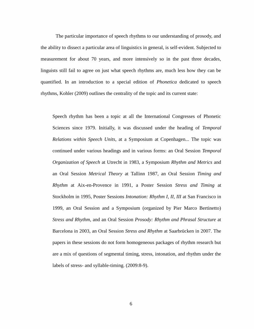
The particular importance of speech rhythms to our understanding of prosody, and
the ability to dissect a particular area of linguistics in general, is self-evident. Subjected to
measurement for about 70 years, and more intensively so in the past three decades,
linguists still fail to agree on just what speech rhythms are, much less how they can be
quantified. In an introduction to a special edition of Phonetica dedicated to speech
rhythms, Kohler (2009) outlines the centrality of the topic and its current state:
Speech rhythm has been a topic at all the International Congresses of Phonetic
Sciences since 1979. Initially, it was discussed under the heading of Temporal
Relations within Speech Units, at a Symposium at Copenhagen... The topic was
continued under various headings and in various forms: an Oral Session Temporal
Organization of Speech at Utrecht in 1983, a Symposium Rhythm and Metrics and
an Oral Session Metrical Theory at Tallinn 1987, an Oral Session Timing and
Rhythm at Aix-en-Provence in 1991, a Poster Session Stress and Timing at
Stockholm in 1995, Poster Sessions Intonation: Rhythm I, II, III at San Francisco in
1999, an Oral Session and a Symposium (organized by Pier Marco Bertinetto)
Stress and Rhythm, and an Oral Session Prosody: Rhythm and Phrasal Structure at
Barcelona in 2003, an Oral Session Stress and Rhythm at Saarbrücken in 2007. The
papers in these sessions do not form homogeneous packages of rhythm research but
are a mix of questions of segmental timing, stress, intonation, and rhythm under the
labels of stress- and syllable-timing. (2009:8-9).
7
Indeed, the current state of speech-rhythms could be more easily summarized by the areas
in which linguists differ rather than by which they agree. A widespread attempt to
quantify speech rhythm production has led to the development of metrics (usually related
to segment variability, e.g. Low and Grabe 1995, Deterding 2001) that reportedly
compare the rhythms of languages or dialects. Some of these metrics have been adopted
in the past because they were easy to calculate; in some cases they do crudely
approximate supposed differences in speech-rhythms, although they only encapsulate a
small segment of rhythmic perception (Arvaniti 2009). However, current studies point to
the necessity of aligning perception and production data (e.g. Barry, Adreeva, and
Koreman 2009), of doing so in a more statistically sound manner, and including all
relevant information (e.g. Loukina, Kochanski, Rosner, and Keane 2011).
In fact, regardless of methodological differences, one central fact has become clear
in recent literature: in attempting to find acoustic evidence of a perceived difference in
speech rhythms, it is not enough to simply use those interval metrics that appear to
conveniently reflect perception. This is to say that certain metrics that have been applied
to speech rhythm discrimination studies appear to (at least partially) reflect differences
between two languages that are traditionally described as belonging to different rhythm
classes. Nonetheless, it is hasty to adopt a metric for quantifying speech rhythms simply
because it classifies Spanish as more syllable-timed than English, for instance. First one
must determine what exactly the metric measures. For instance, is vowel duration
variability truly akin to perceived rhythmic differences? Also, is the manner in which
these metrics are measured, calculated, and reported statistically sound? In fact, as we will
see in the following chapters, many traditional metrics are not exhaustively informative to

8
rhythmic differences for several reasons. Firstly, as Chapters 2 and 3 will describe in
detail, some of these metrics are not calculated in a statistically sound manner, and fail to
address a full-range of word-frequencies. Equally troubling is the fact that many of these
metrics are presented as a single value intended to address, for instance, the vowel
duration variability of an entire phrase, a speaker, or even a speaker type. This occurs in
the presentation of a mean PVI value, or a single standard deviation of vowel durations.
Finally, the assumption that, say, Spanish and English belong to different rhythm classes,
so all utterances of Spanish differ from all utterances of English has certainly never been
proven. In fact, rhythmic variation in speakers appears to contribute a great deal to certain
interval metrics, regardless of rhythm class (e.g. Loukina et al. 2009). In fact, up to this
point, it has not been proven that Spanish does in fact differ from English in terms of
syllabic rhythm; hence the need for the current dissertation.
To begin to address these issues, one must critically assess the utility of these
measures in a multifactorial manner, allowing for non-linear trends and interactions
between metrics of speech rhythm (see Chapter 3). This approach allows one to consider
multiple factors that may contribute to our perception of speech rhythms. Cues of duration
variability, and vowel duration variability in particular have been reported to affect
rhythmic perception (e.g. Low and Grabe 1995; Deterding 2001). However, other factors
potentially contribute to speech rhythms as well. For instance, other prosodic cues, F0 and
intensity, have been shown to work with segment duration to indicate lexical stress. While
these are not strictly considered to contribute to rhythm, it is certainly a possibility that
they may play a role in our perception of rhythmic differences; this possibility is explored
in Chapter 5. Meanwhile, corpus-based frequencies have been shown to effect various
9
aspects of pronunciation (e.g. Bell et al. 2009), so it is conceivable that rhythms (or cues
that effect the perception of rhythms) vary with frequency. This possibility is explored
further in Chapters 3 and 5. By using various sophisticated statistical approaches to
rhythmic data, it is possible to avoid, or at least minimize such methodological pitfalls.
1.3. Production Speech Rhythm Studies1
As a result of the continuous view of speech rhythms (e.g. Dasher and Bolinger 1982),
linguists sought to relatively classify the production of language rhythms. That is, rather
than classify a language as either (absolutely) syllable-timed or (absolutely) stress-timed,
languages or varieties/dialects of languages were compared to other languages or other
varieties/dialects of the same language. Low and Grabe (1995) made significant strides in
the study of speech rhythms in their study of prosodic patterns in Singapore English
compared to British English. This study is significant in focus and methodology. Firstly, it
examined two varieties of the same language, comparing native (L1) and second language
(L2) English speakers. Secondly, it introduced the Pairwise Variability Index (henceforth
the PVI, see Appendix 1, Section 2) as a new measure intended to relatively classify
speech rhythms by measuring the variation between successive sets of vowels as opposed
to the more limiting measure of overall variation within a phrase (as cited in Carter
2007:5). This study served to provide a framework for further speech rhythm studies and
studies of cross-varietal speech rhythms of a single language in particular.
The PVI (see Figure 1.1) is the measure of the absolute difference of the vowel
duration of two adjacent syllables divided by the average vowel duration of the same two
1 A variety of metrics have been suggested as quantifiers of speech rhythms. The metrics in this section are
calculated on two different ranges of vowel durations in Appendix A.

10
adjacent syllables; thus, a sentence with n syllables yields n-1 PVIs. These PVIs represent
the variability of vowel duration, with lower PVIs representing a more syllable-timed
language and higher PVIs representing a more stress-timed language.
𝑃𝑉𝐼 =∣∣(𝑣𝑜𝑤𝑒𝑙𝑑𝑢𝑟𝑎𝑡𝑖𝑜𝑛1 − 𝑣𝑜𝑤𝑒𝑙𝑑𝑢𝑟𝑎𝑡𝑖𝑜𝑛2)∣∣
𝑚𝑒𝑎𝑛(𝑣𝑜𝑤𝑒𝑙𝑑𝑢𝑟𝑎𝑡𝑖𝑜𝑛1, 𝑣𝑜𝑤𝑒𝑙𝑑𝑢𝑟𝑎𝑡𝑖𝑜𝑛2)
Figure 1.1: Equation for calculation of PVI (e.g. Low and Grabe 1995), also knows as the nPVI (Low Grabe, and Nolan 2000).
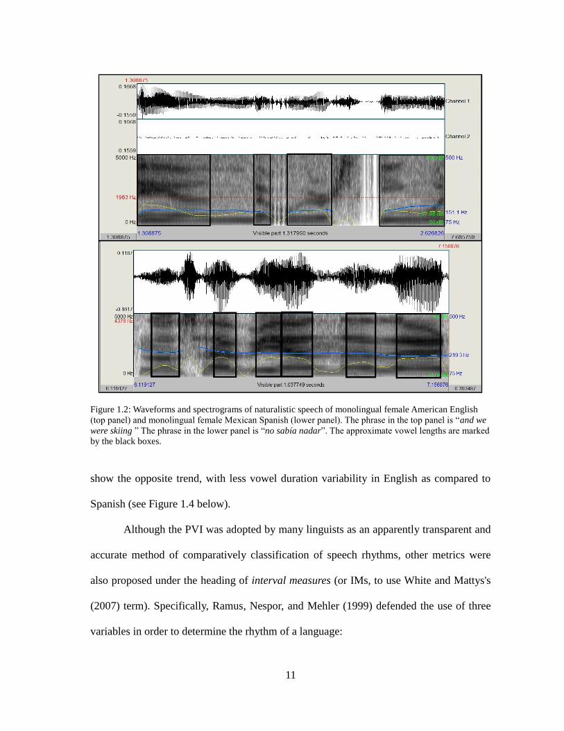
Consider Figure 1.2. The top panel denotes the approximate vowel durations of a stress-
timed language, English, while the lower panel represents the vowel durations of a
syllable timed language, Spanish. The PVI scores for the top panel would be higher, due
to the higher variability of vowel durations, and compared to the lower panel. If vowel
duration variability is indeed a reflection of rhythm class distinctions, Low and Grabe's
(1995) PVI would reflect this difference, with the stress-timed language in the top panel
displaying a higher PVI as compared to the syllable-timed language in the lower panel. It
is important to note three things.
First, PVIs do not represent an index of 'the absolute rhythm of a language' –
instead, they allow the comparison of the rhythms of two or more languages or varieties.
Second, the PVI has been reported as a mean for each utterance (or even a speaker, e.g.
Grabe and Low 2002), rather than a series of individual PVI scores (see Chapter 2).
Thirdly, these spectrograms are meant as a representation of how the PVI works; such
short phrases are certainly not indicative of the overall rhythmic nature of a language or
even a speaker. In fact, it is possible to choose two phrases from the same speakers that
11
Figure 1.2: Waveforms and spectrograms of naturalistic speech of monolingual female American English
(top panel) and monolingual female Mexican Spanish (lower panel). The phrase in the top panel is ―and we
were skiing ‖ The phrase in the lower panel is ―no sabía nadar‖. The approximate vowel lengths are marked
by the black boxes.
show the opposite trend, with less vowel duration variability in English as compared to
Spanish (see Figure 1.4 below).
Although the PVI was adopted by many linguists as an apparently transparent and
accurate method of comparatively classification of speech rhythms, other metrics were
also proposed under the heading of interval measures (or IMs, to use White and Mattys's
(2007) term). Specifically, Ramus, Nespor, and Mehler (1999) defended the use of three
variables in order to determine the rhythm of a language:

12
the percentage of a sentence taken up by vowel duration (%V);
the average standard deviation of vowel duration (∆V); and
the average standard deviation of consonant duration (∆C).
(see Appendix 1, Section 3, 4, and 5, respectively). However, in applying these metrics,
Ramus et al. (1999) suggest that only %V and ∆C reflect differences in speech rhythms.
Deterding (2001) proposed measuring the duration of the entire syllable, rather
than only the vowel duration, arguing that some syllables may be longer than others
regardless of the presence of vowels. The author used a normalizing equation for syllable
length similar to the PVI called the Variability Index (VI).
Low, Grabe, and Nolan (2000) revisited speech rhythms of Singapore and British
English and discussed the application of speech-rate normalization to the PVI. That is, the
authors differentiated between the PVI as in Figure 1.1 (from Low and Grabe 1995),
which they called nPVI, for normalized PVI, and the rPVI, or raw PVI, calculated as in
Figure 1.3 below. As with the nPVI, Low, Grabe, and Nolan presented the rPVI as a mean
of a series of PVI values for an utterance.
𝑃𝑉𝐼 = ∣∣(𝑣𝑜𝑤𝑒𝑙𝑑𝑢𝑟𝑎𝑡𝑖𝑜𝑛1 − 𝑣𝑜𝑤𝑒𝑙𝑑𝑢𝑟𝑎𝑡𝑖𝑜𝑛2)∣∣
Figure 1.3: Equation for calculation of rPVI (Low, Grabe, and Nolan 2000).
Low, Grabe, and Nolan (2000) argue that the nPVI is superior as it normalizes the metric
for differing speech rates between speakers. The vast majority of linguists have adopted

13
the nPVI, eschewing the rPVI completely. Thus, for the remained of this dissertation, the
term PVI will refer to nPVI (unless otherwise noted), as in Figure 1.1.
While Low, Grabe, and Nolan (2000) compared first language (L1) speakers and
second language (L2) speakers, the more recent studies of Carter (2005, 2007) as well as
Fought (2003) investigated bilingual Chicano speakers of Spanish and English. Bunta and
Ingram (2007) also examined the acquisition of Spanish-English bilingual speech rhythms
in children using vocalic and intervocalic PVI values, and concluded that bilingual and
monolingual speakers differ in speech rhythms, particularly in the youngest participants,
age approximately 4 years, although these differences diminished for older speakers.
White and Mattys (2007), undertook a more exhaustive investigation of the
relative merits of the PVI and other IMs by applying both normalized and raw pairwise
variability indices as well as the IMs suggested by Ramus et al. (1999) to both cross-
varietal and cross-language utterances. Additionally, they tested the correlation of these
metrics with speech-rate, exploring the effectiveness and/or necessity of rate-
normalization measures. Although previous studies had compared competing metrics of
duration variability (e.g. Low et al. 2000), White and Mattys' (2007) study was more
comprehensive: their goal was to compare the metrics used to classify duration variability,
as opposed to dedicating their work to the sole task of classifying the rhythms of specific
languages or varieties. The study concluded that the rate-normalized nPVI, the rate-
normalized standard deviation of vowel duration VarcoV, as well as the percentage of an
intonational unit comprised by vowels best distinguished between syllable and stress-
timed languages as well as between L1 and L2 speakers.

14
Even though White and Mattys (2007) constitutes important progress, it still
leaves room for improvement in several areas. First, the statistical assessment of the
performance of the metrics is incomplete; they report whether or not certain effects are
significant, but fail to report the relative strength of each effect. Thus, one cannot evaluate
the relative statistical performance of each metric due to their failure to report R2-values,
beta coefficients, etc. Furthermore, their exploration does not include a truly
multifactorial analysis, which could potentially reveal a far more complex picture of the
behavior of the metrics. Secondly, a specific weakness of the PVI, is mentioned by the
authors: "PVI scores derived alternating patterns and monotonic geometric series may be
the same, so that, for example PVI(2, 4, 2, 4, 2, 4) and PVI(2, 4, 8, 16, 32, 64) are equal"
(White and Mattys 2007:519). While White and Mattys (2007) mention this weakness,
they make no suggestions for the improvement of this metric.
Chapters 2 and Chapter 3 will discuss the PVI in more depth. This is particularly
important as it has been so widely adapted in speech rhythm research. These two chapters
will assess the utility of the PVI (amongst other metrics, e.g. Chapter 3) is distinguishing
between two dialects of Spanish: monolingual Mexican Spanish and bilingual Chicano
Spanish. Chapter 2 identifies some shortcomings in the utility of the PVI, particularly in
its failure to account for the great of amount of variation in vowel durations that occurs
for each participant. Chapter 3 goes on to compare the PVI to other IMs in a
multifactorial analysis and determines that it is less effective in distinguishing between
the two dialects of Spanish. In fact, it shows that the PVI is only effective in a rather small
range of word frequencies.

15
A few speech rhythms studies have employed more statistically advanced
methodology (as compared to the aforementioned study). In particular, Loukina,
Kochanski, Shih, Keane, and Watson (2009) used automatic segmentation of durations,
rather than the manual segmentation employed in most rhythm studies (e.g. Low and
Grabe 1995). This study evaluates 15 interval metrics in classifying the speech rhythms of
English, Greek, Russian, French and Mandarin. This automatic segmentation allowed the
authors to evaluate larger corpora; they conclude that while there is a fair amount of
rhythmic variation between languages, there is also a comparable amount of variation
within languages. Some IMs did appear to be more effective in distinguishing rhythms,
but there is no single metric that consistently distinguishes between the rhythms of the
various languages examined. The authors conclude that speech rhythms are a two or
three-dimensional phenomenon (Loukina et al. 2009:1534).
Callier (2011) applies the PVI of syllable duration and a speech rate normalized
standard deviation of syllable durations (VARCOS) in order to examine the Mandarin of
six Chinese characters from the same show. Callier suggests that some sociolinguistic
factors may be relevant in determining both the rhythm and final syllable lengthening of
the utterances examined. The only sociolinguistic factor related to rhythm discussed was
gender. The three female characters show greater syllable duration variability than the
three male characters in terms of PVIS. The author compares this increased duration
variability in women to ―the widespread impression of women‘s pitch and intonation as
highly dynamic or ―swoopy‖ (Henton 1995).‖ (Callier 2011:48).
Harris and Gries (2011) apply multifactorial methodology and corpus-based
frequency effects in their evaluation of the efficacy of various metrics in distinguishing

16
the speech rhythms of Chicano and Mexican Spanish. Their conclusions regarding IMs is
in agreement with those of Loukina et al. (2009), namely that no single IM is sufficient in
distinguishing speech rhythms. Furthermore, they show a) that it is necessary to include
corpus-based frequency effects in speech rhythm analysis, as frequency affects duration
cues, and b) it is necessary to use a multifactorial approach in the analysis of IMs, as it is
possible to see interactions, as well as main effects. Loukina et al. (2011) are largely in
agreement with Loukina et al. (2009); in examining the efficacy of various IMs in
distinguishing five languages in a spoken corpus; no single rhythm measure was
successful in discerning between all five languages.
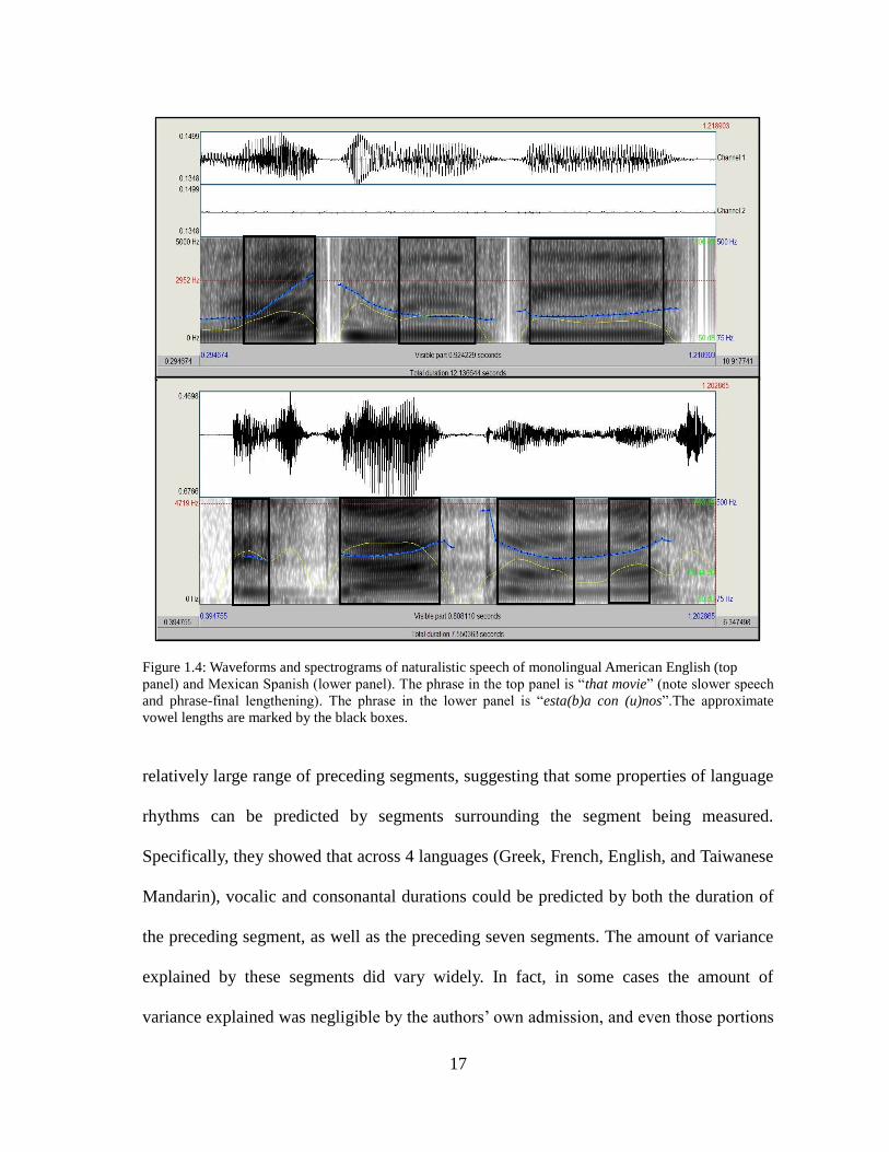
The failure of any single IM to distinguish between languages according to speech
rhythm is not entirely surprising. Compare Figure 1.4 to Figure 1.2 above and recall that
the PVI and other metrics of speech rhythms are largely based upon the concept that
stress-timed languages will display more variable interval (and especially vowel)
durations as compared to syllable-timed languages. As Figure 1.4 shows, this trend varies
with speaker performance. The stress-timed English in the top panel displays quite regular
vowel durations as compared to the syllable-timed Spanish in the lower panel. Given that
there is a fair amount of rhythmic variation within languages (e.g. Loukina et al. 2009),
the reliability of any measure based on interval durations as a correlate of speech rhythms
is certainly questionable.
Beyond traditional IMs, several studies have suggested that additional cues,
including intensity and spectral prominence can help determine rhythm (e.g. Lee and
Todd 2004). Kochanski, Loukina, Keane, Shih, and Rosner (2010) show that the acoustic
properties of segments can be predicted from preceding segments, and extend into a
17
Figure 1.4: Waveforms and spectrograms of naturalistic speech of monolingual American English (top
panel) and Mexican Spanish (lower panel). The phrase in the top panel is ―that movie‖ (note slower speech
and phrase-final lengthening). The phrase in the lower panel is ―esta(b)a con (u)nos‖.The approximate
vowel lengths are marked by the black boxes.
relatively large range of preceding segments, suggesting that some properties of language
rhythms can be predicted by segments surrounding the segment being measured.
Specifically, they showed that across 4 languages (Greek, French, English, and Taiwanese
Mandarin), vocalic and consonantal durations could be predicted by both the duration of
the preceding segment, as well as the preceding seven segments. The amount of variance
explained by these segments did vary widely. In fact, in some cases the amount of
variance explained was negligible by the authors‘ own admission, and even those portions

18
that fared better were not extremely well-explained by the predictors; the maximum
coefficient of determination r2 was 43%. Not surprisingly, the portions of the corpus that
consisted of participants reading poetry were better by surrounding segments, as
compared to those portions where participants read prose.
Thus, while it is certain that acoustic cues contribute to the intuition that languages
differ rhythmically, not only is there a lack of consensus as to which cue(s) do contribute
to this perceived difference and how one would quantify this difference, but it appears
that these cues behave in a multidimensional manner (Loukina et al. 2009) and do not
affect words of different frequencies in the same manner (Harris and Gries 2011).
1.4. Speech Rhythm Discrimination Studies
In addition to the ever-increasing body of works attempting to identify and implement
interval measures in the classification of the production of speech rhythms, there has also
been a simultaneous (although admittedly smaller) effort to evaluate the perception of
speech rhythms. These experiments determine if participants can discriminate between
languages of different rhythm classes. They have been performed with infant participants
(e.g. Christophe and Morton 1998) and adult participants (e.g. Ramus and Mehler 1998).
The stimuli used in speech rhythm discrimination studies include unaltered recorded
speech (in the case of infants, e.g. Christophe and Morton 1998), low-pass filtered speech
(Mehler et. al. 1998), and resynthesized speech (e.g. Ramus and Mehler 1999). In the case
of the latter two stimuli, recorded speech is altered in a manner that reportedly preserves
syllabic rhythm while degrading other acoustic cues that may allow language
discrimination; this will be referred to as utterance degradation in the current chapter. The

19
remainder of this section will discuss speech rhythm discrimination studies and the
implications of these works on the methodology of this dissertation. It will first present
the stimuli used in various speech rhythm discrimination studies (unaltered utterances,
low-pass filtered utterances, and resynthesized utterances). Each of these methodologies
will be exemplified by noteworthy studies that employ these approaches. It will then
address a methodological debate, namely whether low-pass filtered stimuli are superior to
resynthesized stimuli in speech rhythm perception experiments. These discussions are
relevant to the methodologies employed in later chapters, and especially in Chapter 4,
where a speech rhythm discrimination task with English, Portuguese, and Spanish stimuli
is conducted.
As previously mentioned, a major argument for the existence of speech rhythms is
the fact that infants and neonates appear to distinguish between languages based solely
upon rhythmic information (the rhythm hypothesis). It is accepted that infants can
distinguish between their mother tongue and a foreign language, or are sensitive to the
‗foreignness‘ of a language (e.g. Christophe and Morton 1998). In fact, this ability has
been demonstrated in fetuses as well (e.g. Kisilevsky et al. 2009). It has been
hypothesized that infants exploit rhythmic cues in this language discrimination (given that
fetuses are also capable of distinguishing between their maternal language and a foreign
language as mentioned, it is possibly, and even probable that rhythm sensitivity begins in-
utero). Due to infants' hypothesized abilities to distinguish between languages of different
rhythm classes, they have been the subject of speech rhythm perception experiments.
When using infant participants, it is theoretically possible to use unaltered speech stimuli,
which is not possible in the case of older participants. In addition, utterance degradation

20
has been used in the case of infants as well as adults. For instance, Nazzi, Jusczyk, and
Johnson (2000) showed that five-month old children are able to discriminate between
unaltered Japanese and English (mora-timed and stress-timed respectively) and low-pass
filtered Japanese and Italian (mora-timed and syllable-timed respectively, more on low-
pass filtering below). These results are in agreement with Nazzi et al., who, studying
language discrimination of low-pass filtered utterances by newborns, concluded that
―newborns use prosodic and, more specifically, rhythmic information to classify
utterances into broad language classes defined according to global rhythmic properties‖
(1998:1). In general, these results reinforce the notion that babies are capable of accessing
prosodic information in general, and rhythmic information in particular. However, not all
literature is in agreement on this point. For instance, Christophe and Morton (1998)
maintain that two-month old infants born to English-speaking parents are able to
discriminate between English and Japanese (stress-timed and mora-timed) but not
between French and Japanese (syllable-timed and mora-timed), suggesting that infants are
sensitive to the foreignness of a language (i.e. if it is their maternal tongue or not) but not
sensitive to the distinction between rhythm classes. However, the authors do not
demonstrate that the infants are not exploiting rhythmic cues in the distinction between
their maternal language and a foreign language.
While infants can, in theory, be tested for rhythm class discrimination with
unaltered utterances, this is not possible with adult participants. Adult participants exploit
multiple acoustic cues in language discrimination (phonemic and phonotactic inventory,
for instance). In order to remove information not related to syllabic rhythm, utterances
have been acoustically altered for use as stimuli in language discrimination tasks.

21
Sentences filtered at 450 Hz (that is, utterances where all sonic energy below 450 Hz is
muted) maintain prosodic features that would contribute to speech rhythm perception,
while making it impossible to infer what language is being spoken from the speech signal
(Arvaniti and Ross 2012:4). This process, known as low-pass filtering has been exploited
in studies of speech rhythm discrimination. For example, Nazzi et al. (1998) showed that
French neonates could discriminate between low-pass filtered Japanese and English
(respectively a mora-timed language and a stress-timed language) but not between
English and Dutch stimuli (two stress-timed languages). This study employed a non-
nutritive sucking task (habituation/ dishabituation in Christophe and Morton 1998),
where the neonates were allowed to suck on a pacifier connected to a pressure transducer;
by measuring high amplitude sucking on the pacifier, the author determined that the
newborns discriminate languages of different rhythm classes, even if those languages are
unknown to the neonates, as was the case with English and Japanese stimuli. However,
the infants were unable to discriminate between two stress-timed languages. Referring to
the aforementioned study, among others, Nazzi and Ramus state that the fact that children
are sensitive to rhythm from a very young age suggests that ―infants‘ acquisition of the
metrical segmentation procedure appropriate to the processing of (the rhythmic class of)
their native language might rely on an early sensitivity to rhythm.‖ (2003:238).
Ramus and Mehler (1999) apply an alternate method of utterance degradation,
known as speech resynthesis. The authors suggest that previous methodologies utilizing
low-pass filters preserve some segmental information, and may even corrupt the rhythmic
signal by allowing unwanted amplification of certain phonemes, leaving the possibility
that the results of Mehler et al. (1988) and Nazzi et al. (1998) may reflect infants' ability

22
to distinguish intonational differences, rather than rhythmic differences. Ramus and
Mehler's speech resynthesis, modeled after the development at IPO at Eidenhoven (as
cited in Ramus and Mehler, 1999:515), measures acoustic signals in an utterance, and,
using an appropriate algorithm, resynthesizes the spoken material in order to preserve
only certain acoustical cues. Ramus and Mehler (1999) applied four transformations
(named for the phonemes chosen to resynthesize the speech):
1. ―saltanaj‖: preserves global intonation, syllabic rhythm, and phonotactic structure.
2. ―sasasa‖: preserves global intonation and syllabic rhythm.
3. ―aaaa‖: preserves only global intonation.
4. ―flat sasasa‖: preserves only syllabic rhythm.
This fourth treatment is of specific interest to language-rhythm studies. By replacing all
consonants with /s/ and all vowels with /a/, then resynthesizing resulting sentences with a
constant fundamental frequency of 230 Hz., the syllabic rhythm is preserved, while all
other cues are degraded. When applying the ―flat sasasa‖ treatment, Ramus and Mehler
(1999) conclude that subjects could easily discriminate between rhythm classes (in this
case English and Japanese, that is, between stress-timed and mora-timed, respectively),
showing that rhythm is a robust cue for language discrimination.
Ramus et al. (2000) classify syllable-timed English, stress-timed Spanish, and
reportedly intermediately-timed Polish and Catalan (classified as such according the
interval measures of duration variability proposed and calculated by Ramus et al. (1999),
namely the average standard deviation of vowel duration (∆V), the average standard

23
deviation of consonant duration (∆C), and the percentage of an UTTERANCE comprised
of vowel (%V)). The authors applied ―sasasa‖ and ―flat sasasa‖ resynthesis to the
languages, and found that participants were able to discriminate English from Spanish,
English from Polish, and Spanish from Polish for the conditions retaining only syllabic
rhythm (that is ―flat sasasa‖). Meanwhile, participants were able to distinguish English
from Catalan and Polish from Catalan, but not Catalan from Spanish. The authors
concluded that Catalan rhythm is similar to that of Spanish, while Polish is neither
typologically stress-timed nor syllable-timed, as participants failed to distinguish Polish
from both a stress and syllable-timed language (here they rank Catalan as syllable-timed
because it was indistinguishable from Spanish). As predicted, Spanish and English were
distinguishable.
White, Laurence, Mattys, and Wiget (2012), following Ramus et al. (1999) is
using speech resynthesis showed that participants were able to distinguish between
languages of different rhythmic categories as well as between two dialects of English. The
authors explain this discrimination between two syllable-timed dialects by suggesting that
participants use speech rate in distinguishing languages or dialects, but that they are also
able to correctly categorize languages when speech rate is normalized, thus demonstrating
that participants do distinguish languages with purely duration information. White et al.‘s
(2012) finding are not in agreement with those of Loukina et al. (2009) who maintain that
differences in speech rate alone do not account for perceived differences in speech
rhythms. This study shows that speech rate alone cannot distinguish between languages
without the inclusion of interval metrics (presumably by participating in an interaction
with these IMs). However, as IMs should not greatly differ for two dialects of native
24
monolingual English (according to traditional rhythm class distinctions, although this is
not necessarily empirically proven), it remains difficult to view speech resynthesis as a
dependable method of preparing stimuli for speech rhythm discrimination studies.
A consensus regarding the relative merits of low-pass filtering and speech
resynthesis in speech rhythm perceptions studies has not been reached. White et al.
(2012), following Ramus and Mehler (1999), maintain that ―low-pass filtering merely
attenuates rather than eliminates segmental information.‖ (2012:666). That is, according
to White et al. (2012), low pass utterances still allow listeners to access residual
information such as phonemic inventories and phonotactic regularities, for instance.
However, other studies continued to use the low-pass filtering methods for perception
experiments (i.e. that used by Mehler et al. 1988, mentioned above). One logical reason
for this is that low-pass filtered stimuli are more faithful to the original speech signal,
while resynthesized stimuli are more heavily altered. Furthermore, various works
employing speech resynthesis have come under criticism. For instance, Arvaniti and Ross
(2012) criticize Ramus, Dupoux, and Mehler (2003), a perception study using speech
resynthesis, as opposed to low-pass filtering, as presenting results incompatible with the
idea of rhythms classes.
As mentioned, some authors have defended the previously described speech
resynthesis (e.g. Ramus, Dupoux, and Melher 2003; White et al. 2012), while others have
maintained that low-pass filtering is preferable in speech rhythm perception studies (see
also Nazzi et al. 1998). Neither of these methods of UTTERANCE degradation has been
conclusively proven to be superior, although both appear to have certain merits in speech
rhythm discrimination studies. However, given the less than reliable results in studies
25
using speech resynthesis (e.g. Ramus, Dupoux, and Mehler 2003; White et al. 2012) and
the fact that the process of speech resynthesis produces a stimulus far more altered than a
stimulus produced by low-pass filtering, this dissertation will adopt low-pass filtering in a
speech rhythm discrimination study to follow. This will be described in Chapter 4.
1.5. Conclusion
The simple fact that speech rhythms have been long described and have been subjected to
many attempts to empirically quantify these differences suggests that this linguistic
conundrum is worthy of investigation. The existence of rhythmic differences are also
supported by studies showing that infants can distinguish between languages of different
rhythmic classes (e.g. Nazzi et al. 1998), adults can discriminate between rhythm classes
in degraded utterances (e.g. Mehler et al. 1988), and that speech timing appears to be
biologically hard wired in a speaker (Wretling and Eriksson 1998).
However, apart from a general consensus that languages do indeed differ
rhythmically, the question of how to quantify these rhythmic differences, especially in
production, has eluded linguists (e.g. White and Mattys 2007). For these reason this
dissertation will experimentally evaluate both the production and perception of speech
rhythms across various languages, and incorporate multifactorial analyses and corpus-
based frequency effects.
The remainder of this work will be structured as follows: Chapter 2 discusses two
data treatments applied to the speech of monolingual Mexican Spanish speakers and
bilingual Californian English/Spanish speakers. Its main purpose is to analyze the PVI as
a classifier of speech rhythms. Chapter 3 discusses a multifactorial analysis of measures

26
of speech rhythm; it is unique in its statistical approach to speech rhythms and serves to
evaluate the efficacy of various IMs, and shed some light on the behavior of bilingual
speech rhythms and their relation to the traditional rhythm classes. Chapter 4 and
Chapter 5 build upon these findings. First, Chapter 4 conducts a perception-based
experiment in order to classify the relative rhythms of utterances of English, Portuguese,
and Spanish. Next, Chapter 5 uses these classifications as the basis for a study of the
production of these same utterances, making their relative rhythmic classifications from
Chapter 4 the dependent variable in a multinomial analysis of traditional correlates of
speech rhythms. Finally Chapter 6 presents the conclusions of these studies in the
context of their importance to speech rhythms, prosody, phonetics and phonology, and
linguistics at large.
27
Chapter 2
A comparative evaluation of the PVI in speech rhythm discrimination
Overview
As mentioned in the previous chapter, the PVI (pairwise variability index) is often favored
by linguists as an apparently transparent and simple method of comparing speech
rhythms. However, from a statistical standpoint, it has certain shortcomings (e.g. White
and Mattys 2007). In order to evaluate the soundness and efficacy of this metric, the
current chapter presents four different methods of evaluating speakers‘ PVI scores, three
based on previous literature, and one more statistically robust evaluation of PVI scores.
As all four data treatments are performed upon the same data set, it provides an ideal
comparison of the methodologies. The two speaker groups evaluated are bilingual
Spanish/English speakers and monolingual Mexican Spanish speakers.
Although most works involving the PVI evaluate the mean of PVI scores for a
speaker or utterance, some go on to report a single mean PVI for each speaker type (e.g.
Carter 2005). Thus, the first treatment uses the mean PVI score of all the Spanish of
monolingual Mexican speakers and the mean PVI of all the bilingual Chicano speakers;
this is called the Speakertype Mean PVI Method. The second data treatment follows
various works (e.g. Grabe and Low 2002; Carter 2005) in evaluating each speakers‘ mean
PVI, and will be referred to as the Speaker Mean PVI Method. The third data treatment
follows various works (e.g. Low and Grabe 1995; Low, Grabe, and Nolan 2000) in
evaluating the mean PVI of each utterance (or intonation phrases to use Grabe and Low's
(2002) terminology); this will be referred to as the Utterance Mean PVI Method. The

28
fourth data treatment evaluates all PVIs, rather than using a measure of central tendency.
That is, each pair of successive vowel durations contributes one PVI score. A binomial
logistic regression then evaluates these PVI scores in order to predict the dependent
variable, SPEKAERTYPE (monolingual or bilingual); this method will be referred to as
the Cumulative PVI Method. After a general introduction, the speaker groups whose
unscripted speech is used to evaluate how well these treatments of the PVI differentiate
between rhythmic classes are described. The different statistical processes are each
described separately and their results are presented and briefly discussed; these
discussions touch upon linguistic implications of the data, but methodological
implications are more crucial to the current chapter; in fact, as Chapter 3 evaluates the
same speaker groups in a more in-depth manner, linguistic implications are most
thoroughly discussed there. To conclude the current chapter, an overall discussion
compares and contrasts the four different approaches to speech rhythm evaluation and
presents methodological implications. This affords a unique perspective as to the
effectiveness of vowel duration interval metrics in the comparison of speech rhythms.
2.1 Introduction
The PVI proves a widely used metric in speech rhythm research. However, it is not
without its critics (e.g. Detering 2001). One major criticism, which was mentioned in
Chapter 1, involves the use of a single mean PVI for an utterance, speaker, or speaker
type. In addition to the fact that two PVIs of the same value do not necessarily reflect the
same or equivalent series of vowel durations (White and Mattys 2007:519), there are
additional shortcomings of the use of the mean of PVI values to evaluate speech rhythms.

29
One, which is somewhat self-evident, is that it is more statistically viable to consider all
the scores for a speaker or speaker type, namely the Cumulative PVI Method mentioned
above; a binomial logistic regression evaluates all PVI scores rather than relying on a
measure of central tendency, such as the mean. Given the availability of computer-aided
statistical processing, this method is not only widely available to researchers, but also
potentially far more robust in providing a fine-grained perspective of vowel duration
variability in naturalistic speech. Thus, the purpose of the current chapter is to compare
methods of evaluating PVI scores, considering the use of the mean as a measure of central
tendency (Speakertype Mean PVI Method, Speaker Mean PVI Method and Utterance
Mean PVI Method) and the use of all the PVI values without a measure of central
tendency (Cumulative PVI Method); in this manner, this chapter sheds light on the best
methodological treatment of the PVI as well as the metric‘s efficacy. Additionally, it was
hoped that these studies would be informative as to the relative position of the Spanish of
the two speaker groups on the speech rhythm continuum. These two groups, which will be
described in detail below, are monolingual Mexican Spanish speakers and
English/Spanish bilingual speakers from California.
2.2. Data
2.2.1. Spontaneous Speech
The studies in this chapter follow Deterding (2001) and Carter‘s (2005, 2007) methods of
recording and analyzing spontaneous speech. Many linguists examine recordings of
subjects reading written sentences aloud. This method allows for close control of the
material and the avoidance of potential complications, e.g., the presence of diphthongs or

30
vowel-less syllables, can be controlled for. Furthermore, subjects can be recorded at
similar distances from the microphone and can be asked to repeat sentences where pauses
or self-correction occurs. However, Deterding (2001) and Carter's various studies of
speech rhythm differ in this count. In order to capture more natural speech rhythms, they
analyzed recorded spontaneous speech rather than sentences read out loud. Although both
spontaneous and scripted speech are still being studied, all other things being equal,
natural recorded speech is more likely to reflect spoken language rhythms since "[i]t is
well known that there are differences between read and unscripted speech" (Deterding
2001:220). In order to achieve this, the current study uses a small specialized corpus of
semi-directed interviews. Subjects were recorded responding to oral questions designed to
elicit narrative responses delivered with minimum interruption on the part of the
interviewer.
2.2.2. Test Subjects
For this study, two speaker groups were used: ten monolingual Spanish speakers (Group
A), and ten bilingual English/ Spanish speakers (Group B). These groups were chosen for
two reasons. First, due to the Mexican heritage of the bilingual speakers, the influence of
Mexican Spanish on their bilingual Spanish is especially strong. Second, the geographic
proximity of California to Mexico allows for a considerable amount of contact between
Mexican Spanish and Californian Chicano Spanish, especially given the number of recent
immigrants from Mexico living in California. Thus, both speaker groups share similar
linguistic roots in their Spanish, which is traditionally labeled a syllable-timed language,
the only difference being that Group B also speaks English, a stressed-timed language.
31
In order to control extraneous variables as much as possible, the study selected test
subjects according specific guidelines. Accordingly, the subjects were between the ages of
18 and 25 and currently enrolled in a four-year university at the time of recording,
assuring test subjects of a similar age and education level. For each test group, five
women and five men were recorded.
The first group, Group A, consisted of ten monolingual Spanish speakers
representing speakers of what is traditionally considered a syllable-timed language. In
interests of minimizing dialectal variation, subjects in the monolingual Spanish group
were all born and raised in a single region of Mexico, in this case the greater Mexico City
area and had never lived in a foreign country. The monolingual Spanish speakers were
enrolled in a four-year Mexican university, Universidad Nacional Autónoma de México
(UNAM) at the time of recording.
The second group, Group B, consisted of ten bilingual English/Spanish speakers.
The speakers were second-generation Spanish speakers intended to be representative of
the Chicano population in California. Thus, they were born in California to parents who
emigrated from Mexico to California during or after their teen years. Second-generation
Spanish speakers generally speak Spanish in the home but learn English outside the home,
normally through school. This makes them the ideal case studies for bilingualism because
they speak both languages from a young age, although they are often dominant in English
(e.g. Montrul 2004a, b, 2005). At the time of the study, speakers were enrolled in upper-
division Spanish courses at the University of California, Santa Barbara, which means they
either took, or tested out of, two years of Spanish instruction at university level plus all
their coursework and interaction with instructors is in Spanish.

32
2.2.3. Hypothesis
Although, the principal purpose of this chapter is to evaluate the PVI, there were some
expectations as to the behavior of these two speaker groups. These groups of speakers
make for an interesting test case given the opposing classifications of English and
Spanish. The monolingual speakers speak what is traditionally regarded as a syllable-
timed language whereas the bilingual speakers also speak what is traditionally regarded as
a stress-timed language. It is not unreasonable to expect that this contrast will be reflected
in the vowel duration variability of the speakers, especially given the results of Carter
(2005, 2007) and Fought (2003) who found that Chicano English tends to be more
syllable-timed (more similar to Spanish) than American English, and, in the case of
Carter, African American English. Thus, it was expected that Chicano Spanish would be
more stress-timed than that of their monolingual counterparts (e.g. MacLeod and Stoel
Gammon 2005 for similar findings for voice-onset times in Canadian English and
French).
2.2.4. Data Logging
Vowel duration was recorded for each phrase according to accepted methodology, as
described by White and Mattys (2001) for determining the onset and offset of the vocalic
nucleus. Accordingly, a visual inspection of speech waveforms and wideband
spectrograms using PRAAT phonetic software (Boersma and Weenink 2010) was carried
out in order to determine and mark the onset and offset of vowels and measure their
durations. The current study calculated a PVI according to the aforementioned equation,

33
resulting in a series of PVIs for each test subject. Starting at the beginning of the
recording, sentences or phrases displaying a minimal interruption or interference were
selected and examined in order to record a minimum of 50 data points per speaker. Once
these 50 data points were extracted, vowel durations were recorded until the end of the
current sentence or phrase. As in Carter (2007), for both English and Spanish, the syllable
directly before a pause (as would be denoted by a period, comma, etc.) or hesitation
marker, restart, or repair was eliminated due to common elongation of the pre-pausal
syllable. The calculation of PVIs and all statistical analysis of data were completed using
R software for statistical computing and graphics (R Development Core Team, 2013)2.
2.2.5. Treatment of special cases
Given the spontaneous nature of the speech, unnatural syllable elongations due to speaker
confusion were eliminated. Regarding Spanish diphthongs, the methodology employed by
Carter (2007) was adopted. Specifically, Spanish diphthongs not marked by orthographic
accents will be considered as a single vowel. English canonical diphthongs /ai/, /oi/ and
/aw/ are also measured as a single vowel. In instances of specific individual
complications, such as syllable deletion, these were addressed on a case-by-case basis.
2.3. Speakertype Mean PVI
2.3.1. Statistical Evaluation: Speakertype Mean PVI
As mentioned, studies employing the PVI for speech rhythm distinction tend to
discriminate between using the mean of a speaker's PVI scores or the mean of the PVI
2 I wish to thank Prof. Stefan Th. Gries of UCSB for writing the R function to calculate the PVI values.

34
scores for each utterance; however, some go on to report a single mean PVI score for each
speaker type. It is unclear from the literature just how these means are calculated. Taking
Carter (2005) as an example, both overall speaker type PVI means are reported, as well as
mean PVI scores for each speaker. It is possible that these speaker type mean PVI scores
are based upon each speaker's mean PVI score, as in Figure 2.1.
Speakertype X:
Mean PVI- Speaker: Mean(PVI, PVI2, …, PVIn)
Mean PVI- Speaker2: Mean(PVI, PVI2, …, PVIn)
Mean PVI- Speakern: Mean(PVI, PVI2, …, PVIn)
Speakertype X PVI Score: Mean(Mean PVI- Speaker Mean PVI- Speaker2… Mean
PVI- Speakern)
Figure 2.1: Possible method of calculation for Speakertype Mean PVI score.
However, it is also possible that Carter (2005) calculated the mean PVIs as in in Figure
2.2. This chapter will use the more statistically sound option ("statistically more sound" in
that it loses less information). The method above involves taking the 'mean of a mean', but
the current chapter avoids this by calculating the Speakertype Mean PVI as below.
Speakertype X: Mean(Speaker: PVI, PVI2, …, PVIn + Speaker2: PVI, PVI2, …,
PVIn... + Speakern: PVI, PVI2, …, PVIn)
Figure 2.2: Speakertype Mean PVI score as calculated in the current chapter.
2.3.2. Results: Speakertype Mean PVI
As previously mentioned, the expectation for this data set was that the bilingual Chicano
speakers would show more vowel duration variability as compared to the monolingual
speakers due to their dominance in a stressed time language. Thus, it was expected that
the Chicano speakers would have higher PVI scores than the monolingual participants.

35
However, the results of the Speaker Mean PVI analysis did not reflect the original
hypothesis. In fact, the mean PVI of Mexican speakers were higher than that of the
bilingual Californian speakers. The mean PVI of the Mexican subjects was 0.44 (95%
confidence interval= 0.412 : 0.468; sd=0.324) while the mean PVI of the bilingual
Californian speakers was 0.361 (95% confidence interval= 0.338 : 0.383; sd=0.262).
According to a Wilcoxon rank sum test, this difference in means is highly significant: W
= 114118, p < 0.001 (see Figure 2.3).
2.3.3. Discussion: Speakertype Mean PVI
The fact that the data do not reflect the original hypothesis provides several points of
interest for discussion. The fact that native Spanish speakers show more variation in
vowel duration than their bilingual counterparts may well be related to the monolingual
speakers‘ dominance of the language.
This will be discussed more in detail following the results of Chapter 3, as these
results are better contextualized in consideration of some methodological implications of
the calculation of the PVI and its use as a classifier of speech rhythms. A more relevant
point to consider here is the viability of these conclusions given the methodology applied.
While it is current practice in some speech rhythm literature to present and discuss the
mean PVIs for each speaker type (e.g. Carter 2005), this is statistically problematic. Not
only does the use of the means 'wash away' much information from the data, but PVIs
appear to not be normally-distributed, at least in the current data, making the mean an
unreliable measure of central tendency; according to a Shapiro-Wilk test of normality, the
PVI values from which the means are calculated are not normally distributed (W =

36
Figure 2.3: The mean PVIs for each speaker, grouped according to speaker type; the Bs are bilingual
participants and the Ms are monolingual participants. The black diamonds represent the mean for each
speaker type and the horizontal line represents the mean PVI for all speakers.
0.9323, p < .0001). Each speaker type's PVI values also deviate from normality
(SPEAKERTYPE= bilingual W= 0.9366, p < .0001; SPEAKERTYPE= monolingual W =
0.9354, p < .0001). While it would a possibility to use a different measure of central
tendency, such as the median (as in Carter 2007) or a weighted mean, it is still the case
that there is a great deal of variation in the distribution of the PVI values, suggesting that
any measure of central tendency would remove a great amount of information about
rhythmic variation within speaker types (and within speakers, see below). However, in
order to contextualize the methodology applied in previous literature, the next two

37
sections evaluate the mean PVI for each speaker (e.g. Grabe and Low 2002) and the mean
PVI for each utterance (e.g. Low and Grabe 1995).
2.4. Speaker Mean PVI
2.4.1. Statistical Evaluation: Speaker Mean PVI
The data evaluation in the current section followed Carter (2005) and Grabe and Low
(2002) in calculating a mean PVI for each speaker, rather than for each utterance (as in
Low and Grabe 1995, for example). Each speaker's mean PVI was calculated as the mean
of all of their PVI scores (as opposed to basing them on the mean of each utterance).
Observed mean PVI values are plotted above on Figure 2.3. While previous studies using
Speaker Mean PVI scores simply report the means (and perhaps a mean for each speaker
type as well), the current chapter used a more statistically advanced technique in order to
better evaluate the utility of this metric in speech rhythm discrimination studies. Thus, a
binary logistic regression was generated to predict SPEAKERTYPE (bilingual or
monolingual) according the SPEAKER MEAN PVI scores.
2.4.2. Results: Speaker Mean PVI
The predictor SPEAKER MEAN PVI was highly significant in predicting
SPEAKERTYPE (p=.02, R2=.60). The resulting model was able to accurately classify
bilingual versus monolingual speakers 85% of the time, which is highly significantly
better than a model that predicts the most frequent level of SPEAKERTYPE 100% of the
time (p<.001)3. The same trend that was present in the previous section, namely that
3 It should be noted that each speaker type was represented 50% in the data, so this model would be correct

38
monolingual speakers displayed higher PVI values than bilingual speakers on a whole
was also present in the current analysis (see Figure 2.44).
Figure 2.4: Predictions for SPEAKERTYPE according to the mean PVI for each speaker. The mean PVI
scores are represented on the horizontal axis, with higher mean PVI scores to the right hand side of the
graph. The prediction for SPEAKERTYPE is represented on the vertical axis, with those values above 0.5
being predicted monolingual.
half of the time. 4 Figures 2.4, 2.6, and 2.8 were generated using the effects package (Fox 2014) for R (R Development
Core Team 2013)

39
2.4.3. Discussion: Speaker Mean PVI
Although the current model is efficient at predicting SPEAKERTYPE according the mean
PVI for each speaker, this is not to say that it is a useful model to accurately understand
speech rhythms. Once again, the use of the mean is very problematic in washing away a
great amount of variation within each speaker that would be otherwise visible.
Furthermore, as mentioned above, the fact that the data from which these means are
derived is not normally distributed proves to be a serious issue when considering the
reliability of this model. According to a Shapiro Wilk test of normality, only four out of
the twenty speakers had normally distributed PVI values. Given that the data are not
normally distributed, these Speaker Mean PVI scores cannot be said to accurately reflect
the central tendency of the speakers.
2.5. Utterance Mean PVI
2.5.1. Statistical Evaluation: Utterance Mean PVI
The data evaluation in the current section is very similar to that of Section 2.4 with the
exception that mean PVI scores were recorded for each utterance (or intonation unit),
rather than for each speaker, as in Low and Grabe (1995), for instance. This theoretically
affords a more fine-grained perspective as compared to the use of the Speaker Mean PVI
Method, as within-speaker variation is visible. As in the previous section, a binary
logistical regression was generated to predict SPEAKERTYPE (bilingual or
monolingual), this time with MEAN UTTERANCE PVI. The mean PVI values are
plotted below in Figure 2.5.

40
Figure 2.5: The mean PVIs for each utterance, grouped according to speaker type; the Bs are bilingual
participants and the Ms are monolingual participants. The black diamonds represent the mean for each
speaker type and the horizontal line represents the mean PVI for all speakers.
2.5.2. Results: Utterance Mean PVI
The predictor UTTERANCE MEAN PVI was highly significant in predicting
SPEAKERTYPE (p<.001, R2=.20). Once again, the monolingual speakers displayed
higher PVI values than bilingual speakers on a whole (see Figure 2.6). However, what is
more informative is that the present model was far less accurate in predicting
SPEAKERTYPE, as compared to the Speaker Mean PVI Method. The R2 value has

41
dropped from .60 in the previous model to .20 here, indicating that far less variation in the
model is explained by the dependent variable. Furthermore, the C score has dropped to
.73, below the threshold of .80 for an accurate model. The current model was able to
accurately classify bilingual versus monolingual speakers 69% of the time. While this still
performs significantly better than a model that predicts the most frequent level of
SPEAKERTYPE 100% of the time (p<.01), this model performs much worse than the
model based on just SPEAKER MEAN PVI scores. It is noteworthy that in the case of the
Utterance Mean PVI Method, it is in fact more statistically viable to consider the mean as
a measure of central tendency. A Shapiro Wilk test for normal distribution revealed that
the distribution of the PVIs was normal for 52 out of 67 utterances tested; one utterance
was too short to perform this test on. However, despite the increased reliability as the
mean utterance PVI as a measure of central tendency, the model performs worse than the
Speaker Mean PVI Method.
2.5.3. Discussion: Utterance Mean PVI
It is troubling that the model that contains more information (that is the Utterance Mean
PVI model contains 68 data points, as compared to 20 in the Speaker Mean PVI model),
and uses a measure of central tendency that can be considered more reliable, is less
accurate in correctly classifying the dependent variable, SPEAKERTYPE. This is not
indicative of the strength of the Speaker Mean PVI Method model; rather, it indicates that
taking the mean of each speaker is removing a good deal of within-speaker variation that
should be considered in speech rhythm discrimination analysis. Unlike the previous
analyses, the non-normal distribution of the PVI values is not a serious concern for the

42
Figure 2.6: Predictions for SPEAKERTYPE according to the mean PVI for each utterance. The mean PVI
scores are represented on the horizontal axis, with higher mean PVI scores to the right hand side of the
graph. The prediction for SPEAKERTYPE is represented on the vertical axis, with those values above 0.5
being predicted monolingual.
use of the mean. However, the model performance suggests the the Utterance Mean PVI
Method fails to discriminate reliably between the two speaker groups. In an attempt of a
more robust analysis, the following analysis will not use the mean to evaluate the PVI
scores, but instead consider all PVI values in the evaluation of the speech rhythms of
monolingual Mexican speaker and bilingual Chicano speakers.

43
2.6. Cumulative PVI
2.6.1 Statistical Evaluation: Cumulative PVI
As mentioned, the statistical evaluation of the Cumulative PVI differs from the previous
methodologies in that, rather than considering the various means of each utterance,
speaker, and/or speaker type, it uses all individual PVI values (that is, for each pair of
successive vowel durations) in a regression analysis. As in Sections 2.3 and 2.4, a binary
logistic regression was created to predict SPEAKERTYPE, but this time according to all
speaker's PVI scores. The observed PVI scores are plotted below on Figure 2.7.
2.6.2. Results: Cumulative PVI
After considering all 1019 data points, PVI was a significant predictor of speaker type
(that is, monolingual vs. bilingual speakers; p<.0001); however, the resulting model had
extremely low classificatory power (R2=.02). The C score has once again dropped from
the previous model to 0.56. The model is able to to correctly identify SPEAKERTYPE,
55% of the time. While the results of this statistical exploration reflect the same trend as
those of the previous models, namely that monolingual speakers display higher vowel
duration variability than their bilingual counterparts (see Figure 2.8), the low
classificatory power of the model is far more noteworthy. Once again, a model that
contains more data points, and thus more information about the vowel duration variability
between speaker types is less accurate than one with fewer data points.
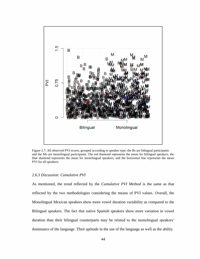
44
Figure 2.7: All observed PVI scores, grouped according to speaker type; the Bs are bilingual participants
and the Ms are monolingual participants. The red diamond represents the mean for bilingual speakers, the
blue diamond represents the mean for monolingual speakers, and the horizontal line represents the mean
PVI for all speakers.
2.6.3 Discussion: Cumulative PVI
As mentioned, the trend reflected by the Cumulative PVI Method is the same as that
reflected by the two methodologies considering the means of PVI values. Overall, the
Monolingual Mexican speakers show more vowel duration variability as compared to the
Bilingual speakers. The fact that native Spanish speakers show more variation in vowel
duration than their bilingual counterparts may be related to the monolingual speakers‘
dominance of the language. Their aptitude in the use of the language as well as the ability

45
Figure 2.8: Predictions for SPEAKERTYPE according to PVI. The PVI scores are represented on the
horizontal axis, with higher mean PVI scores to the right hand side of the graph. The prediction for
SPEAKERTYPE is represented on the vertical axis, with those values above 0.5 being predicted
monolingual.
to employ language across a variety of registers may allow them to employ more variation
in rhythms, leading to a higher PVI. These results are in agreement recent studies on
speech rhythm. Benton, Dockendorf, Jin, Liu, Edmondson concluded that rhythm varies
between speakers, and ―in some cases across genres‖ (2007:1272). Furthermore, it is
difficult to establish rhythmic typologies for an entire language based on a single dialect.
This is exemplified by a difference in rhythms between Californian Chicano Spanish and
Mexican Spanish in Mexico City. Despite the geographical proximity of California and

46
Mexico, the data seems to reflect that the dialects are typologically different. It is
accepted that different varieties of Spanish may have different vowel systems. So, while it
is accepted that intonation defines different varieties, it may be that vowel systems of
differing varieties of Spanish are also marked by rhythmic variety.
However, once again, the fact that more information is associated with a less
accurate classification accuracy is the most central point of import to the current chapter.
Furthermore, the current analysis does not use a measure of central tendency, so the non-
normal distribution of the data is not an issue. Even without this factor, the model does
not perform well in identifying the dependent variable. This indicates that the use of the
mean of PVI scores (whether for speaker type, speaker, or utterance) not only removes a
great deal of relevant information (inter-speaker type, inter-utterance, and inter-speaker
variation) to the study of speech rhythms, but that it does so in a risky manner, due to the
non-normal distribution of the PVI values. This conclusion will be further discussed in the
following section.
2.7. Methodological Implications
After examining the statistical process employed leading to the results discussed in the
current chapter, it is clear that two issues needed to be addressed. At the risk of repetition,
this section will briefly review these two issues in order to better contextualize the results
for the current chapter, The first regards the reporting a mean PVI speaker for speaker or
speaker type, as seen in the first three. Reporting means as measures of central tendency
assumes that the data is (nearly) normally distributed. In the reporting of mean PVI
values, no proof (to the author‘s knowledge) is given in previous speech rhythm literature
47
that PVI values are normally distributed when mean PVIs are reported. In the case of the
current data, in fact, the speaker mean PVIs deviate from a normal distribution, which
indicates that the mean is not a reliable measure of central tendency for PVI values.
Alternate measures of central tendency that do not require normally distributed data (for
example, the median or a weighted mean) would be potential alternate measures that
could be used, but as the remainder of this paragraph will show, this is not the best choice
in evaluating the data. This is due to the fact that it is possible to consider all PVI values,
as in the Cumulative PVI Method. This is a more statistically robust method of evaluating
the data, as no information is removed by the use of a measure of central tendency.
However, when this evaluation is performed, the resulting model is not reliable in
classifying SPEAKERTYPE. This leads to the second issue regarding the PVI as a metric
of speech rhythms, discussed in the paragraph below.
A very important consideration of the analyses in the data is that as each model
increases in terms of the number of data points it considers, it also becomes far less
accurate in classifying the dependent variable. The Speaker Mean PVI Method evaluated
20 data points and was able to correctly classify SPEAKERTYPE 85% of the time; the
Utterance Mean PVI Method evaluated 68 data points and achieved 69% classification
accuracy (although the use of the mean as a measure of central tendency was appropriate
in this case); the Cumulative PVI Method considered 1019 data points and was accurate
only 55% of the time, which is scarcely better than chance. In this final case, due to the
1018 degrees of freedom, PVI is significant as a predictor of SPEAKERTYPE (p<.001),
but the model can only account for about 2% of the variation in the PVIs values, which is

48
to say that it is not particularly effective in assessing the difference in PVI values between
speaker types at all.
The fact that the PVI only works as an accurate classifier of SPEAKERTYPE
when the mean PVI of each speaker type or speaker is considered is very telling; the
variation of PVI values for each speaker is nearly as varied as the difference in PVIs
between speakers. The result of this is that only upon ‗evening out‘ this variation with a
(unreliable) measure of central tendency do the differences between monolingual and
bilingual speakers become evident.
Given that the PVI is ineffective in distinguishing between two dialects of
Spanish, it is apparent that it is necessary to assess these complex data in a more thorough
manner. A multifactorial regression is beneficial in two manners. First, it allows the
inclusion of additional potentially relevant variables, such as other interval metrics (e.g.
Ramus, Nespor, and Mehler‘s (1999) various IMs) and corpus-based frequency measures.
Secondly, a multifactorial approach allows potential interactions between the variables,
affording a much more complete analysis of the behavior of this data set. In this way it is
possible to not only understand the differences in the speech rhythms of the two speaker
groups, but also to understand the efficacy of the various rhythm metrics. This is
particularly important given the lack of consensus of the best IMs for the evaluation of
speech rhythms; in fact, it is not accepted that any one IM is useful in speech rhythm
evaluation (e.g. Loukina et. al 2009). The following chapter will reevaluate the same data
set from the current chapter. However, it will apply a multifactorial approach with the
goal of 1) comparing the speech rhythm of monolingual Mexican Spanish and bilingual

49
Chicano Spanish, and 2) evaluating the efficacy of various IMs for the comparison of
speech rhythms. The results of this methodology are discussed in the following chapter.
2.8. Interim Summary
Before proceeding with the remainder of this dissertation, this section will briefly
summarize the previous two chapters in order to remind the reader of the current state of
speech rhythm research and why the methodologies of the following chapters are
necessary.
As the first chapter states, several factors suggest the existence of speech rhythms,
including widespread perception (Loukina, Kochanski, Rosner, and Keane 2011) and
speech rhythm discrimination by infants (e.g. Nazzi, Bertoncini, and Mehler 1998).
However, while the existence of speech rhythms is not controversial, no single empirical
proof of rhythmic differences between different languages or dialects has been universally
accepted. Two major approaches have been adopted in attempts to quantify speech
rhythms: production and perception studies. In the latter case, the ability of adults to
distinguish between languages of different rhythm classes on the basis of a speech signal
that has been altered to include only syllabic rhythm (e.g. Ramus and Mehler 1999) or the
ability of infants to distinguish between languages of a different rhythm class (on the
basis of an altered or unaltered speech signal, e.g. Nazzi, Jusczyk, and Johnson 2000)
have been given as proof of the existence of speech rhythms. Production studies,
meanwhile, attempt to use interval metrics based upon the measurement of segments of
the speech signal to quantify rhythmic differences between languages or dialects. These
IMs are generally intended to quantify the variability of segment durations, with the

50
general notion that higher segment duration variability is present in stress-timed
languages, while syllable-timed languages have more regular segment durations. The
current chapter investigated the PVI (e.g. Low and Grabe 1995), one of the most widely
used IMs in speech rhythm research and identified several practical shortcomings of this
metric. Due to these shortcomings, Chapter 3 will reevaluate the PVI as well as several
other traditional IMs in distinguishing between utterances of monolingual Mexican
Spanish and bilingual Chicano Spanish. Following this thorough multifactorial analysis,
Chapter 4 uses a perception study of utterances of English, Portuguese, and Spanish in
order to determine if these utterances truly differ from one another in terms of rhythmic
perception. The results of this chapter then lead to the analysis of Chapter 5, which
explores what acoustic properties of these same utterances prompt perceived differences
in rhythm. Finally, the implications of this dissertation are discussed in Chapter 6.
51
Chapter 3
A comparison of measures of speech rhythm in Mexican and Chicano Spanish
speakers
Overview
This chapter considers the same data used in Chapter 2, evaluating the rhythmic
differences between monolingual Mexican Spanish and bilingual Chicano Spanish.
However, this chapter differs in several counts from the analyses presented in the previous
chapter. Rather than employing the Mean PVI Method or the Raw PVI Method, the
chapter uses more advanced methodology in presenting a multifactorial analysis.
Furthermore, rather than only consider the PVI as a metric for distinguishing differing
rhythmic classes, it also considers other IMs. Specifically, it includes IMs as suggested by
Deterding (2001) as well as corpus-based measures of frequency. The remainder of this
chapter will introduce the subject and review the data and methods used (although as the
data are the same as the previous chapter, this description will be brief). The statistical
methodology is discussed and the results follow. A discussion covers the linguistic and
methodological implications of these results, affording a unique perspective as to the
effectiveness of vowel duration interval metrics in the comparison of speech rhythms, as
well as the importance of corpus-based frequency measures to the study of speech
rhythms. Finally, the implications of these findings are presented, and explain how these
results prompt the further investigation in the study of speech rhythms described in this
dissertation.

52
3.1. Introduction
The statistical evaluation performed in the current chapter was undertaken as a direct
result of the results described in Chapter 2. Both of the methods of calculating speaker
PVI scores described in the previous chapter prove inconclusive as to the rhythmic nature
of Monolingual Mexican Spanish as compared to Bilingual Chicano Spanish.
Furthermore, these results also shed doubt on the utility of the PVI as a metric of speech
rhythms. Thus, the current chapter seeks to a) compare the speech rhythms of these two
speaker groups and b) explore more reliable metrics of speech rhythm classification. It
also evaluates the variation of speech rhythms (or at least vowel duration variability)
according to corpus-based frequencies, a novel approach in speech rhythm research5. It
has been shown that certain aspects of pronunciation vary with word frequency (e.g. Bell
et al. 2009; Raymond and Brown 2012); it is not unreasonable to expect that speech
rhythms may do the same.
3.2. Data
The data used in the current chapter is the same data from Chapter 2; thus the discussion
is limited to a quick review of the nature of the data. The data is spontaneous speech
culled from a specialized corpus of semi-directed interviews. The two speaker groups are
each comprised of 5 women and 5 men. The two test groups were used: ten monolingual
Spanish speakers (Group A), and ten bilingual English/ Spanish speakers (Group B). As
mentioned, the subjects were between the ages of 18 and 25 and currently enrolled in a
5 The multifactorial statistical evaluation described in this chapter is from Harris and Gries (2011). I am
grateful to Prof. Stefan Th. Gries for performing that statistical exploration and generating graphical
representations.
53
four-year university assuring test subjects of a similar age and education level. For each
test group, five women and five men were recorded.
3.2.1. Hypothesis
Recall that the monolingual speakers speak a syllable-timed language while the bilingual
speakers also speak a stress-timed language (at least according to a traditional rhythm
class distinctions). In Chapter 2 it was expected that Chicano Spanish would be more
stress-timed than that of their monolingual counterparts due to their dominance in
English, a stress-timed language. However, the results of Chapter 2 ultimately indicate
the opposite trend; Chicano speakers show less variation in terms of vowel duration as
compared to Mexican speakers, so they have what would be regarded as a less stress
timed Spanish as compared to their monolingual counterparts. While, these results cannot
be considered definitive due to the shortcomings of the PVI metric (see Chapter 2), this
trend is reflected in all data evaluations. For this reason the expectations of the current
chapter were different than the original hypothesis; it was expected that the trend
identified in Chapter 2 would be preserved in the current data evaluation as, with
Monolingual Mexican speakers showing more variability in terms of vowel duration as
compared to the Spanish of bilingual Chicano Spanish speakers.
3.2.2. Data Logging
The same data was used in the current chapter as that in Chapter 2, thus the data logging
and treatment of special cases was identical. One way in which the current chapter differs
from the previous one is that the pre-pausal syllable of each Intonational Unit was
54
included as a data point. In previous studies, this syllable was eliminated from the data
due to pre-pausal lengthening (e.g. Low and Grabe 1995). In the case of the current data,
the inclusion of the variable SYLLABLE, which gives the position of the syllable in the
phrase, allows an analysis of the actual behavior of this last (usually elongated) syllable of
the phrase as it relates to the dependent variable SPEAKERTYPE.
3.3. Multifactorial Analysis
3.3.1. Statistical Evaluation: Multifactorial Analysis of Interval Measures
To prepare the data for statistical analysis, each syllable in the data was annotated for a
number of variables. The dependent variable is SPEAKERTYPE, a categorical variable
with two levels, monolingual vs. bilingual; the following is the list of independent
variables (note that several variables that had been suggested as metrics of speech
rhythms were included (e.g. White and Mattys 2007)):
SPEAKERSEX: a categorical variable with two levels, male vs. female;
IU: a numeric variable ranging from 1 to n, where n is the number of IUs
(intonation units; e.g. Du Bois 1991) per speaker; this is included to rule out
within-speaker changes over the course of the interview;
DURATION: a numeric variable providing the length of the vowel in ms;
SYLLABLE: a numeric variable representing the position of the syllable in the
IU; this is included as a control covariate to make sure that changes over the
course of an IU would be controlled for;
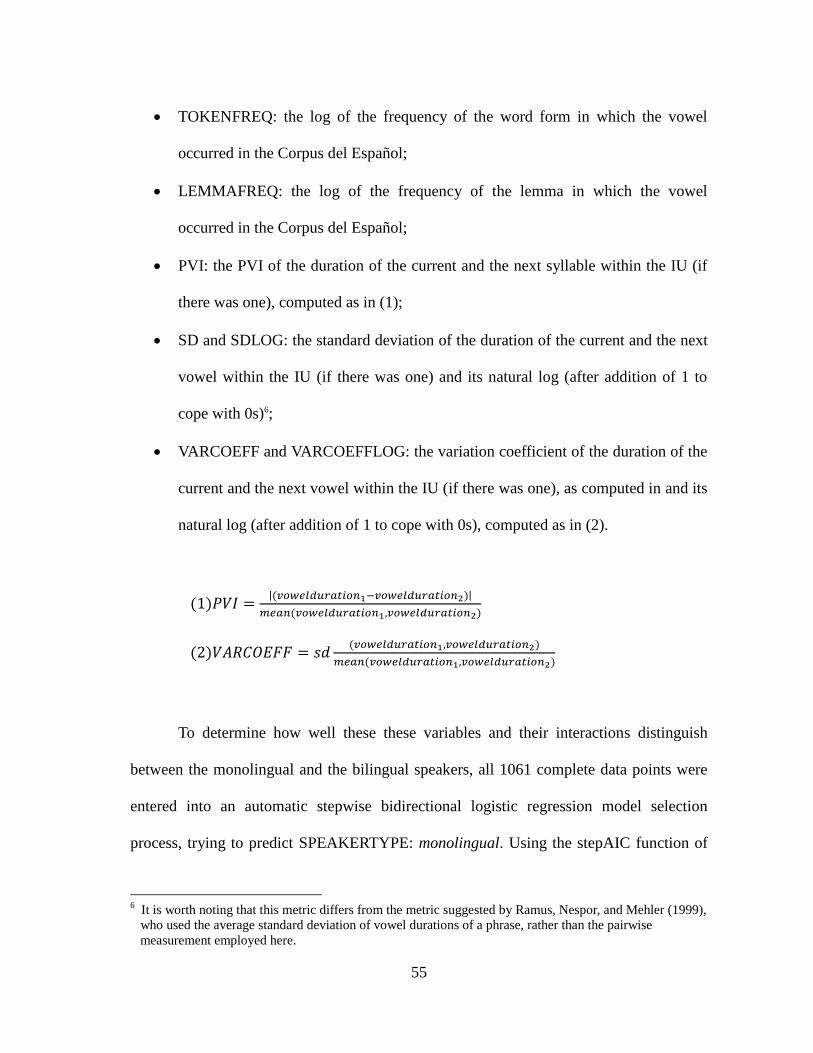
55
TOKENFREQ: the log of the frequency of the word form in which the vowel
occurred in the Corpus del Español;
LEMMAFREQ: the log of the frequency of the lemma in which the vowel
occurred in the Corpus del Español;
PVI: the PVI of the duration of the current and the next syllable within the IU (if
there was one), computed as in (1);
SD and SDLOG: the standard deviation of the duration of the current and the next
vowel within the IU (if there was one) and its natural log (after addition of 1 to
cope with 0s)6;
VARCOEFF and VARCOEFFLOG: the variation coefficient of the duration of the
current and the next vowel within the IU (if there was one), as computed in and its
natural log (after addition of 1 to cope with 0s), computed as in (2).
(1)𝑃𝑉𝐼 =∣∣(𝑣𝑜𝑤𝑒𝑙𝑑𝑢𝑟𝑎𝑡𝑖𝑜𝑛1;𝑣𝑜𝑤𝑒𝑙𝑑𝑢𝑟𝑎𝑡𝑖𝑜𝑛2)∣∣
𝑚𝑒𝑎𝑛(𝑣𝑜𝑤𝑒𝑙𝑑𝑢𝑟𝑎𝑡𝑖𝑜𝑛1,𝑣𝑜𝑤𝑒𝑙𝑑𝑢𝑟𝑎𝑡𝑖𝑜𝑛2)
(2)𝑉𝐴𝑅𝐶𝑂𝐸𝐹𝐹 = 𝑠𝑑(𝑣𝑜𝑤𝑒𝑙𝑑𝑢𝑟𝑎𝑡𝑖𝑜𝑛1,𝑣𝑜𝑤𝑒𝑙𝑑𝑢𝑟𝑎𝑡𝑖𝑜𝑛2)
𝑚𝑒𝑎𝑛(𝑣𝑜𝑤𝑒𝑙𝑑𝑢𝑟𝑎𝑡𝑖𝑜𝑛1,𝑣𝑜𝑤𝑒𝑙𝑑𝑢𝑟𝑎𝑡𝑖𝑜𝑛2)
To determine how well these these variables and their interactions distinguish
between the monolingual and the bilingual speakers, all 1061 complete data points were
entered into an automatic stepwise bidirectional logistic regression model selection
process, trying to predict SPEAKERTYPE: monolingual. Using the stepAIC function of
6 It is worth noting that this metric differs from the metric suggested by Ramus, Nespor, and Mehler (1999),
who used the average standard deviation of vowel durations of a phrase, rather than the pairwise
measurement employed here.
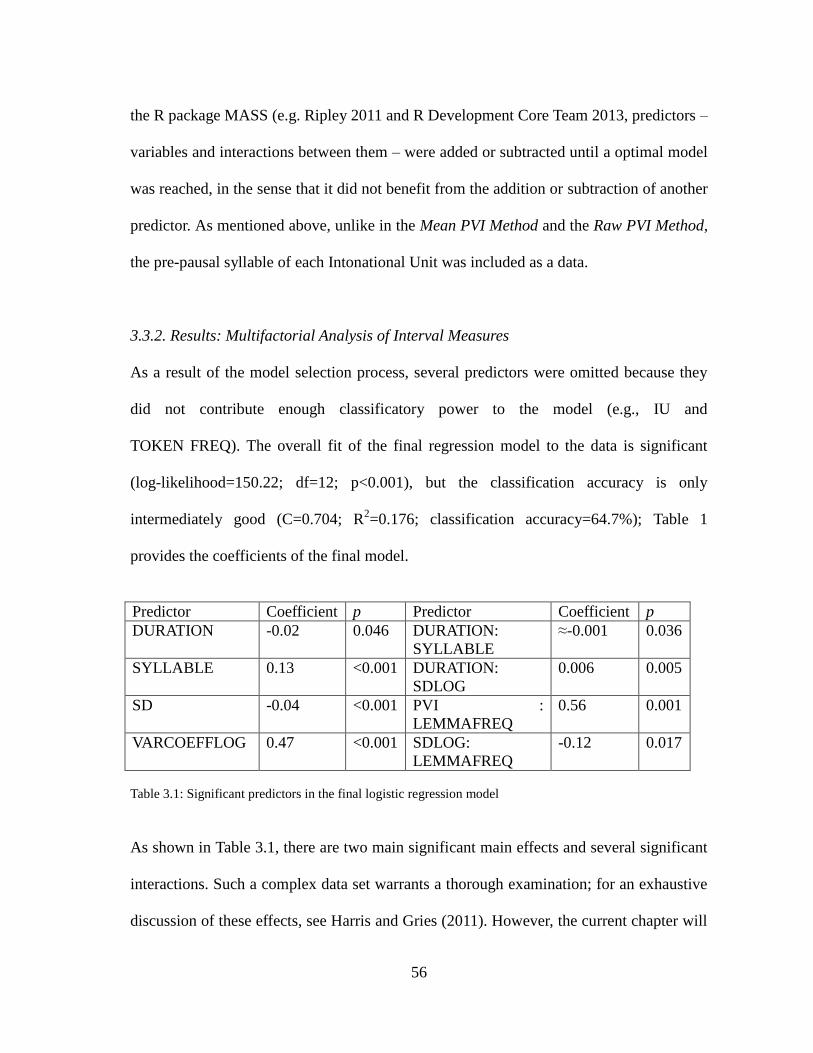
56
the R package MASS (e.g. Ripley 2011 and R Development Core Team 2013, predictors –
variables and interactions between them – were added or subtracted until a optimal model
was reached, in the sense that it did not benefit from the addition or subtraction of another
predictor. As mentioned above, unlike in the Mean PVI Method and the Raw PVI Method,
the pre-pausal syllable of each Intonational Unit was included as a data.
3.3.2. Results: Multifactorial Analysis of Interval Measures
As a result of the model selection process, several predictors were omitted because they
did not contribute enough classificatory power to the model (e.g., IU and
TOKEN FREQ). The overall fit of the final regression model to the data is significant
(log-likelihood=150.22; df=12; p<0.001), but the classification accuracy is only
intermediately good (C=0.704; R2=0.176; classification accuracy=64.7%); Table 1
provides the coefficients of the final model.
Predictor Coefficient p Predictor Coefficient p
DURATION -0.02 0.046 DURATION:
SYLLABLE
≈-0.001 0.036
SYLLABLE 0.13 <0.001 DURATION:
SDLOG
0.006 0.005
SD -0.04 <0.001 PVI :
LEMMAFREQ
0.56 0.001
VARCOEFFLOG 0.47 <0.001 SDLOG:
LEMMAFREQ
-0.12 0.017
Table 3.1: Significant predictors in the final logistic regression model
As shown in Table 3.1, there are two main significant main effects and several significant
interactions. Such a complex data set warrants a thorough examination; for an exhaustive
discussion of these effects, see Harris and Gries (2011). However, the current chapter will

57
only discuss the relevant methodological implications of certain interactions upon the
study of speech rhythms.
3.3.2.1. Main Effects
Figure 3.1 shows the main effects of SD and VARCOEFFLOG on the predicted
probability of monolingual: As the variability of two vowels increases in terms of SD, the
prediction is becoming more likely to be bilingual. However, as the variability of two
vowels increases in terms of VARCOEFFLOG – i.e., the measure of dispersion less
affected by the mean duration – the prediction is becoming more likely to be monolingual,
at least on the whole.
Figure 3.1:The main effects SD (left) and VARCOEFFLOG (right) Note: the tick-marked cross in the right
panel indicates quantiles.

58
3.3.2.2. Interactions
Let us now turn to variables participating in interactions relevant to the present chapter‘s
discussion, namely, the effects related to lemma frequency. Interestingly, there are two
interactions that involve the corpus-based frequency of the lemma and two ways of
measuring the variability of the syllable, the first of which is represented in Figure 3.2.
This shows that the correlation of LEMMAFREQ and SDLOG differs between speakers.
More specifically, with high-frequency lemmas, the variability values of mono- and
bilingual speakers do not differ, which means SDLOG cannot distinguish the speaker
types. However, with words whose lemma frequency is below 9, monolingual speakers
have lower SDLOG values.
Figure 3.2: The interaction LEMMAFREQ : SDLOG
Figure 3.3 represents the interaction LEMMAFREQ : PVI. With medium and
high-frequency lemmas, the variability values of mono- and bilingual speakers do not

59
differ, but otherwise the overall trends differ. For monolingual speakers, variability as
measured by PVIs is positively correlated with LEMMAFREQ: more frequent words
have higher PVIs than less frequent words, but it is the other way round for bilingual
speakers. Also, the data show that PVIs can only distinguish mono- and bilingual speakers
for words from the extremes of the frequency spectrum: lemmas with LEMMAFREQ<4
and with LEMMAFREQ>9.
3.4. Discussion: Multifactorial Analysis
3.4.1. Main Effects: SD and VARCOEFFLOG
As mentioned above, both significant main effects, SD and VARCOEFFLOG, are
measures of duration variability which seem to predict opposite overall trends in speaker-
Figure 3.3: The interaction LEMMAFREQ : PVI

60
type: SD is positively correlated with bilingualism whereas the overall trend of
VARCOEFFLOG is negatively correlated with it. That is, SD reflects the same trend
observable for both the Mean PVI and Raw PVI calculations, namely that Monolingual
Mexican speakers display more vowel duration variability than Bilingual Chicano
speakers. Both SD and VARCOEFFLOG are calculated with the standard deviation of the
vowel duration within an IU but only the latter controls for the mean syllable duration.
This section will first discuss the main effect of SD and then VARCOEFFLOG.
It is SD that behaves more as would be expected by traditional rhythm class
distinctions (but does not the reflect the hypothesis of the current chapter); due to the
influence of English, the bilingual speakers' speech should be more variable in vowel
duration than the monolingual speakers' speech, which is exactly what SD reflects. This is
compatible with Low and Grabe (1995, 2000), Fought (2003), and Carter (2005, 2007).
The former studied L1 vs. L2 speakers, finding that Singapore English tended to be more
syllable-timed than British English. The speakers in the two latter studies were more
similar to those of the current study, in that participants were bilingual, and Chicano
speakers of Spanish and English, although both studies examined English rather than
Spanish. In those studies, the English of Spanish-English bilinguals was more uniform
and syllable-timed (i.e. more 'Spanish like') than that of European- and African-
Americans (in Carter 2005, 2007), once again suggesting the results reflected by SD, that
is, that bilingual speakers would have more variability in vowel duration, reflecting a
more 'English like' Spanish. It is important to note that all of the aforementioned studies
used the PVI as a metric of duration variability whereas, in the current study, the PVI was
not a significant predictor of speaker type (although it did participate in one significant

61
interaction); instead it was SD that reflected the expected influence of bilingualism. Keep
in mind that while SD is intended to measure the same acoustic property as the PVI,
vowel duration variability, it is calculated in an alternate manner. In addition to the
differing IMs utilized between the aforementioned studies and the statistically significant
effect of SD, the related VARCOEFFLOG reveals a more complex trend.
As mentioned above, at first glance the trend of VARCOEFFLOG appears to be
the opposite of the expected trend and that reflected by SD: Figure 3.1 suggests an overall
positive correlation, according to which monolingual speakers display more variability in
vowel duration than bilingual speakers. In other words, it suggests that the Spanish of
monolingual speakers is closer in rhythm to English than that of bilingual Spanish-
English speakers; this, of course, is in agreement with the trend identified by the PVI in
the first two statistical treatments described (see Chapter 2). However, the overall picture
is more complex than a brief glance at the smoother might suggest (additionally it is more
complex than the simplistic trend suggested in the earlier analyses of the PVI). In
examining the present case of VARCOEFFLOG, it becomes obvious that, while there is
an overall positive correlation, this is a case where the prediction is most strongly
'bilingual' in the small range of exactly intermediate variability. Meanwhile, the extreme
ranges of variability largely lead to the prediction of 'monolingual'. In fact, as the course
of the smoother line indicates when related to the quantiles, bilingual speakers tend to
group around the mean of VARCOEFFLOG. This would indicate that monolingual
speakers are able to employ a full range of vowel duration variability, ranging from zero
variability to the most variable syllable pairs, whereas bilingual speakers tend to display
an intermediate level of variability according to VARCOEFFLOG, displaying syllable
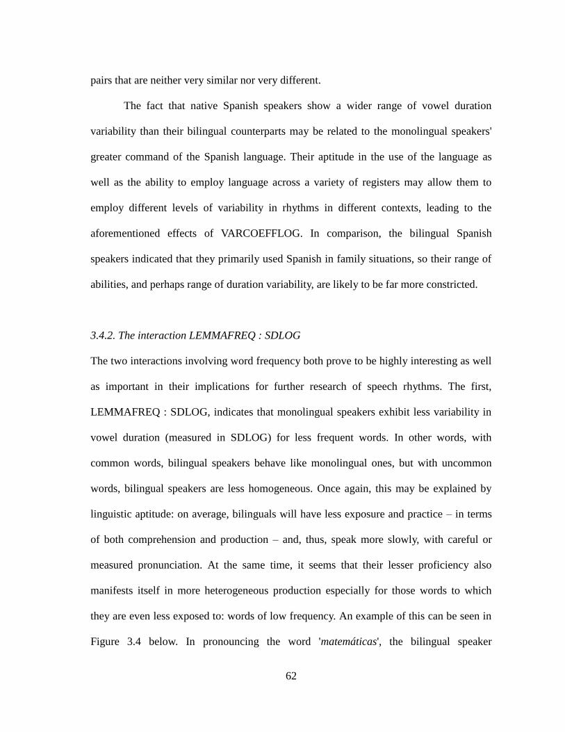
62
pairs that are neither very similar nor very different.
The fact that native Spanish speakers show a wider range of vowel duration
variability than their bilingual counterparts may be related to the monolingual speakers'
greater command of the Spanish language. Their aptitude in the use of the language as
well as the ability to employ language across a variety of registers may allow them to
employ different levels of variability in rhythms in different contexts, leading to the
aforementioned effects of VARCOEFFLOG. In comparison, the bilingual Spanish
speakers indicated that they primarily used Spanish in family situations, so their range of
abilities, and perhaps range of duration variability, are likely to be far more constricted.
3.4.2. The interaction LEMMAFREQ : SDLOG
The two interactions involving word frequency both prove to be highly interesting as well
as important in their implications for further research of speech rhythms. The first,
LEMMAFREQ : SDLOG, indicates that monolingual speakers exhibit less variability in
vowel duration (measured in SDLOG) for less frequent words. In other words, with
common words, bilingual speakers behave like monolingual ones, but with uncommon
words, bilingual speakers are less homogeneous. Once again, this may be explained by
linguistic aptitude: on average, bilinguals will have less exposure and practice – in terms
of both comprehension and production – and, thus, speak more slowly, with careful or
measured pronunciation. At the same time, it seems that their lesser proficiency also
manifests itself in more heterogeneous production especially for those words to which
they are even less exposed to: words of low frequency. An example of this can be seen in
Figure 3.4 below. In pronouncing the word 'matemáticas', the bilingual speaker

63
pronounces the word more slowly (and perhaps more carefully); the bilingual speaker
takes about .74 seconds to pronounce the word while the monolingual speaker takes about
.69 seconds (neither of these words were phrase final, and both were the first mention of
the word, so, in theory, phrase position and information structure should not affect the
duration of these words, although this is simply one ad hoc example; it should also be
noted that the bilingual speaker in the upper panel is female while the monolingual
speaker in the lower panel is male).
Figure 3.4: A waveform and spectrogram comparison of two pronunciations of a low frequency word,
matemáticas (lemma frequency in Corpus del Espanol 20th
Century Files (Davies, 2002-) = 2) in the current
data. The bilingual speaker's speech signal is in the upper panel and the monolingual speaker's speech signal
is in the lower panel.
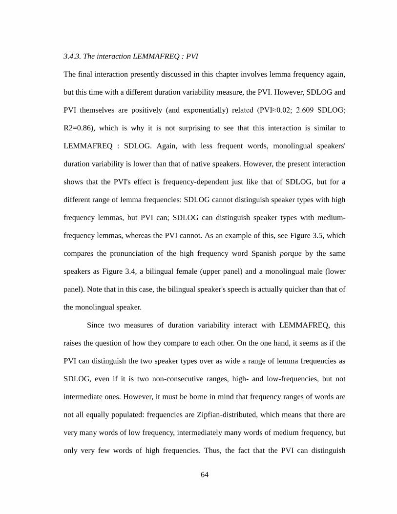
64
3.4.3. The interaction LEMMAFREQ : PVI
The final interaction presently discussed in this chapter involves lemma frequency again,
but this time with a different duration variability measure, the PVI. However, SDLOG and
PVI themselves are positively (and exponentially) related (PVI≈0.02; 2.609 SDLOG;
R2=0.86), which is why it is not surprising to see that this interaction is similar to
LEMMAFREQ : SDLOG. Again, with less frequent words, monolingual speakers'
duration variability is lower than that of native speakers. However, the present interaction
shows that the PVI's effect is frequency-dependent just like that of SDLOG, but for a
different range of lemma frequencies: SDLOG cannot distinguish speaker types with high
frequency lemmas, but PVI can; SDLOG can distinguish speaker types with medium-
frequency lemmas, whereas the PVI cannot. As an example of this, see Figure 3.5, which
compares the pronunciation of the high frequency word Spanish porque by the same
speakers as Figure 3.4, a bilingual female (upper panel) and a monolingual male (lower
panel). Note that in this case, the bilingual speaker's speech is actually quicker than that of
the monolingual speaker.
Since two measures of duration variability interact with LEMMAFREQ, this
raises the question of how they compare to each other. On the one hand, it seems as if the
PVI can distinguish the two speaker types over as wide a range of lemma frequencies as
SDLOG, even if it is two non-consecutive ranges, high- and low-frequencies, but not
intermediate ones. However, it must be borne in mind that frequency ranges of words are
not all equally populated: frequencies are Zipfian-distributed, which means that there are
very many words of low frequency, intermediately many words of medium frequency, but
only very few words of high frequencies. Thus, the fact that the PVI can distinguish
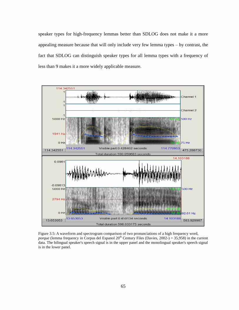
65
speaker types for high-frequency lemmas better than SDLOG does not make it a more
appealing measure because that will only include very few lemma types – by contrast, the
fact that SDLOG can distinguish speaker types for all lemma types with a frequency of
less than 9 makes it a more widely applicable measure.
Figure 3.5: A waveform and spectrogram comparison of two pronunciations of a high frequency word,
porque (lemma frequency in Corpus del Espanol 20th
Century Files (Davies, 2002-) = 35,958) in the current
data. The bilingual speaker's speech signal is in the upper panel and the monolingual speaker's speech signal
is in the lower panel.
66
3.5. Implications
The findings discussed above lead to a general conclusion, which in turn entails two more
specific implications. This general conclusion is that the multifactorial method employed
in the current chapter provides a much more fine-grained perspective than the more
simplistic methodologies of Chapter 2. The non-linear trend observed in the main effect
VARCOEFFLOG for instance, would not be clear with a simple linear regression and the
simplistic use of the PVI is virtually useless as a metric for the comparison of speech
rhythms. Furthermore, interactions between predictors display important trends that
would not be clear without the methodology employed. This is to say that in investigating
a facet of linguistics as complex as speech rhythms, it is crucial to use the methodology
best suited to the data, taking special care to utilize all the modern computational
methodologies available (this fact, of course, is not exclusive to speech rhythms, but
applies to all fields of linguistics). The first more specific implication is that the data shed
further doubt on the utility of the PVI, especially given the results of Chapter 2. The PVI
is simplistic in summarizing the complexity of vowel duration variability, and, by
extension, speech rhythms. In the case of the Mean PVI and Raw PVI analyses, the PVI‘s
high variability for individual speakers prevents a final model with low prediction
accuracy (particularly in the case of Raw PVI), meaning that it is not ultimately useful in
the quantification of vowel duration variability. In the case of the multifactorial analysis,
the PVI does not feature as a main effect in the final regression model and only features in
one interaction (with LEMMAFREQS); its classificatory power is therefore more limited
than that of other predictors. Also, even within said interaction, the PVI's classificatory
power is restricted to a smaller subset of the data than the competing measure of SDLOG:

67
this is to say that the range of words for which the PVI will be useful is smaller than that
of SDLOG. In addition to these empirical findings, it is worth restating the design
weaknesses of the PVI. On the one hand, the PVI as often used is a mean of means of
means. However, it is well-known that means are really only appropriate measures of
central tendencies for normally-distributed data, and in the data, the PVIs of 18 of the 20
speakers are significantly different from normality (and one of the two remaining
speakers' PVIs are very close to that, too, with pShapiro-Wilk test=0.051). Related to this, the
'nested averaging' simply ignores a lot of variability that a more comprehensive approach
would want to account for. For example, the 'nested averaging' also does not allow one to
study PVIs on a syllable-by-syllable basis (since only an average will be considered in the
traditional approach), and rules out the incorporation of, for instance, frequency effects
for lemmas (as in the current chapter), words, syllables as well as other lexically-specific
predictors.
Second, it is clear that such measures interact with corpus-derived lemma
frequencies. It is interesting to note in this connection, however, that it is lemma, not
token frequency that is more relevant to the speakers in the present data, which is
surprising since usually word/token frequencies are more decisive for process of
articulation. Regardless of which type of frequency will turn out to be more relevant to
duration variability, future studies should not only try to approach duration variability in
quantitatively more advanced ways (i.e., multifactorially) but also take frequency effects
based on corpus data into consideration.
With regard to the utility of different measures in general, such data as could be
useful to explore which of the measures result in the largest discriminatory power. With
68
regards to the study of speech rhythms, several statistical steps are self-evident, given the
results discussed in this chapter. Findings like these indicate why measures such as the
PVI may be too simplistic – the multiple averaging decontextualizes all variability – and
why even the present approach can only be a starting point to explore duration variability
in the rich and authentic contexts in which it occurs. For this reason, in order to evaluate
speech rhythms, it is essential to 1) assess the data in a multifactorial manner, thereby
assessing all relevant metrics and avoiding pitfalls, such as the overgeneralization of the
PVI mentioned above, and 2) include corpus-based frequency effects, which have been
shown to affect various areas of pronunciation, including duration variability. Thus, the
researcher avoids picking and choosing those metrics that conveniently reflect apparent
rhythmic differences, and are easily assessed and summarized, and, instead, allows the
admittedly complex data set to be reflected in a statistically sophisticated and
methodologically sound manner.
Finally, it is not enough to only include production data in the assessment of
speech rhythms. It is clear that perception plays a major role in distinguishing rhythms
(e.g. Nazzi, Bertoncini, and Mehler 1998), therefore the remaining chapters of my
dissertation will concentrate on that aspect of human cognitive abilities. Perception data
will be the starting point to define rhythmic classes of utterances, empirically evaluating
speech rhythm perception, then this rhythmic classification will be used as the dependent
variable in a multifactorial analysis of speech rhythm production.
This methodology avoids the error of assuming that different languages inherently
belong to different rhythm classes and instead relies upon experimental data to determine
rhythmic differences from a perceptual standpoint. It then employs current computational

69
methodology in assessing speech rhythm perception, using the methods described in the
current chapter as a starting point.
The remainder of the dissertation follows this structure: Chapter 4 assesses
perception experiments of English, Portuguese, and Spanish speech rhythms. Chapter 5
analyzes production data collected in an exhaustive experiment spanning native speakers
from different languages on opposite ends of the syllable-timing vs. stress-timing
spectrum. Finally Chapter 6 will be devoted to the conclusions that can be drawn from
these studies, their implications for the field of linguistics and future developments in
speech rhythm research.
70
Chapter 4
Perception of English, Portuguese, and Spanish Speech Rhythms
Overview
This chapter describes several experiments performed in order to evaluate the perceptual
differences in the speech rhythms of English, Spanish, and Portuguese. While perception
experiments have been performed in the past (e.g. Ramus and Melher 1999), the current
methods employed seek to both a) determine the relative position of these utterances of
the three languages on the speech rhythm continuum and b) use these relative rankings as
the dependent variable for a multifactorial analysis of the production of these same three
languages (see Chapter 5). Thus, by using perception as the basis for an exploration of
production, this study avoids a common pitfall of language rhythm studies, namely the
assumption that all utterances of a language belong to the same rhythm class. After an
introduction, two pilot studies and a third larger-scaled perception experiment are
presented. In the conclusion, the results of these experiments are discussed in the wider
context of this dissertation; in particular, their relation to the statistical evaluation in
Chapter 5 is presented.
4.1. Introduction
Given the results of the experiments described in Chapter 2 and Chapter 3, the current
chapter seeks to quantitatively evaluate the perception of speech rhythms of English,
Portuguese, and Spanish. More specifically, the results of these chapters suggest that one
cannot rely upon a single metric in order to attempt to differentiate between rhythm

71
classes in data; this is an especially important point given the fact that there is evidence of
within-language (and within-speaker) variation (e.g. Loukina et al. 2009). Metrics of
speech rhythm appear to participate in interactions and non-linear behavior, suggesting
the need for a sophisticated statistical analysis of speech rhythm data. However, an
additional consideration is necessary before addressing speech rhythm metrics. The
parallel development of instrumental measurements as correlates of language-rhythms and
perception-based studies, as seen in Chapter 1, suggests the next logical step, namely a
combination of perception and production methodologies. This has been achieved in part
by Ramus, Dupoux, Zangl, and Mehler‘s (2000) use of previous IM measurements from
Ramus, Nespor and Mehler (1999). However, three characteristics of a methodologically
sound study of language-rhythms are necessary. Firstly, one must use an advanced
statistical evaluation of the data (e.g. the multifactorial statistical approach to acoustic
correlates employed in Chapter 3). Secondly, it is not sufficient to only include vowel
duration cues in evaluated language rhythms. Syllabic durations (Deterding 2001) and
correlates of lexical stress (i.e. duration, but also F0 and intensity) must also be included
in said analysis; duration, intensity, and pitch have been shown to increase for stressed
syllables (e.g. Marshall, Charles W. and Patrick W. Nye, 1983). Thirdly, speech low-pass
filtering (Arvaniti 2012) must be applied to a perception study, while the statistical
analysis of the production is performed upon the same utterances used in the perception
study. That is, without making assumptions about the rhythmic classes, this methodology
allows the exploration of which acoustic cues, if any, cause perceptual differences,
regardless of language.

72
The following section will first describe the conceptual design behind the
language rhythms perception experiment. Following are three experimental processes.
The first two are pilot studies intended to evaluate and improve methodology employed in
this chapter‘s perception experiment. The third is a rhythm perception test with 20
university students. Each experiment will include information about experimental design,
data, statistical processing, and results. Finally, the conclusions of this chapter will be
discussed, as well as how these conclusions determine the methodology employed in
Chapter 5.
4.2. Perception Experiment: Conceptual Design
As previously mentioned, speech rhythms were originally discussed as a perceptual
difference (e.g. Pike 1945); to use of the words of Barry, Andreeva, and Koreman (2009),
―rhythm typology has its roots in auditory observation.‖ At this point, it was assumed that
languages of different rhythm classes all differ from one another rhythmically. However,
this assumption has not been empirically proven; for example, no one has conclusively
demonstrated that all Spanish utterances differ from all English utterances (although it has
been shown that some Spanish utterances differ rhythmically from some English
utterances). In fact, while some languages do appear to differ from one another in terms of
(broadly-defined) speech rhythms, there is also a substantial amount of within-language
rhythmic variation (Loukina, Kochanski, Shih, Keane, and Watson 2009). The
experiments described in the current chapter attempt to ascertain whether utterances of
English, Portuguese, and Spanish differ in an intra-language manner, an inter-language
manner, or both. That is, this study compares English to Spanish, English to Portuguese,

73
but also English to English (etc.) in a perception experiment. The purpose of this is
twofold. It is, of course, one of the major goals of this dissertation to quantitatively
evaluate the relative positions of these three languages on the speech rhythm continuum.
A second goal of this chapter is to use the analysis of these utterances as the dependent
variable in a multifactorial study of the production of these utterances, reported in
Chapter 5. Thus, rather than assume that all utterances of different languages represent
different rhythm classes, the current study will first evaluate the perceptual differences of
these languages and create a hierarchy of the various utterances used. In the following
chapter, a multifactorial analysis of these utterances will investigate which (if any)
production metrics prompt these perceived rhythmic differences.
Mexican Spanish, Peninsular Portuguese, and American English comprise the
languages that provide utterances to be used as production and perception data for the
current study. The opposite rhythmic classification of Spanish and English provide
optimal samples of the opposing extremes of the speech-rhythm continuum. Meanwhile,
Portuguese has a somewhat intermediate classification; Frota and Vigário, (2001) assessed
the rhythmic typologies of both varieties of Portuguese (Brazilian and Peninsular) using
the rhythm metrics introduced by Ramus, Nespor, and Mehler (1999) and determined that
they display mixed rhythms. Peninsular Portuguese is characterized by a mix of stress and
syllable-timed characteristics, while Brazilian Portuguese displays syllable-timed and
mora-timed characteristics, suggesting that the speech-rhythm continuum is not solely
comprised of more or less stress or syllable-timed languages. Furthermore, Frota, Vigário,
and Martin (2002), demonstrated that, under certain conditions, European Portuguese

74
adults could distinguish filtered Peninsular and Brazilian Portuguese utterances from the
reportedly more stress-timed Dutch.
As Peninsular Portuguese has been assessed as having an intermediate
classification, displaying some stress-timed characteristics and some syllable-timed
characteristics, this variety appears to have a central or mixed rhythmic typology. This
provides an optimal language as it should fall between the two extreme poles of the
speech rhythm continuum, syllable-timed Spanish and stress-timed English. Thus, the
expected resulting classification of the test languages, according to traditional rhythmic
typologies is illustrated in Table 4.1.
Poles of Rhythm
Continuum
More Syllable
Timed
More Stressed
Timed
Proposed phonetic
characteristics
less variable
segment durations
more variable
segment durations
Languages Spanish
Portuguese English
Table 4.1: Expected Position of test language on Speech Rhythm Continuum
As illustrated in Table 4.1, the traditional rhythmic distinctions suggest that the test
languages would manifest themselves in the rhythmic hierarchy, ranging from the most
stress-timed, English, to the most syllable-timed, Spanish, with Peninsular Portuguese
falling somewhere between the two in perception data.
The perception studies described in this chapter rely upon the low-pass filtering
methodology (e.g. Melher et al. 1988) rather than the speech resynthesis methodology
(e.g. Ramus and Mehler 1999). Although recent speech rhythm studies have employed

75
both methodologies (e.g. Arvaniti 2012 for low-pass filtering; White et al. 2012 for
speech resynthesis), and both methodologies have been defended (see Chapter 1 for
discussion), the current study follows Arvaniti (2012) in using low-pass filtering because
the process is more faithful to the original speech signal. A more authentic prompt is
conceivably more reliable in reflecting speech rhythm perception. Upon low-pass filtering
at 450 Hz, non-syllabic information has been removed from the utterances (Arvaniti
2012); participants in the current study heard three low-pass filtered utterances and were
cued to state which two utterances out of the three were most similar. Thus, without
relying upon traditional rhythm class distinctions, the true manner in which languages are
perceived is evident. By extracting a sufficient number of similarity ratings for
UTTERANCE pairs, it is possible to statistically determine which utterances are most
similar by performing cluster analysis using the hclust function for R (R Development
Core Team, 2013).
A word about the maternal languages of the participants in the perception study is
necessary. Although the ability to distinguish between two different speech rhythms is
presumably universal, especially considering the work showing infants abilities to
distinguish speech rhythms (e.g. Mehler et al. 1988), the native language of the
participants could affect the data. Thus, although the current experiment does not restrict
participants in the perception test according to native language, it does explore variation
amongst the participants in order to prevent the skewing of data by individual
participants/ and or 'nationalities' (as indicative of native language spoken, see Figure 4.2
and Figure 4.3).
76
4.3. Perception Experiment: Pilot Studies 1 and 2
The task in this experiment relies on participants‘ ratings of the similarity of various
utterances. However, unlike previous experiments, which rely upon scale ratings (eg.
Arvaniti 2012), this experiment relied upon direct comparison between various utterances.
That is, the participants were presented with three utterances and then asked which of two
among the three were most similar. As previously mentioned, the current study uses low
pass filtering (Mehler et al. 1988) rather than speech resynthesis (Ramus and Mehler
1999).
4.3.1. Experimental design
Two English, two Portuguese, and two Spanish utterances were selected from a corpus of
semi-directed interviews representing spontaneous speech; as previously mentioned, "[i]t
is well known that there are differences between read and unscripted speech" (Deterding
2001:220). Each set of two utterances of one language came from the same speaker. The
speakers were all females enrolled in a four-year university located in California, Lisbon,
and Mexico City respectively at the time of recording and each was a monolingual
speaker of their language. Utterances were chosen by the author and verified by a second
phonologist to be similar in length and syllable number, to contain minimal pitch
excursions, and to display similar levels of mean pitch. The following steps were
undertaken to prepare the utterances for the experimental task: 1) Scale times to start at 0
seconds and end at 10 seconds; 2) Scale peak amplitude to .99; 3) Scale intensity average
intensity to 70 dB; 4) Low-pass filter utterances at 450 Hz. See Figure 4.1.

77
Figure 4.1: A comparison of the unedited Spanish utterance in the top panel and the low-pass filtered
utterance in the lower panel, as used in the current perception experiments. This phrase is ―esta(b)a con
(u)nos amigos en.‖
After hearing each group of three utterances, participants were prompted to
indicate which two utterances of the three were more similar. No further instruction or
training block was used to prepare participants for the task. The training block was not
necessary for two reasons. Firstly, differences in speech rhythms are theoretically
perceptible universally, regardless of the native language of the listener; infants are able to
distinguish rhythmic cues in language discrimination tasks (see Mehler et al. 1988 for
low-pass filtered data and Ramus and Mehler 1999 for speech resynthesis data) and

78
speech timing seems to be biologically hard wired into the speaker (Wretling and
Eriksson, 1998). Secondly, due to the utterance selection and low-pass filtering mentioned
above, in theory only rhythmic cues were available to participants, although non-rhythmic
cues (e.g. intensity, F0) were included as independent variables in the analysis of Chapter
5 to allow for the possibility that these cues were salient to participants. Two different
methods were piloted using these experimental cues. The following sections will describe
these two pilot studies and the conclusions as to experimental design drawn from these
pilot studies.
4.3.2. Perception Study: Pilot Study 1
For reasons of efficiency, the first series of experiments that comprise the data for Pilot
Study 1 were administered to participants in groups. The participants were the members of
beginning Spanish and Portuguese classes. Three total classes were tested in this
experiment: 11 students of an elementary Spanish class, 18 students of an elementary
Spanish class, and 14 students of an elementary Portuguese class. Although it is possible
that this language learning would somehow bias the rhythmic perception of participants,
this fact was deemed inconsequential for three reasons. Firstly, as mentioned, rhythm is
theoretically a universal difference that exists between languages of different classes.
Secondly, these students were all in first-year language classes, so it is questionable that
minimal language instruction would significantly alter their perceptions of speech
rhythms, especially given that it appears that rhythm perception is acquired at a very
young age. As mentioned in Chapter 1, Nazzi, Berteconi, and Mehler (1998), for
instance, showed that French neonates could discriminate between a mora-timed language
79
and a stress-timed language. Thirdly, as these series of tests served as a pilot experiment,
the main goal was to finalize methodology to be used; thus the availability of participants,
rather than participant selection, was the most important facet of this pilot study.
The six low-pass filtered utterances were grouped into the twenty possible sets of
three utterances without repeating the same UTTERANCE twice in any set. For each of
the three classes, these sets were all randomized, both in the order of the twenty sets
presented, as well as the order within which each set of three was presented. (See Table
4.2 for all the combinations of utterances used in Perception Study: Pilot Study 1 and
Perception Study: Pilot Study 2.) These randomized orders were presented in a slide show.
The slide show informed students of which set (1-20) and which clip (1-3) within each set
was playing. This was intended to keep students informed of what set was being tested
during the study. The students responded to the question by hand on a response sheet
distributed at the beginning of each experiment. The response sheet included a
participant's consent to participate. In then asked for the participant‘s name, age, and
native language. Finally, it had the following instructions: ―You will hear a series of sets
of three audio clips. After listening to all three clips, circle a, b, or c to indicate which two
clips are most similar. You will only hear each set one time each.‖ (see Appendix X for the
response sheets used). The slide show and accompanying audio clips were played using
the in-classroom media set up with consisted of a projector and two speakers. After the
experiment performed, a brief discussion was conducted with the participants. Firstly,
participants were asked for feedback on the task they had performed, such as length of
task, ease, potentially confusing elements, etc.
80
This original pilot study revealed several methodological shortcomings. Firstly,
from a conceptual standpoint, administering randomized orders of prompts to large
groups of students at one time is questionable. It is difficult to ensure that each participant
group is the same size, which makes controlling the potential variation between
randomized orders difficult to say the least. Beyond this, controlling environmental
factors becomes difficult. Auditory issues such as construction and grounds keeping tools
being used near the classroom made it difficult for some students to hear the prompts.
Furthermore, as the students sat at various distances from the speakers, some students
heard the prompts at a louder volume as compared to others, and there was variation
classroom to classroom in the volume at which the media equipment played the prompts.
In fact, media equipment failure made it impossible to finish one of the classroom
experiments. Finally, the students themselves voiced two major issues: firstly, it was
difficult to follow along with the different clips being played, due to the difficulty of
writing responses on the response sheet while simultaneously attempting to view the
screen indicating which clip was being played; secondly, the experiment was too long. It
took nearly 20 minutes to complete all the varying sets of clips, and participant fatigue
played a major factor. Some students stopped answering questions towards the end of the
survey, others circled only one letter answer to all the final questions, or wrote ―I don‘t
know.‖ As mentioned above, only two of the three participant groups were able to
complete the task, and even the complete data that was gathered still had some
shortcomings as discussed above; for this reason, I will not discuss any results of these
experiments. Instead, these pilot experiments served to optimize experimental design,
leading to the second pilot experiment described in the following section.

81
Set Clip 1 Clip 2 Clip 3
1 Portuguese 1 Portuguese 2 Spanish 1
2 Portuguese 1 Portuguese 2 Spanish 2
3 Portuguese 1 Spanish 1 Spanish 2
4 Portuguese 2 Spanish 1 Spanish 2
5 Portuguese 1 Portuguese 2 English 1
6 Portuguese 1 Spanish 1 English 1
7 Portuguese 1 Spanish 2 English 1
8 Portuguese 2 Spanish 1 English 1
9 Portuguese 2 Spanish 2 English 1
10 Spanish 1 Spanish 2 English 1
11 Portuguese 1 Portuguese 2 English 2
12 Portuguese 1 Spanish 1 English 2
13 Portuguese 1 Spanish 2 English 2
14 Portuguese 1 English 1 English 2
15 Portuguese 2 Spanish 1 English 2
16 Portuguese 2 Spanish 2 English 2
17 Portuguese 2 English 1 English 2
18 Spanish 1 Spanish 2 English 2
19 Spanish 1 English 1 English 2
20 Spanish 2 English 1 English 2
Table 4.2. All combinations of utterances combined to comprise the 20 sets used in Perception Experiment:
Pilot Study 1 and Perception Experiment: Pilot Study 2.
4.3.3. Perception Study: Pilot Study 2
Following the first pilot study, two major issues needed to be addressed. Firstly, the fact
that the number of students in each classroom differed made it more problematic to
control for the potentially biasing order in which the prompts were presented to

82
participants. If there are differences according to the order in which the utterances are
presented to the participants, the method used in Perception Pilot Study 1 would make it
more difficult to account for this statistically. Secondly, as mentioned, environmental
differences classroom to classroom make this approach less than optimal. Thirdly, some
students found it difficult to listen to the clips and respond by hand while keeping their
place during the task. In order to address these issues, Perception Pilot Study 2 was
undertaken in order to design a computerized version of the same task. By using
headphones and a computerized testing program, pseudorandomization of the prompts
was possible and the potentially biasing environmental issues were eliminated.
The computerized test was designed using Open Sesame (Mathôt, Schreij, and
Theeuwes, 2012), an open source experiment builder for the social sciences. The
computerized test followed these steps:
1. The experiment began with a participant consent form.
2. After this, participants were prompted to write their name and maternal
language. The next screen gave instructions: ―You will hear sounds clips 1,
2, and 3. After listening, indicate which clips are more similar. Wait just a
moment…‖
3. As each clip (utterance) played, the screen displayed to the participants
which clip they were hearing (1, 2, or 3).
4. After the third clip, the screen asked participants, ―Which are more
similar?‖ and they were given the choice to respond with a mouse click:
o ―a. 1 and 2‖

83
o ―b. 2 and 3‖
o ―c. 1 and 3‖
5. After responding, the participants saw as a screen that said, ―Next set.‖
6. After completing the final set, the screen read, ―You‘re all finished. Thank
you!‖
The main purpose of this second pilot study was to finalize methodology and
experimental design. Thus, while this process was ongoing, several graduate students
from the department of Spanish and Portuguese were recruited to pilot the experiment.
Because many of these students were familiar with the nature of the experiment, none of
the data logged from their participation was analyzed. However, feedback from these
participants was valuable in trouble shooting both the design of the experiment and the
functionality of the computerized testing program, as well as the automatic data logging
process. Open Sesame automatically outputs data from experiments to spreadsheet
software (Mathôt, Schreij, and Theeuwes, 2012).
After optimizing the computerized testing program, it still remained to evaluate
the experimental task itself. As in Perception Pilot Study 1, participants indicated that the
experiment was too long. One also attested that he began to recognize utterances from
previous sets. Thus, it was determined that the experiment should be significantly shorter
in order to avoid participant fatigue. Following this second pilot study, the final
methodology to be used in the perception experiment was chosen, as described in the
following section.
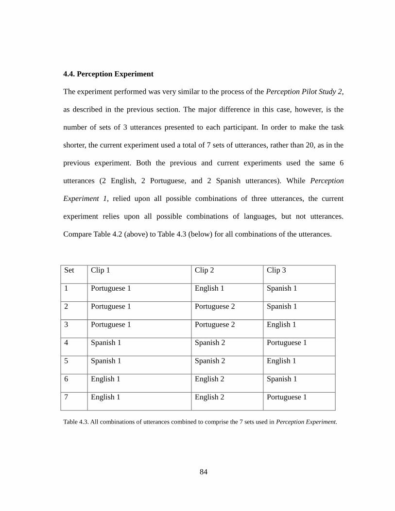
84
4.4. Perception Experiment
The experiment performed was very similar to the process of the Perception Pilot Study 2,
as described in the previous section. The major difference in this case, however, is the
number of sets of 3 utterances presented to each participant. In order to make the task
shorter, the current experiment used a total of 7 sets of utterances, rather than 20, as in the
previous experiment. Both the previous and current experiments used the same 6
utterances (2 English, 2 Portuguese, and 2 Spanish utterances). While Perception
Experiment 1, relied upon all possible combinations of three utterances, the current
experiment relies upon all possible combinations of languages, but not utterances.
Compare Table 4.2 (above) to Table 4.3 (below) for all combinations of the utterances.
Set Clip 1 Clip 2 Clip 3
1 Portuguese 1 English 1 Spanish 1
2 Portuguese 1 Portuguese 2 Spanish 1
3 Portuguese 1 Portuguese 2 English 1
4 Spanish 1 Spanish 2 Portuguese 1
5 Spanish 1 Spanish 2 English 1
6 English 1 English 2 Spanish 1
7 English 1 English 2 Portuguese 1
Table 4.3. All combinations of utterances combined to comprise the 7 sets used in Perception Experiment.
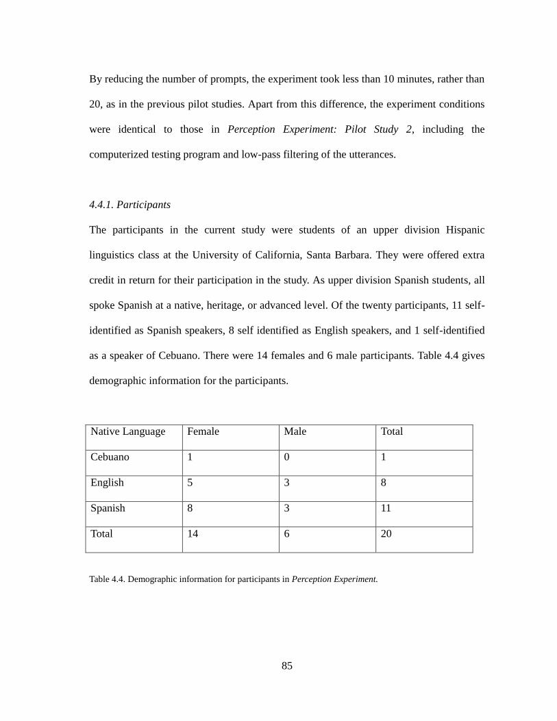
85
By reducing the number of prompts, the experiment took less than 10 minutes, rather than
20, as in the previous pilot studies. Apart from this difference, the experiment conditions
were identical to those in Perception Experiment: Pilot Study 2, including the
computerized testing program and low-pass filtering of the utterances.
4.4.1. Participants
The participants in the current study were students of an upper division Hispanic
linguistics class at the University of California, Santa Barbara. They were offered extra
credit in return for their participation in the study. As upper division Spanish students, all
spoke Spanish at a native, heritage, or advanced level. Of the twenty participants, 11 self-
identified as Spanish speakers, 8 self identified as English speakers, and 1 self-identified
as a speaker of Cebuano. There were 14 females and 6 male participants. Table 4.4 gives
demographic information for the participants.
Native Language Female Male Total
Cebuano 1 0 1
English 5 3 8
Spanish 8 3 11
Total 14 6 20
Table 4.4. Demographic information for participants in Perception Experiment.
86
4.4.2. Data Collection
Open Sesame (Mathôt, Schreij, and Theeuwes, 2012) was once again used to test
participants, who participated individually using a computer and headphones. Unlike the
pilot test, five different pseudorandomized orders of the sets and prompts were used; these
pseudorandomized orders will be referred to Treatments 1-5. As there were 20
participants, each pseudorandomized order was taken by four different students. The
participants read and electronically signed a computerized consent form, then were
prompted to write their name and maternal language. In this case, they were also
prompted to write what number test they were taking; this was a safeguard to make sure
that the correct pseudorandomized test was being given. After the preliminary steps, the
students responded to the same instructions: ―You will hear sounds clips 1, 2, and 3. After
listening, indicate which clips are more similar. Wait just a moment…‖ After hearing each
set of three clips, they responded to, ―Which are more similar?‖ and they were given the
choice to respond with a mouse click to ―a. 1 and 2‖, ―b. 2 and 3‖, or ―c. 1 and 3.‖ Finally,
they saw a screen which read: You‘re all finished. Thank you!‖ The students‘ responses
were automatically logged onto spreadsheet software by Open Sesame (Mathôt, Schreij,
and Theeuwes, 2012).
4.4.3. Data treatment
After collecting the data, a cluster analysis using the function hclust from the package
stats (R Core Team and contributors worldwide) was undertaken. Three questions were
addressed in this data analysis: 1) Do the different pseudo-randomized orders (or
treatments) behave in an idiosyncratic manner? 2) Do the participants behave in an
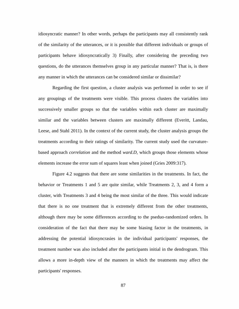
87
idiosyncratic manner? In other words, perhaps the participants may all consistently rank
of the similarity of the utterances, or it is possible that different individuals or groups of
participants behave idiosyncratically 3) Finally, after considering the preceding two
questions, do the utterances themselves group in any particular manner? That is, is there
any manner in which the utterances can be considered similar or dissimilar?
Regarding the first question, a cluster analysis was performed in order to see if
any groupings of the treatments were visible. This process clusters the variables into
successively smaller groups so that the variables within each cluster are maximally
similar and the variables between clusters are maximally different (Everitt, Landau,
Leese, and Stahl 2011). In the context of the current study, the cluster analysis groups the
treatments according to their ratings of similarity. The current study used the curvature-
based approach correlation and the method ward.D, which groups those elements whose
elements increase the error sum of squares least when joined (Gries 2009:317).
Figure 4.2 suggests that there are some similarities in the treatments. In fact, the
behavior or Treatments 1 and 5 are quite similar, while Treatments 2, 3, and 4 form a
cluster, with Treatments 3 and 4 being the most similar of the three. This would indicate
that there is no one treatment that is extremely different from the other treatments,
although there may be some differences according to the pseduo-randomized orders. In
consideration of the fact that there may be some biasing factor in the treatments, in
addressing the potential idiosyncrasies in the individual participants' responses, the
treatment number was also included after the participants initial in the dendrogram. This
allows a more in-depth view of the manners in which the treatments may affect the
participants' responses.

88
Figure 4.2. A dendrogram representing the similarity of the randomized orders presented to the participants.
The relative distance is represented by the height along the y-axis
Regarding the second question, a similarity matrix was generated to determine
how the participants rated the similarity of the various utterances. In this case, the
languages were conflated due to relatively sparse data. That is, the utterances Spanish 1
and Spanish 2 were conflated as Spanish, Portuguese 1 and Portuguese 2 were conflated
as Portuguese, and English 1 and English 2 were conflated as English. Using this
similarity matrix, a dendogram was generated for all participants. After each participant‘s
initials, the pseudo-randomized treatment order was included as well, in order to
determine if the participants‘ grouping was influenced by the order in which they were
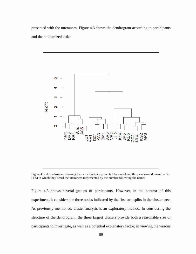
89
presented with the utterances. Figure 4.3 shows the dendrogram according to participants
and the randomized order.
Figure 4.3. A dendrogram showing the participants (represented by name) and the pseudo-randomized order
(1-5) in which they heard the utterances (represented by the number following the name)
Figure 4.3 shows several groups of participants. However, in the context of this
experiment, it considers the three nodes indicated by the first two splits in the cluster tree.
As previously mentioned, cluster analysis is an exploratory method. In considering the
structure of the dendrogram, the three largest clusters provide both a reasonable size of
participants to investigate, as well as a potential explanatory factor; in viewing the various

90
clusters, some of the pseudo-randomized orders occur in certain clusters. Specifically, the
first pseudo-randomized order occurs exclusively in the second cluster from the left, and
the second pseudo-randomized order in the third cluster, or node, from the left.
Meanwhile, the third, fourth, and fifth orders seem to be distributed relatively evenly
between the clusters.
Given the structure observed in Figure 4.3, a series of dendrograms demonstrating
the manner in which the utterances clustered according to the participants‘ responses was
generated, using the distance manhattan and method ward.D. The participants were
grouped into three different groups based upon the three nodes in Figure 4.3. These
dendrograms are represented in Figure 4.4.
Figure 4.4 shows three different dendrograms according to the participants‘
grouping from Figure 4.4. What is immediately apparent is that all three groups of
participants consistently grouped the two Portuguese utterances as more similar, as
compared to the other languages. For the remaining languages, one group was able to
consistently classify the utterances according to language. Group 1, represented in the top
left panel of Figure 4.4 not only grouped all utterances of the same language together, but
also ranked the two Romance languages as more similar to one another as compared to
English, a Germanic language; this would be expected based upon typology. The other
two groups did display some cross-linguistic clustering, with utterances of Spanish and
English being rated as more similar to one another, as opposed to the utterances of the
same language.
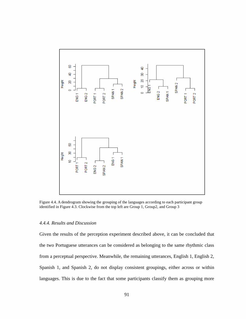
91
Figure 4.4. A dendrogram showing the grouping of the languages according to each participant group
identified in Figure 4.3. Clockwise from the top left are Group 1, Group2, and Group 3
4.4.4. Results and Discussion
Given the results of the perception experiment described above, it can be concluded that
the two Portuguese utterances can be considered as belonging to the same rhythmic class
from a perceptual perspective. Meanwhile, the remaining utterances, English 1, English 2,
Spanish 1, and Spanish 2, do not display consistent groupings, either across or within
languages. This is due to the fact that some participants classify them as grouping more

92
similarly based on language distinctions, grouping Spanish with Spanish and English with
English, while others classify them as grouping across languages, grouping certain
Spanish with certain English utterances. Thus, it can be concluded that these utterances
are all rhythmically different from one other, based upon the perception of participants in
the current experiment.
This is noteworthy in that it is contrary to traditional rhythmic class distinctions.
According to the typical concept of rhythm, Spanish and English should be maximally
different, as they represent syllable and stress-timed languages, respectively (e.g. Carter
2005). Meanwhile, Portuguese is described as a more intermediate language, falling
between stress-timed English and syllable-timed Spanish (e.g. Frota and Vigário 2001).
Thus, from the perspective of traditionally described rhythmic distinctions, it would
follow that Portuguese would be more likely to be perceived as similar to English and/or
Spanish, while English and Spanish would be maximally different in terms of syllabic
rhythm. However, as seen Figure 4.4, the case is the opposite. While Spanish and English
are grouped together by some participant groups, Portuguese is never grouped with either
Spanish or English. This would suggest that Portuguese is maximally different from
English and Spanish, with participants rating Spanish and English as more similar. There
are two potential explanations for this. The first is that Portuguese is in fact more
rhythmically different from English and Spanish than the traditional rhythm class and
rhythm continuum would suggest. This could be due to duration cues, such as vowel
reduction, which occurs in Peninsular Portuguese (Macedo and Koike 1992). The second
explanation is that the participants are not making the distinction according to
traditionally defined rhythmic classes, but instead using other acoustic cues associated

93
with the utterances. Both of these questions are worthy of investigation, and prompt the
statistical evaluation in Chapter 5, where both of these possibilities are investigated.
Chapter 5 undertakes a multifactorial analysis of the acoustic and duration correlates of
the utterances used in the current perception experiment in order to evaluate what, if any,
acoustic correlates potentially prompt these perceptual differences. If the former case is
true and Portuguese is rhythmically distinct from English and Spanish, this will be
theoretically reflected in one of the metrics intended to evaluate speech rhythms. Non-
rhythmic cues are also included in the multifactorial analysis in order to account for the
latter possibility, namely that participants are grouping these utterances according to some
salient non-rhythmic cue. In order to ascertain what differences in the utterances caused
the participants to maximally distinguish between all utterances except for the two
Portuguese utterances, Chapter 5 considers the acoustic properties of English 1, English
2, Spanish 1, Spanish 2, and combines Portuguese 1 and Portuguese 2 into a single
variable, Portuguese.

94
Chapter 5
Production Data of English, Portuguese, and Spanish
Overview
This chapter describes the evaluation of the acoustic correlates of the utterances used in
the aforementioned perception experiment of the speech rhythms of English, Portuguese,
and Spanish. The main purpose of the approach is to identify acoustic variables that
prompt perceived differences in rhythms. The following sections will describe the data
and variables, statistical processing, results, and finally discuss the conclusions and
implications of this data set. A series of post hoc analyses follow and then a final
discussion concludes this chapter.
5.1. Data and Variables
5.1.1. Data
As mentioned, the variables in this chapter are derived from the utterances that were
analyzed in Chapter 4. These 6 clips were culled from the specialized corpus of
naturalistic speech of English, Spanish, and Portuguese. As mentioned in the previous
chapter, 2 clips of each language (for a total of 6 clips from 3 speakers) were chosen from
the corpus and verified by the author and another phonetician7 to be similar in F0, lacking
major pitch excursions, and lacking any major audible differences. They were then
evaluated in a perceptual experiment according to their similarity in terms of syllabic
rhythm. The two English and two Spanish clips were all shown to be maximally different,
7 Thanks to Dr. Viola G. Miglio for her help in verifying the utterances to be used in the current chapter, as
well as for her help in dividing them into smaller phonological units (see below).
95
while the two Portuguese clips were maximally similar. Thus the two Portuguese samples
were combined into a single level of the variable UTTERANCE. This results in five
levels of UTTERANCE: English 1, English 2, Portuguese, Spanish 1, and Spanish 2. The
following sections will discuss how a variety of correlates of speech rhythms, as well as
some additional prosodic variables, were derived from these utterances. In order to derive
some variables, it was necessary to divide the utterances into phonological constituents.
The next section will discuss how the utterances were divided into phonological
constituents according to established guidelines. Next, the dependent variable and the
independent variables analyzed in the current chapter are presented.
5.1.2. Variables: Phonological Constituents
It was necessary to divide the utterances into phonological constituents in order to
calculate the standard deviations of certain phonological features (e.g. segment duration,
intensity, and pitch). The standard deviation of segment durations are commonly used
correlates in some speech rhythm studies (e.g. Ramus, Nespor, and Mehler 1999).
However, it is not possible to include one single standard deviation for each utterance, as
in Ramus, Nespor, and Mehler (1999), who use a mean standard deviation (of several
utterances) for each speaker. In the current data set, this would lead to a one-to-one
correlation between each utterance and the single standard deviation that represents it.
The result of this one-to-one correlation is a model with one main effect (standard
deviation) with perfect predictive power; this model is ultimately entirely uninformative
as to the role of segment duration variability in the perception of speech rhythms. Thus it
is necessary to include units of the utterance that are larger than the syllable yet smaller

96
than the entire utterance; these units are determined according to prosodic constituents. It
is necessary to define the boundaries of prosodic constituents in order to investigate these
effects and consider their role in rhythm perception.
Various phonological constituents comprised of prosodic units have been
proposed. In a structural theory of stress and metrical prominence such as Metrical
Phonology (Liberman 1975), for instance, prosodic prominence is no longer bound to
specific segments, but rather to suprasegmental components. Prosodic or metrical
components, in turn, obey the so-called Strict Layer Hypothesis (SLH, Selkirk 1984),
whereby all components on one level of metrical analysis comprise all components from
the level immediately below, and only those. These prosodic components are hierarchical
in nature. Thus, prosodic constituent structure is laid out according to a 'prosodic
hierarchy' as follows (Selkirk 1984):
Utt Utterance
IP intonational phrase
PhP phonological phrase
PWd prosodic word
Ft foot
σ syllable
While these constituents were largely motivated theoretically rather than empirically, they
do provide a basis for the constituents used in the current study. However, due to the
length of the utterances (approximately ten seconds each), the six prosodic constituents

97
listed above prove to be too many. Accordingly, the utterances were divided into four
levels:
Utterance
Intonational Phrase
Phonological Phrase
Syllable
The process for the actual division of these units was based upon the division prescribed
by the ToBI (for Tones and Break Indices) system (Beckman and Ayers Alam 1997). The
ToBI system, which is used to transcribe the intonational patterns and other prosodic
aspects of a language, is based upon the autosegmental metrical (AM) framework (e.g.
Pierrehumbert 1980). The AM framework distinguishes between two types of tonal events
involving F0: pitch accents and edge tones. The former events, pitch accents, are
associated with the nucleus of a syllable while the latter events, edge tones, are associated
with the boundaries of prosodic constituents (Ladd 1996). The ToBI system prescribes the
labeling of these discrete intonational events in two different manners following
Pierrehumbert and Hirschberg (1990), as cited in Beckman and Ayers Alam (1997:8). The
ToBI system has, in fact, four different tiers for labeling:
1. a tone tier
2. an orthographic tier
3. a break tier
4. a miscellaneous tier

98
As the tone tier and the break tier ―represent the core prosodic analysis‖ (Beckman and
Ayers Alam 1997:8), this study is concerned with these two tiers. The tone tier is the
location of the transcription of the two tonal events defined by the AM framework,
namely pitch accents and event tones. The break tier allows for the labeling of groupings
of prosodic constituents. This labeling is based on ―the subjective strength of its [the
current word‘s] association with the next word, on a scale from 0 (for the strongest
perceived conjoining) to 4 (for the most disjoint).‖ (Beckman and Ayers Alam 1997:9,
square brackets are mine). These break indices can be roughly defined as follows (from
Beckman and Ayers Alam 1997):
1. ―cases of clear phonetic marks of clitic groups‖
2. ―most phrase-medial word boundaries‖
3. ―a strong disjuncture marked by a pause or virtual pause, but with no tonal marks;
i.e. a well-formed tune continues across the juncture OR a disjuncture that is
weaker than expected at what is tonally a clear intermediate or full intonation
phrase boundary.‖
4. ―intermediate (intonation) phrase‖
5. ―(full) intonation phrase‖
By considering these tone break labels in conjunction with the two types of tonal events
labeled on the tone tier, the utterances in the current study were divided in the
aforementioned prosodic units. It is worth mentioning that, in this division, it is not
possible to consider the prosodic events solely; one must also consider the content of the
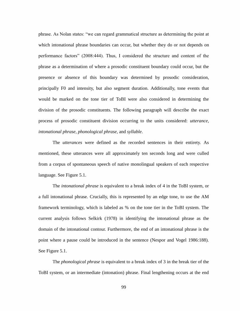
99
phrase. As Nolan states: ―we can regard grammatical structure as determining the point at
which intonational phrase boundaries can occur, but whether they do or not depends on
performance factors‖ (2008:444). Thus, I considered the structure and content of the
phrase as a determination of where a prosodic constituent boundary could occur, but the
presence or absence of this boundary was determined by prosodic consideration,
principally F0 and intensity, but also segment duration. Additionally, tone events that
would be marked on the tone tier of ToBI were also considered in determining the
division of the prosodic constituents. The following paragraph will describe the exact
process of prosodic constituent division occurring to the units considered: utterance,
intonational phrase, phonological phrase, and syllable.
The utterances were defined as the recorded sentences in their entirety. As
mentioned, these utterances were all approximately ten seconds long and were culled
from a corpus of spontaneous speech of native monolingual speakers of each respective
language. See Figure 5.1.
The intonational phrase is equivalent to a break index of 4 in the ToBI system, or
a full intonational phrase. Crucially, this is represented by an edge tone, to use the AM
framework terminology, which is labeled as % on the tone tier in the ToBI system. The
current analysis follows Selkirk (1978) in identifying the intonational phrase as the
domain of the intonational contour. Furthermore, the end of an intonational phrase is the
point where a pause could be introduced in the sentence (Nespor and Vogel 1986:188).
See Figure 5.1.
The phonological phrase is equivalent to a break index of 3 in the break tier of the
ToBI system, or an intermediate (intonation) phrase. Final lengthening occurs at the end

100
of the phonological phrase (Nespor and Vogel 1986). These breaks were determined in
consideration of the prosodic properties of each case, rather than relying solely upon the
lexical word at hand. Specifically, F0 and intensity were considered in this labeling
process. Each phonological phrase could contain one or more accentual phrase, an
accentual phrase contain a maximum of one pitch accent (Beckman and Pierrehumbert
1986)8; however, the current study distinguished phonological phrases from accentual
phrases in that phonological phrases contain boundary tones (e.g. Nespor and Vogel 1986)
while accentual phrases do not (see Beckman and Pierrehumber 1986 for English).9 See
Figure 5.1.
The syllable was defined primarily according to the syllabification of each lexical
item. However, in special cases where the syllabification was inconsistent with the
traditional lexical syllabification, the phonetic performance of the speaker was
considered.
In addition to the previously mentioned grouping of prosodic constituents, the
presence of lexical stress was coded. STRESS (yes or no) was simply determined as the
location of lexical stress in a word as determined by the standard pronunciation of
American English, European Portuguese, and Mexican Spanish (see Wilson 1993 for
English, Hutchinson and Loyd 1996 for Portuguese, and Canfield 1981 for Spanish). This
was labeled regardless of the actual presence or absence of stress as a prosodic event and,
in conjunction with frequency affects and syllable structure, could be used to determine
8 The current dissertation differs from Beckman and and Pierrehumbert in that is does not distinguish
between the accentual phrase and the intermediate phrase as the utterances from which these units were
determined were only about 10 seconds in length, and, thus did not require such differentiation. 9 Note that in English, at least, the relationship between the accentual phrase and the prosodic word is not
clear (Beckman andand Pierrehumber 1986:269-270).

101
Figure 5.1: The utterance English 1 divided into prosodic units as described in the current chapter. This
utterance has been divided into three panels, with each panel representing an intonational phrase. These
intonational phrases have been parceled into smaller phonological phrases where relevant. The utterance
reads as follows, with curly brackets representing the intonational phrase and square brackets representing
the phonological phrase: {[I hydroplaned] [and my tires were bald] [and so I just]} {[spun out and] [hit the
center guardrail and I didn’t know how to stop the car and it just like kept going]} {[and I was freaking
out]}. For a complete representation of the data used in the current experiment, see Appendix 2.
probabilistic patterns that could affect rhythm due to the internal syllabic structure of a
language. Thus, STRESS (yes or no) was coded according to prescribed lexical patterns of
language, rather than the performance of the speaker. While it would have been possible
to code this variable according to correlates of stress, such as pitch, duration, or intensity
(Fry 1955, 1958), there was no compelling reason to expect that the performance of the
participants would greatly deviate from prescribed lexical stress patterns given that they

102
were native speakers of their respective languages. Furthermore, the difficulty in
distinguishing lexical stress from phrase-level stress (e.g. Ortega-Llebaria and Prieto
2007) makes the use of prescribed lexical stress patterns more practical. While this
variable does not factor in the main Random Forest and multifactorial analyses in the
current chapter, it was used in post hoc exploration of syllable duration.
Meanwhile, PITCHACCENT (YES or NO) was concerned with the presence of a
pitch accent within a prosodic word, regardless of the supposed presence of a lexical
accent. Following Fry (1955, 1958), this variable was defined as the presence of higher
and/or changing F0, increased intensity, and/or increased syllable duration in order to
mark prominence in a prosodic word or phonological phrase and was equivalent to a pitch
event marked as * in the ToBI system. It has been traditionally held that in stress
languages pitch accent can only occur on the syllable of a word bearing lexical stress (e.g.
Goldsmith 1978). Thus, a syllable could be [+ stress, + pitch accent], [+ stress, - pitch
accent], or [- stress, - pitch accent], but not [- stress, + pitch accent]. Thus, a pitch accent
was considered as potentially capable of occurring in the lexically stressed syllable of a
word.
5.1.3. Dependent Variable and Independent Variables
Given the results of the data exploration described in Chapter 4, the utterances were
combined into the following five levels: English 1, English 2, Portuguese (comprised of
Portuguese 1 and Portuguese 2), Spanish 1, and Spanish 2. Thus, UTTERANCE (English
1, English 2, Portuguese, Spanish 1, Spanish 2) serves as the dependent variables in a
Random Forest analysis of the following variables.

103
These utterances were examined using PRAAT (Boersma and Weenink 2010) in
order to record vowel duration, syllable duration, mean pitch, maximum pitch, minimum
pitch for each vowel, and mean intensity for each vowel. Regarding the use of mean for
pitch and intensity, one must consider the distribution of the data. Mean as a measure of
central tendency assumes normally (or nearly normally) distributed data. In order to
explore the distribution of pitch and intensity in the current data, the first 50 vowels of the
data were examined in order to determine if the F0 and intensity were normally
distributed. For each vowel, the intensity and F0 were measured every 10 milliseconds.
Then the data points pertaining to each vowel were tested for normality of distribution
using a Shapiro-Wilk test. For the 50 distributions of intensity, 27 were normally
distributed and 23 were not. for the 50 distributions of F0, 27 were normally distributed
and 23 were not. See Figures 5.2 and Figure 5.3. Although not all of the data tested were
normally distributed, the current experiment considers the mean pitch and mean intensity
measures for two reasons. Firstly, the majority of the data did not significantly deviate
from normal distribution. Furthermore, it is quite common for linguists to consider mean
pitch and mean intensity across a segment in prosody studies (e.g. Gervain and Werker
2013). Thus, the mean of F0 and intensity were adopted, especially given the fact that the
use of mean affords a more direct comparison with correlates used in other studies.
(Nonetheless, just like in the above critique of averaging across non-normal PVI-values,
future work would be well advised to explore statistics other than the mean for subsequent
statistical analysis.)
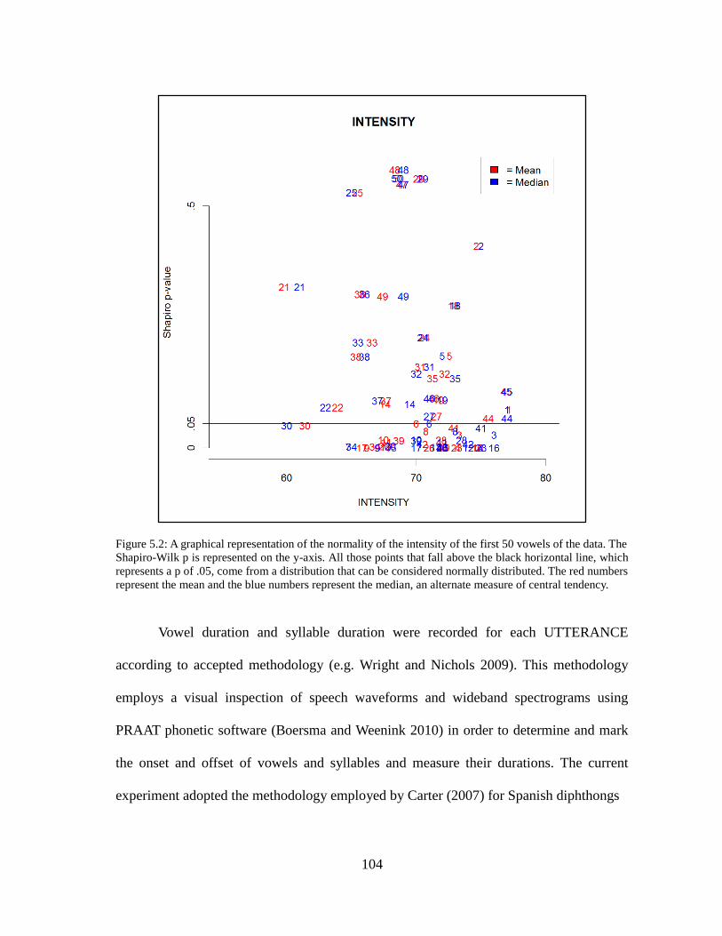
104
Figure 5.2: A graphical representation of the normality of the intensity of the first 50 vowels of the data. The
Shapiro-Wilk p is represented on the y-axis. All those points that fall above the black horizontal line, which
represents a p of .05, come from a distribution that can be considered normally distributed. The red numbers
represent the mean and the blue numbers represent the median, an alternate measure of central tendency.
Vowel duration and syllable duration were recorded for each UTTERANCE
according to accepted methodology (e.g. Wright and Nichols 2009). This methodology
employs a visual inspection of speech waveforms and wideband spectrograms using
PRAAT phonetic software (Boersma and Weenink 2010) in order to determine and mark
the onset and offset of vowels and syllables and measure their durations. The current
experiment adopted the methodology employed by Carter (2007) for Spanish diphthongs

105
Figure 5.3: A graphical representation of the normality of the pitch of the first 50 vowels of the data. The
Shapiro-Wilk p is represented on the y-axis. All those points that fall above the black horizontal line, which
represents a p of .05, come from a distribution that can be considered to be normally distributed. The red
numbers represent the mean and the blue numbers represent the median, an alternate measure of central
tendency.
and considered Spanish diphthongs as a single vowel. In instances of specific individual
complications, such as syllable deletion, these were addressed on a case-by-case basis.
The following variables were recorded and calculated for consideration in order to
predict the dependent variable, UTTERANCE:
DURATION_V: a numeric variable providing the length of the vowel in ms;

106
DURATION_S: a numeric variable providing the length of the syllable in ms;
PVIV: the PVI of the duration of the current and the next vowel within the IU (if
there was one), computed as in (1);
PVIS: the PVI of the duration of the current and the next syllable within the IU (if
there was one), computed as in (1);
SDS_INT_PHRASE and SDS_PHON_PHRASE: the standard deviation of the
duration of the syllable in the intonational phrase and the phonetic phrase;
SDV_INT_PHRASE and SDV_PHON_PHRASE: the standard deviation of the
duration of the current and the next vowel within the IU (if there was one) and its
natural log (after addition of 1 to cope with 0s);
SDPITCH_INTO_PHRASE and SDPITCH_INT_PHRASE: the standard
deviation of the mean pitch across each vowel within the intonational phrase and
the phonetic phrase;
SDPITCH_PAIRWISE: the standard deviation of the mean pitch of each adjacent
pair of vowels.
MAX_PITCH: the maximum pitch of each vowel;
MIN_PITCH: the minimum pitch of each vowel;
MEAN_PITCH: the mean pitch of each vowel;
PVI_PITCH: the PVI of the mean pitch of the current and the next syllable within
the utterance, computed as in (2);
SDINTENSITY_INT_PHRASE and SDINTENSITY_PHON_PHRASE: the
standard deviation of the mean intensity across each vowel duration within the
intonational phrase and the phonetic phrase;
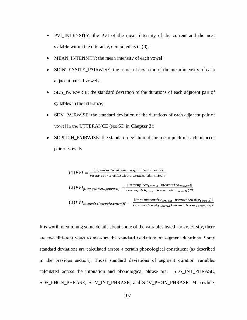
107
PVI_INTENSITY: the PVI of the mean intensity of the current and the next
syllable within the utterance, computed as in (3);
MEAN_INTENSITY: the mean intensity of each vowel;
SDINTENSITY_PAIRWISE: the standard deviation of the mean intensity of each
adjacent pair of vowels.
SDS_PAIRWISE: the standard deviation of the durations of each adjacent pair of
syllables in the utterance;
SDV_PAIRWISE: the standard deviation of the durations of each adjacent pair of
vowel in the UTTERANCE (see SD in Chapter 3);
SDPITCH_PAIRWISE: the standard deviation of the mean pitch of each adjacent
pair of vowels.
(1)𝑃𝑉𝐼 =∣∣(𝑠𝑒𝑔𝑚𝑒𝑛𝑡𝑑𝑢𝑟𝑎𝑡𝑖𝑜𝑛1;𝑠𝑒𝑔𝑚𝑒𝑛𝑡𝑑𝑢𝑟𝑎𝑡𝑖𝑜𝑛2)∣∣
𝑚𝑒𝑎𝑛(𝑠𝑒𝑔𝑚𝑒𝑛𝑡𝑑𝑢𝑟𝑎𝑡𝑖𝑜𝑛1,𝑠𝑒𝑔𝑚𝑒𝑛𝑡𝑑𝑢𝑟𝑎𝑡𝑖𝑜𝑛2)
(2)𝑃𝑉𝐼𝑝𝑖𝑡𝑐ℎ(𝑣𝑜𝑤𝑒𝑙𝑎,𝑣𝑜𝑤𝑒𝑙𝐵) =∣∣(𝑚𝑒𝑎𝑛𝑝𝑖𝑡𝑐ℎ𝑣𝑜𝑤𝑒𝑙𝑎;𝑚𝑒𝑎𝑛𝑝𝑖𝑡𝑐ℎ𝑣𝑜𝑤𝑒𝑙𝑏)∣∣
(𝑚𝑒𝑎𝑛𝑝𝑖𝑡𝑐ℎ𝑣𝑜𝑤𝑒𝑙𝑎:𝑚𝑒𝑎𝑛𝑝𝑖𝑡𝑐ℎ𝑣𝑜𝑤𝑒𝑙𝑏) 2⁄
(3)𝑃𝑉𝐼𝑖𝑛𝑡𝑒𝑛𝑠𝑖𝑡𝑦(𝑣𝑜𝑤𝑒𝑙𝑎,𝑣𝑜𝑤𝑒𝑙𝐵) =∣∣(𝑚𝑒𝑎𝑛𝑖𝑛𝑡𝑒𝑛𝑠𝑖𝑡𝑦𝑣𝑜𝑤𝑒𝑙𝑎;𝑚𝑒𝑎𝑛𝑖𝑛𝑡𝑒𝑛𝑠𝑖𝑡𝑦𝑣𝑜𝑤𝑒𝑙𝑏)∣∣
(𝑚𝑒𝑎𝑛𝑖𝑛𝑡𝑒𝑛𝑠𝑖𝑡𝑦𝑣𝑜𝑤𝑒𝑙𝑎:𝑚𝑒𝑎𝑛𝑖𝑛𝑡𝑒𝑛𝑠𝑖𝑡𝑦𝑣𝑜𝑤𝑒𝑙𝑏) 2⁄
It is worth mentioning some details about some of the variables listed above. Firstly, there
are two different ways to measure the standard deviations of segment durations. Some
standard deviations are calculated across a certain phonological constituent (as described
in the previous section). Those standard deviations of segment duration variables
calculated across the intonation and phonological phrase are: SDS_INT_PHRASE,
SDS_PHON_PHRASE, SDV_INT_PHRASE, and SDV_PHON_PHRASE. Meanwhile,

108
SDS_PAIRWISE and SDV_PAIRWISE are calculated in pairwise manner, as in Chapter
3 (as well as Harris and Gries 2011)10. This pairwise calculation is akin to the calculation
of the PVI. While neither of these calculations of the standard deviations of segment
durations are exactly equivalent to the metric suggested by Ramus, Nespor, and Mehler
(1999), which takes the mean of the standard deviations of a speaker‘s utterances, those
variables calculated across the phonological constituents are more similar to that metric in
that they consider a series of standard deviations, rather than the standard deviation of two
adjacent values.
5.2. Statistical Evaluation and Results
This section will describe two statistical evaluations of the variables mentioned above in
order to predict the dependent variable UTTERANCE (English 1, English 2, Portuguese,
Spanish 1, Spanish 2). The first is an ensemble method, Random Forest, which identifies
those variables that are significant predictors of the dependent variable. These predictors
were then entered in a maximal multinomial model and an automated model selection
process was employed in order to identify those variables most important to the prediction
of the dependent variable.
10
This distinction also exists for the calculation of standard deviation for F0 and intensity. The standard
deviation of these features across phonological constituents are SDPitch_Int_Phrase and
SDPitch_Int_Phrase and SDIntensity_Int_Phrase and SDIntensity_Phon_Phrase. Meanwhile,
SDIntensity_Pairwise and SDPitch_Pairwise are calculated in a pairwise manner. However, metrics
related to intensity and pitch are not commonly included in speech rhythm studies. [weird note
formatting: the 10 is too large and the hanging indent is different from previous ones]
109
5.2.1. Random Forest
5.2.1.1. Random Forest Data Treatment
Random Forests are a series of decision trees; each of these trees is based upon a random
subset of the available predictors and available data (Breiman 2001). As each tree is
―calculated on random subsets of the data, using a subset of randomly restricted and
selected predictors for each split in each classification tree…‖(Strobl et al. 2008) they are
―able to better examine the contribution and behavior that each predictor has, even when
one predictor‘s effect would usually be overshadowed by more significant competitors in
simpler models‖ (Strobl, Malley, and Tutz 2009 as cited in Shih 2011:1).
The current chapter undertook a Random Forest exploration in response to
problems of multicollinearity between the variables listed in the section above. As some
variables are derived from one another, there were many instances of multicollinearity;
this occurs when two or more variables are highly correlated. This can make the
coefficients and p-values of the model extremely unstable, making it impossible to
determine the cause of the model's predictions, as well as the (directions of) effects of
individual predictors. Due to this complication, the results of a multinomial model
selection process were not conclusive as to the research questions; there was evidence of
multicollinearity amongst the variables (as would be expected, although the procedure for
diagnosing and treating multicollinearity in multinomial models is not as yet well defined
to the author‘s knowledge). Random Forests are not susceptible to multicollinearity in the
same manner as regression models; ―One advantage of RF [Random Forest] is that it can
handle this collinearity‖ (Immitzer, Atzberger, and Koukal 2012:2683). Because the
decision trees comprising a Random Forest are generated on a random subset of the

110
variables and data, a tree at a certain point in the forest may not contain collinear
variables.
The current chapter used the function randomforest and method cforest_unbiased
from the library party (Hothorn, Hornik, Strobl, and Achim Zeileis 2006). It follows
established methodology in experimenting with a variety of settings (e.g. ntree and mtry11)
and using these settings with different random seeds (e.g. Strobl, Hothorn, Zeileis 2009).
After trying various settings, the optimal settings of ntree 1501 and mtry 5 were used. It
then generated a plot visualizing the conditional importance measure; this has been
suggested as an alternate to the permutation importance measure in the case that the
predictors may be correlated (Strobl, Hothorn, and Zeileis 2009). The resulting random
forest model was 100% accurate in predicting the dependent variable, UTTERANCE. I
then generated a plot visualizing the conditional importance measure. The conditional
importance measure determines the relative importance of variables in predicting the
dependent variable by sub-sampling the data set without replacement. As compared to the
permutation importance measure, the conditional importance measure considers the
importance of the variables ―given the other predictor variables in the model‖ (Strobl,
Hothron, and Zeileis 2009:15). This plot is a visualization of the concept that variables
whose variable importance value is greater than the absolute value of the lowest negative-
scoring variable are informative predictors of the dependent variable (Strobl, Malley, and
Tutz 2009). See Figure 5.4.
11
ntree is a parameter of randomforest that varies the number of trees generated by the random forest and
mtry specifies the number of independent variables that are sampled at each node for the random forest
algorithm.

111
5.2.1.2. Random Forest Results
As seen in Figure 5.4, 11 of the 22 variables can be considered informative to the
dependent variable. Before moving on to a more fine-grained analysis based on these
results, a few implications about speech rhythm are worth mentioning. First, this section
will address those variables that are not important in the classification of the dependent
variables. It will then move on to those variables that are important in the Random Forest.
Recall that one of the most commonly used metrics in the attempted classification
of speech rhythms is the PVI. Despite recent studies showing that the PVI alone does not
consistently distinguish between languages of different rhythm classes (Loukina,
Kochanski, Shih, Keane, and Watson 2009, Harris and Gries 2011), current rhythm
studies persist in using the PVI as a metric of speech rhythms (e.g Henriksen 2013).
Figure 5.4 suggests that this metric is not an effective predictor for the current data, in
addition to the methodological shortcomings described previously, particularly in
Chapter 2. The PVI of vowel durations, which is used most commonly in previous
rhythm literature (here the PVIV, which measures vowel duration variability), does not
meet the criteria to be considered a significant predictor of UTTERANCE. Furthermore,
the PVIS, which measures syllable duration variability, fares even worse in the presence
of other predictors. While the results of Chapter 3, as well as the aforementioned
literature, would suggest that the PVI would prove a poor classifier of differing rhythms,
this evidence of the weak classificatory power of the PVI is especially telling due to the
nature of the data; these utterances have been verified via a perception experiment as
perceptibly rhythmically different. That is, while other studies have relied upon the
assumption that all utterances of a language of one rhythm class differ from all utterances
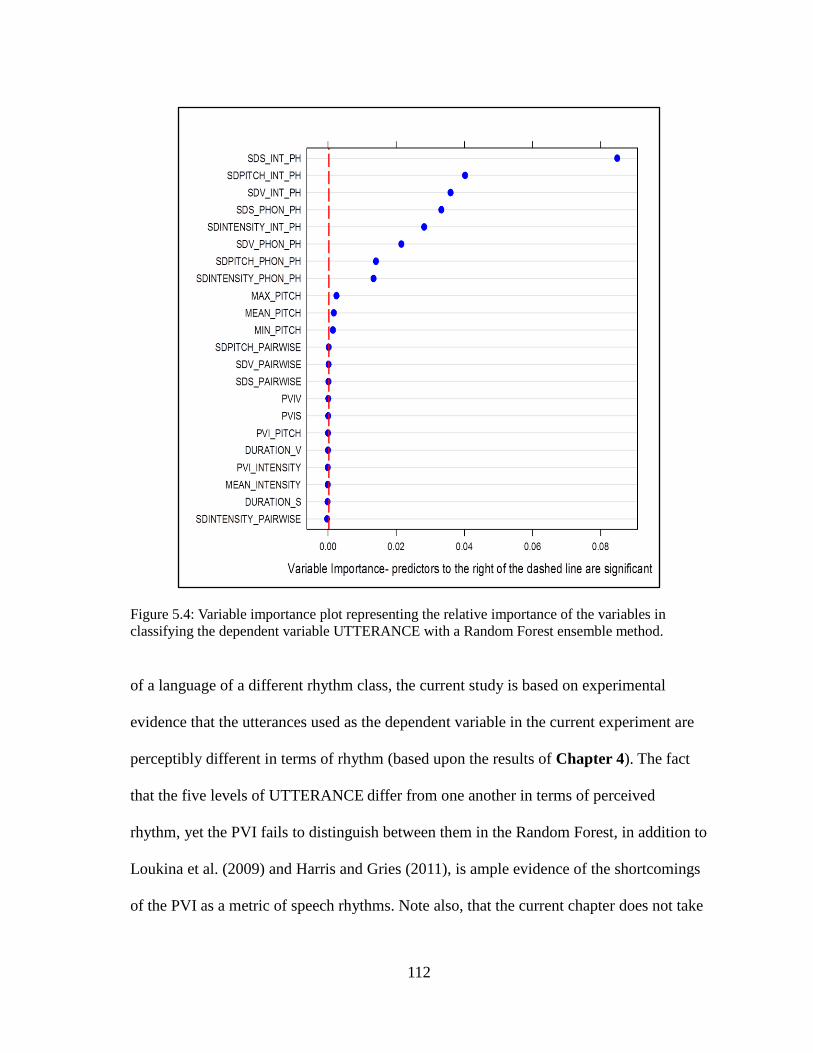
112
Figure 5.4: Variable importance plot representing the relative importance of the variables in
classifying the dependent variable UTTERANCE with a Random Forest ensemble method.
of a language of a different rhythm class, the current study is based on experimental
evidence that the utterances used as the dependent variable in the current experiment are
perceptibly different in terms of rhythm (based upon the results of Chapter 4). The fact
that the five levels of UTTERANCE differ from one another in terms of perceived
rhythm, yet the PVI fails to distinguish between them in the Random Forest, in addition to
Loukina et al. (2009) and Harris and Gries (2011), is ample evidence of the shortcomings
of the PVI as a metric of speech rhythms. Note also, that the current chapter does not take
113
a speaker or speaker type‘s mean PVI value (the so-called Mean PVI Method in Chapter
2) and instead considers all the of each utterance‘s PVI values (the Raw PVI Method in
Chapter 2). However, even with this more statistically sound method of calculating this
metric (as well as avoidance of the issue of non-normal distribution of the data), the PVI
is not a significant predictor of UTTERANCE.
It is also worth noting that SDV_PAIRWISE, which is akin to SD (and related to
SDLOG) from Chapter 3, is not a significant classifier of the dependent variables.
Instead, the standard deviations of segments defined across the phonological constituents
phonological phrase and especially intonational phrase, prove to be more useful in the
Random Forest ensemble. Recall that these variables, particularly SDV_INT_PHRASE
and SDV_PHON_PHRASE, are more similar (although certainly not equivalent) to the
mean standard deviation of vowel duration used in early rhythm studies (e.g. Ramus,
Nespor, and Mehler 1999).
This section will now turn its attention to those variables that are important in the
classification of UTTERANCE. Firstly, it is noteworthy that SDS_INT_PHRASE is by
far the most important variable in predicting the five levels of UTTERANCE. This means
that the most important variable in the ensemble is related to segment duration variability,
as has been long suggested in speech rhythm studies. However, the variable that measures
the duration variability of the entire syllable fares better than SDS_INT_PHRASE, which
measures just the vowel duration variability. Note that these variables related to segment
duration variability were significant, while those variables related to segment duration
(DURATION_V and DURATION_S) were not significant. This hearkens back to the
concept that certain languages privilege the syllable as a prosodic unit (thus lower

114
SDS_INT_PHRASE), while other languages privilege stress patterns (thus higher
SDS_INT_PHRASE); this is in agreement with Dasher and Bolinger‘s (1982)
phonological account of rhythm. However, it is equally important to note that the second
most important variable is not related to segment duration variability:
SDPITCH_INT_PHRASE. This suggests that one cannot only consider segment duration
variability in the discrimination of rhythm classes. In fact, in addition to pitch, variables
related to intensity are also included amongst those important in the ensemble (e.g.
SDINTENSITY_INT_PHRASE and SDINTENSITY_PHON_PHRASE).
Of the 11 significant variables, 7 of them are related to pitch and intensity, leaving
only four related to segment duration variability. This is in agreement with Dauer‘s (1987)
conclusion that simple measures of inter-stress intervals or syllable durations are not
effective in determining rhythm class. Instead, it appears that a multidimensional cluster
of prosodic cues lead to perceived differences in what linguists commonly call speech
rhythms. Even when additional prosodic cues (that is, F0 and intensity) have been
normalized and dampened in the speech signal (see Chapter 4), they still contribute to
perceived differences. The following section will present conclusions to the Random
Forest analysis.
5.2.1.3. Random Forest Conclusions and Discussion
Several important conclusions can be drawn from the Random Forest ensemble method
described here, although additional exploration and analysis is necessary to fully
understand the data and especially to understand the way in which the various utterances
relate in terms of speech rhythms (see following section).
115
An important conclusion in the context of wider rhythm research is that segment
duration variability is indeed related to (and in this case, most important to) our
perception of speech rhythm distinctions. In this way, researchers have been correct in
attempting to identify metrics of segment duration in order to distinguish between
languages of different rhythm classes. As mentioned above, it is syllable duration
variability, rather than vowel duration variability that proves most important in the current
data set (although vowel duration variability does prove relevant as well). This is
noteworthy, as the majority of previous speech rhythm research has depended upon vowel
duration rather than syllable duration in their metrics. The current results suggest that
researchers would be better served in considering the entire syllable instead in their
metrics. One explanation for this behavior is that syllables have much more potential
variation in their structure, than vowels, which means that rhythmic differences may
indeed be correlated with the syllabic structure of a language. This is in agreement with
Dasher and Bolinger (1982) who suggested that the phonotactic structure of a language
contributes to rhythmic differences; languages with more complex syllable structure tend
to have more syllable duration variability and are stress-timed, while languages with
simpler syllables have less syllable duration variability and are syllable-timed. Given this
suggestion, it is surprising that not more researchers have chosen to consider syllable
duration rather than vowel duration in their speech rhythm research.
A second conclusion from the current Random Forest ensemble is that while
segment duration variability does play a vital role in speech rhythms, one cannot ignore
other prosodic cues. As mentioned, variability in pitch and variability in intensity also
lead to perceived differences in the low-pass filtered utterances. As tends to be the case in

116
linguistics, one cannot focus entirely on one variable or feature to the point of ignoring
others. Instead, the entirety of the speech process must be considered.
As mentioned above, while the Random Forest ensemble method is very useful in
determining which variables are most useful in distinguishing between the utterances,
there is a second step that allows for a more in-depth exploration of this data set, as well
as a potentially simplified model (as compared to the Random Forest). Thus, the
following section uses the results from the Random Forest as a starting point in choosing
variables for a multinomial regression attempting to classify the same dependent variable,
UTTERANCE. Several variables identified by the Random Forest ensemble are largely
redundant; any variable defined across both the phonological phrase and the intonational
phrase contains much of the similar information, especially given that these two
phonological constituents completely overlap at times, and are therefore identical.
Furthermore, MAX_PITCH and MIN_PITCH are both closely related to MEAN_PITCH.
Thus, the following data analysis attempts to accurately predict the dependent variable
with a simplified set of non-redundant variables by choosing the variable with the most
predictive power from the groups of redundant variables.
5.2.2. Regression and ctree Analysis
As mentioned, it is the goal of the current section to accurately predict UTTERANCE
(English 1, English 2, Portuguese, Spanish 1, Spanish 2) with a subset of the metrics
identified as significant in the preceding Random Forest analysis. Furthermore, these
predictors should be neither redundant nor show evidence of multicollinearity.

117
As mentioned in Section 5.1, there were a total of 22 predictors coded and/or
calculated. Of these 22 independent variables, 11 were identified as significant by the
Random Forest ensemble in Section 5.2.1. Of these, the current analysis started with 5
variables as main effects (as well as considering their two-way interactions) in order to
avoid redundancy and multicollinearity. The five main effects were chosen as those
effects with the highest predictive power within each five categories. The categories
defined and variables selected are shown in Table 5.1.
Category Variable
syllable duration variability SDS_INT_PH
vowel duration variability SDV_INT_PH
pitch variability SDPITCH_INT_PH
intensity variability SDINTENSITY_INT_PH
numeric pitch MAX_PITCH
Table 5.1: five categories defined from the Random Forest ensemble and the most predictive variable
belonging to each category.
Thus, the following variables were recorded and calculated for consideration in order to
predict the dependent variable, UTTERANCE:
SDS_INT_PH : the standard deviation of the duration of the syllable in the
intonational phrase;

118
SDV_INT_PH : the standard deviation of the duration of the vowel in the
intonational phrase;
SDPITCH_INT_PH: the standard deviation of the mean pitch across the
vowel in the intonational phrase
SDINTENSITY_INT_PH: the standard deviation of the mean intensity
across each vowel duration within the intonational phrase
MAX_PITCH: the maximum pitch of each vowel
After selecting these five predictors, a thorough data exploration was undertaken. The
purpose of this exploration was to identify potential issues with the data, considering their
distribution and the presence of potential outliers. A series of multinomial regressions
were performed, using an automated stepwise bidirectional model selection process,
stepAIC from the library MASS (Venables and Ripley 2002). This process deletes and
adds interactions and variables according to AIC, a criterion that weighs the added
complication of adding an additional predictor to the model against the added predictive
power of that predictor. These regressions considered a) the complete data set with no
transformations; b) two subsets of the data with outliers deleted but no transformations; c)
the complete data set with some log and square root transformations to improve the
normality of the variables; d) two subsets of the data with outliers deleted and some log
and square root transformations to improve the normality of the variables. The data were
also examined for evidence of multicollinearity for each of these data explorations.
Finally, these same series of data points were examined using the smaller Phonological
Phrase, rather than the Intonational Phrase (see Section 5.1.2.).

119
Following this process, three conclusions were reached. Firstly, as suggested by
Figure 5.4, the metrics based upon the Intonational Phrase perform better in predicting the
dependent variable, as compared to the Phonological Phrase. Thus for the remainder of
this chapter, SDS_INT_PHRASE will be referred to simply as SDS,
SDINTESITY_INT_PHRASE will be referred to as SDINTENSITY, and
SDPITCH_INT_PHRASE will be referred to as SDPITCH. Secondly, the data were
optimized when two series of data points were removed. One set of eight data points that
showed very high duration variability (SDS>300, SDV>200) were removed. A second set
of seven data points that showed very high intensity variability (SDINTENSITY>9) were
removed. Both of these sets of data points also showed extremely high pitch variability
(SDPITCH>100). Finally, the various regressions showed that three variables were
consistently informative in the classification of the dependent variable UTTERANCE:
SDS, SDINTENSITY, and SDPITCH were consistently highly significant in predicting
UTTERANCE, either as main effects or as interactions. SDV did occasionally participate
in a significant interaction in the final model, but as this metric is collinear with SDS, a
significant predictor of UTTERANCE. In all models generated, SDS was the more
powerful predictor of the two metrics of duration variability; thus SDS was chosen for the
following data analysis rather than the standard deviation of vowel duration. The final
predictor, MAXPITCH, was not a significant predictor of utterance in any of the models
generated.
Given the conclusions above and the categorical nature of the dependent variable,
a conditional inference tree (using the package party, Hothorn, Hornik, Strobl, and Zeileis.
2006), was generated. The package's ctree function generates such trees, which are

120
regression trees that split the dependent variable based on certain values or levels of the
independent variables; these trees are based upon a recursive partitioning algorithm that
performs significance tests at each stage of the algorithm (Hothorn, Hornik, and Zeileis
no date). The data set had the outlying data points removed as mentioned in the previous
paragraph, but no transformations were performed upon the data. The results of this
analysis are presented in the following section.
5.2.2.1. Results and Discussion
Conditional inference trees were generated to predict the dependent variable,
UTTERANCE, according to the following three independent variables: SDS, SDPITCH,
and SDINTENSITY (all based upon the Intonational Phrase, see above). The resulting
model was able to correctly classify UTTERANCE 98.5% of the time, which performs
better than a model that classifies the dependent variable as the most frequent level of
UTTERANCE 100% of the time (p < .001). The results of this data analysis are
represented in Figure 5.5 below.
In consideration of the results of the conditional inference trees, the following sections
will discuss each of the three predictors, the standard deviation of syllable length, the
standard deviation of mean intensity, and the standard deviation of mean pitch. It will first
discuss those levels of UTTERANCE that can be predicted based solely upon SDS; it will
then consider the predictions that also consider SDINTENSITY and SDPTICH. Section
5.2.2.1.1 will describe the behavior of the variables seen in Figure 5.5 and the section that
follows it will describe the linguistic implications of these effects.

121
5.2.2.1.1. Conditional inference tress predicting UTTERANCE
Starting with the highest node, node number 1 in Figure 5.5 divides English 2, from the
other levels of UTTERANCE on the basis of the predictor SDS, the standard deviation of
vowel duration. Thus English 2 is associated with very high syllable duration variability;
that is, English 2 is predicted when SDS values are higher than 163. The other utterance
associated with high syllable duration variability is Portuguese, as seen from the split
below node 6. When SDS is between 107 and 163, Portuguese is predicted.
The other two utterances that are predicted based solely upon SDS are those
utterances associated with extremely low syllable duration variability. English 1 and, to a
lesser degree, Portuguese are predicted by the conditional inference trees when the
standard deviation of syllable duration falls below 65. Spanish 2 is also predicted when
SDS is quite low, between 65 and 80.
For the area of intermediate syllable duration variability, when SDS is between 32
and 107, SDINTENSITY and SDPITCH interact with SDS in order to predict
UTTERANCE. Node 7 splits the levels of UTTERANCE into two groups based upon
SDINTENSITY. English 1 is associated with greater variability in intensity as compared
to Portuguese. Meanwhile Spanish 1 can occur with both high and low levels of
SDINTENSITY. Those Spanish 1 phrases that are pronounced with less variability in
pitch also display less variability in intensity, and Spanish1 phrases with greater
variability in intensity also display more variability in syllable duration variability.
Meanwhile, Portuguese is predicted with greater SDPITCH and English 1 is predicted as
having less syllable duration variability (as seen above). The following section will
discuss the linguistic implications of these effects.

122
Figure 5.5: A visual representation of the conditional inference trees to predict the dependent variable
UTTERANCE.
123
5.2.2.1.2. Linguistic Implications
This section will consider the implications of the conditional inference trees. First the
English utterances are discussed. Portuguese is addressed next and the Spanish utterances
follow.
Traditional rhythm typology would suggest that the English utterances would have
high variability in syllable duration, as does English 2, which is predicted when SDS is
greater than 163. However, notice that the split in node 3 associates very low syllable
duration variability with English 1. This is exactly the opposite of traditional rhythm class
typology, as the utterance is predicted with extremely low syllable duration variability.
Keep in mind that both of the utterances are from the same speaker. The fact that these
two utterances do not behave in a uniform manner is in agreement with Loukina,
Kochanski, Shih, Keane, and Watson (2009), who conclude that while rhythms vary
between languages, they also vary within languages. Thus, it is not particularly surprising
to find two utterances of the same language from the same speaker occupying different
areas of syllable duration variability.
Portuguese is associated with both relatively high syllable duration variability,
when SDS is greater than 107 but less than 163, and also with very low levels of syllable
duration variability, also the prediction is less strong. Recall that Frota and Vigário (2001)
concluded that Portuguese has an intermediate rhythm class. In this sense, Portuguese
follows the traditional rhythm class typology by displaying some high syllable duration
variability and some low syllable duration variability. Notice also that Portuguese is
predicted when syllable duration variability is intermediate to low, intensity variability is
low, but pitch variability is high. These predictions could be indicative of vowel deletion

124
in unstressed syllables. Increased intensity has been shown to be a correlate of stress in
European Portuguese (Ferreira 2008:11), and unstressed vowels have been shown to have
a reduced system (Frota and Vigário 2001). Perhaps those vowels that are unstressed, and
thus not very variable in terms of intensity, also show less variability in terms of duration,
as they are uniformly short. At the same time, pitch variability remains relatively high,
suggesting that unstressed vowels may still maintain a similarly level of F0 variability as
do stressed vowels (this increased pitch variability may also be associated with the
distinction between plastic and non-plastic languages in the coding of new and given
information, see paragraph below). This potential explanation is only a speculation at this
point; especially given that vowel duration did not factor into the model as a significant
predictor (see Random Forest analysis above). However, it does provide an explanation
for the behavior of Portuguese in Figure 5.6. See Figure 5.7 for an example of vowel
deletion in Portuguese from the data.
In terms of SDPITCH, Spanish 1 shows low pitch variability and Portuguese
shows high pitch variability. One explanation for the behavior of these languages is the
distinction between plastic and non-plastic languages in information structure. Languages
such as English and Dutch are traditionally considered plastic languages; plastic
languages tend to use pitch excursions to signal new information (equivalent to narrow
focus) in a narrative. Meanwhile Spanish, which is considered a non-plastic language,
uses word order instead (Zubizarreta and Nava 2010; Swerts, Krahmer, and Avesani
2002). Much like the case of speech rhythms, the status of Portuguese as a plastic or non-
plastic language is less clearly defined. As Romance languages such as Spanish and
Italian are typically considered to be non-plastic languages (Zubizarreta and Nava 2010;
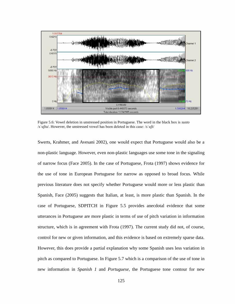
125
Figure 5.6: Vowel deletion in unstressed position in Portuguese. The word in the black box is susto
/sˈuʃtu/. However, the unstressed vowel has been deleted in this case: /sˈuʃt/
Swerts, Krahmer, and Avesani 2002), one would expect that Portuguese would also be a
non-plastic language. However, even non-plastic languages use some tone in the signaling
of narrow focus (Face 2005). In the case of Portuguese, Frota (1997) shows evidence for
the use of tone in European Portuguese for narrow as opposed to broad focus. While
previous literature does not specify whether Portuguese would more or less plastic than
Spanish, Face (2005) suggests that Italian, at least, is more plastic than Spanish. In the
case of Portuguese, SDPITCH in Figure 5.5 provides anecdotal evidence that some
utterances in Portuguese are more plastic in terms of use of pitch variation in information
structure, which is in agreement with Frota (1997). The current study did not, of course,
control for new or given information, and this evidence is based on extremely sparse data.
However, this does provide a partial explanation why some Spanish uses less variation in
pitch as compared to Portuguese. In Figure 5.7 which is a comparison of the use of tone in
new information in Spanish 1 and Portuguese, the Portuguese tone contour for new

126
information is flatter (and thus less variable) than the Spanish contour for new
information .
Figure 5.7: A comparison of the pitch contours for new information in Portuguese (left panel) and Spanish
(right panel) from the current data set. The Portuguese word vida is on the left and the Spanish word playa
is on the right. Both are the first mention of these words in the dialogue.
The utterance Spanish 2 follows traditional rhythm class distinctions by displaying
low duration variability, as would be expected of a syllable-timed language. Meanwhile,
Spanish 1 is associated with a low to intermediate level of syllable duration variability,
although predictions for this level of UTTERANCE are affected by variability in intensity
and pitch. In fact, Spanish 1 is the only level of UTTERANCE that is affected by all three
variables, showing lower variability in intensity and pitch simultaneously and greater
variability in intensity and syllable duration variability simultaneously. It is not surprising
that these prosodic variables work in conjunction. Duration, pitch, and intensity have all
been shown to be correlates of lexical stress for instance (e.g. Fry 1955, 1958), so it
follows that these features would also be present in variation in syllabic rhythm. In fact,
the use of these cues as a correlate of lexical stress provide an explanation for the
behavior of these variables. The prediction for Spanish 1 under nodes 7 and 8 could be
unstressed syllables, which would have low pitch variability and low intensity variability,
127
as seen in Figure 5.5. Meanwhile, the predictions for Spanish 1 that have high intensity
also have higher syllable duration variability. This could be indicative of lexical stress,
with greater intensity and duration, leading to higher standard deviation of syllable
duration.
The conditional inference trees show some adherence to traditional rhythm class
and language typologies, while at other points the data do not follow these typologies. In
terms of rhythm, Portuguese and Spanish most closely follow rhythm typologies, while
the two English utterances do not behave in a uniform manner; English 2 follows
traditional speech rhythm class distinctions by displaying high syllable duration
variability while English 1 behaves in exactly the opposite manner, displaying extremely
low syllable duration variability. This suggests the general conclusion that in a general
sense speech rhythm typologies may hold true, but speaker performance creates a great
deal of variation, making it very difficult to assess language-wide rhythmic typology on
the basis of a few speakers. An additional conclusion of this interaction is that, in addition
to the varied behavior of vowel segment duration variability, it is even harder to predict
the behavior of such variables in consideration of additional prosodic cues such as
intensity and pitch. Put simply, it is difficult to tease apart intensity, pitch, and rhythm as
they all work in conjunction for discursive purposes.
5.2.1.3 General Discussion
The conclusions mentioned in the discussions above all point to a few practical
implications to the rhythmic behavior of the three languages that provide the utterances in
the current data set and the study of speech rhythms at large. At the risk of repetition, the
most apparent fact related to the behavior of these languages is that although languages in

128
the broad sense appear to adhere loosely to traditionally defined rhythm typologies, the
rhythmic variation that occurs in individual performance of single individuals (as well as
the variation between speakers of the same language, e.g. Chapter 2 and Chapter 3)
makes it hard to distinguish rhythm typology based solely upon a limited amount of
speakers or sufficiently large sets of data. This suggests that the automated methodology
pioneered by Loukina, Kochanski, Shih, Keane, and Watson (2009) provides a promising
route for further investigation into these matters.
5.3 Post Hoc Analyses
Following the analysis described in this chapter, there still remained several questions to
investigate via post hoc analysis. The current section investigates two questions. The first
issue to be investigated is whether there is any correlation between correlates of duration
variability, pitch, intensity, and/or segment duration with corpus-based frequency
analysis; as seen in Chapter 3, some measures of duration variability interact with
corpus-based frequency variables. Thus, it its necessary to consider the role of frequency
in the current data. The second issue investigated is if there is any correlation between
syllable structure and the various utterances. The conditional inference trees analysis
concluded that speaker performance made generalizations about speech rhythm classes
difficult; this is especially true given that additional prosodic cues such as F0 and
intensity work in conjunction with vowel duration variability. However, in a broad sense,
the data do appear to reveal consistency between traditional rhythm typologies and the
current data. Dasher and Bolinger (1982) suggested that perceived rhythmic differences
are a product of phonological properties of a language. In order to further investigate this,

129
the current chapter considers the syllabic structure of the utterances that comprise the
current data in order to assess this possibility. The remainder of this section reviews these
two issues via linear models.
5.3.1. Corpus-based Frequency Variables
As mentioned in Chapter 3, certain phonological variables have been shown to vary with
corpus-based frequency effects (e.g. Bell et al. 2009; Raymond and Brown 2012). Further,
the results of Chapter 3 show that these frequency effects extend to some correlates of
vowel duration variability; specifically, the PVI (of vowel durations) and the (logged)
standard deviation of vowel durations behave differently with lemma frequency. In
consideration of these facts, it is necessary to consider frequency effects in the current
data. However, the dependent variable of the data explorations described in the current
chapter was determined according to stimuli from which no individual lexical item was
recoverable. For this reason, it would be unsound to consider these frequency effects in
predicting the dependent variable used in the previous analyses. However, a post hoc
analysis permits one to investigate whether the predictors identified as significant by the
Random Forest vary with word frequency. Thus, the correlation strength between each of
the highest ranking variables (according to the Random Forest analysis) representing
segment duration variability, pitch, and intensity were investigate for their correlation
with the following variables, as well as syllable duration (DURATION_S):
TOKEN_PM_LOG: the log of the frequency of the word form per million (after
addition of 1 to cope with 0‘s) in which the segment occurred in the Corpus del

130
Español- 20th
Century Files (Davies 2002-), Corpus do Português- 20th
Century
Files (Davies and Ferreira 2006-), Corpus of Historical American English- 20th
Century Files (Davies 2010-);
LEMMA_PM_LOG: the log of the frequency of the lemma per million (after
addition of 1 to cope with 0‘s)in which the segment occurred in the Corpus del
Español- 20th
Century Files (Davies 2002-), Corpus do Português- 20th
Century
Files (Davies and Ferreira 2006-), Corpus of Historical American English- 20th
Century Files (Davies 2010-);
The highest-ranking variables representing segment duration variability, pitch, and
intensity were SDS, SDPITCH, SDINTENSITY (recall that the full name of these
variables were SDS_INT_PH, SDPITCH_INT_PH, and SDINTENSITY_INT_PH).
DURATION_S was also included as a correlate for segment duration (as opposed to
duration variability). A preliminary exploration of the correlation between these variables
and TOKEN_PM_LOG and LEMMA_PM_LOG revealed that both of these frequency
variables behaved in a very similar manner. As they both represent different metrics of
corpus-based word frequency, the current analysis will only discuss TOKEN_PM_LOG to
avoid redundancy.
A Pearson‘s product-moment correlation test revealed no correlation between
TOKEN_PM_LOG and SDS_INT_PH (t = -0.05, df = 209, p = 0.9, r= -0.0034) or
between TOKEN_PM_LOG and SDINTENSITY_INT_PH (t = -1.47, df = 209, p = 0.14,
r=-0.1012). The correlation test did reveal a significant correlation between
TOKEN_PM_LOG and SDPITCH_INT_PH (t = -2.2304, df = 209, p = 0.02679, r = -

131
0.1524). There was also a significant correlation between TOKEN_PM_LOG and
DURATION_S (t = -3.60, df = 209, p < 0.001, cor = -0.2415). The following sections will
first consider the correlation between DURATION_S and TOKEN_PM_LOG, and then
the correlation between SDPITCH_INT_PH and TOKEN_PM_LOG.
5.3.1.1. Frequency and Syllable Duration
There is a significant correlation between token frequency and the syllable duration in the
intonational phrase, but this simple correlation does not show if a) stress affects this effect
or b) if this effect varies across languages (or utterances).
To further explore this possibility, a linear model was generated consideration in
order to predict the dependent variable, DURATION_S with the following independent
variables:
TOKEN_PM : the log of the frequency of the word form per million (after
addition of 1 to cope with 0‘s) in which the segment occurred in the Corpus del
Español- 20th
Century Files (Davies 2002-), Corpus do Português- 20th
Century
Files (Davies and Ferreira 2006-), Corpus of Historical American English- 20th
Century Files (Davies 2010-);
STRESS : a binary variable that describes whether the segment from which the
metrics are derived has lexical stress (yes or no);
UTTERANCE: the UTTERANCE from which the segment is derived; note that
this has the original six levels English 1, English 2, Portuguese 1, Portuguese 2,
Spanish 1, Spanish 2;
132
A maximal model was generated with all three predictors and their two-way interactions.
An automatic model selection process was employed using the function stepAIC from the
library MASS (Venables and Ripley 2002). As mentioned, this process adds and removes
interactions and independent variables in order to minimize AIC, which weighs additional
model complexity versus predictive improvement of the model caused by each additional
predictor. The final resulting model was highly significant (p < 0.001) but only explained
a small amount of the variance in the model (adjusted R-squared = 0.1975). It featured
two significant main effects: UTTERANCE (p = 0.000202) and TOKEN_PM (p =
0.001105). It also featured one significant interaction: STRESS : UTTERANCE (p =
0.002143). The following two paragraphs will discuss first TOKEN_PM (the only
significant main effect that does not participate in the significant interaction) and then the
interaction STRESS : UTTERANCE.
Figure 5.812 shows the main effect of token frequency on syllable durations. It is
clear that, in the present data, highly frequent words are pronounced with far shorter
syllables, while less frequent words are pronounced more slowly, leading to longer
syllable durations. This makes sense from the perspective of both production and
perception. Less familiar words may be pronounced more slowly as the speaker is less
familiar with these words. However, keep in mind that all 3 speakers who contributed
these utterances were native monolingual speakers of their respective languages. Given
their familiarity with the language, it may be that their careful pronunciation of less
frequent words was intended to ease the processing load for the intended audience. This is
12
Figures 5.7, 5.8, 5.9, and 5.10 were generated using the effects package (Fox 2014)
for R (R Development Core Team 2013).

133
Figure 5.8: the main effect of Log Token Frequency per Million in predicting the duration of the syllables in
a post hoc analysis. Syllable durations are represented on the y-axis. (Log) Token frequency per million
words is represented on the x-axis, with highly frequent words represented to the right side of the graph.
perhaps even more likely the case given that a) this effect does not vary across the three
languages (or six utterances) represented and b) the semi-directed interviews of the
Spanish portions of the corpus were conducted by a non-native speaker of Spanish. This
provides a potential alternate explanation to the conclusions of Chapter 3, where
frequency effects on pronunciation were attributed to speaker aptitude. However, given
that the speaker groups of Chapter 3 (monolingual Spanish versus bilingual Spanish)
were different than those of the current chapter, these results do not contradict those of

134
Chapter 3. In fact, it is possible that both speaker aptitude and concerns for listener
perception were both at play in the currently observed effects.
Although the interaction STRESS : UTTERANCE was not informative as the
main inquiry of the current post hoc analysis, as it does not involve corpus-based
frequency effects, it is worth examining the interaction in order to more fully understand
the data set. A few trends can be observed in Figure 5.9; firstly it is observable that the
utterances differ between languages in some cases and within languages in other cases,
Figure 5.9: The interaction STRESS : UTTERANCE in prediction the dependent variable syllable duration
(DURATION_S) in a post hoc analysis. The syllable durations are represented on the y-axis; the left panel
represents syllables without lexical stress, and the right panel represents stressed syllables.

135
and these changes differ in the case of stressed syllables. Perhaps the most
counterintuitive trend observable is that of English 2, where unstressed syllables are
longer than stressed syllables. Longer vowel duration is generally considered a correlate
of lexical stress in languages where duration is not phonological (e.g. Fry 1958), as is the
case in English, Spanish, and Portuguese, so one would expect the opposite. However, the
syllable durations of English 2 seem to be quite long in general, so it is difficult to make
generalizations on the case of this limited data. In terms of vowel reduction of unstressed
vowels, there does not seem to be a consistent language-based typology observable in the
current data (of course, this effect examines syllable, rather than vowel duration). Recall
that Dasher and Bolinger (1982) suggested that syllable-time languages display less
vowel reduction as compared to stress-timed languages. This concept is not reinforced by
the current data set, as the syllable durations do not vary between stressed and unstressed
syllables in a consistent manner when grouped according to language. In general, this
interaction further illustrates the general conclusion of the current chapter that there the
production of individual speakers features a large amount of prosodic variation, even
between two different phrases in the same conversation. This may vary further between
stressed and unstressed syllables as well.
5.3.1.2. Frequency and Pitch
As in the previous section, the current analysis uses a multifactorial model to investigate
the manner in which pitch variability varies with token frequency. This affords a
perspective of how stress affects this effect and its variation across languages (or

136
utterances). A linear model was generated consideration in order to predict the dependent
variable, SDPITCH_INT_PH with the following independent variables:
TOKEN_PM : the log of the frequency of the word form per million (after
addition of 1 to cope with 0‘s) in which the segment occurred in the Corpus del
Español- 20th
Century Files (Davies 2002-), Corpus do Português- 20th
Century
Files (Davies and Ferreira 2006-), Corpus of Historical American English- 20th
Century Files (Davies 2010-);
STRESS : a binomial variable that describes whether the segment from which the
metrics are derived has lexical stess (yes or no);
UTTERANCE: the UTTERANCE from which the segment is derived; note that
this has the original six levels English 1, English 2, Portuguese 1, Portuguese 2,
Spanish 1, Spanish 2;
As in the previous section, a maximal model was generated with all four predictors and
their two-way interactions. The same automatic model selection process was employed
(stepAIC from the library MASS (Venables and Ripley 2002)). The final resulting model
was highly significant with a p = < 0.001). However, it only explained a small percentage
of the variance in the model (adjusted R-squared = 0.2409). It featured two significant
main effects: the highly significant UTTERANCE (p < 0.001) and the marginally
significant TOKEN_PM (p = 0.05244). Although this represents only marginal
significance level, it is beneficial to discuss this effect in the context of the linear model
(rather than as a simple correlation between SDPITCH_INT_PH and TOKEN_PM), as it

137
keeps the other predictors at a baseline level, allowing us to observe the behavior of the
corpus-based frequency effects in isolation. For this reason, the following two paragraphs
will first address the correlation between SDPITCH_INT_PH and TOKEN_PM; it will
then discuss SDPITCH_INT_PH and UTTERANCE.
As Figure 5.10 shows, low frequency words are pronounced with far more pitch
excursions as compared to high frequency words. This effect is strikingly similar to that
of DURATION_S. It appears that pitch movement is featured more prominently in the
Figure 5.10: the main effect of Log Tokens per Million in predicting the standard deviation of pitch within
the intonational phrase. The variability of mean pitch is represented on the y-axis, and the token frequency
is represented on the x-axis, with higher frequency words more to the right.

138
presence of longer durations. This is not surprising, as pitch and duration have been
shown to work in conjunction in certain prosodic environments; for instance, both vowel
duration and pitch have been shown to increase as a correlate of lexical stress (e.g. Fry
1958). However, these two effects, while varying with corpus-based frequencies, do not
vary between stressed and unstressed syllables (in the current model). It is also interesting
to note that in the two previous analyses, syllable duration and pitch movement are both
present. However, the correlate of intensity variability (SD_INTENSITY_INT_PH) was
not significantly correlated with the frequency effects. In terms of stress, it has been
suggested that intensity is a less reliable correlate as compared to segment duration and
F0; intensity is ―generally considered a weak cue in the perception of linguistic stress‖
(Sluijter and van Heuven 1996:2471). The current post hoc analyses are in agreement
with this general conclusion13.
Figure 5.11 makes it clear that the variability of mean pitch varies according to the
utterances. As was the case with STRESS : UTTERANCE, this effect is not informative
to the main query of this analysis, namely the variance of certain prosodic elements with
corpus-based frequency effects. This being said, the trends observable in this variable are
similar the conclusions of the interaction STRESS : UTTERANCE from the previous
analysis. Namely, pitch excursions vary both between speakers and within speakers in the
current data. It is also interesting to note that the high syllable durations observed in
English 2 in the previous analysis appear to coincide with more pitch excursions observed
in the current analysis.
13
As a reminder, the correlates of pitch (F0) and intenesity are based upon the low-pass filtered signal,
while the durations related to segment duration (here DURATION_S) are taken from the full speech
signal.

139
5.3.2. Syllabic Structure
As mentioned in the introduction to the post hoc analysis, while variation in speaker
production make broad generalizations about rhythm class difficult according to such
limited data, there still does seem to be some consistency between traditional rhythmic
typology and the results of the current chapter in certain environments. Recall that Dasher
and Bolinger (1982) suggested that speech rhythm differences can be attributed to
phonological phenomena. The authors suggested that vowel reduction of unstressed
Figure 5.11: The standard deviation of mean pitch in the intonational phrase divided
according to the six original utterances that comprise this data set. The variability of mean pitch is
represented on the y-axis, with higher variability being higher on the axis.
140
vowels is correlated with stress-timed languages. However, the results of the previous
analysis do not seem to reflect this concept, although the data set is admittedly limited
(see STRESS : UTTERANCE, Figure 5.9). The other feature that Dasher and Bolinger
(1982) attribute to stress-timed languages is more complex syllable structure. Although a
more encompassing study of cross-linguistic variation in syllabic structure would be the
subject of a large corpus study, the current dissertation undertook a post hoc analysis of
syllabic structure in order to examine whether Dasher and Bolinger‘s (1982) concept
holds true in the current data.
In order to assess the syllabic structure of the language, the current data were
coded according to the number of letters in each syllable. As this variable is somewhat
susceptible to spelling conventions in the various languages, diphthongs and consonant
clusters comprising a single phoneme were coded as a single letter, rather than two. A
multinomial model was generated to predict the dependent variable
UTTERANCE(English 1, English 2, Portuguese, Spanish 1, Spanish 2) with the
dependent variable LETTERS_SYLLABLE. The resulting model was highly significant
(p < 0.001). However, the model only performed intermediately well in classifying
UTTERANCE. It correctly classified the UTTERANCE from which the syllable was
derived 32% of the time (keep in mind that this is a multinomial model with 5 levels).
This is significantly higher than a baseline model that randomly chooses the
UTTERANCE (p < 0.001). The following paragraph will consider the behavior of
LETTERS_SYLLABLE in the prediction of UTTERANCE.
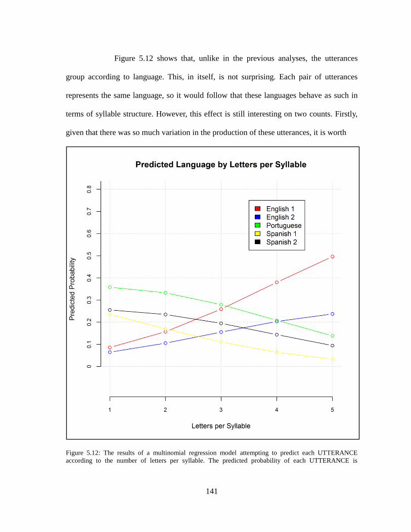
141
Figure 5.12 shows that, unlike in the previous analyses, the utterances
group according to language. This, in itself, is not surprising. Each pair of utterances
represents the same language, so it would follow that these languages behave as such in
terms of syllable structure. However, this effect is still interesting on two counts. Firstly,
given that there was so much variation in the production of these utterances, it is worth
Figure 5.12: The results of a multinomial regression model attempting to predict each UTTERANCE
according to the number of letters per syllable. The predicted probability of each UTTERANCE is

142
represented on the y-axis; the utterances themselves are coded according to the color of the line/dots
representing them. Letters per syllable is represented on the x-axis.
noting that in terms of syllable structure, the utterances are quite similar within languages.
Secondly, and more importantly, the results of this model are more in line with traditional
speech rhythm typology. Consider the speech rhythm continuum: As English is a
prototypical stress-timed language, it would be associated with complex syllable types
(Dasher and Bolinger 1982). This is exactly what the data reflect; English utterances have
a high predicted probability when the syllable is longer and a lower predicted probability
when the syllable is shorter. The Romance languages, meanwhile, group together. Spanish
behaves in the manner one would expect from a syllable-timed language, with stronger
predictions in the simple syllable types and weaker predictions in more complex syllable
types. Portuguese, follows the same linear trend as the two Spanish utterances, although it
has stronger predictions in both areas. This is due to the fact that the Portuguese
UTTERANCE is comprised of two utterances combined into one according to the results
of Chapter 4. As it has more data points as compared to the other levels of UTTERANCE
it will have overall stronger predictions (Portuguese has 64 segments, while English 1 has
44, English 2 has 27, Spanish 1 has 31, and Spanish 2 has 45). In order to a) get a more
fine-grained perspective of the behavior of the Portuguese utterances in the data and b)
get a more fine-grained perspective of the data in terms of language rhythmic typology, a
second data exploration was undertaken. In this analysis, the 6 original utterances
(English 1, English 2, Portuguese 1, Portuguese 2, Spanish 1, Spanish 2) were used as the
levels of the dependent variable UTTERANCE, rather than the 5 used in the original
multinomial analysis of the current chapter.
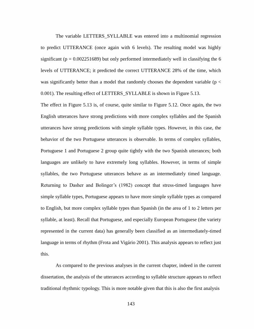
143
The variable LETTERS_SYLLABLE was entered into a multinomial regression
to predict UTTERANCE (once again with 6 levels). The resulting model was highly
significant (p = 0.002251689) but only performed intermediately well in classifying the 6
levels of UTTERANCE; it predicted the correct UTTERANCE 28% of the time, which
was significantly better than a model that randomly chooses the dependent variable (p <
0.001). The resulting effect of LETTERS_SYLLABLE is shown in Figure 5.13.
The effect in Figure 5.13 is, of course, quite similar to Figure 5.12. Once again, the two
English utterances have strong predictions with more complex syllables and the Spanish
utterances have strong predictions with simple syllable types. However, in this case, the
behavior of the two Portuguese utterances is observable. In terms of complex syllables,
Portuguese 1 and Portuguese 2 group quite tightly with the two Spanish utterances; both
languages are unlikely to have extremely long syllables. However, in terms of simple
syllables, the two Portuguese utterances behave as an intermediately timed language.
Returning to Dasher and Bolinger‘s (1982) concept that stress-timed languages have
simple syllable types, Portuguese appears to have more simple syllable types as compared
to English, but more complex syllable types than Spanish (in the area of 1 to 2 letters per
syllable, at least). Recall that Portuguese, and especially European Portuguese (the variety
represented in the current data) has generally been classified as an intermediately-timed
language in terms of rhythm (Frota and Vigário 2001). This analysis appears to reflect just
this.
As compared to the previous analyses in the current chapter, indeed in the current
dissertation, the analysis of the utterances according to syllable structure appears to reflect
traditional rhythmic typology. This is more notable given that this is also the first analysis

144
Figure 5.13: The predicted probability of each UTTERANCE according to letters per syllable. In this case,
all six original utterances are included, rather than the five used in the current chapter‘s multinomial
analysis, in order to investigate language typology. identifying these rhythmic differences on the basis of a few phrases, or just a few speakers
of these data where the various utterances consistently group according to language. This
reflects the general conclusion that speech-rhythm generalizations can be identified by

145
phonological features of a language, but speaker production is varied enough that is far
less reliable.
5.4. Discussion
This chapter (as well as the analysis of Chapter 4) provides a unique methodology in
speech rhythm research; by combining perception and production data in the same
analysis, a new paradigm is presented that avoids assumptions along the lines of
traditional rhythm class distinctions. Instead, it defines the relative rhythmic similarity of
utterances (via the perception experiment in Chapter 4) before undertaking an analysis of
the production of these utterances. This production analysis is based upon both traditional
and novel metrics for speech rhythm study.
While the results of this chapter are quite promising for speech rhythm research,
there are two potential shortcomings of the data analysis that should be mentioned. Firstly,
the data set upon which this chapter is based is quite small, being comprised of 6
utterances of approximately 10 seconds each. While a relatively large amount of prosodic
cues can be extracted from a data set this small, it does lead to the question of just how
representative these particular utterances are of the dialects/ languages that they represent.
It is for this reason that the conclusions reached herein are treated as a) representative of
individual speaker variation in speech rhythm productions, and b) indicative of those
prosodic elements that prompt perceptual differences in speech rhythm (here Chapter 4 is
also important). The only point where language- wide conclusions (or projections, at
least) are possible in when discussing the post hoc analysis of syllable structure, where
the languages behaved according to traditional rhythmic typology in a very uniform
146
manner. On the subject of speech rhythm perception, it is also worth mentioning that the
limitations of the perception experiment in Chapter 4, which was necessary to the
analysis of Chapter 5, necessitated the small data set used.
The second concern about the current analysis concerns overfitting. Data
overfitting occurs when the model (the predictors and interactions intending to predict the
dependent variable) is particularly well fit to predicting the dependent variable in the
current data, but fails to generalize to other similar data sets. This occurs when the
predictors are used to fit the idiosyncratic distribution of the data set, but the predictors
cannot be generalized to language in a more general manner, which of course is (often)
the goal of linguistic investigation. This is a concern for the current dataset, as the
predictors are able to classify the dependent variable in a very accurate manner. The
solution to this, which is beyond the scope of the current investigation, but should be
considered in future research is to apply the same predictors and interactions identified as
significant predictors of UTTERANCE by the multinomial analysis and apply them to a
novel data set. If these same predictors are able to classify the dependent variable with an
accuracy level that is a significant improvement over chance, this will indicate that the
model can be applied to different data sets, and not just the data set from which it was
generated. Because a perception experiment would be necessary to achieve this, it would
not be a practical undertaking at the present moment, but would certainly be worth
consideration in future research.
One particularly promising result of the current chapter is the introduction of a
new manner of considering the standard deviation of segment durations. While previous
literature has considered the mean standard deviation of segment durations for a phrase or
147
speaker (e.g. Ramus, Nespor, and Mehler 1999) or the standard deviation of two
consecutive segment durations (Harris and Gries 2011), the current chapter instead took
the standard deviation of segment across two phonological constituents, the phonological
phrase and the intonational phrase. As mentioned, these constituents were based upon
previous literature, specifically Selkirk (1984) and the ToBI system (e.g. Beckman and
Ayers Alam 1997). According to the random effects ensemble methodology, the standard
deviations calculated across both of the aforementioned constituents outperformed the
pairwise standard deviation variables. Furthermore, they are far more informative from a
statistical standpoint as compared to the mean standard deviation mentioned. Firstly,
modern computational methodology makes a measure of central tendency such as the
mean unnecessarily simplistic, as it summarizes a lot of potentially valuable information.
Secondly, as was the case with the PVI scores, to the author‘s knowledge, no previous
literature presenting mean standard deviations as a metric of speech rhythm has
demonstrated that these standard deviations are normally distributed. Thus, this chapter‘s
new methods for calculating standard deviations of segment durations represents a
significant contribution to speech rhythms. In terms of metrics of speech rhythms, this
chapter also provides further evidence to the unfit nature of the PVI as a correlate of
speech rhythms. Because this has been well discussed in several preceding chapters as
well as the current chapter, the shortcomings of the PVI will be mentioned about this at
the moment.
The other conclusions of the current chapter that are noteworthy were both
mentioned previously. It is clear that speech rhythm in terms of segment duration
variability do not behave individually, or ‗in a vacuum‘. Instead, these cues interact with
148
other prosodic cues; specifically, the multinomial analysis in the chapter shows that they
interact with intensity and pitch. However, given that the variability of pitch was a
significant predictor of UTTERANCE in the Random Forest analysis, it is also probable
that pitch cannot be ignored in studying the perception of rhythms; this concept is further
reinforced by the post hoc analysis, which demonstrates that the standard deviation of
pitch in the intonational phrase varies with token frequency. Finally, as mentioned, while
some languages do behave in agreement with traditionally defined speech rhythm classes,
speaker performance often makes it difficult to empirically verify speech rhythm. This is
particularly clear in viewing the post hoc analysis, which shows that, despite major
differences in terms of speaker performance, the various utterances group strongly
together by language in terms of syllabic structure. This is in agreement with Ramus,
Nespor, and Mehler (1999) who conclude that their variables, %V and ∆C reflect rhythm
class due to the varying syllabic structure of languages. They associate a greater variety of
syllable types with ∆C, as languages with greater complexity of syllabic structures will
also show more variability in consonantal interval lengths. In a similar manner, they
suggest that those languages with more complex syllable types will have more
consonants, thus a lower %V.
This effect closely matches speech rhythm typology. This is the major conclusion
of this chapter: while traditional speech rhythm typology is strongly related to the syllabic
structure of a language, these structural differences are often not immediately apparent in
production data due to the idiosyncratic performances of individual speakers. Thus, one
can easily correlate more complex syllable types with so-called stress-timed languages

149
and more simple syllable types with syllable-timed languages, but these differences are
not always apparent in the absence of extremely large data sets.
150
Chapter 6.
Implications, Directions for Further Study and Concluding Remarks
Overview
This concluding chapter will discuss the linguistic and practical implications of the
various studies discussed in this dissertation, as well as suggesting further steps in speech
rhythm research given the results of this dissertation. It begins with a summary of the
results and discussion of the current research. The implications for linguistics follow,
focusing specifically on typological implications. These conclusions are presented in
perspective of the current state of phonetics/ phonology in order to provide a more
complete perspective of the importance of the findings. The next section reviews the
methodological implications of this dissertation and is followed by a discussion of the
current research on a practical level and the potential application of these findings to non-
academic fields, i.e. technology development and forensics. It then discusses the
implications of the current dissertation for future speech rhythm research, considering
some shortcomings of the current dissertation, methodological aspects of the various
speech rhythms studies and how they may be applied to other linguistic queries, as well as
new directions for speech rhythm research. Finally, some concluding remarks are
presented.
151
6.1. Dissertation Summary
This dissertation set out to a) comparatively assess the speech rhythms of two different
dialects of Spanish, as well as to compare the rhythms of English, Portuguese, and
Spanish; b) assess the efficacy of various interval metrics that have been used to classify
and compare speech rhythms in previous literature; and c) develop new IMs for speech
rhythm classification and introduce a new paradigm in speech rhythm research.
Chapter 1 reviews past literature on speech rhythms and discusses some
methodologies employed in attempts to quantify these rhythms. Specifically, it shows
that, according to previous literature, languages (and dialects) do indeed appear to differ
in terms of rhythm. However, conclusive empirical proof of the existence and anture of
these differences, either from production data or perception data, has not been presented.
Chapter 2 uses the PVI, a widely adopted metric reported to distinguish between
languages (and dialects) of different rhythm classes (e.g. Low and Grabe 1995), in an
attempt to distinguish between the speech rhythms of monolingual Mexican Spanish and
bilingual Chicano Spanish speakers. While this chapter gives some evidence that these
two dialects differ in terms of rhythms, with bilingual speakers showing less vowel
duration variability, it also identifies shortcomings in the use of the PVI as a metric of
vowel duration variability. Specifically, the use of the mean PVI as a measure of central
tendency is unsound, as the PVI scores do not appear to be normally distributed.
Furthermore, this simplistic methodology removes a large amount of variation in the data,
leaving far less informative results, as compared to more sophisticated methods of
calculating IMs. Even when the PVI scores are considered as a series of values, with no
measure of central tendency, the resulting predictive power of the model is extremely low.
152
This is all to suggest that the PVI proves largely ineffective in distinguishing between
languages on the case of differing speech rhythms.
Chapter 3 reevaluates the same data, but this time employs a multifactorial
regression, which allows the simultaneous consideration of a variety of IMs, as well as
their potential interactions. Three major conclusions are drawn in this chapter. Firstly,
once again, the PVI proves to be a largely ineffective metric in predicting monolingual
versus bilingual Spanish. Secondly, other IMs, specifically those related to the standard
deviation of vowel durations measured in a pairwise manner prove to be more effective in
distinguishing monolingual Mexican and bilingual Chicano Spanish. Thirdly, these
measures of vowel duration variability vary with corpus-based word frequency, meaning
that speakers use vowel durations differently when a word is more or less frequent.
Chapter 4 is a perception experiment. In this chapter, 6 utterances (2 English, 2
Portuguese, and 2 Spanish) are low-passed filtered in order to preserve only syllabic
rhythm. Participants are then asked to rate the relative similarity of these utterances. A
cluster analysis indicates that while all the English and all the Spanish utterances are rated
as maximally different, the two Portuguese utterances are rated as similar. This is
interesting in that Spanish and English are traditionally considered to be maximally
different in terms of rhythm, with the former being syllable-timed and the latter being
stress-timed. Portuguese, meanwhile, is considered an intermediate language in terms of
rhythm (Frota and Vigário 2001), displaying some stress timed characteristics and some
syllable-timed characteristics. However, in this chapter it is Portuguese that proves
maximally different from Spanish and English, which are classified as similar at times.
The results of Chapter 4 serve as the dependent variable for the following chapter.

153
Chapter 5 analyzes the acoustic properties of the utterances used in the perception
experiment in order to evaluate what, if any, prosodic correlates (e.g. segment duration,
pitch, intensity) prompt the perceptual differences identified in Chapter 4. It begins with
a Random Forest analysis of a several variables in predicting UTTERANCE (English 1,
English 2, Portuguese, Spanish 1, Spanish 2). These variables represent both traditional
and novel metrics that could contribute to perceived differences in speech rhythms; they
include measures of segment duration variability, pitch variability, and intensity
variability. Once the most effective predictors are identified, this chapter uses a
multinomial regression in order to identify those variables and interactions that
significantly predict the dependent variable. Chapter 5 concludes that segment duration
variability does indeed contribute to our perception of rhythmic difference, but that pitch
and intensity do as well. Several post hoc analyses follow. Of particular interest is the
analysis that shows the complexity of syllabic structure appears to group the various the
various utterances by language according to rhythmic typology, with the syllable-timed
English having the most complex syllable structures, the stress-timed Spanish having the
most simple syllable structure, and the intermediately-timed Portuguese falling between
the two. This suggests that perceived differences in speech rhythms may be an artifact of
the syllabic complexity of a language, but that variation in speaker performance makes
these differences hard to quantify on the basis of a few utterances or a few speakers.
The studies described here not only represent a step forward for empirical speech
rhythm research, but also introduce a new research paradigm. Chapter 3 addresses the
importance of the consideration of corpus-based frequency measures in speech rhythm
154
research14. Chapters 4 and 5 introduce a methodology that allows the consideration of
both production and perception data in two linked analyses. This avoids making any
assumptions about the rhythm class of the languages represented by the data beforehand.
Chapter 5 also introduces several new metrics for speech rhythm classification and
comparison, particularly those based upon prosodic constituents, as well as identifying the
importance of pitch and intensity in speech rhythm perception. In this manner, the current
dissertation represents a thorough statistical evaluation of traditional speech rhythm
metrics, the introduction of a new research paradigm, and the development of several
useful metrics for empirical studies of speech rhythms. Furthermore the multinomial
analysis and post hoc analyses of Chapter 5 suggest that perhaps speech rhythms should
be considered in terms of syllabic structure, as the utterances tested appear to reflect
traditional rhythm class distinctions. This would suggest that the next logical step in
speech rhythm research is to correlate the results of studies of the production and
perception of speech rhythm with corpus-based data that compare the syllabic structures
and word frequencies of the languages considered. As mentioned, the results of a post hoc
analysis of Chapter 5 do suggest that in terms of syllabic structure, Spanish and English
are maximally different, while Portuguese falls between the two, as suggested by
traditional rhythmic class distinctions (e.g. that Spanish is syllable-timed, English is
stress-timed, and Portuguese has an intermediate rhythm). In this manner, the current
dissertation, in addition to being methodologically innovative, is informative as to the
relative positions of English, Portuguese, and Spanish on the speech rhythm continuum.
14
A consideration already laid out by Harris and Gries (2011), who discuss the role of corpus-based
frequency data in speech rhythm research.

155
6.2. Linguistic Implications
This section will discuss the implications of this dissertation for linguistic theory. It will
cover implications for the studies of speech rhythms, language typology, and broader ones
still for phonetics/ phonology.
As mentioned, in the introduction, the study of speech rhythms is a well-studied
area of linguistic investigation. This being said, there is still very little consensus in the
study of speech rhythms, and no universally accepted methodologies for their
quantification. To this field of study, the current dissertation adds some productive
descriptions of the behavior of speech rhythms. One conclusion is mentioned above,
namely the concept outlined in Chapter 5: perceived differences in speech rhythms (that
is, the traditionally described speech rhythm distinctions) appear to be a product of two
factors, one of which is an artifact of the particular language being spoken, and one of
which varies with speaker production as influenced by a series of factors such as, but not
limited to, dialect, register, languages in contact, age of speaker, speaker sex, etc. The
factor which is related to the language spoken and can be said to largely reflect traditional
rhythm typologies is the relative complexity of the syllabic structure of a language. There
is an observable trend suggesting the import of a language‘s syllabic structure in terms of
purported position on the speech rhythm continuum. While this has been suggested in the
past (e.g. Dasher and Bolinger 1982), current speech rhythm research seems to have
largely ignored the role of syllabic structure in speech rhythm. This is perhaps the most
surprising conclusion of this dissertation: that the data reflect traditional rhythmic
typologies in terms of syllabic structure. This is to say that the concept that languages are
arranged along a rhythm continuum, with certain more extreme languages at the

156
respective syllable and stress-timed poles, and more intermediate languages falling
between the endpoints holds up in light of the post hoc analyses of Chapter 5. The reason
that this is surprising is because the past 20 to 30 years of speech rhythm research has
attempted to find these distinctions. While the metrics and methodologies used to quantify
these differences seem to have only crudely suggested these distinctions (for the most
part), the current dissertation has shown that the intuition about rhythmic differences
appears to be correct (although, the concept that speech rhythms are a dichotomy does not
hold true). This is to say that, at least in the case of speech rhythms, tried and true
typological assumptions seem worthy of investigation.
The second factor contributing to speech rhythm distinctions is segment duration
variability and, to a lesser extent, F0 and intensity. It is precisely segment duration
variability that has been the focus of the majority of speech rhythm research over the past
twenty years; these studies have been trying to summarize segment duration variability
(and, in particular, vowel duration variability) in order to distinguish between languages
of different rhythm classes. While factors such as syllable duration variability and vowel
duration variability do appear to contribute to our perception of rhythmic differences, due
to a great amount of variation in speaker performance, it is hard to summarize rhythmic
differences solely on the basis of a few utterances or a few speakers of any given
language. It is also noteworthy that other factors, namely F0 and intensity, interact with
vowel and syllable durations, making the concept of studying speech rhythms, and
especially speech rhythms perception ‗in a vacuum‘, so to speak, hasty. While Chapter 5
shows that syllable duration variability contributes most to perceived differences in
speech rhythms, both pitch variability and intensity variability contribute significantly as

157
well (see Figure 5.4). Despite the fact that these other prosodic cues may not constitute
what we have traditionally termed syllabic rhythm, as they do vary with segmental
duration, they cannot be ignored when considered what contributes to perceived rhythmic
differences in spoken language.
Consider also that the results of STRESS : UTTERANCE in predicting
DURATION_S (that is, the interactions between if a syllable has lexical stress or not in
differing utterances predicts the duration of the syllable) indicate that vowel reduction
does not behave uniformly in two different utterances in the same language from the same
speaker. This is a further indication that small scale production-based rhythm studies will
continue to fail to identify rhythmic variation according to language-based rhythm
classes. This is not to say that the study of speech rhythms via production-based studies
should be completely abandoned. However, given the great amount of variation amongst
speakers of the same language that has often rendered such studies less-than-optimal, the
addition of a corpus-based study of the syllabic structure of the languages examined
would greatly aid in the interpretation of the results of the production-based studies.
Additionally, I would like to suggest that another practical solution to this issue would be
large data sets of production data that might allow some typological conclusions to be
reached. Perhaps in the presence of larger data sets, speaker variation will be
overshadowed by larger typological patterns. In practical terms, automated segment
boundary marking such as that of Loukina et al. (2009) offer a particularly promising
avenue in both eliminating researcher bias and allowing for the collection of large sets of
data.
158
I would also like to make an observation regarding the various IMs used in this
dissertation. When addressing segment duration variability, there are 3 different scales of
IM: a) those IMs that deal with segment duration variability on a very local level, between
just two adjacent syllables, such as the PVI or SD_PAIRWISE (SD_LOG from Chapter
3); b) those IMs that deal with segment duration variability on a larger scale, the
phonological phrase, such as SDS_PHON_PHRASE and SDV_PHON_PHRASE; and c)
those IMs that deal with segment duration variability on the largest scale in the current
context, the intonational phrase, such SDS_INT_PHRASE and SDV_INT_PHRASE. It is
noteworthy that in terms of efficacy in classifying the utterances in Chapter 5, (b) is more
effective than (a), and (c) is more effective than (b). Given that the dependent variable of
this model was determined according to perception data, it would appear that differences
in speech rhythms are determined according to a relatively large segment of an utterance
or sentence. Those metrics that focus on a more local segment, comparing the variability
of two adjacent syllables, do not prove to be significant in classifying UTTERANCE in
the Random Forest analysis (see Figure 5.4). Even those variables that consider a smaller
segment of the utterance do not perform as well as those variables that consider the
segment duration variability in the larger intonational phrase. This suggests that speech
rhythm differences are not perceived only on the level of immediately adjacent syllables,
but across a speech signal lasting several seconds. In terms of just how speech rhythms
behave, perhaps they serve in helping distinguish prosodic constituents. Past literature has
suggested that infants and children exploit speech rhythms in order to parse words and
intonational units; for instance, Nazzi, Bertoncini, and Mehler (1998) show that the
acquisition of English rhythmic patterns influences how infants segment speech into
159
word-like constituents and Gerken and McIntosh (1993) show similar results for speech
segmentation during early childhood. The data presented in Chapter 5 suggest that even
larger segments of the speech signal appear to be cued by differences in segment duration
variability, as evidenced by changes in segment duration variability metrics across
different phonological units. Past literature has suggested that prosodic cues contribute to
the parsing of phrases; for instance, Leas (1976) advocates the use of pitch in
automatically determining phrase boundaries. Thus, the fact that syllable duration
variability, pitch variability, and intensity variability appear to vary between intonational
phrases is a plausible extension of the concept that one role of prosodic cues is to indicate
intonational boundaries to ease the parsing of speech. This is also in agreement with
literature that shows that speech timing is not simply an artifact of the time necessary to
produce each segment contained in an utterance (e.g. Kozhevnikov and Christovich 1965,
Allen 1969, Lehiste 1971, 1972).
In consideration of the literature mentioned in the previous paragraph, one
implication that has not been addressed in the current dissertation is worth discussing:
how are speech rhythms actually acquired by speakers? As mentioned, it is clear that
segment durations (amongst other prosodic cues) are used to mark the boundaries of
phonological constituents. However, these higher-level cues seem to be strongly
engrained in a speaker. Ohala (1975) showed that there appears to be some underlying
pattern or structure to the timing of speech, as opposed to each segment being produced
when the previous segment is complete. Additionally, Wretling and Erikson (1998)
showed that it is difficult to mimic the timing of phonemes, suggesting that this timing is
somehow hardwired into an adult speaker‘s phonological system. However, as seen in

160
Chapter 3, the effect of the use of English is visible in the rhythm of Spanish/ English
heritage speakers, despite their having acquired what was throughout their infancy and
early childhood a monolingual Spanish prosodic system; these speakers were born to
monolingual speakers of Spanish. Several studies have shown that the rhythmic system is
acquired at a very young age (e.g. Nazzi, Bertoncini, and Mehler 1998), likely the parsing
of words or intonational units. The current dissertation suggests that while rhythm does
appear to be employed at a young age (as suggested by the aforementioned literature),
rhythmic systems are capable of undergoing change in the case of language contact. For
this reason, there is still more research required to better understand about the period
when prosody, and rhythm in particular, is acquired and how easily this feature can be
altered after acquisition.
6.3. Methodological Implications
As there have been several different experimental approaches employed throughout this
dissertation, this section will consider three noteworthy methodological aspects of this
dissertation. First, it will consider interval measures for speech rhythm comparison, then
the combination of perception and production data, and conclude withsome statistical
implications of the methodology employed
As mentioned previously, the majority of studies of speech rhythms have relied
upon interval metrics (IMs) to attempt to quantify speech rhythm production (i.e. Low
and Grabe‘s (1995) PVI or Ramus, Nespor, and Mehler‘s (1999) ∆V). However, the
various IMs employed have been criticized for only quantifying a small facet of the
various features that lead to differences in speech rhythm perception. For instance,
161
Loukina et al. (2011) conclude that no single rhythm measure (or IM) was successful in
discerning between all five languages they evaluated. This dissertation is in agreement
with previous literatures‘ criticisms of various traditional IMs. It has pointed out several
shortcomings of the PVI in particular (see Chapters 2, 3, and 5); namely, this metric
relies upon an unreliable measure of central tendency given its distribution and is only
able to distinguish between a relatively restricted range of word frequencies (at least in
the data from Chapter 3). Thus, one of the most commonly employed IMs proves to be
ineffective in distinguishing speech rhythms.
The combination of production and perception data from Chapters 4 and 5 proves
a promising avenue, not just for the study of speech rhythms, but also in the applications
of this methodology to other areas of linguistic investigation. The advantages of this
method in the study of speech rhythms has already been mentioned, namely that no
assumptions are made beforehand about rhythm class. Instead, it uses cluster analysis of
perception data to empirically determine the similarity and dissimilarity of the data at
hand. This, of course, is highly beneficial in making no assumptions about the nature of
speech rhythms before statistically analyzing the rhythmic characteristics of this data.
Other areas of phonetics and phonology may benefit from a similar approach. For
instance, studies contrasting intonational differences between dialects may benefit from
addressing whether these differences are perceptually salient. Dialectology in general
would potentially benefit from this approach in fact; while many features such as vowel
quality and tone contours have been attributed as contributing to dialectal variation, the
question as to whether these features actually contribute to a perceivable difference may
be worthy of investigation. For instance, the variety of monolingual Spanish represented
162
in the current dissertation, namely Mexico City Spanish, has been described as displaying
vowel reduction in unstressed vowels (Lope Blanch 1972). Thus, it is likely that this
variety has greater variability in vowel duration as compared to other varieties of Spanish.
However, whether this proposed difference is actually perceivable to untrained listeners is
also a valid question, as it allows one to evaluate whether differences in speech rhythms
contribute to perceived differences between different varieties of a language.
Chapter 5 is informative about the utility of several IMs for speech rhythm
comparison. Figure 5.4, in particular shows the relative importance of several variables in
classifying the utterances as English 1, English 2, Portuguese, Spanish 1, and Spanish 2.
In the end, it is segment duration variability that contributes the most to perceived
differences in speech rhythms (e.g. the standard deviation of syllable and vowel
durations), but these perceptual differences are also affected by changes in intensity and
pitch. This analysis is also noteworthy in that it presents novel methods of calculating
these effects that prove to be more effective than traditional IMs in this data. The
particular nature of these novel metrics is discussed thoroughly in Chapter 5.
Many of the statistical implications of this dissertation have already been touched
upon in the conclusion of several other chapters, as well as briefly in the current chapter.
This dissertation uses several different approaches to analyze speech rhythms (linear and
multinomial regression, cluster analysis, Random Forests). It is worth noting that the
statistical sophistication employed herein provides a fine-grained perspective of the
factors at play in our perception of rhythms. In addition to the strength of the statistical
modeling of the current dissertation, it is worth mentioning that it addresses model
assumptions, particularly those of normality and non-collinearity of variables. This

163
dissertation represents a thorough statistical analysis utilizing a variety of approaches; in
this way, it is a good example of advanced methodology in empirically verified linguistic
research. With a larger data set, the use of a mixed model would also be possible; this
would likely be the next logical step for speech rhythm research in the vein of this
dissertation.
It is important that researchers are prepared to use a variety of different statistical
approaches according to the nature of the data at hand. In some cases, multiple attempts to
analyze the data may be necessary before the correct analysis is identified. Given the state
of the field, which increasingly values statistically sound methodology, a thorough
statistical approach will serve as a great benefit to our field, encouraging sound research
and requiring that linguists are able to justify their methodology. It is important to note
that just because an approach may be considered correct, this does not indicate that it is
the best approach (and it is critical to consider and address model assumptions).
Hopefully this dissertation has served as an example of some of the potential approaches
that are available to linguists and will challenge methodologies employed, especially in
the study of speech rhythms, which has been historically plagued by faulty methodology
and metrics (the current dissertation does not mean to suggest, however, that there are no
previous methodologically sound studies of speech rhythms; in fact, several are very
advanced, e.g. Loukina et al. 2009).
In analyzing speech rhythms, certain statistical considerations are of vital
importance. In particular, analyses of speech rhythms based upon IMs risk
multicollinearity, as the metrics are often derived from one another. Ensemble methods
such as Random Forest (discussed in Chapter 5) have been shown to deal with collinear

164
variables (e.g. Immitzer, Atzberger, and Koukal 2012:2683). Other examples of
questionable statistical methodology have been present in past speech rhythm research.
Simple assumptions of models and metrics have been largely ignored (e.g. the use of the
mean PVI method without proof of normality of distribution, e.g. Low and Grabe 1995).
This is to say that it is imperative to more fully consider the statistical implications of the
methodologies employed.
6.4. Practical Applications
6.4.1. Technological Implications
The application of prosody in the development of certain technologies is by no means
novel. Specifically, Lea (1973, 1976) has long advocated the import of prosodic cues in
speech recognition algorithms. However, Lea has suggested cues apart from those most
widely associated with speech rhythms. In particular, Lea (1973) suggests that stressed
syllables contain more salient information that can be employed in speech recognition
systems as they tend to not be reduced and are pronounced with more volume (as
compared to unstressed syllables) and Lea (1976) suggests that intonational curves can be
used to automatically determine prosodic units which are helpful in the parsing of
information by speech recognition technology.
To these conclusions, the current dissertation would like to add the potential
import of speech rhythms in speech recognition. An understanding of the syllabic
structure of a language (as touched upon in the post hoc analysis of Chapter 5) and the
syllable reduction that commonly occurs in a language would greatly benefit an algorithm
intended to perform speech recognition. That is, those characteristics suggested by Dasher

165
and Bolinger (1982) as contributing to speech rhythms should be taken into account when
developing technology for speech recognition. Furthermore, these characteristics must be
understood from an empirical (rather than theoretical) perspective. The methodology
employed in the current dissertation is helpful in providing some preliminary conclusions
on the nature of speech rhythm variation between utterances, speakers, and languages that
are potentially applicable to speech recognition technology.
6.4.2. Forensic Applications
The application of prosodic cues to the forensic sciences may prove to be even more
valuable in comparison to the potential use of speech rhythms in speech recognition
technology discussed in the previous section. Forensic linguistics, in particular, could
greatly benefit from the investigation in the current dissertation. Forensic linguistics can
be described as the intersection of legal and/or law enforcement interests with linguistic
research. In particular, forensic linguistics performs in four areas of investigation: ―(i)
identification of author, language, or speaker; (ii) intertextuality, or the relationship
between texts; (iii) text-typing or classification of text types such as threats, suicide notes,
or predatory chat; and (iv) linguistic profiling to assess the author‘s dialect, native
language, age, gender, and educational level‖ (Chaski 2013:333). Harris, Gries, and
Miglio (2014) argue for the use of prosodic data in forensic linguistics. Of particular
interest to the current discussion, they argue that the methodologies used in Chapter 3 of
the current dissertation have great potential in dialect identification, which is a segment of
linguistic profiling as defined by Chaski (2013). Determining speech rhythms of various
speakers (defined narrowly in this context as the variability of vowel durations) may
166
allow the identification of speakers‘ dialects. This methodology is promising in that
speakers' vowel duration variability varies with word frequency; as the differences in
dialect are more visible in words with low frequencies, this information could be
exploited in a task intended to identify bilingual vs. monolingual speakers, for instance.
By asking comparing speakers‘ performance in low-frequency words, dialectal
identification would be possible.
In addition to the possible applications mentioned above, which is largely relevant
to the research in Chapter 3, Chapter 5 is also promising in terms of language
identification. In particular, the Random Forest methodology provides an example of a
largely automated method that performs extremely well in distinguishing between various
utterances. The fact that the Random Forest method is largely automated is a positive trait
for forensic linguistics as it helps minimize researcher bias and provides highly replicable
methodology. This is in line with Chaski‘s (2013) best practices for forensic linguistics.
Furthermore, the fact that this analysis was performed in the case of a (mostly)
impoverished speech signal is promising, as forensic linguistics may often occur in the
case of a speech signal that is not laboratory quality; this ties to the concept of
forensically viable data (e.g. Chaski 2013), as it appears that this method would be
effective even in the case of data with sub-optimal recording quality.
While it is not within the scope of the current dissertation to provide an exhaustive
discussion of how these methodologies are directly applicable to technology and the
forensic sciences, suffice to say that the potential practical applications of the
methodologies outlined herein do appear promising. In fact, in linguistics in general, such
practical applications may prove to be vital to the future of the field, as they provide an
167
impetus for new scholars and potential sources of funding to encourage future research.
6.5. The Future of Speech Rhythm Research
The current dissertation provides several experiments that suggest the next steps for
speech rhythm research. In particular, the combination of production and perception data
seem a promising avenue for understanding what exactly prompts differences in perceived
speech rhythms. By considering the results of these combined production/perception
studies in conjunction with corpus data, providing information about both syllabic
structure and type/token frequency, a more complete perspective of speech rhythms from
both a language-wide typological standpoint as well as in terms of individual speaker
production is possible. It is this distinction between language rhythm class as defined by
syllabic structure and variation in speaker performance that is central to our understanding
of speech rhythms. In addition, as discussed above, the current dissertation does utilize a
range of statistically sound methodologies in approaching the data sets in full
consideration of model assumption.
One interesting avenue for future speech rhythm research not addressed in this
dissertation is the relationship between speech rhythms and meaning. While the current
dissertation has discussed the use of rhythms in dividing utterances into smaller prosodic
constituents, it has not addressed just what speakers may intend to convey with changes in
rhythm. However, it would be hasty to assume that there is no iconicity in speech
rhythms. Chapter 3 showed that monolingual Spanish speakers were able to employ a
greater range of vowel duration variability as compared to speakers with lower aptitude in
Spanish. This chapter posited that this was due to speakers‘ abilities to exploit a full range

168
of vowel duration variability, perhaps for expressive purposes, as compared to heritage
speakers. This would suggest that varying rhythms may play a role in expressing a
speaker‘s intended meaning of a word or phrase. Other prosodic cues, in particular
intonation, have been shown to play a role in information structure (e.g. Vallduví 1992),
expression of emotion (Devillers 2013), expression of surprise (Abelin 2013), etc. The
relationship between rhythm and iconicity has not, to the author‘s knowledge, been
explored, but given that other prosodic factors known to interact with rhythm, have been
connected to meaning, this avenue of research certainly seems promising.
While this dissertation does represent a step forward for speech rhythm research,
there are a few shortcomings worth of distinction. Two issues, discussed in Section 5.5 are
of particular concern; as they have been quite thoroughly discussed, this section will
simply remind the reader of these issues, as they will likely be of concern for future
speech rhythm research. The first is the size of the data set considered in Chapters 4 and
5. In terms of the distinction of speech rhythms via production data, just a few utterances
from a few speakers are often insufficient to accurately distinguish languages with IMs, as
utterances‘ productions on a small scale seem to be largely rhythmically idiosyncratic.
That is, a single speaker shows a great amount of variation in their rhythmic production.
The conclusions of Chapter 5 are derived from a small data set. This fact is unavoidable,
as the analysis is based upon the perception study carried out in Chapter 4. However,
despite the sparse data, the analysis still allowed several conclusions.
The second issue discussed in Section 5.5 is data overfitting. This is the case when
the model constructed is particularly well-suited to the idiosyncrasies of the data set, so-
well so, in fact, that the model does not necessarily apply to other similar data sets. This is

169
of concern as the predictions and conclusions derived from the model at hand cannot be
said to apply to the community of speakers at large. Given a larger data set (see paragraph
above), it would be possible to verify that data overfitting were not an issue in the current
analysis, particularly in that of Chapter 5; for instance, a larger data set would allow
bootstrapping to diagnose data overfitting. Shortcomings notwithstanding, the current
dissertation represents a significant progress for empirical speech rhythm research.
6.6. Concluding Remarks
As the preceding section has quite thoroughly outlined, the contributions of the current
dissertation and its implications for various facets of linguistics and beyond, as well as
suggesting the next logical steps in terms of future speech rhythm research, these
concluding remarks will be relatively brief. This dissertation addressed a well-studied and
contentious area of linguistics, namely the quantification of speech rhythms. It is the
sincere hope of the author that two things have been accomplished through the long
process of this research. Firstly, hopefully this work has clarified the nature of speech
rhythms. One of the goals of this dissertation was to empirically examine the rhythmic
nature of English, Portuguese, and Spanish. This was achieved in the preceding chapters,
but it is the hope of the current dissertation that some of these conclusions should be able
to be extended to other languages (see discussion of data overfitting above). The second
goal that has hopefully been achieved by this dissertation is to challenge linguists‘
methodologies in their approach to all manner of linguistic query. By providing advanced
empirical methodology and combining perception and production data, this dissertation
has hopefully served to spark thought and discussion, positively influencing the quality of

170
research performed in speech rhythms, prosody, phonetics and phonology, and linguistics
at large.
171
References
Abeline, A. 2013. Emotional McGurk effect and gender difference – A Swedish study. In
S. Hancil and D. Hirst (eds). Prosody and Iconicity John Benjamins B.B.
Amsterdam, The Netherlands. 75-88.
Abercrombie, D. 1967. Elements of general phonetics. Edinburgh: Edinburgh University
Press.
Allen, G.A. 1969. Structure of timing in speech production. Paper read at the meeting of
the Acoustical Sociey of America, San Diego, November 4, 1969.
Arvaniti, A. 2009. Rhythm, Timing, and the Timing of Rhythm. Phonetica 66(1-2). 46–
63.
Arvaniti, A. and T Ross. 2012. Rhythm classes and speech perception. Phonetica 66(1-2),
1-15.
Barry, W., B. Andreeva, and J. Koreman. 2009. Do rhythm measures reflect perceived
rhythm? Phonetica 66(1–2). 78–94.
Beckman, M. and G. Ayers Elam. 1997. Guidelines for ToBI Labelling. Unpublished
manuscript, Ohio State University.Version 3.0 March 1997. [http://ling.ohio-
state.edu/Phonetics/etobi_homepage.html].
Beckman, M. and J. Pierrehumbert. 1986. Intonational Structure in Japanese and
English. Phonology Yearbook 3. 255-309.
Beckman M., M. Díaz-Campos, J. McGory, T. Morgan. 2002. Intonation across Spanish,
in the Tones and Break Indices framework, in Probus 14(2002), 9- 36.
Bell, A., J. Brenier, M. Gregory, C. Girand, and D. Jurafsky. 2009. Predictability effects
on durations of content and function words in conversational English. Journal of
Memory and Language 60(1). 92–111.
Benton, Matthew, Liz Dockendorf, Wenhua Jin, Yang Liu, Jerry Edmondson. 2007. The
continuum of speech rhythm: computational testing of speech rhythm of large
corpora from natural Chinese and English speech, in Proc. of the 16th ICPhS.
Saarbrücken 1269-1272.
Boersma, P. and D. Weenink. 2010. Praat: doing phonetics by computer (Version 5.1.29
[Computer program]. Retrieved June 21, 2009, from <http://www.praat.org/>.
Breiman, L. 2001. Random Forests. Machine Learning 45(1): 5-32.
Bunta F. and D. Ingram. 2007. The acquisition of speech rhythm by bilingual Spanish-
and English-speaking 4- and 5-year-old children. Journal of Speech, Language,
and Hearing Research 50(4). 999-1014.
Callier, P. 2011. Social meaning in prosodic variation. University of Pennsylvania
Working Papers in Linguistics 17(1). 39-50.
Canfield, D. 1981. Spanish Pronunciation in the Americas. Chicago, IL: The University
of Chicago Press.
Carter, P. 2005. Quantifying rhythmic differences between Spanish, English, and Hispanic
English. Theoretical and Experimental Approaches to Romance Linguistics:
Selected Papers from the 34th Linguistic Symposium on Romance Languages 63–
75.

172
Carter, P. 2007. Phonetic variation and speaker agency: Mexicana identity in a North
Carolina Middle School. University of Pennsylvania Working Papers in
Linguistics 13(2). 1–14.
Chaski, Carole. 2013. Best practices and admissibility of forensic author identification.
Journal of Law and Policy 21(2). 333-376.
Christophe, A. and J. Morton. 1998. Is Dutch native English? Linguistic analysis by 2-
month olds. Developmental Science 1(2). 215-219.
Dasher, R. and Bolinger, D. (1982). On pre-accentual lengthening, Journal of the
International Phonetic Association, 12, pp. 58-69.
Dauer, R. 1987. Phonetic and phonological components of language rhythm. Proceedings
of the 11th International Congress of Phonetic Sciences 5. 447–450.
Davies, M. 2002-. Corpus del Español: 100 million words, 1200s-1900s. Available online
at <http://www.corpusdelespanol.org>.
Davies, M. and M. Ferreira. 2006-. Corpus do Português: 45 million words, 1300s-1900s.
Available online at <http://www.corpusdoportugues.org>.
Davies, M. 2010-. The Corpus of Historical American English: 400 million words, 1810-
2009. Available online at <http://corpus.byu.edu/coha/>.
Delforge, A.M. 2008. Unstressed vowel reduction in Andean Spanish. In Laura Colantoni
and Jeffrey Steele (Eds.), Selected Proceedings of the 3rd Conference on
Laboratory Approaches to Spanish Phonology. 107-124. Somerville, MA:
Cascadilla Proceedings Project.
Deterding, D. 2001. The measurement of rhythm: a comparison of Singapore English and
British English. Journal of Phonetics 29(2). 217–230.
Devillers, L. 2013; Automatic detection of emotion from real-life data. In S. Hancil and
D. Hirst (eds). Prosody and Iconicity John Benjamins B.B. Amsterdam, The
Netherlands. 75-88.
Du Bois, J. 1991. Transcription design principles for spoken discourse research.
Pragmatics 1(1). 71–106.
Everitt, B., S. Landau, M. Leese, and D. Stahl. 2011. Cluster Analysis (5th
Edition).
Published online: John Wiley and Sons, Ltd.
Face, T. 2005. Reconsidering a Focal Typology: Evidence from Spanish and Italian.
Italian Journal of Linguistics 17, 2. 271-289.
Ferreira, L. 2008. High Initial Tones and Plateaux in Spanish and Portuguese Neutral
Declaratives: Consequences to the Relevance of F0, Duration and Vowel Quality
as Stress Correlates. Ann Arbor, MI: ProQuest.
Fought, C. 2003. Chicano English in context. London: Anthony RoI Ltd.
Fox, J. 2014. effects package for R. <http://cran.r-
project.org/web/packages/effects/index.html>.
Frota, S. 1997. On the prosody and intonation of focus in European Portuguese. In Fer
nando Martínez-Gil and Alfonso Morales-Front (eds.), Issues in the
phonology and morphology of the major Iberian languages, 359-392. Wash
ington, D.C.: Georgetown University Press.
Frota, S. 2000. Prosody and Focus in European Portuguese: Phonological Phrasing and
Intonation. New York: Garland.

173
Frota, S. and M. Vigário. 2001. On the correlates of rhythmic distinctions: the Euro
pean/Brazilian Portuguese case. Probus 13.2. 247- 275.
Frota, S., M. Vigário, and F. Martins. 2002. Language discrimination and rhythm class:
evidence from Portuguese. Retrieved October 31, 2011, from <www.psu.edu>.
Fry, D. B. 1955. Duration and intensity as physical correlates of linguistic stress. Journal
of the Acoustical Society of America 27, 765–768.
Fry, D. B. 1958. Experiments in the perception of stress. Language and Speech 1(2), 120-
152.
Gerken, L. A., and McIntosh, B. J. 1993. Interplay of function morphemes and prosody in
early language. Developmental Psychology 29. 448-457.
Gervain, J. and J. Werker. 2013. Prosody cues word order in 7-month bilingual infants.
Nature Communications 4. 1490-1495.
Goldsmith, J. (1978) English as a tone language. Communication and Cognition 11, 453-
476.
Grabe, E. and E.L. Low. 2002. duration variability in speech and the rhythm class
hypothesis. In C. Gussenhoven and N. Warner (eds.). Laboratory Phonology VII,
Berlin: Mouton de Gruyter. 515-546
Gries, S. 2009. Statistics for Linguistics with R: A Practical Introduction. Berlin: De
Gruyter Mouton.
Gussenhoven, C. 2002. The phonology of intonation. State-of-the-article. GLOT
International 6, 271-284.
Harris, M. and S. Gries. 2011. Measures of speech rhythms and the role of corpus-based
word frequency: a multifactorial comparison of Spanish(-English) speakers. 2011.
International Journal of English Studies 11(2). 1-22.
Harris, Michael J., Stefan Th. Gries, and Viola G. Miglio. (to appear). Prosody and its
application to forensic linguistics. LESLI- Linguistic Evidence in Security, Law,
and Intelligence.
Henton, C. 1995. Pitch dynamism in female and male speech. Language and
Communication 15. 43–61.
Henriksen, N. 2013. The acquisition of second language rhythm by Spanish-English
bilinguals. Paper presented at Second Language Research Forum, Provo, UT.
Hothorn, T., K. Hornik, C. Strobl, A. Zeileis. No date. ctree: Conditional inference
trees. <http://cran.r-project.org/web/packages/partykit/vignettes/ctree.pdf>.
Hothorn, T., K. Hornik, C. Strobl, A. Zeileis. 2006. party package for R.
<http://cran.rproject.org/web/packages/party/index.html>.
Hothorn, T., K. Hornik, C. Strobl, A. Zeileis. 2014. partykit: A Modular Toolkit for
Recursive Partioning in R. Working Paper 2014-10. Working Papers in Economics
and Statistics, Research Platform Empirical and Experimental Economics,
Universitaet Innsbruck. URL <http://Econ
Papers.RePEc.org/RePEc:inn:wpaper:2014-10>.
Hutchinson, A. and J. Lloyd. 1996. Portuguese: An Essential Grammar. London,
England: Routledge.
Immitzer, M., C. Atzberger and T. Koukal. 2012. Tree Species Classification with
Random Forest Using Very High Spatial Resolution 8-Band WorldView-2 Satellite
Data. Remote Sens 4, 2661-2693

174
Kisilevsky, B. S., Hains, S. M., Brown, C. A., Lee, C. T., Cowperthwaite, B., Stutzman, S.
S., Wang, Z. 2009. Fetal sensitivity to properties of maternal speech and language.
Infant Behavior and Development, 32(1), 59–71.
Kohler, K. 2009. Whither speech rhythm research? Phonetica 66(1–2). 5–14.
Kozhevnikov, N.A. and L.A. Chistovich. 1965. Speech: Articulation and Perception. U.S.
Dept. of Commerce translation, JPRS. 30-543.
Ladd, R. 1996. Intonational Phonology. Cambridge University Press: Cambridge.
Lea, W. 1973. Evidence that Stressed Syllables are the Most Readily Decoded
Portions of Continuous Speech. 2013 Archival Reprint of presentation at the 86th
Meeting, Acoustical Society of America, Los Angeles, CA.
Lea, W. 1976. The Importance of Prosodic Analysis in Speech Understanding Systems.
2013 Archival Reprint of research conducted by the author under the DARPA
Contract DAHC 15-73-0-0310.
Lee, C., and Todd, N. (2004). Towards an auditory account of speech rhythm: application
of a model of the auditory ―primal sketch‖to two multi-language corpora.
Cognition, 93(3), 225–254. doi:10.1016/j.cognition.2003.10.012
Lehiste, I. 1970. Suprasegmentals. The M.I.T. Press.
Lehiste, I. 1971. Temporal organization of spoken language. In Form and Substance, L.L.
Hammerich, R. Jakobson, and E. Zwirner. Adamizk Forlag. 159-169.
Lope Blanch, J. 1972. En torno a las vocales caedizas del español mexicano. Estudios
sobre el español de México. México: Editorial Universidad Nacional Autóno-
ma de México.
Loukina, A., Kochanski, G., Shih, C., Keane, E., and Watson, I. 2009. Rhythmmeasures
with language independent segmentation, 1531–1534.
Loukina, A., G. Kochanski, B. Rosner, and E. Keane. 2011. Rhythm measures and
dimensions of duration variation in speech. Journal of the Acoustical Society of
America 129(5). 3258-3270.
Low, Ee Ling and Grabe, Esther. 1995. Prosodic patterns in Singapore English.
Proceedings of the XIIIth International Congress of Phonetic Sciences, Stockholm,
Vol 3, 636-639.
Low, E., E. Grabe, and F. Nolan. 2000. Quantitative characterizations of speech rhythm:
syllable-timing in Singapore English. Language and Speech 43(4). 377–401.
Lucas, A. 2009. amap Package for R. < http://mulcyber.toulouse.inra.fr/projects/amap/>.
MacLeod, A. and C. Stoel‐ Gammon. 2005. Voice onset time (VOT) in Canadian French
and English: Monolingual and bilingual adults. Journal of the Acoustical Society
of America 117(4). 2429-2429.
Marshall, C. and P. Nye. 1983. Stress and vowel duration effects on syllable recognition.
Journal of the Acoustic Society of America 74(2). 433- 443.
Martínez-Celdrán, E., A.M. Fernández-Planas, and J. Carrera-Sabaté. 2003. Castilian
Spanish. Journal of the International Phonetic Association, 33(02). 255-259.
Mathôt, S., D. Schreij, and J. Theeuwes. 2012. OpenSesame: An open-source, graphical
experiment builder for the social sciences. Behavior Research Methods, 44(2),
314-324. doi:10.3758/s13428-011-0168-7.

175
Mehler, J., P. Jusczyk, G. Dehaene-Lambertz, N. Halsted, J. Bertoncini, Claudine Amiel-
Tison. 1988. A precursor of language acquisition in young infants. Cognition
29(2). 143-178.
Montrul, S. 2004a. Convergent outcomes in second language acquisition and first
language loss. In Monika Schmid, Barbara Köpke, Merel Keijzer, and Lina
Iilemar (eds.), First language attrition, 259–280. Amsterdam and Philadelphia
:John Benjamins.
Montrul, S. 2004b. Subject and object expression in Spanish heritage speakers: A case of
morphosyntactic convergence. Bilingualism: Language and Cognition 7(2). 125–
142.
Montrul, S. 2005. Second language acquisition and first language loss in adult early
bilinguals: Exploring some differences and similarities. Second Language
Research 21(3). 199–249.
Nazzi, T. and F. Ramus. 2003. Perception and acquisition of language rhythms by infants.
Speech Communication 41. 233- 243.
Nazzi, T., J. Berteconi, J. Mehler. 1998. Language discrimination by newborns: Towards
understanding the role of rhythm. Journal of Experimental Pyschology: Human
Perception and Performance 24(3). 756-766.
Nespor, M. and I. Vogel. 1986. Prosodic Phonology. Dordrecht: Foris.
Nolan, F. 2008. Intonation. In Bas Aarts and April McMahon (eds.) The Handbook of
American Linguistics. 433-457. Malden, MA: Blackwell Publishing.
Ohala, J. J. 1975. The temporal regulation of speech. In: G. Fant and M. A. A. Tatham
(eds.), Auditory analysis and the perception of speech. New York: Academic
Press. 431 - 453.
Oller, D. 1973. The effect of position in UTTERANCEon speech segment duration in
English. The Journal of the Acoustical Society of America 54(5). 1235-1247.
Ortega-Llebaria, M. and P. Prieto. 2007. Disentangling stress from accent in Spanish:
Production patterns of the stress contrast in deaccented syllables. Amsterdam
Studies in the Theory and History of Linguistic Science Series 4(282). 155-178.
Pierrehumbert, J.B. 1980. The phonology and phonetics of English intonation. PhD
dissertation, MIT. Published 1988 by Indiana University Linguistics Club.
Pike, K. 1945. The intonation of American English. Ann Arbor: University of Michigan
Press.
R Development Core Team. 2013. R: A language and environment for statistical
computing. R Foundation for Statistical Computing, Vienna, Austria.
<http://www.R-project.org/>.
R Core Team and contributors worldwide. stats Package for R. <http://cran.r-
project.org/web/packages/stats/index.html>.
Ramus, F. 2002. Acoustic correlates of linguistic rhythm: Perspectives. In Proceedings of
speech prosody 2002, 115–120. Aix-en-Provence.
Ramus, F., E. Dupoux, and J. Mehler. 2003. The psychological reality of rhythm studies:
perceptual studies. Availale online from <www.iscp.net>.
Ramus, F., E. Dupoux, R. Zangl, and J. Mehler. 2000. An empirical study of language
rhythms. Retrieved November 9th, 2011 from <www.cogprints.org>.

176
Ramus, F. and J. Mehler. 1999. Language identification with suprasegmental cues: A
study based on speech resynthesis. Journal of the Acoustical Society of America
105(1), 512-521.
Ramus, F., M. Nespor, and J. Mehler. 1999. Correlates of linguistic rhythm in the speech
signal. Cognition 73(3). 265–292.
Raymond, W. and E. Brown. 2012. Are effects of word frequency effects of context of
use? An analysis of initial fricative reduction in Spanish. In S. Gries and D. Divjak
(eds.), Frequency effects in language: learning and processing. Berlin and New
York: Mouton de Gruyter.
Ripley, B. 2011. MASS. Version 7.3-13 Package for R.
Scott, D., S. Isard, and B. Boyson-Bardies. 1985. Perceptual isochrony in English and
French. Journal of Phonetics 13. 155-162.
Selkirk, Elisabeth O. 1978. On prosodic structure and its relation to syntactic structure, in
T. Fretheim, ed., Nordic Prosody II. Trondheim: Tapir, 111-140.
Selkirk, E. 1981. On the nature of phonological representation, in J.
Anderson, J. Laver and T. Meyers, eds., The Cognitive Representation of
Speech, Amsterdam: North Holland.
Selkirk, E. 1984. Phonology and syntax: The relation between sound and structure.
Cambridge, MA: MIT Press.
Shih, S. 2011. Random Forests for categorical dependent variables: an informal quick
start R guide.[Online] Available from http://www. stanford. edu/~ stephsus/R-
randomforest-guide. pdf
Sluijter, A.M. and V.J. van Heuven. 1996. Spectral balance as an acoustic correlate of
linguistic stress. The Journal of the Acoustical Society of America 11. 2471-2485.
Strobl, C., L. Boulesteix, T. Kneib, T. Augustin, and A. Zeileis. 2008. Conditional variable
importance for random forests. BMC Bioinformatics 9. 307-318.
Strobl, C., J. Malley, and G. Tutz. 2009. An Introduction to Recursive Partitioning:
Rational, Application, and Characteristics of Classification and Regression Trees,
Bagging, and Random Forests. Psychological Methods 14(4): 323-348
Strobl, C., T. Hothorn, and A. Zeileis. 2009. Party on! A new, conditional variable-
importance measure. The R Journal 1-2. 14-17.
Strobl, C., and A. Zeileis. 2008. Danger! High power- Exploring the statistical properties
of a test for random forest variable importance. Available at < http://www.stat.uni-
muenchen.de>. Technical Report Number 017, 2008. 1-8.
Swerts, M., Krahmer, E. and Avesani, C. 2002. Prosodic marking of information status in
Dutch and Italian: a comparative analysis. Journal of Phonetics 30. 629-654.
Thomas, E. and P. Carter. 2006. Prosodic rhythm and African American English. English
World Wide 27(3). 331–355.
Vallduví, E. 1992. The informational component. Garland Publishers: New York/London.
Venables, W. and Ripley, B. 2002. Modern Applied Statistics with S. Fourth Edition.
Springer, New York.
White, L. and S. Mattys. 2007. Calibrating rhythm: First language and second language
studies. Journal of Phonetics 35(4). 501–522.
White, L., S. Mattys, and L. Wiget. 2012. Language categorization by adults is based on
sensitivity to durational cues, not rhythm class. Journal of Memory and
177
Language 66(2012). 665-679.
Wilson, K. 1993. The Columbia Guide to Standard American English. New York, NY:
Columbian University Press.
Wretling, P. and Eriksson, A. 1998. Is articulatory timing speaker specific? — Evidence
from imitated voices. In Branderud, P. and H. Traunmuller (eds.) Proceedings of
FONETIK 98. Stockholm: Dept. Linguistics, Stockholm University.
Wright, R. and D. Nichols. 2009. Measuring Vocal Duration in Praat. Retrieved from
<http://courses.washington.edu/l453/Duration.pdf>.
Zubizarreta, M.L. and E. Nava. 2010. Encoding discourse-based meaning: prosody vs.
syntax. Implications for Second Language Acquistion. Lingua 121(4). 652-669.
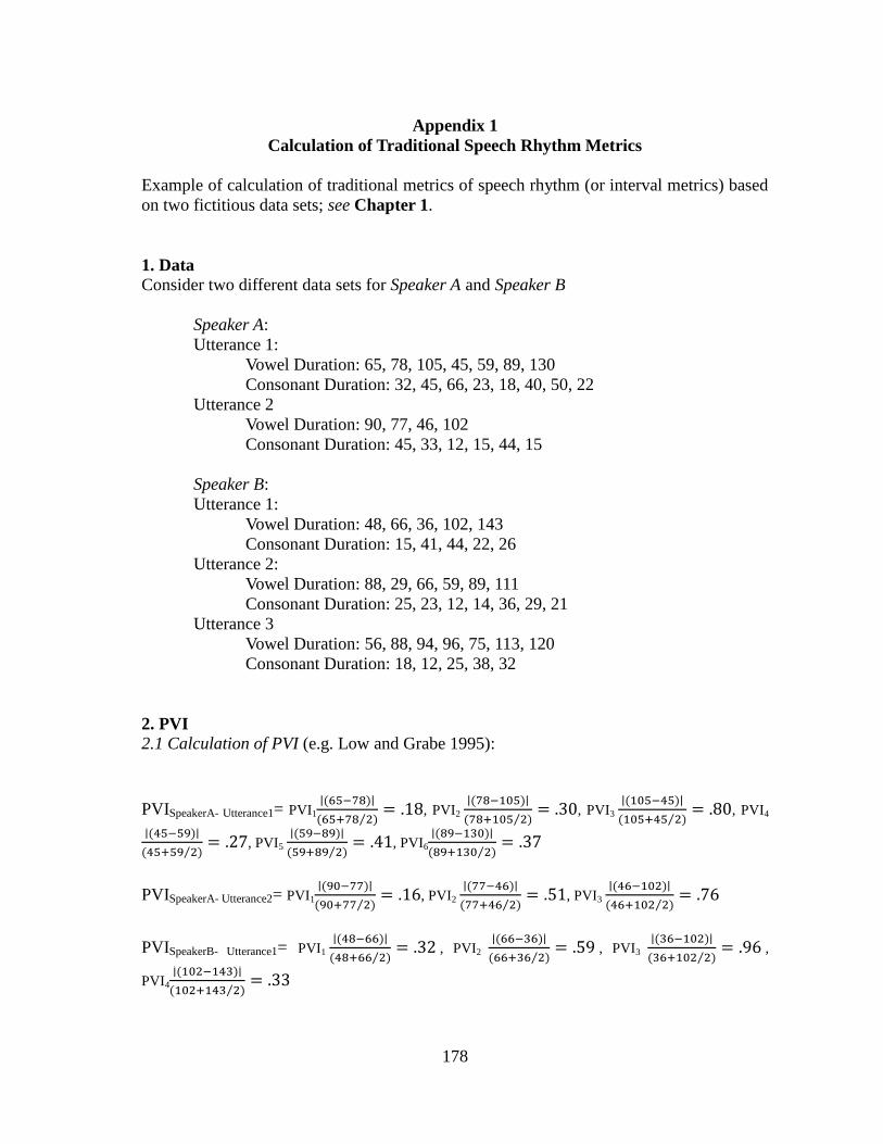
178
Appendix 1
Calculation of Traditional Speech Rhythm Metrics
Example of calculation of traditional metrics of speech rhythm (or interval metrics) based
on two fictitious data sets; see Chapter 1.
1. Data
Consider two different data sets for Speaker A and Speaker B
Speaker A:
Utterance 1:
Vowel Duration: 65, 78, 105, 45, 59, 89, 130
Consonant Duration: 32, 45, 66, 23, 18, 40, 50, 22
Utterance 2
Vowel Duration: 90, 77, 46, 102
Consonant Duration: 45, 33, 12, 15, 44, 15
Speaker B:
Utterance 1:
Vowel Duration: 48, 66, 36, 102, 143
Consonant Duration: 15, 41, 44, 22, 26
Utterance 2:
Vowel Duration: 88, 29, 66, 59, 89, 111
Consonant Duration: 25, 23, 12, 14, 36, 29, 21
Utterance 3
Vowel Duration: 56, 88, 94, 96, 75, 113, 120
Consonant Duration: 18, 12, 25, 38, 32
2. PVI
2.1 Calculation of PVI (e.g. Low and Grabe 1995):
PVISpeakerA- Utterance1= PVI1
∣∣(65;78)∣∣
(65:78 2⁄ )= .18, PVI2
∣∣(78;105)∣∣
(78:105 2⁄ )= .30, PVI3
∣∣(105;45)∣∣
(105:45 2⁄ )= .80, PVI4
∣∣(45;59)∣∣
(45:59 2⁄ )= .27, PVI5
∣∣(59;89)∣∣
(59:89 2⁄ )= .41, PVI6
∣∣(89;130)∣∣
(89:130 2⁄ )= .37
PVISpeakerA- Utterance2= PVI1
∣∣(90;77)∣∣
(90:77 2⁄ )= .16, PVI2
∣∣(77;46)∣∣
(77:46 2⁄ )= .51, PVI3
∣∣(46;102)∣∣
(46:102 2⁄ )= .76
PVISpeakerB- Utterance1= PVI1
∣∣(48;66)∣∣
(48:66 2⁄ )= .32 , PVI2
∣∣(66;36)∣∣
(66:36 2⁄ )= .59 , PVI3
∣∣(36;102)∣∣
(36:102 2⁄ )= .96 ,
PVI4
∣∣(102;143)∣∣
(102:143 2⁄ )= .33

179
PVISpeakerB- Utterance2= PVI1
∣∣(88;29)∣∣
(88:29 2⁄ )= 1.01, PVI2
∣∣(29;66)∣∣
(29:66 2⁄ )= .78, PVI3
∣∣(66;59)∣∣
(66:59 2⁄ )= .11, PVI4
∣∣(59;89)∣∣
(59:89 2⁄ )= .41, PVI5
∣∣(89;111)∣∣
(89:111 2⁄ )= .22
PVISpeakerB- Utterance3= PVI1
∣∣(56;88)∣∣
(56:88 2⁄ )= .44 , PVI2
∣∣(88;94)∣∣
(88:94 2⁄ )= .07 , PVI3
∣∣(94;96)∣∣
(4:96 2⁄ )= .02 , PVI4
∣∣(96;75)∣∣
(96:75 2⁄ )= .25, PVI5
∣∣(75;113)∣∣
(75:113 2⁄ )= .40, PVI6
∣∣(113;120)∣∣
(113:120 2⁄ )= .06
2.2. Reporting and interpretation of PVI Scores
Low and Grabe (1995) report the mean PVI for utterances as follows:
Speaker A: Mean PVIUtterance1 .39, MeanPVIUtterance2 .47
Speaker B: Mean PVIUtterance1 .55, MeanPVIUtterance2 .51, MeanPVIUtterance3 .21
This would mean that MeanPVISpeaker-Utterance3 is associated with less variable vowel
durations, or a syllable-timed speech, while is associated MeanPVISpeaker-Utterance1 is
associated with more variable vowel durations, or a stress-timed speech. Grabe and Low
(2002) report a mean for each speaker as follows:
Mean PVISpeakerA: .42
Mean PVISpeakerB: .40
In this case, Speaker B would be associated with more regularly timed vowel durations,
suggesting syllable-timed speech, while Speaker A would be associated with stress timed
speech.15
3. %V
3.1. Calculation of % V (Ramus, Nespor, and Mehler 1999)
% VSpeakerA- Utterance1 = (65:78:105:45:59:89:130)
(𝑆𝑒𝑛𝑡𝑒𝑛𝑐𝑒𝑙𝑒𝑛𝑔𝑡ℎ)= .66
% VSpeakerA- Utterance2 =(90:77:46:102)
(𝑆𝑒𝑛𝑡𝑒𝑛𝑐𝑒𝑙𝑒𝑛𝑔𝑡ℎ)= .66
% VSpeakerB- Utterance1 =
% VSpeakerB- Utterance2 =
% VSpeakerB- Utterance3 = (56:88:94:96:75:113:120)
(𝑆𝑒𝑛𝑡𝑒𝑛𝑐𝑒𝑙𝑒𝑛𝑔𝑡ℎ)= .84
15
In some literature, it is not clear if speaker's mean PVI scores are calculated on the basis of each utterance
mean PVI score, rather than as above (e.g. Carter 2005).

180
3.2. Reporting and interpretation of %V
Ramus, Nespor, and Mehler (1999) present the average %V for each speaker as follows.
%VSpeakerA= .66
%VSpeakerB= .68
The authors associate lower %V with stress-timed languages, so Speaker A would be
associated with stress-timed speech.
4. ∆V
4.1. Calculation of ∆V (Ramus, Nespor, and Mehler 1999)
∆VSpeakerA- Utterance1 = 𝑆𝑡𝑎𝑛𝑑𝑎𝑟𝑑𝐷𝑒𝑣𝑖𝑎𝑡𝑖𝑜𝑛(65,78,105,45,59,89,130) = 29
∆VSpeakerA- Utterance2 = 𝑆𝑡𝑎𝑛𝑑𝑎𝑟𝑑𝐷𝑒𝑣𝑖𝑎𝑡𝑖𝑜𝑛(90,77,46,102) = 24
∆VSpeakerB- Utterance1 = 𝑆𝑡𝑎𝑛𝑑𝑎𝑟𝑑𝐷𝑒𝑣𝑖𝑎𝑡𝑖𝑜𝑛(48,66,36,102,143) = 44
∆VSpeakerB- Utterance2 = 𝑆𝑡𝑎𝑛𝑑𝑎𝑟𝑑𝐷𝑒𝑣𝑖𝑎𝑡𝑖𝑜𝑛(8,29,66,59,89,111) = 29
∆VSpeakerB- Utterance3 = 𝑆𝑡𝑎𝑛𝑑𝑎𝑟𝑑𝐷𝑒𝑣𝑖𝑎𝑡𝑖𝑜𝑛(56,88,94,96,75,113,120) = 22
4.2. Reporting and interpretation of ∆V
Ramus, Nespor, and Mehler (1999) report mean ∆V for each speaker, so these data would
be reported as:
Mean ∆VSpeakerA = 26.5
Mean ∆VSpeakerB = 31.7
Although they use this variable in a rhythm experiment, the authors ultimately conclude
that ∆V is not directly related to rhythm class (Ramus, Nespor, and Mehler 1999:8).
5. ∆C
5.1. Calculation of ∆C (Ramus, Nespor, and Mehler 1999)
∆CSpeakerA- Utterance1 = 𝑆𝑡𝑎𝑛𝑑𝑎𝑟𝑑𝐷𝑒𝑣𝑖𝑎𝑡𝑖𝑜𝑛(32,45,66,23,18,40,50,22) = 16
∆CSpeakerA- Utterance2 = 𝑆𝑡𝑎𝑛𝑑𝑎𝑟𝑑𝐷𝑒𝑣𝑖𝑎𝑡𝑖𝑜𝑛(45,33,12,15,44,15) = 15
∆CSpeakerB- Utterance1 = 𝑆𝑡𝑎𝑛𝑑𝑎𝑟𝑑𝐷𝑒𝑣𝑖𝑎𝑡𝑖𝑜𝑛(15,41,44,22,26) = 13
∆CSpeakerB- Utterance2 = 𝑆𝑡𝑎𝑛𝑑𝑎𝑟𝑑𝐷𝑒𝑣𝑖𝑎𝑡𝑖𝑜𝑛(25,23,12,14,36,29,21) = 8
∆CSpeakerB- Utterance3 = 𝑆𝑡𝑎𝑛𝑑𝑎𝑟𝑑𝐷𝑒𝑣𝑖𝑎𝑡𝑖𝑜𝑛(18,12,25,38,32) = 10
5.2. Reporting and interpretation of ∆C
Ramus, Nespor, and Mehler (1999) report mean ∆C for each speaker, so these data would
be reported as:
Mean ∆CSpeakerA = 15.5
Mean ∆CSpeakerB = 10.4

181
They associate higher ∆C with stress-timed languages, so Speaker A would be associated
with more stress-timed speech while Speaker B would be considered to display syllable-
timed speech.
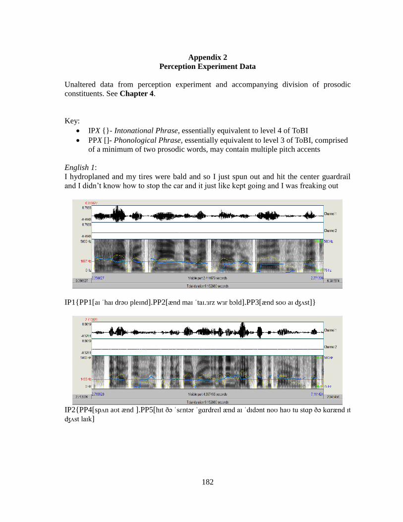
182
Appendix 2
Perception Experiment Data
Unaltered data from perception experiment and accompanying division of prosodic
constituents. See Chapter 4.
Key:
IPX {}- Intonational Phrase, essentially equivalent to level 4 of ToBI
PPX []- Phonological Phrase, essentially equivalent to level 3 of ToBI, comprised
of a minimum of two prosodic words, may contain multiple pitch accents
English 1:
I hydroplaned and my tires were bald and so I just spun out and hit the center guardrail
and I didn‘t know how to stop the car and it just like kept going and I was freaking out
IP1{PP1[aɪ ˈhaɪ drəʊ pleɪnd].PP2[ænd maɪ ˈtaɪ.ɜrz wɜr bɔld].PP3[ænd soʊ aɪ ʤʌst]}
IP2{PP4[spʌn aʊt ænd ].PP5[hɪt ðə ˈsɛntər ˈgɑrdreɪl ænd aɪ ˈdɪdənt noʊ haʊ tu stɑp ðə kɑrænd ɪt
ʤʌst laɪk]
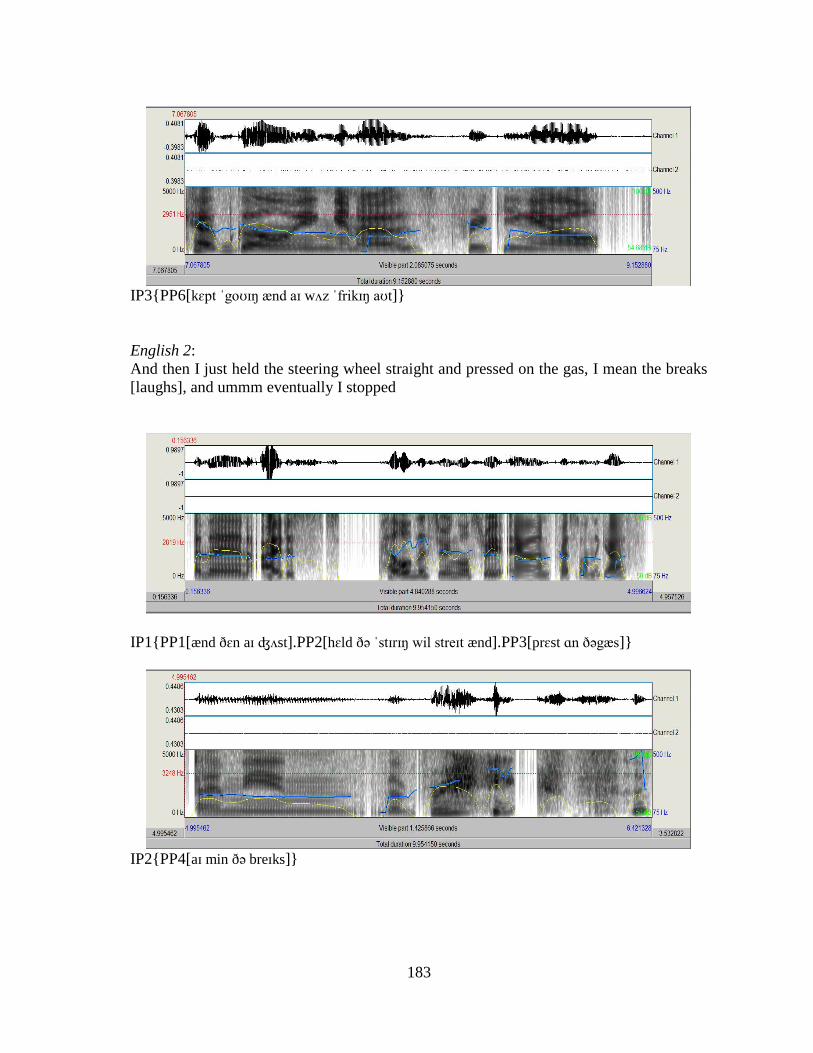
183
IP3{PP6[kɛpt ˈgoʊɪŋ ænd aɪ wʌz ˈfrikɪŋ aʊt]}
English 2:
And then I just held the steering wheel straight and pressed on the gas, I mean the breaks
[laughs], and ummm eventually I stopped
IP1{PP1[ænd ðɛn aɪ ʤʌst].PP2[hɛld ðə ˈstɪrɪŋ wil streɪt ænd].PP3[prɛst ɑn ðəgæs]}
IP2{PP4[aɪ min ðə breɪks]}

184
IP3{PP5[ænd ummm].PP6[ɪˈvɛnʧəwəli aɪ stɑpt]}
Portuguese 1:
O susto maior da minha vida foi quando engoli caju muito rapidamente e fiquei sem
respirar por algum tempo
IP1{PP1[u sˈuʃt mɐjˈɔɾ dɐ mˈiɲɐ vˈidɐ].PP2[foj kuˈɐdu eɡulˈi kɐʒˈu]}
IP2{PP3[mˈuit ʀˌapidɐmˈetɘ]}

185
IP3{PP4[ii fikˈɐj sɐj ʀɘʃpiɾˈaɾ ]
IP4{PP5[puɾ alɡˈu tˈepu]}
Portuguese 2:
Mas a mente em que gosto mais que no ultimo filme o regresso do rei a batalha final entre
os orcs e os humanos
IP1{PP1[mɐʃ ɐ mˈet].PP2[ ɐj ke kɘ ɡˈoʃtu majʃ]}

186
IP2{PP3[kɘ nu ultˈimu fˈilm]}
IP3{PP4[u ʀɘɡɾˈɛsu du ʀˈɐj]}
IP4{PP5[ɐ bɐtˈaʎɐ finˈal}

187
IP5{PP6[ˈetɾɘ uʃ ɔɾkʃ i].PP7[uʃ umˈɐnuʃ]}
Spanish 1:
Esta(b)a con (u)nos amigos en, en el mar en la playa, y entonces uno de ellos no sabía
nadar y.
IP1{PP1[est´aa kon nos a´miɣos en]
IP2{PP2[en el maɾ].PP3[en la ´plaʝa]}

188
IP3{PP4[ i en´tonses].PP5[´uno ðe ´eʎoz no sa´βia na´ðaɾ i]}
Spanish 2:
Les piden encuentran la computadora entonces y es una Mac no entonces, llegan, y de
esas viejitas que tienen como bolita y son de colores
IP1{PP1[les ´piðen].PP2[eŋ´kwentɾan la komputa´ðoɾa en´tonses]}
IP2{PP3[i es ´una mak no en´tonses].PP4[´ʎeɣan]}
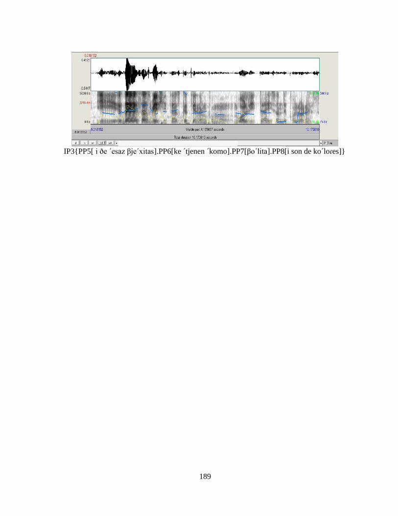
189
IP3{PP5[ i ðe ´esaz βje´xitas].PP6[ke ´tjenen ´komo].PP7[βo´lita].PP8[i son de ko´loɾes]}
Related Documents