Karlsruhe Reports in Informatics 2020,1 Edited by Karlsruhe Institute of Technology, Faculty of Informatics ISSN 2190-4782 Ubiquitäare Systeme (Seminar) und Mobile Computing (Proseminar) SS 2019 Mobile und Verteilte Systeme Ubiquitous Computing Teil XIX Herausgeber: Erik Pescara, Paul Tremper, Jan Formanek, Michael Hefenbrock, Yiran Huang, Ployplearn Ravivanpong, Johannes Riesterer, Long Wang, Ingmar Wolff, Yexu Zhou, Michael Beigl 2020 KIT – University of the State of Baden-Wuerttemberg and National Research Center of the Helmholtz Association

Welcome message from author
This document is posted to help you gain knowledge. Please leave a comment to let me know what you think about it! Share it to your friends and learn new things together.
Transcript
Karlsruhe Reports in Informatics 2020,1 Edited by Karlsruhe Institute of Technology, Faculty of Informatics
ISSN 2190-4782
Ubiquitäare Systeme (Seminar) und
Mobile Computing (Proseminar) SS 2019
Mobile und Verteilte Systeme
Ubiquitous Computing Teil XIX
Herausgeber: Erik Pescara, Paul Tremper, Jan Formanek, Michael Hefenbrock, Yiran Huang, Ployplearn Ravivanpong, Johannes Riesterer, Long Wang, Ingmar Wolff, Yexu Zhou, Michael Beigl
2020
KIT – University of the State of Baden-Wuerttemberg and National
Research Center of the Helmholtz Association

Please note: This Report has been published on the Internet under the following Creative Commons License: http://creativecommons.org/licenses/by-nc-nd/4.0/
Ubiquitare Systeme (Seminar)und
Mobile Computing (Proseminar)SS 2019
Mobile und Verteilte SystemeUbiquitous Computing
Teil XIX
HerausgeberErik Pescara, Paul Tremper
Jan Formanek, Michael HefenbrockYiran Huang, Ployplearn Ravivanpong
Johannes Riesterer, Long WangIngmar Wolff, Yexu Zhou, Michael Beigl
Karlsruhe Institute of Technology (KIT)Fakultat fur Informatik
Lehrstuhl fur Pervasive Computing Systems (PCS) und TECO
Interner Bericht 2020-01
KIT – University of the State of Baden-Wuerttemberg and National Laboratory of the Helmholtz Association www.kit.edu

ii
Vorwort
Die Seminarreihe Mobile Computing und Ubiquitare Systeme existiert seit dem Win-tersemester 2013/2014. Seit diesem Semester findet das Proseminar Mobile Computing amLehrstuhl fur Pervasive Computing System statt. Die Arbeiten des Proseminars werdenseit dem mit den Arbeiten des zweiten Seminars des Lehrstuhls, dem Seminar UbiquitareSysteme, zusammengefasst und gemeinsam veroffentlicht.
Die Seminarreihe Ubiquitare Systeme hat eine lange Tradition in der ForschungsgruppeTECO. Im Wintersemester 2010/2011 wurde die Gruppe Teil des Lehrstuhls fur Per-vasive Computing Systems. Seit dem findet das Seminar Ubiquitare Systeme in jedemSemester statt. Ebenso wird das Proseminar Mobile Computing seit dem Wintersemester2013/2014 in jedem Semester durchgefuhrt. Seit dem Wintersemester 2003/2004 werdendie Seminararbeiten als KIT-Berichte veroffentlicht. Ziel der gemeinsamen Seminarreiheist die Aufarbeitung und Diskussion aktueller Forschungsfragen in den Bereichen Mobileund Ubiquitous Computing.
Dieser Seminarband fasst die Arbeiten der Seminare des Sommersemesters 2019 zusam-men. Wir danken den Studierenden fur ihren besonderen Einsatz, sowohl wahrend desSeminars als auch bei der Fertigstellung dieses Bandes.
Karlsruhe, den 01. Oktober 2019 Erik PescaraPaul TremperJan Formanek
Michael HefenbrockYiran Huang
Ployplearn RavivanpongJohannes Riesterer
Long WangIngmar Wolff
Yexu ZhouMichael Beigl
iii


Contents
Cem OzcanHot Topics in Intelligent User Interfaces . . . . . . . . . . . . . . . . . . . . . . . . . . . . . . . . . . . . . . . . . 1
Rudolf KellnerRoom Recognition Using Audio Signals. . . . . . . . . . . . . . . . . . . . . . . . . . . . . . . . . . . . . . . . .18
Julian WestermannUbiquitous Object Imaging Using Audio Signals . . . . . . . . . . . . . . . . . . . . . . . . . . . . . . . . 43
Denis JagerVergleich Verschiedener Architekturen Kunstlicher Intelligenz . . . . . . . . . . . . . . . . . . . 58
Evgeni CholakovEdge Computing - An overview of a cloud extending technology . . . . . . . . . . . . . . . . 67
Ilia ChupakhinVergleich von Feuchtesensoren in Bezug auf Genauigkeit . . . . . . . . . . . . . . . . . . . . . . . . 86
Marco GoltzeReview von Strukturlernalgorithmen . . . . . . . . . . . . . . . . . . . . . . . . . . . . . . . . . . . . . . . . . . 110
Jan Niklas KielmannNeuro-evolution as an Alternative to Reinforcement Learning for Playing AtariGames . . . . . . . . . . . . . . . . . . . . . . . . . . . . . . . . . . . . . . . . . . . . . . . . . . . . . . . . . . . . . . . . . . . . . . . . 123
Carolin LigensaHot topics in Human-Computer-Interaction . . . . . . . . . . . . . . . . . . . . . . . . . . . . . . . . . . . 146
v

Anna Carolina SteyerExplainable Deep Neural Networks . . . . . . . . . . . . . . . . . . . . . . . . . . . . . . . . . . . . . . . . . . . . 167
Aufmerksamkeitssteuerung durch Haptische Schnittstellen in BeobachtungsaufgabenLeon Huck . . . . . . . . . . . . . . . . . . . . . . . . . . . . . . . . . . . . . . . . . . . . . . . . . . . . . . . . . . . . . . . . . . . . 192
vi
Hot Topics in Intelligent User Interfaces
Cem Ozcan
Karlsruher Institut fur Technologie
Zusammenfassung. Vor allem in den letzten Jahren wurden Com-puter immer mehr dazu eingesetzt, uns bei der Losung komplexerProbleme zu assistieren. Aufgrund der steigenden Komplexitat derAufgaben gewinnt eine effiziente Interaktion zwischen Mensch undMaschine fur Nutzer also immer mehr an Bedeutung.Eine Forschungsrichtung, die dieses Problem untersucht, ist die For-schung im Bereich “Intelligent User Interfaces“. In diesem Gebietkonzentriert man sich auf die Entwicklung von intuitiven Benutzer-schnittstellen, die die Interaktion mit einem Intelligenten Systemerleichtern und intuitiver gestalten sollen [16,30].
Die aktuelle Forschung richtet sich dabei hauptsachlich auf dieLosung von Problemen im Gebiet “Information retrieval“ durch denEinsatz von “Recommender Systems“ (Siehe section 2), die nahtloseIntegration von Mobilen und Tragbaren Geraten in den Alltag (siehesection 3) und die Bewaltigung komplexer Aufgaben durch den Einsatzmultimodaler Interaktion (Siehe section 4).Im Folgenden werden Paper aus der Konferenz “ACM Intelligent UserInterfaces“ [2] vorgestellt, die reprasentativ fur die aktuelle Forschungin diesem Bereich sind.
Schlusselworter: Intelligent User Interfaces, Recommender Systems,Explainable Artificial Intelligence, Ubiquitous Computing, MultimodalInterfaces, Human-Centered Computing, Human-Computer-Interaction
1 Einleitung
Als “Intelligent User Interface“ werden Schnittstellen zur Kommunikation zwi-schen Mensch und Maschine bezeichnet, die Aspekte der kunstlichen Intelligenzverwenden, um sich dem Nutzer anzupassen. Diese Adaption der Schnittstellean den Nutzer wird, je nach Beschaffenheit und Einsatzgebiet der Schnittstelle,unterschiedlich umgesetzt und hat demzufolge auch unterschiedliche Auswir-kungen auf die Wahrnehmung des Nutzers vom System:
Recommender Systems losen durch personalisierte Empfehlungen das Pro-blem der Informationsuberflutung und ermoglichen dem Nutzer eine effizientereKommunikation mit dem System. Im Forschungsfeld Ubiquitous Computingwerden Moglichkeiten zur Integration von mobilen und tragbaren Geraten inden menschlichen Alltag untersucht, um alltagliche Probleme des Nutzers zu
Hot Topics in Intelligent User Interfaces 1
2 Cem Ozcan
losen und die Interaktion mit Geraten so naturlich und intuitiv wie moglich zugestalten. Multimodale Interfaces werden verwendet, um die Mensch-Maschine-Interaktion der zwischenmenschlichen Interaktion anzunahern und dem Nutzersomit zu erlauben, komplexe Aufgaben effizienter zu losen.
Ziel dieser Arbeit ist es, die genannten Einsatzgebiete intelligenter Benut-zerschnittstellen, unter Verwendung relevanter Paper der Konferenz “ACMIntelligent User Interfaces“, vorzustellen.
2 Recommender Systems
2.1 Grundlagen
Recommender Systems sind vor allem im Zeitalter der Digitalisierung effektiveDienste, die die Mensch-Maschine-Interaktion erleichtern sollen. Durch Analy-se des Nutzerverhaltens versuchen Recommender Systems vorherzusehen, wel-che Inhalte (im Folgenden auch Items genannt) fur den Nutzer interessant seinkonnten, um diese dann dem Nutzer zu empfehlen. Das tragt zu einer verbes-serten Wahrnehmung vom System von Seiten des Nutzers bei und verbessert soauch die User Experience [6,12,17] .Das Filtern von irrelevanten Informationen erwies sich, vor allem in den letztenJahren, als effektiver Ausweg aus der Informationsuberflutung [24,29] und ge-wann fur Nutzer zunehmend an Bedeutung. Diese haben durch den Einsatz vonRecommender Systems Zugang zu mehr relevanten Informationen, die bei einerRecherche ohne Hilfe eines solchen Systems, teilweise in der Masse untergegan-gen waren. Wie in [13] beschrieben kann das Auslassen relevanter Informationenbeispielsweise im Gesundheitswesen fatale Folgen nach sich ziehen.Auch fur Unternehmen, die ihre Inhalte im Internet anbieten, spielen Recom-mender Systems eine wichtige Rolle. Gesammelte Nutzerdaten werden dazu ein-gesetzt, Massenwerbung nach und nach durch personalisierte Werbung und Pro-duktempfehlungen zu ersetzen, was sich auch im Konsumverhalten der Nutzerbemerkbar macht:Nach eigenen Angaben haben Netflix und YouTube je 75 und 70 Prozent ihrerAnsichten und Amazon 35 Prozent ihrer Verkaufe ihrem Recommender Systemzu verdanken [15,32].Die Genauigkeit der Empfehlungen sind demnach von großer Bedeutung sowohlfur die Nutzer als auch fur die Anbieter des Systems.Fur die Forschung in diesem Gebiet ergibt sich daher die Herausforderung, dasEmpfehlen und Filtern von Inhalten durch Personalisierung, zusatzlicher Para-metrisierung und Kontextualisierung so prazise wie moglich zu gestalten, ohnedabei die User Experience und Benutzbarkeit des Systems zu komprimieren.Im Folgenden werden verschiedene Klassen von Recommender Systems und zumThema relevante Paper vorgestellt, die Ansatze zur Verbesserung der Empfeh-lungen untersuchen.
2 Cem Ozcan
Hot Topics in Intelligent User Interfaces 3
2.2 Content-based filtering
AllgemeinInhaltsbasiertes Filtern ist eines der am haufigsten verwendeten Ansatze bei derImplementierung von Recommender Systems. Grundlegende Informationen, diedem System bekannt sein mussen, sind fruhere Itembewertungen der Nutzersund moglichst viele Attribute, die einen Item so prazise wie moglich beschrei-ben. Basierend auf diesen Daten werden Items kategorisiert und Nutzerprofileerstellt [29].Folgende Voraussetzungen mussen erfullt sein, damit ein Item I einem Nutzer Uempfohlen wird:
– I wurde noch nicht von Nutzer U bewertet– I ist ahnlich zu anderen Items, die U in der Vergangenheit positiv bewertet
hat
Haufig werden Item- und Nutzerprofile als Term Frequency-Inverse DocumentFrequency-Vektoren (TF-IDF-Vektoren) dargestellt und die Ahnlichkeit zweierItems mithilfe von Korrelationskoeffizienten oder Abstandsfunktionen berech-net [26,29].
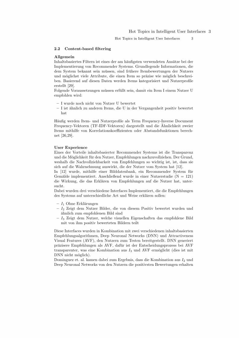
User ExperienceEines der Vorteile inhaltsbasierter Recommender Systems ist die Transparenzund die Moglichkeit fur den Nutzer, Empfehlungen nachzuvollziehen. Der Grund,weshalb die Nachvollziehbarkeit von Empfehlungen so wichtig ist, ist, dass siesich auf die Wahrnehmung auswirkt, die der Nutzer vom System hat [12].In [12] wurde, mithilfe einer Bilddatenbank, ein Recommender System furGemalde implementiert. Anschließend wurde in einer Nutzerstudie (N = 121)die Wirkung, die das Erklaren von Empfehlungen auf die Nutzer hat, unter-sucht.Dabei wurden drei verschiedene Interfaces Implementiert, die die Empfehlungendes Systems auf unterschiedliche Art und Weise erklaren sollen:
– I1 Ohne Erklarungen– I2 Zeigt dem Nutzer Bilder, die von diesem Positiv bewertet wurden und
ahnlich zum empfohlenen Bild sind– I3 Zeigt dem Nutzer, welche visuellen Eigenschaften das empfohlene Bild
mit von ihm positiv bewerteten Bildern teilt
Diese Interfaces wurden in Kombination mit zwei verschiedenen inhaltsbasiertenEmpfehlungsalgorithmen, Deep Neuronal Networks (DNN) und AttractivenessVisual Features (AVF), den Nutzern zum Testen bereitgestellt. DNN generiertprazisere Empfehlungen als AVF, dafur ist der Entscheidungsprozess bei AVFtransparenter, was eine Kombination aus I3 und AVF ermoglicht (dies ist mitDNN nicht moglich).Dominguez et. al. kamen dabei zum Ergebnis, dass die Kombination aus I2 undDeep Neuronal Networks von den Nutzern die positivsten Bewertungen erhalten
Hot Topics in Intelligent User Interfaces 3

4 Cem Ozcan
hat. Die Kombination aus I3 und Attractiveness Visual Features ist zwar dietransparenteste Methode, hat aber relativ unprazise Empfehlungen im Vergleichzu anderen Kombinationen. Das hat eine schlechtere Wahrnehmung und Bewer-tung des Systems aus Sicht der Nutzer zufolge.Aus [12] kann man also Folgern, dass bei der Implementierung eines Recommen-der Systems Wert auf Transparenz gelegt werden sollte, wenn diese die Qualitatder Empfehlungen nicht abschwacht.
2.3 Collaborative filtering
AllgemeinAnders als beim inhaltsbasieten Filtern werden beim kollaborativem Filtern kei-ne Informationen uber den Inhalt eines Items im System benotigt. Stattdessenwerden, je nach Ansatz, Nutzer- bzw. Itemprofile basierend auf deren Bewer-tungshistorie erstellt:
User-based approachEs werden Nutzerprofile basierend auf Bewertungen, die die Nutzer in derVergangenheit uber Items abgegeben haben, erstellt. Typischerweise wirdder k-Nearest-Neighbour-Algorithmus eingesetzt, um Nutzerprofile mitahnlicher Bewertungshistorie zu finden.Falls hinreichend viele Nutzer, die sich in der Nachbarschaft des NutzersU befinden, ein Item I positiv bewertet haben, so bekommt Nutzer U eineEmpfehlung fur Item I [20,29].
Item-based approachEs werden Itemprofile basierend auf Bewertungen, die die Items von Nutzernerhalten haben, erstellt.Zwei Items sind genau dann ahnlich, wenn es hinreichend viele Nutzer gibt,die beide Items bewertet haben. Außerdem muss eine Korrelation im Bewer-tungsverhalten der Nutzer, bezogen auf genannte Items, existieren.Diese Informationen werden dann dafur verwendet, die Bewertung eines Nut-zers fur ein Item abzuschatzen [20,21].
Context-specific trust [24]Mit der Hypothese, dass kollaboratives Filtern hohes Verbesserungspotentialbesitzt, hat man in [24] und [14] versucht, mit Modifikationen am kollaborativenFiltern auf bessere Empfehlungen zu kommen.Die grundlegende Idee des Ansatzes in [24] ist dabei, den Kontext bei der Wahlder Nachbarschaft eines Nutzers zu berucksichtigen. Dazu werden die in [4]eingefuhrten Definitionen fur “Trust“ (Vertrauenswurdigkeit) modelliert undbei der Wahl ahnlicher Profile als zusatzlicher Parameter berucksichtigt:
4 Cem Ozcan
Hot Topics in Intelligent User Interfaces 5
Profile-Level trustDie Vertrauenswurdigkeit eines Nutzers U ist abhangig davon, wie prazisedie Empfehlungen sind, die andere Nutzer, aufgrund ihrer Ahnlichkeit zuU, erhalten haben.
Item-Level trustSei I ein von Nutzer U bewertetes Item. Die Vertrauenswurdigkeit von Uim Bezug auf I ist abhangig davon, ob I haufig erfolgreich anderen Nutzernempfohlen wurde, weil diese ahnlich zu U sind.
O’Donovan et. al. haben verschiedene kollaborative Filteralgorithmen mit ihrenModellen erweitert und die Qualitat der Empfehlungen miteinander verglichen.Zur Evaluierung der Algorithmen wurde ein Datensatz mit 950 Profilen mit jedurchschnittlich 105 Filmbewertungen verwendet.Die Ergebnisse waren recht Eindeutig: Jeder Algorithmus, der um denzusatzlichen Parameter “Trust“ erweitert wurde, hat bessere Empfehlungsergeb-nisse geliefert, als der unmodifizierte Algorithmus. Die modifizierten Algorith-men waren zwischen 3 und 22 % weniger Fehleranfallig in ihren Empfehlungen,als der unmodifizierte Algorithmus.
2.4 Vergleich beider Ansatze
Inhaltsbasiertes FilternZum Einen ist es nicht notwendig, Personliche Informationen uber die Nutzerzu halten und zum Anderen lost die Kategorisierung der Items das sogenannte“New-Item-Problem“ [5,29]. Beim inhaltsbasierten Filtern konnen also, andersals beim kollaborativem Filtern, auch neue Produkte empfohlen werden, ohnezuvor eine Bewertung zu erhalten. Des Weiteren ist es fur Nutzer einfacher nach-zuvollziehen, weshalb sie bestimmte Empfehlungen bekommen, was sich positivauf die User Experience auswirkt (siehe section 2.2) [12] .
Kollaboratives FilternDas Hauptproblem inhaltsbasierten Filterns ist der, dass Nutzer nur Empfehlun-gen erhalten, die sich in dieselben Kategorien einordnen lassen, wie die bereitsvom Nutzer bewerteten Items. Durch kollaboratives Filtern konnen Nutzer auchEmpfehlungen aus Kategorien bekommen, die ihnen noch unbekannt waren.Ein Problem des kollaborativen Filterns ist das sogenannte “Cold-Start-Problem“. Neue Nutzer haben keine Bewertungshistorie, weswegen das Systemihnen keine Items empfehlen kann.
2.5 Hybrid Recommender Systems
Um von den Vorteilen mehrerer verschiedener Empfehlungsalgorithmen zu pro-fitieren werden haufig “Hybrid Recommender Systems“ (hybride Empfehlungs-dienste) verwendet. Dies sorgt in der Regel fur prazisere Empfehlungen als tra-ditionelles kollaboratives oder inhaltsbasiertes Filtern [5].
Hot Topics in Intelligent User Interfaces 5

6 Cem Ozcan
In [18] wurde beispielsweise ein Hybrid Recommender System mit traditionellemkollaborativem Filtern verglichen. Nicht nur waren die Empfehlungen des Hy-brid Recommender Systems akkurater, es war außerdem dank inhaltsbasierterAspekte moglich, Empfehlungen wie in [12] zu Begrunden.
Personalized Explanations [18]Wie auch schon in [12] (siehe section 2.2) wurde in [18] versucht, die Emp-fehlungen eines Recommender Systems mithilfe unterschiedlicher Methoden zuerklaren.Kouki et. al. haben dafur ein Hybrid Recommender System implementiert, dassieben verschiedene Arten von Erklarungen fur die Empfehlungen anbietet unddiese in verschiedenen Formaten (visuell oder textuell) darstellt.Die verschiedenen Erklarungsansatze lassen sich dabei in zwei Kategorien einord-nen. Inhaltsbasierte Erklarungen, die Empfehlungen basierend auf deren Inhaltbegrunden und nutzerbasierte Erklarungen, die Empfehlungen basierend auf derPraferenz ahnlicher Nutzer begrunden.Ziel der Studie [18] war es, durch Variation der Anzahl verschiedener Erklarungenfur eine Empfehlung, herauszufinden, welchen Einfluss diese auf die Nutzer ha-ben.Zur Beantwortung dieser Fragen, wurde das Recommender System mithilfe einerNutzerstudie (N = 198) evaluiert. Basierend auf einem Datensatz der Musik-plattform Last.fm wurden diesen Nutzern Musikinterpreten vorgeschlagen. DieVorschlage wurden wie schon in [12] von Begrundungen begleitet, die dem Nut-zer helfen sollen, die Empfehlungen zu verstehen.Kouki et. al. haben nach einer Befragung genannter Nutzer herausgefunden,dass:
1. Nutzer inhaltsbasierte Erklarungen uberzeugender als nutzerbasierte Er-klarungen fanden
2. Nutzer im Durchschnitt drei bis vier verschiedene Erklarungsansatze fur ihreEmpfehlungen bevorzugen
3. Nutzer die textuelle Darstellung der Erklarungen der visuellen Darstellungvorziehen
Ein weiteres interessantes Ergebnis der Studie in [18] war, dass die Genauigkeitdes Empfehlungsalgorithmus nicht zu Zwecken der Erklarbarkeit abgeschwachtwerden sollte. Auf ein ahnliches Ergebnis sind auch Dominguez et. al. in [12]gekommen (siehe section 2.2).
2.6 Ausblick
Recommender Systems sind schon seit einigen Jahren fester Bestandteil deselektronischen Handels und sind fur eine Pluralitat der Einnahmen vieler E-Commerce-Unternehmen verantwortlich. Durch den weitlaufigen Einsatz vonRecommender Systems richtet sich die Forschung in diesem Bereich also nichtauf die Exploration neuer Einsatzmoglichkeiten, sondern zielt vielmehr auf die
6 Cem Ozcan
Hot Topics in Intelligent User Interfaces 7
Verbesserung der Prazision von Empfehlungen ab. Um die Qualitat von Emp-fehlungen zu verbessern, werden typischerweise zusatzliche Kontextinformatio-nen in den Empfehlungsprozess hinzugezogen. Damit das Recommender Systemallerdings Skalierbar bleibt, muss der zusatzliche Rechenaufwand des Empfeh-lungsprozesses minimal gehalten werden.Ein anderer Ansatz ist die Kombination von Recommender Systems mit Ex-plainable Artificial Intelligence. Das Ziel ist es, durch Erklarungen, den Empfeh-lungsprozess so transparent wie moglich zu gestalten. Diese Erklarungen tragenzwar nicht zur Verbesserung der Empfehlungen bei, scheinen aber ein wichtigerFaktor bei der Wahrnehmung des Nutzers vom System zu sein.
3 Ubiquitous Computing
3.1 Grundlagen
Der Begriff “Ubiquitous Computing“ beschreibt die Eingliederung von Com-putern in den menschlichen Alltag und wurde bereits 1991 von Mark Weiser(1952-1999) verwendet und gepragt [37]. Das Ziel des “Ubiquitous Computing“ist es, das alltagliche Leben des Menschen mithilfe von intelligenten Geraten,die aus dem Hintergrund heraus agieren, zu erleichtern. Weisers Vorstellung des21. Jahrhunderts hat sich als richtig herausgestellt: Heutzutage suchen Nutzerdie Interaktion mit Computern nicht langer aktiv auf, vielmehr ist die Mensch-Maschine-Interaktion allgegenwartig ohne dabei im Vordergrund unseres Lebenszu sein.Die Veroffentlichungen der Konferenz “Intelligent User Interfaces“ beschaftigensich vor allem mit den Themen “Mobile Computing“ und “Wearable Compu-ting“, da Smartphones und andere mobile bzw. tragbare Gerate zunehmend anBedeutung in unserem Alltag gewinnen.
3.2 Wearable Computing
”Wearable devices“ sind am Korper getragene Gerate, die den Nutzer im Alltag
unterstutzen sollen, ohne dabei von diesem als storend empfunden zu werden.Ein typisches Beispiel fur Wearables aus dem kommerziellen Bereich sindFitnessarmbander:Durch die Positionierung am Handgelenk des Nutzers konnen diese den Nutzerdurch das Messen der Vitalfunktionen und Korperbewegung (Pulsmesserund Schrittzahler) beim Sport unterstutzen, ohne dessen Bewegungen einzu-schranken.In der Forschung hingegen, werden Wearables vor allem mit Blick auf dieVerbesserung der Mensch-Maschine-Interaktion eingesetzt.
Hot Topics in Intelligent User Interfaces 7
8 Cem Ozcan
3.3 Assistive Intelligent User Interfaces
Eine Vielzahl der Arbeiten, die auf der Konferenz vorgestellt werden, richtet sichauf Unterstutzungstechnologien zur Hilfe von Menschen mit kognitiven Beein-trachtigungen [10,23]. Speziell Wearables beispielsweise werden hauptsachlichdafur eingesetzt, um die Kommunikation und Interaktion zwischen seh- bzw.horgeschadigten Personen mit Personen ohne jeweilige Einschrankungen zu er-leichtern [8,27,28,38].Paudyal et. al. haben sich sowohl in [27] als auch in [28] mit dem Einsatz vonWearables zur Erkennung von Gesten in der Gebardensprache beschaftigt:
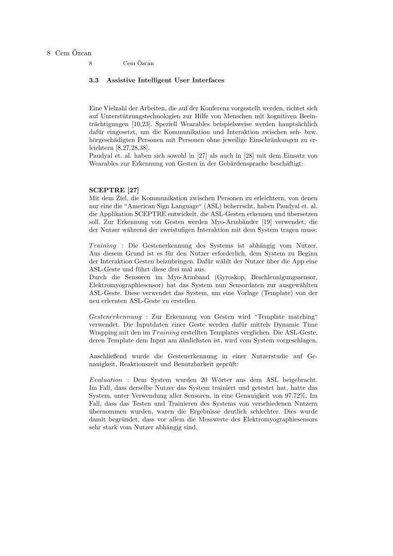
SCEPTRE [27]Mit dem Ziel, die Kommunikation zwischen Personen zu erleichtern, von denennur eine die “American Sign Language“ (ASL) beherrscht, haben Paudyal et. al.die Applikation SCEPTRE entwickelt, die ASL-Gesten erkennen und ubersetzensoll. Zur Erkennung von Gesten werden Myo-Armbander [19] verwendet, dieder Nutzer wahrend der zweistufigen Interaktion mit dem System tragen muss:
Training : Die Gestenerkennung des Systems ist abhangig vom Nutzer.Aus diesem Grund ist es fur den Nutzer erforderlich, dem System zu Beginnder Interaktion Gesten beizubringen. Dafur wahlt der Nutzer uber die App eineASL-Geste und fuhrt diese drei mal aus.Durch die Sensoren im Myo-Armband (Gyroskop, Beschleunigungssensor,Elektromyographiesensor) hat das System nun Sensordaten zur ausgewahltenASL-Geste. Diese verwendet das System, um eine Vorlage (Template) von derneu erlernten ASL-Geste zu erstellen.
Gestenerkennung : Zur Erkennung von Gesten wird “Template matching“verwendet. Die Inputdaten einer Geste werden dafur mittels Dynamic TimeWrapping mit den im Training erstellten Templates verglichen. Die ASL-Geste,deren Template dem Input am ahnlichsten ist, wird vom System vorgeschlagen.
Anschließend wurde die Gestenerkennung in einer Nutzerstudie auf Ge-nauigkeit, Reaktionszeit und Benutzbarkeit gepruft:
Evaluation : Dem System wurden 20 Worter aus dem ASL beigebracht.Im Fall, dass derselbe Nutzer das System trainiert und getestet hat, hatte dasSystem, unter Verwendung aller Sensoren, in eine Genauigkeit von 97.72%. ImFall, dass das Testen und Trainieren des Systems von verschiedenen Nutzernubernommen wurden, waren die Ergebnisse deutlich schlechter. Dies wurdedamit begrundet, dass vor allem die Messwerte des Elektromyographiesensorssehr stark vom Nutzer abhangig sind.
8 Cem Ozcan
Hot Topics in Intelligent User Interfaces 9
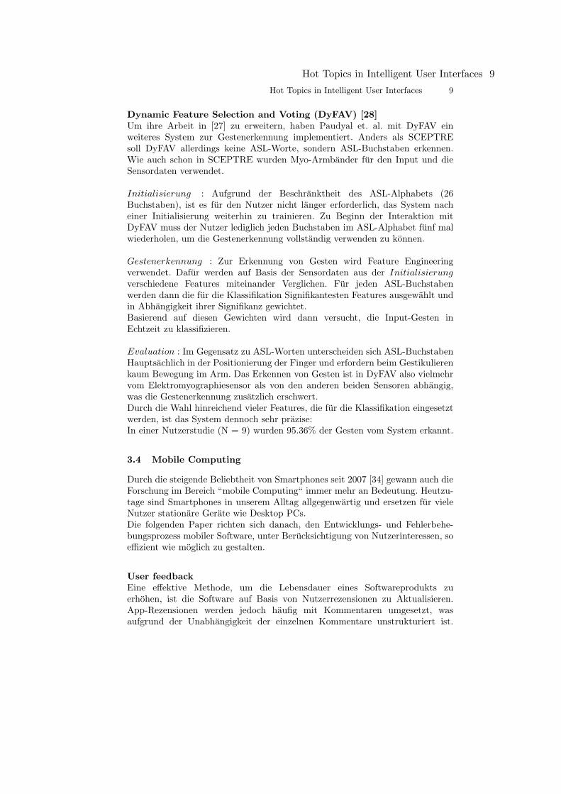
Dynamic Feature Selection and Voting (DyFAV) [28]Um ihre Arbeit in [27] zu erweitern, haben Paudyal et. al. mit DyFAV einweiteres System zur Gestenerkennung implementiert. Anders als SCEPTREsoll DyFAV allerdings keine ASL-Worte, sondern ASL-Buchstaben erkennen.Wie auch schon in SCEPTRE wurden Myo-Armbander fur den Input und dieSensordaten verwendet.
Initialisierung : Aufgrund der Beschranktheit des ASL-Alphabets (26Buchstaben), ist es fur den Nutzer nicht langer erforderlich, das System nacheiner Initialisierung weiterhin zu trainieren. Zu Beginn der Interaktion mitDyFAV muss der Nutzer lediglich jeden Buchstaben im ASL-Alphabet funf malwiederholen, um die Gestenerkennung vollstandig verwenden zu konnen.
Gestenerkennung : Zur Erkennung von Gesten wird Feature Engineeringverwendet. Dafur werden auf Basis der Sensordaten aus der Initialisierungverschiedene Features miteinander Verglichen. Fur jeden ASL-Buchstabenwerden dann die fur die Klassifikation Signifikantesten Features ausgewahlt undin Abhangigkeit ihrer Signifikanz gewichtet.Basierend auf diesen Gewichten wird dann versucht, die Input-Gesten inEchtzeit zu klassifizieren.
Evaluation : Im Gegensatz zu ASL-Worten unterscheiden sich ASL-BuchstabenHauptsachlich in der Positionierung der Finger und erfordern beim Gestikulierenkaum Bewegung im Arm. Das Erkennen von Gesten ist in DyFAV also vielmehrvom Elektromyographiesensor als von den anderen beiden Sensoren abhangig,was die Gestenerkennung zusatzlich erschwert.Durch die Wahl hinreichend vieler Features, die fur die Klassifikation eingesetztwerden, ist das System dennoch sehr prazise:In einer Nutzerstudie (N = 9) wurden 95.36% der Gesten vom System erkannt.
3.4 Mobile Computing
Durch die steigende Beliebtheit von Smartphones seit 2007 [34] gewann auch dieForschung im Bereich “mobile Computing“ immer mehr an Bedeutung. Heutzu-tage sind Smartphones in unserem Alltag allgegenwartig und ersetzen fur vieleNutzer stationare Gerate wie Desktop PCs.Die folgenden Paper richten sich danach, den Entwicklungs- und Fehlerbehe-bungsprozess mobiler Software, unter Berucksichtigung von Nutzerinteressen, soeffizient wie moglich zu gestalten.
User feedbackEine effektive Methode, um die Lebensdauer eines Softwareprodukts zuerhohen, ist die Software auf Basis von Nutzerrezensionen zu Aktualisieren.App-Rezensionen werden jedoch haufig mit Kommentaren umgesetzt, wasaufgrund der Unabhangigkeit der einzelnen Kommentare unstrukturiert ist.
Hot Topics in Intelligent User Interfaces 9

10 Cem Ozcan
Aus diesem Grund ist es sehr schwierig fur Entwickler, fur die Entwicklungrelevantes Feedback aus den Kommentaren zu extrahieren [11].Zur Losung dieses Problems haben Su’a et. al. QuickReview entwickelt [35]:QuickReview ist ein Intelligent User Interface, das das Rezensierten vonApps benutzerfreundlicher gestalten soll und außerdem Entwicklern erlaubt,effizient fur die Entwicklung relevante Informationen aus diesen Rezensionen zugewinnen:
Interaktion : QuickReview stellt dem Nutzer eine Liste von Features derApp, die dieser bewerten mochte, zur Verfugung. Der Nutzer kann dann einFeature auswahlen, das es kritisieren mochte, und bekommt dann eine Listevon Issues vorgeschlagen, die abhangig vom ausgewahlten Feature ist. Um eineApp zu rezensieren, muss der Nutzer also lediglich ein fehlerhaftes Featureauswahlen und aus einer Liste von Issues diejenigen auswahlen, die den Fehleram besten beschreiben.Um diese Adaptivitat zu gewahrleisten, werden vorhandene Kommentare uberdie zu Bewertende App, mittels Natural Language Processing nach Haufigvorkommenden Feature, Issue Paaren untersucht.
Feedback : Durch Rezensionen nach diesem Schema kann QuickRevieweine nach Haufigkeit sortierte Liste aus Feature, Issue Paaren prasentieren.Entwickler konnen diese Liste dann zur Identifizierung und anschließenderBehebung von Bugs verwenden.
Evaluation : Zur Evaluation des Systems wurde eine Nutzerbefragung (N= 20) durchgefuhrt, bei der die Nutzer zunachst die App “MyTracks“ nutzenund spater unter Verwendung von QuickReviw rezensieren sollten. Anschließendhaben die Nutzer die Benutzbarkeit und kognitive Uberlastung von QuickReviwbewertet. Als Kontrollinstanz wurde das traditionelle Rezensionssystem vonGoogle Play verwendet, welches auf einfachen Kommentaren basiert.QuickReview hat zwar in beiden Kategorien besser abgeschnitten als GooglePlay, diese Unterschiede waren jedoch statistisch nicht signifikant genug, umeine Aussage uber die Praferenz der Nutzer zu treffen.Allerdings ist bei der Durchfuhrung der Studie aufgefallen, dass die Nutzungvon QuickReview deutlich weniger Zeit in Anspruch genommen hat, als dasSchreiben von Kommentaren auf Google Play. Das fuhrt zu der Vermutung,dass QuickReview aufgrund der Zeitersparnis Nutzer dazu anregen konnte,mehr Rezensionen abzugeben als traditionelle Systeme.Ein weiterer Vorteil ist offensichtlicherweise die Zeitersparnis fur die Entwickler,da QuickReview das Problem der Informationsuberflutung fur diese lost.
3.5 Ausblick
Mobile Gerate, wie Smartphones, sind im Vergleich zu tragbaren Geraten be-reits allgegenwartig und in den menschlichen Alltag integriert. Der Fokus deraktuellen Forschung liegt daher viel mehr auf dem Gebiet Wearable Computing:
10 Cem Ozcan

Hot Topics in Intelligent User Interfaces 11
Die meisten Paper der Konferenz gehen auf spezifische Alltagssituationen einund versuchen diese durch den Einsatz tragbarer Gerate zu verbessern. In [22]beispielsweise, werden tragbare Gerate an einem Nutzer angebracht, um dessenStimme, Gestik und Blick wahrend einer Prasentation zu messen und diesemautomatisiertes Feedback zu geben.Weitaus nutzlicher ist der Einsatz von tragbaren Geraten aber, wenn es um dieImplementierung assistiver Technologien geht. Nichtinvasive tragbare Gerate,wie beispielsweise Armbander, haben das Potential durch ihre Allgegenwartigkeitdie Lebensqualitat von Horgeschadigten signifikant zu verbessern.Aufgrund des Nutzens und der bisherigen Befunde ist also anzunehmen, dassassistive Technologien auch in Zukunft Fokus im Bereich Wearable Computingbleiben werden.
4 Multimodal Interfaces
4.1 Grundlagen
Traditionellerweise ist die Mensch-Maschine-Interaktion mit vielen Systemenunimodal, es wird also nur eine Art der Eingabe verwendet, um das Systemzu steuern. Mittlerweile werden aber neben Tastatur, Maus und Touchscreensauch andere Eingabemoglichkeiten wie Spracherkennung, Gestenerkennung undEye Tracking immer praziser und beliebter und konnen fur eine EffektivereKommunikation zwischen Mensch und Maschine eingesetzt werden.[1]Dieser Fortschritt motiviert dazu, die Mensch-Maschine-Interaktion an zwi-schenmenschliche Interaktionen anzunahern, indem die Interaktion multimodalgestaltet wird [25,31,36].
multimodale Interfaces kombinieren mehrere Interaktionsmoglichkeiten mitein-ander und helfen Nutzern somit, komplexe Aufgaben effizienter zu bewaltigen[9]. Das System ist somit durch den Einsatz mehrerer Interaktionsmoglichkeitenweniger Fehleranfallig und sorgt durch die erhohte Prazision in der Erkennungvon Nutzereingaben fur eine bessere Wahrnehmung des Systems.Das Ziel multimodaler Interfaces ist es also, die Starken der einzelnen Moda-litaten zu kombinieren, ohne dass die Interaktion mit dem System vom Nutzerals kontraintuitiv wahrgenommen wird.
4.2 Natural Language Interfaces
Ein großes Problem bei der Bedienung von Geraten mittels Sprachsteuerung ist,dass Nutzer haufig nicht wissen, wie genau sie Befehle formulieren mussen, damitsie das System versteht. Dies fuhrt haufig zu Kommunikationsfehlern zwischenNutzer und Gerat und hat daher die Auswirkung, dass Nutzer eine negativeWahrnehmung von der Sprachsteuerung oder sogar vom gesamten System haben.Um dem entgegenzuwirken, wird in [33] versucht, Sprachbefehle in die Benut-zeroberflache zu integrieren, um somit Nutzer mit der sprachlichen Interaktion
Hot Topics in Intelligent User Interfaces 11

12 Cem Ozcan
mit dem System vertraut zu machen und Kommunikationsfehler zu vermeiden.Srinivasan et. al. implementierten dafur ein multimodales Interface fur ein einfa-ches Programm zur Bildbearbeitung. Nutzer sollen dazu in der Lage sein, sowohlmittels Touchscreen, als auch mithilfe von Sprachbefehlen mit dem System zuinteragieren.In der Umsetzung wurden drei verschiedene Interfaces implementiert und mit-einander verglichen:
– Exhaustive : Der Nutzer kann ein Fenster aufrufen, auf dem alle moglichenSprachbefehle aufgelistet sind. Um die kognitive Belastung auf den Nutzerso gering wie moglich zu halten, werden nur Befehle eingeblendet, die in derjeweiligen Situation verwendbar sind.
– Adaptive : Es werden Situationsabhangige Sprachbefehle im Bezug aufeinzelne UI-Objekte empfohlen. Der Nutzer kann durch einfaches Zeigen aufein UI-Objekt eine Liste von Sprachbefehlen auftauchen lassen. Das Systemversucht auf Basis vergangener Befehle vorherzusehen, welche Befehle derNutzer als nachstes verwenden wollen konnte. Diese werden dann in derListe angezeigt.
– Embedded : In dem Teil der Benutzeroberflache, mit dem der Nutzer inter-agiert, werden neben den UI-Elementen auch die zugehorigen Sprachbefehleangezeigt.
Zur Evaluation des Systems wurden die unterschiedlichen Interfaces in einerNutzerstudie (N = 16) getestet und miteinander verglichen. Um die Testbedin-gungen so realistisch wie moglich zu gestalten, wurde die Plattform UserTesting[3] verwendet. Die Teilnehmer haben kein ausfuhrliches Training mit dem Sys-tem erhalten und haben es auf ihren eigenen Geraten getestet.Am ende der Studie wurde festgestellt, dass die Interfaces Adaptive undEmbedded deutlich mehr zur sprachlichen Interaktion mit dem System ange-regt haben, als das Interface Exhaustive.Des Weiteren hatte die Empfehlung von Befehlen hauptsachlich zwei Auswir-kungen auf die Nutzer: Zum einen hatten die Empfehlungen zur Folge, dass nurein recht kleiner Anteil aller Spracherkennungsfehler (18%) daran lagen, dassNutzer sich falsch ausgedruckt haben.Zum anderen haben sich Nutzer dank der Empfehlungen dazu angeregt gefuhlt,die Spracherkennungsfunktion zu nutzen und hatten trotz hoher Fehlerquote inder Spracherkennung (44%) eine positive Wahrnehmung vom Spracherkennungs-aspekt des Systems.
4.3 Touch gestures
Dank ihrer Kompaktheit sind Smartphones und vor allem Tablets fur dasLesen von Dokumenten wie geschaffen. Die Suche nach relevanten Dokumenten
12 Cem Ozcan
Hot Topics in Intelligent User Interfaces 13
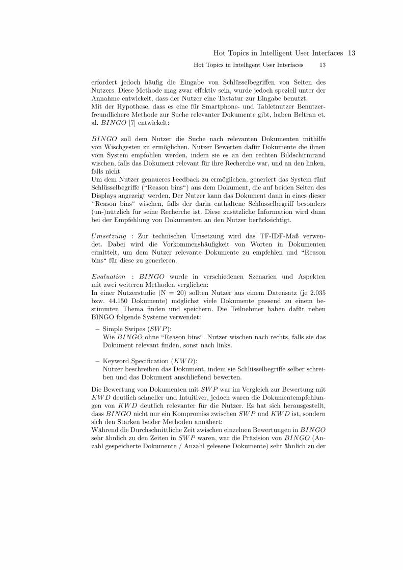
erfordert jedoch haufig die Eingabe von Schlusselbegriffen von Seiten desNutzers. Diese Methode mag zwar effektiv sein, wurde jedoch speziell unter derAnnahme entwickelt, dass der Nutzer eine Tastatur zur Eingabe benutzt.Mit der Hypothese, dass es eine fur Smartphone- und Tabletnutzer Benutzer-freundlichere Methode zur Suche relevanter Dokumente gibt, haben Beltran et.al. BINGO [7] entwickelt:
BINGO soll dem Nutzer die Suche nach relevanten Dokumenten mithilfevon Wischgesten zu ermoglichen. Nutzer Bewerten dafur Dokumente die ihnenvom System empfohlen werden, indem sie es an den rechten Bildschirmrandwischen, falls das Dokument relevant fur ihre Recherche war, und an den linken,falls nicht.Um dem Nutzer genaueres Feedback zu ermoglichen, generiert das System funfSchlusselbegriffe (“Reason bins“) aus dem Dokument, die auf beiden Seiten desDisplays angezeigt werden. Der Nutzer kann das Dokument dann in eines dieser“Reason bins“ wischen, falls der darin enthaltene Schlusselbegriff besonders(un-)nutzlich fur seine Recherche ist. Diese zusatzliche Information wird dannbei der Empfehlung von Dokumenten an den Nutzer berucksichtigt.
Umsetzung : Zur technischen Umsetzung wird das TF-IDF-Maß verwen-det. Dabei wird die Vorkommenshaufigkeit von Worten in Dokumentenermittelt, um dem Nutzer relevante Dokumente zu empfehlen und “Reasonbins“ fur diese zu generieren.
Evaluation : BINGO wurde in verschiedenen Szenarien und Aspektenmit zwei weiteren Methoden verglichen:In einer Nutzerstudie (N = 20) sollten Nutzer aus einem Datensatz (je 2.035bzw. 44.150 Dokumente) moglichst viele Dokumente passend zu einem be-stimmten Thema finden und speichern. Die Teilnehmer haben dafur nebenBINGO folgende Systeme verwendet:
– Simple Swipes (SWP ):Wie BINGO ohne “Reason bins“. Nutzer wischen nach rechts, falls sie dasDokument relevant finden, sonst nach links.
– Keyword Specification (KWD):Nutzer beschreiben das Dokument, indem sie Schlusselbegriffe selber schrei-ben und das Dokument anschließend bewerten.
Die Bewertung von Dokumenten mit SWP war im Vergleich zur Bewertung mitKWD deutlich schneller und Intuitiver, jedoch waren die Dokumentempfehlun-gen von KWD deutlich relevanter fur die Nutzer. Es hat sich herausgestellt,dass BINGO nicht nur ein Kompromiss zwischen SWP und KWD ist, sondernsich den Starken beider Methoden annahert:Wahrend die Durchschnittliche Zeit zwischen einzelnen Bewertungen in BINGOsehr ahnlich zu den Zeiten in SWP waren, war die Prazision von BINGO (An-zahl gespeicherte Dokumente / Anzahl gelesene Dokumente) sehr ahnlich zu der
Hot Topics in Intelligent User Interfaces 13
14 Cem Ozcan
von KWD. Auch in einer anschließenden Nutzerbefragung wurde das von denNutzern bestatigt.BINGO sei wie SWP sehr intuitiv (BINGO bewertet mit 7, SWP mit 7.6 von10), wahrend es wie KWD relevante Dokumente empfiehlt (BINGO bewertetmit 7.5, KWD mit 7.5 von 10).
4.4 Ausblick
Wie auch schon im Bereich Ubiquitous Computing erortern Paper der Konferenzdie Einsatzmoglichkeiten von Multimodal Interfaces. Das liegt hauptsachlich dar-an, dass multimodale Interaktion mit Geraten zu kompliziert fur eine sporadischeNutzung ist und die ungeteilte Aufmerksamkeit des Nutzers erfordert. Der Nach-teil darin liegt, dass Nutzer haufig nur eine Modalitat zur Eingabe nutzen, unddie Anderen einfach ignorieren.Multimodal Interfaces werden daher zur Bewaltigung komplexer Aufgaben ein-gesetzt, statt Probleme im Alltag zu losen. Wie bereits in [33] angesprochen,ermoglicht multimodale Interaktion Experten eine effizientere Kommunikationmit dem Gerat und erlaubt es ihnen, mehrere Aufgaben zur selben Zeit zu erledi-gen. Ein weiteres Beispiel, das reprasentativ fur die Forschung in diesem Bereichist, ist die Arbeit an Head-Up-Displays (HUD). In [9] werden Touchscreens durchHUDs in Kombination mit Eye-Tracking ersetzt, um Piloten die Erfullung vonAufgaben wahrend des Fliegens zu erleichtern.
5 Gemeinsamkeiten und Unterschiede
Gemeinsamkeiten und Unterschiede zwischen den Papern der Konferenz sindstark vom vorgestellten Thema abhangig. Die Paper zu Recommender Systemsbeispielsweise, stellen die technische Umsetzung neuer Methoden und Algorith-men vor. Das hat zur Folge, dass die Methoden und Algorithmen einfach unterVerwendung von Datensatzen evaluiert werden konnen.In Gebieten wie “Ubiquitous Computing“ und “Multimodal Interfaces“ sindstattdessen Nutzerstudien notig, da hier in erster Linie verschiedene Ein-satzmoglichkeiten untersucht werden.Die Notwendigkeit von Nutzerstudien ist besonders dann ein Problem, wenn sichdie Forschung auf sehr spezifische Szenarien richtet:Bei der Evaluation assistiver Systeme fur horgeschadigte Personen beispielswei-se, ist es schwer, Studienteilnehmer zu finden, die die Gebardensprache konnen.
6 Fazit
Ein Großteil der Forschung richtet sich auf die Losung von Problemen imBereich “Information Retrieval“ mithilfe von Recommender Systems. DerGrund, weshalb gerade Recommender Systems zentral zur Forschung in diesemGebiet sind, liegt am weit verbreiteten Einsatz von Recommender Systems im
14 Cem Ozcan
Hot Topics in Intelligent User Interfaces 15
elektronischen Handel.Auf der Konferenz vorgestellte Paper beschaftigen sich dabei vor allem mit derVerbesserung der “User Experience“ bei der Interaktion mit dem System undkommen haufig zum Entschluss, dass die Genauigkeit und Nachvollziehbarkeitvon Empfehlungen fur die Wahrnehmung eines Recommender Systems vongroßer Bedeutung sind.
Anders verhalt es sich bei der Forschung im Bereich “Ubiquitous Compu-ting“ und “Multimodal Interfaces“:Viele Paper versuchen eine sinnvolle Verwendung fur tragbare Gerate undmultimodale Interfaces zu finden, indem sie versuchen, diese in verschiedeneSituationen zu integrieren. Durch die Allgegenwartigkeit und intuitive Be-dienbarkeit von Smartphones erweist es sich als schwer, Alltagssituationen zufinden, in denen Nutzer tragbare Gerate und multimodale Interaktion einemSmartphone mit Touchscreens vorziehen wurden.Aus diesem Grund konzentriert sich die Forschung auf spezifischere Situationen:Tragbare Gerate werden deshalb zur Prazisierung assistiver Technologien ver-wendet, wahrend multimodale Interaktion haufiger zur Bewaltigung komplexerAufgaben eingesetzt wird.
Literatur
1. Amazon sold tens of millions of echo devices in 2018.https://www.cnet.com/news/amazon-sold-tens-of-millions-of-echo-devices-in-2018/. Accessed: 2019-06-29.
2. Intelligent user interfaces. https://iui.acm.org/2019/. Accessed: 2019-06-18.3. Usertesting. https://www.usertesting.com/. Accessed: 2019-06-30.4. Alfarez Abdul-Rahman and Stephen Hailes. A distributed trust model. In Procee-
dings of the 1997 workshop on New security paradigms, pages 48–60. ACM, 1998.5. Gediminas Adomavicius and Alexander Tuzhilin. Toward the next generation of
recommender systems: A survey of the state-of-the-art and possible extensions.IEEE Transactions on Knowledge & Data Engineering, (6):734–749, 2005.
6. Paritosh Bahirat, Yangyang He, Abhilash Menon, and Bart Knijnenburg. A data-driven approach to developing iot privacy-setting interfaces. In 23rd InternationalConference on Intelligent User Interfaces, pages 165–176. ACM, 2018.
7. Juan Felipe Beltran, Ziqi Huang, Azza Abouzied, and Arnab Nandi. Don’t justswipe left, tell me why: Enhancing gesture-based feedback with reason bins. InProceedings of the 22nd International Conference on Intelligent User Interfaces,pages 469–480. ACM, 2017.
8. Syed Masum Billah, Vikas Ashok, and IV Ramakrishnan. Write-it-yourself withthe aid of smartwatches: A wizard-of-oz experiment with blind people. In 23rd In-ternational Conference on Intelligent User Interfaces, pages 427–431. ACM, 2018.
9. Pradipta Biswas and Jeevithashree DV. Eye gaze controlled mfd for militaryaviation. In 23rd International Conference on Intelligent User Interfaces, pages79–89. ACM, 2018.
10. Cong Chen, Ajay Chander, and Kanji Uchino. Guided play: digital sensing andcoaching for stereotypical play behavior in children with autism. In Proceedings of
Hot Topics in Intelligent User Interfaces 15

16 Cem Ozcan
the 24th International Conference on Intelligent User Interfaces, pages 208–217.ACM, 2019.
11. Ning Chen, Jialiu Lin, Steven CH Hoi, Xiaokui Xiao, and Boshen Zhang. Ar-miner: mining informative reviews for developers from mobile app marketplace. InProceedings of the 36th International Conference on Software Engineering, pages767–778. ACM, 2014.
12. Vicente Dominguez, Pablo Messina, Ivania Donoso-Guzman, and Denis Parra. Theeffect of explanations and algorithmic accuracy on visual recommender systems ofartistic images. In Proceedings of the 24th International Conference on IntelligentUser Interfaces, pages 408–416. ACM, 2019.
13. Ivania Donoso-Guzman and Denis Parra. An interactive relevance feedback inter-face for evidence-based health care. In 23rd International Conference on IntelligentUser Interfaces, pages 103–114. ACM, 2018.
14. Lukas Eberhard, Simon Walk, Lisa Posch, and Denis Helic. Evaluating narrative-driven movie recommendations on reddit. In Proceedings of the 24th InternationalConference on Intelligent User Interfaces, pages 1–11. ACM, 2019.
15. Ian MacKenzie et. al. How retailers can keep up with consumers.https://www.mckinsey.com/industries/retail/our-insights/how-retailers-can-keep-up-with-consumers. Accessed: 2019-06-18.
16. Kristina Hook. Steps to take before intelligent user interfaces become real. Inter-acting with computers, 12(4):409–426, 2000.
17. Joseph A Konstan and John Riedl. Recommender systems: from algorithms to userexperience. User modeling and user-adapted interaction, 22(1-2):101–123, 2012.
18. Pigi Kouki, James Schaffer, Jay Pujara, John O’Donovan, and Lise Getoor. Per-sonalized explanations for hybrid recommender systems. In Proceedings of the24th International Conference on Intelligent User Interfaces, pages 379–390. ACM,2019.
19. Thalmic Labs. Myo gestensteuerungsarmband - schwarz.https://www.robotshop.com/de/de/myo-gestensteuerungsarmband-schwarz.html.Accessed: 2019-06-26.
20. Greg Linden, Brent Smith, and Jeremy York. Amazon. com recommendations:Item-to-item collaborative filtering. IEEE Internet computing, (1):76–80, 2003.
21. Gregory D Linden, Jennifer A Jacobi, and Eric A Benson. Collaborative recommen-dations using item-to-item similarity mappings, July 24 2001. US Patent 6,266,649.
22. Alaeddine Mihoub and Gregoire Lefebvre. Social intelligence modeling using wea-rable devices. In Proceedings of the 22Nd International Conference on IntelligentUser Interfaces, IUI ’17, pages 331–341, New York, NY, USA, 2017. ACM.
23. Leo Neat, Ren Peng, Siyang Qin, and Roberto Manduchi. Scene text access: acomparison of mobile ocr modalities for blind users. 2019.
24. John O’Donovan and Barry Smyth. Trust in recommender systems. In Proceedingsof the 10th international conference on Intelligent user interfaces, pages 167–174.ACM, 2005.
25. Sharon Oviatt and Philip Cohen. Perceptual user interfaces: multimodal interfacesthat process what comes naturally. Communications of the ACM, 43(3):45–53,2000.
26. Martin Kuhl Max Leonhardt Christoph Schroer Achim Volz Lukas Weinel Christi-an Wigger Christof Wolke Marius Wybrands Patrick Bruns, Christian Eilts. Daten-strombasierte Recommender-Systeme. Carl von Ossietzky Universitat Oldenburg.
27. Prajwal Paudyal, Ayan Banerjee, and Sandeep KS Gupta. Sceptre: a pervasive,non-invasive, and programmable gesture recognition technology. In Proceedings of
16 Cem Ozcan
Hot Topics in Intelligent User Interfaces 17
the 21st International Conference on Intelligent User Interfaces, pages 282–293.ACM, 2016.
28. Prajwal Paudyal, Junghyo Lee, Ayan Banerjee, and Sandeep KS Gupta. Dyfav:Dynamic feature selection and voting for real-time recognition of fingerspelled al-phabet using wearables. In Proceedings of the 22nd International Conference onIntelligent User Interfaces, pages 457–467. ACM, 2017.
29. Francesco Ricci, Lior Rokach, and Bracha Shapira. Introduction to recommendersystems handbook. In Recommender systems handbook, pages 1–35. Springer, 2011.
30. Edwina L Rissland. Ingredients of intelligent user interfaces. International Journalof Man-Machine Studies, 21(4):377–388, 1984.
31. Monica Sebillo, Giuliana Vitiello, and Maria De Marsico. Multimodal Interfaces,pages 1838–1843. Springer US, Boston, MA, 2009.
32. Joan E. Solsman. Youtube’s ai is the puppet master over most of what you watch.https://www.cnet.com/news/youtube-ces-2018-neal-mohan/. Accessed: 2019-06-18.
33. Arjun Srinivasan, Mira Dontcheva, Eytan Adar, and Seth Walker. Discovering na-tural language commands in multimodal interfaces. In Proceedings of the 24th In-ternational Conference on Intelligent User Interfaces, pages 661–672. ACM, 2019.
34. Statista. Endkundenabsatz von smartphones weltweit von 2007 bis2018. https://de.statista.com/statistik/daten/studie/12856/umfrage/absatz-von-smartphones-weltweit-seit-2007/. Accessed: 2019-06-29.
35. Tavita Su’a, Sherlock A Licorish, Bastin Tony Roy Savarimuthu, and TobiasLanglotz. Quickreview: A novel data-driven mobile user interface for reportingproblematic app features. In Proceedings of the 22nd International Conference onIntelligent User Interfaces, pages 517–522. ACM, 2017.
36. Alex Waibel, Minh Tue Vo, Paul Duchnowski, and Stefan Manke. Multimodalinterfaces. Artificial Intelligence Review, 10(3-4):299–319, 1996.
37. Mark Weiser. The computer for the 21 st century. Scientific american, 265(3):94–105, 1991.
38. Qian Zhang, Dong Wang, Run Zhao, and Yinggang Yu. Myosign: enabling end-to-end sign language recognition with wearables. In Proceedings of the 24th Inter-national Conference on Intelligent User Interfaces, pages 650–660. ACM, 2019.
Hot Topics in Intelligent User Interfaces 17
Room Recognition Using Audio Signals
Rudolf Kellner [[email protected]]
Tutor: Long Wang [[email protected]]
1 Karlsruher Institut für Technologie, 76131 Karlsruhe, Germany
[email protected] 2 Technology for Pervasive Computing (TECO), 76131 Karlsruhe, Germany
Abstract. In recent years multiple approaches for room recognition using audio
signals have been published. This paper describes and evaluates many of them.
The focus thereby is on approaches that do not require additional infrastructure
and solely require a handheld device on the client side. The paper categorizes
all those systems into either active or passive sound fingerprinting. Some ap-
proaches achieve a recognition accuracy of over 90% under optimal conditions.
The results show, that active sound fingerprinting outclasses its passive coun-
terpart in all respects. However, using acoustic signals comes with some draw-
backs like susceptibility towards background noises or an increasing dataset
size.
Keywords: Room recognition, indoor localization, sound fingerprinting.
1 Introduction
Due to the technological progress in recent years, especially regarding the mobile
computing sector, new and existing challenges gain in importance. One of them is
indoor localization. Localization outdoors with a precision of up to a few centimeters
is a long-solved topic. GPS, a navigation system owned by the US government which
is available to the public since the 1980s, is the most commonly used service. Despite
its flaws, for example a high energy consumption in comparison to other techniques
[8], it offers a reliable and precise localization of up to one to five meters in real-time
usage. Galileo [9], a European alternative to GPS which is expected to launch in
2020, could be a future alternative.
Indoor localization on the other hand still lags relevant and practicable break-
throughs. However, several approaches to solve this issue have been studied and con-
ducted in past years. Most of them are using smartphones as the source for signal
input. This paper categorizes those approaches by two factors.
The first one being which sensors and signal types are used to calculate the position of
the device. Some approaches even require additional hardware in form of beacons [7]
or access points. Measuring Wi-Fi signals and acoustic data are the most commonly
used methods. While using one type of signal or sensor can achieve satisfactory re-
18 Rudolf Kellner

2
sults, some applications combine multiple signal types to achieve higher recognition
accuracy. Tachikawa et al. [5] combined data from an accelerometer, magnetometer,
barometer, Wi-Fi module, in addition to the microphone and speaker.
The second factor is the type of localization that is being performed. While the au-
thors of Did you see Bob [1] calculate relative positions in order to enable navigation
between two devices, SurroundSense [2] was designed to identify the context in
which a device is currently in, e.g. a bathroom or a coffee shop. Batphone [3] and
Room Recognize [4] are two examples for applications, that take the approach of
SurroundSense one step further and aim at a room-level approach for indoor localiza-
tion. Therefore, they are able to differentiate multiple rooms of the same type, e.g.
bedrooms or meeting rooms.
Although this paper presents a short but detailed overview of different technologies
used for indoor localization, it focuses on approaches using audio signals. Room
recognition, one area of application of localization, thereby is the main focal point.
Section two briefly lists and describes the most common technologies applicable for
indoor localization. Section 3 focuses on active sound fingerprinting explaining the
technical background and describing the most promising approaches. Section 4 has
the same structure, but for passive sound fingerprinting. To conclude this paper, Sec-
tion 5 reflects the author’s opinion on the state of room recognition using audio sig-
nals as of today.
2 Indoor Localization Techniques
To give the reader a better overview of this topic, this section describes multiple tech-
niques used for indoor localization, each with at least one example application. Each
technique consists of different hardware, used signals for localization, or both. Even
though quite a few signal types applicable for localization exists, only few of them
deliver reliable results on their own. But many can help increasing accuracy when
used in addition to other signal types. Those complementary types are therefore not
listed in particular but mentioned if they have been used by some applications.
2.1 Wi-Fi based localization
Wi-Fi based solutions for localization are among those, that have been around for the
longest time that do not require specialized hardware. Ever since the wireless network
specification 802.11b has been added to the IEEE 802 set of LAN protocols in the
year 1999, wireless LAN has seen a rapid growth regarding the adoption of this tech-
nology. Haeberlen et al. [6] published their results regarding indoor localization using
the 802.11 wireless network protocol in the year 2004. Under optimal conditions, they
achieved a recognition accuracy of 95 percent. However, the result depends on the
number of access points available in the building. In their reference office building,
which was about 12.500 square meters in size with more than 200 offices and meeting
rooms, there were 33 operational access points. With each access point representing
Room Recognition Using Audio Signals 19
3
one dimension, they were working with a 33-dimensional signal space. To decrease
training time and sample sizes, they treated each room as a single position rather than
measuring the signal strength every x meters. This resulted in 510 different locations,
where training data had to be collected. The overall training process took 28 man-
hours according to Haeberlen et al. [6].
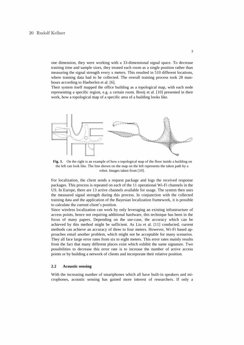
Their system itself mapped the office building as a topological map, with each node
representing a specific region, e.g. a certain room. Booij et al. [10] presented in their
work, how a topological map of a specific area of a building looks like.
Fig. 1. On the right is an example of how a topological map of the floor inside a building on
the left can look like. The line shown on the map on the left represents the taken path by a
robot. Images taken from [10].
For localization, the client sends a request package and logs the received response
packages. This process is repeated on each of the 11 operational Wi-Fi channels in the
US. In Europe, there are 13 active channels available for usage. The system then uses
the measured signal strength during this process. In conjunction with the collected
training data and the application of the Bayesian localization framework, it is possible
to calculate the current client’s position.
Since wireless localization can work by only leveraging an existing infrastructure of
access points, hence not requiring additional hardware, this technique has been in the
focus of many papers. Depending on the use-case, the accuracy which can be
achieved by this method might be sufficient. As Liu et al. [11] conducted, current
methods can achieve an accuracy of three to four meters. However, Wi-Fi based ap-
proaches entail another problem, which might not be acceptable for many scenarios.
They all face large error rates from six to eight meters. This error rates mainly results
from the fact that many different places exist which exhibit the same signature. Two
possibilities to decrease this error rate is to increase the number of active access
points or by building a network of clients and incorporate their relative position.
2.2 Acoustic sensing
With the increasing number of smartphones which all have built-in speakers and mi-
crophones, acoustic sensing has gained more interest of researchers. If only a
20 Rudolf Kellner

4
smartphone is needed on the client side, this lowers the barriers of using a system for
consumers. Acoustic sensing also enables multiple areas of application.
Song et al. [12] and Rossi et al. [13] developed a system based on acoustic sensing for
room-level localization. By leveraging room specific features of echoes, both systems
are able to determine the current room the user is positioned in with an accuracy of 89
to 99 percent, depending on the room size, occupancy and background noise. Kunze
et al. [14] implemented a method for object localization. Using only a smartphone,
they could determine the current location the device is situated in., e.g. if it is lying on
a couch or is put inside a drawer. Therefore, they utilized the vibration motor of the
smartphone in addition to measuring the response echo of the environment to an emit-
ted sound. Tung et al. [15] presented a possibility for indoor location tagging. This
enables a smartphone to detect its position with an accuracy of up to 1cm. This makes
use-cases such as enabling Wi-Fi on the smartphone if placed on a certain position
available to users. The same can be achieved by using NFC tags, but with additional
hardware required.
Regardless which type of localization is being performed, two different methods ex-
ists of how acoustic sensing can be carried out. Those two methods are active- as well
as passive sound fingerprinting. Passive sound fingerprinting solely relies on meas-
urements of the acoustic background spectrum of rooms. Each measurement result is
stored as a fingerprint. From these fingerprints, the system creates a unique room
label to later identify a certain room [3]. When performing active sound fingerprint-
ing, the device on the client side actively emits a specific sound through its speakers
and measures the corresponding impulse response. Section 3 and 4 describe those two
methods in detail.
2.3 With additional infrastructure
While most approaches independent from additional required hardware achieve room-
or meter-level localization when being indoors, more precise localization might be
necessary or wanted in certain scenarios. Independent of technology, various papers
have been published in which the authors achieved accuracy of up to a few centime-
ters. Liu et al. [16] proofed, that the need for extra hardware must not necessarily lead
to an inferior method. While it is indeed true that the client-side is more restricted
regarding devices necessary for the localization process, a specialized infrastructure at
the location must not have a huge impact for either side. Neither the costs nor the
required space are a matter of relative importance for e.g. a large store if the system
only requires a few beacons [7, 16, 17] or access points [6, 18]. While Wi-Fi based
localization works with most existing infrastructure, the precision can always be in-
creased by increasing the number of access points. Another advantage of these meth-
ods is that for most applications no training data must be acquired in advance. It is
sufficient if the system knows the location of the hardware inside the building. If that
is the case, the location of a device can then be calculated based on the received sig-
nals of one or more senders.
Room Recognition Using Audio Signals 21
5
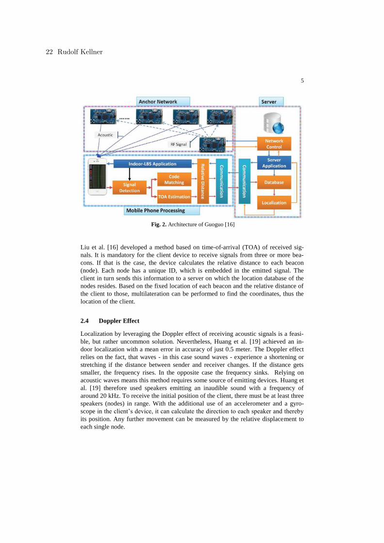
Fig. 2. Architecture of Guoguo [16]
Liu et al. [16] developed a method based on time-of-arrival (TOA) of received sig-
nals. It is mandatory for the client device to receive signals from three or more bea-
cons. If that is the case, the device calculates the relative distance to each beacon
(node). Each node has a unique ID, which is embedded in the emitted signal. The
client in turn sends this information to a server on which the location database of the
nodes resides. Based on the fixed location of each beacon and the relative distance of
the client to those, multilateration can be performed to find the coordinates, thus the
location of the client.
2.4 Doppler Effect
Localization by leveraging the Doppler effect of receiving acoustic signals is a feasi-
ble, but rather uncommon solution. Nevertheless, Huang et al. [19] achieved an in-
door localization with a mean error in accuracy of just 0.5 meter. The Doppler effect
relies on the fact, that waves - in this case sound waves - experience a shortening or
stretching if the distance between sender and receiver changes. If the distance gets
smaller, the frequency rises. In the opposite case the frequency sinks. Relying on
acoustic waves means this method requires some source of emitting devices. Huang et
al. [19] therefore used speakers emitting an inaudible sound with a frequency of
around 20 kHz. To receive the initial position of the client, there must be at least three
speakers (nodes) in range. With the additional use of an accelerometer and a gyro-
scope in the client’s device, it can calculate the direction to each speaker and thereby
its position. Any further movement can be measured by the relative displacement to
each single node.
22 Rudolf Kellner
6
3 Active sound fingerprinting
As the name suggests, active sound fingerprinting works by emitting sounds of specif-
ic frequencies and measuring its impulse response. The frequency differs depending
on each approach. While some systems are emitting an – to the human – inaudible
sound with a frequency slightly above 20 kHz, devices in other approaches emit audi-
ble sounds. Audible frequencies reside between 20 Hz und 20 kHz but slightly vary
for each human. Another important aspect of active sound fingerprinting is how to
deal with the recorded responses. Various techniques and algorithms therefore exist,
each coming with advantages as well as some disadvantages. This chapter describes
those technical factors in detail and compares the most promising approaches for
room recognition using active sound fingerprinting.
Because acoustic sensing and hence active sound fingerprinting is based on recording,
comparing and matching of fingerprints, training data must be collected for each loca-
tion at which future localization or recognition is intended. However, the required size
of training data differs from approach to approach.
This technique is also often combined with different techniques or data from other
sensors to further improve accuracy. The implementation of a specific system hence is
not limited to just one method.
3.1 Technical background
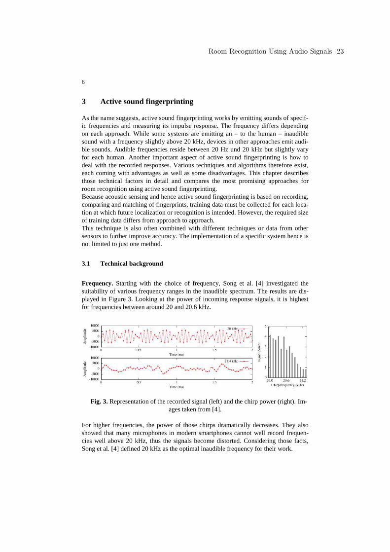
Frequency. Starting with the choice of frequency, Song et al. [4] investigated the
suitability of various frequency ranges in the inaudible spectrum. The results are dis-
played in Figure 3. Looking at the power of incoming response signals, it is highest
for frequencies between around 20 and 20.6 kHz.
Fig. 3. Representation of the recorded signal (left) and the chirp power (right). Im-
ages taken from [4].
For higher frequencies, the power of those chirps dramatically decreases. They also
showed that many microphones in modern smartphones cannot well record frequen-
cies well above 20 kHz, thus the signals become distorted. Considering those facts,
Song et al. [4] defined 20 kHz as the optimal inaudible frequency for their work.
Room Recognition Using Audio Signals 23
7
Tachikawa et al. [5] go for a different approach by playing an audible sound. But
instead of limiting the emitted sound to just one frequency, they perform a full sweep
from 20 Hz to 20 kHz, thus sampling the full audible range. In order to minimize the
impact for users, they limit the sound duration to 0.1 seconds.
Impulse Response Measurement. An accurate measurement of the incoming re-
sponse to an outgoing audio signal is one of the key tasks in room recognition, be-
cause the responds contains specific room features. As a result, many important pa-
rameters can be derived from the impulse response. Stan et al. [20] compared the
most commonly used techniques for impulse measurement. Among these are the
Maximum Length Sequence (MLS) and the Sine Sweep technique. Some given facts
apply independent from a specific technique. First, the emitted sound must be re-
membered and reproducible. Second, for better recognition, the signal-to-noise ratio
of the response must be as high as possible. This ratio can be improved by averaging
multiple measured output signals before starting with the deconvolution of the re-
sponse [20].
The MLS is a periodic two-level signal which has a higher power than short impulses
by the same output but a longer duration. This results in a better signal-to-noise ratio.
The underlying theory is based on the assumption, that MLS works best with linear,
time-invariant (LTI) systems. If that is not the case, the impulse responses contain
distortion artifacts. An important aspect is that they have almost identical properties
as a white noise [21]. An MLS signal of an M order in one period has a sample count,
thus a length of:
L = 2M -1 (1)
MLS can be generated by using maximal linear feedback shift registers, which recur-
sive function can be displayed as followed [13]:
(2)
Let the responses of an impulse be h[n] and the MLS be s[n], then the output y[n] is:
y[n] = (h*s) [n] (3)
It is known that the room impulse response can be obtained by circular cross-
correlation between the determined output signal and the measured input signal [13].
As a result, when taking the cross-correlation of y[n] and s[n] and assuming that Øss is
an impulse (h[n] = Øys), the equation simplifies to:
Øys = h[n] ∗ Øss = h[n] (4)
Sine Wave Sweep is a method not dependent on LTI systems, thus better suitable for
room-type recognition as carried out in [22]. It uses an exponential sine sweep (ESS)
whose frequencies grow with time. The frequency growth rate can be freely chosen.
24 Rudolf Kellner
8
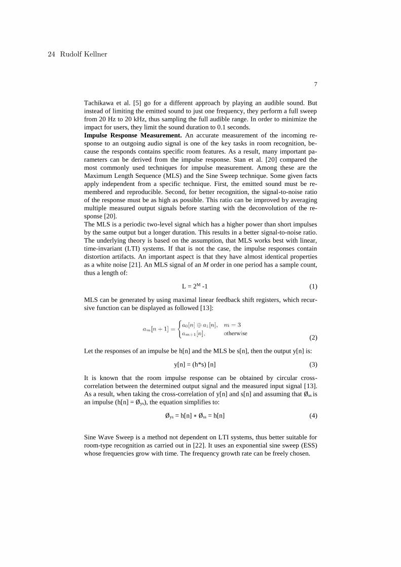
Using this technique, the impulse response (IR) can be deconvolved. Separating each
impulse response corresponding to the considered harmonic distortion order is rela-
tively easy because distortions are easy to recognize (shown in Figure 4).
Fig. 4. Exponential Sine Sweep on the left and its measurement with distortions on
the right [23]. The upper shorter lines thereby represent the distortions.
The linear impulse response thereby is free from any non-linearity. This is assured
because the distortion appears prior to its linear impulse response [20]. Due to the fact
that the emitted sweep must extend from 20 Hz to 20.000 Hz, the device emits an
audible sound.
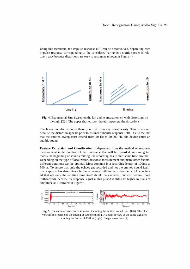
Feature Extraction and Classification. Independent from the method of response
measurement is the duration of the timeframe that will be recorded. Assuming t=0
marks the beginning of sound emitting, the recording has to start some time around t.
Depending on the type of localization, response measurement and many other factors,
different durations can be optimal. Most common is a recording length of 100ms to
500ms. To assure that only the echoes get recorded and not the emitted sound itself,
many approaches determine a buffer of several milliseconds. Song et al. [4] conclud-
ed that not only the emitting time itself should be excluded, but also several more
milliseconds, because the response signal in this period is still a lot higher in terms of
amplitude as illustrated in Figure 5.
Fig. 5. The entire acoustic trace since t=0 including the emitted sound itself (left). The blue
vertical line represents the ending of sound emitting. A zoom-in view of the same signal ex-
cluding the buffer of 13.8ms (right). Image taken from [4].
Room Recognition Using Audio Signals 25
9
For further processing the complete response is mostly [e.g. 5, 13, 22] processed in
multiple frames with a sliding windows of different window size and overlap. To
reduce errors and minimize the impact of outliers, each window can get smoothened
using a filter, e.g. Hamming Filter.
Common audio features can then be extracted from each frame. Among typical audio
features are [24]:
─ Spectral flux (SF)
─ Auto Correlation Function (ACF)
─ Zero crossing rate (ZCR)
─ Linear Bands (LINBANDS)
─ Logarithmic Bands (LOGBANDS)
─ Linear Predictive Coding (LPC)
─ Line spectral frequencies (LSF)
─ Daubechies Wavelet coefficient histogram features (DWCH)
─ Mel-Freq. Cepstral Coefficients (MFCC)
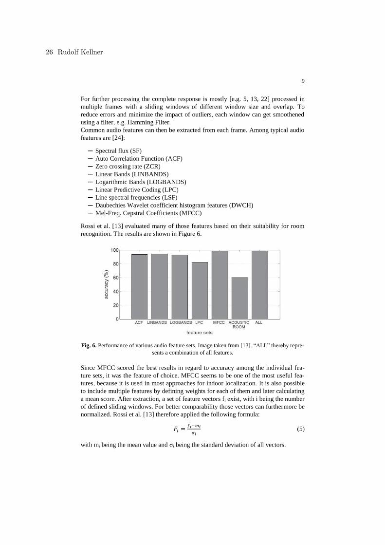
Rossi et al. [13] evaluated many of those features based on their suitability for room
recognition. The results are shown in Figure 6.
Fig. 6. Performance of various audio feature sets. Image taken from [13]. “ALL” thereby repre-
sents a combination of all features.
Since MFCC scored the best results in regard to accuracy among the individual fea-
ture sets, it was the feature of choice. MFCC seems to be one of the most useful fea-
tures, because it is used in most approaches for indoor localization. It is also possible
to include multiple features by defining weights for each of them and later calculating
a mean score. After extraction, a set of feature vectors fi exist, with i being the number
of defined sliding windows. For better comparability those vectors can furthermore be
normalized. Rossi et al. [13] therefore applied the following formula:
𝐹𝑖 =𝑓𝑖−𝑚𝑖
𝜎𝑖 (5)
with mi being the mean value and σi being the standard deviation of all vectors.
26 Rudolf Kellner
10
The chosen features can now be used for classification. The goal of classification is to
use a suitable algorithm in order to gather information from labeled data. It is in addi-
tion to Regression one of the two categories of Supervised Learning. The difference is
that Regression predicts numerical values while Classification predicts a category for
each entry of the dataset. Therefore, many different algorithms exist, e.g. Logistic
Regression, K-Nearest Neighbors, Support Vector Machine (SVM), Naive Bayes or
decision trees. A general comparison of various algorithms regarding performance
can be found in [25]. For room recognition, Tung et al. [15] evaluated different algo-
rithms within the scope of their work and came to the conclusion, that one-against-all
SVM performs best. It is a specific implementation of the Support Vector Machine,
which in turn is one of the most popular machine learning methods today. Initially
designed for binary classification [27], it is the choice in many works about room
recognition and indoor localization. Another popular library for SVMs is LIBSVM
[26]. Another viable algorithm is Random Forest. Tachikawa et al. [5] are using the
Random Forest with custom Decision Trees implemented. The final result then is
performed by a majority vote.
Deep Learning. Recent progress in Neural Networks opened another possibility
which can replace feature extraction and classification as described above. Since these
steps rely on manual feature engineering which deep learning can automate these
steps and thus simplify the process. As described in [4], two different types of deep
models exist, that are also viable for feature extraction of audio signals. Deep Neural
Networks (DNN) and Convolutional Neural Networks (CNN). As described by
Krizhevsky et al. [29], CNNs are more flexible, since their depth and breadth can be
varied. DNN allows a one-dimensional input only, while CNN can process data com-
ing from multiple input arrays. Both models are already in use for various use cases
such as image or language recognition. Song et al. [4] evaluated both in terms of via-
bility for feature extraction of audio signals and concluded, that CNN outperforms
DNN. Hence, they are using CNN for further work.
Convolutional Neural Networks consists of a series of stages each with one or multi-
ple layers. The first stages typically consist of two types of layers. Convolutional and
pooling layers. Convolutional layers thereby detect local conjunctions of features
from the previous layer. Pooling layers work by merge semantically similar features
into one feature [28].
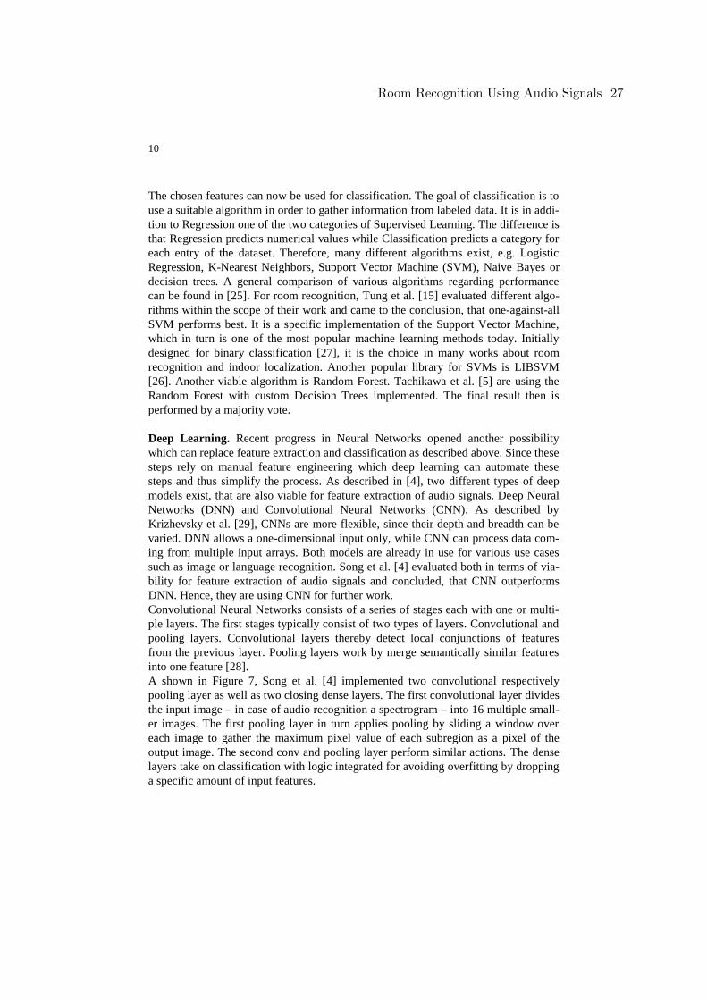
A shown in Figure 7, Song et al. [4] implemented two convolutional respectively
pooling layer as well as two closing dense layers. The first convolutional layer divides
the input image – in case of audio recognition a spectrogram – into 16 multiple small-
er images. The first pooling layer in turn applies pooling by sliding a window over
each image to gather the maximum pixel value of each subregion as a pixel of the
output image. The second conv and pooling layer perform similar actions. The dense
layers take on classification with logic integrated for avoiding overfitting by dropping
a specific amount of input features.
Room Recognition Using Audio Signals 27
11
Fig. 7. Structure of the Convolutional Neural Network as used in [4].
As for any neural network, extensive training is required for reasonable results. The
choice of Hyperparameters of the algorithm can highly affect the results as well.
Number of epochs, Batch size, Number of hidden layers and units, or Weight initiali-
zation are some of them. An article on the Towards Data Science Homepage [30]
describes the just mentioned hyperparameter and many more in detail.
Since training such a neural network requires extensive amount of processing power,
room recognition services using this method rely on a server in the cloud for conduct-
ing their work. If not, future localization on the client device would experience much
longer processing times as well as a noticeable battery drain.
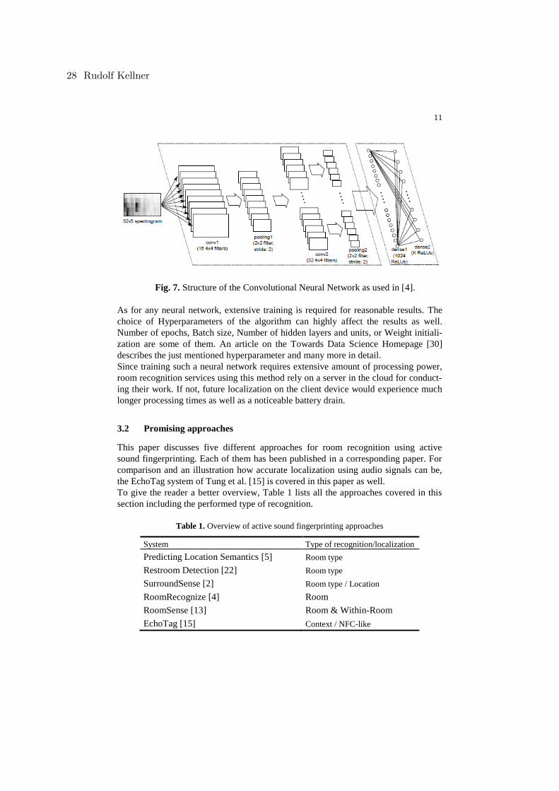
3.2 Promising approaches
This paper discusses five different approaches for room recognition using active
sound fingerprinting. Each of them has been published in a corresponding paper. For
comparison and an illustration how accurate localization using audio signals can be,
the EchoTag system of Tung et al. [15] is covered in this paper as well.
To give the reader a better overview, Table 1 lists all the approaches covered in this
section including the performed type of recognition.
Table 1. Overview of active sound fingerprinting approaches
System Type of recognition/localization
Predicting Location Semantics [5] Room type
Restroom Detection [22] Room type
SurroundSense [2] Room type / Location
RoomRecognize [4] Room
RoomSense [13] Room & Within-Room
EchoTag [15] Context / NFC-like
28 Rudolf Kellner
12
Room type recognition. Even though the first 3 methods [5, 22, 2] perform similar
recognition, they are not directly comparable regarding their results accuracy. [5] and
[22] attempt to recognize specific types of rooms or areas, e.g. restroom or smoking
area. The training data of [22] thereby does not include any data from exact locations
they later tried to classify. Thus, their system can later theoretically be used at any
location of the given type. [5] follows a similar trail. Their sensor data during the
training phase is manually collected featuring unknown location classes. As the name
suggests, [22] solely focuses on one type of room, that is restrooms. [5] extended their
method to six location classes. SurroundSense [2] on the other hand features multiple
location types as well but requires previous data collection from each of them. Among
those locations are a restaurant, a coffee shop and a grocery store.
In regard to utilized sensors, [5] is the most sophisticated approach. It uses data from
a barometer, magnetometer, Wi-Fi signals, as well as acceleration data in addition to
the speaker and microphone used for active probing. They detect a place by utilizing
acceleration data. If a user stays at the same place for a longer period of time, the
localization process gets initiated. The first step is to cluster recognized places based
on previously recorded Wi-Fi signals. This step reduces the number of possible plac-
es, which are now further analyzed using data from the mentioned sensors. Other
benefits of this intermediate step are a reduced error rate in recognition and a faster
classification process. Using this method, the authors could achieve an overall classi-
fication accuracy F-measure of 78%. Some room types thereby have better accuracies
in detection as others. The accuracy of detecting an elevator was about 90% while the
desk class often got classified as a meeting room due to similar conditions. They
found the active sound fingerprinting as the most helpful input. But using only this
data resulted in an accuracy of about 50%. They also conducted that data from the
barometric sensor contributed more to the final result than magnetic data. Those re-
sults show that despite sound fingerprinting being the most useful input data, combin-
ing data from multiple sensors leads to better accuracy in room recognition.
The authors of [22] illustrated, that despite real indoor localization being the more
viable approach, room type recognition still has its place for existence. In times of
always-on devices getting adopted more widely, there needs to exist a way to exclude
certain places from recordings, e.g. sound or video. One of these places are public
restrooms, where recordings of any type are not appropriate. In regard to this topic,
they developed their system. Unlike the described method of Tachikawa et al. [5],
only active sound fingerprinting was used to capture the impulse responses (IR) of
each restroom. No other sensors were therefore utilized. In order to better predict real-
life performance, the recorded samples of restrooms that are later classified were ex-
cluded from the training. They collected IR data from 103 restrooms with 30 samples
for each room at different spots inside the location. The results show, that they could
achieve an accuracy of above 90% most of the time, depending on which phone was
used. Thereby always the same phone was used for recording the training set and later
recognition. In order to evaluate their work against its robustness towards background
noises, they collected additional data for a restroom. For the new recordings, they
varied the occupancy rate from 14% up to 100%. Each person thereby used the re-
stroom as a normal person would including flushing the toilet and washing their
Room Recognition Using Audio Signals 29

13
hands. They tested this newly collected data using the same data corpus as before.
The achieved results were similar to the previous with an accuracy of above 90%.
This experiment proves, that active sound fingerprinting can be robust against various
background noises. However, an important aspect the authors worked out within their
work is the fact that the accuracy dramatically drops (down to 43%-63%) when dif-
ferent phones are used for collecting the training data and later recognition. For the
authors this is attributable to the differences in hard- and software of each phone.
SurroundSense, a relatively old approach by todays standards going back to the year
2009, included data from a light sensor in addition to acoustic data for their recogni-
tion technique. They collected data from six distinct places using a Laptop with an
additional attached sensor, because smartphones we know today did not exist at that
time. However, they already started evaluating their approach on a Nokia N95 device.
For localization, they compared the fingerprints of light and sound data with the once
previously collected. Therefore, they compared each fingerprint with a “simple
matching algorithm” [2], which output is a value of similarity. More precise, it is the
inverse of the Euclidian distance. The smaller the distance, the higher the similarity.
During evaluation, the output value of the algorithm was the highest for each correct
location. In other words, it identified all places correctly. Nevertheless, the similarity
value of a location often was almost identical to that of another location. The authors
did not state, how their method performs when classifying more than six places or
how robust it is against changes in background audio or different light conditions.
Room and within-room recognition. The ability to differentiate between multiple
rooms of the same type opens many possibilities, e.g. indoor navigation or tour
guides. Two viable solutions for this topic are consecutively described in this chapter.
RoomSense [13] and RoomRecognize [4].
The authors of RoomSense aim at not only recognizing specific rooms, but also cer-
tain positions within each room. Therefore, they selected 20 rooms and a total of 67
positions at which impulse response data was collected. As the authors stated, that is
the equivalent of about one position every 9m2. To achieve within-room recognition,
two orientations where chosen for each position; towards the center of each room and
towards the opposite direction. For each orientation, training data of 40 measurements
were carried out, which results in a dataset of 5360 IR measurements in total. For
feature extraction and classification, the MLS technique, MFCC, and an SVM classi-
fier (Chapter 3.1) were used. Using all training data, the recognition performance
averaged at 98,2%. This high accuracy is based on the high density of training posi-
tions which plays an important role regarding the performance of recognition. Figure
8 illustrates the change in accuracy when lowering the density of 9m2.
30 Rudolf Kellner
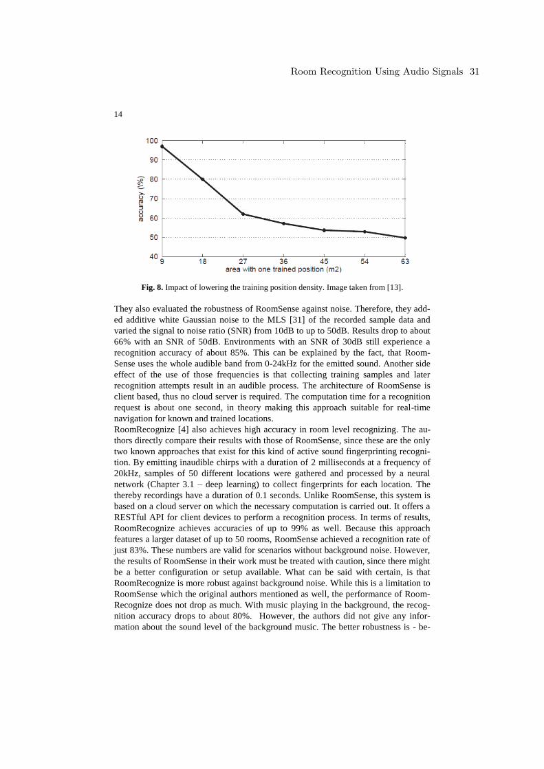
14
Fig. 8. Impact of lowering the training position density. Image taken from [13].
They also evaluated the robustness of RoomSense against noise. Therefore, they add-
ed additive white Gaussian noise to the MLS [31] of the recorded sample data and
varied the signal to noise ratio (SNR) from 10dB to up to 50dB. Results drop to about
66% with an SNR of 50dB. Environments with an SNR of 30dB still experience a
recognition accuracy of about 85%. This can be explained by the fact, that Room-
Sense uses the whole audible band from 0-24kHz for the emitted sound. Another side
effect of the use of those frequencies is that collecting training samples and later
recognition attempts result in an audible process. The architecture of RoomSense is
client based, thus no cloud server is required. The computation time for a recognition
request is about one second, in theory making this approach suitable for real-time
navigation for known and trained locations.
RoomRecognize [4] also achieves high accuracy in room level recognizing. The au-
thors directly compare their results with those of RoomSense, since these are the only
two known approaches that exist for this kind of active sound fingerprinting recogni-
tion. By emitting inaudible chirps with a duration of 2 milliseconds at a frequency of
20kHz, samples of 50 different locations were gathered and processed by a neural
network (Chapter 3.1 – deep learning) to collect fingerprints for each location. The
thereby recordings have a duration of 0.1 seconds. Unlike RoomSense, this system is
based on a cloud server on which the necessary computation is carried out. It offers a
RESTful API for client devices to perform a recognition process. In terms of results,
RoomRecognize achieves accuracies of up to 99% as well. Because this approach
features a larger dataset of up to 50 rooms, RoomSense achieved a recognition rate of
just 83%. These numbers are valid for scenarios without background noise. However,
the results of RoomSense in their work must be treated with caution, since there might
be a better configuration or setup available. What can be said with certain, is that
RoomRecognize is more robust against background noise. While this is a limitation to
RoomSense which the original authors mentioned as well, the performance of Room-
Recognize does not drop as much. With music playing in the background, the recog-
nition accuracy drops to about 80%. However, the authors did not give any infor-
mation about the sound level of the background music. The better robustness is - be-
Room Recognition Using Audio Signals 31
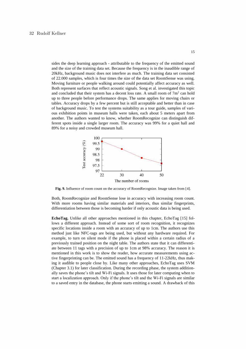
15
sides the deep learning approach - attributable to the frequency of the emitted sound
and the size of the training data set. Because the frequency is in the inaudible range of
20kHz, background music does not interfere as much. The training data set consisted
of 22.000 samples, which is four times the size of the data set RoomSense was using.
Moving furniture or people walking around could potentially affect accuracy as well.
Both represent surfaces that reflect acoustic signals. Song et al. investigated this topic
and concluded that their system has a decent loss rate. A small room of 7m2 can hold
up to three people before performance drops. The same applies for moving chairs or
tables. Accuracy drops by a few percent but is still acceptable and better than in case
of background music. To test the systems suitability as a tour guide, samples of vari-
ous exhibition points in museum halls were taken, each about 5 meters apart from
another. The authors wanted to know, whether RoomRecognize can distinguish dif-
ferent spots inside a single larger room. The accuracy was 99% for a quiet hall and
89% for a noisy and crowded museum hall.
Fig. 9. Influence of room count on the accuracy of RoomRecognize. Image taken from [4].
Both, RoomRecognize and RoomSense lose in accuracy with increasing room count.
With more rooms having similar materials and interiors, thus similar fingerprints,
differentiation between those is becoming harder if only acoustic data is being used.
EchoTag. Unlike all other approaches mentioned in this chapter, EchoTag [15] fol-
lows a different approach. Instead of some sort of room recognition, it recognizes
specific locations inside a room with an accuracy of up to 1cm. The authors use this
method just like NFC-tags are being used, but without any hardware required. For
example, to turn on silent mode if the phone is placed within a certain radius of a
previously trained position on the night table. The authors state that it can differenti-
ate between 11 tags with a precision of up to 1cm at 98% accuracy. The reason it is
mentioned in this work is to show the reader, how accurate measurements using ac-
tive fingerprinting can be. The emitted sound has a frequency of 11-22kHz, thus mak-
ing it audible to people close by. Like many other approaches, EchoTag uses SVM
(Chapter 3.1) for later classification. During the recording phase, the system addition-
ally saves the phone’s tilt and Wi-Fi signals. It uses those for later computing when to
start a localization approach. Only if the phone’s tilt and the Wi-Fi signals are similar
to a saved entry in the database, the phone starts emitting a sound. A drawback of this
32 Rudolf Kellner

16
approach is, that accuracy drops over time. Depending on the location by about 40%
down to 56%. This is due to indoor activity like removing or adding objects. The
authors state that in order to counter this drop in performance continuously training is
required.
3.3 Detailed overview of approaches using active sound fingerprinting
For a final overview and better evaluation by the reader, a table with detailed infor-
mation on the here described approaches is presented (Table 2). The most important
distinguishing features are thereby included. However, the overall recognition results
are not directly comparable due to multiple facts. First, those numbers represent the
results under optimal conditions. Disturbances are not considered in this table, be-
cause each approach has its own to deal with, which often differ from the ones anoth-
er approach has to deal with. Second, the room count included in the training set var-
ies highly. With increasing number of fingerprints collected the accuracy drops. Last,
it is not recommended to compare approaches of a different recognition type.
Table 2. Summary of approaches utilizing active sound fingerprinting
Predicting
Location Se-
mantics [5]
Restroom
Detection
[22]
Surround-
Sense [2]
RoomRecog-
nize [4]
RoomSense
[13]
EchoTag
[15]
Recognition type Room type Room type Room type Room Room &
Within-Room Location
accuracy room-level room-level room-level room-level 300cm 1cm
Number of rooms 6 classes
24 rooms
103 + non
restrooms 6 50 20 11 tags
Data set size N/A 7.474 N/A 22.000 5360 N/A
Feature extraction
& classification
MFCC, Ran-
dom Forest
MFCC,
LibSVM
Euclidian
distance
Deep Learn-
ing
MLS, MFCC,
SVM N/A, SVM
Architecture client client client client-server client client
Emitted sound
duration & fre-
quency
100ms
SineSweep *
100ms
SineSweep *
N/A
20-250Hz
100ms
20kHz
680ms
0-24kHz
420ms
11-22kHz
Sensors used
Microphone
Speaker
Barometer
Magnetometer
Wi-Fi
Accelerator
Microphone
Speaker
Microphone
Speaker
Light
Microphone
Speaker
Microphone
Speaker
Microphone
Speaker
Wi-Fi
Gyroscope
Room Recognition Using Audio Signals 33
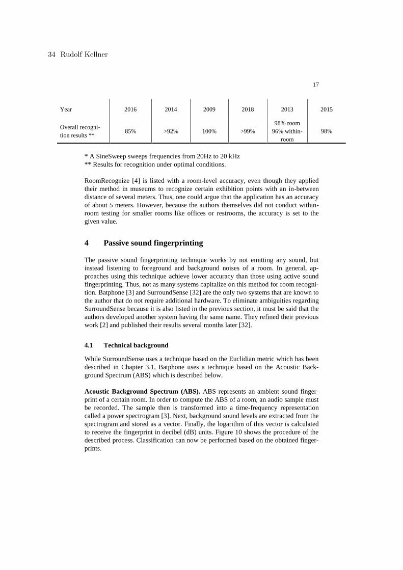
17
Year 2016 2014 2009 2018 2013 2015
Overall recogni-
tion results ** 85% >92% 100% >99%
98% room
96% within-
room
98%
* A SineSweep sweeps frequencies from 20Hz to 20 kHz
** Results for recognition under optimal conditions.
RoomRecognize [4] is listed with a room-level accuracy, even though they applied
their method in museums to recognize certain exhibition points with an in-between
distance of several meters. Thus, one could argue that the application has an accuracy
of about 5 meters. However, because the authors themselves did not conduct within-
room testing for smaller rooms like offices or restrooms, the accuracy is set to the
given value.
4 Passive sound fingerprinting
The passive sound fingerprinting technique works by not emitting any sound, but
instead listening to foreground and background noises of a room. In general, ap-
proaches using this technique achieve lower accuracy than those using active sound
fingerprinting. Thus, not as many systems capitalize on this method for room recogni-
tion. Batphone [3] and SurroundSense [32] are the only two systems that are known to
the author that do not require additional hardware. To eliminate ambiguities regarding
SurroundSense because it is also listed in the previous section, it must be said that the
authors developed another system having the same name. They refined their previous
work [2] and published their results several months later [32].
4.1 Technical background
While SurroundSense uses a technique based on the Euclidian metric which has been
described in Chapter 3.1, Batphone uses a technique based on the Acoustic Back-
ground Spectrum (ABS) which is described below.
Acoustic Background Spectrum (ABS). ABS represents an ambient sound finger-
print of a certain room. In order to compute the ABS of a room, an audio sample must
be recorded. The sample then is transformed into a time-frequency representation
called a power spectrogram [3]. Next, background sound levels are extracted from the
spectrogram and stored as a vector. Finally, the logarithm of this vector is calculated
to receive the fingerprint in decibel (dB) units. Figure 10 shows the procedure of the
described process. Classification can now be performed based on the obtained finger-
prints.
34 Rudolf Kellner
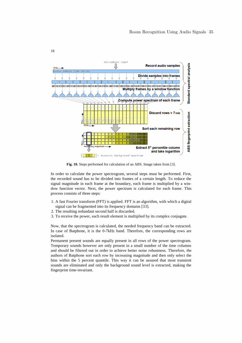
18
Fig. 10. Steps performed for calculation of an ABS. Image taken from [3].
In order to calculate the power spectrogram, several steps must be performed. First,
the recorded sound has to be divided into frames of a certain length. To reduce the
signal magnitude in each frame at the boundary, each frame is multiplied by a win-
dow function vector. Next, the power spectrum is calculated for each frame. This
process consists of three steps:
1. A fast Fourier transform (FFT) is applied. FFT is an algorithm, with which a digital
signal can be fragmented into its frequency domains [33].
2. The resulting redundant second half is discarded.
3. To receive the power, each result element is multiplied by its complex conjugate.
Now, that the spectrogram is calculated, the needed frequency band can be extracted.
In case of Batphone, it is the 0-7kHz band. Therefore, the corresponding rows are
isolated.
Permanent present sounds are equally present in all rows of the power spectrogram.
Temporary sounds however are only present in a small number of the time columns
and should be filtered out in order to achieve better noise robustness. Therefore, the
authors of Batphone sort each row by increasing magnitude and then only select the
bins within the 5 percent quantile. This way it can be assured that most transient
sounds are eliminated and only the background sound level is extracted, making the
fingerprint time-invariant.
Room Recognition Using Audio Signals 35
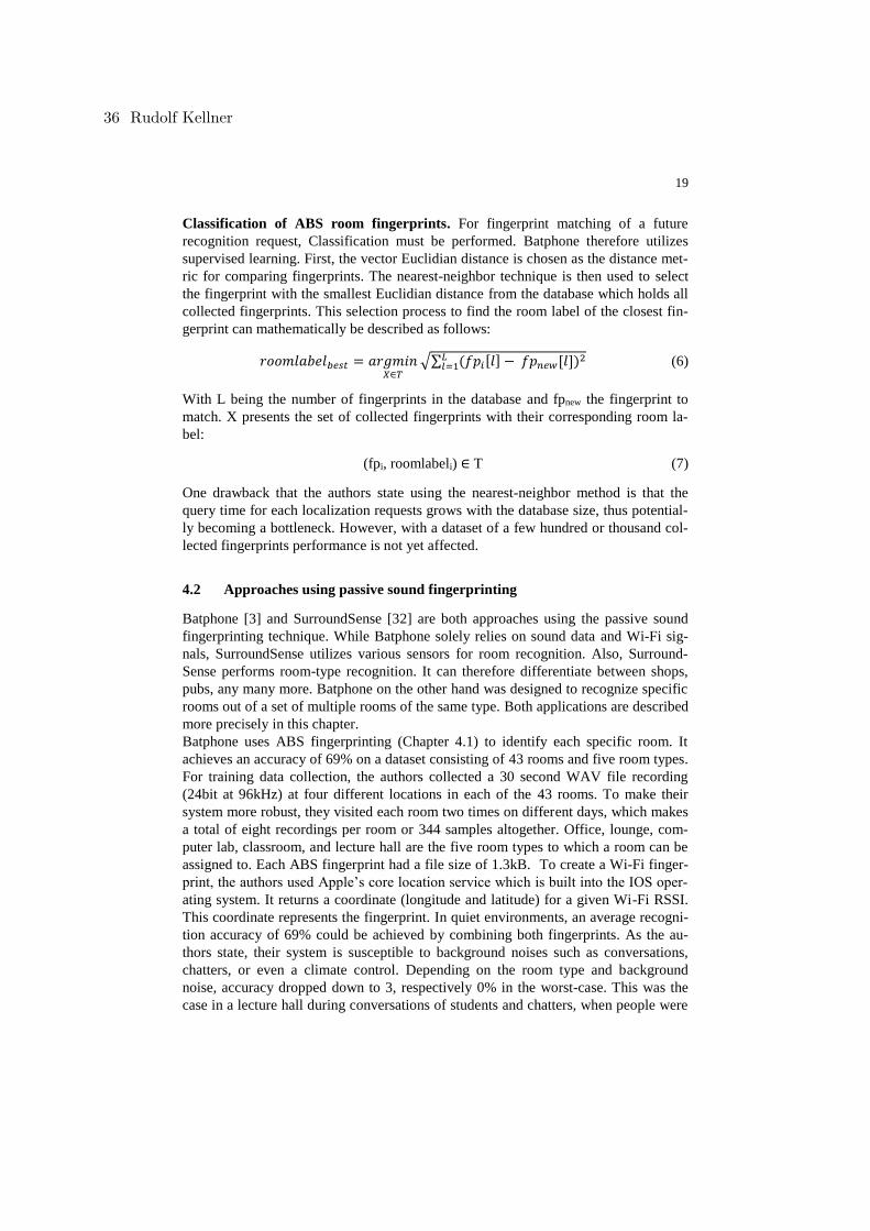
19
Classification of ABS room fingerprints. For fingerprint matching of a future
recognition request, Classification must be performed. Batphone therefore utilizes
supervised learning. First, the vector Euclidian distance is chosen as the distance met-
ric for comparing fingerprints. The nearest-neighbor technique is then used to select
the fingerprint with the smallest Euclidian distance from the database which holds all
collected fingerprints. This selection process to find the room label of the closest fin-
gerprint can mathematically be described as follows:
𝑟𝑜𝑜𝑚𝑙𝑎𝑏𝑒𝑙𝑏𝑒𝑠𝑡 = 𝑎𝑟𝑔𝑚𝑖𝑛𝑋∈𝑇
√∑ (𝑓𝑝𝑖[𝑙] − 𝑓𝑝𝑛𝑒𝑤[𝑙])2𝐿𝑙=1 (6)
With L being the number of fingerprints in the database and fpnew the fingerprint to
match. X presents the set of collected fingerprints with their corresponding room la-
bel:
(fpi, roomlabeli) ∈ T (7)
One drawback that the authors state using the nearest-neighbor method is that the
query time for each localization requests grows with the database size, thus potential-
ly becoming a bottleneck. However, with a dataset of a few hundred or thousand col-
lected fingerprints performance is not yet affected.
4.2 Approaches using passive sound fingerprinting
Batphone [3] and SurroundSense [32] are both approaches using the passive sound
fingerprinting technique. While Batphone solely relies on sound data and Wi-Fi sig-
nals, SurroundSense utilizes various sensors for room recognition. Also, Surround-
Sense performs room-type recognition. It can therefore differentiate between shops,
pubs, any many more. Batphone on the other hand was designed to recognize specific
rooms out of a set of multiple rooms of the same type. Both applications are described
more precisely in this chapter.
Batphone uses ABS fingerprinting (Chapter 4.1) to identify each specific room. It
achieves an accuracy of 69% on a dataset consisting of 43 rooms and five room types.
For training data collection, the authors collected a 30 second WAV file recording
(24bit at 96kHz) at four different locations in each of the 43 rooms. To make their
system more robust, they visited each room two times on different days, which makes
a total of eight recordings per room or 344 samples altogether. Office, lounge, com-
puter lab, classroom, and lecture hall are the five room types to which a room can be
assigned to. Each ABS fingerprint had a file size of 1.3kB. To create a Wi-Fi finger-
print, the authors used Apple’s core location service which is built into the IOS oper-
ating system. It returns a coordinate (longitude and latitude) for a given Wi-Fi RSSI.
This coordinate represents the fingerprint. In quiet environments, an average recogni-
tion accuracy of 69% could be achieved by combining both fingerprints. As the au-
thors state, their system is susceptible to background noises such as conversations,
chatters, or even a climate control. Depending on the room type and background
noise, accuracy dropped down to 3, respectively 0% in the worst-case. This was the
case in a lecture hall during conversations of students and chatters, when people were
36 Rudolf Kellner
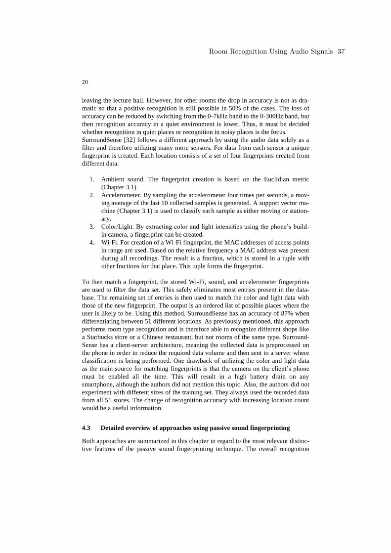
20
leaving the lecture hall. However, for other rooms the drop in accuracy is not as dra-
matic so that a positive recognition is still possible in 50% of the cases. The loss of
accuracy can be reduced by switching from the 0-7kHz band to the 0-300Hz band, but
then recognition accuracy in a quiet environment is lower. Thus, it must be decided
whether recognition in quiet places or recognition in noisy places is the focus.
SurroundSense [32] follows a different approach by using the audio data solely as a
filter and therefore utilizing many more sensors. For data from each sensor a unique
fingerprint is created. Each location consists of a set of four fingerprints created from
different data:
1. Ambient sound. The fingerprint creation is based on the Euclidian metric
(Chapter 3.1).
2. Accelerometer. By sampling the accelerometer four times per seconds, a mov-
ing average of the last 10 collected samples is generated. A support vector ma-
chine (Chapter 3.1) is used to classify each sample as either moving or station-
ary.
3. Color/Light. By extracting color and light intensities using the phone’s build-
in camera, a fingerprint can be created.
4. Wi-Fi. For creation of a Wi-Fi fingerprint, the MAC addresses of access points
in range are used. Based on the relative frequency a MAC address was present
during all recordings. The result is a fraction, which is stored in a tuple with
other fractions for that place. This tuple forms the fingerprint.
To then match a fingerprint, the stored Wi-Fi, sound, and accelerometer fingerprints
are used to filter the data set. This safely eliminates most entries present in the data-
base. The remaining set of entries is then used to match the color and light data with
those of the new fingerprint. The output is an ordered list of possible places where the
user is likely to be. Using this method, SurroundSense has an accuracy of 87% when
differentiating between 51 different locations. As previously mentioned, this approach
performs room type recognition and is therefore able to recognize different shops like
a Starbucks store or a Chinese restaurant, but not rooms of the same type. Surround-
Sense has a client-server architecture, meaning the collected data is preprocessed on
the phone in order to reduce the required data volume and then sent to a server where
classification is being performed. One drawback of utilizing the color and light data
as the main source for matching fingerprints is that the camera on the client’s phone
must be enabled all the time. This will result in a high battery drain on any
smartphone, although the authors did not mention this topic. Also, the authors did not
experiment with different sizes of the training set. They always used the recorded data
from all 51 stores. The change of recognition accuracy with increasing location count
would be a useful information.
4.3 Detailed overview of approaches using passive sound fingerprinting
Both approaches are summarized in this chapter in regard to the most relevant distinc-
tive features of the passive sound fingerprinting technique. The overall recognition
Room Recognition Using Audio Signals 37
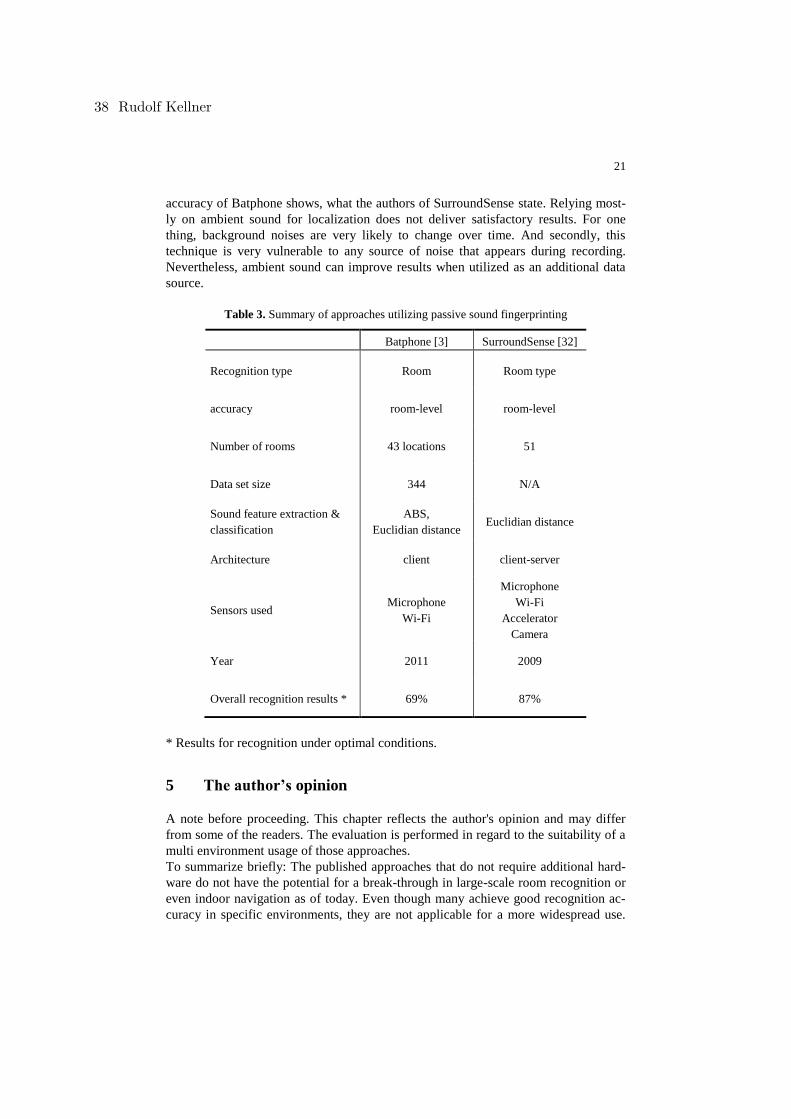
21
accuracy of Batphone shows, what the authors of SurroundSense state. Relying most-
ly on ambient sound for localization does not deliver satisfactory results. For one
thing, background noises are very likely to change over time. And secondly, this
technique is very vulnerable to any source of noise that appears during recording.
Nevertheless, ambient sound can improve results when utilized as an additional data
source.
Table 3. Summary of approaches utilizing passive sound fingerprinting
Batphone [3] SurroundSense [32]
Recognition type Room Room type
accuracy room-level room-level
Number of rooms 43 locations 51
Data set size 344 N/A
Sound feature extraction &
classification
ABS,
Euclidian distance Euclidian distance
Architecture client client-server
Sensors used Microphone
Wi-Fi
Microphone
Wi-Fi
Accelerator
Camera
Year 2011 2009
Overall recognition results * 69% 87%
* Results for recognition under optimal conditions.
5 The author’s opinion
A note before proceeding. This chapter reflects the author's opinion and may differ
from some of the readers. The evaluation is performed in regard to the suitability of a
multi environment usage of those approaches.
To summarize briefly: The published approaches that do not require additional hard-
ware do not have the potential for a break-through in large-scale room recognition or
even indoor navigation as of today. Even though many achieve good recognition ac-
curacy in specific environments, they are not applicable for a more widespread use.
38 Rudolf Kellner
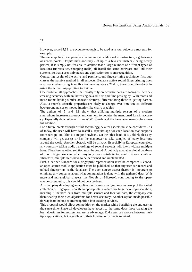
22
However, some [4,13] are accurate enough to be used as a tour guide in a museum for
example.
The same applies for approaches that require an additional infrastructure, e.g. beacons
or access points. Despite their accuracy - of up to a few centimeters - being nearly
perfect, it is simply not feasible to assume that a large number of different types of
locations (universities, shopping malls) all install the same hardware and link their
systems, so that a user only needs one application for room recognition.
Comparing results of the active and passive sound fingerprinting technique, first out-
classes the passive method in all respects. Because active sound fingerprinting does
also work when using inaudible frequencies above 20kHz, there is no drawback in
using the active fingerprinting technique.
One problem all approaches that mostly rely on acoustic data are facing is their de-
creasing accuracy with an increasing data set size and time passing by. With more and
more rooms having similar acoustic features, differentiating those is getting harder.
Also, a room’s acoustic properties are likely to change over time due to different
background noises or moved interior like chairs or tables.
The authors of [5] and [32] show, that utilizing multiple sensors of a modern
smartphone increases accuracy and can help to counter the mentioned loss in accura-
cy. Especially data collected from Wi-Fi signals and the barometer seem to be a use-
ful addition.
For a future break-through of this technology, several aspects must be considered. As
of today, the user will have to install a separate app for each location that supports
room recognition. This is a major drawback. On the other hand, it is unlikely that any
company will get access or has the manpower to take samples of many locations
around the world. Another obstacle will be privacy. Especially in European countries,
any company taking audio recordings of several seconds will likely violate multiple
laws. Therefore, another solution must be found. A publicly available global database
of room fingerprints to which anybody can contribute to would be one solution.
Therefore, multiple steps have to be performed and implemented.
First, a defined standard for a fingerprint representation must be composed. Second,
an open-source mobile application must be published, so that any user can record and
upload fingerprints to the database. The open-source aspect thereby is important to
eliminate any concerns about what computation is done with the gathered data. With
more and more global players like Google or Microsoft contributing to the open-
source community, this should not be a problem.
Any company developing an application for room recognition can now pull the global
collection of fingerprints. With an appropriate standard for fingerprint representation,
meaning it includes data from multiple sensors and location data, the company can
then develop their own algorithms for better accuracy. Another option made possible
tis way is to include room recognition into existing services.
This proposal would allow competition on the market while benefiting the end user at
the same time. Since all developers have access to the same data, those creating the
best algorithms for recognition are in advantage. End users can choose between mul-
tiple applications, but regardless of their location only one is required.
Room Recognition Using Audio Signals 39

23
References
1. Ionut Constandache, Xuan Bao, Martin Azizyan, and Romit Roy Choudhury: Did you see
Bob?: human localization using mobile phones. In: MobiCom 2010, pp. 149–160 (2010).
2. Martin Azizyan, and Romit Roy Choudhury: SurroundSense: mobile phone localization
using ambient sound and light. In: ACM SIGMOBILE Mobile Computing and Communi-
cations Review, Volume 13 Issue 1, pp. 69-72 (January 2009).
3. Stephen P. Tarzia, Peter A. Dinda, Robert P. Dick, and Gokhan Memik: Indoor localiza-
tion without infrastructure using the acoustic background spectrum. In: Proceedings of
ACM MobiSys 2011, pp. 155–168 (2011).
4. Qun Song, Chaojie Gu, and Rui Tan: Deep Room Recognition Using Inaudible Echos. In:
Proceedings of the ACM on Interactive, Mobile, Wearable and Ubiquitous Technologies,
Volume 2, No. 3, Article 135 (2018).
5. Masaya Tachikawa, Takuya Maekawa, and Yasuyuki Matsushita: Predicting location se-
mantics combining active and passive sensing with environment-independent classifier. In:
UbiComp '16 Proceedings of the 2016 ACM International Joint Conference on Pervasive
and Ubiquitous Computing, pp. 220-231 (2016).
6. Andreas Haeberlen, Eliot Flannery, Andrew M. Ladd, Algis Rudys, Dan S. Wallach, and
Lydia E. Kavraki: Practical robust localization over large-scale 802.11 wireless networks.
In: MobiCom '04 Proceedings of the 10th annual international conference on Mobile com-
puting and networking, pp. 70-84 (2004).
7. Roy Want, Andy Hopper, Veronica Falcão, and Jonathan Gibbons: The active badge loca-
tion system. In: ACM Transactions on Information Systems (TOIS) Volume 10 Issue 1,
pp. 91-102 (1992).
8. I. Constandache, S. Gaonkar, M. Sayler, R. R. Choudhury, and L. Cox: EnLoc: Energy-
efficient localization for mobile phones. In: IEEE INFOCOM 19-25 April 2009 (2009).
9. European Global Navigation Satellite Systems Agency Homepage,
https://www.gsa.europa.eu/european-gnss/galileo/galileo-european-global-satellite-based-
navigation-system, last accessed 2019/06/24.
10. O. Booij, B. Terwijn, Z. Zivkovic, and B. Krose: Navigation using an appearance based
topological map. In: Proceedings 2007 IEEE International Conference on Robotics and
Automation (2007).
11. H Liu, Y Gan, J Yang, S Sidhom, Y Wang, S Sidhom, Y. Wang, Y. Chen, and F. Ye: Push
the limit of WiFi based localization for smartphones. In: Mobicom '12 Proceedings of the
18th annual international conference on Mobile computing and networking, pp. 305-316
(2012).
12. Q Song, C Gu, and R Tan: Deep Room Recognition Using Inaudible Echos. In: Proceed-
ings of the ACM on Interactive, Mobile, Wearable and Ubiquitous Technologies Volume 2
Issue 3 (2018).
13. M Rossi, J Seiter, O Amft, S Buchmeier, and G. Tröster: RoomSense: an indoor position-
ing system for smartphones using active sound probing. In: AH '13 Proceedings of the 4th
Augmented Human International Conference, pp. 89-95 (2013).
14. Kai Kunze and Paul Lukowicz: Symbolic Object Localization Through Active Sampling
of Acceleration and Sound Signatures. In: UbiComp 2007: Ubiquitous Computing, pp.
163-180 (2007).
15. Yu-Chih Tung and Kang G. Shin: EchoTag: Accurate Infrastructure-Free Indoor Location
Tagging with Smartphones. In: MobiCom '15 Proceedings of the 21st Annual International
Conference on Mobile Computing and Networking, pp. 525-536 (2015).
40 Rudolf Kellner
24
16. Kaikai Liu, Xinxin Liu, and Xiaolin Li: Guoguo: Enabling Fine-grained Indoor Localiza-
tion via Smartphone. In: MobiSys '13 Proceeding of the 11th annual international confer-
ence on Mobile systems, applications, and services, pp 235-248 (2013).
17. Nissanka B. Priyantha, Anit Chakraborty, and Hari Balakrishnan: The Cricket Location-
Support System. In: MobiCom '00 Proceedings of the 6th annual international conference
on Mobile computing and networking, pp. 32-43 (2000).
18. Paul Castro, Patrick Chiu, Ted Kremenek, and Richard Muntz: A Probabilistic Room Lo-
cation Service for Wireless Networked Environments. In: UbiComp 2001: Ubicomp 2001:
Ubiquitous Computing, pp. 18-34 (2001).
19. Wenchao Huang, Yan Xiong, Xiang-Yang Li, Hao Lin, Xufei Mao, Panlong Yang, and
Yunhao Liu: Accurate Indoor Localization Using Acoustic Direction Finding via Smart
Phones. In: Proc. of IEEE INFOCOM (2014).
20. GB Stan, JJ Embrechts, and D Archambeau: Comparison of different impulse response
measurement techniques. In: Journal of the Audio Engineering Society Volume 50 Issue 4,
pp. 249-262 (2002).
21. LiveScience Homepage, https://www.livescience.com/38387-what-is-white-noise.html,
last accessed 2019/06/29.
22. Mingming Fan, Alexander Travis Adams, and Khai N. Truong: Public Restroom Detection
on Mobile Phone via Active Probing. In: ISWC '14 Proceedings of the 2014 ACM Interna-
tional Symposium on Wearable Computers, pp. 27-34 (2014).
23. Franco Policardi: MLS and Sine-Sweep technique comparison in room-acoustic measure-
ments. In: ELEKTROTEHNIŠKI VESTNIK 78(3) ENGLISH EDITION, pp. 91-95
(2011).
24. Dalibor Mitrović, Matthias Zeppelzauer, and Christian Breiteneder: Features for Content-
Based Audio Retrieval. In: Advances in Computers, pp. 71-150 (2010).
25. Rich Caruana, and Alexandru Niculescu-Mizil: An empirical comparison of supervised
learning algorithms. In: Proceeding ICML '06 Proceedings of the 23rd international con-
ference on Machine learning, pp. 161-168 (2006).
26. CC Chang, and CJ Lin: LIBSVM: A library for support vector machines. In: ACM Trans-
actions on Intelligent Systems and Technology Volume 2 Issue 3 (2011).
27. Y Liu, and YF Zheng: One-against-all multi-class SVM classification using reliability
measures. In: Proceedings. 2005 IEEE International Joint Conference on Neural Networks
(2005).
28. Yann LeCun, Yoshua Bengio, and Geoffrey Hinton: Deep learning. In: Nature 521, 7553,
pp. 436–444 (2015).
29. A Krizhevsky, I Sutskever, and GE Hinton: ImageNet Classification with Deep Convolu-
tional Neural Networks. In: Advances in Neural Information Processing Systems 25
(2012).
30. Towards Data Science Homepage, https://towardsdatascience.com/a-walkthrough-of-
convolutional-neural-network-7f474f91d7bd, last accessed 2019/07/01.
31. London South Bank University, Shafiul Alam: Assignment on: Effect of Additive White
Gaussian Noise (AWGN) on the Transmitted Data,
https://pdfs.semanticscholar.org/0320/f32a1580fc1f3bf5f015b7eefefcfc9d10c4.pdf (2008),
last accessed 2019/07/02.
32. Martin Azizyan, Ionut Constandache, and Romit Roy Choudhury: SurroundSense: mobile
phone localization via ambience fingerprinting. In: MobiCom '09 Proceedings of the 15th
annual international conference on Mobile computing and networking, pp. 261-272 (Sep-
tember 2009).
Room Recognition Using Audio Signals 41

25
33. W.T. Cochran, J.W. Cooley, D.L. Favin, H.D. Helms, R.A. Kaenel, W.W. Lang, G.C. Ma-
ling, D.E. Nelson, C.M. Rader, and P.D. Welch: What is the fast Fourier transform?. In:
Proceedings of the IEEE Volume: 55, Issue: 10, pp. 1664-1674 (1967).
42 Rudolf Kellner
Ubiquitous Object Imaging Using Audio Signals
Julian Westermann, Long Wang
Karlsruhe Institute of Technology - [email protected], [email protected]
Abstract. Object imaging is a field of research that is important fora various number of applications. A popular acoustic imaging techniqueis the ultrasound (US) imaging technique used for medical diagnosis.Because in todays society almost everybody owns an ubiquitous deviceaka smartphone there is a founded interest in bringing imaging tech-niques to the smartphone. As an example this allows to perform medicalultrasound based diagnosis in urgent situations like at the scene of anaccident. As taking images with a camera is widely used an alternativemight be acoustic imaging. This paper will present imaging techniquesthat are based on acoustic signals like US. For the most of these examplesdedicated hardware is needed to extend the smartphones functionality.However there is one approach that only uses a smartphones built-inspeaker and microphone. By presenting these techniques it is shown thattodays smartphones are already powerful enough to perform the task ofobject imaging.
1 Introduction
Camera based imaging is widely used and enjoys great popularity. However thisimaging approach still lacks in quality when it comes to taking images at darkplaces. This is only one property where acoustic based imaging is superior tocamera based imaging. Because acoustic signals are not dependent on lightingcondition they can be used for taking images in dark places, for example in acave or at night. Furthermore acoustic signals can propagate around obstructionswhich allows to see around corners[1] and they can penetrate materials allowingto detect weapons hidden under clothes[2].
When it comes to fields of application smartphone based acoustic imaginghas a broad spectrum of use cases. By bringing ultrasound diagnosis to a mobiledevice usage in urgent situations like the scene of an accident or on a battlefieldcan become possible. Obstacles in dark places like a cave can also be detectedwhen using acoustic signals and can thereby help to navigate through situationswith bad lighting conditions. At an airport or at crowded places like concertsan acoustic based imaging technique can help to detect weapons hidden underclothes like mentioned befor. However the advantage is hereby that it can com-plement commodity security scanners by detecting non-metallic weapons. At lastit is also possible to detect the wear level of a tool and thereby be able to decideif it needs to be replaced or is still fully functional.
Ubiquitous Object Imaging Using Audio Signals 43
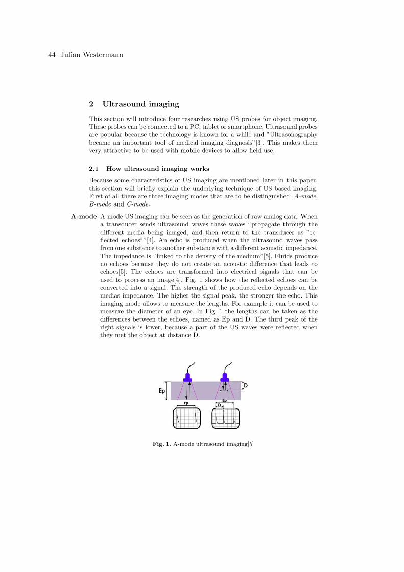
2 Ultrasound imaging
This section will introduce four researches using US probes for object imaging.These probes can be connected to a PC, tablet or smartphone. Ultrasound probesare popular because the technology is known for a while and ”Ultrasonographybecame an important tool of medical imaging diagnosis”[3]. This makes themvery attractive to be used with mobile devices to allow field use.
2.1 How ultrasound imaging works
Because some characteristics of US imaging are mentioned later in this paper,this section will briefly explain the underlying technique of US based imaging.First of all there are three imaging modes that are to be distinguished: A-mode,B-mode and C-mode.
A-mode A-mode US imaging can be seen as the generation of raw analog data. Whena transducer sends ultrasound waves these waves ”propagate through thedifferent media being imaged, and then return to the transducer as ”re-flected echoes””[4]. An echo is produced when the ultrasound waves passfrom one substance to another substance with a different acoustic impedance.The impedance is ”linked to the density of the medium”[5]. Fluids produceno echoes because they do not create an acoustic difference that leads toechoes[5]. The echoes are transformed into electrical signals that can beused to process an image[4]. Fig. 1 shows how the reflected echoes can beconverted into a signal. The strength of the produced echo depends on themedias impedance. The higher the signal peak, the stronger the echo. Thisimaging mode allows to measure the lengths. For example it can be used tomeasure the diameter of an eye. In Fig. 1 the lengths can be taken as thedifferences between the echoes, named as Ep and D. The third peak of theright signals is lower, because a part of the US waves were reflected whenthey met the object at distance D.
Fig. 1. A-mode ultrasound imaging[5]
44 Julian Westermann
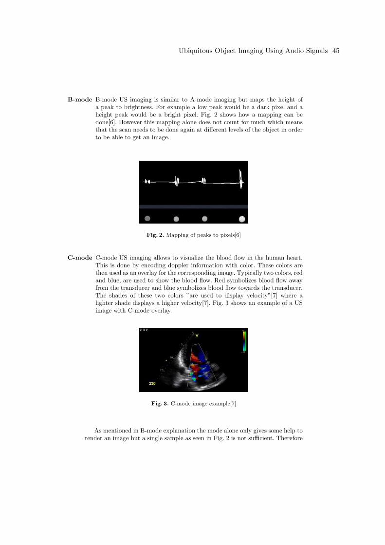
B-mode B-mode US imaging is similar to A-mode imaging but maps the height ofa peak to brightness. For example a low peak would be a dark pixel and aheight peak would be a bright pixel. Fig. 2 shows how a mapping can bedone[6]. However this mapping alone does not count for much which meansthat the scan needs to be done again at different levels of the object in orderto be able to get an image.
Fig. 2. Mapping of peaks to pixels[6]
C-mode C-mode US imaging allows to visualize the blood flow in the human heart.This is done by encoding doppler information with color. These colors arethen used as an overlay for the corresponding image. Typically two colors, redand blue, are used to show the blood flow. Red symbolizes blood flow awayfrom the transducer and blue symbolizes blood flow towards the transducer.The shades of these two colors ”are used to display velocity”[7] where alighter shade displays a higher velocity[7]. Fig. 3 shows an example of a USimage with C-mode overlay.
Fig. 3. C-mode image example[7]
As mentioned in B-mode explanation the mode alone only gives some help torender an image but a single sample as seen in Fig. 2 is not sufficient. Therefore
Ubiquitous Object Imaging Using Audio Signals 45

it is necessary to repeat the imaging procedure at different spots or by tiltingthe transducer left and right to get more samples and thereby creating an image.For tilting the transducer there are two possible ways as can be seen in Fig. 4and Fig. 5.
Fig. 4. Manual sweeping[6]Fig. 5. Virtual sweeping by using morechannels and phase shift[6]
Fig. 4 shows an image that has been created by manuelly tilting the trans-ducer left and right, thereby producing an image using the B-mode scan.Fig. 5 shows how 4 piezoelement elements (4 channel transducer) can be used tocreate the same effect as in Fig. 4. The 4 channels are used in a way that not allsend at the same time. Moreover the elements are used with a phase shift. Thismeans that as in Fig. 4 the first channel is delayed by π, second by 0.6π, thirdby 0.3π and the fourth is not delayed at all. These different delays create a wavebarrier that is moving from left to right as the channel delays change over time.This method is called beamforming.
2.2 Introduction of probes
In this section I introduce the probes and give information about Application,Usability, Connectivity and Processing where possible.
2.2.1 Smartphone-based Portable Ultrasound Imaging System[3]: Thefirst probe that shall be introduced is a prototype probe from Seewong Ahn etal. Their ”smart US imaging system (SMUS)”[3] consists of a Samsung GalaxyS5 and a self developed 16-channel probe. Fig. 6 shows the probe connected tothe smartphone.
ApplicationThe application scenario for this probe is ”point-of-care diagnosis”[3]. It is
46 Julian Westermann

Fig. 6. Smart US imaging system[3]
meant to support point-of-care diagnosis by supplying a probe that can pro-vide real-time images. Its need is justified by lining out that commercialsystems exist but are either too heavy in weight or do only provide a small3.5 inch display with low resolution.
ConnectivityFig. 6 shows that the probe provides an interface to connect to a processingdevice. The probe can be connected using the USB 3.0 protocol. This inter-face is sufficient to provide 58 fps real-time B-mode imaging.
ProcessingThe probe performs ”beamforming and mid-processing procedures”[3]. Pro-cessing, image rendering and displaying is done on the Galaxy S5. Generationand processing of samples is divided into four sections: Analog front-end, Dig-ital front-end, Mid processing and Back-end processing.Fig. 7 includes all of these four sections. The analog front-end consists oftwo 8-channel pulsers, as well as ADC and noise amplifiers. This front-endhas a sampling frequency of 40MHz. Its task is to generate US pulses. Thecontrolling task when to send out these pulses is taken by the digital front-end. It is also the digital front-end that receives the signal echo after beingprocessed by the amplifier and Analog-to-Digital-Converter. It an be seen asblocks Analog Front-end Chip and Pulser Chip.Digital front-end is divided into transmit beamformer, controlling the trans-mission of US signals, and receive beamformer that receives the signals con-verted by the analog front-end. It is located in the FPGA-block.Mid processing has the task of filtering and demodulation of the signal thatit receives by the digital front-end. This processing is done in hardware onthe probe itself and can be found in the FPGA-block as well. After that thedata is then sent to the smartphone via USB interface.The smartphone is the last processing section; back-end processing as rep-resented by the block named Smart Device. The processing uses the smart-phones GPU with OpenGL 3.0 to generate the B-mode image. Unfortunately
Ubiquitous Object Imaging Using Audio Signals 47
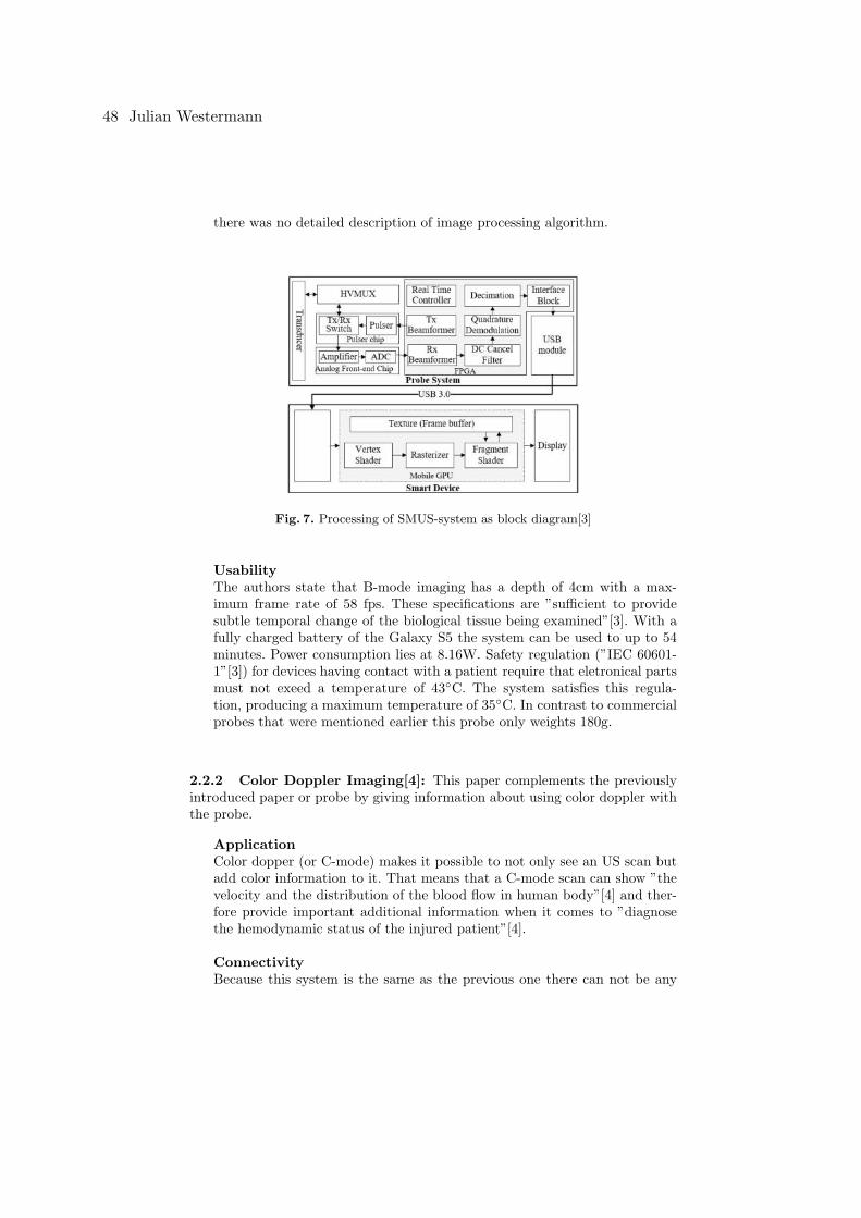
there was no detailed description of image processing algorithm.
Fig. 7. Processing of SMUS-system as block diagram[3]
UsabilityThe authors state that B-mode imaging has a depth of 4cm with a max-imum frame rate of 58 fps. These specifications are ”sufficient to providesubtle temporal change of the biological tissue being examined”[3]. With afully charged battery of the Galaxy S5 the system can be used to up to 54minutes. Power consumption lies at 8.16W. Safety regulation (”IEC 60601-1”[3]) for devices having contact with a patient require that eletronical partsmust not exeed a temperature of 43◦C. The system satisfies this regula-tion, producing a maximum temperature of 35◦C. In contrast to commercialprobes that were mentioned earlier this probe only weights 180g.
2.2.2 Color Doppler Imaging[4]: This paper complements the previouslyintroduced paper or probe by giving information about using color doppler withthe probe.
ApplicationColor dopper (or C-mode) makes it possible to not only see an US scan butadd color information to it. That means that a C-mode scan can show ”thevelocity and the distribution of the blood flow in human body”[4] and ther-fore provide important additional information when it comes to ”diagnosethe hemodynamic status of the injured patient”[4].
ConnectivityBecause this system is the same as the previous one there can not be any
48 Julian Westermann
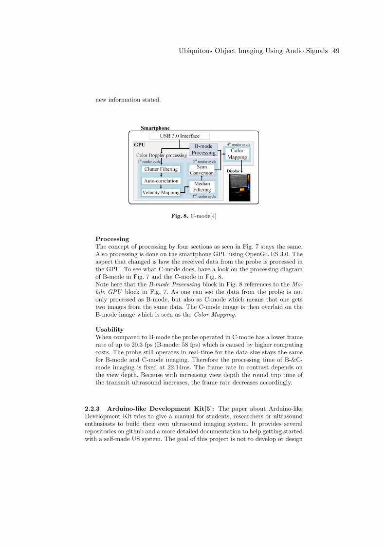
new information stated.
Fig. 8. C-mode[4]
ProcessingThe concept of processing by four sections as seen in Fig. 7 stays the same.Also processing is done on the smartphone GPU using OpenGL ES 3.0. Theaspect that changed is how the received data from the probe is processed inthe GPU. To see what C-mode does, have a look on the processing diagramof B-mode in Fig. 7 and the C-mode in Fig. 8.Note here that the B-mode Processing block in Fig. 8 references to the Mo-bile GPU block in Fig. 7. As one can see the data from the probe is notonly processed as B-mode, but also as C-mode which means that one getstwo images from the same data. The C-mode image is then overlaid on theB-mode image which is seen as the Color Mapping.
UsabilityWhen compared to B-mode the probe operated in C-mode has a lower framerate of up to 20.3 fps (B-mode: 58 fps) which is caused by higher computingcosts. The probe still operates in real-time for the data size stays the samefor B-mode and C-mode imaging. Therefore the processing time of B-&C-mode imaging is fixed at 22.14ms. The frame rate in contrast depends onthe view depth. Because with increasing view depth the round trip time ofthe transmit ultrasound increases, the frame rate decreases accordingly.
2.2.3 Arduino-like Development Kit[5]: The paper about Arduino-likeDevelopment Kit tries to give a manual for students, researchers or ultrasoundenthusiasts to build their own ultrasound imaging system. It provides severalrepositories on github and a more detailed documentation to help getting startedwith a self-made US system. The goal of this project is not to develop or design
Ubiquitous Object Imaging Using Audio Signals 49
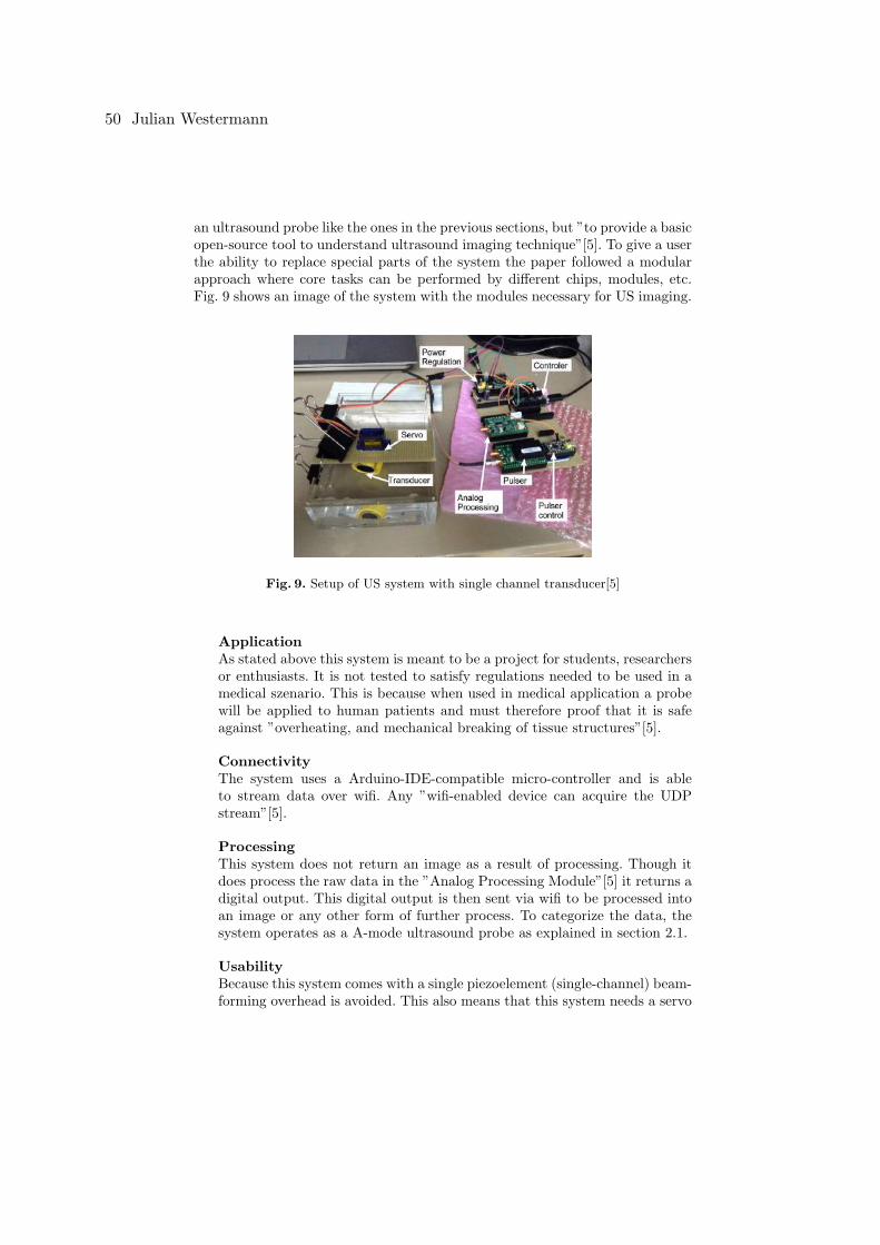
an ultrasound probe like the ones in the previous sections, but ”to provide a basicopen-source tool to understand ultrasound imaging technique”[5]. To give a userthe ability to replace special parts of the system the paper followed a modularapproach where core tasks can be performed by different chips, modules, etc.Fig. 9 shows an image of the system with the modules necessary for US imaging.
Fig. 9. Setup of US system with single channel transducer[5]
ApplicationAs stated above this system is meant to be a project for students, researchersor enthusiasts. It is not tested to satisfy regulations needed to be used in amedical szenario. This is because when used in medical application a probewill be applied to human patients and must therefore proof that it is safeagainst ”overheating, and mechanical breaking of tissue structures”[5].
ConnectivityThe system uses a Arduino-IDE-compatible micro-controller and is ableto stream data over wifi. Any ”wifi-enabled device can acquire the UDPstream”[5].
ProcessingThis system does not return an image as a result of processing. Though itdoes process the raw data in the ”Analog Processing Module”[5] it returns adigital output. This digital output is then sent via wifi to be processed intoan image or any other form of further process. To categorize the data, thesystem operates as a A-mode ultrasound probe as explained in section 2.1.
UsabilityBecause this system comes with a single piezoelement (single-channel) beam-forming overhead is avoided. This also means that this system needs a servo
50 Julian Westermann
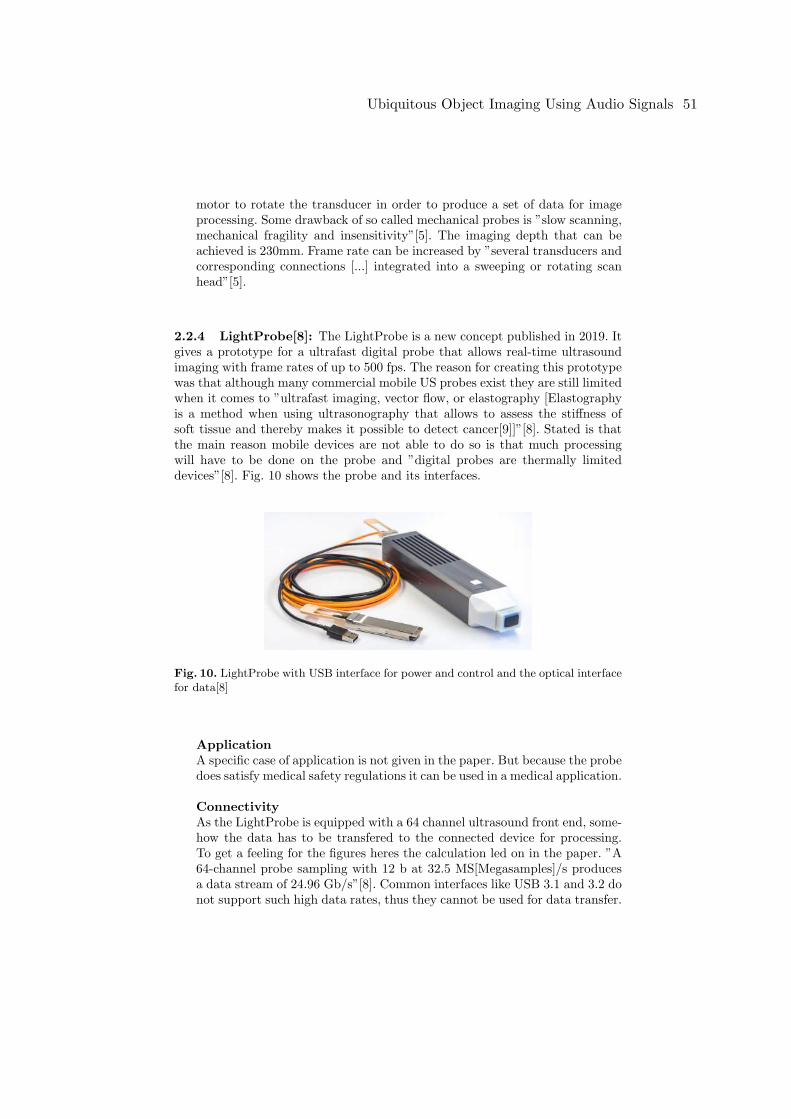
motor to rotate the transducer in order to produce a set of data for imageprocessing. Some drawback of so called mechanical probes is ”slow scanning,mechanical fragility and insensitivity”[5]. The imaging depth that can beachieved is 230mm. Frame rate can be increased by ”several transducers andcorresponding connections [...] integrated into a sweeping or rotating scanhead”[5].
2.2.4 LightProbe[8]: The LightProbe is a new concept published in 2019. Itgives a prototype for a ultrafast digital probe that allows real-time ultrasoundimaging with frame rates of up to 500 fps. The reason for creating this prototypewas that although many commercial mobile US probes exist they are still limitedwhen it comes to ”ultrafast imaging, vector flow, or elastography [Elastographyis a method when using ultrasonography that allows to assess the stiffness ofsoft tissue and thereby makes it possible to detect cancer[9]]”[8]. Stated is thatthe main reason mobile devices are not able to do so is that much processingwill have to be done on the probe and ”digital probes are thermally limiteddevices”[8]. Fig. 10 shows the probe and its interfaces.
Fig. 10. LightProbe with USB interface for power and control and the optical interfacefor data[8]
ApplicationA specific case of application is not given in the paper. But because the probedoes satisfy medical safety regulations it can be used in a medical application.
ConnectivityAs the LightProbe is equipped with a 64 channel ultrasound front end, some-how the data has to be transfered to the connected device for processing.To get a feeling for the figures heres the calculation led on in the paper. ”A64-channel probe sampling with 12 b at 32.5 MS[Megasamples]/s producesa data stream of 24.96 Gb/s”[8]. Common interfaces like USB 3.1 and 3.2 donot support such high data rates, thus they cannot be used for data transfer.
Ubiquitous Object Imaging Using Audio Signals 51

As a result a optical interface is used that provides a data rate of 40 Gb/s.However the use of a optical interface requires that the back end device, inthis case a commodity PC, must be equipped with special hardware.
ProcessingAs mentioned earlier the probe itself does not process raw data into imagedata but processes analog into digital data. This is because LightProbe fol-lows a the Software-Defined Architecture, which means that all processingis done in software. This all raw data is sent to the PC via the optical inter-face. However the developers allowed to add hardware processing blocks tothe probe. Beause of the high amount of input data (24.6 Gb/s) a GPU withsufficient processing power must be chosen. The used GPU is the NvidiaTesla 100 with a processing power of 15 TFLOP/s.
UsabilityBy using 64-channeled transducer the probe allows a high frame rate of up to500 fps with a average power consumption of 7.1 W. As a consequence of thehigh frame rate much power is consumed and thereby much heat is produced.However this probe is able to be used in a medical application which meansthat the heat must be dissipated quickly thus it does not heat up to over43◦C. Moreover the probe must be disinfected prior usage which cancels outair cooling as a way of thermal management. Therefore the paper introduceda ”Dynamic Thermal Management”[8] which regulates the probes tempera-ture using multiple thermal sensors at places where much heat is produced. Ifthe ”thermal-aware-performance (TAP) controller”[8] detects too high tem-peratures the imaging frame rate is reduced to lower power consumption.However ”to provide a consistent Qualtity of Service”[8] a Boost-Mode issupported that allows the user to increase frame rate for a specified amountof time (2 s) and ”a defined periodocity (every 5 s)”[8].
3 AIM: Acoustic Imaging on a Mobile[2]
While all the previous presented systems used external hardware, this conceptuses a Samsung Galaxy S7 and its built-in speaker and microphone. Motivationwas that smartphones become more and more powerful and smartphone camerasare getting better. But they still have problems when taking images in the darkor under obstruction. AIM sees its application in security scanning. Thereby ituses the property of acoustic signals, that they can penetrate materials and allowan under clothes weapon detection.
Fig. 11 shows the process of how an image is taken with AIM. When the userstarts imaging the phones speaker sends out short periodic acoustic signals, socalled chirps, within a frequency of 10 KHz to 22 KHz whereas the microphonerecords the reflected acoustic signals. To get a complete image the user has tomove the phone along a trajectory to mimic a microphone array.
52 Julian Westermann
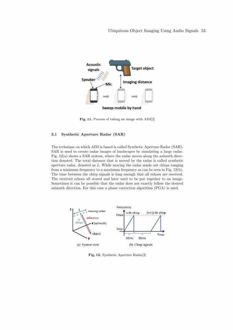
Fig. 11. Process of taking an image with AIM[2]
3.1 Synthetic Aperture Radar (SAR)
The technique on which AIM is based is called Synthetic Aperture Radar (SAR).SAR is used to create radar images of landscapes by simulating a large radar.Fig. 12(a) shows a SAR system, where the radar moves along the azimuth direc-tion denoted. The total distance that is moved by the radar is called syntheticaperture radar, denoted as L. While moving the radar sends out chirps rangingfrom a minimum frequency to a maximum frequency as can be seen in Fig. 12(b).The time between the chirp signals is long enough that all echoes are received.The received echoes all stored and later used to be put together to an image.Sometimes it can be possible that the radar does not exactly follow the desiredazimuth direction. For this case a phase correction algorithm (PGA) is used.
Fig. 12. Synthetic Aperture Radar[2]
Ubiquitous Object Imaging Using Audio Signals 53
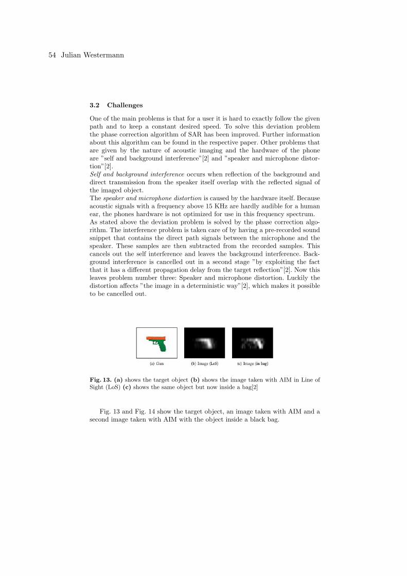
3.2 Challenges
One of the main problems is that for a user it is hard to exactly follow the givenpath and to keep a constant desired speed. To solve this deviation problemthe phase correction algorithm of SAR has been improved. Further informationabout this algorithm can be found in the respective paper. Other problems thatare given by the nature of acoustic imaging and the hardware of the phoneare ”self and background interference”[2] and ”speaker and microphone distor-tion”[2].Self and background interference occurs when reflection of the background anddirect transmission from the speaker itself overlap with the reflected signal ofthe imaged object.The speaker and microphone distortion is caused by the hardware itself. Becauseacoustic signals with a frequency above 15 KHz are hardly audible for a humanear, the phones hardware is not optimized for use in this frequency spectrum.As stated above the deviation problem is solved by the phase correction algo-rithm. The interference problem is taken care of by having a pre-recorded soundsnippet that contains the direct path signals between the microphone and thespeaker. These samples are then subtracted from the recorded samples. Thiscancels out the self interference and leaves the background interference. Back-ground interference is cancelled out in a second stage ”by exploiting the factthat it has a different propagation delay from the target reflection”[2]. Now thisleaves problem number three: Speaker and microphone distortion. Luckily thedistortion affects ”the image in a deterministic way”[2], which makes it possibleto be cancelled out.
Fig. 13. (a) shows the target object (b) shows the image taken with AIM in Line ofSight (LoS) (c) shows the same object but now inside a bag[2]
Fig. 13 and Fig. 14 show the target object, an image taken with AIM and asecond image taken with AIM with the object inside a black bag.
54 Julian Westermann
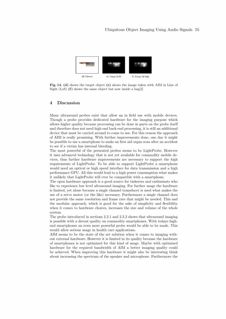
Fig. 14. (d) shows the target object (e) shows the image taken with AIM in Line ofSight (LoS) (f) shows the same object but now inside a bag[2]
4 Discussion
Many ultrasound probes exist that allow an in field use with mobile devices.Though a probe provides dedicated hardware for the imaging purpose whichallows higher quality because processing can be done in parts on the probe itselfand therefore does not need high end back-end processing, it is still an additionaldevice that must be carried around to come to use. For this reason the approachof AIM is really promising. With further improvements done, one day it mightbe possible to use a smartphone to make an first aid organ scan after an accidentto see if a victim has internal bleeding.The most powerful of the presented probes seems to be LightProbe. Howeverit uses advanced technology that is not yet available for commodity mobile de-vices, thus further hardware improvements are necessary to support the highrequirements of LightProbe. To be able to support LightProbe a smartphonewould need an optical or high speed interface for data transmission and a highperformance GPU. All this would lead to a high power consumption what makesit unlikely that LightProbe will ever be compatible with a smartphone.The open hardware approach is a good source for tinkerers and enthusiasts wholike to experience low level ultrasound imaging. For further usage the hardwareis limited, yet alone because a single channel transducer is used what makes theuse of a servo motor (or the like) necessary. Furthermore a single channel doesnot provide the same resolution and frame rate that might be needed. This andthe modular approach, which is good for the sake of simplicity and flexibilitywhen it comes to hardware choices, increases the size and volume of the wholesystem.The probe introduced in sections 2.2.1 and 2.2.2 shows that ultrasound imagingis possible with a decent quality on commodity smartphones. With todays high-end smartphones an even more powerful probe would be able to be made. Thiswould allow serious usage in health care applications.AIM seems to be the state of the art solution when it comes to imaging with-out external hardware. However it is limited in its quality because the hardwareof smartphones is not optimized for this kind of usage. Maybe with optimizedhardware for the required bandwidth of AIM a better imaging quality couldbe achieved. When improving this hardware it might also be interesting thinkabout increasing the spectrum of the speaker and microphone. Furthermore the
Ubiquitous Object Imaging Using Audio Signals 55
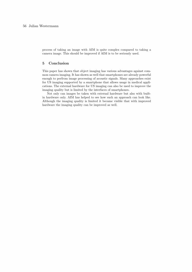
process of taking an image with AIM is quite complex compared to taking acamera image. This should be improved if AIM is to be seriously used.
5 Conclusion
This paper has shown that object imaging has various advantages against com-mon camera imaging. It has shown as well that smartphones are already powerfulenough to perfrom image processing of acoustic signals. Many approaches existfor US imaging supported by a smartphone that allows usage in medical appli-cations. The external hardware for US imaging can also be used to improve theimaging quality but is limited by the interfaces of smartphones.
Not only can images be taken with external hardware but also with built-in hardware only. AIM has helped to see how such an approach can look like.Although the imaging quality is limited it became visible that with improvedhardware the imaging quality can be improved as well.
56 Julian Westermann
References
1. H. Bedri, M. Feigin, M. Everett, G. L. Charvat, R. Raskar, et al., “Seeing aroundcorners with a mobile phone?: synthetic aperture audio imaging,” in ACM SIG-GRAPH 2014 Posters, p. 84, ACM, 2014.
2. W. Mao, M. Wang, and L. Qiu, “Aim: Acoustic imaging on a mobile,” in Proceedingsof the 16th Annual International Conference on Mobile Systems, Applications, andServices, MobiSys ’18, (New York, NY, USA), pp. 468–481, ACM, 2018.
3. S. Ahn, J. Kang, P. Kim, G. Lee, E. Jeong, W. Jung, M. Park, and T.-k. Song,“Smartphone-based portable ultrasound imaging system: Prototype implementationand evaluation,” in 2015 IEEE International Ultrasonics Symposium (IUS), pp. 1–4,IEEE, 2015.
4. E. Jeong, Sua Bae, M. Park, W. Jung, J. Kang, and T. Song, “Color doppler imag-ing on a smartphone-based portable us system: Preliminary study,” in 2015 IEEEInternational Ultrasonics Symposium (IUS), pp. 1–4, Oct 2015.
5. L. Jonveaux, “Arduino-like development kit for single-element ultrasound imaging,”Journal of Open Hardware, vol. 1, no. 1, 2017.
6. H. S. P. Explained, “ultrasound - b scan explained.” https://www.youtube.com/
watch?v=Tg_KJ0XqnJ8, 2016. Accessed on 05-07-2019.7. T. Binder and M. Altersberger, “1.8.2.1 principles of color doppler.” https://www.
123sonography.com/ebook/principles-color-doppler, 2019. Accessed on 05-07-2019.
8. P. A. Hager and L. Benini, “Lightprobe: A digital ultrasound probe for software-defined ultrafast imaging,” IEEE transactions on ultrasonics, ferroelectrics, andfrequency control, 2019.
9. S. M. Dictionary, “elastography.” https://medical-dictionary.
thefreedictionary.com/elastography, 2012. Accessed on 06-07-2019.
Ubiquitous Object Imaging Using Audio Signals 57

Vergleich Verschiedener Architekturenkunstlicher Intelligenz
Denis Jager
Karlsruher Institut fur Technologie
Abstract. In dieser Ausarbeitung sollen verschiedene Architekturenkunstlicher Intelligenz nach ihren Anforderungen und Entscheidungsdi-mensionen verglichen werden. Die Architekturen kunstlicher Intelligenzlassen sich in uberwachtes Lernen, unuberwachtes Lernen undbestarkendes Lernen unterteilen.
58 Denis Jager
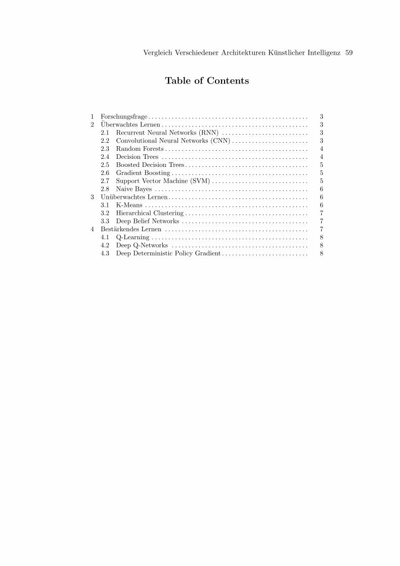
Table of Contents
1 Forschungsfrage . . . . . . . . . . . . . . . . . . . . . . . . . . . . . . . . . . . . . . . . . . . . . . . . 32 Uberwachtes Lernen . . . . . . . . . . . . . . . . . . . . . . . . . . . . . . . . . . . . . . . . . . . . 3
2.1 Recurrent Neural Networks (RNN) . . . . . . . . . . . . . . . . . . . . . . . . . . 32.2 Convolutional Neural Networks (CNN) . . . . . . . . . . . . . . . . . . . . . . . 32.3 Random Forests . . . . . . . . . . . . . . . . . . . . . . . . . . . . . . . . . . . . . . . . . . . 42.4 Decision Trees . . . . . . . . . . . . . . . . . . . . . . . . . . . . . . . . . . . . . . . . . . . . 42.5 Boosted Decision Trees . . . . . . . . . . . . . . . . . . . . . . . . . . . . . . . . . . . . . 52.6 Gradient Boosting . . . . . . . . . . . . . . . . . . . . . . . . . . . . . . . . . . . . . . . . . 52.7 Support Vector Machine (SVM) . . . . . . . . . . . . . . . . . . . . . . . . . . . . . 52.8 Naive Bayes . . . . . . . . . . . . . . . . . . . . . . . . . . . . . . . . . . . . . . . . . . . . . . 6
3 Unuberwachtes Lernen. . . . . . . . . . . . . . . . . . . . . . . . . . . . . . . . . . . . . . . . . . 63.1 K-Means . . . . . . . . . . . . . . . . . . . . . . . . . . . . . . . . . . . . . . . . . . . . . . . . . 63.2 Hierarchical Clustering . . . . . . . . . . . . . . . . . . . . . . . . . . . . . . . . . . . . . 73.3 Deep Belief Networks . . . . . . . . . . . . . . . . . . . . . . . . . . . . . . . . . . . . . . 7
4 Bestarkendes Lernen . . . . . . . . . . . . . . . . . . . . . . . . . . . . . . . . . . . . . . . . . . . 74.1 Q-Learning . . . . . . . . . . . . . . . . . . . . . . . . . . . . . . . . . . . . . . . . . . . . . . . 84.2 Deep Q-Networks . . . . . . . . . . . . . . . . . . . . . . . . . . . . . . . . . . . . . . . . . 84.3 Deep Deterministic Policy Gradient . . . . . . . . . . . . . . . . . . . . . . . . . . 8
Vergleich Verschiedener Architekturen Kunstlicher Intelligenz 59

3
1 Forschungsfrage
In Zukunft sollen KIs immer automatisierter entworfen und genutzt werden.Dazu ist es wichtig zu wissen welche Architektur kunstlicher Intelligenz bei demjeweiligen Problem angewendet werden soll. Um dies zu erreichen werden indiesem Paper einige der wichtigsten Architekturen kunstlicher Intelligenz anhandihrer Anwendungsgebiete, Vorteile und Nachteile aufgefuhrt.
2 Uberwachtes Lernen
Es werden nun einige Grundlagen zu uberwachtem Lernen angefuhrt. Daraufhinsollen verschiedene Architekturen dieser Kategorie anhand ihrer Anwendungs-gebiete, Vorteile und Nachteile aufgezahlt werden.
Trainingsdaten: Beim Uberwachten Lernen beinhaltet jedes Trainingsbeispieleinen oder mehrere Inputs und einen gewunschten, zugehorigen Output.
Vorgehen: Durch die iterative Optimierung einer Zielfunktion lernenuberwachte Lernalgorithmen gewunschte Outputs fur neue Inputsvorherzusagen.
Kategorien Wenn die Outputs in diskrete Werte unterteilt werden konnenhandelt es sich um eine Klassifikation. Bei der Regression ist keine Einteilung zudiskreten Werten moglich. Die Outputs sind hier kontinuierliche Werte.
2.1 Recurrent Neural Networks (RNN)
Anwendungen:
1. Spracherkennung [4]2. Schreibschrifterkennung [4]
Vorteile:
1. Starkes Modell fur die Verarbeitung sequenzieller Datenstrome [4]2. Großerer Zustandsraum und dynamischer als hidden Markov models [4]
Nachteile:
1. Potenziell falsche Ausrichtung als Trainingsziel [4]
2.2 Convolutional Neural Networks (CNN)
Anwendungen:
1. Klassifikation von Bildern [2]
60 Denis Jager
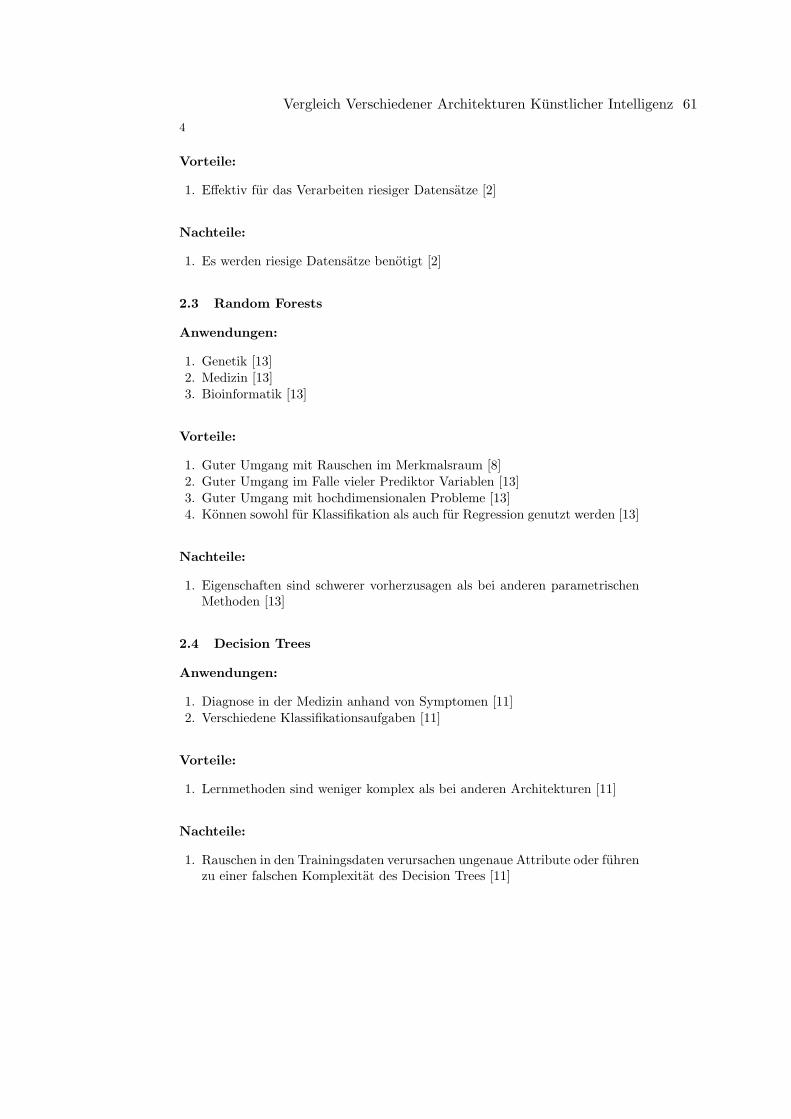
4
Vorteile:
1. Effektiv fur das Verarbeiten riesiger Datensatze [2]
Nachteile:
1. Es werden riesige Datensatze benotigt [2]
2.3 Random Forests
Anwendungen:
1. Genetik [13]2. Medizin [13]3. Bioinformatik [13]
Vorteile:
1. Guter Umgang mit Rauschen im Merkmalsraum [8]2. Guter Umgang im Falle vieler Prediktor Variablen [13]3. Guter Umgang mit hochdimensionalen Probleme [13]4. Konnen sowohl fur Klassifikation als auch fur Regression genutzt werden [13]
Nachteile:
1. Eigenschaften sind schwerer vorherzusagen als bei anderen parametrischenMethoden [13]
2.4 Decision Trees
Anwendungen:
1. Diagnose in der Medizin anhand von Symptomen [11]2. Verschiedene Klassifikationsaufgaben [11]
Vorteile:
1. Lernmethoden sind weniger komplex als bei anderen Architekturen [11]
Nachteile:
1. Rauschen in den Trainingsdaten verursachen ungenaue Attribute oder fuhrenzu einer falschen Komplexitat des Decision Trees [11]
Vergleich Verschiedener Architekturen Kunstlicher Intelligenz 61

5
2.5 Boosted Decision Trees
Anwendungen:
1. Partikel Identifikation in der Physik [12]2. Datenklassifikation [12]
Vorteile:
1. Starke Lernmethode mit hoher Performanz [12]2. Effizient bei hoher Attributanzahl [12]
Nachteile:
1. Kleine Anderungen in den Trainingsdaten konnen zu großen Anderungen imBaum und in den Ergebnissen fuhren [12]
2.6 Gradient Boosting
Anwendungen:
1. Reisezeit Prognosen [15]
Vorteile:
1. Weniger sensitiv gegenuber einer erhohten Vorhersagemenge als andere Mod-elle [15]
2. Gute Vorhersageperformanz und Vorhersagegenauigkeit [15]
Nachteile:
1. Performanz ist stark von den Parametern des Modells beeinflusst [15]
2.7 Support Vector Machine (SVM)
Anwendungen:
1. Text Kategorisierung [7]
Vorteile:
1. Vollautomatisch, das heißt keine manuelle Parameter Einstellung notig [7]2. Guter Umgang mit hochdimensionalen Inputs [7]3. Robust [7]
62 Denis Jager

6
2.8 Naive Bayes
Anwendungen:
1. Text Klassifikation [10]
Vorteile:
1. Parameter fur jedes Attribut konnen separat gelernt werden, wodurch dasLernen vor allem fur eine große Zahl an Attributen vereinfacht wird [10]
3 Unuberwachtes Lernen
Es werden nun einige Grundlagen zu unuberwachtem Lernen angefuhrt. Da-raufhin sollen verschiedene Architekturen dieser Kategorie anhand ihrer Anwen-dungsgebiete, Vorteile und Nachteile aufgezahlt werden.
Trainingsdaten: Beim Unuberwachten Lernen beinhaltet jedes Trainingsbei-spiel einen oder mehrere Inputs. Im Gegensatz zum Uberwachten Lernen fehlendie zugehorigen, gewunschten Outputs.
Vorgehen: Vom Algorithmus sollen selbststandig Strukturen in den Daten ge-funden werden, wie zum Beispiel Ahnlichkeiten zwischen mehreren Trainings-beispielen. Neue Inputs konnen dann auf Anwesenheit einer solchen Ahnlichkeituberpruft werden. Der Algorithmus verfahrt dann entsprechend.
3.1 K-Means
Anwendungen:
1. Clustering
Vorteile:
1. Einfach zu implementieren
Nachteile:
1. Es ist schwer den Wert fur K zu bestimmten [3]2. Nicht effektiv bei globalem Cluster [3]3. Bei unterschiedlichen Startpartitionen kann auch das Ergebnis sich
verandern [3]
Vergleich Verschiedener Architekturen Kunstlicher Intelligenz 63
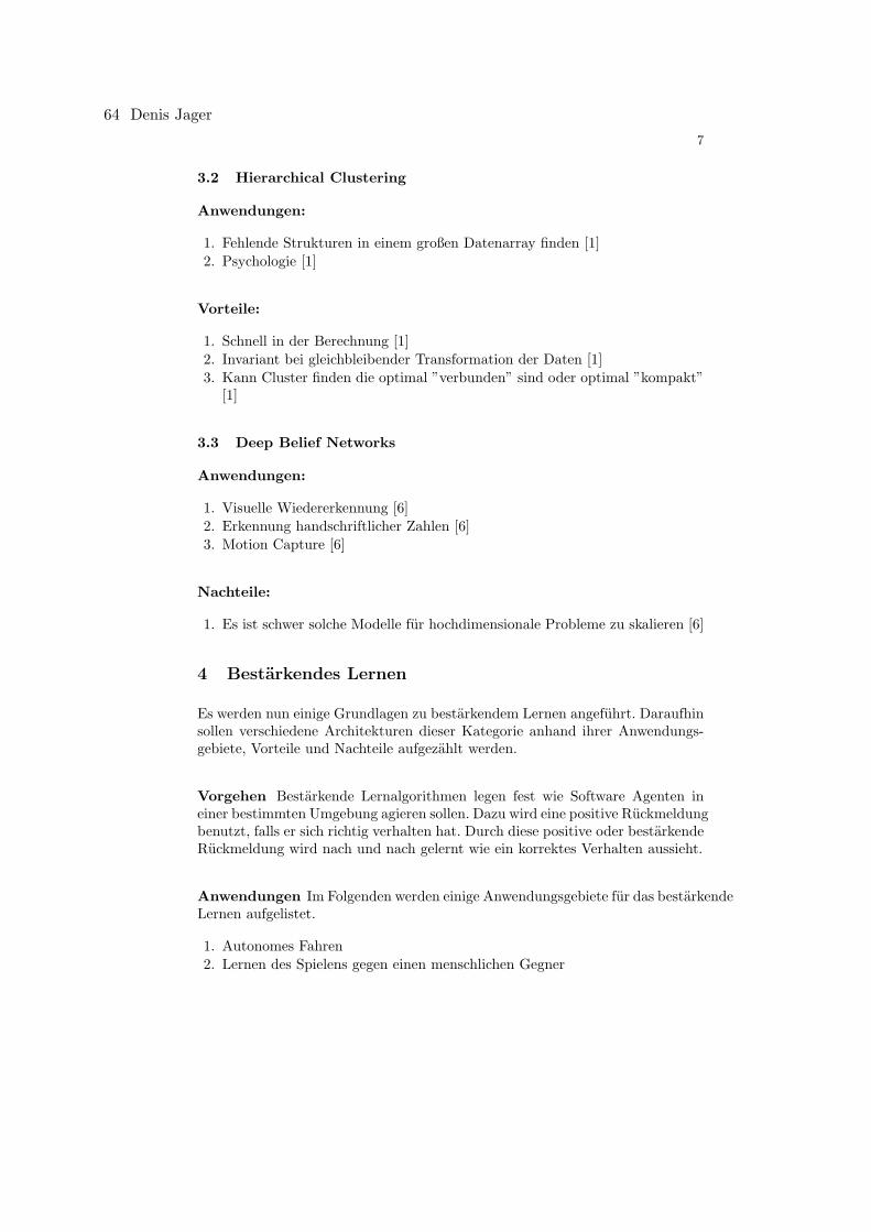
7
3.2 Hierarchical Clustering
Anwendungen:
1. Fehlende Strukturen in einem großen Datenarray finden [1]
2. Psychologie [1]
Vorteile:
1. Schnell in der Berechnung [1]
2. Invariant bei gleichbleibender Transformation der Daten [1]
3. Kann Cluster finden die optimal ”verbunden” sind oder optimal ”kompakt”[1]
3.3 Deep Belief Networks
Anwendungen:
1. Visuelle Wiedererkennung [6]
2. Erkennung handschriftlicher Zahlen [6]
3. Motion Capture [6]
Nachteile:
1. Es ist schwer solche Modelle fur hochdimensionale Probleme zu skalieren [6]
4 Bestarkendes Lernen
Es werden nun einige Grundlagen zu bestarkendem Lernen angefuhrt. Daraufhinsollen verschiedene Architekturen dieser Kategorie anhand ihrer Anwendungs-gebiete, Vorteile und Nachteile aufgezahlt werden.
Vorgehen Bestarkende Lernalgorithmen legen fest wie Software Agenten ineiner bestimmten Umgebung agieren sollen. Dazu wird eine positive Ruckmeldungbenutzt, falls er sich richtig verhalten hat. Durch diese positive oder bestarkendeRuckmeldung wird nach und nach gelernt wie ein korrektes Verhalten aussieht.
Anwendungen Im Folgenden werden einige Anwendungsgebiete fur das bestarkendeLernen aufgelistet.
1. Autonomes Fahren
2. Lernen des Spielens gegen einen menschlichen Gegner
64 Denis Jager

8
4.1 Q-Learning
Anwendungen:
1. Web System Konfiguration2. Nichtmenschlicher Spieler in Spielen [5]
Vorteile:
1. Einfacher Weg fur Agenten das optimale Handeln in kontrollierten MarkovUmgebungen zu lernen [14]
Nachteile:
1. Uberschatzen von Aktionswerten unter bestimmten Bedingungen [5]
4.2 Deep Q-Networks
Anwendungen:
1. Autonomes Fahren [9]2. Nichtmenschlicher Spieler [9]
Vorteile:
1. Gut fur Probleme mit hochdimensionalem Uberwachungsraum [9]2. Kann bei vielen Aufgaben die Strategien auch ”end-to-end” lernen [9]
Nachteile:
1. Kann nur mit diskreten und niedrigdimensionalen Aktionsraumen umgehen[9]
4.3 Deep Deterministic Policy Gradient
Anwendungen:
1. Nichtmenschlicher Spieler [9]
Vorteile:
1. Kann kompetitive Strategien fur alle Aufgaben lernen [9]
Nachteile:
1. Instabil bei anspruchsvollen Problemen [9]
Vergleich Verschiedener Architekturen Kunstlicher Intelligenz 65

9
References
1. Administrator. 241 1.tif.2. Alex Krizhevsky, Ilya Sutskever, and Geoffrey E. Hinton. Imagenet classification
with deep convolutional neural networks.3. Preeti Arora, Deepali, and Shipra Varshney. Analysis of k-means and k-medoids
algorithm for big data. Procedia Computer Science, 78:507–512, 2016.4. Alex Graves, Abdel-rahman Mohamed, and Geoffrey Hinton. Speech recognition
with deep recurrent neural networks. In 2013 IEEE International Conferenceon Acoustics, Speech and Signal Processing, pages 6645–6649. IEEE, 26.05.2013- 31.05.2013.
5. Hado van Hasselt, Arthur Guez, David Silver. Deep reinforcement learning withdouble q-learning.
6. Honglak Lee, Roger Grosse, Rajesh Ranganath, and Andrew Y. Ng. Convolutionaldeep belief networks for scalable unsupervised learning of hierarchical representa-tions.
7. Thorsten Joachims. Text categorization with support vector machines: Learningwith many relevant features.
8. Christopher Krauss, Xuan Anh Do, and Nicolas Huck. Deep neural networks,gradient-boosted trees, random forests: Statistical arbitrage on the s&p 500. Eu-ropean Journal of Operational Research, 259(2):689–702, 2017.
9. Timothy P. Lillicrap, Jonathan J. Hunt, Alexander Pritzel, Nicolas Heess, TomErez, Yuval Tassa, David Silver, and Daan Wierstra. Continuous control withdeep reinforcement learning.
10. Andrew McCallum and Kamal Nigam. A comparison of event models for naivebayes text classification.
11. J. R. Quinlan. Induction of decision trees.12. Byron P. Roe, Hai-Jun Yang, Ji Zhu, Yong Liu, Ion Stancu, and Gordon McGregor.
Boosted decision trees as an alternative to artificial neural networks for particleidentification. Nuclear Instruments and Methods in Physics Research Section A:Accelerators, Spectrometers, Detectors and Associated Equipment, 543(2-3):577–584, 2005.
13. Carolin Strobl, James Malley, and Gerhard Tutz. An introduction to recursive par-titioning: rationale, application, and characteristics of classification and regressiontrees, bagging, and random forests. Psychological methods, 14(4):323–348, 2009.
14. Christopher J.C.H. Watkins and Peter Dayan. Q-learning.15. Yanru Zhang and Ali Haghani. A gradient boosting method to improve travel time
prediction. Transportation Research Part C: Emerging Technologies, 58:308–324,2015.
66 Denis Jager
Edge Computing - An overview of a cloudextending technology
Evgeni [email protected]
Karlsruher Institut fur Technologie
Abstract. Cloud computing is a powerful technology which has provenitself through the years, but it is demanding in price. Moreover, with therising number of Internet of Thing devices, a time is coming in whichcloud computing will not be able to cope with the amount of data to pro-cess and, what is more, it use leads to high internet traffic congestions.Fog computing was the first extension of cloud computing presented inorder to cope with the disadvantages of cloud computing. Physically ex-tending the cloud showed great results, but still the option remained togo even further, closer to the end user. Therefore, we introduce edge com-puting as an extension of the cloud computing technology which aims tooffload the cloud and bring the computing of data closer to the end de-vices, which all together form the edge of the network.One of its greatestadvantages is the fact that the concept is based on already developedtechnologies such as Software Defined Networks and Network FunctionVirtualization. Edge computing reveals itself as a technology from whichthe cloud and the network could benefit. It is able to accelerate networkservices while reducing the internet traffic. It assists in providing fasterand better services for the Internet of Things devices and it is a crucialstep in the realisation of the 5G network. The following paper presentsan overview of this new and emerging concept.
1 Introduction
1.1 Motivation
Cloud computing is an idea which can be traced back to the early 60s of thelast century. In the 90s we came closer to making the idea possible by introduc-ing VPN. Traffic was switched in a way so it would improve the overall use ofthe internet bandwidth.It was the 2000s when the cloud as we know it todaywas brought to life.[4] The technology of cloud computing brought with itselfnot only technological but also business advantages for the customers. Buyingyour own hardware is an expensive investment which is profitable if only thefull computing capacity of the system is used. Most of the businesses, especiallythe small ones, hardly ever achieve this. Therefore, paying only for the usedservices is a smarter idea.[5] Furthermore, cloud computing offers the possibilityfor software and data to be accessed easily by different kinds of client devices
Edge Computing - An overview of a cloud extending technology 67
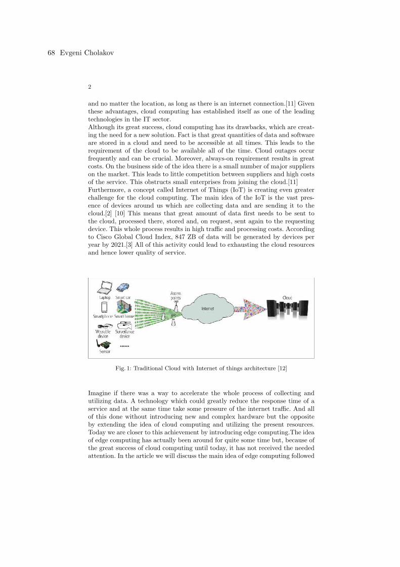
2
and no matter the location, as long as there is an internet connection.[11] Giventhese advantages, cloud computing has established itself as one of the leadingtechnologies in the IT sector.Although its great success, cloud computing has its drawbacks, which are creat-ing the need for a new solution. Fact is that great quantities of data and softwareare stored in a cloud and need to be accessible at all times. This leads to therequirement of the cloud to be available all of the time. Cloud outages occurfrequently and can be crucial. Moreover, always-on requirement results in greatcosts. On the business side of the idea there is a small number of major supplierson the market. This leads to little competition between suppliers and high costsof the service. This obstructs small enterprises from joining the cloud.[11]Furthermore, a concept called Internet of Things (IoT) is creating even greaterchallenge for the cloud computing. The main idea of the IoT is the vast pres-ence of devices around us which are collecting data and are sending it to thecloud.[2] [10] This means that great amount of data first needs to be sent tothe cloud, processed there, stored and, on request, sent again to the requestingdevice. This whole process results in high traffic and processing costs. Accordingto Cisco Global Cloud Index, 847 ZB of data will be generated by devices peryear by 2021.[3] All of this activity could lead to exhausting the cloud resourcesand hence lower quality of service.
Fig. 1: Traditional Cloud with Internet of things architecture [12]
Imagine if there was a way to accelerate the whole process of collecting andutilizing data. A technology which could greatly reduce the response time of aservice and at the same time take some pressure of the internet traffic. And allof this done without introducing new and complex hardware but the oppositeby extending the idea of cloud computing and utilizing the present resources.Today we are closer to this achievement by introducing edge computing.The ideaof edge computing has actually been around for quite some time but, because ofthe great success of cloud computing until today, it has not received the neededattention. In the article we will discuss the main idea of edge computing followed
68 Evgeni Cholakov
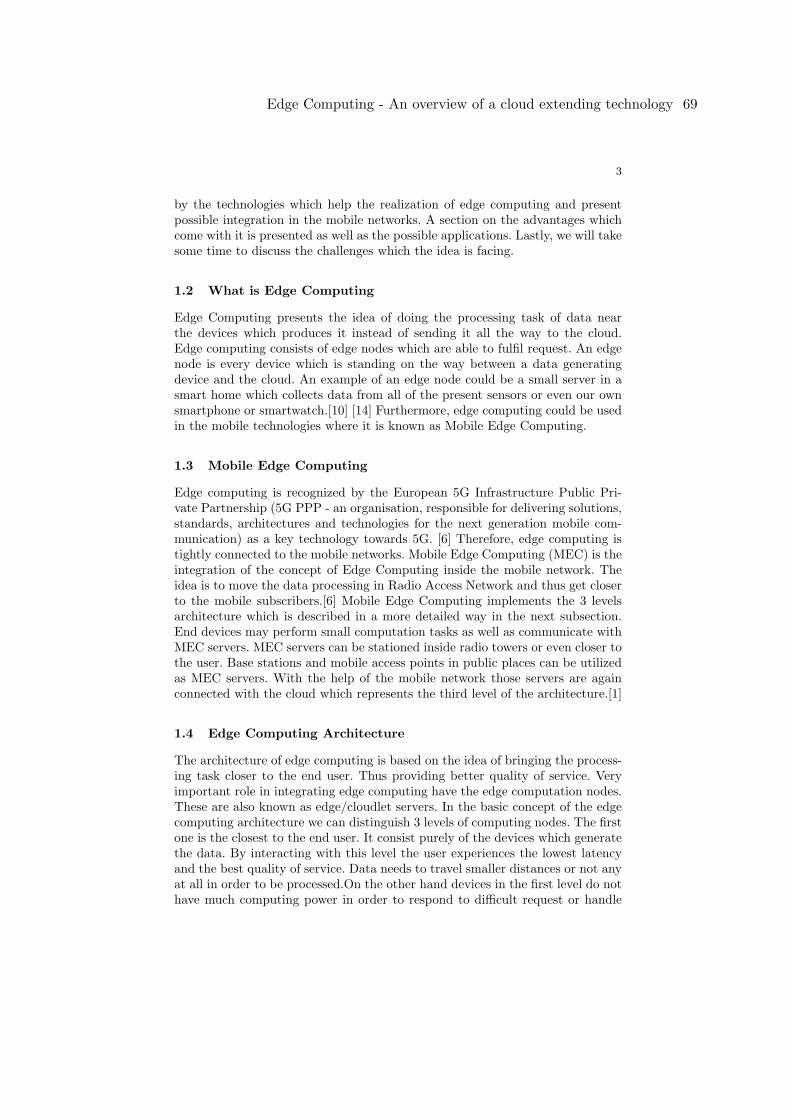
3
by the technologies which help the realization of edge computing and presentpossible integration in the mobile networks. A section on the advantages whichcome with it is presented as well as the possible applications. Lastly, we will takesome time to discuss the challenges which the idea is facing.
1.2 What is Edge Computing
Edge Computing presents the idea of doing the processing task of data nearthe devices which produces it instead of sending it all the way to the cloud.Edge computing consists of edge nodes which are able to fulfil request. An edgenode is every device which is standing on the way between a data generatingdevice and the cloud. An example of an edge node could be a small server in asmart home which collects data from all of the present sensors or even our ownsmartphone or smartwatch.[10] [14] Furthermore, edge computing could be usedin the mobile technologies where it is known as Mobile Edge Computing.
1.3 Mobile Edge Computing
Edge computing is recognized by the European 5G Infrastructure Public Pri-vate Partnership (5G PPP - an organisation, responsible for delivering solutions,standards, architectures and technologies for the next generation mobile com-munication) as a key technology towards 5G. [6] Therefore, edge computing istightly connected to the mobile networks. Mobile Edge Computing (MEC) is theintegration of the concept of Edge Computing inside the mobile network. Theidea is to move the data processing in Radio Access Network and thus get closerto the mobile subscribers.[6] Mobile Edge Computing implements the 3 levelsarchitecture which is described in a more detailed way in the next subsection.End devices may perform small computation tasks as well as communicate withMEC servers. MEC servers can be stationed inside radio towers or even closer tothe user. Base stations and mobile access points in public places can be utilizedas MEC servers. With the help of the mobile network those servers are againconnected with the cloud which represents the third level of the architecture.[1]
1.4 Edge Computing Architecture
The architecture of edge computing is based on the idea of bringing the process-ing task closer to the end user. Thus providing better quality of service. Veryimportant role in integrating edge computing have the edge computation nodes.These are also known as edge/cloudlet servers. In the basic concept of the edgecomputing architecture we can distinguish 3 levels of computing nodes. The firstone is the closest to the end user. It consist purely of the devices which generatethe data. By interacting with this level the user experiences the lowest latencyand the best quality of service. Data needs to travel smaller distances or not anyat all in order to be processed.On the other hand devices in the first level do nothave much computing power in order to respond to difficult request or handle
Edge Computing - An overview of a cloud extending technology 69
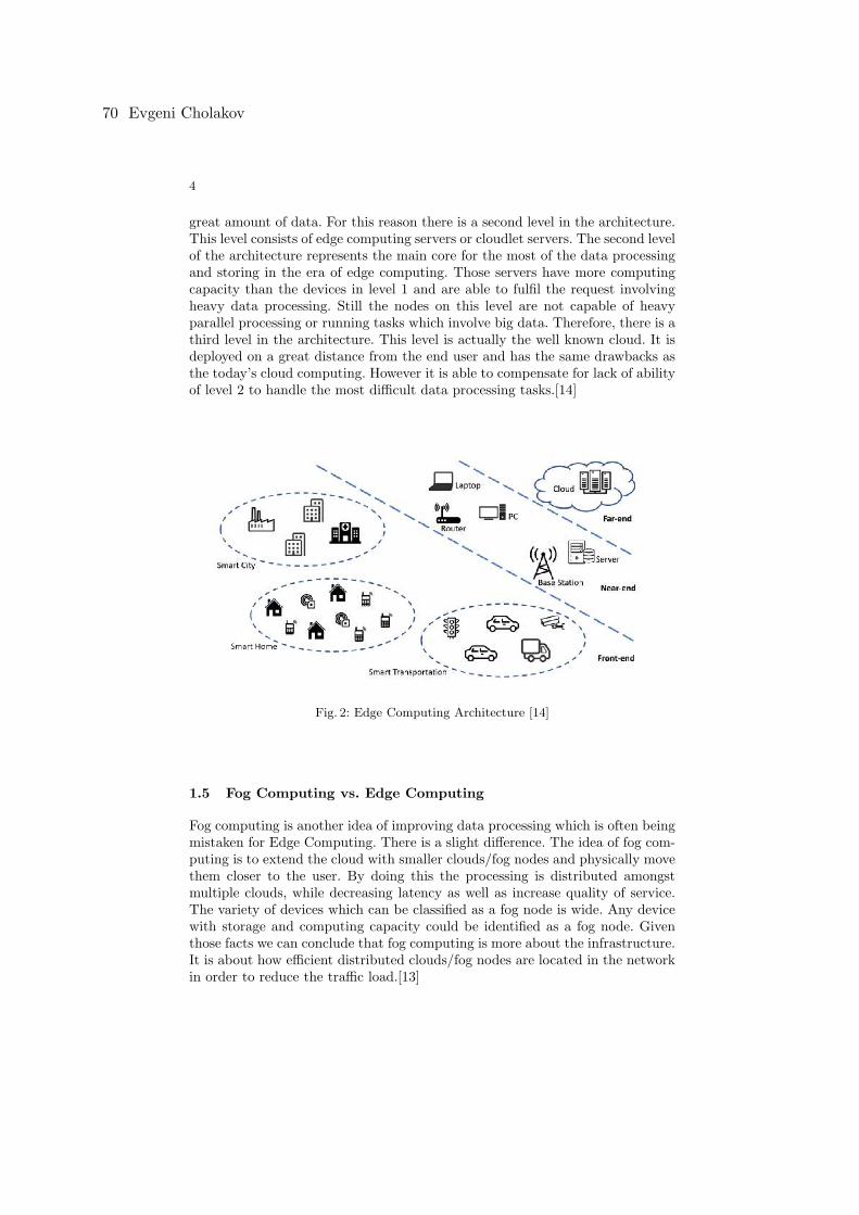
4
great amount of data. For this reason there is a second level in the architecture.This level consists of edge computing servers or cloudlet servers. The second levelof the architecture represents the main core for the most of the data processingand storing in the era of edge computing. Those servers have more computingcapacity than the devices in level 1 and are able to fulfil the request involvingheavy data processing. Still the nodes on this level are not capable of heavyparallel processing or running tasks which involve big data. Therefore, there is athird level in the architecture. This level is actually the well known cloud. It isdeployed on a great distance from the end user and has the same drawbacks asthe today’s cloud computing. However it is able to compensate for lack of abilityof level 2 to handle the most difficult data processing tasks.[14]
Fig. 2: Edge Computing Architecture [14]
1.5 Fog Computing vs. Edge Computing
Fog computing is another idea of improving data processing which is often beingmistaken for Edge Computing. There is a slight difference. The idea of fog com-puting is to extend the cloud with smaller clouds/fog nodes and physically movethem closer to the user. By doing this the processing is distributed amongstmultiple clouds, while decreasing latency as well as increase quality of service.The variety of devices which can be classified as a fog node is wide. Any devicewith storage and computing capacity could be identified as a fog node. Giventhose facts we can conclude that fog computing is more about the infrastructure.It is about how efficient distributed clouds/fog nodes are located in the networkin order to reduce the traffic load.[13]
70 Evgeni Cholakov

5
2 Enabling technologies
In order to make the idea of edge computing reality we need to examine anduse some of the already developed technologies in the networking sector. In thefollowing sections we are going to look in the technologies which are assistingthe realisation of edge computing. Edge computing relies not only on cloudcomputing but also on technologies such as Network Function Virtualization(NFV), Software Defined Networks (SDN) and network slicing.
2.1 Network Function Virtualization
Network Function Virtualization is a technology in the networking which is usedin order to provide multi-tenancy servers, which are located closer to the user.Earlier, every content provider had to use its own hardware in order to pro-vide service to its users. Different hardware systems mean that it is harder tostandardise services. Failures and errors are difficult to fix. The greatest draw-back was that, to relocate a service, the content providers needed physicallyto relocate the server or order a new one. NFV enables a single server to beused by different content providers. The idea is to have a single hardware whichhas is own operating system and uses virtualization in order to provide hard-ware resources to different services. Content providers only need to provide afunctioning software. To sum up NFV provides easier migration, flexibility andscalability.[15]For example in the case of a flash crowd event the resources of an edge comput-ing server might be exhausted. By using the technology of NFV the server mayallocate additional resources on another near edge computing server withoutconcerning compatibility.[13]
2.2 Software Defined Networks
Software Defined Networks are another networking technology which is recog-nised as the future of networking. By SDN there is a strong separation betweendata and control layer. The traditional model of a router has both layers inte-grated. This means that a routers makes its own routing decision based on datawhich is sent to it. In the SDN the routers are replaced with simple switcheswhich only switch packets. The control functions are placed in a single con-troller which makes the routing decisions and sends them in form of rules to theswitches. The switches save those rules in tables and when they receive a packetthey switch it, based on the rules in their tables. SDNs provide centralized con-trol of the network. Flexibility is provided and the whole network can be easilyadjusted. This means that new network services can be also easily added.SDNprovides an agile and easy to manage connectivity which can span across manyservers and devices at the edge of the network.[13] [15]
Edge Computing - An overview of a cloud extending technology 71
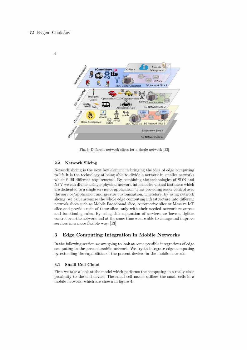
6
Fig. 3: Different network slices for a single network [13]
2.3 Network Slicing
Network slicing is the next key element in bringing the idea of edge computingto life.It is the technology of being able to divide a network in smaller networkswhich fulfil different requirements. By combining the technologies of SDN andNFV we can divide a single physical network into smaller virtual instances whichare dedicated to a single service or application. Thus providing easier control overthe service/application and greater customization. Therefore, by using networkslicing, we can customize the whole edge computing infrastructure into differentnetwork slices such as Mobile Broadband slice, Automotive slice or Massive IoTslice and provide each of these slices only with their needed network resourcesand functioning rules. By using this separation of services we have a tightercontrol over the network and at the same time we are able to change and improveservices in a more flexible way. [13]
3 Edge Computing Integration in Mobile Networks
In the following section we are going to look at some possible integrations of edgecomputing in the present mobile network. We try to integrate edge computingby extending the capabilities of the present devices in the mobile network.
3.1 Small Cell Cloud
First we take a look at the model which performs the computing in a really closeproximity to the end device. The small cell model utilizes the small cells in amobile network, which are shown in figure 4.
72 Evgeni Cholakov
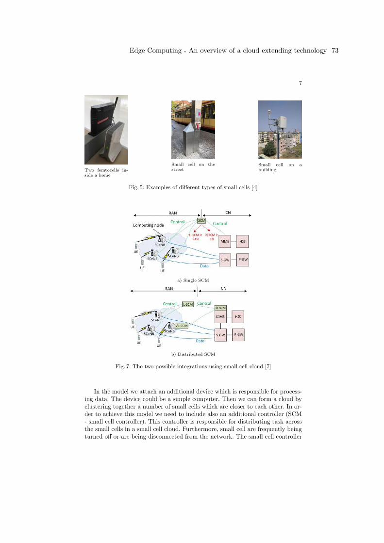
7
Two femtocells in-side a home
Small cell on thestreet
Small cell on abuilding
Fig. 5: Examples of different types of small cells [4]
a) Single SCM
b) Distributed SCM
Fig. 7: The two possible integrations using small cell cloud [7]
In the model we attach an additional device which is responsible for process-ing data. The device could be a simple computer. Then we can form a cloud byclustering together a number of small cells which are closer to each other. In or-der to achieve this model we need to include also an additional controller (SCM- small cell controller). This controller is responsible for distributing task acrossthe small cells in a small cell cloud. Furthermore, small cell are frequently beingturned off or are being disconnected from the network. The small cell controller
Edge Computing - An overview of a cloud extending technology 73
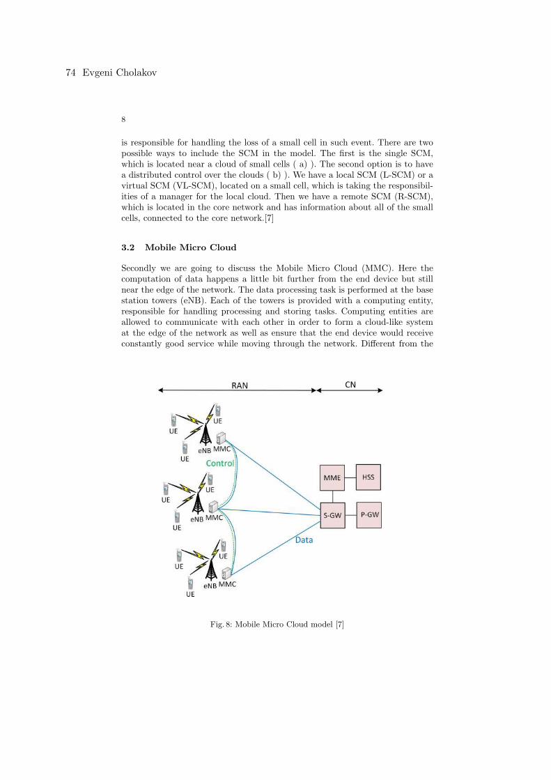
8
is responsible for handling the loss of a small cell in such event. There are twopossible ways to include the SCM in the model. The first is the single SCM,which is located near a cloud of small cells ( a) ). The second option is to havea distributed control over the clouds ( b) ). We have a local SCM (L-SCM) or avirtual SCM (VL-SCM), located on a small cell, which is taking the responsibil-ities of a manager for the local cloud. Then we have a remote SCM (R-SCM),which is located in the core network and has information about all of the smallcells, connected to the core network.[7]
3.2 Mobile Micro Cloud
Secondly we are going to discuss the Mobile Micro Cloud (MMC). Here thecomputation of data happens a little bit further from the end device but stillnear the edge of the network. The data processing task is performed at the basestation towers (eNB). Each of the towers is provided with a computing entity,responsible for handling processing and storing tasks. Computing entities areallowed to communicate with each other in order to form a cloud-like systemat the edge of the network as well as ensure that the end device would receiveconstantly good service while moving through the network. Different from the
Fig. 8: Mobile Micro Cloud model [7]
74 Evgeni Cholakov
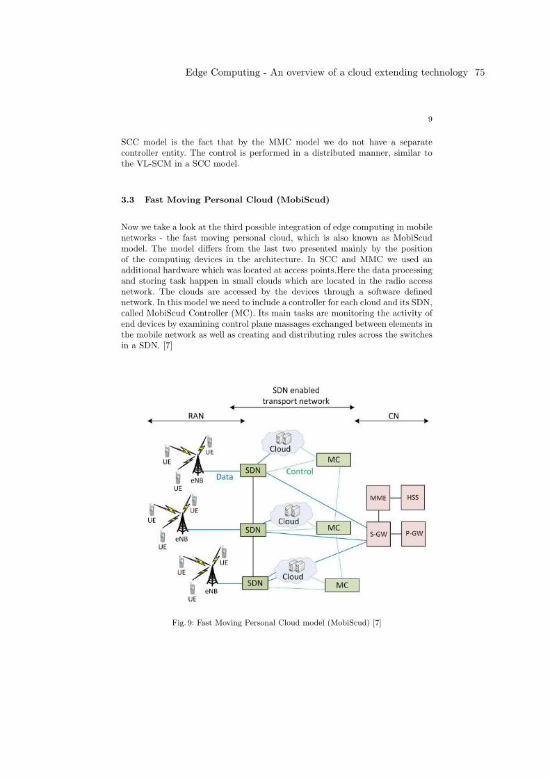
9
SCC model is the fact that by the MMC model we do not have a separatecontroller entity. The control is performed in a distributed manner, similar tothe VL-SCM in a SCC model.
3.3 Fast Moving Personal Cloud (MobiScud)
Now we take a look at the third possible integration of edge computing in mobilenetworks - the fast moving personal cloud, which is also known as MobiScudmodel. The model differs from the last two presented mainly by the positionof the computing devices in the architecture. In SCC and MMC we used anadditional hardware which was located at access points.Here the data processingand storing task happen in small clouds which are located in the radio accessnetwork. The clouds are accessed by the devices through a software definednetwork. In this model we need to include a controller for each cloud and its SDN,called MobiScud Controller (MC). Its main tasks are monitoring the activity ofend devices by examining control plane massages exchanged between elements inthe mobile network as well as creating and distributing rules across the switchesin a SDN. [7]
Fig. 9: Fast Moving Personal Cloud model (MobiScud) [7]
Edge Computing - An overview of a cloud extending technology 75
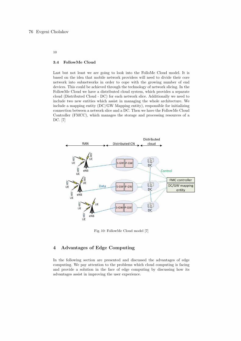
10
3.4 FollowMe Cloud
Last but not least we are going to look into the FolloMe Cloud model. It isbased on the idea that mobile network providers will need to divide their corenetwork into subnetworks in order to cope with the growing number of enddevices. This could be achieved through the technology of network slicing. In theFollowMe Cloud we have a distributed cloud system, which provides a separatecloud (Distributed Cloud - DC) for each network slice. Additionally we need toinclude two new entities which assist in managing the whole architecture. Weinclude a mapping entity (DC/GW Mapping entity), responsible for initializingconnection between a network slice and a DC. Then we have the FollowMe CloudController (FMCC), which manages the storage and processing resources of aDC. [7]
Fig. 10: FollowMe Cloud model [7]
4 Advantages of Edge Computing
In the following section are presented and discussed the advantages of edgecomputing. We pay attention to the problems which cloud computing is facingand provide a solution in the face of edge computing by discussing how itsadvantages assist in improving the user experience.
76 Evgeni Cholakov
11
4.1 Responsiveness
The time which an application or service takes to accomplish a task, also knownas response time or responsiveness, is crucial for today’s quality of service. Itis known that the average user keeps his attention on a task for no more than10 seconds. Anything slower than that leads to worse user experience.[9] Fur-thermore, there are numerous technologies which are time-sensitive. This meansthat they require very short response time in order to function properly andprovide good services. Edge computing could achieve those result and satisfythe low response time demand by utilizing the computing capacity of the edgedevices. Combined with an algorithm which prioritizes tasks and decides whichto be performed locally and which to be sent to a near edge computing server,it could be a step towards faster responsiveness.[14]To prove its ability to perform crucial tasks faster there is a face recognitionplatform developed which utilizes the edge nodes rather than the cloud. Theresult show that a task is performed for a total of 169 ms rather than 900 mswhich were needed by the platform if it was using the cloud for computation.Moreover, by wearable assistance devices, the response time is reduced from 80ms to 200 ms by using the technology of the edge computing.[10]
4.2 Internet traffic
Driven by the growing number of IoT devices, the internet traffic has increasedsignificantly in the recent years. More and more devices generate data and needcomputation capacity in order to process it. This capacity is provided by thecloud but when all of the devices transmit packages to the cloud the internettraffic becomes congested which could lead to great delays and packet losses.Edgecomputing reveals a solution to this problem by distributing the computing ca-pacity in edge servers physically located on key locations. Data from differentdevices does not need to travel large distance and also to the same server. More-over, by using the computing power of the data generating device, some taskscan be performed locally and thus not cause any traffic at all.[8] [14]
4.3 Power consumption
Always sending and receiving data requires for the Wifi interface of the deviceto be always functioning. This is an activity which requires a lot of power dueto the high energy demand of the Wifi interface. IoT devices have very limitedpower at disposal. Therefore, it is crucial for the devices to save it. Moreover,when the traffic in the network is increased, the congestions can cause a needfor the device to use, for a long period of time, its internet interface. Therefore,a lot of power will be wasted. Edge computing provides the opportunity for thedevices to transmit data for a shorter period of time or not at all. Hence thepower consumption will be reduced.[14] [10]
Edge Computing - An overview of a cloud extending technology 77
12
4.4 Storage
The edge computing concept provides a distributed storage system. This meansthat data could be stored across different physical devices at the edge of thenetwork and not in a centralized cloud system. This method of storing datacould lead to lower storage requirements for the cloud, lower pressure on thecloud and hence could result in a drop of the prices of the storage service ofthe cloud. Furthermore, a great advantage of the edge computing is its abilityto enable the technology of data replication. Because it is a distributed system,data will be divided and stored in fixed blocks on different devices. Those blocksoverlap and give us the opportunity to restore lost blocks of data by using otherones from neighbouring edge severs. Moreover, by edge computing the deviceswhich store the data can be physically located at different places. This providesthe ability to replicate data and store it at different locations. By doing this thedanger of loosing data could be significantly decreased.[14] [8]
5 Application of Edge Computing
In the following section we will discuss some of the applications of edge comput-ing. Scenarios will be presented in which edge computing plays a significant roleand helps in providing a better service.
5.1 Surveillance Cameras
One of the most famous possible application of edge computing is by collectingdata from surveillance cameras. This example provides a simple and clear viewof the possibilities of edge computing. In a scenario where we have a missingperson, one way of finding them is by processing the records of video cameras.But in an urban environment, where there is a huge number of cameras, alsoa huge number of data needs to be processed. It is a really heavy task if all ofthe cameras need to send their data to the cloud. Also, the processing wouldtake a lot of time and slow down the search. Time is really important in thosesituations. By using edge computing the cloud is relieved from this huge pressureand time can be reduced. The cloud only needs to produce the request and thensend it to the devices. Each of the devices performs its own processing of its owndata and only needs to report the results to the cloud. A lot of traffic costs canbe saved as well as processing time can be reduced.[10] [14]
5.2 Smart Environment
One of the ideas which have gained a huge popularity lately is the idea of smartenvironment. In the following subsections we divide the idea in some of its basiccomponents.
78 Evgeni Cholakov
13
Smart Grid An idea which is being discussed lately is the idea of smart grid.Smart grid is being called the next generation of power grid. But in order tobe achieved a lot of sensors, meters and other tracking devices need to be used.They need to be able to communicate fast and their data should be efficientlycollected and processed. Here the concept of edge computing appears to be oneof the enabling technologies for smart grid.
Smart Home Other technology assisted by the edge computing is the smarthome. An average household nowadays consists of many appliances and elec-tronic devices. Each of these technologies is equipped with numbers of sensorsand trackers. In order to provide the user with rich and useful information aswell as an easy control over the home, all of the data from these devices needsto be processed efficiently. Moreover, this data is only relevant for the currenthome and therefore there is no point in processing it in the cloud. Imagine ifevery smart home, which generates tons of data, sends it to the cloud for process-ing. Huge network congestions as well as high pressured will be the results. Byproviding and edge gateway and using an edge operating system we can enabledata to be collected and processed locally and thus relieve the network and cloudfrom a great pressure. Furthermore, the quality of the user experience could bestrongly increased.[10]
Smart Transportation Autonomous driving is one of the researched technolo-gies nowadays. In order to control and coordinate a large number of vehicles a lotof information from different sensors needs to be processed in a vehicle to vehiclenetwork. In this use case the delay is crucial, therefore fast data transmittingand processing is required. Edge computing could satisfy those requirements ofsmart transportation. There is currently proposed infrastructure-based vehiclecontrol system by Sasaki. By enabling source sharing between edge and cloudservers the latency is significantly decreased.[14]
Smart City By combining huge numbers of smart homes and the other men-tioned smart technologies we can expand to a smart city. In a smart city therewould a vast number of sensors without counting the ones which would be usedin the previously mentioned technologies. A smart city would generated PBs ofinformation per day which could strongly affect the network transport and cloudcapacity in a bad way. Furthermore, for cases which involve emergency or publicsafety, time is really important and delay should be minimized. We have alreadydiscussed the ability of edge computing to tackle those problems, therefore it isone of the main steps towards achieving a smart city.[10]
5.3 Content delivery and network acceleration
Network content which is accessed by users is stored on the servers of the contentproviders. When requested the request is handled by those servers. When the
Edge Computing - An overview of a cloud extending technology 79
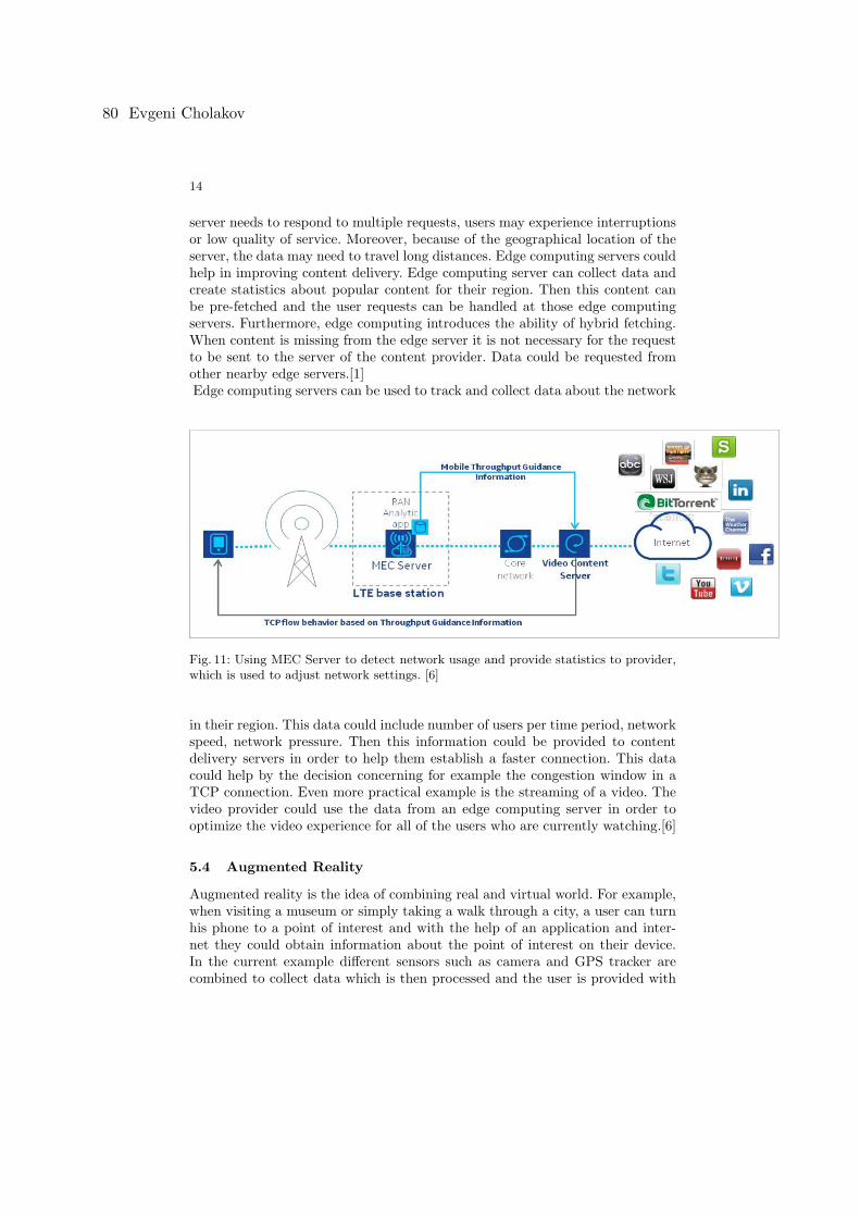
14
server needs to respond to multiple requests, users may experience interruptionsor low quality of service. Moreover, because of the geographical location of theserver, the data may need to travel long distances. Edge computing servers couldhelp in improving content delivery. Edge computing server can collect data andcreate statistics about popular content for their region. Then this content canbe pre-fetched and the user requests can be handled at those edge computingservers. Furthermore, edge computing introduces the ability of hybrid fetching.When content is missing from the edge server it is not necessary for the requestto be sent to the server of the content provider. Data could be requested fromother nearby edge servers.[1]Edge computing servers can be used to track and collect data about the network
Fig. 11: Using MEC Server to detect network usage and provide statistics to provider,which is used to adjust network settings. [6]
in their region. This data could include number of users per time period, networkspeed, network pressure. Then this information could be provided to contentdelivery servers in order to help them establish a faster connection. This datacould help by the decision concerning for example the congestion window in aTCP connection. Even more practical example is the streaming of a video. Thevideo provider could use the data from an edge computing server in order tooptimize the video experience for all of the users who are currently watching.[6]
5.4 Augmented Reality
Augmented reality is the idea of combining real and virtual world. For example,when visiting a museum or simply taking a walk through a city, a user can turnhis phone to a point of interest and with the help of an application and inter-net they could obtain information about the point of interest on their device.In the current example different sensors such as camera and GPS tracker arecombined to collect data which is then processed and the user is provided with
80 Evgeni Cholakov

15
a response. In the case of augmented reality low latency and fast processing arecrucial for the realisation of the idea. Therefore, edge computing proves itselfas an excellent technology for the case. Data could be sent to and processedin MEC servers closer to the desired point of interest rather than in a distantcloud server. The response time gets faster and the network is not additionallyloaded. Moreover, this data is irrelevant for anything else outside of the zone ofthe point of interest.[6] [1]Examples for augmented reality are Google Goggles, Layar, Junaio. Brian Com-puter Interaction is another example for AR which utilizes the power of edgecomputing. The idea is to detect human brainwaves with the help of a headsetand a phone. Then data is sent to a mobile edge server where it is processed.Communication with the cloud could also be used but only for archiving pur-poses.[1]
6 Challenges of Edge Computing
We already discussed what are the advantages of the edge computing and howit could improve the overall performance of network services. We have also givenexamples for possible applications. But it since it is still a new technology whichis being developed there are challenges which are still to be tackled. In thefollowing section we will discuss some of the problems which edge computing isfacing and give examples of ideas which could help in solving them.
6.1 Programmability and Integration
In the centre of the idea of edge computing is the combination and utilizationof various physical devices and different network topologies. This means thatapplications and services need to be able to cope with different platforms andresources. By cloud computing the infrastructure is transparent to the user. Theydo not know how an application is being ran. All that is requested from the useris a functioning software which is then given to the cloud service provider. Thecloud service provider is responsible fro deciding how and where the computa-tion happens in the cloud. Moreover, this enables the developers to use only oneprogramming language and design the software for a single platform since it isran only in the cloud. By edge computing the situation differs significantly. Mostof the platforms utilized by edge computing are heterogeneous. The runtime andresources of different platforms may differ. Therefore developers face a seriousproblem in order to design a service which can function properly on all types ofplatforms. [14] [10]A possible solution to this challenge could be the concept of computing stream.It is defined as a flow or series of functions/computations which can happen any-where on the data path. Those functions/computations could range from a singleaspect of a service/application to a whole functionality of a service/application.The user can decide where the processing of data should happen and what data
Edge Computing - An overview of a cloud extending technology 81
16
should be transported. Therefore, most of data can be processed on the edge de-vices (what the main idea of edge computing is) and less functions/computationscan be trusted to the different heterogeneous systems along the path. What ismore transport costs are additionally reduced.[10]
6.2 Naming
When it comes to programming a system which communicates with a great num-ber of other systems and devices the naming scheme is of great importance. Itis crucial for data communication to identify things and address them. By edgecomputing there is currently no naming scheme which has been standardized.Because of the large number of IoT devices and other edge nodes we can as-sume that each of them has its own structure and way of providing a service.Therefore developers need to examine and understand numerous protocols forcommunication in order to be able to design a reliable service. A naming schemecapable of fulfilling the demands of edge computing should pay a lot of atten-tion to privacy and security as well as be able to cope with dynamic networksand mobility of things. Nowadays we have standardized naming schemes such asDNS or URI which are able to satisfy the needs of cloud computing but prove tobe not enough in order to be implemented in edge computing. Furthermore themost famous and typical naming scheme based on IP addresses seems to be tooheavy and complex considering the fact that most of the edge nodes are resourceconstrained.[10] [14]Two naming schemes have been proposed for the concept of edge computing butthey still have some drawbacks which stop them from being generally accepted.Named Data Networking is the first one which has a hierarchical name structure.It proves to be human friendly but lacks the ability to separate data informationfrom hardware information which is a serious security drawback. Moreover it re-quires additional proxy in order to be used with more communication protocolssuch as ZigBee or Bluetooth. MobilityFirst is the second proposed scheme whichtackles the problem of NDN by being able to separate hardware information. Onthe other hand MobilityFirst requires a global unique identification which is farfrom being human friendly.[10] [14]In [10] there is a proposed concept of a naming scheme for a smaller and morelocal network of edge devices. The idea is to let the edgeOS to name the dif-ferent devices in a human friendly way. A structure for the name of the deviceis: (location).(role).(description of the data which is provided). For example ina smart home where an edgeOS is responsible for managing the devices couldsend information about the current temperature of the the air conditioner in theliving room in the following way: livingroom.airconditioner.currenttemperature.And it could be interpreted by an application as: ”The current temperature ofthe air conditioner in the living room is ...” .This seems to be a simple namingscheme which helps application to obtain and interpret data about numerousdevices in a fast way. Furthermore, it provides better service management andprogrammability for the service providers.
82 Evgeni Cholakov

17
6.3 Service Management
In order for the edge computing to be a reliable system some fundamental fea-tures need to be covered. Firstly there needs to be a good differentiation ofinformation. It means that service need to be clearly prioritized. For exampledata which is classified as emergency data needs to processed before any otherdata. Secondly extensibility is really important. It allows the user to add a newdevice easy to the system without worrying about compatibility. Isolation ofapplications and service is the third crucial point. A failure of a service or anapplication should not obstruct the functioning of the whole system. And lastbut not least, we need to pay attention to reliability. When a failure occurs itcould be caused by many reasons. It is a good idea for the service to be ableto detect the right reason for the failure and inform the user. To achieve thishowever all of the nodes involved in the network should be able to send reliablystatus or diagnosis information. Furthermore compared to WiFi and Bluetooththe connection reliability of edge nodes is not pleasing. Therefore data sensingand communication cannot be classified as reliable.[10]
6.4 Security and Privacy
It is well known that data is at its most vulnerable state when it is being trans-mitted. By cloud computing data needs to travel long distances before beingstored or processed and hence the time period in which it can be hijacked isgreat. By edge computing data needs to be transmitted at significantly shorterdistances or not at all. Thus attackers have little or no opportunity in hijackingsensitive data.[8] However a significant issues concerning security and privacystill remain. First of all a great number of devices generate sensitive user data.It is really important for this data to be really well secured. For example, byextracting data about the commodity usages of a house an attacker could de-termine when the owner is present and when not. The edge nodes are owned bythird party providers and some of them are not as secured as others. Thereforedata could be exposed to serious attacks when stored there. It is a problem toprovide all of the edge nodes with the same security. Today there are currentlydeveloped technologies which defend data on edge nodes but they are resourcehungry. Some of the edge nodes do not have the needed resources in order to usethose methods of protection.Ownership of data has always been a discussed question especially nowadayswith all of the privacy problems which the end users are facing. When storingdata on servers provided by a third party there are a lot of privacy issues con-cerning who has more control over the data. Therefore, it is a good idea to storethe data as close to the edge as possible even on the edge of the network itselfand providing the end user with full rights and control over their own data.[10][14]
Edge Computing - An overview of a cloud extending technology 83
18
7 Conclusion
With the growing numbers of devices which people are using and the integrationof new services which require a heavy amount of data, we are in a great need ofaccelerating the data processing methods. The concept of edge computing seemsto be the right extension of the current cloud computing model.The internetis slowly moving from a centralized control to the edge of the network. In thepaper we presented edge computing - the idea of processing data at the edge ofthe network - as a technology which could significantly assist the bright futureof the internet. We discussed how it differs from the traditional cloud model byutilizing the data generators and other nodes the data path in order to performfaster computing. A great plus of the concept is that it would not require a newcomplex hardware but the opposite, it uses the present devices. And ,what ismore, its functionality is based on innovative and well developed technologiesin the networking sector such as SDN and NFV. Then we introduced possibleways, how we can integrate it in the present mobile network. Edge computingis establishing itself as an important aspect of achieving 5G. The advantageswhich come with the integration of edge computing are numerous. We discussedits ability to accelerate the response time of the offered services as well as de-crease the traffic through the network. It is a step closer to more environmentalfriendly IT with its ability to reduce power consumption. Moreover, it providesnew storage opportunities and helps to tackle some of the issues concerning theprivacy of cloud computing. Furthermore, we took a look at the possible appli-cation of edge computing. We saw that it could play a great role in differentaspects of our lives. Its usefulness scales on different levels - from helping inour everyday life by enabling smart homes to accelerating the whole internet byassisting the content providers. Edge computing could become a significant partof our environment. Last but not least we paid attention to the challenges whichit is facing. Since edge computing is still a developing technology it is normal forit to have its still unsolved problems. On the other hand we introduced possiblesolutions which are currently being researched and could be brought to life inthe near future. To sum up edge computing is still a concept which needs to bedeeply examined and tested but it seems to be a technology which is coming inthe near future and it will be here to stay.
References
[1] Nasir Abbas et al. “Mobile edge computing: A survey”. In: IEEE Internetof Things Journal 5.1 (2017), pp. 450–465.
[2] Luigi Atzori, Antonio Iera, and Giacomo Morabito. “The internet of things:A survey”. In: Computer networks 54.15 (2010), pp. 2787–2805.
[3] “Cisco Global Cloud Index 2016-2021 White Paper”. In: ().[4] “Cloud Computing”. In: Wikipedia ().[5] Robert L Grossman. “The case for cloud computing”. In: IT professional
11.2 (2009), pp. 23–27.
84 Evgeni Cholakov
19
[6] Yun Chao Hu et al. “Mobile edge computing—A key technology towards5G”. In: ETSI white paper 11.11 (2015), pp. 1–16.
[7] Pavel Mach and Zdenek Becvar. “Mobile edge computing: A survey onarchitecture and computation offloading”. In: IEEE Communications Sur-veys & Tutorials 19.3 (2017), pp. 1628–1656.
[8] Saksham Mittal, Neelam Negi, and Rahul Chauhan. “Integration of edgecomputing with cloud computing”. In: 2017 International Conference onEmerging Trends in Computing and Communication Technologies (ICETCCT).IEEE. 2017, pp. 1–6.
[9] Jakob Nielsen. “Response Times: The 3 Important Limits”. In: ().[10] Weisong Shi et al. “Edge computing: Vision and challenges”. In: IEEE
Internet of Things Journal 3.5 (2016), pp. 637–646.[11] J Srinivas, K Venkata Subba Reddy, and A MOIZ Qyser. “Cloud com-
puting basics”. In: International journal of advanced research in computerand communication engineering 1.5 (2012), pp. 343–347.
[12] Xiang Sun and Nirwan Ansari. “EdgeIoT: Mobile edge computing for theInternet of Things”. In: IEEE Communications Magazine 54.12 (2016),pp. 22–29.
[13] Tarik Taleb et al. “On multi-access edge computing: A survey of the emerg-ing 5G network edge cloud architecture and orchestration”. In: IEEE Com-munications Surveys & Tutorials 19.3 (2017), pp. 1657–1681.
[14] Wei Yu et al. “A survey on the edge computing for the Internet of Things”.In: IEEE access 6 (2017), pp. 6900–6919.
[15] Zitterbart. “Telematik Vorlesung”. In: ().
Edge Computing - An overview of a cloud extending technology 85

Vergleich von Feuchtesensoren in Bezug aufGenauigkeit
Proseminar Mobile Computing03.05.2019
Ilia ChupakhinBetreuer Jan Formanek
1 Karlsruher Institut für Technologie, Kaiserstraße 12, 76131 Karlsruhe, [email protected]
https://www.kit.edu/2 Technology for Pervasive Computing (TECO), Vincenz-Prießnitz-Straße 1,76131
Karlsruhe, [email protected]://www.teco.edu/
Zusammenfassung. Bestimmte Modelle von Feuchtesensoren wurdenmit einem Referenzsensor in Bezug auf Genauigkeit verglichen. Der Re-ferenzsensor ist SHT75. Die zu vergleichenden Sensoren sind SHT31,HTU21D, BME280, DHT22. Es waren jeweils vier Exemplare von SHT31,HTU21D, DHT22 und drei Exemplare von BME280 vorhanden. Der Re-ferenzsensor war ein Einzelstück. Die Messungen wurden bei vier unter-schiedlichen relativen Luftfeuchtigkeitsniveaus durchgeführt. Die gemes-senen Werte wurden mithilfe von statistischen Methoden analysiert undanschließend wurde anhand der untersuchten Stichprobe auf die zu er-wartende Genauigkeit der gesamten Population von gegebenen Sensorengeschlossen.
Schlüsselwörter: Sensor · Luftfeuchtigkeit · Vergleich · SHT75 ·SHT31 · HTU21D · BME280 · DHT22
1 Einleitung
1.1 Motivation
Es gibt eine große Auswahl von Feuchtesensoren auf dem Markt. Die wichtigstenKriterien bei der Wahl eines Sensors sind der Preis und die Messgenauigkeit. Diebeiden Kriterien korrelieren miteinander: üblicherweise, je höher der Preis ist,umso höher ist die Messgenauigkeit. Doch manchmal kostet ein Sensor fünf- oderzehnmal so viel wie ein anderer, obwohl laut ihren Datenblättern der teurere nurum ein Prozent präziser die Luftfeuchtigkeit messen kann als der billigere. DerPreisunterschied wird umso spürbarer, wenn man die Sensoren in großen Mengenbraucht. Deshalb will man sich für billigere Sensoren entscheiden, wenn ein sol-cher Präzisionsunterschied für den beabsichtigten Einsatzzweck nur wenig oder
86 Ilia Chupakhin

2 Ilia Chupakhin
komplett irrelevant ist. Allerdings entspricht die in den Datenblättern angege-bene Messgenauigkeit manchmal nicht der tatsächlichen. Darüber hinaus fehlenoft die Angaben über die zu erwartende Streuung von Messwerten. Diese Pro-bleme sind insbesondere bei billigen Sensoren öfter anzutreffen. Deswegen wollteman zuerst eine kleine Menge von Sensoren kaufen und ihre Messgenauigkeitexperimentell überprüfen, bevor man die Sensoren in großen Mengen einkauft.
1.2 Zielsetzung
Im Rahmen des Proseminars wird eine Stichprobe von vier unterschiedlichenModellen der Feuchtesensoren mit einem Referenzsensor in Bezug auf Messge-nauigkeit verglichen. Von jedem Modell außer dem Referenzsensor werden meh-rere Exemplare untersucht. Die Messungen werden bei vier unterschiedlichenrelativen Luftfeuchtigkeitsstufen durchgeführt. Danach werden die gesammeltenDaten einer statistischen Analyse unterzogen. Basierend auf der statistischenAnalyse wird eins der untersuchten Modelle von Feuchtesensoren gefunden, des-sen Messwerte den Messwerten vom Referenzsensor am nächsten liegen.
1.3 Begriffe und Abkürzungen
Luftfeuchtigkeitsstufe oder Luftfeuchtigkeitsniveau - relative Luftfeuchtigkeit 50%,60%, 70% oder 80%.RH(kommt von relative humidity) - relative Luftfeuchtigkeit.Mit Luftfeuchtigkeit wird die relative Luftfeuchtigkeit gemeint.Mit Sensor wird Feuchtesensor gemeint.Mit Testsensor wird einer der mit dem Referenzsensor zu vergleichenden Senso-ren gemeint, also HTU21D, SHT31, BME280 oder DHT22.
2 Vorbereitung auf das Messexperiment
Bevor das Messexperiment durchgeführt werden konnte, mussten die dafür be-nötigten Soft- und Hardwarekomponenten erstellt beziehungsweise zusammen-gesetzt werden. Außerdem musste eine passende experimentelle Umgebung ein-gerichtet werden.
2.1 Hardware
Die Datenblätter für die benutzten Hardware-Elemente sind im Literaturver-zeichnis verlinkt.Referenzsensor: SHT75Die zu vergleichenden Sensoren: SHT31, HTU21D, BME280, DHT22Mikrocontroller: NodeMCU ESP32SD-Speicherkartenmodul: PollinSD-Speicherkarte: Kingston 16GB
Vergleich von Feuchtesensoren in Bezug auf Genauigkeit 87
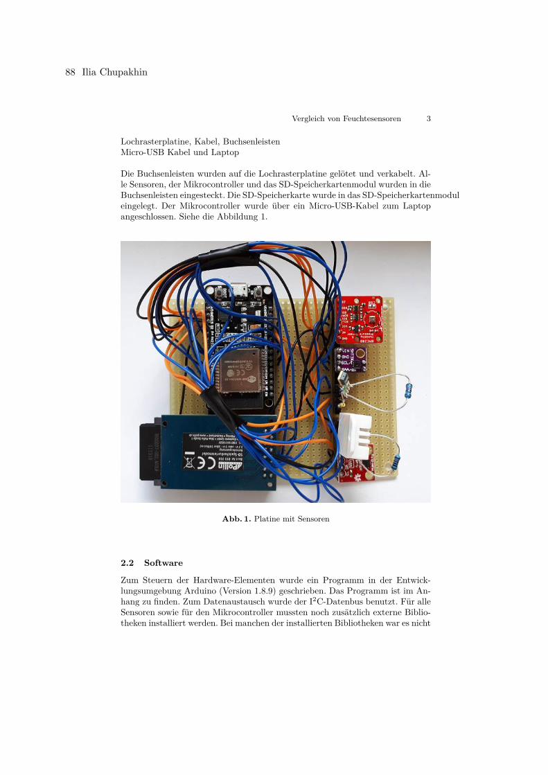
Vergleich von Feuchtesensoren 3
Lochrasterplatine, Kabel, BuchsenleistenMicro-USB Kabel und Laptop
Die Buchsenleisten wurden auf die Lochrasterplatine gelötet und verkabelt. Al-le Sensoren, der Mikrocontroller und das SD-Speicherkartenmodul wurden in dieBuchsenleisten eingesteckt. Die SD-Speicherkarte wurde in das SD-Speicherkartenmoduleingelegt. Der Mikrocontroller wurde über ein Micro-USB-Kabel zum Laptopangeschlossen. Siehe die Abbildung 1.
Abb. 1. Platine mit Sensoren
2.2 Software
Zum Steuern der Hardware-Elementen wurde ein Programm in der Entwick-lungsumgebung Arduino (Version 1.8.9) geschrieben. Das Programm ist im An-hang zu finden. Zum Datenaustausch wurde der I2C-Datenbus benutzt. Für alleSensoren sowie für den Mikrocontroller mussten noch zusätzlich externe Biblio-theken installiert werden. Bei manchen der installierten Bibliotheken war es nicht
88 Ilia Chupakhin

4 Ilia Chupakhin
vorgesehen, dass man die PIN-Nummern für serial clock und serial data Kanä-le nach seiner Wahl eingeben kann. Diese Funktionalität war aber notwendig,weil mehrere Sensoren zu einem Mikrocontroller angeschlossen werden mussten.Deswegen wurden folgende Funktionen zusätzlich zu den bereits vorhandenenimplementiert:
– In der Datei Adafruit_SHT31.h:
boolean begin ( int sda , int s c l , uint8_t i2caddr = SHT31_DEFAULT_ADDR) ;
– In der Datei Adafruit_SHT31.cpp:
boolean Adafruit_SHT31 : : begin ( int sda , int s c l , uint8_t i2caddr ) {Wire . begin ( sda , s c l ) ;_i2caddr = i2caddr ;r e s e t ( ) ;return t rue ;
}
– In der Datei Adafruit_HTU21DF.h:
boolean begin ( int sda , int s c l ) ;
– In der Datei Adafruit_HTU21DF.cpp:
boolean Adafruit_HTU21DF : : begin ( int sda , int s c l ) {Wire . begin ( sda , s c l ) ;r e s e t ( ) ;Wire . beg inTransmiss ion (HTU21DF_I2CADDR) ;Wire . wr i t e (HTU21DF_READREG) ;Wire . endTransmission ( ) ;Wire . requestFrom (HTU21DF_I2CADDR, 1 ) ;return (Wire . read ( ) == 0x2 ) ; // a f t e r r e s e t shou ld be 0x2
}
Das geschriebene Programm funktioniert folgendermaßen:Nach dem Einschalten des Mikrocontrollers wird eine neue Textdatei auf derSD-Speicherkarte einmal erstellt. Die Temperatur- und Luftfeuchtigkeitswertewerden von allen Sensoren einmal pro Sekunde ausgelesen. Die Werte werdentemporär auf dem Mikrocontroller gespeichert. Nach zehn Auslesezyklen werdendie gespeicherten Werte in die erstellte Textdatei hingeschrieben. Danach wirddas Programm wie vorher abgearbeitet.
Vergleich von Feuchtesensoren in Bezug auf Genauigkeit 89
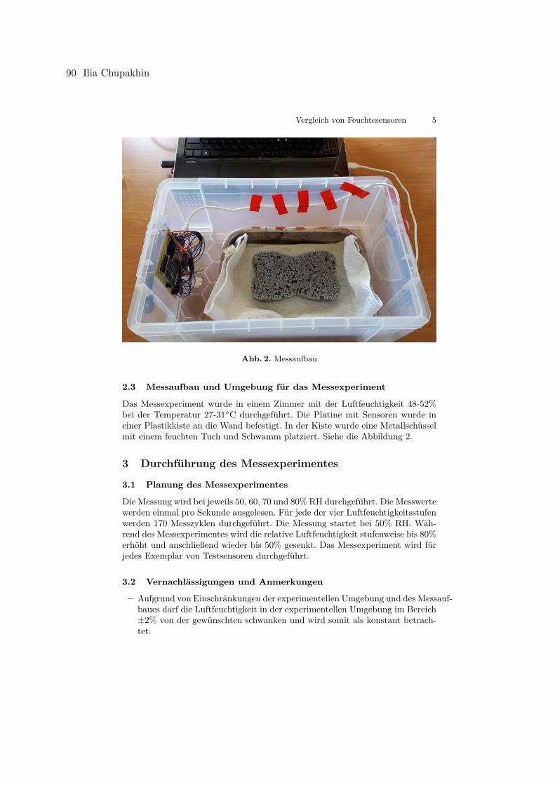
Vergleich von Feuchtesensoren 5
Abb. 2. Messaufbau
2.3 Messaufbau und Umgebung für das Messexperiment
Das Messexperiment wurde in einem Zimmer mit der Luftfeuchtigkeit 48-52%bei der Temperatur 27-31◦C durchgeführt. Die Platine mit Sensoren wurde ineiner Plastikkiste an die Wand befestigt. In der Kiste wurde eine Metallschüsselmit einem feuchten Tuch und Schwamm platziert. Siehe die Abbildung 2.
3 Durchführung des Messexperimentes
3.1 Planung des Messexperimentes
Die Messung wird bei jeweils 50, 60, 70 und 80% RH durchgeführt. Die Messwertewerden einmal pro Sekunde ausgelesen. Für jede der vier Luftfeuchtigkeitsstufenwerden 170 Messzyklen durchgeführt. Die Messung startet bei 50% RH. Wäh-rend des Messexperimentes wird die relative Luftfeuchtigkeit stufenweise bis 80%erhöht und anschließend wieder bis 50% gesenkt. Das Messexperiment wird fürjedes Exemplar von Testsensoren durchgeführt.
3.2 Vernachlässigungen und Anmerkungen
– Aufgrund von Einschränkungen der experimentellen Umgebung und des Messauf-baues darf die Luftfeuchtigkeit in der experimentellen Umgebung im Bereich±2% von der gewünschten schwanken und wird somit als konstant betrach-tet.
90 Ilia Chupakhin
6 Ilia Chupakhin
– Um die Luftfeuchtigkeit in der Plastikkiste während der Messung konstantzu halten, wird der Kistendeckel manipuliert.
– Die Sensoren besitzen unterschiedliche Antwortzeiten. Laut den Datenblät-tern sind die Antwortzeiten: 8 Sekunden für SHT75, 10 Sekunden für HTU21D,8 Sekunden für SHT31, 1 Sekunde für BME280, nicht angegeben für DHT22.Damit die Antwortzeiten möglichst kleine Auswirkung auf die Messergebnis-se haben, wird nach dem Wechseln zu der nächsten Luftfeuchtigkeitsstufezwei Minuten gewartet, bis die nächste Messung startet.
– Die einzelnen Sensoren werden nicht parallel, sondern nacheinander vomMikrocontroller angesprochen. Trotzdem wird angenommen, dass die Luft-feuchtigkeitswerte von allen fünf Sensoren zum gleichen Zeitpunkt ausge-lesen werden, weil das Auslesen aller Sensoren insgesamt weniger als 200Millisekunden dauert und in der experimentellen Umgebung sind jeglicheÄnderungen der Luftfeuchtigkeit innerhalb so einer kurzen Zeitspanne ver-nachlässigbar.
– Aus Kostengründen war die Stichprobe relativ klein. Es waren ein Exem-plar von dem Referenzsensor, drei Exemplare von BME280 und jeweils vierExemplare von den anderen Sensoren vorhanden. Die Größe der Stichprobespiegelt sich in der Breite des Konfidenzintervalles wider.1
– Die Messung bei der steigenden und anschließend bei der senkenden Luft-feuchtigkeit war notwendig, um die Hysterese von Sensoren herauszufinden.Das heißt, die Messewerte bei derselben Luftfeuchtigkeit können unterschied-lich ausfallen abhängig davon, ob die Luftfeuchtigkeit vor der Messung ge-stiegen oder gesunken ist.
3.3 Ablauf des Messexperimentes
Die relative Luftfeuchtigkeit im Zimmer wurde im Bereich 48-52% während desgesamten Messexperimentes konstant gehalten. Die Plastikkiste wurde auf denTisch nahe des Laptops gestellt. Die ersten Exemplare von den Testsensoren wur-den angeschlossen. Der Mikrocontroller wurde zum Laptop angeschlossen. DieMesswerte waren auf dem Bildschirm zu sehen und wurden einmal pro Sekun-de aktualisiert. Die Messung bei der Luftfeuchtigkeit 50% wurde durchgeführt.Danach wurde die Metallschüssel mit einem feuchten Tuch und Schwamm in diePlastikkiste eingelegt. Die Luftfeuchtigkeit in der Kiste ist auf 60% gestiegen. DieMessung bei der Luftfeuchtigkeit 60% wurde durchgeführt. Danach wurde derDeckel auf die Kiste gelegt, so dass sie etwa zu 2/3 abgedeckt war. Die relativeLuftfeuchtigkeit in der Kiste ist auf 70% gestiegen. Die Messung bei der Luft-feuchtigkeit 70% wurde durchgeführt. Danach wurde die Kiste mit dem Deckelkomplett abgedeckt. Die Luftfeuchtigkeit in der Kiste ist auf 80% gestiegen. Die1 Siehe das Kapitel Auswertung der Messergebnisse
Vergleich von Feuchtesensoren in Bezug auf Genauigkeit 91
Vergleich von Feuchtesensoren 7
Messung bei der Luftfeuchtigkeit 80% wurde durchgeführt. Anschließend wur-den analog die Messungen bei der absteigenden Luftfeuchtigkeit durchgeführt.Das Messexperiment wurde für alle Exemplare von Testsensoren durchgeführt(insgesamt vier Mal).
4 Auswertung der Messergebnisse
Nachdem das Messexperiment abgeschlossen war, mussten die Messergebnissemithilfe von statistischen Methoden ausgewertet werden. Die Textdateien mitden Messdaten wurden im Programm Apache OpenOffice Calc bearbeitet.Zuerst wurden die Messdaten manuell gefiltert. Die Messungen während denÜbergängen zwischen Luftfeuchtigkeitsstufen wurden entfernt. Auch die Mes-sungen in den nächsten zwei Minuten nach dem Übergang mussten entfernt wer-den, um den Einfluss von unterschiedlichen Antwortzeiten der Sensoren auf diestatistische Auswertung zu reduzieren. Während der Messung kam es manchmalzu den leichten Überschreitungen von den vereinbarten Grenzen von ±2% RH.Diese Daten wurden ebenso aus den zu analysierenden Messdaten entfernt.Danach wurde in jeder Messung und für jeden Sensor die Abweichung von denReferenzwerten ausgerechnet.
A = ϕref − ϕ (1)
A - Abweichung, ϕref - relative Luftfeuchtigkeit gemessen von dem Referenzsen-sor, ϕ - relative Luftfeuchtigkeit gemessen von einem Testsensor.Die Abbildungen drei bis sechs sind Streudiagramme, die die Abweichungen derMesswerte von den Referenzwerten während der Messung bei 50% RH zeigen.Die Streudiagramme für die Messungen bei den anderen Luftfeuchtigkeitsstu-fen sind im Anhang zu finden. Zur Erinnerung, die Messwerte wurden einmalpro Sekunde ausgelesen und für jede Luftfeuchtigkeitsstufe wurden 170 Mess-werte analysiert. An der Stelle sollte es angemerkt werden, dass die Kurven aufden Streudiagrammen für die Messungen bei 50 und 80% RH glatter als für dieMessungen bei 60 und 70% RH sind. Das liegt daran, dass während der Messun-gen bei 60 und 70% RH die Luftfeuchtigkeit stärker schwankte als bei 50 und80% RH. Der Kistendeckel musste oft hin- und hergeschoben werden, damit dieLuftfeuchtigkeit im Bereich 60±2%RH beziehungsweise 70±2%RH bleibt. Dadie Sensoren unterschiedliche Antwortzeiten haben, schwankten auch die Abwei-chungen zwischen den einzelnen Messungen stärker als während der Messungenbei 50% und 80% RH.
Anschließend wurde für jedes Exemplar der Testsensoren und für jede Luft-feuchtigkeitsstufe die absolute durchschnittliche Abweichung von den Referenz-werten ausgerechnet.
A = 1170 ·
170∑
i=1|Ai| (2)
Absolute durchschnittliche Abweichung bedeutet, dass es irrelevant ist, ob zum
92 Ilia Chupakhin
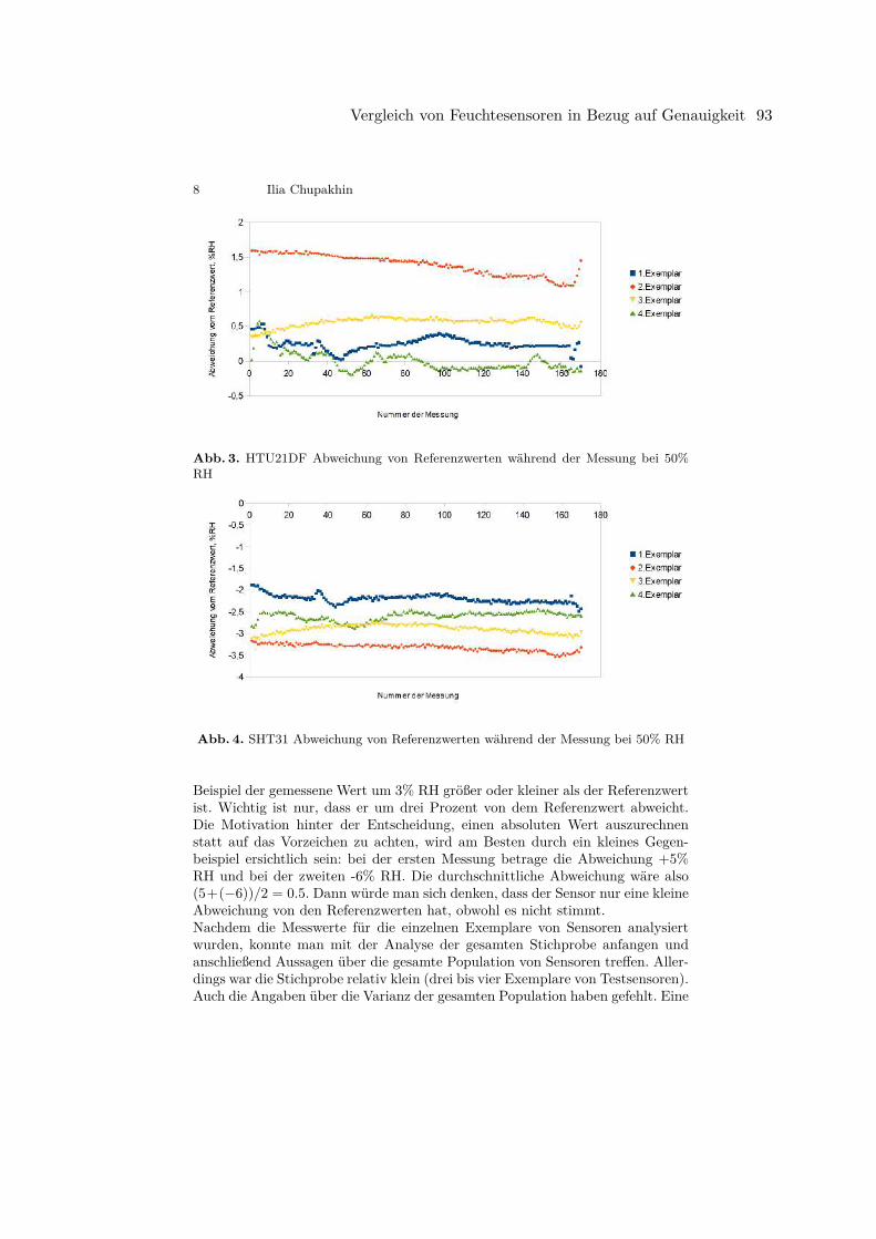
8 Ilia Chupakhin
Abb. 3. HTU21DF Abweichung von Referenzwerten während der Messung bei 50%RH
Abb. 4. SHT31 Abweichung von Referenzwerten während der Messung bei 50% RH
Beispiel der gemessene Wert um 3% RH größer oder kleiner als der Referenzwertist. Wichtig ist nur, dass er um drei Prozent von dem Referenzwert abweicht.Die Motivation hinter der Entscheidung, einen absoluten Wert auszurechnenstatt auf das Vorzeichen zu achten, wird am Besten durch ein kleines Gegen-beispiel ersichtlich sein: bei der ersten Messung betrage die Abweichung +5%RH und bei der zweiten -6% RH. Die durchschnittliche Abweichung wäre also(5+(−6))/2 = 0.5. Dann würde man sich denken, dass der Sensor nur eine kleineAbweichung von den Referenzwerten hat, obwohl es nicht stimmt.Nachdem die Messwerte für die einzelnen Exemplare von Sensoren analysiertwurden, konnte man mit der Analyse der gesamten Stichprobe anfangen undanschließend Aussagen über die gesamte Population von Sensoren treffen. Aller-dings war die Stichprobe relativ klein (drei bis vier Exemplare von Testsensoren).Auch die Angaben über die Varianz der gesamten Population haben gefehlt. Eine
Vergleich von Feuchtesensoren in Bezug auf Genauigkeit 93
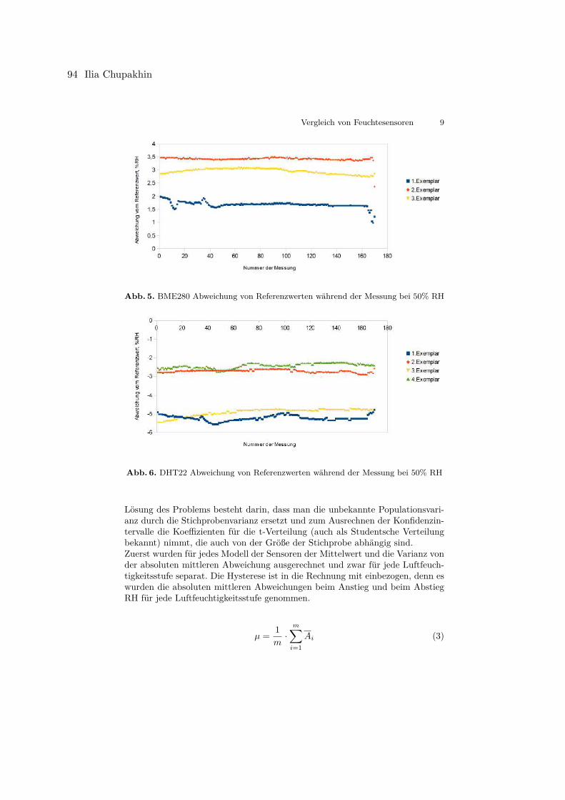
Vergleich von Feuchtesensoren 9
Abb. 5. BME280 Abweichung von Referenzwerten während der Messung bei 50% RH
Abb. 6. DHT22 Abweichung von Referenzwerten während der Messung bei 50% RH
Lösung des Problems besteht darin, dass man die unbekannte Populationsvari-anz durch die Stichprobenvarianz ersetzt und zum Ausrechnen der Konfidenzin-tervalle die Koeffizienten für die t-Verteilung (auch als Studentsche Verteilungbekannt) nimmt, die auch von der Größe der Stichprobe abhängig sind.Zuerst wurden für jedes Modell der Sensoren der Mittelwert und die Varianz vonder absoluten mittleren Abweichung ausgerechnet und zwar für jede Luftfeuch-tigkeitsstufe separat. Die Hysterese ist in die Rechnung mit einbezogen, denn eswurden die absoluten mittleren Abweichungen beim Anstieg und beim AbstiegRH für jede Luftfeuchtigkeitsstufe genommen.
µ = 1m·
m∑
i=1Ai (3)
94 Ilia Chupakhin
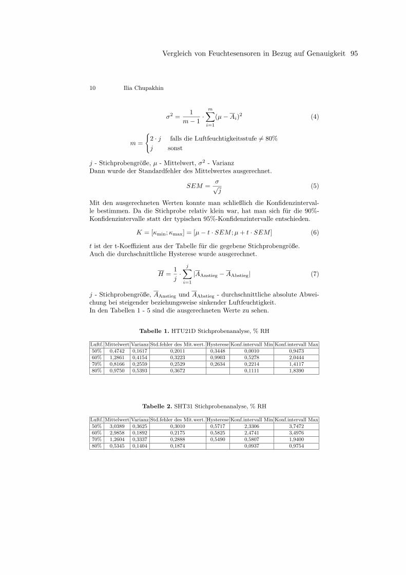
10 Ilia Chupakhin
σ2 = 1m− 1 ·
m∑
i=1(µ−Ai)2 (4)
m ={
2 · j falls die Luftfeuchtigkeitsstufe 6= 80%j sonst
j - Stichprobengröße, µ - Mittelwert, σ2 - VarianzDann wurde der Standardfehler des Mittelwertes ausgerechnet.
SEM = σ√j
(5)
Mit den ausgerechneten Werten konnte man schließlich die Konfidenzinterval-le bestimmen. Da die Stichprobe relativ klein war, hat man sich für die 90%-Konfidenzintervalle statt der typischen 95%-Konfidenzintervalle entschieden.
K = [κmin;κmax] = [µ− t · SEM ;µ+ t · SEM ] (6)
t ist der t-Koeffizient aus der Tabelle für die gegebene Stichprobengröße.Auch die durchschnittliche Hysterese wurde ausgerechnet.
H = 1j·
j∑
i=1|AAnstieg −AAbstieg| (7)
j - Stichprobengröße, AAnstieg und AAbstieg - durchschnittliche absolute Abwei-chung bei steigender beziehungsweise sinkender Luftfeuchtigkeit.In den Tabellen 1 - 5 sind die ausgerechneten Werte zu sehen.
Tabelle 1. HTU21D Stichprobenanalyse, % RH
Luftf. Mittelwert Varianz Std.fehler des Mit.wert. Hysterese Konf.intervall Min Konf.intervall Max50% 0,4742 0,1617 0,2011 0,3448 0,0010 0,947360% 1,2861 0,4154 0,3223 0,9903 0,5278 2,044470% 0,8166 0,2559 0,2529 0,2634 0,2214 1,411780% 0,9750 0,5393 0,3672 0,1111 1,8390
Tabelle 2. SHT31 Stichprobenanalyse, % RH
Luftf. Mittelwert Varianz Std.fehler des Mit.wert. Hysterese Konf.intervall Min Konf.intervall Max50% 3,0389 0,3625 0,3010 0,5717 2,3306 3,747260% 2,9858 0,1892 0,2175 0,5825 2,4741 3,497670% 1,2604 0,3337 0,2888 0,5490 0,5807 1,940080% 0,5345 0,1404 0,1874 0,0937 0,9754
Vergleich von Feuchtesensoren in Bezug auf Genauigkeit 95
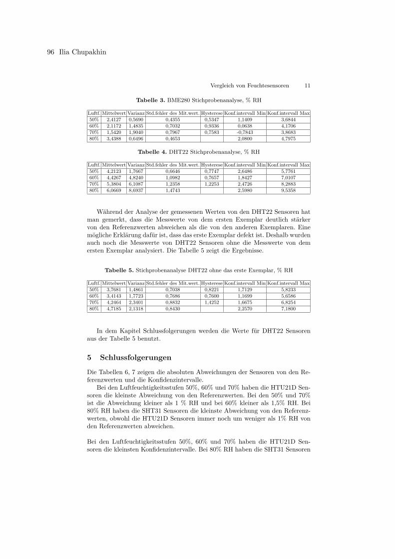
Vergleich von Feuchtesensoren 11
Tabelle 3. BME280 Stichprobenanalyse, % RH
Luftf. Mittelwert Varianz Std.fehler des Mit.wert. Hysterese Konf.intervall Min Konf.intervall Max50% 2,4127 0,5690 0,4355 0,5347 1,1409 3,684460% 2,1172 1,4835 0,7032 0,9336 0,0638 4,170670% 1,5420 1,9040 0,7967 0,7583 -0,7843 3,868380% 3,4388 0,6496 0,4653 2,0800 4,7975
Tabelle 4. DHT22 Stichprobenanalyse, % RH
Luftf. Mittelwert Varianz Std.fehler des Mit.wert. Hysterese Konf.intervall Min Konf.intervall Max50% 4,2123 1,7667 0,6646 0,7747 2,6486 5,776160% 4,4267 4,8240 1,0982 0,7657 1,8427 7,010770% 5,3804 6,1087 1,2358 1,2253 2,4726 8,288380% 6,0669 8,6937 1,4743 2,5980 9,5358
Während der Analyse der gemessenen Werten von den DHT22 Sensoren hatman gemerkt, dass die Messwerte von dem ersten Exemplar deutlich stärkervon den Referenzwerten abweichen als die von den anderen Exemplaren. Einemögliche Erklärung dafür ist, dass das erste Exemplar defekt ist. Deshalb wurdenauch noch die Messwerte von DHT22 Sensoren ohne die Messwerte von demersten Exemplar analysiert. Die Tabelle 5 zeigt die Ergebnisse.
Tabelle 5. Stichprobenanalyse DHT22 ohne das erste Exemplar, % RH
Luftf. Mittelwert Varianz Std.fehler des Mit.wert. Hysterese Konf.intervall Min Konf.intervall Max50% 3,7681 1,4861 0,7038 0,8221 1,7129 5,823360% 3,4143 1,7723 0,7686 0,7600 1,1699 5,658670% 4,2464 2,3401 0,8832 1,4252 1,6675 6,825480% 4,7185 2,1318 0,8430 2,2570 7,1800
In dem Kapitel Schlussfolgerungen werden die Werte für DHT22 Sensorenaus der Tabelle 5 benutzt.
5 Schlussfolgerungen
Die Tabellen 6, 7 zeigen die absoluten Abweichungen der Sensoren von den Re-ferenzwerten und die Konfidenzintervalle.
Bei den Luftfeuchtigkeitsstufen 50%, 60% und 70% haben die HTU21D Sen-soren die kleinste Abweichung von den Referenzwerten. Bei den 50% und 70%ist die Abweichung kleiner als 1 % RH und bei 60% kleiner als 1,5% RH. Bei80% RH haben die SHT31 Sensoren die kleinste Abweichung von den Referenz-werten, obwohl die HTU21D Sensoren immer noch um weniger als 1% RH vonden Referenzwerten abweichen.
Bei den Luftfeuchtigkeitsstufen 50%, 60% und 70% haben die HTU21D Sen-soren die kleinsten Konfidenzintervalle. Bei 80% RH haben die SHT31 Sensoren
96 Ilia Chupakhin
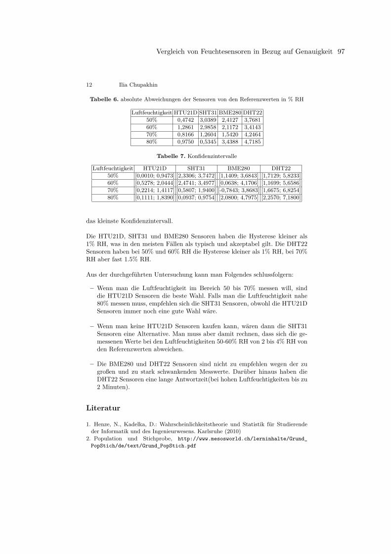
12 Ilia Chupakhin
Tabelle 6. absolute Abweichungen der Sensoren von den Referenzwerten in % RH
Luftfeuchtigkeit HTU21D SHT31 BME280 DHT2250% 0,4742 3,0389 2,4127 3,768160% 1,2861 2,9858 2,1172 3,414370% 0,8166 1,2604 1,5420 4,246480% 0,9750 0,5345 3,4388 4,7185
Tabelle 7. Konfidenzintervalle
Luftfeuchtigkeit HTU21D SHT31 BME280 DHT2250% [0,0010; 0,9473] [2,3306; 3,7472] [1,1409; 3,6843] [1,7129; 5,8233]60% [0,5278; 2,0444] [2,4741; 3,4977] [0,0638; 4,1706] [1,1699; 5,6586]70% [0,2214; 1,4117] [0,5807; 1,9400] [-0,7843; 3,8683] [1,6675; 6,8254]80% [0,1111; 1,8390] [0,0937; 0,9754] [2,0800; 4,7975] [2,2570; 7,1800]
das kleinste Konfidenzintervall.
Die HTU21D, SHT31 und BME280 Sensoren haben die Hysterese kleiner als1% RH, was in den meisten Fällen als typisch und akzeptabel gilt. Die DHT22Sensoren haben bei 50% und 60% RH die Hysterese kleiner als 1% RH, bei 70%RH aber fast 1.5% RH.
Aus der durchgeführten Untersuchung kann man Folgendes schlussfolgern:
– Wenn man die Luftfeuchtigkeit im Bereich 50 bis 70% messen will, sinddie HTU21D Sensoren die beste Wahl. Falls man die Luftfeuchtigkeit nahe80% messen muss, empfehlen sich die SHT31 Sensoren, obwohl die HTU21DSensoren immer noch eine gute Wahl wäre.
– Wenn man keine HTU21D Sensoren kaufen kann, wären dann die SHT31Sensoren eine Alternative. Man muss aber damit rechnen, dass sich die ge-messenen Werte bei den Luftfeuchtigkeiten 50-60% RH von 2 bis 4% RH vonden Referenzwerten abweichen.
– Die BME280 und DHT22 Sensoren sind nicht zu empfehlen wegen der zugroßen und zu stark schwankenden Messwerte. Darüber hinaus haben dieDHT22 Sensoren eine lange Antwortzeit(bei hohen Luftfeuchtigkeiten bis zu2 Minuten).
Literatur
1. Henze, N., Kadelka, D.: Wahrscheinlichkeitstheorie und Statistik für Studierendeder Informatik und des Ingenieurwesens. Karlsruhe (2010)
2. Population und Stichprobe, http://www.mesosworld.ch/lerninhalte/Grund_PopStich/de/text/Grund_PopStich.pdf
Vergleich von Feuchtesensoren in Bezug auf Genauigkeit 97
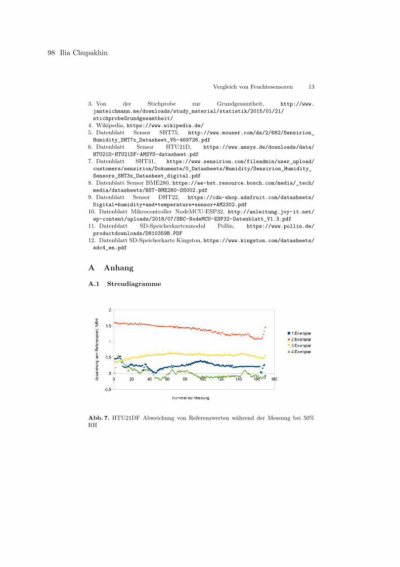
Vergleich von Feuchtesensoren 13
3. Von der Stichprobe zur Grundgesamtheit, http://www.janteichmann.me/downloads/study_material/statistik/2015/01/21/stichprobeGrundgesamtheit/
4. Wikipedia, https://www.wikipedia.de/5. Datenblatt Sensor SHT75, http://www.mouser.com/ds/2/682/Sensirion_
Humidity_SHT7x_Datasheet_V5-469726.pdf6. Datenblatt Sensor HTU21D, https://www.amsys.de/downloads/data/
HTU21D-HTU21DF-AMSYS-datasheet.pdf7. Datenblatt SHT31, https://www.sensirion.com/fileadmin/user_upload/
customers/sensirion/Dokumente/0_Datasheets/Humidity/Sensirion_Humidity_Sensors_SHT3x_Datasheet_digital.pdf
8. Datenblatt Sensor BME280, https://ae-bst.resource.bosch.com/media/_tech/media/datasheets/BST-BME280-DS002.pdf
9. Datenblatt Sensor DHT22, https://cdn-shop.adafruit.com/datasheets/Digital+humidity+and+temperature+sensor+AM2302.pdf
10. Datenblatt Mikrocontroller NodeMCU-ESP32, http://anleitung.joy-it.net/wp-content/uploads/2018/07/SBC-NodeMCU-ESP32-Datenblatt_V1.3.pdf
11. Datenblatt SD-Speicherkartenmodul Pollin, https://www.pollin.de/productdownloads/D810359B.PDF
12. Datenblatt SD-Speicherkarte Kingston, https://www.kingston.com/datasheets/sdc4_en.pdf
A Anhang
A.1 Streudiagramme
Abb. 7. HTU21DF Abweichung von Referenzwerten während der Messung bei 50%RH
98 Ilia Chupakhin
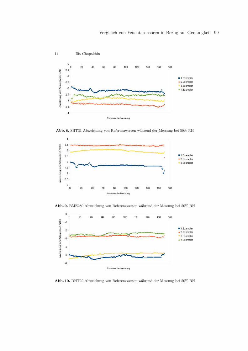
14 Ilia Chupakhin
Abb. 8. SHT31 Abweichung von Referenzwerten während der Messung bei 50% RH
Abb. 9. BME280 Abweichung von Referenzwerten während der Messung bei 50% RH
Abb. 10. DHT22 Abweichung von Referenzwerten während der Messung bei 50% RH
Vergleich von Feuchtesensoren in Bezug auf Genauigkeit 99
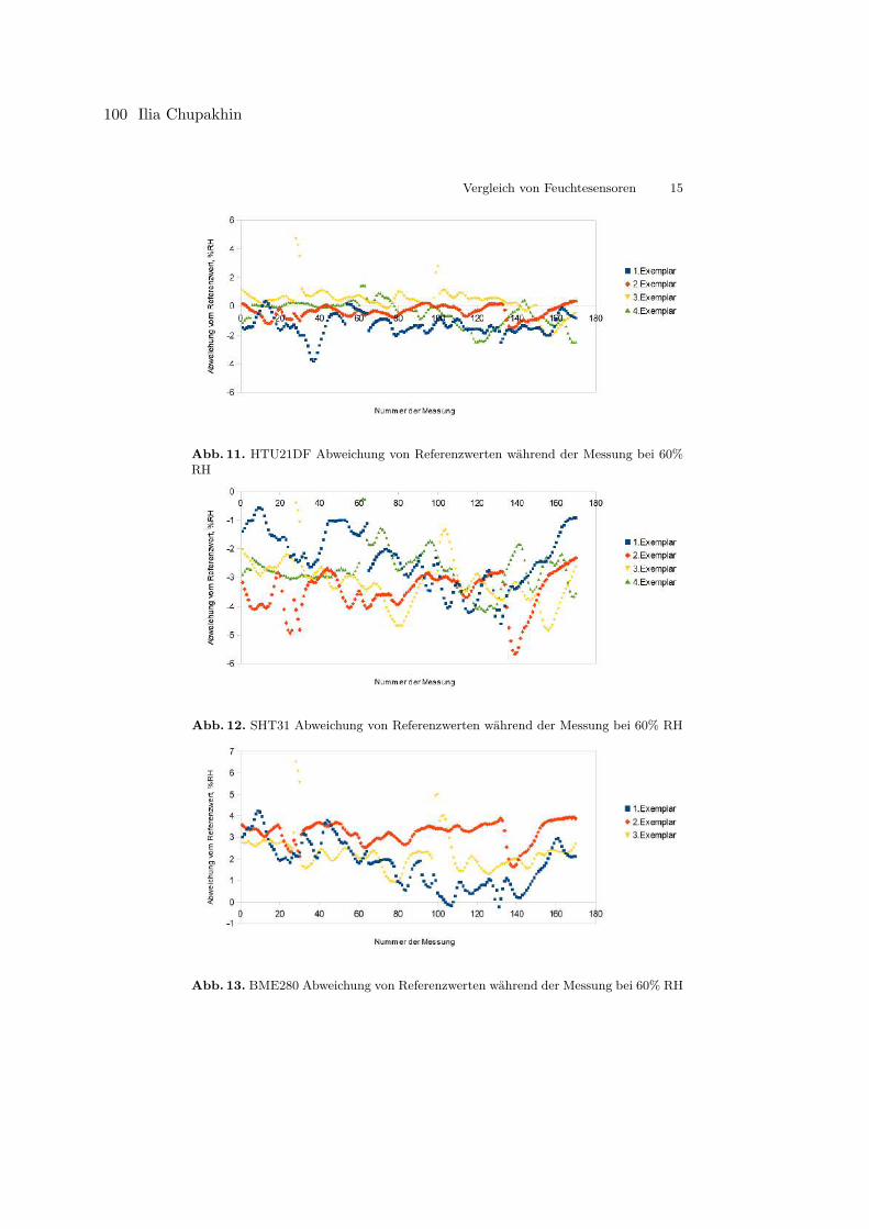
Vergleich von Feuchtesensoren 15
Abb. 11. HTU21DF Abweichung von Referenzwerten während der Messung bei 60%RH
Abb. 12. SHT31 Abweichung von Referenzwerten während der Messung bei 60% RH
Abb. 13. BME280 Abweichung von Referenzwerten während der Messung bei 60% RH
100 Ilia Chupakhin
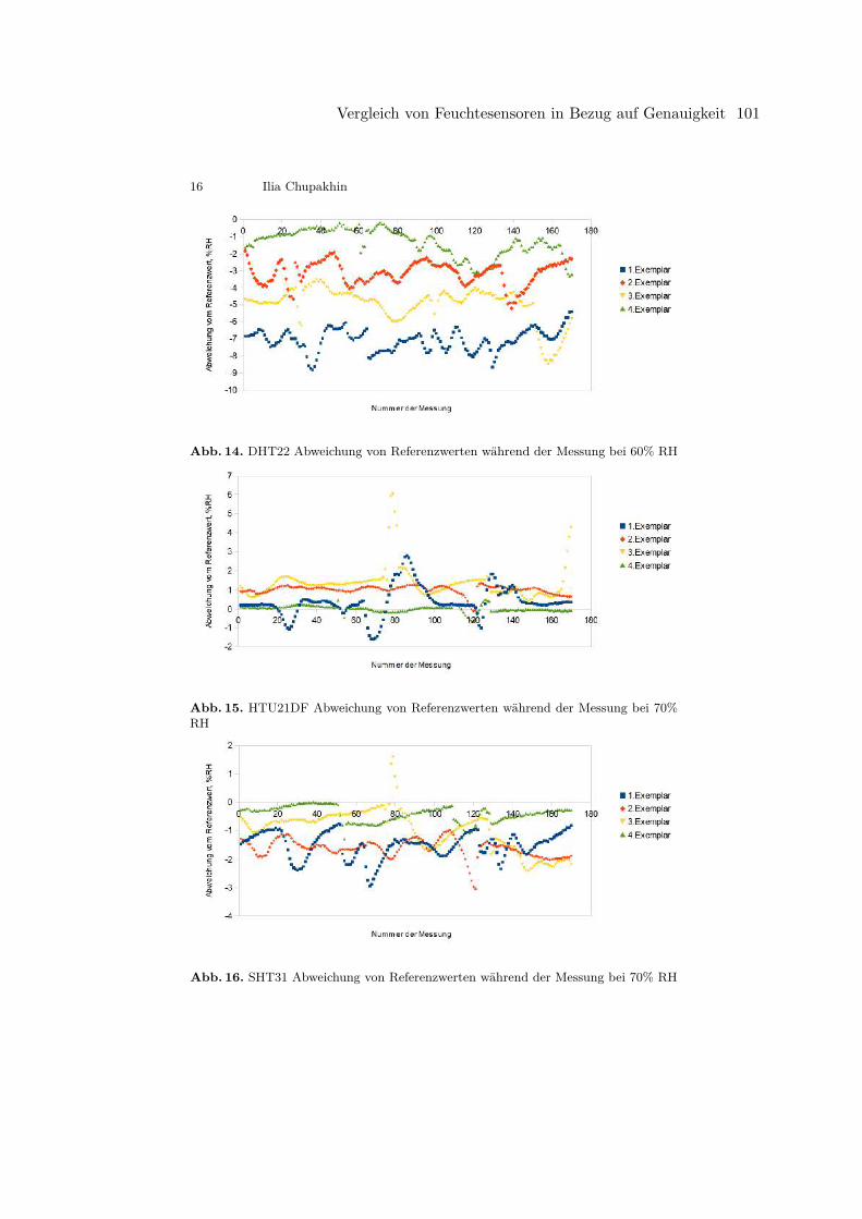
16 Ilia Chupakhin
Abb. 14. DHT22 Abweichung von Referenzwerten während der Messung bei 60% RH
Abb. 15. HTU21DF Abweichung von Referenzwerten während der Messung bei 70%RH
Abb. 16. SHT31 Abweichung von Referenzwerten während der Messung bei 70% RH
Vergleich von Feuchtesensoren in Bezug auf Genauigkeit 101
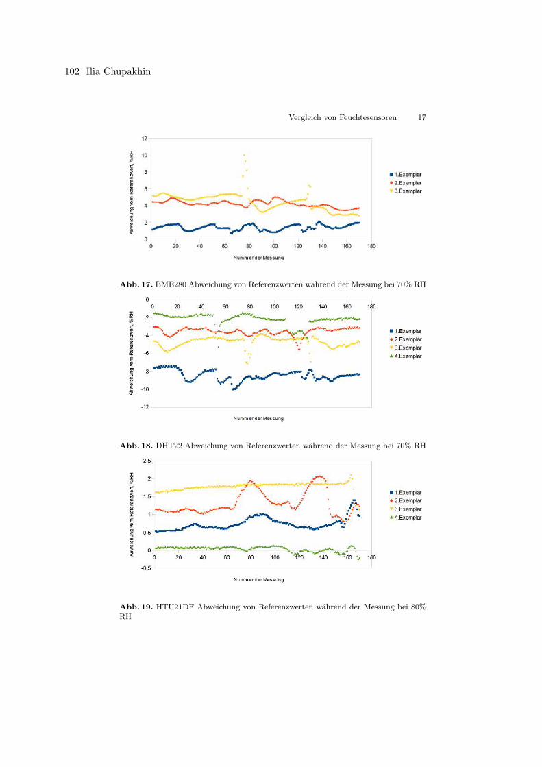
Vergleich von Feuchtesensoren 17
Abb. 17. BME280 Abweichung von Referenzwerten während der Messung bei 70% RH
Abb. 18. DHT22 Abweichung von Referenzwerten während der Messung bei 70% RH
Abb. 19. HTU21DF Abweichung von Referenzwerten während der Messung bei 80%RH
102 Ilia Chupakhin
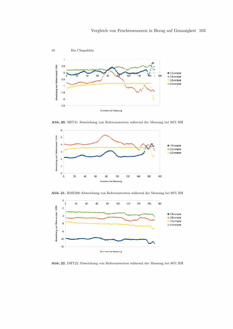
18 Ilia Chupakhin
Abb. 20. SHT31 Abweichung von Referenzwerten während der Messung bei 80% RH
Abb. 21. BME280 Abweichung von Referenzwerten während der Messung bei 80% RH
Abb. 22. DHT22 Abweichung von Referenzwerten während der Messung bei 80% RH
Vergleich von Feuchtesensoren in Bezug auf Genauigkeit 103
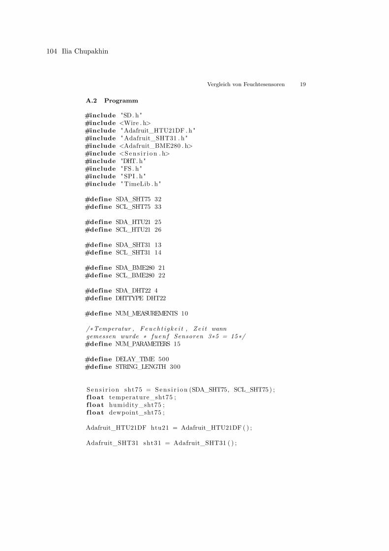
Vergleich von Feuchtesensoren 19
A.2 Programm
#include "SD. h "#include <Wire . h>#include "Adafruit_HTU21DF . h "#include " Adafruit_SHT31 . h "#include <Adafruit_BME280 . h>#include <Sen s i r i on . h>#include "DHT. h "#include "FS . h "#include " SPI . h "#include " TimeLib . h "
#define SDA_SHT75 32#define SCL_SHT75 33
#define SDA_HTU21 25#define SCL_HTU21 26
#define SDA_SHT31 13#define SCL_SHT31 14
#define SDA_BME280 21#define SCL_BME280 22
#define SDA_DHT22 4#define DHTTYPE DHT22
#define NUM_MEASUREMENTS 10
/∗Temperatur , Feuch t i g k e i t , Ze i t wanngemessen wurde ∗ f u en f Sensoren 3∗5 = 15∗/#define NUM_PARAMETERS 15
#define DELAY_TIME 500#define STRING_LENGTH 300
Sen s i r i on sht75 = Sen s i r i on (SDA_SHT75, SCL_SHT75 ) ;f loat temperature_sht75 ;f loat humidity_sht75 ;f loat dewpoint_sht75 ;
Adafruit_HTU21DF htu21 = Adafruit_HTU21DF ( ) ;
Adafruit_SHT31 sht31 = Adafruit_SHT31 ( ) ;
104 Ilia Chupakhin

20 Ilia Chupakhin
Adafruit_BME280 bme280 = Adafruit_BME280 ( ) ;TwoWire wire_bme280 = TwoWire ( 5 ) ;
DHT dht22 (SDA_DHT22, DHTTYPE) ;
/∗measurements [ x ] [ y ] :x i s t i−t e Messungy=0 Temp. SHT75y=1 Feucht . SHT75y=2 d ie s e i t dem Einscha l t en des M i k r o k o n t r o l l e r s vergangene Ze i t
in Mi l l i s ekunden SHT75y=3 Temp. HTU21y=4 Feucht . HTU21y=5 d ie s e i t dem Einscha l t en des M i k r o k o n t r o l l e r s vergangene Ze i t
in Mi l l i s ekunden HTU21y=6 Temp. SHT31y=7 Feucht . SHT31y=8 d ie s e i t dem Einscha l t en des M i k r o k o n t r o l l e r s vergangene Ze i t
in Mi l l i s ekunden SHT31y=9 Temp. BME280y=10 Feucht .BME280y=11 d ie s e i t dem Einscha l t en des M i k r o k o n t r o l l e r s vergangene Ze i t
in Mi l l i s ekunden BME280y=12 Temp. DHT22y=13 Feucht .DHT22y=14 d ie s e i t dem Einscha l t en des M i k r o k o n t r o l l e r s vergangene Ze i t
in Mi l l i s ekunden DHT22∗/f loat measurements [NUM_MEASUREMENTS] [NUM_PARAMETERS] ;
int counter = 0 ;int totalMeasurementCounter = 0 ;char f i leName [ 3 2 ] ;
void doMeasurement ( ) {
sht75 . measure(&measurements [ counter ] [ 0 ] , &measurements [ counter ] [ 1 ] ,&dewpoint_sht75 ) ;
measurements [ counter ] [ 2 ] = ( f loat ) m i l l i s ( ) ;
htu21 . begin (SDA_HTU21, SCL_HTU21) ;measurements [ counter ] [ 3 ] = htu21 . readTemperature ( ) ;measurements [ counter ] [ 4 ] = htu21 . readHumidity ( ) ;
Vergleich von Feuchtesensoren in Bezug auf Genauigkeit 105

Vergleich von Feuchtesensoren 21
measurements [ counter ] [ 5 ] = ( f loat ) m i l l i s ( ) ;
sht31 . begin (SDA_SHT31, SCL_SHT31 ) ;measurements [ counter ] [ 6 ] = sht31 . readTemperature ( ) ;measurements [ counter ] [ 7 ] = sht31 . readHumidity ( ) ;measurements [ counter ] [ 8 ] = ( f loat ) m i l l i s ( ) ;
measurements [ counter ] [ 9 ] = bme280 . readTemperature ( ) ;measurements [ counter ] [ 1 0 ] = bme280 . readHumidity ( ) ;measurements [ counter ] [ 1 1 ] = ( f loat ) m i l l i s ( ) ;
measurements [ counter ] [ 1 2 ] = dht22 . readTemperature ( ) ;measurements [ counter ] [ 1 3 ] = dht22 . readHumidity ( ) ;measurements [ counter ] [ 1 4 ] = ( f loat ) m i l l i s ( ) ;
}
void printLastMeasurement ( ) {
S e r i a l . p r i n t ( "SHT75␣Temp: ␣ " ) ; S e r i a l . p r i n t (measurements [ counter ] [ 0 ] ) ;S e r i a l . p r i n t ( " ; ␣Hum: ␣ " ) ; S e r i a l . p r i n t (measurements [ counter ] [ 1 ] ) ;S e r i a l . p r i n t ( " ; ␣Time : ␣ " ) ; S e r i a l . p r i n t l n (measurements [ counter ] [ 2 ] ) ;
S e r i a l . p r i n t ( "HTU21DF␣Temp: ␣ " ) ; S e r i a l . p r i n t (measurements [ counter ] [ 3 ] ) ;S e r i a l . p r i n t ( " ; ␣Hum: ␣ " ) ; S e r i a l . p r i n t (measurements [ counter ] [ 4 ] ) ;S e r i a l . p r i n t ( " ; ␣Time : ␣ " ) ; S e r i a l . p r i n t l n (measurements [ counter ] [ 5 ] ) ;
S e r i a l . p r i n t ( "SHT31␣Temp: ␣ " ) ; S e r i a l . p r i n t (measurements [ counter ] [ 6 ] ) ;S e r i a l . p r i n t ( " ; ␣Hum: ␣ " ) ; S e r i a l . p r i n t (measurements [ counter ] [ 7 ] ) ;S e r i a l . p r i n t ( " ; ␣Time : ␣ " ) ; S e r i a l . p r i n t l n (measurements [ counter ] [ 8 ] ) ;
S e r i a l . p r i n t ( "BME280␣Temp: ␣ " ) ; S e r i a l . p r i n t (measurements [ counter ] [ 9 ] ) ;S e r i a l . p r i n t ( " ; ␣Hum: ␣ " ) ; S e r i a l . p r i n t (measurements [ counter ] [ 1 0 ] ) ;S e r i a l . p r i n t ( " ; ␣Time : ␣ " ) ; S e r i a l . p r i n t l n (measurements [ counter ] [ 1 1 ] ) ;
S e r i a l . p r i n t ( "DHT22␣Temp: ␣ " ) ; S e r i a l . p r i n t (measurements [ counter ] [ 1 2 ] ) ;S e r i a l . p r i n t ( " ; ␣Hum: ␣ " ) ; S e r i a l . p r i n t (measurements [ counter ] [ 1 3 ] ) ;S e r i a l . p r i n t ( " ; ␣Time : ␣ " ) ; S e r i a l . p r i n t l n (measurements [ counter ] [ 1 4 ] ) ;S e r i a l . p r i n t l n ( " " ) ;
}
void writeMeasurementsOnSdCard ( ) {char bu f f e r [NUM_MEASUREMENTS] [STRING_LENGTH] ;for ( int i = 0 ; i < NUM_MEASUREMENTS; i++) {
106 Ilia Chupakhin

22 Ilia Chupakhin
St r ing measurement = St r ing ( totalMeasurementCounter ) + " ; "+ St r ing (measurements [ i ] [ 0 ] ) + " ; "+ St r ing (measurements [ i ] [ 1 ] ) + " ; "+ St r ing (measurements [ i ] [ 2 ] )+ " ; " + St r ing (measurements [ i ] [ 3 ] )+ " ; " + St r ing (measurements [ i ] [ 4 ] )+ " ; " + St r ing (measurements [ i ] [ 5 ] )+ " ; " + St r ing (measurements [ i ] [ 6 ] )+ " ; " + St r ing (measurements [ i ] [ 7 ] )+ " ; " + St r ing (measurements [ i ] [ 8 ] )+ " ; " + St r ing (measurements [ i ] [ 9 ] ) + " ; "+ St r ing (measurements [ i ] [ 1 0 ] ) + " ; "+ St r ing (measurements [ i ] [ 1 1 ] )+ " ; " + St r ing (measurements [ i ] [ 1 2 ] )+ " ; " + St r ing (measurements [ i ] [ 1 3 ] ) + " ; "+ St r ing (measurements [ i ] [ 1 4 ] ) ;
measurement . toCharArray ( bu f f e r [ i ] ,STRING_LENGTH) ;totalMeasurementCounter++;
}appendFile (SD, fi leName , bu f f e r ) ;
}
void createFi leName ( f s : : FS &f s ) {St r ing f i l eNameStr = " /measurements_ " ;char f i leNameChar [ 3 2 ] ;int numOfFiles = 0 ;F i l e d i r = f s . open ( " / " ) ;while ( d i r . openNextFi le ( ) ) {
numOfFiles++;}f i l eNameStr = f i l eNameStr + St r ing ( numOfFiles ) + " . txt " ;f i l eNameStr . toCharArray ( fi leName , 3 2 ) ;S e r i a l . p r i n t ( " Created␣name : ␣ " ) ;S e r i a l . p r i n t l n ( f i leName ) ;
}
void wr i t eF i l e ( f s : : FS &fs , const char ∗ message ){createFi leName ( f s ) ;S e r i a l . p r i n t f ( " Writing ␣ f i l e : ␣%s \n" , f i leName ) ;F i l e f i l e = f s . open ( fi leName , FILE_WRITE) ;i f ( ! f i l e ){
S e r i a l . p r i n t l n ( " Fa i l ed ␣ to ␣open␣ f i l e ␣ f o r ␣ wr i t i ng " ) ;
Vergleich von Feuchtesensoren in Bezug auf Genauigkeit 107
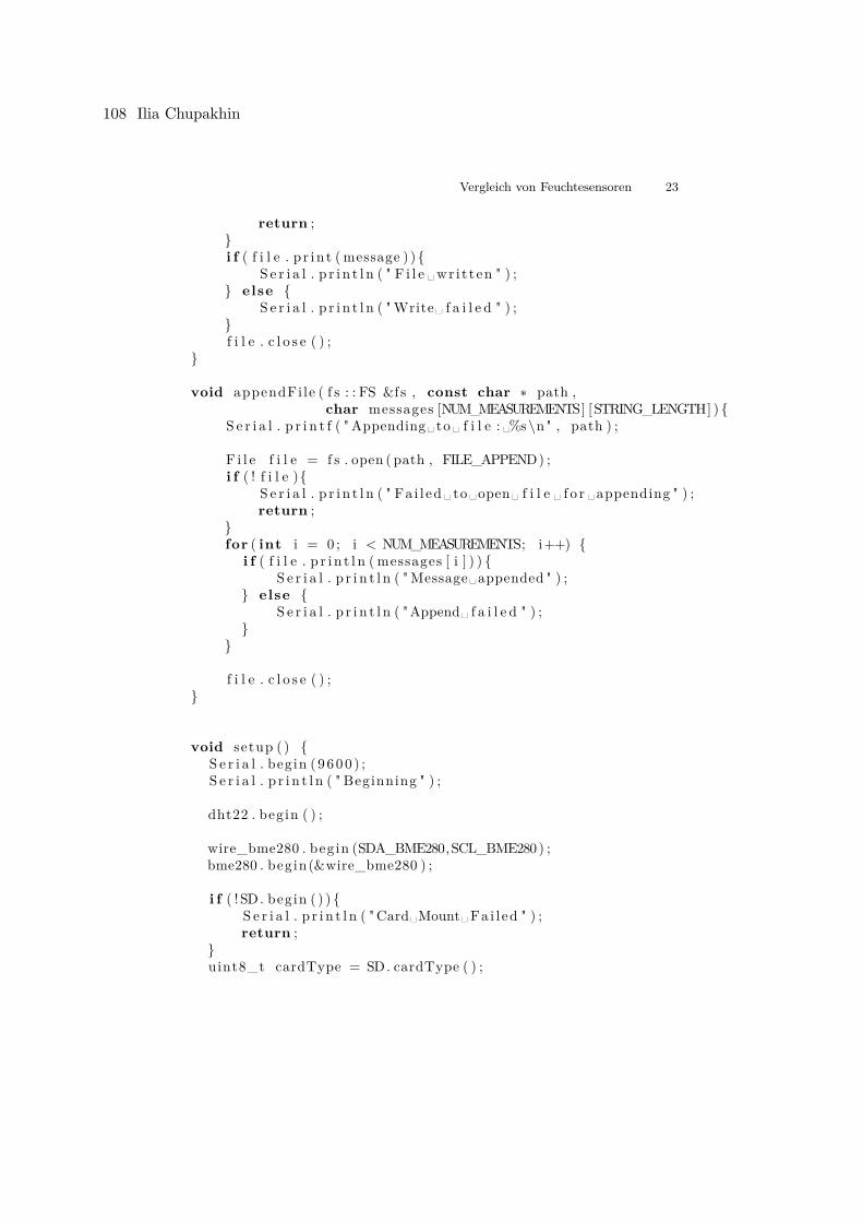
Vergleich von Feuchtesensoren 23
return ;}i f ( f i l e . p r i n t ( message ) ){
S e r i a l . p r i n t l n ( " F i l e ␣ wr i t t en " ) ;} else {
S e r i a l . p r i n t l n ( "Write␣ f a i l e d " ) ;}f i l e . c l o s e ( ) ;
}
void appendFile ( f s : : FS &fs , const char ∗ path ,char messages [NUM_MEASUREMENTS] [STRING_LENGTH] ) {
S e r i a l . p r i n t f ( " Appending␣ to ␣ f i l e : ␣%s \n " , path ) ;
F i l e f i l e = f s . open ( path , FILE_APPEND) ;i f ( ! f i l e ){
S e r i a l . p r i n t l n ( " Fa i l ed ␣ to ␣open␣ f i l e ␣ f o r ␣appending " ) ;return ;
}for ( int i = 0 ; i < NUM_MEASUREMENTS; i++) {
i f ( f i l e . p r i n t l n ( messages [ i ] ) ) {S e r i a l . p r i n t l n ( "Message␣appended " ) ;
} else {S e r i a l . p r i n t l n ( "Append␣ f a i l e d " ) ;
}}
f i l e . c l o s e ( ) ;}
void setup ( ) {S e r i a l . begin ( 9600 ) ;S e r i a l . p r i n t l n ( " Beginning " ) ;
dht22 . begin ( ) ;
wire_bme280 . begin (SDA_BME280,SCL_BME280) ;bme280 . begin(&wire_bme280 ) ;
i f ( ! SD. begin ( ) ) {S e r i a l . p r i n t l n ( "Card␣Mount␣ Fa i l ed " ) ;return ;
}uint8_t cardType = SD. cardType ( ) ;
108 Ilia Chupakhin
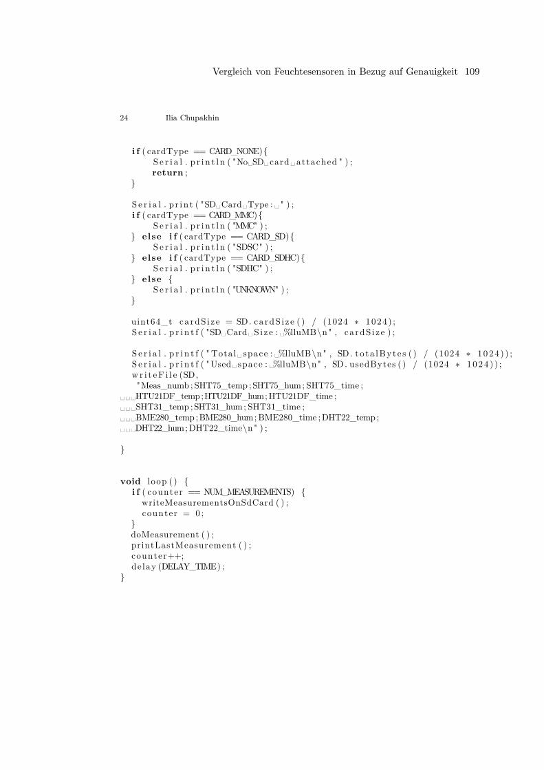
24 Ilia Chupakhin
i f ( cardType == CARD_NONE){S e r i a l . p r i n t l n ( "No␣SD␣card ␣ attached " ) ;return ;
}
S e r i a l . p r i n t ( "SD␣Card␣Type : ␣ " ) ;i f ( cardType == CARD_MMC){
S e r i a l . p r i n t l n ( "MMC" ) ;} else i f ( cardType == CARD_SD){
S e r i a l . p r i n t l n ( "SDSC" ) ;} else i f ( cardType == CARD_SDHC){
S e r i a l . p r i n t l n ( "SDHC" ) ;} else {
S e r i a l . p r i n t l n ( "UNKNOWN" ) ;}
uint64_t cardS i z e = SD. ca rdS i z e ( ) / (1024 ∗ 1024) ;S e r i a l . p r i n t f ( "SD␣Card␣ S i z e : ␣%lluMB\n" , ca rdS i z e ) ;
S e r i a l . p r i n t f ( " Total ␣ space : ␣%lluMB\n" , SD. to ta lByte s ( ) / (1024 ∗ 1024 ) ) ;S e r i a l . p r i n t f ( "Used␣ space : ␣%lluMB\n" , SD. usedBytes ( ) / (1024 ∗ 1024 ) ) ;w r i t eF i l e (SD,"Meas_numb ; SHT75_temp ;SHT75_hum; SHT75_time ;
␣␣␣HTU21DF_temp;HTU21DF_hum;HTU21DF_time ;␣␣␣SHT31_temp ;SHT31_hum; SHT31_time ;␣␣␣BME280_temp ;BME280_hum;BME280_time ;DHT22_temp ;␣␣␣DHT22_hum;DHT22_time\n" ) ;
}
void loop ( ) {i f ( counter == NUM_MEASUREMENTS) {
writeMeasurementsOnSdCard ( ) ;counter = 0 ;
}doMeasurement ( ) ;printLastMeasurement ( ) ;counter++;de lay (DELAY_TIME) ;
}
Vergleich von Feuchtesensoren in Bezug auf Genauigkeit 109
Review von Strukturlernalgorithmen
Marco Goltze
Karlsruher Institut für Technologie, Kaiserstraße 12, Karlsruhe, Germany [email protected]
Abstract. Diese Arbeit gibt zum Einstieg in das Thema eine Einführung in
Wahrscheinlichkeitstheorie und probabilistische graphische Modelle und stellt
daraufhin die verschiedenen Möglichkeiten zum Lernen in probabilistischen
graphischen Modellen dar. Dabei gibt es in der Literatur eine Vielzahl von An-
sätzen, die dazu geeignet sind, die Parameter oder die Struktur von probabilisti-
schen graphischen Modellen abzuändern, zu verbessern oder sie Struktur sogar
gänzlich neu zu erlernen. Diese Arbeit betrachtet das Lernen von Parametern
nicht im Detail und nur der Vollständigkeit halber. Stattdessen wird sich vor al-
lem auf Verfahren zum Lernen der Strukturen in probabilistischen graphischen
Modellen konzentriert, wobei zwischen gerichteten und ungerichteten Graphen
sowie zwischen constraintbasierten, scorebasierten und hybriden Ansätzen un-
terschieden wird. Nachdem die verschiedenen Algorithmen vorgestellt worden
sind, werden sie in Hinblick auf verschiedene Aspekte miteinander verglichen.
Es zeigt sich dabei, dass große Unterschiede in der Komplexität der Ansätze be-
stehen und sich die Performance ebenfalls stark unterscheidet. Zudem wird her-
ausgestellt werden, dass es sehr stark von den Daten und Variablen abhängig
ist, wie gut ein Ansatz für einen konkreten Anwendungsfall geeignet ist.
Keywords: Bayes’sche Netze, Markov Netze, Probabilistische graphische Mo-
delle, Strukturlernen.
1 Einleitung
Ein probabilistisches graphisches Modell ist ein Netzwerk, das aus Knoten besteht,
die durch Kanten miteinander verbunden sind. Der Begriff probabilistisch kommt hier
zur Anwendung, weil mit jeder Kante eine Wahrscheinlichkeitsverteilung einhergeht,
die das Verhältnis zwischen den Knoten, die für Zufallsvariablen stehen, beschreibt
[1]. Die Kanten, die die Zufallsvariablen verbinden, können in einem solchen Modell
entweder gerichtet oder ungerichtet sein. Sind die Kanten gerichtet, spricht man von
einem Bayes’schen Netz. Sind die Kanten dagegen nicht gerichtet, so nennt man die-
ses probabilistische graphische Modell ein Markov-Netz [2].
Man bezeichnet den Graphen auch als „Struktur“ und die bedingten Wahrschein-
lichkeiten als „Parameter“. Liegen verschiedene Zufallsvariablen vor, so kann entwe-
der durch Expertenwissen oder über mathematische Verfahren zum Strukturlernen die
Struktur ermittelt werden [3]. Innerhalb der Strukturlernverfahren ist zunächst zwi-
schen scorebasierten und constraintbasierten Ansätzen zu unterscheiden. Während in
110 Marco Goltze
2
scorebasierten Ansätzen die relative Häufigkeitsverteilung nicht bekannt ist und an-
hand der Daten die Struktur des Netzwerks durch Vergleich verschiedener Muster
ausgewählt wird, suchen constraintbasierte Ansätze nach einem Netzwerk, das sowohl
die Markov Bedingung, als auch die „bedingten Unabhängigkeiten in der Wahr-
scheinlichkeitsverteilung“ [3] erfüllt [3]. Fortgeschrittene Algorithmen nutzen nicht
nur constraint- oder scorebasierte Elemente, sondern enthalten Bestandteile beider
Kategorien, sodass man hier von hybriden Ansätzen sprechen kann [4]. Sobald die
Struktur eines Netzwerkes durch die verschiedenen Methoden ermittelt worden ist,
können Verfahren aus dem Bereich des Parameterlernens Anwendung finden, die
dazu in der Lage sind, in einem vorliegenden Graphen eine Wahrscheinlichkeitsver-
teilung ermitteln [3].
In dieser Arbeit sollen vor allem zwei Fragen beantwortet werden. Die erste lautet,
welche Verfahren zum Lernen der Struktur von probabilistischen graphischen Model-
len in der Literatur vorgestellt worden sind. Darauf aufbauend lautet die zweite Frage,
wie sich diese Verfahren voneinander unterscheiden. Dies bezieht sich sowohl auf
den Aufbau der Algorithmen als auch auf die Anwendungsmöglichkeiten und die
Qualität der Ergebnisse, die die verschiedenen Ansätze liefern.
Inhaltlich wird diese Arbeit zunächst in einige theoretische Grundlagen einführen,
damit die späteren Kapitel darauf aufbauen können. Kapitel 2 behandelt daher einige
elementare Begriffe der Wahrscheinlichkeitstheorie und führt in probabilistische gra-
phische Modelle ein. Dabei wird zwischen Bayes’schen Netzen und Markov-Netzen
unterschieden. Im Anschluss daran wird in Kapitel 3 aufgezeigt, wie die verschiede-
nen Arten des Lernens klassifiziert werden können und es wird ein Überblick über die
konkreten Ansätze gegeben. Der Fokus wird dabei auf Strukturlernverfahren liegen,
während Verfahren des Parameterlernens nur der Vollständigkeit halber erwähnt wer-
den. Kapitel 4 vergleicht die zuvor vorgestellten Strukturlernalgorithmen in Hinblick
auf verschiedene Kriterien miteinander, bevor abschließend die Ergebnisse zusam-
mengefasst werden und ein Ausblick gegeben wird.
2 Grundlagen
In diesem Kapitel soll zur Einführung in das Thema zunächst ein Überblick über die
theoretischen Grundlagen gegeben werden. Dazu wird zunächst über die Grundlagen
der Wahrscheinlichkeitstheorie zum Satz von Bayes hingeführt. Zudem wird eine
Einführung in probabilistische graphische Modelle gegeben, sodass im Anschluss
daran die vorgestellten Themen bei Bayes’schen Netzen und Markov-Netzen zusam-
mengebracht werden können. Zudem wird auch auf mögliche Anwendungsfelder der
beiden Arten graphischer Modelle eingegangen, um die theoretischen Aspekte etwas
leichter greifbar zu machen.
2.1 Absolute Wahrscheinlichkeit
Die Wahrscheinlichkeit für das Eintreten eines Ereignisses A kann durch
P(A) (1)
Review von Strukturlernalgorithmen 111
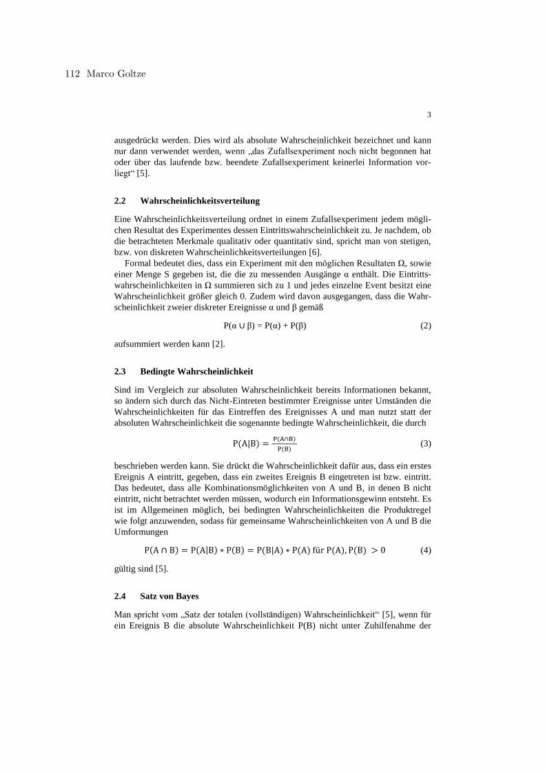
3
ausgedrückt werden. Dies wird als absolute Wahrscheinlichkeit bezeichnet und kann
nur dann verwendet werden, wenn „das Zufallsexperiment noch nicht begonnen hat
oder über das laufende bzw. beendete Zufallsexperiment keinerlei Information vor-
liegt“ [5].
2.2 Wahrscheinlichkeitsverteilung
Eine Wahrscheinlichkeitsverteilung ordnet in einem Zufallsexperiment jedem mögli-
chen Resultat des Experimentes dessen Eintrittswahrscheinlichkeit zu. Je nachdem, ob
die betrachteten Merkmale qualitativ oder quantitativ sind, spricht man von stetigen,
bzw. von diskreten Wahrscheinlichkeitsverteilungen [6].
Formal bedeutet dies, dass ein Experiment mit den möglichen Resultaten Ω, sowie
einer Menge S gegeben ist, die die zu messenden Ausgänge α enthält. Die Eintritts-
wahrscheinlichkeiten in Ω summieren sich zu 1 und jedes einzelne Event besitzt eine
Wahrscheinlichkeit größer gleich 0. Zudem wird davon ausgegangen, dass die Wahr-
scheinlichkeit zweier diskreter Ereignisse α und β gemäß
P(α ∪ β) = P(α) + P(β) (2)
aufsummiert werden kann [2].
2.3 Bedingte Wahrscheinlichkeit
Sind im Vergleich zur absoluten Wahrscheinlichkeit bereits Informationen bekannt,
so ändern sich durch das Nicht-Eintreten bestimmter Ereignisse unter Umständen die
Wahrscheinlichkeiten für das Eintreffen des Ereignisses A und man nutzt statt der
absoluten Wahrscheinlichkeit die sogenannte bedingte Wahrscheinlichkeit, die durch
P(A|B) = P(A∩B)
P(B) (3)
beschrieben werden kann. Sie drückt die Wahrscheinlichkeit dafür aus, dass ein erstes
Ereignis A eintritt, gegeben, dass ein zweites Ereignis B eingetreten ist bzw. eintritt.
Das bedeutet, dass alle Kombinationsmöglichkeiten von A und B, in denen B nicht
eintritt, nicht betrachtet werden müssen, wodurch ein Informationsgewinn entsteht. Es
ist im Allgemeinen möglich, bei bedingten Wahrscheinlichkeiten die Produktregel
wie folgt anzuwenden, sodass für gemeinsame Wahrscheinlichkeiten von A und B die
Umformungen
P(A ∩ B) = P(A|B) ∗ P(B) = P(B|A) ∗ P(A) für P(A), P(B) > 0 (4)
gültig sind [5].
2.4 Satz von Bayes
Man spricht vom „Satz der totalen (vollständigen) Wahrscheinlichkeit“ [5], wenn für
ein Ereignis B die absolute Wahrscheinlichkeit P(B) nicht unter Zuhilfenahme der
112 Marco Goltze
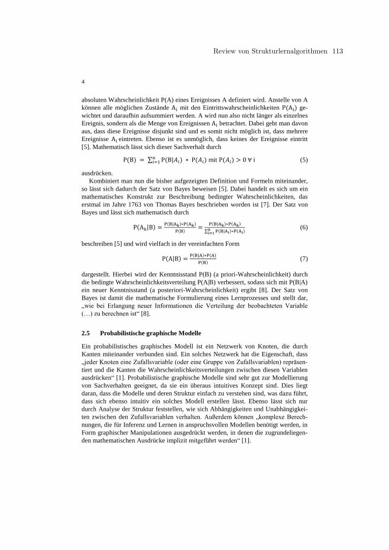
4
absoluten Wahrscheinlichkeit P(A) eines Ereignisses A definiert wird. Anstelle von A
können alle möglichen Zustände Ai mit den Eintrittswahrscheinlichkeiten P(Ai) ge-
wichtet und daraufhin aufsummiert werden. A wird nun also nicht länger als einzelnes
Ereignis, sondern als die Menge von Ereignissen Ai betrachtet. Dabei geht man davon
aus, dass diese Ereignisse disjunkt sind und es somit nicht möglich ist, dass mehrere
Ereignisse Ai eintreten. Ebenso ist es unmöglich, dass keines der Ereignisse eintritt
[5]. Mathematisch lässt sich dieser Sachverhalt durch
P(B) = ∑ P(B|𝐴𝑖) ∗ P(𝐴𝑖)𝑛𝑖=1 mit P(𝐴𝑖) > 0 ∀ i (5)
ausdrücken.
Kombiniert man nun die bisher aufgezeigten Definition und Formeln miteinander,
so lässt sich dadurch der Satz von Bayes beweisen [5]. Dabei handelt es sich um ein
mathematisches Konstrukt zur Beschreibung bedingter Wahrscheinlichkeiten, das
erstmal im Jahre 1763 von Thomas Bayes beschrieben worden ist [7]. Der Satz von
Bayes und lässt sich mathematisch durch
P(Ak|B) =P(B|Ak)∗P(Ak)
P(B)=
P(B|Ak)∗P(Ak)
∑ P(B|Ai)∗P(Ai)ni=1
(6)
beschreiben [5] und wird vielfach in der vereinfachten Form
P(A|B) =P(B|A)∗P(A)
P(B) (7)
dargestellt. Hierbei wird der Kenntnisstand P(B) (a priori-Wahrscheinlichkeit) durch
die bedingte Wahrscheinlichkeitsverteilung P(A|B) verbessert, sodass sich mit P(B|A)
ein neuer Kenntnisstand (a posteriori-Wahrscheinlichkeit) ergibt [8]. Der Satz von
Bayes ist damit die mathematische Formulierung eines Lernprozesses und stellt dar,
„wie bei Erlangung neuer Informationen die Verteilung der beobachteten Variable
(…) zu berechnen ist“ [8].
2.5 Probabilistische graphische Modelle
Ein probabilistisches graphisches Modell ist ein Netzwerk von Knoten, die durch
Kanten miteinander verbunden sind. Ein solches Netzwerk hat die Eigenschaft, dass
„jeder Knoten eine Zufallsvariable (oder eine Gruppe von Zufallsvariablen) repräsen-
tiert und die Kanten die Wahrscheinlichkeitsverteilungen zwischen diesen Variablen
ausdrücken“ [1]. Probabilistische graphische Modelle sind sehr gut zur Modellierung
von Sachverhalten geeignet, da sie ein überaus intuitives Konzept sind. Dies liegt
daran, dass die Modelle und deren Struktur einfach zu verstehen sind, was dazu führt,
dass sich ebenso intuitiv ein solches Modell erstellen lässt. Ebenso lässt sich nur
durch Analyse der Struktur feststellen, wie sich Abhängigkeiten und Unabhängigkei-
ten zwischen den Zufallsvariablen verhalten. Außerdem können „komplexe Berech-
nungen, die für Inferenz und Lernen in anspruchsvollen Modellen benötigt werden, in
Form graphischer Manipulationen ausgedrückt werden, in denen die zugrundeliegen-
den mathematischen Ausdrücke implizit mitgeführt werden“ [1].
Review von Strukturlernalgorithmen 113
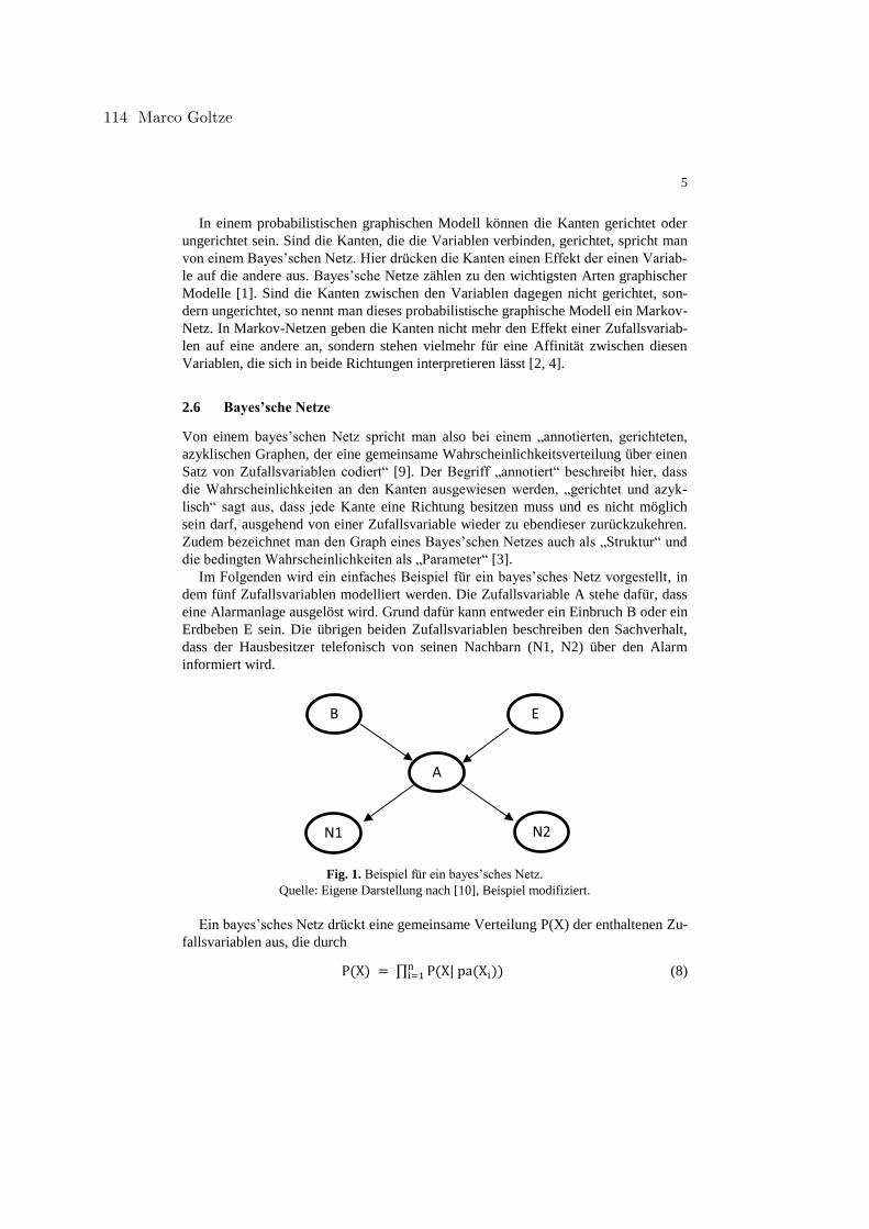
5
In einem probabilistischen graphischen Modell können die Kanten gerichtet oder
ungerichtet sein. Sind die Kanten, die die Variablen verbinden, gerichtet, spricht man
von einem Bayes’schen Netz. Hier drücken die Kanten einen Effekt der einen Variab-
le auf die andere aus. Bayes’sche Netze zählen zu den wichtigsten Arten graphischer
Modelle [1]. Sind die Kanten zwischen den Variablen dagegen nicht gerichtet, son-
dern ungerichtet, so nennt man dieses probabilistische graphische Modell ein Markov-
Netz. In Markov-Netzen geben die Kanten nicht mehr den Effekt einer Zufallsvariab-
len auf eine andere an, sondern stehen vielmehr für eine Affinität zwischen diesen
Variablen, die sich in beide Richtungen interpretieren lässt [2, 4].
2.6 Bayes’sche Netze
Von einem bayes’schen Netz spricht man also bei einem „annotierten, gerichteten,
azyklischen Graphen, der eine gemeinsame Wahrscheinlichkeitsverteilung über einen
Satz von Zufallsvariablen codiert“ [9]. Der Begriff „annotiert“ beschreibt hier, dass
die Wahrscheinlichkeiten an den Kanten ausgewiesen werden, „gerichtet und azyk-
lisch“ sagt aus, dass jede Kante eine Richtung besitzen muss und es nicht möglich
sein darf, ausgehend von einer Zufallsvariable wieder zu ebendieser zurückzukehren.
Zudem bezeichnet man den Graph eines Bayes’schen Netzes auch als „Struktur“ und
die bedingten Wahrscheinlichkeiten als „Parameter“ [3].
Im Folgenden wird ein einfaches Beispiel für ein bayes’sches Netz vorgestellt, in
dem fünf Zufallsvariablen modelliert werden. Die Zufallsvariable A stehe dafür, dass
eine Alarmanlage ausgelöst wird. Grund dafür kann entweder ein Einbruch B oder ein
Erdbeben E sein. Die übrigen beiden Zufallsvariablen beschreiben den Sachverhalt,
dass der Hausbesitzer telefonisch von seinen Nachbarn (N1, N2) über den Alarm
informiert wird.
Fig. 1. Beispiel für ein bayes’sches Netz.
Quelle: Eigene Darstellung nach [10], Beispiel modifiziert.
Ein bayes’sches Netz drückt eine gemeinsame Verteilung P(X) der enthaltenen Zu-
fallsvariablen aus, die durch
P(X) = ∏ P(X| pa(Xi))ni=1 (8)
B E
A
N1 N2
114 Marco Goltze
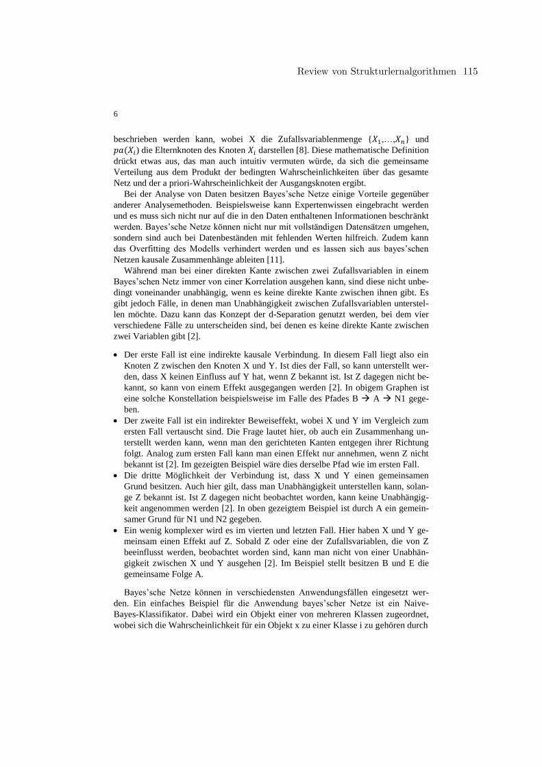
6
beschrieben werden kann, wobei X die Zufallsvariablenmenge {𝑋1,…,𝑋𝑛} und
𝑝𝑎(𝑋𝑖) die Elternknoten des Knoten 𝑋𝑖 darstellen [8]. Diese mathematische Definition
drückt etwas aus, das man auch intuitiv vermuten würde, da sich die gemeinsame
Verteilung aus dem Produkt der bedingten Wahrscheinlichkeiten über das gesamte
Netz und der a priori-Wahrscheinlichkeit der Ausgangsknoten ergibt.
Bei der Analyse von Daten besitzen Bayes’sche Netze einige Vorteile gegenüber
anderer Analysemethoden. Beispielsweise kann Expertenwissen eingebracht werden
und es muss sich nicht nur auf die in den Daten enthaltenen Informationen beschränkt
werden. Bayes’sche Netze können nicht nur mit vollständigen Datensätzen umgehen,
sondern sind auch bei Datenbeständen mit fehlenden Werten hilfreich. Zudem kann
das Overfitting des Modells verhindert werden und es lassen sich aus bayes’schen
Netzen kausale Zusammenhänge ableiten [11].
Während man bei einer direkten Kante zwischen zwei Zufallsvariablen in einem
Bayes’schen Netz immer von einer Korrelation ausgehen kann, sind diese nicht unbe-
dingt voneinander unabhängig, wenn es keine direkte Kante zwischen ihnen gibt. Es
gibt jedoch Fälle, in denen man Unabhängigkeit zwischen Zufallsvariablen unterstel-
len möchte. Dazu kann das Konzept der d-Separation genutzt werden, bei dem vier
verschiedene Fälle zu unterscheiden sind, bei denen es keine direkte Kante zwischen
zwei Variablen gibt [2].
• Der erste Fall ist eine indirekte kausale Verbindung. In diesem Fall liegt also ein
Knoten Z zwischen den Knoten X und Y. Ist dies der Fall, so kann unterstellt wer-
den, dass X keinen Einfluss auf Y hat, wenn Z bekannt ist. Ist Z dagegen nicht be-
kannt, so kann von einem Effekt ausgegangen werden [2]. In obigem Graphen ist
eine solche Konstellation beispielsweise im Falle des Pfades B → A → N1 gege-
ben.
• Der zweite Fall ist ein indirekter Beweiseffekt, wobei X und Y im Vergleich zum
ersten Fall vertauscht sind. Die Frage lautet hier, ob auch ein Zusammenhang un-
terstellt werden kann, wenn man den gerichteten Kanten entgegen ihrer Richtung
folgt. Analog zum ersten Fall kann man einen Effekt nur annehmen, wenn Z nicht
bekannt ist [2]. Im gezeigten Beispiel wäre dies derselbe Pfad wie im ersten Fall.
• Die dritte Möglichkeit der Verbindung ist, dass X und Y einen gemeinsamen
Grund besitzen. Auch hier gilt, dass man Unabhängigkeit unterstellen kann, solan-
ge Z bekannt ist. Ist Z dagegen nicht beobachtet worden, kann keine Unabhängig-
keit angenommen werden [2]. In oben gezeigtem Beispiel ist durch A ein gemein-
samer Grund für N1 und N2 gegeben.
• Ein wenig komplexer wird es im vierten und letzten Fall. Hier haben X und Y ge-
meinsam einen Effekt auf Z. Sobald Z oder eine der Zufallsvariablen, die von Z
beeinflusst werden, beobachtet worden sind, kann man nicht von einer Unabhän-
gigkeit zwischen X und Y ausgehen [2]. Im Beispiel stellt besitzen B und E die
gemeinsame Folge A.
Bayes’sche Netze können in verschiedensten Anwendungsfällen eingesetzt wer-
den. Ein einfaches Beispiel für die Anwendung bayes’scher Netze ist ein Naive-
Bayes-Klassifikator. Dabei wird ein Objekt einer von mehreren Klassen zugeordnet,
wobei sich die Wahrscheinlichkeit für ein Objekt x zu einer Klasse i zu gehören durch
Review von Strukturlernalgorithmen 115
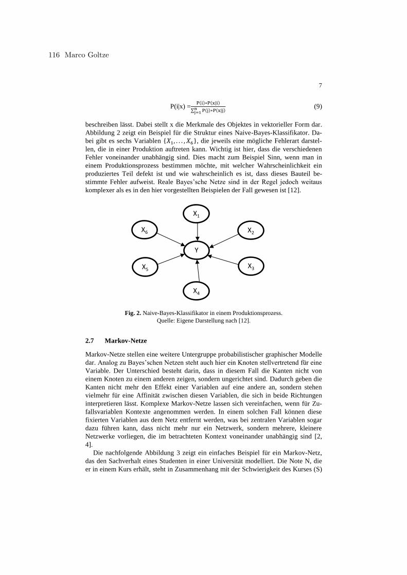
7
P(i|x) =P(i)∗P(x|i)
∑ P(j)∗P(x|j)nj=1
(9)
beschreiben lässt. Dabei stellt x die Merkmale des Objektes in vektorieller Form dar.
Abbildung 2 zeigt ein Beispiel für die Struktur eines Naive-Bayes-Klassifikator. Da-
bei gibt es sechs Variablen {𝑋1, . . . , 𝑋6}, die jeweils eine mögliche Fehlerart darstel-
len, die in einer Produktion auftreten kann. Wichtig ist hier, dass die verschiedenen
Fehler voneinander unabhängig sind. Dies macht zum Beispiel Sinn, wenn man in
einem Produktionsprozess bestimmen möchte, mit welcher Wahrscheinlichkeit ein
produziertes Teil defekt ist und wie wahrscheinlich es ist, dass dieses Bauteil be-
stimmte Fehler aufweist. Reale Bayes’sche Netze sind in der Regel jedoch weitaus
komplexer als es in den hier vorgestellten Beispielen der Fall gewesen ist [12].
Fig. 2. Naive-Bayes-Klassifikator in einem Produktionsprozess.
Quelle: Eigene Darstellung nach [12].
2.7 Markov-Netze
Markov-Netze stellen eine weitere Untergruppe probabilistischer graphischer Modelle
dar. Analog zu Bayes’schen Netzen steht auch hier ein Knoten stellvertretend für eine
Variable. Der Unterschied besteht darin, dass in diesem Fall die Kanten nicht von
einem Knoten zu einem anderen zeigen, sondern ungerichtet sind. Dadurch geben die
Kanten nicht mehr den Effekt einer Variablen auf eine andere an, sondern stehen
vielmehr für eine Affinität zwischen diesen Variablen, die sich in beide Richtungen
interpretieren lässt. Komplexe Markov-Netze lassen sich vereinfachen, wenn für Zu-
fallsvariablen Kontexte angenommen werden. In einem solchen Fall können diese
fixierten Variablen aus dem Netz entfernt werden, was bei zentralen Variablen sogar
dazu führen kann, dass nicht mehr nur ein Netzwerk, sondern mehrere, kleinere
Netzwerke vorliegen, die im betrachteten Kontext voneinander unabhängig sind [2,
4].
Die nachfolgende Abbildung 3 zeigt ein einfaches Beispiel für ein Markov-Netz,
das den Sachverhalt eines Studenten in einer Universität modelliert. Die Note N, die
er in einem Kurs erhält, steht in Zusammenhang mit der Schwierigkeit des Kurses (S)
X6 X2
X1
X5 X3
X4
Y
116 Marco Goltze
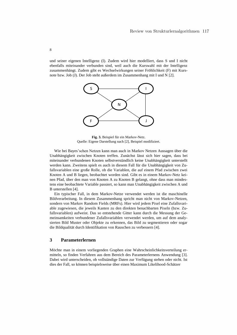
8
und seiner eigenen Intelligenz (I). Zudem wird hier modelliert, dass S und I nicht
ebenfalls miteinander verbunden sind, weil auch die Kurswahl mit der Intelligenz
zusammenhängt. Zudem gibt es Wechselwirkungen seiner Fröhlichkeit (F) mit Kurs-
note bzw. Job (J). Der Job steht außerdem im Zusammenhang mit I und N [2].
Fig. 3. Beispiel für ein Markov-Netz.
Quelle: Eigene Darstellung nach [2], Beispiel modifiziert.
Wie bei Bayes’schen Netzen kann man auch in Markov Netzen Aussagen über die
Unabhängigkeit zwischen Knoten treffen. Zunächst lässt sich hier sagen, dass bei
miteinander verbundenen Knoten selbstverständlich keine Unabhängigkeit unterstellt
werden kann. Zweitens spielt es auch in diesem Fall für die Unabhängigkeit von Zu-
fallsvariablen eine große Rolle, ob die Variablen, die auf einem Pfad zwischen zwei
Knoten A und B liegen, beobachtet worden sind. Gibt es in einem Markov-Netz kei-
nen Pfad, über den man von Knoten A zu Knoten B gelangt, ohne dass man mindes-
tens eine beobachtete Variable passiert, so kann man Unabhängigkeit zwischen A und
B unterstellen [4].
Ein typischer Fall, in dem Markov-Netze verwendet werden ist die maschinelle
Bildverarbeitung. In diesem Zusammenhang spricht man nicht von Markov-Netzen,
sondern von Markov Random Fields (MRFs). Hier wird jedem Pixel eine Zufallsvari-
able zugewiesen, die jeweils Kanten zu den direkten benachbarten Pixeln (bzw. Zu-
fallsvariablen) aufweist. Das so entstehende Gitter kann durch die Messung der Ge-
meinsamkeiten verbundener Zufallsvariablen verwendet werden, um auf dem analy-
sierten Bild Muster oder Objekte zu erkennen, das Bild zu segmentieren oder sogar
die Bildqualität durch Identifikation von Rauschen zu verbessern [4].
3 Parameterlernen
Möchte man in einem vorliegenden Graphen eine Wahrscheinlichkeitsverteilung er-
mitteln, so finden Verfahren aus dem Bereich des Parameterlernens Anwendung [3].
Dabei wird unterscheiden, ob vollständige Daten zur Verfügung stehen oder nicht. Ist
dies der Fall, so können beispielsweise über einen Maximum Likelihood-Schätzer
S I
N
F J
Review von Strukturlernalgorithmen 117
9
L = 1
N ∑ ∑ logP(xi|pa(xi), Dl)li (10)
für jeden Knoten direkt die Parameter bestimmt werden, wobei N die Anzahl der
Datensätze und D die Daten selbst beschreibt. Dies kann dann über die Knoten auf-
summiert werden, um die Log-Likelihood (Normalisiert) L zu erhalten [5].
Die Vorgehensweise zur Parameterschätzung ändert sich, wenn die Daten nicht
vollständig bekannt sind. In diesem Fall ist es möglich, einen Expectation Maximati-
on Algorithmus zu nutzen, welcher mehrere Schritte durchläuft, um die Parameter zu
ermitteln. Dabei werden die fehlenden Daten geschätzt und dann iterativ angepasst,
was nicht immer zu globalen, zumindest jedoch zu lokalen Maxima führt [5].
4 Strukturlernen in gerichteten Netzwerken
Die Anwendung von Strukturlernverfahren setzt ein vorhandenes Netzwerk voraus,
das die zugrundeliegenden Sachverhalte möglichst gut abbildet. Beziehungen zwi-
schen Zufallsvariablen und Wahrscheinlichkeitsverteilungen sind jedoch nicht per se
von vornherein bekannt. Liegen verschiedene Zufallsvariablen vor, so kann entweder
durch Expertenwissen oder über Strukturlernverfahren die Struktur ermittelt werden,
sodass daraufhin ein gerichteter, azyklischer Graph vorliegt [3].
Die Algorithmen zum Lernen der Struktur Bayes’scher Netze können wiederum in
zwei Kategorien unterteilt werden. Das Lernen kann entweder scorebasiert oder cons-
traintbasiert erfolgen. Während in scorebasierten Ansätzen die relative Häufigkeits-
verteilung nicht bekannt ist und anhand der Daten die Struktur des Netzwerks durch
Vergleich verschiedener Muster ausgewählt wird, suchen constraintbasierte Ansätze
nach einem Netzwerk, das sowohl die Markov Bedingung, als auch die „bedingten
Unabhängigkeiten in der Wahrscheinlichkeitsverteilung“ [3] erfüllt [3].
4.1 Scorebasierte Ansätze
Scorebasierte Ansätze versuchen immer, einen Graphen zu finden, der eine Zielfunk-
tion optimiert. Als Zielfunktion können dabei verschiedenste Scores verwendet wer-
den. Beispiele sind hier eine Likelihood-Funktion, die einen Fit zu den Daten berech-
net, das Bayes-Informations-Krieterium (BIC), das die Likelihood über alle mögli-
chen Parametrisierungen aufsummiert oder bestrafende Ansätze, die statt der Like-
lihood die a-posteriori Wahrscheinlichkeit betrachten [2].
Scorebasierte Ansätze können nochmals in exakte und gierige Algorithmen unter-
teilt werden, wobei zweitere vor allem dann verwendet werden, wenn es sich um sehr
große Graphen handelt und eine exakte Berechnung nicht mehr im Rahmen der Mög-
lichkeiten liegt [4].
Selbst innerhalb der exakten Ansätze lassen sich die Algorithmen weiter klassifi-
zieren. So können Branch-and-Bound-Verfahren, partial order covers oder lineare
Programmierung zum Einsatz kommen [4].
B&B-Verfahren
118 Marco Goltze
10
Partial order covers
Verfahren mit linearer Programmierung
Ein Beispiel für gierige Ansätze ist der Greedy Equivalence Search Algorithmus von
Chickering aus dem Jahre 2002 [13]. In der Regel bei einem Graph ohne Kanten star-
tend besteht dieser Algorithmus aus Vorwärts- und Rückwärtsschritten, in denen Kan-
ten hinzugefügt, bzw. entfernt werden. Im Zuge dessen wird bestimmt wie sich eine
zu maximierende Zielfunktion durch das Hinzufügen und Entfernen der Kanten ver-
ändert. Klarer Vorteil dieses Ansatzes ist, dass er unter bestimmten Bedingungen in
der Lage ist, nicht nur ein lokales, sondern sogar ein globales Optimum auszumachen
[4]. Der Algorithmus kann in verschiedenen Varianten angewendet werden und es
zeigt sich, dass er zum Teil an seine Grenzen geraten kann. Aus diesem Grund ist er
von verschiedenen Autoren angepasst und erweitert worden ist. Ein Beispiel dafür ist
die Arbeit von Alonso-Barba et. al. (2013), welche den Algorithmus in neun Abwand-
lungen beschreibt. Beispielsweise werden durch die Definition von Constraints die
Verbindung zwischen bestimmten Zufallsvariablen ausgeschlossen, sodass der Algo-
rithmus noch besser und effizienter auf große Netze angewendet werden kann [14].
Da es sich hierbei um constraintbasiertes Vorgehen handelt, könnten diese Abwand-
lungen des GES Ansatzes ebenso zu den hybriden Ansätzen gezählt werden.
Greedy Hill Climbing Algorithmus
4.2 Constraintbasierte Ansätze
Grow Shrink Algorithmus
4.3 Hybride Ansätze
Strukturlernansätze können nicht nur score- bzw. constraintbasiert sein, sondern auch
Elemente beider Kategorien enthalten. Ein Beispiel für einen solchen hybriden Ansatz
ist der Sparse-Candidate-Algorithmus, der in [15] beschrieben wird. Dieser Ansatz
verläuft iterativ von einem leeren Graph zu einem Zielnetzwerk. Jede Iteration besteht
dabei aus einem Restriktions- und einem Maximierungsschritt. Im Restriktionsschritt
werden für jeden Knoten basierend auf den vorliegenden Daten mögliche Elternkno-
ten bestimmt, wodurch die Anzahl der möglichen Netzwerke massiv eingeschränkt
wird. Im Maximierungsschritt wird dann eine Zielfunktion maximiert. Es gibt für
jeden der Schritte mehrere Möglichkeiten der Konzeption und Durchführung, wobei
die Auswahl des Restriktionsschrittes in der Regel unabhängig von der Auswahl des
Maximierungsschrittes erfolgen kann. Der Restriktionsschritt kann in einem einfachen
Fall für zwei Knoten X und Y über
∑ Px,y (x, y) log(P(x,y)
P(x)P(y)) (11)
Review von Strukturlernalgorithmen 119
11
einen nicht-negativen Wert berechnen, der durch das gemeinsame Vorkommen von
Daten in X und Y steigt. Dieser Ansatz kann noch abgewandelt oder erweitert wer-
den, soll für diese Übersicht jedoch vorerst in dieser Form genügen. Auch der Maxi-
mierungsschritt kann auf verschiedene Arten erfolgen. Beispielsweise über einen
Greedy-Hill-Climbing-Algorithmus, wie er zuvor in dieser Arbeit vorgestellt wurde.
Häufig kommt es jedoch noch immer zu dem Problem eines sehr großen Suchraumes,
was sich durch den Einsatz von Dekompositionsansätzen verringern lässt. Hier sind
beispielsweise die Separator-Dekomposition oder die Cluster-Tree-Dekomposition zu
nennen. Abschließend muss sich für ein Abbruchkriterium entschieden werden. Dabei
gibt es zwei Möglichkeiten. Erstens kann der Algorithmus abbrechen, wenn sich in
einem Schritt im Vergleich zu einem vorherigen Schritt die Elternknoten nicht mehr
ändern. Die zweite Möglichkeit ist analog dazu eine Nicht-Verbesserung des Wertes
der Zielfunktion [15].
Ein weiteres Beispiel für hybride Verfahren ist der Ansatz von de Campos et al.
aus dem Jahre 2009 [16]. Hier werden zunächst Constraints für Parameter und Struk-
tur gebildet, die daraufhin in einem Branch-and-Bound Verfahren berücksichtigt wer-
den, das eine global optimale Lösung findet. Dennoch kann das Verfahren aufgrund
eines Abbruchkriteriums jederzeit abgebrochen werden und es liegt dennoch die
Struktur vor, die von allen bisher getesteten Strukturen den höchsten Zielfunktions-
wert aufweist. Ein weiterer Vorteil ist die Möglichkeit der Parallelisierung des Algo-
rithmus [16].
5 Lernen in ungerichteten Netzwerken
Analog zu gerichteten Bayes’schen Netzen können auch in ungerichteten Markov
Netzwerken constraintbasierte oder scorebasierten Ansätze zum Lernen der Struktur
angewendet werden. Auch in diesem Fall gibt es in beiden Fällen verschiedene An-
sätze, die sich zum Teil deutlich voneinander unterscheiden [2].
5.1 Scorebasierte Ansätze
Das Bayes-Informationskriterium erweist sich bei Markov-Modellen als weniger
nützlich, weshalb hier eher auf approximative Ansätze gesetzt wird [2].
Noch keine Beispiele
5.2 Constraintbasierte Ansätze
Noch keine Beispiele
6 Vergleich der Algorithmen
Vergleich folgt wenn Algorithmen alle abgehandelt wurden
120 Marco Goltze
12
7 Zusammenfassung und Ausblick
In dieser Arbeit wurde zunächst ausgehend von den Grundlagen der Wahrscheinlich-
keitstheorie zu probabilistischen graphischen Modellen hingeführt. Daraufhin wurden
diese Modelle klassifiziert und es wurde dargestellt, welche Möglichkeiten des Ler-
nens in probabilistischen graphischen Modellen bestehen. Es wurde auf verschiedens-
te scorebasierte, constraintbasierte und hybride Möglichkeiten und Algorithmen ein-
gegangen, über die die Struktur von Bayes’schen Netzen und Markov-Netzen synthe-
tisiert werden kann. Das Lernen von Parametern, das in einem nächsten Schritt auf ein
vorhandenes probabilistisches graphisches Modell angewendet werden kann, wurde
der Vollständigkeit halber erwähnt, nicht jedoch im Detail abgehandelt, da der Fokus
dieser Arbeit klar auf Strukturlernalgorithmen liegt.
Beim Vergleich der in der Literatur vorgestellten Algorithmen zeigt sich, dass viele
neu veröffentlichte Ansätze nicht in all ihren Bestandteilen gänzlich neu sind. Viel-
mehr werden häufig bereits bekannte Algorithmen genutzt und mit einem neuen An-
satz kombiniert oder leicht abgeändert, um deren Performance zu verbessern. Es sind
sowohl in der Vorgehensweise als auch in der Performance der Ansätze große Diffe-
renzen zu erkennen. Dieser Vergleich wird im Detail in Kapitel 6 gezogen.
Die Literaturrecherche zeigt zudem, dass es fundierte Werke zu den Grundlagen in
Wahrscheinlichkeitstheorie und zu probabilistischen graphischen Modellen gibt. Für
konkrete Strukturlernansätze ist die Literaturgrundlage allerdings recht unübersicht-
lich aufgebaut, weil nie in einem einzigen Paper ein zusammenhängender Überblick
über Strukturlernalgorithmen und deren Verwendung und Performance erstellt wor-
den ist. Dies wurde in dieser Arbeit versucht, aufgrund der Vielfältigkeit der Ansätze
kann jedoch nicht die Vollständigkeit des Überblicks erwartet werden. Dies sollte in
einer zukünftigen Arbeit nochmals in einem größeren Umfang angegangen werden.
References
1. Bishop CM (2009) Pattern recognition and machine learning, Corrected at 8th
printing 2009. Information science and statistics. Springer, New York, NY
2. Koller D, Friedman N (2009) Probabilistic graphical models: Principles and
techniques. Adaptive computation and machine learning. MIT Press, Cam-
bridge, Mass.
3. Neapolitan RE (2004) Learning bayesian networks. Pearson Prentice Hall Upper
Saddle River, NJ
4. Drton M, Maathuis MH (2016) Structure Learning in Graphical Modeling
5. Bosch K (2015) Großes Lehrbuch der Statistik. Walter de Gruyter GmbH & Co
KG
6. Scharnbacher K (2013) Betriebswirtschaftliche Statistik: Lehrbuch mit prakti-
schen Beispielen. Gabler Verlag
7. Bayes T (1763) LII. An essay towards solving a problem in the doctrine of
chances. By the late Rev. Mr. Bayes, FRS communicated by Mr. Price, in a let-
Review von Strukturlernalgorithmen 121

13
ter to John Canton, AMFR S. Philosophical transactions of the Royal Society of
London(53): 370–418
8. Borth M (2004) Wissensgewinnung auf Bayes-Netz-Mengen. Dissertation, Uni-
versität Ulm
9. Friedman N, Geiger D, Goldszmidt M (1997) Bayesian network classifiers.
Mach Learn 29(2-3): 131–163
10. Pearl J (2014) Probabilistic Reasoning in Intelligent Systems: Networks of Plau-
sible Inference, 1. Auflage. Elsevier Reference Monographs, s.l.
11. Heckerman D (1995) A Tutorial on Learning With Bayesian Networks
12. Dörn S (2018) Bayes-Netze. In: Programmieren für Ingenieure und Naturwis-
senschaftler: Intelligente Algorithmen und digitale Technologien. Springer Ber-
lin Heidelberg, Berlin, Heidelberg, pp 149–181
13. Chickering DM Optimal Structure Identification With Greedy Search. In: Jour-
nal of Machine Learning Research, vol 3, pp 507–554
14. Alonso-Barba JI, delaOssa L, Gámez JA et al. (2013) Scaling up the Greedy
Equivalence Search algorithm by constraining the search space of equivalence
classes. International Journal of Approximate Reasoning 54(4): 429–451. doi:
10.1016/j.ijar.2012.09.004
15. Friedman N, Nachman I, Pe'er D Learning Bayesian Network Structure from
Massive Datasets: The Sparse Candidate Algorithm. In: Proceedings of the Fif-
teenth conference on Uncertainty in artificial intelligence, pp 206–215
16. Campos CP de, Zeng Z, Ji Q Structure learning of Bayesian networks using
constraints. In: ICML '09 Proceedings of the 26th Annual International Confer-
ence on Machine Learning, pp 113–120
122 Marco Goltze
Neuro-evolution as an Alternative toReinforcement Learning for Playing Atari Games
Jan Niklas Kielmann
TECO, Karlsruhe Institute of Technology
Abstract. This article presents four neuro-evolution approaches, dis-cusses their advantages and disadvantages and compares their resultsin the Atari domain. Specifically, conventional neuro-evolution (CNE),Covariance Matrix Adaptation Evolution Strategy (CMA-ES), NeuroEvo-lution of Augmenting Topologies (NEAT) and HyperNEAT are introduced.Four different state representations for Atari games are presented andevaluated. The results show that neuro-evolution can learn effective strate-gies for many Atari games. Algorithms using a direct encoding schemeperform the best on abstract state representations whereas an indirectencoding like HyperNEAT is needed to learn agents based on raw-pixelinputs. The algorithms partly learn fixed action sequences without tak-ing the game state into account which is possible as Atari games aredeterministic. For this reason an evaluation on random game starts isproposed which would test the generalization of the learned strategiesand would also allow a better comparison with current reinforcementlearning algorithms.
1 Introduction
The Atari 2600 game console was one of the first consoles released for the homemarket. Today it is used as a challenging reinforcement learning benchmark.The reasons for this are the simple inputs, large amount of available games, lowresolution graphics and efficient emulators [3]. Goal is a learning algorithm thatcan learn to play different Atari games without prior knowledge and using thesame set of hyperparameters for all of them.
Backpropagation-based reinforcement learning methods like DQN[15], A3C[14]and PPO[21] achieve state-of-the-art results for training agents that can playthese Atari games. In many games the learned agents outperform human players.However, there are also games left were the agents are vastly inferior to theirhuman counterpart. These are mostly games that require long term planning andhave a sparse reward function like Montezuma’s Revenge. For this reason it isstill a very active field of research.
Evolutionary approaches for evolving neural networks, also called neuro-evolution algorithms, are a promising alternative to backpropagation-based meth-ods [12, 20, 26]. These black-box optimization methods can deal with sparserewards, do not need to backpropagate gradients and can handle long time hori-zons [20]. This article will introduce four different neuro-evolution algorithms and
Neuro-evolution as an Alternative to Reinforcement Learning for Playing AtariGames 123
2 Jan Niklas Kielmann
present their advantages and disadvantages. Their results on different Atari gameswill be compare among themselves and with results of backpropagation-basedapproaches.
2 Neuro-evolution Algorithms
Artificial neural networks (ANN) are computational models that are inspired bybiological neural networks. However, their goal is not necessarily to model thehuman brain as closely as possible. They consist of a number of interconnectedneurons which can be represented as a directed graph. Each of these connectionsbetween two neurons has a weight assigned to it which represents the connectionstrength. The neurons are small computing units that usually calculate theweighted sum of their inputs and apply an activation function to calculate theiroutput [5].
In order to solve a specific task with an artificial neural network, its weightsneed to be learned. There are learning algorithms that do this in a supervisedfashion, like the backpropagation of errors. Here labeled training data is usedto compute the error of the network and adjust the weights so that the error isminimized[19].
Evolutionary algorithms provide another method for finding the best weightsof an ANN. The field of using evolutionary algorithms to evolve the weights andstructure of ANNs is called neuro-evolution. The evolution of artificial neuralnetworks requires that it is encoded into a vector of numbers, the genome. Eachelement in this genome vector is called a gene. The genome needs to hold all theinformation to create the corresponding ANN which is called the phenotype. Byusing a fixed topology for the network only the weights of the connections needto be encoded in the genome. However, it is also possible to evolve the networkstructure along with the weights. This requires a more complex encoding. Theseencodings can generally be categorized into direct and indirect encodings[25](also called weak and strong representations [4]).
Direct EncodingIn a direct encoding each neuron and each connection is directly representedin the genome[4]. If the network topology is fixed and only the weights need tobe encoded, each weight would be represented sequentially in the genome. Thismeans each gene directly represents a connection weight [6].
A direct encoding that allows the evolution of the network structure needs toalso encode each connection. This can be done by representing the connectionmatrix of the graph in the genome. However, this limits the number of possiblenotes, if the genome is defined to have a fixed length. It is also hard to performcrossover operations, where two genomes are combined, because the resultinggenome must still represent a valid network [25]. For example the resultingnetwork should not contain sub-networks that are not connected to the rest ofthe neurons.
124 Jan Niklas Kielmann
Neuro-evolution for Playing Atari Games 3
Indirect EncodingAn indirect encoding does not specify each neuron and connection separately.Instead it only specifies rules that can be used to construct the neural network.For example these rules can simulate cell division [8]. This allows large networksto be encoded in a compact way. However, the indirect encoding also implicitlyrestricts the set of possible network structures, which might not include theoptimal solution [25].
A neuro-evolution algorithm typically starts out with an initial set of randomnetworks, each encoded into a genome. This set is called the initial populationand is iteratively optimized. In each iteration, also called generation, the networksare evaluated using a fitness function which ranks the performance of the network.For instance, this could be the score reached in a game. Networks with low fitnessscores get discarded. Only the fittest individuals in the population survive andget to reproduce. In this context reproduction means that two networks are becombined in a process called crossover. The resulting networks created duringthis reproduction phase are called the offspring. Moreover random mutationsare applied to the genomes of the current generation. After some iterations thisprocess leads to neural networks that reach a high fitness score.
In the following sections four neuro-evolution algorithms will be introduced.Conventional neuro-evolution is the least complex one. It was chosen as a baselineto test whether the more advanced techniques used by the other algorithmsprovide a benefit in the Atari domain. The CMA-ES algorithm is a wildly usedoptimization algorithm for non-convex optimization problems. It was selectedbecause it is not specific to neuro-evolution and has been used to solve manyother problems. It represents a set of algorithms that only evolve the networkweights and do not use any methods that are specific to the evolution of networks.The NEAT algorithm was chosen as it is a well known neuro-evolution algorithmthat successfully evolves the network structure along with the network weights.It is used to test the hypothesis that the evolution of the network structureprovides a benefit over more general algorithms like CMA-ES. Lastly, the Hyper-NEAT algorithm is used as a representative of indirect encoding neuro-evolutionalgorithms.
2.1 Conventional neuro-evolution
The term conventional neuro-evolution is not clearly defined. Here the definitionof Hausknecht et al.[12] will be used. They describe it as a neuro-evolutionalgorithm that only optimizes the network weights and uses a fixed networktopology. A direct encoding for the network weights is used and common crossoverand mutation operators are applied to it.
The crossover operator describes how two genomes in the current populationare combined to create a new individual for the next population. There areseveral different techniques which can be seen in Figure 1. In the single-pointcrossover one point in the genomes is chosen at random after which the twogenomes are swapped. In the double-point crossover two such points are selected
Neuro-evolution as an Alternative to Reinforcement Learning for Playing AtariGames 125
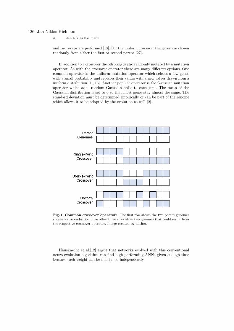
4 Jan Niklas Kielmann
and two swaps are performed [13]. For the uniform crossover the genes are chosenrandomly from either the first or second parent [27].
In addition to a crossover the offspring is also randomly mutated by a mutationoperator. As with the crossover operator there are many different options. Onecommon operator is the uniform mutation operator which selects a few geneswith a small probability and replaces their values with a new values drawn from auniform distribution [11, 13]. Another popular operator is the Gaussian mutationoperator which adds random Gaussian noise to each gene. The mean of theGaussian distribution is set to 0 so that most genes stay almost the same. Thestandard deviation must be determined empirically or can be part of the genomewhich allows it to be adapted by the evolution as well [2].
Fig. 1. Common crossover operators. The first row shows the two parent genomeschosen for reproduction. The other three rows show two genomes that could result fromthe respective crossover operator. Image created by author.
Hausknecht et al.[12] argue that networks evolved with this conventionalneuro-evolution algorithm can find high performing ANNs given enough timebecause each weight can be fine-tuned independently.
126 Jan Niklas Kielmann
Neuro-evolution for Playing Atari Games 5
Advantages
• Very simple and straight forwardto implement.
• Low complexity makes paralleliza-tion easy and allows to scale up tomany CPUs.
• Can achieve very good results whenused at large scale.
Disadvantages
• Only network weights are learned.A good network architecture mustbe chosen beforehand.
• Multiple runs with different archi-tectures needed.
• Can be slow to converge becauseno advanced techniques are used toadjust the steps size and direction.
2.2 CMA-ESThe Covariance Matrix Adaptation Evolutionary Strategy (CMA-ES) is a stochas-tic method for continuous parameter optimization of non-linear, non-convexfunctions. It can be used to evolve the weights of a fixed topology neural networkthat optimizes a complex fitness function. The main idea is to use a multi-variatenormal distribution to generate the population by sampling from it. The parame-ters of the distribution are then updated based on the fittest individuals in thegenerated population [12]. In each iteration of the algorithm the following stepsare executed [10]:1. Sample λ genomes from the distribution N (m, C) where m is the mean and
C the covariance matrix of the multivariate normal distribution2. Create ANNs for all λ genomes and evaluate their fitness3. Choose µ individuals with the highest fitness4. Update the mean m using the fittest µ individuals5. Update the covariance matrix C using the fittest µ individuals
Mean UpdateThe goal of the mean update is to move the mean closer to the genomes thatperformed well. In the next generation this will cause more samples to be takenfrom this region. The CMA-ES algorithm sets the new mean m′ to the weightedaverage of the µ fittest individuals:
m′ =µ∑
i=1wixi
µ∑
i=1wi = 1, w1 ≥ w2 ≥ . . . ≥ wµ > 0
wherexi is the i-th genome in the population sorted by fitness.wi is the weight of the genome xi.
All weights are greater than 0 and sum up to 1. They are usually chosen ina way that assigns the highest weight to the fittest individual and reduces theweight linearly for the other individuals (e.g. wi ∝ µ − i + 1) [10].
Neuro-evolution as an Alternative to Reinforcement Learning for Playing AtariGames 127
6 Jan Niklas Kielmann
Covariance Matrix UpdateThe covariance matrix should be updated in a way that biases the sampling ofthe next population towards the direction of the most successful individuals ofthe last generation [12]. The original covariance matrix that was used to createthe population, can be estimated using the sample covariance matrix [18]:
Csample = 1λ − 1
λ∑
i=1(xi − 1
λ
λ∑
j=1xj)(xi − 1
λ
λ∑
j=1xj)T
In order to compute a better covariance matrix only the best µ individuals areused and weighted. This is similar to the weighting of the mean update. MoreoverCMA-ES uses the true mean m that was used to create the population insteadof the mean calculated on the sampled population [10]:
Cµ = 1µ
µ∑
i=1wi(xi − m)(xi − m)T
This update rule estimates the variance of the step size xi − m instead of thevariance within the sampled population [10]. Figure 2 shows that this updatemethod leads to a higher variance in the direction of better performing individuals.This enables CMA-ES to make bigger steps in the right direction when the bestsolutions are far away and narrow the search space when the best solutions areclose to the mean. [9]
One drawback is the run time of O(n2), where n is the number of genes inthe genome, due to the calculation of the covariance matrix [10]. This can beproblematic for the evolution of ANNs which can have a large number of weights.
Advantages
• Fast convergence due to the adap-tive step size
• Empirically successful in many ap-plications [10].
• Can deal with non-convex andnoisy objective functions which isthe case for optimizing ANNs
• Very few hyperparameters• Rigorous mathematical derivation
Disadvantages
• Just like the conventional neuro-evolution only the weights arelearned. A human expert has tochoose a network architecture be-forehand.
• Large ANNs with high-dimensionalinputs like images can not beevolved due to the large computa-tional complexity.
2.3 NEAT
NeuroEvolution of Augmenting Topologies (NEAT) is a method that allows toevolve the structure and weights of an artificial neural network simultaneously. Ithas been successfully applied in numerous domains like robot control[25], videogames[12, 23] and even physics[1]. When evolving the structure along with theweights, Stanley and Miikkulainen[25] identified three main challenges:
128 Jan Niklas Kielmann
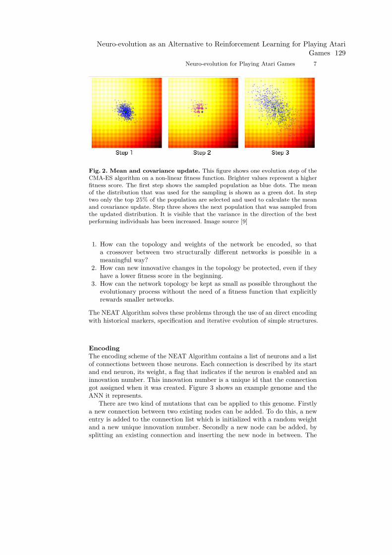
Neuro-evolution for Playing Atari Games 7
Fig. 2. Mean and covariance update. This figure shows one evolution step of theCMA-ES algorithm on a non-linear fitness function. Brighter values represent a higherfitness score. The first step shows the sampled population as blue dots. The meanof the distribution that was used for the sampling is shown as a green dot. In steptwo only the top 25% of the population are selected and used to calculate the meanand covariance update. Step three shows the next population that was sampled fromthe updated distribution. It is visible that the variance in the direction of the bestperforming individuals has been increased. Image source [9]
1. How can the topology and weights of the network be encoded, so thata crossover between two structurally different networks is possible in ameaningful way?
2. How can new innovative changes in the topology be protected, even if theyhave a lower fitness score in the beginning.
3. How can the network topology be kept as small as possible throughout theevolutionary process without the need of a fitness function that explicitlyrewards smaller networks.
The NEAT Algorithm solves these problems through the use of an direct encodingwith historical markers, specification and iterative evolution of simple structures.
EncodingThe encoding scheme of the NEAT Algorithm contains a list of neurons and a listof connections between those neurons. Each connection is described by its startand end neuron, its weight, a flag that indicates if the neuron is enabled and aninnovation number. This innovation number is a unique id that the connectiongot assigned when it was created. Figure 3 shows an example genome and theANN it represents.
There are two kind of mutations that can be applied to this genome. Firstlya new connection between two existing nodes can be added. To do this, a newentry is added to the connection list which is initialized with a random weightand a new unique innovation number. Secondly a new node can be added, bysplitting an existing connection and inserting the new node in between. The
Neuro-evolution as an Alternative to Reinforcement Learning for Playing AtariGames 129
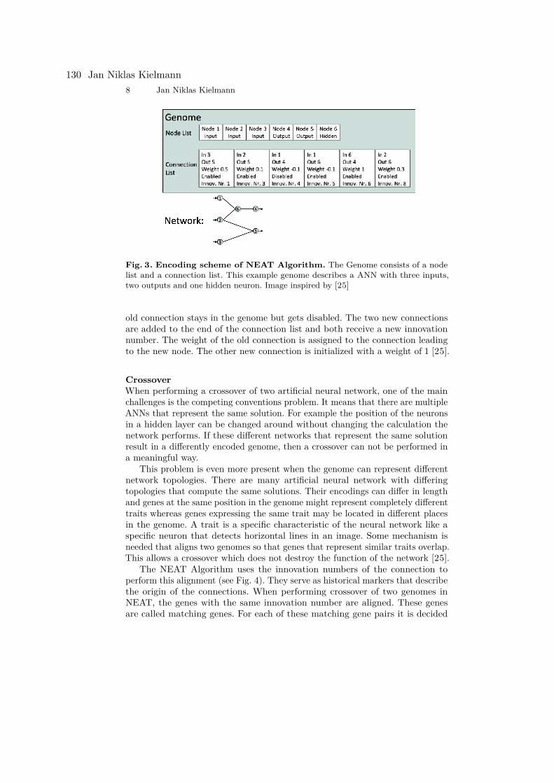
8 Jan Niklas Kielmann
Fig. 3. Encoding scheme of NEAT Algorithm. The Genome consists of a nodelist and a connection list. This example genome describes a ANN with three inputs,two outputs and one hidden neuron. Image inspired by [25]
old connection stays in the genome but gets disabled. The two new connectionsare added to the end of the connection list and both receive a new innovationnumber. The weight of the old connection is assigned to the connection leadingto the new node. The other new connection is initialized with a weight of 1 [25].
CrossoverWhen performing a crossover of two artificial neural network, one of the mainchallenges is the competing conventions problem. It means that there are multipleANNs that represent the same solution. For example the position of the neuronsin a hidden layer can be changed around without changing the calculation thenetwork performs. If these different networks that represent the same solutionresult in a differently encoded genome, then a crossover can not be performed ina meaningful way.
This problem is even more present when the genome can represent differentnetwork topologies. There are many artificial neural network with differingtopologies that compute the same solutions. Their encodings can differ in lengthand genes at the same position in the genome might represent completely differenttraits whereas genes expressing the same trait may be located in different placesin the genome. A trait is a specific characteristic of the neural network like aspecific neuron that detects horizontal lines in an image. Some mechanism isneeded that aligns two genomes so that genes that represent similar traits overlap.This allows a crossover which does not destroy the function of the network [25].
The NEAT Algorithm uses the innovation numbers of the connection toperform this alignment (see Fig. 4). They serve as historical markers that describethe origin of the connections. When performing crossover of two genomes inNEAT, the genes with the same innovation number are aligned. These genesare called matching genes. For each of these matching gene pairs it is decided
130 Jan Niklas Kielmann
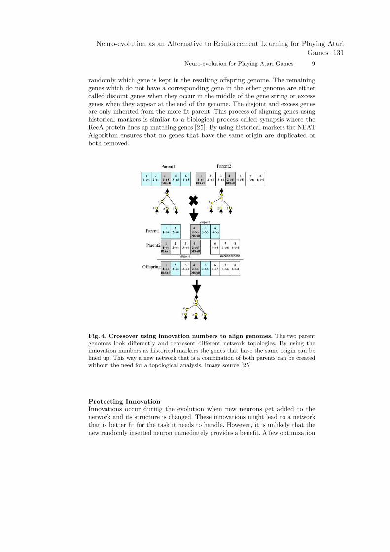
Neuro-evolution for Playing Atari Games 9
randomly which gene is kept in the resulting offspring genome. The remaininggenes which do not have a corresponding gene in the other genome are eithercalled disjoint genes when they occur in the middle of the gene string or excessgenes when they appear at the end of the genome. The disjoint and excess genesare only inherited from the more fit parent. This process of aligning genes usinghistorical markers is similar to a biological process called synapsis where theRecA protein lines up matching genes [25]. By using historical markers the NEATAlgorithm ensures that no genes that have the same origin are duplicated orboth removed.
Fig. 4. Crossover using innovation numbers to align genomes. The two parentgenomes look differently and represent different network topologies. By using theinnovation numbers as historical markers the genes that have the same origin can belined up. This way a new network that is a combination of both parents can be createdwithout the need for a topological analysis. Image source [25]
Protecting InnovationInnovations occur during the evolution when new neurons get added to thenetwork and its structure is changed. These innovations might lead to a networkthat is better fit for the task it needs to handle. However, it is unlikely that thenew randomly inserted neuron immediately provides a benefit. A few optimization
Neuro-evolution as an Alternative to Reinforcement Learning for Playing AtariGames 131
10 Jan Niklas Kielmann
steps will be needed before a performance increase can be observed. Most ofthe time an innovation will cause the fitness score of the individual to decrease.Because of that, most innovations will not stay in the population for long enoughwhich makes it impossible for complex network structures to emerge during theevolution. Therefore innovations need to be protected, so new structures get timeto be optimized.
NEAT uses speciation to solve this problem. Genomes which represent Net-works with a similar structure and weights belong to the same species and onlythe individuals in the same species compete against each other. This requiresa measure that describes the similarity of two networks. In NEAT this is donewith the compatibility distance which is defined as:
δ = c1E
N+ c2D
N+ c3 ∗ W
The historical markers are used to compute the number of excess genes E anddisjoint genes D. W is the average weight distance of matching genes. The factorN is the length of the genome and is used to normalize the number of excess anddisjoint genes. All three terms are scaled by a coefficient c1, c2 or c3. They allowto adjust the balance between the three factors [25].
This compatibility distance can now be used to sort the population into species.For that a list of species is maintained, each with one random representative fromthe last generation. A genome of the current generation is placed into a species ifits compatibility distance δ with the representative is lower than some thresholdδt. In the case that a genome is not compatible with any existing species, a newspecies with this genome as its representative is created [25].
To determine which individuals are allowed to reproduce explicit fitnesssharing is used. The number of offspring a species produces is proportionally tothe average fitness of this species. The best performing genomes in each speciesare mutated and recombined by crossover. The offspring replaces all individualsin the species [25]. This ensures that each species is allowed to create some newindividuals for the next generation even if the performance of the species is lowerthan that of the others.
Minimizing the TopologyStanley and Miikkulainen[25] argue that it is desirable to find networks with asfew neurons as possible. This minimizes the dimensionality of the weight spacethat needs to be searched. Many neuro-evolution algorithms start out with apopulation of random topologies. This, however, leads to unnecessarily complexnetwork structures. NEAT, on the other hand, starts out with a set of minimalNetworks that contain no hidden units. This way only structural changes thatprovide a benefit will survive the selection process and the algorithm is biasedtowards minimal solutions. This process does not need an additional term inthe fitness function for penalizing bigger networks which would require anotherhyperparameter.
132 Jan Niklas Kielmann
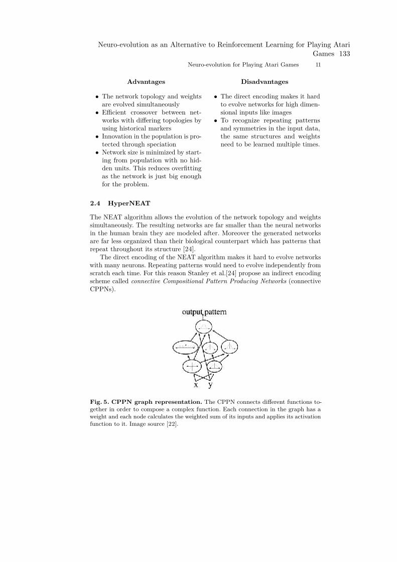
Neuro-evolution for Playing Atari Games 11
Advantages
• The network topology and weightsare evolved simultaneously
• Efficient crossover between net-works with differing topologies byusing historical markers
• Innovation in the population is pro-tected through speciation
• Network size is minimized by start-ing from population with no hid-den units. This reduces overfittingas the network is just big enoughfor the problem.
Disadvantages
• The direct encoding makes it hardto evolve networks for high dimen-sional inputs like images
• To recognize repeating patternsand symmetries in the input data,the same structures and weightsneed to be learned multiple times.
2.4 HyperNEAT
The NEAT algorithm allows the evolution of the network topology and weightssimultaneously. The resulting networks are far smaller than the neural networksin the human brain they are modeled after. Moreover the generated networksare far less organized than their biological counterpart which has patterns thatrepeat throughout its structure [24].
The direct encoding of the NEAT algorithm makes it hard to evolve networkswith many neurons. Repeating patterns would need to evolve independently fromscratch each time. For this reason Stanley et al.[24] propose an indirect encodingscheme called connective Compositional Pattern Producing Networks (connectiveCPPNs).
Fig. 5. CPPN graph representation. The CPPN connects different functions to-gether in order to compose a complex function. Each connection in the graph has aweight and each node calculates the weighted sum of its inputs and applies its activationfunction to it. Image source [22].
Neuro-evolution as an Alternative to Reinforcement Learning for Playing AtariGames 133
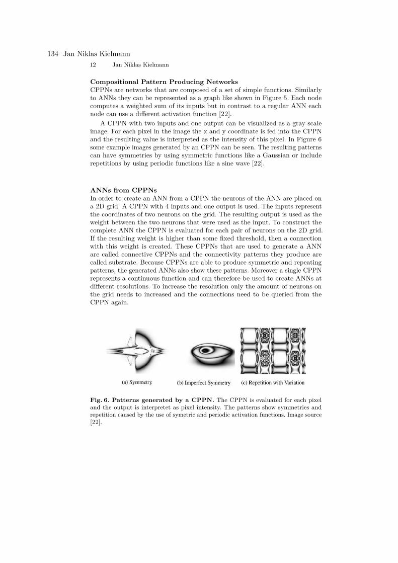
12 Jan Niklas Kielmann
Compositional Pattern Producing NetworksCPPNs are networks that are composed of a set of simple functions. Similarlyto ANNs they can be represented as a graph like shown in Figure 5. Each nodecomputes a weighted sum of its inputs but in contrast to a regular ANN eachnode can use a different activation function [22].
A CPPN with two inputs and one output can be visualized as a gray-scaleimage. For each pixel in the image the x and y coordinate is fed into the CPPNand the resulting value is interpreted as the intensity of this pixel. In Figure 6some example images generated by an CPPN can be seen. The resulting patternscan have symmetries by using symmetric functions like a Gaussian or includerepetitions by using periodic functions like a sine wave [22].
ANNs from CPPNsIn order to create an ANN from a CPPN the neurons of the ANN are placed ona 2D grid. A CPPN with 4 inputs and one output is used. The inputs representthe coordinates of two neurons on the grid. The resulting output is used as theweight between the two neurons that were used as the input. To construct thecomplete ANN the CPPN is evaluated for each pair of neurons on the 2D grid.If the resulting weight is higher than some fixed threshold, then a connectionwith this weight is created. These CPPNs that are used to generate a ANNare called connective CPPNs and the connectivity patterns they produce arecalled substrate. Because CPPNs are able to produce symmetric and repeatingpatterns, the generated ANNs also show these patterns. Moreover a single CPPNrepresents a continuous function and can therefore be used to create ANNs atdifferent resolutions. To increase the resolution only the amount of neurons onthe grid needs to increased and the connections need to be queried from theCPPN again.
Fig. 6. Patterns generated by a CPPN. The CPPN is evaluated for each pixeland the output is interpretet as pixel intensity. The patterns show symmetries andrepetition caused by the use of symetric and periodic activation functions. Image source[22].
134 Jan Niklas Kielmann
Neuro-evolution for Playing Atari Games 13
Substrate ConfigurationThe previous paragraph stated that the neurons of the ANN are placed on a2D grid. However, it is also possible to use other layouts. These layouts arecalled substrate configurations. For example a 3D grid can be used to layoutthe neurons. This would require a CPPN with six inputs, as the position of oneneuron is now specified by three coordinates. The substrate layout is not limitedto grid structures. For example it is possible to arrange the neurons in concentriccircles. The neurons can be referenced using polar coordinates.
In addition to the substrate configuration the input and output neurons mustbe defined. On a 2D grid the top row could be input neurons and the bottom rowthe output neurons. All neurons in between would be hidden units. Choosing asubstrate configuration and the layout of input and output neurons is applicationdependent. The goal is to model the geometry of the problem. For example inthe case of image classification it makes sense to place the neurons on a 2D-grid,as neighbouring pixels contain related information. However, if the task is tocontrol a round robot that can freely move on a 2D plane and has touch sensorsin all directions, then it would be best to layout the neurons corresponding tothe sensors in a circle to match the real world geometry of the robot.
CPPN evolutionANNs and CPPNs are structurally very similar. This means the NEAT algo-rithm can be used to evolve them with a few teaks. The NEAT encoding forthe nodes receives an additional field that specifies the used activation function.Furthermore, the compatibility distance function that is used for the speciationis adjusted to take differing activation functions into account. The total numberof activation functions that are different in the two genomes is counted andadded as a further weighted term to the compatibility distance function. Thiscauses individuals with differing activation functions to form separate species [22].
The HyperNEAT algorithm can be summarized by the following steps [24]:
1. Choose a layout for the neurons (substrate configuration) and define theinput and output neurons.
2. Initialize a population with minimal CPPNs with random weights. They areencoded using the NEAT encoding scheme.
3. Iterate for N generations or until solution is found:(a) For each CPPN in the population do:
i. Evaluate the CPPN for each possible connection between neurons. Ifthe resulting output exceeds a threshold, a new connection is createdwith a weight set to the output.
ii. Run the resulting ANN in the task domain to obtain its fitness score.(b) Reproduce the CPPNs through mutation, crossover and speciation ac-
cording to the NEAT algorithm described in Section 2.3.
Neuro-evolution as an Alternative to Reinforcement Learning for Playing AtariGames 135
14 Jan Niklas Kielmann
Advantages
• The network topology and weightsare evolved simultaneously
• The indirect encoding allows toevolve networks with high dimen-sional inputs
• ANNs generated by CPPNs containsymmetries and repetitions
• Knowledge about the problem ge-ometry is incorporated by choosingthe substrate configuration
• One evolved CPPN can be usedto generate ANNs for any desiredinput resolution
Disadvantages
• The indirect encoding makes thealgorithm more complex and forinputs with a low dimensionalitythe simpler NEAT algorithm oftenoutperforms HyperNEAT
• Choosing the right substrate config-uration requires domain knowledgeand experience
3 Atari Research Environment
The Atari 2600 was the first popular home video game console. It was releasedin 1977 and over the time over 1000 games were created for the system [17]. Thiswas possible through the use of a general purpose CPU, which allowed the gamecode to be stored on cartridges separate from the console hardware [3]. This largeamount of available games is one reason for using Atari games as a benchmark forlearning algorithms. It allows an algorithm to be designed and tested on a subsetof these games and test its generalization abilities on the remaining games.
Moreover the 1.19Mhz CPU used by the Atari 2600 is not very powerfulcompared to modern processors. Because of this many Atari games can besimulated in parallel and the simulation speed is significantly higher than onthe original console. This is another reason for using Atari games as a researchenvironment. Most learning algorithms need to simulate the game many timesbefore learning a useful strategy. There are already many emulators like the“Stella”1 emulator. Frameworks like “OpenAI Gym”2 and the “Arcade LearningEnvironment”3 provide a layer on top of these emulators and allow learningalgorithms to interface with the games.
Another advantage is the small action and state space of Atari games. Thecontroller of the Atari 2600 consists of a single button and a joystick that canbe in 9 different states (middle, up, down, left, right, up-left, up-right, down-left,down-right). This results in 18 distinct input combinations the agent can choosefrom. The observable state space consists of the 160 × 210 pixel values (upto 128 possible colors) and basic sound effects. This keeps the search spacefor possible policies small enough to be explored by learning agents while still
1 https://stella-emu.github.io/2 https://gym.openai.com/3 https://github.com/mgbellemare/Arcade-Learning-Environment
136 Jan Niklas Kielmann

Neuro-evolution for Playing Atari Games 15
allowing interesting and complex games. These games have interesting gamedynamics but are limited to a small 2D world with few agents.
Fig. 7. Left: The Atari 2600 video game console. Right: Screenshots of 8 different Atarigames. They show the simple, low resolution graphics of the Arari 2600.https://upload.wikimedia.org/wikipedia/commons/b/b9/Atari-2600-Wood-4Sw-Set.jpghttps://atariage.com/images/query_headers/Atari2600_Screenshots_Header.jpg
3.1 State Representation
Raw Atari frames are 210 x 160 pixel images with 128 unique colors. This highdimensional input space is computationally demanding and requires large neuralnetworks with many parameters. For this reason different representations of thegame state are used that have varying levels of abstraction.
Object RepresentationThis is the most abstract state representation using the least general features. Atemplate based object detector is used to extract the position of different objectson the screen. The objects are categorized in classes like enemy or player. Ahuman has to extract the sprites of these objects and sort them into the correctclass. At run-time the extracted sprites are compared with the contents of thescreen to detect the objects. For animated sprites multiple images are extracted.This means the algorithm does not need to learn the pixel representation of theobjects and the category they belong to. At the same time, however, this alsomeans that algorithms using the object representation are the least general, asthey require human knowledge to extract relevant objects. To reduce the inputdimensionality the object positions are represented on a scaled down 8 x 10 gird[12].
Neuro-evolution as an Alternative to Reinforcement Learning for Playing AtariGames 137
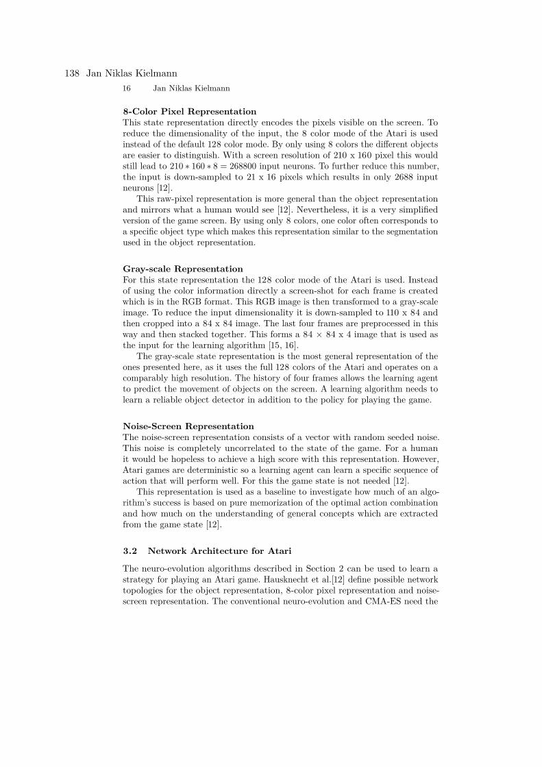
16 Jan Niklas Kielmann
8-Color Pixel RepresentationThis state representation directly encodes the pixels visible on the screen. Toreduce the dimensionality of the input, the 8 color mode of the Atari is usedinstead of the default 128 color mode. By only using 8 colors the different objectsare easier to distinguish. With a screen resolution of 210 x 160 pixel this wouldstill lead to 210 ∗ 160 ∗ 8 = 268800 input neurons. To further reduce this number,the input is down-sampled to 21 x 16 pixels which results in only 2688 inputneurons [12].
This raw-pixel representation is more general than the object representationand mirrors what a human would see [12]. Nevertheless, it is a very simplifiedversion of the game screen. By using only 8 colors, one color often corresponds toa specific object type which makes this representation similar to the segmentationused in the object representation.
Gray-scale RepresentationFor this state representation the 128 color mode of the Atari is used. Insteadof using the color information directly a screen-shot for each frame is createdwhich is in the RGB format. This RGB image is then transformed to a gray-scaleimage. To reduce the input dimensionality it is down-sampled to 110 x 84 andthen cropped into a 84 x 84 image. The last four frames are preprocessed in thisway and then stacked together. This forms a 84 × 84 x 4 image that is used asthe input for the learning algorithm [15, 16].
The gray-scale state representation is the most general representation of theones presented here, as it uses the full 128 colors of the Atari and operates on acomparably high resolution. The history of four frames allows the learning agentto predict the movement of objects on the screen. A learning algorithm needs tolearn a reliable object detector in addition to the policy for playing the game.
Noise-Screen RepresentationThe noise-screen representation consists of a vector with random seeded noise.This noise is completely uncorrelated to the state of the game. For a humanit would be hopeless to achieve a high score with this representation. However,Atari games are deterministic so a learning agent can learn a specific sequence ofaction that will perform well. For this the game state is not needed [12].
This representation is used as a baseline to investigate how much of an algo-rithm’s success is based on pure memorization of the optimal action combinationand how much on the understanding of general concepts which are extractedfrom the game state [12].
3.2 Network Architecture for Atari
The neuro-evolution algorithms described in Section 2 can be used to learn astrategy for playing an Atari game. Hausknecht et al.[12] define possible networktopologies for the object representation, 8-color pixel representation and noise-screen representation. The conventional neuro-evolution and CMA-ES need the
138 Jan Niklas Kielmann
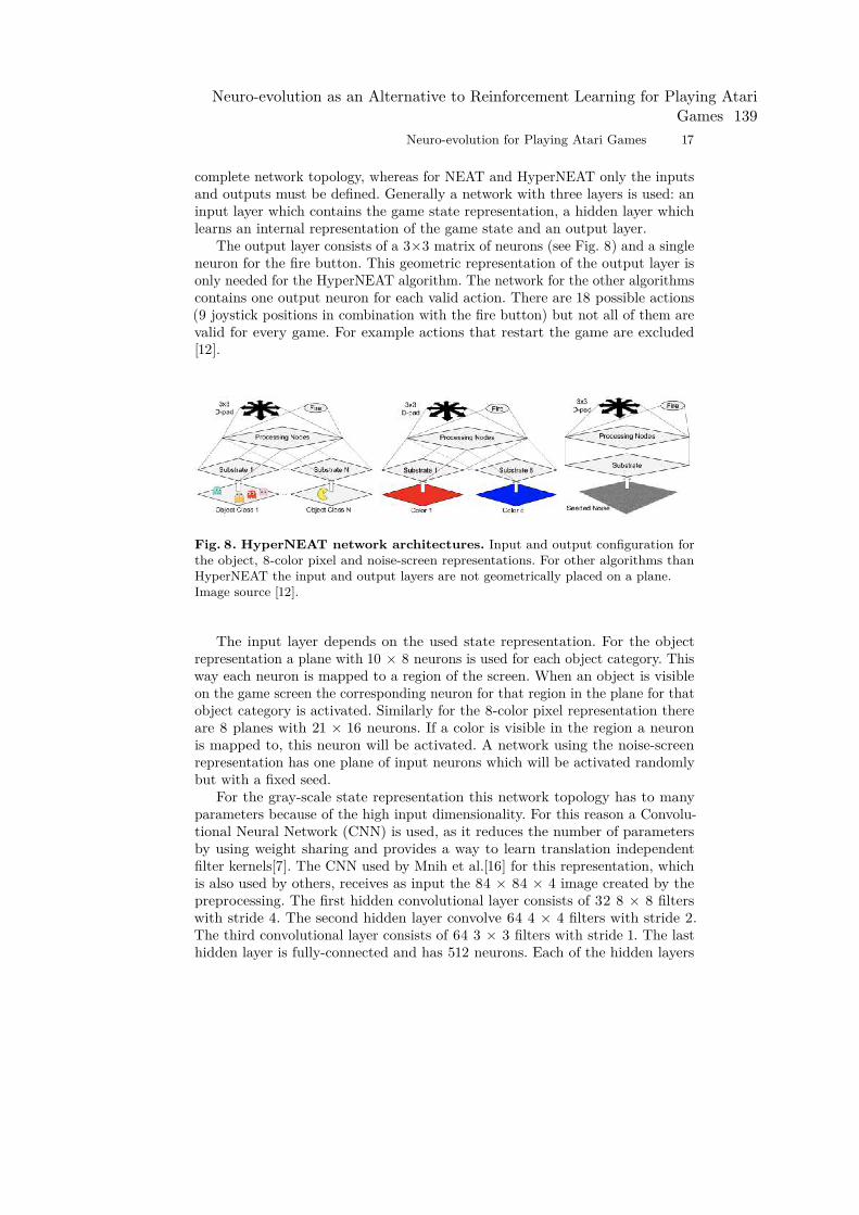
Neuro-evolution for Playing Atari Games 17
complete network topology, whereas for NEAT and HyperNEAT only the inputsand outputs must be defined. Generally a network with three layers is used: aninput layer which contains the game state representation, a hidden layer whichlearns an internal representation of the game state and an output layer.
The output layer consists of a 3×3 matrix of neurons (see Fig. 8) and a singleneuron for the fire button. This geometric representation of the output layer isonly needed for the HyperNEAT algorithm. The network for the other algorithmscontains one output neuron for each valid action. There are 18 possible actions(9 joystick positions in combination with the fire button) but not all of them arevalid for every game. For example actions that restart the game are excluded[12].
Fig. 8. HyperNEAT network architectures. Input and output configuration forthe object, 8-color pixel and noise-screen representations. For other algorithms thanHyperNEAT the input and output layers are not geometrically placed on a plane.Image source [12].
The input layer depends on the used state representation. For the objectrepresentation a plane with 10 × 8 neurons is used for each object category. Thisway each neuron is mapped to a region of the screen. When an object is visibleon the game screen the corresponding neuron for that region in the plane for thatobject category is activated. Similarly for the 8-color pixel representation thereare 8 planes with 21 × 16 neurons. If a color is visible in the region a neuronis mapped to, this neuron will be activated. A network using the noise-screenrepresentation has one plane of input neurons which will be activated randomlybut with a fixed seed.
For the gray-scale state representation this network topology has to manyparameters because of the high input dimensionality. For this reason a Convolu-tional Neural Network (CNN) is used, as it reduces the number of parametersby using weight sharing and provides a way to learn translation independentfilter kernels[7]. The CNN used by Mnih et al.[16] for this representation, whichis also used by others, receives as input the 84 × 84 × 4 image created by thepreprocessing. The first hidden convolutional layer consists of 32 8 × 8 filterswith stride 4. The second hidden layer convolve 64 4 × 4 filters with stride 2.The third convolutional layer consists of 64 3 × 3 filters with stride 1. The lasthidden layer is fully-connected and has 512 neurons. Each of the hidden layers
Neuro-evolution as an Alternative to Reinforcement Learning for Playing AtariGames 139
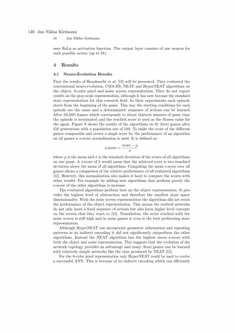
18 Jan Niklas Kielmann
uses ReLu as activation function. The output layer consists of one neuron foreach possible action (up to 18).
4 Results
4.1 Neuro-Evolution Results
First the results of Hausknecht et al. [12] will be presented. They evaluated theconventional neuro-evolution, CMA-ES, NEAT and HyperNEAT algorithms onthe object, 8-color pixel and noise screen representation. They do not reportresults on the gray-scale representation, although it has now become the standardstate representation for this research field. In their experiments each episodestarts from the beginning of the game. This way the starting conditions for eachepisode are the same and a deterministic sequence of actions can be learned.After 50,000 frames which corresponds to about thirteen minutes of game timethe episode is terminated and the reached score is used as the fitness value forthe agent. Figure 9 shows the results of the algorithms on 61 Atari games after150 generations with a population size of 100. To make the score of the differentgames comparable and create a single score for the performance of an algorithmon all games a z-score normalization is used. It is defined as:
z-score = score − µ
σ
where µ is the mean and σ is the standard deviation of the scores of all algorithmson one game. A z-score of 2 would mean that the achieved score is two standarddeviation above the mean of all algorithms. Computing the mean z-score over allgames allows a comparison of the relative performance of all evaluated algorithms[12]. However, this normalization also makes it hard to compare the scores withother results. For example by adding new algorithms that perform poorly thez-score of the other algorithms is increase.
The evaluated algorithms perform best on the object representation. It pro-vides the highest level of abstraction and therefore the smallest state spacedimensionality. With the noise screen representation the algorithms did not reachthe performance of the object representation. This means the evolved networksdo not only learn a fixed sequence of actions but also learn higher level conceptson the screen that they react to [12]. Nonetheless, the score reached with thenoise screen is still high and in some games it even is the best performing staterepresentation.
Although HyperNEAT can incorporate geometric information and repeatingpatterns in its indirect encoding it did not significantly outperform the otheralgorithms. Instead the NEAT algorithm has the highest mean z-score withboth the object and noise representation. This suggests that the evolution of thenetwork topology provides an advantage and many Atari games can be learnedwith relatively simple networks like the ones produced by NEAT [12].
For the 8-color pixel representation only HyperNEAT could be used to evolvea successful ANN. This is because of its indirect encoding which can efficiently
140 Jan Niklas Kielmann
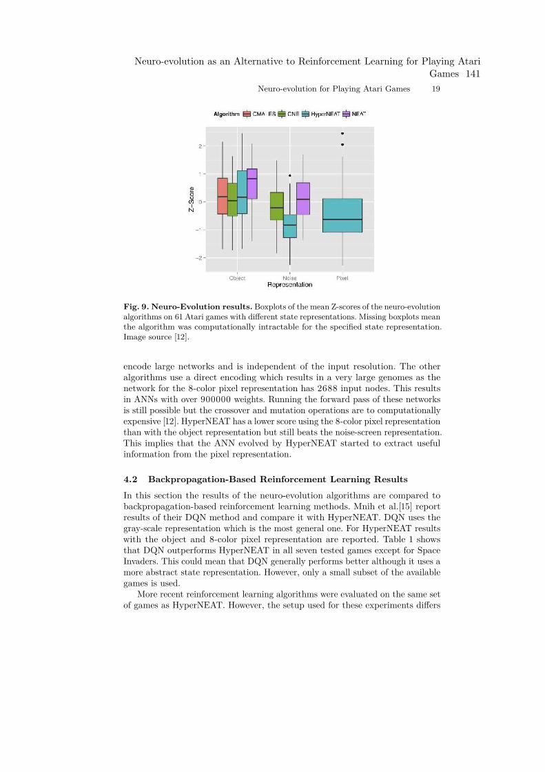
Neuro-evolution for Playing Atari Games 19
Fig. 9. Neuro-Evolution results. Boxplots of the mean Z-scores of the neuro-evolutionalgorithms on 61 Atari games with different state representations. Missing boxplots meanthe algorithm was computationally intractable for the specified state representation.Image source [12].
encode large networks and is independent of the input resolution. The otheralgorithms use a direct encoding which results in a very large genomes as thenetwork for the 8-color pixel representation has 2688 input nodes. This resultsin ANNs with over 900000 weights. Running the forward pass of these networksis still possible but the crossover and mutation operations are to computationallyexpensive [12]. HyperNEAT has a lower score using the 8-color pixel representationthan with the object representation but still beats the noise-screen representation.This implies that the ANN evolved by HyperNEAT started to extract usefulinformation from the pixel representation.
4.2 Backpropagation-Based Reinforcement Learning ResultsIn this section the results of the neuro-evolution algorithms are compared tobackpropagation-based reinforcement learning methods. Mnih et al.[15] reportresults of their DQN method and compare it with HyperNEAT. DQN uses thegray-scale representation which is the most general one. For HyperNEAT resultswith the object and 8-color pixel representation are reported. Table 1 showsthat DQN outperforms HyperNEAT in all seven tested games except for SpaceInvaders. This could mean that DQN generally performs better although it uses amore abstract state representation. However, only a small subset of the availablegames is used.
More recent reinforcement learning algorithms were evaluated on the same setof games as HyperNEAT. However, the setup used for these experiments differs
Neuro-evolution as an Alternative to Reinforcement Learning for Playing AtariGames 141
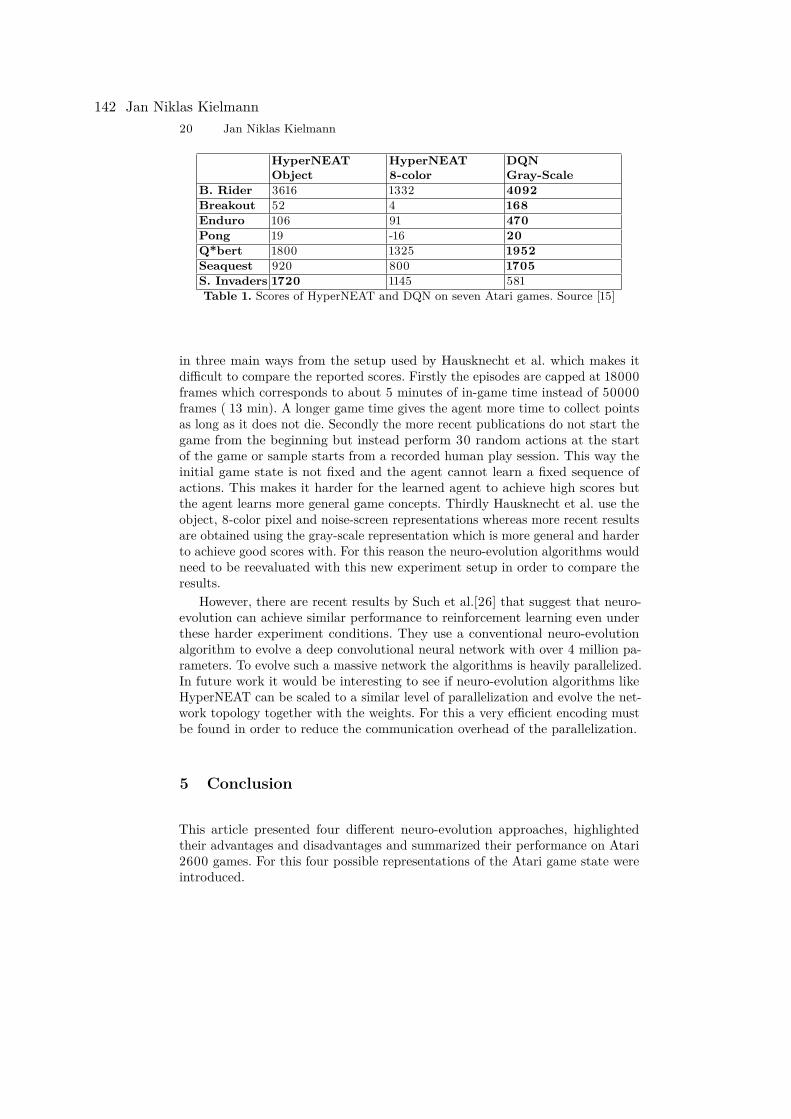
20 Jan Niklas Kielmann
HyperNEATObject
HyperNEAT8-color
DQNGray-Scale
B. Rider 3616 1332 4092Breakout 52 4 168Enduro 106 91 470Pong 19 -16 20Q*bert 1800 1325 1952Seaquest 920 800 1705S. Invaders 1720 1145 581Table 1. Scores of HyperNEAT and DQN on seven Atari games. Source [15]
in three main ways from the setup used by Hausknecht et al. which makes itdifficult to compare the reported scores. Firstly the episodes are capped at 18000frames which corresponds to about 5 minutes of in-game time instead of 50000frames ( 13 min). A longer game time gives the agent more time to collect pointsas long as it does not die. Secondly the more recent publications do not start thegame from the beginning but instead perform 30 random actions at the startof the game or sample starts from a recorded human play session. This way theinitial game state is not fixed and the agent cannot learn a fixed sequence ofactions. This makes it harder for the learned agent to achieve high scores butthe agent learns more general game concepts. Thirdly Hausknecht et al. use theobject, 8-color pixel and noise-screen representations whereas more recent resultsare obtained using the gray-scale representation which is more general and harderto achieve good scores with. For this reason the neuro-evolution algorithms wouldneed to be reevaluated with this new experiment setup in order to compare theresults.
However, there are recent results by Such et al.[26] that suggest that neuro-evolution can achieve similar performance to reinforcement learning even underthese harder experiment conditions. They use a conventional neuro-evolutionalgorithm to evolve a deep convolutional neural network with over 4 million pa-rameters. To evolve such a massive network the algorithms is heavily parallelized.In future work it would be interesting to see if neuro-evolution algorithms likeHyperNEAT can be scaled to a similar level of parallelization and evolve the net-work topology together with the weights. For this a very efficient encoding mustbe found in order to reduce the communication overhead of the parallelization.
5 Conclusion
This article presented four different neuro-evolution approaches, highlightedtheir advantages and disadvantages and summarized their performance on Atari2600 games. For this four possible representations of the Atari game state wereintroduced.
142 Jan Niklas Kielmann
Neuro-evolution for Playing Atari Games 21
The conventional neuro-evolution algorithm is simple to implement andcan easily be parallelized but only optimizes the network weights and has nomechanisms in place to achieve a faster convergence.
CMA-ES is a wildly used method for solving black-box optimization withan adaptive step size and few hyperparameters. However, it also only evolvesthe network weights and can be computationally expensive for high-dimensionalinputs.
The NEAT algorithm allows the evolution of the network topology along withthe weights. It does so by starting out with a minimal network topology whichmakes sure that the found network is as small as possible. Nonetheless, for verylarge inputs the direct encoding used by NEAT becomes inefficient and repeatingpatterns in the network need to be independently evolved multiple times.
HyperNEAT addresses the problems of NEAT by using an indirect encod-ing scheme based on CPPNs. This allows the efficient evolution of very largenetworks with repeating patterns. This added complexity does, however, leadto worse performance for low-dimensional input problems where NEAT usuallyoutperforms HyperNEAT.
The results published by Hausknecht et al. showed these neuro-evolutionalgorithms are able to evolve successful networks for playing Atari games. Thelearned strategies beat human players in three games and discovered opportunitiesfor infinite scores in three more games [12]. Direct encoding algorithms like NEATand CMA-ES performed better than the indirect encoding of HyperNEAT on low-dimensional input representations like the object and noise-screen representation.NEAT was able to achieve higher scores than the other direct encoding methods,suggesting that the evolution of a minimal network topology provides an advantageover fixed topology networks. HyperNEAT was the only algorithm capable oflearning based on the 8-color pixel representation. Here the indirect encodingenabled the evolution of large networks with repeating structures which areneeded for dealing with high-dimensional state representations.
The learned agents often exploit a fixed sequence of actions that are hard toreproduce by human players. Agents trained using the noise-screen representationsstill achieve comparably high scores. This means the agent learns to play thegame without any information about the game state. This only works becauseAtari games are deterministic and the episodes always start at the beginning ofthe game. In future work it would be interesting to evaluate these neuro-evolutionalgorithms on random starts. This can be done by performing a number ofrandom actions at the beginning of the game or by choosing a random gamestate from a recorded human play session. This way the evolved network mustreact to the objects on the screen and it would not be possible to achieve a goodperformance with the noise-screen representation.
Mnih et al.[15] showed that the DQN reinforcement learning algorithm outper-forms HyperNEAT in some games. However, only the results on a small subset ofgames were reported. A more detailed comparison of the results of neuro-evolutionand reinforcement learning algorithms would require experiments performed inthe same conditions. In particular the neuro-evolution algorithms would need to
Neuro-evolution as an Alternative to Reinforcement Learning for Playing AtariGames 143
22 Jan Niklas Kielmann
be evaluated on random starts and the gray-scale state representation. For thisscaled up versions of the presented neuro-evolution algorithms utilizing heavyparallelization would need to be developed similar to the results of Such et al.[26].
6 Outlook
There is evidence that the performance of neuro-evolution algorithms can begreatly increased by scaling them up to run on big computer clusters[26]. Becauseno gradients need to be calculated and exchanged between all computing nodes,neuro-evolution algorithms are easy to parallelize. Using a simple conventionalneuro-evolution algorithm Such et al.[26] were able to achieve promising resultson the Atari domain. A future research topic would be to answer the question ifmore advanced algorithms like NEAT could also be scaled up in a similar fashionto further increase the performance.
Another idea for further research would be to adapt NEAT to evolve CNNsinstead of simple feed forward networks. CNNs have the advantage that they candeal with high dimensional inputs like images by finding translation invariantpatterns. The direct encoding of the NEAT algorithm would need to be adaptedto include parameters like kernel size and the number of feature maps whichwould be evolved by the algorithm together with the weights.
Lastly, hybrid approaches of neuro-evolution and backpropagation basedsolutions could be tried out. Evolution would be used to find the best networktopology whereas backpropagation would be used to learn the weights. This waythe the strengths of both methods could be combined.
References
1. Aaltonen, T., Adelman, J., Akimoto, T., Albrow, M., González, B.A., Amerio,S., Amidei, D., Anastassov, A., Annovi, A., Antos, J., et al.: Measurement of thetop-quark mass with dilepton events selected using neuroevolution at cdf. Physicalreview letters 102(15), 152001 (2009)
2. Bäck, T., Schwefel, H.P.: An overview of evolutionary algorithms for parameteroptimization. Evolutionary computation 1(1), 1–23 (1993)
3. Bellemare, M.G., Naddaf, Y., Veness, J., Bowling, M.: The Arcade LearningEnvironment: An Evaluation Platform for General Agents. Journal of ArtificialIntelligence Research 47, pages 253-279 (2012)
4. Braun, H., Weisbrod, J.: Evolving neural feedforward networks. In: Artificial NeuralNets and Genetic Algorithms. pp. 25–32. Springer (1993)
5. Floreano, D., Dürr, P., Mattiussi, C.: Neuroevolution: from architectures to learning.Evolutionary Intelligence 1(1), 47–62 (jan 2008)
6. Fogel, D.B., Fogel, L.J., Porto, V.: Evolving neural networks. Biological cybernetics63(6), 487–493 (1990)
7. Goodfellow, I., Bengio, Y., Courville, A.: Deep Learning. MIT Press (2016)8. Gruau, F., Whitley, D.: Adding learning to the cellular development of neural
networks: Evolution and the baldwin effect. Evolutionary computation 1(3), 213–233(1993)
144 Jan Niklas Kielmann
Neuro-evolution for Playing Atari Games 23
9. Ha, D.: A visual guide to evolution strategies. blog.otoro.net (2017), http://blog.otoro.net/2017/10/29/visual-evolution-strategies/
10. Hansen, N.: The cma evolution strategy: A tutorial (Apr 2016)11. Hasan, B.H.F., Saleh, M.S.M.: Evaluating the effectiveness of mutation operators on
the behavior of genetic algorithms applied to non-deterministic polynomial problems.Informatica 35(4) (2011)
12. Hausknecht, M., Lehman, J., Miikkulainen, R., Stone, P.: A neuroevolution approachto general atari game playing. IEEE Transactions on Computational Intelligence andAI in Games 6(4), 355–366 (2014)
13. Mirjalili, S.: Evolutionary Algorithms and Neural Networks. Springer InternationalPublishing (2018)
14. Mnih, V., Badia, A.P., Mirza, M., Graves, A., Lillicrap, T., Harley, T., Silver,D., Kavukcuoglu, K.: Asynchronous methods for deep reinforcement learning. In:International conference on machine learning. pp. 1928–1937 (2016)
15. Mnih, V., Kavukcuoglu, K., Silver, D., Graves, A., Antonoglou, I., Wierstra, D.,Riedmiller, M.: Playing atari with deep reinforcement learning. arXiv preprintarXiv:1312.5602 (2013)
16. Mnih, V., Kavukcuoglu, K., Silver, D., Rusu, A.A., Veness, J., Bellemare, M.G.,Graves, A., Riedmiller, M., Fidjeland, A.K., Ostrovski, G., et al.: Human-level controlthrough deep reinforcement learning. Nature 518(7540), 529 (2015)
17. Montfort, N.: Racing the beam: The atari video computer system (2011)18. Olive, D.J., Olive, D.J., Chernyk: Robust multivariate analysis. Springer (2017)19. Rumelhart, D.E., Hinton, G.E., Williams, R.J.: Learning internal representations by
error propagation. Tech. rep., California Univ San Diego La Jolla Inst for CognitiveScience (1985)
20. Salimans, T., Ho, J., Chen, X., Sidor, S., Sutskever, I.: Evolution strategies as ascalable alternative to reinforcement learning. arXiv preprint arXiv:1703.03864 (2017)
21. Schulman, J., Wolski, F., Dhariwal, P., Radford, A., Klimov, O.: Proximal policyoptimization algorithms. arXiv preprint arXiv:1707.06347 (2017)
22. Stanley, K.O.: Compositional pattern producing networks: A novel abstraction ofdevelopment. Genetic programming and evolvable machines 8(2), 131–162 (2007)
23. Stanley, K.O., Bryant, B.D., Miikkulainen, R.: Evolving neural network agents in thenero video game. Proceedings of the IEEE pp. 182–189 (2005)
24. Stanley, K.O., D’Ambrosio, D.B., Gauci, J.: A hypercube-based encoding for evolvinglarge-scale neural networks. Artificial life 15(2), 185–212 (2009)
25. Stanley, K.O., Miikkulainen, R.: Evolving neural networks through augmentingtopologies. Evolutionary computation 10(2), 99–127 (2002)
26. Such, F.P., Madhavan, V., Conti, E., Lehman, J., Stanley, K.O., Clune, J.: Deepneuroevolution: Genetic algorithms are a competitive alternative for training deepneural networks for reinforcement learning (Dec 2017)
27. Syswerda, G.: Uniform crossover in genetic algorithms. In: Proceedings of the3rd International Conference on Genetic Algorithms. pp. 2–9. Morgan KaufmannPublishers Inc., San Francisco, CA, USA (1989)
Neuro-evolution as an Alternative to Reinforcement Learning for Playing AtariGames 145
Hot topics in Human-Computer-Interaction
Carolin Ligensa
Chair for Pervasive Computing Systems
Abstract. This paper identifies emerging topics in the field of HumanComputer Interaction (HCI) of significant and growing importance. Itidentifies those focus points to be health, new research methods in HCI andnovel ways of interacting with computers. For health research, there wasa clear tendency on finding ways to integrate commonly used technologiesinto daily health struggles as well as defining the role of social media.In the area of finding new research methods in HCI, improvement wassought for studies through collecting, evaluating and translating data.The field titled as novel ways of interacting with computers deals notonly with the design of such novel ways and the evaluation thereof, butalso all kind of new possibilities appearing through those ways. It focuseson eye-tracking, epidermal devices and virtual reality.Different types of papers are distinguished and various research techniquesidentified and analyzed.
Keywords: HCI, Hot Topics, Health, Medicine, Mental Illness, Assistive Tech-nologies, Fitness, Research, Computer-Interaction, Eye-Tracking, Epidermaldevices, Virtual Reality
1 Introduction
This work aims to identify hot-topics of today’s Human Computer Interaction(HCI) research. The main focus of HCI research is the improvement of userinteraction with any kind of technology. Nowadays technology is integrated intodaily activity in every area of our lives. This makes HCI a field that could not bemore versatile.
To identify the focus of today’s research, I looked at the list of the best pa-pers and honorable mentions of CHI 2019 [1]. CHI is the leading internationalconference on Human Computer Interaction taking place once a year, held byACM, the Association for Computing Machinery. With its international relevance,it was the natural choice to investigate HCI research.
This paper summarizes 26 papers in the areas that were identified as hot topicsas an attempt on giving the reader an overview over the topics most relevant intoday’s research. It draws connections between the different topics, identifyingprominent and overarching focal points. It also distinguishes different types ofpapers and identifies and analyzes various research techniques.
146 Carolin Ligensa

2 Carolin Ligensa
2 Emerging Topics in HCI
2.1 OverviewFigure 1 gives an overview over the many topics represented on the CHI 2019best paper and honorable mentions list [1]. This word cloud was created basedon reading the abstracts of all 150 papers and in this way making deductions totheir content.
Fig. 1. Wordcloud compiled of the Best Papers and Honorable Mentions of CHI 2019.
As can be seen in Fig. 1, there was a great variety of topics covered multipletimes in current research. This is due to the fact that HCI is a very versatilefield. In this paper however not all of these areas can be covered. The main focusis going to be on the three biggest areas that were identified: health, challengesof HCI research and interaction with computers in new ways.
2.2 HealthAs can be see in Fig. 1, the biggest part of today’s research focuses on healthissues. In the following, this topics is divided into the areas of Medicine, Mental
Hot topics in Human-Computer-Interaction 147

Hot topics in Human-Computer-Interaction 3
Health, Assistive Technology for Disabilities and Fitness for a better overview ofthe wide range of topics this field represents.
MedicineThe most well-known area of health management is traditional medicine. Treat-ment however does not solely take place in clinics or doctor’s offices anymore.In the following, two novel ways of diagnosing and dealing with disease areintroduced.
Self Management In the year 2020, 157 million people all over the world will besuffering from chronical health conditions [19]. Already today, 50 million peoplein Europe alone suffer from so called multimorbidity, meaning they suffer frommultiple chronical health conditions [9]. With a steadily increasing number ofchronically ill people, tools for self-care become increasingly important. Self-carewas defined by the World Health organization as “the ability of individuals, fami-lies and communities to promote health, prevent disease, maintain health, andto cope with illness and disability with or without the support of a health-careprovider” [18]. Tools for self-care are mostly mobile applications that help thepatients deal with multiple tasks needed to be carried out every day. Improvingon those tools can save a lot of time and effort and thus significantly improvequality of life [9].
While use of such tools has clearly shown health benefits, it has been observedthat people affected find it challenging to stick to self-care mechanisms [19]. Rajet al. [19] investigate the role of context in self-management at the exampleof Diabetes Type-1 patients. Context in this case can be any environment orcircumstance, e.g. home/travel, work/school, weekends/working days. They findthat these contexts highly influence factors like nutrition, physical activity, moodand, in this special case, insulin. Being aware of those contexts can potentially beused for “providing support at the right time, at the right place, and in the rightway” and thus encouraging people, not pressuring them. Data regarding thesecontexts can easily be taken from the user’s smartphones. The challenge hereclearly lies in the design of those context-sensitive self-care tools. This includesfinding relevant factors as well as solutions on how integrate them best. So-calledcontextual frames help understanding the same factors in different contexts andthereby can help adjusting and optimizing the support to each individual.
Doyle et al. [9] focus on the special burdens experienced by people with mul-timorbidity using self-care technology. Additionally, they concentrate on elderpeople, as the probability for chronic disease grows hand in hand with age. Olderpeople might face additional challenges like a lack of sensory, physical and / orcognitive skills as well as technological affinity when interacting with technology.As a consequence, technology for elder people should be “accessible, easy to useand intuitive, shortening the learning curve for this cohort“ [9]. They also foundthat the daily treatment of multiple illnesses often equals excessive demands on
148 Carolin Ligensa
4 Carolin Ligensa
the patient’s side. From keeping track of symptoms and taking a potentially vastamount of medication to managing healthcare visits and doctor’s appointments,the list of tasks can be overwhelming and sometimes even contradictive. Priori-tizing tasks provides a starting point for the patient and supports decisions whenhaving to choose between contradicting assignments. When designing medicinalcare for people with multiple chronic illnesses, it can further be helpful to lookat the bigger picture of all their illnesses rather than seeing and treating eachone individually. Another benefit can be the co-use of the self-care applicationby both patient and care-taker, as both possess unique but valuable insight intothe patient’s condition. The patient has a leading edge on his personal state ofhealth while the care taker can see things from a medicinal perspective.
Online Health Communities Online Health Communities are online forums thatallow people with similar diagnosis to connect. They act as a support system andoffer advice on illness-related issues [27, 28].
As people seek medical advice to personal health problems, they have to re-veal a much greater amount of personal data than e.g. when seeking for help in atech forum. So-called self-disclosure, “the process by which one person verballyreveals information about himself or herself to another” [27], is important forothers to understand the exact terms of the problem and give advice accordingly.This of course makes the author vulnerable. Looking at the big picture of socialmedia, people have shown to be more likely to disclose personal informationthat might reflect in them negatively in private channels, meaning to a specifiedaudience, rather than in public for everyone to see. Anonymity brings safety.Online Health Communities provide both private and public channels, yet theyget used differently: Primarily used are public channels for all matters of support;private channels are merely used for follow-ups. Being a community for a specifiedgroup of people already gives a more private feel to the public channels. [27]
Another interesting observation made by Young et al. [26] is the differentia-tion and the distribution of different social roles amongst members of OnlineHealth Communities. While some people might be focused on sharing illness-related information, others might want to share their personal story or give adviceto others. What role a member will fill is mostly depended on their goal, theirdesire to interact with other members and their expectations from joining thecommunity. Over the course of their in the community, every member will obtaindifferent roles, yet stay equally distributed in the community as a whole.
Young et al. [28] have observed these behaviors and patterns to slightly shift whenlooking at Online Health Communities for illnesses with unknown cause. At theexample of a Facebook support group for Vulvodynia, they found that membersprimarily used the platform “to collectively make sense of their condition”. Therewas also a significantly larger amount of entries concerning how to self-managedaily life with the illness. Additionally, they discovered potential added benefit ofself-tracking devices for diseases with unknown cause. Provided with the resulting
Hot topics in Human-Computer-Interaction 149
Hot topics in Human-Computer-Interaction 5
pool of first-hand patient data, it might be possible to collectively find a reasonfor the illness.
Mental IllnessSimilar to the online communities discussed in the previous sections, Andalibi’spaper [5] focusses on what existing social media networks can do. Sharing mentalhealth issues on identified social networks can be intimidating, since unfortu-nately, there is still a stigma attached to mental illnesses [5, 11]. Yet it has provento offer the possibility to form deeper bonds with similar-conditioned peoplethan looking for support on an anonymous website. Victims of mental illnessessharing them online have shown to turn into role-models for others and therebyexperienced health improvement themselves. This mentorship-relationship ishowever complicated by social media platforms, as they “lack affordances thatenable the community, particularly new or occasional users, to effectively finddiscussions as they become buried below new content” [28]. A new function oflabelling oneself as a specific group could help finding people with a shared diag-nosis. Integrating an online health community into everyday social media insteadof marginalizing them also might benefit the demise of mental health stigmata [5].
This is particularly important as more and more people are affected by this. Stud-ies have shown that especially students are increasingly affected by mental healthproblems. It is even said that mental health is “the hidden price of education”.Not only leading to suicide and a lower life-quality, but a decrease in academicperformance too, it is naturally recognized as a problem by Universities andresearchers. As a result, digital phenotyping was introduced. Digital Phenotypingis a “health surveillance technology” that monitors digital activity. It is proven todetect signs for stress, mood and even signs for depression and suicidal thoughts.It can be applied to monitor all students to identify those affected by mentalproblems or just specific people that are known to have those issues. It can alsobe used to monitor students as a whole to give an overview of the general mentalcondition on Campus as an additional resource to the many studies that havebeen conducted on this topic. While this technique might help in identifyingstudents with mental health issues that do not seek for help, it remains unclearwhat is then supposed to help them. Services of counselling and support arealready hopelessly overrun by students with the same problems who do to seekhelp. The collected data could however be of value when designing methods tohelp victims of mental health diseases. The HCI challenge here lies in bringingthe technology to the people, since most feel uncomfortable being monitored intheir daily digital activities. In a study executed by Rooksby et al., participantswere most concerned about the violation of privacy. These concerns howeveroften came from not fully understanding what was being recorded. Therefore, auser-friendly design of this approach is crucial. [21]
Smartphones take quite powerful roles in our everyday life. It seems only naturalto include them in the design of new ways to ensure mental health. Doherty at al.
150 Carolin Ligensa

6 Carolin Ligensa
[8] explore the possibilities of the mental health screening of antenatal womanthrough self-reporting. An alarming 50 percent of pregnant women suffering fromprenatal depression remain undiagnosed. While there are examinations of thisillness, those are primarily performed face to face. Women have reported to feeluncomfortable in those situations, unsure of expectations and afraid of stigmata.The leading cause for maternal mortality in the UK is suicide, and not only themothers are at risk, but the children too. In the study run by Doherty at al.,pregnant women were provided with an app on their mobile devices where theycould self-report on their mood. This data was then stored encrypted and onlywhen showing risk to a participant’s health shared with a doctor to instantly makehelp available to the patient. Of the women that were diagnosed with prenataldepression through this app, two-thirds weren’t detected by conventional methods.
Mental Illness being an increasing field of interest was already recognized bySanches et al. [22]. They too found the biggest focus of research in this field tobe on self-tracking technology and automated diagnosis. In their paper, theyevaluate existing research on affective disorders such as depression, bipolarismand anxiety and suggest improvements to today’s research. They recognize themain goal of HCI research in this area to be the “positioning Information andCommunication Technologies [...] as an important component of therapies, pre-vention strategies or self-management for people dealing with affective disorders,as well as their peers, caregivers or clinical staff” [22]. Most fitting for this wouldbe full-cycle studies: gathering information, translating that data into design andafter that evaluating, e.g. through clinical trials, and thus getting feedback ontheir effectiveness. Yet they observed a tendency to overreach on data collectionand underplay on translating that data into novel technologies. Another point wasthe collaboration of both technology and therapy. One informing the other, theycan improve best when working closely together. Involvement of in-clinic patientsin technology design was also found to be beneficial, as they have valuable inputto contribute. Considering that research subjects in this case are people sufferingfrom affective disorders, there is a need for encouraging taking precautions tonot affect those people, often more unstable and vulnerable, in a negative way.Lastly, they found that novel technologies were in no way utilized on the scalethey could be. As seen in one case of virtual reality exposure therapy, this couldpotentially hold great possibilities and improvements.
Assistive Technologies for Disabilities
Assistive Technologies for People with Visual Impairments With technologies likeAlexa and Siri HomePod, Voice User Interfaces increasingly become more present.Not only are they capable of making daily life at home more comfortable, theycould also be highly beneficial in other environments. One example is supportingpeople with visual impairments, as for them, speech seems to be the simplestand most intuitive way of interacting with technology.
Hot topics in Human-Computer-Interaction 151
Hot topics in Human-Computer-Interaction 7
Metatla et al. [15] explore this at the defined example of visually impairedstudents in mainstream schools. It was found that while more and more studentswith visual impairments are send to mainstream schools and educated togetherwith sighted students, there still seems to be a social barrier between the bothgroups. Visually impaired students have a harder time participating in classand are often socially isolated. One explanation for this might be that assistivelearning techniques are usually designed for single person use and therefore,complicate interactive study techniques like group work projects used in class.The elimination of this example could be easily achieved by a technology awareof its surroundings and context: during group work, the technology would beused on a speaker, enabling interactions all students, visually impaired andsighted. Switching from group work to individual studies could then be easilyachieved by plugging in headphones. Another observation made was that visuallyimpaired students in mainstream schools preferred to use assistive technology ontheir tablets or smartphones. Technology that was developed especially for thispurpose, e. g. ear pieces, were perceived as socially awkward, embarrassing andisolating the user in a “technology-bubble”.
There are however challenges visually impaired people have to face when inter-acting with smartphones. Not only touch input can often be more troubling, asvisually impaired people tend to only have one hand available with the otherhand holding on to a cane, a guide-dog or an accompanying person. Speechoutput in public raises a number of issues as well, starting with the compromisingof output through environmental noise. Privacy concerns have to be considered.Again, there was unease about social salience and awkwardness. These struggleswere motivation to Wang et al. [25] for designing their new technology EarTouch.In their approach, interaction with the phone takes place thorough tap anddraw gestures of the ear. Holding the smartphone against the ear is a commonposition, e.g. when taking a phone call or listening to an audio message. Itenables confidential speech output and does not stand out in any ostracizing way.Especially challenging was not only the natural condition of the ear, which madeit harder to track gestures. The ergonomics too were reversed to what is knownfrom finger interaction, as not the ear, but the device is moved. Ultimately, a userstudy found their design to be a success, describing it as “easy, fast and fun to use”.
Another troubling matter for visually impaired people is the input of text usinga smartphone keyboard. When editing text on a smartphone keyboard, mostsighted people rely heavily on auto-correcting techniques. These algorithms how-ever cannot simply be copied to screen-reader keyboards for visually impairedpeople, as their typing mechanisms are significantly different. They enter textletter by letter, not progressing to the next one until the current one is vali-dated. Those factors slow down text input enormously. This lead Shi et al. [23]to develop “VIPBoard”, a smart screen-reader keyboard with an adapted auto-correction algorithm. During text input, their algorithm calculates the probabilityfor each letter to come next, considering preceding text as well as touch input
152 Carolin Ligensa
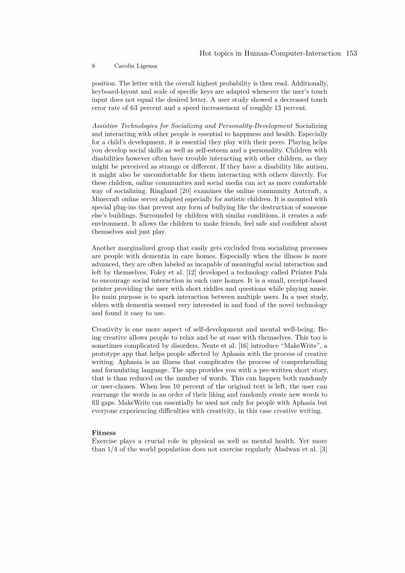
8 Carolin Ligensa
position. The letter with the overall highest probability is then read. Additionally,keyboard-layout and scale of specific keys are adapted whenever the user’s touchinput does not equal the desired letter. A user study showed a decreased toucherror rate of 63 percent and a speed increasement of roughly 13 percent.
Assistive Technologies for Socializing and Personality-Development Socializingand interacting with other people is essential to happiness and health. Especiallyfor a child’s development, it is essential they play with their peers. Playing helpsyou develop social skills as well as self-esteem and a personality. Children withdisabilities however often have trouble interacting with other children, as theymight be perceived as strange or different. If they have a disability like autism,it might also be uncomfortable for them interacting with others directly. Forthese children, online communities and social media can act as more comfortableway of socializing. Ringland [20] examines the online community Autcraft, aMinecraft online server adapted especially for autistic children. It is mounted withspecial plug-ins that prevent any form of bullying like the destruction of someoneelse’s buildings. Surrounded by children with similar conditions, it creates a safeenvironment. It allows the children to make friends, feel safe and confident aboutthemselves and just play.
Another marginalized group that easily gets excluded from socializing processesare people with dementia in care homes. Especially when the illness is moreadvanced, they are often labeled as incapable of meaningful social interaction andleft by themselves. Foley et al. [12] developed a technology called Printer Palsto encourage social interaction in such care homes. It is a small, receipt-basedprinter providing the user with short riddles and questions while playing music.Its main purpose is to spark interaction between multiple users. In a user study,elders with dementia seemed very interested in and fond of the novel technologyand found it easy to use.
Creativity is one more aspect of self-development and mental well-being. Be-ing creative allows people to relax and be at ease with themselves. This too issometimes complicated by disorders. Neate et al. [16] introduce “MakeWrite”, aprototype app that helps people affected by Aphasia with the process of creativewriting. Aphasia is an illness that complicates the process of comprehendingand formulating language. The app provides you with a pre-written short story,that is than reduced on the number of words. This can happen both randomlyor user-chosen. When less 10 percent of the original text is left, the user canrearrange the words in an order of their liking and randomly create new words tofill gaps. MakeWrite can essentially be used not only for people with Aphasia buteveryone experiencing difficulties with creativity, in this case creative writing.
FitnessExercise plays a crucial role in physical as well as mental health. Yet morethan 1/4 of the world population does not exercise regularly Aladwan et al. [3]
Hot topics in Human-Computer-Interaction 153
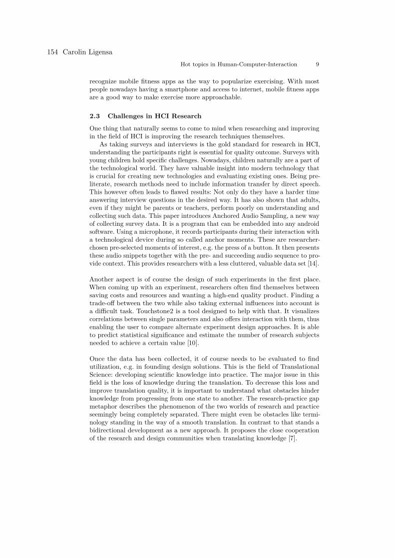
Hot topics in Human-Computer-Interaction 9
recognize mobile fitness apps as the way to popularize exercising. With mostpeople nowadays having a smartphone and access to internet, mobile fitness appsare a good way to make exercise more approachable.
2.3 Challenges in HCI Research
One thing that naturally seems to come to mind when researching and improvingin the field of HCI is improving the research techniques themselves.
As taking surveys and interviews is the gold standard for research in HCI,understanding the participants right is essential for quality outcome. Surveys withyoung children hold specific challenges. Nowadays, children naturally are a part ofthe technological world. They have valuable insight into modern technology thatis crucial for creating new technologies and evaluating existing ones. Being pre-literate, research methods need to include information transfer by direct speech.This however often leads to flawed results: Not only do they have a harder timeanswering interview questions in the desired way. It has also shown that adults,even if they might be parents or teachers, perform poorly on understanding andcollecting such data. This paper introduces Anchored Audio Sampling, a new wayof collecting survey data. It is a program that can be embedded into any androidsoftware. Using a microphone, it records participants during their interaction witha technological device during so called anchor moments. These are researcher-chosen pre-selected moments of interest, e.g. the press of a button. It then presentsthese audio snippets together with the pre- and succeeding audio sequence to pro-vide context. This provides researchers with a less cluttered, valuable data set [14].
Another aspect is of course the design of such experiments in the first place.When coming up with an experiment, researchers often find themselves betweensaving costs and resources and wanting a high-end quality product. Finding atrade-off between the two while also taking external influences into account isa difficult task. Touchstone2 is a tool designed to help with that. It visualizescorrelations between single parameters and also offers interaction with them, thusenabling the user to compare alternate experiment design approaches. It is ableto predict statistical significance and estimate the number of research subjectsneeded to achieve a certain value [10].
Once the data has been collected, it of course needs to be evaluated to findutilization, e.g. in founding design solutions. This is the field of TranslationalScience: developing scientific knowledge into practice. The major issue in thisfield is the loss of knowledge during the translation. To decrease this loss andimprove translation quality, it is important to understand what obstacles hinderknowledge from progressing from one state to another. The research-practice gapmetaphor describes the phenomenon of the two worlds of research and practiceseemingly being completely separated. There might even be obstacles like termi-nology standing in the way of a smooth translation. In contrast to that stands abidirectional development as a new approach. It proposes the close cooperationof the research and design communities when translating knowledge [7].
154 Carolin Ligensa
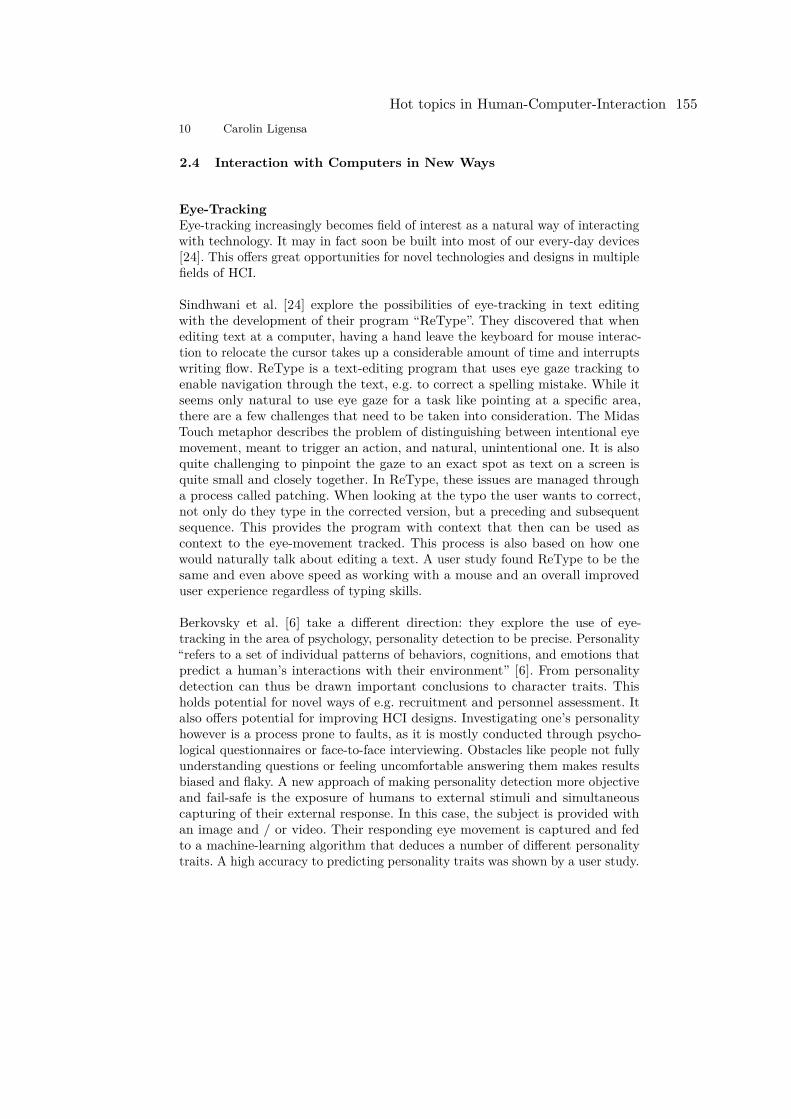
10 Carolin Ligensa
2.4 Interaction with Computers in New Ways
Eye-TrackingEye-tracking increasingly becomes field of interest as a natural way of interactingwith technology. It may in fact soon be built into most of our every-day devices[24]. This offers great opportunities for novel technologies and designs in multiplefields of HCI.
Sindhwani et al. [24] explore the possibilities of eye-tracking in text editingwith the development of their program “ReType”. They discovered that whenediting text at a computer, having a hand leave the keyboard for mouse interac-tion to relocate the cursor takes up a considerable amount of time and interruptswriting flow. ReType is a text-editing program that uses eye gaze tracking toenable navigation through the text, e.g. to correct a spelling mistake. While itseems only natural to use eye gaze for a task like pointing at a specific area,there are a few challenges that need to be taken into consideration. The MidasTouch metaphor describes the problem of distinguishing between intentional eyemovement, meant to trigger an action, and natural, unintentional one. It is alsoquite challenging to pinpoint the gaze to an exact spot as text on a screen isquite small and closely together. In ReType, these issues are managed througha process called patching. When looking at the typo the user wants to correct,not only do they type in the corrected version, but a preceding and subsequentsequence. This provides the program with context that then can be used ascontext to the eye-movement tracked. This process is also based on how onewould naturally talk about editing a text. A user study found ReType to be thesame and even above speed as working with a mouse and an overall improveduser experience regardless of typing skills.
Berkovsky et al. [6] take a different direction: they explore the use of eye-tracking in the area of psychology, personality detection to be precise. Personality“refers to a set of individual patterns of behaviors, cognitions, and emotions thatpredict a human’s interactions with their environment” [6]. From personalitydetection can thus be drawn important conclusions to character traits. Thisholds potential for novel ways of e.g. recruitment and personnel assessment. Italso offers potential for improving HCI designs. Investigating one’s personalityhowever is a process prone to faults, as it is mostly conducted through psycho-logical questionnaires or face-to-face interviewing. Obstacles like people not fullyunderstanding questions or feeling uncomfortable answering them makes resultsbiased and flaky. A new approach of making personality detection more objectiveand fail-safe is the exposure of humans to external stimuli and simultaneouscapturing of their external response. In this case, the subject is provided withan image and / or video. Their responding eye movement is captured and fedto a machine-learning algorithm that deduces a number of different personalitytraits. A high accuracy to predicting personality traits was shown by a user study.
Hot topics in Human-Computer-Interaction 155
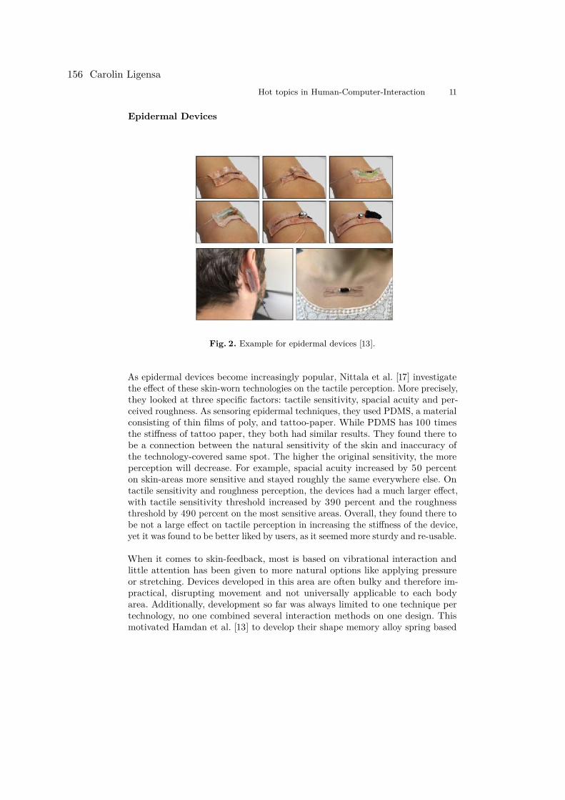
Hot topics in Human-Computer-Interaction 11
Epidermal Devices
Fig. 2. Example for epidermal devices [13].
As epidermal devices become increasingly popular, Nittala et al. [17] investigatethe effect of these skin-worn technologies on the tactile perception. More precisely,they looked at three specific factors: tactile sensitivity, spacial acuity and per-ceived roughness. As sensoring epidermal techniques, they used PDMS, a materialconsisting of thin films of poly, and tattoo-paper. While PDMS has 100 timesthe stiffness of tattoo paper, they both had similar results. They found there tobe a connection between the natural sensitivity of the skin and inaccuracy ofthe technology-covered same spot. The higher the original sensitivity, the moreperception will decrease. For example, spacial acuity increased by 50 percenton skin-areas more sensitive and stayed roughly the same everywhere else. Ontactile sensitivity and roughness perception, the devices had a much larger effect,with tactile sensitivity threshold increased by 390 percent and the roughnessthreshold by 490 percent on the most sensitive areas. Overall, they found there tobe not a large effect on tactile perception in increasing the stiffness of the device,yet it was found to be better liked by users, as it seemed more sturdy and re-usable.
When it comes to skin-feedback, most is based on vibrational interaction andlittle attention has been given to more natural options like applying pressureor stretching. Devices developed in this area are often bulky and therefore im-practical, disrupting movement and not universally applicable to each bodyarea. Additionally, development so far was always limited to one technique pertechnology, no one combined several interaction methods on one design. Thismotivated Hamdan et al. [13] to develop their shape memory alloy spring based
156 Carolin Ligensa

12 Carolin Ligensa
mechanotactile interfaces “Springlets”. Shape memory alloy springs are a typeof spring that is especially slim and flexible. Placed in ergonomic stickers, theyare movement resistant and can easily be applied to every area of the bodylike arms or near the head. When a current is applied, they contract similar tohuman muscle. As can be seen in Fig. 3, there are two different types of actuators.For skin actuators, the interaction takes place at the two ends of the springwhere it is attached to the skin. Examples are pinching and directional stretching.End-effector actuators support interactions like pressing, pulling, dragging andexpanding by having an additional object added to the spring that is then ma-nipulated by contractions. Even combining two springs or changing the currentapplied for a different effect is possible. Not only do Springlets offer a wide rangeof novel ways to interact with skin that are completely silent, they are also easyand cheap to produce and very compact. This could be highly beneficial in manyareas like in health and fitness, navigation and Virtual Reality.
Fig. 3. The two different types of Springlets developed: skin actuators and end-effectoractuators [13].
Hot topics in Human-Computer-Interaction 157
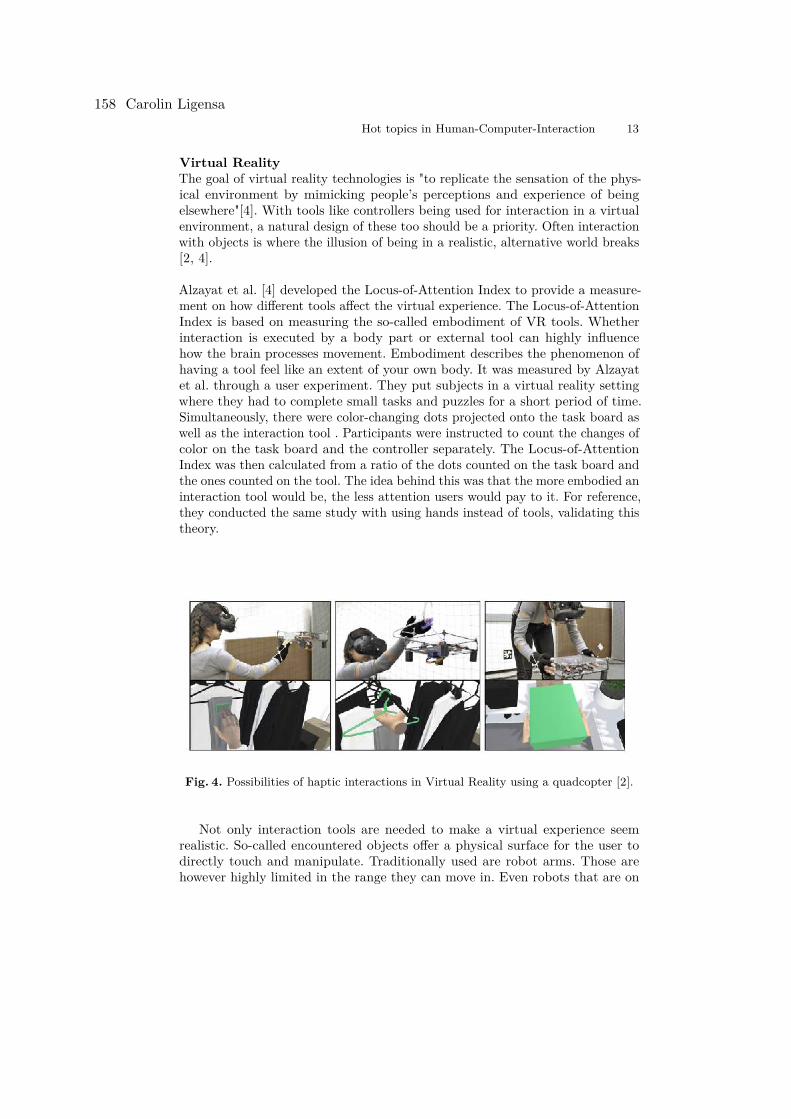
Hot topics in Human-Computer-Interaction 13
Virtual RealityThe goal of virtual reality technologies is "to replicate the sensation of the phys-ical environment by mimicking people’s perceptions and experience of beingelsewhere"[4]. With tools like controllers being used for interaction in a virtualenvironment, a natural design of these too should be a priority. Often interactionwith objects is where the illusion of being in a realistic, alternative world breaks[2, 4].
Alzayat et al. [4] developed the Locus-of-Attention Index to provide a measure-ment on how different tools affect the virtual experience. The Locus-of-AttentionIndex is based on measuring the so-called embodiment of VR tools. Whetherinteraction is executed by a body part or external tool can highly influencehow the brain processes movement. Embodiment describes the phenomenon ofhaving a tool feel like an extent of your own body. It was measured by Alzayatet al. through a user experiment. They put subjects in a virtual reality settingwhere they had to complete small tasks and puzzles for a short period of time.Simultaneously, there were color-changing dots projected onto the task board aswell as the interaction tool . Participants were instructed to count the changes ofcolor on the task board and the controller separately. The Locus-of-AttentionIndex was then calculated from a ratio of the dots counted on the task board andthe ones counted on the tool. The idea behind this was that the more embodied aninteraction tool would be, the less attention users would pay to it. For reference,they conducted the same study with using hands instead of tools, validating thistheory.
Fig. 4. Possibilities of haptic interactions in Virtual Reality using a quadcopter [2].
Not only interaction tools are needed to make a virtual experience seemrealistic. So-called encountered objects offer a physical surface for the user todirectly touch and manipulate. Traditionally used are robot arms. Those arehowever highly limited in the range they can move in. Even robots that are on
158 Carolin Ligensa
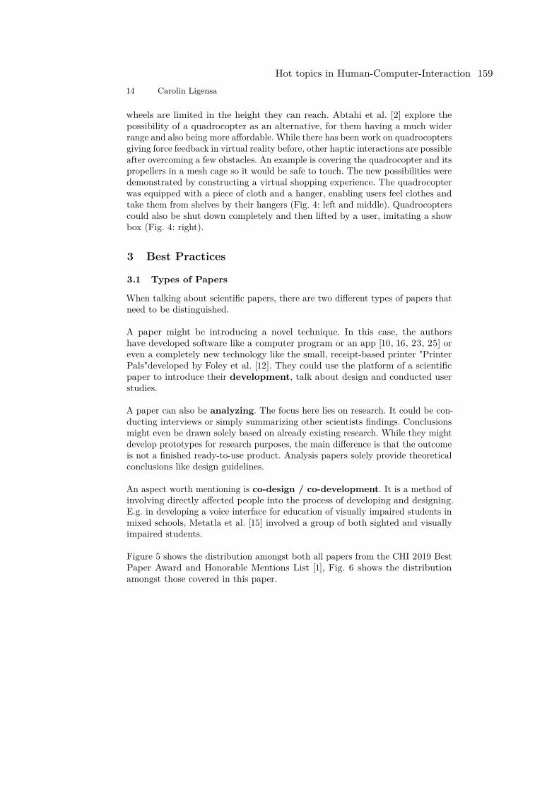
14 Carolin Ligensa
wheels are limited in the height they can reach. Abtahi et al. [2] explore thepossibility of a quadrocopter as an alternative, for them having a much widerrange and also being more affordable. While there has been work on quadrocoptersgiving force feedback in virtual reality before, other haptic interactions are possibleafter overcoming a few obstacles. An example is covering the quadrocopter and itspropellers in a mesh cage so it would be safe to touch. The new possibilities weredemonstrated by constructing a virtual shopping experience. The quadrocopterwas equipped with a piece of cloth and a hanger, enabling users feel clothes andtake them from shelves by their hangers (Fig. 4: left and middle). Quadrocopterscould also be shut down completely and then lifted by a user, imitating a showbox (Fig. 4: right).
3 Best Practices
3.1 Types of Papers
When talking about scientific papers, there are two different types of papers thatneed to be distinguished.
A paper might be introducing a novel technique. In this case, the authorshave developed software like a computer program or an app [10, 16, 23, 25] oreven a completely new technology like the small, receipt-based printer "PrinterPals"developed by Foley et al. [12]. They could use the platform of a scientificpaper to introduce their development, talk about design and conducted userstudies.
A paper can also be analyzing. The focus here lies on research. It could be con-ducting interviews or simply summarizing other scientists findings. Conclusionsmight even be drawn solely based on already existing research. While they mightdevelop prototypes for research purposes, the main difference is that the outcomeis not a finished ready-to-use product. Analysis papers solely provide theoreticalconclusions like design guidelines.
An aspect worth mentioning is co-design / co-development. It is a method ofinvolving directly affected people into the process of developing and designing.E.g. in developing a voice interface for education of visually impaired students inmixed schools, Metatla et al. [15] involved a group of both sighted and visuallyimpaired students.
Figure 5 shows the distribution amongst both all papers from the CHI 2019 BestPaper Award and Honorable Mentions List [1], Fig. 6 shows the distributionamongst those covered in this paper.
Hot topics in Human-Computer-Interaction 159
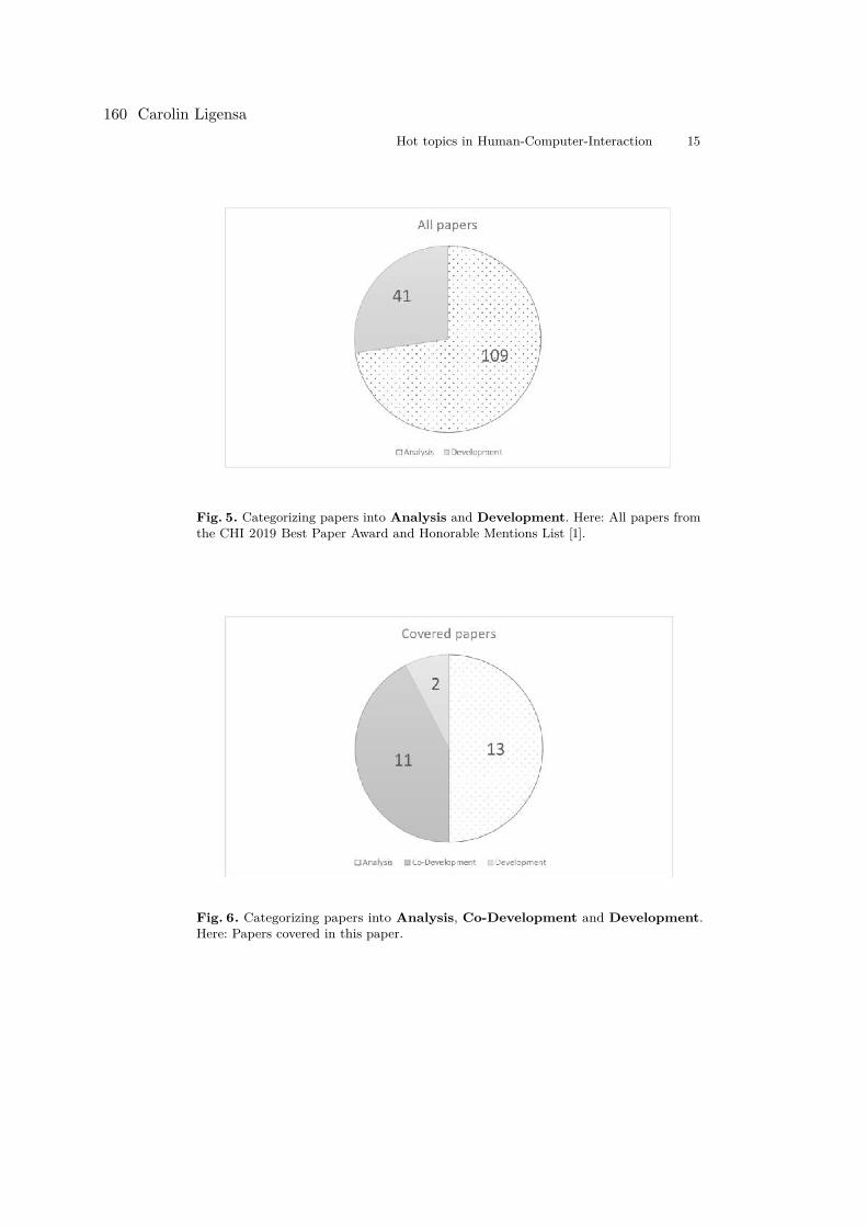
Hot topics in Human-Computer-Interaction 15
Fig. 5. Categorizing papers into Analysis and Development. Here: All papers fromthe CHI 2019 Best Paper Award and Honorable Mentions List [1].
Fig. 6. Categorizing papers into Analysis, Co-Development and Development.Here: Papers covered in this paper.
160 Carolin Ligensa
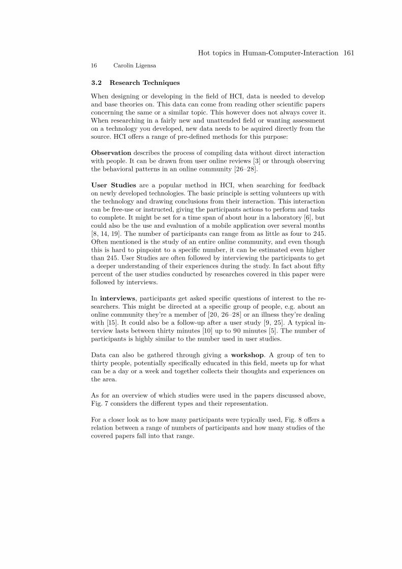
16 Carolin Ligensa
3.2 Research Techniques
When designing or developing in the field of HCI, data is needed to developand base theories on. This data can come from reading other scientific papersconcerning the same or a similar topic. This however does not always cover it.When researching in a fairly new and unattended field or wanting assessmenton a technology you developed, new data needs to be aquired directly from thesource. HCI offers a range of pre-defined methods for this purpose:
Observation describes the process of compiling data without direct interactionwith people. It can be drawn from user online reviews [3] or through observingthe behavioral patterns in an online community [26–28].
User Studies are a popular method in HCI, when searching for feedbackon newly developed technologies. The basic principle is setting volunteers up withthe technology and drawing conclusions from their interaction. This interactioncan be free-use or instructed, giving the participants actions to perform and tasksto complete. It might be set for a time span of about hour in a laboratory [6], butcould also be the use and evaluation of a mobile application over several months[8, 14, 19]. The number of participants can range from as little as four to 245.Often mentioned is the study of an entire online community, and even thoughthis is hard to pinpoint to a specific number, it can be estimated even higherthan 245. User Studies are often followed by interviewing the participants to geta deeper understanding of their experiences during the study. In fact about fiftypercent of the user studies conducted by researches covered in this paper werefollowed by interviews.
In interviews, participants get asked specific questions of interest to the re-searchers. This might be directed at a specific group of people, e.g. about anonline community they’re a member of [20, 26–28] or an illness they’re dealingwith [15]. It could also be a follow-up after a user study [9, 25]. A typical in-terview lasts between thirty minutes [10] up to 90 minutes [5]. The number ofparticipants is highly similar to the number used in user studies.
Data can also be gathered through giving a workshop. A group of ten tothirty people, potentially specifically educated in this field, meets up for whatcan be a day or a week and together collects their thoughts and experiences onthe area.
As for an overview of which studies were used in the papers discussed above,Fig. 7 considers the different types and their representation.
For a closer look as to how many participants were typically used, Fig. 8 offers arelation between a range of numbers of participants and how many studies of thecovered papers fall into that range.
Hot topics in Human-Computer-Interaction 161
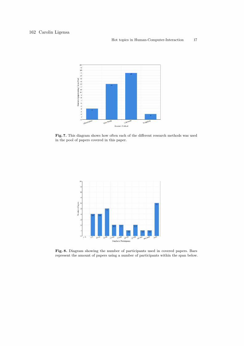
Hot topics in Human-Computer-Interaction 17
Fig. 7. This diagram shows how often each of the different research methods was usedin the pool of papers covered in this paper.
Fig. 8. Diagram showing the number of participants used in covered papers. Barsrepresent the amount of papers using a number of participants within the span below.
162 Carolin Ligensa
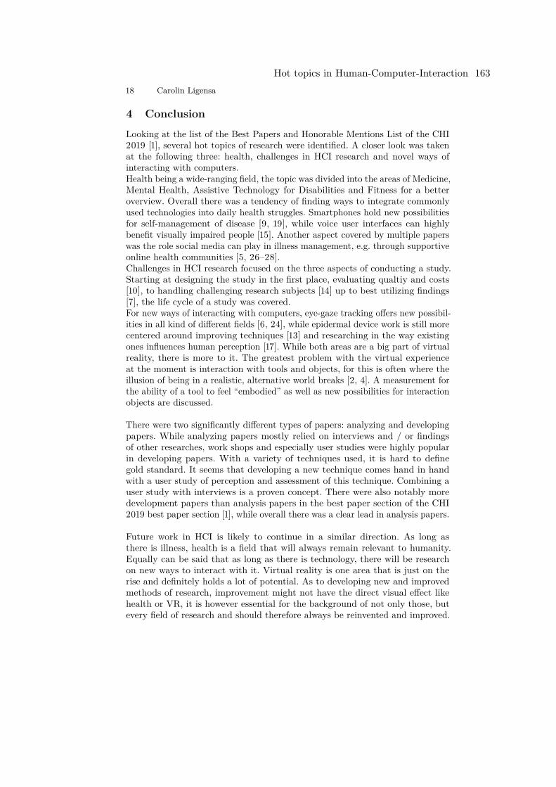
18 Carolin Ligensa
4 ConclusionLooking at the list of the Best Papers and Honorable Mentions List of the CHI2019 [1], several hot topics of research were identified. A closer look was takenat the following three: health, challenges in HCI research and novel ways ofinteracting with computers.Health being a wide-ranging field, the topic was divided into the areas of Medicine,Mental Health, Assistive Technology for Disabilities and Fitness for a betteroverview. Overall there was a tendency of finding ways to integrate commonlyused technologies into daily health struggles. Smartphones hold new possibilitiesfor self-management of disease [9, 19], while voice user interfaces can highlybenefit visually impaired people [15]. Another aspect covered by multiple paperswas the role social media can play in illness management, e.g. through supportiveonline health communities [5, 26–28].Challenges in HCI research focused on the three aspects of conducting a study.Starting at designing the study in the first place, evaluating qualtiy and costs[10], to handling challenging research subjects [14] up to best utilizing findings[7], the life cycle of a study was covered.For new ways of interacting with computers, eye-gaze tracking offers new possibil-ities in all kind of different fields [6, 24], while epidermal device work is still morecentered around improving techniques [13] and researching in the way existingones influences human perception [17]. While both areas are a big part of virtualreality, there is more to it. The greatest problem with the virtual experienceat the moment is interaction with tools and objects, for this is often where theillusion of being in a realistic, alternative world breaks [2, 4]. A measurement forthe ability of a tool to feel “embodied” as well as new possibilities for interactionobjects are discussed.
There were two significantly different types of papers: analyzing and developingpapers. While analyzing papers mostly relied on interviews and / or findingsof other researches, work shops and especially user studies were highly popularin developing papers. With a variety of techniques used, it is hard to definegold standard. It seems that developing a new technique comes hand in handwith a user study of perception and assessment of this technique. Combining auser study with interviews is a proven concept. There were also notably moredevelopment papers than analysis papers in the best paper section of the CHI2019 best paper section [1], while overall there was a clear lead in analysis papers.
Future work in HCI is likely to continue in a similar direction. As long asthere is illness, health is a field that will always remain relevant to humanity.Equally can be said that as long as there is technology, there will be researchon new ways to interact with it. Virtual reality is one area that is just on therise and definitely holds a lot of potential. As to developing new and improvedmethods of research, improvement might not have the direct visual effect likehealth or VR, it is however essential for the background of not only those, butevery field of research and should therefore always be reinvented and improved.
Hot topics in Human-Computer-Interaction 163
Hot topics in Human-Computer-Interaction 19
References
1. Chi 2019 best papers & honourable mentions (2019), https://chi2019.acm.org/2019/03/15/chi-2019-best-papers-honourable-mentions/, last visited on07.07.2019
2. Abtahi, P., Landry, B., Yang, J.J., Pavone, M., Follmer, S., Landay, J.A.: Beyond theforce: Using quadcopters to appropriate objects and the environment for haptics invirtual reality. In: Proceedings of the 2019 CHI Conference on Human Factors inComputing Systems. p. 359. ACM (2019)
3. Aladwan, A., Kelly, R.M., Baker, S., Velloso, E.: A tale of two perspectives: Aconceptual framework of user expectations and experiences of instructional fitnessapps. In: Proceedings of the 2019 CHI Conference on Human Factors in ComputingSystems. p. 394. ACM (2019)
4. Alzayat, A., Hancock, M., Nacenta, M.A.: Quantitative measurement of toolembodiment for virtual reality input alternatives. In: Proceedings of the 2019 CHIConference on Human Factors in Computing Systems. p. 443. ACM (2019)
5. Andalibi, N.: What happens after disclosing stigmatized experiences on identifiedsocial media: Individual, dyadic, and social/network outcomes. In: Proceedings of the2019 CHI Conference on Human Factors in Computing Systems (2019)
6. Berkovsky, S., Taib, R., Koprinska, I., Wang, E., Zeng, Y., Li, J., Kleitman, S.:Detecting personality traits using eye-tracking data. In: Proceedings of the 2019 CHIConference on Human Factors in Computing Systems. p. 221. ACM (2019)
7. Colusso, L., Jones, R., Munson, S.A., Hsieh, G.: A translational science model forhci. In: Proceedings of the 2019 CHI Conference on Human Factors in ComputingSystems (2019)
8. Doherty, K., Marcano-Belisario, J., Cohn, M., Mastellos, N., Morrison, C., Car, J.,Doherty, G.: Engagement with mental health screening on mobile devices: Resultsfrom an antenatal feasibility study. In: Proceedings of the 2019 CHI Conference onHuman Factors in Computing Systems. p. 186. ACM (2019)
9. Doyle, J., Murphy, E., Kuiper, J., Smith, S., Hannigan, C., Jacobs, A., Dinsmore,J.: Managing multimorbidity: Identifying design requirements for a digital self-management tool to support older adults with multiple chronic conditions. In:Proceedings of the 2019 CHI Conference on Human Factors in Computing Systems. p.399. ACM (2019)
10. Eiselmayer, A., Wacharamanotham, C., Beaudouin-Lafon, M., Mackay, W.: Touch-stone2: An interactive environment for exploring trade-offs in hci experiment design.In: Proceedings of the 2019 CHI Conference on Human Factors in ComputingSystems. OSF Preprints (2019)
11. Feuston, J.L., Piper, A.M.: Everyday experiences: Small stories and mental illnesson instagram. In: Proceedings of the 2019 CHI Conference on Human Factors inComputing Systems. p. 265. ACM (2019)
12. Foley, S., Welsh, D., Pantidi, N., Morrissey, K., Nappey, T., McCarthy, J.: Printerpals: Experience-centered design to support agency for people with dementia. In:Proceedings of the 2019 CHI Conference on Human Factors in Computing Systems. p.404. ACM (2019)
13. Hamdan, N.A.h., Wagner, A., Voelker, S., Steimle, J., Borchers, J.: Springlets:Expressive, flexible and silent on-skin tactile interfaces. In: Proceedings of the 2019CHI Conference on Human Factors in Computing Systems (2019)
14. Hiniker, A., Froehlich, J.E., Zhang, M., Beneteau, E.: Anchored audio sampling: Aseamless method for exploring children’s thoughts during deployment studies. In:
164 Carolin Ligensa
20 Carolin Ligensa
Proceedings of the 2019 CHI Conference on Human Factors in Computing Systems.p. 8. ACM (2019)
15. Metatla, O., Oldfield, A., Ahmed, T., Vafeas, A., Miglani, S.: Voice user interfaces inschools: Co-designing for inclusion with visually-impaired and sighted pupils. In:Proceedings of the 2019 CHI Conference on Human Factors in Computing Systems(2019)
16. Neate, T., Roper, A., Wilson, S., Marshall, J.: Empowering expression for users withaphasia through constrained creativity. In: Proceedings of the 2019 CHI Conferenceon Human Factors in Computing Systems. p. 385. ACM (2019)
17. Nittala, A.S., Kruttwig, K., Lee, J., Bennewitz, R., Arzt, E., Steimle, J.: Like asecond skin: Understanding how epidermal devices affect human tactile perception. In:Proceedings of the 2019 CHI Conference on Human Factors in Computing Systems(2019)
18. Organization, W.H.: Self care for health: a handbook for community health workers &volunteers (2013), http://apps.searo.who.int/PDS_DOCS/B5084.pdf, last visited on07.07.2019
19. Raj, S., Toporski, K., Garrity, A., Lee, J.M., Newman, M.W.: My blood sugar ishigher on the weekends: Finding a role for context and context-awareness in thedesign of health self-management technology. In: Proceedings of the 2019 CHIConference on Human Factors in Computing Systems. p. 119. ACM (2019)
20. Ringland, K.E.: A place to play: the (dis) abled embodied experience for autisticchildren in online spaces. In: Proceedings of the 2019 CHI Conference on HumanFactors in Computing Systems. p. 288. ACM (2019)
21. Rooksby, J., Morrison, A., Murray-Rust, D.: Student perspectives on digitalphenotyping: The acceptability of using smartphone data to assess mental health. In:Proceedings of the 2019 CHI Conference on Human Factors in Computing Systems. p.425. ACM (2019)
22. Sanches, P., Janson, A., Karpashevich, P., Nadal, C., Qu, C., Daudén Roquet, C.,Umair, M., Windlin, C., Doherty, G., Höök, K., et al.: Hci and affective health:Taking stock of a decade of studies and charting future research directions. In:Proceedings of the 2019 CHI Conference on Human Factors in Computing Systems. p.245. ACM (2019)
23. Shi, W., Yu, C., Fan, S., Wang, F., Wang, T., Yi, X., Bi, X., Shi, Y.: Vipboard:Improving screen-reader keyboard for visually impaired people with character-levelauto correction. In: Proceedings of the 2019 CHI Conference on Human Factors inComputing Systems. p. 517. ACM (2019)
24. Sindhwani, S., Lutteroth, C., Weber, G.: Retype: Quick text editing with keyboard andgaze. In: Proceedings of the 2019 CHI Conference on Human Factors in ComputingSystems. p. 203. ACM (2019)
25. Wang, R., Yu, C., Yang, X.D., He, W., Shi, Y.: Eartouch: Facilitating smartphone usefor visually impaired people in mobile and public scenarios. In: Proceedings of the2019 CHI Conference on Human Factors in Computing Systems. p. 24. ACM (2019)
26. Yang, D., Kraut, R.E., Smith, T., Mayfield, E., Jurafsky, D.: Seekers, providers,welcomers, and storytellers: Modeling social roles in online health communities. In:Proceedings of the 2019 CHI Conference on Human Factors in Computing Systems. p.344. ACM (2019)
27. Yang, D., Yao, Z., Seering, J., Kraut, R.: The channel matters: Self-disclosure,reciprocity and social support in online cancer support groups. In: Proceedings of the2019 CHI Conference on Human Factors in Computing Systems (2019)
Hot topics in Human-Computer-Interaction 165

Hot topics in Human-Computer-Interaction 21
28. Young, A.L., Miller, A.D.: "this girl is on fire": Sensemaking in an online healthcommunity for vulvodynia. In: Proceedings of the 2019 CHI Conference on HumanFactors in Computing Systems. p. 129. ACM (2019)
166 Carolin Ligensa
Explainable Deep Neural Networks
Anna Carolina Steyer
TECO, Karlsruhe Institute of Technology
Abstract. Artificial neural networks have a growing importance in ourdaily life, but still they are like black boxes when it comes to explainingtheir decisions. This paper introduces eight methods from the literaturewhich analyze the contributions of the input to explain single decisions.The covered approaches are: Sensitivity analysis, Taylor decomposition,Deconvolution, Guided backpropagation, Guided Grad-CAM, Layer-wiserelevance propagation, Attention-based models and Explaining black boxsequence-to-sequence models. The approaches differ in their applicabilityto different neural architectures, in how much information they use fromthe forward pass and whether they can distinguish negative from positiverelevance.
Keywords: Explainable artificial intelligence (XAI), Deep neural networks, De-convolution, Layer-wise relevance propagation, Guided backpropagation, Machineteaching, Verification
1 Introduction
Artificial neural networks have become increasingly ubiquitous. They can enhanceour everyday life with music and product recommendations, auto-correction andintelligent smartphone cameras. Although it is annoying if these services donot always work perfectly, it does not have a huge impact on us. An entirelydifferent matter is though if intelligent systems for autonomous driving, medicaldiagnosis or military operations fail. In those cases, human life is involved andit is thus absolutely crucial to be able to justify the decisions based on suchpredictions. Neural networks have the drawback that most of them appear to beblack boxes in the sense that they aren’t transparent concerning their decisionmaking. Therefore, methods for explaining the reasoning of neural networkspost hoc are needed. Explaining neural networks is about capturing the modelthe network has learned after it has been trained. Trying to achieve full modelinterpretability is not practical since the models learned by deep neural networksare too complex. This paper’s focus lies on methods for explaining single decisionsby analyzing the contributions of each input feature to the output of interest(local understanding). Before going into the details of these local explanationmethods in Sect. 3, we will first give a brief introduction to neural networks andthe architectures that those methods are designed for in Sect. 2. Section 4 willconclude with comparing these methods and giving an outlook.
Explainable Deep Neural Networks 167
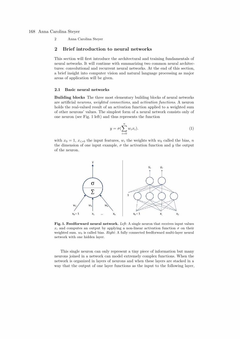
2 Anna Carolina Steyer
2 Brief introduction to neural networks
This section will first introduce the architectural and training fundamentals ofneural networks. It will continue with summarizing two common neural architec-tures: convolutional and recurrent neural networks. At the end of this section,a brief insight into computer vision and natural language processing as majorareas of application will be given.
2.1 Basic neural networks
Building blocks The three most elementary building blocks of neural networksare artificial neurons, weighted connections, and activation functions. A neuronholds the real-valued result of an activation function applied to a weighted sumof other neurons’ values. The simplest form of a neural network consists only ofone neuron (see Fig. 1 left) and thus represents the function
y = σ(n∑
i=0wixi). (1)
with x0 = 1, xi>0 the input features, wi the weights with w0 called the bias, nthe dimension of one input example, σ the activation function and y the outputof the neuron.
Fig. 1. Feedforward neural network. Left: A single neuron that receives input valuesxi and computes an output by applying a non-linear activation function σ on theirweighted sum. w0 is called bias. Right: A fully connected feedforward multi-layer neuralnetwork with one hidden layer.
This single neuron can only represent a tiny piece of information but manyneurons joined in a network can model extremely complex functions. When thenetwork is organized in layers of neurons and when these layers are stacked in away that the output of one layer functions as the input to the following layer,
168 Anna Carolina Steyer
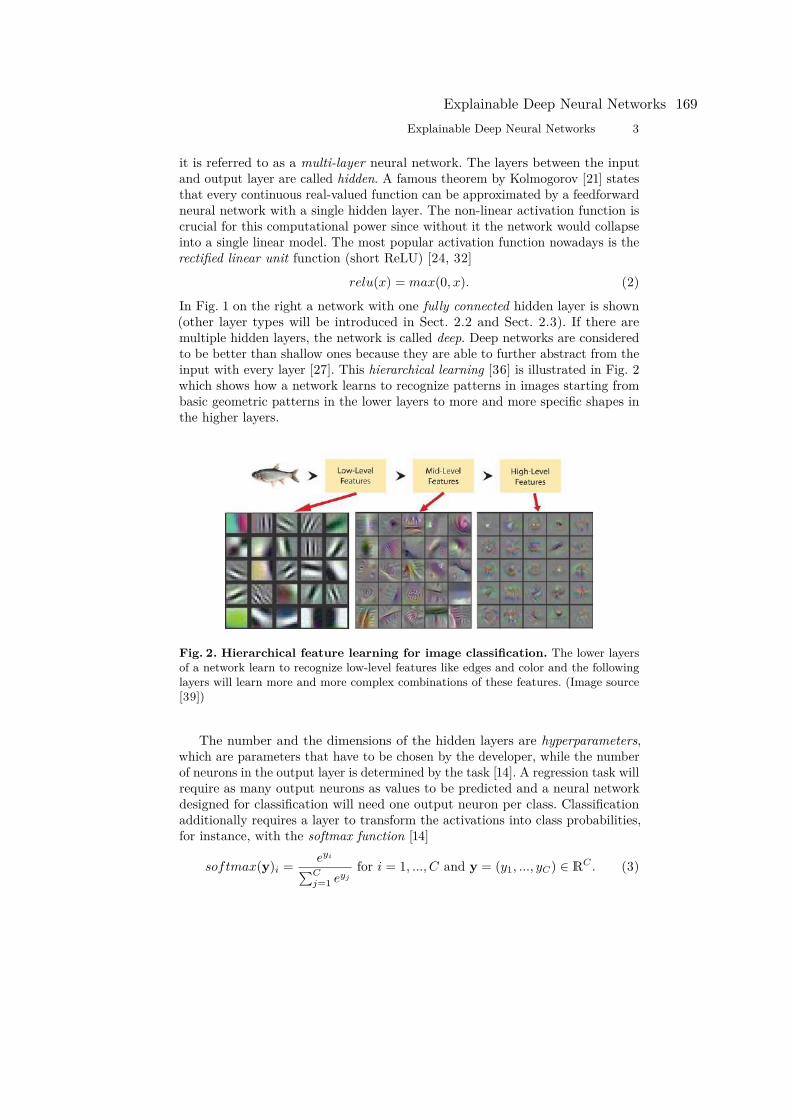
Explainable Deep Neural Networks 3
it is referred to as a multi-layer neural network. The layers between the inputand output layer are called hidden. A famous theorem by Kolmogorov [21] statesthat every continuous real-valued function can be approximated by a feedforwardneural network with a single hidden layer. The non-linear activation function iscrucial for this computational power since without it the network would collapseinto a single linear model. The most popular activation function nowadays is therectified linear unit function (short ReLU) [24, 32]
relu(x) = max(0, x). (2)
In Fig. 1 on the right a network with one fully connected hidden layer is shown(other layer types will be introduced in Sect. 2.2 and Sect. 2.3). If there aremultiple hidden layers, the network is called deep. Deep networks are consideredto be better than shallow ones because they are able to further abstract from theinput with every layer [27]. This hierarchical learning [36] is illustrated in Fig. 2which shows how a network learns to recognize patterns in images starting frombasic geometric patterns in the lower layers to more and more specific shapes inthe higher layers.
Fig. 2. Hierarchical feature learning for image classification. The lower layersof a network learn to recognize low-level features like edges and color and the followinglayers will learn more and more complex combinations of these features. (Image source[39])
The number and the dimensions of the hidden layers are hyperparameters,which are parameters that have to be chosen by the developer, while the numberof neurons in the output layer is determined by the task [14]. A regression task willrequire as many output neurons as values to be predicted and a neural networkdesigned for classification will need one output neuron per class. Classificationadditionally requires a layer to transform the activations into class probabilities,for instance, with the softmax function [14]
softmax(y)i = eyi
∑Cj=1 eyj
for i = 1, ..., C and y = (y1, ..., yC) ∈ RC . (3)
Explainable Deep Neural Networks 169
4 Anna Carolina Steyer
Training Neural networks are trained with labeled data (supervised learning)and end-to-end by repeatedly doing 1. a forward pass for one training example,2. comparing the output with the known correct result (the ground truth) and3. backpropagating the error signal to compute the weight updates accordinglybackward pass . The objective of the training process is to find the weights thatminimize the loss function which quantifies how bad the error is with respect tothe labeling. The loss function over N training examples for a regression taskcould be the mean squared error [14]
1N
N∑
i=1(yi − yi)2 (4)
with y the predicted value and y the true label. Since the loss function subject toinputs and weights is very complex, the optimum cannot be computed analytically.Instead, a numerical optimization technique called gradient descent (illustratedin Fig. 3) is often used which adjusts each weight wij in the network towardsthe negative gradient of the loss L [14]
wij = wij − η∂L
∂wij. (5)
The learning rate η determines how fast the weights are updated and usuallyis close to zero to avoid fluctuations. If the learning rate is fixed, the algorithmmight more likely miss the optimum or get stuck in a local minimum or plateau.Hence, there are various optimization techniques that define how the learning ratevaries in order to improve convergence (e.g. Adadelta [49]). Also, since the loss isnot only dependent on the weights but also on the training data, the amount oftraining data that is used for one weight update has to be chosen [14]. Updatingthe weights for each single training example is called stochastic gradient descentwhich causes the loss function to fluctuate heavily. Though this helps to findpotentially better minima, it also hinders convergence. An alternative techniqueis the slower batch gradient descent which performs only one weight update basedon all training examples by taking the average over the whole dataset. Mini batchgradient descent is a compromise between those two variants and thus betweenconvergence and exploration. This approach divides the training examples intomini-batches and computes the weight updates based on one mini-batch at atime. This method is computationally efficient, produces stable loss gradientsand convergence and if stuck in local minima it is likely to find its way out.
2.2 Convolutional neural networks
Building blocks Since convolutional neural networks (CNNs) [23] are very pop-ular in image processing, the following explanation will focus on two-dimensionalinput data like images. It has to be remarked though that they can as well be usedfor one-dimensional data, e.g. in natural language or speech processing [43], andeven for three-dimensional data like videos [17]. The most important components
170 Anna Carolina Steyer
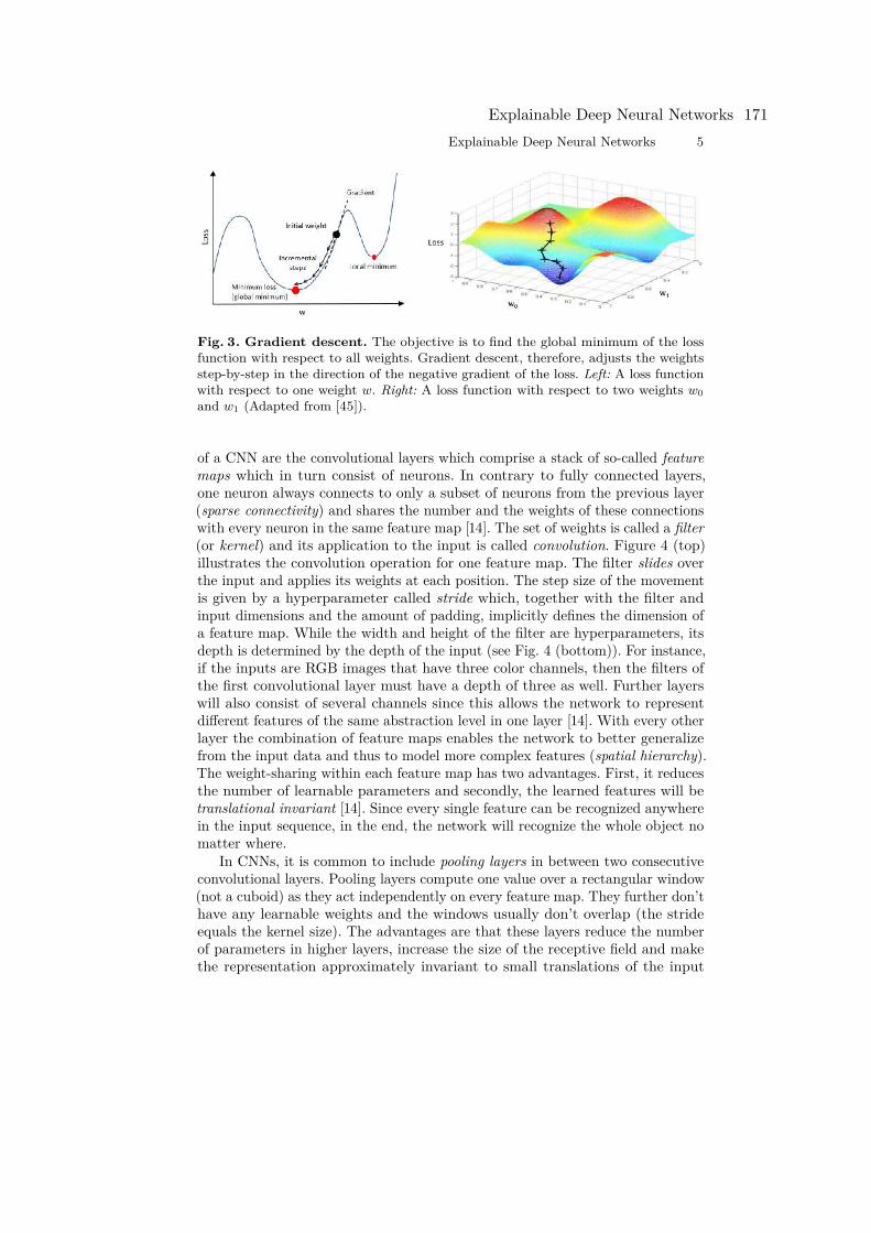
Explainable Deep Neural Networks 5
Fig. 3. Gradient descent. The objective is to find the global minimum of the lossfunction with respect to all weights. Gradient descent, therefore, adjusts the weightsstep-by-step in the direction of the negative gradient of the loss. Left: A loss functionwith respect to one weight w. Right: A loss function with respect to two weights w0and w1 (Adapted from [45]).
of a CNN are the convolutional layers which comprise a stack of so-called featuremaps which in turn consist of neurons. In contrary to fully connected layers,one neuron always connects to only a subset of neurons from the previous layer(sparse connectivity) and shares the number and the weights of these connectionswith every neuron in the same feature map [14]. The set of weights is called a filter(or kernel) and its application to the input is called convolution. Figure 4 (top)illustrates the convolution operation for one feature map. The filter slides overthe input and applies its weights at each position. The step size of the movementis given by a hyperparameter called stride which, together with the filter andinput dimensions and the amount of padding, implicitly defines the dimension ofa feature map. While the width and height of the filter are hyperparameters, itsdepth is determined by the depth of the input (see Fig. 4 (bottom)). For instance,if the inputs are RGB images that have three color channels, then the filters ofthe first convolutional layer must have a depth of three as well. Further layerswill also consist of several channels since this allows the network to representdifferent features of the same abstraction level in one layer [14]. With every otherlayer the combination of feature maps enables the network to better generalizefrom the input data and thus to model more complex features (spatial hierarchy).The weight-sharing within each feature map has two advantages. First, it reducesthe number of learnable parameters and secondly, the learned features will betranslational invariant [14]. Since every single feature can be recognized anywherein the input sequence, in the end, the network will recognize the whole object nomatter where.
In CNNs, it is common to include pooling layers in between two consecutiveconvolutional layers. Pooling layers compute one value over a rectangular window(not a cuboid) as they act independently on every feature map. They further don’thave any learnable weights and the windows usually don’t overlap (the strideequals the kernel size). The advantages are that these layers reduce the numberof parameters in higher layers, increase the size of the receptive field and makethe representation approximately invariant to small translations of the input
Explainable Deep Neural Networks 171
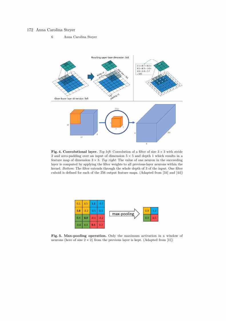
6 Anna Carolina Steyer
Fig. 4. Convolutional layer. Top left: Convolution of a filter of size 3 × 3 with stride2 and zero-padding over an input of dimension 5 × 5 and depth 1 which results in afeature map of dimension 3 × 3. Top right: The value of one neuron in the succeedinglayer is computed by applying the filter weights to all previous-layer neurons within thekernel. Bottom: The filter extends through the whole depth of 3 of the input. One filtercuboid is defined for each of the 256 output feature maps. (Adapted from [34] and [44])
Fig. 5. Max-pooling operation. Only the maximum activation in a window ofneurons (here of size 2 × 2) from the previous layer is kept. (Adapted from [11])
172 Anna Carolina Steyer
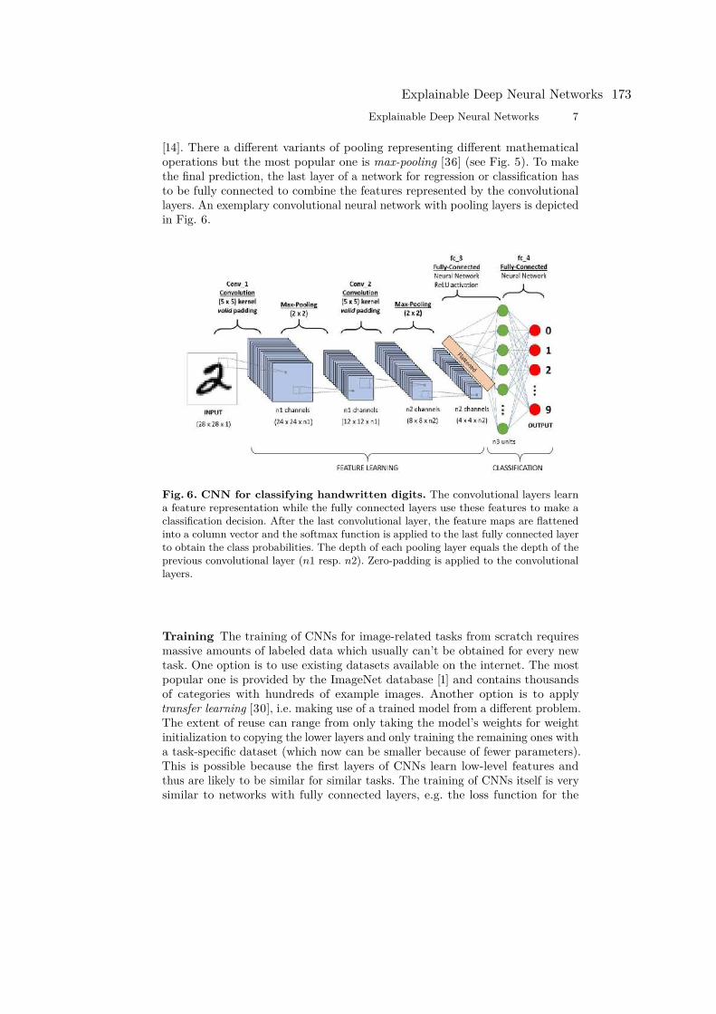
Explainable Deep Neural Networks 7
[14]. There a different variants of pooling representing different mathematicaloperations but the most popular one is max-pooling [36] (see Fig. 5). To makethe final prediction, the last layer of a network for regression or classification hasto be fully connected to combine the features represented by the convolutionallayers. An exemplary convolutional neural network with pooling layers is depictedin Fig. 6.
Fig. 6. CNN for classifying handwritten digits. The convolutional layers learna feature representation while the fully connected layers use these features to make aclassification decision. After the last convolutional layer, the feature maps are flattenedinto a column vector and the softmax function is applied to the last fully connected layerto obtain the class probabilities. The depth of each pooling layer equals the depth of theprevious convolutional layer (n1 resp. n2). Zero-padding is applied to the convolutionallayers.
Training The training of CNNs for image-related tasks from scratch requiresmassive amounts of labeled data which usually can’t be obtained for every newtask. One option is to use existing datasets available on the internet. The mostpopular one is provided by the ImageNet database [1] and contains thousandsof categories with hundreds of example images. Another option is to applytransfer learning [30], i.e. making use of a trained model from a different problem.The extent of reuse can range from only taking the model’s weights for weightinitialization to copying the lower layers and only training the remaining ones witha task-specific dataset (which now can be smaller because of fewer parameters).This is possible because the first layers of CNNs learn low-level features andthus are likely to be similar for similar tasks. The training of CNNs itself is verysimilar to networks with fully connected layers, e.g. the loss function for the
Explainable Deep Neural Networks 173
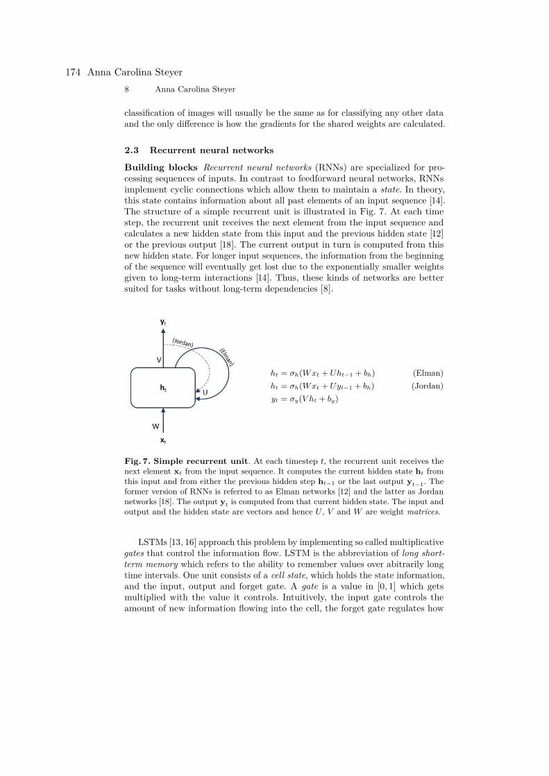
8 Anna Carolina Steyer
classification of images will usually be the same as for classifying any other dataand the only difference is how the gradients for the shared weights are calculated.
2.3 Recurrent neural networks
Building blocks Recurrent neural networks (RNNs) are specialized for pro-cessing sequences of inputs. In contrast to feedforward neural networks, RNNsimplement cyclic connections which allow them to maintain a state. In theory,this state contains information about all past elements of an input sequence [14].The structure of a simple recurrent unit is illustrated in Fig. 7. At each timestep, the recurrent unit receives the next element from the input sequence andcalculates a new hidden state from this input and the previous hidden state [12]or the previous output [18]. The current output in turn is computed from thisnew hidden state. For longer input sequences, the information from the beginningof the sequence will eventually get lost due to the exponentially smaller weightsgiven to long-term interactions [14]. Thus, these kinds of networks are bettersuited for tasks without long-term dependencies [8].
ht = σh(W xt + Uht−1 + bh) (Elman)ht = σh(W xt + Uyt−1 + bh) (Jordan)yt = σy(V ht + by)
Fig. 7. Simple recurrent unit. At each timestep t, the recurrent unit receives thenext element xt from the input sequence. It computes the current hidden state ht fromthis input and from either the previous hidden step ht−1 or the last output yt−1. Theformer version of RNNs is referred to as Elman networks [12] and the latter as Jordannetworks [18]. The output yt is computed from that current hidden state. The input andoutput and the hidden state are vectors and hence U , V and W are weight matrices.
LSTMs [13, 16] approach this problem by implementing so called multiplicativegates that control the information flow. LSTM is the abbreviation of long short-term memory which refers to the ability to remember values over abitrarily longtime intervals. One unit consists of a cell state, which holds the state information,and the input, output and forget gate. A gate is a value in [0, 1] which getsmultiplied with the value it controls. Intuitively, the input gate controls theamount of new information flowing into the cell, the forget gate regulates how
174 Anna Carolina Steyer
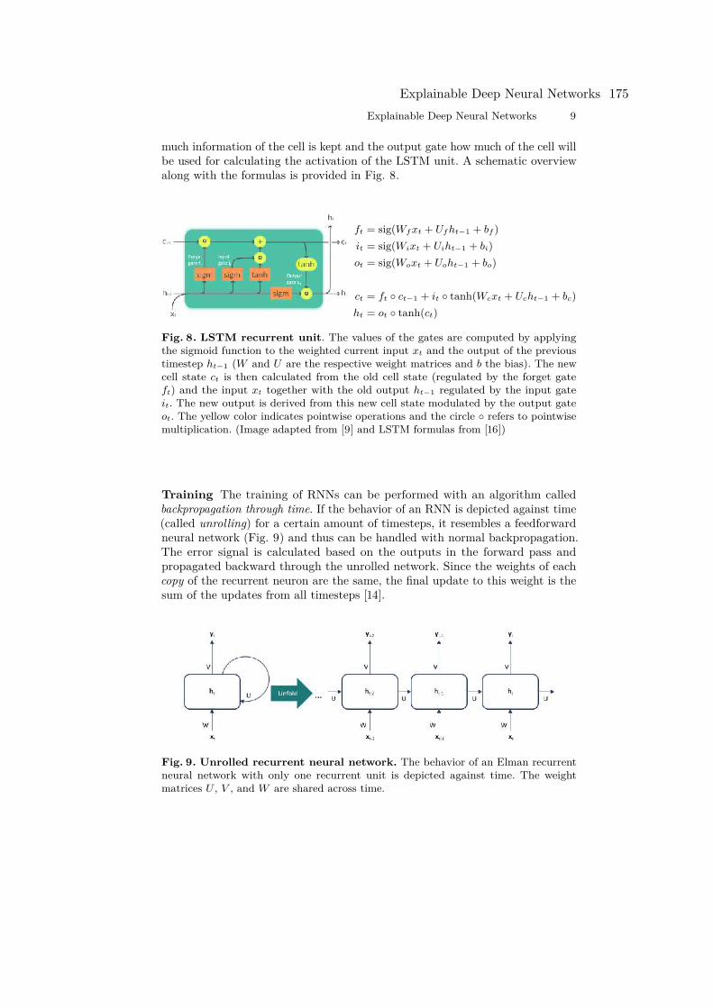
Explainable Deep Neural Networks 9
much information of the cell is kept and the output gate how much of the cell willbe used for calculating the activation of the LSTM unit. A schematic overviewalong with the formulas is provided in Fig. 8.
ft = sig(Wf xt + Uf ht−1 + bf )it = sig(Wixt + Uiht−1 + bi)ot = sig(Woxt + Uoht−1 + bo)
ct = ft ◦ ct−1 + it ◦ tanh(Wcxt + Ucht−1 + bc)ht = ot ◦ tanh(ct)
Fig. 8. LSTM recurrent unit. The values of the gates are computed by applyingthe sigmoid function to the weighted current input xt and the output of the previoustimestep ht−1 (W and U are the respective weight matrices and b the bias). The newcell state ct is then calculated from the old cell state (regulated by the forget gateft) and the input xt together with the old output ht−1 regulated by the input gateit. The new output is derived from this new cell state modulated by the output gateot. The yellow color indicates pointwise operations and the circle ◦ refers to pointwisemultiplication. (Image adapted from [9] and LSTM formulas from [16])
Training The training of RNNs can be performed with an algorithm calledbackpropagation through time. If the behavior of an RNN is depicted against time(called unrolling) for a certain amount of timesteps, it resembles a feedforwardneural network (Fig. 9) and thus can be handled with normal backpropagation.The error signal is calculated based on the outputs in the forward pass andpropagated backward through the unrolled network. Since the weights of eachcopy of the recurrent neuron are the same, the final update to this weight is thesum of the updates from all timesteps [14].
Fig. 9. Unrolled recurrent neural network. The behavior of an Elman recurrentneural network with only one recurrent unit is depicted against time. The weightmatrices U , V , and W are shared across time.
Explainable Deep Neural Networks 175
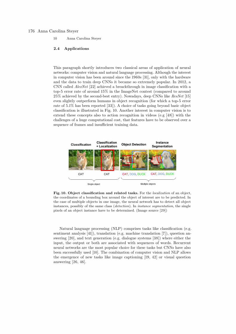
10 Anna Carolina Steyer
2.4 Applications
This paragraph shortly introduces two classical areas of application of neuralnetworks: computer vision and natural language processing. Although the interestin computer vision has been around since the 1960s [31], only with the hardwareand the data to train deep CNNs it became so extremely popular. In 2012, aCNN called AlexNet [22] achieved a breackthrough in image classification with atop-5 error rate of around 15% in the ImageNet contest (compared to around25% achieved by the second-best entry). Nowadays, deep CNNs like ResNet [15]even slightly outperform humans in object recognition (for which a top-5 errorrate of 5.1% has been reported [33]). A choice of tasks going beyond basic objectclassification is illustrated in Fig. 10. Another interest in computer vision is toextend these concepts also to action recognition in videos (e.g [48]) with thechallenges of a huge computational cost, that features have to be observed over asequence of frames and insufficient training data.
Fig. 10. Object classification and related tasks. For the localization of an object,the coordinates of a bounding box around the object of interest are to be predicted. Inthe case of multiple objects in one image, the neural network has to detect all objectinstances, possibly of the same class (detection). In instance segmentation, the singlepixels of an object instance have to be determined. (Image source [29])
Natural language processing (NLP) comprises tasks like classification (e.g.sentiment analysis [41]), translation (e.g. machine translation [7]), question an-swering [20], and text generation (e.g. dialogue systems [38]) where either theinput, the output or both are associated with sequences of words. Recurrentneural networks are the most popular choice for these tasks but CNNs have alsobeen successfully used [10]. The combination of computer vision and NLP allowsthe emergence of new tasks like image captioning [19, 42] or visual questionanswering [26, 46].
176 Anna Carolina Steyer
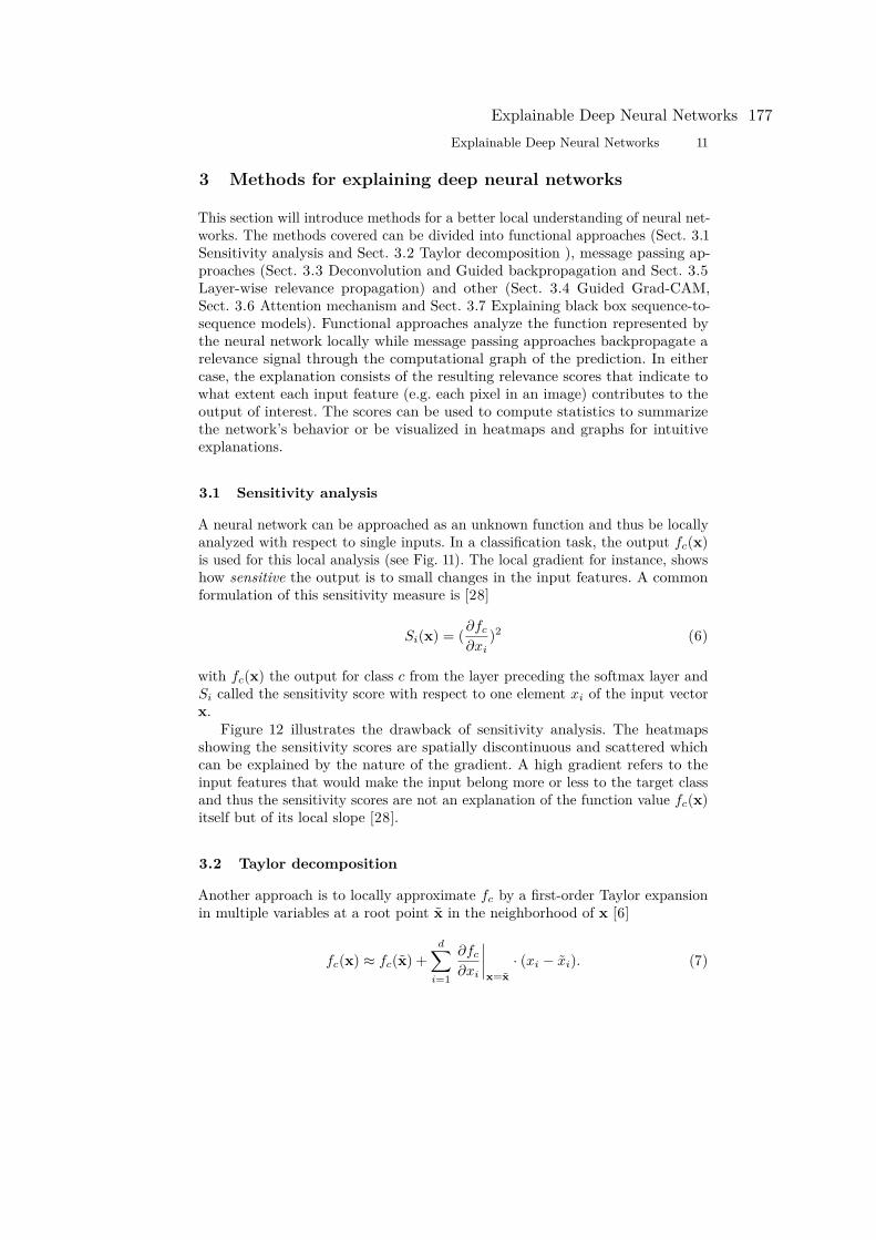
Explainable Deep Neural Networks 11
3 Methods for explaining deep neural networks
This section will introduce methods for a better local understanding of neural net-works. The methods covered can be divided into functional approaches (Sect. 3.1Sensitivity analysis and Sect. 3.2 Taylor decomposition ), message passing ap-proaches (Sect. 3.3 Deconvolution and Guided backpropagation and Sect. 3.5Layer-wise relevance propagation) and other (Sect. 3.4 Guided Grad-CAM,Sect. 3.6 Attention mechanism and Sect. 3.7 Explaining black box sequence-to-sequence models). Functional approaches analyze the function represented bythe neural network locally while message passing approaches backpropagate arelevance signal through the computational graph of the prediction. In eithercase, the explanation consists of the resulting relevance scores that indicate towhat extent each input feature (e.g. each pixel in an image) contributes to theoutput of interest. The scores can be used to compute statistics to summarizethe network’s behavior or be visualized in heatmaps and graphs for intuitiveexplanations.
3.1 Sensitivity analysis
A neural network can be approached as an unknown function and thus be locallyanalyzed with respect to single inputs. In a classification task, the output fc(x)is used for this local analysis (see Fig. 11). The local gradient for instance, showshow sensitive the output is to small changes in the input features. A commonformulation of this sensitivity measure is [28]
Si(x) = (∂fc
∂xi)2 (6)
with fc(x) the output for class c from the layer preceding the softmax layer andSi called the sensitivity score with respect to one element xi of the input vectorx.
Figure 12 illustrates the drawback of sensitivity analysis. The heatmapsshowing the sensitivity scores are spatially discontinuous and scattered whichcan be explained by the nature of the gradient. A high gradient refers to theinput features that would make the input belong more or less to the target classand thus the sensitivity scores are not an explanation of the function value fc(x)itself but of its local slope [28].
3.2 Taylor decomposition
Another approach is to locally approximate fc by a first-order Taylor expansionin multiple variables at a root point x in the neighborhood of x [6]
fc(x) ≈ fc(x) +d∑
i=1
∂fc
∂xi
∣∣∣∣x=x
· (xi − xi). (7)
Explainable Deep Neural Networks 177
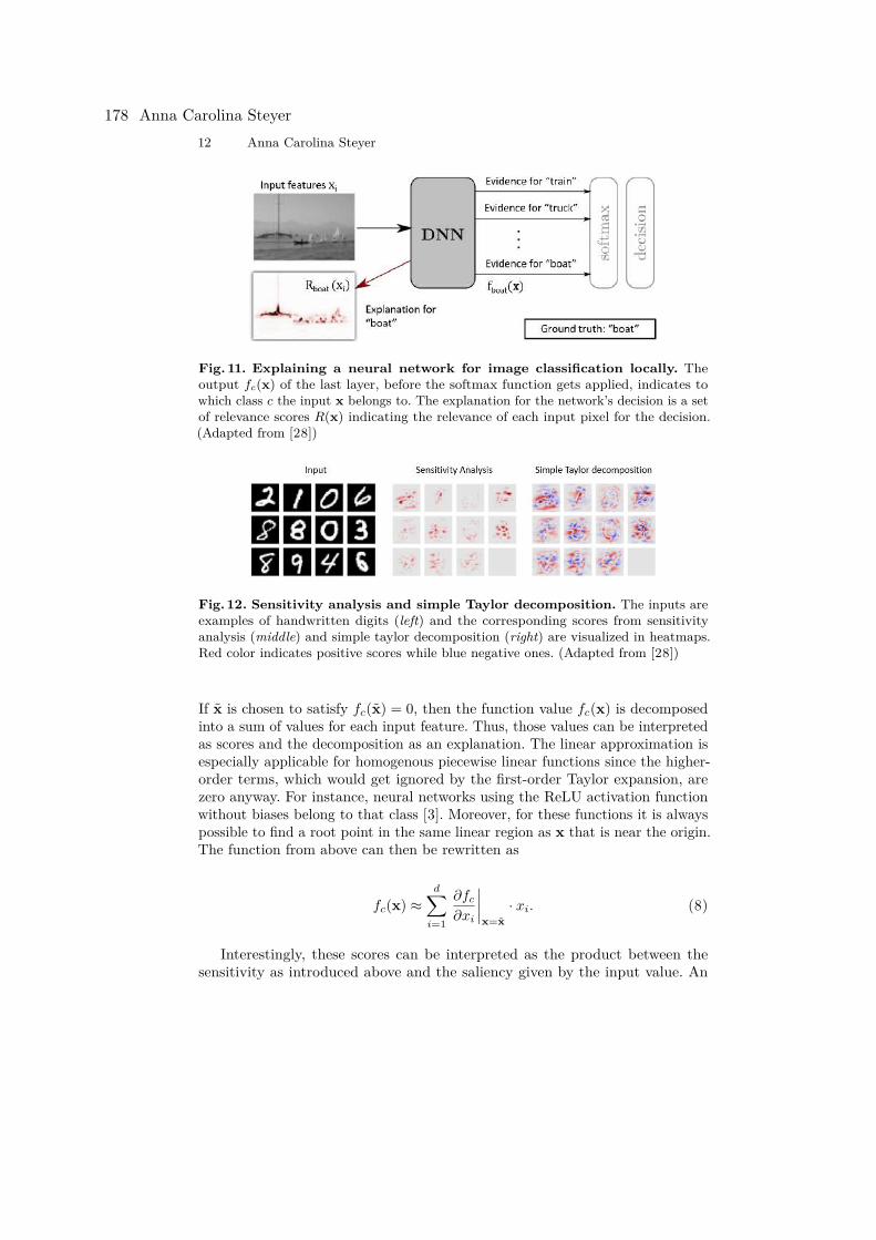
12 Anna Carolina Steyer
Fig. 11. Explaining a neural network for image classification locally. Theoutput fc(x) of the last layer, before the softmax function gets applied, indicates towhich class c the input x belongs to. The explanation for the network’s decision is a setof relevance scores R(x) indicating the relevance of each input pixel for the decision.(Adapted from [28])
Fig. 12. Sensitivity analysis and simple Taylor decomposition. The inputs areexamples of handwritten digits (left) and the corresponding scores from sensitivityanalysis (middle) and simple taylor decomposition (right) are visualized in heatmaps.Red color indicates positive scores while blue negative ones. (Adapted from [28])
If x is chosen to satisfy fc(x) = 0, then the function value fc(x) is decomposedinto a sum of values for each input feature. Thus, those values can be interpretedas scores and the decomposition as an explanation. The linear approximation isespecially applicable for homogenous piecewise linear functions since the higher-order terms, which would get ignored by the first-order Taylor expansion, arezero anyway. For instance, neural networks using the ReLU activation functionwithout biases belong to that class [3]. Moreover, for these functions it is alwayspossible to find a root point in the same linear region as x that is near the origin.The function from above can then be rewritten as
fc(x) ≈d∑
i=1
∂fc
∂xi
∣∣∣∣x=x
· xi. (8)
Interestingly, these scores can be interpreted as the product between thesensitivity as introduced above and the saliency given by the input value. An
178 Anna Carolina Steyer

Explainable Deep Neural Networks 13
example of output scores from the simple Taylor decomposition method Eq. (8)is shown in Fig. 12 in a heatmap.
3.3 Deconvolution and guided backpropagation
Both, the deconvolution method of Zeiler and Fergus [50] and the guided back-propagation method by Springenberg et al. [40] revert the computations ofCNNs layerwise to tell what pixels of an input image have been relevant forthe classification decision. The relevance signal is, starting at the output layer,backpropagated through the computational graph down to the input layer. Again,the initial relevance value is the activation for the class of interest from the layerprevious to the softmax layer (Fig. 11). The explanation methods are designedfor CNNs with max-pooling layers that use the ReLU activation function. Theconvolutional layers get inverted by applying the transposed filter matrices tothe relevance signal while the unpooling assigns all relevance to the neuron withthe maximum activation from the layer below. For the reversion of the ReLUnon-linearity, the deconvolution approach keeps all positive relevance and mapsall negative to zero which equals applying the ReLU function to the relevancesignal. In contrast, guided backpropagation additionally uses the activations fromthe forward pass to only keep the relevance values that are positive and alsocorrespond to a positive activation. The differences between the two methods forreverting the ReLU non-linearity are illustrated in Fig. 13.
Fig. 13. Reverting the ReLU-nonlinearity. Left: Application of the ReLU activationfunction in the forward pass. Middle: The backpropagation of the relevance signalthrough the ReLU-nonlinearity for the deconvolution method. This equals applyingthe ReLU function again and thus keeping only the positive relevance. Right: Guidedbackpropagation additionally keeps only the relevance values which are positive andcorrespond to a positive activation from the forward pass. (Adapted from [40])
By using the activations from the forward pass only in the unpooling layers,the deconvolution method highly depends on the network architecture. If appliedto a network without any pooling layers, the heatmaps for one output would thuslook the same regardless of the input (see Fig. 14). This is not only problematicfor explaining a particular decision but also with more complex input images sincethere can not exist a single heatmap for visualizing the relevant features of allkinds of images that belong to one class. For this reason, guided backpropagationmight be preferred to the deconvolution method, especially for networks withoutor only a few max-pooling layers. A drawback of both methods is that since
Explainable Deep Neural Networks 179
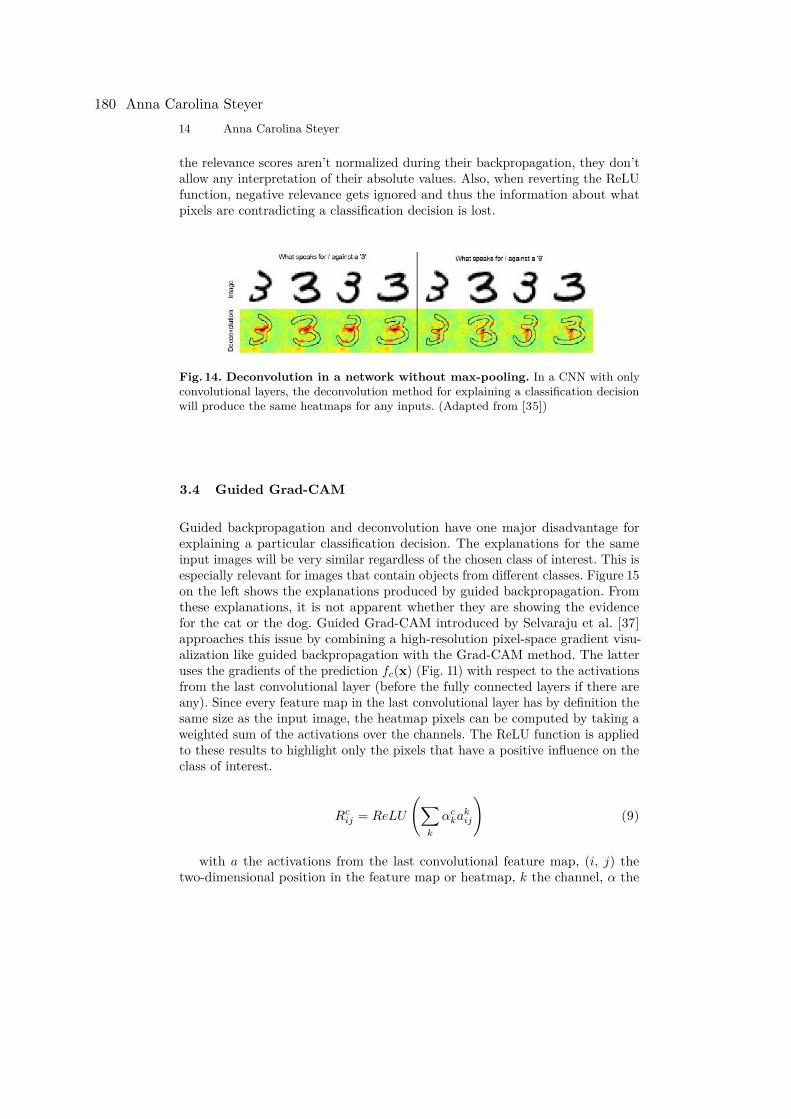
14 Anna Carolina Steyer
the relevance scores aren’t normalized during their backpropagation, they don’tallow any interpretation of their absolute values. Also, when reverting the ReLUfunction, negative relevance gets ignored and thus the information about whatpixels are contradicting a classification decision is lost.
Fig. 14. Deconvolution in a network without max-pooling. In a CNN with onlyconvolutional layers, the deconvolution method for explaining a classification decisionwill produce the same heatmaps for any inputs. (Adapted from [35])
3.4 Guided Grad-CAM
Guided backpropagation and deconvolution have one major disadvantage forexplaining a particular classification decision. The explanations for the sameinput images will be very similar regardless of the chosen class of interest. This isespecially relevant for images that contain objects from different classes. Figure 15on the left shows the explanations produced by guided backpropagation. Fromthese explanations, it is not apparent whether they are showing the evidencefor the cat or the dog. Guided Grad-CAM introduced by Selvaraju et al. [37]approaches this issue by combining a high-resolution pixel-space gradient visu-alization like guided backpropagation with the Grad-CAM method. The latteruses the gradients of the prediction fc(x) (Fig. 11) with respect to the activationsfrom the last convolutional layer (before the fully connected layers if there areany). Since every feature map in the last convolutional layer has by definition thesame size as the input image, the heatmap pixels can be computed by taking aweighted sum of the activations over the channels. The ReLU function is appliedto these results to highlight only the pixels that have a positive influence on theclass of interest.
Rcij = ReLU
(∑
k
αckak
ij
)(9)
with a the activations from the last convolutional feature map, (i, j) thetwo-dimensional position in the feature map or heatmap, k the channel, α the
180 Anna Carolina Steyer
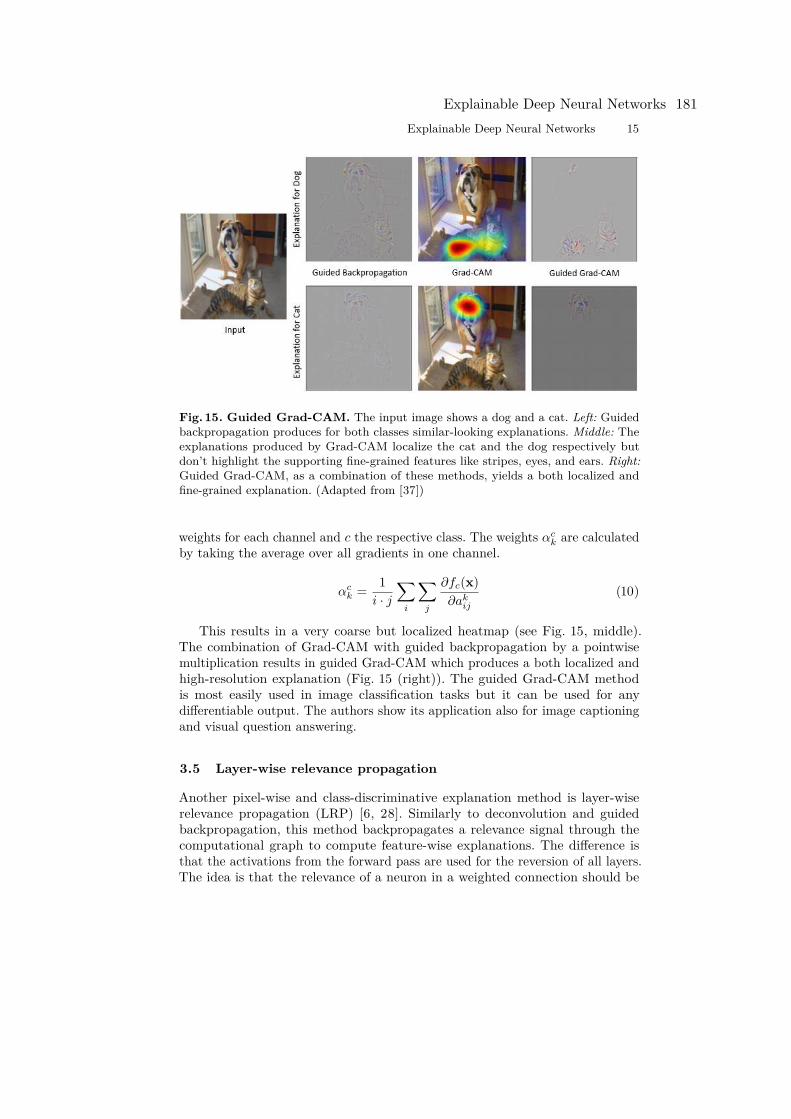
Explainable Deep Neural Networks 15
Fig. 15. Guided Grad-CAM. The input image shows a dog and a cat. Left: Guidedbackpropagation produces for both classes similar-looking explanations. Middle: Theexplanations produced by Grad-CAM localize the cat and the dog respectively butdon’t highlight the supporting fine-grained features like stripes, eyes, and ears. Right:Guided Grad-CAM, as a combination of these methods, yields a both localized andfine-grained explanation. (Adapted from [37])
weights for each channel and c the respective class. The weights αck are calculated
by taking the average over all gradients in one channel.
αck = 1
i · j
∑
i
∑
j
∂fc(x)∂ak
ij
(10)
This results in a very coarse but localized heatmap (see Fig. 15, middle).The combination of Grad-CAM with guided backpropagation by a pointwisemultiplication results in guided Grad-CAM which produces a both localized andhigh-resolution explanation (Fig. 15 (right)). The guided Grad-CAM methodis most easily used in image classification tasks but it can be used for anydifferentiable output. The authors show its application also for image captioningand visual question answering.
3.5 Layer-wise relevance propagation
Another pixel-wise and class-discriminative explanation method is layer-wiserelevance propagation (LRP) [6, 28]. Similarly to deconvolution and guidedbackpropagation, this method backpropagates a relevance signal through thecomputational graph to compute feature-wise explanations. The difference isthat the activations from the forward pass are used for the reversion of all layers.The idea is that the relevance of a neuron in a weighted connection should be
Explainable Deep Neural Networks 181
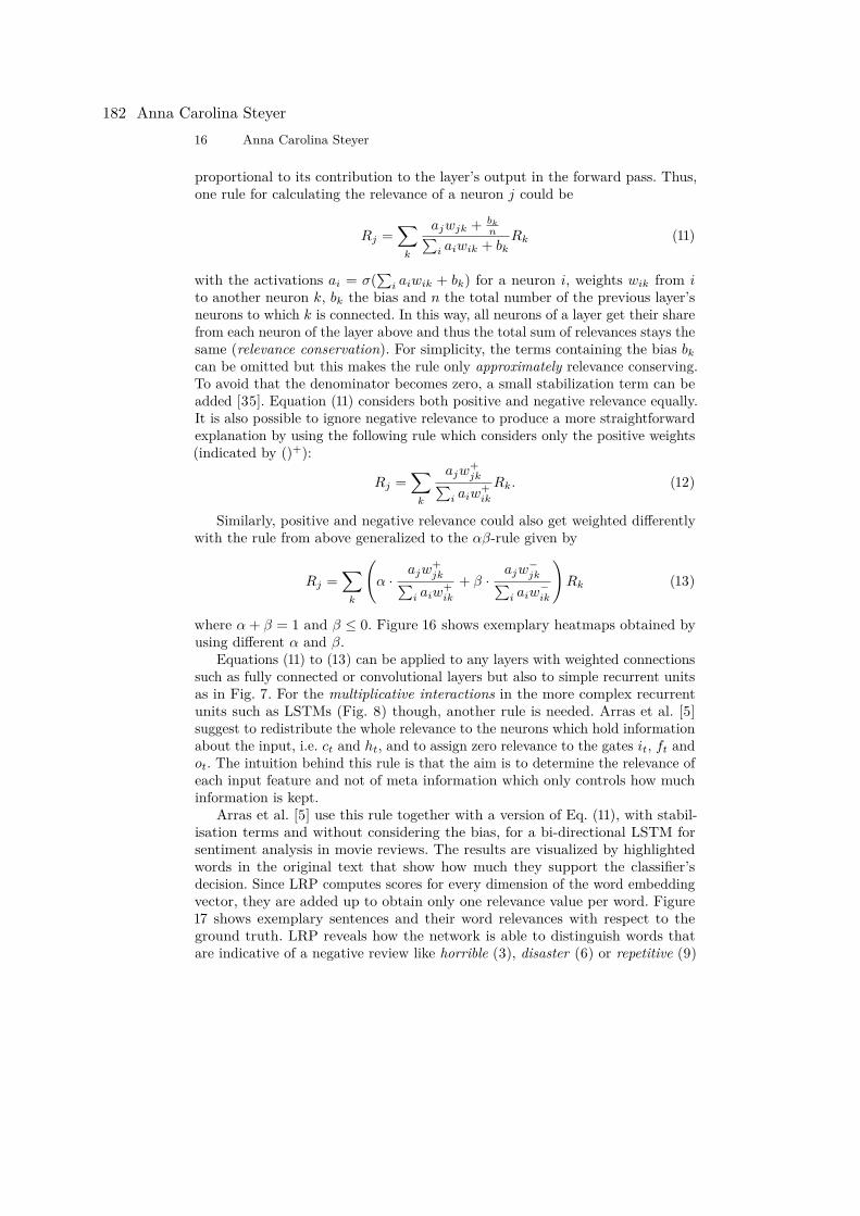
16 Anna Carolina Steyer
proportional to its contribution to the layer’s output in the forward pass. Thus,one rule for calculating the relevance of a neuron j could be
Rj =∑
k
ajwjk + bk
n∑i aiwik + bk
Rk (11)
with the activations ai = σ(∑
i aiwik + bk) for a neuron i, weights wik from ito another neuron k, bk the bias and n the total number of the previous layer’sneurons to which k is connected. In this way, all neurons of a layer get their sharefrom each neuron of the layer above and thus the total sum of relevances stays thesame (relevance conservation). For simplicity, the terms containing the bias bk
can be omitted but this makes the rule only approximately relevance conserving.To avoid that the denominator becomes zero, a small stabilization term can beadded [35]. Equation (11) considers both positive and negative relevance equally.It is also possible to ignore negative relevance to produce a more straightforwardexplanation by using the following rule which considers only the positive weights(indicated by ()+):
Rj =∑
k
ajw+jk∑
i aiw+ik
Rk. (12)
Similarly, positive and negative relevance could also get weighted differentlywith the rule from above generalized to the αβ-rule given by
Rj =∑
k
(α ·
ajw+jk∑
i aiw+ik
+ β ·ajw−
jk∑i aiw
−ik
)Rk (13)
where α + β = 1 and β ≤ 0. Figure 16 shows exemplary heatmaps obtained byusing different α and β.
Equations (11) to (13) can be applied to any layers with weighted connectionssuch as fully connected or convolutional layers but also to simple recurrent unitsas in Fig. 7. For the multiplicative interactions in the more complex recurrentunits such as LSTMs (Fig. 8) though, another rule is needed. Arras et al. [5]suggest to redistribute the whole relevance to the neurons which hold informationabout the input, i.e. ct and ht, and to assign zero relevance to the gates it, ft andot. The intuition behind this rule is that the aim is to determine the relevance ofeach input feature and not of meta information which only controls how muchinformation is kept.
Arras et al. [5] use this rule together with a version of Eq. (11), with stabil-isation terms and without considering the bias, for a bi-directional LSTM forsentiment analysis in movie reviews. The results are visualized by highlightedwords in the original text that show how much they support the classifier’sdecision. Since LRP computes scores for every dimension of the word embeddingvector, they are added up to obtain only one relevance value per word. Figure17 shows exemplary sentences and their word relevances with respect to theground truth. LRP reveals how the network is able to distinguish words thatare indicative of a negative review like horrible (3), disaster (6) or repetitive (9)
182 Anna Carolina Steyer
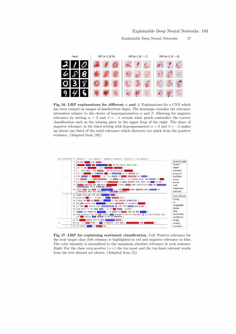
Explainable Deep Neural Networks 17
Fig. 16. LRP explanations for different α and β. Explanations for a CNN whichhas been trained on images of handwritten digits. The heatmaps visualize the relevanceintensities subject to the choice of hyperparameters α and β. Allowing for negativerelevance by setting α = 2 and β = −1 reveals what pixels contradict the correctclassification such as the missing piece in the upper loop of the eight. The share ofnegative relevance in the third setting with hyperparameters α = 3 and β = −2 makesup about one third of the total relevance which distracts too much from the positiveevidence. (Adapted from [28])
Fig. 17. LRP for explaining sentiment classification. Left: Positive relevance forthe true target class (left column) is highlighted in red and negative relevance in blue.The color intensity is normalized to the maximum absolute relevance in each sentence.Right: For the class very positive (++) the ten most and the ten least relevant wordsfrom the test dataset are shown. (Adapted from [5])
Explainable Deep Neural Networks 183
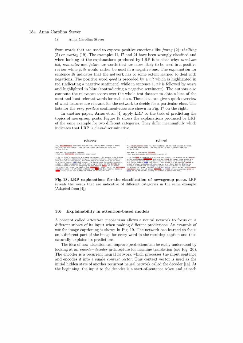
18 Anna Carolina Steyer
from words that are used to express positive emotions like funny (2), thrilling(5) or worthy (19). The examples 11, 17 and 21 have been wrongly classified andwhen looking at the explanations produced by LRP it is clear why: must-seelist, remember and future are words that are more likely to be used in a positivereview while fails would rather be used in a negative one. The explanation forsentence 18 indicates that the network has to some extent learned to deal withnegations. The positive word good is preceded by a n’t which is highlighted inred (indicating a negative sentiment) while in sentence 1, n’t is followed by wasteand highlighted in blue (contradicting a negative sentiment). The authors alsocompute the relevance scores over the whole test dataset to obtain lists of themost and least relevant words for each class. These lists can give a quick overviewof what features are relevant for the network to decide for a particular class. Thelists for the very positive sentiment-class are shown in Fig. 17 on the right.
In another paper, Arras et al. [4] apply LRP to the task of predicting thetopics of newsgroup posts. Figure 18 shows the explanations produced by LRPof the same example for two different categories. They differ meaningfully whichindicates that LRP is class-discriminative.
Fig. 18. LRP explanations for the classification of newsgroup posts. LRPreveals the words that are indicative of different categories in the same example.(Adapted from [4])
3.6 Explainability in attention-based models
A concept called attention mechanism allows a neural network to focus on adifferent subset of its input when making different predictions. An example ofuse for image captioning is shown in Fig. 19. The network has learned to focuson a different part of the image for every word in the resulting caption and thusnaturally explains its predictions.
The idea of how attention can improve predictions can be easily understood bylooking at an encoder-decoder architecture for machine translation (see Fig. 20).The encoder is a recurrent neural network which processes the input sentenceand encodes it into a single context vector. This context vector is used as theinitial hidden state of another recurrent neural network called the decoder [14]. Atthe beginning, the input to the decoder is a start-of-sentence token and at each
184 Anna Carolina Steyer
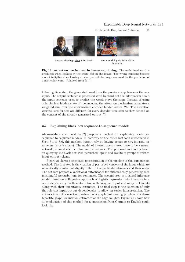
Explainable Deep Neural Networks 19
Fig. 19. Attention mechanism in image captioning. The underlined word isproduced when looking at the white blob in the image. The wrong captions becomemore intelligible when looking at what part of the image was used for the prediction ofa particular word. (Adapted from [47])
following time step, the generated word from the previous step becomes the newinput. The output sentence is generated word by word but the information aboutthe input sentence used to predict the words stays the same. Instead of usingonly the last hidden state of the encoder, the attention mechanism calculates aweighted sum over the intermediate encoder hidden states [25]. The attentionweights used for this are different for every decoder time step as they depend onthe context of the already generated output [7].
3.7 Explaining black box sequence-to-sequence models
Alvarez-Melis and Jaakkola [2] propose a method for explaining black boxsequence-to-sequence models. In contrary to the other methods introduced inSect. 3.1 to 3.6, this method doesn’t rely on having access to any internal pa-rameters (oracle access). The model of interest doesn’t even have to be a neuralnetwork, it could also be a human for instance. The proposed method is basedon querying the black box with perturbed inputs and results in groups of relatedinput-output tokens.
Figure 21 shows a schematic representation of the pipeline of this explanationmethod. The first step is the creation of perturbed versions of the input which aresemantically similar but slightly differ in the particular elements and their order.The authors propose a variational autoencoder for automatically generating suchmeaningful perturbations for sentences. The second step is a causal inferencemodel based on a Bayesian approach of logistic regression which results in aset of dependency coefficients between the original input and output elementsalong with their uncertainty estimates. The final step is the selection of onlythe relevant input-output dependencies to allow an easier interpretation. Theauthors treat this selection problem as a graph partitioning problem of a densebipartite graph for interval estimates of the edge weights. Figure 22 shows howan explanation of this method for a translation from German to English couldlook like.
Explainable Deep Neural Networks 185
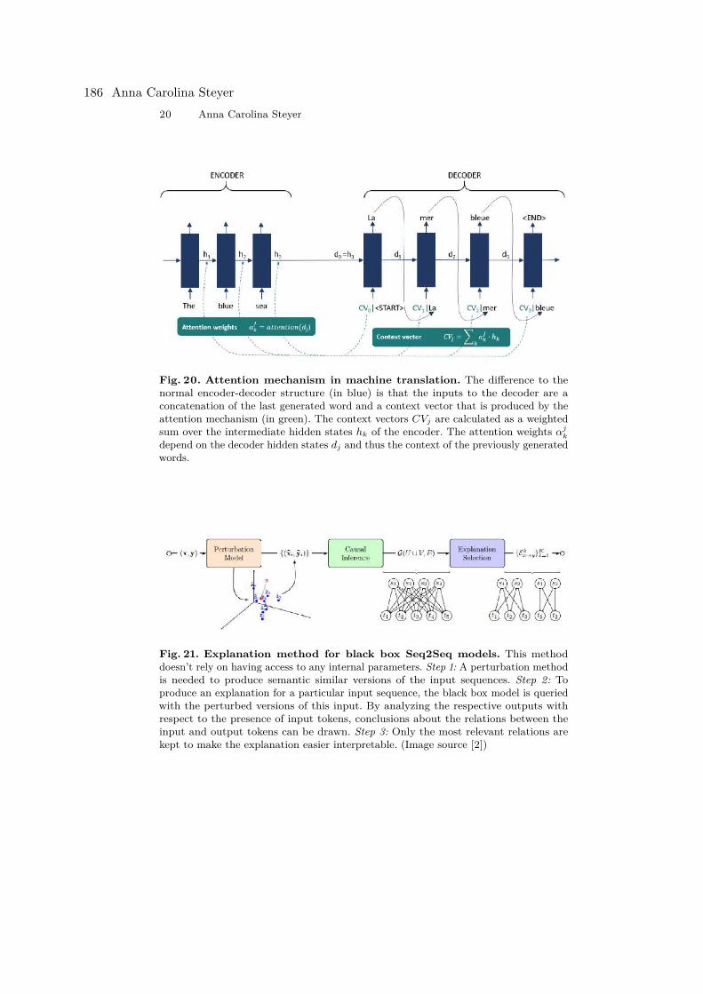
20 Anna Carolina Steyer
Fig. 20. Attention mechanism in machine translation. The difference to thenormal encoder-decoder structure (in blue) is that the inputs to the decoder are aconcatenation of the last generated word and a context vector that is produced by theattention mechanism (in green). The context vectors CVj are calculated as a weightedsum over the intermediate hidden states hk of the encoder. The attention weights αj
k
depend on the decoder hidden states dj and thus the context of the previously generatedwords.
Fig. 21. Explanation method for black box Seq2Seq models. This methoddoesn’t rely on having access to any internal parameters. Step 1: A perturbation methodis needed to produce semantic similar versions of the input sequences. Step 2: Toproduce an explanation for a particular input sequence, the black box model is queriedwith the perturbed versions of this input. By analyzing the respective outputs withrespect to the presence of input tokens, conclusions about the relations between theinput and output tokens can be drawn. Step 3: Only the most relevant relations arekept to make the explanation easier interpretable. (Image source [2])
186 Anna Carolina Steyer
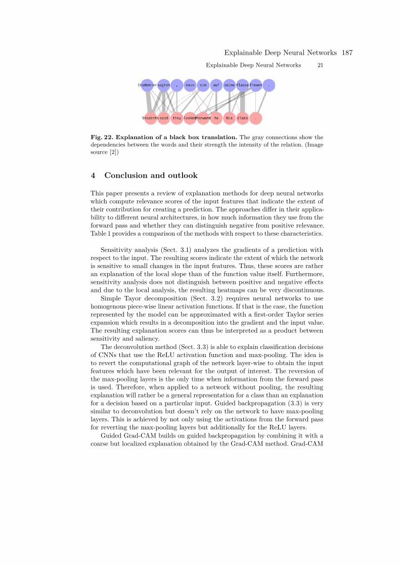
Explainable Deep Neural Networks 21
Fig. 22. Explanation of a black box translation. The gray connections show thedependencies between the words and their strength the intensity of the relation. (Imagesource [2])
4 Conclusion and outlook
This paper presents a review of explanation methods for deep neural networkswhich compute relevance scores of the input features that indicate the extent oftheir contribution for creating a prediction. The approaches differ in their applica-bility to different neural architectures, in how much information they use from theforward pass and whether they can distinguish negative from positive relevance.Table 1 provides a comparison of the methods with respect to these characteristics.
Sensitivity analysis (Sect. 3.1) analyzes the gradients of a prediction withrespect to the input. The resulting scores indicate the extent of which the networkis sensitive to small changes in the input features. Thus, these scores are ratheran explanation of the local slope than of the function value itself. Furthermore,sensitivity analysis does not distinguish between positive and negative effectsand due to the local analysis, the resulting heatmaps can be very discontinuous.
Simple Tayor decomposition (Sect. 3.2) requires neural networks to usehomogenous piece-wise linear activation functions. If that is the case, the functionrepresented by the model can be approximated with a first-order Taylor seriesexpansion which results in a decomposition into the gradient and the input value.The resulting explanation scores can thus be interpreted as a product betweensensitivity and saliency.
The deconvolution method (Sect. 3.3) is able to explain classification decisionsof CNNs that use the ReLU activation function and max-pooling. The idea isto revert the computational graph of the network layer-wise to obtain the inputfeatures which have been relevant for the output of interest. The reversion ofthe max-pooling layers is the only time when information from the forward passis used. Therefore, when applied to a network without pooling, the resultingexplanation will rather be a general representation for a class than an explanationfor a decision based on a particular input. Guided backpropagation (3.3) is verysimilar to deconvolution but doesn’t rely on the network to have max-poolinglayers. This is achieved by not only using the activations from the forward passfor reverting the max-pooling layers but additionally for the ReLU layers.
Guided Grad-CAM builds on guided backpropagation by combining it with acoarse but localized explanation obtained by the Grad-CAM method. Grad-CAM
Explainable Deep Neural Networks 187
22 Anna Carolina Steyer
analyzes the activations of the last convolutional layer to localize the regions thatare relevant with respect to a particular classification decision which results in aboth class-discriminative and high-resolution explanation.
Layer-wise relevance propagation (3.5) uses the weights of the network to-gether with the activations from the forward pass to distribute a relevance signalin the computational graph. The relevance signal is usually the activation in thelast layer that corresponds to the outcome which is to be explained. The distri-bution preserves the total relevance and allows also for negative relevance whichindicates features that contradict a prediction. In theory, LRP can be applied toany networks with monotonous activations and examples of its application tocomputer vision and NLP classification tasks with CNNs and LSTMs exist.
The attention mechanism (Sect. 3.6) is an example of a neural architecturethat naturally provides explanations of its reasoning. In contrary to the otherapproaches, it aims at explaining the prediction of an output sequence and notof a classification or regression. Attention is usually used for encoder-decoderarchitectures and its scores indicate which input features have been importantfor predicting a particular element of an output sequence.
The approach from Sect. 3.7 is also designed for explaining sequence-to-sequence models and excels by not requiring any information from the modelor the forward pass like weights or activations. To infer dependencies betweenthe elements of an input and and output sequence, the black box is queriedwith semantic similar versions of the input. The resulting input-output pairs areanalyzed to associate the occurence of tokens in the input and output.
Various factors like the application of neural networks in transport, medicineand military and the current European legislation will foster explainable arti-ficial intelligence in the near future. This paper provided insights into variousapproaches for designing local explanation methods and such techniques willlikely be further developed, especially towards the applicability to a wider rangeof architectures. In addition to the development of explanation methods, theinterest in optimizing future neural networks towards an improved explainabilityand not only the best accuracy might also grow. Furthermore, techniques likethe attention mechanism show the possibility of developing neural networks thatcan provide an explanation of their reasoning from the start.
References
1. (2016), http://www.image-net.org/2. Alvarez-Melis, D., Jaakkola, T.S.: A causal framework for explaining the predictions
of black-box sequence-to-sequence models. arXiv:1707.01943 (2017)3. Arora, R., Basu, A., Mianjy, P., Mukherjee, A.: Understanding deep neural networks
with rectified linear units. arXiv:1611.01491 (2016)4. Arras, L., Horn, F., Montavon, G., Müller, K.R., Samek, W.: "What is relevant in a
text document?": An interpretable machine learning approach. PloS one 12(8) (2017)5. Arras, L., Montavon, G., Müller, K.R., Samek, W.: Explaining recurrent neural
network predictions in sentiment analysis. arXiv:1706.07206 (2017)
188 Anna Carolina Steyer
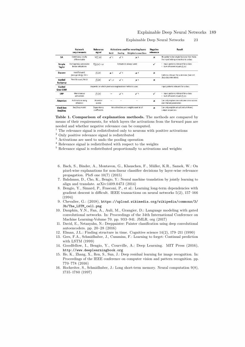
Explainable Deep Neural Networks 23
Table 1. Comparison of explanation methods. The methods are compared bymeans of their requirements, for which layers the activations from the forward pass areneeded and whether negative relevance can be computed.1 The relevance signal is redistributed only to neurons with positive activations2 Only positive relevance signal is redistributed3 Activations are used to undo the pooling operation4 Relevance signal is redistributed with respect to the weights5 Relevance signal is redistributed proportionally to activations and weights
6. Bach, S., Binder, A., Montavon, G., Klauschen, F., Müller, K.R., Samek, W.: Onpixel-wise explanations for non-linear classifier decisions by layer-wise relevancepropagation. PloS one 10(7) (2015)
7. Bahdanau, D., Cho, K., Bengio, Y.: Neural machine translation by jointly learning toalign and translate. arXiv:1409.0473 (2014)
8. Bengio, Y., Simard, P., Frasconi, P., et al.: Learning long-term dependencies withgradient descent is difficult. IEEE transactions on neural networks 5(2), 157–166(1994)
9. Chevalier, G.: (2018), https://upload.wikimedia.org/wikipedia/commons/3/3b/The_LSTM_cell.png
10. Dauphin, Y.N., Fan, A., Auli, M., Grangier, D.: Language modeling with gatedconvolutional networks. In: Proceedings of the 34th International Conference onMachine Learning-Volume 70. pp. 933–941. JMLR. org (2017)
11. David, E., Netanyahu, N.: Deeppainter: Painter classification using deep convolutionalautoencoders. pp. 20–28 (2016)
12. Elman, J.L.: Finding structure in time. Cognitive science 14(2), 179–211 (1990)13. Gers, F.A., Schmidhuber, J., Cummins, F.: Learning to forget: Continual prediction
with LSTM (1999)14. Goodfellow, I., Bengio, Y., Courville, A.: Deep Learning. MIT Press (2016),
http://www.deeplearningbook.org15. He, K., Zhang, X., Ren, S., Sun, J.: Deep residual learning for image recognition. In:
Proceedings of the IEEE conference on computer vision and pattern recognition. pp.770–778 (2016)
16. Hochreiter, S., Schmidhuber, J.: Long short-term memory. Neural computation 9(8),1735–1780 (1997)
Explainable Deep Neural Networks 189

24 Anna Carolina Steyer
17. Ji, S., Xu, W., Yang, M., Yu, K.: 3D convolutional neural networks for human actionrecognition. IEEE transactions on pattern analysis and machine intelligence 35(1),221–231 (2012)
18. Jordan, M.I.: Serial order: A parallel distributed processing approach. In: Advances inpsychology, vol. 121, pp. 471–495. Elsevier (1997)
19. Karpathy, A., Fei-Fei, L.: Deep visual-semantic alignments for generating imagedescriptions. In: Proceedings of the IEEE conference on computer vision and patternrecognition. pp. 3128–3137 (2015)
20. Kembhavi, A., Seo, M., Schwenk, D., Choi, J., Farhadi, A., Hajishirzi, H.: Are yousmarter than a sixth grader? Textbook question answering for multimodal machinecomprehension. In: Proceedings of the IEEE Conference on Computer Vision andPattern Recognition. pp. 4999–5007 (2017)
21. Kolmogorov, A.N.: On the representation of continuous functions of many variablesby superposition of continuous functions of one variable and addition. In: DokladyAkademii Nauk. vol. 114, pp. 953–956. Russian Academy of Sciences (1957)
22. Krizhevsky, A., Sutskever, I., Hinton, G.E.: Imagenet classification with deepconvolutional neural networks. In: Advances in neural information processing systems.pp. 109–1105 (2012)
23. Le Cun, Y., Jackel, L.D., Boser, B., Denker, J.S., Graf, H.P., Guyon, I., Henderson,D., Howard, R.E., Hubbard, W.: Handwritten digit recognition: Applications ofneural network chips and automatic learning. IEEE Communications Magazine27(11), 41–46 (1989)
24. LeCun, Y., Bengio, Y., Hinton, G.: Deep learning. Nature 521(7553), 436 (2015)25. Luong, M.T., Pham, H., Manning, C.D.: Effective approaches to attention-based
neural machine translation. arXiv:1508.04025 (2015)26. Malinowski, M., Rohrbach, M., Fritz, M.: Ask your neurons: A neural-based approach
to answering questions about images. In: Proceedings of the IEEE internationalconference on computer vision. pp. 1–9 (2015)
27. Mhaskar, H., Liao, Q., Poggio, T.: When and why are deep networks better thanshallow ones? In: Thirty-First AAAI Conference on Artificial Intelligence (2017)
28. Montavon, G., Samek, W., Müller, K.R.: Methods for interpreting and understandingdeep neural networks. Digital Signal Processing 73, 1–15 (2018)
29. Ouaknine, A.: (2018), https://medium.com/zylapp/review-of-deep-learning-algorithms-for-object-detection-c1f3d437b852
30. Pan, S.J., Yang, Q.: A survey on transfer learning. IEEE Transactions on knowledgeand data engineering 22(10), 1345–1359 (2009)
31. Papert, S.A.: The summer vision project (1966)32. Ramachandran, P., Zoph, B., Le, Q.V.: Searching for activation functions.
arXiv:1710.05941 (2017)33. Russakovsky, O., Deng, J., Su, H., Krause, J., Satheesh, S., Ma, S., Huang, Z.,
Karpathy, A., Khosla, A., Bernstein, M.: Imagenet large scale visual recognitionchallenge. International journal of computer vision 115(3), 211–252 (2015)
34. Saha, S.: (2018), https://towardsdatascience.com/a-comprehensive-guide-to-convolutional-neural-networks-the-eli5-way-3bd2b1164a53
35. Samek, W., Binder, A., Montavon, G., Lapuschkin, S., Müller, K.R.: Evaluating thevisualization of what a deep neural network has learned. IEEE transactions on neuralnetworks and learning systems 28(11), 2660–2673 (2016)
36. Schmidhuber, J.: Deep learning in neural networks: An overview. Neural networks 61,85–117 (2015)
190 Anna Carolina Steyer
Explainable Deep Neural Networks 25
37. Selvaraju, R.R., Cogswell, M., Das, A., Vedantam, R., Parikh, D., Batra, D.:Grad-cam: Visual explanations from deep networks via gradient-based localization. In:Proceedings of the IEEE International Conference on Computer Vision. pp. 618–626(2017)
38. Serban, I.V., Sordoni, A., Bengio, Y., Courville, A., Pineau, J.: Building end-to-enddialogue systems using generative hierarchical neural network models. In: ThirtiethAAAI Conference on Artificial Intelligence (2016)
39. Siddiqui, S.A., Salman, A., Malik, M.I., Shafait, F., Mian, A., Shortis, M.R., Harvey,E.S.: Automatic fish species classification in underwater videos: exploiting pre-traineddeep neural network models to compensate for limited labelled data. ICES Journal ofMarine Science 75(1), 374–389 (2017)
40. Springenberg, J.T., Dosovitskiy, A., Brox, T., Riedmiller, M.: Striving for simplicity:The all convolutional net. arXiv:1412.6806 (2014)
41. Tang, D., Qin, B., Liu, T.: Document modeling with gated recurrent neural networkfor sentiment classification. In: Proceedings of the 2015 conference on empiricalmethods in natural language processing. pp. 1422–1432 (2015)
42. Vinyals, O., Toshev, A., Bengio, S., Erhan, D.: Show and tell: A neural image captiongenerator. In: Proceedings of the IEEE conference on computer vision and patternrecognition. pp. 3156–3164 (2015)
43. Waibel, A., Hanazawa, T., Hinton, G., Shikano, K., Lang, K.J.: Phoneme recognitionusing time-delay neural networks. IEEE Transactions on Acoustics, Speech, andSignal Processing 37(3), 328–339 (1989)
44. Wang, C.F.: (2018), https://towardsdatascience.com/a-basic-introduction-to-separable-convolutions-b99ec3102728
45. Wang, R.: (2018), https://thisgirlreina.wordpress.com/2018/07/11/stochastic-gradient-descent-with-restarts/
46. Xu, H., Saenko, K.: Ask, attend and answer: Exploring question-guided spatialattention for visual question answering. In: European Conference on ComputerVision. pp. 451–466. Springer (2016)
47. Xu, K., Ba, J., Kiros, R., Cho, K., Courville, A., Salakhudinov, R., Zemel, R., Bengio,Y.: Show, attend and tell: Neural image caption generation with visual attention. In:International conference on machine learning. pp. 2048–2057 (2015)
48. Yue-Hei Ng, J., Hausknecht, M., Vijayanarasimhan, S., Vinyals, O., Monga, R.,Toderici, G.: Beyond short snippets: Deep networks for video classification. In:Proceedings of the IEEE conference on computer vision and pattern recognition. pp.4694–4702 (2015)
49. Zeiler, M.D.: ADADELTA: an adaptive learning rate method. arXiv:1212.5701 (2012)50. Zeiler, M.D., Fergus, R.: Visualizing and understanding convolutional networks. In:
European conference on computer vision. pp. 818–833. Springer (2014)
Explainable Deep Neural Networks 191

Aufmerksamkeitssteuerung durch HaptischeSchnittstellen in Beobachtungsaufgaben
Leon Huck?
Karlsruher Institut fur Technologie
Zusammenfassung. In dieser Arbeit wird der Einsatzbereich der Auf-merksamkeitssteuerung durch haptische Schnittstellen in Beobachtungstatigkeitenerkundet. Aufmerksamkeitssteuerung wird als eine Ressource definiert,die es zu verwalten gilt. Fur Beobachtungsaufgaben werden die Kriteri-en Relevanz und Erschopfung als entscheident vorgestellt. Die haptischenSchnittstellen werden nach ihrer Reizubertragung (Elektrische Impulseoder Druck) unterschieden. Dabei lassen sich Charakteristike, wie diePosition auf der Haut, die Beruhrungsflache und die Dauer, erkennen.Bei den Anwendungen wird zwischen dem jeweiligen Einsatzbereich un-terschieden:
– Sinneswiederherstellung: Simulation anderer Sinne uber haptischeSignale.
– Zwischenmenschliche Kommunikation: Informationsubertragung uberhaptische Signale, um die Kommunikation zwischen Menschen zuermoglichen und zu verbessern.
– Leistungssteigerung: Verbesserung von menschlichen Leistungen durchden Einsatz von haptischen Schnittstellen zur Informationsubertragung.
– Erweiterung des Wahrnehmungsspektrums: Verwenden von hapti-schen Schnittstellen um kunstliche Sinne zu erzeugen.
– Zuverlassigkeit Erzeugung: Erweiterung von bereits bestehenden Sys-temen mit redundanten haptischen Schnittstellen.
? Unter der Betreuung von: Erik Pescara
192 Aufmerksamkeitssteuerung durch Haptische Schnittstellen in Beobachtungsaufgaben
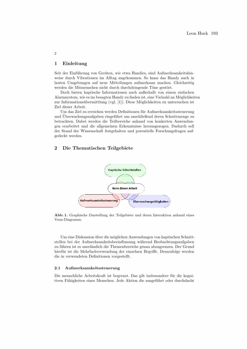
2
1 Einleitung
Seit der Einfuhrung von Geraten, wie etwa Handies, sind Aufmerksamkeitshin-weise durch Vibrationen im Alltag angekommen. So kann das Handy auch inlauten Umgebungen auf neue Mitteilungen aufmerksam machen. Gleichzeitigwerden die Mitmenschen nicht durch durchdringende Tone gestort.
Doch bieten haptische Informationen auch außerhalb von einem einfachenAlarmsystem, wie es im besagten Handy zu finden ist, eine Vielzahl an Moglichkeitenzur Informationsubermittlung (vgl. [1]). Diese Moglichkeiten zu untersuchen istZiel dieser Arbeit.
Um das Ziel zu erreichen werden Definitionen fur Aufmerksamkeitssteuerungund Uberwachungsaufgaben eingefuhrt um anschließend deren Schnittmenge zubetrachten. Dabei werden die Teilbereiche anhand von konkreten Anwendun-gen erarbeitet und die allgemeinen Erkenntnisse herausgezogen. Dadurch sollder Stand der Wissenschaft festgehalten und potentielle Forschungsfragen auf-gedeckt werden.
2 Die Thematischen Teilgebiete
Abb. 1. Graphische Darstellung der Teilgebiete und deren Interaktion anhand einesVenn-Diagramm.
Um eine Diskussion uber die moglichen Anwendungen von haptischen Schnitt-stellen bei der Aufmerksamkeitsbeeinflussung wahrend Beobachtungsaufgabenzu fuhren ist es unerlasslich die Themenbereiche genau abzugrenzen. Der Grundhierfur ist die Mehrfachverwendung der einzelnen Begriffe. Demzufolge werdendie in verwendeten Definitionen vorgestellt.
2.1 Aufmerksamkeitssteuerung
Die menschliche Arbeitskraft ist begrenzt. Das gilt insbesondere fur die kogni-tiven Fahigkeiten eines Menschen. Jede Aktion die ausgefuhrt oder durchdacht
Leon Huck 193
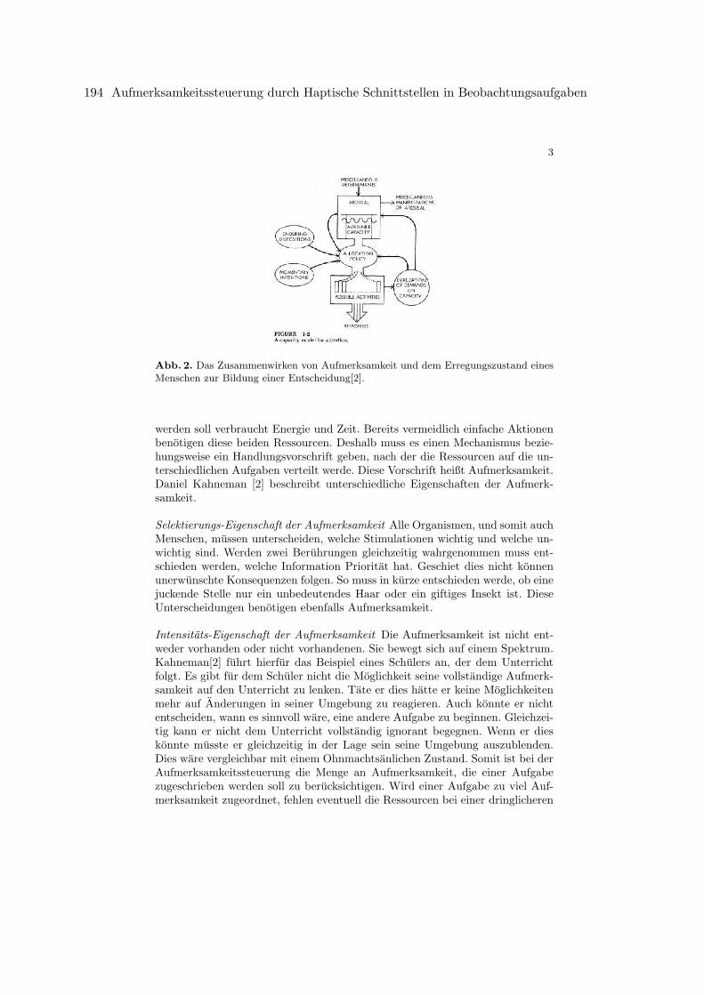
3
Abb. 2. Das Zusammenwirken von Aufmerksamkeit und dem Erregungszustand einesMenschen zur Bildung einer Entscheidung[2].
werden soll verbraucht Energie und Zeit. Bereits vermeidlich einfache Aktionenbenotigen diese beiden Ressourcen. Deshalb muss es einen Mechanismus bezie-hungsweise ein Handlungsvorschrift geben, nach der die Ressourcen auf die un-terschiedlichen Aufgaben verteilt werde. Diese Vorschrift heißt Aufmerksamkeit.Daniel Kahneman [2] beschreibt unterschiedliche Eigenschaften der Aufmerk-samkeit.
Selektierungs-Eigenschaft der Aufmerksamkeit Alle Organismen, und somit auchMenschen, mussen unterscheiden, welche Stimulationen wichtig und welche un-wichtig sind. Werden zwei Beruhrungen gleichzeitig wahrgenommen muss ent-schieden werden, welche Information Prioritat hat. Geschiet dies nicht konnenunerwunschte Konsequenzen folgen. So muss in kurze entschieden werde, ob einejuckende Stelle nur ein unbedeutendes Haar oder ein giftiges Insekt ist. DieseUnterscheidungen benotigen ebenfalls Aufmerksamkeit.
Intensitats-Eigenschaft der Aufmerksamkeit Die Aufmerksamkeit ist nicht ent-weder vorhanden oder nicht vorhandenen. Sie bewegt sich auf einem Spektrum.Kahneman[2] fuhrt hierfur das Beispiel eines Schulers an, der dem Unterrichtfolgt. Es gibt fur dem Schuler nicht die Moglichkeit seine vollstandige Aufmerk-samkeit auf den Unterricht zu lenken. Tate er dies hatte er keine Moglichkeitenmehr auf Anderungen in seiner Umgebung zu reagieren. Auch konnte er nichtentscheiden, wann es sinnvoll ware, eine andere Aufgabe zu beginnen. Gleichzei-tig kann er nicht dem Unterricht vollstandig ignorant begegnen. Wenn er dieskonnte musste er gleichzeitig in der Lage sein seine Umgebung auszublenden.Dies ware vergleichbar mit einem Ohnmachtsanlichen Zustand. Somit ist bei derAufmerksamkeitssteuerung die Menge an Aufmerksamkeit, die einer Aufgabezugeschrieben werden soll zu berucksichtigen. Wird einer Aufgabe zu viel Auf-merksamkeit zugeordnet, fehlen eventuell die Ressourcen bei einer dringlicheren
194 Aufmerksamkeitssteuerung durch Haptische Schnittstellen in Beobachtungsaufgaben
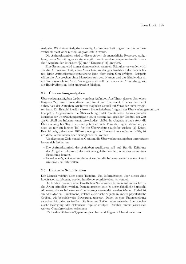
4
Aufgabe. Wird einer Aufgabe zu wenig Aufmerksamkeit zugeordnet, kann dieseeventuell nicht oder nur zu langsam erfullt werde.
Die Aufmerksamkeit wird in dieser Arbeit als menschliche Ressource aufge-fasst, deren Verteilung es zu steuern gilt. Somit werden beispielsweise die Berei-che ”Aspekte der Intensitat”[2] und ”Erregung”[2] ignoriert.
Eine Steuerung wird immer dann erreicht, wenn ein Stimulus verwendet wird,der die Aufmerksamkeit, eines Menschen, zu der gewunschten Information lei-tet. Diese Aufmerksamkeitssteuerung kann uber jeden Sinn erfolgen. Beispielewaren das Ansprechen eines Menschen mit dem Namen und das Einblenden ei-nes Warnsymbols im Auto. Vorweggreifend soll hier auch eine Anwendung, wiedie Handyvibration nicht unerwahnt bleiben.
2.2 Uberwachungsaufgaben
Uberwachungsaufgaben fordern von dem Aufgaben-Ausfuhrer, dass er uber einenlangeren Zeitraum Informationen aufnimmt und uberwacht. Uberwachen heißtdabei, dass der Aufgaben-Ausfuhrer moglichst schnell auf Veranderungen reagie-ren kann. Ein Beispiel hierfur ware ein Sicherheitsbeauftragter, der Uberwachungsmonitoreuberpruft. Angenommen die Uberwachung findet Nachts statt. AuszeichnendesMerkmal der Uberwachungsaufgabe ist, in diesem Fall, dass der Großteil der Zeitder Großteil der Informationen unverandert bleibt. Im Gegensatz dazu steht dieUberwachung bei Tag. Hier sind potentiell viele Veranderungen erkennbar, je-doch ist nur ein kleiner Teil fur die Uberwachungsaufgabe wichtig [3]. DiesesBeispiel zeigt, dass eine Differenzierung von Uberwachungsaufgaben notig istum diese vereinfachen oder ermoglichen zu konnen.
Als allgemeine Ziele von allen Geraten, die Uberwachungsaufgaben unterstutzenlassen sich festhalten:
– Die Aufmerksamkeit des Aufgaben-Ausfuhrers soll auf, fur die Erfullungder Aufgabe, relevante Informationen geleitet werden, ohne das es zu einerErmudung kommt.
– Es soll ermoglicht oder vereinfacht werden die Informationen in relevant undirrelevant zu unterteilen.
2.3 Haptische Schnittstellen
Der Mensch verfugt uber einen Tastsinn. Um Informationen uber diesen Sinnubertragen zu konnen, werden haptische Schnittstellen verwendet.
Die fur den Tastsinn verantwortlichen Nervenzellen konnen auf unterschiedli-che Arten stimuliert werden. Dementsprechen gibt es unterschiedliche haptischeAktuator, die zu Informationsubertragung verwendet werden konnen. Dabei istein Aktuator ein Bauelement, welches elektrische Signale in andere physikalischeGroßen, wie beispielsweise Bewegung, umsetzt. Dabei ist eine Unterscheidungzwischen Aktuator zu treffen. Die Kommunikation kann entweder uber mecha-nische Bewegung oder elektrische Impulse erfolgen. Daruber hinaus lassen sichweitere Charakteristiken erkennen:
Fur beiden Aktuator-Typen vergleichbar sind folgende Charakteristiken:
Leon Huck 195
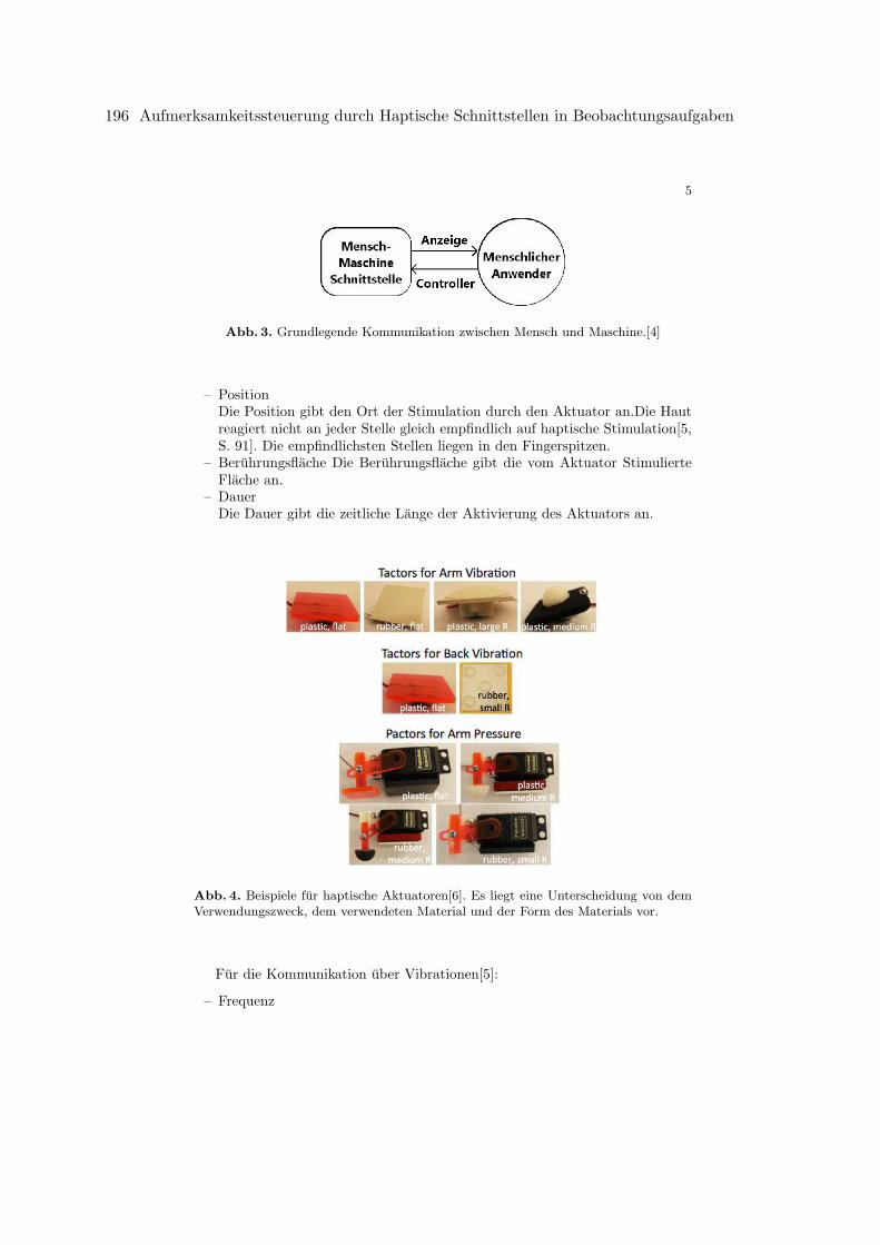
5
Abb. 3. Grundlegende Kommunikation zwischen Mensch und Maschine.[4]
– PositionDie Position gibt den Ort der Stimulation durch den Aktuator an.Die Hautreagiert nicht an jeder Stelle gleich empfindlich auf haptische Stimulation[5,S. 91]. Die empfindlichsten Stellen liegen in den Fingerspitzen.
– Beruhrungsflache Die Beruhrungsflache gibt die vom Aktuator StimulierteFlache an.
– DauerDie Dauer gibt die zeitliche Lange der Aktivierung des Aktuators an.
Abb. 4. Beispiele fur haptische Aktuatoren[6]. Es liegt eine Unterscheidung von demVerwendungszweck, dem verwendeten Material und der Form des Materials vor.
Fur die Kommunikation uber Vibrationen[5]:
– Frequenz
196 Aufmerksamkeitssteuerung durch Haptische Schnittstellen in Beobachtungsaufgaben
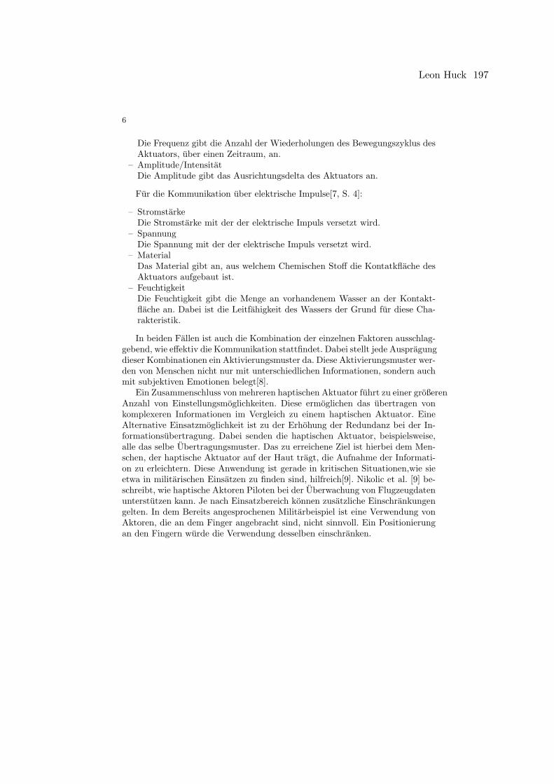
6
Die Frequenz gibt die Anzahl der Wiederholungen des Bewegungszyklus desAktuators, uber einen Zeitraum, an.
– Amplitude/IntensitatDie Amplitude gibt das Ausrichtungsdelta des Aktuators an.
Fur die Kommunikation uber elektrische Impulse[7, S. 4]:
– StromstarkeDie Stromstarke mit der der elektrische Impuls versetzt wird.
– SpannungDie Spannung mit der der elektrische Impuls versetzt wird.
– MaterialDas Material gibt an, aus welchem Chemischen Stoff die Kontatkflache desAktuators aufgebaut ist.
– FeuchtigkeitDie Feuchtigkeit gibt die Menge an vorhandenem Wasser an der Kontakt-flache an. Dabei ist die Leitfahigkeit des Wassers der Grund fur diese Cha-rakteristik.
In beiden Fallen ist auch die Kombination der einzelnen Faktoren ausschlag-gebend, wie effektiv die Kommunikation stattfindet. Dabei stellt jede Auspragungdieser Kombinationen ein Aktivierungsmuster da. Diese Aktivierungsmuster wer-den von Menschen nicht nur mit unterschiedlichen Informationen, sondern auchmit subjektiven Emotionen belegt[8].
Ein Zusammenschluss von mehreren haptischen Aktuator fuhrt zu einer großerenAnzahl von Einstellungsmoglichkeiten. Diese ermoglichen das ubertragen vonkomplexeren Informationen im Vergleich zu einem haptischen Aktuator. EineAlternative Einsatzmoglichkeit ist zu der Erhohung der Redundanz bei der In-formationsubertragung. Dabei senden die haptischen Aktuator, beispielsweise,alle das selbe Ubertragungsmuster. Das zu erreichene Ziel ist hierbei dem Men-schen, der haptische Aktuator auf der Haut tragt, die Aufnahme der Informati-on zu erleichtern. Diese Anwendung ist gerade in kritischen Situationen,wie sieetwa in militarischen Einsatzen zu finden sind, hilfreich[9]. Nikolic et al. [9] be-schreibt, wie haptische Aktoren Piloten bei der Uberwachung von Flugzeugdatenunterstutzen kann. Je nach Einsatzbereich konnen zusatzliche Einschrankungengelten. In dem Bereits angesprochenen Militarbeispiel ist eine Verwendung vonAktoren, die an dem Finger angebracht sind, nicht sinnvoll. Ein Positionierungan den Fingern wurde die Verwendung desselben einschranken.
Leon Huck 197

7
3 Anwendungen
Nun stellt sich die Frage in welchen Auspragungen diese Teilgebiete zusammen-gefuhrt werden konnen. Deshalb sollen im folgenden Anwendungen, die alle dreiTeilgebiete umfassen beleuchtet werden.
3.1 Sinneswiederherstellung
Menschliche Sinne konnen, von Geburt an oder im laufe der Zeit, nicht, odernur eingeschrankt, funktionsfahig sein. Um diesen Leistungsverlust ausgleichenzu konnen bedarf es technischer Hilfsmittel. Hierbei bietet die menschliche Hauteine Moglichkeit zur Aufnahme von Informationen, die typischerweise uber an-dere Sinne aufgenommen werden wurden.
Sehvermogen Nach dem Stand der Forschung ist das Auge das Leistungs-starkste Sinnesorgan, gemessen an der ubertragenen Datenmenge[10]. Dabei liegtdie absolute Leistung ca. bei der eines Ethernet-Kabels mit 10 Mbit/s[10]. DerSehsinn kann somit bereits aus technischen grunden nicht vollstandig uber dieHaut simuliert werden. Die fur die Uberwachung der Umwelt wichtigen Infor-mationen lassen sich von den unwichtigen differenzieren.
Lesen Geschriebene Worte sind eine Darstellung der menschlichen Sprache.Im Fall der Einschrankung des Sehvermogens ist auch die Fahigkeit zu lesenbeeintrachtigt.
Abb. 5. Rahmendaten des Optacons.[5]
Optacon Eine Losung fur diese Einschrankung wurde von Bliss et al. 1970 inForm des ”Optacon” entwickelt (Zitiert nach:[5]). Dabei werden auf einer Anzei-geflache die Buchstaben in Form von Vibrationen dargestellt. Das identifiezierender Buchstaben ubernimmt ein Scanner, der uber geschrieben Worte bewegtwerden kann. Mit diesem Gerat ist war es moglich zwischen 50 und 100 Wortein der Minute zu lesen [5]. Bliss et al. [11] identifiert in seiner Arbeit drei TestsCharakteristiken, die einen Einblick in die Leistung eines ”Direkt Ubersetzersmit taktilem Ausgang”[11] bieten.
198 Aufmerksamkeitssteuerung durch Haptische Schnittstellen in Beobachtungsaufgaben

8
– LesbarkeitDie Lesbarkeit beschreibt, mit welcher Wahrscheinlichkeit, die gelesene In-formation von dem Benutzer, wie vorgesehen interpretiert wird. Fur dasErreichen der Charakteristik muss es moglich sein Buchstaben zu unter-scheiden. Auch ist die Erneuerungsrate, mit dem das Gerat die Buchstabenneu zeichnet, von Bedeutung. Eine zu geringe Wiederholungsrate kann zuMissverstandnissen fuhren.
– LesegeschwindigkeitDie Lesegeschwindigkeit gibt an, wie schnell Worter bzw. Buchstaben gele-sen werden konnen. Diese Charakteristik hangt mit dem Trainingsstand desAnwenders zusammen.
– Lesbarer AusschnittIn dem Lesbaren Ausschnitt konnen Buchstaben willkurlich erkannt werden.Je großer dieser Ausschnitt ist, desto langer kann ein Anwender lesen ohneAnderungen an einem Gerat vorzunehmen.
3.2 Zwischenmenschliche Kommunikation
Die Zwischenmenschliche Kommunikation ist ein komplexer Vorgang, bei demzumeist viele Sinne beansprucht werden. Uber den Horsinn werden die Informa-tionen aufgenommen, die in der gesprochenen Sprache zu finden sind. Der Seh-sinn wird verwendet um Lippen zu lesen und somit ein besseres Verstandnis zu er-zeugen. Daruber hinaus kann uber ihn die emotionale Lage des Gesprachspartnerseingeschatzt werden und auf Gesten, wie ein Handschlag, reagiert werden. Je-doch gibt es auch Umgebungen, in denen diese Kommunikationswege unterbun-den werden. Der Gerauschpegel kann zu hoch sein um Sprache zu verstehen. DieLichtverhaltnisse konnen zu dunkel sein um den anderen Menschen zu sehen,mit dem Kommuniziert wird [1].
Des weiteren konnen auch durch Unfalle, Alter oder Krankheiten die Au-gen und Ohren beeintrachtigt sein. Um die Fahigkeit der Zwischenmenschli-chen Kommunikation zu erhalten sind Seh- und Horhilfen verbreitete technischeWerkzeuge. Eine weitere Alternative ist das Umverlagern der Kommunikationauf einen anderen Sinn[1].
Frank A. Geldard [1] beschreibt hierzu in seiner Arbeit die Entwicklung derForschung, die versucht die zwischenmenschliche Kommunikation auf den Tast-sinn zu verlagern. Zuerst wird beschrieben, wie die Haut dazu genutzt werdenkann wie ein Ohr zu funktionieren. Dabei wird die Haut als Trommelfell ver-wendet. Dieser Ansatz liefert nach einer Einlernphase von 30h ein Vokabularvon einigen einzelnen Worten[1]. Das Problem bei dieser Anwendung liegt in derZuverlassigkeit. Bei einer Wiederkennungsrate von ca. 75
Tactons Die Idee, fur die haptische Wahrnehmung spezialisierte Vibrationsmus-ter zu erstellen, wird von Stephen Brewster und Lorna M. Brown[12] behandelt.Ihr Vorschlag ist sogenannte Tactile Icons (Tactons) zu verwenden, die haptischgut differenzierbar sind. Dabei orientieren sie sich an musik ahnlichen Mustern,
Leon Huck 199
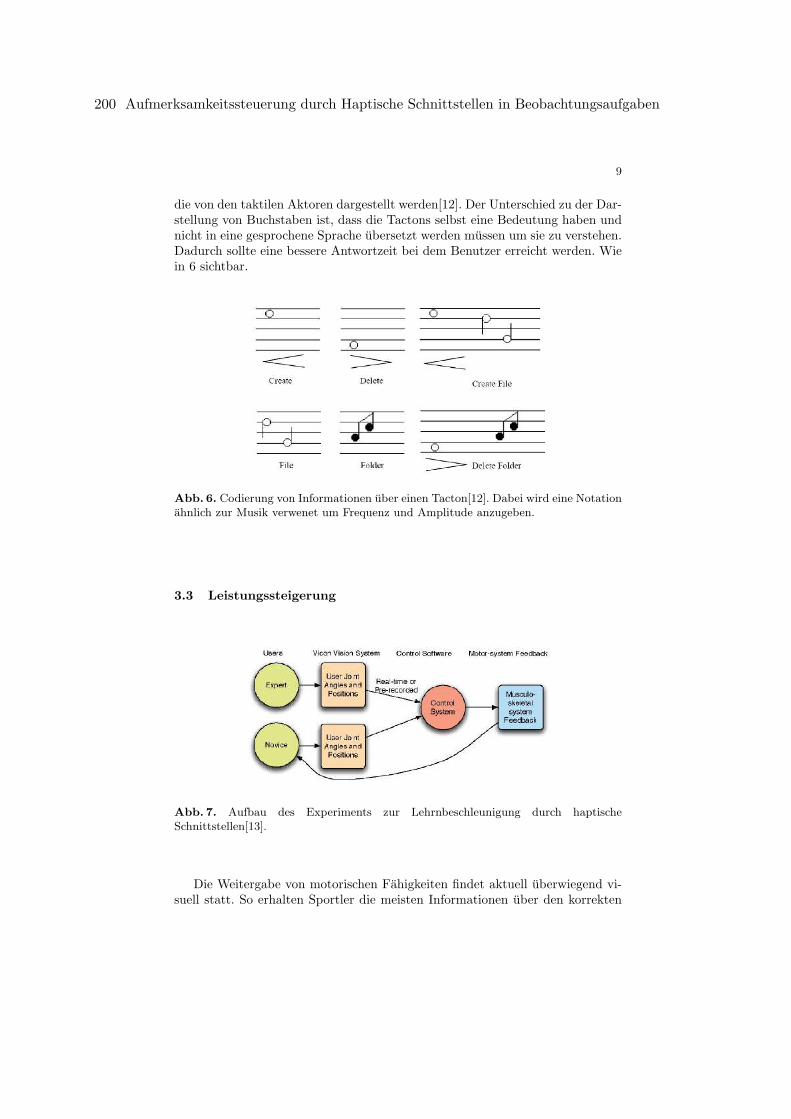
9
die von den taktilen Aktoren dargestellt werden[12]. Der Unterschied zu der Dar-stellung von Buchstaben ist, dass die Tactons selbst eine Bedeutung haben undnicht in eine gesprochene Sprache ubersetzt werden mussen um sie zu verstehen.Dadurch sollte eine bessere Antwortzeit bei dem Benutzer erreicht werden. Wiein 6 sichtbar.
Abb. 6. Codierung von Informationen uber einen Tacton[12]. Dabei wird eine Notationahnlich zur Musik verwenet um Frequenz und Amplitude anzugeben.
3.3 Leistungssteigerung
Abb. 7. Aufbau des Experiments zur Lehrnbeschleunigung durch haptischeSchnittstellen[13].
Die Weitergabe von motorischen Fahigkeiten findet aktuell uberwiegend vi-suell statt. So erhalten Sportler die meisten Informationen uber den korrekten
200 Aufmerksamkeitssteuerung durch Haptische Schnittstellen in Beobachtungsaufgaben
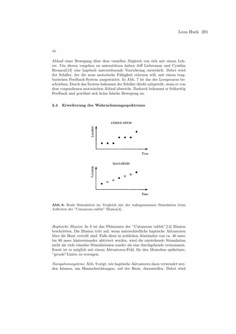
10
Ablauf einer Bewegung uber dem visuellen Abgleich von sich mit einem Leh-rer. Um diesen vorgehen zu unterstutzen haben Jeff Lieberman und CynthiaBreazeal[13] eine haptisch unterstutzende Vorrichtung entwickelt. Dabei wirdder Schuler, der die neue motorische Fahigkeit erlernen will, mit einem trag-barischen Feedback-System ausgestattet. In Abb. 7 ist das der Lernprozess be-schrieben. Durch das System bekommt der Schuler direkt mitgeteilt, wenn er vondem vorgesehenen motorischen Ablauf abweicht. Dadurch bekommt er fruhzeitigFeedback und gewohnt sich keine falsche Bewegung an.
3.4 Erweiterung des Wahrnehmungsspektrums
Abb. 8. Reale Stimulation im Vergleich mit der wahrgenommen Stimulation beimAuftreten der ”Cutaneous rabbit” Illusion[4].
Haptische Illusion In 8 ist das Phanomen der ”Cutaneous rabbit”[14] Illusionbeschrieben. Die Illusion tritt auf, wenn unterschiedliche haptische Aktuatorenuber die Haut verteilt sind. Falls diese in zeitlichen Abstanden von ca. 40 msecbis 80 msec hintereinander aktiviert werden, wird die entstehende Stimulationnicht als viele einzelne Stimulationen sonder als eine durchgehende vernommen.Somit ist es moglich mit einem Aktuatoren-Feld, fur den Menschen spuhrbare,”gerade”Linien zu erzeugen.
Navigationssysteme Abb. 9 zeigt, wie haptische Aktuatoren dazu verwendet wer-den konnen, um Himmelsrichtungen, auf der Haut, darzustellen. Dabei wird
Leon Huck 201
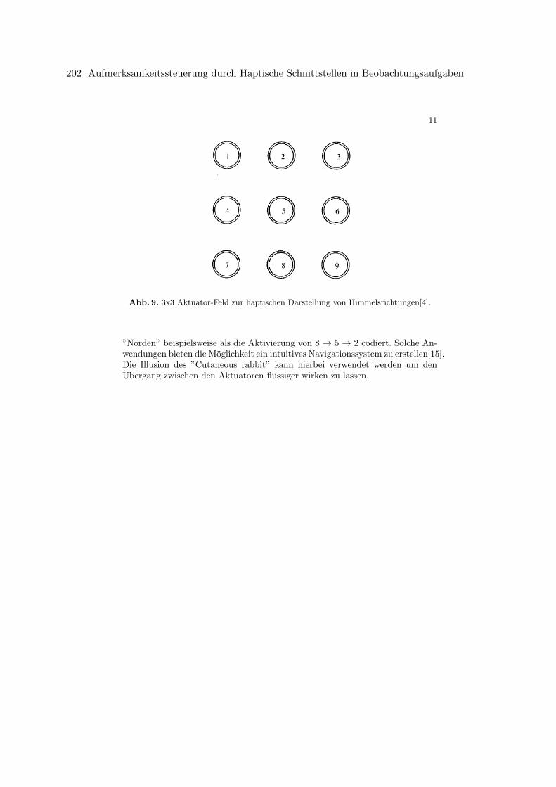
11
Abb. 9. 3x3 Aktuator-Feld zur haptischen Darstellung von Himmelsrichtungen[4].
”Norden” beispielsweise als die Aktivierung von 8 → 5 → 2 codiert. Solche An-wendungen bieten die Moglichkeit ein intuitives Navigationssystem zu erstellen[15].Die Illusion des ”Cutaneous rabbit” kann hierbei verwendet werden um denUbergang zwischen den Aktuatoren flussiger wirken zu lassen.
202 Aufmerksamkeitssteuerung durch Haptische Schnittstellen in Beobachtungsaufgaben
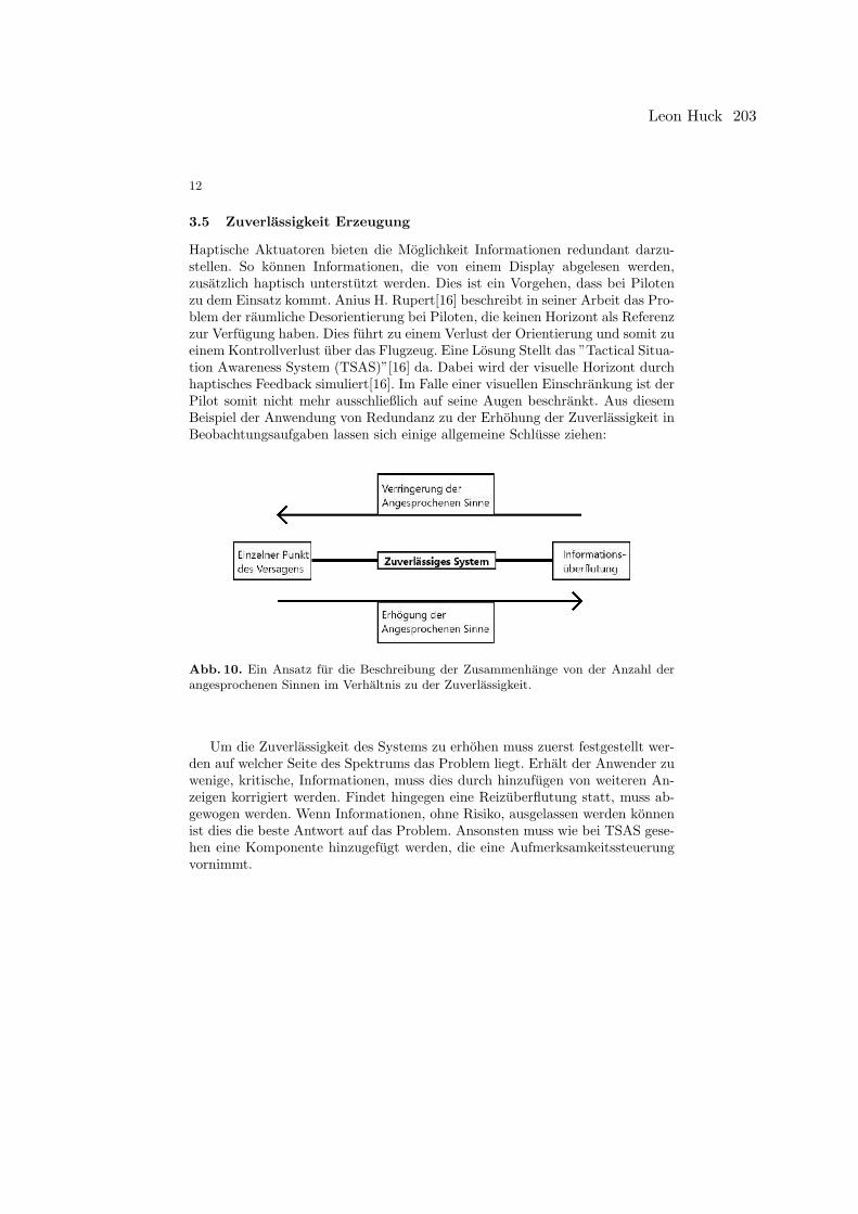
12
3.5 Zuverlassigkeit Erzeugung
Haptische Aktuatoren bieten die Moglichkeit Informationen redundant darzu-stellen. So konnen Informationen, die von einem Display abgelesen werden,zusatzlich haptisch unterstutzt werden. Dies ist ein Vorgehen, dass bei Pilotenzu dem Einsatz kommt. Anius H. Rupert[16] beschreibt in seiner Arbeit das Pro-blem der raumliche Desorientierung bei Piloten, die keinen Horizont als Referenzzur Verfugung haben. Dies fuhrt zu einem Verlust der Orientierung und somit zueinem Kontrollverlust uber das Flugzeug. Eine Losung Stellt das ”Tactical Situa-tion Awareness System (TSAS)”[16] da. Dabei wird der visuelle Horizont durchhaptisches Feedback simuliert[16]. Im Falle einer visuellen Einschrankung ist derPilot somit nicht mehr ausschließlich auf seine Augen beschrankt. Aus diesemBeispiel der Anwendung von Redundanz zu der Erhohung der Zuverlassigkeit inBeobachtungsaufgaben lassen sich einige allgemeine Schlusse ziehen:
Abb. 10. Ein Ansatz fur die Beschreibung der Zusammenhange von der Anzahl derangesprochenen Sinnen im Verhaltnis zu der Zuverlassigkeit.
Um die Zuverlassigkeit des Systems zu erhohen muss zuerst festgestellt wer-den auf welcher Seite des Spektrums das Problem liegt. Erhalt der Anwender zuwenige, kritische, Informationen, muss dies durch hinzufugen von weiteren An-zeigen korrigiert werden. Findet hingegen eine Reizuberflutung statt, muss ab-gewogen werden. Wenn Informationen, ohne Risiko, ausgelassen werden konnenist dies die beste Antwort auf das Problem. Ansonsten muss wie bei TSAS gese-hen eine Komponente hinzugefugt werden, die eine Aufmerksamkeitssteuerungvornimmt.
Leon Huck 203

13
4 Selbststandigkeitserklarung
Ich versichere hiermit, dass ich die vorliegende Arbeit selbststandig verfasst, undweder ganz oder in Teilen als Prufungsleistung vorgelegt und keine anderen alsdie angegebenen Hilfsmittel benutzt habe. Samtliche Stellen der Arbeit, die be-nutzten Werken im Wortlaut oder dem Sinn nach entnommen sind, habe ichdurch Quellenangaben kenntlich gemacht. Dies gilt auch fur Zeichnungen, Skiz-zen, bildliche Darstellungen und dergleichen sowie fur Quellen aus dem Internet.
Name: Leon HuckTitel der Arbeit: Aufmerksamkeitssteuerung durch Haptische Schnittstellen
in BeobachtungsaufgabenOrt, Datum: Karlsruhe, den 30.08.2019
204 Aufmerksamkeitssteuerung durch Haptische Schnittstellen in Beobachtungsaufgaben
14
Literatur
1. Frank A. Geldard. Some neglected possibilities of communication. Science,131(3413):1583–1588, 1960.
2. Daniel Kahneman. Attention and effort, volume 1063. Citeseer, 1973.3. Angus Craig. Nonparametric measures of sensory efficiency for sustained monito-
ring tasks. Human Factors, 21(1):69–77, 1979. PMID: 468268.4. Hong Z. Tan and Alex Pentland. Tactual displays for sensory substitution and
wearable computers. In ACM SIGGRAPH 2005 Courses, SIGGRAPH ’05, NewYork, NY, USA, 2005. ACM.
5. Lynette A. Jones and Nadine B. Sarter. Tactile displays: Guidance for their designand application. Human Factors, 50(1):90–111, 2008. PMID: 18354974.
6. Y. Zheng and J. B. Morrell. Haptic actuator design parameters that influenceaffect and attention. In 2012 IEEE Haptics Symposium (HAPTICS), pages 463–470, March 2012.
7. K. A. Kaczmarek, J. G. Webster, P. Bach-y-Rita, and W. J. Tompkins. Electrotac-tile and vibrotactile displays for sensory substitution systems. IEEE Transactionson Biomedical Engineering, 38(1):1–16, Jan 1991.
8. M. A. Baumann, K. E. MacLean, T. W. Hazelton, and A. McKay. Emulatinghuman attention-getting practices with wearable haptics. In 2010 IEEE HapticsSymposium, pages 149–156, March 2010.
9. Mark I Nikolic, Aaron E Sklar, and Nadine B Sarter. Multisensory feedback insupport of pilot-automation coordination: the case of uncommanded mode transiti-ons. In Proceedings of the Human Factors and Ergonomics Society Annual Meeting,volume 42, pages 239–243. SAGE Publications Sage CA: Los Angeles, CA, 1998.
10. Kristin Koch, Judith McLean, Ronen Segev, Michael A. Freed, I. I. Berry, Micha-el J., Vijay Balasubramanian, and Peter Sterling. How ¡em¿much¡/em¿ the eyetells the brain. Current Biology, 16(14):1428–1434, June 2019.
11. J. C. Bliss, M. H. Katcher, C. H. Rogers, and R. P. Shepard. Optical-to-tactileimage conversion for the blind. IEEE Transactions on Man-Machine Systems,11(1):58–65, March 1970.
12. Stephen Brewster and Lorna M. Brown. Tactons: Structured tactile messages fornon-visual information display. In Proceedings of the Fifth Conference on Australa-sian User Interface - Volume 28, AUIC ’04, pages 15–23, Darlinghurst, Australia,Australia, 2004. Australian Computer Society, Inc.
13. Jeff Lieberman and Cynthia Breazeal. Development of a wearable vibrotactilefeedback suit for accelerated human motor learning. In Proceedings 2007 IEEEInternational Conference on Robotics and Automation, pages 4001–4006. IEEE,2007.
14. Frank A Geldard and Carl E Sherrick. The cutaneous”rabbit”: A perceptual illu-sion. Science, 178(4057):178–179, 1972.
15. Hong Tan, Robert Gray, J Jay Young, and Ryan Taylor. A haptic back display forattentional and directional cueing. Haptic, 2003.
16. Angus H Rupert. An instrumentation solution for reducing spatial disorientationmishaps. IEEE Engineering in Medicine and Biology Magazine, 19(2):71–80, 2000.
Leon Huck 205
Related Documents