\u003ctitle\u003eOptimization of resonances in photonic crystal slabs\u003c/title\u003e

Optimization of Resonances in Photonic Crystal Slabs

Robert P. Liptona, Stephen P. Shipmana, and Stephanos Venakidesb

aLouisiana State University, Baton Rouge, LA, USAbDuke University, Durham, NC, USA

ABSTRACT

Variational methods are applied to the design of a two-dimensional lossless photonic crystal slab to optimizeresonant scattering phenomena. The method is based on varying properties of the transmission coefficient thatare connected to resonant behavior. Numerical studies are based on boundary-integral methods for crystalsconsisting of multiple scatterers. We present an example in which we modify a photonic crystal consisting of anarray of dielectric rods in air so that a weak transmission anomaly is transformed into a sharp resonance.

Keywords: photonic crystal, resonance, optimization, transmission

1. OVERVIEW

Resonant electromagnetic scattering behavior in photonic crystal slabs (as sheets, films, or walls) is closelyconnected to anomalous behavior of the transmission of energy through them. It has been observed empiricallyand through numerical simulations that leaky waveguide modes, Fabry-Perot bandgap resonances, and otherresonant phenomena coincide in the frequency domain with narrow regions of enhanced transmission or reflectionof incident waves (see Refs. 1, 2, 3, and 4).

In this report, we develop a method for designing infinite periodic photonic crystal slabs that have certaindesired electromagnetic resonant properties. Motivated by the connection between resonant behavior and trans-mission, our method focuses on modifying or optimizing those properties of a photonic crystal slab that have arelation to its transmission coefficient. We do this by developing the variational calculus of the transmitted en-ergy as a function of the material parameters. We restrict our analysis to lossless materials in a two-dimensionalreduction, in which the design parameters are the dielectric permittivity ε, the magnetic permeability µ, and thestructure of the crystal.

Our numerical methods are based on free Green’s functions and boundary integrals and are therefore suitedto crystals whose period consists of a finite number of disjoint scatterers with smooth boundaries. In particular,we apply the variational calculus to the manipulation of resonant properties of crystals that are built of circulardielectric rods embedded in a contrasting dielectric medium.

Cox and Dobson (Refs. 5 and 6) have devised a gradient-search method for optimizing and creating bandgapsfor two-dimensional photonic crystals that are infinite in both directions. This is based on the generalized gradientof the bandwidth derived from the variational calculus of the dispersion relation of the periodic structure.Resonant scattering behavior in photonic crystal slabs is known to be related to complex dispersion relations(Ref. 4): source fields at real frequencies near a complex eigenvalue produce resonant scattering in the crystaland enhanced or inhibited transmission. A method based on the manipulation of these dispersion relations holdspromise for engineering crystal slabs with desired resonant properties. In this study, we approach the problemby manipulating the transmission as a function of the structure and material properties of dielectric crystals.

Further author information: (Send correspondence to S.P.S)R.P.L.: E-mail: [email protected], Telephone: 1 225 578 1569; supported by grants AFOSR F49620-02-1-0041 andNSF DMS-0296064S.P.S.: E-mail: [email protected], Telephone: 1 225 578 1674; supported by LA Board of Regents grant LEQSF(2003-06)-RD-A-14S.V.: E-mail: [email protected], Telephone 1 919 660 2815; supported by grants ARO-DAAD19-99-1-0132 and NSFDMS-0207262.

2. THE MATHEMATICAL FRAMEWORK

Our photonic crystal slab consists of an array of lossless rods perpendicular to the xy-plane embedded in alossless medium of contrasting dielectric permittivity ε and magnetic permeability µ. The array is periodicin the y direction and truncated to a finite width in the x direction. In a cross-section (Fig. 1), one periodof the structure consists of a finite number of domains Dj , j = 1, . . . , n, with boundaries ∂Dj , and we putD = ∪n

j=1Dj . We assume that each rod, as well as the exterior medium is homogeneous. We consider freetime-harmonic electromagnetic fields that are polarized so that either the electric field points out of the planeand the magnetic field is transverse to the rods (the transverse magnetic, or TM, case) or the magnetic fieldpoints out of the plane (the TE case). In either case, we denote the out-of-plane component by ψ(x, y)e−iωt,where ω is the reduced frequency∗, and the Maxwell equations reduce to the Helmholtz equation

∇2ψ + εµω2ψ = 0.

This equation holds in the interiors of the regionsDj and in the exterior medium, where the values of ε and µ takeon different constant values. In the TM case, the Maxwell equations imply the following matching conditions forthe interior and exterior limiting values of the electric field component ψ on ∂D.

ψint = ψext

µext∂nψint = µint∂nψext

In the TE case, µext and µint are replaced by εext and εint, so it is sufficient to work out the analysis for the TMcase.

We assume further that the field ψ is pseudoperiodic in y, that is

ψ(x, y) = ψ(x, y)eiβy,

in which ψ(x, y) has period 2π in the variable y. Such fields are called Bloch waves. The pseudo-periodicity allowsus to restrict the analysis to one period of the structure, which is the strip S = (x, y) : −∞<x<∞, 0≤y≤2π(Fig. 1).

A pseudo-periodic radiating fundamental solution of the Helmholtz equation in a homogeneous medium (εand µ constant) is given by G(x− x, y − y), where G(x, y) satisfies

∇2G+ εµω2G = −

∞∑

k=−∞δ(x, y − 2πk)e2πkiβ .

For values of β and ω such that εµω2 − (m+ β)2 6= 0 for all integers m, its Fourier form is

G(x, y) = −1

4π

∞∑

m=−∞

1

νm

exp (νm|x| + i(m+ β)y) .

The Green’s function is built of a finite number of propagating plane-wave modes, for which νm = iκm,κm > 0, m = m1, . . . ,m2, and infinitely many decaying (evanescent) modes, for which νm < 0. The Green’sfunction, together with Green’s identities reduce much of the theory of the Helmholtz equation to boundaryintegrals and shows us that the asymptotic behavior of bounded solutions in the strip S as |x| → ∞ is simply asuperposition of plane waves traveling to the right and left:

ψ ∼

m2∑

m=m1

(a±me

iκmx + b±me−iκmx

)ei(m+β)y (x → ±∞)

∗We define the reduced frequency by ω = fL/c, where c is the speed of light, L is the period of the structure, and fis the frequency in cycles per time. The reduced spatial variables (x, y) are related to the physical variables (X,Y ) by(x, y) = 2π(X,Y )/L.

The strip S

x

y

2

Figure 1. A cross-section of a photonic crystal slab consisting of an array of homogeneous dielectric rods standingperpendicular to the xy-plane. The rod structure is periodic in the y-direction, with period 2π, and extends indefinitelyas y → ±∞. The rod structure is finite in the x-direction. Exterior to the rods is a homogeneous material of contrastingdielectric permittivity extending to infinity to the right and left. Pseudo-periodic fields in the plane can be analyzed inthe strip S = (x, y) : −∞<x<∞, 0≤y≤2π consisting of a single period of the dielectric permittivity function.

The solution approaches the asymptotic form exponentially as |x| → ∞.

In the scattering problem that we study in this paper, a source field incident upon the slab at an angle θfrom the left is given:

ψinc = eiκmxei(m+β)y,

where m is an integer such that (m + β)2 < εµω2. This is a plane wave whose angle of incidence with the slabis θ= arcsin m+β√

εµω. β can always taken to lie in the interval [−1/2, 1/2), and m = 0 and β = 0 corresponds to

normal incidence.

The total field ψ has the asymptotic form

ψ ∼ eiκmxei(m+β)y +

m2∑

m=m1

rme−iκmxei(m+β)y (x → −∞)

ψ ∼

m2∑

m=m1

tmeiκmxei(m+β)y (x→ ∞),

in which rm and tm are the coefficients of the modes of the fields reflected by the slab and transmitted throughit, respectively.

3. THE VARIATIONAL CALCULUS

Let x0 be any positive number large enough so that D is contained in the truncated strip Ω = (x, y) : −x0 <x < x0, 0 ≤ y ≤ 2π; let Γ− and Γ+ denote the left and right boundaries of Ω: Γ± = (±x0, y) : 0 ≤ y ≤ 2π;put Γ = Γ− ∪ Γ+; and let n denote the outward-pointing normal vector to Γ.

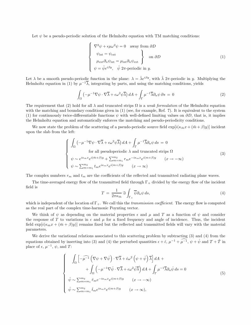
Let ψ be a pseudo-periodic solution of the Helmholtz equation with TM matching conditions:

∇2ψ + εµω2ψ = 0 away from ∂D

ψint = ψext

µext∂nψint = µint∂nψext

on ∂D

ψ = ψeiβy, ψ 2π-periodic in y.

(1)

Let λ be a smooth pseudo-periodic function in the plane: λ = λeiβy, with λ 2π-periodic in y. Multiplying theHelmholtz equation in (1) by µ−1λ, integrating by parts, and using the matching conditions, yields

∫

Ω

(−µ−1∇ψ · ∇λ+ εω2ψλ

)dA+

∫

Γ

µ−1λ∂nψ ∂s = 0 (2)

The requirement that (2) hold for all λ and truncated strips Ω is a weak formulation of the Helmholtz equationwith the matching and boundary conditions given in (1) (see, for example, Ref. 7). It is equivalent to the system(1) for continuously twice-differentiable functions ψ with well-defined limiting values on ∂D, that is, it impliesthe Helmholtz equation and automatically enforces the matching and pseudo-periodicity conditions.

We now state the problem of the scattering of a pseudo-periodic source field exp[i(κmx+(m+β)y)] incidentupon the slab from the left:

∫

Ω

(−µ−1∇ψ · ∇λ+ εω2ψλ

)dA+

∫

Γ

µ−1λ∂nψ ds = 0

for all pseudoperiodic λ and truncated strips Ω

ψ ∼ eiκmxei(m+β)y +∑m2

m=m1rme

−iκmxei(m+β)y (x → −∞)

ψ ∼∑m2

m=m1tme

iκmxei(m+β)y (x → ∞)

(3)

The complex numbers rm and tm are the coefficients of the reflected and transmitted radiating plane waves.

The time-averaged energy flow of the transmitted field through Γ+ divided by the energy flow of the incidentfield is

T =1

2πκm

=

∫

Γ+

ψ∂nψ ds, (4)

which is independent of the location of Γ+. We call this the transmission coefficient. The energy flow is computedas the real part of the complex time-harmonic Poynting vector.

We think of ψ as depending on the material properties ε and µ and T as a function of ψ and considerthe response of T to variations in ε and µ for a fixed frequency and angle of incidence. Thus, the incidentfield exp[i(κmx + (m + β)y)] remains fixed but the reflected and transmitted fields will vary with the materialparameters.

We derive the variational relations associated to this scattering problem by subtracting (3) and (4) from the

equations obtained by inserting into (3) and (4) the perturbed quantities ε+ ε, µ−1 + µ−1, ψ + ψ and T + T inplace of ε, µ−1, ψ, and T :

∫

Ω

[−µ−1

(∇ψ + ∇ψ

)· ∇λ+ εω2

(ψ + ψ

)λ]dA +

+

∫

Ω

(−µ−1∇ψ · ∇λ+ εω2ψλ

)dA+

∫

Γ

µ−1λ∂nψ ds = 0

ψ ∼∑m2

m=m1rme

−iκmxei(m+β)y (x → −∞)

ψ ∼∑m2

m=m1tme

iκmxei(m+β)y (x → ∞),

(5)

T =1

2πκm

=

∫

Γ+

(ψ∂nψ + ψ∂nψ + ψ∂nψ

)ds. (6)

We have assumed that the support of µ−1 is inside Ω so that it does not contribute to the boundary integralalong Γ.

We now seek a function λ that represents the variation of the transmission functional. This means that λ ischosen so that the part of (6) that is linear in ψ is equal to the imaginary component of the linear part of (5)

that involves ψ but not ε or µ−1. Thus, we seek λ such that, for all perturbations ψ satisfying the asymptoticconditions in (5),

=

[∫

Ω

(−µ−1∇ψ · ∇λ+ εω2ψλ

)dA+

∫

Γ

µ−1λ∂nψ ds

]= µ−1

ext =

∫

Γ+

(ψ∂nψ + ψ∂nψ

)ds. (7)

(We have multiplied T by the constant 2πκmµ−1ext for convenience.) Once we have found such a function λ, we

use (5) and (6) to deduce that

T =µext

2πκm

=

∫

Ω

[µ−1∇ψ · ∇λ− εω2ψλ

]dA + h.o.t., (8)

where “h.o.t.” refers to the higher order terms that are quadratic in the perturbation. This equation gives T in

terms of ε and µ−1. We remark that both sides of (7) are independent of the truncation boundary Γ, assumingthat the perturbations ε and µ are contained in Ω. That the left-hand side is independent of Γ is evident from(5). That the right-hand side is independent of Γ is seen as follows: T in equation (6) is (a constant multiple of)

the difference of the energy flows of ψ and ψ + ψ through Γ+, which is independent of the x-value of Γ+. The

quadratic term =∫Γ+ψ∂nψ ds is also independent of Γ+: ψ is a radiating pseudo-periodic field; it has a Fourier

expansion

ψ =

∞∑

m=−∞ame

νmxei(m+β)y,

where νm = iκm for the finite number of propagating modes and νm < 0 for the rest, and we compute

=

∫

Γ+

ψ∂nψ ds =

m2∑

m=m1

κm|am|2,

which is independent of x.

We now show that a solution λ to the following adjoint problem satisfies (7):

∫

Ω

(−µ−1∇φ · ∇λ+ εω2φλ

)dA+

∫

Γ

µ−1φ∂nλ ∂s = 0

for all pseudoperiodic φ and truncated strips Ω

λ ∼∑m2

m=m1τme

iκmxei(m+β)y (x→ −∞)

λ ∼∑m2

m=m1tme

iκmxei(m+β)y +∑m2

m=m1ρme

−iκmxei(m+β)y (x → ∞)

(9)

This is an “antiradiating” scattering problem, in which the source field is a sum of plane waves traveling to theright, equal to the transmitted field in the scattering problem for ψ, and the “scattered field” is antiradiating.The problem can also be interpreted in a physical sense if we use the time harmonic factor eiωt instead of e−iωt.Then the problem for λ is just the scattering problem in which the transmitted field of ψ is reversed and sentback toward the slab from the right. The left-hand side of (7) can now be rewritten and calculated using (9):

=

[∫

Ω

(−µ−1∇ψ · ∇λ+ εω2ψλ

)dA+

∫

Γ

µ−1λ∂nψ ds

]=

= =

∫

Γ

µ−1(λ∂nψ − ψ∂nλ

)ds = =

(4πiµ−1

ext

m2∑

m=m1

κmtmtm

). (10)

λmt

ψ mtmr

mτ

ψ mt

ρm

incident

rm

x 8 x 8

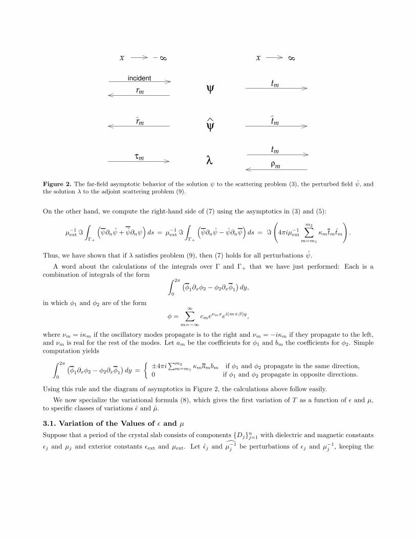
Figure 2. The far-field asymptotic behavior of the solution ψ to the scattering problem (3), the perturbed field ψ, andthe solution λ to the adjoint scattering problem (9).

On the other hand, we compute the right-hand side of (7) using the asymptotics in (3) and (5):

µ−1ext =

∫

Γ+

(ψ∂nψ + ψ∂nψ

)ds = µ−1

ext =

∫

Γ+

(ψ∂nψ − ψ∂nψ

)ds = =

(4πiµ−1

ext

m2∑

m=m1

κmtmtm

).

Thus, we have shown that if λ satisfies problem (9), then (7) holds for all perturbations ψ.

A word about the calculations of the integrals over Γ and Γ+ that we have just performed: Each is acombination of integrals of the form ∫ 2π

0

(φ1∂xφ2 − φ2∂xφ1

)dy,

in which φ1 and φ2 are of the form

φ =

∞∑

m=−∞cme

νmxei(m+β)y,

where νm = iκm if the oscillatory modes propagate is to the right and νm = −iκm if they propagate to the left,and νm is real for the rest of the modes. Let am be the coefficients for φ1 and bm the coefficients for φ2. Simplecomputation yields

∫ 2π

0

(φ1∂xφ2 − φ2∂xφ1

)dy =

±4πi

∑m2

m=m1κmambm if φ1 and φ2 propagate in the same direction,

0 if φ1 and φ2 propagate in opposite directions.

Using this rule and the diagram of asymptotics in Figure 2, the calculations above follow easily.

We now specialize the variational formula (8), which gives the first variation of T as a function of ε and µ,to specific classes of variations ε and µ.

3.1. Variation of the Values of ε and µ

Suppose that a period of the crystal slab consists of components Djnj=1 with dielectric and magnetic constants

εj and µj and exterior constants εext and µext. Let εj and µ−1j be perturbations of εj and µ−1

j , keeping the

boundaries of the domains Dj fixed. Then (8) gives

T ≈µext

2πκm

=n∑

j=1

[µ−1

j

∫

Dj

∇ψ · ∇λ dA − εjω2

∫

Dj

ψλ dA

]

=µext

2πκm

=n∑

j=1

[µ−1

j

(µjεjω

2

∫

Dj

ψλ dA −

∫

∂Dj

λ∂nψ ds

)− εjω

2

∫

Dj

ψλ dA

], (11)

in which “≈” means equal to leading (linear) order in the variations εj and µ−1j . The last equality is a result of

integration by parts.

3.2. Variation of the Boundaries

Now suppose that the constants εj and µj are fixed and that vj is a vector field on the boundary ∂Dj . Let h be

a small positive number, and let T + T be the transmission due to scattering by the perturbed crystal, in whichthe jth component has boundary defined by allowing ∂Dj to flow along the vector field vj for a distance of h.Then (8) gives

T =µext

2πκm

=n∑

j=1

∫

Dj

[±(µ−1

j − µ−1ext

)∇ψ · ∇λ ∓ (εj − εext)ω

2ψλ]dA + o(h),

where Dj is the region that passed from exterior to interior, in which case the upper sign is taken, or frominterior to exterior, in which case the lower sign is taken. Taking the limit as h → 0, we obtain the variationalgradient of T with respect to variations v = vj

nj=1 of the boundary ∂D:

δT

δ(∂D)= lim

h→0

T

h=

µext

2πκm

=

n∑

j=1

∫

∂Dj

[(µ−1

j − µ−1ext

)∇ψ ·∇λ − (εj − εext)ω

2ψλ]vj ·n ds (12)

3.3. Variation of Circular Components

We now specialize (12) further and take the ∂Dj to be circles and compute the gradient of T with respect totheir radii rj and centers (xj , yj). If we let vj = n, then vj · n = 1, and (12) gives

∂T

∂rj=

µext

2πκm

=

n∑

j=1

∫

∂Dj

[(µ−1

j − µ−1ext

)∇ψ ·∇λ − (εj − εext)ω

2ψλ]ds. (13)

Letting vj = ~ı, the unit normal vector pointing in the direction of the x-axis, and the vj = ~, the unit normalvector pointing in the direction of y-axis, we obtain

∂T

∂xj

=µext

2πκm

=n∑

j=1

∮

∂Dj

[(µ−1

j − µ−1ext

)∇ψ ·∇λ − (εj − εext)ω

2ψλ]dy, (14)

∂T

∂yj

= −µext

2πκm

=n∑

j=1

∮

∂Dj

[(µ−1

j − µ−1ext

)∇ψ ·∇λ − (εj − εext)ω

2ψλ]dx, (15)

where the integration is taken counter-clockwise.

4. NUMERICAL METHODS

In this Section, we describe the algorithm and numerical methods by which we alter and optimize resonantbehavior in a crystal slab and present an example. The basic algorithm goes as follows:

1. Start with a structure whose transmission coefficient T (β, ω) exhibits resonant features to be optimized.

2. Choose a set of frequencies and directions in which the transmission or extrema in the transmission coeffi-cient should move.

3. Find the variational gradient of the transmission with respect to the structural parameters.

4. Compute the smallest change in the parameters that gives the desired change in the transmission.

5. Increment the structure by the computed amount.

6. Update the set of frequencies if necessary.

7. Go back to 3.

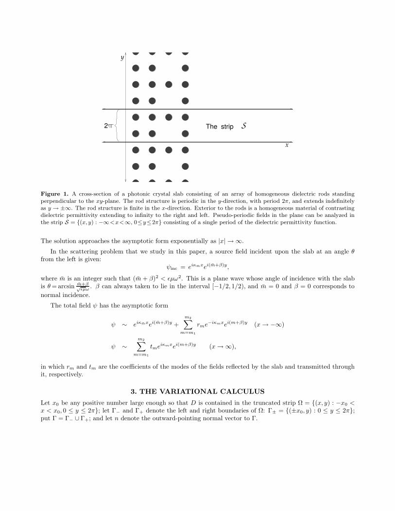
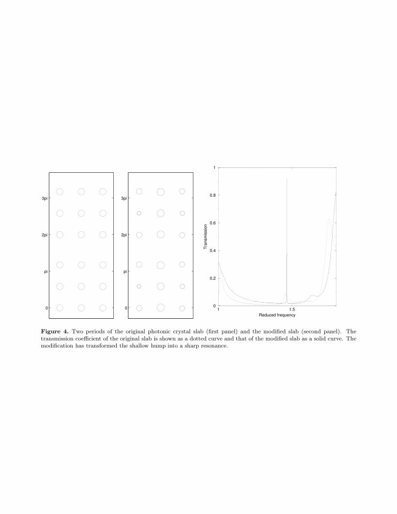
In our example, we begin with a square lattice of circular dielectric rods with ε = 12 and µ = 1 in air(ε = µ = 1), truncated to a slab three rods thick (Fig. 4), with a periodic channel running through it. Thechannel is created by adding an additional horizontal strip of air space between every three rows of rods. Thus,the new period in the y-direction is the “supercell” consisting of a 3×3 array of rods plus the additional horizontalstrip.

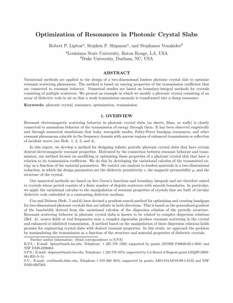
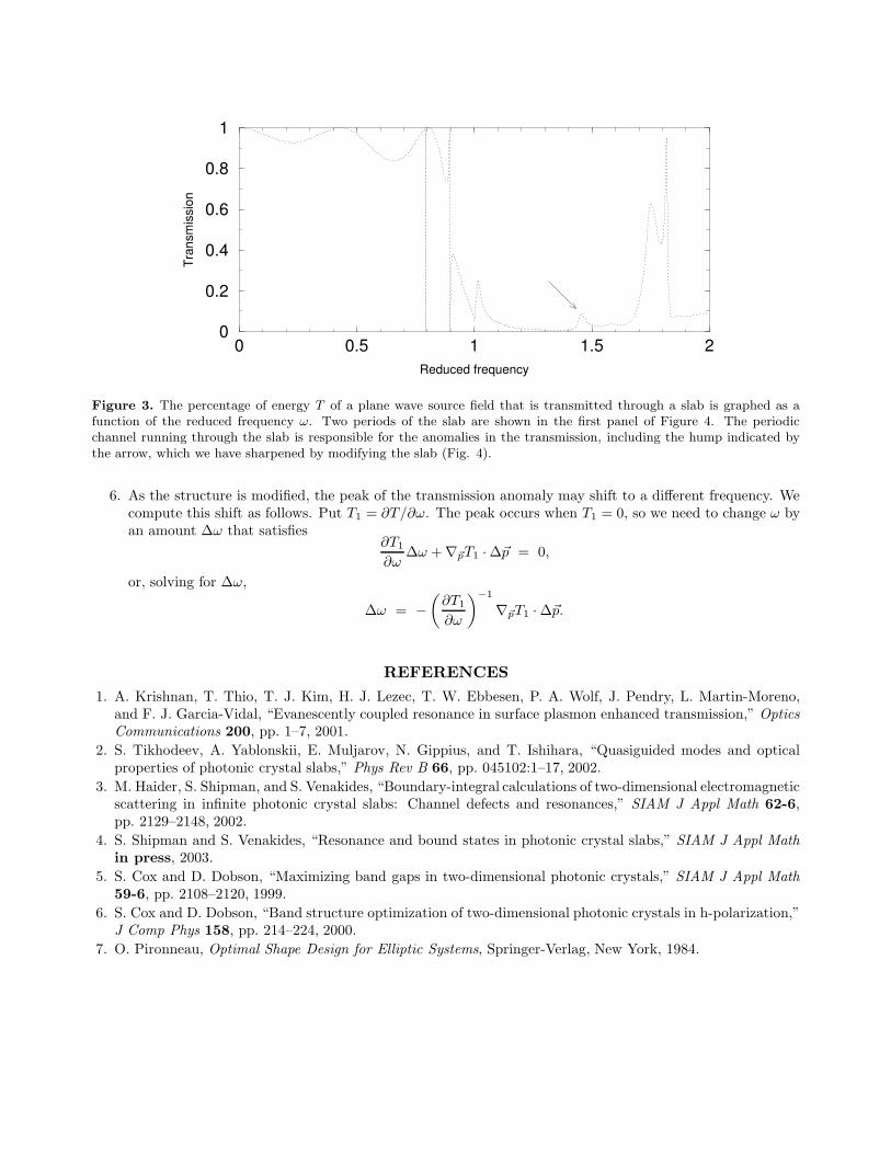
Figure 3 shows the transmitted energy through the initial structure as a function of frequency, where thesource field is a plane wave normally incident to the slab from the left. The region of low transmission fromabout ω = 0.9 to about ω = 1.7 coincides approximately with the bandgap for the initial square lattice. Theperiodic channel is the cause of the anomalous features—sharp spikes and the shallow hump, marked with anarrow, at the right end of the region. This hump corresponds to a mode going through the channel (see Ref. 3 forsome discussion on such modes). We wish to modify the rod structure so as to sharpen this resonant scatteringbehavior, leaving the angle of incidence fixed. Figure 4 shows the modified structure and the resulting resonantspike in the transmission coefficient.

We use this example to explain our numerical methods for carrying out the algorithm.

1. To compute the transmission coefficient, we must solve the scattering problem (3), or equivalently (1),numerically. We do this using the method of boundary integrals based on Green’s identities and thepseudo-periodic Green’s function. Details can be found in Ref. 3.

2. We choose the frequency at which the peak of the transmission anomaly occurs, where we seek to increasethe transmission, and two neighboring frequencies, where we seek to decrease the transmission.

3. We choose to restrict our admissible structures to arrays of circular rods with a fixed dielectric contrastof 12. Our design variables are the radii and centers of the rods. We compute the variational gradientby solving the scattering problems (3) and (9) numerically and computing the integrals (13), (14), and(15). We denote the gradient of the transmission with respect to these parameters by ∇~pT , where ~p is the27-dimensional vector of (x, y)-coordinates of the centers and the radii of the nine rods in the supercell.

4. Let M denote the 3 × 27 matrix whose rows are equal to ∇~pT at the three chosen frequencies, and let ~bdenote the vector of desired increments in T at these frequencies. We compute the smallest vector ∆~p thatproduces the change ~b by solving the 3 × 3 system

MM t~x = ~b

for x and putting∆~p = M t~x.

0 0.5 1 1.5 2Reduced frequency

0

0.2

0.4

0.6

0.8

1

Tran

smis

sion

Figure 3. The percentage of energy T of a plane wave source field that is transmitted through a slab is graphed as afunction of the reduced frequency ω. Two periods of the slab are shown in the first panel of Figure 4. The periodicchannel running through the slab is responsible for the anomalies in the transmission, including the hump indicated bythe arrow, which we have sharpened by modifying the slab (Fig. 4).

6. As the structure is modified, the peak of the transmission anomaly may shift to a different frequency. Wecompute this shift as follows. Put T1 = ∂T/∂ω. The peak occurs when T1 = 0, so we need to change ω byan amount ∆ω that satisfies

∂T1

∂ω∆ω + ∇~pT1 · ∆~p = 0,

or, solving for ∆ω,

∆ω = −

(∂T1

∂ω

)−1

∇~pT1 · ∆~p.

REFERENCES

1. A. Krishnan, T. Thio, T. J. Kim, H. J. Lezec, T. W. Ebbesen, P. A. Wolf, J. Pendry, L. Martin-Moreno,and F. J. Garcia-Vidal, “Evanescently coupled resonance in surface plasmon enhanced transmission,” Optics

Communications 200, pp. 1–7, 2001.

2. S. Tikhodeev, A. Yablonskii, E. Muljarov, N. Gippius, and T. Ishihara, “Quasiguided modes and opticalproperties of photonic crystal slabs,” Phys Rev B 66, pp. 045102:1–17, 2002.

3. M. Haider, S. Shipman, and S. Venakides, “Boundary-integral calculations of two-dimensional electromagneticscattering in infinite photonic crystal slabs: Channel defects and resonances,” SIAM J Appl Math 62-6,pp. 2129–2148, 2002.

4. S. Shipman and S. Venakides, “Resonance and bound states in photonic crystal slabs,” SIAM J Appl Math

in press, 2003.

5. S. Cox and D. Dobson, “Maximizing band gaps in two-dimensional photonic crystals,” SIAM J Appl Math

59-6, pp. 2108–2120, 1999.

6. S. Cox and D. Dobson, “Band structure optimization of two-dimensional photonic crystals in h-polarization,”J Comp Phys 158, pp. 214–224, 2000.

7. O. Pironneau, Optimal Shape Design for Elliptic Systems, Springer-Verlag, New York, 1984.

0

pi

2pi

3pi

0

pi

2pi

3pi

1 1.5Reduced frequency

0

0.2

0.4

0.6

0.8

1

Tran

smis

sion

Figure 4. Two periods of the original photonic crystal slab (first panel) and the modified slab (second panel). Thetransmission coefficient of the original slab is shown as a dotted curve and that of the modified slab as a solid curve. Themodification has transformed the shallow hump into a sharp resonance.