WAVE INDUCED OSCILLATIONS IN HARBORS OF ARBITRARY SHAPE Jiin - Jen Lee Project Supervisor: Fredric Raichlen Associate Professor of Civil Engineering Supported by U. S. Army Corps of Engineers Contract No. DA - 22 - 079 - CIVENG - 64 - 11 W. M. Keck Laboratory of Hydraulics and Water Resources Division of Engineering and Applied Science California Institute of Technology Pasadena, California Report No. KH - R - 20 December 1969

Welcome message from author
This document is posted to help you gain knowledge. Please leave a comment to let me know what you think about it! Share it to your friends and learn new things together.
Transcript
WAVE INDUCED OSCILLATIONS IN HARBORS
O F ARBITRARY SHAPE
J i in- J e n Lee
P r o j e c t Supervisor:
F r e d r i c Raichlen Assoc ia te P r o f e s s o r of Civil Engineering
Supported by U. S. A r m y Corps of Engineers
Contract No. DA-22-079-CIVENG-64-11
W. M. Keck Labora tory of Hydraul ics and Water Resources Division of Engineering and Applied Science
California Inst i tute of Technology Pasadena , California
Repor t No. KH-R-20 December 1969

. . 11
ACKNOWLEDGMENTS
The writer wishes to express his deepest gratitude to his thesis
advisor, Professor Fredr ic Raichlen, who suggested this research
problem and offered the most valuable guidance and encouragement
throughout every phase of this investigation. The advice and encour -
agement oi Professors Vito A. Vanoni and Norman H. Brooks a r e also
deeply appreciated.
The writer also wishes to express his appreciation to Professors
Theodore Y. T. Wu, Thomas K. Caughe~, Herbert B. Keller, and
Donald S. Cohen for the helpful discussions during the development of
the theoretical analysis of this problem. The help f rom Profes sox
James J. Morgan and Mr. Soloukid Pourian in developing the technique
for controlling corrosion of the wave energy dissipators i s very much
appreciated.
The writer i s deeply indebted to Mr. Elton F. Daly, supervisor
of the shop and laboratory, for his assistance and patient instruction in
both designing and building the experimental se t up. Appreciatim i s
also due Robert L. Greenway who assisted with the construction of the
experimental apparatus; Mr. Albert F. W. Chang who assisted i n the
computer programming; Mr. Joseph L. Hammack who assisted in
performing experiments and reducing data; Mes s r s. George Chan,
Yoshiaki Daimon, and Claude Vidal who assisted in data reduction;
Mr. Carl Green who prepared the drawings; Mr. Carl Eastvedt who
did the photographic work; Mrs. Arvilla I?. Krugh who typed thc

... 111
manuscript; and Mrs. Pat r ic ia Rankin who offered many valuable
suggestions in preparing the manuscript. The wri ter also wishes to
express his s incere appreciation to h is officemate, Mr. Edmund A.
Prych, for friendly and helpful advice during the l as t three years.
This resea rch was supported by the U. S. Army corps of Engineers
under Contract DA-22-079- CIVENG-64- 11. The experiments were
conducted in the W. M. Keck Laboratory of Hydraulics and Water
Resources at the California Institute of Technology.
Except for Appendix V, this repor t was submitted by the wri ter in
November, 1969, a s a thesis with the same title to the California
Institute of Technology in part ial fulfillment of the requirements for the
degree of Doctor of Philosophy in Civil Engineering.

ABSTRACT
Theoretical and experimental studies were conducted to
investigate the wave induced oscillations in an arbitrary shaped
harbor with constant depth which i s connected to the open-sea.
A theory termed the "arbitrary shaped harbor" theory i s
developed. The solution of the Helmholtz equation, v2f + kaf = 0,
i s formulated as an integral equation; an approximate method is
employed to solve the integral equation by converting i t to a matrix
equation. The final solution i s obtained by equating, at the harbor
entrance, the wave amplitude and i ts normal derivative obtained f rom
the solutions for the regions outside and inside the harbor.
Two special theories called the circular harbor theory and the
rectangular harbor theory a re also developed. The coordinates inside
a c i r r i ~ l a r a n d a rectangular harbor a re separable: therefore, the
solution for the region inside these harbors i s obtained by the method
of separation of variables. For the solution in the open- sea region,
the s m e method i s used as that employed for the arbitrary shaped
harbor theory. The f i n d solution i s also obtained by a matching
prnceihlre s i m i l a r t n that i l s e d f n r the arhitrary s h a p e d harbor theory.
These two special theories provide a useful analytical check on the
arbitrary shaped harbor theory.
Experiments were conducted to verify the theories in a wave
basin 15 ft wide by 3 1 ft long with an effective system of wave energy
dissipators mounted along the boundary to simulate the open-sea
condition.
Four harbors were investigated theoretically and experimentally:
0 circular harbors with a lo0 opening and a 60 opening, a rectangular
harbor, and a model of the East and West Basins of Long Beach Harbor
located in Long Beach, California.
Theoretical solutions for these four harbors using the arbitrary
shaped harbor theory were obtained. In addition, the theoretical
solutions for the circular harbors and the rectangular harbor using the
two special theories were also obtained. In each case, the theories
have proven to agree well with the experimental data.
It i s found that: ( 1) the resonant frequencies for a specific
harbor a r e predicted correctly by the theory, although the amplification
factors at resonance a re somewhat larger than those found experi-
mentally, (2) for the circular harbors, as the width of the harbor
entrance increases, the amplification at rcsonance dccrcsses , but the
wave number bandwidth at resonance increases, ( 3 ) each peak in the
curve of entrance velocity vs incident wave period corresponds to a
distinct mode of resonant oscillation inside the harbor, thus the
velocity at the harbor entrance appears to be a good indicator for
r a sollance in harbor s of complicatecl shape, (4) the results show that
the present theory can be applied with confidence to prototype harbors
with relatively uniform depth and reflective interior boundaries.

TABLE OF CONTENTS
Chapter
1. INTRODUCTION
2. LITERATURE SURVEY
2. 1 Wave Oscillations in Harbors of Simple Shape
2.2 Wave Oscillations in Harbors of Complex Shape
3. THEORETICAL ANALYSIS FOR AN ARBITRARY SHAPED HARBOR
3. 1 Development of the Helmholtz Equation
3 . 2 Solution of the Helmholtz Equation for an Arbitrary Shaped Harbor
3 . 2 . 1 Wave function inside the harbor (Region I1 )
3 . 2 . 2 Wave function outside the harbor (Region I)
3 . 2 . 3 Matching the solution for each region at the harbor entrance
3 . 2 . 4 Velocity at the harbor entrance
3. 3 The Numerical Analysis
Rcgion 11: Evaluation of matrices defined in Eq. 3. 15
Region 11: Method of solution for wave function fz
Region I: Evaluation of matrix H defined in Eq. 3 . 3 3
Harbor Entrance: Matching procedure
Page
1
4
4
10
15
15
2 0
2 2
3 0
3 6
3 8
4 1
4 1
48
49
5 0

TABLE O F CONTENTS (Cont'd)
Chapter Page - 3. 4 Confirmation of the Numerical Analysis 5 1
3.4. 1 The f i r s t example: a circle 5 3
3.4.2 The second example: a square 5 9
4. THEORETICAL ANALYSIS FOR TWO HARBORS WITH SPECIAL SHAPES 6 2
4. 1 Theoretical Analysis for a Circular Harbor 6 3
4, 1. 1 Wave function inside the circular harbor 63
4. 1.2 Wave function outside the circular harbor 7 0
4. 1. 3 Matching the solution for each region at the harbor entrance 7 3
4. 2 Theoretical Analysis for a Rectangular Harbor 7 5
4.2. 1 Wave function inside the rectangular harbor 7 6
4.2.2 Matching the solution for each region a t the harbor entrance 8 0
5. EXPERIMENTAL EQUIPMENT AND PROCEDURES 82
5. 1 Wave Basin 8 2
5.2 Wave Generator
5.3 Measurement of Wave Period
5.4 Measurement of Wave Amplitude 87
5.4. 1 Wave gage 8 7
5.4.2 Measurement of standing wave amplitude 92 for the closed harbor

- viii -
TABLE O F CONTENTS (Cont'd)
Chapter Page
5. 5 Measurement of Velocity 9 3
5.6 Wave Energy Dissipating System 9 7
5.7 Harbor Models 102
5.8 Instrument Carriage and Traversing Beam 106
6. PRESENTATION AND DISCUSSION OF RESULTS 110
6. 1 Characteristics of the Wave Energy Dissipation System
6.2 Cigcular Harbor With a lo0 Opening and a 60 Opening 118
6. 2. 1 Introduction 118
6.2.2 Response of harbor t o incident waves 119
6.2 .3 Variation of wave amplitude inside the harbor: comparison of experiments and theory 132
6.2.4 Variation of wave amplitude inside the harbor for the modes of resonant oscillation 150
6.2. 5 Total velocity at the entrance of the circular harbor 172
6. 2. 5 . 1 Introduction 172
6. 2. 5. 2 Velocity distribution in a depthwise direction 175
6.2. 5. 3 Velocity distribution across the harbor entrance 179
6.2. 5.4 Velocity at the harbor entrance as a function of wave number parameter, ka 1 8 4

TABLE O F CONTENTS (Cont 'd)
Chapter
Rectangular Harbor
6.3. 1 Introduction
6.3.2 Response of ha rbo r to incident waves
A Harbor With Complicated Shape : A Model of the E a s t and Wes t Bas ins of Long Beach Harbor
6.4. 1 Introduction
6 . 4. 2 Respunse 01 harbvr to iilcirlent waves
6. 4. 3 Variat ion of wave ampli tude inside the h a r b o r f o r one mode of r e sonan t osci l la t ion
6 . 4. 4 Velocity a t the h a r b o r en t rance a s a function of wave number p a r a m e t e r , k a
7. CONCLUSIONS
LIST O F REFERENCES
LIST O F SYMBOLS
APPENDIX I: WEBER'S SOLUTION O F THE HELMHOLTZ EQUATION
APPENDIX 11: DERIVATION O F EQ. 3. 12
APPENDIX 111: EVALUATION O F THE FUNCTIONS f j o 9 fyo, Jc3 AND Yc
APPENDIX IV: SUMMARY O F THE STROKES O F THE WAVE MACHINE USED IN EXPERIMENTAL STUDIES
APPENDIX V: COMPUTER PROGRAM
Page
192
192
19 3
197
197
200
2 10
2 13
2 17
223
23 1
237
245
249
253
254

LIST O F FIGURES
-Numb e r Description Page
3. 1 Definition sketch of the coordinate system 16
3.2 Definition sketch of an arbi t rary shaped harbor 2 1
3.3 Definition sketch of the harbor boundary approximated by straight-line segments 2 7
3.4 Change of derivatives f rom normal to tangential direction 43
3. 5 Definition sketch of a circular domain 5 4
3.6 Definition sketch of a square domain 54
4. 1 Definition sketch of a circular harbor 6 5
4.2 Definition sketch of a rectangular harbor 7 7
5. 1 Drawing of the wave basin and wave generator (modified f rom Raichlen (1965) )
5.2 Overall view of the wave basin and wave generator with wave f i l ter and absorbers in place 8 3
5.3 Wave generator and overhead support with wave filter and wave absorbers in place 8 5
5.4 Motor drive, eccentric, and light source and perforated disc for wave period measurement
5. 5 Schematic diagram and circuit of photo- cell device (from Raichlen (1965) ) 8 8
5.6 Drawing of a typical wave gage (from Raichlen ( 1965) )
5. 7 Circuit diagram for wave gages (from Raichlen (1965) )
-xi-
LIST O F FIGURES (Cont'd)
Number Description
5. 8 Typical calibration curves of a wave gage
5.9 Photograph of a hot-film sensor (from Raichlen (1967) )
5. 10 Hot-film anemometer, linearizer, and recording unit
5. 11 Wave energy dissipators placed in the basin
5. 12 Section of wave filter
5. 13 Bracket and structural f rame for supporting wave absorbers
5. 14 False-walls and supporting frames representing the "coastline"
5. 15 Rectangular harbor in place in the basin
5. 16 Circular harbor with a 10' opening
5. 17 Circular harbor with a 60° opening
5. 18 Model of the East and West Basins of Long Beach Harbor (Long Beach, California)
5. 19 Map sllowing the pvsition of the East anif West Basins of Long Beach Harbor and the model planform. (The harbor model i s shown with dashed lines. )
5.20 Instrument carriage and traversing beam shown mounted above lo0 opening circular harbor
6. 1 Reflection coef. , Kr, as a function of the incident wave steepness, Hi/L, for Dissipator A (m=38)
6 . 2 Reflection coef. , Kr, as a function of the incident wave steepness, Hi/L, for Dissipator B (rn=50)
6.3 The variation of the measured reflection coef., Kr, with the measured transmission coef. , Kt, for various wave dissipators
Page
9 1

LIST O F FIGURES (Cont'd)
Number
6.4
Description Page
0 'Response. curve of the circular harbor with a 10 opening at the center 12 1
0 Response curve of the circular harbor with a 10 opening at r = O . 7 ft, 0=45O 122
Response curve of the circular harbor with a 60' uper~irrg a1 the ceriler 125
Response curve of the circular harbor with a 60° opening at r=O. 7 f t , 6=45O 126
Wave amplitude distribution inside the circular harbor with a 10° opening for ka=O. 502 133
Wave amplitude distribution inside the circular harbor with a 10° opening for ka= 1. 988 136
Wave amplitude distribution inside the circular harbor with a lo0 opening for ka=3. 188 137
Comparison of wave amplitude distribution along r = O . 7 f t for the circular harbor with a 10° opening for three different incident wave amplitudes (ka=3. 188) 139
Wave amplitude distribution along s ix fixed angular positions inside the circular harbor with a 100 opening for ka=3.89 1 14 1
Wave amplitude distribution inside the circular harbor with a 100 opening for ka=3. 89 1 142
Wave amplitude distribution inside the circular harbor with a 60° opening for ka=O. 540 143
Wave amplitude distribution inside the circular harbor with a 60° opening for ka=Z. 153 145
Wave amplitude distribution inside the circular harbor with a 600 opening for ka=3.38 147
Wave amplitude distribution inside the circular harbor with a 600 opening for ka=3.953 148
Contour drawings of water surface elevation for three modes of f r ee oscillation in a closed circular basin 153

LIST O F FIGURES (Cont'd)
Description Page Number
6. 19 Contour drawing and photographs showing the water surface for the circular harbor with a lo0 opening, Mode No. 1, ka=0.35
Contour drawing and photographs showing the water surface for the circular harbor with a 60° opening, Mode No. 1, ka=0.46
Contour drawing and photographs showing the water surface for the circular harbor with a lo0 opening, Mode No. 2, ka= 1.99
Contour drawing and photographs showing the water surface for the circular harbor with a 60° opening, Mode No. 2, ka=2. 15
Contour drawing and photographs showing the water surface for the circular harbor with a lo0 opening, Mode No. 3, ka=3. 18
Contour drawing and photographs showing the water surface for the circular harbor with a 60° opening, Mode No. 3, ka=3.38
Contour drawing and photographs showing the water surface for the circular harbor with a lo0 opening, Mode No. 4, ka=3.87
Contour drawing and photographs showing the water surface for the circular harbor with a 600 opening Mode No. 4, ka.=3. 96
Typical record of the wave amplitude and of the velocity after using the linearizing circuit
Velocity distribution in a depthwise direction at the entrance of the circular harbor with a lo0 opening
Velocity distribution across the entrance of the circular harbor with a 100 opening
Velocity distribution across the entrance of the circular harbor with a 60° opening
Total velocity at the harbor entrance as a function of ka for the circular harbor with a lo0 opening

LIST OF FIGURES (Cont'd)
Description Page
'Velocity at the harbor entrance as a function of ka: 0 comparison of theory and experiment (10 opening
circular harbor)
Total velocity at the harbor entrance as a function of ka for the circular harbor with a 600 opening
Velocity a t the center of the harbor entrance as a function of ka: comparison of theory and experiment (60° opening circular harbor)
Response curve for a fully open rectangular harbor
The model of the East and West Basins of Long Beach Harbor, Long Beach, California
Response curve at point A of the Long Beach Harbor model
Response curve at point B of the Long Beach Harbor model
Response curve at point C of the Long Beach Harbor model
Response curve at point D of the Long Beach Harbor model
Response curve of the maximum amplification for the model of Long Beach Harbor compared with the data of the rnodcl study by Knspp and Vanoni (1945)
The theoretical wave amplitude distribution in the Long Beach Harbor model Ika=3.38)
Wave amplitude distribution inside the harbor model of Knapp and Vanoni (1945) for six minute .waves (ka=3.30) (see Knapp and Vanoni (1945), p. 133)
Total velocity at the harbor entrance as a function of ka for the Long Beach Harbor model

LIST O F FIGURES (Cont'd)
,Number 'Description
A. 1. 1. Definition sketch for a hounded domain
A. 1.2 Definition sketch for an unbounded domain
A. 2. 1 Definition sketch for an interior point approaching a boundary point of a smooth curve
A. 2. Z Definition sketch for an interior point approaching a corner point a t the boundary
Page
2 44

Number Description Page
3. 1 Comparison of the approximate solution with the theoret ical solution of the Helmholtz equation in a c i rcular domain. 5 7
3 . 2 Comparison of the approximate solution with the theoret ical solution of the Helmholtz equation i n a square domain. 6 0
6. 1 Model wave energy dissipators 113

CHAPTER 1
INTRODUCTION
1.1 BACKGROUND
A natural or an artificial harbor can exhibit frequency- (or
period-) dependent water surface oscillations when exposed to incident
water waves in a way which is similar to the response of mechanical
and acoustical systems which a re exposed to exterior forces, pressures
o r displacements. For a particular harbor, i t i s possible that for
certain wave periods the wave amplitude at a particular location inside
the harbor may be much larger than the amplitude of the incident wave,
whereas for other wave periods significant attenuation may occur at the
same location. This phenomenon of harbor resonance has generally
been thought to be caused by waves f rom the open-sea incident upon
the harbor entrance, although other possible excitations may be earth-
quakes, local winds, and local atmospheric pressure anomalies, etc.
These resonant oscillations (also termed s eiche and harbor
surging) can cause significant damage to moored ships and adjacent
structures. The ship and i ts mooring lines also constitu*e a dynamic
system; therefore, if the period of resonant oscillation of the harbor
i s close to that of the ship-mooring system, an extremely serious
problem could result. In addition, the currents induced by this
oscillation can cause navigation hazards.

- 2 -
There have been natural and artificial harbors in various
locations around the world where r e sonant oscillations have occurred
and have caused damage to ships and dockside facilities, e. g. Table
Bay Harbor, Cape Town, South Africa; Monterey Bay, California and
Marina del Rey, Los Angeles, California. In order to correct an
existing resonance problem one must f i r s t be able to predict the
response of that particular harbor to incident waves, i. e. the expected
wave amplitude at various locations within the harbor for various wave
periods, so that the effect of any change of the interior can be investi-
gated. Until quite recently such a study was done using a hydraulic
model alone. If an acceptable analytical solution of the problem could
be developed i t could be used in conjunction with a hydraulic model to
prnvide n g ~ i i d e for the most effective and efficient use of the laboratory
model.
1.2 OBJECTIVE AND SCOPE O F PRESENT STUDY
The major objective of this study i s to investigate, both
theoretically and experimentally, the response of an arbitrary shaped
harbor of constant depth to periodic incident waves. The harbors a r e
considered to be directly connected to the open-sea with no artificial
boundary condition imposed at the harbor entrance. The laboratory
experiments a r e conducted in order to verify the theoretical solution
for different harbors.

In Chapter 2 previous studies of the harbor resonance p~ob lem
a re surveyed. A theoretical analysis i s presented in Chapter 3 by
which one may predict the response of an arbitrary shaped harbor of
constant depth to incident wave system. In Chapter 4 a theoretical
analysis is presented for two harbors with special shapes: a circular
harbor and a rectangular harbor. These analyses provide theoretical
results which can be compared to those of the general theory developed
in Chapter 3 . In Chapter 5 the experimental equipment and procedures
a re described. The experimental and theoretical results a re presented
and discussed in Chapter 6. Conclusions a re stated in Chapter 7.
CHAPTER 2
LITERATURE SURVEY
2.1 WAVE OSCILLATIONS I N HARBORS O F SIMPLE SHAPE
A significant amount of work has been done on resonant
oscillations i n harbors of idealized planform such as a circular harbor
or a rectangular harbor. The methods of approach used for solving
these problems ranged from imposing a prescribed boundary condition
at the harbor entrance to matching, a t the harbor entrance, the solution
obtained for the regions inside and outside the harbor.
McNown ( 1 9 5 2 ) studied both theoretically and experimentally some
of the response characteristics of a circular harbor of constant depth
excited by waves incident upon a small entrance gap. The analysis was
to solve Laplace's equation:
with certain prescribed boundary conditions. The boundary conditions
used included the linearized f r ee surface condition at thc watcr eurfscc
and the condition that the velocity normal to all solid boundaries was
zero. However, the assumption was made at the harbor entrance that
the c res t of a standing wave occurred at the entrance when the harbor
was in resonance and the water surface remained essentially horizontal
across the small entrance. Thus, for resonant motion, this hypotheses

-5 -
led to a boundary condition identical to that for a completely closed
circular basin. Therefore, the wave frequencies associated with
resonant oscillations would bc thosc cigcnvalucs for thc frcc oscillation
of a circular basin. Based on this assumption, McNown computed the
amplitude variation inside the harbor for various modes of oscillation
and found the theoretical results compared reasonably well with the
experiments. This imposed condition at the harbor entrance i s not
satisfactory in the sense that the slope of the water surface at the
harbor entrance should be part of the solution of the problem and
should not be imposed initially. However, i t can be shown that the
resonant frequencies (or the wave numbers) associated with the circular
harbor a r e indeed close to that for the f ree oscillation in the closed
L a s i l l il llle erltr auce ia v e r y sn~al l .
Using the same idea of assuming an antinode at the harbor
entrance for resonant oscillation, Kravtchenko and McNown ( 1955) have
studied seiche (wave oscillations) in a rectangular harbor. In that
study the definition of resonance was similar to that used by McNown
(19521, i. e. the modes of oscillation corresponding to the closed basin
configuration were termed resonant all others termed non-resonant.
For non-resonant oscillations the boundary condition, at the harbor
entrance would have to be determined from observations in the
laboratory.
Extending McNown's work for circular harbors, ( 1954,
1957) investigated, both experimentally and theoretically, the problem
of the rectangular harbor with a wide entrance. Both the experimental

- 6 -
and mathematical models consisted of a rectangular harbor with an
asymmetric entrance to which a relatively long wave channel was
connected. A theoretical solution was obtained for the amplitude
distribution within the partially closed harbor by matching up the
entrance velocities between the two domains: the harbor and the
attendant wave channel. Good agreement was found between the
theoretical solution and the experimental data. However, the solution
obtained was not for the more realistic problem of a harbor connected
directly to the open-sea.
Biesel and LeMehaute (1955, 1956) and LeMehaute (1960, 1961)
studied the resonant oscillations in rectangular harbors with various
types of entrances: fully open, partially open, change in depth at the
entrance and combinations of these as well as a sloping beach inside
the harbor. The harbor was connected to a wave basin having a width
less than half of a wave length and an infinite length in the direction
of wave propagation. The method which was used was based on
complex number calculus with a direct application of the superposition
of Wle various incidenl, refleeled, and transmitted waves. An
expression was developed for the amplification factor (defined as the
wave amplitude at the rear of the harbor to the incident wave
amplitude). However, in order to use that result an empirical
reflection coefficient and attenuation parameter a r e needed, in general
the values of these parameters a re not obvious.
The problem of a rectangular harbor connected directly to the
open-sea has been ably treated, theoretically, by Miles and Munk ( 196 1).
Their work was an important contribution since i t included the effect of

-7 -
the wave radiation from the harbor mouth to the open-sea. This
effect limits the maximum wave amplitude within the harbor for
the invicid case to a finite value even at resonance. They considered
an arbitrary shaped harbor and formulated the problem as an integral
equation in terms of a Green's function. This
g(x, y, s), must satisfy the Helmholtz equation
and have a vanishing normal derivative on the
Green's function ,
inside the harbor:
boundary of the harbor
except at the entrance where the normal derivative of the Green's
function i s a delta function. Unfortunately, as they have noted, the
Green's function for an arbitrary shaped harbor i s beyond reach. Thus,
they have applied this general formulation to a harbor of simple shape:
a rectangular harbor, and found most interestingly that a narrowing of
the harbor entrance leads not to a reduction in harbor surging
(oscillation), but to an enhancement. This result was termed by them
the "harbor paradox". At that time, there were considerable
differences in opinion a s to the existance of the paradox. LeMehaute
(1962) suggested that if it had been possible to introduce the effect of
viscous dissipation into the anlysis the paradox would become invalid.
(However, the present study on circular harbors, both theoretically
and experimentally, has supported the ''harbor paradoxt', although
the experimental data also show that viscous dissipation of energy i s
most important for harbors with small openings. (see Subsection
6.2.2). )

-8-
Ippen and Raichlen (1962) and Raichlen and Ippen (1965) have
studied, both theoretically and experimentally, the wave induced
oscillations in a smaller rectangular harbor connected to a larger
highly reflective rectangular wave basin. The solution was obtained
by solving the boundary value problem in both regions, i. e. the region
inside the harbor and the region in the wave basin, using the matching
condition that the water surface is continuous at the harbor entrance.
Because of the high degree of coupling between the small rectangular
harbor and its attendant wave basin the response characteristics of
the harbor as a function of incident wave period were radically different
from a similar prototype harbor connected to the open-sea. The
former was characterized by a large number of closely spaced spikes
as opposed to the latter that would have discrete resonant modes of
oscillation. Those results most emphatically demonstrated the
importance of adequate energy dissipators in the model system when
investigating resonance of a harbor connected to the open-sea. It was
pointed out that in order to reduce the coupling effect of the reflections
of Lhe wave energy w h i c h i s radiated from the harbor entrance,
efficient wave absorbers and wave filters in the main wave basin a re
necessary. A subsequent study by Ippen, Raichlen and Sullivan (1962)
showed that the coupling effect i s indeed significantly reduced by the
use of artificial energy dissipators in the main wave basin.
Ippen and Goda (1963) also studied, both theoretically and experi-
mentally, the problem of a rectangular harbor connected to the open-
sea. In that analysis the waves radiated from the harbor entrance to

the open-sea were evaluated using the Fourier transformation method
which was different from the point source method employed by Miles
and Mnnk (1961). The solution inside the rectangular harbor w a s
obtained by the method of separation of variables and expressed in
te rms of the slope of water surface at the harbor entrance. The
solution in the open-sea region was obtained by superimposing the
standing wave and the radiated wave (also expressed in terms of the
slope of the water surface at the harbor entrance). Thus by matching
the wave amplitude, at the entrance, from the solutions in both
regions the final solution was obtained. Fairly good agreement was
found between the theory and the experiments conducted in a wave
basin (9 ft wide and 11 ft long) where satisfactory wave energy dissi-
patora wcrc inotdlcd around thc boundary t o simulatc thc "opcn oca".
These previous studies of the wave induced oscillations in a
harbor with a special shape have helped to understand some of the
characteristics of the harbor resonance problem. However, the
practical application of these studies is limited simply because i t i s
not probable that the shape of an actual harbor will be as simple as
those studied.
In the following section previous studies on harbors of more
complex shape will be surveyed.

- 10 -
2.2 WAVE OSCILLATIONS IN HARBORS O F COMPLEX SHAPE
Knapp and Vanoni (1945) conducted a hydraulic model study
in connection with the harbor improvements at the Naval Operating
Base, Terminal Island, California (The present East and West Basins
of Long Beach Harbor). The initial phase of that study helped to
choose the lroptimum" mole alignment and an extensive ser ies of
experiments was then conducted to completely determine the water
motions in the basin so defined. A harbor response in which the
r n ~ x i m u m vertical water motion anywhere within the basin was plotted
against incident wave period was obtained for a range of prototype wave
periods f rom 10 sec to 15 min. Contours of water surface elevation
throughout the basin were determined for various wave and surge
periods. These measurements have delineated the characteristic
modes of oscillation of the basin and established the regions of maxi-
mum and minimum motion in the basin. That study demonstrated the
need and the meri t of a model study to determine the location and the
magnitude of the amplification in a harbor of complex shape when
exposed to incident periodic waves.
Research and model studies on the surging problem in Table Bay
Harbor, Cape Town, South Africa were conducted by Wilson between
1942- 195 1. (That work was made known in two papers: Wilson, 1959,
1960. ) In that study Table Bay Harbor was shown to be affected by two
forms of surging, one of which was responsible for the ranging of
moored ships, the other for a pumping action of the basin and attendant
navigational hazard. These model studies helped to reduce the surging
inside the harbor.
-11-
Although model studies can provide many answers and a r e by fa r
still the most reliable way of obtaining information concerning the wave
induced oscillations i n harbors, they a r e generally very expensive. and,
most importantly, require a considerable amount of time. Therefore,
many researchers have searched for methods of theoretically analyzing
the wave induced oscillations in a harbor of arbitrary shape which
although perhaps not replacing the model tests at least provide a useful
guide for the experimental program.
Wilson, Hendrickson and Kilmer (1965) have studied the two -
dimensional and three-dimensional oscillations in an open basin of
variable depth. For the two-dimensional oscillation the method is
similar to oGne used earl ier by Raichlen (196513) in which attention i s
directed to free oscillations in a closed basin. In the analysis they
have assumed that the wave lengths a r e large compared to the water
depths; the equation of continuity combined with the linearized dynamic
f ree surface condition was written i n the form of a difference equation.
The periods of oscillation and the variation of the water surface
elevation within the harbor were obtained by solving for the eigenvalues
and eigenvector s of the resultant system of difference equations. How-
ever, in this approach, an artificial boundary condition was assumed
at the entrance to the harbor or bay. The boundary condition which
was used results either f rom an assumed nodal line at the entrance or
using certain observed amplitudes. Although this method of approach
gives some useful answers, i t i s not a complete solution to the problem.

-An ideal solution would automatically take care of the entrance
condition by matching the wave amplitudes and velocities at the harbor
entrance derived from solutions for the domain of the harbor and of
the open-sea.
Leendertse (1967) has developed a numerical model for the pro-
pagation of long-period waves in an arbitrary shaped basin. In that
study, the partial differential equations for shallow water waves
(continuity and linearized momentum equations) were replaced by a
difference equation to operate in spatial- and time- coordinates on
definite points of a grid system. The results agreed well with certain
field measurement; however, the water surface elevations at the open
boundary still must be given.
Most recently a study conducted by Hwang and Tuck ( 1969)
developed an analytical method to solve the harbor resonance problem
for harbors of arbitrary shape and constant depth connected to the
open- sea. Their method of approach i s to superimpose scattered
waves which a re caused by the presence of the boundary on the standing
wave system. The scattered waves are conlputed by a distribution
of sources (chosen as the Hankel function ~ ( " ( k r ) ) with an unknown 0
strength to be determined along the coastline and the boundary of the
L)
harbor. Thus the potential function rpt(x) at any point ;(x, y) in space
can be expressed as:

- 13-
3
where yo(x) represents the standing wave system and q(Go) i s the
source strength along the entire coastline which includes the boundary
4
of the harbor. The strength q(x ) was determined numerically such 0
that the boundary condition ?%= 0 was satisfied along the entire an
reflecting boundary. This method did not require a matching condition
at the harbor entrance; the calculation of the source strength q(<)
along the entire reflecting boundary must be terminated at some
-t
distance f rom the harbor entrance (q(x ) = 0 between that location and 0
-F - ) Physically, this implies that the influence of the source distri-
bution at some distance away from the entrance i s negligible; however,
for an arbitrary shaped harbor the position at which the source strength
becomes zero i s not obvious unless t r ia l calculations a r e made.
Although the theoretical solutions for wave induced oscillations
in harbors, especially for an arbitrary shaped harbor, a r e limited,
there i s a considerable amount of literature in other fields such as
optics, acoustics, electromagnetics, and mechanical vibrations which
deal with similar physical problems. Some of these studies which a re
pertinent a r e concerned with the scattering of acoustic waves by
surfaces of arbitrary shape (Friedman and Shaw (1962), Banaugh and
Goldsmith (1963 a, b), Shaw (1967), etc. ), sound radiation from an
arbitrary body o r vibrating surfaces (Chen and Schweikert ( 1963 ),
Chertock (1964), Copley (1967), Kuo (1968), etc. ), and the scattering
of electromagnetic waves by cylinders of arbitrary cross section
(Mullin, Sandburg, and Velline (1965), Richmond (1965), etc. ).

-14-
Mathematical equations which describe these problems a r e nearly
identical to those for the water wave problem. Thus, similar
analytical techniques may be used for the harbor resonance problem.
In fact, the investigation of Hwang and Tuck ( 1969) as well as this
independent study a r e closely related to some of the literature just
cited.

CHAPTER 3
THEORETICAL ANALYSIS FOR AN ARBITRARY SHAPED HARBOR
The theoretical solution for the wave induced oscillations in
an arbitrary shaped harbor with a constant depth i s presented in this
chapter. The solution to the boundary value problem i s formulated
as an integral equation, and an approximate method i s presented to
solve this integral equation by converting i t to a matrix equation
which can be solved using a high-speed digital computer. The final
solution i s obtained using a matching condition at the harbor entrance,
i , e. equating, at the harbor entrance, the wave amplitude and i ts
normal derivative obtained from the solutions in the regions outside
and inside the harbor. The numerical analysis i s described in this
chapter and examples are presented which confirm the numerical
techniques used; a comparison of the theoretical and experimental
results dealing with thc full problem of thc response of a harbor to
incident waves will be presented in Chapter 6.
3 . 1 DEVELOPMENT OF THE HELMHOLTZ EQUATION
In order to solve the problem mathematically, the flow
i s assumed irrotational so that a velocity potential I may be defined,
such that the fluid particle velocity vector can be expressed as the
3 + gradient of the velocity potential , i . e. u = V d , where t i i s the velacity
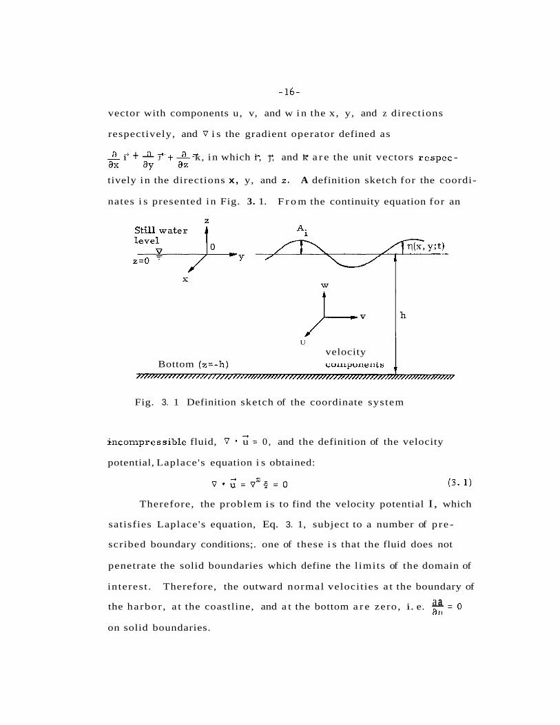
vector with components u, v, and w i n the x, y, and z directions
respectively, and V i s the gradient operator defined as
a + a * - a + + -+ -+ - i + - J + -k, in which i , j , and k a r e the unit vectors respec- ax ay a~ tively in the directions x, y, and z . A definition sketch for the coordi-
nates i s presented in Fig. 3. 1. F r o m the continuity equation for an
Fig. 3. 1 Definition sketch of the coordinate system
U
velocity Bottom (z=-h) r;ulnpur~erlts
--t
i.ncompressible fluid, V u = 0 , and the definition of the velocity
1-
potential, Laplace's equation i s obtained:
- ' 2 v e u = v @ = O (3 . 1)
Therefore, the problem is to find the velocity potential I, which
7 7 1 P ~ / / / m / / m R / / / / N / / 7 / / ~ ~
satisfies Laplace's equation, Eq. 3. 1, subject to a number of p re-
scribed boundary conditions;. one of these i s that the fluid does not
penetrate the solid boundaries which define the l imits of the domain of
interest . Therefore, the outward normal velocities a t the boundary of
a a the harbor , a t the coastline, and a t the bottom a r e zero, i. e. - = 0 an on solid boundaries.
- 17-
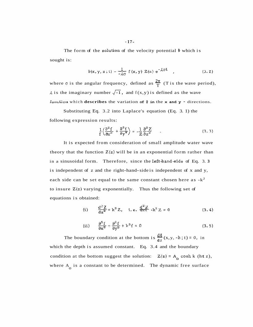
The form of the soluti-on of the velocity potential P, which i s
sought is:
2 TT where o i s the angular frequency, defined as - (T i s the wave period), T
,i, i s the imaginary number ,Jz, and f (x, y) i s defined as the wave
lurlclivrl w h i c h describes the variation of iP in the x and y - directions.
Substituting Eq. 3.2 into Laplace's equation (Eq. 3. 1) the
following expression results :
It i s expected from consideration of small amplitude water wave
theory that the function Z(z) will be in an exponential form rather than
in a sinusoidal form. Therefore, since the lefthand-side of Eq. 3. 3
i s independent of z and the right-hand- side i s independent of x and y,
each side can be set equal to the same constant chosen here a s -k2
to insure Z(z) varying exponentially. Thus the following set of
equations i s obtained:
d2 z (i) ==k2z, i . e . d a Z - k 2 ~ = 0 dza
dm The boundary condition at the bottom i s - (x, y, -h ; t ) = 0 , in d z
which the depth i s assumed constant. Eq. 3.4 and the boundary
condition at the bottom suggest the solution: Z(z) = A. cosh k (h t z),
where A i s a constant to be determined. The dynamic free surface 0

condition from small amplitude wave theory, neglecting surface
tension, can be combined with this expression and Eq. 3 .2 to give:
where q i s the wave amplitude a t the position (x, y ) and at the time t,
A. i s the wave amplitude a t the c res t of the incident wave (see Fig. 1
3. I ) , and g i s the acceleration of gravity.
A = - L
o cosh kh
Therefore, the function Z(z) in the velocity potential, Eq. 3 . 2 , can
be expressed as:
Aig cosh k(zSh) Z(z) = -
cosh kh
Thus the velocity potential 9 becomes :
1 Aig cosh k (zSh) - A d H (x,y, z ; t) = - cosh kh f ( x , ~ ) e A0 ( 3 . 8 )
Substituting Eqs. 3. 6 and 3. 8 into the linearized kinematic free
surf ace condition obtained from the small amplitude wave theory:
the well known "dispersion relation" for water waves i s obtained:
is2 = gk tanh (kh) . (3. 10)

The dispersion relation re la tes the wave frequency to the wave number
and the depth of the water; therefore, the a rb i t ra ry constant, k, used
in Eqs. 3.4 and 3. 5 is the w a v e i l u r n l e r , k, whicli appears in the
dispersion relation, where k is defined a s - 2n (L i s the wave length). L 7
In order to complete the expression for the velocity potential
@, i. e. Eq. 3.2, the main problem which remains i s to determine the
wave function f (x, y ) , which sat isf ies Eq. 3. 5, commonly known a s the
Helmholtz equation (Eq. 3. 5 is repeated he r e fo r clarity. ):
subject to the following boundary conditions:
(i) = 0 along all fixed boundaries such a s the coastline and
the boundary of the harbor (where n denotes the outward
normal f rom the boundary).
(ii) a s ,/xa t Y2 -+my there i s no effect of the harbor on the wave
system; this is defined a s the radiation condition. Physi-
cally, the radiation condition means that the outgoing
radiated wave emanating f rom the harbor entrance will
decay a t an infinite distance f rom the harbor. Mathernati-
cally, the radiation condition i s needed in order to ensure
a unique solution of wave function f (x, y ) in the unbounded
domain.
In the following section (Section 3 .2 ) the method for solving the
Helmholtz equation, Eq. 3. 5, for an a rb i t ra ry shaped harbor will be
presented, thereby allowing one to determine Lhe wave induced
oscillations i n such a harbor.
-20-
3 . 2 SOLUTION O F THE HELMHOLTZ EQUATION FOR AN
ARBITRARY SHAPED HARBOR
The procedure in the developinent of the theory of the
response of an arbitrary shaped harbor to incident wave systems i s
as follows:
(i) The domain of interest shown in Fig. 3.2 i s divided into
two regions: the infinite ocean region (Region I), and
tht: region bounded b y the limits of the harbor (Region 11).
The coastline which in part forms the shoreward limit of
Region I i s located along the x-axis and i s considered to
be perfectly reflecting and perpendicular to the bottom.
(ii) The wave function f, i s determined in Region I in terms
a t the harbor of the unknown normal derivative - 9n
entrance. Likewise, the wave function f2 i s evaluated
in Region I1 in terms of the unknown normal derivative
8% - at the harbor entrance. 8 11
(iii) The condition i s used that at the entrance the wave
amplitude and the slope of the water surface obtained
from the solution in Region I must equal to these quantities
obtained f rom the solution in Region 11, i. e. with reference
to Fig. 3 . 2 , at y=O in the region between A and 3, f, = f,
8% - af2 and -- - . This "continuity condition" i s used to an an
solve for the unknown normal derivatives of the wave
(Note that the function f , at the harbor entrance: an.

Region I (Open-sea)
v2f, s k2fl = 0
integration
Fig. 3.2 Definition sketch of an arbitrary shaped harbor

negative sign resul ts f rom the sign convention that the
outward normal to the domain of in teres t i s considered
to be positive. )
(iv) Once the normal derivative of the wave function af2 a t an the harbor entrance is obtained, the wave function f, i n
Region 11, i. e. inside the harbor, can then be evaluated.
In the Subsection 3 . 2 . 1, the solution of the wave function f2
inside the harbor is presented, followed by the solution of wave
function fl in the infinite ocean region presented i n Subsection 3. 2. 2.
In Subsection 3. 2 . 3 the procedure for matching the solutions a t the
harbor entrance i s shown, leading to the desired resul t of the
response of an a rb i t ra ry shaped harbor to incident wave systems.
3 . 2 . 1 Wave Function h s i d c thc Harbor (Rcgion 11)
In Region II Green's identity formula (see Appendix I,
Eq. A. 1. 1) i s applied and the Hankel function of the 1st kind and
zero o rder , ~ y ) ( k r ) , i s chosen to be the fundamental solution of the
two-dimensional Helmholtz equation, Eq. 3. 5. The function ~! ) (k r )
i s chosen because it satisfies the Helmholtz equation, and possesses
the proper type of singularity a t the origin, w h k h will be discussed.
Therefore, the wave function f, a t any position i n the domain of
interest can be expressed in integral fo rm a s a function of the value
af2 of f2 and the value of - a t the boundary. (This derivation has been an
discussed by Baker and Copson (1950) and i s r e fe r red to a s Weber's
solution of the Helmholtz equation; it i s presented i n Appendix I. )

3
f 2 (x i - -$SF, (z0)& ( ~ y ) ( k r ) ) - ~ : " (k r ) & (f, (gO))l .-I d ~ ( ; ~ ) (3. 11)
3 4
dhere: f, (x') i s the wave function f2 at the position x shown in Fig
Fig. 3. 2,
-+ x i s the position vector of the field point (x, y) inside the
harbor ,
f, (go) i s the wave function f, on the boundary a t the position
4
x i s the position vector of the source point (xo, yo) on the 0
boundary (the significance of the aource point will be
discussed presently),
3
af, (x0) i s the outward normal derivative of f, a t the boundary
an +
source point x 0'
r i s the distance between the field and source points,lxf - zoI, and
,L i s the imaginary number of JT.
The integration indicated by Eq. 3. 11 i s to be performed along
the boundary of the harbor traveling i n a counterclockwise direction
a s indicated i n Fig. 3.2.
It i s worthwhile to point out that similar to the ar gurnents used
i n potential theory, Eq. 3 . 1 1 represents the potential a t the position
2 as a combination of the contributions f rom the two different kinds of
singularities (or source points). Looking f i r s t at the second par t in
the integrand of Eq. 3. 11, it i s seen that this represents a simple
a d source o r a sink located on the boundary with strength %f, (xo). On
- 24 -
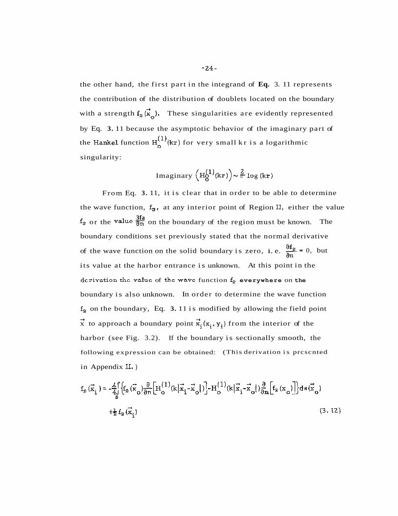
the other hand, the f i rs t part in the integrand of Eq. 3. 11 represents
the contribution of the distribution of doublets located on the boundary
with a strength f2 (<). These singularities a r e evidently represented
by Eq. 3. 11 because the asymptotic behavior of the imaginary part of
the Hankel function ~ ; " ( k r ) for very small k r i s a logarithmic
singularity:
Imaginary ( ~ ( ' ) ( k r ) ) - - o IT log (kr)
From Eq. 3. 11, i t i s clear that in order to be able to determine
the wave function, f2, at any interior point of Region 11, either the value
3fa f, or the value g ~ ; on the boundary of the region must be known. The
boundary conditions set previously stated that the normal derivative
af2 - 0, but of the wave function on the solid boundary i s zero, i. e. - - an
i t s value at the harbor entrance i s unknown. At this point in the
derivation thc valuc of thc wave function f2 everywhere on the
boundary i s also unknown. In order to determine the wave function
f 2 on the boundary, Eq. 3. 11 i s modified by allowing the field point
--t -4
x to approach a boundary point xj (xi, yj ) from the interior of the
harbor (see Fig. 3.2). If the boundary i s sectionally smooth, the
following expression can be obtained: (This derivation i s prcscnted
in Appendix 11. )

Rearranging Eq. 3. 12 one obtains:
(3. 13)
To solve Eq. 3. 13 for the value of f, on the boundary for an
arbitrary shaped harbor, an approximate method i s proposed. In the
approximate method the integral equation i s converted to a matrix
equation. (Similar approaches used in solving an integral equation
have been employed by others, e. g. , Banaugh and Goldsmith (1963),
Chertock (1964), Copley (19671, Mikhlin and Smolitskiy (1967). ) This
i s accomplished by dividing the boundary into a sufficiently large
number of segments where along each segment the average value on
+ a -+ a (1) that segment of f8(x ), a , f s ( x o ) , ~ :"(kr) , - (H (kr)). is used. The o an o
line integral of Eq. 3. 13, which represents the wave function f2 , i s
approximated by a finite summation of the contributions of the
singularities f rom each segment, where the singularities a re the
average values just mentioned and a re considered to be located a t
the center of each segment.
Writing the integral equation Eq. 3. 13 as a summation one
obtains :
where the boundary i s divided into N segments, and:
+ r i s the distance between the points x. and Gi and i s defined i j J
3 -+ as r i j =Ixj-xil= r . . ,
3 1

-26-
-t
x i s the position vector for the field point on the boundary, i
2. i s the position vector for the source point on the boundary, J
and
A s . i s the length of the jth segment of the boundary. J
The segments of the boundary will be numbered counterclockwise
starting f rom the right-hand-side of the harbor opening; with reference
to Fig. 3 . 3 the starting point i s point B. It should be noted that because
of this approximate representation of the boundary, the original curved
boundary i s replaced by a boundary approximating it and composed of
straight-line segments.
Eq. 3. 14 can be written in a matrix form as:
o r rearranging this expression:
k where b = - - and the following notation i s used: 0 2


-28 -
The evaluation of these matrix elements will be discussed in Section
3 . 3 which deals with the numerical analysis. It should be noted that
special care must be taken in evaluating the matrices,especially the
elements when i=j .
If the inverse of the matrix (boGn-I) exists, where I i s the
identity matrix, the vector X_ can be expressed as:
X = ( b o ~ n - ~ ) - ' (bocp) , - - (3. 18)
in which (b0Gn-I)' i s defined as the inverse of the matrix (boGn-I).
The vector P in Eqs. 3.16 and 3 . 18 involve the unknown normal
derivatives of the wave function at the harbor entrance as well as the
normal derivatives of the wave function on the boundary. These latter
values a re zero, i. e. the values of the normal derivative of the
wave function fg for the segment i=p+l , . . . . . N a re zero. The vector
P can be represented in the following way: -
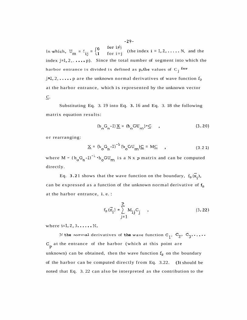
inwhich, U = Sij = { y for iiij (the index i = 1.2 ,..... N, and the m for i= j
index j=l, 2 , . . . . . p). Since the total number of segment into which the
harbor entrance i s divided i s defined as p,the values of C - for J
j=l, 2, . . . . . p a r e the unknown normal derivatives of wave function f,
a t the harbor entrance, which i s represented by the unknown vector
C. -
Substituting Eq. 3. 19 into Eq. 3. 16 and Eq. 3. 18 the following
matr ix equation resul ts :
o r rearranging:
X = ( b o ~ n - ~ ) - ' (boGUm)C = MC , - - (3 .2 1)
where M = ( ~ " G ~ - I ) - ' -b0GUm i s a N x p matr ix and can be computed
directly.
3
Eq. 3 . 2 1 shows that the wave function on the boundary, f, (xi),
can be expressed a s a function of the unknown normal derivative of f2
a t the harbor entrance, i. e. :
where i=l, 2 , 3 . . . . . . N. Lf the l~ori-nal derivatives of the wave function C C2, C30 . - -
C a t the entrance of the harbor (which at this point a r e P
unknown) can be obtained, then the wave function f2 on the boundary
of the harbor can be computed directly f rom Eq. 3.22. (It should be
noted that Eq. 3. 22 can also be interpreted as the contribution to the
wave function on the boundary at a particular point from the super-
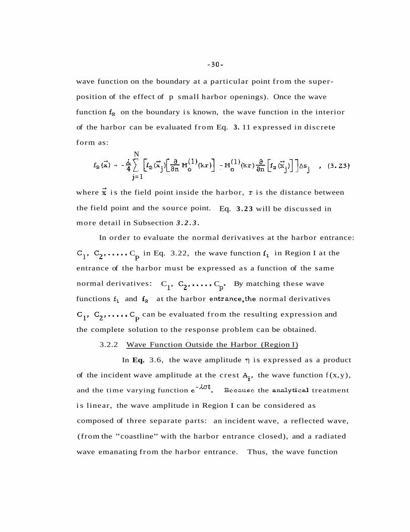
position of the effect of p small harbor openings). Once the wave
function f2 on the boundary i s known, the wave function in the interior
of the harbor can be evaluated from Eq. 3. 11 expressed in discrete
form as:
N
where 2 i s the field point inside the harbor, r i s the distance between
the field point and the source point. Eq. 3 . 2 3 will be discus sed in
more detail in Subsection 3 . 2 . 3 .
In order to evaluate the normal derivatives at the harbor entrance:
C1, C2,. . . . . C in Eq. 3.22, the wave function f l in Region I at the P
entrance of the harbor must be expressed as a function of the same
normal derivatives : C 1 , C2, . . . . . C By matching these wave P'
functions f l and f, at the harbor entrance,the normal derivatives
C1, C2,. . . . . C can be evaluated from the resulting expression and P
the complete solution to the response problem can be obtained.
3.2.2 Wave Function Outside the Harbor (Region I)
In Eq. 3.6, the wave amplitude y i s expressed as a product
of the incident wave amplitude at the crest Ai, the wave function f (x, y),
and the time varying function c -*Ot. Bccausc the analytical treatment
i s linear, the wave amplitude in Region I can be considered as
composed of three separate parts: an incident wave, a reflected wave,
(from the "coastline" with the harbor entrance closed), and a radiated
wave emanating from the harbor entrance. Thus, the wave function

in Region I can be separated into three parts:
f, = f . -t f + f 3 1 r
where: fi represents an incident wave function,
fr represents a reflected wave function considered to occur
as if the harbor entrance were closed,
fs represents the radiated wave function due to the presence
of the harbor.
It should be noted that Eq. 3. 24 implies that the wave amplitude in
-Lot -Lot RegionI, q l = A i f l e , i s e q u i v a l e n t t o q , = A i ( f i + f r f f 3 ) e . This implies that any differences among the wave amplitudes for the
three portions: qi , qr, and compared to the amplitude of q l
a r e incorporated in constants contained i n the wave functions: fi, f r ,
and f a .
The incident wave function, f., can be specified i n an arbi t rary 1
fashion; for example, a periodic incident wave with the wave ray a t
an angle a to the x-axis (the coastline in Fig. 3 . 2 ) can be represented
a s fi(x, y ) = cos (ky sin a) e cos a. The reflected wave function f r ,
can be represented by f,(x, y ) = fi(x, -y). For the case of a periodic
incident wave with the wave ray perpendicular to the coastline (a=90°),
the function which represents the x and y variation of the incident
wave, f . (x, y), can be represented by cos ky. This i s thc cssc which 1
was treated experimentally in this study and therefore the following
discussion will be concerned with periodic waves normally incident
to the coastline.

- 3 2 -
The wave function f, in Eq. 3.24 must satisfy the Helmholtz
equation in Region I (Eq. 3. 5):
with the following boundary conditions :
8% - (i) - - 0 on boundary AC and an
0 (3 . 2 5 )
Bc' (as shown in Fig. 3 . 2 ) ,
(ii) 3=-& on boundary AB (harbor entrance) , an an
(iii) l im f l = f i t f r , and the radiation condition (where r2 = x 2 t y 2 ) . r 2 + m
Boundary condition (i) states that the normal velocity i s zero at
the coastline. The second boundary condition (ii) states that the slope
of the water surface i s continuous at the harbor entrance and the value
from Region I is equal in magni tude to that obtained a t the entrance
f rom Region 11. The negative sign i s specified for the adapted sign
convention that the outward normal to the domain of interest i s con-
sidered positive. For the case of normal wave incidence in Fig. 3.2
i t i s noted that the normal to the boundary in Region I i s in the direc-
tion of the y-axis. The las t boundary csndition (iii) specifies that
the radiated wave in Region I emanating from the harbor entrance
will decay to zero at infinity, hence at infinity only the standing wave
resulting from the incident and reflected waves remains.
As mentioned ear l ier , the reflected wave function f i s known r
once the incident wave function fl is specified. Therefore, to complete
the evaluation of the wave function f,, the main problem i s to evaluate
the radiated wave function fS . Since the analytical treatment i s linear,

-33-
the functions f i , f r ~ and fa all must satisfy the same differential
equation, Eq. 3.25. In addition the boundary conditions in Region I
can be simplified since the normal derivative of the wave function i s
zero on the impermeable boundaries being considered. With reference
a a to Fig. 3 . 2 , on the boundary CABC' +fi f f ) = -(f. t f r ) = 0, and r ay 1
hence boundary condition (ii) can be replaced by af3 = -2 an
af at harbor Bn
entrance (boundary G) . Thus, the radiation function f3 in Region I
can be formulated as satisfying the Helmholtz equation:
with the following boundary conditions:
(i) 5 = 0 on boundary and an
= O , (3.26)
- BC1 (as shown in Fig. 3 . 2 ) ,
af3 = (ii) - an an
on boundary TB (harbor entrance) ,
(iii) lim fg = 0 and the radiation condition (where r 2 = xa + Y2) . ra +w
It i s noted the these boundary conditions a re reduced from those
associated with Eq. 3.25.
To construct a solution for the radiated wave function f n in
Eq. 3 . 2 6 , Green's identity formula (Appendix I, Eq. A. 1. 1) will be
used again and the fundamental solution ~ ( " ( k r ) used in previous 0
section will be used here also. The fundamental solution ~ ( " ( k r ) also 0
satisfies the radiation condition at infinity, i. e. boundary condition
(iii), since as kr- i t asymptotically goes to zero:

-34-
If the fundamental solution is multiplied by the time dependent function
e the resultant expression represents an outgoing radiated wave
satisfying boundary condition (iii) (see Appendix I):
The radiated wave function fa in Region I can be expressed
using Weber's formula in a similar fashion as Eq. 3 . 11 was used
for the expression of the wave function f, in Region 11.:
3 4
where xo i s the source point (xo, 0) along the x-axis, x i s the field
point (x, y) in Region I, and r i s the distance between the field point
and the source point, i. e. r = J(x-xo)' + y2 (see Fig. 3.2).
In order to find the radiated wave function fa on the x-axis, the
field point (x, y) i s allowed to approach the x-axis at the point (xi, 0).
{This approach i s the same as in the treatment of Region 11.. ) Thus,
the following equation can be obtained (see Appendix 11):
The t e rm a [ ~ ( " ( k r ) ] in the integral can be expanded to become a n - o
+ -k~! ' ) (kr) - ar However, because the field point x. (x., 0) and the
an- 1 1 + a r
source point x (x 0) a r e all on the x-axis, the t e r m- is equal to o 0' an
zero. Therefore, the f i r s t t e rm inside the integral in Eq. 3.30 i s
af equal to zero and can be eliminated. In the second term, Z(X,, 0) ,
the normal derivative of the radiated wave function f a , i s equal to zero
-35-
everywhere except across the harbor entrance. The integr a1 unit
ds(xo, 0) becomes dxo because the integration i s to be performed along
x-axis. Thus, Eq. 3.30 can be simplified to:
Using boundary condition (ii) of Eq. 3.26, Eq. 3 . 3 1 can be rewritten
as:
Eq. 3.32 shows that the radiation wave function fa at the harbor
entrance can be expressed as a function of the unknown normal deri-
vative of the wave function at the harbor entrance computed from
a Region 11, i. e. in terms of =f, (xo, 0).
Eq. 3.32 can be expressed in summation form similar to Eq.
where the matrix H. = ~ L ' ) ( k r . .)AS is a p x p matrix (the evaluation 1 j IJ j'
of the elements of this matrix especially for i= j will be discussed in
Subscction 3 . 3 . 3 ) , r . . i s the distancc 1 xi-xj I whcrcin x x arc thc
1J i' j
midpoints of the ith
and jth segments of the harbor entrance respect-
ively. The term C. in Eq. 3.33 i s the normal derivative of the wave 1 ih function f, at the j segment of the harbor entrance, As. i s the length
J
of the jth segment of the harbor entrance, and p i s the total number
ol segments into which the harbor elltrance has beau divided.

Because the incident wave function plus the reflected wave
function at the harbor entrance, f . + f i s a constant, by substituting 1 r'
Eq. 3 . 3 3 into Eq. 3 . 2 4 the wave function fl at the harbor entrance
can be represented as: P
where i=l, 2 , . . . . . p. The f i r s t t e r m at the right hand side of Eq. 3 . 3 4
represents the incident wave plus the reflected wave if the entrance
i s closed and for convenience it i s chosen as unity; the second term
represents the contribution of the radiated wave to the total wave
system.
3 . 2 . 3 Matching the Solution for Each Region at the Harbor
Entrance
Eq. 3 . 2 2 shows that f rom the solution in Region 11, the
wave function at the boundary of the harbor can be expressed in terms
of the normal derivatives of the wave function f, at the .entrance of the
harbor, C.. The corresponding equation in Region I, Eq. 3 . 3 4 shows J
h a t the w a v e function at the harbor eiltrailce can also be expressed as
a function of C Since the water surface must be continuous at the j'
harbor entrance, the wave functions from Regions I and 11 must be
equal at the entrance, i. e. fl = f,. Thus, by matching the two solutions
at the harbor entrance, one i s able to determine the unknown function
C This i s done in the following fashion: j'
Take the f i r s t p equations from Eq. 3 . 2 2 for the wave function
f, at the harbor entrance:

in which the index i= l , 2 , . . . . . p, (p is the number of segments into
which the harbor entrance i s divided). The matrix M in Eq. 3. 35 i s a P
p x p matr ix obtained from the fir s t p rows of the matrix M. + -i
Equating Eqs. 3 . 34 and 3. 35, i. e. f, (xi) = f, (xi), for i = l , 2 , . . . . p
the following matrix equation i s obtained:
M C = 1 -t boHC_ I (3.36a) P- -
C - = ( M - bOH)-' - 1 , (3.36b) P
where M and H a r e each p x p matrices, (M -b H)-I i s the inverse P P 0
A of the matrix (M -b H), the t e r m b is equal to -- as defined ear l ier , P 0 0 2
and 1 i s the vector with each p element equal to unity. Therefore, the
value of the normal derivative of the wave function at the harbor
entrance for each of the p-segments, C_, can be obtained from Eq.
3.36b.
With the normal derivatives of the wave function f, at the harbor
entrance obtained by this matching procedure, the wave function on the
boundary can now be calculated from Eq. 3.22 and the wave function at
any position inside the harbor can be determined from Eq. 3.23 or the
equivalent expression:
- 3 8- -+
where ;. i s at the mid-point of the jth segment of the boundary, x i s J
4
the position of the interior point and r i s the distance between x and j
4 + x, i. e. r= Ix.-XI. It should be noted that Eq. 3.23 i s written in the
J
f o rm of Eq. 3 . 3 7 because the normal derivative of the wave function
at the boundary i s zero except at the harbor entrance.
In order to determine the response of the harbor to incident
waves, the wave amplitude inside the harbor i s usually compared to
the incident plus the reflected wave amplitude which exists in the "open-
sea" in the absence of the harbor, i. e. the harbor entrance i s closed.
A parameter called the "amplification factor" i s defined as the ratio of
the wave amplitude at any position (x, y ) inside the harbor to the incident
plus reflected wave amplitude at the coastline (with the entrance closed).
In Eq. 3 .38 , R i s defined as the amplification factor. The wave
function f, (x, y) i s a complex number; therefore, i n compnting the wave
amplitude the absolute value i s taken.
3 . 2.4 Velocity at the Harbor Entrance
With the wave function f2 (x, y) determined in Subsection
3 . 2 . 3 , the calculation of the velocity potential $ (x, y, z;t) for the region
insidc thc harbor i s now complete:
1 Aig cosh k(zlh) -Lot qx, y, ~ ; t ) = - cosh kh fz (xt Y) e Lo

- 3 9 -
In accordance with the definition sketch presented in Fig. 3. 1,
the velocities at the position (x, y, z ) in the directions of x, y, z a r e
defined as follows:
'am 1 ~~g C O S ~ k ( ~ i - h ) u(x, y, z;t) = Real tG) = ~ e a l [ - 0 cosh kh - ax af2 (x, y)e-'ot] ,!3.40a)
1 Aig cosh k(x+h) V(X, y, z;t) = Real (-$) = =Real [ E cash kh
af2 - (x, y)e-'ot] ay
, (3.40b)
and the total velocity at any position (x, y, z ) and time t , can be
expressed as:
The velocity at the harbor entrance i s of interest because it i s
directly related to the kinetic energy transmitted into the harbor. This
total velocity VI i s a periodic function of time. In order to find the .L
maximum total velocity for all time, the function ~ " ' j x , y, z;t) i s differ -
entiated with respect to time and the derivative i s se t equal to zero;
from this condition one can determine the time for which the velocity
i s a maximum. Thus, the maximum total velocity, which i s denoted
:k as Vo, at a particular position (x, o, z ) at the harbor entrance can be
calculated as follows :
% 2 ~ : A; cos 2(a, -a, ) + Z A ~ A ; cos 2(al -a,) )"I" (3.41)

af, cosh k(zSh) = I By I cosh kh
wherein the subscripts R and I which appear in the expressions for
al , a,, as denote the rea l par t and imaginary part respectively.
As will be discussed in Subsection 6.2. 5, experiments were
conducted to measure the velocity at the harbor entrance using a hot-
film anemometer. The hot-film sensor was oriented with i ts long-
itudinal axis parallel both to the "coastline" and the bottom, and, hence,
it was primarily sensitive to the velocities in the y and z directions
(the v and w components respectively). For comparison with the
cxperimentd data the theoretical value of the ma-ximum resultant
velocity of the v and w components, which i s denoted as Vo, can be
determined by setting u2 equal to zero in Eq. 3.40d (or Al = 0 in
Eq. 3.41):
( 3 . 4 2 ) where Az , A3, a,, and a3 a r e defined in Eq. 3.4 1.
3 . 3 THE NUMERICAL ANALYSIS
Section 3. 2 was concerned only with the transformation of
the Weber's solution of the Helmholtz equation (Eq. 3. 11) into an
integral equation (Eq. 3. 13) and the formulation of an approximate
solution to this integral equation. In this section the methods for
evaluating the elements of the matrices defined i n Eqs. 3. 15 and 3 . 3 3
will be discussed as well as the numerical method for solving the
wave function f, in Region I1 and the matching procedure.
3 . 3 . 1 Region 11: Evaluation of Matrices Defined in Eq. 3. 15
i) Off-diagonal elements of the matrix Gn
As defined in Eq. 3. 14 the notation G. (x y . ) i s used for 1 i' 1
-+ i= l , 2 , . . . . . N, to refer to the field points, and the notation x . ( x y . ) J ' J for j= l ,2 , . . . . . N i s used to refer to the source points. The elements
(GuIij for i f j can be evaluated as follows:
in which r . . = J(xi-xjla + (y . -JT.)' i s the distance between the mid- 1J 1 J
points of the ith segment and the jth segment of the boundary. The
Hankel function ~ ! l ) ( k r . .) in Eq. 3 . 4 3 can be expres sed in terms of the 1J
Bes sel functions by the equations :

Hence, Eq. 3.44 i s known once the argument k r i s known. i.i
8 r > i n Eq. 3.43 can be evaluated as follows: The te rm an
In the right-hand side of Eq. 3.45 the differentiation with respect to
the outward normal direction of the boundary, n, i. e. (E) and (g) , j j
can be changed into differentiation with respect to the tangential
a direction along the boundary, as. Therefore, according to the
definition sketch of Fig. 3.4, Eq. 3.45 can be rewritten as:
Referring to the definition of rij and performing the differentiation of
ar.. ar. . and 2 Eq. 3.46 becomes: ax
j ayj
Writing the te rms (3) and (2) in difference form Eq. 3.47 becomes: j j
Therefore, the off -diagonal elements of the matrix G can bc evduatcd n
by substituting Eqs. 3.44 and 3.48 into Eq. 3.43.

Fig. 3 . 4 Change of derivatives f r o m normal to tangential direct ion

ii) Diagonal elements of the Matrix Gn
For matrix Gn, since the source and field points are located
at the mid-point of the straight-line segments which have been used
to approximate the boundary, the diagonal elements of the matrix G,
correspond to the condition of the coincidence of a particular field
point and source point. Due to the singular behavior of the Hankel
function H! "(kr ) as kr-0, special attention must be given in
evaluating these diagonal elements.
The function Yl (x) in Eq. 3 . 4 4 can be expressed as a series as
(see Hildebrand (1962) p. 147):
in which y = 0. 577216.. . i s termed Euler's constant, and the logarithm
i s to the Naperian base e (= 2.7128), (all logarithms will be to this
basc u n l c o ~ indicated othcrwisc). Thc real part of Hankel function
(1) H1 (kr) presented in Eq. 3 . 4 4 i s Jl (kr) which i s approximately equal
kr to 2 when k r becomes very small; therfore, J, (kr)-+O as kr-*O. Thus,
from Eq. 3 . 4 9 as kr+O the function Yl (kr) can be approximated as:
for kr+O . Thus, the diagonal elements of the matrix G, can be evaluated as
the limiting value as r approaches zero (Eq. 3 . 4 3 for i=j):
l im (1) a r l im (Gdii = r 4 0 ( - k ~ , ( k r ) = ) ~ s ~ = . _ ~ - k [ ~ , ( k r ) + L Y , ( k r ) ] ~ A s ~

Therefore, in evaluating the diagonal elements of the matrix Gn, the
a r Ern most important step i s to evaluate the te rm - in Eq. 3. 5 1. r-0 r
The definition of r is:
where (x y.) a re the coordinates of the mid-point of the ith segment on i' 1
the boundary thus the t e rm can be expressed in a form similar to
Eq. 3.47:
and g i n Eq. 3. 52 The terms (x-xi), (y-yi), as,
Taylor's ser ies in the neighborhood of (xi, yi):
can be expanded in a
ax - (AS) ' as (xs). 1 + (xSS). 1 AS + (xSSSIi 2 ! t.. . . where the subscript s refers to differentiation with respect to s. (The
index i means that the values of interest a re evaluated at the mid-point
of the ith segment. ) The expansion ( y-yi) and can be done in exactly as
the same way by changing x to y i n Eqs. 3.53 and 3.54.
8r - lim
in Eq. 3. 5 1 can be evaluated using the definition Thus the termr30
of r , Eq. 3.52, and Eqs. 3. 53 and 3. 54 to give:
a r a r l i m K l im an r+O T- = AS-0 r
The numerator of Eq. 3. 55 can be arranged as:
where o(ns3) means terms of order ns3.
The denominator of Eg. 3.55 can be arranged as:
this expression can be simplified farther to become ( A S )" t AS^)
because in reference to Fig. 3 . 4 the t e rm < + yz i s equal to unity.
Thus, neglecting the higher order terms in Eq. 3. 55, this
expression can be approximated as :
Therefore, the diagonal elements of the matrix G can be found from n
Eq. 3.5 1 and the approximation described in Eq. 3.56:
In Eq. 3. 57, the first and second derivatives of x 6 p YS* X s S * YSS arc?
evaluated at the mid-point of the ith segment of the boundary.
For a boundary which i s originally composed of straight lines
the value of xsyss and y x in Eq. 3.57 a r e both equal to zero s S S
(because the second derivatives xss and yss are both zero); therefore
the diagonal elements of the matrix tin are equal to zero. P'or a
curved boundary which has been approximated by straight-line segments
the expression of the f i rs t and second derivatives, x and xS S, can be s
written i n a d i f f e r e n c e form as:

where x. i s the x coordinate at the mid-point of the ith segment of the 1
boundary, xi I i s the x coordinate at the beginning of the ith
segment -z
of the boundary, and x i s W e x coordinate at the end of the i th it*
segment of the boundary, Asi- l, Asi, and AS^+^ a r e the length of the, (i- l)th
ith, and (it l)th segments of the boundary. The derivatives ys, yss can
be evaluated in exactly the same way by changing x to y in Eqs. 3.58.
iii) Off-diagonal elements of the matrix G
The elements (G).. for i#j can be evaluated directly 1J
following expression:
(1) (G). . = Ho (kr. .)As = [J (kr. .) t LYo(kr. .)1asj 1~ 13 j 0 1~ v J
by the
(3.59)
For a given value of krij, in Eq. 3. 59, the function Jo(kr. .) and Yo (kr . .) 1J 1J
a re known functions.
iv) Diagonal elements of the matrix G
The diagonal elements of the matrix correspond to the case of
i = j in Eq. 3.59. As before, due to the singular behavior of the function
Y (kr), special attention must be given in evaluating the diagonal 0
elements of matrix G. Using the asymptotic formula of Jo(kr) and
Y (kr ) as the argument for k r approach zero, the following approxi- 0
mations a r e obtained (see Hildebrand ( 1962) ):

Jo (kr ) rn 1 ,
Therefore, as kr+0 the Hankel function H;)(kr) can be expressed as:
13L1)(kr) = Jo(kr) t ,LYo(kr) FI. 1 t log ~r Ft (for kr-0)
where y is the Eulerts constant as mentioned earlier.
Using this asymptotic formula for the Hankel function H:)(kr).
the diagonal elements of the matrix G can be evaluated by performing
the following integration to determine the average of this function over
the length of the segment of interest:
k As. = [1 +A$ [log(+) -0.422781 ] nsi
where i=l, 2,. . . . . N.
3. 3. 2 Region 11: Method of Solution for Wave Function f-,
In Subsection 3. 3. 1 the methods for evaluating the elements
of the matrices G and G have been discussed; thus, the next step i s to n
evaluate the matrix M, as defined in Eq. 3.2 1, in order to determine the
variation of the wave function f2 along the boundary of the harbor. As
shown in Eq. 3.22 the wave function f, along the boundary of the harbor
can be expressed as a function of the unknown normal derivative of the
wave function f, at the harbor entrance, i. e. C1. C 2 , . . . . . C Eq. P'
3 .22 i s repeated here for clarity:

wherein M.. i s a 1J
matrix equation,
The matrix (boGn
N x p matrix which i s the solution of the following
rearranged from that shown in Eq. 3.21:
(boGn - I) M = boGUm . (3.61)
-I) i s a N x N matrix, i ts elements can be determined
as described in Subsection 3.3. 1 using the definitions of bo and I given
in Subsection 3.2. 1. The right-hand- side of Eq. 3.6 1, matrix boGUm,
is s N x p matrix, where Um is defined by Eq. 3 . 19. (It should be
noted that the matrices G, Gn and M shown in Eq. 3.61 a re all complex
numbered matrices. )
To solve Eq. 3.6 1 for the complex numbered matrix M, a sub-
routine for the IBM 360175 digital computer: llCSLECD/Complex System
of Linear Equations and Complex Determinant1' was used which i s
available at the Booth Computing Center of the California Institute of
Technology. The subroutine i s based on the Gaussian elimination
method where rows a re interchanged leading to the conversion of the
left-hand side matrix in Eq. 3.61 to an upper triangular matrix. The
sulutiou of M i s theu obtairled b y Lackward substilutiorl.
3.3.3 Region I: Evaluation of Matrix H Defined in Eq. 3.33
The matrix H defined in Eq. 3.33 can be evaluated in the
same way as was matrix G. The matrix H will be called the "radiation
matrix" because it i s the main part of the radiated wave function f3 (G) described in Eq. 3.33; it i s a p x p matrix and its off -diagonal elements
can be evaluated in a manner similar to that shown in Eq. 3.59:
(1) (H). . = Ho (kr. .)As = [ ~ ~ ( k r ~ ~ ) + ,I, Yo(kr. .)]As (3.62) 13 13 j 13 j
(for i # j and i, j= l , 2 , . . . . . p) . The diagonal elements can be evaluated in a manner similar to that
shown in Eq. 3.60:
(for i=l, 2 , . . . . .p) . 3.3 .4 Harbor Entrance: Matching Procedure
After s blving Eq. 3.6 1 for the N x p matrix M and evaluating
the elements of the matrix H as outlined in Subsection 3.3.3, the next
important step i s the matching of the two solutions from Region I and
Region II at the harbor entrance. Eq. 3. 36a i s the result of this
matching procedure and the object of this section is to describe how
the vector C_ (the normal derivative of the wave function at the harbor
entrance) i s obtained.
Eq. 3 , 36a is first rewritten as:
(M - boH) C_ = 1 P
in which M i s a p s p matrix as explained in Subsection 3.2.3. To P
solve Eq. 3.64 for the vector C - again involves the subroutine "CSLECD/
Complex System of Linear Equations and Complex Determinant ", but
this time the matrix size i s only p x p and the solution C i s a p x 1
vector . After evaluating the vector C_, the procedure for determining the
qnantities of interest such as the response of the harbor, the
amplitude distribution, etc. a re described in Subsection 3.2.3.

-51-
3 . 4 CONFIRMATION O F THE NUMERICAL ANALYSIS
The theory for an arbi t rary shaped harbor has been pre-
sented in Sections 3 . 2 and 3 . 3 . However, prior to evaluating the wave
induced oscillations of an actual harbor, i t i s necessary to make sure
that the method presented in Subsection 3 . 2 . 1 and the numerical pro-
cedure presented in Subsections 3 . 3 . 1 and 3 . 3 . 2 a re correct. There-
fore, the approximate solution obtained using the method developed
will be tested by comparing i t with the exact solution of the Helmholtz
equation for two different shapes. These two shapes a re a circle and
a square. They a re chosen for several reasons: ( 1) the theoretical
solution for both shapes can be obtained easily, ( 2 ) the boundary of a
circle represents an extreme case for which the tangent to the boundary
is rontinuously changing direction, and ( 3 ) the boundary of a square
(or a rectangular) represents another extreme case that i s composed
of four straight lines; along each line the direction of the tangent to
the boundary remains the same.
The procedure for this tes t program can be outlined as follows:
1) A theoretical solution i s selected for the wave function,
f, that satisfies the Helmholtz equation, v2f + k2f = 0,
in the domain of interest (either a circle or a square).
2 ) Based on this theoretical solution the value of the wave
function, f , at the boundary of the domain, the value of
af i t s normal derivative at the boundary of the domain, - any
and the value of f at any position inside the domain a re

- 5 2 -
calculated. (It should be noted that the boundaries for
these two test examples do not necessarily represent
solid boundariesr )
3 ) The boundary of the domain i s divided into N segments;
af the average of the theoretical values of f and an on
each segment a re calculated.
4) These averaged theoretical values of the normal
a f derivative F~ for each segment on the boundary are
used to calculate the value of f for each corresponding
segment by the method described in Subsection 3 . 2 . 1.
One test of this approximate method i s the comparison
of this computed value with the theoretical value of f on
the boundary of the domain. Any difference between
these two results which i s found can be attributed to the
approximations resulting from converting the integral
equation (Eq. 3. 13) to the matrix equation (Eq. 3. 15).
5) The computed value of f (Step 4) and the theoretical
a f value of - on the boundary of the domain are used to an
compute the value of f at various locations inside the
domain using Eq. 3 .37 . The values of f so obtained a re
compared with the theoretical values. The difference
i s the e r ro r admitted in Step 4 plus the e r ro r due to
using Eq. 3.37 which has been used as an approximation
to the exact solution, Eq. 3. 11.

-53-
ar 6) The theoretical values of f and - at the boundary of the an
domain a r e used to caluclate the value of f at some
points inside the domain by using Eq. 3 . 3 7 ; the values
of f so obtained a re compared with the theoretical
values. The difference is solely due to the use of Eq.
3. 37 which approximates the exact equation, Eq. 3. 11.
It should be noted that these two examples (circle and square) a r e
not directly connected with the actual problem of wave induced oscill-
ations in harbors, since the boundary conditions imposed by this tes t
program (steps 2 and 3) do not correspond to the boundary conditions
prescribed for the harbor oscillation problem (as described in Section
3. 1). Rather, these examples a re employed in a mathematical sense
serving as an analytical check for the approximate method that will be
used in solving the problem which i s of major concern: wave induced
oscillations in an arbitrary shaped harbor.
3.4. 1 The Fi rs t Example: A Circle
The f i rs t example that will be investigated i s a circular
domain, s definition sketch of which i s presented in Fig. 3 . 5. The
Helmholtz equation i s written in polar coordinates as :
The steps outlined previously a re followed; the following parti -
cular solution which satisfies the Helmholtz equation, Eq. 3.65, i s
selected:
f ( r , 8 ) = J, (kr) cos 0

Fig. 3 . 5 Definition sketch of a circular domain
direction of integration C
Fig. 3 .6 Definition sketch of a square domain

-55-
thus, differentiating Eq. 3. 66 with respect to r one obtains:
1 ~ ~ ( r , B ) ] = [ k ~ ~ ( k r ) ar - F ~ l ( k r ) ] c o s 8 . (3.67)
Suppose a boundary of the domain is located at r=a, then the value of f
af and - on the boundary can be expressed as: an
f(a, 0 ) = J, (ka) cos 0 , (3.68a)
a f a f I - an (a, 0 ) =G (a, 8 ) = [kJ0(ka) - ; Jl(ka)] cos 0 . (3.68b)
The boundary is then divided into 36 segments (each segment
includes 10' of the central angle). On each segment the average
8f theoretical value of the functions f(a, 8 ) and =(a, 8) can be evaluated
as follows:
= J, (ka) 'it* - 'i-+
9
1 sin 8. 1 - sin 8
1t2 i-k = [k.Jo(ka) - a JI &a)] it+ - ei-+ ? (3.69b)
- where (fii and (g): are the average theoretical values on the boundary
of the domain of f A d $ for the ith
segment, (apei-$ are the coor-
dinates of the beginning of the ith segment of the boundary, and
(a, Ria) a r e the coordinates of the end of the ith segment of the
boundary.

- In Step 4, the value of ($1 , presented in Eq. 3. 69 b for each
1
segment i s used to calculate the value of f of each segment on the
boundary by the approximate method of Subsection 3.2. 1. These
computed values will be denoted as ic. The value of rc and Tshould
be very close i f the approximate method i s to be useful. Three
different values of ka, i. e. ka=O. 30, 2.25, 3. 75 have been tested
(where k i s the wave number in f t - I and a i s the radius of the circular
domain and chosen a s 0.75 f t for this case) . The approximate result
(Fc) agreed with the theoretical values (A within 0. 1% to 3% for ka=O. 3
and 3.75 respectively. The effect of the magnitude of ka on the
solution will be discussed more fully in Chapter 6. -
After the values of f on the boundary, i. e. f , have been C
obtained, the value of f at any interior point can be computed using
Eq. 3.37 (Step 5). The results for ka=O. 30, 2.25 and 3.75 a r e
presented in Table 3. 1. For each value of ka, the value of f at five
interior points a re computed. The theoretical value of f at each
interior point i s calculated using Eq. 3.66 and presented in Col. 3.
The results of Step 5 , i. e..the computed approximate values of f at
each interior point, a r e presented in Col. 4. The difference between
the value in Cols. 3 and 4 can be attributed to: (i) the e r ro r admitted
in the approximate solution, Eq. 3. 15, which i s used to approximate
the integral equation (Eq. 3. 13) in evaluating the value of f on the
boundary (Step 4), and (ii) the e r ro r admitted in the use of Eq. 3.37 to
approximate the exact solution, Eq. 3. 11, in evaluating the value of
f for the interior points.

Table 3. 1 Comparison of the approximate solution with ;he theoretical solution of the Helmholtz equation in a circular domain
Position of Thecretical Value
Interior Point 1 o f f
(r , 0) (Step 2)
Computed Value of f
(Step 5) 141 (2)
Computed Value of f
(step 6) (5) (3)
Computed Value I Computed Value of f of f
r (ft) I 8 (deg. I I Real Part I haginary Part
(Ste
Real Part Imaginary Part
-0.00001
-0.00000
0.00001
-0.00000
0.00000
0.00000

- 58 -
The results of Step 6 a re shown in Col. 5; they a re obtained by
a f using the theoretical values of f and an at the boundary (Eqs. 3.69) to
compute the value of f at the interior point by applying Eq. 3 . 3 7 . The
difference between the theoretical results of Col. 3 and the approximate
results in Col. 5 is solely due to the use of Eq. 3.37 which approxi-
mates the exact solution of Eq. 3. 11.
It should be noted that Step 6 applied to a given domain does not
correspond to a mathematically realistic boundary value problem,
af simply because both the value of f and - on the boundary are usually an
not given in advance; usually one or the other i s given. However, i t
does give an indication of how good the approximation of Eq. 3.37 is ,
a f if the correct boundary values f and - a re provided. Step 5 does an
correspond to a mathematically realistic boundary value problem and
in fact i t i s basically the procedure used for solving the harbor reso-
a f nance problem, that is: given a particular value of - at the boundary, an
calculate the value of f at the boundary and finally calculate the value
of f at any interior point ( r , 8).
It i s expected that if the number of segments into which the
boundary of the domain i s divided i s increased, the results of the
approximate method will agree better with the theoretical results.
0 The results for N=45 (each segment includes 8 of the central angle)
a re presented in Cols. 6 and 7 of Table 3. 1. By comparing Cols. 3 ,
4, and 6 (also comparing Cols. 3, 5, and 7 ) it i s seen that as the
number of boundary segment i s increased the results of the approxi-
mate method compared to the theoretical results a re improved only
slightly.

3.4.2 The Second Example: A Square
Suppose the square has sides of length b as shown in Fig.
3 . 6 , then a simple particular solution of the function f that satisfies
the Helmholtz equation, Eq. 3.5, can be chosen as:
f(x, y) = cos (% x)cosh (d(')'- k2 Y) (for k < 2 2b (3.70a)
I T f(x, y ) = cos (2 x) cos (b2 - (2)" y) (for k >- 2b ) (3. 70b)
thus, the outward normal derivative of the function f at the boundary of
the domain can be evaluated as following:
af af - = -i-
an ax9 for x=-b, -b s y 5 0
The steps outlined previously a r e followed. The boundary of the
square domain i s divided equally into 40 segments. The theoretical
value of f at any interior point (x, y) can be calculated by Eqs. 3. 70
once the value of wave number k i s fixed. The results for two different
values of kb, i. e. kb = 0.50 and 2.0 (where k i s the wave number and
the length of sides of the square domain i s b = 0.50 f t ) a r e presented in
Table 3.2. For each value of kb the value of f at nine interior points
a r e computed. The theoretical values of f at each point for kb = 0. 50
a r e computed using Eq. 3.70a; the theoretical values of f for kb = 2.0
a r e computed using Eq. 3.70b. These theoretical values a r e presented
in Col. 3 of Table 3.2. The approximate results of the value of f in

. . . . . . . . . d d d d d d d d o o o o o o o o o o . I I I I I I I I I I
o m o u? r- m N N "> 0 0 0 0 0 0
. . . . . . . . O O O O O O O O C
d d d d d d d d c . . . . . . . . , O O O O O O O O C
I I I 8 I I t
t - m \ o o o o m m n m m S m O m N b l a N N - N N N N - C m m m l P l Y I V l m m V O O O O O O O O C
d d d d d d d d d I I I , , I
m o m O O * * o o m r - 0 N * O . . . - 0 -
d d d d d d d d d
u ? ~ v l O O O O Q O N N N - b l - * - b
d d d d d d d d d I I I I I I I , ,
m o o u ? ~ o o o o N d - N N * b - -
d d d d d d d d d I I I I I I t I I

-61-
Step 5 a re shown in Col. 4, while the results of Step 6 a re shown in
Col. 5. Comparing the results in Cols. 3 and 4, it i s seen that
dependent upon the position of the interior point the results agree
within 1% to 3010, and, as expected, the results in Col, 5 a r e closer
to the theoretical results (Col. 3) .
The results for N=48 (each side of the boundary contains 12
boundary segments) a r e presented in Cols. 6 and 7. Comparing the
results in Cols. 3, 4, and 6 (also Cols. 3, 5, and 7 ) i t i s seen that the
results for N=48 agree better with the theoretical value than when the
boundary i s divided into 40 segments.
From the results of these two examples, a circle and a square,
which were used it i s seen that this numerical method and the approxi-
mations i t entails can be used to solve the Helmholtz equation with
reasonable accuracy. Thus, the real problem of determining wave
induced oscillations in an arbitrary shaped harbor which may have
both c n r v e d and /or straight lined boundaries can be approached with
confidence.
CHAPTER 4
THEORETICAL ANALYSIS FOR TWO HARBORS
WITH SPECIAL SHAPES
Two theories which deal with the wave induced oscillations i n
a circular and a rectangular harbor a r e presented in this chapter.
A circular harbor represents one extreme case for which the tangent
to the boundary of the harbor i s continuously changing direction; a
rectangular harbor represents another extreme case whose boundary
i s composed of four straight lines and along each line the tangent to
the boundary remains in the same direction. 'l'hus, these two
special theoretical solutions provide a useful analytical check for
the approximate theory developed in Chapter 3 for an arbitrary
shaped harbor as well as being used to compare to the results of
experiments conducted in the laboratory. The results for these
particular cases and their comparison with the theory developed
for arbi t rary shapes discussed i n Chapter 3 applied to these two
harbors will be presented in Chapter 6.

- 6 3 -
4.1 THEORETICAL ANALYSIS FOR A CIRCULAR HARBOR
The theory developed in Chapter 3 can be used for any
arbitrary shaped harbor. However, if the harbor i s a special shape
such as circular, the coordinates inside the harbor a r e separable
and a different method can be used to obtain a solution in Region II.
(For a l ist of separable coordinate systems see Morse and Feshback
(1953) pp. 656-666. ) The theoretical analysis for a circular'harbor
based on this approach will be presented in this section.
In the analysis, the wave function f2 which satisfies the Helm-
holtz equation, Eq. 3. 5, in Region I1 i s found by the method of
separation of variables. The solution for the open- sea, Region I,
which i s used for this devehpment i s the same a s that presented in
Chapter 3. By matching the solutions in both regions a t the harbor
entrance, the complete solution of the wave induced oscillation in
a circular harbor can be obtained.
4. 1. 1 Wave Function Inside the Circular Harbor
For the wave function f2 inside the circular harbor,
the Helmholtz equation, Eq. 3 . 5, i s written in cylindrical
coordinates:
The boundary conditions that the function f, must satisfy are:

-64-
where a i s the radius of the circular harbor, 200 is the central
angle of the harbor opening, and C(B) i s the initially unknown normal
derivative of the wave function f2 at the harbor entrance. A definition
sketch of the circular harbor showing both regions: Region I (the
"open-sea") and Region I1 (inside the harbor), i s presented in Fig. 4.1.
The solution of Eq. 4. 1 will be constructed by Fourier ser ies ,
by f i rs t seeking the solution of f, ( r , 8 ) in the form of:
Substituting Eq. 4. 3 into Eq. 4. 1, i t i s found that the function f ( r , 0 ) m
must satisfy the following differential equation:
This equation i s a form of the Bessel equation; hence, its solution
can be expressed as:
wherein the function J (kr ) i s the Bes sel function of the fir s t kind, m
and Y (k r ) i s the Bessel function of the second kind; am and 3 m m
a r e arbitrary constants to be determined.
The function Y (kr ) possesses a singular behavior a t r=O, but m
since the solution of the wave function f 2 ( r , 8 ) must be smooth and
finite at r = O , the constant @ must be zero. Thus, from Eq. 4.3, m
the solution of Eq. 4. 1 can be expressed as:

Region I (Open- s e a ) 1Y
Fig. 4. 1 Definition ske tch of a c i r cu l a r h a r b o r

Because J (kr) i s equivalent to (- l ) m ~ (kr), Eq. 4. 6 i s equivalent - m m
to: m
where Am and Bm are constants with real and imaginary parts to
be determined. For this particular case where the incident wave
propagates in the direction of 8=0 the wave function f2 (r, 8) i s an
even function of 0 , i. e. the wave amplitude i s symmetrical with
respect to the center line 8=0. Therefore, the constant B in Eq. 4.7 m
i s set equal to zero. Hence, the general solution to Eq. 4. 1 reduces
to:
f , ( r , 8 ) =l AmJm(kr) cos me . m=O
Differentiating Eq. 4. 8 with respect to r, and evaluating the resulting
expression at the honndary, r = a one obtains:
03
rn where: kJml(ka) = kJm- (ka)- - J (ka). The coefficients Am must a an
be determined such that Eq. 4.9 will satisfy the prescribed boundary
conditions, Eq. 4. 2. To evaluate the coefficients Am, the method
of Fourier cosine transformation will be used, by f i r s t multiplying
both sides of Eq. 4. 9 by cos nR and integrating the resulting
expression with respect to 8 f rom zero to ZIT:

2Tr " -(a, 8) cos nede = r0 1 [A cos me m k ~ m ' ( k a ) ] cos nede m
m = 0
=l J kJm1(ka)Am cos me cos nede m= 0
If m#n, upon integration Eq. 4. 10 i s equal to zero, and i f m=n=O,
Eq. 4. 10 is equal to:
Therefore, the constant A. can be evaluated as:
on the other hand, if m=n#O, Eq. 4. 10 becomes:
Thus, the coilstant Am can be evaluated as:
f 2 n af2 (a, 0 ) cos medo J, ar
Because the normal derivative of the wave function on the
af boundary, --Z(a, €I), i s zero everywhere except at the harbor entrance, a r as shown in Eq. 4.2, Eqs. 4. 12 and 4. 14 can be simplified further.

Using the relations:
JoJ(ka) = - Jl (ka);
the constants A o7 Am in Eqs. 4. 12 and 4. 14 can be written in the
following forms:
where is a dummy variable of integration and c(T) represents the
normal derivative of the wave function evaluated at the entrance.
Therefore, the solution to Eq. 4. 1 and the boundary conditions,
Eq. 4.2,can be obtained by the substitution of Eqs. 4. 15 into Eq. 4.8:
If the harbor entrance i s small, i t i s assumed that C(8) can
be approximated by a constant C. and hence. Eq. 4.16 can be
expressed as:

In order to determine the coefficient C, i. e. the average of
the normal derivative of the wave function across the harbor entrance,
the wave function f, evaluated at the harbor entrance has to be set
equal to the wave function in Region I evaluated a t the entrance. This
means that at the entrance the average of the wave anxplitude across
the entrance must be the same when determined either in Region I
o r Region 11. For this purpose, the average of the wave function
f 2 across the harbor entrance (designated as y2 ) i s determined as:
- f, = - J '0 fa (a, 8)de
- B o
(ka)[sin meo ] - -
m 1. (4.18) ( 1 - J (ka) J o a m
Eq. 4. 18 i s written in abbreviated form defining the bracketed term
on the right-hand-side as M . therefore: c'
- f2 = C e M .
C (4. 19)
The ser ies M can be calculated once the radius a, the central angle C
of the entrance 200, and the wave number k a r e fixed. It i s noted
that Eq. 4. 19 i s similar to Eq. 3.35; in both of these equations the
wave function at the harbor entrance i s expressed in terms of i ts
normal derivative at the harbor entrance. (It should be recalled

that the normal derivative of the wave function is proportional to the
horizontal velocity. ) The next step in the solution i s to express the
average value of f, (for Region I) at the harbor entrance also as a -
function of the average normal derivative of the wave function, C,
so that by equating the solutions a t the harbor entrance in both regions
the value of C can be determined.
4. 1.2 Wave Function Outside the Harbor
As mentioned in Subsection 4. 1. 1, the harbor entrance
i s considered small. Thus, even though the harbor entrance i s an
a r c in Region I1 and a chord in Region I, the difference between the
length of the a r c and that of the chord i s assumed to be negligible.
As developed in Subsection 3.2.2. the wave function at the harbor
entrance obtained from the solution in Region I can be expressed as:
fl (x, 0) = 1 t 11) ($1 L2 (x0, 0) HO (klx-xO 1 )dxo
AB
where AB i s the chord at the harbor entrance, the function C(x 0 ) 0'
i s the normal derivative specified in Eq. 4.2, the negative sign i s
specified for the adapted sign convention that the outward normal
derivative to the domain of interest i s considered positive. (Eq. 4.20
i s an integral form of the Eq. 3.34 that was developed previously. )
The first terlm on the right-hand-side of Eq. 4. 20 represwlts tlie

incident wave and reflected wave at the harbor entrance if the
entrance i s closed; the second t e rm represents the radiated wave
from the entrance,
In order to facilitate performing the integration in Eq. 4.20,
the origin of the coordinate system i s shifted to the left corner of
the harhnr e n f r a n c e (point A i n r e f e r e n r e fn Fig. 4. 1 ). T n keep
the same approximation as mentioned in Section 4. 1. 1, the function
C ( x o , 0) i s approximated by a constant C. Thus, Eq. 4.20 can be
simplified by taking the constant C outside the integral sign:
The Hankel function HL1)(klx-x I ) in Eq. 4. 2 1 can be separated into 0
i t s rea l and imaginary parts:
where r= lx -x I i s the distance between the field point (x, 0 ) and the 0
source point (x 0). Substituting Eq. 4.22 into Eq. 4.2 1 and per - 0 '
forming the integration across the harbor entrance, i t becomes:
L where the terms f . (x ,0) and-f (x,O) a r e the results of theinte-
J 0 = YO
gration of the rea l par t and imaginary part of the Hankel function
("(kr) in Eq. 4.21. The interested reader i s referred to Appendix Ho
III for the detailed derivationof f . (x,O) and f (x,O), (see Eqs. A.3 .3 J 0 YO

and A. 3.6). In order to determine the value of 5 by the matching -
procedure, the average of the wave function, fl , across the harbor
entrance can be found as:
where As is thc lcngth of thc chord across thc harbor cntrsncc.
Substituting Eq. 4.23 into Eq. 4.24 one obtains:
where:
kZl (n! )2 (Znt l ) ( n t l )

- 73 -
The development of the se r ies for Jc and Yc a r e also presented in
Appendix I11 (see Sections 111. 3 and 111. 4).
4. 1. 3 Matching the Solution for Each Region a t the Harbor
Entrance
With the average wave function f, a t the harbor entrance
(f,) for Region I1 obtained f rom Eq. 4. 19 and the average wave function
f, a t the harbor entrance (fi) fo r Region I obtained f rom Eq. 4.25,
the two svlut ioi~s can now be inatched to solve for the average norinal
- derivative of the wave function, C. Eq. 4.25 i s simplified as:
/L where Bo = -F ( J~ As, i n which J and Yc a r e defined by C C
Eqs. 4.26a and 4.26b.
Equating Eq. 4. 19 to Eq. 4.27, one obtains:
thus, the average value of the normal derivative of the wave function
a t the harbor entrance, C, can be determined f rom Eq. 4.28 as:
where Mc and Bo a r e defined by Eqs. 4. 19 and 4.27 respectively.
After the value of the average normal derivative of the wave
function a t the harbor entrance, C, has been determined f rom
Eq. 4.29, the wave function fi at any position (r, 6 ) inside the harbor
can be calculated f rom Eq. 4. 17. It should be noted that the functions
C and fz (r, 0 ) a r e both complex numbers.

- 74-
Once the value of the complex number C has been determined
by Eq. 4. 29, the amplification factor, R, a t any position ( r , 8) for
a pdrLiculdr wdve rlurriber k c d ~ i be evducrted i n exactly the s a n e way
a s discussed in Subsection 3.2.3 (as shown i n Eq. 3.38):
quantities of interest are averaged over the full entrance; however,
i f a better approximation i s intended, the harbor entrance can be
divided into p segments. Thus, there a r e p complex constants C 1'
C2, . . . . . C i. e. the average normal derivative of the wave function P'
for each segment, to be determined by the matching procedure. The
average value of the wave function for each entrance segment i s
expressed as a function of C 1' C2' . . . . . C ; thus, a set of equations
P
s imi lar to those used i n the approximate method and shown in Eq. 3.35
can be developed. As for the solution i n Region I, Eq. 3.34 developed
i n Chapter 3 represents the wave function f, for each entrance segment
and can be used i n the solution instead of Eq. 4.25. Therefore,
by matching the average value of f, and f, a t each entrance segment,
= /q
a se t of p simultaneous linear equations can be obtained; the value
of the normal derivative of wave function for each segment, i. e. C
-likJl (ka) m= 1 n m [ k ~ ~ - l(ka) -= J (ka)] a m
It should be mentioned that the analysis presented in this
section so f a r i s concerned only with one complex constant C which
i s determined through the matching procedure. This means that the
Jo(kr)eo " 2 Jm(kr) sin meo cos me +I ( 4 . 3 0 )

- 7 5 -
CZ," ... C ~ '
can be determined by solving this set of simultaneous
equations similar to what was discussed in Subsection 3.2.3. After
evaluating the value of C C2, . . . . . C the wave function f2 ( r , 8 ) P'
a t any position inside the harbor can be calculated.
It should also be noted that even though there i s no limitation
on the number of segments into which the harbor entrance can be
divided the entrance st i l l cannot be very large. This i s because to
use the theoretical a n a l y s i s presented in this section Llie a rc arid Lhe
chord a t the entrance must be approximately the same length. In
addition if the harbor entrance i s very large, the harbor geometry
can no longer be considered as circular and the method of separation
of variables cannot be applied.. . For such cases i t i s necessary to
r e so r t to the approximate methods described in Chapter 3.
4.2 THEORETICAL ANALYSIS FOR A RECTANGULAR HARBOR
Another example for which the coordinates inside the
harbor a r e separable i s a harbor with a rectangular shape. Similar
to the circular harbor, for a rectangular harbor the solution inside
the harbor (Region 11) can be obtained in an eigen function expansion
with the coefficients to be deterinined by the boundary conditions.
The solution i n Region I1 that will be presented below i s the same
a s the work of Ippen and Goda (1963), since i t involves the standard
separation of variable method. For the solution in Region I, the
method discussed in the previous section, i. e. Subsection 4. 1.2, will
be used. This method i s different f rom the Fourier transformation
method that Ippen and Goda (1963) used in their work. This theoretical

analysis can be used a s a check both of the theory developed by Ippen
and Coda (1963) as well a s the theory developed in Chapter 3 for an
arbi t rary shaped harbor.
4 .2 . 1 Wave Function Inside the Rectangular Harbor
For the wave function f 2 (x, y) inside the rectangular
harbor , the Helmholtz equation. Eq. 3. 5 , i s written in rectangular
coordinates:
the wave function f2 must satisfy the following boundary conditions:
a f (ii) 2 (x, -4 , ) = 0 av
for O<x<b
af2 0 for O<x<do or d o + d < x C b
(iii) - (x, 0 ) = { 8~ c(*) for d s x s d t d
0 0
A definition sketch of the rectangular harbor showing both regions:
Region I and Region 11, i s presented i n Fig. 4.2.
Using the method of separation of variables and considering
the boundary conditions (i) and (ii), the solution of the Helmholtz
equation, Eq. 4. 3 1, can be represented by the following infinite
ser ies :
- Jv , and Am i s an arbi t rary where Pm - y-g-
P,(yW , (4.33)
constant to be
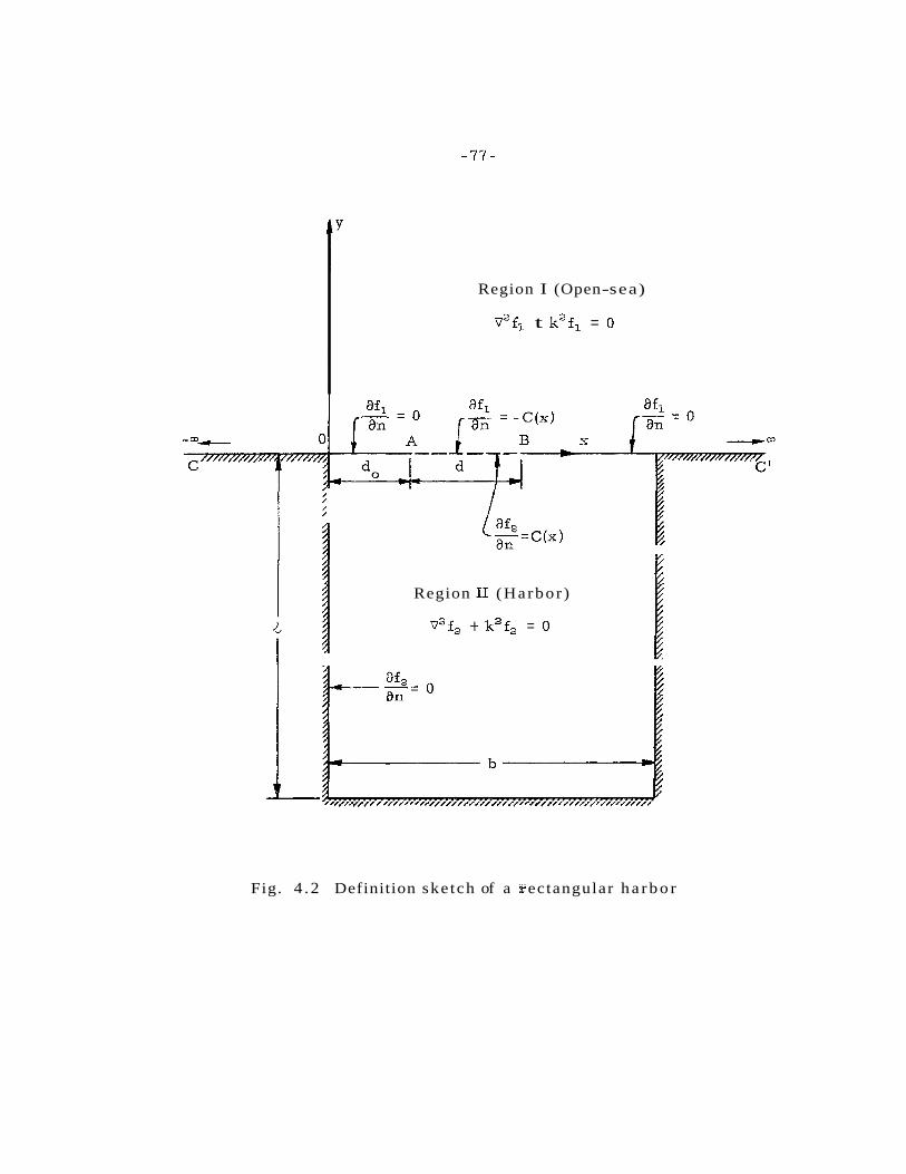
Region I (Open- sea)
v2fi t k2f l = 0
af, (an
Region II (Harbor )
v2f, -t k2f2 = 0
Fig. 4 .2 Definition ske tch of a f ectangular h a r b o r

- 7 8 -
determined. It i s obvious that Eq. 4. 33 satisfies the Helmholtz
equation, Eq. 4. 3 1, and also satisfies the boundary conditions (i)
and (ii) in Eq. 4. 32. Thus, the constants A have to be determined m
so that the solution f2 (x, y ) will satisfy the boundary condition (iii) in
Eq. 4. 32.
Differentiating Eq. 4. 3 3 with respect to y, one obtains: CO
af2 m~ - ( x , y) = m
1 1 A ~ * B ~ [ C O S x sinh 0 (Y +&), aY m= 0
Evaluating Eq. 4.34 at y=O and expanding, one obtains:
w
8% m r - (x, 0) =A k(-sin k&) + ay 0
Am B,(sinh Dm&) cos - p c . m= 1
The coefficients A and Am can be determined by the Fourier 0
cosine transformation method which was used in Subsection 4. 1. 1.
Using this method the following expressions a r e obtained for A. and Am:
2 at, ,+d-td, - --(x,O)dx jd G ( x ) d x bdOay
A = - - - 0
O 2k (-sin k&) bk sin k t 9
m r mn J ~ ~ ' ~ ~ C(x) cos-xdx - 3 b
*m - - . (4, 36b)
G sinh 0 2 m bFm sinh
If C(x) can be approximated by a constant c, as has been done
in Subsection 4. 1. 1, the coefficients A. and Am in Eqs. 4. 36a and
4.36b can be evaluated as:

c d bk sin k& '
- mr 2C [sin -jy(d +do) - sin- miid b o ]
rnrBm sinh Bm&
Substituting Eqs. 4. 37 into Eq. 4. 33, the solution of the wave function
f2 inside the harbor can be written as:
wherein:
So - - d cos k ( v + & ) bk sin k& I
CO fn71. 2 ( s i n y ( d +do) -sin- b d o j m?r cos x cosh p,(y + & ) .
m= 1 mrSm sinh em& b
The complex constant C, i. e. the average normal derivative of the
wave function across the harbor entrance, in Eq. 4.38 has to be
determined by a matching procedure similar to that used previously.
The matching procedure used for the rectangular harbor i s to
equate the average wave function f, evaluated a t the harbor entrance
(f,) to the average wave function fl evaluated at the harbor entrance
Fl 1.
The average wave function f, a c ro s s the harbor entrance &)
can be evaluated as:

where:
4.2.2 Matching of the Solution for Each Region at the Harbor
Entrance
The average wave function, f 2 , determined in Region I1
at thc harbor entrance can be obtained f rom Eq. 4.39. For the
solution in Region I, the relation developed in Subsection 4. 1.2, -
i. e. Eq. 4.27, can be used for the average wave function, fl. Thus
by matching these two solutions at the harbor entrance, the average
normal derivative of the wave function across the harbor entrance, c, can be determined. Equating Eq. 4.39 to Eq. 4.27 one obtains:
thus, the value of C can be determined as:
After the value of C has been determined from Eq. 4.41, the
wave function f, at any position (x, y) inside the rectangular harbor
can be determined using Eq. 4.38. The absolute value of the wave
function f2 (x, y ) i s equal to the amplification factor at the position
(x, y ) as was shown in Eq. 3.38 and Eq. 4.30.

- 81-
It i s noted that in the circular harbor theory developed in
Section 4. 1, the harbor entrance i s limited by the requirement
that the a rc i s approximately equal to the chord at the harbor
entrance. This type of limitation does not exist in the rectangular
harbor theory developed in this section, since no matter how large
the harbor entrance i s , the geometry in Region I1 i s still rectangular
and the separation of variable method can be used. For the case of
a wide harbor entrance compared to the length of the harbor the
entrance can be divided into a number of segments using the matching
procedure to equate the average value of fl and the average value of f,
at each segment at the entrance. Therefore, a set of simultaneous
equations can be obtained ; the value of the normal derivative of the
wave function C for each segment can be determined by solving
these simultaneous equations. after the normal derivative of the
wave function for each entrance segment has been determined, the
wave function fi (x, y) at any position inside the harbor can be
calculated.

CHAPTER 5
EXPERIMENTAL EQUIPMENT AND PROCEDURES
5. 1 WAVE BASIN
A wave basin 1 ft 9 in. deep, 15 f t 5 in wide, and 31 ft
5 in. long shown in Figs. 5. 1 and 5. Z was used for the experiments.
The vert ical walls of the basin we re constructed of 314 in. mar ine
plywood with the floor constructed of 1 in. mar ine plywood. The
basin floor was located 10 in. above the laboratory floor. This can
be seen in Figs. 5. 1 and 5.2 where a substructure supporting the
basin floor was built to allow for proper leveling of the basin floor
and to ra i se the basin to a more comfortable working level. This
substructure consisted of wood s i l l s and joists; seven wood si l ls
(1-5/8 in. x 3-5/8 in. with the short dimension vert ical) were
fastened to the laboratory floor, 2 ft 8 in. on center running the
length of the basin Perpendicular to these si l ls , a system of
joists (1-518 in. x 7-518 in. with the long dimension vertical) was
fastened on 1 ft 4 in. centers. The upper face of the joists was
4- leveled to within - 1/32 in. by placing shim mater ia l between the
s i l l and the joist a t each intersection. The 1 in. plywood was then
glued and screwed to the joists to become the basin floor and the
314 i nve r t i c a l walls and their supporting structure were fastened
in place. (For additional details of the construction of the basin, see

Fig. 5. 1 Drawing of the wave basin and wave generator
(modified f rom Raichlen (1965))
Fig. 5. 2 Over-all view of the wave basin and wave generator with
wave filter and absorbers in place

-84-
Raichlen (1965). ) In order to ensure watertightness and to provide
a level bottom, before this study was initiated, a layer of polyester
r e s i n ("CYBOND 2 5 0 1 P a r t I" manufactured by Amer ican Cyanarnid
Company) approximately 1 /4 in. thick was poured into the basin.
The res in sought i t s own level before i t solidified; therefore, a
t bottom which was horizontal to within at leas t -0. 02 in. was obtained
by this treatment. All the joints were sealed by fiber glass cloth and
res in and the interior of the basin was then painted with an epoxy
base paint. After this t reatment the wave basin remained f ree of
leaks throughout the course of the experiments.
Also shown in Figs. 5. 1 and 5.2 a r e wave energy dissipaters:
a wave f i l ter located in front of the wave machine and wave absorbers
located along two sides of the basin. The details of the constructlon
and the characterist ics of these units will be presented in Sections
5. 6 and 6. 1 respectively.
5.2 WAVE GENERATOR
The wave generator used for this study was a pendulum
type designed to operate either as a paddle- o r piston-type wave
machine; i t s detailed description and design consideration were
given by Raichlen (1965). A photograph of the wave generator and
the overhead support i s shown i n Fig. 5. 3. It i s seen that the plate
of the generator i s obscured by the wave filter; however, this shows
the arrangement of the filter relative to the senerating surface. The
gerleratirlg s u ~ l a c e w a s d r l ~ L U I I I ~ I I U I I ~ plate 11 It 8 ill. lung, 2 It high,

Fig. 5.3 Wave generator and overhead support with wave filter and wave absorber in place
Fig. 5.4 Motor drive, eccentric, and light source and perforated disc for wave period measurement

-86-
and 1/4 in. thick attached to a structural aluminum angle frame
which provided rigidity. As can be seen in Fig. 5.3, this assembly
was suspended from three pairs of a rms connected to an overhead
structure which in turn was fastened to the reinforced concrete ceiling
beam. Each supporting a r m was 2 ft 9 in. long with the upper end of
each forward a r m able to be moved along a slot which was an a rc of
radius 2 f t 9 in. Hence, when the forward a r m at each support was
parallel to the rear arm the wave machine operated as a piston-type
generator; when the upper end of the forward supporting a r m was
moved to the furthermost forward position, the wave machine operated
as a paddle-type wave generator with the bottom of the generating plate
acting as an imaginary hinge point. This arrangement facilitated the
generation of shallow water and deep water waves. The wave generator
was driven by two arms connected to independent eccentrics which in
turn were connected through a pulley system to a 1- 1/2 hp variable
speed motor. This arrangement can be seen in Fig. 5.4. The
eccentrics allowed for a maximum wave machine stroke of 12 in, , but
careful adjustment was necessary to insure that both eccentrics had
identical settings. This was accomplished by measuring the stroke of
the generator at two locations using dial gages, and i t was possible
to adjust the eccentrics to within 0. 001 in. of each other. The motor
was a 1- 1/2 hp U. S. Varidrive Motor with a 10:l speed range and a
continuous variation over this range. Wave periods ranging from 0.34
sec to 3.8 sec could be obtained with this system.

-87 -
5 .3 MEASUREMENT O F WAVE PERIOD
A pulse counting technique was used for the determination
uf the wave period. A s can also be seen i n Fig. 5. 4 , the pulse was
generated by interrupting a light beam, which was directed a t a photo-
cel l , by a d isc with 360 evenly spaced holes arranged in a c i rc le near
i t s outer edge. The d isc was direct ly connected to one eccentr ic of
the wave drive mechanism. A schematic d iagram and circuit of the
photocell device i s presented i n Fig. 5. 5. The voltage pulses so
generated by the photocell c i rcui t were counted over an interval of
10 seconds by a Beckman/Berkeley Division Industrial Counter Model
735 1. The wave period in seconds was obtained simply by dividing
the product of the number of holes t imes the counting interval (3600)
by the number of counts regis tered by the counter in 1U seconds.
Hence, the period measured was an average over a 10 second interval ;
throughout an experiment this period varied a t mos t by $0. 03%.
5 . 4 MEASUREMENT O F WAVE AMPLITUDE
5.4. 1 Wave Gage
Resistance wave gages were used in conjunction with the
Sanborn (150 s e r i e s ) r ecorde r for the measurement of wave amplitude.
A drawing of a typical wave gage i s shown i n Fig. 5.6. The wave gage
consisted of two 0. 010 in, d iameter s tainless s tee l wi res 3-112 in.
long, spaced 118 in. apart . The wi res were stretched taut and
para l le l i n a f r a m e constructed of 118 in. diameter s tainless steel.

P E R F O R A T E D D I S C
V O L T A G E O U T T O C O U P T E R
Fig. 5. 5 Schematic diagram and circuit of photo-cell device ( f r o m Raichlen (1965) )
b----- 2.37"
Fig. 5. 6 Drawing of a typical wave gage ( f r o m Raichlen (1965) )

The wires were insulated electrically f rom each other, except that
current could pass f rom one wire to the other through the water in
which the gage was immersed.
A circuit diagram for the wave gage i s shown in Fig. 5. 7. A
Sanborn Carr ier Preamplifier (Model 150 - 1100 AS) supplied the
2400 cps - 4. 5 volt excitation for the gages and in turn received the
output f rom the wave gages which after demodulation and amplification
w e r e displayed on the recording unit. The displacement of the stylus
of the recorder was proportional to the probe resistance, which in
turn was proportional to the depth. of immersion of wires.
The wave gage was calibrated before and after an experiment
(approximately one hour apart). Three typical calibration curves
a r e presented in Fig. 5. 8 for a wave gage with three different
attenuation settings of the amplifier, i. e. x50, x20, x10. The ordinate
shows the immersion plus withdrawal in centimeters while the
abscissa shows the stylus deflection of the recorder in millimeters.
The calibration of wave gage was performed manually by f i rs t
increasing i ts immersion U. US cm, then returning to the original
position and withdrawing i t 0.05 cm. The same procedure was then
repeated with a larger increment of immersion and withdrawal. A
calibration curve representing an average over the duration of an
experiment was used i n the data reduction procedure. Most cali -
bration curves were essentially linear and showed very little change
during an experiment as can be seen in Fig. 5.8.

P O R T I O N I N T E R N A L T O R E C O W D E R
Fig. 5. 7 Circu i t d i ag ram f o r wave gages ( f rom Raichlen (1965) )
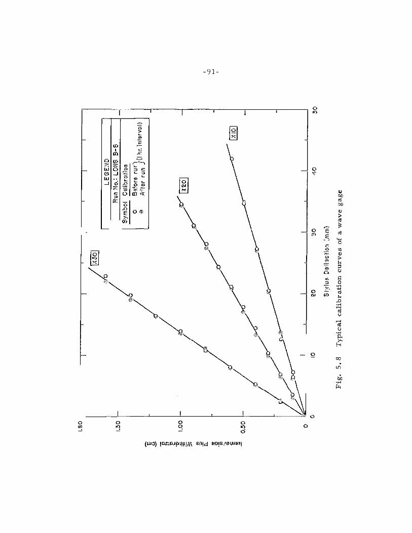

5.4.2 Measurement of Standing Wave Amplitude for the Closed
Harbor
A s rrlentiuned i n Subsection 3 . 2 . 3 , the amplification
factor i s defined as the wave amplitude at a particular location inside
the harbor divided by the sum of the amplitude of the incident and the
reflected wave when the harbor entrance i s closed; this lat ter i s the
standing wave amplitude. Therefore, i n order to determine the
amplification factor experimentally, both the wave amplitude inside
the harbor and the standing wave amplitude when the entrance i s
closed must be measured.
The amplitude inside the harbor i s measured i n a straight-
forward manner using the res is tance wave gages just described. Due
to the variation in the standing wave amplitude along a c res t , caused
by the diffraction of waves off the edges of the wave machine and by
the wave absorbers (see also Ippen and Goda (1963)), i t was necessary
to use an average amplitude of the standing wave ac ross the entrance
in defining the amplification factor.
This average standin? wave amplitude along the "coastline" was
obtained a s follows. With the harbor entrance clo sed, three wave
gages were placed 1 /4 in, f r om the false wall (which represents the
"coastline") with the wires i n a plane parallel to the wall. One wave
gage was located on the center line of t5e harbor entrance, and the
other two gages were located 2 f t to either side. After the wave
amplitude at these three locations had been determined, the wave

amplitude a t the two l imits of the harbor entrance were determined
by interpolation after fitting a second order polynomial to the
measured values. The subroutine "AITKEN/Polynomial Interpolation
FunctionJ' available a t the Booth Computing Center of the California
Institute of Technology was used to accomplish this. The average of
the wave amplitude measured by the center gage and those interpolated
a s just described was used to represent the standing wave amplitude.
Therefore, the amplification factor was determined by dividing the
measured wave amplitude a t a given location inside the harbor by the
standing wave amplitude so determined.
5 . 5 MEASUREMENT OF VELOCITY
The velocity at the harbor entrance was measured using a
hot-film anemometer manufactured by Thermo-Systems, Inc. (Heat
Flux System Model 1020A). The sys tem minimized the effect of the
thermal iner t ia of the probe by keeping the sensitive element at a
constant temperature (constant res is tance) and using the heating
current as the measure of the heat t ransfer and hence the velocity of
the flow. The sensor was a glass cylinder (with a diameter of 0. 001 in.
o r 0.006 in. ) coated with a platinum fi lm which i n turn was covered
with a sputtered quartz layer; the platinum and quartz coatings were
- 5 each approximately 10 in. thick. The sensor was supported by two
insulated needles, and for the experiments, the sensor was aligned
with i t s longitudinal axis paral lel to the bottom of the basin and per-
pendicular to the incoming wave ray. A photograph of one sensor i s
shown i n Fig. 5. 9 with the associated electronics shown in Fig. 5. 10.

Fig. 5 . 9 Photograph of a hot-film sensor
(from Raichlen 11967) )
9334
Fig. 5. 10 Hot-film anemometer, l inearizer, and recording unit

The output of the hot-film sensor i s not linearly proportional to
the flow velocity; instead, it has the following general relation (see
Hi1ue( ( l959)) ;
where E i s the output voltage of the anemometer, I i s the current a
to the sensor, Rw is the operating resistance, V is the fluid v e l o c i L y
normal to the axis of the hot-film sensor, and cl and c, a r e constants
which depend upon the propert ies of the hot-film and the temperature
difference between it and the fluid. In steady flow, the exponent c3 in
Eq. 5. 1 i s usually taken as f /2 ; such a relationship i s referred to as
King's law ( see Hinze (1959)).
Fo r a constant temperature system, the operating resistance of
the sensor , Rw' is kept constant by electronic feedback. The value
(Rw-Ru)/R (wherein R i s the cold res is tance of the hot-film sensor) r, b0 g
i s usually called the "over-heat rat iof ' . For present experiments, an
over-heat rat io of 2% to 3% was used.
Assuming King's law applies for the present experiments (see
Subsection 6.2.5 for a discussion of the shortcomings of this
assumption), Eq. 5. 1 can be writ ten as : -1
E = (c, + C , , , / V ) ~ 9
providing a simple relationship which can be linearized so that the
output voltage i s directly proportional to the fluid velocity. In order
to accomplish this, a linearizing circuit built by Townes (1965) was
used.

- 96 -
The sequence of operation of the l inearizer i s a s follows. The
output of the anemometer was f i r s t amplified to the best operating
level fo r the l inearizer (approximately 10 volts) and used as the input
to the f i r s t squaring circuit of the l inear izer ; the output f rom the f i r s t
squaring circuit, S I , can be expressed as:
S1 = ( c a k y = caD (c, + c, R) , ( 5 . 3 )
where ca i s the amplification by the preamplifier.
It can be seen f rom Eq. 5. 3 that the output of the f i r s t squaring
circuil S1 is r io t e q u a l l o zero when the fluid velocity is zero. There-
fore, a mean voltage was subtracted f rom that shown in Eq. 5. 3 ,
when the velocity was equal to zero. Hence, the signal can then be
expressed as:
S b = S T - c 2 c 1 = c ~ c 2 J ~ a . ( 5 . 4 )
This voltage was then amplified again to the bes t operating level
for the l inearizer, and introduced to the second squaring circuit. The
final output voltage f rom that stage, S,, can be expressed as:
Thus, after the linearizing operation, the output voltage f rom
the second squaring circuit, S2, is linearly proportional to the fluid
velocity, V. It should be noted that the relationship shown i n Eq. 5,
implies that King's law (Eq. 5.2) applies. A calibration i s required
if one i s to determine the constant av in Eq. 5. 5 and thus the absolute
velocity; for the present experiments no attempt was made to calibrate

-97-
the sensor. If the applicability of Eq. 5. 5 i s assumed, the relative
velocity a t two positions can be obtained as the ratio of the final
output voltage S , a t those two positions. For example, for the experi-
ments dealing with the velocity distribution across the harbor
entrance the output voltage a t various positions can be normalized
with respect to either the value at the center or the average value
across the entrance; both normalizations yield information regarding
the shape of the velocity distribution across the enlrance.
5.6 WAVE ENERGY DISSIPATION SYSTEM
Two types of wave energy dissipators were employed in
the present experiments: a wave filter placed in front of the wave
generator, and wave absorbers located along the side-walls of the
wave basin. This system was designed to simulate open-sea conditions
in the restricted laboratory basin, and the design criterion and
characterist ics of the system will be discussed i n Section 6. 1.
An overall view of the wave energy dissipator s i s shown in the
photograph, Fig. 5. 11. The wave filter, shown in front of the wave
generator in Fig. 5. 11, was 11 ft 9 in. long, 1 f t 4 in. high and 5 ft
deep in the direction of wave p r u p a g a t i o r ~ a n d w a s constructed of 70
sheets of galvanized iron wire screen in three sections each 3 f t 11 in.
long. The wire diameter of the screens was 0.0 1 1 in with 18 wires
per inch in one direction and 14 wires per inch in the other. As seen
in Fig. 5. 12 each section of the filter had three vertical stiffening
pleats located approximately 1 f t apart on each sheet; in addition,
right angle bends each 0.8 in. long were made a t the top and bottom

9320
Fig. 5. 11 Wave energy dissipators placed in the basin

(a) Front view
f b ) Side view
Fig. 5. 12 Section of wave filter
9337
Fig. 5. 13 Bracket and structural frame for supporting wave absorbers

of each sheet to further stiffen them. Seventy identical sheets were
then fastened together with 6 stainless steel rods of 1 /8 in. diameter.
Spacers consisting of 1 /8 in. I. D. lucite tubing 0. 8 in. long were
placed on each rod to maintain a uniform spacing. These lucite
spacers can be seen from the side view of the filter in Fig. 5. 12. The
right angle bends a t the top and the bottom of each screen also served
as spacers. The 70 sheets were then tacked together by soldering to
becv111e d reldtively st i l l u d l that could stdrld by i t s o w n rigidity in
the wave basin, resisting the waves without fixed supports.
While the wave filter was built to stand in the wave basin by i ts
own rigidity without additional support, the wave absorbers, shown in
Fig. 5. 11, were supported by structural f rames outside the wave
basin. (One of these structural f rames i s shown i n Fig. 5. 13. ) The
wave absorbers, placed along the side-walls of the basin, were each
1 f t 6 in. high, 1 ft 10 in. thick, and 30 ft long and consisted of 50
layers of the same galvanized i ron screen as used in the wave filter.
To construct these wave absorbers, a unit of 10 screens, each 30 f t
long, 1 ft 6 in. wide spaced 3/8 in. apart was held together by
brackets at each end of the screens. The spacers were composed of
pieces of pressed fiberboard called Benelex (3/8 in. thick, 2 in. wide,
1 f t 6 in. long) placed between each screen. Benelex was used since
it absorbed only a small amount of water compared to some other
materials. A bracket was fastened over the screens and spacers
clamping the 10 screens together firmly as a unit. The screens in a
unit of 10 layers were then stretched taut by 3/8 in. diameter stainless

- 10 1-
steel rods which connected f r o m the brackets a t the ends of the units
to the s t ructura l f rames located outside the basin. Holes were drilled
into the wall of the basin for the rods; fittings with "0"-ring seals were
mounted in the wall to prevent the leakage around the rods, Therefore,
the rods transmitted a l l the tension required to hold the screens taut
to the structural f rames a t each end: hence no significant forces were
applied to the basin walls. Five identical units (a total of 50 layers of
screens) were built i n this manner along each side of the basin as
shown i n Fig. 5. 11.
The wave energy dissipating system provided a large a r e a of
galvanized i ron i n the wave basin, 9. 0 ft2 of wi re sc reen per ft3 of
basin water. Because of the chemical reaction between the wire
screens and the water when the screens were initially installed the
zinc i n the galvanized screens deposited in the basin. This not only
decreased the amount of zinc that protected the wi res of the screens
but the reaction also produced a coating of undissolved zinc on the
water surface. The la t ter effect led to undesirable operating charac-
ter is t ics of the wave gages. For this reason, it was necessary to
introduce additives to the water to reduce and even prevent this
reaction. A se r ies of experiments were conducted in o rder to find
a proper additive. It w a s found that a technical grade of sodium
dichromate (Na, Cr,Clr)added to the water in a concentration of 500 ppm
(by weight) could accomplish this. The concentration of the sodium
dichromate was checked periodically by a light absorption technique
and if the concentration was found to be l e s s than desired, more was

- 102-
added. In order that this additive could function properly a s a
corrosion inhibitor, i t was necessary to keep the pH of the water l e s s
than 6. 5; usually the pH was maintained in the range of 6.2 to 6. 5 by
periodically adding hydrochloric acid (HC1). This treatment of the
basin water proved to be successful in both preserving the wire
screens and eliminating the precipitate on the water surface, and it
had no observable effect on the wave gages.
5 .7 HARBOR MODELS
Four different harbors with constant depth were investi-
gated experimentally: a rectangular harbor, a circular harbor with
0 0 a 10 opening, a circular harbor with a 60 opening, and a model of
the Eas t and West Basins of the Long Beach Harbor (Long Beach,
California). The harbor models were designed so that each would
f i t into a false-wall simulating a perfectly reflecting "coastline" and
it was installed 27 f t 6 in. f r om and paral lel to the wave paddle, i. e.
2 ft. 6 in. f rom the back-wall of the basin. The false-wall was made
of lucite 318 in. thick and 1 f t 3 in. high mounted to a f rame composed
of galvanized i ron angles constructed in two identical pieces: the
east-wing and the west-wing. Each wing extended 4 ft 9 i z f r o m I f t
off the center of the wave basin to the inner most screen of the wave
absorbers. Aphotographof thesuppor t ingf ramesandthewal l s i s
presented i n Fig. 5 . 14- The walls were weighted to hold them in
place without d i rect connections to the basin floor, In line with the
false-wall, lucite spacers 318 in. thick, 1 in. wide and 1 ft 6 in. high
were placed between each screen of the absorbers. These spacers
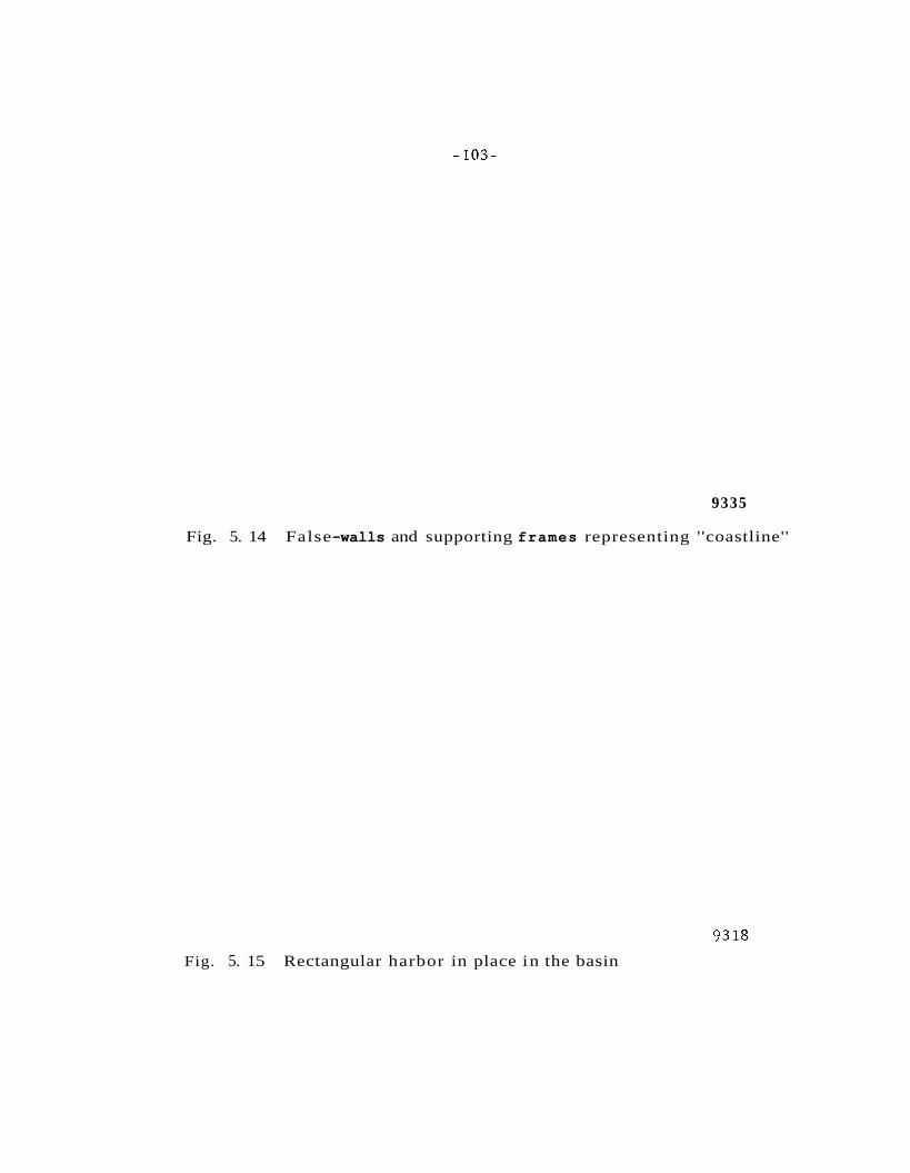
9335
Fig. 5. 14 False -walls and supporting frames representing ''coastline''
Fig. 5. 15 Rectangular harbor in place in the basin

which can be seen in upper left-hand-portion of Fig. 5. 13 were placed
to prevent waves penetrating through the absorbers to the still water
region behind the false wall thereby creating undesirable oscillations
i n the basin.
In the following, a brief description of the harbor models is
presented:
(i) Rectangular harbor: The rectangular harbor was 12-1/4 in.
long, 2-3/8 in. wide with a fully open entrance and it was constructed
of 1/4 in. thick lucite. Fig. 5. 15 shows how the rectangular harbor
was placed in relation to the false-wall inside the wave basin. It
should be mentioned that the false-wall, "coastline", shown i n Fig.
5. 15 was different f rom the false-wall described in the previous para-
graph. This wall was constructed f rom plywood ( 3 /4 in. thick) and
painted with an epoxy based paint. However, it was found that this
wall expanded due to water absorption; therefore, after the experi-
ments with the rectangular harbor were finished this false-wall was
replaced by the one constructed of lucite just described which was
used for al l subsequent experiments.
0 (ii) Circular harbors : The two circular harbors (a 10 opening
and a 60° opening), shown in Figs. 5. 16 and 5. 17, were each 1 f t 6 in.
diarnetcr and 1 ft 3 in. high, and thcy wcrc constructcd of 1 /4 in.
lucite plate which was heated and bent to shape. The cylinders were
each connected on the top and the bottom to two 1/2 in. lucite rein-
forcing plates with holes cut to an inside diameter of 1 f t 6 - 1/2 in. ;
this i s clearly shown in Figs. 5. 16 and 5. 17. These two reinforcing

0 9323
Fig. 5, 16 Circular harbor with a 10 opening
0 9325
Fig. 5. 17 Circular harbor with a 60 opening

-106-
plates were necessary to keep the planform of the harbors circular.
The two vertical plates shown near the harbor entrance in both Figs.
5. 16 and 5. 17 connected to the harbor fitted into the two foot space
which had been left in the false-walls just described; thereby resulting
in a smooth "coastline" extending from the wave absorbers to the
limits of the harbor entrance.
(iii) Model of Long Beach Harbor: The model of Long Beach
Harbor shown in Fig. 5. 18 was also constructed from 1 f 4 in. thick
lucite plate. The shape of the planform of the harbor was cut f rom
two lucite sheets using dimensions such that when the vertical
boundary walls were cemented in place the inside dimension of the
harbor would be as desired. These supporting plates can be seen a t
the top and bottom of the harbor model in Fig. 5. 18. This model was
composed of 15 pieces of lucite cemented to the supporting plates
and rubber cement was used a s filets in the corners. The planform
o f the model was simplified f r o m the existing harbor and can be
compared to the prototype in the map (Fig. 5. 19) which was extracted
from the U. S. C. & G. S. map No. 5 147.
5 .8 INSTRUMENT CARRIAGE AND TRAVERSING BEAM
A photograph of the instrument carriage and traversing
beam i s presented in Fig. 5.20; also seen in this photograph i s the
frame which was placed outside the model of the harbor to support
the instrument carriage. This f rame, constructed of galvanized
steel angles, was bolted to four pads that were cemented to the basin
floor. An aluminum plate 3 /8 in. thick, 2 ft 4 in. square with a

Fig. 5. 18 Model of the Eas t and West Basins of Long Beach Harbor (Long Beach, California)
Fig. 5. 19 Map showing the position of the Eas t and West Basins of Long Beach Harbor and the model planform. (The harbor model i s shown with dashed lines. )

circular hole of 2 f t inside diameter was mounted to the top of the
s t ructura l f rame. The carriage which was supported at three points
with ball bearings was f r ee to rotate with the hole in the plate as i t s
guide and coupled with the t ravers ing beam the wave gage could
therefore be moved to any position inside the harbor. The complete
f rame could be moved toward o r away f rom the false-wall so that the
center of the circular hole on the aluminum plate coincided with the
center of the circular harbor. In addition, the f rame could be leveled
by adjusting the bolts on the supporting pads s o that the wave gages
remained a t the same immers ion if moved to other positions within
the harbor.
The traversing beam shown in Fig. 5 .20 consisted of an alum-
inum channel to which two lead screws (16 threads per inch) were
mounted. These screws were connected to a gear arrangement at
one end so that they could be rotated either alone o r simultaneously.
T h e s c r e w s pasqed thrnugh twn threaded hlockq t o which t h e w a v e
gages were attached. As the lead screws were rotated these blocks
moved in slots cut in the channel thus positioning the wave gages.

Fig. 5.20 Instrument carriage and traversing beam shown mounted
above lo0 opening circular harbor

CHAPTER 6
PRESENTATION AND DISCUSSION OF RESULTS
Experimental and theoretical results a r e presented in this chapter
which deal with the wave induced oscillations of three harbors with
6 specific shapes: circular harbors with 10 and 6u0 openings, a
rectangular harbor, and a model of the East and West Basins of Long
Beach Harbor located in Long Beach, California. All the harbors
investigated were of constant depth and were connected to the open-sea;
thus, an effective wave energy dissipating system was necessary to
simulate these open- sea conditions in the laboratory. The character -
ist ics of the wave energy dissipators chosen for this system will be
discussed fir st, followed by the presentation and discussion of the
results for the three harbors mentioned. All numerical computations
were accomplished using an IBM 360175 high speed digital computer.
6. 1 CHARACTERISTICS O F THE WAVE ENERGY DISSIPATION
SYSTEM
The theories developed in Chapter 3 and 4 t reat the case of
a harbor connected to the open-sea which lead to the existence of the
"radiation condition1', i. e . the radiated waves which emanate from the
harbor entrance decay to zero at an infinite distance f rom the harbor.
However, in the laboratory, experiments must be conducted in a wave
basin of finite size; thus, the radiated waves f rom the harbor will be

reflected from the wave paddle and the sidewalls of the basin unless
effective energy dissipators a r e provided. Indeed in the absence of
dissipators Ippen and Raichlen (1962) (also Raichlen and Ippen (1965) )
have shown that the response curve of a rectangular harbor connected
to a highly reflective basin i s characterized by numerous closely
spaced resonant spikes. This result i s strikingly different f rom the
response curve for a rectangular harbor connected to the open-sea
which was subsequently studied by Ippen and Goda (1963) where fewer
modes of resonant oscillation were observed over similar ranges of
wave period. In this section the design considerations and character-
ist ics of the wave energy dissipating system (described in Section 5.6)
which was used in these experiments to alleviate this problem will be
presented and discussed.
A theoretical and experimental investigation of wave energy
dissipators composed of wire mesh screens aligned normal to the
direction of wave propagation was conducted by Goda and Ippen ( 1963).
In their analysis each screen was considered to be composed of
numerous equally spaced circular cylinders aligned vertically and
horizontally; i t was assumed that there was no wave reflection from the
energy dissipator, and the energy dissipated by each cylinder was
assumed to be independent of i t s proximity to the other cylinders.
Therefore, the total energy dissipation was taken to be equal to the
sum of that f rom each of the cylinders in the unit. Based on these
assumptions, Goda and Ippen ( 1963) developed the following semi-
empirical equation for the transmission coefficient of such a
dissipalor:

where: K = transmission coefficient, defined as the ratio of the 1rans.crlitled wave height to the incident wave height, Ht /Hi,
m = number of layers of screens,
D = diameter of the screen wire,
S = center to center distance between wires,
cr = circular wave frequency (2n/T),
v = kinematic viscosity of the fluid,
L = wave length, and
cp(h/L) = depth effect factor which i s a function of the ratio of depth to wave length. (The interested reader i s referred to Coda and Ippen (1963) Eq. 2 .29 for this expression; for deep water waves i t is equal to 1.8 1. )
Based on the experimentally determined values of the transmission
coefficient, Kt, and the reflection coefficient, Kr, for various dissi-
pator s , an empirical relation was obtained to correlate these
quantities :
wherein K i s defined as the ratio of the reflected wave height to the r
incident wave height, Hr /Hi.
To confirm the validity of Eqs. 6. 1 and 6.2 so that they could
be used with confidence in designing the wave energy dissipators for
this study (described in Section 5.6) a se r ies of experiments using
model dis sipators was conducted. These experiments were carried
out in a wave tank 1 f t 6 in. wide, 1 ft 9 in. deep, and 3 1 ft long using
a paddle type wave generator and using the procedures employed by

Goda and Ippen (1963). Two model dissipators were tested, denoted
here as Dissipator A and Dissipator B; their characteristics a r e
presented in Table 6. 1.
Table 6. 1 Model wave energy dissipators
Dis sipator
.L. .I.
For this study the horizontal and vertical spacing of the wires were not equal and the value denoted as S i s the average spacing (see Section 5. 6).
Mesh (S)+ Averaged Center to Center Spacing
of Wires (in. )
A dissipator i s called a wave filter if it i s placed between the
wave generator and the back-wall of the wave tank; i t i s called wave
absorber if placed against a reflecting surface of the tank. In order
to dctcrminc thc transmission and rcflcction cocfficicnts of thc wavc
filter, two wave gages were used to measure the wave envelope in the
region ahead and behind the wave filter. To determine the reflection
coefficient of the wave absorber one wave gage was used to measure
the wave envelope in the region in front of the wave absorber. It can
be shown that the incident and reflected waves can be determined
simply from such wave envelopes ( see Ippen, 1966, pp. 46-49).
The experimental and theoretical variation of the reflection
coefficient, Kr, with the incident wave steepness , Hi/L, for Dis s i -
pators A and B a re presented in Figs. 6. 1 and 6. 2 respectively. In
both Figs. 6. 1 and 6.2, the experimentally determined reflection
Screen Wire Diameter
(D)
(in. )
Distance Between
Layers of Screens
(in. )
Number of Layers of Screens
(m)

Fig. 6. 1 Reflection ~ i e f , , E(, , as a function of the
Fig. 6. 2 Reflection coef ., K*, as a function of the
incident wave steepness, Hi/L, for

- 115-
coefficients a re presented for each dissipator used both as an absorber
and as a filter. The former refers to the case where the dis sipator
was placed against the back-wall of the wave tank, while the latter
refers to the case where the dissipator was located between the wave
machine and the back-wall. The theoretical curves presented in Figs.
6. 1 and 6.2 a r e computed in the following way: f i rs t , the transmission
coefficient, K i s computed from Eq. 6. 1, and the reflection coeffi- t ' cient, IIr, is then determined from the empirical relation, Eq. 6. 2.
The experimental data presented in Fig. 6. 1 show considerable scatter;
however, the data follow the trend predicted by Eqs. 6. 1 and 6.2, i. e.
for a constant wave period the reflection coefficient, Kr, decreases
as the wave steepness, H increases, and for a constant wave
steepness, the reflection coefficient, Kr, increases as the wave
period, T, increases.
Similar data a re presented in Fig. 6.2 for Dissipator B where
the number of screens has been increased from 38 to 50 and the
spacing of the screens reduced from 0 . 5 in. to 0 . 375 in. By comparing
Figs. 6. 1 and 6.2, as expected, it i s seen that Dissipator B i s more
efficient than Dis sipator A.
In Fig. 6.3 the experimentally determined reflection and trans-
mission coefficients for these two dissipators a re shown. The experi-
mental data obtained by Goda and Ippen (1963) which were the basis
for their empirical relation, Eq. 6.2, a r e also included in Fig. 6.3.
Three relations: Kr = K ~ ' , Kr = and Kr = K ~ ~ , a r e shown in
Fig. 6.3 for reference. It i s seen that the experimental data show
considerable scatter; nevertheless, the results for Dissipator A agree
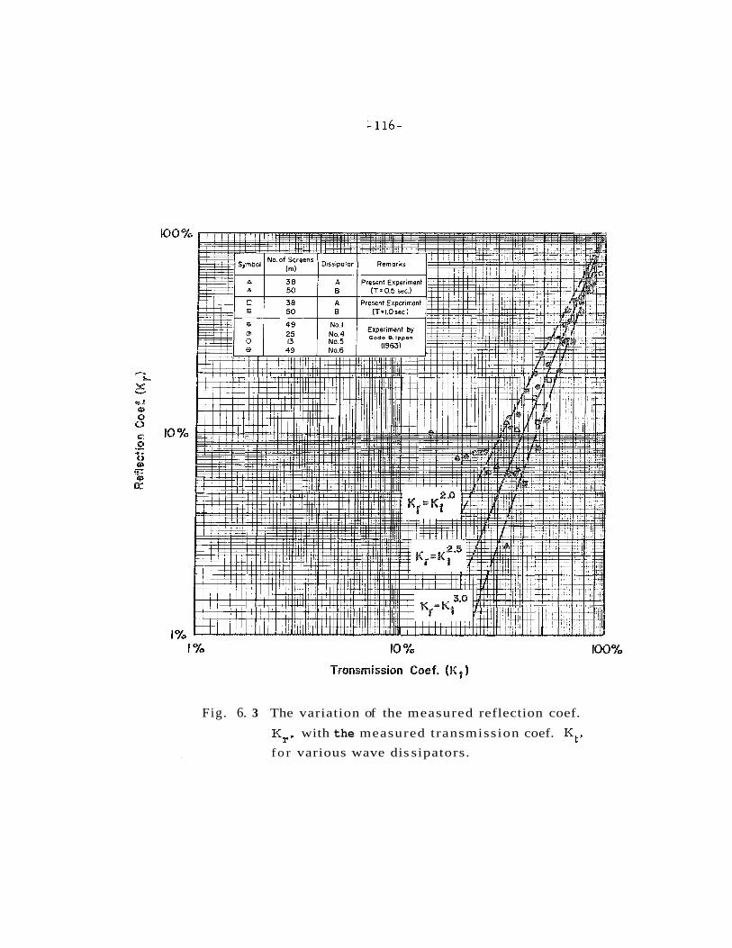
Fig. 6. 3 The variation of the measured reflection coef.
Kr, with the measured transmission coef. Kt,
f o r various wave dis sipators.

- 117-
best with the expression: K = K ~ ~ ' 6 , and the results for Dissipator B r
with: Kr = K~"". This difference for the two dissipators suggests
that the wave energy dissipation characteristics might be affected by
the spacing between the screens which was neglected in the analysis
by Goda and Ippen (1963). The results also show that for a constant
reflection coefficient. K the transmission coefficients, r' Kt, obtained
from the present experiments a r e somewhat larger than those obtained
by Goda and Ippen (1963).
The most important characteristic of the wave energy dissipators
in simulating the unbounded open-sea is the reflection coefficient, * Kr
It was suggested by Ippen and Goda (1963) that the reflection coefficient,
Kr, of wave fi l ters and absorbers should be l e s s than 2070 for proper
simulation of open-sea conditions in a restricted wave basin. The wave
absorbers finally chosen for this investigation consisted of 50 layers of
screens with a spacing of 0.375 in. between screens (as described in
Section 5 . 6). Therefore, the wave energy dissipation characteristics
of the wave absorbers used a r e identical to those of Dissipator B used
in these preliminary experiments and shown in Fig. 6.2. With
reference to Fig. 6.2, except for very small incident wave steepnesses
the reflection coefficient of the absorbers i s estimated to be less than
20% for the majority of thc harbor rcsonsncc cxpcrirncnts which wcre
conducted.
The wave filter used, which has been described in Section 5.6,
consisted of 70 layers of screens with a spacing of 0.8 in. between
layers of screens. The reflection coefficient of the wave filter is
expected to be less than that of the wave absorbers for comparable

-118-
incident wave steepnesses due to the smaller number of screens and
spacing in the latter. Therefore, it i s expected that except again for
the case of an extremely small wave steepnes ses, the reflection
coefficient of the wave filter used i s less than 20%.
In order to ensure that the open-sea condition was properly
modeled in the wave basin using the wave energy dis sipators described,
in initial phases of this study the response to periodic incident waves
of a fully open rectangular harbor (2-3/8 in. wide and 1 ft 1/4 in. long
and identical to that studied by Ippen and Goda (1963) ) was studied
experimentally. The results obtained agreed well with both the
theoretical "open- s ea solution" and the experimental results obtained
by Ippen and Goda (1963). Thus, the open-sea condition for the
radiated wave was considered to have been simulated properly in these
experiments. The results of these experiments will be presented and
discussed in detail later in Section 6.3.
6.2 CIRCULAR HARBOR WITH A 10' OPENING AND A 60' OPENING
6.2. 1 Introduction
As discussed previously, the wave induced oscillations in
a circular harbor connected to the open-sea can be evaluated by using
either the special theory developed in Section 4. 1 (if the chord which
represents the harbor entrance can be approximated by an arc of the
circle) or using the general theory developed in Chapter 3 for an
arbritrary shaped harbor. In this section, the theoretical results
obtained from these two theories a re compared to the experimental

- 119-
0 results for harbors with a l o 0 and a 60 opening. In order to verify
the theory the following results will be presented and discussed:
the variation of the amplification factor at a fixed position
inside the harbor as a function of incident wave number (or
wave period),
the variation of the wave amplitude inside the harbor for
various resonant modes,
the variation of the total velocity at the harbor entrance as
a function of incident wave number, and
the distribution of velocity across the harbor entrance for
various wave numbers.
6.2.2 Response of Harbor to Incident Waves
The response of a harbor i s defined, for this study, as the
variation of the amplification factor, R, with the wave number para-
meter ka (wherein k is the wave number and a i s a characteristic
plsnform dimension of the harbor, the radius for the circular harbor).
The function ka i s of course dependent upon wave period and depth
whereas the amplification factor R i s also a function of position. The
amplification factor R i s defined as the wave amplitude a t the position
(r, 8 ) divided by the standing wave amplitude which exists in the wave
basin with the harbor entrance closed for the wave number (or period)
of interest. Over some range of wave number the wave amplitude
inside the harbor may be amplified while over another range it may
be attenuated. Physically, for such a harbor this resonance results
f rom the trapping of incident wave energy inside the harbor a t
- 120-
particular wave numbers (or wave periods) which depend on the
geometry of the harbor as well as the depth.
Two response curves for a circular harbor with a l o0 opening
a r e presented in Figs. 6.4 and 6. 5, where the two theories described
in Chapters 3 and 4 a re compared to experiments. The experiments
w e r e conducted i n a circrdar harhor of 1. 5 ft diameter with the depth
of water constant and equal to I f t i n both the harbor and the "open-sea".
In both figures, the solid line represents the theoretical curve
computed from the theory for an arbi t rary shaped harbor (Chapter 3 ) ;
the theory for the circular harbor (Section 4. 1) i s shown with dashed
lines. The theoretical amplification factor was calculated using Eq.
Eq. 3 . 3 8 and Eq. 4.30 for the arbitrary shaped harbor theory and
the circular harbor theory respectively. The experimental ampli -
fication factor was obtained by dividing the wave amplitude at the
point investigated inside the harbor (center of the harbor or the
0 position: r=O. 7 f t , 0=45 ) by the average wave amplitude of the
standing wave system at the harbor entrance. The standing wave
system was measured at the "coastline" when the entrance was closed;
the procedure for obtaining the average wave amplitude of the standing
wave system was described in Section 5.4.
Fig. 6. 4 shows the response at the center of the harbor while
0 Fig. 6. 5 shows the response at the postion r = O . 7 ft, 8=45 . The center
of the harbor i s a unique position to investigate because i t i s the
location having an equal distance to any point on the boundary. The
0 position: r = O . 7 ft, e=45 i s near the harbor entrance and was chosen
because i t was of interest to know whether the harbor entrance had any
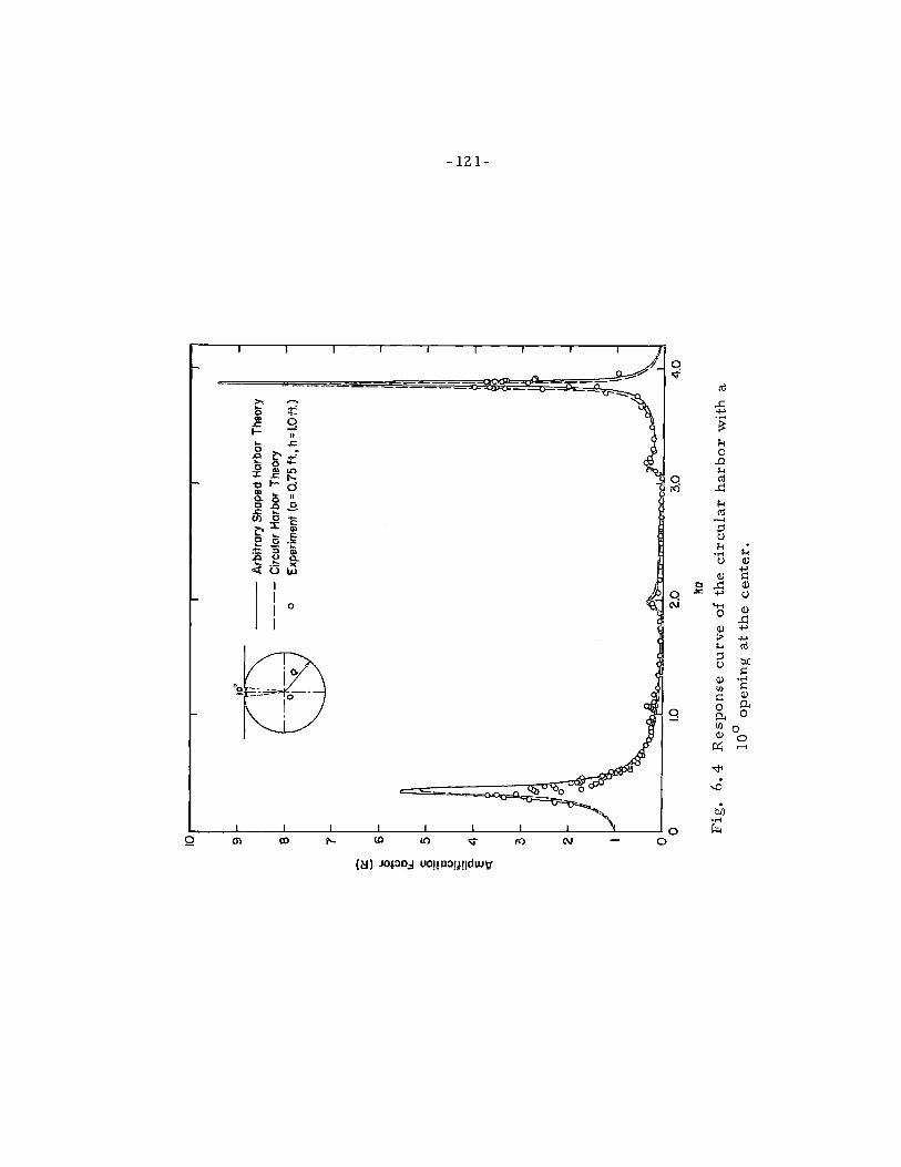

special influence on the response that might not be predicted by the two
theories. In the experiments the wave amplitude at these two positions
was measured simultaneously; however, the gages were separated by
a3out one radius, thus any disturbance caused by one of the wave gages
would not be expected to seriously affect the other.
For the case of a circular harbor with a lo0 opening the a r c and
the chord at the harbor entrance a re almost the same length, there-
fore the theory for the circular shaped harbor developed in Section 4. 1
can be considered to be applicable. In using the theory for an arbi-
t ra ry shaped harbor, the boundary of the circular harbor was divided
into 36 segments with each segment containing lo0 of the central angle.
Since the harbor entrance was represented by one of these segments,
only one unknown complex constant of the normal derivative of the
wave function (e) needs to be evaluated by the matching procedure.
In Figs. 6.4 and 6.5 reasonably good agreement i s seen between
the experimental data and the theoretical rc sults. Bccauoc the cncrgy
dissipation due to viscous effects i s not considered in the theoretical
analysis, the theoretical values near resonance are, as expected,
higher than the experimental values; more discussion of this will be
presented later in this subsection. Four maxima in the range of ka
that were investigstcd can bc sccn in thc curvcs in Figs. 6 . 4 and 6 . 5 ;
the values of ka for these four are: 0.35, 1. 988, 3. 18, and 3.87.
These correspond to four distinct modes of resonant oscillation; the
shape of the water surface for these modes of oscillation will be

- 124-
discussed in detail in Subsection 6.2.4. It can also be seen in Figs.
6 .4 and 6.5 that the response in region of ka w 3.87 i s very peaked,
i. c. s la rgc amplification fac tor and a narrow wave number band-
width (range of ka); the theoretical amplification factor at the center
of the harbor i s nearly 10.
As the width of the harbor entrance increases, the difference
between the length of the chord and the a r c at the entrance increases
and the theory for the circular harbor developed in Section 4. 1 may
no longer be satisfactory. In order to examine the effect of the small
entrance approximation of the circular harbor theory on the harbor
response when the entrance to the open-sea i s relatively large, a
0 circular harbor with a 60 opening was investigated. In this case the
Icngth of the chord and the a r c at the entrance differ by d i m o s t 570,
0 Two response curves for the circular harbor with a 60 opening
a r e presented in Figs. 6.6 and 6.7. Fig. 6.6 shows the response
curve for the center of the harbor; this position corresponds to that
shown in Fig. 6.4 and experimental data f rom two circular harbors
(1. 5 and 0. 5 ft diameter) a re included. This smaller harbor was
used to obtain data at smaller values of ka than could be obtained
with the 1.5 f t diameter harbor. Fig. 6.7 shows the response curve
0 for the position: r = O . 7 f t , 0=45 corresponding in location to the
curve shown in Fig. 6. 5; experimental data for only the circular
harbor of 1. 5 f t diameter a r e included for that location. As before,
at both locations theoretical curves obtained from each of the theories
a r e shown.


- 127-
In using the theory for an arbitrary shaped harbor, the boundary
of the harbor (including the harbor entrance) was divided into 36
segments, and for this case the harbor entrance was represented by
six of these boundary segments. Therefore, six complex constants
of the normal derivative of the wave function (2) at the harbor
entrance were determined by the matching procedure. However,
when applying the circular harbor theory, only one constant was used
at the entrance, i. e. the average normal derivative of the wave function
across the harbor entrance (c) obtained by the matching procedure
discussed in Section 4. 1.
The theoretical results presented in Figs. 6.6 and 6.7 show good
agreement with the experimental data. Note that in Fig. 6.6, data
obtained from experiments conducted in a circular harbor of 0.5 ft
diameter a re denoted by solid circles. These data combined with the
data obtained in the harbor of larger diameter (1. 5 f t ) show that the
response curve of the harbor at a particular location i s only a function
of ka.
From the theoretical results presented in Figs. 6.6 and 6.7,
i t appears that for the two theories there i s a small difference in the
value of the wave number parameter, ka, which i s predicted at reso-
nance. This difference i s probably caused by the different treatment
at the harbor entrance for the two theories: for the circular harbor
theory one segment was used whereas for the arbitrary shaped
harbor theory the entrance was divided into six segments. In fact,

- 128-
it i s seen f rom Figs. 6.6 and 6. 7 that in the location of the peaks
the experiment agrees better with the arbi t rary shaped harbor theory.
The values of ka fo r the four modes of oscillation shown in these
figures can be denoted by ka = 0.46, 2. 15, 3 . 3 8 , 3.96 which a r e the
average values f r om the two theories.
It should be noted that these four maxima a r e well defined in
Fig. 6. 7 whereas the third maximum i s not obviously shown i n the
response curve for the center of the harbor (Fig. 6. 6). This problem
of defining the resonant mode of oscillation solely by a response curve
such a s this will be discussed m o r e fully in Subsection 6.2. 5.4. The
amplitude distribution corresponding to these resonant modes will be
discussed in Subsections 6.2.3 and 6.2.4.
By comparing E'ig. 6 .4 with k'ig. 6. 6 and P'ig. 6. 5 with P'ig. 6. 7
one i s able to observe the effect of the s ize of the harbor opening on
the amplification of waves inside the. harbor. It i s obvious f rom these
figures that the maxima which appeared in Figs. 6 .4 and 6. 5 for the
0 harbor with a 10 opening a r e replaced by peaks of smaller ampli-
fication factors and l a rger bandwidth for the harbor with a 60°
opening (see Figs. 6.6 and 6.7). This effect was called the "harbor
paradox" by Miles and Munk ( 1962). In addition, in comparing these
0 figures it is seen that fo r the 60 opening, the values of ka of the
modes of resonant oscillation a r e larger than the values of ka for
0 the corresponding modes for the harbor with a f O opening.

- 129-
Another characterist ic that can be observed f rom a comparison
of Fig. 6 .4 with Fig. 6.6 and Fig. 6. 5 with Fig. 6. 7 i s that the
theoretical resul ts agree with the experimental resul ts better for the
harbor with the l a rge r opening. In order to explain this, some con-
sideration must be given to the effect of energy dissipation at r eso-
nance. In the theore t i ca l analysis it w a s shown that the radiation
of energy f rom the harbor to the open-sea, l imits the amplification
a t resonance. In nature in addition to the radiation effect, viscous
dissipation of energy l imits the maximum amplification even more.
Since the theory only treated the effect of radiation, one expects the
theoretical values of the amplification factor i n the region of reso-
nance to be l a rger than the experimental values. Moreover, for the
same incident wave characterist ics the energy dissipation a t the
entrance due to viscous effects a r e relatively more important for the
harbor with a smaller entrance. Thus a better agreement between
the experimental and theoretical results i s apparent for the harbor
with a 60° opening. On the other -hand the resul ts i n Figs. 6.4 to 6. 7
demonstrate that the wave numbers (o r periods) at resonance a r e
correct ly predicted by the two theories. These effects for the harbor
a r e s imi lar to those for a single -degree-of-freedom oscillator where
viscous dissipation, &fects resonant amplification much more than it
affects the natural periods of oscillation.
The agreement between the theories and the experiment i s eyen
more encouraging since the experiments conducted for the response
curves presented in Figs. 6 .4 to 6. 7 covered the range of waves

f rom shallow water waves to deep water waves. The conventional
method of classifying waves is: shallow water waves for h / L .: 1/20,
intermediate waves for l/ZO < h/L < 1 / Z , and deep water waves for
h / L > 112 (wherein L i s the wave length, h i s the depth); thus, the
experiments conducted for ka < 0. 236 (a=O. 75 ft ) a r e shallow water
waves, whereas those for 0.236 < ka < 2.36 a re intermediate waves
and for ka > 2.36 the waves a r e deep water waves. It should also be
mentioned that the experiments were accomplished using a wide-
range of stroke settings of the wave machine (see Appendix IV).
Since this range of stroke settings results in a wide range of incident
wave steepnesses the good agreement between the theories and the
experiments also emphasize the applicability of these linear theories
even quite close to resonance.
It was mentioned in Chapter 3 that in using the theory for an
arbitrary shaped harbor, the boundary of the harbor must be divided
into a sufficiently large number of segments. The word "sufficient"
implies that the results obtained using the approximate theory must
agree with the exact solution within an allowable limit. Obviously,
as the number of segments increases, the accuracy of the approximate
theory compared to an exact theory will improve; however, with this
increase both the reqvired computer storage and computation time may
increase significantly. Therefore, these factors may place a practi-
cal lower limit on the length of the segments into which the boundary
i s divided, and therefore, consideration must be given to the relative
size of each segment.

-131-
The following consider ations a r e necessary in determining the
segment length: when the boundary i s divided and replaced by
straight- l inc scgmcnts thcoc mus t be a good approximation to the
actual boundary, and the length of each straight-line segment, As,
must be small compared with the wave length, L. To understand this
second criterion, i t i s recalled that in the approximate theory the
wave function along each boundary-segment i s represented by a
constant value located at the mid-point of the segment; thus, the
length, As, must be small compared to the wave length, L. Therefore,
within the distance of one wave length there a r e a number of these
segments along which the wave function i s evaluated, thereby assuring
the proper representation of the wave form. This criterion can be
represented best by Lhe parwneter kAs. It was s h w r ~ i r l Subsectiuu
3 . 4 . 1 (Table 3. 1) that by using the same number of segments the
approximate solution agreed better with the exact solution for a
smaller wave number k than for larger wave numbers. Thus, in
considering the size of As, the case of larger values of k (smaller
wave lengths) i s more cri t ical than the case of small k. For the
circular harbors studied experimentally and simulated theoretically,
the length of the segments, As, used was 0. 13 ft (for N=36) and the
largest value of ka for which the experiments were performed was
approximately 4. 0 (which corresponds to k=5. 3 f t -I). Therefore,
the critical value of kAs in the present case i s 0. 69. Judging by the
good agreement realized between the approximate theory and the

experimental results , i t is concluded that the boundary of the harbor
was divided into segments which were sufficiently small; this criterion
corresponds to the ratio: AS /L% l / 9 . Therefore, a conservative
statement of the criterion for segment length can be stated as: the
harbor perimeter should be divided into a number, N, straight-line
segments such that the ratio of the length of the largest segment to
the smallestwave length to be considered i s less than about one-tenth.
6 . 2 . 3 Variation of Wave Amplitude Inside the Harbor:
Comparison of Experiments and Theory
The results presented in Subsection 6.2.2 on the response
of the two circular harbors to incident waves demonstrate that the
theoretical results obtained from the arbitrary shaped harbor theory
and the circular harbor theory agree well with the experimental data.
Both theories will be tested further in this section by comparing the
theoretical results with the experimental results for the wave arnpli-
fmde distribution inside the harhnr fnr v a r i o ~ ~ s values of the wave
number parameter ka.
The wave amplitude distribution within the circular harbor with
0 a 10 opening i s presented in Fig. 6.8 for a value of ka= 0. 502. In
Fig. 6.8 the variation of wave amplitude with angular location i s
shown along two circular paths: the upper portion of the figure for
r = 0. 7 ft ( r / a = . 935) and the lower portion for r = 0.2 f t ( r / a = -267).
The abscissa in Fig. 6.8 i s the angular position, e , in degrees and
the ordinate i s the wave amplitude normalized with respect to the

10" kc^ = 0.582 h = 1.0 f i.
Arbitrary Shaped Harbor Theory ---- Circular Harbor Theory
0 Experiment ( 0 ' 4 C 180~) @ Experiment (180>@~ 3360~)
8 (Degrees)
Fig. 6. 8 W a v c amplitude distribution inside the circular
harbor with a lo0 opening f o r ka=O. 502

- 134-
wave amplitude at the position of r = 0. 7 ft, 8 = 180'. (The wave
amplitude at r = 0.7 f t , 8 = 180° i s chosen for normalization as i t
i s the maximum value which was measured along the two circular
paths, i. e. r = 0.7 ft and 0.2 f t . ) In Fig. 6. 8 and in other figures
throughout this section, the solid line represents the theoretical
amplitude distribution obtained from the theory for an arbitrary
shaped harbor (Chapter 3) applied to this special shape; the amplitude
distribution obtained from the theory described in Section 4. 1 for a
circular harbor is shown by a dashed line. Since the theoretical wave
function, thus wave amplitude, inside the harbor i s symmetrical about
a diameter which bisects the entrance ( 8 = oO), the theoretical results
presented only cover the range of 0 from 0' to 180°.
Experiments were conducted to measure the wave amplitude for
0' < 0 < 360' along certain radii: in Fig. 6.8 the experimental data
0 for o0 2 0 5 180 a re denoted by an open circle while the data for
180' < 0 5 360° a re denoted by a solid circle. Reasonably good agree-
ment i s seen between the theories and the experimental results; how-
ever, for r = 0.2 ft, the theoretical results calculated from the theory
for the arbitrary shaped harbor differ by about 1070 from the results
of circular harbor theory, the experimental results agreeing better
0 with the latter. The experimental data for o0 < 0 I 180 agree we11
with those for 180' < 0 Ir 360' thus demonstrating the symmetry of the
wave amplitude inside the harbor with respect to the diameter at
0 e = o .

- 135-
Fig. 6 . 9 shows the WRVP amplitnde distribntion along rirclilar
paths with r = 0.7 f t and r = 0.2 ft for ka = 1.988 for the harbor with
a lo0 opening. As in Fig. 6.8 the wave amplitude at various locations
i s normalized with respect to the wave amplitude at the position of
0 r = 0.7 ft, 0 = 180 which i s again the maximum of points measured.
This value of ka corresponds to the second maximum in the response
curves shown in Figs. 6.4 and 6.5. It i s seen that the theoretical
resul ts agree well with the experimental data at the locations where
the measurements were made. At this value of ka, the wave
oscillation inside the harbor is termed the 'lsloshing mode"; this
mode of oscillation will be discussed more fully in Subsection 6.2.4.
Fig. 6. 9 shows, for r = 0.7 f t a region of negative water surface
displacements(negative wave amplitudes) in the region 0' < 8 < 97O
0 with positive displacements in the region 97 < 8 < 180°. Similarly,
fo r r = 0.2 f t two regions a r e seen with opposite phase, i. e. the
0 region 0 < @ < l03O with negative displacements and the r e g h n
103' < 8 < 180° with positive displacements.
Similar results for a value of k a = 3. 188 a r e presented in
Fig. 6 . 10; this value of ka corresponds to that of the third maximum
i n the response curves shown in Figs. 6.4 and 6.5. The ordinate
in Fig. 6 . 10 i s the relative wave amplitude normalized with respect
to the wave amplitude a t the position r = 0. 7 f t , 6 = 95O, where this
amplitude i s the maximum which was measured along both circular
paths ( r = 0. 7 f t and r = 0.2 ft). For this mode of oscillation two
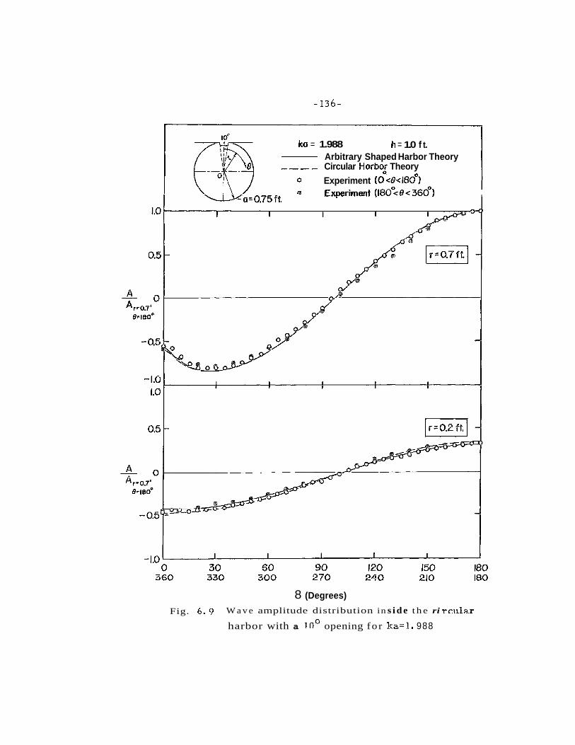
ka = 1.988 h = 1.0 f t. Arbitrary Shaped Harbor Theory
---- Circular Harko$ Theory
0 Experiment (0 <8<180°) @ Experiment (180%6< 360')
8 (Degrees)
Fig. 6 . 9 W a v e amplitude distribution in s i d e t h e ri rclilar
harbor with a lo0 opening fo r ka=l. 988

loa ka = 3.188 h = 1.0 ft.
Arbitrary Shaped Harbor Theory ---- Circular Harbo~ Theory
0 Experiment (0 <8<180~) Experiment (180% ec 360')
@ (Degrees 1 Fig. 6. 10 Wave amplitude distribution inside the circular
harbor with a lo0 opening for ka=3. 188

- 138-
nodal lines exist in the harbor (see Subsection 6.2.4 for a more
complete discussion); thus, the nodal lines cross the two circular
paths at two locations along each path: 8 = 50° and 138O for r = 0.7 ft
and 0 = 73O and 123O for r = 0.2 ft. Therefore, in the upper portion
of Fig. 6. 10 (r = 0. 7 f t ) negative water surface displacements a r e
evident in the regions o0 < 0 < 50' and 138O < R < 180° while positive
displacements a re shown in the region 50° < 0 < 138'. Positive and
negative water surface displacements can also be seen fur r = 0. 2 ft.
To investigate whether the shape of the water surface i s des-
cribed well by a linear theory experiments were conducted where the
wave amplitude distribution inside the harbor at r = 0.7 f t was
measured for various incident wave amplitudes. These results a re
presented in Fig. 6. 11 for three different incident wave amplitudes:
Ai = 0.0023 f t , 0.0066 ft, and 0. 0105 ft. The value of ka for these
experiments was 3. 188 which corresponds to the third resonant mode
of oscillation (see Figs. 6.4, 6. 5, and 6. 10). The theoretical curves
which a r e shown in Fig. 6. 11 a r e the same as those presented in the
upper portion of Fig. 6. 10. The agreement of the experimental data
among themselves and with the two linear theories additionally
support the linearity assumption made in the theory (for these
experiments the incident wave steepnesses are: 0. 003 < Hi/ l , < 0 . 0 14).
The major deviation from other data appears to be for the results
corresponding to the smallest incident wave amplitude where experi-
mental problems of accurate measurement may arise.

- 140-
The variation of the wave amplitude radially at s ix , fixed,
angular positions: 0 = oO, 30°, 45O, 90°, 135O, 180' i s shown in
Fig. 6. 12 for ka = 3.891. The abscissa in Fig. 6. 12 i s the relative
radial position, r/a,and the ordinate i s the relative wave amplitude
normalized with respect to the wave amplitude at the center of the
harbor where a maximum occurs. Experimental results a re also
shown for 8 = 270° and a re included along with the data and theory
0 0 for 8 = 90 a s the oscillation is symmetric about 8 = 0 . It i s seen
that the theoretical results agree well with the experimental data
for all of the values of 8 which were investigated. In Fig. 6. 13 these
results have been replotted in a manner similar to Figs. 6.8 through
6. 11 again showing the amplitude variation along the two circular
paths: r = 0.2 f t and r = 0. 7 ft.
The previous discussions have shown the applicability of the
theories developed in predicting the wave amplitude distribution in a
0 circular harbor with a small opening (10 ). In a similar manner
0 experiments were conducted using a harbor with a 60 opening. The
theoretical distribution of wave amplitude within the harbor i s com-
pared to the results of these experiments in Figs. 6. 14 through 6. 17.
Fig. 6. 14 shows the wave amplitude distribution along r = 0. 7 f t
0 and r = 0.2 f t at ka = 0. 540 for thc harbor with a 60 ' opening. This
value of ka i s approximately the same as that which corresponds to the
f i rs t maximum in the response curves presented in Figs. 6 .6 and 6.7.

ka = 3.891 h= 1.0 ft. - Arbitrary Shaped Harbor Theory ---- Circular Harbor Thaory
) Experiment 0~0.75 ft
0 0.5 1.0 0 0.5 1.0
r/a ria
Fig. 6. 12 Wave amplitude distribution along six fixed angular
positionsinside the circular harbor with a lo0
opening for ka=3.89 1

ka = 3.891 k = 1.0 i t. Arbitrary Shaped Harbor Theory
---- Circular Harbo~ Theory 0 Experiment (0 <8<180°)
riment (180%~ 360~)
e (Degrees )
Fig. 5. 13 Wave amplitude distribution inside the circular
ha rbor with a l o 0 opening f o r ka=3.89 1

kca = 0.540 h= 1.0 f t Arbitrary Shaped Harbor Theory
--- Circular Harbor Theory 0 Experiment (0'6 8 6 180~)
o=0,75 ft Experiment ( 1 8 0 ~ ~ 0 ~ 3 6 0 )
0 30 60 90 120 150 180 360 330 300 270 210 180
B (Degrees)
Fig. 6. 14 Wave amplitude distribution inside the circular
harbor with a 60' opening fo r ka=O. 540

The wave amplitude i s normalized with respect to the wave amplitude
a t the position: r = 0. 7 ft, 8 = 1 8 0 ~ . Note that the theoretical curve
a t r = 0 .7 ft computed using the arbi t rary shaped harbor theory covers
0 only the region 30° 5 8 5 180 . The experimental data obtained along
the circular path r = 0. 7 ft for the region 8 < 30° a r e in fact outside
Region I1 as defined in the arbitrary shaped harbor theory (see Fig.
3. 1). Therefore, it i s unrealistic to compare these experiments to
this theory for 9 < 30° and r = 0.7 ft. However, in the theory for the
circular harbor i t was assumed that the a r c was approximately equal
to the chord a t the harbor entrance, implying that the region along
r = 0. 7 f t for 8 < 30' i s also contained in Region 11. Therefore, only
the theoretical curve computed using the circular harbor theory i s
presented for comparison with the experiments in this region. It
can be seen that the wave amplitude i s relatively constant along these
circular paths except in the region near the harbor entrance and that
+he theoretiral r e s d t s agreewellwith the experimentaldata. As
expected, there i s some disagreement between the experimental data
and the circular harbor theory in the region near entrance ( 0 < 30° and
r = 0. 7 ft).
Similar results a r e presented in Fig. 6. 15 for a value of ka
equal to 2. 153. This value of ka i s the same as for the second maximum
in the response curves presented in Figs. 6 .6 and 6.7. It can be seen
that the general shape of the water surface (wave amplitude distribution)
i s similar to the one shown in Fig. 6 .9 for the case of a 10' opening.

43 (Degrees 1 Fig. 6 . 15 Wave amplitude distribution inside the circular
harbor with a 60' opening for ka=2. 153

For this case the intersections of the nodal line with the chosen
circular paths occur at a larger value of 8 : 10.5~ for r = 0.7 ft and
116' for r = 0.2 ft. This indicates that the nodal line for this mode
of oscillation i s located closer to the back wall region than for the
0 case of a 10 opening.
Theoretical and experimental results a r e presented in Fig. 6. 16
for kaZ3.38, which corresponds to the value of ka at the third
maximum in the response curve of Fig. 6.7. The wave amplitude has
been normalized with respect to the wave amplitude at the position of
r = O . 7 ft, 8 = loo0, where the amplitude at that location was the maxi-
mum of those measured. The shape of the water surface for the
harbor with a lo0 opening which corresponds to this mode of oscillation
has been shown in Fig. 6. 10. By comparing Fig. 6. 16 with Fig. 6. 10
certain similarities and differences between the shape of water surface
for the two different openings readily can be seen: the general shape
of the wave amplitude distribution i s similar. However, the inter-
sections of nodal lines with the circular path r = 0. 7 ft occur at a
larger value of 8 (8 = 54' and 145O) for the harbor with a 60° opening
and for this case the nodal line does not intersect the circular path
for r = 0.2 ft. It i s seen that the theories agree well with the experi-
~ n e r & i . l d a t a throughout.
Fig. 6. 17 shows the results at a value of ka = 3.953; this
corresponds to the value of ka for the fourth maximum in the response
curves shown in Fig. 6.7. The wave amplitude shown in

aoQ ka = 3.380 h = 1.0 f f.
Arbitrary Shaped Harbor Theory ---- Circular Harbor Theory
o Experiment (oO< @:180°) o=0,75ft, a Exp@rimenf(180~~8c360)
6' (Degrees)
Fig. 6. 16 Wave amplitude distribution inside the circular
harbor with a 60' opening for ka=3.38

6 (Degrees 1
Fig. 6. 17 Wave amplitude distribution inside the circular 0 harbor with a 60 opening for ka=3.953
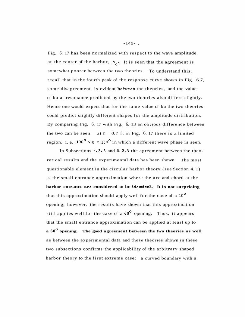
-149- -
Fig. 6. 17 has been normalized with respect to the wave amplitude
at the center of the harbor, Ac. It i s seen that the agreement i s
somewhat poorer between the two theories. To understand this,
recall that in the fourth peak of the response curve shown in Fig. 6.7,
some disagreement i s evident between the theories, and the value
of ka at resonance predicted by the two theories also differs slightly.
Hence one would expect that for the same value of ka the two theories
could predict slightly different shapes for the amplitude distribution.
By comparing Fig. 6. 17 with Fig. 6. 13 an obvious difference between
the two can be seen: a t r = 0.7 f t in Fig. 6. 17 there i s a limited
region, i. e. loo0 < e < 130° in which a different wave phase is seen.
In Subsections 6.2.2 and 6. 2 . 3 the agreement between the theo-
retical results and the experimental data has been shown. The most
questionable element in the circular harbor theory (see Section 4. 1)
i s the small entrance approximation where the a r c and chord at the
harbor cntrancc arc considcrcd to bc identical. It i s not surpriaing
that this approximation should apply well for the case of a 10'
opening; however, the results have shown that this approximation
still applies well for the case of a 60° opening. Thus, i t appears
that the small entrance approximation can be applied at least up to
0 a 60 opening. The good agreement between the two theories as well
as between the experimental data and these theories shown in these
two subsections confirms the applicability of the arbitrary shaped
harbor theory to the f i r s t extreme case: a curved boundary with a

- 150-
continuously varying tangent. The application of the arbi t rary shaped
harbor theory fo r the second extreme case, a harbor composed of
straight -lined boundaries will be presented and discussed in
Section 6.3.
6.2.4 Variation of Wave Amplitude Inside the Harbor for the
Modes of Resonant Oscillation
As mentioned in Subsection 6.2.2, there a r e four distinct
modes of oscillation shown in the response curves for the circular
harbor with a lo0 opening as well a s 60' opening within the range of
ka that has been investigated. In Subsection 6.2.3 wave amplitude
distributions along two circular paths inside the harbor for various
modes of oscillation have been described in order to compare the
theories to the experimental data. However, the complete shape of
the water surface inside the harbor for various resonant modes has
not been presented yet. In order to understand more fully the shape
of the modes of resonant oscillation for circular basins and how they
change with changes in the width of the entrance, for each resonant
mode described by the response curves of Figs. 6 .4 through 6.7, a
figure will be presented showing the contour lines of the f ree surface
(lines of constant water surface elevation) along with photographs fo r
thcsc modes.
It i s of interest to compare the shape of water surface for each
mode of oscillation for the closed circular basin with the cor res -
ponding modes for a circular harbor with a lo0 opening and with a

-151-
60' opening. This comparison will indicate the effect of the size of
the harbor opening on the variation of the wave amplitude inside the
harbor.
The wave oscillation in a closed basin i s usually referred to as
the f ree oscillation in a basin. Suppose the wave function in a closed
circular basin of constant depth i s f (r , 8), which satisfies the Helm-
holtz equation, Eq. 4. 1, and also satisfies the condition that fluid does
a not penetrate the boundary of the harbor, i. e. -f (a, 8) = 0, where a r
a i s the radius of the harbor. As was discussed in Chapter 4, a
solution of the wave function f ( r , 8 ) can be expressed as:
f (r , 0 ) = Jm(kr) cos m8 ,
where m i s zero or a positive integer.
The boundary condition and Eq. 6. 3 indicate that the following condition
must be satisfied:
This condition requires that in order to get a nontrivial solution for the
wave function f ( r , 9), the values of ka must be restricted to those which
satisfy Eq. 6 . 4; these roots are often referred to as the eigenval~ies.
The values of ka which satisfy Eq. 6.4 have been tabulated, e. g. see
Morse and Feshback (1953), and several of these eigenvalues are:
m=O, ka = 3.83, 7.02, . . . . m = l , ka = 1.84, 5.33, . . . . m=2, ks = 3.05, 6 . 7 0 , . . . . m=3, ka = 4.20, 8.02, . . . .

The value of ka for the free modes of oscillation that will be
used to compare with the wave induced oscillations in the circular
harbors are: ka = 1.84, 3. 05, 3 . 8 3 . Thus, the wave functions which
correspond to these values of ka a re as follows:
f ( r , 8 ) = Jo (5. 1 l r ) (for m=O, ka = 3 . 8 3 )
f ( r , 8 ) = J1(2.45r)cos 0 ( f o r m = l , k a = 1.84) (6 .6 )
f ( r , 8 ) = J, (4.065r) cos 20 (for m=2, ka = 3. 05)
In deriving these, the value of "a" is taken as 0. 75 ft, the radius of
the circular harbor (lo0 opening and 60° opening) that was investigated
experimentally. As shown in Eq. 3.6, the value of the wave function,
f , i s proportional to the wave amplitude; thus, for the closed basin
A the relative water surface elevation, - , can be obtained by eval-
uating f from Eq. 6. 6 and normalizing with respect to i ts maximum
value.
Contour lines for these three modes of oscillation at the time of
maximum water surface displacement are shown in Figs. 6. 18 a, b, c.
The contour lines result from the intersection of a horizontal plane
with the disturbed free surface; the value of each line i s the ratio of
the water surface displacement at that location normalized with respect
to the maximum displacement in the basin. The positive water surface
elevations are represented by solid lines, while the negative water
surface elevations a re described by shown dashed lines.
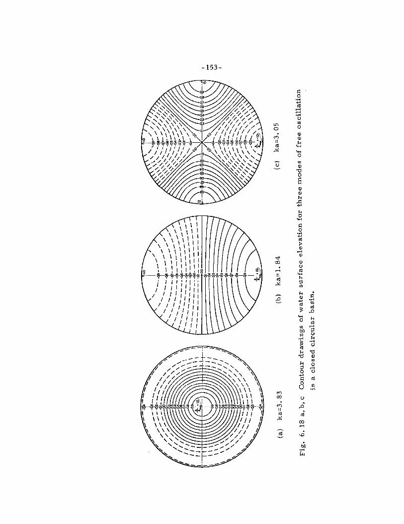

- 154-
The contour drawing of Fig. 6. 18 a shows a nodal circle located
at the position of r /a = 0. 628; i n this mode of oscillation the contour
lines a r e a ser ies of concentric circles, so that the wave amplitude
(or water surface elevation) does not vary with respect to 8. Fig.
6. 18 b shows a nodal diameter at the position 9 = 90° which divides
the basin into two regions of opposite wave phases; this i s usually
referred to as the "sloshing mode". The contour drawing of Fig.
6. 18 c shows two nodal diameters at the positions 0 = 45O and 1 3 5 ~ ;
the basin i s divided into four regions with each quarter 180° out of
phase with i ts neighbor.
It should be noted that if the basin i s no longer completely
closed, however small the opening may be, the solution of the wave
function i(r, 8) i s no longer limited to the eigenvalues described
by Eqs. 6.5. As discussed in Chapter 4, the solution of the wave
function f ( r , 8 ) inside the harbor i s continuously dependent upon the
wave number k (or the incident wave period). The response curves
presented in Subsection 6.2. 2 show that resonant oscillations may
occur for particular wave numbers producing a large amplification
of the wave amplitude inside the harbor. Modes of resonant oscill-
ation will be described in the following discussions with corresponding
0 0 modes fnr the case of the 10 opening and the 60 opening discussed
together. Therefore, the similarities and differences between the
shape of the f ree surface for the two harbors readily can be seen.

- 155-
A contour drawing and two photographs showing the water surface
for the circular harbor with a lo0 opening a re presented in Fig. 6. 19
for a value of ka = 0.35. This value of ka corresponds to the fir s t
maximum in the response curves presented in Figs. 6.4 and 6.5. The
value of the wave amplitude within the harbor presented in this contour
drawing (or in any other contour drawing that will be presented in this
subsection) i s calculated from the circular harbor theory developed in
Section 4. 1. As mentioned earlier , the value of each contour line
represents the water surface elevation normalized with respect to the
maximum elevation within the harbor; for this mode of oscillation
this maximum wave amplitude i s located at the boundary of the harbor
(r = 0. 75 ft) at 0 = 180°. It should be noted that all the contour lines
a r e perpendicular to the solid boundary corresponding to the boundary
condition that no fluid penetrates a solid boundary. By observing this
contour drawing it i s obvious that the wave amplitude i s fairly uniform
throughout the harbor, and that either positive or negative water dis -
placements occur simultaneously within the harbor. Thus, this mode
of oscillation can be called the "pumping mode"; there i s no "pumping
mode" in the case of the f ree oscillation in a closed circular basin
because i t i s impossible to satisfy conservation of mass. The two
~hotographs provided in Fig. 6. 19 show thc case of a positive water
surface displacement, i. e. above the still water surface. Photographs
generally show only displacement along the boundary of the harbor,
not the variation of the water surface in the interior of the harbor.


- 157-
In the photographs , positive water surface displacement appears as
dark stripes along the boundary of the harbor. Some indication of the
interior oscillation i s provided by shadows on the bottom seen in
subsequent photographs; for this mode of oscillation the water surface
elevation i s evidently so smooth that no such shadow appears in the
bottom.
For reasons of convenience, the pumping mode will be named
Mode No. 1 , and other resonant modes which occur at larger values
of ka will then be named Modes No. 2, No. 3, etc. These modes of
oscillation will be discussed later in this section.
A similar figure for Mode No. 1 (the "pumping mode") for the
0 harbor with a 60 opening i s presented in Fig. 6. 20. This mode of
oscillation occurs at ka = 0.46, which i s the value of ka at the f i r s t
maximum in the response curves presented in Figs. 6.6 and 6.7. As
can be seen from the contour drawing the water surface elevation i s
fairly constant throughout the harbor and in the phase throughout. The
shapes of the water surface shown in Figs. 6. 19 and 6.20 a re similar;
0 however, for the case of a 60 opening the variation i s larger than for
0 the harbor with a 10 opening
The shape of Mode No. 2 ("sloshing mode") for the case of a
0 10 opening i s presented in Fig. 6.21. This mode of oscillation,
which corresponds to the second maximum in the response curves
of Figs. 6.4 and 6.5 occurs at a value of ka = 1. 99. The contour
drawing shows a nodal line located near z diameter of the harbor at

Fig. 6.20 Contour drawing and photographs showing the water su r f ace for tke circular harbor with 0
a 60 opening, Mode No. 1, ka=0.46


- 160-
0 6 = 90 . As before, the lines of constant positive water surface
elevation a r e represented by solid lines, while the surf ace contours
below the still water level a r e shown dashed. The 4x0 photographs
provided a r e for opposite phase: when the water surface displacement
i s near a maximum or a minimum. The upper photograph in Fig. 6.2 1
shows a positive water surf ace displacement approximately in the
0 region 90 < 6 < 180°. The lower photograph shows a negative water
surf ace displacement in this same region. In the photographs positive
water surface displacements appear as a dark str ipe along the boundary
of the harbor; however, negative water surface displacements a r e not
easily seen. The shadows which appear on the bottom of the harbor
a r e caused by a ser ies of short wave length ripples on the water
surface; however, because their amplitude i s small compared with
the main water surface displacement, they a r e not easily detected by
measurement except near the nodes. For different modes of
oscillation, the pattern of the shadows change; this will be more
evident when other modes of oscillation a re discussed.
A similar mode of oscillation i s presented in Fig. 6. 22 for the
0 circular harbor with a 60 opening. For this opening, this mode of
oscillation occurs at a value of k a = 2. 15 which corresponds to the
second peak in the response curve of Figs. 6.6 and 6.7. For the l o 0
opening this mode occurs at ka = 1. 99, and for the completely closed
basin i t occurs at ka = 1. 84. Therefore, the trend i s for t he wave
number at resonance to decrease as the entrance width decreases,
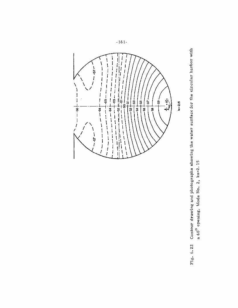

- 162-
approaching the value of k for that mode for the closed basin. The
upper photograph in Fig. 6.22 shows a positive water surface dis-
placement in the region opposite the harbor entrance (approximately
100' < 0 < 180°) and the lower photograph, shows a negative water
surface in this region.
It i s of interest to compare the contour drawings of Figs. 6.2 1
and 6.22 with the one shown in Fig. 6. 18 b for the case of a closed
circular basin where the three figures represent the same mode of
oscillation: the "sloshing mode". A direct comparison of Figs. 6. 18 b
6.2 1, and 6.22 reveals changes in the water surface shape as the width
of the harbor opening increases. In the case of a closed basin (Fig. 0 6. 18 b) the nodal line i s a diameter at 0 = 90°, for a 10 opening
(Fig. 6.21) the nodal line occurs at a position slightly off the center
and closer to the region of the back wall; for the case of 60° opening
(Fig. 6.22) the nodal line occurs at a position further off the center
towards the back wall. Specifically, the relative wave amplitude at
the center of the harbor is: A/Ama 0 = -0.08 for 10 opening,
= -0. 18 for 60° opening. The wave amplitude at the harbor
entrance changes significantly for the three cases: for the closed
basin, (Fig. 6. 18 b) a maximum amplitude (antinode) occurs at the
boundary at 8 = oO; however, this antinode does not exist for the
0 0 case of a 10 opening or a 60 opening. This disappearance of the
antinode at the entrance when the harbor i s no longer completely
closed contradicts the assumption made by McNown ( 1952) in his

- 163-
solution of oscillations in circular harbors. (His as sumption i s that
an antinode exists at the harbor entrance fo r smal l openings. )
In Fig. 6.23, a contour drawing and two photographs for Mode
0 No. 3 a r e presented for the case of a 10 opening. This mode of
oscillation, which corresponds to the third peak in the response
curves shown in Figs. 6.4 and 6.5, occurs at k a = 3. 18. In the
contour drawing, there a r e two nodal lines; maximum wave amplitude
0 occurs a t the boundary at 0 = 95 and i t s symmetrical counterpart i s
0 at 8 = 265O. (The wave pattern i s symmetr ic with respect to 8 = 0 . ) The two photographs shown differ 180° in phase. The upper photo-
graph of Fig. 6.23 shows an oscillation with the same phase a s the
contour drawing; thus, a positive water surface displacement i s shown
i n the photograph approximately in the -region 50° < 8 < 140°. The
lower photograph of Fig. 6.23 shows a negative water surface dis-
placement in the same region. It i s seen that the shadows on the
bottom for this mode of oscillation are quite different from t h o s e shown
in Figs. 6.2 1 and 6.22, and hence they must be related to the mode of
oscillation.
A similar mode of oscillation for the case of a 60° opening is
presented i n Fig. 6.24. This made occurs at k a = 3.38 and co r r e s -
ponds to the t h i r d peak in t h e response curve of Fig. 6. 7. Two nodal
lines a r e seen in the contour drawing; the maximum wave amplitude
occurs a t the boundary a t 8 = 100O (and 2 6 0 ~ ) . The upper photograph
in Fig. 6.24 shows a wave motion i n phase with that shown in the


- 166-
contour drawing; thus the positive water surface displacement along
the boundary i s seen in the dark stripe in the region 55' < 8 < 145'.
The lower photograph shows the moti.ion about 180° out of phase with
that on the upper photograph. The shadows on the bottom as seen in
the photographs a r e similar to those shown in Fig. 6.23; however,
they a r e certainly different f rom those shown in Figs. 6.2 1 and 6.22
for Mode No. 2.
For the case of a closed basin (Fig. 6. 18 c) , the position of the
maximum amplitude occurs at four points on the boundary of the basin
8 = oO, 90°, 180°, and 270°, and the two nodal diameters ( 8 = 45O
and 135") a re perpendicular to each other. For the case of a 10'
opening (Fig. 6.23) the two nodal lines a re shifted slightly and no
longer intersect, whereas for the harbor with a 60O opening (Fig.
6.24) the two nodal lines a re shifted even further apart. The wave
arnplitudes at the center have also changed considerably a s the
cntrancc width incressesr zero for the case of s closed basin,
0
A'Amax = -0. 125 for the case of a 10 opening, and A/Amax = -0.44
for the harbor with a 60° opening. As mentioned earlier , the wave
amplitudes at the harbor entrance also change with changes in the size
of the opening: for the case of a closed basin (Fig. 6. 18 c) a maximum
wave amplitude (antinode) exists at the boundary at 9 = oO; however,
0 for the case of a 10 opening or a 60' opening an antinode does not
exist at the entrance. It should be noted that as the wave parameter
ka increases, the ratio of the harbor radius to the wave length a /L
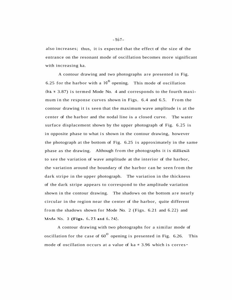
also increases; thus, i t i s expected that the effect of the size of the
entrance on the resonant mode of oscillation becomes more significant
with increasing ka.
A contour drawing and two photographs a r e presented in Fig.
6.25 for the harbor with a 10' opening. This mode of oscillation
(ka = 3.87) i s termed Mode No. 4 and corresponds to the fourth maxi-
mum i n the response curves shown in Figs. 6.4 and 6.5. From the
contour drawing i t i s seen that the maximum wave amplitude i s at the
center of the harbor and the nodal line is a closed curve. The water
surface displacement shown by the upper photograph of Fig. 6.25 i s
in opposite phase to what i s shown in the contour drawing, however
the photograph at the bottom of Fig. 6.25 i s approximately in the same
phase as the drawing. Although from the photographs i t i s difiicult
to see the variation of wave amplitude at the interior of the harbor,
the variation around the boundary of the harbor can be seen from the
dark stripe in the upper photograph. The variation in the thickness
of the dark stripe appears to correspond to the amplitude variation
shown in the contour drawing. The shadows on the bottom a re nearly
circular in the region near the center of the harbor, quite different
f rom the shadows shown for Mode No. 2 (Figs. 6.21 and 6.22) and
Mnde Nn. 3 (Figs. 6.23 and 6.24).
A contour drawing with two photographs for a similar mode of
0 oscillation for the case of 60 opening i s presented in Fig. 6.26. This
mode of oscillation occurs at a value of ka = 3.96 which i s corres -

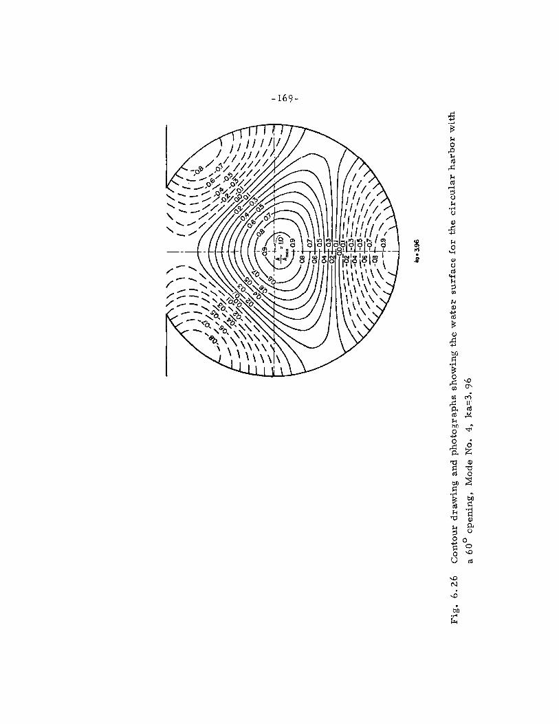

pollding to the fourth peak i r r the r espunse curves shown in Fig. 6. 7.
It i s seen from the contour drawing that the maximum wave amplitude
i s again located at the center of the harbor. The nodal line i s no
longer a closed curve as for the case of a 10' opening but in this case
it interesects the boundary of the harbor. As in Fig. 6.25, the upper
and lower photographs in Fig. 6.26 a re approximately 180° out of
phase. The variation of the water surface elevation around the
boundary again can be seen from the dark stripe in the upper photo-
graph; i t shows a variation along the boundary similar to that shown
in the contour drawing, but with opposite phase.
It i s interesting to compare the contour drawings of Figs. 6.25
and 6.26 and 6. 18 a: for the case of closed basin the contour lines a re
a series of concentric circles and the nodal line i s represented by a
0 nodal circle (Fig. 6. 18 a); however, for the case of a 10 opening
(Fig. 6.25) the contour lines a re no longer represented by a series
of circles, although in the region near the center of the harbor they
are in fact close to circular. As the harbor opening increases to
60° (Fig. 6.26) a significant change in the contour lines can be
observed: the nodal line i s no longer a continuous closed line as in
0 the case of a 10 opening, or a circle as in Fig. 6. 18 a; instead i t
intersects the boundary of the harbor, and even contours near the
center of the harbor a re no longer circular in form. However, the
center of the harbor still remains the position of the maximum wave
amplitude.

- 171-
The results presented in this subsection showed the wave
amplitude distribution for four modes of resonant oscillation in the
0 0 range of ka investigated for both the cases of a 10 and a 60 opening.
Except for Mode No. 1 (the "pumping mode") which does not exist in
a completely closed circular basin, each mode corresponds to a free
mode of oscillation in the closed basin. The results in this subsection
can be summarized as:
(1) The corresponding modes uf oscillation for the c a s e of a
lo0 opening and a 60° opening are basically similar,
however, the detailed shape of the free surface is different.
(2) The value of ka at which a particular mode of oscillation
0 occurs in the harbor with a 60 opening i s larger than the
value of ka for the corresponding mode .hr the case of a 10"
opening which itself i s larger than the value of ka for the '
corresponding mode in a closed basin. Hence the tendency
i s for the wave number parameter (ka) at resonance to
approach the value for a closed basin as the entrance width
decreases.
( 3 ) No antinode exists at the harbor entrance although an anti-
node might occur at that position in a closed circular basin.
(4) The e f f e c t nf the width of harhnr entrance nn the shape o f
water surface elevation inside the harbor i s more pronounced
for those modes of oscillation at higher frequencies,
i. e. larger values of ka.

- 172-
6.2. 5 Total Velocity at the Entrance of the Circular Harbor
6.2.5. 1 Introduction
In Subsection 3.2.4 the method for analytically evaluating
the velocity at the harbor entrance was discussed. The velocity at the
harbor entrance i s of interest because i t i s directly related to the
kinetic energy transmitted into the harbor. For the present study, the
value of the wave function, f,, i ts normal derivative, E2 as well as ay '
the derivative e, evaluated at the harbor entrance are determined
during the process of computing the response curves for various values
of the wave number parameter, ka. Hence, the theoretical value of
the total velocity at the harbor entrance can be obtained readily from
Eq. 3.41.
As mentioned in Section 5.5, the velocity was measured at the
entrance of the circular harbors fivith a lo0 opening and a 60° opening)
using a hot-film anemometer with a linearizing circuit. In steady flow,
either in air or in water, the output from a hot-film anemometer gener-
ally has been found to follow King's Law (Eq. 5.2). Thus, after em-
ploying the linearization procedure described in Section 5.5 the voltage
i s directly proportional to the velocity as reported by Townes ( 1965),
Raichlen (1967) and Lee (1967). However, at the time of the present
experiments the use of hot-film anemometers in oscillatory flows had
not been reported in the literature. Considering the relation of these
velocity measurements to the major objectives of the experimental
program, a basic assumption was made in reducing these experimental

- 173-
data: King's Law was assumed to apply equally well for oscillatory
flows; thus, after using the l inearizer the output signal was assumed
to be linearly proportional to the fluid velocity. Therefore, the ratio
of two output voltages f rom the l inearizer was considered to be equal
to the ratio of the two corresponding velocities.
Recently, Das (1968) used a single hot-film sensor in water to
measure turbulence in an oscillatory flow. The results showed that
with one of the hot-film sensors which was used , the relation between
the voltage output and the fluid velocity was: E~ v ~ ' ~ ~ (wherein E
i s the hot-film anemometer output voltage and V i s the resultant fluid
velocity in a direction perpendicular to the axis of the hot-film sensor) ,
while another sensor behaved as: E~ v O * 45 . The lat ter relation
i s close to King's Law ( E ~ - V* ' ) whereas the former i s quite
different.
A typical output f rom the linearizing circuits as recorded on the
Sanborn recordcr (dcocribcd i n Scction 5. 4 ) i~ p r c ~ c n t c d i n Fig. 6 .27
(Column C). This velocity measurement was made at the center of the
entrance of the harbor with a 10" opening with a wave period of 0. 684
sec. The record corresponds to the velocity at three depthwise
locations: z = -0. 10 ft, -0. 15 ft, and -0.25 ft. As expected, the
velocity decreases as the distance between the hot-film sensor and
the water surface increases. In Fig. 6.27 also the wave amplitude
0 i s shown at two positions inside the harbor, i. e. r = 0.2 ft, R = 35 ,
and r = 0. 7 ft, 0 = 215'. It i s seen that the waves in these two

Fig. 6.27 Typical record of thewave amplitude and of the
velocity after using the linearizing circuit

0 positions a r e 180 out of phase (this was also shown in the contour
drawing of Fig. 6.2 1 evaluated for the same wave number). F rom Fig.
6. 27, it i s seen that within one wave period, the velocity reaches i t s
maximum value twice, since in a periodically oscillating flow the
hot-film sensor cannot differentiate the direction of the velocity.
In determing the velocity f rom such records the peak value of the
output signal f rom the linearizing circuit a s recorded was averaged.
This average value, using the notation of Section 5. 5, i s denoted as S,.
If this value, S, , is truly linearly proportional to the fluid velocity,
then f r o m Eq. 5 . 5 it i s equal to avV. Therefore, assuming this
proportionality to be true, the relative velocity at any two positions
can be obtained f rom the ratio of the corresponding values of S, with-
out prior evaluation of a f rom calibration. (This assumption was v
used to determine the relative velocities that will be presented in the
following subsections even though there i s some conflict with the
results of Das, 1968. )
6. 2. 5.2 Velocity distribution in a depthwise direction
The vertical distribution of the velocity a t the entrance
of the harbor with a lo0 opening, averaged ac ross the entrance, i s p re-
sented in Fig. 6.28 for three different values of the wave number
parameter, ka, ( three wave periods): ka = 0.482, 1.988, 3.922. 'l'he
ordinate of Fig. 6.28 is the relative depthwise position, z/h, (where
z /h = 0 re fe r s to the st i l l water surface) and the abscissa i s the
relative velocity normalized with respect to the velocity measured
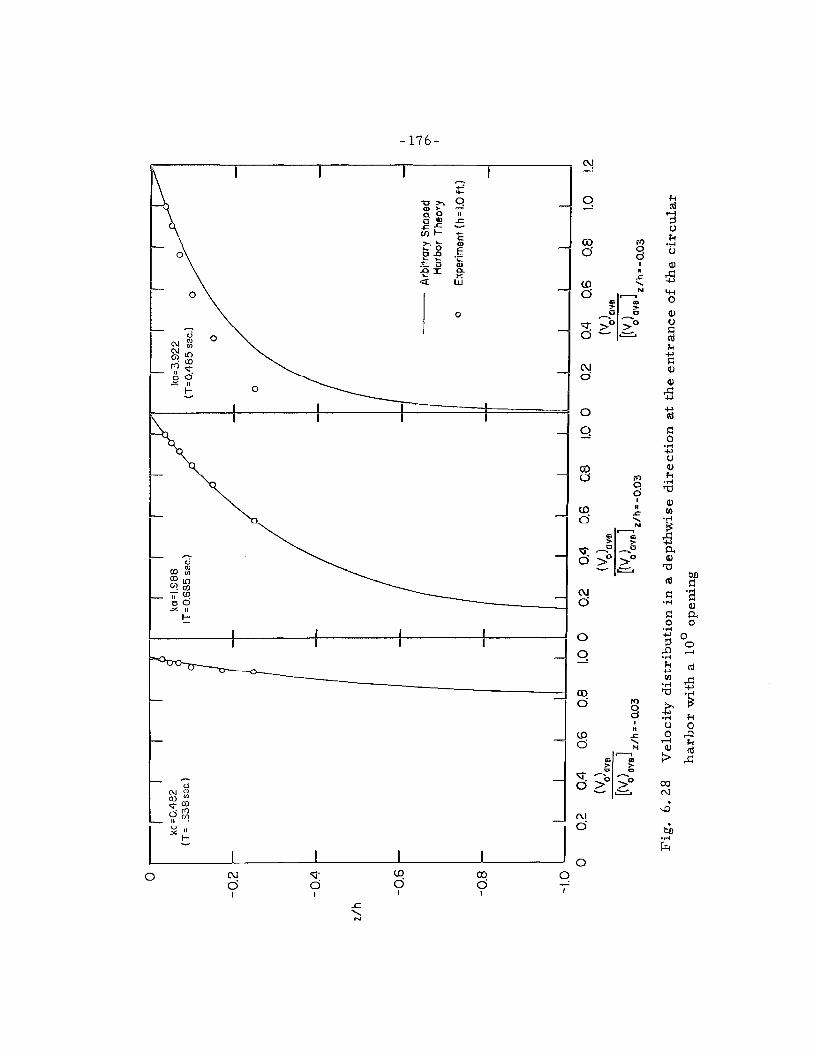

- 177-
nearest the water surface (z ld = -0.03). The theoretical velocity
distribution was calculated using Eq. 3.42 (since the hot-film sensor
i s primarily sensitive to the v and w velocity components); the value
of f, and i?f at the entrance were obtained from the arbitrary shaped ay
harbor theory. In these experiments, measurements of velocity were
made at five lateral locations across the harbor entrance for each
vertical position ( z Ih) and each experimental point shown in Fig. 6.28
is thcrcforc the average of the results at these lateral locations.
(The locations will be described fully in Subsection 6.2.5.3. )
According to the conventional method of clas sifying water waves,
the distribution curve for ka = 0.482 in Fig. 6.28 i s similar to the
typical vertical distribution of fluid particle velocities for shallow
water waves. (For the present experiments, as mentioned in Sub-
section 6.2.2, shallow water waves occur in the region 0 < ka < 0.236,
intermediate waves in the region 0.236 < ka < 2.36, and deep water
waves in the region ka > 2. 36. ) The distribution curve for ka = 1. 988
belongs to intermediate wave category and the curve for ka = 3.922
corresponds to deep water waves in which the velocity decreases
rapidly as the distance from the water surface increases. It i s seen
that the experimental data for ka = 0.482 (wave period T = 1. 838 sec)
and ka = 1.988 ( T = 0.685 sec) agree well with the theoretical curves;
however, the experimental data for ka = 3.922 (T = 0.485 sec) differ
considerably from theory. This may indicate that the assumption of
linearity between the fluid velocity and the output voltage from the

- 178-
linearizer i s reasonable for ka = 0.482 and 1.988 but not for ka = 3. 922,
where the wave frequency i s larger. In the following, some of the
weakness in the experimental procedure and the method of data
reduction will be discussed.
From Eq. 3.42, it i s seen that the total velocity at the harbor
entrance i s proportional to the incident wave amplitude A;, and
inversely proportional to the wave frequency u. In the experiments,
for the same stroke of the wave machine, the standing wave amplitude
at the harbor entrance (with the entrance closed) for ka = 3.922 was
approximately one-half of that for ka = 1. 988 because the wave filter
i s more efficient at higher frequencies ; without the filter wavemaker
theory implies the reverse. Therefore, experimentally the velocity
at the entrance for ka = 3. 922 was small compared to the velocity for
ka = 1.988. Specifically for the hot-film sensor placed at the center
of the entrance at the position z/h = -0.03, for k a = 1.988 ( T = 0.685
sec) the output voltage from the linearizer was 28.5 volts; however,
for ka = 3.922 (T = 0.485 sec), the output voltage was only 2.66 volts,
at this location. As the sensor was moved to the position z/h = -0.25
the recorded output voltage was less than 0.3 volts for k a = 3.922. It
i s felt that the disagreement between the experimental and theoretical
results for ka = 3.922 as shown in Fig. 6.28 could be due to experi -
mental e r ro r in measuring the small varltage or velocity.

6 . 2 . 5 . 3 Velocity distribution across the harbor
entrance
The velocity distribution across the entrance of the
0 circular harbor with a 10 opening i s presented in Fig. 6.29 for
k a = 0.482, 1.988, and 3. 922. The abscissa i s the relative lateral
d d position, x / ~ (where d is the width of the harbor entrance; x / ~ = 0
refers to the center of the entrance, and x/$ = f 1 refers to the
la teral limits of the entrance). The upper portion of Fig. 6.29 shows
the velocity distribution normalized with respect to the average
velocity across the entrance while in lower portion of the figure the
velocities a re normalized with respect to the velocity at the center.
The theoretical curves shown a re obtained from the arbitrary shaped
harbor theory (Eq. 3.42), where the entrance was divided into five
0 equal segments with each segment having a central angle of 2 and
the boundary was divided into 35 equal segments. The wave function
af, f2 and i ts normal derivative - at the mid-point of each segment at ay
the entrance were obtained by the matching procedure (Subsection
ar2 3 . 2 . 3 ) . With these values of f2 and - , the velocity V at the mid- ay 0
point of each entrance segment was calculated from Eq. 3.42 for a
particular vertical position z. The average velocity across the
entrance, denoted as (Vo)ave, was obtained by computing the arilh-
metic average of the velocities Vo at a particular elevation for the
five segments. In Fig. 6.29 the normalized theoretical velocities so
computed a re denoted by "plus signs" and a solid line fitted through
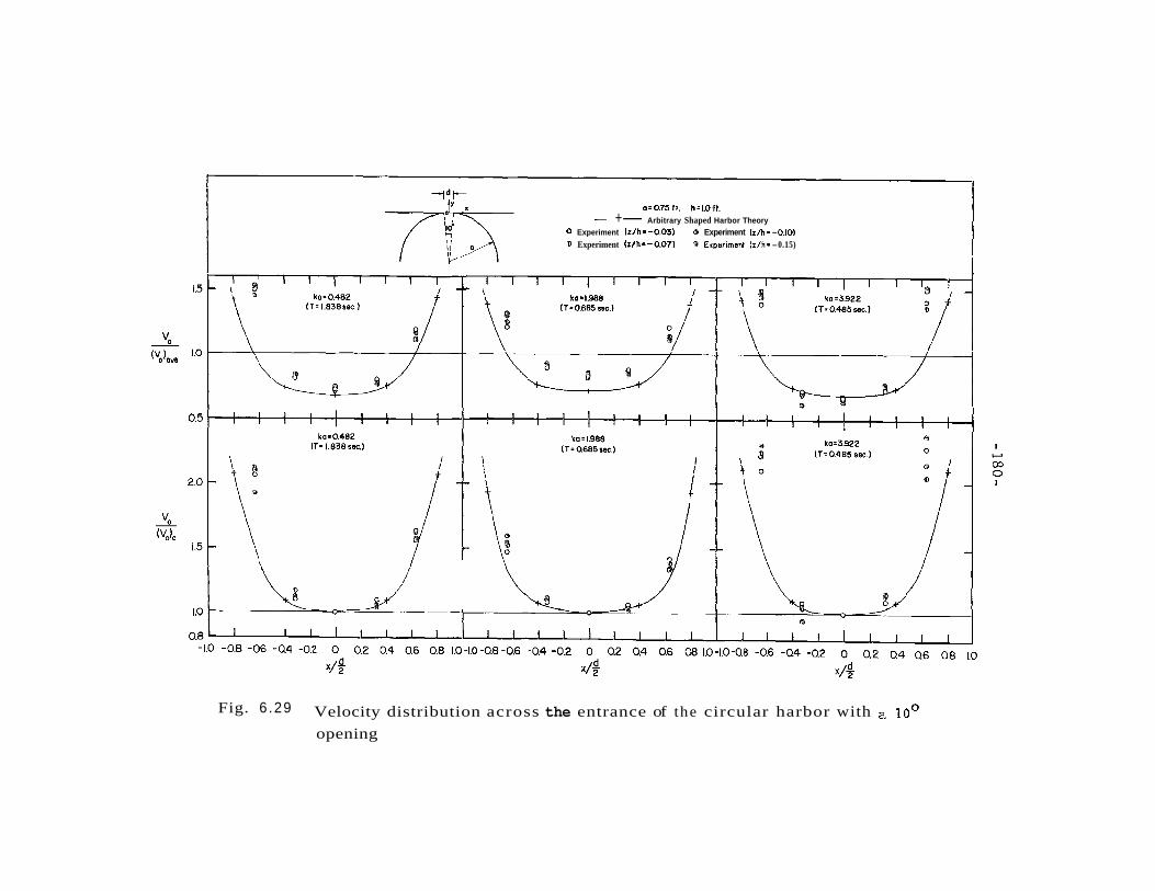
a=O.75 f l . h=l.Ofi . - +- Arbitrary Shaped Harbor Theory
0 Experiment W h = - 0 . 0 3 1 Experiment (z/hS-0.10) a Experiment ( z / h = - 0 . 0 7 ) '81 Experiment (z/h= -0.15)
Fig. 6.29 Velocity distribution across the entrance of the circular harbor with a lo0
opening

these values i s drawn for reference. For a specific value of ka, the
velocity Vo i s a function of vertical position z (see Eq. 3.42); however,
in the range 0 > z / h > -0. 15 corresponding to the experimental data
shown, the relative velocity Vo/(V ) at the entrance i s essentially o ave
independent of z. Therefore, in Fig. 6.29 only one theoretical curve
i s presented for each value of ka.
Experimental measurements were conducted by placing the hot-
film sensor parallel to "the coastline" and the bottom at five lateral
d positions: x / ~ = 0, -0. 32, -0.64, 0.32, 0.64. In the upper portion
of Fig. 6 .29 , these experimental data a re shown in terms of
v0/(V ) for each lateral position at : z/h = -0.03, -0. 07, -0. 10, o ave
and -0. 15. Comparing the theoretical and experimental results, the
experimental data a re generally larger than the theoretical values,
although they qualitatively follow the trend predicted by the theory,
i. e. the velocity increases toward the two limits of the entrance. It
i s felt that in part the reason for the disagreement could be caused by
underestimating the experimental value of (V ) o ave* Due to the
relatively large value of the ratio of the length of the hot-film sensor
to the width of the harbor entrance, measurements could not be made
close to the edges of the entrance where the velocities were large.
Thus, the average value of the data at the five locations i s probably
smaller than the true average velocity. In order to reduce the influ-
ence of the experimentally determined average velocity and to more
positively confirm the theoretical velocity distribution across the

entrance, the same data were normalized with respect to the velocity
at the center of the harbor entrance, (Volt. These results a r e pre-
sented i n Lhe lower portion of Fig. 6 .29 with the theoretical curves
shown fo r comparison. It i s seen that the experimental data quali-
tatively agree with the theory; the major disagreement again i s for the
case of ka = 3. 922 (T = 0.485 sec) where one possible reason for this
has been discussed in Subsection 6.2.5.2. From Fig. 6.29 i t i s seen
that for the case of a lo0 opening the velocity distributions for these
three values of ka a r e similar in that the velocity increases toward
the entrance limits.
0 Similar results for the harbor with a 60 opening a re presented
in Fig. 6.30 for four values of ka, i. e. k a = 0.64, 2.22, 3. 30, and
4. 0 1. In obtaining the theoretical curves the arbitrary shaped harbor
theory and Eq. 3.42 were used again with the harbor entrance divided
0 into six equal segments (each segment having a 10 central angle) and
the h n l ~ n d a r ~ divided into 31) eqwal segments. As before, in Fig. 6 . 3 0
for each value of ka presented, a curve i s drawn through the theoreti-
cally computed values of v ~ / ( v ~ ) ~ ~ ~ which have been plotted at the
mid-point of each segment. The theoretical curve for ka = 0 .64 can
be considered as representing the velocity distribution corresponding
to M o d e No. 1 (fhe m o d e " ) . (For a d e s c r i p t i o n o f the shape
of this resonant mode of oscillation the reader i s referred to Sub-
section 6. 2.4. ). The velocity distribution for Mode No. 2 ( the
"sloshing mode") i s represented by the curve for ka=2. 22, while

0 Exper~men: (z/h=-0.05) e Experiment (z/h = -0.15)
-1.0 -0.8 -0.6 -0.4 -0.2 0 0.2 0.4 0.6 0.8 81.0-1.0-0.8 -0.6 -0.4 -0.2 0 0.2 0.4 0.6 0.8 1.0 d
x / ~ d x / p
Fig . 6. 30 Velocity distribution across the entrance of the
circular harbor with a 60' o2ening

- 184-
Modes No. 3 and No. 4 correspond to ka = 3.30 and 4.0 1 respectively.
It i s interesting to note that the velocity distribution for the third mode
(ka= 3.30) i s strikingly different in appearance than those of the other
three.
For the harbor with a 60° opening, the length of the hot-film
sensor i s much smaller compared with the width of the entrance than
0 for the 10 case just discussed; hence, measurements could be made
relatively closer to the entrance limits. Therefore, i t is felt that the
experimentally determined average across the entrance, (Vo lave'
i s reasonably good, and the results a r e only normalized with
respect to the average velocity in comparing experiments to theory.
Experimental data at two vertical positions: z/h = -0.05 and -0. 15
a re shown in Fig. 6.30. Considering the assumptions made in the
data reduction procedure i t i s somewhat surprizing that the experi-
mental data agree as well with the theory as they do. The major
diaagrecment betwcen experiments and theory again i s at the largest
value of ka, i. e. ka = 4.0 1.
6 . 2. 5.4 Velocity at the harbor entrance as a function
of wave number parameter, ka
It i s possible in determining the response curve for a
particular harbor that because of the location chosen the anlplificaliun
factor at that position is small for all incident wave numbers whereas
a nearby location has associated with i t large amplification factors for
particular wave numbers. Therefore, one response curve alone may

not always clearly indicate all resonant conditions. A parameter
which may be used as an indicator of resonance, which i s independent
of location, i s the total velocity at the harbor entrance. Since this
velocity i s associated with the energy input into the harbor, a larger
velocity at the entrance at one wave number compared to another would
mean a larger kinetic energy input and resultant larger potential
energies and hence water surface amplitudes inside the harbor for
that wave number. Therefore, a curve showing the variation of the
entrance velocity with the incident wave number parameter, ka, may
prove to be a useful tool to indicate resonance, In this subsection
such curves for the case of a circular harbor with a lo0 opening and
a 60' opening will be presented and discussed.
As mentioned earlier , Eq. 3.41 can be used to calculate the 4.
total velocity at the entrance, v:, and if both sides of Eq. 3.41 a re
normalized with respect to the maximum horizontal water particle
velocity for a shallow water wave, one obtains:
wherein Al , Az , A3 , al , as, and as a re defined in Eq. 3 . 4 1. In using
Eq. 6.7 the value of A, and A3 a t the harbor entrance are easily
a f obtained since fz and for each entrance segment a r e determined ay
f rom the matching procedure. The value of 2 in A, i s approximated

- 186-
by e, wherein Af, represents the difference in the value of wave
function f2 of two neighboring entrance segments and Ax represents the
distance between them.
Fig. 6. 3 1 shows the variation of the total velocity at the entrance
of the circular harbor with a l o 0 opening as a function of the wave
number parameter ka. This curve is calculated from Eq. 6. 7 for
z=0 (the water surface) and as before, the water depth,h, i s 1 ft. The
*i .*. ordinate in Fig. 6. 3 1 i s (wherein ( ~ i ) ~ ~ ~ represents .L
the average total velocity, v:, across the harbor entrance); the
abscissa i s the wave number parameter ka. There a re four maxima
in the curve shown in Fig. 6.3 1, the value of ka associated with each
maximum is : k a = 0.35, 1.98, 3. 18, and 3.87 and these values
correspond to those associated with the four modes of resonant
oscillation predicted by the arbitrary shaped harbor theory and shown
in the response curves, Figs. 6.4 and 6.5.
In an attempt to compare the theory with the velocity measure-
ments using the hot-film anemometer, Eq. 3.42 i s used for the theo-
retical calculations. (Since the hot-film sensor in these experiments
was primarily sensitive to the v and w velocity components, it i s
unrealistic to compare the experiments with Eq. 6. 7. ) Fig. 6.32 - -
shows the variation of Wu),ve/L~~,),v,] as a function of ka = 1.988
ka; the curve shown as a solid line was evaluated from Eq. 3.42 using
values of f, and ilfa at the entrance determined by the method discussed ay
in Chapter 3 (arbitrary shaped harbor theory). The velocity ratio

- Arbitrary Sha~ed Harbor Theory (z=O.Off., h=l.Oft.,a=0.75ft.,)
ko Fig. 6. 3 1 Total velocity at the harbor entrance as a
function of ka for the ci rcular harbor with a lo0 opening
Fig. 6. 3 2 Velocity a t the harbor entrance a s a function of ka: comparison of theory and experiment ( 100 opening circular harbor)

- 188-
a f computed from Eq. 3.42 using the values of f, and -3 determined ay
by the method of Section 4. 1 (circular harbor theory) i s shown in
Fig. 6.32 a s a dashed curve. In using Eq. 3.42, the value of the
incident wave amplitude Ai i s taken as a constant for all values of
ka.
Experiments were conducted by placing the hot-film sensor at
z= -0.03 ft; for each value of ka, measurements were made at five
d lateral locations across the entrance ( x / ~ = 0. 0, 0.32, 0.64, -0. 32,
-0.64). The average of the output voltage from the linearizer at these
five locations i s denoted as S,. As just mentioned in the theory the
incident wave amplitude was considered constant for all wave numbers.
However, in the experiment i t i s impossible to maintain this condition,
in fact for the range of ka investigated the wave amplitude varied
more than a factor of three. Therefore, to compare the experimental
data to the theory, this effect of the varying incident wave amplitude
mu st be eliminated. This was accomplished by dividing the voltage,
S, , by the incident wave amplitude at that wave number. This ratio
was then normalized with respect to that at ka=l. 988 and the resulting
data a r e shown in Fig. 6.32.
In Fig. 6.32 i t i s seen that the two theoretical curves agree well
and the experimental data agree reasonably wcll with thcsc thcories.
However, at large values of ka, again, the data and theories show
poorer agreement.

- 189-
The variation of the velocity at the harbor entrance with ka i s
presented in Fig. 6.33 for the harbor with a 60° opening. The curve
i s again obtained from Eq. 6. 7 evaluated at the water surface for a
total depth of 1. 0 ft. It i s seen that the values of ka for the four
maxima in Fig. 6 . 3 3 are: ka=O. 50, 2. 18, 3 .38 , 3. 97. Again, these
values correspond to those predicted by the arbitrary shaped harbor
theory. (See the response curves in Figs. 6.6 and 6.7. ) It should be
noted that the third maximum was not clearly defined in the response
curve shown in Fig. 6.6 because of the location chosen (it did appear
at the other location,see Fig. 6. 7); this clearly emphasizes the import-
ance of the entrance velocity as an indicator of resonance. Comparing
Fig. 6. 33 with Fig. 6. 3 1, i t appears that the average velocity across
the entrance at resonance i s significantly less for the case of a 60°
opening; however, the wave number band-width associated with the
maxima i s larger for the 60° case compared to the harbor with a lo0
opening. This phenomenon is similar to that shown by the response
curve presented in Subsection 6 . 2 . 2 .
For the 60° opening, the velocity at the center of the harbor
entrance also was measured using the hot-film anemometer. The
sensor was located at a vertical position z= -0.05 f t at the center of
thc cntrance (thc watcr dcpth again was 1. 0 ft). Thc voltages from thc
linearizer at various values of ka were then normalized with respect
to that at ka=2.25 using the same correction procedure as was just
described for the harbor with a 10' opening. These data a re presented
in Fig. 6.34; in contrast to Fig. 6.32 where average velocities

Arbitrary Shaped Horbw Theory
(z=O.Oft.,h=1.0fi.,a=0.75s'%) P
2 E s
m
Fig. 6. 33
3.c
ka
Total velocity at the harbor entrance as a function of ka for the circular harbor with a 60° opening
o k o 1.0 2.0 3.0 6.0
ka Fig. 6. 34 Velocity at the center of the harbor entrance as a function
of ka: comparison of theory and experiment (SO0 opening circular harbor)
Arbikoiy Shaped Harbor Theory 0 Experiment No. I @ Experiment Na2 @ Experiment Na 3
Experiment Mo.4 0
I
I I
I I I 1

across the entrance were used, here the normalized velocity i s that
obtained at the center of the entrance.
For this case o d y Llle LlleureLicdl curve ublained f rv rn the
arbitrary shaped harbor theory is shown, since the circular harbor
theory had not been used to determine the values of f a and 2 at the
center of the entrance (it was used only to determine the average
values of f, and af2 across the entrance). an
Although the experimental data show consider able scatter, they
agree qualitatively with the theory, The results from experiments
performed at four different times a re shown in Fig. 6.34 providing
additional confidence in the experimental procedure. The value of ka
associated with the maxima in Fig. 6. 34 are different from that of
Fig. 6. 33 especially the third and fourth peaks. 'I'his i s because far
different values of ka, the shape of the velocity distribution across the
harbor entrance i s not the same (see Fig. 6 . 3 0 ) . Thus, the relative
velocity at the center of the entrance. ( v ~ ) ~ / L ( v ~ ) ~ ] , i s not ka=2.25
necessarily equal to the relative average velocity across the entrance,
r 1 (Vo)ave/~(Vo)ave~ka=2. 25 shown in Fig. 6.33 .
The results presented in this subsection have demonstrated that
a maximum average total velocity at the harbor entrance corresponds
to a resonant mode of oscillation inside the harbor. It i s obvious that
such velocity considerations will be even more useful for a harbor
with a complicated shape; more discussion of this will be given in
Subsection 6.4.4.
- 192 -
6.3 RECTANGULAR HARBOR
6.3. 1 Introduction
In the initial phases of this investigation a ser ies of
experiments was conducted to study the response of a narrow, fully
open rectangular harbor to incident waves. As mentioned in Section
6. 1, the primary purpose of these experiments was to ensure that the
"open-sea" condition was simulated properly in the laboratory basin
when using the dissipators described in Section 5.6. This was done
by comparing the experimental results to the experiments and the
theoretical analysis for a rectangular harbor presented by fppen and
Goda (1963). Their theoretical solution had been confirmed reason-
ably well by experiments conducted by them using a fully open rectan-
gular harbor ( 2 - 3 /8 ill. wide, 1 f l 1/4 ill. l u r ~ g ) irmlalled ill a basin
l l f t l o n g a n d 9 f t w i d e w i t h "satisfactoryHwave energydissipators
placed for the simulation of the "open- sea". In this study the harbor
dimensions were identical to theirs and the only difference was the
basin was larger and the dis sipators were more efficient than theirs
(see Sections 5. 1 and 6. 1).
In addition these early experiments also served to provide data
to compare to the theory for an arbitrary shaped harbor presented in
Chapter 3 as well as the rectangular harbor theory presented in
Section 4. 2. In the following subsection these theoretical results will
be compared to the experimental data of this study a s well as to the
theory and experimental results obtained by Ippen and Goda (1963).

- 193-
6.3.2 Response of Harbor to Incident Waves
The response of a fully open rectangular harbor to
periodic incident waves i s presented in Fig. 6.35. The abscissa i s
the wave number parameter k4 (where i s a characteristic dimension
of the harbor, in this case the length of the harbor). The ordinate
i s the amplification factor, R, defined as the wave amplitude at the
center of the backwall of the harbor divided by the average standing
wave amplitude at the harbor entrance when the entrance i s closed
(see Section 5.4 for a more complete discussion of the latter).
Experimentally it i s not possible to measure the wave amplitude
exactly at the backwall; in fact the measurements were made at a
point 114 in. f rom the backwall and about 3 /4 in. off-center. Since
the slope of the water surface so near the backwall i s essentially zero
and the motion of this narrow harbor over the range of k4 considered
i s practically two-dimensional, this difference between the location
of the experiments and the point of definition of the theoretical value
of R i s considered unimportant in the comparison of theoretical and
experimental results. 'l'he depth of the water was constant and equal
to 0.844 f t in both the harbor and "open- sea", and the range of the
stroke of the wave machine for these experiments i s presented in
the table in Appendix IV.
In Fig. 6. 35, the solid line represents the curve computed from
the theory for an arbitrary shaped harbor (Chapter 3); the theory for
the rectangular harbor (Section 4.2 ) i s shown with long dashed lines,
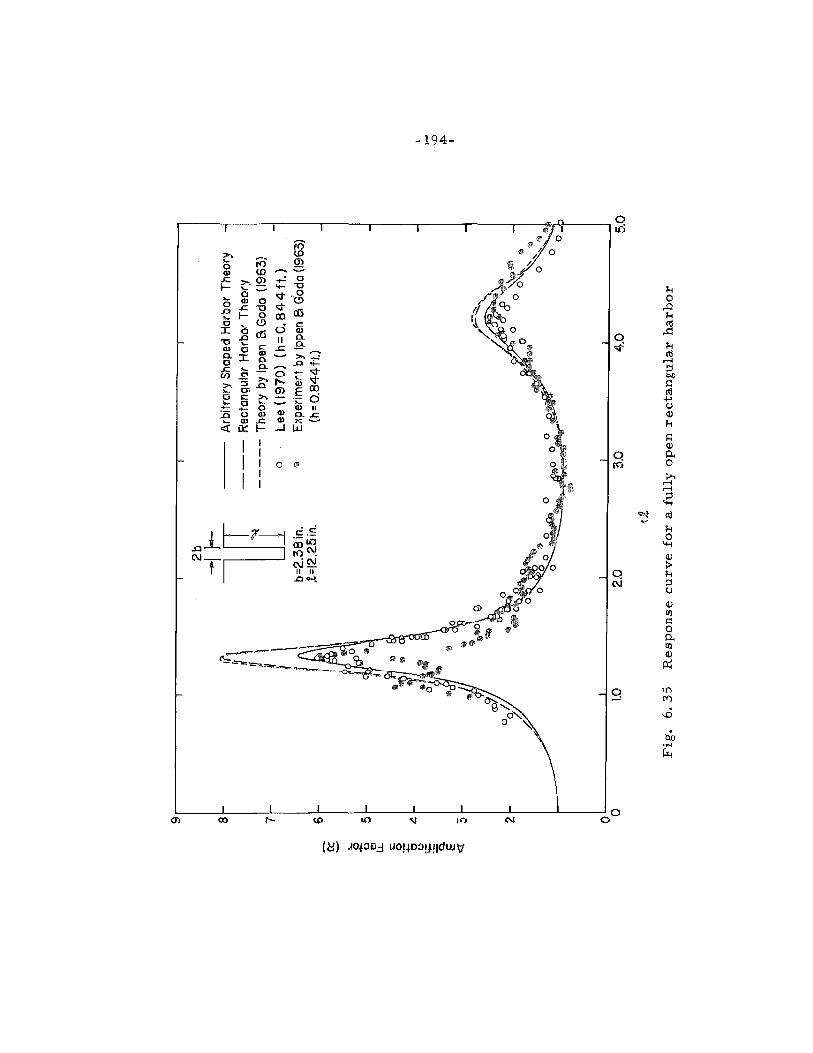

while the theory developed by Ippen and Goda ( 1963) i s represented by
a line composed of short dashes. The experimental data obtained
f rom the present studies a re denoted by open circles while the experi-
mental data of Ippen and Goda (1963) a re shown as solid circles.
In using the arbitrary shaped harbor theory the boundary of the
harbor is divided into 47 segments (N=47) of 11neq11al length including
three segments at the harbor entrance. Since the boundary of the
rectangular harbor i s composed of straight lines, as discussed in
Subsection 3. 3. 1, the diagonal elements of the matrix G are equal n
to zero, i. e. in Eq. 3. 57, (G ).. = 0 for i=l, 2. . . . .47. After following n 1.1
the procedures described in Chapter 3 the response curve shown i s
obtained.
In using the rectangular harbor theory the method described in
Section 4.2 i s used. For a fully open rectangular harbor, Eq. 4.38,
which describes the wave function f, in the region inside the harbor,
can bc simplified, since the entrance and the width of the harbor a re
equal Therefore, the te rm S (x, y) defined in Eq. 4. 38 i s equal m
to zero and can be simplified to:
f , ( x , ~ ) = C ~ s ~ ( x , ~ ) (6.8)
Thus, the average normal derivative of the wave function at the
harbor entrapce shown in Eq. 4.41 can be simplified also as:

- 196-
1 A 2 where S = -G cot kt and Bo = --(J + A-Y ) As as defined in Eq. 4.27. 0 2 c l r c
The Fourier transformation method used by Ippen and Goda (1963)
for the evaluation of the radiation wave function f3 in the region outside
the harbor i s different from the present rectangular harbor theory in
which Green's identity formula and the Hankel function a re used.
However, the method used for Region 11, i. e. inside the harbor, i s the
same. Therefore, the difference between the results of the theory of
Ippen and Goda (1963) and this theory can be attributed to the difference
between the methods used to evaluate the radiation function f, ; from
Fig. 6.35 any differences appear to be quite small.
From Fig. 6.35 i t is seen that the three theoretical curves agree
fairly well with the experimental results, although the theoretical
curve obtained from the arbitrary shaped harbor theory agrees better
with the experiments near resonance than the other two theoretical
curves. This may be because in using the arbitrary shaped harbor
theory, the entrance was divided into three segments and the solution
was matched at each segment as compared to the other two theories
where only the average solution across the entrance was matched.
Another feature of Fig. 6 . 3 5 i s that the present experimental data
agree better with the theoretical curves than do the experimental data
of Ippen and Goda (1963), especially in the vicinity of resonance. This
i s probably because the wave basin for the present experiments i s both
wider and longer than the wave basin used by Ippen and Goda, hence
the incident wave i s more ncarly two dimcnaional; ~ E O thc prcscnt

- 197-
'energy dissipators a r e more efficient than those used by Ippen and
Goda (1963) and therefore the "open- sea" condition i s simulated more
satisfactorily. This i s supported by the fact that the data of Ippen and
Goda ( 1963) show fluctuations in the region 1. 10 < k4 < 1. 70 indicating
that the "open-sea" condition is not properly simulated in this frequency
range where the incident wave length i s large resulting in small wave
steepness. Such fluctuations do not appear in the data corresponding
to the present experiments.
As mentioned before, these experimental results led to the
conclusion that the open- sea condition was being properly simulated
in the laboratory and no additional modification of the wave energy
dissipators was necessary. Moreover, the agreement between the
theoretical and experimental results as shown in Fig. 6 .35 has demon-
strated that the arbitrary shaped harbor theory can also be applied
successfully to a harbor with straight sides and sharp interior corners.
6,4 A HARBOR WITH COMPLICATED SHAPE: A MODEL OF THE
EAST AND WEST BASINS OF LONG BEACH HARBOR
6.4. 1 Introduction
As discussed in Sections 6.2 and 6.3, the theoretical
solution of the wave induced oscillations in the two specially shaped
harbors: circular and rectangular, can be obtained by using the
general theory for an arbitrary shaped harbor developed in Chapter 3.
The theoretical results for these special harbors obtained from the
arbitrary shaped harbor theory have been shown to agree well with

- 198-
the more exact theories developed in Chapter 4, and with the
experimental results.
These two special shaped harbors a r e of importance because, as
mentioned ear l ier , the circular harbor represents an extreme shape in
which the boundary of the harbor i s curved and the tangent to the
boundary i s continuously changing direction whereas the rectangular
harbor represents the other extreme where the boundary i s composed
of straight lines, along each side the tangent to the boundary does not
change direction. The boundary of any arbitrary shaped harbor i s in
fact usually a combination of these two cases.
In order to test the arbitrary shaped harbor theory further, a
harbor of complicated shape was studied both theoretically and experi-
mentally. In planform this harbor model i s slightly modified from the
existing harbor of the East and West Basins of the Long Beach Harbor
located in Long Beach, California; the horizontal scale i s 1 to 4700.
Also it d i f f e r s only slightly f rom the hydraulic model s t u d i e d by
Knapp and Vanoni (1945) wherein a distorted hydraulic model was used
with attention given to the bathymetry.
A sketch of the model of the East and West Basins of Long Beach
Harbor which was used in this investigation i s presented in Fig. 6.36
which shows the width of the harbor entrance as 0.2 ft and the
characteristic dimension of the harbor, a, equal to 1.44 ft. The depth
of the water in the experiments was constant in both the harbor and
the "open-sea" and equal to 1 f t .


The theory for an arbitrary shaped harbor developed in Chapter
3 i s used to calculate the response curves, the wave amplitude
distribution inside the harbor, and the total velocity at the harbor
entrance. In applying the theory, the boundary of the harbor is
divided into 75 unequal straight-line segments including two segments
for the harbor entrance. The segments a re numbered counter-clock-
wise starting from the right-hand limit of the harbor entrance and this
numbering system i s shown in Fig. 6. 36.
6.4.2 Response of Harbor to Incident Waves
Response curves at four different locations inside the
harbor are presented in Figs. 6 - 3 7 to 6.40. The fnnr points are
designated as point A, B, C, D and, for convenience, they a r e shown
in Fig. 6. 36 along with their coordinates in the model: A(0.30 ft,
-0. 525 ft), B(0. 30 ft,-0. 96 f t ) , C(l. 32 ft, -0. 96 f t ) and D(-0.45 ft,
- 1.245 f t ) , where the f i rs t number inside the bracket i s the x-coord-
inate and the second number i s the y -coordinate. For all of the
response curves, the abscissa is the wave number parameter, ka
(where again k i s the wave number, and "a" i s a characteristic length
equal to 1.44 f t and shown in Fig. 6.36); the ordinate i s the ampli-
fication factor R, as defined earlier.
It is seen that the theoretical results agree well with the experi-
mental data at all four locations and show that the response of this
harbor to periodic waves i s much more complicated than the response
curves for either a circular or a rectangular harbor. As discussed


-205-
in Section 6.2, the shape of the modes of resonant oscillation inside
a harbor is simpler for an incident wave of smaller wave frequency,
i. e. a smaller value of ka. As the incident wave frequency increases,
the shape of mode of oscillation inside the harbor becomes more
complex. The results shown in Figs. 6. 37 to 6. 40 also confirm this.
For example, at the fir s t resonant mode (ka = 0.6 1) the amplification
factors at the four different positions (Points A, B, C, and D) differ
only slightly. However, for the mode corresponding to ka = 7.62, the
amplification factors at the four locations differ considerably; the
amplification factors at the points B and D are much smaller than those
at the points C and A.
One common feature of the four response curves is that while
the theory has predicted the frequency of every resonant mode of
oscillation correctly, the theoretical amplification factor at resonance
i s slightly larger than the experimental data especially for the
resonant modes at larger values of ka. This can be attributed to the
observation made in Subsection 6.2 .2 that in using the same number
of segments for the boundary of the harbor at all wave periods, the
theoretical results for a smaller value of ka a re more accurate than
the results which correspond to large ka; therefore, better agreement
between the theory and experiments i s expected and observed for small
values of ka. (This means that the value of kAs i s smaller for the
former case than the latter case. ) In addition the energy dissipation i s
larger at resonance for large values of ka, thus also tending to
decrease the experimental amplification factors compared to those
determined theoretically.

It can also be seen f rom the response curves that the agreement
between the theoretical solution and the experimental data is reason-
ably good at each of the locations; there i s no location where better
agreement i s seen compared to another. This uniformity of the agree-
ment between the theory and experiments suggests that the theory has
also accurately predicted the wave amplitude distribution inside the
harbor for each mode of resonant oscillation.
In the application of the arbi t rary shaped harbor theory
(Chapter 3 ) the singularities a re always assumed to be located at the
mid-point of each boundary segment. Therefore if an interior point
(x, y ) i s too close to the mid-point of a particular boundary segment,
the wave function f, (x, y) calculated from Eq. 3 . 3 7 might be in e r ro r
because of the excessive influence of that particular singularity
(possibly as large as 10 or 20%). To avoid this i t was found that the
interior point investigated should be more than one-half of the length
of the segment ( $ A S ) away f rom the harbor boundary. If the wave
function desired i s at a location very close to the boundary i t can be
obtained either by: interpolating between the value at the boundary
(Eq. 3 .22 ) and the value of f,(x, y) at a point which i s at a distance
of approximately &AS f rom the boundary or by reducing the length of
the segment L o alluw the interior point ol interest Lo be closer to the
boundary.
-207-
As mentioned before, a response curve at a particular location
inside the harbor does not necessarily show the maximum amplification
within the harbor. The variation of the maximum amplification within
the entire basin plotted as a function of the wave number parameter,
ka, is presented in the response curve of Fig. 6.41. The ordinate
is the ratio of the maximum wave amplitude within the harbor, regard -
less of location, to the standing wave amplitude with the entrance
closed. This curve shows every possible mode of resonant oscillation
for the range of ka that has been investigated, as well as the maximum
amplification for each mode. It i s obvious that the maximum arnpli-
fication does not always occur at the same location within the harbor
for different values of ka. This can be seen by comparing Fig. 6.4 1
with Figs. 6.37 through 6.40.
The experimental data from a model study conducted by Knapp
and Vanoni (1945) a re included in Fig. 6.4 1 for comparison. Data
corresponding to the harbor with a 600 ft harbor opening are repre-
sented by open circles while the data for a 2000 ft opening are repre-
sented by solid circles. The prototype gate opening corresponding
to the present model i s 940 ft. It should be mentioned that the
original data (see Knapp and Vanoni, '1945, p. 89) were plotted as the
maximum amplification factor as a function of prototype wave period.
In order to compare these data with the present theory the wave period
has been converted to the wave parameter, ka. For this conversion,
the prototype water depth was taken as an average of 40 ft, and the

prototype characteristic dimension of the harbor a = 6768 ft was used.
(The experimental data shown in Fig. 6.4 1 corresponds to prototype
wave periods which range from 2Q min. to 15 min. )
The experimental data from Knapp and Vanoni (1945) show
decreasing amplification factors with decreasing harbor opening
contradicting one conclusion made in the study of circular harbors
(Subsection 6.2.2): decreasing the harbor opening increases the
wave amplification in the harbor at resonance. However, if one
considers the other conclusion made in Subsection 6.2.2 that the
viscous dissipation of energy i s more important for a harbor with a
smaller opening this contradiction may be resolved. Since i t i s
entirely possible in Long Beach Harbor that energy dissipation for the
harbor with a 600 ft opening i s so large compared to that for the
harbor with a 2000 ft opening that the increase in the resonant ampli-
fication due to closing the entrance i s more than compensated by
energy dissipation. It i s possible that if the harbor entrance were
much larger than 2000 ft, the amplification factor at resonance would
be less,thus, in agreement with the "harbor paradox". This has not
been investigated in this study.
Both the data and the theoretical curve presented in Fig. 6.41
more emphatically sfiuw an in~portant requirement of harbor rcsonance
studies. That is, in order to insure that certain modes of oscillation
a r e not missed in hydraulic model studies, a sufficient small interval
between wave periods must be used in evaluating the response.

-210-
6 . 4 . 3 Variation of Wave Amplitude Inside the Harbor for One
Mode of Resonant 0 s cillation
Experiments were not conducted specifically to measure
the distribution of wave amplitude inside the Long Beach Harbor model
at resonance as was done in the investigation of circular harbors.
However as mentioned previously. the theoretical amplitude distribution
inside the harbor had been reasonably confirmed by the experiments
shown in the response curves of Figs. 6.37 through 6.40. The
distribution of wave amplitude inside the harbor for one particular
mode of resonant oscillation determined from the arbitrary shaped
harbor theory is presented in Fig. 6 .42 for a value of k a = 3.38. The
magnitude of this resonant peak can be seen in any of the response
curves (Figs. 6. 37 through 6.41); attention i s directed to the fact
that this i s the second largest maximum amplification among the nine
resonant modes presented in Fig. 6.41. In the prototype, for this
value of ka, using the average depth of 40 ft the wave period i s 6. 1
minutes.
In Fig. 6.42 the wave amplitude has been normalized with
respect to the wave amplitude at point C; the coordinates of this
position have been presented in Fig. 6.36. Positive water surface
displacements are shown by solid lines and negative displacements
by long dash lines. Two nodal lines a r e seen, one in the East Basin
and one in the West Basin with maxima occurring at the ends of each
basin and the minimum occurring near the confluence of the two. For

Fig. 6.43 Wave amplitude distribution inside the harbor model of
Knapp and Vanoni (1945) for six minute waves (ka=3.30)
(see Knapp and Vanoni (1945), p. 133)

this mode of oscillation i t can be seen that neither a node nor an
antinode exists at the entrance.
Irl the r~lvriel sludy cvnducled by Knapp and Vanoni (1945) meas -
urements were made of the wave amplitude distribution inside the
harbor for various modes of resonant oscillation, and contour drawings
s imi lar to Fig. 6.42 were constructed. One such wave amplitude
distribution i s shown in Fig. 6.43. It i s apparent f rom comparing
Figs. 6.42 to 6.43 that in this investigation the boundary of the model
has been simplified, especially the Eas t Basin. The contours of
constant water surface elevation a r e shown a s all solid lines in Fig.
6.43 since the positive and negative displacements were not different-
iated in that study. It is seen that two nodal lines exist, one in each
basin, and the maxima exist at the end of each basin as well as near
the entrance.
By comparing Figs. 6.43 to 6.42 the similari t ies in the ampli-
tude distribution a r e striking. Except for the region near the entrance
the location of the two nodes and the maxima a r e similar for the two
models even though the boundary of the model used for present study
has been simplified. Difference between the amplitude distribution
near the entrance can probably be attributed to the difference of the
" c n a s t 1 i n e s " f n r the two cases. Another difference between the two
models which may contribute to the differences between the amplitude
distribution shown in Figs. 6.42 and 6.43 i s that all boundaries were
vert ical and the depth was constant in the model of this investigation
compared to the more realist ic treatment of the boundaries and
bathymetry in the distorted hydraulic model of Knapp and Vanoni (1945).
6.4.4 Velocity at the Harbor Entrance as a Function of Wave
Number Parameter , ka
The theoretical curves and the experimental data
presented in Subsection 6. 2. 5.4 established the proposition that the
fluid velocity at the harbor entrance reaches a maximum when a
resonant oscillation develops inside the harbor. For the model of the
East and West Basins of the Long Beach Harbor, no velocity
measurements were made at the harbor entrance; however, theoreti-
cally this variation was investigated using the arbi t rary shaped harbor
theory.
The variation of the average velocity a t the harbor entrance
*i (normalized with respect to ,,@ T ) as a function of the wave number
parameter, ka, i s presented in Fig. 6.44. Recall that the harbor
entrance of the Long Beach Harbor model was divided into two
segments (see Fig. 6.36); thus, the ordinate in Fig. 6.44 represents
Ai the average value of V: /& at the water surface for the two
entrance segments. (As before, the velocity i s computed using
Eq. 6.7. )
It i s seen that there are 9 maxima in the range of ka presented
in Fig. 6.44; the values of ka associated with these are: 0.6 1, 1. 50,
3 .38 , 4.96, 5.30, 5.70, 6.60, 7. 10, and 7.64. These values of ka
a r e exactly the same as those associated with the maxima in the
response curve of maximum amplification presented in Fig. 6.41.

-215-
This clearly demonstrates that each maximum of the total entrance
velocity i s associated with a mode of resonant oscillation inside the
harbor, no matter how small the value of the peak.
A curve like Fig. 6.41 i s not easy to obtain, because in order to
obtain a value of the maximum amplification anywhere inside the harbor
for a particular wave number the amplification factor a t many points
inside the harbor must be determined. However, the curve shown in
Fig. 6.44 i s relatively easy to obtain since one needs only the values
of the wave function f,, the normal derivative ata and the derivative 2 ay '
at the harbor entrance when evaluating the total velocity f rom Eq. 6. 7.
For a harbor with a complicated shape, i t i s possible that an
interaction of wave motion between interconnected basins inside the
harbor may develop and produce a resonant oscillation with only a
small velocity at the harbor entrance. For example, the peak
associated with ka = 1. 50 in Fig. 6.44 i s indeed very small; however,
at this value of ka, a resonant oscillation does exist inside the harbor
a s can be seen f r o m the response curves in Figs. 6.40 and 6.41. The
same i s true for ka = 5. 30 and 5. 70 a t which the peaks in the velocity
curve (Fig. 6.44) a r e also small, but considerable resonant oscillation
does develop in the harbor as shown in the response curves in Figs.
6.38, 6. 39, and 6.41 (for ka=5.30) and Figs. 6.40 and 6.41 (for k a =
5. 70). Therefore, i n using this method of determining the periods of
the resonant modes ca re must be taken that a small interval in wave
period i s used i n the computations.

-2 16-
Fig. 6.44 shows that the velocity at the entrance for the pumping
mode (ka = 0.6 1) i s nearly four times that which exist for any other
mode of oscillation. Using the prototype dimensions described
previously the period of this mode of oscillation i s approximately 33
minutes and could possibly be excited by tsunami. If the amplitude
of an incident wave were 0. 5 ft (using the average depth of 40 ft) Fig.
6.44 indicates that the maximum average entrance velocity for tMs
mode would be about 10 fps and for modes of smaller wave period the
velocities a r e in the order of 2 fps. Such velocities could cause
significant damage to structures located near the entrance.
The results presented in Section 6.4 have shown good agreement
between the theoretical analysis and the laboratory experiments demon-
strating again the applicability of the arbitrary shaped harbor theory
to harbors with complicated planforms and constant depth. The
variation of the velocity at the harbor entrance as a function of the wave
number parameter ka proves to be a good indicator for resonance
inside the harbor. It has also been shown that the present theoretical
results agree qualitatively with the experimental data obtained from a
model study conducted by Knapp and Vanoni (1945), although the plan-
form of the model investigated by them was more complicated and
also included depthwise variations.

The major objective of the present study has been to investigate,
both theoretically and experimentally, the response of an arbitrary
shaped harbor (with constant depth) to periodic incident waves. In
order to ensure that the general theory which was developed (termed
the arbitrary shaped harbor theory) could be applied to a harbor with
a complicated shape this theory was f i r s t applied to two special shaped
harbors: a circular harbor and a rectangular harbor. For these two
cases different theories termed the circular harbor theory and the
rectangular harbor theory were developed and compared to the general
theory. Experiments were then conducted for the circular and rectangu
la r harbors to verify the theoretical solutions. The general theory (the
arbitrary shaped harbor theory) was also applied to a harbor of more
complicated shape: a simplified, constant depth, model of the East
and West Basins of the Long Beach Harbor. Experiments were also
conducted to confirm the theoretical predictions.
From this study the following major conclusions, applying to the
circular harbors, the rectangular harbor, and the Long Beach Harbor
model, can be drawn:

- 2 l 8 -
1. The present linear -inviscid-theory termed the arbitrary
shaped harbor theory predicts the response of an arbitrary
shaped harbor (with constant depth) to periodic incident
waves quite well even near resonance.
2. The theoretical prediction of the resonant frequencies (or
the wave number parameter, ka, at resonance) agree well
with the experimental data. The theoretical amplification
factor at resonance i s generally somewhat larger than the
experimental data especially for the resonant modes at
larger values of ka.
3. The open-sea condition has been simulated properly in the
wave basin used for the experiments; the reflection
coefficient for the wave energy dissipators which were used
i s estimated to be less than 20% for most of the experiments
which were conducted.
4. Because of the wave radiation from the harbor entrance to
the open-sea region which has been considered in this
inviscid theory, the amplification of the wave amplitude
inside the harbor at resonance i s finite. The effect of
viscous dissipation, which has not been considered in this
theory, i s to decrease the amplification near rcsonancc
even more.
5. The average total velocity across the harbor entrance
reaches a maximum when a resonant oscillation develops
inside the harbor; thus, the variation of the velocity at the

- 2 19-
harbor entrance with wave number has been found to be a
good indicator for resonance.
Since a relatively more detailed study has been made for circular
harbors some of the important conclusions concerning this shape can be
stated as follows:
6. The theoretical solution for a circular harbor with a lo0
opening obtained using the arbitrary shaped harbor theory
agrees well with those obtained from the circular harbor
theory and the experiments. These results included the
resonant wave numbers, the amplification factors, the
shape of water surface inside the harbor for various modes
of oscillations, and certain velocities at the harbor
entrance.
7. For the circular harbor with a 60' opening both theories
only differ slightly in the prediction of the value of the wave
number parameter (ka) at resonance: the arbitrary shaped
harbor theory agrees better with the experimental results
in this respect. The shapes of the modes of oscillation
also have been predicted correctly by both theories; thus,
the small entrance approximation for the circular harbor
theory can bc applicd at lcast up to s harbor opening with s
60" central angle.
8. As the width of the harbor entrance increases, the ampli-
fication at resonance decreases, but the wave number band-

width at resonance increases: thus, the '!harbor paradox1'
was confirmed both theoretically and experimentally for
this shape.
Experiments show that the effect of viscous dissipation of
energy which i s neglected in the present theories i s more
important for harbors with a smaller opening.
There a r e four modes of resonant oscillations in the range
of ka investigated for the harbors with a l o 0 and a 60°
opening. Except for the "pumping modef', which does not
exist in a completely closed circular basin, each mode
corresponds to a free mode of oscillation in the closed
basin. The corresponding modes of oscillation for the two
harbors and the closed basin a re basically similar; how-
ever, the detailed shape of the f ree surface differs among
the three.
I I. The wave number paravlletcr (ka) st resonance approaches
the value for a closed basin as the entrance width decreases.
12. No antinode, or node, exists at the harbor entrance
although an antinode might occur at that position for a
closed circular basin.
13. For a larger edrauce widlll Lhe distrilmtiull ul the valucity
across the harbor entrance varies significantly for different
modes of oscillation.

-221-
14. The experimental data regarding the variation of entrance
velocity with the wave number parameter agree reasonably
well with the theoretical results . In addition to the general conclusions the following conclusions
can be added for the rectangular harbor:
15. The theoretical results obtained from the present
rectangular harbor theory a re almost identical to those
obtained by the theory of Ippen and Goda (1963) ; thus, any
difference in the two methods for evaluating the radiated
waves appear to be quite small.
16. The theoretical results obtained from the arbitrary shaped
harbor theory applied to the rectangular harbor agree
better with the experiments near resonance than the
rectangular harbor theory developed in this study or the
theory of Ippen and Goda (1963). Perhaps this i s due to the
r'act that when using the arbitrary shaped harbor theory
three segments were used in the matching procedure while
in the other two lleuries u u l y Llle dverage solution across
the entrance was matched.
17. The present experimental data agree better with the theo-
retical results than do the experimental data of Ippen and
Goda (1963) especially in the vicinity of resonance, pro-
bably because the wave basin used for present experiments
i s both wider and longer and the present wave energy
dissipators a r e more efficient than in that study; thus the

- 2 2 2 -
incident wave i s more nearly two-dimensional and the
"open- sea" condition i s simulated more satisfactorily.
The following conclusions may be drawn for the model of the East
and West Basins of the Long Beach Harbor in addition to the conclusions
stated earl ier .
18. The theoretical results agree w e l l with the experiinental
data fox the response at four different positions within the
harbor. The uniformity of agreement at the four locations
suggests that the theory has also predicted correctly the
shape of the various modes of oscillations.
19. The present theoretical results also agree qualitatively with
the experimental data obtained from a model study
conducted by Knapp and Vanoni (1945) although the planform
of the model investigated by Knapp and Vanoni was more
complicated and their study included depthwise variations.
LO. The results show that the present theory can be applied
with confidence to prototype harbors with relatively uniform
depth and reflective interior boundaries.

LIST OF REFERENCES
1. Apte , A. S. , and Marcou, C. (1954), "Seiche i n Ports", Fifth
Conference on Coastal Engineering, Grenoble, France,
pp. 85-94.
2. Apte , A. S. (1957), l 'Recherches Theoriques e t Experimentales
sur Les Mouvements des Liquids Pcsants Avcc Surface Libr e",
Publications Scientifiques e t Techniques du Ministere de
L'Air, No. 333.
3 . Baker, B. B. , and Copson, E. T. (1950), The Mathematical
Theory of Huygen's Principle, Oxford University P r e s s ,
London.
4. Banaugh, R. P. , and Goldsmith, W. (1963), "Diffraction of
Steady Acoustic Waves by Surfaces of Arbitrary Shape",
The Journal of the Acoustical Society of America, Vol. 35,
No. 10, pp. 1590-1601.
5. Banaugh, R. P. , and Goldsmith, W . (1Y63), "Diffraction of
Steady Eleastic Waves by Surfaces of Arbitrary Shape",
Journal of Applied Mechanics ASME, Vol. 30, Series E,
No. 4, pp. 589-597.
6. Biesel, I?. , and LeMehaute, B. (1955), "Etude Theorique de La
Reflexion de La Houle su r Certains Obstacles", LaHouille
Blanche, March-April, pp. 130-140.

-224-
LIST O F REFERENCES (Cont'd)
Biesel, F. , and LeMehaute, B. (1956), "Mo~vements de Reson-
ance a Deux Dimensions dans une Enceinte Sous L' Action
dlOndes Incidente s 'I, LaHouille Blanche, July -August,
pp. 348-374.
Ca r r , J. H. (1953), "Long-Period Waves o r Surges in Harbors",
Transactions, ASCE, Vo. 118, pp. 588-616.
Chen, L. H. , and Schweikert, D. G. (1963), "Sound Radiation f rom
an Arbi t rary Body", The Journal of the Acoustical Society of
America , Vol. 35, No. 10, pp. 1626-1632.
Chertock, G. (1964), "Sound Radiation f rom Vibrating Surfaces",
The Journal of the Acoustical Society of America, Vol. 36,
No. 7, pp. 1305-1313.
Copley, L. G. (1967), "Integral Equation Method for Radiation f rom
Vibrating Bodies", The Journal of the Acoustical Society of
America, Vol. 41, No. 4, pp. 807-816.
Courant, R. and Hilbert, D. (1953, 1962), Method of Math-
ematical Physics, Vol. I and 11, Interscience Publishers Inc.,
New York.
Das, M. M. (1968), llExtended Application of a Single Hot-film
Probe for the Measurement of Turbulence in a Flow Without
Mean Velocity", HEL 2-20, Hydraulic Engineering Laboratory,
University of California, Berkeley, California.

LIST O F REFERENCES (Cont 'd)
Dettrnan, J. W. (1965). Applied Complex Var iab les , The Mac-
mi l l an Company, New York.
F r i edman , M. B. , and Shaw, R. (1962), "Diffraction of Pu l se s
by Cylindrical Obs tac les of Arb i t r a ry C r o s s Section",
Jou rna l of Applied Mechanics ASME, Vol. 29, Se r i e s E,
No. 1, pp. 40-46,
Goda, Y., and Ippen, A. T. (1963), "Theoret ical and Exper i -
lrlerllal Il~vesLigaLiurl u1 Wave Erierg y DissipaLor s Cor~lposed
of Wi re Mesh Screens 1' , Repor t No. 60, Hydrodynamics
Labora tory , M. I. T.
Hildebrand, F. B. (1962), Advanced Calculus fo r Applications,
Prent ice- Hal l , Inc. , Englewood Cliffs, New J e r s e y .
Hino, M, , and Hino, K. (1965), "Response Charac t e r i s t i c s of
Tokyo Bay to Incident Long Waves", Coastal Engineering i n
Japan, Vol. 8 , pp. 57-69.
Hinze, J. 0. ( 19 59), Turbulence, McGraw-Hill Book Company,
New York.
Hwang, L. S. , and Tuck, E. 0. (1969), "On the Osci l la t ions of
H a r b o r s of Arb i t r a ry Shape", Submitted to Jou rna l of Fluid
Mechanics (publication pending).
Ippen, A. T . , Edi tor (1966), E s t u a r y and Coastline Hydro-
dynamics , McGraw-hil l Book Company, New York.

LIST OF REFERENCES (Cont'd)
Ippen, A. T. , and Goda, Y. ( 1963), "Wave Induced Oscillations
in Harbors: The Solution fo r a Rectangular Harbor
Connected to the Open-Sea", Report No. 59, Hydrodynamics
Laboratory, M. I. T.
Ippen, A. T. , and Raichlen, F. (1962), "Wave Induced
Oscillations in Harbors: The Problem of Coupling of Highly
Reflective Basins ", Report No. 49, Hydrodynamics
Laboratory, M. I. T.
24. Ippen, A. T. , Raichlen, F. , and Sullivan, R. K. ( 1962), "Wave
Induced Oscillations i n Harbors: Effect of Energy
Dis sipators in Coupled Basin Systems", Report No. 52,
Hydrodynamics Laboratory, M. I. T.
25. Kellog, 0. D. (1953), Foundations of Potential Theory, Dover
Publications, Inc., New York.
26. Keulegan, G. H. (1968), "Wave Damping Effects of Screens",
Research Rapur t No. 2-12, U. S. Arimy Engineer Waterways
Experimental Station.
27. Knapp, R. T. , and Vanoni, V. .A. (1945), "Wave and Surge Study
for the Naval Operating Base, Terminal Island, California1',
Hydraulic Structure Laboratory of the California Institute of
Technology.
28. Kravtchenko, J., and McNown, J. S. (1955). "Seiche in Rectan-
gular Ports 1' , Quarterly of Applied Mathematics, Vol 13,
pp. 19-26.

LIST O F REFERENCES (Cont 'd)
29. Kuo, E. Y. T. (1968), "Acoustic Field Generated by a Vibrating
Boundary: I. Genera l Formula t ion and Sonar - Dome Noise
Loading", The Jou rna l of the Acoust ical Society of Amer ica ,
Vol, 43, No. I , pp. 25-31.
30. Lamb, H. (1945), Hydrodynamics , Sixth Edition, Dover Publi-
cat ions, New York.
3 1. Lee, J. J. [1967), Discussion of paper "Some Turbulence
Measu remen t s i n Water" by F. Raichlen, Jou rna l of the
Engineering Mechanics Division, ASCE, Vol. 93, No. EM 6,
pp. 287-293.
32. Leender t se , J. J. (1967), "Aspects of a Computational Model f o r
Long- Pe r iod Water Wave Propagation1' Memorandum,
RM-5294-PR, The Rand Corporation.
33. LeMehaute, B. (1960), " Per iodica l Gravi ty Wave on a Dis-
continuity", Jou rna l of the Hydraul ics Division, ASCE,
Vol. 86, No. H Y 9, pp. 11-41.
34. LeMehaute, B. (196 I ) , "Theory of Wave Agitation i n a Harbor" ,
J o u r n a l of the Hydraul ics Division, ASCE, Vol. 87,
No. HY 2, pp, 31-50.
35. LeMehaute, B, (1962), Discussion of the paper "Harbor Paradox"
by J. Miles and W. Munk, Jou rna l of the Waterways and
H a r b o r s Division, ASCE, Vol. 88, No. WW 2 , pp. 173- 185.

LIST O F REFERENCES (Cont'd)
36. McNown, J. S. (1952), "Waves and Seiche i n Idealized Ports",
Gravity Wave Symposium, National Bureau of Standards
Circular 5 2 1.
37. Mikhlin, S.G., andsmol i t skiy , K.L. (1967), Approximate
Methods for Solution of Differential and Integral Equations,
American Elsevier Publishing Company, N e w York.
38. Miles, J. , and Munk W. (196 l) , "Harbor Paradox", Journal of
the Waterways and Harbors Division, ASCE, Vol. 87,
No. WW 3, pp. 11 1- 130.
39. Morse, P. M. , and Feshback, H. (1953), Method of Theoretical
Physics, Vol. I and 11, McGraw-Hill Book Company, New
York.
40. Mullin, C. R. , Sandburg, R. , and Velline, C. 0. (1965), "A
Numerical Technique for the Determination of Scattering
Cross Sections of Infinite Cylinders of Arbi t rary Geometrical
Cross Sectiorl", Trarlsactiorls of Antellnas and Propagation,
IEEE, Vol. AP- 13, pp. 141- 149.
41. Muskhelishvili, N. I. ( 1946), Singular Integral Equations,
P. Noordhoff Ltd. , Groningen, Holland.
42. Raichlen, F. ( 1965 ), "Wave-Induced Oscillations of Small Moored
Vessels" , Report KH-R- 10, W. M. Keck Laboratory of
Hydraulics and Water Resources , California Institute of
Technology.

LIST OF REFERENCES (Cont'd)
-43. Raichlen, F. , and Ippen, A. T. (1965a), "Wave Induced
Oscillations in Harbors ", Journal of the Hydraulics Division,
ASCE, Vol. 91, No. HY 2, pp. 1-26.
44. Raichlen, F. (1965b), "Long Period Oscillations in Basins of
Arbitrary Shapes", Chapter 7, Coastal Engineering, Santa
Barbara Speciality Conference, pp. 1 1 5 - 145.
45. Raichlen, F. (1967), "Some Turbulence Measurements in Watert' ,
Journal of the Engineering Mechanics Division, ASCE,
Vol. 93, No. EM 2 , pp. 73-97.
46. Richmond, J. H. (1965), "Scattering by a Dielectric Cylinder of
Arbitrary Cross Section Shape", Transactions of
Antennas and Propagation,IEEE , Vol. AP- 13, pp. 334-341,
47. Shaw, R. P. (1967), "Diffraction of Acoustic Pulses by Obstacles
of Arbitrary Shape with a Robin Boundary Condition", The - Journal of the Acoustical Society of America, Vol. 41,
No. 4, pp. 855-859.
48. Stoker, J. J. (1957), Water Waves, Interscience Publishers Inc. ,
New York..
49. Townes, H, W. (1965), "Flow Over a Rough Boundary", Thesis
presented to the California Institute of Technology, at
Pasadena, California, in partial fulfillment of the require-
ments for the degree of Doctor of Philosophy.
LIST OF REFERENCES (Cont'd)
50. Watson, G. N. (1945), A Trea t i se on the Theory of Bessel
Functions, The Macmillan Comapny, New York.
5 1. Wilson, B. W. (1959), "Research and Model Studies on Wave
Action in Table Bay Harbor, Cape Town", Transaction of
the South African Institution of Civil Engineers, Vol. I,
No. 6 and 7 (June, July 1959) ; Vol. 11, No. 5 (May 1960).
52. Wilson, B.W., Hendrickson, J.A., andKi lmer , R.C. (1965),
"Feasibility Study for a Surge -Action Model of Monterey
Harbor, California", Report 2 - 136, Science Engineering
Associates, San Marino, California.

LIST OF SYMBOLS
A Wave amplitude.
Ai Incident wave amplitude.
Amax Maximum wave amplitude within the harbor.
A1 , A2, A3 Functions representing the magnitude of the velocity cornporlants (defined in Eq. 3. 41).
Characteristic dimension of a harbor, the radius of a circular harbor.
Bo A function representing the average radiation effect at the harbor entrance (defined in Eq. 4.27).
L bo
A constant equal to --. 2
b Width of a rectangular harbor.
Normal derivative of the wave function at the harbor entrance.
Average of the normal derivative of the wave function across the harbor entrance.
c_ A vector representing the normal derivative of the wave function at the mid-point of each entrance segment.
c, , c, , c3, Constants associated with the hot-film sensor and the
'a7 % linearization procedure.
D Diameter of the screen wires of the wave energy dis sipator.
D, D l , D2 Used in Appendix I and Appendix 11 representing various domains of interest.
d Width of the harbor entrance.
Distance from left-hand boundary of the rectangular harbor to the left-hand limit of the harbor entrance.
E Output voltage of the hot-film anemometer,
e Base of the Naperian logarithm.

LIST O F SYMBOLS (Co11l;'d)
g
H.. 1J
Wave fnnr t ion which describes t h e variation of the velocity potential i n the x and y directions.
Wave function in Region I (in the open-sea).
Wave function in Region I1 (inside the harbor).
Radiat ed wave function.
Incident wave function.
Reflected wave function.
An infinite se r ies defined in Eq. 4.23 and Eq. A. 3.3 .
An infinite se r ies defined in Eq. 4.23 and Eq. A. 3.6.
An N x N matrix defined in Eq. 3. 17d (elements of the matrix a r e defined in Eqs. 3. 59 and 3.60).
An N x N matr ix defined in Eq. 3. 17b (elements of the matr ix a r e defined in Eqs. 3.43 and 3. 57).
Green's function.
Acceleration due to gravity.
Radiation matr ix (a p x p matrix, see Eq. 3. 3 3 ) , the elements of the matr ix a r e defined in Eqs. 3.62 and 3.63.
Wave height.
Incident wave height.
Reflected wave height.
Transmitted wave height.
Zero and f i r s t o rders of the Hankel function of f i r s t kind.
Watcr depth.
Indentity matrix.
Electrical currents to the hot -film sensor.

.LIST OF SYMBOLS (Cont'd)
Unit vectors in the directions x, y, x respectively.
Bessel function of the f i rs t kind and order m.
An infinite ser ies defined in Eq. 4.26a and Eq. A. 3. 7.
Reflection coefficient.
Transmission coefficient.
Wave number.
Wave length.
Length of a rectangular harbor.
Logarithm to the Naperian base (e=2. 7 128).
A N x p matrix defined in Eq. 3 . 2 1.
An infinite ser ies defined in Eqs. 4. 18 and 4. 19.
A p x p matrix defined in Eq. 3. 35, (a matrix formed by the p rows and p columns of the matrix M).
Number of layers of screens.
Total number of segments into which the boundary of the harbor (including entrance) i s divided.
Outward normal to the boundary of the domain.
Order of magnitude.
A N-dimensional vector representing the normal derivative of the wave function at the mid-point of the straight-line segments of the harbor boundary.
Total number of segments into which the harbor entrance i s divided.
A function used in Appendix I1 representing the contri- bution to the value of wave function as the field point approaching a boundary point.
Source strength along the reflecting boundary (see Eq. 2.3).

LIST O F SYMBOLS (Cont'd)
Amplification factor.
Radius of a large circle.
Operating resistance of the hot-film sensor.
Distance between points or radial position in a polar coordinates.
Center to center distance between the screen wires.
Output voltage of the f i r s t squaring circuit of the linear- izer of the hot-film anemometer.
Output voltage of the linearizer of the hot-film anemometer.
Output voltage of the bias control, after using the f i rs t squaring circuit of the linearizer of the hot-film anemometer.
Special functions defined in Eq. 4.38.
Average of S Sm across the harbor entrance (defined in Eq. 4.39). 0'
Tangent to the boundary of the domain i n a counter- clockwise direction.
Length of the boundary segments . Wave period.
Time.
A N x p matrix with the diagonal of the f i r s t p rows equal to unity, all other elements equal to zero (Eq. 3. 19).
Velocity components in x , y, z directions.
Velocity vector with components u, v, w,
Resultant fluid velocity in the direction perpendicular to the longitudinal axis of the hot-film sensor,
1
Total velocity defined as (u2 + v2 + w2)%.
LIST O F SYMBOLS (Cont'd)
a, , a,, a3
av
Maximum total velocity with respect to time at a location. 4,
Average of V: ac ross the harbor entrance.
Maximum resultant velocity of the components v and w with respect to time at a location.
Average of V across the h a r b n r e n t r a n c e . 0
Value of V at the center of the harbor entrance. 0
A N-dimensional vector defined in Eq. 3. 17a representing the wave function at the boundary of the harbor.
Coordinate axis in horizontal direction parallel to the coastline.
Position vector for the point (x, y).
Bessel function of the second kind of o rder rn.
An infinite se r ies defined in Eq. 4.26b and Eq. A. 3, 9 ,
Coordinate axis in horizontal direction perpendicular to the coastline.
Function which describes the variation of the velocity potcntial in dcpthwio e direction z.
Coordinate axis in vert ical direction.
Quantities a t the jth segment of the boundary.
Firsttsecond part ial derivatives with respect to the tangent of the boundary.
Spatial average value,
A p-dimensional vector with each element equal to unity.
Interior angle of a boundary point ( see Fig. A. 2. 2).
Phase angles defined in Eq. 3.4 1.
Calibration constant of the hot-film sensor.

'LIST OF SYMBOLS (Cont'd)
A constant defined in Eq. 4. 33.
A large circle.
Euler's constant ( y o . 5772 16. . . . . ). Difference operator.
Kronecker delta,
Radius of a circle.
Displacement of water surface elevation from the mean water level.
Angular position.
Kinematic viscosity of the fluid.
1 Sum of an infinite ser ies , p(n) = 1 - . n
n= 1 A small circle or a half circle with a radius c.
Circular wave frequency ( 2 ~ / T).
Velocity potential.
Depth affect factur (Eq. 6 . 1).
Potential function for standing wave system (Eq. 2.3).
Total potential function (defined in Eq. 2. 3) .
Gradient operator.
Laplacian operator.
Boundary of a domain.
Absolute value.

APPENDIX I
WEBER'S SOLUTION OF THE HELMHOLTZ EQUATION
The derivation of Weber's solution of the two dimensional
Helmholtz equation i n a bounded domain (as used in Eq. 3. 11) and an
unbounded domain (as used i n Eq. 3.29) will be presented in this
appendix. This subject has been discussed by Baker and Copson (1950) ;
the interested reader i s referred to that book for other related topics
as well.
I. 1 Weber's Solution in a Bounded Domain
Let 8D be a closed curve boundi~g a domain D in the x-y
plane, i f f and g a r e two functions whose f i r s t - and second-order partial
derivatives a r e continuous within the domain D and on the boundary aD,
then Green's identity formula gives (see Kellog (1953)):
(A. 1. 1)
where a /an means differentiation along the outward normal to the
boundary of the domain.
If the functions f and g a r e both solutions of the two-dimensional
Helmholtz equation,

then the right.-hand-side of Eq. A. 1. 1 equals to zero, thus, Eq, A. 1. 1
reduces to:
(A. 1. 3 )
In particular, if g = ~ b ' ) ( k r ) , where r denotes the distance f rom a point
;(X, y) and if the point ;(x, y) l ies outside the domain D, one obtains
(A. 1.4)
3
However, i f x(x, y) l ies inside the domain D, Eq. A. 1.4 no longer
holds since ~ ( " ( k r ) has a logarithmic singularity at the point ;(x, y) 0
2 (H( "(kr) --*-log k r , as r + 0 ) . To avoid this singularity, Green's
0 'Tr /
identity formula will be applied to the region Dl, bounded externally by -3
a D and internally by a circle p with i ts center at x and with radius c 0
(see Fig. A. 1, 1). Thus, Green's identity formula, Eq. A. 1. 1,
becomes:
Since the singularity i s now outside the domain D, , by taking g=~L1) (k r ) ,
the right-hand-side of Eq. A. 1. 5 i s equal to zero. Thus, one obtains:
BD
Note that the direction of n on the
hand-side of Eq. A. 1.6 i s inward
Po (A. 1.6)
boundary p as shown in the right- 0
...r toward the center x(x, y), i. e. out-

ward from the boundary of the domain Dl (see Fig. A. I, 1); for
convenience this differentiation i s changed to the r direction (negative
n direction). Thus, one obtains:
Po (A. 1.7)
Since the integral around the boundary 8D does not depend upon the
radius c of the circle po, the right-hand-side of Eq. A. 1. 7 can be
evaluated at a radius c as small as desired. Thus the right-hand-side
of Eq. A. 1. 7 can be written as:
l im €4 0 J[f (HA1)(kr)) - ~ i ' ) ( k r ) $$ ] ds .
Po
(A. 1.8)
By using the asymptotic behavior of the Hankel function for r-0:
(1) 2 Ho (kr) -- 1 + A; log (kr) ,
a f the limit of Eq. A. 1. S can be evaluated. Since the functions f and - a r +
a r e continuous at x(x, y), the second t e rm and the f i rs t t e rm of Eq.
A. 1.8 can be evaluated as follows:
277 'af -+ limJ €40 ~b" (k r )% ds =lirnS s-+O ( l + ~ $ l o ~ ( k e ) ) c d 8 ( ~ ( x ) + o ( ~ ) ) = 0 (A. 1. 9a)
Po
(A. 1. 9b)
Substituting Eqs. A. 1.9 a and b into Eq. A. 1.7, one obtains:

a (1) f ) = - [fz ( H ~ (kr)) - ~ y ) ( k r ) f - ] ds (A. lo 10)
This completes the proof of the following theorem due to Weber:
Let f be a solution of the Helmholtz equation
in a closed domain D, whose f i rs t- and second-order partial
derivatives a r e continuous within and on the closed boundary aD. --t
Then the function of f at any interior point x can be expressed as:
-+ where r i s the distance from the interior point x to the boundary,
and a/an means differentiation along the outward normal to the
boundary aD.
I. 2 Weber's Solution in an Unbounded Domain
Suppose the function f i s a solution of the Helmholtz
equation, v2f t k2f = 0, outside the domain D, i. e. in the unbounded
domain, whose f i r s t- and second-order partial derivatives a re con-
tinuoue on/and outside the closed curve aD. Then the Green's identity
formula can be applied to a region D, bounded internally by the closed
curve aD and externally by a circle r with radius Ro which i s so chosen
that the circle I' encloses the closed curve 8D (see Fig. A. 1.2).
Thus, from the theorem presented in SectionI. 1 one obtains:
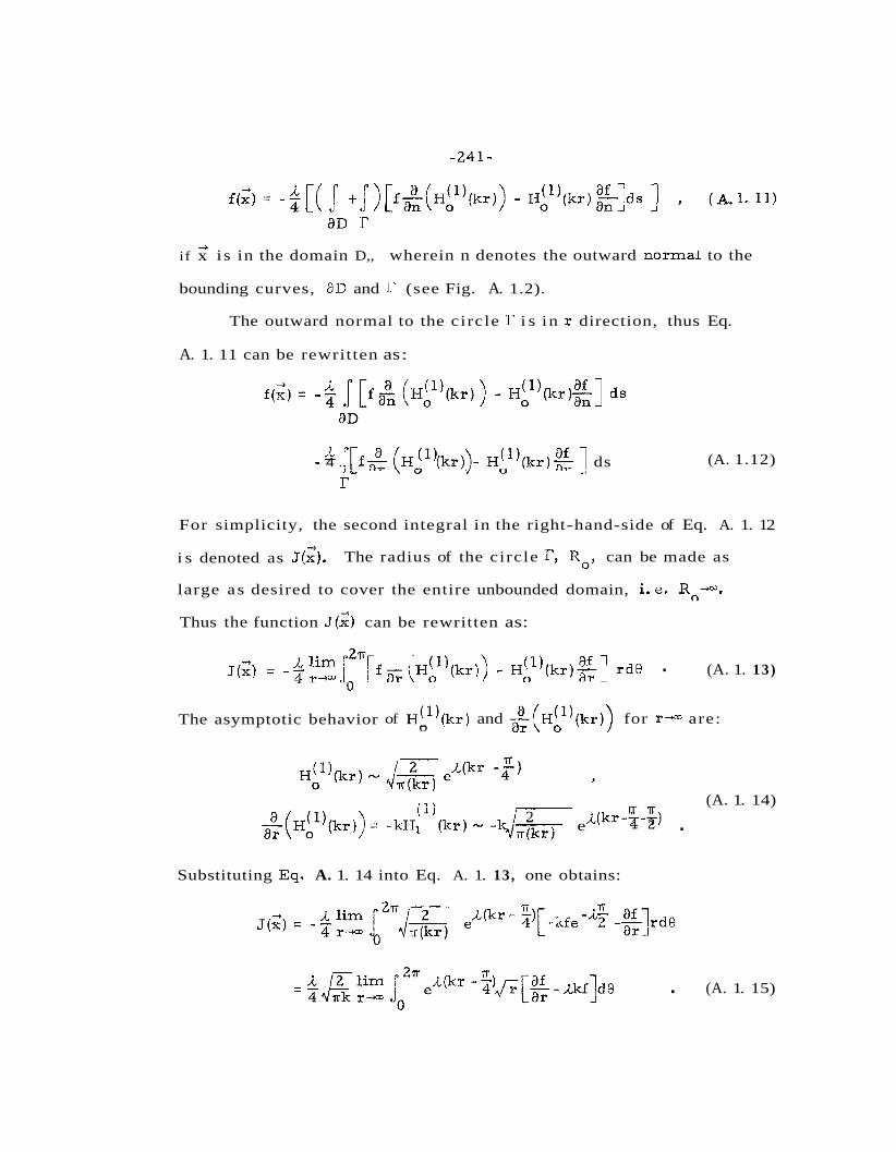
4
i f x i s in the domain D,, wherein n denotes the outward normal to the
bounding curves, aD and i? (see Fig. A. 1.2).
The outward normal to the circle T i s in r direction, thus Eq.
A. 1. 1 1 can be rewritten as :
- 4 . /[f & (H: l)(kr))- J3L1)(kr) $ ] ds (A. 1.12)
r
For simplicity, the second integral in the right-hand-side of Eq. A. 1. 12 3
i s denoted as J(x). The radius of the circle r, Ro, can be made as
large as desired to cover the entire unbounded domain, i. e . Ro+mr
Thus the function ~(2) can be rewritten as:
- Hqkrpg rde . n
(A. 1. 13)
The asymptotic behavior of ~ ( " ( k r ) and s(H:)(kr)) for r-rn are: 0
IT n (A. 1. 14) 2 *(kr ----)
e 4 2 .
Substituting Eq- A. 1. 14 into Eq. A. 1. 13, one obtains:
. (A. 1. 15)

-242-
Thus the function ~ ( 2 ) tends to zero, if the function:
(A. 1. 16)
uniformly with respect to 4 a s r -+ w. This condition, Eq. A. 1. 16 , i s
referred to a s the "Sommerfeld radiation condition". A sufficient
condition for this i s that the function f should behave like ~ ( " ( k r ) for 0
a f la rge values of r . Since for f = ~ ( " ( k r ) , and - = -k~ ! l ) (k r ) , the o ar
Sommerfeld radiation condition i s satisfied as r + 03:
This completes the proof for the following Weber's theorem in an
unbounded domain:
Let f be a solution of - + - a2f + k2f = 0 , whose f i r s t - and second- ax2 a p order part ial derivatives a r e continuous outside and on a closed
curve aD and le t
J;(E- kkf) 3 0
uniformly with respect to 8, as r + a, then the function f(;) at a
fixed point 2 located outside the domain bounded by aD, i. e.
inside the unbounded domain,can be expressed as:
where r i s the distance between the fixed point and the boundary
and n denotes the outward normal to the boundary 8D (in the
direction out of the unbounded domain].

Fig. A. 1. 1 Definition ske tch fo r a bounded domain
Fig. A. 1.2 Definition slrctch for an unbounded domain

APPENDIX 11
DERIVATION OF EQ. 3. 12
The Weber's solution of the two-dimensional Helmholtz equation
expressed the wave function f at an interior point as a function of the
wave function and its normal derivative at the boundary as follows
(see also Eq, 3. 11):
+ In order to determine the wave function f(xo) along the boundary, the
field point i s allowed to approach the boundary at a point Zi: the path
of integration i s deformed around a small half circle, p with radius 0'
s (see Fig. A. 2. 1). Then Eq. A. 2. 1 can be written as:
The radius of the half circle po, E, can be made to approach zero,
i. e. E -+ 0; using the definition of Cauchy principal value Eq. A. 2.2 can
thus be rewritten as:

where the f i r s t integral represents the Cauchy principal value and the
-#
second te rm , Q(xi), represents the limit of the integration along the
+ small half circle po as s -r 0. This limit value, Q(xi), can be evaluated
by the procedures which will be discussed in the following.
Since along the small half circle po, the direction of n i s in the --t
direction of r, the function Q(x:) can be rewritten as: 1
4 ,i lim .(xi)=-- 4 s-0 ~[f(<)&(~6"(kr))-~b~)(kr)~(f(2~))]ds(2~) . ( ~ 2 . 4 )
The asymptotic formulas of the Hankel functions for very small
argument (r + 0) are:
2 ~ ( " ( k r ) o - l + i;log (kr ) ;
(A. 2.5)
Substituting Eq. A. 2.5 into Eq. A. 2 .4 one obtains:
+ ,i, l im Q(x,) = - - ' L 1
A l im + o(c))
-?\
= &f (xi) 7 (A. 2.6)
since as €40 the limit of the second integral in Eq. A. 2.6 i s zero.

Substituting Eq. A. 2.6 into Eq. A. 2.3, i t becomes:
4 + where r = Ixo - xil *
-+ If the point x. i s a corner point on the boundary (see Fig. A. 2. 2) ,
1 4
the result of Eq. A. 2. 1 a s approaching xi can be expressed as:
S
(A. 2.8)
where the interior angle a i s defined in Fig. A. 2.2. For a smooth
curvc a i~ c q u d to n, thus Eq. A. 2. 8 is identical to Eq. A. 2 . 7.
(The approach used for these derivations can also be found in a
number of books; for example, s ee Muskhelishvili (1946) and Dettrnan

integration 1
Fig. A. 2. 1 Definition sketch for an interior point approaching a boundary point on a smooth curve.
Fig. A. 2 . 2 Definition sketch for an interior point approaching a corner point at the boundary

APPENDIX III
EVALUATION O F THE FUNCTIONS fjo, fyo, Jc, AND Yc
111. 1 The Evaluation of the Function fjo
The function f i n Eq. 4. 23 i s defined as: j 0
x AS-x f jo(x ,o) = [J f J ] ~ ~ ( l i r ) d r , (A. 3. 1)
0 0
where As i s the width of the harbor entrance. The Bes se l function
J (kr) in Eq. A. 3. 1- can b e represented i n an infinite se r ies as: 0
Jo (kr ) = 1 (A. 3 . 2 ) n! n! n= 0
Substituting Eq. A. 3.2 into Eq. A. 3. 1 and interchanging the order
of integration and summation one obtains:
111.2 The Evaluation of the Function f YO
The ftmction f in Eq. 4.23 i s defined as: YO
(A. 3.4)
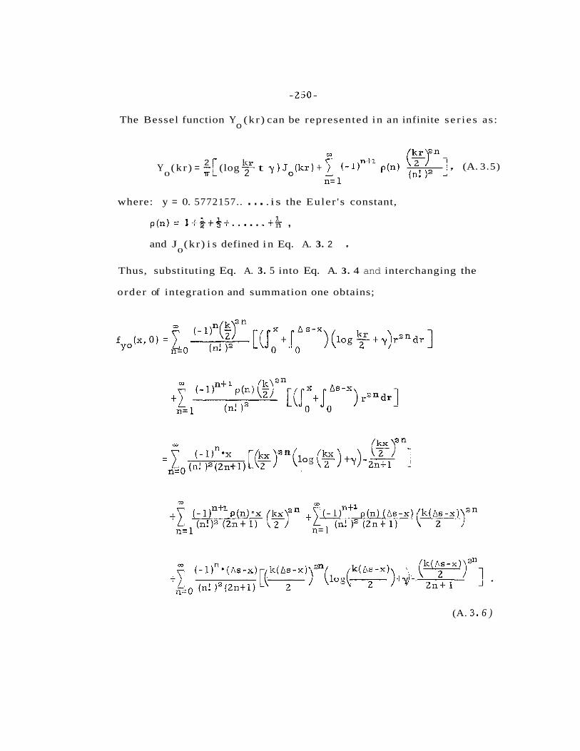
-250-
The Bessel function Y (k r ) can be represented in an infinite se r ies as: 0
m 2 [1 kr
Y (k r ) = --; (log - t y ) ~ ~ ( k r ) t 7 (-l)nt' p(n) (n! )a 2 I , (A. 3.5)
0 7T L. A .d
n= 1
where: y = 0. 5772157.. . . . . i s the Euler ' s constant,
1 p ( n ) = l - t & + * + . . . . . .+E ,
and J (k r ) i s defined i n Eq. A. 3. 2 0
Thus, substituting Eq. A. 3. 5 into Eq. A. 3. 4 and interchanging the
order of integration and summation one obtains;
(A. 3 , 6 )
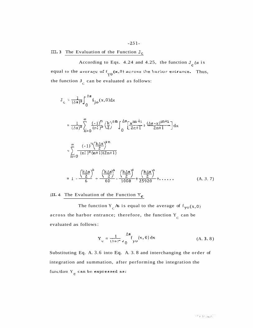
111. 3 The Evaluation of the Function Jc
According to Eqs. 4.24 and 4.25, the function JcAs i s
equal to the averagt: 01 f (x, 0 ) acrvss Llle Ildrbvr eiilrdnce. Thus, Y 0
the function J can be evaluated a s follows: C
Jc = - f . (x, 0)dx
(A. 3. 7)
111. 4 The Evaluation of the Function YG
The function Y As i s equal to the average of f (x, 0 ) C YO
across the harbor entrance; therefore, the function Y can be C
evaluated as follows :
1 AS y = - f (x,O)dx (A. 3 . 8 )
Substituting Eq. A. 3 .6 into Eq. A. 3. 8 and interchanging the order of
integration and summation, after performing the integration the
f u n ~ t i o n Y canbe expressed a s : C

25920 [log (F)ty-g] t... . . (A. 3 , 9 )

APPENDIX IV
.SUMMARY O F THE STROKES O F THE WAVE GENERATOR
USED IN EXPERIMENTAL STUDIES
Harbor Model
Ci rcu lar Harbor
( l o 0 Opening)
Ci rcu lar Harbor
(60° Opening)
Rectangular
Harbor
Long Beach
Harbor
Stroke of Wave
Generator
( inches)
Range of ka
Covered i n
Exper iments

APPENDIX V
COMPUTER PROGRAM
The computer program for calculating the response of an arbit-
r a ry shaped harbor to the periodic incident waves which are normal to
the coastline and that used for calculating the total velocity a t the harbor
entrance a re contained in this appendix.
In order to i l lustrate the application of these computer programs
the specific example of the model of the East and West Basins of the
Long Beach Harbor will be used. Certain input data corresponding to
this harbor model will be listedand the output using these programs will
be shown; these results correspond to the theoretical results discussed
in the text.
V. 1. Computer Program for the Response of an Arbitrary Shaped Harbor
The computer program and a subroutine (CSLECD) for calculating
the response of an arbitrary shaped harbor to the periodic incident waves
which a re normal to the coastline a r e contained in pp. 258 to 260-
The input data that a r e needed in using this program are:
(i) the number of boundary segments including the harbor
entrance (N) and the number of entrance segments (NP) ,
(ii) the coordinates of the beginning and the end of each
boundary segment (PX(I ) , P Y (I) ),
(iii) the value of the characteristic dimension (A), water depth
(DEPTH), and the width of the harbor opening (HAOP), (The

width of the harbor opening will not be used for calculation
rather i t i s used for identification only. )
(iv) the number of interior points to be calculated (M) and the
coordinates of these interior points (PX(I ) , P Y (I) ), and
(v) the incident wave number (K).
These input data for the Long Beach Harbor model for one parti-
cular wave number (k=2.35 ft-I) a re listed in p. 261. The coordinates
of 7 5 boundary segments and 90 interior points a re arranged according
to the coordinates used in Fig. 6 . 3 6 . Thus, pn in t A of Fig. 6, 36
corresponds to MESS (26), point B corresponds to MESS (88), point C
corresponds to MESS (81), and point D corresponds to MESS (68).
The output data for the Long Beach Harbor model a re presented
on pp. 262 to 263 . They contain the complex value and the absolute
value of the normal derivative of the wave function (DFDC) a t the center
of the two entrance segments, the complex value and the absolute value
of the wave function for the 75 boundary se,ments, (Q(1, I ) ) , and the
complex value and the absolute value of the wave function (F2) for the
90 interior points. The results of the absolute value of F2 at the mesh
point Nu. 26, 88, 8 1, and 68 correspol~l to the theoretical results shown
in Figs. 6.37 to 6.40 for ka=3.384. The output value of F2MAX corres-
ponds to the theoretical result shown in Fig. 6. 41 for the same value of
ka. The output values of FRA for the 90 mesh points correspond to the
wave amplitude distribution curve shown in Fig. 6.42 (except the sign
has been reversed).

-256-
It should be noted that the programs a r e written so that calculations
for other wave numbers can be made after the calculations for the f i r s t
wave number a r e completed. The computer program i s written in
FORTRAN I V compatible to IBM 360/75 digital computer.
Some of the symbols used in the computer program a r e defined in
the following:
Total no. of segments into which the boundary i s divided.
Total no. of seglnents into which the harbor entrance is divided.
Total no. nf interior pnints to he r a l r d a t e d .
Number which defines the boundary segments (including the harbor entrance).
The x-coordinate a t the beginning of the ith segment of the boundary (also used as the x-coordinate of the interior points).
The y-coordinate a t the beginning of the ith segment of the boundary (also used as the y-coordinate of the interior points ).
The x-coordinate of the mid-point of the ith segment of the boundary.
The y-coordinate of the mid-point of the ith segment of the boundary.
Number which defines a particular interior point.
Characteristic dimension of the harbor (a).
Harbor opening in ft.
Water depth in ft.
Wave number.
Wave number parameter (ka).
Distance between field and source points.
Changes in x - coordinate s between the beginning and the end of the i th boundary segment
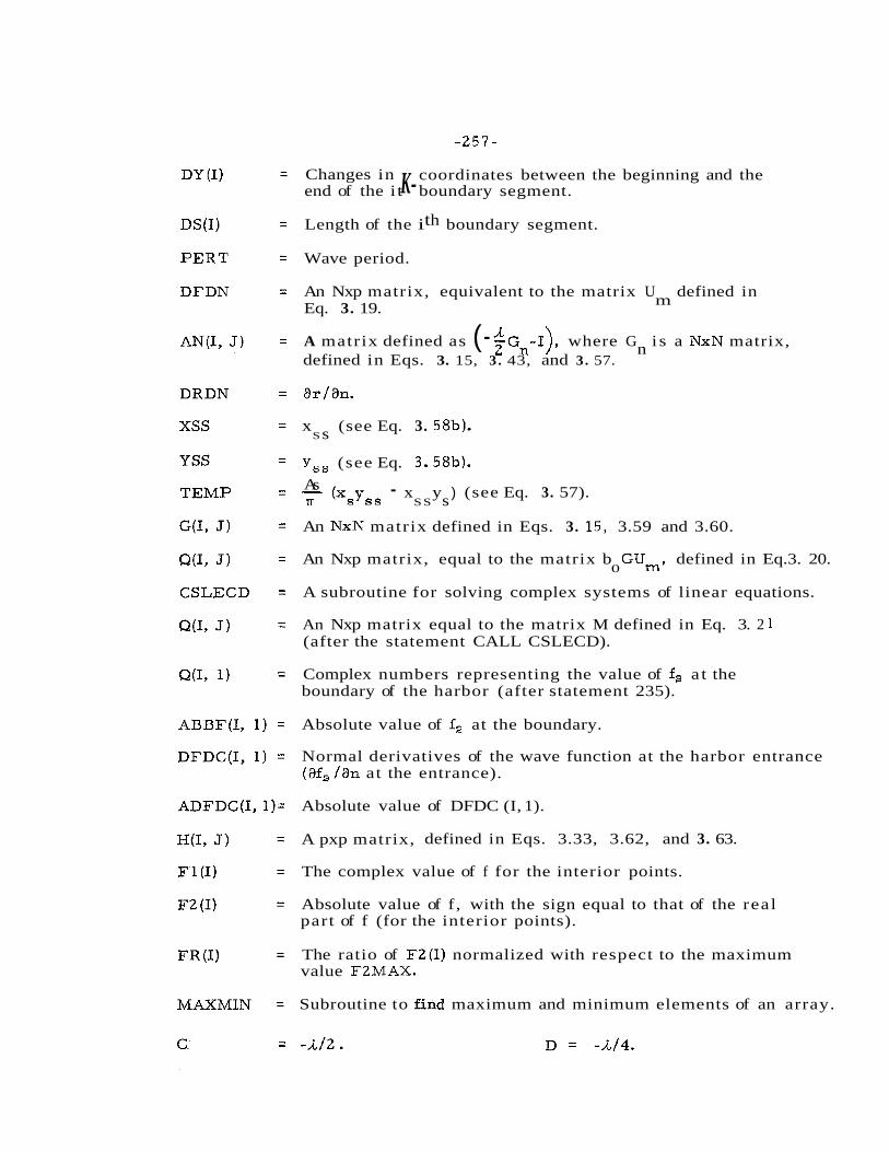
Changes in coordinates between the beginning and the K- end of the i t boundary segment.
Length of the ith boundary segment.
Wave period.
An Nxp matrix, equivalent to the matrix U defined in m Eq. 3. 19.
A A matrix defined as (- Z ~ n - ~ ) , where G i s a NxN matrix, n defined in Eqs. 3. 15, 3. 43, and 3. 57.
x (see Eq. 3. 58b). S s
Y,, (see Eq. 3.58b).
As - n ( X s ~ s s - x y ) (see Eq. 3. 57).
S S s
An NxN matrix defined in Eqs. 3. 15, 3.59 and 3.60.
An Nxp matrix, equal to the matrix b Gum, defined in Eq.3. 20. 0
A subroutine for solving complex systems of linear equations.
An Nxp matrix equal to the matrix M defined in Eq. 3. 2 1 (after the statement CALL CSLECD).
Complex numbers representing the value of f, a t the boundary of the harbor (after statement 235).
Absolute value of f, at the boundary.
Normal derivatives of the wave function at the harbor entrance (af, /an at the entrance).
Absolute value of DFDC (I, 1).
A pxp matrix, defined in Eqs. 3.33, 3.62, and 3. 63.
The complex value of f for the interior points.
Absolute value of f , with the sign equal to that of the real part of f (for the interior points).
The ratio of F2(I) normalized with respect to the maximum value F2MAX.
Subroutine to firid maximum and minimum elements of an array.

- 258 - W T E R w P E ~ I I I D I C I N C I D E N T WAVES -
INTEGER P REAL K COMPLEX AN1 7 5 1 7 5 j.41 7 5 ~ 2 0 l o O E T ~ C 1 G l 7 5 1 7 5 I . F l ( 1 0 0 ) COMPLEX H l 7 5 ~ 2 0 l r O F D C ( ~ ~ . Z ) , D I O G Q N ~ F D IMENSION ADFDC( 7 5 r l ) p X O l l ) r X I 7 6 I t Y 0 ( 1 ) . Y 1 7 b l r D S O l l ) r D S l 7 6 1 7
1 DX( 7 5 l r O Y ( 7 5 ) r R ( 7 5 1 7 5 I r D F O N I 7 5 9 2 0 ) . A B B F ( 7 5 1 1 1 r 2 F 2 l 1 0 0 l r F R ( 1 0 0 l ~ P X ~ 1 0 0 l t P Y ~ 1 O O ~ t M E S S l l O O l ~ N S E G ~ 7 5 ~
DATA P I / 3 . 1 4 1 5 9 2 6 /
READ INPIJT DATA READ ( 5 t l l NINP
1 FORMAT ( 3 1 5 ) READ(5.21 INSEG(II,PX(II,PVII)~I=l~N)
2 FORMAT 11512F15,OI P X l N c l l = P X l 1 ) P Y I N e l l = P Y ( l ) P X ( N + Z l = P X l Z I P Y ( N + Z I = P Y I Z ) CALCIJLATE M I D P O I N T OF EACH SEGMENT 0 0 5 I = l t N XII)=0,5*lPXlI~cPX~I+l)l YII)=O.S*IPYllltPY11+1)) o X l I ) = P X ~ I + 1 l - P X I I ) O Y I I ) = P Y ( I + l ) - P Y 1 1 ~ OS~I~=SORTlOX~Il**2+DYlIl**2l
5 CONTINUE X O I l ) = X I N ) X I N + l ) = X I l ) Y O I l ) = V ( N ) Y l N t l ) = Y ( l l O S O I 1 I = D S I N I O S ( N t l I = D S I 1 ) DO 1 5 I=I.;N I l = l + l R I I t l l = O DO 2 5 J = l l s N R I l r J l = S O R T l ~ X I I ~ - X ~ J l ~ * * 2 + l Y ~ 1 1 - Y ( J ~ ~ * * 2 ~ R I J s 1 I = R l I t J )
2 5 CONTINUE I 5 CONTINUE
READ 1 5 ~ 4 1 A 4 FORMAT 14F10.01
HEAD 1 5 ~ 4 1 HAOP.UtPlH READ COORDiNATES OF I N T E R I O R POINT I N T O PX AN0 P Y REAO (5.1) M REAO 1 5 r 2 l I M E S S I I I ~ P X ( I I ~ P Y ( I I F ~ ~ ~ ~ ~ ~ ~
1 6 READ ( 5 9 1 7 ) K 17 FORMAT ( F 1 0 - 0 )
EKA=A*K P E R T = ( 2 ~ O * P I ) I l S Q R T ( 3 2 ~ 2 * K * T A N H l K * O E P T H ) ~ ~ CALCULATE U N I T MATRIX OF DFDN I N s N P I 0 0 1 1 5 I = l p N DO 1 2 5 .I=l.NP
1 2 5 OFONI I , J )=OeO I F II.GT.NP1 GO TO 1 1 5 DFDN 11.11=1.0
1 1 5 CONTINUE C CALCULATE ELEMENTS OF THE E A T R I X A N = l C * G N - i l
0 0 3 5 I=1 ,N DO 4 5 J = l r N I F I J .ER- 1 1 GO TO 1 0 ARG=K*R I I , J ) DRDN=IIYlI)-YIJ)l*OX(J)- ( X ( 1 ) - X ( J 1 A N I I ~ J ) = - C ~ K * C ~ P L X ( B E S J ~ I & R G ) I R E ~ Y ~ GO T o 4 5
1 0 CONTINUE Y SS=
=h.O*((Yllcll-Y(IIl/(OSlI+ll+DS~I)I- / lnslI-l~+DSlI)*c~SlI+l~l
XSS= = b . O * ~ ~ X l I + 1 ) - X ~ I l l / l D S ( l + l ) c D S ~ I ~ l - / I D S I I - l ) + D S ~ l ) + D S ~ I + l ) ) TEMP=(DX(I)*YSS-XSS*OYllll/PI ANIIII)=CMPLX(O.OITEHPI*C-~~O
4 5 CONTINI IE 3 5 CONTINUE
C CALCl lLATE THE R IGHT HAND S I D E VECTOR Q DO 1 3 5 P=l .NP DO 5 5 I = l . N U I I r P ) = L n P C x 1 U . r O * ~ DO 6 5 J=l ,N I F (P.NE.1) 6 0 TO 3 0 I F I J .ER, I 1 GO TO 2 0

AKG=K*R ( I. J ) G ( I I J ) = C M P L X ( B E S J O ( A K G l t B E S Y O ( A R G I ) * O S ( J ~ GO TO 3 0 G ( I t I l = C M P L X ( 1 ~ ~ T ~ U O P I * ~ A L O G ( K * D S ~ J l * ~ 2 5 l - O 4 2 2 7 9 l I + O S ( I I Q(IpP)=O(IrPI+GlItJ)*DF0N(JvP) C O N T I N U E B ( I . P ) = C ; O ( I t P l CONTINUE CONTINUE CALL C S L E C V I A N I N s Q ~ N P ~ O E T I I E R ) 0 0 1 4 5 I = l r N 0 0 1 4 5 J = l r 2 OFOC~I;Jl=CMPLX~O.OtOOOl O=CMPLX(O.,-0.251 CALCIILATE HAVE FUNCTION OF EXTERIOR PROHLEM AN0 WATCHING 0 0 2 1 5 I = l . N P 0 0 2 1 5 J=l ,NP I F ( I ,EU .J I 6 0 TO 2 1 0 H ~ I 1 J l = C M P L X ( B E S J O ~ K * R ~ I ~ J l 1 ~ B E S Y O ~ K + R I I ~ J l ~ l * 0 S ~ J l GO TO 2 1 5 H(I~Il=CMPLX(1~0~THOOPI*(ALUG~K*DS(Il*~25l-0.42279))*DS~Il CONTINUE DO 2 2 5 I = l r N P 0FDC(1511=CMPLX(1.0,0001 DO 2 2 5 J = l r N P H ( I . J l = Q ( I . J l - C * H ( 1 9 J l CAI 1 T S I FCOfH.NP.nFOC,IFDFT~IFRI WRITE ( h r 6 1 FORMAT ( 1 H 1 1 WRITE (6 ,191 K FORMAT ( Z X 3 H K = F 1 0 c 5 , 2 X o ' ( l / F T I * I WRITE ( 6 ~ 3 8 1 FORMAT ( / / / .ZX; 'COMPLEX VALUE OF DFOC AT THE ENTRANCE ( l / F T l ' t / I H R I T E (6.8) ( D F D C ( I 1 l I ~ I = l . N P ) FORMAT ( lX .bF13 ,51 0 0 3 0 5 I = 1 7 N P A D F D C ( I ~ 1 I = C A B S ~ D F O C ~ I t 1 1 1 WRITE I b t 6 8 ) F O R M A T ( / / / , ~ X V ' A B S U L U T E VALUE OF DFOC AT THE ENTRANCE I l / F T I * * / l WRITE (6 ;R I I A O F O C ( I , l I F l = l . N P I CALCULATE BOUNDARY WAVE FUNCTION F 0 0 2 3 5 I = l r N 0 0 235 J = l r N P O F D C ( I + ~ ~ = O F O C I I ~ Z ~ + O ~ I O J ~ * D F O C ( J ~ ~ ) DO 2 4 5 I = l + N P ( I 1 l l = D F D C ( I r Z l ABBF(1711=CABS(O( I i 111 CONTINUE H R I T E 1 6 1 4 8 ) FORMAT ( / / / rZX126HBOUMDARY F FUNCTION Q ( I + l ) s / I WRITE Ib rB) ( O ( I r l ) s l = l r N I H R I T E ( 6 9 1 4 8 ) FORMAT ( / / / cZX . 'ABSOLUTE VALUE OF THE BOUNDARY F FUNCTIOM' I / I H R I T E l b r R l ( P B B F I I r l l r l = l t N ) H R I T E (6.6) WRITE 1 6 - 1 1 9 ) HADPIDEPTH FORMAT (ZXs 'HARBDR OPENING I F T . I = ' v F 7 * 3 9 5 X t ' D E P T H (FT, I= 'oF7,31 WRITE l b r 1 9 l K WRITE ( 6 ~ 2 9 1 EKA FORMAT IZX3HKA=F10.51 WRITE l 6 p 1 2 9 1 PERT FORMAT (ZX,'PERIOO T = * , F I O . S t Z X t ' ~ S E C s ) @ J CALCULATE WAVE FUNCTION F FOR INTERIOR POINTS DO 7 5 J = l * M F=C#PLX(Or rOr ) 0 0 8 5 I = l r N R 1 = S O R T ~ ~ X ~ I l - P X ~ J l l * * Z + ~ Y ~ I l - P Y ~ J I 1 r + Z ) R 1 K = # W 1 D G D N = K * C M P L X ( 8 E S J 1 ~ R 1 K ~ ~ B E S Y 1 ~ R 1 K 1 l * ~ ~ P X ~ J ~ - X ~ I l l * O Y ~ I l
- I ~ Y I J I - Y I I I I J U X I I I I ~ ~ I F=F+
+ O ( I ~ 1 J * O G O N - O F O C ~ I ~ 1 J * C F : P L X ~ B E S J O ~ R 1 K l ~ 8 E S Y O ~ R l K I l * O S ~ l l 8 5 C O h l I N l J E
F=O+F F I I J I - F FZ(Jl=SIGN(CABSfFJtREAL(FIl
7 5 CDNTlNUE CALL M A X M I N I F Z ~ M . F ~ M X T F ~ M N I F 2 M A X = A M A X l ~ A B S ( F 2 M X I ~ A B S ( F 2 M N l I 0 0 6 0 5 J = l r M
6 0 5 F R I J l = F Z ( J l / F Z M A X WRITE f b r 1 9 9 J FZMAX
1 9 9 FORMAT ( / / .2Xp'F2MAX=' pF 10.5) H R I T E (6 .991
9 9 FORMAT I / / 1 2 X v ' M E S H ' r B X o ' P X ' r ~ X ~ ' Y Y ' * ~ ~ X I ' F C M P L X ' D ~ ~ X ~ ' F ~ ~ ~ + 1 O X o e F R A , ' ~ / I
WRITE ( 6 ~ 9 1 ~ M E S S ~ J ~ ; P X I J ~ ~ P Y ( J ~ ~ F ~ ~ J ~ D F ~ ( J ~ . F H ~ J ~ ~ J ~ ~ ~ ~ ~ 9 FORMAT ( l X t 1 5 e F l l r 3 r F l l r 3 ~ 2 F 1 3 - 5 e F 1 3 - 5 t F l 1 - 3 1
GO TO 1 6 END
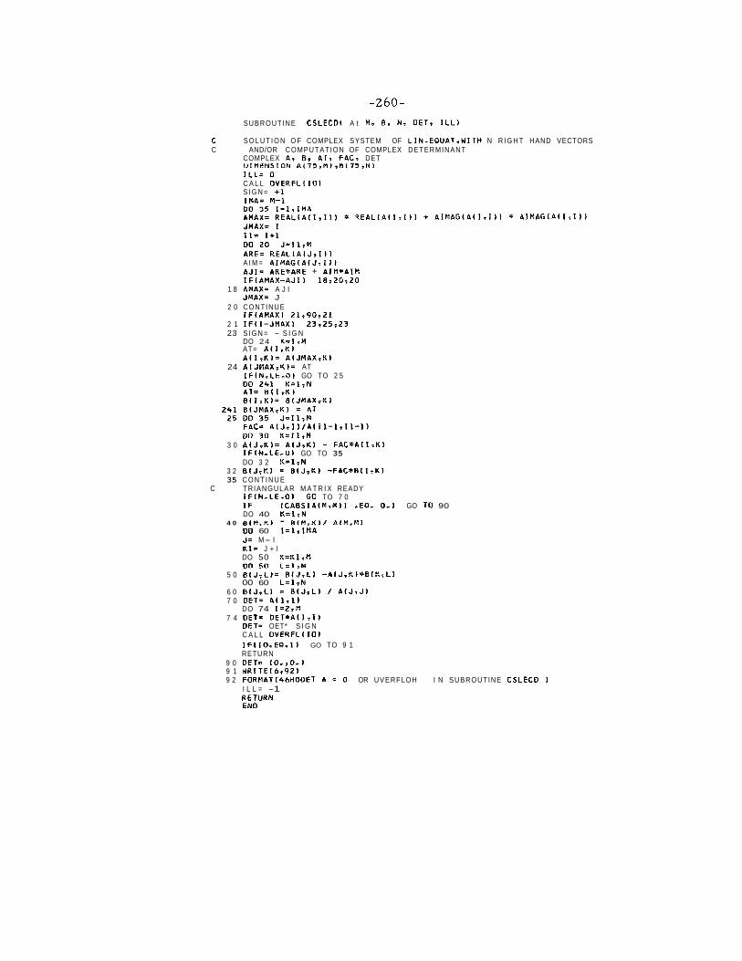
SUBROUTINE C S L E C D I A t Mp B v N ? O E T t I L L )
C S O L U T I O N O F COMPLEX SYSTEM OF LIN.EQUAT.UITH N R I G H T HAND VECTORS C AND/OR COMPUTATION OF COMPLEX DETERMINANT
COMPLEX A r By AT, F A G S DET D I M e N S I O N A I 7 5 r P l ) ~ R l 7 5 , N ) I L L = 0 C A L L O V E R F L I I O S I G N = + l
ARE= R E A L ( A I J ~ 1 1 1 A I M = A I M A G ( A ( J I I I t A J I = ARE*ARE + A I M * A l M I F I A M A X - A J I ) 1 8 . 2 0 1 2 0
1 8 AMAX= A J I JMAX= J
2 0 CONTINUE I F I A M A X ) 2 1 t 9 0 t 2 1
2 1 I F l l - J M A X I 2 3 r 2 5 t Z 3 23 S I G N = - S I G N
DO 24 K=IIM AT= A ( 1 , K ) B l I ? K ) = A I J M A X F K I
24 A I J N A X I K ) = AT IF IN ,LE ,O) GO TO 2 5
3 0 A ( J * K ) = A I J o K ) - F A C * A l I e K l I F l N , L E - 0 1 GO TO 35 DO 3 2 K = l s N
3 2 B l J o h l = B I J q K ) - F A C * B l I s K l 35 C O N T I N U E
C TR IANGULAR M A T R I X READY I F l N . L E - 0 ) GO TO 7 0 I F I C A B S l 4 l M ~ W l ) .EO, 0 - 1 GO TO 90 DO 40 K = l r N
4 0 B I N , K ) - B I M . K ) / A 1 M . M ) 00 60 I = l r I M A J= M- I K 1 = J + l DO 50 K = K l r M 130 50 L = l .M
5 0 B ( J ; L I = B ( J v L 1 - A I J p K ) * B l K r L l 00 60 L = l o N
6 0 0 l J . L ) = R I J v L ) / A ( J e J ) 7 0 OET= A ( 1 ; l )
DO 74 I = Z ? M 7 4 OET= D E T * A l I , 1 )
DET= OET* S I G N C A L L O V F R F L ( I O 1 I F I I O . E O . 1 1 GO TO 9 1 RETURN
9 0 OET= (OlrO.l 9 1 H R I T E l 6 t 9 2 1 9 2 FORMAT l46HOOET A = 0 OR UVERFLOH I N SUBROUTINE CSLECO I
I L L = -1 RETURN END

DATA INPUT

DATA OUTPUT
CCNPLEX VbLUE OF DFOC AT THE ENTRANCE I I I F T )
- 1,04198 - 9,81575 -0,95365 -8=74154
ABSOLUTE YALUE OF OFDC AT THE ENTRANCE I 1 / F T )
S-87088 8,79368
BOLNCARV F FUNCTION Q ( I r 1 )
ABSOLUTE YALUE OF THE BOUMCARV F FUNCTION
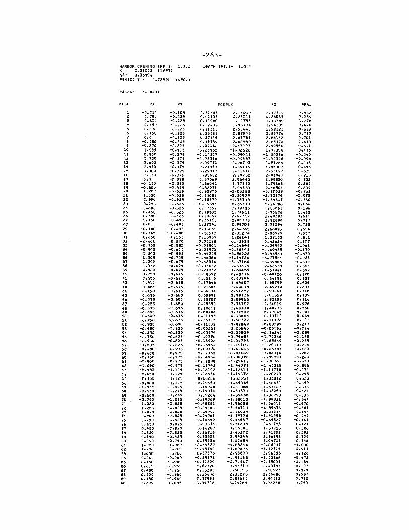
HARBOR C P E N I N G l F T . l = d.2~: UEPTH I F T . ) = K = 2.350'YJ I l I F T l KA= 3.384'13 PERICD T = C.72890 15EC.J
F C K P L X
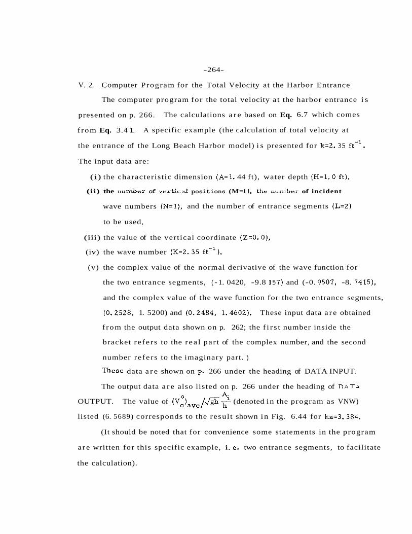
-264-
V. 2. Computer Program for the Total Velocity at the Harbor Entrance
The computer program for the total velocity a t the harbor entrance i s
presented on p. 266. The calculations a r e based on Eq. 6.7 which comes
f rom Eq. 3.4 1. A specific example (the calculation of total velocity at
the entrance of the Long Beach Harbor model) i s presented for k=2.35 f t - l .
The input data are:
(i) the characterist ic dimension (A=l . 44 ft), water depth (H=l. 0 f t) ,
(ii) the rlumber of vertical positions (M= I), the nu~mber of incident
wave numbers (N=l), and the number of entrance segments (L=2)
to be used,
(iii) the value of the vert ical coordinate (Z=0. O),
(iv) the wave number (K=2.35 f t - I ) ,
(v) the complex value of the normal derivative of the wave function for
the two entrance segments, ( - 1. 0420, -9.8 157) and (-0. 9507, -8. 7415),
and the complex value of the wave function for the two entrance segments,
(0.2528, 1. 5200) and (0.2484, 1.4602). These input data a r e obtained
f rom the output data shown on p. 262; the f i r s t number inside the
bracket re fe r s to the r ea l pa r t of the complex number, and the second
number re fe rs to the imaginary part. )
~ h e s e data a r e shown on p. 266 under the heading of DATA INPUT.
The output data a r e also listed on p. 266 under the heading of DATA
*i OUTPUT. The value of ( ~ z ) ~ ~ ~ / & & ~ (denoted i n the program as VNW)
listed (6. 5689) corresponds to the resul t shown in Fig. 6.44 for ka=3.384.
(It should be noted that for convenience some statements in the program
a re written for this specific example, i. e. two entrance segments, to facilitate
the calculation).

- 265-
Some of the symbols used in the program a re listed in the following:
z(J) = Vertical positions (2).
K(I) = Wave numbers (k).
KA (1) = Wave number parameter associated with K(1) (ka).
CF(1, J) = The complex value of f2 at the harbor entrance for K(1) and the J~~ entrance segment.
DF(I, J ) = The complex value of af, /an at the harbor entrance for K(1) and the ~ t h entrance segment.
DFX(1, J) = The complex value of af2 /ax at the harbor entrance for K{I) and the Jth entrance segment.
DFXR(1, J) = The r e d par t of 8fz /ax at the harbor entrance for K(1) a d the ~ t h entrance segment.
= The imaginary part of af, /ax at the harbor entrance for K(1) and the Jth entrance segment.
= The absolute value of af, /ax at the harbor entrance for K(1) and the ~ t h entrance segment.
= The real part of af, /an at the harbor entrance for K(1) and the J~~ entrance segment.
= The imaginary part of i3f2 /an at the harbor entrance for K(1) and the J~ entrance segment.
= The absolute value -of af2 /an a t the harbor entrance for K(1) and the J'th entrance segment.
= The rea l part of f, at the harbor entrance for K(1) and the ~ t h entrance segment.
= The imaginary part of f, at the harbor entrance for K(1) and the ~ t h entrance segment.
= The absolute value of f, at the harbor entrance for K(1) and the Jth entrance segment.
= Circular wave frequency (a) associated with K(1).
= Wave period associated with K(1).
= Averaged total velocity across the entrance normalized with respect to the maximum horizontal water particle velocity in shallow water for K(1). (This quantity i s -equivalent to -
;t Ai (Vo lave , see Eq. 6.7. )

,COMPUTER PROGRAM FOR THE TOTAL V E L O C I T Y AT THE HARBOR ENTRANCE
R E A L KIKA COMPLEX O F X t 1 0 0 . 3 ) CORPLEX C F 1 1 0 0 : 3 ) ~ D F 1 1 0 0 ~ 3 1 D I M E N S I O N D F X R l 1 0 0 ~ 3 l ~ O F X 1 l 1 0 0 ~ 3 ~ 1 F F X I 1 0 0 ~ 3 ) D I M E h S I O N Z l l O O I ~ K l 1 0 0 1 ~ F l 1 0 0 1 3 ) . F F t 1 O O ~ 3 l t O F R ~ l O O ~ 3 l ~ D F ~ t l O O ~ 3 ~ ~ * F R 1 1 0 0 ~ 3 ) ~ F 1 ~ 1 0 0 p 3 ) 5 S G M l 1 O O l ~ T l 1 O O l r T O T A L 1 3 r l l ~ K A l 1 0 0 l r
ip V E L 1 1 0 0 1 3 ) r V A V 1 1 0 0 ) . V N H 1 1 0 0 1 DATA T O T A L l 4 H T O T V e 4 H E L e4H P I = 3 , 1 4 1 5 9 K t A U 1 3 v L I A v H
F O R H A T I 8 F 1 0 . 0 ) R E A D 1 5 r l l MIN F L F O R M A T 1 5 1 1 0 1 R E A 0 1 5 ~ 2 ) I Z I J I t J = l r H ) R E A D 1 5 r 2 1 l K I 1 I t I = l . N l R E A D l 5 . 2 ) I I D F I I r l I r O F I I ~ 2 ) r C F l I ~ l I r C F I I o 2 I 1 ~ I ~ l r N I 00 5 0 4 J = l r L DO 4 0 5 I = l r N F I I ; J I = C A B S ( C F I I ; J I I F F I I r J I = C A 8 S I D F I l r J I ) F I I ~ J l - F ( I ~ J l ~ F ( l g J l
F F I I Q J I = F F I I ~ J I * F F I I ~ J ) D F R I I s J ) = R E A L I D F I I . J I I O F I I I I J I - A I H A G I O F I I s J 1 l F R I I . J l = R E A L I C F l l r J l ) F I I I D J I ~ A ~ ~ ~ A G I C F ~ ~ ~ J ~ COMTIMUE CONTINUE 00 5 0 5 J - l t L DO 5 0 6 Ie1.N OFXRlI~JI=IFRlI~1l-FRIIt2ll/O-1 nFXll1..Il-~F1I1.1~-FIll.?~l/O.l DFXII,Jl=CEPLXIOFXRlItJltDFXIlI~Jll F F X I I q J ) = C A B S f O F X l l r J ) I F F X I I ; J ) ~ F F X I I J J ~ * F F X I I ~ J ) C O N T I W E CONTINUE C S = S O R T I 3 2 . 2 * H l DO 1 0 5 J J ~ ~ F H H I = Z l J J ) + H DO 65 1=1.#
.... , E R I T E l b o 1 9 1 I S G ~ ~ I I ) ~ T I I I ~ K ~ ~ I ~ K A I I I F Y M V I I I ~ ~ = ~ ~ # )
19 FORt4PTI5FL2,41 105 C O N T I M J E
STOP EPJD
DATA I M P U T
DATA OUTPUT
V E R T I C A L P C S I T I L N = 0.0 FT
Related Documents