Two-way multi-lane traffic model for pedestrians in corridors

arX

iv:1

105.

0203

v1 [

mat

h-ph

] 1

May

201

1

Two-way multi-lane traffic model for pedestrians incorridors

Cecile Appert-Rolland, Pierre Degond and Sebastien Motsch

May 3, 2011

Cecile Appert-Rolland

1-University Paris-Sud; Laboratory of Theoretical PhysicsBatiment 210, F-91405 ORSAY Cedex, France.

2-CNRS; LPT; UMR 8627Batiment 210, F-91405 ORSAY Cedex, France.email: [email protected]

Pierre Degond

3-Universite de Toulouse; UPS, INSA, UT1, UTMInstitut de Mathematiques de Toulouse

F-31062 Toulouse, France.4-CNRS; Institut de Mathematiques de Toulouse UMR 5219

F-31062 Toulouse, France.email: [email protected]

Sebastien Motsch

5-Department of Mathematics University of MarylandCollege Park, MD 20742-4015, USA.email: [email protected]

AMS subject classification: 90B20, 35L60, 35L65, 35L67, 35R99, 76L05Key words: Pedestrian traffic, two-way traffic, multi-lane traffic, macroscopic model,

Aw-Rascle model, Congestion constraint.Acknowledgements: This work has been supported by the french ’Agence Nationale

pour la Recherche (ANR)’ in the frame of the contract ’Pedigree’ (contract number ANR-08-SYSC-015-01). The work of S. Motsch is partially supported by NSF grants DMS07-07949, DMS10-08397 and FRG07-57227.

Abstract

We extend the Aw-Rascle macroscopic model of car traffic into a two-way multi-lane model of pedestrian traffic. Within this model, we propose a technique for thehandling of the congestion constraint, i.e. the fact that the pedestrian density cannotexceed a maximal density corresponding to contact between pedestrians. In a firststep, we propose a singularly perturbed pressure relation which models the fact thatthe pedestrian velocity is considerably reduced, if not blocked, at congestion. In a

1

http://arxiv.org/abs/1105.0203v1

second step, we carry over the singular limit into the model and show that abrupttransitions between compressible flow (in the uncongested regions) to incompressibleflow (in congested regions) occur. We also investigate the hyperbolicity of the two-way models and show that they can lose their hyperbolicity in some cases. We studya diffusive correction of these models and discuss the characteristic time and lengthscales of the instability.

1 Introduction

Crowd modeling and simulation is a challenging problem which has a broad range ofapplications from public safety to entertainment industries through architectural andurban design, transportation management, etc. Common and crucial needs for theseapplications are the evaluation and improvement (both quantitatively and qualitatively) ofexisting models, the derivation of new experimentally-based models and the constructionof hierarchical links between these models at the various scales.

The goal of this paper is to propose a phenomenological macroscopic model for pedes-trian movement in a corridor. A macroscopic model describes the state of the crowdthrough locally averaged quantities such as the pedestrian number density, mean velocity,etc. Macroscopic models are opposed to Individual-Based Models (IBM’s) which followthe location and state of each agent over time. Macroscopic models provide a descriptionof the system at scales which are large compared to the individuals scale. Although theydo not provide the details of the individuals scale, they are computationally more efficient.In particular, their computational cost does not depend on the number of agents, but onlyon the refinement level of the spatio-temporal discretization. In addition, by comparisonswith the experimental data, they give access to large-scale information about the system.This information can provide a preliminary gross analysis of the data, which in turn canbe used for building up more refined IBM’s. This procedure requires that the link be-tween the microscopic IBM and the macroscopic model has been previously established.Therefore, macroscopic models which can be rigorously derived from IBM’s are crucial.

The present work focuses on a one-dimensional model of pedestrian traffic in corridors.This setting has several advantages:

1. It makes the problem essentially one-dimensional and is a preliminary step for thedevelopment of more complex multi-dimensional problems. The present work willconsider that pedestrian traffic occurs on discrete lanes. This approximation canbe viewed as a kind of discretization of the actual two-dimensional dynamics. Itprepares the terrain for the development and investigation of truly two-dimensionalmodels.

2. We can build up on previous experience in the field of traffic flow models. Ourapproach relies on the Aw-Rascle model of traffic flow [3], which has been proven anexcellent model for traffic flow engineering [42]. In the present work, this approachwill be extended to two-way multi-lane traffic flow of pedestrians.

3. It is easier to collect well-controlled experimental data in corridors than in openspace (see for instance [34]).

2

4. The relation of the macroscopic model to a corresponding microscopic IBM is moreeasily established in the one-dimensional setting. In [2], it has been proven thatthe Aw-Rascle model can be derived from a microscopic Follow-the-Leader modelof car traffic. The proof uses a Lagrangian formulation of the Aw-Rascle model.The correspondence between the Lagrangian formulation and the IBM cannot becarried over to the two dimensional case, because of the very special structure ofthe Lagrangian model in one-dimension.

The most widely used models of pedestrian traffic are IBM’s. Several families ofmodels have been developed. Rule based models [38] have been used in particular forthe development of games and virtual reality, with several possible levels of description.But their aim is more to have a realistic appearance rather than really reproducing arealistic behavior. More robust models are needed for example to test and improve thegeometry of various types of buildings. Physicists have proposed some models inspiredfrom the fluid simulation methods. In the so-called ’social force’ model [18, 20, 21], theequations of motion for each pedestrian have the form of Newton’s law where the forceis the sum of several terms each representing the ’social force’ under consideration. Itobviously relies on the analogy existing between the displacement of pedestrians and themotion of particles in a gas. It describes quite well dense crowds, but not the individualtrajectories of a few interacting pedestrians. Other approaches have been developed inthe framework of cellular automata [9, 16, 31]. In these models, the non-local interactionsbetween pedestrians are made local through the mediation of a virtual floor field. Thesemodels also are meant to describe the motion of crowds, not of individuals. Besides, asystematic study of the isotropy of cellular automata models is still lacking. More recently,some geometrical models have been developed. Pedestrians try to predict each others’trajectories, and to avoid collisions [17, 33, 40]. The knowledge of other pedestrians’trajectories depends on the perception that the pedestrian under consideration has, whichmay vary with time. [35] takes into account the fact that this knowledge is acquiredprogressively. Another type of perception based on the visual field is proposed in [32].These models describe well the individual trajectories of a few interacting pedestrians,but it is not obvious yet whether they can handle crowds.

By contrast to microscopic IBM’s, macroscopic crowd models are based on the anal-ogy of crowd flow with fluid dynamics. A first approach has been proposed in [22]. In[19], a fluid model is derived from a gas-kinetic model through a moment approach andphenomenological closures. Recently, a similar approach has been proposed in [1]. In[23, 24, 25], a continuum model is derived through optimal control theory and differentialgames. It leads to a continuity equation coupled with a potential field which describes thevelocity of the pedestrians. Other phenomenological models based on the analogy withthe Lighthill-Whitham-Richards model of car traffic have been proposed by [4, 10, 11].In [36, 37], instead of considering a continuous time evolution described by PDE’s, theevolution of measures is performed on a discrete time scale. In the present paper, weshall consider a continuous time description. Macroscopic models provide a description ofthe system at large spatial scales. They can be heuristically justified for a long corridorstretch like a subway corridor, when the spatial inhomogeneities are weak (such as lowvariations of the density or velocity in the direction of the corridor). Of course, theycannot be used when the spatial inhomogeneities are at the same scale as for instance

3

the mean-interpedestrian distance in the longitudinal direction. In the case of narrowcorridors, this mean-interpedestrian distance is larger because there are less pedestriansin a cross-section, and the condition of weak spatial inhomogeneities is more stringent.From a rigorous standpoint, the derivation of macroscopic models from Individual-Basedmodels requires that the number of agents be large, which is obviously questionable inmost situations in pedestrians and highway traffic. Still there is a large literature devotedto macroscopic models which seem to provide adequate models for large scale dynamics.

We will be specifically interested in two-way multi-lane traffic flow models with aparticular emphasis on the handling of congestions. These points have been previouslyaddressed in [41] for pedestrian counter-flows, [39] for multi-lane traffic and [29, 30] for thetreatment of congestions. However, to the best of our knowledge, none of these differentfeatures have been included in the same model at the same time. The most difficult pointis the treatment of congestions. In the recent approach [29, 30] the congestion constraint(i.e. the limitation of the density by a maximal density corresponding to contact betweenpedestrians) is enforced by means of convex optimization tools (for IBM’s) or techniquesborrowed from optimal transportation such as Wasserstein metrics (for continuum mod-els). However, these abstract methods do not leave much space for parameter fitting todata and cannot distinguish between the behavior of pedestrians and say, sheep. Ourtechnique relies on the explicit derivation of the dynamics of congestions, in the spirit ofearlier work for traffic [6, 7, 13]. This procedure was initiated in the seminal work [8].

The outline of the paper is as follows. We first present the modeling approach for aone-way one-lane Aw-Rascle model (1W-AR) of pedestrian flow in corridors in section 2.We then successively extend this model into a two-way one-lane Aw-Rascle model (2W-AR) in section 3 and to a two-way multi-lane Aw-Rascle model (ML-AR) in section 4. Ineach section, we present the corresponding Aw-Rascle model, together with a simplifiedversion of it supposing that the pedestrian desired velocity is constant and uniform. Werefer these simplified models as ”Constant desired velocity Aw-Rascle” (CAR) models.Therefore, we successively have the 1W-CAR, 2W-CAR and ML-CAR models as Constantdesired velocity versions of respectively the 1W-AR, 2W-AR and ML-AR models. The1W-CAR model can be recast in the form of the celebrated Lighthill-Whitham-Richards(LWR) model of traffic.

Finally, for each of these models, we propose a specific treatment of congestion regions.This treatment consists in introducing a singular pressure in the AR model which tendsto infinity as the density approaches the congestion density (i.e. the density at which theagents are in contact to each other). This singularly perturbed pressure relation providesa significant reduction of the flow when the density reaches this maximal density. A smallparameter ε controls the thickness of the transition region. In the limit ε → 0, two phasesappear: an uncongested phase where the flow is compressible and a congested phaseswhere the flow is incompressible. The transition between these two phases is abrupt, bycontrast to the case where ε stay finite, where this transition is smooth. The locationof the transition interface is not given a priori and is part of the unknowns of the limitproblem.

Table 1 below provides a summary of the various proposed models and their relations.One interesting characteristics of two-way models as compared to one-way models

is that they may lose their hyperbolicity in situations close to the congestion regime.

4

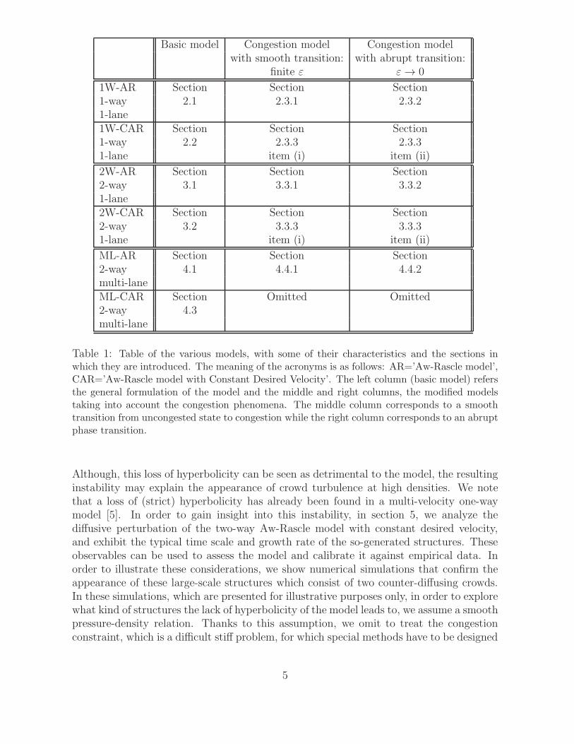
Basic model Congestion model Congestion modelwith smooth transition: with abrupt transition:

finite ε ε → 0

1W-AR Section Section Section1-way 2.1 2.3.1 2.3.21-lane1W-CAR Section Section Section1-way 2.2 2.3.3 2.3.31-lane item (i) item (ii)

2W-AR Section Section Section2-way 3.1 3.3.1 3.3.21-lane2W-CAR Section Section Section2-way 3.2 3.3.3 3.3.31-lane item (i) item (ii)

ML-AR Section Section Section2-way 4.1 4.4.1 4.4.2multi-laneML-CAR Section Omitted Omitted2-way 4.3multi-lane

Table 1: Table of the various models, with some of their characteristics and the sections inwhich they are introduced. The meaning of the acronyms is as follows: AR=’Aw-Rascle model’,CAR=’Aw-Rascle model with Constant Desired Velocity’. The left column (basic model) refersthe general formulation of the model and the middle and right columns, the modified modelstaking into account the congestion phenomena. The middle column corresponds to a smoothtransition from uncongested state to congestion while the right column corresponds to an abruptphase transition.

Although, this loss of hyperbolicity can be seen as detrimental to the model, the resultinginstability may explain the appearance of crowd turbulence at high densities. We notethat a loss of (strict) hyperbolicity has already been found in a multi-velocity one-waymodel [5]. In order to gain insight into this instability, in section 5, we analyze thediffusive perturbation of the two-way Aw-Rascle model with constant desired velocity,and exhibit the typical time scale and growth rate of the so-generated structures. Theseobservables can be used to assess the model and calibrate it against empirical data. Inorder to illustrate these considerations, we show numerical simulations that confirm theappearance of these large-scale structures which consist of two counter-diffusing crowds.In these simulations, which are presented for illustrative purposes only, in order to explorewhat kind of structures the lack of hyperbolicity of the model leads to, we assume a smoothpressure-density relation. Thanks to this assumption, we omit to treat the congestionconstraint, which is a difficult stiff problem, for which special methods have to be designed

5

(see e.g. [15, 14] for the case of Euler system of gas dynamics and [6, 13] for the AR model).

2 One-way one-lane traffic model

2.1 An Aw-Rascle model for one-lane one-way pedestrian traffic

In this section, we construct a one-lane one-way continuum model of pedestrian traffic incorridors. In this model, we will pay a particular attention to the occurrence of conges-tions. We encode the congestion effect into a constraint of maximal total density. Thiswork is inspired by similar approaches for vehicular traffic, which have been developed in[6, 7, 13].

For that purpose, the building block is a one-lane, one-way Aw-Rascle (1W-AR) modelwhich has been proposed for vehicular traffic flow [3]. This model belongs to the class ofsecond-order models in the sense that it considers that both the density and the velocityare dynamical variables which are subject to time-differential equations. By contrast, firstorder models use the density as the only dynamical variable and prescribe the density fluxas a local function of the density. The Aw-Rascle model with constant desired velocityconsidered in section 2.2 is an example of a first order model.

Definition 2.1 (1W-AR model) Let ρ(x, t) ∈ R the density of pedestrians on the lane,u ∈ R+ their velocity, w(x, t) ∈ R+ the desired velocity of the pedestrian in the absenceof obstacles and p(ρ) the velocity offset between the desired and actual velocities of thepedestrian. The 1W-AR model is written:

∂tρ+ ∂x(ρu) = 0, (1)

∂t(ρw) + ∂x(ρwu) = 0, (2)

w = u+ p(ρ). (3)

In this model, the offset p(ρ) is an increasing function of the pedestrian density. Byanalogy with fluid mechanics, this offset will be often referred to as the pressure, but itsphysical dimension is that of a velocity.

Using the mass conservation equation, we can see that the desired velocity is a La-grangian quantity (i.e. is preserved by the flow), in the sense that:

∂tw + u∂xw = 0. (4)

It is natural, since the desired velocity is a quantity which is attached to the particles andshould move together with the particles at the flow velocity.

This model has been studied in great detail in [3] and proven to derive from a follow-the-leader model of car traffic in [2]. Of particular interest is the fact that this model ishyperbolic, with two Riemann invariants. The first one is obviously the desired velocity was (4) testifies. The second one is less obvious but is nothing but the actual flow velocityu. Indeed, from (4) and using (1), we get:

∂tu+ u∂xu = −(∂tp+ u∂xp)

= −p′(ρ)(∂tρ+ u∂xρ)

= p′(ρ)ρ∂xu,

6

and therefore

∂tu+ (u− p′(ρ)ρ)∂xu = 0. (5)

Therefore, information about the fluid velocity propagates with a velocity

cu = u− p′(ρ)ρ. (6)

In the reference frame of the fluid, this gives raise to waves moving upstream the flowwith a speed equal to −p′(ρ)ρ.

Remark 1 We can also consider the evolution of ρu instead of that of u. We obtain from(4) and using (1):

∂t(ρu) + ∂x(ρuu) = −(∂t(ρp) + ∂x(ρpu))

= −ρ(∂tp+ u∂xp)

= −ρdp

dt, (7)

where we have introduced the material derivative d/dt = ∂t+u∂x. This form is motivatedby the observation [3] that drivers do not react to local gradients of the vehicle densitybut rather to their material derivative in the frame of the driver. This modification tostandard gas dynamics like models of traffic was crucial in obtaining a cure to the variousdeficiencies of second order models as observed by Daganzo [12]. Eq. (7) can also be putin the form

∂t(ρu) + ∂x(ρuw) = −∂t(ρp)

= −π′(ρ)∂tρ

= π′(ρ)∂x(ρu), (8)

with

π(ρ) = ρp(ρ), π′(ρ) = ρp′(ρ) + p(ρ). (9)

We will consider the 1W-AR model as a building block for the pedestrian model. Inorder to make the connection with a microscopic view of pedestrian flow, we consider asubcase of this model in the section below.

2.2 Constant desired velocity

This one-way Constant Desired Velocity Aw-Rascle (1W-CAR) model assumes that thepedestrians can have only two velocities: either a fixed uniform velocity V which is thesame for all pedestrians and does not vary with time ; or zero, indicating that theyare immobile. In other words, if because of the high density of obstacles in front, thepedestrians cannot proceed further with the velocity V , they have to stop.

In this case,

w = V

7

f(ρ)

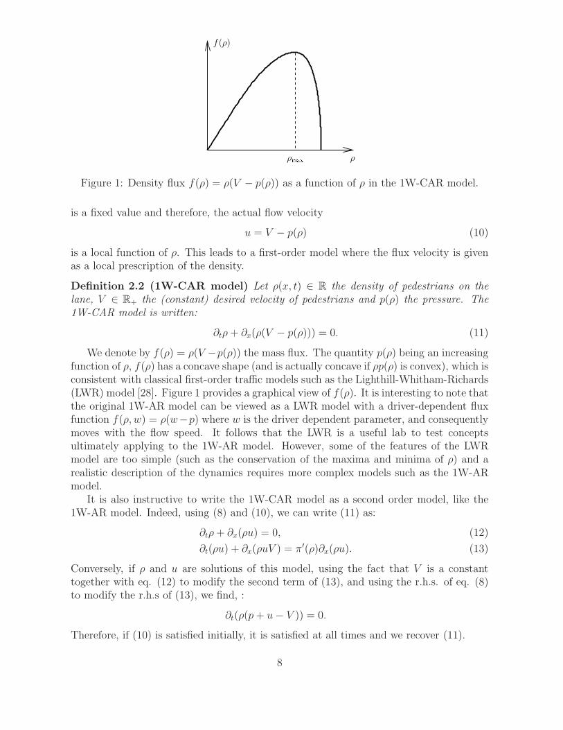
ρρmaxFigure 1: Density flux f(ρ) = ρ(V − p(ρ)) as a function of ρ in the 1W-CAR model.

is a fixed value and therefore, the actual flow velocity

u = V − p(ρ) (10)

is a local function of ρ. This leads to a first-order model where the flux velocity is givenas a local prescription of the density.

Definition 2.2 (1W-CAR model) Let ρ(x, t) ∈ R the density of pedestrians on thelane, V ∈ R+ the (constant) desired velocity of pedestrians and p(ρ) the pressure. The1W-CAR model is written:

∂tρ+ ∂x(ρ(V − p(ρ))) = 0. (11)

We denote by f(ρ) = ρ(V −p(ρ)) the mass flux. The quantity p(ρ) being an increasingfunction of ρ, f(ρ) has a concave shape (and is actually concave if ρp(ρ) is convex), which isconsistent with classical first-order traffic models such as the Lighthill-Whitham-Richards(LWR) model [28]. Figure 1 provides a graphical view of f(ρ). It is interesting to note thatthe original 1W-AR model can be viewed as a LWR model with a driver-dependent fluxfunction f(ρ, w) = ρ(w−p) where w is the driver dependent parameter, and consequentlymoves with the flow speed. It follows that the LWR is a useful lab to test conceptsultimately applying to the 1W-AR model. However, some of the features of the LWRmodel are too simple (such as the conservation of the maxima and minima of ρ) and arealistic description of the dynamics requires more complex models such as the 1W-ARmodel.

It is also instructive to write the 1W-CAR model as a second order model, like the1W-AR model. Indeed, using (8) and (10), we can write (11) as:

∂tρ+ ∂x(ρu) = 0, (12)

∂t(ρu) + ∂x(ρuV ) = π′(ρ)∂x(ρu). (13)

Conversely, if ρ and u are solutions of this model, using the fact that V is a constanttogether with eq. (12) to modify the second term of (13), and using the r.h.s. of eq. (8)to modify the r.h.s of (13), we find, :

∂t(ρ(p+ u− V )) = 0.

Therefore, if (10) is satisfied initially, it is satisfied at all times and we recover (11).

8

Remark 2 The 1W-CAR model in the form (12), (13) has an interesting interpretationin terms of microscopic dynamics, when the pedestrians have two velocity states, themoving one with velocity V and the steady one, with velocity 0. Indeed, denoting byg(x, t) the density of moving pedestrians and by s(x, t) that of steady pedestrians, we have

ρ = g + s.

Because the moving pedestrians move with velocity V , we can write the pedestrian flux ρuas

ρu = V g. (14)

Since by (11), ρu = ρ(V − p(ρ)), we deduce that

g = ρ(1 − p(ρ)

V), s = ρ

p(ρ)

V.

Not surprisingly, the offset velocity scaled by the particle velocity is nothing but the pro-portion of steady particles and it is completely determined by the total density ρ.

We deduce from (14) that system (12), (13) can be rewritten in the form:

∂t(g + s) + ∂x(V g) = 0, (15)

∂t(V g) + ∂x(V2g) = V π′(ρ)∂xg, (16)

Dividing (16) by V and subtracting to (15), we find:

∂tg + ∂x(V g) = π′(ρ)∂xg,

∂ts = −π′(ρ)∂xg.

Thus, the term π′(ρ)∂xg represents the algebraic transfer rate from immobile to movingparticles, while −π′(ρ)∂xg represents the opposite transfer. Therefore, this model assumesthat the pedestrians decide to stop or become mobile again, based not only on local ob-servation of the surrounding density, but on the observation of their gradients. Moreprecisely, keeping in mind that π′(ρ) and V have the same sign, the transfer rate fromthe immobile to moving state is positive if the moving particle density increases in thedownstream direction, indicating a lower congestion. Symmetrically, the transfer ratefrom the moving to immobile state increases if the moving particle density decreases inthe downstream direction, indicating an increase of congestion. These evaluations of thevariation of the moving particle density derivative are weighted by increasing functions ofthe density, meaning that the reactions of the pedestrians to their environment are fasterif the density is large.

We now turn to the introduction of the density constraint in the 1W-AR or 1W-CARmodels.

9

2.3 Introduction of the maximal density constraint in the 1W-

AR model

The maximal density constraint (also referred to below as the congestion constraint) isimplemented in the expression of the velocity offset or pressure p. Two ways to achievethis goal are proposed.

In the first one, p is a smooth function of the particle density which blows-up at theapproach of the maximal allowed density ρ∗.

In the second one, congestion results in an incompressibility constraint which producesnon-local effects with infinite speed of propagation of information. In congested regions,the pressure is no longer a function of the density but becomes implicitly determined bythe incompressibility constraint. The transition from uncongested to congested regions isabrupt and appears as a kind of phase transition. This second approach can be realizedas an asymptotic limit of the first approach where compression waves (or acoustic wavesby analogy with gas dynamics) propagate at larger and larger speeds (so-called low Mach-number limit).

Below, we successively discuss these two strategies. Then, we specifically consider theintroduction of the congestion constraint within the 1W-CAR model.

2.3.1 Congestion model with smooth transitions between uncongested andcongested regions

To implement the congestion constraint, we will highly rely on previous work [6, 7, 13],where this constraint has been implemented in the 1W-AR model. We take a convexfunction p(ρ) such that p(0) = 0, p′(0) ≥ 0 and p(ρ) → ∞ as ρ → ρ∗. More explicitly, wecan choose for instance for the pressure:

p(ρ) = pε(ρ) = P (ρ) +Qε(ρ), (17)

P (ρ) = Mρm, m > 1, (18)

Qε(ρ) =ε

(

1ρ− 1

ρ∗

)γ , γ > 1. (19)

P (ρ) is the background pressure of the pedestrians in the absence of congestion (andis taken in the form of an isentropic gas dynamics equation of state). Qε is a correctionwhich turns on when the density is close to congestion (i.e. ε ≪ 1 is a small quantity), andmodifies the background pressure to have it match the congestion condition p(ρ) → ∞ asρ → ρ∗.

Indeed, as long as ρ−ρ∗ is not too small, the denominator in (19) is finite and Qε(ρ) isof order ε. Thus the pressure p is dominated by the P term. However, a crossover occurswhen

(

1

ρ− 1

ρ∗

)γ

∼ ε,

i.e. whenρ∗ − ρ ∼ ρρ∗ε1/γ. (20)

10

ε1/γ

ρ

pε(ρ)

pε

P

Qε

ρ∗

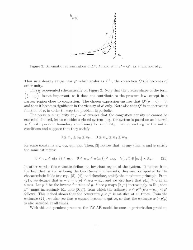
Figure 2: Schematic representation of Qε, P , and pε = P +Qε, as a function of ρ.

Thus in a density range near ρ∗ which scales as ε1/γ , the correction Qε(ρ) becomes oforder unity.

This is represented schematically on Figure 2. Note that the precise shape of the term(

1ρ− 1

ρ∗

)γ

is not important, as it does not contribute to the pressure law, except in a

narrow region close to congestion. The chosen expression ensures that Qε(ρ = 0) = 0,and that it becomes significant in the vicinity of ρ∗ only. Note also that Qε is an increasingfunction of ρ, in order to keep the problem hyperbolic.

The pressure singularity at ρ = ρ∗ ensures that the congestion density ρ∗ cannot beexceeded. Indeed, let us consider a closed system (e.g. the system is posed on an interval[a, b] with periodic boundary conditions) for simplicity. Let u0 and w0 be the initialconditions and suppose that they satisfy

0 ≤ um ≤ u0 ≤ uM, 0 ≤ wm ≤ w0 ≤ wM,

for some constants um, uM, wm, wM. Then, [3] notices that, at any time, u and w satisfythe same estimates:

0 ≤ um ≤ u(x, t) ≤ uM, 0 ≤ wm ≤ w(x, t) ≤ wM, ∀(x, t) ∈ [a, b]× R+. (21)

In other words, this estimate defines an invariant region of the system. It follows fromthe fact that, u and w being the two Riemann invariants, they are transported by thecharacteristic fields (see eqs. (5), (4)) and therefore, satisfy the maximum principle. From(21), we deduce that w − u = p(ρ) ≤ wM − um, and we also have that p(ρ) ≥ 0 at alltimes. Let p−1 be the inverse function of p. Since p maps [0, ρ∗) increasingly to R+, thenp−1 maps increasingly R+ onto [0, ρ∗), from which the estimate ρ ≤ p−1(wM − um) < ρ∗

follows. This indeed shows that the constraint ρ < ρ∗ is satisfied at all times. From theestimate (21), we also see that u cannot become negative, so that the estimate w ≥ p(ρ)is also satisfied at all times.

With this ε-dependent pressure, the 1W-AR model becomes a perturbation problem,

11

written as follows:

∂tρε + ∂x(ρ

εuε) = 0, (22)

∂t(ρεwε) + ∂x(ρ

εwεuε) = 0, (23)

wε = uε + pε(ρε). (24)

The next section investigates the formal ε → 0 limit.

2.3.2 Congestion model with abrupt transitions between uncongested andcongested regions

In the limit ε → 0, the uncongested motion remains unperturbed until the density hitsthe exact value ρ∗. Once this happens, congestion suddenly turns on and modifies thedynamics abruptly. In the uncongested regions, the flow is compressible ; it becomesincompressible at the congestion density ρ∗. Therefore, in the limit ε → 0, the abrupttransition from uncongested motion (when ρ < ρ∗) to congested motion (when ρ = ρ∗)corresponds to the crossing of a phase transition between a compressible to an incom-pressible flow regime.

In the limit ε → 0, the arguments of [6, 7, 13] can be easily adapted. Suppose thatρε → ρ < ρ∗. In this case, Qε(ρε) → 0 and we recover an 1W-AR model associated to thepressure P (ρ):

∂tρ0 + ∂x(ρ

0u0) = 0, (25)

∂t(ρ0w0) + ∂x(ρ

0w0u0) = 0, (26)

w0 = u0 + P (ρ0). (27)

If on the other hand, ρε → ρ∗, then Qε(ρε) → Q with 0 ≤ Q ≤ wM. Therefore, thetotal pressure is such that pε(ρε) → p with P (ρ∗) ≤ p. In this case, the model becomesincompressible:

∂xu0 = 0, (28)

∂tw0 + u0∂xw

0 = 0, (29)

w0 = u0 + p, with P (ρ∗) ≤ p. (30)

Note that in this congested region, the density does not vary (it is equal to ρ∗) and cannotdetermine the pressure anymore. Indeed, the functional relation between the density andthe pressure is broken and p may be varying with x even though ρ does not. The spatialvariations of p compensate exactly (through (30)) the variations of w0, in such a waythat all the pedestrians, whatever their desired velocity is, move at the same speed in thecongestion region.

This can also be seen when taking the limit ε → 0 in (5). Indeed, if ρε → ρ∗ withpε(ρε)(= wε−uε) staying finite, then ρε−ρ∗ = O(ε1/γ) (see (20)) and dpε/dρ ∼ ε−1/γ → ∞.Therefore, in the congested regime, the derivative of the pressure with respect to thedensity becomes infinite. Inserting this in (5) shows that ∂xu

ε → 0. This ensures thatall the pedestrians move at the same speed. Simultaneously, this blocks any further

12

increase of the density, which cannot become larger than ρ∗. Indeed, the mass conservationequation (1) tells us that

d

dtρε = ∂tρ

ε + uε∂xρε = −ρε∂xu

ε,

and consequently, if ∂xuε → 0, any further increase of the density is impeded.

In the general case, we expect that the two limit regimes coexist. The congestedregion may appear anywhere in the flow, depending on the initial conditions. Congestionregions must be connected to uncongested regions by interface conditions. Across theseinterfaces, ρ and ρw, which are conserved quantities obey the Rankine-Hugoniot relations.The quantity w, which is thought of as the (locally averaged) pedestrians’ desired velocityis modified across the interfaces through these relations. However, the bounds (21) arepreserved (see [3]).

Connecting congested and uncongested regions is a delicate problem which has beeninvestigated in [6] by a careful inspection of Riemann problem solutions. Specifically, [6]treats the special case M = 0 in (17)-(19). The present choice of the pressure (17)-(19)is slightly different: in the limit ε → 0, it produces a non-zero pressure in the uncon-gested region, while [6] considers that uncongested regions are pressureless in this limit.Pressureless gas dynamics develops some unpleasant features (such as the occurrence ofvacuum, weak instabilities, and so on). Keeping a non-zero pressure in the uncongestedregion in the limit ε → 0 allows to bypass some of these problems and represents animprovement over [6]. Of course, the precise choice of m and M must be fitted againstexperimental data.

We do not attempt to derive interface conditions between uncongested and congestedregions for the present choice of the pressure. Indeed, the perturbation problem (22)-(24),even with a small value of ε is easier to treat numerically than the connection problembetween the two models (25)-(27) and (28)-(30). Therefore, we will not regard the limitmodel as a numerically effective one, but rather, as a theoretical limit which provides someuseful insight. Still, the numerical treatment of the perturbation problem requires somecare. Of particular importance is the development of Asymptotic-Preserving schemes, i.e.of schemes that are able to capture the correct asymptotic limit when ε → 0. This is notan easy problem because of the blow up of the pressure near ρ∗. Indeed, due to the blowup of the characteristic speed in (5), the CFL stability condition of a classical explicitshock-capturing method leads to a time-step constraint of the type ∆t = 0(ε1/γ) → 0as ε → 0. For this reason, classical explicit shock-capturing methods cannot be used toexplore the congestion constraint when ε → 0 and Asymptotic-Preserving schemes areneeded.

Another reason for considering the perturbation problem (22)-(24) instead of the limitmodel is that the congestion may appear gradually rather than like an abrupt phasetransition from compressible to incompressible motion. In particular, for large pedestrianconcentrations, some erratic motions occur (this is referred to as crowd turbulence) andmight be modeled by a suitable (may be different) choice of the perturbation pressure Qε.

13

2.3.3 Introduction of the congestion constraint in the constant desired ve-locity 1W-CAR model

(i) Congestion model with smooth transitions. The smooth pressure relations (17)-(19)can be used for the 1W-CAR model. Because ρ now satisfies a convection equation:

∂tρ+ (V − (ρp)′(ρ))∂xρ = 0,

the initial bounds are preserved. Indeed, suppose that

0 ≤ ρm ≤ ρ0 ≤ ρM < ρ∗,

for some constants ρm, ρM, then, at any time, ρ satisfy the same estimates.

0 ≤ ρm ≤ ρ(x, t) ≤ ρM < ρ∗, ∀(x, t) ∈ [a, b]× R+.

In this way, the constraint 0 ≤ ρ ≤ ρ∗ is always satisfied. However, the fact that thebounds on the density are preserved by the dynamics can be viewed as unrealistic. Inreal pedestrian traffic, strips of congested and uncongested traffic spontaneously emergefrom rather space homogeneous initial conditions. The generation of new maximal andminimal bounds is an important feature of real traffic systems which is not well takeninto account in the 1W-CAR model and more generally, in LWR models.

(ii) Congestion model with abrupt transitions. If the limit ε → 0 is considered, and if theupper bound ρM = ρεM depends on ε and is such that ρεM → ρ∗, then, some congestionregions can occur. The limit model in the uncongested region does not change, and isgiven by the single conservation relation (11) with the pressure p(ρ0) = P (ρ0). In thecongested region, we have ρ0 = ρ∗, which implies ∂xu

0 = 0. In terms of the moving andsteady pedestrian densities, the congested regime means that

∂xg0 = 0, s0 = ρ∗ − g0,

i.e. both the steady and moving pedestrian densities are uniform in the congested region.

3 Two-way one-lane traffic model

3.1 An Aw-Rascle model for two-way one-lane pedestrian traffic

The extension of the 1W-AR model to 2-way traffic, denoted by 2W-AR model, may seemrather easy, the 2-way traffic is written as a system of two 1-way models. However, wewill see that the mathematical properties of the 2-way models are rather different fromtheir one-way counterpart.

Definition 3.1 (2W-AR model) Let ρ± the density of pedestrians, u± their velocity,w± their desired velocity and p the pressure, with an index + for the right-going pedestrians

14

and − for the left-going ones. The 2W-AR model for 2-way traffic is written:

∂tρ+ + ∂x(ρ+u+) = 0,

∂tρ− + ∂x(ρ−u−) = 0,

∂t(ρ+w+) + ∂x(ρ+w+u+) = 0,

∂t(ρ−w−) + ∂x(ρ−w−u−) = 0,

w+ = u+ + p(ρ+, ρ−),

w− = −u− + p(ρ−, ρ+).

The coupling of the two flows of pedestrians in the 2W-AR model is through theprescription of the pressures which are functions of the densities of the two species ρ+ andρ−. Our conventions are that the desired velocities w± and the velocity offsets p(ρ±, ρ∓)are magnitudes, and as such, are positive quantities. The actual velocities u± are signedquantities: u+ > 0 for right-going pedestrians and u− < 0 for left-going pedestrians.These conventions explain the different signs in factor of the velocities for (31) and (31).However, we do not exclude that, in particularly congested conditions, the right-goingpedestrians may have to go backwards (i.e. to the left) or vice-versa, the left-goingpedestrians have to go to the right. Therefore, we do not make any a priori assumptionon the sign of u±. For obvious symmetry reasons, the same pressure function is used forthe two particles, with reversed arguments. The function p is increasing with respect toboth arguments since the velocity offset of one of the species increases when the densityof either species increases.

Some of the properties of the 1W-AR system extend to the 2W-AR one. For instance,the desired velocities are Lagrangian variables, as they satisfy:

∂tw+ + u+∂xw+ = 0,

∂tw− + u−∂xw− = 0.

Unfortunately, the velocities u+ and u− do not constitute Riemann invariants any longerbecause of the coupling induced by the dependence of p upon ρ+ and ρ−. For this reasoninitial bounds on u+ and u− are not preserved by the flow, as they were in the case ofthe 1W-AR model. Since the velocity offsets p(ρ+, ρ−) and p(ρ−, ρ+) are not bounded apriori, the velocities u+ and u− can reverse sign when the velocity offsets are large. This isexpected to reflect the fact that a dense crowd moving in one direction may force isolatedpedestrians going the other way to move backwards. Of course, such a situation is onlyexpected in close to congestion regimes.

Nonetheless, the evolution of the pedestrian fluxes reflects the same phenomenologyas in the one-way case, namely that pedestrians react to the Lagrangian derivative of thepressure, as shown by the following eqs. (which are the 2-way equivalents of eq. (7)):

∂t(ρ+u+) + ∂x(ρ+u+u+) = −ρ+

(

d

dt

)

+

[p(ρ+, ρ−)],

∂t(ρ−u−) + ∂x(ρ−u−u−) = ρ−

(

d

dt

)

−

[p(ρ−, ρ+)],

15

where the material derivatives (d/dt)± = ∂t + u±∂x depend on what type of particles isconcerned. These equations can also be put in the form (equivalent to (8) for the 1W-ARmodel):

∂t(ρ+u+) + ∂x(ρ+u+w+) =[

p(ρ+, ρ−) + ρ+ ∂1p|(ρ+,ρ−)

]

∂x(ρ+u+) +

+ρ+ ∂2p|(ρ+,ρ−) ∂x(ρ−u−), (31)

∂t(ρ−u−)− ∂x(ρ−u−w−) = −[

p(ρ−, ρ+) + ρ− ∂1p|(ρ−,ρ+)

]

∂x(ρ−u−)

−ρ− ∂2p|(ρ−,ρ+) ∂x(ρ+u+), (32)

where we denote by ∂1p and ∂2p the derivatives of the function p with respect to its firstand second arguments respectively. This form of the equations will be used below for thederivation of the Constant Desired Velocity model.

The 2W-AR model is not always hyperbolic. Before stating the result, we introducesome notations. We define:

c++ = ∂1p(ρ+, ρ−), c+− = ∂2p(ρ+, ρ−), (33)

c−+ = ∂2p(ρ−, ρ+), c−− = ∂1p(ρ−, ρ+). (34)

We assume that p is increasing with respect to both arguments, which implies that allquantities defined by (33), (34) are non-negative. This assumption simply means that thepedestrian speed is reduced if the densities of either categories of pedestrians increase.For a given state (ρ+, w+, ρ−, w−), the fluid velocities are given by:

u+ = w+ − p(ρ+, ρ−), u− = −w− + p(ρ−, ρ+).

We also define the following velocities

cu+= u+ − ρ+c++, cu−

= u− + ρ−c−−.

These are the characteristic speeds (6) of the 1W-AR system. Specifically, cu+is the wave

at which information about velocity would propagate in a system of right-going pedestri-ans without coupling with the left-going ones. A similar explanation holds symmetricallyfor cu−

.We now have the following theorem, the proof of which is elementary and left to the

reader.

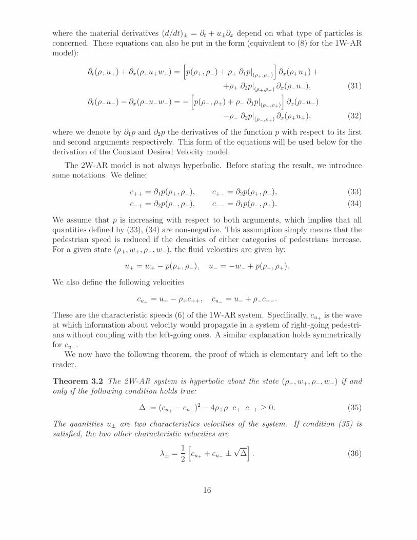
Theorem 3.2 The 2W-AR system is hyperbolic about the state (ρ+, w+, ρ−, w−) if andonly if the following condition holds true:

∆ := (cu+− cu−

)2 − 4ρ+ρ−c+−c−+ ≥ 0. (35)

The quantities u± are two characteristics velocities of the system. If condition (35) issatisfied, the two other characteristic velocities are

λ± =1

2

[

cu++ cu−

±√∆]

. (36)

16

Non-hyperbolicity occurs when the two characteristic velocities cu+and cu−

of the uncou-pled systems are close to each other. In this case, the first term of ∆ is close to zero anddoes not compensate for the second term, which is negative. These conditions happen inparticular when both velocities cu+

and cu−are close to zero, which corresponds to the

densities where the fluxes ρ+u+, ρ−u− are maximal as functions of the densities ρ+, ρ−respectively. In particular, in the one-way case with constant speed of figure 1, this wouldcorrespond to the point ρmax. These conditions correspond to the onset of congestion.Therefore, instabilities linked to the non-hyperbolic character of the model will developin conditions close to congestion.

The occurrence of regions of non-hyperbolicity is not entirely surprising. The insta-bility of two counter-propagating flows is a common phenomenon in fluid mechanics. Inplasma physics, the instability of two counter-propagating streams of charged particlesis well known under the two-stream instability. The situation here is extremely similar,in spite of the different nature of the interactions (which are mediated by the long-rangeCoulomb force in the plasma case).

The occurrence of a non-hyperbolic region is often viewed as detrimental, because inthis region, the model is unstable. On the other hand, self-organization phenomena likelane formation or the onset of crowd turbulence cannot be described by an everywherestable model. For instance, morphogenesis is explained by the occurrence of the Turinginstability in systems of diffusion equations. Here, diffusion is not taken into account andthe instability originates from a different phenomenon. However, in practice, some smallbut non-zero diffusion always exists. This diffusion damps the small scale structures butkeeps the large scale structures growing. The typical size of the observed structures canbe linked to the threshold wave-number below which instability occurs.

Numerical simulations to be presented in a forthcoming work will allow us to determinewhether the phenomena which are observed in dense crowds may be explained by thistype of instability. In section 5, a stability analysis of a diffusive two-way LWR modelwill provide more quantitative support to these concepts.

3.2 The constant desired velocity Aw-Rascle model for two-way

one-lane pedestrian traffic

To construct the two-way constant desired velocity Aw-Rascle model (2W-CAR) for two-way one-lane pedestrian traffic, we must set

w+ = w− = V, (37)

and

u+ = V − p(ρ+, ρ−), u− = −V + p(ρ−, ρ+). (38)

This leads to the following model:

Definition 3.3 (2W-CAR model) Let ρ+ and ρ− the densities of pedestrians movingto the right and to the left respectively, V the (constant) desired velocity of pedestrians

17

and p the pressure term. The 2W-CAR model is written:

∂tρ+ + ∂x(ρ+(V − p(ρ+, ρ−))) = 0, (39)

∂tρ− − ∂x(ρ−(V − p(ρ−, ρ+))) = 0. (40)

These are two first-order models coupled by a velocity offset which depends on thetwo densities.

We can find the same interpretation of this model in terms of moving and steadyparticles as in the one-way model case. Using (31), (32) and (37), we can write:

∂tρ+ + ∂x(ρ+u+) = 0, (41)

∂tρ− + ∂x(ρ−u−) = 0, (42)

∂t(ρ+u+) + ∂x(ρ+u+V ) =[

p(ρ+, ρ−) + ρ+ ∂1p|(ρ+,ρ−)

]

∂x(ρ+u+) +

+ρ+ ∂2p|(ρ+,ρ−) ∂x(ρ−u−), (43)

∂t(ρ−u−)− ∂x(ρ−u−V ) = −[

p(ρ−, ρ+) + ρ− ∂1p|(ρ−,ρ+)

]

∂x(ρ−u−)

−ρ− ∂2p|(ρ−,ρ+) ∂x(ρ+u+). (44)

Conversely, if ρ+, u+, ρ−, u− are solutions of this model, using the same method as in theone-way case, we easily find that:

∂t(ρ±(p± u± − V )) = 0.

Therefore, if (38) is satisfied initially, it is satisfied at all times and we recover (39), (40).Now, we denote by g±(x, t) the density of the moving particles and by s±(x, t) that of

the steady particles with a + (respectively a −) indicating the right-going (respectivelyleft-going) pedestrians. Although steady, the pedestrians have a desired motion either tothe right or to the left, and we need to keep track of these intended directions of motions.We have

ρ± = g± + s± and ρ±u± = ±V g±.

We deduce that

s+ρ+

=p(ρ+, ρ−)

V,

s−ρ−

=p(ρ−, ρ+)

V.

Therefore, the offset velocities p(ρ+, ρ−) and p(ρ−, ρ+) scaled by the particle velocity Vrepresent the proportions of the steady particles s+/ρ+ and s−/ρ− respectively. Now, wecan rewrite (41)-(44) as follows:

∂t(g+ + s+) + ∂x(V g+) = 0,

∂t(g− + s−)− ∂x(V g−) = 0,

∂t(V g+) + ∂x(V2g+) =

[

p(ρ+, ρ−) + ρ+ ∂1p|(ρ+,ρ−)

]

∂x(V g+)

−ρ+ ∂2p|(ρ+,ρ−) ∂x(V g−),

∂t(V g−)− ∂x(V2g−) = −

[

p(ρ−, ρ+) + ρ− ∂1p|(ρ−,ρ+)

]

∂x(V g−) +

+ρ− ∂2p|(ρ−,ρ+) ∂x(V g+).

18

By simple linear combinations, this system is equivalent to

∂tg+ + ∂x(V g+) =[

p(ρ+, ρ−) + ρ+ ∂1p|(ρ+,ρ−)

]

∂xg+

−ρ+ ∂2p|(ρ+,ρ−) ∂xg−,

∂tg− − ∂x(V g−) = −[

p(ρ−, ρ+) + ρ− ∂1p|(ρ−,ρ+)

]

∂xg− +

+ρ− ∂2p|(ρ−,ρ+) ∂xg+,

∂ts+ = −[

p(ρ+, ρ−) + ρ+ ∂1p|(ρ+,ρ−)

]

∂xg+ + ρ+ ∂2p|(ρ+,ρ−) ∂xg−,

∂ts− =[

p|(ρ−,ρ+) + ρ−∂1p|(ρ−,ρ+)

]

∂xg− − ρ−∂2p|(ρ−,ρ+)∂xg+.

Like in the one-way model, we find that the transition rates from the steady to movingstates or vice-versa depend on the derivatives of the concentrations of moving pedestrians.Now, both the left and right going pedestrian total densities appear in the expressions ofthe transitions rates for either species. This is due to the coupling through the pressureterm, which depends on both densities.

Like the 2W-AR model, the 2W-CAR model is not always hyperbolic. Using the samenotations as in the previous section, we have the:

Theorem 3.4 The 2W-CAR system is hyperbolic about the state (ρ+, ρ−) if and only ifcondition (35) is satisfied. In this case, the two characteristic velocities are given by (36).

This can be seen directly from equations (39) and (40), once they are put under the form

∂t

(

ρ+ρ−

)

+

(

cu+−ρ+c+−

ρ−c−+ cu−

)

∂x

(

ρ+ρ−

)

= 0.

We refer to the end of section 3.1 for more comments about this property.

3.3 Introduction of the congestion constraint in the 2W-AR

model

3.3.1 Congestion model with smooth transitions

It is difficult to make a prescription for the function p. Its expression should be fitted toexperimental data. Here we propose a form which allows us to investigate the effects ofcongestion. We propose:

p(ρ+, ρ−) = pε(ρ+, ρ−) = P (ρ) +Qε(ρ+, ρ−), with ρ = ρ+ + ρ− (45)

P (ρ) = Mρm, m ≥ 1, (46)

Qε(ρ+, ρ−) =ε

q(ρ+)(

1ρ− 1

ρ∗

)γ , γ > 1. (47)

The rationale for this formula is as follows. First, in uncongested regime, we expectthat the velocity offsets of the right and left going pedestrians are the same, this common

19

offset being a function of the total particle density. Thus, the uncongested flow pressureP given by (46) is a function of ρ only, and has the same shape as in the one-way case.Congestion occurs when the total density ρ becomes close to ρ∗. Therefore, formula(47) resembles (19), except for the prefactor q(ρ+). With this choice of the pressure, weanticipate that the constraint

ρ = ρ+ + ρ− ≤ ρ∗

will be satisfied everywhere in space and time, like in the one-way case.The prefactor q(ρ+) takes into account the fact that the velocity offset for the majority

particle is smaller than that of the minority particle. Therefore, we prescribe q to be anincreasing function of ρ+. For further usage, we note the following formula, which followsfrom eliminating ((1/ρ)− (1/ρ∗))γ between Qε(ρ+, ρ−) and Qε(ρ−, ρ+):

q(ρ+)Qε(ρ+, ρ−) = q(ρ−)Q

ε(ρ−, ρ+). (48)

It is more convenient to express this formula as

Qε(ρ+, ρ−)

Qε(ρ−, ρ+)=

q(ρ−)

q(ρ+),

remembering that q is an increasing function. This formula states that the velocity offsetfor the right and left-going particles are inversely proportional to the ratios of a (functionof) the densities. Since q is increasing and taking ρ− < ρ+ as an example, we deducethat the velocity offset of the right-going particles will be less than that of the left-goingparticles. In other words, the flow of the majority category of pedestrians is less impededthan that of the minority one. In order to keep Qε(ρ±, ρ∓) small whenever ρ < ρ∗, werequire that q(ρ±) = O(1) when ρ± < ρ∗ . Physically relevant expressions of q(ρ±) canbe obtained from real experiments. A possible extension, that we will not consider here,would be to have different functions q+(ρ+) and q−(ρ−). This could model the fact thatfor example, a crowd heading towards a train platform could be more pushy than the onegoing in the opposite direction.

The 2W-AR model with ε-dependent pressure becomes a perturbation problem:

∂tρε+ + ∂x(ρ

ε+u

ε+) = 0,

∂tρε− + ∂x(ρ

ε−u

ε−) = 0,

∂t(ρε+w

ε+) + ∂x(ρ

ε+w

ε+u

ε+) = 0,

∂t(ρε−w

ε−) + ∂x(ρ

ε−w

ε−u

ε−) = 0,

wε+ = uε

+ + pε(ρε+, ρε−),

wε− = −uε

− + pε(ρε−, ρε+).

3.3.2 Congestion model with abrupt transitions

This case corresponds to the formal limit ε → 0 of the previous model. Suppose thatρε → ρ < ρ∗. In this case, Qε(ρε±, ρ

ε∓) → 0 and we recover a 2W-AR model associated to

the pressure P (ρ):

20

∂tρ0+ + ∂x(ρ

0+u

0+) = 0,

∂tρ0− + ∂x(ρ

0−u

0−) = 0,

∂t(ρ0+w

0+) + ∂x(ρ

0+w

0+u

0+) = 0,

∂t(ρ0−w

0−) + ∂x(ρ

0−w

0−u

0−) = 0,

w0+ = u0

+ + P (ρ0), u0+ ≥ 0,

w0− = −u0

− + P (ρ0), u0− ≤ 0.

If on the other hand, ρε → ρ∗, then Qε(ρε+, ρε−) → Q+ and Qε(ρε−, ρ

ε+) → Q−. Fur-

thermore, following (48), Q+ and Q− are related by:

q(ρ0+) Q+ = q(ρ0−) Q−. (49)

Therefore, the total pressure is such that pε(ρε+, ρε−) → p+ and pε(ρε−, ρ

ε+) → p− with

P (ρ∗) ≤ p± and p+ and p− related through (49) (with Q± replaced by p± − P (ρ∗)).We stress the fact that Q± and consequently p± are not local function of ρ0+, ρ

0− (only

the ratio Q+/Q− = q(ρ0−)/q(ρ0+) is a local function of ρ0+, ρ

0−). Indeed the value of Q± of

two different solutions of the model may be different, even if the local values of (ρ0+, ρ0−)

are the same. Therefore, there is no local function of (ρ0+, ρ0−) which can match the value

of Q±.Then, in this case, the model becomes:

∂tρ0+ + ∂x(ρ

0+u

0+) = 0,

∂tρ0− + ∂x(ρ

0−u

0−) = 0,

∂t(ρ0+w

0+) + ∂x(ρ

0+w

0+u

0+) = 0,

∂t(ρ0−w

0−) + ∂x(ρ

0−w

0−u

0−) = 0,

w0+ = u0

+ + p+ with P (ρ∗) ≤ p+,

w0− = −u0

− + p− with P (ρ∗) ≤ p−,

ρ0+ + ρ0− = ρ∗, (50)

q(ρ0+) (p+ − P (ρ∗)) = q(ρ0−) (p− − P (ρ∗)). (51)

Relations (50) and (51) furnish the two supplementary relations which allow us to computethe two additional quantities p+ and p−. The last relation (51) specifies how, at congestion,the left and right going pedestrians share the available space. We see that this sharingrelation depends upon the choice of the function q. Obviously, q is an input of the modelwhich must be determined from the experimental measurements. If some flow asymmetrymust be taken into account (like if one crowd is more pushy than the other one), differentfunctions q+(ρ+) and q−(ρ−) can be used.

This model is a system of first-order differential equations in which the fluxes areimplicitly determined by the constraint (50). As a consequence of this constraint, thetotal particle flux ρ0+u

0+ + ρ0−u

0− is constant within the congestion region. We note the

difference between this constrained model and the constrained 1W-AR model (see section2.3.2). In the 1W-AR model, there was a single unknown congestion pressure p and

21

a single density constraint ρ = ρ∗. In the 2W-AR model, there are two congestionpressures p+ and p−, which play a similar role in the dynamics of their associated categoryof pedestrians. However, there is still a single density constraint, acting on the totaldensity ρ+ + ρ− = ρ∗. The additional condition which allows for the computation ofthe two congestion pressures is provided by the ’space-sharing’ constraint (51). The twoconstraints express very different physical requirements and must be combined in orderto find the two congestion pressures which, themselves, have a symmetric role.

3.3.3 Introduction of the congestion constraint in the 2W-CAR model

(i) Congestion model with smooth transitions. The smooth pressure relations (45)-(47)can be used for the 2W-CAR model. With this pressure relation, we anticipate that thebound ρ ≤ ρ∗ is enforced.

(ii) Congestion model with abrupt transitions. If the limit ε → 0 is considered, then, thelimit model in the uncongested region remains of the same form, i.e. is given by (39),(40) with the pressure given by p(ρ0+, ρ

0−) = P (ρ0+ + ρ0−). In the congested region, using

the same arguments as in section 3.3.2, we find that (ρ0+, ρ0−) satisfies:

∂tρ0+ + ∂x(ρ

0+(V − p+)) = 0,

∂tρ0− − ∂x(ρ

0−(V − p−)) = 0,

ρ0+ + ρ0− = ρ∗, (52)

q(ρ0+) (p+ − P (ρ∗)) = q(ρ0−) (p− − P (ρ∗)). (53)

Again, this model gives rise to a system of first order differential equations in which thefluxes are implicitly determined by the constraints (52), (53). As a consequence of thisconstraint, the total particle flux ρ0+u

0+ + ρ0−u

0− (where u0

± = V − p±) is constant withinthe congestion region.

4 Two-way multi-lane traffic model

4.1 A Two-way multi-lane Aw-Rascle model of pedestrians

We now consider a multi-lane model to describe the structure of the flow in the crosssectional direction to the corridor. The models presented so far considered averagedquantities in the cross section of the corridor. However, it is a well observed phenomenonthat two-way pedestrian flow presents interesting spontaneous lane structures (see e.g.[9]), with a preferential side depending on sociological behavior: pedestrians show a pref-erence to the right side in western countries, while the preference is to the left in Japan forinstance. In order to allow for a description of the cross-section of the flow, we discretizespace in this cross-sectional direction and suppose that pedestrians walk along discretelanes, like cars on a freeway, with lane changing probabilities depending on the state ofthe downwind flow. In this way, we design a model which may, if the parameters aresuitable chosen, exhibit the spontaneous emergence of a structuration of the flow into

22

lanes. We stress however, that the lanes in our model must be viewed as a mere spatialdiscretization and that spontaneously emerging pedestrian lanes may actually consist ofseveral contiguous discrete lanes of our model.

Let k ∈ Z be the lane index. So far, we consider an infinite number of lanes. Of course,there is a maximal number of K lanes and k ∈ {1, . . . , K}. Extra-conditions due to thefiniteness of the number of lanes are discarded here for simplicity. For each of the lane, wewrite a 2W-AR model in the form described in section 3, supplemented by lane-changingsource terms.

Definition 4.1 (ML-AR model) For any index k ∈ Z, let ρk,± the density of pedes-trians in the k-th lane, uk,± their velocity, wk,± their desired velocity and pk a pressureterm, with an index + for the right-going pedestrians and − for the left-going ones. TheML-AR model is given by:

∂tρk,+ + ∂x(ρk,+ uk,+) = Sk,+, (54)

∂tρk,− + ∂x(ρk,− uk,−) = Sk,−, (55)

∂t(ρk,+wk,+) + ∂x(ρk,+wk,+ uk,+) = Rk,+, (56)

∂t(ρk,−wk,−) + ∂x(ρk,−wk,− uk,−) = Rk,−, (57)

wk,+ = uk,+ + pk(ρk,+, ρk,−), (58)

wk,− = −uk,− + pk(ρk,−, ρk,+). (59)

where Sk,± and Rk,± are source terms coming from the lane-changing transition rates.

We allow for different pressure relations in the different lanes, to take into account forinstance that the behavior of the pedestrians may be more aggressive in the fast lanesthan in the slow ones, or to take into account that circulation along the walls may bedifferent than in the middle of the corridor. This point must be assessed by comparisonswith the experiments. We specify the pressure relation in each lane in the form of (45),(47) with parameter values depending on k.

We denote by

ρk = ρk,+ + ρk,−,

the total density on the k-th lane. We assume that the congestion density ρ∗ is the samefor all lanes (this assumption can obviously be relaxed).

4.2 Interaction terms in the multi-lane model

We assume that pedestrians prefer to change lane than to reduce their speed, i.e. theychange lane if they feel that the offset velocity of their lane (i.e. pk(ρk,+, ρk,−) in thecase of right-going pedestrians on lane k) increases. If facing such an increase, right-going pedestrians change from lane k to lanes k ± 1 (not changing their direction ofmotion) with rates λ+

k→k±1. Similarly, these rates are λ−k→k±1 for left-going pedestri-

ans. These rates increase with the value of (d/dt)k,+(pk(ρk,+, ρk,−)) for λ+k→k±1 and with

(d/dt)k,−(pk(ρk,−, ρk,+)) for λ−k→k±1 to indicate that the lane changing probability is in-

creased when an increase of the downstream density is detected. We have denoted by

23

(d/dt)k,± the material derivatives for particles moving on the k-th lane in the positiveor negative direction: (d/dt)k,± = ∂t + uk,±∂x. Strongly congested lanes do not attractnew pedestrians. Therefore, λ+

k→k+1 is also a decreasing functions of ρk+1 which vanishesat congestion, when ρk+1 = ρ∗. Similarly, λ−

k→k+1 is decreasing with ρk+1 and vanishesat congestion ρk+1 = ρ∗ and λ±

k→k−1 decreases with ρk−1 and vanishes at congestionρk−1 = ρ∗.

Given these assumptions on the transition rates, the lane-changing source terms forthe density equations are written:

Sk,α = λαk+1→k ρk+1,α + λα

k−1→k ρk−1,α − (λαk→k+1 + λα

k→k−1)ρk,α, α = ±. (60)

It is easy to see that this formulation gives:∑

k∈Z

Sk,α = 0, α = ±

which implies the balance equation of the total number of particles moving in a givendirection:

∂tρα + ∂xjα = 0, ρα =∑

k∈Z

ρk,α, jα =∑

k∈Z

ρk,αuk,α, α = ±.

Concerning the rates Rk,±, we consider that wk,± being a Lagrangian quantity, thequantities ρk,±wk,± vary according to the same rates as the densities themselves. Hence,we let:

Rk,α = λαk+1→k ρk+1,αwk+1,α + λα

k−1→k ρk−1,αwk−1,α

−(λαk→k+1 + λα

k→k−1)ρk,αwk,α, α = ±. (61)

The material derivatives of wk,± satisfy:(

dwk,+

dt

)

k,+

:= ∂twk,+ + uk,+ ∂xwk,+ =1

ρk,+(Rk,+ − wk,+ Sk,+) =

= λ+k+1→k

ρk+1,+

ρk,+(wk+1,+−wk,+) + λ+

k−1→k

ρk−1,+

ρk,+(wk−1,+−wk,+),

(

dwk,−

dt

)

k,−

:= ∂twk,− + uk,− ∂xwk,− =1

ρk,−(Rk,− − wk,− Sk,−) =

= λ−k+1→k

ρk+1,−

ρk,−(wk+1,−−wk,−) + λ−

k−1→k

ρk−1,−

ρk,−(wk−1,−−wk,−).

The right-hand sides of these equations are not zero because the arrival of pedestrians fromdifferent lanes with a different preferred velocity modifies the average preferred velocity.

4.3 The ’constant desired velocity version’ of the two-way multi-lane Aw-Rascle model of pedestrians

To construct the constant desired velocity Aw-Rascle model for two-way multi-lane pedes-trian traffic (ML-CAR model), we must set

wk,+ = wk,− = V, (62)

24

and

uk,+ = V − p(ρk,+, ρk,−), uk,− = −V + p(ρk,−, ρk,+). (63)

We can check in this case that Sk,± and Rk,± have been defined in a coherent way by (60)and (61), i.e. that they are such that equations (54-55) and (56-57) become equivalent.The corresponding model is written:

Definition 4.2 (ML-CAR model) Let ρk,± the density of pedestrians in the k-th lane,V the constant desired velocity of pedestrian and pk the pressure term. The ML-CARmodel is given by:

∂tρk,+ + ∂x

(

ρk,+(V − pk(ρk,+, ρk,−)))

= Sk,+,

∂tρk,− − ∂x

(

ρk,−(V − pk(ρk,−, ρk,+)))

= Sk,−,

where Sk,± is given by (60).

The features of this model are those of the two-way, one-lane CAR model of section3.2, combined with the features of the source terms Sk,± as outlined in section 4.2.

4.4 Introduction of the congestion constraint in the multi-lane

ML-AR model

4.4.1 Congestion model with smooth transitions

The prescription for the pressure functions pk are the same as in section 3.3.1, except fora possible k-dependence of the constants, namely:

pk(ρk,+, ρk,−) = pεk(ρk,+, ρk,−) = Pk(ρk) +Qεk(ρk,+, ρk,−),

Pk(ρk) = Mkρmkk , mk ≥ 1,

Qεk(ρk,+, ρk,−) =

ε

qk(ρk,+)(

1ρk

− 1ρ∗

)γk , γk > 1.

With this pressure law, the ML-AR model becomes a perturbation problem. This isindicated by equipping all unknowns with an exponent ε. This pressure relation can beused in the constant desired velocity model of section 4.3 where all particles move withthe same speed V .

4.4.2 Congestion model with abrupt transitions

This case corresponds to the formal limit ε → 0 of the previous model. Suppose thatρεk → ρk < ρ∗. In this case, Qε

k(ρεk,+, ρ

εk,−) → 0 and we recover a ML-AR model associated

25

to the pressure Pk(ρk):

∂tρ0k,+ + ∂x(ρ

0k,+ u0

k,+) = S0k,+,

∂tρ0k,− + ∂x(ρ

0k,− u0

k,−) = S0k,−,

∂t(ρ0k,+w0

k,+) + ∂x(ρ0k,+w0

k,+ u0k,+) = R0

k,+,

∂t(ρ0k,−w0

k,−) + ∂x(ρ0k,−w0

k,− u0k,−) = R0

k,−,

w0k,+ = u0

k,+ + Pk(ρ0k),

w0k,− = −u0

k,− + Pk(ρ0k).

If on the other hand, ρεk → ρ∗, the model becomes:

∂tρ0k,+ + ∂x(ρ

0k,+ u0

k,+) = S0k,+,

∂tρ0k,− + ∂x(ρ

0k,− u0

k,−) = S0k,−,

∂t(ρ0k,+w0

k,+) + ∂x(ρ0k,+w0

k,+ u0k,+) = R0

k,+,

∂t(ρ0k,−w0

k,−) + ∂x(ρ0k,−w0

k,− u0k,−) = R0

k,−,

w0k,+ = u0

k,+ + pk,+ with P (ρ∗) ≤ pk,+,

w0k,− = −u0

k,− + pk,− with P (ρ∗) ≤ pk,−,

ρ0k,+ + ρ0k,− = ρ∗,

qk(ρ0k,+) (pk,+ − Pk(ρ

∗)) = qk(ρ0k,−) (pk,− − Pk(ρ

∗)).

The source terms are unchanged compared to the ε > 0 case, and the interpretation ofthe model is the same as in section 3.3.2. Performing the limit ε → 0 in the constantdesired velocity model of section 4.3 follows a similar procedure and is left to the reader.

5 Study of the diffusive two-way, one-lane CAR mod-

els

In this section, we restrict ourselves to the 2W-CAR model presented in section 3.2(i.e. without the introduction of the maximal density constraint), and we investigate thestability of a diffusive perturbation of this model. The goal of this section is to showthat the addition of a small diffusivity stabilizes the large wave-numbers in the region ofstate space where hyperbolicity is lacking. The threshold value of the wave-number belowwhich the instability grows can be related to the size of macroscopic structures observedin real crowd flows.

5.1 Theoretical analysis

We consider the following model which is a slight generalization of the 2W-CAR model:

∂tρ+ + ∂xf(ρ+, ρ−) = δ ∂2xρ+, (64)

∂tρ− − ∂xf(ρ−, ρ+) = δ ∂2xρ−. (65)

26

Typically, for the 2W-CAR model, f(ρ+, ρ−) = ρ+(V − p(ρ+, ρ−)) but we do not restrictourselves to this simple flux prescription. The assumptions on f are that for fixed ρ−,the function ρ+ → f(ρ+, ρ−) has the bell-shaped curve of figure 1, which is characteristicof the LWR flux. For fixed ρ+, the function ρ− → f(ρ+, ρ−) is just assumed decreasing,meaning that the flux of right-going pedestrians is further reduced as the density of left-going pedestrians increases. By symmetry, the diffusivities δ are assumed to be the samefor the two species of particles. Of course, the diffusivities may depend on the densitiesthemselves, in which case they may be different. But we will discard this possibility here.We denote by

c++ = ∂1f(ρ+, ρ−), c+− = ∂2f(ρ+, ρ−),

c−+ = ∂2f(ρ−, ρ+), c−− = ∂1f(ρ−, ρ+).

These quantities are related to those defined in section 3.1 for the 2W-AR model by

c++ = cu+, c+− = −ρ+c+−, c−− = −cu−

, c−+ = −ρ−c−+. (66)

With the assumptions on f , we have that c+− ≤ 0, c−+ ≤ 0, while c++ (resp. c−−)decreases from positive to negative values when ρ+ (resp. ρ−) increases.

Any state such that (ρ+, ρ−) is independent of x is a stationary solution. We study thelinearized stability of the system about these uniform steady states. Denoting by (r+, r−)its unknowns, the linear system is written:

∂tr+ + c++∂xr+ + c+−∂xr− = δ ∂2xr+, (67)

∂tr− + c−+∂xr+ + c−−∂xr− = δ ∂2xr−. (68)

We look for solutions which are pure Fourier modes of the form r± = r± exp i(ξx − st)where r± is the amplitude of the mode, ξ and s are its wave number and frequency.Inserting the Fourier Ansatz into (67), (68) leads to a homogeneous linear system for(r+, r−). This system has non-trivial solutions if and only if the determinant of the linearsystem cancels. This results in a relation between s and ξ (the dispersion relation). Inthis analysis, we restrict to ξ ∈ R and are looking for the time stability of the model. Wedenote by λ = s/ξ the phase velocity of the mode.

A given mode remains bounded in time, and therefore stable, if and only if the imag-inary part of s is non-positive. In the converse situation, the mode is unstable. Thesystem is said linearly stable about the uniform state (ρ+, ρ−) if and only if all the modesare stable for all ξ ∈ R. In the converse situation, the system is unstable, and it is theninteresting to look at the range of wave numbers ξ ∈ R which generate unstable modes.The following result follows easily from simple calculations:

Proposition 1 (i) Suppose (ρ+, ρ−) are such that the following condition:

∆ := (c++ + c−−)2 − 4c+−c−+ ≥ 0, (69)

is satisfied, then the uniform steady state with uniform densities (ρ+, ρ−) is linearly stableabout (ρ+, ρ−). For any given ξ ∈ R, there exist two modes whose phase velocities λ±(ξ)are given by

λ±(ξ) =1

2

[

c++ − c−− − 2iδξ ±√∆]

. (70)

27

(ii) Suppose that (ρ+, ρ−) are such that (69) is not true. Then, the uniform steady statewith uniform densities (ρ+, ρ−) is linearly unstable about (ρ+, ρ−). Moreover, we have

|ξ| ≤√

|∆|2δ

⇐⇒ ∃ a mode such that Im s > 0 (unstable mode). (71)

The phase velocity is given by

λ±(ξ) =1

2

[

c++ − c−− − 2iδξ ± i√

|∆|]

. (72)

We note that if (66) is inserted in (69), we recover (35). Therefore, the addition of diffusiondoes not change the criterion for stability or instability. However, in the unstable case,all modes are unstable for the diffusion-free model (this would correspond to δ = 0 in(71)). The addition of a non-zero diffusivity stabilizes the modes corresponding to thesmall scales (large ξ). However, the large scale modes (small ξ) remain unstable. We alsonote that, in the stable case, letting the diffusivity go to zero allows us to recover thecharacteristic speed of the diffusion-free model (36).

For unstable modes, (72) provides the typical growth rate νg: it is equal to the positiveimaginary part of |ξ|λ+ , and given by

νg =

√

|∆|2

|ξ| − δξ2.

It is maximal for

|ξ| =√

|∆|4δ

.

Therefore, the typical length scale Ls of the unstable structures is given by the inverse ofthis wave-number:

Ls =4δ

∆,

because the other modes, having smaller growth rate, will eventually disappear comparedto the amplitude of the dominant one. These length scale Ls and time scale 1/νg maybe related to observations and provide a way to assess the model and calibrate it againstempirical data.

5.2 Numerical simulations

In this part, we want to investigate numerically the system (64),(65) and in particular weare interested in the profile of the solutions whether the system is in a hyperbolic regionor not.

With this aim, we first fix a flux function f(ρ+, ρ−) defined as:

f(ρ+, ρ−) = ρ+g(ρ+ + ρ−)

ρ+ + ρ−, (73)

28

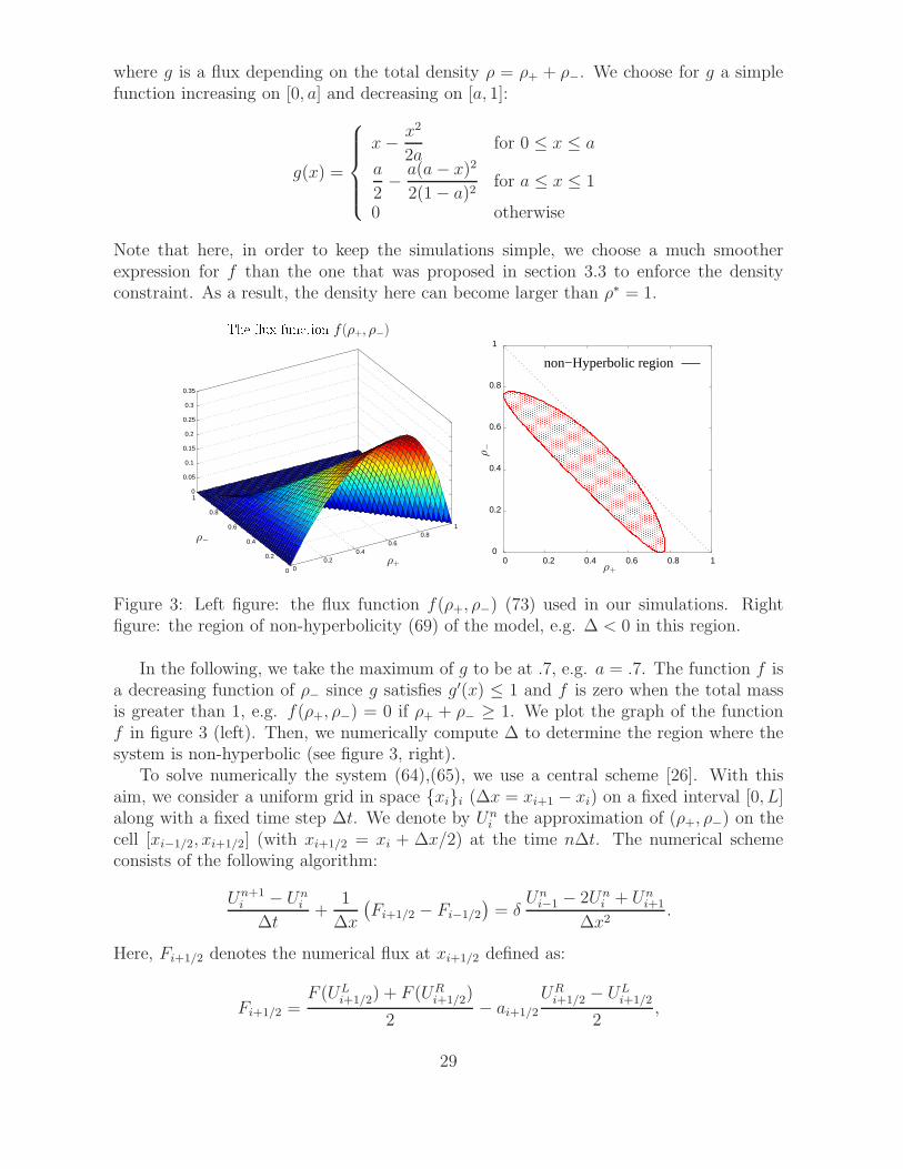
where g is a flux depending on the total density ρ = ρ+ + ρ−. We choose for g a simplefunction increasing on [0, a] and decreasing on [a, 1]:

g(x) =

x− x2

2afor 0 ≤ x ≤ a

a

2− a(a− x)2

2(1− a)2for a ≤ x ≤ 1

0 otherwise

Note that here, in order to keep the simulations simple, we choose a much smootherexpression for f than the one that was proposed in section 3.3 to enforce the densityconstraint. As a result, the density here can become larger than ρ∗ = 1.

00.2

0.40.6

0.81

0

0.2

0.4

0.6

0.8

10

0.05

0.1

0.15

0.2

0.25

0.3

0.35

The �ux fun tion f (ρ+, ρ−)

ρ+

ρ−0

0.2

0.4

0.6

0.8

1

0 0.2 0.4 0.6 0.8 1��

��

non−Hyperbolic region

ρ−

ρ+

Figure 3: Left figure: the flux function f(ρ+, ρ−) (73) used in our simulations. Rightfigure: the region of non-hyperbolicity (69) of the model, e.g. ∆ < 0 in this region.

In the following, we take the maximum of g to be at .7, e.g. a = .7. The function f isa decreasing function of ρ− since g satisfies g′(x) ≤ 1 and f is zero when the total massis greater than 1, e.g. f(ρ+, ρ−) = 0 if ρ+ + ρ− ≥ 1. We plot the graph of the functionf in figure 3 (left). Then, we numerically compute ∆ to determine the region where thesystem is non-hyperbolic (see figure 3, right).

To solve numerically the system (64),(65), we use a central scheme [26]. With thisaim, we consider a uniform grid in space {xi}i (∆x = xi+1 − xi) on a fixed interval [0, L]along with a fixed time step ∆t. We denote by Un

i the approximation of (ρ+, ρ−) on thecell [xi−1/2, xi+1/2] (with xi+1/2 = xi + ∆x/2) at the time n∆t. The numerical schemeconsists of the following algorithm:

Un+1i − Un

i

∆t+

1

∆x

(

Fi+1/2 − Fi−1/2

)

= δUni−1 − 2Un

i + Uni+1

∆x2.

Here, Fi+1/2 denotes the numerical flux at xi+1/2 defined as:

Fi+1/2 =F (UL

i+1/2) + F (URi+1/2)

2− ai+1/2

URi+1/2 − UL

i+1/2

2,

29

where F is the flux of the system F (ρ+, ρ−) = (f(ρ+, ρ−),−f(ρ−, ρ+))T , the vectors UL

i+1/2

and URi+1/2 are respectively the left and right value of (ρ+, ρ−) at xi+1/2 computed using a

MUSCL scheme [27] and ai+1/2 is the maximum eigenvalues (36) of the system at xi andxi+1:

ai+1/2 = max(|λ±i |, |λ±

i+1|).As initial condition, we use a uniform stationary state (ρ+, ρ−) perturbed by stochasticnoise:

ρ+(0, x) = ρ+ + σǫ+(x) , ρ−(0, x) = ρ− + σǫ−(x),

with ǫ+(x) and ǫ−(x) two independent white noises and σ the standard deviation of thenoise. We use periodic boundary condition for our simulations. The parameters of oursimulations are the following: space mesh ∆x = 1, time step ∆t = .2 (CFL= .406),diffusion coefficient δ = .4 and standard deviation of the noise σ = 10−2. We use periodicboundary conditions.

To illustrate our numerical scheme, we use three different initial conditions. First, wepick two values for (ρ+, ρ−) in the hyperbolic region:

ρ+ = .35 , ρ− = .3.

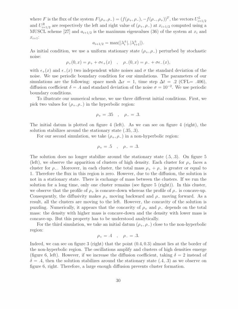
The initial datum is plotted on figure 4 (left). As we can see on figure 4 (right), thesolution stabilizes around the stationary state (.35, .3).

For our second simulation, we take (ρ+, ρ−) in a non-hyperbolic region:

ρ+ = .5 , ρ− = .3.

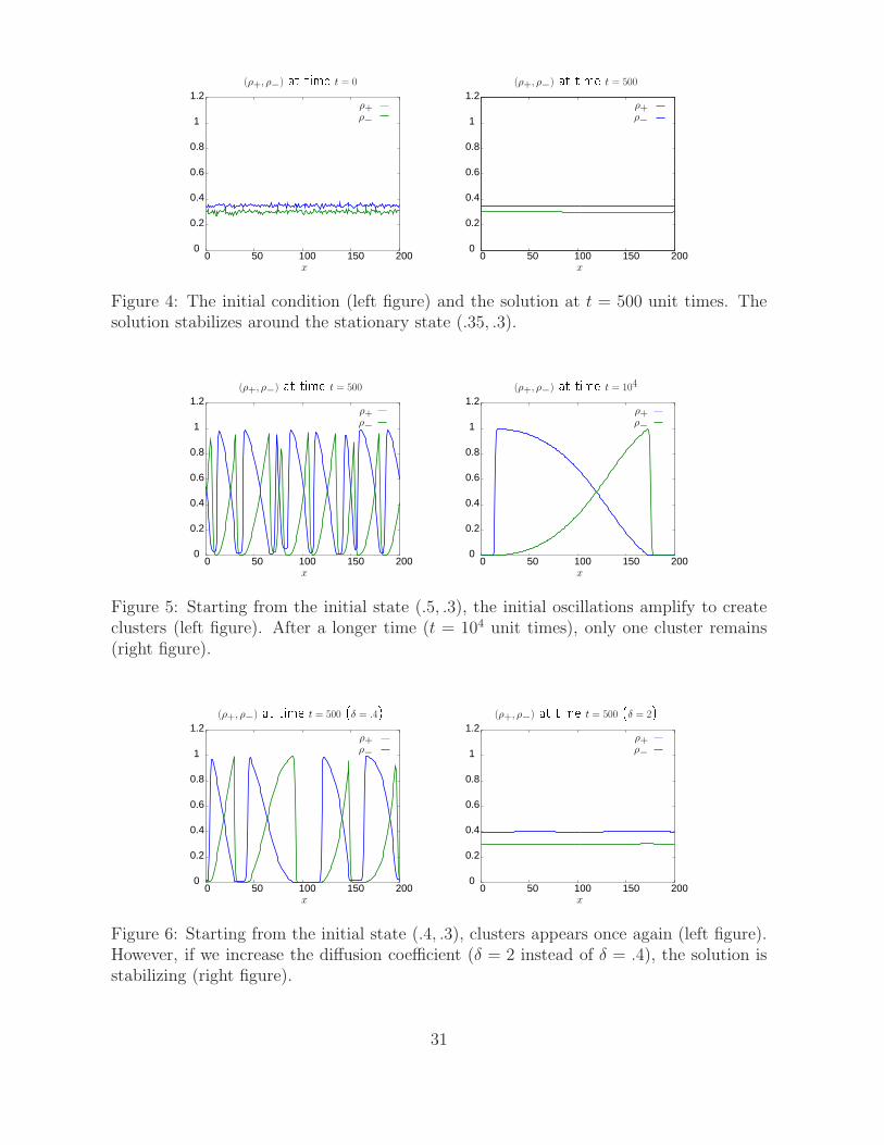
The solution does no longer stabilize around the stationary state (.5, .3). On figure 5(left), we observe the apparition of clusters of high density. Each cluster for ρ+ faces acluster for ρ−. Moreover, in each cluster, the total mass ρ+ + ρ− is greater or equal to1. Therefore the flux in this region is zero. However, due to the diffusion, the solution isnot in a stationary state. There is exchange of mass between the clusters. If we run thesolution for a long time, only one cluster remains (see figure 5 (right)). In this cluster,we observe that the profile of ρ+ is concave-down whereas the profile of ρ− is concave-up.Consequently, the diffusivity makes ρ+ moving backward and ρ− moving forward. As aresult, all the clusters are moving to the left. However, the concavity of the solution ispuzzling. Numerically, it appears that the concavity of ρ+ and ρ− depends on the totalmass: the density with higher mass is concave-down and the density with lower mass isconcave-up. But this property has to be understood analytically.

For the third simulation, we take an initial datum (ρ+, ρ−) close to the non-hyperbolicregion:

ρ+ = .4 , ρ− = .3.

Indeed, we can see on figure 3 (right) that the point (0.4, 0.3) almost lies at the border ofthe non-hyperbolic region. The oscillations amplify and clusters of high densities emerge(figure 6, left). However, if we increase the diffusion coefficient, taking δ = 2 instead ofδ = .4, then the solution stabilizes around the stationary state (.4, .3) as we observe onfigure 6, right. Therefore, a large enough diffusion prevents cluster formation.

30

0

0.2

0.4

0.6

0.8

1

1.2

0 50 100 150 200

(ρ+, ρ−) at time t = 0

ρ+ρ−

x

0

0.2

0.4

0.6

0.8

1

1.2

0 50 100 150 200

(ρ+, ρ−) at time t = 500

ρ+ρ−

x

Figure 4: The initial condition (left figure) and the solution at t = 500 unit times. Thesolution stabilizes around the stationary state (.35, .3).

0

0.2

0.4

0.6

0.8

1

1.2

0 50 100 150 200

(ρ+, ρ−) at time t = 500

ρ+ρ−

x

0

0.2

0.4

0.6

0.8

1

1.2

0 50 100 150 200

(ρ+, ρ−) at time t = 104

ρ+ρ−

x

Figure 5: Starting from the initial state (.5, .3), the initial oscillations amplify to createclusters (left figure). After a longer time (t = 104 unit times), only one cluster remains(right figure).

0

0.2

0.4

0.6

0.8

1

1.2

0 50 100 150 200

(ρ+, ρ−) at time t = 500 (δ = .4)ρ+ρ−

x

0

0.2

0.4

0.6

0.8

1

1.2

0 50 100 150 200

(ρ+, ρ−) at time t = 500 (δ = 2)ρ+ρ−

x

Figure 6: Starting from the initial state (.4, .3), clusters appears once again (left figure).However, if we increase the diffusion coefficient (δ = 2 instead of δ = .4), the solution isstabilizing (right figure).

31

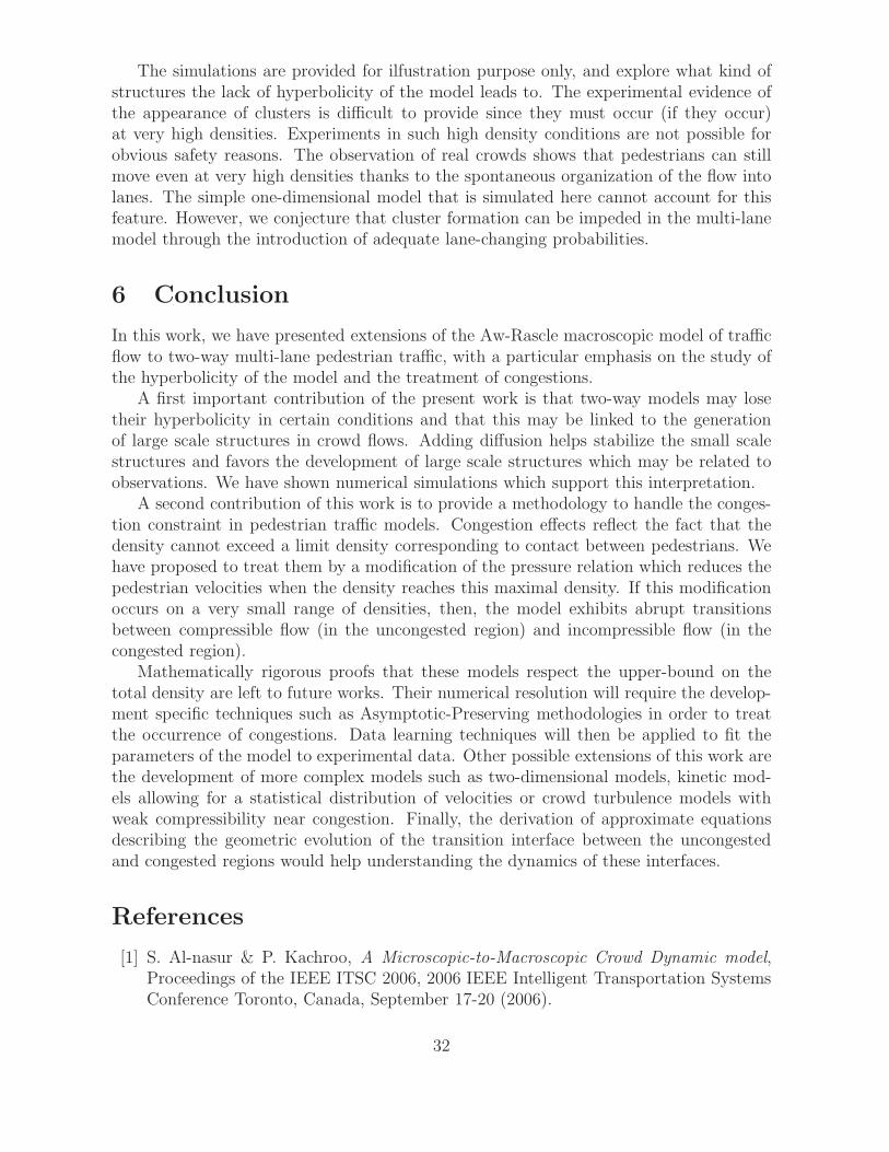
The simulations are provided for ilfustration purpose only, and explore what kind ofstructures the lack of hyperbolicity of the model leads to. The experimental evidence ofthe appearance of clusters is difficult to provide since they must occur (if they occur)at very high densities. Experiments in such high density conditions are not possible forobvious safety reasons. The observation of real crowds shows that pedestrians can stillmove even at very high densities thanks to the spontaneous organization of the flow intolanes. The simple one-dimensional model that is simulated here cannot account for thisfeature. However, we conjecture that cluster formation can be impeded in the multi-lanemodel through the introduction of adequate lane-changing probabilities.

6 Conclusion

In this work, we have presented extensions of the Aw-Rascle macroscopic model of trafficflow to two-way multi-lane pedestrian traffic, with a particular emphasis on the study ofthe hyperbolicity of the model and the treatment of congestions.

A first important contribution of the present work is that two-way models may losetheir hyperbolicity in certain conditions and that this may be linked to the generationof large scale structures in crowd flows. Adding diffusion helps stabilize the small scalestructures and favors the development of large scale structures which may be related toobservations. We have shown numerical simulations which support this interpretation.

A second contribution of this work is to provide a methodology to handle the conges-tion constraint in pedestrian traffic models. Congestion effects reflect the fact that thedensity cannot exceed a limit density corresponding to contact between pedestrians. Wehave proposed to treat them by a modification of the pressure relation which reduces thepedestrian velocities when the density reaches this maximal density. If this modificationoccurs on a very small range of densities, then, the model exhibits abrupt transitionsbetween compressible flow (in the uncongested region) and incompressible flow (in thecongested region).

Mathematically rigorous proofs that these models respect the upper-bound on thetotal density are left to future works. Their numerical resolution will require the develop-ment specific techniques such as Asymptotic-Preserving methodologies in order to treatthe occurrence of congestions. Data learning techniques will then be applied to fit theparameters of the model to experimental data. Other possible extensions of this work arethe development of more complex models such as two-dimensional models, kinetic mod-els allowing for a statistical distribution of velocities or crowd turbulence models withweak compressibility near congestion. Finally, the derivation of approximate equationsdescribing the geometric evolution of the transition interface between the uncongestedand congested regions would help understanding the dynamics of these interfaces.

References

[1] S. Al-nasur & P. Kachroo, A Microscopic-to-Macroscopic Crowd Dynamic model,Proceedings of the IEEE ITSC 2006, 2006 IEEE Intelligent Transportation SystemsConference Toronto, Canada, September 17-20 (2006).

32

[2] A. Aw, A. Klar, A. Materne, M. Rascle, Derivation of continuum traffic flow modelsfrom microscopic follow-the-leader models, SIAM J. Appl. Math., 63 (2002), 259–278.MR1952895 (2003m:35148)

[3] A. Aw, M. Rascle, Resurrection of second order models of traffic flow, SIAM J. Appl.Math., 60 (2000), 916–938. MR1750085 (2001a:35111)

[4] N. Bellomo, C. Dogbe, On the modelling crowd dynamics: from scaling to secondorder hyperbolic macroscopic models, Math. Models Methods Appl. Sci., 18 (2008),1317–1345. MR2438218 (2009g:92074)

[5] S. Benzoni-Gavage, R. M. Colombo, An n-populations model for traffic flow, Euro-pean J. Appl. Math., 14 (2003), 587–612. MR2020123 (2004k:90018)

[6] F. Berthelin, P. Degond, M. Delitala, M. Rascle, A model for the formation andevolution of traffic jams, Arch. Rat. Mech. Anal., 187 (2008), 185–220. MR2366138(2008h:90022)

[7] F. Berthelin, P. Degond, V. Le Blanc, S. Moutari, J. Royer, M. Rascle, A Traffic-Flow Model with Constraints for the Modeling of Traffic Jams, Math. Models MethodsAppl. Sci., 18, Suppl. (2008), 1269-1298. MR2438216 (2010f:35233)

[8] F. Bouchut, Y. Brenier, J. Cortes, J. F. Ripoll, A hierachy of models for two-phaseflows, J. Nonlinear Sci., 10 (2000), 639–660. MR1799394 (2001j:76109)

[9] C. Burstedde, K. Klauck, A. Schadschneider, J. Zittarz, Simulation of pedestriandynamics using a 2-dimensional cellular automaton, Physica A, 295 (2001), 507–525. arXiv:cond-mat/0102397

[10] C. Chalons, Numerical approximation of a macroscopic model of pedestrian flows,SIAM J. Sci. Comput., 29 (2007), 539–555. MR2306257 (2008a:35188)

[11] R. M. Colombo, M. D. Rosini, Pedestrian flows and nonclassical shocks, Math. Meth-ods Appl. Sci., 28 (2005), 1553–1567. MR2158218 (2006b:90009)

[12] C. Daganzo, Requiem for second order fluid approximations of traffic flow, Transp.Res. B, 29 (1995), 277–286.

[13] P. Degond, M. Delitala, Modelling and simulation of vehicular traffic jam formation,Kinet. Relat. Models, 1 (2008), 279–293. MR2393278 (2009a:90022)

[14] P. Degond, J. Hua, L. Navoret, Numerical simulations of the Euler system withcongestion constraint, preprint. arXiv:1008.4045

[15] P. Degond, M. Tang, All speed scheme for the low Mach number limit of the IsentropicEuler equations, Commun. Comput. Phys., 10 (2011), 1-31. arXiv:0908.1929

[16] R. Y. Guo, H. J. Huang, A mobile lattice gas model for simulating pedestrian evacu-ation, Physica A, 387 (2008), 580–586.

33

[17] S. J. Guy, J. Chhugani, C. Kim, N. Satish, M. C. Lin, D. Manocha, P. Dubey,Clearpath: Highly parallel collision avoidance for multi-agent simulation, in ACMSIGGRAPH/Eurographics Symposium on Computer Animation (SCA), pp. 177–187(2009).

[18] D. Helbing, A mathematical model for the behavior of pedestrians, Behavioral Science,36 (1991), 298–310.

[19] D. Helbing, A fluid dynamic model for the movement of pedestrians, Complex Sys-tems, 6 (1992), 391–415.

[20] D. Helbing, P. Molnar, Social force model for pedestrian dynamics, Physical ReviewE, 51 (1995), 4282–4286.

[21] D. Helbing, P. Molnar, Self-organization phenomena in pedestrian crowds in: F.Schweitzer (ed.) Self-Organization of Complex Structures: From Individual to Col-lective Dynamics, pp. 569–577, Gordon and Breach, London (1997).

[22] L. F. Henderson, On the fluid mechanics of human crowd motion, TransportationResearch, 8 (1974), 509–515.

[23] S. Hoogendoorn, P. H. L. Bovy, Simulation of pedestrian flows by optimal control anddifferential games, Optimal Control Appl. Methods, 24 (2003), 153–172. MR1988582(2004d:93088)

[24] R. L. Hughes, A continuum theory for the flow of pedestrians, Transportation Re-search B, 36 (2002), 507–535.

[25] R. L. Hughes, The flow of human crowds, Ann. Rev. Fluid Mech., 35 (2003), 169–182.

[26] A. Kurganov, E. Tadmor, New high-resolution central schemes for nonlinear con-servation laws and convection-diffusion equations, J. Comput. Phys., 160 (2000),240–282. MR1763829 (2001c:65102)

[27] R. J. LeVeque, ”Finite volume methods for hyperbolic problems”, Cambridge Uni-versity Press (2002).

[28] M. J. Lighthill, J. B. Whitham, On kinematic waves. I: flow movement in long rivers.II: A theory of traffic flow on long crowded roads, Proc. Roy. Soc., A229 (1955), 281–345. MR0072605 (17,309e) and MR0072606 (17,310a).

[29] B. Maury, A. Roudneff-Chupin, F. Santambrogio, A macroscopic crowd motion modelof gradient flow type, Math. Models Methods Appl. Sci., 20 (2010), 1787–1821.MR2735914

[30] B. Maury, J. Venel, A mathematical framework for a crowd motion model, C. R.Acad. Sci. Paris, Ser. I, 346 (2008), 1245–1250. MR2473301 (2009m:91150)

34

[31] K. Nishinari, A. Kirchner, A. Namazi, A. Schadschneider, Extended floor field CAmodel for evacuation dynamics, IEICE Transp. Inf. & Syst., E87-D (2004), 726–732.arXiv:cond-mat/0306262

[32] J. Ondrej, J. Pettre, A-H. Olivier, S. Donikian, A synthetic-vision based steeringapproach for crowd simulation, in SIGGRAPH ’10 (2010).

[33] S. Paris, J. Pettre, S. Donikian, Pedestrian reactive navigation for crowd simulation:a predictive approach, Eurographics, 26 (2007), 665–674.

[34] Pedigree team, Pedestrian flow measurements and analysis in an annular setup, inpreparation.

[35] J. Pettre, J. Ondrej, A-H. Olivier, A. Cretual, S. Donikian, Experiment-based mod-eling, simulation and validation of interactions between virtual walkers, in SCA ’09:Proceedings of the 2009 ACM SIGGRAPH/Eurographics Symposium on ComputerAnimation, pp.189-198 (2009).

[36] B. Piccoli, A. Tosin, Pedestrian flows in bounded domains with obstacles, Contin.Mech. Thermodyn., 21 (2009), 85-107. arXiv:0812.4390

[37] B. Piccoli, A. Tosin, Time-evolving measures and macroscopic modeling of pedestrianflow, Arch. Ration. Mech. Anal., 199 (2010), 707–738. arXiv:0811.3383

[38] C. W. Reynolds, Steering behaviors for autonomous characters, in Proceedings ofGame Developers Conference 1999, San Jose, California, pp. 763-782 (1999).

[39] V. Shvetsov, D. Helbing, Macroscopic dynamics of multi-lane traffic, Phys. Rev. E59 (1999), 6328-6339. arXiv:cond-mat/9906430

[40] J. van den Berg, H. Overmars, Planning time-minimal safe paths amidst unpredictablymoving obstacles, Int. Journal on Robotics Research 27 (2008), 1274–1294.

[41] W. G. Weng, S. F. Shena, H. Y. Yuana, W. C. Fana, A behavior-based model forpedestrian counter flow, Physica A 375 (2007), 668–678.

[42] M. Zhang, A non-equilibrium traffic model devoid of gas-like behavior, TransportationRes. B 36 (2002), 275–290.

35

Two-way multi-lane traffic model for pedestrians in corridors

Documents