Two-Stage Financial Risk Tolerance Assessment - Imperial College

Journal of Banking and Finance

Manuscript Draft

Manuscript Number: 08-2011

Title: Two-Stage Financial Risk Tolerance Assessment Using Data Envelopment Analysis

Article Type: Full Length Article

Keywords: Data Envelopment Analysis; Financial risk tolerance; Risk assessment; "Know your client" rule;

Questionnaire

Abstract: Typical questionnaires administered by financial advisors to assess financial risk tolerance are

embedded with stereotypes, have seemingly unscientific scoring approaches and mostly treat risk as a one-

dimensional concept. In this work, a novel tool was developed to assess relative risk tolerance using Data

Envelopment Analysis (DEA). It is essentially a questionnaire that characterizes risk by its five distinct

elements: propensity, attitude, capacity, knowledge, and time horizon. Results from surveying over 180

individuals and analysis using the Slacks-based measure type of DEA efficiency models show that the

multidimensionality of risk must be considered for complete assessment of risk tolerance. This approach

provides insight into the relationship between risk, its elements and other variables. In particular, the

perception of risk varies by gender. The tool could ultimately serve as a "risk calculator" which might provide

legal compliance to the "Know Your Client" rule that exists for Canadian financial institutions and their

advisors.

This paper is being submitted for the special issue of the Journal of Banking and Finance, “Performance Measurement in the Financial Services Sector: Frontier Efficiency Methodologies and Other Innovative Techniques.” The special issue will be based on papers presented at the JBF conference of the same name being held in London on July 4-5, 2008.

Two-Stage Financial Risk Tolerance Assessment Using Data Envelopment Analysis

Abstract Typical questionnaires administered by financial advisors to assess financial risk

tolerance are embedded with stereotypes, have seemingly unscientific scoring approaches and mostly treat risk as a one-dimensional concept. In this work, a novel tool was developed to assess relative risk tolerance using Data Envelopment Analysis (DEA). It is essentially a questionnaire that characterizes risk by its five distinct elements: propensity, attitude, capacity, knowledge, and time horizon. Results from surveying over 180 individuals and analysis using the Slacks-based measure type of DEA efficiency models show that the multidimensionality of risk must be considered for complete assessment of risk tolerance. This approach provides insight into the relationship between risk, its elements and other variables. In particular, the perception of risk varies by gender. The tool could ultimately serve as a “risk calculator” which might provide legal compliance to the “Know Your Client” rule that exists for Canadian financial institutions and their advisors.

Manuscript - Angela Tran and Joseph ParadiClick here to view linked References

http://ees.elsevier.com/jbf/viewRCResults.aspx?pdf=1&docID=826&rev=0&fileID=3734&msid=5841998C-B98D-4E37-87FB-CDF683576C8C



Two-Stage Financial Risk Tolerance Assessment Using Data Envelopment Analysis

Angela T. Trana,*, Joseph C. Paradib,

a Centre for Management of Technology and Entrepreneurship, University of Toronto, 200 College Street, Toronto, Ontario, Canada M5S3E5

b Centre for Management of Technology and Entrepreneurship, University of Toronto, 200 College Street, Toronto, Ontario, Canada M5S3E5

July 18, 2008

___________________________________________________________________________ Abstract

Typical questionnaires administered by financial advisors to assess financial risk

tolerance are embedded with stereotypes, have seemingly unscientific scoring approaches and mostly treat risk as a one-dimensional concept. In this work, a novel tool was developed to assess relative risk tolerance using Data Envelopment Analysis (DEA). It is essentially a questionnaire that characterizes risk by its five distinct elements: propensity, attitude, capacity, knowledge, and time horizon. Results from surveying over 180 individuals and analysis using the Slacks-based measure type of DEA efficiency models show that the multidimensionality of risk must be considered for complete assessment of risk tolerance. This approach provides insight into the relationship between risk, its elements and other variables. In particular, the perception of risk varies by gender. The tool could ultimately serve as a “risk calculator” which might provide legal compliance to the “Know Your Client” rule that exists for Canadian financial institutions and their advisors.

JEL Classification: C61 ; G32 Keywords: Data Envelopment Analysis; Financial risk tolerance; Risk assessment; “Know your client” rule; Questionnaire ___________________________________________________________________________ * Corresponding author. Tel.: +1 416 978 6924; Fax: +1 416 978 3877. Email addresses: [email protected] (Angela T. Tran), [email protected] (Joseph C. Paradi).

2

1. Introduction

“Know Your Client” (KYC) rules mandate Canadian financial advisors to consider a client’s

personal circumstances, financial status, investment objectives and risk tolerance when

determining whether or not a financial transaction is suitable for such client. Of these factors,

financial risk tolerance is the most challenging to assess because it is unquantifiable. Intuitively,

“knowing a client” involves the establishment of a relationship between an advisor and an

investor through personal interviews. However, due to time constraints, advisors increasingly

deal with clients through the telephone and/or E-mails. Moreover, while the Internet allows the

financial services industry to offer investment services over the World Wide Web, it introduces a

paradoxical challenge: how do financial institutions comply with the KYC rule and assess risk

tolerance if investors do not interact with advisors?

Currently, risk tolerance assessment questionnaires are administered over the Internet or

in person by advisors who need to follow financial planning protocol and to comply with

fiduciary investment standards. These questionnaires help create a risk “profile” from which an

appropriate investment portfolio can be recommended. However, the value of these risk profiles

is debatable since questionnaires vary across institutions and do not provide a consistent profile

of the same client who may consequently receive different advice from advisors depending on

which test is used. This inconsistency – attributed to biases and stereotypes, invalid questions, a

disregard for psychometrics, and the treatment of risk as a one-dimensional concept – may

potentially expose an investor to unnecessary risk.

Although financial risk tolerance has been studied extensively, there is a lack of

consensus on its definition: the words “profile”, “attitude”, “capacity” and “tolerance” are often

used interchangeably. In theory, risk tolerance is a multidimensional concept consisting of five

3

key elements – propensity, attitude, capacity, knowledge, and time horizon – which all must be

individually assessed, and then combined to obtain a complete risk profile. To date, the

reliability and validity of so-called risk assessment questionnaires have suffered without a

universally-accepted definition of risk tolerance, resulting in misguided assessments that are

either incomplete (when different elements are collated) or incorrect (when one element, such as

capacity, is treated synonymously to tolerance). Moreover, advisors are inevitably influenced by

demographic stereotypes, many of which are embedded into these questionnaires. Research on

age, gender, income, etc., and their correlation with risk tolerance has yielded inconclusive

results, prompting the need for a better understanding of client demography and risk tolerance to

eliminate these biases.

Most questionnaires are in multiple choice form with the same scoring motif: each

possible answer to every question is assigned a score. Upon completion of a questionnaire, a

final risk score is generated by summing the scores of the selected answers for all the questions

and then interpreted by the advisor. For example, a lower score may indicate a risk averse

investor whereas a higher score might indicate a risk seeking investor. However, summation

without weights inappropriately treats collected data equally when the relationships across

questions (from which demographic and psychological variables are obtained) are unclear.

Addressing this mathematical simplicity, Ardehali et al. (2005) first used a nonparametric

linear programming technique called Data Envelopment Analysis (DEA) to compute “risk

tolerance scores” from data collected using a questionnaire created by a commercial firm,

ProQuest. DEA treated each response to each psychological question as one dimension of risk

tolerance without prior knowledge of the relationship between the questions. The results were

encouraging, but suggested that DEA would be an even more effective tool for obtaining a single

4

risk tolerance index when accompanied by a questionnaire specifically designed for analysis with

DEA, as ProQuest’s was not. In other words, the ideal questionnaire would have responses to

questions that are easily manipulated (scored) for pre-selected variables, each representing one

dimension of risk tolerance and thereby taking advantage of DEA’s mathematical strength.

The purpose of this work was to create a novel survey tool supported with DEA to assess

the relative risk tolerance of a group of investors objectively, validly and reliably: a

questionnaire that characterizes risk by five distinct elements. DEA generates risk tolerance

“scores” between 0 and 1 for each client, where the most aggressive investors are given a score

of 1, while all other clients are scored as fractions of the riskiest investors. In effect, this is the

first step towards developing a risk “calculator” software package for financial advisors (or Web-

based securities sales systems) to use in their everyday assessments which may offer solid

information on risk tolerance while satisfying the KYC rule.

2. Risk Tolerance

2.1. Mathematical Definitions of Risk

Taking on risk is the price of achieving returns: investors who prefer low risk and accept

lower returns are risk averse, while those who prefer high risk for possible greater returns are

aggressive risk takers. The simplest mathematical definition of risk is as an uncertainty of future

rates of return on investments, in terms of expected mean return E(x) and standard deviation σ:

∑=

=n

s

srspxE1

)()()( (2.1)

[ ]∑=

−=n

s

xEsrsp1

22 )()()(σ (2.2)

p(s) and r(s) are the probability of and rate of return for outcome s, respectively. When the

probability distribution is symmetric about the mean, σ is used as a measure of risk, reflecting

5

outcome volatility. However, it equally weights upside and downside potential, and rewards

consistency; an investment that consistently loses 3% every month can still earn a standard

deviation of zero, making it appear low risk. Thus, any measure of risk should reflect the threat

of asset erosion or falling short of one’s needs, as opposed to the average long-run or expected

payoff only.

Utility theory quantifies relative satisfaction gained from a particular level of wealth x.

Risk aversion can be expressed as a concave utility function U(x) such as Equation 2.3, while

risk seeking behaviour and risk neutrality can be described by convexity and linearity,

respectively. Note that R is an individual’s risk tolerance.

RxexU /1)( −−= (2.3)

Another representation of risk aversion was introduced by Pratt in 1964. A risk averse

individual with initial wealth W who is presented with an actuarially neutral gamble of z~ dollars

(i.e. 0)~( =zE and a small variance 2zσ ) has a risk premium π (Equation 2.4). U(W) is the

individual’s utility, absolute risk aversion is )()(

WUWU

′′′− and relative risk aversion is )(

)(WU

WUW′′′⋅− . The

reciprocal of relative risk aversion is the coefficient of relative risk tolerance )()(

WUWWU′′⋅

′−=θ .

⎟⎟⎠

⎞⎜⎜⎝

⎛′′′

−=)()(

21 2

WUWU

zσπ (2.4)

Since utility functions may not capture complicated psychological effects, Kahneman and

Tversky (1979) developed prospect theory to account for how individuals heuristically weigh

potential outcomes* x1, x2, … and their probabilities p1, p2, … (Equation 2.5).

)()()()()( 2211 xvpwxvpwxU += (2.5)

* Lower outcomes are losses and larger outcomes are gains.

6

w is a probability weighting function that incorporates the tendency of overreacting to small

probability events and underreacting to medium and large probabilities. The value function v

assigns a utility value to an outcome and is asymmetric about a reference point (v(0) = 0),

implying that risk tolerance level depends on whether the prospects are framed as either gains or

losses, and not on absolute value.

2.2. Risk Assessment with Questionnaires

The financial services industry administers questionnaires to assess a client’s risk tolerance

for two main advantages. First, while interviews provide a thorough assessment, advisors lack

the time required to build a significant relationship with their client and therefore find

convenience with questionnaires. Second, assessment by interview can be unreliable because it

is qualitative and generally unstructured with conclusions drawn from cognitive biases

(Roszkowski et al., 2005). Hence, a quantitative instrument, such as a questionnaire, allows a

more standardized and repeatable assessment, as well as the translation of observations into

numerical values. However, questionnaires vary across different financial institutions; Yook and

Everett (2003) reported that six “investor risk tolerance” questionnaires did not provide a

consistent picture of the same client who consequently received six different recommendations,

motivating the need for a reliable measure of risk tolerance.

2.3. Demography of Risk

Research on the demography of risk has yielded results which have either led to conflicting

conclusions or have challenged intuition. Inconsistencies can be attributed to the lack of

consensus on the definition of risk tolerance and choice of experimental methodology. Many

studies use census data collected by the Survey of Consumer Finances through which risk

7

tolerance is elicited from one question with four possible answers†. Despite its simplicity, the

response is treated as a score of risk tolerance and correlated with demographic variables using

various statistical methods. Table 2.1 summarizes the predictive effect of demographic variables

on risk tolerance.

Table 2.1: Demography of Risk Tolerance Demographic Variable Relationship with Risk Tolerance

Age Inconclusive Gender Greater for men Marital and Family Status Inconclusive Race and Ethnicity Inconclusive Investor Experience, Financial Knowledge and Education

Increases with experience, education, knowledge of risk and personal finance

Income and Wealth Increases with income and wealth

Occupation Greater for self-employed, higher ranked, professionals, and those in the private sector

Age: Some researchers have shown that financial risk tolerance decreases with age

because older individuals have less time to recover from any losses incurred from investments

(e.g. Bajtelsmit, 1996; Hallahan, 2004; Palsson, 1996; Riley, 1992; Sung, 1996) while others

have argued that it increases with age (e.g. Grable, 1998; Wang, 1997) since younger individuals

are likely limited by financial resources to endure short term losses.

Gender: Most, if not all, studies have shown that women are less risk tolerant than men

to degrees varying with situational context, framing and probabilities (e.g. Bajtelsmit, 1996;

Eckel, 2002; Grable, 1998; Grable 2000; Palsson, 1996; Roszkowski, 2005). It is unknown

whether this difference is an inherent characteristic in client gender or the effect of stereotyping

by advisors (e.g. Fehr-Duda, 2006; Roszkowski, 2005), or pronounced by other variables such as

† Which of the statements comes closest to the amount of financial risk that you and your (spouse/partner) are willing to take when you save or make investments?

1. Take substantial financial risks expecting to earn substantial returns; 2. Take above average financial risks expecting to earn above average returns; 3. Take average financial risks expecting to earn average returns; or 4. Not willing to take any financial risks.

8

age. For example, younger men are more risk tolerant than younger women, but older men are

less risk tolerant than older women (e.g. Chaulk, 2003; Grable, 1999).

Marital and Family Status: Although family transitions influence financial risk

tolerance, the effects of marital status and parenthood are uncertain. Some studies have reported

that single persons are more risk tolerant than those who are married (e.g. Hallahan, 2004; Sung,

1996), while others have argued the opposite (e.g. Roszkowski, 2004; Yao, 2005). Other

findings include: husbands being more risk tolerant than their wives; single men being more risk

tolerant than single women; younger married individuals being less risk tolerant than older single

individuals; and individuals with children being less risk tolerant than those without children,

although the number of dependents may be insignificant (e.g. Chaulk, 2003; Riley, 1992).

Race and Ethnicity: Generally, Whites are more risk tolerant than non-Whites (e.g. Sung,

1996), but this may depend on the degree of risk: Blacks and Hispanics are found to be 84% and

53%, respectively, as likely as Whites to take some risk, but are 1.3 times and 1.4 times,

respectively, more likely as Whites to accept substantial risk (Yao, 2005).

Investment Experience, Financial Knowledge and Education: Individuals with a higher

level of education, investment experience and financial knowledge are more likely to take

financial risk (e.g. Finke, 2003; Grable, 1998; Grable, 2000; Hallahan, 2004; Sung 1996).

Income, Wealth and Occupation: Greater wealth and income correlates with greater

financial risk tolerance as losses incurred from investments are more easily afforded (e.g. Finke,

2003; Grable, 2000; Hallahan, 2004; Riley, 1992). Those who are self-employed, working in the

private sector, professionals, and/or holding a higher ranking occupational status, are also more

risk tolerant (Quattlebaum, 1998).

9

2.4. Multidimensionality of Risk

In risk assessment, words such as “profile”, “attitude”, “capacity” and “tolerance” are often

used interchangeably, as if the only difference between them is semantic, possibly resulting in

erroneous conclusions. Cordell (2001) defines risk tolerance as a multidimensional entity with

four distinct elements: propensity, attitude, capacity and knowledge. Also, a client’s time

horizon is an influential factor. Hence, to determine an individual’s overall risk tolerance

completely, each component of risk (Figure 2.1) should be evaluated.

Attitude

Capacity

Propensity

Time Horizon

Knowledge

Attitude

Capacity

Propensity

Time Horizon

Knowledge

Figure 2.1: Multidimensionality of Risk as Adapted from Cordell (2001)

Advisors often review a client’s past financial activity to infer something about his/her

risk tolerance. Ratios associated with risk propensity include high-risk to low-risk investments,

liabilities to assets or income, and amount spent on gambling to annual salary. Risk attitude is

the “emotional” element, defined as the willingness to incur risk. Risk capacity refers to the

financial ability to incur risk and is influenced by age, dependents, income, net worth, and time

horizon. Finally, risk knowledge reflects on one’s understanding of the risk-return trade-off. It

is particularly important that overall risk tolerance remain differentiated from its elements in

cases where assessment is difficult (i.e. for those with the willingness to incur risk but not the

financial ability, or those with the financial ability to incur risk but not the willingness to do so).

10

3. Methodology

3.1. The New Questionnaire and Dataset Description

A new questionnaire (Appendix A) was designed specifically for post-processing with

Data Envelopment Analysis (DEA). It was created after a comprehensive review of

questionnaires from over 30 banks and financial advisor groups. Every question from each

questionnaire was analyzed, with those appropriate for DEA adopted or slightly modified. A

novel feature was the incorporation of the multidimensionality of risk through five separate

sections, each corresponding to an element of risk. As risk attitude was determined by subjective

psychological questions, possible responses were presented such that they could be scored using

the Likert scale. All other elements were mostly gauged by objective demographic questions

prompting for exact numerical values.

The questionnaire was successfully administered to 187 individuals from all over the

world. The data was biased towards males (58%) and the average age was 39 years old. The

majority was married or in a stable relationship (66%) and over 50% had no dependents. Over

70% had at least a University-level Bachelor’s degree, with a high mean income ($90,100) and

mean net worth ($331,800). Also, 71% were full-time workers, and while 82% reside in Canada,

only 47% were born in Canada with much immigration from Asia and Europe. Greater diversity

through a larger distribution would have mitigated biases in this sample; however, this sample

size was sufficient for DEA (the minimum is 72). Furthermore, the questionnaire was reviewed

by several financial institutions that agreed on its validity, but reliability tests have yet to be

completed.

11

3.2. Data Envelopment Analysis (DEA)

In 1978, Charnes, Cooper, and Rhodes published the first article on Data Envelopment

Analysis (DEA), a nonparametric fractional linear programming technique that can be used to

rank and compare the relative performance of decision making units (DMUs) operating under

comparable conditions. For each DMUo (o = 1, …, n), DEA computes an empirical efficiency

score oθ defined as the ratio of the sum s of weighted outputs (yr for r = 1, …, s) and the sum of

m weighted inputs (xi for i = 1, …, m) (Equation 3.1).

momoo

sosooo xvxvxv

yuyuyu++++++

=......

2211

2211θ (3.1)

Input weights vi (i = 1, …, m) and output weights ur (r = 1, …, s) are derived from the data such

that each DMU’s θ is maximized. Empirically efficient DMUs (with the highest observed

output for given level of inputs) form a piecewise linear efficient frontier and have a score of 1.

Inefficient DMUs have a score between 0 to 1 based on their distance to the frontier.

DEA was applied to risk tolerance assessment, utilizing certain aspects of Ardehali et al.’s

methodology (2005). Clients or investors were defined as DMUs with those most risk seeking

forming an empirical risk frontier. Inputs or risk inhibiting factors were defined as variables that

decrease one’s ability or willingness to take risk while outputs or risk enabling factors were

defined as variables that increase one’s ability or willingness to take risk. Thus, individuals with

a “risk score” of 1 exhibited risk seeking behaviour while all others were less risky and scored as

fractions of the riskiest investors.

3.3. Slacks-Based Measure of Efficiency Model

The data collected from the questionnaire was analyzed with non-oriented Slacks-based

measure of efficiency (SBM) models (Equation 3.2) to capture the effect of slacks (all

12

inefficiencies) in the scores produced. The SBM efficiency score ]1,0[∈ρ is a ratio of the

average relative input consumption to the average relative output production (Charnes, 1994).

However, because SBM can only handle semi-positive data and is not translation invariant, some

data had to be scaled and categorized into one of 5 or 10 equal intervals. Furthermore, constant

returns-to-scale was selected for all models since in this context, DEA compared behaviours of

individuals essentially making a personal multicriteria decision about risk.

10Where)...,,1(0

)...,,1(0

)...,,1(0

)...,,1(

)...,,1( Subject to

/11

/11Minimize

1

1

1

1

≤≤=≥

=≥

=≥

==−

==+

+

−=

+

−

+

=

−

=

=

+

=

−

∑

∑

∑

∑

o

r

i

j

rorj

n

jrj

ioi

n

jjij

s

rror

m

iioi

o

srs

mis

njλ

srysy

mixsx

yss

xsm

ρ

λ

λ

ρ

(3.2)

Above, j is the index for n individuals; i is the index for m risk inhibitors; r is the index for

s risk enablers; xij represents the value that individual j has specified for risk inhibitor i; yrj

represents the value that individual j has specified for risk enabler r; −is is the amount individual

o exceeds the value of risk inhibitor i relative to its riskiest peers; +rs is the amount individual o

is short on the value of risk enabler r relative to its riskiest peers; jλ is the weight of individual j

as a peer for individual o; and oρ is the risk score for individual o.

13

3.4. Two-Stage DEA Model

The data collected from the questionnaire was manipulated for desired variables applicable

to five DEA SBM models, one corresponding to each element of risk (Table 3.1). Variables

were selected based on a literature survey which provided information about whether to treat

them as inhibitors (which decrease the ability to take risk) or enablers (which increase the ability

to take risk).

Table 3.1: Variables of Elements 1. Propensity 3. Attitude

Variable Type Variable Type Liabilities-to-Assets Ratio Enabler 13 Psychological Questions Enabler Liabilities-to-Income Ratio Enabler 4. Knowledge

2. Capacity Variable Type Variable Type Knowledge of Financial Markets Enabler Liabilities-to-Assets Ratio Inhibitor Investment Experience Enabler Liabilities-to-Income Ratio Inhibitor Understanding of Risk-Return Trade-off Enabler Net Worth = Assets – Liabilities Enabler 5. Time Horizon Income Enabler Variable Type Number of Dependents Inhibitor Time Horizon Enabler Education Enabler Age Inhibitor

Initially for the first stage of analysis, five DEA scores (one for each element) were to be

generated for each client. However, as time horizon and knowledge are not influenced by other

elements and have one and three variables, respectively, the variables of these two elements were

merged with variables in the Attitude, Capacity and Propensity models (Figure 3.1). Ultimately,

three element scores were generated for each respondent. Each score is relative, ranging from 0

to 1, and indicates how a client relates in that particular element compared to all other clients;

that is, a score of 0 would suggest that a client is not in agreement with that element while a

score of 1 would suggest full agreement. For example, scores of 0.5 and 0.9 for capacity and

attitude, respectively, would imply that a client’s financial ability to incur risk is moderate, while

his/her willingness to incur monetary risk is high compared to all other clients in the dataset.

14

Attitude+ Knowledge

Propensity+ Knowledge

Capacity+ Time Horizon

+ Knowledge

MergingElements

Attitude

Capacity

Propensity

Time Horizon

Knowledge

Attitude+ Knowledge



+ Knowledge

Attitude+ Knowledge



+ Knowledge

MergingElements

Attitude

Capacity

Propensity

Time Horizon

Knowledge

Attitude

Capacity

Propensity

Time Horizon

Knowledge

Figure 3.1: Knowledge and Time Horizon merged with Attitude, Capacity and Propensity Models

A second stage of analysis was conducted to examine the multidimensionality of risk and

the effect of each element on overall risk tolerance (Figure 3.2). Essentially, once the Attitude,

Capacity and Propensity scores were computed for each client, they were encompassed into one

model to generate a final risk tolerance score between 0 and 1 for each client; the riskiest

investors were given a score of 1, while all others scored less than 1.

First Stage Second Stage

Attitude Score

Capacity Score

Propensity Score Final Risk Tolerance Score

Variables calculated from data collected

from the questionnaire are

used as inputs (inhibitors) and

outputs (enablers)

elementscores

treated as outputs

Attitude Model

Capacity Model

Propensity Model

Modelencompassing all elements

First Stage Second Stage

Attitude Score

Capacity Score

Propensity Score Final Risk Tolerance Score

Variables calculated from data collected

from the questionnaire are

used as inputs (inhibitors) and

outputs (enablers)

elementscores

treated as outputs

Attitude Model

Capacity Model

Propensity Model

Modelencompassing all elements

Figure 3.2: Two-Stage DEA Model for Risk Tolerance

4. Results and Discussion

4.1. First Stage Models

Table 4.1 presents the results of SBM DEA models of the first stage.

Table 4.1: First Stage Models Model Individuals on the Frontier Average Score Median Minimum

Attitude 15 of 187 0.567 ± 0.168 0.534 0.262 Capacity 43 of 187 0.492 ± 0.318 0.361 0.087 Propensity 7 of 187 0.506 ± 0.197 0.441 0.25

The Attitude Model identifies 15 respondents as the most willing to incur monetary risk,

consequently assigning these individuals with a risk attitude score of 1. They generally have a

15

greater knowledge of financial markets and understanding of risk-return trade-off (which are the

best determinants of risk attitude with correlation coefficients of 0.75 and 0.64), investing

experience, mean income and net worth, compared to the rest of the sample. Also, they have a

smaller liabilities-to-assets ratio, less formal education, and are more likely married. Moreover,

correlation coefficients reveal that the psychological questions used are appropriate and equally

important to assessing attitude.

The Capacity Model identifies 43 respondents as having the greatest financial ability to

incur risk relative to the entire sample, giving these individuals a risk capacity score of 1. They

have a greater average income, net worth and investing experience, and are less likely to have

dependents and liabilities.

The Propensity Model identifies 7 respondents as having the greatest tendency to take

risk based on their past financial decisions, assigning these individuals with a risk propensity

score of 1. They have a substantially higher net worth, income and investing experience, and are

likely older, married, with dependents and have less liabilities. The liabilities ratios are the

strongest determinants of risk propensity, followed by knowledge of financial markets with

coefficients of 0.67, 0.77 and 0.56, respectively.

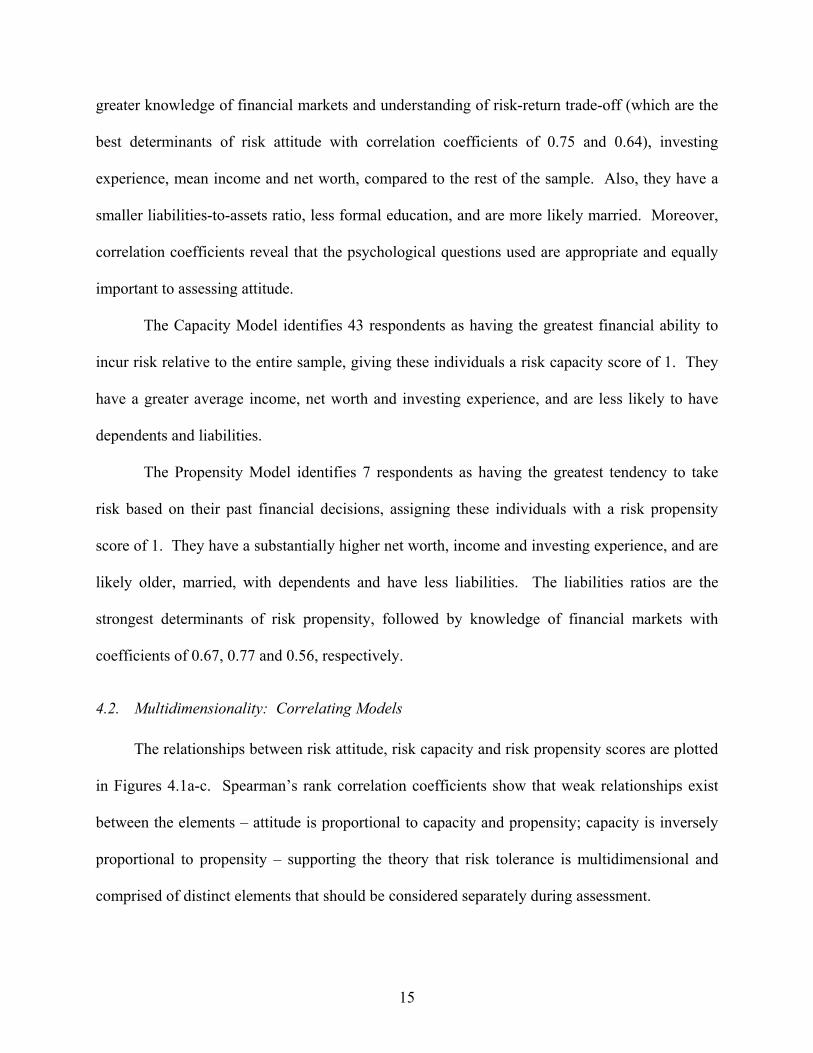
4.2. Multidimensionality: Correlating Models

The relationships between risk attitude, risk capacity and risk propensity scores are plotted

in Figures 4.1a-c. Spearman’s rank correlation coefficients show that weak relationships exist

between the elements – attitude is proportional to capacity and propensity; capacity is inversely

proportional to propensity – supporting the theory that risk tolerance is multidimensional and

comprised of distinct elements that should be considered separately during assessment.

16

a) ρ = 0.341

0

0.2

0.4

0.6

0.8

1

0 0.2 0.4 0.6 0.8 1

Attitude Score

Cap

acity

Sco

re

b) ρ = 0.505

0

0.2

0.4

0.6

0.8

1

0 0.2 0.4 0.6 0.8 1

Attitude Score

Prop

ensi

ty S

core

c) ρ = -0.136

0

0.2

0.4

0.6

0.8

1

0 0.2 0.4 0.6 0.8 1

Capacity Score

Prop

ensi

ty S

core

Figure 4.1: a) Risk Attitude and Risk Capacity; b) Risk Attitude and Risk Propensity; c) Risk Capacity and Risk Propensity

4.3. Second Stage Model

After observing the multidimensionality, attitude, capacity, and propensity scores were

used as “outputs” in another SBM DEA model, to generate an all-encompassing risk tolerance

score for each individual. This Second Stage Model identifies 3 of 187 respondents as the most

overall risk tolerant investors, assigning them a final risk score of 1. The mean, median and

minimum final risk tolerance scores are 0.458 ± 0.157, 0.436 and 0.185, respectively.

While knowledge of financial markets and understanding of risk-return trade-off have

coefficients of 0.64 and 0.50, respectively, all other variables are weakly related to risk tolerance.

The riskiest respondents are much younger, without dependents and unexpectedly have a

substantially lower average income and net worth. Notably, these conclusions are based on the

characteristics of the three individuals only and hence, generalizing these is not advisable.

17

Question 14 of the questionnaire explains to each participant that the data collected will

compute to a final risk score between 0 (risk avoiding) and 100 (risk seeking), then prompts for a

guess of what this score will be. Forty-two women and 69 men assessed themselves as more risk

tolerant than shown by DEA whereas 37 women and 38 men assessed themselves as less risk

tolerant, implying that DEA tends to estimate risk tolerance conservatively. The discrepancy in

scores may also be due to precision: second stage scores are generated to 3 significant digits

whereas self-assessed scores are provided as an integer in intervals of fives or tens (i.e. one

significant digit).

4.4. Analysis of Risk Tolerance by Demography

Average risk attitude, risk capacity, risk propensity and risk tolerance of different

demographic groups by age, education, income, net worth, liabilities-to-assets ratio and

liabilities-to-income ratio, number of dependents, knowledge of financial markets, and

understanding of risk-return trade-off investment experience were examined.

Age: Figure 4.2 shows the average DEA scores for ten age ranges. Despite the

fluctuations, both risk attitude and risk tolerance (second stage) remain fairly constant, whereas

risk capacity decreases with age and risk propensity increases until a peak at approximately age

40 before declining.

Education: Figure 4.3 shows that average DEA scores increase with education.

Income and Net Worth: Figures 4.4 and 4.5 show the average DEA scores for ten income

brackets and ten net worth brackets, respectively. Fluctuations in the data make it difficult to

draw conclusions about their relationships to risk. However, it appears that all risk scores

increase with net worth and stay constant with income.

18

0.3

0.4

0.5

0.6

0.7

0 1 2 3 4 5 6 7 8 9 10

Age

Scor

e

Attitude Capacity Propensity Second Stage / Tolerance

Figure 4.2: Average Risk Scores by Age

1: Age ≤ 25; 2: 25 < Age ≤ 29.375; 3: 29.375 < Age ≤ 33.75; 4: 33.75 < Age ≤ 38.125;

5: 38.125 < Age ≤ 42.5; 6: 42.5 < Age ≤ 46.875; 7: 46.875 < Age ≤ 51.25; 8: 51.25 < Age ≤ 55.625;

9: 55.625 < Age ≤ 60; 10: Age > 60

0.2

0.3

0.4

0.5

0.6

0.7

0.8

1 2 3 4 5 6 7 8

Education Attained

Scor

e


Figure 4.3: Average Risk Scores by Education 1: Less than High School; 2: High School Degree or Equivalent;

3: Some College But No Degree; 4: Associate Degree; 5: Bachelor’s Degree;

6: Master’s Degree; 7: Doctorate; 8: Professional Degree

0.4

0.5

0.6

0.7

1 2 3 4 5 6 7 8 9 10

Income

Scor

e


Figure 4.4: Average Scores by Income

1: I ≤ $20000; 2: $20000 ≤ I < $42500; 3: $42500 ≤ I < $65000; 4: $65000 ≤ I < $87500;

5: $87500 ≤ I < $110000; 6: $110000 ≤ I < $132500; 7: $132500 ≤ I < $155000; 8: $155000 ≤ I < $177500;

9: $177500 ≤ I < $200000; 10: I ≥ $200000

0.2

0.4

0.6

0.8

1 2 3 4 5 6 7 8 9 10

Net Worth

Scor

e


Figure 4.5: Average Scores by Net Worth

1: NW ≤ $0; 2: $0 ≤ NW < $75000; 3: $75000 ≤ NW < $150000; 4: $150000 ≤ NW < $225000; 5: $225000 ≤ NW < $300000; 6: $300000 ≤ NW < $375000; 7: $375000 ≤ NW < $450000; 8: $450000 ≤ NW < $525000; 9: $525000 ≤ NW < $600000;

10: NW ≥ $600000

Liabilities-to-Assets and Liabilities-to-Income Ratios: Figures 4.6 and 4.7 show the

average DEA scores for five liabilities-to-asset ratio and liabilities-to-income ratio brackets,

respectively. Risk capacity and risk tolerance decrease with increasing liabilities-to-asset and

liabilities-to-income ratios, while both risk attitude and risk propensity scores increase.

Number of Dependents: Figure 4.8 shows the average DEA scores plotted against the

numbers of dependents. As expected, risk capacity and risk tolerance decreases with more

dependents, but unexpectedly risk attitude and risk propensity scores increase.

19

Investment Knowledge, Understanding and Experience: Figures 4.9 and 4.10 show the

average DEA scores for five levels of increasing knowledge of financial markets and five levels

of increasing understanding of risk-return trade-off, respectively, derived from the Likert scale.

Figure 4.11 shows the average DEA scores for five investment experience levels. As expected,

all risk scores increase with greater investment knowledge, understanding and experience.

0.3

0.4

0.5

0.6

0.7

0.8

1 2 3 4 5

Liabilities/Assets

Scor

e


Figure 4.6: Average Scores by

Liabilities-to-Asset Ratio 1: L/A ≤ 0.01; 2: 0.01 ≤ L/A < 0.34;

3: 0.34 ≤ L/A < 0.77; 4: 0.77 ≤ L/A < 1.0; 5: L/A ≥ 1.0

0.2

0.3

0.4

0.5

0.6

0.7

0.8

1 2 3 4 5

Liabilities/IncomeSc

ore


Figure 4.7: Average Scores by

Liabilities-to-Income Ratio 1: L/I ≤ 0.01; 2: 0.01 ≤ L/I < 0.84;

3: 0.84 ≤ L/I < 1.67; 4: 1.67 ≤ L/I < 2.5; 5: L/I ≥ 2.5

0.2

0.3

0.4

0.5

0.6

0.7

0 1 2 3

Number of Dependents

Scor

e


Figure 4.8: Average Risk Scores by

Number of Dependents

0.3

0.4

0.5

0.6

0.7

0.8

0.9

1 2 3 4 5

Knowledge of Financial Markets

Scor

e


Figure 4.9: Average Scores by Knowledge of

Financial Markets

20

0.3

0.4

0.5

0.6

0.7

0.8

0.9

1 2 3 4 5

Understanding of Risk-Return Trade-Off

Scor

e


Figure 4.10: Average Scores by Understanding of Risk-Return Trade-off

0.3

0.4

0.5

0.6

0.7

0.8

1 2 3 4 5

Investment Experience

Scor

e


Figure 4.11: Average Scores by Investment Experience

1: 0 ≤ Years < 8; 2: 8 ≤ Years < 16; 3: 16 ≤ Years < 24; 4: 24 ≤ Years < 32; 5: 32 ≤ Years ≤ 40

4.5. Differences in Gender

In all models, the majority of individuals that are identified as “riskiest” and therefore form

the risk frontier are men. Hence, women are consistently scored lower than men (Table 4.2).

While the discrepancy in risk attitude score is consistent with the literature, and there is only a

slight difference in risk propensity between genders, the difference in risk capacity is

unexpected, especially since in this sample, women with the greatest risk capacity also have a

higher income and net worth.

To determine whether risk is viewed differently by gender, all models were re-run to

accommodate men and women separately. Table 4.2 shows that all scores for women increased,

proving that there is an inherent difference in the way men and women perceive risk. Comparing

self-assessed scores to DEA scores generated in the model exclusive to women, 54 women

assessed themselves as less risk tolerant than shown by DEA while 24 women assessed

themselves as more risk tolerant. In the model exclusive to men, 66 men assessed themselves as

less risk tolerant than DEA suggests while 41 men assessed themselves as more risk tolerant.

These trends in risk aversion are consistent with the literature.

21

Table 4.2: Comparison of Scores by Gender Attitude Model

Individuals on the Frontier Average Score Median Minimum 15 of 187 0.567± 0.168 0.534 0.262 10 of 187 0.589 ± 0.170 0.549 0.310

All Men

Women 5 of 187 0.537 ± 0.163 0.514 0.262 Men only 10 of 108 0.589 ± 0.170 0.549 0.310 Women only 34 of 79 0.765 ± 0.224 0.719 0.330

Capacity Model Individuals on the Frontier Average Score Median Minimum

43 of 187 0.492 ± 0.318 0.361 0.09 27 of 187 0.521 ± 0.332 0.322 0.128

All Men


Propensity Model Individuals on the Frontier Average Score Median Minimum

7 of 187 0.506 ± 0.197 0.441 0.25 6 of 187 0.516 ± 0.194 0.455 0.25

All Men


Second Stage Model Individuals on the Frontier Average Score Median Minimum

3 of 187 0.458 ± 0.157 0.436 0.185 2 of 187 0.476 ± 0.165 0.446 0.185

All Men


5. Conclusion and Future Work

A novel questionnaire specifically designed for post-processing by Data Envelopment

Analysis (DEA) was created as a measurement tool for risk tolerance assessment. To

accommodate the demographic, socioeconomic and psychological nature of the data, the Slacks-

based measure of efficiency (SBM) models were selected to provide an all-encompassing final

risk score. The findings that arose from these DEA models are consistent with the literature;

hence, the use of this questionnaire as a method for risk assessment has proven to be feasible. In

particular, the incorporation of the multidimensionality of risk was successful and verified; risk

attitude, risk capacity, and risk propensity share a weak correlation with one another – implying

22

that these elements of risk rightfully be assessed separately. This work also offers insight into

the relationship between certain demographics and risk as summarized in Table 5.1.

Table 5.1: Effects of Selected Variables on Risk Tolerance and its Elements

Attitude Capacity Propensity Overall Risk Tolerance Age n/a - + to 40, - from 40 n/a Education + + + + Number of Dependents + -- + - Financial Status

Income n/a n/a n/a n/a Net worth + + + +

Liabilities-to-Assets + -- ++ - Liabilities-to-Income + -- ++ -

Financial Knowledge Of Markets ++ ++ ++ ++

Of Risk-Return Trade-off ++ ++ ++ ++ Investment Experience ++ ++ ++ ++

+: slight positive correlation; ++: strong positive correlation; -: slight negative correlation, --: strong negative correlation; n/a: undetermined or inconclusive

As expected, the best indicators for risk tolerance are those variables associated with

financial knowledge and understanding. Table 5.2 summarizes the average profile of those

determined “risky” by DEA relative to the entire sample.

Table 5.2: Average Profile of “Riskiest” Individuals as Determined by DEA Models

and by Comparison to The Entire Sample Attitude Capacity Propensity Overall Risk Tolerance

Age Older Younger Older Younger Education Less Same Less Less Marital Status Married Same Married Married Number of Dependents Same Less More Less Financial Status

Income Higher Higher Higher Lower Net worth Higher Higher Higher Lower

Liabilities-to-Assets Lower Lower Lower Same Liabilities-to-Income Higher Lower Lower Higher

Financial Knowledge Of Markets Greater Greater Same Greater

Of Risk-Return Trade-off Greater Greater Same Greater Investment Experience Greater Greater Greater Greater

While the characteristics of individuals with the greatest willingness to incur risk,

greatest capacity to take risk, and greatest tendency to take risk are expected, the average profile

of the individuals with “complete” risk tolerance is surprising, with respect to lower income and

23

net worth and greater liabilities. Furthermore, women were consistently found to be less risk

tolerant than men, suggesting that there is an inherent difference in the way men and women

perceive the concept of risk.

Finally, despite the need for a greater and more diverse sample, these results, which are

representative of high net worth individuals, are still extremely encouraging. This questionnaire

is likely to become the first of its kind to determine risk with multidimensionality, and logical

scientific and mathematical backing. This work significantly contributes to the construction of a

“risk calculator” that may be used by financial institutions for risk tolerance assessment. In fact,

software for this “risk calculator” is in development, generating risk scores for clients that can

then be used by advisors to recommend the appropriate investment portfolio. Ultimately, the risk

calculator can serve as a web-based evaluation system that could feed into automated securities

sales systems, and be a means to learn about risk and its trends.

Future research opportunities include: matching DEA generated scores to portfolios of

financial institutions; comparing relative DEA frontiers to a theoretical, absolute risk frontier;

establishing mathematical relationships between variables using multivariate analysis; and

imposing the Assurance Region (which limits the region of input and output weights to specific

ranges) to SBM instead of creating one’s own ranges and intervals.

Acknowledgements

The authors wish to thank Geoff Davey and Nicki Potts of FinaMetrica Pty Ltd., and Dr. Walter

Rosocha of Kingsway Wealth Management for their cooperation in this work.

24

Appendix A: Questionnaire * Copyright FinaMetrica Pty Ltd

PERSONAL INFORMATION Gender: Male Female Year of Birth: Place of Birth:

North America Central America South America Europe Australia/New Zealand

Middle East West or Central Asia East, South, Southeast Asia Africa Other

Country of Residence: Postal Code / Zip Code:

STATUS AND DEPENDENTS Personal Status:

Single Common-Law or de facto Relationship Married Divorced Widowed

Number of Dependent(s)‡: Dependent(s) Information:

Dependent Age Dependent Age 1 6 2 7 3 8 4 9 5 10

EDUCATION AND EMPLOYMENT

Highest Level of Education Attained: Less than High School High School Graduate or Equivalent Some College But No Degree Associate Degree Bachelor’s Degree Master’s Degree Professional School Degree (e.g. MD, LLB, JD, DDS, DVM) Doctorate (e.g. PhD, EdD, DrPH)

Employment Status: Full-time Part-time Self-employed (e.g. consultant) Business owner (working in the business) Retired Home-maker Student Unemployed

At what age do you plan to retire?

FINANCIAL INFORMATION AND STABILITY Annual Household Income Before Tax (Average over last 5 years from all sources: salary, investment income, pension or social security, etc.): $ Liquid Assets§: $

‡ Dependents are individuals that you are financially supporting or are responsible for.

25

Fixed Assets**: $

Outstanding Loans and Liabilities (Total Debt): $ Monthly Expenses: $ How much money do you gamble per month? (Include all types of gambling – lotteries, scratch tickets, casino, poker, sports gambling, etc.) $ Over the next 2-3 years, your income will be:

Very unstable Somewhat less stable than today As stable as today Somewhat more stable than today Very stable

KNOWLEDGE

Which statement best describes your investment knowledge? I have limited knowledge and rely exclusively on other sources (financial advisor, accountant, family, etc.). I understand basic investment principles but do not actively follow the financial markets. I have a general understanding of financial markets and follow their progress occasionally. I have a good working knowledge of financial markets and follow the markets actively. I have in-depth knowledge (which includes options and strategies), manage my own portfolio, and follow the

financial markets daily. How many years have you been investing?

UNDERSTANDING Understanding the relationship between risk and return (illustrated in graph below) is important in assessing one’s tolerance for risk. Low levels of risk are associated with low potential returns and low potential losses whereas high levels of risk are associated with high potential returns and high potential losses. In other words, taking on some risk is the price of achieving returns – if you want to make money, you cannot eliminate all risk. The goal is to find an appropriate balance: one that generates some return but still allows you to sleep at night. Where along this risk-return trade-off curve would you feel comfortable being on?

INVESTMENT OBJECTIVES AND TIME HORIZON

Please select your primary investment objective: Retirement Education Wealth accumulation Large purchase or down payment (for home, car, vacation, renovation) Other

§ Liquid assets are cash or securities that can quickly be converted into cash. E.g. money in savings and/or chequing accounts, stocks, bonds, etc. ** Fixed assets are physical items that cannot quickly be converted into cash. E.g. real estate, vehicles, collections, furniture, equipment, etc.

% Risk

% Return

Low RiskLow Return

High RiskHigh Return

A

B

CD E

More RiskMore Return

% Risk

% Return

Low RiskLow Return

High RiskHigh Return

A

B

CD E

More RiskMore Return

A B C D E

26

For how many years from now do you plan to invest towards reaching your objective (as selected above)? When (i.e. how many years from now) do you expect to begin withdrawing money from the cumulative funds in your primary investment? Once you begin withdrawing money from your primary investment, for how many years do you expect withdrawals to last?

FINANCIAL RISK ATTITUDE 1. *How much confidence do you have in your ability to make good financial decisions?

None A little A reasonable amount A great deal Complete

2. How do you feel about the following statement: “I can easily adapt to significant unexpected and unfavourable financial changes”?

Not applicable Disagree Slightly disagree Neither agree or disagree Slightly agree Agree

3. Which of the following best describes your attitude towards financial risk? A very low risk taker A low risk taker An average risk taker A high risk taker A very high risk taker

4. This graph shows the potential range of gains and losses on a per dollar basis of an investment in four hypothetical portfolios at the end of a one-year period. The number above each bar shows the best potential gain (in %) for that portfolio, while the number below each bar shows the worst potential loss (in %). With only this information, which portfolio would you choose to invest in?

Portfolio A Portfolio B Portfolio C Potfolio D

5. Realizing that any market-based investment may move up or down in value over time, with which of the portfolios below would you feel most comfortable? Note: The profiles shown below are over the same period.

Portfolio A Portfolio B Portfolio C

6.8% Overall Return 9.8% Overall Return 12.8% Overall Return

-40%-20%

0%20%40%60%

-40%-20%

0%20%40%60%

-40%-20%

0%20%40%60%

48.7

25.4

36.7

11.8

-2.5-10.1

-16.0-21.7

-30.0

-20.0

-10.0

0.0

10.0

20.0

30.0

40.0

50.0

60.0

Cha

nge

Per

Dol

lar

Per

Ann

um (%

)

Portfolio A Portfolio B Portfolio C Portfolio D

27

6. With which investment portfolio do you feel most comfortable? Portfolio Average Long-Term Annual Return Chance of Decline Over Any One Year

A 5% 10% B 9% 15% C 11% 20% D 20% 25%

7. All investment decisions involve the possibility of making money and a chance of losing all or a portion of the investment. When making an investment decision, which is more significant?

I would consider the potential loss first. I would consider the potential loss somewhat more than the potential gain. Both potential loss and gain are about the same to me. I would consider the potential gain somewhat more than the potential loss. I would consider the potential gain first.

8. You have just received a substantial sum of money. How would you invest it? In something that offers moderate current income and has low risk In something that offers high current income with moderate risk In something that offers high total return (current income plus capital appreciation) with moderately high

risk In something that offers substantial capital appreciation with very high risk I would not invest it.

9. *Which word comes to mind when you think of “financial risk”? Danger Uncertainty Indifference Opportunity Thrill

10. Compared to other people with the same financial and socioeconomic status, how would you rate your ability to tolerate the stress associated with important financial matters?

Very low Low Average High Very high

11. *Faced with a choice between greater job security with a small pay raise or a much higher pay raise but less job security, which would you select?

Definitely greater job security Probably greater job security Not sure Probably higher pay raise Definitely higher pay raise

12. *Imagine you have a job where you could choose to be paid a secure salary, a commission or a mix of the two. Which would you pick?

All salary Mainly salary Equal mix of salary and commission Mainly commission All commission

13. Assuming that you are investing for the long-term, how would you feel if the value of your portfolio dropped: a. 5%?

I cannot tolerate any loss. Very uncomfortable. I cannot tolerate this or any more loss. Quite uncomfortable. I can tolerate this drop but not any more loss. Somewhat uncomfortable. I can tolerate this drop and a little more loss. Comfortable. I can tolerate this loss and more.

This question continues on the next page...

28

b. 10%? Very uncomfortable. I cannot tolerate this or any more loss. Quite uncomfortable. I can tolerate this drop but not any more loss. Somewhat uncomfortable. I can tolerate this drop and a little more loss. Comfortable. I can tolerate this loss and more.

c. 15%? Very uncomfortable. I cannot tolerate this or any more loss. Quite uncomfortable. I can tolerate this drop but not any more loss. Somewhat uncomfortable. I can tolerate this drop and a little more loss. Comfortable. I can tolerate this loss and more.

d. 20%? Very uncomfortable. I cannot tolerate this or any more loss. Quite uncomfortable. I can tolerate this drop but not any more loss. Somewhat uncomfortable. I can tolerate this drop and a little more loss. Comfortable. I can tolerate this loss and more.

e. 25%? Very uncomfortable. I cannot tolerate this or any more loss. Quite uncomfortable. I can tolerate this drop but not any more loss. Somewhat uncomfortable. I can tolerate this drop and a little more loss. Comfortable. I can tolerate this loss and more.

f. 30%? Very uncomfortable. I cannot tolerate this or any more loss. Quite uncomfortable. I can tolerate this drop but not any more loss. Somewhat uncomfortable. I can tolerate this drop and a little more loss. Comfortable. I can tolerate this loss and more.

g. 40%? Very uncomfortable. I cannot tolerate this or any more loss. Quite uncomfortable. I can tolerate this drop but not any more loss. Somewhat uncomfortable. I can tolerate this drop and a little more loss. Comfortable. I can tolerate this loss and more.

h. 50%? Very uncomfortable. I cannot tolerate this or any more loss. Quite uncomfortable. I can tolerate this drop but not any more loss. Somewhat uncomfortable. I can tolerate this drop and a little more loss. Comfortable. I can tolerate this loss and more.

14. *The results of this questionnaire will be computed to yield a final “risk score” on a scale of 0 to 100. In

practice, however, the scores range from 20 to 80, with the average being 50. When the scores are graphed they follow the familiar bell-shaped curve of the Normal distribution (see below). About two-thirds of all scores are between 40 and 60.

What do you think your score will be? _______

0 2010 4030 50 807060 10090

Risk-AvoidingConservative

Risk-SeekingAggressive

Increasing Risk Score

Ave

rage

Ris

k Sc

ore

0 2010 4030 50 807060 100900 2010 4030 50 807060 10090

Risk-AvoidingConservative

Risk-SeekingAggressive

Increasing Risk Score

Ave

rage

Ris

k Sc

ore

29

References Ardehali, P.H., Paradi, J.C., Asmild, M., 2005. Assessing financial risk tolerance of portfolio investors using data

envelopment analysis. International Journal of Information Technology & Decision Making 4 (3), 491-519. Bajtelsmit, V.L., Bernasek, A., 1996. Why do women invest differently than men? Association for Financial

Counselling and Planning Education, 1-10. Charnes, A., Cooper, W.W., Rhodes, E.L., 1978. Measuring the efficiency of decision making units. European

Journal of Operational Research 2 (6), 429-444. Charnes, A., Cooper, W.W., Lewin, A.Y., Seiford, L.M., 1994. Data Envelopment Analysis: Theory, Methodology

and Applications. Kluwer Academic Publishers: Boston. Chaulk, B., Johnson, P.J., Bulcroft, R., 2003. Effects of marriage and children on financial risk tolerance: a

synthesis of family development and prospect theory. Journal of Family and Economic Issues 24 (3), 257-279. Cordell, D.M., 2001. RiskPACK: how to evaluate risk tolerance. Journal of Financial Planning 14 (6), 36-40. Eckel, C.C., Grossman, P.J., 2002. Sex differences and statistical stereotyping in attitudes toward financial risk.

Evolution and Human Behavior 23, 281-295. Finke, M.S., Huston, S.J., 2003. The brighter side of financial risk: financial risk tolerance and wealth. Journal of

Family and Economic Issues 24 (3), 233-256. Fehr-Duda, H., De Gennaro, M., Schubert R., 2006. Gender, financial risk and probability weights. Theory and

Decision 60, 283-313. Grable, J.E., Lytton R.H., 1998. Investor risk tolerance: testing the efficacy of demographics as differentiating and

classifying factors. Financial Counselling and Planning 9 (1), 61-74. Grable, J.E., Lytton R.H., 1999. Assessing financial risk tolerance: do demographic, socioeconomic and attitudinal

factors work? Family Relations and Human Development/Family Economics and Resource Management, 1-9. Grable, J.E., 2000. Financial risk tolerance and additional factors that affect risk taking in everyday money matters.

Journal of Business Psychology 14 (4), 625-630. Hallahan, T.A., Faff, R.W., McKenzie, M.D., 2004. An empirical investigation of personal financial risk tolerance.

Financial Services Review 13, 57-78. Kahneman, D., Tversky A., 1979. Prospect theory: an analysis of decision under risk. Econometrica 47 (2), 263-

292. Palsson, A., 1996. Does the degree of relative risk aversion vary with household characteristics? Journal of

Economic Psychology 17, 771-787. Pratt, J.W., 1964. Risk aversion in the small and in the large. Econometrica 41, 153-161. Quattlebaum, O., 1998. Loss aversion: the key to determining individual risk. Journal of Financial Planning 1 (1),

66-68. Riley, W.B., Chow, K.V., 1992. Asset allocation and individual risk aversion. Financial Analysts Journal 48, 32-

37. Roszkowski, M.J., Delaney, M.M., Cordell, D.M., 2004. The comparability of husbands and wives on financial risk

tolerance. Journal of Personal Finance 3 (3), 129-144. Roszkowski, M.J., Grable, J.E., 2005. Gender stereotypes in advisors’ clinical judgments of financial risk tolerance:

objects in the mirror are closer than they appear. Journal of Behavioural Finance 6 (4), 181-191. Sung, J., Hanna S., 1996. Factors related to household risk tolerance: an ordered probit analysis. Consumer

Interest Annual 42, 227-228. Wang H., Hanna, S., 1997. Does risk tolerance decrease with age? Financial Counselling and Planning 8 (2), 27-

32. Yao, R., 2005. The effect of gender and marital status on financial risk tolerance. Journal of Personal Finance 4 (1),

66-85. Yao, R., Gutter, M.S., Hanna, S.D., 2005. The financial risk tolerance of Blacks, Hispanics and Whites. Financial

Counselling and Planning 16 (1), 51-62. Yook, K. C., Everett, R., 2003. Assessing risk tolerance: questioning the questionnaire method. Journal of

Financial Planning, 48–55.

Two-Stage Financial Risk Tolerance Assessment - Imperial College

Documents