Two Combinatorial Problems involving Lottery Schemes

Two Combinatorial Problems

involving Lottery Schemes:

Algorithmic Determination of Solution Sets

A.P. Burger

Department of Mathematics and StatisticsUniversity of VictoriaVictoria, BC, Canada

[email protected]

W.R. Grundlingh & J.H. van Vuuren

Department of Applied MathematicsUniversity of StellenboschMatieland, South Africa

[email protected], [email protected]

Abstract. Suppose a lottery scheme consists of randomly selectinga winning n–set from a universal m–set, while a player participatesin the scheme by purchasing a playing set of any number of n–setsfrom the universal set prior to the winning draw, and is awarded aprize if k (or more) elements in the winning n–set match those of atleast one of the player’s n–sets in his playing set (1 ≤ k ≤ n ≤ m).Such a prize is called a k–prize. The player may wish to constructa smallest playing set for which the probability of winning a k–prizeis at least ψ (0 < ψ ≤ 1), no matter which winning n–set is chosenfrom the universal set. Alternatively, the player might only be able topurchase a playing set of cardinality `, in which case he may wish toconstruct his playing set so as to maximise his chances of winning ak–prize. In this paper these two combinatorial optimisation problemsare considered. The aim of the paper is twofold: (i) to derive growthproperties of and establish bounds on solutions to these problemsanalytically, and (ii) to develop a number of algorithmic approachestoward finding respectively upper and lower bounds on the solutionsto these problems numerically.

Keywords: Lottery, Incomplete lottery problem, Resource utilisation.

AMS Subject Classification: 05C69.

Utilitas Final Copy, 38 pages File: finalLottery.tex

1 Introduction

Suppose a participant of a lottery scheme wishes to play in a manner so asto be at least 100ψ% sure of winning a (lesser) prize, 0 < ψ ≤ 1. Supposethe lottery scheme 〈m,n; k〉 consists of randomly selecting a winning n–setw from the universal set Um = {1, 2, . . . ,m}, while a player participates inthe scheme by purchasing a playing set L of any number of n–sets from Umprior to the winning draw, and is awarded a prize if at least k elements ofw match those of at least one of the player’s n–sets in L. In such a casethe player may wish to construct his playing set so that the probability ofhaving at least one n–set in L overlapping in at least k elements with w isat least ψ, no matter which winning n–set w is chosen from Um. With thisobjective in mind, the player may well wonder what the cardinality of sucha smallest feasible set L might be and how to go about constructing sucha set of smallest cardinality.

To make the above description more precise, let Φ(A, s) denote the set

of all (unordered) s–sets from a set A, so that |Φ(A, s)| =(

|A|s

)

. Also, letthe neighbourhood of v, N [v] denote the set of all n–sets from Um havingat least one k–subset in common with v ∈ Φ(Um, n), that is,

N [v] = {φ ∈ Φ(Um, n) | Φ(φ, k) ∩ Φ(v, k) 6= ∅} .

We consider the following problem.

Definition 1 (Incomplete lottery problem) Define a 100(1− ψ)%-incomplete lottery set for 〈m,n; k〉 as a subset Lψ(Um, n; k) ⊆ Φ(Um, n)with the property that

⋃

l∈Lψ(Um,n;k)

N [l]

has cardinality at least dψ(

mn

)

e. Then the incomplete lottery problem is:what is the smallest possible cardinality of a 100(1−ψ)%–incomplete lotteryset Lψ(Um, n; k)? Denote the answer to this problem by the incompletelottery number Lψ(m,n; k)1. An incomplete lottery set Lψ(Um, n; k) ofminimum cardinality Lψ(m,n; k) will be referred to as an Lψ(m,n; k)–setfor 〈m,n; k〉. �

1In the case where ψ = 1 the incomplete lottery number is referred to as the com-plete lottery number or simply the lottery number for 〈m,n; k〉, and is usually denotedL(m,n,n;k) in the literature. The reason for including four parameters in the notationis that authors usually allow the governing body of the lottery to draw a t–set as winningset, while players of the lottery draw n–sets, with n 6= t in general, and denote the cor-responding (complete) lottery number by L(m,n, t;k). However, in this paper we shallalways take n = t, thereby considering only lottery numbers of the form L(m, n,n;k).Hence a four parameter notation is superfluous in our case.

2

The incomplete lottery problem is certainly of interest from a combina-torial point of view, but perhaps the following problem, which is essentiallythe inverse of the incomplete lottery problem, is of more interest from apractical point of view. Suppose a participant of a lottery scheme wishesto play in a manner so as to maximise his chance of winning a k–prize inthe lottery 〈m,n; k〉, by constructing a playing set L of fixed cardinality(perhaps as dictated by resources available to the participant). Using thesame notation as above, this alternative problem may be defined formallyas follows.

Definition 2 (Resource utilisation problem) The resource utilisationof a playing set L` = {v1, . . . , v`} ⊆ Φ(Um, n) in the lottery 〈m,n; k〉 is de-fined as the proportion

∣

∣∪ì=1N [vi]∣

∣ /(

mn

)

, and the resource utilisation prob-lem is: given a fixed playing set cardinality 1 ≤ ` ≤ L1(m,n; k), what is themaximum resource utilisation that may be achieved by some set L`? Denotethe answer to this problem by the resource utilisation number,

Ψ`(m,n; k) = maxv1,...,v`∈Φ(Um,n)

∣

∣

∣

⋃`

i=1 N [vi]∣

∣

∣

(

m

n

) .

A playing set of cardinality ` that realises this maximum resource utilisationof Ψ`(m,n; k) will be referred to as a Ψ`(m,n; k)–set for 〈m,n; k〉. �

Two different, well–studied combinatorial problems, closely related tothe complete lottery problem, are the packing and covering problems [2, 3,5, 9, 11, 17, 18]. Although further investigations into the determination ofpacking and covering numbers will not be considered in this paper, thesedefinitions are presented to clarify their distinction from the complete lot-tery problem (a special case of the problem in Definition 1), and to obtainupper bounds for incomplete lottery numbers, as will be demonstrated inthe next section.

Definition 3 (Packing problem) Define a packing set for 〈m,n; k〉 as asubset P ⊆ Φ(Um, n) with the property that, for any elements p1, p2 ∈ P,it holds that Φ(p1, k) ∩Φ(p2, k) = ∅. Then the packing problem is: what isthe largest possible cardinality of a packing set P for 〈m,n; k〉? Denote theanswer to this problem by the packing number P (m,n; k). �

Definition 4 (Covering problem) Define a covering set for 〈m,n; k〉as a subset C ⊆ Φ(Um, n) with the property that, for any element φk ∈Φ(Um, k), there exists an element c ∈ C such that {φk}∩Φ(c, k) 6= ∅. Thenthe covering problem is: what is the smallest possible cardinality of a cover-ing set C for 〈m,n; k〉? Denote the answer to this problem by the coveringnumber C(m,n; k). �

3

We illustrate the two newly defined incomplete lottery and resourceutilisation problems (and the subtle difference between the complete lotteryproblem and the covering problem) by means of a brief example.

Example 1 Consider the small lottery scheme 〈7, 3; 2〉. A player con-structs a playing set by selecting 3–sets from U7 = {1, . . . , 7} and wins aprize if at least one 3–set exhibits a 2–subset match with the winning 3–set.In order to ensure that every possible pair from U7 is in the player’s playingset, the player might play the complete lottery set L1 = {{1, 2, 3}, {1, 4, 5},{1, 6, 7}, {2, 4, 6}, {2, 5, 7}, {3, 4, 7}, {3, 5, 6}}. Since every pair from U7 ap-pears exactly once in L1, the scheme 〈7, 3; 2〉 is called a Steiner system, inwhich case it is known that P (7, 3; 2) = C(7, 3; 2) = 7. However, the playermay achieve the same goal by playing the much smaller complete lotteryset L2 = {{1, 2, 3}, {1, 5, 7}, {2, 5, 7}, {3, 4, 6}}, from which it follows thatL1(7, 3; 2) ≤ 4. By exhaustively verifying that no complete lottery set ofcardinality 3 exists for 〈7, 3; 2〉, one may deduce that indeed L1(7, 3; 2) = 4.L2 is therefore an L1(7, 3; 2)–set for 〈7, 3; 2〉.

Now suppose the player is not interested in a guarantee (100% assur-ance) of winning a 2–prize, but will instead settle for a 90% assuranceof winning a prize. One incomplete lottery set that would achieve thisgoal, is given by L3 = {{1, 4, 5}, {2, 4, 5}, {3, 6, 7}}. This is true, because|N [{1, 4, 5}]∪N [{2, 4, 5}]∪N [{3, 6, 7}]|/

(

73

)

= 3235 ≥ 0.9. Although other in-

complete lottery sets of cardinality 3 yield a similar result, no such sets ofcardinality 2 exist, from which we conclude that L0.9(7, 3; 2) = 3. ThereforeL3 is an example of an L0.9(7, 3; 2)–set for 〈7, 3; 2〉. In fact, L3 is also anL 32

35(7, 3; 2)–set for 〈7, 3; 2〉.

Finally, consider the playing set L4 = {{1, 5, 7}, {3, 4, 6}} of cardinality`=2<L1(7, 3; 2)=4. Since |N [{1, 5, 7}]∪N [{3, 4, 6}]|/

(

73

)

= 2635 , it follows

that Ψ2(7, 3; 2) ≥ 2635 . It may be verified exhaustively, by considering all

(

352

)

possible 3–set combinations of cardinality 2 from U7, that Ψ2(7, 3; 2) ≤ 2635 .

Hence Ψ2(7, 3; 2) = 2635 and thus L4 is an example of a Ψ2(7, 3; 2)–set for

〈7, 3; 2〉. �

The incomplete lottery and resource utilisation problems are inverses ofeach other in the sense of the following proposition, which is easy to prove.

Proposition 1 Let 0 < ψ ≤ 1 be a real number and let m,n, k, ` be naturalnumbers such that 1 ≤ k ≤ n ≤ m. Then Lψ(m,n; k) ≤ ` if and only ifΨ`(m,n; k) ≥ ψ. �

Note that if Ψ`(m,n; k) = ψ in the above proposition, then it alsoholds that Lψ(m,n; k) = `, but that the converse of this special case is notnecessarily true.

4

To the best knowledge of the authors only the complete lottery problem(i.e., the case where ψ = 1) appears in the combinatorial literature (asearly as 1964). The reader is referred to [4] for a brief survey of work onthe complete lottery problem. However, the incomplete lottery problemand the resource utilisation problem seem to be novel contributions to thebody of literature on lottery schemes.

2 Properties of Parameters Lψ(m, n; k) and Ψ`(m, n; k)

The following preliminary result may be derived via a simple counting ar-gument (see, for example, [4] and [10]).

Proposition 2 The number of n–sets from Um that have at least one k–subset in common with some n–set v ∈ Φ(Um, n) (excluding v itself) isgiven by

r =n−1∑

i=k

(

n

i

)(

m− n

n− i

)

(1)

for all 1 ≤ k ≤ n ≤ m. �

Using the above result it is possible to derive bounds for the parametersLψ(m,n; k) and Ψ`(m,n; k) from the known existence (and hence bound-edness) of the complete lottery number L1(m,n; k).

Theorem 1 (Boundedness of Lψ(m,n; k) and Ψ`(m,n; k)) Both theincomplete lottery number Lψ(m,n; k) and the resource utilisation numberΨ`(m,n; k) exist, and, in fact,

⌈

ψ(

m

n

)

r + 1

⌉

≤ Lψ(m,n; k) ≤ P (m,n; k) ≤ C(m,n; k) ≤

(

m

k

)

(2)

andr + `(

m

n

) ≤ Ψ`(m,n; k) ≤ min

{

1,(r + 1)`

(

m

n

)

}

(3)

for all 1 ≤ k ≤ n ≤ m, all 0 < ψ ≤ 1 and all 0 < ` ≤ L1(m,n; k), where ris given in (1).

Proof: Suppose Lψ = {l1, l2, . . . , lLψ(m,n;k)} is an Lψ(m,n; k)–setfor the lottery 〈m,n; k〉 and that the set Vi contains all elements φn ∈Φ(Um, n) such that Φ(φn, k) ∩ Φ(li, k) 6= ∅, excluding li itself, for all i =1, . . . , Lψ(m,n; k). Then |Vi| = r according to Proposition 2. At best,

5

the sets {Vi ∪ li} and {Vj ∪ lj} are disjoint for all i 6= j, in which case(r + 1)Lψ(m,n; k) ≥ ψ

(

m

n

)

, from which the first inequality in (2) follows.

For the second inequality in (2) it suffices to show that every maximalpacking set is also an incomplete lottery set. Suppose P is a packing setof cardinality P (m,n; k) for 〈m,n; k〉. Then, for every p ∈ Φ(Um, n)\P , itholds that Φ(p, k)∩Φ(p′, k) 6= ∅ for some p′ ∈ P , implying that P is indeedalso a (possibly non–minimal) incomplete lottery set, for any 0 < ψ ≤ 1.

Let C be a covering set of cardinality C(m,n; k) for 〈m,n; k〉, but sup-pose that P (m,n; k) > C(m,n; k). Then there exists a φ∗

n ∈ Φ(Um, n)\Csuch that Φ(φ∗n, k) ∩ Φ(c, k) = ∅ for all c ∈ C, contradicting the fact that Cis a covering set for 〈m,n; k〉 and therefore yielding the third inequality in(2).

The final upper bound in the inequality chain (2) is achieved by theexistence of a covering set C∗ of cardinality

(

mk

)

for 〈m,n; k〉, where the

first k entries of elements of C∗ consist of all(

mk

)

elements of Φ(Um, k), andthe remaining n − k entries consist of randomly chosen elements from theremaining m− k elements from Um in each case. Then C∗ is a covering setfor 〈m,n; k〉 by construction, and hence C(m,n; k) ≤

(

mk

)

.

The lower bound on Ψ`(m,n; k) in (3) may be obtained by construct-ing a playing set L of cardinality 0 < ` ≤ L1(m,n; k) for 〈m,n; k〉 asfollows: Select any n–set l1 ∈ Φ(Um, n) and suppose l1 shares k–subsetswith the subset V1 of elements from Φ(Um, n), excluding l1 itself. NowL′ = Φ(Um, n)\V1 is clearly a complete lottery set for 〈m,n; k〉. This istrue, because if the winning n–set, w, is an element of L′, then certainlythere exists an element l′ ∈ L′ such that Φ(l′, k) ∩ Φ(w, k) 6= ∅, namelythe element l′ = w. Otherwise, if w ∈ V1, then Φ(l1, k) ∩ Φ(w, k) 6= ∅.Therefore ` ≤ L1(m,n; k) ≤ |L′| =

(

mn

)

− r. Hence there exist at least`− 1 elements in the set Φ(Um, n)\{V1 ∪ {l1}}. Choose any `− 1 elementsl2, l3, . . . , l` from this last set to complete the construction of L. Then theresource utilised by L is at least (r + `)/

(

mn

)

.

The trivial upper bound Ψ`(m,n; k) ≤ 1 in (3) is obtained by anyL1(m,n; k)–set for 〈m,n; k〉 (i.e., by letting ` = L1(m,n; k)). The non–trivial upper bound Ψ`(m,n; k) ≤ (r + 1)`/

(

mn

)

in (3) is attained when itis possible to construct a playing set L = {l1, l2, . . . , l`} for 〈m,n; k〉 withthe property that {Vi ∪ {li}} ∩ {Vj ∪ {lj}} = ∅ for all i 6= j = 1, . . . , `,where Vi denotes the set of all n–sets from Um that share a k–subset withli (excluding li itself), for all i = 1, . . . , `. In this case the resource utilisedby L is

∑

i=1

|Vi ∪ {li}|(

m

n

) =∑

i=1

r + 1(

m

n

) =(r + 1)`

(

m

n

)

6

by Proposition 2. In cases where it is not possible to construct a playingset L in a manner that all sets Vi are pairwise disjoint, it follows by theinclusion–exclusion principle that the resource utilised by any playing setof cardinality ` for 〈m,n; k〉 is strictly less than (r + 1)`/

(

mn

)

. �

The bounds on Lψ(m,n; k) and Ψ`(m,n; k) in Theorem 1 serve thepurpose of establishing the existence of solutions to the incomplete lotteryand resource utilisation problems, but are typically very weak (wide apart)for large values of m, prompting an investigation into algorithmic methodsfor improving these bounds. This will be the topic of the next section.However, we conclude this section with a number of growth properties ofthe parameters Lψ(m,n; k) and Ψ`(m,n; k) with respect to variations oftheir arguments, as well as with an isomorphism result showing that certaindifferent lottery schemes are in fact equivalent.

Theorem 2 (Growth properties of Lψ(m,n; k) and Ψ`(m,n; k))(a) Lψ(m′, n; k) ≤ Lψ(m,n; k) for all 1 ≤ k ≤ n ≤ m′ < m and 0 < ψ ≤ 1.(b) Lψ(m,n′; k) ≥ Lψ(m,n; k) for all 1 ≤ k ≤ n′ < n ≤ m and 0 < ψ ≤ 1.(c) Lψ(m,n; k′) ≤ Lψ(m,n; k) for all 1 ≤ k′ < k ≤ n ≤ m and 0 < ψ ≤ 1.(d) Lψ′(m,n; k) ≤ Lψ(m,n; k) for all 1 ≤ k ≤ n ≤ m and 0 < ψ′ < ψ ≤ 1.(e) Ψ`(m

′, n; k) ≥ Ψ`(m,n; k) for all 1 ≤ ` ≤ L1(m′, n; k) and 1 ≤ k ≤

n ≤ m′ < m.(f) Ψ`(m,n

′; k) ≤ Ψ`(m,n; k) for all 1 ≤ ` ≤ L1(m,n; k) and 1 ≤ k ≤n′ < n ≤ m.(g) Ψ`(m,n; k′) ≥ Ψ`(m,n; k) for all 1 ≤ ` ≤ L1(m,n; k′) and 1 ≤ k′ <k ≤ n ≤ m.(h) Ψ`′(m,n; k) ≥ Ψ`(m,n; k) for all 1 ≤ `′ < ` ≤ L1(m,n; k) and 1 ≤k ≤ n ≤ m.

Proof: (a) Suppose Lψ is an Lψ(m,n; k)–set for 〈m,n; k〉, and thatm′ < m, for some 0 < ψ ≤ 1. Consider the following reduction methodto obtain a (possibly non–minimal) 100(1−ψ)%–incomplete lottery set for〈m− 1, n; k〉 from Lψ .

Reduction method: Consider a two–dimensional tabular rep-resentation of Lψ, consisting of Lψ(m,n; k) rows denoting then–sets in Lψ and m columns denoting the elements of Um, inwhich the (i, j)–th cell contains a cross if j ∈ Um is an elementof the i–th n–set of Lψ , and is empty otherwise.

The remaining part of Lψ, obtained by temporarily disregardingsome j–th column in the above tabular representation (someof the resulting rows will represent n–subsets of Um\{j} and

7

some might represent (n−1)–subsets of Um\{j}) will collectivelyshare k–subsets of Um\{j} with a proportion, ψj , of elementsfrom Φ(Um\{j}, n). Note that an n–set that has a k–match withLψ , will have a k–match with exactly m− n of the m possiblereductions. Thus counting the total number of n–sets with ak–match over all possible reductions, we have

∑m

j=1

(

m−1n

)

ψj =(

mn

)

ψ × (m − n). The average of the proportions ψ1, . . . , ψm(i.e., when removing columns 1, . . . ,m) is given by

∑m

j=1 ψj

m=

∑m

j=1

(

m−1n

)

ψj(

m−1n

)

m=

(

mn

)

ψ(m− n)(

m−1n

)

m= ψ.

Thus there exists a j∗ ∈ Um such that ψj∗ ≥ ψ.

Now permanently remove column j∗ from the tabular represen-tation of Lψ , and place a cross in any empty cell of each rowthat now contains only n − 1 crosses as a result of the perma-nent column deletion. The result is a tabular representation ofa 100(1− ψj∗)%–incomplete lottery set for 〈m− 1, n; k〉, whichis also a 100(1− ψ)%–incomplete lottery set for 〈m− 1, n; k〉.

By (possibly repeated) application of the above reduction method toLψ, a 100(1− ψ)%–incomplete lottery set for 〈m′, n; k〉 may be obtained,implying that Lψ(m′, n; k) ≤ Lψ(m,n; k) = |Lψ |.

(b) Suppose L′ψ = {T ′

1, . . . , T′Lψ(m,n′;k)} is an Lψ(m,n′; k)–set for

〈m,n′; k〉, and that n′ < n, for some 0 < ψ ≤ 1. We show, by consideringthe construction method outlined below, that a (possibly non–minimal)100(1− ψ)%–incomplete lottery set for 〈m,n′ + 1; k〉 may be constructedfrom L′

ψ.

Construction method: Append, to each n′–set, T ′i , in L′ψ an

arbitrary element of Um\T′i to form an (n′ + 1)–set Ti, for each

i = 1, . . . , Lψ(m,n′; k). Define the set

Lψ =

Lψ(m,n′;k)⋃

i=1

Ti.

It is easy to see that if any w ∈ Φ(Um, n′) has a k–match with L′ψ, then w

also has a k–match with Lψ . By the definition of L′ψ it follows that at least

100ψ% of the elements of Φ(Um, n′) have a k–match with L′ψ . It remains

to be shown that at least 100ψ% of the elements of Φ(Um, n′ +1) also havea k–match with L′

ψ and hence with Lψ. Append to each φn′ ∈ Φ(Um, n′)all possible single elements from Um\φn′ to form m− n′ new (n′ + 1)–sets.

8

Now, if a particular n′–set, φn′ , has a k–match with L′ψ , then each of its

associated (n′ +1)–sets (m−n′ of them) will also have a k–match with L′ψ .

Therefore at least 100ψ% of all the appended (n′ + 1)–sets have a k–matchwith L′

ψ . Note that every element of Φ(Um, n′+1) occurs exactly n′+1 times

amongst the set of appended (n′ + 1)–sets, because each of the elementsof Φ(Um, n′ + 1) is constructed from a different n′–set φn′ ∈ Φ(Um, n′).Therefore, if we remove all duplicates amongst the appended (n′ + 1)–sets, the proportion of (n′ + 1)–sets that have a k–match with L′

ψ remainsunchanged. Hence at least 100ψ% of the elements of Φ(Um, n′ + 1) have ak–match with Lψ . Therefore Lψ is a 100(1− ψ)%–incomplete lottery setfor 〈m,n′ + 1; k〉.

By (possibly repeated) application of the above construction methodto the set L′

ψ , a 100(1− ψ)%–incomplete lottery set for 〈m,n; k〉 may beobtained, hence Lψ(m,n; k) ≤ Lψ(m,n′; k).

(c) Suppose Lψ is an Lψ(m,n; k)–set for 〈m,n; k〉, and that k′ < k,for some 0 < ψ ≤ 1. Therefore there exists a subset Vψ ⊆ Φ(Um, n) ofcardinality at least dψ

(

m

n

)

e with the property that, for any φn ∈ Vψ, thereexists an l ∈ Lψ such that Φ(φn, k) ∩ Φ(l, k) 6= ∅. But for any φk ∈Φ(φn, k)∩Φ(l, k) it holds that Φ(φk, k

′)∩Φ(l, k′) 6= ∅ (or equivalently thatΦ(φn, k

′)∩Φ(l, k′) 6= ∅), implying that Lψ is also a (possibly non–minimal)100(1 − ψ)%–incomplete lottery set for 〈m,n; k′〉. Hence Lψ(m,n; k′) ≤Lψ(m,n; k).

(d) Suppose Lψ is an Lψ(m,n; k)–set for 〈m,n; k〉, where 1 ≤ k ≤ n ≤m, and that 0 < ψ′ < ψ ≤ 1. Therefore there exists a subset Vψ ⊆ Φ(Um, n)of cardinality at least dψ

(

mn

)

e with the property that, for any φn ∈ Vψ, thereexists an l ∈ Lψ such that Φ(φn, k)∩Φ(l, k) 6= ∅. This condition also holds

for any φ′n ∈ V′ψ ⊆ Vψ (where V

′

ψ has a cardinality of at least dψ′(

mn

)

e),implying that Lψ is a (possibly non–minimal) 100(1 − ψ′)%–incompletelottery set for 〈m,n; k〉. Hence Lψ′(m,n; k) ≤ Lψ(m,n; k).

(e) Suppose, to the contrary, that Ψ`(m′, n; k) < Ψ`(m,n; k) for some

m′ < m. Then it follows, by Proposition 1, that LΨ`(m,n;k)(m′, n; k) >

`. However, due to the (trivial) inequality Ψ`(m,n; k) ≤ Ψ`(m,n; k), itfollows (again by Proposition 1) that LΨ`(m,n;k)(m,n; k) ≤ `. ThereforeLΨ`(m,n;k)(m,n; k) ≤ ` < LΨ`(m,n;k)(m

′, n; k), which contradicts the resultof Theorem 2(a). This implies that Ψ`(m

′, n; k) ≥ Ψ`(m,n; k).

(f) Suppose, to the contrary, that Ψ`(m,n′; k) > Ψ`(m,n; k) for some

n′ < n. Then it follows, by Proposition 1, that LΨ`(m,n′;k)(m,n; k) > `.However, due to the (trivial) inequality Ψ`(m,n

′; k) ≤ Ψ`(m,n′; k), it fol-

lows (again by Proposition 1) that LΨ`(m,n′;k)(m,n′; k) ≤ `. Therefore

LΨ`(m,n′;k)(m,n′; k) ≤ ` < LΨ`(m,n′;k)(m,n; k), which contradicts the re-

sult of Theorem 2(b). This implies that Ψ`(m,n′; k) ≤ Ψ`(m,n; k).

9

(g) Consider a Ψ`(m,n; k)–set L for 〈m,n; k〉, and suppose that ` ≤L1(m,n; k′) for some k′ < k. Then it follows, from (1), that r is a de-creasing function of k, implying that every l ∈ L shares common k′–subsetswith more elements of Φ(Um, n) than it shares k–subsets with elements ofΦ(Um, n). Consequently Ψ`(m,n; k′) ≥ Ψ`(m,n; k).

(h) Let L′ be a Ψ`′(m,n; k)–set for 〈m,n; k〉 and suppose that 0 < `′ <` ≤ L1(m,n; k). By adding any ` − `′ n–sets l 6∈ ∪l∈L′N [l] to L′, a newplaying set L (of cardinality `) is constructed with at least one more elementin ∪l∈LN [l] than in ∪l′∈L′N [l′]. Hence Ψ`′(m,n; k) ≤ Ψ`(m,n; k). �

The following result enables us to focus our attention on only half ofthe parameter values m, n and k; the other half being accounted for by theproposition, the proof of which may be found in [10]. Although the resultfor the case of complete lottery numbers is well-known, the result may begeneralised as below, because the proof is independent of the value of ψ;it only involves the overlapping n–set structure of Φ(Um, n), essentiallyshowing that 〈m,n; k〉 ' 〈m,m− n,m+ k − 2n〉.

Proposition 3 (Isomorphism results)Suppose 0 < ψ ≤ 1 is a real number and that ` is a natural number satisfying` ≤ L1(m,n; k). Then

Lψ(m,n; k) = Lψ(m,m− n;m+ k − 2n)

Ψ`(m,n; k) = Ψ`(m,m− n;m+ k − 2n)

for all 1 ≤ k ≤ n ≤ m satisfying 2n < m+ k. �

Due to the divergence of the upper and lower bounds in Theorem 1for realistic values of the lottery parameters 〈m,n; k〉, the remainder of thispaper is devoted to various algorithmic approaches towards improving theseanalytic bounds numerically.

3 Algorithmic Bounds on Lψ(m, n; k) and Ψ`(m, n; k)

In this section we consider a number of algorithmic approaches towardsestablishing upper and lower bounds for respectively incomplete lottery andresource utilisation numbers. A total of six algorithms were implemented,and this section has been organised into subsections accordingly, presentingthe algorithms in order of increasing level of performance. The lottery〈20, 4; 3〉, for which the complete lottery number is known to satisfy 111 ≤L1(20, 4; 3) ≤ 148 (see [11]), was chosen as example to demonstrate theworking and efficiency of the algorithms throughout this section.

10

The main approaches behind the different algorithms presented in thissection may be classified as follows:

• Repetitive generation of elements in a playing set L(i) of cardinality `performed independently from preceding playing sets L(i−1) (Classicalrandom algorithm in §3.1 and Distributed random algorithm in §3.2).

• Iterative construction of a playing set L(i) of cardinality i from aprevious playing set L(i−1) of cardinality i− 1 (Minimal overlappingalgorithm in §3.3 and Neighbourhood removal algorithm in §3.4).

• Successive modification of a playing set L of cardinality ` (Tabu searchalgorithm in §3.5 and Intelligent genetic algorithm in §3.6).

The numerical work presented in this section was in certain instancescomputationally rather taxing, and hence all implemented algorithms wererun on a Linux–based MOSIX cluster of workstations. MOSIX is a set of en-hancements of the Linux kernel for supporting cluster computing. The coreof MOSIX consists of adaptive (on–line) resource sharing (load–balancing,memory ushering and I/O optimisation) algorithms and a pre–emptive pro-cess migration mechanism that allows a cluster of workstations and servers(nodes) to work cooperatively as if part of a single system. The cluster mayinclude a large number (up to 65 535) of nodes, which can be any combina-tion of workstations, servers or single–processors of any speed. MOSIX isimplemented within the Linux kernel and it maintains compatibility withstandard Linux, hence there is no need to modify any user–level files, pro-grams or binaries. When activated, normal Linux processes may be allo-cated and migrate automatically and transparently to other nodes withinthe cluster in order to achieve a better resource usage of the cluster. Asthe demands for resources change across the cluster, processes may migrateagain, as many times as necessary, to continue optimising the overall re-source usage. More specifically, the MOSIX cluster used for the numericalwork in this and the following sections consisted of more than 50 CPUs thatincluded Celeron 900 MHz and Intel Celeron 1 GHz processors (each with256 MB memory) as well as a single Intel Pentium IV 1.5 GHz master nodeprocessor (with 512 MB memory), while the collection of stand–alone com-puters consisted of a Pentium III 800 MHz dual processor and a PentiumIII 600 MHz dual processor (each with 512 MB memory), a Celeron 700MHz (with 256 MB memory) and 59 Pentium 133 MHz processors (eachwith 64 MB memory).

In order to derive bounds on the (worst case) complexity measure of thealgorithms in this section, an upper bound on the complexity of determiningthe resource utilisation Ψ`(m,n; k) of a given playing set of cardinality ìs required. To determine whether two n–sets share a common k–subset,n comparisons are necessary. In a possible worst case scenario, it might

11

be necessary to examine all ` elements of a playing set in search of a k–subset intersection. We therefore deduce that the number of comparisonsperformed in order to determine the resource utilisation Ψ`(m,n; k) of aplaying set of cardinality ` in a worst case scenario is given by

τΨ`(m,n;k) = O

(

n `

(

m

n

))

. (4)

3.1 Classical random algorithm

The classical random algorithm consists of repeatedly generating a randomplaying set of (user) pre–specified cardinality `. In the event that a car-dinality ` playing set yields a resource utilisation of at least ψ (some userpre–specified value), an upper bound on Lψ(m,n; k) is obtained (the upperbound being Lψ(m,n; k) ≤ `), otherwise a lower bound on Ψ`(m,n; k) isestablished.

Algorithm 1 (Classical random algorithm)INPUT: The lottery parameters 〈m,n; k〉, a playing set cardinality `, adesired resource utilisation ψ, the number of iterations allowed Iterations.OUTPUT: Lψ(m,n; k) ≤ ` or Ψ`(m,n; k) ≥ ruBest.

(1) index← 1, ruBest← 0.

(2) Generate random playing set L of cardinality `.

(3) Determine the resource utilisation ru of L.

(4) If (ru ≥ ψ) then output Lψ(m,n; k) ≤ `. STOP.

(5) If (ru > ruBest) then ruBest← ru.

(6) index← index+ 1.

(7) If (index < Interations) then goto (2), otherwise outputΨ`(m,n; k) ≥ ruBest. STOP. �

The implementation of Algorithm 1 is intuitive and elementary. Withthe reasonable assumption that the generation of a random playing set ofcardinality ` has a worst case complexity of O(`), the worst case complexityof Algorithm 1 is O(` τΨ`(m,n;k)Iterations), with τΨ`(m,n;k) given in (4).

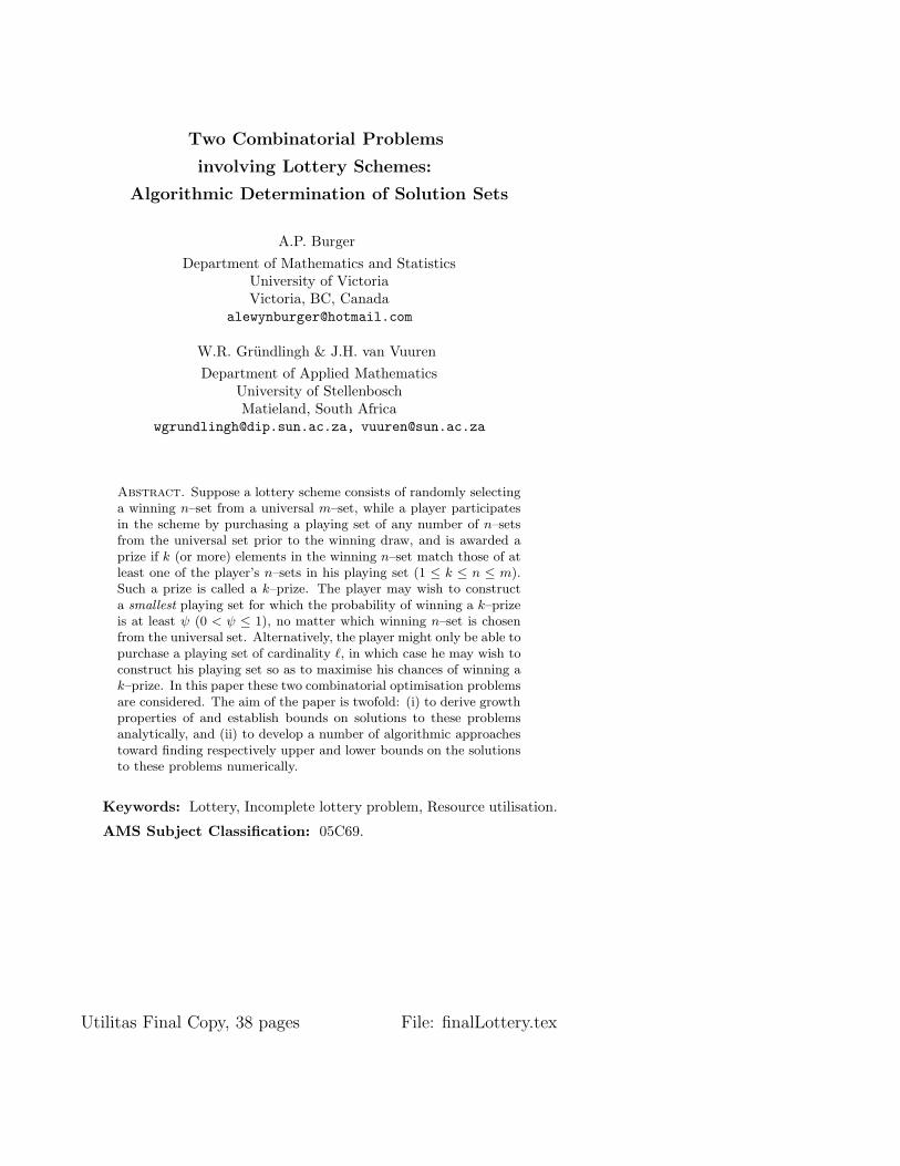
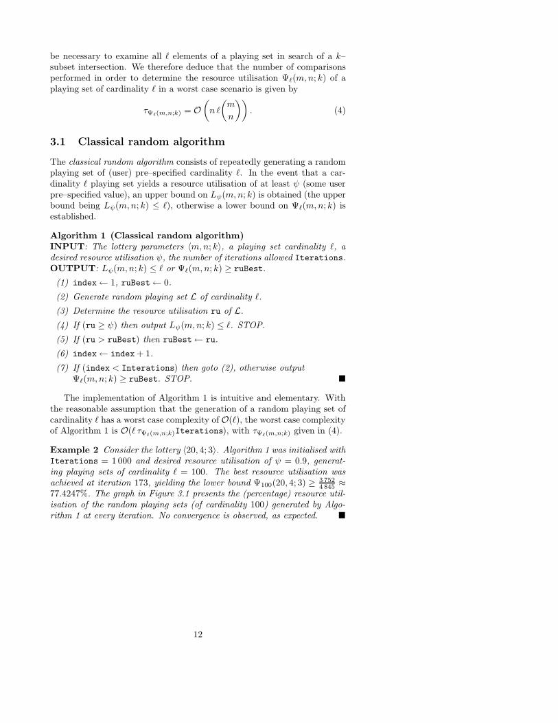
Example 2 Consider the lottery 〈20, 4; 3〉. Algorithm 1 was initialised withIterations = 1 000 and desired resource utilisation of ψ = 0.9, generat-ing playing sets of cardinality ` = 100. The best resource utilisation wasachieved at iteration 173, yielding the lower bound Ψ100(20, 4; 3) ≥ 3 752

4 845 ≈77.4247%. The graph in Figure 3.1 presents the (percentage) resource util-isation of the random playing sets (of cardinality 100) generated by Algo-rithm 1 at every iteration. No convergence is observed, as expected. �

12

��

� � � � �� "!#$ %

& #

& %

' #

' %

( #

) # #+* # #-, # #/. # # % # #/$ # # & # #-' # #0( # #1)"# # #

Figure 3.1: Lower bound on the resource utilisation for 〈20, 4; 3〉 usinga hundred 4–sets from U20 at every iteration, obtained by Algorithm 1.The upper, middle and lower solid (—) lines respectively represent themaximum, mean and minimum resource utilisation.

The main advantage of this implementation is the fast unconditionalplaying set generation, although from Figure 3.1 the independence of suc-cessive iterations is evident, yielding no visible improvement trend duringapplication of the algorithm. The algorithm is not expected to yield verygood results in general, but it does yield a bench mark against which theperformance of other algorithms may be tested.

3.2 Distributed random algorithm

As a possible improvement to the classical random algorithm in the previoussection, the generation of playing sets (Step (2) in Algorithm 1) may beconstrained. Let fL(i) denote the frequency of occurrence of the elementi ∈ Um in a playing set L. Then the constraint to generate a playing set Lsuch that fL(i) may only take the value

⌊

mn

⌋

−1,⌊

mn

⌋

or⌊

mn

⌋

+1 (dependingon the divisibility properties of m by n) may be added to Algorithm 1, thusforcing the elements of Um to be utilised approximately equally in L. Thisconstraint on the generation of n–sets seems intuitively justifiable, due tothe fact that “spreading out” n–sets (and hence distributing the elementsof Um across the n–sets of L) in a playing set is expected to yield a greaterresource utilisation.

Algorithm 2 (Distributed random algorithm)INPUT: The lottery parameters 〈m,n; k〉, a playing set cardinality `, a

13

desired resource utilisation ψ, the number of iterations allowed Iterations.OUTPUT: Lψ(m,n; k) ≤ ` or Ψ`(m,n; k) ≥ ruBest.

(1) index← 1, ruBest← 0.

(2) Generate random playing set L of cardinality ` such that fL(i) ∈{⌊

mn

⌋

− 1,⌊

mn

⌋

,⌊

mn

⌋

+ 1}

for all 1 ≤ i ≤ m.

(3) Determine the resource utilisation ru of L.

(4) If (ru ≥ ψ) then output Lψ(m,n; k) ≤ `. STOP.

(5) If (ru > ruBest) then ruBest← ru.


(7) If (index < Interations) then goto (2), otherwise outputΨ`(m,n; k) ≥ ruBest. STOP. �

The distributed random algorithm performs marginally better than theclassical random procedure presented in Algorithm 1 in the sense that ityields a higher mean resource utilisation at a fractional increase in worstorder complexity measure. Assuming the choice of an element for inclusionin any n–set has worst case complexity O(m) (i.e., examining all elements1 ≤ i ≤ m in search of a minimum fL(i)), the worst case complexitymeasure of Algorithm 2 is O(m` τΨ`(m,n;k)Iterations), with τΨ`(m,n;k)

given in (4).

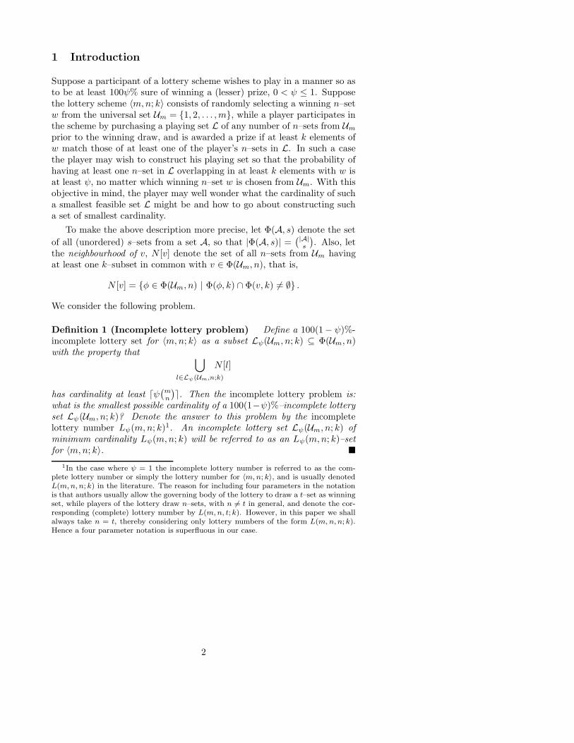
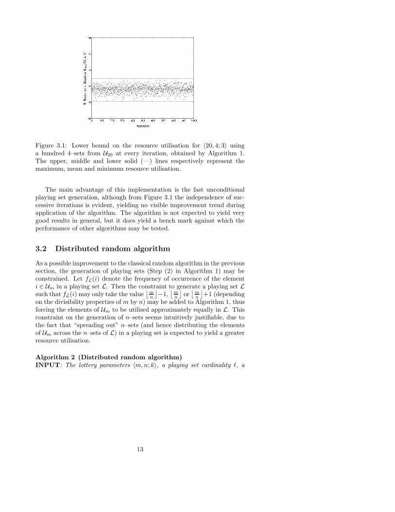
Example 3 (cont. of Example 2) Reconsider the lottery 〈20, 4; 3〉 (inExample 2). Algorithm 2 was initialised with Iterations = 1 000, a desiredresource utilisation of ψ = 0.9, and generating playing sets of cardinality` = 100. The best resource utilisation was achieved at iteration 715, yield-ing the lower bound Ψ100(20, 4; 3) ≥ 3 805

4 845 ≈ 78.5346% in comparison tothe bound Ψ100(20, 4; 3) ≥ 77.4247% found by Algorithm 1. The graph inFigure 3.2 represents the (percentage) resource utilisation of the condition-ally generated random playing sets (of cardinality 100) at every iteration ofAlgorithm 2. Again no convergence is observed, as expected. �

Although conditions are imposed on the generation of playing sets, thereis still no improvement trend in the resource utilised by successively gener-ated playing sets during the algorithm implementation.

3.3 Minimal overlapping algorithm

It is intuitively expected that the more elements of Um shared by any twoelements of Φ(Um, n), the less resource is utilised. It is therefore reasonable

14

��

� � � � �� "!#$ %

& #

& %

' #

' %

( #

) # #+* # #-, # #/. # #0% # # $ # # & # #-' # #-( # #1)"# # #

Figure 3.2: Lower bound on the resource utilisation for 〈20, 4; 3〉 usinga hundred 4–sets from U20 at every iteration, obtained by Algorithm 2.The upper, middle and lower solid (—) lines respectively represent themaximum, mean and minimum resource utilisation.

to assume that, in order to increase the resource utilised by a given playingset L, the elements of L should be chosen so that the cardinality of inter-section between any two n–sets in L is minimised. This is the principlebehind the following heuristic algorithm.

Algorithm 3 (Minimal overlapping algorithm)INPUT: The lottery parameters 〈m,n; k〉, a playing set cardinality `, adesired resource utilisation ψ.OUTPUT: Lψ(m,n; k) ≤ ` or Ψ`(m,n; k) ≥ ruBest.

(1) index← 0, ruBest← 0, L(0) ← {}, ovrlps← 0.

(2) vindex←{}, ovrlps←min1≤j<index{oL(index)(vj , vindex)}.

(3) v∗ ← { first element with (minimum fL(index)(i)) &(oL(index)(vj , vindex ∪ v∗) ≤ ovrlps) for all i = 1, . . . ,m}.

(4) If (v∗ = {}) (i.e., no such element exists) then ovrlps← ovrlps+ 1and goto (3), otherwise vindex ← vindex ∪ {v∗}.

(5) If (|vindex| = n) then L(index+1) ← {L(index) ∪ vindex} and index ←index+ 1.

(6) If (index < `) then goto (2), otherwise goto (7).

(7) ruBest← RU(

L(`))

.

(8) If (ruBest ≥ ψ) then output Lψ(m,n; k) ≤ `, otherwise outputΨ`(m,n; k) ≥ ruBest. STOP. �

15

In Algorithm 3 a playing set L(i) (of cardinality i) is constructed from aplaying set L(i−1) (of cardinality i−1) by adding an n–set vi ∈ Φ(Um, n) toL(i−1) such that vi is “as mutually disjoint as possible” from any v ∈ L(i−1)

(i.e., for any u, v ∈ L(i), |u∩v| is minimised). In the event that vi shares one(or more) element(s) with any v ∈ L(i−1), any single element overlappingis preferred above a double element overlapping, which in turn is preferredabove a triple element overlapping, etc. The described procedure leads toan approximately even distribution of the frequency of occurrences fL(i)(j),j = 1, . . . ,m.

The main components of Algorithm 3 are the maintenance of the fre-quencies fL(i)(j) (j = 1, . . . ,m) and the overlapping function oL(i) (vl1 , vl2),where vl1 , vl2 ∈ L

(i). Here the function oL(i) (vl1 , vl2) returns the num-ber of common elements shared between the n–sets vl1 , vl2 ∈ L

(i) (i.e.,oL(i)(vl1 , vl2) = |vl1 ∩ vl2 |, where vl1 , vl2 ∈ L

(i)).

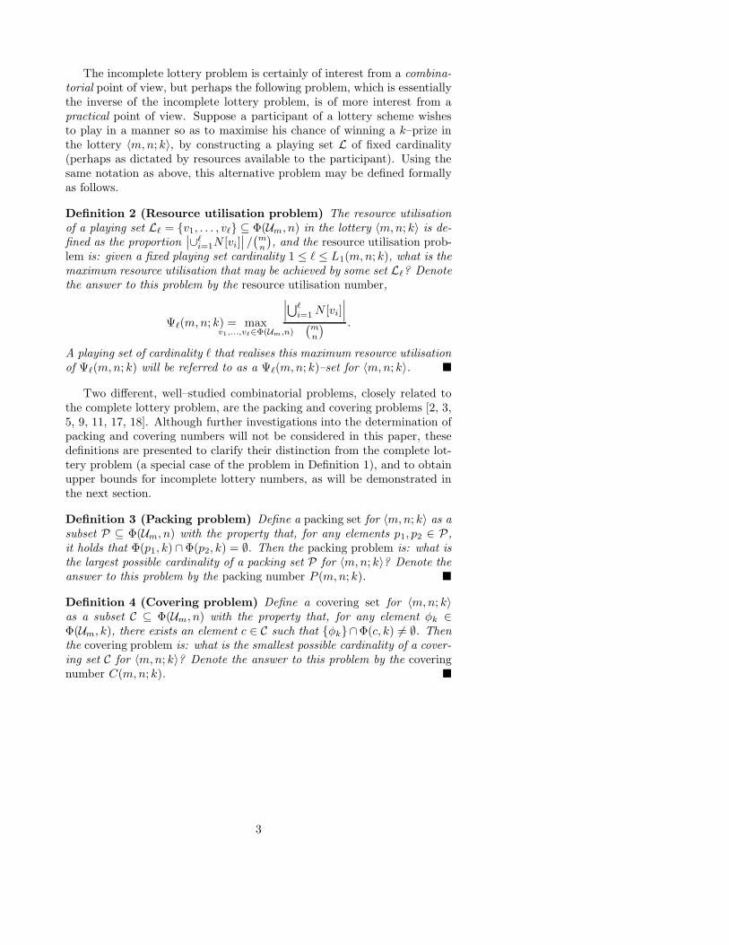
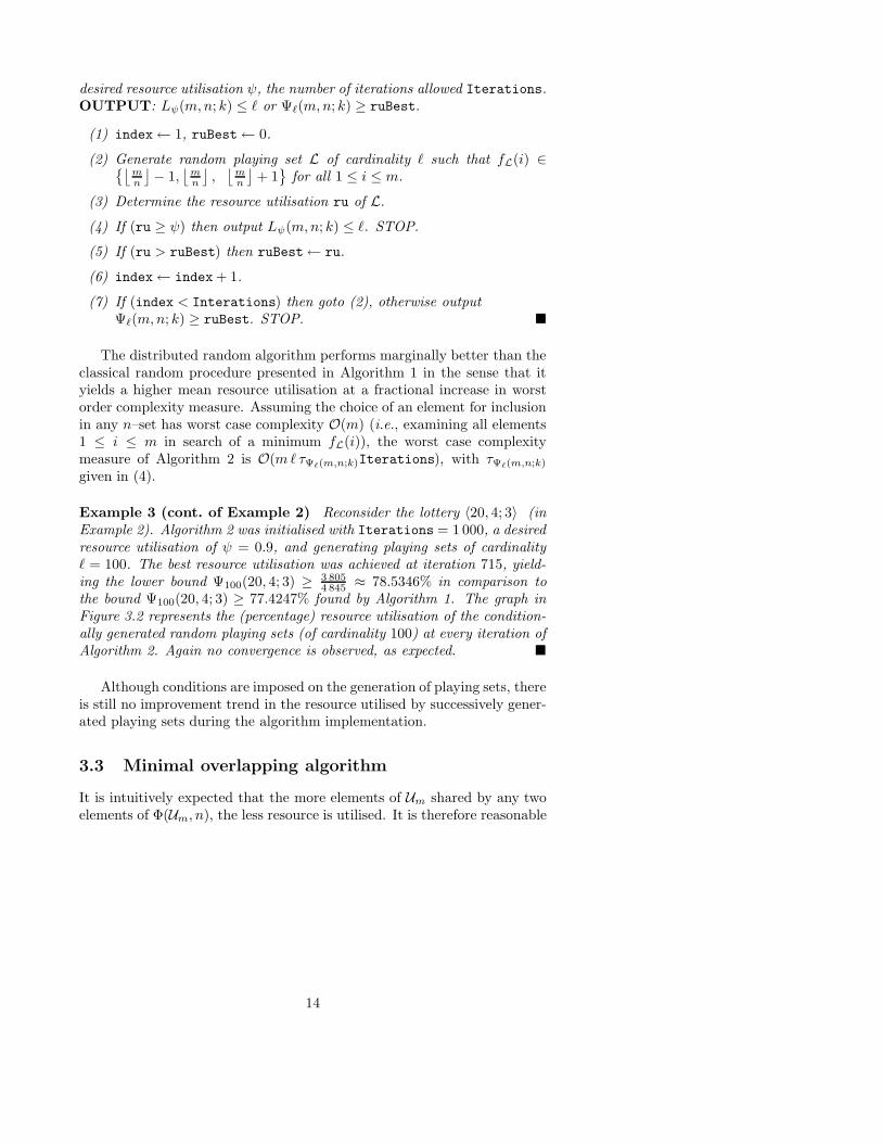
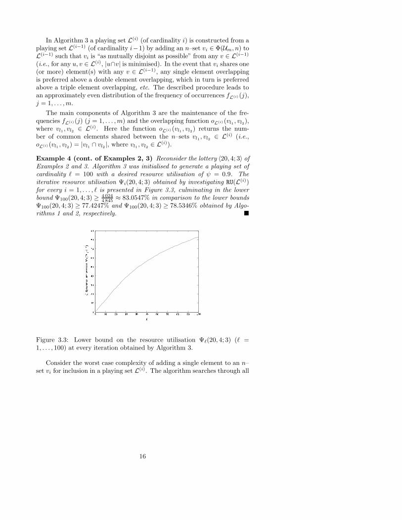
Example 4 (cont. of Examples 2, 3) Reconsider the lottery 〈20, 4; 3〉 ofExamples 2 and 3. Algorithm 3 was initialised to generate a playing set ofcardinality ` = 100 with a desired resource utilisation of ψ = 0.9. Theiterative resource utilisation Ψi(20, 4; 3) obtained by investigating RU(L(i))for every i = 1, . . . , ` is presented in Figure 3.3, culminating in the lowerbound Ψ100(20, 4; 3) ≥ 4 024

4 845 ≈ 83.0547% in comparison to the lower boundsΨ100(20, 4; 3) ≥ 77.4247% and Ψ100(20, 4; 3) ≥ 78.5346% obtained by Algo-rithms 1 and 2, respectively. �

��

��

�� "! � # �"$ ��% ��& �'� � ��

� �

� �

� �

� �

! �

# �

$ �

% �

& �

Figure 3.3: Lower bound on the resource utilisation Ψ`(20, 4; 3) (` =1, . . . , 100) at every iteration obtained by Algorithm 3.

Consider the worst case complexity of adding a single element to an n–set vi for inclusion in a playing set L(i). The algorithm searches through all

16

frequencies of occurrence fL(i)(j) (j = 1, . . . ,m), evaluating each oL(i) (vi, u)for all u ∈ L(i−1). This may be performed via m(i−1) comparisons and theprocess is executed for every element in vi (i.e., n times) and sequentiallyfor every v ∈ L(i) (i.e., i times). The computation of the resource utilisationis suppressed until the end (for the playing set L(`)) of Algorithm 3 (andmay therefore be considered of constant complexity) and is consequentlyexcluded as a complexity consideration. From this it is possible to concludethat the worst case complexity of Algorithm 3 is O(mn`2).

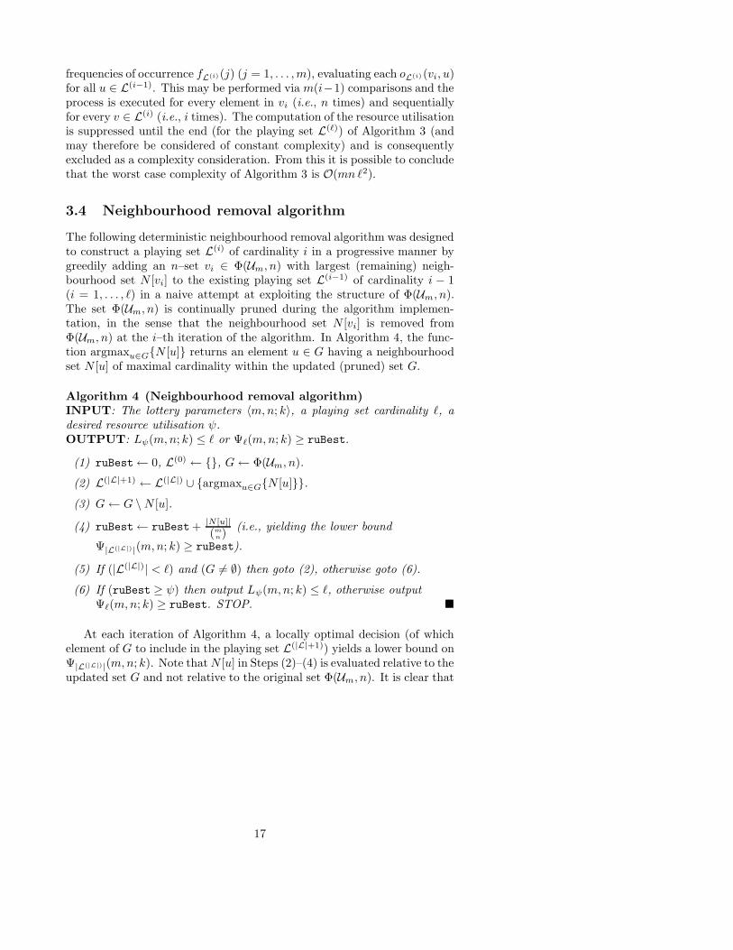
3.4 Neighbourhood removal algorithm

The following deterministic neighbourhood removal algorithm was designedto construct a playing set L(i) of cardinality i in a progressive manner bygreedily adding an n–set vi ∈ Φ(Um, n) with largest (remaining) neigh-bourhood set N [vi] to the existing playing set L(i−1) of cardinality i − 1(i = 1, . . . , `) in a naive attempt at exploiting the structure of Φ(Um, n).The set Φ(Um, n) is continually pruned during the algorithm implemen-tation, in the sense that the neighbourhood set N [vi] is removed fromΦ(Um, n) at the i–th iteration of the algorithm. In Algorithm 4, the func-tion argmaxu∈G{N [u]} returns an element u ∈ G having a neighbourhoodset N [u] of maximal cardinality within the updated (pruned) set G.

Algorithm 4 (Neighbourhood removal algorithm)INPUT: The lottery parameters 〈m,n; k〉, a playing set cardinality `, adesired resource utilisation ψ.OUTPUT: Lψ(m,n; k) ≤ ` or Ψ`(m,n; k) ≥ ruBest.

(1) ruBest← 0, L(0) ← {}, G← Φ(Um, n).

(2) L(|L|+1) ← L(|L|) ∪ {argmaxu∈G{N [u]}}.

(3) G← G \N [u].

(4) ruBest← ruBest+ |N [u]|

(mn)(i.e., yielding the lower bound

Ψ|L(|L|)|(m,n; k) ≥ ruBest).

(5) If (|L(|L|)| < `) and (G 6= ∅) then goto (2), otherwise goto (6).

(6) If (ruBest ≥ ψ) then output Lψ(m,n; k) ≤ `, otherwise outputΨ`(m,n; k) ≥ ruBest. STOP. �

At each iteration of Algorithm 4, a locally optimal decision (of whichelement of G to include in the playing set L(|L|+1)) yields a lower bound onΨ|L(|L|)|(m,n; k). Note thatN [u] in Steps (2)–(4) is evaluated relative to theupdated set G and not relative to the original set Φ(Um, n). It is clear that

17

the construction is dependent on the sequence in which n–sets (togetherwith their respective neighbourhoods) of G are removed. The algorithmgenerally yields better bounds than those obtained by Algorithms 1, 2 and3, as may be seen in the following example.

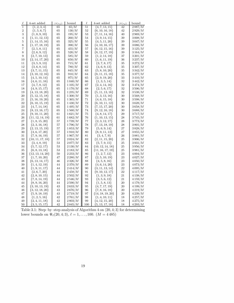
Example 5 (cont. of Examples 2–4) Reconsider the lottery 〈20, 4; 3〉 ofExamples 2–4. Using Algorithm 4 with ` = 100 and ψ = 0.9, Table 3.1 wasgenerated, yielding the improved bound Ψ`(20, 4; 3) ≥ 4 293

4 845 ≈ 88.61% incomparison to the lower bounds Ψ100(20, 4; 3) ≥ 77.4247%, Ψ100(20, 4; 3) ≥78.5346% and Ψ100(20, 4; 3) ≥ 83.0547% obtained by Algorithms 1, 2 and 3respectively. �

Algorithm 4 takes no global consideration of the choice of n–sets thatare chosen for addition to the playing set L(i). Therefore, one possible dis-advantage of this greedy algorithmic implementation is the fact that theneighbourhoods of elements of the pruned set G (Step (3) in Algorithm4) may become drastically smaller and disjoint as the cardinality of G de-creases. In the case of attempting to find a 100(1−ψ)%–incomplete lotteryset for 〈m,n; k〉, this may force an unnecessarily large increase in the car-dinality of a 100(1 − ψ)%–incomplete lottery set towards the end of theimplementation.

In order to determine a worst case complexity estimate for Algorithm4, consider the algorithm execution after i − 1 iterations. The cardinalityof the set G after i − 1 iterations (and therefore the number of n–sets toconsider for inclusion in L(i)) is given by

(

m

n

)

− |∪ij=1N [vj ]|. Each of thesepossible n–sets may have a neighbourhood set cardinality of at most r + 1(where r is given in (1)) for which the individual resource utilisation mustbe evaluated, implying that the worst case complexity of Algorithm 4 isO

(

`((

mn

)

− | ∪ij=1 N [vj ]|)

(r + 1)τΨ`(m,n;k)

)

which is O(

r `(

mn

)

τψ`(m,n;k)

)

.

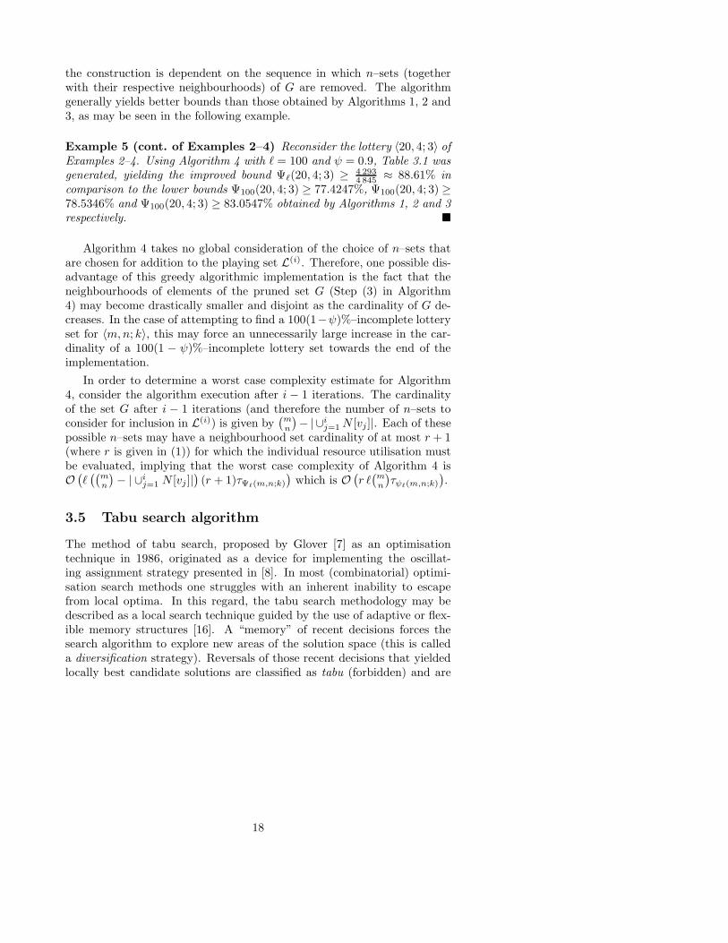
3.5 Tabu search algorithm

The method of tabu search, proposed by Glover [7] as an optimisationtechnique in 1986, originated as a device for implementing the oscillat-ing assignment strategy presented in [8]. In most (combinatorial) optimi-sation search methods one struggles with an inherent inability to escapefrom local optima. In this regard, the tabu search methodology may bedescribed as a local search technique guided by the use of adaptive or flex-ible memory structures [16]. A “memory” of recent decisions forces thesearch algorithm to explore new areas of the solution space (this is calleda diversification strategy). Reversals of those recent decisions that yieldedlocally best candidate solutions are classified as tabu (forbidden) and are

18

` 4-set added |N[v`]| bound ` 4-set added |N[v`]| bound1 {1, 2, 3, 4} 65 65/M 51 {4, 7, 13, 15} 42 2 887/M2 {1, 5, 6, 7} 65 130/M 52 {6, 10, 16, 18} 42 2 929/M3 {1, 8, 9, 10} 65 195/M 53 {7, 11, 14, 16} 40 2 969/M4 {1, 11, 12, 13} 65 260/M 54 {3, 9, 14, 15} 39 3 008/M5 {1, 14, 15, 16} 65 325/M 55 {4, 5, 11, 20} 39 3 047/M6 {1, 17, 18, 19} 65 390/M 56 {4, 10, 16, 17} 39 3 086/M7 {2, 5, 8, 11} 65 455/M 57 {6, 12, 15, 16} 39 3 125/M8 {2, 6, 9, 12} 65 520/M 58 {8, 12, 17, 19} 39 3 164/M9 {2, 7, 10, 13} 65 585/M 59 {1, 2, 14, 18} 37 3 201/M10 {2, 14, 17, 20} 65 650/M 60 {1, 6, 11, 19} 36 3 237/M11 {3, 5, 9, 13} 65 715/M 61 {3, 7, 8, 17} 35 3 272/M12 {3, 6, 8, 14} 65 780/M 62 {4, 6, 9, 13} 35 3 307/M13 {3, 7, 11, 15} 65 845/M 63 {5, 8, 10, 20} 35 3 342/M14 {3, 10, 12, 16} 65 910/M 64 {8, 11, 15, 18} 35 3 377/M15 {4, 5, 10, 14} 65 975/M 65 {2, 9, 19, 20} 33 3 410/M16 {4, 6, 11, 16} 65 1 040/M 66 {1, 3, 5, 14} 32 3 442/M17 {4, 7, 8, 12} 65 1 105/M 67 {2, 4, 14, 16} 32 3 474/M18 {4, 9, 15, 17} 65 1 170/M 68 {2, 5, 6, 17} 32 3 506/M19 {4, 13, 18, 20} 65 1 235/M 69 {5, 11, 13, 16} 32 3 538/M20 {5, 12, 15, 18} 65 1 300/M 70 {1, 3, 13, 16} 30 3 568/M21 {5, 16, 19, 20} 65 1 365/M 71 {4, 6, 15, 18} 30 3 598/M22 {6, 10, 15, 19} 65 1 430/M 72 {6, 10, 11, 12} 30 3 628/M23 {4, 7, 14, 18} 65 1 495/M 73 {7, 15, 17, 20} 30 3 658/M24 {8, 13, 16, 17} 65 1 560/M 74 {9, 12, 16, 18} 30 3 688/M25 {9, 10, 11, 20} 61 1 621/M 75 {4, 8, 14, 17} 29 3 717/M26 {11, 12, 14, 19} 61 1 682/M 76 {1, 10, 13, 15} 28 3 745/M27 {1, 8, 15, 20} 57 1 739/M 77 {2, 3, 12, 17} 28 3 773/M28 {2, 3, 16, 18} 57 1 796/M 78 {7, 13, 18, 19} 28 3 801/M29 {2, 13, 15, 19} 57 1 853/M 79 {5, 6, 9, 14} 27 3 828/M30 {3, 6, 17, 20} 57 1 910/M 80 {8, 9, 11, 13} 27 3 855/M31 {7, 9, 16, 19} 57 1 967/M 81 {3, 4, 7, 9} 26 3 881/M32 {10, 11, 17, 18} 57 2 024/M 82 {2, 11, 15, 20} 25 3 906/M33 {3, 4, 8, 19} 53 2 077/M 83 {5, 7, 9, 15} 25 3 931/M34 {5, 7, 12, 17} 53 2 130/M 84 {10, 12, 14, 18} 25 3 956/M35 {6, 8, 13, 18} 53 2 183/M 85 {11, 16, 17, 19} 25 3 981/M36 {12, 13, 14, 20} 50 2 233/M 86 {1, 2, 7, 12} 23 4 004/M37 {1, 7, 10, 20} 47 2 280/M 87 {2, 5, 10, 19} 23 4 027/M38 {6, 13, 14, 17} 46 2 326/M 88 {4, 5, 8, 16} 23 4 050/M39 {1, 4, 12, 19} 44 2 370/M 89 {4, 6, 14, 20} 23 4 073/M40 {1, 9, 11, 17} 44 2 414/M 90 {3, 11, 13, 14} 22 4 095/M41 {2, 6, 7, 20} 44 2 458/M 91 {9, 10, 12, 17} 22 4 117/M42 {2, 8, 10, 15} 44 2 502/M 92 {1, 3, 9, 18} 21 4 138/M43 {7, 8, 14, 19} 44 2 546/M 93 {3, 5, 6, 12} 21 4 159/M44 {8, 9, 16, 20} 44 2 590/M 94 {1, 5, 8, 13} 20 4 179/M45 {3, 10, 13, 19} 43 2 633/M 95 {4, 7, 17, 19} 20 4 199/M46 {3, 12, 18, 20} 43 2 676/M 96 {7, 8, 16, 18} 20 4 219/M47 {5, 9, 18, 19} 43 2 719/M 97 {14, 18, 19, 20} 20 4 239/M48 {1, 2, 5, 16} 42 2 761/M 98 {1, 4, 10, 11} 18 4 257/M49 {2, 4, 11, 18} 42 2 803/M 99 {4, 12, 15, 20} 18 4 275/M50 {3, 5, 15, 17} 42 2 845/M 100 {5, 13, 17, 18} 18 4 293/M

Table 3.1: Step–by–step analysis of Algorithm 4 on 〈20, 4; 3〉 for determininglower bounds on Ψ`(20, 4; 3), ` = 1, . . . , 100. (M = 4 485)

19

avoided (or penalised) when making decisions about selecting the next bestcandidate solution. In contrast to such recency–based memory structures,frequency–based memory structures store frequency measures relating to theoccurrence of attributes in the solutions encountered. To avoid an alreadytraced path of solutions, the procedure records information about movesrecently made, employing one or more tabu lists. The nature of any tabulist is, of course, problem specific and is usually implemented in the formof a FILO (First–In–Last–Out) list, where new elements added force ex-pulsion of the last elements from the list (therefore maintaining a constantlist order). The function of such lists is not to prevent a move from beingrepeated, but to prevent it from being reversed. Furthermore, the prohi-bition of reversal is conditional rather than absolute. In particular, tabusearches proceed with the assumption that poor choices (by accident ordesign) yield no benefit, except for the purpose of avoiding a solution pathalready examined [7].

A key aspect in the implementation of a tabu search is the processingand length of the tabu lists. The length of a tabu list describes how manyof the past moves should be remembered and is referred to as a tabu tenure.Exact definitions regarding the tabu tenure remain problem specific. Al-lowing entries in a tabu list to have a preemptively large penalty, none ofthe tabu moves will be considered as long as non–tabu moves exist. Thepenalties may be allowed to decay as a function of time and/or tabu listlength, allowing older tabu moves to be considered in preference to morerecent ones (if no move other than a tabu move exists). Although thispreemptive penalty scheme seems reasonable, cycling solutions may resultand this strategy therefore defies the chief purpose of tabu lists. A differentresolution, more faithful to the principle of tabu lists, is to incorporate aso–called aspiration criterion which overrides the tabu status of a move ifthe resulting trial solution improves on the best solution obtained thus far(other aspiration criteria also exist [7, 13]). For additional tabu parametersand tabu list management rules, the reader is referred to [7, 14].

Tabu searches typically also employ longer term strategies of intensifica-tion. Intensification strategies are designed to exploit those good solutionsby intensifying the local search around their respective neighbourhoods inthe solution space. Additionally, tabu searches usually operate without ref-erence to randomisation and are therefore basically deterministic, althoughthey may also be applied in conjunction with probabilistic methods [13].Traditionally, tabu searches explore the whole neighbourhood of a specificsolution in order to select its successor. This may become computation-ally intensive for large problems, although methods exist whereby only aproportion of the candidate solutions are examined. Candidate list strate-gies work on this principle, by considering only a subset of a solution’s

20

neighbourhood when seeking a successive solution (see, for example, [15]).

In the tabu search algorithm implemented for finding lower bounds onΨ`(m,n; k) (or alternatively upper bounds on Lψ(m,n; k)) candidate solu-tions are represented as binary vectors b of length

(

mn

)

and weight `, where

the i–th bit bi (1 ≤ i ≤(

mn

)

) takes the value 1 if the i–th (lexicographi-cally ordered) n–set in Φ(Um, n) is included in the candidate solution, and0 otherwise.

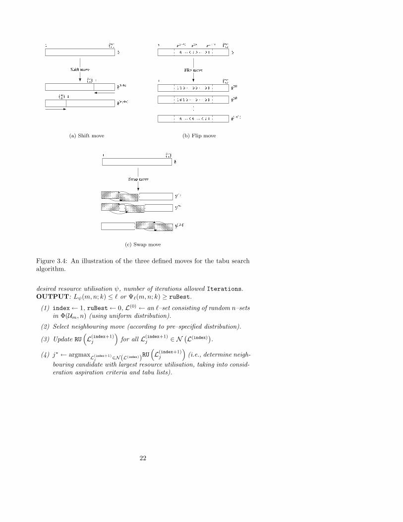
The initial candidate solution is randomly generated, and the followingthree neighbouring moves were considered for this tabu search implemen-tation:

• Shift move: A shift length (between 1 and(

mn

)

−1) is randomly cho-sen (from a uniform distribution), and applied to a candidate solution

b, which results in two neighbouring candidates, b(left) and b(right) (aleft and right shift modulo

(

mn

)

). See Figure 3.4(a). The inverse(opposite direction) of the selected move is added to the tabu list.

• Flip move: Define 1 ≤ p(j) ≤(

mn

)

, j = 1, . . . , ` as the position ofthe j–th 1–bit in b (i.e., bp(j) = 1 for all j = 1, . . . , `). A bit index1 ≤ ι ≤ `, randomly chosen from a uniform distribution, defines theneighbourhood of a binary vector solution candidate as all the vectors

b(i) with b(i)

p(ι)= 0 and b

(i)j = 1 for all j = p(ι−1) +1, . . . , p(ι)−1, p(ι) +

1, . . . , p(ι+1) − 1 (i.e., bit b(i)j is “flipped” to take the value b

(i)j + 1

(mod 2) for all possible p(ι−1) < j < p(ι+1)). See Figure 3.4(b). Theflip information is recorded in the tabu list and any move reversing aflip in a specific range of the resulting bit flipped position is classifiedas tabu.

• Swap move: Subvectors of a specified size in a candidate solution bare swapped. The neighbouring candidates are defined as all possiblecombinations of swaps of such subvectors. Incorporating a variationto candidate list strategies, the subvector size is randomly chosen(from a uniform distribution) such that at least 100 and at most5 000 (in increments of 100) neighbouring candidates exist. See Figure3.4(c). The swap information is recorded in the tabu list and any movereversing a swap is classified as tabu.

In the following algorithm, let the specific candidate solution neighbour-hood (given any of the defined moves) of a solution candidate L∗ be defined

as N (L∗). Also, the function RU(

L(i)j

)

represents the resource utilisation

of the j–th neighbouring candidate solution at iteration i of the algorithm.

Algorithm 5 (Tabu search algorithm)INPUT: The lottery parameters 〈m,n; k〉, a playing set cardinality `, a

21

��

��

� � � � ��

� � ! " � ��

(a) Shift move

#%$ & ')(+*�,.-

/0 1 2 354

/ 6 7�8/ 6 9�8

:::/ 6 ; <=; 8

0 1 2 354

0?>)@�@�@%>�AB>)@�@ @%>B0CED F G CHD F I�J GCED F K�J G

0LAB>)@�@ @%>M>)@�@ @%>B00?>BAB>)@�@ @%>)@�@ @%>B0

0?>)@�@�@%>L>)@�@�@%>�AN0

(b) Flip move

OPOPOOPOPOQPQPQQPQPQ

RPRPRRPRPRSPSPSSPSPS

TPTPTPTTPTPTPTUPUPUPUUPUPUPU

VPVPVPVVPVPVPVWPWPWPWWPWPWPW

XPXPXPXXPXPXPXYPYPYPYYPYPYPY

ZPZPZPZPZZPZPZPZPZ[P[P[P[P[[P[P[P[P[

\�]L^�_=à�b�c

d e f�gd e h�g

iiid e j klj g

m n o p�qd

(c) Swap move

Figure 3.4: An illustration of the three defined moves for the tabu searchalgorithm.

desired resource utilisation ψ, number of iterations allowed Iterations.OUTPUT: Lψ(m,n; k) ≤ ` or Ψ`(m,n; k) ≥ ruBest.

(1) index← 1, ruBest← 0, L(0) ← an `–set consisting of random n–setsin Φ(Um, n) (using uniform distribution).

(2) Select neighbouring move (according to pre–specified distribution).

(3) Update RU(

L(index+1)j

)

for all L(index+1)j ∈ N

(

L(index))

.

(4) j∗ ← argmaxL

(index+1)j

∈N(L(index))RU(

L(index+1)j

)

(i.e., determine neigh-

bouring candidate with largest resource utilisation, taking into consid-eration aspiration criteria and tabu lists).

22

(5) If(

RU(

L(index+1)j∗

)

> ruBest)

then ruBest← RU(

L(index+1)j∗

)

.

(6) If (ruBest ≥ ψ) then output Lψ(m,n; k) ≤ `. STOP.

(7) L(index+1) ← L(index+1)j∗ , and add move to tabu list.


(9) If (index ≤ Iterations) then goto (2), otherwise output thatΨ`(m,n; k) ≥ ruBest. STOP. �

The following example illustrates the consequences and effectiveness ofeach individual move and investigates some combined attributes of the tabumoves.

Example 6 (cont. of Examples 2–5) Reconsider the lottery 〈20, 4; 3〉 ofExamples 2–5. Algorithm 5 was initialised with Iterations = 1 000 anda desired resource utilisation of ψ = 0.9. The tabu tenure was taken asb(

204

)

/20c = 242, while the simple aspiration criterion was adopted of al-lowing a tabu move when it yielded a better resource utilisation than anyencountered up to that point. The algorithm generated playing sets of car-dinality ` = 100 and was executed for the following different cases:

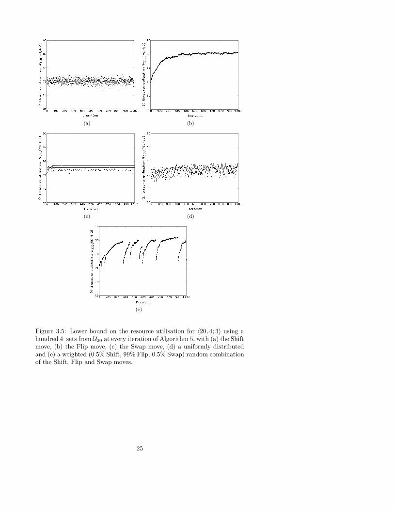
1: The selection of neighbouring moves was restricted to the Shift move,with the best resource utilisation obtained at iteration 98, yielding thelower bound Ψ100(20, 4; 3) ≥ 3 769

4 845 ≈ 77.7915%. See Figure 3.5(a).

2: The selection of neighbouring moves was restricted to the Flip move,with the best resource utilisation obtained at iteration 701, yieldingthe lower bound Ψ100(20, 4; 3) ≥ 4 158

4 845 ≈ 85.8204%. See Figure 3.5(b).

3: The selection of neighbouring moves was restricted to the Swap move,with the best resource utilisation obtained at iteration 96 (with anaverage of 2 600 possible neighbouring candidate solutions per itera-tion), yielding the lower bound Ψ100(20, 4; 3) ≥ 3 806

4 845 ≈ 78.5552%. SeeFigure 3.5(c).

4: A uniform distribution between all three neighbouring moves was used,with the best resource utilisation at iteration 1 000, yielding the lowerbound Ψ100(20, 4; 3) ≥ 3 840

4 845 ≈ 79.2570%. See Figure 3.5(d).

5: A 0.5%, 99% and 0.5% weighted distribution between the respectiveShift, Flip and Swap neighbouring moves was utilised, with the bestresource utilisation obtained at iteration 902, yielding the lower boundΨ100(20, 4; 3) ≥ 4 169

4 845 ≈ 86.0475%. See Figure 3.5(e).

23

From the results obtained, it is clear that the Flip move (Case 2) repre-sents a good intensification strategy, while the Shift and Swap moves (Cases1 and 3) may represent possible diversification strategies. This hypothesisis validated by the incorporation of a weighted distribution of both strate-gies (evident in Case 5) yielding a marginal improvement in the resourceutilised with an even distribution of strategies (Case 4). Although the bestlower bound on the resource utilisation Ψ100(20, 4; 3) obtained by Algorithm5 is weaker than that obtained by Algorithm 4, this is not the case in general,as will be demonstrated in §4. �

It is assumed that a tabu tenure of λ is used throughout the follow-ing complexity considerations. Additionally, the complexity of generatingany neighbouring candidate is considered constant due to the operationsperformed (AND, OR and XOR) being bit–related.

First consider the worst case complexity of determining the next locallyoptimal non–tabu candidate solution when only the Shift move is utilisedas a possible neighbouring move. Trivially only two possible neighbouringcandidates exist. For both these candidates, a search through λ tabu movesare performed (in a possible worst case or due to the incorporation of as-piration criteria) and their respective resource utilisations are determined.Therefore, the worst case complexity of the Shift move is O(λ τΨ`(m,n;k)).Secondly, consider the worst case complexity given that only the Flip moveis applied to generate neighbouring candidate solutions. In a (highly un-likely, yet possible) worst case scenario, the binary vector b may be com-pletely unbalanced (i.e., the distribution of 1–bit values are clustered ateither or both ends). Then, only one specific set of

(

mn

)

− (` + 1) neigh-bouring candidates exists, for which their respective resource utilisationsrequire evaluation (each with a complexity of O(τΨ`(m,n;k))) as well as asearch through λ possible tabu moves. It therefore follows that the worstcase complexity of the Flip move is O(λ

(

m

n

)

τΨ`(m,n;k)). Finally, we considerthe worst case complexity when only the Swap move is employed as a possi-ble tabu search move for generating neighbouring candidate solutions. Themaximum number of neighbouring candidates in a possible worst case wastaken as 5 000 (and therefore considered constant), and similar complexityarguments to when the Flip move is used, holds for the Swap neighbour-ing move. We therefore deduce that the worst case complexity of the tabusearch Swap move is O(λ τΨ`(m,n;k)).

3.6 (Intelligent) genetic algorithm

Based on Darwin’s evolution theory, genetic algorithms (or evolution pro-grams) may be described as learning methods simulating biological evolu-

24

��

� �� ! "$#%&('

) %

) '

*+%

*('

,+%

- %+%/. %+%10+%+%12 %+% '+%+% &(%+% ) %+%/*(%+%1,+%+% -$%+%+%

(a)

34 567 89:58;<=< 6>;<7 ?@ ABBC DE�FG HIJ

K L�M�N OPL Q R$STU�V

W T

W V

X(T

X�V

Y(T

Z T(T\[ T+T1] T(T1^ T(T_V T(T/U(T+T W T+T1X+T(T/Y(T+T`Z$T(T+T

(b)

ab cde fghcfijkj dlije mn oppq rs�tu vwx

y z�{�| }�z+~ �$��

� �

� �

�(�

��

�(�

��+�/�+�+�1�+�(�1� �(� �+�+� �(�+� � �+�1�+�(� �(�+� �$�+�(�

(c)

�� ¡¢

£ ¤�¥(¦+§�¤ ¨ ©«ª¬�®

¯ ¬

¯ ®

°+¬

°(®

±+¬

²�¬+¬/³ ¬(¬/´+¬(¬/µ ¬+¬ ®+¬+¬ +¬(¬ ¯ ¬+¬/°(¬+¬ ±+¬(¬ ²$¬(¬+¬

(d)

¶· ¸¹º »¼½¸»¾¿À¿ ¹Á¾¿º ÂÃ ÄÅÅÆ ÇÈ�ÉÊ ËÌÍ

Î Ï�Ð(Ñ+Ò�Ï Ó Ô«ÕÖ×�Ø

Ù Ö

Ù Ø

Ú+Ö

Ú(Ø

Û+Ö

Ü�Ö+Ö/Ý Ö(Ö/Þ+Ö(Ö/ß Ö+Ö Ø+Ö+Ö1×+Ö(Ö1Ù Ö+Ö Ú(Ö+Ö Û+Ö(Ö Ü$Ö(Ö+Ö

(e)

Figure 3.5: Lower bound on the resource utilisation for 〈20, 4; 3〉 using ahundred 4–sets from U20 at every iteration of Algorithm 5, with (a) the Shiftmove, (b) the Flip move, (c) the Swap move, (d) a uniformly distributedand (e) a weighted (0.5% Shift, 99% Flip, 0.5% Swap) random combinationof the Shift, Flip and Swap moves.

25

Program EvolutionBegin

t← 0Initialise P (t)Evaluate Fitness(P (t))While (Fitness(P (t)) < Tolerance) DoBegin

t← t+ 1Select P (t) from P (t− 1)Change P (t) [Crossover & Mutation]Evaluate Fitness(P (t))

EndEnd

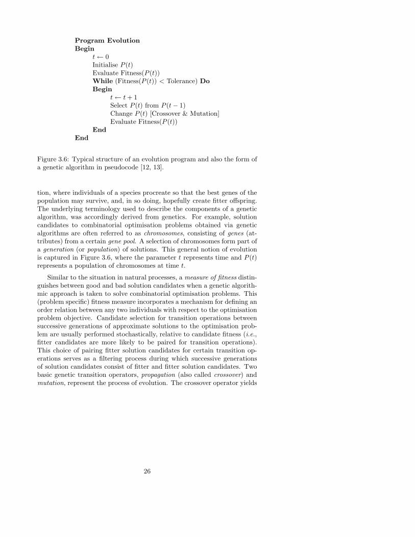
Figure 3.6: Typical structure of an evolution program and also the form ofa genetic algorithm in pseudocode [12, 13].

tion, where individuals of a species procreate so that the best genes of thepopulation may survive, and, in so doing, hopefully create fitter offspring.The underlying terminology used to describe the components of a geneticalgorithm, was accordingly derived from genetics. For example, solutioncandidates to combinatorial optimisation problems obtained via geneticalgorithms are often referred to as chromosomes, consisting of genes (at-tributes) from a certain gene pool. A selection of chromosomes form part ofa generation (or population) of solutions. This general notion of evolutionis captured in Figure 3.6, where the parameter t represents time and P (t)represents a population of chromosomes at time t.

Similar to the situation in natural processes, a measure of fitness distin-guishes between good and bad solution candidates when a genetic algorith-mic approach is taken to solve combinatorial optimisation problems. This(problem specific) fitness measure incorporates a mechanism for defining anorder relation between any two individuals with respect to the optimisationproblem objective. Candidate selection for transition operations betweensuccessive generations of approximate solutions to the optimisation prob-lem are usually performed stochastically, relative to candidate fitness (i.e.,fitter candidates are more likely to be paired for transition operations).This choice of pairing fitter solution candidates for certain transition op-erations serves as a filtering process during which successive generationsof solution candidates consist of fitter and fitter solution candidates. Twobasic genetic transition operators, propagation (also called crossover) andmutation, represent the process of evolution. The crossover operator yields

26

as result new solution candidates (called children) inheriting properties ofcandidates taking part in the process (called parents). Children typicallyreplace parent candidates in order to maintain a constant population cardi-nality at every iteration of the genetic algorithm. The mutation operator,on the other hand, is specifically incorporated to perturb solution can-didates away from possible local optima (in the solution space) when anessentially stagnant population of candidate solutions is encountered. Mu-tation therefore typically involves the exploration of different (possibly new)areas of the solution space. It should be evident that mutations might alsolead to less fit candidate solutions (as with the case of the crossover oper-ator), although such weakening mutations are usually corrected by similarmutation and/or crossovers with fitter candidates of successive generations.Both the definitions of genetic operators and of fitness measure are problemspecific and therefore vary from application to application.

Traditionally, genetic algorithms are used in multi–dimensional opti-misation problems with large solution spaces in which the following two(possibly contradicting) goals are pursued: (i) an effective search throughthe whole solution space (or at least a representative part thereof) and (ii)the progressive improvement of specific good solutions. Efficient genetic al-gorithms maintain a good balance between scouting (of the solution space)and local improvement (of successive specific solutions).

Genetic algorithms may be employed in search of (upper and lower)bounds on Lψ(m,n; k) and Ψ`(m,n; k) (respectively). Candidates in a pop-ulation are represented by playing sets of cardinality ` and therefore consistof elements from Φ(Um, n). The chromosome population is initialised, us-ing randomly selected n–sets from Φ(Um, n). The cardinality of the unionof the neighbourhood sets of elements in a playing set lends itself as anintuitive and realistic fitness measure of the playing set. Chromosomes arerandomly paired (in the genetic crossover procedure) using a population fit-ness distribution relative to their individual fitness (i.e., the fitter [weaker]candidates in a population possess the propensity to pair with other fit [lessfit] candidates).

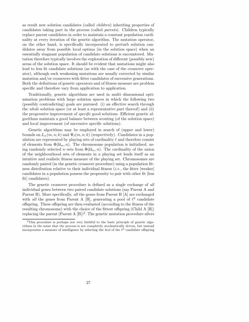
The genetic crossover procedure is defined as a single exchange of allindividual genes between two paired candidate solutions (say Parent A andParent B). More specifically, all the genes from Parent B [A] are exchangedwith all the genes from Parent A [B], generating a pool of `2 candidateoffspring. These offspring are then evaluated (according to the fitness of theresulting chromosome) with the choice of the fittest offspring (Child A [B])replacing the parent (Parent A [B])2. The genetic mutation procedure alters

2This procedure is perhaps not very faithful to the basic principle of genetic algo-rithms in the sense that the process is not completely stochastically driven, but insteadincorporates a measure of intelligence by selecting the best of the `2 candidate offspring

27

��

��

��

�! �"�#%$& � �! �"�#%$& �

� "�'�(�(�'�)�#*"+-,/. 0213%45476�89�:�;

+-,/. 0213%45476�<9�: ;

+-,/. 0213%454=6�69�:�;

+-,/. 0213%454=6�>9�: ;(a) Crossover procedure

?�?�@�A�B�A�C�D�A ?�B�A�E�A�FDA ?*E�A�G�A�F�D�D

H�I�J�K�L?�?�@�A�B�A�C�D�A ?@�A�B�A�E�DA ?*E�A�G�A�F�D�D

M!N�O�P%QRSUTWV X�YZ�[2[7\�]^�_�`

SUTWV X�YZ�[2[7\�a^�_ `

bdc�R�NeR J�f Q

(b) Mutation procedure

Figure 3.7: Illustration of the (a) crossover procedure performed on twoparent chromosomes yielding two (fitter) children (Child 1 [2] is obtainedfrom Parent 1 [2] by the exchange of gene 2 [3] from Parent 2 [1] with gene2 [1] from Parent 1 [2]) and (b) mutation procedure on a single chromosomeyielding a (weaker) child (the Child is obtained from the Parent by replacinggene 2 with the random gene {1, 2, 4}) for 〈7, 3; 2〉.

a random proportion of genes in a random proportion of solution candidates(using a uniform distribution). These proportions are given respectivelyby the parameters gMutate and cMutate in Algorithm 6. Figure 3.7(a)[(b)] presents an illustrative example of the crossover [mutation] operationperformed on chromosomes for 〈7, 3; 2〉.

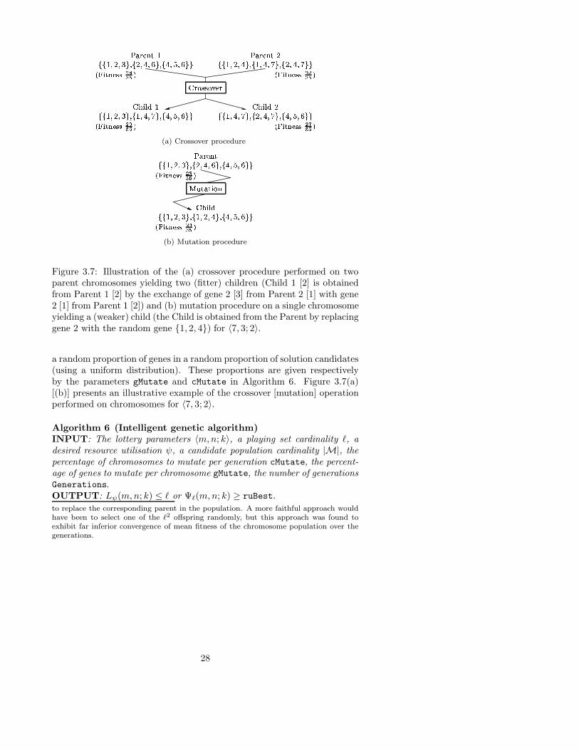
Algorithm 6 (Intelligent genetic algorithm)INPUT: The lottery parameters 〈m,n; k〉, a playing set cardinality `, adesired resource utilisation ψ, a candidate population cardinality |M|, thepercentage of chromosomes to mutate per generation cMutate, the percent-age of genes to mutate per chromosome gMutate, the number of generationsGenerations.OUTPUT: Lψ(m,n; k) ≤ ` or Ψ`(m,n; k) ≥ ruBest.

to replace the corresponding parent in the population. A more faithful approach wouldhave been to select one of the `2 offspring randomly, but this approach was found toexhibit far inferior convergence of mean fitness of the chromosome population over thegenerations.

28

(1) index← 1, ruBest← 0, L(0)j ← an `–set consisting of random n–sets

in Φ(Um, n) for all j = 1, . . . , |M| (using uniform distribution).

(2) Update RU(

L(index)j

)

for all j = 1, . . . , |M|.

(3) If(

RU(

L(index)j

)

> ruBest)

then

index∗ ← argmaxj∈{1,...,|M|}RU(

L(index)j

)

and

ruBest← RU(

L(index∗)j

)

.

(4) If (ruBest ≥ ψ) then output Lψ(m,n; k) ≤ `. STOP.

(5) Perform transition procedures: Crossover & Mutation (according tothe parameters gMutate and cMutate).


(7) If (index ≤ Generations) then goto (2), otherwise outputΨ`(m,n; k) ≥ ruBest. STOP. �

This process is iterated for a (user) pre–specified number of genera-tions or until a certain fitness tolerance is obtained (for this specific im-plementation, the tolerance may be given by some minimally acceptableaverage population fitness or if one candidate represents a Lψ(m,n; k)–setfor 〈m,n; k〉). In Algorithm 6, chromosome i of a population M and itsresource utilisation is represented by L(i) and RU(L(i)), respectively.

In the following example, the impact of individual parameter variationsare considered. This sheds light on the effectiveness of genetic algorithmsin the context of maximising resource utilisation or finding 100(1− ψ)%–incomplete lottery sets.

Example 7 (cont. of Examples 2–6) Reconsider the lottery 〈20, 4; 3〉 ofExamples 2–6. Three independent parameter variations were considered(for every case Generations = 200):

1: Algorithm 6 was initialised with a random population consisting of

|M| = 20 candidate solutions, each representing a playing set L(0)j

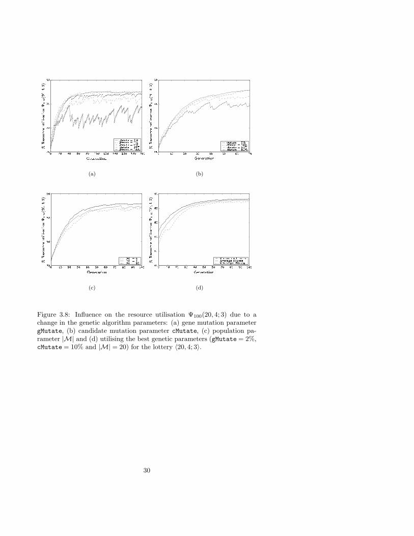
(j = 1, . . . , 20) of ` = 100 genes (4–sets). In every generation,cMutate = 5% of the population candidates were subjected to muta-tion. The parameter gMutate was initialised to take the values (i) 1%,(ii) 2%, (iii) 5%, (iv) 10% and (v) 25% respectively. The maximumpopulation fitness (and hence the best resource utilisation) per gener-ation is presented in Figure 3.8(a). The best resource utilisation wasobtained with a gene mutation percentage of gMutate = 2%, yieldingthe lower bound Ψ100(20, 4; 3) ≥ 4 250

4 845 ≈ 87.7193%.

29

��

�� "!$#"% &'�() *

+,(

+ *

-,(

."(0/,(21 ( +,(43 (,( 3"."( 3 /,( 3 1 ( 3 +,(5."(,(

6 7 8 9 : 9 ;=< 3?>6 7 8 9 : 9 ;=< .,>6 7 8 9 : 9 ;=< *,>6 7 8 9 : 9 ;=< 3 ( >6 7 8 9 : 9 ;=< .,*,>

(a)

@A BCDEFGBEHIJI CKHIDLM NOOP QR�ST UVW

X�Y�Z�Y ["\$]?^ _�Z` a ` b"` c,` d ` e ` f,` g"`g e

h,`

h e

i,`

j k l m n m o=p e,qj k l m n m o=p a ` qj k l m n m o=p b e,qj k l m n m o=p e ` q

(b)

rs tuvwxytwz{|{ u}z{v~� ��

�� "��"� �� "�2�,�2� �0� �2� �0�"�2�,�2� � � � �

� �

� �

�,�

� �

¡¢ $£ � ¡¢ $£ � � ¡¢ $£ �"�

(c)

¤¥ ¦§¨©ª«¦©¬® §¯¬¨°± ²³³´ µ¶�·¸ ¹º»

¼�½�¾�½ ¿"À�Á"Â Ã�¾ÄÆÅ Ä�Ç"Ä2È,Ä2É,Ä0Ê,Ä�Ë Ä0Ì Ä�Í,Ä2Î Ä Å?Ä,ÄË Ê

Ì Ä

Ì Ê

Í,Ä

Í Ê

Î,Ä

Ï�Ð Ñ�Ð ÒÔÓ�ÒÖÕ Ð × Ñ�Ø Ù ÙÚÜÛ Ø Ý Þ,ß,ØÔÕ Ð × Ñ�Ø Ù ÙÏàÞ,á�Ð ÒÔÓ�ÒÖÕ Ð × Ñ�Ø?Ù Ù

(d)

Figure 3.8: Influence on the resource utilisation Ψ100(20, 4; 3) due to achange in the genetic algorithm parameters: (a) gene mutation parametergMutate, (b) candidate mutation parameter cMutate, (c) population pa-rameter |M| and (d) utilising the best genetic parameters (gMutate = 2%,cMutate = 10% and |M| = 20) for the lottery 〈20, 4; 3〉.

30

2: The parameter cMutate was initialised to take the values (i) 5%,(ii) 10%, (iii) 25% and (iv) 50% respectively. Algorithm 6 was fur-ther randomly initialised with a population consisting of |M| = 20

candidate solutions, each describing a playing set L(0)j (j = 1, . . . , 20)

of ` = 100 genes (4–sets). Every candidate subjected to mutation, hadgMutate = 5% of its respective genes mutated. The maximum popula-tion fitness (and hence the best resource utilisation) per generation ispresented in Figure 3.8(b). The best resource utilisation was obtainedwith a candidate mutation percentage of cMutate = 10%, yielding thelower bound Ψ100(20, 4; 3) ≥ 4 261

4 845 ≈ 87.9463%.

3: The number of candidate solutions |M| in a population was variedto take the values (i) 6, (ii) 10 and (iii) 20. A single chromosome(cMutate = 1

|M|) of the |M| candidates in the population, was sub-

jected to a mutation of gMutate = 5% genes. The maximum popula-tion fitness (and hence the best resource utilisation) per generation ispresented in Figure 3.8(c). The best resource utilisation was obtainedwith a candidate population of |M| = 20, yielding the lower boundΨ100(20, 4; 3) ≥ 4 260

4 845 ≈ 87.9257%.

Using these results, the following additional case was considered.

4: Algorithm 6 was initialised with gMutate = 2%, cMutate = 10% ina population of |M| = 20 candidate solutions, thus utilising the bestempirically obtained parameter values from Cases 1–3. Figure 3.8(d)represents the minimum, mean and maximum generation fitness (orequivalently the resource utilisation Ψ100(20, 4; 3)) as a function ofthe population generation. The best resource utilisation was obtainedin generation 99, yielding the lower bound Ψ100(20, 4; 3) ≥ 4 277

4 845 ≈88.2766%.

Although the best lower bound on the resource utilisation Ψ100(20, 4; 3)obtained by Algorithm 6 is weaker than that obtained by Algorithm 4, thisis not the case in general, as will be demonstrated in §4. �

Consider the complexity of performing the crossover procedure (of Algo-rithm 6) between any two individual candidates of a populationM. Everypossible gene exchange is considered in the generation of child candidates,which may be performed in 2`2|M| operations. For each of the possiblefuture offspring, the resource utilisation is calculated in order to extractthose children that are fittest, leading to a complexity of O

(

Generations

`2|M|τΨ`(m,n;k)

)

. Consider, on the other hand, the complexity of per-forming the mutation procedure on a generation of candidate solutions. A

31

random selection of gMutate×` genes in cMutate×|M| individuals are mu-tated (replaced by random n–sets). The choice of candidates and relevantgenes may each be considered of constant complexity. This leads to theconclusion that the mutation procedure has a complexity of O(` gMutate×|M|cMutate) per generation. With both procedures being performed inde-pendently (and hence having complexityO(Generations (`2|M|τΨ`(m,n;k)+` gMutate|M|cMutate))), we deduce that the worst case complexity of Al-gorithm 6 is O

(

Generations `2|M|τΨ`(m,n;k)

)

.

One serious disadvantage of the genetic algorithm implementation in de-termining lower bounds on the resource utilisation Ψ`(m,n; k), as opposedto the tabu search optimisation heuristic of Algorithm 5, is the crossoverprocedure making a considerable contribution to the computational com-plexity. Tabu search implementations for finding bounds on Lψ(m,n; k) andΨ`(m,n; k) become less attractive as the cardinality of Φ(Um, n) increases.This limitation is even more acute in the case of the genetic algorithm.

4 Comparison of Algorithmic Performances

The relative performances of the six algorithms presented in §3 are com-pared in this section, so that a ranking of the algorithms may be achievedin terms of the quality of the bounds they produce (on average). This isdone by applying the algorithms to a number of small lotteries in §4.1, af-ter which we apply the algorithms, in §4.2, to arguably the most popularrealistic lottery scheme in operation in the world.

4.1 Some small lotteries

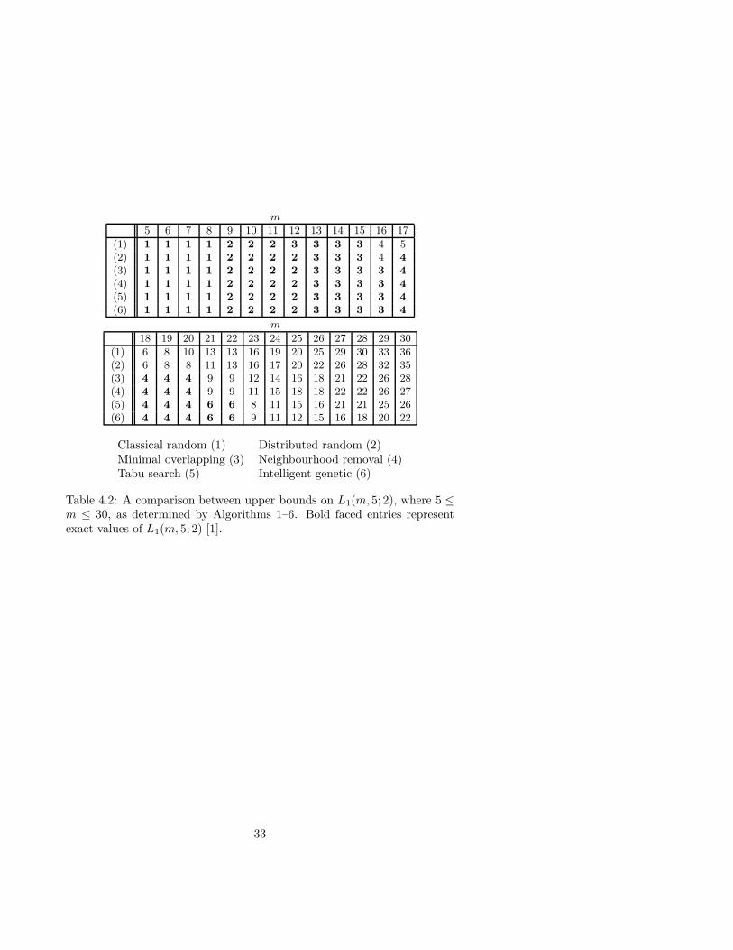
Algorithms 1–6 were implemented with the intention of finding completelottery sets for 〈m, 5; 2〉, where 5 ≤ m ≤ 30, in order to provide the readerwith an impression of the relative algorithmic performances. The smallestcomplete lottery set cardinalities determined after 1 000 iterations [gener-ations] by the algorithms (hence upper bounds on L1(m, 5; 2)) are sum-marised in Table 4.2. The table provides some evidence towards our claimthat the six algorithms in §3 were presented in order of increasing level ofaverage performance.

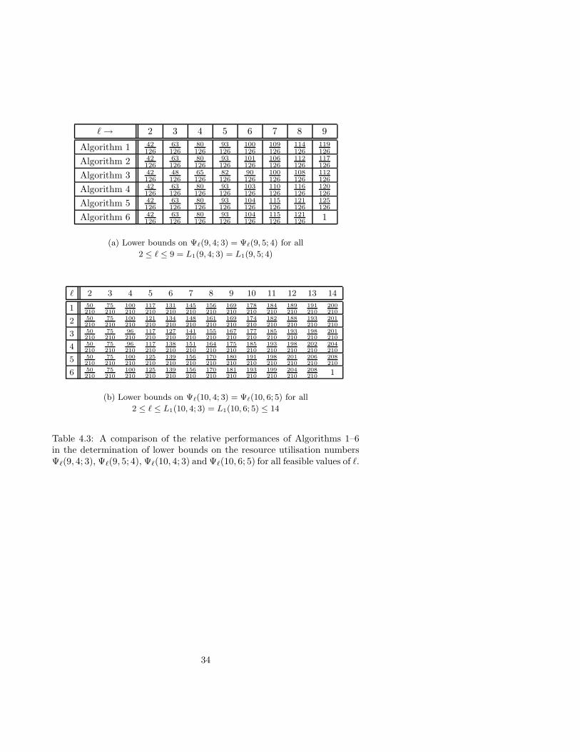
Further evidence of this claim may be found in Table 4.3, where lowerbounds are found on resource utilisation numbers Ψ`(9, 4; 3) = Ψ`(9, 5; 4)for all 2 ≤ ` ≤ 9 = L1(9, 4; 3) = L1(9, 5; 4) and on Ψ`(10, 4; 3) = Ψ`(10, 6; 5)for all 2 ≤ ` ≤ L1(10, 4; 3) = L1(10, 6; 5) ≤ 14, by virtue of Proposition 3.

32

m

5 6 7 8 9 10 11 12 13 14 15 16 17

(1) 1 1 1 1 2 2 2 3 3 3 3 4 5(2) 1 1 1 1 2 2 2 2 3 3 3 4 4

(3) 1 1 1 1 2 2 2 2 3 3 3 3 4

(4) 1 1 1 1 2 2 2 2 3 3 3 3 4

(5) 1 1 1 1 2 2 2 2 3 3 3 3 4

(6) 1 1 1 1 2 2 2 2 3 3 3 3 4

m

18 19 20 21 22 23 24 25 26 27 28 29 30

(1) 6 8 10 13 13 16 19 20 25 29 30 33 36(2) 6 8 8 11 13 16 17 20 22 26 28 32 35(3) 4 4 4 9 9 12 14 16 18 21 22 26 28(4) 4 4 4 9 9 11 15 18 18 22 22 26 27(5) 4 4 4 6 6 8 11 15 16 21 21 25 26(6) 4 4 4 6 6 9 11 12 15 16 18 20 22

Classical random (1) Distributed random (2)Minimal overlapping (3) Neighbourhood removal (4)Tabu search (5) Intelligent genetic (6)

Table 4.2: A comparison between upper bounds on L1(m, 5; 2), where 5 ≤m ≤ 30, as determined by Algorithms 1–6. Bold faced entries representexact values of L1(m, 5; 2) [1].

33

`→ 2 3 4 5 6 7 8 9

Algorithm 1 42126

63126

80126

93126

100126

109126

114126

119126

Algorithm 2 42126

63126

80126

93126

101126

106126

112126

117126

Algorithm 3 42126

48126

65126

82126

90126

100126

108126

112126

Algorithm 4 42126

63126

80126

93126

103126

110126

116126

120126

Algorithm 5 42126

63126

80126

93126

104126

115126

121126

125126

Algorithm 6 42126

63126

80126

93126

104126

115126

121126 1

(a) Lower bounds on Ψ`(9, 4; 3) = Ψ`(9, 5; 4) for all

2 ≤ ` ≤ 9 = L1(9, 4; 3) = L1(9, 5; 4)

` 2 3 4 5 6 7 8 9 10 11 12 13 14

1 50

210

75

210

100

210

117

210

131

210

145

210

156

210

169

210

178

210

184

210

189

210

191

210

200

210

2 50

210

75

210

100

210

121

210

134

210

148

210

161

210

169

210

174

210

182

210

188

210

193

210

201

210

3 50

210

75

210

96

210

117

210

127

210

141

210

155

210

167

210

177

210

185

210

193

210

198

210

201

210

4 50

210

75

210

96

210

117

210

138

210

151

210

164

210

175

210

185

210

193

210

198

210

202

210

204

210

5 50

210

75

210

100

210

125

210

139

210

156

210

170

210

180

210

191

210

198

210

201

210

206

210

208

210

6 50

210

75

210

100

210

125

210

139

210

156

210

170

210

181

210

193

210

199

210

204

210

208

2101

(b) Lower bounds on Ψ`(10, 4; 3) = Ψ`(10, 6; 5) for all

2 ≤ ` ≤ L1(10, 4; 3) = L1(10, 6; 5) ≤ 14

Table 4.3: A comparison of the relative performances of Algorithms 1–6in the determination of lower bounds on the resource utilisation numbersΨ`(9, 4; 3), Ψ`(9, 5; 4), Ψ`(10, 4; 3) and Ψ`(10, 6; 5) for all feasible values of `.

34

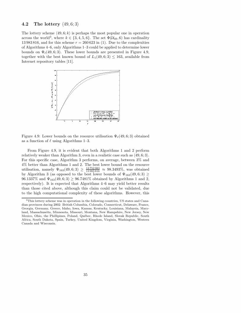
4.2 The lottery 〈49, 6; 3〉

The lottery scheme 〈49, 6; k〉 is perhaps the most popular one in operationacross the world3, where k ∈ {3, 4, 5, 6}. The set Φ(U49, 6) has cardinality13 983 816, and for this scheme r = 260 623 in (1). Due to the complexitiesof Algorithms 4–6, only Algorithms 1–3 could be applied to determine lowerbounds on Ψ`(49, 6; 3). These lower bounds are presented in Figure 4.9,together with the best known bound of L1(49, 6; 3) ≤ 163, available fromInternet repository tables [11].

��

�

�� ! " # $%� � & # � ' ( $)*� � ' � + , ' - ". � ! " # $%� � & # � ' ( $/0� ! � $1� �2# 3 - � � 4.� � & # � ' ( $

5 ( - # - ' � �6 - � # , � -6, ' � � � � � ' � # !7�- � '*8 ! # 9*!.+�# , ! ":# !.' ( -6� ! ' - ! - '

; < <

= <

> <

? <

@ <

A <

B <

C <

D <

; <

< D < B < @ < > < ; < < ; D < ; B < ; @ <

Figure 4.9: Lower bounds on the resource utilisation Ψ`(49, 6; 3) obtainedas a function of ` using Algorithms 1–3.

From Figure 4.9, it is evident that both Algorithms 1 and 2 performrelatively weaker than Algorithm 3, even in a realistic case such as 〈49, 6; 3〉.For this specific case, Algorithm 3 performs, on average, between 3% and4% better than Algorithms 1 and 2. The best lower bound on the resourceutilisation, namely Ψ163(49, 6; 3) ≥ 13 752 983

13 983 816 ≈ 98.3493%, was obtainedby Algorithm 3 (as opposed to the best lower bounds of Ψ163(49, 6; 3) ≥96.1337% and Ψ163(49, 6; 3) ≥ 96.7481% obtained by Algorithms 1 and 2,respectively). It is expected that Algorithms 4–6 may yield better resultsthan those cited above, although this claim could not be validated, dueto the high computational complexity of these algorithms. However, this

3This lottery scheme was in operation in the following countries, US states and Cana-dian provinces during 2002: British Columbia, Colorado, Connecticut, Delaware, France,Georgia, Germany, Greece, Idaho, Iowa, Kansas, Kentucky, Louisiana, Malaysia, Mary-land, Massachusetts, Minnesota, Missouri, Montana, New Hampshire, New Jersey, NewMexico, Ohio, the Phillipines, Poland, Quebec, Rhode Island, Slovak Republic, SouthAfrica, South Dakota, Spain, Turkey, United Kingdom, Virginia, Washington, WesternCanada and Wisconsin.

35

limitation may possibly be alleviated to some extent with the aid of parallelprogramming techniques.

5 Conclusion

In this paper, two new combinatorial problems on lottery schemes were for-mulated: the incomplete lottery problem and the resource utilisation prob-lem. In the former problem one seeks an answer to the following question:“What is the fewest number of lottery tickets required to be at least 100ψ%sure of winning a (lesser) prize in a lottery draw?” In the latter problem oneseeks to answer the following question: “If only ` lottery tickets are bought,how should they be constructed so as to maximise the chance of winninga (lesser) prize in a lottery draw?” These two problems are essentially in-verses of one another, and the former is a generalisation of the well knowncomplete lottery problem, where one seeks the minimum number of tick-ets to be guaranteed a (lesser) prize during a lottery draw. The answers tothese two combinatorial optimisation problems were denoted by Lψ(m,n; k)(called the incomplete lottery number) and Ψ`(m,n; k) (called the resourceutilisation number) respectively, for the lottery scheme 〈m,n; k〉.

In §2 analytic bounds on Lψ(m,n; k) and Ψ`(m,n; k) were established,and certain growth properties with respect to variations in the parame-ters m, n, k, ` and ψ were proved. In §3 six algorithms were designedto obtain tighter, numerical lower and upper bounds on Ψ`(m,n; k) andLψ(m,n; k), respectively. Algorithm 2 (called the distributed random algo-rithm) achieves a marginal improvement on the performance of Algorithm1 (called the classical random algorithm), although neither algorithm ex-ploits the overlapping structure of the universe Φ(Um, n) in terms of theway in which solution candidates are determined. As a possible improve-ment, Algorithm 3 (called the minimal overlapping algorithm) incorporatesa mechanism for constructing interdependent playing sets. From the re-sults obtained, no significant general improvement occurs for small valuesof ` > 2, although improvements upon the performance of Algorithms 1and 2 are observed in larger, more realistic lottery cases.

Algorithm 4 (called the neighbourhood removal algorithm) embodies aneffective local optimisation strategy for relatively small values of `. Thealgorithm’s progress tends to deteriorate towards the end of the implemen-tation, due to a break up into disjoint sets of the neighbourhoods of elementsnot yet incorporated into the (incomplete) lottery set. The improvements inperformance of the optimisation techniques of Algorithms 5 (a tabu search)and 6 (an intelligent genetic algorithm), as compared to those of the firstfour algorithms, are visible in the bounds obtained in Tables 4.2 and 4.3.

36

More specifically, Algorithm 6 is the only algorithm that found L1(m,n; k)–sets (complete lottery sets of minimum cardinality) for all the known lotterynumbers L1(m,n; k) for which 1 ≤ k ≤ n ≤ m ≤ 10. Algorithm 6 thereforerepresents a potentially good method for finding (near–) optimal playingsets for lottery schemes. However, the practical applicability of this algo-rithm diminishes rapidly as the cardinality of Φ(Um, n) increases, due tothe computationally intensive nature of the crossover procedure.

Acknowledgements

This paper is based upon work which formed part of the second au-thor’s PhD study and he gratefully acknowledges financial assistance fromthe Harry Crossley Foundation, the Wilhelm Frank Stipendium Trust, theSouth African Department of Labour Scarce Skills Scholarship Programmeand the Graduate Merit Bursary Fund at the University of Stellenbosch.Research towards this paper was also supported financially by the SouthAfrican National Research Foundation under grant number GUN 2053755and by Research Sub-Committee B at the University of Stellenbosch. Anyopinions, findings and conclusions or recommendations expressed in this pa-per are those of the authors and do not necessarily reflect the views of theSouth African National Research Foundation or the Department of Labour.

References

[1] R. Belic, Lotto Systems and Toto Systems to win Wheelgame, [Online], [cited 2002, April 23], Available from:http://www.xs4all.nl/~rbelic/

[2] A.E. Brouwer, Packing and Covering of(

kt

)

–sets, pp. 89–97 in A.Schrijver (Ed): Packing and Covering in Combinatorics, Mathema-tisch Centre Tracts, 106, Mathematisch Centrum, Amsterdam, (1979).

[3] A.E. Brouwer, On the packing of quadruples without common triples,Ars Combinatoria, 5 (1978), pp. 3–6.

[4] A.P. Burger, W.R. Grundlingh & J.H. van Vuuren, Towardsa characterisation of lottery set overlapping structures, Submitted.

[5] Center for Communications Research, CCR La JollaHome Page, [Online], [cited 2002, April 20], Available from:http://www.ccrwest.org/

[6] R. Davies & G.F. Royle, Graph domination, tabu search and thefootball pool problem, Discrete Mathematics, 74 (1997), pp. 217–228.

37

[7] F. Glover, Future paths for Integer Programming and links to Ar-tificial Intelligence, Computers & Operations Research, 13(5) (1986),pp. 533–549.

[8] F. Glover, Heuristics for Integer Programming using surrogate con-straints, Decision Sciences, 8 (1977), pp. 156–166.

[9] D.M. Gordon, G. Kuperberg & O. Patashnik, New Construc-tions for Covering Designs, Journal of Combinatorial Designs, 3(4)(1995), pp. 269–284.

[10] W.R. Grundlingh, Two New Combinatorial Problems involvingDominating Sets for Lottery Schemes, PhD dissertation, Universityof Stellenbosch, South Africa, to be submitted.

[11] P.C. Li, Ben Li’s Lotto Tables Page, [Online], [cited 2002, April 23],Available from:http://www.cs.umanitoba.ca/~lipakc/lottotables.html

[12] Z. Michalewicz, Genetic Algorithms + Data Structures = Evolutionprograms, Springer–Verlag, Berlin, (1999).

[13] Z. Michalewicz & D.B. Fogel, How to Solve It: Modern Heuris-tics, Springer–Verlag, Berlin, (2000), pp. 115–134, 139–155.

[14] K. Nonobe & T. Ibaraki, A tabu search approach to the constraintsatisfaction problem as a general problem solver, European Journal ofOperational Research, 106 (1998), pp. 599–623.

[15] P.R.J. Ostergard, Constructing covering codes by tabu search, Jour-nal of Combinatorial Designs, 5(1) (1997), pp. 71–80.

[16] M. Pirlot, General local search methods, European Journal of Oper-ational Research, 92 (1996), pp. 493–511.

[17] J. Schonheim, On Coverings, Pacific Journal of Mathematics, 14(1964), pp. 1 405–1411.

[18] J. Schonheim, On the number of mutually disjoint triples in Steinersystems and related maximal packing and minimal covering systems,pp. 311–318 in W.T. Tutte (Ed): Recent Progress in Combinatorics,Academic Press, New York, (1969).

38

Two Combinatorial Problems involving Lottery Schemes

Documents