Twinam Zoning and Economic Geography

Contents lists available at ScienceDirect

Journal of Urban Economics

journal homepage: www.elsevier.com/locate/jue

Zoning and the economic geography of cities☆

Allison Shertzera,c, Tate Twinamb, Randall P. Walsha,c,⁎

aUniversity of Pittsburgh, United StatesbUniversity of Washington Bothell, United StatescNBER, United States

A R T I C L E I N F O

Keywords:ZoningPersistenceLand useHousing pricesRegulation

A B S T R A C T

Comprehensive zoning is ubiquitous in U.S. cities, yet we know surprisingly little about its long-run impacts. Weprovide the first attempt to measure the causal effect of land use regulation over the long term, using as oursetting Chicago's first comprehensive zoning ordinance adopted in 1923. Our results indicate that zoning playeda central role in establishing residential neighborhoods free of industrial and commercial uses. The separation ofuses established by the zoning ordinance persists to the present day and is reflected in housing prices, thelocation of polluting industrial sites, and population density.

1. Introduction

“This zoning law does not impose a very serious limit on the use of land,for if all the land in Chicago were built to the limit allowed by the zoninglaw, the entire population of the United States could be housed in the city…. Moreover, whenever there is any possibility of a higher use for anyblock or parcel of land than the one for which it is zoned, it is not verydifficult to have it zoned for the higher use, as the five thousandamendments to the zoning law testify.”

-Homer Hoyt, One Hundred Years of Land Values in Chicago

Among economists, conventional wisdom suggests market forces arethe primary determinant of the spatial distribution of economic activitywithin cities. This emphasis on market forces can be seen theoreticallyand empirically. Both the monocentric city model and more recentmodels of agglomeration all tie market processes to the determinationof land use patterns. In empirical work, the focus on markets and pricesin determining the location of economic activity can be observed in thevoluminous literatures on agglomeration economies, transportation

costs, and residential sorting dynamics.1

The central role economists ascribe to market forces stands in starkcontrast to the conventional understanding of zoning ordinances, whichare typically thought of as endogenous, merely reflecting the locationalchoices of competing economic actors.2 This view of zoning laws,however, is based on a surprisingly thin evidentiary base. Given theprevalence of urban planning and zoning laws in contemporaryAmerican society (except for Houston, every major city in the UnitedStates is subject to a comprehensive body of zoning laws), it is sur-prising that no work has been done evaluating the long-run impacts ofland use regulation on the spatial organization of cities.

Accordingly, in this paper, we present a systematic empirical as-sessment of the long-term effects of zoning on the overall arrangementof economic activity in a city. Our analysis focuses on the city ofChicago, which adopted a comprehensive zoning ordinance for the firsttime in 1923. The distinguishing feature of our empirical approach isthat we are able to observe land use patterns at the lot level for theentire city of Chicago before its first zoning law was implemented.Previous scholarship on the relationship between zoning and land use

https://doi.org/10.1016/j.jue.2018.01.006Received 1 August 2017; Received in revised form 7 November 2017; Accepted 23 January 2018

☆ Antonio Diaz-Guy, Phil Wetzel, Jeremy Brown, Andrew O'Rourke provided outstanding research assistance. Support for this research was provided by the NSF (SES-1459847).Additional support was provided by the Central Research Development Fund and the Center on Race and Social Problems at the University of Pittsburgh. We thank Werner Troesken,Mark Partridge, David Huffman, Leah Brooks, Daniel McMillen, Edward Coulson, and seminar participants at Yale, Tulane, Rochester, the Urban Economics Association, AREUEA, theUniversity of South Carolina, the Lincoln Institute of Land Policy, Florida State University, the Federal Reserve Bank of Philadelphia, and the University Center for Social and UrbanResearch (UCSUR) at the University of Pittsburgh. We are grateful to Gabriel Ahlfeldt and Daniel McMillen for providing the land price data. We also thank David Ash and the CaliforniaCenter for Population Research for providing support for the microdata collection, Carlos Villareal and the Center for Population Economics at the University of Chicago for the Chicagostreet file, and Martin Brennan and Jean-Francois Richard for their support of the project.

⁎ Corresponding author at: University of Pittsburgh, United States.E-mail address: [email protected] (R.P. Walsh).

1 For reviews of these literatures, see Duranton and Puga (2015), Combes and Gobillon (2015), Redding and Turner (2015) and Kuminoff et al. (2013).2 Two examples of papers that find zoning evolves to reflect the highest-value use for land include Wallace (1988) and Munneke (2005). On the other hand, both McDonald and

McMillen (1998) and Zhou et al. (2008) provide evidence of a short-run price effects associated with different types of zoning. The notion that zoning is an ineffectual or fleetingconstraint on land use patterns is itself controversial; to quote William Fischel (2001), this notion is “completely at odds with the attention paid to [zoning] by otherwise rational people”(The Homevoter Hypothesis, p. 57).

Journal of Urban Economics 105 (2018) 20–39

Available online 31 January 20180094-1190/ © 2018 Elsevier Inc. All rights reserved.

T

http://www.sciencedirect.com/science/journal/00941190

https://www.elsevier.com/locate/jue

https://doi.org/10.1016/j.jue.2018.01.006


mailto:[email protected]


http://crossmark.crossref.org/dialog/?doi=10.1016/j.jue.2018.01.006&domain=pdf

has not utilized city-wide land use patterns in the years preceding theadvent of zoning laws and therefore has had trouble cleanly identifyingthe impact of zoning on land use. Our findings suggest that the existingliterature understates the importance of zoning in shaping urban formin contemporary American cities.

Specifically, we consider an array of city block-level outcomes, in-vestigating the long-run influence of zoning on the location of manu-facturing activity, commercial uses, residential areas, population den-sity and polluting facilities. At a similar spatial scale, we also evaluatezoning's impact on present day housing prices. This analysis indicatesthat Chicago's 1923 zoning ordinance has had a sizable impact onpresent day land use. To understand the role of zoning vis-à-vis otherkey land use drivers, we use standardized multiple-partial regression toevaluate the relative importance of five different categories of vari-ables: zoning, pre-existing land uses, pre-existing transportation net-works, geography, and pre-existing demographics. We find that theimpact of initial zoning classification is roughly similar in magnitude tothat of pre-existing land use in determining present day use.Furthermore, while both are clearly important, our results indicate thattransportation networks and geography, the stalwarts of urban land usetheory, are less important than zoning for determining land use over thelong run.

Finally, we examine the extent to which the organization of eco-nomic activity across the city as a whole shifted following zoning. Wedocument a high degree of mixing of residential, commercial, and in-dustrial activity in the city prior to zoning. Land use as imagined by thezoning board exhibited considerably more separation of uses, and thisseparation did in fact emerge by the end of the twentieth century.Following on this line of analysis, we consider the case of Houston,arguably the only major city in the U.S. which lacks a comprehensivezoning ordinance. We present evidence that polluting land uses (ToxicsRelease Inventory facilities) are less segregated in “un-zoned” Houstonthan they are in comparable zoned cities in Texas (Austin, Dallas andSan Antonio). Finally, utilizing our empirical analysis of Chicago, weconstruct estimates of the distribution of these polluting land uses inChicago both under zoning and in a counterfactual world withoutzoning. The resulting comparison suggests a zoning impact that isqualitatively very similar to what we find in our analysis of cities inTexas. These city-level results provide evidence that zoning can reshapethe general spatial organization of a city over the long term.

Existing work on zoning has documented the fact that supply re-strictions arising from higher overall levels of land use regulation areassociated with higher land prices (Quigley and Raphael, 2005;Ihlanfeldt, 2007; Glaeser and Ward, 2009; Turner et al., 2014). Theseanalyses largely focus on residential density restrictions, ignoring theextent to which different uses are separated by zoning; this is perhapsinevitable due to the ubiquity of separation of uses in U.S. cities.

A second literature seeks to disentangle the impact of various typesof use restrictions on prices. Early results in this literature suggestedthat zoning did not respond to market forces once in place. Studies ofparcel re-zoning suggest that zoning evolves over time in a manner thatreflects the highest-valued land use for the affected parcels, indicatingthat the market influences zoning to some extent (Wallace 1988;Munneke 2005). The question of how zoning shaped urban spatialstructure has received comparatively less attention in economics, andrecent papers have largely focused on the existence of short-run priceeffects associated with different types of use zoning (McDonald andMcMillen 1998; Zhou et al., 2008). Our contribution is to place localgovernment institutions in context as a determinant of land use patternsover the long term.

2. Background on zoning

2.1. Brief history of zoning in the United States

New York City passed the first comprehensive zoning ordinance in

the United States in 1916. Over the next twenty years, facilitated by therapid enactment of state enabling ordinances modeled on a templatedeveloped by the U.S. Department of Commerce, over 700 additionalcities adopted comprehensive zoning ordinances (Advisory Committeeon Zoning, 1926). The demand for zoning was rooted in the prevailingcondition of American cities, many of which saw rapid unplannedgrowth following large-scale European immigration and industrializa-tion that began in the mid-nineteenth century.

Extremely high residential densities, combined with poor water andwaste disposal infrastructure, led to high rates of infectious disease inmajor cities (Troesken, 2004). Noxious industrial uses were frequentlylocated in densely populated areas and routinely encroached on higher-end retail and office districts. Many urban residents objected to the“canyon effect” created by unbroken rows of skyscrapers, citing thepotential negative effects of reduced sunlight exposure and airflow onpublic health (Hall, 2002, pp. 36–47). Coinciding with this growth andsqualor was the rise of the Progressive movement, whose proponentssought to apply scientific and technical expertise to the problem ofmanaging overpopulated industrial cities. These reformers foundcommon cause with powerful real estate interests, whose overarchingconcern was the protection of property values from threats posed by theunrestricted encroachment of undesirable land uses (Bassett, 1922).

2.2. Land use and zoning in Chicago

In many ways, Chicago was typical of the largest U.S. cities at thistime. Overcrowding was prevalent, especially in black and first-gen-eration immigrant communities (Shertzer et al., 2016). Dense sky-scraper development in the central business district caused substantialcontroversy, and the unrestricted spread of commercial and industrialdevelopment threatened property values in higher income residentialneighborhoods (Schwieterman and Caspall, 2006). Development inChicago was also geographically constrained by both Lake Michiganand the Chicago River. While these conditions were shared by manymajor cities and spurred the adoption of land use regulation nationally,Chicago was exceptional in some ways beyond its rank as the second-largest city in the U.S. By the 1920s, the city had a highly developedfixed rail public transportation system and a significant number ofbuildings that are still standing today. This relatively large stock ofdurable capital may have blunted the impact of zoning in Chicago re-lative to cities that were less built up in the 1920s. Chicago is alsoknown for having an especially corrupt local government, which mayhave made zoning variances easier to obtain. These caveats may limitthe generalizability of our findings, which in part motivates our ana-lysis of Texas cities in Section 6.

Chicago's city government had made previous attempts to controlundesirable land uses, including an 1837 municipal code that pro-hibited landowners from maintaining nuisances such as dead animals,dung, putrid meat, or fish entrails on their property. However, suchpiecemeal approaches proved insufficient to meet the public demandfor controlled development. In 1921, the newly created Chicago ZoningCommission began preparing a comprehensive zoning ordinance. TheCommission, composed of eight aldermen and fourteen representativesfrom the Chicago community, spent eighteen months surveying existingland use in Chicago before issuing the initial statute. While the ordi-nance was designed by the Commission, the commission solicitedfeedback from numerous civic organizations and held public hearings inan attempt to create what they called a “people's ordinance”(Chicago Zoning Commission, 1922).

The ordinance that resulted from this process regulated landthrough separately defined and overlaying districts restricting alloweduses and building volumes. This dual-map system was typical of zoningordinances in major cities at this time (see, e.g., New York City, 1917;Seattle, 1923; Boston, 1924; Baltimore, 1931). Four distinct use dis-tricts were included: residential (single-family housing), apartment,commercial, and manufacturing. These use districts were hierarchical,

A. Shertzer et al. Journal of Urban Economics 105 (2018) 20–39

21

with apartment districts allowing residential uses, commercial districtsallowing both apartments and single-family homes, and manufacturingdistricts allowing any use. Volume districts imposed restrictions onmaximum lot coverage, aggregate volume, and height. The five volumedistricts in Chicago's ordinance were also hierarchical, with district 5allowing the tallest buildings. Non-conforming uses existing at the timeof the ordinance's passage were allowed to continue. However, thesenon-conforming uses could not be extended and, during any ten-yearperiod, renovation expenditures were limited to an aggregate cost of nomore than 50% of the value of the building.

The question of how closely the initial zoning ordinance followedexisting land use has been explored in previous work, which found thatzoning was sensitive to existing land uses, proximity to transportationnetworks, and distance to waterways (McMillen and McDonald, 1999).In other work, we show that the distribution of minority groups alsoimpacted the initial zoning ordinance; in particular, southern black andfirst-generation immigrant neighborhoods were more likely to be zonedfor industrial uses (Shertzer et al., 2016). In order to disentangle acausal effect of historical zoning on contemporary land use from per-sistence in land use over time, we require variation in how similar lotswere zoned in 1923. We find that although zoning was influenced byextant uses, there remains significant variation in zoning outcomesacross individual lots that were located at similar points along thecommercial and/or manufacturing activity spectrum.

3. Data

There are eight components to the dataset used in our analysis. Fiveof these components are contemporary: the Chicago MetropolitanAgency for Planning's (CMAP's) 2005 land use inventory; theEnvironmental Protection Agency's Toxics Release Inventory (TRI);Chicago's 2012 zoning classification map; block-level demographic datafrom the 2000 U.S. census; and transaction prices for single-familyhomes in Chicago for the years 2000–2012 from DataQuick InformationSystems. The other three data components are historical: the ChicagoZoning Board's 1922 land use survey, maps of Chicago's 1923 zoningordinance, and enumeration district-level demographic data aggregatedfrom the 1920 U.S. Census. Details on the construction of the variablesused in the empirical analysis can be found in the Appendix. Table A.1provides summary statistics of the various historical land use, historicalzoning, and contemporary outcome variables. Except as otherwisenoted, the unit of observations in our analysis is a single city block. Abrief description of each of our data sources follows.

3.1. CMAP land use inventory

Our primary source of information on contemporary land use inChicago is a 2005 comprehensive land use inventory compiled by theChicago Metropolitan Agency for Planning. The survey measures actualland use at the acre to one-half acre level (a typical city block inChicago is five acres) and distinguishes between a wide array of landuses: single-family and multifamily residential use are classified sepa-rately while commercial uses are separated into ten different classesand industrial uses are divided into four different classes.3 The in-ventory also accounts separately for a variety of institutional, trans-portation, and open space uses.

3.2. The toxics release inventory

The Toxics Release Inventory (TRI) is an annually-updated in-ventory of industrial facilities in the United States. The TRI has been thebasis for measuring exposure to industrial pollution and/or locally

undesirable land uses (LULUs) in numerous empirical studies.4 We in-clude in our analysis all sites that reported to the TRI at any point be-tween 1987 and 2010.

3.3. 2012 zoning

Zoning data come from the City of Chicago and delineates the cityinto residential, commercial, industrial, and other miscellaneous cate-gories. We focus on the first three categories, as the others (e.g.,planned unit developments featuring bespoke zoning arrangements) arenot classifiable in terms of historical zoning.

3.4. 2000 census block data

Our contemporary land use data is supplemented with census block-level population and housing unit count data from the 2000 U.S.Census. GIS block maps were obtained from NHGIS. We attach thecensus block-level data to individual city blocks using areal interpola-tion.

3.5. Home sales

Our housing price data encompasses the universe of single-familyhome sales in Chicago over the years 2000–2012. In addition to saleprices, the data includes housing characteristics such as lot size,building square footage, number of stories, number of bedrooms andbathrooms, and the age of the building at sale. These data come fromcome from DataQuick Information Systems, under a license agreementwith the vendor.

3.6. The 1922 Chicago land use survey

The historical land use survey we draw upon was conducted by theChicago Zoning Commission in 1922 for the purposes of informing thedrafting process for the 1923 zoning ordinance. We geocoded the entirepre-zoning survey for our study. From these survey maps we obtain thelocation of commercial and manufacturing land uses in the city; we alsoobtain the location and number of stories for every building with fouror more stories. The data contains one commercial class and severalmanufacturing use classes. When delineating between areas withcommercial and manufacturing uses, we include the lightest manu-facturing class (Manufacturing A/Light Industry) with the commercialuses.

3.7. Comprehensive zoning ordinance of 1923

We digitized the initial zoning ordinance for Chicago, recordingboth use zoning and volume zoning. Use zoning delineated all areas ofthe city into one of four distinct districts: residential (single-familyhomes), apartment, commercial, and manufacturing. These use districtswere hierarchical, with apartment districts allowing residential uses,commercial districts allowing both apartments and single-familyhomes, and manufacturing districts allowing any use.5 The residentialcategory was rarely used in the initial zoning ordinance; only threepercent of the enumeration districts in our sample have any zoning ofthis type. The volume districts in the zoning ordinance are essentiallyrough concentric rings radiating out from the central business district.

3 In the analysis, we aggregate the distinct commercial and industrial land use cate-gories.

4 For instance, see Bui and Mayer (2003), Banzhaf and Walsh (2008), andPerlin et al. (1995).

5 There were additional gradations within the commercial and manufacturing districts,with certain objectionable commercial uses barred if they were within 125 ft of a re-sidential or apartment district, while certain manufacturing uses were barred if they werewithin 100–200 ft of a residential, apartment, or commercial district. Some commercialuses within 125 ft of residential or apartment districts also saw restrictions on the hoursduring which trucking activities could occur.


22

Under volume district 1, buildings were essentially capped at 3 storiesin height. For district 2, the maximum height was on the order of 8stories; district 3, eleven stories; and district 4, sixteen stories. District5, which was restricted to the central business district, allowed amaximum building height about 22 stories. If a building satisfied re-quirements on additional setbacks from the street, the allowed heightwas increased. There were no density “minimums,” only restrictions onthe maximum volume, height, and lot coverage. Further details on theuse and density zoning ordinances, including sample images, can befound in the Appendix.

3.8. Census enumeration district data for 1920

There is evidence that neighborhood demographics impacted theinitial zoning ordinance (Shertzer et al., 2016). Therefore, in our em-pirical work we include a number of controls for 1920 demographiccomposition. Specifically, we obtained overall population counts,counts of the number of southern and northern blacks, and counts offirst- and second-generation European immigrants from the 1920census, aggregated to the enumeration district level and then aeriallyinterpolated to city blocks.

4. Zoning and land use: descriptive evidence

We begin with visual evidence on the relationship between pre-zoning land use patterns, Chicago's 1923 zoning ordinance, and con-temporary land use patterns. The three panels in Fig. 1 focus on in-dustrial land uses. The location of pre-zoning (1922) industrial uses arepresented in Panel A.6 While industry was concentrated along theChicago River, there were isolated industrial uses scattered across all ofthe developed portions of the city, particularly west of downtown. Incontrast, the initial zoning ordinance (Panel B) restricted industrial usesto locations along the Chicago River, Lake Michigan shoreline, rail-roads, or near existing concentrations of heavy industry. Furthermore,large tracts for industry were set aside in the outlying areas of the city.New industrial uses were disallowed from entire areas of the city southand west of the central business district. Panel C shows the location ofindustrial uses in 2005. Despite the grandfather clause, which per-mitted the continuation of pre-existing non-conforming uses, the vastmajority of isolated uses disappeared over the ensuing eighty years,with most industrial uses now locating in areas that were zoned forindustry in 1923. We note however that, in spite of the presence ofmanufacturing zoning, industrial uses also disappeared from the lake-front region of the city.

Similarly, commercial land uses evolved over this eighty-yearperiod to a pattern that was reflective of the 1923 ordinance. Fig. 2replicates Fig. 1 for commercial uses. Panel A shows that commercialuses essentially carpeted the developed portion of the city in 1922. Incontrast, the new zoning ordinance restricted commercial activity tomain streets and large tracts around the CBD and bordering the lake(Panel B). Present day land use (Panel C) suggests remarkable success inremoving commercial uses from minor streets; the distribution ofcommerce in 2005 is very similar to the pattern established by the 1923zoning ordinance, following a grid pattern along with major streets.

To give a further sense of the raw correlations and to highlight theidentifying variation in our data, Table 1 summarizes the relationshipbetween historical land uses, the 1923 zoning ordinance, and presentday land uses. Panel A reports the correspondence between historicaluses and the 1923 ordinance.7 Not surprisingly, pre-existing uses werereflected in the new zoning rules: 77% of blocks with pre-existing

commercial uses included some zoning for commerce and 63% ofblocks with industrial uses included some zoning for industry. Con-versely, 9% of blocks without pre-existing industry included industrialuse zoning and 39% of blocks without pre-existing commerce includedzoning for commercial uses. In total, over 40% of all city blocks ex-perienced zoning that did not reflect pre-existing land uses. This di-vergence likely arose from the zoning board's top-down approach andthe planning ideology of the era, which emphasized the value of theseparation of “incompatible” uses. Aspirational zoning for future com-mercial areas and the concentration of industry away from the down-town no doubt played a role as well, as is clear from Figs. 1 and 2.Importantly, Table 1 indicates the existence of useful variation in ourdata for studying how zoning affected the later evolution of land use.

Having established the presence of considerable variation in his-torical zoning outcomes given pre-existing uses, we turn our attentionto the extent of change in land use over the 1923–2005 period inChicago. Previous scholarship provides almost no evidence on themicro-level persistence of land use over this level of time scale. Thus,one contribution of our paper is documenting the persistence of landuse for a complete city over an eighty-year span. We are interested inthe extent of persistence because if the distribution of land use hadalready been locked in place by 1922, there would be little scope forzoning to have shaped contemporary uses. However, this is not the case:The patterns of land use in the city have shifted dramatically. Panel B ofTable 1 summarizes these shifts. There is much divergence. Only 52% ofblocks with historical commercial uses hosted any commercial activityin 2005 and only 47% of blocks which historically hosted manu-facturing activity still have such uses today. Conversely, 21% of blockswithout historical commercial uses have commerce today; the analo-gous figure for manufacturing is 8%. Thus, while there is clearly per-sistence in land use, there are also substantial changes in land usecomposition over time. Below, we argue that zoning can explain asignificant portion of this dynamism.

5. Empirical results at the city block level

We now turn to assessing the causal effect of Chicago's first zoningordinance in determining present day land use at the city-block level.We begin with linear models and attempt to control for all relevantconfounding factors that may have influenced both the zoning board'sdecisions and future land use. The digitized comprehensive pre-zoningland use survey of 1922 allows us to form an extensive suite of controlvariables for pre-existing commercial uses, manufacturing sites, and tallbuildings. We also use digitized 1920 enumeration district-level censusdata to control for the demographic composition of each block. Weaccount for geographic factors such as proximity to the central businessdistrict, Lake Michigan, or a major river (in most cases, the ChicagoRiver) as well. Additional controls are included for proximity to rail-roads and major streets. Finally, to capture the latent developmentpotential of each block, we include a measure of land values transcribedby Gabriel Ahlfeldt and Daniel McMillen from the 1913 edition ofOlcott's Blue Books (see McMillen, 2012).

Because we observe and employ the same geographic, land use,transportation and demographic data that was available to the ZoningCommission when it drew the initial ordinance, it may be reasonable toassume that we can control for all relevant confounds and identify acausal relationship using this strategy. Of course, there is always aconcern that there may be unobserved factors that influenced both thezoning law and contemporary land use. For instance, the members ofthe Zoning Commission may have been aware of features of a neigh-borhood (unobserved to us) suggesting that it would transition awayfrom industrial uses in the future. In a second set of analyses we exploitthe fact that, while zoning borders are sharp, any unobserved con-founds will likely vary continuously over space. In particular, we verifyour main results with both nonparametric and parametric regressiondiscontinuity models that should be robust to any confounding

6 White spaces in the maps are mainly large parks and Midway airport; some of thesmaller white spaces are due to missing or damaged land use maps.

7 Because the commercial use zone allowed for the types of light industry that wereclassified as Manufacturing A in the 1922 land use survey, we treat Manufacturing A as acommercial use for the comparisons in Table 1.


23

Fig. 1. Distribution of industrial land use in 1922 and 2005 and zoning for industry in 1923. Notes: This image contrasts 1922 land use with 1923 zoning and 2005 land use. Blue areas inpanel A contained industrial uses prior to zoning. Blue areas in panel B were zoned for industry. Blue areas in panel C contained industry in 2005. (For interpretation of the references tocolor in this figure legend, the reader is referred to the web version of this article.)

Fig. 2. Distribution of Commercial land use in 1922 and 2005 and zoning for commerce in 1923. Notes: This image contrasts 1922 land use with 1923 zoning and 2005 land use. Red areasin panel A contained commercial uses prior to zoning. Red areas in panel B were zoned for commercial use. Red areas in panel C contained commercial uses in 2005. (For interpretation ofthe references to color in this figure legend, the reader is referred to the web version of this article.)


24

variables for which we fail to control.We consider a number of different outcome variables in our ana-

lysis. To examine the impact of zoning on commercial and industrialactivity, we regress indicators for the presence of such activities todayon the full suite of historical covariates discussed above. To examineresidential use, we regress the share of each city block devoted to singleand multifamily residences on our covariates. Our baseline specificationis of the form:

= ′ + ′ +Outcome zoning β controls γ1923 1922 ɛ ,i i i i (1)

where 1922 controls include all variables describing geography, landuse, transportation, demographics, and land prices at the block levelprior to the introduction of zoning as well as densities of historical usesin 500 and 1000 foot rings around each block. The historical use zoningvariables we include are the percentage of the block zoned for com-mercial use, manufacturing use, or single-family homes; the omittedcategory is zoning for apartment buildings. We also include volumezoning variables measuring the percentage of the block zoned for eachof volume districts 1, 2, and 3; volume districts 4 and 5 together formthe omitted category.8 We use robust standard errors throughout theanalysis (White, 1980).9

In addition to the analysis of present day land use, we examine theimpact of zoning on single-family home prices. In these regressions, weinclude housing characteristics, census tract fixed effects, and year-month of sale fixed effects as well as the historical covariates discussedabove. Finally, one might expect heterogeneous effects of zoning acrossdifferent levels of pre-existing development. To capture this possibility,we replicate much of our analyses on subsamples of the data split at the

median level of population density (17 persons per acre). The above-median density areas reflect the developed portion of the city radiatingout from the central business district. The below-median density areasare largely in the undeveloped outlying portions of the city.10 Whereappropriate, as a further robustness check, we also split the samplebased on pre-existing levels of commercial and industrial development.

5.1. Land use regressions

We begin by analyzing the impact that zoning had on the location ofspecific land uses today. Tables 2 through 4 present results for in-dustrial, commercial and residential land uses, respectively. All vari-ables are scaled so that the reported coefficients reflect the influence ofa one standard deviation change in their respective variables. Column 1of Table 2 reports the estimated impact of historical zoning variables onthe likelihood that a block hosted manufacturing activity in 2005,conditional on our controls. All else equal, blocks that received moremanufacturing and/or commercial zoning in 1923 were significantlymore likely to host manufacturing activity in 2005 than were blocksthat received residential or apartment (omitted category) zoning.11 Aone standard deviation increase in the percent of manufacturing zoningis associated with a 1.7 percentage point increase in the likelihood of ablock having manufacturing activity – a fairly large effect given thatonly 7.7% of city blocks experienced manufacturing activity in 2005.

Commercial use zoning had a comparably large positive effect onfuture manufacturing activity. While, relative to apartment zoning,zoning for single-family homes had no impact on the likelihood ofmanufacturing activity. Relative to the densest volume categories(classes 4 and 5 which together comprise the omitted category fordensity zoning), larger shares of all three lower density zoning classeswere negatively associated with the likelihood of manufacturing ac-tivity on a block in 2005, suggesting that conditional on use zoning,manufacturing uses developed in places where the densest constructionwas permitted.

The remaining columns of Table 2 explore heterogeneity in theimpact of zoning across locations with differing initial conditions.Columns 2 and 3 split the sample between blocks that had pre-existingindustrial uses and those that did not. Fully 95% of our sample lies inthe latter category, so it is unsurprising that our full-sample results areessentially unchanged for this subsample (Column 2). In those locationsthat had pre-existing manufacturing activity (Column 3) we are gen-erally measuring the impact of zoning on the survival of these uses.Focusing on volume zoning and commercial use zoning, we find resultsthat are similar in magnitude as those predicting the presence of in-dustrial uses in areas which previously had none. In contrast, manu-facturing zoning itself appears not to matter for this subsample. Onepotential explanation for this result is the combination of small samplesize and collinearity between the use and volume zoning overlays. Tothis point, when the volume district zoning variables are omitted fromthe analysis (Column 4), the coefficient on manufacturing zoning be-comes large in magnitude and highly significant. The Table's final twocolumns subdivide the sample by pre-existing population densities.Although one may have expected zoning to matter more in places thatwere not already built up, manufacturing zoning seems to have had alarger impact on the portion of Chicago that was developed in 1922.This result may reflect the successful efforts of the zoning commissionto concentrate the widely scattered industrial uses that existed in thedeveloped areas of Chicago in 1922.

Use zoning also appears to have exerted a strong influence on thedistribution of commercial activity (Table 3). Across the entire city

Table 1Historical land use, 1923 zoning ordinance, and modern day land use.

Panel A. Historical land use and the 1923 zoning ordinance

Any historical commercial zoning?

No YesNo historical commercial/mfg A uses 61% 39%Historical commercial/mfg A uses 23% 77%

Any historical industrial zoning?

No YesNo historical mfg. B, C or S 91% 9%Some historical mfg B, C or S 38% 62%

Panel B. Historical land use and modern day land use

Any modern commercial uses?

No YesNo historical commercial/mfg A uses 79% 21%Historical commercial/mfg A uses 48% 52%

Any modern industrial uses?

No YesNo historical mfg. B, C or S 92% 8%Some historical mfg B, C or S 53% 47%

Notes: The unit of observation is a city block. Because the commercial use zone allowedfor the types of light industry that was classified as Manufacturing A in the 1922 land usesurvey, we treat Manufacturing A as a commercial use for these comparisons. Panel Adescribe the correspondence between land uses in 1922 and zoning in 1923. Panel Bdescribes the correspondence between land uses in 1922 and those in 2005.

8 Volume district 5 was concentrated around the central business district, and volumedistrict 4 included provisions very similar to that of district 5 and formed a tight boundaryaround district 5. We aggregate the two in the analysis.

9 Using the method of Conley (1999) to construct standard errors robust to spatialautocorrelation consistently resulted in smaller standard errors. To be conservative, wereport robust standard errors and not the Conley standard errors.

10 An alternative measure of development based on a linear index of populationdensity, density of different pre-existing uses, and geographic factors like proximity to theCBD and Lake Michigan yielded a very similar sample and led to very similar results.

11 Here we consider a block to host manufacturing if at least 5 percent of its area isdevoted to one of the four industrial land uses classified by CMAP.


25

(Column 1), a one standard deviation increase in the percentage ofcommercial zoning is associated with an 11 percentage point increasein the likelihood of commercial use today, an increase of 28% withrespect to the mean. In contrast to manufacturing, inclusion in one ofthe lower volume districts is associated with increased shares of com-mercial uses. Single-family residential zoning is associated with lesscommercial activity.

Looking across locations that differ in terms of pre-existing level ofcommercial activity (Columns 2–4) and population density (Columns 5and 6), we find a meaningful and statistically significant impact ofcommercial zoning across all subsamples, with the largest impacts oc-curring in locations that had lower population densities or no pre-ex-isting commercial uses. We attribute this result to the zoning commis-sion's successful effort to create new commercial areas in outlyingareas. The impact of volume districting is concentrated in the developedportions of the city. These are the regions of the city where the highest

volume districts occur (omitted category). Overall, the pattern of resultssuggest that the volume district coefficients reported in Column 1 (fullsample) are generally driven by differences between being in one of thetwo high volume districts as opposed to one of the three low volumedistricts.

Finally, in Table 4 we investigate the impact of zoning on the lo-cation of multifamily and single-family housing. Again we see zoning'spersistent impact. Single-family residential zoning is associated with alarger share of single-family housing and a lower share of multi-familyhousing. The single-family home effect is particularly large for the areasof Chicago that were undeveloped in 1922. A one standard deviationincrease in single-family residential zoning (relative to apartmentzoning) was associated with a 4 percentage point increase in the shareof a block used for single-family homes, an increase of 10% relative tothe mean. We speculate that zoning may have been crucial for estab-lishing residential neighborhoods comprised entirely of single-family

Table 2Impact of 1923 zoning on the contemporary land use: manufacturing.

Dependent variable= 1 if manufacturing activity in block in 2005

(1) (2) (3) (4) (5) (6)

Percent manufacturing zoning 0.017*** 0.018*** −0.009 0.069*** 0.016*** 0.027***(0.003) (0.003) (0.025) (0.025) (0.0039) (0.004)

Percent commercial zoning 0.061*** 0.056*** 0.052* 0.006 0.047*** 0.097***(0.004) (0.004) (0.027) (0.024) (0.0049) (0.008)

Percent single family res. zoning −0.002 −0.002* −0.146 −0.143 −0.006*** −0.011***(0.001) (0.001) (0.163) (0.158) (0.0017) (0.003)

Percent volume district 1 zoning −0.050*** −0.039*** −0.151* −0.118*** −0.039***(0.012) (0.013) (0.085) (0.0455) (0.013)

Percent volume district 2 zoning −0.051*** −0.042*** −0.114** −0.112*** −0.029**(0.012) (0.013) (0.049) (0.0432) (0.013)

Percent volume district 3 zoning −0.027*** −0.023*** −0.032 −0.033* −0.024***(0.008) (0.008) (0.025) (0.0193) (0.008)

Mean of dependent variable 0.077 0.056 0.473 0.473 0.074 0.081Std. dev. of dependent variable 0.267 0.230 0.500 0.500 0.261 0.273Sample restriction None # Mfg= 0 # Mfg> 0 # Mfg> 0 Undeveloped DevelopedR-squared 0.344 0.242 0.460 0.455 0.446 0.309Observations 14,582 13,830 752 752 7221 7361

Notes: Outcome variable is an indicator that equals 1 if the city block contained any manufacturing activity in 2005. Models include full set of spatial, demographic, and land use controlsdescribed in Section IV. Estimation uses OLS. Zoning variables are standardized on the full sample (columns (1)–(4)), undeveloped sample (column (5)), or developed sample (column(6)). Columns (5) and (6) restrict to the section of the city below and above median 1920 population density, respectively.

Table 3Impact of 1923 zoning on the contemporary land use: commercial uses.

Dependent variable=1 if commercial activity in block in 2005

(1) (2) (3) (4) (5) (6)

Percent commercial zoning 0.108*** 0.191*** 0.105*** 0.034*** 0.133*** 0.078***(0.005) (0.008) (0.012) (0.009) (0.0068) (0.0078)

Percent manufacturing zoning 0.015*** 0.007 0.01 0.016 −0.001 0.032***(0.005) (0.006) (0.014) (0.014) (0.0067) (0.0075)

Percent single family res. zoning −0.020*** −0.011*** −0.013 −0.011 −0.016*** 0.000(0.003) (0.003) (0.014) (0.036) (0.0042) (0.0036)

Percent volume district 1 zoning 0.056*** −0.02 −0.006 0.042 −0.002 0.046***(0.019) (0.037) (0.051) (0.028) (0.0611) (0.0150)

Percent volume district 2 zoning 0.088*** −0.005 0.042 0.068*** 0.031 0.094***(0.018) (0.037) (0.051) (0.024) (0.0576) (0.0201)

Percent volume district 3 zoning 0.025** −0.024 0.028 0.016 0.007 0.034**(0.011) (0.022) (0.031) (0.013) (0.0254) (0.0140)

Mean of dependent variable 0.373 0.219 0.427 0.614 0.321 0.424Std. dev. of dependent variable 0.484 0.414 0.495 0.487 0.467 0.494Sample restriction None # Com=0 0<# Com≤ 2 # Com>2 Undeveloped DevelopedR-squared 0.337 0.304 0.322 0.250 0.376 0.327Observations 14,582 7483 2963 4136 7221 7361

Notes: Outcome variable is an indicator that equals 1 if the city block contained any commercial activity in 2005. Models include full set of spatial, demographic, and land use controlsdescribed in Section IV. Estimation uses OLS. Zoning variables are standardized on the full sample (columns (1)–(4)), undeveloped sample (column (5)), or developed sample (column(6)). Columns (5) and (6) restrict to the section of the city below and above median 1920 population density, respectively.


26

homes in the portion of the city that was undeveloped when the ordi-nance was introduced, explaining the relatively large effect in this partof the sample. Meanwhile, relative to apartment zoning, every othertype of use zoning is negatively associated with the share of the blockdedicated to single-family and/or multi-family dwellings in 2005. Theseresults hold across both developed and undeveloped sections of the city.

5.2. Spatial discontinuities

A potential concern with the above findings is that, despite our largeset of control variables, they may be driven by some unobserved pathdependence in land use that is correlated with the initial zoning out-come. In this case our estimates would not reflect the causal effect ofzoning. To address this concern, we present the results from a borderidentification exercise in the spirit of Black (1999). We isolate sub-samples of blocks that are within 500 ft of the border between twodifferent use zoning types. We then estimate local linear regressions onthe residuals from OLS regressions run on each border subsample.12

Figs. 3–6 display the results from these nonparametric regressions onthe residuals. Included on these figures as plotted points are the binnedaverages from the underlying residuals. Appendix Table A.2 reportsanalogous linear regression results.

We begin with the boundary between residential zones (single fa-mily and apartment) and non-residential zones (commercial and man-ufacturing). Panel A of Fig. 3 shows how the unexplained component of2005 commercial use varies relative to this boundary. We find a distinctdiscontinuity at the border, with the likelihood of commercial use beingapproximately 0.4 standard deviations (20 percentage points) higher onthe commercial/manufacturing side of the border. This difference de-clines as we move farther away from the border to the left (and furtherinto districts were commercial activity is permitted). This result isconsistent with the findings of our linear model. Further, it suggeststhat commercial uses prefer to locate near residential areas, perhapsdue to customer proximity.

Because zoning was impacted by pre-existing uses, one might beconcerned that the number of pre-existing commercial uses varieddiscretely across these zoning boundaries in a manner that is not ade-quately addressed by our residual modeling. As a further robustnesscheck, we present the same nonlinear regressions limiting the analysisto subsamples with the following characteristics: no pre-existing com-mercial uses on either side of the border (Panel B); exactly one or twocommercial uses on each side of the border (Panel C); and three or morecommercial uses on each side of the border (Panel D). The clear dis-continuity in the likelihood of having commercial uses today is evidentin all three subsamples.

Next, we consider the impact of commercial-industrial borders onthe location of industrial activity. In Fig. 4, the left-hand sides of theborder consist of commercially zoned blocks (where manufacturingactivity was prohibited) while the right-hand sides consist of blockswith manufacturing zoning. We see a sharp discontinuity in the like-lihood of modern industrial uses on different sides of the border;manufacturing uses are much more likely to locate in manufacturingzones. Again, this finding is consistent with the nature of the zoninglaw, which restricted the location of manufacturing uses relative tocommercial uses. As was the case with our baseline regression results,the impact of industrial zoning is less clear in locations with pre-ex-isting manufacturing uses (Panel C). While the border analysis shows nodiscrete jump in this subsample, the upward slope of the relationship issuggestive of a zoning-driven agglomeration effect under which man-ufacturing activity is increasing in proximity to the center of manu-facturing zones.

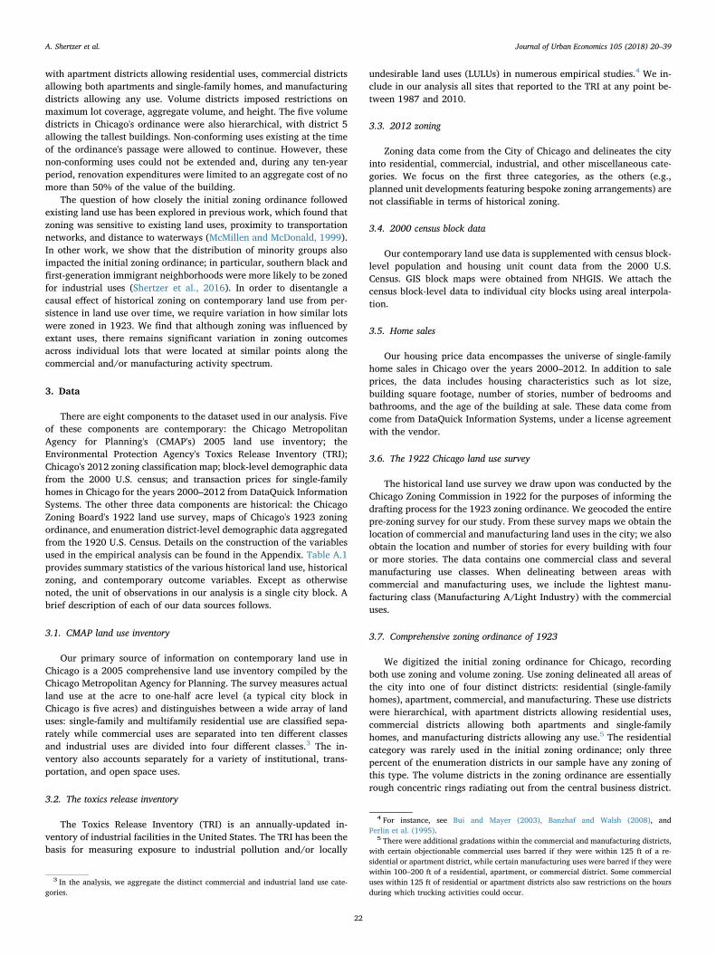
In Fig. 5, we remain focused on the commercial/industrial borders.However, we now assess their impact on commercial activity. In con-trast to the industrial uses analyzed in Fig. 4, commercial activitieswere permitted on both sides of these borders. While overall levels ofcommercial activity are generally higher on the commercial side of theborder, we find no evidence of a discrete change. Thus, summarizethese three sets of results, for uses where zoning binds we find a discretejump at the boundary. When zoning does not bind, we find no suchdiscrete jump.

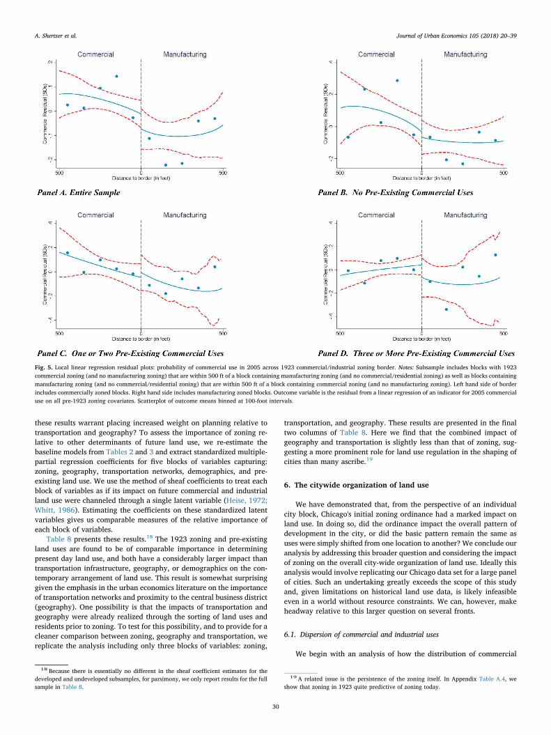
Finally, Fig. 6 considers the difference in the percentage of a blockdevoted to single-family residential use, comparing blocks which re-ceived the lowest density zoning with blocks that received the nextlowest density zoning (which accommodated mid-rise apartment

Table 4Impact of 1923 zoning on the contemporary land use: residential areas.

Percent single-family residential Percent multifamily residential

(1) (2) (3) (4) (5) (6)

Percent single family residential zoning 0.040*** 0.052*** 0.037*** −0.029*** −0.032*** −0.030***(0.003) (0.0039) (0.0038) (0.003) (0.0023) (0.0029)

Percent commercial zoning −0.034*** −0.051*** −0.027*** −0.047*** −0.033*** −0.065***(0.003) (0.0046) (0.0039) (0.003) (0.0035) (0.0053)

Percent manufacturing zoning −0.013*** −0.010 −0.035*** −0.057*** −0.040*** −0.068***(0.003) (0.0059) (0.0040) (0.003) (0.0035) (0.0050)

Percent volume district 1 zoning 0.118*** 0.043 0.076*** −0.048*** 0.023 −0.040***(0.011) (0.0366) (0.0070) (0.011) (0.0326) (0.0107)

Percent volume district 2 zoning 0.034*** −0.027 0.014* 0.007 0.059* 0.001(0.011) (0.0340) (0.0077) (0.010) (0.0303) (0.0140)

Percent volume district 3 zoning 0.013** −0.020 0.016*** −0.009 0.004 −0.008(0.006) (0.0142) (0.0046) (0.006) (0.0122) (0.0095)

Mean of dependent variable 0.388 0.593 0.187 0.291 0.143 0.436Std. dev. of dependent variable 0.396 0.383 0.291 0.339 0.247 0.354Sample restriction None Undeveloped Developed None Undeveloped DevelopedR-squared 0.546 0.456 0.354 0.433 0.318 0.334Observations 14,582 7221 7361 14,582 7221 7361

Notes: Outcome variable in columns (1)–(3) is the percentage of the city block devoted to single-family residential use in 2005. Outcome variable in columns (4)–(6) is the percentage ofthe city block devoted to multifamily residential use in 2005. Models include full set of spatial, demographic, and land use controls described in Section IV. Estimation uses OLS. Zoningvariables are standardized on the full sample (columns (1) and (4)), undeveloped sample (columns (2) and (5)), or developed sample (columns (3) and (6)). Columns (2) and (5) restrict tothe section of the city below median 1920 population density. Columns (3) and (6) restrict to the section of the city above median 1920 population density.

12 This approach allows us to control for confounds that vary continuously across thediscrete zoning boundaries. We estimate the border regressions on residuals from a modelincluding all of our control variables in order to control for any observed confounds thatvary discretely at the zoning boundaries. There is very little qualitative difference be-tween the residual analyses presented here and border regressions that do not includethese controls.


27

complexes). There is a sharp discontinuity, with lower density blockshosting 0.3 standard deviations (12 percentage points) more single-fa-mily housing than neighboring higher density blocks. The effect ofdensity zoning is evident across both high and low population densitysubsamples.

Taken as whole the non-parametric border analysis confirm theresults from our simple linear models. Parametric border regressionswhich correspond to these non-linear models are included in AppendixTable A.2 and corroborate the nonparametric results.

5.3. The effect of zoning on LULUs, density and prices

We next broaden our analysis to consider the impact of zoning onseveral additional margins that drove the adoption of these ordinances:exposure to undesirable land uses, population density, and home prices.A major motivation for the establishment of manufacturing use zones inthese early land use plans was the desire to constrain the location oflocally undesirable land uses so that they would not “destroy real estatefor residential and retail business purposes.”13 To evaluate the long-runimpact of zoning on the location of these LULUs, we assess the impact ofthe 1923 zoning ordinance on the distribution of polluting (TRI) facil-ities later in the twentieth century. The results presented in Table 5demonstrate that 1923 manufacturing zoning had a quantitatively sig-nificant impact on where such polluting facilities are located today. Aone standard deviation increase in the share of a neighborhood zoned

for manufacturing is associated with a 1.4 percentage point increase inthe likelihood of a city block hosting a TRI facility; this is a quantita-tively large effect given that only 1.8% of blocks in our sample hosted aTRI facility during the analysis period. Commercial zoning had a si-milar, but smaller in magnitude, effect. This relationship is stable acrossthe no pre-existing manufacturing, undeveloped, and developed sub-samples. As with our above analysis of manufacturing outcomes, thesmall sample of blocks that already had manufacturing in 1922 re-sponds differently. In these blocks, we see that zoning apparently hadno impact on the location of TRI facilities today.

Population density is another concern that both explicitly and im-plicitly underpinned the Zoning Commission's work.14 Table 6 showsthat, relative to zoning for apartments, zoning for single family homes,commercial and manufacturing uses all lead to lower population den-sities in 2010. Volume zoning also impacted future density. Here, theprimary distinction being between the lowest volume districts (1 and 2)and the highest volume districts (3–5). To give a sense of magnitude,the model predicts that a one standard deviation increase in the per-centage of a block receiving both single-family zoning and volumedistrict 1 zoning is associated with a 7 person per acre decline in po-pulation density; given that the city-wide average population density is28 persons per acre, this is a sizable impact.

Property values were also a key driver of Chicago's initial zoningordinance, particularly for real estate interests. Prior to passage of theordinance, Ivan O. Ackley, former president of the Chicago Real Estate

Fig. 3. Local linear regression residual plots: probability of commercial use in 2005 across 1923 commercial/apartment zoning border. Notes: Subsample includes blocks with 1923commercial/manufacturing zoning that are within 500 ft of a block containing only apartment/residential zoning as well as apartment/residential only blocks within 500 ft of a blockcontaining commercial/manufacturing zoning. Left hand side of border includes commercial/manufacturing blocks. Right hand side includes apartment/residential blocks. Outcomevariable is the residual from a linear regression of an indicator for 2005 commercial use on all pre-1923 zoning covariates. Scatterplot of outcome means binned at 100-foot intervals.

13 New York Times, July 26, 1916. 14 See Chicago Zoning Commission (1922) and Shertzer et al. (2016).


28

Board, predicted that comprehensive zoning would increase propertyvalues in Chicago by one billion dollars (more than 25%).15 While weare not in a position to assess Ackley's prediction regarding zoning'simpact on the overall price level, we can explore how spatial differencesin the 1923 zoning patterns are reflected in housing prices today.Table 7 reports the effects of the 1923 zoning ordinance on single-fa-mily home sale prices over the period 2000–2012, controlling forhousing characteristics, all pre-zoning control variables, and censustract fixed effects. Our results suggest that the patterns of land use es-tablished by the 1923 ordinance are still relevant in today's housingmarket.

To characterize historical zoning around a given home's location, foreach zoning designation, we compute its share within a quarter mile ofthe home, between a quarter and half mile away, and between a halfand a full mile away. Full sample results are presented in Column 1. Ourstrongest finding is that single-family residential zoning is associatedwith higher home values in both the immediate vicinity of the homeand further away. Moving from the proximate region to further away, aone standard deviation increase in the share of single-family homezoning is associated with a 1.2%, 1.4%, or 1.6% increase in home va-lues, respectively. Commercial zoning in the immediate vicinity is as-sociated with lower home values, while commercial zoning in the mostdistant region (between half and a full mile) increases home values,suggesting that homebuyers value access to commercial activity, solong as it is not right next door.

Manufacturing uses are also associated with higher home sale valueswhen they are between one half and a full mile away. This effect isstrongest in the developed portion of the sample (see Column 2).16

Focusing on the developed sample, historical manufacturing appears tobe associated with higher home values for the high-density portion ofthe sample whether it was in the immediate vicinity or more distant.Supplemental analysis shows that this effect is driven by the subset ofhomes located in relatively high-poverty census block-groups today,which may reflect a preference by low-income central city residents foraccessible manufacturing jobs.17

Taken together, these results demonstrate that contemporary homeprices have been impacted by the 1923 ordinance's lasting effect onChicago's spatial structure. They further suggest that, to the extent thatthe ordinance lead to the concentration of residential uses, zoning inChicago has likely increased residential property values.

5.4. Zoning vs. transportation and geography

Economists have typically focused on the role of transportation costsand geography in determining urban spatial structure. Our analysissuggests zoning also can have a lasting impact on land use patterns. Do

Fig. 4. Local linear regression residual plots: probability of industrial use in 2005 across 1923 commercial/industrial zoning border. Notes: Subsample includes blocks with 1923commercial zoning (and no manufacturing zoning) that are within 500 ft of a block containing manufacturing zoning (and no commercial/residential zoning) as well as blocks containingmanufacturing zoning (and no commercial/residential zoning) that are within 500 ft of a block containing commercial zoning (and no manufacturing zoning). Left hand side of borderincludes commercially zoned blocks. Right hand side includes manufacturing zoned blocks. Outcome variable is the residual from a linear regression of an indicator for 2005 industrialuse on all pre-1923 zoning covariates. Scatterplot of outcome means binned at 100-foot intervals.

15 Chicago Tribune, January 15, 1922.

16 P-value in the undeveloped sample is 0.17.17 Appendix Table A.3 shows analogous estimation results on the developed portion of

the sample by poverty quartiles. Large positive impacts of manufacturing zoning bothwithin a quarter mile and a full mile on home values are apparent for the subsample ofcity blocks in the top quartile of poverty rates only.


29

these results warrant placing increased weight on planning relative totransportation and geography? To assess the importance of zoning re-lative to other determinants of future land use, we re-estimate thebaseline models from Tables 2 and 3 and extract standardized multiple-partial regression coefficients for five blocks of variables capturing:zoning, geography, transportation networks, demographics, and pre-existing land use. We use the method of sheaf coefficients to treat eachblock of variables as if its impact on future commercial and industrialland use were channeled through a single latent variable (Heise, 1972;Whitt, 1986). Estimating the coefficients on these standardized latentvariables gives us comparable measures of the relative importance ofeach block of variables.

Table 8 presents these results.18 The 1923 zoning and pre-existingland uses are found to be of comparable importance in determiningpresent day land use, and both have a considerably larger impact thantransportation infrastructure, geography, or demographics on the con-temporary arrangement of land use. This result is somewhat surprisinggiven the emphasis in the urban economics literature on the importanceof transportation networks and proximity to the central business district(geography). One possibility is that the impacts of transportation andgeography were already realized through the sorting of land uses andresidents prior to zoning. To test for this possibility, and to provide for acleaner comparison between zoning, geography and transportation, wereplicate the analysis including only three blocks of variables: zoning,

transportation, and geography. These results are presented in the finaltwo columns of Table 8. Here we find that the combined impact ofgeography and transportation is slightly less than that of zoning, sug-gesting a more prominent role for land use regulation in the shaping ofcities than many ascribe.19

6. The citywide organization of land use

We have demonstrated that, from the perspective of an individualcity block, Chicago's initial zoning ordinance had a marked impact onland use. In doing so, did the ordinance impact the overall pattern ofdevelopment in the city, or did the basic pattern remain the same asuses were simply shifted from one location to another? We conclude ouranalysis by addressing this broader question and considering the impactof zoning on the overall city-wide organization of land use. Ideally thisanalysis would involve replicating our Chicago data set for a large panelof cities. Such an undertaking greatly exceeds the scope of this studyand, given limitations on historical land use data, is likely infeasibleeven in a world without resource constraints. We can, however, makeheadway relative to this larger question on several fronts.

6.1. Dispersion of commercial and industrial uses

We begin with an analysis of how the distribution of commercial

Fig. 5. Local linear regression residual plots: probability of commercial use in 2005 across 1923 commercial/industrial zoning border. Notes: Subsample includes blocks with 1923commercial zoning (and no manufacturing zoning) that are within 500 ft of a block containing manufacturing zoning (and no commercial/residential zoning) as well as blocks containingmanufacturing zoning (and no commercial/residential zoning) that are within 500 ft of a block containing commercial zoning (and no manufacturing zoning). Left hand side of borderincludes commercially zoned blocks. Right hand side includes manufacturing zoned blocks. Outcome variable is the residual from a linear regression of an indicator for 2005 commercialuse on all pre-1923 zoning covariates. Scatterplot of outcome means binned at 100-foot intervals.

18 Because there is essentially no different in the sheaf coefficient estimates for thedeveloped and undeveloped subsamples, for parsimony, we only report results for the fullsample in Table 8.

19 A related issue is the persistence of the zoning itself. In Appendix Table A.4, weshow that zoning in 1923 quite predictive of zoning today.


30

and manufacturing land uses today reflects the goals of the 1923 or-dinance. Recall Figs. 1 and 2, which show that considerable mixing ofuses took place before zoning. Indeed, 82% of blocks in the developed

portion of the city contained commercial activity prior to zoning, and10% contained heavy industry. Focusing on the developed subsample ofthe city so that we can evaluate the ability of zoning to reshape existing

Fig. 6. Local linear regression residual plots: percent of block devoted to single-family residential use across 1923 volume zoning borders. Notes: Left hand side of border includes blockswith the lowest level of 1923 density zoning. Right hand side includes blocks with the next lowest level of 1923 density zoning (accommodating mid-rise apartment complexes). Panel Brestricts the sample to blocks with below median population density in 1920; Panel C restricts to blocks with above median population density in 1920. Outcome variable is the residualfrom a linear regression of the share of the block devoted to single-family residential use in 2005 on all pre-1923 zoning covariates. Scatterplot of outcome means binned at 100-footintervals.

Table 5Impact of 1923 zoning on LULUs (TRI facilities).

Dependent variable= 1 if TRI facility in block

(1) (2) (3) (4) (5)

Percent manufacturing zoning 0.014*** 0.013*** −0.001 0.015*** 0.011***(0.002) (0.002) (0.018) (0.0035) (0.0037)

Percent commercial zoning 0.005*** 0.004*** −0.006 0.007*** 0.006**(0.002) (0.002) (0.016) (0.0022) (0.0022)

Percent single family residential zoning 0.000 0.000 −0.070 −0.000 −0.001*(0.001) (0.001) (0.095) (0.0010) (0.0005)

Percent volume district 1 zoning −0.001 0.003 −0.007 −0.006 −0.003(0.006) (0.005) (0.059) (0.0227) (0.0047)

Percent volume district 2 zoning −0.001 0.003 −0.01 −0.008 −0.001(0.006) (0.005) (0.040) (0.0216) (0.0066)

Percent volume district 3 zoning −0.001 0.001 −0.005 0.001 −0.002(0.004) (0.003) (0.020) (0.0092) (0.0049)

Mean of dependent variable 0.018 0.011 0.145 0.019 0.016Std. dev. of dependent variable 0.132 0.104 0.352 0.137 0.127Sample restriction None # Mfg= 0 # Mfg>0 Undeveloped DevelopedR-squared 0.180 0.094 0.310 0.256 0.132Observations 14,582 13,830 752 7221 7361

Notes: Outcome variable is an indicator that equals 1 if the city block contained any TRI facilities over the period 1987–2010. Models include full set of spatial, demographic, and land usecontrols described in Section IV. Estimation uses OLS. Zoning variables are standardized on the full sample (columns (1)–(3)), undeveloped sample (column (4)), or developed sample(column (5)). Columns (4) and (5) restrict to the section of the city below and above median 1920 population density, respectively.


31

urban areas, we begin by calculating the spatial distribution of parcelexposure to industrial and commercial uses. Specifically, we overlay thedeveloped portion of the city with a mesh of evenly-spaced points(250 ft apart). For each point, we measure the distance to the nearestindustrial (commercial) land use in 1922 and plot the distribution ofthese distances. We compare this distribution to that of distances to1923 industrial (commercial) zoning and 2005 industrial (commercial)land use. The results of this analysis are presented in Panels A and B ofFig. 7. When land uses are thoroughly mixed throughout the city, thedensity of distances will be concentrated near zero. If uses are segre-gated into zones, there will be more mass in the right tail of the density.

The solid lines in these graphs plot the density of distances frompoints in the city to their nearest 1922 commercial and industrial useneighbors. It is clear that the mass is concentrated near zero; almost alllocations were within a half mile of an industrial use in 1922 and withina tenth of a mile of a commercial use. The dashed lines plot the densityof distances envisioned by the zoning ordinance. The zoning board'spreoccupation with separating uses is evident here as the zoning den-sities have substantially more mass farther from zero, indicating thatmany locations in the city were placed in residential zones isolated fromcommercial and manufacturing activity. The intermittently dashed anddotted lines demonstrate the extent to which the zoning board's goalswere achieved; these lines plot the density of distances to industrial andcommercial uses in 2005. A comparison across the two sets of densitiesshows that the spatial distribution of land use today is much closer tothat envisioned by Chicago's planners in 1923 than it is to the actuallandscape to which these planners were reacting; thus, providing sug-gestive evidence that zoning has played a role in shaping the city'soverall land use patterns as well.

6.2. Houston, zoning and land use patterns

More direct evidence on the ability of zoning to affect patterns ofdevelopment at the city-wide level could be found by comparing out-comes in zoned and un-zoned cities. However, zoning is ubiquitous inthe United States, with virtually every sizable municipality subject to azoning ordinance. Only one major city in the U.S. has so far resisted theimplementation of zoning: Houston, Texas. Many scholars argue thatHouston provides a free-market counterfactual to the zoned city(Siegan, 1970, 1973). However, in lieu of zoning, Houston actuallyemploys a wide array of strategies to legally control land use and thereis some debate about how to view Houston vis-à-vis zoning.20 None-theless, it is the case that Houston lacks an overall planning framework

Table 6Impact of 1923 zoning on present day population density.

(1) (2) (3)

Percent commercial zoning −2.487*** −2.956*** −2.601***(0.281) (0.297) (0.447)

Percent manufacturing zoning −1.655*** −1.371*** −1.179***(0.120) (0.162) (0.203)

Percent single family res. zoning −3.556*** −2.753*** −4.383***(0.222) (0.254) (0.378)

Percent volume district 1 zoning −3.694*** 4.717 −3.651***(1.271) (4.114) (1.008)

Percent volume district 2 zoning −2.233* 5.410 −3.251**(1.279) (3.893) (1.399)

Percent volume district 3 zoning −0.103 1.521 −0.689(0.768) (1.744) (1.000)

Mean of dependent variable 27.74 23.84 31.56Std. dev. of dependent variable 23.73 19.27 26.86Sample restriction None Undeveloped DevelopedR-squared 0.333 0.397 0.349Observations 14,582 7221 7361

Notes: Outcome variable is persons per acre in the city block in 2000. Models include fullset of spatial, demographic, and land use controls described in Section IV. Estimation usesOLS. Zoning variables are standardized on the full sample (column (1)), undevelopedsample (column (2)), or developed sample (column (3)). Columns (2) and (3) restrict tothe section of the city below and above median 1920 population density, respectively.

Table 7Impact of 1923 zoning on contemporary single family house prices.

(1) (2) (3)

Percent commercial zoning within¼ mile

−0.00862** −0.0116 −0.00637*(0.00379) (0.00843) (0.00357)

Percent mfg. zoning within ¼ mile −0.00389 0.0224*** −0.00770(0.00391) (0.00808) (0.00497)

Percent residential zoning within ¼mile

0.0118*** 0.00379 0.0157***(0.00368) (0.00678) (0.00471)

Percent commercial zoning between¼ and ½ mile

−0.00424 −0.00766 0.00173(0.00527) (0.0110) (0.00464)

Percent mfg. zoning between ¼ and½ mile

0.00848 0.0224** 0.00118(0.00523) (0.0114) (0.00648)

Percent residential zoning between¼ and ½ mile

0.0144*** −0.000661 0.0200***(0.00394) (0.00727) (0.00512)

Percent commercial zoning between½ and 1 mile

0.0165* 0.0200 0.0129(0.00911) (0.0176) (0.00784)

Percent mfg. zoning between ½ and1 mile

0.0443*** 0.0588** 0.0134(0.00815) (0.0245) (0.00967)

Percent residential zoning between½ and 1 mile

0.0162*** −0.00306 0.0223***(0.00492) (0.0135) (0.00620)

Constant 12.74*** 11.59*** 12.65***(0.217) (0.325) (0.419)

Sample restriction None Developed UndevelopedR-squared 0.794 0.822 0.704Observations 50,556 18,378 32,178

Notes: Observations are individual home sales between 2000 and 2012. Models includefull set of spatial, demographic, and land use controls described in Section IV as well ashousing characteristics, census tract fixed effects, and year-month sale fixed effects. Es-timation uses OLS. Zoning variables are standardized on the full sample (column (1)),undeveloped sample (column (2)), or developed sample (column (3)). Columns (2) and(3) restrict to the section of the city above and below median 1920 population density,respectively. The dependent variable is the log of the sales price.

Table 8Sheaf statistics: developed Chicago (1923).

Commercial Industrial Commercial Industrial

Zoning 0.152*** 0.075*** 0.191*** 0.111***0.004 0.004 0.004 0.004

Geography 0.072*** 0.058*** 0.071*** 0.060***0.007 0.004 0.006 0.003

Transportation 0.100*** 0.019*** 0.115*** 0.026***0.004 0.003 0.004 0.003

Demographics 0.031*** 0.007***0.007 0.003

Land Use 0.152*** 0.092***0.008 0.004

Notes: Table presents the sheaf coefficients and standard errors for the estimated latentvariables capturing the impact of zoning, pre-existing land use, transportation, demo-graphics, and geography; the estimated latent variables are standardized to have standarddeviation of one for comparability of coefficients (Heise 1972; Whitt 1986). Outcomevariables are indicators for commercial and industrial land use in 2005.

20 The most prominent of these strategies is restrictive covenants or deed restrictions.These are agreements between neighboring property owners which legally bind them toobserve certain limitations on the use of their property. Restrictive covenants are fre-quently employed to limit uses to single-family homes, preventing the encroachment ofcommercial or industrial activity. The implementation of restrictive covenants in Houstondiffers markedly from its pre-zoning implementation in U.S. cities. Due to the issue oflegality and the high coordination and enforcement costs associated with covenants, thestate of Texas granted the Houston city government the power to enforce covenants di-rectly, without recourse to the court system (Susman, 1966; Kapur, 2004). Thus, theenforcement of covenants in Houston is similar to the enforcement of zoning in othercities. In Houston, covenants are employed to impose a wide range of restrictions beyonduse, regulating setbacks, minimum lot sizes, structural density, landscaping, noise levels,and architectural features. To lower coordination costs and permit covenants to moreclosely mimic zoning, covenants in Houston can be created or renewed by a simplemajority of lot owners in an area. The unanimous agreement of property owners is nolonger required, moving this policy far from the realm of consensual contract.


32

designed to guide growth and create distinct zones for incompatibleuses. As a result, the city has seen multiple referenda on the issue, mostrecently in 1993 when zoning was defeated by a narrow margin (Kapur,2004). Specific objections to the lack of zoning in Houston have focusedon the poor treatment of low-income communities and a feeling that thecurrent system allows excessive mixing of uses, leading to “ugly chaos”(Verhovek, 1993). Thus, there may be scope to use Houston as acounterfactual.

To assess the extent to which land use patterns actually differ inHouston relative to a hypothetical zoned version of the city, we analyzethe diffusion of TRI facilities in Houston relative to that in threeneighboring cities that employ comprehensive zoning: Austin, Dallas,and San Antonio.21 We focus on polluting facilities because separationfrom undesirable land uses is central to municipal zoning and becausethe TRI provides a readily available source of directly comparable data

for cross-city comparisons.22 We measure diffusion of TRI facilitiesusing the same approach that is discussed above for manufacturing andcommercial uses in Chicago.

Panel C of Fig. 7 shows that the distribution of distances from pointsthroughout the city of Houston to the nearest TRI facility has a greatermass near zero than that of Dallas; a result that is even more striking forAustin and San Antonio. A convenient summary is provided by thepercentage of points that lie within one mile of a TRI facility. In Austin,Dallas, and San Antonio this is 30%, 44%, and 43%, respectively; inHouston, it is 65%. The extent to which Houston represents an “un-zoned” counterfactual remains an open question. It is, however, clearlydistinct from the un-zoned state of early twentieth century Chicago. Ourcursory analysis of TRI facilities suggests that land use patterns in re-latively un-regulated Houston differ measurably from comparable citiesthat experienced formal zoning.

Fig. 7. Distribution of distances to nearest industrial or commercial use. Notes: Panel A shows the distribution of distances from each point of a mesh of equidistant (250 foot spaced)points to the nearest 1922 industrial use (blue line), nearest 1923 industrial zoning (green line), and nearest 2005 industrial use (red line). Analysis is restricted to the portion of the citywith above median population density in 1920. Panel B repeats the analysis for commercial uses and zoning. Panel C reports a distribution of distances to TRI facilities over 1987–2010 infour Texas cities, restricting to the area within 10 miles of the central business district. Panel D reports a similar analysis for the distribution of distances to predicted TRI facilities inChicago under zoning (red line) and under a counterfactual of unrestricted zoning (blue line). (For interpretation of the references to color in this figure legend, the reader is referred tothe web version of this article.)

21 To account for the different spatial extents of these cities, we take only the portionsof each city within 10 miles of its central business district. Results are similar if the entireextent of each city is used.

22 The criteria for classifying TRI facilities is established by the EPA and will not reflectidiosyncratic differences in the classification of land use across different cities.


33

6.3. Chicago counterfactual

Would a lack of zoning in Chicago have given rise to a landscapemore akin to Houston's? To answer this question, we conclude our workwith a statistical counterfactual analysis based on the TRI regressionresults. Using the results in Column 1 of Table 5, we predict the locationof TRI facilities under the actual 1923 zoning ordinance and under acounterfactual in which we set the zoning everywhere at its most per-missive level on both volume and use dimensions (high-density/in-dustrial). We then compute the distribution of distances as in thecomparisons above. The results, presented in Panel D of Fig. 7, areconsistent with our analysis of cities in Texas. They suggest that zoningshifted the distribution of TRI distances away from the origin sig-nificantly and provide further evidence that zoning has had a sig-nificant impact on the overall city-wide pattern of land use.

7. Conclusion

Comprehensive zoning is central to the lives of urban residents inthe United States, yet we know surprisingly little about how these po-licies have shaped contemporary cities. In this paper we provide thefirst attempt to measure the causal effect of land use regulation over thelong term, using as our setting the first comprehensive zoning ordi-nance adopted by the city of Chicago in 1923. Our analysis relies onboth the digitized ordinance and a lot-level land use survey undertakenin 1922, enabling us to control for a rich set of pre-zoning character-istics as well as identify the boundaries between areas zoned for dif-ferent uses.

The results of this study indicate that zoning has had a broader andmore significant impact on the spatial distribution of economic activity

than was previously believed. In particular, zoning may be more im-portant than either geography or transportation networks – the work-horses of urban economic geography models – in explaining wherecommercial and industrial activity are located. Furthermore, ratherthan simply “following the market,” zoning appears to be a powerfultool for achieving separation of uses. Our results strongly suggest thatover the long-run urban planning has been effective in creating re-sidential neighborhoods that are distant from undesirable manu-facturing uses, and that houses in these neighborhoods are more valu-able as a result.

We close with implications of our findings. First, more work isneeded to understand the institutions that drive aggregate land usepatterns. Previous research has focused on the causes of macro-levelpersistence such as agglomeration economics, locational fundamentals,durable capital, and natural advantages (Krugman, 1991; Davis andWeinstein, 2002; Glaeser and Gyourko, 2005; Redfearn, 2009; Bleakleyand Lin, 2012). At the same time, block-level persistence has receivedfar less attention, and institutional factors such as zoning have been leftlargely unexplored. While we establish that zoning played a prominentrole in Chicago's development, the mechanisms through which it in-fluenced future land use are less clear. Did zoning establish early pat-terns of development that then persisted to the present? Or was zoningitself persistent, perpetuating itself through later revisions of the ordi-nance? Recent work by Twinam (2017) in Seattle suggests that bothchannels may play a prominent role; however, more research is ne-cessary to document this phenomenon thoroughly. Regardless, our re-sults suggest that policymakers have great power to shape the overallform of cities, and the spatial arrangement of economic activity inurban areas a century from now may be largely the consequence of landuse regulation choices made today.

Appendix

A.I. Data Appendix

This section describes the eight components of the dataset compiled for this paper in more detail.

(1) CMAP land use inventoryOur primary source of information on contemporary land use in Chicago is drawn from a 2005 comprehensive land use inventory compiled bythe Chicago Metropolitan Agency for Planning, the official regional planning organization for Cook County and the six neighboring counties. TheCMAP land use inventory was created to inform the development of a comprehensive regional plan. The survey is based on 2005 aerial pho-tography as well as data from other government and private organizations. The survey measures land use at the acre to one-half acre level (atypical city block in Chicago is five acres) and distinguishes between a wide array of land uses: single-family and multifamily residential use areclassified separately while commercial uses are separated into ten different classes and industrial uses are divided into four different classes. Theinventory also accounts separately for a variety of institutional, transportation, and open space uses.

(2) The Toxics Release InventoryThe Toxics Release Inventory (TRI) is an annually-updated inventory of industrial facilities in the United States. It was created in 1986 followingseveral high-profile toxic waste management disasters with the aim of informing the public about potential environmental hazards in theircommunities. Facilities which manage or release into the environment certain hazardous chemicals in quantities greater than certain thresholdsmust report these quantities to the EPA, and these are compiled into the TRI. The TRI has been the basis for measuring exposure to industrialhazards and/or locally undesirable land uses (LULUs) in numerous empirical studies.23 We include in our analysis any sites that reported to theTRI at any point between 1987 and 2010.

(3) 2012 ZoningZoning data come from the City of Chicago and delineates the city into residential, commercial, industrial, and other miscellaneous categories.We focus on the first three categories, as the others (e.g., planned unit developments featuring bespoke zoning arrangements) are not classifiablein terms historical zoning.

(4) 2000 Census block dataOur contemporary land use data is supplemented with counts of housing units, African Americans, and Hispanics at the census block level for theyear 2000. Census data and GIS block maps were obtained from NHGIS. We attached the census block data to our Chicago city block data usingareal interpolation.

(5) Home salesOur housing price data encompasses the universe of single-family home sales in Chicago over the years 2000–2012. In addition to sale prices, thedata includes housing characteristics such as lot size, building square footage, number of stories, number of bedrooms and bathrooms, and the

23 See for instance, Banzhaf and Walsh (2008)


34

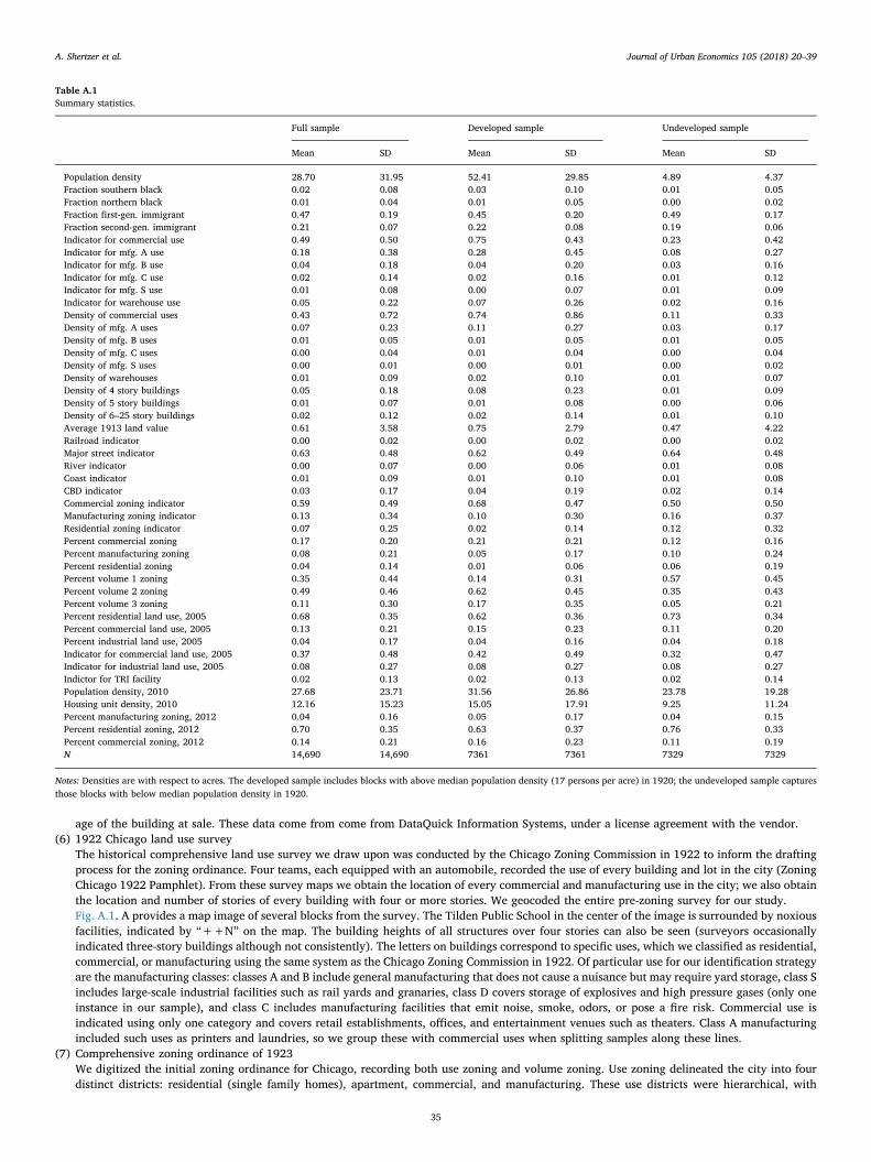
age of the building at sale. These data come from come from DataQuick Information Systems, under a license agreement with the vendor.(6) 1922 Chicago land use survey

The historical comprehensive land use survey we draw upon was conducted by the Chicago Zoning Commission in 1922 to inform the draftingprocess for the zoning ordinance. Four teams, each equipped with an automobile, recorded the use of every building and lot in the city (ZoningChicago 1922 Pamphlet). From these survey maps we obtain the location of every commercial and manufacturing use in the city; we also obtainthe location and number of stories of every building with four or more stories. We geocoded the entire pre-zoning survey for our study.Fig. A.1. A provides a map image of several blocks from the survey. The Tilden Public School in the center of the image is surrounded by noxiousfacilities, indicated by “++N” on the map. The building heights of all structures over four stories can also be seen (surveyors occasionallyindicated three-story buildings although not consistently). The letters on buildings correspond to specific uses, which we classified as residential,commercial, or manufacturing using the same system as the Chicago Zoning Commission in 1922. Of particular use for our identification strategyare the manufacturing classes: classes A and B include general manufacturing that does not cause a nuisance but may require yard storage, class Sincludes large-scale industrial facilities such as rail yards and granaries, class D covers storage of explosives and high pressure gases (only oneinstance in our sample), and class C includes manufacturing facilities that emit noise, smoke, odors, or pose a fire risk. Commercial use isindicated using only one category and covers retail establishments, offices, and entertainment venues such as theaters. Class A manufacturingincluded such uses as printers and laundries, so we group these with commercial uses when splitting samples along these lines.

(7) Comprehensive zoning ordinance of 1923We digitized the initial zoning ordinance for Chicago, recording both use zoning and volume zoning. Use zoning delineated the city into fourdistinct districts: residential (single family homes), apartment, commercial, and manufacturing. These use districts were hierarchical, with

Table A.1Summary statistics.

Full sample Developed sample Undeveloped sample

Mean SD Mean SD Mean SD

Population density 28.70 31.95 52.41 29.85 4.89 4.37Fraction southern black 0.02 0.08 0.03 0.10 0.01 0.05Fraction northern black 0.01 0.04 0.01 0.05 0.00 0.02Fraction first-gen. immigrant 0.47 0.19 0.45 0.20 0.49 0.17Fraction second-gen. immigrant 0.21 0.07 0.22 0.08 0.19 0.06Indicator for commercial use 0.49 0.50 0.75 0.43 0.23 0.42Indicator for mfg. A use 0.18 0.38 0.28 0.45 0.08 0.27Indicator for mfg. B use 0.04 0.18 0.04 0.20 0.03 0.16Indicator for mfg. C use 0.02 0.14 0.02 0.16 0.01 0.12Indicator for mfg. S use 0.01 0.08 0.00 0.07 0.01 0.09Indicator for warehouse use 0.05 0.22 0.07 0.26 0.02 0.16Density of commercial uses 0.43 0.72 0.74 0.86 0.11 0.33Density of mfg. A uses 0.07 0.23 0.11 0.27 0.03 0.17Density of mfg. B uses 0.01 0.05 0.01 0.05 0.01 0.05Density of mfg. C uses 0.00 0.04 0.01 0.04 0.00 0.04Density of mfg. S uses 0.00 0.01 0.00 0.01 0.00 0.02Density of warehouses 0.01 0.09 0.02 0.10 0.01 0.07Density of 4 story buildings 0.05 0.18 0.08 0.23 0.01 0.09Density of 5 story buildings 0.01 0.07 0.01 0.08 0.00 0.06Density of 6–25 story buildings 0.02 0.12 0.02 0.14 0.01 0.10Average 1913 land value 0.61 3.58 0.75 2.79 0.47 4.22Railroad indicator 0.00 0.02 0.00 0.02 0.00 0.02Major street indicator 0.63 0.48 0.62 0.49 0.64 0.48River indicator 0.00 0.07 0.00 0.06 0.01 0.08Coast indicator 0.01 0.09 0.01 0.10 0.01 0.08CBD indicator 0.03 0.17 0.04 0.19 0.02 0.14Commercial zoning indicator 0.59 0.49 0.68 0.47 0.50 0.50Manufacturing zoning indicator 0.13 0.34 0.10 0.30 0.16 0.37Residential zoning indicator 0.07 0.25 0.02 0.14 0.12 0.32Percent commercial zoning 0.17 0.20 0.21 0.21 0.12 0.16Percent manufacturing zoning 0.08 0.21 0.05 0.17 0.10 0.24Percent residential zoning 0.04 0.14 0.01 0.06 0.06 0.19Percent volume 1 zoning 0.35 0.44 0.14 0.31 0.57 0.45Percent volume 2 zoning 0.49 0.46 0.62 0.45 0.35 0.43Percent volume 3 zoning 0.11 0.30 0.17 0.35 0.05 0.21Percent residential land use, 2005 0.68 0.35 0.62 0.36 0.73 0.34Percent commercial land use, 2005 0.13 0.21 0.15 0.23 0.11 0.20Percent industrial land use, 2005 0.04 0.17 0.04 0.16 0.04 0.18Indicator for commercial land use, 2005 0.37 0.48 0.42 0.49 0.32 0.47Indicator for industrial land use, 2005 0.08 0.27 0.08 0.27 0.08 0.27Indictor for TRI facility 0.02 0.13 0.02 0.13 0.02 0.14Population density, 2010 27.68 23.71 31.56 26.86 23.78 19.28Housing unit density, 2010 12.16 15.23 15.05 17.91 9.25 11.24Percent manufacturing zoning, 2012 0.04 0.16 0.05 0.17 0.04 0.15Percent residential zoning, 2012 0.70 0.35 0.63 0.37 0.76 0.33Percent commercial zoning, 2012 0.14 0.21 0.16 0.23 0.11 0.19N 14,690 14,690 7361 7361 7329 7329

Notes: Densities are with respect to acres. The developed sample includes blocks with above median population density (17 persons per acre) in 1920; the undeveloped sample capturesthose blocks with below median population density in 1920.


35

apartment districts allowing residential uses, commercial districts allowing both apartments and single-family homes, and manufacturing dis-tricts allowing any use.24 The residential category was rarely used in the initial zoning ordinance; only three percent of the enumeration districtsin our sample have any zoning of this type. Fig. A.1.B shows a section of a use zoning map from an area west of the downtown along the ChicagoRiver. Zones for apartments, commercial activity, and manufacturing can all be seen.The volume districts in the zoning ordinance are essentially rough concentric rings radiating out from the central business district. Fig. A.1.C

Table A.2Zoning border regressions.

A. Blocks within 500 ft of both a residential or apartment block and some commercial or industrial zoning: probability of commercial use

(1) (2) (3) (4)

Commercial side of border 0.719*** 0.688*** 0.751*** 0.731***(0.0305) (0.0488) (0.0675) (0.0989)

Distance to nearest comm. or mfg. zoning −0.211*** −0.195*** −0.347** −0.024(0.0510) (0.0587) (0.1355) (0.2971)

Distance to nearest res. or apt. zoned block −0.028 0.052 −0.072 −0.131(0.0923) (0.2027) (0.2016) (0.1329)

Sample restriction None # Com=0 0<# Com≤ 2 # Com>2Observations 10,805 5662 2297 2846R-squared 0.398 0.358 0.399 0.296

B. Blocks within 500 ft of both commercial and industrial zoning: probability of industrial use

(1) (2) (3)

Manufacturing side of border 0.326*** 0.292*** 0.148(0.0642) (0.0772) (0.1782)

Distance to nearest comm. zoning 0.178 0.159 0.463(0.2550) (0.3214) (0.5618)

Distance to nearest mfg. zoning −0.310*** −0.365*** −1.077*(0.1059) (0.1188) (0.6278)

Sample restriction None # Mfg=0 # Mfg>0Observations 3118 2758 360R-squared 0.338 0.250 0.547

C. Blocks within 500 ft of both commercial and industrial zoning: probability of commercial use

(1) (2) (3) (4)

Commercial side of border 0.177*** 0.197** 0.044 0.189(0.0593) (0.0946) (0.1383) (0.1249)

distance to nearest comm. zoning −0.086 −0.103 −0.878 −0.143(0.2043) (0.2741) (0.5683) (0.6571)

Distance to nearest mfg. zoning 0.350** 0.560* 0.596* −0.118(0.1476) (0.3039) (0.3303) (0.2351)

Sample restriction None # Com=0 0<# Com≤ 2 # Com>2Observations 2945 1136 699 1110R-squared 0.245 0.245 0.304 0.292

D. Blocks within 500 ft of residential (single family) zoning: percent of block dedicated to single family residential

(1) (2) (3)

Low density (volume 1) side of border 0.523*** 0.562*** 0.450***(0.0605) (0.0797) (0.1380)

Distance to nearest volume 1 zoning −0.102 −0.102 −0.244(0.1795) (0.2972) (0.2544)

Distance to nearest volume 2 zoning 0.047 -0.042 0.108(0.1197) (0.1430) (0.3439)

Sample restriction None Undeveloped DevelopedObservations 2518 1634 884R-squared 0.502 0.480 0.459

Notes: Panel A replicates the analysis from Fig. 3 using OLS. Similarly, Panels B, C and D replicate Figs. 4, 5, and 6, respectively. Sample restrictions are with respect to 1922 land use. Thedeveloped sample includes blocks with above median population density (17 persons per acre) in 1920; the undeveloped sample captures those blocks with below median populationdensity in 1920. All models include the full set of historical covariates.

24 There were additional gradations within the commercial and manufacturing districts, with certain objectionable commercial uses barred if they were within 125 ft of a residential orapartment district, while certain manufacturing uses were barred if they were within 100–2000 ft of a residential, apartment, or commercial district. Some commercial uses within 125 ftof residential or apartment districts also saw restrictions on the hours during which trucking activities could occur.


36

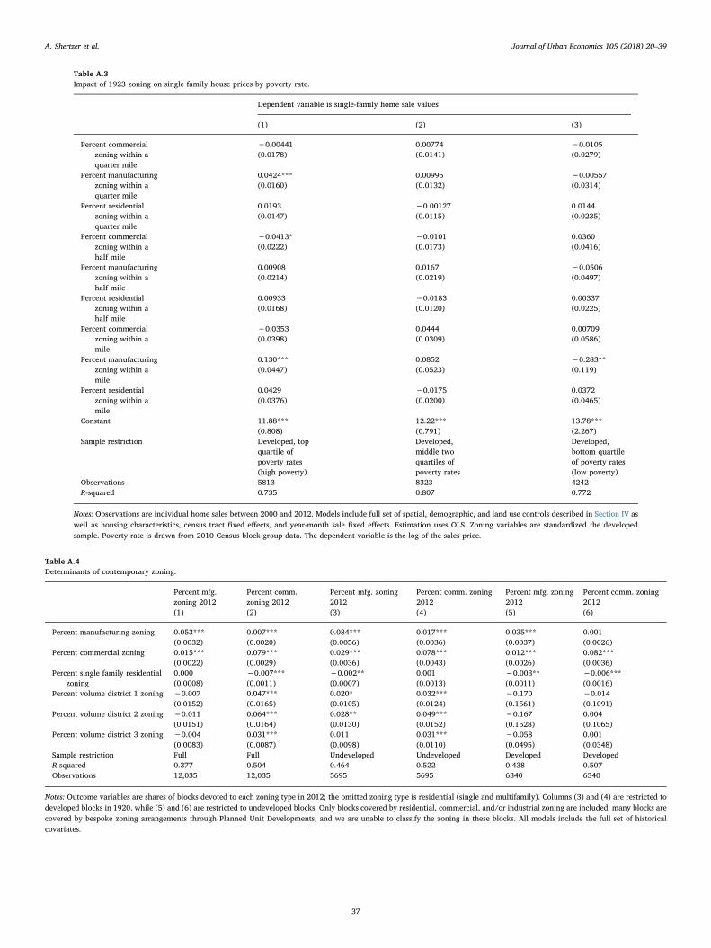
Table A.3Impact of 1923 zoning on single family house prices by poverty rate.

Dependent variable is single-family home sale values

(1) (2) (3)

Percent commercialzoning within aquarter mile

−0.00441 0.00774 −0.0105(0.0178) (0.0141) (0.0279)

Percent manufacturingzoning within aquarter mile

0.0424*** 0.00995 −0.00557(0.0160) (0.0132) (0.0314)

Percent residentialzoning within aquarter mile

0.0193 −0.00127 0.0144(0.0147) (0.0115) (0.0235)

Percent commercialzoning within ahalf mile

−0.0413* −0.0101 0.0360(0.0222) (0.0173) (0.0416)

Percent manufacturingzoning within ahalf mile

0.00908 0.0167 −0.0506(0.0214) (0.0219) (0.0497)

Percent residentialzoning within ahalf mile

0.00933 −0.0183 0.00337(0.0168) (0.0120) (0.0225)

Percent commercialzoning within amile

−0.0353 0.0444 0.00709(0.0398) (0.0309) (0.0586)

Percent manufacturingzoning within amile

0.130*** 0.0852 −0.283**(0.0447) (0.0523) (0.119)

Percent residentialzoning within amile

0.0429 −0.0175 0.0372(0.0376) (0.0200) (0.0465)

Constant 11.88*** 12.22*** 13.78***(0.808) (0.791) (2.267)

Sample restriction Developed, topquartile ofpoverty rates(high poverty)

Developed,middle twoquartiles ofpoverty rates

Developed,bottom quartileof poverty rates(low poverty)

Observations 5813 8323 4242R-squared 0.735 0.807 0.772

Notes: Observations are individual home sales between 2000 and 2012. Models include full set of spatial, demographic, and land use controls described in Section IV aswell as housing characteristics, census tract fixed effects, and year-month sale fixed effects. Estimation uses OLS. Zoning variables are standardized the developedsample. Poverty rate is drawn from 2010 Census block-group data. The dependent variable is the log of the sales price.

Table A.4Determinants of contemporary zoning.

Percent mfg.zoning 2012

Percent comm.zoning 2012

Percent mfg. zoning2012

Percent comm. zoning2012

Percent mfg. zoning2012

Percent comm. zoning2012

(1) (2) (3) (4) (5) (6)

Percent manufacturing zoning 0.053*** 0.007*** 0.084*** 0.017*** 0.035*** 0.001(0.0032) (0.0020) (0.0056) (0.0036) (0.0037) (0.0026)

Percent commercial zoning 0.015*** 0.079*** 0.029*** 0.078*** 0.012*** 0.082***(0.0022) (0.0029) (0.0036) (0.0043) (0.0026) (0.0036)

Percent single family residentialzoning

0.000 −0.007*** −0.002** 0.001 −0.003** −0.006***(0.0008) (0.0011) (0.0007) (0.0013) (0.0011) (0.0016)

Percent volume district 1 zoning −0.007 0.047*** 0.020* 0.032*** −0.170 −0.014(0.0152) (0.0165) (0.0105) (0.0124) (0.1561) (0.1091)

Percent volume district 2 zoning −0.011 0.064*** 0.028** 0.049*** −0.167 0.004(0.0151) (0.0164) (0.0130) (0.0152) (0.1528) (0.1065)

Percent volume district 3 zoning −0.004 0.031*** 0.011 0.031*** −0.058 0.001(0.0083) (0.0087) (0.0098) (0.0110) (0.0495) (0.0348)

Sample restriction Full Full Undeveloped Undeveloped Developed DevelopedR-squared 0.377 0.504 0.464 0.522 0.438 0.507Observations 12,035 12,035 5695 5695 6340 6340

Notes: Outcome variables are shares of blocks devoted to each zoning type in 2012; the omitted zoning type is residential (single and multifamily). Columns (3) and (4) are restricted todeveloped blocks in 1920, while (5) and (6) are restricted to undeveloped blocks. Only blocks covered by residential, commercial, and/or industrial zoning are included; many blocks arecovered by bespoke zoning arrangements through Planned Unit Developments, and we are unable to classify the zoning in these blocks. All models include the full set of historicalcovariates.


37

shows the digitization of these districts with each enumeration district assigned to the volume district most common within its borders. Thevolume district 1 maximum building height was 33 ft, corresponding to roughly three stories. For district 2, the maximum height was about sixstories; district 3, eleven stories; and district 4, sixteen stories. District 5, which was restricted to the central business district, allowed amaximum building height about 22 stories. If a building satisfied requirements on additional setbacks from the street, the allowed height wasgreater. There were no density “minimums,” only restrictions only the maximum volume, height, and lot coverage.

(8) Census Enumeration District Data for 1920In the empirical work we control for four categories of racial and ethnic minorities in 1920 since there is evidence that the spatial distribution ofthese groups impacted the initial zoning ordinance (Shertzer et al., 2016). We obtained counts of the number of blacks and white ethnic groupsfrom the 1920 census at the enumeration district level using the genealogy website Ancestry.com. Enumeration districts were small adminis-trative units used internally by the Census Bureau to divide cities up into small areas that could be surveyed by one person.25 In order to placeindividuals in 1920 urban space, we digitized the 1920 enumeration district map of Chicago. We first used written descriptions of the enu-meration districts available on microfilm from the National Archives. The information from these microfilms has been digitized and madeavailable on the web due to the work of Stephen P. Morse.26 Second, we took digital photographs of the physical map of the 1920 censusenumeration districts of Chicago from the National Archives. Working primarily with a geocoded (GIS) historic base street map developed by theCenter for Population Economics at the University of Chicago, we generated a GIS representation of the Chicago enumeration district map that isconsistent with the historic street grid.27

We define southern blacks to be individuals who report their race as black or mulatto and their place of birth as in the South.28 We define“second-generation” blacks, that is, individuals born in the North but with southern-born fathers, in the southern black category. Northern blacks aredefined as black or mulatto individuals who were both born outside the South with fathers born outside the South. First-generation immigrantsinclude all foreign-born individuals plus second-generation individuals under the age of 18, the latter of whom are presumably children residing inthe same household as their foreign-born parents. Second-generation immigrants are defined as individuals who were born in the U.S. and who are atleast 18 years old with foreign-born fathers.29

References

Banzhaf, S.H., Walsh, R.P., 2008. Do people vote with their feet? An empirical test ofTiebout's mechanism. Am. Econ. Rev. 98 (3), 843–863.

Bassett, E.M., 1980. Zoning. National Municipal League. White H. A heteroskedasticity-consistent covariance matrix estimator and a direct test for heteroskedasticity.Econometrica: Journal of the Econometric Society 817–838.

Bleakley, H., Lin, J., 2012. Portage and path dependence. Q. J. Econ. 127 (2), 587–644.Bui, L.T.M., Mayer, C.J., 2003. Regulation and capitalization of environmental amenities:

Fig. A.1. Land use survey and use zoning map samples. Notes: A portion of the 1922 land use survey map created by the Chicago Zoning Commission. These blocks are located just acrossthe Chicago River to the west of the downtown. Numbers indicate building heights in stories. Black squares within parcels indicate commercial uses; letters sometime accompany these toindicate a specific commercial activity. V indicates a vacant lot/building. Letters followed or preceded by a single+ indicate light industrial uses. Letters preceded by ++ indicateheavier industrial uses; in particular, ++N indicates uses which “by reason of excessive noise, odor, fumes, gases, etc., affect the adjacent territory.” Notes: This image shows the area ofChicago west of the downtown along the Chicago River. Unhatched areas are zoned for apartments, hatched areas are zoned for commercial uses, and cross-hatched areas are zoned formanufacturing. Notes: This map shows volume districts in the Chicago zoning ordinance with enumeration districts assigned to the volume district in which the majority of its area fell.District 5 (darkest hue) permitted the tallest buildings, up to 22 stories. District 1 (lightest hue) was the most restrictive, allowing only buildings with three or fewer stories.

25 The Census Bureau did not switch to a mail-based survey system until 1960.26 Website: http://stevemorse.org/ed/ed.php.27 These data are available on line at http://uadata.org/.28 We use an eleven state definition of the South, defining the region to include Alabama, Arkansas, Florida, Georgia, Louisiana, Mississippi, North Carolina, South Carolina, Tennessee,

Texas, and Virginia.29 Using these definitions, we avoid the standard problem in the segregation literature of immigrant populations being diluted by the presence of their native-born children (see

Cutler et al., 2008).


38

http://Ancestry.com

http://refhub.elsevier.com/S0094-1190(18)30005-6/sbref0002







http://stevemorse.org/ed/ed.php

http://uadata.org/

evidence from the toxic release inventory in Massachusetts. Rev. Econ. Stat. 85 (3),693–708.

Chicago Zoning Commission 1922, “Zoning Chicago” (pamphlet).Combes, P.P., Gobillon, L., 2015. The empirics of agglomeration economies. Handbook of

regional and urban economics Vol. 5. Elsevier, pp. 247–348.Conley, T.G., 1999. GMM estimation with cross sectional dependence. J. Econom. 92 (1),

1–45.Cutler, D.M., Glaeser, E.L., Vigdor, J.L., 2008. Is the melting pot still hot? Explaining the

resurgence of immigrant segregation. Rev. Econ. Stat. 90 (3), 478–497.Davis, D.R., Weinstein, D., 2002. Bones, bombs and break points: the geography of eco-

nomic activity. Am. Econ. Rev. 92 (5), 1269–1289.Dep't of Commerce Advisory Committee on Zoning. A Standard State Zoning Enabling

Act. (1926).Duranton, G., Puga, D., 2015. Urban land use. In: Duranton, Gilles, Henderson, J.Vernon,

Strange, William C. (Eds.), Handbook of Regional and Urban Economics 5. North-Holland, pp. 467–560 Chapter 8.

Fischel, W.A., 2001. The Homevoter Hypothesis: How Home Values Influence LocalGovernment Taxation, School Finance, and Land use Policies. Harvard UniversityPress, Cambridge.

Glaeser, E.L., Gyourko, J., 2005. Urban decline and durable housing. J. Political Econ.113 (2), 345–375.

Glaeser, E.L., Ward, B.A., 2009. The causes and consequences of land use regulation:evidence from Greater Boston. J. Urban Econ. 65 (3), 265–278.

Hall, P., 2002. An Intellectual History of Urban Planning and Design in the TwentiethCentury, third ed. Wiley-Blackwell Publishing.

Heise, D.R., 1972. Employing nominal variables, induced variables, and block variables inpath analyses. Sociol. Methods Res. 1 (2), 147–173.

Ihlanfeldt, K.R., 2007. The effect of land use regulation on housing and land prices. J.Urban Econ. 61 (3), 420–435.

Kapur, T.M., 2004. Land use regulation in Houston contradicts the city's free market re-putation. Environmental Law Reporter News and Analysis 34 (1), 10045–10063.

Krugman, P., 1991. Increasing returns and economic geography. J. Political Econ. 99 (3),483–499.

Kuminoff, N.V., Kerry Smith, V., Timmins, Christopher, 2013. The new economics ofequilibrium sorting and policy evaluation using housing markets. J. Econ. Lit. 51 (4),1007–1062.

McDonald, J.F., McMillen, D.P., 1998. Land values, land use, and the first Chicago zoningordinance. J. Real Estate Financ. Econ. 16 (2), 135–150.

McMillen, D.. “Conditionally Parametric Quantile Regressions for Spatial Data: AnAnalysis of Land Values in Early Nineteenth Century Chicago.” Working paper. 2012.

McMillen, D.P., McDonald, J.F., 1999. Land use before zoning: the case of 1920s Chicago.Reg. Sci. Urban Econ. 29, 473–489.

Munneke, H.J., 2005. Dynamics of the urban zoning structure: an empirical investigationof zoning change. J. Urban Econ. 58 (3), 455–473.

Perlin, S.A., Setzer, R.W., Creason, J., Sexton, K., 1995. Distribution of industrial airemissions by income and race in the United States: an approach using the toxic re-lease inventory. Environ. Sci. Technol. 29 (1), 69–80.

Redding, S.J., Turner, M.A., 2015. Transportation costs and the spatial organization ofeconomic activity. In: Duranton, Gilles, Henderson, J.Vernon, Strange, William C.(Eds.), Handbook of Regional and Urban Economics 5. North-Holland, pp.1339–1398 Chapter 20.

Quigley, J.M., Raphael, S., 2005. Regulationthe high cost of housing in California. Am.Econ. Rev. 95 (2), 323–328.

Redfearn, C.L., 2009. Persistence in urban form: The long-run durability of employmentcenters in metropolitan areas. Reg. Sci. Urban Econ. 39 (2), 224–232.

Schwieterman, J.P., Caspall, D.M., 2006. The Politics of Place: A History of Zoning inChicago. Lake Claremont Press.

Shertzer, A., Twinam, T., Walsh, R.P., 2016. Race, ethnicity, and discriminatory zoning.Am. Econ. J.: Appl. Econ. 8 (3), 217–246.

Siegan, B.H., 1970. Non-zoning in Houston. J. Law Econ. 13 (1), 71–147.Siegan, B.H., 1973. Land use Without Zoning. Free Press.Susman, T.M., 1966. Municipal enforcement of private restrictive covenants: an in-

novation in land use control. Texas Law Rev. 44, 741–768.Troesken, W., 2004. Water, race, and disease. MIT Press.Turner, M.A., Haughwout, A., van derKlaauw, W., 2014. Land use regulation and welfare.

Econometrica 82 (4), 1341–1403.Twinam, T.. “The long-run impact of zoning: Institutional hysteresis and durable capital

in Seattle, 1920–2015.” Working paper. 2017.Wallace, N.E., 1988. The market effects of zoning undeveloped land: does zoning follow

the market? J. Urban Econ. 23 (3), 307–326.Verhovek, S.H., 1993. 'Anything Goes' Houston May Go the Limit: Zoning. New York

Times.Whitt, H.P., 1986. The sheaf coefficient: a simplified and expanded approach. Soc. Sci.

Res. 15 (2), 174–189.Zhou, J., McMillen, D.P., McDonald, J.F., 2008. Land values and the 1957 comprehensive

amendment to the Chicago zoning ordinance. Urban Stud. 45 (8)), 1647–1661.


39






































































Twinam Zoning and Economic Geography

Documents