Tutorials Mecway Finite Element Analysis Version 8.0 2017 1

Welcome message from author
This document is posted to help you gain knowledge. Please leave a comment to let me know what you think about it! Share it to your friends and learn new things together.
Transcript

Tutorials
Mecway Finite Element AnalysisVersion 8.0
2017
1
Contents
Chapter 1Getting Started 3
1.1 Quick Start, 31.2 Basic Operations in the Graphics Area, 41.3 Solution, 81.4 Manual Meshing, 10
Chapter 2Analysis Types 16
2.1 Static Analysis of a Pressurized Cylinder, 172.2 Thermal Analysis of a Plate being Cooled, 222.3 Heat Flow Through a Solid Part, 262.4 Thermal Stress, 282.5 Free Vibration of a Cantilever Beam, 302.6 Dynamic Response of a Crane Frame, 342.7 Dynamic Response of a Solid Part, 372.8 DC Circuit, 392.9 Electrostatic Analysis of a Capacitor, 422.10 Acoustic Analysis of an Organ Pipe, 452.11 Buckling of a Column, 49
Chapter 3Operations 52
3.1 Extrude, 523.2 Loft, 563.3 Refine Local 2D, 593.4 Mirror Symmetry, 613.5 Cyclic Symmetry, 633.6 CAD Work-flow, 653.7 Local Refinement with CAD Models, 683.8 Mixed Materials, 693.9 Mixed Materials with CAD Assemblies, 713.10 Constraint Equations, 743.11 Advanced Manual Meshing, 75
2

1Chapter 1Getting Started
These tutorials assume that you are new to Mecway and indeed may be new to finite elementanalysis. Here you will find step by step instructions to get you started using the program. Once youhave learned the basic concepts and operations, you can find more comprehensive information in thecompanion ‘Manual’.
1.1 Quick StartThis is a very simple tutorial showing you how to create a working model from scratch. You can skipthis if you prefer a more in depth introduction from the other tutorials.
Step 1
Change to Select faces mode.
Step 2
Click the Quick cube button to create a hexahedron element.
Step 3
Right click the right-most face and clickLoads & constraints then New fixedsupport. Click OK in the box thatappears.
Step 4
Drag with the middle mouse button to rotate the model so the opposite face is towards you. If youdon't have a middle mouse button, use the Rotate tool button and the left mouse button.
3

Step 5
Right click the opposite face and click Loads &constraints then New pressure. Enter the value 5and press OK.
Step 6
Right click the Default component in the outline tree and click Assign newmaterial. Choose Isotropic and enter a Young's modulus of 50000.Press OK.
Step 7
Press solve.
Step 8
Right click Solution and choose New stress and strain →von Mises stress. Then click the new von Mises stressitem to display it. The color key shows a 5 Pa uniformstress due to the pressure load.
1.2 Basic Operations in the Graphics AreaBecause the graphics is so much a part of Mecway, let us look first at a data file which displays amodel and its solution.Step 1
File->Open, Basic_graphics_tutorial.liml in the tutorials folder where Mecway has been installed.This is a contrived example merely to show the graphics features.
4

There are three parts to the screen the toolbars at the top, arranged into model-building tools and the graphics display options. the model structure and solution displayed in an outline tree in the left panel a graphics area which displays the mesh
This sample is a beam with a T-shaped end and has already been solved. One end is totally fixed, asif built into a wall. At the free end, a downwards force is applied at seven locations. The self-weight ofthe beam has been neglected.
Step 2
Toggle the display of element surfaces.
5

Toggle element edge display.
Step 3
Select nodes
Turn off the display of elements surfaces andturn on element edges. Drag over the modelto select nodes, including internal nodes.
Click in an open space to deselect the nodes.Then click a node to select it. Hold the Ctrl keydown and click a couple of nodes to add to theselection set. If a node is already selected and it'sclicked on while holding down the Ctrl key, it becomes deselected.
Drag a node to a new location. Repeat the action onanother node, but this time hold down the Shift key.You'll notice that the node is fixed and cannot bedragged.
Edit->Undo or Ctrl + Z to return the displaced node.
Click in an open space to deselect the nodes.
Select faces . Drag over the model to see that only surfaces are selected.
Click in an open space to deselect the surfaces.
6

Select elements . Drag to see that only elements have been selected.
The Ctrl key has the same effect while selecting faces or elements as it does with selecting nodes.
Step 4
The display of loads and constraints can betoggled off or on.
Step 5
Click the Z arrowhead of the triad at the bottom right corner of the graphics area to viewthe model parallel to the screen.
Left or right clicking the arrowheadswill display the different views of themodel parallel to the screen.
Click the blue dot to return to an isometric view.
Step 6
To rotate the view, drag with the middle mouse button (or wheel).
7

To see a small feature more clearly, zoom into that area by placing the mouse over that area (noclicking required) and rotating the mouse wheel for a larger display of the small feature. Rotating themouse wheel the other way will make the model's display become smaller.
If the model's display seems to be half out of the graphics area, you need to pan the model back intoview. Drag it using the right mouse button.
If the model does not fully appear in the graphics area after you have used the zoom, rotate or pan,use the fit to window tool-button
Step 7
Use the tape measure tool-button to check the lengths. Click a node but continue keeping themouse button pressed and move the cursor across to another node. Mecway will give a readoutof that distance.
Step 8
Tools->Volume will give volume of the entire mesh. This tool can be used to obtain the volume of aselected part of the mesh. The selection can be element nodes, faces or elements.
Similarly the Tool->Surface area will give the area of the selected faces. The selections can only beelement faces.
1.3 SolutionStep 1
This tutorial uses the same file as the previous tutorial. So if it is not already open in Mecway, use theFile->Open, Basic_graphics_tutorial.liml in the tutorials folder where Mecway has been installed.
In the solution section of the outline tree click on displacement → magnitude. The graphics displaywill update to show the results of the solved model. The units used in the legend on the display scalecan be changed by clicking on them.
Step 2
Click the Deformed view tool-button to visualize an exaggerated displacement of the structure.
Click the Undeformed shape to superimpose an outline of the undeformed shape onto thedeformed mesh.
8

Step 3
Right click Solution in the outline tree and choose new stress and strain → von Mises stress toadd von Mises stress to the solution.
Step 4
Click the table tool-button to display the displacements, rotations and stresses at each node inspreadsheet-style cells which you can then copy and paste into your own spreadsheet.
Step 5
Use the animation tool-button to animate the deflection. Smooth deformation between the twoextremes of movement is simulated. You can choose the scale factor. This tool is especially useful forvisualizing solutions in vibration analysis.
Step 6
This slider can be used to cut-away the model to look inside it. You will need torotate the model suitably so that the cut occurs where you want it. Don't forget to
return to its leftmost position before doing any editing of the mesh.
To return to the model that does not display the results, click any of the items in the outline tree that isnot below Solution.
Now that you have some experience in manipulating the graphics of the model, it’s time to learn howto create them from scratch. The next section will walk you through the case we have just studied.
9

1.4 Manual Meshing
Always begin a manual mesh by creating a coarse mesh; it can always be refined later. A coarse meshsimply means larger and fewer elements, and a refined mesh means smaller and more elements.Creating a coarse mesh requires less labor and, if things go wrong, it will be less frustrating.
Just as in the real world where everything has three dimensions (length, width, height), thegeometrical properties of finite elements are also three dimensional in nature. Some elements willappear on the screen as being clearly three dimensional elements, while others will appear on thescreen as flat and two dimensional. Nevertheless, the elements that appear flat and two dimensionaldo actually have the third dimension, of thickness.
Elements that appear three dimensional on the screen will usually be created from a two dimensionalflat shape, so modeling typically starts with what appears on the screen as a flat two dimensionalmesh. This initial 2D mesh can be created either by a combination of nodes and elements or by usingready-made template patterns. Editing tools are available for modifying the two dimensional mesh asyou create and form it. Once the coarse mesh is complete, whether it be two dimensional or threedimensional in appearance, it will need to be refined before running the solver.
Here is a tutorial to illustrate how the manual meshing tools work together to create the model used inthe introductory chapter. We will recreate the T-shaped thick beam used in section 1.2 to illustrateMecway's graphics tools. At the end you may wish to use some of the skills you have learned tomodify the length and thickness of the beam to make it more realistic.
Step 1
The analysis type should be Static 3D. If it's not, right click the item, then select Analysis settings to change the analysis type.
Use the Mesh tools->Create->Node... or and enter the following coordinates.X 0Y 0Z 0Leave the units as meters (m).
Click the Add button. Repeat for the following coordinates, then click Close.11,0,011,1,00,1,0
Click the Z arrowhead to view the XY plane parallel to the screen.
To view the entire model, use fit to window
10
Step 2
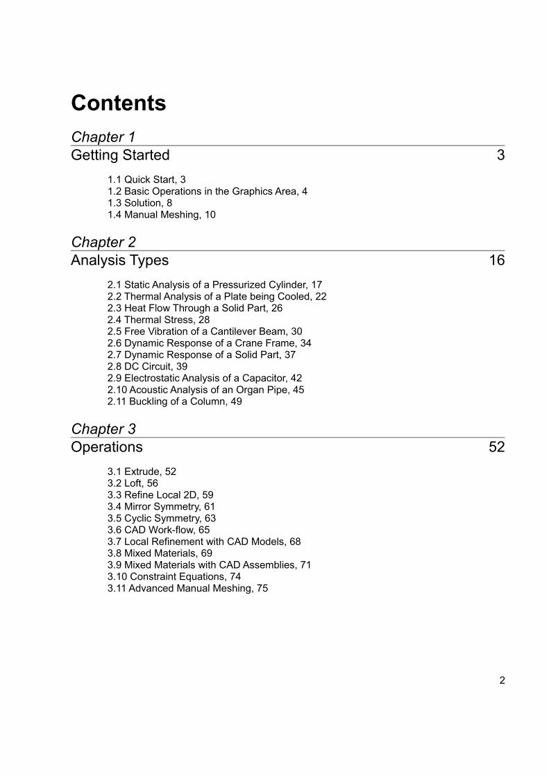
Mesh tools->Create->Element... Select and click the four nodes then click Close.The order of the clicked nodes will affect the orientation of the mesh refinement that will be done in thenext step. In this tutorial, the element is formed using the node order 1-2-3-4.
Step 3
Mesh tools->Refine->Custom...Number of subdivisionsR 11S 4T 1Click OK
Step 4
Activate select faces
Drag to select the entire mesh.
Mesh tools->Extrude... Direction +ZThickness 2, units mNumber of subdivisions 2
Click the blue dot to view an isometric display of the model.
11
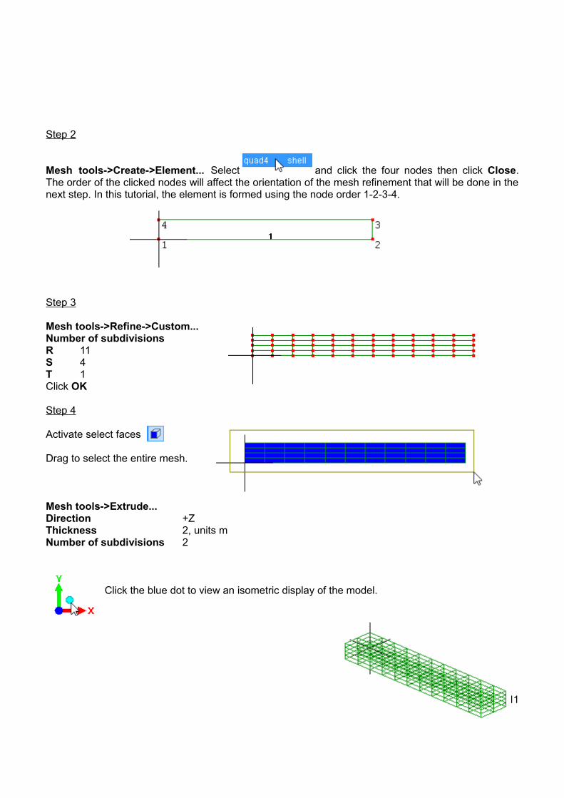
Click in the open space of the graphics area to deselect the elements.
Step 5
Activate select faces
To improve clarity use the show element surfaces tool-button to hide the internal elements.
Select these two faces by clicking one face then holding the Ctrl key whileclicking the second face.
The Ctrl key can be used while selecting items. It works by adding the new items to the currentlyselected items, and if the clicked item is already selected it will become deselected.
Mesh tools->Extrude... Direction +NormalThickness 3, unit ftNumber of subdivisions 1
Notice that you can use a mixture of differentunits for different quantities.
Drag with the middle mouse button or wheel to rotate theview of the model or use this if you don't have amiddle button.
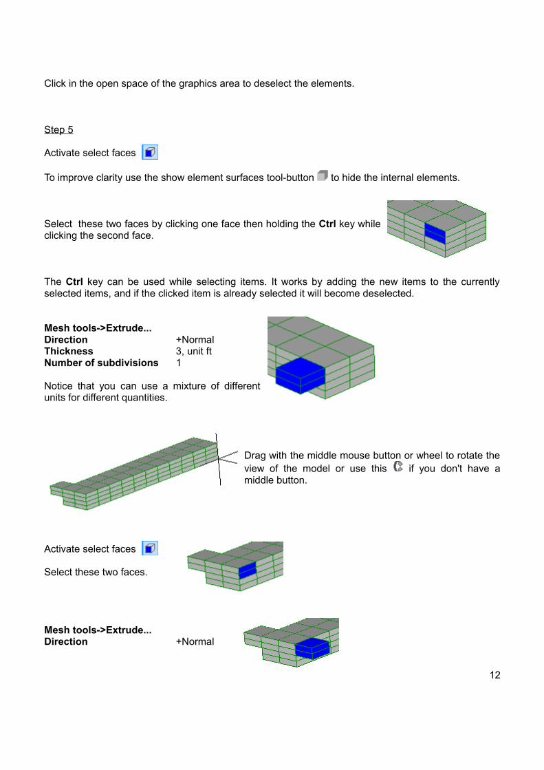
Activate select faces
Select these two faces.
Mesh tools->Extrude... Direction +Normal
12

Thickness 3, unit ftNumber of subdivisions 1
Step 6
Click in an open space of the graphics area to deselect the model.
Activate select nodes to see that these are 8 node hexahedrons.
Change these 8 node hexahedrons into the more accurate 20 nodehexahedrons using Mesh tools->Change element shape... select hex20and click OK to accept. The hex8 elements give a linear approximation to thedisplacement field, whilst the hex20 elements give a quadratic approximation.
Step 7
Right click, Assign new material
Mechanical tabIsotropic selectYoung's modulus 200, unit GPaPoisson's ratio 0.3
A material is now associated with the elements.
Step 8
In order for a part to develop stresses, all rigid body motion must be resisted. The left face of this model will be constrained.
Activate select faces
13
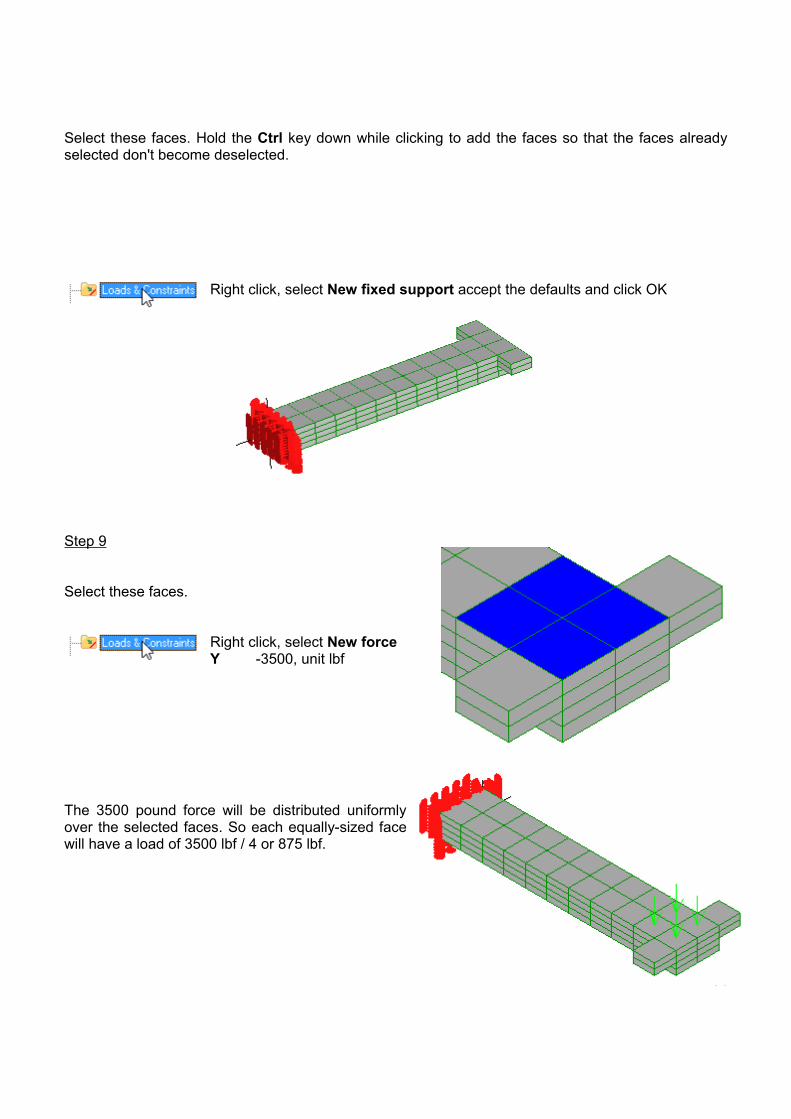
Select these faces. Hold the Ctrl key down while clicking to add the faces so that the faces alreadyselected don't become deselected.
Right click, select New fixed support accept the defaults and click OK
Step 9
Select these faces.
Right click, select New force Y -3500, unit lbf
The 3500 pound force will be distributed uniformlyover the selected faces. So each equally-sized facewill have a load of 3500 lbf / 4 or 875 lbf.
14
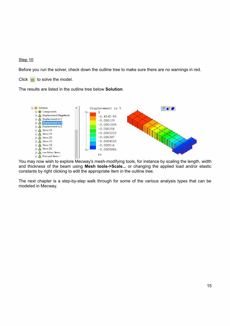
Step 10
Before you run the solver, check down the outline tree to make sure there are no warnings in red.
Click to solve the model.
The results are listed in the outline tree below Solution.
You may now wish to explore Mecway's mesh-modifying tools, for instance by scaling the length, widthand thickness of the beam using Mesh tools->Scale... or changing the applied load and/or elasticconstants by right clicking to edit the appropriate item in the outline tree.
The next chapter is a step-by-step walk through for some of the various analysis types that can bemodeled in Mecway.
15

2Chapter 2Analysis Types
While the typical user does not need an in-depth study of the mathematics behind finite elementanalysis, you do need to understand the behavior of elements in order to represent a given physicalproblem correctly.
Finite element analysis is not like CAD (computer aided design) software where you simply create ageometry and take a print-out. Instead, it follows the law of 'Garbage in, Garbage out'. Your choice ofelement type, mesh layout and constraints will strongly affect the accuracy of the solution.
We recommend to beginners that you confine your models to text-book problems with known solutionsrather than attempting real world problems with unverifiable solutions. When you get to the pointwhere you're solving real world problems, never accept the results at face value. Rather, validate themby comparing the results to hand calculations, experimental observations or knowledge from pastexperience.
This chapter contains tutorials to initiate you into using Mecway's basic analysis capabilities. Morespecific features like thermal-stress problems, composite materials, cyclic symmetry and constraintequations are described in Chapter 4 Specific Operations and the companion Manual.
Not all types of elements can be used for all types of analysis. The Manual liststhe elements that are available for use in each type of analysis. When creatingelements, if you see an N/A ('not applicable') next to the type of element, itmeans it can't be used to solve that type of analysis. However, you can use non-applicable elements as construction tools provided you change them using Meshtools->Change element shape... , or delete them before solving.
The outline tree presents all the information you need about your model andallows you to perform various actions on the model itself. You will alwaysbegin at the top, changing the analysis type if you do not want the default,3D static analysis.
Items that appear in red indicate missing or erroneous information, so rightclick them for a What's wrong? clue.
The constraints and loads that you apply will be listed in the Loads & Constraints section. Aftersolving the model the field values will be listed below Solution.
16
2.1 Static Analysis of a Pressurized CylinderA cylinder of 2m radius, 10m length, 0.2m thickness, Young's modulus 15000 N/m2 and Poisson ratio0.285 will be analyzed to determine its hoop stress caused by an internal pressure of 100N/m2.
From shell theory, the circumferential or hoop stress for a thin cylinder of constant radius and uniforminternal pressure is given by :
σ = (pressure × radius) / thickness
σ = (100 × 2) / 0.2
σ = 1000 N/m2
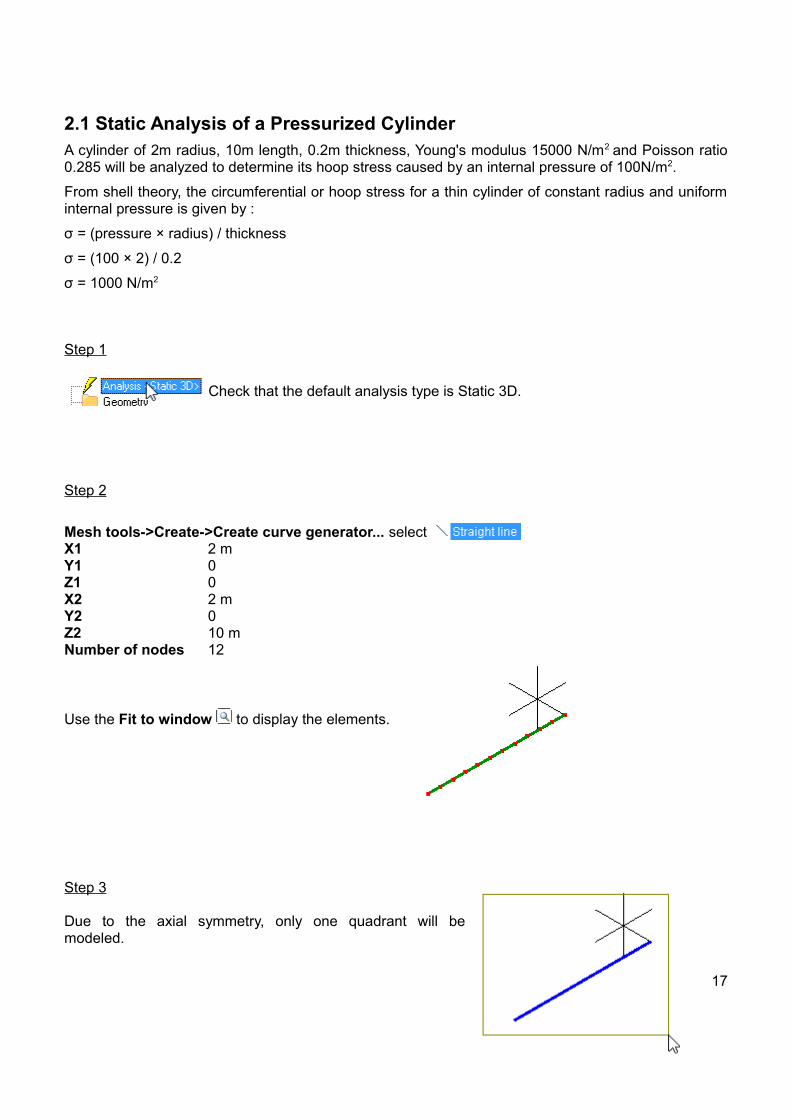
Step 1
Check that the default analysis type is Static 3D.
Step 2
Mesh tools->Create->Create curve generator... select X1 2 mY1 0Z1 0X2 2 mY2 0Z2 10 mNumber of nodes 12
Use the Fit to window to display the elements.
Step 3
Due to the axial symmetry, only one quadrant will bemodeled.
17

Activate select faces and drag to select all the elements.
Mesh tools->Revolve...Axis of revolution +ZAngle 90 °Number of subdivisions 8
Step 4
Right click, Assign new materialGeometric tab select Shell/membraneThickness 0.2 m
Mechanical tabselect IsotropicYoung's modulus 200E9 PaPoisson's ratio 0.285
Step 5
Right click the X arrowhead to view the YZ plane parallel to the screen.
Activate select faces, activate show element surfaces, and activate show shell thickness
Because of the mirror symmetry only one quadrant of the cylinder has been modeled. At the planes ofmirror symmetry, the nodes must be constrained so that they do not move out of the plane. Also, nobending must occur in that plane of symmetry.
To enforce mirror symmetry at the edge in the YZplane, drag to select the thickness of the shell.
18

Right click, New displacement and select the X option.
Right click, New node rotation and select the Z option.
Right click the Y arrowhead to view the ZX plane parallel to the screen.
To enforce mirror symmetry at the edge in the ZX plane, drag to select the thicknessof the shell.
Right click, New displacement and select the Y option.
Right click, New node rotation and select the Z option.
Right click the Z arrowhead to view the XY plane parallel to the screen.
To eliminate rigid body translation motion along the Z axis drag to select theshell thickness in the XY plane.
Right click, New displacement and select the Z option.
19
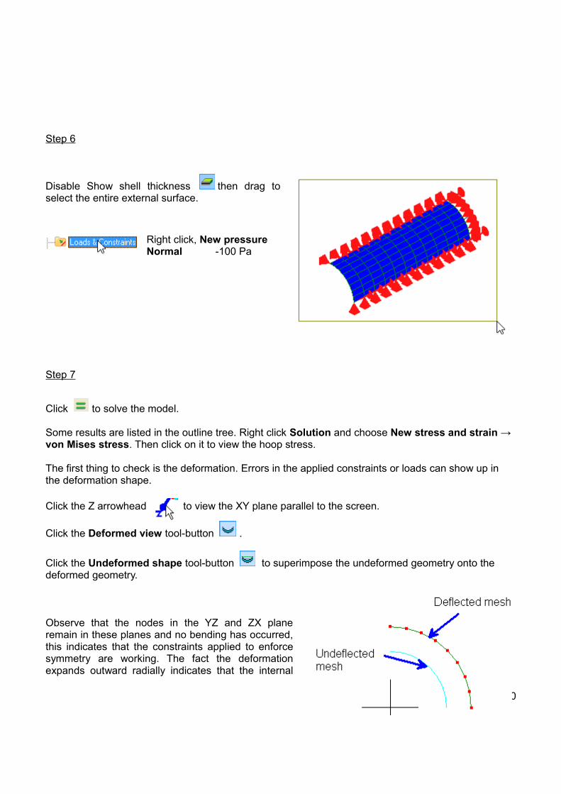
Step 6
Disable Show shell thickness then drag toselect the entire external surface.
Right click, New pressureNormal -100 Pa
Step 7
Click to solve the model.
Some results are listed in the outline tree. Right click Solution and choose New stress and strain → von Mises stress. Then click on it to view the hoop stress.
The first thing to check is the deformation. Errors in the applied constraints or loads can show up in the deformation shape.
Click the Z arrowhead to view the XY plane parallel to the screen.
Click the Deformed view tool-button .
Click the Undeformed shape tool-button to superimpose the undeformed geometry onto the deformed geometry.
Observe that the nodes in the YZ and ZX planeremain in these planes and no bending has occurred,this indicates that the constraints applied to enforcesymmetry are working. The fact the deformationexpands outward radially indicates that the internal
20

pressure has been correctly applied.
The computed hoop stress is only 0.48% different from the hand calculations. This is close enough not to need further mesh refinement.
21

2.2 Thermal Analysis of a Plate being CooledA plate of cross-section thickness 0.1m at an initial temperature of 250°C is suddenly immersed in anoil bath of temperature 50°C. The material has a thermal conductivity of 204W/m/°C, heat transfercoefficient of 80W/m2/°C, density 2707 kg/m3 and a specific heat of 896 J/kg/°C. It is required todetermine the time taken for the slab to cool to a temperature of 200*C.
For Biot numbers less than 0.1, the temperature anywhere in the cross-section will be the same withtime. A quick calculation shows that this is true.
Bi = hL/k = (80)(0.1)/(204) = 0.0392
The 4 node quadrilateral element interpolates temperature linearly, and is able to represent unsteadystates of heat transfer so this element will be selected for the model.
We need to have a rough estimate of the time required to reach a temperature of 200*C. In this case,from classical heat transfer theory the following lumped analysis heat transfer formula can be used.
(T(t)-Ta)/(To-Ta) = e-(mt)
Ta = temperature of oil bath
To = initial temperature
where m = h/ ρ Cp(L/2)
h = heat transfer coefficient
ρ = density
Cp = specific heat
L = thickness
m = 80/[(2707)(896)(0.1/2)]
m = 1/1515.92 s-1
(200 - 50) / (250 - 50) = e(-t/1515.92)
t = ln (4) X 1515.92
t = 436 s
Step 1
Right click, Edit. Select Thermal TransientTime period 450 sTime step 1 s
A slider is displayed to show the duration of the analysis, which in this case is 450 seconds. It will beutilized when viewing the results.
22

Step 2
Click the Z arrowhead to view the XY plane parallel to the screen.
Mesh tools->Create->Node...
X 0Y 0Z 0
The node appears as a red dot at the origin.
If you don't see the node make sure you've activated the node select mode
Add more nodes using the following coordinates with units of m:(0.1,0,0)(0.1,0.2,0)(0,0.2,0)
Use the Fit to window to display the nodes.
Step 3
Mesh tools -> Create > Element... Select and click the four nodes.
The order of nodes will affect the way the element gets subdivided in a following step.So, to keep the order the same, start at the lower left corner and go counter-clockwise.
23
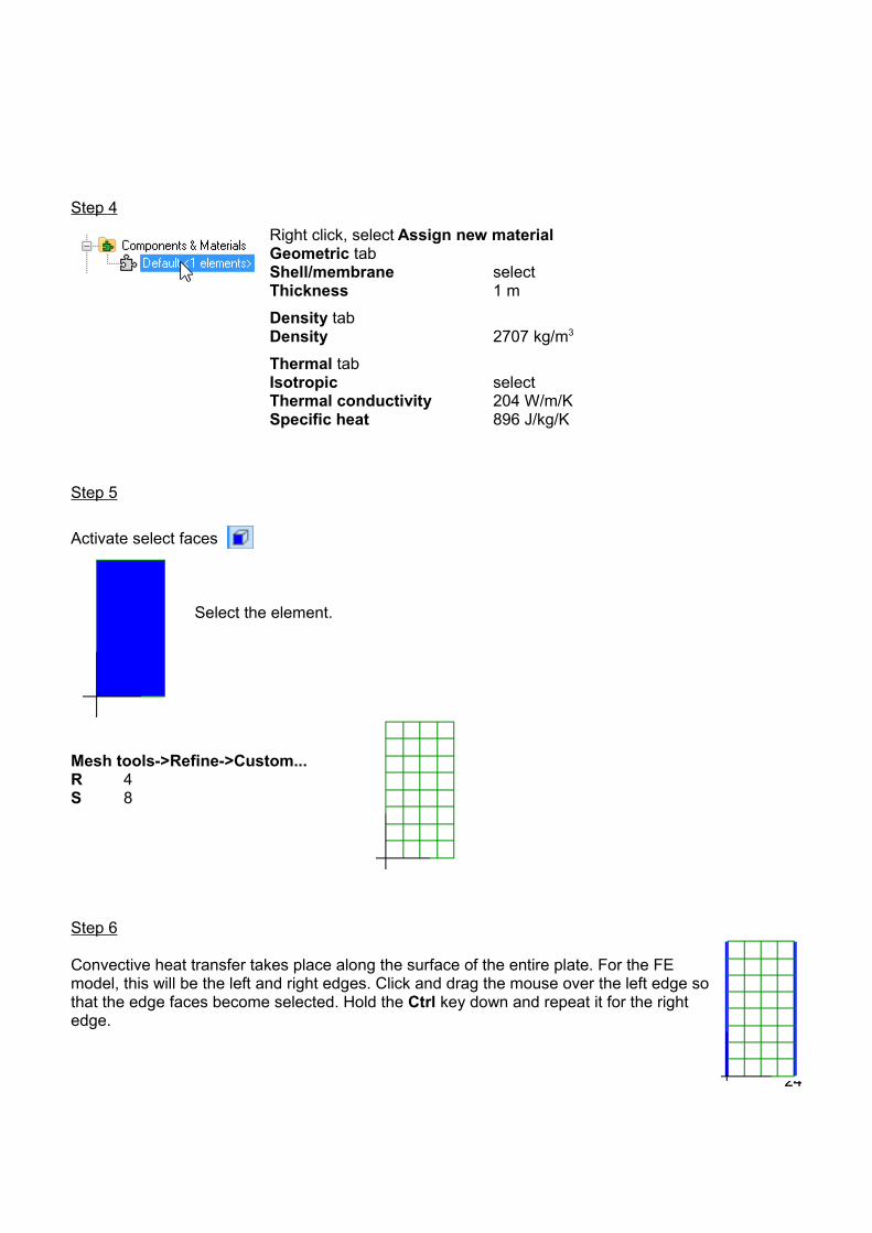
Step 4
Right click, select Assign new materialGeometric tabShell/membrane selectThickness 1 m
Density tabDensity 2707 kg/m3
Thermal tabIsotropic selectThermal conductivity 204 W/m/KSpecific heat 896 J/kg/K
Step 5
Activate select faces
Select the element.
Mesh tools->Refine->Custom...R 4S 8
Step 6
Convective heat transfer takes place along the surface of the entire plate. For the FEmodel, this will be the left and right edges. Click and drag the mouse over the left edge sothat the edge faces become selected. Hold the Ctrl key down and repeat it for the rightedge.
24

Right click then select New convection
Ambient temperature 50 °C. Note that the unit is not K.Heat transfer coefficient 80 W/m2/K
Step 7
Drag a rectangle to select the entire mesh.
Right click and select New temperature. Ensure °C is selected then type 250 in thetext-box.
Step 8
Click to solve the model. The results are listed in the outline tree below Solution.
Click
Drag the slider to view the temperature changes with time.
25

If you click a node the temperature profile of that node will be displayed in the timeline.
From the results we see that it takes about440 seconds to reach the temperature of200°C.
For transient thermal models if your results show a strange oscillation of temperatures every othertime-step, use a smaller time-step value and refine the mesh further. If the solver stops with an out ofmemory error message, use decimation as explained in the accompanying Manual.
2.3 Heat Flow Through a Solid PartStep 1
Open TransientThermalTutorial.liml from the tutorials folder whereMecway has been installed.
Step 2
26

Double click Analysis General tabTime period 300 sTime step 10 s
Step 3
Right click Meshed_Geometry and select Assign new materialDensity tabDensity 2700 kg/m3
Thermal tabIsotropicThermal conductivity 200 W/m/KSpecific heat 890 J/kg/K
Step 4
Right click the arrowhead of the Y-axis to display the model parallelto the screen.
Activate the Select nodes mode.
Drag to select the entire mesh.
Edit → Circle selection
Hold the Ctrl key down and drag to deselect the nodes of the innerdiameter.
Right click Initial Conditions and select New temperatureApply to <848 Selected nodes>
22 °C
27
This sets the selected nodes to an initial temperature of 22 °C. The reason the nodes of the innerdiameter were deselected is because a constant temperature is going to be applied to the innerdiameter. It's not physically possible for a node to be both at an initial temperature of 22 °C and adifferent constant temperature at the same time.
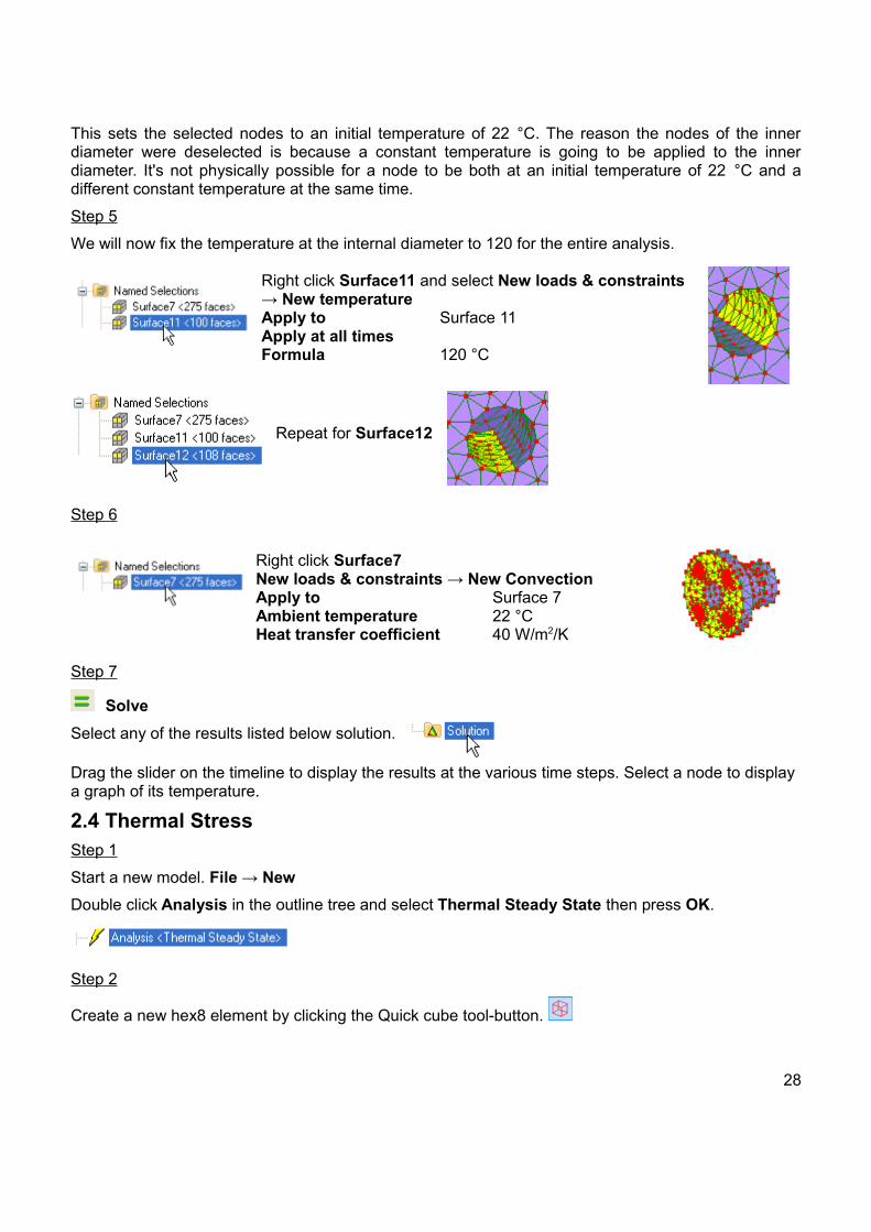
Step 5
We will now fix the temperature at the internal diameter to 120 for the entire analysis.
Right click Surface11 and select New loads & constraints→ New temperatureApply to Surface 11Apply at all timesFormula 120 °C
Repeat for Surface12
Step 6
Right click Surface7 New loads & constraints → New ConvectionApply to Surface 7Ambient temperature 22 °CHeat transfer coefficient 40 W/m2/K
Step 7
Solve
Select any of the results listed below solution.
Drag the slider on the timeline to display the results at the various time steps. Select a node to display a graph of its temperature.
2.4 Thermal StressStep 1
Start a new model. File → New
Double click Analysis in the outline tree and select Thermal Steady State then press OK.
Step 2
Create a new hex8 element by clicking the Quick cube tool-button.
28
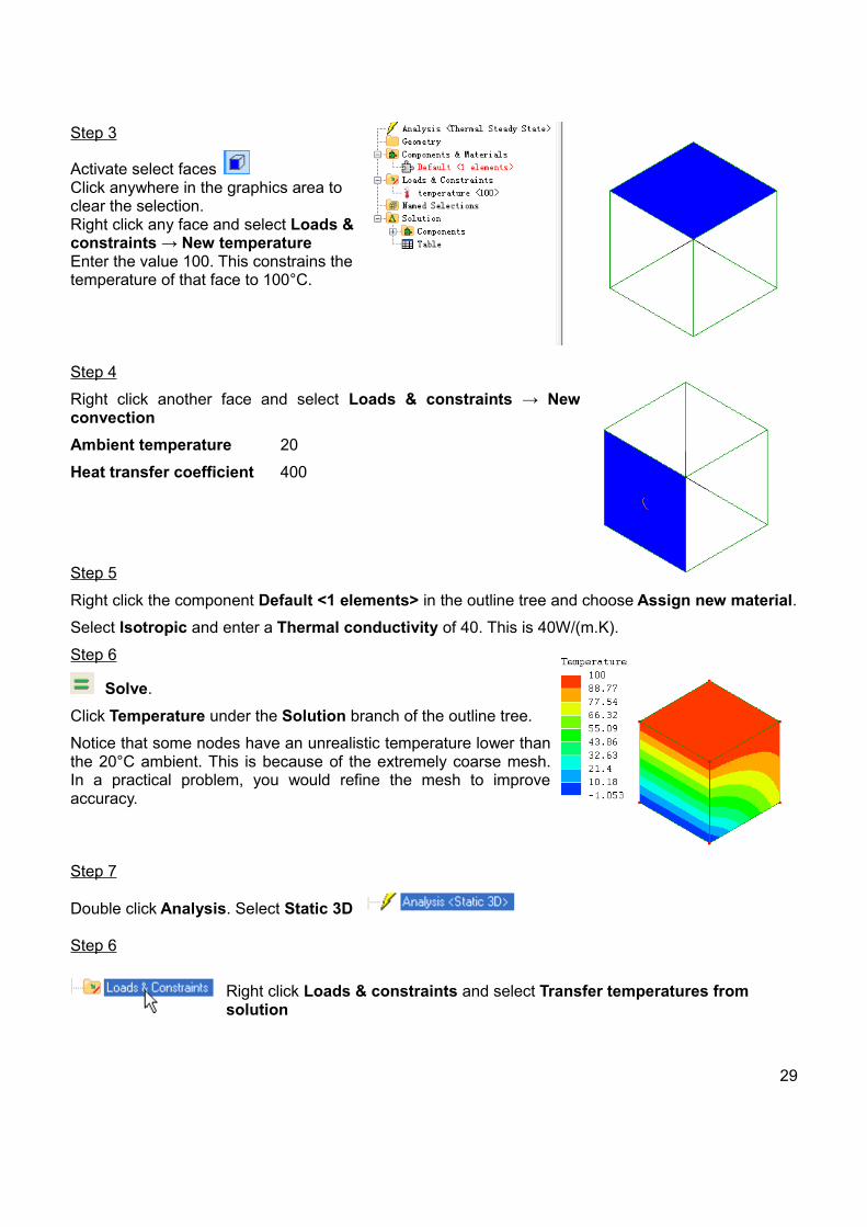
Step 3
Activate select faces Click anywhere in the graphics area toclear the selection.Right click any face and select Loads &constraints → New temperatureEnter the value 100. This constrains thetemperature of that face to 100°C.
Step 4
Right click another face and select Loads & constraints → Newconvection
Ambient temperature 20
Heat transfer coefficient 400
Step 5
Right click the component Default <1 elements> in the outline tree and choose Assign new material.
Select Isotropic and enter a Thermal conductivity of 40. This is 40W/(m.K).
Step 6
Solve.
Click Temperature under the Solution branch of the outline tree.
Notice that some nodes have an unrealistic temperature lower thanthe 20°C ambient. This is because of the extremely coarse mesh.In a practical problem, you would refine the mesh to improveaccuracy.
Step 7
Double click Analysis. Select Static 3D
Step 6
Right click Loads & constraints and select Transfer temperatures from solution
29

Step 7
Right click Loads & constraints and select New thermal stressReference temperature 20
The reference temperature is the initial temperature of the nodes that are now at the temperatures which were transferred from the thermal analysis solution.
Step 8
Right click Material and select Edit
Mechanical tabIsotropicYoung's modulus 200E09Thermal expansion coefficient 11E-06
Density tabDensity 7800
Step 9
Right click any face and choose Loads & constraints → New fixed support
Step 10
Solve
The solution now shows the cube deformed by thermal expansion.
2.5 Free Vibration of a Cantilever Beam
A cantilever beam of length 1.2m, cross-section 0.2m × 0.05m, Young's modulus 200×109 Pa, Poissonratio 0.3 and density 7860 kg/m3. The lowest natural frequency of this beam is required to bedetermined.
For thin beams, the following analytical equation is used to calculate the first natural frequency :
f = (3.52/2π)[(k / 3 × M)]1/2
f = frequency
M = mass
M = density × volume
M = 7860 × 1.2 × 0.05 × 0.2
30

M = 94.32 kg
k = spring stiffness
k = 3×E×I / L3
I = moment of inertia of the cross-section.
E = Young's modulus
L = beam length
I = (1/12)(bh3)
I = (1/12) (0.2 × 0.053)
I = 2.083×10⁻⁶ m4
k = (3 × 200×109 × 2.083×10-6) / 1.23
k = 723.379×10³ N/m
f = (3.52/2 × 3.14) [(723.379×10³/ 3 × 94.32)]1/2
f = 28.32 Hz
Step 1
Right click, Edit, then select Modal Vibration 2D.
Number of modes 3
Step 2
Mesh tools->Create->Node... X 0Y 0Z 0
The node appears as a red dot at the origin.
If you don't see the node make sure you've in the node select mode
31
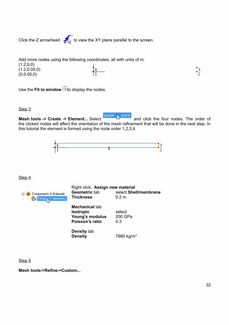
Click the Z arrowhead to view the XY plane parallel to the screen.
Add more nodes using the following coordinates, all with units of m.(1.2,0,0)(1.2,0.05,0)(0,0.05,0)
Use the Fit to window to display the nodes.
Step 3
Mesh tools -> Create -> Element... Select and click the four nodes. The order ofthe clicked nodes will affect the orientation of the mesh refinement that will be done in the next step. Inthis tutorial the element is formed using the node order 1,2,3,4.
Step 4
Right click, Assign new materialGeometric tab select Shell/membraneThickness 0.2 m
Mechanical tabIsotropic selectYoung's modulus 200 GPaPoisson's ratio 0.3
Density tabDensity 7860 kg/m3
Step 5
Mesh tools->Refine->Custom...
32
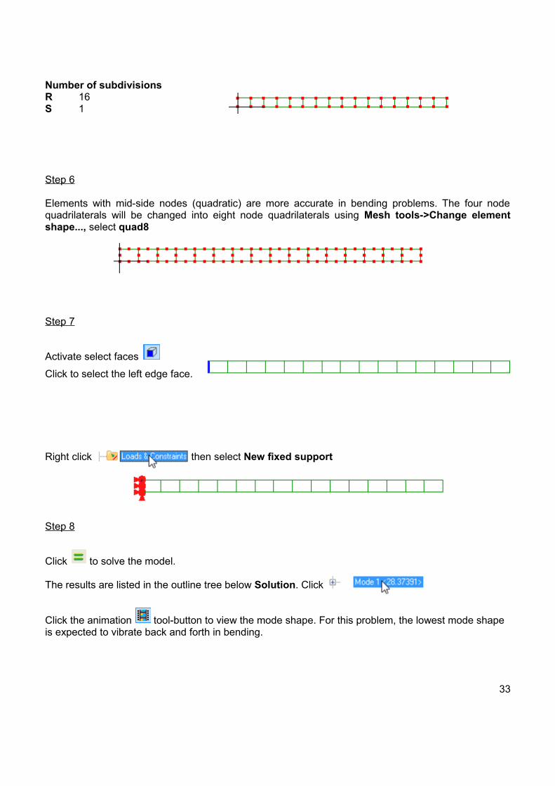
Number of subdivisionsR 16S 1
Step 6
Elements with mid-side nodes (quadratic) are more accurate in bending problems. The four nodequadrilaterals will be changed into eight node quadrilaterals using Mesh tools->Change elementshape..., select quad8
Step 7
Activate select faces
Click to select the left edge face.
Right click then select New fixed support
Step 8
Click to solve the model.
The results are listed in the outline tree below Solution. Click
Click the animation tool-button to view the mode shape. For this problem, the lowest mode shape is expected to vibrate back and forth in bending.
33
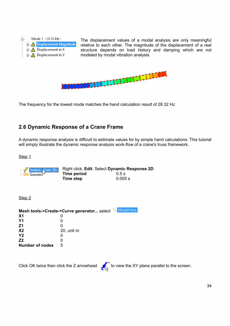
The displacement values of a modal analysis are only meaningfulrelative to each other. The magnitude of the displacement of a realstructure depends on load history and damping which are notmodeled by modal vibration analysis.
The frequency for the lowest mode matches the hand calculation result of 28.32 Hz
2.6 Dynamic Response of a Crane Frame
A dynamic response analysis is difficult to estimate values for by simple hand calculations. This tutorialwill simply illustrate the dynamic response analysis work-flow of a crane's truss framework.
Step 1
Right click, Edit. Select Dynamic Response 2DTime period 0.5 sTime step 0.005 s
Step 2
Mesh tools->Create->Curve generator... select X1 0Y1 0Z1 0X2 20, unit mY2 0Z2 0Number of nodes 5
Click OK twice then click the Z arrowhead to view the XY plane parallel to the screen.
34

Use the Fit to window to display the whole mesh.
Activate select elements
Drag to select all the elements. Right click on the selectedelements and select Element properties. Select the check-boxnext to Truss to convert these elements from beam elements totruss.
Step 3
With all elements still selectedMesh tools->Move/copy...Y 5, unit mCopy selectClick Apply then Close.
Step 4Mesh tools->Create->Element... Select and click
the nodes to form the pattern shown.
Step 5
Right click, Assign new materialGeometric tabGeneral section selectCross-sectional area 0.0225, unit m2
Mechanical tabIsotropic selectYoung's modulus 20E09, unit PaPoisson's ratio 0.3
Density tabDensity 7860, unit kg/m3
Click OK.
Step 6
35

Activate select nodes
Select these two nodes. Hold the Ctrl key down while selecting thesecond node so as not to deselect the first node.
Right click then select New displacement, select Y and click OK.
Select this node alone.
Right click then select New displacement, select X and click OK.
Step 7
Select this node.
Right click then select New forceYTable select
0 00.01 -10.49 -10.5 0
Choose units s and N then click OK.
Step 10
36
Click to solve the model.
The results are listed in the outline tree below Solution.
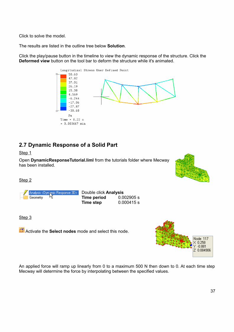
Click the play/pause button in the timeline to view the dynamic response of the structure. Click the Deformed view button on the tool bar to deform the structure while it's animated.
2.7 Dynamic Response of a Solid PartStep 1
Open DynamicResponseTutorial.liml from the tutorials folder where Mecwayhas been installed.
Step 2
Double click Analysis Time period 0.002905 sTime step 0.000415 s
Step 3
Activate the Select nodes mode and select this node.
An applied force will ramp up linearly from 0 to a maximum 500 N then down to 0. At each time stepMecway will determine the force by interpolating between the specified values.
37

Right click Loads & Constraints and select New forceApply to <Selected nodes>XTable 0 0
0.001535 5000.00307 0
Step 4
Right click Surface15 and select New loads &constraints → New fixed support
Step 5
Solve
Select any of the results below the Solution group in the outline tree.
Drag the slider on the timeline to display the results atthe various time steps. Select a node to display agraph of its displacement.
38

2.8 DC Circuit
The following circuit will be solved for the voltage drop across the resistances, and the currents.
Current flowing through the 40Ω and 50Ω resistorsis12V/(40Ω+50Ω) = 0.13A
Current flow through the 60Ω resistor is 12V/60Ω = 0.2A
The voltage drop across the 40Ω resistor is0.13A×40Ω = 5.3V
Voltage drop across the 50Ω resistor is
0.13A×50Ω = 6.7V
Voltage drop across the 60Ω resistor is 12V
Step 1
Right click, Edit. Select DC Current Flow.
Step 2
Click the Z arrowhead to view the XY plane parallel to thescreen.
Click the New element tool and click in the graphics area to formthe following three line elements. For the 2nd and 3rd elements, becareful to click on existing nodes so they are linked together.
Step 3
As each element has a different resistance, they need to be separate components.
Activate select elements
39

Right click on the selected element and select Add elements to new component
Right click on the new component and select Assign new material. Electric tabResistor selectResistance 40 Ω
Repeat this step for the second element.
Electric tabResistor selectResistance 50 Ω
As there is only one element left in the Default under Components & Materials, right click to Assign a new material.
Electric tabResistor selectResistance 60
Step 4
Activate Select nodes Right click on this selected node then selectLoads & constraints -> New electric potentialtype 0 in the text-box.
40
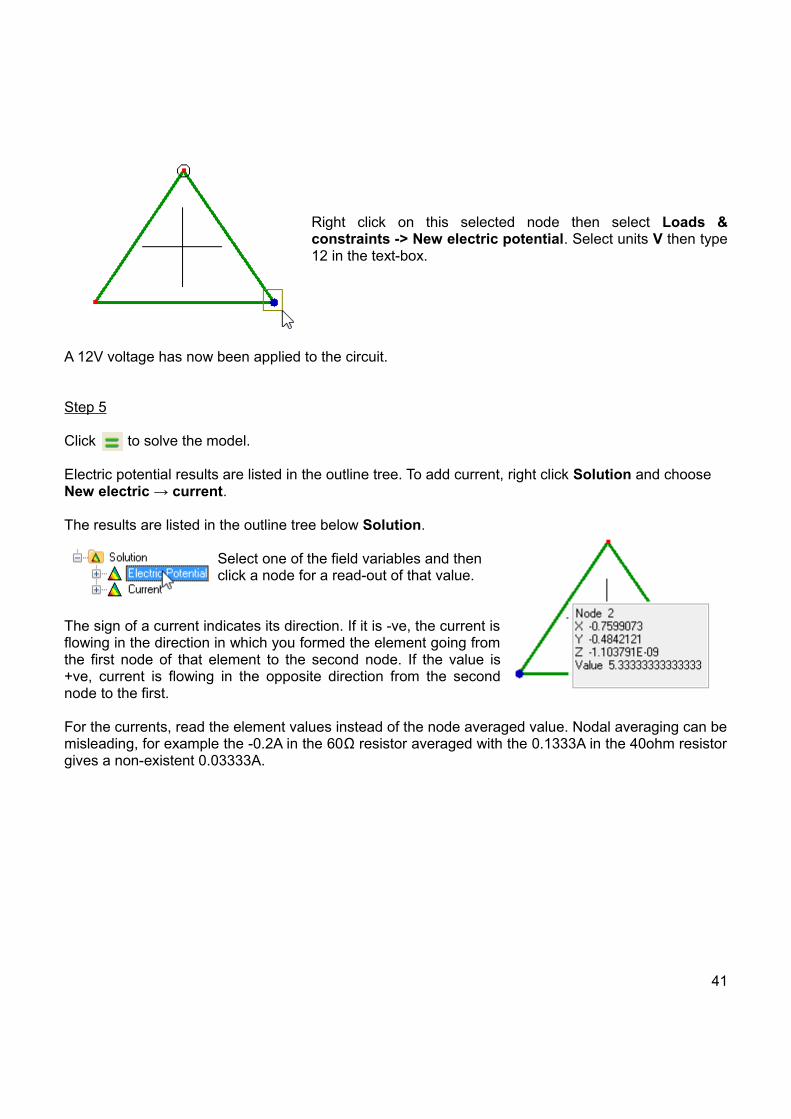
Right click on this selected node then select Loads &constraints -> New electric potential. Select units V then type12 in the text-box.
A 12V voltage has now been applied to the circuit.
Step 5
Click to solve the model.
Electric potential results are listed in the outline tree. To add current, right click Solution and choose New electric → current.
The results are listed in the outline tree below Solution.
Select one of the field variables and thenclick a node for a read-out of that value.
The sign of a current indicates its direction. If it is -ve, the current isflowing in the direction in which you formed the element going fromthe first node of that element to the second node. If the value is+ve, current is flowing in the opposite direction from the secondnode to the first.
For the currents, read the element values instead of the node averaged value. Nodal averaging can bemisleading, for example the -0.2A in the 60Ω resistor averaged with the 0.1333A in the 40ohm resistorgives a non-existent 0.03333A.
41

2.9 Electrostatic Analysis of a Capacitor
The electric field in a simple two plate capacitor will be modeled. The plates are 0.005 m apart with airin between, and a potential difference of 1.5V.
The expected electric field, E = potential difference / distance between plates
E = 1.5 / 0.005 = 300 V/m
Step 1
Right click, Edit. Select Static 2D
Step 2
Click the Z arrowhead to view the XY plane parallel to the screen.
Mesh tools->Create->Node... X 0Y 0Z 0
A red dot appears at the origin.
Add more nodes using the following coordinates, allwith units of m.(0.015,0,0)(0.015,0.005,0)(0,0.005,0)
Use the Fit to window to display the nodes
42

Step 3
In this tutorial the area between the two plates of the capacitor will be defined using two node lineelements, and then the 2D automesher will then be used to fill the region with quadrilateral or triangleelements.
Mesh tools -> Create > Element... Select and click the four nodes to form the areabetween the two plates.
Step 4
Mesh tools->Automesh 2D...Maximum element size 0.001 maccept the rest of the defaults
Step 5
Right click, Assign new materialGeometric tabThickness 1 m
Electric tabIsotropic selectRelative permittivity 1
43
Step 6
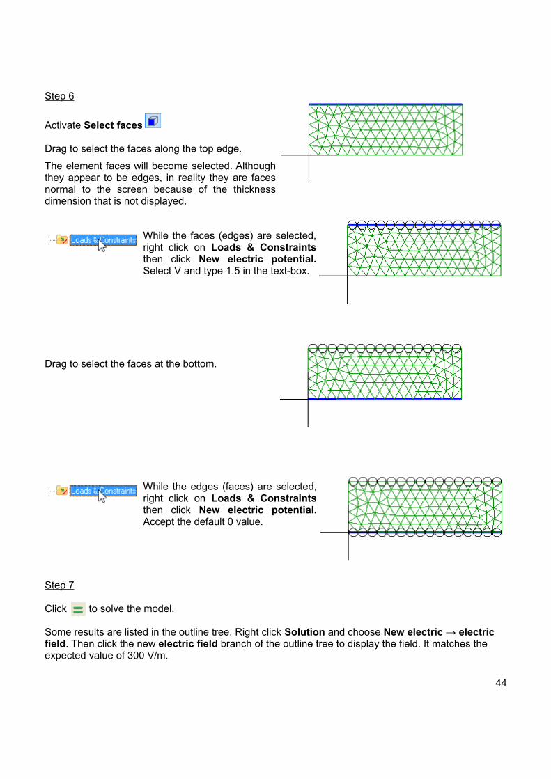
Activate Select faces
Drag to select the faces along the top edge.
The element faces will become selected. Althoughthey appear to be edges, in reality they are facesnormal to the screen because of the thicknessdimension that is not displayed.
While the faces (edges) are selected,right click on Loads & Constraintsthen click New electric potential.Select V and type 1.5 in the text-box.
Drag to select the faces at the bottom.
While the edges (faces) are selected,right click on Loads & Constraintsthen click New electric potential.Accept the default 0 value.
Step 7
Click to solve the model.
Some results are listed in the outline tree. Right click Solution and choose New electric → electric field. Then click the new electric field branch of the outline tree to display the field. It matches the expected value of 300 V/m.
44
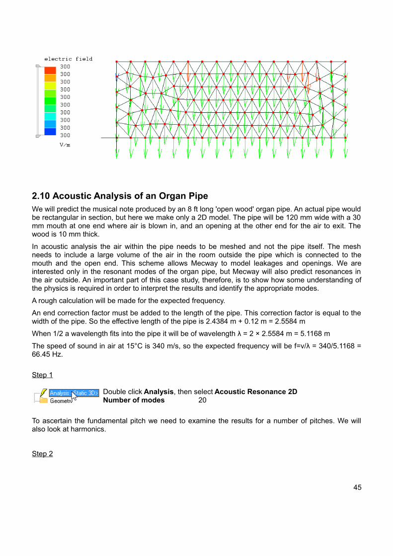
2.10 Acoustic Analysis of an Organ PipeWe will predict the musical note produced by an 8 ft long 'open wood' organ pipe. An actual pipe wouldbe rectangular in section, but here we make only a 2D model. The pipe will be 120 mm wide with a 30mm mouth at one end where air is blown in, and an opening at the other end for the air to exit. Thewood is 10 mm thick.
In acoustic analysis the air within the pipe needs to be meshed and not the pipe itself. The meshneeds to include a large volume of the air in the room outside the pipe which is connected to themouth and the open end. This scheme allows Mecway to model leakages and openings. We areinterested only in the resonant modes of the organ pipe, but Mecway will also predict resonances inthe air outside. An important part of this case study, therefore, is to show how some understanding ofthe physics is required in order to interpret the results and identify the appropriate modes.
A rough calculation will be made for the expected frequency.
An end correction factor must be added to the length of the pipe. This correction factor is equal to thewidth of the pipe. So the effective length of the pipe is 2.4384 m + 0.12 m = 2.5584 m
When 1/2 a wavelength fits into the pipe it will be of wavelength λ = 2 × 2.5584 m = 5.1168 m
The speed of sound in air at 15°C is 340 m/s, so the expected frequency will be f=v/λ = 340/5.1168 =66.45 Hz.
Step 1
Double click Analysis, then select Acoustic Resonance 2DNumber of modes 20
To ascertain the fundamental pitch we need to examine the results for a number of pitches. We willalso look at harmonics.
Step 2
45
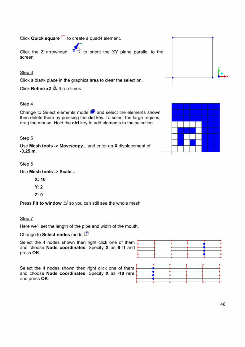
Click Quick square to create a quad4 element.
Click the Z arrowhead to orient the XY plane parallel to thescreen.
Step 3
Click a blank place in the graphics area to clear the selection.
Click Refine x2 three times.
Step 4
Change to Select elements mode and select the elements shownthen delete them by pressing the del key. To select the large regions,drag the mouse. Hold the ctrl key to add elements to the selection.
Step 5
Use Mesh tools -> Move/copy... and enter an X displacement of -0.25 m.
Step 6
Use Mesh tools -> Scale... :
X: 10
Y: 2
Z: 0
Press Fit to window so you can still see the whole mesh.
Step 7
Here we'll set the length of the pipe and width of the mouth.
Change to Select nodes mode
Select the 4 nodes shown then right click one of themand choose Node coordinates. Specify X as 8 ft andpress OK.
Select the 4 nodes shown then right click one of themand choose Node coordinates. Specify X as -10 mmand press OK.
46
Select the 2 nodes shown then right click one of themand choose Node coordinates. Specify X as 30 mmand press OK.
Step 8
Here we'll set the pipe's width and wall thickness.
Select the 4 nodes shown then right click one of themand choose Node coordinates. Specify Y as 620 mmand press OK.
Select the 4 nodes shown then right click one of themand choose Node coordinates. Specify Y as 630 mmand press OK.
Select the 4 nodes shown then right click one of themand choose Node coordinates. Specify Y as 490 mmand press OK.
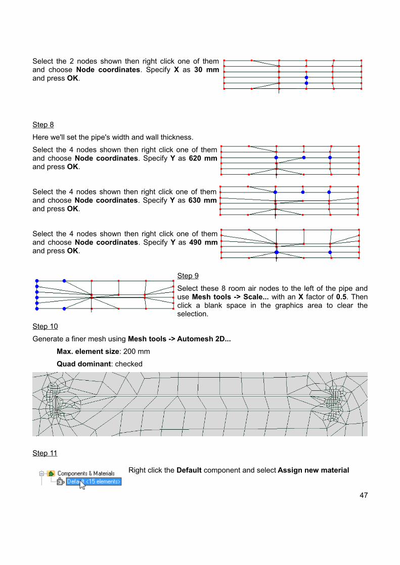
Step 9
Select these 8 room air nodes to the left of the pipe anduse Mesh tools -> Scale... with an X factor of 0.5. Thenclick a blank space in the graphics area to clear theselection.
Step 10
Generate a finer mesh using Mesh tools -> Automesh 2D...
Max. element size: 200 mm
Quad dominant: checked
Step 11
Right click the Default component and select Assign new material
47

Mechanical tabIsotropic selectSpeed of sound 340
Step 13
The mesh building is now complete so click to solve the model.
The modal frequencies are listed in the outline tree below Solution. Click the nodes for a read-out ofthe field variable there.
The subtlety in this case study is in interpreting the results. From the 20 calculated modes we want topick out the fundamental pitch of the pipe itself. Click through the various modes and observe thatmost show red, yellow and blue patches for the room air elements.
The 4th mode at 64.59 Hz is different because the ‘room’ is almost at constant pressure (color). Zoomin on the pipe and notice that the magnitude of the maximum pressure inside the pipe is much higherthan anywhere outside the pipe. This identifies mode 4 as the fundamental pitch of the organ pipe.Half a wavelength fits inside the pipe. The frequency matches the hand calculated value very well.
Similarly Mode 8 at 131 Hz has an almost constant pressure in the room and high, variable pressurein the pipe. This is the first harmonic at twice the frequency of mode 4, sounding one octave higher. Afull wavelength fits inside the pipe.
48
2.11 Buckling of a Column
The eigenvalue buckling of a column with a fixed end will be solved. The column has a length of100mm, a square cross-section of 10mm and Young's modulus 200000 N/mm2 .
The critical load for a fixed end Euler column is π2EI/(4L2)
E = Young's modulus
I = moment of inertia
I = 104/12 = 833.33mm4
L = length
Critical load = π2 200000 × 833.33 / (4×1002)= 41123.19
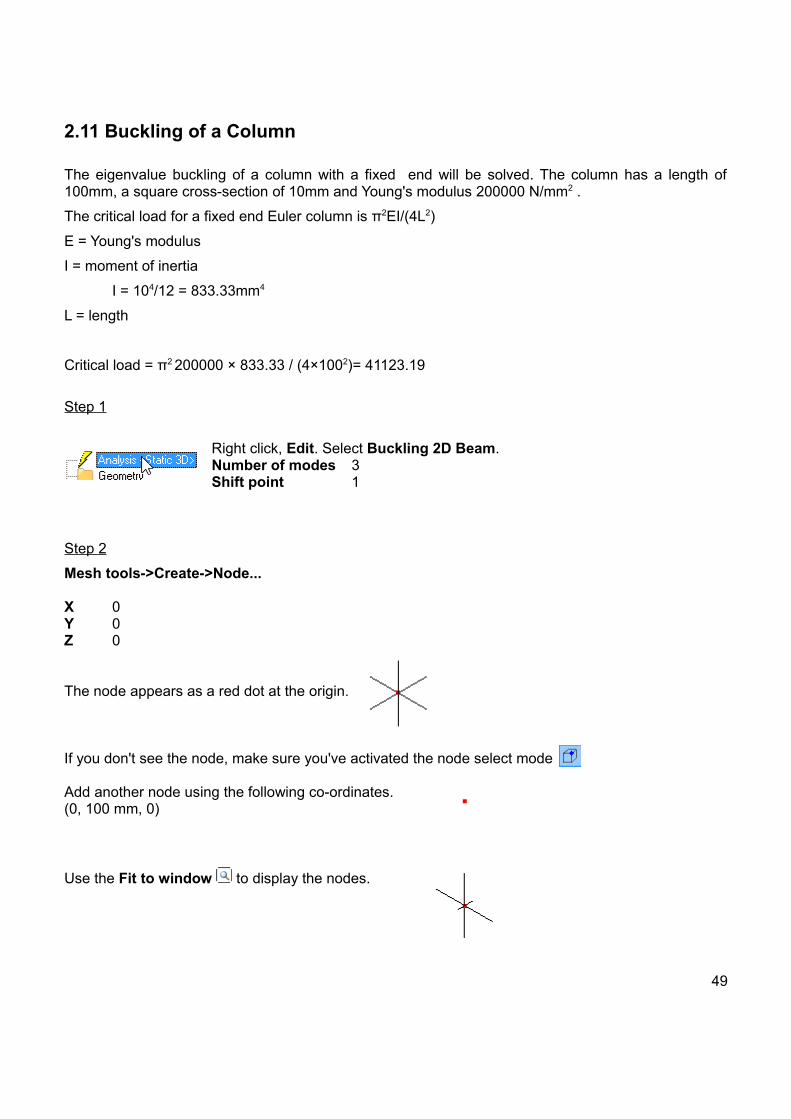
Step 1
Right click, Edit. Select Buckling 2D Beam.Number of modes 3Shift point 1
Step 2
Mesh tools->Create->Node...
X 0Y 0Z 0
The node appears as a red dot at the origin.
If you don't see the node, make sure you've activated the node select mode
Add another node using the following co-ordinates.(0, 100 mm, 0)
Use the Fit to window to display the nodes.
49
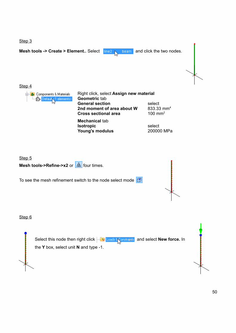
Step 3
Mesh tools -> Create > Element.. Select and click the two nodes.
Step 4
Right click, select Assign new materialGeometric tabGeneral section select2nd moment of area about W 833.33 mm4
Cross sectional area 100 mm2
Mechanical tabIsotropic selectYoung's modulus 200000 MPa
Step 5
Mesh tools->Refine->x2 or four times.
To see the mesh refinement switch to the node select mode
Step 6
Select this node then right click and select New force. In
the Y box, select unit N and type -1.
50
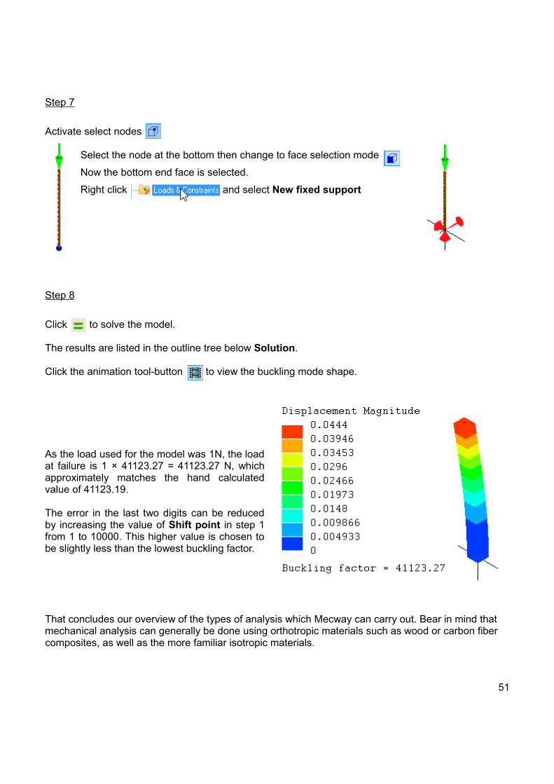
Step 7
Activate select nodes
Select the node at the bottom then change to face selection mode
Now the bottom end face is selected.
Right click and select New fixed support
Step 8
Click to solve the model.
The results are listed in the outline tree below Solution.
Click the animation tool-button to view the buckling mode shape.
As the load used for the model was 1N, the loadat failure is 1 × 41123.27 = 41123.27 N, whichapproximately matches the hand calculatedvalue of 41123.19.
The error in the last two digits can be reducedby increasing the value of Shift point in step 1from 1 to 10000. This higher value is chosen tobe slightly less than the lowest buckling factor.
That concludes our overview of the types of analysis which Mecway can carry out. Bear in mind that mechanical analysis can generally be done using orthotropic materials such as wood or carbon fiber composites, as well as the more familiar isotropic materials.
51
3Chapter 3Operations
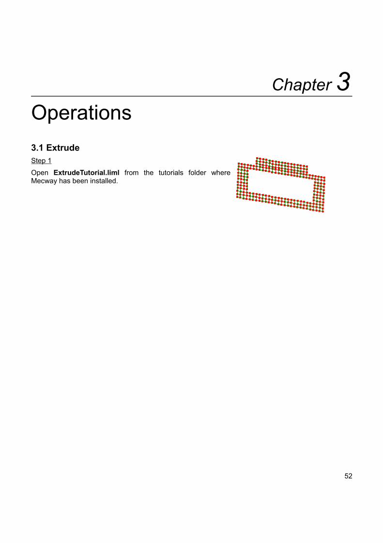
3.1 ExtrudeStep 1
Open ExtrudeTutorial.liml from the tutorials folder whereMecway has been installed.
52

Step 2
Activate Select faces
Drag the mouse over the entire mesh so that it becomesselected.
53

Step 3
Mesh tools → Extrude...
Thickness 5 m
Number of subdivisions 3
Direction +Z
54

Step 4
The extrusion step turned off Select faces soreactivate it again.
Select the faces at the bottom.
Mesh tools → Extrude...
Thickness 5 m
Number of subdivisions 3
Direction +Normal
55

3.2 LoftStep 1
Open LoftTutorial.liml from the tutorials folder where Mecway hasbeen installed.
56

Step 2
Display node and element numbers.
Note down the node numbers of any two corresponding nodes oneach profile. In this example the bottom corner node numbers are 12and 135.
57

Step 3
Activate Select faces.
Drag to select the profile of node number 135.
58

Step 4
Mesh tools → Loft...
Number of subdivisions 4
A node in selected faces 135
The corresponding node 12
3.3 Refine Local 2D
Step 1
Open RefineLocal2dTutorial.liml from the tutorials folder where Mecway has been installed.
Step 2
Drag the mouse to select the nodes shown below. Don't worry if you selected a few extra nodes, this isonly an illustration.
59
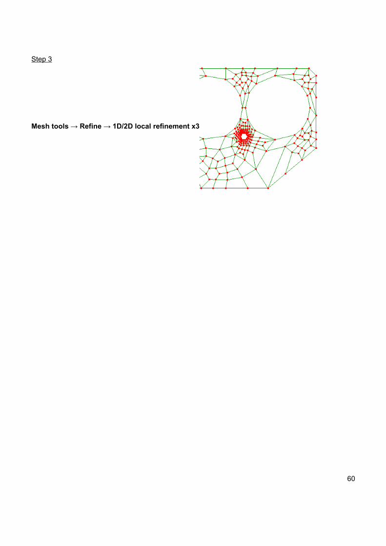
Step 3
Mesh tools → Refine → 1D/2D local refinement x3
60

3.4 Mirror SymmetryStep 1
This revolved shell can be modeled as only onequadrant. Open MirrorSymmetryTutorial.liml from thetutorials folder where Mecway has been installed.
61
Step 2
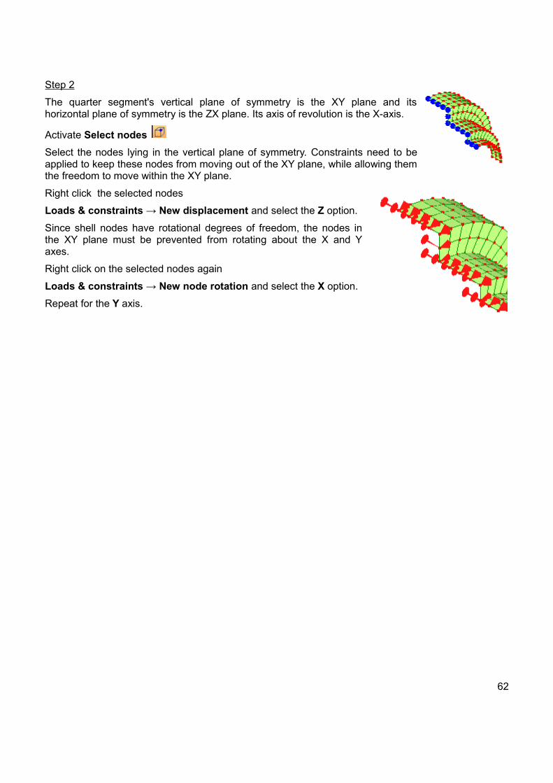
The quarter segment's vertical plane of symmetry is the XY plane and itshorizontal plane of symmetry is the ZX plane. Its axis of revolution is the X-axis.
Activate Select nodes
Select the nodes lying in the vertical plane of symmetry. Constraints need to beapplied to keep these nodes from moving out of the XY plane, while allowing themthe freedom to move within the XY plane.
Right click the selected nodes
Loads & constraints → New displacement and select the Z option.
Since shell nodes have rotational degrees of freedom, the nodes inthe XY plane must be prevented from rotating about the X and Yaxes.
Right click on the selected nodes again
Loads & constraints → New node rotation and select the X option.
Repeat for the Y axis.
62

Step 3
While still in Select nodes mode, select the nodes lying in the horizontalplane of symmetry. Constraints need to be applied to keep these nodes frommoving out of the ZX plane or rotating about any axis lying in that plane.
Right click on the selected nodes
Loads & constraints → New displacement and select the Y option.
Right click on the selected nodes again
Loads & constraints → New node rotation and select the Xoption.
Repeat for the Z axis.
3.5 Cyclic Symmetry
Instead of modeling the entire wheel using solid elements, onlyone segment will be modeled using cyclic symmetry.
Step 1
Open CyclicSymmetryTutorial.liml from the tutorials folder where Mecway hasbeen installed.
63
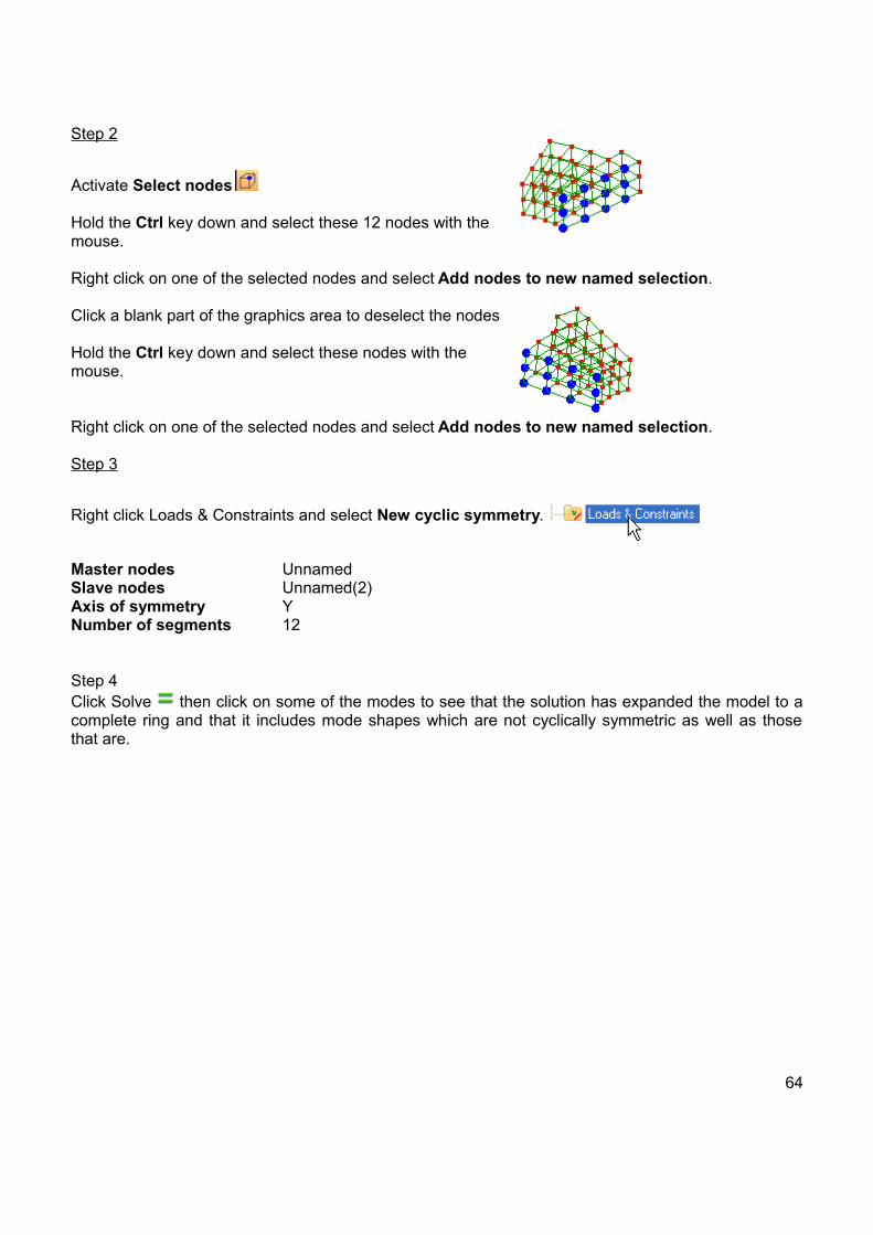
Step 2
Activate Select nodes
Hold the Ctrl key down and select these 12 nodes with themouse.
Right click on one of the selected nodes and select Add nodes to new named selection.
Click a blank part of the graphics area to deselect the nodes
Hold the Ctrl key down and select these nodes with themouse.
Right click on one of the selected nodes and select Add nodes to new named selection.
Step 3
Right click Loads & Constraints and select New cyclic symmetry.
Master nodes UnnamedSlave nodes Unnamed(2)Axis of symmetry YNumber of segments 12
Step 4Click Solve then click on some of the modes to see that the solution has expanded the model to acomplete ring and that it includes mode shapes which are not cyclically symmetric as well as thosethat are.
64

3.6 CAD Work-flowStep 1
Use File → Open or right click and select ImportSTEP/IGES file
Open the file CadWorkflowTutorial.stp from the tutorials folder whereMecway has been installed.
Drag anywhere in the graphics area using the middle mouse button torotate it so the faces are distinct.
65

Step 2
Right click the file name and select Generate Mesh
Step 3
Right click the component and select Assign newmaterial. In the Mechanical tab select Isotropic thentype 200E09 in the text box for Young's modulus
Step 4
Click the file name to return to the geometry view then right click a surface and select Loads &constraints then New fixed support.
66

Step 5
Use the middle mouse button to rotate themodel, then right click the inclined surface andselect Loads & constraints, then selectPressure. Type 1000 to apply a normal pressureto the selected surface.
67
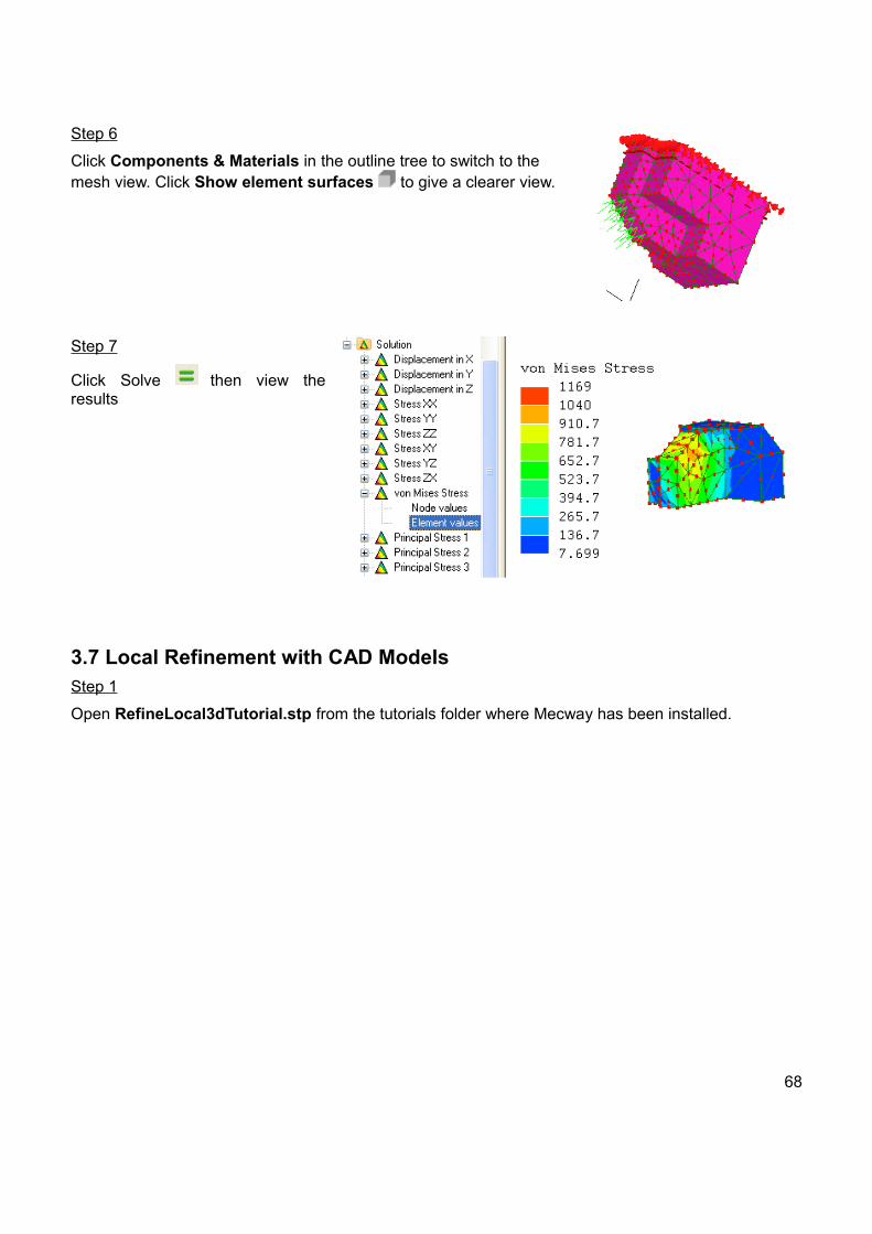
Step 6
Click Components & Materials in the outline tree to switch to themesh view. Click Show element surfaces to give a clearer view.
Step 7
Click Solve then view theresults
3.7 Local Refinement with CAD ModelsStep 1
Open RefineLocal3dTutorial.stp from the tutorials folder where Mecway has been installed.
68

Step 2
Right click the filename and select Generate mesh
Step 3
Activate Select nodes
Right click a node and choose New local refinement then press OK to accept the default values.
Step 4
Right click the filename and select Generate mesh
Multiple local refinements can be applied following the same procedure.
3.8 Mixed MaterialsStep 1
Open a new instance of Mecway.
Step 2
Click Quick cube
Step 3
Click Refine
69

Step 4
Right click the Default component in the outline tree andselect Assign new material. Choose Isotropic andenter:
Young's modulus 200e9
Poisson's ratio 0.3
Click Close
Step 5
Change to Select elements mode andselect two of the 8 elements. Hold the Ctrl key whileclicking on each element.
70
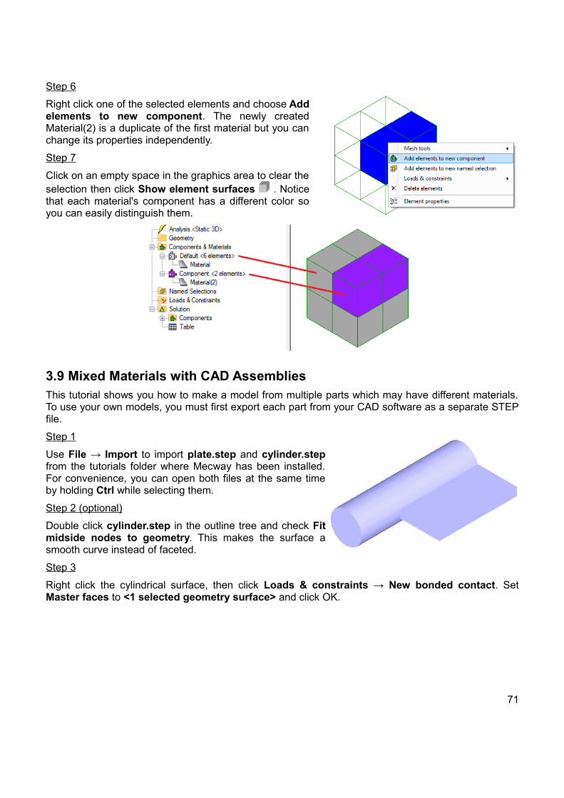
Step 6
Right click one of the selected elements and choose Addelements to new component. The newly createdMaterial(2) is a duplicate of the first material but you canchange its properties independently.
Step 7
Click on an empty space in the graphics area to clear theselection then click Show element surfaces . Noticethat each material's component has a different color soyou can easily distinguish them.
3.9 Mixed Materials with CAD AssembliesThis tutorial shows you how to make a model from multiple parts which may have different materials.To use your own models, you must first export each part from your CAD software as a separate STEPfile.
Step 1
Use File → Import to import plate.step and cylinder.stepfrom the tutorials folder where Mecway has been installed.For convenience, you can open both files at the same timeby holding Ctrl while selecting them.
Step 2 (optional)
Double click cylinder.step in the outline tree and check Fitmidside nodes to geometry. This makes the surface asmooth curve instead of faceted.
Step 3
Right click the cylindrical surface, then click Loads & constraints → New bonded contact. SetMaster faces to <1 selected geometry surface> and click OK.
71
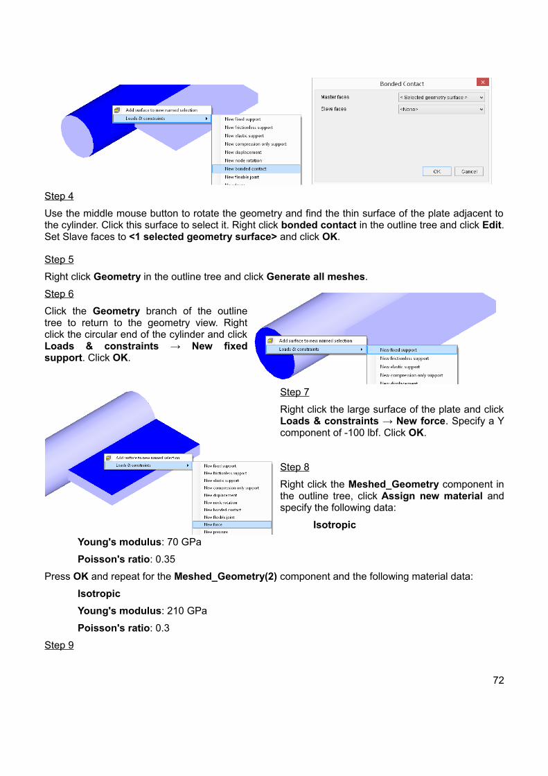
Step 4
Use the middle mouse button to rotate the geometry and find the thin surface of the plate adjacent tothe cylinder. Click this surface to select it. Right click bonded contact in the outline tree and click Edit.Set Slave faces to <1 selected geometry surface> and click OK.
Step 5
Right click Geometry in the outline tree and click Generate all meshes.
Step 6
Click the Geometry branch of the outlinetree to return to the geometry view. Rightclick the circular end of the cylinder and clickLoads & constraints → New fixedsupport. Click OK.
Step 7
Right click the large surface of the plate and clickLoads & constraints → New force. Specify a Ycomponent of -100 lbf. Click OK.
Step 8
Right click the Meshed_Geometry component inthe outline tree, click Assign new material andspecify the following data:
Isotropic
Young's modulus: 70 GPa
Poisson's ratio: 0.35
Press OK and repeat for the Meshed_Geometry(2) component and the following material data:
Isotropic
Young's modulus: 210 GPa
Poisson's ratio: 0.3
Step 9
72
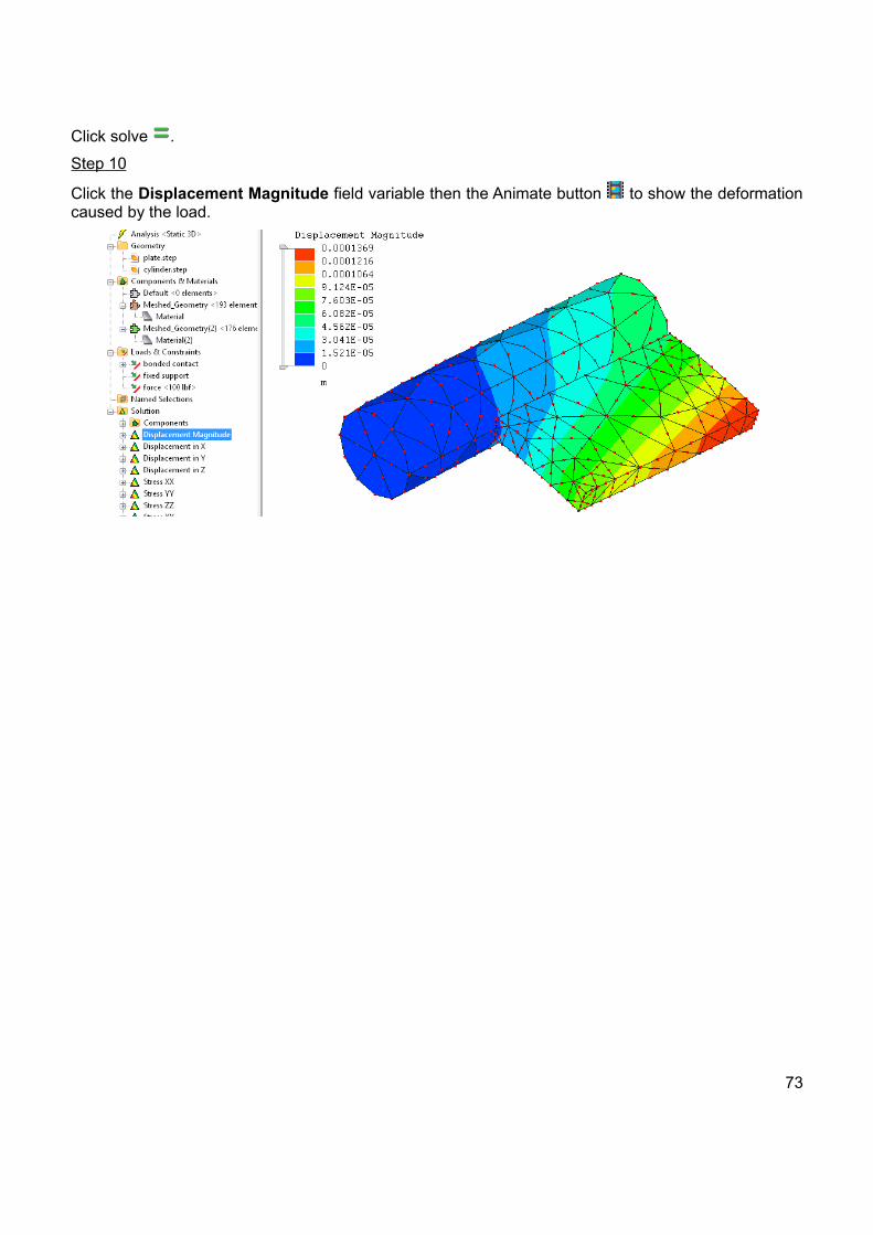
Click solve .
Step 10
Click the Displacement Magnitude field variable then the Animate button to show the deformationcaused by the load.
73
3.10 Constraint EquationsStep 1
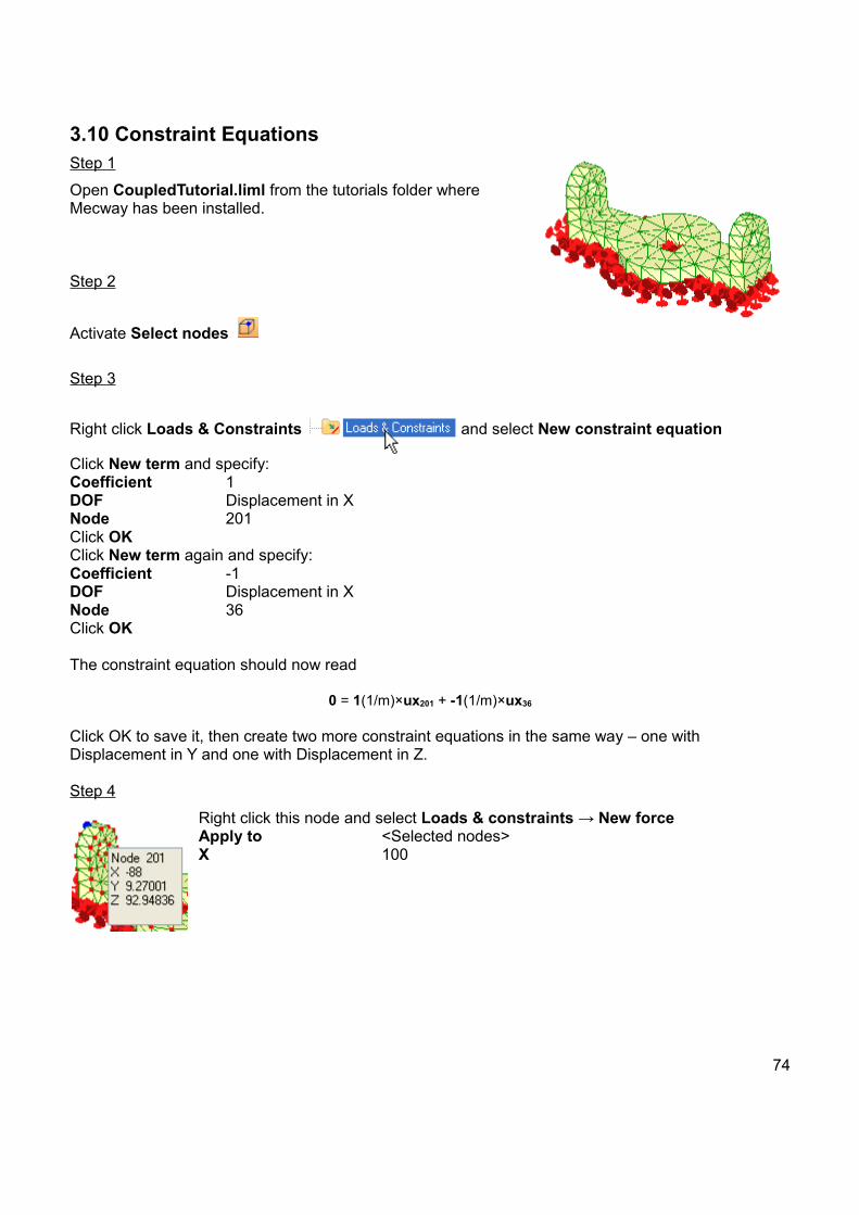
Open CoupledTutorial.liml from the tutorials folder whereMecway has been installed.
Step 2
Activate Select nodes
Step 3
Right click Loads & Constraints and select New constraint equation
Click New term and specify:Coefficient 1DOF Displacement in XNode 201Click OKClick New term again and specify:Coefficient -1DOF Displacement in XNode 36Click OK
The constraint equation should now read
0 = 1(1/m)×ux201 + -1(1/m)×ux36
Click OK to save it, then create two more constraint equations in the same way – one with Displacement in Y and one with Displacement in Z.
Step 4
Right click this node and select Loads & constraints → New force Apply to <Selected nodes>X 100
74

Step 5
Right click , Solve
The two nodes have the same displacement as if they are connected by a rigid, non-rotating bar.
3.11 Advanced Manual MeshingStep 1
Identify the most difficultfeatures and model thembefore the easierfeatures.
In this model the sideholes that intersect withthe through hole are themost difficult, so this willbe modeled first.
Step 2
Mesh tools->Create->Node...
Next node's coordinates:X 12Y 0Z 0
Click the Add button
Change Y to 100 click Addchange X to -12 click Addchange Y to 0 click Addclick Close
Click the Z arrowhead to view the model parallel to the screen.
75

View->Fit to window
Mesh tools->Create->Element...
Create a line2 element by clicking on the bottom-right node, then the top-right node. Repeat this to create a total of 4 elements as shown.
For now it has been modeled to a width of 24 but later it will be stretched to the actual width of 50. Thiswas necessary because the left and right faces will be rotated in a later step and we didn't want themto penetrate other elements inside the mesh.
Step 3
Mesh tools->Create->Curve generator...
D1 16D2 16
Click OK to exit the ellipse dialog but don't exit the curve generator dialog just yet.
Change the Y = 8*sin(p) into Y= 25 +8*sin(p). This will move the circle up by 25where we would like it to be positioned. Change the Number of elements to 12. ClickOK to exit the curve generator dialog.
Step 4
Mesh tools->Create->Curve generator...
D1 16D2 16
Click OK to exit the ellipse dialog but don't exit the curve generator dialog.
Change the Y = 8*sin(p) into Y= 75 +8*sin(p), this will move the circle up by 25where we would like it to be positioned. Change the Number of elements to 12. ClickOK to exit the curve generator dialog.
76

Step 5
You will be meshing this with the 2D automesher. But before doing so, you have to delete duplicatenodes created during the meshing operations using Mesh tools->Merge nearby nodes with aDistance tolerance of 0.001. Note the change in node numbers in the status bar after this commandhas been run.
Mesh tools->Automesh 2D...Maximum element size 8
The automesher will briefly run in a separate window andthen close.
Step 6
Select these nodes. Right click on the selected nodes and choose Node coordinates and enter 25 for the X coordinate.
Select these nodes. Right click on the selected nodes and choose Node coordinates andenter -25 for the X coordinate.
77
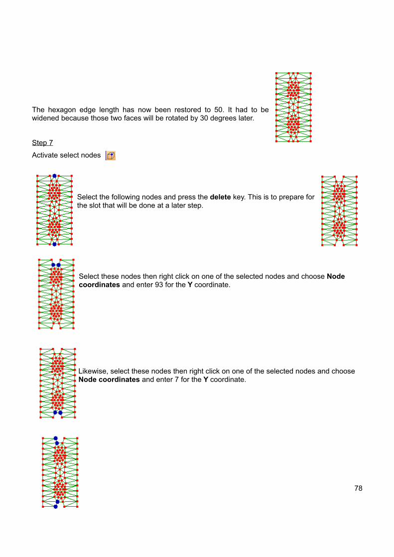
The hexagon edge length has now been restored to 50. It had to bewidened because those two faces will be rotated by 30 degrees later.
Step 7
Activate select nodes
Select the following nodes and press the delete key. This is to prepare forthe slot that will be done at a later step.
Select these nodes then right click on one of the selected nodes and choose Node coordinates and enter 93 for the Y coordinate.
Likewise, select these nodes then right click on one of the selected nodes and choose Node coordinates and enter 7 for the Y coordinate.
78

Select these nodes. Hold the Ctrl key while selecting them. Right click on one of the selected nodes and choose Node coordinates and enter -5 for the X coordinate.
Select these nodes. Hold the Ctrl key while selecting them. Right clickon one of the selected nodes and choose Node coordinates and enter5 for the X coordinate.
The mesh is now prepared for the 10×7 slot
Step 8
Mesh tools->Create->Element...quad4 shell
Click the nodes to form quadrilaterals.
Step 9
Activate select faces
79

Select the entire mesh.
Mesh tools->Extrude...Direction +ZThickness 23.3Number of subdivisions 3
Step 10
Activate select nodes
Select the entire mesh, Mesh tools->Move/copy... Z 20
Step 11
Activate select nodes
We will be using this co-ordinate information to rotate the right hand face.
80
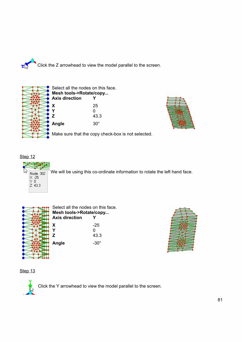
Click the Z arrowhead to view the model parallel to the screen.
Select all the nodes on this face.Mesh tools->Rotate/copy...Axis direction Y
X 25Y 0Z 43.3
Angle 30°
Make sure that the copy check-box is not selected.
Step 12
We will be using this co-ordinate information to rotate the left hand face.
Select all the nodes on this face.Mesh tools->Rotate/copy...Axis direction Y
X -25Y 0Z 43.3
Angle -30°
Step 13
Click the Y arrowhead to view the model parallel to the screen.
81

Activate select nodes
Select these nodes. Mesh tools->Fit to curved surface...
Cylinder selectCenterX 0Y 0Z 0Radius 20AxisY select
Step 14
Activate select nodes
Select the entire model. Mesh tools->Rotate/copy...Axis direction YX 0Y 0Z 0Angle 60°Copy selected
With the newly created elements selected, repeat the Mesh tools->Rotate/copy... with the same parameters and just click Apply.
82
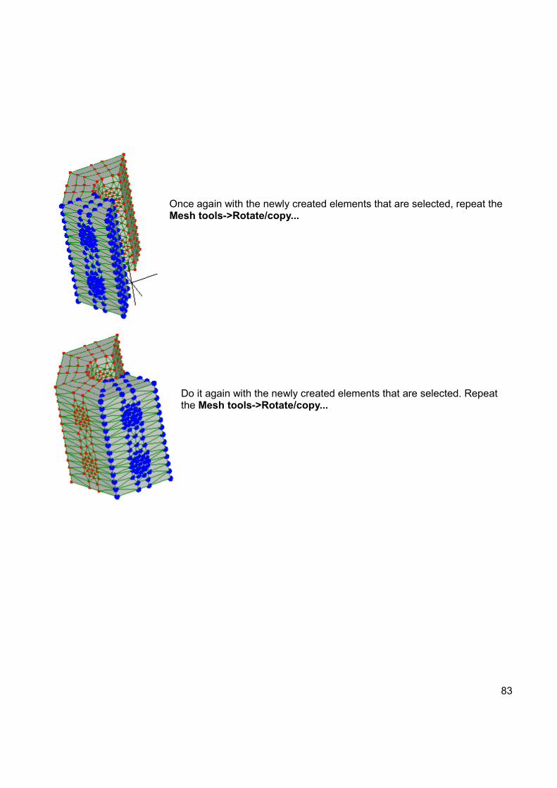
Once again with the newly created elements that are selected, repeat the Mesh tools->Rotate/copy...
Do it again with the newly created elements that are selected. Repeat the Mesh tools->Rotate/copy...
83

Once more for the final time.
That completes the hexagonal shape. Now use the Mesh tools->Merge nearby nodes with a Distance tolerance of 0.01 to eliminate duplicate nodes created during the meshing operations. Note the change in node numbers in the status bar.
Step 15
Activate select nodes
Click the Z arrowhead to view the model parallel to the screen.
84
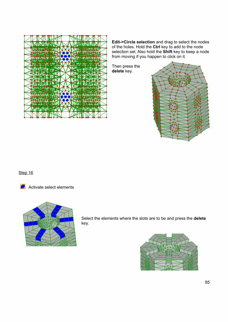
Edit->Circle selection and drag to select the nodesof the holes. Hold the Ctrl key to add to the node selection set. Also hold the Shift key to keep a nodefrom moving if you happen to click on it.
Then press the delete key.
Step 16
Activate select elements
Select the elements where the slots are to be and press the delete key.
85

Step 17
Activate select elements
Similarly, rotate the model and select the elements where the slots are to be and press the delete key.
Step 18
As this is a coarse mesh use the Mesh tools->Refine->x2 to refine the mesh further.
86

That concludes this Tutorials guide. Hopefully you will now be quite familiar with Mecway, and have confidence to modify the examples above and build your own models from scratch. For more detailed information and samples, see the companion Manual.
87
Related Documents

![Unknown Author - Tutorials in Finite Element Analysis Using MSC-Patran-Nastran [Unknown]](https://static.cupdf.com/doc/110x72/552d56a05503466f768b46db/unknown-author-tutorials-in-finite-element-analysis-using-msc-patran-nastran-unknown.jpg)