Tutorial 9. Using a Single Rotating Reference Frame Introduction This tutorial considers the flow within a 2D, axisymmetric, co-rotating disk cavity system. Understanding the behavior of such flows is important in the design of secondary air passages for turbine disk cooling. This tutorial demonstrates how to do the following: • Set up a 2D axisymmetric model with swirl, using a rotating reference frame. • Use the standard k- and RNG k- turbulence models with the enhanced near-wall treatment. • Calculate a solution using the pressure-based solver. • Display velocity vectors and contours of pressure. • Set up and display XY plots of radial velocity and wall y + distribution. • Restart the solver from an existing solution. Prerequisites This tutorial is written with the assumption that you have completed Tutorial 1, and that you are familiar with the ANSYS FLUENT navigation pane and menu structure. Some steps in the setup and solution procedure will not be shown explicitly. Problem Description The problem to be considered is shown schematically in Figure 9.1. This case is similar to a disk cavity configuration that was extensively studied by Pincombe [1]. Air enters the cavity between two co-rotating disks. The disks are 88.6 cm in diameter and the air enters at 1.146 m/s through a circular bore 8.86 cm in diameter. The disks, which are 6.2 cm apart, are spinning at 71.08 rpm, and the air enters with no swirl. As the flow is diverted radially, the rotation of the disk has a significant effect on the viscous flow developing along the surface of the disk. Release 12.0 c ANSYS, Inc. March 12, 2009 9-1

Welcome message from author
This document is posted to help you gain knowledge. Please leave a comment to let me know what you think about it! Share it to your friends and learn new things together.
Transcript

Tutorial 9. Using a Single Rotating Reference Frame
Introduction
This tutorial considers the flow within a 2D, axisymmetric, co-rotating disk cavity system.Understanding the behavior of such flows is important in the design of secondary airpassages for turbine disk cooling.
This tutorial demonstrates how to do the following:
• Set up a 2D axisymmetric model with swirl, using a rotating reference frame.
• Use the standard k-ε and RNG k-ε turbulence models with the enhanced near-walltreatment.
• Calculate a solution using the pressure-based solver.
• Display velocity vectors and contours of pressure.
• Set up and display XY plots of radial velocity and wall y+ distribution.
• Restart the solver from an existing solution.
Prerequisites
This tutorial is written with the assumption that you have completed Tutorial 1, andthat you are familiar with the ANSYS FLUENT navigation pane and menu structure.Some steps in the setup and solution procedure will not be shown explicitly.
Problem Description
The problem to be considered is shown schematically in Figure 9.1. This case is similarto a disk cavity configuration that was extensively studied by Pincombe [1].
Air enters the cavity between two co-rotating disks. The disks are 88.6 cm in diameterand the air enters at 1.146 m/s through a circular bore 8.86 cm in diameter. The disks,which are 6.2 cm apart, are spinning at 71.08 rpm, and the air enters with no swirl. Asthe flow is diverted radially, the rotation of the disk has a significant effect on the viscousflow developing along the surface of the disk.
Release 12.0 c© ANSYS, Inc. March 12, 2009 9-1

Using a Single Rotating Reference Frame
RotatingDisk
RotatingDisk
Outflow
Inflow71.08 rpm
6.2 cm
44.3 cm
4.43 cm
Figure 9.1: Problem Specification
As noted by Pincombe [1], there are two nondimensional parameters that characterizethis type of disk cavity flow: the volume flow rate coefficient, Cw, and the rotationalReynolds number, Reφ. These parameters are defined as follows:
Cw =Q
ν rout
(9.1)
Reφ =Ωr2
out
ν(9.2)
where Q is the volumetric flow rate, Ω is the rotational speed, ν is the kinematic viscosity,and rout is the outer radius of the disks. Here, you will consider a case for which Cw =1092 and Reφ = 105.
9-2 Release 12.0 c© ANSYS, Inc. March 12, 2009

Using a Single Rotating Reference Frame
Setup and Solution
Preparation
1. Download single_rotating.zip from the User Services Center to your workingfolder (as described in Tutorial 1).
2. Unzip single_rotating.zip.
The file disk.msh can be found in the single rotating folder created after unzip-ping the file.
3. Use FLUENT Launcher to start the 2D version of ANSYS FLUENT.
For more information about FLUENT Launcher, see Section 1.1.2 in the separateUser’s Guide.
Note: The Display Options are enabled by default. Therefore, once you read in the mesh,it will be displayed in the embedded graphics window.
Step 1: Mesh
1. Read the mesh file (disk.msh).
File −→ Read −→Mesh...
As ANSYS FLUENT reads the mesh file, it will report its progress in the console.
Step 2: General Settings
General
1. Check the mesh.
General −→ Check
ANSYS FLUENT will perform various checks on the mesh and report the progressin the console. Make sure that the reported minimum volume is a positive number.
2. Examine the mesh (Figure 9.2).
Extra: You can use the right mouse button to check which zone number correspondsto each boundary. If you click the right mouse button on one of the boundariesin the graphics window, information will be displayed in the ANSYS FLUENTconsole about the associated zone, including the name of the zone. This featureis especially useful when you have several zones of the same type and you wantto distinguish between them quickly.
Release 12.0 c© ANSYS, Inc. March 12, 2009 9-3

Using a Single Rotating Reference Frame
MeshFLUENT 12.0 (2d, dp, pbns, lam)
Figure 9.2: Mesh Display for the Disk Cavity
3. Define new units for angular velocity and length.
General −→ Units...
In the problem description, angular velocity and length are specified in rpm and cm,respectively, which is more convenient in this case. These are not the default unitsfor these quantities.
(a) Select angular-velocity from the Quantities list, and rpm in the Units list.
(b) Select length from the Quantities list, and cm in the Units list.
(c) Close the Set Units dialog box.
9-4 Release 12.0 c© ANSYS, Inc. March 12, 2009

Using a Single Rotating Reference Frame
4. Specify the solver formulation to be used for the model calculation and enable themodeling of axisymmetric swirl.
General
(a) Retain the default selection of Pressure-Based in the Type list.
(b) Retain the default selection of Absolute in the Velocity Formulation list.
For a rotating reference frame, the absolute velocity formulation has somenumerical advantages.
(c) Select Axisymmetric Swirl in the 2D Space list.
Release 12.0 c© ANSYS, Inc. March 12, 2009 9-5
Using a Single Rotating Reference Frame
Step 3: Models
Models
1. Enable the standard k-ε turbulence model with the enhanced near-wall treatment.
Models −→ Viscous −→ Edit...
(a) Select k-epsilon in the Model list.
The Viscous Model dialog box will expand.
(b) Retain the default selection of Standard in the k-epsilon Model list.
(c) Select Enhanced Wall Treatment in the Near-Wall Treatment list.
(d) Click OK to close the Viscous Model dialog box.
The ability to calculate a swirl velocity permits the use of a 2D mesh, so thecalculation is simpler and more economical to run. This is especially importantfor problems where the enhanced wall treatment is used. The near-wall flowfield is resolved through the viscous sublayer and buffer zones (that is, the firstmesh point away from the wall is placed at a y+ of the order of 1).
For details, see Section 4.12.4 in the separate Theory Guide.
9-6 Release 12.0 c© ANSYS, Inc. March 12, 2009

Using a Single Rotating Reference Frame
Step 4: Materials
Materials
For the present analysis, you will model air as an incompressible fluid with a density of1.225 kg/m3 and a dynamic viscosity of 1.7894×10⁻⁵ kg/m-s. Since these are the defaultvalues, no change is required in the Create/Edit Materials dialog box.
1. Retain the default properties for air.
Materials −→ air −→ Create/Edit...
Extra: You can modify the fluid properties for air at any time or copy anothermaterial from the database.
2. Click Close to close the Create/Edit Materials dialog box.
For details, see Chapter 8 in the separate User’s Guide.
Release 12.0 c© ANSYS, Inc. March 12, 2009 9-7

Using a Single Rotating Reference Frame
Step 5: Cell Zone Conditions
Cell Zone Conditions
Set up the present problem using a rotating reference frame for the fluid. Then define thedisk walls to rotate with the moving frame.
9-8 Release 12.0 c© ANSYS, Inc. March 12, 2009

Using a Single Rotating Reference Frame
1. Define the rotating reference frame for the fluid zone (fluid-7).
Cell Zone Conditions −→ fluid-7 −→ Edit...
(a) Select Moving Reference Frame from the Motion Type drop-down list.
(b) Enter 71.08 rpm for Speed in the Rotational Velocity group box.
(c) Click OK to close the Fluid dialog box.
Release 12.0 c© ANSYS, Inc. March 12, 2009 9-9

Using a Single Rotating Reference Frame
Step 6: Boundary Conditions
Boundary Conditions
9-10 Release 12.0 c© ANSYS, Inc. March 12, 2009

Using a Single Rotating Reference Frame
1. Set the following conditions at the flow inlet (velocity-inlet-2).
Boundary Conditions −→ velocity-inlet-2 −→ Edit...
(a) Select Components from the Velocity Specification Method drop-down list.
(b) Enter 1.146 m/s for Axial-Velocity.
(c) Select Intensity and Hydraulic Diameter from the Specification Method drop-down list in the Turbulence group box.
(d) Enter 2.6% for Turbulent Intensity.
(e) Enter 8.86 cm for Hydraulic Diameter.
(f) Click OK to close the Velocity Inlet dialog box.
Release 12.0 c© ANSYS, Inc. March 12, 2009 9-11

Using a Single Rotating Reference Frame
2. Set the following conditions at the flow outlet (pressure-outlet-3).
Boundary Conditions −→ pressure-outlet-3 −→ Edit...
(a) Retain the default selection of Normal to Boundary from the Backflow DirectionSpecification Method drop-down list.
(b) Select Intensity and Viscosity Ratio from the Specification Method drop-downlist in the Turbulence group box.
(c) Enter 5% for Backflow Turbulent Intensity.
(d) Retain the default value of 10 for Backflow Turbulent Viscosity Ratio.
(e) Click OK to close the Pressure Outlet dialog box.
Note: ANSYS FLUENT will use the backflow conditions only if the fluid isflowing into the computational domain through the outlet. Since backflowmight occur at some point during the solution procedure, you should setreasonable backflow conditions to prevent convergence from being adverselyaffected.
9-12 Release 12.0 c© ANSYS, Inc. March 12, 2009

Using a Single Rotating Reference Frame
3. Accept the default settings for the disk walls (wall-6).
Boundary Conditions −→ wall-6 −→ Edit...
(a) Click OK to close the Wall dialog box.
Note: For a rotating reference frame, ANSYS FLUENT assumes by default that allwalls rotate at the speed of the moving reference frame, and hence are movingwith respect to the stationary (absolute) reference frame. To specify a non-rotating wall, you must specify a rotational speed of 0 in the absolute frame.
Release 12.0 c© ANSYS, Inc. March 12, 2009 9-13

Using a Single Rotating Reference Frame
Step 7: Solution Using the Standard k-ε Model
1. Set the solution parameters.
Solution Methods
(a) Retain the default selection of Least Squares Cell Based from the Gradient listin the Spatial Discretization group box.
(b) Select PRESTO! from the Pressure drop-down list in the Spatial Discretizationgroup box.
The PRESTO! scheme is well suited for steep pressure gradients involved inrotating flows. It provides improved pressure interpolation in situations wherelarge body forces or strong pressure variations are present as in swirling flows.
(c) Select Second Order Upwind from the Momentum, Swirl Velocity, Turbulent Ki-netic Energy, and Turbulent Dissipation Rate drop-down lists.
Use the scroll bar to access the discretization schemes that are not initiallyvisible in the task page.
9-14 Release 12.0 c© ANSYS, Inc. March 12, 2009

Using a Single Rotating Reference Frame
2. Set the solution controls.
Solution Controls
(a) Retain the default values in the Under-Relaxation Factors group box.
Note: For this problem, the default under-relaxation factors are satisfactory.However, if the solution diverges or the residuals display large oscillations,you may need to reduce the under-relaxation factors from their defaultvalues.
For tips on how to adjust the under-relaxation parameters for different situa-tions, see Section 26.3.2 in the separate User’s Guide.
Release 12.0 c© ANSYS, Inc. March 12, 2009 9-15
Using a Single Rotating Reference Frame
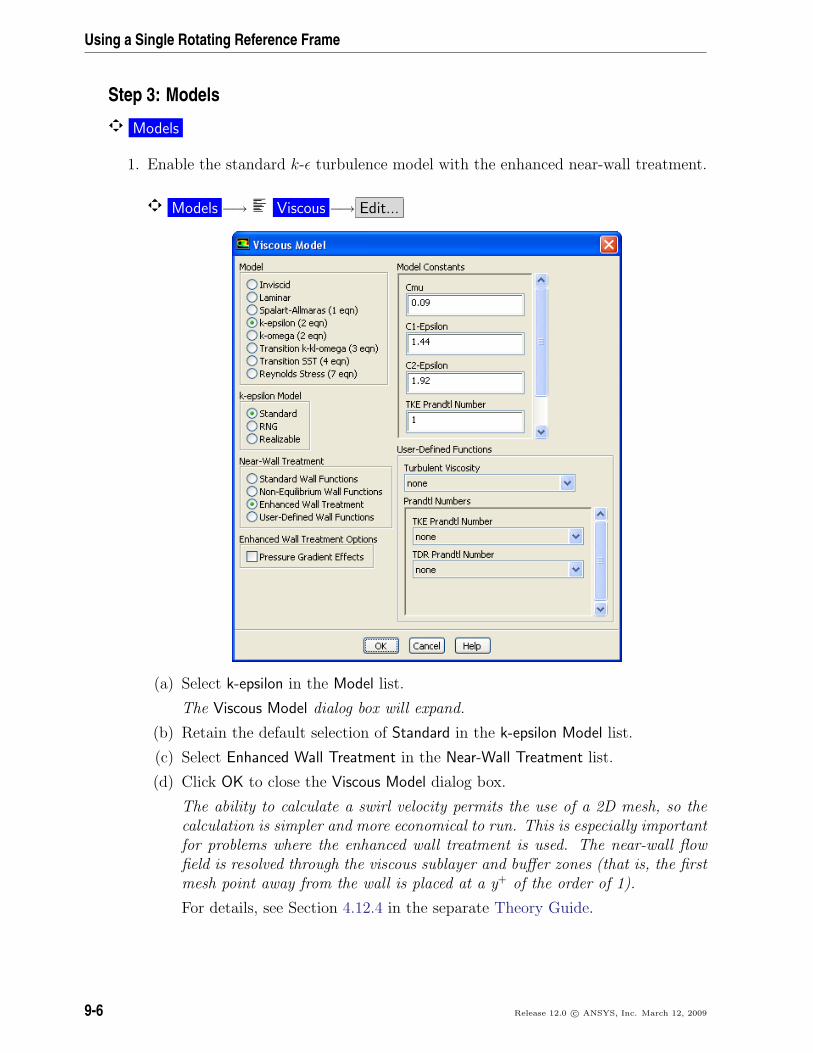
3. Enable the plotting of residuals during the calculation.
Monitors −→ Residuals −→ Edit...
(a) Ensure that Plot is enabled in the Options group box.
(b) Click OK to close the Residual Monitors dialog box.
Note: For this calculation, the convergence tolerance on the continuity equation iskept at 0.001. Depending on the behavior of the solution, you can reduce thisvalue if necessary.
9-16 Release 12.0 c© ANSYS, Inc. March 12, 2009

Using a Single Rotating Reference Frame
4. Enable the plotting of mass flow rate at the flow exit.
Monitors (Surface Monitors)−→ Create...
(a) Enable the Plot and Write options for surf-mon-1.
Note: When the Write option is selected in the Surface Monitor dialog box,themass flow rate history will be written to a file. If you do not enabletheWrite option, the history information will be lost when you exit ANSYSFLUENT.
(b) Select Mass Flow Rate from the Report Type drop-down list.
(c) Select pressure-outlet-3 from the Surfaces selection list.
(d) Click OK in the Surface Monitor dialog box to enable the monitor.
Release 12.0 c© ANSYS, Inc. March 12, 2009 9-17
Using a Single Rotating Reference Frame
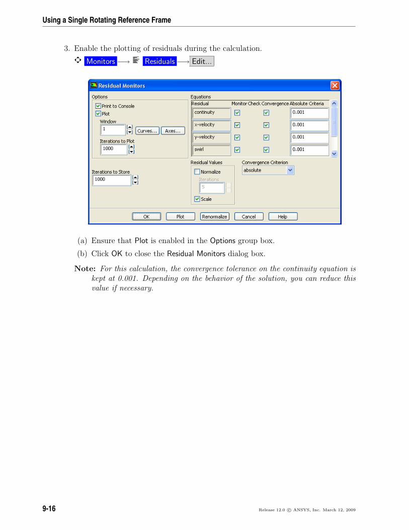
5. Initialize the flow field using the boundary conditions set at velocity-inlet-2.
Solution Initialization
(a) Select velocity-inlet-2 from the Compute From drop-down list.
(b) Click Initialize.
6. Save the case file (disk-ke.cas.gz).
File −→ Write −→Case...
9-18 Release 12.0 c© ANSYS, Inc. March 12, 2009
Using a Single Rotating Reference Frame
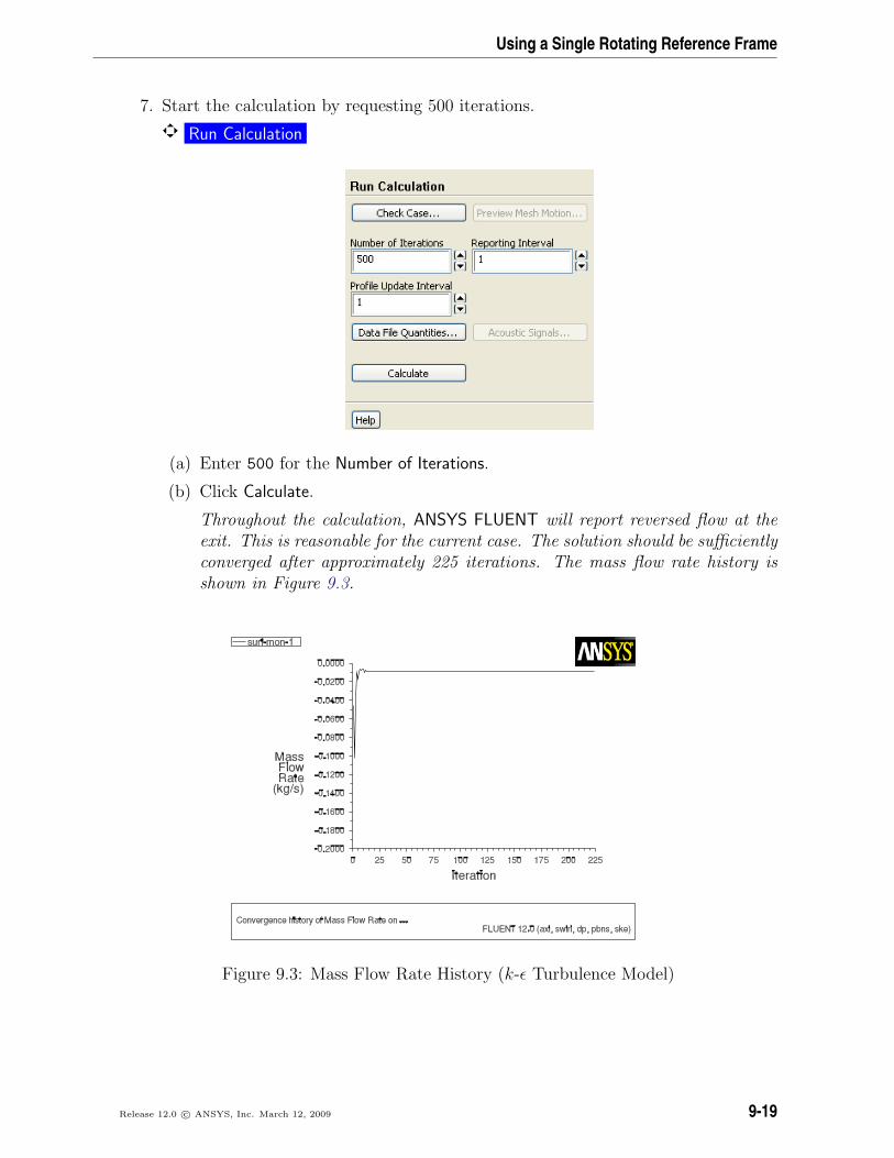
7. Start the calculation by requesting 500 iterations.
Run Calculation
(a) Enter 500 for the Number of Iterations.
(b) Click Calculate.
Throughout the calculation, ANSYS FLUENT will report reversed flow at theexit. This is reasonable for the current case. The solution should be sufficientlyconverged after approximately 225 iterations. The mass flow rate history isshown in Figure 9.3.
Figure 9.3: Mass Flow Rate History (k-ε Turbulence Model)
Release 12.0 c© ANSYS, Inc. March 12, 2009 9-19
Using a Single Rotating Reference Frame
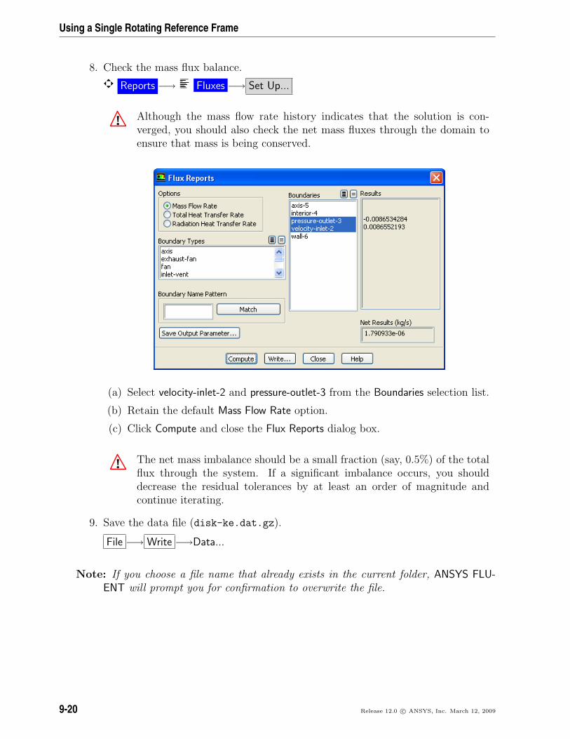
8. Check the mass flux balance.
Reports −→ Fluxes −→ Set Up...
! Although the mass flow rate history indicates that the solution is con-verged, you should also check the net mass fluxes through the domain toensure that mass is being conserved.
(a) Select velocity-inlet-2 and pressure-outlet-3 from the Boundaries selection list.
(b) Retain the default Mass Flow Rate option.
(c) Click Compute and close the Flux Reports dialog box.
! The net mass imbalance should be a small fraction (say, 0.5%) of the totalflux through the system. If a significant imbalance occurs, you shoulddecrease the residual tolerances by at least an order of magnitude andcontinue iterating.
9. Save the data file (disk-ke.dat.gz).
File −→ Write −→Data...
Note: If you choose a file name that already exists in the current folder, ANSYS FLU-ENT will prompt you for confirmation to overwrite the file.
9-20 Release 12.0 c© ANSYS, Inc. March 12, 2009
Using a Single Rotating Reference Frame
Step 8: Postprocessing for the Standard k-ε Solution
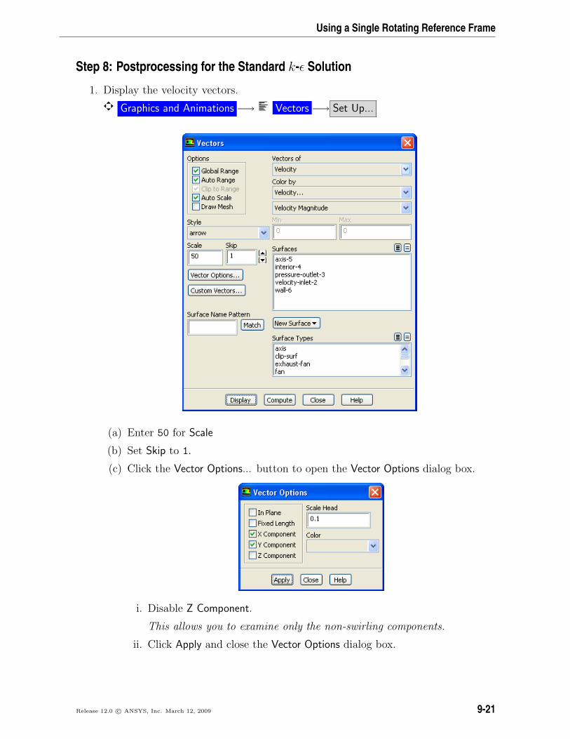
1. Display the velocity vectors.
Graphics and Animations −→ Vectors −→ Set Up...
(a) Enter 50 for Scale
(b) Set Skip to 1.
(c) Click the Vector Options... button to open the Vector Options dialog box.
i. Disable Z Component.
This allows you to examine only the non-swirling components.
ii. Click Apply and close the Vector Options dialog box.
Release 12.0 c© ANSYS, Inc. March 12, 2009 9-21
Using a Single Rotating Reference Frame
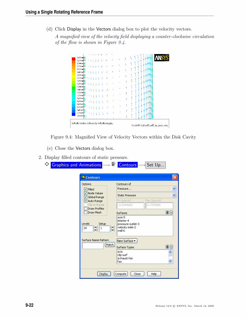
(d) Click Display in the Vectors dialog box to plot the velocity vectors.
A magnified view of the velocity field displaying a counter-clockwise circulationof the flow is shown in Figure 9.4.
Figure 9.4: Magnified View of Velocity Vectors within the Disk Cavity
(e) Close the Vectors dialog box.
2. Display filled contours of static pressure.
Graphics and Animations −→ Contours −→ Set Up...
9-22 Release 12.0 c© ANSYS, Inc. March 12, 2009
Using a Single Rotating Reference Frame
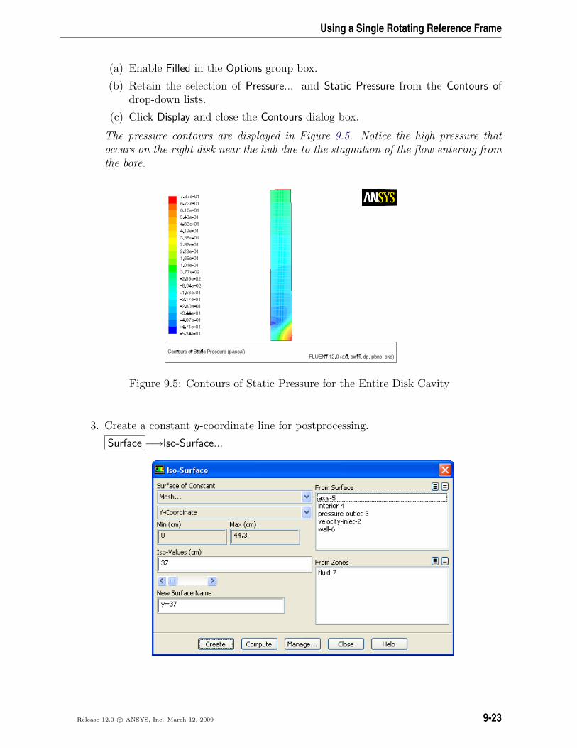
(a) Enable Filled in the Options group box.
(b) Retain the selection of Pressure... and Static Pressure from the Contours ofdrop-down lists.
(c) Click Display and close the Contours dialog box.
The pressure contours are displayed in Figure 9.5. Notice the high pressure thatoccurs on the right disk near the hub due to the stagnation of the flow entering fromthe bore.
Figure 9.5: Contours of Static Pressure for the Entire Disk Cavity
3. Create a constant y-coordinate line for postprocessing.
Surface −→Iso-Surface...
Release 12.0 c© ANSYS, Inc. March 12, 2009 9-23

Using a Single Rotating Reference Frame
(a) Select Mesh... and Y-Coordinate from the Surface of Constant drop-down lists.
(b) Click Compute to update the minimum and maximum values.
(c) Enter 37 in the Iso-Values field.
This is the radial position along which you will plot the radial velocity profile.
(d) Enter y=37cm for the New Surface Name.
(e) Click Create to create the isosurface.
Note: The name you use for an isosurface can be any continuous string ofcharacters (without spaces).
(f) Close the Iso-Surface dialog box.
4. Plot the radial velocity distribution on the surface y=37cm.
Plots −→ XY Plot −→ Set Up...
(a) Select Velocity... and Radial Velocity from the Y Axis Function drop-down lists.
(b) Select the y-coordinate line y=37cm from the Surfaces selection list.
(c) Click Plot.
Figure 9.6 shows a plot of the radial velocity distribution along y = 37 cm.
9-24 Release 12.0 c© ANSYS, Inc. March 12, 2009

Using a Single Rotating Reference Frame
Figure 9.6: Radial Velocity Distribution—Standard k-ε Solution
(d) Enable Write to File in the Options group box to save the radial velocity profile.
(e) Click the Write... button to open the Select File dialog box.
i. Enter ke-data.xy in the XY File text entry box and click OK.
5. Plot the wall y+ distribution on the rotating disk wall along the radial direction(Figure 9.7).
Plots −→ XY Plot −→ Set Up...
(a) Disable Write to File in the Options group box.
(b) Select Turbulence... and Wall Yplus from the Y Axis Function drop-down lists.
Release 12.0 c© ANSYS, Inc. March 12, 2009 9-25

Using a Single Rotating Reference Frame
(c) Deselect y=37cm and select wall-6 from the Surfaces selection list.
(d) Enter 0 and 1 for X and Y respectively in the Plot Direction group box.
(e) Click the Axes... button to open the Axes - Solution XY Plot dialog box.
i. Retain the default selection of X from the Axis group box.
ii. Disable Auto Range in the Options group box.
iii. Retain the default value of 0 for Minimum and enter 43 for Maximum inthe Range group box.
iv. Click Apply and close the Axes - Solution XY Plot dialog box.
(f) Click Plot in the Solution XY Plot dialog box.
Figure 9.7 shows a plot of wall y+ distribution along wall-6.
Figure 9.7: Wall Yplus Distribution on wall-6—Standard k-ε Solution
9-26 Release 12.0 c© ANSYS, Inc. March 12, 2009

Using a Single Rotating Reference Frame
(g) Enable Write to File in the Options group box to save the wall y+ profile.
(h) Click the Write... button to open the Select File dialog box.
i. Enter ke-yplus.xy in the XY File text entry box and click OK.
Note: Ideally, while using enhanced wall treatment, the wall y+ should be inthe order of 1 (at least < 5) to resolve viscous sublayer. The plot justifiesthe applicability of enhanced wall treatment to the given mesh.
(i) Close the Solution XY Plot dialog box.
Step 9: Solution Using the RNG k-ε Model
Recalculate the solution using the RNG k-ε turbulence model.
1. Enable the RNG k-ε turbulence model with the enhanced near-wall treatment.
Models −→ Viscous −→ Edit...
(a) Select RNG in the k-epsilon Model list.
Release 12.0 c© ANSYS, Inc. March 12, 2009 9-27
Using a Single Rotating Reference Frame
(b) Enable Differential Viscosity Model and Swirl Dominated Flow in the RNG Op-tions group box.
The differential viscosity model and swirl modification can provide better ac-curacy for swirling flows such as the disk cavity.
For more information, see Section 4.4.2 in the separate Theory Guide.
(c) Retain Enhanced Wall Treatment as the Near-Wall Treatment.
(d) Click OK to close the Viscous Model dialog box.
2. Continue the calculation by requesting 200 iterations.
Run Calculation
The solution converges after approximately 105 additional iterations.
3. Save the case and data files (disk-rng.cas.gz and disk-rng.dat.gz).
File −→ Write −→Case & Data...
Step 10: Postprocessing for the RNG k-ε Solution
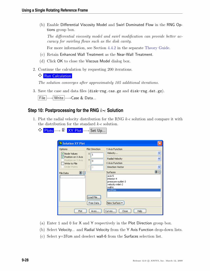
1. Plot the radial velocity distribution for the RNG k-ε solution and compare it withthe distribution for the standard k-ε solution.
Plots −→ XY Plot −→ Set Up...
(a) Enter 1 and 0 for X and Y respectively in the Plot Direction group box.
(b) Select Velocity... and Radial Velocity from the Y Axis Function drop-down lists.
(c) Select y=37cm and deselect wall-6 from the Surfaces selection list.
9-28 Release 12.0 c© ANSYS, Inc. March 12, 2009
Using a Single Rotating Reference Frame
(d) Disable the Write to File option.
(e) Click the Load File... button to load the k-ε data.
i. Select the file ke-data.xy in the Select File dialog box.
ii. Click OK.
(f) Click the Axes... button to open the Axes - Solution XY Plot dialog box.
i. Enable Auto Range in the Options group box.
ii. Click Apply and close the Axes - Solution XY Plot dialog box.
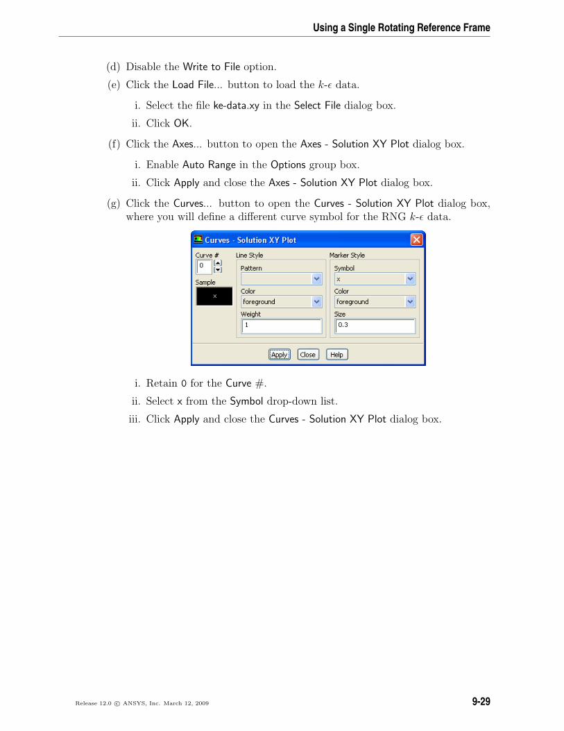
(g) Click the Curves... button to open the Curves - Solution XY Plot dialog box,where you will define a different curve symbol for the RNG k-ε data.
i. Retain 0 for the Curve #.
ii. Select x from the Symbol drop-down list.
iii. Click Apply and close the Curves - Solution XY Plot dialog box.
Release 12.0 c© ANSYS, Inc. March 12, 2009 9-29

Using a Single Rotating Reference Frame
(h) Click Plot in the Solution XY Plot dialog box (Figure 9.8).
Figure 9.8: Radial Velocity Distribution—RNG k-ε and Standard k-ε Solutions
The peak velocity predicted by the RNG k-ε solution is higher than that pre-dicted by the k-ε solution.This is due to the less diffusive character of the RNGk-ε model. Adjust the range of the x axis to magnify the region of the peaks.
(i) Click the Axes... button to open the Axes - Solution XY Plot dialog box, whereyou will specify the x-axis range.
i. Disable Auto Range in the Options group box.
ii. Retain the value of 0 for Minimum and enter 1 for Maximum in the Rangedialog box.
iii. Click Apply and close the Axes - Solution XY Plot dialog box.
9-30 Release 12.0 c© ANSYS, Inc. March 12, 2009

Using a Single Rotating Reference Frame
(j) Click Plot.
The difference between the peak values calculated by the two models is nowmore apparent.
Figure 9.9: RNG k-ε and Standard k-ε Solutions (x = 0 cm to x = 1 cm)
2. Plot the wall y+ distribution on the rotating disk wall along the radial directionFigure 9.10.
Plots −→ XY Plot −→ Set Up...
Release 12.0 c© ANSYS, Inc. March 12, 2009 9-31

Using a Single Rotating Reference Frame
(a) Select Turbulence... and Wall Yplus from the Y Axis Function drop-down lists.
(b) Deselect y=37cm and select wall-6 from the Surfaces selection list.
(c) Enter 0 and 1 for X and Y respectively in the Plot Direction group box.
(d) Select any existing files that appear in the File Data selection list and click theFree Data button to remove the file.
(e) Click the Load File... button to load the RNG k-ε data.
i. Select the file ke-yplus.xy in the Select File dialog box.
ii. Click OK.
(f) Click the Axes... button to open the Axes - Solution XY Plot dialog box.
i. Retain the default selection of X from the Axis group box.
ii. Retain the default value of 0 for Minimum and enter 43 for Maximum inthe Range group box.
iii. Click Apply and close the Axes - Solution XY Plot dialog box.
(g) Click Plot in the Solution XY Plot dialog box.
Figure 9.10: wall-6—RNG k-ε and Standard k-ε Solutions (x = 0 cm to x = 43 cm)
9-32 Release 12.0 c© ANSYS, Inc. March 12, 2009

Using a Single Rotating Reference Frame
Summary
This tutorial illustrated the setup and solution of a 2D, axisymmetric disk cavity problemin ANSYS FLUENT. The ability to calculate a swirl velocity permits the use of a 2D mesh,thereby making the calculation simpler and more economical to run than a 3D model.This can be important for problems where the enhanced wall treatment is used, and thenear-wall flow field is resolved using a fine mesh (the first mesh point away from the wallbeing placed at a y+ on the order of 1).
For more information about mesh considerations for turbulence modeling, see Section 12.3in the separate User’s Guide.
Further Improvements
The case modeled in this tutorial lends itself to parametric study due to its relativelysmall size. Here are some things you may wish to try:
• Separate wall-6 into two walls.
Mesh −→ Separate −→Faces...
Specify one wall to be stationary, and rerun the calculation.
• Use adaption to see if resolving the high velocity and pressure-gradient region ofthe flow has a significant effect on the solution.
• Introduce a non-zero swirl at the inlet or use a velocity profile for fully-developedpipe flow. This is probably more realistic than the constant axial velocity usedhere, since the flow at the inlet is typically being supplied by a pipe.
• Model compressible flow (using the ideal gas law for density) rather than assumingincompressible flow text.
This tutorial guides you through the steps to reach an initial solution. You may be ableto obtain a more accurate solution by using an appropriate higher-order discretizationscheme and by adapting the mesh. Mesh adaption can also ensure that the solution isindependent of the mesh. These steps are demonstrated in Tutorial 1.
References
1. Pincombe, J.R., “Velocity Measurements in the Mk II - Rotating Cavity Rig with aRadial Outflow”, Thermo-Fluid Mechanics Research Centre, University of Sussex,Brighton, UK, 1981.
Release 12.0 c© ANSYS, Inc. March 12, 2009 9-33

Using a Single Rotating Reference Frame
9-34 Release 12.0 c© ANSYS, Inc. March 12, 2009
Related Documents