Bayan Almukhlif مخلفن ال | بيا1 Tutorial 6-ch6 Exercise 1: (same Example 6.1 page 297) Municipal wastewater treatment plants are required by Jaw to monitor their discharges into rivers and streams on a regular basis. Concern about the reliability of data from one of these self- monitoring programs led to a study in which samples of effluent were divided and sent to two laboratories for testing. One-half of each sample was sent to the Wisconsin State Laboratory of Hygiene, and one-half was sent to a private commercial laboratory routinely used in the monitoring program. Measurements of biochemical oxygen demand (BOD) and suspended solids (SS) were obtained, for n = 11 sample splits, from the two laboratories. The data are displayed in Table 6.1 a) Test of 0 : =0 b) Construct 95% Simultaneous C.I for the components of the mean difference vector . c) Construct 95% Bonferroni Simultaneous intervals for the components of the mean difference vector . Compare the lengths of these intervals with those of the simultaneous intervals constructed in part (b). d) Use 2 to test 0 :=0 and construct 95% Simultaneous C.I for the components of the mean difference vector . (suppose n is large ) Solution: a) 0 :=[ 1 2 ]=[ 0 0 ] . 1 : ≠ 0 ; ℎ = 1 − 2 #Test statistic for vector of mean differences 2 = ( − ) ′ −1 ( − ), 0 2 ≥ ( − 1) − ,−, Note: From R result 0 . 2 = = 2 ( − (−1) )≥ , −, ( − 1) − ,−, 1− = 10 ∗ 2 ∗ 2,9 , 0.95 9 = 10 ∗ 2 ∗ 4.25649 9 = 9.4589 =[ −9.3636 13.2727 ] ; =[ 199.255 88.309 88.309 418.618 ] , −1 =[ 0.0055363 −0.0011679 −0.0011679 0.0026352 ] Since 2 = 13.6312 > 9.4589, we reject 0 :=0 and conclude that there is a nonzero mean difference between the measurements of the two laboratories. b) The 100(1 − ) % Simultaneous Intervals for individual Mean differences (Paired Comparisons):

Welcome message from author
This document is posted to help you gain knowledge. Please leave a comment to let me know what you think about it! Share it to your friends and learn new things together.
Transcript

Bayan Almukhlif 1 | بيان المخلف
Tutorial 6-ch6
Exercise 1: (same Example 6.1 page 297)
Municipal wastewater treatment plants are required by Jaw to monitor their discharges into rivers
and streams on a regular basis. Concern about the reliability of data from one of these self-
monitoring programs led to a study in which samples of effluent were divided and sent to two
laboratories for testing. One-half of each sample was sent to the Wisconsin State Laboratory of
Hygiene, and one-half was sent to a private commercial laboratory routinely used in the
monitoring program. Measurements of biochemical oxygen demand (BOD) and suspended solids
(SS) were obtained, for n = 11 sample splits, from the two laboratories. The data are displayed in
Table 6.1
a) Test of 𝐻0: 𝛿 = 0⃗⃗
b) Construct 95% Simultaneous C.I for the components of the mean difference vector 𝛿.
c) Construct 95% Bonferroni Simultaneous intervals for the components of the mean
difference vector 𝛿. Compare the lengths of these intervals with those of the simultaneous
intervals constructed in part (b).
d) Use 𝜒2 to test 𝐻0: 𝛿 = 0 and construct 95% Simultaneous C.I for the components of the
mean difference vector 𝛿. (suppose n is large )
Solution:
a) 𝐻0: 𝛿 = [𝛿1
𝛿2] = [
00
] 𝑉. 𝑆 𝐻1: 𝛿 ≠ 0 ; 𝑤ℎ𝑒𝑟𝑒 𝛿 = 𝜇𝑑1 − 𝜇𝑑2
#Test statistic for vector of mean differences 𝛿
𝑇2 = 𝑛(�̅� − 𝛿)′𝑆𝑑−1 (�̅� − 𝛿), 𝑅𝑒𝑗𝑒𝑐𝑡 𝐻0 𝑖𝑓 𝑇2 ≥
(𝑛 − 1)𝑃
𝑛 − 𝑃𝐹𝑃,𝑛−𝑃,𝛼
Note: From R result 𝑅𝑒𝑗𝑒𝑐𝑡 𝐻0 𝑖𝑓 𝑇. 2 = 𝐹 = 𝑇2 (𝑛−𝑃
(𝑛−1)𝑃) ≥ 𝐹𝑃, 𝑛−𝑃, 𝛼
(𝑛 − 1)𝑃
𝑛 − 𝑃𝐹𝑃,𝑛−𝑃, 1−𝛼 =
10 ∗ 2 ∗ 𝐹2,9 , 0.95
9=
10 ∗ 2 ∗ 4.25649
9= 9.4589
�̅� = [−9.363613.2727
] ; 𝑆𝑑 = [199.255 88.30988.309 418.618
] , 𝑆𝑑−1 = [
0.0055363 −0.0011679−0.0011679 0.0026352
]
Since 𝑇2 = 13.6312 > 9.4589, we reject 𝐻0: 𝛿 = 0 and conclude that there is a nonzero
mean difference between the measurements of the two laboratories.
b) The 100(1 − 𝛼) % Simultaneous Intervals for individual Mean differences (Paired
Comparisons):

Bayan Almukhlif 2 | بيان المخلف
𝛿𝑖 𝜖 [�̅�𝑖 ∓ √(𝑛−1)𝑃
𝑛−𝑃𝐹𝑃,𝑛−𝑃,𝛼 √
𝑆𝑑𝑖2
𝑛 ]
95% 𝐶. 𝐼 𝑓𝑜𝑟 𝛿1𝜖[−22.4617 , 3.74175 ] 𝑎𝑛𝑑 95% 𝐶. 𝐼 𝑓𝑜𝑟 𝛿2𝜖[−5.70600, 32.2460 ]
c) Bonferroni 100(1 − 𝛼) % Simultaneous C.I for individual Mean differences (Paired
Comparisons):
𝛿𝑖 𝜖 [𝑑�̅� ∓ 𝑡𝑛−1,𝛼
2𝑃 √
𝑆𝑑𝑖2
𝑛 ]
1 −𝛼
2𝑃= 1 −
0.05
2(2)= 0.9875 ; 𝑡𝑛−1,
𝛼
2𝑃= 𝑡10, 0.9875 = 2.63377
𝛿1𝜖 [ −9.36 ∓ 2.63377 ∗ √199.255
11] ≫≫ [−20.5799 , 1.85986]
𝛿2𝜖 [ 13.27 ∓ 2.63377 ∗ √418.618
11] ≫≫ [−2.98036 ,29.5036 ]
Compare the lengths of these intervals with simultaneous intervals constructed in part (b)
95% 𝐵𝑜𝑛𝑓𝑒𝑟𝑟𝑜𝑛𝑖 𝐶. 𝐼: { 𝛿1𝜖[−20.5799 , 1.85986]
𝛿2𝜖[−2.98036 ,29.5036 ]
95% 𝑆𝑖𝑚𝑢𝑙𝑡𝑎𝑛𝑒𝑜𝑢𝑠 𝐶. 𝐼: { 𝛿1𝜖[−22.4617 , 3.74175 ]
𝛿2𝜖[−5.70600, 32.2460 ]
Simultaneous confidence intervals are larger than Bonferroni's confidence intervals.
d) Suppose n and n-p are large 𝑇2~𝜒𝑝2
𝑇2 = 𝑛(�̅� − 𝛿)′𝑆𝑑−1 (�̅� − 𝛿), 𝑅𝑒𝑗𝑒𝑐𝑡 𝐻0 𝑖𝑓 𝑇2 ≥ 𝜒 𝑝, 𝛼
2
𝛿𝑖 𝜖 [𝑑�̅� ∓ √𝜒 𝑝, 𝛼2 √
𝑆𝑑𝑖2
𝑛 ]
𝜒 2, 0.052 = 5.991465
Since 𝑇2 = 13.6312 > 5.99 , we reject 𝐻0: 𝛿 = 0 and conclude that there is a nonzero
mean difference between the measurements of the two laboratories.
95% 𝑆𝑖𝑚𝑢𝑙𝑡𝑎𝑛𝑒𝑜𝑢𝑠 𝐶. 𝐼 𝑏𝑦 𝑢𝑠𝑒 𝜒2 : { 𝛿1𝜖[−19.7814 , 1.0541]
𝛿2𝜖[−1.8274 , 28.3728 ]
Bayan Almukhlif 3 | بيان المخلف
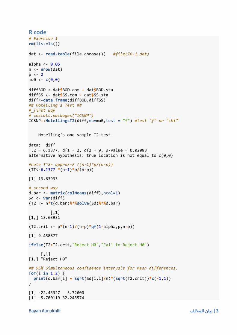
R code # Exercise 1 rm(list=ls()) dat <- read.table(file.choose()) #file(T6-1.dat) alpha <- 0.05 n <- nrow(dat) p <- 2 mu0 <- c(0,0) diffBOD <-dat$BOD.com - dat$BOD.sta diffSS <- dat$SS.com - dat$SS.sta diff<-data.frame(diffBOD,diffSS) ## Hotelling's Test ## #_first way # install.packages("ICSNP") ICSNP::HotellingsT2(diff,mu=mu0,test = "f") #test "f" or "chi"
Hotelling's one sample T2-test data: diff T.2 = 6.1377, df1 = 2, df2 = 9, p-value = 0.02083 alternative hypothesis: true location is not equal to c(0,0)
#note T^2= approx-F ((n-1)*p/(n-p)) (TT<-6.1377 *(n-1)*p/(n-p))
[1] 13.63933
#_second way d.bar <- matrix(colMeans(diff),ncol=1) Sd <- var(diff) (T2 <- n*t(d.bar)%*%solve(Sd)%*%d.bar)
[,1] [1,] 13.63931
(T2.crit <- p*(n-1)/(n-p)*qf(1-alpha,p,n-p))
[1] 9.458877
ifelse(T2>T2.crit,"Reject H0","Fail to Reject H0")
[,1] [1,] "Reject H0"
## 95% Simultaneous confidence intervals for mean differences. for(i in 1:2) { print(d.bar[i] + sqrt(Sd[i,i]/n)*(sqrt(T2.crit))*c(-1,1)) }
[1] -22.45327 3.72600 [1] -5.700119 32.245574
Bayan Almukhlif 4 | بيان المخلف
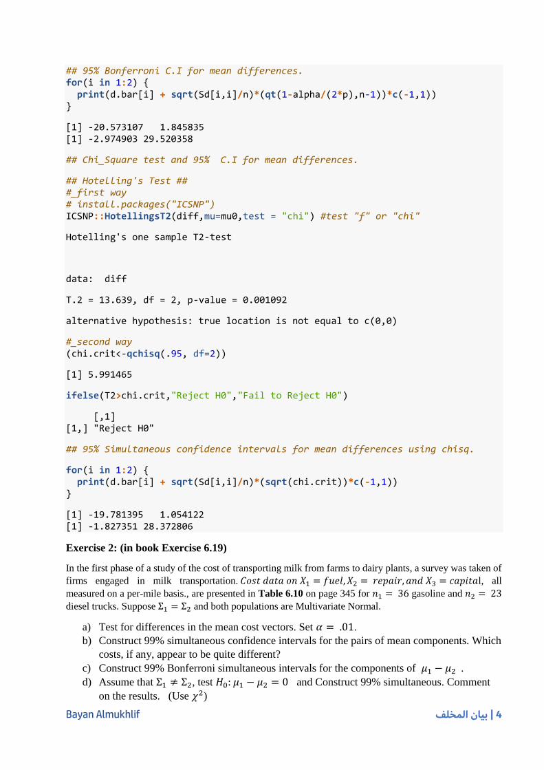
## 95% Bonferroni C.I for mean differences. for(i in 1:2) { print(d.bar[i] + sqrt(Sd[i,i]/n)*(qt(1-alpha/(2*p),n-1))*c(-1,1)) }
[1] -20.573107 1.845835 [1] -2.974903 29.520358
## Chi_Square test and 95% C.I for mean differences.
## Hotelling's Test ## #_first way # install.packages("ICSNP") ICSNP::HotellingsT2(diff,mu=mu0,test = "chi") #test "f" or "chi"
Hotelling's one sample T2-test
data: diff
T.2 = 13.639, df = 2, p-value = 0.001092
alternative hypothesis: true location is not equal to c(0,0)
#_second way (chi.crit<-qchisq(.95, df=2))
[1] 5.991465
ifelse(T2>chi.crit,"Reject H0","Fail to Reject H0")
[,1] [1,] "Reject H0"
## 95% Simultaneous confidence intervals for mean differences using chisq.
for(i in 1:2) { print(d.bar[i] + sqrt(Sd[i,i]/n)*(sqrt(chi.crit))*c(-1,1)) }
[1] -19.781395 1.054122 [1] -1.827351 28.372806
Exercise 2: (in book Exercise 6.19)
In the first phase of a study of the cost of transporting milk from farms to dairy plants, a survey was taken of
firms engaged in milk transportation. 𝐶𝑜𝑠𝑡 𝑑𝑎𝑡𝑎 𝑜𝑛 𝑋1 = 𝑓𝑢𝑒𝑙, 𝑋2 = 𝑟𝑒𝑝𝑎𝑖𝑟, 𝑎𝑛𝑑 𝑋3 = 𝑐𝑎𝑝𝑖𝑡𝑎l, all
measured on a per-mile basis., are presented in Table 6.10 on page 345 for 𝑛1 = 36 gasoline and 𝑛2 = 23
diesel trucks. Suppose Σ1 = Σ2 and both populations are Multivariate Normal.
a) Test for differences in the mean cost vectors. Set 𝛼 = .01.
b) Construct 99% simultaneous confidence intervals for the pairs of mean components. Which
costs, if any, appear to be quite different?
c) Construct 99% Bonferroni simultaneous intervals for the components of 𝜇1 − 𝜇2 .
d) Assume that Σ1 ≠ Σ2, test 𝐻0: 𝜇1 − 𝜇2 = 0 and Construct 99% simultaneous. Comment
on the results. (Use 𝜒2)

Bayan Almukhlif 5 | بيان المخلف
Solution:
a) 𝐻0: 𝜇1 − 𝜇2 = [
𝜇11
𝜇12
𝜇13
] − [
𝜇21
𝜇22
𝜇23
] = [000
] 𝑉. 𝑆 𝐻1: 𝜇1 − 𝜇2 ≠ 0
𝑇2 = [(�̅�1 − �̅�2) − (𝜇1 − 𝜇2)]′ [(1
𝑛1+
1
𝑛2) 𝑆𝑃𝑜𝑜𝑙𝑒𝑑]
−1
[(�̅�1 − �̅�2) − (𝜇1 − 𝜇2)]
𝑪𝒓𝒊𝒕𝒊𝒄𝒂𝒍 𝒅𝒊𝒔𝒕𝒂𝒏𝒄𝒆: 𝑪𝟐 =(𝑛1 + 𝑛2 − 2)𝑃
𝑛1 + 𝑛2 − 𝑃 − 1𝐹𝑃, 𝑛1+𝑛2−𝑃−1, 𝛼
𝑅𝑒𝑗𝑒𝑐𝑡 𝐻0 𝑖𝑓 𝑇2 ≥(𝑛1 + 𝑛2 − 2)𝑃
𝑛1 + 𝑛2 − 𝑃 − 1𝐹𝑃, 𝑛1+𝑛2−𝑃−1, 𝛼
Note: From R result 𝑅𝑒𝑗𝑒𝑐𝑡 𝐻0 𝑖𝑓 𝑇. 2 = 𝐹 = 𝑇2 (𝑛1+𝑛2−𝑃−1
(𝑛1+𝑛2−2)𝑃) ≥ 𝐹𝑃, 𝑛1+𝑛2−𝑃−1, 𝛼
�̅�1 = [12.2198.1139.590
] , �̅�2 = [10.10610.76218.168
]
𝑆1 = [23.0134 12.3664 2.9066
17.5441 4.773113.9633
] , 𝑆2 = [4.3623 0.7599 2.3621
25.8512 7.685746.6544
]
𝑆𝑃𝑜𝑜𝑙𝑒𝑑 =(𝑛1 − 1)
𝑛1 + 𝑛2 − 2𝑆1 +
𝑛2 − 1
𝑛1 + 𝑛2 − 2 𝑆2 ; 𝑛1 = 36 ; 𝑛2 = 23, 𝑝 = 3
𝑆𝑃𝑜𝑜𝑙𝑒𝑑 = 𝟎. 𝟔𝟏𝟒𝟎 𝑆1 + 𝟎. 𝟑𝟖𝟔𝟎𝑆2
𝑆𝑃𝑜𝑜𝑙𝑒𝑑 = [15.8141 7.8863 2.69647.8863 20.7507 5.8974
2.6964 5.8974 26.5821] ; [(
1
𝑛1+
1
𝑛2) 𝑆𝑃𝑜𝑜𝑙𝑒𝑑]
−1
= [ ]
𝑪𝟐 =171
55𝐹3, 55, 0.99 =
171
55(4.159081) = 12.93096 ≈ 13
Since 𝑇2 = 50.9128 > 13 , we Reject 𝐻0 at the 𝛼 = 0.01 level. There is a difference in the mean
cost vectors between Gasoline trucks and Diesel trucks.
b) 99% simultaneous confidence intervals
(𝝁𝟏𝒊 − 𝝁𝟐𝒊) ∈ [ (�̅�1 − �̅�2) ± 𝑪√ (1
𝑛1+
1
𝑛2) 𝑆𝑖𝑖, 𝑃𝑜𝑜𝑙𝑒𝑑 ]
99% 𝑆𝑖𝑚𝑢𝑙𝑡𝑎𝑛𝑒𝑜𝑢𝑠 𝐶. 𝐼 ∶ {
𝜇11 − 𝜇21 𝜖[ −1.7043 , 5.9303 ]
𝜇12 − 𝜇22𝜖[−7.0223 , 1.7229 ]
𝜇13 − 𝜇23𝜖[ −13.5265 , −3.6286 ]
c) 99% Bonferroni C.I
(𝝁𝟏𝒊 − 𝝁𝟐𝒊) ∈ [ (�̅�1 − �̅�2) ± 𝒕𝒏𝟏+𝒏𝟐−𝟐 ,
𝜶𝟐𝒑
√ (1
𝑛1+
1
𝑛2) 𝑆𝑖𝑖, 𝑃𝑜𝑜𝑙𝑒𝑑 ]

Bayan Almukhlif 6 | بيان المخلف
𝒕𝒏𝟏+𝒏𝟐−𝟐 ,
𝜶𝟐𝒑
= 𝒕𝟑𝟔+𝟐𝟑−𝟐, 𝟎.𝟗𝟗𝟖 = 𝟑. 𝟎𝟔𝟒
99% 𝐵𝑜𝑛𝑓𝑒𝑟𝑟𝑜𝑛𝑖 𝐶. 𝐼: {
𝜇11 − 𝜇21 𝜖[−1.1396 , 5.3655 ]
𝜇12 − 𝜇22𝜖[−6.3754 , 1.0760 ]
𝜇13 − 𝜇23𝜖[ −12.7943 , −4.3608 ]
d) Assumption Σ1 ≠ Σ2. By using “large sample theory” ( n1 = 36, n2 = 23) we have,
Result (6.4): 𝑇2 = [(�̅�1 − �̅�2) − (𝜇1 − 𝜇2)]′ [1
𝑛1𝑆1 +
1
𝑛2𝑆2]
−1[(�̅�1 − �̅�2) − (𝜇1 − 𝜇2)]
𝑅𝑒𝑗𝑒𝑐𝑡 𝐻0 𝑖𝑓 𝑇2 ≥ 𝜒 𝑝 , 𝛼2
𝜒 3 , 0.012 = 11.3448
Since 𝑇2 = 43.1763 > 11.34 , we Reject 𝐻0 at the 𝛼 = 0.01 level. This is consistent with the
result in part (a).
(𝝁𝟏𝒊 − 𝝁𝟐𝒊) ∈ [ (�̅�1 − �̅�2) ± √𝝌 𝒑 , 𝜶𝟐 √ (
1
𝑛1𝑆1 +
1
𝑛2𝑆2)
𝒊𝒊
]
99% 𝑆𝑖𝑚𝑢𝑙𝑡𝑎𝑛𝑒𝑜𝑢𝑠 𝐶. 𝐼 𝑏𝑦 𝑢𝑠𝑒 𝜒2 : {
𝜇11 − 𝜇21 𝜖[ −0.95364 , 5.17956 ]
𝜇12 − 𝜇22𝜖[−6.9252 , 1.6258 ]
𝜇13 − 𝜇23𝜖[ −13.8133, −3.3418 ]
R code # Exercise 6.19 rm(list=ls()) data2 <- read.table(file.choose()) #file(T6-10.dat) names(data2) <-c("fuel","repair","capital","truck_type")
##compute Hotelling Test ## #_first way z<- cbind(data2$fuel,data2$repair,data2$capital) ICSNP::HotellingsT2(z ~data2$truck_type,test = "f")
Hotelling's two sample T2-test data: z by data2$truck_type T.2 = 16.375, df1 = 3, df2 = 55, p-value = 1e-07 alternative hypothesis: true location difference is not equal to c(0,0,0)
# note 𝑇2 = (𝑎𝑝𝑝𝑟𝑜𝑥 𝐹) ((𝑛1+𝑛2−2)𝑃
𝑛1+𝑛2−𝑃−1)
#_second way man.Res<- manova(cbind(fuel,repair,capital) ~truck_type,data=data2) summary(man.Res)
Df Pillai approx F num Df den Df Pr(>F) truck_type 1 0.4718 16.375 3 55 1e-07 ***

Bayan Almukhlif 7 | بيان المخلف
Residuals 57 --- Signif. codes: 0 '***' 0.001 '**' 0.01 '*' 0.05 '.' 0.1 ' ' 1
# Look to see which differ(comparing each two pop mean) #ANOVA summary.aov(man.Res)
Response fuel : Df Sum Sq Mean Sq F value Pr(>F) truck_type 1 62.66 62.656 3.9619 0.05135 . Residuals 57 901.44 15.815 --- Signif. codes: 0 '***' 0.001 '**' 0.01 '*' 0.05 '.' 0.1 ' ' 1 Response repair : Df Sum Sq Mean Sq F value Pr(>F) truck_type 1 98.53 98.529 4.7483 0.03348 * Residuals 57 1182.77 20.750 --- Signif. codes: 0 '***' 0.001 '**' 0.01 '*' 0.05 '.' 0.1 ' ' 1 Response capital : Df Sum Sq Mean Sq F value Pr(>F) truck_type 1 1032.5 1032.53 38.845 5.966e-08 *** Residuals 57 1515.1 26.58 --- Signif. codes: 0 '***' 0.001 '**' 0.01 '*' 0.05 '.' 0.1 ' ' 1
#there is significant difference in mean capital cost between Gasoline and Diesel trucks.
## CI ## plyr::count(data2$truck_type) #library(plyr)
x freq 1 diesel 23 2 gasoline 36
table(data2$truck_type) #library(base) diesel gasoline 23 36
alpha <- 0.01 n1 <-length(which((data2$truck_type=="gasoline"))) n2 <-length(which((data2$truck_type=="diesel"))) p <- 3 #mean vector of gasoline pop and mean vector of diesel pop. xbar1<-colMeans(data2[data2$truck_type=="gasoline",-4]) xbar2<-colMeans(data2[data2$truck_type=="diesel",-4])
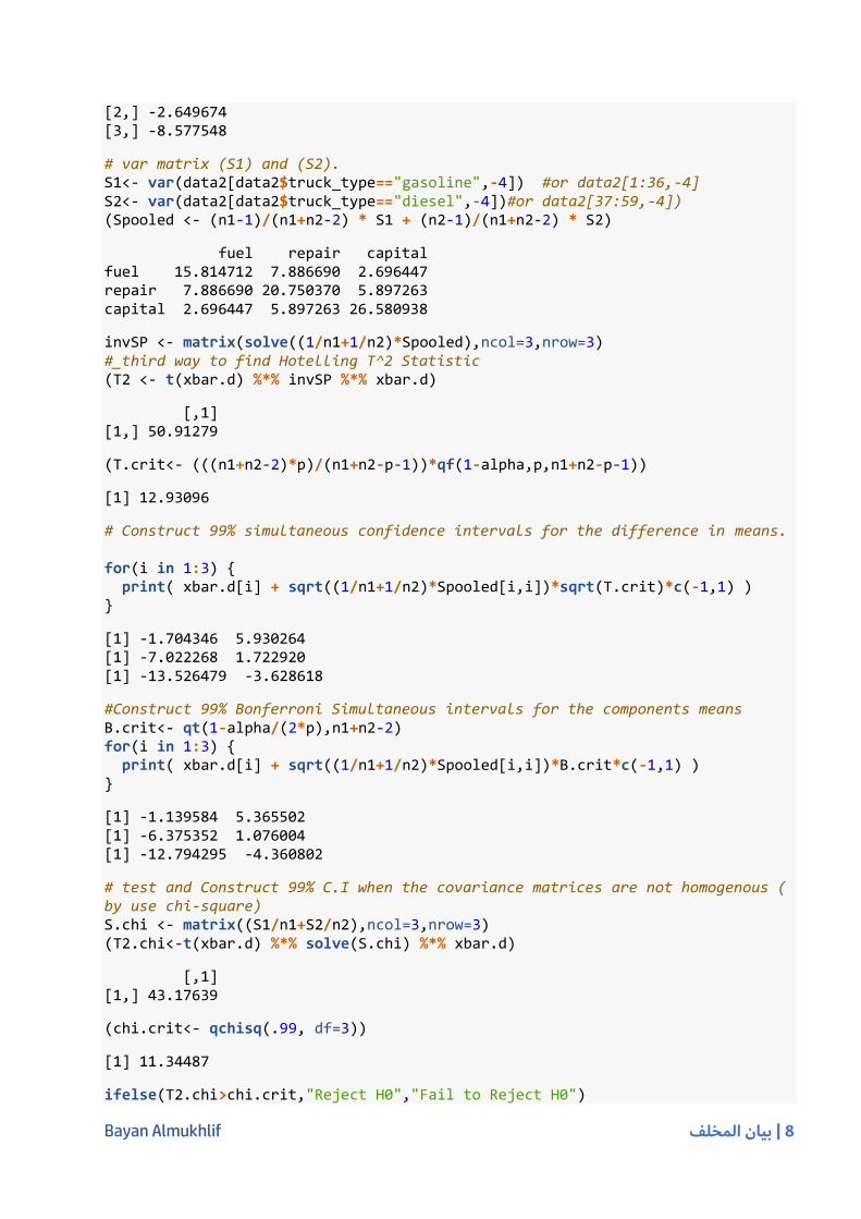
(xbar.d <- matrix(xbar1 - xbar2,ncol=1,nrow=3))
[,1] [1,] 2.112959
Bayan Almukhlif 8 | بيان المخلف
[2,] -2.649674 [3,] -8.577548
# var matrix (S1) and (S2). S1<- var(data2[data2$truck_type=="gasoline",-4]) #or data2[1:36,-4] S2<- var(data2[data2$truck_type=="diesel",-4])#or data2[37:59,-4]) (Spooled <- (n1-1)/(n1+n2-2) * S1 + (n2-1)/(n1+n2-2) * S2)
fuel repair capital fuel 15.814712 7.886690 2.696447 repair 7.886690 20.750370 5.897263 capital 2.696447 5.897263 26.580938
invSP <- matrix(solve((1/n1+1/n2)*Spooled),ncol=3,nrow=3) #_third way to find Hotelling T^2 Statistic (T2 <- t(xbar.d) %*% invSP %*% xbar.d)
[,1] [1,] 50.91279
(T.crit<- (((n1+n2-2)*p)/(n1+n2-p-1))*qf(1-alpha,p,n1+n2-p-1))
[1] 12.93096
# Construct 99% simultaneous confidence intervals for the difference in means. for(i in 1:3) { print( xbar.d[i] + sqrt((1/n1+1/n2)*Spooled[i,i])*sqrt(T.crit)*c(-1,1) ) }
[1] -1.704346 5.930264 [1] -7.022268 1.722920 [1] -13.526479 -3.628618
#Construct 99% Bonferroni Simultaneous intervals for the components means B.crit<- qt(1-alpha/(2*p),n1+n2-2) for(i in 1:3) { print( xbar.d[i] + sqrt((1/n1+1/n2)*Spooled[i,i])*B.crit*c(-1,1) ) }
[1] -1.139584 5.365502 [1] -6.375352 1.076004 [1] -12.794295 -4.360802
# test and Construct 99% C.I when the covariance matrices are not homogenous (by use chi-square) S.chi <- matrix((S1/n1+S2/n2),ncol=3,nrow=3) (T2.chi<-t(xbar.d) %*% solve(S.chi) %*% xbar.d)
[,1] [1,] 43.17639
(chi.crit<- qchisq(.99, df=3))
[1] 11.34487
ifelse(T2.chi>chi.crit,"Reject H0","Fail to Reject H0")

Bayan Almukhlif 9 | بيان المخلف
[,1] [1,] "Reject H0"
for(i in 1:3) { print(xbar.d[i] + sqrt(S.chi[i,i])*sqrt(chi.crit)*c(-1,1)) }
[1] -0.9536442 5.1795620 [1] -6.925188 1.625840 [1] -13.813277 -3.341819
Exercise 3: (in book Example 6.10 and 6.11)
The Wisconsin Department of Health and Social Services reimburses nursing homes in the state for
the services provided. The department develops a set of formulas for rates for each facility, based
on factors such as level of care, mean wage rate, and average wage rate in the state.
Nursing homes can be classified on the basis of ownership (private party, non-profit organization,
and government) and certification (skilled nursing facility, intermediate care facility, or a
combination of the two). One purpose of a recent study was to investigate the effects of ownership
or certification (or both) on costs. Four costs, computed on a per-patient-day basis and measured in
hours per patient day, were selected for analysis:
𝑿𝟏 = 𝑐𝑜𝑠𝑡 𝑜𝑓 𝑛𝑢𝑟𝑠𝑖𝑛𝑔 𝑙𝑎𝑏𝑜𝑟 .
𝑿𝟐 = 𝑐𝑜𝑠𝑡 𝑜𝑓 𝑑𝑖𝑒𝑡𝑎𝑟𝑦 𝑙𝑎𝑏𝑜𝑟.
𝑿𝟑 = 𝑐𝑜𝑠𝑡 𝑜𝑓 𝑝𝑙𝑎𝑛𝑡 𝑜𝑝𝑒𝑟𝑎𝑡𝑖𝑜𝑛 𝑎𝑛𝑑 𝑚𝑎𝑖𝑛𝑡𝑒𝑛𝑎𝑛𝑐𝑒 𝑙𝑎𝑏𝑜𝑟.
𝑿𝟒 = 𝑐𝑜𝑠𝑡 𝑜𝑓 ℎ𝑜𝑢𝑠𝑒𝑘𝑒𝑒𝑝𝑖𝑛𝑔 𝑎𝑛𝑑 𝑙𝑎𝑢𝑛𝑑𝑟𝑦 𝑙𝑎𝑏𝑜𝑟.
A total of n = 516 observations on each of the p = 4 cost variables were initially separated according
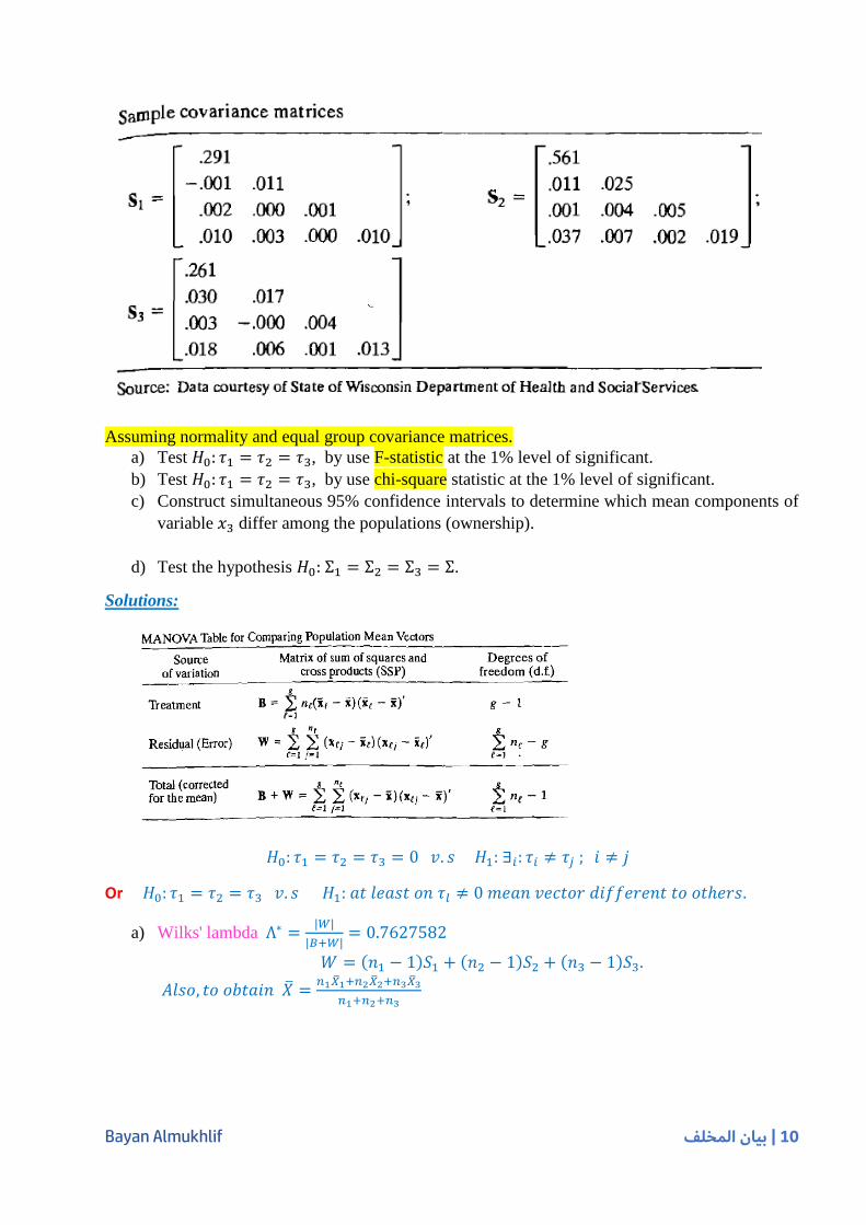
to ownership. Summary statistics for each of the g = 3 groups are given in the following table.
Bayan Almukhlif 10 | بيان المخلف
Assuming normality and equal group covariance matrices.
a) Test 𝐻0: 𝜏1 = 𝜏2 = 𝜏3, by use F-statistic at the 1% level of significant.
b) Test 𝐻0: 𝜏1 = 𝜏2 = 𝜏3, by use chi-square statistic at the 1% level of significant.
c) Construct simultaneous 95% confidence intervals to determine which mean components of
variable 𝑥3 differ among the populations (ownership).
d) Test the hypothesis 𝐻0: Σ1 = Σ2 = Σ3 = Σ.
Solutions:
𝐻0: 𝜏1 = 𝜏2 = 𝜏3 = 0 𝑣. 𝑠 𝐻1: ∃𝑖: 𝜏𝑖 ≠ 𝜏𝑗 ; 𝑖 ≠ 𝑗
Or 𝐻0: 𝜏1 = 𝜏2 = 𝜏3 𝑣. 𝑠 𝐻1: 𝑎𝑡 𝑙𝑒𝑎𝑠𝑡 𝑜𝑛 𝜏𝑙 ≠ 0 𝑚𝑒𝑎𝑛 𝑣𝑒𝑐𝑡𝑜𝑟 𝑑𝑖𝑓𝑓𝑒𝑟𝑒𝑛𝑡 𝑡𝑜 𝑜𝑡ℎ𝑒𝑟𝑠.
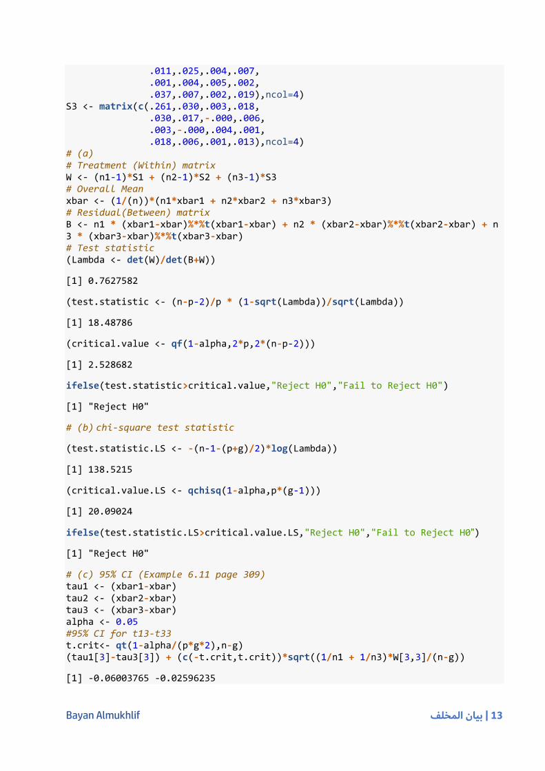
a) Wilks' lambda Λ∗ =|𝑊|
|𝐵+𝑊|= 0.7627582
𝑊 = (𝑛1 − 1)𝑆1 + (𝑛2 − 1)𝑆2 + (𝑛3 − 1)𝑆3.
𝐴𝑙𝑠𝑜, 𝑡𝑜 𝑜𝑏𝑡𝑎𝑖𝑛 �̅� =𝑛1�̅�1+𝑛2�̅�2+𝑛3�̅�3
𝑛1+𝑛2+𝑛3

Bayan Almukhlif 11 | بيان المخلف
𝑤𝑖𝑡ℎ 𝑃 ≥ 1 𝑎𝑛𝑑 𝑔 = 3 ≫≫ Test statistic: (Σ 𝑛𝑙−𝑃−2
𝑃) (
1−√Λ∗
√Λ∗ ) = 𝟏𝟖. 𝟒𝟖𝟕𝟖𝟔
critical value = 𝐹2𝑃,2(Σ 𝑛𝑙 −𝑃−2 ),1− 𝛼 = 𝑭𝟐(𝟒) , 𝟐(𝟓𝟏𝟎), 𝟎.𝟗𝟗 = 𝟐. 𝟓𝟐𝟖𝟔𝟖𝟐 since 𝟏𝟖. 𝟒𝟖𝟕𝟖𝟔 > 𝟐. 𝟓𝟐𝟖𝟔𝟖𝟐 , we reject 𝐻0 at the 1% level and conclude that average costs
differ, depending on type of ownership.
b) Other statistics for checking the equality of several multivariate means, Bartlett has shown
that if 𝐻0 is true and Σ 𝑛𝑙 = 𝑛 is large,
Test statistic for Larg Σ 𝑛𝑙 𝑖𝑠: 𝑇 = − (𝑛 − 1 −𝑃 + 𝑔
2) 𝑙𝑛 (
|𝑊|
|𝐵 + 𝑊|)
we reject 𝐻0 at significance level 𝛼 if 𝑇 > 𝜒𝑃(𝑔−1),𝛼2
𝑇 = − (𝑛 − 1 −𝑃 + 𝑔
2) 𝑙𝑛 (
|𝑊|
|𝐵 + 𝑊|) = 𝟏𝟑𝟖. 𝟓𝟐𝟏𝟓
𝜒𝑃(𝑔−1),1−𝛼2 = 𝜒4(2),0.99
2 = 𝟐𝟎. 𝟎𝟗𝟎𝟐𝟒
Since 𝑻 > 𝜒8 ,0.992 we reject 𝐻0 at the 1% level. This result is consistent with the result based on
the foregoing F-statistic.
c) simultaneous 95% confidence intervals to determine which mean components of
variable 𝑥3 differ among the populations.
By use Result 6.5: (𝜏𝑘𝑖 − 𝜏𝑙𝑖) ∈ [ �̅�𝑘𝑖 − �̅�𝑙𝑖 ± 𝑡𝑛−𝑔 ,𝛼
𝑃𝑔(𝑔−1) √
𝑤𝑖𝑖
𝑛−𝑔 (
1
𝑛𝑘+
1
𝑛𝑙) ],
𝑙 < 𝑘 = 1, . . , 𝑔 ; 𝑤𝑖𝑖 𝑖𝑠 𝑡ℎ𝑒 𝑖𝑡ℎ 𝑑𝑖𝑎𝑔𝑜𝑛𝑎𝑙 𝑒𝑙𝑒𝑚𝑒𝑛𝑡 𝑜𝑓 𝑾.
𝜏13 − 𝜏33 ∈ [−0.06003765 , −0.02596235]
𝜏13 − 𝜏23 ∈ [−0.05760551 , −0.02639449]
𝜏23 − 𝜏33 ∈ [−0.02022171 , 0.01822171]
We conclude that the average maintenance and labor cost for government-owned
nursing homes is higher by .025 to .061 hour per patient day than for privately

Bayan Almukhlif 12 | بيان المخلف
owned nursing homes
Thus, a difference in this cost exists between private and non-profit nursing homes,
but no difference is observed between non-profit (2) and government nursing homes (3).
d) Test the hypothesis 𝐻0: Σ1 = Σ2 = Σ3 = Σ at 0.05 level.
Box's Test for Equality of Covariance Matrices page 332
𝑢 = [∑1
(𝑛𝑙 − 1)𝑙−
1
∑ (𝑛𝑙 − 1)𝑙] [
2𝑃2 + 3𝑃 − 1
6(𝑃 + 1)(𝑔 − 1)] ; 𝑙 = 1,2, … , 𝑔
𝑀 = [∑ (𝑛𝑙 − 1)𝑙
] ln|𝑆𝑝𝑜𝑜𝑙𝑒𝑑| − ∑ [(𝑛𝑙 − 1) 𝑙𝑛|𝑆𝑙|]𝑙
𝑆𝑝𝑜𝑜𝑙𝑒𝑑 =1
∑ (𝑛𝑙 − 1)𝑙[(𝑛1 − 1)𝑆1 + (𝑛2 − 1)𝑆2 + ⋯ + (𝑛𝑙 − 1)𝑆𝑔]
𝐓𝐞𝐬𝐭 𝐬𝐭𝐚𝐭𝐢𝐬𝐭𝐢𝐜: 𝐶 = (1 − 𝑢)𝑀 ~ 𝜒𝑣,𝛼2
Degrees of freedom: 𝑣 =12
𝑃(𝑃 + 1)(𝑔 − 1)
we reject 𝐻0 at significance level 𝛼 if 𝐶 > 𝜒𝑣,𝛼2
Since 𝑪 = 𝟐𝟒𝟎. 𝟗𝟏𝟏𝟐 > 𝜒20 ,0.952 = 𝟑𝟏. 𝟒𝟏𝟎𝟒 , it is clear that 𝐻0 is rejected at any reasonable
level of significance. We conclude that the covariance matrices of the cost variables associated
with the three populations of nursing homes are not the same.
R Code # Example 6.10 & 6.11 page 306 rm(list=ls()) # note: Examples 6.10-6.12 are limited by the summary statistics rather than raw data - calculations are bit off due to rounding alpha <- 0.01 n1 <- 271 n2 <- 138 n3 <- 107 n <- n1 + n2 + n3 p <- 4 g <- 3 xbar1 <- matrix(c(2.066,0.480,0.082,0.360),ncol=1) xbar2 <- matrix(c(2.167,0.596,0.124,0.418),ncol=1) xbar3 <- matrix(c(2.273,0.521,0.125,0.383),ncol=1) S1 <- matrix(c(.291,-.001,.002,.010, -.001,.011,.000,.003, .002,.000,.001,.000, .010,.003,.000,.010),ncol=4) S2 <- matrix(c(.561,.011,.001,.037,
Bayan Almukhlif 13 | بيان المخلف
.011,.025,.004,.007, .001,.004,.005,.002, .037,.007,.002,.019),ncol=4) S3 <- matrix(c(.261,.030,.003,.018, .030,.017,-.000,.006, .003,-.000,.004,.001, .018,.006,.001,.013),ncol=4) # (a) # Treatment (Within) matrix W <- (n1-1)*S1 + (n2-1)*S2 + (n3-1)*S3 # Overall Mean xbar <- (1/(n))*(n1*xbar1 + n2*xbar2 + n3*xbar3) # Residual(Between) matrix B <- n1 * (xbar1-xbar)%*%t(xbar1-xbar) + n2 * (xbar2-xbar)%*%t(xbar2-xbar) + n3 * (xbar3-xbar)%*%t(xbar3-xbar) # Test statistic (Lambda <- det(W)/det(B+W))
[1] 0.7627582
(test.statistic <- (n-p-2)/p * (1-sqrt(Lambda))/sqrt(Lambda))
[1] 18.48786
(critical.value <- qf(1-alpha,2*p,2*(n-p-2)))
[1] 2.528682
ifelse(test.statistic>critical.value,"Reject H0","Fail to Reject H0")
[1] "Reject H0"
# (b) chi-square test statistic
(test.statistic.LS <- -(n-1-(p+g)/2)*log(Lambda))
[1] 138.5215
(critical.value.LS <- qchisq(1-alpha,p*(g-1)))
[1] 20.09024
ifelse(test.statistic.LS>critical.value.LS,"Reject H0","Fail to Reject H0")
[1] "Reject H0"
# (c) 95% CI (Example 6.11 page 309) tau1 <- (xbar1-xbar) tau2 <- (xbar2-xbar) tau3 <- (xbar3-xbar) alpha <- 0.05 #95% CI for t13-t33 t.crit<- qt(1-alpha/(p*g*2),n-g) (tau1[3]-tau3[3]) + (c(-t.crit,t.crit))*sqrt((1/n1 + 1/n3)*W[3,3]/(n-g))
[1] -0.06003765 -0.02596235

Bayan Almukhlif 14 | بيان المخلف
#95% CI for t13-t23 (tau1[3]-tau2[3]) + (c(-t.crit,t.crit))*sqrt((1/n1 + 1/n2)*W[3,3]/(n-g))
[1] -0.05760551 -0.02639449
#95% CI for t23-t33 (tau2[3]-tau3[3]) + (c(-t.crit,t.crit))*sqrt((1/n2 + 1/n3)*W[3,3]/(n-g))
[1] -0.02022171 0.01822171
# (d) Testing for Equality of Covariance Matrices. #Example 6.12 page 311 (Spooled <- (1/(n-g)) *((n1-1) * S1 + (n2-1) * S2 + (n3-1)* S3))
[,1] [,2] [,3] [,4] [1,] 0.356906433 0.008610136 0.0019395712 0.0188635478 [2,] 0.008610136 0.015978558 0.0010682261 0.0046881092 [3,] 0.001939571 0.001068226 0.0026881092 0.0007407407 [4,] 0.018863548 0.004688109 0.0007407407 0.0130233918
u <- (1/(n1-1) + 1/(n2-1) + 1/(n3-1) - 1/(n - g)) * ((2*p^2 + 3*p - 1)/(6*(p+1)*(g-1))) (M <- (n - g)*log(det(Spooled)) - ( (n1-1)*log(det(S1)) + (n2-1)*log(det(S2)) + (n3-1)*log(det(S3)) ) )
[1] 244.146
(C <- (1-u)*M)
[1] 240.9112
v <- (1/2)*p*(p+1)*(g-1) (C.crit <- qchisq(1-alpha,v) )
[1] 31.41043
ifelse(C > C.crit,"Reject H0","Fail to Reject H0")
[1] "Reject H0"
Exercise 4: (In book Exercise 6.24) one way MANOVA
Researchers have suggested that a change in skull size over time is evidence of the interbreeding of
a resident population with immigrant populations. Four measurements were made of male
Bayan Almukhlif 15 | بيان المخلف
Egyptian skulls for three different time periods: period 1 is 4000 B.C., period 2 is 3300 B.C., and
period 3 is 1850 B.C. The data are shown in Table 6.13 on page 349
The measured variables are
X 1 = maximum breadth of skull ( mm), X2 = basibregmatic height of skull ( mm)
X 3 = basialveolar length of skull ( mm), X4: nasal height of skull (mm)
a) Construct a one-way MAN OVA of the Egyptian skulls data. Use a = 0.05.
b) Construct 95 % simultaneous confidence intervals to determine which mean components
differ among the populations represented by the three time periods.
c) Check normality assumptions for each group
d) Test the hypothesis 𝐻0: Σ1 = Σ2 = Σ3 = Σ at 0.05 level.
Solution:
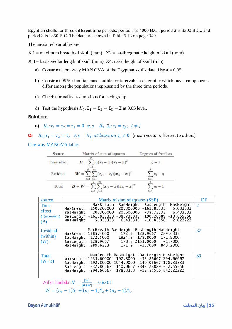
a) 𝐻0: 𝜏1 = 𝜏2 = 𝜏3 = 0 𝑣. 𝑠 𝐻1: ∃𝑖: 𝜏𝑖 ≠ 𝜏𝑗 ; 𝑖 ≠ 𝑗
Or 𝐻0: 𝜏1 = 𝜏2 = 𝜏3 𝑣. 𝑠 𝐻1: 𝑎𝑡 𝑙𝑒𝑎𝑠𝑡 𝑜𝑛 𝜏𝑙 ≠ 0 (mean vector different to others)
One-way MANOVA table:
source Matrix of sum of squares (SSP) DF
Time
effect
(Between)
(B)
MaxBreath BasHeight BasLength NasHeight MaxBreath 150.200000 20.300000 -161.83333 5.033333 BasHeight 20.300000 20.600000 -38.73333 6.433333 BasLength -161.833333 -38.733333 190.28889 -10.855556 NasHeight 5.033333 6.433333 -10.85556 2.022222
2
Residual
(within)
(W)
MaxBreath BasHeight BasLength NasHeight MaxBreath 1785.4000 172.5 128.9667 289.6333 BasHeight 172.5000 1924.3 178.8000 171.9000 BasLength 128.9667 178.8 2153.0000 -1.7000 NasHeight 289.6333 171.9 -1.7000 840.2000
87
Total
(W+B)
MaxBreath BasHeight BasLength NasHeight MaxBreath 1935.60000 192.8000 -32.86667 294.66667 BasHeight 192.80000 1944.9000 140.06667 178.33333 BasLength -32.86667 140.0667 2343.28889 -12.55556 NasHeight 294.66667 178.3333 -12.55556 842.22222
89
Wilks' lambda Λ∗ =|𝑊|
|𝐵+𝑊|= 0.8301
𝑊 = (𝑛1 − 1)𝑆1 + (𝑛2 − 1)𝑆2 + (𝑛3 − 1)𝑆3.

Bayan Almukhlif 16 | بيان المخلف
The exact distribution of Λ∗ can be derived for the special case listed in Table 6.3 in the
textbook at page 303/324pdf.
𝑤𝑖𝑡ℎ𝑒 𝑃 ≥ 1 𝑎𝑛𝑑 𝑔 = 3 ≫≫ Test statistic: (Σ 𝑛𝑙−𝑃−2
𝑃) (
1−√Λ∗
√Λ∗ ) = 𝟐. 𝟎𝟒𝟗𝟏
critical value = 𝐹2𝑃,2(Σ 𝑛𝑙 −𝑃−2 ),1− 𝛼 = 𝑭𝟖 , 𝟏𝟔𝟖, 𝟎.𝟗𝟓 = 𝟏. 𝟗𝟗𝟑𝟗 since 𝟐. 𝟎𝟒𝟗 > 𝟏. 𝟗𝟗𝟑𝟗 , we reject 𝐻0 at the 5% level implying there is a time period effect.
There is a difference of male Egyptian skulls for three different time periods.
b) For pairwise comparisons in treatment means, the Bonferroni approach can be used to
construct simultaneous confidence intervals for the components of the differences 𝜏𝑘𝑖 − 𝜏𝑙𝑖.
From Result 6.5, For the MANOVA model, with confidence level at 100(1-𝛼)%
By use Result 6.5: (𝜏𝑘𝑖 − 𝜏𝑙𝑖) ∈ [ �̅�𝑘𝑖 − �̅�𝑙𝑖 ± 𝑡𝑛−𝑔 ,𝛼
𝑃𝑔(𝑔−1) √
𝑤𝑖𝑖
𝑛−𝑔 (
1
𝑛𝑘+
1
𝑛𝑙) ],
𝑙 < 𝑘 = 1, . . , 𝑔 ; 𝑤𝑖𝑖 𝑖𝑠 𝑡ℎ𝑒 𝑖𝑡ℎ 𝑑𝑖𝑎𝑔𝑜𝑛𝑎𝑙 𝑒𝑙𝑒𝑚𝑒𝑛𝑡 𝑜𝑓 𝑾.
The calculation of above equation for each pair is calculated by R:
𝜏1[1] − 𝜏2[1] ∈ (−4.442312, 2.442312) 𝜏1[1] − 𝜏3[1] ∈ (−6.542312, 0.3423115)
𝜏2[1] − 𝜏3[1] ∈ (−5.542312, 1.342312) 𝜏1[2] − 𝜏2[2] ∈ (−2.673706, 4.473706)
𝜏1[2] − 𝜏3[2] ∈ (−3.773706, 3.373706)
𝜏2[2] − 𝜏3[2] ∈ (−4.673706, 2.473706) 𝜏1[3] − 𝜏2[3] ∈ (−3.68011, 3.88011)
𝜏1[3] − 𝜏3[3] ∈ (−0.6467765, 6.913443)
𝜏2[3] − 𝜏3[3] ∈ (−0.7467765, 6.813443)
𝜏1[4] − 𝜏2[4] ∈ (−2.061423, 2.661423)
𝜏1[4] − 𝜏3[4] ∈ (−2.394756, 2.328089)
𝜏2[4] − 𝜏3[4] ∈ (−2.694756, 2.028089)
All the simultaneous intervals include zero . If changes exist, then these changes might be in
maximum breath and basialveolar length of skull from time periods 1 to 3.
F-statistics and p-values for ANOVA's:
𝐻0: 𝜇1𝑖 = 𝜇2𝑖 = 𝜇3𝑖 = 0 𝑣. 𝑠 𝐻1: 𝑎𝑡 𝑙𝑒𝑎𝑠𝑡 𝑜𝑛 𝜇𝑙𝑖 ≠ 0, 𝑖 = 1,2,3,4, 𝑙 = 1,2,3
variables F P-value Diction at 0.05 level
X1: Maximum breath 3.6595 0.02979 Reject 𝐻0: 𝜇11 = 𝜇21 = 𝜇31
X2: Basialveolar Height 0.4657 0.6293 Accept 𝐻0: 𝜇12 = 𝜇22 = 𝜇32
X3: Basialveolar length 3.8447 0.02512 Reject 𝐻0:𝜇13 = 𝜇23 = 𝜇33
X4: Nasal Height 0.1047 0.9007 Accept 𝐻0: 𝜇14 = 𝜇24 = 𝜇34
c) We investigate the skull data and find that the normality assumption is verified for each
period.

Bayan Almukhlif 17 | بيان المخلف
d) Test the hypothesis 𝐻0: Σ1 = Σ2 = Σ3 = Σ at 0.05 level.
Box's Test for Equality of Covariance Matrices page 332
𝑢 = [∑1
(𝑛𝑙 − 1)𝑙−
1
∑ (𝑛𝑙 − 1)𝑙] [
2𝑃2 + 3𝑃 − 1
6(𝑃 + 1)(𝑔 − 1)] ; 𝑙 = 1,2, … , 𝑔
𝑀 = [∑ (𝑛𝑙 − 1)𝑙
] ln|𝑆𝑝𝑜𝑜𝑙𝑒𝑑| − ∑ [(𝑛𝑙 − 1) 𝑙𝑛|𝑆𝑙|]𝑙
𝑆𝑝𝑜𝑜𝑙𝑒𝑑 =1
∑ (𝑛𝑙 − 1)𝑙[(𝑛1 − 1)𝑆1 + (𝑛2 − 1)𝑆2 + ⋯ + (𝑛𝑙 − 𝑔)𝑆𝑔]
𝐓𝐞𝐬𝐭 𝐬𝐭𝐚𝐭𝐢𝐬𝐭𝐢𝐜: 𝐶 = (1 − 𝑢)𝑀 ~ 𝜒𝑣,𝛼2
Degrees of freedom: 𝑣 =12
𝑃(𝑃 + 1)(𝑔 − 1)
we reject 𝐻0 at significance level 𝛼 if 𝐶 > 𝜒𝑣,𝛼2
Note: From R result, Chi-Sq (approx.) = 𝐶 = (1 − 𝑢)𝑀
Since p-value = 0.3943 > 0.05 or ( C=21.048 < 31.4104) , we Accept 𝐻0: 𝛴1 = 𝛴2 = 𝛴3 = 𝛴
R Code #Exercise 6.24: one way MANOVA #skull data rm(list=ls()) data<- read.table(file.choose()) #file (T6.13) names(data) <- c("MaxBreath","BasHeight","BasLength","NasHeight","Period") data$Period<- as.factor(data$Period) table(data$Period) 1 2 3 30 30 30
# one-way MANOVA test fit<-manova(cbind(MaxBreath,BasHeight,BasLength,NasHeight)~Period,data=data) (fitsummary<-summary(fit, test="Wilks"))
Df Wilks approx F num Df den Df Pr(>F) Period 2 0.8301 2.0491 8 168 0.04358 * Residuals 87 --- Signif. codes: 0 '***' 0.001 '**' 0.01 '*' 0.05 '.' 0.1 ' ' 1
# Look to see which differ(Compute one_way ANOVA test for each variable). summary.aov(fit)
Response MaxBreath : Df Sum Sq Mean Sq F value Pr(>F) Period 2 150.2 75.100 3.6595 0.02979 * Residuals 87 1785.4 20.522 --- Signif. codes: 0 '***' 0.001 '**' 0.01 '*' 0.05 '.' 0.1 ' ' 1 Response BasHeight : Df Sum Sq Mean Sq F value Pr(>F)

Bayan Almukhlif 18 | بيان المخلف
Period 2 20.6 10.300 0.4657 0.6293 Residuals 87 1924.3 22.118 Response BasLength : Df Sum Sq Mean Sq F value Pr(>F) Period 2 190.29 95.144 3.8447 0.02512 * Residuals 87 2153.00 24.747 --- Signif. codes: 0 '***' 0.001 '**' 0.01 '*' 0.05 '.' 0.1 ' ' 1 Response NasHeight : Df Sum Sq Mean Sq F value Pr(>F) Period 2 2.02 1.0111 0.1047 0.9007 Residuals 87 840.20 9.6575
#one_way ANOVA fit11<-aov(MaxBreath~Period,data=data) summary(fit11)
Df Sum Sq Mean Sq F value Pr(>F) Period 2 150.2 75.10 3.66 0.0298 * Residuals 87 1785.4 20.52 --- Signif. codes: 0 '***' 0.001 '**' 0.01 '*' 0.05 '.' 0.1 ' ' 1
# MANOVA Table B <- fitsummary$SS$Period # Matrix of SSP treatment (Between) W <- fitsummary$SS$Residuals #Matrix of SSP residual (Within) Total<- B+W # Wilk’s Lambda n <- dim(data)[1] p <- dim(data[,-5])[2] Lambda <- det(W)/(det(B+W)) FV <- ((n-p-2)/p)*((1-sqrt(Lambda))/sqrt(Lambda))#Distribution of Wilks' Lambda table in page 324. alpha <- 0.05 qf(1-alpha,df1=2*p,df2=2*(n-p-2))
[1] 1.993884
# pair comparison ( simultaneous 95% CI ) g <- 3 n1 <- length(which((data$Period==1))) n2 <- length(which((data$Period==2))) n3 <- length(which((data$Period==3))) n <- n1+n2+n3 xbar1 <- colMeans(data[data$Period==1,-5]) xbar2 <- colMeans(data[data$Period==2,-5]) xbar3 <- colMeans(data[data$Period==3,-5]) xbar <- (n1*xbar1+n2*xbar2+n3*xbar3)/(n1+n2+n3) S1 <- cov(data[data$Period==1,-5]) S2 <- cov(data[data$Period==2,-5]) S3 <- cov(data[data$Period==3,-5]) W <- (n1-1)*S1+(n2-1)*S2+(n3-1)*S3

Bayan Almukhlif 19 | بيان المخلف
qtlevel <- qt(1-alpha/(p*g*(g-1)),df=n-g) for ( i in 1:p ){ # \tau_{1i}-\tau_{2i} LCI12 <- (xbar1[i]-xbar2[i])-qtlevel*sqrt(W[i,i]/(n-g)*(1/n1+1/n2)) UCI12 <- (xbar1[i]-xbar2[i])+qtlevel*sqrt(W[i,i]/(n-g)*(1/n1+1/n2)) cat("tau1[",i,"]-tau2[",i,"] belongs to (",LCI12,",",UCI12,")\n",sep="") # \tau_{1i}-\tau_{3i} LCI13 <- (xbar1[i]-xbar3[i])-qtlevel*sqrt(W[i,i]/(n-g)*(1/n1+1/n3)) UCI13 <- (xbar1[i]-xbar3[i])+qtlevel*sqrt(W[i,i]/(n-g)*(1/n1+1/n3)) cat("tau1[",i,"]-tau3[",i,"] belongs to (",LCI13,",",UCI13,")\n",sep="") # \tau_{2i}-\tau_{3i} LCI23 <- (xbar2[i]-xbar3[i])-qtlevel*sqrt(W[i,i]/(n-g)*(1/n2+1/n3)) UCI23 <- (xbar2[i]-xbar3[i])+qtlevel*sqrt(W[i,i]/(n-g)*(1/n2+1/n3)) cat("tau2[",i,"]-tau3[",i,"] belongs to (",LCI23,",",UCI23,")\n",sep="") }
tau1[1]-tau2[1] belongs to (-4.442312,2.442312) tau1[1]-tau3[1] belongs to (-6.542312,0.3423115) tau2[1]-tau3[1] belongs to (-5.542312,1.342312) tau1[2]-tau2[2] belongs to (-2.673706,4.473706) tau1[2]-tau3[2] belongs to (-3.773706,3.373706) tau2[2]-tau3[2] belongs to (-4.673706,2.473706) tau1[3]-tau2[3] belongs to (-3.68011,3.88011) tau1[3]-tau3[3] belongs to (-0.6467765,6.913443) tau2[3]-tau3[3] belongs to (-0.7467765,6.813443) tau1[4]-tau2[4] belongs to (-2.061423,2.661423) tau1[4]-tau3[4] belongs to (-2.394756,2.328089) tau2[4]-tau3[4] belongs to (-2.694756,2.028089)
# CI12 <- (xbar1[i]-xbar2[i])+qtlevel*sqrt(W[i,i]/(n-g)*(1/n1+1/n2))*c(-1,1) #cat("tau1[",i,"]-tau2[",i,"] belongs to (", CI12 ,")\n",sep=" ")
# Check normality for each group skull1 <- data[data$Period==1,-5] mah1 <- mahalanobis(skull1, xbar1, S1) #Note: qchisq(ppoints(30),df=p) = qchisq(((1:n1)-0.5)/n1,df=p) plot(qchisq(ppoints(30),df=p),sort(mah1), main="", xlab="Theoretical Quantiles",ylab="Sample Quantiles")

Bayan Almukhlif 20 | بيان المخلف
# test multivariate normal (cutoff <- qchisq(0.50,p))
[1] 3.356694
satisfy <- which(mah1<= cutoff) k1<-length(satisfy) (k1/n1)*100 # 53% of data fall within 50% contour
[1] 53.33333
skull2<- data[data$Period==2,-5] mah2 <- mahalanobis(skull2, xbar2, S2) plot(qchisq(ppoints(30),df=p),sort(mah2), main="", xlab="Theoretical Quantiles",ylab="Sample Quantiles")
satisfy2 <- which(mah2<= cutoff) k2<-length(satisfy2) (k2/n2)*100 # 53% of data fall within 50% contour
[1] 53.33333
Bayan Almukhlif 21 | بيان المخلف
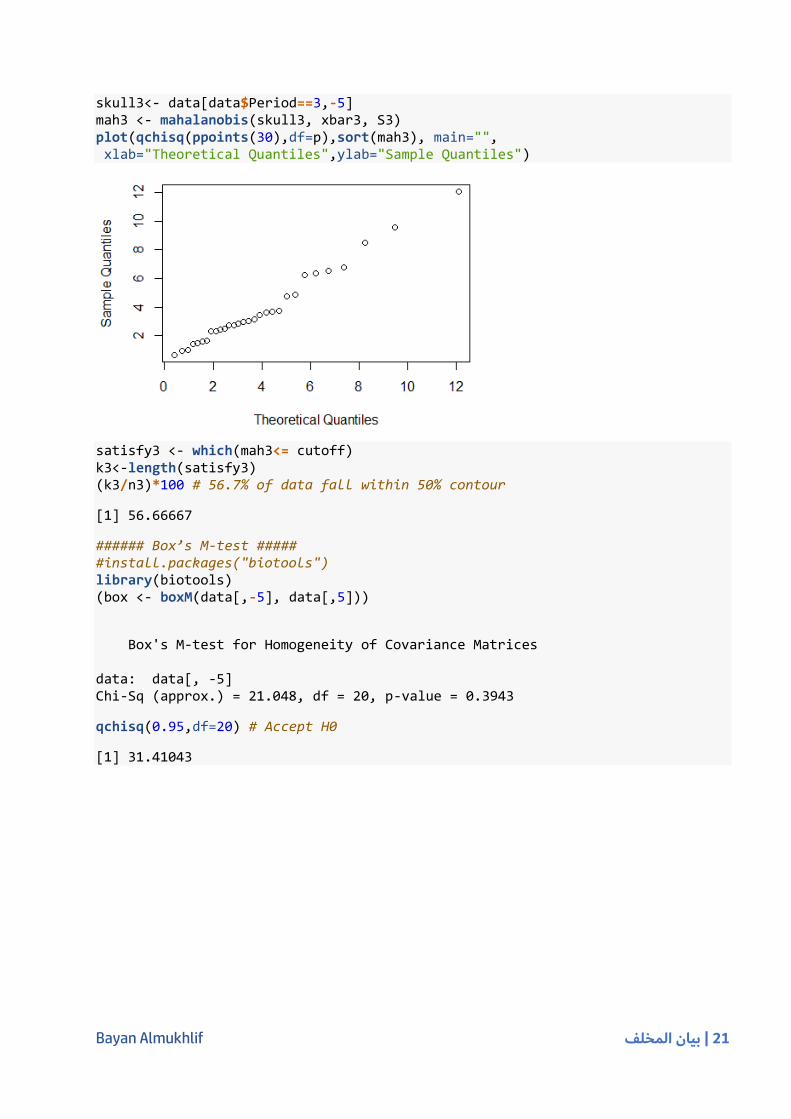
skull3<- data[data$Period==3,-5] mah3 <- mahalanobis(skull3, xbar3, S3) plot(qchisq(ppoints(30),df=p),sort(mah3), main="", xlab="Theoretical Quantiles",ylab="Sample Quantiles")
satisfy3 <- which(mah3<= cutoff) k3<-length(satisfy3) (k3/n3)*100 # 56.7% of data fall within 50% contour
[1] 56.66667
###### Box’s M-test ##### #install.packages("biotools") library(biotools) (box <- boxM(data[,-5], data[,5]))
Box's M-test for Homogeneity of Covariance Matrices data: data[, -5] Chi-Sq (approx.) = 21.048, df = 20, p-value = 0.3943
qchisq(0.95,df=20) # Accept H0
[1] 31.41043

Bayan Almukhlif 22 | بيان المخلف
Exercise 5: (in book Example 6.13 page 339pdf : A two-way multivariate analysis of variance of plastic film data)
The optimum conditions for extruding plastic film have been examined using a technique called
Evolutionary Operation. In the course of the study that was done, three responses 𝑋1 =
𝑡𝑒𝑎𝑟 𝑟𝑒𝑠𝑖𝑠𝑡𝑎𝑛𝑐𝑒, 𝑋2 = 𝑔𝑙𝑜𝑠𝑠, 𝑎𝑛𝑑 𝑋3 = 𝑜𝑝𝑎𝑐𝑖𝑡𝑦, were measured at two levels of the factors,
rate of extrusion and amount of an additive.
The measurements were repeated n = 5 times at each combination of the factor
levels. The data are displayed in Table 6.4.
a) Write two-way MANOVA table.
b) Test for interactions, and if the interactions do not exist, test for factor 1 and factor 2
main effects. Use F-test test with 𝜶 = 𝟎. 𝟎𝟓.
Solution:
First: Test for interaction (𝐹1 ∗ 𝐹2) is carried out before the tests for main factor effects.
𝐼𝑛 𝑔𝑒𝑛𝑒𝑟𝑎𝑙: 𝐻0F1∗F2: γij = 0 𝑣. 𝑠 𝐻1F1∗F2
: 𝐴𝑡 𝑙𝑒𝑎𝑠𝑡 𝑜𝑛𝑒 𝛾𝑖𝑗 ≠ 0
where i = 1, … , g ; j = 1, … , b
𝐻0F1∗F2: γij = 0 𝑣. 𝑠 𝐻1F1∗F2
: 𝐴𝑡 𝑙𝑒𝑎𝑠𝑡 𝑜𝑛𝑒 𝛾𝑖𝑗 ≠ 0 ; i = 1,2; j = 1,2
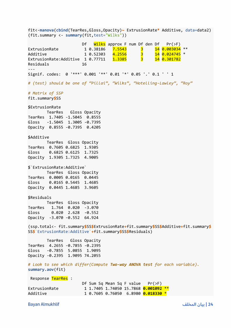
Since 𝑝. 𝑣𝑎𝑙𝑢𝑒 = 0.30178 > 𝛼 = 0.05 , we can not reject 𝐻0F1∗F2: γij = 0.
There are no interaction effects between F1 and F2 (change in rate of extrusion and amount of an
additive). So we can study each factor alone.
Or 𝐹𝐹1∗𝐹2= 1.3385 < 𝐹3,14 = 3.3438 , we can not reject 𝐻0F1∗F2
Second: we will study effect of rate of extrusion on 3 responses.
𝐻0F1: 𝜏1 = 𝜏2 = 0 𝑣. 𝑠 𝐻1𝐹1
: 𝐴𝑡 𝑙𝑒𝑎𝑠𝑡 𝑜𝑛𝑒 𝜏𝑙 ≠ 0
Since 𝑝. 𝑣𝑎𝑙𝑢𝑒 = 0.00303 < 𝛼 = 0.05 , we reject 𝐻0F1. so, the change in rate of extrusion affect
the 3 variables (tear resistance, gloss, and opacity).

Bayan Almukhlif 23 | بيان المخلف
Or 𝐹𝐹1= 7.5543 > 𝐹3,14 = 3.3438 , we reject 𝐻0F1
Third: we will study effect of amount of an additive on 3 responses.
𝐻0F2: 𝛽1 = 𝛽2 = 0 𝑣. 𝑠 𝐻1𝐹2
: 𝐴𝑡 𝑙𝑒𝑎𝑠𝑡 𝑜𝑛𝑒 𝛽𝑙 ≠ 0
Since 𝑝. 𝑣𝑎𝑙𝑢𝑒 = 0.0247 < 𝛼 = 0.05 , we reject 𝐻0F2. So, change in amount of an additive affect
the 3 variables (tear resistance, gloss, and opacity)
Or 𝐹𝐹2= 4.2556 > 𝐹3,14 = 3.3438 , we reject 𝐻0F2
MANOVA table:
Source of
variation
Matrix of SSP df
F1:
rate of
extrusion
1.7405 -1.5045 0.8555 -1.5045 1.3005 -0.7395 0.8555 -0.7395 0.4205
g-1=1
F2:
amount of
an additive
0.7605 0.6825 1.9305 0.6825 0.6125 1.7325 1.9305 1.7325 4.9005
b-1=1
F1*F2 0.0005 0.0165 0.0445 0.0165 0.5445 1.4685 0.0445 1.4685 3.9605
(g-1) (b-1) =1
Residual
(Error)
1.764 0.020 -3.070 0.020 2.628 -0.552 -3.070 -0.552 64.924
gb(n-1) =16
Total 4.2655 -0.7855 -0.2395 -0.7855 5.0855 1.9095 -0.2395 1.9095 74.2055
gbn-1= 19
R Code _two way MANOVA # Example 5 (6.13 Page 318 (339pdf)) rm(list=ls()) data <- read.table(file.choose()) #file T6-4 names(data) <- c("ExtrusionRate","Additive","TearRes","Gloss","Opacity") # For computerized approaches - make appropriate columns factors, but this can be really annoying so don't do it in dat data2 <- data data2[,1] <- as.factor(data2[,1]) data2[,2] <- as.factor(data2[,2]) ## Part (a) alpha <- 0.05
Bayan Almukhlif 24 | بيان المخلف
fit<-manova(cbind(TearRes,Gloss,Opacity)~ ExtrusionRate* Additive, data=data2) (fit.summary <- summary(fit,test="Wilks"))
Df Wilks approx F num Df den Df Pr(>F) ExtrusionRate 1 0.38186 7.5543 3 14 0.003034 ** Additive 1 0.52303 4.2556 3 14 0.024745 * ExtrusionRate:Additive 1 0.77711 1.3385 3 14 0.301782 Residuals 16 --- Signif. codes: 0 '***' 0.001 '**' 0.01 '*' 0.05 '.' 0.1 ' ' 1
# (test) should be one of “Pillai”, “Wilks”, “Hotelling-Lawley”, “Roy” # Matrix of SSP fit.summary$SS
$ExtrusionRate TearRes Gloss Opacity TearRes 1.7405 -1.5045 0.8555 Gloss -1.5045 1.3005 -0.7395 Opacity 0.8555 -0.7395 0.4205 $Additive TearRes Gloss Opacity TearRes 0.7605 0.6825 1.9305 Gloss 0.6825 0.6125 1.7325 Opacity 1.9305 1.7325 4.9005 $`ExtrusionRate:Additive` TearRes Gloss Opacity TearRes 0.0005 0.0165 0.0445 Gloss 0.0165 0.5445 1.4685 Opacity 0.0445 1.4685 3.9605 $Residuals TearRes Gloss Opacity TearRes 1.764 0.020 -3.070 Gloss 0.020 2.628 -0.552 Opacity -3.070 -0.552 64.924
(ssp.total<- fit.summary$SS$ExtrusionRate+fit.summary$SS$Additive+fit.summary$SS$`ExtrusionRate:Additive`+fit.summary$SS$Residuals)
TearRes Gloss Opacity TearRes 4.2655 -0.7855 -0.2395 Gloss -0.7855 5.0855 1.9095 Opacity -0.2395 1.9095 74.2055
# Look to see which differ(Compute Two-way ANOVA test for each variable). summary.aov(fit)
Response TearRes : Df Sum Sq Mean Sq F value Pr(>F) ExtrusionRate 1 1.7405 1.74050 15.7868 0.001092 ** Additive 1 0.7605 0.76050 6.8980 0.018330 *
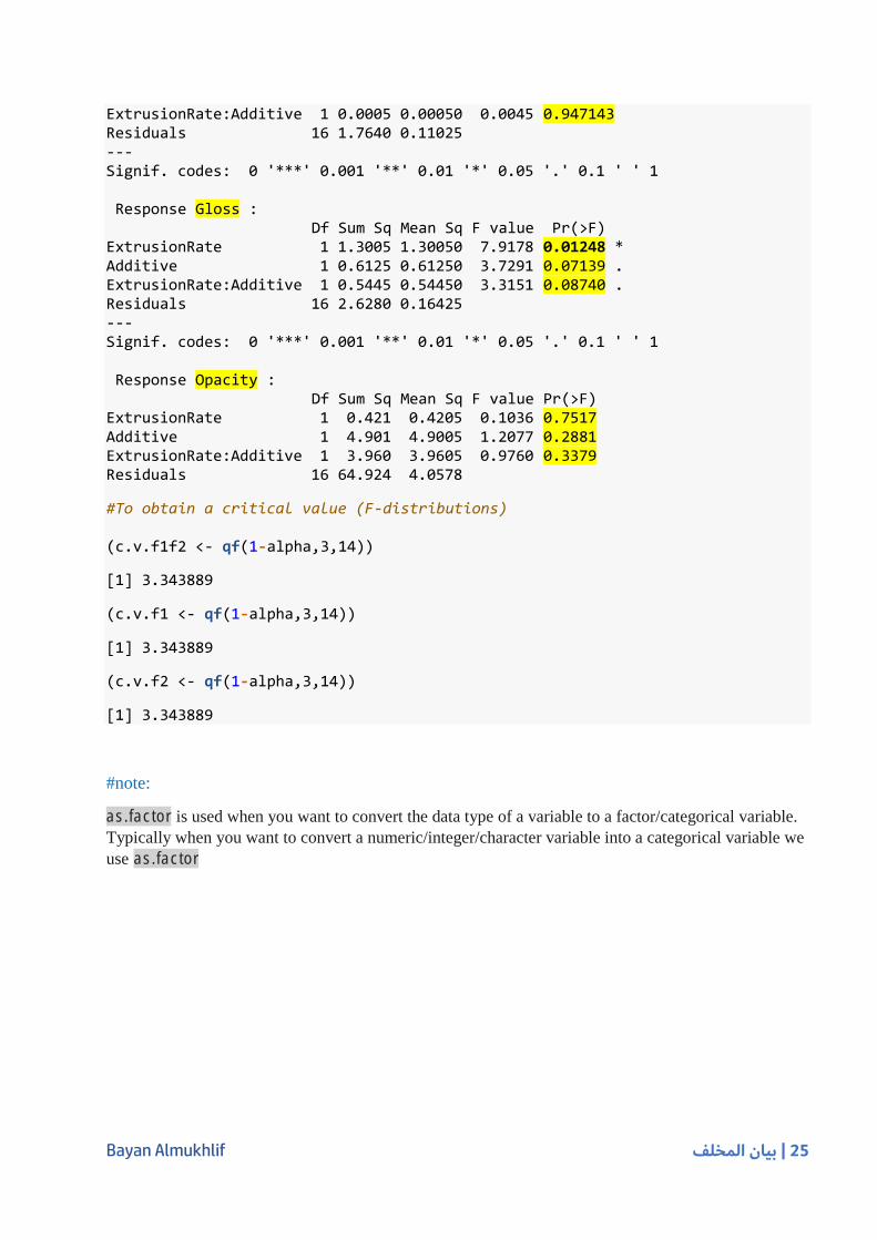
Bayan Almukhlif 25 | بيان المخلف
ExtrusionRate:Additive 1 0.0005 0.00050 0.0045 0.947143 Residuals 16 1.7640 0.11025 --- Signif. codes: 0 '***' 0.001 '**' 0.01 '*' 0.05 '.' 0.1 ' ' 1 Response Gloss : Df Sum Sq Mean Sq F value Pr(>F) ExtrusionRate 1 1.3005 1.30050 7.9178 0.01248 * Additive 1 0.6125 0.61250 3.7291 0.07139 . ExtrusionRate:Additive 1 0.5445 0.54450 3.3151 0.08740 . Residuals 16 2.6280 0.16425 --- Signif. codes: 0 '***' 0.001 '**' 0.01 '*' 0.05 '.' 0.1 ' ' 1 Response Opacity : Df Sum Sq Mean Sq F value Pr(>F) ExtrusionRate 1 0.421 0.4205 0.1036 0.7517 Additive 1 4.901 4.9005 1.2077 0.2881 ExtrusionRate:Additive 1 3.960 3.9605 0.9760 0.3379 Residuals 16 64.924 4.0578
#To obtain a critical value (F-distributions) (c.v.f1f2 <- qf(1-alpha,3,14))
[1] 3.343889
(c.v.f1 <- qf(1-alpha,3,14))
[1] 3.343889
(c.v.f2 <- qf(1-alpha,3,14))
[1] 3.343889
#note:
as.factor is used when you want to convert the data type of a variable to a factor/categorical variable.
Typically when you want to convert a numeric/integer/character variable into a categorical variable we
use as.factor
Related Documents


![TUTORIAL: BASIC OPERATIONS [1] AN EXERCISE ON HOW …miniahn/ecn726/gauss_basics.pdf · TUTORIAL: BASIC OPERATIONS [1] AN EXERCISE ON HOW TO USE GAUSS • On your computer, create](https://static.cupdf.com/doc/110x72/5c4a83d893f3c34aee5376a3/tutorial-basic-operations-1-an-exercise-on-how-miniahnecn726gaussbasicspdf.jpg)