Tutorial 11. Use of User-Defined Scalars and User-Defined Memories for Modeling Ohmic Heating Introduction The purpose of this tutorial is to illustrate the use of user-defined scalars (UDS) and user defined memories (UDM) for modeling the electric resistance heating of fluids. Ohmic heating is an advanced food processing method used to heat liquid foods, where electricity is passed through the liquid food itself. Through this process, the electrical energy is converted to heat energy. Conventional food processing heating methods can damage food quality due to the relatively slow energy transfer rate and significant tem- perature gradients associated with conduction and convection driven heat transfer. In comparison, Ohmic heating uniformly heats the entire mass, ensuring a product of better quality. In this tutorial you will learn how to: • Use the UDS for modeling the electrical current continuity equation. • Use the UDM for storing the data at each cell center. • Use the source terms to model the volumetric heating. • Setup the solver and perform iterations. • Check the convergence. • Examine the results. • Perform postprocessing of UDS and UDM. Prerequisites This tutorial assumes that you have little experience with FLUENT but are familiar with the interface. c Fluent Inc. August 22, 2006 11-1

Welcome message from author
This document is posted to help you gain knowledge. Please leave a comment to let me know what you think about it! Share it to your friends and learn new things together.
Transcript
Tutorial 11. Use of User-Defined Scalars and User-DefinedMemories for Modeling Ohmic Heating
Introduction
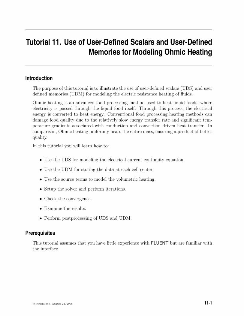
The purpose of this tutorial is to illustrate the use of user-defined scalars (UDS) and userdefined memories (UDM) for modeling the electric resistance heating of fluids.
Ohmic heating is an advanced food processing method used to heat liquid foods, whereelectricity is passed through the liquid food itself. Through this process, the electricalenergy is converted to heat energy. Conventional food processing heating methods candamage food quality due to the relatively slow energy transfer rate and significant tem-perature gradients associated with conduction and convection driven heat transfer. Incomparison, Ohmic heating uniformly heats the entire mass, ensuring a product of betterquality.
In this tutorial you will learn how to:
• Use the UDS for modeling the electrical current continuity equation.
• Use the UDM for storing the data at each cell center.
• Use the source terms to model the volumetric heating.
• Setup the solver and perform iterations.
• Check the convergence.
• Examine the results.
• Perform postprocessing of UDS and UDM.
Prerequisites
This tutorial assumes that you have little experience with FLUENT but are familiar withthe interface.
c© Fluent Inc. August 22, 2006 11-1
Use of User-Defined Scalars and User-Defined Memories for Modeling Ohmic Heating
Problem Description
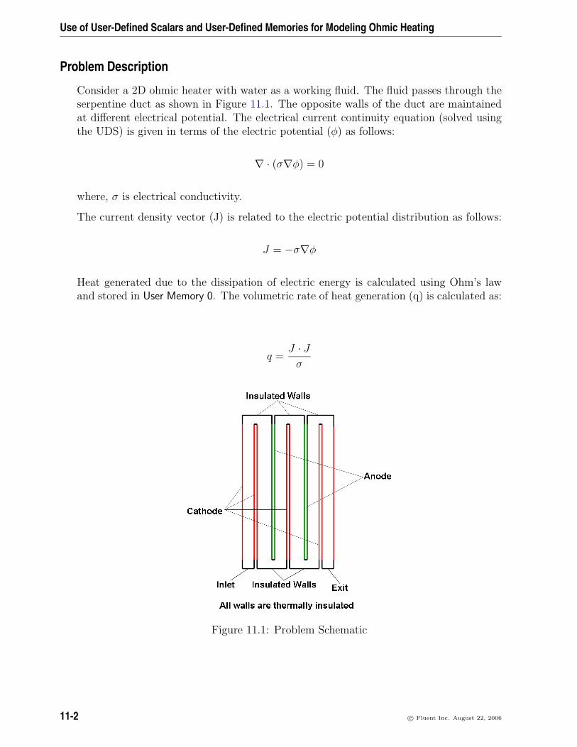
Consider a 2D ohmic heater with water as a working fluid. The fluid passes through theserpentine duct as shown in Figure 11.1. The opposite walls of the duct are maintainedat different electrical potential. The electrical current continuity equation (solved usingthe UDS) is given in terms of the electric potential (φ) as follows:
∇ · (σ∇φ) = 0
where, σ is electrical conductivity.
The current density vector (J) is related to the electric potential distribution as follows:
J = −σ∇φ
Heat generated due to the dissipation of electric energy is calculated using Ohm’s lawand stored in User Memory 0. The volumetric rate of heat generation (q) is calculated as:
q =J · Jσ
Figure 11.1: Problem Schematic
11-2 c© Fluent Inc. August 22, 2006
Use of User-Defined Scalars and User-Defined Memories for Modeling Ohmic Heating
Preparation
1. Copy the mesh file, ohmic heater.msh, and the directory, libudf, to your workingdirectory.
2. Start the 2D double precision solver of FLUENT.
Setup and Solution
Step 1: Grid
1. Read the mesh file, ohmic heater.msh.
File −→ Read −→Case...
FLUENT will read the mesh file and report the progress in the console.
2. Check the grid.
Grid −→Check
This procedure checks the integrity of the mesh. Make sure the reported minimumvolume is a positive number.
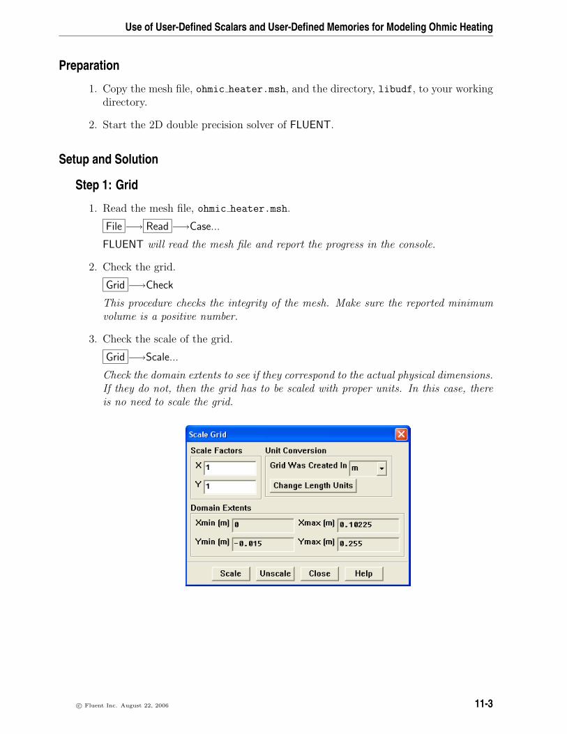
3. Check the scale of the grid.
Grid −→Scale...
Check the domain extents to see if they correspond to the actual physical dimensions.If they do not, then the grid has to be scaled with proper units. In this case, thereis no need to scale the grid.
c© Fluent Inc. August 22, 2006 11-3
Use of User-Defined Scalars and User-Defined Memories for Modeling Ohmic Heating
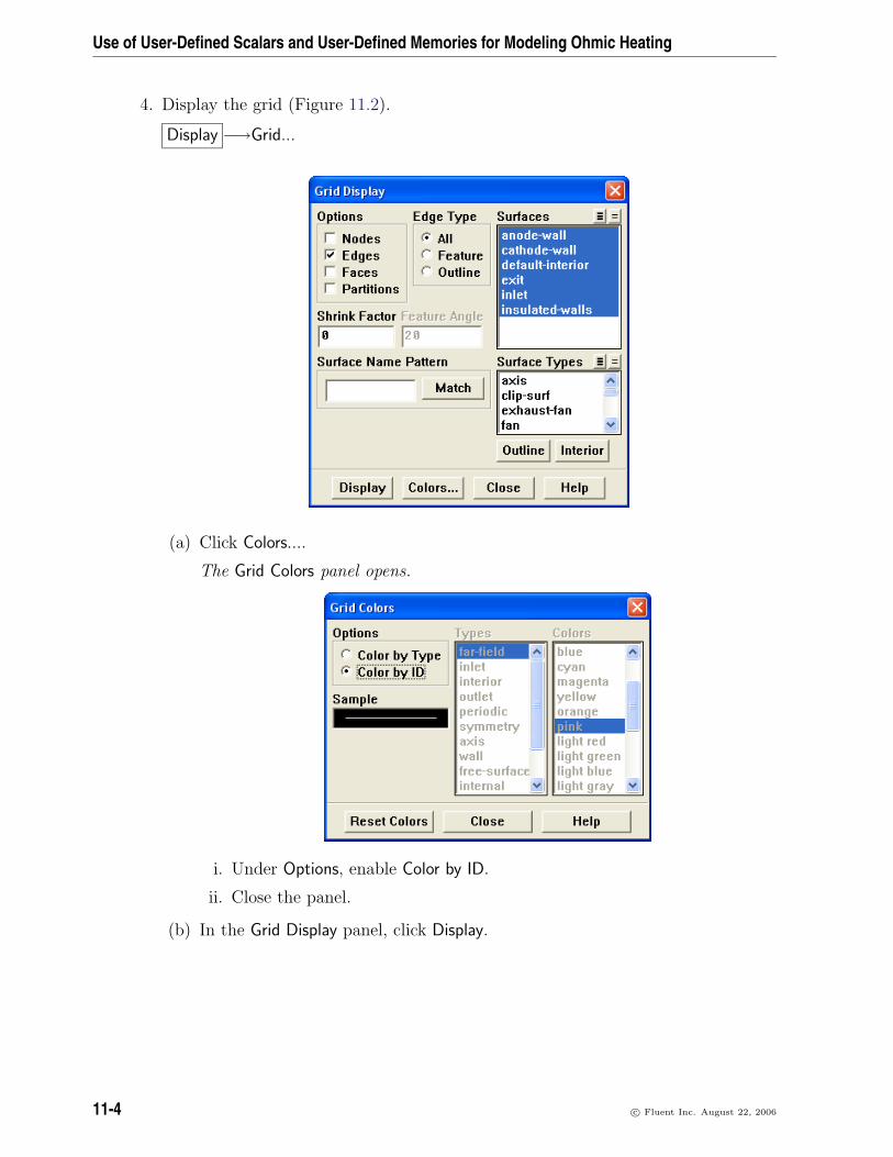
4. Display the grid (Figure 11.2).
Display −→Grid...
(a) Click Colors....
The Grid Colors panel opens.
i. Under Options, enable Color by ID.
ii. Close the panel.
(b) In the Grid Display panel, click Display.
11-4 c© Fluent Inc. August 22, 2006

Use of User-Defined Scalars and User-Defined Memories for Modeling Ohmic Heating
Grid Apr 28, 2006FLUENT 6.2 (2d, dp, segregated, lam)
Figure 11.2: Grid Display
Step 2: Models
1. Retain the default solver settings.
Define −→ Models −→Solver...
The problem is to be solved in steady state with 2D laminar conditions.
c© Fluent Inc. August 22, 2006 11-5
Use of User-Defined Scalars and User-Defined Memories for Modeling Ohmic Heating
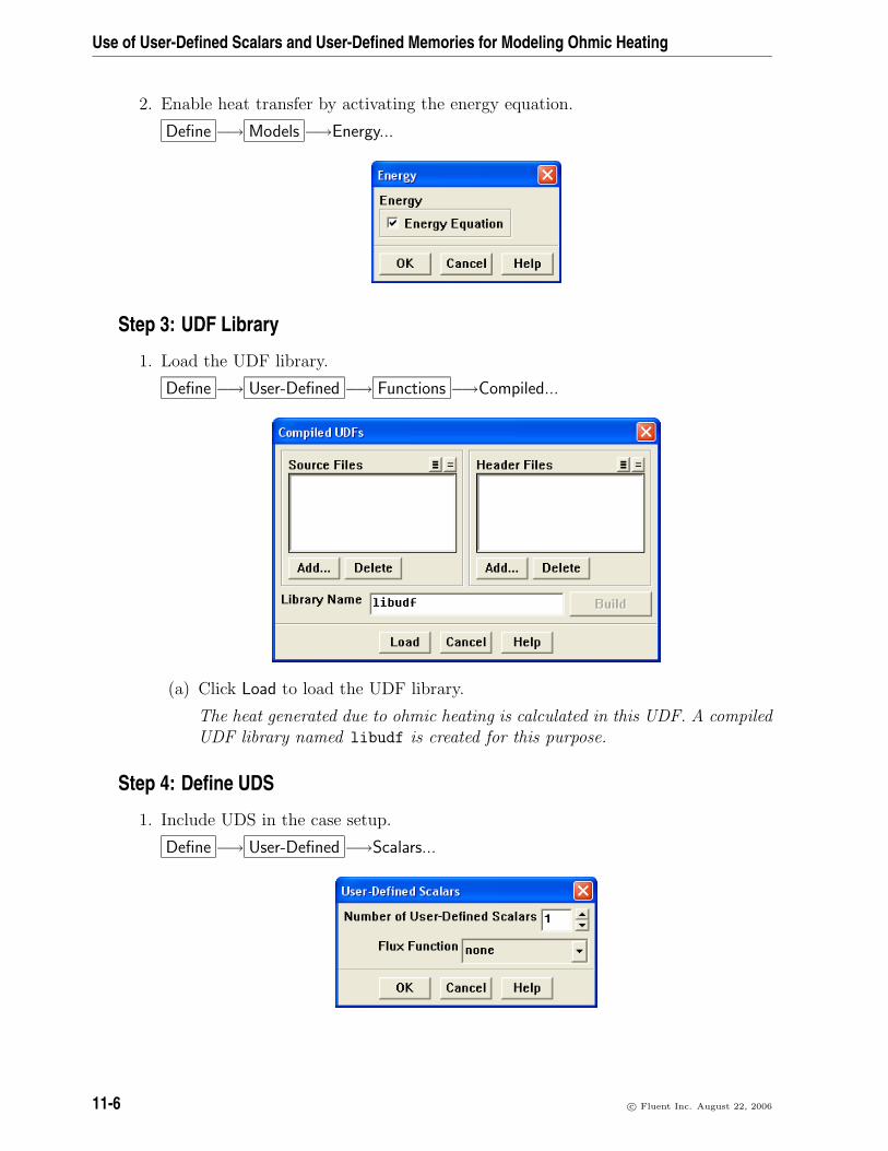
2. Enable heat transfer by activating the energy equation.
Define −→ Models −→Energy...
Step 3: UDF Library
1. Load the UDF library.
Define −→ User-Defined −→ Functions −→Compiled...
(a) Click Load to load the UDF library.
The heat generated due to ohmic heating is calculated in this UDF. A compiledUDF library named libudf is created for this purpose.
Step 4: Define UDS
1. Include UDS in the case setup.
Define −→ User-Defined −→Scalars...
11-6 c© Fluent Inc. August 22, 2006
Use of User-Defined Scalars and User-Defined Memories for Modeling Ohmic Heating
(a) Increase Number of User-Defined Scalars to 1.
(b) Keep the default selection of none in the Flux Function drop-down list.
Flux Function defines the convection flux for UDS transport. In this case, it isassumed that current convection is negligible, therefore, no need to specify anyfunction.
(c) Click OK in the User Defined Scalars panel.
An information dialog box pops up with the message Available material proper-ties or methods have changed. Please confirm the property values before contin-uing.
(d) Click OK to close the dialog box.
Since the UDS is enabled, UDS diffusivity will be required. You will set it inStep 6.
By enabling this feature, FLUENT solves the transport equation for an arbitraryUDS. The UDS equation is solved in the same way as FLUENT solves transportequation for any other scalar (e.g., temperature, species mass fraction).
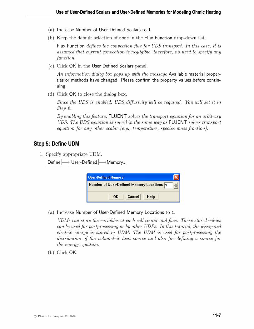
Step 5: Define UDM
1. Specify appropriate UDM.
Define −→ User-Defined −→Memory...
(a) Increase Number of User-Defined Memory Locations to 1.
UDMs can store the variables at each cell center and face. These stored valuescan be used for postprocessing or by other UDFs. In this tutorial, the dissipatedelectric energy is stored in UDM. The UDM is used for postprocessing thedistribution of the volumetric heat source and also for defining a source forthe energy equation.
(b) Click OK.
c© Fluent Inc. August 22, 2006 11-7
Use of User-Defined Scalars and User-Defined Memories for Modeling Ohmic Heating
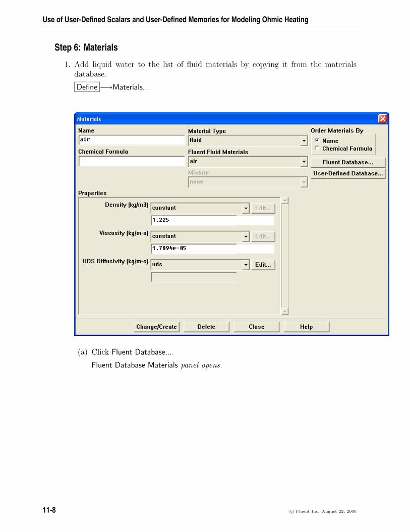
Step 6: Materials
1. Add liquid water to the list of fluid materials by copying it from the materialsdatabase.
Define −→Materials...
(a) Click Fluent Database....
Fluent Database Materials panel opens.
11-8 c© Fluent Inc. August 22, 2006
Use of User-Defined Scalars and User-Defined Memories for Modeling Ohmic Heating
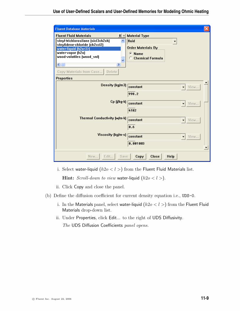
i. Select water-liquid (h2o < l >) from the Fluent Fluid Materials list.
Hint: Scroll-down to view water-liquid (h2o < l >).
ii. Click Copy and close the panel.
(b) Define the diffusion coefficient for current density equation i.e., UDS-0.
i. In the Materials panel, select water-liquid (h2o < l >) from the Fluent FluidMaterials drop-down list.
ii. Under Properties, click Edit... to the right of UDS Diffusivity.
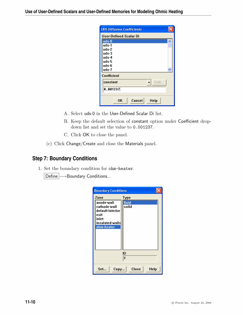
The UDS Diffusion Coefficients panel opens.
c© Fluent Inc. August 22, 2006 11-9
Use of User-Defined Scalars and User-Defined Memories for Modeling Ohmic Heating
A. Select uds-0 in the User-Defined Scalar Di list.
B. Keep the default selection of constant option under Coefficient drop-down list and set the value to 0.001237.
C. Click OK to close the panel.
(c) Click Change/Create and close the Materials panel.
Step 7: Boundary Conditions
1. Set the boundary condition for ohm-heater.
Define −→Boundary Conditions...
11-10 c© Fluent Inc. August 22, 2006
Use of User-Defined Scalars and User-Defined Memories for Modeling Ohmic Heating
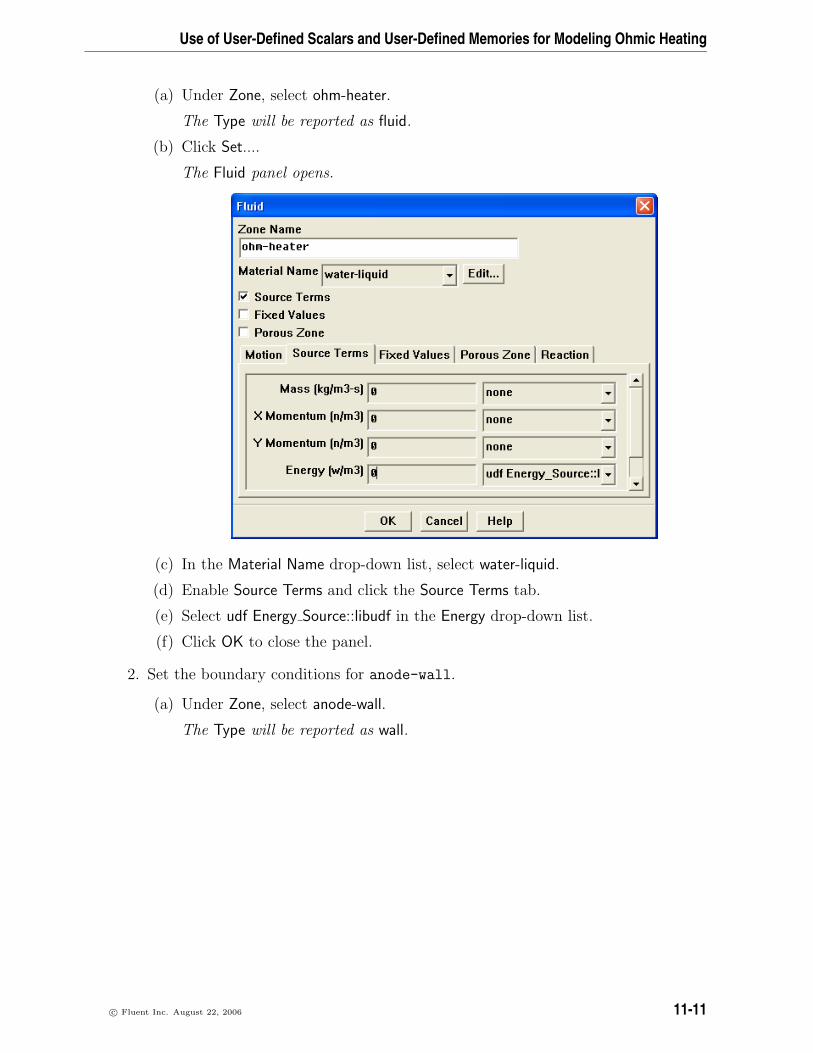
(a) Under Zone, select ohm-heater.
The Type will be reported as fluid.
(b) Click Set....
The Fluid panel opens.
(c) In the Material Name drop-down list, select water-liquid.
(d) Enable Source Terms and click the Source Terms tab.
(e) Select udf Energy Source::libudf in the Energy drop-down list.
(f) Click OK to close the panel.
2. Set the boundary conditions for anode-wall.
(a) Under Zone, select anode-wall.
The Type will be reported as wall.
c© Fluent Inc. August 22, 2006 11-11
Use of User-Defined Scalars and User-Defined Memories for Modeling Ohmic Heating
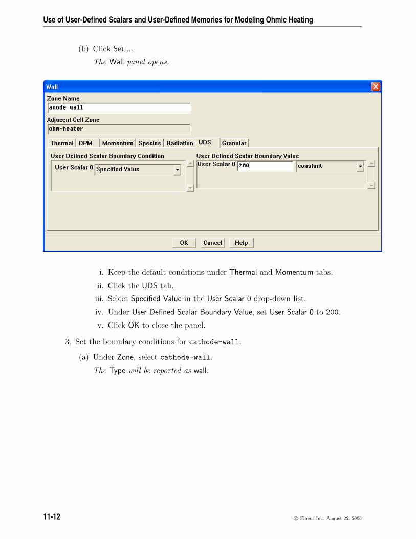
(b) Click Set....
The Wall panel opens.
i. Keep the default conditions under Thermal and Momentum tabs.
ii. Click the UDS tab.
iii. Select Specified Value in the User Scalar 0 drop-down list.
iv. Under User Defined Scalar Boundary Value, set User Scalar 0 to 200.
v. Click OK to close the panel.
3. Set the boundary conditions for cathode-wall.
(a) Under Zone, select cathode-wall.
The Type will be reported as wall.
11-12 c© Fluent Inc. August 22, 2006
Use of User-Defined Scalars and User-Defined Memories for Modeling Ohmic Heating
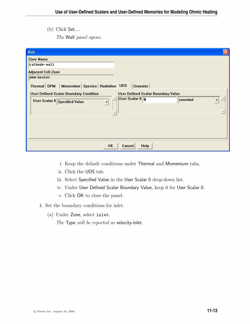
(b) Click Set....
The Wall panel opens.
i. Keep the default conditions under Thermal and Momentum tabs.
ii. Click the UDS tab.
iii. Select Specified Value in the User Scalar 0 drop-down list.
iv. Under User Defined Scalar Boundary Value, keep 0 for User Scalar 0.
v. Click OK to close the panel.
4. Set the boundary conditions for inlet.
(a) Under Zone, select inlet.
The Type will be reported as velocity-inlet.
c© Fluent Inc. August 22, 2006 11-13
Use of User-Defined Scalars and User-Defined Memories for Modeling Ohmic Heating
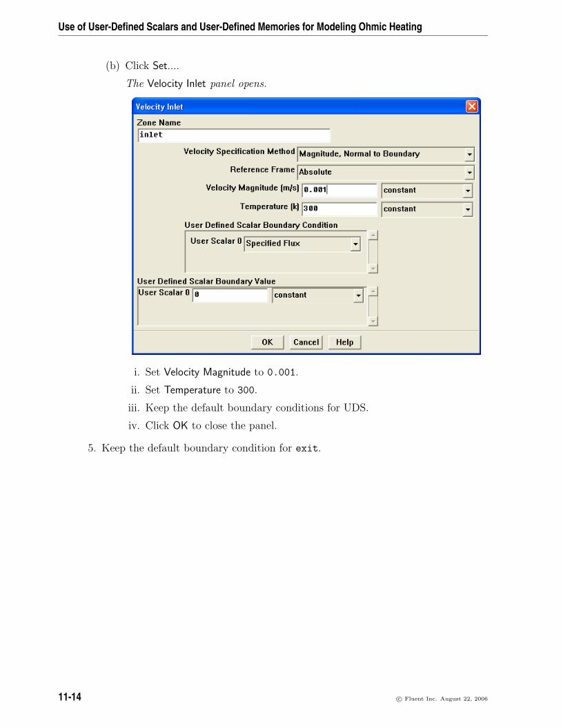
(b) Click Set....
The Velocity Inlet panel opens.
i. Set Velocity Magnitude to 0.001.
ii. Set Temperature to 300.
iii. Keep the default boundary conditions for UDS.
iv. Click OK to close the panel.
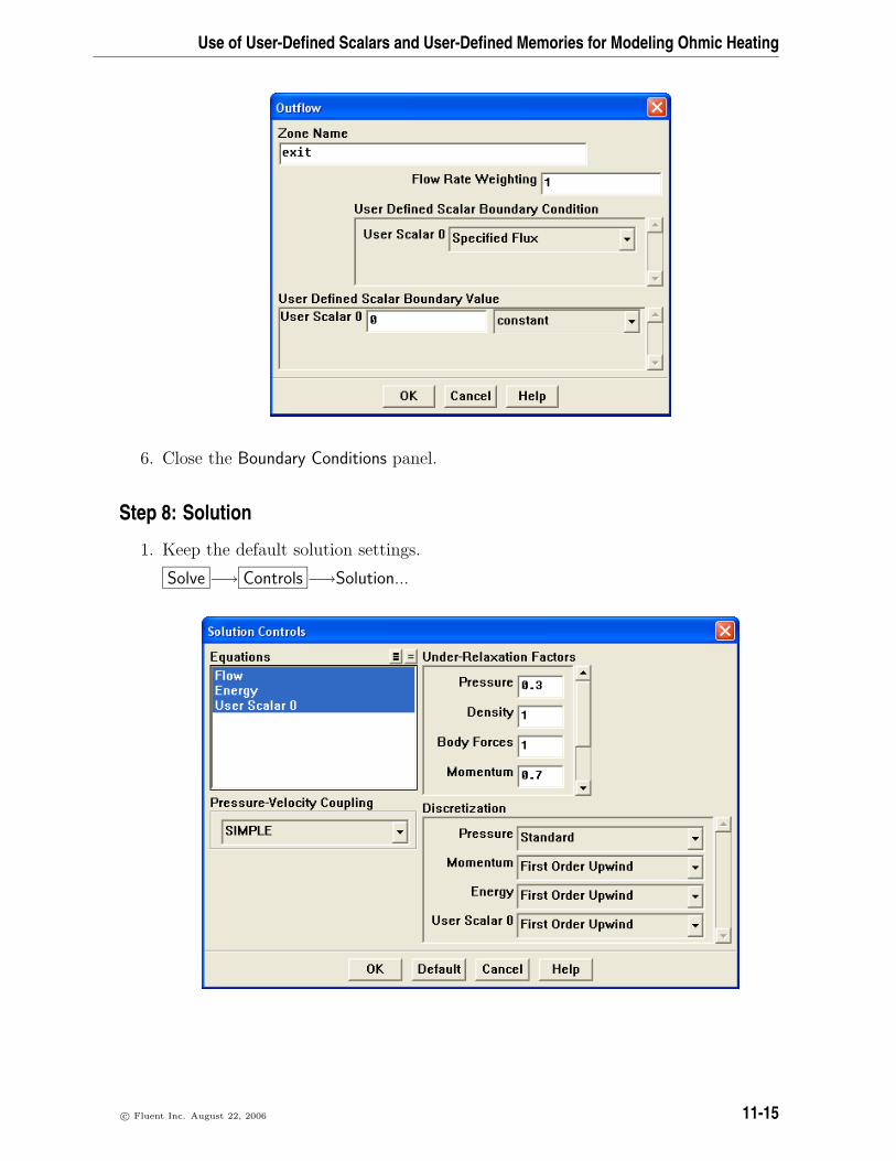
5. Keep the default boundary condition for exit.
11-14 c© Fluent Inc. August 22, 2006
Use of User-Defined Scalars and User-Defined Memories for Modeling Ohmic Heating
6. Close the Boundary Conditions panel.
Step 8: Solution
1. Keep the default solution settings.
Solve −→ Controls −→Solution...
c© Fluent Inc. August 22, 2006 11-15
Use of User-Defined Scalars and User-Defined Memories for Modeling Ohmic Heating
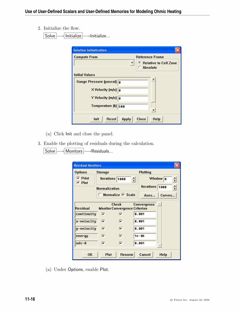
2. Initialize the flow.
Solve −→ Initialize −→Initialize...
(a) Click Init and close the panel.
3. Enable the plotting of residuals during the calculation.
Solve −→ Monitors −→Residuals...
(a) Under Options, enable Plot.
11-16 c© Fluent Inc. August 22, 2006
Use of User-Defined Scalars and User-Defined Memories for Modeling Ohmic Heating
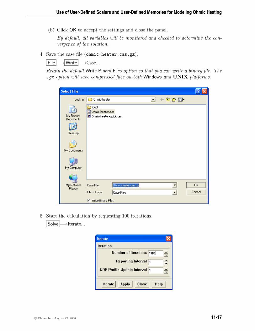
(b) Click OK to accept the settings and close the panel.
By default, all variables will be monitored and checked to determine the con-vergence of the solution.
4. Save the case file (ohmic-heater.cas.gz).
File −→ Write −→Case...
Retain the default Write Binary Files option so that you can write a binary file. The.gz option will save compressed files on both Windows and UNIX platforms.
5. Start the calculation by requesting 100 iterations.
Solve −→Iterate...
c© Fluent Inc. August 22, 2006 11-17
Use of User-Defined Scalars and User-Defined Memories for Modeling Ohmic Heating
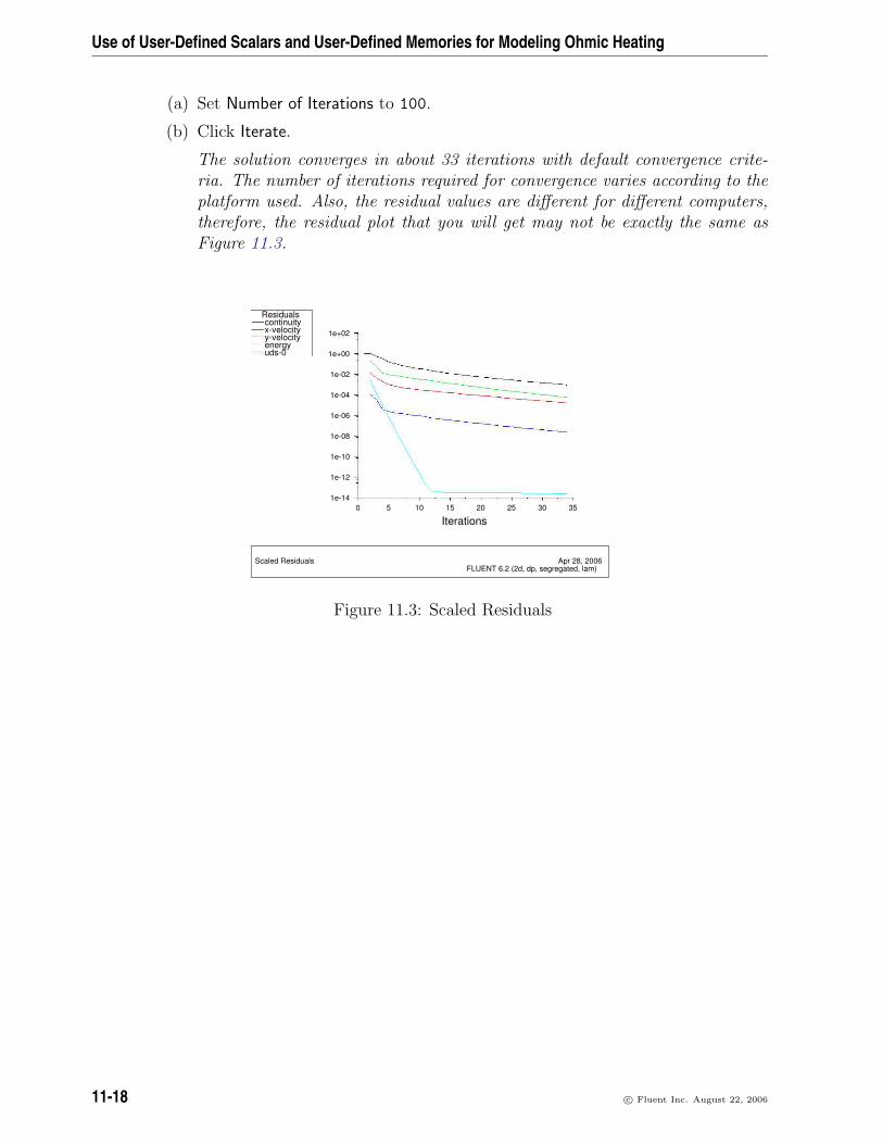
(a) Set Number of Iterations to 100.
(b) Click Iterate.
The solution converges in about 33 iterations with default convergence crite-ria. The number of iterations required for convergence varies according to theplatform used. Also, the residual values are different for different computers,therefore, the residual plot that you will get may not be exactly the same asFigure 11.3.
Scaled Residuals Apr 28, 2006FLUENT 6.2 (2d, dp, segregated, lam)
Iterations
1e-14
1e-12
1e-10
1e-08
1e-06
1e-04
1e-02
1e+00
1e+02
0 5 10 15 20 25 30 35
uds-0
Residualscontinuityx-velocityy-velocityenergy
Figure 11.3: Scaled Residuals
11-18 c© Fluent Inc. August 22, 2006
Use of User-Defined Scalars and User-Defined Memories for Modeling Ohmic Heating
Step 9: Check for Convergence
There are no universal metrics for judging convergence. The unconverged results maybe very misleading. The residual definitions that are useful for one class of problem aresometimes not suitable for other classes of problems. Therefore, it is a good idea tojudge convergence not only by examining residual levels, but also by monitoring relevantintegrated quantities and checking for mass and energy balances.
There are three methods to check the convergence:
• Monitoring the residuals.
Convergence occurs when the convergence criterion for each variable is reached.The default criterion is that each residual will be reduced to a value less than 1e-3,except the energy residual, for which the default criterion is 1e-6. These criteriaare useful for a wide range of problems, but at times, it may be required to tightenthese criteria, based on the validity of other convergence checks.
• Overall mass, momentum, energy and scalar balances are obtained.
Check the overall mass, momentum, energy and scalar balances in the Flux Reportspanel. The net imbalance should be less than 0.2% of the net flux through thedomain.
• When the solution no longer changes with iterations.
Sometimes the residuals may not fall below the convergence criteria set in the casesetup. However, monitoring the representative flow variables through iterations mayshow that the residuals have stagnated and do not change with further iterations.This could also be considered a convergence check.
1. Check global mass balance.
Report −→Fluxes...
c© Fluent Inc. August 22, 2006 11-19
Use of User-Defined Scalars and User-Defined Memories for Modeling Ohmic Heating
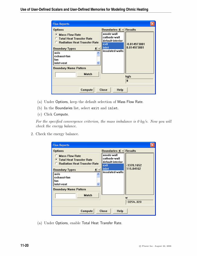
(a) Under Options, keep the default selection of Mass Flow Rate.
(b) In the Boundaries list, select exit and inlet.
(c) Click Compute.
For the specified convergence criterion, the mass imbalance is 0 kg/s. Now you willcheck the energy balance.
2. Check the energy balance.
(a) Under Options, enable Total Heat Transfer Rate.
11-20 c© Fluent Inc. August 22, 2006
Use of User-Defined Scalars and User-Defined Memories for Modeling Ohmic Heating
(b) In the Boundaries list, select exit and inlet.
(c) Click Compute.
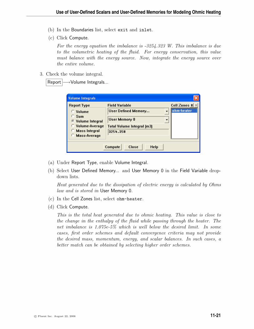
For the energy equation the imbalance is -3254.323 W. This imbalance is dueto the volumetric heating of the fluid. For energy conservation, this valuemust balance with the energy source. Now, integrate the energy source overthe entire volume.
3. Check the volume integral.
Report −→Volume Integrals...
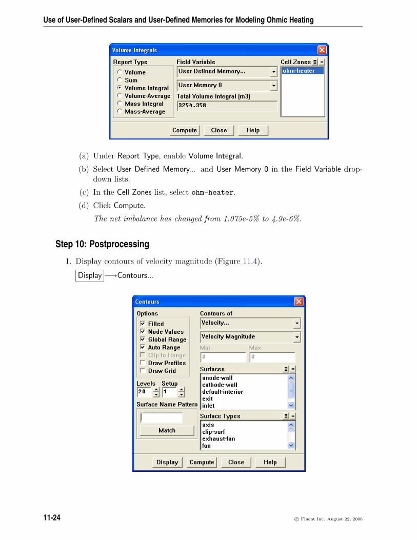
(a) Under Report Type, enable Volume Integral.
(b) Select User Defined Memory... and User Memory 0 in the Field Variable drop-down lists.
Heat generated due to the dissipation of electric energy is calculated by Ohmslaw and is stored in User Memory 0.
(c) In the Cell Zones list, select ohm-heater.
(d) Click Compute.
This is the total heat generated due to ohmic heating. This value is close tothe change in the enthalpy of the fluid while passing through the heater. Thenet imbalance is 1.075e-5% which is well below the desired limit. In somecases, first order schemes and default convergence criteria may not providethe desired mass, momentum, energy, and scalar balances. In such cases, abetter match can be obtained by selecting higher order schemes.
c© Fluent Inc. August 22, 2006 11-21
Use of User-Defined Scalars and User-Defined Memories for Modeling Ohmic Heating
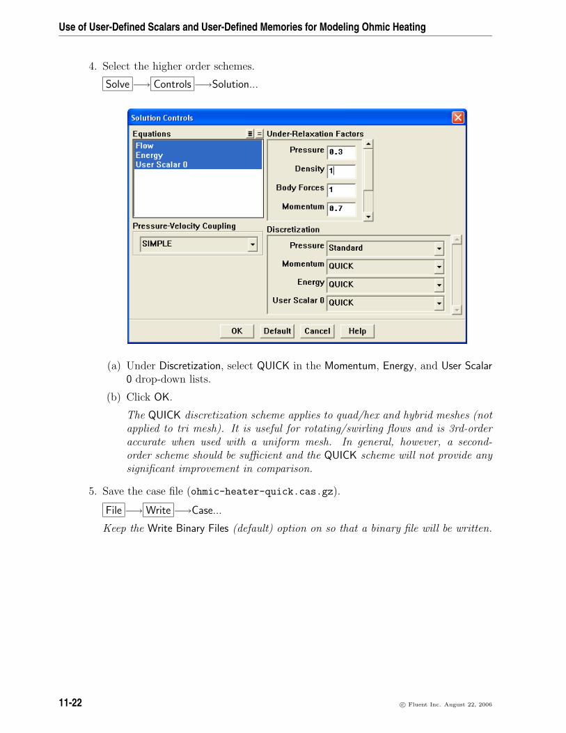
4. Select the higher order schemes.
Solve −→ Controls −→Solution...
(a) Under Discretization, select QUICK in the Momentum, Energy, and User Scalar0 drop-down lists.
(b) Click OK.
The QUICK discretization scheme applies to quad/hex and hybrid meshes (notapplied to tri mesh). It is useful for rotating/swirling flows and is 3rd-orderaccurate when used with a uniform mesh. In general, however, a second-order scheme should be sufficient and the QUICK scheme will not provide anysignificant improvement in comparison.
5. Save the case file (ohmic-heater-quick.cas.gz).
File −→ Write −→Case...
Keep the Write Binary Files (default) option on so that a binary file will be written.
11-22 c© Fluent Inc. August 22, 2006
Use of User-Defined Scalars and User-Defined Memories for Modeling Ohmic Heating
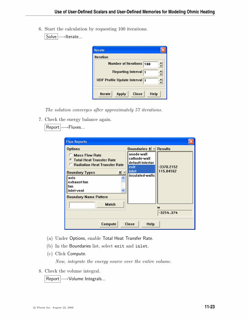
6. Start the calculation by requesting 100 iterations.
Solve −→Iterate...
The solution converges after approximately 57 iterations.
7. Check the energy balance again.
Report −→Fluxes...
(a) Under Options, enable Total Heat Transfer Rate.
(b) In the Boundaries list, select exit and inlet.
(c) Click Compute.
Now, integrate the energy source over the entire volume.
8. Check the volume integral.
Report −→Volume Integrals...
c© Fluent Inc. August 22, 2006 11-23
Use of User-Defined Scalars and User-Defined Memories for Modeling Ohmic Heating
(a) Under Report Type, enable Volume Integral.
(b) Select User Defined Memory... and User Memory 0 in the Field Variable drop-down lists.
(c) In the Cell Zones list, select ohm-heater.
(d) Click Compute.
The net imbalance has changed from 1.075e-5% to 4.9e-6%.
Step 10: Postprocessing
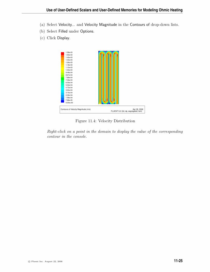
1. Display contours of velocity magnitude (Figure 11.4).
Display −→Contours...
11-24 c© Fluent Inc. August 22, 2006
Use of User-Defined Scalars and User-Defined Memories for Modeling Ohmic Heating
(a) Select Velocity... and Velocity Magnitude in the Contours of drop-down lists.
(b) Select Filled under Options.
(c) Click Display.
Contours of Velocity Magnitude (m/s) Apr 28, 2006FLUENT 6.2 (2d, dp, segregated, lam)
1.58e-03
0.00e+007.88e-051.58e-042.36e-043.15e-043.94e-044.73e-045.52e-046.30e-047.09e-047.88e-048.67e-049.46e-041.02e-031.10e-031.18e-031.26e-031.34e-031.42e-031.50e-03
Figure 11.4: Velocity Distribution
Right-click on a point in the domain to display the value of the correspondingcontour in the console.
c© Fluent Inc. August 22, 2006 11-25
Use of User-Defined Scalars and User-Defined Memories for Modeling Ohmic Heating
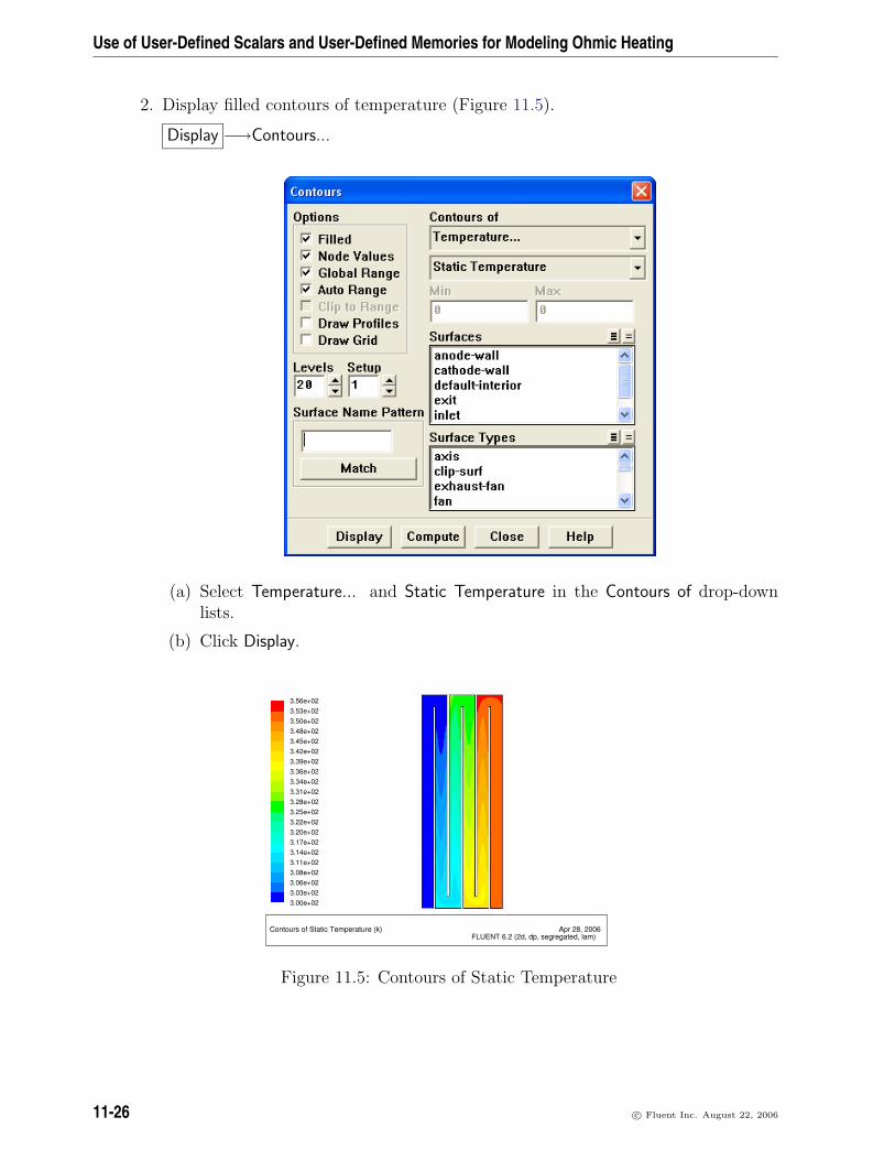
2. Display filled contours of temperature (Figure 11.5).
Display −→Contours...
(a) Select Temperature... and Static Temperature in the Contours of drop-downlists.
(b) Click Display.
Contours of Static Temperature (k) Apr 28, 2006FLUENT 6.2 (2d, dp, segregated, lam)
3.56e+02
3.00e+023.03e+023.06e+023.08e+023.11e+023.14e+023.17e+023.20e+023.22e+023.25e+023.28e+023.31e+023.34e+023.36e+023.39e+023.42e+023.45e+023.48e+023.50e+023.53e+02
Figure 11.5: Contours of Static Temperature
11-26 c© Fluent Inc. August 22, 2006
Use of User-Defined Scalars and User-Defined Memories for Modeling Ohmic Heating
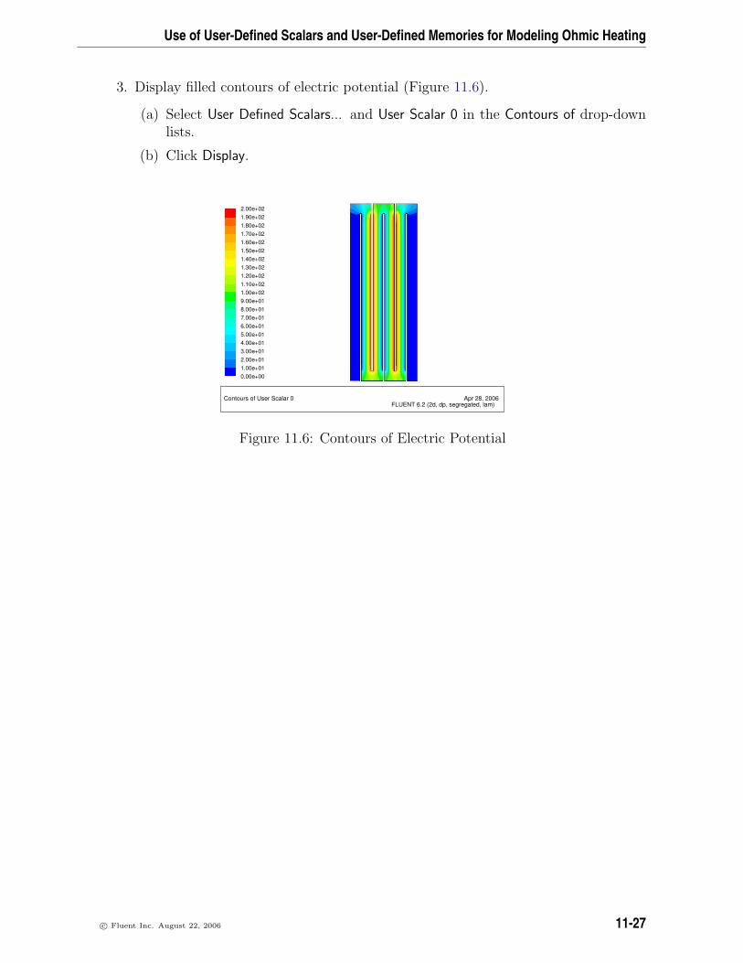
3. Display filled contours of electric potential (Figure 11.6).
(a) Select User Defined Scalars... and User Scalar 0 in the Contours of drop-downlists.
(b) Click Display.
Contours of User Scalar 0 Apr 28, 2006FLUENT 6.2 (2d, dp, segregated, lam)
2.00e+02
0.00e+001.00e+012.00e+013.00e+014.00e+015.00e+016.00e+017.00e+018.00e+019.00e+011.00e+021.10e+021.20e+021.30e+021.40e+021.50e+021.60e+021.70e+021.80e+021.90e+02
Figure 11.6: Contours of Electric Potential
c© Fluent Inc. August 22, 2006 11-27
Use of User-Defined Scalars and User-Defined Memories for Modeling Ohmic Heating
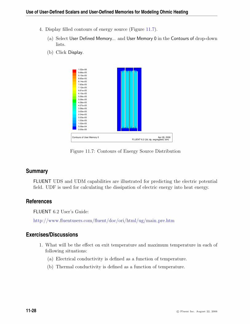
4. Display filled contours of energy source (Figure 11.7).
(a) Select User Defined Memory... and User Memory 0 in the Contours of drop-downlists.
(b) Click Display.
Contours of User Memory 0 Apr 28, 2006FLUENT 6.2 (2d, dp, segregated, lam)
1.02e+06
0.00e+005.09e+041.02e+051.53e+052.03e+052.54e+053.05e+053.56e+054.07e+054.58e+055.09e+055.59e+056.10e+056.61e+057.12e+057.63e+058.14e+058.65e+059.15e+059.66e+05
Figure 11.7: Contours of Energy Source Distribution
Summary
FLUENT UDS and UDM capabilities are illustrated for predicting the electric potentialfield. UDF is used for calculating the dissipation of electric energy into heat energy.
References
FLUENT 6.2 User’s Guide:
http://www.fluentusers.com/fluent/doc/ori/html/ug/main pre.htm
Exercises/Discussions
1. What will be the effect on exit temperature and maximum temperature in each offollowing situations:
(a) Electrical conductivity is defined as a function of temperature.
(b) Thermal conductivity is defined as a function of temperature.
11-28 c© Fluent Inc. August 22, 2006
Use of User-Defined Scalars and User-Defined Memories for Modeling Ohmic Heating
2. What will be the effect on the pumping power requirement in each of followingsituations:
(a) Thermal conductivity is defined as a function of temperature.
(b) Electrical conductivity is defined as a function of temperature.
(c) Viscosity is defined as a function of temperature.
Links for Further Reading
http://www.fsid.cvut.cz/ zitny/zitny/ohmic.htm
c© Fluent Inc. August 22, 2006 11-29

Use of User-Defined Scalars and User-Defined Memories for Modeling Ohmic Heating
11-30 c© Fluent Inc. August 22, 2006
Related Documents