Tutorial 1 Verification and Validation Americo Barbosa da Cunha Junior Universidade do Estado do Rio de Janeiro – UERJ NUMERICO – Nucleus of Modeling and Experimentation with Computers http://numerico.ime.uerj.br [email protected] www.americocunha.org Uncertainties 2018 April 8, 2018 Florian´ opolis - SC, Brazil A. Cunha Jr (UERJ) Uncertainty Quantification in Computational Predictive Science 1 / 30

Welcome message from author
This document is posted to help you gain knowledge. Please leave a comment to let me know what you think about it! Share it to your friends and learn new things together.
Transcript
Tutorial 1Verification and Validation
Americo Barbosa da Cunha Junior
Universidade do Estado do Rio de Janeiro – UERJ
NUMERICO – Nucleus of Modeling and Experimentation with Computers
http://numerico.ime.uerj.br
www.americocunha.org
Uncertainties 2018April 8, 2018
Florianopolis - SC, Brazil
© A. Cunha Jr (UERJ) Uncertainty Quantification in Computational Predictive Science 1 / 30

Verification and Validation (V&V)
VerificationAre we solving the equation right?It is an exercise in mathematics.
ValidationAre we solving the right equation?It is an exercise in physics.
© A. Cunha Jr (UERJ) Uncertainty Quantification in Computational Predictive Science 2 / 30
G. Iaccarino, A. Doostan, M. S. Eldred, and O. Ghattas. Introduction to Uncertainty Quantification
Techniques. Minitutorial at SIAM CSE Conference, 2009
A. Doostan and P. Constantine. Numerical Methods for Uncertainty Propagation. Short Course at
USNCCM13, 2015

V&V for Mass-Spring-Damper Oscillator
© A. Cunha Jr (UERJ) Uncertainty Quantification in Computational Predictive Science 3 / 30

Mass-Spring-Damper Oscillator
x + 2 ξ ωn x + ω2n x = (f /m) sin (ω t)
x(0) = v0, x(0) = x0
© A. Cunha Jr (UERJ) Uncertainty Quantification in Computational Predictive Science 4 / 30
Picture from http://www.shimrestackor.com/Physics/Spring_Mass_Damper/spring-mass-damper.htm

Model equation
x + 2 ξ ωn x + ω2n x = (f /m) sin (ω t)
⇐⇒[φ1
φ2
]︸ ︷︷ ︸
φ
=
[0 1
−ω2n −2 ξ ωn
][φ1
φ2
]+
[0
(f /m) sin (ω t)
]︸ ︷︷ ︸
f (t,φ)
where φ1 = x and φ2 = x .
© A. Cunha Jr (UERJ) Uncertainty Quantification in Computational Predictive Science 5 / 30
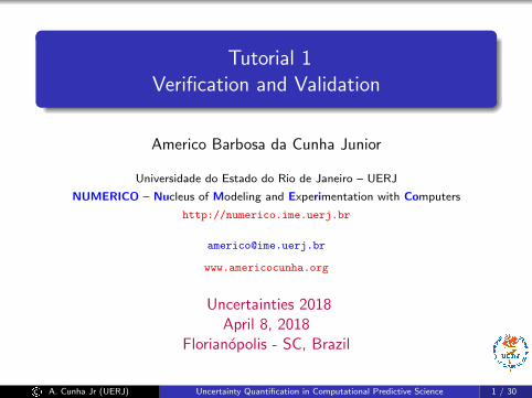
Reference solution
The unforced case, that corresponds to f = 0, has an analyticalsolution, which is given by
x = Ae−ξωnt sin (ωd t + φ),
where
ωd = ωn
√1− ξ2,
A =
√x2
0 +
(v0 + ξ ωn x0
ωd
)2
,
φ = tan−1
(x0 ωd
v0 + ξ ωn x0
).
This solution will be used as reference in Verification step.
© A. Cunha Jr (UERJ) Uncertainty Quantification in Computational Predictive Science 6 / 30
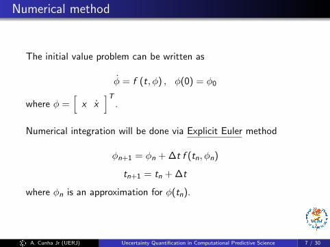
Numerical method
The initial value problem can be written as
φ = f (t, φ) , φ(0) = φ0
where φ =[x x
]T.
Numerical integration will be done via Explicit Euler method
φn+1 = φn + ∆t f (tn, φn)
tn+1 = tn + ∆t
where φn is an approximation for φ(tn).
© A. Cunha Jr (UERJ) Uncertainty Quantification in Computational Predictive Science 7 / 30

main_verification1.m
clc; clear all; close all;m = 1.0; ksi = 0.1; wn = 4.0; f = 0; w = 5.0;x0 = 1.0; v0 = 0.0; t0 = 0.0; t1 = 10.0; N = 3000;
dphidt=@(t,phi)[0 1; −wn^2 −2*ksi*wn]*phi ...+ [0; (f/m)*sin(w*t)];
[time,phi] = euler(dphidt,[x0;v0],t0,t1,N);
wd = wn*sqrt(1−ksi^2);A = sqrt(x0^2 + ((v0+ksi*wn*x0)/wd)^2);theta = atan((x0*wd)/(v0+ksi*wn*x0));x_true = A*exp(−ksi*wn*time).*sin(wd*time+theta);
subplot(2,1,1)plot(time,phi(1,:),'b','LineWidth',3);legend('Euler')subplot(2,1,2)plot(time,x_true, 'g','LineWidth',3);legend('True')
© A. Cunha Jr (UERJ) Uncertainty Quantification in Computational Predictive Science 8 / 30
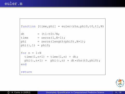
euler.m
function [time,phi] = euler(rhs,phi0,t0,t1,N)
dt = (t1−t0)/N;time = zeros(1,N+1);phi = zeros(length(phi0),N+1);phi(:,1) = phi0;
for n = 1:Ntime(1,n+1) = time(1,n) + dt;phi(:,n+1) = phi(:,n) + dt*rhs(t0,phi0);
end
return
© A. Cunha Jr (UERJ) Uncertainty Quantification in Computational Predictive Science 9 / 30

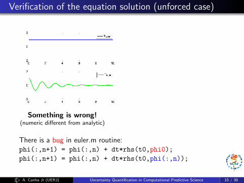
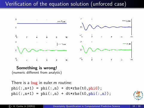
Verification of the equation solution (unforced case)
Something is wrong!(numeric different from analytic)
Is the code working fine?!
There is a bug in euler.m routine:phi(:,n+1) = phi(:,n) + dt*rhs(t0,phi0);
phi(:,n+1) = phi(:,n) + dt*rhs(t0,phi(:,n));
© A. Cunha Jr (UERJ) Uncertainty Quantification in Computational Predictive Science 10 / 30

Verification of the equation solution (unforced case)
Something is wrong!(numeric different from analytic)
Is the code working fine?!
There is a bug in euler.m routine:
phi(:,n+1) = phi(:,n) + dt*rhs(t0,phi0);
phi(:,n+1) = phi(:,n) + dt*rhs(t0,phi(:,n));
© A. Cunha Jr (UERJ) Uncertainty Quantification in Computational Predictive Science 10 / 30

Verification of the equation solution (unforced case)
Something is wrong!(numeric different from analytic)
Is the code working fine?!
There is a bug in euler.m routine:phi(:,n+1) = phi(:,n) + dt*rhs(t0,phi0);
phi(:,n+1) = phi(:,n) + dt*rhs(t0,phi(:,n));
© A. Cunha Jr (UERJ) Uncertainty Quantification in Computational Predictive Science 10 / 30
Apparently yes!absolute error ≤ 0.03

main_verification2.m
clc; clear all; close all;m = 1.0; ksi = 0.1; wn = 4.0; f = 10.0; w = 5.0;x0 = 1.0; v0 = 0.0; t0 = 0.0; t1 = 10.0; N = 3000;
dphidt=@(t,phi)[0 1; −wn^2 −2*ksi*wn]*phi ...+ [0; (f/m)*sin(w*t)];
[time,phi] = euler(dphidt,[x0;v0],t0,t1,N);
plot(time,phi(1,:),'LineWidth',3);
© A. Cunha Jr (UERJ) Uncertainty Quantification in Computational Predictive Science 11 / 30

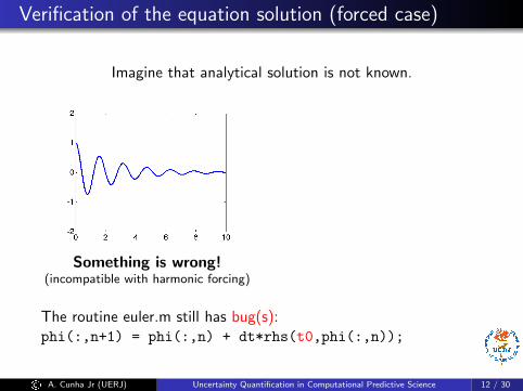
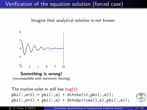
Verification of the equation solution (forced case)
Imagine that analytical solution is not known.
Something is wrong!(incompatible with harmonic forcing)
Is this the correct response?
The routine euler.m still has bug(s):phi(:,n+1) = phi(:,n) + dt*rhs(t0,phi(:,n));
phi(:,n+1) = phi(:,n) + dt*rhs(time(1,n),phi(:,n));
© A. Cunha Jr (UERJ) Uncertainty Quantification in Computational Predictive Science 12 / 30

Verification of the equation solution (forced case)
Imagine that analytical solution is not known.
Something is wrong!(incompatible with harmonic forcing)
Is this the correct response?
The routine euler.m still has bug(s):
phi(:,n+1) = phi(:,n) + dt*rhs(t0,phi(:,n));
phi(:,n+1) = phi(:,n) + dt*rhs(time(1,n),phi(:,n));
© A. Cunha Jr (UERJ) Uncertainty Quantification in Computational Predictive Science 12 / 30
Verification of the equation solution (forced case)
Imagine that analytical solution is not known.
Something is wrong!(incompatible with harmonic forcing)
Is this the correct response?
The routine euler.m still has bug(s):phi(:,n+1) = phi(:,n) + dt*rhs(t0,phi(:,n));
phi(:,n+1) = phi(:,n) + dt*rhs(time(1,n),phi(:,n));
© A. Cunha Jr (UERJ) Uncertainty Quantification in Computational Predictive Science 12 / 30
To answer this question it is necessary tocompare numerical results with the exact solution
(which is supposed to be unknown).
What is the altermative?Method of Manufactured Solutions

Method of Manufactured Solutions
The idea is to construct (manufacture) an initial value problem (IVP)in which the solution is known, and use it to test the numericalintegrator functionality.
1 Choose the form of model equations
φ = f (t, φ) , φ(0) = φ0 (?)
2 Define a manufactured solution Θ such that Θ(0) = φ0,which does not verify (?), i.e. Θ 6= f (t,Θ).
3 Compute the residue function R(t) := Θ− f (t,Θ) 6= 0.
4 Define the manufactured IVP
Θ = f (t,Θ) +R(t), Θ(0) = φ0,
which is verifyed by the manufactured solution Θ.
© A. Cunha Jr (UERJ) Uncertainty Quantification in Computational Predictive Science 13 / 30
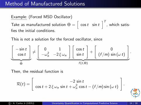
Method of Manufactured Solutions
Example: (Forced MSD Oscillator)
Take as manufactured solution Θ =[
cos t sin t]T
, which satis-
fies the initial conditions.
This is not a solution for the forced oscillator, since[− sin t
cos t
]︸ ︷︷ ︸
Θ
6=
[0 1
−ω2n −2 ξ ωn
][cos tsin t
]+
[0
(f /m) sin (ω t)
]︸ ︷︷ ︸
f (t,Θ)
.
Then, the residual function is
R(t) =
[−2 sin t
cos t + 2 ξ ωn sin t + ω2n cos t − (f /m) sin (ω t)
].
© A. Cunha Jr (UERJ) Uncertainty Quantification in Computational Predictive Science 14 / 30
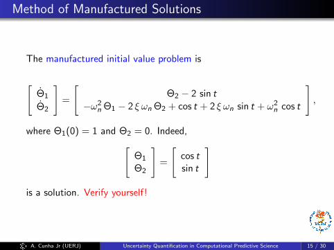
Method of Manufactured Solutions
The manufactured initial value problem is
[Θ1
Θ2
]=
[Θ2 − 2 sin t
−ω2n Θ1 − 2 ξ ωn Θ2 + cos t + 2 ξ ωn sin t + ω2
n cos t
],
where Θ1(0) = 1 and Θ2 = 0. Indeed,[Θ1
Θ2
]=
[cos tsin t
]
is a solution. Verify yourself!
© A. Cunha Jr (UERJ) Uncertainty Quantification in Computational Predictive Science 15 / 30
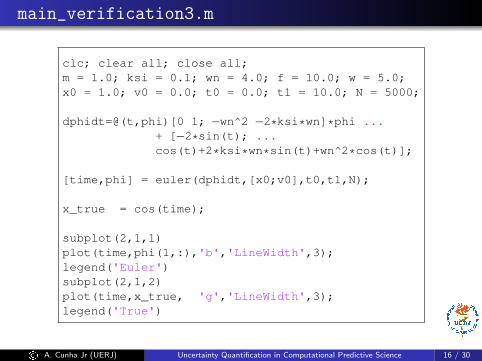
main_verification3.m
clc; clear all; close all;m = 1.0; ksi = 0.1; wn = 4.0; f = 10.0; w = 5.0;x0 = 1.0; v0 = 0.0; t0 = 0.0; t1 = 10.0; N = 5000;
dphidt=@(t,phi)[0 1; −wn^2 −2*ksi*wn]*phi ...+ [−2*sin(t); ...cos(t)+2*ksi*wn*sin(t)+wn^2*cos(t)];
[time,phi] = euler(dphidt,[x0;v0],t0,t1,N);
x_true = cos(time);
subplot(2,1,1)plot(time,phi(1,:),'b','LineWidth',3);legend('Euler')subplot(2,1,2)plot(time,x_true, 'g','LineWidth',3);legend('True')
© A. Cunha Jr (UERJ) Uncertainty Quantification in Computational Predictive Science 16 / 30

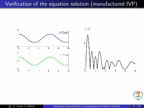
Verification of the equation solution (manufactured IVP)
Euler method is working fine!
© A. Cunha Jr (UERJ) Uncertainty Quantification in Computational Predictive Science 17 / 30
Verification of the equation solution (manufactured IVP)
Euler method is working fine!
© A. Cunha Jr (UERJ) Uncertainty Quantification in Computational Predictive Science 17 / 30

Verification of the equation solution (manufactured IVP)
Euler method is working fine!
© A. Cunha Jr (UERJ) Uncertainty Quantification in Computational Predictive Science 17 / 30
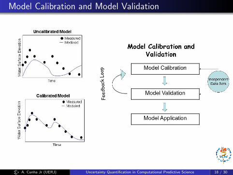
Model Calibration and Model Validation
© A. Cunha Jr (UERJ) Uncertainty Quantification in Computational Predictive Science 18 / 30
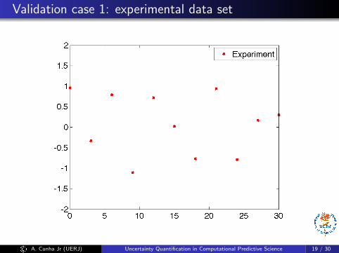
Validation case 1: experimental data set
© A. Cunha Jr (UERJ) Uncertainty Quantification in Computational Predictive Science 19 / 30

main_validation1.m
clc; clear all; close all;m = 1.0; ksi = 0.1; wn = 4.0; f = 10.0; w = 5.0;x0 = 1.0; v0 = 0.0; t0 = 0.0; t1 = 30.0; N = 5000;
dphidt=@(t,phi)[0 1; −wn^2 −2*ksi*wn]*phi ...+ [0; (f/m)*sin(w*t)];
[t,phi] = euler(dphidt,[x0;v0],t0,t1,N);
t_exp = [ 0.0, 3.0, 6.0, 9.0,12.0,15.0,...18.0,21.0,24.0,27.0,30.0];
x_exp = [ 0.96,−0.33, 0.79,−1.11,0.72,0.02,...−0.77, 0.94,−0.79, 0.17,0.30];
plot(t,phi(1,:),'b',t_exp,x_exp,'xr','LineWidth',3);axis([t0 t1 −2 2])legend('Model','Experiment')
© A. Cunha Jr (UERJ) Uncertainty Quantification in Computational Predictive Science 20 / 30

Validation case 1: predictions and observations
Good agreement between experiment and simulation!Validated Model!
© A. Cunha Jr (UERJ) Uncertainty Quantification in Computational Predictive Science 21 / 30

Validation case 1: predictions and observations
Good agreement between experiment and simulation!Validated Model!
© A. Cunha Jr (UERJ) Uncertainty Quantification in Computational Predictive Science 21 / 30
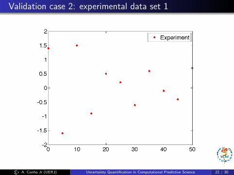
Validation case 2: experimental data set 1
© A. Cunha Jr (UERJ) Uncertainty Quantification in Computational Predictive Science 22 / 30

main_validation2.m (1/3)
clc; clear all; close all;m = 1.0; ksi = 0.1; wn = 4.0; f = 10.0; w = 5.0;x0 = 1.0; v0 = 0.0; t0 = 0.0; t1 = 50.0; N = 5000;
dphidt=@(t,phi)[0 1; −wn^2 −2*ksi*wn]*phi ...+ [0; (f/m)*sin(w*t)];
[t,phi] = euler3(dphidt,[x0;v0],t0,t1,N);
t_exp = [ 0.0, 4.9, 9.9,14.9,20.0,25.0,...30.0,35.0,40.0,44.9,49.9];
x_exp = [ 1.4,−1.6, 1.5,−0.9,0.5,0.2,...−0.6, 0.6,−0.1,−0.4,0.7];
figure(1)plot(t,phi(1,:),'b',t_exp,x_exp,'xr','LineWidth',3);axis([t0 t1 −2 2])set(gca,'fontsize',18)legend('Model','Experiment')
© A. Cunha Jr (UERJ) Uncertainty Quantification in Computational Predictive Science 23 / 30

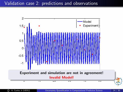
Validation case 2: predictions and observations
Experiment and simulation are not in agreement!Invalid Model!
© A. Cunha Jr (UERJ) Uncertainty Quantification in Computational Predictive Science 24 / 30
Validation case 2: predictions and observations
Experiment and simulation are not in agreement!Invalid Model!
© A. Cunha Jr (UERJ) Uncertainty Quantification in Computational Predictive Science 24 / 30

main_validation2.m (2/3)
m = 1.0; ksi = 0.05; wn = 3.2; f = 15.0; w = 5.5;x0 = 1.5; v0 = −0.4;
dphidt=@(t,phi)[0 1; −wn^2 −2*ksi*wn]*phi ...+ [0; (f/m)*sin(w*t)];
[t_cal,phi_cal] = euler3(dphidt,[x0;v0],t0,t1,N);
figure(2)plot(t,phi(1,:),'b',t_cal,phi_cal(1,:),'g',...
t_exp,x_exp,'xr','LineWidth',3);axis([t0 t1 −2 2])set(gca,'fontsize',18)legend('Uncalibrated','Calibrated','Experiment')
© A. Cunha Jr (UERJ) Uncertainty Quantification in Computational Predictive Science 25 / 30
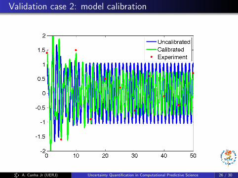
Validation case 2: model calibration
Good agreement after calibration!Calibrated Model!
© A. Cunha Jr (UERJ) Uncertainty Quantification in Computational Predictive Science 26 / 30
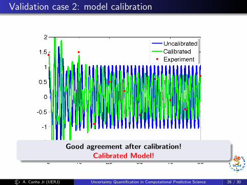
Validation case 2: model calibration
Good agreement after calibration!Calibrated Model!
© A. Cunha Jr (UERJ) Uncertainty Quantification in Computational Predictive Science 26 / 30
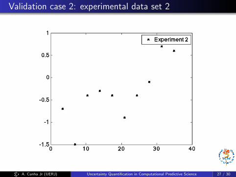
Validation case 2: experimental data set 2
© A. Cunha Jr (UERJ) Uncertainty Quantification in Computational Predictive Science 27 / 30
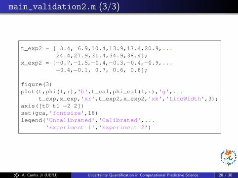
main_validation2.m (3/3)
t_exp2 = [ 3.4, 6.9,10.4,13.9,17.4,20.9,...24.4,27.9,31.4,34.9,38.4];
x_exp2 = [−0.7,−1.5,−0.4,−0.3,−0.4,−0.9,...−0.4,−0.1, 0.7, 0.6, 0.8];
figure(3)plot(t,phi(1,:),'b',t_cal,phi_cal(1,:),'g',...
t_exp,x_exp,'xr',t_exp2,x_exp2,'xk','LineWidth',3);axis([t0 t1 −2 2])set(gca,'fontsize',18)legend('Uncalibrated','Calibrated',...
'Experiment 1','Experiment 2')
© A. Cunha Jr (UERJ) Uncertainty Quantification in Computational Predictive Science 28 / 30

Validation case 2: calibrated model and new observations
Good agreement between new experiment and simulation!Validated Model!
© A. Cunha Jr (UERJ) Uncertainty Quantification in Computational Predictive Science 29 / 30

Validation case 2: calibrated model and new observations
Good agreement between new experiment and simulation!Validated Model!
© A. Cunha Jr (UERJ) Uncertainty Quantification in Computational Predictive Science 29 / 30

References
C. J. Roy and W. L. Oberkampf, A comprehensive framework for verification, validation, and uncertainty
quantification in scientific computing. Computer Methods in Applied Mechanics and Engineering, 200:2131–2144, 2011.
C. J. Roy, Review of code and solution verification procedures for computational simulation. Journal of
Computational Physics, 205: 131–156, 2005.
W. L. Oberkampf, T. Trucano and C. Hirsch, Verification, validation, and predictive capability in
computational engineering and physics. Applied Mechanics Reviews, 57: 345–384, 2004.
W. L. Oberkampf and C. J. Roy, Verification and Validation in Scientific Computing. Cambridge UniversityPress, 1st edition, 2010.
© A. Cunha Jr (UERJ) Uncertainty Quantification in Computational Predictive Science 30 / 30
Related Documents